
The acoustics of the steel string guitar - UNSWorks
418
The acoustics of the steel string guitar Author: Inta, Ra Ata Publication Date: 2007 DOI: https://doi.org/10.26190/unsworks/17545 License: https://creativecommons.org/licenses/by-nc-nd/3.0/au/ Link to license to see what you are allowed to do with this resource. Downloaded from http://hdl.handle.net/1959.4/40471 in https:// unsworks.unsw.edu.au on 2022-07-31
-
Upload
khangminh22 -
Category
Documents
-
view
0 -
download
0
Transcript of The acoustics of the steel string guitar - UNSWorks

The acoustics of the steel string guitar
Author:Inta, Ra Ata
Publication Date:2007
DOI:https://doi.org/10.26190/unsworks/17545
License:https://creativecommons.org/licenses/by-nc-nd/3.0/au/Link to license to see what you are allowed to do with this resource.
Downloaded from http://hdl.handle.net/1959.4/40471 in https://unsworks.unsw.edu.au on 2022-07-31

THE ACOUSTICS OF THE STEEL STRING GUITAR
ByRa Inta
SUBMITTED IN TOTAL FULFILMENT OF THE
REQUIREMENTS FOR THE DEGREE OF
DOCTOR OF PHILOSOPHY
SCHOOL OF PHYSICS
THE UNIVERSITY OF NEW SOUTH WALES
SYDNEY, AUSTRALIA
September 6, 2007

To the memory of Tamzin Sherwood
(1977-2000)
Sic Transit Gloria Astra
ii

Table of Contents
Table of Contents iii
Abstract vii
Acknowledgements viii
Why study the acoustics of the guitar? (An overview) 1
0.1 Introduction . . . . . . . . . . . . . . . . . . . . . . . . . . . . . . . . 1
0.2 Outstanding problems of interest . . . . . . . . . . . . . . . . . . . . 4
0.3 The approach in this thesis . . . . . . . . . . . . . . . . . . . . . . . . 4
0.4 Overview . . . . . . . . . . . . . . . . . . . . . . . . . . . . . . . . . . 6
1 Previous work 9
1.1 A brief history of the guitar . . . . . . . . . . . . . . . . . . . . . . . 9
1.2 Early work in acoustics . . . . . . . . . . . . . . . . . . . . . . . . . . 14
1.3 Previous work on stringed musical instruments and related systems . 15
2 How the guitar produces sound 29
2.1 The basic anatomy of the guitar . . . . . . . . . . . . . . . . . . . . . 29
2.2 Specialised anatomical features . . . . . . . . . . . . . . . . . . . . . 34
2.3 Excitation methods . . . . . . . . . . . . . . . . . . . . . . . . . . . . 38
2.4 The Helmholtz resonator . . . . . . . . . . . . . . . . . . . . . . . . . 43
2.5 Soundboard-air cavity coupling: the two-mass oscillator model . . . . 46
2.6 Three-mass oscillator model . . . . . . . . . . . . . . . . . . . . . . . 56
2.7 The importance of bracing . . . . . . . . . . . . . . . . . . . . . . . . 58
2.8 General behaviour in various frequency regimes . . . . . . . . . . . . 62
2.9 Resonant modes of the guitar . . . . . . . . . . . . . . . . . . . . . . 65
2.10 Interpretation of response curves . . . . . . . . . . . . . . . . . . . . 74
2.11 Acoustic radiativity of the guitar . . . . . . . . . . . . . . . . . . . . 77
iii

2.12 Conclusion . . . . . . . . . . . . . . . . . . . . . . . . . . . . . . . . . 80
3 The Construction of the Guitar 82
3.1 Introduction . . . . . . . . . . . . . . . . . . . . . . . . . . . . . . . . 83
3.2 Material used in construction . . . . . . . . . . . . . . . . . . . . . . 84
3.3 Damping . . . . . . . . . . . . . . . . . . . . . . . . . . . . . . . . . . 93
3.4 Traditional techniques of construction . . . . . . . . . . . . . . . . . . 99
3.5 Recent innovations . . . . . . . . . . . . . . . . . . . . . . . . . . . . 121
3.6 Phases of construction examined in this thesis . . . . . . . . . . . . . 122
4 Applications of the Finite Element Method to instrument construc-
tion 124
4.1 Methods and motives for using finite element calculations . . . . . . . 125
4.2 Inputs for the model . . . . . . . . . . . . . . . . . . . . . . . . . . . 129
4.3 Brace scalloping . . . . . . . . . . . . . . . . . . . . . . . . . . . . . . 131
4.4 Glue bonds . . . . . . . . . . . . . . . . . . . . . . . . . . . . . . . . 141
4.5 The free guitar soundboard . . . . . . . . . . . . . . . . . . . . . . . 142
4.6 Guitar body . . . . . . . . . . . . . . . . . . . . . . . . . . . . . . . . 148
4.7 Conclusion: Applications of finite element simulations to instrument
construction . . . . . . . . . . . . . . . . . . . . . . . . . . . . . . . . 150
5 Experimental: Selection of Materials 152
5.1 Timber used in the guitars studied . . . . . . . . . . . . . . . . . . . 153
5.2 Measurement techniques . . . . . . . . . . . . . . . . . . . . . . . . . 155
5.3 Measuring and controlling the moisture content of wood . . . . . . . 162
5.4 Selection criteria . . . . . . . . . . . . . . . . . . . . . . . . . . . . . 168
5.5 Bracing material . . . . . . . . . . . . . . . . . . . . . . . . . . . . . 169
5.6 Soundboard material . . . . . . . . . . . . . . . . . . . . . . . . . . . 176
5.7 Bridge material . . . . . . . . . . . . . . . . . . . . . . . . . . . . . . 180
5.8 Neck material . . . . . . . . . . . . . . . . . . . . . . . . . . . . . . . 181
5.9 Fingerboard material . . . . . . . . . . . . . . . . . . . . . . . . . . . 183
5.10 Back, sides, binding and other materials . . . . . . . . . . . . . . . . 188
5.11 Damping measurements . . . . . . . . . . . . . . . . . . . . . . . . . 188
5.12 Results . . . . . . . . . . . . . . . . . . . . . . . . . . . . . . . . . . . 188
5.13 Conclusion . . . . . . . . . . . . . . . . . . . . . . . . . . . . . . . . . 192
iv

6 Experimental: Plates, bodies and the guitar 193
6.1 Experimental measurement techniques . . . . . . . . . . . . . . . . . 194
6.2 Simple plates . . . . . . . . . . . . . . . . . . . . . . . . . . . . . . . 196
6.3 Free guitar soundboards . . . . . . . . . . . . . . . . . . . . . . . . . 205
6.4 Guitar bodies . . . . . . . . . . . . . . . . . . . . . . . . . . . . . . . 210
6.5 The thinned soundboard . . . . . . . . . . . . . . . . . . . . . . . . . 217
6.6 Binding the soundboard . . . . . . . . . . . . . . . . . . . . . . . . . 222
6.7 Discussion . . . . . . . . . . . . . . . . . . . . . . . . . . . . . . . . . 225
7 Experimental: Completed instruments and parameter evolution 231
7.1 Effects from the addition of the neck . . . . . . . . . . . . . . . . . . 231
7.2 Addition of the bridge . . . . . . . . . . . . . . . . . . . . . . . . . . 240
7.3 The polished instruments . . . . . . . . . . . . . . . . . . . . . . . . . 246
7.4 Effects of lacquer curing . . . . . . . . . . . . . . . . . . . . . . . . . 250
7.5 Short term ageing and playing in . . . . . . . . . . . . . . . . . . . . 254
7.6 The effects of brace scalloping . . . . . . . . . . . . . . . . . . . . . . 266
7.7 Parameter evolution . . . . . . . . . . . . . . . . . . . . . . . . . . . 280
7.8 Results/Comments . . . . . . . . . . . . . . . . . . . . . . . . . . . . 290
8 A lexicon and a preliminary study of subjective responses to guitar
sounds 296
8.1 Introduction . . . . . . . . . . . . . . . . . . . . . . . . . . . . . . . . 296
8.2 Study I—establishing a guitar timbre lexicon . . . . . . . . . . . . . . 298
8.3 Study II—evaluation of guitar sounds . . . . . . . . . . . . . . . . . . 308
8.4 Discussion . . . . . . . . . . . . . . . . . . . . . . . . . . . . . . . . . 328
9 Conclusion and Further Work 330
A Some derivations and measurements 335
A.1 The Helmholtz resonator . . . . . . . . . . . . . . . . . . . . . . . . . 335
A.2 Soundboard-air cavity coupling parameters . . . . . . . . . . . . . . . 339
A.3 Two mass model for a cantilever beam driven at the base . . . . . . . 342
A.3.1 Change in frequency of bending mode of a profiled beam . . . 343
A.4 Measurements of dimensions of the guitar soundboards . . . . . . . . 350
B Vibratory data acquisition system (ACUZ) 351
B.1 Background . . . . . . . . . . . . . . . . . . . . . . . . . . . . . . . . 351
B.2 Design and operation . . . . . . . . . . . . . . . . . . . . . . . . . . . 352
v

B.3 Impedance spectroscopy . . . . . . . . . . . . . . . . . . . . . . . . . 355
C Alternative methods of measuring mechanical properties of wood 356
D Soundboard thickness measurement device 361
D.1 Outline of soundboard thickness problem . . . . . . . . . . . . . . . . 361
D.2 The Hall effect . . . . . . . . . . . . . . . . . . . . . . . . . . . . . . 364
D.3 Measurements of soundboard thinning . . . . . . . . . . . . . . . . . 368
D.4 The device . . . . . . . . . . . . . . . . . . . . . . . . . . . . . . . . . 369
D.5 Methodology and usage . . . . . . . . . . . . . . . . . . . . . . . . . . 370
E Excitation and coupling apparatus 374
E.1 Magnetic coupling apparatus . . . . . . . . . . . . . . . . . . . . . . . 374
E.2 Cup-hook support mechanism . . . . . . . . . . . . . . . . . . . . . . 378
E.3 Magnetic support mechanism . . . . . . . . . . . . . . . . . . . . . . 379
E.4 Materials used in excitation stand . . . . . . . . . . . . . . . . . . . . 380
E.5 Design of excitation stand . . . . . . . . . . . . . . . . . . . . . . . . 380
E.6 Specific operating techniques . . . . . . . . . . . . . . . . . . . . . . . 382
F Lists of terms in describing the timbre of guitar sounds 383
F.1 . . . . . . . . . . . . . . . . . . . . . . . . . . . . . . . . . . . . . . . 383
Bibliography 386
vi

Abstract
To improve the replication of acoustic guitars, measurements of three Martin OOOstyle steel-string guitars were made at various stages of their construction. Theguitars were constructed in parallel, as similar to each other as possible, with theexception of the soundboard material—which were made of Sitka spruce, Engelmannspruce and Western Red cedar.To improve the similarity of the instruments, methods were developed to measureand control the material properties of key components before their incorporation intothe instruments, including a device to measure the thickness of a guitar soundboardattached to the back and sides of the instrument.Some of these measurements were compared to numerical models of the instrumentand, after the establishment of a lexicon to describe guitar sounds, some physicalfactors contributing towards the timbre of guitar sounds were determined.The results of these investigations may be developed to improve the consistency inthe manufacture of stringed musical instruments.
vii

Acknowledgements
Thankfully, this is not an Academy AwardsTM
speech, so I am able to properly thank
the following, without whom this project would have been impossible. These truly
are debts I will not ever be able to repay.
First, I would like to thank my supervisor, Prof. Joe Wolfe, who was supportive
and generous well above and beyond the usual obligatory demands placed on super-
visors. Joe has not only been a mentor in my scientific life, but also contributed
much to my broader existence, both in the day-to-day, and the philosophical sense.
A true captain of men as well as sailing ships.
Gerard Gilet, my industrial supervisor: I am indebted to his extraordinary fore-
sight in recognising the importance of research on improving the construction of the
guitar—especially in an industry with such ‘slim overheads’. This is evident not only
in his support of this project, but in his history of supporting research in a collegial
and intelligent manner. I hope I have helped in some small way.
Dr John Smith, my co-supervisor: I am grateful for his continuous suggestions
and expertise offered, as well as his broad knowledge, which helped me solve innu-
merable problems with his many great ideas. One day I hope I will visit Mileto, too.
(The) John Tann: No amount of muffins would equal the accumulated help I have
received from this man. From my very first day on this project (helping him make
an anechoic chamber) until the very(!) last minute, help support and inspiration
was ungrudgingly, nay, willingly, offered.
An acknowledgement of foresight and support rightly belongs to the Australian
viii

ix
Research Council. This is not offered as a platitude: I really am grateful for support
to what may have looked like a high-risk venture!
I would also like to thank:
Emery Schubert: For help with the psychoacoustical aspects of this project. It would
have been a right SASS-P without him. David Vernet, Matthieu Maziere and Davy
Laille: It was a pleasure working with you all. I hope you remember your brief stay
in Australia fondly and wish you well for the future.
The people in the Music Acoustics Lab, including Paul Dickens, Attila Stopic,
Jane Cavanagh, Manfred Yew, Alex Tarnopolsky, Claudia Fritz, David Bowman,
Ben Lange, Romano Crivici, Michael Lea, Harry Vatiliotis, Ryan France, Pierre-
Yves Placais, Olivier Marnette and the many others who passed through in the time
I was there. You have all helped make my PhD life richer and more enjoyable in
innumerable ways.
The people at the Gilet Guitars workshop: Darrell ‘Deathride’ Wheeler, Michael
Prendergast and Charles Cilia, plus Arjuna, Charles Milne, Pete, and Frank. I would
have had a lot of expensive firewood without your help.
I would also like to thank the good people of the UNSW School of Physics, in-
cluding Jules, Tony Travolta, Cormac, Sue Hagon, Bosco, Steve ‘Yaarrgh’ Curran,
Dr Matty, Vincent, Gary Keenan, Tammy Reztsova and so many others for provid-
ing such a stimulating environment. So many good people. So many good times.
Of course, any acknowledgements would not be complete without especially
thanking Aunt Elly, Doug Lloyd-Jones, and Jim Williams for their continuous sup-
port and help through the years. I am grateful to your input and inspiration for so
many things.
More fundamentally, it would not have been possible without my parents, Frida
and Scotty, and my ‘little’ brothers Rory, Chad and Zigs. It must have seemed like
I have taken forever to write this!
I would also like to thank Professor Joseph Lai, Dr Theo Evans, and the CSIRO
Termite Group, for their patience and understanding while finishing this project at
the same time as embarking on another exciting adventure.
Sydney, Australia Ra Inta

x

Why study the acoustics of theguitar? (An overview)
0.1 Introduction
“[A] clear overall understanding of the structural dynamics of the instrument is a
critical element in understanding how to produce a quality instrument. All good
luthiers intuitively understand this, but...much of musical instrument development
proceeds in an empirical, Edison-like way, guided by individuals with keen ears ex-
perienced in their construction” —M. French & G. Bissinger French and Bissinger
[2001]
After the voice, the guitar is probably the most popular musical instrument in
the Western world. Basic physical and engineering properties of the guitar have been
well studied over the last four decades, driven by the needs and curiosity of players
and instrument builders, as well as the interest of scientific researchers. Much of
the fundamental behaviour of the instrument is well understood but less well known
are the various effects on the overall sound due to interactions among elements of
the instrument. Most scientific investigation has been on the acoustic, as opposed
to the electric, guitar. The electric guitar is outside the scope of the present work
and hence the term guitar will hereafter refer to the acoustic guitar and will usually
1

2
mean the steel-string (folk) guitar specifically.
Guitar-makers (or luthiers) have traditionally developed techniques that were
passed onto them by their predecessors. Adjustments are generally made to construc-
tion processes according to the needs of musicians; methods are improved through
newly available technologies and the innovation of their colleagues. Experimenta-
tion usually involves modification of a preexisting technique, often with the desire to
adhere to some particular guidance principle. The experiments that are deemed suc-
cessful are retained, whilst the unsuccessful endeavours are either modified further
or discarded. Developments have been influenced by the ‘environment’ determined
by the technology and æsthetic tastes of the time. For example, one of the princi-
pal aims in acoustic guitar design has been to produce a louder instrument Morrish
[1997]. This led to an increase in the surface area of the soundboard and, as a con-
sequence, the plates of the guitar had to be reinforced with braces (struts) in order
to maintain structural integrity Romanillos [1987]. The mechanical attributes of the
bracing system influence the guitar’s sound. Much of the innovation in the last few
decades has involved some alteration of the bracing system; for example the Aus-
tralian luthier, Greg Smallman, produces instruments with carbon fibre/balsawood
composite braces in a lattice shape Fletcher and Rossing [1998], and Michael Kasha,
among others, experimented with asymmetric bracing designs Kasha [1995], Eban
[1985], Margolis [1986]. Many of these experiments are successful. However, in
general, there have been few strong, specific, guiding principles obtained through
scientific research and development for a luthier to follow in making design and con-
struction innovations. Further, most luthiers have a strong personal intuition about

3
the overall effect of design and production changes, but it is usually very hard to
communicate intuition objectively.
The lack of clear measurable objective goals may be attributed to a number of
reasons, including:
• a lack of isolation of important measurable parameters leading to an optimi-
sation of these parameters (assuming these parameters exist: §1.3) and;
• the complexity of engineering the instrument and characterising the construc-
tion materials, and;
• many guitar manufacturers do not (or do not feel able to) hold this as a high
priority
Probably the factor most retarding progress in understanding the vibrational
behaviour of the guitar is because of the last reason: although many guitar manu-
facturers see research and development of the guitar as an important issue, it is often
perceived as a frivolous activity. Perhaps if more specific goals were isolated, more
manufacturers would be more willing to invest more in innovation. Although there
are many areas that would benefit from a more scientific understanding, this thesis is
a series of investigations of some specific questions raised by the guitar manufacturer,
Gerard Gilet.

4
0.2 Outstanding problems of interest
Many phenomena associated with sound production of the guitar may be understood
through the application of physical principles. For example, the loudness of the
instrument depends on the fraction of the string’s vibrational energy radiated as
sound and, consequently, one might assume that this would be simple to optimise.
However, this is not as straight-forward as would seem at first; musicians tend to
desire qualities of guitar sounds such that there is usually a compromise between
the ‘loudness’ and the ‘tone quality’ (including the sustain and ‘intonation’) of the
instrument, which has been noted in industry Gerken [2001].
Gerard Gilet is interested in the mechanisms behind a range of issues related
to the construction of the guitar: How would it be best to control the material
properties of important components, such as the braces and soundboards? How to
characterise the finished instrument in a meaningful way? How do different species
of wood affect the behaviour of the soundboard? How would he better quantify the
subjective demands on the timbre of the instrument?
0.3 The approach in this thesis
This thesis addresses some of the problems described in §0.2. The approach is mostly
experimental and relates to work done specifically on the steel-stringed acoustic
guitar and some related simple systems. The main questions addressed are:
1. How important is the soundboard material and what are the important prop-
erties?

5
2. How important are the brace dimensions and techniques associated with the
bracing?
3. How do vibratory properties of components influence the final instrument?
Three high quality steel-string acoustic guitars, all OOO models with solid wooden
soundboards, were constructed, in parallel, by the author. They were built as simi-
larly as possible—with the exception of the soundboard material: one was made of
Engelmann spruce (Picea engelmannii), one of Sitka spruce (Picea sitchensis) and
the last of Western Red cedar (Thuya plicata).
A primary goal was a scientific study of some of the vibratory and acoustic
properties at various stages of construction. Care had been taken to control or to
select some important material properties of components, before they were incorpo-
rated into the instruments, to minimise cross-instrumental variation. To control the
components (except the soundboard) it was necessary to match these properties.
Construction was performed at the Gilet Guitars1 guitar manufacturing workshop
under the supervision of the master luthier, Gerard Gilet. The OOO design was
chosen because it is a model made with a relatively high level of consistency at this
workshop. The Gilet workshop was also a stockist of guitar woods, making a selec-
tion of materials possible from a number of specimens.
1Gilet Guitars, Unit 8-10 Booralee St, Botany, Sydney, Australia

6
0.4 Overview
Chapter 1 reviews the understanding of the operation and behaviour of the guitar,
its acoustic and vibratory behaviour. It also surveys some useful methods relating
to the timbre of the instrument and the history of the instrument.
Chapter 2 introduces the guitar and some relevant technical developments. The
essential concepts and nomenclature are discussed, because there are important dif-
ferences in the language used for similar concepts between scientists and luthiers.
Some basic mechanical models of systems related to the guitar, such as the Helmholtz
resonator, the two and three mass coupled oscillator model, normal vibratory modes
of plates and beams, and the radiativity of simple systems are included.
Chapter 3 covers technical details involved in the construction of the guitar, in-
cluding the materials and design heuristics employed by luthiers. There is a detailed
discussion on the properties of wood. These are important in ascertaining the use
of scientific studies in improving the instrument. A physical interpretation behind
some common techniques traditionally used in making the guitar is given.
Chapter 4 summarises numerical modelling work performed by David Vernet,
Davy Laille and Matthieu Maziere, in collaboration with myself, on the guitars
studied in this thesis, as well as some simpler vibratory systems. Models using the
software packages CASTEM and CATIA, are compared to experiments to examine

7
the validity of the assumption of material anisotropy and to examine the relation-
ships that adhesive bonds and free plate modes have on the finished instrument.
Chapter 5 describes experimental work on the selection of materials for use in
constructing a guitar. The importance of testing material properties of components
is emphasised.
Chapter 6 describes experimental work done on the soundboards and bodies of
the guitars before completion. Differences among the three guitars are tracked dur-
ing construction. A description of an invention developed by John Smith and myself
to measure the thickness distribution of a guitar soundboard is given.
Chapter 7 presents experimental work done on the completed instruments. Re-
sults of tests done on pressure and dynamic mass responses as a function of frequency
are reported, and compared to Chladni figures made at the same time. Analyses of
the Helmholtz, coupling and free-plate frequencies are presented. The use of these
are examined with regards to characterising particular instruments.
Chapter 8 consists of two studies on the subjective impressions of guitar timbre.
The first establishes a lexicon for describing acoustic guitar sounds. This lexicon
is used as a tool in the second study, which examines the effect of some physical
variables on recorded guitar sounds, through the use of psychoacoustic techniques.
Chapter 9 concludes the study with a discussion on the usefulness and relevance

8
of the work presented here to those in the guitar making industry, as well as to those
interested in the physical behaviour of the acoustic guitar. Problems encountered
in this work are highlighted and some suggestions are made as to the direction of
possible further work to be done.

Chapter 1
Previous work
“My secret is one you have witnessed many times, and one that I can’t leave to
posterity, because it must with my body go to the grave, for it consists of the tactile
senses in my finger pads, in my thumb and index finger that tell the intelligent builder
if the top is or is not well made, and how it should be treated to obtain the best tone
from the instrument”—Antonio de Torres Jurado (1817-1892) [Romanillos, 1987]
This chapter discusses previous work, firstly on stringed instruments in general,
and then to the guitar in particular. A small history of the instrument and a brief
overview of the psychoacoustics of music are included. Detailed treatment of some
of the methods described in this section are given in Chapter 2. The terminology of
components of the guitar are given in §2.1.
1.1 A brief history of the guitar
There is much written on the history of the guitar. The traditional ancestors of
the modern guitar are a four course ‘guitarra’ family (guitarra morisca and guitarra
9

10
Date Event1265 Reference to guitarra in ‘Ars Musica’ (Juan Gil of Zamora)
1283-1350 References to guitarra in poetry (Archpriest of Hita)1306 Guitarra played at the Feast of Westminster
1400’s Vihuela developed1600-1650 Much music for the guitar. Popularity rivalling the lute. 5th course added1770-1800 Sixth string added, courses1 replaced by single strings1800-1850 Guitar popular, in performing and publishing
1850 Scalloped cross bracing developed (C. F. Martin)1850-1892 Guitar design modernised (Torres)
1900 Steel strings used on some acoustic guitars1902 OOO model guitar developed (C. F. Martin company)1916 First guitar performance in a concert hall (Segovia)1928 First electric guitar advertised1929 14th body fret on steel-string guitars1948 Gut strings wholly replaced by nylon (partly due to Segovia)1980 Carbon fibre used in lattice brace system (Greg Smallman)
Table 1.1: A brief history of the guitar (From [Morrish, 1997, Longworth, 1975,Richardson, 1995b, Atherton, 1990])
latina, then popularly used for strummed accompaniment), and the Spanish vihuela,
a six course instrument with a small body, similar to the lute. Both were in use
throughout the 15th century. The guitarra had a fairly rotund body, not unlike
that of gourd-based instruments, with a relatively small soundboard and a carved
‘rose’, similar to those of the traditional lute. The vihuela was even smaller and was
fairly unrefined [Morrish, 1997]. The popularity of the lute has left an etymological
remnant: a maker of guitars, violins or lutes is known as a luthier.
A five string guitar, incorporating features of the vihuela and the guitarra, ap-
peared in the 16th century when the popularity of the vihuela had diminished. The
lute was still widely used at this time, but was surpassed in popularity by the guitar
in the late 17th century. The number of strings was not standardised to 6 until the

11
late 18th century, although not all modern guitars have 6 strings. The 4, 12 and, to
a lesser degree, the 7 and 8 string guitars, also find some modern usage.
There were many prolific performers, composers and publishers of guitar music in
the classical and romantic periods, including Fernando Sor, Mauro Guilliani, Matteo
Carcassi, and Fernando Carulli. The violinist Niccolo Paganinni played, and Antonio
Stradivari made, some guitars. Guitar concerts were common and Sor played the
first solo guitar concert at the London Philharmonic Concert (1817). The fingerboard
was made longer and the body was joined at the 12th fret (halfway along the string’s
active length) to enable playing the higher range more easily in the chitarra battente,
an antecedent of the guitar [Bethancourt, 1999]. The bridge was moved to a more
central position in the soundboard and a saddle was added to improve sound clarity,
around the middle of 1600’s at the earliest.
The guitar declined in popularity until Francisco Tarrega (1852-1909) who did
much to improve the image of the instrument. He transcribed many pieces for the
guitar and introduced the technique of playing with the fingernail, thereby increasing
the timbral range; prior to this the instrument had mostly been an accompaniment
and was usually strummed.
The Spanish luthier Antonio de Torres Jurado (1817-1892) is often dubbed the
‘father of the modern guitar’ and had much to do with refining the design to obtain
an instrument that is essentially the same as the majority of classical and flamenco
guitars made today. Torres was concerned with increasing the loudness of the in-
strument and made many major design changes, notably by increasing the surface
area and by introducing bracing to the soundboard and back plate to structurally

12
reinforce against the increased string tension and mass [Romanillos, 1987]. The de-
velopment of the traditional ‘fan’ bracing arrangement is commonly attributed to
him, although his predecessors Josef Pages and Louis Panormo used similar systems
[Richardson, 1997]. Torres was also interested in improving the guitar through better
understanding of the underlying mechanics. There is a popular anecdote that he con-
structed an instrument with a conventional spruce guitar soundboard—but the back
and sides were made of papier-mache—to demonstrate the acoustic importance of
the soundboard. He once stated that he could not teach his secret to others because
it was impossible to communicate the subjective tactile feedback system between
thumb and index finger that was deemed indispensable in the quality control process
[Romanillos, 1987]. Other influential luthiers from the early 20th century include
Santos Hernandez and Manuel Ramirez.
The guitarist Andres Segovia (1893-1987), influenced by Tarrega, helped make
the guitar a respected concert instrument. He travelled widely and inspired many
people to contribute to the playing and composition of music for guitars and their
manufacture. Segovia is credited with the replacement of strings made of catgut
(dehydrated sheep intestines) with those of nylon [Huber, 1991].
To further improve the loudness and the sustain of the instrument, strings made
of steel wire (already used in the mandolin) were used to make the steel string guitar
at the beginning of the 20th century by the luthiers Orville Gibson and Christian
Frederick Martin [Gilbert, 1999]. However, the increased static tension of the strings
requires substantial alteration of the soundboard and bridge structure. The sound-
board reinforcement system known as cross bracing (§2.2) was developed in the

13
1800’s and first used on parlour guitars. It only gained widespread use upon its
application to the steel string guitar, because of its superior structural strength,
and is now commonly used in steel-string guitars. The process of scalloping braces
(§3.4) was originally developed by Christian Frederick Martin (1796-1873) in the the
1840’s [Longworth, 1975]. The OOO model guitar was also developed by the C. F.
Martin company, in 1902 by Frank Henry Martin (1866-1948), as a further attempt
to compete with the comparatively loud stringed instruments such as banjos and
mandolins. The OOO designation arose from the use of the symbol ‘OM’ by the C.
F. Martin company to represent their ‘Orchestra Model’ and was shortened to ‘O’
[Longworth, 1975]. A larger size (in terms of body volume and soundboard area) was
the ‘OO’. The OOO model is larger yet again. This company was also responsible
for another innovation widely used in steel-string guitars: joining the body to the
finger board at the 14th fret [Longworth, 1975], to enable playing at higher registers
(for comparison, this fret is the 12th for classical guitars and the electric guitar is
generally made to be accessible to the 22nd or even the 24th fret).
Many popular musical movements feature the guitar as a central instrument,
including the blues, some strains of jazz, many strains of pop, modern folk, skif-
fle, rock ’n’ roll, country and western, bluegrass, hippy/psychedelic/folk/hard rock,
Latin American salsa, industrial/death/thrash/glam/heavy/nu metal and grunge.
This spans a large fraction of the major popular musical movements from the 1950’s
until the present day, representing a huge global market2.
2For example, in 2002 guitar sales produced over $US900 million in revenue and almost one
million new electric, and almost one million new acoustic, guitars were sold in the United States
alone [Cruz, 2003].

14
The increase in popularity from the 1950’s until the present has seen a corre-
sponding increase in acoustic guitar production. However, despite this, the majority
of design modifications over this period have been æsthetic or improvements to the
pick-up and amplification system, with the exception of the increasing use of alter-
native construction materials. Perhaps the most striking of these attempts has been
the introduction of carbon fibre lattice bracing on the classical guitar soundboard in
1980 by the Australian luthier, Greg Smallman [Atherton, 1990]. There are guitars
that are partially or wholly made of carbon fibre (such as the RainsongTM
guitars)
and there is research into the application of other synthetic materials to the guitar
[Besnainou, 1995].
1.2 Early work in acoustics
The study of the acoustics of musical instruments is one of the earliest mathematical
sciences. It is widely believed that the Pythagoreans were inspired to search for
mathematical order in nature because of their work on the harmonic relationships
of the vibrations of strings; this is the first known example of experimental physics
[Sedgwick and Tyler, 1917]. Many prominent physicists have contributed to the field
of acoustics, including Galileo Galilei, Isaac Newton, Chandrasekhara Raman and
Julian Schwinger. However, two great works from the late 19th century serve to sum-
marise most of the field of acoustics and vibration up to then, and are still widely
referred to in the literature: Hermann L. F. Helmholtz’s 1885 text On the Sensations
of Tone as a Physiological Basis for the Theory of Music [Helmholtz, 1885], and the
two volume The Theory of Sound [Strutt, 1869] written by John William Strutt (3rd
Baron Rayleigh) in 1869.

15
An excellent summary of music acoustics is The Physics of Musical Instruments
[Fletcher and Rossing, 1998] by N. H. Fletcher and T. D. Rossing, although there
are many other good examples [Benade, 1990, 1960, Hall, 1980, Pollard and Harris,
1979, Rossing, 1990].
1.3 Previous work on stringed musical instruments
and related systems
Much of the work done on other stringed instruments can be easily applied to the
behaviour of the acoustic guitar—in fact a large number of studies have been on
the violin, which are usually applicable to the guitar. For example, a work that has
provided inspiration for research in the field of stringed musical instruments in gen-
eral is Carleen Hutchins’ article The science of the violin [Hutchins, 1962]. Relevant
material presented here is treated in more technical detail in Chapter 2.
Aside from the study of vibrating strings mentioned at the beginning of §1.2,
the first detailed investigations into the acoustics of stringed instruments were most
probably made by instrument makers. There is anecdotal evidence that luthiers
from northern Italy in the 16th to mid 18th century (culminating most notably in
the Amati, Stradivari and Guarneri families) used a ‘tap-tone’ method to characterise
instrument wood and to ‘tune’ the free-plates of violins before assembly [Hutchins,
1993]. The earliest known quantitative measurements of the vibratory properties of

16
stringed instrument bodies were made by Felix Savart and the violin maker J. B.
Vuillaume in the early 19th Century [Hutchins, 1999, Bissinger, 2001].
The majority of stringed musical instruments rely on a soundboard or stretched
membrane coupled to an air cavity. The soundboard, and usually the back and
sides, is a system of thin plates and therefore the vibratory properties of plates are
important in characterising the behaviour of these instruments (§2.9). One of the first
investigations into the vibrations of plates was made by Sophie Germaine [Germaine,
1821] and there is also a very good treatment by Rayleigh [Strutt, 1869]. Because the
plates used on stringed instruments are generally very anisotropic, and the geometry
often complex, the mathematical analysis of the vibratory properties can be fairly
involved [Szilard, 1974, Lekhitskii, 1968, 1963]. Therefore theoretical treatments of
complicated plates are largely restricted to numerical models (e.g. [Chaigne, 2002])
(§4).
Much of the research in guitar acoustics has concentrated on the resonance or
normal modes of plates, because this determines many of the important features of
the output intensity spectrum of the instrument, and some of the transient behaviour.
This combination is often referred to as the character of the instrument, although it
is unclear what this musical term exactly refers to in terms of spectral and transient
features [McIntyre and Woodhouse, 1978].
The motion of the air is important in sound production. At low frequencies the
air in the internal cavity of the guitar is similar to that of a Helmholtz resonator,
where a ‘plug’ of air vibrates in the throat of a rigid vessel enclosing a volume of air
(§2.4), first studied by Hermann Helmholtz in the 1860’s [Helmholtz, 1885].
At higher frequencies, standing waves somewhat similar to the simple air modes

17
found in a long pipe (with both ends closed) are produced in the internal air cavity,
first characterised in the guitar and the violin by Erik Jansson [Jansson, 1977].
Beams and elastic properties. The soundboard of the guitar is usually re-
inforced with wooden beams, or braces (§2.2). To understand the contribution the
braces have on the vibratory behaviour, it is necessary to study the dynamics of
vibrating beams or bars [Timoshenko, 1934, Rossing, 2000]. This type of analysis
requires some knowledge of the material properties, viz. the elastic moduli, damping
and mass density. The study of vibrating beams provides an important means of
characterising these properties (§2.7) [Dunlop and Shaw, 1991, Harjono, 1998]. It
has long been recognised that the material properties of woods used to make stringed
instruments are worth investigation to the luthier [Richardson, 1994], and this is re-
flected in the volume of material published on the subject [Bucur, 1995, Schleske,
1990, Forest Products Laboratory, 1999, Bodig and Jayne, 1982]. A more difficult
quantity to measure in wood is the damping factor [Haines, 2000] (§3.2).
Electromechanical analogies. Stringed musical instruments are a complicated
engineering system. It is useful to draw on the substantial work done on analogous
systems. The modern study of mechanical vibration and acoustics exploits analo-
gies made to electronic circuit theory, enabling vibratory structures to be studied
in the same way as circuit networks [Skudrzyk, 1968]. There are also acoustic ap-
plications of some techniques developed in the field of quantum mechanics [Levine
and Schwinger, 1948, Forbes and Pike, 2004, Cummings, 1977]. The modelling of

18
instruments using electrical analogues and transmission line theory is helpful in quan-
titative calculation as well as giving insights into the behaviour of the instrument.
Notably, John Schelleng gave a remarkable and influential model of the violin as
an electrical circuit [Schelleng, 1963]. The model treats all the important vibratory
components (the bowed string, bridge, soundboard and back-plate and the f -holes
and internal air cavity) as effective circuits, able to interact. Colin Gough examined
the transmission of string energy to the body of stringed instruments as an electrical
transmission line system [Gough, 1981]. Analogously to electrical transformers, the
body of a stringed musical instrument functions acts as an apparatus to match (im-
perfectly) the mechanical impedance of the string vibration to that of the air, such
that power transfer from the strings to the air is reasonably efficient. However, it is
not desirable to have an extremely high transmission efficiency; both of these works
have given insights into coupling between the strings and the body, elucidating the
problem of the ‘wolf-note,’ which is a result of too strong coupling between a par-
ticular string and body mode, which gives rise to a very loud, irritating, inharmonic
sound which is harsh but has very little sustain. String-body coupling is dependent
on the interaction between the player’s finger and the string [Pavlidou, 1997], and
the motion of the string in polarisations perpendicular and parallel to the plane of
the soundboard [Richardson, 1997]. To give a more realistic sensation of timbre,
synthesised tones from a plucked guitar string require modelling of how the string
couples with the body in both polarisations [Lewney, 2000, Chaigne, 2002]. The
strength of string-body coupling contributes to the compromise between sustain (or
‘tone’) and loudness noted by guitar makers and players [Gerken, 2001].

19
Simple models of the guitar. Models presented for the guitar (or violin)
system have various levels of detail. Because the body of the guitar has a finite
stiffness and a relatively large area, there is some coupling between the body and
the motion of the air—in fact this is, at least implicitly, an important design factor.
A simple model for the low frequency coupling between the air and the sound-
board, assuming each is a simple oscillator able to interact, was first investigated
by Jurgen Meyer [Meyer, 1974] and developed by Ian Firth [Firth, 1977], Graham
Caldersmith [Caldersmith, 1978], Ove Christensen and Bo Vistisen [Christensen and
Vistisen, 1980] (§2.5). These models predict the observation of additional soundboard
modes due to coupling with the guitar body effectively behaving as a Helmholtz res-
onator. The soundboard and air motion are in opposite phase at frequencies below
the Helmholtz resonance and are in phase above it [Christensen and Vistisen, 1980].
These predictions agree well with the experiments reported in these studies.
Investigations of the low frequency behaviour of the guitar can give information on
many effective quantities (equivalent piston area, effective masses) and it is possible
to calculate the strength of coupling between the soundboard and the air in the
cavity [Christensen and Vistisen, 1980]. Knowledge of these parameters enable fairly
descriptive models to be made of the pressure response of the instrument [Wright,
1996, Becache et al., 2005].
The back-plate may be modelled as an additional oscillator [Christensen, 1984]
(§2.6). As with the case of string-body coupling, there is an optimisation problem
concerning body-air coupling: too little coupling leads to poor overall sound produc-
tion, whereas coupling that is too high will lead to undesirably sharp peaks in the
output sound spectrum. Extensions of these models for higher frequencies have been

20
developed by Ove Christensen [Christensen, 1983], Howard Wright [Wright, 1996]
and Antoine Chaigne et al. [Becache et al., 2005].
Results from [Christensen and Vistisen, 1980] show the coupling strengths for
classical guitars to be about 0.8 for the guitars studied, compared to 0.63 for a violin
measured by Ian Firth [Firth, 1976/77]. A related parameter, the radiation efficiency
(the fraction of energy put into the bridge that is converted into sound) is also an
important quantity. Joseph Lai and Marion Burgess measured mean efficiencies of
13% and 14% for two guitars over the range 50 → 550 Hz [Lai and Burgess, 1990].
Effects of plate bracing. Investigations into the bracing effects of the guitar
have been conducted by Jurgen Meyer [Meyer, 1983a], Bernard Richardson [Richard-
son, 1982], Thomas Rossing [Rossing and Eban, 1999] and by M. J. Elejabarrieta et
al. [Elejabarrieta et al., 2000,?]. Nearly all of these studies are on the bracing of the
classical guitar. However, there is at least one study on the effect of the cross-bracing
used on a steel-string guitar [Ross and Rossing, 1979] which shows a difference in
the phase of the sound pressure radiated by a fan-braced guitar (with respect to the
motion of the bridge) compared to a cross-braced instrument. Thomas Rossing then
compared the vibratory behaviour of guitar soundboards before and after the brac-
ing was added, finding that, without bracing, the soundboard behaved much like a
simple rectangular plate, which was complicated greatly by the addition of the braces
[Rossing, 1982]. The modes of the guitar are very sensitive to changes made in the
soundboard bracing and greatly affect how the strings drive the body [Lewney, 2000].
Much of the experimental work done by luthiers is unpublished and/or hard

21
to obtain. However, there are a few specialised repositories and forums for the
discussion of scientifically technical applications in luthiery, including the (now de-
funct) Journal of the Catgut Acoustical Society, the (also defunct) Guild of American
Luthierie Quarterly and the leftbrain luthier internet discussion board. Many jour-
nals on acoustics also feature papers on stringed instruments, including the Journal
of the Acoustical Society of America, Acta Acustica and the Journal of Sound and
Vibration.
Many of the scientific projects involving luthiers could be classed in two cate-
gories: luthiers who welcome the application of principles from physics to the manu-
facture of their instrument, and trained physicists or engineers applying their science
to luthiery. It would be fair to say the former group are in the majority, but the
distinction is not exact; the manufacture of high quality instruments is an exact-
ing process and therefore attracts those with a highly technical inclination. Well-
known examples of the former include Antonio de Torres Jurado, Greg Smallman
and Manuel Velazquez. The scientist/luthiers include Carleen Hutchins [Hutchins,
1998], Bernard Richardson [Richardson, 1995b], Graham Caldersmith [Caldersmith,
1985], Michael Kasha [Kasha, 1995] and Simon Marty [Marty, 1987a]. Members of
both of these groups have done much to promote the advancement of scientific appli-
cation to luthiery and most of these people have had many students or apprentices
who have made important contributions to the field. There are also many examples
of long-term collaborative projects between groups of luthiers and scientists, such as
those involving Erik Jansson [Jansson, 2002], Thomas Rossing [Ross and Rossing,
1979, Rossing and Eban, 1999] and Antoine Chaigne [Chaigne and Rosen, 1999].

22
Timbre and the guitar
Although loudness is regarded as important, it is not the only characteristic of the
sound produced by the acoustic guitar. The timbre of the guitar sound is more
complicated to define (for example “The quantity determining discrimination be-
tween two complex tones having the same pitch and loudness”) [Acoustical Society
of America, 1960] and to measure. Without a working definition of timbre it is dif-
ficult to determine the perceived effects of physical modification to a guitar sound.
The importance of understanding aspects of timbre is recognised and investigations
on timbre range from telephony [Szlichcinski, 1979] to the interpretation of sonar
sounds [Salomon, 1958].
Much of the work has focussed on determining the number of dimensions of the
semantic space of timbre, derived from factor analysis of responses to acoustic stimuli.
Previous investigations into the dimensionality of timbre [Grey, 1977, 1978, Kerrick
et al., 1969, Lichte, 1941, McGee, 1964, Salomon, 1958, Terhardt, 1978, von Bismarck,
1974b,a, Wedin and Goude, 1972, Wessel, 1978] have given a dimensionality of 3-
8, although some of these studies relate to sounds not in a musical context, or to
tones that have a constant temporal character. For example, John Grey [Grey,
1977] defines a three-dimensional timbral space (transient behaviour, synchronicity
of transients and the spectral energy distribution) as a result of multidimensional
scaling of responses to sound stimuli.
A three dimensional model for timbre was also identified in [Jensen and Arnspang,
1999], which claimed a relationship among the spectral envelope, the temporal en-
velope and the level of noise of the stimulus. Other three factor models for timbre,

23
resulting from the reduction of a number of descriptors, give dimensions of ‘activity’,
‘pleasantness’ and ‘high’ [Kerrick et al., 1969] (accounting for 90% of the variance
of the stimuli given) ‘balanced’, ‘power’ and ‘thin’ [Enomoto and Yoshida, 1968]
(90% of the variance), and ‘brightness,’ ‘roughness,’ and ‘fullness’ [Lichte, 1941]. A
four-factor model (‘sharpness’, ‘compactness’, ‘fullness’ and ‘colour’) for timbre, ac-
counting for 91% of the total variance of steady tones, is presented in [von Bismarck,
1974b]. An eight factor model specifying the dimensions ‘magnitude’, ‘æsthetic’,
‘clarity’, ‘security’, ‘relaxed’, ‘familiarity’ and ‘colour’ (the eighth factor was not
specified but has the attributes ‘scraping,’ ‘soft’ and ‘smooth’) accounted for 42% of
the variance of complex sonar sounds [Salomon, 1958]. The variation in the number
of dimensions of these studies suggest that care is required in the universal applica-
tion of the results.
An obvious extension of this type of study is to relate measurable features to the
timbre of a sound. For example, [Wold et al., 1996] give the principal components
‘loudness’, ‘pitch’, ‘brightness’, ‘bandwidth’ and ‘harmonicity’.) A study by John
Grey suggests that purely (long time averaged) spectral features may account for
much of the timbre for some tones (e.g. those made by the bassoon) while others
may be determined by temporal cues (such as those made by the clarinet or trumpet)
[Grey, 1978].
The guitar is potentially able to express a considerable range in timbre, both
through variations in playing technique and instrument design [Schneider, 1977,
1985]. The effect on the perceived timbre of the instrument due to alterations is

24
obviously important to luthiers, and many have an intuitive idea of the results of
changes made gained from experience. For example, a list of construction factors
that have an important effect on the timbre of the guitar is given in [McLeod and
Welford, 1971]:
Shape and size of the body Acoustic properties of the woodsThickness of body members Details of bracingGlue bonds/joints Fingerboard geometryBridge/saddle/nut String propertiesSize and placement of the soundhole
However, it is difficult to develop and to control parameters based on purely in-
tuitive concepts. Tests have been constructed to examine the nature of timbre in the
guitar. Erik Jansson showed that trained listeners broadly agree upon the ‘quality’
of guitars in a listening test [Jansson, 2002]. Responses to changes made to the
structure of the guitar show that the level should be high in the range 80− 1000 Hz
to give a ‘full’ sound, high in the range 1 − 3 kHz to give ‘brilliance’ and ‘clarity’
(although too high a level here gives ‘harsh’ sound), a high level above 3 kHz is good
for chords, affecting the tone just after plucking (too high a component also gives
harshness) [Meyer, 1983b]. High pass filtering of the sound of the guitar at 4 kHz
gives only sounds associated with plucking transients. Sounds low-pass filtered at
2 kHz sound ‘dull’ and ‘hollow’, and below 500 Hz gives a ‘dull’ sound, with in-
distinct attack. Finally, high-pass filtering of guitar sounds above 500 Hz gives the
perception of a ‘clear’ but ‘thin’ tone [Jansson, 2002]. Studying four guitars with a
range in quality, Ricardo Boullosa et al., found that the perceived quality of a guitar
was determined largely by the least mean tuning error3 and the greatest radiation
3Defined, in cents, as: 1200 log2(measured frequency
nominal frequency)

25
efficiency [Boullosa et al., 1999]. Antoine Chaigne, Anders Askenfelt and Erik Jans-
son used synthesised guitar tones to show that dominant resonances can strongly
influence perceived quality by synthesising guitar tones after asking participants to
choose the guitar sound among other recordings of real plucked stringed instruments
[Chaigne et al., 1992]. Howard Wright, in analysing responses due to changes in
modal parameters of a synthesised model of the guitar, concluded that the modal
parameters most influential on perceived tone quality are the effective area, followed
by the effective mass, the mode frequency and then the Q-value of the particular
mode [Wright, 1996].
If it is determined exactly what players and listeners want from the timbre of
a guitar, a luthier may then experiment with design modifications until the desired
sound is achieved. Unfortunately there is not even a lexicon agreed upon to describe
guitar timbre sensations, let alone established physical measures relating to aspects
of the timbre. One way to better quantify musical timbre is to develop an agreed
set of descriptors to describe the sound of the guitar, and then to test a number
of people to determine which of these are highly valued, in response to stimuli in
the form of guitar sounds. The determination of physical measures (e.g. spectral or
temporal features) relating to these timbral dimensions is then possible, enabling the
instrument maker to develop instruments that are optimised in particular timbral
dimensions by applying the appropriate physical principles to their craft.
The effect of components on timbre. The material properties of the compo-
nents of the guitar contribute to the sensation of the timbre of the instrument. By

26
synthesising the sound of xylophone bars of varying material properties, and test-
ing the psychoacoustic response of participants to the synthesis, Vincent Roussarie,
Stephen McAdams and Antoine Chaigne found that slight changes in material prop-
erties have a significant effect on the perceived timbre of the struck bars [Roussarie
et al., 1998]. The way in which the individual components of the instrument interact
are also important. Carleen Hutchins found that the difference in frequency between
a particular air cavity mode (A1) and a body mode (B1) largely determined whether
a violin would be suitable for a solo, orchestral or chamber instrument [Hutchins,
1989].
The techniques developed in Chapter 5 might be used to enhance the techniques
that luthiers use to select appropriate material for components of the guitar and could
be further developed for a routine testing programme in the workshop. Although
an improved testing programme would not necessarily guarantee any particular in-
strument would be made ‘better’ per se, it would reduce the failure rate—which is
high, even for the most experienced luthiers [Gilet, 2000, Richardson, 1995b]. By
making this selection process more quantitative, the ability to replicate a particular
instrument would be improved. It would then also be possible to communicate the
results to other luthiers.
There appear to be no simple and clear means of determining universal ‘quality
predictors,’ and it is not even certain these predictors exist, even on a subjective
level. However, isolation of such predictors would be highly beneficial. For exam-
ple one of the more obvious and easily measured parameters is the loudness of the

27
instrument; it was largely with this well defined objective that the Greg Smallman
guitar design was developed, having a very light soundboard and stiff back and sides
[Atherton, 1990]. An obvious selection criterion for the bracing material is to have
a high Young’s modulus in the longitudinal direction (§5.5). The density is also
important for many components. An optimal measure for the soundboard material
is not known. In the absence of definite optimisation strategies, emulation of suc-
cessful instruments is inevitable, in which case it would be useful to build a database
of appropriate measures such as the Young’s moduli or radiation ratio [Schelleng,
1963, Harjono and Dunlop, 1998] (§5.4) of the components of desired instruments.
Knowing the properties of the components, it is then possible to control, or select
components from a supply, for the desired properties.
A quantitative relationship between the behaviour of the free soundboard and
that of the soundboard attached to the back and sides would be very useful. How-
ever, considering the difficulties in finding this relationship reported by others (e.g.
[Schleske, 2000]) such a relationship is not expected to be found without great dif-
ficulty. For example, the nodal topology of the free soundboards tends to be ‘open’
while that of the soundboards attached to the sides tends to be ‘closed’ (§6.7).
An accurate simulation of the behaviour of the guitar would enable luthiers to
anticipate the result of changes to a design of the instrument without going through
the expensive process of construction. Given sufficiently accurate measurements
of the material properties of components, an accurate model may be made of the
components and, consequently, modifications to the design of the guitar.

28
The use of psychoacoustics, as part of a programme to further the field of mu-
sic acoustics, would be beneficial to the guitar maker because the instruments are
designed (apart from physical and technical limitations) according to human pref-
erence. A proper treatment would require an ad hoc study on guitar sounds, which
might allow the maker to determine the psychoacoustic effects of components of the
guitar [Meyer, 1983a].

Chapter 2
How the guitar produces sound
“The profound study of nature is the most fertile source of mathematical discoveries”
— Joseph Fourier
In this chapter, sound production by the guitar is examined, with regard to the
application of physical principles to the manufacture of guitars. Some mathematical
derivations of useful quantities are given, as well as some means of interpreting
these quantities with regard to experiments on the instrument. Some examples are
illustrated with my own measurements.
2.1 The basic anatomy of the guitar
There is a rich terminology associated with the guitar, in both making and playing
the instrument. The modern guitar consists of a long thin neck and an air cavity
enclosed by the body, a box formed by five or six plates glued together. The sides (or
ribs) separate the top-plate (or soundboard) from the back-plate. The overall shape
of the body is shown in Figure 2.1.
The part of the body between the neck and the soundhole is called the upper
29

30
TOP SIDE BACK
HE
AD
-
ST
OC
K
BO
DY
NE
CK
Nut (0th fret)
Strings
Machine heads
Frets
Body fret (14th)
Rosette
Sound hole
Soundboard
Bridge
Saddle
Butt
Sides
Back-plate
Heel
Lon
git
ud
ina
lax
is
Transverse axis Depth axis
Figure 2.1: The important elements of a modern steel-string acoustic guitar. Theguitar shown is the Gilet OOO-style with an Engelmann spruce soundboard.

31
bout. The larger area, the lower bout, on the soundboard is separated from the up-
per bought by the soundhole, which allows air to flow in and out of the air cavity.
The soundhole is usually bounded by a ring of wood (the rosette or rose §3.4). The
neck extends from the edge of the upper bout and follows the main symmetry axis
of the guitar (the centre-line or longitudinal axis.) The concave area between the
upper and lower bouts is called the waist.
The modern acoustic steel-string (sometimes called a folk guitar) guitar usually
has 6 parallel metal wires (strings) running from the bridge (a piece of dense wood
located in the centre of the lower bout of the sound board) and terminating on the
head-stock, at the end of the neck. There are variants with 4, 7, 8 or 12 strings but
we shall hereby be concentrating solely on the 6 string variety.
The tension of each string is controlled, for tuning, by a separate machine head
(or tuning head), a simple geared screw located on the head-stock. The linear mass
density of each string is chosen so that standard tuning requires a tension of about
100 → 140 Newton each (Table 2.1). Because of the finite bending stiffness, lower
pitched strings usually have additional wire wrapped around a core, to increase the
linear mass density.
The fingerboard or fret board is the playing surface of the neck. It is directly be-
low the strings and is made of durable wood and inlaid with small metal bars (frets)
running perpendicular to the strings. A piece of bone or ivory (the nut) holds the
strings in place at the point where the fingerboard joins the head-stock. The strings
are firmly stopped at the other end by the saddle, a thin sliver of bone/ivory/hard

32
String Open note Frequency Diameter Static tension (nominal) TensionLength
(Hz) (mm) (N) (Nm−1)1 E4 329.6 0.30 103.6 159.92 B3 246.9 0.41 103.6 159.93 G3 196.0 0.61 134.3 207.24 D3 146.8 0.81 135.5 209.25 A2 110.0 1.07 132.9 205.16 E2 82.4 1.35 115.5 178.3
Table 2.1: Typical mechanical properties of steel guitar strings (D’Addario EJ16Phosphor Bronze/Light 0.012′′ → 0.053′′). The fundamental frequencies and tensionsassume a 648mm (251
2
′′) scale length and standard tuning (concert pitch A2=110 Hz).
Strings 3-6 have wire coiled around the core to increase the linear mass density.
polymer1 on the upper surface of the bridge. The saddle strongly restricts the mo-
tion of the strings at this point. The distance between the nut and the saddle (the
active vibratory region of the string) is known as the scale length (typically 648 mm
for steel stringed guitars).
The player shortens the effective length of a string by pressing a finger behind a
fret. The frets are spaced such that the pitch increases by a semi-tone2 in going from
one fret to the fret immediately towards the bridge on the same string. The frets
are numbered in ascending pitch, with the nut defined as the ‘0th fret’. The 12th
fret produces an octave, theoretically half the length of the open string. However,
due to end effects from the finite bending stiffness of the string, and the increase in
tension, the string length is slightly less than half the open length3. The body meets
the neck at the body fret. This occurs at the 12th fret on a classical guitar, but the
1TUSQTM
has become an industry accepted alternative to these animal products.2ie: the frequency is multiplied by
12√
2 = 1.059463.3Because this effect increases with string diameter, the saddle is usually placed at a slight angle,
with the third string sometimes displaced.

33
body fret is the 14th for most modern steel-string guitars.
By convention, the string with the highest pitch is called the first. The classical
guitar has strings 1 to 3 made of nylon and 4 to 6 are metal wound around fibrous
silk or nylon. The steel-string guitar has strings 1-2, and possibly 3, of a single wire
and strings 3 (or 4) to 6 with additional wire coiled around a single wire core.
Because the longitudinal grain direction is always in the direction of the long
axis of the guitar, this will be denoted the longitudinal axis of the guitar without
confusion. For the same reason, the axis in the plane of the soundboard, but perpen-
dicular to the longitudinal, will be called the transverse axis. The axis orthogonal
to both the longitudinal and the transverse axes will be called the depth axis.
The tension in the strings tends to rotate the bridge and deform the soundboard.
To make the instrument relatively loud, the soundboard must be thin and span
a relatively large area (§3.4). Hence structural reinforcement is required. This is
usually in the form of wooden braces. The bracing system—especially that of the
soundboard—plays an important role in sound production [Ramirez, 1986, Ross and
Rossing, 1979, Rossing, 1982, Richardson, 1998, 1982, Marty, 1987b] . This is exam-
ined further in §2.2 and §3.4. The back is also braced to make it more robust but
the effects of this bracing system is not studied here.

34
Figure 2.2: Isometric view of the OOO guitar used here. The axis conventions usedhere are shown. [Figure courtesy of Davy Laille and Matthieu Maziere]
2.2 Specialised anatomical features
Largely because of the various demands of musicians, there is much variation in the
design parameters of different models. It is the aim of the present work to investi-
gate how the guitar performs on a technical level, rather than to give a definitive
report on various guitar designs. The guitar model studied here is a variant of the
Martin Guitar Co. OOO steel-string acoustic, a popular model, with a standard
bracing system, although there are some minor proprietary design features unique
to the Gilet workshop. A schematic of this particular model is shown in Figure 2.2.
Distinguishing features include an enlarged lower bout with an upper bout shaped
similarly to the more common ‘Dreadnought’ model.

35
The soundboard bracing system
One of the most important design features of the OOO steel-string models made
here is the Martin Guitar Co. style cross bracing system, shown in Figure 2.3,
the distinguishing features being two wooden beams attached to the inside of the
soundboard in an ‘X’ shape, covering most of the lower bout. This bracing system
is made asymmetric by the two ‘tone braces’ extending from one of the ‘X’ braces.
The bracing system is described in more detail in §3.4.
Figure 2.3: The soundboard brac-ing system used here (Gilet Gui-tars OOO Series, 2000.) [Cour-tesy of Davy Laille and MatthieuMaziere]
Figure 2.4: Photograph of one ofthe soundboards used here
The bridge
The bridge on a guitar is located in the middle of the soundboard. It fixes one
end-point of the strings to the body such that energy from the vibrating string is

36
Figure 2.5: Schematic of bridge type used in steel string guitars (From [Williams,1986a])
transmitted to the rest of the instrument and, ultimately, to the air. The design
and material of the bridge varies much, especially between the steel-string and the
classical guitar. Classical and steel-string guitars have similar saddles but differ in
the way the strings are terminated and in the overall shape of the bridge. A plan of
a typical bridge used in steel-string guitars is shown in Figure 2.5 [Williams, 1986a].
The bridge for a steel-string has six collinear holes to insert the strings (the strings
on steel string and electric guitars have metal balls at one end for this reason.) The
strings are held in place with conical wedges (bridge pins). The channel that holds
the saddle is at an angle of about 4o from the base, because of a small length cor-
rection necessary due to the variation in string bending stiffness.
There is usually a piece of dense wood (usually maple) known as a bridge-plate
forming part of the internal soundboard bracing (Figure 2.4) to provide strength and
rigidity to the area directly under the bridge.
It is common for the soundboard to have some positive curvature. In this case

37
the underside of the bridge will need to be given the same curvature. The guitars
made here have a curvature of a chord from a sphere of approximately 7.62 m (25
feet) in radius.
The neck
The neck is an important component of the guitar and has important low frequency
interactions with some other major components of the instrument; modal analysis of
the free guitar show that the neck forms part of a longitudinal bending mode along
the axis of the instrument (e.g. [Alonso Moral and Jansson, 1982, French and Hosler,
2001, Russell and Pedersen, 1999]).
Although the vibratory modes of the guitar derived from the motion of the neck
do not appear to affect greatly the sound of the instrument directly, they do have
an effect on the tactile sensation of the instrument, having a significant effect on
the ‘feel’ of the instrument [Bissinger and Hutchins, 2001, Hutchins, 1985, Askenfelt
and Jansson, 1992], because humans are most sensitive at frequencies less than a few
hundred Hertz [Brisben et al., 1999].
As is common, the necks used here contain internal steel rods (truss-rods) to
control the amount of curvature the neck displays. However, unlike the traditional
method of glueing a dovetail joint between the two, the necks are connected to the
bodies of the instrument by a bolt-on neck system §3.4.

38
2.3 Excitation methods
The previous chapter highlighted some of the major design innovations made by
luthiers. The changes to the design of stringed instruments in general have several
physical constraints, viz. those regarding structural integrity, and those pertaining
to the actual sound of the instrument. Mechanical vibrations in the instrument
system require conversion into mechanical vibrations in the air. In normal playing
conditions the strings are excited by either plucking with the finger (Figure 2.6), or
‘picking’ with a plectrum (a small, typically teardrop-shaped, piece of plastic, metal,
shell or bone).
Either of these deforms the string, whose energy is then transferred to the guitar
body via the bridge. Three dimensional simulations of the interaction between the
finger and the string suggest that the friction and mechanical properties of the finger
and the plucking direction are the most influential on the interaction between the
string and the body and is affected to a lesser degree by the velocity of the finger-tip
[Pavlidou, 1997].
There are other means of obtaining sound from the instrument by exciting the
strings or the body, giving rise to a large range in timbre of the instrument and
the number of playing techniques. The strings may be bowed, sustained magneti-
cally (the e-BowTM
or FernandezTM
sustaining bridge) or mechanically (in the case of
‘feedback’), scratched or struck with other objects. Also the body may be struck
or rubbed, giving rise to particular sounds often exploited by musicians [Schneider,
1985].

39
Some of these excitation methods are used by researchers in the study of the
instrument, although it is usually desirable to have more control over the excitation
than in most of the methods described. Excitation of the strings excites the body at
a number of frequencies, usually without explicit knowledge of the spectral energy
distribution. It can thus be difficult to isolate the normal modes of the actual
instrument (§2.9). Generally, the instrument is driven by external means, such as
with an oscillating magnetic field acting on a permanent magnet attached to the
instrument, a sound source (such as a loudspeaker) or mechanically, with some sort
of shaker or impulse device. The body or strings may be given an impulse by being
struck with an object. There have been attempts to make a device that plucks a
string reproducibly (such as [Cass, 2003, Sali and Kopac, 2000]) but this has not
been as successful as have the equivalent devices for bowed stringed instruments (a
‘bowing machine’ as in [McLennan, 2000].) A device such as this would be very
useful, because it would provide excitation more like that associated with the usual
sound of the guitar, but it would be more reproducible than the response obtained
by using human players.
Interaction between the strings and the guitar body
The transverse modes of a vibrating guitar string are well studied and are generally
better understood than the normal modes of the body of the instrument. Because
the usual manner of excitation of the instrument is via the strings, it is important
to understand the interaction between the two vibratory systems [Gough, 1981].
Mechanical properties of the strings used on the guitars studied here (‘steel strings’,

40
Figure 2.6: The action of plucking a guitar string. Shown are the relative positionsof the finger-tip and the string, as viewed along the string axis, before, during andafter the plucking action. The arrows represent the relative velocities, the dottedcircles are the initial positions of the string.
Table 2.1) are different to those of the ‘nylon string’ sets typically used on the classical
or flamenco guitar.
The coupling of string motion to a body mode of the instrument at the same
frequency may be given by Equation 2.3.1 [Gough, 1981]:
[μ∂2
∂t2+ μ
ω
QS
∂
∂t− T
∂2
∂x2]y(x, t) = f(x)ejωt (2.3.1)
Here, x is the displacement along the axis of the string, t is the time and y(x, t) is
the amplitude of the string at right angles to the string axis and the angular frequency
of the driving force is ω. The linear mass density of the string is represented by μ,
QS is the Q-value of the particular string resonance and T is the (static) tension in
the string. f(x) is the distributed force per unit length, an arbitrary function of x.
The second term represents the losses of the string, both radiative and mechanical.
Taking the series solution y(x, t) = (∑
n an sin knx)ejωt, where kn = nπL
, for a string
of total length L. The an are the amplitude of the nth Fourier components:

41
an =2
m· fn
ω2n − ω2 + j ω2
QS
(2.3.2)
Where fn =∫ L
x=0f(x) sin knx · dx.
The coupling strength between the string and the body normal modes is then
[Gough, 1981]:
α =2QB
nπ
√2μL
Meff.
(2.3.3)
Where QB is the Q-value and Meff. is the effective mass of the guitar body mode
(at the string-body interface) closest to the nth mode of the string of length L and
linear string mass density μ. For α < 1, the coupling is weak and the frequencies
of normal modes are not significantly perturbed but the string motion is slightly
damped by the coupling. For strong coupling, α > 1, the resonance frequency of
the closest normal mode is split symmetrically about the unperturbed frequency
by the damping of both (by Δf � 2QB). For α � 1, the coupling is extremely
strong and the mode frequencies are shifted significantly from their unperturbed val-
ues. Although the effects of this coupling have a profound effect on the timbre of
the instrument [Pavlidou, 1997, Wright, 1996], it is difficult to isolate a string-body
coupling region that is ideal for musicians: the coupling needs to be strong enough
so that energy is transferred to the body and contributes to the loudness and high
frequency component of the radiation (which relates to the musical concept ‘bright-
ness’) but too strong coupling may lead to inharmonic and poorly sustained sound
(contributing to the guitar wolf-note), as energy from the string is rapidly dissipated
[Gough, 1981, Wright, 1996].

42
The string-finger interaction of both hands is important. The point where the
finger forces the string onto the fret is not a perfect node for vibratory waves in the
string with polarisations parallel to the plane of the fingerboard; the transmission
coefficient of vibratory waves from the strings to the bridge having this polarisa-
tion is much lower than that for waves orthogonal to the plane of the soundboard
[Richardson, 1982]. Transverse waves in the string with polarisations perpendicu-
lar to the plane of the soundboard have the strongest effect on the volume of air
moved by the soundboard. Control of the initial polarisation of the vibrating string
is most probably exploited by players, because it gives some degree of control over
the longevity and timbre of a particular note. The polarisation cross-section (i.e. in
the plane perpendicular to the longitudinal axis) of the string pulses describes an
ellipse, depending on which direction the string is plucked in [Gough, 1981]. This is
important to manufacturers. The master luthier, Gerard Gilet, often observes the
right hand position players use on a new instrument; if they prefer to play too close to
the bridge, the instrument requires enhancement at higher frequencies and requires
a less bright sound if the player consistently plucks the instrument as close to the
fingerboard as possible [Gilet, 2000]. Longitudinal and torsional string modes do not
affect the radiated sound or store a great amount of the string’s energy [Strutt, 1869].
Because the strings are important in determining the output sound of the in-
strument, the string properties contribute to the variation in measurable parameters
in the characterisation of a particular instrument. For example, changes associated
with the typical deterioration of the strings tend to increase the decay rate at high

43
frequencies and make the string more inharmonic [Hanson, 1987]. To simplify the
measurements on the guitars studied here, we will be concerned with the physical
properties of the instrument itself. String resonances and their interactions com-
plicate these and, therefore, tests were conducted on the instruments without the
strings attached. The guitar has been shown to be a linear system [Richardson,
1982], so the deformation due to the string tension should superpose, to first order.
2.4 The Helmholtz resonator
An important motion of the guitar that produces sound at lower frequencies is one
in which the body enclosure acts as if it were a Helmholtz resonator coupled to the
lowest vibratory mode of the soundboard. Neglecting the motion of the body, this
motion may be treated as a simple harmonic oscillator with one degree of freedom,
where the ‘spring’ is comprised of the air inside the enclosure, and the ‘mass’ is that of
the air in the region of the soundhole. The frequency of an ideal Helmholtz resonator
(a container with rigid walls, enclosing a relatively large volume of air, V , and a
cylindrical throat4 with length l, of small (S � πl2) constant cross-sectional area S
and assuming the wavelength is much longer than the largest single dimension of the
container so that the pressure distribution is effectively uniform) may be expressed
(Appendix A.1):
fH =c
2π
√S
V l(2.4.1)
4The term throat is used here to represent the length of an open pipe connected to the main
body of the resonator. This is usually referred to as the ‘neck’ of the vessel, but is replaced here to
reduce confusion with the neck of the actual guitar.

44
l’ = l 0 l’ = l +0.61r 0 l’ = l +0.85r
0l’ = l +1.70r0
r
a) b) c) d)
Figure 2.7: End corrections for the fundamental pressure standing waves in pipeswith a) One end stopped and the other unbaffled, of negligible radius b) One endstopped and the other unbaffled, of radius r ([Strutt, 1869, Levine and Schwinger,1948]) c) One end closed and the other with infinite baffle([Strutt, 1869, Fletcherand Rossing, 1998]) d) Pipe open and baffled at each end by an infinite plane.
where ρ is the density, and c the speed of sound, in air.
The geometry is complicated by the shape of the moving air mass, which may be
quantified by an effective length, l∗. This results from the inertia of the air oscillating
about the plane of the soundhole, which is dependent on the throat geometry (Figure
2.7). The application of the end correction to calculating the Helmholtz resonance is
validated with a simple experiment in Appendix A.1. Of course there are limitations
on the application of this simple treatment [Sacksteder, 1987].
For a lossless circular pipe of radius R, with an infinite baffle at one end the end
correction is l∗ = 0.85R [Strutt, 1869, Fletcher and Rossing, 1998]. For a circular
pipe with an infinite baffle at each end, the effective length is additive and therefore
l∗ = 1.70R. Although Figure 2.7 illustrates the velocity amplitude for a fundamental
standing wave in a pipe, the end correction applies to the Helmholtz resonator for
the same reasons, although the very long wavelength associated with the resonance
of this example (� 3 m) means there is no node in the centre.

45
In the case of the guitar, the length of the circular ‘pipe’ (viz. the thickness of the
soundboard, � 2.5 mm) is small and the effective length of the ‘pipe’ at the soundhole
is approximately equal to the end effects due to the large diameter and the conditions
of both external surfaces of the soundboard around the soundhole. The effective
length of the ‘throat’ of the body of a guitar considered as a Helmholtz resonator,
with soundhole diameter d = 2R and soundboard thickness at the soundhole, h, is
given by:
l∗ = h + 0.85d (2.4.2)
Typically, h = 2.5 mm and d = 96.0 mm, so l∗ = 2.5 + 0.85 × 96.0 = 84.2 mm.
Hence Equation A.1.12 may be simplified by substituting l = l∗:
f0 =c
2π
√πd2
4V (h + 0.85d)=
c
4
√d2
πV (h + 0.85d)(2.4.3)
and, because h � l∗,
f0 � c
2π
√πd
3.4V� 0.153 · c
√d
V(2.4.4)
Generally, for a modern guitar, the Helmholtz frequency tends to occur at about
100-150 Hz (Table 2.2) and this is recognised by luthiers as an important contribu-
tion to the radiated sound. The air resonance in this frequency region is not that of
an ideal Helmholtz resonator because the walls of the enclosure are not rigid and are
lossy. The requirement that the soundboard couple with the air cavity means that
interaction between the vibrating plates and the air is not at all negligible so that

46
the frequency is altered by the coupling (§2.5). The term ‘Helmholtz resonance’ in
the remainder of this thesis refers to the coupled motion between the ideal Helmholtz
resonator and other components of the vibratory system. Also the plate is not an in-
finite plane and the spring constant of the Helmholtz resonator has some dependence
on the height of the sides [Dickens, 1978] as well as the position of the soundhole
[Meyer, 1974].
Consideration of this analogy between a Helmholtz resonator and the low fre-
quency motion of the guitar provides an explanation why some makers sometimes
introduce cardboard or brass tubes (a ‘tornavoz’ [Romanillos, 1987]) directly below
(with the same diameter as) the soundhole, to lower the dominant radiating res-
onances of the instrument. This would increase the effective throat length of the
Helmholtz resonator and thereby lower the frequency of the Helmholtz resonance
and other air-coupled modes. This technique has also been useful in determining
the extent of low frequency air/soundboard coupling in the instrument [Christensen
and Vistisen, 1980]. Because of the typical frequency range of this resonance, if
the soundhole is covered or restricted, the loudness of notes about A2 (110 Hz) is
noticeably reduced.
2.5 Soundboard-air cavity coupling: the two-mass
oscillator model
At low frequencies, the wavelength of sound in air is much longer than the char-
acteristic dimensions of the guitar and the sound radiation may be modelled as
47
a simple monopole or piston source [Christensen and Vistisen, 1980, Christensen,
1984, Wright, 1996]. The simplest model to describe the mechanical nature of the
guitar involves the two important low frequency vibratory components of the guitar
system—the soundboard and the air cavity. The two-mass oscillator model here
treats the soundboard of the guitar as a simple harmonic oscillator, coupled with the
air enclosed by the body and the soundhole acting as another oscillator [Christensen
and Vistisen, 1980, Caldersmith, 1978, Firth, 1977]. The relationship between the
coupled and uncoupled frequencies of the resonators are (see Appendix A.2):
f 2p + f 2
H = f 2+ + f 2
− (2.5.1)
Where f+ and f− are the higher and lower coupled frequencies, fp is the effective
frequency of the soundboard (including air loading) and fH is the frequency of the
(uncoupled) effective Helmholtz resonator.
Assuming this simple model, mobility and sound pressure functions (measured
at the soundboard) are obtained, with features similar to that in Figure 2.8
[Christensen and Vistisen, 1980] . Two local maxima (‘peaks’) are separated by
a local minimum (‘trough’) at an intermediate frequency. The electromechanical
(Force-Voltage) circuit diagram is given in Figure 2.9 [Fletcher and Rossing, 1998].
This model is limited to frequencies in the region of the coupled oscillators and
assumes that the bandwidth of both elements is small enough so that no significant
overlap occurs with other elements in the system. This is a valid assumption for the
low frequency behaviour of the instrument and explains the three lowest frequency

48
Figure 2.8: Mobility and pressure spectra investigating the extent of low frequencycoupling between the soundboard and the air cavity. Curves (1) refer to the un-perturbed guitar system. Curves (2) Represent mass loading effects (39.3 g addedto soundboard). Curves (3) show the effects of increasing the effective length ofthe soundhole by the introduction of a tube with the same diameter of the sound-hole. Curves (4) show effects of restricting air-flow through the soundhole. From[Christensen and Vistisen, 1980].
minima in the acoustic response of the instrument. Although the soundboard and in-
ternal air volume comprise a continuous coupled system, higher frequency behaviour
could be modified to account for higher frequency soundboard vibrational modes by
adding additional circuit elements to those in Figure 2.9 [Christensen, 1984].
At f−, the air in the soundhole is almost 180◦ out of phase with the bridge of the
guitar and is in phase at f+, as shown in Figure 2.10.

49
Figure 2.9: a) Schematic of the mass and stiffness interaction of a simple model guitarinteraction between the soundboard, the air cavity and the air in the soundhole areatreated as two coupled simple harmonic oscillators, and b) the electromechanicalcircuit analogue for the two-mass model of the guitar. The effective stiffness of theinternal air cavity is not depicted in a) (From [Fletcher and Rossing, 1998].)
p/F: Magnitude and phase
0
5
10
15
20
25
30
35
40
45
70
78.1
86.1
94.2
102
110
118
127
135
143
151
159
167
175
183
191
199
Frequency (Hz)
Mag
nit
ud
e (
dB
, arb
itra
ry)
0
90
180
135
45
Re
lati
ve
ph
ase
0
0
0
0
0
Magnitude
Phase
Figure 2.10: The low frequency phase relationship of pressure measured at the sound-hole in response to a force on the bridge of a guitar. For the low frequency mode,of frequency f−, the motion of the air in the soundhole is almost 150o out of phasewith the motion of the bridge. The next mode, of frequency f+, is in phase with themotion of the bridge. (Measurement from Engelmann spruce guitar, 2 years afterpolishing.)
50
Free plate, membrane and coupling frequencies
These equations enable another means of characterising stringed instruments. The
coupling between the soundboard and the air is of great importance. If the fre-
quencies of the lowest three turning points in the mobility spectrum are measured,
parameters derived using these equations might be applied in manufacturing instru-
ments with greater consistency.
Rearranging Equation 2.5.1, the fundamental frequency of the soundboard loaded
by the air in the cavity may be expressed as:
fp =√
f 2+ + f 2
− − f 2H (2.5.2)
From Equation A.2.11 the coupling frequency is:
fpH = 4
√f 2
H(f 2+ + f 2
−) − f 2+f 2
− − f 2H (2.5.3)
By using this and Equation A.2.4 the frequency of the uncoupled soundboard is:
fp,0 =f+f−fH
(2.5.4)
These expressions are simple combinations of the measurable low frequency turn-
ing points of the mobility spectrum. A basic prescription for measuring or charac-
terising stringed instruments might then be:
1. Measure frequencies f+, f− and fH from the acoustic frequency response spec-
trum
2. Obtain the air-loaded plate frequency f 2p = f 2
+ + f 2− − f 2
H

51
3. Calculate the free-plate frequency fp,0 = f+f−
fH
4. Calculate the coupling frequency fpH = 4√
f 2H(f 2
+ + f 2−) − f 2
+f 2− − f 4
H
It is also useful to express these quantities in terms of a normalised frequency, by
division by fH . Expressing such normalised frequencies using a �, (fi :→ fi
fH≡ �i)
the frequency relations can then be simplified to:
�2p = �
2+ + �
2− − 1 (2.5.5)
�2p,0 = �+�−
�2pH =
√�2
p − �2p,0 =
√�2
+ + �2− − �+�− − 1
�a = �2pH =
√�2
+ + �2− − �+�− − 1
Using data from several guitars with various configurations (such as altered brac-
ing) from [Meyer, 1974], Ove Christensen and Bo Vistisen showed that the low
frequency soundboard/air coupling parameter, �pH , for classical guitars measured
by them and [Meyer, 1974], ranges from 0.7 to 0.9. Because the soundpost transmits
energy from the soundboard to the back plate, we should not expect high values for
low frequency soundboard/air coupling in violin family instruments, with a slight
correlation between soundboard frequency and coupling [Christensen and Vistisen,
1980]. From a violin in [Firth, 1976/77], this was calculated to be 0.63 [Christensen
and Vistisen, 1980]. A meta-study of these results and others from measurements
made by previous authors [Hutchins, 1989, Christensen and Vistisen, 1980, Firth,

52
GuitarStudy (instrument) Resonance frequency (Hz) Coupling
parameterf− fH f+ �pH
[Christensen and Vistisen, 1980] 100 123 214 0.91[Firth, 1977] (Levin LG-17) 90 112 179 0.86[Erndl, 1999] 108 150 205 0.80(Gilet OO (1998)) 108 140 180 0.72(Gilet MJ (1998)) 80 115 160 0.83[Le Pichon et al., 1998] 121 152 216 0.78(ES, finished) 91.5 126.5 158.8 0.72(Aria ‘WO-RN’) 94.2 126.5 156.1 0.69(Gilet OO) 115.7 172.3 274.5 0.96
Table 2.2: Meta-study of low frequency coupling in guitars.
ViolinStudy Instrument f− (Hz) fH (Hz) f+ (Hz) �pH
[Hutchins, 1989] V1 278 375 474 0.72V2 272 368 485 0.76V3 267 354 447 0.71V4 276 389 476 0.70V5 272 334 461 0.74
[Firth, 1976/77] 278 295 457 0.63
Table 2.3: Meta-study of low frequency coupling in violins.
1977, Erndl, 1999, Le Pichon et al., 1998] (Tables 2.2 and 2.3) show �pH to range
from 0.69 to 0.96 for the guitar and 0.63 to 0.76 for the violin.
Effective masses and stiffness of plates at resonance
Because of the complicated nature of the structures being studied, many of the para-
meters examined are effective values. The value of an effective variable may depend
on how the measurement or calculation was performed. The following calculations

53
0.6
0.65
0.7
0.75
0.8
0.85
0.9
0.95
1
Christensen
Firth
GQ3
GQ1
GF_SS
GF_ES
GF_W
RC
Co
up
lin
g p
ara
me
ter,
F pH
Guitar study
Low frequency coupling parameter
Figure 2.11: ‘Christensen’ refers to the guitar studied in [Christensen and Vistisen,1980], ‘Firth’ refers to the Levin guitar LG-17 in [Firth, 1977]. The remainder arethe guitars studied in this thesis.

54
are valid in the vicinity of a resonance mode and we might expect different val-
ues obtained from different resonances. The particular resonance is labelled with a
subscript i but we shall mostly be concerned with the lowest, i = 1.
At low frequencies, approximating the free soundboard as a simple harmonic
oscillator, and, knowing the mass of the plate and the resonance frequency of the ith
normal mode, an effective stiffness may be defined:
fi =1
2π
√Kp∗mp
(2.5.6)
Differentiating this with respect to the mass mp, the effective mass, mp∗ is [Schel-
leng, 1963]:
mp∗ = −fi
2
1∂fi
∂mp
(2.5.7)
This may be re-arranged to obtain the effective stiffness, Kp∗:
Kp∗ = 4π2f 2i mp∗ = −2π2f 3
i
1∂fi
∂mp
(2.5.8)
The term ∂fi
∂mpmay be measured by observing the frequency perturbation of the
ith resonance frequency by adding a range of masses at the excitation point. If the
amount of mass added is small, the effect is approximately linear. This is shown, for
example, on the violin (Figure 2.12).
However these measurements are from the coupled resonance at f+ (an example
of similar measurements on the guitar are shown in Figure 2.13). Because f+ is asso-
ciated with coupled modes, using measurements of ∂fi
∂mpfor this resonance alone leads
to an overestimation of the effective stiffness of the guitar soundboard [Christensen

55
Mass Perturbation of f+ (violin)
540
550
560
570
0 1 2 3 4 5 6
Added Mass (g)
Fre
qu
en
cy (
Hz)
Figure 2.12: Mass perturbation of the f+ resonance of a violin. (∂f+
∂m= const. =
−4500 Hz·kg−1, The value of the least-squares fit parameter, (R2 = 0.9977, for 4 datapoints) indicates the change in frequency is linear for this mass range. Measurementsby John McLennan in [McLennan, 1993].)
and Vistisen, 1980]. Similarly, measurement of the effect of mass-loading on the f−
frequency leads to an underestimation of the stiffness (Figure 2.14).
Mass Perturbation of f+ (guitar)
135
140
145
150
155
160
0 20 50 100 150 200
Added mass (g)
Fre
qu
en
cy (
Hz)
.
Figure 2.13: Mass perturbationof the f+ resonance of a guitar.Here, ∂f+
∂m� −4400 Hz · kg−1
(R2 = 0.9771, for 6 data, mea-surements made on ES guitar).
Mass Perturbation of f- (guitar)
75
80
85
90
95
0 20 50 100 150 200
Added mass (g)
Fre
qu
en
cy (
Hz)
Figure 2.14: Mass perturbationof the f− resonance of a guitar.Here, ∂f
−
∂m� −3300 Hz · kg−1
(R2 = 0.9845, for 6 data, mea-surements made on ES guitar).
Further, because the resonances f− and f+ are coupled, especially for large loads,
neither resonance is well approximated by a simple harmonic oscillator, i.e. with
resonance frequency proportional to 1√mp
(Equation 2.5.6).
Nevertheless the free-plate frequencies fp,0, calculated from Equation 2.5.4, agree

56
well with Equation 2.5.6 (Figure 2.15). The solid lines in Figure 2.15 are calculations
of the frequency dependence on mass loading for a simple harmonic oscillator with
constant stiffness which is determined from the measurements with mass loads of
50 g. This gives a post hoc justification for the approximation of a simple oscillator,
Equation 2.5.6. Results of calculations of the effective stiffness values of soundboards
of the guitars studied in this thesis, and for the completed instruments, are presented
in §7.7.
Graham Caldersmith derived from first principles an approximation to calculate
the effective stiffness of a guitar soundboard by knowing the distribution and material
properties of the bracing and the dimensions and approximate mean displacement
of the soundboard at resonance [Caldersmith, 1978]. This is in good agreement with
experiment and the analysis shows the stiffness contribution from the bracing system
(in a classical guitar) to be of the same order of magnitude as that of the soundboard
itself.
2.6 Three-mass oscillator model
The two mass oscillator model may be extended to incorporate the motion of another
important component, the back-plate, as a third harmonic oscillator [Meyer, 1974].
There are two possibilities [Fletcher and Rossing, 1998]:
(i) fp > fb, ie the fundamental resonance frequency of the soundboard is higher
than that of the back-plate. This will increase the value of f+; or

57
0 0.05 0.1 0.15 0.2 0.25 0.3 0.35 0.460
80
100
120
140
160
180
Added mass (kg)
Fre
qu
en
cy (
Hz)
Measured f− Calculated
Measured f+ Calculated
Measured fp,0 Calculated
Figure 2.15: Mass perturbation of the fp,0 compared to the f+ and f− resonances of aguitar. Note that the calculated free-plate frequencies, fp,0, are better approximatedby a simple harmonic oscillator model than those of the coupled resonances f+ orf− alone. Measurements made on ES guitar.

58
(ii) fp < fb, the fundamental resonance frequency of the soundboard is lower
than that of the back-plate. This will decrease the value of f+.
Most guitars have a lower soundboard fundamental frequency than that of the
back-plate, fp < fb, hence the effect of back-plate coupling is generally a lowering of
the frequency of the two peaks f− and f+ in the mobility or dynamic mass spectra.
If the coupling is strong enough, there will also be a bifurcation of the f+ peak. This
is not usually the case with the guitar but may occur with the violin because the
latter has a soundpost connecting the two plates (Figure 2.16).
2.7 The importance of bracing
The primary function of the bracing used on the plates of the guitar is to maintain
the structural integrity of the instrument. However the choice of soundboard bracing
also has a large effect on the sound produced, and much of the recent innovation in
guitar design has been to do with this [French and Hosler, 2001]. The bracing of
the modern classical guitar is largely due to the famous luthier, Antonio de Torres
Jurado (1817-1892) who pioneered the symmetric bracing system still commonly used
on modern classical guitars [Romanillos, 1987]. The C. F. Martin Guitar Company
introduced an asymmetric ‘X’ bracing system in the 1850’s, which is the most widely
used bracing system in modern steel-string guitars and is the system used on the
guitars studied in this thesis [Longworth, 1975].

59
p/F: Magnitude and phase
0
5
10
15
20
25
30
35
40
261.1
269.2
277.2
285.3
293.4
301.5
309.5
317.6
325.7
333.8
341.8
349.9
358.0
Frequency (Hz)
Mag
nit
ud
e (
dB
, arb
itra
ry)
0
90
180
135
45
Re
lati
ve
ph
ase
0
0
0
0
0
Magnitude
Phase
Figure 2.16: The low frequency phase relationship between pressure at one of the‘f ’-holes and force on the bridge of a violin. Measured from Powerhouse Twin Violin1 [Inta et al., 2005]. The two higher peaks close to being in phase are most probablygenerated by coupling with the back-plate.
Figure 2.17: Electromechanical diagram of the mechanical elements comprising thethree-mass oscillator model, as applied to the guitar; the back-plate is introduced inaddition to the two mass model in §2.5. From [Fletcher and Rossing, 1998].

60
In an investigation on the effect of a number of soundboard bracing configura-
tions on the response of classical guitars, Jurgen Meyer found that the traditional
Torres ‘fan-bracing’, with between five and seven braces were optimal [Meyer, 1983a].
Bernard Richardson found that braces running across the grain of the soundboard
had more influence on the soundboard modes than those aligned with the grain
[Richardson, 1982, 1983] but were not as influential on the mechanics of the sound-
board as its thickness distribution [Richardson and Roberts, 1985]. M. J. Elejabar-
rieta et al. looked at the effects of bracing on a classical guitar during construction,
showing the addition of braces around the soundhole reduced a number of modes
and greatly altered the admittance response of the free soundboard [Elejabarrieta
et al., 2000, 2001] . Thomas Rossing and Gila Eban examined the low frequency
modes of a soundboard with a novel bracing system, which showed little difference
to the more conventional classical guitar bracing system [Rossing and Eban, 1999].
Cross-bracing alters the coupling between the air cavity and the soundboard
modes: the phase change at the lowest resonance (A0) between the air cavity and
the soundboard is lower for cross-braced instruments than that for fan-bracing, where
the phase difference is very close to 180◦ [Ross and Rossing, 1979, Firth, 1977]. For
example, in §2.5 I measured the relative phase change as slightly less than 150◦
for the Engelmann spruce guitar (Figure 2.10). The dipolar soundboard modes are
often not strong radiators for guitars with symmetric bracing [Christensen, 1984].
The symmetry of these dipoles may be broken by the use of asymmetric bracing
(such as cross-bracing) and may improve radiation from dipolar as well as higher
frequency modes. Technical details of the cross-bracing system studied in this thesis
are given in §3.4.

61
Vibration of a cantilever beam
The bracing system of the plates of the guitar is a system of slender beams. Slender
beams are simple enough systems to measure the Young’s modulus of the beam
material using resonance methods [Schlagel, 1957, Dunlop and Shaw, 1991, Harjono,
1998]. Hence the vibratory behaviour of beams is a useful means of characterising
this important material property of the components used in guitars as well as in
determining the vibratory behaviour of the actual bracing components.
For a simple, slender beam with Young’s modulus E, moment of inertia I and
mass m [McLachlan, 1951, Sokolnikoff, 1946]:
δ2
δx2(EI · δ2ξ
δx2) = −m
δ2ξ
δt2(2.7.1)
where δ denotes a small change in a variable, x is the distance along the axis
from one end of the beam and ξ is the perpendicular displacement, at time t.
The general solution for the displacement of a uniform beam is [Boas, 1983]:
ξ(x) = A cosh(kx) + B sinh(kx) + C cos(kx) + D sin(kx) (2.7.2)
The boundary conditions for a homogeneous cantilever beam of length L, with
perpendicular displacement ξ as a function of position on the beam axis, x, are:
ξ(0) = 0dξ(0)
dx= 0
d2ξ(L)
dx2= 0
d3ξ(L)
dx3= 0 (2.7.3)
Indicating there is no vertical displacement or slope at the fixed point (x = 0),
and zero bending moment and shearing force at the beam’s extremity (x = L).

62
The coefficients si = {1.194, 2.988, 5.000, 7.000, ...}∞i=1 are dependent on the bound-
ary conditions in Equation 2.7.3, and are computed by solving relation 2.7.4.
cos(kiL) · cosh(kiL) = −1 (2.7.4)
Where ki ≡ 4
√mω2
i
EY Iis the wavenumber for the ith resonance mode.
For an isotropic, homogeneous beam, with constant cross-section and length L
much longer than any other dimension, we can find the frequency of vibration of the
ith resonance mode at low amplitudes:
fi =πcκ
8L2· s2
i (2.7.5)
Where κ is the radius of gyration of the beam in the plane perpendicular to the
longitudinal beam axis and π = 3.14 and c is the speed of sound in the material.
The apparatus used to measure the frequency of the wooden beams is a clamp
system similar to [Harjono, 1998] (§5.2), and the measured response is that of a two
mass system (see Appendix A.3).
2.8 General behaviour in various frequency regimes
The guitar responds and radiates differently at different excitation frequencies. Al-
though the frequency range of the fundamental of the notes able to be played
on a steel-stringed acoustic guitar tuned to concert pitch and standard tuning is

63
82 → 1050 Hz (Table 2.1). Although excitation outside this frequency range is
induced through higher harmonics of the strings or beating between strings, Ove
Christensen showed that most of the radiated acoustic energy in classical guitar
music occurs between 200 Hz and 800 Hz in the time-averaged output spectrum
[Christensen, 1983]. However, considering that the human ear is most sensitive in
the range of 1000 → 5000 Hz, the importance of higher modes should not be ne-
glected. For example, it is likely that the sensation of ‘brightness’ is determined
largely in the frequency range 1− 3kHz [Jansson, 2002]. The frequency ranges given
below are approximate values and are dependent on the particular instrument being
studied.
An illustration of the progression and shape of the low frequency soundboard
modes is given in Figure 2.18. At very low frequencies (≈ 0 → 90 Hz) vibratory
modes involve the bending of the entire guitar, including the neck. At low fre-
quencies (≈ 90 → 250 Hz) the bulk motion of the body is important, and this
is where most interaction with the soundboard and the Helmholtz motion of the
internal air cavity (§2.4). Moderate frequencies (≈ 200 → 600 Hz) involve large
movement of the soundboard and, consequently, this is where most of the studies of
the finished guitar using the technique of Chladni figures (§2.9) are performed. Some
resonances in this frequency range are due to coupling between fundamental plate
resonances and higher internal air cavity modes [Jansson, 1977]. Higher frequencies
(≈ 600 → 1200 Hz) correspond to fairly localised motion of the soundboard. High
frequencies (≈ 1200 → 10000 Hz) involve rather more complicated interactive mo-
tions involving the soundboard, bridge and other elements. A summary of this is

64
+ _
T(2,1)
+
_
T(1,2)
+ __
T(3,1) T(2,2)
+
_
T(1,1)1
+
+
T(1,1)2
_+
_
+
Figure 2.18: The first six modes of a guitar soundboard. The relative phase of theair in the soundhole is given in the T(1,1)1 and T(1,1)2 modes to distinguish the twomodes. The T(2,2) mode is often referred to as the T(4,1) mode in other works.

65
Description Frequency range (Hz) Main vibratory componentsVery low 0 → 70 Entire instrument, including neck
Low 70 → 150 Body/airModerate 150 → 600 Large soundboard/air
High 600 → 1200 Small soundboardVery high 1200 → 10000 Bridge/soundboard
Table 2.4: Important guitar components as a function of frequency. ‘Large sound-board’ refers to bulk motion of the soundboard with a simple nodal topology (ableto be unambiguously characterised with a pair of integers). ‘Small soundboard’ de-notes relatively local movements of portions of the soundboard and more complicatedtopology of the nodal lines.
given in Table 2.4.
2.9 Resonant modes of the guitar
The guitar may be viewed as a system of coupled oscillators, and the efficient trans-
fer of energy from the strings to sound in the air is dependent on the exploitation of
resonances. To characterise the vibratory behaviour of the guitar, it is necessary to
study the modes of individual components and how the components relate to each
other.
Assuming the important components are well coupled mechanically (such as the
soundboard/sides, bridge/soundboard bonds and the neck/body joint), and that and
the strings are coupled optimally to the body (§2.3 and §3.4), the most important
vibratory element of the guitar system is the soundboard [Caldersmith, 1978]. Some
work has gone into finding a relationship between the frequency response of the ‘free’

66
soundboard (i.e. not bound to the back and sides) and that of the plate attached to
the back and sides, so far with only limited success [Schleske, 2000]. One reason for
this is that the boundary conditions imposed on the soundboard by the attachment
to the back and sides is undetermined. This ‘hinge joint’ between the soundboard
and the sides is usually reinforced with strips of wood (linings) with a triangular
cross-section (§3.4). The linings strengthen the joint by increasing the area of the
bonding surfaces. There have been attempts to determine the effect of this joint,
such as by using a reversible clamping system [Meyer, 1983a] but it is difficult to
determine how closely this resembles the completely glued joint. There are also com-
plications introduced by interactions with the enclosed air cavity [Caldersmith, 1985,
Christensen and Vistisen, 1980, Fletcher and Rossing, 1998] and other components.
Vibratory modes of rectangular and circular plates
The most important components contributing to the sound radiated from the guitar
(viz. the soundboard and back-plates and the sides) are in the form of plates.
Consider the simplest case i.e. that of a membrane (a perfectly flexible, infinitely
thin, uniform solid under a constant tension great enough to not be affected by
vibrations of small amplitude). The motion is described by [Strutt, 1869]:
w − c2∇2w = 0 (2.9.1)
where w is the transverse displacement of the membrane.
This is similar to the ideal string except that the transverse amplitude is a func-
tion of two spatial dimensions. In the case of a rectangular membrane, it is convenient

67
to express in terms of rectangular Cartesian co-ordinates with x and y axes parallel
to the edges of the rectangle: w :→ w(x, y, t). To maintain the tension, the edge con-
ditions of a membrane are clamped, i.e. w(0, y) = w(a, y) = w(x, 0) = w(y, b) = 0,
a and b being the length of the rectangle in the x and y directions, with one corner
as the origin, (0,0). So, analogously to the ideal string, a solution to Equation 2.9.1
is:
w = sin (mπx
a) sin (
nπy
b) cos (ωt) (2.9.2)
Where m and n are integers and ω2 = c2π2(m2
a2 + n2
b2). The nodal system (w(x, y) =
0) is therefore in the form of straight lines, parallel to the edges, with the equations
y = bn, 2b
n, ...,
(n−1)bn
and x = am
, 2am
, ...,(m−1)a
mrespectively.
For a circular membrane of radius a, it is convenient to solve Equation 2.9.1 using
polar coordinates (with origin (0,0) at the centre of the membrane):
w = Jn(kr) cos nθ cos ωt (2.9.3)
The edge condition is Jn(ka) = 0, where Jn(x) is the nth order Bessel function.
So the nodal distribution can be represented as:
Jn(kr) cos nθ = 0 (2.9.4)
So there is a series of concentric circles, described by Jn(kr) = 0, and diameters,
distributed with the angles θ = (2m+1)π2n
.
A plate is more complicated because it has a finite compliance; the restoring force
of a plate with no applied stresses is internal. This introduces a term dependent on

68
the bending stiffness into the differential equation of motion.
Assuming a thin isotropic plate of thickness h, Poisson’s ratio ν, mass density
ρ and Young’s modulus EL = ET ≡ E, with no externally applied force, and small
amplitudes of vibration, the equation of motion becomes [Strutt, 1869]:
w + c4∇4w = 0 (2.9.5)
Where c4 = Eh2
12ρ(1−ν2). If w ∝ cos ωt, then, by taking k2 = ω
c2, Equation 2.9.5
becomes:
(∇4 − k4)w = 0 (2.9.6)
The solution of Equation 2.9.6 for a rectangular plate with clamped edges may
be expressed as [Skudrzyk, 1968]:
w = Am,n · sin(mπx
a) · sin(
nπy
b) · cos(ωmnt) (2.9.7)
where Am,n is the amplitude and
ωmn = ωnpm2 + ωbpn
2 =c2π2
a2· m2 +
c2π2
b2· n2 (2.9.8)
and m and n are integers. For example, the (1,2) mode (i.e. m = 1, n = 2):
w = A1,2 · sin(πx
a) · sin(
2πy
b) · cos((
c2π2
a2+
4c2π2
b2)t) (2.9.9)
Similarly to the membrane, the solution for the case of the circular plate is found
by solving Equation 2.9.6 in polar coordinates. For a free edge, the solution becomes:

69
wn = P cos nθ − α(Jn(kr) + λJn(jkr)) cos ωt (2.9.10)
Also similarly to the membrane, the nodal system has n diameters symmetrically
distributed as cos nθ − α and concentric circles in the form of Jn(kr)+λJn(jkr) = 0,
where λ and k are to be determined by the boundary conditions. For example, for
free edges and n = 0:
2(1 − ν) + jkaJ0(jka)
J ′0(jka)
+ kaJ0(ka)
J ′0(ka)
= 0 (2.9.11)
where J ′n(x) = dJn(x)
dx.
Because of its basic overall geometry, at lower frequencies the guitar soundboard
acts similarly to a simple rectangular plate if the orthotropic nature of the plate is
taken into account (Table 6.2). The similarity diverges at higher frequencies, because
the overall shape is not exactly rectangular and the bracing system locally alters the
properties of the plate.
Vibratory modes of the guitar soundboard
The most important sound producing component of the guitar is the soundboard
[Caldersmith, 1978]. At low frequencies, the soundboard of the guitar has vibra-
tory modes qualitatively similar to that of isotropic rectangular or circular plates,
although the braces influence the nodal distributions. The simple vibratory modes in
Table 2.6 are deemed important by many luthiers and occur in the frequency range
80 → 600 Hz. At higher frequencies (� 600 Hz), multipole (i.e. spherical radiation
modes greater than a dipole) vibrational modes occur, and at frequencies � 1000 Hz

70
Mode description LabelAir Ai
Soundboard T (m, n)i
Body Bi
Table 2.5: Nomenclature of specific modes used on stringed instruments. Note thatthe mode labels for the guitar soundboard, once attached to the back and sidesdenote the number of antinodal regions, as in [Wright, 1996], in contrast to thatused to denote the number of nodes on a free or simply supported simple plate.
there is significant overlap of various spherical radiation modes, the so-called ‘reso-
nance continuum’ [Caldersmith, 1986, Christensen, 1984]. The pressure amplitude of
the radiated sound from the first soundboard mode of the guitar is almost an order
of magnitude larger than any higher normal modes [Christensen, 1984] and most of
the energy radiated from the instrument is at frequencies below 1 kHz [Christensen,
1983].
There is some confusion regarding the labels denoting resonance modes of plates
of stringed musical instruments: the (m, n) terminology used in §2.9 describes the
normal modes of simple rectangular (or circular) plates, where n is an integer de-
scribing the number of nodal lines in the x (angular) direction, and m describes the
number of nodal lines (concentric rings) in the y (radial) direction.
To differentiate among air, soundboard, back-plate and other vibratory modes,
many authors use the convention of a letter and a set of integers, as in Table 2.5
([Alonso Moral and Jansson, 1982, Jansson, 1971, Hutchins, 1989] and developed for
the guitar in [Wright, 1996]). Note that here the numbers refer to the number of
antinodal regions, in contrast to the labelling system used in Table 2.6.

71
Mode Label Description used by luthiersT(1, 1)1 MonopoleT(1, 1)2 MonopoleT(1, 2) Cross dipoleT(2, 1) Long dipoleT(1, 3) Tripole
Table 2.6: Nomenclature for normal vibratory modes on a plate (usually associatedwith the back and sides of a stringed instrument).
Table 2.6 gives alternative descriptive terms for various resonances, in terms of
their radiative (multipole) nature [Caldersmith, 1985]. Luthiers commonly describe
soundboard modes in terms of the multipole.
This convention is convenient for low frequency modes, but it is impossible to
discriminate among higher frequency modes using a single pair of integers because
of the more complicated geometry and mechanical anisotropy (e.g. Figure 2.19).
Some modes occur at multiple frequencies. The T(1, 1) mode is measured at two
different frequencies due to coupling with air motion at the soundhole (§2.5) and
may be measured at a third frequency if the back plate is made to couple with other
air modes [Caldersmith, 1985]. This appears as multiple peaks in the corresponding
pressure response spectrum, but appears topologically as the same T(1, 1) standing
wave configuration.
The T(1, 1)i and T(1, 3) modes involve a large net movement of air and, conse-
quently, dominate sound production at lower frequencies. The design of the guitar is
such that as the excitation frequency is increased above the T(1, 1)i modes there is a
constructive contribution to sound production from the T(1, 3) mode [Caldersmith,
1985].

72
Figure 2.19: Example of a high frequency
(8452 Hz) Chladni mode of a guitar sound-
board. It would be impossible to charac-
terise this with a simple integer pair.
The vibratory modes of an isotropic
plate with simple geometry (§2.9)
are a series of normal modes (i.e.∫ ∫(wawb)dxdy = 0). Most of the vi-
bratory modes of the soundboard at-
tached to the back and sides involve cou-
pling with other components of the in-
strument, as well as the air. The ex-
periments in this thesis do not attempt
to decouple these elements on the mea-
sured instruments and therefore normal-
ity of the observed vibratory modes can-
not be guaranteed. The resonances of
the plates will be referred to as vibra-
tory modes, but are not necessarily nor-
mal vibratory modes; in very important
cases they will refer to coupled modes.
Methods used in determining plate resonances
There are many ways to determine the normal modes of vibratory systems. The
simplest methods involve the human sensory system: the visual, hearing and tactile
systems can be fairly good at detecting the relative amplitude of resonances, although
this is hard to communicate objectively. Another simple method is that employed
originally by Ernst Chladni in 1787 [Chladni, 1787]. Most of the spatial information

73
on soundboard modes of the guitar in this thesis will be derived from the analysis of
Chladni figures.
Chladni figures
If a plate is continuously excited at a frequency of a vibratory mode the spatial po-
sitioning of maxima and minima of vibration become time-independent. Because of
the two-dimensional geometry of the plate, the loci of the nodes form lines instead
of points as they would for a one dimensional string (§2.9). If a fine particulate
material is evenly distributed over the upper surface of the plate the particles will
tend to settle into the nodal positions (although in the case of very light particulates,
the opposite may be true, as observed by Savart with lycopodium powder [Strutt,
1869]). The nodes are not necessarily areas of zero vibration; rather they comprise
local vibratory minima. Some of the lower frequency Chladni modes of the guitar
soundboard are not standing waves of the plate but are the central area of the sound-
board undergoing a ‘membrane’ motion (§2.5). In this case the particulate material
is cleared from the central region, but the boundary of aggregated particulate mate-
rial is altered if the amplitude of excitation is changed.
A disadvantage of this technique is that the plates have to be supported hori-
zontally, and only relatively flat objects may be measured, but is readily applicable
to instruments with flat plates such as the guitar [Erndl, 1999], and plates with a
limited amount of simple curvature in the vertical direction, such as a free violin
plate [Bossy and Carpentier, 1998].
A related technique, holographic interferometry [Jansson, 1971, Richardson, 1988],

74
extracts similar vibratory information on the spatial distribution of the vibratory
modes, from the interference of coherent monochromatic light sources, but is not re-
stricted by the same gravitational constraints or strong surface curvature and imper-
fections [Rossing, 2000]. Some information about the relative amplitude of vibration
is also gained through this method. A disadvantage of holographic interferometry
is that it requires relatively sophisticated and expensive apparatus and often takes
a long time to prepare correctly, which makes it prohibitive for most luthiers to use
routinely in the workshop.
Because of the simplicity of the Chladni figure method, it is used extensively by
many luthiers in the determination of plate properties of the instrument during and
after construction. However, there is demand from a group of luthiers to make more
quantitative measurements of their instruments (for example [Richardson, 1995b,
Hutchins, 1962, Brune, 1985b]). This is made difficult because there is not yet a
widely accepted measure to use in evaluation of an instrument. Consequently, for
any novel measure to be acceptable, it is important to relate this to the traditional
Chladni method.
2.10 Interpretation of response curves
The various vibratory modes of the guitar soundboard produce particular spectral
features as a response to excitation of the instrument, which are, in turn, dependent
on the relative characteristics of the plates and other components. Therefore, to char-
acterise the effect of these components and, hence, to improve the reproducibility of
manufacture of a particular instrument, it is most useful to look at the spectrum of

75
an appropriate ratio, commonly involving pressure, acceleration, velocity or force.
The most usual of these frequency dependent ratios are dynamic mass ( forceacceleration
),
mobility (velocityforce
), (respectively the reciprocals of accelerance and the mechanical im-
pedance) and the pressure force ratio (pressureforce
), expressed as the Fourier transform of
the time-varying quantity in question, with the numerator being the output resulting
from the input in the denominator known as a transfer function.
Measurements of vibratory quantities made at the same position as the excitation
are called driving point functions, although are sometimes also referred to as transfer
functions. Some features of the transfer function, in principle, enable a particular
instrument to be characterised. This might have many practical applications, such
as in the quality control of production instruments.
The data presented in this thesis on the characterisation of materials (Chapter
5) relies on the interpretation of the dynamic mass spectra of samples. The data
used in Chapter 6 and Chapter 7 is in the form of dynamic masses and pressure force
ratios. Chladni modes are most often obtained at the points of steepest gradient in
the dynamic mass (Figure 2.20). In this thesis, the dynamic masses (and mobilities)
are driving point measurements made at the bridge, and the pressure force ratios
are transfer functions from a force applied at the bridge and the sound pressure
is measured at the soundhole (or f -hole in the case of the violin). Dynamic mass
is an effective parameter, and represents the phase difference between the applied
force and the resulting acceleration of a body. The dynamic mass spectrum has a
large range in magnitude around resonances and so it is conventional to express the
dynamic mass spectra on a decibel (dB) scale.
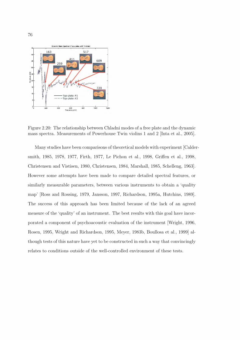
76
Figure 2.20: The relationship between Chladni modes of a free plate and the dynamicmass spectra. Measurements of Powerhouse Twin violins 1 and 2 [Inta et al., 2005].
Many studies have been comparisons of theoretical models with experiment [Calder-
smith, 1985, 1978, 1977, Firth, 1977, Le Pichon et al., 1998, Griffen et al., 1998,
Christensen and Vistisen, 1980, Christensen, 1984, Marshall, 1985, Schelleng, 1963].
However some attempts have been made to compare detailed spectral features, or
similarly measurable parameters, between various instruments to obtain a ‘quality
map’ [Ross and Rossing, 1979, Jansson, 1997, Richardson, 1995a, Hutchins, 1989].
The success of this approach has been limited because of the lack of an agreed
measure of the ‘quality’ of an instrument. The best results with this goal have incor-
porated a component of psychoacoustic evaluation of the instrument [Wright, 1996,
Rosen, 1995, Wright and Richardson, 1995, Meyer, 1983b, Boullosa et al., 1999] al-
though tests of this nature have yet to be constructed in such a way that convincingly
relates to conditions outside of the well-controlled environment of these tests.

77
200-500 Hz
550-700 Hz
1000-1250 Hz
2000-5000 Hz1500 Hz
800 Hz
Figure 2.21: Principal radiation directions for a violin. From [Meyer, 1972].
2.11 Acoustic radiativity of the guitar
At lower frequencies (< 350 Hz) the guitar essentially radiates sound spherically,
with increasingly complex spatial configurations at higher frequencies [Le Pichon
et al., 1998], similarly with other stringed instruments, such as the violin in Figure
2.21 [Meyer, 1972].
For the guitar, the majority of the radiated energy is in the monopole form [Chris-
tensen, 1984], where the entire body is able to flex, producing a large net volume

78
change [Caldersmith, 1985].
If the instrument is assumed to be a simple point source radiator, a result of
driven by a sinusoidal force with amplitude F, at an angular frequency of ω, the air
pressure at a distance r from a single (uncoupled) mode with resonant frequency
ω0, damping γ, and effective mass m and effective area A may be expressed as
[Christensen and Vistisen, 1980]:
p = FA
m
ρ
4πr
ω2
(ω20 − ω2) + jγω
(2.11.1)
where ρ is the density of the air. Thus the pressure amplitude is greater for a
low effective mass and high effective radiating area.
However, for a constant excitation force the intensity of acoustic radiation from
the guitar, in general, not only a function of distance from the instrument but also
has an angular dependence, especially at higher frequencies. This distribution of
acoustic intensity in space can be represented by radiative contributions from each
resonance mode, which can be modelled using spherical harmonics [Derogis et al.,
1995].
Pmn (x) = (1 − x2)
m2
dmPn(x)
dxm, Pn(x) =
1
2nn!
dn(x2 − 1)n
dxn(2.11.2)
For the nth degree spherical harmonic:
Yn(φ, θ) = an0Pn(cos φ) +n∑
m=1
(anm cos mθ + bnm sin mθ)Pmn (cos φ) (2.11.3)

79
The solution of Laplace’s equation (∇2T = 0) in a sphere (r = a = constant a ≥0 ε R) which is dependent only on the angle as r → a and is finite at r = 0 is of the
form:
T (r, φ, θ) =∞∑
n=0
(r
a)nYn(φ, θ) (2.11.4)
Taking θ = 0:
T (r, φ, 0) =∞∑
n=0
(r
a)nYn(φ, 0)
=∞∑
n=0
(r
a)n[an0Pn(cos φ) +
n∑m=1
(anm + bnm)Pmn (cos φ)]
=∞∑
n=0
(r
a)n[ano
1
2nn!
dn(cos2 φ − 1)n
dxn+
n∑m=1
(anm + bnm) sinm φ] (2.11.5)
Or by taking φ = 0 :
T (r, 0, θ) =∞∑
n=0
(r
a)nYn(0, θ)
=∞∑
n=0
(r
a)n[an0
1
2nn!
dnconst.
dxn+
n∑m=1
[anm cos mθ + bnm sin mθPmn0]]
= 0 (2.11.6)
The angular, radial and frequency dependence of the acoustic radiation from the
instrument is then:
Hn(r, θ, φ, ω) = h(2)n (jkr)Pn(cos θ) (2.11.7)

80
where the h(2)n (jkr) are the spherical Hankel functions, and Pn(cos θ) represent
the nth order Legendre’s polynomial in cos(θ).
The former can be expressed as:
h(2)n (jkr) = J0(jkr) − iY0(jkr) (2.11.8)
Where J0(x) = 1 − x2
22 + x4
24(2!)2− x6
26(3!)2+ ...
and the latter, Y0(jkr), are the Taylors’ series solutions to the differential equation
(1 − x2)y′′ − 2xy′ + n(n + 1)y = 0 (2.11.9)
with x = cos θ [Boas, 1983].
With the requirement that Pn(1) = 1, the first few Legendre polynomials are:
P0(x) = 1, P1(x) = x and P2(x) = 12(3x2 − 1).
2.12 Conclusion
A quantitative description of how important elements contribute towards producing
the sound of the guitar has been developed, after the definition of important com-
ponents of the guitar. Some methods have been developed to characterise vibratory
modes of the instrument, such as through plate resonances and the effect of the low
frequency air cavity (Helmholtz) resonance. Simple models of important coupled
systems, such as the string/body and soundboard/air cavity were presented. Some
possible measures were derived to characterise a particular instrument so that the

81
probability of reproducing a particular instrument may be improved. The next chap-
ter examines the properties of the common materials and methods used in making
guitars.

Chapter 3
The Construction of the Guitar
“The art of making a good instrument is a complex marriage between ‘sound quality’,
playability and visual æsthetics—with a little bit of whim and luck thrown in for
good measure.” —Bernard E. Richardson [Richardson, 1995b]
The physical models, as presented in the previous chapter, help illuminate many
of the instrument design and construction decisions made by luthiers. However, a
large part of this illumination is given through the clarity of hindsight. If a maker
experiments with a variation in design, they usually have some idea of the outcome,
and is not often done in a quantitative manner. The lack of objective measures of
the ‘sound quality’ of a particular instrument means that design innovations and
testing methods applied by makers are usually performed in an ad hoc fashion and,
in this environment, trial-and-error experiments have provided the most satisfactory
results. The lack of controlled scientific experiments in this area means that the
consistency of high quality instruments is not assured—even among expert makers
[Richardson, 1988]. This chapter examines necessary technical details on important
construction processes. The details of techniques described here are those carried
82

83
out in the Gilet workshop.
3.1 Introduction
Modifications to the design of the guitar are not dictated solely by acoustic consid-
erations. A particular instrument may well have what is agreed upon as a ‘good’
sound but if it is not appealing in an æsthetic, economic and ergonomic sense it
will be very hard to sell such an instrument. The ergonomic and visually æsthetic
attributes of the guitar are recognised as important but are beyond the scope of the
present work. Most components serve structural, acoustic and æsthetic functions
simultaneously. However, only modifications relevant to the acoustic and vibratory
behaviour of the guitar will be addressed in this thesis.
An important trend in the last two hundred years has been for an increased sound-
board area, in response to demand for a louder instrument [Morrish, 1997, McIntyre
and Woodhouse, 1978]. This requires thicker and more rigidly braced soundboards
with stronger materials to retain structural integrity, and to efficiently couple with
the air.
The other variations that affect the timbre are not obvious. Historically, many
changes in construction techniques are a result of technological advances (such as
the adoption of aliphatic resins instead of animal hide glue) or the availability of
materials. The species of wood used on the soundboard has a great effect on the
tone. A range of timbers are used for this purpose [Richardson, 1998, Gerken, 2001,

84
Morrish, 1997, Belair guitars, 2002, Worland guitars, 2004]. For instance the North
American timber, Sitka spruce (Picea sitchensis), is now accessible to most luthiers,
whereas the decline in stock of the popular Brazilian Rosewood (Dalbergia nigra)
now makes it extremely difficult to obtain legally in most countries.
3.2 Material used in construction
Wood is the most widely used building material in the world: the word ‘material’
itself derives from the Latin word for timber, materia. Wood is by far the most
widely used material in manufacturing stringed instruments. Despite the variety of
construction materials currently available (such as synthetic polymers and carbon
fibre composites [Besnainou, 1995]), luthiers have usually continued using wood.
Do damping and elastic properties of wood appear to be preferred by players and
listeners? Many luthiers have experimented with other materials but it appears
there is difficulty accepting an instrument whose sound is unlike that produced by a
natural timber. The manufacture of stringed instruments requires some knowledge
of the engineering properties of the wood species used.
The structure of wood
There are several works on how the bulk properties of wood relate to the cellu-
lar and microscopic nature of the material [Bucur, 1995, Gibson and Ashby, 1997,
Haines, 2000, Bodig and Jayne, 1982, Forest Products Laboratory, 1999]. Wood is
a complicated composite of hard-celled cellulose microfibrils (organic cells known

85
as tracheids) embedded in a lignin (phenyl propane based polymer) and hemicellu-
lose resin matrix. Wood exhibits great variation in its mechanical properties [Forest
Products Laboratory, 1999, Chomcharm and Skaar, 1983, Caldersmith and Freeman,
1990] . The seasonal variation in the cell wall density of a tree is evident, when look-
ing at the end of the cut log, as a concentric ring structure known as growth rings
formed by the walls of the long slender tracheids. The orientation parallel to the
axis of the tracheids is known as the grain direction (Figure 3.1.) The tracheids are
cellulosic polymers (based on the mer C5H10O5), as is hemicellulose. However, the
tracheids exhibit a very high degree of polymerisation (5000 → 10000) compared to
the hemicellulose (150 → 200) [Flinn and Trojan, 1975]. Because the microstructure
of wood is composed of these long polymer chains embedded in a resin, the mechan-
ical properties of wood are highly anisotropic. This is illustrated in Table 3.1, which
also illustrates some of the variation found in the density and elastic moduli in some
commonly used timbers [Kaye and Laby, 1973]. However a table such as this one is
inadequate for determining high quality wood to be used for constructing elements
of a guitar; the quantities shown here are a rough illustration of typical properties
of common species. The material properties within a log vary because of the grain
distribution, and show massive variations at the cellular level in the growth ring
plane (about 1 → 10μm) [Gibson and Ashby, 1997]. To some extent the material
properties are less variable on larger scales, because of the effect of averaging over
many cells. The wood used in guitar soundboards is always cut such that the long
axis is parallel to the long axis of the tree (§3.2). In doing this, the speed of sound is
higher and the values of damping lower than for wood cut at an angle to the grain
[Schleske, 1990].

86
Figure 3.1: The principal axesuseful for modelling wood asan orthotropic material. From[Schleske, 1990].
Taking the tree trunk as a series of concen-
tric cylindrical shells, and, cutting thin enough
rectangular prisms, the growth ring curvature is
negligible and occurs in straight parallel lines or-
thogonal to both the longitudinal and the tan-
gential axis. The wood specimens examined
in this thesis are generally such that dimen-
sions in the growth ring plane are small enough
(� 12 mm), so the properties are essentially or-
thotropic, as shown in Figure 3.1. The principal
axes are denoted by the following subscripts:
i =
⎧⎨⎩
L (longitudinal) parallel to the grain;R (radial) in the radial direction;T (tangential) orthogonal to L and R.
A piece of timber that is cut from a log as a
rectangular prism, so that the long axis is parallel
to the grain fibre orientation, and so the width
of the prism is in the radial direction, is said to be quarter-sawn. Most woods used
for the top, back and side plates, and the braces of the guitar, are of quarter-sawn
timber. As Table 3.1 suggests, there is a direct relationship between the speed of
sound and the angle to the grain, along the length of a given specimen of wood
[Schleske, 1990].
In addition to being quarter-sawn, the timber used for the two halves of the
soundboard (and sometimes the back) is book-matched, where the material is two

87
Wood Relative density Young’s modulus AnisotropySpecies Longitudinal Radial Transverse ratio
EL(GPa) ER(GPa) ET (GPa) EL
ER
Ash 0.7 16 1.6 0.9 17.8Balsa 0.2 6 0.3 0.1 60.0Beech 0.7 14 2.1 1.1 12.7Birch 0.6 16 1.1 0.6 26.7
Mahogany 0.5 12 1.1 0.6 20.0Oak 0.7 11 — — —
Walnut 0.6 11 1.2 0.6 18.3Teak 0.6 13 — — —
Douglas Fir 0.5 16 1.1 0.8 20.0Scots Pine 0.5 16 1.1 0.6 26.7
Spruce 0.4 → 0.5 10 → 16 0.4 → 0.9 0.4 → 0.6 11.1 → 40
Table 3.1: Some examples of the range of material properties exhibited by differ-ent species of wood. Notice that many wood species, including spruce, are highlyanisotropic in their elasticity (i.e. EL
ER
� 1). From [Kaye and Laby, 1973].
plates from directly neighbouring cuts (Figure 3.2) and the grain features and density
distribution are symmetric about reflection along the L axis, much like a book.
The complexity of wood structure means that a great variation in physical prop-
erties occurs not only amongst individuals within a species, but even among neigh-
bouring pieces extracted from the same tree (§5.5 and Table 5.5, [Caldersmith and
Freeman, 1990]). This makes the processes of timber selection and quality control
important for optimising the mechanical properties of components for an instrument
and in improving the rate of replication of a particular instrument. In general the
mechanical properties vary the most between the grain (L) direction and the other
two (R,T) directions. For Sitka spruce, the Young’s modulus in the grain direc-
tion is often more than twenty times that in the other directions [Forest Products
Laboratory, 1999, Harjono and Dunlop, 1998].

88
a) b)
Figure 3.2: Schematics of the process of a) quarter-sawing and b) book-matchingwood from raw log form. Most high quality sound boards are of book-matchedquarter-sawn timber. From [Williams, 1986a].

89
Bulk properties and the use of wood
Aside from the variation in mechanical properties with direction, wood also varies in
mechanical properties as a function of other parameters. One of the most important
of these is the internal moisture content of the wood. Wood is hygroscopic, interacting
with the moisture in the ambient atmosphere to reach an equilibrium of the mass
proportion of internal water. The moisture content is defined as the mass fraction
of free water in the wood:
Υ =minital − mdry
mdry
(3.2.1)
where minitial is the initial mass and mdry is the mass of the sample with all of
the free water removed. The process used in this thesis to obtain the dry mass is
the oven-dry method [Forest Products Laboratory, 1999] and the technique used is
detailed in §5.3.
Significant seasonal differences in the equilibrium moisture content (EMC) [Simp-
son, 1998] give changes in the mass density and the elastic moduli (§5.3). It is there-
fore important to control, or at least measure, the moisture content of the wood
when making other measurements of the properties of woods. All high quality wood
used in stringed musical instruments undergoes a period of seasoning, where the
wood is stored in an environment with a controlled humidity and temperature for an
extended period of time (often for many decades) to allow the wood to equilibrate.
The most well understood and important equilibrium process here is that of the in-
ternal concentration of water in free liquid form. Although there is believed to be an

90
amount of chemical equilibration (including the varying degree of polymerisation)
which has a complicated relationship with the moisture content of the wood, the
seasoning process results in greater mechanical stability of the material. Differences
in mechanical properties have been observed between a well seasoned and a ‘merely’
dry piece of wood [Manno, 1988].
Some seasoning processes involve steeping the freshly cut wood in a body of wa-
ter to remove the more volatile matter in the sapwood [Hamlin, 2004] and there is
one account that the wood used for making the Cremonese violins were stored in the
same housings as livestock and the urea, from the urine of the animals, accelerated
the seasoning process [Lolov, 1984].
The equilibrium moisture content (EMC) of a live (or recently felled) tree is
generally about 30 → 200% [Forest Products Laboratory, 1999], whereas the nominal
EMC of a piece of wood in typical atmospheric conditions where the work of this
thesis was done (viz. values given in a table of material property data for Sydney,
Australia) is at 12% [Simpson, 1998].
Luthiers often fabricate the soundboard and bracing in an environment that is
conducive to the adsorption of adhesives: as dry as practical, without damaging the
microstructure. The soundboards constructed here were made in a controlled envi-
ronment with a relative humidity of 43 ± 2% within the Gilet workshop.
Although the wood specimens used in the manufacture of high quality stringed
instruments is usually of very high quality, they may have many inhomogeneous
features or defects, as a result of natural processes occurring while the tree is growing.

91
The grain density may often be irregular, so that the growth rings are not parallel.
An extreme defect of this nature is when a branch or other growth is encountered,
producing a knot. There may also be disconnected regions of volatile material (pitch-
pockets). Invariably, the elastic moduli and strength of a piece of timber is strongest
when there are no defects (clear wood) [Forest Products Laboratory, 1999].
Elastic moduli and densities
The simplest non-trivial stress-strain relation for solid materials is Hooke’s law. If
σi represents the stress (applied force in the ith direction per unit area in the plane
perpendicular to i) then, for an ideal elastic material, there exists a corresponding
strain in the ith direction, ξi, according to the following relationship:
Ei =σi
ξi
= elastic modulus for the material (3.2.2)
Where Ei is the relevant elastic modulus in the ith direction. One would ex-
pect that the most reliable method for determining this in a specimen would be to
directly measure the resulting strain from a given applied stress, but this so called
static measurement method can be difficult to apply in practice and may not accu-
rately represent the dynamical behaviour of the sample because of time dependent
effects such as mechanical hysteresis (e.g. creep) [McIntyre and Woodhouse, 1986].
Pulsed ultrasonic vibrations are used for material characterisation for more isotropic
materials [McMaster, 1959] but, because of scattering within the grain layers, a nat-
ural filtered bandpass system is set-up, making the measurements dependent on the
band frequencies, although Voichita Bucur has done much work in this area [Bucur,

92
1995]. A reliable method for determining the elastic and damping properties of sam-
ples at the frequencies of interest is by vibrating the beam at audio frequencies and
analysing the subsequent behaviour under certain restraints (a dynamic measure-
ment method [Schlagel, 1957, Dunlop and Shaw, 1991, Harjono and Dunlop, 1998]).
This has the advantage of accurately measuring the damping and determining the
elastic properties. There is also a difference in dynamic EL and damping compared
to static measurements [Ouis, 2002]. The group velocity of vibratory waves in a large
solid (‘speed of sound’) in the ith direction of the material, ci, is dependent on the
appropriate elastic properties and density of the material in question. In this case
the lateral vibrations of a slender beam are measured, and it is necessary to know
the speed of longitudinal compression waves through the beam. In this case the
important elastic constant is the longitudinal Young’s modulus EL and the relevant
inertial property is the bulk mass density, ρ. So the speed of sound is then:
cL =
√EL
ρ(3.2.3)
A simplifying assumption is that the elasticity of wood is homogeneous (the elas-
tic properties are independent of any particular point under consideration) thereby
ignoring the obvious variability of wood on a microscopic scale (§3.2). It is inad-
visable to extrapolate the following treatment to wood with linear dimensions much
different to what is presented in this thesis. If a typical sample of spruce is much
larger than about 5 mm in the tangential direction, the assumption of orthotropy
becomes unreasonable, and if the sample is too small the detailed microscopic nature
of the wood is significant [Gibson and Ashby, 1997].

93
Wood species Mass Radiation Modulus Logarithmicdensity Ratio Ratio decrement
cL
ρEL
ET
δ × 102
(kg · m−3) (m4 · kg−1 · s−1)Western Red cedar 305-380 14.4-16.4 11.1-25.0 2.1-4.4
Sitka spruce 405-475 11.5-14.0 16.7-33.3 2.7-4.6Californian Redwood 390-400 10.8 2.9-3.7 2.5-3.1
Norway spruce 450-490 8.7-11.0 7.1-12.5 2.7-4.4European maple 570-670 6.0-7.0 4.2-5.6 3.2-4.2
Table 3.2: Measurements of physical properties of representative specimens of clearwood from species important for use in stringed musical instruments [Dunlop andShaw, 1991].
3.3 Damping
Damping is a measure of the loss of energy of a dynamic system to the environment,
resulting ultimately in the form of heat. There are a few accepted measures to quan-
tify damping, each with a slightly different purpose. The most useful expressions
of damping describe how the system loses energy over time. For a linear vibratory
system with viscous losses, this can be expressed most conveniently by the amount
of energy lost per vibratory cycle, which is easily translated to the frequency domain.
Radiative damping can be measured by looking at the decay time of the system.
If a linear oscillatory system is excited by a relatively large initial impulsive force ( ie:
occurring over a relatively short time) and is then left free of external influences, a
global maximum occurs within the first cycle, directly after the impulse, and will have
progressively smaller amplitudes. The decay time is the time taken for the amplitude
(the displacement at the same phase angle) to become e−1 = 0.37 of the initial value.

94
The damping or loss factor, d, of a particular resonance is the reciprocal of the
quality factor, Q, of that resonance. If f1 and f2 represent the lower and higher fre-
quencies directly surrounding the resonance frequency f0 where the spectral power
has dropped to half the local maximum, then f2 − f1 ≡ Δf is the bandwidth of the
resonance. The damping can then be expressed as in Equation 3.3.1.
d =1
Q=
f0
Δf(3.3.1)
In practice, this method is experimentally expedient for d � 0.001 → 0.6. If
d � 0.6, no standing waves are able to form, making amplitude measurements
impossible, while if d � 0.001, the resonance peaks become too narrow, making
measurement of the bandwidth, Δf , difficult [Schlagel, 1957].
Time (arbitrary)
Am
pli
tud
e (
arb
itra
ry)
Figure 3.3: Theoretical damping for a ma-
terial with low damping constant (From
[Schlagel, 1957]).
Another, related, measure of damp-
ing is the logarithmic decrement, δ.
This is the ratio of any two consec-
utive displacement amplitudes. This
measure is useful if the damping is ef-
fectively viscoelastic (ie strictly pro-
portional to velocity only; the sub-
stance is both viscous and elastic when
experiencing deformation) and there-
fore would expect the displacement en-
velope to decrease exponentially over
time.

95
It may also be convenient to analyse a system in terms of the phase shift between
stress and strain produced by damping. If we introduce the concept of a Dynamic
Elastic Modulus [Schlagel, 1957]:
E∗ = E ′ + jE ′′ = E ′(1 + jd) (3.3.2)
Where E∗ is a complex quantity and d, the loss factor from Equation 3.3.1, is a
function of the loss angle, δ:
d = tan δ =E ′′
E ′=
I(E∗)
R(E∗)(3.3.3)
and the conventional elastic modulus may be obtained by taking E = E ′ =
R(E∗).
The loss factor of the ith resonance may be found by examining the time taken
for the peak amplitude of the system to fall to 60dB below the maximum (the
reverberation time, Trev.) and the frequency of that resonance:
di =loge(103)
πTrev.fi
=2.199
Trev.fi
(3.3.4)
These damping measures may be related to the Q-value of the appropriate reso-
nance by:
d =1
Q= tan δ (3.3.5)

96
Damping in wood
Because of the complicated nature of wood, there are several different mechanisms
responsible for losses in the acoustic and mechanical vibration of wooden compo-
nents. The largest internal source of damping is in the lignins, because the structure
of the cellulosic microfibrils are fairly crystalline.
Internal damping is an important vibratory characteristic of wood that has been
largely overlooked in previous works, partly because of the difficulty of measurement.
A reliable method of determining it is through low audio-frequency vibration [McIn-
tyre and Woodhouse, 1986]. Measurements of Sitka spruce give a nominal damping
factor of d ∼ 0.02 [Haines, 2000]. However there is a great variation in damping be-
tween specimens, making it difficult to guarantee the accuracy of a general value for
a particular piece of wood. There is also some variation of damping with frequency
[McIntyre and Woodhouse, 1986].
The anelasticity of wood
Calculation of the Young’s moduli of wood samples from the lowest resonance fre-
quency assumes that damping is a constant of the material. However there is some
dependence on frequency of the elastic moduli and damping measured here, as well
as in other studies on the vibroelastic properties of wood [Ouis, 2002, Haines, 2000].
If the effect is significant, this compromises the assumption of ideal elasticity
(Hooke’s law, Equation 3.2.2). Assuming the dynamic behaviour is non-plastic (i.e.
no mechanical hysteresis occurs), this phenomenon is known as anelasticity. It is

97
not clear if there is significant mechanical hysteresis at stress amplitudes normally
encountered in the stringed musical instruments.
The damping of musical instrument wood is noticeably frequency dependent. It
would hence be appropriate for the present application to use values obtained in the
frequency range of interest, 0 → 1200 Hz.
There is evidence for this frequency dependent nature of damping of materials
other than wood, for example in Figures 3.4 and 3.5, where relaxation processes
occur on the lattice level between atoms of various elements in alloy form.
Figure 3.4: The dependence ofdamping (logarithmic decrement)on frequency is different for paraf-fin and steel (From [American In-stitute of Physics, 1972]).
Figure 3.5: An example of thefrequency dependance of damp-ing (in this case, the logarithmicdecrement) for a metallic alloy.‘German silver’ is an alloy of cop-per, zinc and nickel (nominallyCu0.5Zn0.2Ni0.3) (From [AmericanInstitute of Physics, 1972])
The relationship between stress and strain is more complicated than that in
Equation 3.2.2, due to the introduction of linear independence of the rates of change
of both stress and strain, giving the relaxation equation[Skudrzyk, 1968]:

98
ξ + τξ ξ = K(σ + τσσ) (3.3.6)
Here τξ and τσ are constants (the relaxation times) for the strain and internal
stress of the material respectively. These quantities represent the time the compliant
elements take to return to equilibrium after some deformation, and the time taken
for the corresponding internal stresses to equilibrate. If the vibrations are periodic,
the time derivative operator can be replaced: ∂∂t
:→ jω. So, putting Equation 3.3.6
into Equation 3.2.2, the complex Young’s modulus becomes:
E =σ
ξ=
1 + jωτξ
K(1 + jωτσ)=
1
K[(1 + ω2τξτσ) + jω(τξ − τσ)
1 + ω2τ 2σ
] (3.3.7)
and the usual expression for the Young’s modulus is obtained by taking the real
part of Equation 3.3.7:
EY = R(E) =1
K[1 + ω2τξτσ
1 + ω2τ 2σ
] (3.3.8)
So, for relaxation processes, the elasticity is a constant for very low frequencies
(relaxation times are very much quicker than the forced vibrations) and for very
high frequencies (the material stiffens because it does not have a chance to relax to
equilibrium) and increases to a maximum at intermediate frequencies, determined
by the relative magnitudes of τξ and τσ. Some solids, such as rubbers, have a fairly
large range of relaxation times and some metals, such as iron and brass, also exhibit
characteristic relaxation spectra because of internal heat conduction on a microscopic
level. A nominal value for the relaxation time in wood is τ � 10−7 s [Ouis, 2002].
It is conceivable this would occur in wood because of its microscopically complex

99
composition and structure, although the extent of this effect is unknown. There
has been some investigation into the microscopic phenomena responsible for this be-
haviour in wood, which shows that links between long polymer chains are broken
and reformed in a different configuration, resulting in a time-dependent stress-strain
relation similar to that of velcro [Keckes et al., 2003]. It is also possible that relax-
ation on a molecular and macromolecular level in important wooden components of
stringed musical instruments may be responsible for the ‘playing in’ effect of these
instruments, as studied in the work of Carleen Hutchins, among others [Hutchins,
1998, Turner, 1997].
Because the measurement of damping in wood is frequency dependent, it is im-
portant to qualify the frequency region a damping parameter was obtained from.
For the soundboard braces, the frequency range of interest is quite low (� 1000 Hz).
3.4 Traditional techniques of construction
The manufacture of stringed musical instruments has a long tradition and history
and many techniques have been developed for particular instruments that are readily
applicable to others. Many of the techniques used in making guitars are derived from
other, more established, instruments such as the violin. An example of this is the
selection of materials using the tap-tone method. However, over time, the manu-
facturing philosophies of guitar makers have diverged from those of makers of other
stringed instruments. For example most makers of violins only use sharp blades to
shape the plates of the instrument, whereas guitar makers generally use a range of

100
blades, power tools and abrasives. Novelty is considered acceptable, both in design
and in manufacturing techniques.
One of the principles in making guitars has been of increasing simplicity, with
an emphasis on pragmatism. The guitar is a simple instrument to build compared
to most other stringed instruments. It is essentially a system of flat plates1 and is
relatively easy to prepare and to assemble.
Testing and quality control is necessary for establishing a luthier’s reputation.
The practised luthier builds up a vast database of various physical characteristics
important to the construction of a good instrument. There is usually a great reliance
on direct sensory measurement. Useful information may be gained through visual,
tactile, auditory and even olfactory cues. Often the assessment is done intuitively or
subconsciously, and the maker is said to have a ‘feel’ for the technique in question
[Morrish, 1997].
A common mechanical device constructed for a particular task, but not incorpo-
rated into the final instrument, in order to save labour, alleviate tedious activity or
improve safety, is known as a jig. For example, the sides of the instrument are held
together in a jig to retain them in a bent form while the soundboard and back are
glued on. The bridges used on the guitars studied in this thesis are held in a jig so
that the shape is well controlled, enabling a high probability of replication.
It is very difficult to reverse the result of removing too much material from
a wooden component, without compromising or altering the properties. For this
1The sides are initially flat plates that are bent to shape under high temperature and humidity.

101
reason most components are made larger than the final product. This tends to
reduce the probability of reproducing a particular instrument. Consequently, for the
three guitars studied in this thesis, the dimensions of all important components were
made to be those of the smallest member of the set. For example, a common method
of altering the output of the instrument is to remove wood from the soundboard.
In the present study, the soundboards of three guitars were thinned after glueing
to the rest of the body. Each was thinned to an acceptable level, according to
the prescription outlined below, and then the thickness distribution of each was
measured. The portion of each soundboard was made as thick as the thinnest point
for each of the three soundboards.
Tap-tones
One of the most well known traditional methods of appraising wooden components
for use in stringed instruments is the ‘tap-tone’. The luthier holds the piece of wood
at the appropriate position (depending on the geometry; for a slender beam this is
usually at the nodal position of the fundamental free-free mode, viz. 22.4% of the
length of the beam) and strikes the wood percussively. The material properties of
the wood—especially any bulk defects—affect the vibratory properties of important
sound-producing components of the guitar [Ezcurra, 1996]. A considerable amount
of useable information may also be gained from the tactile response of the sample
[Romanillos, 1987]. The extent to which the tap-tone method is useful depends on
the experience of the luthier. It is difficult to articulate the results of a tap-tone
test objectively without some instrumentation. The techniques used in this study
to measure the properties of wood (§5.2 and Appendix C) do so by objective and

102
accurate means which are able to be communicated effectively.
The soundboard
The soundboard is a thin, initially flat, wooden plate. It is composed of two book-
matched plates joined such that the regions with denser growth ring structure (i.e.
that which was closer to the heart of the original tree) are along the central axis
of the guitar. Apart from the æsthetic appeal, this is so that the soundboard is
structurally reinforced toward the centre of the plate. The stiffness distribution of
the soundboard is therefore inhomogeneous by design.
The soundboard is made thin so that it has a relatively small mass for a rela-
tively large area enabling the efficient transmission of vibrations to the surrounding
air. However it must be strong enough to withstand the tension load on the sound-
board produced by the strings. Furthermore, if sound is transmitted too efficiently
from the string, there is less energy in the string to sustain the notes being played on
the strings, which is partly responsible for the ‘play-off between loudness and tone’
[Gerken, 2001].
The famous luthier Antionio de Torres Jurado demonstrated the importance of
the soundboard in the production of sound from the guitar [Romanillos, 1987]. The
soundboard is usually made of spruce or cedar because of their high stiffness to mass
ratio, as well as their desirable damping and anisotropic material properties [Dunlop
and Shaw, 1991].

103
Thinning the soundboard
Some higher quality guitars have their soundboard thinned after being glued to the
sides and back. Usually the edges of the lower bout are thinned, leaving the central
region in the lower bout and all of the upper bout untouched. This increases the
radiation output at middle frequencies (300 → 700 Hz) [Kruger, 1982]. The edges
are made more flexible and less massive.
The luthier marks the thickness on points at the edge of the soundboard, going
from the edges just below the soundhole and smoothly reducing to the thinnest
portion near the butt at 1.5 mm. In this area, the soundboard is marked with a
pencil in a line approximately 80 mm from the edge, following the boundary of the
edges of the soundboard, as in Figure 3.6.
The two tools used to thin the soundboard are a flat carpenter’s plane and sand-
paper glued to the large face of a flat block (175 × 75 × 25 mm) of TeflonR©(poly-
tetrafluoroethylene (PTFE)) in order to give a flat abrasive surface. Therefore, in
conjunction with the thinning prescription, the profile of the soundboard should be
rectilinear. We would not expect much localised variation of the thickness gradient
on scales below about 40 mm in the longitudinal or lateral directions.
During this process, the experienced luthier often listens for the change in acoustic
response when removing soundboard material; the act of sanding or rubbing hands
over the soundboard [Williams, 2003] provides a source of a broad band vibratory
signal over the appropriate frequency range. This is compared with a response
remembered from past experience. Hence this method does not explicitly depend on
the soundboard thickness distribution per se. However for the purpose of controlling

104
Figure 3.6: Working diagram of soundboard thinning procedure, as explained byGerard Gilet to the author.

105
the three guitars in this thesis, it was necessary to have similar thickness distributions
for all three soundboards. Measurement of the thickness variation of the soundboard
at this point is quite difficult; a solution to this problem is given in §6.5.
The back and sides
Ideally the back and sides provide a stiff enclosure so that much of the sound is
radiated from the front of the instrument. This is more of a priority for the classical
guitars than for steel-string instruments because of the necessity of the instrument
to ‘project’ sound in a concert environment (i.e. to strongly radiate sound towards
an audience). Consequently the materials for the back and sides need to have a high
mechanical impedance, such as is found in rosewood or mahogany. The back and
sides of the guitars studied in this thesis are of Sapele mahogany (Entandrophragma
cylindricum).
The sides are made from two initially flat plates and are bent into shape by a
process of heating, at a high moisture content, over a side-jig having springs to force
the sides to the contour of the final instrument. The back-plate is a system of two
plates glued together in a similar way to the soundboard. The back and the sides
are reinforced with a simple bracing system. In addition, the back-plate has a piece
of spruce about 20 mm wide and 3 mm thick (a marriage-strip) to reinforce the joint
between the two plates.

106
Bracing in the OOO steel string guitar
The asymmetric cross-bracing system is the most commonly used in reinforcing the
soundboards of steel string guitars. This style of bracing was adopted after devel-
opment by the C. F. Martin Co. in the late 1890’s [Longworth, 1975]. This bracing
system would be symmetric about the longitudinal axis if it were not for the two
‘tone-braces’ extending through the central region of the soundboard (Figure 3.7).
The tone-braces extend through much of the lower bout and strongly influence the
output sound of the instrument. The large uppermost brace in the upper bout, the
transverse bar, is the largest brace of the system. This and the bridge-plate, which
covers the internal region of the soundboard directly underneath the bridge, are the
only braces not made from Stika spruce. The former is made of Amoora (Amoora
cucullata) and the latter is of Sugar maple (Acer saccharum).
Sitka spruce is the preferred brace material for the back and soundboard because
it has a high stiffness-to-mass ratio [‘the Doc’, 2005, Sheppard, 1997]. However,
Engelmann spruce is occasionally used for the ‘tone-braces’ in the lower bout of
the X-bracing system, and it is thought this has some effect on the output sound
[Sheppard, 1997].
Profiling braces
Once the brace-wood has been selected and made into rectangular beams, it is com-
mon to shape the cross-section so that it resembles an isosceles triangle atop a
rectangle, with the length of the base of the triangle being the same as the adjoining

107
Transverse bar (TV)
Left X-brace (XBL) Right X-brace (XBR)
Soundhole braces (HB)
Left radial brace 1 (RB1)
Bridge plate (BP)
Right radial braces (RBx)
Tone brace 1 (TB1)
Tone brace 2 (TB2)
Left radial brace 2 (RB2)
30
0 m
m
Figure 3.7: The Martin X bracing system used on the guitars studied here. Notethe asymmetry of the bracing system is due to the two ‘tone-braces,’ covering asignificant area of the lower bout.

108
Figure 3.8: Working diagram showing measurement of dimensions of left and rightcross braces, including measurements of brace dimensions. Braces shown are WR-CXBL and WRCXBR, the main cross-braces for the Western Red cedar soundboard.

109
b
a
b2Profiling
a
b
Figure 3.9: The initial brace cross-section is a simple rectangle. This is modified toan isosceles triangle atop a rectangle with a common edge. The apices are furthermodified in the scalloping process such that the cross-section is no longer constant.Figure after [Vernet, 2001].
side of the rectangle (Figure 4.3). The effect of brace profiling is simulated for a
simple brace/plate system, using a finite element model, is presented in §4.3, and
the theoretical effect of this on the normal modes of a slender beam was given in
§2.7.
Considering the requirement to retain a large gluing surface, this profiled cross-
section is more optimal for a bracing beam than a simple rectangle because the
stiffness is a function of the cube of the thickness and only linear with width. There-
fore much of the mass of the brace is reduced with little reduction in stiffness. Some
luthiers have extended this treatment to a parabolic cross-section to further optimise
the function of the braces [van Linge, 1996]. Another example of a brace optimi-
sation technique is the carbon fibre/balsa composite braces used in e.g. Smallman
guitars, which are effectively a type of I-beam.
The main X braces both have a small (roughly 20 mm long) length retaining the
rectangular section (the knuckle) to fit the braces together.

110
One important modification to brace geometry is the process of profiling, a tech-
nique used by luthiers to optimise the stiffness to weight ratio of beams by altering
their cross-section from that of a rectangle to a pentagon. While having the same
total height, a sharp apex is formed, by an isosceles triangle on top of a rectangle
with a width equal to the base of the triangle. Because the geometry is different,
there is some divergence from the vibratory behaviour of a simple beam with rectan-
gular cross-section, due to the change in the radius of gyration, κ, in the direction
of the applied excitation force. Because the resonant frequencies of a simple beam
are proportional to its cross-sectional radius of gyration, κ (see Equation 2.7.5), al-
tering the cross-sectional geometry of the beam will result in a corresponding shift
in frequency. Denoting the changed state as primed variables in Equation 2.7.5 and
the original geometry with unprimed variables, the frequency ratio for the ith mode
is:
f ′i
fi
=
πcκ′s2
i
8L2
πcκs2
i
8L2
=κ′
κ=
√I ′
I
For a rectangular cross-section, height a (in the plane of vibration), ICM = Ma2
12, and,
for an isosceles triangle of height h, the rotational moment of inertia is I ′CM = Mh2
18.
The change in resonance frequencies is thus:
f ′
f=
√12h2
18a2
=h
a
√2
3

111
Thus the frequency ratio becomes:
f ′
f=
√2h√3a
Finally, if the new height is identical to the original, h = a, then the frequency ratio
is simply:
f ′
f=
√2
3
Hence the resonant frequency of a given lateral mode of a cantilever, whose cross-
sectional shape has been made into an irregular pentagon, symmetric upon reflection
about the vertical axis, from a rectangle of identical height, is shifted lower, to about
82% of the original. Therefore the practice of profiling braces significantly reduces the
mass of the brace with little corresponding loss in stiffness in the vertical direction.
This enables more efficient impedance matching between the vibrations of the braced
soundboard and the air because the braces give similar reinforcement with less mass.
The frequencies of the normal vibratory modes are approximately 82% that of the
original brace.
Scalloping braces
The alteration of the cross-section of the braces, so that they are no longer constant
(‘scalloping’, Figure 3.10) was first widely introduced by the Martin Guitar Co. in
the early 1900’s [Longworth, 1975].
This technique is commonly used to alter instruments to produce a more ‘mellow’
tone [Ford, 2005] but the effect has not been well studied mechanically. Scalloping

112
Unscalloped brace Brace with sides scalloped Fully scalloped brace
Figure 3.10: Side view of the scalloping processes of a wooden brace. A beam ofconstant, rectangular, cross-section is shaped such that the edges are tapered witha concavity (partially scalloped) and the middle of the brace is also made concave(fully scalloped brace.)
cannot be performed on some instruments because of the resulting decrease in struc-
tural integrity.
In the present study, important braces on the soundboard (those occupying the
central position on the soundboard: the lower bout portion of the X-braces, and
the larger of the two ‘tone-braces’) went through an intermediary stage of scalloping
where not as much material was removed (§7.6) compared to the completely scalloped
instruments (§7.6.)
Because it is relatively difficult to scallop braces on a soundboard attached to the
back and sides, this process is usually performed before the soundboard is glued to
the rest of the body. It is, however, sometimes required in order to alter the sound
of a fully constructed instrument, in accordance with the wishes of the musician.
Therefore it is useful to examine the changes induced by scalloping the braces of the
finished instruments. Because it was planned ab initio to scallop the braces in the
guitars studied, a template (i.e. a simple shape designed to fit into place inside the
guitars, providing a solid boundary) was constructed from PerspexTM
sheet (2 mm
thick) for each tone-brace at both stages of scalloping (Figure 3.11.) The outlines
of the two stages were marked in pencil on both the braces in each guitar when the
soundboard was being worked on, before attaching it to the back and sides. The

113
templates were used during the scalloping procedure to judge the proximity to the
wanted brace geometry.
A small thumb-plane, some pieces of sandpaper, a small plane mirror and a
portable light-source (Figure 3.12) were used to scallop the braces in accordance
with the markings on the braces and the scalloping templates in Figure 3.11. The
template was sometimes bonded to the inside of the braces with plasticine and all
the work was performed by hand, using the soundhole for access.
Also, a finite element model was constructed to investigate the effects of brace
scalloping in §4.3.
The bridge and saddle system
The bridge/saddle system (§2.2) is the most important element in the conversion of
the vibratory energy of the string to acoustic radiation. Its central position on the
soundboard means that the bridge/saddle system contributes a significant amount
of mass and stiffness to the soundboard, influencing the vibratory modes of the in-
strument at all frequencies (§7.2).
The analogy between the bridge and an impedance transformer is very useful. To
interact efficiently with the air, it is desirable to have a soundboard with a relatively
low mechanical impedance. However, the relatively high impedance of the strings
(i.e. a relatively large amount of force is concentrated over a small area at the
saddle) means that an impedance interface is required to transform the vibration.
Because of this, the wood used for bridges is generally very dense, with relatively
high Young’s moduli, such as ebony or rosewood.

114
Tone-brace template 1
Tone-brace template 2
X-brace template 2
X-brace template 1
Material: 2mm Perspex sheet
Figure 3.11: Outline of the templates used for scalloping the tone-braces in theguitars.

115
Figure 3.12: The tools used in scalloping the tone-braces.
Figure 3.13: Photograph of theset-up for the scalloping proce-dure after the soundboard hasbeen attached to the back andsides.
Figure 3.14: A luthier scallops thebraces with a small thumb-plane,working from inside the sound-hole.

116
The bridge is cut from a flat plate of wood (Figure 2.5), and is made with the aid
of a jig, so that bridges are able to be reproduced with a relatively high degree of
precision. The bridges of the guitars studied here are of ‘Indian’ rosewood (Dalbergia
laterfolia). Measurements of the effect of the bridge on the vibratory characteristics
of the guitars studied in this thesis are given in §7.2.
Break angle and string correction
The strings of a steel-string guitar are held in by the bridge pins (§2.2) which are
some distance (≈ 10 mm) behind the saddle. Hence the strings in this region are
bent over the saddle, making an angle to the plane of the soundboard. This angle
is known as the break angle (the term also applies to the strings terminating at the
nut). A small break angle allows relative motion between the string and the saddle
(or nut), contributing to unpleasant ‘buzzing’ sounds [Ford, 2005]. A high break
angle creates excessive mechanical stress at the saddle and may contribute to the
strings breaking at this point. The optimal break angle is said to be 20◦ → 25◦
[Fishman Transducers, 2004]. Also the saddle is aligned at an angle to the rest
of the bridge, in the plane of the soundboard, because of the string compensation
mentioned in §2.1 [Fletcher and Rossing, 1998].
Linings
The joints between the sides and the soundboard and the back plates are important
for the structural integrity and function of the guitar. To increase the strength of
these bonds, strips of wood (linings) are introduced to the internal interface between

117
the plates and the sides. Because the linings are constrained to follow the curvature
of the sides, the linings are usually made more flexible in the lateral direction through
a series of regular thin cuts (kerfs).
The bindings
The bindings are pieces of timber used to reinforce the boundary formed at the
soundboard and the sides of the guitar. The guitars studied in this thesis also have
a herring-bone, which is a strip of wood joined to the binding material, extending
about 5 mm toward the centre of the soundboard. The effect of the bindings on the
vibration of the guitar soundboards studied here is examined in §6.6.
The neck joint
The neck is the structural member of the guitar that supports the fingerboard, and is
roughly as long as the body of the guitar. The joint between the body and the neck
needs to be strong enough to withstand the tension of the strings in the longitudinal
direction as well as any lateral forces on the instrument. Hence the top portion
of the body usually has a solid block of wood (the neck-block) to enable a strong
mechanical coupling. Traditionally, the neck is joined with adhesives and a dove-tail
joint. However, the guitars studied in this thesis make use of a neck-joint relying
on bolts (a bolt-on neck system), developed initially by Robert Taylor of the Taylor
Guitar Co. This system allows easier access to the neck for maintenance than does
the traditional system, and there is no vibratory disadvantage if the mechanical
coupling is made well [Ford, 2005].

118
Schematics of the necks used here are given in Figure 3.15. The vibratory effects
of the addition of the neck to the body are examined in §7.1.
The surface polish
The process of polishing the guitar involves the application of protective material
onto the outer surface of the exposed plate areas. This process enhances the æsthetic
quality of the instruments, helping to protect the exterior, and provides a buffer
against humidity and thermal changes to the wooden components.
A range of polishes are used on guitars. All require some solvent, most of which
evaporates over time. Once the solvent has disappeared, the polish becomes harder
and is said to be cured.
There is debate on the effect of the polish on the sound of stringed instruments in
general, especially in the case of the violin [Schleske, 2000, Barlow and Woodhouse,
1989, Schelleng, 1968, Fryxell, 1984]. However, it is widely asserted among luthiers
that the best resulting finish is one that is applied as thinly as possible. Nevertheless,
the polish must be sufficient to seal the surface wood cells such that sweat and other
foreign matter does not penetrate the protective barrier [Williams, 1986a]. Before
the application of the actual polish, some alteration of the surface properties of the
guitar occurs. A progression of finer sandpaper is used over all surfaces to be pol-
ished, to P1000 grade (1000 abrasive particles per square centimetre) such that no
scratches larger than ∼ 0.3 mm are visible and there are no sharp discontinuities in
the surface gradient.

119
Figure 3.15: A schematic and dimensions of the neck used here. Dimensions in mil-limetres. The scales do not apply to this reproduction. Image courtesy of MattheiuMaziere and Davy Laille.

120
The polish used on the guitars studied here is a nitrocellulose lacquer, applied
with a pneumatic spray-gun. The effects of the application of polish to the guitar
on the vibratory response of the soundboard is given in §7.3. The effects of allowing
the polish to cure for a period of 63 days are examined in §7.4.
Aesthetic elements
As well as being an engineering structure, a good quality guitar is often a work of art.
There are many elements that serve a primarily æsthetic function. Decoration of the
instrument was reduced to a minimum through the influence of de Torres Jurado
[Romanillos, 1987]. However, some elements of the guitar are purely cosmetic. The
rosette (§2.1) is an annular structure enclosing the soundhole, and is embedded in the
surface of the soundboard. It is usually made from small pieces of various timbers or
mother-of-pearl (the interior layers of the shell of the oyster Pinctada maxima). The
rosette may also protect the soundboard from crack propagation near the soundhole.
The most prominent and intricate cosmetic feature of the (steel-string) guitar is
usually the inlay. The inlay is made of attractive material, commonly mother-of-
pearl or abalone, although semi-precious gemstones have also been used. The inlay
is generally found as position markings on the fingerboard and a motif (often the
luthier’s trademark) is commonly found on the head-stock. Some instruments have
inlay figures on the rosette and the bindings.
The rosettes used on the instruments in this study are a mixture of ebony, spruce
and a rosewood arranged in a ring formation. The butt-strips are of the same material
as the bindings (rosewood and spruce). The inlays on the fingerboards are small thin

121
discs of mother-of-pearl and the fret markers on the uppermost side of the neck are
of high density polyethylene. There are no inlays on the head-stocks.
The butt-strip is a small decorative plate to cover the line formed by the joining
of the sides at the butt of the guitar. The material used for the butt-strips in the
guitars studied in this thesis is the same material used for the bindings.
3.5 Recent innovations
The design of the guitar is still evolving. Improvements are made due to the innova-
tion of the instrument makers and their collaborators. Much inspiration and many
design ideas are borrowed from other instruments. For example, there have been
attempts at installing a soundpost into the instrument, similar to that in the violin,
such as that by Joel Laplane [Laplane et al., 1995]. Laplane also made instruments
with internal bridges and multiple soundholes in various positions, and physical at-
tributes of the instruments, such as the resonance modes, were measured [Chaigne
and Rosen, 1999]. There has been experimentation with the bracing system to ad-
dress particular issues, such as the common occurrence of a nodal line on or near the
third string at the T(2, 1) (see mode nomenclature in Table 2.5) soundboard mode
(at a frequency of about 200 → 300 Hz) producing a large ‘dead area’ on the lower
notes of this string. It is recognised by luthiers and researchers that an approach
using physical principles would be beneficial to the guitar industry as a whole (but
not without some resistance [Kasha, 1995, Brune, 1985b, Wyszkowski, 1985, Hamp-
ton, 1985, Eban, 1985, Brune, 1985a, Williams, 1986b, Wyszkowski, 1986, Margolis,
1986, Brune, 1986]). An oft-quoted success of innovative guitar manufacture is that

122
made by Greg Smallman, in using a lattice-style soundboard bracing system made
of a carbon fibre/balsa composite [Atherton, 1990]. This enabled a great reduction
in mass of the soundboard, creating a much louder instrument.
Because of the novelty seeking nature of many guitar players, and the economic
benefits associated with innovation, it is likely that luthiers will continue to experi-
ment with design features to remain competitive with their peers.
3.6 Phases of construction examined in this thesis
Dynamic mass and pressure force ratio spectra, as well as Chladni figures were
measured at ten stages of construction on the three guitars: the braced soundboards,
the bodies directly after the soundboard was glued to the back and sides, after
applying the bindings, after thinning the soundboard, after putting the bridge on,
after polishing, after allowing to cure and then to age for almost two years, and
then partly and then fully scalloping the cross- and tone-braces. It is inconvenient
to include the full name of each construction stage with the measurements, so the
construction phases will be referred to by the abbreviations in Table 3.3.

123
Construction stage AbbreviationFree soundboard SB
Bodies only BDYAfter binding BB
After thinning BTTWithout neck WON
With bridge GBAfter polishing GF
Allowing polish to dry GHAgeing two years 2yr
Braces partly scalloped SCL50Braces fully scalloped SCL100
Table 3.3: Abbreviations for the construction stages investigated throughout thestudy of the three guitars in this thesis.

Chapter 4
Applications of the Finite Element
Method to instrument
construction
“It is nice to know that the computer understands the problem. But I would like to
understand it too”—Eugene Wigner (1902-1995)
The speed and processing capability of modern computing systems, and the wide
range of software written for them, enables the mechanical modelling of vibratory
systems to be performed easily. The Finite Element Method (FEM) has been applied
in a wide range of problems in mechanical and more specialised types of engineering.
Systems previously modelled range from nuclear reactors [Campbell, 1995] to novel
aerospace transportation vehicles [Abdul-Aziz, 1996].
This chapter summarises some of the work done in collaboration with three un-
dergraduate students from the Ecole Normale Superieure in France working on this
project at The University of New South Wales: David Vernet in 2001 [Vernet, 2001],
124

125
Davy Laille and Mathieu Maziere (both in 2002) [Laille, 2002, Maziere, 2002]. Mo-
tives and methods for using the FEM are given in §4.1. Selection of the appropriate
model and values of material properties and boundary conditions are given in §4.2.
This is followed by applying this method to the problem of scalloping braces on
the guitar soundboard (§4.3) and to the soundboard (§4.5) and the finished guitar
(§4.6) after preliminary study is made on the influence of glue bonds between impor-
tant elements (§4.4). Finally, there is discussion of the application of finite element
methods to the manufacture of guitars (§4.7).
4.1 Methods and motives for using finite element
calculations
Although most of the work in this thesis is of an empirical nature, it is useful to
compare the results of these experiments with numerical simulations based on known
geometry and material properties. This enables interpretation of the experimental
results and also provides, in principle, a tool for the luthier in the diagnosis and design
of instruments, without performing the costly procedure of constructing or modify-
ing existing instruments. It is convenient to perform these numerical simulations
using available and relatively inexpensive computers. The contents of this chapter
rely on two finite element software packages: CASTEM 2000 and Catia V5R7. The
computer used to model using the CASTEM program was a single desktop PC with
a Pentium IIITM
processor rated with a clock ‘speed’ of 800MHz and RAM of 512MB
capacity. The computer system used to run the Catia package was a member of a
cluster of undetermined processing rate, although it is estimated it normally would

126
not process calculations much faster than the machine just mentioned.
The prescription for constructing an FEM of a dynamical system involves the di-
vision of a system into many localised elements, where each element has the mechan-
ical parameters in the linear differential equation for a simple harmonic oscillatory
system, assuming simple viscous damping:
mξ + Rξ + kξ = F (t) (4.1.1)
where ξ is the time-dependent displacement, m is the mass of the element, R the
viscous damping coefficient, k the stiffness of the element and F (t) the resultant of
the external force on the element, which is dependent on the imposed constraints
or boundary conditions, and the neighbouring elements. Solutions to the dynamical
system are obtained numerically for each element.
Previous FEM work done on the guitar
A good overview of numerical models relating to the guitar is given by Antoine
Chaigne [Chaigne, 2002]. Oliver Rogers used an FEM to calculate modal frequencies
on free violin plates after the removal of wood at various parts [Rodgers, 1990]. Ove
Christensen and Bo Vistisen [Christensen and Vistisen, 1980, Christensen, 1984]
presented a simple model of the sound output of the guitar and the coupling effect of
the air by assuming the soundboard and back-plate and the internal air cavity were
simple (point) radiators. Elejabarrieta, Ezcurra and Santamarıa [Elejabarrieta et al.,
2001] modelled the guitar soundboard at various stages of construction, comparing

127
it with a soundboard being constructed by a luthier. The model was modified to
include the hinged boundary properties introduced by joining the soundboard to the
sides (§2.9).
A model, initiated by Bernard Richardson and Gordon Walker [Walker, 1991]
and refined by Bernard Richardson and Howard Wright [Wright and Richardson,
1995, Wright, 1996, Wright and Richardson, 1997], used the methods outlined in
[Christensen and Vistisen, 1980, Christensen, 1984] to simulate the sound output by
the complete guitar and performed psychoacoustic tests using tones synthesised from
this model. It was found that the effective mass and monopole areas of each mode
contributed more to the perception of tone quality than the frequency or Q-value of
the mode nearest in frequency to that considered.
A model of the sound radiation field of the guitar was created, and compared
with experiment, by Alexis Le Pichon, Svein Berge and Antoine Chaigne [Le Pichon
et al., 1998].
Gregoire Derveaux, Antoine Chaigne, Patrick Joly and Elaine Becache [Derveaux
et al., 2003, Becache et al., 2005] presented a model of the guitar with a high degree of
sophistication and completeness. This work models the motion of the plucked string
through to the field of the sound radiated by the instrument. This work involved
collaboration of a group of engineers and guitar-makers.
The models presented below are detailed simulations relating specifically to the
vibratory properties of the steel-string acoustic guitars studied in this thesis. How-
ever, to achieve sufficient accuracy, it is necessary to investigate some aspects of
similar systems to observe the calculated effects of brace scalloping and adhesive
coupling.

128
The FEM software packages
CASTEM 2000 was initially developed by the Mechanical Department of Technology
(DMT) of the French Police Station and Atomic Energy, for modelling thermal activ-
ity in nuclear reactor vessels, and was further developed to model vibratory systems
numerically. In CASTEM, the mesh has to be programmed and each component has
to be explicitly entered as a set of vector co-ordinates.
Using Catia, it is easy to define relatively complicated mesh geometries because
the more limited options allow means of programming via a graphical user interface.
CASTEM gives the user more precision and control over the program structure, as
well as having a broader range of commands and analysis tools, such as the options of
orthotropy and of the output of transfer functions, but is time-consuming to program.
Calculations of a reasonable mesh size can take a long time to perform on a typical
desktop personal computer. Using Catia, on the other hand, it is very difficult
to control the mesh size and geometry, which makes it harder to compare results
to experiment. Occasionally small changes in input parameters can result in large
differences in the output [Maziere, 2002]. It is convenient to construct structures
with complicated geometry in Catia and it is capable of producing sophisticated
animations or rendered drawings of the results.

129
4.2 Inputs for the model
The accuracy of the simulation of vibratory systems depends on the precision of the
boundary conditions and material properties of each component, which are derived
empirically. Also important are the assumptions made about the overall model. For
example, the assumption of isotropy would make computation faster and more effi-
cient, but is of course inappropriate for wood (§3.2).
The assumption of homogeneity is also not appropriate here. The soundboard of
an acoustic guitar is generally made of two plates glued together so that the grain
features and grain density are symmetric about the main axis of the instrument
(i.e. ‘book-matched’ §3.2, §3.4). Because the thickness of the plate is small in the
tangential (T) direction, there is negligible variation in properties in this direction.
However, we should expect the material properties to vary considerably in the radial
(R) direction (§3.2).
Measurements of the spatial variation of Young’s modulus (using the nondestruc-
tive methods described in §5.2) from 11 samples of wood material directly surround-
ing the simple square plates modelled in §4.3, distributed according to Figure 4.1,
showed there were some substantial differences in the resonant frequencies, with
discrepancies of up to 25%, in the case of the fundamental free-plate mode (0,2)
[Vernet, 2001]. Hence the assumption of homogeneity is inappropriate for models of
the guitar soundboards in §4.5 and §4.6.
Measurement of the Young’s modulus in the transverse and radial directions, the

130
Figure 4.1: Illustration of the spatial position of samples taken from wooden materialsurrounding the rectangular plates modelled in §4.3. From [Vernet, 2001].

131
shear moduli Gij or the Poisson’s ratios νij (where i, j are the principal axes L, R and
T) is more difficult. This is partly because of the relatively small size of the samples
(� 100 mm long, � 20 mm wide and � 3 mm thick). All the plates considered here
are thin (i.e. the thickness is no more than 1% of the smallest lateral dimension) so
the value of the Young’s modulus in the direction parallel to the radial axis, ER, is
not important at lower frequencies. For long thin beams, such as the brace material,
the Young’s moduli ER and ET are not as important. Nevertheless, parameters are
required as input for the simulation. Nominal values of the remaining elastic prop-
erties that were not measured were taken from [Forest Products Laboratory, 1999].
The models in §4.6 are performed on Catia, which does not explicitly support
orthotropic input. In this case, orthotropy was simulated by introducing an array
of identical reinforcing rods into the soundboard, of negligible mass and with mag-
nitudes of Young’s moduli necessary to produce the anisotropy found in wooden
soundboards [Laille, 2002, Maziere, 2002].
Hence the wooden components modelled here are assumed to be orthotropic and
the soundboards are assumed to be inhomogeneous along the transverse axis (the
orthotropy is important because the soundboard of the guitar is designed actively to
exploit the innate anisotropy and inhomogeneity of wood [Locke, 2005]).
4.3 Brace scalloping
The process and purpose of brace scalloping is described in §3.4. It may be possible to
relate the change in timbre ascribed to scalloping to the appropriate transfer function

132
characterising the plate. However, the changes to the geometry are complicated,
making it difficult to predict the result. The FEM makes it possible to model the
effects of scalloping on the vibratory behaviour of a plate with bracing. The model
results are first compared with those of two simple thin wooden plates, both in the
shape of a square, with a single diagonal brace, after which the complete guitar
soundboard is analysed. Experiments involving the scalloping of important braces
on the soundboards of finished guitars are presented in §7.6.
Simple plates
The single most important contribution to the sound of the guitar is thought to be
that of the braced soundboard [Meyer, 1983a, Richardson, 1982, Elejabarrieta et al.,
2000, 2001, Rossing and Eban, 1999] . Studying the vibratory behaviour of the free
guitar soundboard is complicated by the details of the bracing structure. It is useful
to compare the vibratory behaviour of a guitar soundboard with a FEM simulation
to understand the important dynamics, but, to be confident of the model, it is help-
ful to compare to a plate of simpler geometry and bracing configuration.
Because the wood is inhomogeneous and orthotropic, the mesh has to be divided
into regions of different properties. Laminar shell elements were used to model
soundboard and braces, both before and after scalloping the braces.
The model was compared to experiments using the Chladni figure technique
(§2.9). Figure 4.2 shows a comparison between Chladni figure experiments on two
simple wooden plates, KBS1 and KBS2, and modal analysis using an FEM [Vernet,
2001].

133
Figure 4.2: Comparison between predictions made by FEM and measurement ofmode shapes and frequencies for two simple wooden plates, KBS1 and KBS2. From[Vernet, 2001].

134
b
a
b2Profiling
a
b
Figure 4.3: The initial brace cross-section was a simple rectangle, measuring 12 ×
8mm. This was modified to an isosceles triangle atop a rectangle with a commonedge. The apices were further modified in the scalloping process such that the cross-section was no longer constant. Figure after [Vernet, 2001].
Braces with constant cross-section
The longitudinal Young’s moduli EL and the mass densities ρ of 11 candidates for
wooden braces having rectangular cross-section (12 × 8mm) made of Stika spruce
were measured. The two most similar in EL (ca. 12 GPa) were retained. Then one
of these was cut longitudinally to give a constant pentagonal cross-section of the
same height as the original (Figure 4.3). The rectangular brace was altered in height
so that it had the same moment of inertia (in the plane perpendicular to the base
of the strut). Both braces were glued diagonally to the simple plates (KBS1 for the
pentagonal and plate KBS2 for the rectangular brace) in the same way a brace is
glued to a guitar soundboard.
The results of Chladni figures on these simple plates are given in Figure 4.4. The
amplitudes of some of the peaks in the transfer functions are of greater magnitude
for the plate with the triangular brace configuration, compared to the rectangular
bracing. The agreement in the measured modal frequencies between the two plates
was within 4%, the greatest difference being at the fifth mode (ca. 450 Hz) where
the brace is a node.

135
Figure 4.4: Comparison of Chladni figures of simple rectangular wooden plates, eachwith a single diagonal brace with rectangular (KBS2) and triangular cross-section(KBS1). The solitary dark point appearing in each image is the position of the smallrare-earth magnet used to drive the plate, in combination with a solenoid. From[Vernet, 2001].
The simulation predicts more distinct modes than are detected experimentally.
In the frequency range 0 − 1000 Hz, 12 modes were identified in the FEM; seven
distinct modes were found experimentally.
Simple rectangular wooden plates having a single scalloped brace The
scalloping process (§3.4) begins with removal of material from both ends of the brace
(‘partly scalloped’) and then from the middle (‘fully scalloped’).
Numerical simulation of the motion of each rectangular plate predicts a lowering
in modes 1, 2 and 3 with little change in mode 5, in response to scalloping the single
diagonal brace. This is confirmed by experiment (Figure 4.5). Agreement with the
measured modal frequencies is good. Experimentally, the sixth mode is lowered in
frequency (from 650 Hz to 580 Hz). This mode has a large number of nodal and

136
FEM calculations Chladni figure measurements
Figure 4.5: Comparison of FEM calculations with measurements of Chladni figuresof simple rectangular plates with single braces partly scalloped. From [Vernet, 2001].
antinodal lines crossing the brace.
Comparison of the partly scalloped plate system to that with a fully scalloped
brace show a 13% increase in the frequency of the second mode, a 8% decrease in
the third mode and little differences in the fourth and fifth mode frequencies (Figure
4.6). Again, this agrees well with experiment (Figure 4.7). Modes with nodal lines
near the region of the brace are affected the most, notably mode four (ca. 280 Hz).
Some differences in the dynamic mass spectra are noticeable at higher frequencies
(30 → 20, 000 Hz, Figure 4.8). However the apparatus used for excitation (Bruel
and Kjær 4809 shaker) and detection (Bruel and Kjær 8001 impedance head) are

137
FEM calculations Chladni figure measurements
Figure 4.6: Comparison of FEM calculations with measurements of Chladni figuresof simple rectangular plates with single braces fully scalloped. From [Vernet, 2001].

138D
yn
am
ic m
ass
(d
B)
0
Frequency (Hz)
Half scalloped strut
Fully scalloped strut
0
50
-10
1000
Figure 4.7: Comparison of dynamic mass measurements of simple wooden plateswith a single brace after scalloping the edges of the braces and after scalloping themiddle part of the brace also. From [Vernet, 2001].

139
Frequency (kHz)
-200
Dy
na
mic
ma
ss (
dB
)
50
20
0
Half scalloped strut
Fully scalloped strut
Figure 4.8: Higher frequency response function of plate with a single diagonal brace.The two plots are that with and without brace scalloping. From [Vernet, 2001]
linear only in the frequency range 0 → 6 kHz. There are some obvious large relative
differences in the magnitudes of the dynamic mass between the plates at about 5,
7.5 and 9 kHz. The peaks are broadened and the peaks are also slightly lowered in
frequency.
The FEM models used here simulate the motion of the plates with the condition
of a free edge. The mass load of the magnet and the sand used to create the Chladni
figures tend to decrease the frequencies of most of the normal modes compared to free-
free conditions by � 5%. There is good agreement between the FEM and experiment
with the frequency and nodal distribution of low frequency vibratory modes, both
before and after brace scalloping of the simple plates. At these frequencies, little
difference is seen in modal frequencies and geometries between the scalloped and the

140
unscalloped plate systems. However both the Q-value and the amplitude of higher
frequency peaks in the dynamic mass spectra increase after scalloping.

141
4.4 Glue bonds
Because all of the important components in a guitar are joined by an adhesive, it
is important to determine whether this bond affects the vibratory properties of the
guitar under the conditions considered here. The mass due to the relatively small
amount of glue required to form a good bond is small in comparison with the brace
itself, so the effect due to mass loading is probably small. However it is conceivable
the bond would damp and either stiffen or weaken the bonded area, depending on
the type of adhesive used.
The comparison of an FEM model with an experiment of the coupling between
a single wooden brace and a simple plate was performed using the simply braced
rectangular structures in §4.3 [Maziere, 2002, Laille, 2002].
For the three lowest frequency modes, the agreement between modelled and ex-
perimental mode frequencies were very similar. However, this agreement diverges at
higher frequencies and it is difficult to determine whether the differences are because
of inhomogeneity of the wood or the coarseness of the FEM mesh. To simplify the
analysis of the influence of glue on interactions between vibrating wooden members,
the interaction between two slender beams, glued together, was studied.
Modifying the simple beam equation (Equation 2.7.1) to obtain a system of two
beams coupled by a glue bond, Maziere and Laille found that the two beams are
essentially co-moving until the glue begins moving at f = fcrit.. However, even if
the Young’s modulus of the adhesive were very small, the critical frequency is quite
high (fcrit. > 20 kHz). Therefore the experimental apparatus used for examining

142
Beam 1
Beam 2
Glue
x
y(x)
Figure 4.9: Geometry of a two-beam cantilever with beam elements coupled by anintermediary adhesive. After [Laille, 2002].
the vibratory behaviour of beams in §5.2 would not be capable of experimentally
verifying any plasticity of the glue bond.
This does not mean that there is no effect of the coupling adhesive on the dy-
namics of two coupled beams below 20 kHz, but it shows there is no tendency for
any in-plane relative motion of two adhesively-coupled beams within the frequency
range of interest. It is therefore appropriate to assume that the wooden braces glued
to the main soundboard may be modelled as if they were joined with no means of
relative displacement.
4.5 The free guitar soundboard
A model was created in CASTEM of the OOO guitar soundboards studied in §6.3,
using a mesh containing approximately 9000 elements [Vernet, 2001]. A larger mesh

143
Figure 4.10: Comparison between experiment and FEM calculation of the first fourmodes of a steel-string guitar soundboard. The numbers given are the frequencies(Hz) that the particular mode occurs. From [Vernet, 2001].
size was not possible because the displacement matrix to be solved has an immutable
size limit. The results were then compared to the modes identified experimentally
in §6.3.
The FEM predicted 12 possible normal modes in the frequency range 50 →
800 Hz. Experimental techniques such as Chladni figures (§6.3) or laser holography
[Jansson, 1971, Richardson, 1982] do not indicate there are this many distinct vibra-
tory modes in this frequency range. Although the Chladni figure method indicates
up to 14 figures in this frequency range (Figure 6.7), these are not all distinct modes;
there are more likely a total of seven. Experimental Chladni figures and calculated
normal modes from the FEM model on the free soundboard of a steel-string guitar
for the first four modes compare well (Figure 4.10).

144
At higher frequencies the areas bounded by nodal lines are usually smaller and
local inhomogeneities in the elastic properties of the wood, which the model is not
able to resolve, become more important. Further, the spatial distribution of the
nodes becomes more complicated so discretisation errors in the mesh become much
more important. Finally, the model used here does not account for the load on
the soundboard surface due to the surrounding air. The mass loading and mode
damping effects of the experimental excitation apparatus and the sand used in vi-
sualising the Chladni figures also affect the vibratory behaviour of the soundboard
and this method gives no direct means of determining the amplitude distribution on
the soundboard surface, unlike the FEM model in [Vernet, 2001].
Scalloping braces on the soundboard
Figure 4.11 shows the results of the FEM calculation presented here for the OOO
steel-string guitar soundboards with a standard Martin cross-brace system with scal-
loped cross-braces. Scalloping of the middle of the cross-braces and the upper tone-
brace was not performed on these soundboards until the guitar was completely fin-
ished (§7.6) hence there is no experimental data in Figure 4.11. Figure 4.12 shows a
calculation for the same soundboard, similar except that only the upper tone-brace
was scalloped. Figure 4.13 shows the results of FEM calculation of a steel-string
guitar having both the cross and the tone braces scalloped.
Again, the two lowest frequency modes are not affected by scalloping the cross-
braces because, in both cases, their central region is not a node at these frequencies.
The third mode is decreased by 33 Hz (25%) and the fourth mode decreased in fre-
quency by 7 Hz.

145
Before
scalloping
After
scalloping
the
cross-braces
Figure 4.11: Calculation of normal modes of a free soundboard of a steel-stringacoustic guitar with standard Martin cross-bracing, after scalloping the cross-bracesonly. From [Vernet, 2001].

146
Before
scalloping
After
scalloping
tone
brace
Figure 4.12: Calculation of normal modes of a free soundboard of a steel-stringacoustic guitar with standard Martin cross-bracing, after scalloping the upper tone-brace only. From [Vernet, 2001].

147
Before
scalloping
After
scalloping
cross
and tone
braces
Figure 4.13: Calculation of normal modes of a free soundboard of a steel-stringacoustic guitar with standard Martin cross-bracing, after scalloping the cross-bracesand the upper tone-brace. From [Vernet, 2001].

148
Although the experiments on scalloped bracing on the guitar soundboard §7.6
are of the plate attached to the back and sides, and are therefore altered by the
interaction with the air and the back and sides, the results compare well with the
model (Figure 4.11). Differences are only large for the third and fourth soundboard
modes, T(2,2) and T(3,2) (Figure 7.39), where there is a slight lowering of frequency
and a broadening of the peak at these modes. There is a slight lowering of the first
soundboard mode frequencies (Table 7.6).
4.6 Guitar body
Using the model of the free soundboard (§4.5) and geometric measurements of steel-
string guitars, an FEM of a complete guitar was constructed, including the strings.
The complete guitar is required to withstand the considerable tension placed on the
soundboard and neck by the strings (> 700N with standard tuning.) The properties
of standard guitar strings were measured, and the results were used to model strings
on the complete guitar. Although the strings add a significant amount of tension
to the soundboard, they contribute little to the dynamic motion of the soundboard
[Laille, 2002, Maziere, 2002]. The model was used to construct an animation showing
the vibratory modes of the soundboard [Laille and Maziere, 2002]. An important
limitation of this model is that Catia is not able to model interactions of the guitar
plates with the air, which is being frequency dependent (§2.8), and has a significant
effect on the mode frequencies (§2.5).
The neck is an important element of the guitar at low frequencies. The two

149
Figure 4.14: Low frequency modes of the complete guitar incorporating the neck ofthe instrument. From [Laille and Maziere, 2002].
first modes of vibration of the entire guitar that involve interaction with the neck,
are given in Figure 4.14. Measurements of the pressure force ratio spectra after
the addition of the neck show features occurring close to these frequencies, but not
without the neck (§7.1). Similar motion is displayed in modal analysis studies of
the low frequency modes of guitars [Russell and Pedersen, 1999, French and Hosler,
2001].

150
4.7 Conclusion: Applications of finite element sim-
ulations to instrument construction
The advantage to manufacturers of a reliable model of the vibratory behaviour of
the guitar is that it would be possible to trial novel design modifications without
constructing the instrument. Detailed modelling of the vibratory behaviour of the
guitar is useful for predicting the effect of particular techniques used by luthiers in
the manufacture of guitars. It is shown here that accurate determination of the
geometry, density and Young’s moduli is necessary. Such measurement is possible
using techniques described in §5.2, if nominal values for ER and νij are assumed for
the appropriate wood species.
For example, modelling of brace scalloping on a simple rectangular wooden plate
with a single wooden diagonal brace shows there is very good agreement with Chladni
figure measurements, both in modal shape and frequency for the lowest five modes.
The modes affected the most are those with a nodal lines near the position of the
brace, especially those with a number of phase changes along the length of the brace.
Measurement shows that the Q-factor of high frequency peaks in the dynamic mass
spectrum of simple plates with a scalloped brace is increased, and there is a general
lowering of peak frequencies. An instrument with a soundboard modified in this way
should thus have less variation in radiated output with excitation frequency.
These conclusions for the simple braced plate systems apply for the model of the
free guitar soundboard; the third soundboard mode is affected most by the scalloping

151
of both the lower part of the cross-braces and the tone-brace.
The model of the free soundboard was then used to model the complete guitar
[Laille and Maziere, 2002]. Coupling effects from the neck contribute to very low
frequency modes (ca. 60 Hz) of the guitar (qv §7.1).
Future calculations
Some of the data in chapters 5, 6 and 7 could be further applied to numerical simu-
lation of the guitar. However, it would be more useful if the models in this chapter
were improved by addressing some of the challenges raised.
Further, while CASTEM 2000 is able to produce transfer functions of the mod-
elled system, it is more difficult to program the detailed geometry required in mod-
elling a guitar and it has a limited mesh size. Catia is more convenient to program
complicated mesh geometries, but does not directly support the modelling of or-
thotropic materials. Neither package is currently able to model the interactions of
plates with the surrounding air.
Modelling the effect of these changes on the overall sound produced by the guitar
would be more complicated and is not performed here.

Chapter 5
Experimental: Selection of
Materials
“While felling three spruce trees with a fellow violin maker at an altitude of 1700
metres, we were amazed by the differences in sound that were produced when the seg-
ments of the trunk came crashing down in the steep mountain terrain: One would
make a dull sound while the other would be bright and clear as a bell.”—Martin
Schleske (1965-)
To produce wooden musical instruments with consistent mechanical properties,
one must characterise the material properties of its components before construc-
tion. This chapter presents some techniques used to determine the important mate-
rial properties, according to the luthier, of components incorporated into the steel-
stringed acoustic guitars studied in this thesis. The Young’s modulus in the longi-
tudinal direction EL is important for braces. This is also true for the soundboard,
along with the Young’s modulus in the transverse direction, ET , and the mass den-
sity ρ. There may be some sensitivity of vibratory modes involving a large amount of
152

153
torsion to variation in the shear modulus GLR, but the shear modulus GLT and the
Young’s modulus in the radial direction, ER, are not as important for determining
the vibratory properties of thin plates [Ezcurra, 1996]. For thin beams and plates,
the variation in Poisson’s ratio for wood has little effect on the resulting dynamics.
The important soundboard braces are characterised by driving point dynamic
mass measurements (§5.2). For the soundboards, the driving point dynamic mass
at the bridge point, the damping of important resonances, and the spatial distribu-
tion of the normal vibratory modes by use of Chladni patterns (§6.3) are measured.
Other components have less stringent vibratory and acoustic requirements [Meyer,
1983a].
The choice of wood species used for the various components of the guitars studied
here are described in §5.1. The method used in measuring the elastic properties of
wooden samples are given in §5.2, and some alternatives to this are presented in
Appendix C. Desirable properties of the important components of the guitar are
presented in §5.4, including measurements of the components incorporated into the
guitars studied here. Internal damping of the components are given in §5.11 and the
results are summarised in §5.12.
5.1 Timber used in the guitars studied
The great variety of species used in the manufacture of any individual guitar il-
lustrates the level of exploitation and optimisation of the mechanical and æsthetic
properties a luthier requires in order to produce a high quality instrument. A list

154
of the timbers used in manufacture of the components of the guitars studied here is
given in Table 5.1. Not only is Sitka spruce sought after for brace material (§5.5), it
is also used commonly for soundboard timber in steel-string guitars, giving a gener-
ally ‘bright’ sound (i.e. radiating relatively high power at high frequency [Schubert
et al., 2004]). Engelmann spruce soundboards also give a relatively ‘bright’ sound
but they are more ‘mellow’ than Sitka spruce soundboards. Western Red cedar is
said to give even greater ‘mellowness’ [Belair guitars, 2002, Worland guitars, 2004,
Alaska specialty woods, 2005]. Cedar is used more commonly in classical guitars.
The three timbers mentioned here are commonly used for making soundboards and
it is for this reason that these three timber species have been chosen for the present
work. The other materials used in the construction of these instruments are used on
production instruments made in the Gilet Guitars workshop.
Mahogany or rosewood is commonly used for back and side materials because of
their visual beauty [Romanillos, 1987], but these timbers are also dense and provide
a stiff enclosure so that more sound energy is radiated through the top of the in-
strument. The neck and neck-block are made from Amoora (Amoora culcullata), a
dense timber with a high surface hardness. The fingerboard is of ‘African’ rosewood
1 (Dalbergia holideria) and the bridge is made of ‘Indian’ rosewood2 (Dalbergia lat-
erfolia) which are both visually attractive and also very dense, hard and resistant
to moisture induced degradation. The tail-block is made of high quality hardwood
ply (to reduce cracks forming along the grain) and is a combination of timbers. The
1This common term applies to a number of similar timber species originating in Africa.2This common term applies to a number of similar timber species originating in India.

155
linings of the instrument (§3.4) help the glueing of the top soundboard and back
plate to the sides and, depending on the style of lining, need to have a high grain
density to prevent splitting due to the enforced curvature. The rosettes (§3.4) used
here are manufactured from a combination of rosewood, ebony and maple cut into
small square cross-sections (� 4 mm2) approximately 2 mm high. These are glued
in a series of concentric rings. The butt-strip (§3.4) is made of a rectangular plate
of rosewood with a small border of maple, the same thickness and type as the maple
used in the bindings. The inlays (§3.4) have a purely decorative purpose and are
made of mother-of-pearl. The nut is made of cattle bone. The saddles are made of
a hard polymer (TUSQTM
) and the bridge pins are also of a durable polymer. The
frets and the machine (tuning) heads are made primarily of stainless steel.
5.2 Measurement techniques
A beam resonance measurement technique similar to that used by John Dunlop, M.
Shaw and Redes Harjono [Dunlop and Shaw, 1991, Harjono, 1998], is used to measure
the Young’s modulus of wooden beams. The specimen to be tested is placed in the
jaws of an aluminium clamp, as in Figure 5.2, so that the jaws firmly hold the beam
halfway along its length. A time-varying force is applied to the base of the clamp
by a shaker/vibrator (Bruel & Kjær 4809), with an impedance head (Bruel & Kjær
8001, force sensitivity: 379 mV/N Acceleration sensitivity: 3.12 mV/ms−2 Linear
frequency range: 0 → 6500 Hz)). This enables measurement of the time-varying
force and acceleration at this point. The dynamic mass (the ratio of these quanti-
ties) of the system is then analysed; the normal modes of the system are identified

156
Component Wood TypeBotanical Name Common name
Soundboard 1 Picea sitchensis Sitka spruceSoundboard 2 Picea engelmannii Engelmann spruceSoundboard 3 Thuya plicata Western Red cedar
Back Entandrophragma cylindricum Sapele mahoganySides Entandrophragma cylindricum Sapele mahoganyNeck Amoora cucullata Amoora
Neck block Amoora cucullata AmooraSoundboard bracing Picea sitchensis Sitka spruce
Back bracing Picea sitchensis Sitka spruceMarriage strips Picea sitchensis Sitka spruceTransverse bars Amoora cucullata Amoora
Fingerboard Dalbergia holideria African rosewoodBridge Dalbergia laterfolia Indian rosewood
Bridge-plate Acer saccharum Sugar mapleTop linings Elaeocarpus grandis Blue fig
Back linings Entandrophragma cylindricum Sapele mahoganyBindings Dalbergia laterfolia Indian rosewood
Acer saccharum Sugar mapleTail block various various
Rosette various variousButt-strip various various
Table 5.1: Woods used in manufacture of the three Martin OOO style guitars madeand studied in this thesis.

157
by resonance features on the dynamic mass spectra.
Assuming a wooden beam held in this manner is a transversely vibrating can-
tilever, the Young’s modulus Ei (in the direction parallel to the beam axis) may be
obtained by measurement of the frequency of the ith mode of vibration, fi:
Ei = ρ(8fiL
2
πs2
i κ)2 (5.2.1)
where κ is the radius of gyration of the beam in the direction of the applied
excitation. For beams with a constant rectangular cross-section, of height t, κ = t√12
.
Here, L is the half-length and ρ is the mass density of the sample. By solving
Equation 2.7.4 the coefficients for the cantilever beam system, si, are:
si = 1.194, 2.988, 5, 2.000j − 1.000 (5.2.2)
for i = 1, 2, 3, ... and j ≥ 3.
An example of a typical dynamic mass driving point function for a wooden beam
is shown in Figure 5.1. This gives the frequency of each normal mode of the beam, fi.
One of the advantages of this clamping system is that the clamp has a relatively
small contact area with the wood samples, which minimises mechanical interference.
Most importantly, the measurements are nondestructive. The results of measure-
ments made on wood material suitable for soundboard braces, from a single large
block of wood, are presented in Table 5.6. Some alternative measurement techniques
are presented in Appendix C, which could be of use to a luthier in the characterisa-
tion of materials.

158
80 100 120 140 160 180 200−40
−30
−20
−10
0
10
20
30
40
50
Frequency (Hz) [ Δ f=1 Hz ]
Dyn
am
ic M
ass
[re
f: 0
dB
=8
.23
× 1
0−
3 N
/ms
−2
]
Dynamic Mass: Strut 1A
fo
=133 Hz
Figure 5.1: Dynamic mass driving point function for a typical wooden beam sample,used for soundboard bracing, held in the clamping system used here.
Figure 5.2: Clamping system used for measurement of vibratory behaviour of woodenbeam samples (From [Harjono, 1998]).

159
Component Mass (g)B&K8001 impedance head 30.7Holding shaft 17.2Clamp 21.9Mica washers 1.0Total mass 70.6
Table 5.2: Masses of apparatus used in clamping system used to measure EL forwooden beams. The mass in front of the impedance head is 40.1 grams.

160
The cantilever behaviour of the system
The assumption that the vibrational behaviour of long beams held in the clamp
used here can be effectively modelled as a cantilever is based on the assumption that
the clamp sufficiently ensures no relative rectilinear or rotational motion is allowed.
Is this assumption appropriate? The frequency ratios of consecutive normal modes
of a cantilever are calculated (for example [Timoshenko, 1934, Sokolnikoff, 1946,
McLachlan, 1951, Skudrzyk, 1968, Landau and Lifshitz, 1970]).
Because Ei ∝ f2
i
s4
i
(Equation 5.2.1) and, for a viscoelastic solid, Ei+1
Ei� 1, (i.e.
the Young’s modulus is independent of the mode of vibration) the progression of the
mode frequencies should then be:
fi+1
fi
= (si+1
si
)2 (5.2.3)
Comparisons between the theoretical frequencies and measurements of a single
aluminium rod with a circular cross-section are shown in Table 5.3. For this experi-
ment the nodal and antinodal positions were found by touch: the tip of the author’s
index finger was lightly touched to the surface of the beam and moved slowly along
the length until the maxima/minima were detected. This method is effective at fre-
quencies below about 1 kHz, after which human tactile sensitivity is very limited for
small amplitudes [Brisben et al., 1999].
The aluminium beam used here has a mass of 25.0 ± 0.5 g, a diameter of 6.00 ±0.02 mm, and a total length of 1.022±0.002 m. The uncertainty in the exact position
of the anitinodes is much higher than that for the nodes (±13 mm, compared to
±2 mm at 560 Hz, the frequency of the mode i = 4.) The measured vibratory

161
0.774L
0.868L
0.500L 0.906L0.644L0.356L
Mode 1Mode 2Mode 3Mode 4
xx=Lx=0
y(x)
Figure 5.3: Theoretical motion of a cantilever beam for the first four normal modes.Numbers indicate nodal positions as a fraction of total length.
behaviour of this beam is in good agreement with what we would expect from a
cantilever.
The relation cL =√
EL
ρis used without concern for any other type of wave. In
fact, this is valid only if the length of the beam, L, is much more than the largest
lateral dimension, d (viz. Ld
� 18) [Stubna and Liska, 2001], after which the analysis
of the motion becomes more involved. The braces to be tested here have dimensions
8.0 × 13.5 × 460.0 mm, so Ld
= 34.1. For smaller Ld, shear deformations are not
negligible and a proper treatment would require an application of the Timoshenko
beam equation [Timoshenko, 1934].

162
Mode, i Frequency ratio Nodal positions, xL
1 (Theoretical) 1 0 - - -(Aluminium beam) 1 0 - - -
2 (Theoretical) 6.26 0 0.774 - -(Aluminium beam) 6.05 0 0.788 - -
3 (Theoretical) 17.54 0 0.500 0.868 -(Aluminium beam) 16.94 0 0.511 0.881 -
4 (Theoretical) 34.37 0 0.356 0.644 0.906(Aluminium beam) 32.94 0 0.364 0.654 0.902
Table 5.3: Comparison of nodal positions for normal modes of a theoretical cantileverbeam and experiment on an aluminium beam with a constant cross-section, using thesystem described here. The frequency ratio is the frequency of the mode divided bythe frequency of the fundamental mode (i = 1). The nodal positions are expressedas a fraction of the total length of the beam.
5.3 Measuring and controlling the moisture con-
tent of wood
The moisture content of all important wood samples used was measured. For exam-
ple, the large block of Sitka spruce used to select brace wood for the three guitars
studied here (§5.5) had been seasoned for two years but, immediately after process-
ing to produce brace stock, the moisture content of some of the brace-wood from
the interior of the block was above the approximate 12% that should be expected
for equilibrium with the humid Sydney environment. For example, strut 4B was
initially at 14.4%. After 63 days, it had equilibrated to 11.5%.
There are various means of measuring the moisture content of wood, involving
electrical resistance, capacitance, x-ray, or ultrasonic methods, but the most accurate
is that of measuring the mass loss after completely drying a specimen, the oven-dry

163
method [Forest Products Laboratory, 1999]. With this method, care must be taken
to not use such a high temperature that will result in moisture sorption hysteresis,
(e.g. by the release some of the more volatile matter) thereby decreasing the mass
of the sample in addition to the actual water loss. Although there is a small amount
of sorption hysteresis in any sample of wood dried to a very low moisture content,
because of permanent changes to the microstructure, it is a relatively small effect if
performed gradually [Forest Products Laboratory, 1999]. The process of achieving
ambient equilibrium moisture content is at a higher rate in drying from a very humid
environment than that of absorbing water when going from a very dry environment
[Fryxell, 1990]. As a rule of thumb, to reach the equilibrium moisture content of the
environment, the ratio of the water absorbtion rate to the desorption rate, for the
same mass of wood, is approximately 0.85 [Forest Products Laboratory, 1999].
A thermostatically controlled oven with an air cavity of 0.07 m3 was used to
oven-dry the wooden samples. The drying temperature was set to 101 ± 2◦C (some
tests were performed at lower temperatures) and the mass of the sample (having
the same initial mass and dimensions as the specimens to be incorporated into each
instrument) was checked periodically until no variation of mass with time was mea-
sured. Care was taken so that measurement of the mass of the sample, taken in the
ambient environment, was made over the smallest time possible (approximately 90
seconds) because absorbtion of moisture is very rapid at low moisture levels. Cotton
gloves were worn to minimise moisture and oils being adsorbed into the wood during
handling.

164
0 50 100 150 200 250 300 350 400 45020.6
20.8
21
21.2
21.4
21.6
21.8
22
22.2
22.4
22.6Desorption rate of wood sample (oven dry method, brace 4B)
Time elapsed (minutes)
Sam
ple
mas
s (g
ram
s)
Figure 5.4: Measurement of the desorption of a wooden brace sample in an oven atconstant temperature (Temperature: 80◦C).
An example of the rate of moisture loss for samples of brace wood in this oven is
given in Figure 5.4. The moisture content, Υ, of an oven-dried sample is defined as:
Υ =minital − mdry
mdry
(5.3.1)
where minitial is the initial mass and mdry is the mass after the oven-drying process.
This (oven dry) mass is determined when the sample mass is no longer decreasing
with time in the drying oven and is a function of the required accuracy of mea-
surement and the limit of precision of the mass balance, as well as exposure to the
ambient humidity during measurement.
The results of measurements of the Western Red cedar sample WRC0 gave
minitial = 2.327 g and mdry = 2.135 g, hence the moisture content was 9.0% . The
uncertainty in the moisture content values, ΔΥ, may be derived from the masses
and the uncertainty in the mass measurements thus:

165
ΔΥ =(3mdry − mf )Δm
(mdry + Δm)mdry
(5.3.2)
where mdry is a constant, mf is the mass of the specimen when measured, and
Δm is the uncertainty in the mass measurement of both masses.
As an example, brace 4B had a dry mass of mdry = 20.2 g. At an equilibrium
moisture content of 11.4%, mf = 22.5 g and Δm = 0.05 g, and therefore ΔΥ =
0.47%. For mf = mdry (i.e. Υ = 0%) with the same brace, ΔΥ = 0.49%. These
values are typical for the braces measured here, so the uncertainty in the equilibrium
moisture content will be taken as being ΔΥ = 0.5% for the brace wood samples.
The above treatment is an example of how to accurately determine the moisture
content of a sample of wood. Because wood is so hygroscopic, it is important to know
the moisture content in order to control for quality and measurement of properties.
The oven-dry method, although an accurate method of measuring moisture content,
is rather time-consuming. There are quicker methods available that use devices
to measure the change in electrical properties (the conductivity or the dielectric
constant) due to the presence of moisture but they are often less accurate, species
dependent, and are often constrained in their effective measurement range [Simpson,
1998].
Variation of EL with moisture content
Measurements of the Young’s modulus in the longitudinal direction on soundboard
and brace samples are given in Table 5.4 as a function of the moisture content.
Naıve calculation suggests the changes in speed of sound of the material are not
merely from mass loading effects of the additional water. If this were the case, for

166
Sample Density f1 EL Moisture contentkg · m−3 Hz GPa %
WRC0 300.58 1199 6.49 8.99WRC0 297.35 1213 6.58 7.8
ES0 390.23 1280 10.44 8.99ES0 389.71 1284 10.22 8.8
Strut 4B (20.2) 157.6 17.4 0.0Strut 4B (20.8) 148.6 15.9 3.3Strut 4B (21.4) 148.1 16.2 6.0Strut 4B (21.6) 145.4 15.8 6.9
Table 5.4: The variation of Young’s modulus in the longitudinal direction, EL, withmoisture content for small samples of wood. Values of EL were obtained throughmeasurement of the vibration of a long cantilever beam of a sample of wood, after theoven-dry mass of the sample was measured, allowing determination of the moisturecontent.
the cantilever beam, f1 ∝ κcL
L2 , where f1 is the frequency of the first mode of the
cantilever, κ is the moment of inertia in the axis of the lateral bending. cL is the
speed of sound, in the longitudinal direction, within a beam of length L. Denoting
moisture content dependence with a subscript Υ:
f1,Υ ∝ tΥcL,Υ
L2
Υ
(5.3.3)
In general, the change in dimensions of a piece of wood are dependent on the
moisture content, and these changes differ along the principal axes. The change
in the longitudinal direction is negligible for spruce [Forest Products Laboratory,
1999], and the changes in the volume and in length in the tangential direction, in
drying from the green state to some moisture content Υ (below 30%), are given
approximately by the shrinkage rates, SV,Υ and ST,Υ, in equations 5.3.4 and 5.3.5:

167
SV,Υ = 0.1150.3 − Υ
0.3(5.3.4)
ST,Υ = 0.0750.3 − Υ
0.3(5.3.5)
Taking the ratio at Υ = 0% and using the definition of moisture content, Equation
5.3.1:
tΥ
t0=
ST,Υ
ST,0
(5.3.6)
VΥ
V0
=SV,Υ
SV,0
mΥ
m0
= 1 + Υ
Expressing the speed of sound as cL,Υ =√
EL,Υ
ρΥ
and using Equation 5.3.3, the
ratio of the frequency of the first mode of the beam at moisture content Υ, f1,Υ to
the frequency of the same mode at Υ = 0 %, f1,0 is:
f1,Υ
f1,0
=tΥ
t0
√ρ0
ρΥ
√EL,Υ
EL,0
(5.3.7)
=ST,Υ
ST,0
√SV,Υ
SV,0
1
1 + Υ
√EL,Υ
EL,0
=
√(0.3 − Υ)3
0.33(1 + Υ)
√EL,Υ
EL,0

168
Using the data from Table 5.4 for strut 4B at Υ = 6%, the frequency ratio be-
comes f1,0.06
f1,0.00= 0.940±0.007. But if the Young’s moduli are independent of moisture
content (√
EL,Υ
EL,0� 1), as is the case with viscoelastic solids [American Institute of
Physics, 1972] , then from Equation 5.3.7 f1,0.06
f1,0.00= 0.6950±0.005. Therefore there are
changes to the magnitude of EL with moisture. Although this treatment is probably
a little simplistic, it is plausible that this behaviour could be explained by stronger
hydrogen and other intramolecular bonds as a result of the rehydration process.
These microscopic quantities have a great influence on the properties of the material
[Gibson and Ashby, 1997, Gibson, 1989].
5.4 Selection criteria
The selection of appropriate materials requires much ‘hands-on’ experience to mas-
ter. With practice, assessment of some properties of timber may be carried out
without the aid of measuring tools. However this is limited to a few properties and
takes many years to become proficient (§3.4).
For bracing (§5.5), it is desirable to possess a high elastic modulus. This, for
beams of the same height and cross-section, is proportional to the stiffness-to-mass
ratio3, a quantity luthiers value highly in determining brace material [Gilet, 2000].
The fingerboard(§5.9), neck(§5.8) and head-stock material need to have a high sur-
face hardness and moisture resistance. Depending on the type of guitar, the back
and sides(§5.10) should be made of a stiff, dense wood. It is less clear what is most
3hEL( κ
M)2, where h is the height of the brace, EL the longitudinal Young’s modulus, κ the
radius of gyration and M the total mass of the brace.

169
desirable for wood on the bridge (§5.7) and soundboard(§5.6). It has been conjec-
tured that the quantity ρcL = EL
cL=
√ELρ or the radiation ratio, cL
ρ=
√EL
ρ3 are
desirable parameters to ‘optimise’ (in this case to emulate known values for desirable
instruments) for plate material [Schelleng, 1963]. However optimising this quantity
alone is unlikely to result in a consummate component. For example, the internal
damping of these components have a great, but largely unquantified, effect on the
vibratory and acoustic behaviour of the guitar [Haines, 2000, Schleske, 1990].
5.5 Bracing material
Despite their important structural and acoustic function (§2.1), braces are probably
the simplest components to optimise in terms of mechanical properties: a luthier
desires a brace with a high EL. However it is difficult to compare the effect of this
to existing instruments because measurement of the brace material is not commonly
carried out, nor controlled experimentation on the effects of braces with variable EL.
As a species, Sitka spruce tends to have a high EL, and thus is commonly used for
braces [Bourgeois, 1994].
Grouping brace material by similarity of elasticity
Because the purpose here is to obtain three similar guitars, it is required to obtain
three sets of brace material that have the most similar EL. I took a sample of 20
braces from the same seasoned and quarter-sawn block of Sitka spruce aligned so
that the length of the block was parallel to the grain. These were labelled in three

170
Figure 5.6: Measurement scheme for the dimensions of a brace. The effective heightis the mean of the three heights.
consecutive groups (Figure 5.5).
1A 2A 3A 4A 5A 6A 7A
7B6B5B4B3B2B1B
1C 2C 3C 7C6C5C4C
Sitka spruce brace wood
Figure 5.5: Labels of a block of Sitka
spruce cut into brace material.
The dimensions and masses of these
braces, as measured over an hour4 are in
Table 5.5.
The most important braces, for both
structural and acoustic purposes, are the
main cross-braces (§3.4) [Ross and Ross-
ing, 1979]. Table 5.6 summarises the
longitudinal Young’s moduli, EL (esti-
mated from the first normal mode of a
cantilever with the length dimensions of
4Effects due to possible changes in moisture content should not be noticeable over this short
duration.

171
Table 5.5) of a selection of braces taken from the same block of Sitka spruce (Picea
sitchensis).
Three pairs were selected to be as similar to each other as possible. If the entire
set of Young’s moduli is Y = {yi}Ni=1
where yi represents, in increasing order of mag-
nitude, the ith longitudinal Young’s modulus in a sample of size N . The differences
between the ith and jth Young’s moduli are defined as dij = −dji = (yi−yj). To sim-
plify the notation, define di ≡ di,i+1. In order to find the most similar Young’s moduli,
di is minimised, by examining the differences between these differences. Defining the
second-order difference as the difference between the yith, yjth and ykth Young’s
modulus in the longitudinal direction:
Dijk ≡ dij − djk = yi − 2yj + yk (5.5.1)
and, for convenience, define:
Di ≡ Di+2,i+1,i = (di+2 − di+1) − (di+1 − di) = yi+2 − 2yi+1 + yi (5.5.2)
The lowest values of |Di| in the sample are retained for the cross-braces in the
instruments. The most similar set is removed from the selection and then the calcu-
lation is repeated, without replacements. The lowest values of |Di| are then found
in the modified set and this process is continued until all required specimens are
obtained. Results from the cross-brace sample are summarised in Table 5.7.
From these results, the braces are arranged in sets of three with the most similar
values of elasticity, as in Table 5.8, or pairs with the greatest similarity in Table 5.9.

172
Label Mass Length Width Height 1 Height 2 Height 3(g) (mm)
1A 24.133 460.00 8.00 11.24 12.20 11.422A 24.062 460.00 8.00 11.30 12.00 9.583A 24.277 460.00 8.00 11.71 13.70 13.244A 24.443 460.00 8.00 11.40 14.00 13.685A 24.968 460.00 8.00 11.58 13.84 13.406A 24.063 460.00 8.00 11.70 13.50 13.421B 23.644 460.00 8.00 13.60 14.08 11.482B 23.025 460.00 8.00 13.20 14.00 11.803B 22.494 460.00 8.00 11.64 13.98 11.524B 23.055 460.00 8.00 11.88 14.06 13.485B 22.304 460.00 8.00 13.00 13.54 11.706B 23.004 460.00 8.00 11.58 13.70 13.407B 23.306 460.00 8.00 13.30 13.68 11.301C 22.351 460.00 8.00 13.12 14.00 13.202C 24.661 460.00 8.00 13.22 14.18 10.723C 23.480 460.00 8.00 11.54 13.82 13.424C 23.403 460.00 8.00 11.68 13.90 13.105C 22.800 460.00 8.00 13.58 13.84 11.586C 22.588 460.00 8.00 11.72 14.00 13.287C 22.973 460.00 8.00 11.52 13.92 13.30
±0.0005 ±0.02 ±0.01
Table 5.5: Mass and length measurements of braces taken from a single block ofSitka spruce. (Sample moisture content 11.5 ± 0.5%).

173
Strut Mean volume Density f1 EL
(mm3) (kg · m−3) (Hz) (GPa)1A 42762 ± 166 564.36 ± 2.20 133.24 16.19 ± 0.532A 40333 ± 163 596.58 ± 2.42 130.55 16.55 ± 0.563A 47435 ± 172 512.04 ± 2.40 131.89 14.49 ± 0.604A 47435 ± 172 509.89 ± 2.40 129.20 13.96 ± 0.605A 47619 ± 172 524.33 ± 1.90 135.93 15.72 ± 0.506A 47362 ± 172 508.07 ± 1.85 122.47 12.46 ± 0.431B 48024 ± 172 492.34 ± 1.78 138.62 15.34 ± 0.482B 47840 ± 172 481.29 ± 1.74 145.35 16.56 ± 0.503B 45558 ± 169 493.74 ± 1.85 145.35 16.92 ± 0.514B 48355 ± 173 476.79 ± 1.72 148.04 16.54 ± 0.495B 46920 ± 171 475.36 ± 1.74 145.35 16.28 ± 0.496B 47435 ± 172 484.96 ± 1.77 142.66 16.09 ± 0.497B 46957 ± 171 496.33 ± 1.82 141.31 16.23 ± 0.501C 49459 ± 174 451.91 ± 1.60 142.66 14.88 ± 0.452C 46773 ± 171 527.29 ± 1.94 139.97 16.62 ± 0.523C 45301 ± 164 518.31 ± 1.88 145.35 17.64 ± 0.534C 47435 ± 172 493.37 ± 1.80 138.62 15.46 ± 0.495C 47840 ± 172 476.59 ± 1.73 139.97 15.15 ± 0.476C 47840 ± 172 472.16 ± 1.71 149.39 16.95 ± 0.507C 47509 ± 172 483.55 ± 1.76 148.04 17.74 ± 0.53
±1.8 Hz
Table 5.6: The longitudinal Young’s moduli, EL, of braces taken from a single blockof Sitka spruce. Measurements were obtained of the fundamental vibratory mode(with frequency f1) of each brace held in a cantilever beam apparatus. The samplemoisture content was 11.5 ± 0.5%.

174
EL ranking Label EL Difference, di Second order difference, Di
(GPa)1 6A 12.46 1.5 -0.972 4A 13.96 0.53 -0.143 3A 14.49 0.39 -0.124 1C 14.88 0.27 -0.085 5C 15.15 0.19 -0.076 1B 15.34 0.12 0.147 4C 15.46 0.26 0.118 5A 15.72 0.37 -0.279 6B 16.09 0.1 -0.0610 1A 16.19 0.04 0.0111 7B 16.23 0.05 0.2112 5B 16.28 0.26 -0.2513 4B 16.54 0.01 0.0014 2A 16.55 0.01 0.0515 2B 16.56 0.06 0.2416 2C 16.62 0.3 -0.2717 3B 16.92 0.03 0.6618 6C 16.95 0.69 -0.5919 3C 17.64 0.1 -20 7C 17.74 - -
Table 5.7: Differences of first and second order in Young’s moduli of a selection ofbraces. Data is obtained from Table 5.6.
Set EL ranking Label Second order difference, Dijk
i, j, k (GPa)1 13,14,15 4B,2A,2B 0.002 10,11,12 1A,7B,5B 0.013 5,6,7 5C,1B,4C -0.074 2,3,4 4A,3A,1C -0.145 8,9,16 5A,6B,2C 0.166 18,19,20 6C,3C,7C -0.597 1,17 6A,3B -
Table 5.8: Braces from a single block of Sitka spruce arranged in triplets accordingto similarity of EL magnitudes. This is achieved by calculating the minimum of thesecond order difference, |Dijk|, without replacement. Data is from Table 5.6.

175
Set EL ranking Label dij
i, j (GPa)1 14,15 2A,2B 0.012 17,18 3B,6C 0.033 10,11 1A,7B 0.044 19,20 3C,7C 0.065 13,16 4B,2C 0.086 6,7 1B,4C 0.127 9,12 5B,6B 0.198 4,5 1C,5C 0.279 3,8 5A,3A 1.2310 1,2 4A,6A 1.50
Table 5.9: Braces from a single block of Sitka spruce arranged in doublets accordingto similarity of EL magnitudes. This is taken as the minimum of the differences |dij|without replacement. Data is from Table 5.6.

176
Spatial Distribution of Young's Modulus
12
13
14
15
16
17
18
1 2 3 4 5 6 7
Brace
Yo
un
g's
Mo
du
lus
(GP
a) A series
B series
C series
Figure 5.7: The spatial distribution of EL for neighbouring braces made from asingle block of Sitka spruce. There appears to be little correlation of EL with nearneighbours in either direction. The spruce block was of high quality seasoned timber.Data from Table 5.6.
Spatial distribution of mechanical properties of wood
The measured EL of a brace might be expected to be similar to that of a proximate
brace. This does not appear to be the case. Figure 5.7 shows the measured variation
in EL for wood to be used as cross-brace material (seasoned Sitka spruce of high
quality). There appears to be little, if any, correlation between neighbours in the
transverse (labels ‘1’-‘7’) or the radial (labels ‘A’-‘C’) directions. Although the wood
tested here is of high quality, these results are typical of a given wood sample [Forest
Products Laboratory, 1999] and demonstrate the need to test each sample of wood
individually to achieve acceptable quality control.
5.6 Soundboard material
Three soundboard materials most commonly used on steel-string guitars were com-
pared and contrasted. Because the tests performed here are designed to control for
the material similarity of as many important components as possible, excepting the

177
Sample Length Width Thickness Grain density Commentmm mm−1
WRC0 99.0 20.0 3.91 0.700 moisture controlWRC1 100.0 20.0 3.94 0.700 -WRC2 99.5 20.0 3.84 0.450 -WRC3 100.0 20.0 3.78 0.429 → 1.000 cross-grain (i = T )ES0 99.5 20.0 3.84 0.550 moisture controlES1 100.0 20.0 3.96 0.425 -ES2 100.0 20.0 3.78 0.650 -ES3 90.0 20.0 3.82 0.400 → 0.923 cross-grain (i = T )SS1 99.0 20.0 4.44 0.850 -
±0.25 mm ±0.01 mm ±0.001 mm−1
Table 5.10: Dimensions of soundboard samples (at 9.0% moisture content).
soundboards, it was not necessary to control for variation between the soundboard
materials; characterisation being sufficient.
Measurements of the dimensions, grain densities, and moisture conditions of sam-
ples of the wood from the soundboards of the guitars studied here are given in Table
5.10. The longitudinal Young’s moduli and densities are given in Table 5.11. Note
that only one sample was available from the Sitka spruce soundboard due to the
loss of much of the surrounding wood. Because the soundboard is composed of two
book-matched and quarter-sawn (§3.2) pieces of timber, identification of the distance
of each sample from the centre of the soundboard is possible by examining the grain
density. The higher the grain density, the closer the sample is to the central axis of
the guitar.
Because the soundboard is constructed in an environment with a controlled rela-
tive humidity that is lower than the ambient (43± 2%), the soundboards are unable
to be exposed to the ambient atmosphere for very long because of the tendency to

178
Sample Direction Volume Mass Density f1 Ei
i mm3 g kg · m−3 Hz GPaWRC0 L 7700 ± 100 2.327 301 ± 5 1198.6 6.5 ± 0.2WRC1 L 7900 ± 100 2.356 299 ± 5WRC2 L 7600 ± 100 2.417 316 ± 6WRC3 T 7600 ± 100 2.303 305 ± 6ES0 L 7600 ± 100 2.982 390 ± 7 1280.1 10.4 ± 0.4ES1 L 7900 ± 100 3.003 379 ± 7ES2 L 7600 ± 100 2.963 392 ± 7ES3 T 6900 ± 100 2.715 395 ± 7SS1 L 8800 ± 200 3.797 432 ± 8
±0.001 ±0.6
Table 5.11: Some measured mechanical properties of soundboard samples at 9.0%moisture content. Ei is the Young’s modulus of the sample, in the direction i (viz.L or T) obtained from f1, the frequency of the first cantilever mode of the sample.
Sample Direction Density f1 Ei Moisture contenti kg · m−3 Hz GPa (%)
WRC0 L 297 ± 5 1213 6.6 ± 0.2 7.8WRC1 L 302 ± 5 1211 6.8 ± 0.2 10.0WRC2 L 320 ± 6 - - 10.2WRC3 T 308 ± 6 - - 10.2
ES0 L 390 ± 7 1284 10.2 ± 0.4 8.8ES1 L 385 ± 7 1259 9.3 ± 0.3 10.7ES2 L 398 ± 7 1289 11.1 ± 0.4 10.6ES3 T 401 ± 7 414 0.70 ± 0.03 10.7SS1 L 438 ± 8 1480 11.2 ± 0.4 10.6
±0.6 ±0.1
Table 5.12: Mechanical properties of soundboard samples, at various moisture con-tents. Ei is the Young’s modulus of the sample, in the direction i (viz. L or T)obtained from f1, the frequency of the first cantilever mode of the sample.

179
Sample Axis Moisture ci ρcici
ρ
contenti (%) (ms−1) (kg · m−2s−1 × 10⁶) (m4kg−1s−1 × 10⁻³)
WRC0 L 7.8 4714 ± 82 1.40 ± 0.03 63 ± 2WRC1 L 10 4745 ± 80 1.43 ± 0.03 64 ± 2WRC2 L 10.2 - - -WRC3 T 10.2 - - -
ES0 L 8.8 5114 ± 110 1.99 ± 0.06 76 ± 2ES1 L 10.7 4915 ± 91 1.89 ± 0.05 78 ± 2ES2 L 10.6 5281 ± 106 2.10 ± 0.06 75 ± 2ES3 T 10.7 1321 ± 31 0.53 ± 0.02 304 ± 9SS1 L 10.6 5057 ± 101 2.21 ± 0.06 87 ± 2
Table 5.13: Some properties of soundboard sample materials derived from Table5.12.
Soundboard Mass(g)
Sitka spruce 306.7Engelmann spruce 276.3Western Red cedar 249.3
±0.05
Table 5.14: Masses of the guitar soundboards before glueing to the sides and back.Measurements were made after storage in a humidity and temperature controlledenvironment, resulting in an equilibrium moisture content of approximately 8%.
curl or warp due to moisture absorption. Therefore measurements made outside of
this controlled environment must be made as quickly as possible so that the sound-
boards do not reach the ambient equilibrium moisture content and suffer structural
damage as a consequence. Measurements of the total masses of the soundboards
(before glueing onto the sides and back) were made directly after removal from this
controlled environment (Table 5.14).

180
Bridge Masssample (g)
1 572 573 574 565 576 577 578 57
±1
Table 5.15: Masses of a selection of bridge stock material of similar dimensions.
5.7 Bridge material
The masses of a selection of eight potential pieces of bridge wood of approximately
the same dimensions were measured (Table 5.15).
There was not a large variation in the mass of each sample. Three bridge sets
were taken, each with a mass of 57 ± 1 g.
The bridges have been made to the same dimensions as each other to within
±0.2 mm in any direction. Despite their seemingly complicated geometry (Figure
2.5) the shape is reproducible to this accuracy because there are specialised tools
(jigs) to manufacture the bridges (§3.4) and the grain fibres in the species of wood
used (Indian rosewood, Dalbergia laterfolia) are very short and packed closely to-
gether. This allows fine adjustments in thickness to be made. During construction,
the sizes of all three bridges were compared to each other and adjusted.
In order to provide a convenient and reversible coupling between the excitation
and measurement apparatus and the guitar, a single neodymium-iron-boron (NdFeB)

181
Sample Mass Density f1 EL Moisture content(g) (kg · m−3) (Hz) (GPa) (%)
1L 6.419 848 ± 2.6 557 13.4 ± 0.1 -2L 6.883 847 ± 2.5 632 15.2 ± 0.1 -3L 6.836 851 ± 2.6 608 14.6 ± 0.1 -1M 0.331 994 ± 28 - - 15.3 ± 0.12M 0.308 952 ± 27 - - 17.6 ± 0.13M 0.285 998 ± 30 - - 17.8 ± 0.2
±0.0005 ±0.6 Hz
Table 5.16: Properties of sample material from the bridges used here. The uncer-tainties for densities of the ‘M’ sample series are higher than that for the ‘L’ seriesbecause of their less regular geometry.
permanent rare-earth magnet was inserted into the bridge of each guitar. This
modification to the bridge is discussed in Appendix E.
The three most similar magnets were selected from a sample of 16, following
measurements of their magnetic flux densities (Table 5.17).
Each magnet was a cylinder, 6.0 mm in length, with a 6.0 mm diameter, and
had a mass of 1.3 g. A hole was drilled into the centre of each bridge such that the
magnets to be inserted would fit tightly and protrude 1.0 mm from the surface. A
very small amount of cyanoacrylate adhesive (‘Hot Stuff Superglue’) was applied to
the slight cone made by the drill bit.
5.8 Neck material
The wood used for the necks is the species Amoora cucullata. Because the appropri-
ate material property to optimise here is not known, and obtaining a suitable sample
from each set of neck stock material was difficult, the three neck woods most similar
to each other in density were taken from a selection of 27. These measurements were

182
Magnet Field Strength(mT)
Maximum Minimum Maximum−Minimum
2
Maximum+Minimum
2
1 384 -470 427.0 -862 394 -462 428.0 -683 399 -464 431.5 -654 369 -414 391.5 -455 399 -475 437.0 -766 372 -446 409.0 -747 337 -419 378.0 -828 388 -466 427.0 -789 386 -466 426.0 -8010 409 -483 446.0 -7411 394 -465 429.5 -7112 376 -430 403.0 -5413 389 -453 421.0 -6414 392 -468 430.0 -7615 363 -432 397.5 -6916 371 -450 410.5 -79
±0.5
Table 5.17: Selection of cylindrical rare earth (NdFeB) magnets to be incorporatedinto the bridges. Each is 6.0 mm high, with a 6.0 mm diameter, and has a mass of1.3 g.
Bridge Mass Density EL Moisture content(g) (kg · m−3) (GPa) (%)
1 34.094 478.6 13.4 15.32 34.212 509.9 15.2 17.63 34.805 500.1 14.6 17.8
Table 5.18: Some material properties of the bridges used on the guitars stupid here.

183
Length (mm) 660 ± 2Width (mm) 85 ± 1Height (mm) 20 ± 0.5Volume (m3) 1.12 ± 0.04
Table 5.19: Dimensions of neck wood timber (Amoora cucullata) in unprocessedform.
made in the workshop. The dimensions of the rough neck wood were identical within
the uncertainty of each length (Table 5.19).
Each set was weighed on a balance (Maul digital balance. Limit of resolution:
±5 g). The measured masses and densities are in Table 5.20. The wood sets with the
same mass (670 g) were chosen, although inspection revealed that the uncertainty
in the density, due largely to the volume uncertainty, was so high that only sets 4,
6, 8 and 20 were significantly different in magnitude from this choice of sets. The
sets 12, 13 and 26 were chosen for the three guitars. Set 10 was found to have a
visible defect. The density of the wood for the necks out of for all three guitars was
600 ± 30 kg · m−3. Measurements of the moisture content and the Ei of the neck
wood were not made.
5.9 Fingerboard material
Ebony or Rosewood are preferred woods for the fingerboard because of their re-
sistance to mechanical wear. For the guitars in this thesis, the African rosewood
species (Dalbergia holideria) was used. The masses of 25 similar fingerboard stock
were measured and more detailed measurements were made of the dimensions of nine
of the samples with very similar masses (Table 5.21). From this, samples 15, 22, 12

184
Neck Mass Densitysample (g) (kg · m−3)
1 685 611 ± 262 700 624 ± 273 650 579 ± 254 735 655 ± 285 640 570 ± 256 740 660 ± 287 700 624 ± 278 810 722 ± 309 690 615 ± 26
10 670 597 ± 2611 660 588 ± 2512 670 597 ± 2613 670 597 ± 2614 700 624 ± 2715 700 624 ± 2716 680 606 ± 2617 640 570 ± 2518 685 611 ± 2619 680 606 ± 2620 810 722 ± 3021 690 615 ± 2622 665 593 ± 2523 730 651 ± 2824 625 557 ± 2425 670 597 ± 2626 670 597 ± 2627 690 615 ± 26
±5
Table 5.20: Masses and densities of neck wood before processing. Sets 12, 13 and 26were chosen. Set 10 was found to have a visible defect and was discarded.

185
and 23 were the most similar by density, but sample 22 was visibly different to the
other three and excluded. The densities of the fingerboards used on the three guitars
are summarised in Table 5.22.

186
Sample Mass Density(g) (kg · m−3)
1 2452 3053 315 908 ± 684 3255 3356 3857 3008 3209 300
10 315 940 ± 7111 33512 310 899 ± 6813 315 866 ± 6114 315 1113 ± 8515 310 894 ± 6716 26517 30518 27519 29520 27521 34022 315 896 ± 6723 310 899 ± 6824 35025 310 804 ± 56
±2.5
Table 5.21: Measured masses of fingerboard material (African rosewood, Dalbergia
holideria) of similar dimensions. Approximate densities of fingerboard material wereselected from similar masses of samples

187
Guitar Sample Density(kg · m−3)
1 12 899 ± 682 15 894 ± 673 23 899 ± 68
Table 5.22: Densities of the fingerboards (African rosewood, Dalbergia holideria)used in the guitars studied in this thesis. The sample labels are from Table 5.21.

188
5.10 Back, sides, binding and other materials
The back and sides of all three guitars are of Sapele mahogany. It is desirable to
have backs and sides possess a high incidence of medullary rays, a grain feature
whereby there are clusters of cellulosic fibres running in a tangential direction to the
main grain. These have high æsthetic value but may also contribute to an increase
in strength in directions perpendicular to the grain. The three sets used on the
guitars studied in this thesis were chosen by the master luthier, Gerard Gilet, as
those possessing the highest density of medullary ray clustering from a selection of
20. Each set comprised a total of four plates: two for the sides and two for the
back. Each set is from the same quarter-sawn, book-matched, block of mahogany.
The binding, lining rosette and head-stock veneer materials were each consecutive
specimens from identical sources. All of these materials were selected by eye and
were based on the experience of the luthiers in the Gilet workshop.
5.11 Damping measurements
The damping factors of some braces were measured (Table 5.23). These results
agree broadly with [Haines, 2000], although it is unknown what effect a variation in
damping values of components have on the resulting instrument.
5.12 Results
Four experienced luthiers at the Gilet Guitars workshop tested the braces, using their
own appraisal methods (static flexing and close visual examination). They broadly

189
Brace f1 Δf Q d EL ELd
(Hz) (×10−2) (GPa)1A 241.1 6.1 39.7 2.51 16.19 0.551B 251.1 10.7 23.5 4.26 15.34 0.651C 257.1 11.1 23.2 4.31 14.88 0.61
Table 5.23: Damping measurements, d, of some braces used here. The damping iscalculated from the quality factor of the dynamic mass of the first cantilever modeof the beam, Q, which is obtained from the bandwidth, Δf , and frequency f1 of thefundamental cantilever mode.
Pair EL rank Label dij Grain Density Destinationi, j (GPa) mm−1
1 17,18 3B,6C 0.03 2.5,� 2.0 XB12 10,11 1A,7B 0.04 0.8, 1.0 XB23 15,16 2B,2C 0.06 1.6, 1.4 XB3
Table 5.24: Final destination and description of wooden cross braces, selected ac-cording to similarity of EL. The dij represent the difference in the magnitude of theEL between the pair. Destination ‘XB’ represents a ‘cross-brace’. See §3.4.
agreed upon the ranking of the brace stiffness as measured here. Also, the cause
of the extremely low EL value (12.5 GPa) for brace 6A was discovered: a knot and
longitudinal grain discontinuity (a ‘pitch pocket’) was found to occur longitudinally
through the brace material. This was not obvious from previous inspection but was
discovered in the profiling process (§3.4), where wood was removed from the outside
surface.
A summary of the braces used for the three soundboards is in Tables 5.24, 5.25
and 5.26.
Measurements for the important quantities of many of the components are listed
in Table 5.27.

190
Triple EL ranking Label Dij Grain Density Destination Visible Differencesi, j, k (GPa) (mm−1)
1 5,6,7 5C,1B,4C -0.07 1.0, 0.5, 0.9 TB1,TB2,TB3 1B is much darker(almost grey).5C and 4Cmanymedullary rays
2 8,9,12 5A,6B,5B -0.18 1.1, 1.0, 1.0 RB1,RB2,RB3 5A darker (greyish)and wavy grain.6B many and 5Bquite a lot ofmedullary rays
Table 5.25: Final destination and description of wooden tone and radial braces,selected according to similarity of EL. The Dij is the second-order difference of themagnitude of the EL within the triplet. Destination ‘TB’ refers to a ‘tone-brace’ and‘RB’ stands for ‘radial brace’. See §3.4.
Guitar Brace Label EL Density(GPa) (kg · m−3)
1 XBL 3B 16.9 493.7(Western Red XBR 6C 17.0 472.2
cedar) TB 5C 15.2 476.6RB 5A 15.7 524.3
2 XBL 1A 16.2 564.4Engelmann spruce XBR 7B 16.2 496.2
TB 1B 15.3 492.3RB 6B 16.1 485.0
3 XBL 2B 16.6 481.3Sitka spruce XBR 2C 16.6 527.3
TB 4C 15.5 493.4RB 5B 16.3 475.4
± � 0.56 ± � 2.42
Table 5.26: Summary of soundboard brace properties incorporated into the threeguitars. Exact uncertainties are in Table 5.6. The brace labels ‘XBL’ etc. follow theconventions given in §3.4

191
Guitar Component(sample) Density Grain Ei Moisturedensity content
(kg · m−3) (mm−1) (GPa) (%)1 Soundboard(WRC1) 301.9 0.700 6.8 10.0Western Soundboard(WRC2) 320.0 0.450 - 10.2Red Soundboard(WRC3) 307.9 0.429 − 1.000 - 10.2cedar Brace, XBL(3B) 493.74 ± 1.85 2.5 16.92 ± 0.51 11.5 ± 0.5
Brace, XBR(6C) 472.16 ± 1.71 2.0 16.95 ± 0.50 11.5 ± 0.5Brace, TB(5C) 476.59 ± 1.73 1.0 15.15 ± 0.47 11.5 ± 0.5Brace, RB(5A) 524.33 ± 1.90 1.1 15.72 ± 0.50 11.5 ± 0.5Brace -Brace -Brace -Brace -Bridge(1L) 847.6 ± 2.6 - 13.4 ± 0.01 15.33 ± 0.05Neck(12) 597 ± 26 - - -Fingerboard(12) 899 ± 68 - - -
2 Soundboard(ES2) 398.0 0.650 11.1 10.6Engel- Soundboard(ES1) 385.0 0.425 9.3 10.7mann Soundboard(ES3) 401.1 0.400 − 0.923 0.74 10.7spruce Brace, XBL(1A) 564.36 ± 2.20 0.8 16.2 11.5 ± 0.5
Brace, XBR(7B) 496.33 ± 1.82 1.0 16.19 ± 0.53 11.5 ± 0.5Brace, TB(1B) 492.34 ± 1.78 0.5 15.34 ± 0.48 11.5 ± 0.5Brace, RB(6B) 484.96 ± 1.77 1.0 16.09 ± 0.49 11.5 ± 0.5Brace -Brace -Brace -Brace -Bridge(2L) 846.8 ± 2.5 - 15.2 ± 0.01 17.56 ± 0.06Neck(13) 597 ± 26 - - -Fingerboard(15) 894 ± 67 - - -
3 Soundboard(SS1) 483.3 0.850 11.2 10.6Sitka Brace, XBL(2B) 481.29 ± 1.74 1.6 16.56 ± 0.50 11.5 ± 0.5spruce Brace, XBR(2C) 527.29 ± 1.94 1.4 16.62 ± 0.52 11.5 ± 0.5
Brace, TB(4C) 493.37 ± 1.80 0.9 15.46 ± 0.49 11.5 ± 0.5Brace, RB(5B) 475.36 ± 1.74 1.0 16.28 ± 0.49 11.5 ± 0.5Brace -Brace -Brace -Brace -Bridge(3L) 851.0 ± 2.6 - 14.6 ± 0.01 17.77 ± 0.07Neck(26) 597 ± 26 - - -Fingerboard(23) 899 ± 68 - - -
Table 5.27: Summary of measured properties of components used in the three guitarshere.

192
5.13 Conclusion
Under direction of an experienced luthier the appropriate wood species to be incor-
porated into the guitars studied in this thesis have been determined. Techniques
were then developed to measure important parameters relating to the vibratory be-
haviour of some of the more important components. These parameters and optimal
values were inferred from the experience of luthiers. The three most similar sets of
bridges, necks, backs, sides, fingerboards and soundboard braces were chosen from a
selection of similar woods. In the case of the soundboards, which is the only designed
difference between the three guitars, the longitudinal Young’s moduli and densities
were measured. The moisture contents of the brace-wood, soundboards and bridges
were also determined.
It is now a matter to test the instruments as these components are added and
modified in Chapters 6 and 7.

Chapter 6
Experimental: Plates, bodies and
the guitar
“Sometimes a difference can be heard...[by] removing just 0.1 mm of wood from
a few square centimetres of a plate of some 3 mm thickness [of a violin sound-
board]” —M.E. McIntyre and J. Woodhouse, The Acoustics of Stringed Musical
Instruments[McIntyre and Woodhouse, 1978]
Although the relationship between the vibratory modes of the free plate and
those of the finished instrument is not determined (§2.9), important effects may be
observed with the co-evolution of soundboards of the three different wood species
used on the guitars studied in this chapter, as they progress from the free soundboard
state to the finished instrument. Descriptions of each construction phase examined
in this chapter are contained in chapter 3.
193

194
6.1 Experimental measurement techniques
Measurements of vibratory properties depend strongly on the support system. For
example, resonances of the mounting and support structures may strongly interfere
with those of the system being measured [Døssing, 1988a,b]. Because, in practice,
only a finite range of frequencies may be measured, often the most effective method
of minimising the effect of support resonances is to arrange the support resonances
to be confined to frequencies outside the range of interest. If a high mass support of
low stiffness is used, most of the energy of the supporting structural resonances will
be at sufficiently low frequencies. Preliminary tests on a rectangular plywood plate
and the free guitar soundboards used a suspension system comprising long rubber
bands connected to massive retort stands. The rubber bands were attached to small
squares of manila card and glued to the plates with polyvinyl acetate (PVA) adhesive
and left to dry for approximately 14 hours. The total mass of these rubber/manila
attachments are estimated to be 4 g. This system was chosen such that the en-
ergy of structural resonances of the support system occur at frequencies below that
measured here. For the bodies and successive construction stages, a similar system
was used, although with slight modifications to allow for a nondestructive means of
attaching the supports to the guitar (Appendix E). The bodies were coupled to the
supports initially by means of ‘cup-hooks’ (§E.2) but a simpler mechanical coupling
method was adopted, using large rare-earth magnets (cylinders 10.0 mm high and
12.5 mm in diameter, a mass of 8.7 g and a surface magnetic flux density of 0.5 T
at the surface) after the bindings (§3.4) were applied to the bodies. This coupling
system is described in detail in Appendix E.3).

195
All of the vibratory measurements made in this chapter are of driving point dy-
namic masses, Chladni figures and pressure force ratios driven by a shaker (Bruel
and Kjær 4809) attached to the central bridge point. On the soundboards this is the
centre of the space occupied by the bridge (200 mm from the butt, along the cen-
tral axis) and on the plywood pilot soundboard this is half the width and 200 mm
from one end (Figure 6.1). This point is used because it is the centre of the line
where the force from the excited (‘played’) string is transmitted to the soundboard,
via the bridge. It is possible to measure at each of the string termination points
on the bridge. However, this study compares three instruments at many stages of
construction, and measurement at this many excitation points is not necessary. In-
vestigations into transfer function measurements at these points on the bridge do not
show a large variation, as long as they are made in the same direction [Richardson,
1982, Lai and Burgess, 1990].
The primary vibratory detector was an impedance head (Bruel and Kjær 8001)
mounted to the shaft of the shaker. Coupling between the soundboard or guitar body
and the excitation/detection apparatus was achieved by using a magnetic clamp sys-
tem, as described in Appendix E. The end of the impedance head had a large NdFeB
rare earth magnet (a cylinder 10 mm high and 12.5 mm in diameter, mass 8.7 g and
magnetic flux density 0.5 T at the surface) attached via a locking shaft mechanism.
The bridge point had a smaller magnet made of the same NdFeB material (a cylin-
der 6 mm high, diameter 6 mm, mass 1.2 g and magnetic flux density 0.2 T at the
surface). For the rectangular plywood plate, the shaker and impedance head were
supported by a rope, pulley and laboratory jack suspension system (Appendix E).

196
Material Nonstructural plywood (3 ply pine, outside grains longitudinal)Length 510.0 ± 0.5 mmWidth 254.0 ± 0.5 mm
Thickness 3.50 ± 0.25 mmTotal mass 289.4 ± 0.05 g
Bridge position 200 mm from one end, halfway along widthMagnet type NdFeB permanent rare earth (250 mT at surface)Magnet size Cylinder 5.5 mm height, 5.5 mm diameter
Magnet mass 1.0 ± 0.05 g
Table 6.1: Properties of an anisotropic rectangular wooden plate used to develop ameasurement system for the free guitar soundboards.
6.2 Simple plates
The vibrational properties of a simple plate are much more complicated than those
of a homogeneous beam or string. In turn, the motion of an anisotropic plate is
more complicated than that of an isotropic plate [Szilard, 1974, Lekhitskii, 1968,
1963]. In anticipation of measurements of the guitar soundboards (§6.3), which are
not only anisotropic, but also have an additional bracing structure, it is useful to
study a simpler system to investigate the essential characteristics and methodology
to be applied in measurement of free guitar soundboards. This rectangular plate
provides a rough approximation to the guitar soundboards. The overall dimensions,
density (Table 6.1) as well as the nominal values of their elastic moduli, are similar
enough to expect their low frequency behaviour to be qualitatively similar to that
of the guitar soundboards studied in §6.3.
The rectangular plate is supported by three rubber bands on retort stands, ad-
justed so that the board is level with the coupling magnet and is facing down such
that it is just above the magnetic clamp (Appendix E) connected to the shaker, as in
Figure 6.3. The excitation and measurement position remains fixed, at the central

197
200
254
3.5
510
Non-structural plywood (3-ply) NdFeB rare-earth magnet
Dimensions in mm
Figure 6.1: Dimensions of an anisotropic wooden plate, with approximately similardimensions and mass to the guitar soundboards being studied.

198
Shaker (B&K 4809)
Impedance head (B&K 8001)
NdFeB Rare-earth magnet
Simple rectangular plate
Ilmenite sand
Mechanical supports
Figure 6.2: Side view of the set-up used to measure the dynamic mass spectrum andChladni figures of a simple rectangular wooden plate. This is a developmental stagefor the actual guitar soundboards studied in this thesis.

199
Amplifier Shaker
Impedance head
Frequency counterComputer
Digital camera
Stand and suport
PlateSand
Magnetic clamp
Stand and suport
Rubber bandsRubber bands
Figure 6.3: Diagram of the set-up used to measure the dynamic mass spectrumand Chladni figures of a simple rectangular wooden plate. The specifications of theapparatus used is supplied in the main text.
bridge point.
Dynamic mass of a rectangular wooden plate
The driving point dynamic mass spectrum at the bridge point is shown in Figure
6.4. Most of the peaks correspond to Chladni modes (§6.2), as illustrated in Figure
6.6. The peak at 349 Hz is an unidentified experimental artifact.

200
100 200 300 400 500
Frequency (Hz)
0
Dy
na
mic
ma
ss (
dB
, arb
itra
ry r
efe
ren
ce)
Figure 6.4: Measured dynamic mass spectrum of a thin rectangular plywood platehaving dimensions roughly that of a guitar soundboard.

201
Chladni figures of an anisotropic rectangular wooden plate
The shaker(B&K 4809)/impedance head(B&K8001) combination is driven by a man-
ual sweep function generator (TFG 8101, Topward Electronic Instruments Co.) and
a power amplifier (ELWS 2-5007). Accurate frequency determination is made by
connecting a frequency counter (Tektronix CDC250) to the function generator. The
force and acceleration outputs from the impedance head are displayed through a
digital oscilloscope (Tektronix TDS210). To take records of the Chladni figures, a
digital camera (Apple Quicktake 100) is mounted directly above the board. The fine
particulate used for imaging the Chladni figures is black ilmenite sand (Rainbow
Beach, Fraser Island). From a sample of 11 Chladni figures, the average mass of
sand used for each Chladni figure on each soundboard (§6.3) is 3.5 ± 0.2g, which
gives a mean areal mass density of 20 gm−2 at the initial stage, when the sand is
evenly distributed over the entire soundboard. This is approximately 1.4% of the
total mass for the lowest mass (Western Red cedar) soundboard, although we would
expect this mass load to have a minimal effect on the standing wave configuration
and frequency once the sand is aligned along the nodal surfaces [Strutt, 1869].
The nomenclature convention is that described in §2.9. Frequencies of the modes
are presented in Table 6.2 and photographs of these modes are given in Figure 6.5.
In practice, the identification of a standing wave configuration using the Chladni
figure method occurs when the particles show the greatest motion. The uncertainty

202
of the frequency of each mode varies inversely with the Q-factor of the transfer func-
tion. Generally the largest frequency interval between that of a normal mode and the
nearest frequency that is definitely not a normal mode is about 5 Hz, although this
is approximate because many modes extend over a much broader frequency range.
In many cases, most of the particles appear to move violently over this broad fre-
quency range. The perceived loudness is also used as an additional tool to judge
the frequency of the resonance peak, which can contribute to the uncertainty in the
frequency of that mode. Some modes have a number of distinct phase relationships
between the vibrating components. This results in the same mode being measured at
more than one frequency. For example, the Western Red cedar soundboard exhibits
a (0, 3) mode, at 171 Hz, 154 Hz and 166 Hz). However care must be taken with
this interpretation, because it is sometimes unclear in the case where the vibratory
modes have a high bandwidth and may not occur at distinct frequencies, but over a
broad frequency range.
The results of a finite element simulation of this rectangular plate, using the AN-
SYS (Swanson Analysis Systems, Inc.) package, are compared to the measurements
of the vibratory modes in Table 6.2. Values of the material properties of Pinus ra-
diata were taken from [Forest Products Laboratory, 1999]. Because a single driving
point is used, it is difficult to resolve modes that have nodal regions that intersect
this point. All the calculated modes that are not detected with the Chladni method
have modes with this property, with the exception of the (3,0) mode. Calculated at
194 Hz, this is close to the frequency measured for the (2,2) mode (180 Hz).

203
Mode Frequency (Hz)Measured Calculated
(1,1) - 36(0,2) 69 70(2,0) 95 92(1,2) - 101(2,1) 122 117(2,2) 180 188(0,3) - 194(1,3) - 221(3,0) - 253(3,1) - 275(2,3) 307 308(3,2) - 342(0,4) 398 379(1,4) - 405(3,3) - 495(2,4) - 484(4,0) - 495(4,1) - 514
Table 6.2: Comparison of measured and calculated frequency of vibratory modes ofa suspended rectangular plywood soundboard. Calculations were performed usingthe ANSYS package with values of material properties of Pinus radiata taken from[Forest Products Laboratory, 1999]. The paired integer mode convention (m,n) isthat of §2.9.

204
069 Hz(0,2)
122 Hz
(2,1)
095 Hz
(2,0)
153 Hz
(2,1)
251 Hz(2,2)
180 Hz(2,2)
084 Hz(0,2)
398 Hz(0,4)
284 Hz(2,2)
300 Hz(2,3)
307 Hz(2,3)
Figure 6.5: Modes shapes and frequencies of a thin rectangular plywood plate havingdimensions roughly that of a guitar soundboard.

205
Conclusion: Simple rectangular plates
Structurally, the system here is simple enough to be able to interpret the Chladni
modes of the plate without the complications introduced by the complex bracing
structure of the free guitar soundboards. The modes in Figure 6.5 are able to be
characterised completely by the simple (m, n) nomenclature described in §2.9. Most
importantly, study of this plate is useful in the development of an excitation and mea-
surement system for the guitar soundboards. An important result from this study
is the relationship between the driving point function of the dynamic mass and the
distribution of standing waves on the surface of the plate (i.e. Chladni figures, as in
Figure 6.6): the Chladni figures occur at frequencies where the relative phase in the
dynamic mass spectrum is a local extremum—usually where the magnitude has a
highly negative gradient. It can be difficult to excite the plate with sufficient ampli-
tude to identify all the vibratory modes. The detection of a particular mode, using
Chladni figures, relies directly on human perception. This relationship might enable
makers to identify Chladni modes from the dynamic mass spectrum, which would
enable rapid, objective, and quantitative plate characterisation of the instrument.
6.3 Free guitar soundboards
How is the behaviour of the free plates related to that of the completed instrument?
Work on this question is represented by a significant proportion of the studies on the
behaviour of stringed instruments [Schleske, 2000, Ezcurra, 1996, Richardson, 1988,
1982, Jansson, 1988, Meyer, 1983a, Rodgers, 1990, 1991, Stetson, 1977, Kruger, 1982].
In §5.6, measurements were made on samples of the timber surrounding the

206
Figure 6.6: Illustration of the relationship between the dynamic mass spectrum andthe Chladni modes of a simple rectangular plate.

207
soundboard. Each soundboard was weighed (Table 7.4) and the lengths of various
parts were measured. The overall dimensions of each soundboard are described in
Appendix A.4. Individual brace geometries of each were measured (such as in Figure
3.8).
The Western Red cedar soundboard has the lowest values of speed of sound in
the longitudinal direction (cL � 4700 ms−1) compared to the Engelmann spruce
(cL � 4900 ms−1) or the Sitka spruce (cL � 5100 ms−1; Table 5.13). Therefore,
because of the similar geometry and boundary conditions, most of the peaks in
the dynamic mass spectrum of the Western Red cedar soundboard are of lower
frequencies than for corresponding spectral features in the two spruce soundboards
(Figure 6.8). Frequencies of the vibratory modes may be compared for all three
soundboards as results of the Chladni figure method, Figure 6.7. The frequencies
of the modes of the Sitka spruce soundboard, which has the highest value of cL,
are generally higher than that for the same given mode of the Engelmann spruce
soundboard.
The system damping of measured dynamic mass spectra of the Western Red
cedar soundboard is generally higher (a low quality factor for most peaks and a
higher ‘background level’) than the other two, and most of the peaks are of a lower
magnitude. The transfer function gives information on both the magnitude and the
relative phase between the force and the acceleration at this point (the top and
bottom graphs in Figure 6.8 respectively). A dramatic change in the value of phase
with frequency indicates a change in vibratory mode. The frequencies of the Chladni
figures of the plates (Figure 6.7) of the free soundboards correspond well to that of
rapid phase variations in the dynamic mass measurements.

208
ES: 68 Hz
WRC: 69 Hz
SS: 73 Hz
ES: 681 Hz
WRC: --- Hz
SS: ---- Hz
ES: 647 Hz
WRC: 624 Hz
SS: 676 Hz
ES: 610 Hz
WRC: --- Hz
SS: 590 Hz
ES: 587 Hz
WRC: --- Hz
SS: 591 Hz
ES: 519 Hz
WRC: 546 Hz
SS: 549 Hz
ES: 476 Hz
WRC: 69 Hz
SS: --- Hz
ES: 428 Hz
WRC: 400 Hz
SS: --- Hz
ES: 357 Hz
WRC: 335 Hz
SS: --- Hz
ES: 241 Hz
WRC: 232 Hz
SS: 239 Hz
ES: 180 Hz
WRC: 166 Hz
SS: 185 Hz
ES: 150 Hz
WRC: 131 Hz
SS: 152 Hz
ES: 136 Hz
WRC: 127 Hz
SS: 137 Hz
ES: 150 Hz
WRC: ---- Hz
SS: 152 Hz
Figure 6.7: Chladni figures for free guitar soundboards. The figures presented arethose for the Engelmann spruce soundboard and are representative of the topologyof the other two soundboards.

209
0 100 200 300 400 500 600 70010
−3
10−2
10−1
100
Frequency (Hz)
Dyn
amic
mas
s (k
g)
Engelmann spruceSitka spruceWestern Red cedar
Figure 6.8: Magnitude of the dynamic mass spectra of the three soundboards, withfree edges.

210
Because of the considerable local increase in stiffness and mass due to the bracing,
most of the Chladni figures of guitar soundboards possess some nodal regions aligned
with the braces, especially the transverse bar and that of the longest ‘tone brace’,
which are located above the soundhole and in a central position on the soundboard
respectively.
6.4 Guitar bodies
The soundboard of each guitar, including the bracing system, is glued onto the sides
and back to form the body. The body is designed to exploit the coupling between
the plates and the enclosed air cavity [Meyer, 1974, Firth, 1977, Caldersmith, 1978,
Christensen and Vistisen, 1980]. This makes the vibratory properties more com-
plicated (§2.5). The neck, added later, also couples with the body, producing low
frequency modes (§2.5 and §7.1).
The mechanical support and coupling system for measurements of the vibratory
behaviour of the guitar bodies studied here is described in Appendix E. The sup-
port system described in Appendix E.2 is used for this and all subsequent stages of
construction until the bindings are installed (§6.6), after which the system described
in Appendix E.3 is adopted.

211
Soundboard type Sitka spruce Engelmann spruce Western Red cedarSoundhole diameter d (mm) 96 96 96
Soundboard area (m2) 0.1475 0.1475 0.1475Mean depth (mm) 112 112.5 112.3
Volume V (l 16.52 16.60 16.57Calculated fH (Hz) 122.1 121.8 121.9Measured fH (Hz) 120.0 119.5 125.2
Table 6.3: Body and soundboard dimensions of the three guitars and their calculatedHelmholtz frequencies and measured values. Measurements are derived from theresponse spectra in Table §7.7.
Measuring the Helmholtz resonance of the body
As shown in §2.4, some basic assumptions lead to the simple expression (Equation
A.1.12) for the frequency of an ideal Helmholtz resonator. This concept may be ap-
plied to the low frequency air motion of the guitar body, and is important in sound
production over a broad frequency range [Christensen, 1984].
The area of 0.1475 m2 for the Sitka spruce soundboard is slightly greater than
the area of two classical guitar soundboards calculated in [Christensen and Vistisen,
1980] of 0.1400 m2.
The soundhole of each guitar was made circular with a relatively high precision:
each has a diameter of 96.0 ± 0.1 mm.
The volume was measured by filling the air cavity with polystyrene spheres
(‘beans’), (Table 6.4).

212
Soundboard Internal volumetype (direct) (mass difference)
(l) (l)Sitka spruce 14.32 14.60 ± 0.07
Engelmann spruce 14.47 14.33 ± 0.06Western Red cedar 14.32 13.99 ± 0.06
Table 6.4: The volume of the internal air cavities of the three guitars.
Dynamic mass spectra and Chladni figures of the bodies
The dynamic mass measurements of the bodies are given in Figure 6.9. These spectra
are very different to those of the free soundboards, reflected also in the Chladni
figures made at this construction stage (Figure 6.11). Because of the changes made
to the boundary conditions of the edges of the plates, the vibratory modes have
different characteristics. In addition to coupling between the internal air cavity and
the soundboard, such as the low frequency coupling between the Helmholtz resonance
and the plate fundamental gives rise to two prominent minima between 90 Hz and
200 Hz (Figure 6.10) the low frequency air-body coupling region, (§2.5, [Christensen
and Vistisen, 1980]).
Because the measurement is only made at a single point, the dynamic mass
spectrum alone does not illustrate the spatial distribution of a given vibratory mode
of the soundboard. These measurements are supplemented with Chladni figures of
the soundboard.
The transition between vibratory modes is indicated by a rapid variation in the
dynamic mass spectrum. A demonstration of this relationship between the dynamic
mass and the Chladni figures, for the Engelmann spruce guitar, is shown in Figure
6.12.

213
0 100 200 300 400 500 600 700 800 900 100010
−1
100
101
102
Frequency (Hz)
Dyn
amic
mas
s (k
g)
Engelmann spruceSitka spruce
Figure 6.9: Dynamic mass of two of the three guitar bodies (Engelmann spruce andSitka spruce) directly after glueing the soundboard to the back and sides.

214
0 100 200 300 400 500 600 700 800 900 1000
10−2
100
102
Engelmann spruce
Dyn
amic
mas
s (k
g)
BDYSB
0 100 200 300 400 500 600 700 800 900 1000
10−2
100
102
Dyn
amic
mas
s (k
g)
Sitka spruce Frequency (Hz)
Figure 6.10: Dynamic mass of two of the three guitar bodies (Engelmann spruce andSitka spruce) directly after glueing the soundboard to the back and sides, comparedto that for the free soundboards. The free soundboard spectra have been raised inoverall magnitude to be the same as for the bodies.

215
ES: 138 Hz
WRC: 135 Hz
SS: 130 Hz
ES: 985 Hz
WRC: 901 Hz
SS: 914 Hz
ES: 887 Hz
WRC: --- Hz
SS: 841 Hz
ES: --- Hz
WRC: 725 Hz
SS: 736 Hz
ES: 671 Hz
WRC: 654 Hz
SS: 668 Hz
ES: 599 Hz
WRC: 593 Hz
SS: --- Hz
ES: 559 Hz
WRC: 535 Hz
SS: 553 Hz
ES: 454 Hz
WRC: 432 Hz
SS: 447 Hz
ES: 344 Hz
WRC: 357 Hz
SS: 353 Hz
ES: 314 Hz
WRC: 316 Hz
SS: --- Hz
ES: 405 Hz
WRC: --- Hz
SS: 400 Hz
ES: 161 Hz
WRC: --- Hz
SS: 159 Hz
Figure 6.11: The set of Chladni figures for the guitar bodies after the soundboardis glued to the back and sides. The figures used are that of the body with a Sitkaspruce soundboard. The T(2,1) mode at 314 Hz was not observed in Sitka spruce,hence the Engelmann spruce figure is used here.

216
0 100 200 300 400 500 600 700 800 900 100010
−1
100
101
102
Frequency (Hz)
Dyn
am
ic m
ass
(kg
)
Engelmann spruceSitka spruce
138Hz
559Hz
161Hz
314Hz
344Hz
387Hz
405Hz
454Hz
490Hz
599Hz 671Hz
887Hz
985Hz
Figure 6.12: Illustration of the relationship between the dynamic mass and Chladnifigures of guitar bodies directly after glueing the soundboard to the back and sides.The Chladni figures are those of the Sitka spruce soundboard.

217
6.5 The thinned soundboard
The soundboards of high quality guitars are not of uniform thickness (§3.4 and
§D.1). It has been shown that the thickness distribution of the guitar soundboard is
extremely important in determining the sound of the instrument [Richardson, 1998,
Meyer, 1983a, Elejabarrieta et al., 2000]; there is evidence that radiation in middle
frequencies (T(1,2) and T(3,1) [364 → 432 Hz for guitar BR2 in [Wright, 1996] and
400 → 550 Hz in the guitars studied here]) is strongly affected [Kruger, 1982]. It is
common to thin the soundboards of high quality guitars after joining to the back
and sides. In this case, the luthier often applies vibro-acoustic tests to determine
the amount of thinning required. Describing the conventional testing procedure is
difficult: the apprentice luthier is instructed to listen for an audible difference in the
loudness of the tap response of the body [Gilet, 2000]. Measurement of the thickness
of the soundboard at this stage is difficult because of the complicated geometry of the
bracing system and the body itself. Consequently, luthiers performing this procedure
have limited knowledge of the thickness distribution of the soundboard, which makes
replication of a particular instrument difficult.
To solve this problem, John Smith and I developed a thickness measuring de-
vice based on a calibrated magnet-Hall probe system [Inta and Smith, 2003]. A
permanent magnet in the shape of a cylinder is used as a source for which the result-
ing magnetic field strength is detected by a Hall probe. Because the magnetic flux
density decreases monotonically with distance along the axis of the cylinder, and,
because the relative magnetic permeability is very close to unity for all wood, the
magnetic flux density can be calibrated to gauge the displacement from the surface

218
Figure 6.13: Thickness distribution of the Sitka spruce soundboard, as obtained from‘Giletometer’ thickness measurements
of the magnet. The magnet can then be placed on the inner surface of the guitar
soundboard and the thickness measured to the outer surface of the soundboard, at
the point directly above, with the Hall probe (Appendix D).
It is thus possible to obtain the thickness distribution of the soundboards after
they have been thinned but are attached to the back and sides. All three soundboards
have been made so as to give the same thickness distribution, within ±0.2 mm, on
measurements spaced at 40 mm, over the whole soundboard (Figure 6.13). Braces
show clearly, of course (Figure 6.14). Because the thickness of the soundboard is
not usually measured directly, it is difficult to compare the soundboard thickness
distribution in Figure 6.13 to other guitars manufactured using this technique.
Dynamic mass spectra, measured at the bridge point on the guitars, after thin-
ning the soundboards, are given in Figure 6.15. Because of the differences in the

219
Figure 6.14: Superposition of the soundboard bracing geometry on the measuredsoundboard thickness distribution of the Sitka spruce soundboard.
soundboard timber, the removal of the same volume of material might be expected
to result in different vibratory responses among the soundboards. The Western Red
cedar soundboard underwent the larger changes than the two spruce soundboards,
confirming the result in [Kruger, 1982] and showing much difference in the spectrum
especially at the T(1,2) mode, but also is affected at least to 1 kHz, the highest
frequency measured here.
For this, and all subsequent construction stages, measurements of the pressure
at the soundhole of the guitars, in response to a measured force (pressure force ratio
spectra) are made at the central bridge point. This measurement for the guitars
after the soundboard has been thinned is presented in Figure 6.16. The microphone
used for these measurements is not calibrated and hence the overall air pressure
magnitude is arbitrary. However, the response is linear over this small frequency
range and so the pressure is subject only to a constant scaling factor.

220
0 100 200 300 400 500 600 700 800 900 1000130
140
150
160
170
180
Engelmann spruceDyn
amic
mas
s (d
B [0
dB=
8.2×
10−
3 N/(
ms−
2 )])
After thinningBefore thinning
0 100 200 300 400 500 600 700 800 900 1000130
140
150
160
170
180
190
Western Red cedar Frequency (Hz)
Figure 6.15: Dynamic mass of guitar bodies directly after ‘thinning’ the soundboard.

221
0 100 200 300 400 500 600 700 800 900 1000−50
−40
−30
−20
−10
0
10
20
30
40
50
Frequency (Hz)
Pre
ssur
e fo
rce
ratio
(dB
, arb
itrar
y re
f.)
Engelmann spruceSitka spruceWestern Red cedar
Figure 6.16: Pressure force ratio of guitar bodies directly after ‘thinning’ the sound-board.

222
Soundboard f(T(1,2)) (Hz)Top thinned Bindings added
ES 382 409SS 391 400
WRC 395 419
Table 6.5: The changes in the frequency of the T(1,2) soundboard mode of theguitar bodies with the binding process. The Western Red cedar soundboard is mostaffected.
6.6 Binding the soundboard
The joint between the sides and the soundboard constrains the edge of the sound-
board so it is no longer free. The binding process, including the herring-bone (§3.4),
reinforces this joint. The nature of this alteration has not been well investigated
[Hutchins, 1962], although it should influence the vibratory behaviour of the bound
soundboard. The dynamic mass spectra of the guitar soundboards after the binding
process are presented in Figure 6.17. Like the thinning process, the T(1,2) mode is
affected strongly by the binding process. However, the effect is to increase slightly
the frequency of this mode (Table 6.5).
Perhaps the most dramatic differences are in the pressure force ratio spectra (Fig-
ure 6.18). The amplitude is generally lower for all three guitars, with the exception
of the low frequency air-body coupled modes (f− and f+) which remain the same,
although the Q-value of the associated peaks is noticeably increased. The Chladni
figures are more pronounced with the addition of the bindings and there appears to
be a new mode at approximately 800 Hz. This is presumably to do with a stiffening
of the edges of the body, making the nodal regions more defined.

223
0 100 200 300 400 500 600 700 800 900 1000
10−2
100
102
Engelmann spruce
After bindingBefore binding
0 100 200 300 400 500 600 700 800 900 1000
10−2
100
102
Dyn
amic
mas
s (k
g)
Sitka spruce
0 100 200 300 400 500 600 700 800 900 1000
10−2
100
102
Western Red cedar Frequency (Hz)
Figure 6.17: Dynamic mass spectra of guitar soundboards before and after binding.

224
0 100 200 300 400 500 600 700 800 900 1000−100
−50
0
50
Engelmann spruce
0 100 200 300 400 500 600 700 800 900 1000−100
−50
0
50
Engelmann spruce
Pre
ssu
re f
orc
e r
ati
o (
dB
, arb
itra
ry r
efe
ren
ce)
0 100 200 300 400 500 600 700 800 900 1000−100
−50
0
50
Western Red cedar Frequency (Hz)
After bindingBefore binding
Figure 6.18: Pressure force ratios of the guitar bodies before and after binding.

225
6.7 Discussion
A simple relationship between the behaviour of the free soundboard and that of
the soundboard attached to the body would be very useful. A relationship of this
kind has not yet been found. Preliminary investigations on a rectangular plate have
proven useful in quantifying the low frequency vibratory behaviour of a system sim-
ilar enough to the free soundboards and agree well with finite element simulation
of the system. These investigations illustrate the close relationship between the dy-
namic mass spectrum and the Chladni figures, which are more traditionally used by
luthiers as a testing or diagnostic tool. However, unlike the Chladni figure method,
the results of dynamic mass (and pressure force ratio) measurements give informa-
tion on the relative amplitudes and Q-values of vibratory modes (Figure 7.42). In
addition, measurements of this kind are able to be made in a fraction of the time it
takes to characterise the instrument using Chladni figures over the same frequency
range. These test methods are generally more sensitive to alterations made to the
instrument and allow the luthier to compare measurements of particular instruments
in their inventory as well as instruments made by another luthier.
Because of the differences in boundary and coupling conditions between the free
soundboards and those of the soundboard attached to the back and sides, it is dif-
ficult to compare the vibratory behaviour directly. This is evident in the dynamic
mass spectra (Figure 6.19). For instance, the nodal topology is ‘open’ for most of
the low frequency modes of the free plates, whereas the nodal regions mostly form
closed loops on the soundboard of the guitar bodies. However, the majority of mode

226
frequencies are higher for Sitka spruce in the free soundboard as well as the body
state.
Aside from the poor control of the raw materials (in terms of quantitative mea-
sures, Chapter 5) there are other aspects of the manufacture of guitar soundboards
that make it difficult to replicate accurately the acoustic output of any given in-
strument. There are other constraints imposed on instrument manufacture that
potentially interfere with acoustic concerns, such as the æsthetic value of the instru-
ments [Richardson, 1995b]. But probably the greatest impediment to the replication
of good instruments is that the practising luthier generally has only a set of ‘rules
of thumb’ when manufacturing their instruments. For example, the fact that there
is still much active experimentation in soundboard bracing design [Ramirez, 1986,
Rossing and Eban, 1999, Marty, 1987b] (and much debate on this subject [Brune,
1985b, Wyszkowski, 1985, Williams, 1986b]) means that an optimal soundboard
bracing system is yet to be found.
How much soundboard material to remove? With the traditional method (§3.4),
the final thickness distribution is not known. Using a magnet and a Hall probe, with
the appropriate calibration, the thickness distributions of the three soundboards
studied in this thesis were made equal to each other, after measurement and refine-
ment of the thickness of each soundboard.
The process of thinning the soundboard has the effect of ‘smoothing’ and lowering
the frequency of many of the peaks in the dynamic mass spectra (e.g. Engelmann
spruce 409 → 384,338 → 331 Figure 6.20). Addition of the bindings reverses this to
some extent: it raises the frequency of some of these modes (e.g. Engelmann spruce

227
0 100 200 300 400 500 600 700 800 900 100010
−1
100
101
102
103
Engelmann spruce
0 100 200 300 400 500 600 700 800 900 100010
−1
100
101
102
103
Sitka spruce
Dyn
amic
mas
s (k
g)
0 100 200 300 400 500 600 700 800 900 100010
−1
100
101
102
103
Western Red cedar Frequency (Hz)
SBBDYBBBTT
Figure 6.19: Dynamic mass spectra of each soundboard at successive stages of con-struction until the addition of the bindings. The construction stages are coded thus(Table 3.3): ‘SB’: free soundboards, ‘BDY’: Body (soundboard glued on to the backand sides), ‘BTT’: Body with the soundboard thinned, ‘BB’: The bodies after thebindings have been added.

228
0 100 200 300 400 500 600 700 800 900 100010
−1
100
101
102
103
Engelmann spruce
0 100 200 300 400 500 600 700 800 900 100010
−1
100
101
102
103
Sitka spruce
Dyn
amic
mas
s (k
g)
0 100 200 300 400 500 600 700 800 900 100010
−1
100
101
102
103
Western Red cedar Frequency (Hz)
BDYBBBTT
Figure 6.20: Dynamic mass spectra for the three guitar bodies at successive stagesof construction.
384 → 409) whilst altering others very little (e.g. Engelmann spruce 315 → 315,
333 → 333). In addition, the overall magnitudes of the dynamic masses are much
lower for this stage, which, cœteris paribus, are an indication of better radiativity at
these frequencies [Wright, 1996]. For both the soundboard thinning and the binding
stage, the Western Red cedar soundboard was affected more than the Engelmann
spruce or the Sitka spruce soundboards over the measured range. For example,
the peak relating to the lowest frequency motion of the air in the soundhole, with
frequency f−, is very much lower in the case of Western Red cedar (Table 6.6).
Comparisons of the pressure force ratios for two stages (after the bodies were
thinned and after addition of the bindings) are in Figure 6.21. The magnitude of the

229
Coupled frequency (Hz)ES SS WRC
f− fH f+ f− fH f+ f− fH f+
BDY 97 121 162 100 121 162 97 125 164BTT 91 121 157 97 120 160 90 121 158BB 90 119 157 94 119 161 89 119 156
±1
Table 6.6: Low frequency air soundboard coupling frequencies for the guitar bodiesat successive construction stages.
pressure force ratio is generally much higher for that of the thinned soundboards.
A notable equality is at the lowest air cavity-soundboard coupling mode, where the
motion of the air in the soundhole is 180◦ out of phase with that of the soundboard,
and is close to equal with the in-phase part of that mode.
Measurements made during subsequent construction phases are presented in
Chapter 7, beginning with the addition of the neck.

230
0 100 200 300 400 500 600 700 800 900 1000−50
0
50
Engelmann spruce
0 100 200 300 400 500 600 700 800 900 1000−50
0
50
Pre
ssu
re f
orc
e r
ati
o (
dB
, arb
itra
ry r
efe
ren
ce)
Sitka spruce
0 100 200 300 400 500 600 700 800 900 1000−50
0
50
Western Red cedar Frequency (Hz)
BTTBB
Figure 6.21: Pressure force ratio spectra for the three guitar bodies at consecutivestages of construction. The solid line is the measurement after the soundboards werethinned, while the dotted line is that of the soundboard before thinning.

Chapter 7
Experimental: Completedinstruments and parameterevolution
“And when one sweetly sings, then straight I long,
To quaver on her lips ev’n in her song,
Or if one touch the lute with art and cunning,
Who would not love those hands for their swift running?” —P. Ovidius Naso, Amores
(English translation by Christopher Marlowe)
7.1 Effects from the addition of the neck
A description of the function of the neck and how it is attached to the guitar body
is given in §3.4. The neck (including the head-stock, but not the fingerboard) is
almost as long as the actual guitar body (476 mm and 493 mm respectively) and has
a mass (including the fingerboard) of roughly 45% of the guitar bodies (Table 7.1).
The neck is therefore a significant structural member of the instrument.
231

232
Soundboard Mass of component (g)type Neck Bolts Body
Sitka spruce 549.3 24.5 1269.7Engelmann spruce 555.2 24.6 1225.5Western Red cedar 561.7 24.6 1216.2
Table 7.1: Masses of components before assembling the neck and the body. Notethat neck masses are measured without the tuning heads, and the body masses aremeasured after routing a small (∼ 3×10×300 mm) channel for the truss-rod (§2.2).
The extent of the influence of the neck on the vibratory behaviour of the guitar
(i.e. the guitar body with a neck attached) may be reckoned by examining the
vibratory properties of the body before and after neck assembly. Some results of this
addition are quite obvious. Before the addition of the neck, Chladni figures show
a nodal region along the perimeter of the head-block (the piece of solid wood that
serves as an anchor-point on the body for the neck), at 700 Hz for the Engelmann
spruce, 814 Hz for Sitka spruce (Figure 7.1—not detected in the Western Red cedar).
With the addition of the neck, the nodal line in this area changes from a straight
line, perpendicular to the axis of the body, to that of a concavity with a focus
towards the head-block (Figure 7.2). This is probably a node of a flexural mode of
the whole instrument, including the neck, although the motion of the neck is not
directly measured here.
The phase relationships between the force and acceleration measured at the bridge
point show there is a weak low frequency feature common to all three of the guitars
with the necks attached which does not exist when the necks are not present (Figure
7.3). For the Engelmann spruce guitar, this occurs at 65 Hz, 57 Hz for the Sitka
spruce and 62 Hz for the Western Red cedar guitar (Figure 7.7). This is in the
frequency range observed in [French and Hosler, 2001]. Features are also seen in the

233
Head block
Figure 7.1: Chladni figure illustrating the detail of a nodal region taking the shape ofthe perimeter of the head-block. (From Engelmann spruce, after binding, at 700 Hz).
Without neck With neck Without neck With neck
Figure 7.2: Changes in the shape of some Chladni figures with the addition ofthe neck, in the vicinity of the head-block. (Figures from Engelmann spruce withbindings compared to those with neck attached).

234
relative phases between the air pressure measured at the soundhole and the force
measured at the bridge, at 59 Hz and 210 Hz for the Engelmann spruce soundboard,
57 Hz [95◦](only) (49 Hz,[88◦])for the Sitka spruce soundboard and 62 Hz and 205 Hz
for the Western Red cedar soundboard (Figure 7.6.) q.v. In Figure 7.7 there are
features at (65 Hz,[26◦]) and (51 Hz,47◦)] for the Engelmann spruce, (57 Hz,[22◦])
and (38 Hz,49◦) for the Sitka spruce and (62 Hz,[14◦]) and (50 Hz,18◦)] for the
Western Red cedar soundboard.
There are also Chladni figures at the same frequencies for the Engelmann spruce
and the Western Red cedar, with a node occurring near the bridge point, which
again could be a node of the first flexural (free-free) mode of a beam equivalent to
the entire instrument.
The low frequency features in the dynamic mass spectra are close to those calcu-
lated to be due to motion as a result of the addition of the neck (59 Hz and 188 Hz)
in the FEM calculations performed by Laille and Maziere in §4.6.
Changes with the addition of the neck in Figure 7.8 show some differences around
600 Hz and 800 Hz. Examination of the Chladni figures shows the modification of
modes at e.g. 609/675Hz → 581/616/638 Hz and 749/815Hz → 709/797/832Hz for
the Engelmann spruce soundboard. The guitars studied here have a bolt-on neck
system, and there are no vibratory losses detected, which might be expected if there
were incomplete mechanical coupling between the body and the neck.

235
0 100 200 300 400 500 600 700 800 900 1000
10−2
100
102
Engelmann spruce
GNBWON
0 100 200 300 400 500 600 700 800 900 1000
10−2
100
102
Dyn
amic
mas
s (k
g)
Sitka spruce
0 100 200 300 400 500 600 700 800 900 1000
10−2
100
102
Western Red cedar Frequency (Hz)
Figure 7.3: Dynamic mass spectra of the three guitars after the addition of the neck.The differences in the spectra Engelmann spruce and Western Red cedar observedabout 400 Hz are the T(1,2) modes, where there is a node passing through thesoundhole. This area might act as a pivot point for the vibration of the neck.

236
0 100 200 300 400 500 600 700 800 900 100010
−3
10−2
10−1
100
101
Dyn
amic
mas
s (k
g)
0 100 200 300 400 500 600 700 800 900 1000−200
−150
−100
−50
0
50
100
150
200
Rel
ativ
e ph
ase
(deg
ree)
Frequency (Hz)
Engelmann spruceSitka spruceWestern Red cedar
Figure 7.4: Magnitude and phase of the dynamic mass of the guitars before theaddition of the neck, as a comparison of the three guitars.

237
0 100 200 300 400 500 600 700 800 900 100010
−3
10−2
10−1
100
101
102
Dyn
amic
mas
s (k
g)
0 100 200 300 400 500 600 700 800 900 1000−200
−150
−100
−50
0
50
100
150
200
Rel
ativ
e ph
ase
(deg
ree)
Frequency (Hz)
Engelmann spruceSitka spruceWestern Red cedar
Figure 7.5: Magnitude and phase of the dynamic mass of the guitars after theaddition of the neck, as a comparison of the three guitars.

238
40 45 50 55 60 65 70 75 8060
80
100
120
Engelmann spruce
40 45 50 55 60 65 70 75 8060
80
100
120
Pre
ssu
re f
orc
e r
ati
o p
ha
se (
de
gre
e)
Sitka spruce
40 45 50 55 60 65 70 75 8060
80
100
120
Western Red cedar Frequency (Hz)
With neckWithout neck
Figure 7.6: The low frequency effects of the neck on the phase of pressure force ratio.
0 10 20 30 40 50 60 70 80
−100
0
100
Engelmann spruce
With neckWithout neck
0 10 20 30 40 50 60 70 80
−100
0
100
DY
nam
ic m
ass
phas
e (d
egre
e)
Sitka spruce
0 10 20 30 40 50 60 70 80
−100
0
100
Western Red cedar Frequency (Hz)
Figure 7.7: The effects of addition of the neck on the relative phase of low frequencydynamic mass.

239
0 100 200 300 400 500 600 700 800 900 1000
−100
0
100
Engelmann spruce
0 100 200 300 400 500 600 700 800 900 1000
−100
0
100
Rel
ativ
e ph
ase
(deg
ree)
Sitka spruce
0 100 200 300 400 500 600 700 800 900 1000
−100
0
100
Western Red cedar Frequency (Hz)
With neckWithout neck
Figure 7.8: Phase of the pressure force ratio of the guitars before and after theaddition of the neck.

240
7.2 Addition of the bridge
The mass of the bridge (34 g) is a significant fraction of the total mass of the
soundboard (12% in the case of Engelmann spruce, 11% for Sitka spruce and 14%
for the Western Red cedar soundboard). Because it occupies a central position of
the soundboard, the bridge affects the vibratory behaviour of low frequency modes
of the soundboard because of the mass load and the added stiffness also has an effect
on higher frequency modes (Figure 7.9). In a study on the effect of various bridges
on the behaviour of the guitar, Jurgen Meyer found that the most desirable bridge
was that with the least mass [Meyer, 1983a].
After adding the bridge, the Western Red cedar has a lower magnitude of pres-
sure force ratio in the frequency range 500 → 650 Hz, in comparison to the other two
guitars; this includes the T(1,2) and T(2,2) modes (Figure 7.10). In both of these
modes, nodal areas of the Chladni figures coincide with the position of the bridge for
the Engelmann spruce and the Sitka spruce. For the Western Red cedar, the bridge
is largely an antinodal area for most modes. One might expect that the efficiency
in transmission of vibration from the bridge to the soundboard, at modes where the
bridge occupies a node, should be greatly reduced [Jansson, 2002].
The phase difference between the force and the acceleration at the bridge point
after addition of the bridge is shown in Figure 7.11. In all three guitars, the frequen-
cies associated with the lowest coupled motion between the soundboard and the air
in the soundhole (f−, fH and f+) are increased slightly (Table 7.2). This includes
the Helmholtz resonances, which might be expected because of the reduction of the

241
0 100 200 300 400 500 600 700 800 900 1000
10−2
100
102
Engelmann spruce
0 100 200 300 400 500 600 700 800 900 1000
10−2
100
102
Dyn
amic
mas
s (k
g)
Sitka spruce
0 100 200 300 400 500 600 700 800 900 1000
10−2
100
102
Western Red cedar Frequency (Hz)
With bridgeWithout bridge
Figure 7.9: The changes in dynamic mass due to the addition of the bridge. Effectsare great in the T(1, 2)2 frequency region (300 → 500 Hz)

242
0 100 200 300 400 500 600 700 800 900 1000−50
0
50
Engelmann spruce
With bridgeWithout bridge
0 100 200 300 400 500 600 700 800 900 1000−50
0
50
Pre
ssur
e fo
rce
ratio
(dB
, arb
itrar
y re
f.)
Sitka spruce
0 100 200 300 400 500 600 700 800 900 1000−50
0
50
Western Red cedar Frequency (Hz)
Figure 7.10: Changes in the pressure force ratio spectra due to the addition of thebridge.

243
Frequency ES SS WRCf− 89 → 92 Hz 94 → 97 Hz 89 → 89 HzfH 116 → 127 Hz 119 → 127 Hz 116 → 127 Hzf+ 153 → 158 Hz 159 → 164 Hz 153 → 156 Hz
Table 7.2: The change in low frequency air-body coupling due to the addition of thebridge. The effects on the shift in the coupled frequencies are much more pronouncedthan for any other construction stage considered here.
compliance of the body, especially in the lateral direction.
At higher frequency, there is little effect on the phase of the dynamic mass of the
bridge point until the T(1, 2)2 mode, at about 300 Hz. Without the bridge, all three
have a phase difference of nearly 180◦ which then decreases to about 60◦ (71◦, 51◦
and 67◦ for Engelmann spruce, Sitka spruce and Western Red cedar respectively) at
higher frequency, after five local turning points. The addition of the bridge reduces
these turning points to a single minimum (with a phase difference in dynamic mass
of 110◦, 130◦ and 143◦ for Engelmann spruce, Sitka spruce and Western Red cedar),
which is associated with the T(1,2) mode. Before the bridge is added, the modes
between 350 Hz and 450 Hz comprise several different configurations of dividing the
soundboard longitudinally into two vibrating areas. Two of these configurations are
shown in the Chladni figures in Figure 7.12. These separate configurations occur at
slightly different frequencies, which is evident in the dynamic mass spectra. With
the addition of the bridge, there is only one configuration: a nodal line occurring
along the axis of the bridge, perpendicular to the axis of the guitar. In the case of
the T(2,2) mode, the effect of the increased local stiffness from the addition of the
bridge (Figure 7.13) is evident: the nodal lines form along a direction perpendicular

244
0 100 200 300 400 500 600 700 800 900 1000
−100
0
100
Engelmann spruce
0 100 200 300 400 500 600 700 800 900 1000
−100
0
100
Rel
ativ
e ph
ase
(deg
ree)
Sitka spruce
0 100 200 300 400 500 600 700 800 900 1000
−100
0
100
Western Red cedar Frequency (Hz)
With bridgeWithout bridge
Figure 7.11: The change of relative phase between force and acceleration at thebridge point, upon adding the bridge.
to the axis of the guitar. The pressure force ratio in this region is greater when the
guitars have no bridge. This situation is reversed at about 450 Hz, after which the
phase difference is generally greater for the guitar with no bridge.
The bridge adds a highly anisotropic component of stiffness to the soundboard: it
effectively another brace of the soundboard [Richardson, 1982]. Of all the construc-
tion phases following the manufacture of the soundboard and bracing, the addition of

245
306Hz 339Hz
504Hz
310Hz 362Hz
537Hz
312Hz 339Hz
431Hz
Without Bridge With Bridge
Engelmann Spruce Sitka Spruce Western Red Cedar
Without Bridge Without Bridge With BridgeWith Bridge
T(1,2) mode
Figure 7.12: Chladni figures of the T(1,2) mode before and after the addition of thebridge. Several distinct configurations of this mode are made degenerate with theaddition of the bridge, simplifying the motion. This is most obvious in the case ofthe Sitka spruce soundboard. This is seen as a ‘smoothing’ effect in the dynamicmass spectra (Figure 7.9).
528Hz 581Hz
Engelmann Spruce
Without Bridge With Bridge
538Hz 642 Hz
Western Red Cedar
Without Bridge With Bridge
546Hz 681Hz
Sitka Spruce
Without Bridge With Bridge
T(2,2) mode
Figure 7.13: Chladni figures of the T(2,2) mode before and after the addition of thebridge. Several distinct configurations of this mode are made degenerate with theaddition of the bridge, simplifying the motion.

246
the bridge is the most influential on the sound output. Modes with nodal regions in
the vicinity of the bridge position, such as the T(1,2) and T(2,2) modes, have a few
possible configurations, which are reduced with the addition of the bridge. This is
observed in the dynamic mass spectra as a reduction of the distinct maxima/minima
around the frequency of these modes.
7.3 The polished instruments
The application of a protective coating to the external surfaces of the guitar (§3.4)
may conceivably add some mass, damping and stiffness to the plates of the guitar.
The significance of this on the resulting sound has been debated ([Haines, 2000,
Schleske, 2000, Barlow and Woodhouse, 1989, Fryxell, 1984] §3.4).
The guitars studied here have a polish comprised of a thin coat (∼ 150μm) of
nitrocellulose lacquer. The dynamic mass spectra of the guitars three days after
application of the finish are presented in Figure 7.14 and the pressure force ratio
spectra are in Figure 7.15.
The frequency of the modes occurring approximately between 810 and 840 Hz
are lowered slightly (Engelmann spruce 832 → 819 Hz Sitka spruce 849 → 842 Hz
and Western Red cedar 818 → 814 Hz) and the pressure force ratio is reduced in
this region also.
The T(1,2) and T(2,2) modes are lowered by 5 − 6 Hz, indicating that there is
some effect of a mass load on these modes. The greatest differences in the dynamic
mass spectra are at frequencies near 1 kHz (Figure 7.16). Is is expected that the
effects on vibratory behaviour arising from the polish should be more significant at
higher frequencies.

247
0 100 200 300 400 500 600 700 800 900 1000
10−2
100
102
Engelmann spruce
0 100 200 300 400 500 600 700 800 900 1000
10−2
100
102
Dyn
amic
mas
s (k
g)
Sitka spruce
0 100 200 300 400 500 600 700 800 900 1000
10−2
100
102
Western Red cedar Frequency (Hz)
GFGB
Figure 7.14: Dynamic mass of guitar bodies before and after application of a nitro-cellulose lacquer polish.

248
0 100 200 300 400 500 600 700 800 900 1000−50
0
50
Engelmann spruce
0 100 200 300 400 500 600 700 800 900 1000−40
−20
0
20
40
Pre
ssur
e fo
rce
ratio
(dB
, arb
itrar
y re
f.)
Sitka spruce
0 100 200 300 400 500 600 700 800 900 1000−50
0
50
Western Red cedar Frequency (Hz)
After polishingBefore polishing
Figure 7.15: Pressure force ratios of guitar bodies after application of a nitrocelluloselacquer polish.

249
0 100 200 300 400 500 600 700 800 900 100010
−3
10−2
10−1
100
101
102
Frequency (Hz)
Dyn
amic
mas
s (k
g)
After polishingBefore polishing
Figure 7.16: Dynamic mass spectrum of a guitar before and after applying a ni-trocellulose lacquer polish. Shown are the measurements for the Engelmann sprucesoundboard. There are measurable differences in the magnitudes at T(1,2), T(2,2)and what appears to be the T(5,3) soundboard mode.

250
7.4 Effects of lacquer curing
Because the polish is applied with the aid of a volatile solvent base, there is a period
of time required to evaporate the solvent (curing). The dynamic mass spectra, after
a curing period (53 days), are shown in Figure 7.17. The transfer function of the air
pressure measured at the soundhole in response to a force at the bridge is given in
Figure 7.18.
0 100 200 300 400 500 600 700 800 900 100010
−3
10−2
10−1
100
101
Dyn
amic
mas
s (k
g)
0 100 200 300 400 500 600 700 800 900 1000−200
−150
−100
−50
0
50
100
150
200
Rel
ativ
e ph
ase
(deg
ree)
Frequency (Hz)
Engelmann spruceSitka spruceWestern Red cedar
Figure 7.17: Dynamic mass of guitar bodies after hardening of the nitrocelluloselacquer polish.

251
0 100 200 300 400 500 600 700 800 900 1000−50
0
50
Pre
ssur
e fo
rce
ratio
(dB
, arb
itrar
y re
f.)
0 100 200 300 400 500 600 700 800 900 1000
−150
−100
−50
0
50
100
150
Frequency (Hz)
Engelmann spruceSitka spruceWestern Red cedar
Figure 7.18: Pressure force ratio of guitar bodies after hardening of the nitrocelluloselacquer polish.

252
0 100 200 300 400 500 600 700 800 900 1000
10−2
100
102
Engelmann spruce
0 100 200 300 400 500 600 700 800 900 1000
10−2
100
102
Dyn
amic
mas
s (k
g)
Sitka spruce
0 100 200 300 400 500 600 700 800 900 1000
10−2
100
102
Western Red cedar Frequency (Hz)
After curingBefore curing
Figure 7.19: The changes in dynamic mass after the curing of the nitrocellulosepolish on the guitars.
The effect of polish curing has little measurable effect on the dynamic mass spec-
tra (Figure 7.19) or the pressure force ratio (Figure 7.20), except for some reduction
in the magnitude of the dynamic mass around the T(1, 2)2 mode (about 504, 537
and 474 Hz for the Engelmann spruce, Sitka spruce and Western Red cedar guitars
respectively.)

253
0 100 200 300 400 500 600 700 800 900 1000−100
−50
0
50
Engelmann spruce
0 100 200 300 400 500 600 700 800 900 1000−50
0
50
Pre
ssur
e fo
rce
ratio
(dB
, arb
itrar
y re
f.)
Sitka spruce
0 100 200 300 400 500 600 700 800 900 1000−50
0
50
Western Red cedar Frequency (Hz)
After curingBefore curing
Figure 7.20: The changes in pressure force ratio after the polish is allowed 53 daysto ‘cure’.

254
7.5 Short term ageing and playing in
Some of the effects of ‘playing in’ have been studied in the violin [Hutchins, 1998,
1989]. It is very difficult to separate the effects of playing an instrument from that
of ageing or environmental exposure [Inta et al., 2005]. It is also difficult to quantify
the ‘amount’ any particular instrument has been played. The dynamic mass spectra
of the three guitars after a period of two years of playing all three instruments,
for roughly equal amounts, are given in Figure 7.21. The pressure force ratios at
this stage are displayed in Figure 7.22. The total amount of playing time was not
long, less than ten hours for each instrument. It is expected that any conceivable
component of measured change in vibratory properties due to playing effects would
be comparatively small. It is not known whether the small amount the guitars have
been played have ‘played in’ the instruments to the extent that would alter the
vibratory properties of the instrument commensurate with the anecdotal evidence of
musicians [Hutchins, 1998, Turner, 1997].
There is very little difference in the dynamic mass after ageing (and a small
amount of playing) the guitars for two years (Figure 7.23).
There is also little difference in the pressure force ratio spectra except between
800 and 1000 Hz, most obviously in the case of the Engelmann spruce guitar (Figure
7.24).

255
0 100 200 300 400 500 600 700 800 900 100010
−3
10−2
10−1
100
101
102
Dyn
amic
mas
s (k
g)
0 100 200 300 400 500 600 700 800 900 1000−200
−150
−100
−50
0
50
100
150
200
Rel
ativ
e ph
ase
(deg
ree)
Frequency (Hz)
Engelmann spruceSitka spruceWestern Red cedar
Figure 7.21: Dynamic mass of guitar bodies after ageing and some playing of allthree guitars for two years.

256
0 100 200 300 400 500 600 700 800 900 1000−80
−60
−40
−20
0
20
40
60
Frequency (Hz)
Pre
ssur
e fo
rce
ratio
(dB
, arb
itrar
y re
f.)
Engelmann spruceSitka spruceWestern Red cedar
Figure 7.22: Pressure force ratio of the three guitars after ageing and some smallamount of playing the instruments for two years.

257
0 100 200 300 400 500 600 700 800 900 1000
10−2
100
102
Engelmann spruce
0 100 200 300 400 500 600 700 800 900 1000
10−2
100
102
Dyn
amic
mas
s (k
g)
Sitka spruce
0 100 200 300 400 500 600 700 800 900 1000
10−2
100
102
Western Red cedar Frequency (Hz)
After ageingBefore ageing
Figure 7.23: Changes to the three guitars due to an ageing (and some playing) periodof two years.

258
0 100 200 300 400 500 600 700 800 900 1000−100
−50
0
50
Engelmann spruce
0 100 200 300 400 500 600 700 800 900 1000−50
0
50
Pre
ssur
e fo
rce
ratio
(dB
, arb
itrar
y re
f.)
Sitka spruce
0 100 200 300 400 500 600 700 800 900 1000−50
0
50
Western Red cedar Frequency (Hz)
After ageingBefore ageing
Figure 7.24: Pressure force ratio spectra due to an ageing (and some playing) periodof two years. There is very little difference except small decreases about 900 Hz.

259
Effects due to an applied mass load
The effects of a mass load applied to the guitar soundboards were investigated. A
load was applied by bonding a brass mass with a thin layer of plasticine to two
different points on the soundboard: directly next to (but not touching) the driving
point, and a central region of the soundboard about 10 mm below the base of the
bridge. Both points were along the central axis of the guitar (Figure 7.29). The
application of a mass load enables the characterisation of the soundboards in terms
of a simple mass-spring system (§7.7) by measurement of the resulting vibratory
properties. Some luthiers have been known to use plasticine as a diagnostic tool to
indicate where mass should be removed to produce a desired alteration of the output
sound of the instrument [Gilet, 2000].
The addition of a 100 gram mass to the driving point reduces the pressure force
ratio in the low frequency soundboard/air cavity coupling region, at frequencies up to
approximately 300 Hz (Figure 7.25). There is little difference in the frequency range
300 → 800 Hz. Most of the soundboard modes have antinodal areas in the region of
the bridge, with the exception of the T(1,2) mode (occurring between 300 → 800 Hz)
where a nodal line passes directly through the bridge region. A mass added to a nodal
region has little effect on the motion, compared to that of an antinode [Strutt, 1869].
There is a reduction in the pressure force ratio of the guitars at about 900 Hz, where
the bridge occupies an antinodal region of a soundboard mode around this frequency.
The induced phase differences due to mass loading are shown in Figure 7.26.

260
Figure 7.28 shows the same effect on the Engelmann spruce soundboard alone, with
an intermediary 50 gram mass load at the driving point.
0 100 200 300 400 500 600 700 800 900 1000−50
0
50
Engelmann spruce
100 gram load at driving pointNo mass load
0 100 200 300 400 500 600 700 800 900 1000−50
0
50
Pre
ssur
e fo
rce
ratio
(dB
, arb
itrar
y re
f.)
Sitka spruce
0 100 200 300 400 500 600 700 800 900 1000−50
0
50
Western Red cedar Frequency (Hz)
Figure 7.25: The effects on the pressure force ratio due to mass loading the threeguitars, two years after finishing. Shown are the spectra for the unloaded sound-boards and those for soundboards with 100 grams added to the driving point at thebridge.
Figure 7.27 shows the effect of adding the 100 gram mass to a point in the centre
of the Sitka spruce soundboard on the pressure force ratio. In the low frequency
soundboard/air cavity coupling region, the effect of the two positions of the 100

261
0 100 200 300 400 500 600 700 800 900 1000
−150
−100
−50
0
50
100
150
Frequency (Hz)
Engelmann spruceSitka spruceWestern Red cedar
Re
lati
ve
ph
ase
(de
gre
e)
Figure 7.26: The effects on the phase between soundhole air pressure and the appliedforce at the bridge due to mass loading the three guitars, two years after finishing.Shown are the phases for the unloaded soundboards and those for soundboards with100 grams added to the driving point at the bridge.

262
0 100 200 300 400 500 600 700 800 900 1000−50
−40
−30
−20
−10
0
10
20
30
40
50
Pre
ssur
e fo
rce
ratio
(dB
, arb
itrar
y re
f.)
Frequency (Hz)
No mass load100 gram load at driving point100 gram load on soundboard
Figure 7.27: The effects of mass loading a guitar soundboard (Sitka spruce) onmeasured pressure force ratio spectra (two years after finishing) due to 100 gramsadded to the driving point and also to a central region of the soundboard, as inFigure 7.29.

263
gram mass is identical to the same mass load applied to the driving point. However,
the pressure force ratio in the range 300 → 800 Hz, which was little altered by the
same mass added to the driving point, is now greatly reduced. The T(1,2) mode
(occurring about 300 → 800 Hz) has an antinode in the centre of the bridge and
therefore is strongly affected by an added mass. Many modes above this have nodal
lines along the axis of the guitar, especially in the lower bout below the bridge. It
is interesting to note that there is some increase in the pressure force ratio above
700 Hz and it is likely the addition of mass to a nodal region of a particular vibratory
mode could enhance this mode.
The addition of a mass load has a controllable perturbing effect on the vibratory
behaviour of the guitar soundboard. This may be used as a means of characterising
the guitar soundboard.

264
0 100 200 300 400 500 600 700 800 900 1000−50
−40
−30
−20
−10
0
10
20
30
40
50
Pre
ssur
e fo
rce
ratio
(dB
, arb
itrar
y re
f.)
Frequency (Hz)
No mass load50 gram load at driving point100 gram load at driving point
Figure 7.28: Effects on the pressure force ratio on the Englemann spruce soundboarddue to mass loading at the driving point.

265
Figure 7.29: Photograph of the position of the 100 gram mass in a central positionon the soundboard of the guitar. The masses are adhered using plasticine at thispoint or very close to the driving point at the bridge.

266
7.6 The effects of brace scalloping
Partly scalloped braces
Figure 7.30 shows the dynamic mass spectra and associated phases of the guitar
soundboards after the tone-braces have been partly scalloped. Figure 7.31 shows
the pressure force ratios and associated phases of the guitar soundboards after the
tone-braces have been partly scalloped.
0 100 200 300 400 500 600 700 800 900 1000
10−2
100
102
Engelmann spruce
0 100 200 300 400 500 600 700 800 900 1000
10−2
100
102
Dyn
amic
mas
s (k
g)
Sitka spruce
0 100 200 300 400 500 600 700 800 900 1000
10−2
100
102
Western Red cedar Frequency (Hz)
Braces partially scallopedBraces unscalloped
Figure 7.30: Dynamic mass spectra of the guitars before and after the tone-braceshave been partly scalloped.

267
0 100 200 300 400 500 600 700 800 900 1000−50
0
50
Engelmann spruce
0 100 200 300 400 500 600 700 800 900 1000−50
0
50
Pre
ssur
e fo
rce
ratio
(dB
, arb
itrar
y re
f.)
Sitka spruce
0 100 200 300 400 500 600 700 800 900 1000−50
0
50
Western Red cedar Frequency (Hz)
Braces partially scallopedBraces unscalloped
Figure 7.31: Pressure force ratio spectra of the guitars before and after the tone-braces have been partly scalloped.

268
Mass loading of partially scalloped braces
The soundboards were loaded with mass after the tone-braces had been partly scal-
loped. Figure 7.32 shows the effect on the pressure force ratio spectra, after mass
was added to the driving point at the centre of the bridge. The effects of adding
mass to different parts of the soundboard, in similar fashion to that illustrated by
Figure 7.27, and in §7.5 are shown in Figure 7.33. Effects similar to that in §7.5 are
observed for all three guitars.

269
0 100 200 300 400 500 600 700 800 900 1000−50
0
50
Engelmann spruce
0 100 200 300 400 500 600 700 800 900 1000−50
0
50
Pre
ssur
e fo
rce
ratio
(dB
, arb
itrar
y re
f.)
Sitka spruce
0 100 200 300 400 500 600 700 800 900 1000−50
0
50
Western Red cedar Frequency (Hz)
No mass load50 gram load at driving point100 gram load at driving point
Figure 7.32: The effects of mass loading the driving point on the pressure force ratioof the guitars.

270
0 100 200 300 400 500 600 700 800 900 1000−50
0
50
Engelmann spruce
0 100 200 300 400 500 600 700 800 900 1000−50
0
50
Sitka spruce
Pre
ssur
e fo
rce
ratio
(dB
, arb
itrar
y re
fere
nce
leve
l)
0 100 200 300 400 500 600 700 800 900 1000−50
0
50
Western Red cedar Frequency (Hz)
No mass loading50 gram load on soundboard100 gram load on soundboard
Figure 7.33: The effects of mass loading the soundboard on the pressure force ratioof the guitars.

271
Fully scalloped braces
The dynamic mass spectra after fully scalloping the tone-braces of the guitars and
the associated phase between force and acceleration is given in Figure 7.34. The
pressure force ratio spectra after fully scalloping the tone-braces of the guitars is
given in Figure 7.35.
0 100 200 300 400 500 600 700 800 900 1000
10−2
100
102
Engelmann spruce
0 100 200 300 400 500 600 700 800 900 1000
10−2
100
102
Dyn
amic
mas
s (k
g)
Sitka spruce
0 100 200 300 400 500 600 700 800 900 1000
10−2
100
102
Western Red cedar Frequency (Hz)
Braces partially scallopedBraces fully scalloped
Figure 7.34: Dynamic mass spectra of the guitars with fully scalloped and partlyscalloped tone-braces.

272
0 100 200 300 400 500 600 700 800 900 1000−50
0
50
Engelmann spruce
Partially scalloped bracesFully scalloped braces
0 100 200 300 400 500 600 700 800 900 1000−50
0
50
Pre
ssur
e fo
rce
ratio
(dB
, arb
itrar
y re
f.)
Sitka spruce
0 100 200 300 400 500 600 700 800 900 1000−50
0
50
Western Red cedar Frequency (Hz)
Figure 7.35: Pressure force ratios for guitars with fully scalloped and partly scallopedtone-braces.

273
f(T (2, 2)2) f(T (3, 2))ES SS WRC
2yr 683 677 637SCL50 679 680 638SCL100 670 700 623
ES SS WRC743 804 606744 762 666746 747 743
Table 7.3: The frequencies of Chladni figures, in response to brace scalloping.
Mass loading of fully scalloped braces
Pressure force ratios of Engelmann spruce soundboard after fully scalloping the tone-
braces, with mass loading the driving point are given in Figure 7.36.
Mass loading at various points on the soundboard are shown for Engelmann
spruce (Figure 7.37) and Sitka spruce (Figure 7.38.)
Summary of brace scalloping
The progression of the dynamic mass spectra during the three phases of brace scal-
loping studied here are given in Figure 7.39. The corresponding changes in pressure
force ratio are given in Figure 7.40.
The dynamic mass spectra show that all three of the soundboards are affected in
the frequency range 650−750 Hz, which includes the T(2, 2)2 and the T(3, 2) modes
(Table 7.3.)
These modes have nodal lines extending through the area reinforced by the ‘tone-
braces’ responsible for the asymmetry of this particular bracing system (Figure 7.41.)
This gives some evidence for the importance of these braces on the output sound of
the instrument.

274
0 100 200 300 400 500 600 700 800 900 1000−40
−30
−20
−10
0
10
20
30
40
50
Pre
ssur
e fo
rce
ratio
(dB
, arb
itrar
y re
f.)
Frequency (Hz)
No mass load20 gram load at driving point50 gram load at driving point100 gram load at driving point
0 100 200 300 400 500 600 700 800 900 1000−80
−60
−40
−20
0
20
40
60
Pre
ssur
e fo
rce
ratio
(dB
, arb
itrar
y re
f.)
Frequency (Hz)
No mass load50 gram load at driving point100 gram load at driving point
0 100 200 300 400 500 600 700 800 900 1000−60
−40
−20
0
20
40
60
Pre
ssur
e fo
rce
ratio
(dB
, arb
itrar
y re
f.)
Frequency (Hz)
No mass load20 gram load at driving point50 gramload at driving point100 gram load at driving point
Figure 7.36: Pressure force ratios of the guitar soundboards after fully scalloping thetone-braces, and loading the driving point with additional mass.

275
0 100 200 300 400 500 600 700 800 900 1000−50
−40
−30
−20
−10
0
10
20
30
40
50
Pre
ssur
e fo
rce
ratio
(dB
, arb
itrar
y re
f.)
Frequency (Hz)
No mass load50 gram load on soundboard100 gram load on soundboard
Figure 7.37: Pressure force ratios of the Engelmann spruce soundboard after fullyscalloping the tone-braces, with mass loading at the bridge and a central position ofthe soundboard (Figure 7.29).

276
0 100 200 300 400 500 600 700 800 900 1000−50
−40
−30
−20
−10
0
10
20
30
40
50
Pre
ssur
e fo
rce
ratio
(dB
, arb
itrar
y re
f.)
Frequency (Hz)
No mass load50 gram load on soundboard100 gram load on soundboard
Figure 7.38: Pressure force ratios of the Sitka spruce soundboard after fully scallop-ing the tone-braces, with mass loading at the bridge and a central position of thesoundboard (Figure 7.29).

277
0 100 200 300 400 500 600 700 800 900 100010
−1
100
101
102
103
Engelmann spruce
Fully scallopedPartially scallopedNot scalloped
0 100 200 300 400 500 600 700 800 900 100010
−1
100
101
102
103
Sitka spruce
Dyn
amic
mas
s (k
g)
0 100 200 300 400 500 600 700 800 900 100010
−1
100
101
102
103
Western Red cedar Frequency (Hz)
Figure 7.39: Dynamic mass spectra for all three guitars at three stages of tone-bracescalloping: no scalloping, partially scalloped and fully scalloped.

278
0 100 200 300 400 500 600 700 800 900 1000−50
0
50
Engelmann spruce
Unscalloped bracesPartially scalloped bracesFully scalloped braces
0 100 200 300 400 500 600 700 800 900 1000−50
0
50
Pre
ssur
e fo
rce
ratio
(dB
, arb
itrar
y re
f.)
Sitka spruce
0 100 200 300 400 500 600 700 800 900 1000−50
0
50
Western Red cedar Frequency (Hz)
Figure 7.40: Pressure force ratios for all three guitars at three stages of tone-bracescalloping: no scalloping, partially scalloped and fully scalloped.

279
Bracing
Bridge
Nodal regions Scalloped areas
Figure 7.41: Schematic of the T(3, 2) soundboard mode, with the brace and bridgepositions marked. Also marked are the areas of the braces that have been scalloped.This mode has many nodes aligning with the ‘tone-braces’, and therefore bracescalloping of these braces is influential on the measured vibratory spectra.
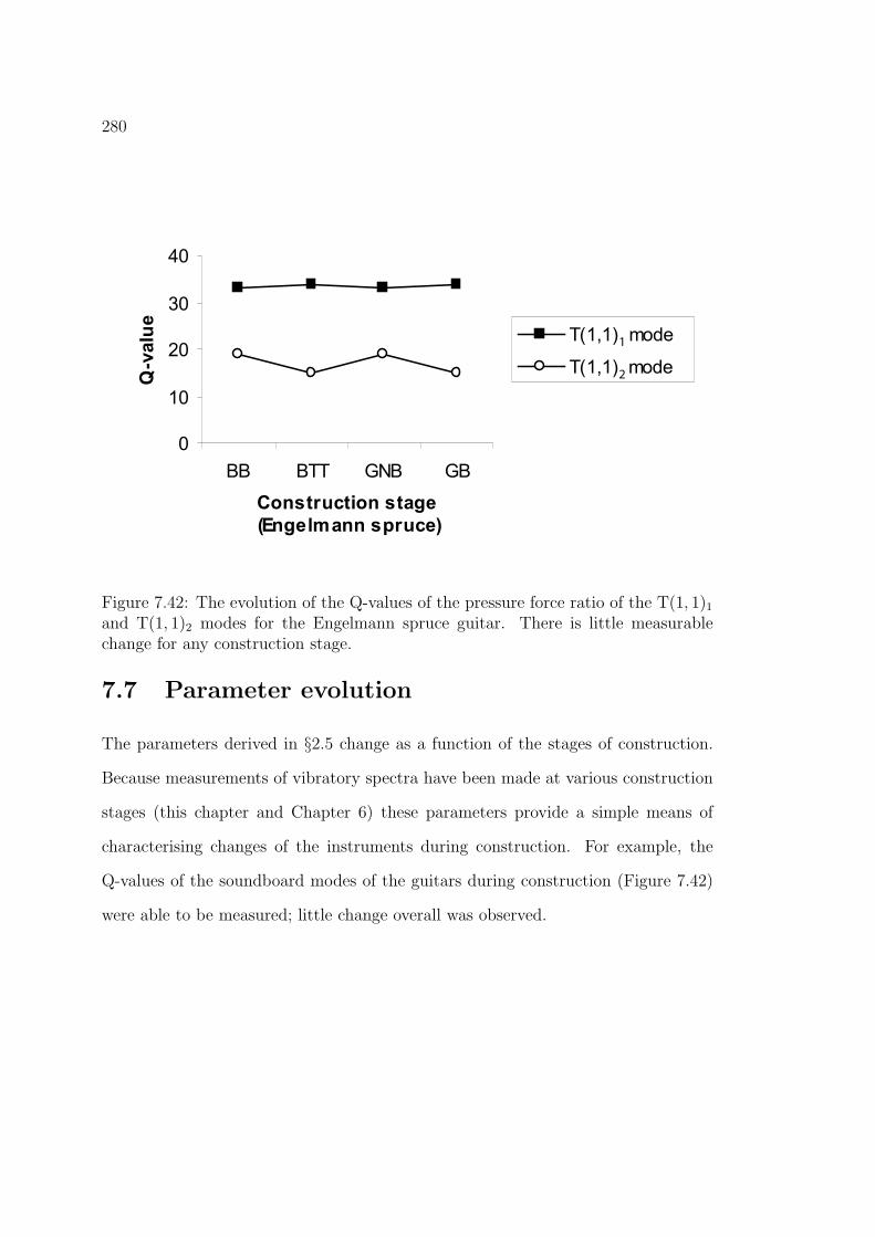
280
0
10
20
30
40
BB BTT GNB GB
Construction stage
(Engelmann spruce)
Q-v
alu
e
T(1,1) mode
T(1,1) mode
1
2
Figure 7.42: The evolution of the Q-values of the pressure force ratio of the T(1, 1)1
and T(1, 1)2 modes for the Engelmann spruce guitar. There is little measurablechange for any construction stage.
7.7 Parameter evolution
The parameters derived in §2.5 change as a function of the stages of construction.
Because measurements of vibratory spectra have been made at various construction
stages (this chapter and Chapter 6) these parameters provide a simple means of
characterising changes of the instruments during construction. For example, the
Q-values of the soundboard modes of the guitars during construction (Figure 7.42)
were able to be measured; little change overall was observed.

281
Soundboard Mass f1 Kp∗
(kg) (Hz) (kN · m−1)Engelmann spruce 0.2763 68 50.4
Sitka spruce 0.3067 73 64.5Western Red cedar 0.2493 69 46.9
Table 7.4: Effective stiffness values for the free guitar soundboards. Frequencies aretaken as the frequency where the phase in the dynamic mass spectrum (Figure 6.8)in the region of the free (2,0) mode (Figure 6.7) is a local minimum.
Effective free plate, Helmholtz, and membrane frequenciesand low frequency coupling
This section is a summary of the low frequency parameters (§2.5) as measured for
the three guitars at the various stages of construction examined in this chapter and
Chapter 6.
Free soundboards: effective stiffnesses
By assuming the deflection of the soundboard obeys Hooke’s law, the effective stiff-
ness of a guitar soundboard may be defined (§2.5) as Kp∗ = 4π2f 21 m, where f1 is the
fundamental frequency (in this case the (0,2) mode) and m is the mass of the free
plate. The effective free plate soundboard stiffnesses are given in Table 7.4. Values
for f1 are from Figure 6.8.
The effective stiffness values of the free guitar soundboards compare to Kp∗ =
74 kN ·m−1 given in [Caldersmith, 1978] for a classical guitar soundboard. This value
results from a semi-empirical calculation of the soundboard and bracing, making
simple assumptions about the structure. The effective stiffness for the soundboards
attached to the back and sides are given in Table 7.5.

282
Soundboard Kp∗
(kN · m−1)Engelmann spruce 232.5
Sitka spruce 279.7Western Red cedar 201.3
Table 7.5: Calculation of the effective stiffness of guitar soundboards after glueingto the sides and back. Calculations are taken from the mass of the plate and thecalculations of the free-plate frequencies (including fluid loading from the air) in thelow frequency air coupled region (§7.7).
Guitar bodies: effective stiffness
The effective stiffness values for a steel-string guitar soundboard attached to the
back and sides (Table 7.5) compare to the value of Kp∗ = 128 kN · m−1 given in
[Christensen and Vistisen, 1980], although, as the case with Table 7.4, the only
available comparison is with a classical guitar soundboard.
The frequency at which the air pressure in the soundhole is closest to 180◦ out of
phase with the force at the bridge, f−, that of the in-phase motion, f+ as well as that
of the equivalent Helmholtz resonator, f0, may be obtained from the low frequency
turning points in the dynamic mass spectra of the guitars [Firth, 1977, Christensen
and Vistisen, 1980]. These coupled frequencies are given in Table 7.6.
These data may then be used to calculate the frequency of the fundamental plate
mode, fp (Figure 7.44) as well as that uncoupled with the air, fp,0 (Figure 7.45).
The lowest frequency that the air and the soundboard couple at, fph (Figure 7.46),
are given in Table 7.7.

283
Helmholtz Frequencies
100
105
110
115
120
125
130
BDY
BTT
BB
GNB
WO
NGB
GF
GH
2yr
SCL50
SCL100
Construction stage
Fre
q (
Hz)
ES
SS
WRC
Figure 7.43: The progression of frequencies for an equivalent Helmholtz resonator.
Table 7.8 lists �pH values calculated for the three guitars at various stages of
construction. It is possible this parameter may be used to characterise a particular
instrument, but it is not known how it relates to the measurable spectra or subjective
quality of the instruments.
The equivalent Helmholtz resonance is altered as a result of successive construc-
tion stages (Figure 7.43.) The greatest change occurs when the bridge is added to the
instruments, effectively reducing the body compliance, which raises the Helmholtz
frequency by approximately 10%.

284
Soundboard Construction stage Frequency (Hz)f− f0 f+
Engelmann Body 96.6 119.5 161.6spruce Top-thinned 91.4 120.0 157.8
Binding 90.2 117.8 156.0Guitar (no bridge) 88.8 115.8 152.5Without neck 89.0 117.2 154.5With bridge 91.6 126.5 157.6Finished 91.8 126.5 158.6Lacquer hardening 93.0 126.9 159.0Played 2 years 94.2 126.4 158.8Partially scalloped 91.5 126.6 158.6Fully scalloped 91.7 126.4 156.1
Sitka Body 98.0 120.0 160.0spruce Top-thinned 97.0 119.7 160.1
Binding 94.2 118.7 160.6Guitar (no bridge) 94.2 118.6 159.6Without neck 94.2 115.8 153.7With bridge 96.8 126.3 163.0Finished 97.0 126.5 164.2Lacquer hardening 98.1 126.6 164.4Played 2 years 99.5 126.4 164.1Partially scalloped 97.0 126.6 164.2Fully scalloped 97.0 126.7 159.0
Western Body 96.8 125.2 163.3Red Top-thinned 90.4 121.0 157.8cedar Binding 88.9 118.5 154.9
Guitar (no bridge) 88.8 115.8 153.5Without neck 89.0 115.8 150.7With bridge 89.0 126.5 156.3Finished 91.8 126.5 157.6Lacquer hardening 91.5 126.6 157.2Played 2 years 91.5 126.4 157.5Partially scalloped 88.9 127.0 156.2Fully scalloped 86.3 126.9 153.6
Table 7.6: A summary of the low frequency coupling frequencies, as derived fromthe measured dynamic mass spectra at each construction phase.

285
Soundboard Construction stage Frequency (Hz)fp fp,0 fph
Engelmann Body 145.5 130.6 87.5spruce Top-thinned 137.3 120.2 89.2
Binding 136.3 119.5 88.0Guitar (no bridge) 133.2 116.9 85.9Without neck 134.4 117.3 87.7With bridge 131.2 114.1 90.5Finished 132.5 115.1 91.2Lacquer hardening 133.5 116.5 90.9Played 2 years 134.6 118.3 90.0Partially scalloped 132.3 114.6 91.4Fully scalloped 129.6 113.2 89.3
Sitka Body 106.0 103.9 45.8spruce Top-thinned 143.9 129.7 86.4
Binding 143.5 127.5 88.4Guitar (no bridge) 142.4 126.7 87.7Without neck 138.2 125.1 82.5With bridge 141.4 125.0 91.4Finished 142.8 126.0 92.2Lacquer hardening 143.6 127.4 91.6Played 2 years 144.4 129.2 90.3Partially scalloped 142.6 125.8 92.2Fully scalloped 136.5 121.7 88.5
Western Body 142.7 126.3 91.2Red Top-thinned 135.7 117.8 90.3cedar Binding 133.6 116.2 88.4
Guitar (no bridge) 134.3 117.7 86.6Without neck 131.2 115.8 84.5With bridge 127.9 110.0 90.9Finished 131.3 114.3 90.4Lacquer hardening 130.6 113.6 90.3Played 2 years 131.2 114.0 90.5Partially scalloped 127.2 109.3 90.8Fully scalloped 122.2 104.5 89.7
Table 7.7: Derived low frequency parameters, as in §2.5 and §2.5 from data in Table7.6.

286
Soundboard Construction stage FpH
Engelmann Body 0.73spruce Top-thinned 0.74
Binding 0.75Guitar (no bridge) 0.74Without neck 0.75With bridge 0.72Finished 0.72Lacquer hardening 0.72Played 2 years 0.71Partially scalloped 0.72Fully scalloped 0.71
Sitka Body -spruce Top-thinned 0.72
Binding 0.74Guitar (no bridge) 0.74Without neck 0.71With bridge 0.72Finished 0.73Lacquer hardening 0.72Played 2 years 0.71Partially scalloped 0.73Fully scalloped 0.70
Western Body 0.73Red Top-thinned 0.75cedar Binding 0.75
Guitar (no bridge) 0.75Without neck 0.73With bridge 0.72Finished 0.71Lacquer hardening 0.71Played 2 years 0.72Partially scalloped 0.72Fully scalloped 0.71
Table 7.8: Low frequency coupling parameter as a function of construction phase (lowfrequency coupling frequency normalised by the Helmholtz frequency, from [Chris-tensen and Vistisen, 1980].)

287
Top-plate Frequencies
120
125
130
135
140
145
150
BDY
BTT
BB
GNB
WO
NGB
GF
GH
2yr
SCL50
SCL100
Construction stage
Fre
q (
Hz)
ES
SS
WRC
Figure 7.44: The progression of calculated frequencies of free soundboards, with anair load, from low frequency coupling features.

288
Free Top-plate Frequencies
100
105
110
115
120
125
130
135
BDY
BTT
BB
GNB
WO
NGB
GF
GH
2yr
SCL50
SCL100
Construction stage
Fre
q (
Hz)
ES
SS
WRC
Figure 7.45: The evolution with construction of calculated uncoupled fundamentalfree-soundboard frequencies of the guitars.

289
Coupling Frequencies
80
82
84
86
88
90
92
94
BDY
BTT
BB
GNB
WO
NGB
GF
GH
2yr
SCL50
SCL100
Construction stage
Fre
q (
Hz)
ES
SS
WRC
Figure 7.46: The evolution with construction of calculated low frequencyair/soundboard coupling frequencies of the guitars.

290
Construction state dfp,0
dm(Hz · g−1)
ES SS WRCNo scalloping -7.9 -8.5 -7.9Partially scalloped -6.1 -7.1 -5.7Fully scalloped -6.1 -6.6 -6.0
Table 7.9: The change in calculated free soundboard frequencies in response toadded mass load. An indication of the linearity of the relationship is given by theleast squares fit parameter: R2 > 98%. The added mass ranged from 0 to 200 grams.cf. Figure 7.49.
Effective mass, stiffness and area
The changes in frequency of the calculated free soundboard in response to mass
loading at the driving point are given in Table 7.9.
The effect of brace scalloping was to lower the calculated free soundboard fre-
quencies progressively (Figure 7.49.) Because little mass was removed in comparison
to the total mass of the soundboard, this reduced the effective stiffness at low fre-
quencies (Figures 7.48 and 7.49) being more important than the (modest) reduction
in mass.
For the dimensionless low-frequency air-soundboard coupling parameter, �pH ,
the scalloping process improves the (Hooke’s) linear nature of the equivalent spring
obtained from the response of low frequency coupling under an added mass load, but
does not greatly affect the actual value (Table 7.10.) The construction stage that
affects �pH the most is the addition of the bridge.
7.8 Results/Comments
The construction stage that had the most profound effect on these measurements for
all three guitars, was the addition of the bridge. The bridge, along with reducing

291
Mass perturbation of free-plate frequencies
(tone-braces not scalloped)
70
80
90
100
110
120
130
140
0 20 50 100 200
Added mass (g)
Fre
qu
en
cy (
Hz)
ES
SS
WRC
Mass perturbation of free-plate frequencies
(tone-braces partially scalloped)
60
70
80
90
100
110
120
130
140
0 20 50 100 150 200
Added mass (g)
Fre
qu
en
cy (
Hz)
ES
SS
WRC
Mass perturbation of free-plate frequencies
(tone-braces fully scalloped)
70
80
90
100
110
120
130
140
0 20 50 100 150 200
Added mass (g)
Fre
qu
en
cy (
Hz)
ES
SS
WRC
Figure 7.47: The effect on the calculated uncoupled free-plate fundamental frequencyof guitar soundboards by mass loading at successive stages of tone-brace scalloping.The mass-loading gradient and linearity of the perturbation by mass loading pro-gression, as calculated from least-squares linear fit are in Table 7.9.

292
Effective stiffnesses of guitar soundboards
0
50000
100000
150000
200000
250000
BDY
BTT
BB
GNB
WO
NGB
GF
GH
2yr
SCL50
SCL100
Construction stage
Sti
ffn
es
s (
N/m
)
ES
SS
WRC
Figure 7.48: The effective stiffness of each guitar soundboard at successive construc-tion phases, as calculated from the mass of plate and the uncoupled fundamentalsoundboard frequency.
d�pH
dm(g−1)
Construction state ES SS WRCNo scalloping -0.026 -0.027 -0.033Partially scalloped -0.027 -0.023 -0.020Fully scalloped -0.019 -0.02 -0.021
Table 7.10: The change in low frequency air soundboard coupling as an expressionof the dimensionless low frequency coupling parameter �pH (§2.5, §2.5). Here, thelinear least-squares fit parameter, R2 > 96%

293
Effective stiffness
(tone-braces not scalloped)
100000
120000
140000
160000
180000
200000
220000
0 20 50 100 200
Added mass (g)
Eff
ecti
ve s
tiff
ness (
N/m
)
ES
SS
WRC
Effective stiffness
(tone-braces partially scalloped)
100000
120000
140000
160000
180000
200000
220000
0 20 50 100 150 200
Added mass (g)
Eff
ecti
ve s
tiff
ness (
N/m
)
ES
SS
WRC
Effective stiffness
(tone-braces fully scalloped)
100000
120000
140000
160000
180000
200000
220000
0 20 50 100 150 200
Added mass (g)
Eff
ecti
ve s
tiff
ness (
N/m
)
ES
SS
WRC
Figure 7.49: The effect of mass loading on effective stiffness of guitar soundboards,as calculated from the mass of each plate, plus load, and the calculated uncoupledfundamental soundboard frequency.

294
the number of distinct Chladni modes, increased the effective Helmholtz frequencies
of the guitars. No other construction stage had a significant effect on the Helmholtz
frequencies. Although the bridge adds some mass, it adds enough stiffness to alter
the character of modes that have nodal regions nearby, notably the T(1, 2)2 and
T(2, 2) modes. For this reason, the bridge should be considered as part of the brace
system, and not just a termination point for the string.
The addition of the neck introduces low frequency modes, around 60 Hz, in-
corporating the entire length of the instrument and it is expected this would have
implications for the tactile response of the instrument, but does not appear to greatly
affect the radiated sound. In addition, there are no mechanical losses associated with
an incomplete mechanical coupling between the neck and the body, suggesting that
the bolt-on neck system used is equivalent to the more traditional glue-on neck sys-
tem, in terms of vibratory response.
The effect of the polish used (nitrocellulose lacquer) has a small effect on the
measured spectra, lowering and damping the T(1, 2)2, T(2, 2) and T(5, 3) modes.
Allowing the volatile solvents in the polish to evaporate for a period of 53 days had
the effect of slightly lowering the frequency of the T(2, 2) mode. There was little
difference in the measured properties of the guitars after a period of ageing, with
only a small amount of playing, for two years.
Apart from a small lowering in fundamental frequency, the effects of brace scal-
loping were not important at frequencies up until about 650 Hz, corresponding to the

295
T(3, 2) mode. The modes at these frequencies have nodal lines that are in areas that
are close to the regions of the soundboard braces that are scalloped. The tone-braces
especially appear important at these modes. Scalloping also appears to improve the
fit of frequency change induced by an applied mass load at the driving point.

Chapter 8
A lexicon and a preliminary study
of subjective responses to guitar
sounds
“If ever there’s an obscene noise to be made on an instrument, it’s going to come
out of a guitar. On a saxophone you can play sleaze. On a bass you can play balls.
But on a guitar you can be truly obscene.”—Frank Zappa (1940-1993)
8.1 Introduction
It would be desirable to determine how physical changes made to acoustic guitars
affect how the sound is perceived by human beings. It is obviously important for
a luthier to know how their manufacturing techniques influence the sensations ex-
perienced by a human listener. One approach is to perform measurements of the
responses of human subjects exposed to sounds produced by the instrument with
various physical configurations. This is a difficult task; previous studies on the re-
sults of changes to the instrument do not make it clear how traditional ‘physical’
296

297
measurements of the response of an instrument relate to the resulting subjective im-
pression [Meyer, 1983b, Hutchins, 1989, Richardson, 1994, Wright and Richardson,
1997, Boullosa et al., 1999].
Psychoacoustic studies of timbre [Grey, 1977, 1978, Kerrick et al., 1969, Lichte,
1941, McGee, 1964, Salomon, 1958, Terhardt, 1978, von Bismarck, 1974b, Wedin and
Goude, 1972, Wessel, 1978, Wright, 1996, Meyer, 1983b, Gridnev and Porkenhov,
1976, Boullosa et al., 1999] typically examine the responses of a participant exposed
to external stimuli. These responses are usually in the form of a difference between
two stimuli, or with the ranking of certain parameters defined within the test.
However, the specific details of the type of stimulus and the mechanics of how
the test is applied is often important, which imposes constraints on the range of
the variables being studied. For example, the perceived timbre of notes of a guitar
string plucked with the fingernail differs markedly from that when a plectrum is used
[Schneider, 1977]. Because the purpose of Study I (§8.2) is to construct a vocabulary
to describe the timbre of guitar sounds with as large a range as possible, no stimulus
is given.
Once an agreed lexicon is established, it is then possible to determine the re-
dundancy of particular terms, by analysing the responses of participants exposed
to guitar sounds. From the results of other studies of the factor analysis of tim-
bre (§1.3), it should be possible, in principle, to characterise guitar sounds using a
limited number of dimensions. This is the purpose of Study II (§8.3).

298
8.2 Study I—establishing a guitar timbre lexicon
There is an extensive informal literature reporting descriptions of the timbre of
acoustic guitar sounds. Within this literature there appears to be some consistency
in the descriptive terms (descriptors) used. The aim of this study is to formalise these
descriptors, producing an acceptable lexicon to describe the timbre of an acoustic
guitar. The terms need to be meaningful (to a large proportion of the population
requiring the use of these terms) and should be broad enough to cover the variation
in timbre expressed by the instrument. This list could then be used to obtain in-
formation from the responses of participants in a test to determine the perceptual
features of given guitar sounds, as in Study II (§8.3).
Method and procedure
This study consists of two parts: a controlled literature search to obtain a list of
descriptors, and a survey to determine how these descriptors are rated, in terms of
their usefulness in describing a guitar sound.
A selection of guitar magazines and websites were obtained from a collection of
magazines and through a search of websites that sold or reviewed acoustic guitars.
The terms used to describe the timbre of the instruments—usually adjectives—were
taken from these reviews. The frequency that the terms occurred in this sample
of the literature was recorded. In addition, some guitar repairers were consulted
regarding the terms they used to describe guitar sounds.

299
The list of descriptors resulting from the literature search was presented to par-
ticipants to rate in terms of how useful they found the descriptor in describing guitar
music. The survey does not rely on stimuli. Instead, it relies on the participants’
memory of all the acoustic guitar sounds they had heard before. There is precedence
for this type of survey [Schubert, 2003]; this method does not constrain the partici-
pant to a narrow range of sounds (which may lack important components of interest)
and is also convenient to administer. On the other hand this approach is strongly
dependent on the participants’ memory of sounds as well as their experience with
using the particular words in this environment.
Because of the prevalence of the internet and World Wide Web networks, an
‘online’ format solved the logistical problems of distribution, advertising and supply.
Because the test was conducted without external stimuli, data transfer consisted
only of fairly small text files. The test was in the form of an interactive online ‘web
survey’ spanning 9 pages and taking approximately 5-12 minutes to complete. Par-
ticipants were asked to respond with their first impressions, to every term in the list,
after the instructions:
“Take a few minutes to think of the sounds produced by any acoustic guitar being
played. Which of the following terms (if any), in your opinion, would be useful for
describing the tone quality (‘timbre’) of a guitar sound?”
The web-pages were written in PHP (Personal Home Page) and the interface were

300
forms generated by the users’ web-browsers via HTML (Hyper-Text Mark-up Lan-
guage.) The terms referred to are provided in Appendix F. The usefulness (‘utility’)
of each term was rated on a seven-point scale, (1-7, 7 defining the most useful). The
order that terms appeared in each examination was randomised to reduce ordering
effects and biases. Participants were asked to state their general musical experience
and how much they played or listened to acoustic guitar music. Opportunity was
given to add additional comments and to suggest further expressions.
Validity checking of the survey
Because of the lack of control of the participants in a web-based test, it is necessary
to ascertain whether the responses obtained were sufficiently consistent and valid.
Participants were advised that some sort of validity check would be used during the
test. Two types of checks were introduced for this purpose: repeated measures and
syntactic logic check.
Repeated Measures There were exactly 3 repetitions of particular terms in each
test. The difference in scores between the repeats and the original were taken
for the three repeats. The terms that were repeated were selected at random,
although the positions they occurred at were constant for each test:
1. Between term 27 and 28, a repeat of term 12 occurred
2. Between term 63 and 64, a repeat of term 47 occurred
3. Between term 102 and 103, a repeat of term 69 occurred

301
Syntactic logic check Exactly 3 terms were added that could not be used to make
a sensible sentence in the context of the survey. Generally, for a term to be a
useful timbre descriptor, it is required to be an adjective. The following terms,
not adjectival, were inserted:
1. Between term 15 and 16: ‘please enter a 1 here’
2. Between term 58 and 59: ‘albert einstein’
3. Between term 89 and 90: ‘radium’
These terms also appeared at the same position for each participant.
It is not expected that a large portion of respondents would answer an identical
value for each of the repeated terms (Except for ‘please enter a 1 here’). However
large enough discrepancies would render the entire data set from that participant
unusable because of their unreliability. The sum of the square of the differences in
the repeats was examined. If this was greater than eight, then the responses from
the participant was discarded. One participant was discarded for this reason.
The URL address for the web survey was distributed on the University of New
South Wales all-physics email list, posted on the newsgroups rec.music.makers.guitar.acoustic
and rec.music.classical.guitar, and various UNSW students, including those from the
music course MUSI2142 (Musicology 2B), participated.

302
Results of the literature search
The terms resulting from the literature search were almost all ‘positive’ in the eval-
uative sense. This is because it is usually guitars of relatively high quality that are
reviewed in popular magazines and websites, and/or the reviewer is trying to sell
the instrument. Because the largest possible range of acoustic guitar sounds was
required, consultation was undertaken with some guitar repairers, who had seen a
range of instruments requiring significant amelioration, in order to add terms with
more negative emotive connotations to the list. The literature search ceased when
84 terms were found (Figure 8.1).
Figure 8.1: The frequency of all terms encountered in the literature study, illustratingthe frequency distribution. Because of limitations on space, only a selection of termsare labelled.
A total of 112 words or short phrases were obtained. It was necessary to reduce
this set to a more manageable number of terms. Judging from previous studies
[Rasch and Plomp, 1982, Enomoto and Yoshida, 1968, Kerrick et al., 1969, Grey,

303
Rank Descriptor Frequency occurring in literature sample1 full 212 rich 203 clear 174 bright 155 warm 146 balanced 117 mellow 9
8= boomy 78= clean 7
10= powerful 610= sweet 6
Table 8.1: The ten most frequently encountered descriptors in the selective literaturesearch.
1977] the descriptions of the timbre of a variety of sound stimuli are able to be
expressed using a small number of terms. Therefore data from listening tests should
be expected to show a clustering in correlations between these terms and responses
to stimulus in the form of guitar sounds with varying timbre.
Participant details and experience
The participants were asked for personal details, including name, age group, occupa-
tion, how often they heard live and recorded acoustic guitar music, years of experience
playing a musical instrument, and years of experience playing the acoustic guitar.
Comparing how certain demographic groups answered the survey may provide useful
data. For example, one might expect those with many years of experience in guitar
playing to be more familiar with the terms used than those who had never played at
all. The distribution of participants’ experience with playing a musical instrument,
and those playing the acoustic guitar, are shown in Figures 8.2 and 8.3.

304
Figure 8.2: All participants, experience with a musical instrument.
Analysis
A total of 245 surveys were completed over a period of 30 days. The uncertainty
of the mean of each term, ΔU , was taken as the standard error. With a possible
range between one and seven, the mean score, from all terms and participants, was
3.74 ± 0.01 and ranged from ‘bright’ (5.67 ± 0.11) to ‘boofy’ (1.49 ± 0.07). The
entire list, for all participants, is included in Table F.1 (Appendix F). There were
no apparent effects due to the particular order the terms appeared in.

305
Lexicon responsesTerm Mean response Rankingbright 5.7 1warm 5.5 2clear 5.5 3crisp 5.4 4rich 5.3 5full 5.3 6
balanced 5.1 7mellow 5.1 8tinny 5.0 9
twangy 5.0 10clean 5.0 11bassy 5.0 12thin 4.9 13
ringing 4.9 14trebly 4.9 15
metallic 4.9 16.5 (16=2)powerful 4.9 16.5 (16=2)brilliant 4.8 18boomy 4.7 19deep 4.7 20dead 4.7 21
vibrant 4.6 22
Table 8.2: The 22 terms of highest mean rating, from all 245 participants in theguitar timbre lexicon study. This is expressed as the mean response. Each term hada standard error of ±0.1.

306
Literature StudyTerm Frequency Rankingfull 21 1rich 20 2clear 17 3bright 15 4warm 14 5
balanced 11 6mellow 9 7boomy 7 8.5 (8=2)clean 7 8.5 (8=2)
powerful 6 10.5 (10=2)sweet 6 10.5 (10=2)crisp 5 12.5 (12=2)
punchy 5 12.5 (12=2)big 4 15 (14=3)
brilliant 4 15 (14=3)tight 4 15 (14=3)bassy 3 19.5 (17=6)bluesy 3 19.5 (17=6)natural 3 19.5 (17=6)
percussive 3 19.5 (17=6)ringing 3 19.5 (17=6)strong 3 19.5 (17=6)
Table 8.3: The 22 most frequentterms from the literature search.

307
Comparison of guitar timbre lexicon to literature search
Of the 20 terms most frequently occurring in the literature and the 20 highest mean
responses from the survey, 13 terms were the same (Table 8.2). To compare the
ranking of both data sets, Spearman’s rank correlation is an appropriate statistical
measure.
Comparing the rankings of the frequency of the terms in the reviewed portion
(i.e. omitting the descriptors obtained through consultation) of the literature study
(N = 84), to the rankings of the terms from the responses of participants who had
25 years or more experience with the acoustic guitar, yielded a correlation coefficient
of rs = 0.57 (p < 0.001). Hence there is some positive correlation between the utility
of a descriptor of guitar timbre and the frequency the term occurs in the literature.
Study I—conclusion
The descriptors of guitar sounds were obtained from a controlled literature search
and were judged for usefulness in a web survey. A correlation of rS = 0.57 was found
between the utility rating of each descriptor and the frequency it occurred in the
literature.
This list may be of use to the acoustic guitar community and will be used to help
participants to describe their impression of a guitar sound recording in Study II. It
is also possible this method of testing could be applied to other musical instruments.

308
8.3 Study II—evaluation of guitar sounds
In recordings of guitars being played, several variables could conceivably affect the
timbre and other perceptual attributes of a guitar sound reproduced through an
audio system. This study investigates the effect of some variables on the perceived
distinctions among recordings of steel-string acoustic guitars.
Study II: method and materials
Three guitars of varying commercial value were recorded simultaneously at four dif-
ferent locations. Each instrument was played a total of eight times. Some of the
variation in the recorded sound due to the type of guitar (GQ), the microphone
positions (RM) and that due to the particular performance (RP) were quantified by
varying these parameters.
Guitar quality
The three guitars ranged from a fairly expensive hand-made model, a medium-priced
style guitar and an inexpensive model. There is no well-identified objective measure
for the quality of an acoustic steel-string guitar. The commercial value generally
attributed by musicians and dealers to similar instruments of each type is taken as
a rough indicator of the quality of the instrument.

309
Figure 8.3: All participants, guitar playing experience
Parameter Value Mass (kg) Estimated priceGQ3 2.2300 GreatestGQ2 2.0016GQ1 2.0212 Least
Table 8.4: The three guitars used in Study II to determine the effect of variation inthe commercial value of the instrument.

310
Microphone position Parameter value Microphone typeNear guitar bridge RM1 R0DE NT3Near guitar neck RM2 R0DE NT3
Overhead RM3 R0DE NT3Player’s head (stereo) RM4 2 Optimus tie clip microphones
Table 8.5: The four microphones systems, at separate positions around the guitar,to make recordings for the pilot test. The three R0DE microphones are of cardiodmono type, and the headphone system is a stereo combination of two small electretcardiod microhones.
Microphone position
The directivity of the radiation from stringed instruments is frequency dependent
[Meyer, 1972], is influenced by the player’s presence, and is complicated by reflec-
tions. The perceived timbre of sounds recorded at different positions may be different
and it is not obvious where the most appropriate recording location is. The four mi-
crophone positions were (Figure 8.4, Table 8.5) near the bridge (RM=1), near the
neck (RM=2), directly overhead (RM=3) (about one metre above the soundhole),
and at the ears of the player (RM=4).
During the test, the participants were not explicitly aware of the recording posi-
tion of any particular track they were exposed to.
Variation in performance
To further decrease variation in the performances, the same piece was played each
time. The piece to be played is important: it is desirable to have the piece in a
musical context, but it is not desirable to have a long excerpt. For the luthier,
the most valuable piece is that which a potential buyer of a guitar might play,
assuming they were to judge an instrument based solely upon the sound it made.

311
It was decided to play an ascending one octave G-major scale (from G2) followed
by an arpeggiated open G,C,D chord progression. It would be ideal to have the
sound produced by a particular instrument to be reproducible, while also sounding
as realistic as possible. Usually the player has some degree of control over the timbre
of the sound produced, in addition to the loudness and pitch. Using an automated
device to excite the instrument is possible, but present models do not sound realistic
[Cass, 2003]. Instead, a human player was chosen: Sydney guitar player and teacher
John Morris.
The recordings were made in one session lasting three hours in a studio equipped
with a professional digital recording system designed for the recording of acoustic
guitar music. The performances were all made by the same performer, who was
blindfolded and wore a headset with microphones attached near the position of the
player’s ears. Neither the performer nor the recording engineer knew the purpose of
the test. The guitars were fitted with new strings (Martin ‘Acoustic SP Phosphor
Bronze’, Light Gauge (0.30, 0.41, 0.64, 0.81, 1.07, 1.37 mm diameters))and tuned
to standard tuning (E2, A2, D3, G3, B3 and E4) using an electrical guitar tuner.
The tuning was checked periodically during the session. The player was handed each
instrument in a prearranged pseudorandom order, with an associated three digit
numerical performance code.
These recordings were recorded onto audio CD (sampling rate 44.1 kHz, with
16 bit depth audio). The factorial design of the study, gives a total of 96 separate
tracks (eight performances of the three guitars, each recorded at four microphone
positions).

312
RM4
RM1
RM2
RM31
me
tre
Figure 8.4: The four microphone
positions used to record the guitar
sounds used as stimuli in Study II.
Study II: procedure
The pilot study was installed on three comput-
ers in a survey format, using software developed
by Emery Schubert. Three identical models of
computer were used (Apple PowerMac 7200/120,
running Mac OS 8.6 with a 120 MHz PPC 601
central processor and a 16 bit 44.1 kHz AWACS
Sound IC1 sound processor with Philips Stereo
Headphones SBC HP100).
The participants were exposed to the stimuli
in the form of the tracks from the audio CD. Each
stimulus was associated with a survey page con-
taining drop-down lists of the perceptual quan-
tities obtained from §8.2, which the participant
rated as an integer between zero and ten. The
decision to use a unipolar (0 to 10), as opposed
to a bipolar (-5 to +5) rating scale, was made
after considering the semantic implications in some cases. It was thought many
respondents would interpret a negative scale of e.g. ‘brightness’ as being the diamet-
ric opposite to ‘brightness’ (‘anti-brightness’?), as opposed to a lack of the quality
‘brightness’. Similarly, terms incorporating ‘lacking X’ were removed, if the quality
‘X’ were present. The participants underwent a small training session, comprising
1Audio Waveform Amplifier and Converter. Conforms to IT&T ASCO Audio-Stereo Codec
Specifications.

313
How much did you like the sound? (preference))overall quality of this instrument (quality)
dry loudness bright balancedbassy boomy trebly warm
ringing thin tinny fullbell-like clear dead crisp
rich muddy powerful brilliantmidrangey clarity deep twangy
mellow woody punchy bottomydull metallic shimmering harmonics percussive
Table 8.6: The variables that participants rated in response to stimuli in the pilottest.
two stimuli deemed to span the range of guitar quality, both recorded from the head-
set microphones (i.e. taking GQ=1, 3 while holding RM=4). Thereafter, the stimuli
were provided by playing tracks from the audio CD in pseudorandom order. Because
this study required the participant to respond to many questions (34) on each sound
stimulus (Table 8.6), there is a greater probability of operator fatigue. A test of 32
examples (i.e. 1/3 of the total stimuli on the audio CD) required a participant’s
undivided attention for at least 90 minutes. The test was designed with two rest
breaks, as well as an option to end the test at any stage after the initial training
period. As a result, the participants were not forced to respond to all stimuli and
therefore the test is of an incomplete factorial design.

314
Results
Overall analysis of descriptors
There were a total of 95 observations, from five respondents. The training session
was the same for all participants: tracks 78 and 92 (GQ=1,3, RM=4). The six
terms with the highest variance from track 78 were (mean (variance), N=5): ‘dry’
4.6 (18.8), ‘bassy’ 5.6 (16.3), ‘punchy’ 4.6 (13.3), ‘dull’ 4.8 (12.7), ‘midrangey’
4.9 (11.3) and ‘deep’ 6.4 (11.3). The five terms with the highest variation from
track 92 were: ‘tinny’ 3.2 (15.7), ‘dull’ 4.4 (13.8), ‘twangy’ 4.4 (11.3), ‘brilliant’
4.6 (9.8) and ‘ringing’ 3.2 (9.7).
In addition to these two tracks, the randomised audio track sequence meant that
there were five cases where two different participants were exposed to the same track.
In these cases, there does not appear to be good agreement in the rating of the tracks
with the term ‘dry’. This may be an indication that the participants were unsure
how to use this as a descriptor, because the magnitudes were very low in general
(mean ± standard error(number observations) 4.0 ± 0.5(62)) second only to ‘dull’
(3.9± 0.5(62)), compared to the overall mean for all descriptors (4.95± 0.04(3230)).
This is also a comparatively high standard error; the majority (26 of the 34 terms)
had a standard error of 0.3 or less.
Effects of varying the guitar
The mean and standard errors of the preference and quality responses, as a function
of guitar of varying commercial value, are given in Table 8.8. However, the differences
in the preference and quality ratings with different guitars were not significant. A

315
Descriptor Mean± standard deviation (observations)dull 3.88 ± 3.14(93)dry 3.98 ± 2.90(89)thin 3.57 ± 2.87(94)dead 2.52 ± 2.59(93)
muddy 2.27 ± 2.44(93)boomy 4.18 ± 2.41(95)punchy 4.72 ± 2.39(95)twangy 4.36 ± 2.36(95)
tinny 2.35 ± 2.28(92)bassy 4.76 ± 2.27(94)
percussive 4.18 ± 2.25(84)metallic 4.35 ± 2.19(93)powerful 5.09 ± 2.16(95)
woody 4.78 ± 2.01(95)trebly 5.33 ± 2.00(95)
brilliant 5.65 ± 1.96(95)ringing 5.17 ± 1.95(95)
deep 5.23 ± 1.92(95)bell-like 4.55 ± 1.91(84)
full 6.27 ± 1.86(95)warm 5.59 ± 1.85(95)
mellow 5.84 ± 1.84(95)overall quality 6.39 ± 1.74(93)
bright 5.82 ± 1.72(95)rich 6.06 ± 1.72(95)
How much did you like the sound? 6.47 ± 1.71(94)midrangey 4.71 ± 1.68(90)
clarity 6.33 ± 1.62(94)clear 6.37 ± 1.61(95)
balanced 5.49 ± 1.56(91)bottomy 5.54 ± 1.54(95)loudness 5.40 ± 1.40(94)
crisp 5.34 ± 1.36(95)shimmering harmonics 5.07 ± 1.31(88)
Table 8.7: Overall mean of responses from Study II, in order of standard deviation,to show the range of the responses. The number of observations of each term are inparentheses.

316
Guitar Mean±Standard error (count)Preference Quality
GQ1 6.5 ± 0.3(28) 6.6 ± 0.3(28)GQ2 6.8 ± 0.2(42) 6.7 ± 0.2(41)GQ3 6.0 ± 0.4(25) 5.8 ± 0.4(25)
Table 8.8: Overall mean response ratings of preference and quality, according tonominal quality of guitar. GQ1 is the instrument of lowest market value.
one-way ANOVA test for ‘preference’ gives F2,92 = 2.01 (p=0.14) and, for ‘quality’,
F2,92 = 2.24 (p=0.11). It is therefore concluded that the listeners cannot distinguish
between instruments of various market values, at least for such a small sample.
Effects of varying microphone position
There were apparently clear differences in the perceived timbre due to where the
recording microphone was positioned (Table 8.9), although this was not significant
for preference, F3,91 = 2.16 (p=0.10), quality F3,91 = 1.55 (p=0.21), loudness F3,91 =
1.28 (p=0.29) and dry F3,91 = 0.13 (p=0.95).
The headset microphone pair were rated higher (within the standard errors) than
the other three positions in the case of ‘preference’, ‘quality’, ‘balanced’, ‘warm’,
‘full’, ‘clear’, ‘mellow’ and ‘bottomy’. The microphone at the neck was rated higher
than the others in ‘bell-like’, ‘crisp’, ‘powerful’, ‘woody’ and ‘metallic’. For the
overhead microphone, this was clearly higher in ‘thin’, ‘dead’ and ‘dull’. Finally, the
bridge microphone was seen as high in terms of the variables ‘bassy’ and ‘midrangey’.
Therefore the microphone position clearly has a great impact on the perception of
timbre from the guitar, with a largely positive reaction to the stimulus from the

317
Descriptor RM=1 (Bridge) RM=2 (Neck) RM=3 (Overhead) RM=4 (Headset)preference 6.2 ± 0.4(18) 6.6 ± 0.3(29) 5.9 ± 0.4(21) 7.1 ± 0.3(27)loudness 5.6 ± 0.3(18) 5.6 ± 0.3(29) 4.9 ± 0.3(21) 5.7 ± 0.3(27)bright 5.7 ± 0.4(18) 6.0 ± 0.3(29) 5.8 ± 0.4(21) 5.8 ± 0.4(27)
balanced 5.2 ± 0.3(18) 5.5 ± 0.3(29) 5.4 ± 0.3(21) 5.9 ± 0.4(27)bassy 5.4 ± 0.4(18) 4.7 ± 0.4(29) 4.1 ± 0.4(21) 4.9 ± 0.5(27)boomy 4.3 ± 0.5(18) 4.5 ± 0.5(29) 3.5 ± 0.5(21) 4.2 ± 0.5(27)trebly 5.2 ± 0.4(18) 5.7 ± 0.4(29) 5.4 ± 0.4(21) 5.0 ± 0.4(27)warm 5.7 ± 0.5(18) 5.4 ± 0.4(29) 5.1 ± 0.4(21) 6.1 ± 0.3(27)ringing 5.6 ± 0.4(18) 5.5 ± 0.4(29) 5.0 ± 0.4(21) 4.7 ± 0.4(27)thin 3.0 ± 0.7(18) 3.7 ± 0.6(29) 4.3 ± 0.6(21) 3.3 ± 0.5(27)tinny 2.3 ± 0.6(18) 2.3 ± 0.4(29) 2.6 ± 0.5(21) 2.5 ± 0.5(27)full 6.2 ± 0.4(18) 6.2 ± 0.3(29) 5.6 ± 0.4(21) 6.9 ± 0.4(27)
bell-like 4.9 ± 0.4(18) 5.2 ± 0.3(29) 4.6 ± 0.4(21) 3.7 ± 0.3(27)clear 6.1 ± 0.4(18) 6.3 ± 0.3(29) 6.0 ± 0.3(21) 6.9 ± 0.3(27)dead 2.7 ± 0.7(18) 1.8 ± 0.4(29) 3.7 ± 0.6(21) 2.5 ± 0.4(27)crisp 5.3 ± 0.3(18) 5.7 ± 0.3(29) 5.0 ± 0.4(21) 5.3 ± 0.2(27)rich 5.9 ± 0.4(18) 6.2 ± 0.3(29) 5.5 ± 0.3(21) 6.5 ± 0.4(27)
muddy 3.0 ± 0.7(18) 1.8 ± 0.4(29) 2.7 ± 0.6(21) 2.2 ± 0.4(27)powerful 5.4 ± 0.5(18) 5.7 ± 0.4(29) 4.0 ± 0.4(21) 5.2 ± 0.4(27)brilliant 5.9 ± 0.4(18) 5.6 ± 0.4(29) 5.3 ± 0.4(21) 5.8 ± 0.4(27)
midrangey 5.1 ± 0.3(18) 4.7 ± 0.4(29) 4.4 ± 0.3(21) 4.7 ± 0.3(27)clarity 5.9 ± 0.5(18) 6.6 ± 0.3(29) 5.8 ± 0.4(21) 6.9 ± 0.2(27)deep 5.4 ± 0.3(18) 5.2 ± 0.3(29) 4.9 ± 0.4(21) 5.4 ± 0.5(27)
twangy 4.8 ± 0.5(18) 4.6 ± 0.4(29) 4.1 ± 0.5(21) 4.0 ± 0.5(27)mellow 5.5 ± 0.4(18) 5.4 ± 0.4(29) 5.9 ± 0.4(21) 6.4 ± 0.4(27)woody 4.8 ± 0.4(18) 5.1 ± 0.4(29) 4.7 ± 0.4(21) 4.4 ± 0.5(27)punchy 5.0 ± 0.4(18) 5.2 ± 0.5(29) 4.3 ± 0.5(21) 4.3 ± 0.5(27)bottomy 5.7 ± 0.4(18) 5.4 ± 0.3(29) 5.0 ± 0.3(21) 6.0 ± 0.3(27)
dull 3.6 ± 0.8(18) 3.0 ± 0.5(29) 5.1 ± 0.8(21) 4.1 ± 0.6(27)metallic 4.4 ± 0.4(18) 5.0 ± 0.4(29) 3.9 ± 0.5(21) 4.1 ± 0.4(27)
shimmering 5.1 ± 0.4(18) 5.2 ± 0.1(29) 5.0 ± 0.4(21) 4.8 ± 0.2(27)harmonicspercussive 4.6 ± 0.4(18) 4.8 ± 0.4(29) 4.2 ± 0.5(21) 3.6 ± 0.4(27)
dry 4.2 ± 0.7(18) 4.1 ± 0.5(29) 4.2 ± 0.7(21) 3.8 ± 0.6(27)quality 6.2 ± 0.5(18) 6.3 ± 0.3(29) 6.0 ± 0.4(21) 7.0 ± 0.3(27)
Table 8.9: Responses to stimuli in the pilot study, as a function of microphoneposition. Responses expressed as (mean ± standard error (number of observations)).

318
0
1
2
3
4
5
6
7
8
pre
fere
nce
loudness
bright
bala
nced
bassy
boom
y
trebly
warm
ringin
g
thin
tinny
full
bell-lik
e
cle
ar
dead
crisp
rich
muddy
pow
erf
ul
brillia
nt
mid
rangey
cla
rity
deep
twangy
mellow
woody
punchy
bott
om
y
dull
meta
llic
shim
mering h
arm
onic
s
perc
ussiv
e
dry
quality
Descriptor
Mean
resp
on
se
RM1
RM2
RM3
RM4
Figure 8.5: Mean responses to stimuli in the pilot study, as a function of microphoneposition. The errors are taken as standard errors.
headset microphone pair and a mildly negative reaction from the overhead micro-
phone. However, these differences are not significant, as rated through ANOVA of
key descriptors.
Effects of variation in performance
Within this experimental design, this is the least controllable—and least reliable—
parameter that is varied. Each performance is at least subtly different, even when
performed on the same instrument and recorded by the same microphone. In this
study, there were a total of 24 separate performances, but, because the instrument
was varied, the performance was also a function of changing guitar quality. These
were recorded at the four different microphone positions, described in the previous
section. In listening tests, Jurgen Meyer showed that the performance slightly affects

319
the perceived quality of a guitar sound [Meyer, 1983b]. It is concluded that there is
only a minor effect on the perception of timbre from the performances used in this
pilot study.
Reduction of response data
Because of the factorial design of this study, an efficient method of reducing the data
is with a factor analysis. The analysis is exploratory because we have no a priori
expectation of the effect each descriptor contributes to any potential factor.
I performed a maximum likelihood common factor analysis, conducted using Mat-
lab, to construct orthogonal axes based on the extent of correlation between the
descriptors. These axes were rotated using the varimax method so that they were
aligned with the principal components (i.e. the ‘main effects’).
The optimal number of dimensions to describe guitar sounds
The number of dimensions describing a semantic space is generally a compromise
between simplicity of interpretation (fewer dimensions) and an adequate span of the
semantic space.
Overall, for the data analysed here, a single linear factor would be inadequate to
describe the space: there are 28 descriptors (from a total of 34) that have a very large
estimated specific variance (Table 8.11). On the other hand, while a ten factor model
would account for more of the variance of the space (77.3% compared to 23.7%), it
would would be unwieldy as a descriptive tool.

320
Descriptor Standard errordull 0.4
boomy 0.3dry 0.3thin 0.3bassy 0.3dead 0.3
powerful 0.3muddy 0.3
full 0.3percussive 0.3
tinny 0.3preference 0.3brilliant 0.2punchy 0.2clarity 0.2
bottomy 0.2woody 0.2deep 0.2
metallic 0.2quality 0.2ringing 0.2bell-like 0.2
rich 0.2twangy 0.2trebly 0.2clear 0.2warm 0.2bright 0.2
shimmering harmonics 0.2loudness 0.2mellow 0.2
midrangey 0.1balanced 0.1
crisp 0.1
Table 8.10: The variation (expressed as a standard error for all 24 performances) inthe response of each descriptor as a function of the performance.

321
Number of Proportion of Range of specificfactors total variance variance of descriptors
(%) ψ � 0.50 ψ � 0.85 ψ � 0.251 23.7 28 18 02 39.4 21 9 43 56.4 11 0 64 63.1 5 0 85 66.8 3 (midrangey, balanced, bassy) 0 106 69.5 2 (midrangey, balanced) 0 117 71.7 2 ” ” ” 0 138 73.5 2 ” ” ” 0 149 74.9 2 ” ” ” 0 17
10 77.3 1 (midrangey) 0 19
Table 8.11: The optimal number of dimensions of the semantic space used to de-scribe guitar sounds, in terms of the number of descriptors (out of the total 34) notadequately spanned by the number of independent linear factors (showing high rel-ative variance) and those well represented by the dimensions of the space (showinglow relative variance).
The high degree of variance observed in some variables (viz. ‘midrangey’, ‘bal-
anced’ and ‘bassy’) in the models with more than four factors is probably due to
the uncertainty in the meaning of the descriptor. This is not surprising, because
participants were forced to respond to each sound stimulus by rating all 34 descrip-
tors. These terms can therefore be interpreted as statistically very noisy, and are
ipso facto not useful in a description of guitar sounds.
A common ‘rule of thumb’ for choosing the number of dimensions resulting from
a factor analysis is the Kaiser-Guttman rule: there are a sufficient number of fac-
tors if they have eigenvalues greater than one. However, this strictly applies only
to principal component analysis [DeCoster, 1998] and often overestimates the true
number of factors [Lance et al., 2006]. Another criterion for suitability is the ‘scree

322
Factors 1 2 3 4 5 6 7 8eigenvalues 8.07 7.85 7.89 6.35 7.01 6.47 6.52 6.19
5.54 5.79 5.63 5.27 4.57 4.60 4.575.50 4.98 4.47 4.49 4.22 4.23
4.51 3.80 2.91 2.84 3.002.16 2.87 2.81 2.95
2.33 2.36 2.401.02 0.91
0.73
Table 8.12: The eigenvalues of each dimension for multiple factor models of the entiredata set. The model having an eigenvalue less than one is the eight factor model.Therefore, according to the Kaiser-Guttman rule, no more than seven dimensionsare required to span the semantic space here.
test’ whereby the eigenvalues (or total variance spanned by the model) are plotted
against the number of factors in the model. An optimal number of dimensions may
be found near a sharp change in slope of the graph (an ‘elbow’). Finally, another
common factor optimisation method is examining the proportion of the total vari-
ance spanned by the factors, although this is an arbitrary cut-off. For the present
study it is most important that the results may be interpreted in a context suitable
for describing guitar sounds.
According to the Kaiser-Guttman rule, a seven factor model adequately spans
the semantic space (Table 8.12). However, this method tends to overestimate the
optimal number of dimensions [Lance et al., 2006].
A scree-plot of the data (Figure 8.6) has an elbow between the three and four
factor models suggesting that this many dimensions are optimal.
The descriptors with a high positive correlation, assuming a single linear factor,

323
1 2 3 4 5 6 7 8 9 1020
30
40
50
60
70
80
Pro
port
ion
of to
tal v
aria
nce
(%)
Number of factors
Figure 8.6: A scree plot of the total amount of variance spanned against the numberof linear factors in a model for the overall responses to the pilot study. The optimalnumber of factors is obtained at the ‘elbow’ of the graph.

324
Sign FactorF1 F2 F3 F4
‘Preference’ ‘Power’ ‘Brightness’ ‘Percussion’preference ( 0.74 ) mellow ( 0.76 ) bright ( 0.76 ) percussive ( 0.90 )
quality ( 0.73 ) bottomy ( 0.75 ) trebly ( 0.75 ) punchy ( 0.82 )+ rich ( 0.72 ) full ( 0.69 ) metallic ( 0.69 ) woody ( 0.78 )
brilliant ( 0.61 ) deep ( 0.69 ) clear ( 0.59 ) bell-like ( 0.78 )clear ( 0.60 ) loud ( 0.64 ) clarity ( 0.59 ) boomy ( 0.61 )dull ( -0.87 ) thin ( -0.41 ) midrangey ( -0.28 ) warm ( -0.28 )dry ( -0.81 ) tinny ( -0.30 ) deep ( -0.2457 ) dull ( -0.22 )
- dead ( -0.71 ) shimmering ( -0.26 ) muddy ( -0.23 ) preference (-0.21 )harmonics
muddy ( -0.59 ) bell-like ( -0.17 ) warm ( -0.22 ) dead ( -0.19 )tinny ( -0.54 ) trebly ( -0.15 ) bassy ( -0.16 ) quality ( -0.18 )
Table 8.13: The principal factors associated with a four factor model of the overallresponses. The factors are listed in order of influence on the variation in the data.The titles of each factor are merely a label to represent the group of descriptors.The five terms with the largest factor loadings (positive and negative) are included,along with their factor loadings.
are: ‘preference’, ‘quality’, ‘clear’, ‘rich’ and ‘brilliant’. Those having a highly nega-
tive weighting for this factor are ‘dry’, ‘dull’, ‘dead’, ‘muddy’ and ‘tinny’. This single
factor could be roughly associated with the preference each participant has for the
sound and accounts for 23.7% of the variance overall. A two factor model retains
this original factor for preference, with a second factor associated positively with
‘punchy’, ‘woody’, ‘boomy’, ‘percussive’ and ‘ringing’, and negatively with ‘dead’,
‘warm’, ‘preference’, ‘dull’ and ‘bright’.
The best compromise according to the criteria mentioned, and considering the
advantages of parsimony, is a model assuming four linear factors, in Table 8.13.
Not surprisingly, all models have a very strong positive correlation between the
responses for ‘preference’ and ‘quality’ of a given stimulus. This factor is important

325
Sign FactorF1 F2 F3 F4
‘Power’ ‘Brightness’ ‘Percussion’ ‘Dullness’full ( 0.76 ) bright ( 0.83 ) percussive ( 0.91 ) dull ( 0.91 )
bottomy ( 0.75 ) trebly ( 0.74 ) punchy ( 0.85 ) dry ( 0.80 )+ mellow ( 0.74 ) clear ( 0.69 ) woody ( 0.80 ) dead ( 0.73 )
deep ( 0.68 ) metallic ( 0.69 ) bell-like ( 0.76 ) muddy ( 0.56 )warm ( 0.66 ) clarity ( 0.67 ) boomy ( 0.64 ) tinny ( 0.55 )thin ( -0.48 ) muddy ( -0.31 ) warm ( -0.27 ) rich ( -0.59 )tinny ( -0.39 ) midrangey ( -0.24 ) full ( -0.16 ) brilliant ( -0.51 )
- shimmering ( -0.28 ) deep ( -0.24 ) bright ( -0.16 ) clear ( -0.47 )harmonics
trebly ( -0.19 ) dead ( -0.21 ) dull ( -0.15 ) clarity ( -0.39 )bell-like ( -0.18 ) warm ( -0.14 ) clarity ( -0.14 ) full ( -0.35 )
Table 8.14: The principal factors associated with a four factor model of the overallresponses, with the descriptors ‘preference’ and ‘quality’ removed from the data pool.The factors are listed in order of influence on the variation in the data. The titlesof each factor are merely a label to represent the group of descriptors. The fiveterms with the largest factor loadings (positive and negative) are included, alongwith their factor loadings. Notice that, after the factor associated with ‘preference’,the structure has residual factors occurring in a very similar order.
for the study here, but has not, in general, been addressed by the above studies.
Results of a four factor model of the same data set, with the responses to ‘preference’
and ‘quality’ removed, is similarly displayed in Table 8.14.
Notice that, after the initial factor of ‘preference’, similar factors arise and in
the same order as the four factors in Table 8.13. This suggests that these factors
are robust, despite the fact that this new model accounts for only 59% of the total
variance of the responses (compared to 63% including ‘preference’ and ‘quality’). A
three factor model (Table 8.15), accounting for 52% of the variance, retains similar
factors, although the order of the factors associated with ‘Brightness’ and ‘Power’
are reversed.

326
Sign FactorF1 F2 F3
‘Brightness’ ‘Power’ ‘Percussion’clear ( 0.86 ) full ( 0.75 ) punchy ( 0.87 )
brilliant ( 0.84 ) bottomy ( 0.73 ) percussive ( 0.83 )+ bright ( 0.81 ) mellow ( 0.72 ) woody ( 0.80 )
clarity ( 0.79 ) deep ( 0.69 ) bell-like ( 0.72 )rich ( 0.70 ) warm ( 0.66 ) ringing ( 0.72 )dull ( -0.61 ) thin ( -0.53 ) warm ( -0.31 )dry ( -0.60 ) tinny ( -0.44 ) full ( -0.11 )
- muddy ( -0.60 ) shimmering ( -0.31 ) dead ( -0.07 )harmonics
dead ( -0.59 ) trebly ( -0.27 ) rich ( -0.06 )deep ( -0.27 ) twangy ( -0.20 ) dull ( -0.04 )
Table 8.15: A three factor model of the overall responses, with the descriptors ‘pref-erence’ and ‘quality’ removed from the data pool. The factors are listed in order ofinfluence on the variation in the data. The titles of each factor are merely a label torepresent the group of descriptors. The five terms with the largest factor loadings(positive and negative) are included, along with their factor loadings. Again, thestructure is similar to the model including the ‘preference’ and ‘quality’ descriptors,although in this case factor F1 (‘Brightness’) is a more significant factor than factorF2 (‘Power’). Factor F3 remains associated with ‘Percussion’.

327
It is interesting to speculate on the role of these factors in describing the timbre
of sounds. The importance of the factor associated with ‘brightness’ has been em-
phasised by many studies (e.g. [Grey, 1977, von Bismarck, 1974b, Wessel, 1978]),
and might be related to the position of the spectral centroid [Wessel, 1978, Wold
et al., 1996, Schubert et al., 2004]. The existence of the factor of ‘percussion’ might
reflect the important effect of transients on the sound of the guitar [Jansson, 2002].
Study II—Conclusion
For the stimulus considered, it was found that there was more agreement with some
timbral descriptors than others (i.e. some were more ‘useful’ than others), based on
the degree of variation of the ratings of these terms on the stimuli. For instance,
the descriptors ‘dry’, ‘dull’, ‘thin’, ‘dead’ and ‘muddy’ had a high degree of vari-
ation, while there was comparatively little for ‘crisp’, ‘shimmering harmonics’ and
‘loudness’. This extends some of the results from Study I, but is constrained by the
particular stimulus used in this test.
Surprisingly the instrument with the highest commercial value was generally
rated with a slightly lower quality and preference than the other two instruments.
It was also shown that listeners could consistently rate different instruments accord-
ing to ‘quality’, which is not, a priori, obvious. However, the differences were not
significant, which is not surprising for the small sample size.
It was shown that the position of the recording microphone might have some
effect on the timbre of the resulting sound, although again, ANOVA did not show

328
a significant difference. The stereo pair at the ears of the player were rated slightly
higher on many attributes, including ‘preference’ and ‘quality’.
In timbre ratings, the variation in responses was small between separate perfor-
mances, agreeing with [Meyer, 1983b].
The dimensionality of the semantic space associated with the timbre of the
recorded guitar sounds appears to be four, viz. ‘preference’, ‘power’, ‘brightness’
and ‘percussion’. However, the four factor model accounts for only 63.1% of the
variance of the data examined here.
8.4 Discussion
An important element of the sound of the guitar is the timbre, and would form
an indispensable element in a study to determine the perceptual differences in the
three guitars studied in this thesis. However, the phenomenon of timbre is poorly
understood. Considering the difficulty of finding an explicit relationship between
parameters associated with physical acoustics and the resulting timbre, the creation
of an agreed list of terms to describe the range of timbre of acoustic guitar sounds
is a good initial step towards a programme to quantify the musical concept of tim-
bre. The on-line survey of the usefulness of terms obtained from guitar literature
and language used by guitar makers has given a list of terms useful in describing
the timbre of guitar sounds (Appendix F). A positive link was also found between
the frequency of terms or expressions found in a selective literature review with a

329
large enough sample (rS = 0.57, p < 0.01). This naturally suggests similar studies
be made on the lexicon of the timbre of other instruments. This would reduce the
labour required in a more general search for relationships between physical acoustics
and musical timbre.
This list was then used in a pilot study to determine the dimensionality of these
descriptions, finding it to be at least four dimensional (‘Power’, ‘Brightness’, ‘Percus-
sion’ and ‘Dullness’). Important to the perception of the sound of the guitar are the
microphone position and the quality of the instrument. The particular performance
was found to be important also, but not as much as the other variables considered.

Chapter 9
Conclusion and Further Work
“Unfortunately what is little recognized is that the most worthwhile scientific books
are those in which the author clearly indicates what he does not know; for an author
most hurts his readers by concealing difficulties”—Evariste Galois (1811-1832)
Many of the problems associated with the construction and design of the gui-
tar result from the generally ad hoc or trial-and-error approach to manufacturing
principles. This thesis has illustrated that a possible solution to these problems is
to isolate key measurable parameters, and to optimise these parameters. However,
it is recognised that the isolation and measurement of many of these parameters
are confounded by the complexity involved in engineering the instrument, and the
variability of the materials and components used therein.
To this end, it was found here that characterisation of important material prop-
erties relating to the vibratory behaviour of components, such as the Young’s moduli
and mass densities of the soundboard braces and the soundboard and bridge materi-
als (§5.5, §5.6 and §5.7), was necessary in order to control the resulting instruments
330

331
(Chapter 5). The general techniques developed therein might help luthiers to isolate
optimisation criteria for the guitar as part of a routine testing programme in the
workshop.
It has also been shown that measurement of the dynamic mass and pressure force
ratio transfer functions of the soundboard complement analysis using Chladni figures
(§6.2), the more traditional diagnosis tool used by luthiers. However, measurement
of these transfer functions enable much more rapid and accurate assessment of the
properties of a guitar during and after construction than the traditional method and
has the added advantage of being able to be compared to other instruments mea-
sured in the same way.
The effect of different soundboard timbers. The construction and measure-
ment of very similar guitars would enable the luthier to better understand the effect
and importance of timber selection for the soundboard. In this thesis, such a study
was conducted on three similarly made guitars, using three commonly used wood
species but with very different properties. Not surprisingly, out of the three timbers
used for the soundboards here, Sitka spruce, Engelmann spruce and Western Red
cedar, the Sitka spruce and Engelmann spruce were the most similar throughout all
construction phases measured here (Chapters 6 and 7). Comparing the same modes,
the Western Red cedar soundboard had lower frequencies than the corresponding
modes for the other two soundboards for the free soundboards, except in the case
of the mode at ca. 546 Hz (§6.3). The differences in mode frequencies between the
soundboard materials is not as definite at low frequency, but at frequencies above
400 Hz, corresponding modal frequencies are also lower for the Western Red cedar

332
than for the other two soundboards. The effect of thinning (§6.5), binding (§6.6)
adding the bridge (§7.2) have a much greater effect on the Western Red cedar sound-
board than the other two. The effect of tone- and cross-brace scalloping was much
more marked on the effective soundboard stiffness on the Western Red cedar than
the Sitka spruce and Engelmann spruce, which were again very similar (§7.7).
The relative importance of major construction phases. The vibratory
properties of ten major construction phases were measured in this thesis (§3.6). The
motion of the free soundboard (§6.3) is very different to that of the soundboard
attached to the back and sides (§6.4) because of the different boundary conditions
and coupling with the internal air cavity.
After gluing the soundboard to the back and sides, the construction stage with
the most impact on the vibratory behaviour of the guitar is the addition of the bridge
to the soundboard (§7.2). This suggests that proper characterisation or design of
the guitar soundboard ought to include the bridge as a component; several possible
configurations of some modes (because of the phase relations between the oscillating
elements) are reduced in number by the addition of the bridge (§7.2). In addition,
the measured (effective) Helmholtz resonance of each of the three guitars was affected
the most by the addition of the bridge (§7.2).
The polish used on the guitars studied in this thesis (nitrocellulose lacquer) had
little effect on the measured vibratory behaviour of the guitars (§7.3), except a
damping and slight lowering of the frequency of some modes (viz. T(1, 2)2, T(2, 2)
and T(5, 3)).
The effect of scalloping the cross- and tone-braces did not have a great effect on
the dynamic mass or pressure force ratio at low frequency, except for soundboard

333
modes that had nodes near the areas of the braces that were scalloped, such as
the T(3, 2) mode, ca. 650 Hz (§7.6). However, the calculated effective stiffness of
each soundboard was greatly reduced with the brace scalloping process, especially
between the partly and fully scalloped states (§7.7).
The effect of thinning the soundboard. Many, if not most, high quality
guitars do not have a uniform thickness distribution (§3.4). Often the thinning of
the soundboard occurs after it is glued to the back and sides, which makes it surpris-
ingly difficult to measure the thickness except at points close to the soundhole. John
Smith and I constructed a device employing magnetic field strength measurement
to measure the thickness distribution of a non-uniform guitar soundboard [Inta and
Smith, 2003], which could be employed routinely in a workshop (§6.5).
The use of Finite Element Modelling for guitar makers. The free sound-
board was modelled by David Vernet, Davy Laille and Matheiu Maziere in §4.5, com-
paring well with Chladni figures made on the soundboard having the same measured
properties. A FEM model of the complete guitar was also made (§4.6). However, in
this case, comparison to experiment was only able to be made on a qualitative basis
because the FEM models were not constructed to enable model coupling with the
air, which has a great effect on the vibratory motion of the instrument (§2.5). The
effects of brace scalloping were modelled (§4.3), agreeing with experiments showing
that scalloping decreases the Q-value of resonances of the brace and slightly lowers
the resonant frequencies. The data collected on these three instruments might be
used in a more advanced simulation of the guitar.

334
The problem of describing the timbre of guitar sounds. Finally, a lexicon
of terms for the timbre of guitar sounds was constructed by sampling a number of
terms from the literature and surveying a group of people to get the most useful
descriptors arising (§8.2). A positive correlation was found between the frequency
of descriptors found in the literature and the mean responses from the survey. The
timbre of these guitar sounds appeared to be able to be determined by using three
to four parameters (§8.4). An obvious extension of this work is to apply this method
to other instruments to generate a more general description of musical timbre. This
would provide a basis for investigating the effect that changes to the design of the
guitar have on the timbre of the instrument, and thus provide measurable parame-
ters to optimise, thereby improving the instrument. Considering the extent of the
characterisation of the the properties of the guitars studied in this project, it would
be advantageous to perform psychoacoustic listening tests on the instruments. The
work performed in Chapter 8 provides necessary background in order to make such
tests more meaningful.

Appendix A
Some derivations andmeasurements
A.1 The Helmholtz resonator
Consider a container with rigid walls, enclosing a relatively large volume of air, V ,
and a cylindrical throat with length l, of small (S � πl2) constant cross-sectional
area S. Assuming the wavelength is much longer than the largest single dimension
of the container so that the pressure distribution is effectively uniform. Knowing
the density, ρ, and speed of sound, c, in air, the mass-acceleration for the air in the
throat may be expressed as:
lSρξ (A.1.1)
where ξ is the time dependent displacement of the air in the throat of the con-
tainer and the Newtonian dot notation, ξ and ξ, represent the time derivative and the
second time derivative of the displacement of the air from the equilibrium position.
335

336
The air inside forms a ‘spring’, with a restoring force of:
c2ρξS2
V(A.1.2)
where the angular frequency, ω is related to the frequency, f , by ω = 2πf
Approximating the damping as viscous, the frictional force may be expressed as:
ρωk
2πS2ξ (A.1.3)
where the wavenumber, k, is related to the wavelength, λ, by k = 2πλ
and the
speed of sound in air may be expressed as c = fλ = ωk.
Adding equations A.1.1, A.1.2 and A.1.3, the time dependent force equation due
to an external force is:
lSρξ +ρωk
2πS2ξ +
c2ρξS2
V= SPejωt (A.1.4)
The forcing function on the right hand side of Equation A.1.4 is composed of the
pressure amplitude, P , and a time-varying complex exponential (e = 2.718... and
j2 = −1) with angular frequency, ω and time, t.
Substitution of the volume displacement, X = Sξ, makes algebraic manipulation
more convenient [Wood, 1940]. Then X = Sξ and X = Sξ and Equation A.1.4 may
be re-expressed:
lSρX +ρωk
2πS2X + ρS =
c2ρXS2
V= SPejωt (A.1.5)
which is analogous to an oscillatory electrical circuit.

337
X =Pejωt
ρωk
2π+ j(ρωl
S− ρc2
V ω)
(A.1.6)
Using this analogy an acoustic impedance, ZA, may be defined as the ratio of
the sound pressure at the source to the rate of change of volume displacement of the
surface of the source:
ZA =Pejωt
X=
Pejωt
Sξ=
ρωk
2π+ j(
ρωl
S− ρc2
V ω) (A.1.7)
The acoustic resistance is the real component:
RA ≡ R(ZA) =ρωk
2π(A.1.8)
and the acoustic reactance is the imaginary component:
I(ZA) =ρωl
S− ρc2
V ω(A.1.9)
Where the term ρωl
Sis the mass reactance and the term ρc2
V ωis known as the
stiffness reactance. The frequency of resonance of the system is where the reactance
becomes zero. Defining the frequency where this occurs as ω = ωH :
ρωH l
S=
ρc2
V ωH
(A.1.10)
So:
ωH = c
√S
V l(A.1.11)
Or:
ωH
2π= fH =
c
2π
√S
V l(A.1.12)

338
Volume 2.920 ± 0.005 × 10⁻³ m3
Throat length 80 ± 1 mmThroat diameter: 32.5 ± 0.1 mmThroat cross-section 8.30 ± 0.05 × 10⁻⁴ m2
Calculated f0 (no length correction) 102.9 ± 0.1 HzCalculated f0 (length correction at both ends) 92.1 ± 0.1Hz
Table A.1: Data from a simple Helmholtz resonator. Excitation is a simple pres-sure impulse. Calculation of f0 assumes c = 343 ms−1. End corrections are madeassuming circular unflanged pipe at both ends.
Thus the Helmholtz frequency is determined by the speed of sound in air and
basic geometric properties of the resonator.
Simple experiment validating effective length due to an end
correction
Data from an experiment conducted on a simple Helmholtz resonator are given in
Table A.1. The frequencies calculated differ strongly between corrected and uncor-
rected values. The length correction was obtained from the assumption of a circular
unflanged pipe at each ends, so l∗ = 2× 0.6133R [Levine and Schwinger, 1948]. The
Fourier transform of the pressure response in the experiment is shown in Figure A.1,
where the frequency of the main peak, associated with the Helmholtz resonance, was
found to be 92.2 ± 0.7 Hz.

339
Frequency (Hz)
27.5 1408055 110 220 440 880 1760 3520 7040
-12
-24
-36
-48
-60
-72
-84
-96 So
un
dp
ress
ure
(d
B, a
rbit
rary
)
Simple Helmholtz resonator
Figure A.1: Fourier transform of sound pressure response of an experiment on asimple Helmholtz resonator. Note the peak at 92 Hz.
A.2 Soundboard-air cavity coupling parameters
This treatment is largely a summary of [Christensen and Vistisen, 1980] and [Calder-
smith, 1978]. Consider the uncoupled elements. Assuming no air loading or coupling,
a simple vibrating plate of mass mp, and effective stiffness Kp∗, has a resonance fre-
quency:
fp,0 =1
2π
√Kp∗
mp
(A.2.1)
Now consider the soundboard as if it had negligible stiffness and an effective area
Ap∗ enclosing the internal air cavity. The resonant frequency of this air may be
expressed:
fa =1
2π
√μA2
p∗
mp
(A.2.2)
Where μ ≡ ρc2
V. The natural frequency of the soundboard loaded by the air in
the cavity volume is then given by:

340
fp =1
2π
√Kp∗ + μA2
p∗
mp
(A.2.3)
or, alternatively:
f 2p = f 2
p,0 + f 2a (A.2.4)
The finite stiffness of the soundboard causes the total volume and losses of the
cavity to deviate from the uncoupled state as a function of time. Assuming the
associated fluctuations in each vibratory cycle to be adiabatic, the cavity is subject to
a pressure change of Δp = −μΔV . The resulting force exerted on the two oscillators
is then Ap∗Δp on the soundboard and SΔp on the air in the soundhole. Assuming
viscous damping associated with the motions of each oscillator (Rp and RV ) and,
defining the driving force on the soundboard as F , the coupled equations of motion
for the two oscillators are:
mpxp = F − Kpxp − Rpxp + Ap∗Δp (A.2.5)
mhXh = SΔp − RhXh
Where xp is the net displacement of the soundboard from the equilibrium position,
Xh is the net volume displacement of the air in the soundhole from equilibrium, and
mh = ρSl∗ is the mass of air in the soundhole. If the soundboard is constrained from
moving (xp = 0) the frequency of the air in the soundhole is
fh =1
2π
√μS2
mh
(A.2.6)

341
whereby the familiar expression for the Helmholtz frequency (Equation A.1.12)
may be obtained.
For a sinusoidally time-varying force, F :→ F0ejωt and taking the loss parameters
γp ≡ Rp
mp
and γa ≡ Ra
ma
, the velocity of the soundboard is:
vp = jωF0
mp
[ω2
h − ω2 + jωγp
D] (A.2.7)
Similarly, the velocity function of the air in the soundhole is:
vh =−jωF0
mp
Ap∗
S[ω2
h
D] (A.2.8)
Where the denominator, D, is:
D = (ω2p − ω2 + jωγp)(ω
2h − ω2 + jωγh) − ω2
pH (A.2.9)
The coupling frequency fpH , is then given by:
f 4pH =
1
(2π)4
α2
mpma
= f 2Hf 2
a (A.2.10)
Resonances in the velocity functions occur when D = 0. Solving the quadratic
in Equation A.2.9 yields the solution:
f 2±
=1
2(f 2
p + f 2h) ± 1
2
√(f 2
p − f 2h)2 + 4f 4
pH (A.2.11)
And hence [Christensen and Vistisen, 1980]:
f 2p + f 2
H = f 2+ + f 2
−(A.2.12)

342
This is a special case of the more general result of coupled oscillatory systems,
where the quadrature sum of the uncoupled oscillator frequencies is the same as that
for the coupled oscillators [Christensen and Vistisen, 1980].
A.3 Two mass model for a cantilever beam driven
at the base
Consider the motion of a cantilever beam held by a clamp that is applying a sinu-
soidally varying force to the base, in a direction perpendicular to the longitudinal
axis of the beam. The model of two coupled oscillators may be applied thus [Har-
jono, 1998]: take the mass of the beam to be M , the displacement of the free end
(from equilibrium) as x2, the mass of the clamp system as m and its displacement
(also from equilibrium) as x1, the effective stiffness of the entire system, k, and the
viscous damping (of the system) to be R. The equation of motion for the beam is
then:
−Mω2x2 + (k + jωR)(x2 − x1) = 0 (A.3.1)
and that for the clamp:
−mω2x1 + (k + jωR)(x1 − x2) = F (ω) (A.3.2)
and by noting that, because, x1 = −ω2x1,
x2 = x1jωR + k
−Mω2 + k + jωR(A.3.3)
The force resulting from the clamp acceleration is then:

343
F (ω) = x1[−mω2 + (k + jωR)(1 − k + jωR
−Mω2 + k + jωR)] (A.3.4)
= x1[−mω2 + (k + jωR)(−Mω2
−Mω2 + k + jωR)] (A.3.5)
(A.3.6)
And therefore the dynamic mass of the beam is then:
F (ω)
x1(ω)=
−1
ω2[−mω2 + (k + jωR)(
−Mω2
−Mω2 + k + jωR)] (A.3.7)
= m +M(k + jωR)
−Mω2 + k + jωR(A.3.8)
A.3.1 Change in frequency of bending mode of a profiled
beam
Rectangular cross-section
To find the second moment of area (i.e.moment of inertia) about a neutral bending
axis, it is necessary to find the centre of mass about the given axis. Considering only
the y component, the centre of mass for a rectangular cross-section of width b and
height a (Figure A.2) is:
yCM =1
M
∫ a
y=0
ydm (A.3.9)
Now
m(y) = My
a

344
x=b
y=a
y
x
x=y=0
Figure A.2: Beam with rectangular cross-section
so:
dm
dy=
M
a(A.3.10)
therefore:
yCM =1
M
∫ a
y=0
yM
ady
⇒yCM =
1
a
[y2
2
]a0
=a
2
similarly,
xCM =b
2
The moment of inertia, defined as
I =
∫ R
r=0
r2dm (A.3.11)

345
and using Equation A.3.10 gives:
IT =M
a
∫ a
y=0
y2dy
=M
a
∫ a
y=0
y2dy
=M
a[y3
3]ay=0
So:
IT =Ma2
3
The parallel axis theorem (Equation A.3.12)
IT = ICM + Md2 (A.3.12)
gives the total moment of inertia IT , at some point a distance d from the axial point
passing through some point with a parallel axis of bending. Yet
d2 = y2CM =
a2
4
so:
ICM = IT − Md2 = Ma2
3− Ma2
4= Ma2
(4−312
)
Where ICM is the moment of inertia at the centre of mass, and M the total mass
of the beam.
Hence:
ICM =Ma2
12(A.3.13)

346
Triangular cross-section
For an isosceles triangle, height h and width b (Figure A.3)
m(y) = Marea from y = 0 to y
total area
= My( b
2+ b(h−y)
2h)
bh2
= My(2 − y
h)
h
ie: m(y) = My(2h−y)
h2
⇒ dm
dy= M
2(h − y)
h2(A.3.14)
And thus:
IT =
∫ h
y=0
y2 2m
h2(h − y)dy =
2M
h2
∫ h
y=0
(hy2 − y3)dy
=2M
h2[hy3
3− y4
4]hy=0 =
Mh2
6.
From Equation A.3.9, yCM = 1M
∫ h
y=0ydm
And, using Equation A.3.14,
yCM =1
M
∫ h
y=0
2M
h2(h − y)dy
=2
h2
[hy2
2− y3
3
]hy=0
=2Mh4
h2[1
3− 1
4] =
h
3
The square of the distance from y = 0 to y = h3
is d2 = h2
9
Hence, from Equation A.3.12:
ICM =Mh2
6− Md2 = Mh2(
1
6− 1
9) = Mh2(
3 − 2
18)

347
y=h
y=0
x=-b/2 x=+b/2
y=y’
y
x
Figure A.3: Isosceles triangle, height h, base length b
Therefore:
ICM =Mh2
18(A.3.15)
Pentagonal cross-section, symmetric about xCM
Often the cross-section of the key braces on the soundboard of the guitar are modified
from a rectangular shape to that of an isoceles triangle atop a rectangle with the
same width as the base of the triangle, as in Figure A.4.
For the triangular section,
y =h2 − 2(h2 − h1)
bx (A.3.16)
so
m(y) = M
(1 −
b2
(h2−y)2
h2−h1
b2(h2 + h1)
)= M
(1 − (h2 − y)2
h22 − h2
1
)(A.3.17)

348
y=y’
y
x
y=0
x=-b/2 x=+b/2
y=h1
y=h2
Figure A.4: Schematic of a beam with pentagonal cross-section, symmetric uponreflection about the centre of mass in the x-direction.
and thus
dm
dy= M
(2(h2 − y)
h22 − h2
1
)(A.3.18)
So
yCM =1
M
(∫ h1
y=0
y2M
h1 + h2
· dy +
∫ h2
y=h1
y2M(h2 − y)
h22 + h2
1
· dy
)(A.3.19)
=h2
1
h1 + h2
+2h3
1 + h32 − 3h2
1h2
3(h21 + h2
2)
And, using Equation A.3.18,
Iy
M=
∫ h1
y=0
y2 2
h1 + h2
· dy +
∫ h2
y=h1
y2 2(h2 − y)
h22 + h2
1
· dy (A.3.20)
=
(2h3
1
3(h1 + h2)+
h42 + 3h4
1 − 4h31h2
6(h21 + h2
2)
)
Using Equation A.3.12, the radius of gyration about the centre of mass is κCM :

349
κ2CM =
Iy
M− y2
CM (A.3.21)
=2h3
1
3(h1 + h2)+
3h41 + h4
2 − 4h31h2
6(h21 + h2
2)−(
h21
h1 + h2
+2h3
1 + h32 − 3h2
1h2
3(h21 + h2
2)
)2
This unwieldy expression may be simplified by substitution of values for a brace
with a profiled cross-section.
For slender homogeneous beams of constant cross-section with common boundary
conditions, fi ∝ κ (Equation 2.7.5). So the change in frequency of the normal
bending modes of a beam, as a result of the profiling process from a brace (§3.4)
with an original height of h2 may be found thus:
(fnew
fold
)2
=12
h22
(2h3
1
3(h1 + h2)+
h42 + 3h4
1 − 4h31h2
12(h21 + h2
2)−(
h21
h1 + h2
+2h3
1 + h32 − 3h2
1h2
3(h21 + h2
2)
)2)
(A.3.22)

350
A.4 Measurements of dimensions of the guitar sound-
boards
Overall widths of the guitar soundboards were measured at 35 mm intervals (Figure
A.5).
0
20
40
60
80
100
120
140
160
180
200
0 35 70 105 140 175 210 245 280 315 350 385 420 455 490 500
Longitudinal distance (mm)
La
tera
l ex
ten
sio
n (
mm
)
Figure A.5: Measurements of the lateral dimensions of the Sitka spruce guitar sound-board as a function of distance along the main axis of the guitar.

Appendix B
Vibratory data acquisition system(ACUZ)
“Fourier’s Theorem is not only one of the most beautiful results of modern analysis,
but it may be said to furnish an indispensable instrument in the treatment of nearly
every recondite question in modern physics”—Lord W. T. Kelvin and P. G. Tait
[Thomson and Tait, 1867]
B.1 Background
The measurements reported in this thesis are made using variants of ’ACUZ’1, a
system developed within the Music Acoustics Laboratory of The University of New
South Wales for the rapid measurement of the frequency dependence of transfer
functions. [Wolfe et al., 1995]. Although the system is most commonly used for
the acoustic impedance spectroscopy of musical wind instruments, it is used here to
measure the transfer functions of a range of linear vibro-acoustic systems.
1‘ACoUstic Z’, where Z represents the impedance to be measured
351

352
Figure B.1: The ACUZ system, as applied to wind instruments. From [Wolfe et al.,1995].
B.2 Design and operation
The version of ACUZ used is based on an Apple Mac IIci computer with a 16 bit
analogue interface card (National Instruments NB-A2100).
The electrical stimulus is synthesised from a series of equally spaced frequency
components covering the frequency range of interest - in most of these experiments
they are spaced � 0.69 Hz apart, covering the range 10 → 1000 Hz. (There is always
a compromise between frequency resolution and signal to noise ratio: more frequency
components produces improved frequency resolution, but the signal to noise ratio of
each component is reduced).
The relative phase between the frequency components is adjusted to minimise
the resultant maximum amplitude of the synthesised waveform. This improves the
overall signal to noise ratio as the overall amplitude of all components can then be
increased [Smith, 1995]. This is achieved by introducing random phase relationships
between the Fourier components such that the maximum amplitude of the sum of
the Fourier components is minimised with respect to that of any other attempted
configuration (minimisation of the ‘crest-factor’.) This process may be repeated and
the best solution accepted by the user. The approach is similar to the Monte Carlo

353
method, except that the choice of the number of configuration attempts is left to
the user. Consequently there are usually only a small number of configurations tried
before a solution is accepted. It is possible to apply a numerical algorithm for this
purpose [Guillaume et al., 1991, Shroeder, 1970] although this has not been imple-
mented at this time.
If the system is linear (this is the case for vibratory modes of the guitar sound-
board [Richardson, 1982]) the choice of signal averaging is possible, by repeating the
output signal a number of times.
This electrical stimulus is then amplified and passed to an electromagnetic shaker
(B& K 4809). The driving point dynamic masses are detected by a B& K 8001
impedance head with a stereo input line back to the computer. The pressure force
ratio measurements are driven in the same way, and the force portion is also measured
with the B& K 8001 impedance head, but the pressure response is measured using
an Optimus tie-clip microphone.
Although presently a laboratory measurement tool, ACUZ was designed to be
capable of industrial application in the workshop or factory.
Dynamic mass measurements
The dynamic mass is a measure of the frequency dependent effective mass ( force(ω)acceleration(ω)
)
of a system in response to vibratory excitation. In general the force and acceleration

354
may be measured at distinct points in space (the transfer function) but here the
force and acceleration are made at identical positions and is known as the driving
point dynamic mass.
Pressure force ratio measurements
Because the ultimate product of the acoustic guitar is the sound it produces, it would
seem logical to measure some kind of pressure response of the instrument. Direct
pressure measurements in response to some time-varying excitation at the bridge are
sometimes difficult to apply in comparative tests, because the applied force at the
bridge is variable and we would expect this to have a large effect on the output pres-
sure. This issue is resolved if we examine the transfer function of a measured pressure
response to the time-varying force applied to the bridge (pressure(ω)force(ω)
). Because of the
complex geometry of acoustic radiation, the spatial position that pressure measure-
ments are made is also important. I have chosen the centre of the soundhole, in the
plane of the top of the soundboard, as a fixed point to measure the pressure response
of the instrument.
The transfer functions of the pressure measured at the soundhole to the force
applied to the bridge gives some indication of the magnitude of pressure arising from
a particular force applied and may be more useful in the sense that we can measure
the resulting sound pressure output due to a known applied force at the bridge. This
quantity may also be used to calculate an effective area, Aeff.(ω) = force(ω)pressure(ω)
. This
effective area must not be interpreted directly as a geometric area of the soundboard,
but as relating to the effective area of a simple piston source of radiation. The ratio

355
of this effective area to the effective mass, Aeff.
Meff.
is proportional to the total output
pressure of the guitar, assuming it is a simple, uncoupled, source of radiation as
in Equation B.2.1 from [Christensen and Vistisen, 1980] and developed in [Wright,
1996].
p(ω) = F (ω)Aeff.
Meff.
ω2
(ω20 − ω2) − jγω
(B.2.1)
Where γ represents the losses of the simple radiator.
B.3 Impedance spectroscopy
Interpretation of impedance spectra (or transfer functions) can be difficult because of
the great volume of data usually received. As with any other branch of experimental
physics, it is important to minimise the information recieved while retaining the
important features. In the case of vibratory measurements, often the means of
mechanically support has an influence on the measured spectra, and interpretation
must be made with this in mind.

Appendix C
Alternative methods of measuringmechanical properties of wood
“Every piece of wood will have a unique set of vibrational properties because it has
a unique set of elastic moduli and damping rates, even if cut from the same log”
—Graham Caldersmith [Caldersmith and Freeman, 1990]
There are viable alternatives to the technique used to measure the Young’s mod-
ulus of a wooden beam, in §5.2. For example, by exciting a wooden beam, simply
supported at the nodes of the mode of interest, through the attachment of a small
permanent magnet to the beam, in close proximity to a mechanically fixed solenoid,
driven by a signal generator, it is possible to measure the free-free vibrations of the
beam. Impulse excitation may also be used, and this is in fact applied widely by
luthiers as the primary selection method for musical instrument woods (as the ‘tap-
tone’ method, §3.4). The methods that I developed in the following are not only
useful as a comparison to the clamping method, but also may be of use to a luthier
in accurate material selection.
356

357
A: Optoelectronic detection
Similar tests on the normal modes of vibration of a wooden beam may be achieved,
using a different excitation, support, and detection system to that used in §5.2.
Figure C.1 shows the set-up for measuring the normal modes of a beam, simply
supported by two foam-rubber triangular prisms. The beam is simply supported at
22.4% of the total length from each end, giving a good approximation to free-free
boundary conditions at the lowest normal mode. This is where the two nodes of
the fundamental of the free-free beam would occur, thereby minimising mechanical
interference effects due to the support system. A small permanent rare-earth magnet
(A NdFeB cylinder 3 mm high and 6 mm in diameter, with mass 1.3 g and a surface
field strength of � 200 mT) was attached to the underside of the centre of the brace,
using double-sided tape, and a small square (5 mm × 5 mm) of silvered mica was
affixed to the top. The apparatus used to excite the beam was an air-core solenoid
(inductance: 170 mH, resistance: 0.53 Ω) driven by an amplified signal generator,
placed about 5 mm directly below the rare-earth magnet. The optoelectronic detec-
tion system comprised a 10 mW HeNe laser (λ = 633 nm) incident on the mica sheet
and a position sensing device (UDT Sensors, Inc. SLS5-1 duo-lateral super-linear
PSD (one-dimensional series)) was placed in the path of the reflected light, aligned
so that when the beam flexed, the reflected light would move along the sensing axis
of the detector. The output voltage of the detector is analysed using an oscilloscope
(Kenwood 20 MHz CS-1021).
This detection system is essentially a crude laser vibrometer.

358
He-Ne laser
Wooden beam
Supports
Position sensor
Figure C.1: Set up for measuring the normal modes of a simply supported woodenbeam. Excitation is electromechanical and detection is optoelectronic. Water vapour(from evaporating liquid nitrogen) is used in to illustrate the path of the laser beamfor illustrative purposes and is not used in actual measurement.
Mass loading of the braces, by adding another magnet of the same mass to the
original, did little to alter the frequency or amplitude of the normal modes, although
this method is extremely sensitive to manner of beam support, and it is likely that
better results may be obtained by using more rigid supports than those used here.

359
B: ‘Tap-tone’ method
The ‘tap-tone’ method is able to be carried out with a minimum of equipment, and
it is likely this has been used in wood selection by luthiers for hundreds of years
[Hutchins, 1999, Bissinger, 2001]. A wooden beam is held vertically at a nodal
position for the fundamental free-free mode (for a beam of constant cross-section
this is about 22.4% of the total length from each end) between finger and thumb
and impulse excitation is achieved through impact. This is essentially the traditional
method presented in §3.4 although objective measurement of the pressure response of
the impact is recorded through a microphone fixed on a stand, approximately 15 mm
from the centre of the beam, onto Digital Audio Tape. This is then transferred to a
computer and a fast Fourier transform is taken to obtain the frequency and damping
of the fundamental mode. The impact is achieved by striking the beam lightly in
the centre with a small hand-held brass rod. This rod was used, as opposed to a
luthier’s traditional striking tool (a bare knuckle), to improve reproducibility of the
applied force and striking point. The microphone was also positioned at the end of
the beam to compare height and width modes.
Although the human hearing system is well known for its sophisticated sens-
ing capabilities, sensitive to small relative variations in frequency and amplitude
[Helmholtz, 1885], much additional information can be provided by tactile feedback
though the fingers, especially with regards to mechanical damping. This provides
vital information on bulk defects such as grain irregularities (§3.2), which tend to
produce undesirable vibratory, acoustic and æsthetic properties.
Table C.1 shows the results of listening tests using a reference tone through the

360
Strut Profiled Fundamental frequency (Hz)Height Width
1A yes, complicated 245 171.02A yes (cracked grain) 304.5 182.753A yes - -4A yes 301 182.255A no 179.5 109.06A yes, fully 265.3 161.51B no 189 110.02B yes 318 202.53B yes 173 108.04B yes 278 198.05B no 190 116.06B no 188 116.07B yes, asymm - -1C yes 322.75 197.252C yes 195 308.53C yes 323.75 198.754C no 189 110.55C no 191 111.06C yes 169.5 103.07C yes 323.5 204.25
±0.25Hz
Table C.1: Fundamental frequencies of wooden beams using a variant of the ‘tap-tone’ method
right channel in a set of stereo headphones and playing the recorded tap tone in the
left channel.

Appendix D
Soundboard thicknessmeasurement device
“What soundboard thickness does he work to? He gestured with his thumb meeting
his index finger raised to eye level, squinting slightly and rubbing them as if feeling an
imaginary soundboard. ‘I prefer to use these rather than a caliper. It does not really
interest me what the measurement is.’...clearly, he finds that he can dimension his
guitar plates better without a micrometer, because he believes only the fingers can
ask all the necessary questions of a piece of wood”—William Cumpiano, interviewing
Manuel Velazquez [Cumpiano, 1982]
D.1 Outline of soundboard thickness problem
The practice of thinning the soundboard of high quality guitars has been discussed
in §3.4. The shape of the guitar body makes it extremely difficult to introduce a
traditional mechanical gaging device such as a rule, callipers, or a spring-loaded
thickness gage. The soundhole is generally less than 100 mm in diameter, reducing
361

362
Sound board
Braces
Bridge
SaddleStrings
Figure D.1: The soundboard as viewed from within the soundhole, looking toward thebridge. Observe that the intervening braces are much thicker than the soundboarditself.
access or mobility of such devices. Even if this were overcome, the device in ques-
tion would have to navigate the complicated geometry of the wooden braces on the
soundboard (Figure D.1) which can be more than four times the thickness of the
actual soundboard.

363
Possible mechanisms to measure thicknesses in woods
Vibro-acoustic
Ultrasonic methods are commonly used for nondestructive thickness measurements
[McMaster, 1959]. This can include pulse return time (time-of-flight) or standing
wave methods. The disadvantages of using ultrasonic pulses to determine the elastic
properties of wood are discussed in §3.2. These disadvantages, such as grain layer
scattering, dependence on moisture content, and frequency dependence also make
accurate thickness determination difficult.
Nuclear radiation
For most matter, we are able to apply Equation D.1.1 and calibrate the reduction in
transmitted intensity I of some specific type of nuclear radiation through a thickness,
x, of material with a characteristic linear absorption coefficient μ.
I = Ioe−μx (D.1.1)
Generally, μ is dependent on the kinetic energy as well as the type of radiation
used (viz. α, β, γ or 10n)
Because α-particles are strongly ionising, they interact very strongly with nor-
mal matter and as a consequence do not tend to penetrate more than a few mil-
limetres at any energy. For γ and β radiation, the linear absorption coefficient
varies directly with both moisture content and density and inversely with energy,
although the difference in the magnitude of μ for the two types of radiation mean
that wood is virtually opaque for even very thin specimens of wood (For 0.047 MeV

364
γ, μγ = 0.65 → 1.1 mm−1 [density range 330 → 620 kg · m−3], compared to β en-
ergies of 0.5 MeV, giving μβ � 30 mm−1). Because neutrons interact very strongly
with hydrogen, the transmission of lower energy particles are dependent on moisture
content. Higher energy neutrons enable nondestructive analysis of trace elements in
the wood by analysing radioisotope production [Forest Products Laboratory, 1999].
Therefore, although useful for other purposes, the use of radioactive sources to
determine wood thickness is problematic at best. Aside from the issues of safety
and social stigma, this method suffers considerably from the fact that obtaining
radioactive sources is probably difficult for most luthiers.
Magnetic fields
Because most non-ferromagnetic materials, including wood, have a relative perme-
ability close to one (i.e. μR � 1) [American Institute of Physics, 1972], it is possible
to insert wood into a magnetic field without noticeably altering the flux geometry. If
a source provides a magnetic field with suitable geometry, such as one with monoton-
ically decreasing flux density with distance, it is possible to determine the distance
from the source by measuring the flux density. Wood that is entered into this field
will not affect the intensity or geometry of the measured magnetic field.
D.2 The Hall effect
The effect of an external magnetic field, with flux density B, applied to a charge of
magnitude q, moving with velocity v, is to exert a force F according to Equation

365
D.2.1.
F = qv × B (D.2.1)
This applies to free charges as well as those moving in the environment of an
electrical conductor. If we arrange a steady rate of charge flow at right angles to the
external magnetic field then the force on the charges will be in a direction orthogonal
to both the direction of charge flow and the direction of the applied magnetic field.
Thus, for a flow of electrons in a conductor of a finite size, charges will tend to
accumulate on one side of the conductor. The separation of charges produces an
electric field E = F
qin the direction of the electron accumulation. The resulting
potential difference across the conductor is known as a Hall voltage, VH in Equation
D.2.2.
VH = |v| · |B| (D.2.2)
This phenomenon is known as the Hall effect, after investigation into this in 1879
by the then 24 year old graduate student, Edwin H. Hall.
A useful application of this effect involves measurement of the Hall voltage in
response to an unknown magnetic field. By knowing the carrier density and the
dimensions of the element used as a Hall probe, calibration of the probe provides
a sensitive and accurate means of measuring a magnetic field. The prevalence of
modern electronic integrated circuit technology has enabled Hall probes to be made
compact and cheap. Consequently there have been many useful applications, from

366
automobile velocimeters to liquid level sensors [Micronas Semiconductor Holding
AG, 2004].
Choice of magnetic field source
For a permanent cylindrical magnet, the flux density decreases monotonically with
distance from the source along the cylindrical axis, so we may calibrate the magnetic
field strength to determine the distance from the source in this direction. Ferromag-
netic materials are able to hold a bulk net magnetisation due to the formation of
magnetic domains on the crystal scale in response to an externally applied magnetic
field. This magnetisation is stable if the members of the crystal lattice are free to
align with the external field and this freedom is then restricted. This is usually
performed thermodynamically. The crystal is heated above a critical temperature
where the magnetic phase transition occurs (known as the Curie temperature) and
then cooled quickly (quenched) so that the magnetic field configuration is ‘frozen’.
This may also be performed mechanically, as is found when a wood chisel is able to
align with the Earth’s magnetic field upon continual impact. The long-lived stability
of this magnetic field leads to the term ‘permanent’ magnet, although the magnetic
field is hardly permanent if the magnet is raised above the Curie temperature with-
out an externally applied magnetic field.
Modern research into material properties and manufacturing techniques have led
to the availability of cheap and very strong permanent magnets. These so-called

367
‘rare-earth’ magnets also rely on the properties of crystalline ferromagnetic mate-
rials, but supplement the iron lattice with the addition of elements from the lan-
thanide series. The strong net magnetic moment of individual lanthanide atoms
greatly increases the coercivity of the material and thus is able to maintain a per-
manent magnetic field strength many orders of magnitude above that achievable by
ferromagnetic materials alone.
Magnetic field distribution around a finite solid
The spatial distribution of the magnetic field strength surrounding permanent mag-
nets in the shape of finite solids, even for relatively simple geometries, is more com-
plicated to calculate than many elementary treatments might imply. A permanent
magnet in the shape of a cylinder is not a pure magnetic dipole. Especially in the
case where the diameter is of a similar size to the height of the cylinder, end effects
are not negligible.
If we take a permanent magnet with the geometry as in Figure D.2 we may get the
magnetic field strength along the axis of the magnet (ie parallel to the polarisation
of the magnetic field) as a function of the distance from the surface as in Equation
D.2.3.
B =Br
2[
(x + h)√R2 + (x + h)2
− x√R2 + x2
] (D.2.3)
(For R = 3.0 mm and h = 3.0 mm)

368
R
h
N
Figure D.2: Magnetic field around a finite cylindrical permanent magnet, of heighth and radius R.
Also:
F � 0.577B2A (D.2.4)
D.3 Measurements of soundboard thinning
[Rodgers, 1990][Kruger, 1982][Stetson, 1977][Burkhardt and Fisher, 2002][Schleske,
2002] The soundboard thinning process occurs after the soundboard is attached to
the back and sides. Because glueing of the soundboard to the sides is a difficult and
risky procedure to reverse, measurements of the mass reduction effects of thinning
each soundboard, such as in Table D.1, are taken of the guitar body in toto even
though it is only from the soundboard that material is removed.

369
Soundboard Sitka spruce Engelmann spruce Western Red cedarInitial thickness (mm) 3.2 3.2 3.2Body mass, before (kg) 1.3035 1.2312 1.2530Body mass, after (kg) 1.2836 1.2241 1.2448
Mass loss (g) 19.9 7.1 8.2Mass loss (%) 1.52 0.58 0.65
Initial soundboard mass (kg) 0.3067 0.2763 0.2493
Table D.1: Soundboard mass reduction due to thicknessing. Note that the masschange measurements are made on the guitar bodies, not the soundboards.
Figure D.3: A version of the Hall Effect thickness measurement device designed tomeasure thickness changes in guitar soundboards
D.4 The device
A diagram giving the conceptual layout of the device is given in Figure D.4. A
version of the thickness device using the principles exemplified above is illustrated
in Figure D.3.

370
Figure D.4: Schematic of Hall effect thickness device
D.5 Methodology and usage
Initial tests
An acrylic (Polymethyl-methacrylate (PMMA)/PerspexTM
) plate has holes drilled
in a grid formation such that the rare-earth source magnet may be inserted into
each grid-point. The plate is placed flat on the guitar soundboard and the source
magnet is inserted into a grid-point. The ‘Giletometer’ is positioned on the other
side of the soundboard, approximately opposite the source magnet. The output is
examined for a local distance minimum and recorded. This enables a matrix of
soundboard thicknesses to be made. This method was initially trialled on three
pieces of flat spruce with arbitrary thickness. A comparison is made between this

371
probe and conventional vernier measurements in Table D.2. This initial trial is with
eight separate magnets of similar length dimensions and field strengths to the single
source.
Preliminary tests on the guitar
A new measurement device requires new measurement techniques. The complicated
geometry of the guitar makes it hard to determine an internal point directly opposite
any given point on the external surface of the soundboard. This problem of ‘point
location’ is able to be solved magnetically if we use another magnet (the ‘locating
magnet’) on one side of the soundboard to align the source magnet on the other
surface. If the diameter of the locating magnet is similar to the source, and the mu-
tual attraction is strong enough, the source magnet is forced into a position directly
opposite the locating magnet. If the source magnet is then held in this position while
the locating magnet is carefully replaced by the ‘Giletometer’, measurements of the
thickness at this point may be made. In practice small perturbations are required
to find the local minimum, but this method is quick, convenient, and accurate with
a small amount of training. In making a thickness matrix of a guitar soundboard it
is convenient to embed a locating magnet into an acrylic cylinder, having the same
diameter as the ‘Giletometer’ probe, and to use a plate with holes of this diameter
arranged in a grid. The grid used here is illustrated in Figure D.5.
The spacing of each grid-point is 30 mm, small enough to detect some possible
thickness variation yet large enough to cover the entire soundboard in less than one
hour. Measurements of wood dimensions made with uncontrolled humidity should
ideally be made over the shortest timescale possible. Because of the methods used

372
Position Magnet Distance (mm)Probe Callipers Probe-Callipers
0 1 0.35 0.00 0.352 0.20 0.00 0.203 0.05 0.00 0.054 0.05 0.00 0.055 0.20 0.00 0.206 0.20 0.00 0.207 0.35 0.00 0.358 0.35 0.00 0.35
1 1 2.1 2.06 0.042 2.1 2.16 -0.063 1.9 2.00 -0.104 1.8 1.90 -0.105 2.2 2.38 -0.186 2.1 2.10 0.007 2.0 2.20 -0.208 1.9 2.26 -0.36
2 1 2.2 2.00 0.202 2.1 2.10 0.003 2.2 2.20 0.004 2.2 2.16 0.045 2.1 2.04 0.066 2.0 2.00 0.007 2.2 2.10 0.108 2.1 2.10 0.00
3 1 1.80 1.88 -0.082 2.00 1.96 0.043 2.10 2.10 0.004 2.10 2.16 -0.065 2.10 2.06 0.046 2.05 2.00 0.057 2.10 2.06 0.048 1.70 1.68 0.02
Table D.2: Comparison between ‘Giletometer’ output and vernier calliper measure-ment for pieces of flat spruce

373
30
5
230
56
Figure D.5: Plan of grid template used for determination of thickness matrices ofguitar soundboards
to thin the soundboard (§3.4)we would not expect any local variation of thickness
on scales of less than about 20 mm in the longitudinal or lateral dimensions.

Appendix E
Excitation and coupling apparatus
The acquisition and excitation system is a variant of the ACUZ system described in
Appendix B.
Adopted temporarily, the cup-hook support mechanism was improved by using
powerful permanent NdFeB rare earth magnets (each with a surface magnetic field
density of 0.5 T at the surface).
E.1 Magnetic coupling apparatus
Because the primary method of excitation and detection is distributed over a small
area of the instrument to be studied (the driving point), great care must be taken
in mechanically bonding the two systems. A reversible and nondestructive bond is
required, ruling out the use of strong adhesives or physically intrusive bonds such
as nails or tacks. Also the support method described here makes it impracticable to
employ a bolt or screw coupling method because of restricted rotational freedom of
both systems. Figure E.1 illustrates the mechanical coupling apparatus used here,
based on the attractive forces between two strong permanent rare-earth (NdFeB)
374

375
magnets. Using a strong epoxy adhesive, the cylindrical magnet (height: 12.5 mm,
diameter: 12.5 mm, surface field strength at one pole: 0.5 T) is fixed to the end of
a brass shaft, which is able to slide into an encasing brass tube. The tube has a
threaded end, able to screw into the impedance head at the end of the shaker. A
locking pin with a threaded end secures the two together when the shaft is completely
inside the tube. This magnetic clamp is able to bond to another magnet, arranged
with a north magnetic pole facing the clamp. This then enables the magnetic clamp
to bond to a mechanical system, having a magnet attached, in a reversible and
nondestructive manner. It is important that the bonding forces are larger than
the forces exerted by the excitation system on the driving point of the instrument,
including torque along axes perpendicular to the shaft axis, which may easily lead to
inadequate coupling if the support system is not properly implemented. Incomplete
coupling leads to mechanical damping effects and of course, in the case of complete
decoupling, no measurements are possible at all.
It is a simple matter to place a permanent rare-earth magnet on the other side of
a thin, flat plate of wood and in most cases arranged here, the coupling forces are
adequate. In the case of the finished guitar, it is possible to place a magnet on
the other side of the soundboard and use this as our driving point, but because
we have chosen the central bridge point for this purpose, and the wood thickness
here makes the magnetic coupling forces rather weak, we have instead chosen to
modify the actual bridge of the instrument, so there is a magnet embedded into
the bridge dedicated for this application. This enables ready identification of the
central bridge point and reduces the time taken in positioning magnets for coupling
at each measurement stage. Addition of a magnet in the bridge also enables magnetic

376
Figure E.1: Magnetic clamp apparatus, coupling the excitation and detection systemto the element to be measured.
velocimetry measurements to be made at this point and excitation of the instrument
to be performed through a solenoid.
Figure E.3 illustrates this method of modifying an existing bridge design by
embedding a rare earth magnet into the central region. Although this was performed
here before attaching to the guitar body, it would also be convenient to do this as
a modification to an existing instrument. The added mass is relatively very small,

377
Figure E.2: Magnetic clamp (isometric sketch.)

378
Figure E.3: One of the guitar bridges with an embedded rare-earth magnet to cou-ple the instrument to the excitation/detection apparatus. The visual effect is notunæsthetic
roughly 0.6% of the total mass of the bridge1 and the small reduction in stiffness
of the top surface of the bridge would only become noticeable at relatively high
frequencies. If this point is coupled to the shaker, it is forced to be a point of
maximum amplitude and the added mass of the magnet will not affect the vibratory
response to excitation.
E.2 Cup-hook support mechanism
Mass of body: 1.3 kg, giving a weight of 12.73 N. Breaking strain of each hook:
4.9 N (500g). Spring constant, k, of long bands (8 × size 62 bands):
Long bands (8 × size 62)
Force applied (N) extension (mm) k (Nm−1)0.2 0 —3.2 170 18.824.7 295 15.936.2 435 14.25
So k = 16.33 Nm−1
1(V = π4d2h, d = h = 6.0 mm, ρ = 700 kg · m−3. Percentage of total mass:
Mmagnet−ρV
Mtotal=
1.3−1.70×10−7
·700
200)

379
Short bands (5 × size 62)
Force applied (N) extension (mm) k (Nm−1)1.4 0 —3.2 70 25.714.6 175 18.296.1 280 16.79
And k = 20.26 Nm−1 (graphs in notebook 5)
We are required to suspend a 1.3 kg object with two rubber bands having k1 =
k2 = 16 Nm−1 and two with k3 = k4 = 20 ms−1.
E.3 Magnetic support mechanism
Small rubber bands are useful for low mass objects, such as a violin or guitar sound-
boards, but the higher masses of guitar bodies and the finished instruments means
we could not use the same bands in the same manner. In this case, I have found
‘shock-cord’ (an elastic cord made from nylon and elastic rubber fibres commonly
used on modern sailing vessels) with an uncompressed diameter of 2.5 mm, to serve
this purpose well. The advantages of this support are that it is geometrically sim-
pler (viz. no knots are required) and is more convenient to attach to the pulley
suspension system. The higher spring constant per unit length means that a small
number are able to be used to support an entire instrument, but it also has a much
higher ultimate strain than the rubber bands—so much so that there is practically
no problem with mechanical failure, which is not the case with small rubber bands.
This is an important consideration because mechanical failure of the support system
may have disastrous consequences for the instrument involved. I have experienced

380
mechanical failure of the rubber band supports and it has only been circumstantial
that no instrument was injured. No problems of this kind occurred with the shock-
cord.
For an unstretched length of 0.488 m, the shock-cord was measured to have a
spring constant of 13.07 ± 0.15 Nm−1. For the guitars used here, the unstretched
lengths of each cord was 1.37 metres.
E.4 Materials used in excitation stand
The NdFeB rare earth magnets used have the following properties:
Mass density 7.07 × 10³ kg · m−3
Diameter of large magnets 12.0 mmHeight of large magnets 10 mmField strength at surface 0.494 ± 0.001 T
E.5 Design of excitation stand
The mechanical support system for the guitar and the excitation and detection ap-
paratus is a rectangular prism made of steel ‘Speed-E-Frame’TM
material that is able
to be disassembled for storage (Figure E.4.)

381
Guitar
Elastic supports
Shaker/impedance head
Magnetic clamp
Magnetic supports
Figure E.4: System used to support the guitars during all measurements of transferfunctions after the soundboards were glued to the back and sides.

382
E.6 Specific operating techniques
Docking
Coupling the excitation/detection apparatus to the element being tested is an im-
portant process for accurate measurement. The length of the magnetic clamp unit,
from the end of the impedance head to the tip, is 28 mm. Because the magnet at
the central bridge point of the element to be measured is usually fixed, it is easier
to align the two systems without the internal shaft of the magnetic coupling appa-
ratus (Figure E.1), introducing it when the system is properly aligned. Once this is
performed, and the shaft is locked into place, it is necessary to check the contact at
the bridge point is good; this may be done by inspection.

Appendix F
Lists of terms in describing thetimbre of guitar sounds
F.1
Table F.1 gives the entire list of terms used in the on-line survey to determine a
lexicon of agreed terms to describe the timbre of acoustic guitar sounds, described
in §8.2, arranged in alphabetical order. Also provided are the results of the utility
rating of each term from all 245 respondents. This differed slightly from the responses
of those who had more experience in describing the timbre of guitar sounds, as in
Table F.2.
383

384
Term Utility Term Utility Term Utility(1-7) (1-7) (1-7)
balanced 5.1 ± 0.1 focussed 3.6 ± 0.1 ragtimey 2.7 ± 0.1bassy 5.0 ± 0.1 folksy 3.3 ± 0.1 recessed 1.9 ± 0.1beautiful 3.9 ± 0.1 formal 2.2 ± 0.1 rich 5.3 ± 0.1beefy 3.3 ± 0.1 fresh 3.1 ± 0.1 ringing 4.9 ± 0.1bell-like 4.5 ± 0.1 full 5.3 ± 0.1 robust 3.9 ± 0.1big 4.0 ± 0.1 gently swinging 2.2 ± 0.1 round 3.7 ± 0.1bland 3.6 ± 0.1 glassy 3.4 ± 0.1 scalloped 1.6 ± 0.1bluesy 4.1 ± 0.1 growling 3.7 ± 0.1 scooped 1.8 ± 0.1bold 3.8 ± 0.1 Hawaiian flair 2.2 ± 0.1 sharp 4.2 ± 0.1boofy 1.5 ± 0.1 jazzy 3.7 ± 0.1 shimmering 4.2 ± 0.1boomy 4.7 ± 0.1 killer sound 2.4 ± 0.1 harmonicsbottomy 3.7 ± 0.1 lacking body 3.8 ± 0.1 shiny 2.5 ± 0.1boxy 3.1 ± 0.1 lacking character 3.6 ± 0.1 silky 3.7 ± 0.1bright 5.7 ± 0.1 lacking clarity 4.4 ± 0.1 smooth 4.4 ± 0.1brilliant 4.8 ± 0.1 lacking midrange 4.5 ± 0.1 spatial 2.7 ± 0.1character 3.2 ± 0.1 lacking spatiality 2.4 ± 0.1 spikey 2.7 ± 0.1classic Martin 3.0 ± 0.1 lacklustre 3.3 ± 0.1 squashed 2.2 ± 0.1Dreadnaught lifeless 4.0 ± 0.1 steely 4.2 ± 0.1in spades lightweight 3.1 ± 0.1 stiff 3.3 ± 0.1clean 5.0 ± 0.1 liquid 2.6 ± 0.1 strong presence 4.1 ± 0.1clear 5.5 ± 0.1 loose 2.9 ± 0.1 sweet 4.4 ± 0.1clinical 2.5 ± 0.1 mellow 5.1 ± 0.1 thick 4.0 ± 0.1closed 2.8 ± 0.1 metallic 4.9 ± 0.1 thin 4.9 ± 0.1compressed 3.5 ± 0.1 midrangey 4.1 ± 0.1 tight 4.1 ± 0.1contained 2.9 ± 0.1 modest 3.8 ± 0.1 tinny 5.0 ± 0.1crisp 5.4 ± 0.1 monster tone 2.5 ± 0.1 toppy 2.6 ± 0.1dead 4.7 ± 0.1 muddy 4.5 ± 0.1 transparent 3.3 ± 0.1deep 4.7 ± 0.1 mushy 3.2 ± 0.1 trebly 4.9 ± 0.1defined 4.3 ± 0.1 natural 4.0 ± 0.1 tremendous 2.5 ± 0.1detailed 3.3 ± 0.1 open 4.1 ± 0.1 twangy 5.0 ± 0.1dull 4.4 ± 0.1 out of control 2.0 ± 0.1 unbalanced 4.1 ± 0.1earthy 3.4 ± 0.1 overbearing 2.8 ± 0.1 undisciplined 2.0 ± 0.1edgy 3.5 ± 0.1 peaky 2.6 ± 0.1 vibrant 4.6 ± 0.1electric 3.4 ± 0.1 penetrating 4.3 ± 0.1 vivacious 2.6 ± 0.1fat 4.1 ± 0.1 percussive 4.5 ± 0.1 warm 5.5 ± 0.1fine 3.1 ± 0.1 pleasant 3.8 ± 0.1 woody 4.5 ± 0.1fizzy 1.9 ± 0.1 powerful 4.9 ± 0.1 woofy 2.6 ± 0.1flat 4.2 ± 0.1 punchy 4.5 ± 0.1floppy 2.0 ± 0.1 pure 4.5 ± 0.1
Table F.1: The entire list of terms, in alphabetical order, used in the prepilot studyto obtain an agreed lexicon on descriptions of the timbre of acoustic guitar sounds,described in §8.2. Included is the means of the utility rating for each term, for all245 valid respondents. The uncertainty is taken as the standard error.

385
Term Utility (1-7) Term Utility (1-7) Term Utility (1-7)bright 6.1 ± 0.1 tight 4.4 ± 0.2 earthy 3.0 ± 0.2balanced 5.9 ± 0.2 sweet 4.4 ± 0.2 closed 3.0 ± 0.2bassy 5.8 ± 0.2 defined 4.3 ± 0.2 beefy 3.0 ± 0.2boomy 5.7 ± 0.2 penetrating 4.3 ± 0.2 monster tone 2.9 ± 0.2trebly 5.7 ± 0.1 lifeless 4.3 ± 0.2 woofy 2.9 ± 0.2warm 5.5 ± 0.2 big 4.2 ± 0.2 folksy 2.8 ± 0.2ringing 5.5 ± 0.1 fat 4.2 ± 0.2 fine 2.8 ± 0.2thin 5.4 ± 0.2 lacking 4.2 ± 0.2 overbearing 2.7 ± 0.2lacking 5.4 ± 0.2 character lightweight 2.7 ± 0.2midrange vibrant 4.2 ± 0.2 loose 2.7 ± 0.2tinny 5.4 ± 0.2 pure 4.1 ± 0.2 contained 2.7 ± 0.2full 5.3 ± 0.2 smooth 4.1 ± 0.2 liquid 2.7 ± 0.2bell-like 5.3 ± 0.2 flat 4.0 ± 0.2 ragtimey 2.7 ± 0.2clear 5.2 ± 0.2 robust 4.0 ± 0.2 toppy 2.6 ± 0.2dead 5.2 ± 0.2 bluesy 3.9 ± 0.2 lacking spatiality 2.5 ± 0.2crisp 5.2 ± 0.2 growling 3.9 ± 0.2 killer sound 2.5 ± 0.2rich 5.1 ± 0.2 lacking body 3.9 ± 0.2 peaky 2.5 ± 0.2muddy 5.1 ± 0.2 focussed 3.9 ± 0.2 spatial 2.4 ± 0.2powerful 5.1 ± 0.2 compressed 3.8 ± 0.2 spikey 2.4 ± 0.2brilliant 5.1 ± 0.2 round 3.7 ± 0.2 tremendous 2.3 ± 0.2midrangey 5.0 ± 0.2 transparent 3.6 ± 0.2 shiny 2.3 ± 0.2lacking clarity 4.9 ± 0.2 mushy 3.6 ± 0.2 fresh 2.2 ± 0.2deep 4.9 ± 0.2 steely 3.6 ± 0.2 Hawaiian flair 2.2 ± 0.2twangy 4.9 ± 0.2 silky 3.6 ± 0.2 clinical 2.1 ± 0.2mellow 4.9 ± 0.2 boxy 3.6 ± 0.2 squashed 2.0 ± 0.2woody 4.9 ± 0.2 natural 3.6 ± 0.2 modest 2.0 ± 0.2punchy 4.8 ± 0.2 stiff 3.5 ± 0.2 vivacious 2.0 ± 0.2bottomy 4.7 ± 0.2 beautiful 3.5 ± 0.2 formal 2.0 ± 0.1dull 4.7 ± 0.2 glassy 3.5 ± 0.2 gently swinging 1.8 ± 0.2metallic 4.6 ± 0.2 bold 3.5 ± 0.2 scooped 1.7 ± 0.1shimmering 4.6 ± 0.2 lacklustre 3.5 ± 0.2 scalloped 1.7 ± 0.1harmonics thick 3.4 ± 0.2 floppy 1.7 ± 0.1percussive 4.6 ± 0.2 bland 3.4 ± 0.2 fizzy 1.6 ± 0.1unbalanced 4.6 ± 0.2 sharp 3.4 ± 0.2 recessed 1.6 ± 0.1clean 4.5 ± 0.2 jazzy 3.3 ± 0.2 out of control 1.5 ± 0.1open 4.5 ± 0.2 edgy 3.1 ± 0.2 undisciplined 1.5 ± 0.1strong presence 4.5 ± 0.2 pleasant 3.1 ± 0.2 boofy 1.4 ± 0.1classic Martin 4.4 ± 0.2 electric 3.1 ± 0.2Dreadnaught character 3.0 ± 0.2in spades detailed 3.0 ± 0.2
Table F.2: The entire list of terms used in the prepilot study, as rated by the re-spondents with more experience in describing the timbre of acoustic guitar sounds.

Bibliography
Ali Abdul-Aziz. Structural evaluation of a space shuttle main engine (SSME) high
pressure fuel turbopump turbine blade. Final Contractor Report E-10018, Lewis
Research Center, NASA, Cleveland, Ohio, June 1996.
Acoustical Society of America. American Standards Association-Acoustical Termi-
nology. Number ANSI S1.1. Acoustical Society of America, New York, 1960.
Alaska specialty woods. Alaska—specialty woods. 2005. URL
http://www.alaskaspecialtywoods.com/asn.html. (Accessed June 26,
2005).
J. Alonso Moral and Erik V. Jansson. Eigenmodes, input admittance and the func-
tion of the violin. Acustica, 50:329–337, 1982.
American Institute of Physics. American Institute of Physics Handbook. McGraw-
Hill Book Company, 3rd edition, 1972.
A. Askenfelt and Erik V. Jansson. On vibration sensation and finger touch in stringed
instrument playing. Music Perception, 9(3):311–350, 1992.
Michael Atherton. Australian Made, Australian Played. New South Wales University
Press, Sydney, 1990.
386

387
Claire Barlow and Jim Woodhouse. Of old wood and varnish: peering into the can
of worms. Journal of the Catgut Acoustical Society, 1(4):2–9, 1989.
Elaine Becache, Antoine Chaigne, Gregoire Derveaux, and Patrick Joly. Numerical
simulation of a guitar. Computers and structures, 83:107–126, 2005.
Belair guitars. Belair guitars. October 2002. URL
http://www.belairguitars.com/wood picture.htm. (Accessed June 26,
2005).
Arthur Benade. Horns, Strings and Harmony. Study Science Series. Anchor Books,
New York, 1960.
Arthur Benade. Fundamentals of Musical Acoustics. Dover, New York, 2nd edition,
1990.
Charles Besnainou. From wood mechanical measurements to composite materials
for musical instruments: New technology for instrument makers. MRS Bulletin,
20(3):34–36, 1995.
W. J. Bethancourt. The guitar, pre-1650. URL
http://www.whitetreeaz.com/guitar1650/guitar.htm. (Accessed: December
17, 2005), November 1999.
George Bissinger. Testing of acoustic stringed musical instruments: part 4. Experi-
mental Techniques, pages 43–46, July/August 2001.
George Bissinger and Carleen M. Hutchins. Air-plate→neck fingerboard coupling
and the ‘feel’ of the violin. Journal of the Catgut Acoustical Society, 4(3), May
2001. Reproduced from Catgut Acoustical Society Newsletter #44, November
1985.

388
Mary L. Boas. Mathematical Methods in the Physical Sciences. John Wiley and
Sons, Inc., 2nd edition, 1983.
J. Bodig and B. A. Jayne. Mechanics of wood and wood composites. Van Nostrand
Reinhold, New York, 1982.
Emmanuel Bossy and Renaud Carpentier. Simple methods for studying violin plates.
Technical report, The University of New South Wales and the Ecole Normale
Superieure, 1998.
R. R. Boullosa, F. Orduna-Bustamante, and A. P. Lopez. Tuning characteristics,
radiation efficiency and subjective quality of a set of classical guitars. Applied
Acoustics, 3(56):183–197, March 1999.
Dana Bourgeois. Tapping tonewoods. how the selection of species helps define the
sound of your guitar. Acoustic Guitar, (23), March/April 1994.
A. J. Brisben, S. S. Hsiao, and K. O. Johnson. Detection of vibration transmitted
through an object grasped in the hand. The Journal of Neurophysiology, 81(4):
1548–1558, April 1999.
R. E. Brune. Comments on the Kasha question. Guild of American Luthiers, 4:42,
1985a.
R. E. Brune. Lutherie: Art or science? Guild of American Luthiers, 1:38, 1985b.
R. E. Brune. Letter to the editor. Guild of American Luthiers, 8:3, 1986.
Voichita Bucur. Acoustics of wood. CRC Press, 1995.
G. L. Burkhardt and J. L. Fisher. Clad thickness measurement system. Non-
destructive Detection Journal, 7(8), 2002.

389
Graham Caldersmith. Low range guitar function and design. CAS Newsletter, 27:
19–25, May 1977.
Graham Caldersmith. Guitar as a reflex enclosure. Journal of the Acoustical Society
of America, 63(5):1566–1575, May 1978.
Graham Caldersmith. Radiation from lower guitar modes. American Lutherie, 2:
20–24, 1985.
Graham Caldersmith. Vibration geometry and radiation fields in acoustic guitars.
Acoustics Australia, 14(2):47–51, August 1986.
Graham Caldersmith and Elizabeth Freeman. Wood properties from sample plate
measurements I. Journal of the Catgut Acoustical Society, 1(5):8–12, May 1990.
Sheryl E. Campbell. Random vibration analysis of the TOPAZ-II nuclear reactor
power system. Master’s thesis, Naval Postgraduate School, Monterey, California,
June 1995.
Stephen Cass. A guitar so good it plays itself. IEEE Spectrum, page 15, September
2003.
Antoine Chaigne. Numerical simulations of stringed instruments-today’s situation
and trends for the future. Journal of the Catgut Acoustical Society, 4(5):12–20,
May 2002.
Antoine Chaigne, Anders Askenfelt, and Erik Jansson. Time domain simulation
of string instruments. a link between physical modeling and musical perception.
Journal de Physique, III(2):51–54, 1992.
Antoine Chaigne and Michel Rosen. Analysis of guitar tones for various structural
configurations of the instrument. Journal of the Catgut Acoustical Society, 3(8):
24–32, November 1999.

390
Ernst Chladni. Entdeckungen ber die Theorie des Klanges (‘Discovery of the Theory
of Pitch’). Weidmanns Erben und Reich, Leipzig, Germany, 1787.
A. Chomcharm and C. Skaar. Moisture and transverse dimensional changes during
air-drying of small green hardwood wafers. Wood Science and Technology, 17(3):
227–240, September 1983.
Ove Christensen. The response of played guitars at middle frequencies. Acustica,
53:45–48, 1983.
Ove Christensen. An oscillator model for analysis of guitar sound pressure response.
Acustica, 54:289–295, 1984.
Ove Christensen and Bo B. Vistisen. Simple model for low-frequency guitar function.
Journal of the Acoustical Society of America, 68(3):758–766, September 1980.
Kathy S. Cruz. Trading notes: a Honolulu store owner mixes money
with music. Hawaii Business (Online), October 2003. URL:
http://goliath.ecnext.com/coms2/gi 0199-3268753/
Trading-notes-a-Honolulu-store.html Accessed November 4, 2004.
A. Cummings. Ducts with axial temperature gradients: an approximate solution for
sound transmission and generation. Journal of Sound and Vibration, 51:55–67,
1977.
William R. Cumpiano. Manuel Velazquez: grandmaster of guitarmaking. Journal
of Guitar Acoustics, 5:13, 1982.
Jamie DeCoster. Overview of factor analysis. 1998. URL
http://www.stat-help.com/notes.html. (Accessed December 13, 2005).
P. Derogis, R. Causse, and O. Warusfel. On the reproduction of directivity patterns
using multi-loudpeaker sources. pages 387–392, 1995.

391
Gregoire Derveaux, Antoine Chaigne, Patrick Joly, and Elaine Becache. Time-
domain simulation of a guitar: Model and method (part 1). Journal of the Acousti-
cal Society of America, 6(114):3368–3383, December 2003.
F. T. Dickens. Inertance of the guitar soundhole. Catgut Acoustical Society Newslet-
ter, (29):27–28, 1978.
Ole Døssing. Structural testing part 1. Technical report, Bruel and Kjær, April
1988a.
Ole Døssing. Structural testing part 2. Technical report, Bruel and Kjær, March
1988b.
John I. Dunlop and M. Shaw. Acoustical properties of some australian woods. Jour-
nal of the Catgut Acoustical Society, 1(7):17–20, May 1991.
Gila Eban. Comments on the Kasha question. Guild of American Luthiers, 4:42,
1985.
M. J. Elejabarrieta, A. Ezcurra, and C. Santamarıa. Evolution of the vibrational
behaviour of a guitar soundboard along successive construction phases by means
of the modal analysis technique. Journal of the Acoustical Society of America, 108
(1):369–378, July 2000.
M. J. Elejabarrieta, A. Ezcurra, and C. Santamarıa. Vibrational behaviour of the
guitar soundboard analysed by the finite element method. Acustica, 87:128–136,
2001.
Y. Enomoto and T. Yoshida. Descriptive adjectives on the listening of reproduced
sounds. pages A–5–10, Tokyo, 1968.
Thomas Erndl. Measurement of modes of vibration and transfer functions of the
guitar. Technical report, The University of New South Wales, Sydney, Australia,

392
January 1999. A selection of Chladni patterns from this have been put onto the
World Wide Web: http://www.phys.unsw.edu.au/˜jw/guitar/patterns engl.html.
A. Ezcurra. Influence of the material constants on the low frequency modes of a free
guitar plate. Journal of Sound and Vibration, 194(4):640–644, 1996.
Ian M. Firth. Mechanical admittance measurements on the sound post of the violin
and its action. Acustica, 36:332–339, 1976/77.
Ian M. Firth. Physics of the guitar at the Helmholtz and first top-plate resonances.
Journal of the Acoustical Society of America, 61(2):588–593, February 1977.
Fishman Transducers. Fishman acoustic matrix professional system preamp instal-
lation. 2004.
Neville H. Fletcher and Thomas D. Rossing. The Physics of Musical Instruments.
Springer-Verlag, 1998.
Richard A. Flinn and Paul K. Trojan. Engineering materials and their applications.
Houghton Mifflin Company, Boston, 2nd edition, 1975.
Barbara J. Forbes and E. Roy Pike. Acoustical Klein-Gordon equation: A time-
independent perturbation analysis. Physical Review Letters, 93(5):1–4, July 2004.
Frank Ford. Frets.com. June 2005. URL http://www.frets.com/. (Accessed June
26, 2005).
Forest Products Laboratory. Wood handbook: Wood as an engineering material.
Technical report, Forest Products Laboratory, U.S. Dept. of Agriculture, Forest
Service, 1999.
M. French and George Bissinger. Testing of acoustic stringed musical instruments—
an introduction. Experimental Techniques, pages 40–43, January 2001.

393
M. French and D. Hosler. Testing of acoustic stringed musical instruments: part 3.
Experimental Techniques, pages 45–46, May 2001.
Robert Fryxell. Did early makers use mineral additives in varnish? Journal of the
Catgut Acoustical Society, (41):18–19, May 1984.
Robert Fryxell. Further studies of ‘moisture breathing’ by wood. Journal of the
Catgut Acoustical Society, 1(5):37–38, May 1990.
Teja Gerken. To infinity and beyond. Acoustic Guitar Magazine, 103, July 2001.
Sophie Germaine. Recherches sur la Theorie des Surfaces Elastiques. Courcier, Paris,
1821.
L. J. Gibson. Modelling the mechanical behaviour of cellular materials. Materials
Science and Engineering A, 110:1–36, March 1989.
L. J. Gibson and M. F. Ashby. Cellular solids: Structure and properties. Cambridge
University Press, 2nd edition, 1997.
Andrew Gilbert. The steel string guitar. URL
http://sres.anu.edu.au/associated/fpt/nwfp/guitarsteel/guitar.html.
(Accessed December 17, 2005), 1999.
Gerard Gilet. private communication. 2000.
Colin E. Gough. Theory of string resonances on musical instruments. Acustica, 49
(2):124–140, 1981.
John M. Grey. Multidimensional perceptual scaling of musical timbres. Journal of
the Acoustical Society of America, (61):1270–1277, 1977.
John M. Grey. Timbre discrimination in musical patterns. Journal of the Acoustical
Society of America, 2(64):467–472, 1978.

394
M. Gridnev and V. Porkenhov. On quality estimation of violins and guitars. Akus-
ticheskil Zhurnal, 22(5):691–698, 1976.
S. Griffen, H. Luo, and S. Hanagud. Acoustic guitar function model including sym-
metric and asymmetric plate modes. Acustica, 84:563–569, 1998.
Patrick Guillaume, Johan Schoukens, Rik Pintelon, and Kollar, Istvan. Crest-factor
minimization using nonlinear Chebyshev approximation methods. IEEE Transac-
tions on Instrumentation and Measurement, 40(6):982–989, December 1991.
Daniel W. Haines. The essential mechanical properties of wood prepared for musical
instruments. Journal of the Catgut Acoustical Society, 4(2), November 2000.
Donald E. Hall. Musical Acoustics-An Introduction. Wadsworth Inc., 1980.
Jesse Hamlin. In lake superior’s frigid waters, a berkeley man
found the key to hand-making excellent violins, July 2004. URL
http://www.sfgate.com/cgi-bin/article.cgi?file=/chronicle/archive/
2004/07/31/DDGS97VA8M1.DTL. (Accessed November 24, 2005).
Jamey Hampton. Letter to the editor. Guild of American Luthiers, 3:5, 1985.
Roger J. Hanson. Analysis of ‘live’ and ‘dead’ guitar strings. Journal of the Catgut
Acoustical Society, (48):10–16, November 1987.
Redes D. Harjono. Acoustical properties of some Australian and Indonesian woods.
Master’s thesis, University of New South Wales, March 1998.
Redes D. Harjono and John I. Dunlop. Acoustic properties of some Australian and
Indonesian woods. Journal of the Catgut Acoustical Society, 3(5):10–15, May 1998.
Hermann L. F. Helmholtz. On the Sensations of Tone as a Physiological Basis for
the Theory of Music. Longmans and Co., 2nd edition, 1885.

395
John Huber. The development of the modern guitar. Bold Strummer Ltd., revised
edition, 1991.
Carleen M. Hutchins. The science of the violin. Scientific American, 207(5):77–89,
November 1962.
Carleen M. Hutchins. Effects of an air-body coupling on the tone and playing qual-
ities of violins. Journal of the Catgut Acoustical Society, (44):12–15, November
1985.
Carleen M. Hutchins. A measurable controlling factor in the tone and playing qual-
ities of violins. Journal of the Catgut Acoustical Society, 1(4):10–15, November
1989.
Carleen M. Hutchins. Mode tuning for the violin maker. Journal of the Catgut
Acoustical Society, 2(4):5–9, November 1993.
Carleen M. Hutchins. A measurable effect of long-term playing on violin family
instruments. Journal of the Catgut Acoustical Society, 3(5):38–40, May 1998.
Carleen M. Hutchins. Acoustics and the violin-past, present, and future. URL:
http://shemesh.larc.nasa.gov/Lectures/OldColloq/c-990302.htm Ac-
cessed November 4, 2004, March 1999.
Ra Inta and John Smith. Determining top plate profiles in assembled guitars via
measurements of magnetic field. In C. Don, editor, Proceedings of the Eighth West-
ern Pacific Acoustics Conference, Castlemaine, Australia, April 2003. Australian
Acoustical Society.
Ra Inta, John Smith, and Joe Wolfe. Measurement of the effect on violins of ageing
and playing. Acoustics Australia, 33(1):25–29, April 2005.

396
Erik V. Jansson. A study of acoustical and hologram interferometric measurements
of the top-plate vibrations of a guitar. Acustica, 25:96, 1971.
Erik V. Jansson. Acoustical properties of complex cavities: Prediction and measure-
ment of resonance properties of violin-shaped and guitar shaped cavities. Acustica,
37(4):211–221, 1977.
Erik V. Jansson. Experiments with free violin plates. Journal of the Catgut Acoustical
Society, 1(2):2–6, November 1988.
Erik V. Jansson. Admittance measurements of 25 high quality violins. Acustica, 83
(2):337–341, 1997.
Erik V. Jansson. Acoustics for violin and guitar makers. Kungl Tekniska Hogskolan
(Swedish Department of Speech, Music and Hearing), Stockholm, 4th edition,
2002.
K. Jensen and J. Arnspang. Binary decision tree classification of musical sounds.
Proceedings of the 1999 International Computer Music Conference, San Francisco,
CA, 1999. International Computer Music Association.
Michael Kasha. Designing and testing of new guitars by criteria of applied physics
and psychoacoustics. Journal of the Acoustical Society of America, 97(5):3355,
May 1995.
G. W. C. Kaye and T. H. Laby. Tables of Physical and Chemical Constants. Longman
Group, 14th edition, 1973.
Jozef Keckes, Ingo Burgert, Klaus Fruhmann, Martin Muller, Klaas Kolln, Myles
Hamilton, Manfred Burghammer, Stephan V. Roth, Stefanie Stanzl-Tschegg, and
Fratzl Peter. Cell-wall recovery after irreversible deformation of wood. Nature
Materials, 2:810–814, December 2003.

397
J. S. Kerrick, D. C. Nagel, and R. L. Bennet. Multiple ratings of sound stimuli.
Journal of the Acoustical Society of America, 45:1014, 1969.
W. Kruger. Findings in manipulation of guitar top-plates. Journal of the Catgut
Acoustical Society, 38:19, 1982.
Joseph C. S. Lai and Marion A. Burgess. Radiation efficiency of acoustic guitars.
Journal of the Acoustical Society of America, 88(3):1222–1227, September 1990.
D. Laille and M. Maziere. The virtual guitar. 2002. URL
http://www.phys.unsw.edu.au/music/virtualguitar.html. (Accessed
December, 2002).
Davy Laille. Report on a finite element model of the guitar. Technical report, The
University of New South Wales and the Ecole Normale Superieure, July 2002.
Charles E. Lance, Marcus M. Butts, and Lawrence C. Michels. The sources of four
commonly reported cutoff criteria: what did they really say? Organizational
Research Methods, 9(2):202–220, 2006.
L. D. Landau and E. M. Lifshitz. Theory of Elasticity. Number 7 in Course of Theo-
retical Physics. Pergamon Press, 2nd (English) edition, 1970. English translation
by J. B. Sykes and W. H. Reid.
J. Laplane, E. Minsen, and S. Charron. Different configurations of the same concert
guitar characterised by means of modal analysis and noise transfer. pages 552–557,
1995. (English version).
Alexis Le Pichon, Svein Berge, and Antoine Chaigne. Comparison between experi-
mental and predicted radiation of a guitar. Acustica, 84:136–145, 1998.

398
S. G. Lekhitskii. Theory of elasticity of an anisotropic elastic body. Holden-Day
Series in Mathematical Physics. Holden-Day, Inc., San Francisco, 1963. English
translation by P. Fern.
S. G. Lekhitskii. Anisotropic Plates. Gordon and Breach Science Publishers, New
York, English edition, 1968.
Harold Levine and Julian Schwinger. On the radiation from an unflanged circular
pipe. Physical Review, 73(4):383–406, February 1948.
Mark Lewney. The acoustics of the guitar. PhD thesis, University of Wales, Cardiff,
Wales, 2000.
W. H. Lichte. Attributes of complex tones. Journal of Experimental Psychology, 28:
455, 1941.
Jeremy Locke. Timber selection and its acoustic properties. February 2005.
URL http://www.classicalandflamencoguitars.com/Acoustic.htm. (Ac-
cessed March 21, 2006).
Anthanas Lolov. Bent plates in violin construction. Galpin Society Journal, 37:
10–15, March 1984.
Mike Longworth. Martin guitars: A history. Omnibus Press, London, 1975.
George Manno. Is your wood ready to use? American Luthierie, (13):44, 1988.
Carl Margolis. Comment on the Kasha question. Guild of American Luthiers, 6:45,
1986.
K. D. Marshall. Modal analysis of a violin. Journal of the Acoustical Society of
America, 2(77):695–709, 1985.

399
Simon M. Marty. Assessment of innovations in the construction of the classical guitar.
part I: Analysis of top-plate resonances using FFT techniques and holographic
interferometry. Journal of the Catgut Acoustical Society, 47:26–33, May 1987a.
Simon M. Marty. Assessment of innovations in the construction of the classical
guitar: Part II. New developments in guitar construction. Journal of the Catgut
Acoustical Society, (47):30–33, May 1987b.
Matthieu Maziere. Modelling a guitar using the finite elements method. Technical
report, The University of New South Wales and the Ecole Normale Superieure,
July 2002.
V. E. McGee. Semantic components of the quality of processed speech. Journal of
Speech and Hearing Research, 7:310, 1964.
M. E. McIntyre and J. Woodhouse. The acoustics of stringed musical instruments.
Interdisciplinary Science Reviews, 3:157–173, 1978.
M. E. McIntyre and J. Woodhouse. On measuring wood properties, part 3. Journal
of the Catgut Acoustical Society, (45):14–23, May 1986.
N. W. McLachlan. Theory of Vibrations. Dover Publications, 1951.
John E. McLennan. The profile of violin no. 2. 1993. URL
http://www.phys.unsw.edu.au/music/publications/mclennan/profile2.pdf.
(Accessed June, 2004).
John E. McLennan. A new bowing machine. Journal of the Catgut Acoustical Society,
4(2):55, November 2000.
D. McLeod and R. Welford. The classical guitar: Design and construction. The
Dryad Press, Leicester, 1971.

400
Robert C. McMaster, editor. Nondestructive Testing Handbook, volume 2, chapter 50.
The Ronald Press Co., New York, 1959.
Jurgen Meyer. Directivity of the bowed stringed instruments and its effect on or-
chestral sound in concert halls. Journal of the Acoustical Society of America, 51:
1994–2009, 1972.
Jurgen Meyer. Die abstimmung der grundresonanzen von guitarren. Das Musikin-
strument, 23:179–186, 1974. (English translation in Journal of Guitar Acoustics
5, 19 (1982)).
Jurgen Meyer. The function of the guitar body and its dependence upon construc-
tional details. Publications of the Royal Swedish Academy of Music, 38:77–100,
1983a.
Jurgen Meyer. Quality aspects of the guitar tone. Pub. Royal Swedish Academy of
Music, 38:51–75, 1983b.
Micronas Semiconductor Holding AG. Sensors overview and system solutions. URL
http://www.micronas.com/products/overview/sensors/index.php#apps.
(Accessed November 2, 2004), 2004.
John Morrish, editor. The classical guitar: a complete history. Outline Press Ltd.,
London, September 1997.
D. Ouis. On the frequency dependence of the modulus of elasticity of wood. Wood
Science and Technology, 36:335–346, 2002.
Maria Pavlidou. A Physical Model of the String-Finger Interaction on the Classical
Guitar. PhD thesis, University of Wales, Cardiff, Wales, 1997.
H. F. Pollard and R. W. Harris. An Introduction to Physical Acoustics. First Year
Teaching Unit, School of Physics, University of New South Wales, 1979.

401
Jose (III) Ramirez. Bars and struts. American Luthierie, 8:38, 1986. Reprinted in
The Big Red Book of American Lutherie, Volume One (p.292).
R. A. Rasch and R. Plomp. The Psychology of Music, chapter 1: The Perception of
Musical Tones, pages 1–24. Academic Press, New York, 1982.
Bernard E. Richardson. A physical investigation into some factors affecting the musi-
cal performance of the guitar. PhD thesis, Department of Physics and Astronomy,
University of Wales, Cardiff, Wales, 1982.
Bernard E. Richardson. The influence of strutting on the top-plate modes of the
guitar. Catgut Acoustical Society Newsletter, (40):13–17, 1983.
Bernard E. Richardson. Vibrations of stringed musical instruments. University of
Wales Review, 4, 1988.
Bernard E. Richardson. The acoustical development of the guitar. Journal of the
Catgut Acoustical Society, 2(5):1–10, May 1994.
Bernard E. Richardson. Acoustical design criteria for the guitar. Journal of the
Acoustical Society of America, 97:3354, 1995a.
Bernard E. Richardson. The art and science of guitar construction. July 1995b.
Bernard E. Richardson. The Encylopedia of Acoustics, chapter 132 (Stringed instru-
ments: plucked), pages 1627–1634. John Wiley and Sons, Inc., 1997.
Bernard E. Richardson. The classical guitar: Tone by design. pages 115–120, 1998.
Bernard E. Richardson and G.W. Roberts. The adjustment of mode frequencies
in guitars: a study by means of holographic interferometry and finite element
analysis. volume 2 of SMAC, pages 285–302, Stockholm, 1985. Publication of

402
the Royal Swedish Academy of Music. looked at changes during construction,
w/interferometry.
Oliver E. Rodgers. Influence of local thickness changes on violin plate frequencies.
Journal of the Catgut Acoustical Society, 1(5):13–16, May 1990.
Oliver E. Rodgers. Effect on plate frequencies of local wood removal from violin
plates supported at the edges. Journal of the Catgut Acoustical Society, 1(8):7–11,
November 1991.
J. L. Romanillos. Antonio de Torres, guitar maker—his life and work. Element
Books Ltd, Dorset, 1987.
Michel Rosen. Guitar sounds analysis for various structural configurations of the
instrument. page 572, 1995.
R. E. Ross and Thomas D. Rossing. Plate vibrations and resonances of classical and
folk guitars. Journal of the Acoustical Society of America, 65:S72A, 1979.
Thomas D. Rossing. Modes of vibration of guitar plates with and without bracing.
The Journal of the Acoustical Society of America, 71(S1):S27, April 1982.
Thomas D. Rossing. The Science of Sound. Addison-Wesley, 1990.
Thomas D. Rossing. Science of percussion instruments, volume 3 of Series in popular
science. World Scientific Publishing Co. Pty. Ltd., 2000.
Thomas D. Rossing and Gila Eban. Normal modes of a radially braced guitar deter-
mined by electronic TV holography. Journal of the Acoustical Society of America,
106(5):2991–2996, November 1999.
Vincent Roussarie, Stephen McAdams, and Antoine Chaigne. Perceptual analysis of
synthesized struck bars. In Journal of the Acoustical Society of America, volume
103, page 3007. Journal of the Acoustical Society of America, May 1998.

403
Dan Russell and Paul Pedersen. Modal analysis of an electric guitar. URL
http://www.kettering.edu/∼drussell/guitars/electric.html. (Accessed
December 3, 2004), January 1999.
Richard Sacksteder. How well do we understand Helmholtz resonance? Journal of
the Catgut Acoustical Society, 48:27–28, Novemember 1987.
L. N. Salomon. Semantic approach to the perception of complex sounds. Journal of
the Acoustical Society of America, 30:421, 1958.
John C. Schelleng. The violin as a circuit. Journal of the Acoustical Society of
America, 35(3):326–338, March 1963.
John C. Schelleng. Acoustical effects of violin varnish. Journal of the Acoustical
Society of America, 44(5):1175–1183, 1968.
A. Schlagel. Measurements of Elasticity and Loss Factor for Solid Materials, vol-
ume 4 of Bruel and Kjær Technical Review. October 1957.
Martin Schleske. Speed of sound and damping of spruce in relation to the direction
of grains and rays. Journal of the Catgut Acoustical Society, 1(6):16–20, 1990.
Martin Schleske. Eigenmodes of vibration in the working process of a violin. Journal
of the Catgut Acoustical Society, 4(1):90–95, May 2000.
Martin Schleske. Empirical tools in contemporary violin making, part I: Analysis of
design, materials, varnish, and normal modes. Catgut Acoustical Society Journal,
4(5):50–64, May 2002.
John O. Schneider. The contemporary guitar: The search for new sounds since 1945.
PhD thesis, Department of Physics, University of Wales, Cardiff, August 1977.

404
John O. Schneider. The contemporary guitar, volume 5 of The new instrumentation.
University of California Press, Berkeley and Los Angeles, 1985.
Emery Schubert. Update of the hevner adjective checklist. Perceptual and Motor
Skills, 96:1117–1122, 2003.
Emery Schubert, Joe Wolfe, and Alex Tarnopolsky. Spectral centroid and timbre
in complex, multiple instrumental textures. In S.D. Lipsomb, R. Ashley, R.O.
Gjerdingen, and P. Webster, editors, Proceedings of the 8th International Con-
ference on Music Perception and Cognition, pages 654–657, Adelaide, Australia,
August 2004. Causal Productions.
W. T. Sedgwick and H. W. Tyler. A short history of science. The Macmillan
Company, New York, 1917.
Gerald Sheppard. Acoustic fingerstyle guitar, chapter The question
of handcrafted versus mass-produced instruments. 1997. URL
http://www.acousticfingerstyle.com/HMvsMP.htm. (Accessed November
24, 2005).
M. R. Shroeder. Synthesis of low-peak-factor signals and binary sequences with low
autocorrelation. IEEE Transactions on Information Theory, 16:85–89, January
1970.
William T. Simpson. Equilibrium moisture content of wood in outdoor locations in
the United States and worldwide. Technical Report FPL-RN-0268, Forest Prod-
ucts Laboratory, US Dept. Agriculture, Madison, Wisconsin, August 1998.
Eugen Skudrzyk. Simple and Complex Vibratory Systems. Pennsylvania State Uni-
versity Press, 1968.

405
John R. Smith. Phasing of harmonic components to optimize measured signal-to-
noise ratios of transfer functions. Measurement Science and Technology, 6:1343–
1348, 1995.
I. S. Sokolnikoff. The Mathematical Theory of Elasticity. M cGraw-Hill Book Co.,
Inc., 1946.
Karl A. Stetson. The effect of thickness perturbations on the vibration modes of
plates. Catgut Acoustical Society Newsletter, 28:32–34, 1977.
John William (3rd Baron Rayleigh) Strutt. The Theory of Sound, volume 1 & 2.
The Macmillan Company, 2nd edition, 1869.
Rudolph Szilard. Theory and Analysis of Plates—Clasical and Numerical Methods.
Prentice-Hall, Inc., Englewood Cliffs, New Jersey, 1974.
K. P. Szlichcinski. The art of describing sounds. Applied Ergonomics, 10(3):131–138,
September 1979.
E. Terhardt. Psychoacoustic evaluation of musical sounds. Perception and Psy-
chophyics, 23:483–492, 1978.
Greg ‘the Doc’. How to build an acoustic guitar vol. 5. URL
http://www.musicianshotline.com/archive/monthly/guitar er/04 05.htm.
(Accessed November 24, 2005), May 2005.
William (Lord Kelvin) Thomson and Peter G. Tait. Treatise on natural philosophy
(2 vols). Cambridge University Press, Cambridge, England, 1867.
S. P. Timoshenko. Theory of elasticity. McGraw-Hill, Inc., New York, 1934.
Rick Turner. Instant vintage. Acoustic Guitar Magazine, pages 36–41, February
1997.

406
S. Sali and J. Kopac. Measuring the quality of guitar tone. Experimental mechanics,
40(3):242–247, September 2000.
Igor Stubna and Marek Liska. Formula for correction coefficients for calculating
Young’s modulus from resonant frequencies. Acustica, 87(1):149–150, 2001.
Scott van Linge. Parabolic guitar braces. American Luthierie, (47):15–17, September
1996.
David Vernet. Influence of the guitar bracing using the finite element method. Techni-
cal report, The University of New South Wales and the Ecole Normale Superieure,
August 2001.
G. von Bismarck. Sharpness as an attribute of the timbre of steady sounds. Acustica,
30:159–172, 1974a.
G. von Bismarck. Timbre of steady sounds: A factorial investigation of its verbal
attributes. Acustica, 30:146–159, 1974b.
Gordon P. Walker. Towards a physical model of the guitar. PhD thesis, University
of Wales, Cardiff, Wales, 1991.
L. Wedin and G. Goude. Dimension analysis of instrumental timbre. Scandinavian
Journal of Psychology, 13:228–240, 1972.
David L. Wessel. Timbre space as a musical control structure. Technical report,
IRCAM, Ircam - Centre Georges-Pompidou, December 1978.
Jim Williams. A guitar maker’s handbook. Guitarcraft, Dudley, NSW, Australia,
April 1986a.
Jim Williams. Letter to the editor. Guild of American Luthiers, 5:7, 1986b.
Jim Williams. private communication. June 2003.

407
Erling Wold, Thom Blum, Douglas Keislar, and James Wheaton. Content-based
classification, search and retrieval of audio. IEEE Multimedia, pages 27–36, 1996.
J. Wolfe, J. Smith, G. Brielbeck, and F. Stocker. A system for real time measurement
of acoustic transfer functions. Acoustics Australia, 23(1):19–20, 1995.
A. Wood. The Student’s Physics, vol.II: Acoustics. Blackie and Son Ltd, 1940.
Worland guitars. Worland guitars. 2004. URL
http://www.worlandguitars.com/options/Tops/tops.html. (Accessed
June 26, 2005).
Howard A. K. Wright. The Acoustics and Psychoacoustics of the Guitar. PhD thesis,
University of Wales, 1996.
Howard A. K. Wright and Bernard E. Richardson. Psychoacoustical evaluation of
synthesised guitar tones: Linking tone quality to construction. pages 602–608,
1995.
Howard A. K. Wright and Bernard E. Richardson. On the relationships between the
response of the guitar body and the instrument’s tone quality. Proceedings of the
Institute of Acoustics, 19(5):149–154, 1997.
Paul Wyszkowski. Letter to the editor. Guild of American Luthiers, 3:2, 1985.
Paul Wyszkowski. Comment on the Kasha question. Guild of American Luthiers, 6:
45, 1986.