THE UNIVERSITY OF NEW SOUTH WALES

SCHOOL OF CHEMICAL ENGINEERING AND INDUSTRIAL CHEMISTRY

BLAST FURNACE HEARTH DRAINAGE WITH AND WITHOUT A

COKE-FREE LAYER

A thesis submitted for the Degree of

DOCTOR OF PHILOSOPHY

by

Paul Zulli

1991

UNIVERSITY OF N.S.W.

3 0 MAR 1932LIBRARIES

Dedicated to my loving and devoted wife, Lynette, and children, Melissa, Amanda, Cassandra and Jessica.

Also to my parents, who supported me with their love and encouragement.

-ii-

CERTIFICATE

I hereby declare that this submission is my own work and that, to the best of my knowledge and belief, it contains no material previously published or written by another person nor material which to a substantial extent has been accepted for the award of any other degree or diploma of a university or other institute of higher learning, except where due acknowledgement is made in the text of the thesis.

Paul ZulliB.E. (Chem.) Hons. I, UNSW.

- iii-

SUMMARY

The work reported in this thesis is concerned with improving our

understanding of the physical mechanisms responsible for determining

blast furnace hearth drainage performance. Both physical and

numerical models for hearth drainage are described. Experiments with

the physical models are used to validate the numerical models. The

numerical models are then used to simulate actual blast furnace

drainage conditions and to develop semi-empirical correlations which

are useful in estimating actual hearth drainage conditions.

On the basis of the experimental and theoretical study, we make the

following conclusions:

1. The drainage of slag from the hearth is influenced by the

movement of both the gas-slag and iron-slag interfaces. The

major effect of draining iron from below the taphole level is a

lowering of the gas-slag interface, which in turn,_ affects the

residual slag remaining at the end of a casting operation.

2. Correlations for the residual slag ratio in terms of the

flow-out coefficient must account for the three-dimensional

nature of the flow field in the hearth and must include the

effect of draining iron from below the level of the taphole if

they are to provide realistic estimates of drainage performance.

3. The presence of a coke-free layer affects hearth drainage

performance only for the case where the coke-free layer extends

into the slag phase. This will normally occur only in small

diameter blast furnaces.

-iv-

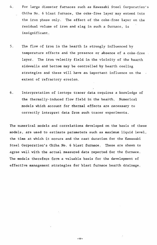
4. For large diameter furnaces such as Kawasaki Steel Corporation's Chiba No. 6 blast furnace, the coke-free layer may extend into the iron phase only. The effect of the coke-free layer on the residual volume of iron and slag in such a furnace, is insignificant.

5. The flow of iron in the hearth is strongly influenced by temperature effects and the presence or absence of a coke-free layer. The iron velocity field in the vicinity of the hearth sidewalls and bottom may be controlled by hearth cooling strategies and these will have an important influence on the extent of refractory erosion.

6. Interpretation of isotope tracer data requires a knowledge of the thermally-induced flow field in the hearth. Numerical models which account for thermal effects are necessary to correctly interpret data from such tracer experiments.

The numerical models and correlations developed on the basis of these models, are used to estimate parameters such as maximum liquid level, the time at which it occurs and the cast duration for the Kawasaki Steel Corporation's Chiba No. 6 blast furnace. These are shown to agree well with the actual measured data reported for the furnace.The models therefore form a valuable basis for the development of effective management strategies for blast furnace hearth drainage.

-v-

ACKNOWLEDGEMENTS

In the context of completing this course of study, I wish to firstly acknowledge and thank Professor W. Val Pinczewski for his encouragement, invaluable suggestions and advice.

I would also like to thank my colleague, Dr. W.B.U. Francis Tanzil, for his advice, support and willingness to offer his time, at any time.

I gratefully acknowledge the support given to me by Dr. John M. Burgess, Dr. John G. Mathieson and other members of staff of the Broken Hill Proprietary Co., and the financial support for research provided by this company.

I wish to thank my fellow graduates, Ian Taggart, Habib Zughbi, Stuart Munro and Andrew Grogan, who were always there to listen and lend a hand. I would also like to thank my brother, Lawrence, who so generously supplied a personal computer for the production of this thesis:

Finally, I wish to express gratitude to my wife, Lynette, who sacrificed countless evenings, weekends and holidays so that this thesis could be completed.

-vi-

LIST OF PUBLICATIONS

1. W.B.U. Tanzil, P. Zulli, J.M. Burgess and W.V. Pinczewski 'Experimental Model Study of the Physical Mechanisms Governing Blast Furnace Drainage'Transactions ISIJ. 1984, Vol. 24, p. 197.

2. W.B.U. Tanzil, P. Zulli and W.V. Pinczewski'Flow of Iron and Slag in the Blast Furnace Hearth'Proceedings Third World Congress of Chemical Engineers. 1986, Tokyo, September, p. 9b-301.

3. J.G. Mathieson, L. Jelenich, P.C. Goldsworthy and P. Zulli 'The Use of Sensing Techniques and Mathematical Models To Improve Blast Furnace Performance'Proceedings 48th Ironmaking Conference. Iron and Steel Society, A.I.M.E., Chicago, 1989, Vol. 48, p. 587.

4. L. Jelenich, P.C. Goldsworthy, P. Zulli and M.G. Hughes 'Operational Control Systems for Liquids and Thermal Management in the Ironmaking Blast Furnace'Proceedings 18th Australasian Chemical Engineering Conference, CHEMECA 90, Auckland, New Zealand, August 27-30, 1990, p. 32.

-vii-

TABLE OF CONTENTS

SUMMARYACKNOWLEDGEMENTS LIST OF PUBLICATIONS1 INTRODUCTION 1

1.1 Status of Ironmaking and Related Technologies 11.2 The Ironmaking Blast Furnace Process 11.3 The Hearth 51.4 Previous Hearth Drainage Studies 8

1.4.1 Liquid Drainage 91.4.2 Metal Flow 15

2 TWO-DIMENSIONAL MODEL STUDY OF HEARTH DRAINAGE 212.1 Introduction 212.2 Governing Equations 232.3 Initial and Boundary Conditions 272.4 Numerical Technique 312.5 Numerical Stability and Accuracy 462.6 Computational Procedure 482.7 Viscous Flow Analog for Flow Through a Packed Bed

and Packing-free Layer 492.7.1 The Analog 492.7.2 Experimental Model 54

2.8 Comparison Between Experimental and NumericalResults 58

2.9 Physical Mechanisms of Single-Liquid Drainage 652.10 Correlation of Residual Slag and Flow-out

Coefficient 792.10.1 Fully Packed Bed 792.10.2 Floating Packed Bed 89

2.11 Conclusions 104

-viii-

3 THREE-DIMENSIONAL MODEL STUDY OF HEARTH DRAINAGE 1063.1 Introduction 1063.2 Governing Equations 1073.3 Initial and Boundary Conditions 1093.4 Numerical Technique 115

3.4.1 Finite-Difference Approximations forCurved Boundary and Free Surface Cells 127

3.4.2 Finite-Difference Approximations forBoundary Conditions 128

3.5 Numerical Stability and Accuracy 1363.6 Computational Procedure 1373.7 Laboratory-scale Experiments 138

3.7.1 Experimental Procedure 1423.8 Numerical Model Results 142

3.8.1 Validation of Numerical Model 1423.8.2 Drainage of Two- and Three-dimensional

Packed Beds With and Without a Packing-free Layer 147

3.9 Correlation of Residual Slag and Flow-out Coefficient 1513.9.1 Fully Packed Bed Hearths * 1513.9.2 Packed Bed-Packing-free Layer Hearths 157

3.10 Application to Blast Furnaces 1633.10.1 Model Formulation 1633.10.2 Model Validation and Application to

Actual Furnace Data 1723.11 Conclusions 178

4 TWO-LIQUID DRAINAGE WITH AND WITHOUT A COKE-FREE LAYER 1804.1 Introduction 1804.2 Governing Equations 1824.3 Initial and Boundary Conditions 1854.4 Numerical Technique 188

4.4.1 Numerical Approximation of the Liquid-liquidInterface 188

-ix-

4.4.2 Differencing Technique 1924.5 Numerical Stability and Accuracy 2024.6 Computational Procedure 2044.7 Experimental 2054.8 Validation of Numerical Model 2054.9 Application to Blast Furnaces 2134.10 Conclusions 222

5 TWO-DIMENSIONAL STUDY OF THE FLOW OF IRON IN ANON-ISOTHERMAL HEARTH 2235.1 Introduction 2235.2 Model Formulation 2255.3 Initial and Boundary Conditions 2325.4 Numerical Scheme 2355.5 Numerical Stability and Accuracy 2475.6 Computational Procedure 2485.7 Model Validation 2495.8 Physical Mechanisms of Iron Drainage in a

Non-isothermal Hearth 2555.8.1 Fully Packed Bed With Under-hearth Cooling 2575.8.2 Packed Bed/Coke - free Layer With Under-hearth

Cooling 2605.8.3 Fully Packed Bed With Side-hearth Cooling 2635.8.4 Packed Bed/Coke - free layer With Side-hearth

Cooling 2665.8.5 Side-and Under-hearth Cooling in a Packed Bed

With and Without a Coke-free Layer 2685.9 Conclusions 272

6 THREE-DIMENSIONAL STUDY OF THE FLOW OF IRON IN ANON-ISOTHERMAL HEARTH 2746.1 Introduction 2746.2 Model Formulation 2756.3 Initial and Boundary Conditions 2826.4 Numerical Technique 286

-x-

6.4.1 Finite - Difference Approximations for Curved Boundary Cells 300

6.4.2 Finite - Difference Approximations for BoundaryConditions 301

6.4.3 Marker Particles 3066.5 Numerical Stability and Accuracy 3106.6 Computational Procedure 3116.7 Interpretation of Radioactive Isotope Tracer

Experiments 3126.7.1 Actual Furnace Tracer Experiments 313

6.8 Conclusions 330REFERENCES 331APPENDIX A A. 1APPENDIX B B. 1APPENDIX C C. 1APPENDIX D D. 1APPENDIX E E. 1APPENDIX F F. 1APPENDIX G G. 1APPENDIX H H. 1PUBLICATIONS

-xi-

LIST OF FIGURES

1.1 Schematic diagram of blast furnace. 31.2 Schematic diagram of blast furnace hearth. 61.3 Experimentally-derived correlation between the

residual ratio and flow-out coefficient (Fukutake and Okabe (1976 a)). 11

1.4 Computed and experimentally-derived liquid-liquid andgas-liquid interfaces (Tanzil (1985)). 14

2.1 Schematic diagram of a two-dimensional, single-liquiddrainage model. 24

2.2 Two-dimensional, computational grid. 282.3 Layout of field variables in computational cell block. 322.4 Control volume fo-r ui+1/2,i- 372.5 Computational cell containing free surface. 422.6 Variables used to define surface elevation. 452.7 Viscous flow analog for flow in a packed bed and flow

between two parallel plates. 512.8 Experimental viscous flow analog. 552.9 Cross-sectional view of experimental viscous flow

analog. 562.10 Comparison between experimentally measured gas-liquid

profiles (Pinczewski and Tanzil (1981)) and computed profiles for a two-dimensional, fully packed bed. 59

2.11 Comparison between experimentally measured andcomputed gas-liquid profiles for a two-dimensional, fully packed bed with a packing-free layer (Run 1 -Drain height =4.5 cm). 60

2.12 Comparison between experimentally measured andcomputed gas-liquid profiles for a two-dimensional, fully packed bed with a packing-free layer (Run 2 -Drain height = 18.5 cm). 61

-xii-

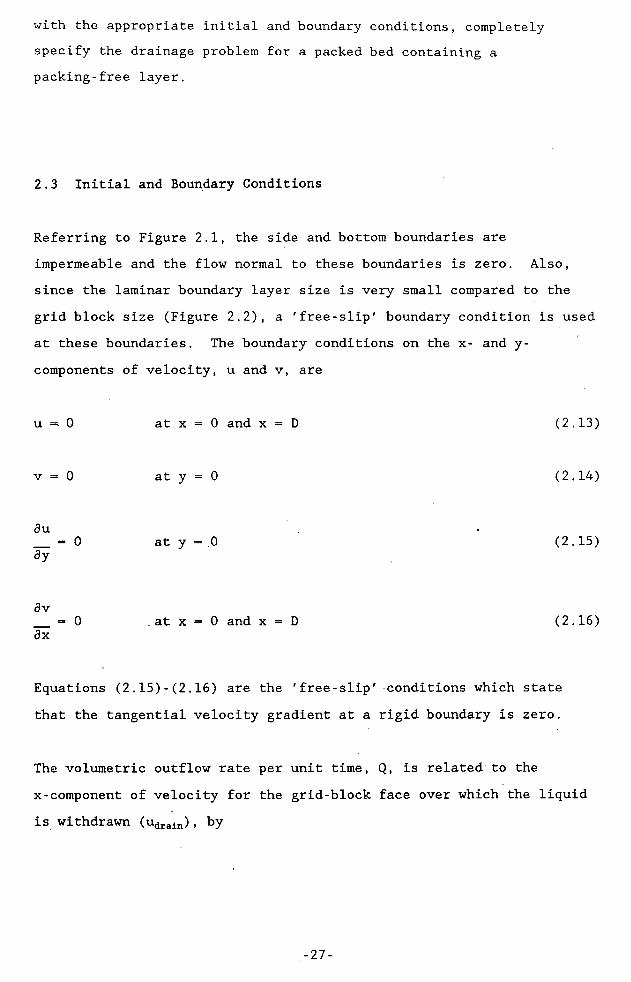
2.13 Experimentally-derived liquid flowrates for Run 1. 632.14 Experimentally-derived liquid flowrates for Run 2. 642.15(a) Computed positions of the gas-liquid interface for a

fully packed bed [(Hth-Hfl)/D =0.23]. 682.15(b) Computed positions of the gas-liquid interface for a

packed bed with a packing-free layer [(Hth-Hfl)/D =0.1]. 69

2.15(c) Computed positions of the gas-liquid interface for a packed bed with a packing-free layer [(Hth-Hfl)/D =0.01]. 70

2.16 Liquid streamline distribution pattern for a fullypacked bed. 72

2.17 Liquid streamline distribution pattern for a packedbed with a packing-free layer. 73

2.18 Comparison between the terminal positions of the gas-liquid interface for (a) a fully packed bed, (b) a packed bed with a continuous packing-free layer and (c) a packed bed with a discontinuous packing-freelayer. 77

2.19 Liquid streamline distribution pattern for a packedbed with a discontinuous packing-free layer. 78

2.20 Slag drainage model as proposed by Fukutake and Okabe(1976 a). 80

2.21 Schematic diagram of the drainage of iron from levels below the level of the taphole (Pinczewski et al(1982). 81

2.22 Slag drainage model based on results followingPinczewski et al (1982). 83

2.23 Relationship between the residual ratio (a) and VoCb/p for values of H**. 87

2.24 Relationship between Vo Cb/p and H** for a = 0.5. 88

-xiii-

2.25 Correlation between the residual ratio (a) and the modified flow-out coefficient (FL*) for a fully packedbed. 90

2.26 Schematic diagram of a hearth with a packed bed and apacking-free layer. 92

2.27 Slag drainage model proposed for a packed bed with apacking-free layer. 93

2.28 Relationship between Vo and a for values of Cb/p. 962.29 Relationship between Vo and Cb/p. 972.30 Relationship between a and Vo Cb/p for values of H**. 982.31 Relationship between Vo Cb/p and H**. 1002.32 Relationship between a and Fr/Reb H**1-94 for values of

Hfl\ 1012.33 Relationship between Fr/Reb H**1-94 and Hfi* for

a = 0.3. 1022.34 Correlation between the residual ratio (a) and the

modified flow-out coefficient accounting for theeffect of a packing-free layer (FL(cfl)). 103

3.1 Schematic diagram of the three-dimensional hearthdrainage model. 108

3.2 Plan and elevation views of the three-dimensionalhearth drainage model. 110

3.3 Representation of the taphole (or outflow boundary) inthe three-dimensional model. 113

3.4 Three-dimensional, computational grid. 1163.5 Plan and elevation views of the computational grid. 1173.6 Layout of field variables for a full cell. 1193.7 Layout of field variables for cells bisected by a

curved boundary. 1203.8 Definition of variables used to compute the pressure

in a cell containing the free surface. 129

-xiv-

3.9 Plan view of the three-dimensional, computational gridshowing the parameter used in defining the 'free-slip' boundary conditions. 131

3.10 Definition of the surface elevation, h. 1353.11 Schematic diagram of the 40 cm diameter experimental

apparatus. 1393.12 Schematic diagram of the 15 cm diameter experimental

apparatus. 1403.13 Wire mesh used to support the packing for the free

layer experiments. 1413.14 Viscosity-temperature relationship for a

glycerol/water mixture (50:50 v/v). 1433.15 Comparison between experimental drainage profiles

(Tanzil (1985)) and computed profiles for athree-dimensional, fully packed bed. 145

3.16 Comparison between experimental and computed drainageprofiles for a three-dimensional, packed bed with a packing-free layer. 146

3.17 Comparison between terminal drainage profiles for a fully packed bed as computed by the two- andthree-dimensional numerical models. 149

3.18 Comparison between terminal drainage profiles for a packed bed with a packing-free layer as computed bythe two- and three-dimensional numerical models. 150

3.19 Relationship between the residual ratio, a, andVo Ch/p for a range of H** values. 154

3.20 Relationship between Vo Cb/p and H** for a fixed valueof the residual ratio, a. 155

3.21 Correlation between the residual ratio, a, and the modified flow-out coefficient, FL*, forthree-dimensional, fully packed beds. 156

-xv-

3.22 Comparison between experimental results reported by Fukutake and Okabe (1976 a) and experimental resultsfrom the present study. 158

3.23 Relationship between the residual ratio, a, andVo Cb/p H**1-4 for a range of Hfl* values. 160

3.24 Relationship between Vo Cb/p H**1-4 and Hfl* fora = 0.5. 161

3.25 Correlation between the residual ratio, a, and themodified flow-out coefficient, FL(cfl) which accounts for the effect of a free layer in a three-dimensional packed bed. 162

3.26 Schematic diagram of the hearth. 1703.27 Cumulative drained tonnages of iron and slag drained

from the hearth of Kawasaki's Chiba No. 6 blastfurnace (Fukutake et al (1981)). 173

3.28 Comparison between the computed drainage profiles forChiba No. 6 blast furnace (Tanzil (1985)) and the average liquid levels computed by the proposed hearth drainage model. 177

4.1 • Schematic diagram of the two-dimensional, two-liquidmodel. 183

4.2 Computational cell containing the liquid-liquidinterface. 191

4.3 Computational grid. 1934.4 Definition of parameters used in the calculation of

the y-component of velocity at the liquid-liquid interface. 201

4.5 Modified viscous flow analog. 2064.6 Experimentally measured drainage rates of

glycerol/water and mercury used for computations shownin Figure 4.7. 209

-xvi-

4.7

4.8

4.9

4.10

4.11

4.12

4.13

4.14

4.15

Comparison between the liquid levels computed by the numerical model for a drainage experiment in a fully packed bed, and the liquid levels measured by experiment (Tanzil (1985)).Comparison between the liquid levels computed by the numerical model for a drainage experiment in a packed bed with a packing-free layer, and the liquid levels measured by experiment.Experimentally measured drainage rates of glycerol/water and mercury used for computations shown in Figure 4.8.Comparison between drainage profiles for Kawasaki's Chiba No. 6 blast furnace computed by the present numerical model with the profiles computed by Tanzil (1985) .Drainage data for Kawasaki's Chiba No. 6 blast furnace: (a)measured, (b) computed by Tanzil (1985). Comparison between the drainage rate for Chiba No. 6 blast furnace predicted by the present numerical model, and the drainage rate as: (a) measured, and (b)computed by Tanzil (1985).Comparison between the cumulative drained volumes for Chiba No. 6 blast furnace predicted by the present numerical model, and the cumulative drained volumes as: (a) measured, and (b) computed by Tanzil (1985). Predicted drainage profiles for Chiba No. 6 blast furnace, with and without a coke-free layer (coke-free layer height = 40 cm).Comparison between the computed cumulative drained volumes for Chiba No. 6 blast furnace with a coke-free layer, and the cumulative drained volumes as: (a)

211

212

214

217

218

219

220

210

-xvii-

measured, (b) computed by the present model for Chiba No. 6 blast furnace without a coke-free layer and (c) computed by Tanzil (1985). 221

5.1 Schematic diagram of the two-dimensional,single-liquid, non-isothermal model. 226

5.2 Computational grid. 2365.3 Layout of field variables. 2375.4 Streamline distribution pattern at 2 minutes into the

cast for a hearth with under-hearth cooling and an initial linear temperature profile (Yashiro et al (1982)). 252

5.5 Streamline distribution pattern computed by thepresent numerical model for hearth conditions similarto that shown in Figure 5.4. 253

5.6 Comparison between the computed hearth temperatureprofiles at 47.5 minutes into the cast and the temperature profiles reported by Yashiro et al (1982). 254

5.7 Streamline distribution patterns in a hearth with afully packed bed, under-hearth cooling and an initial, linear temperature profile. 258

5.8 Streamline distribution patterns in a hearth with afully packed bed, under-hearth cooling and an initial, isothermal temperature profile. 259

5.9 Streamline distribution patterns in a hearth with a packed bed and 0.3 m high coke-free layer, under-hearth cooling and an initial, lineartemperature profile. 261

5.10 Streamline distribution patterns in a hearth with apacked bed and 0.3 m high coke-free layer, under-hearth cooling and an initial, isothermal temperature profile. 262

-xviii-

5.11

5.12

5.13

5.14

5.15

5.16

6.1

6.26.36.4

6.5

6.6

6.7

Streamline distribution patterns in a hearth with a fully packed bed, side-hearth cooling and an initial, isothermal temperature profile.Natural convection currents in a hearth with a fully packed bed, side-hearth cooling and an initial, isothermal temperature profile.Streamline distribution patterns in a hearth with a packed bed and 0.3 m high coke-free layer, side-hearth cooling and an initial, isothermal temperature profile.Streamline distribution patterns in a hearth with a packed bed and a coke-free layer of non-uniform height, side-hearth cooling and an initial, isothermal temperature profile.Streamline distribution patterns in a hearth with a fully packed bed, side- and under-hearth cooling and an initial, isothermal temperature profile.Streamline distribution patterns in a hearth with a packed bed and 0.3 m high coke-free layer, side- and under-hearth cooling and an initial, isothermal temperature profile.Schematic diagram of the three-dimensional, single-liquid, non-isothermal model.Three-dimensional, computational grid.Plan and elevation views of the computational grid. Layout of field variables for a full computational cell.Layout of field variables for a computational cell bisected by the curved boundary.Plan view of the three-dimensional, computational grid showing the parameter used in defining the 'free-slip' boundary conditions.Eight sub-regions defined in a computational cell.

264

265

267

269

270

271

276287288

289

290

302308

-xix-

6.8 Plan view of Broken Hill Proprietary's Port KemblaNo. 5 blast furnace, showing the injection and efflux points for the radioisotope tracer experiments. 316

6.9 Radioisotope tracer concentration for Trial 1 (23 May1984) and Trial 2 (13 June 1984) experiments at Port Kembla No. 5 blast furnace. 317

6.10 Hearth sidewall and plug temperatures for Port Kembla's No. 5 blast furnace during the period23 May-13 June 1984. 321

6.11 Computed path travelled by the radioisotope tracer forthe Trial 1 experiment (23 May 1984), assuming isothermal hearth conditions. 324

6.12 Computed path travelled by the radioisotope tracer forthe Trial 2 experiment (13 June 1984), assuming the hearth is side-hearth cooled. 325

6.13 Computed path travelled by the radioisotope tracer for the Trial 1 experiment (23 May 1984), assuming thehearth is under-hearth cooled. 327

6.14 Computed path travelled by the radioisotope tracer forthe Trial 2 experiment (13 June 1984), assuming the hearth is isothermal and a 40 cm high coke-free layer underlies the coke bed. 329

B. l Schematic diagram showing a side elevationview of the hearth. B.2

C. l Flowchart of program HD21.F0R. C.2D. l Flowchart of program HD31.F0R. D.2E. l Flowchart of program HD22.FOR. E.2F. l Flowchart of program HDT21.F0R. F.2G. l Flowchart of program HDT31.F0R. G.2H. l - Flowchart of program HLSM.FOR. H.2

-xx-

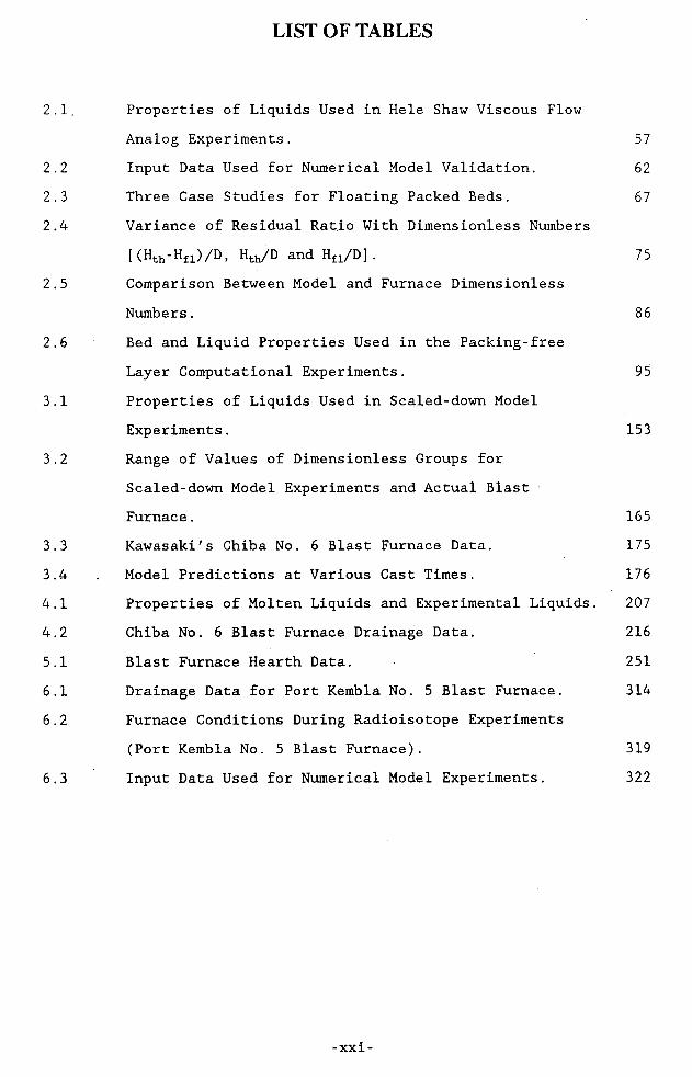
LIST OF TABLES

2.1. Properties of Liquids Used in Hele Shaw Viscous FlowAnalog Experiments. 57

2.2 Input Data Used for Numerical Model Validation. 622.3 Three Case Studies for Floating Packed Beds. 672.4 Variance of Residual Ratio With Dimensionless Numbers

[ (Hth"Hfi)/D, Hth/D and H£1/D], 752.5 Comparison Between Model and Furnace Dimensionless

Numbers. 862.6 Bed and Liquid Properties Used in the Packing-free

Layer Computational Experiments. 953.1 Properties of Liquids Used in Scaled-down Model

Experiments. 1533.2 Range of Values of Dimensionless Groups for

Scaled-down Model Experiments and Actual BlastFurnace. 165

3.3 Kawasaki's Chiba No. 6 Blast Furnace Data. 1753.4 . Model Predictions at Various Cast Times. 1764.1 Properties of Molten Liquids and Experimental Liquids. 2074.2 Chiba No. 6 Blast Furnace Drainage Data. 2165.1 Blast Furnace Hearth Data. 2516.1 Drainage Data for Port Kembla No. 5 Blast Furnace. 3146.2 Furnace Conditions During Radioisotope Experiments

(Port Kembla No. 5 Blast Furnace). 3196.3 Input Data Used for Numerical Model Experiments. 322

-xxi-

1 INTRODUCTION

1.1 Status of Ironmaking and Related Technologies

Although alternate ironmaking processes are already producing significant tonnages of iron (direct reduction processes produced 30 million tonnes in 1984 (Walker 1986)), the iron blast furnace remains the dominant ironmaking process. In the early 1980's, world production of iron declined due in most part to reductions in demand from construction industries, ship building and a trend towards 'lighter, thinner, shorter and smaller products' (Araki (1985)). More recently, world wide variations in iron output have occurred as a result of blowing out of furnaces in Japan and construction of large furnaces in South America (Brazil) (Walker (1986)). Research related to blast furnace technology however, has continued during the 1980's. This research is largely directed to achieving improvements in international competitiveness (Lee (1987)) and on development of second-generation technologies for yield improvement as well as improvements in energy and raw materials utilisation (Kinoshita (1987)).

1.2 The Ironmaking Blast Furnace Process

The size and specific details (eg. ancillary equipment) of blast furnaces vary considerably depending, amongst other things, on iron demand, raw materials and fuel availability. In basic form, the blast furnace is a cylindrically-shaped, vertical counter - current, multi-phase (solid, liquid and gas) reactor. A typical modern furnace

-1-

stands approximately 30 metres high (Figure 1.1). Raw materials (sources of iron oxide which include iron ore, sinter and pellets, coke and fluxes) are charged in discrete batches at the top of the furnace, whilst preheated air, which may be enriched by additions of varying amounts of natural gas, pulverised coal and/or oxygen, is injected through a number of ports or tuyeres located approximately 25 metres below the top. Rather than classify the various structural regions of the blast furnace, it is more instructive to describe the functional classifications pertaining to changes in the iron oxide (ore) as it progresses down the shaft of the furnace.

Raw materials, transported to the top of the furnace using a conveyor or skip car system, are charged into the furnace through a gas-tight distributor system (bell or chute). The individual raw materials are usually introduced sequentially ie. layered charging. As the charged material descends, it is heated and reduced by upward-moving gases produced from the combustion of coke carbon and other fuels in the region surrounding the tuyeres. The ore and fluxes pass through a 'lumpy' or pre-softening stage before being softened, fused and eventually melted (cohesive zone). The position of the cohesive zone varies radially across the furnace and depends upon the tuyere conditions and material distribution at the top of the furnace, particularly on the ore/coke radial distribution pattern.

The molten products (iron-carbon mixture and fluxes or slag) percolate through the unreacted coke, which forms a heterogeneous packed bed beneath the cohesive zone. The coke bed is distinguished by three zones - a coke zone or 'deadman' which serves as the coke supply for the combustion zone around the tuyere, the core zone, where coke is renewed very slowly and the hearth coke bed, which may either rest on or float above the floor of the furnace (Omori (1987)). The molten

-2-

Charging bells

-----10.7m-SHAFT

Stock level

FUSIONZONE 19-Om

36.8 mBOSH

4.3 m

Tuyeres(42)

hearth 6.2 m

14.4 mTapholes (3)

4.8 m

Figure 1.1 Schematic diagram of blast furnace

-3-

liquids accumulate in the hearth and are removed either continuously or intermittently through tapholes around the circumference of the hearth.

The productivity of blast furnaces (measured in tonnes of metal produced per day per cubic metre of inner volume) has been improved by increasing the size of blast furnaces, use of better quality raw materials and operating with higher top pressures and blast temperatures. These developments have necessitated the introduction of new operating practices. These have, in turn, introduced problems such as irregular descent of burden material and abnormal fluctuations in blast pressure, both of which have an adverse effect on the operational stability of the furnace. The stability problem is closely related to conditions in the hearth. In the past, tapping practice involved slag flushing through a cinder notch followed by iron removal through the taphole. Modern day practice, especially for large blast furnaces, involves multiple tapping and a 'tap only' practice since the introduction of high top pressure made slag flushing difficult (Fukutake et al (1981)). Also, in order to attain higher productivity levels, liquids must be drained from the furnace using the taphole only. Operational difficulties arise because large volumes of slag remain in the furnace at the end of the cast due to the high viscosity of slag. Reducing the volume of slag remaining at the end of a cast is important to stable furnace operation and in the last ten years, many studies have been carried out to determine the conditions (tapping operation, state of the coke bed etc.) affecting slag retention in the hearth (Fukutake et al (1976 a), Fukutake et al (1976 b), Burgess et al (1980), Tanzil et al (1984), Tanzil (1985)). Before discussing these studies, it is instructive to consider in some detail, the conditions in the hearth.

-4-

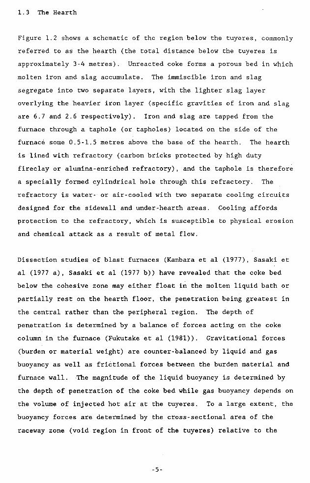
1.3 The Hearth

Figure 1.2 shows a schematic of the region below the tuyeres, commonly referred to as the hearth (the total distance below the tuyeres is approximately 3-4 metres). Unreacted coke forms a porous bed in which molten iron and slag accumulate. The immiscible iron and slag segregate into two separate layers, with the lighter slag layer overlying the heavier iron layer (specific gravities of iron and slag are 6.7 and 2.6 respectively). Iron and slag are tapped from the furnace through a taphole (or tapholes) located on the side of the furnace some 0.5-1.5 metres above the base of the hearth. The hearth is lined with refractory (carbon bricks protected by high duty fireclay or alumina-enriched refractory), and the taphole is therefore a specially formed cylindrical hole through this refractory. The refractory is water- or air-cooled with two separate cooling circuits designed for the sidewall and under-hearth areas. Cooling affords protection to the refractory, which is susceptible to physical erosion and chemical attack as a result of metal flow.

Dissection studies of blast furnaces (Kanbara et al (1977), Sasaki et al (1977 a), Sasaki et al (1977 b)) have revealed that the coke bed below the cohesive zone may either float in the molten liquid bath or partially rest on the hearth floor, the penetration being greatest in the central rather than the peripheral region. The depth of penetration is determined by a balance of forces acting on the coke column in the furnace (Fukutake et al (1981)). Gravitational forces (burden or material weight) are counter-balanced by liquid and gas buoyancy as well as frictional forces between the burden material and furnace wall. The magnitude of the liquid buoyancy is determined by the depth of penetration of the coke bed while gas buoyancy depends on the volume of injected hot air at the tuyeres. To a large extent, the buoyancy forces are determined by the cross-sectional area of the raceway zone (void region in front of the tuyeres) relative to the

-5-

Gas slag interfaceVoJCac

d)S

•£

-6-

igure 1.2 Schematic diagram of blast furnace heart'

hearth cross-sectional area and by the liquid height in the hearth. Since the extent of the raceway zone varies little with furnace size (Fukutake et al (1981)), the effect of gas buoyancy decreases with increasing furnace diameter and for larger furnaces (8-14 metres), the coke bed is likely to penetrate deep into the iron melt and/or sit on the hearth floor. In smaller furnaces (5-8 metres), the bed is likely to float in the bath of molten liquids, the penetration in some furnaces being only into the slag phase (Kanbara et al (1977)).

In terms of liquid movement through the hearth, the penetration of the coke bed into hearth is very important. The region beneath the bed, called the coke-free layer or coke-free zone, offers a much lower resistance to liquid flow than the coke bed itself and as a result, liquid preferentially flows through the coke-free layer. Four particular situations may arise in the hearth, depending on the penetration of the coke bed. When the porous coke bed completely fills the hearth, molten iron and slag must flow through the bed towards the taphole. Under these conditions, it is possible for a coke-free gutter to form about the periphery at the base of the hearth. When such a gutter exists, the bulk of the liquid flow remains through the packed bed but the velocity of the iron in the gutter may be very high and therefore, significant in terms of refractory erosion. If the coke bed floats entirely in the iron melt, the hearth liquids flow through both the coke bed and through the coke-free layer. The proportion of liquid flowing through the coke-free layer increases with decreasing liquid velocity (Ohno et al (1981)). For the case where the bed extends only into the slag layer (Kanbara et al (1977)), the slag volume retained at the end of the cast may be small.

The penetration of the coke bed also affects the thermal balance in the hearth. As a result of hearth cooling, a solidified layer forms above the hearth floor. Previous studies have suggested that erosion

-7-

and regeneration of this solid layer could be related to the development of the coke-free layer (Ohno et al (1981), Ohno et al (1985)). In other words, when the coke-free layer height is small, the liquid velocity is high and the rate of erosion of the solid layer is accelerated. As the solid layer is eroded, the heat losses increase and the regeneration of the solid layer begins.

From the point of view of hearth liquid management and refractory erosion, it is important to control liquid movement in the hearth. Prior to the early 1970's, little was understood of the factors determining liquid movement in the hearth. Subsequent investigators have identified important phenomena such as the downward-tilting of the slag surface (Fukutake et al (1976 a)) and upward-tilting of the iron surface when the iron level is below the level of the taphole (Burgess et al (1981), Tanzil (1985)). These studies have identified the important parameters affecting slag drainage (eg. tapping rate, slag viscosity), giving furnace operators a clearer understanding of the hearth drainage process. The earlier studies were predominantly experimental in nature and considered only the drainage of a single liquid (slag). Later studies (Burgess et al (1981), Ichihara et al (1979), Ohno et al (1982), Fukutake et al (1983), Tanzil (1985)) utilised mathematical models, solved by numerical techniques on large computers, to simulate the hearth drainage processes. These studies are discussed below.

1.4 Previous Hearth Drainage Studies

It is convenient to divide hearth-related research into two major categories. The first is the study of liquid drainage from the hearth and includes research related to slag removal from the furnace and the influence of various operating factors such as metal flow, tapping

-8-

rate and the effect of the coke-free layer on hearth drainage. The second category concerns the study of metal flow in the hearth as it relates to refractory erosion and the influence of the state of the coke bed and hearth cooling. Radioisotope injections into the hearth forms an integral part of metal flow studies and is included in this category.

1.4.1 Liquid Drainage

The first experimental study of liquid drainage from the hearth was reported by Shimozuma et al (1971). The model consisted of a cylindrical container filled only with water and a drain located on the side. A vortex (or tilting of the air-water interface towards the taphole) was observed near the taphole and it was suggested that this could result in poor drainage of pig iron from the hearth.

Later, results from single-liquid experiments carried out by Makhanek et al (1974) confirmed the observations reported by Shimozuma et al (1971) and provided the basis for the hydraulic slope concept.Makhanek et al (1974) proposed that the development of a hydraulic slope or the inclination of the liquid surface to the horizontal towards the taphole, prevented complete removal of pig iron and slag during a cast and that the proportions of each phase left in the hearth increased with hearth diameter, hearth permeability and viscosity of the smelted products. They further suggested that a high liquid flowrate using a larger taphole diameter, is preferred for maximum removal of liquids.

Fukutake and Okabe (1976 a) carried out extensive physical modelling of slag drainage using small cylindrical models, fully packed with

-9-

glass ballotini, in order to determine the conditions under which the hearth is effectively drained. Several simplifying assumptions were made to facilitate the experimental work. These included:

(a) The upper slag surface is initially horizontal(b) The slag drainage rate is constant throughout the cast(c) The bed is isotropic(d) Thermal effects are negligible(e) Coke particles are sufficiently small to provide the only

resistance to flow(f) The iron-slag interface remains horizontal and at the same

level as the taphole for the entire cast

As a consequence of the last assumption (f), it was only necessary to examine the drainage of a single liquid (slag). Fukutake and Okabe (1976 a) measured the volume of liquid remaining in the model at the end of drainage (residual ratio) as a function of initial height and drainage rate. They correlated their residual ratio results (defined as the ratio of the volume of liquid remaining at the end of a cast to that contained at the beginning of drainage) using a dimensionless flow-out coefficient. The correlation was found to be independent of the shape and size of the taphole.

Figure 1.3 shows the experimental results obtained by Fukutake and Okabe (1976 a) together with their correlating function. The figure shows that:

(a) the residual ratio increases monotonically with FL(b) a low slag viscosity, low tapping rate and high bed

permeability result in low slag residual ratios

-10-

-11-

Flow out coefficient

Fukutake and Okabe (1976 b) combined the above residual ratio correlation with a slag mass balance to determine the influence of tapping conditions on the slag residual ratio for both steady and unsteady tapping operations, for actual blast furnaces. They concluded that effective drainage of slag could be achieved when:

(a) a low drainage rate was maintained(b) the frequency of casts was increased(c) thermal control (enabling control of slag viscosity) is

maintained, and(d) good quality coke is used (high coke bed permeability)

Ichihara and Fukutake (1979) simulated single-phase, slag flow in a three-dimensional co-ordinate system using a finite-element method. Their results agreed well with experiments conducted in laboratory models. Ichihara et al (1981) examined the effect of variable tapping rate on the slag residual ratio using a two-dimensional, numerical technique based on the integrated penalty method (Natori and Kawarada (1976)). They concluded that a tapping rate increasing with time results in a greater residual ratio than a constant average rate.This is important for actual operating furnaces where the taphole diameter increases with time as a result of taphole erosion and the drainage rate therefore increases with time.

Burgess et al (1980, 1981) report an experimental and theoretical investigation of the drainage of a single liquid from a two-dimensional, rectangular packed bed using a sidewall outlet. The initial liquid height, liquid viscosity and drainage rate were varied in these experiments. As well, bed heterogeneity resulting from the presence of fine particles in the packed bed, was shown to have an adverse effect on drainage performance. The experiments were

-12-

simulated using a numerical model based on a finite-difference technique (Pinczewski and Tanzil (1981)) and good agreement was obtained with experimental results.

Pinczewski et al (1982) used a two-dimensional, Hele-Shaw apparatus to investigate the simultaneous drainage of iron and slag from the hearth. Previous studies had assumed that the interaction between the drainage of iron and slag was negligible. Pinczewski et al (1982) showed that this assumption was incorrect and that a complex interaction existed between the drainage of the two phases. This study is of particular significance because it provides an explanation for the observed drainage performance of Kawasaki Steel Corporation's Chiba No. 6 blast furnace, which shows that iron and slag are drained simultaneously over most of the casting period (Fukutake et al (1983)). Further, two important qualitative observations were drawn from the study. Firstly, iron continues to flow out of the taphole when the average iron level is below that of the taphole. Pressure gradients developed within the upper liquid (slag) are responsible for this phenomenon (Figure 1.4). Secondly, 'viscous fingering' or an instability of the air-glycerol (gas-slag) interface occurs when the interface velocity is high (rapid drainage). The instability is greatest near the taphole and leads to a high liquid residual ratio. Numerical calculations confirmed these experimental results.

Following this work, Tamiya et al (1983) and Fukutake et al (1983) simulated the two-phase system using a two-dimensional, numerical model based on the Boundary Element Method . They simulated the continuous tapping operation of Chiba No. 6 blast furnace. This furnace has a hearth diameter of 14.1 metres and four tapholes. The total drainage rate of iron and slag combined was assumed to increase linearly with time as the taphole eroded. The results revealed that a maximum liquid level occurs during the cast, which can be controlled by decreasing the 'hearth drainage index', Dh*, where Dh* is the ratio

-13-

E X P E R I M ENTAL04vh

5o ^

^

t i

•

CNiriO N

«I

I I

I I

(^0) x

Eu>

lO00

.”3NC3Hu€Du3.Ctf)LZ

-14-

of the production rate of iron and slag and the hydraulic conductivity of the liquid (the definition of the term Dh* is similar to that of the flow-out coefficient (Fukutake and Okabe (1976 a))). Minimising taphole erosion and shortening the cast duration were shown to have the same effect.

More recently, Tanzil (1985) developed a three-dimensional, numerical model which accounts for the simultaneous flow of slag and iron from the hearth. The model was used to simulate the conditions in the hearth of Chiba No. 6 using the drainage data reported by Fukutake and Okabe (1981). The agreement between the actual furnace drainage performance and that computed with the model, was very good. The model provided, for the first time, a detailed description of the distribution of iron and slag in the hearth of an actual operating furnace during casting. The simulations however required considerable computer time.

1.4.2 Metal Flow

Metal flow in the hearth has traditionally been investigated using radioisotopes injected through the tuyeres. Babarykin et al (1960) used radioisotopes to determine whether convection currents are present in the hearth. Their results showed no evidence of the existence of convection currents in the small diameter furnace used for the trial work.

Miyagwa et al (1965) estimated the extent of erosion of the refractory lining of the hearth using a radioisotope dilution analysis. The estimated volume of refractory eroded from the hearth of Hirohata No. 2 blast furnace compared well with that measured following the quenching of the furnace. Their investigations also showed that the

-15-

flow of iron in the hearth may be peripheral rather than through the coke bed. For the case where iron flows only through the coke bed, Shimomura et al (1978) showed that a relationship existed between the distance travelled by the radioisotope and the peak in concentration of the isotope as measured at the taphole. A deviation from this relationship indicated peripheral (or abnormal) flow of iron in the hearth. The results of this investigation were related to fluctuations in hot metal quality and hearth refractory temperatures.

The effect of coke quality on bed permeability was also investigated using radioisotope injections into the hearth (Nakamura et al (1977)). In this study, a correlation was developed between coke strength and the maximum concentration and travelling time of the radioisotope.

A more fundamental investigation of iron flow in the hearth was carried out by Hara and Tachimori (1978, 1979) and Ohno et al (1981), using laboratory-scale physical models and three-dimensional numerical models of the hearth. It was shown that the influence of iron flow on the formation of skull (solidified iron, coke and a deposited graphite mixed layer) and erosion of the refractory lining, was significant. Based on results from laboratory-scale models of the hearth and residence time distribution theory, Hara and Tachimori (1979) developed relationships for the time of travel of a tracer as a function of the injection point, for both uniformly packed beds and packed beds with a packing-free layer. Ohno et al (1981) used these relationships to analyse results from radioisotope experiments carried out in an actual blast furnace and concluded that the state of the coke bed in the hearth may continually change and that the periodic appearance and disappearance of the coke-free layer was accompanied by fluctuations in furnace floor temperatures. Analyses of radioisotope experiments carried out in actual blast furnaces based on residence time distribution theory have also been reported by Onoye et al (1983), Libralesso et al (1985) and Standish et al (1984).

-16-

Dissection studies of quenched blast furnaces have shown that a stratified layer of iron may form in the hearth (Kanbara et al (1977), Sasaki et al (1977 a)). A mechanistic study of liquid flow patterns associated with the formation of this layer and the influence of the layer on variations in hot metal composition, was carried out by Ohno et al (1982), Yashiro et al (1983) and Yoshizawa et al (1983).

Ohno et al (1982) showed that for a hearth with a coke-free layer and isothermal conditions, stratification of iron did not occur.Stratified flow however, did occur when the iron melt was under-hearth cooled. Using laboratory-scale and numerical models, Ohno et al (1981) showed that a recirculation zone is initially formed below the taphole and that this zone grows until a stagnant layer of iron forms near the hearth floor. The size of the stratified layer was shown to bq dependant upon the initial temperature distribution in the hearth (Yashiro et al (1983)). Yoshizawa et al (1983) showed that the stagnant layer is formed because of temperature gradients in the iron melt (the iron density being a function of temperature) and that the thickness of the layer is dependant upon the ratio of heat conducted to the stagnant zone to that convected in the main flow region and the taphole height.

In a later work, Ohno et al (1985) investigated the effect of hot metal flow on hearth heat transfer using a laboratory-scale, physical model to determine the extent of refractory erosion of the hearth floor. They determined that the rate of heat transfer at the base of the hearth (liquid iron to the under-hearth or external cooling), is governed by the height of the coke-free layer. For a uniformly packed hearth, the rate of heat transfer is described by an equation for a cylindrical packed bed. For the case where a coke-free layer underlies the coke bed, the equation for the rate of heat transfer is analogous to that for laminar flow between two parallel plates.

-17-

A study of iron flow in a hearth where the coke bed only partially penetrates the iron melt (ie. a coke-free gutter formed about the periphery of the hearth), has been reported by Vogelpoth et al (1985) and Peters et al (1985). The aim of the investigations was to determine the conditions under which no coke-free gutter was formed, thus eliminating peripheral erosion of the side walls of the hearth. The relatively high iron velocity in the peripheral gutter was believed to be the primary reason for this type of erosion (Vogelpoth et al (1985)). A series of tests were carried out at Thyssen Stahl AG's Ruhrort No. 8 blast furnace to examine the flow behaviour in the hearth. Ferromanganese ore was charged into the furnace with the burden material. The manganese concentration in the hot metal for the casts following the charging of ferromanganese, was measured. The results of these tests were later analysed using a two-dimensional, electric simulator, which consisted of a homogeneous, electrically conductive paper of constant resistance, connected to a direct current voltage source. The use of such a model is based on the analogy between the flow of an electric current through a conductor and that of a liquid through a fluid flow domain (eg. packed bed) (Bear, 1972).

Senoo et al (1985) also examined flow conditions in the hearth for a partially penetrating, coke bed. A two-dimensional, physical model was used to show that the rate of heat transfer in the hearth was influenced by the physical properties of liquid. In a recent study, Kurita and Tanaka (1986) showed that the liquid flow and temperature distribution in the hearth were strongly related. The existence of a coke-free layer was shown to result in an increase in liquid flow near the hearth floor, thus increasing the temperature gradient near the bottom of the hearth.

The above review shows that the effect of the coke-free layer on slag retention in the hearth is not well understood. This is particularly true for situations where the coke-free layer extends into the iron

-18-

melt and where it only extends into the slag phase. We have therefore developed numerical and experimental models to describe the fluid flow phenomena associated with both situations. The drainage results from these studies, together with those for a fully packed hearth, are correlated using modified forms of the flow-out coefficient (Fukutake and Okabe (1976 a)). Following Fukutake and Okabe (1976 b), the correlation between the residual ratio and flow-out coefficient is combined with mass balance equations, to form the basis of a simplified hearth drainage predictive model. The model predicts the maximum liquid level in the hearth and the cast duration during a casting operation, using drainage information obtained during the actual casting operation such as iron and slag flowrates. For the situation where the coke-free layer extends into the iron melt, we have developed a two-liquid, numerical model to confirm the assumption made by previous investigators (Tanzil (1985), Fukutake et al (1983)) that the effect of the coke-free layer on slag drainage is insignificant.

The review also shows that in general, the analysis of results from tracer experiments carried out in the hearth of an operating blast furnace (Ohno et al (1981), Libralasso et al (1984)), is based on the assumption that thermal effects in the hearth may be ignored ie. the effect of hearth refractory cooling is negligible. Recently, tracer experiments were carried out at Broken Hill's Proprietary Port Kembla's No. 5 blast furnace in order to study the effect of coke properties on hearth permeability (Alleyn et al (1981), Rooney (1986)). An analysis of these data showed that thermal effects may have a major influence on the path followed by the tracer in the hearth. We have therefore developed two- and three-dimensional, non-isothermal models of hearth drainage, which consider the effect of refractory cooling on fluid flow in the hearth. These models are

-19-

shown to provide a rational explanation of the results from the tracer experiments described by Rooney (1986), and also provide a valuable tool for designing future tracer experiments in the hearth.

-20-

2 TWO-DIMENSIONAL MODEL STUDY OF HEARTH DRAINAGE

2.1 Introduction

Previous single - liquid studies concerned with the determination of residual slag in fully packed blast furnace hearths (Fukutake and Okabe (1976 a, b), Burgess et al (1980,1981) and Pinczewski and Tanzil (1981)), have assumed that the iron-slag interface remains horizontal and stationary after it reaches the taphole ie. iron is not drained below the level of the taphole. The hearth material balance model developed by Fukutake and Okabe (1976 a, b) utilises a correlation between residual slag and a flow-out coefficient based on this assumption. Pinczewski and Tanzil (1981) and Tanzil et al (1984) showed that the assumption of a stationary iron-slag interface is not valid and that it may result in significant errors in estimates of residual slag volume. Results from a three-dimensional, two liquid hearth model developed by Tanzil (1985) showed that the average level of the iron-slag interface may be well below the taphole level. The model also showed that the viscous pressure gradients developed within the highly viscous slag layer, are localised near the taphole and that the iron-slag interface is almost horizontal at locations away from the taphole.

Pinczewski and Tanzil (1981) and Tanzil et al (1984) concluded that the major effect of draining iron from below the taphole level is therefore an effective lowering of the gas-slag interface and that this must be incorporated into residual slag/flow-out coefficient correlations if these correlations are to provide reliable estimates of residual liquid volumes in the hearth. Since, with the exception of a small region close to the taphole, the iron-slag interface is

-21-

everywhere almost horizontal, we may, to a first approximation, assume that the iron-slag interface is horizontal but that it is below the level of the taphole and not at the level of the taphole as previously assumed.

In this chapter, we use the assumption of a horizontal iron-slag interface to extend the correlation developed by Fukutake and Okabe (1976 a) to include the effect of the iron-slag interface (effectively a no-flow boundary for slag) being below the taphole level. A correlation is developed, based on the results of computations using a two-dimensional numerical model. The correlation clearly demonstrates the effect on slag drainage of iron being drained below the level of the taphole. The validity of the assumptions made in formulating the numerical model are critically reviewed.

The two-dimensional numerical model is also used to investigate the effect of the presence of a packing-free layer on slag drainage. A modified flow-out coefficient is developed which successfully correlates the slag residual ratio for beds containing a packing-free layer in the slag zone. The modified flow-out coefficient developed represents a significant extension and generalisation of the correlation previously proposed by Fukutake and Okabe (1976 a).

The numerical model is based on the Marker-and-Cell finite-difference method (Welch et al (1965)). This method is used to solve the partial differential equations describing the flow of a liquid in a packed bed with or without a packing-free layer. The experimental measurements used to validate the model are those reported by Pinczewski and Tanzil (1981) for a two-dimensional, fully packed bed. Additional experiments were carried out using a viscous flow analog, modified to include the effect of a coke-free layer.

-22-

2.2 Governing Equations

A schematic diagram of the two-dimensional, single-liquid drainage model is shown in Figure 2.1. The packed bed of length D (representing coke in a blast furnace hearth) is of uniform voidage e, and permeability k. A packing-free layer of thickness Hfl (representing the coke-free layer), may underlie the packed bed. The packing-free layer simulates the case where the coke bed does not fully penetrate the hearth. The bed is saturated with a liquid (slag) to a uniform depth Hliq, which is assumed to be initially in static equilibrium. The liquid is incompressible, of constant density (p) and viscosity (p). Capillary pressure is assumed to be negligible i.e. the gas-liquid interface is abrupt. The liquid is withdrawn from a drain (taphole) at the side of the bed and the flow assumed to be everywhere laminar. The validity of these assumptions with regard to actual conditions in a blast furnace have been discussed previously (Pinczewski et al (1981)).

The general continuity equation for the liquid may be written as

dp__ + V- pV = 0 (2.1)dt

where p is the liquid density and V is the velocity vector. For a liquid of constant density in a two-dimensional (x,y) domain, equation (2.1) reduces to

du <9v_ + _ = 0 (2.2)dx dy

where u and v are the velocity components in the x and y co-ordinate directions respectively. The general equation governing the conservation of momentum for the liquid may be written as

-23-

r-stag interface

CaQ:

5L

o<LO

u>

OL±J00QLUX%

LlILUOz2*:

Q

«*-a*

X-24

-

Figure 2.1 Schematic diagram of a two-dimensional, single-liquid drainage model.

(2.3)dpv__ + V- pVV = - VP + pG - V2: tdt

where P is the liquid pressure, G is the gravitational acceleration vector and r is the stress tensor. This equation applies both to the packing-free layer and the packed bed. For a liquid of constant density (p) and viscosity (p) in the packing-free layer, the viscous stress term can be written as

V2: r = - /iV2V

Therefore, the conservation law for momentum may be written as

dV 1 p__ + V- VV = - _ VP + G + V2V (2.4)d t p p

This is the familiar Navier-Stokes equation which describes the fluid motion in the packing-free layer. The two-dimensional form of equation (2.4) may be written as

du du2 duv 1 3P p d2u d2u+ + = - + ( + )dt dx dy p dx p dx2 dy2

dv duv dv2 1 dP p d2v d2v+ + + g + ( + )dt dx dy p dy p dx2 dy2

(2.5)

(2.6)

Utilising the equation of continuity (equation (2.1)), the Navier-Stokes equation (equation (2.4)) may be re-written in non-conservative form as

dV 1 p__ + V- VV = - _ VP + G + _ V2V (2.7)d t p p

-25-

or as

du 3u 3u 1 3P p 32u d2u+ u + v = - + ( + )d t 3x 3y P <3x p 3x2 dy2

3v dv dv 1 dP p d2v d2v+ u + v = - — + g + _ ( + )3t dx dy P dy p dx2 dy2

(2.8)

(2.9)

In the packed bed region, liquid flow is laminar and the convective terms in equation (2.6) are small when compared with the viscous term and may be neglected. For these conditions, the viscous dissipation term is given by Darcy's law as

/i€V2: t = - __ V

pk

where k is the permeability of the packed bed. The transient form of Darcy's equation (Bear (1971)) is written as

ciV e f.le__ = - _ VP + G + __ V (2.10)d t p pk

The x and y components of the momentum equation are

3u e dP pe_ = -____+ _ u (2.11)dt p dx pk

dv e dP pe_=-____+ g + ___ v (2.12)dt p dy pk

The transient form of Darcy's equation is used in the present study as it has a form compatible with the algorithm used in developing the numerical solution. The equations of motion and continuity, together

-26-

with the appropriate initial and boundary conditions, completely specify the drainage problem for a packed bed containing a packing-free layer.

2.3 Initial and Boundary Conditions

Referring to Figure 2.1, the side and bottom boundaries are impermeable and the flow normal to these boundaries is zero. Also, since the laminar boundary layer size is very small compared to the grid block size (Figure 2.2), a 'free-slip' boundary condition is used at these boundaries. The boundary conditions on the x- and y- components of velocity, u and v, are

u = 0 at x = 0 and x = D (2.13)

v = 0

du

at oll (2.14)

__ =0dy

at y = 0 (2.15)

dv_ = 0 dx

at x = 0 and x = D (2.16)

Equations (2.15)-(2.16) are the 'free-slip' conditions which state that the tangential velocity gradient at a rigid boundary is zero.

The volumetric outflow rate per unit time, Q, is related to the x-component of velocity for the grid-block face over which the liquid is withdrawn (udrain) , by

-27-

X

a

~dCN<NV3SO\Z

-28-

[, compu

Q(t)(2.17)udrain Adrain

where Q(t) is the flowrate of liquid out as a function of time t and Adrain is the area of the grid-block face over which the liquid is withdrawn.

The free surface or gas-liquid interface is a single valued function y, which may be written as

y = h(x,t) (2.18)

where h is the surface elevation above the base of the bed. Using the chain rule of partial differentiation, it is easily shown that

dy dh dx dh_ =_____+ _ (2.19)dt dx dt dt

where,

dx__ is the x-component of the velocity of the free surface,dt

and

dy__ is the y-component of the velocity of the free surface.dt

For the present analysis, we assume that the free surface remains within the packed bed region. The velocities dx/dt and dy/dt are thus interstitial velocities and are related to superficial velocities or components of the specific discharge, us and vs, at the surface by

dx 1_ = _ us (2.20)dt €

-29-

dy 1_ = _ vs (2.21)dt e

Making this substitution and re-arranging, gives the kinematic condition which must be satisfied at the free surface,

<3h 1 Sh_ = _ Os - us _) (2.22)dt e dx

The gas phase pressure at the free surface must be specified and may be any general function of position and time. Since capillary pressure is neglected, the gas phase pressure at the surface is equal to the liquid phase pressure, so that,

PSurf(x,t) = Pgas(x,t) (2.23)

The continuity equation requires that at the boundary between the packed bed and the packing-free zone, the velocity normal to the boundary, u^, is continuous across the boundary.

Initially, the elevation of the free surface is set such that,

7 = Hliq (2.24)

with the pressure everywhere hydrostatic.

Equations (2.1)-(2.12), together with the boundary and initial conditions, equations (2.13)-(2.24), represent the mathematical model for the two-dimensional, isothermal hearth.

-30-

2.4 Numerical Technique

In the present study, a modified Marker-and-Cell (MAC)finite-difference technique on a uniform and non-uniform mesh is used to solve equations (2.1)-(2.26). This technique, initially developed by Welch et al (1965) uses primitive variables (pressure, velocity and temperature) to solve the flow equation.

The technique uses a Eulerian forward-in-time, centred-in-space finite-difference formulation on a staggered computational grid. In the original formulation, the free surface was tracked using massless marker particles superimposed on the flow field (a Lagrangian description). These particles also aided the visualisation of fluid motion in the flow domain. The technique has since been modified by a number of researchers. Chan and Street (1970) used an extrapolation technique for pressure at the free surface (using the pressure at the surface and a neighbouring cell) and incorporated a more stable second order differencing technique for the convective terms (Fromm (1968)). Later, Nichols and Hirt (1971) applied rigorous normal and tangential conditions at the free surface while Viecelli (1971) applied the MAC technique to irregular boundaries. Hirt and Cook (1972) and Nichols and Hirt (1973) both extended the two-dimensional technique to three-dimensional problems. The modified MAC method used in the present work is similar to that of Hirt et al (1975), with the difference that the free surface is described by a single-valued function rather than discrete marker particles.

The computational flow region is divided into a number of uniform or non-uniform cells in the x- and y- directions as shown in Figure 2.2. The location of field variables relative to the computational grid is shown in Figure 2.3. The scalar quantities (pressure and fluid properties) are defined at the centre of each cell and the vector quantity, velocity, is defined at the centre of each side.

-31-

i+1/2 ,j

Figure 2.3 Layout of field variables in computational cell block.

The x-component of velocity is defined at the centre of each vertical side, whilst the y-component is defined at the centre of each horizontal side. The finite-difference notation used in the present study is also shown in Figure 2.3. This network is commonly referred to as a staggered grid (Roache, 1971).

The location of the packed bed/packing free-layer boundary on the mesh is shown in Figure 2.2. The boundary may cut a cell horizontally at the centre (cell (a) in Figure 2.2) or diagonally (cell (b) in Figure 2.2). In each case, the pressure is defined at the boundary ensuring continuity of pressure. Since the finite-difference formulation is ' conservative, mass is conserved for the boundary cell.

The finite-difference form of the continuity equation (equation (2.2)) is simply written as

^ n+l n+1 1 n+1 n+1- (ui+l/2,j " ui-l/2,j) + (vi,j + l/2 " vi, j -I/2) = 0 (2.25)5x 5 y

The momentum equations are approximated in the following manner. The time derivative in equation (2.4) is differenced forward in time, whilst the pressure and viscous force terms are centrally differenced. Upwind (or donor cell) differencing is used to approximate the convective terms in equations (2.5) and (2.6) to ensure stability and convergence. We therefore write for the x- and y-components of cell velocity,

n+1 nui+i/2,j = ui+i/2,j - <5t (PX + CONUX + CONUY + VISCX) (2.26)

n+1 nvi+i/2,j = vi+i/2,j - St (PY + CONVX + CONVY + VISCY + GY) (2.27)

-33-

where CONUX, CONUY, VISCX, CONVX, CONVY and VISCY are all evaluated atthe nth and

CONUX =

CONUY =

CONVX =

CONVY =

time step, PX and PY are evaluated at the (n+l)th time step,

(ui+l/2, j + Ui+3/2,j)2 - (ui- 1/2,j + ui+l/2,j)2

UPWIND 1 ui+l/2,j + ui+3/2,j I (ui+l/2, j ‘ ui+3/2, j

UPWIND lui-l/2, j + ui+l/2,j I (ui-l/2, j ' ui+l/2, j

(vi, j + 1/2 + vi+l,j+l/2) (ui+l/2,j + ui+l/2,j + l)

* (vi, j-1/2 + vi + l,j-l/2) (ui+l/2,j-l + ui+l/2,j)

+ UPWIND |viiJ+1/2 + Vi+1( j+1/21 (ui+l/2,j ' ui+l/2, j + 1)

- UPWIND |vi(j.1/2 + Vi+1j_1/2| (ui+l/2 , j -1 * ui + l/2 , j )

(ui + l/2, j + ui+l/2,j + 1) (vi, j+1/2 + vi+l,j+l/2)

(ui-l/2, j + ui-1/2,j+1) (vi-l,j+1/2 + vi, j + 1/2)

UPWIND |ui+l/2,j + ui+l/2, j + 1 1 (Vi,j + 1/2 ‘ vi+l,j + 1/2 )

UPWIND lUi-l/2,j + Ui.-1/2,j+1I (vi-l,j+1/2 ' vi,j + l/2)

146y (vi,j + 1/2 + vi, j+3/2)2 ' (vi,j-l/2 + vi,j + l/2)2

UPWIND |vi(j + 1/2 + Vij+3/21 (Vij + 2^/2 - Vi(j+3/2)

UPWIND |vi(j_1/2 + (vi(j_1/2 - Vi j+^2)

-34-

VISCX A* 1<5x2

(ui+3/2,j + ui-1/2, j ' 2 Ui+1/2j)

+ ---- (ui+l/2,j + l + ui+l/2, j — 1 ‘ 2 Ui+1/2j)6 y2

VISCY /* 1<5x2 (Vi+1, j + 1/2 + vi-l, j + 1/2 " 2 Vi( j+1/2)

+ ---— (vi,j+3/2 + vi,j-l/2 ' 2 Vifj + 1/2)6 y2

p 5x(P i+l.J pi,j)

P 5y (pi, j+i pi,j)

The value of the term UPWIND determines the degree of upwind differencing applied i.e. with UPWIND equal to zero (no upwinding), the finite-difference approximations become space - centred. When UPWIND equals 1, full, single-point upwinding is applied. Although central differencing is second order accurate in space (0(<5x)2) , a von Neumann analysis (Roache, 1971) shows the scheme to be unstable. Full upwinding introduces sufficient numerical diffusion to stabilise the scheme provided that the Courant condition is not exceeded (ie. fluid is not convected across more than one cell in any one time step). In practice, full upwinding introduces excessive non-physical diffusion

(Roache, 1971) and a value for UPWIND between 0 and 1 is normally used. The actual value used is a compromise between accuracy and stability.

-35-

On a uniform grid, the conservative form of the convective terms provides a simple means of conserving momentum. Consider the finite - difference term CONUX in equation (2.27), which represents the convection of momentum across the face i+1/2 in Figure 2.4. If Gauss' theorem is used to express the integrated value of CONUX over the control volume for ui+1/2,j (shaded region in Figure 2.4) in terms of the boundary fluxes on the sides, it is evident that the fluxes leaving a cell are those entering the neighbouring cells. Conservation of momentum is therefore guaranteed. On a variable grid, conservation of momentum does not automatically imply accuracy (Nichols et al, 1980). For example, if an upwind difference approximation for the convective term, <9u2/<9x is used such that,

CONUX = (ui+1j [ui+ij] - ui(j tui, j ] )/^xi+i/2 (2.28)

where,

ui+l,j = (ui+3/2,j + ui + l/2,j)/2

Ui,j = (ui+l/2,j + Ui -1/2, j)/2

t ui+l,j3 = ui+l/2,j if ui+l,j > 0

= ui+3/2,j if ui+l,j < 0

[Ui.jJ = ui-l/2,j if Ui,j > 0

= ui+l/2,j if Ui,j < 0

then a Taylor series expansion for CONUX about the point i+1/2 gives (see Appendix A),

CONUX = 0.5 CONUX0 (6xi+1 + 3SXi)/(6xi+1 + SxL) (2.29)

The variable mesh reduces the order of accuracy of the approximation by one, and only with Sx equal to a constant (i.e a uniform grid) is the zeroth order term correct. Accuracy is lost because the control volume is not variable centred but rather, space centred. The

-36-

control volume

b Ox,- -+----- dxj+j

Figure 2.4 Control volume for uf +1/2,j-

-37-

stability characteristics of upwind differencing are retained for a variable mesh with no reduction in formal accuracy, if the non-conservative form of the convective term, (V- VV), is used (Nichols et al, 1980). The finite-difference approximations for the convective term on a variable grid may be written as

CONUX ui+l/2,jDXA

DUR + <5xi+1 DUL

+ UPWIND sgn(u) ($xi+1 DUL - 8xt DUR) (2.30)

VAVCONUY = ___

DYB ^Yj-i/2 DUT + <5yj+1/2 DUB

+ UPWIND sgn(v) (6yj+1/2 DUB - 8Yj-1/2 OUT) (2.31)

CONVY Vi,j+l/2 DYA

8 yj DVT + 8 yj+1 DVB

+ UPWIND sgn(v) (<$yj+1 DVB - 8yj DVT) (2.32)

CONVXUAVDXB 8xi-1/2 DVR -f- <Sxi+1/2 DVL

+ UPWIND sgn(u) (<5xi+1/2 DVL - 8xL.1/2 DVR) (2.33)

where,

sgn(u) = sign of ui+1/2>jDXA = 5Xi -l- <$xi+1 + UPWIND sgn(u) (<5xi+1 - 8xl)

DUR = (ui+3/2,j ‘ ui+l/2, j)/^xi+lDUL = (ui+l/2,j ' ui-l/2, j)/^xiVAV = (5xA (vi+1>j + 1/2 + vi+l,j-l/2) + ^xi+l (vi, J+l/2sgn(v) = sign of VAV

+ j-1/2) )/2

-38-

DYB

DUT

DUB

= ($yj+i/2 + 5Yj-i/2 + UPWIND sgn(u) (6yj+1/2 - Sy^1/2))/2

= (ui + l/2,j + l ' ui+l/2, j)/^yj + l/2

= (ui+l/2,j " ui+l/2, j-l)/^Yj-1/2

sgn(v)

DYA

DVT

DVB

UAV

sgn(u)

DXB

DVR

DVL

^ xi+l/2

^xi-l/2

5Yj + l/2

5Yj-l/2

sign of vijj+1/2

5Yj + 5Yj+i + UPWIND sgn(v) (5yj+1 - 5yj)

(vi,j+3/2 ' Vi, j + l/2)/^yj + l

(Vi,j + l/2 ‘ Vi, j-l/2)/^Yj(5yj (ui+1/2 j+1 + ui_1/2 j+1) + 5yj+1 (ui+1/2j + ui_1/2 j))/2

sign of UAV

(<5xi+1/2 + 5xi-i/2 + UPWIND sgn(u) (6xi+1/2 - 5xi_1/2))/2

(vi+l,j+l/2 ' vi , j + l/2)/^xi + l/2

(vi,j + l/2 ‘ vi-l, j + l/2)/^xi-l/2(<5Xi + 6xi+1)/2

(<5Xi + 5xi_1)/2

(tyj + Syj+i)/2(5Yj + <5yj-i)/2

The finite-difference approximations corresponding to Darcy's equation

(equations (2.11) and (2.12)) may be written in implicit form as,

n+1 pk n e 6t Pi,j ’ Pi+l,jLi+l/2, j = [ +1 /? j "b 1 (2.34)

pk + e/i St p ^xi+l/2

n+1 pk n e St Pi,j " Pi,j+1i,j+l/2 = fvi j+1+ - e St r1 (2.35)

pk + ep St P 5y j+1/2

The difference form of the motion equations, equations (2.26) and

(2.27), or (2.34) and (2.35), provide an initial estimate for the

velocity field at the (n+l)th time-level using the nth time-level

velocities. Initially, the updated pressures Pn+1, are unknown and are

therefore estimated by the known Pn values. The resulting intermediate

velocity field will generally not satisfy the continuity condition.

-39-

To conserve mass to within a specified tolerance, the pressure and velocities in each computational cell which is fully occupied by fluid, are relaxed simultaneously. This is done by utilising the compressibility condition first proposed by Chorin (1968) i.e.

SP = - AD (2.36)

where A is a compressibility factor and D is defined as the 'discrepancy' term (Harlow and Welch, 1965) and equal to

D = V- V (2.37)

For a liquid of constant density and dynamic viscosity, the value of A is constant for each computational cell.

Using equation (2.25), equation (2.37) may be approximated by

n+1 m+1 1 n+1 n+1 m+1 ^ n+1 n+1 m+1(Difj) = -- (ui+l/2, j ‘ ui-l/2,j) + -- (vi,j+l/2 " vi,j-l/2) (2.38)

8x 8 y

where the m index refers to the pressure-velocity relaxation level or the iteration number. The pressure change <5P required to drive D to zero in each cell (i,j) is given by

n+1 m+1= - Ai.j

n+1 m+1 (2.39)

where,

1(^i+l/2,j + Pi-1/2,j + Pi, j + 1/2 + Pi, j -1/2)

and,

-40-

p =pk e 51

for the packed bed region, orpk + e/i 61 p <5x

51/3 = ___ for the free layer region

p 8x

Since the above procedure results in changes in cell pressures, it is necessary to also adjust the velocities on each side of the cell. Therefore,

n+l m+1(ui+l/2, j)

n+l m= ( ui+l/2,j) + ^i+1/2,j

n+l m+1(SPi.j) (2.40)

n+l m+1 n+l m' n+l m+1(ui-l/2, j) = (Ui-l/2,j) + Pi-1/2,j (*Pi.j) (2.41)

n+l m+1 n+l m n+l m+1(vi, j + 1/2) = (vi, j+1/2) + Pi,j+1/2 (SPi.j) (2.42)

n+l m+1 n+l m n+l m+1(vi, j-1/2) = (vi,j-l/2) + Pi,j-1/2 (SPi.j) (2.43)

The finite-difference approximation for the compressibility equation (equation (2.39)), is obtained by substituting the above equations for velocity (equations (2.40)-(2.43)) into equation (2.38), and solving for 6Pi(j. The rate of convergence of the iterative process is accelerated by multiplying 5Pi;j by an over-relaxation parameter,(Hirt et al (1975)). The optimum value of w is found by numerical experiments and is usually between 1.8 and 1.9.

The surface cells are treated differently in the pressure-velocity relaxation procedure. A surface cell (Figure 2.5) is defined as one which contains the free surface and therefore is not fully filled with fluid. In such a cell, the pressure at the surface is specified as a boundary condition and a simple linear interpolation or extrapolation

-41-

Figure 2.5 Computational cell containing free surface.

utilising this pressure (Psurf) and a neighbouring cell (Pn), is used to estimate the pressure at the centre of the surface cell (Pi(jSur) • The pressure change for a surface cell (5P±,j) , is then given by,

n+1 m+1 n+1 m+1 n+1 m+1(SPi.j) - U - Di) (P„ ) + D, Psurf - (PiiJaur) (2.44)

where,

‘-’YsurfDi = ______________

^Ysurf + d

with <$ysurf and d defined in Figure 2.5.

Referring to Figures 2.2 and 2.3, the 'free slip' boundary conditions (equations (2.13)-(2.16)) may be written as

U-21j - 0 , uN(j — 0 (2.45)

vi2 = 0 (2.46)

ui,l = ui,2 (2 • 47)

Vl,j = v2,j . VN,j = VN-l,j (2.48)

At the drain, the outflow boundary condition may be written as

Quidpx, jdpy ~ ----- (2.49)

^ ^ y j dpy

where Q represents the instantaneous flowrate, W is the width of the

model and idpx and jdpy are the grid co-ordinates of the drain.

-43-

The kinematic free surface condition is differenced using the Courant-Isaacson-Rees method (1952) with the elevation, h defined at each vertical grid line. Equation (2.22) is approximated by (see Figure 2.6),

n+l n nhi+1/2 = hi + 1/2 + -- (vs

e(2.50)

where,

dh hi+3/2 - hi+1/2 n_ = _____________ if us < 0dx 6xi+1

hi+1/2 ' ^i-1/2 n= __________________ if Us > 0

6Xi

= 0 if us = 0

and us and vs are interpolated velocities at the free surface. A linear interpolation using neighbouring velocities is used to evaluate us and vs.

The surface pressure is set so that (referring to Figure 2.5),

Pi,jsur+1 surf (2.51)

-44-

Figure 2.6 Variables used to define the surface elevation.

2.5 Numerical Stability and Accuracy

The numerical solution of the finite-difference equations described above, is subject to machine round-off error. The stability of the solution is determined by the behaviour of these errors. If errors are amplified with time, numerical instability (i.e. high frequency oscillations) results. Although numerical instability must be avoided, it is also necessary to ensure that the numerical solution is sufficiently accurate for all important spatial variations within the flow field to be resolved satisfactorily. Stability and accuracy of numerical schemes are closely related.

Since implicit finite-difference approximations for equations(2.11)-(2.12) were used, it can be shown that equations (2.34)-(2.35)are stable if the Courant condition is satisfied.

As mass is transported between adjacent cells, the liquid movement is not to exceed one cell per time step. That is,

St < min6x S yFT ’ FT (2.52)

When this is the most restrictive condition (which is usually the case for flows involving no free surface), then a rule of thumb suggests that an appropriate time step is of the order 0.25-0.3 6tmax (Nichols et al, 1980).

A second stability condition is that momentum must not diffuse more than one cell per time step. A linear stability analysis for this condition (Roache, 1971) shows that,

p Sxz Sy2St < _ ________ (2.53)

2p <$x2 + Sy2

-46-

This condition is usually less restrictive than that for convection for the particular problems investigated in this study.

When a free surface is present, the surface-wave Courant condition limits the time step to (Courant et al (1967)),

SxSt < __________ (2.54)

(S iw)1'2

For convective problems, the introduction of upwind differencing usually ensures stability. However, upwinding introduces non-physical diffusion and a consequent loss of accuracy. It is important to minimise the numerical diffusion or non-physical smoothing produced, since the diffusion-like truncation errors introduced by upwind differencing, may completely dominate the numerical solution. A practical compromise between stability and accuracy is obtained by selecting a value for UPWIND using (Nichols et al, 1980),

1 > UPWIND > max| u | St Sx

|v| St

ty .(2.55)

Again, a rule of thumb suggests that the value of UPWIND should be 1.2-1.5 times the value calculated from the right-hand side of the inequality.

The above criteria were used to select appropriate time step sizes for the computations.

-47-

2.6 Computational Procedure

The computational grid is initialised to hydrostatic equilibrium and the flowrate specified as constant or a function of time. The solution procedure for one time increment, 6t, consists of four steps:

1. Compute an initial guess for velocities using the explicit approximations defined by equations (2.26) and (2.27) or (2.34) and (2.35).

2. To satisfy the conservation of mass in each cell, pressures and velocities are adjusted simultaneously, using equation (2.39) (for full cells) and equation (2.44) (for surface cells) for pressure and equations (2.40)-(2.43) for velocities.

3. When the continuity condition is satisfied (equation (2.38)), the free surface is moved using equation (2.50).

4. Steps 1-4 are repeated for successive time steps until the free surface reaches the cell containing the drain, at which time the simulation is terminated.

The listing of a Fortran computer code (HD21.F0R) which was developed to implement the above computational procedure, is given in Appendix C.

-48-

2.7 Viscous Flow Analog for Flow Through a Packed Bed and Packing-free Layer

2.7.1 The Analog

Previously reported work on the drainage of two-dimensional beds (Burgess et al (1980,1981), Pinczewski and Tanzil (1981), Tanzil et al (1984)) has demonstrated the usefulness of experiments carried out in Hele-Shaw viscous flow analogs for validating numerical drainage models. The viscous flow analog is based on the similarity between the partial differential equations governing the viscous flow of a liquid in a packed bed and those describing the flow of a viscous liquid between two closely spaced parallel plates. The viscous flow analog overcomes difficulties in accurately resolving the position of liquid interfaces in two-dimensional packed beds. The problems associated with packed bed experiments include difficulties in transmitting light through the bed in order to facilitate visual observation of the position of the interface and the presence of small capillary effects, which tend to smear the liquid interface. The absence of packing material in the viscous flow analog removes these problems and allows a clear visualisation of the interface during drainage experiments.

In this study, the viscous flow analog used by Tanzil et al (1984) was modified to simulate the effect of a packing-free layer beneath the packed bed. With viscous flow analogs, different permeabilities are modelled by varying the width of the gap between the parallel plates (Bear (1971)). Such models have been used successfully for studying groundwater flows with large open reservoirs eg. earth dams (Bear (1971)). In this study, the packing-free layer is modelled by enlarging the gap between the two plates at the base of the model,

-49-

such that the gap at the base of the model (in the packing-free layer) is much larger than that between the plates in the upper section (the packed layer).

Considering the equations of motion for laminar flow of a viscous, incompressible fluid in cartesian co-ordinates, we may write (Bear(1971)),

Du 1 3P__ = fx -____+ p V2uDt p dx

(2.56)

Dv 1 3P__ = fy - _ __ + P, V2VDt p dy

(2.57)

Dw 1 3P__ = fz - _ __ + p V2wDt p dz

(2.58)

where D in equations (2.56-2.58), is the substantial derivative. For a liquid flowing in the narrow vertical space of width b between two closely spaced, parallel plates (Figure 2.7), the velocity component in the z-direction is negligible (w = 0). Also, the only externalforce acting on the fluid is gravity, so that,

3g 3gfx = - _ = fz = - _ = 0

dx 3z(2.59)

dgfy = - = - g

dy(2.60)

Making these substitutions into equations (2.56) and (2.57) gives

Du 1 3P__ = - _ __ + p V2u (2.61)Dt p dx

-50-

Yt

Figure 2.7 Viscous flow analog for flow in a packed bed and flow between two parallel plates.

-51-

Dv(2.62)

i ap= g - _ __ + p V1 2vDt p 3y

Equations (2.61) and (2.62) are the Navier-Stokes equations for two-dimensional flow and are the equations describing flow in the packing-free layer (equations (2.8) and (2.9)).

For conditions where Darcy's law applies (creeping flow), the inertial terms in equations (2.61)-(2.62) may be neglected ie. the left hand side of the equations is zero. Also, the velocity gradients in the x- and y- directions may be neglected when compared with those in the z-direction i.e. 3u/3x=32u/3x2=3v/3x=32v/3x2=0 .

With the above assumptions, equations (2.61)-(2.62) simplify to

3(P + pg) 32u_________ - p ___ =0 (2.63)

3x 3z2

d(P + pg) 32v_________ - p ___ = 0 (2.64)

dy dz2

The appropriate boundary conditions are:

3u/3z = 3v/3z = 0 at z=0 (i.e. no flow across the boundary), andu = v = 0 at z= ±b/2.

Integrating equations (2.63)-(2.64) yields,

1 b2 3(P + pg)u = __ (z2 - _) _________

2 n 4 3x

1 b2 3 (-P + pg)V = __ (z2 - _) _________

2 n 4 3y

(2.65)

(2.66)

-52-

Integrating equations (2.65) and (2.66) between z=+b/2 and z=-b/2 gives

gb2 <9(P + p g)u = - ___ _________ (2.67)

12/j, 3x

gb2 3(P + pg)v = - ___ _________ (2.68)

12/x 3y

In equations (2.67) and (2.68), u and v represent the superficial velocity components in the x- and y- directions respectively.Comparing these equations with Darcy's equation shows that the constant term, gb2/12/i is equivalent to the hydraulic conductivity of a fluid through a porous medium. Therefore, equations (2.67) and (2.68) may be written as

3(P + Pg)u = - K _________ (2.69)

3x

d(P + pg)v - - K _________ (2.70)

3y

where K equals gb2/12/i. This establishes the analogy between laminar flow in the gap between two parallel plates and flow in a two-dimensional packed bed.

-53-

2.7.2 Experimental Model

A schematic diagram of the viscous flow analog used is shown in Figure 2.8-. Figure 2.9 shows a cross-sectional view of the enlarged gap used to simulate the packing-free layer. The model consists of two parallel perspex plates, 83.4 cm long and 60.0 cm high, separated a uniform distance apart by stainless steel washers (b = 0.13 cm). The apparatus is sealed using a stainless steel gasket (thickness equal to that of the washers), smeared with silicone sealant and inserted into recesses in the plates. At the base of the model, the gap between the plates was carefully machined to enlarge the gap to 2.0 cm. The height of the enlarged gap is constant at 4.0 cm.

Prior to the commencement of each drainage experiment, liquid is injected into the model through ports at the base of the model from reservoirs located at the side. The physical properties of the liquids used to simulate the slag are given in Table 2.1. Sufficient liquid is introduced to establish the desired initial level. A drainage experiment commences when the outlet needle valve is opened to a pre-determined position and a vacuum , regulated by an air bleed, is applied to withdraw liquid out of the apparatus. The air-liquid interface is photographed at regular intervals during the course of drainage, until it reaches the drain. The experiment is terminated at this point. The volume of the liquid collected in the collection flask is measured for comparison with the volume calculated from photographs showing the position of the interface. The temperature of the liquid is monitored through the course of the experiment.

-54-

91.4cm

83.4 cm

2.64cm

GlycerolReservoir

Mercury Reservoir

60.0 cm

CollectionFlask

Air Bleed

To Vacuum Pump

Figure 2.8 Experimental viscous flow analog.

-55-

SECTION A-A

Figure 2.9 Gross-sectional view of experimental viscous flow analog.

-56-

Table 2.1 - Properties of Liquids Used in Hele-Shaw Viscous Flow Analog Experiments

P A*(gm/cm3) (gm/cm.s)

De-mineralised Water 1.00 0.01

Glycerol/Water (50/50) 1.13 0.0651-0.0750

Glycerol/Water (65/35) 1.17 0.105-0.153

-57-

2.8 Comparison Between Experimental and Numerical Results

Experimental drainage data for two-dimensional, homogeneous packed beds were obtained from Pinczewski and Tanzil (1981). These experiments show the position of the air-liquid interface as a function of time during the drainage process. The experiments were carried out in a bed packed with glass beads of 0.2 cm diameter. The bed was filled with distilled water and drained from a taphole 3.0 cm above the base of the model. The dynamic viscosity and density of the liquid were 0.01 gm/cm.s and 1.0 gm/cm3 respectively. The effective porosity of the bed was 0.31. Figure 2.10 shows a comparison between the experimentally measured positions of the gas-liquid interface reported by Pinczewski and Tanzil (1981) and those computed with the numerical model discussed in sections 2.2-2.4. The numerical calculations were performed on a uniform grid with <5x, 6y and St set at 2.0 cm, 2.0 cm and 0.03 s respectively. The excellent agreement between the computed and experimental profiles suggests that the assumptions made in formulating the numerical model are valid.

Figures 2.11 and 2.12 show a comparison between two drainage experiments using the Hele-Shaw viscous flow analog described in the previous section and predictions using the numerical model. In both experiments, the Hele-Shaw model was filled with a 65:35 v/v glycerol/water mixture. Conditions for each experiment are given in Table 2.2 and Figures 2.13 and 2.14. Figures 2.13 (Run 1) and 2.14 (Run 2) show the measured liquid flowrate during each experiment. The flowrate data were obtained by integration of the photographically recorded air-liquid interface profiles. The drain positions and initial liquid heights were 4.5 cm and 26.3 cm for Run 1, and 18.5 cm and 40.4 cm for Run 2. The numerical calculations were performed using a uniform grid with <5x, 8 y and <5t set at 2.085 cm, 1.0 cm and 0.01 s respectively.

-58-

EX

-59

-

igure 2.10 Comparison between experimentally measured gas-liquid profiles (Pinczewski and Tanzil (1981)) and compute* profiles for a two-dimensional, fully packed bed.

Eo>-

S

oo(AO

Q.

1

dO

ujiiiiii

TfS

f-iri

iiiliiiii__

11 8

17 .4' PA C K ED BED

2 2 9

cD

CM

\

COo'n

\

V

C O K E -F R E E LAYER

fQ

=3aaco

-60-

Figure 2.11 Comparison between experimentally measured and computed gas-liquid profiles for a two-dimensl packed bed with a packing-free layer (Run 1 - Drain height = 4.5 cm).

CN

Eo>ct

EX

13cc

-61-

Figure 2.12 Comparison between experimentally measured and computed gas-liquid profiles for a two-dimensl packed bed with a packing-free layer (Run 2 - Drain height = 18.5 cm).

Table 2.2 - Input Data Used For Numerical Model Validation

Run 1 Run 2

Liquid Properties p (gm/cm3) 1.17 1.17

p. (gm/cm. s) 0.137 0.124

Model Parameters <5x (cm) 2.085 2.085

Sy (cm) 1.000 1.000

St (s) 0.010 0.010

-62-

5

0 I--------- .--------- .---------.---------■0 10 20 30 40

TIME (sec)

Figure 2.13 Experimentally-derived liquid flowrates for Run 1.

-63-

FLO

WR

ATE

(cm

/sec

)

10 20 30 40TIME (sec)

Figure 2.14 Experimentally-derived liquid flowrates for Run 2.

-64-

The calculated profiles again agree well with the experimental data and confirm that the numerical model effectively describes the physical mechanisms governing liquid drainage for both fully packed beds and packed beds containing packing-free layers. We therefore conclude that the numerical model may used to investigate slag drainage from a hearth containing a floating or non-floating coke bed for actual furnace conditions.

2.9 Physical Mechanisms of Single-Liquid Drainage

A number of investigators have examined the factors affecting drainage of liquids from the blast furnace hearth (Fukutake and Okabe (1976 a) , Burgess et al (1980, 1981) and Tanzil et al (1984)). Fukutake and Okabe (1976 a) found that the retention of slag in the hearth and in particular, the shape of the gas-slag interface at the end of a cast determines, to a large extent, the effectiveness of liquids removal from the hearth. In a later study, Burgess et al (1980, 1981) and Tanzil et al (1984) showed, using a series of single-liquid drainage experiments, that slag viscosity, flow rate and initial slag height were the major parameters controlling the shape of the interface and therefore, the retained slag volume in a fully packed hearth.

The effect of a coke-free layer on slag retention in the hearth, where the coke-free layer extends into the slag phase, has not previously been considered. Ohno et al (1981) showed that the flow of liquid iron in the hearth was strongly influenced by the presence of a coke-free layer within the iron phase. Relative to the packed bed, the free layer is a region of very low resistance to liquid flow and therefore, liquid will preferentially flow through the coke-free layer.

-65-

One of the difficulties in studying the effect of a coke-free layer on liquid flow, is predicting the shape and position of the coke-free layer. Furnace dissections have shown that the base of the coke bed may be convex (Kanbara et al (1977)) and its position estimated by a series of complex calculations involving a balance between gravitational forces, gas and liquid buoyancy and wall frictional forces (Tleugabulov et al (1972), Makhanek et al (1974) and Monetov et al (1981)).

In this section, we investigate the effect of a coke-free layer on the retention of slag in the hearth using the numerical model described in sections 2.2-2.4. For the numerical experiments, the thickness of the free layer is taken to be uniform across the hearth. This simple geometry is sufficient to identify the major effect of the coke-free layer on residual slag volume.

For the computational experiments, the initial slag height (Hliq), taphole height (Hth) and hydraulic conductivity (K) were all held constant. The values of these parameters are given in Table 2.3. The superficial liquid drainage velocity was also constant at 0.143 cm/s. The heights Hiiq and Hth, are expressed as dimensionless numbers (or ratios) with respect to the hearth diameter, D. The free layer thickness, Hfl, is represented by the dimensionless number (Hth-HfL)/D ie. the dimensionless distance between the taphole and the free layer. The range of values used for this dimensionless number (0.01-0.23) is representative of typical blast furnace values.

Figures 2.15(a,b,c) show the computed positions of the air-liquid interfaces for the three cases considered. The residual ratio, a,

which is defined as the volume of liquid (slag) remaining above the level of the taphole at the end of drainage, relative to the volume originally above the taphole, is also calculated. For the purposes of comparison,. Figure 2.15(a) shows the interface profiles for a fully

-66-

Table 2.3- Three Case Studies For Floating Packed Beds

Case

A B C

Hiiq/D 0.43 0.43 0.43

Hth/D 0.23 0.23 0.23

Hydraulic 2.56 2.56 2.56Conductivity (cm/s)

(Hth - Hfl)/D 0.23 0.10 0.01

-67-

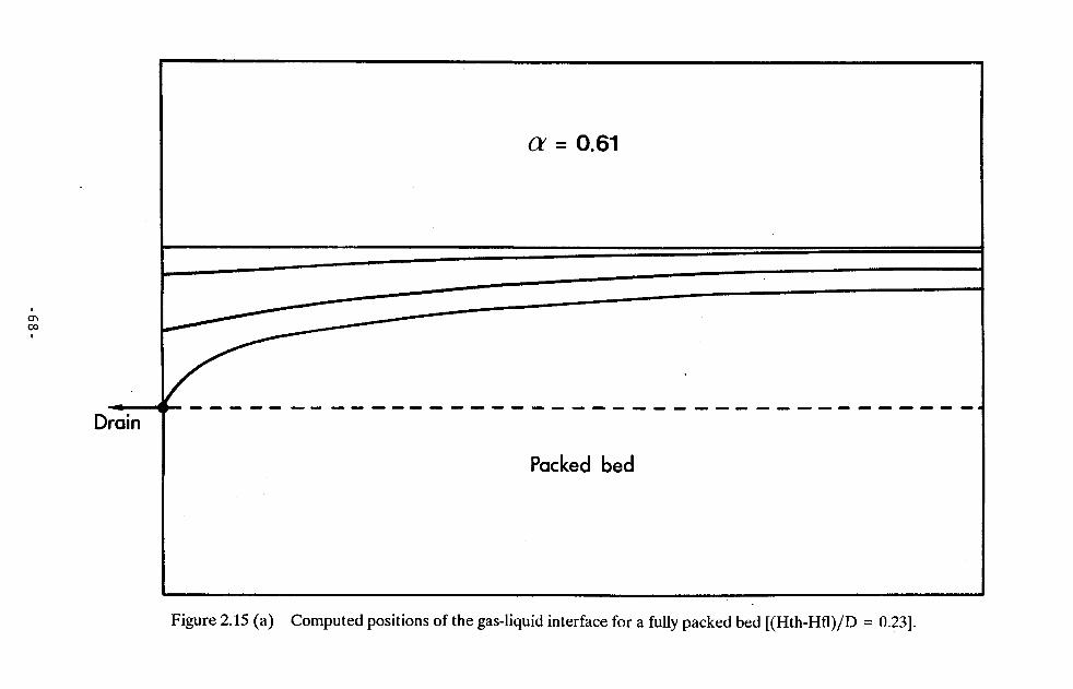
0.61

L-

a

-68-

'igure 2.15 (a) Computed positions of the gas-liquid interface for a fully packed bed [(Hth-Hfl)/D = 0.23].

0.40

-69

-

igure 2.15 (b) Computed positions of the gas-liquid interface for a packed bed with a packing-free layer [(Hth-Hfl)/D = 0.1].

-70-

;ure 2.15 (c) Computed positions of the gas-liquid interface for a packed bed with a packing-free layer [(Hth-Hfl)/D = 0.01].

packed bed ((Hth-Hfl)/D=0.23). Comparing this result with the profiles shown in Figures 2.15(b) ((Hth-Hfl)/D=0.1) and Figure 2.15(c)((Hth-Hfl)/D=0.01), it is clear that the free layer has a marked effect on the shape of the air-liquid interface. These differences are reflected in significantly different residual ratios for each simulation, 0.61, 0.4 and 0.07 respectively.

For the fully packed bed case, the inclination of the interface down towards the taphole is gradual. The slope is accentuated by the large pressure gradients generated in the vicinity of the taphole.

The effect of the free layer is to make the interface more horizontal and to increase the time for the interface to reach the taphole.These effects are best explained by examining the flow distributions in the beds with and without a free layer.

Figures 2.16 and 2.17 show the computed liquid streamlines at similar times for a fully packed bed and for a packed bed with a packing-free layer. Figure 2.16 shows that for the fully packed bed, the streamlines converge towards the taphole. The slope of the air-liquid interface is steepest near the taphole, where the pressure gradients are greatest. In Figure 2.17, for the packed bed with a packing-free layer, the streamlines away from the immediate vicinity of the taphole are directed into the packing-free layer rather than towards the taphole. The bulk of the liquid which arrives at the taphole actually flows through the low resistance, packing-free layer. For the case shown, approximately 70% of the total flow is through the free layer. As a result, the pressure gradients generated in the packed region are greatly reduced when compared with those for the fully packed bed and this in turn reduces the tilt of the air-liquid interface near the taphole. This results in a more efficient drainage and consequently lower residual slag volume.

-71-

Distribution

-72-

igure 2.16 Liquid streamline distribution pattern for a fully packed bed.

Distribution

-73-

igure 2.17 Liquid streamline distribution pattern for a packed bed with a packing-free layer.

Overall, the computations show that the presence of a free layer can have a significant effect on the residual slag volume in a blast furnace hearth. Provided that the iron-slag interface penetrates into the coke-free layer, the residual slag volume is greatly reduced when compared to that for a fully packed bed for similar conditions.

Table 2.4 shows results from a series of numerical drainage experiments for beds with uniform, packing-free layers of different thickness. The residual ratio, a, is given for a wide range of dimensionless numbers, Hth/D, Hfl/D and (Hth-Hfl)/D. These numbers characterise the principal geometric parameters of the bed , namely the taphole level, the free layer height and the distance between the taphole and the free layer respectively. The bed and liquid properties used in these experiments are given in Table 2.3. On the basis of these results, it is possible to conclude that: .

1. The presence of even a very thin packing-free layer can have a significant effect on the residual slag volume (Runs 1 and 2).

2. For the range of packing-free layer thicknesses investigated, the residual volume (a) is independent of layer thickness but dependent on the distance between the taphole and the top of the free layer.

When the results for Runs 3 and 4 (a=0.345, (Hth-Hfl)/D=0.071) together with those for Runs 5 and 6 (a=0.151, (Hth-Hfi)/D=0.050) are compared, it is clear that the residual ratios are equal when the distance between the top of the free layer and the taphole is the same. Furthermore, when the free layer height is maintained constant, but the taphole level is varied as in Runs 7 and 8 (a=0.225, 0.164, Hfl/D=0.019) , and Runs 9 and 10 (a=0.264, 0.408, Hfl/D=0.089 )•, the residual ratio increases with increasing distance between the taphole and the top of the packing-free layer.

-74-

Table 2.4 - Variance of Residual Ratio With Dimensionless Numbers[<Hth-Hfi)/D, Hth/D and Hfl/D]

Run No. a (Hth - Hfl)/D Hth/D Hfi/D

1 0.543 0.230 0.230 0.000

2 0.437 0.200 0.230 0.027

3 0.345 0.071 0.230 0.160

4 0.345 0.071 0.160 0.092

5 0.151 0.050 0.160 0.110

6 0.151 0.050 0.081 0.031

7 0.225 0.140 0.160 0.019

8 0.164 0.069 0.081 0.019

9 0.264 0.074 0.160 0.089

10 0.408 0.140 0.230 0.089

-75-

Although the actual thickness of the packing-free layer is unimportant for the range of thicknesses investigated, the continuity of the free layer is important. Figure 2.18 shows a comparison between the terminal positions of the gas-liquid interfaces for a fully packed bed, a packed bed with a continuous packing-free layer and a packed bed with a discontinuous packing-free layer having the same average thickness as the continuous uniform free layer ie. a packed bed which only partially penetrates to the base of the hearth. The fluid properties used for these computations are given in Table 2.3. The superficial drainage rate was held constant for the each of the three cases (ie. 0.143 cm/s).

The computed streamlines for the discontinuous free layer are shown in Figure 2.19. Clearly, the drainage performance is most affected by the zone of low permeability near to the taphole. The zone of low permeability away from the taphole has little effect on drainage performance. In terms of the residual slag ratio, the result for the discontinuous free layer lies between that for the fully packed bed and for the packed bed with a uniform and continuous free layer.

Overall, the numerical results show that for a continuous packing-free layer, the proximity of the top of the free layer to the taphole is the most important parameter affecting slag drainage from the hearth where the free layer extends into the slag phase. This observation is the basis for the development of a correlation between a and a modified flow-out coefficient which includes the effect of the free layer.

-76-

Fully packed bed

-77-

igure 2.18 Comparison between the terminal positions of the gas-liquid interface for (a) a fully packed bed, (b) a packed bed with a continuous packing-free layer and (c) a packed bed with a discontinuous packing-free layer.

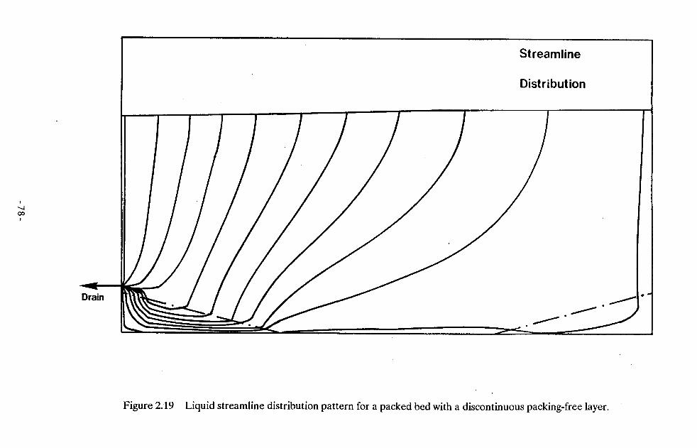
Distribution<D03

Uh

-78-

igure 2.19 Liquid streamline distribution pattern for a packed bed with a discontinuous packing-free

2.10 Correlation of Residual Slag and Flow-out Coefficient

2.10.1 Fully Packed Bed

The correlation developed by Fukutake and Okabe (1976 a) between the residual slag ratio and the flow-out coefficient was based on the assumption that the iron level remains horizontal at the level of the taphole once slag begins to drain out of the hearth. This correlation incorrectly assumes that there is no interaction between the iron and slag drainage and was justified on the basis of the low viscosity of iron relative to that of the slag. It was argued that because of the low viscosity of iron, low pressure gradients were generated in the iron phase. This would result in the iron being drained only down to the level of the taphole with the iron-slag interface remaining horizontal and stationary during the subsequent drainage of slag. Figure 2.20 shows a schematic of the slag drainage model proposed by Fukutake and Okabe (1976 a). In this model, the iron-slag interface is assumed to be horizontal, at the level of the taphole and therefore represents a boundary across which no slag may flow ie. a rigid, no-flow boundary.

Recently reported drainage behaviour from Kawasaki Steel's Chiba No. 6 blast furnace (Fukutake et al (1983)) shows that both iron and slag may flow simultaneously from the furnace over the greater part of the cast. This behaviour is at variance with the above model proposed by Fukutake and Okabe (1976 a) since this model does not permit simultaneous flow of both phases. Numerical studies carried out by Pinczewski et al (1982) and Tanzil (1985) have shown that when iron and slag flow simultaneously over the greater part of the casting period, it is possible to drain the iron phase down to levels considerably below the level of the taphole (Figure 2.21). This must be considered in a slag drainage model if such a model is to provide a realistic estimate of the residual slag volume.

-79-

<+

-80-

Figure 2.20 Slag drainage model as proposed by Fukutake and Okabe (1976 a).

-81-

igure 2.21 Schematic diagram of the drainage of iron from levels below the level of the taphole (Pinczewski et al (1982).

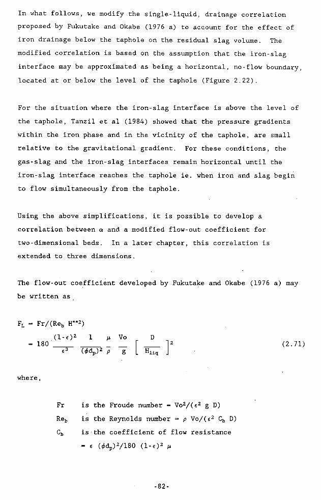
In what follows, we modify the single-liquid, drainage correlation proposed by Fukutake and Okabe (1976 a) to account for the effect of iron drainage below the taphole on the residual slag volume. The modified correlation is based on the assumption that the iron-slag interface may be approximated as being a horizontal, no-flow boundary, located at or below the level of the taphole (Figure 2.22).

For the situation where the iron-slag interface is above the level of the taphole, Tanzil et al (1984) showed that the pressure gradients within the iron phase and in the vicinity of the taphole, are small relative to the gravitational gradient. For these conditions, the gas-slag and the iron-slag interfaces remain horizontal until the iron-slag interface reaches the taphole ie. when iron and slag begin to flow simultaneously from the taphole.

Using the above simplifications, it is possible to develop a correlation between a and a modified flow-out coefficient for two-dimensional beds. In a later chapter, this correlation is extended to three dimensions.

The flow-out coefficient developed by Fukutake and Okabe (1976 a) may be written as

Fl - Fr/(Reb H**2)(l-O2 1

- 180 _______ p Vo D2 (2.71)

(0dp)2 P g

where,

Fr is the Froude number = Vo2/(e2 g D)Reb is the Reynolds number = p Vo/(e2 Cb D)Cb is the coefficient of flow resistance

- 6 Wdp)2/180 (l-o2 M

-82-

£x

-83-

Figure 2.22 Slag drainage model based on results following Pinczewski et al (1982).

H* is the€ is the<t> is thedp is the4 is theP is theVo is theg is theD is theHLia is the

geometric dimensionless number = HIiq/Dporosity of the bedsphericity of the particlesparticle diameterliquid viscosityliquid densitysuperficial velocitygravitational constantdiameter of model or hearthliquid (slag) height

The flow-out coefficient combines all the important parameters affecting slag drainage including the superficial velocity of the slag through the coke bed and the bed and slag physical properties. The correlation between a and FL was developed by considering the relationship between a and four dimensionless numbers ie. the Froude number, the Reynolds number, the Recharge number (the ratio of the amount of liquid flowing out of the hearth to the amount flowing in as a result of production) and bed geometry.

For the slag drainage model proposed in this study , we define a new dimensionless geometry number H** as

D

The introduction of H** is suggested by the derivation for H* (Fukutake and Okabe (1976 a)) (see Appendix B) . Using H** suggests that the initial slag height above the taphole centreline, rather than the total slag height, is the more appropriate parameter for characterising the residual slag ratio in fully packed hearths.

-84-

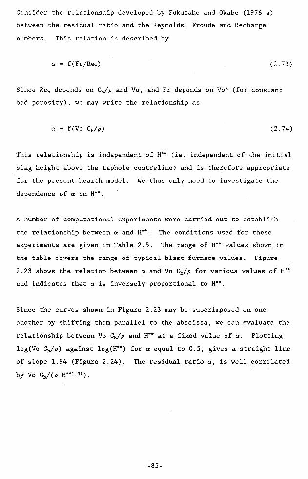
Consider the relationship developed by Fukutake and Okabe (1976 a) between the residual ratio and the Reynolds, Froude and Recharge numbers. This relation is described by

a = f(Fr/Reb) (2.73)

Since Reb depends on Cb/p and Vo, and Fr depends on Vo2 (for constant bed porosity), we may write the relationship as

a = f(Vo Cb/p) (2.74)

This relationship is independent of H** (ie. independent of the initial slag height above the taphole centreline) and is therefore appropriate for the present hearth model. We thus only need to investigate the dependence of a on H**.

A number of computational experiments were carried out to establish the relationship between a and H**. The conditions used for these experiments are given in Table 2.5. The range of H** values shown in the table covers the range of typical blast furnace values. Figure 2.23 shows the relation between a and Vo Cb/p for various values of H** and indicates that a is inversely proportional to H**.

Since the curves shown in Figure 2.23 may be superimposed on one another by shifting them parallel to the abscissa, we can evaluate the relationship between Vo Cb/p and H** at a fixed value of a. Plotting log(Vo Cb/p) against log(H**) for a equal to 0.5, gives a straight line of slope 1.94 (Figure 2.24). The residual ratio a, is well correlated by Vo Cb/(p H**i.94) .

-85-

Table 2.5 - Comparison Between Model and Furnace Dimensionless Numbers

Dimensionless Model Conditions Typical BlastNumber Furnace

Conditions*

Reb*107 1.0-8830 3.6

Fr*109 0.9-5050 1.84

H** 0.11-0.68 0.2-0.35

After Fukutake and OkAbe (1976 a)

87-

igure 2.23 Relationship between the resii

(cm/sec)

Figure 2.24 Relationship between Vo C^/p and H** for a = 0.5.

-88-

The modified flow-out coefficient, FL*, defined in terms of the dimensionless groups, Reb, Fr and H**, becomes

( 1 - € ) 2 1 fjL VoFl* = 180 _____ _____ _ __

e3 (4>dp)2 p gD

^liq " ^th1.94 (2.75)

Figure 2.25 shows the correlation obtained with the modified flow-out coefficient (equation (2.75)) and the computed residual ratios. The correlation is clearly very good and shows that the dimensionless geometric number, H** (the dimensionless number equivalent to the slag height above the taphole centreline) is successful in accounting for the effect of slag being below the level of the taphole as a result of iron being drained from levels below the level of the taphole. This correlation represents a significant improvement over that first proposed by Fukutake and Okabe (1976 a) and will subsequently be extended to three dimensions in the following chapter. The three-dimensional correlation will then be incorporated into an overall hearth mass balance model to provide realistic predictions of liquid levels during a casting operation.

2.10.2 Floating Packed Bed

Dissection studies of small blast furnaces (Higashida blast furnace No. 5 - 646m3 inner volume, Kukioka blast furnace No. 4 - 1279m3 inner volume) indicate that the coke-free layer may extend into the slag phase (Kanbara et al (1977)). The investigations also indicate that the coke-free layer may be non-uniform across the hearth and convex in shape. For this situation, the fully packed bed model presented in

-89-

90-

igure 2.25 Correlation between the residual ratio (a) and the modified flow-o coefficient (Fl ) for a fully packed bed.

the previous section, is clearly not appropriate and we must additionally consider the effect of the coke-free layer on slag drainage.

Figure 2.26 shows a schematic diagram of a hearth consisting of a packed bed and a packing-free layer beneath it. A single-liquid model is proposed to describe the drainage of slag from a hearth where the packing-free layer extends only into the slag phase. Figure 2.27 shows a representation of the model. The model considers the iron-slag interface to be a horizontal, no-flow boundary, always located at a level below that of the drain. The thickness of the packing-free layer (HfI) is assumed to be uniform across the hearth. These approximations facilitate a further modification of the flow-out coefficient and the development of a correlation for a which also accounts for the effect of the packing-free layer.

A complete dimensional analysis of the slag drainage model containing a free layer is complex. The analysis requires a study of the relationships between eight dimensionless groups ie. Reynolds, Froude, recharge and geometric numbers for both the packed bed and packing-free regions. However, it has already been shown that the dominant factor affecting slag drainage for a packed bed with a free layer beneath it, is the proximity of the top of the free layer to the taphole. As a first approximation, we therefore modify the flow-out coefficient defined in equation (2.75), by introducing a geometric dimensionless number which accounts for the position of the top of the free layer relative to that of the taphole. This number, Hfl*, is defined by the following equation,

-91-

DCUJ

uD5-.JZ<u<£:it)

-92-

Figure 2.26 Schematic diagram of a hearth with a packed bed and a packin,

-93-

igure 2.27 Slag drainage model proposed for a packed bed with a packing-free layer.

where Hth and HfI are defined in Figure 2.27. The significance of Hfl* is that in the limit, as the packing-free layer thickness, Hfl, approaches zero, Hfi* approaches unity and the flow-out coefficient approaches that for a fully packed bed. Defining a modified flow-out coefficient FL(cfl) as

FL(cfl) - Fl* Hfl*n (2.77)

shows that for Hfl* equal to unity, FL(cfl) is equal to FL*. The exponent of Hfl* must be determined from actual drainage experiments.

In order to justify the proposed modification of the flow-out coefficient, a series of computational experiments were carried out to demonstrate that the Reynolds, Froude and the packed bed geometric (H**) dimensionless numbers are independent of Hfl*. The conditions used for these computational experiments are given in Table 2.6.

Figure 2.28 shows the relationship between Vo and a for various values of Cb/p (383-3830 s"1) whilst maintaining the bed porosity, initial slag height, free layer size and free layer position all constant. Figure 2.29 shows that plotting log(Vo) against log(Cb/p) results in a straight line having a slope of -1. The relationship between a, Vo and Cb/p may therefore be written as

a = f(Vo Cb/p) (2.78)

This is identical to the relationship reported by Fukutake and Okabe (1976 a) for the case of a fully packed bed.

Figure 2.30 shows the relation between a and Vo Cb/p for various values of H** (0.095 - 0.395) whilst maintaining the position of the free

-94-

Table 2.6 - Bed and Liquid Properties Used in the Packing-free Layer Computational Experiments

Diameter of bed (cm) 40.0

Initial slag height (cm) 13.0-25.0

Taphole height (cm) 3.25-9.21

Packing-free layer height (cm) 0.38-7.8

Hydraulic Conductivity (cm/s) 0.256-2.56

Superficial Liquid Velocity (cm/s) 0.014-0.14

-95-

II

Ookz>

OOo00

oUDO\T

OfN

_DUVZ373>

LJQJ<S)XEL

J

5

£

-96-

igure 2.28 Relationship between Vo and a f<

(cm/sec)

Figure 2.29 Relationship between Vo and C^/p.

-97-

98-

(7D0S/UJD) qDoA

layer constant. Figure 2.31 shows that plotting log(Vo Cb/p) against log(H**) results in a straight line having a slope equal to 1.93. The relationship between a and Vo Cb/p may therefore be written as

a = f(Vo Cb/p H**1-93) (2.79)

This is again identical to the relationship previously developed for a fully packed bed.

The relationships developed above verify previous results which indicated that if the distance between the free layer and the taphole is constant, then the relation between a and FL* (where FL* = Fr/(Reb H**1-94) remains the same.

In order to account for a packing-free layer within the slag phase, we simply investigate the effect of Hfi* on a. A series of computational experiments were carried out for Hfl* values in the range 0.154-0.885. The liquid and bed properties used for the computations are given in Table 2.6.

Figure 2.32 shows the relation between a and Fr/(Reb H**1-94) for different values of Hfl*. The residual ratio, a, increases as Hfi* increases. The curves may be superimposed onto one another by shifting them parallel to the abscissa. This suggests that a relationship exists between Fr/(Reb H**1-94) and Hfl* for fixed values of a. This relationship is found by plotting log(Fr/(Reb H**1-94)) against log(Hfi*) for a equal to 0.30. Figure 2.33 shows that this results in a straight line having a slope equal to -0.5. The residual ratio, a,

is thus correlated with FL(cfl) ie. the slag flow-out coefficient for a hearth with a free layer, which is described by the equation,

(1 - e )2 1 n VoFl* = 180 _____ _____ _ _

e3 (0dp)2 p g - H*1.94

- Hfl °-5 (2.80)

-99-

(cm/sec )

Figure 2.31 Relationship between Vo C^/p and H**.

-100-

-101-

Figure 2.32 Relationship between a

Reb H

Figure 2.33 Relationship between Fr/Re^ FI**1-94 and Hfl* for a = 0.3.

-102-

CD

-103-

igure 2.34 Correlation between the residual ratio (a) and the modified flow-out coefficient accounting for the effect of a packing-free layer (FjJcfl)).

Figure 2.34 shows a plot of all the results obtained from the computational model including those results obtained for a fully- packed bed (Figure 2.25) ie. Hfi* equal to unity. Figure 2.34 shows that the modified flow-out coefficient FL(clf), can be successfully used to correlate a for the range of HfI* values used in the numerical experiments (0.154-1.0). This range is typical of the values which may be expected in actual operating furnaces. The correlation between a and FL(clf) forms the basis for a slag drainage model describing slag retention in small furnaces, where the packing-free layer extends into the slag phase. In the following chapter, we will extend this correlation to three dimensions.

2.11 Conclusions

The drainage of slag from the hearth is influenced both by the movement of the gas-slag and iron-slag interfaces. The major effect of draining iron from below the taphole level is a lowering of the gas-slag interface, which in turn, affects the residual slag remaining at the end of a casting operation.

For a fully packed bed, the effective slag height above the taphole, is the appropriate parameter to use in correlations for slag residual volumes.

In small diameter hearths, where the coke-free layer is likely to extend into the slag phase, it is found that even a very thin coke-free layer will have a significant effect on the residual slag volume. The dominant factor affecting the residual slag volume is the distance between the taphole and the top of the free layer. A

-104-

correlation between the residual ratio and a modified flow-out coefficient, which included this parameter, effectively correlates the results from simulated drainage experiments.

Two-dimensional slag drainage models are useful in providing qualitative estimates of the drainage behaviour of an ironmaking blast furnace. The slag drainage models and correlations developed in this chapter are readily extended to three dimensions. When combined with a mass balance model for the hearth, the three-dimensional correlations will provide more realistic estimates of liquid levels in actual operating blast furnace hearths than is possible using existing flow-out correlations.

-105-

3 THREE-DIMENSIONAL MODEL STUDY OF HEARTH DRAINAGE

3.1 Introduction

The previous chapter considered the case of a two-dimensional hearth. Although the actual ironmaking blast furnace hearth isthree-dimensional, Tanzil (1985) has shown that two-dimensional models are useful in providing a qualitative description of the effect of changes in hearth condition (eg. changes in coke mean size, slag chemistry and temperature or tapping rate) on slag residual volume. However, to provide quantitative estimates of drainage performance in an ironmaking blast furnace, it is necessary to extend the two-dimensional models to three dimensions and this is done in the present chapter. The extension is straightforward and the resulting models are similar to the two-dimensional models described in Chapter 2.

Drainage experiments carried out using laboratory-scale models of the hearth are also described. The data obtained from these experiments are used to both validate the numerical model and to develop correlations between the residual slag ratio, a, and the flow-out coefficients. The correlations are used together with simple material balance calculations to develop a model, which is capable of predicting iron and slag liquid levels and the cast duration, from iron and slag flowrates measured during the actual casting operation. The validity of the model is tested by comparing it with the drainage behaviour of Kawasaki Steel Corporation's Chiba No. 6 blast furnace, which is reported by Fukutake and Okabe (1981).

-106-

3.2 Governing Equations

Figure 3.1 shows a schematic of the three-dimensional model for the cylindrical blast furnace hearth. The symmetry of the flow about the vertical plane on the diameter passing through the taphole, allows the size of the computational problem to be reduced by a factor of two.The model is based on the assumptions that the packed bed is uniform, with a voidage, e, and permeability, k, and that it is saturated with a liquid (slag) to a height Hliq above the base of the model. A packing-free layer of thickness Hfl, may underlie the packed bed. Further, the liquid is assumed to be incompressible, of constant density, p, and viscosity, p,, and is initially in static equilibrium. Capillary pressure is assumed to be negligible (ie. the gas-slag interface is abrupt), while the flow in the hearth is everywhere laminar. These assumptions are similar to those used to develop the two-dimensional model described in the previous chapter.

In three-dimensional, cartesian co-ordinates, the equation of continuity for a liquid with constant density is written as

3u 3v 3w_+_+_= 0 (3.1)dx dy dz

The fluid motion in the packing-free layer is described by the non-conservative form of the Navier-Stokes equation (equation (2.7)). The x-, y- and z- components of velocity, u, v and w respectively, may be written as

3u 3u du du 1 dP p 3 2 u 3 2 u 3 2 u+ u + v + w = + ( + + ) (3.2)

3 t dx 3y 3z p dx p dx2 dy2 3z2

3v 3v 3v 3v 1 3P p 32v 32v 32v+ u + v + w = + ( + + ) (3.3)

3t dx 3y 3z p dy p dx2 dy2 3z2

-107-

Free layer Drain

Figure 3.1 Schematic diagram of the three-dimensional hearth drainage model.

-108-

3w dvr dvr 3w 1 d p m 32w 32w dzw+ u + v + w = - + g + ( + + )

3 t dx dy dz P dz p dx2 3y2 3z2

The transient form of Darcy's law is used to describe the fluid motion in the packed bed of the hearth. The x-, y- and z- components of

velocity, u, v and w respectively, are given by

3u € 3P fie- - + __

d t p dx pk(3.5)

3v e 3P pre= - _ __ + __

d t p dy pk(3.6)

dw e ap pe= - ____+ g + __

d t p 3z pk(3.7)

Equations (3.1)-(3.7), together with the initial and boundary conditions, describe the flow problem.

3.3 Initial and Boundary Conditions

The base and curved boundaries of the model (Figure 3.2) are impermeable and are represented as no-flow boundaries. For the base of the model i.e. the plane z=0 (DE) in Figure 3.2, the following

conditions apply,

w - 0 (3.8)

3u3z

= 0 (3.9)

-109-

Plan

SideElevation

Free layer

x

Figure 3.2 Plan and elevation views of the three-dimensional hearth drainage model.

-110-

(3.10)dv_ = 0 dz

Equations (3.9)-(3.10) are frequently referred to as the 'free-slip' boundary condition.

For the curved boundary in Figure 3.2 (surface ABC), the velocity normal to the boundary must be zero ie.

Un = ° (3.11)

<3w__ =0<9n

(3.12)

where n is the normal to the curved boundary

At the plane of symmetry (plane AC),

v = 0 (3.13)

3u_ - 0 dy

(3.14)

dw_ = 0dy

(3.15)

Equation (3.12) and equations (3.14)-(3.15) are again 'free-slip' boundary conditions.

At the drain (or taphole), the x-direction velocity, udrain, is set by the specified drainage rate and computational grid block geometry,

-111-

Q(t)udrain = A

(3.16)

where Q(t) is the volumetric flowrate (cm3/s) , which may be anarbitrary function of time and A is the outflow cross-sectional areaof the block containing the taphole as shown in Figure 3.3. It should be noted that Q(t) is the flow out from one-half of the model. The actual flow out of the whole of the model is twice Q(t).

The height of the liquid surface above the base of the model isin terms of a single-valued function, h, as

given

z = h(x,y,t) (3.17)

Using the chain rule of partial differentiation, we may write for dz/dt,

dz 3h dx <9h dy dh= + __ +dt dx dt <9y dt <9z

(3.18)

The free surface velocities, dx/dt, dy/dt and dz/dt are related to the specific discharges in the three cartesian directions, us, vs and ws, by the following expressions,

dx 1_ = - usdt e

(3.19)

dy 1_ = _ vsdt €

(3.20)

dz 1_ = - wsdt e

(3.21)

-112-

Figure 3.3 Representation of the taphole (or outflow boundary) in the three-dimensional model.

-113-

where e is the bed voidage.

Substituting equations (3.19)-(3.21) into equation (3.18) and re-arranging gives the kinematic equation which must be satisfied at the free surface,

<3h 1 ah ah__ = _ (ws - us __ - vs __) (3.22)at e dx ay

At the free surface, the surface pressure, Psurf, is set equal to the furnace or gas pressure, Pgas. That is,

Psurf = Pgas (3.23)

At the boundary between the packed bed and packing-free layer, mass is conserved across the boundary and we may write

^n(packed bed) '-Ln(free layer) (3.24)

where u^ is the velocity normal to the boundary.

Since the pressure field is initially hydrostatic, the surface elevation is set to a constant value equal to the initial liquid height, Hiiq ie.

z = Hliq (3.25)

Equations (3.1)-(3.7) and the boundary conditions (equations(3.8)-(3.25)) are solved using the Marker-and-Cell finite-differencenumerical technique.

-114-

3.4 Numerical Technique

The application of the Marker-and-Cell (MAC) finite-difference technique to the hearth drainage problem has been described in Chapter 2. In this section, we will describe the extension of the numerical technique to three dimensions and in particular, the treatment of the curved boundary and the free surface.

Various numerical techniques, based on the MAC finite-difference scheme, have been developed to treat two-dimensional curved or irregular surfaces (Viecelli (1971), Hirt et al (1975), Vander Vorst- et al (1976) and Casulli (1981)). The extension to three dimensions, although straightforward, has not been previously reported. In this study, the method described by Casulli (1981) has been extended to three dimensions. This method was selected because it applies a rigourous continuity condition to the boundary cells, including the cells containing the free surface.

Figure 3.4 shows the three-dimensional hearth, discretised into variable - sized, rectangular parallelepipeds of length 6x, 6 y and 5 z. Figure 3.5 shows the plan and elevation views of the computational grid superimposed over the flow region. The non-uniform grid is more refined in the region close to the taphole. This allows accurate resolution of the steep pressure gradients in the region near to the taphole and avoids the need to resolve the singularity at the centre of the axis of symmetry shown in Figure 3.5. The grid is constructed using a variable mesh generator in the x-y and x-z planes. Equation (3.26) describes the grid generator used.

Di (R - 1)Si =

RN - 1(3.26)

Figure 3.4 Three-dimensional, computational grid.

-116-

Plan View Ay

Computational Singularity

Elevation ViewAz

Figure 3.5 Plan and elevation views of the computational grid.

-117-

where is the length of cell iDi is the length of segment left to be discretised R is the ratio by which grid size is allowed to increase or

decreaseN is the number of cells in each segment

Figure 3.6 shows the locations at which the field variables are defined for a computational cell block. The velocities, u, v and w are defined at the centre of each wall of the parallelepipeds.Pressure is defined at the centroid of the cell.

Figures 3.7(a)-(b) show the location of field variables for cells intersected by the curved boundary. For these cells, a pressure and four velocities must be defined. The pressure is defined at the centroid of an imaginary parallelepiped (Figure 3.7(a) and (b)). Four velocities are defined at the centre of each wall and the remaining two velocities (ie. those defined on the imaginary side of the cell block) are obtained using an appropriate boundary condition.

For a full cell (ie. no curved boundary passing through it), the continuity equation (equation (3.1)) is discretised as follows

1 n+l n+1 1 n+1 n+1<5x (ui + l/2,j,k " ui-l/2,j,k) + -6y (vi, j + l/2,k ‘ vi,j-1/2,k )

1 n+1 n+1-1- _ (wi, j ,k+l/2 ’ wi,j,k-l/2)Sz

The Navier-Stokes equations (equations (3.2)-(3.4)) are discretised in a manner which allows the degree of upwind differencing for the convection terms to be varied. The methodology is similar to that outlined in Chapter 2. The resulting expressions are,

n+1 nui+i/2,j,k = ui+i/2,j,k - St (PX + CONUX + CONUY + CONUZ + VISCX) (3.28)

-118-

i.j.k+1/2w

Figure 3.6 Layout of field variables for a full cell.

i + 1/2,j,k

-119-

(a) LHS cell (b) RHS cell

ij.k+i/2

i + 1/2,j,k

i,j,k+1/2

Figure 3.7 Layout of field variables for cells bisected by a curved boundary.

n+1 nvi,j+i/2,k = vi,j+i/2,k - St (PY + CONVX + CONVY + CONVZ + VISCY) (3.29)

n+l nwi,j',k+i/2 = wi,j,k+i/2 - St (PZ + CONWX + CONWY + CONWZ + VISCZ + GZ)(3.30)

where,

1PX = ---------- (Pi+l,j,k ' Pi.j.k)

^xi+l/2 P

1PY = __________ (Pi.j + l.k - Pi.j.k)

^Yj + 1/2 P

1P^ = ---------- (Pi,j,k+1 ' Pi,j,k)

Sz k+1/2 P

and

<5xi+i/2 = 0.5 (5Xi + 5xi+1) Syj+i/z = 0.5 (ty, + 5yj+i) Szk+1/2 =0.5 (Szk + <$zk+1)

ui+l/2,j,kCONUX = _______ [fiXi DUR + 6xi+1 DULDXA+ UPWIND sgn(u) (6xi+1 DUL - SxL DUR)]

VAVCONUY = __ [DYB DUDTY + DYT DUDBYDYA

+ UPWIND sgn(v) (DYT DUDBY - DYB DUDTY)]

-121-

WAVCONUZ = [DZB DUDTZ + DZT DUDBZ

DZA+ UPWIND sgn(w) (DZT DUDBZ - DZB DUDTZ)]

sgn(u) = si§n of ui+1/2 jjkDXA = 8xL + 6xi+1 + UPWIND sgn(u) (<5xi+1 - 8xL)

DUR = (ui+3/2,j,k " ui+l/2, j ,k)/<5xi+l

DUL = (ui+l/2,j,k ' ui-l/2, j ,k)/^xi

VAV =0.5 (VBT + VBB)VBT = (5Xj_ vi+1>j+1/2 k + <5xi+1 vi j+1/2|k)/(6xi + 5xi+1)VBB = (5Xj_ vi+1j_1/2 k + 6xi+1 vi j.1/2 k)/(«5xi + <Sxi+1)sgn(v) = sign of VAVDYA = DYT + DYB + UPWIND sgn(VAV) (DYT - DYB)DYT = 0.5 (5yj + 6yj+1)DYB = 0.5 (5yj + Syj-i)DUDTY = (ui+l/2, j + l,k ' ui+l/2,j,k) /DYTDUDBY = (ui+l/2,j,k ‘ ui+l/2, j-l,k) /DYB

WAV = 0.5 (WBT -I- WBB)WBT = (5xt wi+1>j k+1/2 + <Sxi+1 wi>j k+1/2)/(6xi + <5xi+1)WBB = (iSXi wi+1j k_1/2 + 6xi+1 w1(j k_1/2)/(6xi + 5xi+1)sgn(w) = sign of WAVDZA = DZT + DZB + UPWIND sgn(WAV) (DZT - DZB)DZT = 0.5 (8zk + <5zk+1)DZB = 0.5 (<5zk + SzY.{)DUDTZ = (ui+l/2, j ,k+l ' ui+l/2, j ,k)/DZTDUDBZ = (ui+l/2,j,k ‘ ui+l/2, j ,k-l)/DZB

VISCX = (n/p) (DUDXSQ + DUDYSQ + DUDZSQ)

-122-

DUDXSQ = 2.0 (. li-i/2,j,k ui+3/2,j,k

+ <5xi+1) 5xi+1 (6xi + 5xi+1)

ui+l/2,j,k.)

6X; Sxi+1

DUDYSQ = (DUDYT -DUDYB)/5yj

1 uDUDYT i+l/2, j + 1,k 6yj

DYT ^Yj+iui+l/2,j,k ^Yj + l

SY j

UBDYT ( sYj 8ys

6 Yj +i+i

5y j.)]

DUDYB 1 ^ui+i/2,j,k j-l

DYB 8yd

ui+l/2 , j-l ,k ^yj

UBDYB (

5yj-isyj-i8y^

8 yj.)]

UBDYT - (8yj ui+1/2>j+1(k + ^Yj+i ui+i/2,j,k)/(6yj + ^Yj+i) UBDYB = (8yj-! ui+1/2(j(k + 8yj ui+1/2>j-1(k)/(5yj + ^Yj-i)

DUDZSQ = (DUDZT -DUDZB)/<5wk

DUDZT1 ^ui+l/2,j,k+l ^ zk ui+l/2, j ,k 6zk+l

DZT ^ zk+l 6zk

5 zk- UBDZT (

^ zk+l)1

& zk+l 5zk

DUDZB1 ui+l/2, j ,k ^zk-l ui+l/2,j,k-l ^ zk

DZB <5zk 6zk-i

6zk-i- UBDZB (

5zk)1

8 zk 6zk-i

-123-

UBDZT (6zk ui+1/2jj k+1 + <5zk+1 ui+1/2>jjk)/(6zk + <5zk+1)UBDZB = (6zk.1 ui+1/2 j k + <5zk ui+1/2jjjk-1)/(6zk + 5zk_1)

GZ = g

Similar expressions may be written for the terms CONVX, CONVY, CONVZ

and VISCY, as well as for CONWX, CONWY, CONWZ and VISCZ.

Darcy's law (equations (3.5)-(3.7)) is discretised as,

n+1 pk n e 81 Pi+l,j,k ' Pi,j,kui+l/2,j,k = [ ui + l/2,j,k ‘

pk + € p St P ^xi + l/2

n+1 pk n e 8t Pi,j+l,k “ Pi,j,kvi, j + 1/2,k = [Vi,j + 1/2,k "pk + ep St P <5yj + l/2

n+1 pk n e 81 Pi,j,k+1 ’ Pi,j,kwi,j,k+l/2 = [wi,j,k+l/2 "pk + ep. St P ^zk+l/2

(3.31)

(3.32)

(3.33)

The momentum equations (3.28)-(3.30) and equations (3.31)-(3.33) are used to provide an initial estimate of the fluid velocities at the (n+l)fch time step from a known pressure field at the nth or current time step. These velocities will generally not satisfy the continuity condition. It is therefore necessary to adjust the pressure and velocity for each computational cell (including the boundary cells) in an iterative manner so that the continuity equation is satisfied (equation (3.27)). The divergence, D, is defined as,

3u 3v 3w__ + __ + (3.34)3x dy dz

Equation (3.34) may be discretised as,

-124-

n+1 m+1 n+1(^i,j,k) = -- (ui+l/2,j,k

5xn+1 m+1 L n+1 n+1 m+1ui-1/2, j , k) + (vi,j + l/2,k ' vi,j-l/2,k)

6y

3- n+1+ -- (wi,j,k+l/2

n+1 m+1wi , j , k-1/2 )

(3.35)

where the index, m, refers to the pressure-velocity iteration step.

Using the incompressibility condition (ie. D=0), equation (3.35) may

be re-written as,

n+1 m+1(Di.j.k)

n+1 n+1 m+1 ^ n+1 n+1 m+1-- (ui+l/2, j ,k ' ui-l/2,j,k) + (vi,j + l/2,k ' vi,j-l/2,k)<5x S y.

n+1+ -- (wi,j,k+l/2

n+1 m+1wi,j,k-l/2)

(3.36)

The pressure in a computational cell occupied by fluid (including the

boundary cells), is adjusted using the compressibility condition

defined by equation (3.37), such that

5P = - AD (3.37)

Equation (3.37) may be approximated by

n+1 m+1(^Pi,j,k) = ' ^i.j.k

n+1(Di, j.k

m+1) (3.38)

Since the pressure in the cell has been changed, it is necessary to

adjust the velocities on each side of the cell. The cell velocities

are adjusted using the following equations,

-125-

n+l m+1( ui + l/2,j,k) =

n+l m( ui + l/2,j,k) + ^i+1/2,j,k

n+l m+1 (3.39)

n+l m+1 n+l m n+l m+1C ui-1/2.j,k) ( ui-l/2,j,k) 0i-l/2,j,k (*Pi,j,k) (3.40)

n+l m+1 n+l m n+l m+1( vi , j + 1/2,k) - (vi, j + 1/2,k) + Pi,j+1/2,k (5Pi,j,k) (3.41)

n+l m+1 n+l m n+l m+1(vi,j-1/2,k) “ ( Vi,j-1/2,k ) + Pi,j-1/2,k (5Pi.j,k) (3.42)

n+l m+1 n+l m n+l m+1(wi, j,k+l/2) ( wi,j,k+1/2) + Pi,j,k+1/2 (SPi.j.k) (3.43)

n+l m+1 n+l m n+l m+1(wi,j,k-l/2) - ( wi,j,k-1/2 ) + Pi,j,k-l/2 (<5P1(j,k) (3.44)

where

p k e St

p k + e /j, 8t p Sx

The free layer region is treated in a manner similar to that for the packed bed region, with the exception that the porosity is set equal to 1 for cells in the free layer. Substituting equations (3.39)-(3.44) into the compressibility condition (equation (3.38)) and solving for <5P, we obtain the following expression for Aijk,

1Ai.j.k = ______________________________________________ (3.45)

(^i+l/2,j,k + ^i-l/2,j,k + £i,j+1/2,k + ^i,j-1/2,k

+ Pi,j,k+1/2 + £i,j,k-1/2)

In order to accelerate the rate of convergence, the compressibility equation (equation (3.38)) is multiplied by a relaxation parameter u>, such that,

-126-

m+1(3.46)

n+l m+1 n+1(£Pi,j,k) = - u Ai(j>k (Di(jk)

Computational experiments show that a value of u> equal to 1.7-1.8 is optimal for the present problem.

3.4.1 Finite-difference Approximations For Curved Boundary and Free Surface Cells

For a cell intersected by the curved boundary, an alternate form of the continuity equation (equation (3.27)) is used to ensure that no fluid crosses the boundary. Equation (3.27) is multiplied by the cell volume (iSXi Sy3 8zk) to obtain,

n+l n+l n+l n+l(ui+l/2,j,k " ui-l/2,j,k) j ^zk + (vi,j + l/2,k ' vi,j-l/2,k) ^xi ^zk

n+l n+l+ (wi,j,k+i/2 - wi,j,k-i/2) 5Xi 8Yj = 0 (3.47)

Equation (3.47) has the following physical interpretation. Since the fluid is incompressible, the volume of fluid entering a cell must balance that leaving the cell. This form of the continuity equation is more appropriate for a boundary cell. For example, consider the right-hand side boundary cell shown in Figure 3.7(b). For such a cell, the discrete form of the continuity equation (equation (3.47)) may be written as,

' (ui-l/2,j,k) ^Yj ^ zk " (vi,j-l/2,k) ^xi ^zk

n+l n+l n+l 2 2+ (wi,j,k+i/2 - wi,j,k-i/2) ^Xi <5yj + u^ (fiXi 6yj) = 0 (3.48)

-127-

where is the velocity normal to the curved boundary. For such a boundary cell, the pressure at the centre of the cell is adjusted using equation (3.38) so as to ensure that the normal velocity, u^, is driven to zero.

For a surface cell (ie. a cell intersected by the free surface) the pressure-velocity relaxation procedure is as follows. Since the pressure at the liquid surface is specified as a boundary condition

(equation (3.23)), the pressure at the centre of a surface cell

(Pi j ksur) i-s adjusted using a linear interpolation or extrapolation between Psurf and Pi 3 ksur-i- The pressure change for the surface cell may be written as

n+l m+1 n+1 m+1 n+1 m+1(«Pi,j,k> - (1 - Di) (Pi.j.ksur-l) + Di Psurf ' (Pf.J.k.ur) 0-49)

where,

zsurfDi - ____________

5zsurf + d

5zsurf and d are defined in Figure 3.8.

(3.50)

3.4.2 Finite-difference Approximations for Boundary Conditions

The difference equations for the boundary conditions at the base and

the plane of symmetry of the model (Figure 3.2), are now described. For the base of the model, the difference form of equations

(3.8)-(3.10) may be written as,

-128-

i,j,ksur-1

1

d

T

Figure 3.8 Definition of variables used to compute the pressure in a cell containing the free surface.

-129-

(3.51)

ui+l/2,j,1 “ ui+l/2,j,2 (3.52)

vi,j+1/2,1 ~ vi,j+1/2,2 (3.53)

At the plane of symmetry (plane AC), equations (3.13)-(3.15) are written as

For a curved boundary cell, the 'free-slip' boundary conditions must be set ie. equations (3.11)-(3.12). The particular form of difference equations for these boundary conditions depends on the cell aspect ratio, Sy^/Syii as described by Hirt et al (1975). For example,

For boundary cells that lie within the bounds, tt/4 > a > 37r/4, the cell aspect ratio, <5y/6x, is greater than 1. For these cells, the y-direction velocity, v, is given by the 'free slip' boundary condition. The x-direction velocity, u, is calculated to ensure that the velocity divergence for the cell is zero. For boundary cells that lie within the bounds 0 < a < tt/4, we may write

VILB-1, j+1/2,k = VILB, j+1/2,k (3.57)

(3.54)

ui+l/2,l,k ~ ui+l/2,2,k (3.55)

wi,1,k+l/2 ~ wi,2,k+l/2 (3.56)

consider the plan view of the computational grid shown in Figure 3.9.

-130-

Figure 3.9 Plan view of the three-dimensional, computational grid showing the parameter used in defining the ’free-slip’ boundary conditions.

-131-

UILB-1/2,j,k = uILB+l/2,j,k

+ 8xi/8y j (VILB, j+1/2,k ' VILB, j -1/2, k )

+ 8xi/8z);i (wILB> j >k+1/2 - WILB, j , k-1/2) (3.58)

where the subscript ILB indicates the left-hand side boundary cell. Similarly, for boundary cells within the bounds 37r/4 < a < n, we may write

VIUB+1,j+1/2,k = VIUB,j+1/2,k (3.59)

uIUB+l/2,j,k = UIUB-1/2,j,k

+ Sxl/8 yj (VIUB, j + 1/2, k ' VIUB, j -1/2 ,k )

+ 8xi/8 Zk (WlUB,j,k+l/2 " WIUB, j,k-1/2) (3.60)

where the subscript IUB indicates the right-hand side boundary cells. For boundary cells within the bounds tt/4 < a < 37r/4, the x-direction velocity is given by the 'free slip' boundary condition and the y-direction velocity is calculated to ensure that the velocity divergence is zero. Thus, for cells bounded by 7r/4 < a < 7r/2, the x- and y-direction velocities are given by

uILB-l/2, j ,k = uILB-l/2, j-l,k (3.61)

VILB,j+1/2,k = VILB,j-1/2,k

+ 8y^/8xi (uILB+1/2i j(k * uILB-l/2, j ,k)

+ 6yj/6zk (WILB, j ,k+l/2 " WILB, j, k-1/2) (3.62)

-132-

For boundary cells within the bounds 7r/2 < a < 37r/4, the x- and y-direction velocities are given by

uIUB+l/2,j,k = uIUB+l/2, j ,k (3.63)

VIUB,j+1/2,k = VIUB,j-1/2,k

+ Syj/Sxi (uIUB+l/2, j,k " UIUB-1/2,j,k)

+ <$yj/<5zk (WIUB, j ,k+1/2 " WIUB,j,k-1/2 )

The 'free slip' boundary condition, equation (3.12) is differenced as follows:

For 0 < a < n/2

WILB-1, j.k+l/2 = wILB,j,k+1/2 (3.65)

and for n/2 < a < n

WIUB+1, j , k+1/2 = WIUB, j ,k+l/2 (3.66)

At the drain, the outflow boundary condition may be written as

UIDPX, JDPY, KDPZ = Q/A (3.67)

where A is the cross-sectional area of the taphole and Q is the drainage rate. The subscripts, IDPX, JDPY and KDPZ, indicate the co-ordinates of the drain cell within the computational grid.

The kinematic surface equation is approximated using theCourant-Issacson-Rees differencing technique. The finite-differenceform of equation (3.22) is written as

-133-

n+1 n St n n ^h n 3hhi+l/2,j+1/2 = “i+1/2, j + 1/2 + -- (ws - us __ ‘ vs __ ) (3.68)e 3x dy

where,

nSh hi+3/2,j+1/2 ‘ hi+1/2,j+1/2dx Sx±

hi+l/2,j+1/2 ' hi-l/2,j+1/25Xi_i

= 0

and

nah hi+l/2,j+3/2 ' i^i+1/2, j + 1/2ay 5yj

hi+l/2,j+1/2 ' ^i+l/2,j-l/2tyj-i

if us < 0

if us > 0

if u" = 0

if v" < 0

if vs > 0

0 if v" = 0

The surface elevation, h, is defined at each vertical line in the grid, as shown in Figure 3.10.

The surface pressure is set equal to the gas pressure, so that

Pi,j,ksur+1 = i’surf (3.69)

-134-

i + 1/2,j + 1/2

i + 1/2,j-1/2

Figure 3.10 Definition of the surface elevation, h.

-135-

3.5 Numerical Stability and Accuracy

The necessary conditions for convergence of the numerical scheme are simply an extension of those for the two-dimensional model as described in Chapter 2. The time step for the computations is constrained by the following three conditions ie.

St < min8 y 8 z

FT ' FT }(3.70)

p 5x2 8y2 Sz2St < __ ______________

2 p. 5x2 + Sy2 + Sz2(3.71)

St <min(Sx, Sy)(g tw)172

(3.72)

Equation (3.70) states that the liquid cannot move through more than one cell in one time step because the difference equations assume fluxes between adjacent cells only. Likewise, equation (3.71) states that momentum must not diffuse more than one cell distance in one time step. Equation (3.72) is the Courant surface-wave condition and for most drainage computations, is the most restrictive condition.

With St chosen, the last parameter needed to ensure numerical stability is the upwinding term, UPWIND. The appropriate value for UPWIND is given by

|u| St |v| St1 > UPWIND > max ( ______ , ______

| w | St_____ ) (3.73)

6x Sy St

A rule of thumb suggests that a value 1.2 to 1.5 times the right-hand side of the inequality (equation (3.73)) is appropriate.

-136-

3.6 Computational Procedure

The computational procedure for the three-dimensional model is similar to that previously described for the two-dimensional model. The computational grid is initialised to hydrostatic equilibrium and the drainage rate set. The basic procedure for advancing a solution through one increment in time, <5t, consists of the following four steps:

1) Explicit approximations of the conservation equations for momentum, equations (3.28)-(3.30) and equations (3.31) - (3.33), are used to compute an initial guess for the new time-level velocities.

2) To satisfy the continuity equation, pressures and velocities are adjusted simultaneously in each computational cell using equation (3.27) or equation (3.47). Equation (3.46) (for a full cell) or equation (3.49) (for a surface cell) is used to update the pressure and equations (3.39)-(3.44) are used to update cell velocities.

3) When the continuity condition has been satisfied, the free surface is moved using equation (3.68).

4) Steps 1-4 are repeated until the free surface reaches the computational cell containing the drain.

The listing of a Fortran computer code (HD31.F0R), developed to implement the above computational procedure, is given in Appendix D.

-137-

3.7 Laboratory-scale Experiments

A series of experiments have been carried out using laboratory-scale, cold liquid models of the hearth. The experimental data are used to validate the numerical model and to develop correlations between the residual ratio and flow-out coefficients for three-dimensional, packed beds with and without packing-free layers.

Two cold liquid models were used for the fully packed bed experiments. Figure 3.11 shows one of the models used. It consists of a rigid and water-tight stainless steel shell, formed into a 40 cm diameter, semi-circular cylinder. Attached to the front of the model is a perspex plate, which allows inspection and photographic recording of the movement of the gas-liquid surface. Seven tapholes are located at the side of the model adjacent to the front plate. Two filling ports connected to liquid reservoirs, permit, liquid to be drip-fed into the model. This prevents any disturbance to the packing, particularly near to the taphole. The model is the physical analog of the numerical model described in the previous section. A smaller 15 cm diameter, cylindrical model shown in Figure 3.12, constructed from perspex, was also used in some of the drainage experiments.

For the fully packed bed experiments, the models were filled with glass ballotini (average particle size = 0.290 cm). A perspex plate was clamped on top of the ballotini to ensure that the bed remained stationary (see Figure 3.11). Drainage experiments with a packing-free layer were carried out using the semi-cylindrical model. Polyethylene balls (average particle size = 0.438 cm.) were used in place of the glass ballotini. The balls were supported on a wire mesh, which was held in place by a number of thin wire rods as shown in Figure 3.13. The low density, polyethylene balls (specific gravity = 0.92) minimized distortion of the supporting mesh.

-138-

Plan view!

40 cm diameter

Perspex plateFront view

To collection

Filling point

Figure 3.11 Schematic diagram of the 40 cm diameter experimental apparatus.

15.0 cm. diameter

Figure 3.12 Schematic diagram of the 15 cm diameter experimental apparatus.

-140-

Hold-downwire/

Drains

Meshdistributor

Filling point

Figure 3.13 Wire mesh used to support the packing for the free layer experiments.

-141-

3.7.1 Experimental Procedure

Before the commencement of a series of experiments, the glass ballotini and polyethylene balls were sized by standard sieving techniques. Uniform packing (ie. a homogeneous bed with no entrapped air) was realised by first filling the model with a known volume of liquid and then carefully pouring the packing material into the model. Excess liquid was then drained from the model. The porosity of the bed was determined by measuring the volume of liquid required to saturate the bed. This measurement was repeated several times. The procedure for performing the drainage experiments is similar to that previously described for the two-dimensional experiments.

Liquid viscosity was measured using a suspended level viscometer (Type BS/IP/SL) placed in a constant temperature bath. A kinematic viscosity-temperature relationship was determined for each liquid used in the experiments. Figure 3.14 shows an example of the viscosity-temperature relationship for a 50:50 glycerol/water mixture.

3.8 Numerical Model Results

3.8.1 Validation of Numerical Model

The three-dimensional numerical model was validated by comparing computed drainage behaviour with that measured in the experiments with the laboratory-scale models described in the previous section.Drainage data for three-dimensional, fully packed beds reported by Tanzil (1985) , were also used. These experiments were carried out using the 40 cm diameter laboratory-scale model which was also described in the previous section.

-142-

Kinematic

viscosity

12 -

Temperature (deg. C)

Figure 3.14 Viscosity-temperature relationship for a glycerol/water mixture (50:50 v/v)

Figure 3.15 shows a comparison between a drainage experiment for a fully packed bed as reported by Tanzil (1985) and the gas-liquid profiles calculated by the three-dimensional numerical model. In the experiment, the taphole was located at the base of the model. The model was filled with glass ballotini (dp = 0.29 cm., e = 0.38) and saturated with a 65:35 glycerol/water mixture (p = 1.17 gm/cm3,H = 0.17 gm/cm s). The initial liquid height was set at 9.2 cm. The drainage rate was set at 9.10 cm3/s for the experiment. The position of the air-liquid interface during the experiment was recorded photographically and is shown as solid lines in Figure 3.15.

The numerical calculation was performed using a computational grid of 560 cells (70 in the x-y plane and 8 in the z-direction). The time step was set at 0.008 s. The numerical results, shown as broken lines in Figure 3.15, are in close agreement with the experimental data and the shape of the air-liquid interface is at all times, well predicted by the model. The calculated blowout time of 55.7 s compares very well with the experimental time of 51 s.

Figure 3.16 shows a comparison between results from a drainage experiment carried out for a packed bed with a free layer (broken lines) and the computed drainage profiles using the numerical model (solid lines). In this experiment, the 40 cm diameter physical model was packed with polyethylene balls (e = 0.35) and saturated with a 65:35 glycerol/water mixture (p = 1.17 gm/cm3, n = 0.17 gm/cm s). The taphole was located 4.4 cm above the base of the model and the height of packing-free layer fixed at 2.0 cm. A constant drainage rate of 14.7 cm3/s was maintained for the experiment.

For the numerical calculation, a computational grid consisting of a total of 770 cells (70 in the x-y plane and 11 in the z-direction) was used. The time step was set at 0.008 s. Again, Figure 3.16 shows that the predicted air-liquid profile agrees very well with

-144-

o

-145-

igure 3.15 Comparison between experimental drainage profiles (Tanzil (1985)) and computed profiles for a three-dimensional, fully packed bed.

or

■aoCl

Eo

cCDEa5o.xO

LU

1 I

I I

I I

a>jo*a>a)ul

OCOoCM

E0oc03•cnb

C3u•-2JU

.c:O)0XEo

cEQ

-146-

Figure 3.16 Comparison between experimental and computed drainage prof! three-dimensional, packed bed with a packing-free layer.

experimental results. The blowout time calculated by the numerical model (63.8 s) also compares very well with the experimental result (66.1 s).

The comparisons between results from the physical and numerical models described above, confirm that the assumptions made in formulating the numerical model are correct. We now describe work which extends the conclusions made in the previous chapter concerned with the effect of

the coke-free layer on hearth drainage in two dimensions, to three dimensions. This will allow predictions to be compared with actual

furnace operating data.

3.8.2 Drainage of Two- and Three- Dimensional Packed Beds With and Without a Packing-free Layer

The two-dimensional study described in Chapter 2 identified two important parameters which determine the drainage behaviour of slag from the hearth. For a fully packed bed, the distance between the gas-liquid interface (furnace gas-slag interface in the actual furnace) and the drain (taphole) was shown to be a significant parameter. The dimensionless geometric number, H** (equal to (HIiq-Hth)/D), was shown to account for slag drainage under conditions where the iron is drained from levels well below the level of the taphole. For beds with a packing-free layer that extends into the

slag phase, the distance between the drain and the top of the packing-free layer is an important parameter. A dimensionless number, Hfi* (equal to (Hth-Hfl)/Hth) , was shown to account for the position of the free layer relative to the taphole.

-147-

In this section, we investigate the drainage performance of two- and three-dimensional packed beds, with and without a packing-free layer, for similar drainage conditions ie. for equal H** and Hfi* values.Using the two- and three-dimensional numerical models previously described, we demonstrate that only the three-dimensional models are capable of providing realistic estimates of the residual slag in the hearth of an actual operating furnace.

Figure 3.17 shows a comparison between the calculated terminal gas-liquid profiles for a two-dimensional numerical drainage experiment in a fully packed bed, and that for a similar numerical experiment in a three-dimensional fully packed bed. The numerical experiments were set-up to simulate conditions in the equivalent three-dimensional physical analog (40 cm diameter model). The two-dimensional model had a width equal to the diameter of the three-dimensional model and a thickness such that both models contained the same liquid volume. The ratio of the Froude number to the Reynolds number (Fr/Reb) and the value of H** were set at 0.04 and 0.2 respectively for both the two- and three-dimensional numerical experiments. The results of the computations show that the residual ratio for the three-dimensional case is considerably higher than that for the two-dimensional model ie. 0.75 cf. 0.61. This is explained by the much higher local liquid velocities and associated pressure gradients in the vicinity of the taphole in the three-dimensional case which result from the convergence of the flow to a point sink rather than a line sink as in the two-dimensional case. The higher pressure gradients cause a more rapid tilting of the gas-liquid interface towards the taphole in the three-dimensional model and consequently, a higher residual ratio results.

Figure 3.18 shows a comparison between results from a two-dimensional numerical experiment for a packed bed with a packing-free layer and the results- from a similar numerical experiment using the

-148-

CD o

ooCOoC\J

ou.

149-

igure 3.17 Comparison between terminal drainage profiles for a fully packed bed a; computed by the two- and three-dimensional numerical models.

-150-

igure 3.18 Comparison between terminal drainage profiles for a packed bed wit packing-free layer as computed by the two- and three-dimensional

three-dimensional numerical model. The numerical models were set-up in a similar manner to that described above. The drainage conditions for these numerical experiments were again similar - the values of Fr/Reb, H** and Hfl* were equal to 0.03, 0.2 and 0.8 respectively. The value of Hfi* is high and therefore the distance between the taphole and the top of the free layer is small. For these conditions, the effect of the free layer is expected to be significant. The results of the numerical experiments show that the effect of the free layer on the residual ratio in the three-dimensional model is not as pronounced as for the two-dimensional case. The residual ratio for the three-dimensional model is very high (a=0.68) compared to the two-dimensional case (a=0.28). This suggests that the dominant factor affecting slag drainage in a three-dimensional, packed bed with a packing-free layer, is the presence of large pressure gradients near the taphole. As shown in Figure 3.18, these pressure gradients result in a sharp tilt of the air-liquid interface towards the taphole and this leads to the early termination of the drainage experiment.

3.9 Correlation of Residual Slag and Flow-out Coefficient

3.9.1 Fully Packed Bed Hearths

In Chapter 2, a correlation between the residual ratio, a, and a modified flow-out coefficient, FL*, was developed for drainage in two-dimensional packed beds. This correlation differed from the correlation between a and FL reported by Fukutake and Okabe (1976 a) in that a new dimensionless geometric number, H**, was shown to account for the effect of slag being drained below the level of the taphole as a result of iron being drained from below the level of the taphole.

-151-

In this section, we extend the correlation between a and FL* developed in Chapter 2 for two-dimensional beds to three dimensions. Since the derivation of H** made no assumption regarding the geometry of the hearth (see Appendix B), we may determine the correlation between a and Fl* by considering the dependence of a on H** only.

A series of drainage experiments were carried out using the three-dimensional, laboratory-scale models described previously, to

investigate the relationship between a on H**. Several liquids of varying density and viscosity were used in the experiments. The properties of these liquids are given in Table 3.1. The experiments were carried out following the procedure outlined earlier in this chapter.

Figure 3.19 shows the relationship between a and Vo Cb/p (range between 2.9-125) for different values of H** (0.145-0.56). The residual ratio, a, decreases for increasing values of H**. The individual curves may be superimposed by shifting them parallel to the abscissa. This suggests that a relationship exists between Vo Cb/p and H** for fixed values of a. Figure 3.20 shows that plotting log(Vo Cb/p) against log(H**) results in a straight line having a slope equal to 1.4. The residual ratio, a, is thus correlated with the modified flow-out coefficient, FL*. For a three-dimensional packed bed, the correlation

may be written as

FrRe^ H**

(1 - e)2 1 [i Vo- 180 _____ _____ _ _

e3 (<f> dp)2 p g(3.74)

Figure 3.21 shows a plot of all the results from the drainage

experiments and shows that the modified flow-out coefficient, FL*,

-152-

Table 3.1 - Properties of Liquids Used in Scaled-down Model Experiments

Liquid Density Viscosity(gm/cm3) (gm/cm.s)

Water 1.0 0.01

Glycerol/Water 1.13 0.060-0.07850:50

Glycerol/Water 1.17 0.065-0.07465:35

Glycerol/Water 1.20 0.213-0.28775:25

-153-

154-

igure 3.19 R

elationship between the residual ratio, a, and V

o C^/p for a range of H

values.

(cm/sec )

**

H

Figure 3.20 Relationship between Vo C^/p and H** for a fixed value of the residual ratio, a.

-155-

oLOoCMdinodCModod

* _j

LiT^

tu

-156-

igure 3.21 Correlation between the residual ratio, ct, and the modified flow-ou coefficient, Fl *, for three-dimensional, fully packed beds.

correlates the residual ratio, a, very well. Results from computational experiments using the three-dimensional model are also shown in Figure 3.21. The computational experiments were carried out for a wide range of FL* values (0.05-0.4), which includes values for operating furnaces . The results lie well within the scatter band of the correlation and follow the monotonically increasing relationship between a and FL*.

Figure 3.22 shows a comparison between the results from drainage experiments carried out by Fukutake and Okabe (1976 a) and the experiments carried out in this study. The plot shows that the experimental results reported by Fukutake and Okabe (1976 a) are well represented by the new correlation between a and the modified flow-out coefficient, FL*. This is to be expected since the modified flow-out coefficient is a more general form of the flow-out coefficient proposed by Fukutake and Okabe (1976 a).

3.9.2 Packed Bed-Packing-free Layer Hearths

In Chapter 2, the drainage of slag from a two-dimensional packed bed with a packing-free layer, was shown to be strongly dependent upon the distance between the taphole level and the top of the packing-free layer (Hfl) . A flow-out coefficient, FL(cfl), which incorporates a geometric dimensionless number, Hfi*, to account for the effect of the packing-free layer, was shown to correlate the residual ratio, a, for a very wide range of drainage conditions. Hfi* was shown to be independent of the Reynolds (Reb) , Froude (Fr) and dimensionless geometric (H**) numbers. The analysis also showed that the relationship between the residual ratio, a, and the ratio, Fr/Reb, was similar to that reported by Fukutake and Okabe (1976 a) for their

-157-

oLOoCMdLOodCMood

*5

Uh

-158-

igure 3.22 Comparison between experimental results reported by Fukutake and Okabe (1976 a) and experimental results from the present study

three-dimensional packed bed experiments. These observations allow

the correlation between a and FL(cfl) to be extended to three

dimensions by simply considering the relationship between a and Hfl*.

Drainage experiments were carried out using a laboratory-scale model

of the hearth (40 cm diameter model) to investigate the effect of Hfl*

on a. For the experiments, values of Hfl* in the range 0.23-1.0 were

used. Several different liquids were used to simulate the slag and

the properties of these liquids are given in Table 3.1.

Figure 3.23 shows the relationship between a and Vo Cb/(p H**1-4) for

different values of Hfl*. The results show that a increases

monotonically for all values of Hfl*. The curves may be superimposed

onto one another by shifting them parallel to the abscissa. Figure

3.24 shows a plot of log(Vo Cb/(p H**1-4)) against log(Hfl’v) for a equal

to 0.5. The linear relationship with slope equal to -1.2 indicates

that the residual ratio, a, is proportional to Vo Cb Hfl*1-2/(p H**1-4) .

Therefore, the flow-out coefficient which accounts for the effect of a

packing-free layer in a three-dimensional hearth, is given by

FL(cf1)Fr Hfl* 1 •2

Re^ H** !-4

(1- €)2 1 p VO180

D1.4

- Hth ' Hfl -e3 (<t> dp)2 p g ^liq " ^th . L Hth J

(3.75)

Figure 3.25 shows the correlation between a and FL(cfl) for all

experimental drainage results including the results from drainage

experiments carried out in fully packed beds. The excellent

correlation between a and Fb(cfl) and the consistency between results

for packed beds with and without a packing-free layer, indicates that

-159-

-160-

Figure 3.23 Relationship between the residual ratio, a, and Vo C^/p H*

for a range of Hfl values.

1000

500 -

Vo Cb

PH 1.4

200 ~

1000.1 0.2 1.0

Figure 3.24 Relationship between Vo C^/p and Hfl* for a = 0.5.

-161-

-162-

igure 3.25 Correlation between the residual ratio, a, and the modified flow- coefficient, FjJcfl) which accounts for the effect of a free layer i three-dimensional packed bed.

the flow-out coefficient, FL(cfl), as defined by equation (3.75), is a general parameter which successfully correlates the residual slag volume under conditions in the hearth of an ironmaking blast furnace.

3.10 Application to the Blast Furnace

3.10.1 Model Formulation

The correlations between a and the flow-out coefficients (FL* and FL(cfl)) developed in the previous section may be used, together with simple material balance calculations, to estimate operating liquid levels in the blast furnace hearth. Such a model is fundamental to the development of an effective hearth liquids management system. For example, if liquid levels in the hearth are rising, a prediction of the maximum level provides the furnace operator with information upon which to judge whether the casts should be overlapped. Furthermore, predictions of the cast duration can ensure better management of hot metal transportation in iron torpedo ladles from the furnace.

Two material balance models have been reported to calculate the levels of iron and slag in the hearth during a casting operation (Fukutake and Okabe (1976 b), Fukutake and Okabe (1981) and Fukutake et al (1983)). Both models are based on the correlation between a and FL as proposed by Fukutake and Okabe (1976 a). As will be shown, both of these models are limited by the previously discussed limitations of their flow-out coefficient-residual ratio correlations. The model proposed by Fukutake and Okabe (1976 b) assumes that the iron-slag interface remains horizontal and level at the taphole. Pinczewski and Tanzil (1981) have shown that this assumption is not valid for conditions in the hearth and as a result, this model cannot correctly predict liquid levels in the hearth.

-163-

A second model proposed by Fukutake et al (1983) is based on a correlation between a dimensionless liquid height and a drainage index. This correlation was developed using a two-dimensional, two-liquid numerical model of hearth drainage. Based on results presented earlier in this chapter, this model also cannot accurately predict liquid levels since it has been clearly demonstrated that two-dimensional results cannot be applied to the three-dimensional hearth.

A better prediction of liquid levels in the hearth can be obtained by incorporating the three-dimensional correlations between a and the flow-out coefficient developed in the previous section. This correlation is coupled with a simple material balance calculation to develop a hearth simulation model which predicts the cast duration and liquid levels (including the maximum liquid level) during a casting operation. The description of the model is limited to that for a fully packed hearth (ie. using the correlation between a and FL*) . The formulation of the model for a hearth containing a packing-free layer, is similar.

In order to apply the experimental correlations to furnace conditions, it is first necessary to establish that the experimental conditions on which the correlations are based, are dynamically similar to those in an actual operating furnace. The conditions are similar if the range of values of the Reynolds, Froude, and geometric dimensionless numbers for the experiments are similar to those for an operating furnace (Bear (1971)). Table 3.2 shows the range of values of dimensionless numbers used for the correlations and for conditions in an actual blast furnace hearth. The dynamic conditions are clearly similar and the correlations are therefore applicable to actual operating furnaces. Furthermore, the Reynolds number, based on particle size, also shows that the assumption of laminar flow is valid for both the model and furnace.

-164-

Table 3.2 - Range of Values of Dimensionless Groups for Scaled-down Model Experiments and Actual Blast Furnaces

Dimensionless Experimental • Blast Furnace EstimateNumber Range

Reb*107 0.41-11700 3.6

Fr*109 0.79-429 1.84

Rep*103 1.54-422 9.6

H** 0.12-1.17 0.2-0.35

Hfi 0.2-1.0 0.3

The model proposed in this study incorporates the correlation between a and FL* with mass balances for iron and slag and calculates the average liquid levels of iron and slag in the hearth. The model assumes a quadratic increase in drainage rate for both iron and slag. The drainage rate from an actual hearth is known to increase with time as the taphole is progressively eroded during the casting operation (Fukutake et al (1983)). The assumption of a quadratic increase in drainage rate is based on measurements of iron and slag drained from Kawasaki's Chiba No. 6 blast furnace as reported by Fukutake and Okabe (1981).

In the model, it is assumed that the iron-slag interface is horizontal but that it may be below the level of the taphole. These assumptions are based on the following arguments. When the average level of iron is above or at the taphole, the large gravitational force acting on the iron mass, maintains the surface horizontal. When the average iron level is below the taphole, the tilting of the iron-slag interface towards the taphole is localised near to the taphole and the average iron interface may to a first approximation, be horizontal (see Tanzil (1985)).

Since we have assumed that the iron and slag drainage rates (QI( Qs, tonnes/minute) vary parabolically with time (t, minutes), Q: and Qs may be written as,

t t2QI=QI(a+b_+c_) (3.76)

T T2

t t2Qs = Qs (d + e _ + f _ ) (3.77)

T T2

-166-

where Qj.Qs are the average iron and slag drainage rates(tonnes/minute)

a,b,c,d,e,f are constants related to the taphole diameter and the taphole erosion rate

T is the cast duration (minutes)

By definition, the cumulative tonnages of iron and slag tapped from the hearth (Mj, Ms, tonnes) may be written as,

TMi - / Qi dt

0= Qi T (3.78)

TMs = J Qs dt0

= Qs T (3.79)

Substituting equations (3.76)-(3.77) into equations (3.78)-(3.79) and integrating with the initial conditions (Q^O, Qs=0 at t=0) gives

M: = (Qx a) t + (Qx b/(2 T)) t* + (Qx c/(3 T2)) t3= Xx t + X2 t2 + X3 t3 (3.80)

Ms = (Qs d) t + (Qs e/(2 T)) t2 + (Qs f/(3 T2)) t3= X4 t + X5 t2 + X6 t3 (3.81)

where

Xi = Qi aX2 = Q: b/(2 T)X3 - Q: c/(3 T2)

-167-

X4 — Qs d

X5 = Qs e/(2 T)X6 = Qs f/(3 T2)

The coefficients Xx-X3 and X4-X6 in equations (3.80)-(3.81) are calculated from actual measurements of cumulative tonnages of iron and slag drained from the hearth.

A simple material balance for the iron phase allows the following expression for the average iron level at time t to be written,

dH:_ VPl Qx dt e Ah e

where

(3.82)

H: is the average height of iron above hearth floor (cm)Vp: is the iron production rate (cm/sec)e is the porosity of the coke bed (-)Ah is the cross-sectional area of the hearth (cm)

Substituting equation (3.76) into equation (3.82) and integrating with the initial conditions (ie. H: = H:0 at t=0, where Hj0 is the initial

height of iron above the hearth) gives,

Vpi t Qx beHi = Hi° + _____ * ___ (a t. + __ t2 + __ t3)

e Ah e 2T 3T2Vpi t 1

= Hx0 + _____ - ___ (X1 t + X2 t2 + X3 t3) (3.83)e Ah e

A similar expression may be written for the average slag level in the hearth. The result is,

-168-

Hs - Hs° + VPs P Qs e fe

(d t + __ t2 + __ t3)2T 3T2

Vps t 1(X* t + X5 t2 + X6 t3) (3.84)

e

where Hs° is the average height of slag above the level of the iron.

The residual slag ratio is defined as the volume of slag remaining above the level of the taphole at the end of drainage relative to the volume originally above the taphole. In order to incorporate the correlation between a and FL* into the material balance calculation, the volume of slag above and below the level of the taphole must be calculated separately. Consider Figure 3.26, which shows a schematic diagram of a hearth. The initial slag level above and below the level of the taphole are Hso and HSB0 respectively. At the end of the cast (t=T), the final slag level above and below the level of the taphole are aHS0 and HSBT respectively. Note that the final slag level above the level of the taphole follows from the definition of a. A slag mass balance over the hearth control volume described in Figure 3.26 may be written as

Mass of = Mass of slag 4- Mass of slag - Mass of slagslag produced accumulated above remaining abovetapped the taphole the taphole at

at the start of the end of tappingtapping

+ Mass of slagaccumulated below

Mass of slag remaining below

the taphole at the the taphole at thestart of tapping end of tapping

(3.85)

-169-

iaHS0

H sbt

I

Figure 3.26 Schematic diagram of the hearth.

Equation (3.85) may be expressed as,

- Vps Ah T + Hso Ah e - a Hso Ah e + HSB0 Ah e - HSBT Ah e ■ 1= _ [(I-0) Hso e + e (Hsbo-Hsbt) + Vps T] (3.86)

Ah

An expression for a may be obtained by re-arranging equation (3.86), such that,

Vps + e (Hso + HsBo - Hsbt) - Ms/Aha = ________________________________ (3.87)

Hso 6

The cumulative tonnage of slag tapped from the furnace at the end of a casting operation may be calculated using either equation (3.79) or equation (3.86). Subtracting equation (3.79) from equation (3.86) we obtain

1_ [(1-a) Hso £ + e (Hsbo-Hsbt) + Vps T] - Qs T - 0 (3.88)Ah

Equation (3.88) is a non-linear equation in terms of the cast period,T, and is solved for T using a standard mathematical technique based on Mueller's iteration method of successive bisection and inverse parabolic interpolation (Kristianssen (1963)). The solution procedure required to solve equations (3.76)-(3.88) consists of the following steps:

1) All necessary data are initialised including the hearthdiameter, taphole height, bed porosity, dripping rates, liquid physical properties and initial liquid levels.

-171-

2) The coefficients, (X1-X6) , in equations (3.80)-(3.81) are calculated using a least-squares regression of measured cumulative iron and slag tonnages available from the current cast.

3) An iterative procedure is used to solve for the cast duration in equation (3.88).

4) The average iron and slag liquid levels (H: ,HS) are calculated using equation (3.83) and equation (3.84) respectively.

6) Steps (l)-(5) are repeated until the casting operation is completed.

This procedure allows predictions of liquid levels and cast duration to be made during the course of a casting operation.

A detailed flowchart and Fortran computer listing are given in Appendix H.

3.10.2 Model Validation and Application to Actual Furnace Data

The model described in the previous section was validated using the iron and slag drainage data from Kawasaki's Chiba No. 6 blast furnace reported by Fukutake and Okabe (1981). Figure 3.27 shows the cumulative iron and slag tonnages drained from the hearth of Chiba No. 6 during a casting operation. Tanzil (1985) used a three-dimensional, two-liquid numerical model to simulate conditions in the hearth for this casting operation. We will compare the average liquid levels of iron and slag as computed by the present model with the predicted iron and slag levels reported by Tanzil (1985) .

-172-

g) 500 ■

»- 400 -

300 -

IS 200 - SLAG

6 100-

Time (minutes)

Figure 3.27 Cumulative drained tonnages of iron and slag drained from the hearth of Kawasaki’s Chiba No. 6 blast furnace (Fukutake et al (1981)).

At the commencement of the casting operation, the iron and slag liquid levels are unknown. Based on the drainage data available, Tanzil (1985) determined the initial liquid levels using a trial-and-error technique (75 cm for iron and 155 cm for slag). The production rates of iron and slag were constant during the casting operation and set at 0.008 cm/s and 0.00717 cm/s respectively. Other relevant casting data are given in Table 3.3.

Figure 3.28 shows the average liquid levels computed by the present model compared with profiles of the iron and slag interfaces reported by Tanzil (1985). The comparison is made at the vertical plane on the diameter passing through the taphole. It is clear that the average liquid levels calculated by the present model agree very well with the profiles computed by Tanzil (1985). The prediction of the cast duration (128 minutes) also compares very well with the actual cast time for this casting operation (ie. 120 minutes) and that predicted by Tanzil (1985) (ie. 115 minutes). Overall, the prediction of the drainage performance of Chiba No. 6 by the present simplified model is excellent.

Consider the situation where only some of the above information (eg. iron and slag flowrates) is available, as is the case in the early stages of the casting operation. Table 3.4 shows the predicted maximum liquid level, the time at which it occurs and the predicted cast duration, at different times during the Chiba No. 6 casting operation. The results show that early in the casting operation (eg. 30 minutes), the model predicts the maximum liquid level in the hearth and the time at which it occurs, very well. In the situation where the predicted maximum liquid level was above a level where liquid accumulation was known to affect the furnace gas distribution and stability, the furnace operator would undertake to rectify this

-174-

Table 3.3 - Kawasaki's Chiba No. 6 Blast Furnace Data

Taphole Height (cm) 100

Initial Slag Level (cm) 155

Initial Iron Level (cm) 75

Hearth Diameter (cm) 1410

Slag Density (gm/cm3) 2.6

Iron Density (gm/cm3) 6.7

Slag Hydraulic Conductivity (cm/s) 8

Iron Hydraulic Conductivity (cm/s) 1500

Coke Bed Porosity (-) 0.35

Dripping Rate of Slag (cm/s) 0.00717

Dripping Rate of Iron (cm/s) 0.008

-175-

Table 3.4 - Model Predictions at Various Cast Times

Cast Time

minutes

Maximum Liquid

Level

(cm)

Time At Which

Maximum Level

Occurs

(minutes)

Predicted Cast

Duration

(minutes)

30 1.992 36 66.5

40 2.014 42 85.1

50 2.028 48 113.5

60 2.023 47 112.5

70 2.022 45 116.8

80 2.019 47 133.9

100 2.021 45 126.2

115 2.022 45 128.5

-176-

Tanzil (1985)

q3

^ in

mo

o

t-

o o

i-lO

CD

T-

ID

CD T

-oCOC\J

33inC\JCOCMo

(LUO

) JM6

jaH

to_£3

u.

-177-

Distance (cm)igure 3.28 Comparison between the computed drainage profiles for Chiba No. 6 b

furnace (Tanzil (1985)) and the average liquid levels computed by the proposed hearth drainage model.

situation by overlapping casts or, if this was not possible, reduce the production rate of iron and slag by reducing the volume of air and other injectants blown into the furnace.

Table 3.4 also shows that early in the casting operation (eg.30 minutes), the predicted cast duration differs significantly from the actual cast duration (66.5 minutes cf. 120 minutes). However, at this early stage in the cast, the casting information is very limited. The prediction of the cast duration improves as more information becomes available, so that at 50 minutes, the predicted cast duration is 113 minutes and this prediction is very close to the actual cast duration of 120 minutes. Also, towards the end of the cast, the variation in the predicted cast duration is low. At 100 minutes into the cast and based on previous model predictions (eg. at 80 minutes), an operator could be confident that the present cast will be completed shortly and that preparation for the furnace blowout and the following cast, could be commenced. This preparation would also include the scheduling of iron torpedo ladles to and from the furnace.

3.11 Conclusions

In this chapter, the correlations between a and modified flow-out coefficients developed in Chapter 2, were extended tothree-dimensional packed beds, with and without a packing-free layer. The correlations, together with the material balance calculations and continuous measurements of iron and slag flowrates, were used to predict parameters such as the maximum liquid level, the time at which it occurs and the cast duration during a casting operation of Kawasaki Steel Corporation's Chiba No. 6 blast furnace. The model developed calculates these parameters with a sufficient degree of accuracy for the model to form the basis for an effective operator guidance system

-178-

for hearth liquids management. Used in this way, the model would provide valuable on-line information to the furnace operator regarding the internal state of liquids in the hearth. As casting performance is often critical to the overall furnace performance, such a model has the potential to provide information essential to the maintenance of a stable furnace operation.

-179-

4 TWO-LIQUID DRAINAGE WITH AND WITHOUT A COKE-FREE LAYER

4.1 Introduction

The extent of penetration of the coke bed into the hearth is determined by a complex balance between the gas buoyancy force, burden weight force and the wall frictional forces (Fukutake and Okabe (1981)). In small diameter blast furnaces, the ratio of the gas buoyancy force to the burden weight force is much higher than for large diameter furnaces. For this reason, the coke-free layer in small diameter furnaces may extend into the slag phase (Kanbara et al (1977)). In the previous two chapters, we showed that when the coke-free layer extends into the slag phase, the effect of the coke-free layer on the volume of residual slag is significant and we would expect that the coke-free layer may have a significant effect on slag drainage performance for small diameter furnaces.

In large diameter furnaces, the coke bed may partially or fully penetrate to the base of the hearth ie. the coke-free layer either extends only into the iron phase or no coke-free layer exists at all in the hearth (Fukutake and Okabe (1981), Peters et al (1985)). In previous studies concerned with the drainage of slag and iron from large diameter furnaces, the effect of the coke-free layer on the volume of residual slag is assumed to be negligible (Pinczewski et al (1982), Fukutake et al (1983), Tanzil (1985)). The basis for this assumption is that the viscous pressure gradients induced in the iron phase by the flow of slag, are considered negligible because the viscosity of iron relative to that of slag is low (Pinczewski et al (1982), Tanzil (1985)). Since the position of the iron-slag interface is determined by an equilibrium between the viscous forces induced by

-180-

the flow of the slag phase and the gravitational force which acts to return the interface to the horizontal, the effect of the coke-free layer, where the coke-free layer extends only into the iron phase, must also negligible.

In this chapter, a two-liquid, two-dimensional numerical model is developed to verify the assumption that where the coke-free layer extends only into the iron phase, the effect of the coke-free layer on the residual slag volume is negligible. A series of two-liquid drainage experiments, using a modified Hele-Shaw viscous flow analog, are described to critically review the assumptions made in formulating the numerical model. The numerical model is applied to an operating blast furnace using drainage data from Kawasaki Steel Corporation's Chiba No. 6 blast furnace (Fukutake and Okabe (1981)). The results predicted by the model are compared with computational results from a two-dimensional, two-liquid numerical model reported by Tanzil (1985). The extension of the numerical model to three dimensions is relatively straightforward and is analogous to the extension described in the previous two chapters.

A further motivation for the model described in this chapter is that although the effect of the coke-free layer in the iron phase on slag drainage was assumed to be negligible, the coke-free layer does have a profound effect on the flow field in the iron phase. The flow field in the iron phase is important in determining the heat distribution in the hearth and on the correct interpretation of actual furnace tracer tests in the hearth. Both of these issues are considered in later chapters.

-181-

4.2 Governing Equations

Figure 4.1 shows a schematic diagram of the two-liquid, two-dimensional model of the hearth. The packed bed of length, D, is assumed to be homogeneous and isotropic. A packing-free layer of height, Hfl, underlies the packed bed. The bed is saturated with two immiscible liquids (liquids 1 and 2) which are assumed to be initially in static equilibrium. The liquids are incompressible and of constant but different density and viscosity. The liquid-liquid and gas-liquid interfaces ((h^x.t) and h2(x,t) respectively) are assumed to be abrupt (ie. capillary pressure is negligible). The liquid-liquid interface is assumed to remain within the packed bed at all times. The liquids flow out from an opening located in the side of the bed above the free layer. The total drainage rate, QT, is specified and the flow throughout the hearth is assumed to be laminar. The assumption of laminar flow in the packed bed has been previously verified. The flow in the coke-free layer may be either laminar or turbulent. Turbulent flow is treated by writing the laminar Navier-Stokes equations with an 'effective' or turbulent viscosity (Bird et al (I960)).

The continuity equation for each liquid is given by

dx <9y

where the values of the subscript L (L=l,2) refer to liquid 1 and liquid 2 respectively.

The flow of liquid in the packed bed is described by Darcy's law. The x- and y-components of velocity for each liquid, uL and vL, are givenby,

-182-

X

Packed bed

Liquid 2 :p2ft

Drain

Liquid 1 p1 /i

Free layer

i

b>2(x,t)

Jh(x,t)

Figure 4.1 Schematic diagram of the two-dimensional, two-liquid model.

-183-

duL € 3P Ml€= - + ___3 t Pl 5x PLk

3vl e 3P= - _ _ + g +at Pl dy

where,

e is thePl is theMl is thek is theg is the

Ml€___ VLP Lk

bed porosity liquid density liquid viscosity bed permeability gravitational constant

(4.2)

(4.3)

The Navier-Stokes equation describes the fluid velocity in the packing-free layer, and may be written as,

3ul 3ul 3ul 1 3P Ml a2uL a2Uj+ UL _ + VL _ = - + ( +

at ax ay Pl 3x Pl 3x2 3y2

avL 3vL 3vL 1 3P Ml 32vl a2V]+ _ + VL _ = - + g + ( +

at ax ay Pl ay Pl ax2 3y2

Equations 4.1-4.5 together with the initial and boundary conditions, describe the two-dimensional, two-liquid drainage problem.

-184-

4.3 Initial and Boundary Conditions

Referring to Figure 4.1, the following boundary conditions apply at the impermeable, no-flow boundaries:

oII

b at x = 0 and x = D (4.6)

vL = 0 at y = 0 (4.7)

<9ul__ =0dy

at y = 0 (4.8)

dvL_ = 0 dx

at x = 0 and x = D (4.9)

At the outflow boundary, we have elected to specify the total velocity (liquids 1 and 2) across the boundary. The volumetric drainage rate is related to this velocity by,

^drainQt (t) A

(4.10)

where A is the cross-sectional area for flow and QT is the total drainage rate, which may be an arbitrary function of time t. The total drainage rate is expressed as,

Qi(t) - Qi(t) + Q2(t) (4.11)

where Qx(t) and Q2(t) are the volumetric drainage rates of liquid 1 and liquid 2 respectively.

The pressure at the gas-liquid interface (free surface) is set such that

-185-

= p (4.12)P surf gas

where Pgas is the gas pressure. Again, for generality, Pgas may be an arbitrary function of the spatial and temporal co-ordinates.

The liquid-liquid and gas-liquid interfaces (hL, L=l,2) may be expressed as a single-valued function, y, where y equals hL(x,t). For the present analysis, we assume that both interfaces remain within the packed bed region. The kinematic surface condition which must be satisfied at each interface (y=hL(x,t)), is given by

3hL 1 3hL__ = _ (vL - uL __ ) (4.13)d t e 3x

where uL and vL are the components of liquid velocity (the specific discharge) at the respective interfaces. Equation 4.13 may be modified to include a production rate of liquid by incorporating an additional term, VpL/e , where VpL is the dripping or inflow rate of the liquid and is assumed to be constant over the entire cross-sectional area of the hearth. The kinematic condition at the interface may then be written as

3hL 1 3hL__ = _ (vL - uL __ + VpL) (4.14)dt e dx

At the boundary between the packed bed and packing-free layer, the continuity condition requires that the normal velocity to the boundary, is continuous. Thus,

^(packed bed) — ^nCfree layer) (4.15)

Assuming negligible capillary pressure, the pressure on either side of the liquid-liquid interface (y=h1(x,t)), is equal ie.

-186-

Pi = p2 (4.16)

The component of velocity normal to the liquid-liquid interface (y=hi(x,t)) on either side of the interface must also be equal. Therefore,

Un = u,, (4.17) 1 2

where n is the direction normal to the interface.

Initially, theequilibrium ie.

two liquids are assumed to be in hydrostatic

y = h2 (4.18)

y = h: (4.19)

where and h2 are constants ie. the interfaces are horizontal and stationary.

-187-

4.4 Numerical Technique

4.4.1 Numerical Approximation of the Liquid-Liquid Interface

The Marker and Cell (MAC) finite-difference technique has been applied to a number of incompressible fluid flow problems with sharp density discontinuities. These have included the study of free surface problems as well as other gas-liquid interface problems (Welch et al (1965), Hirt et al (1975), Nichols et al (1980) and Casulli (1981)). The application of the method to more moderate density discontinuities such as liquid-liquid interface problems, has not been as widely reported (Welch et al (1965), Nichols et al (1980)).

Welch et al (1965) used marker particles to differentiate between computational cells containing fluid and those cells that were empty. The marker particles were also used to differentiate between one fluid and another by using different marker particles for each fluid. In a given Eulerian cell, the density (p) and viscosity (/x) were calculated from the proportion of each type of marker particle, such that,

ni Pi + n2 PzP = ______________

ni + n2(4.20)

nl Pi + n2 P’2P = __________________ni + n2

(4.21)

where plt /xx = density and viscosity of liquid 1 p2, /x2 = density and viscosity of liquid 2 nx = number of liquid 1 marker particles within a cell n2 = number of liquid 2 marker particles within a cell

In two dimensions, the location of the marker particle is computed using the local fluid velocity ie.

-188-

n+1 (4.22)x = x + u S tn

n+l ny = y + v 51 (4.23)

where x, y = x and y co-ordinate of the marker particle u, v = x- and y-component of the local fluid velocity

at the spatial co-ordinates (x,y)St = time stepn = current time-level

Nichols et al (1980) developed the SOLA-VOF finite-difference method and applied the technique to problems with two immiscible fluids. In this method, intermediate values of density are calculated in computational cells containing a liquid-liquid interface. The calculation is based on the fractional volume of fluid (VOF) concept, in which a function, F, is defined such that cells with zero values of F contained a liquid-liquid interface and cells with values of F equal to unity, contained fluid with a density of pF. The time dependence of F is governed by the equation,

<9F dF 3F__ + u__ + v__ = 0 (4.24)dt dx dy

which is the substantial time derivative for the variable F. Equation (4.24) states that F moves with fluid particle velocity. The VOF technique however was not applied to the calculation of intermediate values of viscosity.

The numerical technique used in this study is based on the method reported by Welch et al (1965) and is easily incorporated into the

-189-

modified Marker-and Cell finite-difference technique described previously in Chapter 2. For a computational cell, the density and viscosity of the liquid are given by

P = Nc Pi + (l'Nc) P2 (4.25)

4 = Nc + (1-NC) /x2 (4.26)

where Nc is the proportion of the computational cell occupied by liquid 1. For a computational cell fully occupied by liquid 1, Nc has a value equal to unity, whereas a zero value indicates a cell fully occupied by liquid 2. Intermediate values between zero and unity define cells with values of density and viscosity between those of the homogeneous cells ie. cells containing the liquid-liquid interface. Figure 4.2 shows a schematic diagram of a computational cell containing a liquid-liquid interface. Intermediate values of Nc are computed using the average elevation of the liquid-liquid surface in the cell block. The density and viscosity of the liquid are scalar quantities and are therefore defined at the centre of the computational cell (Figure 4.2).

The procedure described above for calculating two-phase flows is simpler than that previously used by Tanzil (1985), in which each phase was considered as a separate flow field with a common boundary ie. the liquid-liquid interface. This approach results in a significant reduction in computational time over that required for the previous method.

-190-

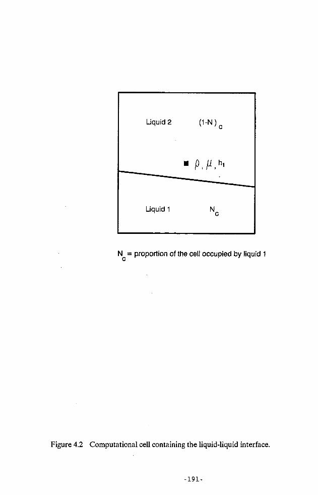
Liquid 2

Liquid 1

Nc

proportion of the cell occupied by liquid 1

Figure 4.2 Computational cell containing the liquid-liquid interface.

-191-

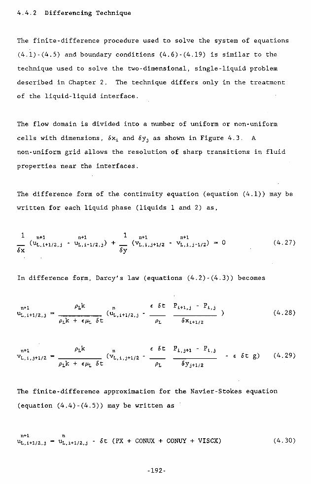
4.4.2 Differencing Technique

The finite-difference procedure used to solve the system of equations (4.1)-(4.5) and boundary conditions (4.6)-(4.19) is similar to the technique used to solve the two-dimensional, single-liquid problem described in Chapter 2. The technique differs only in the treatment of the liquid-liquid interface.

The flow domain is divided into a number of uniform or non-uniform cells with dimensions, Sxi and 5yj as shown in Figure 4.3. A non-uniform grid allows the resolution of sharp transitions in fluid properties near the interfaces.

The difference form of the continuity equation (equation (4.1)) may be written for each liquid phase (liquids 1 and 2) as,

^ n+l -- (UL,i+1/2,jSx

n+l L n+lUL, i -1 / 2, j ) + ( VL, i, j +1 / 2

8y

n+lVL, i , j -1 / 2 ) = 0 (4.27)

In difference form, Darcy's law (equations (4.2)-(4.3)) becomes

n+lUL,i+1/2,j

P-------------- (UL,i+1/2,jPLk + e/zL St

e St Pi+i,j - Pi,j___ ___________ )Pl ^xi+l/2

(4.28)

n+lVL,i,j+1/2

Pl^ n-------------- (vL,i,j + 1/2pLk + e/iL St

6 Pi, j + 1 " Pi.j

Pl j+1/26 St g) (4.29)

The finite-difference approximation for the Navier-Stokes equation (equation (4.4)-(4.5)) may be written as

n+l nuLfi+1/2,j = uL i+1/2 j - St (PX + CONUX + CONUY + VISCX) (4.30)

-192-

Figure 4.3 Computational grid.

-193-

(4.31)n+1 nvL,i,j+i/2 = vL,i,j+i/2 - St (PY + CONVX + CONVY + VISCY + GY)

where,

1SXi pL

(Pi+i,j - pi.j)

1syj pl (Pi,j + 1 ’ Pi,j)

CONUX UL,i+1/2,j

DXADUR + <5xi+1 DUL

+ UPWIND sgn(uL) (<5xi+1 DUL - 8xi DUR) ]

VAVCONUY = ___

DYB ^Yj-1/2 UUT + Yj + 1/2 DUB

+ UPWIND sgn(vL) (5yj+1/2 DUB - Sy.j_1/2 DUT)

sgn(uL)DXADURDULVAV

sgn(vL)DYBDUTDUB

sign of uLii+1/2>j6xi + <$xi+1 + UPWIND sgn(uL) (<$xi+1 - 6xA)(UL, i+3/2,j ' UL,i+1/2, j )/^xi+l

(uL,i+l/2,j ' uL,i-l/2, j)/^xi

(^xi (vL i+li j+1/2 + VL, i+1, j-1/2) +

5xi+1 (vL i j+1/2 + vL,i, j-1/2) )/2 sign of VAV(6yj+1/2 + 5Yj-i/2 + UPWIND sgn(uL) (Syj+1/2 - 8yj.l/z))/2(UL, i + 1/2, j + 1 " UL, i+1/2, j)/<5yj + l/2

(UL,i+1/2,j ' UL,i+1/2, j-l)/^yj-l/2

-194-

CONVY vL,i,j + l/2

DYA 8yj DVT + 8yJ+1 DVB

+ UPWIND sgn(vL) (5yj+1 DVB - 8DVT)

CONVXUAVDXB

5xi_1/2 DVR + 5xi+1/2 DVL

+ UPWIND sgn(uL) (6xi+1/2 DVL ^xi-l/2 DVR)

sgn(vL)DYADVTDVBUAV

sign of vL ij+1/2Syj + 5yj+1 + UPWIND sgn(vL) (6yj+1 - fiyj)

(vL,i,j+3/2 ' vL,i, j + l/2)/^yj + l

(vL,i, j + l/2 ' vL,i,j-l/2)/^yj

(<5yj (uLi+1/2j j + i + uL,i-l/2, j + l) +

^Yj + 1 (uL,i+l/2,j + uL,i-l/2, j) )/2sgn(uL)DXBDVRDVL

^ xi+l/2 ^xi-l/2

= sign of UAV= (5xi+1/2 + 5Xi_1/2 + UPWIND sgn(uL) (6xi+1/2

= (VL, i+l, j + l/2 " vL,i,j + l/2)/^xi+l/2 = (vL,i, j + l/2 " VL, i~l, j+l/2 ) / ^xi-l/2

(8xi + 6xi+1)/2 (8xl + 6x^/2

5yj+i/2 = (<5yj + <5yj+1)/25yj-i/2 = (5y j + 5yj-i)/2

^xi-l/2) ) /2

MlVISCX = [2 [ Ui-l/2,j + ui+3/2,j Ui+l/2,Pl 5xi (5Xi + 5xi+1) 6xi+1 (8xi + 5xi+1) 5Xi <$xi+1

1 1 + f

^.ui+l/2,j-l 5yj ui+l/2, j 5yj + i - UDYT r5yj5yJ+i

5yj 5yj+i/2 5yj+i 5yj+i ty)-i 5yj

1 ^ui+l/2,j 5yj-l ui+i/2,j-i <5yj - UDYB r 5yj-i 5yj5yj-i/2 5yj 5yj-i 5yj 5yj-i

-195-

UDYT - (fiyj ui+i/2ij+i + ^Yj+i ui+i/2,j)/(^yj + ^Yj+i)UDYB = (Syj-i ui+1/2>j + Syj ui+1/2>j-1)/(5yJ + fiy^)

GY = g

The definition of the term, VISCY, follows from that of VISCX. The terms PX, CONUX, CONUY, VISCX, PY, CONVX, CONVY, VISCY and GY are all evaluated at the nth time step.

Equations (4.28)-(4.31) require the pressure to be known at the (n+l)th time step. Since the pressure is known only at the nth time step, equations (4.28)-(4.31) are used to obtain intermediate values of un+1 and vn+1 using Pn instead of Pn+1. The intermediate velocity field will generally not satisfy the continuity condition. To conserve mass, pressure and velocity are relaxed simultaneously following the technique developed by Chorin (1968). The compressibility condition as defined in Chapter 2,

fiP = - A D (4.32)

may be approximated by the following difference equation,

n+l m+1(5Pi(j) =

n+l m+1 (4.33)

where fiP^j is the pressure change needed to satisfy the continuity condition, \L ^ is the compressibility factor and Di j is the divergence term and is defined as

D n+l n+l m+1 n+l--- (uL,i+l/2,j " UL, i -1 / 2, j ) + (vL,i,j + l/2fix 5y

m+1n+lVL, i , j -1 / 2 ) (4.34)

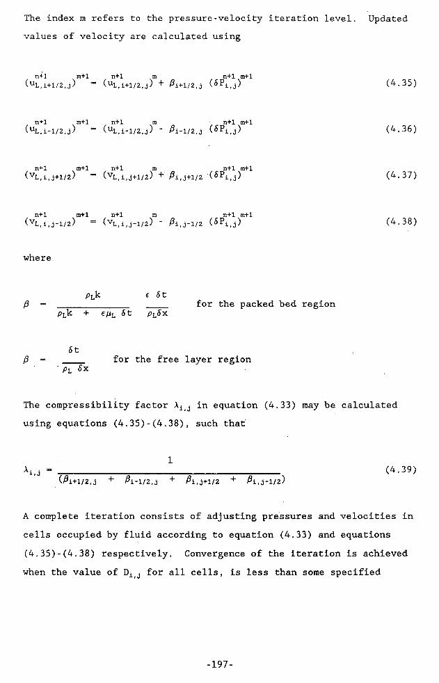
The index m refers to the pressure-velocity iteration level. Updatedvalues of velocity are calculated using

n+l m+1 n+1 m n+1 m+1(UL, i+1/2, j) = (uL,i+l/2,j) + ^i+l/2,j (^-35)

n+1 m+1 n+1 m n+1 m+1(uL,i-l/2,j) = (uL,i-l/2,j) ' ^i-l/2,j (6Pj.fj) (4.36)

n+1 m+1 n+1 m n+1 m+1(VL, i , j +1 / 2 ) = (vL,i,j + l/2) + Pi , j + 1/2 (^^ifj) ( ^ - 37)

n+1 m+1 n+1 m n+1 m+1(VL, i, j -1 / 2 ) = (VL, i, j -1 / 2 ) " Pi , j-1/2 (4.38)

where

pLk e St(3 = _____________ ____ for the packed bed region

PLk + St PlSx

61(3 = ____ for the free layer region

Pl 5x

The compressibility factor XL j in equation (4.33) may be calculated using equations (4.35)-(4.38), such that

1Ai(j = __________________________________________ (4.39)

(£i + l/2,j + P i-l/2,j + Pi, j + 1/2 + ^i,j-1/2)

A complete iteration consists of adjusting pressures and velocities in cells occupied by fluid according to equation (4.33) and equations

(4.35)-(4.38) respectively. Convergence of the iteration is achieved when the value of Di j for all cells, is less than some specified

-197-

tolerance. The convergence may be accelerated by multiplying equation (4.33) by an over-relaxation parameter, co. Values of cj between 1.7-1.9 were found to be optimum for the present problem.

For a cell containing the free surface, the pressure change in the cell (Pijjsur) is given by

n+l m+1 n+1 m+1 n+1 m+1(«Pi.j) - U - <1 i) (P» ) + 'll P,ut£ - (Pi.jsur) (4.40)

where rji is the ratio of the distance between the cell centres and the distance between the free surface and the centre of the interpolation cell, PN is the pressure in a neighbouring cell and Psurf is the gas pressure.

In the numerical technique described above, the incompressibility condition is applied at each cell in such a way as to be effective at time (n+l)5t. This condition ensures that volume is conserved throughout the flow domain. The mass in a particular cell however may vary between time levels as a result of a change in the proportion of each liquid in that cell, particularly near the liquid-liquid interface. Consequently, mass is not necessarily conserved at every time step. The calculation of the discrete liquid properties in the flow domain is however governed by a conservative velocity field and as such, we expect only minor fluctuations in mass at each time step (Welch et al (1965)). Furthermore, we have elected to lag the liquid density field (p) behind the pressure and velocity fields ie. p is evaluated at time n6t. These two finite approximations must be tested by observing the stability of the numerical solution and also by validation with results from physical models. Results from such tests will be discussed later in this chapter.

-198-

The no-flow boundary conditions (equations (4.6)-(4.9)) are approximated by

ul ,2, j ~ 0 , uLNj-0 (4.41)

vL(i>2 = 0 (4.42)

uL,i,i = uLiii2 (4.43)

VL, 1, j = VL, 2, j » VL, N, j = vL,N-l,j (4.44)

The total liquids drainage rate is specified as an outflow boundary condition. The velocity across this boundary, uidpx jdpy, is given by

Qtuidpx, jdpy = ------ (4--45)

^ ^ y j dpy

where QT is the total drainage rate, W is the width of the model and Syjdpy is the drain cell height.

The pressure at the gas-liquid interface is set equal to the gas pressure (equation 4.12). In difference form, this may be written as

, jsur+1 = i*surf (4.46)

The kinematic condition at the liquid-liquid and gas-liquid interfaces, equation (4.13), is approximated using the Courant-Isaacson-Rees method (1952), so that,

n+l n ^ t n n dhLhL,i = hL,i + _ (VL - UL _ ) e dx

(4.47)

-199-

The kinematic condition at the liquid-liquid and gas-liquid interfaces with production of each liquid, equation (4.14), may be written as,

n+1 n ^ b n n dhL nhL(i = hL i + _ (vL - uL _ + VpL)

e dx

where,

(4.48)

ndhL i+1 - hL idx 5xi+1/2

hL,i ' hL,i-l

6Xi-i/2

if uL < 0

if uL > 0

0 if uL = 0

and uL and vL are the interpolated velocities at the interfaces. A linear interpolation of neighbouring velocities is used at the free surface. For the liquid-liquid interface, h1(x,t), a second order Taylor series expansion for the y-component of velocity is used.Figure 4.4 shows two possible situations where the liquid-liquid interface bisects a computational cell. A Taylor series expansion for vL about the point s may be written as

dv h2 <92v+ h

. dY . O+

ro|

dy2

(4.49)

where h is the distance between the point s and the nearest cell velocity. For case (a) in Figure 4.4, the finite-difference approximation of equation (4.49) is

v2-vivL = v0 + h ______ +

Sy0+6yih2~2

Vo-Vr

5y0 6yi(4.50)

-200-

Case (a) Case (b)

Figure 4.4 Definition of parameters used in the calculation of the y-component of

velocity at the liquid-liquid interface.

-201-

where v0, and v2 are the neighbouring cell velocities and <5y0, 8y1

and <5y2 are the cell dimensions in the y-direction.

For.case (b) in Figure 4.4, the finite-difference approximation of

equation (4.49) may be written as

v2-vj. h2vL = v0 + h _______ + __

(Syo+Syi 2

v2-v0

<5y2

v0-vi

<5y0(4.51)

4.5 Numerical Stability and Accuracy

The stability requirements for the two-dimensional, single - liquid

numerical model described in Chapter 2 apply in the homogeneous

regions of the two-liquid drainage problem. At the liquid-liquid

interface, however, the analysis of stability is complicated by the

variation in density and viscosity. In the present study, it was

found that the numerical solution remained stable if the single-liquid

requirements were satisfied.

The time step limitations are given by the following equations,

<$t < min (4.52)

pL 5x2 8y2<5t < ___ ___________ (4.53)

2/iL 6x2 + 8 y2

81 <5x

(s tw)1/2

(4.54)

-202-

Equation (4.52) limits the liquid movement to less than one cell width per time step, St. Similarly, equation (4.53) states that momentum cannot diffuse more than one cell width per time step. The Courant wave condition (equation .(4--54)) is the most restrictive condition for most drainage problems.

To minimise numerical diffusion, the degree of upwind differencing applied to the convective terms in equations (4.30)-(4.31) is limited by

K| St | vL | Stn Sx

1 > UPWIND > maxSy

(4.55)

4.6 Computational Procedure

The initial positions of the liquid-liquid and gas-liquid interfaces are specified. For most drainage problems, the computational grid is initialised to hydrostatic equilibrium. The total flowrate of liquids is specified as a function of the individual phase flowrates and time. The computational procedure through one time step, <5t, consists of the following steps:

1. Compute the initial values of density and viscosity using equations (4.25)-(4.26).

2. Compute an initial guess for velocities using the explicit approximations defined by equations (4.28)-(4.31).

3. To satisfy the continuity condition in each cell, pressures and velocities are adjusted simultaneously, using equation (4.33) (for full cells) or equation (4.40) (for surface cells) for pressure and equations (4.35)-(4.38) for velocities.

4. When the continuity condition is satisfied, equation (4.27), the free surface and liquid-liquid interface are moved using equation (4.47) or equation (4.48).

5. Steps 1-5 are repeated for successive time steps until the free surface reaches the cell containing the drain, at which time the simulation is terminated.

The listing of a Fortran computer code (HD22.FOR) which was developed to implement the above computational procedure, is given in Appendix E.

-204-

4.7 Experimental

A series of two-liquid drainage experiments were carried out using a modified Hele-Shaw viscous flow analog as shown in Figure 4.5. The model has been described previously in Chapter 2. The experimental liquids used were air, various mixtures of glycerol and water, and mercury. These are the experimental analogs for furnace gas, slag and iron phases, respectively. The properties of the liquids are given in Table 4.1. The viscosity of the glycerol/water mixtures was measured using a suspended level viscometer.

Before each drainage experiment, the model was filled with mercury and a glycerol/water mixture to the desired levels and the contents allowed to attain hydrostatic equilibrium (ie. both gas-liquid and liquid-liquid interfaces horizontal). The positions of the gas-liquid and liquid-liquid interfaces were photographically recorded during the drainage experiment until the gas-liquid interface reached the taphole.

4.8 Validation of Numerical Model

The two-dimensional, two-liquid numerical model is validated using experimental drainage data reported by Tanzil (1985) and results from drainage experiments carried out using the modified Hele-Shaw viscous flow analog described in the previous section. Tanzil (1985) carried out experiments for the simultaneous drainage of two immiscible liquids using a Hele-Shaw viscous flow analog. The viscous flow analog was shown to overcome difficulties in accurately resolving the position of liquid interfaces in two-dimensional, fully packed beds. The experiments were carried out using an 80:20 glycerol/water mixture

-205-

91.4cm83.4 cm

2.64cm

GlycerolReservoir

Mercury Reservoir

60.0 cm

CollectionFlask

Air Bleed

To Vacuum Pump

Figure 4.5 Modified viscous flow analog.

Table 4.1 Properties of Molten Liquids and Experimental Liquids

P

(gm/cm3)P

(gm/cm.s)

Iron 6.7 0.05

Slag 2.6 7.0

Glycerol/water (50:50) 1.13 6.5

Mercury 13.6 0.01

-207-

(p=1.21 gm/cm3, pi=0.139 gm/cm.s) and mercury (p=13.6 gm/cm3,^=0.0163 gm/cm.s). The initial liquid levels of the glycerol/water mixture and mercury above the base of the model were 45.9 cm and 16.2 cm respectively. The taphole was located 14.5 cm above the base of the model. Figure 4.6 shows the flowrates of glycerol/water and mercury measured during the experiment.

Figure 4.7 shows a comparison between the liquid levels computed by the numerical model and the experimentally-measured profiles. A non-uniform, computational grid was used for the numerical computations. A fine grid spacing was used near the taphole and the liquid-liquid interface. A total of 441 cells (21 cells in the x- and y- directions respectively) were used, with a maximum cell size of 5 cm and a minimum of 1.76 cm. The time step used was 0.008 s. The computed gas-liquid and liquid-liquid interfaces agree very well with the experimental data. The predicted blowout time of 15.4 s also compares well with the experimental time of 16.0 s.

Figure 4.8 shows a comparison between results from drainage experiments carried out using the modified Hele-Shaw viscous flow analog and the predictions using the numerical model. The height of the free layer was 4.0 cm. Th model was again filled with an 80:20 glycerol/water mixture (p=1.21 gm/cm3, /i=0.0992 gm/cm.s) and mercury (p=13.6 gm/cm3, /i=0.0i63 gm/cm.s). The initial levels of the glycerol/water mixture and mercury were 47.7 cm and 18.1 cm respectively. The taphole was located at 18.1 cm above the base of the model. Figure 4.9 shows the measured liquid flowrates during the experiment. The flowrate data was obtained by integration of the photographically recorded gas-liquid and liquid-liquid interface profiles. The numerical computations were performed using a non-uniform grid consisting of 21 cells in the x-direction and 23 cells in the y-direction (483 cells in total). Additional cells

-208-

Flowrate3

(cm /s)

Glycerol/waterMercury

Time (s)

Figure 4.6 Experimentally measured drainage rates of glycerol/water and mercury used

for computations shown in Figure 4.7.

-209-

-210-

nage experiment in a fully packed bed, and the If

cL EX

=3w

z

w

05 r- N O

) CO

o

o •»- Tt

COt- co

in m

ECDoc03wb

a05 05

1

2B

.•§ 13

^cu >%

3

O

05E3

3

05-C>-.

c_c

•- 0505<J=an

"O053O.

EoCJJA05>_05

’3.2*

-X053c.

•£

.cc0505£05

£)3OA'Cc«

a-

T3

05300 3

05

a- |

x ^2

05 05

05 ^

an _23 •W05E•05

6 | |

a -s s00'C

t05

13

-211-

a packed bed and a

Glycerol/waterFlowrate

(cm /s)

Mercury

0 20 40 60Time (s)

Figure 4.9 Experimentally measured drainage rates of glycerol/water and mercury used

for computations shown in Figure 4.8.

-212-

were placed in the free layer region. The time step was again restricted to 0.008 s. Figure 4.8 shows that the overall agreement between the experimental and numerical profiles is very good. The predicted duration of the .experiment (53.8 s) also compares very well with the measured time (54.9 s).

The results described above indicate that the numerical model may be used to investigate the drainage performance of an operating blast furnace with and without a coke-free layer. This is described in the following section.

4.9 Application to Blast Furnaces

The two-dimensional, two-liquid numerical model is used to examine the drainage performance of a hearth with and without a coke-free layer. Drainage data from Kawasaki's Chiba No. 6 blast furnace reported by Fukutake and Okabe (1981) is used to compare with the computations. Since the actual blast furnace is three-dimensional, only a qualitative comparison with the numerical model is possible. Two numerical simulations were performed. In the first simulation, the hearth is assumed to be fully packed with coke. The results of this simulation are compared with those previously reported for the two-dimensional, two-liquid numerical model developed by Tanzil (1985). In the second simulation, a 0.4 m coke-free layer is assumed to underlie the packed bed. This is the value for the coke-free layer height reported by Ohno et al (1981) for a furnace with a hearth diameter of 11.0 m.

Figure 4.10 shows a comparison between the predicted profiles using the present numerical model and the numerical results reported by

-213-

220

O

T-

O

C\J T

-co

r-

C\1 CO

CO^

^

O

- o

o

oo

o

ECDOc05(f)

b

(LUO

) }L|B!9

H

1aJZ-CvqoZ_clcUjaczC3<UISou D-

<U5"O

C<u <u £ a3-Oc oC/3

’§ g

c «

c c

o h-

U

5 <u3oua-v£-acZZ

13■aoSIz£

3

C

•*—*

ojC/3<DC.OJ-3>c■3a)3a,Eou

<uu3.rP'iZ

214-

computed by Tanzil (1985).

Tanzil (1985) for conditions similar to those for Chiba No. 6 blast furnace. Table 4.2 shows data used in the simulation of the Chiba conditions as reported by Tanzil (1985). The initial iron and slag liquid levels were estimated by Tanzil (1985) by trial and error. Figure 4.11 shows the measured iron and slag drainage rates from Chiba No. 6 and the computed drainage rates reported Tanzil (1985). For the purpose of this study, the computed drainage rates reported by Tanzil (1985) were used for the simulation. As previously described, the present model uses the total drainage rate (iron and slag) as the specified condition at the drain point. The drainage rates for each phase are calculated from a simple mass balance. Tanzil (1985) used the measured slag drainage rate from Chiba No. 6 as the specified condition to compute the iron drainage rate. The agreement between predicted results from the present model and those reported by Tanzil (1985) is very good. The present model predicts:

(a) the tilting of the slag surface towards the taphole(b) the tilting of the iron surface up towards the taphole(c) the maximum average height of slag at approximately

60 minutes into the cast(d) a calculated cast duration time of 132 minutes compared with

131 minutes (Tanzil (1985)).

Figures 4.12 and 4.13 compare the drainage rates and cumulative drained volumes computed by the present model with those computed by Tanzil (1985) and that measured for Chiba No. 6. The agreement between the model results is excellent. The comparison between the calculated iron flowrates early in the cast is influenced by the rapidly changing iron flowrate reported by Tanzil (1985). Clearly, results from the present model compare favourably with those reported by Tanzil (1985).

-215-

Table 4.2 Chiba No. 6 Blast Furnace Drainage Data

Taphole height 100.0 cmInitial slag height 155.0 cmInitial iron height 85.0 cmWidth of model 1560.0 cmLength of model 1000.0 cmSlag density 2.6 gm/cm3Iron density 6.7 gm/cm3Slag viscosity 7.28 gm/cm.sIron viscosity 0.05 gm/cm.sPorosity of bed 0.35Slag production rate 0.00717 cm/sIron production rate 0.008 cm/s

-216-

Tanzil (1985)

Chiba No. 6 Data

Time (minutes)

Figure 4.11 Drainage data for Kawasaki’s Chiba No. 6 blast furnace: (a) measured, (b) computed by Tanzil (1985).

-217-

---------------- Tanzil (1985)

.................. Chiba No. 6 Data---------------- Present Model

o 4 -•4—» ^

Time (minutes)

Figure 4.12 Comparison between the drainage rate for Chiba No. 6 blast furnace predicted by the present numerical model, and the drainage rate as: (a) measured, and (b) computed by Tanzil (1985).

-218-

/Present model Hanzil (1985)

Chiba No. 6 Data

400-

300 -

Time (minutes)

Figure 4.13 Comparison between the cumulative drained volumes for Chiba No. 6 blast furnace predicted by the present numerical model, and the cumulative drained volumes as: (a) measured, and (b) computed by Tanzil (1985).

-219-

240

.£EoCD

cdcr- >? iSILin

o

CVJ t

tCM

CO CO

t— O O

CM

T-

CD CM CO

oooooCOooCOoo

Eo,Q)oc03•(J)b

c-C"OcC3£i£ifCJrec

(wo) iqB

ian

-22

0-

Note: To maintain clarity, markers for the iron profile are omitted

^Present model f - Fully packed bed and | - Packed bed/free layer

Tanzil (1985)

Chiba No. 6 Data

8 600-

500-

■j5 200

R 100-

Time (minutes)

Figure 4.15 Comparison between the computed cumulative drained volumes for Chiba No. 6 blast furnace with a coke-free layer, and the cumulative drained volumes as: (a) measured, (b) computed by the present model for Chiba No. 6 blast furnace without a coke-free layer and (c) computed by Tanzil (1985).

-221-

Figure 4.14 shows the predicted iron and slag profiles during the cast, with and without a coke-free layer. The coke-free layer is assumed to be uniform across the hearth and to extend only into the iron phase. Other input model parameters, including the iron and slag drainage rates, are the same as before (Table 4.2 and Figure 4.11).The results show that the effect of a coke-free layer of size reported for the Chiba No. 6 furnace (Ohno et al (1981)), has a negligible effect on the gas-slag interface and therefore on the residual slag volume. Furthermore, the results show that the movement of the iron-slag interface during the cast is similar to that for a fully packed bed. The calculated cast duration time is therefore close to that for the fully packed bed case (131.5 minutes cf. 132 minutes). Figure 4.15 shows that the difference between the drained volumes of iron and slag as computed by the present model and those computed by Tanzil (1985), is also insignificant.

4.10 Conclusion

For large diameter blast furnaces such as Kawasaki's Chiba No. 6, the coke-free layer may extend into the iron phase only. The effect of the coke-free layer on the residual volume of iron and slag in such a furnace, is insignificant. The drainage performance of a large diameter, high productivity blast furnace such as Chiba No. 6, may be simulated using the assumption that the hearth is fully packed with coke.

-222-

5 TWO-DIMENSIONAL STUDY OF THE FLOW OF IRON IN A NON-ISOTHERMALHEARTH

5.1 Introduction

Radioactive isotopes have been used to infer the condition of the hearth in operating blast furnaces (Babarykin et al (1960), Miyagawa et al (1965) and Nakamura et al (1977)). Injection of isotopes has also been used to determine the extent of erosion of the hearth refractory lining (Babarykin et al (1960), Miyagawa et al (1965)) and the effect of coke quality on the permeability of the hearth (Nakamura et al (1977)). Ohno et al (1981) showed that the formation of skull (solidified iron, coke and a deposited graphite mixed layer) and the erosion of the hearth refractory lining was influenced by the flow distribution of iron in the hearth, which in turn, was strongly influenced by the presence of a coke-free layer (Hara and Tachimori (1978, 1979)). For the situation where the coke bed only partially penetrates to the base of the hearth, Vogelpoth et al (1985) concluded that the erosion of the refractory lining near the lower walls of the hearth was attributable to the flow of iron in the coke-free layer.

The analysis of residence time data from radioactive isotope experiments carried out in an operating blast furnace is difficult because of the complex nature of flow in the hearth. A number of investigators have attempted to analyse such data using the concept of travelling time of the isotope in the hearth (Hara and Tachimori (1979), Ohno et al (1981) and Libralasso et al (1985)). The travelling time is simply the mean residence time for the isotope in the hearth. Ohno et al (1981) and Libralasso et al (1985) showed that the travelling time of the isotope in an isothermal hearth could characterise satisfactorily the state of the coke bed in a hearth in

-223-

the presence or absence of a coke-free layer. Alleyn et al (1981) and Rooney (1986) analysed data obtained from isotope experiments carried out at Broken Hill Proprietary's Port Kembla No. 5 blast furnace in a manner similar to that of Ohno et al (1981) but found that the results of the analysis were inconclusive.

In this chapter, a two-dimensional, single-liquid numerical model for non-isothermal conditions is developed to investigate the physical processes governing the flow of iron in the hearth, where the hearth refractory lining may be side-hearth cooled, under-hearth cooled or both side- and under-hearth cooled. The effect of a coke-free layer for each of these situations and for conditions typical of a large, operating blast furnace, are investigated. In the following chapter, the numerical model is extended to three dimensions and is shown to provide an explanation for the inconclusive results of the isotope experiments reported by Rooney (1986).

The numerical model is based on the Marker-and-Cell finite-difference technique (Welch et al (1965). This technique is used to solve the coupled set of partial differential equations describing the conservation laws for momentum, energy and mass transport in a packed bed with and without a packing-free layer. The Boussinesq approximation is not invoked in the formulation of the mathematical model and the model computes the volume (or density) changes due to temperature variations in the liquid (Casulli (1981)). The numerical model is validated by comparing it with data from numerical experiments reported by Yashiro et al (1982) for a two-dimensional hearth with under-hearth cooling.

-224-

5.2 Model Formulation

Figure 5.1 shows a schematic diagram of the two-dimensional, single -1iquid model system. The rectangular flow domain consists of a packed bed of porosity, e, and permeability, k. A packing-free layer may underlie the packed bed. The height of the packing-free layer may be uniform (Hfi) or it may vary over the width of the model. The bed is saturated with a liquid (simulating liquid iron) with properties which are assumed to be temperature-dependent ie. a liquid of density, p(T), and viscosity, p(T), where T is temperature. The thermal conductivity of the liquid, Kf, is assumed to be constant. The level of the liquid is maintained at a constant height, Hliq, which represents the iron-slag interface. A constant influx or dripping rate of liquid (Vin) into the model is assumed and the liquid is withdrawn from a drain (flowrate, Q) located at the side of the model. The side and bottom boundaries are maintained at fixed temperatures, Ts and Tb respectively. The fixed boundary temperatures simulate cases where side-hearth, under-hearth cooling or both side- and under-hearth cooling are used to control the temperature of the hearth refractory. The temperature, Tin, of the liquid dripping into the model is also specified.

The general continuity equation for the liquid may be written as

dp a Vi_ + (Vi- V) p + p _ = 0 (5.1)at axi

where p is the liquid density and is the velocity component in the co-ordinate direction Xi.

The general equation governing the conservation of momentum for the liquid is

-225-

X

Vin Tiin 'in

Iron/slag interface

Packed bed ( k ,8)

Iron ( p(T), u (T)

Free layer

B

T H,

-1

Figure 5.1 Schematic diagram of the two-dimensional, single-liquid, non-isothermal model.

-226-

p (5.2)DVi ap__ = - __ + pGi - V2; TDt axi

where D is the substantial or material derivative V is the del operatorP is the pressureGi is the gravitational constantt is the stress tensor

In two-dimensional, cartesian co-ordinates, the components of the stress tensor (rxx, r^, rxy and ryx) may be written as,

du 2_ + _ p (V- VO dx 3

(5.3)

dv 2■yy = * 2/i _ + ^ /i (V- Vi) (5.4)

dy 3

au avTxy = - 4 (-- + --)ay ax (5.5)

au avT’yx = - 4 (__ + __ )ay ax

(5.6)

In the packed bed region, the fluid motion is governed by Darcy's equation (Bear (1971)), which may be written in transient form as,

p aVi aP pi____ = - _ + pGi - _ Vi (5.7)e at 3Xi k

The general equation for the conservation of energy is given by (Bird et al (I960)) ,

-227-

(pc ) [_ + (Vi- V)T + T _ ] = VK VTdt dxi

(5.8)

where T is the temperatureCp is the specific heat capacity K is the thermal conductivity

For a liquid with constant thermal conductivity, Kf, the equation for the conservation of energy in the packing-free layer may be written as

where the subscript f denotes the liquid property. In the packed bed region, it is assumed that the liquid velocity is low and that both the solid and liquid phases are well dispersed. For this situation, the difference between the solid (s) and liquid (f) temperatures (Ts and Tf respectively) may be neglected (Bear (1971)). The flow domain may be considered as equivalent to a unique continuum in which the thermal behaviour is described by a single equation for the average temperature, T (T = Ts = Tf) , and where lumped solid-liquid properties apply. Thus, the equation for the conservation of energy in the packed bed is given by,

Equations (5.9)-(5.10) may be written in a more general form as,

(pCp)f [_ + (Vf- V)T + T _ ] = Kf V2T d t

(5.9)

(pCp)fS _ + (pCp)f [(V,- V)T + T _ ] = Kfs V2Tat axi(5.10)

(5.11)

-228-

where f equals f for liquid properties (for the packing-free layer) and fs for lumped solid-liquid properties (for the packed bed).

The density and viscosity of the liquid are assumed to be temperature - dependent. The equation of state relating density to temperature is given by (Bear (1971)),

where 9 is the linear coefficient of thermal expansion and p0 is the liquid density at temperature T0. The equation of state for viscosity is given by (Bear (1971)),

where <f> is the viscosity-temperature coefficient and /j0 is the viscosity at temperature T0.

In many cases of practical interest (eg groundwater flow), the solution of equations (5.1)-(5.13) is simplified by invoking the Boussinesq approximation, which states that the fluid density, p, is constant except in so far as it affects the buoyancy force (Bird et al (I960)). This simplification may result in the introduction of significant errors in the transient term of the continuity equation (equation (5.1)), particularly for cases where large temperature and density variations exist in the flow field (Horne (1975)). If the equation of state for liquid density, equation (5.12), is assumed to describe the density-temperature relationship for liquid iron, the Boussinesq approximation is only valid if the following condition is satisfied (Horne (1975)),

P = Po [1 - *(T - T0)] (5.12)

- UT - T0)4 = 4o e (5.13)

6(T - T0) < 0.01 (5.14)

-229-

For liquid iron, where 9 equals 0.000141K'1 (Yoshikawa et al (1981)) and (T - T0) equals 300K, this condition is clearly violated. The Boussinesq approximation is therefore not an appropriate assumption for liquid iron in the hearth.

Substituting the equation of state for liquid density (equation (5.12)) into the continuity equation (equation (5.1)), differentiating and re-arranging gives

dVi 9 5T dVi_ = [____] [_ + (Vi- V)T + T __ ] (5.15)dXi 1+0TO <9t dXi

Using the conservation of energy equation (equation (5.11)), a further substitution for dT/dt in equation (5.15) upon re-arrangement gives,

dVi 1_ = 6 [_____ Kr V2T + (l-/c) (Vi- V)T] (5.16)dxi (pCp)r

1where 9 = ____________________

[1 + 9 (T0 - (l-/c)T) ]

(pCp)fand k = ____________

(PCp)f

Equation (5.16) is a modified form of the continuity equation. Using equation (5.16), the conservation of energy equation (equation (5.11)) may be written as

5T /c0T__ + A (Vi- V)T = [1 - _____ ] Kf V2T (5.17)5t (P Cp) £■

where A = /c(l + 9(l-/c)T).

-230-

Equations (5.2)-(5.7), (5.12)-(5.13) and (5.16)-(5.17) are the governing equations for thermally-influenced flow in a homogeneous liquid. These equations may be written for a two-dimensional, non-isothermal hearth in the following manner,

du du du dp__ + u __ + v __ = - __+d t dx dy . dx

ddx

du 2 du dv2 n _ - _ A* (_ + _)dx 3 dx dy

dydu dv

P (_ + __)dy dx(5

dv dv dv dP+ u __ + v __ = - __ +

dt dx dy . dy

ddx

du dvP (__ + __)dy dx

dydv 2 du dv

2/i _ - _ /* (_ + _)dy 3 dx dy + P g (5

p du € d t

dP e__ + _ udx k

(5

p dv dP €____ =- __ + _ v + pg€ dt dy k

(5

dT dT dT kQT__ + A (u_ + v_) = [1 - _____ ] Kf V2Tdt dx dy (pCp)f

(5

du dv 1__ + __ = 0 [_____ Kr V2T + (l-/c) (Vi- V)T]dx dy (pCp)f

(5

p = p0 (1 - tf(T - T0))

- *<T - T0)A* = A*o e

(5

(5

• 18)

.19)

.20)

• 21)

.22)

.23)

• 12)

.13)

-231-

Equations (5.12)-(5.13) and (5.18)-(5.23), together with the initial and boundary conditions, completely specify the non-isothermal drainage problem for a packed bed containing a packing-free layer.

5.3 Initial and Boundary Conditions

Consider the two-dimensional model shown in Figure 5.1. The side and bottom boundaries are impermeable and the flow normal to these boundaries is zero. The boundary conditions for the x- and y-components of velocity are therefore the same as those for the isothermal model ie. a 'free-slip' boundary condition, such that

u = 0 at x = 0 and x = D (5.24)

v = 0 at y = 0 (5.25)

3u oll

1 >■>10

at y = 0 (5.26)

3v_ = 03x

at x = 0 and x = D (5.27)

The volumetric outflow rate per unit time, Q, is related to the x-component of velocity for the grid-block face over which the liquid is withdrawn, udrain, by

Q(t)udrain — ------

^■drain(5.28)

where Q(t) is the liquid flowrate as a function of time t and Adrain is the area of the grid-block face over which the liquid is withdrawn.

-232-

At the top boundary of the model, the volumetric inflow rate per unit time, Qin, is related to the volumetric outflow rate per unit time, Q, by the following equation,

Qin(t) = Q(t) - Ve (5.29)

where Qin(t) is the liquid production rate as a function of time t and Ve is the rate of volume change of the liquid due to temperature differences. Ve is equal to the right-hand side of equation (5.23) multiplied by the internal volume of the model. Equation (5.29) states that the level of the upper surface is constant throughout the simulation, which is consistent with the assumption made in formulating the model. The production rate, Qin(t), is uniform across the length of the model and is related to the y-component of velocity at the upper surface, vsurf, by

Qin(t) vsurf = _______A

(5.30)

where A is the cross-sectional area of the model over which the influx of liquid takes place.

The liquid phase pressure at the top surface is specified and may be a function of both position and time. For most simulations, the surface pressure is constant and set equal to the sum of the gas phase pressure (Pgas) and the hydrostatic liquid head of slag (Pliq) ie.

Psurf(x,t) = Pgas + Pliq (5.31)

where Pliq equals psghs, ps is the slag density and hs is the height of slag above the iron level.

-233-

The appropriate boundary conditions for the energy equation are a specified temperature on those boundaries through which a heat flux is allowed or a specification of the gradient in temperature normal to the surfaces through which a flux (or zero flux) is allowed. Thus, for cooling applied to the vertical sides of the model (ie. side-hearth cooling), the boundary conditions on temperature are

T = Ts at x = 0 and x=D (5.32)

5T__ = 0dy

at y = 0 (5.33)

For cooling applied to the base of the model (ie under-hearth cooling), the boundary conditions on temperature are

T = Tb at y = 0 (5.34)

<9T_ = 03x

at x = 0 and x=D (5.35)

The temperature of the liquid flowing across the top boundary is set,such that

T - Tin at y = HLiq (5.36)

The continuity equation requires that at the boundary between the packed bed and the packing-free layer, the velocity normal to boundary, u^, is continuous across the boundary.

Initially, the elevation of the top surface is set such that

y = Hliq (5.37)

-234-

The initial temperature distribution of the liquid is specified by one of two initial conditions ie. the liquid temperature is uniform (isothermal) or it may vary linearly with height of liquid. The isothermal condition may be written such that

T = T0 (5.38)

The linear variation of temperature with height, h, is given by

T = a h + Tb0 (5.39)

where a is the rate of increase in temperature with liquid height and Tb0 is the temperature at y=0.

5.4 Numerical Scheme

The governing equations and corresponding boundary conditions are solved using the modified Marker and Cell finite-difference technique previously described in Chapter 2. The flow domain is divided into a number of non-uniform grid-blocks in the x- and y-directions as shown in Figure 5.2. The field variables, velocity, pressure and temperature are defined at locations shown in Figure 5.3. The x-component of velocity, u, is defined at the centre of each vertical side of a cell and the y-component of velocity, v, at the centre of each horizontal side. The pressure, P, and temperature, T, are defined at the centre of the cell. The density, p, and viscosity, p, are also defined at each cell centre.

The location of the packed-bed/packing-free layer boundary on the computational mesh is shown in Figure 5.2. The boundary may cut a

-235-

-236-

Figure 5.2 Computational grid.

AVi,j + 1

Figure 5.3 Layout of field variables.

-237-

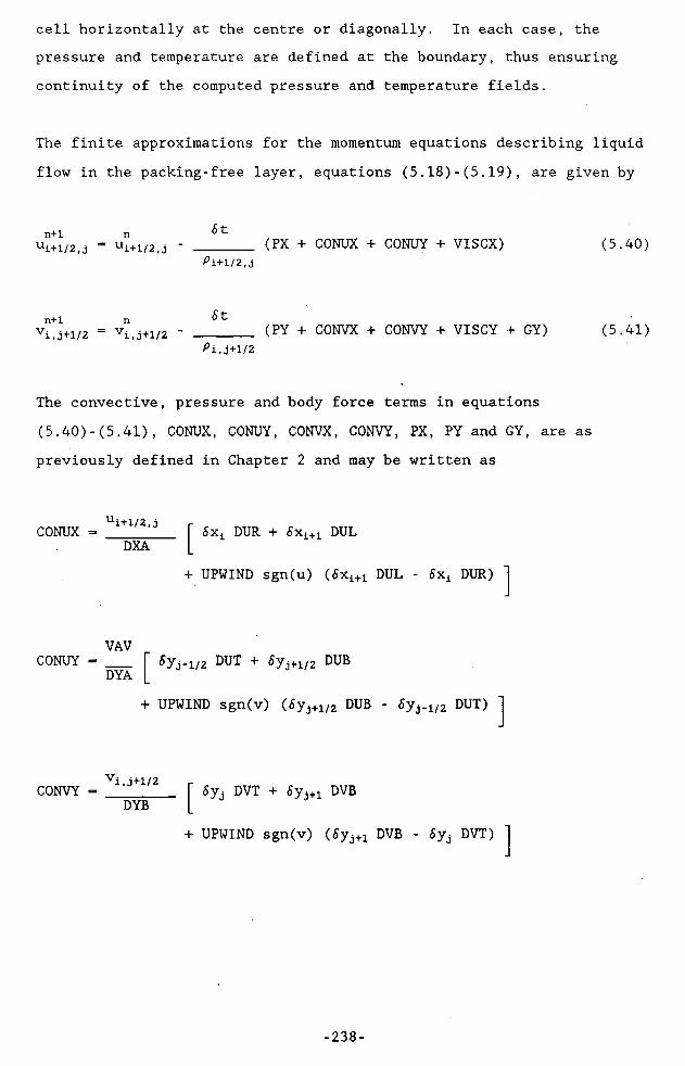
cell horizontally at the centre or diagonally. In each case, the pressure and temperature are defined at the boundary, thus ensuring continuity of the computed pressure and temperature fields.

The finite approximations for the momentum equations describing liquid flow in the packing-free layer, equations (5.18)-(5.19), are given by

n+l nui+l/2,j = ui+l/2,j

8 t______ (PX + CONUX + CONUY + VISCX)Pi+l/2,j

(5.40)

n+l nvi,j+1/2 = vi, j + 1/2

8 t______ (PY + CONVX + CONVY + VISCY + GY)Pi, J + 1/2

(5.41)

The convective, pressure and body force terms in equations(5.40)-(5.41), CONUX, CONUY, CONVX, CONVY, PX, PY and GY, are aspreviously defined in Chapter 2 and may be written as

CONUX Ui+l/2,j

DXA6Xi DUR + 6xi+1 DUL

+ UPWIND sgn(u) (6xi+1 DUL - 8xL DUR)

VAVCONUY = ___

DYA ^Yj-i/2 OUT + <5yj+1/2 DUB

+ UPWIND sgn(v) (6yj+1/2 DUB - 8y^l/2 DUT)

CONVY Vi,j+1/2

DYB8 yj DVT + 5 yj+1 DVB

+ UPWIND sgn(v) (5yj+1 DVB - 8DVT)

-238-

UAVCONVX = ___

DXBiSXi-i/2 DVR + <5xi+1/2 DVL

+ UPWIND sgn(u) (6xi+1/2 DVL - SyLi.1/2 DVR)

1PX = ____ (Pi+1,j - Pi.j)

^ xi+l/2

1PY = ____ (PiiJ+i ' Pi.j)

5Yj + l/2

GY - g

and

sgn(u) =DXADURDULVAVsgn(v) = DYA DUT DUB

sgn(v) =DYBDVT

DVBUAV

sgn(u) =

sign of ui+1/2fj5Xj_ + Sxi+1 + UPWIND sgn(u) (5xi+1 - 8xL)

(ui+3/2,j ‘ ui+l/2, j)/^xi+l(ui+l/2,j ' ui-l/2, j )/^xi(5xt (vi+1j+1/2 + vi+1j_1/2) + 5xi+1 (vi(j+1/2 + vi(j_1/2))/2 sign of VAV

(Syj+1/2 + 5Yj-i/2 + UPWIND sgn(u) (6yj+1/2 - 5yj-1/2))/2(ui+l/2,j + l ‘ ui+l/2, j )/^Yj+l/2 (ui+l/2,j " ui+l/2, j-l)/^yj-l/2

sign of vi>j+1/2Syd + Syj+1 + UPWIND sgn(v) (5yj+1 - Sy^)

(vi,j+3/2 ‘ vi, j + l/2)/^yj + l

(vi,j+l/2 " vi, j-l/2)/^yj(5yj (ui+1/2,j+i + ui_1/2ij+i) + 5yj+1 (ui+1/2jj + ui_1/2j))/2 sign of UAV

-239-

DXB = (6xi+1/2 + 6Xi_1/2 + UPWIND sgn(u) (<5xi+1/2 - 6xi_1/2))/2

= ( vi+l, j + 1/2 ' vi , j-t-1 /2) /^xi+l/2

= (vi,j + l/2 " vi-l, j + l/2)/^xi-l/2

DVR

DVL

5xi+i/2 = (5Xi + 6xi+1)/2

5xi-i/2 = (<^xi + 5xi.1)/2

^yj+i/2 = (5yj + 6yj+1)/2«5yj-i/2 = (^yj + 5yj_i)/2

The finite-difference approximations for the viscous dissipation terms, VISCX and VISCY, are developed using the right-hand side of

equation (5.23). They are written as,

VISCXDX1

/ii+1j DUR - fj,i j DUL

- 1/3 (Ah+itj TAUTi+1j - TAUTi(j)

5yjMi+1/2.j+1/2 (DUYT + DVXT) - /ii+1/2J-1/2 (DUYB + DVXB)

VISCY = ___ /ii i+1 DVT - Mi ; DVBDY1

- 1/3 (/ii>j+1 TAUTi>j+1 - /iij TAUTi(j)

6XiMi+i/2.j+1/2 (DUYT + DVXT) - 4i-i/2,j+1/2 (DUYR + DVXL)

DX1 =2.0 Sxi+1/2

DY1 =2.0 Syj+1/2

DUYT = (ui+1/2>j+1 - ui+1/2(j)/(5yj + 5yj+1)

DVXT = (vi+1j+1/2 - vifj+1/2)/(5xi + 5xi+1)

DUYB = (ui+1/2 j - ui+1/2_j_1)/(5yj + 6yj-i)

-240-

DVXB = (vi+1j_1/2 ' vi,j-1/2)/(<5xi + 6xi+1)DUYR = (ui_1/2(j+i - ui-i/2,j)/(6yj + 5yj+1)DVXL = (vi j+1/2 - vi_1_j+i/2)/(5xi + 6x^1)

where the term TAUT is the finite-difference approximation corresponding to the right-hand side of equation (5.23) and is defined in equation (5.46) below. The viscosities, pi+1/2j+1/2» Mi+1/2,j-1/2 a^d Mi-1/2 j+1/2 are calculated by interpolation using values of the four nearest cells.

All quantities in the convective and viscous fluxes are evaluated at the nth time step, whereas PX and PY are evaluated at the (n+l)th time step. The degree of upwind differencing applied to the convective terms is determined by the value of the term, UPWIND.

The transient form of Darcy's equation (equations (5.20)-(5.21)) is approximated by the following difference equations,

n+lui+l/2,j

P kpk + ep <5t j

n e 5t[ ui+l/2, j + --------

i+1/2,j Pi+l/2,j

i. j - Pi+l.j<$x )]

1+1/2(5.42)

n+lVi,j+1/2

pkpk + ep St

1 11[vi, j + 1/2 +

- i,j + 1/2

e St

Pi,j+1/2

.Pi,j ‘ Pi.j+1

j + 1/2€ 6t g]

(5.43)

The finite-difference form of the energy equation, equation (5.22), is written as

n+l nTi,j = Ti,j '

k e ti»JA (CONTX + CONTY) - (1 - ________ ) COND)(p 0p)j-

(5.44)

-241-

where the convective energy terms (CONTX, CONTY) and the conductive energy term (COND) are evaluated at the nth time step, and A is defined in equation (5.17). Upwind differencing is used to approximate the convective terms in equation (5.44) to ensure stability and convergence. Therefore

CONTX =UAV

DXASx^n2 DTDR + <Sxi+1/2 DTDL

+ UPWIND sgn(u) (<$xi+1/2 DTDR - Sx^^ DTDL)

VAVCONTY = ___

DYA^Yj-i/2 DTDU + 5yj+i/2 DTDB

+ UPWIND sgn(v) (5yj+1/2 DTDB - Syyl/2 DTDU)

UAV - (ui+1/2 j + ui_1/2 j)/2 sgn(u) = sign of UAVDXA = Sxi_1/2 + 5xi+1/2 + UPWIND sgn(u) (6xi+1/2 - Sxi.1/2)

DTDR = (Ti+1j - Ti j)/5xi+1/2DTDL = (Ti(j - Ti_1j)/6xi_1/2VAV = (Vi j+1/2 + vi(j.1/2)/2sgn(v) = sign of VAVDYA = Syj-i/2 + 5yj+1/2 + UPWIND sgn(v) (Syj+1/2 - Sys_1/2)DTDU = (Ti>J+1 - Ti(j)/5yj+1/2DTDB = (Ti(j - Ti(j-1)/5yj-1/2

5xi+i/2 = (5xi + 5xi+1)/2^ x i -1 / 2 = (<5Xi + 6xi_1)/25yj+i/2 = («5yj + 6yj+1)/2^yj-1/2 = + 5yj.1)/2

The conductive energy term in equation (5.44), COND, is differenced as follows

-242-

COND = K1 Ti+l,j - Tx.a Ti,j - Ti-i.j -1

6Xi 6xi+1 + 6Xi SXi + 6*i-i -

1 Ti,j+1 - Ti.j - Ti.j-i -1 -|

. 5Yj L 5Yj+i + Syj <5yj + 8 yj_i

The finite-difference approximation corresponding to the continuity

equation, equation (5.23), is given by

L n+l n+1 L n+1 n+1-- (ui+l/2,j " ui-l/2,j) + (vi,j + l/2 " vi, j-l/2)<5x Sy

1______ COND(p cp)f

+ (1 - k) (CONTX + CONTY) (5.45)

where CONTX, CONTY and COND are as defined in equation (5.44) and 0

and k are defined in equation (5.16). All quantities on the

right-hand side of equation (5.45) are evaluated at the nth step. The

right-hand side of equation (5.45) accounts for the volume changes due

to temperature variations within the liquid. The term, TAUTi j, is set

equal to the right-hand side of equation (5.45), such that

TAUTij = 01

(p Cp)j-COND + (1 - k) (CONTX + CONTY) (5.46)

The difference form of the motion equations (equations (5.40)-(5.43))

provide an initial estimate of the velocity field at the (n+l)th using

the nth time level velocities. Initially, the updated pressures, Pn+1,

are unknown and are estimated using Pn values. The resulting velocity

field will generally not satisfy the continuity condition given by

equation (5.45). Therefore, the pressure and velocity fields are

relaxed simultaneously using the compressibility condition proposed by

Chorin (1968). This condition is given by,

5P = - AD (5.47)

-243-

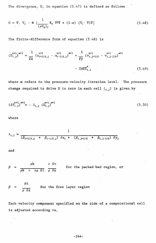
The divergence, D, in equation (5.47) is defined as follows

1D = V. Vi - 0 [____ Kr V2T + (l-/c) (Vi- V)T]

(pCp) f(5.48)

The finite-difference form of equation (5.48) is

n+l m+1 n+l(Di,j) = -- (ui+l/2,jSx

n+l m+1 n+l n+l m+1ui-l/2,j) + (vi, j + 1/2 “ vi, j-l/2)5y

- taut"(J (5.49)

where m refers to the pressure-velocity iteration level. The pressure change required to drive D to zero in each cell j) is given by

n+l m+1(SPl.j) -

n+l m+1(Di.j) (5.50)

where

1(Pi+l/2,j + Pi-1/2,j) ^xi + (^i, j + 1/2 + Pi, j-l/2)

and

pk e <5 tP = ____________ ____ for the packed bed region, or

pk + e/j. 81 p Sx

StP = ____ for the free layer region

p <5x

Each velocity component specified on the side of a computational cell is adjusted according to,

-244-

n+l m+1(ui + l/2,j) = n+l m( ui+l/2,j) + ^i+1/2,j n+l m+l(SPi.j) (5.51)

n+l m+l n+l m n+l m+l( ui-l/2,j) ~ ( ui-1/2,j ) ^i-l/2,j (6Pi,j) (5.52)

n+l m+l n+l m n+l m+l( vi , j + 1/2) ~ (vi,j + 1/2) + Pi,j+1/2 («Pi.j) (5.53)

n+l m+l n+l m n+l m+l(vi,j-l/2) - (Vi(j-l/2> - Pi,j-1/2 («Pi.J> (5.54)

The rate of convergence of the iterative process is accelerated bymultiplying 5Pi(j in equation (5.50) by an over-relaxation parameter, <j>. An optimum value of cj was found from numerical experiments to be in the range 1.7-1.9.

Referring to Figures 5.1 and 5.2, the 'free-slip' boundary conditions (equations (5.24)-(5.27)) may be written as

u2 = 0 , uNj = 0 (5.55)

vi>2 = 0 (5.56)

ui,l = uif2 (5.57)

vi,j = v2(j . vN,j = VN-I,j (5.58)

At the outflow boundary, the x-component of velocity, udrain, is set according to,

Q^drain — ---------

^ ^ yj dpy(5.59)

-245-

where Q represents the instantaneous flowrate, W is the width of the model and <$yjdpy is the drain cell length in the y-direction. The y-component of velocity at the top boundary of the model, M+1, is given by

vi,M+1Q - veD W

(5.60)

where Ve represents the rate of volume expansion of the liquid per unit time, D is the length of the model.

The temperature boundary conditions (equations (5.32)-(5.36)) are applied at the impermeable boundaries and top surface. For side-hearth cooling conditions, equations (5.32)-(5.33) apply. The

finite-difference form of these equations may be written as,

Ti,l - Ti>2 (5.61)

TU = Ts TN,j “ Ts (5.62)

For under-hearth cooling conditions, equations (5.34)-(5.35) apply and in finite-difference form may be written as,

Tl,j - T2,j

Tifi = Tb

TN,j ~ TN-l,j (5.63)

(5.64)

At the top surface, the temperature of the liquid is set so that,

lM+1 ~ iin (5.65)

-246-

The computational procedure requires a specification of the value for density and viscosity outside the flow region. The density and viscosity in the external boundary cell are set equal to the values of those quantities for the image cell inside the boundary. This is done at all 'free-slip' boundaries, such that,

Pl,j = P2,j > Pn,j “ Pn-i.j (5.66)

Pl,j = P2,j > PN.j “ PN-l,j (5.67)

Pi.l - Pi,2 (5.68)

Ah, 1 ~ Pi,2 (5.69)

5.5 Numerical Stability and Accuracy

The numerical stability requirements for equations (5.40)-(5.69) are identical to those described in Chapter 2, with the exception that no free surface problems were investigated in the present study and therefore the Courant wave condition (equation (2.54)) does not apply. The restrictions for the time step, <5t, are:

8t < min (5.70)

p <5x2 <5y28t < __ ________

2/i <$x2 + 8 y2(5.71)

Equation (5.70) is the more restrictive condition. The stability requirement for the energy equation (equation (5.44)) is only slightly more stringent than that for the motion equations (5.40)-(5.41) if the

-247-

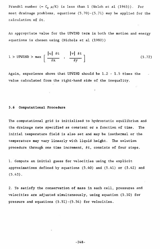
Prandtl number (= Cp \jl/K) is less than 1 (Welch et al (1965)). For most drainage problems, equations (5.70)-(5.71) may be applied for the calculation of <5t.

An appropriate value for the UPWIND term in both the motion and energy equations is chosen using (Nichols et al (1980))

1 > UPWIND > max| u | 81

<5x|v| St

ty(5.72)

Again, experience shows that UPWIND should be 1.2 - 1.5 times the value calculated from the right-hand side of the inequality.

5.6 Computational Procedure

The computational grid is initialised to hydrostatic equilibrium and the drainage rate specified as constant or a function of time. The initial temperature field is also set and may be isothermal or the temperature may vary linearly with liquid height. The solution procedure through one time increment, 6t, consists of four steps.

1. Compute an initial guess for velocities using the explicit approximations defined by equations (5.40) and (5.41) or (5.42) and (5.43).

2. To satisfy the conservation of mass in each cell, pressures and velocities are adjusted simultaneously, using equation (5.50) for pressure and equations (5.51)-(5.54) for velocities.

-248-

3. When the continuity condition is satisfied (equation (5.48)), the temperature is determined by an explicit calculation using equation (5.44).

4. Steps 1-4 are repeated for successive time steps.

A listing of a Fortran computer code (HDT21.F0R), developed to implement the above computational procedure, is given in Appendix F.

5.7 Model Validation

In the previous three chapters, laboratory-scale models for the hearth were used to validate the assumptions made in developing the numerical models for hearth liquid drainage. For the present case, it was not necessary to perform non-isothermal physical experiments because experimental and numerical data to validate the numerical model described above are available in the literature (Yashiro et al (1982), Ohno et al (1981)).

Results from the present numerical model were compared with those reported by Yashiro et al (1982). Yashiro et al (1982) carried out a numerical study of iron flow in the hearth using a two-dimensional, single-liquid model. The numerical experiments, which also considered the effect of under-hearth cooling, were carried out for conditions similar to those in an actual operating furnace. The results reported from these numerical experiments described the flow distribution of iron and also the vertical temperature distribution in the hearth.The experiments were carried out for a hearth with a diameter of 14.0 m and iron height of 2.0 m. The iron was discharged from a taphole with a centreline located 1.45 m above the bottom of the hearth and the height of the coke-free layer was 2.0 m above the

-249-

bottom of the hearth. The temperatures of the bottom boundary of the model and the top surface of the liquid were fixed at 1200°C and 1500°C respectively. An adiabatic boundary condition was set along the vertical sides of the model. Two initial conditions were considered with respect to the initial temperature field. In the first case, the initial temperature field varied linearly with height of iron above the base of the hearth ('linear' case), such that the temperature at the bottom was initially 1200°C, while at the top surface, the temperature was 1500°C. In the second case, the initial temperature field was isothermal and set at 1500°C ('isothermal' case). All other relevant information is given in Table 5.1.

Figures 5.4 and 5.5 show a comparison between the results for the linear case reported by Yashiro et al (1982) and those from the present model, respectively. The numerical calculations were performed using a non-uniform grid with 30 cells in the x-direction (6xtnin = 10 cm, SXjnax = 70 cm) and 18 cells in the y-direction (Symin = 10 cm, <5ymax = 15 cm). The time step was calculated at each time level using equation (5.70). The liquid streamlines are compared at 2 minutes after the commencement of discharge of iron from the hearth. Although the computed vortices in the region below the taphole level are continually changing, the results show good qualitative agreement. The results show that stratification occurs and that the streamlines rarely fall beneath the level of the taphole. The formation of a recirculation cell in the lower corner opposite the taphole, is predicted by both models.

Figure 5.6 shows a comparison between the vertical temperature distributions at 47.5 minutes into the cast as computed by Yashiro et al (1982) and the vertical temperature distribution computed by the present model. The present model results for both the linear and isothermal cases, agree very well with those reported by Yashiro et al (1982). For the linear case, the results show that the temperature

-250-

Table 5.1 - Blast Furnace Hearth Data

Hearth diameter (D) 1400 cmWidth of hearth (W) 1100 cmTaphole height (Hth) 145 cmCoke-free layer height (HfI) 30 cmDepth of iron melt (HIiq) 200 cmIron production rate (Vin) 300 t/hrDistribution of dripping rate uniformTemperature of dripping iron (Tin)Initial melt temperature

1500° C

- isothermal case 1500° C- linear case 1200-1500°C

Bottom wall temperature (Tb) 1200° CSide wall temperature (Ts) 1500° CBed porosity (e) 0.4Bed permeability (k) 0.02469 cm2True density of coke (pc) 2.26 gm/cm3Density of iron (1500°C) (pL) 6.4 gm/cm3Heat capacity of coke (Cpc) 1.686 J/gm.°CHeat capacity of iron (Cpi) 0.907 J/gm.°CThermal conductivity of coke (Kc) 0.05 W/cm.sThermal conductivity of iron (Ki) 0.0165 W/cm.sDynamic viscosity of iron 0.06 gm/cm.sThermal expansion of iron (^) 0.000141°C’1

-251-

Iron-slag interface

1

Figure 5.4 Streamline distribution pattern at 2 minutes into the cast for a hearth with under-hearth cooling and an initial linear temperature profile (Yashiro et al (1982)).

-252-

Iron-slag interface

Figure 5.5 Streamline distribution pattern computed by the present numerical model for hearth conditions similar to that used in Figure 5.4.

-253-

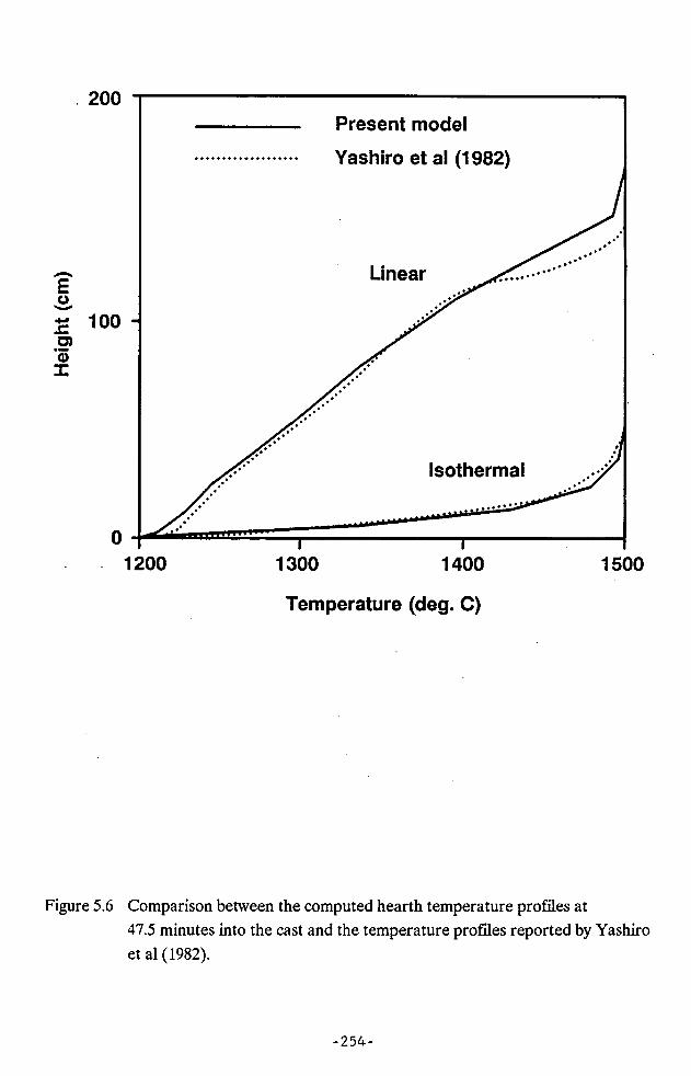
200Present model

Yashiro et al (1982)

Linear

100 -

Isothermal

Temperature (deg. C)

Figure 5.6 Comparison between the computed hearth temperature profiles at47.5 minutes into the cast and the temperature profiles reported by Yashiro et al (1982).

-254-

rises approximately linearly up to 1.2 m above the base of the hearth. This region coincides with the stagnant layer formed beneath the level of the taphole as shown in Figures 5.4 and 5.5. The iron velocity in this layer is very low. In the region above the taphole where the iron velocity is much higher, the temperature gradients are much steeper. For the isothermal case, the temperature rises steeply from the bottom and reaches 1500°C very quickly (approximately 50 cm above the bottom of the hearth). The stagnant layer in the isothermal case is therefore much smaller than that for the linear case.

The comparison between the liquid streamlines and vertical temperature distributions computed by the present numerical model and those reported by Yashiro et al (1982), confirms that the numerical model effectively describes the drainage of iron under non-isothermal conditions. The numerical model may therefore be used to investigate the effects of non-isothermal conditions on the flow of iron in a hearth with a floating or non-floating coke bed.

5.8 Physical Mechanisms of Iron Drainage in a Non-isothermal Hearth

The flow distribution of iron in the hearth and the effect of iron flow on hearth erosion, have been the subject of a number of investigations (Hara and Tachimori (1978, 1979), Ohno et al (1981, 1985)). Hara and Tachimori (1978, 1979) showed that the flow of iron in the hearth is strongly influenced by the presence of a coke-free layer and that the flow determines the extent of refractory lining erosion. On the other hand, Ohno et al (1985) suggested that refractory erosion is dependent primarily on the rate of heat transfer from the iron to the cooling plates. They state that if the height of the coke-free layer is small, the rate of heat transfer from the iron is very high. However, as the height of the coke-free layer

-255-

increases, the rate of heat transfer decreases rapidly. This suggests that for a typical blast furnace hearth, where the height of the coke-free layer may vary between 10 and 100 cm (Ohno et al (1985)), refractory erosion may be governed either by the flow of iron in the coke-free layer (for a coke-free layer height between 10-30 cm), or by the flow in the packed bed (for a coke-free layer height between 40 -100 cm).

If hearth refractory erosion is influenced by the flow in the coke-free layer, then a knowledge of the position of the coke bed in the hearth is fundamental to the control of hearth refractory erosion. In an actual operating furnace, the state of the coke bed may be determined by injecting radioactive isotopes into the hearth and observing the isotope concentration in the iron as it is tapped from the hearth. The shape of the concentration response curves obtained from such experiments is dependent on the position of the coke bed in the hearth (Ohno et al (1981)). Isotope injection experiments have been reported for operating furnaces (Babarykin et al (1960), Nakamura et al (1981), Ohno et al (1981), Alleyn et al (1981) and Libralasso et al (1985)); however, the analysis of the data is not straightforward (Ohno et al (1981), Libralasso et al (1985)) and in some cases, the analysis is inconclusive (Alleyn et al (1981), Rooney (1986)). The difficulty in interpreting residence time data may be attributed to' the complex nature of the flow field in the hearth. A resolution of these difficulties will depend on the development of a better understanding of fluid flow in the hearth.

In this section, we investigate the physical processes which determine the flow distribution of iron in the hearth, using the two-dimensional, numerical model described in sections 5.2-5.4 . In particular, the two-dimensional numerical experiments are carried out to investigate the effect of a coke-free layer on the flow distribution of iron in the hearth, where the hearth may be

-256-

under-hearth cooled, side-hearth cooled or both under- and side-hearth cooled. In the following chapter, the numerical model is extended to three - dimens ions and is used to analyse data obtained from radioactive isotope experiments carried out at Broken Hill Proprietary's Port Kembla No. 5 blast furnace (Rooney (1986)). As already stated,

previous attempts to analyse these data have been inconclusive.

The numerical experiments discussed below consider a number of

different cases, which include,

(i) A hearth fully packed with coke and under-hearth cooling(ii) A hearth with a 0.3 m high coke-free layer underlying the coke

bed and under-hearth cooling(iii) Same as (i) but with side-hearth cooling only(iv) Same as (ii) but with side-hearth cooling only(v) A hearth with a coke-free layer of variable height and

side-hearth cooling only(vi) Same as (i) but with side- and under-hearth cooling(vii) Same as (ii) but with side- and under-hearth cooling

The initial temperature field in the hearth was assumed to be isothermal (ie. set equal to 1500°C) or to vary with height above the base of the hearth, such that the temperature at the bottom is 1200°C, increasing to 1500°C at the top of the iron surface. Other relevant

data for the computational experiments are given in Table 5.1.

5.8.1 Fully Packed Bed With Under-hearth Cooling

Figure 5.7 (a)-(b) and Figure 5.8 show the liquid streamlines for a hearth fully packed with coke and with under-hearth cooling. Figure

5.7 (a) shows the flow distribution at 2 minutes after the

-257-

(a) 2 minutes

(b) 100 minutes

Figure 5.7 Streamline distribution patterns in a hearth with a fully packed bed, under-hearth cooling and an initial, linear temperature profile.

-258-

100 minutes

Figure 5.8 Streamline distribution patterns in a hearth with a fully packed bed, under-hearth cooling and an initial, isothermal temperature profile.

-259-

commencement of the cast for the situation where the initial temperature field is assumed to increase linearly with height. In contrast to the results shown in Figure 5.5 for the flow of iron in a coke-free layer, Figure 5.7 (a) shows that the liquid streamlines converge towards the taphole from above and below the level of the taphole. The streamline pattern above the level of the taphole is similar to that computed for the flow of slag in an isothermal hearth as shown in Figure 2.16. A recirculation zone is shown to be forming in the corner below the taphole. Figure 5.7 (b) shows the liquid streamlines after 100 minutes during the same cast. The recirculation zone has increased in size such that very little iron flows to the taphole from below the level of the taphole. The relative velocity in the recirculation zone (ie. the velocity relative to the average or superficial velocity in the hearth) is approximately 0.24.

Figure 5.8 shows the liquid streamlines after 100 minutes for a hearth with an initial temperature field that is isothermal. Compared to the case of a linear temperature variation (Figure 5.7 (b)), the size of the recirculation zone is much smaller and the iron is shown to flow up towards the taphole from levels well below the level of the taphole. The relative iron velocity in the recirculation zone is approximately 0.6 compared with 1.8 in the region above the taphole. The liquid streamlines above the zone are also typical of the flow of an isothermal liquid in a fully packed bed (see Figure 2.16).

5.8.2 Packed Bed/Coke-free Layer With Under-hearth Cooling

Figure 5.9 (a)-(b) and Figure 5.10 (a)-(d) show the liquid streamlines for a hearth with a 0.3 m high coke-free layer underlying the coke bed. The hearth is under-hearth cooled. For the linear temperature case, the liquid streamlines at 2 minutes (Figure 5.9 (a)) and

-260-

(a) 2 minutes

(b) 100 minutes

Figure 5.9 Streamline distribution patterns in a hearth with a packed bed and 0.3 m high coke-free layer, under-hearth cooling and an initial, linear temperature profile.

-261-

2 minutes (c) 54 minutes

-262-

igure 5.10 Streamline distribution patterns in a hearth with a packed bed and 0.3 m high coke-free layer, under-hearth cooling and an initial, isothermal temperature profile.

100 minutes (Figure 5.9 (b)) after the start of the cast, show that recirculation zones or vortices are formed both in the packed bed region below the level of the taphole and in the coke-free layer. As a result of the recirculation zone, the relative iron velocity in the coke-free layer is low, being approximately 0.6.

Figure 5.10 (a)-(d) show the progressive changes in the flow distribution during a cast where the initial temperature field is isothermal. After 2 minutes (Figure 5.10 (a)), a small vortex has formed in the coke-free layer below the taphole. The streamlines away from the immediate vicinity of the taphole however, are directed into the coke-free layer, in a manner similar to that for an isothermal hearth with a packed bed and coke-free layer (Figure 2.17).Figure 5.10 (b) shows that after 10 minutes, two vortices are formed within the coke-free layer. These vortices change continually with time. Figure 5.10 (c)-(d) show that at both 54 and 100 minutes after the start of the cast, the size of the recirculation zone is such that few streamlines actually enter the coke-free layer. At 100 minutes into the cast, the influence of the coke-free layer on the flow of iron above the free layer is insignificant and the flow distribution at this time is similar to that for a fully packed bed (Figure 5.8). The average relative iron velocity in both the recirculation zone and in the packed bed region, is approximately equal 1.8 and under such conditions, the erosion of the refractory lining at the bottom of the hearth will be increased.

5.8.3 Fully Packed Bed With Side-hearth Cooling

We now consider the situation where the hearth is fully packed with coke and the hearth is side-hearth cooled. The initial temperature field is isothermal. In Figure 5.11 (a), recirculation zones are

-263-

(a) 2 minutes

(b) 54 minutes

Figure 5.11 Streamline distribution patterns in a hearth with a fully packed bed, side-hearth cooling and an initial, isothermal temperature profile.

-264-

54 minutes

Figure 5.12 Natural convection currents in a hearth with a fully packed bed, side-hearth cooling and an initial, isothermal temperature profile.

-265-

formed in the lower corners of the hearth. The bulk of the liquid remains unaffected by the recirculation zones at this time. As indicated by the closer spacing of streamlines, the intensity of the convective motion increases as the cast proceeds (Figure 5.11 (b)). This is particularly evident in the vicinity of the cooler vertical walls and bottom of the hearth. The average relative velocity near the vertical wall away from the taphole is approximately 5.9, which is much higher than the relative velocity in the bulk of the liquid

(approximately 1.8). The strong convective motion of the iron is best explained by examining the flow distribution in the hearth when the taphole is closed ie. the only flow is that induced by natural convection.

Figure 5.12 shows the flow distribution resulting from natural convection only. The symmetrical flow about the mid-plane of the hearth results from specifying equal temperatures along the two vertical walls. As the iron adjacent to the these walls is cooled, it flows down the wall as a result of the higher density of the colder iron. Figure 5.12 also shows that the recirculatory flow induced by the thermal or density gradients is very strong, particularly near the wall. It is also clear that the flow distribution shown in Figure 5.11 (b) results from a distortion of the natural convection cells by the superimposed outflow of iron through the taphole.

5.8.4 Packed Bed/Coke-free Layer With Side-hearth Cooling

Figure 5.13 shows the flow distribution in a hearth with a uniform coke-free layer of height 0.3 m. The initial temperature field is isothermal and side-hearth cooling is applied. In Figure 5.13, the spacing between streamlines indicates that the convective motion is

very strong- in the coke-free layer and weaker adjacent to the vertical

-266-

54 minutes

Figure 5.13 Streamline distribution patterns in a hearth with a packed bed and 0.3 m high coke-free layer, side-hearth cooling and an initial, isothermal temperature profile.

-267-

walls. The maximum relative velocity in the recirculation cell away from the taphole is approximately 59. The flow field shown in Figure 5.13 may cause severe erosion of the refractory lining at the bottom and also along the sidewall of the hearth.

For the situation where the height of the coke-free layer is not uniform but rather, the height varies across the diameter of the hearth (a situation more typical of actual operating furnaces), erosion of the refractory lining resulting from the flow of iron, may be more localised. Figure 5.14 shows the liquid streamlines for a hearth where the maximum height of the coke-free layer is at the walls (1 m) and the minimum height is at the centre of the hearth (0.3 m). Recirculation zones form in each of the lower corners of the hearth. The spacing between the streamlines, particularly in the corner away from the taphole, indicates that the flow of iron in these zones is very strong (relative velocity is approximately 20). Flow of this type causes erosion of the refractory lining near the periphery of the hearth and this may lead to a sudden breakout of molten material from the hearth. This type of erosion is known to occur frequently in actual blast furnaces (Kanbara et al (1977) and Onoye et al (1983)).

5.8.5 Side- and Under-hearth Cooling in a Packed Bed With and Without a Coke-free Layer

In the situation where both side- and under-hearth cooling is applied, the flow distribution in the hearth is largely determined by the ratio of the amount of heat removed from the sidewalls of the hearth to that removed from the bottom. Figure 5.15 (a)-(b) show the liquid streamlines for a hearth fully packed with coke, with the sidewall and bottom temperatures fixed at 1400°C and 1200°C. The initial temperature distribution is isothermal. After 2 minutes, the flow

-268-

1 minute

Figure 5.14 Streamline distribution patterns in a hearth with a packed bed and acoke-free layer of non-uniform height, side-hearth cooling and an initial, isothermal temperature profile.

-269-

(a) 2 minutes

(b) 100 minutes

Figure 5.15 Streamline distribution patterns in a hearth with a fully packed bed, side- and under-hearth cooling and an initial, isothermal temperature profile.

-270-

100 minutes

Figure 5.16 Streamline distribution patterns in a hearth with a packed bed and 0.3 m high coke-free layer, side- and under-hearth cooling and an initial, isothermal temperature profile.

-271-

distribution is dominated by the effect of side-hearth cooling. As the cast proceeds, the effect of under-hearth cooling on the flow distribution becomes more apparent. Figure 5.15 (b) shows the effect of under-hearth cooling on the shape and location of the two recirculation cells formed. Compared to Figure 5.11 (b), the recirculation cells are broader and the cell centres have migrated upwards.

The effect of under-hearth cooling may also be observed in Figure 5.16, which shows the flow distribution in a hearth with a 0.3 m high coke-free layer. As a result of under-hearth cooling, the strong recirculatory flows in the coke-free layer for the case where only side-hearth cooling was applied (Figure 5.13), no longer exist. The relative iron velocity in the free layer however is still higher than that in the bulk of the liquid (4.7 cf. 2.4).

5.9 Conclusions

The flow of iron in the hearth is strongly influenced by the mode of cooling applied ie. side-hearth cooling, under-hearth cooling or both side- and under-hearth cooling. The effect of side-hearth cooling on the flow distribution of iron in the hearth is more pronounced than the effect of under-hearth cooling. The flow distribution of iron is also dependent on the initial state of the iron in the hearth, particularly the iron temperature distribution at the commencement of a casting operation.

The effect of a coke-free layer on the flow distribution of iron and therefore, on the extent of erosion of the refractory lining, is very significant. This is particularly true for the situation where

-272-

side-hearth cooling is applied. For this case, the strong thermally-induced, convective currents may lead to significant erosion of the hearth refractory lining.

The analysis of data from radioactive isotope experiments carried out in operating furnaces clearly requires a consideration of the thermally-influenced flow of iron in the hearth and the effect of a coke-free layer if one is present. Failure to account for these effects will lead to erroneous conclusions when attempting to interpret residence time data. In the following chapter, the two-dimensional model developed in this chapter is extended to three- dimensions, in order to carry out a more quantitative analysis of data from isotope tracer experiments in the hearth of an actual operating blast furnace.

-273-

6 THREE-DIMENSIONAL STUDY OF THE FLOW OF IRON IN A NON-ISOTHERMALHEARTH

6.1 Introduction

Previously reported investigations of radioisotope tracer experiments carried out in the hearth of an operating blast furnace, have assumed that conditions in the hearth are isothermal (Shimomura et al (1978), Ohno et al (1981) and Libralasso et al (1985)). This assumption is necessary in order to analyse the experimental data from such experiments using simple residence time distribution theory. Based on the numerical study described in the previous chapter, it is clear that the assumption of an isothermal hearth may result in considerable errors for situations where the hearth is either side- or under-hearth cooled.

In this chapter, we extend the two-dimensional, non-isothermal numerical model developed in Chapter 5 to three dimensions, in order to interpret data obtained from actual tracer experiments carried out at Broken Hill Proprietary's Port Kembla No. 5 blast furnace (Alleyn et al (1981) and Rooney (1986)). Results from a number of these experiments could not be readily explained using simple residence time distribution theory proposed by previous investigators (Rooney (1986)). In the three-dimensional numerical model, the radioisotope tracer used for the actual furnace experiments, is represented by massless marker particles (Welch et al (1965)). The movement of the marker particle is computed using the calculated velocity field. The computed travelling times of the marker particles are then compared with the measured travelling times of the tracer for the actual

-274-

furnace experiments. This comparison is shown to resolve the ambiguities associated with an interpretation of the tracer data using simple residence time concepts.

6.2 Model Formulation

The mathematical formulation of the three-dimensional, single-liquid, non-isothermal model follows closely the development of the two-dimensional model described in Chapter 5. The Boussinesq approximation is again not invoked in the development of the model.In what follows, we will describe the assumptions on which the three-dimensional model is based, along with the computational details necessary to fully describe the numerical model.

Figure 6.1 shows a schematic diagram of the three-dimensional, cylindrical model under consideration. A useful reduction in the total computation effort is made by utilising the symmetry of the flow about the vertical plane passing through the diameter along the axis of the taphole. This results in a reduction in the computational workload by a factor of two.

The packed bed is assumed to be homogeneous with porosity, e, and permeability, k. A packing-free layer of height (HfI) may underlie the packed bed. The bed is saturated with a liquid of density, p(T), and viscosity, p(T), where T is the liquid temperature. The thermal conductivity of the liquid, Kf, is assumed to be constant. The liquid is withdrawn from a drain located on the side of the model (flowrate, Q)'. The level of the liquid in the model (Hliq) is maintained constant by a uniform dripping rate of liquid (Vin) into the model. The temperature of the side and bottom boundaries are specified as Ts and Tb respectively. The temperature of the liquid dripping into the model

-275-

Iron/slag interface

Packed bed k ,e

Free layer

cFigure 6.1 Schematic diagram of the three-dimensional, single-liquid, non-isothermal

model.

-276-

is also specified (Tin) . The fixed boundary temperatures simulate cases where either side-hearth, under-hearth cooling or both side- and under-hearth cooling are applied to the hearth refractory lining. The plane of symmetry represents an adiabatic no-flow boundary such that no heat flows across the boundary.

The general equation governing the conservation of momentum for the liquid is given by,

DVi dPp __ = - __ + pGi - V2:r (6.1)

Dt dxt

where D is the substantial derivative V is the del operatorP is the pressureGi is the gravitational constantr is the stress tensor

In three-dimensional, cartesian co-ordinates, the components of the stress tensor in equation (6.1) are written as,

du 2rxx = - 2n _ + _ n (V- V,)

dx 3

3v 2r = - 2n _ + _ /i (V- Vi)<9y 3

(6.2)

(6.3)

<3w 2Tzz = ~ 2m _ + _ A* (V- Vi) (6.4)3z 3

du dvrxy = * ^ (__ + __) (6.5)dy dx

-277-

(6.6)du dv

Tyx ~ ~ P (__ + __)dy dx

dv dwTyZ = ’ A* (_ + _)dz dy

dv dw ■zy = - P (__ + __)dz dy

3w 3uxz = - M (-- + _)<3x dz

3w 3uzx = ' M (__ + __)dx 3z

(6.7)

(6.8)

(6.9)

(6.10)

Substituting equations (6.2)-(6.10) into equation (6.1) and re-arranging gives the general equations of motion for a Newtonian liquid, with density and viscosity which are functions of spatial position. These equations apply in the packing-free layer region of the model and may be written as,

P3udt

+ u3udx

<3u <9u+ v _ + w __

dy dzdPdx

d du 2 du dv dw+ __ I" 2/a __ - _ P (__ + __ + __)dx[ dx 3 dx dy dz

d du dv+ __f M (__ + __)dyL dy dx

d dw du+ _1" P (__ + _)dzL dx dz

(6.11)

-278-

dv dv dv dv dP+ u __ + v _ + w __ = - _ +dt dx dy dz dy

d du dvP (__ + __)dy dx

dv 2 du dv dw_ 2/x _ - _ P (_ + _ + _)dy|_ dy 3 dx dy dz

d dw dvP (_ + _)dy dz

(6.12)

dw dw dw dw dP d du dwP _ + u __ + v __ -1- w __ = - _ + P g + __ 4 (_ + _) 'dt dx dy dz dz dx dz dx

dw dv_ P (_ + _)dy[ dy dz

d dw 2 du dv dw2 A* - _ A* ( + + )dz 3 dx dy dz

(6.13)

where u, v and w are the x-, y- and z-components of velocity. The transient form of Darcy's law is used to describe the fluid motion in the packed bed. In three dimensions, these equations are written as follows,

p du dP p.___ = - ___ + _ ue dt dx k

(6.14)

p dv e d t

dp \x__ + _ Vdy k

(6.15)

p dw dP p.___ =- ___ + _w + pge dt dz k

(6.16)

-279-

For a liquid with constant thermal conductivity, Kf, the equation for the conservation of energy in the packing-free layer may be writtenas ,

3T 8Vi(pCp)f (_ + (Vi- V)T + T _ ) = Kf V2T

d t 3Xi(6.17)

where T is temperatureCp is specific heat capacity Vi is the velocity vector

and the subscript f denotes liquid properties.

In the packed bed region, the difference between the solid and liquid temperatures (Ts and Tf respectively) is assumed to be negligible. The equation for the conservation of energy in the packed bed is therefore written as,

where the subscript fs denotes lumped solid-liquid properties. Equations (6.17)-(6.18) may be written in a more general form, such that,

where f equals f for liquid properties (for the packing-free layer) and fs for lumped solid-liquid properties (for the packed bed).

The continuity equation for a liquid with variable density follows from equation (5.23) in Chapter 5 and is written as,

(pCp)fs _ + (pCp)f [(Vr V)T + T __ ] = Kfs V2Tat axi

(6.18)

(6.19)

-280-

1(6.20)

<9u <9v <9w_ + __ + __ = 0 [____ Kc V2T + (l-/c) (Vi- V)T]dx 9y dz (p Cp)r

where 01 + 9(T0 - (l-/c)T)

(pCp)f(pCp)r

Substituting equation (6.20) into equation (6.19) and re-arranging

gives an alternate form for the conservation of energy equation,

<9T 3T <9T <3T k0T__ + A (u __ + v __ + w __) = [1 - _____ ] Kr V2T (6.21)dt dx dy dz (pCp)f

where A = «(1 + 0(l-/c)T) .

The density and viscosity of the liquid are functions of temperature

and are given by the following equations of state,

P - P0 (1 - 0(T - T0)) ' (6.22)

- *<T - T0)A* = Po e (6.23)

where 9 is the linear coefficient of thermal expansion, p0 is the

liquid density at temperature T0, <f> is the viscosity-temperature

coefficient and /i0 is the viscosity at temperature T0.

Equations (6.1)-(6.23) are the governing equations for

thermally-influenced flow of a homogeneous liquid in three dimensions.

Together with the initial and boundary conditions, equations

(6.1)-(6.23) completely specify the non-isothermal drainage problem

for a packed bed containing a packing-free layer.

-281-

6.3 Initial and Boundary Conditions

Referring to Figure 6.1, the appropriate boundary conditions on velocity are similar to those for the isothermal model described in Chapter 3. The base of the model (plane z=0 in Figure 6.1) is an impermeable boundary and the flow normal to the boundary is zero. For the base of the model, the 'free-slip' boundary conditions applying are,

w = 0 (6.24)

<3u_ = 0 (6.25)3z

3v_ = 0 (6.26)dz

Similarly, for the curved, impermeable boundary in Figure 6.1 (surface ABC), the velocity normal to the boundary must also be zero ie.

Un = 0 (6.27)

3w_ = 0 (6.28)3n

where n is the normal to the curved boundary.

At the plane of symmetry or front boundary of the model (plane AC), the 'free-slip' boundary conditions imposed are,

v = 0 (6.29)

-282-

(6.30)3u_ = 0 dy

<9w ■_ = 0 (6.31)dy

At the drain or taphole, the x-direction velocity, udrain, is set according to,

Q(t)udrain = --------- (6.32)

^■drain

where Q(t) is the volumetric flowrate (cm3/s) , which may be an arbitrary function of time and Adrain is the area over which the liquid is withdrawn. It should be noted that Q(t) is the flow out of one-half of the model. The actual flow out of the whole of the model is twice Q(t).

At the top boundary of the model, the volumetric inflow rate per unit time, Qin, is related to the volumetric outflow rate per unit time, Q, by the following equation,

Qin(t) = Q(t) - Ve (6.33)

where Qin(t) is the liquid production rate as a function of time t and Ve is the rate of volume expansion (or contraction) of the liquid due to temperature differences. Ve is equal to the right-hand side of equation (6.20) multiplied by the internal volume of the model. The

production rate, Qin(t), is assumed to be uniform over the

cross-sectional area of the model (A) and is related to the y-component of velocity at the upper surface, vsurf, by

-283-

Qin(t)vsurf = ______ (6.34)A

The above relationships ensure that the upper liquid surface remains stationary over the simulation period. The pressure at the top surface is constant and set equal to the sum of the gas phase pressure (Pgas) and the hydrostatic liquid head of slag (Piiq) ie.

Psurf(x.t) = Pgas + Pliq (6.35)

where Pliq equals psghs, ps is the slag density and hs is the height of slag above the iron level.

The boundary conditions for the energy equation follow from those described in Chapter 5. At the plane of symmetry (plane AC), an adiabatic or zero heat flux condition must apply ie.

3T_ = 0 (6.36)dy

For the conditions where side-hearth cooling is applied, the temperature on the curved boundary surface (ABC) is specified (Ts) together with an adiabatic or zero heat flow condition over the bottom boundary (plane z=0) ie.

T = Ts (6.37)

<3T_ = 0 (6.38)<9z

-284-

For the conditions where under-hearth cooling is applied, the temperature at the bottom boundary (plane z=0) is'Specified (Tb) together with an adiabatic condition over the curved boundary surface (ABC) ie.

T = Tb (6.39)

<3T__ =0 (6.40)3n

where n is the outward normal to the curved boundary. The temperature of the liquid flowing across the top boundary is set, such that,

T = Tin at z = Hliq (6.41)

The continuity equation requires that at the boundary between the packed bed and the packing-free layer, the velocity normal to boundary, un, is continuous across the boundary.

Initially, the elevation of the top surface is set such that,

z = Hliq (6.42)

The initial liquid temperature may be isothermal or it may vary linearly with height of liquid. For the isothermal condition, we may write,

T = T0 (6.43)

For a linear variation of temperature with height, h, the initial temperature is given by

T = a h + Tb0 (6.44)

-285-

where a is the rate of increase in temperature with liquid height and Tb0 is the temperature at z=0.

6.4 Numerical Technique

The numerical aspects of the three-dimensional model are similar to those previously described in Chapter 3 (three-dimensional, single-liquid, isothermal model) and in Chapter 5 (two-dimensional, single-liquid, non-isothermal model). Figure 6.2 shows the three-dimensional hearth, discretised into variable-sized, rectangular parallelepipeds of length 6x, Sy and <5z. Figure 6.3 shows plan and elevation views of the computational grid superimposed over the flow region. The non-uniform grid is more refined in the region close to the taphole. This allows a more accurate resolution of the steep pressure gradients in the region near to the taphole and avoids the need to resolve the singularity at the centre of the axis of symmetry shown in Figure 6.3.

Figure 6.4 shows the locations at which the field variables are defined for a computational cell block. The velocities, u, v and w are defined at the centre of each wall of the parallelepipeds. Pressure, temperature and liquid properties (p, p) are defined at the centroid of the cell.

Figure 6.5(a)-(b) shows the location of field variables for cells intersected by the curved boundary. The pressure, temperature, density and viscosity are defined at the centroid of an imaginary parallelepiped (Figure 6.5(a) and (b)). Four velocities are defined at the centre of each wall. The remaining two velocities (ie. those defined on the imaginary side of the cell block) are obtained by applying the appropriate boundary conditions.

-286-

Figure 6.2

Z

Three-dimensional computational grid.

-287-

Plan View 4v

Computational Singularity

Elevation ViewA*

Figure 6.3 Plan and elevation views of the computational grid.

-288-

u i-1/2,J,k

wi,],k+l/2

u i+l/2,|,k

Figure 6.4 Layout of field variables for a full computational cell.

-289-

(a) LHS cell (b) RHS cell

i,j,k+1/2

i.J.k :

Figure 6.5 Layout of field variables for a computational cell bisected by the curved boundary.

-290-

The finite-difference form of the general equation for fluid motion in the packing-free layer, equations (6.11)-(6.13), may be written as,

n+l nui+l/2,j,k = ui+l/2,j,k

5 t(PX + CONUX 4- CONUY 4- CONUZ + VISCX)

Pi+l/2,j,k

(6.45)

n+l nvi,j+1/2,k = vi,j+1/2,k

<5t (PY + CONVX + CONVY 4- CONVZ + VISCY)Pi,j+1/2,k

(6.46)

n+l nwi,j,k+l/2 = wi,j,k+l/2 "

St(PZ + CONWX 4- CONWY 4- CONWZ 4- VISCZ 4- GZ)

Pi,j.k+1/2

(6.47)

where,

iPX - <pn-i,.j,k

^xi+l/2- Pi.j.k)

lPY - (Pi.jn.k

^ y j+1 / 2- pi.j.k)

lPZ = (Pi,j,k+1

^zk+l/2- Pi.j.k)

and,

-291-

5xi+i/2 = 0.5 (<5Xi + <5xi+1) 5yj+i/2 = 0.5 (5yj + <5yj+i) ^zk+i/2 = 0.5 (5zk + 5zk+1)

ui+l/2, j ,kCONUX = ________ [8xi DUR + <$xi+1 DULDXA

+ UPWIND sgn(u) (6xi+1 DUL - 6xi DUR)]

VAVCONUY = ___ [DYB DUDTY + DYT DUDBY

DYA+ UPWIND sgn(v) (DYT DUDBY - DYB DUDTY)]

CONUZ

sgn(u)DXADURDUL

VAVVBTVBBsgn(v)DYADYTDYBDUDTYDUDBY

WAV■ ___ [DZB DUDTZ + DZT DUDBZDZA

+ UPWIND sgn(w) (DZT DUDBZ - DZB DUDTZ)]

= sign of ui+1/2>jk= 5xt + <5xi+1 + UPWIND sgn(u) (<5xi+1 - Sx^= (ui+3/2,j,k ' ui+l/2, j ,k)/^xi+l = (ui+l/2,j,k " ui-l/2, j ,k)/^xi

=0.5 (VBT + VBB)= (5xt vi+1j+1/2jk + <$xi+1 vi>j+1/2 k)/(5xi + <5xi+1)= (SXi vi+1j_1/2 k + 5xi+1 vi(j-1/2>k)/(5xi + 5xi+1)= sign of VAV= DYT + DYB + UPWIND sgn(VAV) (DYT - DYB)= 0.5 (Sy-j + Syj+1)= 0.5 (Syi + 6yyl)

= (ui+l/2, j + l,k ' ui+l/2, j ,k) /DYT = (ui+l/2,j,k * ui+l/2, j-l,k)/0YB

-292-

WAV 0.5 (WBT + WBB)WBTWBBsgri(w)

DZADZTDZBDUDTZDUDBZ

GZ

VISCX

DX1DUYTDVXTDUYBDVXB

DUZTDWXTDUZBDWXB

= (^Xi wi+l j k+1/2 + 6xi+1 wi j k+1/2)/(6xi + 6xi+1) = (^Xi wi+1j k_1/2 + 5xi+1 wi j_k_1/2)/(5xi + <5xi+1) = sign of WAV= DZT + DZB + UPWIND sgn(WAV) (DZT - DZB)

= 0.5 (Szk + 8zk+1)= 0.5 (6zk + 8zk_!)= (ui+l/2, j ,k+l ' ui+l/2, j ,k ) / DZT

= (ui+l/2,j,k " ui+l/2, j,k-l)/DZB

= g

4DX1

2

8Yj

2

8 zk

4i+i,j,k DUR - DUL

1/3 (Mi+i.j.k TAUTi+i j k ' 4i,j,k TAUTi(j(k)

4i+i/2.j+i/2.k (DUYT + DVXT) - /ii+1/2,j-1/2,k (DUYB + DVXB)

Mi+1/2,j,k+l/2 (DUZT + DWXT) - 4i+i/2(j,k-i/2 (DUZB + DWXB)

= 2.0 <5xi+1/2

= (ui+l/2, j + l,k ' ui+l/2, j ,k)/ (8Yj + = ( vi+l, j + 1/2, k ‘ vi, j + l/2,k)/(^xi +

= ( ui+l/2, j ,k ' ui+l/2, j-1 ,k ) / (8Yj +

= (vi+l, j-l/2,k " vi, j-l/2,k)/(^xi +

5yj+i)5xi+1)

8Yj-i)

5xi+1)

= (ui+l/2, j ,k+l= (wi+l, j ,k+l/2 = ( ui+l/2, j ,k ' = (wi+l, j ,k-l/2

‘ ui+l/2,j,k)/(^zk ' wi, j ,k+l/2)/(^xi ui+l/2, j,k-l)/(8zk ' wi, j,k-l/2)/(^xi

++++

8zk+l)5xi+1)

8zk-i)

8xi+i)

-293

In equations (6.45)-(6.47), the term, TAUT, represents the finite-difference approximation corresponding to the right-hand side of equation (6.20) and is defined in equation (6.52) below. Similar expressions may be written for the terms CONVX, CONVY, CONVZ and VISCY, as well as for CONWX, CONWY, CONWZ and VISCZ in equations (6.45)-(6.47) .

The transient form of Darcy's equation (equations (6.14)-(6.16)) is approximated by the following difference equations,

n+1ui+l/2,j ,k pk -f ep <51

n[ ui+l/2,j ,k

i+1/2,j.k

€ St Pi+l(j,k "

Pi+l/2,j,k ^xi+l/2

(6.48)

n+1vi,j+l/2,k

pkpk + ep St Lvi,j+l/2,k

i, j+l/2,k

€ St Pi,j + l,k " ^i.j.kPi,j + l/2,k j + 1/2

(6.49)

n+1wi,j,k+l/2 Pk

pk + ep <$tn

[wi, j,k+l/2 i.j.k+1/2

€ St Pi.j.k+l " ^i,j,kPi,j,k+l/2 ^zk+l/2

- e 61 g] (6.50)

The equation for the conservation of energy, equation (6.21), may be

written in finite-difference form as follows,

■i,j.k Ti,j,k " St A (CONTX + CONTY + CONTZ)K B Tt ; k

(1 - ________ __) COND(P cp)r

(6.51)

-294-

where the quantities, p, 0, ac and Cp are all evaluated at the centre of the grid block (i,j,k). The convective energy terms (CONTX, CONTY and CONTZ) and the conductive energy term (COND) are evaluated at the nth time step. Upwind differencing is used to approximate the convective terms in equation (6.51) to ensure stability and convergence of the numerical solution. The terms, CONTX, CONTY and CONTZ are therefore written as,

CONTXUAV

DXA6Xi_i/2 DTDR + 6xi+1/2 DTDL

+ UPWIND sgn(u) (Sxi+1/2 DTDR - DTDL)

CONTYVAVDYA

6yj-i/2 DTDT + <5y.j+1/2 DTDB

+ UPWIND sgn(v) (6yj+1/2 DTDB - <$yj-1/2 DTDT)

CONTZWAVDZA

5Zjq-i/2 DTDU + 5zjc+2./2 DTDS

+ UPWIND sgn(w) (<5zk+1/2 DTDS - Szk_1/2 DTDU)

UAV - (ui+1/2<jik + tii_1/2ij>k)/2 sgn(u) = sign of UAV

DXA = <5x^/2 + <5xi+1/2 + UPWIND sgn(u) (Sxi+1/2 - SxL.1/2)DTDR = (Ti+1j k - Ti j k)/6xi+1/2

DTDL = (Ti(j k - Ti.1 (j|k)/<5xi-1/2

VAV = (Vi(j+1/2ik + vi,j-l/2(k )/2 sgn(v) = sign of VAV

DYA = Syyl/2 + 6yj+1/2 + UPWIND sgn(v) («yJ+1/2 - ^-1/2)DTDT = (Ti(j+ljk - Tijj(k)/5yj+1/2 DTDB = (Ti(j k - Ti(j-1(k)/5yj-1/2

-295-

WAV - (wijk+1/2 + wifj ,k-1/2)/2 sgn(u) = sign of WAVDZA ~ 8z k-1/2 + 8zk+i/2 + UPWIND sgn(w) (Szk+1/2 - <5zk_1/2)DTDU H£•H

HII ‘ Ti,j,k)/(5zk+l/2

DTDS = (Ti.j.k * Ti,j,k-l)/^zk-l/2

^xi+i/2 — (5 Xi + <5xi+1)/2 5xi-i/2 = (5xi + 6xi.1)/2 5yj+i/2 = (8 yj + 5yj+1)/2 Syj-1/2 = (8 yj + 5yj-1)/2^zk+l/2 = (^zk + ^zk+l)/2«5zk-i/2 = (8 zk + 6zk.1)/2

The conductive energy term in equation (6.52), COND, is differenced as follows,

COND = K1 . ^Ti+i,j,k (.Ti,j,k ' Ti-l,j,k

) 15Xi 5xi+1 + 8xt 5xt + Sx^

1+ - ^Ti,j+i,k - Ti , j ,k ^ - (Ti’J’k Ti,J"1,k ) 1

sYj 5yj+i + sYj 8 Yj + <5yj-i

1+ . ^Ti,j,k+i - ^,Ti,j,k ' Ti,j,k-1

) 15zk ^ zk+l + 6zk ($zk + ^zk~l

For a cell with no curved boundary passing through it, the continuity equation, equation (6.20), applies. This equation may be written in finite-difference form, such that,

-296-

n+1 n+1n+1 1-- (wi,j,k+l/2 " wi,j,k-l/2)

(p Cp)j-COND

+ (1 - k) (CONTX + CONTY + CONTZ) (6.52)

where CONTX, CONTY, CONTZ and COND are as defined in equation (6.51) and 0 and k are defined in equation (6.20). All quantities on the right-hand side of equation (6.52) are evaluated at the nth step. The term, TAUTi(j k, in equations (6.45)-(6.47) is equal to the right-hand side of equation (6.52), such that,

The equations for the conservation of momentum, equations (6.45)-(6.47) for the packing-free layer and equations (6.48)-(6.50) for the packed bed, provide an initial estimate of the fluid velocities at the (n+l)th time step. Initially, the pressure at the (n+l)th time step is unknown and is approximated by the pressure field at the nth or current time step. The calculated velocities will therefore not satisfy the continuity condition. It is therefore necessary to adjust the pressure and velocity for each computational cell (including the boundary cells) in an iterative manner so that the continuity equation is satisfied (equation (6.52)). The error in the continuity equation, D, is defined as follows,

1TAUTi(j>k = 0 COND +(!-«) (CONTX + CONTY + CONTZ) (6.53)L (P cp)r

1D = V. Vi - © [ Kf V2T + (l-/c) (V^ V)T] (6.54)

(Pcp)f

which may be simply discretised as follows,

-297-

m+1 m+1n+1(^i, j ,k)

n+1= (ui + l/2,j,k6x

n+1 m+1ui-l/2,j,k)

n+1(vi, j+l/2,k

n+1vi , j-1/2,k)

n+1+ -- (wi,j,k+l/2

n+1 m+1wi,j,k-l/2) TAUTi,j.k (6.55)

where the index, m, refers to the pressure-velocity iteration step.The pressure change required to drive D to zero in each cell (i,j,k) is given by the compressibility condition defined by the following equation,

<5P = - AD (6.56)

which may be discretised as follows,

n+1 m+1(£Pi,j,k) = ‘ ^i,j,k

n+1(Di, j.k

m+1) (6.57)

where

ki,j,k[£i+l/2,j,k + Pi-1/2, j ,k + £i,j+l/2,k + /?i,j-l/2,k

+ Pi , j,k+l/2 + Pi,j,k-l/21

and,

pk e 81

pk + e/j St p <5x(for the packed bed region)

or,

St= ____ (for the free layer region)

p <5x

-298-

Since the pressure in each cell has been changed, it is necessary to re-compute the velocities on each side of the cell. The cell velocities are adjusted as follows,

n+l m+1(ui+l/2,j,k) =

n+l m(ui+l/2, j ,k) + ^i+1/2,j,k

n+l m+1(5Pi,j,k) (6.58)

n+l m+1 n+l m n+l m+1(ui-l/2, j.k) (ui-l/2, j ,k) /3i-l/2,j,k (6.59)

n+l m+1 n+l m n+l m+1(vi, j+1/2,k) ( Vi,j + 1/2,k ) + Pi,j+1/2,k (*Pi,j.k) (6.60)

n+l m+1 n+l m n+l m+1(Vi,j-l/2,k) (Vi, j-l/2,k) Pi,j-l/2,k (5pi.j.k) (6.61)

n+l m+1 n+l m n+l m+1(wi, j ,k+l/2) (wl, j ,k+l/2) + Pi.j,k+l/2 (*Pi,j,k) (6.62)

n+l m+1 n+l m n+l m+1(Wi, j ,k-l/2) (wi, j,k-l/2) - Pi,j,k-l/2 (5Pi,j,k) (6.63)

The rate of convergence of the iterative process may be accelerated by multiplying equation (6.57) by a relaxation parameter, u>. Equation (6.57) may then be written as,

n+l m+1 n+l(Di,j,k

m+1) (6.64)

Values of co between 1.8-1.9 were found to be optimum for the drainage problems considered in this study.

-299-

6.4.1 Finite-Difference Approximations For Curved Boundary Cells

The numerical aspects of the three-dimensional model relating to the curved boundary are similar to those described in Chapter 3. For a cell intersected by the curved boundary, an alternate form of the continuity equation (equation (6.52)) is used to ensure that no fluid crosses the boundary. Equation (6.52) is multiplied by the cell volume (SXi 8y^ 8zk) to obtain,

n+1 n+1 n+1 n+1(ui+i/2,j,k ' ui-i/2,j,k) 8yj 8zk + (vi(j+1/2k - vi(j_1/2>k) 8xL 8Zk

n+1 n+1 n+ (wi,j,k+i/2 - wi,j.k-i/2) 8xi 8yj = (TAUTi jjk) 8xL 8yd 8zk (6.65)

Equation (6.65) has the following meaning: the volume of fluid entering a cell must balance the rate of volume expansion (or contraction) due to temperature variations in the fluid. Referring to Figure 6.5 (b), the discretised form of the continuity equation (equation (6.65)) for the right-hand side boundary cell, may be written as,

(■ ui-l/2,j,k) ^zk + (■ vi,j-l/2,k) ^xi ^zk

n+1 n+1 n+1 2 2+ (wifj>k+i/2 - wi,j,k-i/2) Sxi 8yj + Un (fiXi 8yj)

= (TAUT" j k) 8xl 5yd 5zk (6.66)

where u^ is the velocity normal to the curved boundary. For such a boundary cell, the pressure at the centre of the cell is adjusted using equation (6.64) which ensures that the normal velocity, isdriven to zero.

-300-

6.4.2 Finite-Difference Approximations for Boundary Conditions

Referring to Figure 6.2, the finite-difference form of the boundary conditions (equations (6.24)-(6.41)) are described below. For the base of the model (plane z=0), the difference form of equations (6.24)-(6.26) may be written as

wi , j ,k = 0 (6.67)

ui+l/2,j,1 = ui+l/2, j , 2 (6.68)

Vi ,j + 1/2,1 = Vi,j + l/2,2 (6.69)

At the plane of symmetry (plane AC), the boundary conditions,equations (6.29)-(6.31), are written in difference form as

oii>:•n

> (6.70)

ui+l/2,l,k “ ui+l/2,2 ,k (6.71)

wi ,1,k+1/2 = wi,2,k+1/2 (6.72)

At the curved boundary, the 'free-slip' boundary conditions, equations(6.27) -(6.28), are specified. The finite-difference form of equation(6.27) is dependant upon the cell aspect ratio, 5y/<5x. Referring to Figure 6.6, for boundary cells with tt/4 > a > 3tt/4 , the cell aspect ratio, <5y/6x, is greater than 1. For these cells, the y-direction velocity, v, is given by the 'free slip' boundary condition. The x-direction velocity, u, is calculated to ensure that the velocity divergence for the cell is zero.

For boundary cells having 0 < a < tt/4, we may write,

-301-

1 y

X

A

Figure 6.6 Plan view of the three-dimensional, computational grid showing the parameter used in defining the ’free-slip’ boundary conditions.

-302-

VILB-1,j+1/2,k _ VILB,j+1/2,k (6.73)

uILB-l/2,j,k = uILB+l/2,j,k

+ SXi/8 yj (vILBj j + 1/2,k " VILB, j -1/2 , k )

+ Sxi/5zk (WILB> j |k+1/2 - WILB, j.k-1/2)

- SXi TAUTij k (6.74)

where ILB denotes the left-hand side boundary cell. Similarly, for boundary cells with 37r/4 < a < ir, we may write,

VIUB+1, j + l/2,k = VIUB, j + l/2, k (6.75)

uIUB+l/2,j,k = uIUB-l/2,j,k

+ SXi/8 Yj (vIUBj j + 1/2,k " VIUB, j-l/2,k)

+ 8xl/8 Zk (WIUB> j(k+1/2 ' WIUB, j,k-l/2)

+ 5xi TAUTi j>k (6.76)

where IUB denotes the right-hand side boundary cells. For boundary cells with 7r/4 < a < 37r/4, the x-direction velocity is given by the 'free slip' boundary condition and the y-direction velocity is given by the continuity equation. Thus, for cells with 7r/4 < a < 7r/2, the x- and y-direction velocities are given by,

uILB-l/2,j,k = uILB-l/2, j-l,k (6.77)

-303-

VILB,j+1/2,k “ vILB,j-l/2,k

+ Sy^/Sy.i (uILB+1/2, j ,k - uilb-i/2,j,k)

+ <5yj/<5zk (wILB _ j )k+1/2 - WILB, J ,k-l/2)

+ Syj TAUTi)j k (6.78)

For boundary cells with 7r/2 < a < 3tt/4, the x- and y-direction velocities are given by,

uIUB+l/2,j,k = uIUB+l/2,j-l,k

VIUB,j+1/2,k = VIUB,j-l/2,k

+ Syj/SXi (uIUB+1/2>j(k - tiIUB.1/2(j(k)

+ 5yj/6zk (wIUBjjtk+1/2 - wiub,j,k-i/2)

+ Syj TAUTi j(k

(6.79)

(6.80)

The 'free slip' boundary condition, equation (6.28), is differenced as

follows. For 0 < a < 7r/2,

WILB-1, j ,k+l/2 = wILB,j,k+l/2 (6.81)

and for tt/2 < a < tt ,

WIUB+1, j ,k+l/2 = WIUB, j , k+1/2 (6.82)

At the drain, the outflow boundary condition may be written as,

UIDPX,JDPY,KDPZ = Q / A (6.83)

-304-

where Q is the drainage rate and A is the cross-sectional area of the drain. The subscript (IDPX, JDPY, KDPZ) represent the co-ordinates of the drain cell within the computational grid. The z-component ofvelocity at the top boundary of the model, wi 3 K+1, is given by,

Q - veWi,j,K+1 -

Am(6.84)

where Ve represents the rate of volume expansion of the liquid per unit time, Am is the cross-sectional area of the model.

The finite - difference form of the temperature boundary conditions, equations (6.36)-(6.41), which apply at the plane of symmetry, the impermeable boundaries and top surface, are now described. At theplane of symmetry,form, such that,

equation (6.36) may be written in finite-difference

Ti,i,k = Tj. 2>k (6.85)

For side-hearth cooling conditions, equations (6.36) - (6.37) apply and may be written in finite-difference form, such that,

“ Ti,j,2 (6.86)

TILB-l,j,k = Ts i TiuB+i.j.k = Ts (6.87)

For under-hearth cooling conditions, equations (6.38)-(6.39) apply and in finite - difference form they may be written as,

TILB-l,j,k “ TILB,j,k > TIUB+l,j,k ~ TIUB,j,k (6.88)

Ti,j,l = Tb (6.89)

-305-

At the top surface, the temperature of the liquid is set such that

Ti,j,K+l - Tin (6.90)

The computational procedure also requires setting the value of the density and viscosity outside the flow region. The density and viscosity in the external boundary cells are set equal to the values of those quantities for the image cell inside the boundary. This is carried out at all 'free-slip' boundaries such that,

PlLB-lfj,k = PILB, j, k » PlUB+l.j.k = PlUB.j.k (6.91)

4lLB-l,j,k = 4lLB,j,k > MlUB+l.j.k = MlUB.j.k (6.92)

Pi,3,1 = Pi, j,2 (6 • 93)

Pi,3,1 = Pi,3,2 (6 • 94)

Pi ,3 ,K+1 = Pi,j,K (6.95)

Pi , j ,K+1 = Pi,3,^ (6.96)

6.4.3 Marker Particles

In the original formulation of the Marker-and-Cell finite-difference technique developed by Welch et al (1965), the movement of the free surface was followed using massless marker particles superimposed on the two-dimensional, computational flow region. These particles also aided the visualisation of fluid motion in the flow domain. The

-306-

movement of each marker particle in the flow region was computed from

the local fluid velocity, which was calculated using a simple

area-weighted interpolation method employing nearby cell velocities.

In the present study, we extend this technique to three dimensions in

order to describe the movement of the radioisotope tracers in the

hearth. Although the extension to three dimensions is relatively

straightforward, it is tedious insofar as there are many more possible

positions for the marker particle relative to both the flow field and

the cell blocks. The computational procedure for moving the marker

particle at each time step, consists of the following three steps:

1. Determine the position of the marker particle relative to the

computational grid network and cell block.

2. Calculate the x-, y- and z-components of the local fluid velocity

using a volume-weighted interpolation method.

3. Determine the new x-, y- and z-co-ordinates of the marker

particles using the components of the local fluid velocity

calculated in 2.

Referring to Figure 6.3 and 6.7, the location of the cell containing a

marker particle, P, is given by the cell co-ordinates, (IP, JP, KP),

where IP, JP, and KP are equal to i, j and k respectively, when the

following inequalities are satisfied,

N-l N-l (6.97)E 6xt < XP <; E <5xi+1i=2 i=2

M-l M-l (6.98)? $Yj < YP ^ E 6yj+1

-307-

Marker Particle

(Xp, Yp, Zp)

Figure 6.7 Eight sub-regions defined in a computational cell.

-308-

(6.99)L-l L-lS 5zk < Zp ^ S <5zk+1k=2 k=2

In equations (6.97)-(6.99), XP, YP and ZP are the x-, y- and z-components of the distance between the marker particle and the origin, 0 (Figure 6.1).

Referring to Figure 6.7, the location of a marker particle in a cell

block is determined relative to eight sub-regions in the cell block in which the particle may lie. Thus, by way of example, for the computation in the x-direction, the particle lies in the left-hand corner of the cell if the following inequality is satisfied:

Having determined the location of the marker particle, the local fluid velocity may be calculated using a volume-weighted interpolation method using neighbouring cell velocities. For a marker particle within a cell adjacent to an impermeable boundary or the plane of symmetry (Figure 6.3), the interpolation method uses imaginary velocities defined outside the flow region. These velocities are determined by applying the boundary conditions given in section 6.4.2. The location of the marker particle at the (n+l)th time step is given

ip-iS SXi < XP < 0.5 <5xIPi=2 i=2 (6.100)

by,

n+l n(6.101)Xp — Xp -1 Up S t

n+l n(6.102)YP = YP + vP 5t

n+l (6.103)ZP

-309-

where uP, vP and wP are the x-, y- and z-components of the local fluid velocity.

6.5 Numerical Stability and Accuracy

The requirements for numerical stability for the present three-dimensional model are an extension of those described in Chapter 5 for the two-dimensional, non-isothermal model. The time step for the computations, 6t, is constrained by the following two equations ie.

St < minSx S y 6 z

FT FT FT(6.104)

p 8x2 Sy2 St2St < __ ______________ (6.105)

2p. Sx2 + S y2 + St2

An appropriate value for the term, UPWIND, in both the motion and energy equations is given by,

| u| <$t | v| 6t | w| <5t1 > UPWIND > max ( ______ , ______ , ______ ) (6.106)

Sx Sy St

A rule of thumb suggests that a value 1.2 to 1.5 times the right-hand side of the inequality (equation (6.106)) is appropriate.

-310-

6.6 Computational Procedure

The computational procedure for the present three-dimensional model is also similar to that previously described for the two-dimensional model in Chapter 5. The computational grid is initialised to hydrostatic equilibrium and the drainage rate is set. The initial temperature field for the liquid is specified either as isothermal or such that the temperature varies linearly with liquid height. The basic procedure for advancing a solution through one time step, <5t, consists of the following four steps:

1) Explicit approximations for the conservation of momentum equations, equations (6.45)-(6.47) and equations (6.48)-(6.50), are used to compute an initial estimate for the new time-level velocities.

2) To satisfy the continuity equation, equation (6.52) or equation (6.65), pressures and velocities are adjusted simultaneously in each computational cell. Equation (6.57) is used to update the pressure and equations (6.58)-(6.63) are used to update cell velocities.

3) When the continuity condition has been satisfied, the temperature field is determined by an explicit calculation using equation (6.51). The marker particles are moved using equations(6.101)-(6.103).

4) Steps 1-4 are repeated for successive time steps.

A listing of a Fortran computer code (HDT31.F0R), developed to implement the above computational procedure, is given in Appendix G.

-311-

6.7 Interpretation of Radioactive Isotope Tracer Experiments

Tracer experiments using radioactive isotopes, have been used to infer the internal state of the coke bed in the hearth (Babarykin et al (1960), Miyagawa et al (1965), Nakamura et al (1977) and Shimomura et al (1978)). The experiments are generally carried out by injecting capsules containing the isotope, through a tuyere port on the side of the furnace and measuring the concentration of the isotope in the iron and slag cast from the furnace.

The actual interpretation of data from tracer experiments is difficult because of the complex nature of liquid flow in the hearth. Several theoretical studies have been reported in which the experimental data were analysed using simple residence time distribution theory (Shimomura et al (1977), Hara and Tachimori (1979), Ohno et al (1981) and Libralasso et al (1985)). These investigations assumed that the hearth was isothermal.

Shimomura et al (1977) showed that the state of the coke bed in the hearth could be determined by correlating the logarithm of concentration of the isotope in the outflowing iron phase, with the distance between the injection tuyere port and the taphole. A linear relationship between the logarithm of concentration and distance, indicated that the flow of iron was predominantly through the coke bed, whereas deviation from linearity indicated channelling of iron in the hearth ie. a proportion of the iron flow in the hearth was through a coke-free layer.

A similar analysis was carried out by Hara and Tachimori (1979). Relationships between the time of travel of the tracer and the distance between the point of initial impingement of the tracer on the liquid surface and the taphole, were developed for both fully packed beds and packed beds with coke-free layers.

-312-

In the previous chapter, we showed that for non-isothermal conditions in the hearth (ie. where side- and under-hearth cooling are applied to the hearth refractory lining), the flow field for the iron may be very different from that for an isothermal hearth. Robinson and Tester (1986) state that for non-isothermal conditions, residence time distribution theory cannot provide a unique description of the flowing and mixing conditions. Furthermore, Robinson and Tester (1986) suggest that the analysis of tracer experiments under non-isothermal flow conditions, can only be carried out using mathematical models.

In this section, we use the three-dimensional, non-isothermal model described earlier, to analyse data from tracer experiments carried out at Broken Hill Proprietary's Port Kembla No. 5 blast furnace (Rooney (1986)). In the analysis, we use marker particles as described previously in section 6.4.3, to track the movement of the radioisotope tracers in the hearth. In comparing the results of the computational experiments with the actual data from the furnace experiments, we have related the computed travel time of the marker particle to the time at which the measured maximum concentration of the isotope occurs in the actual hearth experiments. The liquid and coke bed properties used for all the computational experiments are given in Table 6.1.

6.7.2 Actual Furnace Tracer Experiments

Port Kembla No. 5 blast furnace is a medium size furnace with an inner working volume of 3045 m3 and with a hearth diameter of 12.15 m. The furnace has three tapholes and the hearth may be side- and under-hearth cooled. The nominal daily production rate is 7000 tonnes of iron. Since iron production is limited by the hearth capacity of this furnace, increases in productivity require improvements in hearth

-313-

Table 6.1 Drainage Data For Port Kembla No. 5 Blast Furnace

Bed porosity (e) 0.4

Bed permeability (k) 0.0247 cm2

True density of coke (pc) 2.26 gm/cm3

Density of iron (1500°C) (Pi) 6.4 gm/cm3

Heat capacity of coke (Cpc) 1.686 J/gm.°C

Heat capacity of iron (Cp^ 0.907 J/gm.°C

Thermal conductivity of coke (Kc) 0.05 W/cm.s

Thermal conductivity of iron 0.0165 W/cm.s

Dynamic viscosity of iron (pL) 0.06 gm/cm.s

Thermal expansion of iron (fli) 0.000141° C"1

Temperature of dripping iron (Tin) 1500°C

Initial melt temperature 1500° C

-314-

permeability. The tracer experiments were carried out to assess the condition of the coke bed in the hearth and to determine the effect of coke strength on the permeability of the coke bed.

Figure 6.8 shows a plan view of the hearth of Port Kembla No. 5 blast furnace and the relative positions of the injection (tuyere) and efflux (taphole) points. The radioactive isotopes used in the tracer experiments (iron: Ag110M, Co60, Au198, slag: La140, Sc46) were injected through the tuyere ports using a pneumatic injector. Samples of the molten liquids cast from the taphole were taken at regular intervals during the cast (iron samples were taken at 2 minutes intervals). The concentration of the isotope in the samples was determined using a scintillation detector.

For these experiments, two flow paths were used - a 'short' and a 'long' path length. Referring to Figure 6.8, the 'short' path experiments involved injecting the isotope into Tuyere 12 or Tuyere 21 and casting liquids from Taphole 2. Tuyeres 12 and 21 are equidistant from Taphole 2 (6m). The 'long' path experiments involved injecting the isotope into Tuyere 14 and casting from Taphole 1 or Taphole 3. Tuyere 14 is equidistant from Tapholes 1 and 3 (12 m).

For the present study, we have limited our analysis to the 'short' path experiments. The reason for this is that the residence time of the tracer in the 'long' path length experiments exceeded the actual cast duration. Thus, for a 'long' path length experiment, the direction of travel of the tracer was altered when the taphole from which the liquids were being cast (Taphole 1 or Taphole 3) was closed and the other taphole was opened.

Figure 6.9 shows results from two 'short' path length experiments in which the radioisotope, Ag110M, was used to characterise the flow of iron in the.hearth. The concentration-time plots for the two

-315-

Plan View Short Path

Long Path

Tuyere 21

Taphole 2

Taphole 3

Tuyere 14

• Taphole 1

Tuyere 12

Figure 6.8 Plan view of Broken Hill Proprietary’s Port Kembla No. 5 blast furnace, showing the injection and efflux points for the radioisotope tracer experiments.

-316-

8

£co

CDQ_Ooco

co

cCDOcoo

6 -

4 “

2 “

Trial 1 (23/5/84) Trial 2 (13/6/84)

I I I

40 60 80Time After Injection (minutes)

100

Figure 6.9 Change in radioisotope tracer concentration during Trial 1 (23 May 1984) and Trial 2 (13 June 1984) experiments at Port Kembla No. 5 blast furnace.

-317-

experiments are significantly different, although the injection point (Tuyere 12) and efflux point (Taphole 2) were the same for each experiment. The result for Trial 1 shows a classical response to a pulse stimulus (Levenspiel (1972)). The isotope is first detected after 12 minutes from the time of injection. The concentration of the isotope increases rapidly to a maximum of 6% at 25 minutes, after which the concentration decreases exponentially with time. The tracer is completely removed from the hearth (ie. no detectable tracer concentration at the outlet) after 70 minutes. The result for Trial 2 however, does not show the same well-defined response as in Trial 1. The isotope is first detected at 25 minutes from the initial injection and a maximum concentration (0.3%) occurs at approximately 40 minutes. The overall residence time for the isotope was very long with 12% of the total amount of isotope injected into the furnace being recovered after a time of 100 minutes, when the experiment was terminated. The results for Trial 2 clearly suggest that conditions in the hearth were considerably different from those for Trial 1.

Table 6.2 shows the casting parameters relating to the tracer experiments described above. The drainage performance and coke properties during the experiments were not significantly different.For example, the average drainage rate of iron over the cast for Trial 1 was 5.3 tonnes/minute, while that for Trial 2 was 5.0 tonnes/minute. Both casts were iron first ie. at the commencement of the cast, iron-only flow was observed. The duration of the initial iron flow for Trial 1 was 25 minutes and that for Trial 2 was 30 minutes. The mean size (dp) and strength of the coke (CSR - coke strength after reaction) fed into the furnace, were also similar (Trial 1: dp = 52.0 mm, CSR = 69.2; Trial 2: dp = 51.0 mm, CSR = 70.2). There are however, significant differences in the thermal state of the iron in the hearth for the two trials. The measured temperature (HMT) and silicon concentration ([Si]) of the iron shown in Table 6.2, are significantly different for the two tracer experiments considered

-318-

Table 6.2 - Furnace Conditions During Radioisotope Experiments (Port Kembla No. 5 Blast Furnace)

CASTING PARAMETERS Trial 1 Trial 2

Date of trial 23/5/84 13/6/84Hot metal temperature (°C) 1505 1535% Si in iron 0.52 0.67Slag ratio (Ca0/Si02) (-) 1.15 1.17% A1203 in slag 14.7 15.0Taphole length (m) 2.5 1.8Iron first (minute) 25 30Iron cast (t) 557 768Iron run time (minute) 105 155Iron run rate (t/minute) 5.3 5.0Mass of iron removedwith isotope (t) 435 610Coke rate (kg/t iron) 485 478Slag volume (kg/t iron) 380 369

COKE PROPERTIES

Arithmetic mean size (mm) 52.0 51.0Sauter mean diameter (mm) 42.1 40.9Coke Strength After Reaction (-) 69.2 70.2

-319-

(Trial 1: HMT = 1505°C, [Si] = 0.52%; Trial 2: HMT = 1535°C, [Si] =0. 67.. The temperature and silicon concentration of iron tapped from the furnace are generally considered to be reliable indicators of the overall thermal state of the hearth (Biswas (1981)). Figure 6.10 shows the trends in thermocouple temperature measurements over the period of the two trials. In particular, the trends in hearth cooling staves, refractory side wall temperatures and the plug temperature indicate that hearth cooling was more severe during Trial 2.Figure 6.10 shows that:

1. The average hearth sidewall stave temperature (staves HI, H2 and H3) decreased from 133°C for Trial 1 to 123°C for Trial 2.

2. The sidewall temperatures of the refractory lining (Rows IV and V) decreased for Trial 2.

3. The hearth plug temperature decreased from 138°C for Trial 1 to 117°C for Trial 2.

An analysis of the tracer responses for the two 'short' path experiments was carried out using the three-dimensional, numerical model described previously. For the computational experiments, the point of initial impingement of the tracer onto the iron surface was determined from the depth of the raceway (Table 6.3). It was assumed that after injection into the furnace, the tracer impacts the back edge of the raceway and falls vertically down from this point onto the liquid surface. The computational grid used for the numerical experiments consisted of 672 cells with a minimum cell size of 30 cm in the x- and z-directions. The time step was determined according to equation (6.104).

-320-

Location of thermocouples in the hearth

</>o>>(O

HJ Tuyere

-

Taphole

Op Side Wall-Row 5 (SW V)

• Side Wall-Row 4 (SW IV)

i1

Plugj

Note:Hearth Is Not Drawn To Scale Short and long thermocouples are in a flux arrangement

SW V (Long)

SW IV (Long)

° 200

SW V (Short)

a.160

SW IV (Short)

Figure 6.10 Hearth sidewall and plug temperatures for Port Kembla No. 5 blast furnace during the period 23 May-13 June 1984.

-321-

Table 6.3 - Input Data Used For Numerical Model Experiments

Iron flowrate (cm3/s) 13800

Iron liquid level (cm) 110

Taphole height (cm) 100

Raceway depth (cm) 100

-322-

Figure 6.11 shows plan and elevation views of the tracer flow path under isothermal hearth conditions, as predicted by the three-dimensional, numerical model. In this case, the tracer is injected through Tuyere 12 and effused from Taphole 2. The hearth is assumed to be fully packed with coke and the initial temperature of iron is assumed to be 1500°C. The average drainage rate of iron from the hearth was 5.3 tonnes/minute and a constant iron level was assumed to exist over the course of the experiment. The taphole is located 100 cm above the bottom of the hearth and is below the level of the iron. Table 6.3 shows other relevant data used for the computation. The results show that for an isothermal, fully packed hearth, the tracer moves uniformly towards the taphole. This type of flow behaviour was discussed in Chapter 2 and under such conditions, the dispersion of the tracer is expected to be small. The computed travelling time for the tracer is 31 minutes, which compares favourably with the time of 25 minutes reported for the Trial 1 experiment. Based on these results, we may conclude that conditions in the hearth during Trial 1 were approximately isothermal.

Figure 6.12 shows the plan and elevation views of the computed tracer movement in a non-isothermal hearth, with the vertical walls cooled ie. side-hearth cooling. The actual inner wall temperature of the hearth, Ts, cannot be measured directly. A calculation based on thermocouple temperatures measured along the side wall of the hearth during Trial 2, provides an estimate for the wall temperature of 1490°C. The hearth is again assumed to be fully packed with coke.The drainage rate of iron is set at 5.0 tonnes/minute and the taphole is 100 cm above the base of the hearth. The other input data relevant to the model are given in Table 6.3.

A comparison of Figures 6.11 and 6.12 shows that the tracer movement is significantly affected by side-hearth cooling. In Chapter 5, we showed that thermally-induced, convective flows were generated

-323-

PLAN VIEWTuyere 2

Tracer path

Taphole 2

Travelling Time

23.5 minutes

ELEVATION VIEW

Iron-slag interface

Tracer pathTaphole 2

Figure 6.11 Computed path travelled by the radioisotope tracer for the Trial 1 experiment (23 May 1984), assuming isothermal hearth conditions.

-324-

PLAN VIEWTuyere 2

Tracer path

Taphole 2

Travelling Time

47 minutes

ELEVATION VIEW

Iron-slag interface

Tracer pathTaphole 2

Figure 6.12 Computed path travelled by the radioisotope tracer for the Trial 2experiment (13 June 1984), assuming the hearth is side-hearth cooled.

-325-

in the iron phase as a result of side-hearth cooling. Under these conditions, the path followed by the tracer is governed by a balance between the thermally-induced, convective flow and the bulk flow of iron towards the taphole. In Figure 6.12, the initial movement of the tracer is shown to be towards the bottom corner of the hearth, rather than directly towards the taphole as occurred for the isothermal experiment (Trial 1). The computed travelling time of the tracer is 47 minutes, which is significantly higher than that for the isothermal case and is of the order of the experimentally-measured time of 40 minutes for Trial 2. Given that the travelling time of the tracer is longer and that dispersion increases with the square root of travelling time, the dispersion of the tracer will be greater for the non-isothermal case. This is consistent with the measured response for Trial 1 (Figure 6.9). This suggests that the difference in tracer response observed in the Trial 1 and Trial 2 experiments, may be explained in terms of the differences between the iron phase flow fields in the hearth for isothermal and non-isothermal conditions ie. by thermally-influenced flows.

The interpretation of the tracer experiments in complex -flow systems is rarely unique and this is true for the experiments described above. Consider Figure 6.13 which shows the computed path travelled by a tracer in the hearth of Port Kembla No. 5 blast furnace, for the case where only under-hearth cooling is applied. The hearth is fully packed with coke and the iron drainage rate is set at 5.3 tonnes/minute. The base temperature is fixed at 1400°C. All other relevant data is given in Table 6.3. Figure 6.13 shows that the path travelled by the tracer towards the taphole is similar to that for the isothermal case (Figure 6.11), with the exception that the path is more direct. This effect is best explained by considering the streamline distribution computed for a two-dimensional hearth subjected to under-hearth cooling as described in Chapter 5 (Figure 5.8). For a furnace with under-hearth cooling, a slow-moving,

-326-

PLAN VIEWTuyere 2

Tracer path

Taphole 2

Travelling Time

29 minutes

ELEVATION VIEW

Iron-slag interface

Tracer pathTaphole 2

Figure 6.13 Computed path travelled by the radioisotope tracer for the Trial 1experiment (23 May 1984), assuming the hearth is under-hearth cooled.

-327-

recirculation zone is formed at the bottom of the hearth. This almost stagnant zone reduces the effective area for bulk flow of iron towards the taphole and therefore, results in an increase in iron velocity.The. computed travelling time of the tracer for the under-hearth cooled furnace is 23 minutes as compared to that for the isothermal hearth of 31 minutes. The experimentally-measured time for Trial 1 of 25 minutes is clearly consistent with both the assumption of under-hearth cooling and isothermal conditions.

Figure 6.14 shows the computed movement of the tracer in the hearth where a 40 cm high coke-free layer is assumed to underlie the coke bed. The hearth is assumed to be isothermal. Other relevant data are given in Table 6.3. The effect of the coke-free layer is to decrease the iron velocity in the coke bed because the bulk of the iron arriving at the taphole actually flows through the coke-free layer.The decrease in iron velocity in the coke bed results in a travelling time for the tracer of 41 minutes. This time may be compared with the previously computed time for the side-hearth cooled furnace (47 minutes) and the experimentally-measured time for Trial 2 (40 minutes). Again, it is clear that a unique interpretation of the Trial 2 experiment is not possible.

The above discussion clearly demonstrates the difficulties in interpreting furnace tracer experiments. A unique interpretation requires a knowledge of bottom and side-wall temperatures, or the geometry of the coke-free zone if one exists. The more complete this information, the greater the certainty with which the unknown information can be estimated from an interpretation of actual tracer test data. This must be borne in mind when designing effective furnace tracer tests.

-328-

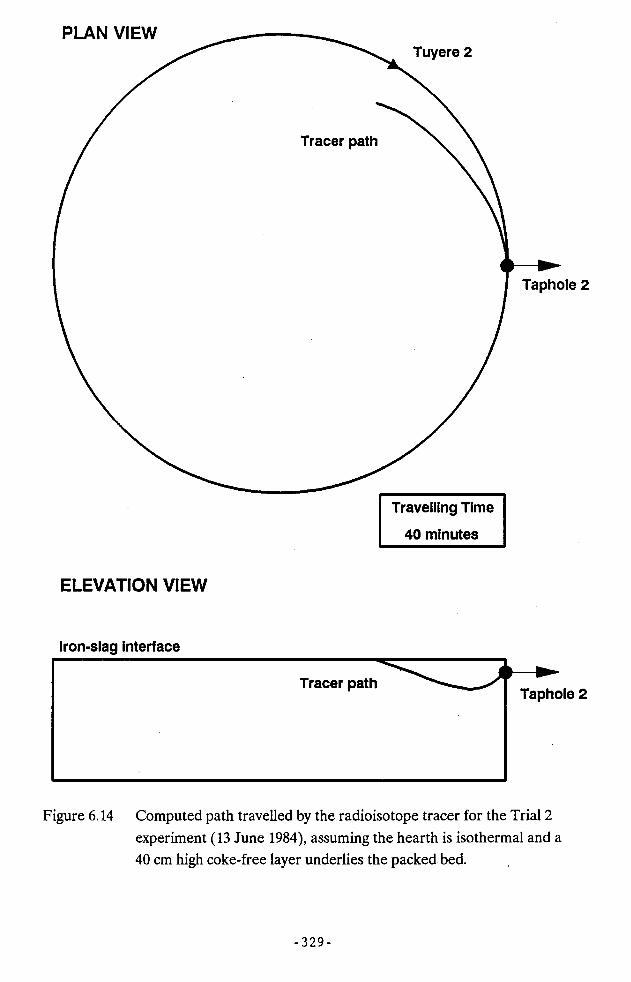
PLAN VIEWTuyere 2

Tracer path

Taphole 2

Travelling Time

40 minutes

ELEVATION VIEW

Iron-slag interface

Tracer pathTaphole 2

Figure 6.14 Computed path travelled by the radioisotope tracer for the Trial 2 experiment (13 June 1984), assuming the hearth is isothermal and a 40 cm high coke-free layer underlies the packed bed.

-329-

6.8 Conclusions

The analysis of radioisotope tracer experiments in the hearth of an operating blast furnace, requires a consideration of the thermally-influenced flow of iron in the hearth. Apparent irregularities in data obtained from the tracer experiments, may be due to changes in the state of the coke bed (ie. variations in bed permeability), and/or to changes in the thermal state of iron in the hearth. For conditions where thermal effects are significant (ie. where side- and under-hearth cooling effects are significant), the analysis of tracer experiments is difficult because of the complex nature of the flow distribution in the hearth. In some cases, a unique description of the overall state of the hearth using tracer experiments, may not be possible.

A three-dimensional, numerical model which accounts for the effect of side- and under-hearth cooling on the flow of iron in a hearth with and without a coke-free layer, has been applied to the study of tracer experiments in the hearth. The model will be a valuable tool both in the understanding of flow behaviour in the hearth and in the design of tracer experiments which will provide more reliable and accurate assessments of the state of the hearth.

-330-

BIBLIOGRAPHY

Abe, Y. ,Yamaguchi, K., Tsuda, A., Shiki, C. and Katahira, H. 'Conditions of Coke Bed in the Hearth (Dissection Results of the Hearth in Kimitsu No. 3 Blast Furnace of Nippon Steel Corporation - I' Transactions ISTJ. 1985, Vol. 25, p. B-239.

Abe, Y., Yamaguchi, K., Tsuda, A., Shiki, C. and Katahira, H. 'Conditions of Coke Bed in the Hearth (Dissection Results of the Hearth in Kimitsu No. 3 Blast Furnace of Nippon Steel Corporation - II'Transactions ISIJ, 1985, Vol. 25, p. B-240.

Alleyn, A.G. and Munive, L.'Hearth Behaviour of Port Kembla Blast Furnaces'Proceedings International Blast Furnace Hearths and Raceways, Australian I.M.M. Symposium Ser. No. 26, A.I.M.M., 1981, p. 11-1.

Amsden, A.A. and Harlow, F.H.'Transport of Turbulence in Numerical Fluid Dynamics'Journal of Computational Physics, 1968, Vol. 3, p. 94.

Amsden, A.A. and Harlow, F.H.'A Simplified MAC Technique for Incompressible Fluid Flow Calculations'Journal of Computational Physics. 1970, Vol. 6, p. 322.

Araki, K.'Production of Iron and Steel'Transactions ISTJ. 1985, Vol. 25, No. 8, p. 837.

-331-

Babarykin, N.N., Zborovskii, A.A., Potapov, A.I. and Rabinovich, E.I. 'Movement of Pig Iron and Slag in the Blast-Furnace Hearth'Stal in English, 1960, Vol. 1, p. 16.

Babarykin, N.N., Galatonov, A.L., Mishin, P.P., Tkachenko, F.F. and Yushin, F.A.'Choking of a Blast-Furnace Hearth'Stal in English. 1962, Vol. 5, p. 341.

Bear, J.'Dynamics Of Fluids in Porous Media'American Elsevier Publishing Co., New York, 1972.

Bear, J.'Hydraulics of Groundwater'McGraw-Hill International Book Co., 1979.

Bejan, A.'Natural Convection in an Infinite Porous Medium with a Concentrated Heat Source'Journal of Fluid Mechanics. 1978, Vol. 89, p. 97.

Bird, R.B., Stewart, W.E. and Lightfoot, E.N.'Transport Phenomena'Wiley and Sons, New York, 1962.

Biswas, A.K.'Principles of Blast Furnace Ironmaking'Cootha Publishing House, Brisbane, Australia, 1981.

-332-

Bulgarelli, U., Casulli, V. and Greenspan, D.'On. Numerical Treatment of Free Surfaces for Incompressible Fluid-flow Problems'Nonlinear Analysis Theory. Methods and Applications. 1980, Vol. 4,No. 5, p. 975.

Burgess, J.M., Jenkins, D., McCarthy, M.J., Nowak, L., Pinczewski,W.V. and Tanzil, W.B.U.'Lateral Drainage of Packed Beds'CHEMECA 80. 8th Australian Chemical Engineering Conference, Melbourne, Australia, August 24-27, 1980, p. 85.

Burgess, J.M., Jenkins, D., McCarthy, M.J.., Nowak, L., Pinczewski,W.V. and Tanzil, W.B.U.'Mathematical and Physical Simulation of Non-Uniform Liquid Drainage in Packed Beds'Proceedings International Blast Furnace Hearths and Raceways, Australian I.M.M. Symposium Ser. No. 26, A.I.M.M., 1981, p. 9-1.

Burgess, J.M., McCarthy, M.J., Jenkins, D.R., Pinczewski, W.V. and Tanzil, W.B.U.'Gas Distribution and Hearth Liquid Model for the Analysis of the Iron Making Blast Furnace'Proceedings Process Technology Conference, Symposium on Application of Mathematical and Physical Models in The Iron and Steel Industry, Iron and Steel Soc., A.I.M.E., Pittsburgh, 1982, Vol. 3, p. 15.

Casulli, V.'Numerical Simulation of Free-Surface Thermally Influenced Flows for Nonhomogenous Fluids'Applied Mathematics and Computation. 1981, Vol. 8, p. 261.

-333-

Casulli, V. and Greenspan, D.'Numerical Simulation of Miscible and Immiscible Fluid Flows in Porous Media'Journal of Society Petroleum Engineers. October, 1982, p. 635.

Chan, R.K.C. and Street, R.L.'A Computer Study of Finite-Amplitide Water Waves'Journal of Computational Physics. 1970, Vol. 6, p. 68.

Chan, Y.T. and Banerjee, S.'Analysis of Transient Three-Dimensional Natural Convection in Porous Media'Journal of Heat Transfer. Transactions ASME, 1981, Vol. 103, May, p. 242.

Chorin, A.J.'A Numerical Method for Solving Incompressible Viscous Flow Problems' Journal of Computational Physics. 1967, Vol. 2, p. 12.

Courant, R., Friedrichs, K. and Lewy, H.'On the Partial Difference Equations of Mathematical Physics'IBM Journal. 1967, March, p. 215.

Courant, R., Isaacson, E. and Rees, M.'On the Solution of Nonlinear Hyperbolic Differential Equations by Finite Differences'Comm. Pure Appl. Math.. 1952, Vol. 5, p. 243.

Curlet, N.W.E., Won, K.J., Clomburg, L.A. and Sarofim, A.F. 'Experimental and Mathematical Modelling of Three Dimensional Natural Convection in an Enclosure'AIChE Journal. 1984, March, Vol. 30, No. 2, p. 249.

-334-

Daly, B.J.'Numerical Study of Two-Fluid Rayleigh-Taylor Instability'Physics of Fluids, 1967, Vol. 10, No. 2, p. 297.

Daly, B.J. and Pracht, W.E.Numerical Study of Density-Current Surges'Physics of Fluids. 1968, Vol. 11, No. 1, p. 15.

Daly, B.J.'A Technique for Including Surface Tension Effects in Hydrodynamic Calculations'Journal of Computational Physics, 1969, Vol. 4, p. 97.

Deville, M.O.'Numerical Experiments on the MAC Code for Slow Flows'Journal of Computational Physics. 1974, Vol. 15, p. 362.

Dietz, P.W.'Effective Thermal Conductivity of Packed Beds'Industrial Engineering and Chemistry Fundamentals. 1979, Vol. 18, No. 3, p. 283.

Dixon, A.G.'Thermal Resistance Models of Packed-Bed Effective Heat Transfer Parameters'AIChE Journal. 1985, Vol. 31, No. 5, p. 826.

Dixon, A.G. and Gresswell, D.L.'Thearetical Prediction of Effective Heat Transfer Parameters in Packed Beds'AIChE Journal, 1979, Vol. 25, No. 4, p. 663.

-335-

Dorofeev, V.N. and Novokhatskii, A.M.'Origin of Difference in Electric Potentials on Blast Furnace Shell' Steel in the USSR. 1984, Vol. 14, No. 1, p. 10.

Dybbs, A. and Schweitzer, S.'Conservation Equations for Non-Isothermal Flow in Porous Media' Journal of Hydrology. 1973, Vol. 23, p. 181.

Easton, C.R.'Homogenous Boundary Conditions for Pressure in the MAC Method' Journal of Computational Physics. 1972, Vol. 9, p. 375.

Elders, J.W.'Steady Free Convection in a Porous Medium Heated from Below' Journal of Fluid Mechanics. 1967, Vol. 27, p. 29.

Elders, J.W.'Transient Convection in a Porous Medium'Journal of Fluid Mechanics. 1967, Vol. 27, p. 609.

Evans, J.L. and Workman, G.M.'Resisting Blast-Furnace Lining Wear - The Thermal Approach' Journal of Iron and Steel Institute. 1973, April, p. 264.

Erwall, L.'The Use of Radioactive Isotopes in the Mining and Iron and Steel Industries'Jernkont. Ann.. 1958, Vol. 142, No. 7, p. 369.

Foote, G.B.'A Numerical Method for Studying Liquid Drop Behaviour : Simple Oscillation'Journal of Computational Physics. 1973, Vol. 11, p. 507.

-336-

Forester, C.K.'A Method of Time-Centering the Lagrangian Marker Particle Computation'Journal of Computational Physics. 1973, Vol. 12, p. 269.

Fromm, J.E.'A method for Reducing Dispersion in Convective Difference Schemes' Journal Computational Physics. 1968, Vol. 3, p. 176.

Fromm, J.E. and Harlow, F.H.'Numerical Solution of the Problem of Vortex Street Development' Physics of Fluids, 1963, Vol. 6, No. 7, p. 975.

Fukutake, T. and Okabe, K.'Experimental Studies of Slag Flow in the Blast Furnace Hearth During Tapping Operation'Transactions ISIJ. 1976 (a), Vol. 16, p. 309.

Fukutake, T. and Okabe, K.'Influences of Slag Tapping Conditions on the Amount of Residual Slag in the Blast Furnace Hearth'Transactions ISIJ. 1976 (b), Vol. 16, p. 317.

Fukutake, T. and Okabe, K.'Keynote Address - The Hearth Drainage of the Blast Furnace' Proceedings International Blast Furnace Hearths and Raceways, Australian I.M.M. Symposium Ser. No. 26, A.I.M.M., 1981 , p. 2-1.

-337-

Fukutake, T., Shikata, H., Ichihara, I., Tamiya, T., Okumura, K. and Kawarada, H.'The Flow of Slag and Metal in the Blast Furnace Hearth During Tapping'Proceedings 42nd Ironmaking Conference. Iron and Steel Society, A.I.M.E., Atlanta, 1983, Vol. 42, p. 567.

Galemin, I.M.'Durability of Carbon Linings in Blast-Furnaces'Stal in English. 1963, Vol. 10, p. 769.

Gdula, S.J., Bialecki, R., Kurposz, K., Nowak, A. and Sucheta, A. 'Mathematical Model of Steady State Heat Transfer in Blast Furnace Hearth and Bottom'Transactions ISIJT 1985, Vol. 25, No. 5, p. 380.

Gorskov.V.K., Myslivtsev, I.V., Ushkov, I.A. and Zhilkin, N.K. 'Checking the State of the Hearth Lining on an Operating Blast Furnace'Stal in English, 1965, Vol. 4, p. 267.

Goryainov, G.E., Liderman, S.M., Nikolaev, G.V. and Shelud'ko, V.V. 'Efficient design of Blast Furnace Hearth Pad'Steel in the USSR r 1982, Vol. 12, p. 400.

Gratsilev, G.M. and Goncharov, V.V.'Durability of Carbon Blocks in the Blast-Furnace Hearth'Stal in English. 1970, Vol. ????, p. 679.

Greenspan, D.'Introductory Numerical Analysis of Elliptic Boundary Value Problems' Harper and Row, New York, 1965.

-338-

Guitjens, J.C. and Luthins, J.N.'Viscous Model Study of Drain Spacing on Sloping Land and Comparison with Mathematical Solution'Water Resources Research. Vol. 1, No. 4, p. 523.

Hara, Y. and Tachimori, M.'Theoretical Analysis of Flow of Molten Iron in Blast Furnace Hearth' Report of 54th Committee of Gakushin (Japan Society for Promotion of Science)T 1978, Report No. 1457 (in English).

Hara, Y. and Tachimori, M.'Experiment With the Model of the Flow of Molten Iron in Blast Furnace Hearths'Report of 54th Committee of Gakushin (Japan Society for Promotion of Science)r 1979, Report No. 1485 (in English).

Harlow, F.H. and Welch, J.E.'Numerical Calculation of Time-Dependent Viscous Incompressible Flow of Fluid With Free-Surface'Physics of Fluids. 1965, Vol. 8, No. 12, p. 2182.

Harlow, F.H. and Welch, J.E.'Numerical Study of Large-Amplitude Free Surface Motion'Physics of Fluids, 1966, Vol. 9, No. 5, p. 842.

Harlow, F.H.'Contour Dynamics for Numerical Fluid-Flow Calculations'Journal of Computational Physics. 1971, Vol. 8, p. 214.

Harlow, F.H. and Amsden, A.A.'A Numerical Fluid Dynamics Calcualtion Method for All Flow Speeds' Journal of Computational Physics. 1971, Vol. 8, p. 197.

-339-

Harlow, F.H. and Amsden, A.A.'Numerical Calculation of Multiphase Fluid Flow'Journal of Computational Physics, 1975, Vol. 17, p. 19.

Hirt, C.W. and Harlow, F.H.'A General Corrective Procedure for the Numerical Solution of Initial-Value Problems'Journal of Computational Physics, 1967, Vol. 2, p. 114.

Hirt, C.W.'Heuristic Stability Theory for Finite-Difference Equations'Journal of Computational Physics, 1968, Vol. 2, p. 339.

Hirt, C.W. and Shannon, J.P.'Free - Surface Stress Conditions for Incompressible Flow Calculations'Journal of Computational Physics. 1968, Vol. 2, p. 403.

Hirt, C.W., Cook, J.L. and Butler, T.D.'A Lagrangian Method for Calculating the Dynamics of an Incompressible Fluid with Free Surface'Journal of Computational Physics. 1970, Vol. 5, p. 103.

Hirt, C.W. and Cook, J.L.'Calculating Three-Dimensional Flows Around Structures and Over Rough Terrain'Journal of Computational Physics. 1972, Vol. 10, p. 324.

Hirt, C.W., Nichols, B.D. and Romero, N.C.'SOLA - A Numerical Solution Algorithm for Transient Fluid Flows'Los Alamos Scientific Laboratory report LA-5852. April, 1975.

-340-

Hirt, C.W. and Nichols, B.D.'Volume of Fluid (VOF) Method for the Dynamics of Free Boundaries' Journal of Computational Physics, 1981, Vol. 39, p. 201.

Hornberger, G.M., Ebert, J. and Remson, I.'Numerical Solution of the Boussinesq Equation for Aquifier - Stream Interaction'Water Resources Research. 1970, Vol. 6, No. 2, p. 601.

Horne, R.N.'Transient Effects in Geothermal Convective Systems'Ph.D Dissertation, University of Auckland, New Zealand, 1975.

Horne, R.N. and O'Sullivan, M.J.'Convection in a Porous Medium Heated from Below : The Effect of Temperature Dependent Viscosity and Thermal Equilibrium Coefficient' Transactions ASME. 1978, Vol. 100, p. 448.

Horton, C.W.'Convection Currents in a Porois Medium'Journal of Applied Physics. 1945, Vol. 16, p. 367.

Hunt, B.'Finite Difference Approximation of Boundary Conditions Along Irregular Boundaries'International Journal of Numerical Methods in Engineering. 1978,Vol. 12, p. 229.

Ichihara, I. et al'Numerical Simulation of Two Dimensional Slag Flow in the Blast Furnace Hearth'Tetsu-to-Hagane. 1981, Vol. 67, No. 4, p. S-55.

-341-

Ichihara, I. and Fukutake, T.'Numerical Calculation of Unsteady Slag Flow in the Blast Furnace Hearth During Tapping'SYSTEMS. Japan UNIVAC Users Association, Tokyo, 1979, p. 39.

Ikeda, M., Fujiwara, S., Nagahara, M., Aoyama, K., Tsutsui, N. and Noda, T.'Dismantling Investigations on Hearth Carbon Blocks in the Nagoya No.l B.F., 2nd Campaign'Transactions ISIJ. 1983 (a), Vol. 23, p. B-39.

Ikeda, M., Fujiwara, S., Nakai, M., Ohkawa, K., Saito, M. and Arao, Y. 'Dismantling Investigations on Hearth Carbon Blocks in the Muroran No.3 B.F., 6th Campaign'Transactions ISIJ, 1983 (b), Vol. 23, p. B-40.

Ikeda, M., Fujiwara, S., Murai, T., Nakai, M., Tachikawa, Y. and Hikita, K.'Experimental Results from Hot Model Hearth Test (Some Structural Studies on Blast Furnace Hearth Linings - I'Transactions ISIJ, 1984 (a), Vol. 24, p. B-141.

Ikeda, M., Fujiwara, S., Murai, T., Nakai, M., Tachikawa, Y. and Hikita, K.'Stress Analysis in Carbon Blocks Under Eccentric Load (Some Structural Studies on Blast Furnace Hearth Linings - II'Transactions ISIJ, 1984 (b), Vol. 24, p. B-142.

Ikeda, M., Fujiwara, S., Murai, T., Kikuchi, A., Tachikawa, Y. and Hikita, K.'FEM Analysis on Thermal Stresses in the Annular Structure (Some Structural Studies on Blast Furnace Hearth Linings - III'Transactions ISIJ, 1984 (a), Vol. 24, p. B-143.

-342-

Ikeda, M., Nagahara, M., Horio, T., Mitsuyasu, T., Nose, M. and Nomura, M.'Dismantling Investigation on Hearth Refractories in Kimitsu No. 3 B.F. of Nippon Steel Corporation (1st Campaign)'Transactions ISIJ. 1985, Vol. 25, p. B-64.

Kanbara, K., Hagiwara, T., Shigemi, A., Kondo, S., Kanayama, Y., Wakabayashi, K. and Hiramoto, N.'Dissection of Blast Furnaces and Their Internal States'Transactions ISIJ. 1977, Vol. 17, p. 371.

Katto, Y. and Masuoka, T.'Criterion for the Onset of Convective Flow in a Fluid in a Porous Media'International Journal of Heat and Mass Transfer, 1967, Vol. 10, p. 297.

Kawate, Y., Sonoi, H., Yokoe, K., Takano, S. and Shimomura, K. 'Measuring Methods for Lining Erosion of the Blast Furnace' Transactions ISIJ, 1982, Vol. 22, p. 799.

Kinoshita, T.'Research and Development in the Japanese Steel Industry'Japan's Iron and Steel Industry 1987 Kawata Publicity Inc., Tokyo, 1987.

Klotz, D., Moser, H. and Rauert, W.'Model Tests to Study Groundwater Flows Using Radioisotopes and Dye Tracers'Developments in Soil Science 2 'Fundamentals of Transport Phenomena in Porous Media'International Association for Hydraulics Research Elsevier Publishing Co., 1972.

-343-

Kojima, K., Nishi, T., Yamaguchi, T., Nakama, H. and Ida, S.'Change in the Properties of Coke in Blast Furnace'Transactions ISIJT 1977, Vol. 17, p. 401.

Kropotov, V.K.'Temperature Measurement in the Hearth Through the Slag Notch'Stal in English. 1960, Vol. 2, p. 89.

Kristiansen, G.K.'Zero of Arbitrary Function'BIT. (1963) , Vol. 3, p. 205.

Kubo, H., Ichihara, I., Morimoto, T. and Morimoto, T.'Thermal Stress Analysis for Study of Wear Mechanism of Blast Furnace Hearth'Transactions ISIJ. 1983, Vol. 23, p. B-38.

Hatano, M., Takashima, H. Kurita, K., Hariki, M. and Mori, K.'A Mathematical Model Simulating Wear Contour of Blast Furnace Hearth' Transactions ISIJ. 1979, Vol. 19, p. S-32.

Kurita, K. and Tanaka, T.'Effect of Liquid Flow on the Temperature Distribution in the Hearth'Transactions ISIJ. 1986, Vol. 26, p. B-334.

van Laar, J. and van Santen, N.'Salamander Formation, Temperature Distribution, and Heat Flow in a Blast-Furnace Bottom and Foundation, Using an Electrical Analog Model' Journal of Iron and Steel Institute, September, 1967, p. 941.

-344-

Lapwood, E.R.'Convection of a Fluid in a Porous Medium'Cambridge Phil. Soc. Proc.. 1948, Vol. 44, p. 508.

Lavrent'ev, M.L.'Some Special Features of the Thermal Work of the Lower Part of the Blast Furnace'Stal in English. 1969, No. 2, p. 135.

Lee, W-P.'Research Institute of Industrial Science and Technology'Research in the Steel Industry, Technical Exchange Session International Iron and Steel Institute, Belgium, 1987.

Lennon, G.P.'Boundary Integral Equation Solution to Axisymmetric Potential Flows - 2. Recharge and Well Problems in Porous Media'Water Resources Research. 1979, Vol. 15, No. 5, p. 1107.

Lennon, G.P., Liu, P.L-F. and Liggett, J.A.'Boundary Integral Solutions to Three-Dimensional Unconfined Darcy's Flow'Water Resources Research. 1980, Vol. 16, No. 4, p. 651.

Leonard, L.A.'Refractories for the Hearth of the Blast Furnace'Iron and Steel, 1971, Vol. 44, No. 6, p. 429.

Levenspiel, 0.'Chemical Reaction Engineering'Wiley and Sons Inc., New York, 1972.

-345-

Libralasso, J.M., Nicolle, R., Steiler, J.M. and Wanin, M.'The Use of Radioactive Tracers in the Blast Furnace'Proceedings 44th Ironmaking Conference, Iron and Steel Society, A.I.M.E., Atlanta, 1985, Vol. 44, p. 565.

Liggett, J.A.'Location of Free Surface In Porous Media'Journal of Hydraulics Division. 1977, April, p. 353.

Litvinenko, V.I., Lavrent'ev, M.L. and Berdnik, A.A.'Effect of Blast Furnace Hearth Choking and How to Prevent It'Stal, 1966, No. 2, p. 94.

Liu, P. L-F. and Liggett, J.A.'Numerical Stability and Accuracy of Implicit Integration of Free Surface Groundwater Equations'Water Resources Research. 1980, Vol. 16, No. 5, p. 897.

Liu, P.L-F., Cheng, A.H-D., Liggett, J.A. and Lee, J.H.'Boundary Integral Equation Solutions to Moving Interface Between Two Fluids in Porous Media'Water Resources Research. 1981, Vol. 17, No. 5, p. 1445.

Lowing, J.'Aspects of Blast Furnace Flow : 1 Diagnostic Approach to Overcoming Blast Furnace Operational Problems'Ironmaking and Steelmaking. 1978, No. 6, p. 239.

McCracken, D.D. and Dorn, W.S.'Numerical Methods and Fortran Programming'John Wiley and Sons Inc., 1964.

-346-

Makhanek, N.G. and Onorin, O.P.'Change in Relationship of Forces Governing Movement of Granular Materials with Gas Being Blown Through a Static Bed and Under Counter-flow Conditions'Stal in English. 1967, Vol. 2, p. 97.

Makhanek, N.G., Onorin, O.P. and Konovalov, K.D.'On the Relationship Between Forces Acting on a Column of Charge Materials in a Blast Furnace'Izv. Vvssh. Uchebn. Zaved Chern. Metall.. 1966, Vol. 10, p. 15.

Makhanek, N.G., Kostyrev, L.M. and Ya. Shparber, L.'Tapping Pig Iron from the Blast Furnace'Steel in the USSR. December, 1974, Vol. 4, No. 12, p. 947.

Meyer, C.H.'Hele-Shaw Flow with a Cusping Free Boundary'Journal of Computational Physics, 1981, Vol. 44, p. 262.

Miura, Y.'Recent Studies on the Properties of Blast Furnace Coke and Their Future Prospects'Transactions ISIJ. 1982, Vol. 22, p. 483.

Miyagawa, K. et al'Use of R.I. Tracer in Blast Furnace'Tetsu-to-Hagane, 1965, Vol. 51, No. 10, p. 1742.

Monetov, G.V. and Kropotov, V.K.'Blast Furnace Hearth Height'Steel in the USSR. 1981, No. 10, p. 559.

-347-

Muskat, M.'The Flow of Homogenous Fluids Through Porous Media'J.W. Edwards Inc., 1946.

Nakamura, N., Togino, Y. and Tateoka, M.'Behaviour of Coke in Large Blast Furnaces'Ironmaking and Steelmaking. 1978, Vol. 5, No. 1, p. 1.

Nakayama, P.I. and Romero, N.C.'Numerical Method for Almost Three-Dimensional Incompressible Fluid Flow and a Simple Internal Obstacle Treatment'Journal Computational Physics, 1971, Vol. 8, p. 230.

Natori, M. and Kawarada, H.Computer Centre Report, University of Tokyo. 1976, No. 5, p. 1.

Nichols, B.D. and Hirt, C.W.'Improved Free Surface Boundary Conditions for Numerical Incompressible Flow Calculations'Journal of Computational Physics. 1971, Vol. 8, p. 434.

Nichols, B.D. and Hirt, C.W.'Calculating Three-Dimensional Free Surface Flows in the Vicinity of Submerged and Exposed Structures'Journal of Computational Physics. 1973, Vol. 12, p. 234.

Nichols, B.D., Hirt, C.W. and Hotchkiss, R.S.'SOLA-VOF - A Solution Algorithm for Transient Fluid Flow with Multiple Free Boundaries'Los Alamos Scientific Laboratory reportL LA-8355, August, 1980.

-348-

Nichols, B.D. and Hirt, C.W.'Numerical Simulation of Boiling Water Reactor Vent - Clearing Hydrodynamics'Nuclear Science and Engineering. 1980, Vol. 73, p. 196.

Nishioka, K. and Yoshida, S.'Strength Estimation of Coke as Porous Material'Transactions ISIJ. 1983, Vol. 23, p. 387.

Ohno, J., Nakamura, M. and Yoshizawa, A.'On the Mechanism of Formation of Stagnant Layer in the Hearth of Blast Furnace (Studies on the Control of Molten Pig Iron and Slag Flow in the Hearth of Blast Furnace - V'Transactions ISIJ. 1982, No. 4, p. B-117.

Ohno, J., Nakamura, M., Hara, Y., Tachimori, M. and Arino, S.'Flow of Iron in Blast Furnace Hearth'Proceedings International Blast Furnace Hearths and Raceways,Australia I.M.M. Symposium Ser. No. 26, A.I.M.M., 1981, p. 10-1.

Onoye, T., Satoh, Y., Uemura, K., Taniguchi, K. and Shimomura, K. 'Examination on Fluid State Region of Iron in a Blast Furnace by the Tracer Method'Transactions ISIJ. 1983, Vol. 23, p. B-276.

Ohno J., Tachimori, M., Nakamura, M. and Hara, Y.'Influence of Hot Metal Flow on the Heat Transfer in a Blast Furnace Hearth'Tetsu-to-Hagane. 1985, Vol. 71, No. 1, p. 34.

Omori, Y.'Blast Furnace Phenomena and Modelling'Elsevier Applied Science, London and New York, 1987.

-349-

Parashakov, V.M., Babushkin, N.M. and Fedotov, P.B.'Assessing Thermal State of Blast-Furnace Hearth and its Application to Analysis of Causes of Tuyere Burning'Steel in the USSR. 1980, Vol. 10, No. 3, p. 111.

Paschkis, V. and Mirsepassi, T.'Temperature Distribution in the Hearths of Blast Furnaces'Iron and Steel Engineer. 1954, February, p. 53.

Paschki^, V. and Mirsepassi, T.'Temperatures and Heat Flow in the Hearths of Blast Furnaces With or Without Underhearth Cooling'Iron and Steel Engineer. June, 1956, p. 116.

Pehlke, R.D. and Henning, G.S.'Heat Flow in Blast Furnace Hearths'Canadian Metallurgical Quarterly. 1976, Vol. 15, No. 1, p. 83.

Peters, K-H., Gudenau, H-W. and Still, G.'Hot Metal flow in a Blast Furnace Hearth - Model Tests'Steel Research, 1985, Vol. 56, No. 11, p. 547.

Pinczewski, W.V. and Tanzil, W.B.U.'Numerical Simulation for the Drainage of Two-Dimensional Packed Beds' Chemical Engineering Science. 1981, Vol. 36, p. 1039.

Pinczewski, W.V., Tanzil, W.B.U., Hoshke, M.I. and Burgess, J.M. 'Simulation of the Drainage of Two Liquids from a Blast Furnace Hearth'Transactions T STJ r 1982, Vol. 22, p. B-202.

-350-

Polovchenko, M.G., Afanas'ev, V.N., Uzlyuk, V.N., Krivosheev,A.A. and Yaroshevskii, N.D.'Study and Measurement of Blast-Furnace Lining Wear'Stal in English. 1960, Vol. 9, p.625.

Pracht, W.E.'A Numerical Method for Calculating Transient Creep Flow'Journal of Computational Physics. 1971, Vol. 7, p. 46.

Quy, N.V.Private Communications, 1985.

Raithby, G.D. and Torrance, K.E.'Upstream-Weighted Differencing Schemes and their Application to Elliptic Problems Involving Fluid Flow'Computers and Fluids. 1974, Vol. 2, p. 191.

Remson, I., Hornberger, G.M. and Molz, F.J 'Numerical Methods in Subsurface Hydrology'John Wiley and Sons, New York, 1971.

Richards, C.W. and Crane, C.M.'The Accuracy of Finite Difference Schemes for the Numerical Solution of Navier-Stokes Equations'Applied Mathematical Modelling. 1979, Vol. 3, p. 205.

de Rivas, E.K.'On the Use of Non-Uniform Grids in Finite Difference Equations' Journal of Computational Physics. 1972, Vol. 10, p. 202.

Roache, P.J.'Computational Fluid Dynamics'Hermosa, Albuquerque, New Mexico, 1971.

-351-

Roache, P.J.'Marching Methods for Elliptic Problems - Part I'Numerical Heat Transfer, 1978, Vol. 1, p. 1.

Robinson, B.A. and Tester, J.W.'Characterization of Flow Maldistribution Using Inlet-outlet Tracer Techniques: An Application of Internal Residence Time Distributions' Chemical Engineering Science. 1986, Vol. 41, No. 3, p. 469.

Rooney, K.A.'Identification of Hearth Liquid Drainage Problems Using Radioactive Tracers'Slab and Plate Products Division (Broken Hill Pty. Co.) Internal Report, 1986.

Rudraiah, N., Veerappa, B. and Balachandra Rao, S.'Effects of Nonuniform Thermal Gradient and Adiabatic Boundaries on Convection in Porous Media'Journal of Heat Transfer. Transactions ASME, 1980, Vol. 102, p. 254.

Rutledge, R.J.'Blast Furnace Hearth Drainage'B.E. Thesis in Chemical Engineering, 1985, University of New South Wales, Sydney, Australia.

Sasaki,K., Nakatani, F., Hatano, M., Watanabe, M., Shimoda, T., Yokotani, K., Ito, T. and Yokoi, T.'Investigation of Quenched No. 2 Blast Furnace at Kokura Works' Transactions ISIJT 1977 (a), Vol. 17, p. 252.

Sasaki, M., Ono, K., Suzuki, A., Okuno, Y. and Yoshizawa, K. 'Formation and Melt-down of Softening-Melting Zone in Blast Furnace' Transactions ISIJ, 1977 (b), Vol. 17, p. 391.

-352-

Scriven, L.E.'Dynamics of a Fluid Interface'Chemical Engineering Science, 1960, Vol. 12, p. 98.

Seki, N., Fukusako, S. and Inaba, H.'Heat Transfer in a Confined Rectangular Cavity Packed With Porous Media'International Journal of Heat and Mass Transfer. 1978, Vol. 21, No. 7, p. 989.

Semenko, A.Y., Shtan'ko, N.I. and Dyshlevich, I.I.'Automatic Monotoring System for Melt Level in Blast Furnace Hearth Steel in the USSR. 1984, Vol. 14, No. 5, p. 215.

Semikin, I.D., Tsygankov, G.T., Borodulin, A.V., Vas'ko, I.P., Kruskal', M.S. and Mirshavka, V.P.'Heat Loss and Thermal Work in the Blast Furnace'Steel in the USSR. August, 1972, Vol. 2, No. 8, p. 602.

Sheldon, J.W. and Dougherty, E.W.'A Numerical Method for Computing the Dynamical Behaviour of Fluid-Fluid Interface in Permeable Media'Journal of Society of Petroleum Engineers. 1964, p. 158.

Senoo, Y., Taguchi, S., Fukutake, T. and Elliott, J.F.'Analysis of Flow and Heat Transfer in Blast Furnace Hearth by Two-dimensional Model Experiments'Transactions ISIJf 1985, Vol. 25, p. B-241.

Sheng, Y.P.'Numerical Computation of Three-Dimensional Circulation in Lake Erie: A Comparison of a Free-Surface Model and a Rigid-Lid Model' Journal of Physical Oceanography, 1978, Vol. 8, p. 713.

-353-

Shih, T-M.'Numerical Heat Transfer'Hemisphere Publishing Co. (Springer-Verlag), 1984.

Shimomura, Y., Nishikawa, K., Arino, S., Katayama, T., Hida, Y. and Isoyama, T.'On the Internal State of the Lumpy Zone of Blast Furnace'Transactions ISIJ. 1977, Vol. 17, p. 381.

Shimomura, Y., Kushima, K. and Arino, S.'The Measurement of Flow of the Molten Iron in the Blast Furnace Floor By R.I. (Study of the Flow Control of the Molten Slag From the Blast Furnace Floor - 1'Tetsu-to-Hagane. 1978, Vol. 64, No. 4, p. S-52.

Shimozuma, T. Miyashita, T., Yamada, K. and Otsuki, M.'On the Permeability and Rough Tapping of Large Blast Furnaces'Tetsu-to-Hagane, 1971, Vol. 57, No. 11, p. S-346.

Slattery, J.C.'Single-Phase Flow Through Porous Media'AlChE Journal, 1969, Vol. 15, No. 6, p. 866.

Spalding, D.B. and Afgan, N.H.'Heat and Mass Transfer in Metallurgical Systems'Hemisphere Publishing Co., 1981.

Spraggs, L.D.'Three-Dimensional Simulation of Thermally-Influenced Hydrodynamic Flows'Ph.D. Dissertation, Stanford University, 1974.

-354-

Standish, N., Reid, R. and Harpley, J.M.'Model Studies of Liquid Flow in Blast Furnace Hearths'Tetsu-to-Hagane, 1983, Vol. 69, p. S-734.

Standish, N. and Campbell, P.J.'Analysis of Liquid Flow in Blast Furnace Hearth'Transactions 1SIJ. 1984, Vol. 24, p. 709.

Strassburger, J.H. (ed.)'Blast Furnace-Theory and Practice'Volumes I-IIGordon and Breach Science Publishing Co., 1969.

Summers, E.M. and Morgan, D.'Performance of Blast Furnaces with Underhearth Cooling'Journal of Iron and Steel Institute. 1969, Vol. 207, p. 154.

Szekely, J.'Fluid Flow Phenomena in Metals Processing'Academic Press, 1979.

Tachimori, M. and Ohno, J.'Numerical Calculations of the Molten Iron Flow in the Blast Furnace' Tetsu-to-Hagane T 1976, Vol. 62, p. S-444.

Tachimori, M., Hara, Y., Arino, T., Sato, H., Matsui, M. and Hayashi, H.'R.I. Determination for the Flow of Molten Iron in the Blast Furnace Hearth'Tetsu-to-Hagane T 1979, Vol. 19, p. S-45.

-355-

Taggart, I.J., Pinczewski, W.V., McCarthy, M.J. and Burgess, J.M. 'Recirculating Gas Flow in the Blast Furnace Raceway Zone'Proc. 8th Australasian Fluid Mechanics Conference. 1983, Vol. 1, p. IB-1.

Tamiya, T., Shikata, H., Kobayashi, K., Ichihara, I., Okumura, K., Fukutake, T. and Kawarada, H.'Numerical Simulation of 2-phase Flow on the Blast Furnace Hearth by Using the Boundary Element Method'Transactions ISIJ. 1983, Vol. 23, p. B-114.

Tanzil, W.B.U.'Blast Furnace Hearth Drainage'Ph.D. Dissertation, University of New South Wales, 1985.

Tanzil, W.B.U. and Pinczewski, W.V.'Blast Furnace Hearth Drainage : Physical Mechanisms'Chemical Engineering Science. 1987, Vol. 42, No. 11, p. 2557.

Tanzil, W.B.U., Zulli, P., Burgess, J.M. and Pinczewski, W.V. 'Experimental Model Study of the Physical Mechanisms Governing Blast Furnace Drainage'Transactions ISIJ. 1984, Vol. 24, p. 197.

Tleugabulov, S.M., Shumakov, L.G. and Fialkov, B.S.'Pressure of the Stock Column in the Blast Furnace'Stal in English. 1965, Vol. 11, p. 861.

Tleugabulov, S.M., Toropygin, B.S. and Eliseev, V.I.'Influence of the Effective Pressure of the Stock Column and Gas-flow distribtuion on Operating Intensity in the Blast Furnace'Steel in the USSR. 1972, Vol. 2, p. 90.

-356-

Tseng, M.T. and Ragan, R.M.'Behaviour of Groundwater Flow Subject to Time-Varying Recharge'Water Resources Research 1973, Vol. 9, No. 3, p. 734.

Varga, R.S.'Matrix Iterative Analysis'Prentice-Hall Inc., 1962.

Viecelli, J.A.'A Method for Including Arbitrary External Boundaries on the MAC Incompressible Fluid Computing Technique'Journal of Computational Physics, 1969, Vol. 4, p. 543.

Viecelli, J.A.'A Computing Method for Incompressible Flows Bounded by Moving Walls'Journal of Computational Physics. 1971, Vol. 8, p. 119.

Vogelpoth, H.-B, Still, G. and Peters, M.'Examinations Concerning the Flow Behaviour of Hot Metal in the Blast Furnace'Stahl und Eisen. 1985, Vol. 105, No. 8, p. 451.

Volovik, G.A., Polovchenko, I.G. and Chechuro, A.N.'The Regime of Release of Smelting Products and the Processes of Desulphurization in the Hearth'Metallurg. 1963, October, No. 10, p. 4.

Volovik, G.A. and Marder, B.F.'Investigation of the Relation Between Pig-iron Temperature,Chemical Composition and the Conditions Under Which it Accumulates in the Blast-Furnace Hearth'Steel in the USSR. 1974 (a), Vol. 4, No. 4, p. 259.

-357-

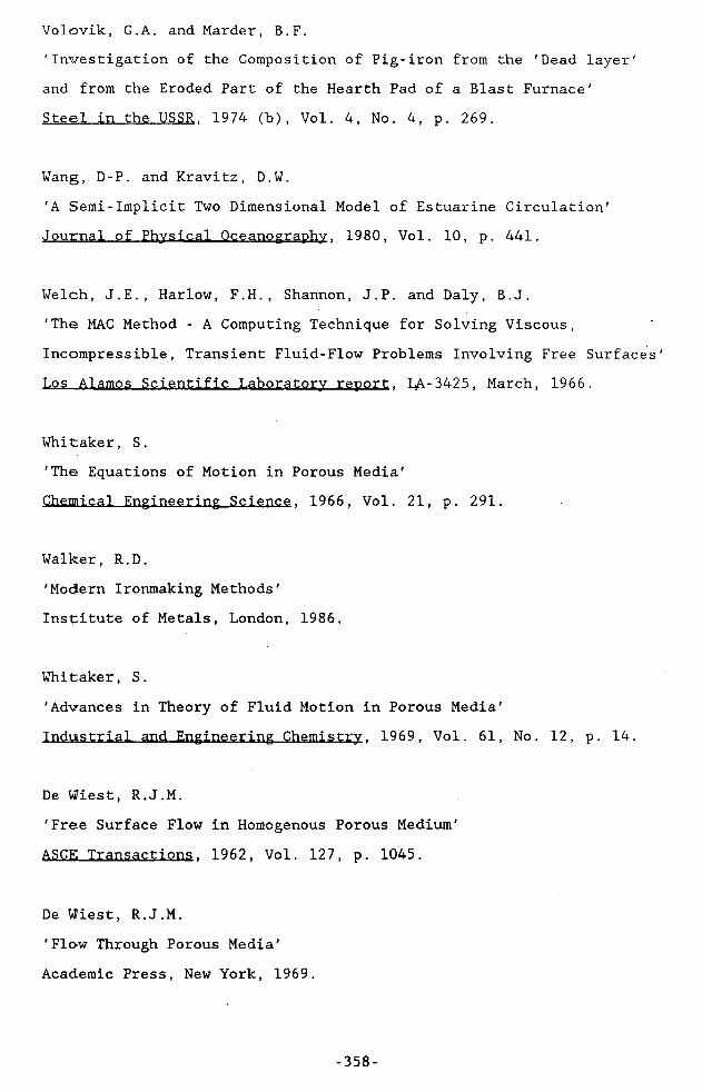
Volovik, G.A. and Marder, B.F.'Investigation of the Composition of Pig-iron from the 'Dead layer' and from the Eroded Part of the Hearth Pad of a Blast Furnace'Steel in the USSR. 1974 (b), Vol. 4, No. 4, p. 269.

Wang, D-P. and Kravitz, D.W.'A Semi-Implicit Two Dimensional Model of Estuarine Circulation' Journal of Physical Oceanography. 1980, Vol. 10, p. 441.

Welch, J.E., Harlow, F.H., Shannon, J.P. and Daly, B.J.'The MAC Method - A Computing Technique for Solving Viscous, Incompressible, Transient Fluid-Flow Problems Involving Free Surfaces' Los Alamos Scientific Laboratory report. LA-3425, March, 1966.

Whitaker, S.'The Equations of Motion in Porous Media'Chemical Engineering Science. 1966, Vol. 21, p. 291.

Walker, R.D.'Modern Ironmaking Methods'Institute of Metals, London, 1986.

Whitaker, S.'Advances in Theory of Fluid Motion in Porous Media'Industrial and Engineering Chemistry. 1969, Vol. 61, No. 12, p. 14.

De W7iest, R. J .M.'Free Surface Flow in Homogenous Porous Medium'ASCE Transactions. 1962, Vol. 127, p. 1045.

De Wiest, R.J.M.'Flow Through Porous Media'Academic Press, New York, 1969.

-358-

Wooding, R.A.'Instability of a Viscous Liquid of Variable Density in a Vertical Hele-Shaw Cell'Journal of Fluid Mechanics. 1960, Vol. 7, p. 501.

Wooding, R.A.'Free Convection of a Fluid in a Vertical Tube Filled with Porous Material'Journal of Fluid Mechanics. 1962, Vol. 13, p. 129.

Yashiro, H., Ohno, J., Nakamura, M., Aya, N. and Yoshizawa, A.'Flow of Molten Iron In Blast Furnace Hearth (Studies on the Control of Molten Pig Iron and Slag Flow in the Hearth of Blast Furnace - VI' Transactions ISIJ. 1983, Vol. 23, p. B-80.

Yen, B.C. and Hsie, C.H.'Viscous Flow Model for Groundwater Movement'Water Resources Research, 1972, Vol. 8, No. 5, p. 1299.

Yoshikawa, F. and Szekely, J.'Mechanism of Blast Furnace Hearth Erosion'Ironmaking and Steelmaking. 1981, Vol. 8, No. 4, p. 159.

Yoshikawa, F., Ichimiya, M., Takatori, S., Nigo, S. and Taguchi, S. 'Estimation of Erosion Lines and Solidified Layers of the Blast Furnace Hearth by Means of the Boundary Element Method'Transactions ISIJ. 1984, Vol. 24, p. B-328.

Yoshizawa, A.'A Proper Tensorial Form of D'Arcy-Ergun Equation'Transactions ISIJ. 1979, Vol. 19, p. 559.

-359-

Yoslhizawa, A., Ohno, J. and Nakamura, M.'Model Analysis of Hearth Flow (Studies on the Control of Molten Pig Iron and Slag Flow in the Hearth of Blast Furnace - VII'Transactions ISIJ. 1983, Vol. 23, p. B-113

Young, J.A. and Hirt, C.W.'Numerical Calculation of Internal Wave Motions'Journal of Fluid Mechanics. 1972, Vol. 56, p. 265.

Zalesak, S.T.'High Order "ZIP" Differencing of Convective Terms'Journal of Computational Physics, 1981, Vol. 40, p. 497.

-360-

APPENDIX A

Consider Figure 2.4, which shows the control volume associated with the convection of momentum by fluid motion in the x-direction ie. the term CONUX in equation 2.26. A Taylor series expansion about the point xi+1/2 gives,

C0NUXi+1/2 = CONUX0 - 0.5 (6xi+1/2 - SxJ (d(CONUX)/dx)Q

= CONUX0 - 0.5 (Sxi+1/2 - SXi) CONUX0/5xi+1/2

= C0NUXo (1-0.5 (5xi+1/2 - 6Xi)/5xi+1/2)

= CONUX0 (Sxi+1/2 - 0.5 (5xi+1/2 + 6Xi) )/<5xi+1/2

= 0.5 C0NUXo (6xi+1/2 + /Sy.i+1/2

Since <$xi+1/2 may be written as

^xi+i/2 = 0-5 (5xi+1 + 5Xi)

then upon substituting and re-arranging, we may write

C0NUXi+1/2 = 0.5 C0NUXo (6xi+1 + 3 5xi)/(6xi+1 + SxL)

-A.l-

APPENDIX B

In Chapter 2, the dimensionless geometric number H**, was introduced. The derivation of H** follows from the derivation of H* described by Fukutake and Okabe (1976 a). Figure B.l shows a side elevation view of a hearth which may represent either a two- or three-dimensional hearth. The datum or reference depth is taken at the taphole centreline. The piezometric head of the liquid above this datum <p, is given by

<P = z + P/pg (B.l)

where z = Hliq-HthP = liquid pressurep = liquid densityg = gravitational constant

The bounding, moving upper surface of the liquid may be described by

tf0(x,y,z,t) = 0 (B.2)

The height of the liquid surface, Z (where Z equals Hliq-Hth) , is a single-valued function of x,y and t, so that

Z = f(x,y,t) (B.3)

The position of the liquid surface may then be described by equation (B.4)

= z - f(x,y,t) = 0 (B.4)

-B.l-

Initially, the liquid is in hydostatic equilibrium ie.

f (x,y, 0) = z = HIiq-Hth (B. 5)

Equation (B.5) states that the piezometric head is everywhere constant and equal to the liquid height above the taphole centreline. Using the characteristic length D (the hearth diameter), we may write the initial condition (equation (B.5)) in dimensionless form

f*(x*,y*,0) = (Hiiq-Hth)/D (B . 6)

The dimensionless geometric number H**, is equal to f*(x*,y*,0).

-B.2-

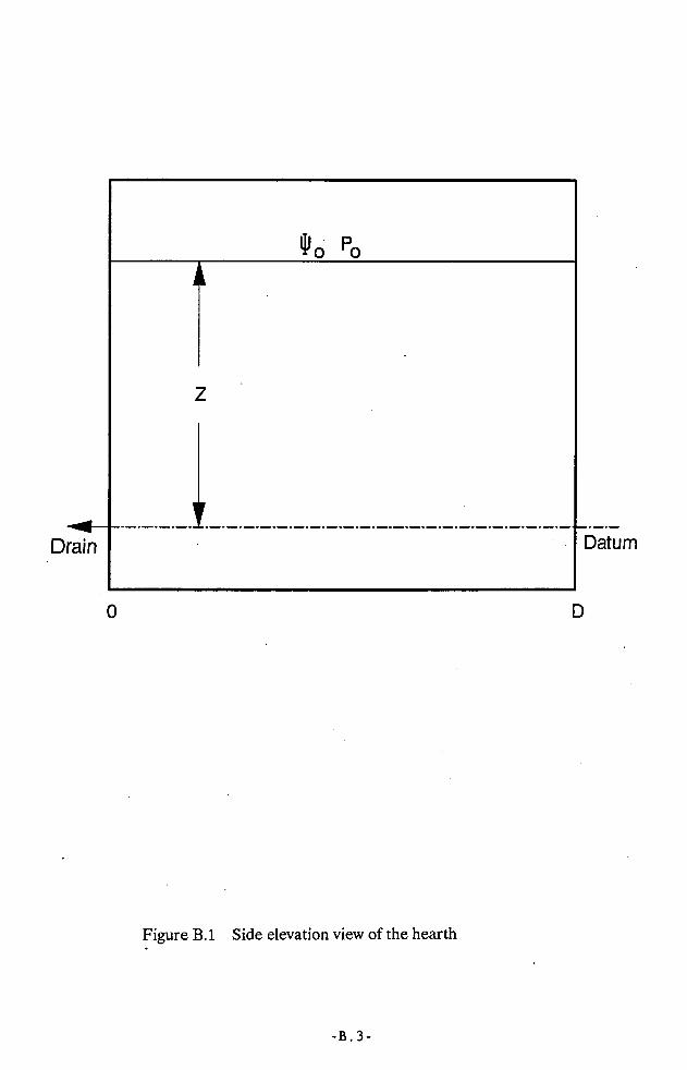
Datum

Figure B. 1 Side elevation view of the hearth

APPENDIX C

The fortran computer code, HD21.F0R, solves for the equations describing the motion of an isothermal liquid in a two-dimensional, homogenous packed bed, with and without a packing-free layer beneath it. The following files are required to execute the program:-

Name of File Description

C0M21.DAT Common blockINIT21.DAT Input data setMESH21.DAT Computational grid data0LD21.DAT Old values of field variablesNEW21.DAT New values of field variablesHEIG21.DAT Surface elevation at completion of simulationRV21.DAT Calculated residual liquid volume at completion

of simulationSTR1...4.DAT Data used for streamline distribution plotsUPDAT.DAT Intermediate values of time, surface elevations and

flowrates

A flowchart of the program is described in Figure (C.l)

-C. 1-

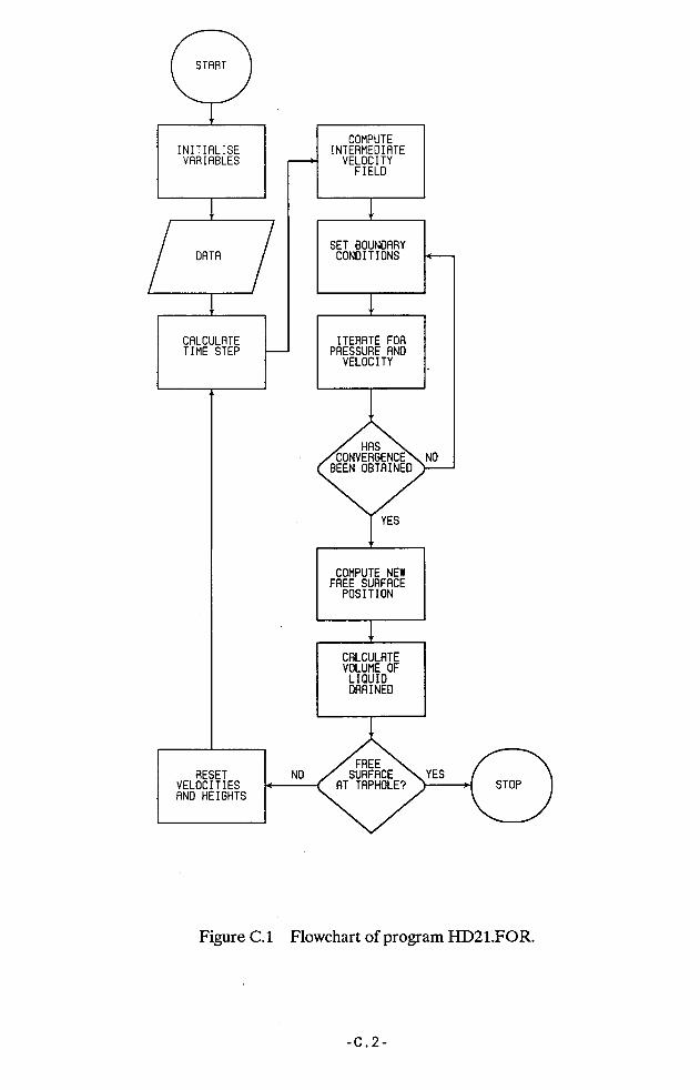
STRRT

/ HRS N. •'CONVERGENCE BEEN OBTRINED

/ FREE \ SURFRCE

RT TRPHOLE?

COMPUTE NEW FREE SURFRCE

POSITION

SET BOUNDRRY CONDITIONS

INITIALISEVARIABLES

RESETVELOCITIES RNO HEIGHTS

COMPUTEINTERMEDIATE

VELOCITYFIELD

ITERATE FOR PRESSURE AND

VELOCITY

CALCULATE TIME STEP

CALCULATE VOLUME OF LIQUID DRAINED

Figure C.l Flowchart of program HD21.FOR.

-C.2-

non

ooo o

ooo o

oo oo

o oo

o o o

o o o o

oooo

oooo

oooo

oooo

o PROGRAM HD21

THIS PROGRAM SOLVES FOR THE FLUID MOTION IN A TWO- DIMENSIONAL BLAST FURNACE WITH AND WITHOUT A COKE-FREE LAYER BENEATH THE COKE BED. THE MAC METHOD AS PROPOSED BY HIRT ET AL (1975) IS USED,i.e. AN UPWIND FINITE DIFFERENCING TECHNIQUE IS USED .> THE NON-CONSERVATIVE FORM OF THE N-S EQN IS USED> A NON-UNIFORM GRID IS USEDAUTHOR: P.ZULLI

SCHOOL OF CHEMICAL ENGINEERING AND INDUSTRIAL CHEMISTRYUNIVERSITY OF NEW SOUTH WALES KENSINGTON, AUSTRALIA

IMPLICIT REAL*8 (A-H.O-Z) INCLUDE 'COM21.DAT'

.INITIALIZE

CALL INITIAL

CALL OTHBC

....COMMENCE ITERATION LOOP ON PRESSURE AND VELOCITYITIME = 1 DO 1 ITNT=1,MAXT IC=0 I CM = 0

. . . .CALCULATE TIME STEP

CALL TSTEP

___ CALCULATE VELOCITIES TO SATISFY N-STOKES OR DARCY'S EQN

CALL MOMEQN

___ CALCULATE THETA AND Q VALUES

CALL CONSTDO 2 ITN=1,MAXITN

. ...SET BOUNDARY CONDITIONS

CALL PRESSBC CALL VELBC

. .. .SWEEP GRID COLUMN BY COLUMN,BOTTOM TO TOP

-C. 3-

DMAX = O.DO DO 3 1=2,NI-1 JSUR = JS(I)

DO 4 J=2 , J SURIF(J.EQ.JSUR.AND.ISURF.EQ.l) GOTO 990

CC ....CALCULATE DIVERGENCE AND PRESSURE CHANGE FOR FULL CELLC

DM = (XV(I+1>J)-XV(I>J))*BDX(I)+(YV(I,J+1)-YV(I,J))*BDY(J) DP = THETA(I,J)*DM GOTO 991

CC ....CALCULATE PRESSURE CHANGE FOR SURFACE CELLC

C

990 DP = (1.ODO-Q(I))*P(I,J-l)+Q(I)*PO-P(I, J)991 IF(DABS(DM).GT.DMAX) IMAX-I

IF(DABS(DM).GT.DMAX) JMAX=JIF(DABS(DM).GT.DMAX) DMAX=DABS(DM)

P(I,J)=P(I,J)+DPXV(I+1,J)=XV(I+1,J)+BETAX(I+1,J)*DP XV(I,J)—XV(I,J)-BETAX(I,J)*DP YV(I,J+1)=YV(I,J+1)+BETAY(I,J+1)*DP YV(I,J)=YV(I,J)-BETAY(I,J)*DP

CC . . ..MAINTAIN DRAIN POINT FLOWRATE C

XV(IDPX+1,JDPY) = FLOW/(DY(JDPY)*WIDTH)4 CONTINUE 3 CONTINUE

CC . . . .CHECK DIVERGENCE C

IF(DMAX.LE.EPSL.AND.IC.GT.0) GOTO 267 IF(ICM.EQ.IC) THENWRITE(6,*)ITNT,ITN,IMAX,JMAX,DMAX ICM = IC+31

END IF IC-IC+1

2 CONTINUE 267 CONTINUE

CC ....NEW FREE SURFACE POSITION CALCULATED

IF(ISURF.EQ.l) THEN CALL FREESUR CALL RV

END IFCC .. ..IF FREE SURFACE HAS REACHED DRAIN-POINT ___ STOPC

IF(ISURF.EQ.1.AND.H(2).LE.TERMH) GOTO 1000 IF(ITNT.NE.MAXT) GOTO 275

CC ....STORE ALL NECESSARY DATA C

CALL OUTPUT

-C.4-

o o

o no

o o

o o

oo on

ooo

onn

oooo .SET ADVANCED VELOCITIES AND HEIGHTS INTO OLD ARRAYS

>»» XVN () , YVN () AND HN() AND CALCULATE NEW SURFACE CELLS.

275 CALL RESET CALL SURCEL

....WRITE OUT DATA NECESSARY FOR STREAMLINE AND ISOTHERM PLOTSCALL PLOTS

1 CONTINUE GOTO 1001

....FINISH RUN

1000 CONTINUE CALL OUTPUTFINISH = 1.0D0/FINISH

1001 CONTINUE STOP END

SUBROUTINE INITIAL

IMPLICIT REAL*8 (A-H,0-Z) INCLUDE 'COM21.DAT'

....OPEN DATA FILES

OPEN(UNIT=4,FILE='INIT21.DAT',STATUS='OLD') OPEN(UNIT-7, FILE-'MESH21.DAT',STATUS='OLD') OPEN(UNIT-10, FILE-'RV21.DAT',STATUS='NEW')

___ INITIALIZATIONREAD(4,*)NI,MI,DT,EPSL,MAXT,MAXITN,FLOWI,WIDTH,PO,HLIQREAD(4,*)HK,RHOS,VIS SREAD(4,*)POR,IDPX,JDPYREAD(4,*)JFLAG,UPWIND,WI,WS,TERMHREAD(4,*)ISURF,IPLOT,RCHREAD(4,*)(JFLP(I),1-1,NI)READ(4,*)(JFLPT(I),I-1,NI)OPEN(UNIT-2,FILE-'NEW21.DAT',STATUS-'NEW')OPEN(UNIT-3,FILE-'HEIG21.DAT',STATUS-'NEW')M-MI-1 N=NI-1 GX=0.0D0 GY-981.0D0 DTIN = DT

.'. . . READ MESH DATA

READ(7,*)(DX(I),1=1,NI) READ(7,*)(DY(J),J-l.MI)

DO 20 1=1,NIBDX(I) = 1.0D0/DX(I)

20 CONTINUE

-C.5-

no

non

non

DO 21 J=1,MIBDY(J) = 1.0D0/DY(J) 21 CONTINUE

. . . .CALCULATE CROSS-SECTIONAL AREA OF MODEL

XAREA = 0.0D0 DO 200 1=2,NXAREA = XAREA+DX(I)

200 CONTINUEXAREA = XAREA*WIDTH

....OPEN OLD DATA FILE AND READ IN DATA

IF(JFLAG.EQ.1) THENOPEN(UNIT-1, FILE-'0LD21.DAT',STATUS='OLD') READ(1,*)TIME READ(1,*)VOL DO 1 1=1,NI+1 DO 2 J=1,MI+1READ(1,*)XVN(I,J),YVN(I,J),P(I,J)

2 CONTINUE1 CONTINUE

DO 3 1=1,NI+1 READ(1,*)HN(I)

3 CONTINUE END IF

CLOSE(UNIT-1, STATUS-'SAVE')....FIRST RUN

CIF(JFLAG.EQ.O) THEN

TIME = 0.0D0 DO 5 J=1,MI+1 DO 6 1=1,NI+1XVN(I,J) = 0.0D0YVN(I,J) = 0.0D0

6 CONTINUE5 CONTINUE

DO 7 1=1,NI+1 HN(I)=HLIQ

7 CONTINUEEND IFCALL SURCELDO 9 1=2,N

PT = PO PTEMP = 0.0D0

DO 10 J =M,2,-1 IF(J.EQ.M) THENHGHT = HLIQ-SUMDY(I)PTEMP = RHOS*GY*HGHT GOTO 11

ELSE" HGHT = 0.5D0*(DY(J)+DY(J+1))PTEMP = RHOS*GY*HGHT

ENDIF11 PT = PT+PTEMP P(I,J) = PT 10 CONTINUE 9 CONTINUE

ENDIF

-C.6-

oooo

oooo

oo

oo oo

ooRETURNEND

SUBROUTINE PRESSBC

IMPLICIT REAL*8 (A-H.O-Z) INCLUDE 'COM2I.DAT'DO 5 J=2,MP(1,J)-P(2,J)P(NI,J)=P(NI-1,J)

5 CONTINUEDO 6 1=2,N J SUR=J S(I)P(I,JSUR+1) = PO P(I,1)=P(I,2)

6 CONTINUE RETURN END

SUBROUTINE VELBC

IMPLICIT REAL*8 (A-H.O-Z)INCLUDE 'C0M21.DAT'XVDP=XV(IDPX+1,JDPY)DO 1 J=2,MI XV(2,J)=0.0D0 XV(NI,J)=0.0D0 YV(1,J)=YV(2,J)YV(NI,J)=YV(N,J)

1 CONTINUEDO 2 1=2,NI+1 YV(I,2)=0.0D0 XV(I,1)=XV(1,2)XV (I, MI) =XV (I, M)

2 CONTINUEDO 3 1=2,NI J SUR=J S(I)IF(JS(I).GT.JS(I-l)) XV(I,JSUR) = XV(I,JSUR-1)IF(JS(I).GT.JS(I+1)) XV(I+1,JSUR) = XV(I+1,JSUR-1)XV(I,JSUR+1) = XV(I,JSUR)IF(ISURF.EQ.O) THENYV(I,JSUR+1) = FLOW/XAREA

ELSEJSL = JS1(I)JSR = JS1(I+1)DAL = HN(I)-SUMD(I)DAR = HN(1+1)-SUMD(1+1)IF(JSL.LT.JSUR) DAL = 0.0D0 IF(JSR.LT.JSUR) DAR = 0.0D0YV(I,JSUR+1) = YV(I,JSUR)-BDX(I)*(DAR*XV(I+1,JSUR)

@ -DAL*XV(I,J SUR))YV(I,JSUR+1) = YV(I,JSUR)-(DY(JSUR)*BDX(I)*(XV(I+I,JSUR)

@ -XV(I,JSUR)))END IF

3 CONTINUE

-C.7-

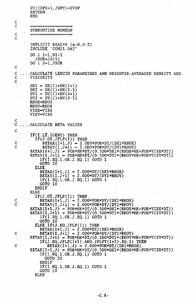
oo

oo o

on

o o o

o oo

on

XV(IDPX+1,JDPY)=XVDPRETURNEND

SUBROUTINE MOMEQN

IMPLICIT REAL*8 (A-H.O-Z) INCLUDE 'C0M21.DAT'DO 1 1=1,NI-1

J SUR=J S(I)DO 1 J=1,J SUR

.CALCULATE LENGTH PARAMETERS AND WEIGHTED-AVERAGED DENSITY AND VISCOSITYDX1 = DX(I)+DX(I+1)DX2 = DX(I)+DX(I-1)DY1 = DY(J)+DY(J+1)DY2 = DY(J)+DY(J-1)RHOX=RHOSRHOY=RHOSVISX=VISSVISY=VISS

. . ..CALCULATE BETA VALUES

IF(I.LT.ICENT) THEN IF(J.GE.JFLP(I)) THEN

BETAX(1+1,J) = 2.ODO*POR*DT/(DX1*RHOX)BETAY(I,J+l) = 2.ODO*POR*DT/(DY1*RHOY)

BETAX(I+1,J) = POR*HK*DT/(0.5DO*DX1*(RHOX*HK+POR*VISX*DT)) BETAY(I,J+1) = POR*HK*DT/(0.5DO*DY1*(RHOY*HK+POR*VISY*DT))

IF(I.EQ.l.OR.J.EQ.l) GOTO 1 GOTO 20

ELSEBETAX(I+1,J) = 2.ODO*DT/(DX1*RHOX)BETAY(I,J+l) = 2.ODO*DT/(DY1*RHOY)IF(I.EQ.l.OR.J.EQ.l) GOTO 1 GOTO 10

END IF ELSE

IF(J.GT.JFLP(I)) THENBETAX(I+1,J) = 2.0DO*POR*DT/(DX1*RHOX)BETAY(I,J+1) = 2.ODO*POR*DT/(DY1*RHOY)

BETAX(I+1,J) = POR*HK*DT/(0.5DO*DX1*(RHOX*HK+POR*VISX*DT)) BETAY(I,J+l) = POR*HK*DT/(0.5DO*DY1*(RHOY*HK+POR*VISY*DT))

IF(I.EQ.l.OR.J.EQ.l) GOTO 1 GOTO 20

ELSE IF(J.EQ.JFLP(I)) THENBETAX(I+1,J) = 2.ODO*DT/(DX1*RHOX)

C BETAY(I,J+l) = 2.ODO*POR*DT/(DY1*RH0Y)BETAY(I,J+l) = POR*HK*DT/(0.5DO*DY1*(RHOY*HK+POR*VISY*DT))

IF(J.EQ.JFLP(I+1).AND.JFLPT(1+1).EQ.l) THEN C BETAX(I+1,J) = 2.ODO*POR*DT/(DX1*RHOX)

BETAX(1+1,J) = POR*HK*DT/(0.5DO*DX1*(RHOX*HK+POR*VISX*DT)) IF(I.EQ.l.OR.J.EQ.l) GOTO 1 GOTO 20

ENDIFIF(I.EQ.l.OR.J.EQ.l) GOTO 1 GOTO 10

ELSE

-C.8-

o o

o o

o o

o oo

oono

nooo

o oo

oBETAX(I+1,J) = 2.ODO*DT/(DX1*RHOX)BETAY(I, J+l) = 2.ODO+DT/(DY1*RH0Y) IF(I.EQ.l.OR.J.EQ.l) GOTO 1 GOTO 10

ENDIF END IF

....CALCULATE INTERMEDIATE X-VELOCITY FIELD (NAVIER-STOKES)

10 SGU = SIGN(1.DO,XVN(1+1,J))DXA = DX(I)+DX(I+1)+UPWIND*SGU*(DX(I+1)-DX(I))DUDR = (XVN(I+2,J)-XVN(I+1,J))*BDX(I+1)DUDL = (XVN(1+1,J)-XVN(I,J))*BDX(I)CONUX = XVN(I+1,J)*(DX(I)*DUDR+DX(I+1)*DUDL+UPWIND*SGU*(DX(I+1)*

@ DUDL-DX(I)*DUDR))/DXAVBT = (DX(I)*YVN(I+1,J+1)+DX(I+1)*YVN(I,J+1))/DX1 VBB = (DX(I)*YVN(I+1,J)+DX(I+1)*YVN(I,J))/DX1 VAV = 0.5D0*(VBT+VBB)SGV = SIGN(l.DO.VAV)DYA = 0.5D0*(DY1+DY2+UPWIND*SGV*(DY1-DY2))DUDTY = (XVN(I+1,J+1)-XVN(I+1,J))/(0.5D0*DY1)DUDBY = (XVN(I+1,J)-XVN(I+1,J-1))/(0.5D0*DY2)CONUY = 0.5D0*VAV*(DY2*DUDTY+DY1*DUDBY+UPWIND*SGV*(DY1*DUDBY-

@ DY2*DUDTY) ) /DYAVISCX = (8.0D0/(3.0D0*DXl*RHOX))*(VISC(I+l,J)

..,@*(XVN(I+2,J)-XVN(I+1,J))@*BDX(I+1)-VISC(I,J)*(XVN(I+1,J)-XVN(I,J))*BDX(I)-0.5D0*BDY(J)* @(VISC(I+1,J)*(YVN(I+1,J+1)-YVN(I+1,J))-VISC(I,J)*(YVN(I,J+l)- @YVN(I,J))))+2.0D0*BDY(J)*(VISC1*((XVN(I+1,J+1)-XVN(1+1,J))/DY1+ @(YVN(I+1,J+l)-YVN(I,J+1))/DX1)-VISC2*((XVN(I+1,J)-XVN(I+1,J-l)) @/DY2+(YVN(I+l,J)-YVN(I,J))/DX1))VISCX - ((4.0D0/DX1)*VISX*((XVN(1+2,J)-XVN(I+1,J)) @*BDX(I+1)-(XVN(I+1,J)-XVN(I,J))*BDX(I))@+2.0D0*BDY(J)*VISX*((XVN(1+1,J+l)-XVN(1+1,J))/DY1+(3 (YVN(1+1,J+l)-YVN(I,J+l))/DXl-(XVN(I+1,J)-XVN(1+1,J-1))@/DY2+(YVN(1+1, J) -YVN(I, J))/DX1))/RHOX PT=(P(I,J)-P(I+l,J))*2.0D0/(DXl*RHOX)XV(1+1,J)=XVN(1+1,J)+DT*(PT-GX-CONUX-CONUY+VISCX)IF(I.GE.ICENT.AND.J.EQ.JFLP(I)) GOTO 20

___CALCULATE INTERMEDIATE Y-VELOCITY FIELD (NAVIER-STOKES)

SGV = SIGN(1.DO,YVN(I,J+l))DYA = DY(J)+DY(J+1)+UPWIND*SGV*(DY(J+1)-DY(J))DVDR = (YVN(I,J+2)-YVN(I,J+l))*BDY(J+l)DVDL = (YVN(I,J+l)-YVN(I,J))*BDY(J)CONVY = YVN(I,J+1)*(DY(J)*DVDR+DY(J+1)*DVDL+UPWIND*SGV*(DY(J+1)*

(a DVDL - DY (J) *DVDR)) /DYAUBT = (DY(J)*XVN(I+1,J+1)+DY(J+1)*XVN(I+1,J))/DY1 UBB = (DY(J)*XVN(I,J+1)+DY(J+1)*XVN(I,J))/DY1 UAV = 0.5D0*(UBT+UBB)SGU = SIGN(1.DO,UAV)DXA = 0.5D0*(DX1+DX2+UPWIND*SGU*(DX1-DX2))DVDTX = (YVN(I+1,J+l)-YVN(I,J+l))/(0.5D0*DX1)DVDBX - (YVN(I,J+l)-YVN(I-1,J+l))/(0.5D0*DX2)CONVX = 0.5D0*UAV*(DX2*DVDTX+DX1*DVDBX+UPWIND*SGU*(DX1*DVDBX-

@ DX2*DVDTX))/DXAVISCY = (8.0D0/(3.ODO*DY1*RHOY))*(VISC(I,J+l)

.@*(YVN(I,J+2) - YVN (I, J+l))@*BDY(J+1)-VISC(I,J)*(YVN(I,J+1)-YVN(I,J))*BDY(J)-0.5D0*BDX(I)* @(VISC(I,J+1)*(XVN(I+1,J+1)-XVN(I>J+1))-VISC(I,J)*(XVN(I+1,J)- @XVN(I,J))))+2.0D0*BDX(I)*(VISC1*((XVN(I+1,J+1)-XVN(I+1>J))/DY1+

-C.9-

noon

o o

o o

noon

no

o o

on

o@(YVN(I+1,J+l)-YVN(I,J+l))/DXl)-VISC2*((XVN(I,J+l)-XVN(I,J)) @/DYl+(YVN(I,J+l)-YVN(I-l.J+l))/DX2))VISCY = ((4.0D0/DY1)*VISS*(YVN(I, J+2)-YVN(I,J+l))

@*BDY(J+1)-(YVN(I,J+l)-YVN(I,J))*BDY(J)@+2.0D0*BDX(I)*VISS*((XVN(I+1,J+l)-XVN(I+1,J))/DY1+ @(YVN(I+1,J+l)-YVN(I,J+l))/DXl-(XVN(I,J+l)-XVN(I,J))@/DYl+ ('YVN (I, J+l) - YVN (I -1, J+l)) /DX2)) /RHOY PT = (P(I,J)-P(I,J+l))*2.0D0/(DYl*RHOY)GYT = (1.0D0-0.5D0*ALPHA*(TN(I,J+l)+TN(I,J)-2.0D0*TO))*GY GYT = GYYV(I, J+l) = YVN(I,J+l)+DT*(PT-GYT-CONVX-CONVY+VISCY)GOTO 1

. . ..CALCULATE INTERMEDIATE X-VELOCITY FIELD (DARCY'S)

20 ETA = RHOX*HK/(RHOX*HK+POR*VISX*DT)20 ETA = 1.0D0-(VISX*POR*DT/(HK*RHOX))XV(I+1,J) = ETA*XVN(I+1,J)+BETAX(I+1,J)*(P(I,J)-P(I+1,J))

. . ..CALCULATE INTERMEDIATE Y-VELOCITY FIELD (DARCY'S)

ETA = 1.0DO-(VISY*POR*DT/(HK*RHOY))YV(I, J+l) = ETA*YVN(I,J+1)+BETAY(I,J+1)*(P(I,J)-P(I,J+1))

@ -GY*POR*DTETA = RHOY*HK/(RHOY*HK+POR*VISY*DT)YV(I,J+l) = ETA*YVN(I,J+1)+BETAY(I>J+1)*(P(I,J)-P(I,J+1)

@ - 0.5DO*RHOY*DY1*GY)1 CONTINUE

FLOW = - FLOWIIF(DABS(FLOW).GE.FLOWI) FLOW = -FLOWI XV(IDPX+1,JDPY) = FLOW/(WIDTH*DY(JDPY))RETURNEND

SUBROUTINE FREESUR

IMPLICIT REAL*8 (A-H.O-Z)INCLUDE 'COM21.DAT'DA = 0.0D0 DAI = O.ODO DO 1 1=2,NI JST = JS1(I)XVS = XVN(I.JST)HMS = HN(I)-SUMD(I)COI = HMS/DY(JST)JL1 = JS(I-l)JR1 = JS(I)BDX1 = 1.0D0/(DX(I)+DX(I-1))YVS = (C0I*(YVN(I-1,JL1+1)*DX(I)+YVN(I,JR1+1)*DX(I-1))+ @(i.ODO-COI)*(YVN(I-l,JST)*DX(I)+YVN(I,JST)*DX(I-1)))*BDX1

IF(JS(I-1).EQ.JDPY+1) THENYVS = (C0I*(YVN(I-1,JL1)*DX(I)+YVN(I,JR1)*DX(I-1))+ @(i.ODO-COI)*(YVN(I-l,JST)*DX(I)+YVN(I,JST)*DX(I-1)))*BDX1 END IFIF(MS.EQ.l) THEN IF(JS(I-1).EQ.JST) THENCOI = (HMS+DY(JST-l)*0.5D0)/(0,5D0*(DY(JST-1)+DY(J ST))) XVS = (1.ODO-COI)*XVN(I,JST-l)+COI*XVN(I,JST)

END IFIF(JS(I-1).LT.JST) THEN

-C.10-

COI = (HMS+DY(JST-l)+DY(JST-2)*0.5D0)/@ (0.5D0*(DY(JST - 1)+DY( JST- 2)) )

XVS = (1.0D0-COI)*XVN(I,J ST-2)+COI*XVN(I,JST-1)ENDIFIF(JS(I-1).GT.JST) THEN

COI = (HMS+DY(JST-1)*0.5D0)/(0.5D0*(DY(JST-1)+DY(JST))) XVS = (1.0DO-COI)*XVN(I,JST-1)+COI*XVN(I,JST)

ENDIFIF(JS(I-1).EQ.JST) THEN

COI = (HMS+DY(JST-1))/DY(JST-l)YVL = (1.ODO-COI)*YVN(I-1,JST-l)+COI*YVN(I-l.JST)

ENDIFIF(JS(I-1).LT.JST) THEN

COI = (HMS+DY(JST-l)+DY(JST-2))/DY(JST-2)YVL = (1.0DO-COI)*YVN(I-l,JST-2)+COI*YVN(I-l,JST-l)

ENDIFIF(JS(I-1).GT.JST) THEN

COI = HMS/DY(JST)YVL = (1.ODO-COI)*YVN(I-1,JST)+COI*YVN(I-1,JST+1)

ENDIFIF(JS(I).EQ.JST) THEN

COI = (HMS+DY(JST-1))/DY(JST-1)YVR = (1.0DO-COI)*YVN(I,JST-1)+COI*YVN(I,JST)

ENDIFIF(JS(I).LT.JST) THEN

COI = (HMS+DY(JST-1)+DY(JST- 2))/DY(JST- 2)YVR = (1.0D0-COI)*YVN(I,J ST- 2)+COI*YVN(I,JST-1)

ENDIFIF(JS(I).GT.JST) THEN

COI = HMS/DY(JST)YVR - (1.0DO-COI)*YVN(I,JST)+COI*YVN(I,JST+1)

ENDIFYVS = (DX(I)*YVL+DX(I-1)*YVR)/(DX(I-1)+DX(I))ENDIFIF(MS.EQ.l) THEN COI = HMS/DY(JST)YVL = (1.0DO-COI)*YVN(I-1,JST)+COI*YVN(I-1,JST+1) IF(JS(I-1).LT.JST) THEN

COI = (DY(JST-1)+HMS)/DY(JST-l)YVL = (1.ODO-COI)*YVN(I-1,JST-l)+COI*YVN(I-I,JST)

ENDIFIF(JS(I-1).GT.JST) THEN

COI - (DY(JST+1)+DY(JST)-HMS)/DY(JST+1)YVL = (1.0DO-COI)*YVN(I-l,JST+2)+COI*YVN(I-l,JST+1)

ENDIFCOI = HMS/DY(JST)YVR = (1.0DO-COI)*YVN(I,JST)+COI*YVN(I,JST+1)IF(JS(I).LT.JST) THEN

COI = (DY(JST-1)+HMS)/DY(JST-1)YVR = (1.ODO-COI)*YVN(I,J ST-l)+COI*YVN(I,JST)

ENDIFIF(JS(I).GT.JST) THEN

COI =* (DY(JST+1)+DY(JST) -HMS)/DY( JST+1)YVR = (1.0DO-COI)*YVN(I,JST+2)+COI*YVN(I,JST+1)

ENDIFIF(JS(I-1).EQ.JDPY+1) THEN YVL = YVN(I-1,JDPY+1)

ENDIFIF(JS(I).EQ.JDPY+1) THEN YVR = YVN(I,JDPY+1)

ENDIFYVS = (DX(I)*YVL+DX(I-1)*YVR)/(DX(I-1)+DX(I))ENDIF

-C.ll-

o o

oooo

oo

oo

IF(I.EQ.2.OR.I.EQ.NI) XVS = 0.0D0IF(XVS.LT.0.0D0) DELH=(HN(1+1)-HN(I))*BDX(I)IF(XVS.GT.0.0D0) DELH=(HN(I)-HN(I-l))*BDX(I-1) IF(XVS.EQ.O.ODO) DELH=0.0D0 H(I)=HN(I)+DT*(YVS-XVS*DELH+RCH)/POR IF(I.LT.NI) DA = DA+YVR*DX(I)*WIDTH IF(I.GT.2) DAI = DAl+YVL*DX(I-l)*WIDTH

1 CONTINUEWRITE(6,*)'YVR',DA WRITE(6,*)'YVL',DAI H(NI+1)=H(NI)H(1)=H(2)RETURNEND

SUBROUTINE RESET

IMPLICIT REAL*8 (A-H,0-Z) INCLUDE 'COM21.DAT'DO 1 I-l.NI+l HN(I) = H(I)

DO 2 J-l.MI+lXVN(I.J) = XV(I,J) YVN(I.J) = YV(I,J)

2 CONTINUE 1 CONTINUERETURNEND

SUBROUTINE SURCELCC •C ....SET SURFACE CELL POSITIONSC

IMPLICIT REAL*8 (A-H,0-Z)INCLUDE 'COM21.DAT'

DO 1 1=2,NIAVHGT = (HN(I)+HN(I+1))*0.5D0- AVHT = HN(I)SUM = 0.0D0

DO 2 J-2.MI SUMT = SUM SUM = SUM+DY(J)IF(SUMT.LT.AVHGT.AND.SUM.GE.AVHGT) THEN

JS(I) = JSUMDY(I) = SUMT+0.5D0*DY(J)

ENDIFIF(SUMT.LT.AVHT.AND.SUM.GE.AVHT) THEN

JS1(I) = J SUMD(I) = SUMT

ENDIF2 CONTINUE 1 CONTINUE JS(NI)=JS(N)JS(1)=JS(2)SUMDY(l) = SUMDY(2)SUMDY(NI) = SUMDY(NI-1)RETURNEND

-C.12-

non noo

n no

n oo

oooo

oooo SUBROUTINE RV

IMPLICIT REAL*8 (A-H.O-Z) INCLUDE 'C0M21.DAT' .

.THIS PROGRAM CALCULATES THE VOLUME OF LIQUID THAT HAS BEEN EVACUATED FROM A 2-DIMENSIONAL BLAST FURNACE MODEL.

. . . .ORIGINAL VOLUME OF LIQUID

XLEN = 0.0D0 DO 1 1=2,NXLEN = XLEN+DX(I)

1 CONTINUEOVOL = HLIQ*WIDTH*XLEN*POR

....PRESENT VOLUME OF LIQUID

IF(TIME.LE.DT) THEN VOLT = OVOL

ELSEVOLT = VOL

END IFVOL = 0.0D0 DO 2 1=2,N

DVOL = DX(I)*WIDTH*(H(I)+H(I+1))*0.5D0 VOL = VOL+DVOL

2 CONTINUEVOL = VOL*PORVOLOUT = (OVOL-VOL)*RHTO*l.OE-6FLOW = (VOLT-VOL+DT*RCH*WIDTH*XLEN)*RHTO*60.0E-6/DT VOLFLOW = (VOLT-VOL+DT*RCH*WIDTH*XLEN)/DTOPEN(UNIT=23,FILE='UPDAT.DAT',STATUS='NEW')WRITE(23,*)TIME,ITN WRITE(23,*)VOLOUT WRITE(23,*)FLOW WRITE(23,*)VOLFLOW WRITE(23, *)(H(I),1=1,NI)CLOSE(UNIT=23,STATUS='SAVE')RETURNEND

SUBROUTINE TSTEP

IMPLICIT REAL*8 (A-H.O-Z) INCLUDE 'COM21.DAT'

___ CALCULATION OF TIME STEP

-C.13-

o o

o o

o o

o o

IF(ISURF.EQ.O) THENIF(TIME.EQ.0.DO) GOTO 13 DT = DTIN DO 11 1=1,NI-1 DO 11 J=1,MI-1

IF(ABS(XVN(1+1,J)).GT.0.0001) THEN IF((DX(I)+DX(I+1))*0.5D0/DABS(XVN(I+1,J)).LT.DT)

@ DT = (DX( I )+DX(I+l)) *0.5DO/DABS (XVN(1+1,J))ENDIFIF(ABS(YVN(I,J+l)).GT.0.0001) THEN IF((DY(J)+DY(J+1))*0.5D0/DABS(YVN(I, J+l)).LT.DT)

@ DT = (DY(J)+DY(J+1))*0.5D0/DABS(YVN(I,J+l))ENDIF

11 CONTINUE 13 DT = 0.25D0*DT

ENDIFTIME =TIME+DTRETURNEND

SUBROUTINE OUTPUT

IMPLICIT REAL*8 (A-H,0-Z)INCLUDE 'COM21.DAT'WRITE(2,*)TIME WRITE(2,*)VOL DO 1 1=1,NI+1 DO 1 J=1,MI+1WRITE(2, *)XV(I,J),YV(I,J),P(I,J)

1 CONTINUEDO 2 1=1,NI+1 WRITE(2,*)HN(I)

2 CONTINUEWRITE(3,*)ITNT,ITN WRITE(3,10)(HN(I),I=1,NI)

10 FORMAT(IX,8F10.5)RETURNEND

SUBROUTINE PLOTS

IMPLICIT REAL*8 (A-H.O-Z) INCLUDE 'COM21.DAT'

IF(IPLOT.EQ.l) THEN IF(ITN.EQ.120) THENOPEN(UNIT=13,FILE='STR1.DAT',STATUS='NEW') GOTO 4290

ELSE IF(ITNT.EQ.600) THENOPEN(UNIT=13,FILE='STR2.DAT',STATUS='NEW') GOTO 4290

ELSE IF(ITNT.EQ.1200) THENOPEN(UNIT=13,FILE='STR3.DAT',STATUS='NEW') GOTO 4290

ELSE IF(ITNT.EQ.3240) THENOPEN(UNIT=13,FILE='STR4.DAT',STATUS='NEW') GOTO- 4290

ENDIF

-C.14-

o o

o o

GOTO 42994290 WRITE(13,*)NI,MI,JDPY

WRITE(13,*)(JFLP(I),1=1,NI)WRITE(13,*)(JFLPT(I),I=1,NI)WRITE(13,*)(DX(I),1=1,NI)WRITE(13,*)(DY(J),J=1,MI)

DO 4289 1=2,NI WRITE(13,*)JS(I)

J SUR=J S(I)WRITE(13,*)(XV(I,J),J=2,JSUR)

4289 CONTINUE4299 CONTINUE

RETURNEND

SUBROUTINE CONST

IMPLICIT REAL*8 (A-H.O-Z)INCLUDE 'C0M21.DAT'DO 1 1=2,N JSUR = JS(I)Q(I) = 0.5D0*(DY(JSUR-l)-l-DY(JSUR) )/(0.5D0*(HN(I)+HN(I+1)+

@ DY(JSUR-1)+DY(JSUR))-SUMDY(I))DO 1 J=2,JSUR

IF(J.LT.JSUR.AND.ISURF.EQ.l) THEN IF(J.EQ.JSUR-l) THEN

W = WS ELSE

W = WI ENDIF

ELSEW = WI

ENDIFTHETA(I,J) = -W/(BETAX(I+1,J)+BETAX(I,J))*BDX(I)+

@ (BETAY(I,J+1)+BETAY(I,J))*BDY(J) '1 CONTINUE

RETURN END

-C.15-

APPENDIX D

The fortran computer code, HD31.F0R, solves for the equations describing the motion of an isothermal liquid in a three-dimensional, homogenous packed bed, with and without a packing-free layer beneath it. The following files are required to execute the program:

Name of File Description

C0M31.DAT Common blockINIT3D.DAT Input data setMESH.DAT Computational grid dataOLD.DAT Old values of field variablesNEW.DAT New values of field variablesHEIG.DAT Surface elevation at completion of simulationRV3D.DAT Calculated residual liquid volume at

of simulationcompletion

ELEVL...4.DAT Surface elevations at specified timessimulation

during the

UPDAT.DAT Intermediate values of time, surfaceflowrates

elevations and

A flowchart of the program is described in Figure (D.l).

-D.l-

START

s HAS ^CONVERGENCE^ BEEN OBTAINED

/ FREE \ SURFACE AT TAPHOLE?

COMPUTE NEW FREE SURFACE POSITION

COMPUTEINTERMEDIATEVELOCITYFIELDINITIALISEVARIABLES

ITERATE FOR PRESSURE AND VELOCITY

SET BOUNDARY CONDITIONS

CALCULATE TIME STEP

CALCULATE VOLUME OF LIQUID DRAINED

RESETVELOCITIES AND HEIGHTS

Figure D.l Flowchart of program HD31.FOR.

-D.2-

ooo

o o o

noo o

oo o

o o o o o o o o o o o o o o o o o o o o

PROGRAM HD31

THIS PROGRAM SOLVES NUMERICALLY, THE FLUID MOTION IN A 3-DIMENSIONAL BLAST FURNACE WITH OR WITHOUT A COKE-FREE LAYER BENEATH THE COKE BED. THE MAC METHOD AS PROPOSED BY HIRT ET AL (1975). AN UPWIND FINITE DIFFERENCING TECHNIQUE IS USED .> THE ONE PHASE, SLAG, IS SIMULATED.> THIS PROGRAM USES VELOCITIES AND PRESSURES.> PROPERTIES ARE DEFINED BY DENSITY, DYNAMIC> VISCOSITY AND PERMEABILITY.AUTHOR: P. ZULLI

SCHOOL OF CHEMICAL ENGINEERING AND INDUSTRIAL CHEMISTRYUNIVERSITY OF NEW SOUTH WALES KENSINGTON AUSTRALIA

DATE : OCTOBER 1984

IMPLICIT REAL*8 (A-H.O-Z)INCLUDE 'COM31.DAT'

____INITIALISECALL INITIAL CALL BETA

____PRESSURE AND VELOCITY ITERATION LOOPDO 1 ITNT=1,MAXT

CALL MOMEQN IC = 0D0 ICM = 0D0

DO 2 ITN=1,MAXITN CALL BC

DMAX =0.0 DO 3 J=2,JUB

ILB = IL(J)IUB = IU(J)

DO 4 I-ILB.IUB KSUR = KS(I,J)

DO 5 K=2,KSURIF(K.EQ.KSUR) GOTO 20

IF(I.EQ.ILB) GOTO 30 IF(I.EQ.IUB) GOTO 40

....CALCULATE DIVERGENCE AND PRESSURE CHANGE FOR FULL CELLDM = (XV(I+1,J,K)-XV(I,J,K))*BDX(I)

@ +(YV(I,J+1,K)-YV(I,J,K))*BDY(J)@ +(ZV(I,J,K+l)-ZV(I,J,K))*BDZTHETA = (BETAX(I+1,J,K)+BETAX(I,J,K))*BDX(I)

@ +(BETAY(I,J+1,K)+BETAY(I,J,K))*BDY(J)(a + (BETAZ (I, J , K+l) 4-BETAZ (I, J , K) ) *BDZ

GOTO 31....CALCULATE DIVERGENCE AND PRESSURE CHANGE FOR BOUNDARY CELL30 DM = XV(I+1,J,K)*DY(J)*DZ-YV(I,J,K)*DX(I)*DZ

@ +(ZV(I,J,K+1)-ZV(I,J,K))*DX(I)*DY(J)*0.5THETA = BETAX(I+1,J,K)*DY(J)*DZ+BETAY(I,J,K)*DX(I)*DZ

(a +(BETAZ(I,J,K+1)+BETAZ(I,J,K))*DX(I)*DY(J)*0.5GOTO 31

-D. 3-

cC ....DRAIN POINT CELLC

40 IF(I.EQ.IDPX.AND.J.EQ.JDPY.AND.K.EQ.KDPZ) THEN DM = (XV(I+1, J ,K)-XV(I,J,K))*DY(J)*DZ

@ -YV(I,J,K)*DX(I)*DZ@ +(ZV( I, J , K+l) - ZV( I, J , K) )*DX(I )*DY( J )*0.5

THETA = (BETAX(I+1,J,K)+BETAX(I,J,K))*DY(J)*DZ @ +BETAY(I,J,K)*DX(I)*DZ@ +(BETAZ(I,J,K+1)+BETAZ(I,J,K))*DX(I)*DY(J)*0.5ELSEDM = -XV(I,J,K)*DY(J)*DZ-YV(I,J,K)*DX(I)*DZ

(a +(ZV(I,J,K+1)-ZV(I,J,K))*DX(I)*DY(J)*0.5THETA = BETAX(I,J,K)*DY(J)*DZ+BETAY(I,J,K)*DX(I)*DZ

@ +(BETAZ(I,J,K+1)+BETAZ(I,J,K))*DX(I)*DY(J)*0.5ENDIF

31 DP = -W*DM/THETA GOTO 50

CC ... CALCULATE PRESSURE CHANGE FOR SURFACE CELLC

20 CONTINUEIF(I.EQ.ILB) THENQ=((HN(I,J)+HN(1+1,J)+HN(1+1,J+l))/3.0)-(DFLOAT(KSUR)- 2.5)*DZ ELSE IF(I.EQ.IUB) THENQ=((HN(I,J)+HN(I+1,J)+HN(I,J+l))/3.0)-(DFLOAT(KSUR)-2.5)*DZ ELSEQ=((HN(I,J)+HN(I+1,J)+HN(I,J+1)+HN(I+1,J+l))/4.0)

(§ - (DFLOAT(KSUR) -2.5)*DZENDIFDP = P(I,J,KSUR-l)+DZ*(PO-P(I,J,KSUR-2))/(Q+DZ)+

(§ 0.5*DZ*DZ*(((PO-P(I,J,KSUR-1))/Q)-((P(I,J,KSUR-1)@-P(I,J.KSUR-2))/DZ))/(Q+DZ)-P(I,J,KSUR)

50 IF(DABS(DM).GT.DMAX) THEN NMAX = I MMAX = J LMAX = K

DMAX = DABS(DM)ENDIF

P(I,J,K) = P(I,J,K)+DPCCC ... ADJUST VELOCITIESC

XV(1+1,J,K) = XV(1+1,J,K)+BETAX(1+1,J,K)*DP XV(I,J,K) = XV(I,J,K)-BETAX(I,J,K)*DPYV(I,J+l,K) = YV(I,J+l,K)+BETAY(I,J+l,K)*DP YV(I,J,K) = YV(I,J,K)-BETAY(I,J,K)^DPZV(I,J,K+1) = ZV(I(J,K+1)+BETAZ(I,J,K+1)*BP ZV(I,J,K) = ZV(I,J,K)-BETAZ(I,J,K)*DP XV(IDPX+1,JDPY,KDPZ) = FLOW*BDY(JDPY)*BDZ

5 CONTINUE 4 CONTINUE 3 CONTINUE

CC . ...CHECK MAXIMUM DIVERGENCEC

IF(DMAX.LE.EPSL.AND.IC.GT.1) GOTO 60 • 2 CONTINUE60 CONTINUE

CC ....NEW FREE SURFACE CALCULATED, VELOCITIES AND ELEVATIONS RENAMED C AND SURFACE CELLS SET.C . ...IF FREE SURFACE HAS REACHED DRAIN-POINT___STOPC

CALL SURFACE

-D.4-

ooo

o o

o o

ooo ooo

o oo

000 oo

n o oo

oCALL RVIF(H(IMAX,2).LE.TERMH) GOTO 100 IF(ITNT.NE.MAXT) GOTO 275

....STORE ALL NECESSARY DATACALL OUTPUT

275 CALL TEMPOUT CALL RESET CALL SURCEL

1 CONTINUE GOTO 130

100 CONTINUE.... STORE DATA

CALL OUTPUT....FINISH BATCH RUN

WRITE(6, *) 'FINISH '.FINISH FINISH = 1.0D0/FINISH WRITE(6, *) 'FINISH '.FINISH

130 STOP END

SUBROUTINE INITIAL

... INITIALISE ALL VARIABLESIMPLICIT REAL*8 (A-H.O-Z)INCLUDE 'COM31.DAT'

... OPEN DATA FILESOPEN(UNIT=2,FILE='NEW.DAT',STATUS='NEW')OPEN(UNIT=3,FILE='HEIG.DAT',STATUS='NEW')OPEN(UNIT=4,FILE='INIT3D.DAT',STATUS='OLD')OPEN(UNIT=10,FILE='RV3D.DAT',STATUS='NEW')OPEN(UNIT=12,FILE='MESH.DAT',STATUS='OLD')

... READ CONSTANTSREAD(4,*)IMAX,JMAX,KMAX,DT,DZ,EPSL,MAXT,MAXITN,W,RAD,R,HLIQ READ(4,*)HK,VISC,RHO,POR,IDPX,JDPY,KDPZ,KFLP,FLOW,FLOWIN,POINTS READ(4,*)J FLAG,ALPHA READ(4,*)TERMH,T1,T2,T3,T4GX = 0.0GY = 0.0GZ = 981.0PO = 0.0JUB = IMAX*0.5ETA = DT*VISC*POR/(HK*RHO)RECHG = FLOWIN/POINTS

. ...CALCULATE THE BOUNDARY CELL POSITIONSDO 13 J=2,JUB IL(J) = J

IU(J) = IMAX-J+1 13 CONTINUE

IL(JUB+1) = IL(JUB)

-D.5-

OO

O

0000

00

oooo

oo

IU(JUB+1) = IU(JUB)IL(JUB+2) = IL(JUB+1)IU(JUB+2) = IU(JUB+1)IL(1) = IL(2)IU(1) = IU(2)

... GENERATE MESHCALL MESH

... OPEN OLD DATA FILEIF(JFLAG.EQ.O) GOTO 4OPEN(UNIT=1,FILE='OLD.DAT',STATUS='OLD')READ(1,*)TIME,ORIGVOL,VOL DO 1 J=1,JUB+2 ILB = IL(J)IUB = IU(J)

DO 2 I=ILB-1,IUB+2 DO 3 K=1,KMAX+1READ(1,*)XV(I,J,K),YV(IIJ,K),ZV(I,J,K),P(I,J,K)

3 CONTINUE 2 CONTINUE 1 CONTINUE

DO 4 J=l,JUB+2 ILB = IL(J)IUB = IU(J)

DO 5 I=ILB-1,IUB+2 READ(1,*)H(I,J)

5 CONTINUE4 CONTINUE

... FIRST RUN

. ...INITIALIZE ALL VELOCITIES TO ZERO AND PRESSURES TO HYDRO­STATICIF(JFLAG.EQ.1) GOTO 20 DO 6 J=l,JUB+2 ILB = IL(J)IUB = IU(J)

DO 7 I-ILB-1,IUB+2 DO 8 K-l,KMAX+1 XV(I,J,K) = 0.0 YV(I,J,K) = 0.0 ZV(I,J,K) = 0.0P(I,J,K) = P0+RH0*GZ*(HLIQ-(DFL0AT(K)-1.5)*DZ)

8 CONTINUE 7 CONTINUE6 CONTINUE

.... INITIALIZE TOP SURFACE HEIGHTDO 9 J-l,JUB+2

ILB = IL(J)IUB = IU(J)

DO 10 I-ILB-1,IUB+2 H(I,J) = HLIQ

10 CONTINUE9 CONTINUE

C20 CALL RESET

CALL SURCELC

RETURNEND

-D.6-

o o o o

o

ooo oo

o non ooo

ooo

o ooo o

o o

o o o SUBROUTINE MESH

... CALCULATE SIZE OF COMPUTATIONAL CELL BLOCKSIMPLICIT REAL*8 (A-H.O-Z)INCLUDE 'C0M31.DAT'

....GENERATES INTERNAL MESH FOR QUADRANT OF MODELDYTTE =0.0 SUMDX =0.0DO 1 1=2,JUB DIS = RAD-SUMDX NSI = JUB-I+1DX(I) = DIS*(R-1.0)/(R**NSI-1.0)SUMDX = SUMDX+DX(I)DYTE = DSQRT(2.0*SUMDX*RAD-SUMDX+SUMDX)DY(I) = DYTE-DYTTE DYTTE = DYTE

1 CONTINUE....SYMMETRY ABOUT CENTRELINE OF SEMICIRCLE (QUADRANT SYMMETRY)

DO 2 I=JUB+1,IMAX-1 DX(I) = DX(IMAX-1+1)

2 CONTINUE....SIDE BOUNDARY CELLS

DX(1) = DX(2)DX(IMAX) = DX(IMAX-l)

,...TOP BOUNDARY CELLSDY(JUB+1) = DY(JUB)

....AXIAL SYMMETRYDY(1) = DY(2)

....INVERSE LENGTHSDO 3 1=1,IMAX BDX(I) = 1.0/DX(I)

3 CONTINUEDO 4 J=1,JUB+1 BDY(J) = 1.0/DY(J)

4 CONTINUE BDZ = 1.0/DZOPEN(UNIT=25,FILE='MESH.OUT',STATUS='NEW')WRITE(25,*)(DX(I),1=1,IMAX)WRITE(25,*)(DY(J),J=1,JUB+1)WRITE(25,*)DZCLOSE(UNIT=25,STATUS='SAVE')RETURNEND

SUBROUTINE BETA

-D. 7-

ooo

ooo

ooo ooo

o no

o on .CALCULATION OF CONSTANT BETA(I,J,K)IMPLICIT REAL*8 (A-H.O-Z)INCLUDE 'C0M31.DAT'DO 1 J=2,JUB

ILB = IL(J)IUB = IU(J)

DO 2 I=ILB,IUB DO 3 K=2,KMAX-1

BETAX(I+1,J,K)BETAX(I,J,K)BETAY(I,J+l,K)BETAY(I,J,K) BETAZ(I,J,K+1)BETAZ(I,J,K)

IF(K\GE.KFLP) THEN BETAX(I+1,J,K) BETAX(I,J,K) BETAY(I,J+l.K) BETAY(I,J,K) BETAZ(I,J,K+1) BETAZ(I,J,K)

END IF CONTINUE CONTINUE CONTINUE RETURN END

DT/((DX(I)+DX(I+1))*RHO*0.5) DT/((DX(I-1)+DX(I))*RHO*0.5) DT/((DY(J)+DY(J+l))*RHO*0.5) DT/((DY(J-1)+DY(J))*RHO*0.5) DT*BDZ/RHO DT*BDZ/RHO

BETAX(I+1,J,K)*POR BETAX(I,J,K)*POR BETAY(I,J+l,K)*POR BETAY(I,J,K)*POR BETAZ(I,J,K+l)*POR BETAZ(I,J,K)*POR

SUBROUTINE BC

. ... SET BOUNDARY CONDITIONSIMPLICIT REAL*8 (A-H.O-Z)INCLUDE 'C0M31.DAT'

. ...BASE BOUNDARY CONDITIONSDO 1 J=2,JUB ILB - IL(J)IUB = IU(J)

DO 2 I-ILB.IUB XV(I+1,J,1) = XV(I+1,J,2)YV(I,J+l,1) = YV(I,J+l,2)ZV(I,J,2) = 0.0P(I,J,1) = P(I,J,2)2 CONTINUE

1 CONTINUE. ...FRONT PLANE BOUNDARY CONDITIONS

DO 3 K-l.KMAX DO 4 I-l.IMAXXV(I+1,1,K) = XV(1+1,2,K)YV(I,2,K) = 0.0ZV(I,1,K+1) = ZV(I,2,K+l)P(I,1,K) = P(I> 2,K)

4 CONTINUE3 CONTINUE

. ...LEFT AND RIGHT CURVED BOUNDARY CONDITIONS DO 5 J=2,JUB

-D.8-

o o o

ILB = IL(J)IUB = IU(J)

DO 6 K=2,KMAX XV(JUB+1,JUB+1,K) YV(JUB,JUB+1,K)YV(JUB+1,JUB+1,K) ZV(JUB,JUB+1,K) ZV(JUB+1,JUB+1,K) P(JUB,JUB+1,K)P(JUB+1,JUB+1,K)

P(ILB-1,J,K) YV(ILB-1,J,K)ZV(ILB-1,J,K)P(IUB+1,J,K) YV(IUB+1,J,K)ZV(IUB+1,J,K)6 CONTINUE

5 CONTINUEDO 7 J=2,JUB

ILB = IL(J)IUB = IU(J)

DO 8 K=2,KSUR-1 XV(ILB,J,K)

XV(IUB+1,J,K)

8 CONTINUE7 CONTINUE

XV (JUB+1,JUB,K) YV (JUB,JUB,K)YV (JUB+1,JUB,K) ZV(JUB,JUB,K)ZV(JUB+1,JUB,K)= P(JUB,JUB,K)= P(JUB+1,JUB,K)= P(ILB,J,K)YV(ILB,J,K) ZV(ILB,J,K)= P(IUB,J,K)- YV(IUB,J,K) ZV(IUB,J,K)

XV(ILB+1,J,K)+DX(ILB)*BDY(J)* (YV(ILB,J+1,K)-YV(ILB,J,K))+ DX(ILB)*BDZ*(ZV(ILB,J,K+1)-ZV(ILB,J,K))

XV(IUB,J,K)-DX(IUB)*BDY(J)*(YV(IUB,J+l,K)-YV(IUB,J,K))- DX(IUB)*BDZ*(ZV(IUB,J,K+1)-ZV(IUB,J,K))

...FREE SURFACE BOUNDARY CONDITIONSDO 9 J=2,JUB ILB = IL(J)

IUB = IU(J)DO 10 I=ILB,IUB KSUR - KS(I,J)

IF(KS(1+1,J).LT.KS(I,J))XV(I+1,J,KSUR) IF(KS(I,J).GT.KS(I,J-l))YV(I,J,KSUR) = XV(I+1,J,KSUR+1) = XV(I+1,J,KSUR)YV(I,J,KSUR+1) = YV(I,J,KSUR)

10 CONTINUE 9 CONTINUE

DO 11 J-2,JUB ILB - IL(J)IUB = IU(J)

KSUR = KS(ILB,J)XV(ILB,J,KSUR)YV(ILB,J+l,KSUR)XV(ILB,J,KSUR+1)YV(ILB,J+l,KSUR+1) =

KSUR = KS(IUB,J)XV(IUB+1,J,KSUR)YV(IUB,J+l,KSUR)XV(IUB+1,J,KSUR+1) =YV(IUB,J+l,KSUR+1) =

KSUR = KS(JUB+1,JUB+1)XV(JUB+1,JUB+1,KSUR)XV(JUB+1,JUB+1,KSUR+1)

KSUR = KS(1,2)YV(1,2,KSUR)YV(1,2,KSUR+1)

KSUR KS (IMAX, 2)YV(IMAX,2,KSUR)

= XV(1+1,J,KSUR-1) YV(I,J,KSUR-1)

XV(ILB,J,KSUR-1)YV(ILB,J+l,KSUR-1)XV(ILB,J,KSUR)YV(ILB,J+l,KSUR)XV(IUB+1,J,KSUR-1)YV(IUB,J+l,KSUR-1)XV(IUB+1,J,KSUR)YV(IUB,J+l,KSUR)

= XV(JUB+1,JUB+1,KSUR-1) XV(JUB+1,JUB+1,KSUR)

YV(1,2,KSUR-1) YV(1,2,KSUR)YV(IMAX,2,KSUR-1)

-D. 9-

noon

on

o o

noon

YV(IMAX,2,KSUR+1) = YV(IMAX,2,KSUR)11 CONTINUEDO 12 1=2,IMAX KSUR = KS(I,1)

XV(1,1,KSUR) = XV(I,1,KSUR-1)XV(1,1,KSUR+1) = XV(1,1,KSUR)12 CONTINUE

DO 13 J=2,JUB ILB = IL(J)IUB = IU(J)

DO 14 I=ILB,IUB KSUR = KS(I,J)IF(I.EQ.ILB) THENZV(I,J,KSUR+1) = ZV(I,J,KSUR)

(a - 2.0D0*DZ*BDX(I) *XV (1+1, J , KSUR)@ +2.0D0*DZ*BDY(J)*YV(I,J,KSUR)

ELSE IF(I.EQ.IUB) THENZV(I,J,KSUR+1) = ZV(I,J,KSUR)@ +2.0D0*DZ*BDX(I)*XV(I,J,KSUR)

@ +2.0D0*DZ*BDY(J)*YV(I,J,KSUR)ELSEZV(I,J,KSUR+1) = ZV(I,J,KSUR)

(a -DZ*BDX(I)*(XV(I+1,J,KSUR)-XV(I,J,KSUR))(a - DZ*BDY(J) * (YV (I, J+l, KSUR) - YV (I, J , KSUR))

END IF14 CONTINUE13 CONTINUE

KSUR = KS(IMAX-1,2)ZV(IMAX-1,2,KSUR+1) = ZV(IMAX-2,2,KSUR+1)

DO 15 J=2,JUB ILB = IL(J)IUB = IU(J)KSUR = KS(ILB,J)

ZV(ILB-1,J,KSUR) = ZV(ILB,J,KSUR)ZV(ILB-1,J,KSUR+1) = ZV(ILB-1,J,KSUR)KSUR = KS(IUB,J)ZV(IUB+1,J,KSUR) = ZV(IUB,J,KSUR)ZV(IUB+1,J,KSUR+1) = ZV(IUB+1,J,KSUR)

15 CONTINUEKSUR = KS(JUB,JUB+1)ZV(JUB,JUB+1,KSUR) = ZV(JUB,JUB,KSUR)ZV(JUB,JUB+1,KSUR+1) = ZV(JUB,JUB+1,KSUR)KSUR = KS(JUB+1,JUB+1)ZV(JUB+1,JUB+1,KSUR) = ZV(JUB+1,JUB,KSUR)ZV(JUB+1,JUB+1,KSUR+1) = ZV(JUB+1,JUB+1,KSUR)DO 16 1=1,IMAX KSUR = KS(I,2)

ZV(I,1,KSUR) = ZV(I,2,KSUR)ZV(I,1,KSUR+1) = ZV(I,1,KSUR)

16 CONTINUEXV(IDPX+1,JDPY,KDPZ) = FLOW*BDY(JDPY)*BDZRETURNEND

SUBROUTINE MOMEQN

___CALCULATION OF INTERMEDIATE VELOCITIESIMPLICIT REAL*8 (A-H.O-Z)

-D.10-

o o o

INCLUDE 'C0M31.DAT'TIME = TIME+DT DO 1221 K=2,KMAX

FLO = 0.0D0 DO 1222 J=2,JUB

ILB = IL(J)IUB = IU(J)

DO 1222 I=ILB,IUBIF(I.EQ.ILB.OR.I.EQ.IUB) THEN

FLO = FLO+0.5D0*DX(I)*DY(J)*ZV(I,J,K)ELSE

FLO = FLO+DX(I)*DY(J)*ZV(I,J,K)ENDIF

1222 CONTINUE 1221 CONTINUE

DO 1 J=2,JUB ILB = IL(J)IUB = IU(J)

DO 2 I=ILB,IUB KSUR = KS(I,J)

DO 3 K=2,KSURIF(K.GE.KFLP) GOTO 10

___CALCULATE INTERMEDIATE X-VELOCITY FIELD (N-STOKES)IF(I.EQ.IUB) GOTO 19 DX1 = DX(I)+DX(I+1)DX2 = DX(I-1)+DX(I)DY1 = DY(J)+DY(J+1)DY2 = DY(J-1)+DY(J)SGU = SIGN(1.DO,XVN(I+1,J,K))DXA = DX1+ALPHA*SGU*(DX(I+1)-DX(I))

DUDR = (XVN(1+2,J,K)-XVN(I+1,J,K))*BDX(I+1)DUDL = (XVN(I+1,J,K)-XVN(I,J,K))*BDX(I)

FUX = XVN(I+1,J,K)*(DX(I)*DUDR+DX(I+1)*DUDL+ALPHA*SGU*@ (DX(I+1)*DUDL-DX(I)*DUDR))/DXAVBT = (DX(I)*YVN(1+1, J+l,K)+DX(I+1)*YVN(I,J+l,K))/DXl VBB = (DX(I)*YVN(I+1,J,K)+DX(I+1)*YVN(I,J,K))/DXl VAV = 0.5*(VBT+VBB)SGV = SIGN(1.DO,VAV)

DYT - 0.5*DY1 DYB = 0.5*DY2DYA - DYT+DYB+ALPHA*SGV*(DYT-DYB)DUDTY = (XVN(I+1,J+l,K)-XVN(I+1,J,K))/DYT DUDBY - (XVN(1+1,J,K)-XVN(1+1,J-1,K))/DYB

FUY = VAV*(DYB*DUDTY+DYT*DUDBY+ALPHA*SGV*(a ( DYT*DUDBY - DYB^DUDTY) ) /DYAWBT = (DX(I)*ZVN(I+1,J,K+1)+DX(I+1)*ZVN(I>J>K+1))/DX1 WBB = (DX(I)*ZVN(I+1,J,K)+DX(I+1)*ZVN(I,J,K))/DX1 WAV - 0.5*(WBT+WBB)SGW = SIGN(1.DO,WAV)

DUDTZ = (XVN(I+1,J,K+1)-XVN(I+1,J,K))/DZ DUDBZ - (XVN(I+1,J,K)-XVN(I+1,J,K-1))/DZ

FUZ - WAV*(DUDTZ+DUDBZ+ALPHA*SGW*@ (DUDBZ-DUDTZ))DUDXSQ = 2.0*(XVN(I,J,K)*BDX(I)/DX1+

(a XVN(I+2,J,K)*BDX(I+1)/DX1-@ XVN(I+1,J,K)*BDX(I)*BDX(I+1))UBDYT - (DY(J)*XVN(I+1>J+1,K)+DY(J+1)*XVN(I+1,J>K))/DY1 UBDYB = (DY(J-1)*XVN(I+1,J,K)+DY(J)*XVN(I+1,J-1,K))/DY2 DUDYT -2.0*(XVN(1+1,J+l,K)*DY(J)*BDY(J+l)-XVN(1+1,J,K)*DY(J+l)*

(a BDY(J)-UBDYT*(DY(J)*BDY(J+1)-DY(J+1)*BDY(J)))/DYlDUDYB = 2.0*(XVN(I+lfJ,K)*DY(J-l)*BDY(J)-XVN(I+l,J-l,K)*DY(J)*

(a BDY(J-l)-UBDYB*(DY(J-1)*BDY(J)-DY(J)*BDY(J-1)))/DY2DUDYSQ = (DUDYT-DUDYB)*BDY(J)

-D.ll-

non

oo o

DUDZSQ = (XVN(1+1,J,K+l)+XVN(1+1,J,K-1)- 2.0*XVN(1+1,J,K))@ *bdz*bdzVISX = VISC*(DUDXSQ+DUDYSQ+DUDZSQ)PT = (P(I,J,K)-P(I+1,J,K))*(BDX(I)+BDX(I+1))*2.0/RHO XV(1+1,J,K) = XVN(I+1,J,K)+DT*(PT+GX-FUX-FUY-FUZ+VISX)

. ...CALCULATE INTERMEDIATE Y-VELOCITY FIELD (N-STOKES)19 IF(I.EQ.ILB.OR.I.EQ.IUB) GOTO 20

UBT = (DY(J)*XVN(I+1,J+1,K)+DY(J+1)*XVN(I+1,J,K))/DY1 UBB = (DY(J)*XVN(I,J+l,K)+DY(J+1)*XVN(I,J,K))/DY1 UAV = 0.5*(UBT+UBB)SGU = SIGN(1.DO,UAV)

DXT = 0.5*DX1 DXB = 0.5*DX2DXA = DXT+DXB+ALPHA*SGU*(DXT-DXB)DVDTX = (YVN(1+1,J+l,K)-YVN(I,J+l,K))/DXT DVDBX = (YVN(I,J+l,K)-YVN(I-1,J+l,K))/DXB

FVX = UAV*(DXB*DVDTX+DXT*DVDBX+ALPHA*SGU*@ (DXT*DVDBX-DXB*DVDTX)) /DXASGV = SIGN(1.DO,YVN(I,J+l,K))DYA = DY1+ALPHA*SGV*(DY(J+1)-DY(J))DVDR = (YVN(I,J+2,K)-YVN(I,J+l,K))*BDY(J+1)DVDL = (YVN(I,J+l,K)-YVN(I,J,K))*BDY(J)

FVY = YVN(I,J+l,K)*(DY(J)*DVDR+DY(J+1)*DVDL+ALPHA*SGV* @(DY(J+1)*DVDL-DY(J)*DVDR))/DYA WBT = (DY(J)*ZVN(I,J+l,K+1)+DY(J+1)*ZVN(I,J, K+l))/DY1 WBB = (DY(J)*ZVN(I,J+l,K)+DY(J+1)*ZVN(I,J,K))/DY1 WAV = 0.5*(WBT+WBB)SGW = SIGN(1.D0.WAV)DVDTZ = (YVN(I,J+l,K+l)-YVN(I,J+l,K))/DZ DVDBZ = (YVN(I,J+l,K)-YVN(I,J+l,K-1))/DZ

FVZ = WAV*(DVDTZ+DVDBZ+ALPHA*SGW*@ (DVDBZ-DVDTZ) )VBDXT = (DX(I)*YVN(1+1,J+l,K)+DX(I+1)*YVN(I,J+l,K))/DX1 VBDXB = (DX(I-1)*YVN(I,J+l,K)+DX(I)*YVN(I-1,J+1,K))/DX2 DVDXT = 2.0*(YVN(1+1,J+l,K)*DX(I)*BDX(I+1)-YVN(I,J+l,K)*DX(I+1)*

@ BDX(I)-VBDXT*(DX(I)*BDX(I+1)-DX(I+1)*BDX(I)))/DXlDVDXB = 2.0*(YVN(I,J+l,K)*DX(I-1)*BDX(I)-YVN(I-1,J+l,K)*DX(I)*

@ BDX (I -1) - VBDXB* (DX (I -1) *BDX (I)-DX(I) *BDX (I -1))) /DX2DVDXSQ = (DVDXT-DVDXB)*BDX(I)DVDYSQ = 2.0*(YVN(I,J,K)*BDY(J)/DY1+

(§ YVN(I, J+2,K)*BDY(J+1)/DY1-(§ YVN(I, J+l, K)*BDY(J )*BDY( J+l) )DVDZSQ = (YVN(I,J+l,K+1)+YVN(I,J+l,K-1)- 2.0*YVN(I,J+l,K))

(a *BDZ*BDZVISY = VISC*(DVDXSQ+DVDYSQ+DVDZSQ)PT = (P(I,J,K)-P(I,J+1,K))*(BDY(J)+BDY(J+1))*2.O/RHO YV(I,J+l,K) = YVN(I,J+1,K)+DT*(PT+GY-FVX-FVY-FVZ+VISY)

....CALCULATE INTERMEDIATE Z-VELOCITY FIELD (N-STOKES)20 UBT = 0.5*(XVN(I+1,J,K+1)+XVN(I+1,J,K))

UBB = 0.5*(XVN(I,J,K+1)+XVN(I,J,K))UAV - 0.5*(UBT+UBB)SGU = SIGN(1.DO,UAV)

DXT = 0.5*DX1 DXB = 0.5*DX2DXA - DXT+DXB+ALPHA*SGU*(DXT-DXB)DWDTX = (ZVN(1+1,J,K+l)-ZVN(I,J,K+l))/DXT DWDBX = (ZVN(I,J,K+l)-ZVN(I-1,J,K+l))/DXB

FWX = UAV*(DXB*DWDTX+DXT*DWDBX+ALPHA*SGU*@ (DXT*DWDBX-DXB*DWDTX))/DXAVBT = 0.5*(YVN(I,J+l,K+1)+YVN(I,J+l,K))VBB = 0.5*(YVN(I,J,K+1)+YVN(I,J,K))VAV = 0.5*(VBT+VBB)

-D.12-

oo o

o o o

on

o o o

non

ooo

SGV = SIGN(1.DO,VAV)DYT = 0.5*DY1 DYB = 0.5*DY2DYA = DYT+DYB+ALPHA*SGV*(DYT -DYB)DWDTY = (ZVN(I,J+1,K+1)-ZVN(I,J,K+1))/DYT DWDBY = (ZVN(I,J,K+l)-ZVN(I,J-1,K+l))/DYB

FWY = VAV*(DYB*DWDTY+DYT*DWDBY+ALPHA*SGV*@ (DYT*DWDBY-DYB*DWDTY))/DYASGW = SIGN(1.DO,ZVN(I,J, K+l))DWDR = (ZVN(I,J,K+2)-ZVN(I,J,K+l))*BDZ DWDL = (ZVN(I,J,K+l)-ZVN(I,J,K))*BDZ

FWZ = ZVN(I,J,K+1)*(DWDR+DWDL+ALPHA*SGW*(§ (DWDL-DWDR))WBDXT = (DX(I)*ZVN(1+1,J,K+1)+DX(I+1)*ZVN(I,J,K+l))/DX1 WBDXB = (DX(I-1)*ZVN(I,J,K+1)+DX(I)*ZVN(I-1,J, K+l))/DX2 DWDXT = 2.0*(ZVN(I+1,J,K+1)*DX(I)*BDX(I+1)-ZVN(I,J,K+l)*DX(1+1)*

@ BDX(I)-WBDXT*(DX(I)*BDX(I+1)-DX(I+1)*BDX(I)))/DXlDWDXB = 2.0*(ZVN(I,J,K+l)*DX(I-1)*BDX(I)-ZVN(I-1,J,K+l)*DX(I)*

@ BDX(I-l)-WBDXB*(DX(I-1)*BDX(I)-DX(I)*BDX(I -1)))/DX2DWDXSQ = (DWDXT-DWDXB)*BDX(I)WBDYT = (DY(J)*ZVN(I,J+1,K+1)+DY(J+1)*ZVN(I,J,K+1))/DY1 WBDYB = (DY(J-1)*ZVN(I,J,K+1)+DY(J)*ZVN(I,J-1,K+l))/DY2 DWDYT = 2.0*(ZVN(I,J+l,K+1)*DY(J)*BDY(J+1)-ZVN(I,J,K+1)*DY(J+l)*

@ BDY(J)-WBDYT*(DY(J)*BDY(J+1)-DY(J+1)*BDY(J)))/DY1DWDYB = 2.0*(ZVN(I,J,K+1)*DY(J-1)*BDY(J)-ZVN(I,J-1,K+1)*DY(J)*

@ BDY(J-l)-WBDYB*(DY(J-1)*BDY(J)-DY(J)*BDY(J-1)))/DY2DWDYSQ = (DWDYT-DWDYB)*BDY(J)DWDZSQ = (ZVN(I,J,K+2)+ZVN(I,J,K)-2.0*ZVN(I,J,K+l))*BDZ*BDZ VISZ = VIS C*(DWDXSQ+DWDYSQ+DWDZSQ)PT = (P(I,J,K)-P(I,J,K+l))*BDZ/RHOZV(I,J,K+1)= ZVN(I,J,K+1)+DT*(PT+GZ-FWX-FWY-FWZ+VISZ)

10 CONTINUE--- CALCULATE INTERMEDIATE X-VELOCITY FIELD (DARCY)

IF(I.EQ.IUB) GOTO 29XV(I+1,J,K) = XVN(I+1,J,K)+BETAX(I+1,J,K)*

(a (P(I, J , K) - P(1+1, J , K)) - ETA*XVN(1+1, J , K) -GX*POR*DT....CALCULATE INTERMEDIATE Y-VELOCITY FIELD (DARCY)29 IF(I.EQ.ILB.OR.I.EQ.IUB) GOTO 30

YV(I,J+l,K) = YVN(I,J+1,K)+BETAY(I,J+1,K)*(a (P(I,J,K)-P(I,J+lfK))-ETA*YVN(I,J+1,K)-GY*POR*DT

. ...CALCULATE INTERMEDIATE Z-VELOCITY FIELD (DARCY)30 ZV(I,J,K+1) = ZVN(I,J,K+l)+BETAZ(I,J,K+l)*@ (P(I,J,K)-P(I,J,K+l))-ETA*ZVN(I,J,K+l)-GZ*POR*DT

3 CONTINUE 2 CONTINUE 1 CONTINUEXV(IDPX+1,JDPY,KDPZ) = FLOW*BDY(JDPY)*BDZRETURNEND

SUBROUTINE SURFACE

.CALCULATE NEW FREE SURFACE POSITIONIMPLICIT REAL*8 (A-H.O-Z)INCLUDE 'COM31.DAT'.MOVE FREE SURFACE USING INTERPOLATED VELOCITIES

-D.13-

o o o n

oooo

oo

DO 1 J=2,JUB+1 ILB = IL(J)IUB = IU(J)

DO 2 I=ILB,IUB+1BDX2 = 1.0D0/(DX(I)+DX(I-1))BDY2 = 1.0D0/(DY(J)+DY(J-1))KS1 = INT(HN(I,J)*BDZ-l.E-6)+2XVELS = (XVN(I,J,KS1)*DY(J-1)+XVN(I,J-1,KS1)*DY(J))*BDY2 YVELS = (YVN(I,J,KS1)*DX(I-1)+YVN(I-1,J,KS1)*DX(I))*BDX2

COI = HN(I,J)*BDZ-DFL0AT(KSl-2)ZVELT = ((ZVN(I,J,KS1+1)*DX(I-1)+ZVN(I-1,J,KS1+1)*DX(I))*

@ DY(J-1)+(ZVN(I-1,J-1,KS1+1)*DX(I)+ZVN(I,J-l.KSl+l)@ *DX(I-1))*DY(J))/((DX(I)+DX(I-1))*(DY(J)+DY(J-1)))

ZVELB = ((ZVN(I,J,KS1)*DX(I-1)+ZVN(I-1,J,KS1)*DX(I))*(a DY(J-1)+(ZVN(I-1,J-1,KS1)*DX(I)+ZVN(I,J-1.KS1)(a *DX(I-1))*DY(J))/((DX(I)+DX(I-1))*(DY(J)+DY(J-1)))

ZVELS = ZVELT*COI+ZVELB*(1.0-COI)IF(XVELS.LT.0.0) DHDX = (HN(I+1,J)-HN(I,J))*BDX(I) IF(XVELS.GT.O.O) DHDX = (HN(I,J)-HN(I-1,J))*BDX(I-1)IF(XVELS.EQ.0.0) DHDX =0.0 IF(YVELS.LT.O.O) DHDY = (HN(I,J+I)-HN(I,J))*BDY(J)

IF(YVELS.GT.O.O) DHDY = (HN(I,J)-HN(I,J-1))*BDY(J-1)IF(YVELS.EQ.0.0) DHDY =0.0 IF(I.EQ.ILB.OR.I.EQ.IUB+1) THEN DHDX = 0.0D0 DHDY = 0.0D0

END IFH(I,J) = HN(I,J)+DT*(ZVELS-XVELS*DHDX-YVELS*DHDY+RECHG)/POR

2 CONTINUE 1 CONTINUE RETURN END

SUBROUTINE RV

....CALCULATION OF THE VOLUME OF LIQUIDS EVACUATED FROM THE 3-DIMENSIONAL BLAST FURNACE MODEL.IMPLICIT REAL*8 (A-H.O-Z)INCLUDE 'COM31.DAT'

. ...CALCULATE ORIGINAL VOLUME OF LIQUIDS

IF(TIME.LE.DT) THENORIGVOL =0.0 DO 1 J=2,JUB

ILB = IL(J)IUB = IU(J)

DO 2 I-ILB.IUBIF(I.EQ.ILB.OR.I.EQ.IUB) THEN DVOL = DX(I)*DY(J)*HLIQ*0.5 ORIGVOL = ORIGVOL+DVOL

ELSEDVOL = DX(I)*DY(J)*HLIQ ORIGVOL = ORIGVOL+DVOL

ENDIF 2 CONTINUE 1 CONTINUE

ORIGVOL = ORIGVOL*POR VOLT = ORIGVOL

ELSE 'VOLT = VOL

-D.14-

oooo

oooo

on

o oo

oEND IF

....CALCULATE RESIDUAL VOLUMEVOL =0.0 DO 3 J=2,JUB

ILB = IL(J)IUB = IU(J)

DO 4 I=ILB,IUBIF(I.EQ.ILB) THENDVOL = DX(I)*DY(J)*(H(I,J)+H(I+l,J)+H(I+l,J+l))/6.0 VOL = VOL+DVOL

ELSE IF(I.EQ.IUB) THENDVOL = DX(I)*DY(J)*(H(I,J)+H(I+l,J)+H(I,J+l))/6.0 VOL = VOL+DVOL

ELSEDVOL = 0.25*DX(I)*DY(J)*

@ (H(I,J)+H(I+1,J)+H(I,J+1)+H(I+1,J+l))VOL = VOL+DVOL

ENDIF4 CONTINUE 3 CONTINUEVOL = VOL*PORVOLOUT = ORIGVOL-VOLFLOWRATE = (VOLT-VOL)/DTOPEN(UNIT=23,FILE-'UPDAT.DAT',STATUS='NEW')WRITE(23, *)'TIME = '.TIME/ NO. OF ITERATIONS = ',ITN WRITE(23, *)'VOLOUT = '.VOLOUT WRITE(23,*)'FLOWRATE = '.FLOWRATE DO 100 J-JUB+1,2,-1

ILB = IL(J)IUB = IU(J)WRITE(23, *)(H(I,J),I=ILB,IUB+1)

100 CONTINUECLOSE(UNIT=23,STATUS='SAVE')RETURNEND

SUBROUTINE SURCEL

. ...DETERMINATION OF COMPUTATIONAL CELLS CONTAINING THE FREE SURFACEIMPLICIT REAL*8 (A-H.O-Z)INCLUDE 'COM31.DAT'

. ... SET SURFACE CELLSDO 1 J-l.JUB

ILB = IL(J)IUB = IU(J)

DO 2 I-ILB.IUB IF(I.EQ.ILB) THEN

KS (I, J) = INT((HN(I,J)+HN(I+1,J)+HN(I+1,J+l))/3.0 @ *BDZ-l.E-5)+2ELSE IF(I.EQ.IUB) THEN

KS (I, J) = INT((HN(I,J)+HN(I+1,J)+HN(I,J+l))/3.0 @ *BDZ-l.E-5)+2ELSE" KS(I,J) = INT(0.25*(HN(I,J)+HN(I+1,J)+HN(I+1,J+1)+HN(I,J+l))

(a *BDZ-l.E-5)+2ENDIF

2 CONTINUE

-D.15-

non noo

n on

o oooo on

1 CONTINUEDO 3 J=2,JUB

ILB = IL(J)IUB = IU(J)H(ILB-l.J) = H(ILB.J)H(IUB+2,J) = H(IUB+1,J) KS(ILB-l.J) = KS(ILB,J)KS(IUB+1,J) = KS(IUB.J)

3 CONTINUEH(JUB,JUB+1) = H(JUB+1,JUB+1) H(JUB+2,JUB+1) = H(JUB+1,JUB+1) H(JUB+1,JUB+2) = H(JUB+1,JUB+1) KS(JUB,JUB+1) = KS(JUB,JUB) KS(JUB+1,JUB+1) = KS(JUB+1,JUB)DO 4 1=1,IMAXKS(I,1) = KS(I,2)H(I,1) = H(I,2)

4 CONTINUERETURNEND

SUBROUTINE RESET

....RENAME NEW TIME LEVEL ARRAYSIMPLICIT REAL*8 (A-H.O-Z) INCLUDE 'COM31.DAT'DO 1 J=l,JUB+2

ILB = IL(J)IUB = IU(J)

DO 2 I-ILB-1,IUB+2 HN(I,J) = H(I,J)

DO 3 K=1,KMAX+1XVN(I,J,K) = XV(I,J,K)YVN(I,J,K) = YV(I,J,K) ZVN(I,J,K) = ZV(I,J,K)

3 CONTINUE 2 CONTINUE 1 CONTINUE RETURN END

SUBROUTINE OUTPUT

....PRINT OUT OF VARIABLESIMPLICIT REAL*8 (A-H.O-Z)INCLUDE 'COM31.DAT'

. ...STORE ALL NECESSARY DATAWRITE(2,*)TIME,ORIGVOL,VOL DO 6 J=l,JUB+2 ILB = IL(J)IUB = IU(J)

DO 7 I-ILB-1,IUB+2 DO 8 K-l,KMAX+1WRITE(2,*)XV(I,J,K),YV(I,J,K),ZV(I,J,K),P(I,J,K)

-D.16-

oooo

oo

ooo

8 CONTINUE 7 CONTINUE 6 CONTINUE

DO 9 J=1,JUB+2 ILB = IL(J)IUB = IU(J)

DO 10 I=ILB-1,IUB+2 WRITE(2,*)H(I,J)

10 CONTINUE9 CONTINUE

... WRITE OUT HEIGHT DATA FOR DISPLAYWRITE(3,*)ITNT,ITN DO 11 J=JUB+1,1,-1

ILB = IL(J)IUB = IU(J)WRITE(3,*)J,ILB,IUB WRITE(3,*)(H(I,J),I=ILB,IUB+1)

11 CONTINUE RETURN END

SUBROUTINE TEMPOUT

....PRINT OUT OF SURFACE POSITIONSIMPLICIT REAL*8 (A-H.O-Z)INCLUDE 'COM31.DAT'IF(TIME.GT.T1-DT.AND.TIME.LT.Tl+DT) THEN OPEN(UNIT-13,FILE='ELEV1.DAT',STATUS-'NEW') WRITE(13,*)'TIME = ',TIME,' NO. OF ITN = ',ITN WRITE(13,*) 'VOLOUT = '.VOLOUT WRITE(13,*)'FLOWRATE = '.FLOWRATE DO 1 J-JUB+1,2,-1

ILB = IL(J)IUB = IU(J)

WRITE(13,*)JWRITE(13,*)(H(I,J),1-ILB,IUB+1)

1 CONTINUE END IFIF(TIME.GT.T2-DT.AND.TIME.LT.T2+DT) THEN OPEN(UNIT-14, FILE-'ELEV2.DAT',STATUS-'NEW')WRITE(14,*)'TIME - '.TIME,' NO. OF ITN - ',ITN WRITE(14,*)'VOLOUT = '.VOLOUT WRITE(14,*)'FLOWRATE - '.FLOWRATE DO 2 J-JUB+1,2,-1

ILB = IL(J)IUB = IU(J)

WRITE(14,*)JWRITE(14,*)(H(I,J),I-ILB,IUB+1)

2 CONTINUE ENDIFIF(TIME.GT.T3-DT.AND.TIME.LT.T3+DT) THEN OPEN(UNIT=15,FILE='ELEV3.DAT',STATUS-'NEW') WRITE(15,*)'TIME = '.TIME,' NO. OF ITN = ',ITN WRITE(15,*)'VOLOUT = '.VOLOUT WRITE(15,*)'FLOWRATE = '.FLOWRATE DO 3 J-JUB+1,2,-1

ILB = IL(J)IUB - IU(J)

WRITE(15,*)JWRITE(15,*)(H(I,J),1-ILB,IUB+1)

-D.17-

3 CONTINUE ENDIFIF(TIME.GT.T4-DT.AND.TIME.LT.T4+DT) THEN OPEN(UNIT-16,FILE='ELEV4.DAT',STATUS='NEW')WRITE(16, *) 'TIME = '.TIME/ NO. OF ITN = ',ITN WRITE(16, *) 'VOLOUT = ',VOLOUT WRITE(16, *)'FLOWRATE = '.FLOWRATE DO 4 J=JUB+1,2,-1

ILB = IL(J)IUB = IU(J)

WRITE(16,*) JWRITE(16,*)(H(I,J),I=ILB,IUB+1)

4 CONTINUE ENDIFIF(H(I,2).LT.TERMH) THEN OPEN(UNIT=17,FILE='ELEV5.DAT',STATUS='NEW') WRITE(17,*)'TIME = '.TIME,' NO. OF ITN = ',ITN WRITE(17,*)'VOLOUT = '.VOLOUT WRITE(17,*)'FLOWRATE = '.FLOWRATE DO 5 J=JUB+1,2,-1

ILB = IL(J)IUB = IU(J)

WRITE(17,*)JWRITE(17,*)(H(I,J),I=ILB,IUB+1)5 CONTINUE

ENDIF RETURN END

-D.18-

APPENDIX E

The fortran computer code, HD22.FOR, solves for the equations describing the motion of two immiscible, isothermal liquids in a two-dimensional, homogenous packed bed, with and without a packing-free layer beneath it. The following files are required to execute the program:-

Name of File Description

COMTNLJ22.DAT Common blockINIT22.DAT Input data setMESH22.DAT Computational grid dataOLD22.DAT Old values of field variablesNEW22.DAT New values of field variablesHEIG22.DAT Surface elevation at completion of simulationRV22.DAT Calculated residual liquid volume at completion

of simulationELEV22.DAT Surface elevations at specified times during the

simulation

UPDAT.DAT Intermediate values of time, flowrates and drainedvolumes

UD22.DAT Intermediate values of surface elevations (gas-liquidand liquid-liquid)

A flowchart of the program is described in Figure (E.l)

-E.l-

STRRT

/CONVERGENCE^ BEEN OBTRINED

/ FREE \ SURFRCE

RT TRPHOLE?

COMPUTE NEW FREE SURFRCE

POSITION

ITERATE FOR PRESSURE AND

VELOCITY

CALCULATE TIME STEP

COMPUTEINTERMEDIATE

VELOCITYFIELD

CALCULATE VOLUME OF

LIQUID DRAINED

SET BOUNDARY CONDITIONS

RESETVELOCITIES AND HEIGHTS

INITIALISEVARIABLES

Figure E.l Flowchart of program HD22.FOR.

-E. 2-

ono

o o

o o o o

o o o

o o o o

o oo

no o o o

nooono

oooo

oooo

oooo

ooo

PROGRAM HD22

THIS PROGRAM SOLVES THE EQUATIONS OF THE FLUID MOTION IN A TWO-DIMENSIONAL BLAST FURNACE WITH AND WITHOUT A COKE-FREE LAYER BENEATH THE COKE BED.THE MAC METHOD AS PROPOSED BY HIRT ET AL (1975) IS USED IE. AN UPWIND FINITE DIFFERENCING TECHNIQUE IS USED.> THE TWO PHASES, IRON AND SLAG ARE SIMULATED> THE NON-CONSERVATIVE FORM OF THE N-S EQN IS USED> A NON-UNIFORM GRID IS USEDAUTHOR: P.ZULLI

SCHOOL OF CHEMICAL ENGINEERING AND INDUSTRIAL CHEMISTRYUNIVERSITY OF NEW SOUTH WALES KENSINGTON AUSTRALIA

DATE : AUGUST 1985

IMPLICIT REAL*8 (A-H.O-Z)INCLUDE 'COMTNU22.DAT'

. . . .INITIALISE VARIABLESCALL INITIAL

. . . .COMMENCE ITERATION LOOP ON PRESSURE AND VELOCITY AND SET BOUNDARY CONDITIONSCALL BCDO 1 ITNT-l.MAXT IC=0 I CM = 0

. . . .CALCULATE TIME STEP CALL TSTEP

. .. .CALCULATE VELOCITIES TO SATISFY N-STOKES OR DARCY'S EQN CALL MOMEQN DO 2 ITN=1,MAXITN

. ... SET BOUNDARY CONDITIONS CALL BC

. . . .SWEEP GRID COLUMN BY COLUMN,BOTTOM TO TOPDMAX - 0.D0 DO 3 1=2,N JSUR = JS(I)

DO 4 J=2,JSURIF(J.EQ.JSUR.AND.ISURF.EQ.l) GOTO 990

. .. .CALCULATE DIVERGENCE AND PRESSURE CHANGE FOR FULL CELLDM = (XV(I+1,J)-XV(I,J))*BDX(I)+(YV(I,J+1)-YV(I,J))*BDY(J) DP = THETA(I,J)*DM GOTO 991

-E.3-

C ... .CALCULATE PRESSURE CHANGE FOR SURFACE CELLC

990 DP = (1.0D0-Q(I))*P(I,J-l)+Q(I)*PO-P(I,J)+2.0D0*Q(I)*VISS*@ ((YVN(I,J+1)-YVN(I,J))*BDY(J))GOTO 992

C991 CONTINUE

IF(DABS(DM).GT.DMAX THEN IMAX-I JMAX=JDMAX=DABS(DM)

ENDIF992 P(I,J)=P(I, J)+DP

XV(1+1,J)=XV(1+1,J)+BETAX(1+1,J)*DP XV(I,J)=XV(I,J)-BETAX(I,J)*DP YV(I,J+1)-YV(I,J+1)+BETAY(I,J+1)*DP YV(I,J)=YV(I,J)-BETAY(I,J)*DP

CC . . . .MAINTAIN DRAIN POINT FLOWRATEC

XV(IDPX+1,JDPY) = FLOW/(DY(JDPY)*WIDTH)C

4 CONTINUE 3 CONTINUE

CC ....CHECK DIVERGENCE C

IF(DMAX.LE.EPSL.AND.IC.GT.0) GOTO 267 2 CONTINUE

267 CONTINUE CC ....NEW SURFACE POSITIONS AND VOLUMES DRAINED CALCULATEDC

IF(ISURF.EQ.1) THEN CALL SURFACE CALL RV CALL REPORT

CC ...... .IF FREE SURFACE HAS REACHED DRAIN-POINT ___STOP

IF(H(2).LE.TERMH) GOTO 1000C

ENDIFC IF(ITNT.NE.MAXT) GOTO 275CC ... STORE ALL NECESSARY DATAC

CALL OUTPUTCC ___ SET ADVANCED VELOCITIES AND HEIGHTS INTO OLD ARRAYSC »»> XVN ( ) , YVN( ) , HN () AND HIN() AND CALCULATE NEW SURFACE CELLSC

275 CALL RESET CALL SURCEL CALL FVALOPEN(UNIT-21.FILE-'UD22.DAT',STATUS='NEW') WRITE(21, *) 'TIME = '.TIME WRITE(21, *) 'ITNT = ',ITNT WRITE(21,*)'ITN = ',ITN WRITE(21,*)(H(I),1=1,NI)WRITE(21,*)(HI(I),1-l.NI)

CLOSE(UNIT-21, STATUS-'SAVE')C1 CONTINUE

CGOTO 1001

-E.4-

ooo

o oo

o o o

ooo

ooo ooo

o oo1000) CONTINUE

CCALL OUTPUTFINISH = 1.0D0/FINISHWRITE(6, *) 'FINISH =',FINISH

C ... .DATA REQUIRED FOR PLOTTING ISOTHERMS,STREAMLINES ETC 1001 CONTINUE

STOP END

SUBROUTINE INITIAL

. . . .INITIALISATION OF VARIABLESIMPLICIT REAL*8 (A-H.O-Z)INCLUDE 'COMTNU22.DAT'

....OPEN DATA FILES0PEN(UNIT=4,FILE='INIT22.DAT',STATUS='OLD')OPEN(UNIT=7,FILE='MESH22.DAT',STATUS='OLD')OPEN(UNIT=13,FILE='ELEV22.DAT',STATUS='UNKNOWN',ACCESS=@'APPEND'.ORGANIZATION-'SEQUENTIAL')OPEN(UNIT=19,FILE='RV22.DAT',STATUS-'UNKNOWN'.ACCESS-

@'APPEND'.ORGANIZATION-'SEQUENTIAL').... INITIALIZATION

READ(4,*)NI,MI,DT,EPSL,MAXT,MAXITN,FLOWS,FLOWI,WIDTH,HLIQ,HLIQI READ(4,*)HK,RH0S,RHOI,VISS,VISI READ(4,*)POR,IDPX,JDPY,JFLPREAD(4,*)J FLAG,IFLAG,ISURF,UPWIND,WI,WS,TERMH READ(4,*)SLRCH,FERCHREAD(4,*)TFLOPR,DTFLOPR,TPRINT,DTPRINTOPEN(UNIT=2,FILE='NEW22.DAT',STATUS='NEW')OPEN(UNIT=3,FILE='HEIG22.DAT',STATUS='NEW')M=MI-1 N-NI-1 GX=0.0D0 GY=981.0D0 PO = 0.0D0 DTIN = DT

.... READ MESH DATAREAD(7,*)(DX(I),1=1,NI)READ(7,*)(DY(J),J=1,MI)

DO 20 1=1,NIBDX(I) = 1.0D0/DX(I)

20 CONTINUEDO 21 J=1,MI

BDY(J) = 1.0D0/DY(J)21 CONTINUE... ORIGINAL VOLUME OF LIQUIDS

XLEN = O.ODO DO 30 1=2,NXLEN = XLEN+DX(I)

30 CONTINUE C

-E.5-

• non

o o

ooo

non

OFEVOL = HLIQI*WIDTH*XLEN*POR OSLVOL = HLIQ*WIDTH*XLEN*POR-OFEVOL

. . . .OPEN OLD DATA FILE AND READ IN DATAIF(JFLAG.EQ.l) THENOPEN(UNIT=1,FILE='OLD22.DAT',STATUS='OLD')

READ(1,*)TIME,TPRINT,TFLOPR,ISTART,NFLAG,MFLAG READ(1,*)FEVOL,S LVOL

DO 1 1=1,NI+1 DO 1 J=1,MI+1READ(1,*)XV(I,J),YV(I,J),P(I,J)

1 CONTINUEDO 2 1=1,NI

READ(1,*)H(I)READ(1,*)HI(I)

2 CONTINUE END IF

. ...FIRST RUNIF(JFLAG.EQ.O) THEN

TIME = -DT DO 3 J=1,MI+1 DO 3 1=1,NI+1

XV(I,J) =0.0D0 YV(I,J) =0.0D0

3 CONTINUEDO 4 1=1,NI H(I)=HLIQ HI(I)=HLIQI4 CONTINUE

END IF....RESET ALL NECESSARY ARRAYS AND CALCULATE SURFACE CELLS

CALL RESET CALL SURCELIF(JFLAG.EQ.O) THENIF(IFLAG.EQ.l) THEN

DO 5 1=1,NI PT = PO PTEMP = 0.D0

DO 5 J-MI-1,1,-1 JINT = JI(I)IF(J.EQ.MI-1) THEN HGHT = HLIQ-SUMDY(I)PTEMP = RHOS*GY*HGHT GOTO 11 FT SFHA = SUMDYI(I)HAVE = HIN(I)

IF(J.LE.JINT-l) THENPTEMP = RHOI*(DY(J+l)+DY(J))

ELSEPTEMP = RHOS*(DY(J+l)+DY(J))

ENDIFIF(J.EQ.JINT-1.AND.HAVE.LT.HA) THEN HAA = HA-HAVE DY1 = DY(J)+DY(J+1)

. PTEMP = 2.0D0*(HAA*RHOS+(0.5DO*DY1-HAA)*RHOI) ENDIF

-E.6-

o o o a

o o

C

C

C

IF(J.EQ.JINT.AND.HAVE.GE.HA) THEN HAA = HAVE-HA DY1 = DY(J)+DY(J+l)PTEMP = 2.0D0*(HAA*RHOI+(0.5D0*DY1-HAA)*RHOS)

ENDIFPTEMP = PTEMP*GY*0.5D0

ENDIF11 PT = PT+PTEMP

P(I,J) = PT5 CONTINUE

ENDIFIF(IFLAG.EQ.2) THEN

DO 6 1=2,N PT = PO PTI = 0.0D0 HGHTOT = 0.D0 PTEMP = O.ODO

DO 6 J=M,2,-1 IF(J.EQ.M) THENHGHT = HLIQ-SUMDY(I)PTEMP = RHOS*GY*HGHT HGHTOT = HGHTOT+HGHT GOTO 10

ELSEHGHT = 0.5D0*(DY(J)+DY(J+1))PTEMP = RHOS*(DY(J+l)+DY(J))*GY*HGHT/

@ (DY(J)+DY(J+1))HGHTOT = HGHTOT+HGHT

IF(HLIQ-HGHTOT.LT.HLIQI) THEN PTEMPI = (RHOI-RHOS)*GY*(HLIQI

@ -(HLIQ-HGHTOT))ENDIF

ENDIF10 PT = PT+PTEMP

PTI = PTI+PTEMPI P(I,J) = PT+PTI

6 CONTINUEENDIFENDIFRETURNEND

SUBROUTINE BC

___ SET BOUNDARY CONDITIONS

IMPLICIT REAL*8 (A-H.O-Z) INCLUDE 'COMTNU22.DAT'DO 1 J=2,MP(1,J)=P(2,J)P(NI,J)=P(NI-1,J)

1 CONTINUEDO 2 1=2,N J SUR=J S(I)P(I,JSUR+1) = PO P(I,1)=P(I,2)

2 CONTINUEXVDP=XV(IDPX+1,JDPY)

-E.7-

non non

oooo

o noon

onC

DO 3 J=2,MI XV(2,J)=0.0D0 XV(NI,J)=0.0D0 YV (1,J)=YV(2,J)YV(NI,J)=YV(N,J)

3 CONTINUE C

DO 4 1=2,NI+1 YV(I,2)=0.0D0 XV(I,1)=XV(1,2)XV(I,MI)=XV(I,M)

4 CONTINUE C

DO 5 1=2,NI J SUR=J S(I)IF(JS(I).LT.JS(1+1)) XV(I,JSUR)=XV(I,JSUR-1)XV(I,JSUR+1) = XV(I,J SUR)IF(ISURF.EQ.0) THENYV(I,JSUR+1) = FLOW/(WIDTH*DX(I)*DFLOAT(NI-2))

ELSEYV(I,JSUR+1) = YV(I,JSUR)-(DY(JSUR)*BDX(I)*(XV(I+1,JSUR)

@ -XV(I, JSUR)))END IF

5 CONTINUEC

XV(IDPX+1,JDPY)=XVDPRETURNEND

SUBROUTINE MOMEQN

___CALCULATE INTERMEDIATE VELOCITIESIMPLICIT REAL*8 (A-H.O-Z)INCLUDE 'COMTNU22.DAT'DO 30 1=1,N JSUR = JS(I)JINT = JI(I)JINTP1 = JI(I+1)

DO 31 J=1,JSUR___CALCULATE LENGTH PARAMETERS AND WEIGHTED-AVERAGED DENSITY AND

VISCOSITYDX1 = DX(I)+DX(I+1)DX2 = DX(I)+DX(I-1)DY1 = DY(J)+DY(J+1)DY2 = DY(J)+DY(J-1)

___VERTICAL PROPERTIESHA = SUMDYI(I)HAVE = HIN(I)

___CALCULATE PROPERTIES FOR IRON AND SLAG PHASESIF(J.LE.JINT-1) THEN VISY = VISI RHOY = RHOI

ELSEVISY = VISS RHOY = RHOS

-E.8-

o o o

o nn

o no

on

ooo ENDIF

....INITIAL INTERFACIAL PROPERTIESIF (J.EQ.JINT-1.AND.HAVE.LT.HA) THEN HAA = HA-HAVEVISY = 2.D0*(HAA*VISS+(DY1*0.5D0-HAA)*VISI)/DY1 RHOY = 2.D0*(HAA*RHOS+(DYl*0.5DO-HAA)*RHOI)/DY1

ELSE IF (J.EQ.JINT.AND.HAVE.GE.HA) THEN HAA = HAVE-HAVISY = 2.D0*((DY1*0.5D0-HAA)*VISS+HAA*VISI)/DY1 RHOY = 2.D0*((DY1*0.5DO-HAA)*RHOS+HAA*RHOI)/DY1

ENDIF

....HORIZONTAL PROPERTIESDX12 = DX1*0.5D0BDXDY = 1.0D0/(DY(J)*DX12)ARL = 0.5D0*DX(I)*(((HIN(I+1)+HIN(I))*0.5D0+HIN(I))*0.5D0

@ -SUMDYI(I)+DY(JINT)*0.5)ARR = 0.5D0*DX(I+1)*(((HIN(I+1)+HIN(I))*0.5D0+HIN(I+1))*0.5D0

@ -SUMDYI(1+1)+DY(JINTP1)*0.5)IF(J.EQ.JINT) THEN

FTX = (ARL+ARR)*BDXDY IF(JI(I).GT.JI(I+1)) FTX = ARL*BDXDY IF(JI(I).LT.JI(I+1)) THEN ARF = DY(J)*DX(I+1)*0.5D0 FTX = (ARF+ARL)*BDXDY

ENDIFVISX = VISS*(1.0D0-FTX)+VISI*FTX RHOX = RHOS*(1.0D0-FTX)+RHOI*FTX

ELSE IF(J.LT.JINT) THENIF(J.EQ.JINT-1.AND.JI(I).GT.JI(1+1)) THEN ARF = DX(I)*DY(J)*0.5D0 FTX = (ARF+ARR)*BDXDY VISX = VISS*(1.0D0-FTX)+VISI*FTX RHOX = RHOS*(1.0D0-FTX)+RHOI*FTX

■ ENDIFVISX = VISI RHOX - RHOI

ELSEIF(J.EQ.JINT+1.AND.JI(I).LT.JI(1+1)) THEN

FTX - ARR*BDXDYVISX = VISS*(1.0D0-FTX)+VISI*FTX RHOX = RHOS*(1.0D0-FTX)+RHOI*FTX

ENDIFVISX = VISS RHOX = RHOS

ENDIF___CALCULATE BETA VALUES

BETAX(I+1,J) = 2.ODO*POR*HK*DT/(DX1*(RHOX*HK+POR*VISX*DT)) BETAY(I,J+1) = 2.ODO*POR*HK*DT/(DY1*(RHOY*HK+POR*VISY*DT)) IF(J.EQ.JFLP) THENBETAX(I+1,J) = 2.0D0*DT/(RH0X*DX1)BETAY(I,J+1) = 2.0D0*DT/(RH0Y*DY1)

ENDIFIF(J.EQ.JFLP) BETAY(I,J+l) = BETAY(I,J+l)*POR IF(J.GT.JFLP)GOTO 33

___CALCULATE INTERMEDIATE X-VELOCITY FIELD (NAVIER-STOKES)SGU = SIGN(1.DO,XVN(I+1,J))

-E.9-

non

o o o n

on

non

DXA = DX(I)+DX(I+1)+UPWIND*SGU*(DX(I+1)-DX(I))DUDR = (XVN(I+2,J)-XVN(I+1,J))*BDX(I+1)DUDL = (XVN(1+1,J)-XVN(I,J))*BDX(I)ACCUX = XVN(1+1,J)*(DX(I)*DUDR+DX(1+1)*DUDL+UPWIND*SGU*(DX(1+1)*

@ DUDL-DX(I)*DUDR))/DXAVBT = (DX(I)*YVN(I+1,J+1)+DX(I+1)*YVN(I,J+1))/DX1 VBB = (DX(I)*YVN(I+1,J)+DX(I+1)*YVN(I,J))/DX1 VAV = 0.5D0*(VBT+VBB)SGV = SIGN(1.DO,VAV)DYA = 0.5D0*(DY1+DY2+UPWIND+SGV*(DY1-DY2))DUDTY = (XVN(I+1>J+1)-XVN(I+1,J))/(0.5D0*DY1)DUDBY = (XVN(I+1,J)-XVN(I+1,J-1))/(0.5D0*DY2)ACCUY = 0.5D0*VAV*(DY2*DUDTY+DY1*DUDBY+UPWIND*SGV*(DY1*DUDBY- VISCT = ((4.0D0/DX1*VISI)*((XVN(1+2,J)-XVN(I+1,J))@*BDX(I+1)-(XVN(I+1,J)-XVN(I,J))*BDX(I))@+2.0D0*BDY(J)*VISI*((XVN(I+1,J+l)-XVN(1+1, J))/DY1+@(YVN(I+1, J+l)-YVN(I,J+l))/DX1)-(XVN(I+1,J)-XVN(I+1,J-l))@/DY2+(YVN(1+1,J)-YVN(I,J))/DX1)))/RHOI PT=(P(I,J)-P(I+l,J))*2.0D0/(DXl*RHOI)XV(1+1,J)=XVN(1+1,J)+DT*(PT-GX-ACCUX-ACCUY+VISCT)

___CALCULATE INTERMEDIATE Y-VELOCITY FIELD (NAVIER-STOKES)33 CONTINUE

IF(J.GE.JFLP) GOTO 32 SGV = SIGN(1.DO,YVN(I,J+l))DYA = DY(J)+DY(J+1)+UPWIND*SGV*(DY(J+1)-DY(J))DVDR = (YVN(I,J+2)-YVN(I,J+l))*BDY(J+1)DVDL = (YVN(I,J+l)-YVN(I,J))*BDY(J)ACCVY = YVN(I,J+1)*(DY(J)*DVDR+DY(J+1)*DVDL+UPWIND*SGV*(DY(J+1)*

@ DVDL-DY(J)*DVDR))/DYAUBT = (DY(J)*XVN(I+1,J+1)+DY(J+1)*XVN(I+1,J))/DY1 UBB = (DY(J)*XVN(I,J+1)+DY(J+1)*XVN(I,J))/DY1 UAV = 0.5D0*(UBT+UBB)SGU = SIGN(1.DO,UAV)DXA = 0.5D0*(DX1+DX2+UPWIND*SGU*(DX1-DX2))DVDTX = (YVN(I+1,J+1)-YVN(I,J+1))/(0.5D0*DX1)DVDBX - (YVN(I,J+1)-YVN(I-1,J+1))/(0.5D0*DX2)ACCVX - 0.5D0*UAV*(DX2*DVDTX+DX1*DVDBX+UPWIND*SGU*(DX1*DVDBX-

(a DX2*DVDTX))/DXAVISCT = ((4.0D0/DY1*VISI(I,J+l))*((YVN(I,J+2)-YVN(I,J+l))

(§*BDY(J+1) - (YVN(I, J+l) - YVN(I, J) )*BDY(J) ) @+2.0D0*BDX(I)*VISI*((XVN(I+l,J+l)-XVN(I+1,J))/DY1+(3 (YVN(I+l,J+l)-YVN(I,J+l))/DX1)-((XVN(I,J+l)-XVN(I,J)) (a/DYl+(YVN(I,J+l)-YVN(I-1,J+l))/DX2)))/RHOY PT = (P(I,J)-P(I,J+1))*2.0D0/(DY1*RH0Y)GYT = GYYV(I,J+l) = YVN(I,J+l)+DT*(PT-GYT-ACCVX-ACCVY+VISCT)GOTO 31

32 CONTINUE___CALCULATE INTERMEDIATE X-VELOCITY FIELD (DARCY'S)

ETA = RHOX*HK/(RHOX*HK+POR*VISX*DT)XV(I+1,J) = ETA*XVN(I+1,J)+BETAX(I+1,J)*(P(I,J)-P(I+1,J))

___CALCULATE INTERMEDIATE Y-VELOCITY FIELD (DARCY'S)ETA = RHOY*HK/(RHOY*HK+POR*VISY*DT)YV(I,J+l) = ETA*YVN(I,J+1)+BETAY(I,J+1)*(P(I,J)-P(I,J+l)

(§ - 0.5DO*GY*RHOY*DY1)31 CONTINUE 30 CONTINUE___CALCULATE THETA AND Q(I) VALUES

-E.10-

o o n

o oooo on

o ooo

o oo o o

ooo

DO 2000 1=2,N JSUR = JS(I)

DO 2000 J=2,JSUR IF(J.LT.JSUR) THEN

....USE LOWER OVER-RELAXATION PARAMETER FOR SURFACE IF(J.EQ.JSUR-l) THENw = wsELSE W = WI

END IFTHETA(I,J) = -W/((BETAX(I+1,J)+BETAX(I,J))*BDX(I)+

@ (BETAY(I,J+1)+BETAY(I,J))*BDY(J))ELSEQ(I) = 0.5D0*(DY(J-1)+DY(J))/(HN(I)+0.5D0*(DY(J-1)+

@ DY( J) ) - SUMDY(I))ENDIF

2000 CONTINUECALL FLOWRATERETURNEND

SUBROUTINE FLOWRATE

___SET DRAINAGE RATEIMPLICIT REAL*8 (A-H.O-Z)INCLUDE 'COMTNU22.DAT'IF(HIN(2).EQ.100.0D0.AND.ISTART.EQ.0) THEN

TS = TIME ISTART = 1

ENDIFFLOWI = 412.86D0*(TIME-TS)IF(FLOWI.GE.12386.0D0) THENFLOWI = 12386.10075D0-0.103428229*TIME+6.3968352E-5*TIME*TIME ENDIFFLOWS = 2390.DO+1.8846D0*TIME+0.000125813D0*TIME*TIME

IF(HIN(2).EQ.100.0D0) THEN FLOW = -(FLOWI+FLOWS)

ELSEFLOW = -FLOWS

ENDIFXV(IDPX+1,JDPY) = FLOW/(WIDTH*DY(JDPY))RETURNEND

SUBROUTINE SURFACE

.CALCULATE NEW GAS-LIQUID AND LIQUID-LIQUID SURFACE POSITIONSIMPLICIT REAL*8 (A-H.O-Z)INCLUDE 'COMTNU22.DAT'DO 1 1=2,NBDX1 = 1.0D0/(DX(I)+DX(I-1)).FREE SURFACE

-E.11-

cJ ST = JS1(I)XVS = 0.5D0*(XVN(I,JST)+XVN(I+1,JST))COI = (HN(I)-SUMD(I))*BDY(JST)YVS = YVN(I,JST)-(YVN(I,JST)-YVN(I,J ST+1))*COI IF(XVS.LT.0.0D0) DELH=2.0D0*(HN(1+1)-HN(I))/(DX(I+1)+DX(I)) IF(XVS.GT.O.ODO) DELH=2.ODO*(HN(I)-HN(I-1))/(DX(I)+DX(I-1)) IF(XVS.EQ.O.ODO) DELH=0.ODO IF(I.EQ.2.OR.I.EQ.N) DELH = 0.ODO H(I)=HN(I)+DT*(YVS-XVS*DELH+SLRCH+FERCH)/POR

CC ___ LIQUID-LIQUID INTERFACEC

JIT = JI1(I)HMS = HIN(I)-SUMDI(I)XVI = 0.5D0*(XVN(I,JIT)+XVN(I,JIT+1))

CIF(HMS.LE.0.5D0*DY(JIT)) THEN

CIF(JST.EQ.JDPY+1) THEN

DYVl = (YVN(I,JIT+1)-YVN(I,JIT-1))/(DY(JIT)+DY(JIT-1))DYV2 = ((YVN(I,JIT+1)-YVN(I,JIT))*BDY(JIT)-(YVN(I,JIT)

@ -YVN(I,JIT-1))*BDY(JIT-1))/(DY(JIT)+DY(JIT-1))HD = HMSYVI = YVN(I,JIT)+HD*DYVl+0.5D0*HD*HD*DYV2

ELSEDYVl = (YVN(I,JIT+2) - YVN(I, JIT))/(DY(JIT+1)+DY(JIT))DYV2 = ((YVN(I,JIT+2)-YVN(I,JIT+1))*BDY(JIT+1)-(YVN(I,JIT+1)

@ -YVN(I,JIT))*BDY(JIT))/(DY(JIT+1)+DY(JIT))HD = DY(JIT)-HMSYVIT = YVN(I, JIT+1) -HD+DYV1+0 . 5D0*HD*HD*DYV2DYVl = (YVN(I,JIT)-YVN(I,JIT-2))/(DY(JIT-1)+DY(JIT-2))DYV2 = ((YVN(I,JIT)-YVN(I,JIT-1))*BDY(JIT-1)-(YVN(I,JIT-1)

(a -YVN(I,JIT-2))*BDY(JIT-2))/(DY(JIT-l)+DY(JIT-2))HD = DY(JIT-1)+HMSYVIB = YVN(I,JIT-l)+HD*DYVl+0.5D0*HD*HD*DYV2 YVI = 0.5D0*(YVIT+YVIB)YVI = YVIB

END IF ELSE

CIF(JST.EQ.JDPY+1) THEN

DYVl = (YVN(I,JIT+2)-YVN(I,JIT))/(DY(JIT)+DY(JIT+1))DYV2 = ((YVN(I,JIT+2)-YVN(I,JIT+1))*BDY(JIT+1)-(YVN(I,JIT+1)

(a -YVN(I,JIT))*BDY(JIT))/(DY(JIT)+DY(JIT+1))HD = DY(JIT)-HMSYVI = YVN(I,JIT+1)-HD*DYVl+0.5D0*HD*HD*DYV2

ELSEDYVl = (YVN(I,JIT+3)-YVN(I,JIT+1))/(DY(JIT+1)+DY(JIT+2))DYV2 = ((YVN(I,JIT+3)-YVN(I,JIT+2))*BDY(JIT+2)-(YVN(I,JIT+2)

(a -YVN(I, JIT+1) )*BDY(JIT+1) )/(DY(JIT+l)-i-DY(JIT+2))HD = DY(JIT)-HMS+DY(JIT+1)YVIT = YVN(I,JIT+2)-HD*DYVl+0.5D0*HD*HD*DYV2DYVl = (YVN(I, JIT+1) - YVN(I, JIT) )/(DY(JIT)-l-DY(JIT-1) )DYV2 = ((YVN(I,JIT+1)-YVN(I,JIT))*BDY(JIT)-(YVN(I,JIT)

@ -YVN(I,JIT-1))*BDY(JIT-1))/(DY(JIT)+DY(JIT-1))HD = HMSYVIB = YVN(I,JIT)+HD*DYVl+0.5D0*HD*HD*DYV2 YVI = 0.5D0*(YVIT+YVIB)YVI = YVIB

END IF ENDIF

CIF(XVI.LT.O.ODO) DELH=2.D0*(HIN(I+1)-HIN(I))/(DX(I+1)+DX(I))

IF(XVI.GT.0.ODO) DELH=2.D0*(HIN(I)-HIN(I-1))/(DX(I)+DX(I-1))IF(XVI.EQ.0.ODO) DELH=0.ODO

-E.12-

onno

on o

o n

oon

on

IF(I.EQ.2.OR.I.EQ.N) DELH = 0.0D0HI(I)=HIN(I)+DT*(YVI-XVI*DELH+FERCH)/PORIF(HI(I).GT.100.0D0) HI(I) = 100.0D0

C1 CONTINUE

CIF(HIN(2).EQ.100.0D0) HI(2) = 100.0D0 H(NI)=H(NI-1)H(1)=H(2)HI(NI)=HI(NI-1)HI(1)=HI(2)RETURNEND

SUBROUTINE RESET

....SET ADVANCED VELOCITIES AND HEIGHTS INTO OLD ARRAYSIMPLICIT REAL*8 (A-H.O-Z)INCLUDE 'COMTNU22.DAT'DO 1 1=1,NI+1 HN(I) = H(I)HIN(I) = HI(I)

DO 2 J=1,MI+1XVN(I,J) = XV(I,J)YVN(I, J) = YV(I,J)

2 CONTINUE 1 CONTINUERETURNEND

SUBROUTINE SURCEL

....SET SURFACE CELL POSITIONSIMPLICIT REAL*8 (A-H,0-Z)INCLUDE 'COMTNU22.DAT'

DO 1 1=2,NI AVHGT = HN(I)AVHGTI = HIN(I)AVHT = HN(I)AVHTI = HIN(I)SUM = 0.0D0 SUMI = 0.0D0

DO 2 J=2,MI SUMT = SUM SUM = SUM+DY(J)IF(SUMT.LT.AVHGT.AND.SUM.GE.AVHGT) THEN

JS(I) = JSUMDY(I) = SUMT+0.5D0*DY(J)

ENDIFIF(SUMT.LT.AVHT.AND.SUM.GE.AVHT) THEN

JS1(I) = J SUMD(I) = SUMT

ENDIFSUMTI = SUMI SUMI = SUMI+DY(J)IF(SUMTI.LT.AVHGTI.AND.SUMI.GE.AVHGTI) THEN

JI(I) = J

-E.13-

ooo o

o o

o o

on

o o

o ooo

ooo

SUMDYI(I) = SUMTI+0.5D0*DY(J)ENDIFIF(SUMTI.LT.AVHTI.AND.SUMI.GE.AVHTI) THEN

JI1(I) = J SUMDI(I) = SUMTI ENDIF

2 CONTINUE 1 CONTINUEJS(NI) = J S(N)JS(1) = JS(2)JI(NI) = JI(N)JI(1) = JI(2)SUMDY(l) = SUMDY(2)SUMDY(NI) = SUMDY(NI-l)SUMDYI(1) = SUMDYI(2)SUMDYI(NI) = SUMDYI(NI-1)RETURNEND

SUBROUTINE OUTPUT

___PRINT OUT RESULTSIMPLICIT REAL*8 (A-H.O-Z)INCLUDE 'COMTNU22.DAT'WRITE(2,*)TIME,TPRINT,TFLOPR,ISTART,NFLAG,MFLAG WRITE(2,*)FEVOL,SLVOL DO 1 I-l.NI+l DO 1 J-l.MI+lWRITE(2,*)XV(I,J),YV(I,J),P(I,J)

1 CONTINUEDO 2 I-l.NI WRITE(2,*)H(I)WRITE(2,*)HI(I)

2 CONTINUEWRITE(3,*)TIME,ITNT,ITN WRITE(3,100)(H(I),1=1,NI)WRITE(3,100)(HI(I),1=1,NI)

100 FORMAT(IX,8F10.5)RETURNEND

SUBROUTINE RV

___CALCULATION OF THE VOLUME OF LIQUIDS EVACUATEDFROM THE 2-DIMENSIONAL BLAST FURNACE MODEL.IMPLICIT REAL*8 (A-H.O-Z)INCLUDE 'COMTNU22.DAT'

___PRESENT VOLUME OF LIQUIDSIF(TIME.LT.DT) THEN FEVOLT = OFEVOL SLVOLT = 0SLVOL

ELSEFEVOLT = FEVOL SLVOLT = SLVOL

-E.14-

o o o o

o o

END IFC

FEVOL = 0.0D0 SLVOL = 0.0D0

CDO 2 1=2,N

DVOLI = DX(I)*WIDTH*HIN(I)FEVOL = FEVOL+DVOLI DVOL = DX(I)*WIDTH*HN(I)-DVOLI SLVOL = SLVOL+DVOL

2 CONTINUEFEVOL = FEVOL*POR SLVOL = SLVOL*PORFEOUT = (OFEVOL-FEVOL)*RHOITO*l.OE-6 SLOUT = (OSLVOL-SLVOL)*RHOSTO*l.OE-6FEFLOW = (FEVOLT-FEVOL+DT*FERCH*WIDTH*XLEN)*RHOITO*60.0E-6/DT SLFLOW = (SLVOLT-SLVOL+DT*SLRCH*WIDTH*XLEN)*RHOSTO*60.0E-6/DT

CIF(HI(2).EQ.100.0D0.AND.MFLAG.EQ.0) THEN WRITE(19,*)TIME WRITE(19,*)FEOUT,SLOUT WRITE(19,*)FEFLOW,SLFLOW MFLAG = 1

END IFIF(TIME.GT.TFLOPR-DT+1E- 5.AND.TIME.LT.TFLOPR+DT-IE- 5) THEN WRITE(19,*)TIME WRITE(19,*)FLOWI,FLOWS WRITE(19,*)FEOUT,SLOUT WRITE(19,*)FEFLOW,SLFLOW

TFLOPR = TIME+DTFLOPR END IF

COPEN(UNIT=23,FILE='UPD22.DAT',STATUS='NEW')WRITE(23,*)TIME FLOWTOT = FLOWI+FLOWS WRITE(23,*)FLOWI,FLOWS,FLOWTOT WRITE(23,*)FEOUT,SLOUT

C WRITE(23,*)FEFLOW,SLFLOWCLOSE(UNIT=23,STATUS='SAVE')RETURNEND

SUBROUTINE TSTEP

___CALCULATION OF TIME STEPIMPLICIT REAL*8 (A-H.O-Z)INCLUDE 'COMTNU22.DAT'

CIF(ISURF.EQ.O) THEN

CIF(TIME.EQ.0.DO) GOTO 13 DT = DTIN DO 11 1=1,NI-1 DO 11 J=1,MI-1

IF(XVN(I+1,J).EQ.O.DO) GOTO 12 IF((DX(I)+DX(I+1))*0.5D0/DABS(XVN(I+1,J)).LT.DT)

@ DT = (DX(I)+DX(I+1))*0.5D0/DABS(XVN(I+1,J))12 IF(YVN(I,J+1).EQ.0.0D0) GOTO 11

IF((DY(J)+DY(J+1))*0.5D0/DABS(YVN(I,J+l)).LT.DT)(a DT = (DY(J)+DY(J+1))*0.5D0/DABS(YVN(I,J+l))

11 CONTINUE13 DT = 0.25D0*DT

END IF

-E.15-

APPENDIX F

The fortran computer code, HDT21.F0R, solves for the equations describing the motion of a non-isothermal liquid in a two-dimensional, homogenous packed bed, with and without a packing-free layer beneath it. The following files are required to execute the program:-

Name of File Description

C0MTNU21.DATINIT21.DATMESH21.DATOLD21.DATNEW21.DATHEIG21.DATRV21.DAT

UPDAT.DAT

STR1..4.DAT

TEMPI..4.DAT

Common blockInput data setComputational grid dataOld values of field variablesNew values of field variablesSurface elevation at completion of simulationCalculated residual liquid volume at completionof simulationIntermediate values of time, flowrates and drained volumesData used for calculation of streamline distribution plotsData used for calculation of isotherm distribution plots

A flowchart of the program is described in Figure (F.l).

START

RUNCOMPLETE?

/free NSURFACE RT TRPHOLE?

' FREE ^ SURFACE COMPUTED?

/ HAS \ CONVERGENCE/ NO BEEN V- OBTAINED? /

CALCULATERESIDUALVOLUME

CALCULATE NEW POSITION OF MARKER PARTICLES

COMPUTE NEW FREE SURFACE POSITION

COMPUTEINTERMEDIATEVELOCITYFIELD

SET BOUNDARY CONDITIONS

INITIALISEVARIABLES

ITERATE FOR PRESSURE AND VELOCITYCALCULATE TIME STEP

COMPUTE NEW TEMPERATURE FIELD

Figure F.l Flowchart of program HDT21.FOR.

-F.2-

nnn n

nn n n

n nn

n non

non

n n n

on n n

n n n

n n n

n n n

n n n

n n n

n n n

n PROGRAM HDT21

THIS PROGRAM SOLVES FOR THE FLUID MOTION IN A TWO- DIMENSIONAL BLAST FURNACE WITH AND WITHOUT A COKE-FREE LAYER BENEATH THE COKE BED. THE MAC METHOD AS PROPOSED BY HIRT ET AL (1975) IS USED,i.e. AN UPWIND FINITE DIFFERENCING TECHNIQUE IS USED .> THERMAL EFFECTS ARE INCLUDED IN THE PROGRAM> SIDE- AND UNDER- HEARTH COOLING ARE SIMULATED> THE NON-CONSERVATIVE FORM OF THE ENERGY EQN IS USED> THE NON-CONSERVATIVE FORM OF THE N-S EQN IS USED> A NON-UNIFORM GRID IS USEDAUTHOR: P.ZULLI

SCHOOL OF CHEMICAL ENGINEERING AND INDUSTRIAL CHEMISTRYUNIVERSITY OF NEW SOUTH WALES KENSINGTON, AUSTRALIA

IMPLICIT REAL*8 (A-H.O-Z) INCLUDE 'COMTNU21.DAT'

.INITIALIZE

CALL INITIAL

.CALCULATE TEMPERATURE DEPENDENT PROPERTIES

CALL PROPCAL CALL OTHBC.CALCULATE TAUTEMP

CALL TAUTEMP

.COMMENCE ITERATION LOOP ON PRESSURE AND VELOCITYITIME = 1 DO 1 ITNT=1,MAXT IC=0 I CM = 0

.CALCULATE TIME STEP

CALL TSTEP

.CALCULATE VELOCITIES TO SATISFY N-STOKES OR DARCY'S EQN

CALL MOMEQN

.CALCULATE THETA AND Q VALUES

CALL CONSTDO 2 ITN=1.MAXITN

-F.3-

cC ....SET BOUNDARY CONDITIONSC

CALL PRESSBC CALL VELBC

CC . . ..SWEEP GRID COLUMN BY COLUMN,BOTTOM TO TOPC

DMAX = 0.D0 DO 3 1=2,NI-1 JSUR = JS(I)

DO 4 J=2,JSURIF(J.EQ.JSUR.AND.ISURF.EQ.l) GOTO 990

CC ___CALCULATE DIVERGENCE AND PRESSURE CHANGE FOR FULL CELLC

DM = (XV(I+1,J)-XV(I,J))*BDX(I)+(YV(I,J+1)-YV(I,J))*BDY(J) DP = THETA(I,J)*(DM-TAUT(I,J))GOTO 991

CC ___CALCULATE PRESSURE CHANGE FOR SURFACE CELLC

C

990 DP = (1.ODO-Q(I))*P(I,J-l)+Q(I)*PO-P(I,J)991 IF(DABS(DM-TAUT(I,J)).GT.DMAX) IMAX=I

IF(DABS(DM-TAUT(I,J)).GT.DMAX) JMAX=JIF(DABS(DM-TAUT(I,J)).GT.DMAX) DMAX=DABS(DM-TAUT(I,J))

P(I,J)=P(I,J)+DPXV(I+1,J)=XV(I+1,J)+BETAX(I+1,J)*DP XV(I,J)=XV(I,J)-BETAX(I,J)*DP YV(I,J+1)=YV(I,J+1)+BETAY(I,J+1)*DP YV(I,J)=YV(I,J)-BETAY(I,J)*DP

CC ___MAINTAIN DRAIN POINT FLOWRATEC

XV(IDPX+1,JDPY) = FLOW/(DY(J D PY)*WIDTH)4 CONTINUE 3 CONTINUE

CC ___CHECK DIVERGENCEC

IF(DMAX.LE.EPSL.AND.IC.GT.0) GOTO 267 IF(ICM.EQ.IC) THENWRITE(6,*)ITNT,ITN,IMAX,JMAX,DMAX ICM = IC+31

END IF IC-IC+1

2 CONTINUE 267 CONTINUE

CC ....CALCULATE TEMPERATURES USING THE HEAT EQUATION AND SET TEMP BC C

CALL TCCALCC ___NEW FREE SURFACE POSITION CALCULATEDC

-F.4-

ooo

no o o

ooo'

no

n oo

oo o o > o o

ooo oo

oIF(ISURF.EQ.l) THEN

CALL FREESUR CALL RV

ENDIF

....IF FREE SURFACE HAS REACHED DRAIN-POINT ___STOP

IF(ISURF.EQ.1.AND.H(2).LE.TERMH) GOTO 1000 IF(ITNT.NE.MAXT) GOTO 275

....STORE ALL NECESSARY DATA

CALL OUTPUT

....SET ADVANCED VELOCITIES, TEMPERATURES AND HEIGHTS INTO OLD RAYS

»»> XVN () , YVN ( ) , TN () AND HN() AND CALCULATE NEW SURFACE CELLS.

275 CALL RESET CALL SURCEL

.... CALCULATE PRODUCT OF TAU AND TEMP AND CALCULATE NEW PROPERTY VALUES

CALL PROPCAL CALL OTHBC CALL TAUTEMP

....WRITE OUT DATA NECESSARY FOR STREAMLINE AND ISOTHERM PLOTSCALL PLOTS

1 CONTINUE GOTO 1001

....FINISH RUN

1000 CONTINUE CALL OUTPUTFINISH - 1.0D0/FINISH

1001 CALL FINPLOT STOPEND

SUBROUTINE INITIAL

IMPLICIT REAL*3 (A-H.O-Z) INCLUDE 'COMTNU21.DAT'

___OPEN DATA FILES

0PEN(UNIT=4,FILE='INIT21.DAT',STATUS='OLD') OPEN(UNIT=7,FILE='MESH21.DAT',STATUS='OLD') OPEN(UNIT=10,FILE='RV21.DAT',STATUS='NEW')

-F.5-

cC ....INITIALIZATION C

READ(4,*)NI,MI,DT,EPSL,MAXT,MAXITN,FLOWI,WIDTH,PO,HLIQREAD(4,*)HK,CPS,CPM,TCS,TCM,RHOM,VIS S,RHTO,VISCTO,DELTA,TO,TIREAD(4,*)POR,IDPX,JDPY,ALPHA,HTCS,HTCB,TCOOL,TS S ET,TBS ETREAD(4 , *) J FLAG,UPWIND,UPWINDT,WI,WS,TERMHREAD(4,*)ISURF,IPLOT,RCHREAD(4,*)(JFLP(I),I-1,NI)READ(4, *)(JFLPT(I),1=1,NI)OPEN(UNIT-2, FILE-'NEW21.DAT',STATUS='NEW')OPEN(UNIT-3, FILE-'HEIG21.DAT',STATUS-'NEW')M-MI-1 N—NI-I GX=0.0D0 GY-981.0D0 DTIN = DT

CC ....READ MESH DATA C

READ(7,*)(DX(I),1=1,NI)READ(7 , *)(DY(J).J-l.MI)

DO 20 1=1,NIBDX(I) = 1.0D0/DX(I)

20 CONTINUEDO 21 J-l.MI

BDY(J) = 1.0D0/DY(J)21 CONTINUE

CC ___CALCULATE CROSS-SECTIONAL AREA OF MODELC

XAREA = 0.0D0 DO 200 1=2,NXAREA = XAREA+DX(I)

200 CONTINUEXAREA = XAREA*WIDTH

CC ....OPEN OLD DATA FILE AND READ IN DATA C

IF(JFLAG.EQ.l) THENOPEN(UNIT=l,FILE-'OLD21.DAT',STATUS-'OLD')READ(1,*)TIME READ (I,*)'VOL DO 1 I-l.NI+l DO 2 J-l.MI+lREAD(1,*)XVN(I,J),YVN(I,J),P(I,J),TN(I,J)

2 CONTINUE1 CONTINUE

DO 3 I-l.NI+l READ(1,*)HN(I)

3 CONTINUE END IFCLOSE(UNIT-1,STATUS-'SAVE')

CC ___FIRST RUNC

IF(JFLAG.EQ.O) THEN TIME = 0.0D0

DO 5 J-l.MI+l DO 6 I-l.NI+lXVN(I, J) = 0.0D0

-F.6-

non

ooo

ooo

YVN(I.J) = 0.0D0 TN(I,J) = TI

6 CONTINUE5 CONTINUE

....INITIAL TEMPERATURE DISTRIBUTION

DO 201 J=1,MITN(1,J) - TN(2,J) TN(NI,J) = TN(NI-l.J)

201 CONTINUEDO 202 1=1,NI TN(I,1) = TBSET

202 CONTINUE

___LINEAR TEMPERATURE PROFILEDO 100 1=1,NI+1

HGT = 0.0D0 DO 100 J=1,MI+1TN(I,J) = 1200.0D0+(300.0D0*HGT/(200.0D0+

@ (DY(MI)+DY(1))*0.5D0))HGT = HGT+(DY(J)+DY(J+1))*0.5D0

100 CONTINUEDO 7 1=1,NI+1 HN(I)=HLIQ

7 CONTINUEEND IFCALL SURCEL

___CALCULATE PROPERTIES OF LIQUID

IF(JFLAG.EQ.O) THEN CALL PROPCAL CALL OTHBCDO 9 1=2,N

PT = PO PTEMP = 0.0D0

DO 10 J =M,2,-1 IF(J.EQ.M) THENHGHT = HLIQ-SUMDY(I)PTEMP = (RHO(I,J)+RHO(I,J+1))*0.5DO*GY*HGHT GOTO 11

ELSEHGHT = 0.5D0*(DY(J)+DY(J+1))PTEMP = (RHO(I,J)*DY(J+l)+RHO(I,J+l)*DY(J))*GY*HGHT,

(a (DY(J)+DY(J+1))END IF

11 PT = PT+PTEMP P(I,J) = PT

10 CONTINUE 9 CONTINUE

END IFRETURNEND

-F.7-

oooo

oooo

oo

oo

oooo SUBROUTINE PRESSBC

IMPLICIT REAL*8 (A-H.O-Z) INCLUDE 'C0MTNU21.DAT'DO 5 J=2,MP(1,J)=P(2,J)P(NI,J)=P(NI-1,J)

5 CONTINUEDO 6 1=2,N J SUR=J S(I)P(I,JSUR+1) = PO P(I,1)=P(I,2)

6 CONTINUE RETURN END

SUBROUTINE VELBC

IMPLICIT REAL*8 (A-H.O-Z)INCLUDE 'COMTNU21.DAT'XVDP=XV(IDPX+1,JDPY)DO 1 J=2,MI XV(2,J)=0.0D0 XV(NI,J)=0.0D0 YV(1,J)=YV(2,J)YV(NI,J)=YV(N,J)

1 CONTINUEDO 2 1=2,NI+1 YV(I,2)=0.0D0 XV(I,1)-XV(1,2)XV (I, MI) =XV (I, M)

2 CONTINUEDO 3 1=2,NI J SUR=J S(I)IF(JS(I).GT.JS(I-l)) XV(I,JSUR) = XV(I,JSUR-1)IF(JS(I).GT.JS(I+1)) XV(I+1,JSUR) = XV(1+1,JSUR-1)XV(I,JSUR+1) = XV(I,J SUR)IF(ISURF.EQ.O) THENYV(I,JSUR+1) = (FLOW+TAUTTOT)/XAREA

ELSEJSL = JS1(I)JSR = JS1(I+1)DAL = HN(I)-SUMD(I)DAR = HN(I+1)-SUMD(I+1)IF(JSL.LT.JSUR) DAL = 0.0D0 IF(JSR.LT.JSUR) DAR = 0.0D0YV(I,JSUR+1) = YV(I,JSUR)-BDX(I)*(DAR*XV(I+1,JSUR)

@ - DAL*XV (I, J SUR) ) +DY (J SUR) *TAUT (I, J SUR)YV(I,JSUR+1) = YV(I,JSUR)-(DY(JSUR)*BDX(I)*(XV(I+1,JSUR)

@ -XV(I,JSUR)))+DY(JSUR)*TAUT(I,JSUR)END IF

3 CONTINUEXV(IDPX+1,JDPY)=XVDPRETURNEND

-F.8-

on o

n nn

n non

no

n nn

nn

nn n

n

SUBROUTINE OTHBC

IMPLICIT REAL*8 (A-H.O-Z)INCLUDE 'C0MTNU21.DAT'DO 1 J=1,MIRHO(1,J) = RHO(2,J)RHO(NI.J) = RHO(N,J) VISC(l.J) = VISC(2,J) VISC(NI,J)= VISC(N.J)

1 CONTINUEDO 2 1=1,NIRHO(1,1) = RHO(1,2)VISC(I,1) = VISC(I,2)

2 CONTINUERETURNEND

SUBROUTINE TCBC

IMPLICIT REAL*8 (A-H.O-Z) INCLUDE 'C0MTNU21.DAT'DO 1 J=1,MI

....BOUNDARY CONDITION - SIDE WALL

T(1,J) = T(2,J) T(NI,J) = T(NI-1,J) 1 CONTINUEDO 2 1=1,NI

___BOUNDARY CONDITION - BOTTOM WALL

T(1,1) = TBSET

___CONSTANT TEMPERATURE AT FREE SURFACE

JSUR = JS(I)T(I,JSUR+1) = TI

2 CONTINUERETURNEND

SUBROUTINE MOMEQN

IMPLICIT REAL*8 (A-H.O-Z) INCLUDE 'COMTNU21.DAT'DO 1 1=1,NI-1

J SUR=J S(I)DO 1 J=1,JSUR

-F. 9-

ooo

o o

no

oo o

oo

ooo ....CALCULATE LENGTH PARAMETERS AND WEIGHTED-AVERAGED DENSITY AND VISCOSITY

DXl = DX(I)+DX(I+1)DX2 = DX(I)+DX(I-1)DY1 = DY(J)+DY(J+l)DY2 = DY(J)+DY(J-1)RHOX=(RHO(I,J)*DX(I+l)+RHO(1+1,J)*DX(I))/DXl RHOY=(RHO(I,J)*DY(J+l)+RHO(I,J+l)*DY(J))/DY1 VISX=(VISC(I,J)*DX(I+1)+VISC(I+1,J)*DX(I))/DX1 VISY=(VISC(I,J)*DY(J+1)+VISC(I,J+1)*DY(J))/DY1

....CALCULATE BETA VALUES

IF(I.LT.ICENT) THEN IF(J.GE.JFLP(I)) THEN

BETAX(I+1,J) = 2.ODO*POR*DT/(DX1*RHOX)BETAY(I,J+l) = 2.ODO*POR*DT/(DY1*RHOY)

BETAX(I+1,J) = POR*HK*DT/(0.5DO*DX1*(RHOX*HK+POR*VISX*DT)) BETAY(I,J+l) = POR*HK*DT/(0.5DO*DY1*(RHOY*HK+POR*VISY*DT)) IF(I.EQ.l.OR.J.EQ.l) GOTO 1

GOTO 20 ELSEBETAX(I+l,J) = 2.ODO*DT/(DX1*RHOX)BETAY(I,J+l) = 2.ODO*DT/(DY1*RHOY)IF(I.EQ.l.OR.J.EQ.l) GOTO 1 GOTO 10

END IF ELSEIF(J.GT.JFLP(I)) THENBETAX(I+l,J) = 2.ODO*POR*DT/(DX1*RHOX)BETAY(I,J+l) = 2.ODO*POR*DT/(DY1+RH0Y)

BETAX(I+l,J) - POR*HK*DT/(0.5DO*DX1*(RHOX*HK+POR*VISX*DT)) BETAY(I,J+l) = POR*HK*DT/(0.5DO*DY1*(RHOY*HK+POR*VISY*DT)) IF(I.EQ.l.OR.J.EQ.l) GOTO 1

GOTO 20ELSE IF(J.EQ.J FLP(I)) THENBETAX(I+l,J) = 2.0D0+DT/(DX1+RHOX)BETAY(I,J+l) = 2.0DO*POR*DT/(DY1*RHOY)

BETAY(I,J+l) = POR*HK*DT/(0.5DO*DY1*(RHOY*HK+POR*VISY*DT)) IF(J.EQ.JFLP(I+l).AND.JFLPT(I+l).EQ.l) THEN

BETAX(I+l,J) = 2.ODO*POR*DT/(DX1*RHOX)BETAX(I+l,J) = POR*HK*DT/(0.5DO+DX1*(RHOX*HK+POR*VISX*DT))

IF(I.EQ.1.OR.J.EQ.1) GOTO 1 GOTO 20

END IFIF(I.EQ.l.OR.J.EQ.l) GOTO 1 GOTO 10

ELSEBETAX(I+l,J) = 2.0D0*DT/(DXl*RHOX)BETAY(I,J+l) = 2.0D0*DT/(DYl*RHOY)IF(I.EQ.l.OR.J.EQ.l) GOTO 1 GOTO 10

ENDIF END IF

___CALCULATE INTERMEDIATE X-VELOCITY FIELD (NAVIER-STOKES)

10 SGU = SIGN(1.DO,XVN(I+l,J))DXA = DX(I)+DX(I+1)+UPWIND*SGU*(DX(I+1)-DX(I))DUDR = (XVN(I+2,J)-XVN(I+1,J))*BDX(I+1)DUDL = (XVN(I+l,J)-XVN(I,J))*BDX(I)ACCUX = XVN(I+l,J)*(DX(I)+DUDR+DX(I+l)*DUDL+UPWIND*SGU+(DX(I+l)*

@ ' DUDL-DX(I)*DUDR))/DXA

-F.10-

oooo

oooo

o o

o

oooo

oooo

oVBT = (DX(I)*YVN(I+1,J+1)+DX(I+1)*YVN(I,J+l))/DXl VBB = (DX(I)*YVN(I+1,J)+DX(I+1)*YVN(I,J))/DX1 VAV = 0.5D0*(VBT+VBB)SGV = SIGN(1.DO,VAV)DYA = 0.5D0*(DY1+DY2+UPWIND*SGV*(DY1-DY2))DUDTY = (XVN(I+1>J+1)-XVN(I+1,J))/(0.5D0*DY1)DUDBY = (XVN(I+1,J)-XVN(I+1,J-1))/(0.5D0*DY2)ACCUY = 0.5D0*VAV*(DY2*DUDTY+DY1*DUDBY+UPWIND*SGV*(DY1*DUDBY- @ DY2*DUDTY))/DYAVISC1 = 0.25D0*(VISC(I+1,J)+VISC(I,J)+VISC(I+1,J+1)+VISC(I,J+1)) VISC2 = 0.25D0*(VISC(I+1,J)+VISC(I,J)+VISC(I+1,J-1)+VISC(I,J-l))VISCT = (8.0D0/(3.0D0*DXl*RHOX))*(VISC(I+l,J)

(9* (XVN (1+2, J) -XVN(1+1, J))@*BDX(I+1)-VISC(I,J)*(XVN(I+1,J)-XVN(I,J))*BDX(I)-0.5D0*BDY(J)* @(VISC(I+1,J)*(YVN(I+1,J+l)-YVN(I+1,J))-VISC(I,J)*(YVN(I,J+l)- @YVN(I,J))))+2.0D0*BDY(J)*(VISC1*((XVN(I+1,J+1)-XVN(I+1,J))/DY1+ @(YVN(I+1,J+l)-YVN(I,J+l))/DX1)-VISC2*((XVN(I+1,J)-XVN(I+1,J-l)) @/DY2+(YVN (1+1, J) - YVN (I, J)) /DX1) )VISCT = ((4.0D0/DX1)*(VISC(I+1,J)*(XVN(I+2,J)-XVN(I+1,J))

(9*BDX(I+1)-VISC(I,J)*(XVN(I+1,J)-XVN(I,J))*BDX(I)-(1.0D0/3.0D0)* @(VISC(I+1,J)*TAUT(I+1,J)-VISC(I,J)*TAUT(I,J)))(9+2.0D0*BDY(J)*(VISC1*((XVN(I+1,J+l)-XVN(I+1,J))/DY1+(9(YVN(I+1,J+l)-YVN(I, J+l))/DXl)-VISC2*((XVN(I+1,J)-XVN(I+1,J-l)) @/DY2+ CYVN (1+1, J) - YVN (I, J)) /DX1))) /RHOX PT=(P(I,J)-P(1+1,J))*2.0D0/(DXl*RHOX)XV(1+1,J)=XVN(1+1,J)+DT*(PT-GX-ACCUX-ACCUY+VISCT)IF(I.GE.ICENT.AND.J.EQ.JFLP(I)) GOTO 20

___CALCULATE INTERMEDIATE Y-VELOCITY FIELD (NAVIER-STOKES)

SGV = SIGN(1.DO,YVN(I,J+l))DYA = DY(J)+DY(J+1)+UPWIND*SGV*(DY(J+1)-DY(J))DVDR = (YVN(I,J+2)-YVN(I,J+l))*BDY(J+1)DVDL = (YVN(I,J+1)-YVN(I,J))*BDY(J)ACCVY = YVN(I,J+1)*(DY(J)*DVDR+DY(J+l)*DVDL+UPWIND*SGV*(DY(J+1)*

(§ DVDL - DY (J) *DVDR)) /DYAUBT = (DY(J)*XVN(I+1,J+1)+DY(J+1)*XVN(I+1,J))/DY1 'UBB = (DY(J)*XVN(I,J+1)+DY(J+1)*XVN(I,J))/DY1 UAV = 0.5D0*(UBT+UBB)SGU = SIGN(1.DO,UAV)DXA = 0.5D0*(DX1+DX2+UPWIND*SGU*(DX1-DX2))DVDTX = (YVN(I+1,J+1)-YVN(I,J+1))/(0.5D0*DX1)DVDBX = (YVN(I,J+l)-YVN(I-1,J+l))/(0.5D0*DX2)ACCVX - 0.5D0*UAV*(DX2*DVDTX+DX1*DVDBX+UPWIND*SGU*(DX1*DVDBX- @ DX2*DVDTX))/DXAVISC1 - 0.25D0*(VISC(I+1,J)+VISC(I,J)+VISC(I+1,J+1)+VISC(I,J+l)) VISC2 = 0.2 5D0* CVISC(I,J)+VISC(I-1,J)+VISC(I,J+l)+VISC(I-1,J+l))VISCT = (8.0D0/(3.ODO*DY1*RHOY))*(VISC(I,J+l)

(3*(YVN(I, J+2) - YVN(I, J+l) )@*BDY(J+1)-VISC(I,J)*(YVN(I,J+l)-YVN(I,J))*BDY(J)-0.5D0*BDX(I)* (a(VISC(I,J+l)*(XVN(I+l,J+1)-XVN(I,J+1))-VISC(I,J)*(XVN(I+1,J)- (aXVN(I,J))))+2.0D0*BDX(I)*(VISCI*((XVN(1+1,J+l)-XVN(1+1,J))/DY1+ @(YVN(I+1,J+l)-YVN(I,J+l))/DX1)-VISC2*((XVN(I,J+l)-XVN(I,J)) (a/DYl+ (YVN (I, J+l) - YVN (I -1, J+l) ) /DX2 ) )VISCT = ((4.0D0/DY1)*(VISC(I,J+l)*(YVN(I,J+2)-YVN(I,J+l)) @*BDY(J+1)-VISC(I,J)*(YVN(I,J+l)-YVN(I,J))*BDY(J)-(1.0D0/3.0D0)*(3 (VISC(I,J+1)*TAUT(I,J+1)-VISC(I,J)*TAUT(I,J)))(§+2.0D0*BDX(I)*(VISC1*((XVN(I+1,J+l)-XVN(1+1,J))/DY1+(9 (YVN(1+1,J+l)-YVN(I,J+l))/DX1)-VISC2*((XVN(I,J+l)-XVN(I,J)) (9/DY1+ (YVN (I, J+l) - YVN (I -1, J+l)) /DX2 ) )) /RHOY PT = (P(I,J)-P(I,J+1))*2.0DO/(DY1*RHOY)

C GYT = (1.ODO-O.5D0*ALPHA*(TN(I,J+1)+TN(I,J)-2.ODO*TO))*GY

-F.11-

o o o

o oo

o n

o o o

o oo

o o

ooGYT = GYYV(I,J+1) = YVN(I, J+l)+DT*(PT-GYT-ACCVX-ACCVY+VIS CT) GOTO 1

....CALCULATE INTERMEDIATE X-VELOCITY FIELD (DARCY'S)

20 ETA = RHOX*HK/(RHOX*HK+POR*VISX*DT)20 ETA = 1.0D0-(VISX*POR*DT/(HK*RHOX))XV(I+1,J) = ETA*XVN(I+1,J)+BETAX(I+1,J)*(P(I,J)-P(I+1,J))

....CALCULATE INTERMEDIATE Y-VELOCITY FIELD (DARCY'S)

ETA = 1.0DO-(VISY*POR*DT/(HK*RHOY))YV(I,J+l) = ETA*YVN(I,J+1)+BETAY(I,J+1)*(P(I,J)-P(I,J+1))

@ -GY*POR*DTETA = RHOY*HK/(RHOY*HK+POR*VISY*DT)YV(I,J+1) = ETA*YVN(I,J+1)+BETAY(I,J+1)*(P(I,J)-P(I,J+1)

@ - 0.5DO*RHOY*DY1*GY)1 CONTINUE

FLOW = - FLOWIIF(DABS(FLOW).GE.FLOWI) FLOW = -FLOWI XV(IDPX+1,JDPY) = FLOW/(WIDTH*DY(JDPY))RETURNEND

SUBROUTINE FREESUR

IMPLICIT REAL*8 (A-H.O-Z)INCLUDE 'COMTNU21.DAT'DA = 0.0D0 DAI = 0.0D0 DO 1 1-2,NI J ST = JS1(I)XVS = XVN(I.JST)HMS = HN(I)-SUMD(I)COI - HMS/DY(JST)JL1 = JS(I-l)JR1 = JS(I)BDX1 = 1.0D0/(DX(I)+DX(I-1))YVS - (C0I*(YVN(I-1,JL1+1)*DX(I)+YVN(I,JR1+1)*DX(I-1))+ @(1.0D0-COI)*(YVN(I-l,JST)*DX(I)+YVN(I,JST)*DX(I-1)))*BDX1

IF(JS(I-1).EQ.JDPY+1) THENYVS = (C0I*(YVN(I-1,JL1)*DX(I)+YVN(I,JR1)*DX(I-1))+

@(1.0D0-COI)*(YVN(I-l,JST)*DX(I)+YVN(I,JST)*DX(I-1)))*BDX1 ENDIF

IF(MS.EQ.l) THEN IF(JS(I-1).EQ.JST) THEN

COI = (HMS+DY(JST-1)*0.5D0)/(0.5D0*(DY(JST-1)+DY(JST))) XVS * (1.0DO-COI)*XVN(I,JST-1)+COI*XVN(I,JST)

ENDIFIF(JS(I-1).LT.JST) THEN

COI = (HMS+DY(JST-l)+DY(JST-2)*0.5D0)/@ (0.5D0*(DY(JST-l)+DY(JST-2)))

XVS = (1.ODO-COI)*XVN(I,JST-2)+COI*XVN(I,JST-1)ENDIFIF(JS(I-1).GT.JST) THEN

COI = (HMS+DY(JST-1)*0.5D0)/(0.5D0*(DY(JST-1)+DY(JST))) XVS - (1.0DO-COI)*XVN(I,JST-1)+COI*XVN(I,JST)

ENDIF

-F.12-

n o

IF(JS(I-1).EQ.JST) THENCOI = (HMS+DY(JST-1))/DY(JST-l)YVL = (1.0D0-COI)*YVN(I-1,JST-1)+COI*YVN(I-l.JST)

END IFIF(JS(I-1).LT.JST) THEN

COI = (HMS+DY(JST-l)+DY(JST-2))/DY(JST-2)YVL = (1.ODO-COI)*YVN(I-1,JST-2)+COI*YVN(I-1,JST-1)

ENDIFIF(JS(I-1).GT.JST) THEN

COI = HMS/DY(JST)YVL = (1.ODO-COI)*YVN(I-1,JST)+COI*YVN(I-l,JST+1)

ENDIFIF(JS(I).EQ.JST) THEN

COI = (HMS+DY(JST-1))/DY(JST-l)YVR = (1.0DO-COI)*YVN(I,JST-1)+COI*YVN(I,JST)

ENDIFIF(JS(I).LT.JST) THEN

COI = (HMS+DY(JST-l)+DY(JST-2))/DY(JST-2)YVR = (1.0DO-COI)*YVN(I,JST-2)+COI*YVN(I,JST-l)

ENDIFIF(JS(I).GT.JST) THEN

COI = HMS/DY(JST)YVR = (1.ODO-COI)*YVN(I,JST)+COI*YVN(I,JST+1)

ENDIFYVS = (DX(I)*YVL+DX(I-1)*YVR)/(DX(I-1)+DX(I))ENDIFIF(MS.EQ.l) THEN COI = HMS/DY(JST)YVL = (1.0DO-COI)*YVN(I-1,JST)+COI*YVN(I-1,JST+1) IF(JS(I-1).LT.JST) THEN

COI - (DY(JST-1)+HMS)/DY(JST-l)YVL = (1.0DO-COI)*YVN(I-1,JST-1)+COI*YVN(I-1,JST)

ENDIFIF(JS(I-1).GT.JST) THEN

COI = (DY(JST+1)+DY(JST)-HMS)/DY(JST+1)YVL = (1.0DO-COI)*YVN(I-l,JST+2)+COI*YVN(I-l,JST+1)

ENDIFCOI = HMS/DY(JST)YVR = (1.0DO-COI)*YVN(I,JST)+COI*YVN(I,JST+1)IF(JS(I).LT.JST) THEN

COI = (DY(JST-1)+HMS)/DY(JST-l)YVR - (1.0D0-COI)*YVN(I,JST-l)+COI*YVN(I,JST)

ENDIFIF(JS(I).GT.JST) THEN

COI = (DY(JST+1)+DY(JST)-HMS)/DY(JST+1)YVR - (1.0D0-COI)*YVN(I,JST+2)+COI*YVN(I,JST+1)

ENDIFIF(JS(I-1).EQ.JDPY+1) THEN YVL - YVN(I-1,JDPY+1)

ENDIFIF(JS(I).EQ.JDPY+1) THEN YVR - YVN(I,JDPY+1)

ENDIFYVS =» (DX(I)*YVL+DX(I-1)*YVR)/(DX(I-1)+DX(I))ENDIFIF(I.EQ.2.OR.I.EQ.NI) XVS = 0.0D0 IF(XVS.LT.O.ODO) DELH=(HN(I+1)-HN(I))*BDX(I) IF(XVS.GT.O.ODO) DELH=(HN(I)-HN(I-l))*BDX(I-1)IF(XVS.EQ.0.0D0) DELH=0.0D0 H(I)=HN(I)+DT*(YVS-XVS+DELH+RCH)/POR IF(I.LT.NI) DA = DA+YVR*DX(I)*WIDTH IF(I.GT.2) DAI = DA1+YVL+DX(I-1)*WIDTH

1 CONTINUE C WRITE(6,*)'YVR',DA

-F.13-

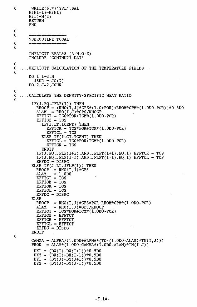
ooo

ooo

oo o

oC WRITE(6,*)'YVL',DAl

H(NI+1)-H(NI)H(1)=H(2)RETURNEND

SUBROUTINE TCCAL

IMPLICIT REAL*8 (A-H.O-Z) INCLUDE 'C0MTNU21.DAT'

....EXPLICIT CALCULATION OF THE TEMPERATURE FIELDSDO 1 1=2,N JSUR = JS(I)

DO 2 J=2,J SUR

___CALCULATE THE DENSITY-SPECIFIC HEAT RATIOIF(J.EQ.JFLP(I)) THENRHOCP = (RHO(I,J)*CPS*(1.0+POR)+RHOM*CPM*(1.ODO-POR))*0.5D0 ALAM = RHO(I,J)*CPS/RHOCP EFFTCT = TCS*POR+TCM*(l.ODO-POR)EFFTCB = TCS

IF(I.LT.ICENT) THENEFFTCR = TCS*POR+TCM*(1.ODO-POR)EFFTCL = TCS

ELSE IF(I.GT.ICENT) THENEFFTCL = TCS*POR+TCM*(l.ODO-POR)EFFTCR = TCS

ENDIFIF(J.EQ.JFLP(I+1).AND.JFLPT(I+1).EQ.1) EFFTCR = TCS IF(J.EQ.JFLP(I-l).AND.JFLPT(I-l).EQ.l) EFFTCL = TCS EFFDC = DISPC

ELSE IF(J.LT.JFLP(I)) THEN RHOCP = RHO(I,J)*CPS ALAM = 1.0D0 EFFTCT = TCS EFFTCB = TCS EFFTCR = TCS EFFTCL = TCS EFFDC = DISPC

ELSERHOCP = RHO(I,J)*CPS*POR+RHOM*CPM*(l.ODO-POR)ALAM = RHO(I,J)*CPS/RHOCP EFFTCT = TCS*POR+TCM*(l.ODO-POR)EFFTCB = EFFTCT EFFTCR = EFFTCT EFFTCL = EFFTCT EFFDC = DISPC

ENDIFGAMMA = ALPHA/(1.ODO+ALPHA*(TO-(1.0D0-ALAM)*TN(I,J)))PROD = ALAM*(1.0D0+GAMMA*(1.0D0-ALAM)*TN(I,J))DX1 = (DX(I)+DX(I+1))*0.5D0 DX2 = (DX(I)+DX(I-1))*0.5D0 DY1 = (DY(J)+DY(J+1))*0.5D0 DY2 = (DY(J)+DY(J-1))*0.5D0

-F.14-

onoo

no

onRH0X1 = (RH0(I,J)*DX(I+1)+RH0(I+1,J)*DX(I))/(DX1*2.0D0) RH0X2 = (RHO(I,J)*DX(I-1)+RHO(I-1,J)*DX(I))/(DX2*2.0DO) RH0Y1 = (RHO(I,J)*DY(J+1)+RHO(I,J+1)*DY(J))/(DY1*2.0DO) RH0Y2 = (RHO(I,J)*DY(J-1)+RHO(I,J-1)*DY(J))/(DY2*2.0DO)UAV = (XV(I+1,J)+XV(I,J))*0.5D0 DTDR = (TN(I+1,J)-TN(I,J))/DX1 DTDL = (TN(I,J)-TN(I-1,J))/DX2 SGU = SIGN(1.DO,UAV)DXA = DX1+DX2+UPWINDT*SGU*(DX1-DX2)CONTX = UAV*(DX2*DTDR+DX1*DTDL+UPWINDT*SGU

@ *(DX1*DTDL-DX2*DTDR))/DXAVAV = (YV(I,J+1)+YV(I,J))*0.5D0 DTDU = (TN(I,J+1)-TN(I,J))/DY1 DTDL = (TN(I,J)-TN(I,J-1))/DY2 SGV = SIGN(1.DO,VAV)DYA = DY1+DY2+UPWINDT*SGV*(DY1-DY2)CONTY = VAV*(DY2*DTDU+DY1*DTDL+UPWINDT*SGV*

@ (DY1*DTDL-DY2*DTDU))/DYACONDX = ((TN(I+1,J)-TN(I,J))*EFFTCR/DX1

(a -(TN(I,J)-TN(I-1,J))*EFFTCL/DX2)*BDX(I)/RHOCPCONDY = ((TN(I,J+1)-TN(I,J))*EFFTCT/DY1

(a - (TN(I, J) -TN(I, J -1)) *EFFTCB/DY2) *BDY(J) /RHOCPT(I,J) = TN(I,J)+DT*(-(CONTX+CONTY)*PROD+

(§ +(CONDX+CONDY)*(1.0D0-ALAM*GAMMA*TN(I,J)))2 CONTINUE 1 CONTINUERETURNEND

SUBROUTINE PROPCAL

IMPLICIT REAL*8 (A-H.O-Z)INCLUDE 'COMTNU21.DAT'DO 1 1=2,N

JSUR = JS(I)DO 2 J=2,JSUR+I

RHO(I.J) = RHTO*(1.0D0-ALPHA*(TN(I,J)-TO)) RHO(I,J) = RHTOVISC(I,J) = VISCTO*DEXP(-DELTA*(TN(I,J)-TO))

2 CONTINUE 1 CONTINUERETURNEND

SUBROUTINE TAUTEMP

IMPLICIT REAL*8 (A-H,0-Z) INCLUDE 'COMTNU21.DAT'TAUTTOT = 0.0D0 DO 1 1=2,N J SUR=J S(I)DO 2 J=2,JSUR

-F.15-

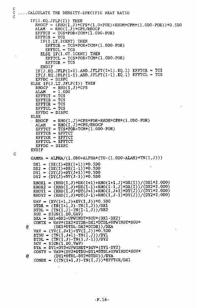
n o o ....CALCULATE THE DENSITY-SPECIFIC HEAT RATIO

IF(J.EQ.J FLP(I)) THENRHOCP = (RHO(I,J)*CPS*(1.0+POR)+RHOM*CPM*(1.0DO-POR))*0.5DO ALAM = RHO(I,J)*CPS/RHOCP EFFTCT = TCS*POR+TCM*(1.0DO-POR)EFFTCB = TCS

IF(I.LT.ICENT) THENEFFTCR = TCS*POR+TCM*(1.0D0-POR)EFFTCL = TCS

ELSE IF(I.GT.ICENT) THENEFFTCL = TCS*POR+TCM*(1.0D0-POR)EFFTCR = TCS

END IFIF(J.EQ.JFLP(I+1).AND.JFLPT(I+1).EQ.l) EFFTCR = TCS IF(J.EQ.JFLP(I-1).AND.JFLPT(I -1).EQ.l) EFFTCL = TCS EFFDC = DISPC

ELSE IF(J.LT.JFLP(I)) THEN RHOCP = RHO(I,J)*CPS ALAM = 1.0D0 EFFTCT = TCS EFFTCB = TCS EFFTCR = TCS EFFTCL = TCS EFFDC = DISPC

ELSERHOCP = RHO(I,J)*CPS*POR+RHOM*CPM*(1.0DO-POR)ALAM = RHO(I,J)*CPS/RHOCP EFFTCT = TCS*POR+TCM*(1.ODO-POR)EFFTCB = EFFTCT EFFTCR = EFFTCT EFFTCL = EFFTCT EFFDC = DISPC

ENDIFGAMMA = ALPHA/(1.0D0+ALPHA*(TO-(1.0D0-ALAM)*TN(I,J)))DX1 = (DX(I)+DX(I+1))*0.5DO DX2 = (DX(I)+DX(I-1))*0.5D0 DY1 = (DY(J)+DY(J+l))*0.5DO DY2 = (DY(J)-t-DY(J-l) )*0.5DORHOX1 = (RHO(I,J)*DX(I+l)+RHO(I+l,J)*DX(I))/(DX1*2.ODO)RHOX2 = (RHO(I,J)*DX(I-1)+RHO(I-1,J)*DX(I))/(DX2*2.0DO) RHOY1 = (RHO(I,J)*DY(J+1)+RHO(I,J+1)*DY(J))/(DY1*2.0DO)RHOY2 - (RHO(I,J)*DY(J-1)+RHO(I,J-1)*DY(J))/(DY2*2.0DO)UAV - (XV(I+1,J)+XV(I,J))*0.5D0 DTDR = (TN(I+1,J)-TN(I,J))/DX1 DTDL = (TN(I,J)-TN(I-1,J))/DX2 SGU = SIGN(1.DO,UAV)DXA = DX1+DX2+UPWINDT*SGU*(DX1-DX2)CONTX = UAV*(DX2*DTDR+DX1*DTDL+UPWINDT*SGU*

(a (DX1*DTDL-DX2*DTDR))/DXAVAV = (YV(I,J+1)+YV(I,J))*0.5D0 DTDU = (TN(I,J+1)-TN(I,J))/DY1 DTDL * (TN(I,J)-TN(I,J-1))/DY2 SGV - SIGN(1.DO,VAV)DYA = DY1+DY2+UPWINDT*SGV*(DY1-DY2)CONTY = VAV*(DY2*DTDU+DY1*DTDL+UPWINDT*SGV*

@ (DY1*DTDL-DY2*DTDU))/DYACONDX = ((TN(I+1,J)-TN(I,J))*EFFTCR/DX1

-F.16-

o o

o o o

o

@ -(TN(I,J)-TN(I-1,J))*EFFTCL/DX2)*BDX(I)/RHOCPCONDY = ((TN(I,J+l)-TN(I,J))*EFFTCT/DY1

@ -(TN(I,J)-TN(I,J-l))*EFFTCB/DY2)*BDY(J)/RHOCPTAUT(I,J) = GAMMA*(CONDX+CONDY+(1.0D0-ALAM)*(CONTX+CONTY)) TAUTTOT = TAUTTOT+(TAUT(I,J)*DX(I)*DY(J)*WIDTH)

2 CONTINUE 1 CONTINUE RETURN END

SUBROUTINE RESET

IMPLICIT REAL*8 (A-H.O-Z) INCLUDE 'COMTNU21.DAT'DO 1 I-l.NI+l HN(I) = H(I)

DO 2 J=1,MI+1XVN(I,J) = XV(I,J)YVN(I,J) = YV(I,J)TN(I,J) = T(I,J)

2 CONTINUE 1 CONTINUERETURNEND

SUBROUTINE SURCELCCC ___SET SURFACE CELL POSITIONSC

IMPLICIT REAL*8 (A-H,0-Z)INCLUDE 'COMTNU21.DAT'

DO 1 1=2,NIAVHGT = (HN(I)+HN(I+1))*0.5D0 AVHT = HN(I)SUM = 0.0D0

DO 2 J=2,MI SUMT = SUM SUM = SUM+DY(J)IF(SUMT.LT.AVHGT.AND.SUM.GE.AVHGT) THEN

JS(I) = JSUMDY(I) = SUMT+0.5D0*DY(J)

END IFIF(SUMT.LT.AVHT.AND.SUM.GE.AVHT) THEN

JS1(I) = J SUMD(I) = SUMT

END IF2 CONTINUE 1 CONTINUE JS(NI)=JS(N)JS(1)=JS(2)SUMDY(l) = SUMDY(2)SUMDY(NI) = SUMDY(NI-l)RETURNEND

-F.17-

ooo oooo

no

n oo

oooo

on o o SUBROUTINE RV

IMPLICIT REAL*8 (A-H.O-Z) INCLUDE 'C0MTNU21.DAT'

.THIS PROGRAM CALCULATES THE VOLUME OF LIQUID THAT HAVE BEEN EVACUATED FROM A 2 - DIMENSIONAL BLAST FURNACE MODEL.

....ORIGINAL VOLUME OF LIQUID

XLEN = 0.0D0 DO 1 1=2,NXLEN = XLEN+DX(I)

1 CONTINUEOVOL = HLIQ*WIDTH*XLEN*POR

___PRESENT VOLUME OF LIQUID

IF(TIME.LE.DT) THEN VOLT = OVOL

ELSEVOLT = VOL

ENDIFVOL = 0.0D0 DO 2 1=2,N

DVOL = DX(I)*WIDTH*(H(I)+H(I+1))*0.5D0 VOL = VOL+DVOL

2 CONTINUEVOL = VOL*PORVOLOUT = (OVOL-VOL)*RHTO*l.OE-6FLOW = (VOLT-VOL+DT*RCH*WIDTH*XLEN)*RHTO*60.0E-6/DT VOLFLOW = (VOLT-VOL+DT*RCH*WIDTH*XLEN)/DTOPEN(UNIT=23,FILE-'UPDAT.DAT',STATUS-'NEW')WRITE(23,*)TIME,ITN WRITE(23,*)VOLOUT WRITE(23,*)FLOW WRITE(23,*)VOLFLOW WRITE(23, *)(H(I),1=1,NI)CLOSE(UNIT-23,STATUS-'SAVE')RETURNEND

SUBROUTINE TSTEP

IMPLICIT REAL*8 (A-H.O-Z) INCLUDE 'COMTNU21.DAT'

.CALCULATION OF TIME STEP

-F.18-

oooo

no

onIF(ISURF.EQ.O) THENIF(TIME.EQ.0.DO) GOTO 13 DT = DTIN DO 11 1=1,NI-1 DO 11 J=1,MI-1

IF(ABS(XVN(1+1,J)).GT.0.0001) THEN IF((DX(I)+DX(1+1))*0.5DO/DABS(XVN(1+1,J)).LT.DT)

@ DT = (DX(I)+DX(I+1))*0.5D0/DABS(XVN(1+1,J))END IFIF(ABS(YVN(I,J+l)).GT.0.0001) THEN IF((DY(J)+DY(J+1)>*0.5DO/DABS(YVN(I,J+l)).LT.DT)

@ DT = (DY(J)+DY(J+1))*0.5D0/DABS(YVN(I,J+l))ENDIF

11 CONTINUE 13 DT = 0.25D0*DT

ENDIFTIME -TIME+DTRETURNEND

SUBROUTINE OUTPUT

IMPLICIT REAL*8 (A-H.O-Z)INCLUDE 'COMTNU21.DAT'WRITE(2,*)TIME WRITE(2,*)VOL DO 1 1=1,NI+1 DO 1 J=1,MI+1WRITE(2,*)XV(I,J),YV(I, J),P(I,J)tT(I,J)

1 CONTINUEDO 2 1=1,NI+1 WRITE(2,*)HN(I)

2 CONTINUEWRITE(3, *)ITNT,ITN WRITE(3,10)(HN(I),I=1,NI)

10 FORMAT(IX,8F10.5)RETURNEND

SUBROUTINE PLOTS

IMPLICIT REAL*8 (A-H.O-Z)INCLUDE 'COMTNU21.DAT'IF(IPLOT.EQ.l) THEN IF(ITN.EQ.120) THEN

OPEN(UNIT-13, FILE-'STR1.DAT',STATUS='NEW') OPEN(UNIT-12,FILE-'TEMPI.DAT',STATUS='NEW') GOTO 4290

ELSE IF(ITNT.EQ.600) THENOPEN(UNIT-13,FILE='STR2.DAT',STATUS='NEW') OPEN(UNIT-12, FILE-'TEMP2.DAT',STATUS-'NEW') GOTO 4290

ELSE IF(ITNT.EQ.1200) THENOPEN(UNIT-13,FILE-'STR3.DAT',STATUS-'NEW') OPEN(UNIT-12, FILE-'TEMP3.DAT',STATUS-'NEW') GOTO 4290

ELSE IF(ITNT.EQ.3240) THENOPEN(UNIT-13,FILE-'STR4.DAT',STATUS-'NEW')

-F.19-

o o

n o o

o

OPEN(UNIT=12,FILE='TEMP4.DAT',STATUS='NEW') GOTO 4290

END IFGOTO 4299

4290 WRITE(13,*)NI,MI,JDPYWRITE(13,*)(JFLP(I),1=1,NI)WRITE(13, *)(JFLPT(I),1=1,NI)WRITE(13,*)(DX(I),1=1,NI)WRITE(13,*)(DY(J),J=1,MI)

DO 4289 1=2,NI WRITE(13,*)JS(I)

J SUR=J S(I)WRITE(13, *)(XV(I,J),J=2,JSUR)

4289 CONTINUEWRITE(12,*)'TIME = '.TIME WRITE(12,*)'ITNT = ',ITNTWRITE(12, *) 'ITN = ',ITNDO 4189 1=2,N WRITE(12,*)IWRITE(12,4190)(TN(I,J),J=2,JSUR+1)

4190 FORMAT(IX,6F13.5)4189 CONTINUE4299 CONTINUE

OPEN(UNIT=12,FILE='TEMP21.DAT',STATUS='NEW') WRITE(12,*)'TIME = '.TIME WRITE(12,*)'ITNT = ',ITNTWRITE(12,*)'ITN = ',ITNDO 4300 1=2,N WRITE(12, *)IWRITE(12,4310)(TN(I,J),J=2,JSUR+1)

4310 FORMAT(IX,6FI3.5)4300 CONTINUE

WRITE(12,*)(HN(I),1=2,NI)CLOSE(UNIT=12,STATUS='SAVE')END IFRETURNEND

SUBROUTINE FINPLOT

IMPLICIT REAL*8 (A-H.O-Z)INCLUDE 'COMTNU21.DAT'IF(IPLOT.EQ.l) THENOPEN(UNIT=12,FILE='TEMP21.DAT',STATUS='NEW') DO 4100 1=2,N WRITE(12,*)JS(I)WRITE(12,4110)(T(I,J),J=2,JSUR+1)

4110 FORMAT(IX,6F13.5)4100 CONTINUE

___DATA REQUIRED FOR PLOTTING ISOTHERMS,STREAMLINES ETC

OPEN(UNIT=13,FILE='STR21.DAT',STATUS='NEW') OPEN(UNIT=14,FILE='TEMPT21.DAT',STATUS='NEW') WRITE(13,*)NI,MI,JDPY WRITE(13,*)(JFLP(I),1=1,NI)WRITE(13,*)(JFLPT(I),I=1,NI)WRITE(13,*)(DX(I),1=1,NI)WRI-TE(13 , *) (DY(I) , J=1, MI)WRITE(14,*)NI,MI,JDPY.TI

-F.20-

o o o

oWRITE(14,*)(JFLP(I),1=1,NI) WRITE(14,*)(JFLPT(I),I=1,NI) WRITE(14,*)(DX(I),1-1,NI) WRITE(14,*)(DY(I),J-l.MI)

DO 4200 1=2,NI WRITE(13,*)JS(I)J SUR=J S(I)WRITE(13,*)(XV(I,J),J=2,JSUR)

4200 CONTINUE C

DO 4202 1=2,N J SUR=J S(I)WRITE(14,*)JS(I)WRITE(14,*)(T(I,J),J=2,JSUR)

4202 CONTINUE END IF RETURN END

SUBROUTINE CONST

IMPLICIT REAL*8 (A-H.O-Z)INCLUDE 'COMTNU21.DAT'DO 1 1=2,N JSUR = JS(I)Q(I) = 0.5D0*(DY(JSUR-1)+DY(JSUR))/(0.5D0*(HN(I)+HN(I+l)+

@ DY(JSUR-1)+DY(JSUR))-SUMDY(I))DO 1 J=2,JSUR

IF(J.LT.JSUR.AND.ISURF.EQ.l) THEN IF(J.EQ.JSUR-1) THENw = wsELSE

W = WI END IF

ELSEW = WI

ENDIFTHETA(I,J) = -W/(BETAX(1+1,J)+BETAX(I,J))*BDX(I)+

@ (BETAY(I, J+l) +BETAY(I, J) )*BDY(J)1 CONTINUE RETURN END

-F.21-

APPENDIX G

The fortran computer code, HDT31.F0R, solves for the equations describing the motion of a non-isothermal liquid in a three-dimen­sional, homogenous packed bed, with and without a packing-free layer beneath it. The following files are required to execute the program

Name of File Description

C0MTNU31.DAT Common blockINIT31.DAT Input data setMESH31.DAT Computational grid dataOLD31.DAT Old values of field variablesNEW31.DAT New values of field variablesHEIG31.DAT Surface elevation at completion of simulationRV31.DAT Calculated residual liquid volume at completion

of simulationELEV1..5.DAT Surface elevations at specified times during

the simulationUPDAT.DAT Intermediate values of time, flowrates and drained

volumesMARK31.DAT Initial positions of marker particlesMARK31.OUT Marker particle positions at specified times during

the simluation

A flowchart of the program is described in Figure (G.l).

-G.l-

START

RUNCOMPLETE?

' FREE N SURFRCE COMPUTEO?

x HRS x. CONVERGENCE^ NO BEEN y— OBTAINED? /

/ FREE \ SURFRCE RT TRPHOLE?

INITIALISEVARIABLES

CALCULATERESIDUALVOLUME

CALCULATE NEW POSITION OF MARKER PARTICLES

SET BOUNDARY CONDITIONS

COMPUTE NEW FREE SURFACE POSITION

COMPUTEINTERMEDIATEVELOCITYFIELD

CALCULATE TIME STEP

COMPUTE NEW TEMPERATURE FIELD

ITERATE FOR PRESSURE AND VELOCITY

Figure G. 1 Flowchart of program HDT3 l.FOR.

-G.2-

n o o

o noo

non

o o o

o o

o no

n o o

o n o

o noo

oooo

onoo

oooo

oooo

ooPROGRAM HDT31

THIS PROGRAM SOLVES NUMERICALLY, THE FLUID MOTION IN A 3-DIMENSIONAL BLAST FURNACE WITH OR WITHOUT A COKE-FREE LAYER BENEATH THE COKE BED. THE MAC METHOD AS PROPOSED BY HIRT ET AL (1975) IS USED.i.e. AN UPWIND FINITE DIFFERENCING TECHNIQUE IS USED .> TEMPERATURE EFFECTS ARE INCLUDED IN THE PROGRAM> THE NON-CONSERVATIVE FORM OF THE ENERGY EQN IS USED> THE NON-CONSERVATIVE FORM OF THE N-S EQN IS USED> A NON-UNIFORM GRID IS USED> TRACERS ARE STUDIED USING MARKER PARTICLESAUTHOR: P.ZULLI

SCHOOL OF CHEMICAL ENGINEERING AND INDUSTRIAL CHEMISTRYUNIVERSITY OF NEW SOUTH WALES KENSINGTON AUSTRALIA

IMPLICIT REAL*8 (A-H.O-Z)INCLUDE 'COMTNU31.DAT'.INITIALIZE VARIABLES AND MESHCALL INITIAL.CALCULATE TEMPERATURE DEPENDENT PROPERTIESCALL PROPCAL CALL OTHBC.CALCULATE TAUTEMPIF(ITEMP.EQ.1) CALL TAUTEMP.COMMENCE ITERATION LOOP ON PRESSURE AND VELOCITY .ITIME = IDO DO 1 ITNT=1,MAXT IC=0D0 ICM - 0D0.CALCULATION OF TIME STEP CALL TSTEP.CALCULATE VELOCITIES TO SATISFY N-STOKES OR DARCY'S EQN CALL MOMEQN.CALCULATE THETA(I,J,K) AND Q(I,J) VALUESCALL CONSTDO 2 ITN=1,MAXITN.SET BOUNDARY CONDITIONSCALL BC DMAX = 0.D0 DO 3 J=2,JUB

ILB = IL(J)IUB = IU(J)

-G. 3-

DO 3 I-IUB,ILB,-1 KSUR = KS(I,J)

DO 3 K=2,KSURIF(K.EQ.KSUR.AND.ISURF.EQ.l) GOTO 20

IF(I.EQ.ILB) GOTO 30 IF(I.EQ.IUB) GOTO 40

CC ....CALCULATE DIVERGENCE AND PRESSURE CHANGE FOR FULL CELL C

DM = (XV(I+1,J,K)-XV(I,J,K))*BDX(I)@ +(YV(I,J+1,K)-YV(I,J,K))*BDY(J)@ +(ZV(I,J,K+l)-ZV(IfJ,K))*BDZ(K)VOL1 = 1.0D0

GOTO 31 CC ....CALCULATE DIVERGENCE AND PRESSURE CHANGE FOR BOUNDARY CELL C

30 DM = XV(I+1,J,K)*DY(J)*DZ(K)-YV(I,J,K)*DX(I)*DZ(K)@ +(ZV(I,J,K+1)-ZV(I,J,K))*DX(I)*DY(J)*0.5D0VOL1 = DX(I)*DY(J)*DZ(K)*0.5D0 GOTO 31

CC ....DRAIN POINT CELL C

40 IF(I.EQ.IDPX.AND.J.EQ.JDPY.AND.K.EQ.KDPZ) THENDM = XV(I+1,J,K)*FAREA-XV(I,J,K)*DY(J)*DZ(K)-YV(I,J,K)

@ *DX(I)*DZ(K)+(ZV(I,J,K+1)-ZV(I,J,K))*DX(I)*DY(J)*0.5D0VOL1 = DX(I)*DY(J)*DZ(K)*0.5D0

ELSE" DM = -XV(I,J,K)*DY(J)*DZ(K)-YV(I,J,K)*DX(I)*DZ(K)

@ +(ZV(I,J,K+1)-ZV(I,J,K))*DX(I)*DY(J)*0.5D0VOL1 = DX(I)*DY(J)*DZ(K)*0.5D0

END IF31 DP = THETA(I,J,K)*(DM-TAUT(I,J,K)*V0L1)

GOTO 50 CC ___CALCULATE PRESSURE CHANGE FOR SURFACE CELLC

20 CONTINUEDZ1 = 0.5D0*(DZ(KSUR-1)+DZ(KSUR))DZ2 = 0.5D0*(DZ(KSUR-l)+DZ(KSUR-2))

CDP = P(I,J,KSUR-I)+DZ1*(P0-P(I,J,KSUR-2))/(Q(I,J)+DZ2)+

@ 0.5D0*DZ1*DZ1*(((PO-P(I,J,KSUR-1))/Q(I,J))-((P(I,J,KSUR-1)- (§ P(I, J ,KSUR -2) )/DZ2) )/(Q(I, J)+DZ2) -P(I, J ,KSUR)

50 IF(DABS(DM-TAUT(I,J,K)*V0L1).GT.DMAX) THEN IMAX = I JMAX = J KMAX = K

DMAX = DABS(DM-TAUT(I,J,K)*V0L1)END IF

P(I,J,K) = P(I,J,K)+DP CC ___ADJUST VELOCITIESC

XV(I+1,J,K) = XV(I+1IJ,K)+BETAX(I+1,J,K)*DP XV(I,J,K) = XV(I,J,K)-BETAX(I,J,K)*DP YV(I,J+l,K) = YV(I,J+1,K)+BETAY(I,J+1,K)*DP YV(I,J,K) = YV(I,J,K)-BETAY(I,J,K)*DPZV(I,J,K+l) = ZV(I,J,K+1)+BETAZ(I,J,K+1)*DP ZV(I,J,K) = ZV(I,J,K)-BETAZ(I,J,K)*DP XV(IDPX+1,JDPY,KDPZ) = FLOW/FAREA

3 CONTINUE CC ___CHECK DIVERGENCEC

-G.4-

nnn nn

n n

nnnn

nn

nnnn

non n

nnnn

nn

nnn

IF(DMAX.LE.EPSL.AND.IC.GT.0D0) GOTO 267 2 CONTINUE

267 CONTINUE....CALCULATE TEMPERATURES USING THE HEAT EQUATION AND SET TEMP BC ....CALCULATE CONCENTRATION OF TRACER AND SET CONC BC ....MOVE MARKER PARTICLES REPRESENTING TRACERS

IF(ITEMP.EQ.l) THEN CALL TCCAL CALL TCBC

END IFIF(IMARK.EQ.l) CALL MARKER

....NEW FREE SURFACE POSITION CALCULATED

....AND IF FREE SURFACE HAS REACHED DRAIN-POINT ___STOPIF(ISURF.EQ.l) THEN CALL SURFACE CALL RVIF(H(NI,2).LE.TERMH) GOTO 100 END IFIF(ITNT.NE.MAXT) GOTO 275

___STORE ALL NECESSARY DATACALL OUTPUT

.... SET ADVANCED VELOCITIES, TEMPERATURES AND HEIGHTS INTO OLD

.... ARRAYS»»> XVN () , YVN ( ) , ZVN () , TN ( ) AND HN() AND CALCULATE NEW SURFACE CELLS.

275 CALL RESET CALL SURCELOPEN(UNIT=17,FILE='UPDATE.DAT',STATUS='NEW')WRITE(17,*)'TIME',TIME WRITE(17,*)'ITNT',ITNT WRITE(17,*)'ITN',ITN CLOSE(UNIT=17,STATUS='SAVE')

___CALCULATE PRODUCT OF TAU AND TEMPAND CALCULATE NEW PROPERTY VALUESCALL PROPCAL CALL OTHBCIF(ITEMP.EQ.l) CALL TAUTEMP

1 CONTINUEGOTO 130

100 CONTINUECALL OUTPUTWRITE(6,*)'FINISH ',FINISH FINISH = 1.0D0/FINISH WRITE(6, *) 'FINISH '.FINISH

130 STOP END

SUBROUTINE INITIAL

....INITIALISE ALL VARIABLES

-G.5-

o o o

o o o

o o o

o o n

ooo

ooo

CIMPLICIT REAL*8 (A-H.O-Z) INCLUDE 'C0MTNU31.DAT'

....OPEN DATA FILESOPEN(UNIT=4,FILE='INIT31.DAT',STATUS='OLD')OPEN(UNIT-7, FILE-'MESH31.DAT',STATUS-'OLD')OPEN(UNIT-10,FILE='RV31.DAT',STATUS-'NEW')OPEN(UNIT-18,FILE-'TAPC31.DAT',STATUS-'NEW')OPEN(UNIT-21,FILE-'MARK31.OUT',STATUS-'NEW')

___INITIALIZATIONREAD(4,*)NI,MI,KI,DT,EPSL,MAXT,MAXITN,RAD,R,FLOW,FLOWI,HLIQ,POREAD(4,*)HK,CPS,CPM,TCS,TCM,RHOM,RHTO,VISCTO,DELTA,TO,TIREAD(4,*)POR,IDPX,JDPY,KDPZ,KFLP,ALPHA,HTCS,HTCB,TCOOLREAD(4,*)UPWIND,UPWINDT,WI,WS,TERMH,RCHREAD(4,*)NOMP,MPI,MPII,TSSET,TBSET,IHTREAD(4,*)JFLAG,ISURF,IMARK,ITEMP,IMESHREAD(4,*)T1,T2,T3,T4OPEN(UNIT-2, FILE-'NEW31.DAT',STATUS-'NEW')OPEN(UNIT-3,FILE-'HEIG31.DAT',STATUS-'NEW')GX = 0.0D0 GY = 0.0D0 GZ = 981.0D0 DTIN - DT JUB = NI*0.5D0

___CALCULATE THE BOUNDARY CELL POSITIONSDO 50 J-2.JUB

IL(J) = J IU(J) = NI-J+1

50 CONTINUEIL(JUB+1) = IL(JUB)IU(JUB+1) = IU(JUB)IL(JUB+2) = IL(JUB+1)IU(JUB+2) = IU(JUB+1)IL(1) = IL(2)IU(1) = IU(2)

___CALL MESH GENERATION SUBROUTINECALL MESHOPEN(UNIT-19, FILE-'MESH31.DAT',STATUS-'NEW')WRITE(19,*)NI,MI,KI WRITE(19,*)(DX(I),1=1,NI)WRITE(19,*)(DY(J),J=1,JUB)WRITE(19,*)(DZ(K),K=1,KI)

___CALCULATE X AND Y DIRECTION DISTANCES TO BE USED IN MARKERPARTICLE MOVEMENTDXT(l) = 0.D0 DXTT = 0.DO DYT(l) = 0.D0 DYTT = 0.DO DO 198 I-2.NI-1

DXT(I) = DXTT+DX(I)DXTT = DXT(I)

198 CONTINUEDO 199 J-2,JUB

DYT(j) - DYTT+DY(J)

-G.6-

ooo

o o o

o oo

o o o o

ooo

DYTT = DYT(J)199 CONTINUE.... CALCULATE DRAIN FLOW AREA

FAREA = DZ(KDPZ)*DSQRT(DX(IDPX)*DX(IDPX)+DY(JDPY)*DY(JDPY))....CALCULATE CHANGE-OVER CELL FOR BOUNDARY CONDITIONS

CENPT1 = RAD*(1.ODO-O.5D0*DSQRT(2.0D0))CENPT2 = RAD*(1.0D0+0.5D0+DSQRT(2.0D0))SUM = 0.0D0

DO 90 1=2,NI-1 SUMT = SUM SUM = SUM+DX(I)IF(SUMT.LT.CENPT1.AND.SUM.GE.CENPT1) IOLS = I IF(SUMT.LT.CENPT2.AND.SUM.GE.CENPT2) IOUS = I

90 CONTINUE.... OPEN OLD DATA FILE AND READ IN DATA

IF(JFLAG.EQ.l) THENOPEN(UNIT=1,FILE='OLD31.DAT',STATUS='OLD')

READ(1,*)TIME READ(1,*)VOL,VOLORIG

DO 100 1=1,NOMPREAD(1,*)XMP(I),YMP(I),ZMP(I)

100 CONTINUEDO 1 J=1,JUB+2

ILB = IL(J)IUB = IU(J)

DO 1 I=ILB-1,IUB+2 DO 1 K=1,KI+1READ(1,*)XV(I,J,K),YV(I,J,K),ZV(I,J,K)READ(1,*)P(I,J,K),T(I,J,K)

1 CONTINUEDO 2 J=l,JUB+2

ILB = IL(J)IUB = IU(J)

DO 2 I=ILB-1,IUB+2 READ(1,*)H(I,J)

2 CONTINUE END IF

___FIRST RUNIF(JFLAG.EQ.O) THEN

TIME = 0.0D0 DO 3 J=l,JUB+2

ILB = IL(J)IUB = IU(J)

DO 3 I=ILB-1,IUB+2 DO 3 K=1,KI+1XV(I,J,K) = 0.0D0 YV(I,J,K) = 0.0D0ZV(I,J,K) = 0.0D0 T(I,J,K) = TI

3 CONTINUE

___INITIAL POSITION OF MARKER PATICLES

-G.7-

o o

o oo

noon

oooo

o

ooo ....INITIAL POSITION OF MARKER PATICLES

IF(IMARK.EQ.1) THENOPEN(UNIT-20.FILE-'MARK31.DAT',STATUS='OLD') READ(20,*)(XMP(I),I-l.NOMP)READ(20, *)(YMP(I),1-l.NOMP)READ(20,*)(ZMP(I),I=l,NOMP)

END IFDO 4 J=1,JUB+2

ILB = IL(J)IUB = IU(J)

DO 4 I=ILB-I,IUB+2 H(I,J)=HLIQ

4 CONTINUEEND IF

___RESET ALL NECESSARY VARIABLESCALL RESET

___CALCULATE POSITION OF SURFACE CELLSCALL SURCEL

.... INITIAL TEMPERATURE BOUNDARY CONDITIONSIF(ITEMP.EQ.1) THEN

CALL TCBC CALL RESET

ENDIF....CALCULATE PROPERTIES OF LIQUID

IF(J FLAG.EQ.0) THEN CALL PROPCAL CALL OTHBC

DO 5 J=1,JUB+1 ILB = IL(J)IUB = IU(J)

DO 5 I-ILB-1,IUB+2 PT = PO PTEMP = 0.0D0

DO 5 K=KI-1,2,-1 IF(K.EQ.KI-1) THENHGHT = HLIQ-SUMDZ(I,J)PTEMP = (RHO(I,J,K)+RHO(I,J,K+1))*0.5DO*GZ*HGHT GOTO 10

ELSEHGHT = 0.5D0*(DZ(K)+DZ(K+1))PTEMP = (RHO(I,J,K)*DZ(K+l)+RHO(I,J,K+l)*DZ(K))*GZ*HGHT

@ (DZ(K)+DZ(K+1))ENDIF

10 PT = PT+PTEMP P(I,J,K) = PT

5 CONTINUE C

ENDIFC

RETURNEND

-G.8-

o o o o o o

o o o

o o

o a

o o o

nnoo

oSUBROUTINE OTHBC

....SET OTHER BOUNDARY CONDITIONSIMPLICIT REAL*8 (A-H.O-Z) INCLUDE 'C0MTNU31.DAT'DO 1 J=2,JUB

ILB = IL(J)IUB = IU(J)

DO 1 K=2 , KI -1 RHO(ILB-l,J,K) RHO(IUB+l,J,K) VISC(ILB-1,J,K) VISC(IUB+1,J,K)

1 CONTINUE

RHO(ILB,J,K) RHO(IUB,J,K) VISC(ILB,J,K) VISC(IUB,J,K)

DO 2 J=2,JUB ILB = IL( J)IUB = IU(J)

DO 2 I=ILB,IUBRHO(I,J,1) = RHO(I,J,2)VISC(I,J,l) = VISC(I,J,2) 2 CONTINUE

DO 3 K=2,KI-1RHO(JUB,JUB+1,K)RHO(JUB+1,JUB+1,K) VISC(JUB,JUB+1,K) VISC(JUB+1,JUB+1,K)

3 CONTINUE

RHO(JUB,JUB,K)RHO(JUB+1,JUB,K) VISC(JUB,JUB,K) VISC(JUB+1,JUB,K)

DO 4 1=2,NI-1 DO 4 K=2,KI-1RHO(I,1,K) = RHO(I,2,K)

'VISC(I,1,K) = VISC(I,2,K) 4 CONTINUERETURNEND

SUBROUTINE TCBC

___SET TEMPERATURE BOUNDARY CONDITIONSIMPLICIT REAL*8 (A-H.O-Z)INCLUDE 'COMTNU31.DAT'

___SET TEMPERATURE IN BOTTOM CELLS VIA HEAT TRANSFER CONSIDERATIONSAT TIME = 0 AND THEN ASSUME THESE TEMPERATURES DO NOT CHANGE

IF(KFLP.LE.O) THENEFFTC = POR*TCS+(l.ODO-POR)*TCM

ELSEEFFTC = TCS

END IFDO 4 J=2,JUB

ILB = IL(J)IUB = IU(J)

DO 4 I=ILB,IUB

-G.9-

o o o

o o o

o oo

o o o

o oo

n ....BOUNDARY CONDITION - BOTTOMIF(TIME.LE.0.0001) THEN IF(IHT.EQ.O) THENT(I,J,1) = T(I,J,2)-(HTCB*DZ(2)/EFFTC)*(T(I,J,2)-TCOOL)

ELSET(I,J,I) = TBSET'

ENDIF END IF

....CONSTANT TEMPERATURE AT FREE SURFACEKSUR = KS(I,J)T(I,J,KSUR+1) = TI

4 CONTINUE....BOUNDARY CONDITION - FRONT PLANE (AXIS OF SYMMETRY)

DO 5 K=2,KI-1 DO 5 1=2,NI-1T(I,1,K) = T(I,2,K)

5 CONTINUE....SET TEMPERATURE IN SIDE CELLS VIA HEAT TRANSFER CONSIDERATIONS

AT TIME = 0 AND THEN ASSUME THESE TEMPERATURES DO NOT CHANGEIF(TIME.LE.0.0001) THEN

....BOUNDARY CONDITION - SIDE WALLDO 1 J=2,JUB

ILB = IL(J)IUB = IU(J)KSUR = KS(ILB,J)

DO 2 K=2,KSURIF(IHT.EQ.O) THEN

IF(K.GE.KFLP) THENEFFTC = POR*TCS+(l.ODO-POR)*TCM

ELSEEFFTC = TCS

ENDIFBDX1 = (2.0D0/(DX(ILB)+DX(ILB+1)))**2 BDY1 = (2.0D0/(DY(J)+DY(J-I)))**2 HTETC = (HTCS/EFFTC)**2 A = BDX1+BDY1-HTETCB = -(2.0DO*(T(ILB+1,J,K)*BDX1+T(ILB,J-1,K)*BDY1)-TCOOL*HTETC) Cl = BDX1*T(ILB+1,J,K)**2+BDY1*T(ILB,J-1,K)**2-HTETC*TCOOL**2 DEL = B*B-4.0D0*A*C1 IF(DEL.LT.0.0D0) DEL = 0.0D0 T(ILB,J,K) = (-B-DSQRT(DEL))/(2.0D0*A)

ELSET(ILB-1,J,K) = TSSET

ENDIF2 CONTINUE

KSUR = KS(IUB,J)DO 3 K=2,KSURIF(IHT.EQ.O) THEN

IF(K.GE.KFLP) THENEFFTC = POR*TCS+(l.ODO-POR)*TCM

ELSEEFFTC = TCS

-G.10-

o o o o

o o o o o o

o

c

c

C

END IFBDX1 = (2.0D0/(DX(IUB)+DX(IUB-1)))**2 BDY1 = (2.0D0/(DY(J)+DY(J-1)))**2 HTETC = (HTCS/EFFTC)**2 A = BDX1+BDY1-HTETCB = -(2.0DO* *(T(IUB-1,J,K)*BDX1+T(IUB,J-1,K)*BDY1)-TCOOL*HTETC)Cl = BDX1*T(IUB-1,J,K)**2+BDY1*T(IUB,J-1,K)**2-HTETC*TCOOL**2DEL = B*B-4.0D0*A*C1IF(DEL.LT.0.ODO) DEL = 0.0D0T(IUB,J,K) = (-B-DSQRT(DEL))/(2.0D0*A)

ELSET(IUB+1,J,K) = TSSET

ENDIF 3 CONTINUE 1 CONTINUE

IF(IHT.EQ.O) THEN DO 6 J=2,JUB DO 6 K=2,KI-1

ILB = IL(J)IUB = IU(J)T(ILB-1,J,K) = T(ILB,J,K) T(IUB+1,J,K) = T(IUB,J,K)

6 CONTINUEDO 7 K=2,KI-1T(JUB+1,JUB,K) = T(JUB+1,JUB+1,K)

7 CONTINUE ELSE

DO 8 K=2,KI-1T(JUB,JUB+1,K) = T(JUB+1,JUB+1,K)

8 CONTINUE ENDIF

T(JUB,JUB,K)= T(JUB+1,JUB,K)

TSSET = TSSET

ENDIFRETURNEND

SUBROUTINE MOMEQN

___CALCULATION OF INTERMEDIATE VELOCITIESIMPLICIT REAL*8 (A-H,0-Z)INCLUDE 'COMTNU31.DAT'DO 1 J=2,JUB

ILB = IL(J)IUB = IU(J)

DO 1 I=ILB,IUB KSUR =-- KS(I, J)

DO 1 K=2,KSUR___CALCULATE LENGTH PARAMETERS AND WEIGHTED-AVERAGED DENSITY AND

• VISCOSITYDX1 = DX(I)+DX(I+1)DX2 = DX(I)+DX(I-1)DY1 = DY(J)+DY(J+1)DY2 = DY(J)+DY(J-1)DZ1 = DZ(K)+DZ(K+1)DZ2 = DZ(K)+DZ(K-1)

-G.11-

o o o o

o o o

RHOX = (RHO(I,J,K)*DX(I+l)+RHO(I+l>J>K)*DX(I))/DXl RHOY = (RHO(I,J,K)*DY(J+l)+RHO(I,J+l,K)*DY(J))/DYl RHOZ = (RHO(I,J,K)*DZ(K+l)+RHO(I,J,K+1)*DZ(K))/DZl VISCX - (VISC(I,J,K)*DX(I+1)+VISC(I+1,J,K)*DX(I))/DX1 VISCY = (VISC(I,J,K)*DY(J+1)+VISC(I,J+1,K)*DY(J))/DY1 VISCZ = (VISC(I,J,K)*DZ(K+1)+VISC(I,J,K+1)*DZ(K))/DZ1 RHOX1 = (RHO(I,J,K)*DX(I-l)+RHO(I-l,J,K)*DX(I))/DX2 RHOY1 = (RHO(I,J,K)*DY(J-1)+RHO(I,J-1,K)*DY(J))/DY2 RHOZ1 = (RHO(I,J,K)*DZ(K-l)+RHO(I,J,K-1)*DZ(K))/DZ2 VISCX1 = (VISC(I,J,K)*DX(I-1)+VISC(I-1,J,K)*DX(I))/DX2 VISCY1 = (VISC(I,J,K)*DY(J-1)+VISC(I,J-1,K)*DY(J))/DY2 VISCZ1 = (VISC(I,J,K)*DZ(K-1)+VISC(I,J,K-1)*DZ(K))/DZ2

___CALCULATE BETA VALUESBETAX(I+1,J,K) = 2.D0*DT/(RHOX*DXl)BETAY(I, J+l,K) = 2.DO*DT/(RHOY*DY1)BETAZ(I,J,K+l) = 2.DO*DT/(RHOZ*DZ1)BETAX(I,J,K) = 2.DO*DT/(RHOX1*DX2)BETAY(I,J,K) = 2.DO*DT/(RHOY1*DY2)BETAZ(I,J,K) = 2.DO*DT/(RHOZ1*DZ2)IF(K.GE.KFLP) THEN

ETAX = (RHOXl^HK)/(RHOX1+HK+VIS CXl*POR*DT)ETAY = (RHOYl*HK)/(RHOYl*HK+VISCYl*POR*DT)ETAZ = (RHOZl*HK)/(RHOZl*HK+VISCZl*POR*DT)BETAX(I,J,K) = BETAX(I,J,K)*POR*ETAX BETAY(I,J,K) = BETAY(I,J,K)*POR*ETAY IF(K.GT.KFLP) BETAZ(I,J,K) = BETAZ(I,J,K)*POR*ETAZ ETAX = (RHOX*HK)/(RHOX*HK+VISCX*POR*DT)ETAY = (RHOY*HK)/(RHOY*HK+VISCY*POR*DT)ETAZ = (RHOZ*HK)/(RHOZ*HK+VISCZ*POR*DT)BETAX(1+1,J,K) - BETAX(I+1,J,K)*POR*ETAX BETAY(I,J+l,K) = BETAY(I,J+l,K)*POR*ETAY BETAZ(I,J,K+1) = BETAZ(I,J,K+l)*POR*ETAZ

END IFIF(J.EQ.l.OR.K.EQ.l) GOTO 1 IF(K.GE.KFLP) GOTO 10

___CALCULATE INTERMEDIATE X-VELOCITY FIELD (NAVIER-STOKES)IF(I.EQ.IUB) GOTO 19SGU = SIGN(1.DO,XVN(1+1,J,K))DXA = DX1+UPWIND*SGU*(DX(I+1)-DX(I))

DUDR = (XVN(I+2,J,K)-XVN(I+1,J,K))*BDX(I+1)DUDL = (XVN(I+1,J,K)-XVN(I,J,K))*BDX(I)

FUX = XVN(I+1,J,K)*(DX(I)*DUDR+DX(I+1)*DUDL+UPWIND*SGU* @ (DX(I+1)*DUDL-DX(I)*DUDR))/DXAVBT = (DX(I)*YVN(I+1,J+1,K)+DX(I+1)*YVN(I,J+1,K))/DX1 VBB = (DX(I)*YVN(I+1,J,K)+DX(I+1)*YVN(I,J,K))/DX1 VAV = 0.5D0*(VBT+VBB)SGV = SIGN(1.DO, VAV)

DYTT = 0.5D0*DY1 DYB = 0.5D0*DY2DYA = DYTT+DYB+UPWIND*SGV*(DYTT-DYB)DUDTY = (XVN(1+1,J+l,K)-XVN(I+1,J,K))/DYTT DUDBY = (XVN(1+1,J,K)-XVN(1+1,J-1,K))/DYB

FUY = VAV*(DYB*DUDTY+DYTT*DUDBY+UPWIND*SGV*@ (DYTT*DUDBY - DYB*DUDTY) ) /DYAWBT = (DX(I)*ZVN(I+l,JtK+l)+DX(I+l)*ZVN(I,J,K+l))/DXl WBB = (DX(I)*ZVN(I+1,J,K)+DX(I+1)*ZVN(I,J,K))/DX1 WAV = 0.5*(WBT+WBB)SGW = SIGN(1.DO,WAV)

DZT = 0.5D0*DZ1 DZB - 0.5D0*DZ2

-G.12-

non

DUDTZ = (XVN(1+1,J,K+l)-XVN(1+1,J,K))/DZT DUDBZ = (XVN(1+1,J,K)-XVN(1+1,J,K-1))/DZB

FUZ = WAV*(DUDTZ*DZB+DUDBZ*DZT+UPWIND*SGW*@ (DUDBZ*DZT-DUDTZ*DZB))VISC1 = ((VISC(I,J,K)*DY(J+1)+VISC(I, J+l,K)*DY(J))*DX(I+1)+

(a(VISC(I+l,J,K)*DY(J+l)+VISC(I+l,J+l,K)*DY(J))*DX(I))/(DXl*DYl) VISC2 = ((VISC(I,J,K)*DY(J-1)+VISC(I,J-1,K)*DY(J))*DX(I+1)+

@(VISC(I+1,J ,K)*DY(J-1)+VISC(I+1,J-1,K)*DY(J))*DX(I))/(DX1*DY2) VISC3 = ((VISC(I,J,K)*DZ(K+1)+VISC(I,J,K+1)*DZ(K))*DX(I+1)+

@(VISC(I+1,J,K)*DZ(K+1)+VISC(I+1,J,K+1)*DZ(K))*DX(I))/(DX1*DZ1) VISC4 = ((VISC(I,J,K)*DZ(K-1)+VISC(I,J,K-1)*DZ(K))*DX(I+1)+ @(VISC(I+1,J,K)*DZ(K-1)+VISC(I+1,J,K-1)*DZ(K))*DX(I))/(DX1*DZ2) VXX = 4.D0/(DX1*DX1)*(VISC(I+1,J,K)*(XVN(I+2,J,K)-XVN(I+1,J,K))*

@DX(I)*BDX(I+1)-VISC(I,J,K)*(XVN(I+1,J,K)-XVN(I,J,K))*DX(I+1)* (9BDX(I)-(1.DO/3.D0)*(VISC(I+1,J,K)*TAUT(1+1,J,K)*DX(I)- @VISC(I,J,K)*TAUT(I,J,K)*DX(I+1)))VXY = 2.0D0*BDY(J)*(VISC1*((XVN(I+1,J+l,K)-XVN(1+1,J,K))/DY1+ @(YVN(I+1,J+l,K)-YVN(I,J+l,K))/DXl)-VISC2*((XVN(I+1,J,K)- (§XVN(I+1,J-l,K))/DY2+(YVN(1+1,J,K)-YVN(I,J,K))/DX1))VXZ = 2.0D0*BDZ(K)*(VISC3*((XVN(1+1,J,K+l)-XVN(I+1,J,K))/DZ1+ @(ZVN(I+1,J,K+1)-ZVN(I,J,K+1))/DX1)-VISC4*((XVN(I+1,J,K)- @XVN(I+1,J,K-1))/DZ2+(ZVN(I+l,J,K)-ZVN(I,J,K))/DX1))VISX = VXX+VXY+VXZPT = (P(I,J,K)-P(I+1,J,K))*BETAX(I+1,J,K)XV(1+1,J,K) = XVN(I+1,J,K)+PT+DT*(GX-FUX-FUY-FUZ+VISX)

___CALCULATE INTERMEDIATE Y-VELOCITY FIELD (N-STOKES)19 IF(I.EQ.ILB.OR.I.EQ.IUB) GOTO 20

UBT = (DY(J)*XVN(I+1,J+1,K)+DY(J+1)*XVN(I+1,J,K))/DY1 UBB = (DY(J)*XVN(I,J+1,K)+DY(J+1)*XVN(I,J,K))/DY1 UAV = 0.5*(UBT+UBB)SGU = SIGN(1.DO,UAV)

DXTT = 0.5*DX1 DXB = 0.5*DX2DXA = DXTT+DXB+UPWIND*SGU*(DXTT-DXB)DVDTX = (YVN(I+1,J+l,K)-YVN(I,J+l,K))/DXTT DVDBX = (YVN(I,J+l,K)-YVN(I-1,J+l,K))/DXB

FVX = UAV*(DXB*DVDTX+DXTT*DVDBX+UPWIND*SGU*(a (DXTT*DVDBX-DXB*DVDTX)) /DXASGV = SIGN(1.DO,YVN(I,J+l,K))DYA = DY1+UPWIND*SGV*(DY(J+1)-DY(J))

DVDR = (YVN(I,J+2,K)-YVN(I,J+l,K))*BDY(J+1)DVDL = (YVN(I,J+l,K)-YVN(I,J,K))*BDY(J)

FVY = YVN(I,J+l,K)*(DY(J)*DVDR+DY(J+l)*DVDL+UPWIND*SGV*(3(DY(J+1)*DVDL-DY(J)*DVDR))/DYA WBT = (DY(J)*ZVN(I,J+l,K+1)+DY(J+1)*ZVN(I,J,K+1))/DYl WBB = (DY(J)*ZVN(I,J+l,K)+DY(J+1)*ZVN(I,J,K))/DYl WAV = 0.5*(WBT+WBB)SGW = SIGN(1.DO,WAV)

DVDTZ = (YVN(I,J+l,K+1)-YVN(I,J+l,K))/DZT DVDBZ = (YVN(I,J+l,K)-YVN(I,J+l,K-1))/DZB

FVZ = WAV*(DVDTZ+DVDBZ+UPWIND*SGW*(a (DVDBZ-DVDTZ))VISC1 - ((VISC(I,J,K)*DY(J-1)+VISC(I,J-l,K)*DY(J))*DX(I+1)+

@(VISC(I+1,J,K)*DY(J-1)+VISC(I+1,J-1,K)*DY(J))*DX(I))/(DX1*DY2) VISC1 = ((VISC(I,J,K)*DY(J+1)+VISC(I,J+l,K)*DY(J))*DX(I-1)+

(a(VISC(I-l,J,K)*DY(J+1)+VISC(I-1,J+1,K)*DY(J))*DX(I))/(DX2*DY1) VISC3 = ((VISC(I,J,K)*DZ(K+1)+VISC(I,J,K+1)*DZ(K))*DY(J+1)+

(3(VISC(I,J+1,K)*DZ(K+1)+VISC(I,J+l,K+1)*DZ(K))*DY(J))/(DYl*DZl) VISC4 = ((VISC(I,J,K)*DZ(K-1)+VISC(I,J,K-1)*DZ(K))*DY(J+1)+ @(VISC(I,J+1,K)*DZ(K-1)+VISC(I,J+l,K-1)*DZ(K))*DY(J))/(DYl*DZ2) VYY = 4.D0/(DY1*DY1)*(VISC(I,J+l,K)*(YVN(I,J+2,K)-YVN(I,J+l,K))*

(9DY(J)*BDY(J+1)-VISC(I,J,K)*(YVN(I,J+l,K)-YVN(I,J,K))*DY(J+1)* @BDY(J)-(l.D0/3.D0)*(VISC(I,J+l,K)*TAUT(I,J+l,K)*DY(J)-

-G.13-

n n o

@VISC(I, J ,K)*TAUT(I, J ,K)*DY(J+1) ) )VYX = 2.0D0*BDX(I)*(VISC1*((XVN(I+1,J+1,K)-XVN(I+1,J,K))/DY1+ @(YVN(I+1,J+l.K)-YVN(I,J+1,K))/DXl)-VISC2*((XVN(I,J+l,K)- @XVN(I,J,K))/DY1+(YVN(I,J+1,K)-YVN(I-1,J+1,K))/DX2))VYZ = 2.0D0*BDZ(K)*(VISC3*((YVN(IfJ+l,K+l)-YVN(I>J+l>K))/DZl+ @(ZVN(I,J+l,K+l)-ZVN(I,J,K+l))/DY1)-VISC4*((YVN(I,J+l,K)-

(§XVN(I,J+l,K-1))/DZ2+(ZVN(I,J+l,K)-ZVN(I,J,K))/DYl))VISY = VYX+VYY+VYZPT = (P(I,J,K)-P(I,J+1,K))*BETAY(I,J+l,K)YV(I,J+l,K) = YVN(I,J+1,K)+PT+DT*(GY-FVX-FVY-FVZ+VISY)

....CALCULATE INTERMEDIATE Z-VELOCITY FIELD (N-STOKES)20 UBT = 0.5*(XVN(I+1,J,K+1)+XVN(I+1,J,K))

UBB = 0.5*(XVN(I,J,K+1)+XVN(I,J,K))UAV = 0.5*(UBT+UBB)SGU = SIGN(l.DO.UAV)

DXTT = 0.5*DX1 DXB = 0.5*DX2DXA = DXTT+DXB+UPWIND*SGU*(DXTT-DXB)DWDTX = (ZVN(1+1,J,K+I)-ZVN(I,J,K+l))/DXTT DWDBX = (ZVN(I,J,K+I)-ZVN(I-I,J,K+l))/DXB

FWX = UAV*(DXB*DWDTX+DXTT*DWDBX+UPWIND*SGU*@ (DXTT*DWDBX-DXB*DWDTX))/DXAVBT = 0.5*(YVN(I,J+1,K+1)+YVN(I,J+1,K))VBB = 0.5*(YVN(I,J,K+l)+YVN(I,J,K))VAV = 0.5*(VBT+VBB)SGV = SIGN(1.DO,VAV)DYTT = 0.5*DY1 DYB = 0.5*DY2DYA = DYTT+DYB+UPWIND*SGV*(DYTT-DYB)DWDTY = (ZVN(I,J+l,K+1)-ZVN(I,J, K+l))/DYTT DWDBY = (ZVN(I,J,K+l)-ZVN(I,J-1,K+l))/DYB

FWY = VAV*(DYB*DWDTY+DYTT*DWDBY+UPWIND*SGV*(a (DYTT*DWDBY-DYB*DWDTY))/DYASGW = SIGN(1.DO,ZVN(I,J,K+l))DZA = DZ1+UPWIND*SGW*(DZ(K+1)-DZ(K)).DWDR = (ZVN(I,J,K+2)-ZVN(I>JIK+l))*BDZ(K+l)DWDL = (ZVN(I,J,K+1)-ZVN(I,J,K))*BDZ(K)

FWZ = ZVN(I,J,K+1)*(DWDR*DZ(K)+DWDL*DZ(K+1)+UPWIND*SGW*@ (DWDL*DZ(K)-DWDR*DZ(K+1)))/DZAVISC1 = ((VISC(I,J,K)*DZ(K+1)+VISC(I,J,K+1)*DZ(K))*DX(I+1)+ @(VISC(I+1,J,K)*DZ(K+1)+VISC(I+1,J,K+1)*DZ(K))*DX(I))/(DX1*DZ1) VISC2 = ((VISC(I,J,K)*DZ(K+1)+VISC(I,J,K+1)*DZ(K))*DX(I-1)+

@(VISC(I-1,J,K)*DZ(K+1)+VISC(I-1,J,K+1)*DZ(K))*DX(I))/(DX2*DZ1) VISC3 = ((VISC(I,J,K)*DZ(K+1)+VISC(I,J,K+1)*DZ(K))*DY(J+1)+

@(VISC(I,J+1,K)*DZ(K+1)+VISC(I,J+1,K+1)*DZ(K))*DY(J))/(DY1*DZ1) VISC4 = ((VISC(I,J,K)*DZ(K+1)+VISC(I,J,K+1)*DZ(K))*DY(J-1)+ @(VISC(I,J-1,K)*DZ(K+1)+VISC(I,J-1,K+1)*DZ(K))*DY(J))/(DY2*DZ1) VZZ = 4.D0/(DZl*DZl)*(VISC(I,J,K+l)*(ZVN(I,J,K+2)-ZVN(I,J,K+1))* @DZ(K)*BDZ(K+1)-VISC(I,J,K)*(ZVN(I,J, K+l)-ZVN(I,J,K))*DZ(K+1)* @BDZ(K) -(l.DO/l.DO^VISC^J.K+l^TAUTa.J.K+l^DZW- favISC^ ,J,K)*TAUT(I,J,K)*DZ(K+1)))VZX = 2.0D0*BDX(I)*(VISC1*((XVN(I+1,J,K+1)-XVN(I+1,J,K))/DZ1+ @(ZVN(I+1,J,K+1)-ZVN(I,J>K+1))/DX1)-VISC2*((XVN(I,J,K+1)- @XVN(I,J,K))/DZ1+(ZVN(I,J,K+l)-ZVN(I-1,J,K+l))/DX2))VZY = 2.0D0*BDY(J)*(VISC3*((YVN(I,J+l,K+l)-YVN(I,J+l,K))/DZ1+@(ZVN(I,J+l,K+l)-ZVN(I,J,K+l))/DYl)-VISC4*((YVN(I,J,K+l)- @YVN(I,J,K))/DZ1+(ZVN(I,J,K+l)-ZVN(I,J-1,K+l))/DY2))VISZ - VZX+VZY+VZZPT = (P(I,J,K)-P(I,J,K+l))*BETAZ(I,J,K+l)ZV(I,J,K+1) = ZVN(IfJ,K+l)+PT+DT*(-GZ-FWX-FWY-FWZ+VISZ)GOTO 1

10 CONTINUE

-G.14-

o o

o o oo

oo

o noon on

o

non

non

non ....CALCULATE INTERMEDIATE X-VELOCITY FIELD (DARCY)

IF(I.EQ.IUB) GOTO 29XV(1+1,J,K) = ETAX*XVN(I+1,J,K)+BETAX(I+1,J,K)*

@ (P(I»J,K)-P(I+1,J,K))___CALCULATE INTERMEDIATE Y-VELOCITY FIELD (DARCY)29 IF(I.EQ.ILB.OR.I.EQ.IUB) GOTO 30

YV(I,J+l,K) = ETAY*YVN(I,J+1,K)+BETAY(I,J+1,K)*@ (P(I,J,K)-P(I,J+1,K))

___CALCULATE INTERMEDIATE Z-VELOCITY FIELD (DARCY)30 ZV(I,J, K+l) = ETAZ*ZVN(I,J,K+l)+BETAZ(I,J,K+l)*@ (P(I,J,K)-P(I,J,K+l))-GZ*POR*DT*ETAZ

1 CONTINUE

XV(IDPX+1,JDPY,KDPZ) = FLOW/FAREARETURNEND

SUBROUTINE TCCAL

___EXPLICIT CALCULATION OF THE TEMPERATURE FIELDSIMPLICIT REAL*8 (A-H,0-Z)INCLUDE 'COMTNU31.DAT'DO 1 J=2,JUB

ILB = IL(J)IUB = IU(J)

DO 1 I=ILB,IUB KSUR = KS(I,J)

___IF THE TEMPERATURE ON THE BOUNDARY IS CALCULATED USING HEAT FLUX(IHT EQUALS ZERO) THEN DO NOT CALCULATE THESE TEMPERATURESIF((I.EQ.ILB.OR.I.EQ.IUB).AND.IHT.EQ.0) GOTO 1DO 1 K=2,KSUR

___CALCULATE THE DENSITY-SPECIFIC HEAT RATIOIF(K.GE.KFLP) THENALAM = RHO(I,J,K)*CPS/

(a (RHO(I,J,K)*CPS*POR+RHOM*CPM*(1.0D0-POR))EFFTC = POR*TCS+(l.ODO-POR)*TCM

ELSEALAM = 1.0D0 EFFTC = TCS

END IFGAMMA = ALPHA/(1.0D0+ALPHA*(TO-(1.0D0-ALAM)*TN(I,J,K)))PROD = ALAM*(1.0D0+GAMMA*(1.0D0-ALAM)*TN(I,J,K))DX1 = (DX(I)+DX(I+1))*0.5D0 DX2 - (DX(I)+DX(I-1))*0.5D0 DY1 = (DY(J)+DY(J+1))*0.5D0 DY2 = (DY(J)+DY(J-1))*0.5D0

-G.15-

o o o

o o o

DZ1 = (DZ(K)+DZ(K+1))*0.5D0 DZ2 = (DZ(K)+DZ(K-1))*0.5D0

CUAV = (XV(I+1,J,K)+XV(I,J,K))*0.5D0 DTDR = (TN(1+1,J,K)-TN(I,J,K))/DX1 DTDL = (TN(I,J,K)-TN(I-1,J,K))/DX2 SGU = SIGN(1.DO,UAV)DXA = DX1+DX2+UPWINDT*SGU*(DX1-DX2)CONVX = UAV*(DX2*DTDR+DX1*DTDL+UPWINDT

@ *SGU*(DX1*DTDL-DX2*DTDR))/DXAC

VAV = (YV(I,J+1,K)+YV(I,JIK))*0.5D0 DTDU = (TN(I,J+l,K)-TN(I,J,K))/DY1 DTDL = (TN(I,J,K)-TN(I,J-1,K))/DY2 SGV = SIGN(l.DO.VAV)DYA = DY1+DY2+UPWINDT*SGV*(DY1-DY2)CONVY = VAV*(DY2*DTDU+DY1*DTDL+UPWINDT

@ *SGV*(DY1*DTDL-DY2*DTDU))/DYAWAV = (ZV(I,J,K+l)+ZV(I,J,K))*0.5D0 DTDU = (TN(I,J,K+1)-TN(I,J,K))/DZl DTDL = (TN(I,J,K)-TN(I,J,K-1))/DZ2 SGW = SIGN(1.D0.WAV)DZA = DZ1+DZ2+UPWINDT*SGW*(DZ1-DZ2)CONVZ = WAV*(DZ2*DTDU+DZ1*DTDL+UPWINDT

(a *SGW*(DZ1*DTDL-DZ2*DTDU))/DZAC

CONDX = ((TN(I+1,J,K)-TN(I,J,K))/DX1-(TN(I,J,K)-TN(I-1,J,K)) (§ /DX2) *BDX(I) *EFFTC/(RHO (I, J , K) *CPS )

CONDY = ((TN(I,J+1,K)-TN(I,J,K))/DY1-(TN(I,J,K)-TN(I,J-1,K)) (§ /DY2)*BDY(J)*EFFTC/(RH0(I,J,K)*CPS)

CONDZ = ((TN(I,J,K+1)-TN(I,J,K))/DZl-(TN(I,J>K)-TN(I,J,K-1)) @ /DZ2)*BDZ(K)*EFFTC/(RHO(I,J,K)*CPS)

CIF(IHT.EQ.0.AND.(I.EQ.ILB.OR.I.EQ.IUB)) GOTO 100 T(I,J,K) = TN(I,J,K)+DT*(-(CONVX+CONVY+CONVZ)*PROD+

(a +(CONDX+CONDY+CONDZ)*(i.ODO-ALAM*GAMMA*TN(I,J,K)))C

1 CONTINUE RETURN END

SUBROUTINE PROPCAL

___TEMPERATURE-DEPENDANT PROPERTIESIMPLICIT REAL*8 (A-H.O-Z)INCLUDE 'COMTNU31.DAT'DO 1 J=2,JUB

ILB = IL(J)IUB = IU(J)

DO 1 I=ILB,IUB KSUR = KS(I,J)

DO 1 K=2 KSUR+1RHO(I,J,K) = RHTO*(l.0D0-ALPHA*(TN(I,J,K)-TO))VISC(I,J,K) = VISCTO*DEXP(-DELTA*(TN(I,J,K)-TO))

1 CONTINUE RETURN END

-G.16-

ooo

o ooo

ono

SUBROUTINE TAUTEMP

CALCULATION OF TAUT TERMIMPLICIT REAL*8 (A-H.O-Z) INCLUDE 'C0MTNU31.DAT'TAUTTOT = 0.0D0 DO 1 J=2,JUB

ILB = IL(J)IUB = IU(J)

DO 1 I-ILB.IUB KSUR = KS(I,J)

DO 1 K=2,KSUR....CALCULATE THE DENSITY-SPECIFIC HEAT RATIO

CC

C

IF(K.GE.KFLP) THENALAM = RHO(I,J,K)*CPS/

@ (RHO(I,J,K)*CPS*POR+RHOM*CPM*(1,ODO-POR))EFFTC = POR*TCS+(1.0D0-POR)*TCM

ELSEALAM = 1.0D0 EFFTC = TCS

END IFGAMMA = ALPHA/(1.0D0+ALPHA*(TO-(1.0D0-ALAM)*TN(I,J,K)))DX1 = (DX(I)+DX(I+1))*0.5D0 DX2 = (DX(I)+DX(I-1))*0.5D0 DY1 = (DY(J)+DY(J+1))*0.5D0 DY2 = (DY(J)+DY(J-1))*0.5D0 DZ1 - (DZ(K)+DZ(K+1))*0.5D0 DZ2 = (DZ(K)+DZ(K-1))*0.5D0UAV = (XV(I+1,J,K)+XV(I,J,K))*0.5D0 DTDR = (TN(I+1,J,K)-TN(I,J,K))/DX1 DTDL = (TN(I,J,K)-TN(I-1,J,K))/DX2 SGU = SIGN(1.DO,UAV)DXA = DX1+DX2+UPWINDT*SGU*(DX1-DX2)CONVX = UAV*(DX2*DTDR+DX1*DTDL+UPWINDT

@ *SGU*(DX1*DTDL-DX2*DTDR))/DXAVAV = (YV(I,J+l,K)+YV(I,J,K))*0.5D0 DTDU - (TN(I,J+1,K)-TN(I,J,K))/DY1 DTDL = (TN(I,J,K)-TN(I,J-1,K))/DY2 SGV = SIGN(1.DO,VAV)DYA = DY1+DY2+UPWINDT*SGV*(DY1-DY2)CONVY = VAV*(DY2*DTDU+DY1*DTDL+UPWINDT

(a *SGV*(DY1*DTDL-DY2*DTDU)) /DYAWAV - (ZV(I,J,K+1)+ZV(I,J,K))*0.5D0 DTDU = (TN(I,J,K+1)-TN(I,J,K))/DZl DTDL = (TN(I,J,K)-TN(I,J,K-1))/DZ2 SGW = SIGN(1.D0.WAV)DZA = DZ1+DZ2+UPWINDT*SGW*(DZ1-DZ2)CONVZ = WAV*(DZ2*DTDU+DZ1*DTDL+UPWINDT

(a *SGW*(DZ1*DTDL-DZ2*DTDU))/DZA

-G.17-

non o o

o non

non

o non o

non on

CONDX = ((TN(1+1,J,K)-TN(I,J,K))/DX1(TN(I,J,K)-TN(I-1,J,K))/DX2)*BDX(I)*EFFTC/(RHO(I,J,K)*CPS) CONDY = ((TN(I,J+l,K)-TN(I,J,K))/DYl

(a-(TN(I,J,K)-TN(I,J-1,K))/DY2)*BDY(J)*EFFTC/(RH0(I,J,K)*CPS) CONDZ = ((TN(I,J,K+l)-TN(I,J,K))/DZ1

(a-(TN(I,J,K)-TN(I,J,K-1))/DZ2)*BDZ(K)*EFFTC/(RH0(I,J,K)*CPS) C

TAUT(I,J,K) = GAMMA*(CONDX+CONDY+CONDZ+(1.ODO-ALAM)@*(CONVX+CONVY+CONVZ))IF(I.EQ.ILB.OR.I.EQ.IUB) THENTAUTTOT = TAUTTOT+TAUT(I,J,K)*DX(I)*DY(J)*DZ(K)*0.5D0

ELSETAUTTOT = TAUTTOT+TAUT(I,J,K)*DX(I)*DY(J)*DZ(K)

END IF1 CONTINUE RETURN END

SUBROUTINE MESH

....CALCULATION OF COMPUTATIONAL CELL BLOCK SIZEIMPLICIT REAL*8 (A-H.O-Z)INCLUDE 'COMTNU31.DAT'IF(IMESH.EQ.l) READ(7,*)(DX(I),I=2,JUB)READ(7,*)(DZ(K),K=1,KI)

___GENERATES INTERNAL MESH FOR QUADRANT OF MODELDYTTE = 0.0D0 SUMDX = 0.0D0DO 1 1=2,JUB DIS = RAD-SUMDX NSI = JUB-I+1IF(IMESH.EQ.O) DX(I) = DIS*(R-1.0)/(R**NSI-1)SUMDX = SUMDX+DX(I)DYTE = DSQRT(2.DO*SUMDX*RAD-SUMDX*SUMDX)DY(I) = DYTE-DYTTE DYTTE = DYTE

1 CONTINUE....SYMMETRY ABOUT CENTRELINE OF SEMICIRCLE (QUADRANT SYMMETRY)

DO 2 I=JUB+1,NI-1 DX(I) = DX(NI-1+1)

2 CONTINUE___SIDE BOUNDARY CELLS

DX(1) = DX(2)DX(NI) = DX(NI-l)

___TOP BOUNDARY CELLSDY(JUB+1) = DY(JUB)

___AXIAL SYMMETRYDY(1) = DY(2)

-G.18-

d d

d d

d d

d d

d d

OO

Odd

d d

ddd ....INVERSE LENGTHS

DO 3 1=1,NI BDX(I) = 1.D0/DX(I)

3 CONTINUEDO 4 J=1,JUB+1 BDY(J) = 1.DO/DY(J)

4 CONTINUEDO 5 K-l.KI BDZ(K) = 1.0D0/DZ(K)

5 CONTINUE

....CALCULATE CROSS-SECTIONAL AREA OF MODELXAREA = 0.D0 XAREAl = 0.D0 DO 6 J=2,JUB

ILB = IL(J)IUB = IU(J)

DO 6 I=ILB,IUBIF(I.EQ.ILB.OR.I.EQ.IUB) THEN DAREA = DX(I)*DY(J)*0.5D0 XAREA = XAREA+DAREA

ELSEDAREA = DX(I)*DY(J)XAREA = XAREA+DAREA XAREAl = XAREA1+DAREA

END IF6 CONTINUE RETURN END

SUBROUTINE BC

___SET BOUNDARY CONDITIONS (VELOCITY AND PRESSURE)IMPLICIT REAL*8 (A-H.O-Z)INCLUDE 'COMTNU31.DAT'

___BASE BOUNDARY CONDITIONSDO 1 J=2,JUB ILB = IL(J)

IUB = IU(J)DO 1 I=ILB-1,IUBXV(I+1,J,1) = XV(I+1,J,2)YV(I,J+l,1) = YV(I,J+l,2)ZV(I,J,2) = 0.0P(I,J,1) = P(I, J,2)

1 CONTINUE___FRONT PLANE BOUNDARY CONDITIONS

DO 2 K=1,KI DO 2 1=1,NI XV(1+1,1,K) YV(I,2,K)ZV (1,1,K+l) P(I,1,K)

2 CONTINUE

XV(1+1,2, K) 0.0ZV(I,2,K+1) P(I,2,K)

-G.19-

o o o

....LEFT AND RIGHT CURVED BOUNDARY CONDITIONSDO 3 J=2,JUB

ILB = IL(J) IUB = IU(J)

DO 3 K=2,KI P(ILB-1,J,K) P(IUB+1,J,K) ZV(ILB-1,J,K) ZV(IUB+1,J,K)

3 CONTINUE

P(ILB,J,K) P(IUB,J,K) ZV(ILB,J,K) ZV(IUB,J,K)

C

C

C

DO 30 K=2,KIXV(JUB+1,JUB+1,K) ZV(JUB,JUB+1,K) ZV(JUB+1,JUB+1,K) P(JUB,JUB+1,K)P(JUB+1,JUB+1,K)

30 CONTINUE

XV(JUB+1,JUB,K) ZV(JUB,JUB,K)ZV(JUB+1,JUB,K)= P(JUB,JUB,K)= P(JUB+1,JUB,K)

DO 40 J=2,JUB ILB = IL(J)IUB = IU(J)

DO 40 I=ILB,IUB,IUB-ILB KSUR = KS(I,J)

DO 40 K=2,KSUR IF(I.LE.IOLS+1) THEN YV(I-1,J,K) = YV(I,J,K)

END IFIF(I.GT.IOLS.AND.I.LE.IL(JUB)) THEN XV(I,J,K) = XV(I,J-1,K)

END IFIF(I.GE.IU(JUB).AND.I.LT.IOUS) THEN XV(1+1,J,K) = XV(I+1,J-1,K)END IFIF(I.GE.IOUS-l) THEN YV(1+1,J,K) = YV(I,J,K)ENDIF

40 CONTINUEDO 4 J=2,JUB ILB = IL(J)IUB = IU(J)

DO 4 I=ILB,IUB,IUB-ILB KSUR = KS(I,J)

DO 4 K=2,KSUR IF(I.LE.IOLS) THENXV(I,J,K) = XV(I+1,J,K)+DX(I)*(BDY(J)*

@ (YV(I,J+1,K)-YV(I,J,K))+BDZ(K)*(a (ZV(I, J ,K+1) - ZV(I, J ,K) ) - TAUT(I, J ,K))ENDIFIF(I.GT.IOLS.AND.I.LT.IOUS) THEN YV(I,J+l,K) = YV(I,J,K)-DY(J)*(BDX(I)*

(a (XV(I+1, J , K) -XV(I, J ,K) )+BDZ(K)*(a (ZV(I, J ,K+1) - ZV(I, J ,K)) - TAUT(I, J ,K))ENDIFIF(I.GE.IOUS) THENXV(1+1,J,K) = XV(I,J,K)-DX(I)*(BDY(J)*

@ (YV(I,J+1,K)-YV(I,J,K))+BDZ(K)*(a (ZV(I, J ,K+1) - ZV(I, J ,K)) - TAUT(I, J ,K))ENDIF

4 CONTINUE

-G.20-

o o

o n o ....FREE SURFACE BOUNDARY CONDITIONS

C

C

DO 5 J=2,JUB ILB = IL(J)IUB = IU(J)

DO 5 I=ILB,IUB KSUR = KS(I,J)IF(KS(1+1,J).LT.KS(I,J)) XV(1+1,J,KSUR) IF(KS(I,J).GT.KS(I,J-1))XV(1+1,J,KSUR+1)YV(I,J,KSUR+1) =

YV(I,J,KSUR) = XV(I+1,J,KSUR) YV(I,J,KSUR)

= XV(1+1,J,KSUR-I) YV(I,J,KSUR-1)

CONTINUE DO 6 J=2,JUB

ILB = IL(J)IUB = IU(J)

KSUR = KS(ILB,J)XV(ILB,J,KSUR)YV(ILB,J+l,KSUR)XV(ILB,J,KSUR+1)YV(ILB,J+l,KSUR+1)

KSUR = KS(IUB,J)XV(IUB+1,J,KSUR)YV(IUB,J+l,KSUR)XV(IUB+1,J,KSUR+1)YV(IUB,J+l,KSUR+1)

KSUR = KS(JUB+1,JUB)XV(JUB+1,JUB+1,KSUR)XV(JUB+1,JUB+1,KSUR+1)XV(JUB+1,JUB+1,KSUR)XV(JUB+1,JUB+1,KSUR+1)

KSUR = KS(2,2)YV(1,2,KSUR)YV(1,2,KSUR+1)

KSUR = KS(NI-1,2)YV(NI,2,KSUR)YV(NI,2,KSUR+1)

CONTINUE DO 7 1=2,NIKSUR = KS(I,2)

XV(1,1,KSUR) = XV(I,l.KSUR-l) XV(1,1,KSUR+1) = XV(1,1,KSUR) CONTINUE

XV(ILB,J,KSUR-1)YV(ILB,J+l,KSUR-1) XV(ILB,J,KSUR)YV(ILB,J+l,KSUR)XV(IUB+1,J,KSUR-1) YV(IUB,J+l,KSUR-1) XV(IUB+1,J,KSUR) YV(IUB,J+l,KSUR)

XV(JUB+1,JUB+1,KSUR-1) XV(JUB+1,JUB+1,KSUR)XV(JUB+1,JUB,KSUR)XV(JUB+1,JUB+1,KSUR)

= YV(1,2,KSUR-1) = YV(1,2,KSUR)YV(NI,2,KSUR-1) YV(NI,2,KSUR)

DO 8 J=2,JUB ILB = IL(J)IUB = IU(J)

DO 8 I=ILB,IUB KSUR = KS(I,J)

P(I,J,KSUR+1) = PO IF(ISURF.EQ.1) THEN IF(I.EQ.ILB) THENZV(I,J,KSUR+1) = ZV(I,J.KSUR)-2.0D0*DZ(KSUR)*BDX(I)*

@ XV(I+1,J,KSUR)+2.0D0*DZ(KSUR)*BDY(J)*@ YV(I,J,KSUR)+DZ(KSUR)*TAUT(I,J,KSUR)

ELSE IF(I.EQ.IUB) THENZV(I,J,KSUR+1) = ZV(I,J,KSUR)+2.0D0*DZ(KSUR)*BDX(I)*

(? XV(I, J , KSUR) +2.0D0*DZ (KSUR) *BDY(J) *(a YV(I, J , KSUR) +DZ(KSUR)*TAUT(I, J , KSUR)

ELSEZV(I,J,KSUR+1)

<3

= ZV(I,J,KSUR)-DZ(KSUR)*BDX(I)*(XV(I+1,J,KSUR)-XV(I,J,KSUR)) -DZ(KSUR)*BDY(J)*(YV(I,J+l,KSUR)-YV(I,J,KSUR)) +DZ(KSUR)*TAUT(I,J,KSUR)

-G.21-

ooo o

ooo

nn

o o o

ENDIFELSEZV(I,J,KSUR+1) = (-FLOW+TAUTTOT)/XAREA ENDIF

8 CONTINUEDO 9 J=2,JUB

ILB = IL(J)IUB = IU(J)

KSUR = KS(ILB,J)ZV(ILB-1,J,KSUR) = ZV(ILB,J,KSUR)ZV(ILB-1,J,KSUR+1) = ZV(ILB-1,J,KSUR)KSUR = KS(IUB,J)ZV(IUB+1,J,KSUR) = ZV(IUB,J,KSUR)ZV(IUB+1,J,KSUR+1) = ZV(IUB+1,J,KSUR)

9 CONTINUE C

KSUR = KS(JUB,JUB)ZV(JUB,JUB+1,KSUR) = ZV(JUB,JUB,KSUR)ZV(JUB,JUB+1,KSUR+1) = ZV(JUB,JUB+1,KSUR)KSUR = KS(JUB+1,JUB+1)ZV(JUB+1,JUB+1,KSUR) = ZV(JUB+1,JUB,KSUR) ZV(JUB+1,JUB+1,KSUR+1) = ZV(JUB+1,JUB+1,KSUR)DO 10 1=1,NI KSUR = KS(I,2)

ZV(I,1,KSUR) = ZV(I,2,KSUR)ZV(1,1,KSUR+1) = ZV(1,1,KSUR)

10 CONTINUE___TAPHOLE BOUNDARY CONDITION

XV(IDPX+1,JDPY,KDPZ) = FLOW/FAREA RETURN END

SUBROUTINE SURFACE

___CALCULATION OF FREE SURFACE MOVEMENTIMPLICIT REAL*8 (A-H.O-Z)INCLUDE 'COMTNU31.DAT'

___MOVE FREE SURFACE WITH INTERPOLATED VELOCITIES -DO 1 J=2,JUB+1

ILB = IL(J)IUB = IU(J)

DO 1 I-ILB,IUB+1IF(J.EQ.JUB+1.AND.I.NE.IUB) GOTO 1

DX2 = DX(I)+DX(I-1)DY2 = DY(J)+DY(J-1)KST = KS1(I,J)KST1 = KS(I,J)KST2 = KS(I-1,J)KST3 = KS(I-1,J-1)KST4 = KS(I,J-l)IF(KST2.EQ.KST+1) KST2 = KST IF(KST3.EQ.KST+1) KST3 = KST IF(I.EQ.IDPX.AND.J.EQ.JDPY+1) THENIF(KS1(IDPX+1,JDPY).LE.KS1(IDPX,JDPY+1)-2) THEN KST4 = KS1(IDPX+1,JDPY)+1

ENDIF ENDIF

-G.22-

c

c

c

c

c

c

c

c

XVS = (XVN(I,J,KST)*DY(J-1)+XVN(I,J-1,KST)*DY(J))/DY2 YVS = (YVN(I,J,KST)*DX(I-1)+YVN(I-1,J,KST)*DX(I))/DX2 ZVT = ((ZVN(I,J,KST1+1)*DX(I-1)+ZVN(I-1,J,KST2+1)*DX(I))*

@ DY(J-1)+(ZVN(I-1,J-1,KST3+1)*DX(I)+ZVN(I,J-1.KST4+1)(a *DX(I-1))*DY(J))/(DY2*DX2)

ZVB = ((ZVN(I,J,KST)*DX(I-1)+ZVN(I-1,J,KST)*DX(I))*DY(J-1)+ @ (ZVN(I-1,J-1,KST)*DX(I)+ZVN(I,J-l,KST)*DX(I-1))*DY(J))(a /(DY2*DX2)

COI = (HN(I,J)-SUMD(I,J))*BDZ(KST)ZVS = ZVB-COI*(ZVB-ZVT)

IF(MSFLAG.EQ.1) THEN HAl = HN(I,J)-SUMD(I.J)HA = HAl/(HAl+DZ(KST-1))ZVS1 = (l.D0/(l.D0-1.5D0*HA))*(ZVN(I,J,KST)-HA*

@ ZVN(I,J,KST-1)+0.5D0*HA*HA1*(-ZVN(I,J,KST)/HAl-@ (ZVN(I,J,KST)-ZVN(I,J,KST-1))*BDZ(KST-l)))

ZVS2 = (l.D0/(l.D0-1.5D0*HA))*(ZVN(I-l,J,KST)-HA*(a ZVN(I-1,J,KST-l)+0.5D0*HA*HAl*(-ZVN(I-l,J,KST)/HAl-(§ (ZVN(I-1,J,KST)-ZVN(I-1,J,KST-1))*BDZ(KST-1)))

ZVS3 = (l.D0/(l.D0-1.5D0*HA))*(ZVN(I-l,J-l,KST)-HA*@ ZVN(I -1,J-1,KST-1)+0.5D0*HA*HA1*(-ZVN(I-1,J-1,KST)/HAl-@ (ZVN(I-1,J-1,KST)-ZVN(I-1,J-1,KST-1))*BDZ(KST-1)))

ZVS4 = (l.D0/(l.DO-1.5D0*HA))*(ZVN(I,J-l,KST)-HA*@ ZVN(I,J-1,KST-1)+0.5D0*HA*HAl*(-ZVN(I,J-l,KST)/HAl-@ (ZVN(I,J-1,KST)-ZVN(I,J-1,KST-1))*BDZ(KST-1)))

HA = HN(I,J)-SUMD(I,J)+DZ(KST-1)DZ1 = (ZVN(I,J,KST)-ZVN(I,J,KST-2))/(DZ(KST-l)+DZ(KST-2))DZ2 = ((ZVN(I,J,KST)-ZVN(I,J.KST-l))*BDZ(KST-1)-

(a (ZVN(I,J,KST-l)-ZVN(I,J,KST-2))*BDZ(KST-2))(a /(DZ(KST- l)+DZ(KST-2))

ZVS1 = ZVN(I,J,KST-1)+HA*DZ1+0.5D0*HA*HA*DZ2

DZ1 = (ZVN(I-1,J,KST)-ZVN(I-1,J,KST-2))/(DZ(KST-l)+DZ(KST- 2)) DZ2 = ((ZVN(I-1,J,KST)-ZVN(I-1,J,KST-l))*BDZ(KST-l)-

(a (ZVN (I-1,J, KST-l) - ZVN (I -1, J , KST - 2)) *BDZ (KST - 2))(a /(DZ(KST-l)+DZ(KST-2))

ZVS2 = ZVN(I -1,J,KST-1)+HA*DZl+0.5D0*HA*HA*DZ2

DZ1=(ZVN(I-1,J-l,KST)-ZVN(I-1,J-l,KST-2))/(a (DZ(KST-l)+DZ(KST-2))

DZ2 = ((ZVN(I-1,J-l,KST)-ZVN(I-1,J-l,KST-l))*BDZ(KST-l)- @ (ZVN(I-1,J-l,KST-l)-ZVN(I-l,J-l,KST-2))*BDZ(KST-2))(a /(DZ(KST-l)+DZ(KST-2))

ZVS3 = ZVN(I-1,J-1,KST-1)+HA*DZl+0.5D0*HA*HA*DZ2

DZ1 = (ZVN(I,J-l,KST)-ZVN(I,J-l.KST-2))/(DZ(KST-1)+DZ(KST-2)) DZ2 - ((ZVN(I,J-1,KST)-ZVN(I,J-1,KST-l))*BDZ(KST-1)-

@ (ZVN(I,J-1,KST-1)-ZVN(I,J-1,KST-2))*BDZ(KST-2))@ /(DZ(KST-1)+DZ(KST-2))

ZVS4 = ZVN(I,J-1,KST-1)+HA*DZ1+0.5D0*HA*HA*DZ2

IF(I.EQ.ILB) THEN ZVS2 = ZVS1

ENDIF

IF(I.EQ.IUB+1) THEN ZVS1 - ZVS2

ENDIF

IF(I.EQ.IUB.AND.J.EQ.JUB+1) THEN ZVS1 = ZVS4 ZVS2 - ZVS3

-G.23-

non

END IF C

IF(I.EQ.2.AND.J.EQ.2) THEN ZVS2 = ZVS1 ZVS3 = ZVS1 ZVS4 = ZVS1

ENDIF C

IF(I.EQ.IDPX+1.AND.J.EQ.2) THEN ZVS1 = ZVS2 ZVS3 = ZVS2 ZVS4 = ZVS2

ENDIF C

ZVS = ((ZVS1*DX(I-1)+ZVS2*DX(I))*DY(J-1)+@ (ZVS3*DX(I)+ZVS4*DX(I-1))*DY(J))@ /(DY2*DX2)

ENDIFC

IF(XVS.LT.O.O) DHDX = (HN(I+1,J)-HN(I,J))*BDX(I) IF(XVS.GT.O.O) DHDX = (HN(I,J)-HN(I-1,J))*BDX(I-1) IF(XVS.EQ.O.O) DHDX =0.0 IF(YVS.LT.O.O) DHDY = (HN(I,J+l)-HN(I,J))*BDY(J)

IF(YVS.GT.O.O) DHDY = (HN(I,J)-HN(I,J-l))*BDY(J-1) IF(YVS.EQ.O.O) DHDY =0.0

IF(I.EQ.ILB.OR.I.EQ.IUB+1) THEN DHDX = O.ODODHDY = O.ODO

ENDIFH(I, J) = HN(I,J)+DT*(ZVS-XVS*DHDX-YVS*DHDY+RCH)/POR

C1 CONTINUE

.... ELEVATION BOUNDARY CONDITIONSDO 2 1=2,NI

•H(I,1) = H(I,2)2 CONTINUE

CDO 3 J=2,JUB

ILB = IL(J)IUB = IU(J)H(ILB-1,J) = H(ILB,J)H(IUB+2,J) = H(IUB+1,J)

3 CONTINUEH(JUB,JUB+1) = H(JUB+1,JUB+I)H(JUB+2,JUB+1) = H(JUB+1,JUB+1)H(JUB+1,JUB+2) = H(JUB+1,JUB+1)

CIF(TIME.GT.T1-DT.AND.TIME.LT.Tl+DT) THEN OPEN(UNIT=13,FILE='ELEV1.DAT',STATUS='NEW') WRITE(13,*)'TIME = ',TIME,' NO.OF ITNS = ',ITN WRITE(13,*)'VOLOUT = ',VOLOUT WRITE(13,*)'FLOWRATE = ',FLOWCAL DO 100 J-JUB+1,2,-1

ILB = IL(J)IUB = IU(J)

WRITE(13,*)JWRITE(13,*)(H(I,J),I=ILB,IUB+1)

100 CONTINUECLOSE(UNIT=13,STATUS='SAVE')ENDIFIF(TIME.GT.T2-DT.AND.TIME.LT.T2+DT) THEN OPEN(UNIT-14,FILE='ELEV2.DAT',STATUS='NEW')

-G.24-

ooo o

o o o o o

o

WRITE(14, *) 'TIME = ',TIME,' NO.OF ITNS = ',ITN WRITE(14,*)'VOLOUT = '.VOLOUT WRITE(14,*)'FLOWRATE = ',FLOWCAL DO 101 J=JUB+1,2,-1

ILB = IL(J)IUB = IU(J)WRITE(14,*)JWRITE(14,*)(H(I,j),I=ILB,IUB+1)

101 CONTINUECL0SE(UNIT=14,STATUS='SAVE')END IFIF(TIME.GT.T3-DT.AND.TIME.LT.T3+DT) THEN OPEN(UNIT=15,FILE='ELEV3.DAT',STATUS='NEW')WRITE(15,*)'TIME = ',TIME,' NO.OF ITNS = ',ITN WRITE(15,*)'VOLOUT = '.VOLOUT WRITE(15,*)'FLOWRATE = '.FLOWCAL DO 102 J=JUB+1,2,-1

ILB = IL(J)IUB = IU(J)WRITE(15,*)JWRITE(15,*)(H(I,J),I=ILB,IUB+1)

102 CONTINUECLOSE(UNIT=15,STATUS='SAVE')ENDIFIF(TIME.GT.T4-DT.AND.TIME.LT.T4+DT) THEN OPEN(UNIT=16,FILE='ELEV4.DAT',STATUS='NEW') WRITE(16,*)'TIME = '.TIME,' NO.OF ITNS = ',ITN WRITE(16,*)'VOLOUT = '.VOLOUT WRITE(16,*)'FLOWRATE = '.FLOWCAL DO 103 J=JUB+1,2,-1

ILB = IL(J)IUB = IU(J)WRITE(16,*)JWRITE(16,*)(H(I,J),I=ILB,IUB+1)

103 CONTINUECLOSE(UNIT=16,STATUS-'SAVE')ENDIFIF(H(NI,2).LT.TERMH) THEN OPEN(UNIT=11,FILE='ELEV5.DAT',STATUS-'NEW') WRITE(11,*)'TIME = '.TIME,' NO.OF ITNS = ',ITN WRITE(11,*)'VOLOUT - '.VOLOUT WRITE(11,*)'FLOWRATE - '.FLOWCAL DO 104 J-JUB+1,2,-1

ILB = IL(J)IUB = IU(J)WRITE(11,*)JWRITE(11,*)(H(I,J),I=ILB,IUB+1)

104 CONTINUECLOSE(UNIT=ll,STATUS='SAVE')ENDIFRETURNEND

SUBROUTINE RV

___CALCULATION OF THE VOLUME OF LIQUIDS EVACUATEDFROM THE 3-DIMENSIONAL BLAST FURNACE MODEL.IMPLICIT REAL*8 (A-H.O-Z)INCLUDE 'COMTNU31.DAT'

___PRESENT VOLUME OF LIQUIDS

-G.25-

o o o

oo

o no

n o

oon

IF(TIME.LE.DT) THEN___CALCULATE ORIGINAL VOLUME OF LIQUIDS

VOLORIG = 0.0D0 DO 1 J=2,JUB

ILB = IL(J)IUB = IU(J)

DO 1 I=ILB,IUBIF(I.EQ.ILB.OR.I.EQ.IUB) THEN DVOL = DX(I)*DY(J)*HLIQ*0.5D0 VOLORIG = VOLORIG+DVOL

ELSEDVOL = DX(I)*DY(J)*HLIQ VOLORIG = VOLORIG+DVOL

END IF1 CONTINUE

VOLORIG = VOLORIG*POR VOLT = VOLORIG

ELSEVOLT = VOL

ENDIF

___CALCULATE RESIDUAL VOLUMEVOL = 0.0D0 DO 2 J=2,JUB

ILB = IL(J)IUB = IU(J)

DO 2 I=ILB,IUBIF(I.EQ.ILB) THENDVOL = DX(I)*DY(J)*(H(I,J)+H(I+1,J)+H(I+1,J+l))/6.0D0 VOL = VOL+DVOL

ELSE IF(I.EQ.IUB) THENDVOL = DX(I)*DY(J)*(H(I,J)+H(I+1,J)+H(I,J+1))/6.0D0 VOL = VOL+DVOL

ELSEDVOL = 0.25D0*DX(I)*DY(J)*

@ (H(I, J)+H(I+1, J)+H(I, J+1)+H(I+1,J+l))VOL = VOL+DVOL

ENDIF 2 CONTINUEVOL = VOL*PORVOLOUT = VOLORIG-VOLFLOWCAL = (VOLT-VOL+DT*RCH*XAREA)/DTOPEN(UNIT=23,FILE='UPDAT.DAT',STATUS='NEW')WRITE(23, *) 'TIME = '.TIME/ NO.OF ITNS = ',ITNWRITE(23,*)'VOLOUT = '.VOLOUT WRITE(23,*)'FLOWRATE = '.FLOWCAL DO 100 J=JUB+1,2,-1

ILB = IL(J)IUB = IU(J)WRITE(23,*)(H(I,J),I=ILB,IUB+1)

100 CONTINUECLOSE(UNIT=23,STATUS='SAVE')RETURN

' END

SUBROUTINE SURCEL

___DETERMINATION OF CELLS CONTAINING FREE SURFACE

-G.26-

OOOO

OO

O O

o oo

oIMPLICIT REAL*8 (A-H.O-Z)INCLUDE 'C0MTNU31.DAT'

. ... SET SURFACE CELLSDO 1 J=2,JUB+1

ILB = IL(J)IUB = IU(J)

DO 1 I=ILB,IUB+1 IF(I.EQ.ILB) THENAVHGT = (HN(I,J)+HN(I+1,J)+HN(I+1,J+l))/3.0D0

ELSE IF(I.EQ.IUB) THENAVHGT = (HN(I,J)+HN(I+1,J)+HN(I,J+1))/3.0D0 ELSEAVHGT = 0.25D0*(HN(I,J)+HN(I+1,J)+HN(I+1,J+1)+HN(I,J+1)) END IF

AVHT = HN(I,J)SUM = 0.0D0 DO 1 K=2,KI

SUMT = SUM SUM = SUM+DZ(K)

IF (J . EQ. JUB+1. OR. I. EQ. IUB+1) GOTO 10 IF(SUMT.LT.AVHGT.AND.SUM.GE.AVHGT) THEN KS(I,J) = KSUMDZ(I,J) = SUMT+0.5D0*DZ(K)ENDIF

10 IF(SUMT.LT.AVHT.AND.SUM.GE.AVHT) THEN KS1(I,J) = K SUMD(I,J) = SUMT

ENDIF1 CONTINUE

DO 4 1=2,NI-1KS(I,1) = KS(I,2)4 CONTINUEKS (1,1) = KS(2,2)KS(NI.l) = KS(NI-1,2)

DO 5 J=2,JUB ILB = IL(J)IUB = IU(J)KS(ILB-l.J) = KS(ILB,J)KS(IUB+1,J) = KS(IUB,J)

5 CONTINUEKS(JUB,JUB+1) = KS(JUB,JUB) KS(JUB+1,JUB+1) = KS(JUB+1,JUB)

RETURN END

SUBROUTINE RESET

___RENAME NEW TIME LEVEL ARRAYSIMPLICIT REAL*8 (A-H.O-Z) INCLUDE 'COMTNU31.DAT'DO 1 J=1,JUB+2

ILB = IL(J)IUB = IU(J)

DO 1 I=ILB-1,IUB+2 HN(I,J) = H(I,J)

-G.27-

non ooo

n oo

ono

ooo o o a

o oo

DO 1 K=1,KI+1XVN(I,J,K) = XV(I,J,K) YVN(I,J,K) = YV(I,J,K) ZVN(I,J,K) = ZV(I,J,K) TN(I,J,K) = T(I,J,K)

1 CONTINUE RETURN END

SUBROUTINE OUTPUT

.... PRINT OUT OF VARIABLESIMPLICIT REAL*8 (A-H.O-Z)INCLUDE 'C0MTNU31.DAT'

___STORE ALL NECESSARY DATAWRITE(2,*)TIMEWRITE(2,*)VOL,VOLORIGCLOSE(UNIT=1,STATUS='DELETE')DO 1 1=1,NOMPWRITE(2,*)XMP(I),YMP(I),ZMP(I)

1 CONTINUEDO 2 J=1,JUB+2 ILB = IL(J)IUB = IU(J)

DO 2 I=ILB-1,IUB+2 DO 2 K=1,KI+1WRITE(2,*)XV(I,J,K),YV(I,J,K),ZV(I,J,K) WRITE(2,*)P(I,J,K),T(I,J,K)

2 CONTINUEDO 3 J=l,JUB+2

ILB = IL(J)IUB = IU(J)

DO 3 I-ILB-1,IUB+2 WRITE(2,*)H(I,J)

3 CONTINUE___WRITE OUT HEIGHT DATA FOR DISPLAY

WRITE(3,*)ITNT,ITN DO 11 J=JUB+1,1,-1

ILB = IL(J)IUB = IU(J)WRITE(3,*)J,ILB,IUBWRITE(3,*)(H(I,J),I=ILB,IUB+1)

11 CONTINUE RETURN END

SUBROUTINE MARKER

.CALCULATION OF MARKER PARTICLE MOVEMENTIMPLICIT REAL*8 (A-H,0-Z)INCLUDE 'COMTNU31.DAT'.LOCATE GRID POSITION OF MARKERSOPEN(UNIT=10,FILE='TIME31.DAT',STATUS='NEW')

-G.28-

o o o o

CMPI = MPI+1DO 100 Ll=l,NOMP

SUMX = 0.0D0 SUMY = 0.0D0 SUMZ = O.ODO

DO 1 I-2.NI-1 SUMX1 = SUMX SUMX = SUMX+DX(I)

IF(SUMX1.LT.XMP(LI).AND.SUMX.GE.XMP(Ll)) THEN MPX(Ll) = I SX = SUMX1+0.5D0*DX(I)SUMXT(Ll) = SUMX1 IF(XMP(L1).LE.SX) THEN

IQ(L1) = 1 ELSE

IQ(L1) = 2 END IF

END IF1 CONTINUE

CDO 2 J=2,JUB

SUMY1 = SUMY SUMY = SUMY+DY(J)

IF(SUMY1.LT.YMP(LI).AND.SUMY.GE.YMP(Ll)) THEN MPY(Ll) = J SY = SUMY1+0.5D0*DY(J)SUMYT(Ll) = SUMY1 IF(YMP(LI).LE.SY) THEN JQ(L1) = 1

ELSEJQ(L1) = 2

ENDIF END IF

2 CONTINUE

DO 3 K=2,KI-1 SUMZ1 = SUMZ SUMZ = SUMZ+DZ(K)

IF(SUMZ1.LT.ZMP(Ll).AND.SUMZ.GE.ZMP(Ll)) THEN MPZ(Ll) = K SZ = SUMZ1+0.5D0*DZ(K)SUMZT(Ll) = SUMZ1 IF(ZMP(L1).LE.SZ) THEN KQ(L1) = 1

ELSEKQ(L1) = 2

ENDIF ENDIF

3 CONTINUE 100 CONTINUE....CALCULATE THE X- AND Y- DIRECTION VELOCITIES OF THE MARKER

PARTICLESDO 101 L=1,NOMP

MPXP(L) = MPX(L)MPYP(L) = MPY(L)MPX1 = MPX(L)MPY1 - MPY(L)MPZ1 = MPZ(L)KSUR = KS(MPXl.MPYl)DX1 = 0.5D0*(DX(MPX1)+DX(MPX1-1))DX2 = 0.5D0*(DX(MPX1)+DX(MPX1+1))

-G.29-

DY1 = 0.5D0*(DY(MPY1)+DY(MPY1-1)) DY2 = 0.5D0*(DY(MPY1)+DY(MPY1+1)) DZ1 = 0.5D0*(DZ(MPZ1)+DZ(MPZ1-1)) DZ2 = 0.5D0*(DZ(MPZ1)+DZ(MPZ1+1))

IF(IQ(L).EQ.1.AND.JQ(L).EQ.1.AND.KQ(L).EQ.l) THEN D1 = DZ(MPZ1-1)*0 . -5D0+ZMP(L) -SUMZT(L)D2 = DZ1-D1D3 = DY(MPY1-1)*0.5D0+YMP(L)-SUMYT(L)D4 = DY1-D3D5 = DX(MPX1-1)*0.5D0+XMP(L)-SUMXT(L)D6 = DX1-D5 GOTO 1001

ELSE IF(IQ(L).EQ.2.AND.JQ(L).EQ.1.AND.KQ(L).EQ.l) THEN Dl = DZ(MPZ1-1)*0.5D0+ZMP(L)-SUMZT(L)D2 = DZ1-D1D3 = DY(MPY1-1)*0.5D0+YMP(L)-SUMYT(L)D4 = DY1-D3D5 = XMP(L)-SUMXT(L)-DX(MPX1)*0.5D0 D6 = DX2-D5 GOTO 1001

ELSE IF(IQ(L).EQ.l.AND.JQ(L).EQ.1.AND.KQ(L).EQ.2) THEN Dl = ZMP(L)-SUMZT(L)-DZ(MPZ1)*0.5D0 D2 = DZ2-D1D3 = DY(MPY1-1)*0.5D0+YMP(L)-SUMYT(L)D4 = DY1-D3D5 = DX(MPX1-1)*0.5D0+XMP(L)-SUMXT(L)D6 = DX1-D5 GOTO 1004

ELSE IF(IQ(L).EQ.2.AND.JQ(L).EQ.l.AND.KQ(L).EQ.2) THEN Dl = ZMP(L)-SUMZT(L)-DZ(MPZ1)*0.5D0 D2 = DZ2-D1D3 = DY(MPY1-1)*0.5D0+YMP(L)-SUMYT(L)D4 = DY1-D3D5 = XMP(L)-SUMXT(L)-DX(MPX1)*0.5D0 D6 = DX2-D5 GOTO 1004

ELSE IF(IQ(L).EQ.l.AND.JQ(L).EQ.2.AND.KQ(L).EQ.l) THEN Dl = DZ(MPZ1-1)*0.5D0+ZMP(L)-SUMZT(L)D2 = DZ1-D1D3 = YMP(L)-SUMYT(L)-DY(MPY1)*0.5D0 D4 = DY2-D3D5 = DX(MPX1-1)*0.5D0+XMP(L)-SUMXT(L)D6 = DX1-D5 GOTO 1002

ELSE IF(IQ(L).EQ.l.AND.JQ(L).EQ.2.AND.KQ(L).EQ.2) THEN Dl = ZMP(L)-SUMZT(L)-DZ(MPZ1)*0.5D0 D2 = DZ2-D1D3 = YMP(L)-SUMYT(L)-DY(MPY1)*0.5D0 D4 = DY2-D3D5 = DX(MPX1-1)*0.5D0+XMP(L)-SUMXT(L)D6 = DX1-D5 GOTO 1003

ELSE IF(IQ(L).EQ.2.AND.JQ(L).EQ.2.AND.KQ(L).EQ.l) THEN Dl = DZ(MPZ1-1)*0.5D0+ZMP(L)-SUMZT(L)D2 = DZ1-D1D3 = YMP(L)-SUMYT(L)-DY(MPY1)*0.5D0 D4 = DY2-D3D5 = XMP(L)-SUMXT(L)-DX(MPX1)*0.5D0 D6 = DX2-D5 GOTO 1002

ELSEDl = ZMP(L)-SUMZT(L)-DZ(MPZ1)*0.5DO D2 = DZ2-D1D3 = YMP(L)-SUMYT(L)-DY(MPY1)*0.5D0

-G.30-

D4 = DY2-D3D5 = XMP(L)-SUMXT(L)-DX(MPX1)*0.5D0 D6 = DX2-D5 GOTO 1003

END IF1001 IF(MPZ(L).EQ.KSUR) THEN

D7 = 1.0D0+(ZMP(L)-SUMZT(L)+DZ(MPZl-l)+0.5D0*DZ(MPZl-2))/@ ((DZ(MPZl-l)+DZ(MPZl-2))*0.5D0)VX1 = XV(MPX1,MPY1-1,MPZ1-2)-D7*(XV(MPX1,MPY1-1,MPZ1-2)-

(a XV (MPX1, MPY1 -1, MPZ1 -1))VX2 = XV(MPXl,MPYl>MPZl-2)-D7*(XV(MPXl,MPYl,MPZl-2)- @ XV(MPX1 ,MPY1 ,MPZ1-1))VX4 = XV(MPX1+1,MPY1-1.MPZ1-2)-D7*(XV(MPX1+1,MPY1-1.MPZ1-2)

@ XV(MPX1+1,MPY1-1,MPZ1-1))VX5 = XV(MPX1+1,MPY1,MPZl-2)-D7*(XV(MPX1+1, MPY1,MPZ1-2)-

(§ XV(MPX1+1 , MPY1 ,MPZ1-1))

1002

ELSE VX1 = VX2 = VX4 =VX5 = ENDIF

(XV(MPX1,MPY1-1,MPZ1-1)*D2+XV(MPX1,MPY1-1,MPZ1)*D1)/DZ1 (XV(MPX1,MPY1,MPZ1-1)*D2+XV(MPX1,MPY1,MPZ1)*D1)/DZ1 (XV(MPX1+1,MPY1-1,MPZ1-1)*D2+XV(MPX1+1,MPY1-1,MPZ1)*D1) /DZ1(XV(MPX1+1,MPY1,MPZ1-1)*D2+XV(MPX1+1,MPY1,MPZ1)*D1)/DZ1

VX3 = (VX1*D4+VX2.*D3)/DY1 VX6 = (VX4*D4+VX5*D3)/DY1VX = (VX3*(DX(MPX1)-XMP(L)+SUMXT(L))+VX6*(XMP(L)-SUMXT(L)))

*BDX(MPX1)IF((IQ(L).EQ.l.AND.JQ(L).EQ.1.AND.KQ(L).EQ.1).OR.(IQ(L).EQ.1.

AND.JQ(L).EQ.2.AND.KQ(L).EQ.1)) GOTO 2001 IF((IQ(L).EQ.2.AND.JQ(L).EQ.1.AND.KQ(L).EQ.1).OR.(IQ(L).EQ.2.

AND.JQ(L).EQ.2.AND.KQ(L).EQ.1)) GOTO 2002IF(MPZ(L).EQ.KSUR) THEND7 = 1.0D0+(ZMP(L)-SUMZT(L)+DZ(MPZl-l)+0.5D0*DZ(MPZl-2))/

((DZ(MPZ1-1)+DZ(MPZ1- 2))*0.5D0)VX1 = XV(MPX1,MPY1,MPZ1-2)-D7*(XV(MPX1,MPY1.MPZ1-2)-

XV(MPX1,MPY1,MPZ1-1))VX2 = XV(MPX1,MPY1+1,MPZ1- 2)-D7*(XV(MPX1,MPY1+1,MPZ1- 2)-

XV(MPX1,MPY1+1,MPZ1-1))VX4 = XV(MPX1+1,MPY1,MPZl-2)-D7*(XV(MPX1+1,MPY1,MPZl-2)- XV(MPX1+1,MPY1,MPZ1-1))

VX5 = XV(MPXl+l,MPYl+l,MPZl-2)-D7*(XV(MPXl+l,MPYl+l,MPZl-2)- XV(MPX1+1,MPY1+1,MPZ1-1))

ELSEVX1 = (XV (MPX1, MPY1, MPZ1 - 1)'A'D2+XV (MPX1 ,MPY1, MPZ1)*D1)/DZ1 VX2 = (XV(MPX1,MPY1+1,MPZ1-1)*D2+XV(MPX1,MPY1+1,MPZ1)*D1)/DZ1 VX4 = (XV(MPX1+1,MPY1,MPZ1-1)*D2+XV(MPX1+1,MPY1,MPZ1)*D1)/DZ1 VX5 = (XV(MPX1+1)MPY1+1,MPZ1-1)*D2+XV(MPX1+1,MPY1+1,MPZ1)*D1)

/DZ1ENDIF VX3 = VX6 =

(VX1*D4+VX2*D3)/DY2 (VX4*D4+VX5*D3)/DY2

IF(MPX1.EQ.JUB.AND.MPY1.EQ.JUB) VX3 = VX1 IF(MPX1.EQ.JUB+1.AND.MPY1.EQ.JUB) VX6 = VX4 VX = (VX3*(DX(MPX1)-XMP(L)+SUMXT(L))+VX6*(XMP(L)-SUMXT(L)))

*BDX(MPX1)IF((IQ(L).EQ.1.AND.JQ(L).EQ.1.AND.KQ(L).EQ.1).OR.(IQ(L).EQ.1.

AND.JQ(L).EQ.2.AND.KQ(L).EQ.l)) GOTO 2001 IF((IQ(L).EQ.2.AND.JQ(L).EQ.1.AND.KQ(L).EQ.1).OR.(IQ(L).EQ.2.

AND.JQ(L).EQ.2.AND.KQ(L).EQ.l)) GOTO 2002

-G.31-

1003<a

(a

<3<3<3

<3

(3

(3(31004(3(3(3(3(3

(3

(3(3(32001(3(3(3(3(3

IF(MPZ(L).EQ.KSUR) THEND7 = 1.0D0+(ZMP(L)-SUMZT(L)+DZ(MPZl-l)+0.5D0*DZ(MPZl-2))/((DZ(MPZl-l)+DZ(MPZl-2))*0.5D0)VX1 = XV(MPX1,MPY1,MPZ1- 2)-D7*(XV(MPX1,MPY1,MPZl- 2) -

XV(MPX1,MPY1,MPZl-1))VX2 = XV(MPX1,MPY1+1,MPZl-2)-D7*(XV(MPX1,MPY1+1,MPZl-2)-

XV(MPX1,MPYl+1,MPZl-1))VX4 = XV(MPXl+l,MPYl,MPZl-2)-D7*(XV(MPXl+l,MPYl,MPZl-2)- XV(MPX1+1,MPY1,MPZl-1))VX5 = XV(MPX1+1,MPYl+1,MPZl-2)-D7*(XV(MPX1+1,MPYl+1.MPZ1-2)-

XV(MPX1+1,MPYl+1,MPZl-1))ELSEVX1 = (XV(MPX1,MPY1,MPZ1)*D2+XV(MPX1,MPY1,MPZ1+1)*D1)/DZ2 VX2 = (XV(MPX1,MPYl+1,MPZ1)*D2+XV(MPX1,MPYl+1,MPZ1+1)*D1)/DZ2 VX4 = (XV(MPX1+1,MPY1,MPZ1)*D2+XV(MPX1+1,MPY1,MPZ1+1)*D1)/DZ2 VX5 = (XV(MPX1+1,MPYl+1,MPZl)*D2+XV(MPX1+1,MPYl+1,MPZ1+1)*D1)

/DZ2END IFVX3 = (VX1*D4+VX2*D3)/DY2 VX6 = (VX4*D4+VX5*D3)/DY2 IF(MPX1.EQ.JUB.AND.MPY1.EQ.JUB) VX3 = VX1 IF(MPX1.EQ.JUB+1.AND.MPY1.EQ.JUB) VX6 = VX4 VX = (VX3*(DX(MPX1)-XMP(L)+SUMXT(L))+VX6*(XMP(L)-SUMXT(L)))

*BDX(MPX1)IF((IQ(L).EQ.1.AND.JQ(L).EQ.l.AND.KQ(L).EQ.2).OR.(IQ(L).EQ.1.

AND.JQ(L).EQ.2.AND.KQ(L).EQ.2)) GOTO 2003 IF((IQ(L).EQ.2.AND.JQ(L).EQ.1.AND.KQ(L).EQ.2).OR.(IQ(L).EQ.2.

AND.JQ(L).EQ.2.AND.KQ(L).EQ.2)) GOTO 2004 IF(MPZ(L).EQ.KSUR) THEND7 = 1.0D0+(ZMP(L)-SUMZT(L)+DZ(MPZl-l)+0.5D0*DZ(MPZl-2))/

((DZ(MPZl-l)+DZ(MPZl-2))*0.5D0)VX1 = XV(MPX1,MPY1-1,MPZl-2)-D7*(XV(MPX1,MPY1-1,MPZl- 2)-

XV(MPX1,MPY1-1,MPZl-1))VX2 = XV(MPX1,MPY1,MPZl-2)-D7*(XV(MPX1,MPY1,MPZl-2)-

XV(MPX1,MPY1,MPZl-1))VX4 = XV(MPX1+1,MPY1-1,MPZl-2)-D7*(XV(MPX1+1.MPYl-l,MPZl-2)-

XV(MPX1+1,MPY1-1,MPZl-1))VX5 = XV(MPX1+1,MPY1,MPZl-2)-D7*(XV(MPX1+1,MPY1,MPZl-2)-

XV(MPX1+1,MPY1,MPZl-1))ELSEVX1 = (XV(MPX1,MPY1-1,MPZ1)*D2+XV(MPX1,MPY1-1,MPZ1+1)*D1)/DZ2 VX2 = (XV(MPX1,MPY1,MPZl)*D2+XV(MPX1,MPY1,MPZ1+1)*D1)/DZ2 VX4 = (XV(MPX1+1,MPY1-1,MPZ1)*D2+XV(MPX1+1,MPY1-1,MPZ1+1)*D1)

/DZ2VX5 = (XV(MPX1+1,MPY1,MPZ1)*D2+XV(MPX1+1,MPY1,MPZ1+1)*D1)/DZ2 ENDIFVX3 = (VX1*D4+VX2*D3)/DY1 VX6 = (VX4*D4+VX5*D3)/DY1VX = (VX3*(DX(MPX1)-XMP(L)+SUMXT(L))+VX6'*(XMP(L)-SUMXT(L)))

*BDX(MPX1)IF((IQ(L).EQ.1.AND.JQ(L).EQ.1.AND.KQ(L).EQ.2).OR.(IQ(L).EQ.1.

AND.JQ(L).EQ.2.AND.KQ(L).EQ.2)) GOTO 2003 IF((IQ(L).EQ.2.AND.JQ(L).EQ.l.AND.KQ(L).EQ.2).OR.(IQ(L).EQ.2.

AND.JQ(L).EQ.2.AND.KQ(L).EQ.2)) GOTO 2004 IF(MPZ(L).EQ.KSUR) THEND7 = 1.0D0+(ZMP(L)-SUMZT(L)+DZ(MPZl-l)+0.5D0*DZ(MPZl-2))/

((DZ(MPZl-l)+DZ(MPZl-2))*0.5D0)VY1 = YV(MPX1-1,MPY1,MPZ1-2)-D7*(YV(MPX1-1,MPY1,MPZ1- 2)-

YV(MPX1-1,MPY1,MPZl-1))VY2 = YV(MPXlfMPYl,MPZl-2)-D7*(YV(MPXl,MPYl,MPZl-2)-

YV(MPX1,MPY1,MPZl-1))VY4 = YV(MPX1-1,MPY1+1,MPZ1- 2)-D7*(YV(MPX1-1,MPY1+1,MPZl- 2)-

YV(MPX1-1,MPY1+1,MPZl-1))VY5 - YV(MPXl,MPYl+l,MPZl-2)-D7*(YV(MPXlfMPYl+l,MPZl-2)-

YV(MPX1,MPY1+1,MPZl-1))

-G.32-

ELSEVY1 = (YV(MPX1-1,MPY1,MPZ1-1)*D2+YV(MPX1-1,MPY1,MPZ1)*D1)/DZ1 VY2 = (YV(MPX1,MPY1,MPZ1-1)*D2+YV(MPX1,MPY1,MPZ1)*D1)/DZ1 VY4 = (YV(MPX1-1,MPYl+l,MPZ1-1)*D2+YV(MPX1-1,MPYl+l,MPZ1)*D1)

@ /DZ1VY5 = (YV(MPX1,MPYl+l,MPZ1-1)*D2+YV(MPX1,MPYl+l,MPZ1)*D1)/DZ1 ENDIFVY3 = (VY1*D6+VY2*D5)/DX1 VY6 = (VY4*D6+VY5*D5)/DX1 IF(MPX1.EQ.IL(MPYl)) VY6 = VY5VY = (VY3*(DY(MPY1)-YMP(L)+SUMYT(L))+VY6*(YMP(L)-SUMYT(L)))

@ *BDY(MPY1)IF((IQ(L).EQ.l.AND.JQ(L).EQ.1.AND.KQ(L).EQ.1).OR.(IQ(L).EQ.1.

(§ AND. JQ(L) . EQ. 1. AND.KQ(L) . EQ. 2)) GOTO 3001IF((IQ(L).EQ.1.AND.JQ(L).EQ.2.AND.KQ(L).EQ.1).OR.(IQ(L).EQ.1.

(a AND. JQ(L) . EQ. 2 .AND.KQ(L) . EQ. 2) ) GOTO 30032002

<3<3<3<3

<3

@2003

(3<3(3(a

(a

IF(MPZ(L).EQ.KSUR) THEND7 = 1.0D0+(ZMP(L)-SUMZT(L)+DZ(MPZl-l)+0.5D0*DZ(MPZl-2))/

((DZ(MPZ1-1)+DZ(MPZ1- 2))*0.5D0)VY1 = YV(MPXl,MPYl,MPZl-2)-D7*(YV(MPXl,MPYl,MPZl-2)-

YV(MPX1,MPY1,MPZ1-1))VY2 = YV(MPXl+l,MPYl,MPZl-2)-D7*(YV(MPXl+l,MPYl,MPZl-2)-

YV(MPX1+1,MPY1,MPZ1-1))VY4 = YV(MPX1,MPYl+l,MPZl-2)-D7*(YV(MPX1,MPYl+l,MPZl-2)-

YV (MPX1,MPYl+l,MPZ1-1))VY5 = YV(MPX1+1,MPYl+l,MPZ1-2)-D7*(YV(MPX1+1,MPYl+l,MPZ1-2)-

YV(MPX1+1,MPYl+l,MPZ1-1))ELSEVY1 = (YV(MPX1,MPY1,MPZ1-1)*D2+YV(MPX1,MPY1,MPZ1)*D1)/DZ1 VY2 - (YV(MPX1+1,MPY1,MPZ1-1)*D2+YV(MPX1+1,MPY1,MPZ1)*D1)/DZ1 VY4 - (YV(MPX1,MPYl+l,MPZ1-1)*D2+YV(MPX1,MPYl+l,MPZ1)*D1)/DZ1 VY5 = (YV(MPX1+1,MPYl+l,MPZ1-1)*D2+YV(MPX1+1,MPYl+l,MPZ1)*D1)

/DZ1ENDIFVY3 = (VY1*D6+VY2*D5)/DX2 VY6 = (VY4*D6+VY5*D5)/DX2 IF(MPX1.EQ.IU(MPY1)) VY6 = VY4VY = (VY3*(DY(MPY1)-YMP(L)+SUMYT(L))+VY6*(YMP(L)-SUMYT(L)))

*BDY(MPY1)IF((IQ(L).EQ.2.AND.JQ(L).EQ.1.AND.KQ(L).EQ.1).OR.(IQ(L).EQ.2.

AND.JQ(L).EQ.1.AND.KQ(L).EQ.2)) GOTO 3002 IF((IQ(L).EQ.2.AND.JQ(L).EQ.2.AND.KQ(L).EQ.1).OR.(IQ(L).EQ.2.

AND.JQ(L).EQ.2.AND.KQ(L).EQ.2)) GOTO 3004 IF(MPZ(L).EQ.KSUR) THEND7 - 1.0D0+(ZMP(L)-SUMZT(L)+DZ(MPZ1-1)+0.5D0*DZ(MPZ1-2))/

((DZ(MPZl-l)+DZ(MPZl-2))*0.5D0)VY1 = YV(MPXl-l,MPYl>MPZl-2)-D7*(YV(MPXl-l,MPYl,MPZl-2)-

YV(MPX1-1,MPY1,MPZ1-1))VY2 = YV(MPXl,MPYl,MPZl-2)-D7*(YV(MPXl,MPYl,MPZl-2)-

YV(MPX1,MPY1,MPZ1-1))VY4 = YV(MPX1-1,MPYl+l.MPZ1-2)-D7*(YV(MPX1-1,MPYl+l.MPZ1-2)-

YV(MPX1-1,MPYl+l,MPZ1-1))VY5 = YV(MPX1,MPYl+l,MPZ1-2)-D7*(YV(MPX1,MPYl+l,MPZ1- 2)-

YV(MPX1,MPYl+l,MPZ1-1))ELSEVY1 = (YV(MPX1-1,MPY1,MPZ1)*D2+YV (MPX1-1,MPY1,MPZ1+1)*D1)/DZ2 VY2 = (YV(MPX1,MPY1,MPZ1)*D2+YV(MPX1,MPY1,MPZ1+1)*D1)/DZ2 VY4 = (YV(MPX1-1,MPYl+l,MPZ1)*D2+YV(MPX1-1,MPYl+l,MPZ1+1)*D1)

/DZ2VY5 = (YV(MPX1,MPYl+l,MPZ1)*D2+YV (MPX1,MPYl+l,MPZ1+1)*D1)/DZ2 ENDIFVY3 = (VY1*D6+VY2*D5)/DX1 VY6 = (VY4*D6+VY5*D5)/DX1 IF(MPX1.EQ.IL(MPYl)) VY6 = VY5VY = (VY3*(DY(MPY1)-YMP(L)+SUMYT(L))+VY6*(YMP(L)-SUMYT(L)))

-G.33-

2004

3001

3002

*BDY(MPY1)IF((IQ(L).EQ.1.AND.JQ(L).EQ.1.AND.KQ(L).EQ.1).OR.(IQ(L).EQ.1 AND.JQ(L).EQ.1.AND.KQ(L).EQ.2)) GOTO 3001 IF((IQ(L).EQ.l.AND.JQ(L).EQ.2.AND.KQ(L).EQ.1).OR.(IQ(L).EQ.1

AND.JQ(L).EQ.2.AND.KQ(L).EQ.2)) GOTO 3003 IF(MPZ(L).EQ.KSUR) THEN

2))/VY1VY2VY4 =VY5 =ELSE VY1 = VY2 = VY4 = VY5 =

2)

END IF VY3 = VY6 =

1.0D0+(ZMP(L)-SUMZT(L)+DZ(MPZl-l)+0.5D0*DZ(MPZ1 ((DZ(MPZ1-l)+DZ(MPZl-2))*0.5D0)

■ YV(MPX1,MPY1,MPZ1- 2)-D7*(YV(MPX1,MPY1.MPZ1-2)- YV(MPXl,MPY1,MPZ1-1))YV(MPX1+1,MPY1,MPZ1- 2)-D7*(YV(MPX1+1,MPY1,MPZ1 YV(MPX1+1,MPY1,MPZ1-1))YV(MPX1,MPYl+l,MPZ1- 2)-D7*(YV(MPX1,MPYl+l,MPZ1- 2)- YV(MPXl,MPYl+l,MPZ1-1))

■ YV(MPX1+1,MPYl+l,MPZ1- 2)-D7*(YV(MPX1+1,MPYl+l,MPZl- 2)- YV(MPX1+1,MPYl+l,MPZ1 -1))

■ CYV(MPX1,MPY1,MPZ1)*D2+YV(MPX1,MPY1,MPZ1+1)*D1)/DZ2■ (YV(MPX1+1,MPY1,MPZ1)+D2+YV(MPX1+1,MPY1,MPZ1+1)*D1)/DZ2 (YV(MPX1,MPYl+l,MPZl)*D2+YV(MPXl,MPYl+l,MPZ1+1)*D1)/DZ2

■ (YV(MPX1+1,MPYl+l,MPZl)*D2+YV(MPX1+1,MPYl+l,MPZ1+1)*D1) /DZ2(VY1*D6+VY2*D5)/DX2 (VY4*D6+VY5*D5)/DX2

IF(MPX1.EQ.IU(MPY1)) VY6 = VY4VY = (VY3*(DY(MPY1)-YMP(L)+SUMYT(L))+VY6*(YMP(L)-SUMYT(L)))

*BDY(MPY1)IF((IQ(L).EQ.2.AND.JQ(L).EQ.1.AND.KQ(L).EQ.1).OR.(IQ(L).EQ.2.

AND.JQ(L).EQ.1.AND.KQ(L).EQ.2)) GOTO 3002 IF((IQ(L).EQ.2.AND.JQ(L).EQ.2.AND.KQ(L).EQ.1).OR.(IQ(L).EQ.2.

AND.JQ(L).EQ.2.AND.KQ(L).EQ.2)) GOTO 3004VZ1 = (ZV(MPX1-1,MPY1-1,MPZ1)*D4+ZV(MPXl-1,MPYl,MPZl)*D3)/DY1 VZ2 - (ZV(MPXl,MPYl-1,MPZl)*D6+ZV(MPXl,MPYl,MPZl)*D5)/DY1 VZ3 = (VZ1*D6+VZ2*D5)/DX1

IF(MPZ(L).EQ.KSUR) THEND7 = 1.0+(ZMP(L)-SUMZT(L)+DZ(MPZ1-1))/DZ(MPZ1-1)VZ4 = (ZV(MPXl-1,MPYl-1,MPZl)*D4+ZV(MPXl-1,MPYl,MPZl)*D3)

/DY1VZ5 = (ZV(MPXl,MPYl-1,MPZl)*D4+ZV(MPXl,MPYl,MPZl)*D3)/DY1 VZ6 - (VZ4*D6+VZ5*D5)/DX1 VZ = VZ6-D7*(VZ6-VZ3)

ELSEVZ4 = (ZV(MPXl-1,MPYl-1,MPZ1+1)*D4+ZV(MPXl-1,MPYl,MPZ1+1)*D3)

/DY1VZ5 = (ZV(MPXl,MPYl-1,MPZ1+1)*D4+ZV(MPXl,MPYl,MPZ1+1)*D3)/DY1 VZ6 = (VZ4*D6+VZ5*D5)/DX1VZ = (VZ3*(DZ(MPZ1)-ZMP(L)+SUMZT(L))+VZ6*(ZMP(L)-SUMZT(L)))

*BDZ(MPZ1)ENDIF GOTO 4000VZ1 = (ZV(MPXl,MPYl-1,MPZl)*D4+ZV(MPXl,MPYl,MPZl)*D3)/DY1 VZ2 = (ZV(MPX1+1,MPYl-1,MPZl)*D4+ZV(MPX1+1,MPYl,MPZl)*D3)/DY1 VZ3 = (VZ1*D6+VZ2*D5)/DX2

IF(MPZ(L).EQ.KSUR) THEND7 = 1.0+(ZMP(L)-SUMZT(L)+DZ(MPZ1-1))/DZ(MPZl-l)VZ4 = (ZV(MPXl,MPYl-1,MPZl)*D4+ZV(MPXl,MPYl,MPZl)*D3)

/DY1VZ5 = (ZV(MPX1+1>MPY1-1,MPZ1)*D4+ZV(MPX1+1,MPY1>MPZ1)*D3)

/DY1VZ6 = (VZ4*D6+VZ5*D5)/DX1 VZ = VZ6-D7*(VZ6-VZ3)

ELSEVZ4 = (ZV(MPXl,MPYl-1,MPZ1+1)*D4+ZV(MPXl,MPYl,MPZ1+1)*D3)/DY1

-G.34-

VZ5 = (ZV(MPX1+1,MPY1-1,MPZ1+1)*D4+ZV(MPX1+1,MPY1,MPZ1+1)*D3) @ /DY1

VZ6 - (VZ4*D6+VZ5*D5)/DX2VZ = (VZ3*(DZ(MPZ1)-ZMP(L)+SUMZT(L))+VZ6*(ZMP(L)-SUMZT(L)))

@ *BDZ(MPZ1)END IF GOTO 4000

C3003 VZ1 = (ZV(MPX1-1,MPY1,MPZ1)*D4+ZV(MPX1-1,MPY1+1,MPZ1)*D3)/DY2

VZ2 = (ZV(MPX1,MPY1,MPZ1)*D4+ZV(MPX1,MPY1+1,MPZ1)*D3)/DY2 VZ3 = (VZ1*D6+VZ2*D5)/DX1

IF(MPZ(L).EQ.KSUR) THEND7 = 1.0+(ZMP(L)-SUMZT(L)+DZ(MPZ1-1))/DZ(MPZ1-1)VZ4 = (ZV(MPX1-1,MPY1,MPZ1)*D4+ZV(MPX1-1,MPY1+1,MPZ1)*D3)

@ /DY1VZ5 = (ZV(MPX1,MPY1,MPZ1)*D4+ZV(MPX1,MPY1+1,MPZ1)*D3)

@ /DY1VZ6 = (VZ4*D6+VZ5*D5)/DX1 VZ = VZ6-D7*(VZ6-VZ3)

ELSEVZ4 = (ZV(MPX1-1,MPY1,MPZ1+1)*D4+ZV(MPX1-1,MPY1+1,MPZ1+1)*D3)

(a /DY2VZ5 = (ZV(MPX1,MPY1,MPZ1+1)*D4+ZV(MPX1,MPY1+1,MPZ1+1) *D3)/DY2 VZ6 = (VZ4*D6+VZ5*D5)/DX1VZ = (VZ3*(DZ(MPZ1)-ZMP(L)+SUMZT(L))+VZ6*(ZMP(L)-SUMZT(L)))

@ *BDZ(MPZ1)ENDIF GOTO 4000

C3004 VZ1 = (ZV(MPX1,MPY1,MPZ1)*D4+ZV(MPX1,MPY1+1,MPZ1)*D3)/DY2

VZ2 = (ZV(MPX1+1,MPY1,MPZ1)*D4+ZV(MPX1+1IMPY1+1,MPZ1)*D3)/DY2 VZ3 = (VZ1*D6+VZ2*D5)/DX2

IF(MPZ(L).EQ.KSUR) THEND7 = 1.0+(ZMP(L)-SUMZT(L)+DZ(MPZ1-1))/DZ(MPZ1-1)VZ4 = (ZV(MPX1,MPY1>MPZ1)*D4+ZV(MPX1,MPY1+1,MPZ1)*D3)

(a /DY1VZ5 = (ZV(MPXl+l,MPYl,MPZl)*D4+ZV(MPXl+lfMPYl+l,MPZl)*D3)

(§ /DY1VZ6 - (VZ4*D6+VZ5*D5)/DX1 VZ = VZ6-D7*(VZ6-VZ3)

ELSEVZ4 = (ZV(MPX1,MPY1,MPZ1+1)*D4+ZV(MPX1,MPY1+1,MPZ1+1)*D3)/DY2 VZ5 = (ZV(MPX1+1>MPY1,MPZ1+1)*D4+ZV(MPX1+1,MPY1+1,MPZ1+1)*D3)

(a /DY2VZ6 = (VZ4*D6+VZ5*D5)/DX2VZ = (VZ3*(DZ(MPZ1)-ZMP(L)+SUMZT(L))+VZ6*(ZMP(L)-SUMZT(L)))

@ *BDZ(MPZ1)ENDIF

CC ___CALCULATE NEW MARKER PARTICLE POSITIONC4000 XMPP = XMP(L)

YMPP = YMP(L)XMP(L) = XMP(L)+DT*VX YMP(L) = YMP(L)+DT*VY ZMP(L) = ZMP(L)+DT*VZ

CC ___MARKER PARTICLE HAS REACHED THE TAPHOLEC

IF(XMP(L).GT.2.0D0*RAD-DX(IDPX)) THEN XMP(L) = 2.0D0*RAD YMP(L) - 0.0D0 ZMP(L) = TERMH

DO 500 Ll=l,NOMP IF(L.EQ.Ll) THEN

-G.35-

ooo

o oo

oo oo

ooo

FL(L1) = DFLOAT(L)IF(DABS(FL(L1)-FL1(Ll)).GT.0) WRITE(10,*)L,TIME

FLl(Ll) = FL(L1)END IF

500 CONTINUE GOTO 101 ENDIF

....RESTRICTIONS ON MARKER PARTICLE POSITION

....SIDE-WALL RESTRICTIONSMPYL = MPYP(L)MPXL = MPXP(L)IF(MPXL.EQ.IL(MPYL).OR.MPXL.EQ.IU(MPYL)) THEN

.... BOUNDARY LINE EQUATIONIF(MPXL.EQ.IL(MPYL)) THENAl = (DYT(MPYL)-DYT(MPYL-I))/(DXT(MPXL)-DXT(MPXL-l)) B1 = DYT(MPYL)-Al*DXT(MPXL)

ELSEAl = (DYT(MPYL)-DYT(MPYL-I))/(DXT(MPXL-1)-DXT(MPXL)) Bl = DYT(MPYL)-Al*DXT(MPXL-1)

ENDIFY1 = A1*XMP(L)+B1 YIP = Al*XMPP+Bl

IF(YMP(L).GE.Y1) THENIF(XMPP.EQ.XMP(L)) GOTO 501 A2 = (YMPP-YMP(L))/(XMPP-XMP(L))B2 = YMPP-A2*XMPP

___DOES PARTICLE CROSS OVER TO NEXT CELL ?501 IF(MPXL.EQ.IL(JUB).AND.(IQ(L).EQ.2.AND.JQ(L).EQ.2))

(a THENIF(XMP(L).GT.DXT(MPXL).OR.(XMP(L).GT.DXT(MPXL).

@ AND.YMP(L).GT.DYT(MPYL))) THENXMP(L) - DXT(MPXL)+lE-6 YMP(L) = DYT(MPYL)-IE-4 GOTO 502

ENDIF ENDIFIF(MPXL.EQ.IU(JUB).AND.(IQ(L).EQ.1.AND.JQ(L).EQ.2))

@ THENIF(XMP(L).LT.DXT(MPXL-1).OR.(XMP(L).LT.DXT(MPXL-1)

(a AND.YMP(L).GT.DYT(MPYL))) THENXMP(L) = DXT(MPXL-1)-IE-6 YMP(L) = DYT(MPYL)-IE-4 GOTO 502

ENDIF

IF(MPXL.EQ.IL(MPYL)) THENIF(YMP(L).LT.DYT(MPYL-1)) THEN XMP(L) = DXT(MPXL-l)+lE-4 YMP(L) = DYT(MPYL-1)-IE-6 GOTO 502

ELSE IF(YMP(L).GT.DYT(MPYL)) THEN XMP(L) = DXT(MPXL)+lE-4 YMP(L) = DYT(MPYL)+1E-6 GOTO 502

ENDIF

-G.36-

ooo

o o o o

oo

oENDIFIF(MPXL.EQ.IU(MPYL)) THENIF(YMP(L).GT.DYT(MPYL)) THEN XMP(L) = DXT(MPXL-l)-IE-4 YMP(L) = DYT(MPYL)+1E-6 GOTO 502

ELSE IF(YMP(L).LT.DYT(MPYL-1)) THEN XMP(L) = DXT(MPXL)+1E-6 YMP(L) = DYT(MPYL-1)-IE-4 GOTO 502

ENDIF ENDIF

....PARTICLE INSIDE BOUNDARY ?IF(YMPP.LT.YIP) THENIF(XMPP.EQ.XMP(L)) THEN YMP(L) = Y1 GOTO 502

ENDIFXMP(L) = (B2-B1)/(A1-A2)YMP(L) = A1*XMP(L)+B1

___ PARTICLE ON BOUNDARY?ELSE IF(YMPP.LT.Y1P+1E-8.AND.YMPP.GT.Y1P-1E-8) THEN

PHI = DATAN(Al)IF(XMPP.EQ.XMP(L)) THEN APHI = 90.DO-PHI

ELSEAPHI = DABS(DATAN((A2-A1)/(A2*A1+1)))

ENDIFDIST = DSQRT((XMPP-XMP(L))**2+(YMPP-YMP(L))**2) ADIST = DIST*DCOS(APHI)BDIST = ADIST*DCOS(PHI)

IF(MPX(L).EQ.IL(MPYL)) THENIF(-1.DO/Al.LT.A2.AND.Al.GT.A2) BDIST = -BDIST

ELSEIF(XMPP.EQ.XMP(L).OR.-1.DO/Al.LT.A2.OR.Al.GT.A2)

@ BDIST = -BDISTENDIF

XMP(L) = XMPP+BDISTYMP(L) = Al*XMP(L)+Bl

ENDIFENDIF

ENDIF

....TOP AND BOTTOM BOUNDARIES RESTRICTIONS502 IF(ZMP(L).LT.O.DO) ZMP(L) = 0.DO

IF(ZMP(L).GT.HLIQ) ZMP(L) = HLIQ 101 CONTINUE

CIF(MPI.EQ.MPII) THEN

DO 10 L=1,NOMPWRITE(21,*)TIME,XMP(L),YMP(L),ZMP(L)

10 CONTINUE MPI = 0

ENDIF C

RETURNEND

-G.37-

oooo

oo

o o o o

o oooo

oo SUBROUTINE TSTEP

....CALCULATION OF TIME STEPIMPLICIT REAL*8 (A-H,0-Z)INCLUDE 'C0MTNU31.DAT'

....CALCULATION OF TIME STEPIF(ISURF.EQ.0) THENIF(TIME.EQ.0.DO) GOTO 13 DT = DTIN DO 11 1=1,NI-1 DO 11 J=1,MI-1 DO 11 K=1,KI-1

IF(ABS(XVN(I+1,J,K)).GT.0.0001D0) THEN IF((DX(I)+DX(I+1))*0.5D0/DABS(XVN(I+1,J,K)).LT.DT)

@ DT = (DX(I)+DX(I+l))*0.5D0/DABS(XVN(I+1,J,K))END IFIF(ABS(YVN(I,J+l.K)).GT.0.0001D0) THENIF((DY(J)+DY(J+1))*0.5D0/DABS(YVN(I,J+l,K)).LT.DT)

@ DT = (DY(J)+DY(J+1))*0.5D0/DABS(YVN(I,J+1,K))ENDIFIF(ABS(ZVN(I,J, K+l)).GT.0.0001D0) THENIF((DZ(K)+DZ(K+1))*0.5D0/DABS(ZVN(I,J,K+1)).LT.DT)

@ DT = (DZ(K)+DZ(K+1))*0.5D0/DABS(ZVN(I,J,K+1))ENDIF

11 CONTINUE 13 DT = 0.25D0*DT

ENDIFTIME =TIME+DTRETURNEND

SUBROUTINE CONST

___CALCULATION OF CONSTANTSIMPLICIT REAL*8 (A-H.O-Z)INCLUDE 'COMTNU31.DAT'DO 1 J=2,JUB

ILB = IL(J)IUB = IU(J)

DO 1 I-ILB.IUB KSUR = KS(I,J)IF(I.EQ.ILB) THENHGT = (HN(I,J)+HN(I+1,J)+HN(I+1,J+1))/3.0D0

ELSE IF(I.EQ.IUB) THENHGT = (HN(I,J)+HN(I+1,J)+HN(I,J+1))/3.0D0

ELSE" HGT = 0.25D0*(HN(I,J)+HN(I+1,J)+HN(I+1,J+1)+HN(I,J+1)) ENDIFQ(I, J) = (0.5D0*(DZ(KSUR-1)+DZ(KSUR))+HGT-SUMDZ(I,J))

-G.38-

ooo

ooo

ooo

cDO 1 K=2 KSURIF(K.LT.KSUR.AND.ISURF.EQ.1) THEN

IF(K.EQ.KSUR-l) THEN w = ws ELSE W = WI

END IF ELSE

W = WI ENDIF

IF(I.EQ.ILB) GOTO 30 IF(I.EQ.IUB) GOTO 40

___FULL CELLTHETA(I,J,K) = -W/((BETAX(I+1,J,K)+BETAX(I,J,K))*BDX(I)

@ +(BETAY(I, J+l,K)+BETAY(I,J,K))*BDY(J)@ +(BETAZ(I,J,K+1)+BETAZ(I,J,K))*BDZ(K))GOTO 1

....BOUNDARY CELL30 THETA(I,J,K) = -W/(BETAX(I+1,J,K)*DY(J)*DZ(K)+BETAY(I,J,K)*DX(I) @ *DZ(K)+(BETAZ(I,J,K+1)+BETAZ(I,J,K))@ *DX(I)*DY(J)*0.5D0)GOTO 1

___DRAIN POINT CELL

C

C

40 IF(I.EQ.IDPX.AND.J.EQ.JDPY.AND.K.EQ.KDPZ) THENTHETA(I,J,K) = -W/(BETAX(I+1,J,K)*FAREA+BETAX(I,J,K)

@ *DY(J)*DZ(K)+BETAY(I,J,K)*DX(I)*DZ(K)(a + (BETAZ (I, J , K+l) +BETAZ (I, J , K) )@ *DX( I)*DY( J)*0.5D0)

ELSE.THETA(I,J,K) = -W/(BETAX(I,J,K)*DY(J)*DZ(K)+BETAY(I,J,K)*DX(I)

@ *DZ(K)+(BETAZ(I,J,K+1)+BETAZ(I,J,K))@ *DX(I)*DY(J)*0.5D0)ENDIF

1 CONTINUERETURNEND

-G.39-

APPENDIX H

The fortran computer code, HLSM.FOR, solves for the mass balance equa tions of iron and slag in the hearth. Using a three-dimensional correlation between the residual ratio and flow-out coefficient (Figure 3.21), the program predicts the cast duration and liquid levels during a casting operation. The following files are required

to execute the program:-

Name of File Description

FCECNST.DAT Input dataINITLVL.DAT Initial surface elevationsVDATA.DAT Available cumulative drained tonnages of iron and

slagHDATA.DAT Calculated (predicted) surface elevations during castTONNES.DAT Actual and predicted drained tonnages of iron and

slag

A flowchart of the program is described in Figure (H.l)

-H.l-

START

READ IN UPDATED FLOWRATE INFORMATION

SUFFICIENT DATA ?

CASTCOMPLETE ’

^CONVERGENCE^ BEEN OBTAINED

ITERATE TO COMPUTE CAST DURATION

INITIALISEVARIABLES

CALCULATE IRON AND SLAG LEVELS

CALCULATE COEFFICIENTS OF FLOWRATE EQUATIONS

Figure H.l Flowchart of program HLSM.FOR

-H.2-

oooo

oooo

oooo

oooo

oPROGRAM HLSM

CTHIS PROGRAM USES CUMULATIVE MASS FLOWRATES TO PREDICT THE CAST DURATION AND LIQUID LEVELS IN THE HEARTH DURING THE CASTING OPERATIONBOTH IRON AND SLAG MAY BE LAGGED IE. THE PROGRAM ALLOWS FOR:

(1) IRON FIRST,(2) SLAG FIRST OR(3) SIMULTANEOUS FLOW

CASTS.AUTHORS: W.B.U. TANZIL AND P. ZULLI

SCHOOL OF CHEMICAL ENGINEERING AND INDUSTRIAL CHEMISTRYUNIVERSITY OF NEW SOUTH WALES KENSINGTON AUSTRALIA

COMMON /A/HIO,HT,HSO,SR,RHOI,DIA,RHOS,AREA,AK,POR COMMON/B/VPS,XS1,XS2,XS3,XS4,AS,BS,CS,QS COMMON/C/VPI,XI1,XI2,XI3,XI4,AI,BI,Cl,QI,TIAGI,TLAGS COMMON/D/A(100,101)DIMENSION TIME(IOO),WI(100),WS(100)EXTERNAL FCTOPEN(UNIT-2.FILE-'FCECNST.DAT',STATUS-'OLD')READ(2,*)READ(2,*)READ(2,*)READ(2,*)READ(2,*) DIA READ(2,*)READ(2,*) HT READ(2,*)READ(2,*)READ(2,*) POR READ(2,*)READ(2,*) VPI READ(2,*)READ(2,*) VPS READ(2,*)READ(2,*) RHOI READ(2,*)READ(2,*) RHOS READ(2,*)READ(2,*) AK READ(2,*)READ(2,*) XLI.XRI READ(2,*)READ(2,*) NITER READ(2,*)READ(2,*) EPS,IEND READ(2,*)READ(2,*) NSTART CLOSE(2)WRITE(6,*)WRITE(6,*)WRITE(6,*)WRITE(6, *)WRITE(6,*)WRITE(6, *)WRITE(6, *)WRITE(6, *)WRITE(6,*)

'DIAMETER=',DIA'TAPHOLE HEIGHT=',HT'POROSITY-',POR'IRON DRIPPING RATE-',VPI'SLAG DRIPPING RATE-',VPS'IRON DENSITY-',RHOI'SLAG DENSITY-',RHOS'SLAG HYDRAULIC CONDUCTIVITY-',AK'TIME BOUNDARY-',XLI,XRI

-H.3-

no

noon

oo

ooo

WRITE(6 , *) 'MAXIMUM TIME ITERATION=NITERWRITE(6 , *) 'TOLERANCE AND MAX NUMBER OF ITERATION=',EPS,IEND WRITE(6,*)'TIME LAG FOR IRON FLOW (MINUTES)'READ(5,*)TLAGIWRITE(6,*)'TIME LAG FOR SLAG FLOW (MINUTES)'READ(5,*)TLAGS TLAGI = TLAGI*60.TLAGS = TLAGS*60.OPEN(UNIT=3,FILE='INITLVL.DAT',STATUS='UNKNOWN')READ(3,*) HIO.HST CLOSE(3)OPEN(UNIT=4,FILE='VDATA.DAT',STATUS='OLD')HSO = HST-HIOAREA = 3.14159*(DIA/2.0)**2.NOBS = 1 TIME(l) = 0.0 WI(1) = 0.0 WS(1) = 0.0

200 CONTINUENOBS = NOBS + 1WRITE(6,*) 'INPUT TIME(MIN), CUMULATIVE IRON AND $SLAG WEIGHT (T)'READ(4 , *) TIME(NOBS),WI(NOBS),WS(NOBS)WRITE(6,*) TIME(NOBS),WI(NOBS),WS(NOBS)TIME(NOBS) = TIME(NOBS)/60.WI(NOBS) = WI(NOBS)/100.WS(NOBS) = WS(NOBS)/100.IF(NOBS.LT.NSTART) GO TO 200

C CALL COEFI(TIME,WI,NOBS,CI1,CI2,CI3)CALL COEFN(TIME,WI,NOBS,CI1,CI2,CI3,CI4)WRITE(6,*)'CI1 CI2 CI3 CI4'WRITE(6,*) CI1,CI2,CI3,CI4 XII = ((Cl2/60.)*0.6)*100000000./(RHOI*36.)XI2 = ((CI3*2.0/(60.*60.))*18.)*1000000./(RHOI*36.**2)XI3 = ((CI4*3.0/(60.*60.*60.))*720.)*10000./(RHOI*36.**3) WRITE(6,*)'XII XI2 XI3'WRITE(6,*) XII,XI2,XI3 XII = Cl1*1000000./(RHOI*36.)XI2 = Cl2*10000./(RHOI*36. **2)XI3 = Cl3*100./(RHOI*36.**3)XI4 = CI4/(RHOI*36.**4)CALL COEFi(TIME,WS,NOBS,CS1,CS2,CS3)CALL COEFN(TIME,WS,NOBS,051,052,053,CS4)WRITE(6,*)'CS1 CS2 CS3 CS4'WRITE(6,*) CS1,CS2,CS3,CS4 XS1 = CS1*1000000./(RHOS*36.)XS2 = CS2*10000./(RHOS*36.**2)XS3 = CS3*100./(RHOS*36.**3)XS4 = CS4/(RKOS*36.**4)XS1 = ((CS2/60.)*0.6)*100000000./(RHOS*36.)XS2 = ((CS3*2.0/(60.*60.))*18.)*1000000./(RHOS*36.**2)XS3 = ((CS4*3.0/(60.*60.*60.))*720.)*10000./(RHOS*36.**3) WRITE(6,*)'XS1 XS2 XS3'WRITE(6,*) XS1,XS2,XS3 XL = XLIDELXL = (XRI-XLI)/NITER N = 0

100 CONTINUE N - N + 1 XR = XL+DELXLCALL RTM1(TEND,F,FCT,XL,XR,EPS,IEND,IER)XL = XRIF(N.GT.NITER) GO TO 110 IF(IER.NE.O) GO TO 100

___WRITE TO OUTPUT FILES ETC

-H.4-

o o

OPEN(UNIT=10,FILE='HDATA.DAT',STATUS='UNKNOWN')OPEN(UNIT-11, FILE-'TONNES.DAT',STATUS-'UNKNOWN')CT = TIME(NOBS)*3600.IF(CT .LT. TLAGI .OR. CT .LT. TLAGS) THEN HICUR=HIO+VPI*CT/PORHSCUR=HSO+VPS*CT/POR-QS*(AS*CT+BS*CT**2/(2.*TEND)

$ +CS*CT**3/(3.*TEND)**2)/(AREA*POR)ELSEHICUR-HI0+VPI*CT/POR-QI*(AI*(CT-TLAGI)+BI*(CT-TLAGI)**2/

$ (2.*(TEND-TLAGI))+CI*(CT-TLAGI)**3/(3.*(TEND-TLAGI)**2))/$ (AREA*POR)

HSCUR-HS0+VPS*CT/POR-QS*(AS*(CT-TLAGS)+BS*(CT-TLAGS)**2/$ (2.*(TEND-TLAGS))+CS*(CT-TLAGS)**3/(3.*(TEND-TLAGS)**2))/$ (AREA*POR)ENDIFWRITE(11,*)TEND/60.,TIME(NOBS)*60.,TLAGI,TLAGSWRITE(11,*)CI1,CI2,CI3,CI4WRITE(11,*)CS1,CS2,CS3,CS4WRITE(11,*)HICUR/100.,(HSCUR+HICUR)/100.CLOSE(11)WRITE(6,*) 'IRON LEVEL AND SLAG LEVEL'TI = -600.DO 30 I = 1,50 TI - TI + 600.IF (TI .LT. TLAGI .OR. TI .LT. TLAGS) THEN HI=HIO+VPI*TI/PORHS=HSO+VPS*TI/POR-QS*(AS*TI+BS*TI**2/(2.*TEND)

$ +CS*TI**3/(3.*TEND)**2)/(AREA*POR)ELSE IF (TI .LT. TEND) THENHI=HIO+VPI*TI/POR-QI*(AI*(TI-TLAGI)+BI*(TI-TLAGI)**2/(2.*

$ (TEND-TLAGI))+CI*(TI-TLAGI)**3/(3.*(TEND-TLAGI)**2))$ /(AREA*POR)HS=HSO+VPS*TI/POR-QS*(AS*(TI-TLAGS)+BS*(TI-TLAGS)**2/(2.*

$ (TEND-TLAGS))+CS*(TI-TLAGS)**3/(3.*(TEND-TLAGS)**2))$ /(AREA*POR)ELSEWRITE(6,*)'******* END OF CAST AT',TEND/60,'MINUTES ********' TI- TENDHI=HIO+VPI*TI/POR-QI*(AI*(TI-TLAGI)+BI*(TI-TLAGI)**2/(2.*

$ (TEND-TLAGI))+CI*(TI-TLAGI)**3/(3.*(TEND-TLAGI)**2))/$ (AREA*POR)HS-HSO+VPS*TI/POR-QS*(AS*(TI-TLAGS)+BS*(TI-TLAGS)**2/(2.*

$ (TEND-TLAGS))+CS*(TI-TLAGS)**3/(3.*(TEND-TLAGS)**2))/$ (AREA*POR)ENDIFHSTOT = HI + HS TOUT = TI/60.HIOUT = HI/100.HTOUT = HSTOT/IOO.WRITE(6,*) TOUT,HIOUT,HTOUT WRITE(10,*) I,TOUT,HIOUT,HTOUT IF(TI .GE. TEND) GOTO 32

30 CONTINUE 32 CONTINUE

CLOSE(IO)PAUSE 'PRESS ENTER TO CONTINUE'WRITE(6,*) 'TO END, INPUT 1 AND PRESS ENTER'ICON-OREAD(5,*) ICON IF(ICON.GT.O) GO TO 210 GO TO 200

110 WRITE(6,*) 'MAXIMUM NUMBER OF ITERATION EXCEEDED'WRITE(6,*) 'RESULTANT FUNCTION-',F WRITE(6,*) 'ERROR PARAMETER-',IER

-H.5-

GOTO 32 210 CLOSE(4)

STOP END

CCCCC

CCCCC

SUBROUTINE COEFI(X,Y,N,Cl,C2,C3)

DIMENSION X(100),Y(100)SY = 0.0 SXY =0.0 SX2Y =0.0 SX = 0.0 SX2 = 0.0 SX3 = 0.0 SX4 = 0.0 SX5 = 0.0 DO 10 I = 1,N SY = SY + Y(I)SXY = SXY + X(I)*Y(I)SX2Y = SX2Y + X(I)**2*Y(I) SX = SX + X(I)SX2 = SX2 + X(I)**2SX3 = SX3 + X(I)**3SX4 = SX4 + X(I)**4SX5 = SX5 + X(I)**5

10 CONTINUEA = SY*SX3-SX2Y*SX B = SX2**2-SX*SX3 C = SY*SX2-SXY*SX D = SX2*SX3-SX*SX4 E = SX3**2-SX*SX5 F = SX2**2-SX*SX3 G = SX2*SX3-SX*SX4 C3 = (A*B-C*D)/(E*F-G*G)C2 = (C-C3*G)/BCl = (SY-C2*SX2-C3*SX3)/SXRETURNEND

SUBROUTINE COEFN(X,Y,N,Cl,C2,C3,C4)

DIMENSION X(100),Y(100)COMMON/D/ A(100,101)

DO 1 1=1,4 DO 1 J-1,5 A(I, J) = 0.0

A(1,1) = N DO 2 1=1,NA(l,2) = A(1,2) + X(I)A(1,3) = A(1,3) + X(I)**2 A(1,4) = A(1,4) + X(I)**3 A(1,5) = A(1,5) + Y(I)A(2,3) = A(2,3) + X(I)**3 A(2,4) = A(2,4) + X(I)**4 A(2,5) = A(2,5) + X(I)*Y(I)A(3,4) = A(3,4) + X(I)**5 A(3,5) = A(3,5) + X(I)**2*Y(I) A(4,4) = A(4,4) + X(I)**6 A(4,5) = A(4,5) + X(I)**3*Y(I)

A(2,1) = A(1,2)

-H.6-

no o

o o

no o

onA( 2,2) = A(1,3) A(2,3) = A(1,4) A( 3,1) = A(1,3) A( 3,2) = A(1,4) A( 3,3) = A(2,4) A(4,1) = A(1,4) A(4,2) = A(2,4) A(4,3) = A(3,4) CALL SOLVE

Cl = A(1,5)C2 = A(2,5)C3 = A(3,5)C4 = A(4,5)RETURNEND

SUBROUTINE SOLVE

COMMON/D/ A(100,101)K = 1DO 70 IROW-1,4

K = K+l ISWAP = IROW

DO 50 IN=K,4IF(ABS(A(ISWAP,IROW))-ABS(A(-IN,IROW)) .GE. 0.0) GOTO 50 ISWAP = IN

50 CONTINUEIF(ISWAP .EQ. IROW) GOTO 99 DO 92 J-1,5

TEMP = A(IROW,J)A(IROW,J) = A(ISWAP,J)

92 A(ISWAP,J) = TEMP 99 PIVOT = A(IROW,IROW)

IF(ABS(PIVOT-1.E-06)) 27,27,2827 WRITE(6, *) 'PIVOT IS TOO SMALL. VALUE OF PIVOT=',PIVOT

STOP28 DO 10 J-1,510 A(IROW,J)=A(IROW,J)/PIVOT

DO 20 1=1,4IF(I .EQ. IROW) GOTO 20 RATIO=A(I,IROW)DO 18 J-1,5

18 A(I,J) = A(I,J)-A(IROW,J)*RATIO 20 CONTINUE 70 CONTINUE

RETURN END

SUBROUTINE COEF(X,Y,N,Cl,C2)

DIMENSION X(100),Y(100)SY = 0.0SXY =0.0SX = 0.0SX2 = 0.0SX3 = 0.0DO 10 I = 1,NSY = SY + Y(I)SXY = SXY + X(I)*Y(I)SX = SX -l- X(I)

-H.7-

SX2 = SX2 + X(I)**2 SX3 = SX3 + X(I)**3 10 CONTINUEC2 = (SY*SX2-SXY*SX)/(SX2**2-SX*SX3)Cl = (SY-C2*SX2)/SX RETURN END

C CC ====================

FUNCTION FCT(TGUESS)C

COMMON /A/HIO,HT,HSO,SR,RHOI, DIA,RHOS,AREA,AK,POR COMMON/B/VPS,XS1,XS2,XS3,XS4,AS,BS,CS,QS COMMON/C/VPI,XI1,XI2,XI3,XI4,AI,BI,CI,QI,TLAGI,TLAGS QS = XS1+XS2*(TGUESS-TLAGS)+XS3*(TGUESS-TLAGS)**2 AS = XS1/QSBS = XS2*2.*(TGUESS-TLAGS)/QS CS = XS3*3.*(TGUESS-TLAGS)**2/QS QI = XI14X12*(TGUESS-TLAGI)+XI3*(TGUESS-TLAGI)**2 AI = XI1/QIBI = XI2*2.*(TGUESS-TLAGI)/QI Cl = XI3*3.*(TGUESS-TLAGI)**2/QI IF (TGUESS. LT. TLAGI) QI = 0.0 IF (TGUESS. LT. TLAGS) QS = 0.0 HSBO = HT - HIO HSATH = HSO - HSBO SUPERV = QS/AREAFL = (SUPERV/AK)*(DIA/HSATH)**1.45 IF(FL.LT.O.Ol) FL=0.01 IF(FL.GT.0.7) FL=0.7ALPHA = 1.22496+0.492932*ALOG(FL)+0.0650993*(ALOG(FL))**2ALPHA = ALPHA + 0.00137090*(ALOG(FL))**3HIEND = HI0+VPI*TGUESS/POR-QI*(TGUESS-TLAGI)/(AREA*POR)HSBT = HT - HIEND

C AMSBT = HSBT*AREA*PORC AMSBO = HSBO*AREA*PORC AMS = (1.-ALPHA)*HSO*AREA*POR+ALPHA*AMSBO-AMSBTC AMS = AMS + VPS*TGUESS*AREA

AMS = AREA*(VPS*TGUESS+(1.-ALPHA)*HSATH*POR+POR*(HSBO-HSBT)) AMS1= QS*(TGUESS-TLAGS)FCT = AMS - AMS1 RETURN END

C C

SUBROUTINE RTM1(X,F,FCT,XLI,XRI,EPS,IEND,IER)C

IER = 0 XL = XLI XR = XRI X = XL TOL = X F = FCT(TOL)IF(F) 1,16,1

1 FL = F X - XR TOL = XF = FCT(TOL)IF(F) 2,16,2

2 FR = FIF(SIGN(1.,FL)+SIGN(1.,FR)) 25,3,25

3 1 = 0

-H.8-

TOLF = 100.*EPS4 1 = 1 + 1

DO 13 K = 1,IEND X = .5*(XL+XR)TOL = X F = FCT(TOL)IF(F) 5,16,5

5 IF(SIGN(1.,F)+SIGN(1.,FR)) 7,6,76 TOL = XL XL = XR XR = TOL TOL = FL FL = FR FR = TOL

7 TOL = F - FL A = F*TOLA = A+AIF(A-FR*(FR-FL))8,9,9

8 IF(I-IEND)17,17,99 XR = X

FR = F TOL = EPSA = ABS(XR)IF(A-1.)11»11,1010 TOL = TOL*A

11 IF(ABS(XR-XL)-TOL)12,12,1312 IF(ABS(FR-FL)-TOLF)14,14,1313 CONTINUE

IER = 114 IF(ABS(FR)-ABS(FL))16,16,1515 X = XL

F = FL16 RETURN17 A = FR - F

DX = (X-XL)*FL*(l.+F*(A-TOL)/(A*(FR-FL)))/TOLXM = XFM = FX = XL - DXTOL = XF = FCT(TOL)IF(F) 18,16,1818 TOL = EPS A = ABS (X)IF(A-1.)20,20,19

19 TOL = TOL*A20 IF(ABS(DX)-TOL)21,21,2221 IF(ABS(F)-TOLF)16,16,2222 IF(SIGN(1.,F)+SIGN(1.,FL))24,23,2423 XR = X

FR = F GO TO 4

24 XL = X FL = F XR = XM FR = FM GO TO 4

25 IER = 2 RETURN END

-H.9-

The following articles have been removed from the digital copy of this thesis. Please see the print copy of the thesis for a complete manuscript.

1.W.B.U. Tanzil, P. Zulli, J.M. Burgess and W.V. Pinczewski'Experimental Model Study of the Physical Mechanisms GoverningBlast Furnace Drainage'Transactions ISIJ. 1984, Vol. 24, p. 197.

2. W.B.U. Tanzil, P. Zulli and W.V. Pinczewski'Flow of Iron and Slag in the Blast Furnace Hearth'Proceedings Third World Congress of Chemical Engineers. 1986,Tokyo, September, p. 9b-301.

3. J.G. Mathieson, L. Jelenich, P.C. Goldsworthy and P. Zulli'The Use of Sensing Techniques and Mathematical Models ToImprove Blast Furnace Performance'Proceedings 48th Ironmaking Conference. Iron and Steel Society,A.I.M.E., Chicago, 1989, Vol. 48, p. 587.

4. L. Jelenich, P.C. Goldsworthy, P. Zulli and M.G. Hughes'Operational Control Systems for Liquids and Thermal Managementin the Ironmaking Blast Furnace'Proceedings 18th Australasian Chemical Engineering Conference,CHEMECA 90, Auckland, New Zealand, August 27-30, 1990, p. 32.