Performance Improvement by Introducing Mobility in WirelessCommunication Networks

Author:Huang, Hailong

Publication Date:2018

DOI:https://doi.org/10.26190/unsworks/20337

License:https://creativecommons.org/licenses/by-nc-nd/3.0/au/Link to license to see what you are allowed to do with this resource.

Downloaded from http://hdl.handle.net/1959.4/59798 in https://unsworks.unsw.edu.au on 2022-09-25

Performance Improvement by IntroducingMobility in Wireless Communication Networks

Hailong Huang

Guided by:

Prof. Andrey V. Savkin

Prof. Aruna Seneviratne

A thesis in fulfilment of the requirements for the degree of

Doctor of Philosophy

School of Electrical Engineering and Telecommunications

Faculty of Engineering

The University of New South Wales

2018.3

ORIGINALITY STATEMENT

‘I hereby declare that this submission is my own work and to the best of my knowledge it contains no materials previously published or written by another person, or substantial proportions of material which have been accepted for the award of any other degree or diploma at UNSW or any other educational institution, except where due acknowledgement is made in the thesis. Any contribution made to the research by others, with whom I have worked at UNSW or elsewhere, is explicitly acknowledged in the thesis. I also declare that the intellectual content of this thesis is the product of my own work, except to the extent that assistance from others in the project's design and conception or in style, presentation and linguistic expression is acknowledged.’

Signed ……………………………………………..............

Date ……………………………………………..............

COPYRIGHT STATEMENT

‘I hereby grant the University of New South Wales or its agents the right to archive and to make available my thesis or dissertation in whole or part in the University libraries in all forms of media, now or here after known, subject to the provisions of the Copyright Act 1968. I retain all proprietary rights, such as patent rights. I also retain the right to use in future works (such as articles or books) all or part of this thesis or dissertation. I also authorise University Microfilms to use the 350 word abstract of my thesis in Dissertation Abstract International (this is applicable to doctoral theses only). I have either used no substantial portions of copyright material in my thesis or I have obtained permission to use copyright material; where permission has not been granted I have applied/will apply for a partial restriction of the digital copy of my thesis or dissertation.'

Signed ……………………………………………...........................

Date ……………………………………………...........................

AUTHENTICITY STATEMENT

‘I certify that the Library deposit digital copy is a direct equivalent of the final officially approved version of my thesis. No emendation of content has occurred and if there are any minor variations in formatting, they are the result of the conversion to digital format.’

Signed ……………………………………………...........................

Date ……………………………………………...........................

PLEASE TYPE THE UNIVERSITY OF NEW SOUTH WALES

Thesis/Dissertation Sheet

Surname or Family name: HUANG

First name: Hailong Other name/s:

Abbreviation for degree as given in the University calendar: PhD

School: Electrical Engineering and Telecommunications Faculty: Engineering

Title: Performance Improvement by Introducing Mobility in Wireless Communication Networks

Abstract 350 words maximum: (PLEASE TYPE)

Communication technology is a major contributor to our lifestyles. Improving the performance of communication system brings withvarious benefits to human beings.

This thesis covers two typical such systems: wireless sensor networks and cellular networks. Both relate to people’s lives closely. For example, people can use wireless sensor networks to get a better understanding of the environment; and use cellular networks tocontact with others. We study the influence of mobility in these two networks. In wireless sensor networks, we consider the usage of mobile sinks to collect sensory data from static nodes. The mobile sinks can be attached to robots or vehicles. For the former case, we consider the non-holonomic model and propose a path planning algorithm. The generated paths are smooth, collision free, closed, and letting all the sensory data be collected. For the latter case, we design data collection protocols for a single mobile sink which aim at balancing the energy consumption among sensor nodes to improve the network lifetime. We also design an algorithm for multiple mobile sinks to collect urgent sensory information within the allowed latency.

Regarding the mobility in cellular networks, we mean the service providers are mobile. Conventional approaches usually consider how to optimally deploy static base stations according to a certain metric, such as throughput. However, due to the explosive demands, it will be difficult to satisfy the user requirements by the current facilities. Base station densification is a solution, but it is not cost efficient, because of the high prices of renting sites and backhaul links. Introducing mobility is to let the base stations fly in the sky, resulting in less investment. We consider one of the key issues of using drones to serve cellular users: drone deployment. From simple to complex, we study how to deploy a given number of drones in the area of interest to maximize the served user number; and what is the minimum number of drones and their placements to serve all the users.

We have implemented all the proposed algorithms by either simulations or experiments, and the results have confirmed the effectiveness of these approaches.

Declaration relating to disposition of project thesis/dissertation

I hereby grant to the University of New South Wales or its agents the right to archive and to make available my thesis or dissertation in whole or in part in the University libraries in all forms of media, now or here after known, subject to the provisions of the Copyright Act 1968. I retain all property rights, such as patent rights. I also retain the right to use in future works (such as articles or books) all or part of this thesis or dissertation.

I also authorise University Microfilms to use the 350 word abstract of my thesis in Dissertation Abstracts International (this is applicable to doctoral theses only).

…………………………………………………………… Signature

……………………………………..……………… Witness Signature

……….……………………...…….… Date

The University recognises that there may be exceptional circumstances requiring restrictions on copying or conditions on use. Requests for restriction for a period of up to 2 years must be made in writing. Requests for a longer period of restriction may be considered in exceptional circumstances and require the approval of the Dean of Graduate Research.

FOR OFFICE USE ONLY Date of completion of requirements for Award:

Acknowledgements

Looking back, although completing the PhD degree was probably the most challeng-ing activity of my first 30 years, I am very grateful for all I have received throughoutmy PhD life.

First and foremost, I am profoundly thankful to my supervisor, Prof. AndreySavkin for his tireless leadership and constant encouragement throughout my won-derful journey of PhD. Andrey has made immeasurable contributions to the ideasbetween these pages and my overall development as a researcher. He always encour-ages me to insist working on my project. I could clearly remember the encourage-ment from him when I got the decision of my first journal submission. I was inspiredby his words, which helped me survive from those days with the sense of loss. I amalso grateful to Prof. Aruna Seneviratne, my co-supervisor. Although he has beenreally busy since I first met him until now (after his promotion, it is a bit harder tomeet him), he would like to put aside his work and listen to me when I knocked hisdoor. His suggestions are really constructive.

This dissertation is the result of three and half years of wonderful collabora-tion. The development and execution of the ideas presented here simply wouldnot have been possible without the deep discussions, and shared excitement ofall the researchers I have met: Suranga Seneviratne (University of Sydney), MingDing (Data61-CSIRO), Kanchana Thilakarathna (University of Sydney), Dali Kaa-far (Macquarie University), Prof. Anura P. Jayasumana (Colorado State University,USA), Prof. Brian D.O. Anderson (Australian National University), etc.

I had three annual progress reviews during my PhD, which were organized by theSchool of Electrical Engineering and Telecommunications, UNSW. The commentsfrom the panels Prof. Victor Solo, Dr. David Clements, Dr. Branislav Hredzak,Dr, Hendra Nurdin, Dr. Iain Skinner, Dr. Pablo Acuna Rios, and Dr. ZourabBrodzeli, are all very helpful. I do appreciate their feedback, which helped correctthe direction of my research.

I would like to acknowledge the financial support I have received from the belowinstitutes: the living expenses from China Scholarship Council, the tuition fee fromUNSW, top-up from Data61-CSIRO (previously NICTA), and postgraduate researchsupport scheme (PRSS) from UNSW, the travelling support from the School ofElectrical Engineering and Telecommunications at UNSW, and also the conferenceregistration fee support from my supervisor.

I have been extremely fortunate to meet and interact with several talented,interesting, and fun research colleagues: Amirhassan Zareanborji, Mohammad TaghiZareifard, Ashanie Gunathillake, Harini Kolamunna, Mosarrat Jahan, Tanvir UlHuque, Samaneh Movassaghi, Hassan Habibi, Rahat Masood, Chao Wang, Ayub

v

Bokani, Amir Hossein, Hang Li, Xiaotian Yang, Arash Khatamianfar, Zhan Shi,etc. Thank you for ensuring that there were very few, if any, dull moments over theyears.

Words can not express my gratitude to my parents for providing me an oppor-tunity to pursue my studies and for spending their whole life making mine better.Thanks to my siblings for believing in me and their constant encouragement. Thanksto my parents in-laws for their long-distance loving support.

On an entirely different note, my special thanks go to my beloved wife, Chao, forher unconditional love, understanding, and unwavering support. I have been luckyto have these luxuries.

Finally, I express my sincere appreciation to all the people who have given me ahand during the last three and half years. Thank you!

vi

Publication list

Journal papers.

1. Huang, Hailong, Savkin, Andrey V., Ding, Ming and Huang, Chao, Data Col-lection and Energy Charging by Mobile Robots in Wireless Sensor Networks:A Survey, IEEE Communications Surveys & Tutorials, under review

2. Huang, Hailong, Savkin, Andrey V., Ding, Ming and Kaafar, Mohamed Ali,Optimized Deployment of Autonomous Drones to Improve User Experience inCellular Networks, IEEE Transactions on Mobile Computing, under review

3. Huang, Hailong and Savkin, Andrey V., The Cluster based Compressive DataCollection for Wireless Sensor Networks with Mobile Sinks, IEEE Internet ofThings Journal, under review

4. Huang, Hailong, Savkin, Andrey V. and Huang, Chao, I-UMDPC: The Improved-Unusual Message Delivery Path Construction for Wireless Sensor Networkswith Mobile Sinks, IEEE Internet of Things Journal, 4 (5), 1528-1536, 2017,IEEE.

5. Savkin, Andrey V. and Huang, Hailong, Optimal Aircraft Planar Navigation inStatic Threat Environments, IEEE Transactions on Aerospace and ElectronicSystems, 53 (5), 2413-2426, 2017, IEEE.

6. Huang, Hailong and Savkin, Andrey V., Viable Path Planning for Data Col-lection Robots in a Sensing Field with Obstacles, Computer Communications,111, 84-96, 2017, Elsevier.

7. Huang, Hailong and Savkin, Andrey V., An energy efficient approach for datacollection in wireless sensor networks using public transportation vehicles,AEU-International Journal of Electronics and Communications, 75, 108–118,2017, Elsevier.

Conference papers.

8. Huang, Hailong and Savkin, Andrey V., Data Collection in NonuniformlyDeployed Wireless Sensor Networks by Public Transportation Vehicles, IEEEVehicular Technology Conference, 2017.

9. Huang, Hailong, Savkin, Andrey V. and Huang, Chao, The impact of MobileNode Coverage on Delay Sensitive Data Delivery, the 36th Chinese ControlConference, 8875-8878, 2017.

vii

10. Savkin, Andrey V. and Huang, Hailong, The problem of minimum risk pathplanning for flying robots in dangerous environments, the 35th Chinese ControlConference, 5404–5408, 2016.

11. Huang, Hailong and Savkin, Andrey V., Optimal Path Planning for a Vehi-cle Collecting Data in a Wireless Sensor Network, the 35th Chinese ControlConference, 8460–8463, 2016.

12. Huang, Hailong and Savkin, Andrey V., Path planning algorithms for a mobilerobot collecting data in a wireless sensor network deployed in a region withobstacles, the 35th Chinese Control Conference, 8464–8467, 2016.

viii

Abstract

Communication technology is a major contributor to our lifestyles. Improving theperformance of communication system brings with various benefits to human beings.

This thesis covers two typical such systems: wireless sensor networks and cellularnetworks. Both relate to peoples lives closely. For example, people can use wirelesssensor networks to get a better understanding of the environment; and use cellularnetworks to contact with others. We study the influence of mobility in these twonetworks. In wireless sensor networks, we consider the usage of mobile sinks tocollect sensory data from static nodes. The mobile sinks can be attached to robotsor vehicles. For the former case, we consider the non-holonomic model and propose apath planning algorithm. The generated paths are smooth, collision free, closed, andletting all the sensory data be collected. For the latter case, we design data collectionprotocols for a single mobile sink which aim at balancing the energy consumptionamong sensor nodes to improve the network lifetime. We also design an algorithmfor multiple mobile sinks to collect urgent sensory information within the allowedlatency.

Regarding the mobility in cellular networks, we mean the service providers aremobile. Conventional approaches usually consider how to optimally deploy staticbase stations according to a certain metric, such as throughput. However, due tothe explosive demands, it will be difficult to satisfy the user requirements by thecurrent facilities. Base station densification is a solution, but it is not cost efficient,because of the high prices of renting sites and backhaul links. Introducing mobilityis to let the base stations fly in the sky, resulting in less investment. We considerone of the key issues of using drones to serve cellular users: drone deployment. Fromsimple to complex, we study how to deploy a given number of drones in the area ofinterest to maximize the served user number; and what is the minimum number ofdrones and their placements to serve all the users.

We have implemented all the proposed algorithms by either simulations or ex-periments, and the results have confirmed the effectiveness of these approaches.

ix

Contents

Acknowledgement v

Publication list vii

Abstract ix

List of Figures xviii

List of Tables xix

1 Introduction 11.1 Communication Networks . . . . . . . . . . . . . . . . . . . . . . . . 1

1.1.1 Wireless Sensor Networks . . . . . . . . . . . . . . . . . . . . 21.1.2 Cellular Networks . . . . . . . . . . . . . . . . . . . . . . . . . 2

1.2 Research Question . . . . . . . . . . . . . . . . . . . . . . . . . . . . 31.3 Contributions . . . . . . . . . . . . . . . . . . . . . . . . . . . . . . . 31.4 Organization . . . . . . . . . . . . . . . . . . . . . . . . . . . . . . . 5

2 Related Work 62.1 Overview . . . . . . . . . . . . . . . . . . . . . . . . . . . . . . . . . . 62.2 Wireless Sensor Networks . . . . . . . . . . . . . . . . . . . . . . . . 7

2.2.1 Traditional data collection approaches . . . . . . . . . . . . . 82.2.2 Data collection approaches based on mobile sinks . . . . . . . 102.2.3 Sink tracking . . . . . . . . . . . . . . . . . . . . . . . . . . . 15

2.3 Cellular Networks . . . . . . . . . . . . . . . . . . . . . . . . . . . . . 172.3.1 Serving users by small BSs . . . . . . . . . . . . . . . . . . . . 172.3.2 Serving users by UAVs . . . . . . . . . . . . . . . . . . . . . . 18

2.4 Summary . . . . . . . . . . . . . . . . . . . . . . . . . . . . . . . . . 19

3 Sink Tracking in a Wireless Sensor Network using a Topology Mapand Robust Extended Kalman Filter 203.1 Motivation . . . . . . . . . . . . . . . . . . . . . . . . . . . . . . . . . 213.2 Problem Statement . . . . . . . . . . . . . . . . . . . . . . . . . . . . 23

3.2.1 Problem Statement . . . . . . . . . . . . . . . . . . . . . . . . 233.2.2 Topology Preserving Maps . . . . . . . . . . . . . . . . . . . . 233.2.3 Motion Model in Physical Domain . . . . . . . . . . . . . . . 243.2.4 Measurement model . . . . . . . . . . . . . . . . . . . . . . . 24

x

CONTENTS

3.2.5 Movement Generation in Topology Domain . . . . . . . . . . . 253.3 Robust Extended Kalman Filter . . . . . . . . . . . . . . . . . . . . . 26

3.3.1 State Estimator . . . . . . . . . . . . . . . . . . . . . . . . . . 273.4 Sink Tracking in Topology Domain . . . . . . . . . . . . . . . . . . . 29

3.4.1 Mobility Models . . . . . . . . . . . . . . . . . . . . . . . . . . 303.4.2 Uncertainties . . . . . . . . . . . . . . . . . . . . . . . . . . . 303.4.3 Simulations . . . . . . . . . . . . . . . . . . . . . . . . . . . . 31

3.5 Topology Tracking VS Physical Tracking . . . . . . . . . . . . . . . . 323.5.1 Mobility Models . . . . . . . . . . . . . . . . . . . . . . . . . . 333.5.2 Simulations . . . . . . . . . . . . . . . . . . . . . . . . . . . . 343.5.3 Evaluations . . . . . . . . . . . . . . . . . . . . . . . . . . . . 35

3.6 Summary . . . . . . . . . . . . . . . . . . . . . . . . . . . . . . . . . 38

4 Viable Path Planning for Data Collection Robots in a Sensing Fieldwith Obstacles 414.1 Motivation . . . . . . . . . . . . . . . . . . . . . . . . . . . . . . . . . 414.2 System Model and Problem Statement . . . . . . . . . . . . . . . . . 444.3 Shortest Viable Path Planning . . . . . . . . . . . . . . . . . . . . . . 494.4 k-Shortest Viable Path Planning . . . . . . . . . . . . . . . . . . . . . 534.5 Simulation results . . . . . . . . . . . . . . . . . . . . . . . . . . . . . 54

4.5.1 Performance of SVPP . . . . . . . . . . . . . . . . . . . . . . 544.5.2 Performance of k-SVPP . . . . . . . . . . . . . . . . . . . . . 564.5.3 Comparing with Multihop Communication . . . . . . . . . . . 57

4.6 Discussion . . . . . . . . . . . . . . . . . . . . . . . . . . . . . . . . . 624.6.1 Extension . . . . . . . . . . . . . . . . . . . . . . . . . . . . . 624.6.2 Limitation . . . . . . . . . . . . . . . . . . . . . . . . . . . . . 624.6.3 Application . . . . . . . . . . . . . . . . . . . . . . . . . . . . 63

4.7 Extension to Point to Point Navigation . . . . . . . . . . . . . . . . . 634.7.1 Extended Problem Statement . . . . . . . . . . . . . . . . . . 634.7.2 Optimal Aircraft Path . . . . . . . . . . . . . . . . . . . . . . 664.7.3 Implementation and Complexity Analysis . . . . . . . . . . . . 714.7.4 Simulation Results . . . . . . . . . . . . . . . . . . . . . . . . 74

4.8 Summary . . . . . . . . . . . . . . . . . . . . . . . . . . . . . . . . . 78

5 Energy Efficient Approach for Data Collection in Wireless SensorNetworks Using a Path Fixed Mobile Sink 835.1 Motivation . . . . . . . . . . . . . . . . . . . . . . . . . . . . . . . . . 835.2 Network Model . . . . . . . . . . . . . . . . . . . . . . . . . . . . . . 855.3 Routing Protocol . . . . . . . . . . . . . . . . . . . . . . . . . . . . . 86

5.3.1 Initial Stage . . . . . . . . . . . . . . . . . . . . . . . . . . . . 865.3.2 Collecting Stage . . . . . . . . . . . . . . . . . . . . . . . . . . 87

5.4 Protocol Analysis . . . . . . . . . . . . . . . . . . . . . . . . . . . . . 915.5 Simulation Results . . . . . . . . . . . . . . . . . . . . . . . . . . . . 93

5.5.1 Parameter impacts . . . . . . . . . . . . . . . . . . . . . . . . 935.5.2 Comparison with existing work . . . . . . . . . . . . . . . . . 96

5.6 Summary . . . . . . . . . . . . . . . . . . . . . . . . . . . . . . . . . 98

xi

CONTENTS

6 The Cluster based Compressive Data Collection for Wireless SensorNetworks with a Path Fixed Mobile Sink 1006.1 Motivation . . . . . . . . . . . . . . . . . . . . . . . . . . . . . . . . . 1016.2 Data Collection Approach . . . . . . . . . . . . . . . . . . . . . . . . 102

6.2.1 Network Model . . . . . . . . . . . . . . . . . . . . . . . . . . 1026.2.2 Approach Overview . . . . . . . . . . . . . . . . . . . . . . . . 1026.2.3 Clustering . . . . . . . . . . . . . . . . . . . . . . . . . . . . . 1036.2.4 Intracluster and Intercluster Transmission . . . . . . . . . . . 1046.2.5 Communication with MS . . . . . . . . . . . . . . . . . . . . . 1056.2.6 Recovery . . . . . . . . . . . . . . . . . . . . . . . . . . . . . . 105

6.3 Analysis on Cluster Radius . . . . . . . . . . . . . . . . . . . . . . . . 1066.4 Implementation . . . . . . . . . . . . . . . . . . . . . . . . . . . . . . 108

6.4.1 Implementation 1 (I1) . . . . . . . . . . . . . . . . . . . . . . 1086.4.2 Implementation 2 (I2) . . . . . . . . . . . . . . . . . . . . . . 110

6.5 Evaluation . . . . . . . . . . . . . . . . . . . . . . . . . . . . . . . . . 1116.5.1 Settings . . . . . . . . . . . . . . . . . . . . . . . . . . . . . . 1116.5.2 Compared algorithms . . . . . . . . . . . . . . . . . . . . . . . 1116.5.3 Results . . . . . . . . . . . . . . . . . . . . . . . . . . . . . . . 112

6.6 Summary . . . . . . . . . . . . . . . . . . . . . . . . . . . . . . . . . 114

7 The Unusual Message Delivery Path Construction With TrajectoryFixed Mobile Sinks 1167.1 Motivation . . . . . . . . . . . . . . . . . . . . . . . . . . . . . . . . . 1167.2 Data Dissemination Protocol . . . . . . . . . . . . . . . . . . . . . . . 118

7.2.1 Assumptions . . . . . . . . . . . . . . . . . . . . . . . . . . . . 1187.2.2 Improved-Unusual Message Delivery Path Construction . . . . 119

7.3 Simulation Results . . . . . . . . . . . . . . . . . . . . . . . . . . . . 1227.3.1 Environment set up . . . . . . . . . . . . . . . . . . . . . . . . 1227.3.2 The influence of Δ . . . . . . . . . . . . . . . . . . . . . . . . 1247.3.3 The influence of α . . . . . . . . . . . . . . . . . . . . . . . . 1257.3.4 The influence of β . . . . . . . . . . . . . . . . . . . . . . . . 125

7.4 Experimental Results . . . . . . . . . . . . . . . . . . . . . . . . . . . 1267.5 Summary . . . . . . . . . . . . . . . . . . . . . . . . . . . . . . . . . 128

8 Optimized Deployment of Autonomous Drones to Improve UserExperience in Cellular Networks 1308.1 Motivation . . . . . . . . . . . . . . . . . . . . . . . . . . . . . . . . . 1318.2 System Model . . . . . . . . . . . . . . . . . . . . . . . . . . . . . . . 1338.3 Problem Statement . . . . . . . . . . . . . . . . . . . . . . . . . . . . 135

8.3.1 Single Drone Deployment (SDD) . . . . . . . . . . . . . . . . 1358.3.2 k Drones Deployment (kDD) . . . . . . . . . . . . . . . . . . . 1368.3.3 Energy aware k Drones Deployment (EkDD) . . . . . . . . . . 1378.3.4 Minimum Drones Deployment (MinDD) . . . . . . . . . . . . 138

8.4 Proposed solutions . . . . . . . . . . . . . . . . . . . . . . . . . . . . 1388.4.1 Solution to SDD . . . . . . . . . . . . . . . . . . . . . . . . . 1388.4.2 Solution to kDD and EkDD . . . . . . . . . . . . . . . . . . . 1388.4.3 Solution to MinDD . . . . . . . . . . . . . . . . . . . . . . . . 140

xii

CONTENTS

8.5 Analysis of the proposed algorithms . . . . . . . . . . . . . . . . . . . 1408.6 Evaluation . . . . . . . . . . . . . . . . . . . . . . . . . . . . . . . . . 143

8.6.1 Simulation Setup . . . . . . . . . . . . . . . . . . . . . . . . . 1438.6.2 Dataset . . . . . . . . . . . . . . . . . . . . . . . . . . . . . . 1448.6.3 Metrics . . . . . . . . . . . . . . . . . . . . . . . . . . . . . . 1458.6.4 Comparing Approaches . . . . . . . . . . . . . . . . . . . . . . 1468.6.5 Simulation results . . . . . . . . . . . . . . . . . . . . . . . . . 1478.6.6 Discussion . . . . . . . . . . . . . . . . . . . . . . . . . . . . . 152

8.7 Summary . . . . . . . . . . . . . . . . . . . . . . . . . . . . . . . . . 152

9 Conclusion and Future Work 1539.1 Contribution of the thesis . . . . . . . . . . . . . . . . . . . . . . . . 1539.2 Future work . . . . . . . . . . . . . . . . . . . . . . . . . . . . . . . . 154

A Construction of tangents 156

B Critical Points under Non-identical Threat Functions 157

C Tangent Lines 158

xiii

List of Figures

2.1 The catogery of the reviewed approaches and the positions of ourcontributions. . . . . . . . . . . . . . . . . . . . . . . . . . . . . . . . 7

3.1 Measurement functions . . . . . . . . . . . . . . . . . . . . . . . . . . 25

3.2 Illustration of the difference of trajectory in physical domain andtopology domain. (a) In physical domain. (b) In topology domain. . . 26

3.3 Measurement function with uncertainty. . . . . . . . . . . . . . . . . 31

3.4 Motion 1. (a) Tracking result in TPM; (b) Errors. . . . . . . . . . . . 32

3.5 Motion 2. (a) Trajectory in physical domain; (b) Tracking result inTPM; (c) Errors. . . . . . . . . . . . . . . . . . . . . . . . . . . . . . 33

3.6 Random movement. (a) In physical domain; (b) Tracking in TPM;(c) Tracking in physical domain. . . . . . . . . . . . . . . . . . . . . . 34

3.7 Comparisons on the random movement. (a) Errors in TPM; (b) Er-rors in physical domain; (c) Percentage of occurrence of predictionerrors. . . . . . . . . . . . . . . . . . . . . . . . . . . . . . . . . . . . 36

3.8 (a) Demonstration of required sensor nodes; (b) Comparison of thenumber of nodes to do detection in two domains. . . . . . . . . . . . 37

3.9 Two illustrative examples for the sensing area coverage. (a) Com-pleted coverage. (b) Uncompleted coverage . . . . . . . . . . . . . . . 39

3.10 Overlap of the two sets of active sensor nodes in two domains . . . . 39

4.1 An illustrative example with one base station, two nodes and onenon-convex obstacle. (a) Sensing field; (b) Convex hull construction;(c) Tangent Graph. . . . . . . . . . . . . . . . . . . . . . . . . . . . . 47

4.2 Simplified Tangent Graph G(V ′, E ′) of G(V,E) in Figure 4.1c. SinceΣ = {C1, C2, C3}, the edges and vertices between C1 and ∂o1 areremoved while the others are remained. Since ∂o1 blocks C2 and C3,∂o1 is inserted into Σ, then we obtain Σ′ = {C1, C2, ∂o1, C3}. Thenumbers near the vertices are the labels of robot configurations. Forexample, Label 0 represents X0. . . . . . . . . . . . . . . . . . . . . . 51

4.3 Tree-like graph of the example shown in Figure 4.2. There are 8 viablepaths starting at X0 and ending at X0. . . . . . . . . . . . . . . . . . 52

4.4 A demonstrative example with n = 10: (a) Tangent Graph; (b) Sim-plified Tangent Graph; (c) Given a south facing initial heading, theshortest viable path length is 749.1m; (d) Given a north facing initialheading, the shortest viable path length is 786.7m . . . . . . . . . . . 56

xiv

LIST OF FIGURES

4.5 The viable paths for instances with different scale: (a) n = 20 andthe path length is 907.0m; (b) n = 30 and the path length is 1078.4m;(c) n = 40 and the path length is 1275.9m; (d) n = 50 and the pathlength is 1352.4m. . . . . . . . . . . . . . . . . . . . . . . . . . . . . . 57

4.6 The impacts of speed on path length and collection time: (a) Pathlength; (b) Collection time. . . . . . . . . . . . . . . . . . . . . . . . . 58

4.7 Average computation time of SVPP for different scale networks. . . . 58

4.8 The impacts of data generation rate on path length and collectiontime: (a) Path length; (b) Collection time. . . . . . . . . . . . . . . . 59

4.9 When k = 2, the paths generated by k-SVPP and viable k-SPLITOURon the instance shown in Figure 4.5d are the same. The two pathlengths are 710.2m and 688.3m respectively. . . . . . . . . . . . . . . 59

4.10 Comparison of k-SVPP and viable k-SPLITOUR when k = 3: (a) k-SVPP (path lengths are 528.8m, 517.2m and 517.0m); (b) k-SPLITOUR(path lengths are 569.2m, 559.4m and 552.8m). . . . . . . . . . . . . 60

4.11 Comparison of k-SVPP and viable k-SPLITOUR when k = 3 on the20 network instances with n = 50 generated in Section 4.5.1. . . . . . 61

4.12 Distributed data loads from Multivariate Gaussian Model where thecovariance matrix is [400, 0; 0, 400]. The node, nearest to the posi-tion of event, generates up to 1MB data during T . (a) Central; (b)Southwest. . . . . . . . . . . . . . . . . . . . . . . . . . . . . . . . . . 61

4.13 Energy consumption by Shortest Path Routing, SVPP without ad-justment, SVPP, k-SVPP, Viable k-SPLITOUR. (a) By sensor nodesand robots; (b) By sensor nodes. . . . . . . . . . . . . . . . . . . . . . 62

4.14 A typical threat level function. . . . . . . . . . . . . . . . . . . . . . . 64

4.15 Demonstration for constructing set M(θ). (a) Initial figure with twoagents locating at P1 and P2 with threat radius R1 and R2. (b) M(0).(c) M(θ1) by applying a critical point of type 2 and θ1 = 0.1. (d)M(θ2) by applying a critical point of type 1 and θ2 = 0.3. . . . . . . 67

4.16 Demonstration for tangent lines. (a) Tangent lines between two circlescentered at two agents. (b) Tangent lines between a circle centeredat an agent and an initial circle. (c) Tangent lines between a circlecentered at a agent and F . (d) Tangent lines between an initial circleand F . . . . . . . . . . . . . . . . . . . . . . . . . . . . . . . . . . . . 68

4.17 The extreme graph and the viable path. (a) An illustrative exampleof G(θ) consisting of the vertices representing by the black solid pointsand the edges representing by the red solid lines and arcs. (b) S1 is aviable path satisfying the heading constraint while S2 and S3 are notas they dissatisfy the heading constraint. . . . . . . . . . . . . . . . . 69

4.18 If a segment of a path is not a straight line segment, lies outside of theinitial circles and does not cross the boundary of M(θ), then thereexists a shorter path. . . . . . . . . . . . . . . . . . . . . . . . . . . 70

4.19 Simulation 1. θ = 0.00. . . . . . . . . . . . . . . . . . . . . . . . . . . 74

4.20 Simulation 2 for crossing the critical point of type 1. (a) θ = 0.00.(b) θ = 0.06. . . . . . . . . . . . . . . . . . . . . . . . . . . . . . . . . 75

xv

LIST OF FIGURES

4.21 Simulation 3 for crossing the critical point of type 2. (a) θ = 0.00.(b) θ = 0.07. . . . . . . . . . . . . . . . . . . . . . . . . . . . . . . . . 75

4.22 Simulation 4 with 6 agents. (a) θ = 0.00. (b) θ = 0.02. (c) θ = 0.08. . 764.23 Simulation 5 with 10 agents. (a) θ = 0.00. (b) θ = 0.09. (c) θ = 0.10. 774.24 Simulation 4 with 6 agents and non-identical threat radii. (a) θ =

0.00. (b) θ = 0.02. (c) θ = 0.03. . . . . . . . . . . . . . . . . . . . . . 794.25 Simulation 5 with 10 agents and non-identical threat radii. (a) θ =

0.00. (b) θ = 0.03. (c) θ = 0.05. . . . . . . . . . . . . . . . . . . . . . 804.26 Comparison with the fuzzy logic algorithm on Simulation 4. . . . . . 814.27 Comparison with the fuzzy logic algorithm on Simulation 5. . . . . . 82

5.1 The operation of the proposed protocol by time line. . . . . . . . . . 865.2 Hop distance construction. When MS is at A, u is within range. Hop

distance of u is 1. Since v and w are within range of u, their hopdistances are 2. When MS is at B, v is within range of MS, then thehop distance is changed to 1. w never comes into range of MS but itis within range of u, thus its hop distance keeps 2. . . . . . . . . . . . 87

5.3 Cluster formation for a WSN with nonuniform node distribution. (a)Considering node distribution; (b) Not considering node distribution.When node distribution is not considered, CHs having similar dis-tance to MS’ trajectory have similar cover range. Thus, the CHs indense areas have more CMs than those in sparse areas. . . . . . . . . 89

5.4 The operations of CH and CMs in CM-CH attachment. . . . . . . . . 905.5 CH competition process. v and w win the competition and become

CHs. . . . . . . . . . . . . . . . . . . . . . . . . . . . . . . . . . . . . 925.6 MS broadcasts Initial-Msg when it is at A and it broadcasts the next

Initial-Msg when it arrives at B. Thus, node u fails to hear such message. 935.7 Topology in each scenario. (a) Uniform node distribution; (b) Nonuni-

form node distribution. . . . . . . . . . . . . . . . . . . . . . . . . . . 945.8 The impacts of k on the number of rounds. . . . . . . . . . . . . . . . 955.9 The impacts of α and R0 on. (a) the number of clusters; (b) the

number of rounds until the first node dies. . . . . . . . . . . . . . . . 955.10 Number of alive nodes in each scenario. (a) Uniform node distribu-

tion; (b) Nonuniform node distribution. . . . . . . . . . . . . . . . . . 965.11 Average energy consumption by the alive nodes. (a) Uniform node

distribution; (b) Nonuniform node distribution. . . . . . . . . . . . . 975.12 Network lifetime over network sizes. (a) Uniform node distribution;

(b) Nonuniform node distribution. . . . . . . . . . . . . . . . . . . . . 985.13 (a) The sensing area covered by the route of a shuttle and a set of

sensor nodes; (b) Number of alive nodes. . . . . . . . . . . . . . . . . 99

6.1 An example of the proposed scheme, where MS is installed on a bus. . 1046.2 The layer model for a cluster. The CM in the outer layer can only send

its data packet to another CM in the inner layer in an opportunisitcmanner; and the CMs in the certer layer send packets directly to theCH. . . . . . . . . . . . . . . . . . . . . . . . . . . . . . . . . . . . . 106

6.3 Comparison of I1 and I2. (a) CH numbers. (b) AHD. . . . . . . . . . 112

xvi

LIST OF FIGURES

6.4 An example of two CHs are more than 2R∗ apart. . . . . . . . . . . . 1136.5 Comparison of I1, I2, MASP, MobiCluster and the analytical model.

(a) Energy consumption. (b) Network lifetime. . . . . . . . . . . . . . 114

7.1 An illustrative example of I-UMDPC operation. . . . . . . . . . . . . 1207.2 Demonstrations of successful delivery. (a) Bus arrives early. (b) Data

arrives early. . . . . . . . . . . . . . . . . . . . . . . . . . . . . . . . . 1217.3 UM delivery routes by I-UMDPC, UMDPC, and Stash for Event A

(Δ = 1.5 minutes, α = 0.997, and β = 1 second). . . . . . . . . . . . . 1237.4 Comparison of I-UMDPC, UMDPC and Stash under different Δ. (a)

Energy consumption. (b) Number of target B nodes. (c) RSD. (d)RPU. . . . . . . . . . . . . . . . . . . . . . . . . . . . . . . . . . . . . 124

7.5 Comparison of I-UMDPC, UMDPC and Stash under different α. (a)Energy consumption. (b) Number of target B nodes. (c) RSD. (d)RPU. . . . . . . . . . . . . . . . . . . . . . . . . . . . . . . . . . . . . 126

7.6 Comparison of I-UMDPC, UMDPC and Stash under different β. (a)Energy consumption. (b) Number of target B nodes. (c) RSD. (d)RPU. . . . . . . . . . . . . . . . . . . . . . . . . . . . . . . . . . . . . 127

7.7 Node deployment for I-UMDPC experiments. (a) Node deployment.(b) Visualization with M nodes’ paths. Black circles are S nodes;Blue square are B nodes and the red curves are M nodes’ paths. (c)RSSI against distance. . . . . . . . . . . . . . . . . . . . . . . . . . . 128

7.8 Comparison of I-UMDPC, UMDPC and Stash in real experiments.(a) Target B node number. (b) RPU. . . . . . . . . . . . . . . . . . . 129

8.1 A street graph. The squares are street points. The length of the pathrepresented by the red line segments is the graph distance between Aand B; and that between A and C is the blue line. . . . . . . . . . . . 134

8.2 (a) gmax vs α. (b) Probability of LoS vs distance. (c) Path loss. . . . 1448.3 (a) The considered residential community in Beijing. (b) UE distri-

bution on the street graph on 21/5/2012. . . . . . . . . . . . . . . . . 1458.4 Average UE numbers using Momo on weekdays and weekends in the

considered area. . . . . . . . . . . . . . . . . . . . . . . . . . . . . . . 1468.5 (a) Average served UE ratio on weekdays. (b) Average served UE

ratio on weekends. . . . . . . . . . . . . . . . . . . . . . . . . . . . . 1488.6 Illustrative example of 2D projections by the proposed approach and

Approach 1. . . . . . . . . . . . . . . . . . . . . . . . . . . . . . . . . 1488.7 (a) Average served UE ratio on weekdays by multiple drones. The

average number of UEs during the peak hour on weekdays is 350. (b)Average spectral efficiency on weekdays by multiple drones. . . . . . . 149

8.8 (a) Average served UE ratio on weekends by multiple drones. Theaverage number of UEs during the peak hour on weekends is 210. (b)Average spectral efficiency on weekends by multiple drones. . . . . . . 149

8.9 (a) Served UE ratio against flying speed. The total numbers of UEsare 350 and 210 for the peak hour on weekdays and weekends respec-tively. (b) Drone projections in the cases of 4m/s, 5m/s, 6m/s, and’Inf’ for the peak hour on a weekday. . . . . . . . . . . . . . . . . . . 150

xvii

LIST OF FIGURES

8.10 (a) Average minimum number of drones to serve γ percent of UEs.(b) Average number of served UEs per drone against γ. (c) Networkcapacity against γ. . . . . . . . . . . . . . . . . . . . . . . . . . . . . 151

A.1 (a) Two tangents are between a point and a convex set shown as thetwo solid lines marked by Max and Min; (b) Four tangents are be-tween two convex sets, marked by Maximax, Maximin, Minimax,and Minimin. . . . . . . . . . . . . . . . . . . . . . . . . . . . . . . . 156

B.1 Calculating critical point of type 2 under non-identical threat radii. . 157

C.1 Tangent lines between 1) a circle and a point outside and 2) two circles.159

xviii

List of Tables

3.1 Simulation Parameters and Uncertainty Details . . . . . . . . . . . . 32

4.1 Notations . . . . . . . . . . . . . . . . . . . . . . . . . . . . . . . . . 454.2 The number of critical points, vertices and edges . . . . . . . . . . . . 78

5.1 Description of control messages . . . . . . . . . . . . . . . . . . . . . 865.2 Parameters of simulations . . . . . . . . . . . . . . . . . . . . . . . . 945.3 Comparison of approaches . . . . . . . . . . . . . . . . . . . . . . . . 96

6.1 Notations . . . . . . . . . . . . . . . . . . . . . . . . . . . . . . . . . 103

7.1 Notations . . . . . . . . . . . . . . . . . . . . . . . . . . . . . . . . . 118

8.1 Parameter configuration . . . . . . . . . . . . . . . . . . . . . . . . . 143

xix

LIST OF TABLES

xx

Chapter 1

Introduction

Contents1.1 Communication Networks . . . . . . . . . . . . . . . . . . 1

1.1.1 Wireless Sensor Networks . . . . . . . . . . . . . . . . . . 2

1.1.2 Cellular Networks . . . . . . . . . . . . . . . . . . . . . . 2

1.2 Research Question . . . . . . . . . . . . . . . . . . . . . . . 3

1.3 Contributions . . . . . . . . . . . . . . . . . . . . . . . . . . 3

1.4 Organization . . . . . . . . . . . . . . . . . . . . . . . . . . 5

1.1 Communication Networks

Communication technology is a major contributor to our lifestyles. With regardof communication, data travels from devices to information sinks, and vice verse.Existing techniques to realize such communication pattern include wireless sensornetworks, cellular network, etc. A traditional wireless sensor network consists of oneor several static sinks and a set of static sensor nodes. With the years of develop-ment, it is found that the hop spot issue is in essence unavoidable in the traditionalwireless sensor networks. In order to tackle this issue, mobility (mobile sinks) hasbeen introduced to wireless sensor networks. Cellular network is another type ofcommunication networks, where cellular users are in essence mobile. Conventionalcellular networks usually use base stations to provide service to users. Users mayexperience bad service if a large amount of users request data simultaneously. Onepromising solution is to deploy Unmanned Aerial Vehicles (UAVs), represented bydrones, airships or balloons, to serve as flying base stations. Consider both wire-less sensor networks with mobile sinks and cellular networks with drones under theframework of mobile networks, the mobile sinks and drones can be regarded asservers, and the sensor nodes and cellular users can be treated as users. The majordifference between these networks is that the users in wireless sensor networks aresensor nodes, which are mostly static; while the users in cellular networks are mo-bile. This thesis studies how to improve system performance by using mobility inthese networks.

1

CHAPTER 1. INTRODUCTION

1.1.1 Wireless Sensor Networks

Wireless sensor networks (WSNs), a multidisciplinary research area, were primar-ily motivated by military applications. Benefiting from technological development,the production cost of sensor nodes created interest in diverse applications, suchas habitat monitoring [1], important machine operation monitoring [2], industrialprocess control [3], intrusion detection [4], disaster management [5], etc. A WSN,consisting of a number of distributed autonomous sensor nodes, has been regardedas a promising means to collect diverse information sources from the physical world,such as temperature, motion, seismic waves, and many others, which definitely helpspeople to have a better understanding of the environment.

Research activities conducted on WSNs can be categorized into three groups:application domain, hardware design and software development. According to var-ious application domains, the requirements of hardware and software in differentWSNs may be varying from each other.

In terms of hardware, the focus is on the production of the main componentsof a sensor node such that it can reliably work. Typically, an autonomous sensornode is composed of: sensor(s); memory; controller; transceiver; and power source.The main component of a sensor node is the sensor(s), which is to detect the nearbyenvironment and the type(s) of the sensor(s) is application depended. A sensor nodeusually periodically senses the environment and the information can be transmittedout to others or stored locally in the memory. The controller performs the pre-configured tasks, processes the sensory data and controls the functionality of othercomponents in the node. The transceiver is a single device, which is used to bothtransmit or receive data packets. The power resource supports power for sensing,communication, data processing and other activities.

Researchers also focus on the software in the sensor nodes. When a WSN is de-ployed, it is expected to work reliably and automatically as long as possible. Supposeall the hardware can support this, then one of the key points is the management ofthe power source. Although the renewable battery has been seen in the market, it isstill in development. So, how to make fully use of the limited battery is a significantproblem in designing a WSN.

1.1.2 Cellular Networks

The considerable growth in demand for higher data rates and other services in cellu-lar networks have accelerated the need to develop more innovative communicationsinfrastructures. Neither the conventional macro cell facilities nor the small cells areable to address such issue in an cost efficient way. Because deploying more of themnot only increases the cost including the equipments and site rental, but also bringswith other issues such as that in the non-peak period, there will be a high percentageof facilities under low load. In such a scenairo, the drones can be integrated into thecurrent communication systems [6] to enhance service in areas with dense traffic,which is believed to be a cost efficient solution.

There are various problems we have to consider to introduce drones into cellularnetworks. In terms of system architecture, how will these drones collaborate theexisting base stations? Regarding only the drone layer, where should they be to

2

1.2. RESEARCH QUESTION

serve users? How long should they work? How to recharge the batteries? etc.These questions need to be answered before practically using drones to assist servingcellular users.

1.2 Research Question

The main topic of this thesis is how to make use of mobility to improve the perfor-mance of mobile networks. Regarding these two types of mobile systems, we studythe below questions:

Considering the fact that the technology of renewable energy in WSNs is not ma-ture [7, 8, 9] and the difficulty of recharging the distributed sensor nodes, minimizingenergy consumption and improving wireless sensor network lifetime is usually theconcern of system designers. Applying mobile sinks is promising in saving energyresource for the sensor nodes. So our first research question is how to make use ofmobile sinks to improve system energy efficiency and network lifetime for wirelesssensor networks.

Since the outdoor cellular data for personal use has been rising steadily, and theexisting infrastructures usually have capacity limitations, cellular users may experi-ence bad service especially when a large number of users request data simultaneously.Deploying more BSs is able to meet the increasing traffic demand. This solution,however, not only results in more cost, but also brings with other problems. DenseBSs may lead to high interference and a high percentage of BSs may have low utilityin non-peak period. In such a scenario, the utilization of drones, which work as fly-ing BSs, is a preferred solution, comparing to that of BS densification. Our secondresearch question is how to make use of flying BSs to improve the user experience.

1.3 Contributions

Having the above questions in mind, we conduct extensive research from variousaspects. In particular, for the first research question, we consider the controllablemobility and constrained mobility. Controllable mobility refers to that the mobilesinks can be fully controlled by network designers without any constrained. Gener-ally, such mobility is easy to handle (see Chapter 4). Constrained mobility refers tothat the mobile sinks have certain constraints. This model is more practical in someapplications, such as collecting data in urban environment WSNs (see Chapter 5, 6and 7). Besides the work proposed to make use of mobility to improve the networkperformance, we study the sink tracking issue, which can provide the network withthe current locations of mobile sinks (see Chapter 3).For the second research ques-tion, we also consider the constrained mobility. Different from Chapter 4, 5, 6 and7, in Chapter 8 we employ drones to serve cellular users. The main contributions ofthis thesis have been summarized as follows:

• Focusing on controllable mobility, the first contribution is the proposal ofa path planning approach which resolves several practical issues not havingbeen sufficiently tackled yet when controllable mobile sinks are used to collect

3

CHAPTER 1. INTRODUCTION

sensory data from sensor nodes. Different from existing methods which simplyregard the mobile sinks as moving points, we use the unicycle robots (withconstant line speed and limited angular velocity). Such model is closer topractice than the point-wise model. Taking into account this model, we need todesign paths which are: smooth, collision free from sensor nodes and obstacles,closed, and letting the sinks read all the sensory data from the sensor nodes.Regarding these features, we define the term of viable path and propose twoapproaches for a single mobile sink and a set of mobile sinks respectively,which are named as: Shortest Viable Path Planning (SVPP) and k-ShortestViable Path Planning (k-SVPP). We have shown that SVPP and k-SVPP areeffective to design viable paths for unicycle mobile sinks with bounded angularvelocity and can save much energy for the nodes compared to the multihoptransmission.

• The second contribution is an approach using a single constrained mobilesink with fixed path to collection data from sensor nodes. The proposed pro-tocol aims at balancing the energy consumption, including energy expenditureto transmit data packet and network overhead across the network, to makethe network operate as long as possible with all nodes alive. We design anenergy-aware unequal clustering algorithm and an energy-aware routing algo-rithm. Theoretical analysis and simulation results confirm the effectiveness ofthe proposed approach against the alternative methods.

• Similar to the framework of the second contribution, the third one also con-siders the scenario of using a single constrained mobile sink with fixed path.The difference lies in that we combine the technique of compressive sensing(CS) and clustering: within clusters, raw reading is transmitted; while CS mea-surement is transmitted between clusters and MS. We present an analyticalmodel to describe the energy consumed by the nodes, based on which we figureout the optimal cluster radius. We present two distributed implementations,whose message complexities at a node are both O(1). We conduct extensivesimulations to investigate their performance and compare with existing workin terms of the energy efficiency.

• The forth contribution is the proposal of an algorithm which targets on deliveryunusual message to the mobile sinks within the allowed latency. Same to thesecond and third contribution, the constrained mobile sinks are attached tovehicles with fixed trajectories, e.g., public transportation vehicles. Insteadof single mobile sink, we use multiple mobile sinks which are attached to thebuses. The proposed data collection consists of sensor nodes, bus stop nodes(which work as the interface between sensor nodes and mobile sinks), andmobile sinks amounted on the buses. Upon detecting any unusual message,the source sensor node transmits the information to a set of selected target busstop nodes. When buses pass by, the information is uploaded. The key issuehere is how the source node selects the bus stop nodes. We formulate it as aninteger programming problem. We take into account the realistic features ofthe buses, such as the timetable and uncertainties in the arrival time as well

4

1.4. ORGANIZATION

as the stopping duration. We conduct simulations and also experiments totest our approach. We show the proposed approach can deliver the unusualmessage to mobile sinks within the allowed latency with higher reliability andefficiency than the alternatives.

• The final contribution of this thesis lies in the study of drone deployment prob-lems in cellular networks. We formulate the constrained drone placementproblems based on a novel street graph model associated with the UE densityfunction (built up based on the real dataset). The performance in terms ofserving UEs is competitive with existing work. The advantage is that the 2Dprojections of drones obtained by our approaches are always valid, since theywill be on the streets. Furthermore, we provide solutions to the multiple droneplacement problem and the problem of minimum number of drones to achievethe required QoS level from the point of Internet Service Provider (ISP), whichcan serve suitable guidelines in practice.

1.4 Organization

The organization of the rest content is briefly outlined: Chapter 2 reviews therelated work. Chapter 3 studies a basic problem when mobility is used to serveWSNs, i.e., sink tracking. Chapter 4 to 8 present the main work of the thesis.Specifically, Chapter 4 considers the scenario of using controllable mobile sinksto collect data from sensor nodes. The problem we focus on is the path planningfor the mobile sinks which are modelled as dubins car. Chapter 5 and 6 considerthe scenario of using a constrained mobile sink for data collection. The focus ishow to efficiently collect data from the sensor nodes such that the network lifetimecan be maximized. Chapter 7 considers the scenario of transmitting the detectedinformation about urgent events to constrained mobile sinks within the allowedlatency. Chapter 8 studies the constrained drone deployment problems. Finally,Chapter 9 of this thesis summarize the key results and highlights the possible futureresearch directions for the problems and solutions presented in the thesis.

5

Chapter 2

Related Work

Contents2.1 Overview . . . . . . . . . . . . . . . . . . . . . . . . . . . . 6

2.2 Wireless Sensor Networks . . . . . . . . . . . . . . . . . . 7

2.2.1 Traditional data collection approaches . . . . . . . . . . . 8

2.2.2 Data collection approaches based on mobile sinks . . . . . 10

2.2.3 Sink tracking . . . . . . . . . . . . . . . . . . . . . . . . . 15

2.3 Cellular Networks . . . . . . . . . . . . . . . . . . . . . . . 17

2.3.1 Serving users by small BSs . . . . . . . . . . . . . . . . . 17

2.3.2 Serving users by UAVs . . . . . . . . . . . . . . . . . . . . 18

2.4 Summary . . . . . . . . . . . . . . . . . . . . . . . . . . . . 19

2.1 Overview

There are lots of existing work in literature on the topics of wireless sensor networksand cellular networks. In this chapter, we only present a survey of work relatedto our studied problems, i.e., how to use mobile sinks to improve network energyefficiency and/or network lifetime in WSNs, and how to improve the user experienceby drones in cellular networks. Note, there are other options to improve the systemperformance of WSNs, i.e., adding energy to the system by either energy harvestingor wireless charging techniques. Because of the breadth of this thesis, we referreaders to [10, 11, 12, 13, 14] and the references therein for more comprehensivereviews.

In this chapter, besides discussing the most related work to our problem, wewill also highlight the positions of our proposed approaches in the literature. Thereviewed approaches fall into the structure shown in Fig. 2.1.

6

2.2. WIRELESS SENSOR NETWORKS

Wireless Sensor

Networks

Communication Networks

Cellular Networks

Small Cells

Static Sinks

Hierarchical structure

Flatstructure

Controllable sink

Constrained sink

Mobile Sinks

Macro Cells Drones

Chapter 4

Chapter 5,6,7

Chapter 8

Sink tracking

Chapter 3

Figure 2.1: The catogery of the reviewed approaches and the positions of our con-tributions.

2.2 Wireless Sensor Networks

A wireless sensor network (WSN) consists of a set of wireless sensor nodes which worktogether to achieve single or multiple goals, e.g., environmental morning, intrusiondetection, target tracking, etc. The wireless sensor nodes usually have on-boardsensors, transmitter, receiver, a micro computer to process the sensory data anda battery. Driven by advances in manufacturing of high density electronics, thewireless sensor node becomes tiny. It handles with various types of sensors and theabilities of communication and data processing have been improved significantly.However, one bottleneck is the slow development in battery technologies. Althoughrenewable energy has been introduced, its application in wireless sensor networks isstill not mature. Thus, the energy constrained nature of sensor nodes is a majorcertain in the development of data collection protocols. Based on the mobility ofbase stations, we classify data collection approaches in wireless sensor networks intotwo categories: static sinks and mobile sinks. Below, we present a brief review ofthese two categories of approaches.

Recently, equipping sensor nodes with mobility can bring many advantages. Forexample, the number of nodes is decreased dramatically to guarantee the coverage ofa given area due to the mobility [15, 16]. Moreover, exploiting mobile sensor nodes toachieve a barrier coverage of the sensing field can be used to minimize the probabilityof undetected intrusion in intrusion detection applications and a sweep coverage canbe used to maximize the event detection rate and in the meantime minimize themissed detections [17]. Considering the fact that most existing WSN application

7

CHAPTER 2. RELATED WORK

still use static sensor nodes, those approaches which employ mobile sensor nodes,are out of the scope of this thesis. Interested readers are refered to [15, 16, 17] andthe references therein. Throughout this thesis, the wireless sensor nodes consideredare static.

2.2.1 Traditional data collection approaches

Traditional data collection approaches refer to those which use static sinks. Thetypical scenario is that a set of sensor nodes is deployed in the area of interest. Thesensor nodes sense ambient conditions, transform the measurements into certainsignals that can be processed to reveal the characteristics about the phenomena ofinterest, then send the data together with the location information to the staticsink. At the sink, a large amount of sampling data at various positions for thesame timestamp constructs a map of the area of interest. The convention way totransmit the sensory data to the static sink is through multi-hop communication,i.e., a sensor node transmits its sampling data to another node which is closer to thesink. It is easy to imagine that the nodes nearby the sink are overloaded than thosefar away. If the sensor nodes all have the same initial energy, the former will runout of battery earlier than the latter. The sink is isolated from the rest of the sensornodes if the nearby nodes die. Approaches arming at improving energy efficiencyand network lifetime can be classified into two categories according to the networkstructure: flat-based routing and hierarchical-based routing.

Flat-based routing protocols

Traditional flat-based routing protocols include flooding protocol [18] or gossiping-based routing [19]. The shortcomings of flooding based protocol include implosion,which is caused by duplicate packets sent to the same node, and resource blind-ness without consideration for energy constraints. Gossiping avoids such issue byrandomly selecting node to send the data packet rather than broadcasting the datapacket. However, the propagation of data causes high delays. To improve the en-ergy utilization and network lifetime, the redundancy within the sensory data mustbe exploited [20]. Directed diffusion [21] aggregates the data coming from differentsources by removing redundancy, reduces the number of transmissions, thus savesnetwork energy and prolongs the network lifetime. Assuming the fixed BS, i.e., thedirection of routing is always known, Minimum Cost Forwarding Algorithm [22] al-lows a node only to maintain the least cost estimate from itself to the BS, insteadof a routing table. When a node transmits a data packet, it broadcasts it to theneighbour nodes. Only that which is on the least cost path between the BS andsource node rebroadcasts it. Gradient-based routing [23] memorizes the number ofhops when the interest is diffused through the entire network. In particular, eachnode manages the depth of the node, which is the minimum number of hops to reachthe BS. The difference between two nodes’ depths is defined as the gradient on thatlink. A data packet is forwarded on a link with the largest gradient.

Compressive Data Gathering (CDG) is proposed in [24]. Consider the sensornodes form a particular tree with the BS as root. Rather than transmitting theraw sensory data, a well defined measurement is relayed to BS. Benefiting from

8

2.2. WIRELESS SENSOR NETWORKS

Compressive Sensing (CS) theory [25, 26], the original readings can be recoveredfrom the well defined measurement. Thus, the number of transmitted data packetsis significantly reduced. In [24], the leaf nodes initiate data transmission. Anynode multiplies a measurement item to its raw reading, adds it to the sum of themeasurements received from all its children, and sends the final sum to its parent.Then, all nodes send the same number of messages regardless of their hop distanceto the BS. More importantly, the transmission load is uniform in the entire network,which avoids the energy hole issue.

Hierarchical-based routing protocols

In hierarchical-based routing protocols, the roles of sensor nodes are different. Someof them act as cluster heads (CHs), which can handle the cluster members (CMs)and execute local aggregation. So this kind of protocols is also known as clusterprotocols. Low Energy Adaptive Clustering Hierarchy (LEACH). [27] randomly se-lects CHs and rotates the role to evenly distribute the energy load among the entirenetwork. CMs are to perform the sensing while CHs are to process the receiveddata packets and transmit the aggregated data packet to BS. Unlike randomly se-lecting the CHs, [28] selects the CHs according to their residual energy and degree.Hybrid Energy-Efficient Distributed Clustering [29] is another cluster protocol. Ittries to evenly distribute the CHs. The probability that two closely located nodesboth becoming CHs is much smaller than LEACH. [30] proposes Unequal RoutingClustering (URC). The authors point out that the sizes of the clusters near the sinkshould be smaller than those far away. Thus, the energy consumption on intra-cluster communication of CHs near the sink is reduced, and these CHs can spendmore energy on inter-cluster communication, i.e., relaying data.

CS based routing approaches can also be extended to the hierarchical-based rout-ing protocols. In CDG [24], every node transmits the same number of packets for onereading. However, when multihop communication is used, the leaf nodes only needto send one packet containing its original reading. Thus, one disadvantage of CDGis the increasing energy consumption at the nodes close to the leaf nodes. Motivatedby this observation, the hybrid CS approach has been proposed [31]. In the hybridCS method, the nodes close to the leaf nodes transmit the raw readings withoutusing CS method, while the nodes close to the sink transmit CS measurements. Inthis way, the overall message complexity is further reduced. The authors of [32] pro-poses a clustering method that uses the hybrid CS. Within clusters, cluster members(CMs) send raw readings to their cluster head (CH). All the CHs and the sink formspanning trees with the sink as the root and CHs transmit CS measurements to thesink. This approach further reduces the message complexity in the entire network.The authors of [33] also use routing trees to collect data, but they claim that thelinks on the routing trees should be scheduled for transmissions such that adjacenttransmissions do not cause harmful interference on one another (thus corruptingthe compressed measurements) while maintaining a maximum spatial reuse of thewireless spectrum.

Although these approaches are able to improve the network lifetime, the energyhole issue is still unavoidable. In the next part, we present a review of work wheremobility is used.

9

CHAPTER 2. RELATED WORK

2.2.2 Data collection approaches based on mobile sinks

Based on the mobility of sinks, we can divide the approaches using mobile sinksinto three groups: random, controllable, and constrained. The random mobilityrefers to that the mobile sinks randomly move in the sensing area. The controllablemobility means that the mobile sinks can be fully controlled to visit any one of thesensor nodes. constrained mobility refers to the case that the mobile sinks havesome frequently visited positions or follow some trajectories. One extreme case ofthe constrained mobility is that the mobile sinks are amounted on some vehicles,such as buses, which paths have been predetermined. Here, we only consider thecontrollable and constrained mobile sinks.

Using controllable mobile sinks

When the mobile sinks are fully controllable, the question of how the mobile sinksmove is often asked. Thereby, lots of publications focus on the path planning forthe mobile sinks such that some certain metrics is met.

One of the most considered metric is the path length. Path length is a reflect ofdata collection delay. Traditional Travelling Salesman Problem [34, 35] is a suitableformulation for the data collection problem using a mobile robot. Given a point set(the set of sensor nodes) in a plane, the objective is to find a minimum-length paththat visits each node exactly once. Here the state of the robot can be representedby two-tuple (x, y) ∈ R

2 representing the robot’s position. A variant of TSP iscalled Asymmetric TSP (ATSP) [36] where the distances between two nodes maybe different in two directions.

With the cost of the robot movement, the sensor nodes’ transmission energydissipation can be reduced. On the other hand, it leads to a long collection time dueto the robot physical speed. To tackle such issue, a class of energy dissipation anddelivery delay trade-off approaches has been proposed. For example, in TSPN basedapproaches[37], the point set is extended to a region set and communication betweenthe node and robot is available once the robot is within the region. Considering thefact that the communication regions of sensor nodes may overlap with each other indense networks, the path planning problem can be formulated as Generalized TSP(GTSP) [38]. It was shown GTSP can be transformed to ATSP through the Noonand Bean transformation [39].

One point worth mentioning is that the TSP based approaches focus more onthe high level path planning while pay less attention to the mobile sinks’ mobilityconstraint. For example, when a non-holonomic robot carries a mobile sink to collectdata from the sensor nodes, the mobility constraint must be considered. As a result,another direction of research has been created. A typical approach is TSP for Dubinsvehicles (DTSP), introduced in [40], is to find the minimum-length path satisfyingthe bounded curvature, given a point set in a plane. Various research effort hasbeen put onto the problem of DTSP, see e.g., [41, 42, 43, 44, 45, 46, 47]. Followingthe idea of DTSP, the authors in [48] proposed a Smooth Path Construction (SPC)scheme to plan path for the robot based on a turning circle model. The producedpath is smooth; however, if applied to grounded robots, the robots may collide withsensor nodes. As a variant of DTSP, TSP for Dubins vehicles with neighbourhoods

10

2.2. WIRELESS SENSOR NETWORKS

(DTSPN) has been studied.

Another aspect needs to be accounted in the consideration of low level pathplanning for realistic robots, i.e., obstacle avoidance. There are lots of existingrobot navigation approaches with obstacle avoidance. Temporarily following theboundary of an obstacle is a standard method employed by many obstacle avoidancealgorithms. The basic idea is to switch between two modes [49]: (a) the movementto-wards the objective and (b) the movement around an obstacle. [50] proposesan improvement, which is an improvement to the condition that the robot usesto stop contouring an obstacle and resume the movement to the destination theso called leaving condition. Such enhancement leads to shorter path from originto destination. [51] makes an alteration on the leaving condition which allows therobot to quit the obstacle boundaries as soon as the global convergence is guaranteed,based on the information of whether the destination is in the free range direction.[52] further improves the leaving condition by exploiting the local sensing: the robotleaves the origin-destiny line when a new collision is detected.

The basic idea of switching between two modes also applies in moving obstacleavoidance. [53] discusses the problem of safe path planning among unpredictablymobile obstacles. Specifically, the starting point as well as the destination are given.The sizes of the obstacles grow over time. It presents an approach to compute theminimal time cost path between origin and destination in the plane that avoidsthese growing obstacles. [54] considers the wall-following task and presents a con-tinuous controller for wheeled mobile robots. The proposed control system has threemodes, and each one is designed to solve a specific instance of the navigating task:re-orientation (to avoid collisions), wall-following (for walls with nearly constant con-tour) and circle-performer (to recover the wall information in open corners.) Thecontroller switches among these modes based on a switching logic which dependson the odometry and distance information. [55] considers the guidance and controlof an autonomous vehicle in problems of border patrolling and avoiding collisionswith moving and deforming obstacles. It consists of properly switching betweenmoveing towards target in straight line, and bypassing obstacles at a pre-defineddistance following a sliding mode control law. The obstacles here are assumed tobe static and convex. [56] extends [55] to the case of dynamic environments whichare cluttered with arbitrarily shaped obstacles. The ability of reaching destinationglobally in such environments was illustrated by experiments with a real wheeledrobot as well as simulations. A biologically inspired algorithm is proposed in [57].Mathematically analysis of this algorithm is provided for the case of round obstacleswhich move with constant velocities. Simulations together experiments demonstratethat the algorithm performs better than some well-known methods such as artificialpotential field and navigation laws based on the obstacle velocity. [58] proposes analgorithm for collision free navigation of a non-holonomic robot in unknown com-plex dynamic environments with mobile obstacles. This algorithm is based on anintegrated representation of the information about the environment that does notrequire to separate obstacles and approximate their shapes by discs or polygons orany information on the obstacles’ velocities. [59] proposes a reactive algorithm tonavigate a planar mobile robot in densely cluttered environments with unpredictablymoving and deforming obstacles. It uses omnidirectional vision of the scene up to

11

CHAPTER 2. RELATED WORK

the nearest reflection point. Apart from access to the desired azimuth, it assumesno further sensing capacity or knowledge of the scene configuration. Many otheravailable schemes can be found in a recent survey [60] and book [61].

The above mentioned approaches focus more on robotics. From the point ofsensor networks, some features should also be considered.

In a WSN, the data loads of the nodes may be different when event-driven sensorsare used. If the nodes’ storage size is fixed, visiting every node with the samefrequency leads to the issue of buffer overflow for the nodes whose data generationrates are large. Considering this, the authors in [62] studied the Mobile ElementScheduling (MES) problem. Different from TSP framework, one node may be visitedmultiple times depending on its data generation rate. To address MES problem,three algorithms, i.e., Earlist Deadline First (EDF), EDF with k-lookahead, andMinimum Weight Sum First (MWSF) were presented. They extended the work tothe case where there are multi mobile robots to be scheduled [63]. The authors in[64] also considered MES problem and proposed a Partitioning-Based Scheduling(PBS) algorithm.

For the long data delivery delay issue, TSPN based approaches can reduce thelatency while its potential is limited. Another approach from sensor networks isto select a subset of nodes as Rendezvous Points (RPs) [65, 66, 67, 68]. The othernodes forward the extracted data to RPs, and the mobile robots just visit RPs. Thusthe data delivery delay can be reduced significantly. [65] formulated the Minimum-Energy Rendezvous Planning (MERP) problem and proposed two algorithms toaddress it. [66] proposed a Mobicluster protocol dealing with some practical issues,for example how to handle the case that RPs run out of energy, which were notcovered by [65]. [67] falls into the same category. But instead of searching thesensor nodes to select RPs, the authors created a lattice graph of the field and setthe vertices as RPs. Two traversal schemes were proposed: Deterministic Walk(DW) and Biased Random Walk (BRW). DW guides the robot to traverse thenetwork following a fixed visiting order, while BRW adapts the robot to the dynamicenvironment. [68] also belongs to this category. The authors proposed a heuristicmechanism to determine RPs and then constructed path for SenCar. Note, the RPsin [67, 68] may not necessarily be the sensor nodes, which differs from the work[65, 66]. Comparing to TSPN, the rendezvous-based approaches are able to cutbackthe path length decidedly and consequently shorten the collection time.

One implied assumption behind the already discussed schemes is that the robotis able to move freely in the field. However, in many realistic applications, themovement of the robot is restricted [69], such as using public transport vehicles [70],[71]. [70] considered the application of highway traffic surveillance using sparselydeployed sensors. Assuming the locations and data loads of the nodes are known, theauthors designed a Transmission Scheduling Algorithm (TSA) to determine the timeslots for each sensor node. Different from [70], the authors in [71] studied the datacollection problem in a large scale network using path-constrained mobile robots.Similar in spirit to the rendezvous-based approaches, a subset of nodes which aregeographically within the communication ranges of the mobile robots serve as RPs.

Some other studies have also considered the case of utilizing multiple robots. Ve-hicle Routing Problem (VRP) [72], a generalization of Travelling Salesman Problem

12

2.2. WIRELESS SENSOR NETWORKS

(TSP), is to design paths for a fleet of vehicles. Also many variants of VRP havebeen proposed taking into account varying factors. More details of VRP can befound in the recent book [73]. Generally, the objective of the VRP framework is tominimize the total cost of all the vehicles’ paths. Applying this kind of approachesmay lead to the situation: some paths’ costs are greater than the others.

Another approach is the cluster-based approach, where the sensor nodes are di-vided into a set of clusters and one robot serves one cluster. The basic considerationof this approach is that usually the number of robots is smaller than that of thenodes. Then the problem can be regarded as a combination of source assignmentand path planning. Many existing clustering approaches have been used to separatethe sensor nodes and then the problem turns to solving the problem with singlerobot in each cluster [48, 74, 75]. For example, K-means was used in [48, 74] andminimum spanning tree algorithm was used in [75]. It is easy to understand thatthe cost in each cluster depends on the clustering results.

To obtain a set of paths with similar costs, k-Travelling Salesman Problem(k-TSP) was studied and the authors in [76] proposed several heuristics includ-ing k-NEARINSERT, k-NEARNEIGHBOR, and k-SPLITOUR, among which k-SPLITOUR is the simplest and performs far superior. Differing from VRP, the goalof k-TSP is to minimize the length of the maximum path and the k-SPLITOURalgorithm starts from a TSP path and then splits it into k subpaths with simi-lar lengths. As an extension, the authors in [77] introduced the contact time fordownloading data from sensor nodes. As the generalization of k -TSP, the authorsin [78, 79] studied k-Travelling Salesman Problem with Neighbourhoods (k-TSPN),where the robots have different initial locations.

Using constrained mobile sinks

One shortcoming of using fully controllable mobile sinks is the increased data col-lection delay, due to the low physical movement. A number of approaches usingtrajectory constrained MSs to collect data in WSNs have been proposed. The MSscan collect data either through single hop communication [80, 81, 82] or multihopcommunication [83, 84]. The authors of [82] consider the scenario where a MS isinstalled on a bus which moves on its fixed path periodically and collects data froma set of sensor nodes deployed near the path. They propose a queuing formulationto model the process of data collection and show that using constrained mobility canlead to large energy saving over convention static WSNs. Further they propose acommunication protocol to assist gathering data by MS. Under the similar context,[80] focuses on the scheduling problem in node-sink transmission and a trade-offbetween the probability of successful information retrieval and node energy con-sumption is studied. Different from [80] which considers sparsely deployed network,the authors of [81] focus on dense networks. They consider the maximization ofdata collection throughput by dividing the traversing time into a set of time slotswith equal duration and studying the problem of assigning nodes to the time slots.One defect of these approaches is that they all use single hop communication, whichrequires that the sensor nodes are deployed within the communication range of MSwhen it moves on the trajectory.

In [83], the assumption, i.e., all the nodes are located within in the communica-

13

CHAPTER 2. RELATED WORK

tion range of MS, is removed while multi-hop communication is used. During themovement, MS broadcasts a packet continuously within its communication range.The nodes that can hear this packet are called subsinks. Subsinks then forward thepacket within their communication ranges. When MS finishes its trip, every nodeknows its shortest hop distance to a subsink as well as the shortest path towardsthe subsink. From MS’s next trip, nodes transmit their sensory data to the corre-sponding subsinks and when MS comes, the subsinks upload the data. Comparedto the single hop case, using multi-hop communication improves the applicabilityand scalability of system. The authors of [84] consider the same problem as [83].They first point out that the shortest path based routing leads to an unbalancedassignment of nodes to subsinks, which further results in that some subsinks havinglong contacting time with MS is associated with a small number of nodes. Thus,the subsinks may not manage to upload all its buffered data. Considering this, theyformulate a constrained assignment problem such that each subsink is associatedwith an appropriate number of nodes, which enables more data can be collected. Bydoing this, the throughput is improved. However, some nodes may be associated toa far away subsink, thus relaying their data consumes more energy than the shortestpath routing.

The above approaches using either single hop or multihop communication arebased on the flat network structure. While the deployment of large scale WSNs andthe need for aggregation necessitate the efficient management of the network topol-ogy to balance the load and prolong the network lifetime. Clustering, as opposedto direct single hop communication schemes, has been shown to be an effective ap-proach for organizing the network, which improves energy efficiency, reduces packetcollisions, and results in increased network throughput under high load [85]. Re-searchers have proposed many well known clustering approaches, such as LEACH[27], EEHC [86], HEED [29], and their extensions. However, they all focus on staticnetworks. The authors of [87] consider the same context as [83, 84], but clustering isintroduced. The data collection protocol presented in [87], MobiCluster, is based ona clustering algorithm, called Unequal Routing Clustering (URC) [88]. The authorsof [88] point out that given a network with a static sink, the sizes of the clustersnear the sink should be smaller than those far away. The reason is as follows. TheCHs near the sink have heavier burden of relaying data compared to the CHs faraway. CHs also need to collect data from their CMs within cluster and aggregate thecollected data. Thus, if the cluster size is identical across the network, the CHs nearthe sink may run out of energy much more quickly than those far away (funnellingeffect). To avoid this, an effective approach is to construct unequal clusters, i.e., theclusters near the sink have smaller sizes while the clusters far away have larger sizes.Thus, the energy consumption on intra-cluster communication of CHs near the sinkis reduced, and these CHs can spend more energy on inter-cluster communication,i.e., relaying data. The authors of [87] adopt a simplified version of URC where onlytwo sizes are considered, and apply it to the scenario of using MS. One drawback ofURC is it assumes that the sink is able to broadcast a packet to all the nodes. Sim-ilar to the defect of [80, 81, 82], this assumption limits the scalability of URC [88],so as MobiCluster [87]. Another drawback is the cluster size depends on a distanceinformation derived from signal strength, which may not be reliable in harsh envi-

14

2.2. WIRELESS SENSOR NETWORKS

ronment. With regard to the disadvantages of URC, the authors of [89] propose anenergy-efficient clustering algorithm (EC), where the cluster size relates to the hopdistance from a CH to the sink, rather than the Euclidean distance. Apparently,compared to URC, EC is more appropriate for large-scale networks. [87, 88, 89]assume the nodes are uniformly deployed. However, in some applications the nodesare not uniformly deployed and the approaches in [87, 88, 89] are not guaranteedto work well. As shown in [90], the unbalanced energy depletion among all thenodes in the circular multihop sensor network (modeled as concentric coronas) isunavoidable, due to the inherent many-to-one traffic pattern. The authors proposea strategy which distributes sensor nodes in a non-uniform manner, to achieve betterbalance of energy depletion across the network by regulating the number of nodesin each subarea. The authors of [91] also focus on nonuniform deployment of sensornodes. They create a sensor movement plan to achieve the desired sensor densitiesfor uniform energy depletion.

2.2.3 Sink tracking

One fundamental requirement in the many aforementioned approaches is the knowl-edge of the locations of sensor nodes and mobile sinks. Generally, these locations re-fer to physical coordinates, which are obtained by Global Positioning System (GPS)[92], Received Signal Strength Indication (RSSI) [93], Angle of Arrive (AOA) [94],Time of Arrival (TOA) [95], and Time Difference of Arrival (TDOA) [96] or someother technologies. Obviously, such means is not cost efficient. The reasons to re-quire the location information of sensor nodes and mobile sinks are different. Forsensor nodes, the location information is simply to indicate where the sensory datacomes from; while for mobile sinks, it is used to efficiently route data packets dy-namically to mobile sinks. Instead of relying on GPS device, an alternative to getthe location information of sensor nodes is to use topological maps [97] based onlyon connectivity Information.

The Topology Preserving Map (TPM) [97], a recent technique, is generated fromthe network’s Virtual Coordinates (VCs). VC reflects the connectivity of the sen-sor nodes. A subset of nodes is selected as anchors and each node’s VC vector isrepresented by the minimum hop distance from itself to the set of anchors. Thenumber of anchors is the dimensionality of nodes’ VC vectors. The problem of an-chor selection is discussed in [98]. By making use of an SVD-based dimensionalityreduction scheme, nodes’ Topological Coordinates (TCs) can be derived, thus re-gaining the directional information lost in VCs to derive TPM. TPM preserves thetopological information of physical sensor networks but takes out the physical dis-tances between sensors. TPM is derived from the hop-distances between sensors andanchors, which is easier to get than physical locations. TPM provides an alternativetool for physical coordinates. [99, 100] presents a Maximum Likelihood-TopologyMaps (ML-TM) that provide a more accurate physical representation, by using theprobability of signal reception, an easily measurable parameter that is sensitive tothe distance. Approach is illustrated using a mobile robot that listens to signalstransmitted by sensor nodes and maps the packet reception probability to a coor-dinate system using a signal receiving probability function. It has been shown that

15

CHAPTER 2. RELATED WORK

the topology coordinates can replace the physical coordinates in some applications.

Regarding the location information of mobile sinks, we can treat them as sometargets and then many existing target tracking approaches can be used: cluster-based methods, tree-based approaches, Particle Filter, Kalman Filter and their vari-ations. In [101], a cluster-based architecture is used to determine the location ofa mobile sink. The selected cluster head sensors carry out tracking algorithm andmember sensors in the cluster collect information about the mobile sink. In [102],a tree-based approach simplifies collaboration among sensors in a localized manner.Particle Filter (PF) is investigated for tracking moving sinks [103]. It provides ananalysis of the effect of various design and calibration parameters on the accuracyof PF. PFs extensions, Auxiliary Particle Filter (APF) and Cost-Reference ParticleFilter (CRPF) are also applied for mobile sink tracking [104]. For Kalman Filter,an adaptive tracking method, which is based on Kalman Filter (KF), is proposedfor linear systems [105]. The tracking region size adapts accordingly to the mobilesink’s acceleration by waking up different numbers of sensors. As an extension ofKF, Extended Kalman Filter (EKF) [106] is obtained by making use of linearizationat the current state and using KF to solve the linear problem. One deviation isdisplayed in [107]. For nonlinear systems, EKF has been utilized in [108], [109],[110], etc. EKF is applied to an energy efficient tracking system where the sam-pling interval is adaptive based on the users’ requirements [108]. In [109], EKF isexplored to deal with the problem of missing measurements for time-varying sys-tems with stochastic nonlinearities. In [110], the problem of mobile sink trackingbased on energy readings of sensors is studied by using an EKF to minimize theestimation error. As an extension of EKF, the time continuous version of RobustExtended Kalman Filter (REKF) is completely formulated in [111] and the timediscrete version is described in [112]. It focuses on the uncertainties of the systemand achieves more robust performance. REKF is applied to derive an estimate ofthe mobile sink’s location in networks where sensors are mobile [113]. Instead oftracking the mobile sink, REKF is also used for sensor localization in Delay-TolerantSensor Networks [114]. REKF is used to estimate the sensor positions for a DTN bya mobile robot, and it is computationally more efficient and robust in comparison toEKF implementation. In [115] and [104], Binary Sensor Networks, where the sensornodes are incapable of measuring distances, are discussed. The authors assume themobile sink is always emitting a signal that can be detected in a range of the circularradius. Under this assumption, the sensors’ output is 1 or 0 representing whetherthe mobile sink is within their sensing ranges. However, to make use of these binaryoutputs, they also assume the sensors know their own locations [116], which mayraise the cost of sensor placement. Removing the need for sensors’ locations willresult in simpler nodes and less sensitive algorithms, and facilitate the large-scaledeployment of networks.

In [117], TPMs is used for tracking a target. It uses the TCs instead of anyphysical distance measurements in WSNs to locate the mobile sinks. However, theaccuracy of this strategy is not guaranteed. It proposes the mobile sink’s VCsare obtained by taking an average of neighbouring sensors’ VCs. Therefore, theaccuracy of the mobile sink’s TCs highly depends on the accuracy of this averagingapproximation. [118] makes use of the topology map to navigate a mobile robot

16

2.3. CELLULAR NETWORKS

towards an emergency source. [119] proposes a real time target search scheme usingtopology map. The objective is to employ a mobile robot to catch the target inthe shortest time. [120] considers the problem of tracking targets. The proposedapproach is a distributed one which consists of a Robust Kalman filter combined witha nonlinear least-square method, and Maximum Likelihood Topology Maps. Theprimary input for estimating target location and direction of motion is provided bytime stamps recorded by the sensor nodes when the target is detected within theirsensing range. An autonomous robot following the target collects this informationfrom sensors in its neighborhood to determine its own path in search of the target.This work is the most relevant one to what we will present in Section 3, while theExtended Robust Kalman Filter is adopted there.

2.3 Cellular Networks

Cellular networks are the major means for people to communicate with others. Thestudy of cellular networks has a long history. Traditionally, researchers usually focuson the macro cell management. The positions of macro cells are determined mainlybased on the long-term traffic behaviour [121]. Due to the explosive demands in re-cent years, users usually have bad experience especially during crowed events [122].Internet Service Providers (ISPs) have been developing more efficient strategies tomeet the requirements of users [123]. Generally, under a common umbrella of net-work densification [124, 125], two main approaches have been studied: the usage ofsmall cells and drones. We respectively present brief reviews on these two kinds ofapproaches.

2.3.1 Serving users by small BSs

Underlaid in a traditional (macro) cellular networks, small BSs can be deployed intraffic hotspots [126, 127]. The key aspect of deploying small BSs is the elaborate siteplanning, which not only impacts on the capacity performance but also influencesthe coverage of the users. [128] studies how to deploy base stations to satisfy bothcell coverage and capacity constraints. Meta-heuristic algorithms: PSO and GWO,are presented to address the optimization problem. User density is considered. [129]considers the problem of deploying macro cells and small BSs. Each small area isassociated with a required data rate. The spectral efficiency on a bandwidth cannotbe lower than a threshold. Approximation algorithms are proposed.

[130] investigates the power consumption models of macro and small BSs in het-erogeneous cellular networks. The authors claim that the energy efficiency of anydeployment is impacted by the power consumption of each individual network ele-ment and the dependency of transmit power and load. [131] introduces sleep modealgorithms for small cell base stations to reduce cellular networks’ power consump-tion. They design small cell driven, core network driven, and user equipment drivenalgorithms, such that the energy consumption is modulated over the variations intraffic load. Similarly, the sleep mode idea is also used in macro cells [132, 133]. Theyformulate the power consumption minimization and energy efficiency maximizationproblems, and determine the optimal operating regimes for macro cells. [134] studies

17

CHAPTER 2. RELATED WORK

the interference management challenge (e.g. power control, cell association) in thesenetworks with shared spectrum access (i.e. when the different network tiers usethe same spectrum). The authors claim that the existing interference managementstrategies are not able to deal with the interference management issue in the prior-itized 5G multi-tier networks, where UEs in different tiers have various priorities toaccess available channels. [135] focuses on the problem of user association betweenmacro cell and small cells. They find that although macro cell can provide strongestdownlink signal, users should be actively pushed onto the small BSs (offloading),which will often be lightly loaded and so can provide a higher rate over time by of-fering the mobile many more resource blocks than the macro cell. [136] studies theissue of joint resource partitioning and offloading. The authors show that resourcepartitioning is required in conjunction with offloading to improve the rate of celledge users in co-channel heterogeneous networks.

2.3.2 Serving users by UAVs

Considering the fact that deploying dense small BSs is not efficient in cost (includesthe equipments, the payments for backhaul and site rental, etc), and involves anelaborate site planning, an alternative solution is the utility of UAVs as intermediatepoints between the existing BSs and User Equipments (UEs). Using drones may notonly be a cost efficient solution, but also be able to handle emergencies, which cannotbe realized by traditional network infrastructure. Some world leading companieshave already started to consider the utility of UAVs, such as Facebook [137] andGoogle [138].

There is a growing number of works on the topic of drone BSs in cellular network.They consider various challenges, including optimal 3D deployment of drones, energylimitations [139], interference management [140] and path planning [141].

Regarding the optimal 3D deployment, the wireless communication model be-tween drones and ground users is usually the first concern, which is quite differentfrom conventional ground BSs to ground users. Different from the schemes of de-termining the positions of BSs, drones have another variable, i.e., altitude. Thisvariable makes the wireless communication model between seriver and user verydifferent from the 2D cases. In [142], air-to-ground pathloss is modelled. It showsthat there are two main propagation situations: UEs have Line-of-Sight (LoS) withdrones and UEs have non-Line-of-Sight (NLoS) with drones due to reflections anddiffractions. A closed form expression for the probability of LoS between drones andUEs is developed in [143]. The authors of [140] investigate the maximum coverageby two drones in the presence and absence of interference between them.

Based on this LoS probability model, two main two problems have been ad-dresses: how to deploy a given number of drones, and how to figure out the mini-mum number of drones to serve all users. [144] considers the problem of deployingone drone in 3D to maximize the number of the served users, and in the meantime,the users receive acceptable service. Exploring the relationship between verticaland horizontal dimensions, [145] solves the problem in [144] by turning the probleminto a circle placement problem. [146] studies the problem of deploying multipledrones. It develops an approach of mapping the drones to high traffic demand areas

18

2.4. SUMMARY

via a neural-based cost function. [147] derives the downlink coverage probabilityfor drones as a function of the altitude (all drones are assumed to fly at the samealtitude) and the antenna gain; and determines the locations of drones to maximizethe total coverage area and the coverage lifetime using circle packing theory. Theauthors of [148] consider the issue of the number of drones and where to deploy themin 3D environment; and design a PSO based heuristic algorithm, such that the usersreceive acceptable downlink rate. [149] proposes a interference aware positioningapproach for UAVs for cell overload and outage compensation.

There are also many publications on some other interesting aspects of drones.In [150], a proactive drone-cell deployment framework to alleviate the workload ofexisting ground BSs is proposed. It involves traffic models for three typical socialactivities: stadium; parade and gathering. Also, it presents a traffic predictionscheme based on the models. Further, it discusses an operation control methodto evenly deploy the drones. [151] studies the scenario where a drone serves usersmoving along a street. It compares with approaches of using small cell base stationsand it shows that the flying BS introduces a significant gain in channel quality andoutperforms that using dense BSs in terms of throughput. [152] proposes a proactivedeployment of cache-enabled drones to improve the quality of experience at users.The drones cache some popular content based on a prediction model. Such cache isable to reduce the data packet transmission delay.

It is also worth mentioning that the drone networks studied can be viewed as aspecial class of networked multi-agent control systems [153, 154, 155, 156, 157, 158,159, 160, 161, 162].

2.4 Summary

In this chapter, we present a brief review on the existing work related to our studiedproblems. Some typical reviewed approaches will be used for comparisons in thenext chapters. For more in depth reviews, readers are referred to the survey papersand books [163, 164, 165, 166, 167, 168, 169, 170, 171]. The literature review aboutusing mobile sinks to collection data in Section 2.2.2 are presented in [172]. Fromthe next chapter, we will present the main contributions of this thesis.

19

Chapter 3

Sink Tracking in a Wireless SensorNetwork using a Topology Mapand Robust Extended KalmanFilter

Contents3.1 Motivation . . . . . . . . . . . . . . . . . . . . . . . . . . . 21

3.2 Problem Statement . . . . . . . . . . . . . . . . . . . . . . 23

3.2.1 Problem Statement . . . . . . . . . . . . . . . . . . . . . . 23

3.2.2 Topology Preserving Maps . . . . . . . . . . . . . . . . . 23

3.2.3 Motion Model in Physical Domain . . . . . . . . . . . . . 24

3.2.4 Measurement model . . . . . . . . . . . . . . . . . . . . . 24

3.2.5 Movement Generation in Topology Domain . . . . . . . . 25

3.3 Robust Extended Kalman Filter . . . . . . . . . . . . . . 26

3.3.1 State Estimator . . . . . . . . . . . . . . . . . . . . . . . . 27

3.4 Sink Tracking in Topology Domain . . . . . . . . . . . . . 29

3.4.1 Mobility Models . . . . . . . . . . . . . . . . . . . . . . . 30

3.4.2 Uncertainties . . . . . . . . . . . . . . . . . . . . . . . . . 30

3.4.3 Simulations . . . . . . . . . . . . . . . . . . . . . . . . . . 31

3.5 Topology Tracking VS Physical Tracking . . . . . . . . . 32

3.5.1 Mobility Models . . . . . . . . . . . . . . . . . . . . . . . 33

3.5.2 Simulations . . . . . . . . . . . . . . . . . . . . . . . . . . 34

3.5.3 Evaluations . . . . . . . . . . . . . . . . . . . . . . . . . . 35

3.6 Summary . . . . . . . . . . . . . . . . . . . . . . . . . . . . 38

20

3.1. MOTIVATION

3.1 Motivation

When mobility is adopted in WSNs, one fundamental challenge is the location up-date of the mobile sink, which impacts on the data routing from sensor nodes to themobile sink. This chapter visits the problem of how to maintain the current locationof the mobile sink. We treat it as a target tracking problem.

A common framework of target tracking works like this: when a target moves ina sensing field, the sensor nodes nearby the target can detect it. A centralized ordistributed algorithm is employed to estimate the target location and/or predict thefuture position based on the sensor nodes’ location information and their measuredvalues such as the distances between sensor nodes and the target. There are twochallenges in this common framework. The first one is the sensor nodes’ location in-formation may be costly to get. Second, the devices to measure distances are usuallyexpensive and may be too large for the tiny nodes. Therefore, the methods whichcan do not depend on the nodes’ locations and measuring distances are attractivefor the networks which consist of a great number of inexpensive sensor nodes.

We propose an approach for such scenario and related operations using sensornodes incapable of distance measurement. Topology Preserving Map (TPM) [97, 99,100] is a new technology for WSNs. It is a rotated and/or distorted version of thereal physical node map to account for connectivity information inherent in VirtualCoordinates (VCs). Making use of the hop distances (VCs) between sensors andanchors instead of physical distance measurements, a set of Topological Coordinates(TCs) is generated by Singular Value Decomposition (SVD) method. The TCsprovided by TPMs is an alternative for physical coordinates for some applicationsdepending on connectivity and location information. TPM preserves the topology ofthe WSNs. Specifically, one sensor node’s neighbour nodes are the same no matterin the physical domain or in TPM. This is the foundation of target tracking usingTPM.

The basic idea of this chapter can be stated as follows. When a mobile sinkmoves into the sensing field, a subset of the sensor nodes detects the sink and keepstrack of receiving probabilities (formally defined in the following section) from themobile sink. Using the TCs of these sensor nodes, which can be obtained afterthe network is deployed, and the measured values, we employ an estimation andprediction algorithm to estimate the mobile sink location and predict its position inthe sensor field m time steps into the future. We use this prediction to wake up anew subset of sensor nodes that are near the predicted position to detect the sink.This new subset of sensor nodes will detect the mobile sink when it arrives and thetracking process continues.

Different from the common framework, we track the mobile sink in the sensingfield using TPM. The expected benefit is that TPM releases the requirement ofnodes’ location as it provides an alternative tool to represent locations which arecalled TCs. However, it also poses its own challenge: distortion, compared to phys-ical coordinate based maps. As shown in [97], some sensor nodes are located alonga straight line. But in its corresponding TPM, the formation of these sensor nodesmay be a curve. Therefore, the transformation of movement from the physical do-main to topology domain brings uncertainties, which we have to deal with to track

21

CHAPTER 3. SINK TRACKING IN A WIRELESS SENSOR NETWORKUSING A TOPOLOGY MAP AND ROBUST EXTENDED KALMAN FILTER

the mobile sink successfully in topology domain. In this chapter, we use a robustalgorithm for estimation and prediction to tackle the uncertainties.

We provide a comprehensive study on the evaluation of the mobile sink trackingperformance using TPM. The performance is compared with the physical trackingwhere the sensor nodes are location aware and capable of measuring distances. Asa distorted version of the physical map, the distance between two nodes in topologymap is not the same as that in physical map. Thus, it is challenging to comparethem directly. Three methods are proposed to evaluate the performance and they allavoid the problem of inconsistent units. The first method focuses on the predictionerrors. Our solution is to transform the movement in topology map back to thephysical domain. By doing this, we compare the prediction errors under the sameunit. The second one is to investigate the number of the required sensor nodes. Asthe predicted position cannot be 100% precise no matter in the physical map ortopology map, we need to select a certain set of sensor nodes to detect the mobilesink each time slot. We argue the larger the prediction error is, the more sensor nodesare needed. So comparing the number of these sensor nodes is another option toevaluate the tracking performance. Thirdly, we pay attention to the effectiveness ofthe selected sets of sensor nodes. We will show in this chapter, the physical trackingis generally more accurate than that in topology domain. Thus, we investigate thepercentage that the topology set can cover the physical set.

The main contribution of this chapter is an approach for sink tracking whensensor nodes are incapable of measuring distance, which is competitive with themesthat are based on distance measurements. It includes:

• We argue the benefits of utilizing TPM for mobile sink tracking: the releaseof sensor nodes’ location and distance measurement. Using sensor nodes’ TCsand their measured values, we analyze the possibility of tracking the mobilesink in TPM and demonstrate it by simulations.

• We employ Robust Extended Kalman Filter [111] to estimate the mobile sink’slocation and predict its future positions in TPM using a rough estimatedmotion model.

• We provide extensive simulations in a network which consists of 550 sensornodes. We target on different kinds of motions ranging from constant orvarying speed to random direction movement where the speed can be constantas well as varying.

• We propose three methods to evaluate the proposed work. These methodsavoid the challenging problem of different units in the physical domain andtopology domain.

The rest of this chapter is organized as follows. Section 3.2 formulates the prob-lem. It describes the Topological Preserving Maps first and then discusses the sinkmobility model and the sensors’ measurement model. Section 3.3 demonstrates theRobust Extended Kalman Filter (REKF) that we use to solve the problem. InSection 3.4, we demonstrate the possibility of tracking using TPM. We provide theestimation performance of our proposed method in constant speed movement as well

22

3.2. PROBLEM STATEMENT

as varying speed movement. Section 3.5 focuses on the prediction performance ofour method. We target on a general movement: random movement. To evaluatethe proposed algorithm, we also employ REKF based method in the physical do-main. Further we propose three methods to compare the proposed method with thephysical case. Finally, Section 3.6 concludes the chapter.

3.2 Problem Statement

3.2.1 Problem Statement

In this section, we formally describe the studied problem. The problem of mobilesink tracking in TPM involves two types of domains: physical domain and topologydomain respectively.

We have a sensing field covered by a wireless sensor network (S) which consistsof n sensor nodes. Using the technology of TPM, every sensor node has their ownTCs. A mobile sink moves in this field. The sensor nodes can output a measuredvalue when the mobile sink moves near them. As we have no knowledge of thesensor nodes’ location information, tracking the target in the physical domain isdifficult. Thus, we introduce a transformation, i.e. the mobile sink’s movementtransformation from the physical domain to topology domain. This transformationrequires a location estimation method to find out the mobile sink’s location in TPMbased on the detecting sensor nodes’ TCs and their measured values. After havingthe location in TPM, the next sub-problems are: 1) how to predict its future positionin TPM; 2) how to activate sensor nodes to detect the mobile sink. The final taskis to use the activated sensor nodes to track the mobile sink.

3.2.2 Topology Preserving Maps

A Virtual Coordinate System (VCS) is based on anchors, which are selected ran-domly or by a well defined strategy [98]. Each node in the network is represented bya VC vector, indicating the shortest hops to each anchor. Directional information isnot involved in VCS. [173] presents a scheme to extract directional information fromVCs in the form of TCs. A network’s TPM is based on TCs. It has been shownto preserve relative position information. In this chapter, we consider dealing withmobile sink tracking in the topology domain rather than the physical domain.

Consider a network with n sensors and m of them are selected as anchors. Thus,each sensor is represented by a VC vector with m elements. Let P be a n×m matrixcontaining VCs of all n nodes. Considering the high computation cost of SingularValue Decomposition (SVD) in extracting TCs from P , calculating SVD items fromanchor set is an alternative for large-scale networks. Let AN be a M ×M matrixcontaining VCs of only the anchor nodes. The way of producing TCs from AN ispresented below:

AN = UA · SA · V TA (3.1)

PSV D = P · V (3.2)

[XTC , YTC ] = [P(2)SV D, P

(3)SV D] (3.3)

23

CHAPTER 3. SINK TRACKING IN A WIRELESS SENSOR NETWORKUSING A TOPOLOGY MAP AND ROBUST EXTENDED KALMAN FILTER

where P(2)SV D and P

(3)SV D in (4.20) are the second and third columns of PSV D in (3.2),

and the set {(XTC , YTC)} consists of coordinate pairs which form the TPM andplay a fundamental role in our work. More details about the TPMs generalizationmethod can be found in [97].

3.2.3 Motion Model in Physical Domain

We focus on the following time-continuous mobility model and measurement modelin physical domain ⎧⎨⎩x = A(x) + Bwn

y = C(x) + vn(3.4)

where x is the state of the system. It may include the position of the mobile sinkas well as the velocity and acceleration. y is the measured output values of thenodes. A(·) is the dynamic model, B is a given matrix. C(·) is the measurementfunction. wn is the process noise and vn is measurement noise. The dynamic modelcan describe various movements. For example, when A(·) is a linear function ofthe state x, we can use this model to represent nearly constant speed movementor nearly constant acceleration movement, both of which can be influenced by thenoise. When A(·) is nonlinear function, it can describe more complex mobility.

C(·) depends on the measurement type of the sensor nodes. In this chapter, weuse the sensor nodes which can output a receiving probability based on the distancebetween the mobile sink and themselves. So it is a nonlinear function of the systemstate. We provide more details in the following part.

3.2.4 Measurement model

In this part, we introduce a function C(d) for sensor nodes which describes theprobability of getting a signal from the mobile sink when the mobile sink is atdistance d from the sensor node. This function satisfies the following constraints:

0 ≤ C(d) ≤ 1, ∀dC(d1) ≤ C(d2), ∀d1 ≥ d2

C(d) = 0, ∀d > d0

(3.5)

where d0 is some given distance. Such function is called the receiving probabilityfunction. An extreme example of such a function is

C(d) =

⎧⎨⎩0, d > d0

1, d ≤ d0(3.6)

Obviously function (6) satisfies all the conditions (5) and this function has thesame formulation of binary sensor nodes mentioned in the related work part. Inbinary sensor nodes, if the distance between the mobile sink and the node is nolarger than d0, it is often assumed that the node can detect the mobile sink. How-ever, function (6) is discontinuous at d0 which is difficult to be implemented in our

24

3.2. PROBLEM STATEMENT

Figure 3.1: Measurement functions

algorithm. Thus we will use the following example of such a function

C(d) =

⎧⎪⎪⎪⎨⎪⎪⎪⎩Ä

1d0

− 1a

äd+ 1, 0 ≤ d ≤ a

ad0(a−d0)

d− aa−d0

, a < d ≤ d0

0, d > d0

(3.7)

where 0 < a < d0. If d =»(X −Xi)2 + (Y − Yi)2 is the distance between the

mobile sink and the sensor i, the sensing range of sensors, and (Xi, Yi) is the TCsof sensor i. As d is a function of the mobile sinks state, the receiving probabilityfunction C(d) can also be formulated as C(x). Thus the output of the sensor nodesis represented by adding the additive noise to C(x), i.e. y = C(x) + vn. Fig. 1demonstrates the illustrative example of the receiving probability function.

We can see from Fig. 1, when a → d0 , measurement function (7) tends to bethe binary model (6).

3.2.5 Movement Generation in Topology Domain

Before providing the motion model in topology domain, we will first look at whatthe difference is between physical domain and topology domain. An illustrativeexample is shown in Fig. 3.2. Fig. 3.2(a) displays the trajectory from middlebottom to middle top in physical domain and Fig. 3.2(b) shows the correspondingtrajectory from right to left in topology domain. We select 5 anchors following theExtreme Node Search (ENS) method [98].

As mentioned before, TPM is a distorted version of the real physical node map.Various examples in [97] can demonstrate this character. Thus, the mobile sink’scorresponding movement in topology map may not be transformed linearly fromthe physical domain. Therefore, in order to track the mobile sink in TPM, wehave to provide a way to generate the mobile sink’s movement. In this chapter, wefollow the same method used in [117]. Consider the mobile sink is surrounded by lneighbour nodes. Let MT (a 1-by-m vector) be the mobile sink’s VCs and PNi

(a1-by-m vector) be the ith neighbour node’s VCs. So the mobile sink’s TCs can be

25

CHAPTER 3. SINK TRACKING IN A WIRELESS SENSOR NETWORKUSING A TOPOLOGY MAP AND ROBUST EXTENDED KALMAN FILTER

Figure 3.2: Illustration of the difference of trajectory in physical domain and topol-ogy domain. (a) In physical domain. (b) In topology domain.

generated based on (3.2) and (4.20):

MTSV D =

(l∑

i=1

PNi/l

)VA

XT = MT 2SV D

YT = MT 3SV D

(3.8)

We also consider the speeds along the two axes as state variables. Then themovement in topology domain can be formulated as follows⎧⎨⎩xT = AT (xT ) + BTwT

yT = CT (xT ) + vT(3.9)

where xT = [Xt, Yt, Xt, Yt] is the state variable in TPM, Xt and Yt are the velocityalong each direction in TPM. wT is the process uncertainty and vT is measurementuncertainty.

3.3 Robust Extended Kalman Filter

In the last section, we express the mobility model and measurement model withTPM. In this part, we will describe the robust mobile sink tracking method andthe Robust Extended Kalman Filter is taken from [111] and originally this frame-work was presented in [174]. Instead of (3.4), we consider a more general nonlinear

26

3.3. ROBUST EXTENDED KALMAN FILTER

uncertain system of the form ⎧⎪⎪⎨⎪⎪⎩x = A(x, u) + Bw

z = K(x, u)

y = C(x) + v

(3.10)

where z is the uncertainty output of this system andK ≥ 0 is the uncertainty model.The uncertainties can be defined by a nonlinear integral constraint shown below:

Φ(x(0)) +∫ s

0L1(w(t), v(t))dt ≤ e+

∫ s

0L2(z(t))dt (3.11)

where Φ, L1, and L2 are all bounded nonnegative functions with continuous partialderivatives satisfying growth conditions of the type

‖ φ(x)− φ(x′) ‖≤ σ (1+ ‖ x ‖ + ‖ x′ ‖) ‖ x− x′ ‖ (3.12)

where e is a positive real number, ‖ · ‖ is the Euclidean norm with σ > 0, andφ = Φ, L1, L2. Uncertainty input w(·) and v(·) satisfying this condition are calledadmissible uncertainties. Note, the constraint (3.11) is a general case of the so-calledintegral quadratic constraint; see e.g. [175].

We consider the problem of characterizing the set of all possible states Xs of(3.10) at time s ≥ 0 which are consistent with a given control input u0(·) and a givenoutput path y0(·); i.e., x ∈ Xs if and only if there exist admissible uncertainties suchthat if u0(t) is the control input and x(·) and y(·) are resulting trajectories, thenx(s) = x, y(t) = y0(t), for all 0 ≤ t ≤ s.

3.3.1 State Estimator

The state estimation set Xs is characterized in terms of level sets of the solutionV (x, s) of the Partial Differential Equation (PDE) (3.13).

∂

∂tV + max

w∈Rm[∇xV.(A(x, u

0) + bw)

− L1(w, y0 − C(x)) + L2(K(x, u0))] = 0

(3.13)

The PDE (3.13) can be viewed as a filter, taking observations u0(·), y0(·), 0 ≤t ≤ s and producing the set Xs as output. The state of this filter is the function;thus V is an information state for the state estimation problem.

Theorem: Assume the uncertain system (3.10), (3.11) satisfies the assumptionsgiven above. Then the corresponding set of possible states is given by

Xs = {x ∈ Rn : V (x, s) ≤ d}

where V (x, t) is the unique viscosity solution of (3.12) in C(RN × [0, s]).Proof can be seen in [111].Here we consider an approximation to the PDE (3.13), which leads to a Kalman

filter-like characterization of the set Xs. Reference [111] presents this as an extendedKalman filter solution to the set-value state estimation problem for a linear plant

27

CHAPTER 3. SINK TRACKING IN A WIRELESS SENSOR NETWORKUSING A TOPOLOGY MAP AND ROBUST EXTENDED KALMAN FILTER

with the uncertainty described by an Integral Quadratic Constraint (IQC). ThisIQC is also presented as a special case of (3.11). We consider the uncertain systemdescribed by (3.10) and an IQC of the form

(x(0)− x0)′ N (x(0)− x0)

+1

2

∫ s

0(w(t)′Q(t)w(t) + v(t)′Rv(t)) dt

≤ e+1

2

∫ s

0z(t)′z(t)dt

(3.14)

where N > 0, Q > 0 and R > 0. For (3.10) and (3.11) the PDE (3.13) can bewritten as

∂

∂tV +∇V.A(x, u

0) +1

2∇xV.BQ−1B∇xV

′.

− 1

2

Äy0 − C(x)

ä′RÄy0 − C(x)

ä+

1

2K(x− u0)′K(x− u0) = 0

V (x, 0) = (x(0)− x0)′ X0 (x(0)− x0)

(3.15)

We now consider a function x(t) defined as

x(t) � maxw∈Rm

V (x, t)

Then it follows∇xV (x(t), t) = 0 (3.16)

And

∇2xV (x(t), t) ˙x(t) +

∂

∂t∇xV (x(t), t) ˙x(t)′ = 0 (3.17)

If we take the gradient with respect to x of PDE (3.15) and evaluate the yieldingequation at x = x(t), and use (3.16) and (3.17), we obtain

∇2xV (x(t), t) ˙x(t) =∇2

xV (x(t), t)A(x(t), u0)

+∇xC(x(t))′R(y0 − C(x(t)))

+∇xK(x(t), u0)′K(x(t), u0)

x(0) = x0

If the matrix ∇2xV (x(t), t) is nonsingular for all t, we can rewrite this equation

as˙x(t) =A(x(t), u0)+î

∇2xV (x(t), t)

ó−1[∇xC(x(t))′R(y0 − C(x(t)))+

∇xK(x(t), u0)′K(x(t), u0)]

x(0) = x0

We earn a rough solution to the PDE (3.15) by approximating V (x, t) with afunction of the form‹V (x, t) =

1

2(x− x(t))′ N(t) (x− x(t)) + φ(t) (3.18)

28

3.4. SINK TRACKING IN TOPOLOGY DOMAIN

The resulting (3.19), (3.20), and (3.21) define our approximate solution to PDE(3.15)

˙x(t) =A(x(t), u0)+

X−1[∇xC(x(t))′R(y0 − C(x(t)))+

∇xK(x(t), u0)′K(x(t), u0)]

x(0) = x0

(3.19)

where X is defined as the solution to the Riccati Differential Equation (RDE)

X +∇xA(x, u0)′X +X∇xA(x, u

0)

+XBQ−1BX −∇xC(x)′R∇xC(x)

+∇xK(x, u0)′∇xK(x, u0) = 0

X(0) = N

(3.20)

and

φ(t) =1

2

∫ t

0[(y0 − C(x))′R(y0 − C(x))

−K(x, u0)′K(x, u0)]dτ(3.21)

Hence, it follows from Theorem 1 that an approximate formula for the set Xs isgiven by

Xs = {x ∈ Rn :1

2(x− x(s))′X(s)(x− x(s)) ≤ e− φ(t)}

This amounts to the so-called Robust Extended Kalman Filter (REKF) gener-alization presented in [111].

Comparing system models (3.4) and (3.10), we can simplify the REKF formulasas follows.

Substitute P (t) = X−1(t) in (3.20), the corresponding Riccati Differential Equa-tion for the mobile sink’s motion model is:

P = A′P + PA+BQ−1B′

+ P [K ′K −∇xC(x)′RC(x)]P

P (0) = N−1

(3.22)

And from (3.18), the state estimator for our system is:

˙x = Ax+ P [∇xC(x)′R(y − C(x)) +K ′Kx]

x(0) = x0

(3.23)

3.4 Sink Tracking in Topology Domain

In this part, we provide the possibility for tracking mobile sink using REKF intopology domain. We use two different motion models to demonstrate the proposedmethod.

29

CHAPTER 3. SINK TRACKING IN A WIRELESS SENSOR NETWORKUSING A TOPOLOGY MAP AND ROBUST EXTENDED KALMAN FILTER

3.4.1 Mobility Models

We use two mobility models to evaluate the proposed method. Firstly we considera simple movement (Motion 1) in physical domain, i.e. constant speed movement.This motion model falls into some realistic applications, e.g. tracking a car which ismoving along a straight road. In this case the system state variable is specified asx = [X, X, Y, X], where X and Y are the mobile sink’s physical coordinates, X andY are the speeds along each axis. The dynamic matrix is as follows

A =

á0 1 0 00 0 0 00 0 0 10 0 0 0

ëThe second model (Motion 2) is more complex than Motion 1, i.e. varying speed

movement. In this case the system state variable is x = [X, X, X, Y, Y , Y ], whereX and X are the accelerations along each axis. If the accelerations keep the same,the dynamic matrix is

A =

⎛⎜⎜⎜⎜⎜⎜⎜⎜⎝

0 1 0 0 0 00 0 1 0 0 00 0 0 0 0 00 0 0 0 1 00 0 0 0 0 10 0 0 0 0 0

⎞⎟⎟⎟⎟⎟⎟⎟⎟⎠Both of these two motion models are only used to describe the movements.

3.4.2 Uncertainties

In realistic mobile sink tracking applications, the precise mobility model of the mo-bile sink and the measurement model are often unavailable to users. The motionmodel and measurement model in TPM cannot be exactly known either. There-fore, the uncertainty in these models is a challenge in the implementation of ourtracking algorithm. In this chapter, we consider both the process uncertainty andmeasurement uncertainty.

Our task is to construct the model (3.8) to implement REKF. In realistic appli-cations, we usually have no knowledge about the precise motion model of the mobilesink. Besides, the movement transformation (3.8) from physical map to topologydomain may be a nonlinear function, which is also unknown. Therefore, to estimatethe movement in topology map, we roughly employ a nearly constant speed motionmodel: xT = ATxT +BTwT , where

AT =

á0 1 0 00 0 0 00 0 0 10 0 0 0

ëWe consider an uncertainty output model which is a linear function of the system

state, i.e. zT = KxT , where K = εI, ε is a positive scalar and I is a unit matrix.

30

3.4. SINK TRACKING IN TOPOLOGY DOMAIN

Figure 3.3: Measurement function with uncertainty.

The process uncertainty is modelled as wT = γzT + wn, where γ ≤ 1 is a givenparameter and wn is the white noise. Substitute zT we have

wT = γεIxT + wn (3.24)

Thus the nearly constant speed motion model for estimation in topology domainbecomes:

xT = ATxT +BTwT = ATxT +BT (γεIxT + wn) (3.25)

Now, we introduce the uncertain measurement function. We add a sine functionand the white noise to (3.7). The estimated measurement function is as follows:

CT (x) = C(x) + ηsin(ξd) + vn (3.26)

where η and ξ are parameters and vn is the white noise. To compare (3.26) with(3.7), we display the two functions in the Fig. 3.3.

3.4.3 Simulations

To examine the performance of the REKF in TPMs, we use a WSN with 550 nodeswhich are deployed in a 30m * 30m sensing field. The parameters and the uncertaintydetails for the simulation can be seen in Table 3.1.

Firstly, we provide a simulation using the illustrative example shown in Fig. 3.2.It is a nearly constant speed movement and the tracking result is shown in Fig. 3.4a.The estimation error (defined as the distance between the actual position and theestimated position) of each step is shown in Fig. 3.4b. The largest estimation errorin this case is about 3.7 units and this is due to the initial condition. The estimationerror in stable stages keeps at about 0.5 units in average.

The second simulation is to track the constant acceleration movement. Supposea mobile sink makes a U-turn in the sensing field. The movement is displayed inFig. 3.5a. The mobile sink starts from (1,1) in the physical domain and its initialspeeds along the two axis are 1.2m/s and 0.48m/s respectively. To make a U-turnas shown in Fig. 3.5a, the acceleration along the two axis are set as -0.04m/s2 and 0.It takes 60 seconds to move to the top left. The movement trajectory in topologicaldomain and the estimated trajectory are shown in Fig. 3.5b. The estimation error

31

CHAPTER 3. SINK TRACKING IN A WIRELESS SENSOR NETWORKUSING A TOPOLOGY MAP AND ROBUST EXTENDED KALMAN FILTER

Table 3.1: Simulation Parameters and Uncertainty Details

Parameter Value Commentn 550 Number of nodesm 5 Number of anchorss 30s/60s Simulation timed0 1.5m Sensing ranget 1s Sampling intervalN 0.1I4 Weighting on initial viscosity solutionwn 0.5I4 Covariance of process noisevn 0.01In Covariance of measurement noiseQ I4 Weighting on process uncertaintyR In Weighting on measurement uncertaintyγ 0.7 Uncertainty parameter for motion modelη 0.05 Uncertainty parameter for measurement modelξ 10 Uncertainty parameter for measurement model

(a) (b)

Figure 3.4: Motion 1. (a) Tracking result in TPM; (b) Errors.

in TPM is demonstrated in Fig. 3.5c. In the stable stage, the estimation error alsoachieves 0.5 units in average.

From the above simulation results, the proposed method is able to track themovements with constant speed and varying speed as well in topology domain. Inthe next section, we evaluate the tracking performance in details.

3.5 Topology Tracking VS Physical Tracking

In this part, we focus on the comparison of the tracking performances in topologydomain and in physical domain. The last section demonstrates the effectiveness ofREKF based tracking method in estimation of the mobile sink, while in this sectionwe pay more attention to the prediction performance.

32

3.5. TOPOLOGY TRACKING VS PHYSICAL TRACKING

(a) (b)

(c)

Figure 3.5: Motion 2. (a) Trajectory in physical domain; (b) Tracking result inTPM; (c) Errors.

3.5.1 Mobility Models

We use a random movement [176] (Motion 3) to evaluate the proposed method.The speed and direction of movement in a new time period have no relation to theprevious values. This model can generate mobile behaviour of pedestrians such assharp turns or sudden stops. It has been studied in [117] to evaluate the proposedmethod therein. But the speed of the mobile sink is required to be constant. Inthis chapter, we release this requirement and let the mobile sink move with varyingspeeds which have an upper bound. Besides, the mobile sink can change its directionby itself and it is assumed it must make a sharp turn when the mobile sink reachesthe boundary of the sensing field.

In this case the system state variable can be represented by x = [X, X, X, Y, Y , Y ],where X and Y are the accelerations along each axis.

In Motion 3 the different speeds may have two situations: 1) in different segmentsof the random movement, the speeds can distinguish from each other; but in eachsegment the speed keeps the same; 2) the speed in each segment of the movementis varying. These two cases are considered as a general version of the above Motion1 and 2 respectively. In this section, we consider both of them.

33

CHAPTER 3. SINK TRACKING IN A WIRELESS SENSOR NETWORKUSING A TOPOLOGY MAP AND ROBUST EXTENDED KALMAN FILTER

(a) (b)

(c)

Figure 3.6: Random movement. (a) In physical domain; (b) Tracking in TPM; (c)Tracking in physical domain.

3.5.2 Simulations

Fig. 3.6a shows a random movement in physical domain. The mobile sink movesin a random way (turning, accelerating or decelerating) and the number besides thearrow represents the moving order.

To track the mobile sink in topology domain, we first need to transform themovement into topology map. Then we need to implement the REKF based track-ing algorithm. We still use a nearly constant speed movement model to estimatethe mobile sink’s location and predict its future position in topology map. Thecorresponding movement in topology map and the tracking result are both shownin Fig. 3.6b.

Different from Section 3.4, we focus on the prediction performance here. Sowe only demonstrate the predicted trajectory in Fig. 3.6b. From Fig. 3.6b wecan see that the REKF based estimation and prediction algorithm can make agood prediction for the mobile sink’s future position. However, when the mobilesink makes a sudden turn, the prediction is not as accurate as the normal movingsituations.

To evaluate the tracking performance using topology map, we also implementthe REKF based algorithm in physical domain. We assume the sensor nodes in

34

3.5. TOPOLOGY TRACKING VS PHYSICAL TRACKING

physical map are capable of measuring distance and their locations are known. Thetracking result is shown in Fig. 3.6c.

3.5.3 Evaluations

In this section, we compare the tracking performances demonstrated above in depth.

An intuitionist way to compare these two tracking results is based on the mag-nitudes of the prediction errors. No matter in which domain, the prediction erroris defined as the gap between the actual position and the predicted position. Wedisplay the prediction errors in physical domain as well as in topology domain inFig. 3.7a.

From Fig. 3.7a, we can see the magnitudes of the prediction errors in topologydomain are about twice of that in physical tracking. However, as the topology mapis a distorted version of the physical coordinate based map, the map size and thespace between two nodes may be different in two maps. Thus, we cannot evaluate thetracking performance by comparing the magnitude of the prediction error directly.One trial is to relate the two units of distance in the two domains. But we findthis relation is not consistent across the whole network. Let’s take the network usedin this chapter as an example (Fig. 3.2). In the physical domain, all the sensornodes are uniformly deployed. The space between any two sensor nodes is the same(Fig. 3.2(a)). However, the situation in its topology map is different (Fig. 3.2(b)).In some parts such as the top left part, it is denser than some other parts such asthe middle part. It is possible to use 6 functions to relate the two units for thisexample. But this method is not feasible for large-scale and complex networks suchas non-uniformly deployed networks. Therefore, we need to find a bridge to linkthese two maps.

In this chapter we provide three methods to evaluate the tracking performancesin the two domains. The basic idea of the first method is: since topology domainhas a different set of units, we may transform one result into the other’s domain.Thus, these two tracking results can be compared under the same unit. We will firstdiscuss the possibility of this method and then provide the comparison result.

As shown in [97], any two adjoined nodes in physical domain are still next twoeach other in topology domain. In addition, any points on the link of these two nodesin physical domain are still between them in topology domain. So any predictedposition in topology domain has a corresponding point in the physical domain. Nowthe problem is to find a way which transforms a point in topology domain to physicaldomain.

The topology map is generated from the virtual coordinates of the nodes bySVD. But so far we have no ideas on how to transform the topology map back to thephysical map. We propose a rough method to compute the corresponding positionin physical domain of the certain point in topology map. Inspired by the preservingcharacteristic, we use some nearby sensor nodes to locate a point’s correspondingposition in physical domain. Suppose a point is located at (XT , YT ) in topologydomain. We can select k nearest sensor nodes by calculating the distances betweenthis point and the all the sensor nodes’ TCs and the set of these k sensor nodes is

35

CHAPTER 3. SINK TRACKING IN A WIRELESS SENSOR NETWORKUSING A TOPOLOGY MAP AND ROBUST EXTENDED KALMAN FILTER

(a) (b)

(c)

Figure 3.7: Comparisons on the random movement. (a) Errors in TPM; (b) Errorsin physical domain; (c) Percentage of occurrence of prediction errors.

represented bySk = {si :|(XT , YT ), (XTsi , YTsi)| ≤

|(XT , YT ), (XTsk , YTsk)|, si, sk ∈ S} (3.27)

The corresponding position is calculated by taking the average of the physical coor-dinates of set Sk

(XP , YP ) =

∑si∈Sk

ÄXPsi

, YPsi

äk

(3.28)

Through (3.27) and (3.28), we can obtain a set of corresponding points of the pre-dicted positions in topology domain tracking and these points are named as corre-sponding predicted positions. Following the definition of prediction error, we pro-vide the comparison of prediction errors and the corresponding prediction errors inmeter. The result is shown in Fig. 3.7b and the occurrence of the prediction errorsare shown in Fig. 3.7c. From Fig. 3.7b and 3.7c we can see the correspondingprediction errors from topology domain are a bit larger than that of physical track-ing. The average of the corresponding prediction errors is 0.65 meters while thatof physical tracking is only 0.47 meters. Therefore, tracking in physical domainoutperforms that in topology map.

Now we propose the second method to evaluate the tracking performance. Itlooks at the problem from a different view compared to the first method. The basic

36

3.5. TOPOLOGY TRACKING VS PHYSICAL TRACKING

(a)

(b)

Figure 3.8: (a) Demonstration of required sensor nodes; (b) Comparison of thenumber of nodes to do detection in two domains.

idea is to evaluate the performance using the number of sensor nodes.Definition1: the required sensor nodes to do the tracking task are the ones that

locate in a certain circle with the predicted position as center and the predictionerror as radius.

Definition 1 is illustrated in Fig. 3.8a. For each time slot, our algorithm predictsa future position. However there exists a gap between the prediction and the actualposition. To detect the mobile sink, we select the sensor nodes locating in the redcircle whose center is the prediction position and radius is the gap. These 8 nodesare the required sensor nodes to guarantee the mobile sink detection.

There may be some cases where the prediction is very accurate. In other words,the gap between the predicted position and the actual position is too small to findone sensor node inside the certain circle. In these situations, we select the sensornode which is the nearest one to the predicted position. We compare the numberof the required sensor nodes in the two domains because this metric avoids theinconvenience of diverse distance units in physical domain and topology domain.The result is shown in Fig. 3.8b. From Fig. 3.8b we can see when we selectthe same number of sensor nodes in the two domains, for example 6, it has 92%possibility to detect the mobile sink in physical domain. However, with this numberof sensor nodes in topology domain, the detection possibility is 84%. To achieve thesame detection possibility, about 9 sensor nodes are needed in topology domain. Tohave 100% possibility of detection for the whole movement, 9 and 15 are requiredin the two domains respectively.

From the above analysis, the tracking performance in physical domain outper-forms that in topology domain. The prediction error in the former is about 0.18meters averagely less than that of the latter and the number of sensor nodes toguarantee the detection of the mobile sink in physical domain is smaller than thatin topology domain. The most significant reason is in physical domain, we assumethe sensor nodes are able to measure the distance between themselves and the mo-bile sink, while in topology domain the sensor nodes can only output a receivingprobability. Therefore, it is reasonable to use more sensor nodes to do detection intopology domain as the cost for the sensor nodes used there is lower than the nodes

37

CHAPTER 3. SINK TRACKING IN A WIRELESS SENSOR NETWORKUSING A TOPOLOGY MAP AND ROBUST EXTENDED KALMAN FILTER

which are capable of measuring distance.Finally, we focus on the effectiveness of tracking in topology domain by con-

sidering the above two conclusions. We mobile sink on another evaluation metric:the sensing area coverage in the following part. It can be seen from the first con-clusion, the tracking performance using sensor nodes which are capable of distancemeasurement is generally better than that using topology map. In other words, thesensor nodes selected according to the prediction in physical domain generally havea higher possibility to detect the mobile sink. In topology domain, we can also selecta subset of the sensor nodes to do detection. Instead of only comparing the numberof these two sets as we do in the second method, we investigate how much thesetwo sets overlap with each other. We provide our analysis result in physical domainwhich is more practical and we test the percentage that the topology set can coverthe physical set.

As we see from Fig. 3.7b, the prediction error of physical tracking is usuallymore accurate than that of topology tracking but there are some cases where thephysical prediction is worse than the topology prediction. In those cases, the topol-ogy set of sensor nodes is more effective than the physical one, which means it isunnecessary to compute the coverage percentage by the topology set. So we onlycompare the sensing area coverage when the physical prediction error is less thanthe corresponding prediction error.

We select 9 and 15 sensor nodes in physical domain and topology domain re-spectively and compute the sensing area coverage. We provide two examples todemonstrate this coverage and they are shown in Fig. 3.9. In most time slots, thetopology set of sensor nodes can fully cover the physical one (Fig. 3.9((a)), whichmeans the topology set has no less possibility for detecting the mobile sink comparedto the physical one. However, there are some time slots in which the topology setcannot 100% cover the physical one (Fig. 3.9(b)). If the mobile sink appears inthe area which is uncovered by the topology set, the sensor nodes selected by thetopology tracking may fail to detect the mobile sink.

As we only compare the sets when the physical prediction error is smaller thanthe topology one, the sensing area coverage can be defined as follows:

Coverage =|T ∩ P ||P | (3.29)

where P and T are two sets of sensor nodes and | · | calculates the element number.The statistic result of this sensing area coverage is shown in Fig. 3.10.

From Fig. 3.10 we can see, in all the time slots we test, the topology set of sensornodes can at least cover the physical set by 50 percent and there are 86% cases wherethis coverage can reach more than 80 percent. Therefore, the set of sensor nodesselected in topology domain also has a high quality in terms of detecting the mobilesink.

3.6 Summary

In this chapter, we tackled the problem of tracking a mobile sink in a wireless sensornetwork where the sensor nodes are incapable of distance measurement and location

38

3.6. SUMMARY

Figure 3.9: Two illustrative examples for the sensing area coverage. (a) Completedcoverage. (b) Uncompleted coverage

Figure 3.10: Overlap of the two sets of active sensor nodes in two domains

unaware. We utilized the sensor nodes’ topology coordinates and their receivingprobabilities to assist the implementation of Robust Extended Kalman Filter intopology domain. The REKF based algorithm can deal with the uncertainties intopology map. Various mobility models have been studied, ranging from simplemodels such constant or varying speed models to random motion models, to demon-strate the effectiveness of the proposed estimation and prediction method. Moreover,we proposed three metrics to evaluate the tracking performance. We compared ourwork in the topology map with that in the physical map. Our results indicated theproposed method is competitive with themes that are based on distance measure-ments. Our framework is costless and is more feasible for large-scale networks withinexpensive sensor nodes.

39

CHAPTER 3. SINK TRACKING IN A WIRELESS SENSOR NETWORKUSING A TOPOLOGY MAP AND ROBUST EXTENDED KALMAN FILTER

The work presented in this chapter plays a fundamental role in the approacheswhere mobile sinks are used to serve WSNs, since the performance of them maydepend on the current location of mobile sinks.

40

Chapter 4

Viable Path Planning for DataCollection Robots in a SensingField with Obstacles

Contents4.1 Motivation . . . . . . . . . . . . . . . . . . . . . . . . . . . 41

4.2 System Model and Problem Statement . . . . . . . . . . 44

4.3 Shortest Viable Path Planning . . . . . . . . . . . . . . . 49

4.4 k-Shortest Viable Path Planning . . . . . . . . . . . . . . 53

4.5 Simulation results . . . . . . . . . . . . . . . . . . . . . . . 54

4.5.1 Performance of SVPP . . . . . . . . . . . . . . . . . . . . 54

4.5.2 Performance of k-SVPP . . . . . . . . . . . . . . . . . . . 56

4.5.3 Comparing with Multihop Communication . . . . . . . . 57

4.6 Discussion . . . . . . . . . . . . . . . . . . . . . . . . . . . . 62

4.6.1 Extension . . . . . . . . . . . . . . . . . . . . . . . . . . . 62

4.6.2 Limitation . . . . . . . . . . . . . . . . . . . . . . . . . . . 62

4.6.3 Application . . . . . . . . . . . . . . . . . . . . . . . . . . 63

4.7 Extension to Point to Point Navigation . . . . . . . . . . 63

4.7.1 Extended Problem Statement . . . . . . . . . . . . . . . . 63

4.7.2 Optimal Aircraft Path . . . . . . . . . . . . . . . . . . . . 66

4.7.3 Implementation and Complexity Analysis . . . . . . . . . 71

4.7.4 Simulation Results . . . . . . . . . . . . . . . . . . . . . . 74

4.8 Summary . . . . . . . . . . . . . . . . . . . . . . . . . . . . 78

4.1 Motivation

This chapter presents the first main contribution of the thesis, which falls into thecategory of using controllable mobility to collect data in WSNs.

41

CHAPTER 4. VIABLE PATH PLANNING FOR DATA COLLECTIONROBOTS IN A SENSING FIELD WITH OBSTACLES

Mobile sink has been regarded as a promising method to prolong the networklifetime. By physical movement, mobile sinks can save much energy resource atsensor nodes, since the communication between them can be done in a relativelyshort distance. As a coin has two sides, one defect of such scheme is that thedata delivery delay is also increased due to the relative slow physical movement.Thus, one important research topic is how to design the path for mobile sinks suchthat all the sensory data can be collected and at the same time, the delivery delay isminimized. One basic approach is to view such problem as the traditional TravellingSalesman Problem (TSP) [34, 35]. The mobile sink is regarded as a salesman andthe sensor nodes are regarded as the delivery destinations. Then, the problem is tofind the shortest path in length such that every sensor node is visited exactly once.When multiple mobile sinks are used, the corresponding problem can be viewed asthe Vehicle Routing Problem (VRP) [177].

Unlike the point-wise model in TSP and VRP based approaches, in this chap-ter, the mobile sinks are modelled as a unicycle moving at a constant speed withbounded angular velocity. This model is also called the Dubins car [178] and it iswell known that the motion of many wheeled robots and unmanned aerial vehiclescan be described by this model [55, 179, 180, 181]. Recent studies have proposedvarious solutions to the path planning problem in data collection. However, severalissues still need further investigation. One is that many existing approaches set thesensor nodes’ locations as target positions for the robots, e.g., see [48], which leads tothe collisions with the sensor nodes. Another issue is that most studies assume thesensing field is obstacle-free, e.g., see [182], which is quite ideal in practice. Further,the dynamic constraint of robots is rarely taken into account in recent algorithms,then the produced paths may have non-smooth corners at the intersections [183].This is a severe limitation in practice because the paths cannot be applied to somerobots such as the considered unicycle robots with bounded angular velocity. Someapproaches assume the data transfer time from the source sensor nodes to the robotsis negligible [62, 63]. It is reasonable for the light data load nodes, but not for thenodes with heavy data loads, such as the nodes equipped with cameras to snapshotover-speed vehicles [70].

With the mentioned concerns, we define a viable path which is smooth, collision-free with sensor nodes/base station and obstacles, closed, and provides enough con-tact time with all the sensor nodes. The viable path takes into account propertiesof both robotics and sensor networks, which is close to reality. The main objectiveis to design the shortest viable path for the considered robots. We formulate theproblem as a variant of Dubins Travelling Salesman Problem with neighbourhoods(DTSPN) [184, 185]. To solve the problem, we propose a Shortest Viable Path Plan-ning (SVPP) algorithm. In essence, our algorithm is based on a roadmap: TangentGraph, which is then modified by a reading adjustment to provide enough contacttime for each node. With the modified Tangent Graph, it determines a permuta-tion of sensor nodes by solving an Asymmetric TSP (ATSP) instance. Having thepermutation, the modified Tangent Graph is simplified and converted to a tree-likegraph, where the edges and vertices unrelated to the permutation are removed. Fi-nally, the shortest viable path is figured out by searching the tree-like graph usinga dynamic programming based method.

42

4.1. MOTIVATION

The viable paths produced by SVPP algorithm can be travelled by the consideredunicycle robots periodically. However, such paths are designed for single mobile sink.For the large scale network, we further consider the situation where multiple mobilesinks are available, which is promising to reduce the average path length for eachsink and shorten the delivery delay. We consider k identical mobile sinks and targeton designing viable paths for them such that the lengths of the k paths are moreor less equal. Then the data delivery delays on these paths can be similar. We firstdiscuss an algorithm by introducing viable path to k-SPLITOUR [76] (denoted asviable k-SPLITOUR), which constructs a whole path using SVPP and then splitsit into k subpaths of more or less equal lengths. We point out that the generatedk viable paths are not guaranteed to be optimal. With this regard, we conduct afurther operation, i.e., reconstruct the k paths respectively using SVPP and thisalgorithm is referred as k-SVPP. It is easy to understand k-SVPP achieves no worseperformance than viable k-SPLITOUR, and in many cases k-SVPP performs better.

For performance evaluation, extensive simulations are conducted. First, SVPPis applied to figure out viable paths for the network instances with different num-bers of nodes and topologies where obstacles exist. We investigate the influences oftwo factors: robot speed and data load on system metrics: path length and collec-tion time. Second, the performance of k-SVPP is demonstrated by comparing withViable k-SPLITOUR. Third, the comparison of the proposed methods with a mul-tihop communication algorithm: Shortest Path Routing is also provided. We studythe influence of data load distributions on data collection performance in terms ofenergy consumption. We find that using mobile robots to collect data saves around95% energy for sensor nodes compared to multihop communication, which definitelyincrease the network lifetime.

Moreover, we use the idea of tangent graph to navigate a flying robot to avoiddetections by the ground sensors, which is called safe mission planning in variousthreat environments.

The key contributions of this chapter include:

1. We propose the concept of viable path which combines the concerns of roboticsand sensor networks.

2. We provide a formulation for the studied problem as a variant of DTSPN andan algorithm called Shortest Viable Path Planning (SVPP).

3. We provide a k-SVPP algorithm to design k viable paths which have approx-imately equal lengths.

4. We present extensive simulations to demonstrate the effectiveness and advan-tages of our algorithms.

5. We further consider the problem of navigating a military aircraft in a threatenvironment to its final destination while minimizing the maximum threatlevel and the length of the aircraft path. The proposed method to constructoptimal low-risk aircraft paths involves a simple geometric procedure and isvery computationally efficient.

43

CHAPTER 4. VIABLE PATH PLANNING FOR DATA COLLECTIONROBOTS IN A SENSING FIELD WITH OBSTACLES

The remaining parts of this chapter are structured as follows. Section 4.2 for-mally describes the studied problem. Section 4.3 provides the suggested SVPPalgorithm and a k -SVPP algorithm dealing with path planning for k robots is pro-posed in Section 4.4. Section 4.5 demonstrates the performance of our algorithms bysimulations and comparisons with the alternatives. Some discussions are providedin Section 8.6.6. Furthermore, the extension of our approach to the problem ofsafe mission planning is discussed in Section 4.7. Finally, Section 4.8 concludes thechapter. The publications related to this chapter include [186], [187], [188], [189].

4.2 System Model and Problem Statement

This section describes the system model, gives the basic assumptions and states ourproblem formally. The main notations used in this chapter are listed in Table 4.1.

Consider a planar robot modelled as a unicycle, whose state can be representedas the configuration X = (x, y, θ) ∈ SE(2), where (x, y) ∈ R

2 is the robot’s positionand θ ∈ S

1 is its heading. The robot travels with a constant speed v and is controlledby the angular velocity u. The dynamics of the robot can be described as

x(t) = v cos θ(t)y(t) = v sin θ(t)

θ(t) = u(t) ∈ [−uM , uM ](4.1)

where uM is the given maximum angular velocity. Such a model describes a planarmotion of many ground robots, missiles, UAVs, underwater vehicles etc [41, 43,55, 181, 190, 191, 192, 193, 194, 195, 196, 197, 198]. The standard non-holonomicconstraint can be represented as:

|u(t)| ≤ uM . (4.2)

Then the minimum turning radius of the robot is

Rmin =v

uM

. (4.3)

Any path (x(t), y(t)) of the robot (4.1) is a plane curve satisfying the follow-ing constraint on its so-called average curvature (see [178]): let P (a) be this pathparametrized by arc length, then

‖P ′(a1)− P ′(a2)‖ ≤ 1

Rmin

|a1 − a2|. (4.4)

Here ‖ · ‖ denotes the standard Euclidean vector norm. Notice that we use theconstraint (4.4) on average curvature because we cannot use the standard definitionof curvature from differential geometry [199] since the curvature may not exist atsome points of the robot path.

Consider a sensor network deployed in a cluttered environment. It consists of abase station (s1) and n − 1 sensor nodes (si, i ∈ [2, n]). We overload si (i ∈ [1, n])as a sensor node/base station and its location. s1 executes the path planning taskand the robot downloads the path before it depart. Consider m disjoint and smooth

44

4.2. SYSTEM MODEL AND PROBLEM STATEMENT

Table 4.1: Notations

Notation CommentsX Configuration of robot

(x, y) Position of robotθ Heading of robotu Angular velocity of robotv Speed of robotuM Maximum angular velocity of robotRmin Minimum turning radius of robotn The number of base station and nodessi Base station or sensor nodem The number of obstaclesoj Obstacle

dsafe Obstacle safety margin∂oj Boundary of the convex hullCi Visiting circle

G(V,E) (Modified) Tangent GraphL Viable path construction functiong Data loadr Data transmission ratee Transmission energy consumption rateδ Required contact timeΣ Permutation of visiting with length nσi The ith element of Σ

G(V ′, E ′) Simplified Tangent GraphP Projection function from SE(2) to R

2

K The blocking numberΣ′ Extended permutation (n′ = n+K)σ′i The ith element of Σ′

L′ Viable path construction functionT tree-like graph, Ti is the ith layer of TL Path lengthz Configuration variableP Viable pathk The number of robotslen Path length function

obstacles (oj, j ∈ [1,m]) in the field. The locations of all the stationary sensor nodesand the obstacles as well as the shapes of the obstacles are known. Let dsafe be thesafety margin for the obstacles and then we can get the safety boundary of oj, seeFigure 4.1b for an example. Since oj can be a non-convex set, its safety boundarycan also be non-convex. As discussed below, our objective is pass the obstacles asfast as possible. Then, moving along the boundary of the convex hull of oj saves time

45

CHAPTER 4. VIABLE PATH PLANNING FOR DATA COLLECTIONROBOTS IN A SENSING FIELD WITH OBSTACLES

comparing to moving along the winding safety boundary. Let ∂oj (j ∈ [1,m]) bethe boundary of the convex hull of oj’s safety boundary. The way to construct suchconvex hull is simple. For the non-convex part, a common tangent line is placed,see Figure 4.1b for an example. Regarding constraint (4.4), we make the followingassumption on ∂oj, j ∈ [1,m].

Assumption 4.2.1. Any ∂oj (j ∈ [1,m]) is a smooth curve with the curvature c(p)at any point p satisfying c(p) ≤ 1

Rmin.

The objective is to design the shortest viable path for robot (4.1). We define theviable path as follows:

Definition 4.2.1. A path P is viable if the following five Conditions are satisfied:1) smooth, collision-free of 2) sensor nodes/base station and 3) obstacles, 4) closedand 5) offers enough contact time to read all the data from sensor nodes.

The motivations behind the viable path include the following practical concerns.First, as aforementioned, since the considered robots’ bounded turning radius, it isinappropriate for them to turn at a spot. Thus, the foremost condition of the viablepath is smoothness. Second, the robot should not traverse the locations of thesensor nodes, otherwise collisions may happen. Besides, since obstacles are possibleto exist in the sensing field, the robot should also be able to avoid them. Further, asmany applications require the robot to execute the data collection task periodically,the closeness feature may facilitate this requirement. Finally, to read all the sensorydata from sensor nodes, the produced path should provide enough time for the robotto communicate with sensor nodes. Next, we detail how to design viable paths.

With respect to Condition 2) and considering the dynamics (4.1), we first de-scribe our visiting circle model.

Definition 4.2.2. The visiting circle is centred at the location of a sensor node/basestation with the radius of Rmin.

The radius of the visiting circle can be smaller than Rmin. But as Rmin isthe minimum turning radius, the robot cannot move along a circle whose radius issmaller than Rmin. Being able to move along the visiting circles facilitates our workin the applications where the stored data cannot be uploaded in a short time. Inthis case, the robot can rotate around the sensor nodes/base station on the visitingcircles until the data uploading is finished. Thus, the radius of the visiting circleis set as Rmin. Similar to dsafe, Rmin can also be regarded as the safety marginof sensor nodes/base station. We use Ci, i ∈ [1, n] to represent the visiting circleand we use the term element to represent either a visiting circle Ci (i ∈ [1, n]) or aboundary ∂oj (j ∈ [1,m]) in the rest of this chapter.

Assumption 4.2.2. Any two elements do not intersect.

Now we construct Tangent Graph [181]. One major component of Tangent Graphis the tangent, defined as a straight line that is simultaneously tangent to two ele-ments and not intersecting with any others. The common point of a tangent and anelement is called the tangent point. The curve between two tangent points on the

46

4.2. SYSTEM MODEL AND PROBLEM STATEMENT

(a)

1o

1osafed

(b)

3s

1s

2s

1o

minR

(c)

Figure 4.1: An illustrative example with one base station, two nodes and one non-convex obstacle. (a) Sensing field; (b) Convex hull construction; (c) Tangent Graph.

same element is called the arc. Let G(V,E) be Tangent Graph, where vertex set Vconsists of a finite set of tangent points and edge set E consists of a finite set oftangents and arcs. Figure 4.1 depicts an example of G(V,E).

We claim that the path for the robot can be formed by a subset of E, since whenthe robot moves on G(V,E), Condition 2) and 3) are satisfied definitely. However,such path is not viable. To make the path smooth, we further consider a headingconstraint.

Definition 4.2.3. The heading constraint refers to that the robot’s heading θ at thebeginning of an edge should be equal to that at the ending of the last edge.

Let edge1, edge2 ∈ E be two edges and they have a common tangent point p. Letθpedge1 and θpedge2 be the robot’s headings at the ending of edge edge1 and beginningof edge edge2 respectively, i.e., at point p. Then, the heading constraint requires:

θpedge1 = θpedge2 . (4.5)

By carefully selecting the edges according to (4.5), the path can be smooth, i.e.,Condition 1) is satisfied.

Now we consider Condition 5), which relates to the communication mode. Withthe visiting circle model, we consider the following assumption.

Assumption 4.2.3. The buffered data is transmitted only when the robot (4.1) ison Ci, i ∈ [1, n].

47

CHAPTER 4. VIABLE PATH PLANNING FOR DATA COLLECTIONROBOTS IN A SENSING FIELD WITH OBSTACLES

Notice as long as the robot is within the transmitting range of the sensor nodes,the sensor nodes can transmit data to the robot even before it arrives at the visitingcircle and after it leaves. But it is practical to consider Assumption 4.2.3. One reasonis that short distance communication guarantees a low data loss rate. Besides, itresults in a relatively low transmission energy consumption.

With respect to Assumption 4.2.3, the node’s data load and data transmissionrate together determine the required contact time. However the arc edge constructedby two tangent points on a visiting circle does not guarantee such contact time. Sowe need to adjust the arc edge when necessary. Let g be the data load of a nodeover a period T and r be the data transmission rate. We consider the non-increasingstaircase model [200] where the data transmission rate r(d) (bit/s) is a function ofdistance (d) between itself and the robot:

r(d) =

⎧⎪⎪⎪⎪⎪⎪⎪⎪⎪⎪⎪⎪⎨⎪⎪⎪⎪⎪⎪⎪⎪⎪⎪⎪⎪⎩

r1, 0 < d ≤ d1

r2, d1 < d < d2...

ri, di−1 < d ≤ di...

0, d > dmax

(4.6)

where dmax is the transmission range of a sensor node. Further, each data trans-mission rate is associated with an energy consumption rate e(d) (J/bit), which ismodelled as a non-decreasing staircase function of d.

For si, the required contact time δi can be calculated by

δi =gi

r(Rmin). (4.7)

With speed v, we obtain the minimum arc length li:

li = δiv =giv

r(Rmin). (4.8)

We introduce two parameters to describe our arc edge adjustment model

a =

úgiv

r(Rmin)2πRmin

ü,

b =giv

r(Rmin)− a · 2πRmin.

(4.9)

Given a visiting circle Ci, i ∈ [1, n], and all the arcs on Ci, any arc p1p2 can beadjusted by

|p1p2| =⎧⎨⎩a · 2πRmin + |p1p2|, if (i)

(a+ 1) · 2πRmin + |p1p2|, if (ii)(4.10)

where(i) : b ≤ |p1p2|(ii) : b > |p1p2|.

48

4.3. SHORTEST VIABLE PATH PLANNING

With the adjustment (4.10), p1p2 is a valid arc edge allowing all the buffereddata to be read by the robot. So we call (4.10) the reading adjustment. If p1p2is selected as a part of path, it means the robot arrives at p1, makes a or a + 1more round trips around si and leaves from p2. In the rest of this chapter, G(V,E)represents the modified Tangent Graph, where V keeps the same and the arc edgeson visiting circles in E are adjusted by (4.10). With this model, extracting a subsetof E satisfies Condition 5).

Finally, with respect to Condition 4) and the shortest path request, we introducethe problem to be addressed as DTSPN in [185, 201]. Let C = {C1, ..., Cn} be aset of goal regions to be visited and Σ = {σ1, ..., σn} be an ordered permutation of{C1, ..., Cn}. Define a projection from SE(2) to R

2 as P : SE(2) → R2, i.e., P(X) =

(x, y). The considered problem is an optimization over all possible permutations Σand configurations X. Stated more formally:

minΣ,X

|L(Xσn , Xσ1)|+n−1∑i=1

|L(Xσi, Xσi+1

)|

s.t. P(Xσi) ∈ σi, i ∈ [1, n]

(4.11)

where L(X1, X2) is the viable subpath (defined below) with minimum-length fromconfiguration X1 to X2 (P(X1) ∈ Ci1 , P(X2) ∈ Ci2 , i1, i2 ∈ [1, n] and i1 �= i2) and|L(X1, X2)| gives the length.

Definition 4.2.4. A viable subpath consists of a subset of E. Any two consecu-tive edges on the viable subpath have a common tangent point where the headingconstraint (4.5) is satisfied.

So far, since the function L makes the generated paths satisfy Condition 1), 2),3) and 5) and formulation of problem (4.11) considers Condition 4) as well as theshortest request, the path produced by solving problem (4.11) is the shortest viablepath for the data collection unicycle robot. Next section discusses how to addressthis problem.

4.3 Shortest Viable Path Planning

Formulated as DTSPN like [184, 185], problem (4.11) is also NP-hard. But unlikeDTSPN having infinite number of possible configurations in each goal region, thecandidate configuration number on Ci, i ∈ [1, n], in problem (4.11) is finite due tothe Tangent Graph. So more appropriately, problem (4.11) is a sampled DTSPN.On the other hand, in the context of sensor networks, sensor nodes are usuallydeployed apart from each other. Then our considered problem is a standard versionof sampled DTSPN, in which any two goal regions do not overlap according toAssumption 4.2.2.

We propose an algorithm called Shortest Viable Path Planning (SVPP). Thebasic idea is similar to [201], where the first stage is to determine the permutationΣ based on G(V,E). In the second stage, we simplify G(V,E) into G(V ′, E ′) andconvert G(V ′, E ′) to a tree-like graph T , and then search the shortest path in T .The main steps of SVPP are outlined as Algorithm 1. The details are given below.

49

CHAPTER 4. VIABLE PATH PLANNING FOR DATA COLLECTIONROBOTS IN A SENSING FIELD WITH OBSTACLES

Algorithm 1 Shortest Viable Path Planning (SVPP)

1: Compute Σ by solving ATSP instance based on G(V,E).2: Compute Σ′ by adding blocking safety boundaries to Σ.3: Simplify G(V,E) to G(V ′, E ′) by remaining the edges and vertices related to Σ′

and deleting others.4: Convert G(V ′, E ′) to tree-like graph T .5: Given an initial configuration, search the shortest path P in T .

In Step 1, to compute Σ, we construct a directed graph. The reason for adirected graph instead of undirected graph lies in Condition 5) of Definition 4.2.1,i.e., different sensor nodes may require different contacting time. We take si, i ∈[1, n] as the vertex set of the directed graph. We construct the edge set as follows.The length of the edge between two vertices takes into account two aspects: thelength of the valid path between their visiting circles and the length of the adjustedarc on the latter vertex. Note, since there may be multiple valid paths between twovisiting circles, see s1 and s2 in Figure 4.2 for an example, here we use the averagelength of them. Thus, the length of the edge from s1 to s2 equals to the summationof the average length and the length of the adjusted arc on the visiting circle of s2.In contrast, the length of the edge from s2 to s1 equals to the summation of theaverage length and the length of the adjusted arc on the visiting circle of s1. Withsuch directed graph, we use a ATSP solver [202] to calculate the permutation Σ.

Having Σ, G(V,E) can be simplified by remaining the tangent edges connectingtwo successful visiting circles in Σ and the corresponding arc edges. When anyobstacle blocks any pair of visiting circles, the edges passing the obstacle safetyboundaries are also remained. By doing this, we can get the blocking number K ≥ 0which counts the occurrence number of blocking two successful visiting circles in Σ.Since one obstacle can block more than one pair of successful visiting circles, thenumber of the blocking obstacles in G′(V ′, E ′) may be smaller than K. We insertthese boundaries to the proper positions in Σ and get an extended permutationΣ′ = {σ′

1, ..., σ′n′}, whose length is n′ = n+K. Obviously, Σ ⊆ Σ′. We call the new

graph the Simplified Tangent Graph G′(V ′, E ′), where V ′ ⊆ V and E ′ ⊆ E. GivenΣ′, the problem (4.11) can be reformulated as:

minX

|L′(Xσ′n′ , Xσ′

1)|+

n′−1∑i=1

|L′(Xσ′i, Xσ′

i+1)|

s.t. P(Xσ′i)∈ σ′

i, i ∈ [1, n′]

(4.12)

where L′ = L.It is worth mentioning that if we name X1 (X2) as the arrival configuration on

Ci1 (Ci2), there is a departure configuration, say X3, on Ci1 such that the headingconstraint (4.5) is satisfied. Then L′(X1, X2) always consists of two edges: one arc

edge ˇ�P(X1)P(X3) and one tangent edge P(X3)P(X2). With such characteristic ofL′, the objective of problem (4.12) can be stated to find the minimum-length path byselecting two configurations from each element in G(V ′, E ′), subject to the headingconstraint (4.5).

50

4.3. SHORTEST VIABLE PATH PLANNING

3s

1s

2s

1o

Figure 4.2: Simplified Tangent Graph G(V ′, E ′) of G(V,E) in Figure 4.1c. SinceΣ = {C1, C2, C3}, the edges and vertices between C1 and ∂o1 are removed while theothers are remained. Since ∂o1 blocks C2 and C3, ∂o1 is inserted into Σ, then weobtain Σ′ = {C1, C2, ∂o1, C3}. The numbers near the vertices are the labels of robotconfigurations. For example, Label 0 represents X0.

Before we describe how to select such configurations, we analyse the number ofpossible paths in G(V ′, E ′). We generate tangents between any pair of elementsto construct G(V,E). Our algorithm to construct tangents is given in A. As therobots only need to move along the boundary of convex hull, we have 4 commontangents and 8 tangent points for each pair of successful elements in G(V ′, E ′).Then one element has 8 configurations, 4 of which are arrival configurations andthe other 4 are departure configurations. For example, in Figure 4.2, X5, X6, X7, X8

are the 4 arrival configurations of C2 and X9, X10, X11, X12 are the 4 departureconfigurations. Also, we notice that from one arrival configuration of one element,we have 2 options to reach the arrival configurations of the next element consideringthe heading constraint (4.5). Then, from a given X0 we have 2n

′paths to reach

σ′n′ . Finally, the robot needs to return to σ′

1 from σ′n′ . Again due to the heading

constraint (4.5), half of the arrival configurations on σ′n′ cannot reach X0, such as

X26 and X28 in Figure 4.2. Therefore, the total number of paths starting and endingat X0 is 2n

′−1.To better demonstrate the viable paths in G(V ′, E ′), we convert it to a tree-

like graph. Given X0, we cut σ′1 into two parts: one part contains the departure

configurations and X0, and the other contains the arrival configurations and X0,then the circle-like graph G(V ′, E ′) turns to be a tree-like graph, which is calledtree-like graph T . Since n′ elements are on G(V ′, E ′) and σ′

1 is divided into twoparts, T consists of n′ + 1 layers, where Ti = σ′

i (i ∈ [1, n′]) and Tn′+1 = σ′1. An

example of T is shown in Figure 4.3.Evolved from G(V ′, E ′), T inherits the feature that given a departure config-

uration, moving from one layer to the next one has only one path. Define zi(i ∈ [1, n′ + 1]) as an arrival configuration variable of layer Ti. Define Li,i+1 asthe path length from an arrival configuration zi on Ti to an arrival configurationzi+1 on Ti+1, then we have

Li,i+1 = |L′(zi, zi+1)|, 1 ≤ i ≤ n′. (4.13)

51

CHAPTER 4. VIABLE PATH PLANNING FOR DATA COLLECTIONROBOTS IN A SENSING FIELD WITH OBSTACLES

0

21

6 8

109 12

1314 1516

17 18 2019

11

22 24 2321

2627 28 25

3029 3132

43

5 7

0

1T

2T

3T

4T

5T

Figure 4.3: Tree-like graph of the example shown in Figure 4.2. There are 8 viablepaths starting at X0 and ending at X0.

Algorithm 2 Shortest Path Search

Input: T , L′

Output: P1: for i = 2, i ≤ n′, i = i+ 1 do2: For each feasible zi ∈ Ti, choose feasible zi−1 ∈ Ti−1 to minimize {L∗

1,i +Li,i+1}. Then L∗

1,i+1 is expressed as a function of zi only.3: end for4: Use the destination configuration z1 to select configurations z∗n′+1, z∗n′ ,..., z∗2 .

z∗1 = z1.

5: P = {L′(z∗1 , z∗2), ...,L′(z∗n′ , z∗n′+1),

ˇ�P(z∗n′+1)P(z∗1)}.

Suppose L∗1,i+1 is the shortest path length from an arrival configuration on T1

to an arrival configuration on Ti+1, 1 ≤ i ≤ n′. Since the initial value of z1 isprescribed, i.e., z1 = X0, it follows that L

∗1,i+1 is only a function of the viable zi+1.

Then

L∗1,i+1 = min {L∗

1,i + Li,i+1}, 1 ≤ i ≤ n′. (4.14)

where L∗1,1 = 0.

Let z∗i , i ∈ [1, n′ + 1], denote the optimal configurations to problem (4.14). Weuse a dynamic programming based method, given by Algorithm 2, to solve problem(4.14).

To end this section, we analyse the time complexity of SVPP. In Step 1, thecomplexity of the ATSP algorithm [202] is O(n3). In Step 2, we check n pairs ofvisiting circles to see whether they are blocked by any boundary of convex hull.In each checking, the worst case is to check all the m obstacles and then the timecomplexity is O(mn). In Step 3, we do a constant number of operations to each

52

4.4. K-SHORTEST VIABLE PATH PLANNING

element in Σ′, then the time complexity of the simplifying procedure is O(n +K).Converting G(V ′, E ′) to T costs O(1) in Step 4. Finally, because the maximumnumber of arrival configurations is 4 on each layer of T , searching the shortest pathin T costs O(n+K). Therefore, the overall time complexity of SVPP is O(n3).

4.4 k-Shortest Viable Path Planning

In Section 4.3, we have only considered the situation of using single robot. ApplyingSVPP to a large scale network may result in a path with unacceptable collectiontime. One possible solution to deal with the long collection time is to employmultiple robots. Given the sensor network, increasing the number of robots candecrease the average path length of the robots. In this scenario, we need to designa viable path for each robot. Given k identical robots whose initial positions are atP(X0) ∈ C1, we aim at finding k viable paths {P1, ..., Pk} such that:

1. Pl, l ∈ [1, k] starts from P(X0) and ends at C1;

2. for each i ∈ [2, n], ∃l ∈ [1, k] such that a) Ci ∩ Pl �= ∅ and b) Ci ∩ Pj = ∅,j ∈ [1, k]\{l}, i.e., each visiting circle is visited by only one viable path;

3. maxl∈[1,k]{|Pl|} is minimized, where the function len(Pl) gives the length of Pl.

Here the objective is to minimize the length of the longest path, denoted as k-length. This objective can make the paths have similar lengths. Since the k robotsmove at the same speed, the collection times of these paths are more or less equal. Itit easy to understand that this problem is a NP-hard problem. If the non-holonomicconstraint is removed, Ci is reduced to si. Then it is reduced to k-TSPN. If k = 1,it is further reduced to TSPN, which is known as NP-hard. So this problem is alsoNP-hard.

Three relevant approaches have been proposed for the case of multiple robots.The first is called Vehicle Routing Problem (VRP) [72]. Since the VRP frameworktargets on minimization of the total length of all the paths, it may lead to thesituation where the lengths of the produced paths are quite different from eachother. The second one is the cluster-based approach which first divides the networkinto several clusters and then finds optimal path in each cluster. The cluster-basedapproach (e.g., K-means [48, 74]) is known for effectively decreasing the problemscale, but the path lengths are still not guaranteed to be similar. The third one isthe split-based approach (e.g., k-SPLITOUR [76]) which is first to construct a wholepath for the single robot and then divided it into several parts by carefully selectingk − 1 split positions. It is noted for generating paths of more or less equal lengths.However, we point the paths generated by k-SPLITOUR may not be guaranteed tobe optimal since it simply connects the initial position to the selected split positions.

Based on these considerations, we propose an algorithm, called k-Shortest Vi-able Path Planning (k-SVPP). k-SVPP is to make use of the profits of the cluster-based and split-based approaches to compensate their defect. Particularly, we usek-SPLITOUR to guide clustering and find optimal path in each cluster. The k-SVPP algorithm is given by Algorithm 3 and its main steps include 1) run SVPP

53

CHAPTER 4. VIABLE PATH PLANNING FOR DATA COLLECTIONROBOTS IN A SENSING FIELD WITH OBSTACLES

Algorithm 3 k-Shortest Viable Path Planning

1: Run SVPP to get path P with length L = |P | and permutation Σ = {σ1, ..., σn}.2: For each l, l ∈ [1, k − 1], find the last visiting circle σi(l) along P such that

len(σ1, σi(l)) ≤ lk(L− 2Lmax) + Lmax. Construct k clusters as follows:

Cluster1 = {σ1, σ2, ..., σi(1)},Clusterl = {σ1, σi(l−1)+1, ..., σi(l)}, l ∈ [2, k − 1],Clusterk = {σ1, σi(k−1)+1, ..., σn}.

3: Run SVPP to compute Pl on Clusterl, l ∈ [1, k].

to get a whole path; 2) use k-SPLITOUR to split the whole path into k parts andget k clusters; and 3) run SVPP to reconstruct the k paths.

In Algorithm 3, Lmax = maxi∈[1,n] |L(Xσ1 , Xσi)|, i.e., the largest length between

the configurations on σ1 and the other visiting circles. Function len() calculatesthe path length between two given configurations. ∪k

l=1Clusterl = {C1, ..., Cn} andClusterl1 ∩ Clusterl2 = C1, l1, l2 ∈ [1, k], l1 �= l2. Note the structure of k-SVPPis the same with k-SPLITOUR. The main differences between them are as follows.First, k-SPLITOUR is originally designed for k-TSP while in k-SVPP all the pathsegments have taken into account the concept of viable path. We can replace all thepaths generated by k-SPLITOUR with viable paths and we call the correspondingmethod viable k-SPLITOUR. Second, in k-SPLITOUR the second (final) step is toconstruct k permutations, i.e.,

Σ1 = {σ1, σ2, ..., σi(1)},Σl = {σ1, σi(l−1)+1, ..., σi(l)}, l ∈ [2, k − 1],

Σk = {σ1, σi(k−1)+1, ..., σn}.while in k-SVPP we conduct a further operation (Step 3), i.e., reconstructing thepath in each cluster. Suppose the lengths of the paths generated by viable k-SPLITOUR and k-SVPP are represented by Lengthl and Length∗

l , l ∈ [1, k] respec-tively. We claim that Lengthl ≥ Length∗

l , ∀l ∈ [1, k]. Then we have maxl{Lengthl} ≥maxl{Length∗

l }, i.e., the k-length of paths by k-SVPP is no greater than that of vi-able k-SPLITOUR. Behind this, the cost is to run SVPP for another k times to getthe k reconstructed paths in k-SVPP while it is straightforward to construct pathsbased on the k permutations in viable k-SPLITOUR.

4.5 Simulation results

This section is divided into three parts. The first part demonstrates the performanceon some instances and investigate the influence of different factors on SVPP. Thesecond part displays the performance of k-SVPP, and the third part provides thecomparison with multihop communication.

4.5.1 Performance of SVPP

We simulate a 200m × 200m virtual field with a set of disjoint obstacles. In thisfield, n (10-50) sensor nodes are randomly deployed outside the obstacles. According

54

4.5. SIMULATION RESULTS

to Assumption 4.2.2, 1) any two obstacles are at least 2dsafe from each other; 2)any two sensor nodes are at least 2Rmin from each other; and 3) any sensor nodeand obstacle are Rmin + dsafe from each other. We further assume that the sensornetwork is connected, i.e., any node has at least one neighbour node within dmax

distance. This enables the nodes to transmit the data to the base via multihopcommunication. The sensor nodes are event driven and the data load g is between 0and 1MB. We consider k identical ground robots, whose maximum angular velocityuM is set as 1rad/s. The speed v is between 1 and 6m/s. Thus the correspondingminimum turning radius Rmin is between 1 and 6m.

This section displays the performance of SVPP. Since the base station is treatedin the same way as sensor nodes, we present them using the same mark in thefollowing figures. An network instance with 10 nodes is shown in Figure 4.4 togetherwith its Tangent Graph, Simplified Tangent Graph. The speed of the robot is takenas 6m/s. Applying the proposed algorithm SVPP, we get the shortest viable path.Here we demonstrate two shortest viable paths given two different initial headings.We also conduct simulations for the networks with 20, 30, 40 and 50 sensor nodesshown in Figure 4.5, where v = 3m/s. In these simulations, we set a small value tog such that the data can be loaded shortly.

Next we investigate the influences of two key parameters, i.e., robot speed v anddata load g on two system metrics: path length and collection time (path length/v).Here v= 1, 2, 3, 4, 5 and 6m/s and n =10, 20, 30, 40, and 50. For each pair of vand n, we simulate 20 independent instances and the results are shown in Figure4.6. For a fixed n, the path length tends to increase with the increasing of v, dueto the increasing of Rmin. Extremely, if v = 0, it turns to the case of TSP. We donot display the TSP paths as they are not viable. In Figure 4.6b, the collectiontime decreases with the increasing of v. From these simulations we can see thatalthough increasing the robot speed raises the path length, the collection time canbe reduced. Note the data load g still takes a small value. When large data load isaccounted, such conclusion may not be appropriate.

On these instances, we measure the computation time of SVPP on a 64-bitWindows machine with the processor of Inter(R) Core(TM) i5-4570CUP @3.20GHz.We display the average time for each network scale in Figure 4.7. It shows that themajor time consumption is made on Step 1 to calculate the permutation, while theprocedures (Step 2-5) to search the path takes relatively short time.

Now we investigate the impact of g on system metrics and we focus on a networksuch as the one shown in Figure 4.4. Here, the data loads are uniform among allthe nodes, which are between 0 and 1MB. For each pair of g and v, we computethe shortest viable path by SVPP and the results are shown in Figure 4.8. We canlearn that for a fixed v, the path length is non-decreasing with g and it has an initialstabilization. For example, for v = 3m/s, with the increasing of g, the path lengthremains at first and then starts to increase after g = 0.08MB. The reason behindthis is amoung the nodes’ regular contact times, the shortest one allows to transmitup to 0.08MB. When g is larger than 0.08MB, at the shortest regular contact timeis not enough, then the reading adjustment applies, which leads to the raising ofthe path length. Another interesting phenomenon is the length of the path withhigher v may be shorter than that with lower v. For example, when g = 0.02MB,

55

CHAPTER 4. VIABLE PATH PLANNING FOR DATA COLLECTIONROBOTS IN A SENSING FIELD WITH OBSTACLES

0 50 100 150 2000

20

40

60

80

100

120

140

160

180

200Sensor NodeVisiting CircleObstacleConvex hullTangentArc

(a)

0 50 100 150 2000

20

40

60

80

100

120

140

160

180

200Sensor NodeVisiting CircleObstacleConvex hullTangentArc

(b)

0 50 100 150 2000

20

40

60

80

100

120

140

160

180

200Sensor NodeVisiting CircleObstacleConvex hullPath

(c)

0 50 100 150 2000

20

40

60

80

100

120

140

160

180

200Sensor NodeVisiting CircleObstacleConvex hullPath

(d)

Figure 4.4: A demonstrative example with n = 10: (a) Tangent Graph; (b) Sim-plified Tangent Graph; (c) Given a south facing initial heading, the shortest viablepath length is 749.1m; (d) Given a north facing initial heading, the shortest viablepath length is 786.7m

the path length with v = 5m/s is longer than that with v = 6m/s. This is becausethe regular contact times on the path with v = 6m/s are still enough for the dataload, while several circles are added to the path with v = 5m/s. Figure 4.8b showsthat the collection time increases with data load and increasing the robot speed canreduce the collection time.

4.5.2 Performance of k-SVPP

This section investigates the performance of k-SVPP.We focus on a network shown in Figure 4.5d. The node in the central of the

field, i.e., s29, is regarded as the base station, and the robots start and end at itsvisiting circle. We present the results of k = 2 and k = 3. For comparison, the pathsgenerated by viable k-SPLITOUR are also displayed. For k = 2, the split visitingcircle is C28. Then {C29, C26, ..., C28} forms the first cluster and {C29, C30, ..., C13}is the second. In this instance, k-SVPP and viable k-SPLITOUR generate thesame paths, see Figure 4.9. For k = 3, the two split visiting circles are C18 andC43. Then {C29, C26, ..., C18} forms the first cluster, {C29, C19, ..., C43} forms thesecond, and {C29, C42, ..., C13} is the third. The three paths generated by k-SVPP

56

4.5. SIMULATION RESULTS

0 50 100 150 2000

20

40

60

80

100

120

140

160

180

200Sensor NodeVisiting CircleObstacleConvex hullPath

(a)

0 50 100 150 2000

20

40

60

80

100

120

140

160

180

200 Sensor NodeVisiting CircleObstacleConvex hullPath

(b)

0 50 100 150 2000

20

40

60

80

100

120

140

160

180

200

Sensor NodeVisiting CircleObstacleConvex hullPath

(c)

0 50 100 150 2000

20

40

60

80

100

120

140

160

180

200

1

2 3

4

5

6 7

8

910

11

12

13

14

15

16

17

18

19

20

21

22

23

24

25

26

27

28

29

30

31

32

3334

3536

37

3839

40 41

42

43

4445

46

47

48

495051

5253

54

55

5657

5859

60

6162

63

6465

Sensor NodeVisiting CircleObstacleConvex hullPath

(d)

Figure 4.5: The viable paths for instances with different scale: (a) n = 20 and thepath length is 907.0m; (b) n = 30 and the path length is 1078.4m; (c) n = 40 andthe path length is 1275.9m; (d) n = 50 and the path length is 1352.4m.

are shown in Figure 4.10a and those of viable k-SPLITOUR is demonstrated byFigure 4.10b. Comparing these two results, we can see that the paths generated byk-SVPP outperform those by viable k-SPLITOUR. The k-length of k-SVPP paths is528.8m and that of viable k-SPLITOUR is 569.2m. Thus, in this instance, k-SVPPsaves path length by 7.6%. The reason behind this improvement is obvious, i.e.,as discussed in Section 4.4, the split permutations are not optimal in the clusters.Thus, the paths constructed based on these permutations are not the shortest.

Further, we apply k-SVPP to more network instances and compare the perfor-mance with viable k-SPLITOUR for k = 3. The results are shown in Figure 4.11 Wecan see that k-SVPP performs no worse than viable k-SPLITOUR and the formeryields 5.5% improvement on average.

4.5.3 Comparing with Multihop Communication

This subsection compares our work with a multihop communication algorithm:Shortest Path Routing. We focus on energy consumption since it is an importantsystem metric when the sensor nodes have limited power supplies. We consider adata transmission rate model of two stairs and the corresponding parameters arer1 = 250KB/s, r2 = 19.2KB/s, d1 = 20m, dmax = d2 = 50m [200]. Associ-

57

CHAPTER 4. VIABLE PATH PLANNING FOR DATA COLLECTIONROBOTS IN A SENSING FIELD WITH OBSTACLES

0 1 2 3 4 5 6 7600

700

800

900

1000

1100

1200

1300

1400

1500

Speed (m/s)

Pat

h Le

ngth

(m)

n=10n=20n=30n=40n=50

(a)

0 1 2 3 4 5 6 70

200

400

600

800

1000

1200

1400

Speed (m/s)

Col

lect

ion

Tim

e (s

)

n=10n=20n=30n=40n=50

(b)

Figure 4.6: The impacts of speed on path length and collection time: (a) Pathlength; (b) Collection time.

10 20 30 40 500

0.2

0.4

0.6

0.8

1

1.2

1.4

Number of Nodes

Com

puta

tion

Tim

e (s

)

Step1Step2−5

Figure 4.7: Average computation time of SVPP for different scale networks.

ated with the transmission rates, the transmission energy consumption rates aree1 = 6.8× 10−6J/bit and e2 = 1.1× 10−5J/bit respectively.

In Shortest Path Routing, every node transmits its data to the base through thepath with shortest distance (such shortest path can be found by existing algorithmssuch as Dijkstra’s algorithm [203]). Since transmitting data usually consumes moreenergy than sensing and receiving, the energy consumption of the network usingmultihop communication can be simply expressed as:

Emultihop =n∑i

ehigi (4.15)

where hi is the hop number from si to the base, gi is the data load of si and eindicates the energy consumption for transmitting one bit data. More details about(4.15) can be found in [84]. If we assume the distance between any pair of nodes islarger than d1, then e = e2. Considering Rmin, the sensor nodes can transmit datato the robots via single hop and the energy consumption rate is e1. We use Esinglehop

58

4.5. SIMULATION RESULTS

0.01 0.1 1650

700

750

800

850

900

950

1000

1050

1100

Data Load (MB)

Pat

h Le

ngth

(m)

v=1m/sv=2m/sv=3m/sv=4m/sv=5m/sv=6m/s

(a)

0.01 0.1 1100

200

300

400

500

600

700

800

Data Load (MB)

Col

lect

ion

Tim

e (s

)

v=1m/sv=2m/sv=3m/sv=4m/sv=5m/sv=6m/s

(b)

Figure 4.8: The impacts of data generation rate on path length and collection time:(a) Path length; (b) Collection time.

0 20 40 60 80 100 120 140 160 180 2000

20

40

60

80

100

120

140

160

180

200

1

2 3

4

5

6 7

8

9

1011

12

13

14

15

16

17

18

19

20

21

22

23

24

25

26

27

28

29

30

31

32

33

34

35

36

37

3839

40 41

42

43

44

45

46

47

48

495051

5253

54

55

5657

58

59

60

61

6263

6465

Sensor NodeVisiting CircleObstacleConvex hullPath1Path2

Figure 4.9: When k = 2, the paths generated by k-SVPP and viable k-SPLITOURon the instance shown in Figure 4.5d are the same. The two path lengths are 710.2mand 688.3m respectively.

to represent the energy consumption when robots are used.

Esinglehop = Enode + Erobot (4.16)

where Enode =∑n

i e1gi and Erobot = λL [204]. L gives the total path length of all therobots. λ depends on the robot and its speed. We will see the value of λ influencesthe performance. Here, λ is set to be 0.035.

In the following part, we focus on the network instances of 50 nodes shown inSection 4.5.1 and 4.5.2. Unlike Section 4.5.1 where we assume uniform data loads,the data loads in this part are distributed in the network, which is more practical.By Multivariate Gaussian Model, we generate the distributed data loads as shown inFigure 4.12. We study four data load distributions. 1) Central: an interested eventoccurs at position (100,100) of the field, see Figure 4.12a. The closer a node to thisposition, the more data it generates. 2) Southwest: an interested event occurs atposition (50,50), see Figure 4.12b. Also, we consider two random distributions. 3)

59

CHAPTER 4. VIABLE PATH PLANNING FOR DATA COLLECTIONROBOTS IN A SENSING FIELD WITH OBSTACLES

0 20 40 60 80 100 120 140 160 180 2000

20

40

60

80

100

120

140

160

180

200

1

2 3

4

5

6 7

8

9

10

11

12

13

14

15

16

17

18

19

20

21

22

23

24

25

26

27

28

29

30

31

32

33

34

35

36

37

3839

40 41

42

43

44

45

46

47

48

495051

5253

54

55

5657

58

59

60

61

6263

6465

Sensor NodeVisiting CircleObstacleConvex hullPath1Path2Path3

(a)

0 20 40 60 80 100 120 140 160 180 2000

20

40

60

80

100

120

140

160

180

200

1

2 3

4

5

6 7

8

9

1011

12

13

14

15

16

17

18

19

20

21

22

23

24

25

26

27

28

29

30

31

32

33

34

35

36

37

3839

40 41

42

43

44

45

46

47

48

4950

Sensor NodeVisiting CircleObstacleConvex hullPath1Path2Path3

62

65

51

52

56

64

61

59

60

54

55

58

57

53

(b)

Figure 4.10: Comparison of k-SVPP and viable k-SPLITOUR when k = 3: (a)k-SVPP (path lengths are 528.8m, 517.2m and 517.0m); (b) k-SPLITOUR (pathlengths are 569.2m, 559.4m and 552.8m).

R-low, the data loads across the network are generated Randomly at a low level(0-0.5MB). 4) R-high, the data loads are generated Randomly at a high level (0.5-1MB).

We apply SVPP, k-SVPP, SVPP-no-adjustment, Shortest Paht Routing and Vi-able k-SPLITOUR on the network shown in Figure 4.5d and the results are displayedin Figure 4.13. Note, the results are mean values on the 20 independent instances.

Figure 4.13a demonstrates the energy consumptions by sensor nodes and robotsto collect data in these four situations. We learn the following things. The energyconsumption by Shortest Path Routing algorithm in Southwest is higher than Cen-tral. The reason is that as the base station locates in the central area, the sensornodes in the Southwest case consume more energy on relaying data, although thetotal data loads of all the nodes are similar in these two cases. Shortest Path Rout-ing algorithm spends the most energy in R-high and least in R-low due to the totalamount of data loads. For the algorithms using robots, SVPP-no-adjustment andSVPP employ single robot while k-SVPP and Viable k-SPLITOUR both employthree robots. Figure 4.13a shows that using single robot consumes less energy thanusing multiple robots. This is reasonable since the total path length of the multiplerobots is longer than the single robot case, as shown in Section 4.5.2. The benefit ofemploying multiple robots is to shorten the collection time. Among the two schemesusing single robot, SVPP costs more energy than SVPP-no-adjustment. The excesspart is used on the rotating movement. We calculate the average collected datapercentage of SVPP-no-adjustment in these four distributions: 55%, 62%, 95% and53%. To collect all the data, the robot needs to do at least one more tour along thepaths. Then SVPP-no-adjustment spends more energy than SVPP. Among the twoschemes using multiple robots, Viable k-SPLITOUR costs more than k-SVPP. Thereason is the same as that discussed in Section 4.5.2. Comparing these schemes onthe four distributions, Shortest Path Routing consumes the least energy in the firstthree cases, since robot movement generally consumes more energy. To exclude the

60

4.5. SIMULATION RESULTS

0 5 10 15 20400

450

500

550

600

650

Network Instance with n=50

k−le

ngth

(m)

k−SVPPViable k−SPLITOUR

Figure 4.11: Comparison of k-SVPP and viable k-SPLITOUR when k = 3 on the20 network instances with n = 50 generated in Section 4.5.1.

050

100150

200

050

100150

2000

0.2

0.4

0.6

0.8

1

xy

Dat

a Lo

ad (M

B)

(a)

050

100150

200

050

100150

2000

0.2

0.4

0.6

0.8

1

xy

Dat

a Lo

ad (M

B)

(b)

Figure 4.12: Distributed data loads from Multivariate Gaussian Model where thecovariance matrix is [400, 0; 0, 400]. The node, nearest to the position of event,generates up to 1MB data during T . (a) Central; (b) Southwest.

influence of movement energy consumption, we display the part consumed by sensornodes only in Figure 4.13b. It shows in every case, using robots to collect data savessensor nodes around 95% energy compared to using multihop communication. Also,in terms of total energy consumption, using multihop communication may spendmore energy when the data loads are large, such as the R-large case in Figure 4.13a.

We indicate that the results shown in Figure 4.13a depends on λ. Increasing thisfactor may lead to large energy consumption by the schemes using robots. Althoughusing robots may consume more than conventional multihop communication in termsof total energy consumption, the approaches of using robots are still promising since:the energy consumption by nodes can be saved prominently as shown in Figure 4.13b;besides, the robots can be recharged much easily than the sensor nodes.

61

CHAPTER 4. VIABLE PATH PLANNING FOR DATA COLLECTIONROBOTS IN A SENSING FIELD WITH OBSTACLES

Central Southwest R−low R−high0

10

20

30

40

50

60

70

80

90

100

Data Load (MB)

Ene

rgy

Con

sum

ptio

n (J

)

Shortest Path RoutingSVPP−no−adjustmentSVPPk−SVPPViable k−SPLITOUR

(a)

Central Southwest R−low R−high0

10

20

30

40

50

60

70

80

90

100

Data Load (MB)

Ene

rgy

Con

sum

ptio

n by

Nod

es(J

) Shortest Path RoutingSVPP−no−adjustmentSVPPk−SVPPViable k−SPLITOUR

(b)

Figure 4.13: Energy consumption by Shortest Path Routing, SVPP without adjust-ment, SVPP, k-SVPP, Viable k-SPLITOUR. (a) By sensor nodes and robots; (b)By sensor nodes.

4.6 Discussion

This section provides some discussions of our work.

4.6.1 Extension

Our proposed algorithms SVPP and k-SVPP are designed for the data collectionsystems with two layers: sensor layer and base station layer. But both of them arenot restricted to the systems of two layers. It can be extended to the systems of threelayers: sensor layer, gateway layer and base station layer, by adding inner networkcommunication protocols between sensor and gateway layers. The sensor nodes canbe clustered locally into different groups and use inner network communication totransmit the extracted data to their corresponding gateways. Then our algorithmswill serve the gateway and base station layers in the same way as we do above. Asrecent studies on the area of WSNs have proposed many network communicationprotocols, extending our work to the three layer systems will be efficient and effective.In Section 4.7, we present a specific extension of SVPP in details.

4.6.2 Limitation

We do not consider the computation capability of robots. In other words, we as-sumed that following the designed paths is able to avoid obstacles. However, thisis based on the accuracy of the given information of obstacles such as shapes andpositions. We notice that that in reality such information may be inaccurate orunavailable, for example when the moveable obstacles exist in the sensing field. Inthis scenario, the proposed algorithms would not be appropriate.

62

4.7. EXTENSION TO POINT TO POINT NAVIGATION

4.6.3 Application

The proposed work can be applied to the applications of using wheeled robots withbounded turning radius, to collect data from sensor nodes. It may save sensor nodesmuch energy in the scenario of large data loads, for example in wireless multimediasensor networks.

The proposed algorithms are originally designed for the applications of collectinginformation from sensor nodes. They can also be applied in a reverse manner, i.e.,to distribute information to the sensor nodes, such as charging the sensor nodes[205, 206, 207] due to the availability of wireless charging technique [208]. Thecharging amount can be regarded as the data load, which is decided by the residualenergy in the node and its capacity.

4.7 Extension to Point to Point Navigation

In the above sections, we focus on the scenario of path planning for a or severalmobile sinks to visit a number of sensor nodes and return to the origin. The approachcan also be used in another way, i.e., navigating a robot or aircraft from a point toanother.

Safe mission planning in various threat environments is an important objectivefor military aircraft such as strike aircraft, cruise missiles and Unmanned AerialVehicles (UAVs). Safe mission planning for such aircraft typically seeks to constructa route from origin to destination that minimizes the risk imposed by enemy threats.Typical examples include minimizing the risk of aircraft detection by radars or otherground sensors [209, 210, 211, 212], minimizing the risk of being destroyed by surface-to-air missiles [213, 214], and minimizing exposure to radiation while passing througha contaminated area.

This class of problems was studies in a number of publications where two mainapproaches were proposed. The first approach is based on minimizing the cumulativethreat exposure when flying through the threat environment [213, 215]. In the secondapproach, the objective is to minimize the probability of being detected [211, 212].An alternative approach to safe military aircraft routing in threat environments isto be presented below. This approach is based on an optimization model where theobjective is to navigate an aircraft to its final destination while obtaining the shortestpath that minimizes the threat level of the aircraft path. In some applications, thismodel is closer to reality.

4.7.1 Extended Problem Statement

We consider an aircraft or a flying robot moving in a plane and modelled as (4.1).The initial position of the aircraft is in a known regionM. Also, there is a point-wiseaircraft final destination F which also belongs to the region M. There are n steadypoint-wise threat agents in the plane with known coordinates P1 = (x1, y1), P2 =(x2, y2), . . . , Pn = (xn, yn). Each threat agent i, 1 ≤ i ≤ n has a known threatlevel continuous function fi(d) which describes the level of threat for a point atstandard Euclidean distance d ≥ 0 from the threat agent i located at (xi, yi). In real

63

CHAPTER 4. VIABLE PATH PLANNING FOR DATA COLLECTIONROBOTS IN A SENSING FIELD WITH OBSTACLES

1

)(dfi

diR0

Figure 4.14: A typical threat level function.

life applications, threat agents can represent surface-to-air missiles or geophysicalobstacles such as mountains or volcanoes from which the aircraft needs to keep asafe distance.

We assume that the threat level functions fi(d) satisfy the following assumption.

Assumption 4.7.1. For any i = 1, 2, . . . , n, there exists a constant Ri > 0 suchthat fi(d) = 0 for all d ≥ Ri, fi(d) > 0 for all 0 ≤ d < Ri, and fi(d1) > fi(d2) forall 0 ≤ d1 < d2 < Ri. Moreover, we assume that Ri > Rmin for all i = 1, 2, . . . , n. Atypical threat level function is shown in Fig. 4.14. Further, it is worth mentioningthat this formulation is different from the conventional risk-theoretic function whichmonotonically increases with the distance.

Moreover, we suppose that the region M satisfies the following assumption.

Assumption 4.7.2. The region M is a convex bounded closed set. The boundary∂D(M) of the region M is a smooth curve with the curvature k(p) at any point psatisfying k(p) ≤ 1

Rifor all i = 1, 2, . . . , n.

Assumption 4.7.2 guarantees that the shape and the boundary of the region Mare relatively simple. This greatly reduces the complexity of the proposed navigationalgorithm.

Definition 4.7.1. A path p(t) = (x(t), y(t)) of the aircraft (4.1) is said to be reach-ing the final destination if there exists a time tf > 0 such that p(tf ) = F andp(t) belongs to the region M for all i, t ∈ [0, tf ]. Furthermore, T [p(·)] denotes themaximum threat level to which the aircraft was exposed on the path p(·):

T [p(·)] := maxi=1,2,...,n,t∈[0,tf ]

fi(di(t)) (4.17)

where di(t) is the distance between the aircraft and the threat agent i at time t:

di(t) :=»(x(t)− xi(t))2 + (y(t)− yi(t))2.

Moreover, L[p(·)] denotes the length of the path p(·).

Definition 4.7.2. A reaching of the final destination path p0(t) = (x0(t), y0(t)) ofthe aircraft (4.1) is said to be optimal if the following two conditions holds:

64

4.7. EXTENSION TO POINT TO POINT NAVIGATION

1. For any other reaching of the final destination path p(t) = (x(t), y(t)), theinequality

T [p0(·)] ≤ T [p(·)] (4.18)

holds.

2. If T [p0(·)] = T [p∗(·)] for some other reaching of the final destination pathp∗(t) = (x∗(t), y∗(t)), then

L[p0(·)] ≤ L[p∗(·)]. (4.19)

If p0(t) is an optimal path, then the number T [p0(·)] is called the minimum achievablethreat level.

Remark 4.7.1. An optimal aircraft path guarantees the minimum possible threatlevel. Moreover, among different paths with the same minimum threat level, theoptimal path has a shortest length.

Problem statement: Our problem is to design an optimal aircraft path. Inother words, the objective is to navigate the aircraft to the final destination Finside the region M while minimizing the maximum threat level and the length ofthe aircraft path.

Example: Minimizing worst case probability of being hit: We introducean example in which the optimal solution requires minimizing the maximum threatlevel. Suppose that the threat agents P1, P2, . . . , Pn are known ground locationsfrom which surface-to-air missiles can be fired to hit the aircraft. Let N be a totalnumber of missiles. The probability of each missile to hit the aircraft depends onthe distance d between the aircraft and the agent from which the missile is firedand is described by a known function f(d). The distribution of missiles betweenthe threat agents P1, P2, . . . , Pn are not known to us. Our objective is to minimizethe worst case (for all missiles distributions between the agents and all enemy firingstrategies) probability that at least one of the N missiles will hit the aircraft.

Let [0, tf ] be the time interval during which the aircraft moves from origin todestination, di(t) be the distance between the aircraft and the agent i at time t.Furthermore, let

dmin := mini=1,2,...,n, t∈[0,tf ]

di(t).

It is obvious that for any aircraft path, the worst case scenario for us is when allN missiles are fired from the closest agents at the moments when the aircraft is atthe shortest distance dmin. In this case, the probability that the aircraft is hit by atleast one missile is

ph = 1− (1− f(dmin))N = 1− (1− θ)N

where θ is the maximum threat level of the trajectory. Therefore, the minimum pos-sible value for the probability ph is delivered by an aircraft path with the minimumpossible threat level θ.

65

CHAPTER 4. VIABLE PATH PLANNING FOR DATA COLLECTIONROBOTS IN A SENSING FIELD WITH OBSTACLES

4.7.2 Optimal Aircraft Path

Now, we build optimal aircraft paths that minimize the threat level and the length.

Notation 4.7.1. In this chapter, d(w, h) denotes the standard Euclidean distancebetween the points w and h. Moreover, d(w,M) denotes the minimum distancebetween the point w and the closed set M .

Definition 4.7.3. Let Pi be a threat agent such that the distance d(Pi, ∂D(M))between Pi and the boundary ∂D(M) of the region M satisfies d(Pi, ∂D(M)) < Ri.Then it immediately follows from Assumption 4.7.2, that there exists a unique pointP∗ at the boundary of M such that d(Pi, ∂D(M)) = d(Pi, P∗). Then the point P∗is called a critical point of type 1, and the number θ := fi(d(Pi, P∗)) > 0 is called acritical threat level of type 1.

Definition 4.7.4. Let Pi and Pj be threat agents such that d(Pi, Pj) < Ri + Rj.Since the threat functions fi(·), fj(·) are continuous and satisfy Assumption 4.7.1,there exists a unique point P∗ at the straight segment connecting Pi and Pj such thatfi(d(Pi, P∗)) = fj(d(Pj, P∗)) > 0. The point P∗ is called a critical point of type 2,and the number θ := fi(d(Pi, P∗)) = fj(d(Pj, P∗)) > 0 is called a critical threat levelof type 2.

Remark 4.7.2. It is obvious that if d(Pi, Pj) < Ri + Rj and the threat functionsfi(·) and fj(·) are identical then the corresponding critical point P∗ is the middle ofthe straight segment connecting Pi and Pj.

Definition 4.7.5. A number θ ≥ 0 is said to be a critical threat level if one of thefollowing conditions holds:

1. θ = 0;

2. θ is a critical threat level of type 1;

3. θ is a critical threat level of type 2.

Further, a point P∗ ∈ M is said to be a critical point if it is either a critical pointof type 1 or a critical point of type 2.

Let θ ≥ 0 be a critical threat level. We now construct a non-convex closed setM(θ) ⊂ M as follows.

Notation 4.7.2. For any i = 1, 2, . . . , n, introduce a radius Ri(θ) > 0 whereRi(θ) := Ri if θ = 0, and Ri(θ) satisfies fi(Ri(θ)) = θ for θ > 0. Notice thatif fi(d) < θ for all d, we do not introduce any Ri(θ). Now we construct the setM(θ) by deleting from the region M all the open disks centred at the threat agentsPi with the radius Ri(θ); see Fig. 4.15.

It is clear that M(θ) consists of all points M for which the threat level definedby (4.17) does not exceed θ. It is also obvious that M(θ1) ⊂ M(θ2) if θ1 ≥ θ2.

66

4.7. EXTENSION TO POINT TO POINT NAVIGATION

F

)0(p

1P

2P

1R

2R

(a)

F

)0(p

)0(M

(b)

F

)0(p

)( 11R

)( 12R

)( 1M

(c)

F

)0(p

)( 21R

)( 22R

)( 2M

(d)

Figure 4.15: Demonstration for constructing set M(θ). (a) Initial figure with twoagents locating at P1 and P2 with threat radius R1 and R2. (b) M(0). (c) M(θ1)by applying a critical point of type 2 and θ1 = 0.1. (d) M(θ2) by applying a criticalpoint of type 1 and θ2 = 0.3.

Definition 4.7.6. A critical threat level θ ≥ 0 is said to be a critical threat level withthe connectivity requirement if there exists a continuous curve belonging to M(θ) andconnecting the aircraft initial position p(0) and the final destination F . Moreover, acritical threat level θ with the connectivity requirement is called the minimum criticalthreat level with the connectivity requirement if the connectivity requirement does nothold for any critical threat level θ∗ < θ.

Assumption 4.7.3. Let θ be the minimum critical threat level with the connectivityrequirement. We assume that Ri(θ) ≥ Rmin for all i = 1, 2, . . . , n.

We also assume that the initial position p(0) = (x(0), y(0)) of the aircraft is farenough from the threat agents P1 = (x1, y1), P2 = (x2, y2), . . . , Pn = (xn, yn), theaircraft final destination F and the boundary of the region M.

Assumption 4.7.4. The following inequalities hold: d(F , p(0)) > 8Rmin and d(Pi, p(0)) >8Rmin + Ri for all i = 1, 2, . . . , n. Finally, the distance between the aircraft initialposition p(0) and the boundary of the region M is greater than 8Rmin.

Assumption 4.7.4 is a technical assumption that is necessary for the proof of ourmain theoretical result.

Definition 4.7.7. There are two circles with the radius Rmin that cross the initialaircraft position p(0) and tangent to the aircraft initial heading α(0). We will callthem the initial circles.

Definition 4.7.8. Let θ be the minimum critical threat level with the connectivityrequirement. A straight line S is said to be a tangent line if one of the followingconditions holds:

67

CHAPTER 4. VIABLE PATH PLANNING FOR DATA COLLECTIONROBOTS IN A SENSING FIELD WITH OBSTACLES

F

(a)

F

(b)

F

(c)

F

(d)

Figure 4.16: Demonstration for tangent lines. (a) Tangent lines between two circlescentered at two agents. (b) Tangent lines between a circle centered at an agent andan initial circle. (c) Tangent lines between a circle centered at a agent and F . (d)Tangent lines between an initial circle and F .

1. The line S is simultaneously tangent to two circles centred at Pi and Pj withradii Ri(θ) and Rj(θ), correspondingly, see Fig. 4.16a for an example.

2. The line S is simultaneously tangent to a circle centred at Pi with radius Ri(θ)and an initial circle, see Fig. 4.16b for an example.

3. The line S is tangent to a circle centred at Pi with radius Ri(θ) and crossesthe final destination F , see Fig. 4.16c for an example.

4. The line S is tangent to an initial circle and crosses the final destination F ,see Fig. 4.16d for an example.

Definition 4.7.9. Points of circles centred at Pi and initial circles belonging totangent lines are called tangent points.

We consider only finite segments of tangent lines between tangent points suchthat their interiors do not cross the interiors of the initial circles. Moreover, weconsider only finite segments of tangent lines between tangent points that belong toM(θ).

Definition 4.7.10. The vertices of the graph G(θ) are the aircraft initial positionp(0), the final destination F and the tangent points. The edges of the graph G(θ)

68

4.7. EXTENSION TO POINT TO POINT NAVIGATION

F

)0(p

(a)

1S

3S

2S

F

)0(p

(b)

Figure 4.17: The extreme graph and the viable path. (a) An illustrative example ofG(θ) consisting of the vertices representing by the black solid points and the edgesrepresenting by the red solid lines and arcs. (b) S1 is a viable path satisfying theheading constraint while S2 and S3 are not as they dissatisfy the heading constraint.

are the tangent segments, arcs of the circles centred at Pi with radii Ri(θ) and theinitial circles that connect the vertices of the graph. The graph G(θ) is called theextreme graph (see e.g. Fig. 4.17a).

Definition 4.7.11. A path connecting the aircraft initial position p(0) and the finaldestination F on the extreme graph is said to be viable if the heading at the end ofeach edge of the path is equal to the heading at the beginning of the next edge of thepath (see Fig. 4.17b).

Remark 4.7.3. If a path connecting the aircraft initial position p(0) and the finaldestination F on the extreme graph is viable it can be a path of the aircraft (sinceRmin < Ri for all i, it follows from Assumptions 4.7.1 and 4.7.2 that any viablepath on the extreme graph G(θ) satisfies the curvature requirement (4.4)). Also, it isobvious that if θ is the minimum critical threat level with the connectivity requirementthen the corresponding critical point is a tangent point. The proposed procedurefor constructing optimal paths reminds in spirit optimal path planning for groundvehicles in complex cluttered environments [181].

Now we are in a position to present the main theoretical result.

Theorem 4.7.1. Suppose that Assumptions 4.7.1, 4.7.2, 4.7.3 and 4.7.4 are satis-fied. Then the following statements hold:

1. The minimum achievable threat level θ is equal to the minimum critical threatlevel with the connectivity requirement.

2. If θ is the minimum critical threat level with the connectivity requirement, thenan optimal aircraft path is a shortest viable path on the extreme graph G(θ).

The proof of Theorem 4.7.1: First, we prove that the minimum achievablethreat level θ is equal to the minimum critical threat level with the connectivityrequirement. Indeed, as in [178], it follows from Ascoli’s Theorem (see e.g. [216])that the minimum achievable threat level exists. Furthermore, it is obvious that the

69

CHAPTER 4. VIABLE PATH PLANNING FOR DATA COLLECTIONROBOTS IN A SENSING FIELD WITH OBSTACLES

2S

2p

Figure 4.18: If a segment of a path is not a straight line segment, lies outside of theinitial circles and does not cross the boundary of M(θ), then there exists a shorterpath.

minimum achievable threat level is a critical threat level. Furthermore, if some crit-ical threat level θ∗ does not satisfy the connectivity requirement then it is obviousthat there does not exist any path in M(θ∗) connecting the aircraft initial positionp(0) and the final destination F . Therefore, the minimum achievable threat level θcannot be less than the minimum critical threat level with the connectivity require-ment. On the other hand, we prove that if θ is the minimum critical threat level,then the set M(θ) contains a shortest reaching the final destination path. Indeed,as in [217], it follows from Ascoli’s Theorem (see e.g. [216]). Furthermore, we provethat this shortest reaching the final destination path is a shortest viable path on theextreme graph G(θ). Indeed, let S be a shortest (minimum length) reaching the finaldestination path. We now prove that the path S does not go inside of any of twoinitial circles. Indeed, consider the circle C of radius 6Rmin centred at p(0). SinceRi(θ) ≤ Ri for all i, it follows from Assumption 4.7.4 that this circle is inside of theset M(θ). Let p1 be the point of the circle at which the path S leaves this circle,and α1 be the trajectory heading at p1. It means that S consists of two segments(p(0), p1) and (p1,F) where (p1,F) is outside of the circle C. Now let S1 be a pathof minimum length connecting the points p(0) and p1 such that it has headings α(0)and α1 at these points, respectively, and the curvature requirement (4.4) is satisfied.It follows from the main result of [217] that such a path exists and S1 belongs to thedisk of radius 8Rmin centred at p(0). Therefore, Assumption 4.7.4 and the fact thatRi(θ) ≤ Ri for all i imply that S1 is inside of the set M(θ). Since, S1 is a minimumlength path, its length is less or equal to the length of (p(0), p1). On the other hand,the length of (p(0), p1) cannot be greater than the length of S1 (if it is not true,then the path consisting of S1 and (p1,F) would be a shorter path reaching the finaldestination than S which contradicts to our assumption that S is a minimum lengthpath. Hence, (p(0), p1) is a shortest path satisfying the curvature constraint (4.4).Therefore, it follows from the main result of [217] that (p(0), p1) consists of segmentsof two or less minimum radius circles and a straight line segment and (p(0), p1) doesnot cross the interiors of the both initial circles. Hence, we have proved that thatthe path S does not go inside of any of two initial circles.

Now let S2 be a minimum length path inside of the set M(θ) connecting thepoints p(0) and F which is not crossing two initial circles. Now we do not assume

70

4.7. EXTENSION TO POINT TO POINT NAVIGATION

that S2 satisfies condition (4.4). Since we have proved that the path S does not goinside of any of two initial circles, the length of S2 is less or equal to the length ofS. Now we prove that S2 consists of segments of the boundaries of the set M(θ)and two initial circles, and straight line segments connecting two different points onthese boundaries. Indeed, we prove it by contradiction. If this statement does nothold, then there exists a point p2 ∈ S2 which is outside of two initial circles and theboundary of the set M(θ), and p2 is not an interior point of a straight line segmentof S2. In this case, in some small neighbourhood of p2 we can replace the segment ofpath S2 containing p2 by a straight line segment which does not intersect two initialcircles and the boundary of the set M(θ); see Fig. 4.18. Therefore, we can constructa path with shorter length than S2 satisfying all the requirements. Furthermore, itfollows from Theorem 5 of [218] that any straight line segment of S2 connects eithertwo tangent points or a tangent point and the final destination point. Hence, thepath S2 may consist of segments of two initial circles, segments of the boundary ofthe set M(θ) and segments of straight lines connecting tangent points or a tangentpoint and the target. Therefore, the path S2 is a viable path on the extreme graphG(θ). Finally, since Ri(θ) ≤ Ri for all i, it follows from Assumptions 4.7.1 and 4.7.2that any viable path on the extreme graph G(θ) satisfies the curvature requirement(4.4). This completes the proof of Theorem 4.7.1.

4.7.3 Implementation and Complexity Analysis

In this section, we describe the implementation of the proposed navigation andpresent the complexity analysis.

Implementation

The input of our algorithm includes p(0), F , Pi, Ri, fi and ∂D(M). Note i = 1, ..., n.The output is the minimum threat level and the shortest path. The overall procedureis outlined below:

1. Compute all the critical points and the corresponding threat levels; the setsof them are represented by CP and Θ respectively;

2. Sort the critical points according to the ascending of threat level (withoutintroducing more notations, CP and Θ denote the sorted sets henceforce); letk = 1;

3. Using CP (k) to construct the corresponding non-convex set M(Θ(k)) andthen the extreme graph G(Θ(k));

4. Check whether G(Θ(k)) satisfies the connectivity requirement; if yes, outputΘ(k) and the shortest path, and exit; otherwise, k = k+1 and repeat Step 3).

According to Definition 4.7.3 and 4.7.4, Step 1) requires the following informationas input: Pi, fi, Ri and ∂D(M). To calculate the critical points of type 1, we needto check whether an agent’s threat range crosses the region boundary according toNotation 4.7.1. Following Definition 4.7.3, the critical points of type 1 are the points

71

CHAPTER 4. VIABLE PATH PLANNING FOR DATA COLLECTIONROBOTS IN A SENSING FIELD WITH OBSTACLES

Algorithm 4 Compute critical points and threat levels

Input: Pi, Ri, ∂D(M), fiOutput: CP , Θ1: CP ← ∅, Θ ← ∅2: for i = 1 : n do3: Find P∗ on ∂D(M) such that d(Pi, P∗) is minimized4: if d(Pi, P∗) < Ri then5: Add P∗ to CP ; add fi(d(Pi, P∗)) to Θ6: end if7: for j = i+ 1 : n do8: if d(Pi, Pj) < Ri +Rj then

9: Compute P∗ by either Pi+Pj

2or Eq. (B.3)

10: Add P∗ to CP and the corresponding threat level to Θ11: end if12: end for13: end for

on the region boundary which are the closest points to the related agents, see e.g.Fig. 4.15. To calculate the critical points of type 2, we need to check whether twoagents’ threat range overlap.

We specify the threat level function fi(d) and threat radius Ri(θ) for all i =1, ..., n as follows:

fi(d) =

⎧⎨⎩1−dRi, 0 ≤ d < Ri

0, d ≥ Ri

(4.20)

Ri(θ) = Ri · (1− θ) (4.21)

It is obvious the proposed piecewise linear threat level functions satisfy all the re-quirements of Assumption 4.7.1.

Considering Remark 4.7.2, i.e., the threat functions are identical, the criticalpoints of type 2 are the middle points of the connection of the related two agents,see e.g. Fig. 4.15. In the situation of non-identical threat functions, the criticalpoint of type 2 is not the middle point. Details of computing such critical pointare presented in Appendix B. The algorithm to compute critical points and threatlevels is given in Algorithm 4. Here we assume n > 1. If n = 1, the critical pointsof type 2 do not exist. In this case, there are at most two critical points of type1. Then, Line 3 of Algorithm 4 should be slightly modified by finding two P∗ ondifferent sides, see e.g., Fig. 4.20a.

Step 2) sorts the critical points according to the threat levels. The idea behindis that if a smaller threat level leads to an extreme graph satisfying the connectivityrequirement, there is no need to check the larger levels.

In Step 3), we build up the non-convex set M(Θ(k)) and then construct theextreme graph G(Θ(k)) based on the selected critical point CP (k). To constructG(Θ(k)), we need to construct all the tangent lines according to Definition 4.7.8.There are two types of tangent lines between: 1) a circle and a point outside; and 2)two circles, both of which can be precisely computed. The formulations of common

72

4.7. EXTENSION TO POINT TO POINT NAVIGATION

tangent lines for these two cases are given in Appendix C.

In Step 4), we need to verify whether G(Θ(k)) meets the requirement of connec-tivity by Breadth First Search (BFS) [219]. If connected, the algorithm BFS can alsofigure out the shortest path from p(0) to F . We finally check whether the headingrequirement is satisfied by all two successful edges. If we can obtain a viable pathunder the current threat level, then it is the minimum threat level and the path isthe optimal one; otherwise, we need to test the next critical point which leads to alarger threat level, i.e., repeat Step 3).

Complexity analysis

Now we analyse the complexity of the proposed algorithm.

Shown as Algorithm 4, the time complexity of Step 1) is O(n2). For the sortingprocedure, many algorithms can be finished with time complexity lower than O(n2),e.g., Heapsort, which is in O(n log(n)). Both of Step 1) and 2) will be executed byonly once.

We point out that our minimum threat level and the shortest path will be foundwithin a finite number of rounds. This number equals to the size of CP . We firstconsider an extreme case to estimate the upper bound of |CP | and then analysisthe complexity of applying BFS in Step 4).

Since any pair of agents have at most one critical point of type 2, the maximumnumber of critical points of type 2 is n(n−1)

2. Since any agent has at most one critical

point of type 1 with the boundary, the maximum number of critical points of type1 is n. So |CP | is upper bounded by n(n+1)

2.

As discussed in Section 4.7.3, the tangent lines can be calculated analytically(the time complexity is O(1)). Any pair of circles can have up to four tangent lines,and there are at most two tangent lines between F and a circle. There are n + 2circles in the graph. In the extreme case, i.e., any agent circle has four commontangent lines with all the other circles, the number of tangent lines is 4C2

n+2 − 4.Note the tangent lines between two initial circles should be taken out. Betweenthe n threat circles and F , there are 2n tangent lines. Thus, the total number oftangent lines is 2n2 + 6n + 2n. The total number of tangent points in the graphis 2(2n2 + 6n) + 2n. Note, the 2 here corresponds to the fact that there are twotangent points for the tangent line between the circles; while for the tangent linebetween the threat circles and F , only the tangent points on the circles should beconsidered. Besides, using BFS to check the connectivity of G(Θ(k)) results in thetime complexity of O(n2).

Overall, in the extreme case, the time complexity of our algorithm is O(n2 +

nlog(n) + n(n+1)2

× n2) = O(n4).

However, we also point that the extreme case does not exist in real applications.In our considered scenario, the agents should be well placed. In other words, notany two agents can have common tangent lines. Besides, not all agents’ threat areasoverlap with the region boundary. Thus, the upper bound of |CP | will be decreasedsignificantly. Here, we consider at most K (a constant) threat circles overlap witheach other simultaneously. In this case, number of critical points of type 2 is atmost Kn/2 and that of critical points of type 1 is no larger than n. Thus, the upper

73

CHAPTER 4. VIABLE PATH PLANNING FOR DATA COLLECTIONROBOTS IN A SENSING FIELD WITH OBSTACLES

0 20 40 60 80 1000

10

20

30

40

50

60

70

80

90

100

X(m)

Y(m

)

BoundaryInitial positioninitial circleDestinationAgentTangent pointsOptimal pathPassed verticesThreat range

Figure 4.19: Simulation 1. θ = 0.00.

bound of |CP | is reduced from O(n2) to O(n). Further, the numbers of vertices andedges in G(Θ(k)) is decreased accordingly, both from O(n2) to O(n).

Therefore, in general, the complexity of our algorithm is O(n2) instead of O(n4).In the next section, we will use some simulation to demonstrate the complexitydifference between the extreme and general cases.

4.7.4 Simulation Results

This section presents examples to demonstrate the efficiency of the proposed method.We first set up the simulation environment. Then, we present the simulations foridentical threat radius and non-identical threat radii. Finally, we compare the pro-posed approach with a fuzzy logic algorithm.

We consider several scenarios and build optimal paths of the aircraft. The aircraftinitial heading to the X-axis is α(0) = π. The speed of the aircraft is set as v =1.5m/s and its maximum angular velocity is uM = 0.5rad/s. Ri is taken as 12mfor Simulation 1, 2, 3 and 4, and 30m for Simulation 5. There is only one agentin Simulation 1 and 2, i.e., n = 1, while n = 2, 6, 10 for Simulation 3, 4 and 5respectively.

Identical threat radius

Fig. 4.19 demonstrates a scenario where M is wide enough and the aircraft is ableto reach the final destination with 0 threat level. However in Fig. 4.20, the aircraftcannot arrive at the final destination with 0 threat level. In this case, the optimalpath crosses a critical point of type 1. Another simulation where the optimal pathcrosses a critical point of type 2 is shown in Fig. 4.21. A complex simulation isdisplayed in Fig. 4.22. Six agents block the region and the aircraft arrives at itsfinal destination with 0.08 threat level. A more challenging simulation is shown inFig. 4.23 where the maximum threat level is 0.10. In these cases, the optimal pathscontain critical points of type 2.

Now we test the complexity analysis in Section 4.7.3 on Simulation 3, 4 and5, where n = 2, 6 and 10. We summarize the actual numbers of critical points,

74

4.7. EXTENSION TO POINT TO POINT NAVIGATION

0 20 40 60 80 100X(m)

0

10

20

30

40

50

60

70

80

90

100

Y(m

)

1

BoundaryInitial positioninitial circleDestinationAgentTangent pointsThreat regionCritical point

(a)

0 20 40 60 80 1000

10

20

30

40

50

60

70

80

90

100

X(m)

Y(m

) BoundaryInitial positioninitial circleDestinationAgentTangent pointsCritical pointOptimal pathPassed verticesThreat range

(b)

Figure 4.20: Simulation 2 for crossing the critical point of type 1. (a) θ = 0.00. (b)θ = 0.06.

0 20 40 60 80 1000

10

20

30

40

50

60

70

80

90

100

X(m)

Y(m

)

1

2BoundaryInitial positioninitial circleDestinationAgentTangent pointsCritical pointThreat range

(a)

0 20 40 60 80 1000

10

20

30

40

50

60

70

80

90

100

X(m)

Y(m

) BoundaryInitial positioninitial circleDestinationAgentTangent pointsCritical pointOptimal pathPassed verticesThreat range

(b)

Figure 4.21: Simulation 3 for crossing the critical point of type 2. (a) θ = 0.00. (b)θ = 0.07.

vertices and edges in the extreme graph in Table 4.2. Furthermore, we provide theestimated numbers of critical points, vertices and edges for both the general caseand the extreme case. For the general case, considering the actual environment, Ktakes 2, 2 and 3 respectively for Simulation 3, 4 and 5. As seen in Table 4.2, theestimations in the general case is more closer to reality than the extreme case.

Non-identical threat radii

We further execute simulations for non-identical threat radii. In Simulation 4, thethreat radii of the six agents are 12, 13, 12, 12, 11 and 10 meters respectively. InSimulation 5, the threat radii are 30, 28, 26, 30, 32, 31, 29, 27, 30 and 28 metersrespectively. The results are demonstrated in Fig. 4.24 and 4.25. Since the threatradii have been changed, correspondingly the achieved threat levels of passing theregion are also different: 0.03 and 0.05 respectively in Simulation 4 and 5.

75

CHAPTER 4. VIABLE PATH PLANNING FOR DATA COLLECTIONROBOTS IN A SENSING FIELD WITH OBSTACLES

0 20 40 60 80 1000

10

20

30

40

50

60

70

80

90

100

X(m)

Y(m

)

1

2

3

4

5

6

BoundaryInitial positioninitial circleDestinationAgentTangent pointsCritical pointThreat range

(a)

0 20 40 60 80 1000

10

20

30

40

50

60

70

80

90

100

X(m)

Y(m

)

1

2

3

4

5

6

BoundaryInitial positioninitial circleDestinationAgentTangent pointsCritical pointThreat range

(b)

0 20 40 60 80 1000

10

20

30

40

50

60

70

80

90

100

X(m)

Y(m

) BoundaryInitial positioninitial circleDestinationAgentTangent pointsCritical pointOptimal pathPassed verticesThreat range

(c)

Figure 4.22: Simulation 4 with 6 agents. (a) θ = 0.00. (b) θ = 0.02. (c) θ = 0.08.

Comparison with existing work

This subsection presents the comparison with a fuzzy logic approach. Fuzzy logichas been used in autonomous vehicle navigation to avoid collisions with obstacles,see e.g., [220, 221]. Since we use the Dubins car model to describe the motion of theaircraft, we have only one output of fuzzy logic system, i.e., angular velocity. We takefront distance, left-front distance, right-front distance, distance to destination, andangle difference between the aircraft’s current heading and the destination angle asinputs. Such system requires the aircraft to measure distances and know its currentlocation.

Before applying the fuzzy logic algorithm to our problem, it is worth mentioningthat such fuzzy logic algorithm requires at least one valid path from origin position todestination in the region. If we regard the threat regions with radii Ri as obstacles,the field is blocked. Since the fuzzy logic system is unable to find the best threatlevel, we simply start from the radius corresponding to the minimum threat levelfound by our proposed approach, and then test some smaller radii.

We apply the fuzzy logic algorithm to Simulation 4 and 5, and the generatedpaths are displayed in Fig. 4.26 and 4.27 respectively. For the sake of comparison,the paths by our approach are also displayed. In Fig. 4.26a, the threat radius is9.2m, which is consistent with the obtained 0.08 threat level. The fuzzy logic system

76

4.7. EXTENSION TO POINT TO POINT NAVIGATION

50 100 150 200 250 300 350 400 45050

100

150

200

250

300

350

X(m)

Y(m

)

1

2

3

4

5

6

7

8

9

10

BoundaryInitial positioninitial circleDestinationAgentTangent pointsCritical pointThreat range

(a)

50 100 150 200 250 300 350 400 45050

100

150

200

250

300

350

X(m)

Y(m

)

1

2

3

4

5

6

7

8

9

10

BoundaryInitial positioninitial circleDestinationAgentTangent pointsCritical pointThreat range

(b)

50 100 150 200 250 300 350 400 45050

100

150

200

250

300

350

X(m)

Y(m

)

BoundaryInitial positioninitial circleDestinationAgentTangent pointsCritical pointOptimal pathPassed verticesThreat range

(c)

Figure 4.23: Simulation 5 with 10 agents. (a) θ = 0.00. (b) θ = 0.09. (c) θ = 0.10.

fails to find a path leading the aircraft from initial position to destination. Further,we test the radii of 8, 7, and 6m, and the generated paths are demonstrated inFig. 4.26b, 4.26c and 4.26d. We observe from these simulations that the best pathgenerated by the fuzzy logic system is in Fig. 4.26c, whose threat level is 0.086 andpath length is 117.2m. But this is still worse than our path, whose threat level andpath length are respectively 0.080 and 112.1m. We execute the same procedure forSimulation 5. The best path generated by the fuzzy logic system is in Fig. 4.27,whose threat level is 0.191 and path length is 389.3m. Again the path produced byour proposed approach outperforms in threat level (0.100) and path length (365.6m).

Through these simulations we find that the threat level of a path generated byfuzzy logic system is uncontrollable. In contrast, our approach is based on a rigorousmathematical analysis and is guaranteed to find the optimal threat level from afinite set of candidates. Further, the length of the paths produced by our approachis proved to be the shortest under the threat level. The presented simulation resultsshow that our approach achieves better performance than the fuzzy logic algorithmin terms of both threat level and path length.

77

CHAPTER 4. VIABLE PATH PLANNING FOR DATA COLLECTIONROBOTS IN A SENSING FIELD WITH OBSTACLES

Table 4.2: The number of critical points, vertices and edges

CP Vertex Edge

n = 2

Round 13

10 9Round 2 13 17General 3 38 55Extreme 3 54 78

n = 6

Round 19

24 26Round 2 26 30Round 3 29 37General 12 78 115Extreme 21 246 366

n = 10

Round 112

96 121Round 2 118 154Round 3 125 171General 25 166 247Extreme 55 566 846

4.8 Summary

This chapter studies the problem of planning shortest viable path for unicycle robotswith bounded turning radius serving as data collectors in a cluttered sensing field.We define a viable path which combines the concerns of both robotics and sensornetworks. In many applications, this term is closer to reality. We formulate theproblem of planning the shortest viable path for a single robot as a variant of DT-SPN. Accordingly, we develop a Shortest Viable Path Planning (SVPP) algorithm.We further consider the problem of planning viable paths for multiple robots andpresented a k-Shortest Viable Path Planning (k-SVPP) algorithm. We conduct sim-ulations with different network scales, robot speeds and distributed data loads toshow the performance of the proposed algorithms. Also comparisons with existingalternatives were provided. We find that SVPP and k-SVPP were effective to designviable paths for unicycle robots with bounded angular velocity. Compared to mul-tihop communication, using our algorithms can save around 95% energy for sensornodes. Further, both increasing the robot speed and employing multiple robots areable to reduce the data collection time significantly. In this chapter, we considerseveral practical issues existing in the utilization of mobile robot to collect data andthe presented results are meaningful in real applications.

Moreover, we apply our approaches to the problem of point to point navigation,with the background of safe mission planning. We propose an optimization modelto navigate an aircraft or a flying robot to its final destination while minimizingthe maximum threat level and the length of the aircraft path. The construction ofoptimal paths involves a simple geometric procedure and is very computationallyefficient. The effectiveness of the proposed method has been demonstrated by il-lustrative examples and comparisons with existing work. It should be pointed outthat we consider a 2D or planar navigation problem. An important direction of

78

4.8. SUMMARY

0 20 40 60 80 100X(m)

0

20

40

60

80

100

Y(m

)1

2

3

4

5

6

BoundaryInitial positioninitial circleDestinationAgentCritical pointThreat range

(a)

0 20 40 60 80 100X(m)

0

20

40

60

80

100

Y(m

)

1

2

3

4

5

6

BoundaryInitial positioninitial circleDestinationAgentCritical pointThreat range

(b)

0 20 40 60 80 100X(m)

0

20

40

60

80

100

Y(m

)

1

2

3

4

5

6

BoundaryInitial positioninitial circleDestinationAgentCritical pointThreat rangeOptimal path

(c)

Figure 4.24: Simulation 4 with 6 agents and non-identical threat radii. (a) θ = 0.00.(b) θ = 0.02. (c) θ = 0.03.

future research will be an extension of the presented planar algorithm to practicallyimportant cases of 3D threat environments.

79

CHAPTER 4. VIABLE PATH PLANNING FOR DATA COLLECTIONROBOTS IN A SENSING FIELD WITH OBSTACLES

50 100 150 200 250 300 350 400 450X(m)

50

100

150

200

250

300

350

Y(m

)

1

2

3

4

5

6

7

8

9

10

BoundaryInitial positioninitial circleDestinationAgentCritical pointThreat range

(a)

50 100 150 200 250 300 350 400 450X(m)

50

100

150

200

250

300

350

Y(m

)

1

2

3

4

5

6

7

8

9

10

BoundaryInitial positioninitial circleDestinationAgentCritical pointThreat range

(b)

50 100 150 200 250 300 350 400 450X(m)

50

100

150

200

250

300

350

Y(m

)

BoundaryInitial positioninitial circleDestinationAgentCritical pointThreat rangeOptimal path

(c)

Figure 4.25: Simulation 5 with 10 agents and non-identical threat radii. (a) θ = 0.00.(b) θ = 0.03. (c) θ = 0.05.

80

4.8. SUMMARY

0 10 20 30 40 50 60 70 80 90 100X(m)

0

10

20

30

40

50

60

70

80

90

100

Y(m

)

Threat region of =0.080

Path of our approachPath of potential approach

(a) R(θ) = 9.2m.

0 10 20 30 40 50 60 70 80 90 100X(m)

0

10

20

30

40

50

60

70

80

90

100

Y(m

) Threat region of =0.20

Threat region of =0.080

Path of our approachPath of fuzzy logic

(b) R(θ) = 8m; threat level: 0.145; pathlength: 118.3m.

0 10 20 30 40 50 60 70 80 90 100X(m)

0

10

20

30

40

50

60

70

80

90

100

Y(m

)

Threat region of =0.30 Threat region of =0.080

Path of our approachPath of fuzzy logic

(c) R(θ) = 7m; threat level: 0.086; pathlength: 117.2m.

0 10 20 30 40 50 60 70 80 90 100X(m)

0

10

20

30

40

50

60

70

80

90

100

Y(m

)

Threat region of =0.40 Threat region of =0.080

Path of our approachPath of fuzzy logic

(d) R(θ) = 6m; threat level: 0.290; pathlength: 108.0m.

Figure 4.26: Comparison with the fuzzy logic algorithm on Simulation 4.

81

CHAPTER 4. VIABLE PATH PLANNING FOR DATA COLLECTIONROBOTS IN A SENSING FIELD WITH OBSTACLES

50 100 150 200 250 300 350 400 450X(m)

50

100

150

200

250

300

350

Y(m

)

Threat region of =0.10

Path of our approachPath of Fuzzy logic

(a) R(θ) = 27m.

50 100 150 200 250 300 350 400 450X(m)

50

100

150

200

250

300

350

Y(m

)

Threat region of =0.333 Threat region of =0.10

Path of our approachPath of Fuzzy logic

(b) R(θ) = 20m; threat level: 0.261;path length: 407.3m.

50 100 150 200 250 300 350 400 450X(m)

50

100

150

200

250

300

350

Y(m

)

Threat region of =0.50 Threat region of =0.10

Path of our approachPath of Fuzzy logic

(c) R(θ) = 15m; threat level: 0.325; pathlength: 373.6m.

50 100 150 200 250 300 350 400 450X(m)

50

100

150

200

250

300

350

Y(m

)

Threat region of =0.667 Threat region of =0.10

Path of our approachPath of Fuzzy logic

(d) R(θ) = 10m; threat level: 0.191;path length: 389.3m.

Figure 4.27: Comparison with the fuzzy logic algorithm on Simulation 5.

82

Chapter 5

Energy Efficient Approach forData Collection in Wireless SensorNetworks Using a Path FixedMobile Sink

Contents5.1 Motivation . . . . . . . . . . . . . . . . . . . . . . . . . . . 83

5.2 Network Model . . . . . . . . . . . . . . . . . . . . . . . . . 85

5.3 Routing Protocol . . . . . . . . . . . . . . . . . . . . . . . . 86

5.3.1 Initial Stage . . . . . . . . . . . . . . . . . . . . . . . . . . 86

5.3.2 Collecting Stage . . . . . . . . . . . . . . . . . . . . . . . 87

5.4 Protocol Analysis . . . . . . . . . . . . . . . . . . . . . . . 91

5.5 Simulation Results . . . . . . . . . . . . . . . . . . . . . . . 93

5.5.1 Parameter impacts . . . . . . . . . . . . . . . . . . . . . . 93

5.5.2 Comparison with existing work . . . . . . . . . . . . . . . 96

5.6 Summary . . . . . . . . . . . . . . . . . . . . . . . . . . . . 98

Chapter 4 focuses on an ideal movement pattern of MSs, i.e., controllablemobility. Such model is easy to manage, while it is difficult to apply to realisticapplications, although it performs well in theory. The basic reason is that in realapplications, the environment in which the MSs are moving is quite complex. It hasnot only obstacles as mentioned in Chapter 4, but also other types of restrictions,for example, the MSs have to move only on roads in urban area. Therefore, it isnecessary to study another mobility pattern, i.e., constrained mobility. Chapter 5, 6,7 and 8 all focus on how this kind of mobility can improve the system performance.

5.1 Motivation

As mentioned in Chapter 2, one side effect of multiple hop communication to trans-mit data packets to the static BSs is the funneling effect [222]. Recent studies have

83

CHAPTER 5. ENERGY EFFICIENT APPROACH FOR DATA COLLECTIONIN WIRELESS SENSOR NETWORKS USING A PATH FIXED MOBILE SINK

shown that using MSs to collect data in WSNs can relieve the funneling effect issue[164, 167]. A MS traversing the sensing field can collect data from sensor nodes overa short range communication link [223, 224], and then the on-board MS transmitsthe collected data wirelessly to a remote center, since it has no energy limitation.Long-hop relaying is not used at sensor nodes and the energy consumption is re-duced. Traversing the sensing field by MS needs to be timely and efficient becausefailure to visit some parts of the field leads to data loss, and infrequently visitingsome areas results in long delivery delay. Besides, the trajectory planning of MS inthese cases become more difficult to cope with. Furthermore, in the urban areas,the planned trajectory sometimes cannot be realized since the MS is constrainedto roads. Alternatively, amounting MS on a vehicle, such as a bus, avoids somedifficulties and can provide better performance for data collection. First, since thebus is already a component of the environment and its trajectory is predefined, thedifficult path planning and complex control of MS’s movement are avoided. Second,instead of visiting each sensor node individually, which is a time consuming taskdue to the low physical speed of MS, combining multihop communication with pathconstrained MS is able to increase the data delivery delay.

This chapter investigates using a MS, which is attached to a bus, to collect datain WSNs with nonuniform node distribution. Such WSNs exist in many applications.For example, in the case of monitoring the air pollution of a city, the industrial areasare usually deployed with more sensors than the residential areas. Also, since theareas of interest may be isolated from each other, using conventional data collectionapproaches is not appropriate due to the limited budget of energy resource. In thiscase, exploiting a MS amounted on a bus is able to relieve the bottleneck of energy atsensor nodes. Because the MS can serve the isolated areas at different time. It is likethat there is a virtual static sink for each area and such sink only works at specifiedtime duration. The specified time duration is the duration during which the MS isin the area. Instead of the coverage problem studied in publications [225, 226, 168],the focus here is on routing the sensory data from source nodes to MS in an energyefficient way such that the energy expenditure is balanced across the entire network.

The main contributions of this chapter are a clustering algorithm and a routingalgorithm. The core of the clustering algorithm lies in the selection of cluster heads(CHs). With the aim of balancing energy consumption, we design unequal coverranges for CHs considering the feature of nonuniform node distribution. The coverrange of a CH depends on its distance to MS and the local node density. Unlikeother works, the distance here is the hop distance instead of Euclidean distance.Removing the ability of measuring Euclidean distance simplifies the sensor nodes.The unequal cover ranges can make the clusters with similar distances to MS haveapproximate sizes such that the energy consumption by CHs can be balanced. Sincethe designed cover range does not exceed the single hop communication range, thecluster members (CMs) consume energy approximately also. The proposed routingalgorithm associates each CH to a CH that is closer to MS’ trajectory. The CHu will associate to a CH v only if v’s hop distance is no larger than u’s. Further,the association accounts the residual energy of CH v and the number of attachedCMs. We compare our approach with some existing ones through simulations and

84

5.2. NETWORK MODEL

we conclude that our approach achieves longer network lifetime 1.The remainder of this chapter is organized as follows: Section 5.2 presents the

network model. Section 5.3 discusses the proposed protocol in details, which isfollowed by some theoretical analysis. Section 5.5 provides extensive simulations toevaluate the proposed approach. Finally, Section 5.6 summarizes this chapter. Thepublications related to this chapter include [227], [228], [229].

5.2 Network Model

Consider a wireless sensor network consisting of n static sensor nodes nonuniformlydeployed in the field. A bus carrying a MS moves the predefined trajectory followingits timetable. We consider the following assumptions.

1. The nodes as well as MS have unique IDs.

2. All the nodes use power control to adjust the transmitting power.

3. If a node works as CH, it aggregates the received data packets within clusterinto one packet; while it does not aggregate the data packets from other CHs.Further, the raw data packets and the aggregated packets have the same size.

We consider the energy dissipation model used in previous work, e.g., [88, 89,230, 231, 232, 233]:

Et(l, d) =

⎧⎨⎩l × Eelec + l × Efs × d2, if d ≤ d0

l × Eelec + l × Emp × d4, if d > d0(5.1)

where Et(l, d) is the total energy dissipated to deliver a single l-bit packet from atransmitter to its receiver over a single link of distance d. The electronic energyEelec depends on electronic factors such as digital coding, modulation, filtering, andspreading of the signal. The amplifier energy in free space Efs or in multipathenvironment Emp depends on the distance from the transmitter to the receiver, andthe threshold is d0.

For receiving data packets, the sensor nodes expand energy according to:

Er(l) = l × Eelec. (5.2)

Note, data packet transmission and control message exchanging both follow models(5.1) and (5.2).

Additionally, we assume that the energy consumption for sensing and data ag-gregation are, respectively,

Es(l) = l × Esens (5.3)

andEa(l) = l × Eaggr (5.4)

where Esens depends on electronic factors and Eaggr relates to the aggregation algo-rithm.

1There are several definitions of network lifetime in the literature. Here we adopt the definitionof network lifetime as the number of rounds until the first node exhausts its energy reserve, whichhas been widely used.

85

CHAPTER 5. ENERGY EFFICIENT APPROACH FOR DATA COLLECTIONIN WIRELESS SENSOR NETWORKS USING A PATH FIXED MOBILE SINK

Initialstage

……

1 Round

Collecting stage

1 Cycle

……

Clustering

CM-CHattach

CH-CHassociate

Data collection

CH election

……

1 Round

1 Cycle

Clustering

CM-CHattach

CH-CHassociate

Data collection

Data collection

1 Round

Data collection

1 Round

…………CH election

Trip 1

Trip2

Trip 3

Time

Figure 5.1: The operation of the proposed protocol by time line.

Table 5.1: Description of control messages

Message DescriptionInitial-Msg hop, IDReturn-Msg hopHop-Msg hmax, hmin

CH-Compete-Msg Energy, IDCH-Win-Msg IDCH-Quit-Msg IDCM-CH-Offer-Msg IDCM-CH-Request-Msg IDCM-CH-Confirm-Msg IDCH-CH-Offer-Msg Energy, CM size, hop, IDCH-CH-Confirm-Msg IDData-Request-Msg ID

5.3 Routing Protocol

The proposed protocol scheme contains two stages: initial and collecting stages.Figure 5.1 illustrates the protocol operation by the time line. Basically, the initialstage aims at making every node aware of the information required to operate thefollowing procedures. The collecting stage consists of a number of data collectioncycles. At the beginning of each cycle, the network constructs cluster formation.In this phase, the sensor nodes transmit control message to their neighbour nodesand build up network structure in a distributed manner. Then a certain number ofdata collection rounds are operated. The control messages used here are describedin Table 5.1.

5.3.1 Initial Stage

The initial stage requires MS to make three trips on its path. The purpose here isto get hop distance to MS’ trajectory as well as local node density for each node.Such information plays a significant role in the collecting stage.

Trip 1. When MS moves, it continuously broadcasts Initial-Msg containing MSID and hop distance (the hop distance equals to 0). A node, which is within thecommunication range of MS, receives the packet and executes the following proce-

86

5.3. ROUTING PROTOCOL

Hop=1

Hop=2Hop=2

A

u

v

Cluster member

Communication rangew

(a)

Hop=1

Hop=2Hop=1

B

u

v

w

(b)

Figure 5.2: Hop distance construction. When MS is at A, u is within range. Hopdistance of u is 1. Since v and w are within range of u, their hop distances are 2.When MS is at B, v is within range of MS, then the hop distance is changed to 1.w never comes into range of MS but it is within range of u, thus its hop distancekeeps 2.

dures to extract some information from the message and modify it: 1) extractingthe ID in the packet as its parent node ID; 2) replacing the ID with its own ID; 3)increasing the hop distance by 1; 4) extracting the hop distance as its hop distanceto MS. Then it broadcasts the modified message to the nodes within its communi-cation range. Note, it is possible for one node to receive more than one message.If the hop distances are different, it selects the smallest one, see Figure 5.2 for anexample; otherwise, it selects the most early received one. At the same time, itkeeps the number of the received messages as its neighbour count. In the end of thistrip, every node i knows its hop distance (hi) to MS, the parent node, as well as theneighbour count (ni).

Trip 2. Every sensor node transmits Return-Msg containing its hop distance toMS to its parent node. On this trip, the MS keeps receiving packets from the nodesnearby. At the end of Trip 2, MS knows the maximum and minimum hop distance(hmax and hmin) from sensor nodes to itself.

Trip 3. MS keeps broadcasting Hop-Msg containing hmax and hmin. The nodesreceive such message extract hmax and hmin and forward the packet to other nodeswithin range. Finally, every node in the network knows hmax and hmin.

5.3.2 Collecting Stage

The collecting stage is the main stage of our protocol. It consists of a number ofdata collection cycles. At the beginning of each cycle, the sensor nodes re-organizethemselves by constructing new clusters. After that, CMs send the sensory data toCHs and CHs send the aggregated data to MS directly or to another CH for relay.When the bus finishes its trip, we say one round of data collection is completed.Thus, each cycle consists of clustering and k rounds of data collection. Obviously,the clustering result plays a significant role in the following data collection sinceit impacts on the energy consumption of both CHs and CMs. The parameter kalso influences the energy consumption. Small k means that the network needs toreconstruct the clusters frequently, resulting in the large amount of control messagesto exchange. On the other hand, large k makes the network operate under one cluster

87

CHAPTER 5. ENERGY EFFICIENT APPROACH FOR DATA COLLECTIONIN WIRELESS SENSOR NETWORKS USING A PATH FIXED MOBILE SINK

structure for a long time, which may lead to the phenomenon that some CHs cannotsurvive the current cycle. Below, we describe the main phases in collecting stage indetails.

CH election

For CH election, we extend the method in [88]. In [88], the authors consider thescenario that the sensor nodes are uniformly deployed and design each CH’s coverrange based on its Euclidean distance to the static base station. In contrast, weconsider the nonuniform deployment of sensor nodes, and we do not use Euclideandistance information since such information may not be reliable in harsh environ-ment and measuring such information is costly. Instead, we use hop distance toperform the cover range calculation. The key equation to computer the cover rangeof each CH is shown below:

Ri = (1− α1√ρi

hmax − hi

hmax − hmin

)R0 (5.5)

where Ri, ρi and hi are respectively the cover range, local node density and hopdistance to MS of CH i, α is a given positive constant, and R0 is the communicationrange of the sensor nodes. Note, ρi is the relative node density, which is estimatedbased on the number of neighbour nodes, i.e., ρi = ni/πR

20/ρ. Here ρ is the average

node density of the sensor network and can be obtained in the node placement phase.The fundamental idea to design the cover range like (5.5) is as follow. To make

two CHs with the same hop to MS have approximately equal number of CMs, wetry to make πR2

i ρi = πR2jρj hold, from which we obtain Ri ∝ 1/

√ρi, i.e., the CH in

the dense area has a smaller cover range while the CH in the sparse area has a largercover range, see Figure 5.3 for an example. Besides, consistent with [88], the largerthe hop distance to MS is, the larger the cover range will be. Thus, Ri ∝ hi. Eq.(5.5) works for both scenarios of uniform and nonuniform node distributions. Foruniform node distribution, node densities are approximately equal across the entirenetwork, thus 1/

√ρi influences Ri little.

With this cover range in place, the network is in the phase of CH election. Aset of CH-candidates is first elected. A node i randomly generates μ ∈ (0, 1) [27].Let ei be node i’s residual energy. If μei > β (β is the given threshold), nodei becomes a CH-candidate; otherwise, it becomes a CM. The CH-candidates turninto a CH election phase. In the CH election phase, every CH-candidate broadcastsCH-Compete-Msg containing its residual energy and ID within its cover range. Theother CH-candidates within such cover range receive the message and compare thecontained residual energy with their own. The competition rules are as follows. TheCH-candidates with the highest residual energy within their cover range becomeCHs. The CHs broadcast CH-Win-Msg to inform their status. The CH-candidatesthat receive CH-Win-Msg quit the CH competition process and broadcast CH-Quit-Msg, because receiving CH-Win-Msg means they are covered by at least one CH’scover range. A CH-candidate that has not received CH-Win-Msg listens for CH-Quit-Msg. Once received CH-Quit-Msg, it ignores the corresponding node and checkwhether its residual energy is the largest in the left set. This process lasts until timerTelection expires. The CH election algorithm is given as Algorithm 9.

88

5.3. ROUTING PROTOCOL

Cluster memberCluster headCommunication link

Communication range

(a) (b)

Figure 5.3: Cluster formation for a WSN with nonuniform node distribution. (a)Considering node distribution; (b) Not considering node distribution. When nodedistribution is not considered, CHs having similar distance to MS’ trajectory havesimilar cover range. Thus, the CHs in dense areas have more CMs than those insparse areas.

CM-CH attachment

After CH election, every CM needs to attach to a CH. The CM-CH attachmentalgorithm is shown as Algorithm 10. In this phase, CH and CM send message orhear alternatively. At the beginning, CH broadcasts a CM-CH-Offer-Msg within itscover range. Once a CM hears a CM-CH-Offer-Msg, it sends a CM-CH-Request-Msg back to the CH. Then, CH sends CM-CH-Confirm-Msg to the CMs from whichit hears the CM-CH-Request-Msg. If a CM cannot hear CM-CH-Offer-Msg fromany CHs, it broadcasts CM-CH-Request-Msg until it joins a CH as shown by Line11-14 and the initial transmitting range is its own cover range. In the end of thisphase, any CH (CM) knows its associated CMs (CH). We introduce several timers tosupport the implementation of CM-CH attachment. CM listens for CM-CH-Offer-Msg until timer Toffer and CH listens for CM-CH-Request-Msg until timer Tasso.After timer Toffer, no matter a CM receives CM-CH-Offer-Msg or not, it starts tosend CM-CH-Request-Msg and listen for CM-CH-Confirm-Msg until timer Tconfirm.We display the operations of CH and CM in this phase in Figure 5.4.

For intra-cluster data collection, TDMA schedule is used. The CH sets up aTDMA schedule based on the number of its CMs and transmits it back to its CMs.After the TDMA schedule is known by all CMs in the cluster, the CM-CH attach-ment phase completes.

CH-CH association

The next phase of the protocol is CH-CH association. The objective of CH-CHassociation is to find a route for each CH such that it can transmit its data to MS.Each CH broadcasts CH-CH-Offer-Msg containing its residual energy, the numberof CMs attached to it (henceforce called CM size), ID and hop l within a rangeof γR0 (γ ≥ 1 is a parameter to adjust the transmitting range). The CH withhigher hop, e.g., l + 1, and hearing such message selects the one with the largest η

89

CHAPTER 5. ENERGY EFFICIENT APPROACH FOR DATA COLLECTIONIN WIRELESS SENSOR NETWORKS USING A PATH FIXED MOBILE SINK

Algorithm 5 CH election

1: μ ←− rand(0, 1)2: if μei > β then3: Broadcast CH-Compete-Msg within Ri

4: Listen for CH-Compete-Msg5: Find the message which contains the largest residual energy ej6: while timer Telection has not expired do7: if ej < ei then8: Broadcast CH-Win-Msg within Ri; exit9: end if10: Listen for CH-Win-Msg11: if CH-Win-Msg is received then12: Broadcast CH-Quit-Msg within Ri; exit13: end if14: Listen for CH-Quit-Msg15: if CH-Quit-Msg is received then16: Get rid of the message corresponding to the ID in CH-Quit-Msg17: From the left messages, find the one which contains the largest residual

energy ej18: end if19: end while20: end if

CH

CM

SendCM-CH-Offer-Msg

Listen forCM-CH-Offer-Msg

Listen forCM-CH-Request-Msg

SendCM-CH-Request-Msg

SendCM-CH-Confirm-Msg

Listen forCM-CH-Confirm-Msg

&

Figure 5.4: The operations of CH and CMs in CM-CH attachment.

(η=residual energy/CM size) and replies a CH-CH-Confirm-Msg to the sender. Theconsideration behind this is that since the nodes are nonuniformly deployed, exactlythe same CM sizes of two CHs cannot be guaranteed. Thus, the CH having smallCM size is able to afford more data relaying tasks. Note the CH having lower hop,e.g., l − 1, may also hear the CH-CH-Offer-Msg from the senders with hop l, butit will simply ignore the message. The CH-CH association algorithm is shown asAlgorithm 11. Note, the CHs with hop 1 do not accept CH-CH-Offer-Msg as thosewith hop l, 2 ≤ l ≤ hmax, so Step 3-13 of Algorithm 11 are skipped.

After all the preparing procedures, the final task is to send data packets to CHsand delivery the buffered data from the CHs near MS’s trajectory to MS. Differentfrom delivering data to a static sink, the connection of a CH with MS varies since MSis moving. To assist the CHs to start and stop transmitting data packets to MS, MSperiodically broadcasts Data-Request-Msg. The CH receiving Data-Request-Msg

90

5.4. PROTOCOL ANALYSIS

Algorithm 6 CM-CH attachment

1: if node i is a CH then2: Broadcast CM-CH-Offer-Msg within Ri.3: Listen for CM-CH-Request-Msg until timer Tasso expires4: Send CM-CH-Confirm-Msg to the CMs5: else6: Listen for CM-CH-Offer-Msg until timer Toffer expires.7: if CM-CH-Offer-Msg is received then8: Send CM-CH-Request-Msg to the CH9: Listen for CM-CH-Confirm-Msg until timer Tconfirm expires10: else11: while CM-CH-Confirm-Msg not received do12: Increase transmitting range and broadcast CM-CH-Request-Msg13: Listen for CM-CH-Confirm-Msg until timer Tconfirm expires14: end while15: end if16: end if

transmits data packets to MS; otherwise, it will not transmit data packets.

5.4 Protocol Analysis

In this section, we present the analysis of the proposed protocol. Since the clus-ters and routing paths are constructed based on control message exchange, we firstdiscuss the message complexity.

We consider the message complexity in terms of sensor nodes instead of MS.In the initial stage, all the sensor nodes forward Initial-Msg, transmit Return-Msgand forward Hop-Msg respectively. The messages add up to: n + n + n, i.e., themessage complexity for the initial stage is O(n). In the collecting stage, the worstcase for CH election is that all n sensor nodes are CH-candidates. In such case, eachnode broadcasts a CH-Compete-Msg. Suppose m CHs are elected, then these CHsbroadcast CH-Win-Msg; while the others broadcast CH-Quit-Msg. In the phaseof CM-CH-Attachment, m CM-CH-Offer-Msgs are transmitted first and then theother n−m CMs send CM-CH-Request-Msgs. Third, n−m CM-CH-Confirm-Msgsare returned. In the phase of CH-CH-Association, m CHs broadcast CH-CH-Offer-Msg. Since the CHs with hop 1 can directly communicate with MS, they do notneed to accept any CH-CH-Offer-Msg. Then, at most m CH-CH-Confirm-Msgs aretransmitted back. Therefore, in the worst case the messages add up to:

n+m+ (n−m)︸ ︷︷ ︸CH election

+m+ 2(n−m)︸ ︷︷ ︸CM-CH

+ 2m︸︷︷︸CH-CH

= 4n+m (5.6)

i.e., the message complexity is O(n).Now we consider the distribution of CHs. Due to Algorithm 9, every CH-

candidate broadcasts a CH-Compete-Msg within its cover range. Any other CH-candidates within such range can receive this message. The one with the highest

91

CHAPTER 5. ENERGY EFFICIENT APPROACH FOR DATA COLLECTIONIN WIRELESS SENSOR NETWORKS USING A PATH FIXED MOBILE SINK

Algorithm 7 CH-CH association, executed by CH i

1: η ← 0, ID← 02: Broadcast CH-CH-Offer-Msg within γR0

3: if hi > 1 then4: Listen for CH-CH-Offer-Msg until Toffer expires5: for each CH-CH-Offer-Msg received from CH j do6: if η < j’s residual energy/CM size then7: η ← j’s residual energy/CM size8: ID← j’s ID9: end if10: end for11: Send CH-CH-Confirm-Msg to the CH with ID12: Listen for CH-CH-Confirm-Msg13: end if

uv

w 0.8J1J

0.5J

Cluster member

Communication range

Figure 5.5: CH competition process. v and w win the competition and become CHs.

residual energy wins the competition and it broadcasts CH-Win-Msg. The CH-candidates that receive such message quit the competition by broadcasting CH-Quit-Msg. As mentioned in Section 5.3.2, in the competition phase, only the CH-candidates that have the highest residual energy within their own cover ranges candirectly decide to be CHs; while all the other CH-candidates whose residual energiesare not the largest have to wait for either CH-Win-Msg or CH-Quit-Msg from theirneighbour CH-candidates, see Figure 5.5 for an example. When CH-candidates u, v,w first exchange CH-Compete-Msg, only v can decide to be CH; while both u and wneed to wait for further messages. Then, v broadcasts CH-Win-Msg and u receivessuch message and broadcasts CH-Quit-Msg. Finally, w receives CH-Quit-Msg. Sincew has only neighbour u, it decides to be CH. In the end of this competition, withinthe cover ranges of v and w, there is no other CHs. To make the conclusion gener-ally: after CH competition process, it is impossible that two CHs are within eachother’s cover range.

Another feature of the proposed protocol is that every sensor node is covered byexactly one CH. This feature can be obtained from the phase of CM-CH attachment.On the one hand, if a sensor node is a CH, it is covered by itself. On the other hand,if it is a CM, it listens for CM-CH-Offer-Msg and then joins the CH which sendsthe message. Since the CHs are elected based on a random manner, there arecases where one or several CMs cannot hear CM-CH-Offer-Msg within Toffer. In

92

5.5. SIMULATION RESULTS

B

u

A

Figure 5.6: MS broadcasts Initial-Msg when it is at A and it broadcasts the nextInitial-Msg when it arrives at B. Thus, node u fails to hear such message.

such cases, the CM proactively sends CM-CH-Request-Msg until it hears CM-CH-Confirm-Msg, and then it joins the CH. In this way, the CHs are able to cover allthe CMs.

Finally, we discuss the implementation of our protocol. Since the hop distancefrom a node to MS’ trajectory influences the cover range, our protocol requires allthe nodes have the correct hop distances. The period for broadcasting Initial-Msgimpacts on the hop distance construction. If a node that should receive Initial-Msgis not covered by two successful broadcasting, it may get a wrong hop distance.An example is demonstrated in Figure 5.6. We notice that this issue relates tothe localizations of sensor nodes, the broadcasting frequency as well as MS movingspeed. Since many applications involve randomly deployment and MS is not energyconstrained in our scenario, to address this issue, we assume MS broadcasts in ahigh frequency such that all the nodes should hear Initial-Msg correctly, instead ofmaking other assumptions.

5.5 Simulation Results

We evaluate the performance of our protocol by simulations under two scenarios.Scenario 1: uniform node distribution shown as Figure 5.7a and Scenario 2: nonuni-form node distribution shown as Figure 5.7b. In Scenario 1, the nodes have approx-imate local density. In contrast, in Scenario 2, the nodes on the left part have largerdensities than the right part. We simulate the proposed protocol using MATLABwith the networks shown in Figure 5.7 and the below mentioned parameters. Sincethe CH election is in a random manner, we execute simulation for each set of pa-rameters independently 100 times. The results shown in this section are the averageresults.

The parameters used in this section are summarized in Table 5.2. The parametersfor energy consumption model are consistent with [88, 233].

5.5.1 Parameter impacts

There are several parameters in our protocol, namely α, β, γ, k, R0. β is thethreshold for whether a node can act as CH-candidate. The larger the β, the smaller

93

CHAPTER 5. ENERGY EFFICIENT APPROACH FOR DATA COLLECTIONIN WIRELESS SENSOR NETWORKS USING A PATH FIXED MOBILE SINK

0 20 40 60 80 1000

20

40

60

80

100

X

Y

(a)

0 20 40 60 80 1000

20

40

60

80

100

X

Y

(b)

Figure 5.7: Topology in each scenario. (a) Uniform node distribution; (b) Nonuni-form node distribution.

Table 5.2: Parameters of simulations

Parameter ValueSensor field 100m× 100mNumber of nodes 250Data packet size 4000 bitsControl message size 400 bitsInitial energy 1JEelec 50nJ/bitEfs 10pJ/(bit m2)Emp 0.0013pJ/(bit m4)Esens 1nJ/bitEaggr 5nJ/(bit packet)d0 87m

the possibility for a node to become CH-candidate. we fix β as 0.1. γ is to adjustthe communication range for a CH in CH-CH-association. The larger the γ, themore neighbour CHs can be found. However, large γ leads to energy waste, sinceenergy consumption is a function of transmitting distance. Also too large γ mayresult in that all the CHs are associated to one CH with lower hop and having thelargest η value, which heavily increases the relaying burden of this CH. we fix γ as2. As mentioned in Section 5.3.2, the larger the k, the fewer control messages needto transmit. But too large k may make some CHs die within a cycle. We considerthe influence of k on the lifetime of a cluster. Here, we select one cluster and testthe number of rounds it can operate with the parameters in Table 5.2. As shown inFig. 5.8, the lifetime increases with k because larger k means more energy is spenton data transmission and less on overhead. We can also see that when k is smallerthan 20, the lifetime raises quickly; after that it increases slightly. Thus, we fix k as30 since it gives a relative long lifetime.

Next we study how α and R0 influence the protocol performance. α ranges from0.2 to 0.6 and R0 is between 10 and 50. We consider the number of clusters under

94

5.5. SIMULATION RESULTS

0 20 40 60 80 100k

900

1000

1100

1200

1300

1400

1500

1600

1700

1800

Num

ber o

f rou

nds

Figure 5.8: The impacts of k on the number of rounds.

10 20 30 40 500

20

40

60

80

100

R0

Num

ber o

f clu

ster

s

Scenario 1, α=0.6Scenario 2, α=0.6Scenario 1, α=0.4Scenario 2, α=0.4Scenario 1, α=0.2Scenario 2, α=0.2

(a)

10 20 30 40 50500

1000

1500

2000

R0

Num

ber o

f rou

nds

until

firs

t nod

e di

es

Scenario 1, α=0.6Scenario 2, α=0.6Scenario 1, α=0.4Scenario 2, α=0.4Scenario 1, α=0.2Scenario 2, α=0.2

(b)

Figure 5.9: The impacts of α and R0 on. (a) the number of clusters; (b) the numberof rounds until the first node dies.

different parameter sets in both Scenario 1 and 2. The result is shown in Figure 5.9a.For a fixed α, the number of clusters decrease with the increasing of R0. Accordingto (5.5), we know when α is fixed, cover range increases with R0. It testifies ourdesign purpose, i.e., the larger the cover range, the smaller the number of clusters.Besides, for a fixed R0, the number of clusters increase with the increasing of α. Thereason behind is as follows. According to (5.5), given R0, α influences the range ofRi. The larger the α, the smaller the lower bound of Ri. In other words, Ri cantake more values when α is set as a larger value. Thus, the number of clusters alsoincreases with α.

Now we consider the network lifetime under different parameter sets. The net-work lifetime is significant in many applications since the sensing field cannot befully monitored once a node dies. The result is shown in Figure 5.9b. For a fixed α,with the increase of R0, the network lifetime tends to increase. The reason behindis as follows. As we assume that each CH aggregates the data packets received fromits CMs into one packet, the larger the number of clusters, the more data packetsare transmitted, resulting in a larger amount of energy consumption. This analysis

95

CHAPTER 5. ENERGY EFFICIENT APPROACH FOR DATA COLLECTIONIN WIRELESS SENSOR NETWORKS USING A PATH FIXED MOBILE SINK

Table 5.3: Comparison of approaches

Approach MASP [84] MobiCluster [87] OursDistance measure No Yes NoNetwork structure Flat Cluster ClusterMS comm. range 30m 100m 30mNode comm. range 30m 60m 30m

0 500 1000 1500 2000 2500 3000 3500Round

0

50

100

150

200

250

300

Num

ber o

f aliv

e no

des

Round=40 Round=960 Round=1840

MASPMobiClusterOurs

(a)

0 500 1000 1500 2000 2500 3000 3500Round

0

50

100

150

200

250

300

Num

ber o

f aliv

e no

des

Round=60 Round=740 Round=1940

MASPMobiClusterOurs

(b)

Figure 5.10: Number of alive nodes in each scenario. (a) Uniform node distribution;(b) Nonuniform node distribution.

is consistent with the result shown in Figure 5.9b, i.e., the network lifetime increasewith the increase of R0.

5.5.2 Comparison with existing work

Since the advantage of applying MS to collect data in WSNs has been shown in theliterature, to make a fair comparison we compare our approach with those whichconsider the scenario of using path constrained MS. Here, we compare with [84] and[87] which are two representative approaches for data collection based on flat andcluster structure respectively. The approach in [87] determines the cover range foreach CH according to the Euclidean distance to MS’ trajectory. Thus, it requiresthe sensor nodes to able to extract the distance information from the received signalstrength. Further, it also requires all the sensor nodes are within the range ofMS. Thus, considering the size of the sensing field, MS communication range is setto be 100m. In contrast, since our approach and [84] use only hop distance, thecommunication range of MS is set as 30m. Since the approach in [87] constructs theclusters with two sizes and considering the sensing field, the communication rangeof sensor nodes is set as 60m. The communication ranges of sensor nodes for theapproach in [84] and ours are set as the same with MS. The basic features of ourapproach, [84] and [87] are shown in Table 5.3.

Here our performance measure is still the network lifetime. The results of ourapproach and the compared ones are shown in Figure 5.10. In both Scenario 1 and 2,

96

5.5. SIMULATION RESULTS

0 500 1000 1500 2000 2500 3000Round

0

0.1

0.2

0.3

0.4

0.5

0.6

0.7

0.8

Ave

rage

ene

rgy

cons

umpt

ion

(mJ)

MASPMobiClusterOurs

(a)

0 500 1000 1500 2000 2500 3000Round

0

0.2

0.4

0.6

0.8

1

Ave

rage

ene

rgy

cons

umpt

ion

(mJ)

MASPMobiClusterOurs

(b)

Figure 5.11: Average energy consumption by the alive nodes. (a) Uniform nodedistribution; (b) Nonuniform node distribution.

the proposed approach achieves the longest network lifetime, which guarantees thenetwork to have good coverage of the interested areas for a long time. Besides, withthe same initial energy amount, no matter if the nodes are uniformly distributedor nonuniformly distributed, the networks can achieve the similar network lifetimeusing the proposed approach. However, the approach of [87] performs differently,i.e., in the uniform node distribution case, it can operate for 960 rounds with allthe nodes alive, while in the nonuniform node distribution case, it can only perform740 rounds. The reason is that it does not take node density into account. Sincethe approach of [84] is based on flat structure, the node distribution impacts little.It performs similarly in both scenarios and both the worst, because the subsinksdefinitely suffer from funnelling effect issue. Comparing the performance of ourapproach and [87], it can be seen that after the first node dies in these two cases,the number of alive nodes in our protocol drops more dramatically than that of [87].This is because in our protocol the energy consumption of the sensor nodes is morebalanced than that of [87]. Figure 5.10 also plots how many rounds each protocolcan operate under the connectivity requirement2. Under this context, the approachof [87] can operate for the longest rounds, because the sensor nodes’ communicationrange is larger. Our approach and the one of [84] cannot work that long due torelatively short communication ranges. Although it is possible to raise the operationrounds by increasing the communication range, it is not necessary since the networkhas already lost full coverage of the sensing field.

Accordingly, the average energy consumptions by the alive nodes in these twoscenarios are displayed in Figure 5.11. The values on Round 0 represents the averageenergy consumption in the initial phase while those after are in the collection phase.The energy consumption at the beginning of each cycle, i.e., for clustering, is addedto the first round. In the initial phase, the proposed approach consumes more energythan the alternatives, since it requires three rounds of control message exchange.In the collection phase, the average energy consumption increases when some nodes

2Connectivity requirement: The sensory data packet at each alive sensor node can be transmit-ted MS. In other words, every alive sensor node should have at least one neighbour node.

97

CHAPTER 5. ENERGY EFFICIENT APPROACH FOR DATA COLLECTIONIN WIRELESS SENSOR NETWORKS USING A PATH FIXED MOBILE SINK

200 250 300Network size

0

500

1000

1500

2000

2500

Num

ber o

f rou

nds

until

firs

t nod

e di

es

MASPMobiClusterOurs

(a)

200 250 300Network size

0

500

1000

1500

2000

2500

Num

ber o

f rou

nds

until

firs

t nod

e di

es

MASPMobiClusterOurs

(b)

Figure 5.12: Network lifetime over network sizes. (a) Uniform node distribution;(b) Nonuniform node distribution.

run out of energy. The fundamental reason is that the average transmission distanceincreases when some nodes die. Comparing Figure 5.11a and 5.11b, we can see thatthe propose approach consumes less energy than those of [84, 87] in the case ofnonuniform distribution.

We further consider four other networks with 200 and 300 nodes uniformly andnonuniformly deployed respectively. We also apply the proposed approach and thecompared ones on these networks. As shown in Figure 5.13, the network lifetimeswith our proposed protocol are the longest.

Moreover, we provide a simulation based on the real trace of the shuttle inWollongong, Australia. The shuttle route is shown in Figure 5.13a and the timetablecan be found on the website of Transport of NSW. 100 sensor nodes are nonuniformlydeployed in this 3× 5 km area (the right part area is with higher density than theleft part area). We apply the proposed approach as well as the two alternatives. Forthis practical case, the buffer overflow may occur since the shuttle does not operateat night. Here we do not consider the buffer overflow issue and only consider thenetwork lifetime. The simulation results are shown in Figure 5.13b. We can see thatthe proposed approach achieves the longest network lifetime.

5.6 Summary

We propose a cluster-based routing protocol to support data collection in WSNswith nonuniformly node distribution using a path fixed MS. It involves an energy-aware and unequal clustering algorithm and an energy-aware routing algorithm.The clustering algorithm constructs clusters with unequal ranges based on the localnode density and hop distance to MS’s trajectory. The resulting clusters have thefeatures: 1) at the same hop distance, the clusters in dense (sparse) area have small(large) cover ranges; 2) with the same density, the clusters close to (far away from)MS’s trajectory have small (large) cover ranges. Such formation helps balance theenergy consumption among clusters. In the routing algorithm, each CH selects aCH with lower hop distance to MS’ trajectory and highest residual energy/CM size

98

5.6. SUMMARY

(a)

0 500 1000 1500 2000 2500 3000Round

0

20

40

60

80

100

120

Num

ber o

f aliv

e no

des

Round=60 Round=690 Round=1680

MASPMobiClusterOurs

(b)

Figure 5.13: (a) The sensing area covered by the route of a shuttle and a set ofsensor nodes; (b) Number of alive nodes.

as the relay CH. By using the above techniques, our protocol works well for WSNswith nonuniformly node distribution and prolongs the network lifetime significantlycomparing to existing work. Moreover, since Euclidean distance measure is notrequired, the system cost is low, which makes the proposed protocol have goodscalability. The proposed approach is for a single MS. When more MSs are available,the cooperation between them may help to increase the performance further, whichis our future consideration.

In this chapter, we study the cluster-based routing protocol assisting by a sin-gle ME. Local aggregation is assumed at CHs. Obviously this method loses someinformation in the original data. In Chapter 6, we will further consider a recenttechnique, i.e., Compressive Sensing, to deal with the original data, which is able torecover the original data from a few measurements.

99

Chapter 6

The Cluster based CompressiveData Collection for WirelessSensor Networks with a PathFixed Mobile Sink

Contents6.1 Motivation . . . . . . . . . . . . . . . . . . . . . . . . . . . 101

6.2 Data Collection Approach . . . . . . . . . . . . . . . . . . 102

6.2.1 Network Model . . . . . . . . . . . . . . . . . . . . . . . . 102

6.2.2 Approach Overview . . . . . . . . . . . . . . . . . . . . . 102

6.2.3 Clustering . . . . . . . . . . . . . . . . . . . . . . . . . . . 103

6.2.4 Intracluster and Intercluster Transmission . . . . . . . . . 104

6.2.5 Communication with MS . . . . . . . . . . . . . . . . . . 105

6.2.6 Recovery . . . . . . . . . . . . . . . . . . . . . . . . . . . 105

6.3 Analysis on Cluster Radius . . . . . . . . . . . . . . . . . 106

6.4 Implementation . . . . . . . . . . . . . . . . . . . . . . . . 108

6.4.1 Implementation 1 (I1) . . . . . . . . . . . . . . . . . . . . 108

6.4.2 Implementation 2 (I2) . . . . . . . . . . . . . . . . . . . . 110

6.5 Evaluation . . . . . . . . . . . . . . . . . . . . . . . . . . . . 111

6.5.1 Settings . . . . . . . . . . . . . . . . . . . . . . . . . . . . 111

6.5.2 Compared algorithms . . . . . . . . . . . . . . . . . . . . 111

6.5.3 Results . . . . . . . . . . . . . . . . . . . . . . . . . . . . 112

6.6 Summary . . . . . . . . . . . . . . . . . . . . . . . . . . . . 114

This chapter still focuses on constrained mobility. Beyond Chapter 5, we applya recent technique to deal with the original data.

100

6.1. MOTIVATION

6.1 Motivation

According to field experiments, data communication contributes majority of energyexpenditure in WSNs [234]. It is well known that the energy consumed for datatransfer by sensor nodes relates to the packet size and the distance the packet travels.When the sensor nodes are static, the distances between them are fixed. However,it is possible to reduce the size of data, benefiting from the compressive sensing(CS) theory [25, 26]. In many situations the sensor nodes are densely deployed,thus the sensory readings are highly spacial/temporal correlated. The CS theorystates that such spacial/temporal correlated data can be recovered from only a smallnumber of measurements with high enough accuracy by using l1-norm minimization.Many researches have already applied CS to the data collection problem in WSNs[24, 31, 32], due to its effectiveness in reducing the traffic load. To the best of ourknowledge, these works mainly focus on the scenario of static sink. However, dueto the requirements of certain applications, the WSNs may consist of several sensorislands and there may be no connectivity between them. In this case, the staticsink cannot collect data from all the sensors. Therefore, designing a data collectionsystem using CS and MS has the following advantages of reducing the number oftransmissions, which in turn prolongs the network lifetime and being suitable to thelarge scale, especially disconnected WSNs.

This chapter presents a complete CS based data collection strategy for delay-tolerant WSNs with constrained MS. Particularly, we consider a system consistingof a set of static sensor nodes and a MS. The constrained MS moves on a fixed pathperiodically. Some sensor nodes are located in proximity to MS’s trajectory, whichenables the communication between MS and sensor nodes. Instead of transmittingdata in a real time manner, (i.e., each individual packet, involving a single reading,is sent out immediately after generation), the transmitted packets involve a set ofreadings. For transmitting packets, we use the hybrid CS rather than the pure CS,since the former requires less transmitted packets. We try to reduce the numberof transmissions across the network by dividing the network into clusters. Clustermembers (CMs) send their raw readings to their cluster heads (CHs), and CHstransmit the CS measurements. One significant problem in our scheme is the clusterradius, which impacts on the energy consumption of the entire network. As discussedin Section 8.5, larger cluster radius leads to higher intracluster energy consumptionand lower intercluster energy consumption. Thus, there should be an optimal pointsuch that the entire energy consumption is minimized. We provide an analyticalmodel to describe the energy consumption of the network and determine the optimalcluster radius.

The main contributions are as follows. A complete scheme for data collectionin WSNs using MS and hybrid CS is presented. We propose an analytical modelto describe the energy consumption by all sensor nodes in the network, based onwhich the optimal cluster radius is figured out. Moreover, two implementations arediscussed to achieve clustering the network with the optimal cluster radius. Theimplementations are fully distributed and do not require location information. Themessage complexities at each node are both O(1). We further conduct extensivesimulations. The results show that the proposed approach achieves around 1.2 and

101

CHAPTER 6. THE CLUSTER BASED COMPRESSIVE DATA COLLECTIONFOR WIRELESS SENSOR NETWORKS WITH A PATH FIXED MOBILE SINK

2 times more network lifetime than two compared schemes.The rest of this chapter is organized as follows. The proposed scheme is discussed

in Section 6.2. Section 8.5 presents an analytical model to figure out the optimalcluster radius. How to implement such scheme is shown in Section 6.4 and theevaluation of the scheme is demonstrated in Section 6.5. Finally, Section 6.6 brieflysummarizes the chapter and discusses some possible future work.

6.2 Data Collection Approach

6.2.1 Network Model

Consider a WSN consisting of N uniformly deployed sensor nodes (with unique IDs)and a MS. MS passes the periphery of the sensor field (length of L and width of W )periodically on its fixed path. It takes T units of time to finish one tour.

Let X be the raw reading matrix by all nodes during the tour of MS. Thus, X isa N × T matrix. xnt, an element of X, is the raw reading by the nth (n = 1, ..., N)node at the tth (t = 1, ..., T ) unit of time. Xn, a row of X, denotes the raw readingsby the nth sensor nodes during the tour of MS and Xt, a column of X, denotesthe raw readings by all nodes at the tth unit of time. Let Y be the matrix of CSmeasurements, whose size isM×T . Yt, a column of Y , denotes the CS measurementsfor the tth unit of time. Φ is the measurement matrix and Ψ is the transform matrix.The fundamental objective is to recover X from Y .

We make the following assumptions for. The sensor nodes have the similarcapabilities, i.e., sensing, computing, storage, communication, but the equippedenergy resource is not necessarily identical. All sensor nodes are able to adjusttransmit power based on distances [200]. The adjustment only occurs in the phaseof clustering; while in data transmission, a node only transmits its data packet toits neighbour nodes within 1 hop range. Other activities such as sensing, receivingpackets and computing also consume energy. Compared to transmitting, the energyconsumed by those activities can be omitted.

The frequently used notations in this chapter are summarized in TABLE 6.1.

6.2.2 Approach Overview

The cluster based hybrid CS method is used together with MS. An illustrativeexample of our scheme is shown in Fig. 6.1. The data collection process follows thefollowing steps.

• The sensor nodes are divided into a number of clusters.

• Within clusters, CMs send raw readings to CH. CHs send CS measurementsto another CH which is closer to MS’s trajectory than itself.

• The CHs, which have uploading nodes (referred to the nodes which are withinthe one hop range of MS), transmit CS measurements to the uploading nodesand the latter upload them when MS approaches.

102

6.2. DATA COLLECTION APPROACH

Table 6.1: Notations

Notation DescriptionT Time for MS to finish one tourN Number of sensor nodesX Raw reading matrixY CS measurementsM Number of CS measurementsL Length of the sensor fieldW Width of the sensor fieldR Cluster radiusC Number of clustersΦ Measurement matrixΨ Transform matrixR0 Communication range of single hopP Transmission power for single hopp The probability a sensor becomes CH

• MS recovers the raw readings via the CS measurements once it finishes thetour.

Several issues should be solved before realizing the above data collection process.

• How to execute clustering: 1) without the knowledge of sensor nodes’ locations;and 2) how many clusters?

• How to recover the raw readings from the CS measurements when clusteringand MS are used?

In the rest, we will tackle these problems.

6.2.3 Clustering

Transmitting CS measurements among CHs will not lead to the energy hole issue,benefiting from CS theory. Hence, unlike [87, 88], the clusters in our work can haveequal radius. Let R be the cluster radius. If the CHs are uniformly distributed,approximately, we have:

CπR2 = LW (6.1)

where C is the number of clusters.

As shown below, R relates to the specific intracluster and intercluster transmis-sion strategy and R influences the entire network energy consumption. In Section6.2.4, we present the communication strategies; and in Section 8.5, we discuss howto determine R.

103

CHAPTER 6. THE CLUSTER BASED COMPRESSIVE DATA COLLECTIONFOR WIRELESS SENSOR NETWORKS WITH A PATH FIXED MOBILE SINK

CM

CH

Intracluster link

Intercluster link

Cluster range

Figure 6.1: An example of the proposed scheme, where MS is installed on a bus.

6.2.4 Intracluster and Intercluster Transmission

In CS based data collection approaches, every node transmits M packets for a unitof time. The authors of [31] claim that such approach increases the traffic loadat the nodes close to the leaf nodes. With this regard, the hybrid CS method isproposed. Further, the authors of [32] use the hybrid CS method with clusters. Inthis subsection, we follow the basic idea of [32]. However, we focus on the scenariowith MS rather than the static sink case in [32].

A CM needs to transmit a vector of raw readings Xn to its CH. As denotedin Section 8.2, Xn is of size T . Once a CH collects all the packets from its CMs,it compresses the raw readings. Consider the cth (c = 1, ..., C) cluster and letHc represent this subset of nodes. The CS measurements from this cluster can becalculated as follows:

YHc = ΦHcXHc (6.2)

where ΦHc is a submatrix of the measurement matrix Φ and the size is M × |Hc|;XHc is a submatrix of the raw reading matrix X and the size is |Hc| × T ; and YHc

is the measurements of this cluster with size M × T . Here |Hc| gives the number ofnodes in cluster Hc.

Following the popular method used in the previous work, instead of transmittingΦHc , each sensor node uses a pseudorandom number generator seeded with a ID togenerate the corresponding measurement coefficients [235]. In our work, CHs executesuch function while CMs only provide their IDs in the transmitted packets.

Once the intercluster packet is ready, a CH transmits it to another CH, which iscloser to MS’s trajectory. Again, hop distance is used for selecting such relay CH. Aswill be discussed in Section 6.4, through exchanging control messages, every sensornode knows a set of nodes which have the smaller hop distance to MS’s trajectorythan itself. By the same way, every CH is able to construct a set of CHs, whose hopcounts are smaller than its own. In the rest, we call these CHs the closer neighbours.The CH randomly chooses one of its closer neighbours and transmits the interclusterpacket to it.

The CH, which receives intercluster packets, compresses its own packet and the

104

6.2. DATA COLLECTION APPROACH

received into one intercluster packet. The new CS measurements are the summationof its own CS measurements and those received. According to (6.2), the sizes of theCS measurements in all the intercluster packets are the same, i.e., M × T . Thisenables the direct compression of the CS measurements, although the number ofnodes vary in different clusters.

6.2.5 Communication with MS

The CHs which are the closest to MS’s trajectory, transmit the CS measurements tothe uploading nodes. The communication between MS and the uploading nodes is acall and send mode. When MS moves on its trajectory, it broadcasts a call messageto announce its presence. The uploading nodes send the CS measurements to MS.Since the uploading nodes may be close to each other, to avoid collision betweenthem, each CH sends data packet to only one of its uploading nodes. Here, wesimply assume a uploading node is able to upload all the stored CS measurementsduring the communication period with MS. Once MS finishes its tour, all the CSmeasurements have been collected. Then, the final CS measurement at MS is:

Y =C∑c=1

YHc (6.3)

(6.3) only considers the relationship between the original CS measurements gen-erated by each CH and the final CS measurements generated by MS. Actually, aspecific YHc may not be known by MS, because additional compression may be doneby relay CHs in the process of opportunistic routing. Although MS has no knowledgeabout where a set of CS measurements come from, it does not impact on recovery.

Note, as will be mentioned in Section 8.5, all the sensor nodes transfer data witheach other using single hop communication. In particular, a CM transfers its rawreadings to its CH through multihops. Intercluster transmission as well as CH-MStransfer are also executed in multihop fashion since shorter wireless link leads to lowdelivery delay.

6.2.6 Recovery

Once MS gets Y , it solves the following problem:

mins∈RN

‖s‖l1s.t.Yt = ΦXt, Xt = Ψs

(6.4)

For one tour, there are totally T problems of (6.4) to be solved. After obtainingthe estimated s, the raw readings are reconstructed by”Xt = Ψs (6.5)

To solve (6.4), MS needs to know the matrices of Φ and Ψ. Ψ is only used inthe data recovery process, thus, it can be generated independently at MS. Φ is usedin the process of compressing raw readings. Thus, it should be identical across thenetwork. As mentioned in Section 6.2.4, it is not necessary to make Φ on the fly,instead, MS can use the IDs in the received packets to generate such matrix.

105

CHAPTER 6. THE CLUSTER BASED COMPRESSIVE DATA COLLECTIONFOR WIRELESS SENSOR NETWORKS WITH A PATH FIXED MOBILE SINK

0R02R

03R

00

RRR

Figure 6.2: The layer model for a cluster. The CM in the outer layer can only sendits data packet to another CM in the inner layer in an opportunisitc manner; andthe CMs in the certer layer send packets directly to the CH.

6.3 Analysis on Cluster Radius

There is a large body of work about determination of the optimal number of clustersin the literature, such as [236]. Before discussing our analysis, it is worth mention-ing the differences and similarities between our work and the existing approaches.First, in the previous work such as [236], it is assumed that the CMs transmit datapackets to their CHs directly. However, as pointed out below, in our approach CMscommunicate with their CHs through multihop communication, i.e., every node usesthe first power level to communicate with the neighbour nodes. Second, the previ-ous approaches use static sink to collect data from the sensor nodes; while we useMS which passes the edge of the sensor field. Further, instead of transmitting rawreadings in the existing work, we adopt CS technique. So, although we both followthe framework: formulating the network energy consumption as a function of theconsidered variable (in our work it is the cluster radius; while in the previous it isthe number of clusters), the formulation discussed here distinguish from the existingones. In this section, we provide the analytical model to determine the radius ofclusters, i.e., R.

Now we consider the energy consumption for intracluster transmission for one MStour. Each CM needs to transmits a packet of size T . As assumed in Section 6.2.3,a CH is at the centre of a cluster with the radius of R. With the above transmissionstrategy, the CMs within a cluster follow the multihop fashion to transmit packetto their CH. The cluster area is divided into � R

R0� rings, as shown in Fig. 6.2. The

CMs within the first ring can communicate with the CH in one hop; those in thesecond need two hops to communicate with the CH; and CMs within the final cancommunicate with the CH in � R

R0� hops. Let h = � R

R0� be the largest hop distance

between a CH and its furthest CM (see Fig. 6.2) and ρ = NLW

be the density ofthe sensor nodes. In the first layer, the number of CMs is πR2

0ρ − 1. Note, the 1

106

6.3. ANALYSIS ON CLUSTER RADIUS

here refers to the CH. The number of CMs in the second layer is π22R20ρ − πR2

0ρ.Following this pattern, the number in the final layer is πh2R2

0ρ−π(h−1)2R20ρ. Thus,

the energy consumption by CMs in one cluster for one MS tour is:

TP ((πR20ρ− 1) · 1 + (π22R2

0ρ− π12R20ρ) · 2+

· · ·+ (πh2R20ρ− π(h− 1)2R2

0ρ) · h)

=TP

ÇπR2

0ρ

Çh(h+ 1)(4h− 1)

6

å− 1

å (6.6)

Since the total number of clusters is C = LWπR2 , the total energy consumption by all

CMs is:

Eintra = TP

ÇπR2

0ρ

Çh(h+ 1)(4h− 1)

6

å− 1

åLW

πR2(6.7)

Approximately, substituting h = RR0, we obtain:

Eintra =2NTP

3R0

R− NTPR0

6

1

R− LWTP

π

1

R2+

NTP

2(6.8)

As seen from (6.8), the energy consumption for intracluster transmission in-creases with R. When R is large enough to cover all the sensor nodes in the field,there is only one cluster. This equals to the case of the conventional strategy, i.e.,every sensor node sends its raw reading to a static sink in the center, which is energyinefficient.

Next, we consider the energy consumption for intercluster transmission. Ben-efiting from CS theory, all the CHs transmit the same size of CS measurements,i.e., MT , no matter where they locate. Averagely, two CHs are 2R apart fromeach other. Thus, the packet of CS measurements may travel �2R

R0� hops in average

between two CHs. Approximately, the CS measurements from the CHs (which arenear the periphery of the field) to MS need to travel � R

R0� hops. There are C = LW

πR2

clusters in the network. We use 2RLLW

C 1 to estimate the number of CHs which trans-mit data to MS. Then, the energy consumption by the CHs can be approximatedby

Einter =MTP

ÇÇC − 2RL

LWC

å2R

R0

+2RL

LWC

R

R0

å=2LWMTP

πR0

1

R− 2L

πR0

(6.9)

With (6.8) and (6.9), we have the total energy consumption by all the sensornodes:

E = a1R + a21

R+ a3

1

R2+ a4 (6.10)

where a1 =2NTP3R0

, a2 =2LWMTP

πR0− NTPR0

6, a3 = −LWTP

πand a4 =

NTP2

− 2LπR0

.Since there is at least one cluster in the network, we have the maximum of R,

i.e., Rmax =»

LWπ. Then, we can figure out the optimal R (no larger than Rmax) to

minimize (6.10).

1Since the CHs are assumed to be uniformly distributed and C CHs occupy the area of LW ,then the number of CHs occupying the area of 2RL is 2RL

LW C.

107

CHAPTER 6. THE CLUSTER BASED COMPRESSIVE DATA COLLECTIONFOR WIRELESS SENSOR NETWORKS WITH A PATH FIXED MOBILE SINK

The above analysis model has limitations in practice. First, for the intraclustercommunication, since the CH may not be exact the center, the corresponding energyconsumption may not follow the layer pattern strictly, i.e., (6.8) is not a precisemodel. Second, the hop count between any two CHs may not always be 2R

R0, thus

(6.9) also provides approximate result.

6.4 Implementation

Let the optimal cluster radius be R∗, which is the solution of (6.10) and the cor-responding energy consumption for data transmission be E∗. As stated in Section8.5, to achieve E∗, the network should be evenly divided into a number of clusterswith the radius of R∗. Further, the CHs should be at the centres of the clusters.According to (6.1), we can calculate the optimal cluster number, C∗. Then, theclustering problem can be transferred to k-median problem [237], which is to figureout C∗ positions for CHs such that the total hop distance from CMs to their CHsis minimized. It has been shown that k-median problem is NP-hard [237]. In thissection, we provide two distributed implementations for clustering.

6.4.1 Implementation 1 (I1)

I1 consists of: MS broadcast, CH election, CM-CH attachment, CH-CH associationand uploading.

MS broadcast

In the first tour, MS broadcasts three values: h∗ = �R∗R0�, p∗ = C∗

Nand a hop count

(initially equals to 0), within the range of R0 when it moves on the predefined path.The nodes that receive such information increase the hop count by 1 and forwardit to the nodes nearby. When MS finishes the tour, all the sensor nodes know h∗,p∗ and their hop counts. If more than one message is received, a node sets its hopcount as the smallest one. To avoid confusion with the below description, such hopcount is referred to as intercluster hop count and it will be used to assist interclustertransmission.

CH election

The next step is to select C∗ CHs. Although we assume the CHs are uniformlydistributed and located in the centres of the clusters in the analytical model, wepoint out it is not necessary to make them at centres in practice. First, selecting suchCHs is a difficult task especially when the geographical information is unavailable.Second, in practice the role of CH will rotate within cluster. Although the CH atthe centre leads to the minimum intracluster energy consumption, such situationwill not last for long. With these observations, we present a simple method to selectapproximate C∗ CHs. Every sensor node generates a number 1 with the probabilityp∗ or 0 with the probability 1− p∗. The sensor nodes which generate the number 1become CHs no matter whether they will be the centres of the clusters.

108

6.4. IMPLEMENTATION

CM-CH attachment

Then, the CHs invite non-CHs into their cluster by broadcasting an Invitation mes-sage within range of R∗. The sensor nodes within range can hear the message andreply a Confirmation message to join the cluster. Note, it is possible that one nodereceives more than one Invitation. In this case, it selects the one with the strongestsignal strength. It is also possible that some nodes are outside R∗ range from all theCHs, which are called isolated nodes. In this case, after the invitation process, i.e.,timer Tinvite expires, the isolated nodes actively sends Joining request within range

of aR∗, where a = 2, . . . , am and am = �√

(L2+W 2)

R∗ �. The selection of am guaranteesthat no node is finally isolated.

CH-CH association

Next, every CH needs to build up the closer neighbour set. As discussed in Section6.2.3, a CH v in the closer neighbours of CH u has smaller intercluster hop countthan u. The process of building up the closer neighbour set is as follows. Each CHbroadcasts an Association message within range of bR∗, b = 1, . . . , am. b starts from1 and increases by 1 until the CH hears a Confirmation message from another CH.Note, a CH only replies the Confirmation message to the CHs with larger interclusterhop count. Further, some CHs will not receive any Confirmation message becausethere are no other CHs with smaller intercluster hop count. After timer Tassociation

expires, these CHs figure out the uploading nodes (with intercluster hop count as1) within the clusters.

Uploading

From the second tour, CMs transmit raw readings to CHs; CHs transmit CS mea-surements to the uploading nodes; and the uploading nodes upload data to MS.

To achieve longer network lifetime, the role of CH is rotated within clustersevery a certain number of tours. Further, clusters will reform every a larger numberof tours. The CH rotation and reclustering strategies help to balance the energyconsumption among sensor nodes. The CH role can be shifted to the CM which hasthe largest residual energy. Reclustering can be achieved by another round of theabove procedure.

Discussion

The advantage of I1 is the simpleness. It does not require location and distanceinformation; while only uses hop information. The disadvantage is that the uniformCH distribution is not guaranteed, since CHs are randomly generated. ReselectingCHs after clustering can push CHs to the centres and then decrease intraclusterenergy consumption. But, this requires further overhead and only improves theenergy efficiency for a short period.

Now we consider the message complexity. For a CH, at first it broadcasts anInvitation message to invite non-CHs to join its cluster and then waits for Confir-mation. If there are isolated nodes, suppose the number of which is NI (NI � N),

109

CHAPTER 6. THE CLUSTER BASED COMPRESSIVE DATA COLLECTIONFOR WIRELESS SENSOR NETWORKS WITH A PATH FIXED MOBILE SINK

in the worst case, a CH replies at most NI Confirmation messages. To build upthe closer neighbour set, a CH may broadcast at most am Association messages andreply at most C∗ Confirmation messages. Therefore, the total number of messages aCH transmits is at most: 1+NI +am+C∗. Since am is upper bounded and C∗ � N(see Section 6.5), the message complexity in the worst case of a CH is O(1). Next,we consider the case for a CM. If it is within R∗ range of any CHs, it replies oneconfirmation message to join cluster; otherwise, it may broadcast at most am − 1Joining request. Therefore, the message complexity is O(1).

6.4.2 Implementation 2 (I2)

I1 cannot guarantee the evenness of CH distribution. The reason is that due tothe randomness of generating CHs, two nodes which locate in close proximity arepossible to both become CHs. I2 is inspired by the observation that if the CHs areevenly distributed, they keep away from each other. So, we introduce a competingmechanism to ensure that every CH is at least a certain distance away from anyother CHs.

CH election

Every node becomes a CH candidate at the beginning of a new cluster formationphase. The competing rules are as follows. A CH candidate broadcasts a Competingmessage involving its ID and residual energy within the range of 2R∗. Then, itlistens for Competing messages from other CH candidates. If it receives Competingmessages, it compares the contained energy recording with its own (denoted by e).Rule 1 : if the latter is larger, it broadcasts a Win message and becomes a CHdirectly; otherwise, it cannot decide to be CH or not and need to check Rule 2and Rule 3. Rule 2 : if a CH candidate receives a Win message, it broadcasts aQuit message. This is because receiving a Win message means its residual energyis not largest within the 2R∗ range and it cannot become CH. A CH candidatewhich has not received win messages, listens for Quit message. Rule 3 : if a CHcandidate receives a Quit message, it removes the corresponding CH candidate fromthe comparing list and checks whether its residual energy is the largest among therest. This process lasts until Telection expires. The pseudocode of the competingscheme is shown in Algorithm 9.

The other steps for the cluster formation and data uploading are the same as I1.

Discussion

We claim that with the competing mechanism, every CH is out of the 2R∗ ranges(or 2h∗ hops) of all the other CHs. Further, in I2, the nodes with large residualenergy are likely to become CHs.

I2 differs from I1 by the competing mechanism, which results in more overheads.We discuss the message complexity for the competing mechanism. First, a CHcandidate needs to broadcast one Competing message. After that, it will broadcasteither a Win message to announce its status as CH or a Quit message. Each nodetransmits two more messages than I1. Therefore, message complexity at a node in

110

6.5. EVALUATION

Algorithm 8 CH election by a node

1: Broadcast Competing message within 2R∗.2: Listen for Competing messages and organize the energy recordings into a list

Eresidual.3: while timer Telection has not expired do4: if e > max(Eresidual) then5: Broadcast Win message within 2R∗; exit6: end if7: Listen for Win message8: if Win message is received then9: Broadcast Quit message within 2R∗; exit10: end if11: Listen for Quit message12: if Quit message is received then13: Remove the energy recording of the Quit message from Eresidual.14: end if15: end while

I2 for clustering is still O(1). The benefits of such two more message transmissionswill be demonstrated in the next section through simulation experiments.

6.5 Evaluation

We conduct simulation experiments to evaluate the performance of the proposedapproach and compare these finding against some related methods.

6.5.1 Settings

We simulate a set of WSNs, where the sensor nodes are assumed to be distributedindependently and uniformly in a field of 20 unit × 10 unit. A MS moves along thelong edge and T=20 unit. The number of sensor nodes (N) ranges from 200 to 800.The number of CS measurements M is set to be 40. The single hop transmissionrange R0 is 1 unit and the corresponding power P is 1 unit. All the simulations areconducted by Matlab.

6.5.2 Compared algorithms

Since the performance of reconstruction accuracy by CS for data collection in WSNshave already been investigated widely in previous work, here we pay attention to theenergy efficiency of the proposed CS and MS combination approach and compareit with other related work. In particular, we consider the below two approaches forcomparison, both of which use MS and are location unaware.

MASP [84]: formulates the data collection using MS as a Maximum AmountShortest Path (MASP) problem. It targets on assigning sensor nodes properly to

111

CHAPTER 6. THE CLUSTER BASED COMPRESSIVE DATA COLLECTIONFOR WIRELESS SENSOR NETWORKS WITH A PATH FIXED MOBILE SINK

200 400 600 800 N

0

5

10

15

20

25

30

35

40

Num

ber o

f clu

ster

s

I1I2Analytical

(a)

200 400 600 800 N

1

1.5

2

2.5

3

3.5

4

4.5

AH

D

I1I2Analytical

(b)

Figure 6.3: Comparison of I1 and I2. (a) CH numbers. (b) AHD.

subsinks such that the overall throughput is maximized and each sensor node usesthe shortest path to transmit the sensory data to its subsink.

MobiCluster [87]: uses clusters for data collection. The clusters are with unequalsizes depending on the distance to MS’ trajectory. The sensor nodes have three roles:rendezvous node (RN), CH and CM. RNs are the nodes within the communicationrange of MS when it moves. CMs send raw readings to CHs. CHs execute anaggregation algorithm to downsize the data packet and transmit it to the CHs closerto MS’s trajectory or RNs. Finally, RNs upload data to MS.

6.5.3 Results

We first demonstrate the performance of I1 and I2. We consider the metrics of CHnumber and the evenness of CH distribution, which is described by the average hopdistance (AHD) from CMs to CHs. When the CH numbers are the same, lowerAHD means CHs are more evenly distributed.

Fig. 6.3a and Fig. 6.3b compare the CH numbers and AHDs by I1, I2 and theanalytical model. Both display the statistic results for 30 independent topologicalnetworks under each network size (N). As seen in Fig 6.3a, the average CH numbersby I1 and I2 are close to the analytical results (C∗), especially I2 when N is small.The CH numbers by I1 and I2 can be either smaller or larger than C∗. The reason forI1 is the random CH selection. For I2, the reason for the upper side is the ”margineffect”. If a node near the margin of the field is with large residual energy, it is likelyto become a CH. Then, the competition scheme may lead to more than C∗ CHs. Thereason for lower side is that two CHs may be more than 2R∗ away from each other.See Fig. 6.4 for an example. This occurs when a CH candidate u at the edge of2R∗ range of CH candidate v is covered by CH candidate w, whose residual energyis larger than u. Thus, v and w, which are more 2R∗ apart, become CHs. We alsofind that the range of CH numbers by I2 is more narrow than I1, which indicatesthat I2 is able to obtain the number of CHs more close to C∗. Correspondingly, theAHDs by I2 are generally smaller than I1, which indicates that I2 achieves betterCH distribution than I1.

112

6.5. EVALUATION

u

vw

0.6J

1J0.8J

CH candidate

2 range22

Figure 6.4: An example of two CHs are more than 2R∗ apart.

Now we compare with MASP and MobiCluster. For MobiCluster, we set severalparameters including the cover ranges for the clusters and the aggregation ratio. Aswe do not focus on the influence of these parameters on MobiCluster, we only selecttypical values which are suitable to our settings. Here, we set two cluster radii as2 and 3 units and the aggregation ratio as 30%. For simplicity, the aggregation isonly adopted within clusters rather than interclusters. The probability of a nodebecoming a CH candidate is 0.2 [88]. For each network size, we randomly selectone of the 30 simulated networks, and apply I1, I2, MASP and MobiCluster toinvestigate the performance in energy efficiency. We focus on two metrics: averagenode energy consumption and network lifetime. See Fig. 6.5a and 6.5b.

Fig. 6.5a demonstrates the average energy consumption of a node per MS trip.With the increase of N , the energy consumption by a node in I1 and I2 decrease,which follow the trend of the analytical model. This is because that when N be-comes larger, the number of clusters increases (see Fig. 6.3a); while AHD becomessmaller (see Fig. 6.3b). Since the multihop communication is adopted, smaller AHDleads to lower energy consumption for intracluster transmission. Further, the inter-cluster energy consumption is unrelated to N , see Eq. (6.9). Thus, the total energyconsumption decreases with N . In Fig. 6.5a, a node in I2 consumes less energy thanthat in I1 averagely, but both of them consume more than the analytical results.The reason is the same as discussed previously, i.e., the CH distributions in I1 andI2 are difficult to be precisely uniform. The energy consumption by Mobiclusterhas the similar trend. But the dropping rate is smaller than I1 and I2. The reasonlies in the CS technique, the benefit of which is more obvious in the cases of largeN . The average node energy consumption in MASP is not influenced much by Nand MASP performs the worst, which indicates that the flat infrastructure is lessefficient than cluster infrastructure.

Fig. 6.5a demonstrates that the proposed approach is more energy efficient thanthe compared ones. But, it only provides the performance for a single MS trip. Tohave an insight of the performance of proposed approach, we further investigate thenetwork lifetime2. The initial energy equipped by the nodes are around 5000 unitsand they are not necessarily identical. In the following simulations, we only considerthe energy consumption for data transmission. Further, for I1, I2 and MobiCluster,reclustering is triggered before each MS trip. But for MASP, the transmission routesremain the same for the whole lifetime, because it is not energy aware. Fig. 6.5bshows the network lifetimes by I1, I2, MASP and MobiCluster for the considered

2The network lifetime refers to the time duration from network deployment to the first noderuns out of battery.

113

CHAPTER 6. THE CLUSTER BASED COMPRESSIVE DATA COLLECTIONFOR WIRELESS SENSOR NETWORKS WITH A PATH FIXED MOBILE SINK

200 400 600 800 N

0

20

40

60

80

100

120

Ave

rage

ene

rgy

cons

umpt

ion

I1I2MobiClusterMASPAnalytical

(a)

200 400 600 800 N

0

5

10

15

20

25

30

35

40

45

Net

wor

k lif

etim

e (n

umbe

r of M

S tr

ips)

I1I2MobiClusterMASP

(b)

Figure 6.5: Comparison of I1, I2, MASP, MobiCluster and the analytical model. (a)Energy consumption. (b) Network lifetime.

networks. The network lifetime by MASP is not influenced much by the node density.Its result is the lowest among the four approaches. This is because of the energy holeissue, i.e., the nodes which can communicate with MS relay large number of datapackets for other nodes. The network lifetime by MobiCluster increase slightly withthe network size and it performs better than MASP due to aggregation strategy.The network lifetimes by I1 and I2 increase more quickly than MobiCluster, whichbenefits from the utility of the hybrid CS technique. The hybrid CS techniquereduces the number of the transmitted packets, thus the energy consumption bythe sensor nodes is also reduced, which in turn improves the network lifetime. I2improves the network lifetime by around 1.2 and 2 times respectively compared toMobiCluster and MASP.

6.6 Summary

This chapter considers the problem of data collection in delay-tolerant WSNs withconstrained MS where the hybrid CS technique is used. We have presented a com-plete data collection strategy which accounts the characteristics of both MS and CStechnique: the network is divided into clusters. We provided an analytical model forthe energy consumption by the proposed data collection strategy, through which theanalytical cluster radius is obtained. We further discussed two fully distributed im-plementations, which do not require the location information of sensor nodes. Themessage complexities are both O(1). Extensive simulations were conducted and thecomparisons with two related approaches, which do not use CS technique, were pro-vided. The simulation results display that the proposed approach, especially I2, ismore efficient than the alternatives and improves the network lifetime by about 1.2and 2 times compared to MobiCluster and MASP. The results are also presented in[238].

In this chapter, we did not consider the issues associated with practical imple-mentation, such as the packet loss and node failure. These issues influence the

114

6.6. SUMMARY

performance of the proposed approach, which are left for future work. Another de-fect is that, also similar to Chapter 5, only a single MS is considered. In Chapter 7,multiple MSs are used.

115

Chapter 7

The Unusual Message DeliveryPath Construction WithTrajectory Fixed Mobile Sinks

Contents7.1 Motivation . . . . . . . . . . . . . . . . . . . . . . . . . . . 116

7.2 Data Dissemination Protocol . . . . . . . . . . . . . . . . 118

7.2.1 Assumptions . . . . . . . . . . . . . . . . . . . . . . . . . 118

7.2.2 Improved-Unusual Message Delivery Path Construction . 119

7.3 Simulation Results . . . . . . . . . . . . . . . . . . . . . . . 122

7.3.1 Environment set up . . . . . . . . . . . . . . . . . . . . . 122

7.3.2 The influence of Δ . . . . . . . . . . . . . . . . . . . . . . 124

7.3.3 The influence of α . . . . . . . . . . . . . . . . . . . . . . 125

7.3.4 The influence of β . . . . . . . . . . . . . . . . . . . . . . 125

7.4 Experimental Results . . . . . . . . . . . . . . . . . . . . . 126

7.5 Summary . . . . . . . . . . . . . . . . . . . . . . . . . . . . 128

Both Chapter 5 and 6 consider using a single MS to collect data from WSNs. Asmentioned in Chapter 2, single MS is associated with many practical issues, such aslong data collection latency. In this Chapter, we focus on using multiple mobilityconstrained MSs to collect data from WSNs where the collection latency is intensive.

7.1 Motivation

Guaranteeing data delivery delay is critical for achieving acceptable quality of servicein delay-intolerant applications, such as earthquake or volcanic eruption warningsystem. The detection of any unusual phenomenon needs to be transmitted to theusers as soon as possible, then the users can take further actions. In this chapter,we use the term UM to represent the message containing the detected unusualphenomenon. Researchers have proposed various solutions to the delivery delay

116

7.1. MOTIVATION

problem in WSNs. One class of approaches uses controllable M node [223, 239,240, 241, 242, 188]. The basic idea is to find an optimal path for M node suchthat a certain metric is optimized. These approaches are able to reduce the energyconsumption by S nodes significantly, but they also pose several other challenges.Since the searching space for M node’s possible position is infinite in the sensingfield, it is hard to solve the path optimization problem. Besides, due to the lowphysical speed of M node, the room of delivery delay improvement is limited.

In this chapter, the Improved-Unusual Message Delivery Path Construction (I-UMDPC) is proposed for WSNs, which exploits predictable mobility, i.e., M nodesare attached to buses. This mobility avoids the control of M nodes’ complex move-ments, which is suitable to the applications in urban areas. Moreover, instead ofsending M nodes to visit S nodes, I-UMDPC adopts the concept of multihop com-munication for delivering UM, which can decrease delivery latency greatly.

One difficulty of transmitting UM to M nodes is the management of routes.Since M nodes are moving, for a S node which has a UM to send (henceforce calledsource node), the routes to M nodes vary with time. To achieve successful UMdelivery, S nodes need to keep track of the latest locations of M nodes. An ideal wayis to flood the network once M nodes move away, such as [243, 244]. However, itresults in a huge network overhead. Thus, frequent propagation of the sink locationupdates should be avoided if the S nodes are not able to harvest energy from theenvironment. An alternative approach is based on clusters [245, 246, 229] or virtualgrids [247, 248, 249], where only cluster heads (CHs) or grid heads need to update thepositions of M nodes, which significantly reduces the energy expenditure. I-UMDPCuses the cluster structure. The S nodes are divided into a number of clusters, eachof which consists of one CH and several cluster members (CMs). Further, a specialnode is placed at each bus stop (henceforce called B node). The B nodes storethe timetable of bus operations, and together with CHs, assist the source nodeto deliver UM. With these components, the overall procedure of I-UMDPC is asfollows. Upon detecting the unusual phenomenon, the source node sends UM to itslocal CH (source CH). The source CH communicates with B nodes through otherCHs to gather the arrival times of the coming buses. Based on these arrival times,the source CH determines a subset of B nodes as delivery targets, such that UM canbe picked up within the allowed delay. When the buses come, B nodes upload UMto the on-board M nodes.

Another difficulty of I-UMDPC lies in the uncertainty in the bus operation.Considering the traffic on road, a bus may arrival at a bus stop on time, early orlate. This feature makes the timetable stored at B nodes unreliable. The stopduration at a stop is also uncertain, which depends on the passengers to get on oroff. Both types of the above uncertainties impact on whether UM can be deliveredin time. In this paper, we propose an optimization problem which aims at using theminimum energy to transmit UM and in the meanwhile maintaining the successfuldelivery probability to a high level.

The main contribution of this chapter is I-UMDPC, which takes into accountthe actual features of bus operation, i.e., the uncertainties in the arrival times aswell as the stop durations. The data collection system uses buses, which alreadyexist in the environment, to carry M nodes. We conduct extensive simulations as

117

CHAPTER 7. THE UNUSUAL MESSAGE DELIVERY PATHCONSTRUCTION WITH TRAJECTORY FIXED MOBILE SINKS

Table 7.1: Notations

Notation DescriptionR Candidate target B node setT Target B node setc The cost to transmit data packet to a B nodeX The instance a bus to arrive at a stopY The duration a bus stops at a stopΔ The maximum allowed delivery latencyt The time required to transmit a data packet to a B nodeh The hop distance from a CH to a B noded Distance between to nodeEt Energy consumption for transmissionα The minimum probability of successfully received the data packet within Δβ The time required for single hop transmission

PSD The probability of successfully deliveredRSD Ratio of successful deliveryRPU Ratio of pick-up

well as practical experiments on our testbed to demonstrate the advantages of theproposed approach against the alternatives. We find that I-UMDPC is able to routeUM to M nodes more reliably and efficiently than the alternatives.

The rest of this chapter is organized as follows. Section 7.2 presents the pro-posed routing protocol in details. The optimization for selecting target B nodes isformulated. Section 7.3 demonstrates extensive simulations inclusive the influencefrom various factors. Section 7.4 shows the experimental results. Finally, Section7.5 gives a brief summary of this chapter. The publications related to this chapterinclude [250], [251].

7.2 Data Dissemination Protocol

The main objective of this work is to develop a routing method that delivers UMfrom source node to M nodes in an energy efficient way such that M nodes receiveUM within the allowed latency. In this section, we first present the basic assumptionsof the system and then describe our approach. The main notations in this chapterare summarized in TABLE 7.1.

7.2.1 Assumptions

We assume the following network characteristics:

• S nodes are randomly deployed and remain static.

• S nodes are equipped with limited initial energy while B nodes and M nodesdo not have any energy constraints.

118

7.2. DATA DISSEMINATION PROTOCOL

• M nodes move on their predefined paths, along which static B nodes are placed.

• M nodes’ movements follow the timetable, but they may arrive at bus stopsearly, on time or late.

• M nodes stop at bus stops for a while and the durations are also uncertain.

7.2.2 Improved-Unusual Message Delivery Path Construc-tion

The overall procedure of I-UMDPC is summarized as follows.

1. Announcement. The source node announces the source CH that it has datafor delivery and transmits the data to the source CH.

2. Quote. The source CH sends Quote to the nearby CHs and B nodes. Thenearby CHs forward the Quote until it reaches a B node.

3. Reply. The B node transmits a Reply message to the source CH. The Replymessage contains the arrival time of the coming bus.

4. Target selection. Source CH selects target B nodes.

5. Delivery. Source CH transmits UM to the targets.

6. Upload. The target B nodes upload the data to the on board M nodes whenthe buses arrive.

Below we provide more details for I-UMDPC. I-UMDPC is based on a two layerstructure where the higher layer consists of B nodes and CHs and the lower layerconsists of CMs. Since this chapter mainly focuses on the delivery of UM, not thecluster formation, any existing approaches can be used. In this chapter, we adoptMax-Min D-Cluster Formation Algorithm [252]. This algorithm provides a load-balanced clustering solution by constructing D-hop clusters, i.e., any CM is at mostD hops away from its CH. An illustration is shown in Fig. 7.1 where D equals to 2.

Any S node can be the source node, no matter if it acts as CH or CM. If a CH isthe source node, Announcement is skipped; otherwise, CM announces its CH aboutthe detection of interested event. Based on the cluster structure, every CH is ableto learn the shortest path to each B node. Then, the source CH sends Quote to Bnodes across the higher layer. As shown in Fig. 7.1, CH a is the source CH of sourcenode s and it sends Quote to CH b, c and d rather than e, since a is aware of thecluster structure. In Quote message, the hop count of being relayed is recorded. Inthe Quote released by source CH, hop count is 0, which is increased by 1 per relay.

Once a B node receives a Quote message, in Step 3 it transmits a Reply messageto the source CH through the reverse path. Such Reply message contains the Bnode ID (denoted by i), the arrival time of the coming bus (which is obtained fromthe store timetable), hop count hi and the energy cost ci. The included informationwill be used in Target Selection in Step 4.

119

CHAPTER 7. THE UNUSUAL MESSAGE DELIVERY PATHCONSTRUCTION WITH TRAJECTORY FIXED MOBILE SINKS

CMCH

Inter cluster linkB node

b

a

f

ds

c

e

g

h

i

l

j

k

m

n

op

q

Intra cluster link

Figure 7.1: An illustrative example of I-UMDPC operation.

Source CH may receive more than one Reply message. In Step 4, it executesTarget Selection procedure, i.e., from the set of candidate targets (denoted by R)select final targets to deliver UM. We provide an optimization based target selectionapproach, which is formulated as a binary linear program. The output of thisoptimization is the set of the target B nodes, denoted by T ⊆ R. To set up ourbinary linear program, we define an indicator function I(i), indicating whether Bnode i belongs to T , i.e.,

I(i) =

⎧⎨⎩1, i ∈ T

0, otherwise(7.1)

Based (7.1), our objective is to minimize the total cost on delivering UM:

min J =∑i∈T

ciI(i). (7.2)

where ci is the cost to transmit data to B node i.Now, we consider the model of successful delivery at B node i. Let Xi be the

arrival instant of a bus at i and Yi be the stop duration at i, with density functionsfXi

(xi) and fYi(yi) respectively. Denote Zi as the instant when the bus departs from

i. Then, Zi = Xi+Yi. Suppose that Xi and Yi are independent, the density functionof Zi is the convolution of fXi

(xi) and fYi(yi), i.e.,

fZi(zi) =

∫ +∞

−∞fXi

(xi)fYi(zi − xi)dxi. (7.3)

Let t0 be the time instant when source node detects an interested event. Letti be the time cost to transmit a message from source CH to B node i. Then, theinstant at which UM arrives at B node i can be approximated by to+3ti. Here, the3 considers the time for transmitting Quote, Reply and UM. Note, this formulationneglects the time cost from source node to source CH. Let Δ be the allowed latency.For simplicity, we subtract t0 from the arrival time of bus, depart time of bus, arrival

120

7.2. DATA DISSEMINATION PROTOCOL

0

(a)

0

(b)

Figure 7.2: Demonstrations of successful delivery. (a) Bus arrives early. (b) Dataarrives early.

time of sensory data at B node i. Without introducing new notations, from now on,both Xi and Zi are t0 free.

One fundamental requirement of successful delivery at B node i is that UMshould arrive at i before the deadline Δ:

3ti ≤ Δ. (7.4)

Otherwise, transmitting data to i is in vain. Two specific situations of successfuldelivery are shown in Fig. 7.2. Fig. 7.2a demonstrates Situation 1 where the busarrives early and UM should arrive before the bus leaves. In this case, the conditionis formulated as follows:

Xi ≤ 3ti ≤ Zi. (7.5)

Fig. 7.2b demonstrates Situation 2 where UM arrives early. Then, it requires thatthe bus arrives before Δ. In this case, the condition is formulated as follows:

3ti ≤ Xi ≤ Δ. (7.6)

Let FXi(xi) and FZi

(zi) be the cumulative distribution functions of Xi and Zi

respectively. The probability that Situation 1 occurs can be calculated by

P1(i) = FXi(3ti)(1− FZi

(3ti)). (7.7)

The probability that Situation 2 occurs can be calculated by

P2(i) = FXi(Δ)(1− FXi

(3ti)). (7.8)

Since Situation 1 and 2 are mutually exclusive, the probability of successful deliveryat B node i is

P (i) = P1(i) + P2(i). (7.9)

We are in the position to introduce the delivery delay requirement. Let α be thethreshold for the probability of successful delivery of sensory data to any M nodes.The delivery delay requirement is formulated as follows:

1−∏i∈T

(1− P (i))I(i) ≥ α. (7.10)

Requirement (7.10) is also called α constraint and it can be transformed into alinear version as follows: ∑

i∈Tln(1− P (i))I(i) ≤ ln(1− α). (7.11)

121

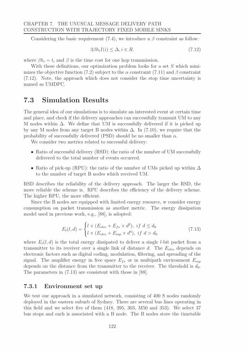
CHAPTER 7. THE UNUSUAL MESSAGE DELIVERY PATHCONSTRUCTION WITH TRAJECTORY FIXED MOBILE SINKS

Considering the basic requirement (7.4), we introduce a β constraint as follow:

3βhiI(i) ≤ Δ, i ∈ R. (7.12)

where βhi = ti and β is the time cost for one hop transmission.With these definitions, our optimization problem looks for a set S which mini-

mizes the objective function (7.2) subject to the α constraint (7.11) and β constraint(7.12). Note, the approach which does not consider the stop time uncertainty isnamed as UMDPC.

7.3 Simulation Results

The general idea of our simulations is to simulate an interested event at certain timeand place, and check if the delivery approaches can successfully transmit UM to anyM nodes within Δ. We define that UM is successfully delivered if it is picked upby any M nodes from any target B nodes within Δ. In (7.10), we require that theprobability of successfully delivered (PSD) should be no smaller than α.

We consider two metrics related to successful delivery:

• Ratio of successful delivery (RSD): the ratio of the number of UM successfullydelivered to the total number of events occurred.

• Ratio of pick-up (RPU): the ratio of the number of UMs picked up within Δto the number of target B nodes which received UM.

RSD describes the reliability of the delivery approach. The larger the RSD, themore reliable the scheme is. RPU describes the efficiency of the delivery scheme.The higher RPU, the more efficient.

Since the B nodes are equipped with limited energy resource, w consider energyconsumption on packet transmission as another metric. The energy dissipationmodel used in previous work, e.g., [88], is adopted:

Et(l, d) =

⎧⎨⎩l × (Eelec + Efs × d2), if d ≤ d0

l × (Eelec + Emp × d4), if d > d0(7.13)

where Et(l, d) is the total energy dissipated to deliver a single l-bit packet from atransmitter to its receiver over a single link of distance d. The Eelec depends onelectronic factors such as digital coding, modulation, filtering, and spreading of thesignal. The amplifier energy in free space Efs or in multipath environment Emp

depends on the distance from the transmitter to the receiver. The threshold is d0.The parameters in (7.13) are consistent with those in [88].

7.3.1 Environment set up

We test our approach in a simulated network, consisting of 400 S nodes randomlydeployed in the eastern suburb of Sydney. There are several bus lines operating inthis field and we select five of them (418, 395, 303, M50 and 353). We select 37bus stops and each is associated with a B node. The B nodes store the timetable

122

7.3. SIMULATION RESULTS

1 2 3 4 5

6

7

8

9

10 11

12

13

14

15

16

17

18

1920

21

22

2324

25

2627

28

2930

31

32

33

34

35

36

37

Source CHEvent ASource node

(a)

1 2 3 4 5

6

7

8

9

10 11

12

13

14

15

16

17

18

1920

21

22

2324

25

2627

28

2930

31

32

33

34

35

36

37

Source CHEvent ASource node

(b)

1 2 3 4 5

6

7

8

9

10 11

12

13

14

15

16

17

18

1920

21

22

2324

25

2627

28

2930

31

32

33

34

35

36

37

Event ASource node

(c)

Figure 7.3: UM delivery routes by I-UMDPC, UMDPC, and Stash for Event A(Δ = 1.5 minutes, α = 0.997, and β = 1 second).

for the corresponding bus operations. They can also learn the distribution of actualarrival over long time observation. These five bus lines are with frequencies 10, 6,13, 8 and 15 minutes respectively. We assume the arrival time and stop duration areindependent and both follow Gaussian distribution. Thus, the departing time alsofollow Gaussian distribution, whose mean and standard deviation can be obtainedfrom those of arrival time and stop duration.

We simulate an interested event: Event A and apply I-UMDPC, UMPDC andStash [253] to deliver UM. We conduct extensive simulations on Event A underdifferent parameter sets. We display the illustrative results by the considered ap-proaches in Fig. 7.3, where Δ = 1.5 minutes, α = 0.997 (three-sigma rule), andβ = 1 second. As seen in Fig. 7.3, the three approaches select 6, 9 and 15 target Bnodes respectively.

In the following parts, we further investigate the impacts of Δ, α and β onthe performance of the considered approaches. Note, the number of B nodes alsoinfluences the performance of I-UMDPC, which has been reported in [251].

123

CHAPTER 7. THE UNUSUAL MESSAGE DELIVERY PATHCONSTRUCTION WITH TRAJECTORY FIXED MOBILE SINKS

0.4 0.6 0.8 1 1.2 1.4 1.6 (minute)

0

0.1

0.2

0.3

0.4

0.5

0.6

0.7E

nerg

y co

nsum

ptio

n (J

)

I-UMDPC totalUMDPC totalStash totalI-UMDPC deliveryUMDPC deliveryStash deliveryI-UMDPC routeUMDPC routeStash route

(a)

0.4 0.6 0.8 1 1.2 1.4 1.6 (minute)

0

5

10

15

20

25

30

35

Num

ber o

f tar

get B

nod

es

I-UMDPCUMDPCStash

(b)

0.4 0.6 0.8 1 1.2 1.4 1.6 (minute)

50

60

70

80

90

100

RS

D (%

)

I-UMDPCUMDPCStash

(c)

0.4 0.6 0.8 1 1.2 1.4 1.6 (minute)

0

10

20

30

40

50

60

70

Ave

rage

RP

U (%

)I-UMDPCUMDPCStash

(d)

Figure 7.4: Comparison of I-UMDPC, UMDPC and Stash under different Δ. (a)Energy consumption. (b) Number of target B nodes. (c) RSD. (d) RPU.

7.3.2 The influence of Δ

We investigate the influence of Δ, which is an application dependent parameter.Here, α = 0.997 and β = 1 second.

As seen from Fig. 7.4a, with the increase of Δ, the energy consumed by I-UMDPC on delivery decreases. For UMDPC, when Δ is between 0.4 and 1.2 min-utes, the energy consumption remains the same; while it decreases when Δ is between1.3 and 1.7 minutes. This is because when Δ is smaller than 1.2 minutes, UMDPCis unable to find feasible solution of the optimization problem. Thus, all 37 B nodesare selected as targets (see Fig. 7.4b). I-UMDPC and UMDPC consume the sameenergy on route construction. I-UMDPC consumes less on delivery than UMDPC.Stash spends more energy than I-UMDPC and UMDPC in both route constructionand delivery. These results are consistent with the numbers of target B nodes asshown in Fig. 7.4b.

As shown in Fig. 7.4c, the RSDs of them increase with Δ. When Δ is between0.4 and 1.2, the RSD of UMDPC is higher than that of I-UMDPC. The reason isthat all the B nodes are selected as targets by UMDPC. When Δ is larger than 1.2,I-UMDPC and UMDPC achieve similar RSD. We also notice that I-UMDPC andUMDPC perform better than Stash. The influence of Δ on RPU is demonstrated

124

7.3. SIMULATION RESULTS

in Fig. 7.4d. The trend of RPU is similar to RSD. When Δ ≤ 1.2, the RPU ofUMDPC is lower than Stash; while when Δ ≥ 1.3, the RPU of UMDPC is largerthan Stash. The reason is that Stash prefers the B nodes which are cheap to deliverto, while UMDPC focuses more on the reliability of delivery. I-UMDPC outperformsUMDPC and Stash for all the considered Δ.

From the above analysis, we conclude that the larger (smaller) Δ, the easier(more difficult) to deliver UM successfully, leading to lower (higher) energy con-sumption and number of target B nodes, and higher (lower) RSD and RPU.

7.3.3 The influence of α

This section considers the impact of α. Here, Δ = 1.5 minutes and β = 1 sec-ond. Since I-UMDPC and UMDPC consume the same amount of energy on routeconstruction and Stash is non-sensitive to the investigated parameters in terms ofenergy consumption, we only display the total amounts here and in the next section.

Here, α takes 0.970, 0.980, 0.990, 0.997 and 0.999. With the increasing of α,the energy consumptions and the numbers of target B nodes by I-UMDPC andUMDPC increase as shown in Fig. 7.5a and Fig. 7.5b, respectively. The reasonlies in α constraint (7.10). For the fixed Δ and β, α constraint impacts on thetarget B nodes. Generally, the more strict (7.10), i.e., the larger α, the more targetB nodes are required, which further influences the energy consumption by targetB nodes. Fig. 7.5c shows that the I-UMDPC and UMDPC become more reliablewith higher α. However, the efficiencies of them decrease with α, see Fig. 7.5d.Similar to the simulations in Section 7.3.2, Stash is non-sensitive to α, thus theenergy consumption and B node number remain constant with varying α. RSD andRPU change slightly due to the random simulation of bus operation.

From these simulations we can observe that I-UMDPC achieves similar reliabilitywith UMDPC and outperforms UMDPC as well as Stash in terms of efficiency.

7.3.4 The influence of β

This section investigates the influence of β. β is a parameter determining the timecost to delivery message to a B node, i.e., ti = βhi, for B node i. Moreover, itimpacts on the probability of collecting a UM from a B node, see Eq. (7.7), (7.8)and (7.9). For small β, the probability of Situation 2 (i.e., the probability thatUM arrives early (7.8), see Fig. 7.2b) is dominant in (7.9). In this case, with theincrease of β, the probability P decreases. In contrast, for large β, the probabilityof Situation 1 (i.e., the probability that M node arrives early (7.7), see Fig. 7.2a)is the dominant in (7.9). Through simulations we find that with the increase of β,P decreases. From the above analysis we can obtain that, the larger β, the smallerP . This is also the reason that the energy consumptions as well as the numbersof target B nodes by I-UMDPC and UMDPC raise with the increase of β, see Fig.7.6a and 7.6b. Another interesting phenomenon in Fig. 7.6a and 7.6b is that whenβ is larger than 2.25 seconds, target B node number by UMDPC is bounded bythe number of available B nodes. This is because that there is no solution to theoptimization problem in UMDPC. In the meanwhile, the energy consumption also

125

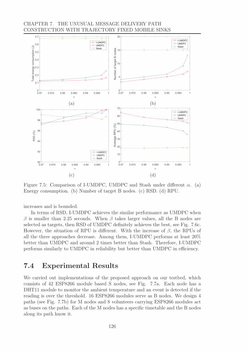
CHAPTER 7. THE UNUSUAL MESSAGE DELIVERY PATHCONSTRUCTION WITH TRAJECTORY FIXED MOBILE SINKS

0.97 0.975 0.98 0.985 0.99 0.995 10

0.1

0.2

0.3

0.4

0.5

0.6

0.7To

tal e

nerg

y co

nsum

ptio

n (J

)

I-UMDPCUMDPCStash

(a)

0.97 0.975 0.98 0.985 0.99 0.995 10

5

10

15

20

Num

ber o

f tar

get B

nod

es

I-UMDPCUMDPCStash

(b)

0.97 0.975 0.98 0.985 0.99 0.995 190

92

94

96

98

100

RS

D (%

)

I-UMDPCUMDPCStash

(c)

0.97 0.975 0.98 0.985 0.99 0.995 10

10

20

30

40

50

60

70

Ave

rage

RP

U (%

)I-UMDPCUMDPCStash

(d)

Figure 7.5: Comparison of I-UMDPC, UMDPC and Stash under different α. (a)Energy consumption. (b) Number of target B nodes. (c) RSD. (d) RPU.

increases and is bounded.In terms of RSD, I-UMDPC achieves the similar performance as UMDPC when

β is smaller than 2.25 seconds. When β takes larger values, all the B nodes areselected as targets, then RSD of UMDPC definitely achieves the best, see Fig. 7.6c.However, the situation of RPU is different. With the increase of β, the RPUs ofall the three approaches decrease. Among them, I-UMDPC performs at least 20%better than UMDPC and around 2 times better than Stash. Therefore, I-UMDPCperforms similarly to UMDPC in reliability but better than UMDPC in efficiency.

7.4 Experimental Results

We carried out implementations of the proposed approach on our testbed, whichconsists of 42 ESP8266 module based S nodes, see Fig. 7.7a. Each node has aDHT11 module to monitor the ambient temperature and an event is detected if thereading is over the threshold. 16 ESP8266 modules serve as B nodes. We design 4paths (see Fig. 7.7b) for M nodes and 8 volunteers carrying ESP8266 modules actas buses on the paths. Each of the M nodes has a specific timetable and the B nodesalong its path know it.

126

7.4. EXPERIMENTAL RESULTS

0.5 1 1.5 2 2.5 (second)

0

0.1

0.2

0.3

0.4

0.5

0.6

0.7

Tota

l ene

rgy

cons

umpt

ion

(J)

I-UMDPCUMDPCStash

(a)

0.5 1 1.5 2 2.5 (second)

0

5

10

15

20

25

30

35

Num

ber o

f tar

get B

nod

es

I-UMDPCUMDPCStash

(b)

0.5 1 1.5 2 2.5 (second)

90

92

94

96

98

100

RS

D (%

)

I-UMDPCUMDPCStash

(c)

0.5 1 1.5 2 2.5 (second)

0

10

20

30

40

50

60

70

Ave

rage

RP

U (%

)

I-UMDPCUMDPCStash

(d)

Figure 7.6: Comparison of I-UMDPC, UMDPC and Stash under different β. (a)Energy consumption. (b) Number of target B nodes. (c) RSD. (d) RPU.

Since the testbed does not have enough nodes as the simulations above andclustering is not the focus of this chapter, clustering is not implemented in theexperiments. We assume the topology of the network is known to the nodes. Thesenodes communicate with each via WiFi. To make a node communicate with only itsneighbour nodes, we set a threshold for the S and B nodes, i.e., -40dB, correspondingto 1 meter, according to the tested Received Signal Strength Indicator (RSSI) in Fig.7.7c. To make B nodes communicate with M nodes only when the latter arrives, weset another threshold for B nodes, i.e., -20dB, corresponding to about 0.2 meters. Inthe simulations, we use βhi to estimate the time to transmit packet between sourcenode and B node i. However, since β is unknown in practice, that estimation isnot precise. Besides, different nodes may have varying β. Thus, in the experiments,such time requirement is measured by the source node, which takes into account thetime of processing and transmitting.

We selected each S node as the source node once by making a fire near it andwe totally did 42 experiments for each of the considered approaches. We set α as0.997, Δ as 1 minute. We summarise the experiment results in Fig. 7.8. Fig. 7.8ashows that Stash always select 8 target B nodes since there are 8 M nodes. Thisnumber by I-UMDPC is always no larger than UMDPC since the former considers

127

CHAPTER 7. THE UNUSUAL MESSAGE DELIVERY PATHCONSTRUCTION WITH TRAJECTORY FIXED MOBILE SINKS

(a)

(b)

0 5 10 15 20Distance (meter)

-100

-80

-60

-40

-20

0

RS

SI(d

B)

(c)

Figure 7.7: Node deployment for I-UMDPC experiments. (a) Node deployment.(b) Visualization with M nodes’ paths. Black circles are S nodes; Blue square are Bnodes and the red curves are M nodes’ paths. (c) RSSI against distance.

the stop time. Fig. 7.8b shows the RPU of Stash is usually the smallest. In otherwords, the selection strategy is inefficient. But there are cases where its RPU islarger than I-UMDPC and UMDPC, for example when the source node is 24 and25. I-UMDPC achieves the best performance in RPU among the three approachesin most experiments, while there are also cases where UMDPC is performs the best.For example, when the source node is 19, I-UMDPC chose 2 target B nodes whileUMDPC chose a third one. One of the 2 B nodes failed to upload UM while thethird one uploaded. Thus, the RPU of I-UMDPC is 50% while that of UMDPC is67%. In summary, I-UMDPC performed the best in 93% cases, which showed itseffectiveness.

7.5 Summary

This chapter considers the applications of wireless sensor networks where the usersrequire fresh report of an event. We define that the report message is fresh if it isdelivered to M nodes within the given latency. We present an Improved-UnusualMessage Delivery Path Construction approach (I-UMDPC) for UM delivery. I-UMDPC combines cluster-based routing, M nodes which are attached to buses and

128

7.5. SUMMARY

0 10 20 30 40Source node

0

1

2

3

4

5

6

7

8

Targ

et B

nod

e nu

mbe

r

I-UMDPC UMDPC Stash

(a)

0 10 20 30 40Source node

0

0.2

0.4

0.6

0.8

1

RP

U(%

)

I-UMDPC UMDPC Stash

(b)

Figure 7.8: Comparison of I-UMDPC, UMDPC and Stash in real experiments. (a)Target B node number. (b) RPU.

an optimization based target B nodes selection procedure. The features of busoperation, i.e., the uncertain arrival time and stop duration at a bus, are formulatedby random variables and accounted in the optimization problem. Through extensivesimulations as well as experiments on our testbed, we show that I-UMDPC is ableto deal with the uncertainties and deliver UM to M nodes with higher reliabilityand efficiency than the alternatives.

Although the models used here are quite practical, some aspects still need to beinvestigated, such as the failure in transmission, which is a key factor impacting onthe collection latency.

129

Chapter 8

Optimized Deployment ofAutonomous Drones to ImproveUser Experience in CellularNetworks

Contents8.1 Motivation . . . . . . . . . . . . . . . . . . . . . . . . . . . 131

8.2 System Model . . . . . . . . . . . . . . . . . . . . . . . . . 133

8.3 Problem Statement . . . . . . . . . . . . . . . . . . . . . . 135

8.3.1 Single Drone Deployment (SDD) . . . . . . . . . . . . . . 135

8.3.2 k Drones Deployment (kDD) . . . . . . . . . . . . . . . . 136

8.3.3 Energy aware k Drones Deployment (EkDD) . . . . . . . 137

8.3.4 Minimum Drones Deployment (MinDD) . . . . . . . . . . 138

8.4 Proposed solutions . . . . . . . . . . . . . . . . . . . . . . . 138

8.4.1 Solution to SDD . . . . . . . . . . . . . . . . . . . . . . . 138

8.4.2 Solution to kDD and EkDD . . . . . . . . . . . . . . . . . 138

8.4.3 Solution to MinDD . . . . . . . . . . . . . . . . . . . . . . 140

8.5 Analysis of the proposed algorithms . . . . . . . . . . . . 140

8.6 Evaluation . . . . . . . . . . . . . . . . . . . . . . . . . . . . 143

8.6.1 Simulation Setup . . . . . . . . . . . . . . . . . . . . . . . 143

8.6.2 Dataset . . . . . . . . . . . . . . . . . . . . . . . . . . . . 144

8.6.3 Metrics . . . . . . . . . . . . . . . . . . . . . . . . . . . . 145

8.6.4 Comparing Approaches . . . . . . . . . . . . . . . . . . . 146

8.6.5 Simulation results . . . . . . . . . . . . . . . . . . . . . . 147

8.6.6 Discussion . . . . . . . . . . . . . . . . . . . . . . . . . . . 152

8.7 Summary . . . . . . . . . . . . . . . . . . . . . . . . . . . . 152

130

8.1. MOTIVATION

Distinguishing from Chapters 4, 5, 6 and 7, this chapter considers the cellularnetworks. Similar to Chapters 5, 6 and 7, we aim at using mobility constraineddrones to improve user experience.

8.1 Motivation

Explosive demands for mobile data are driving mobile operators to respond to thechallenging requirements of higher capacity and improved quality of user experience(QoE) [123]. Deploying more Base Stations (BSs) is able to meet the increasing traf-fic demand. This solution, however, may not only result in more cost for equipmentsand site rental, but also bring with other issues, such as a high percentage of BSshaving low utility in non-peak hours. In this context, the utilization of autonomousdrones, which work as flying BSs, could be a more efficient solution than networkdensification.

Recently, the US government has approved a resolution to increase commercialuse of drones1. Arguably, drones will play a more significantly important role inour daily life in the future. In this chapter, we focus on one of the key issues ofcontent delivery using drones: drone deployment. Generally, the drone deploymentproblem has been studied to find out the optimal 3D positions for drones to serveuser equipments (UEs) on a 2D plane. The altitudes of drones are restricted bylocal regulations. For example, in the US, the maximum allowable altitude is 120meters above the ground [254]. In Australia, the drones should be more than 30meters away from people [255]. Here, we consider a scenario where drones are flyingat a fixed altitude within the allowed range. The drone deployment problem is abit similar to the problem of optimal sensor placement in control [256, 257]. Thedifference is that in control the optimal sensor placement is done in the time domain,while the drone deployment considered in this chapter is in the spatial domain.

Different from most existing work where UEs are assumed to be randomly dis-tributed or following a predefined distribution in a 2D environment [258], here weconsider a more realistic scenario. We focus on urban environment, and only con-sider outdoor UEs. We propose a street graph and the UEs to be served by dronesare near streets. This assumption is reasonable in urban environment as when usersenter buildings, they can switch to Wi-Fi to access the network. Furthermore, in-stead of focusing on modelling the movements of UEs, we propose a UE densityfunction model. Such model reflects the traffic demand at a certain position on thestreet graph during a certain time period. In this chapter, we build up the UE den-sity functions based on a realistic dataset collected from a social discovery mobileApp: Momo2. We assume that the drones are wirelessly connected to the existingBSs [259] via high frequency radios, which do not interfere with the low frequencyradios used by drones and UEs.

Commercial drones often rely on batteries to power their rotors and the on-boardelectronic modules, such as sensors and radios [260]. Hence, the flying time allowed

1https://www.voanews.com/a/trump-ok-test-program-expand-domestic-drone-flights/4085752.html

2http://www.immomo.com

131

CHAPTER 8. OPTIMIZED DEPLOYMENT OF AUTONOMOUS DRONES TOIMPROVE USER EXPERIENCE IN CELLULAR NETWORKS

by the battery is limited. In this chapter, we introduce the idea that the dronescan recharge their battery from the existing powerlines3. For safety, we assume thatthe drones can stop on the utility poles (instead of on powerlines) and rechargethemselves. Then, the routine of a drone is serving UEs, flying to a utility pole,recharging on the utility pole, and then flying back to its serving position. Accordingto the field experiments using Phantom drones [261], the power for flying is over 140watts; while the typical power for transmitting information through radios is usuallyaround 250 milliwatts [262], which is three orders of magnitude less than the formercase. Compared to flying, the energy consumption caused by wireless transmissionis neglected. To guarantee a certain time for serving UEs, the positions of dronesshould be well managed such that they are able to get recharged before running outof battery, since such positions impact the time spent on flying.

From the literature review in Section 2 we can see that, most existing approachesare proactive, which are based on some assumed UE distribution [150, 151, 152].However, the real situation cannot be fully reflected by such distribution model, dueto the high dynamics of realistic UEs. In contrast, the reactive approach is basedon what is happening concurrently. The technique of on-line crowdsensing [263]has been available to collect the dynamic information of UEs. Thus, the reactiveapproach may be more effective in real applications to to provide better service tothe dynamic UEs. Before moving forward to the reactive approach, what we doin this chapter falls into the proactive group. But different from those assuming aspecific distribution of UEs, we make use of a collected dataset called Momo, whichcan better reflect the real UE distribution.

In this chapter, we study four problems about drone deployment from simple todifficult:

• Single Drone Deployment (SDD): where to place a single drone in the area ofinterest to maximize the effectively served UE number;

• k Drones Deployment (kDD): given k available drones, where to deploy themsuch that the effectively served UE number is maximized;

• Energy aware k Drones Deployment (EkDD): given k available drones, theenergy consumption and recharging models, where to deploy them such thatthe effectively served UE number is maximized;

• Minimum Drones Deployment (MinDD): what is the minimum number ofdrones and where to deploy them such that a preferred UE coverage levelcan be achieved, subject to the inner drone distance constraint.

Clearly, the kDD problem is the general case of SDD by extending the numberof drones to k from 1, and the EkDD problem is the general case of kDD by takinginto account the flying time of drones, which has not been considered in the contextof using drones to serve UEs so far in the existing work. The minimum number ofdrones to achieve a certain user coverage level is a problem in which the InternetService Providers (ISPs) are interested, which helps ISPs to consider the trade-offbetween the investment and benefit. Since we assume there a sufficient number of

3http://www.sbs.com.au/news/article/2017/08/23/powerlines-charge-drones-vic-students

132

8.2. SYSTEM MODEL

drones available, when drones are nearly out of battery, battery fresh drones wouldbe deployed to replace them. Thus, the flying time constraint is not considered inMinDD.

We address SDD by finding the maximum coverage street point over the streetgraph, which is relatively easy. For kDD and EkDD, we prove that they can be re-duced to the well known max k-cover problem, which is NP-hard [264]. For MinDD,we prove that it can be reduced to the set cover problem, which is also NP-hard[264]. Thus, we develop three greedy algorithms to solve kDD, EkDD and MinDDrespectively.

To the best of our knowledge, this is the first work to study drone deploymentconstrained to street graph and with the consideration of battery lifetime constraint.We summarize our contributions as follows:

• We propose a street graph model describing the urban area of interest; anda UE density function reflecting the traffic demand at a certain position onstreet graph during a certain period of time.

• We formulate a series of drone deployment problems and prove that they areNP-hard.

• We design greedy algorithms to solve the proposed problems and provide the-oretical analysis on the approximation factors.

• Extensive simulations are conducted to verify the effectiveness of the proposedapproaches.

The rest content is organized as follows. In Section 8.2, we present the systemmodel, and in Section 8.3, we formally formulate the problems. Section 8.4 presentsthe proposed solutions, which is followed by our theoretical analysis in Section 8.5.In Section 8.6, we conduct extensive simulations to evaluate the proposed approachesbased on the realistic network dataset of Momo. Finally, Section 8.7 concludes thischapter and discusses future work.

8.2 System Model

We consider an urban area with UEs that cannot be served by the existing BSsdue to capacity limitation or some malfunction of the infrastructure. We deploydrones to serve these UEs. The drones are assumed to be wirelessly connected toexisting BSs via high frequency radios and there is a central station which managesthe drones.

In this section, we present the system model including a proposed street graphassociated with the UE density function, and the wireless communication model.

We first introduce the street graph model. Let G(V,E, ρ) be the street graph ofthe considered area, where V and E are the sets of street points and edges betweentwo neighbour street points respectively. Each street point is associated with a UEdensity function ρv,t, v ∈ V , describing the number of UEs at v during the tth

(t ∈ [1, T ]) time slot (the total time window we consider is T time slots). Since

133

CHAPTER 8. OPTIMIZED DEPLOYMENT OF AUTONOMOUS DRONES TOIMPROVE USER EXPERIENCE IN CELLULAR NETWORKS

A B

C

Figure 8.1: A street graph. The squares are street points. The length of the pathrepresented by the red line segments is the graph distance between A and B; andthat between A and C is the blue line.

ρ is a function of time, the street graph G also varies with time. To simplify thestatement, we omit the symbol t in the below descriptions.

Definition 8.2.1. The graph distance between two street points v and w on thegraph, i.e., g(v, w), is defined as the length of the shortest path between v and w.

In the example shown in Fig. 8.1, g(A,B) is the length of the path representedby the red line segments; while g(A,C) is the length of the path represented by theblue line segment.

Remark 8.2.1. The physical ground distance between two street points on the streetgraph is always no larger than the corresponding graph distance, according to thetriangle inequality theorem, which states that the sum of the lengths of two sides ofa triangle must always be greater than the length of the third side.

Definition 8.2.2. Let h be the altitude of the drone. The spatial graph distancebetween the drone at (v, h) and a point w on the graph, i.e., d(v, h, w), is defined as:

d(v, h, w) =»g(v, w)2 + h2 (8.1)

Remark 8.2.2. According to Remark 8.2.1, d(v, h, w) is always no smaller than thecorresponding physical spatial distance.

In this chapter, we do not focus on optimizing the altitude of the drones4. Forsimplicity, we fix h in this chapter and then the h in the spatial graph distance canbe omitted without confusion. To avoid hitting tall buildings, we assume the dronescan only fly and hover head over the streets.

Now, we consider the wireless communication model between drones and UEs,i.e., the drones-to-UEs links rather than the BSs-to-drones wireless backhaul links.The drones may have LoS or NLoS with UEs depending on the terrain. Consider adrone hovering over street point v and a UE at street point w. Adopting the realistic3GPP propagation model [262], we have the path loss of signal from the drone tothe UE:

PLλ(d(v, w)) = Aλ +Bλ log(d(v, w)) (8.2)

4This may involve dealing with specific regulations and policies.

134

8.3. PROBLEM STATEMENT

where λ ∈ {LoS,NLoS}.The received power by the UE is computed by:

S(v, w) =Ptx

PLλ(d(v, w))(8.3)

where Ptx is the transmit power of the drone.Then, the signal to noise ratio (SNR) is:

SNR(v, w) =S(v, w)

N0

(8.4)

where N0 is the power of noise.To meet the Quality of Service (QoS) requirement, we require that the SNR at

any UEs should not be lower than a given threshold α:

SNR(v, w) ≥ α (8.5)

otherwise, the received signal cannot be demodulated by the normal UEs.From (8.2), (8.3) and (8.4), we find that whether (8.5) can be satisfied depends

on d(v, w) (g(v, w), as h is fixed in this chapter). Moreover, we find that the graphdistance is upper bounded, beyond which (8.5) will never be met. Let gmax denotesuch upper bound.

Remark 8.2.3. As will be shown later, we use the NLoS situation to compute gmax,which is the worst case. Then, according to Remark 8.2.2, if a drone is placed at v,the UEs within graph distance gmax on the street graph always satisfy (8.5), i.e., canbe served by the drone.

When multiple drones are used, the signal to interference and noise ratio (SINR)at a UE is computed by:

SINR(v, w) =S(v, w)

I +N0

(8.6)

where I is the total interference from all the other drones.

8.3 Problem Statement

In this section, we formulate four drone deployment problems.

8.3.1 Single Drone Deployment (SDD)

We start from the simplest problem: Single Drone Deployment (SDD) i.e., whereto deploy a single drone in the area of interest such that the effectively served UEnumber by the drone is maximized.

Before formulating the problem, we introduce the below definitions.

Definition 8.3.1. The covered street point set is defined as the set of streetpoints, which are covered by the drone. If the drone is deployed at v, the coveredstreet point set can be computed by: S(v) = {w|g(w, v) ≤ gmax}. Correspondingly,we define the covered UE set as the set of UEs which can be served by the droneif it is placed at v, i.e., U(v).

135

CHAPTER 8. OPTIMIZED DEPLOYMENT OF AUTONOMOUS DRONES TOIMPROVE USER EXPERIENCE IN CELLULAR NETWORKS

Remark 8.3.1. Let U denote the set of all UEs on the street graph, then we haveU =

⋃v∈V U(v).

Definition 8.3.2. The benefit achieved by placing a drone at v is defined as thenumber of UEs it can serve, i.e., B(v) =

∑w∈S(v) ρw.

Remark 8.3.2. From Definition 8.3.1, 8.3.2, we have |U(v)| = B(v), ∀ v ∈ V .

We introduce a binary variable z(v) indicating whether the drone is deployed atv:

z(v) =

{1, if the drone is deployed at v

0, otherwise(8.7)

With Definition 8.3.1, 8.3.2 and (8.7), Single Drone Deployment (SDD) can beformulated as follows:

maxz(v)

Ñ ∑w∈S(v)

ρw

éz(v) (8.8)

subject to

S(v) = {w|g(w, v) ≤ gmax} (8.9)

8.3.2 k Drones Deployment (kDD)

Now we consider the second problem: k Drones Deployment (kDD), i.e., where todeploy k drones such that the effectively served UE number is maximized subject tothe minimum distance between any to drones. Another constraint, i.e., the batteryconstraint, will be considered in Section 8.3.3.

In the scenario with multiple drones, a UE may hear signals from more than oneof them, which causes interference. In this chapter, we require that the minimumdistance between any two drones is β. Note that, the system parameter β controlsthe intensity of interference and a lower β may lead to higher interference.

We formulate the k Drones Deployment (kDD) problem as follows:

maxz(v)

∑v∈V

Ñ ∑w∈S(v)

ρw

éz(v) (8.10)

subject to

S(v) = {w|g(w, v) ≤ gmax} (8.11)∑v∈V

z(v) = k (8.12)

g(v, w) > β, ∀ z(v) = 1, z(w) = 1, v �= w (8.13)

As seen in the objective function (8.10), we want to maximize the benefits ofdrone deployment. In comparison to the SDD problem, here (8.13) constrains theinner distance between any pair of drones.

136

8.3. PROBLEM STATEMENT

8.3.3 Energy aware k Drones Deployment (EkDD)

The third problem is named as Energy aware k Drones Deployment (EkDD), whichaims at deploying k drones such that the effectively served UE number is maxi-mized, subject to the inner drone distance constraint and the drone battery lifetimeconstraint.

The off-the-shelf drones often rely on the preloaded battery to power their rotorsand the on-board electronics models. Considering the battery lifetime constraint, werequire an efficient duty management scheme for the available drones to guaranteetheir service.

Typically, there are three states of a drone: Serve (S), Fly (F) and Recharge (R).Denote λS, λF , and λR as the percentages of a time slot during which a drone is in S,F, and R respectively. It is apparent that, λS+λF +λR = 100%. Among these threestates, we assume that only S contributes to network performance, because when adrone is in F or R, the wireless backhaul links may be unstable or unavailable.

We assume that there are a few street points on the graph, which allow thedrones to recharge. In practice, such positions can be placed on the utility poles.Let VR ⊂ V be the set of recharging positions.

Let s be the speed of the drones. Given λS, λF , and λR, we can compute amaximum graph distance gR from the recharging positions, beyond which a dronecannot guarantee its serving time, i.e., λS percent of the full cycle of time slots (S→ F → R → F). For simplicity, we assume that to reach a recharging position vRfrom its current serving position v, a drone first flies over the street to the positionwhose projection is vR, it then lands on the utility pole (whose altitude is hR) torecharge. When the recharging process finishes, it ascends to h and then flies to theserving position v following streets. Consequently, we have

2(g(v, w) + h− hR) ≤ sλF · 1, (8.14)

from which we can obtain

gR =1

2sλF + hR − h. (8.15)

Now, we are ready to formulate the problem with the constraint of rechargingpositions, which is shown below.

maxz(v)

λS

∑v∈V

Ñ ∑w∈S(v)

ρw

éz(v) (8.16)

subject toS(v) = {w|g(w, v) ≤ gmax} (8.17)∑

v∈Vz(v) = k (8.18)

g(v, w) > β, ∀ z(v) = 1, z(w) = 1, v �= w (8.19)

g(v, vR) ≤ gR, ∀ z(v) = 1, ∃ vR ∈ VR (8.20)

Here, we still aim at finding the optimal positions for k drones such that thetotal number of served UEs can be maximized and in the meanwhile any two dronesare at least β apart from each other and any drone must be within gR from thenearest recharging position.

137

CHAPTER 8. OPTIMIZED DEPLOYMENT OF AUTONOMOUS DRONES TOIMPROVE USER EXPERIENCE IN CELLULAR NETWORKS

8.3.4 Minimum Drones Deployment (MinDD)

The above three problems all consider the scenario when drones are limited. Thefinal problem is to seek the minimum number of drones and their deployments suchthat an ISP preferred level of coverage of the UEs can be served (say 98%), whichis called Minimum Drones Deployment (MinDD). Since we assume that we havea sufficient number of drones, the battery constraint can be ignored but the innerdrone distance constrained is still considered.

MinDD can be formulated as follows:

minz(v)

∑v∈V

z(v) (8.21)

subject to

|⋃

{v|z(v)=1}U(v)| ≥ γ|U| (8.22)

g(v, w) > β, ∀ z(v) = 1, z(w) = 1, v �= w (8.23)

where γ in (8.22) is the ISP preferred level of coverage, i.e., the effectively servedUE ratio should not be less than γ.

8.4 Proposed solutions

In this section, we present the solutions to the four considered problems.

8.4.1 Solution to SDD

It is relatively easy to solve SDD using the maximum coverage street point over thestreet graph.

To find the solution, we can search the set of V . For each v ∈ V , find S(v) andcompute B(v). Then, the v having the largest B(v) is the optimal place. Note, thesolution to the problem may not be unique due to the discrete nature of the UEnumber.

8.4.2 Solution to kDD and EkDD

First, we characterize the kDD and EkDD problems as NP-hard ones in Theorem8.4.1.

Theorem 8.4.1. The problems of kDD and EkDD are NP-hard.

Proof. If we ignore constraint (8.13) in kDD, and constraint (8.19) and (8.20) inEkDD, the two problems are reduced to an instance of max k-cover problem, i.e.,given a universe U and sets U(v) ∈ U (v ∈ V ), we are looking for a set V consistingof k elements of v, such that the union of U(v) has maximum cardinality. As shownin [264], the max k-cover problem is NP-hard. So, both of kDD and EkDD are alsoNP-hard.

138

8.4. PROPOSED SOLUTIONS

Algorithm 9 The greedy algorithm for kDD

Input: V , U , β and kOutput: V1: C = ∅.2: V = ∅.3: i = 1.4: while i ≤ k do5: maxv∈{v|v∈V,v /∈V} |C

⋃U(v)|.

6: if g(v, w) > β, ∀ w ∈ V then7: C = C

⋃U(v).

8: V = V ⋃{v}.9: end if10: V = V \ v.11: i = i+ 1.12: end while

We propose greedy algorithms to solve kDD and EkDD respectively as shown inAlgorithms 9 and 10. The basic idea of Algorithm 9 follows that in [265], i.e, in eachiteration, we pick a street point which 1) adds a maximum benefit to the currentbenefit. Since we consider the inner drone distance constraint, we have to furthercheck 2) whether the street point is β away from all the already picked street points.

Clearly, the set V = {v|z(v) = 1}, i.e., the set of street points to deploy drones,is with a cardinality of |V| = k. Let C be the set of UEs which have already beenserved by drones. Initially, both V and C are empty sets. In each iteration, we firstcompute the optimal street point v in V . Second, we check whether (8.13) in kDDis satisfied. If yes, we add the served UEs by v to the set of C and add v to the setof V . Otherwise, we remove v from V .

The intuition of Algorithm 10 is similar to Algorithm 9. For EkDD, with regardsto β constraint, we have another condition to check, i.e., 3) whether the selectedstreet point is within gR from the nearest recharging position, see Line 7 of Algorithm10.

One interesting point worth mentioning is that not all of these k drones can servesimultaneously if the battery constraint is considered, instead, they need to fly tothe recharging positions alternately. Let n be the number of drones which mustrecharge to make the drones work sustainablely. Then, we have that the amount ofconsumed energy should be no larger than the recharged energy, i.e.,

p(k − n) ≤ qn (8.24)

where p is the energy consumption per time slot and q is the recharging energy pertime slot. Here, we only consider the dominant part of the power usage for resistingthe gravity and omit that for other marginal parts of energy consumption such aswind. As a result, flying and hovering of drones consume the same power.

From (8.24), we can obtain:

n ≥ q

q + pk (8.25)

Then, the drones can be divided into � q+pq� groups to recharge by turns.

139

CHAPTER 8. OPTIMIZED DEPLOYMENT OF AUTONOMOUS DRONES TOIMPROVE USER EXPERIENCE IN CELLULAR NETWORKS

Algorithm 10 The greedy algorithm for EkDD

Input: V , U , β, k, VR and gROutput: V1: C = ∅.2: V = ∅.3: i = 1.4: while i ≤ k do5: maxv∈{v|v∈V,v /∈V} |C

⋃U(v)|.

6: if g(v, w) > β, ∀ w ∈ V then7: if g(v, vR) ≤ gR, ∃ vR ∈ VR then8: C = C

⋃U(v).

9: V = V ⋃{v}.10: end if11: end if12: V = V \ v.13: i = i+ 1.14: end while

8.4.3 Solution to MinDD

We characterize the MinDD problem as a NP-hard one in Theorem 8.4.2.

Theorem 8.4.2. The problem of MinDP is NP-hard.

Proof. If we ignore constraint (8.23) and set γ = 100% in MinDD, the problemis reduced to an instance of set cover problem, i.e., given a universe U and setsU(v) ∈ U (v ∈ V ), we are looking for a collection V of the minimum number ofsets from U , whose union is the entire universe U . Formally, V is a set cover if⋃

v∈V U(v) = U . We try to minimize |V|. As shown in [264], the set cover problemis NP-hard, then the generalized and constrained version of set cover problem, i.e.,MinDD, is also NP-hard.

We design a greedy algorithm for MinDD, which is shown in Algorithm 11. Thebasic idea of Algorithm 11 is similar to Algorithm 9, i.e., in each iteration, it picksthe street point which leads to the maximum coverage of UEs and at the same timesatisfying the inner drone distance constraint. Algorithm 11 will terminate when γpercent of all the UEs in U have been covered by the drones. The output V givesthe projections of drones and the number of drones is |V|.

8.5 Analysis of the proposed algorithms

This section analyses the proposed greedy algorithms.We first consider Algorithms 9 and 10. Let OPT be the number of served UEs

by an optimal solution. Let ci be the number of served UEs by the ith (i ≤ k) pickedstreet point, and xi be the number of served UEs by i already picked street points,i.e., xi =

∑ij=1 cj. Then, the remaining unserved UE number can be computed by

yi = OPT − xi. Further, x0 = 0, then y0 = OPT .

140

8.5. ANALYSIS OF THE PROPOSED ALGORITHMS

Algorithm 11 The greedy algorithm for MinDD

Input: V , U , U and βOutput: V1: C = ∅.2: V = ∅.3: while |C| < γ|U| do4: maxv∈{v|v∈V,v /∈V} |C

⋃U(v)|.

5: if g(v, w) > β, ∀ w ∈ V then6: C = C

⋃U(v).

7: V = V ⋃{v}.8: end if9: V = V \ v.10: end while

Since the optimal solution uses k sets to serve OPT UEs, we find that: in the(i + 1)th step, some street point must be able to serve at least 1

kof the remaining

uncovered UEs from OPT , i.e.,

xi+1 ≥yik

(8.26)

In particular, when i = 0, we have:

x1 ≥OPT

k, (8.27)

since y0 = OPT .

Claim 8.5.1. yi+1 ≤ (1− 1k)i+1OPT .

Proof. We use the method of Mathematical Induction to prove the claim.When i = 0, from (8.27) we have

x1 ≥OPT

k

⇒OPT − x1 ≤ OPT − OPT

k

⇒y1 ≤ (1− 1

k)OPT

(8.28)

i.e., the claim is true when i takes 0.Further, we assume yi ≤ (1− 1

k)iOPT and then we derive yi+1 ≤ (1− 1

k)i+1OPT

below:xi+1 ≤ yi − yi+1

⇒yi+1 ≤ yi − xi+1

⇒yi+1 ≤ yi −yik

(using (8.26))

⇒yi+1 ≤ (1− 1

k)i+1OPT.

(8.29)

Therefore, (8.28) and (8.29) prove Claim 8.5.1.

141

CHAPTER 8. OPTIMIZED DEPLOYMENT OF AUTONOMOUS DRONES TOIMPROVE USER EXPERIENCE IN CELLULAR NETWORKS

Now we are in the position to present the main results.

Theorem 8.5.1. Algorithm 9 (Algorithm 10) is a (1 − 1e) approximation of kDD

(EkDD).

Proof. From Claim 8.5.1, we have

yk ≤ (1− 1

k)kOPT

≤ 1

eOPT

(8.30)

Hence, we have

xk = OPT − yk ≥ (1− 1

e)OPT (8.31)

i.e., the number of served UEs by the k street points picked by Algorithm 9 (Algo-rithm 10) is at least (1− 1

e) fraction of the optimal solution OPT .

The above results can also be used in the analysis of Algorithm 11. Let k∗ denotethe optimal solution to MinDD, i.e., k∗ is the minimum number of required dronesto serve at least γ of all the UEs. Let m = γ|U|. Clearly, if we set k = k∗ in kDDor EkDD, OPT = m.

Theorem 8.5.2. Algorithm 11 is a (ln(m) + 1) approximation of MinDD.

Proof. From Claim 8.5.1, we have yi ≤ (1 − 1k∗ )

im. After picking k∗ ln(mk∗ ) street

points, the remaining unserved UE number is:

yi ≤ (1− 1

k∗ )k∗ ln( m

k∗ )m

≤ 1

e

ln( nk∗ )

m

= k∗

(8.32)

The worst case of serving those remaining unserved UEs (at most k∗) is to use atmost k∗ drones, i.e., each drone serves one UE. Then, we have the minimum numberof drones obtained by Algorithm 11 is

k∗ ln(m

k∗ ) + k∗ ≤ k∗(ln(m

k∗ ) + 1)

≤ k∗(ln(m) + 1)(8.33)

Therefore, the minimum number of drones to serve at least γ of all the UEsobtained by Algorithm 11 is a (ln(m)+1) approximation of the optimal solution.

This section analyses the approximation factors for the proposed greedy algo-rithms. In the next section, we will evaluation these algorithms through extensivesimulations.

142

8.6. EVALUATION

Table 8.1: Parameter configuration

Notation Value DescriptionALoS 103.8

LoS path loss parametersBLoS 20.9ANLoS 145.4

NLoS path loss parametersBNLoS 37.5Ptx 20 dBm Drone transmission powerN0 -104 dBm Noise powerh 50 m Drone altitudeα 15 dB SNR thresholdβ 0 - 3gmax Inner drone distanceγ 90% - 98% Level of UE coverages 4 - 8m/s Flying speed of dronesW 100 MHz BandwidthWmax 2 MHz Upper bound of bandwidth at a UEhR 10 m Height of utility poleλS 45% Percentage of one time slot for servingλF 5% Percentage of one time slot for flyingλR 50% Percentage of one time slot for recharging

8.6 Evaluation

In this section, we evaluate our proposed drone deployment strategies based on acollected dataset from a mobile App (Momo). We first introduce the parameters usedin the simulation (Section 8.6.1). Then, we provide details on the realistic datasetin use (Section 8.6.2). Next, we show the metrics for evaluation (Section 8.6.3),followed by the compared approaches (Section 8.6.4). We present the extensivesimulation results are shown (Section 8.6.5). We end this section by discussing theadvantages and disadvantages of the proposed approaches (Section 8.6.6).

8.6.1 Simulation Setup

Table 8.1 provides a quick reference for the used parameters in the simulation.According to the QoS constraint, we can determine gmax from (8.1), (8.2), (8.3),

(8.4) and (8.5). We vary α from 10 to 20 dB and calculate the corresponding gmax forboth LoS and NLoS cases, as shown in Fig. 8.2a. We can find that under the sameα, the LoS case has a larger gmax than of NLoS case. To determine the value of gmax,we further show the probability of LoS under varying distance between transmitterand receiver in Fig. 8.2b, using the model obtained by realistic experiments in[262]. From Fig. 8.2b, we can see that when the distance between the transmitterand receiver is greater than 100 meters, the probability of LoS is less than 20%.Thereby, we use the NLoS case to compute gmax. We select α = 15 dB and thecorresponding gmax becomes 95 m.

Now we discuss how accurate of using graph distance to calculate path loss,

143

CHAPTER 8. OPTIMIZED DEPLOYMENT OF AUTONOMOUS DRONES TOIMPROVE USER EXPERIENCE IN CELLULAR NETWORKS

10 12 14 16 18 20 (dB)

0

2000

4000g m

ax

LoSNLoS

(a)

0 50 100 150 200 250 300Distance between transmitter and receiver (m)

0

0.5

1

Pro

babi

lity

of L

oS

(b)

0 10 20 30 40 50a (m)

80

90

100

110

Pat

h lo

ss (d

B)

LoSNLoS

(c)

Figure 8.2: (a) gmax vs α. (b) Probability of LoS vs distance. (c) Path loss.

instead of the physical distance. Consider two street segments a and b and theyare perpendicular. The graph distance between the two end points is a + b whilethe physical distance is

√a2 + b2. Let gmax = a + b and we compute the path loss

corresponding to the physical distance. Fig. 8.2c shows the path loss of both LoSand NLoS when a is between 1 and gmax/2 meters. The physical distance varieswith a, while the graph distance is fixed to gmax. Obviously, the largest gap occurswhen a = gmax/2, and the corresponding path loss of LoS is only about 3 dB lower,and that of NLoS is only about 6 dB lower than the value calculated by the graphdistance gmax, both of which incur small errors in practice. In short, approximatingthe physical distance by the graph distance has a small impact on the calculationof path loss.

8.6.2 Dataset

To get the UE density function, we make use of the dataset of Momo. When a Momouser has an update, the information of his ID, timestamp, latitude and longitudeis sent to the server. The Momo dataset contains approximately 150 million suchupdates in a period of 38 days, from 21/5/2012 to 27/6/2012 [266]. We extract asubset of this dataset, based on which we build up the UE density function.

The Momo dataset consists of the updates of world-wide users. To make theselected dataset suitable to our problem, we only focus on the updates by the usersin a small residential community in Beijing, China. The latitude of this area is from39.9176N to 39.9242N and the longitude is from 116.4406E to 116.4501E, whichis about 1059 × 721 m2, as shown in Fig. 8.3a. Further, we build up a discretestreet graph according to the area map as shown in Fig. 8.3b. Each street isrepresented by a number of discrete points. From the whole dataset, we select theupdates whose locations fall into the considered latitude and longitude range. Basedon our observation, these updates belong to indoor and outdoor UEs. We remove

144

8.6. EVALUATION

(a)

116.44 116.442 116.444 116.446 116.448 116.45Longtitude

39.917

39.918

39.919

39.92

39.921

39.922

39.923

39.924

39.925

Latit

ude

(b)

Figure 8.3: (a) The considered residential community in Beijing. (b) UE distributionon the street graph on 21/5/2012.

the indoor updates by selecting those falling into the neighbourhoods of the streetpoints. Then, the selected dataset only consists of the updates belonging to the UEsnear the streets. We demonstrate the distribution of such UEs on 21/5/2012 in Fig.8.3b.

The selected subset of data covers more than five weeks including three types ofUE pattens on weekdays, weekends, and public holidays. Since there are only threedays belonging to category of public holidays, in this chapter we only consider theUE pattens on weekdays and weekends. We respectively take the average numbersof UEs for weekdays and weekends and show them in Fig. 8.4, where the duration ofa time slot is one hour. It can be seen that on weekdays the average UE number ismostly larger than weekends. The average total UE number on weekdays is 1003 perday while that on weekends is 727. On weekdays, the UE number increases steadilyfrom 8:00 and arrives at the peak (about 70 UEs) at 16:00, after which it decreases.The UE variation for weekends is different: it increases slowly from 8:00 to 16:00,and from 16:00 to 23:00 the UE number remains at around 40. After 23:00, muchlater than weekdays, it drops down. If we set 40 as a UE number threshold to decidethe usage of drones: on weekdays we need to send drones to serve UEs from 10:00 to22:59, i.e., 13 hours; while on weekends the drones should work for 8 hours between15:00 and 22:59. We need to mention that the number of UEs provided by Fig. 8.4shows only the UEs using Momo. The actual number of UEs should also includethose not using Momo. Although the dataset we have cannot provide us the truetotal number of UEs, it presents the realistic traffic pattens and UE distributions,which is much more closer to reality than random distribution. To make the resultsmore sensible, we introduce a scalar to scale up the UE number according to [267],which is set as 5 in the simulations.

8.6.3 Metrics

In the evaluations, we consider the performance metrics:

• Served UE ratio: The served UE ratio is defined as |⋃v∈V U(v)|/|U| × 100%.

145

CHAPTER 8. OPTIMIZED DEPLOYMENT OF AUTONOMOUS DRONES TOIMPROVE USER EXPERIENCE IN CELLULAR NETWORKS

5:00 7:00 9:00 11:00 13:00 15:00 17:00 19:00 21:00 23:00 1:00 3:00 5:00Time

0

20

40

60

80

Ser

ved

UE

ratio

WeekdaysWeekends

Figure 8.4: Average UE numbers using Momo on weekdays and weekends in theconsidered area.

• Spectral efficiency (SE): a measure of how efficiently a limited frequencyspectrum is utilized by PHY layer protocol. The spectral efficiency at a UE iscomputed by SE = log2(1 + SINR), where SINR is defined in (8.6). In thischapter, we consider the average spectral efficiency:

ASE =1

M

M∑i=1

log2(1 + SINRi) (8.34)

• Number of drones: the number of drones required to serve at least γ percentof UEs.

• Served UE per drone: the average number of UEs served by one drone.

• Network capacity (NC): the number of bits that can be generated in an unitarea of 1 km2, given the bandwidth W . The network capacity is a metricmeasuring the overall performance in both PHY and MAC layers, whose unitis Mbps/km2. For simplicity, we assume that the bandwidth of a drone isevenly allocated to its served UEs and there is a limit on the bandwidth thateach UE can get, i.e., Wmax. As a result, Wi = min( W

Mj,Wmax), where Mj is

the number of UEs served by drone j. Suppose there are k drones in 1 km2,then the network capacity can be computed by:

NC =k∑

j=1

Mj∑i=1

SEi ·Wi (8.35)

8.6.4 Comparing Approaches

As mentioned in Sections 8.1, there are several related work on the topic of dronedeployment problem. For the scenario of placing a single drone, the most relevantwork is [145]. Aiming at serving the maximum UEs, the authors formulate a mixedinteger non-linear problem to find the optimal position of the drone. Further, theauthors formulate a second order cone problem to shorten the cover range of thedrone to save transmission energy. For a fair comparison, we only compare our workwith the results of the mixed integer non-linear problem (MINLP), since shorteninga bit transmission range does not contribute much to the total energy consumption

146

8.6. EVALUATION

by the drone. We acknowledge that the energy consumed for drone movement is thedominant factor.

There are also some related work about placing multiple drones, such as [146]and [148]. However, both of them divide the area of interest into a set of zones orsubareas, which are quite different from our basic model, i.e., the street graph. So wedemonstrate the comparison of our approach with [145] for the case of single dronedeployment; and the comparison with max k-cover (without inner drone distanceconstraint) for the case of multiple drone deployment.

8.6.5 Simulation results

We present simulation results to evaluate the performance of the proposed solutionsrespectively in this part.

Evaluation of SDD

We first show the performance of single drone deployment method. As discussedin Section 8.6.2, on weekdays we deploy a drone from 10:00 to 22:59 for 13 hours;while on weekends the drone work for 8 hours between 15:00 and 22:59. Except[145] (named as Approach 1), we also compare with a random deployment (namedas Random).

We respectively display the served UE ratios on weekdays and weekends in Fig.8.5a and 8.5b. We can see that our proposed method achieves similar performancecompared with [145] in terms of served UE ratio. In theory, the 2D projection ofa drone is constrained on street in our approach; while there is no such limitationin [145]. So the optimum solution by [145] achieves no worse performance in servedUE ratio than ours. However, [145] uses MOSEK solver to address the MINLPand some solutions are local optimums, which are not competitive to our solutions.Further, both of them outperform the random deployment.

It is worthy of mentioning that, as there is no limitation on the 2D projection ofthe drone, over 70% of the solutions by [145] locate off the streets (see the illustrativeexample shown in Fig. 8.6, although the deployment by [145] serves more UEs, theprojection is off street), which have high probability of hitting tall buildings if appliedin urban environment directly. In contract, our solutions are on streets and can beapplied directly to realistic networks, thanks to the street graph model.

Evaluation of kDD

We demonstrate simulation results for deploying multiple drones. When multipledrones are used, as mentioned before, the interference should be taken into accountto assess the user experience. Two main factors influence the interference intensity:the number of drones k, and the distance threshold between two drones β. Here, wevary k from 2 to 8 and β from 0 to 3gmax. Note that, when β is 0, we are solvingthe max k-cover problem, i.e., without the consideration of inner drone distanceconstraint, because constraint (8.19) is always satisfied.

To have an insight of the impacts of these two factors, we focus on the perfor-mance on the peak hour, i.e., from 15:00 to 15:59, on weekdays. We present the

147

CHAPTER 8. OPTIMIZED DEPLOYMENT OF AUTONOMOUS DRONES TOIMPROVE USER EXPERIENCE IN CELLULAR NETWORKS

10:00 12:00 14:00 16:00 18:00 20:00 22:00Time

0

10

20

30

Ser

ved

UE

ratio

(%) Proposed

Approach 1Random

(a)

15:00 17:00 19:00 21:00 23:00Time

0

10

20

30

Ser

ved

UE

ratio

(%) Proposed

Approach 1Random

(b)

Figure 8.5: (a) Average served UE ratio on weekdays. (b) Average served UE ratioon weekends.

116.447 116.448 116.449 116.45Longitude

39.918

39.919

39.920

39.921

Latit

ude

Street pointUEDrone projection by SDDServed range of SDDDrone projection by Approach 1Served range of Approach 1

Figure 8.6: Illustrative example of 2D projections by the proposed approach andApproach 1.

served UE ratio and spectral efficiency in Fig. 8.7a and 8.7b for the peak hour.Note, the results shown here are the average values of 27 weekdays. From theseresults we can see that:

• With the increase of k, the served UE ratio increases; while the average spec-tral efficiency decreases. Because more UEs are covered by drones when k isincreased, and in the same time, the interference is also raised.

• With the increase of β, the served UE ratio slightly decreases; while the averagespectral efficiency increases. This is because increasing β means increasingthe minimum distance between any two drones, which reduces the coverageperformance; but in the meanwhile, it also reduces the strength of interferenceat a UE from other drones, which leads to larger spectral efficiency.

• An interesting finding is that the results when β takes gmax are very similarto those when β = 0 in terms of both served UE ratio and average spectralefficiency. In other words, the standard greedy algorithm for max k-coverproblem inherently avoids placing two drones closely to each other.

The results for the same peak hour on the weekends are shown in Fig. 8.8aand 8.8b. The performance trends are similar to those of weekdays. Comparing

148

8.6. EVALUATION

0 gmax

2gmax

3gmax

Minimum distane between any two drones in meter ( )

0

20

40

60

80

100

Ser

ved

UE

rat

io (

%)

k=2k=4k=6k=8

(a)

0 gmax

2gmax

3gmax

Minimum distane between any two drones in meter ( )

3

3.5

4

4.5

5

5.5

6

6.5

Spe

ctra

l effi

cien

cy (

bit/s

/Hz) k=2

k=4k=6k=8

(b)

Figure 8.7: (a) Average served UE ratio on weekdays by multiple drones. Theaverage number of UEs during the peak hour on weekdays is 350. (b) Averagespectral efficiency on weekdays by multiple drones.

0 gmax

2gmax

3gmax

Minimum distane between any two drones in meter ( )

0

20

40

60

80

100

Ser

ved

UE

rat

io (

%)

k=2k=4k=6k=8

(a)

0 gmax

2gmax

3gmax

Minimum distane between any two drones in meter ( )

3

3.5

4

4.5

5

5.5

6

6.5

Spe

ctra

l effi

cien

cy (

bit/s

/Hz) k=2

k=4k=6k=8

(b)

Figure 8.8: (a) Average served UE ratio on weekends by multiple drones. Theaverage number of UEs during the peak hour on weekends is 210. (b) Averagespectral efficiency on weekends by multiple drones.

the results of weekdays and weekends, we can find that under the same β and k,the served UE ratio on weekdays is similar to weekends (see Fig. 8.7a and 8.8a).But the number of served UEs on weekdays is much larger than weekends due tothe dense distribution of UEs on weekdays. The spectral efficiency on weekdays isabout 10% lower than that on weekends in average (see Fig. 8.7b and 8.8b). Thereason behind this phenomenon is that the distribution of UEs on weekends is moresparse than weekdays. Under the same β and k, the deployments of drones is alsomore sparse, which leads to lower interference, then higher spectral efficiency.

Evaluation of EkDD

In this part, we demonstrate the performance of the solution to the problem ofEkDD.

We assume that the operation power and the energy recharging rate are thesame, i.e., p = q. From (8.25) we have n ≥ 1

2k, i.e., the drones should be divided

into 2 groups. Consider the time slot of 1 hour in this chapter and the state-of-the-art commercial drones, such as DJI5, whose the flying time are around 30 minutes.

5https://www.dji.com

149

CHAPTER 8. OPTIMIZED DEPLOYMENT OF AUTONOMOUS DRONES TOIMPROVE USER EXPERIENCE IN CELLULAR NETWORKS

4 5 6 7 8 Inf0

20

40

60

80

100

Ser

ved

UE

rat

io (

%)

WeekdaysWeekends

(a)

116.44 116.442 116.444 116.446 116.448 116.45Longtitude

39.917

39.918

39.919

39.92

39.921

39.922

39.923

39.924

39.925

Latit

ude

Street pointUtility poleUEs=4m/ss=5m/ss=6m/ss=Inf

(b)

Figure 8.9: (a) Served UE ratio against flying speed. The total numbers of UEs are350 and 210 for the peak hour on weekdays and weekends respectively. (b) Droneprojections in the cases of 4m/s, 5m/s, 6m/s, and ’Inf’ for the peak hour on aweekday.

So in this chapter, we set λS, λF , and λR to 45%, 5% and 50% respectively. Weconsider that there are four utility poles located at the corners of graph, see Fig.8.9b for an example. Here, we fix β as gmax.

As discussed in Section 8.3.3, the flying speed is the main factor impacting on thedrone deployment. Here, we consider various practical flying speeds 4, 5, 6, 7, 8m/s,and present the corresponding performance in served UE ratio for the consideredpeak hour in Fig. 8.9a. The results of kDP are also displayed for comparison,indicated by ’Inf’. For a fair comparison, in EkDD, k = 8; while in kDD, k = 4.Then, in both the cases, 4 drones can serve UEs simultaneously. From Fig. 8.9awe can see that with the increase of s, the served UE ratio increases first and thenremain at a steady level. Because a larger s means wider operation radius for drones,and thus a weaker constraint on the positions of drones. When s is larger than 6m/s,the recharging constraint becomes invalid. Fig. 8.9b shows the drone projections forfour cases of s = 4m/s, s = 5m/s, s = 6m/s and ’Inf’, from which we can find thatthe constraint (8.20) pulls the drones’ positions closer to the recharging positionscompared to the non-constraint case of ’Inf’. When s takes 7 or 8m/s, the positionsof drones are the same with the cases of 6m/s and ’Inf’. So we do not display themin Fig. 8.9b.

In short, taking into account the energy issue, the performance reflects a morepractical scenario. The drones with higher flying speed can achieve better perfor-mance due to the relaxed constraint on its position to recharge its battery.

Evaluation of MinDD

In this part, we show how many drones are needed to serve at least γ percent ofUEs. Here, we fix β as gmax and show the relationship between γ and the minimumnumber of required drones, number of UEs served per drone, and network capacity.We vary γ from 90% to 98%. The results are shown in Fig. 8.10.

150

8.6. EVALUATION

90 92 94 96 98

Coverage requirement in % ( )

10

11

12

13

14

15

16

17

18

Num

ber

of d

rone

s

WeekdaysWeekends

(a)

90 92 94 96 98

Coverage requirement in % ( )

5

10

15

20

25

30

Num

ber

of s

erve

d U

Es

per

dron

e WeekdaysWeekends

(b)

90 92 94 96 98

Coverage requirement in % ( )

100

110

120

130

140

150

160

170

Net

wor

k ca

paci

ty (

Mbp

s/K

m2 )

WeekdaysWeekends

(c)

Figure 8.10: (a) Average minimum number of drones to serve γ percent of UEs. (b)Average number of served UEs per drone against γ. (c) Network capacity againstγ.

• Fig. 8.10a displays the required drone numbers with various γ on weekdaysand weekends for the considered peak hour. We can see that the minimumnumber of drones increases with γ. Since the number of UEs on weekends aremuch smaller than weekdays, fewer drones are needed on weekends than onweekdays to achieve the same level of UE coverage.

• Fig. 8.10b shows that, with the increase of γ, the average number of UEsserved per drone decreases. In other words, the increase of served UE numberis slow than the increase of drone number. We can also see that on weekdaysthe number of UEs served per drone is much higher than weekends, becauseUEs are sparsely distributed on weekends.

• Fig. 8.10c presents the network capacity against γ. We can see that thenetwork capacities on weekdays and weekends both increase with γ. Sincethe total number of UEs on weekends is much smaller than that on weekdays,hence the resource at drones is not fully used. So the network capacity onweekdays is larger than that on weekends.

151

CHAPTER 8. OPTIMIZED DEPLOYMENT OF AUTONOMOUS DRONES TOIMPROVE USER EXPERIENCE IN CELLULAR NETWORKS

8.6.6 Discussion

Advantages

From the above simulation results we can find that to serve more UEs, more dronesare required and the network capacity can be improved. However, the efficiency ofdrone usage, i.e., the average number of served UEs per drone, decreases. Therefore,from the view of ISPs, there is a trade-off between the investment, i.e., the numberof drones, and performance the gain, i.e., the network capacity.

Limitations

By use of practical models and reasonable network assumptions, the proposed solu-tions to the drone deployment problems provide useful guideline for practical dronedeployment. In particular, all the drones are deployed over head streets, whichcan avoid collision with tall buildings. Thus, it is straightforward to apply our ap-proaches to realistic applications. Moreover, we consider the energy constraint ofdrones in the optimization problems, which in our best knowledge has not beenaddressed by the existing work.

8.7 Summary

In this chapter, we adopt a UE density model based on the collected dataset Momo.However, the modern wireless traffic demand is quite dynamic. Thus, more effec-tive models to predict the time-variant UE density are for further study. Besides,we have not touched the performance impact of drone altitude, which is anothersignificant factor in practical drone deployment. Although it is a regulation issue,finding the optimal altitude within the allowed range may improve the number ofserved UEs. Further, the objective function of EkDD is a rough estimation of theserved UE number, because some drones can fly back to the serving positions usingless time than λF of a time slot. The precise formulation requires to consider theserving positions in the objective function, which makes the problem more complex.Moreover, in terms of radio resource management (RRM), we simply allocate theavailable bandwidth evenly to UEs. Optimal allocation of radio resource is worthinvestigating to achieve a larger network capacity [268, 269].

From simple to complex, in this chapter we discussed how to deploy a givennumber of drones to maximize the effectively served UE number; and how to de-termine the minimum number of drones to achieve a certain level of UE coverage.Different from existing work, the drone deployment is formulated based on a streetgraph model in this chapter. The street graph, associated with UE density function(obtained from a realistic dataset Momo), is close to reality. Further, we provedthat the problems are NP-hard, and then greedy algorithms were proposed to solvethe problems. The effectiveness of our approaches was verified by extensive simula-tions on the Momo dataset. Since both the street graph model and the UE densityfunction are quite realistic, the results provided in this chapter provide valuableguidelines for realistic applications. The main content is presented in [270].

152

Chapter 9

Conclusion and Future Work

Contents9.1 Contribution of the thesis . . . . . . . . . . . . . . . . . . 153

9.2 Future work . . . . . . . . . . . . . . . . . . . . . . . . . . . 154

9.1 Contribution of the thesis

This thesis has addressed several challenges of introducing mobility into mobilenetworks, including how to track the mobile sinks and how to make use of themto improve the system performance. We conclude the thesis by highlighting thecontributions and providing some possible future work.

• Viable Path Planning for Data Collection Robots in a Sensing Fieldwith Obstacles: The proposal of a path planning approach resolves severalpractical issues not having been sufficiently addressed so far when mobile sinksare used to collect data. We propose SVPP and k-SVPP and show that theyare effective to design viable paths for unicycle mobile sinks with boundedangular velocity and can save much energy for the nodes through varioussimulations.

• An Energy Efficient Approach for Data Collection in Wireless SensorNetworks with Nonuniform Node Distribution Using Public Trans-portation Vehicles: is an approach using a single mobile sink with fixedpath for data collection. It aims at balancing the energy consumption to makethe network operate as long as possible with all nodes alive. An energy-awareunequal clustering algorithm and an energy-aware routing algorithm are de-signed. Theoretical analysis is also provided.

• A Cluster based Compressive Data Collection for Wireless SensorNetworks with Mobile Sinks: Similarly, this also considers the scenarioof using a single mobile sink with fixed path. The difference lies in that wecombine the technique of compressive sensing (CS) and clustering: withinclusters, raw reading is transmitted; while CS measurement is transmitted

153

CHAPTER 9. CONCLUSION AND FUTURE WORK

between clusters and MS. We present an analytical model to describe theenergy consumed by the nodes, based on which we figure out the optimalcluster radius. Two distributed implementations are presented and simulationsare conducted.

• Unusual Message Delivery Path Construction for Wireless SensorNetworks With Mobile Sinks: The proposal of an algorithm targets ondelivery unusual message to the mobile sinks within the allowed latency. Upondetecting any unusual message, the source node transmits the information toa set of selected target bus stop nodes. When buses pass by, the informationis uploaded. We formulate the bus stop nodes selection as an integer pro-gramming problem. Some realistic features such as the uncertainties in arrivaltime and stopping duration are accounted. By simulations and experiments,we show the proposed approach can deliver the unusual message to mobilesinks within the allowed latency with higher reliability and efficiency than thealternatives.

• Optimized Deployment of Autonomous Drones to Improve User Ex-perience in Cellular Networks: We formulate the constrained drone place-ment problems based on a novel street graph model associated with the UEdensity function (built up based on the real dataset). We prove that the prob-lems are NP-hard and provide greedy solutions. Theoretical analysis on theapproximation factors of the greedy algorithms is provided. Simulations onthe real dataset are conducted. Since the models used here are quite realistic,the results can serve suitable guidelines in practice.

9.2 Future work

The research questions addressed in this thesis have created new opportunities forfurther research. We highlight some of them in this section.

In Chapter 4, we use controllable mobile sinks to collect data from sensor nodes.We assume both the sensor nodes and obstacles are static. However, in practice,the obstacles can also be mobile. Thus, the development of algorithms which cantackle the mobile obstacles for data collection is one future direction.

In Chapter 5 and 6, we only consider the scenario of using single mobile sinkwhich follows a predefined trajectory to collect data from sensor nodes. The exten-sion to multiple mobile sinks with fixed trajectories is worth studying, since it ispromising in large scale networks.

In Chapter 7, we assume the wireless transmission between two nodes is reliable.However, in practice, the failure in transmission occurs frequently. Thus, accountingsuch feature is one possible means to improve our current approach.

In Chapter 8, we present a primary study of using autonomous drones to servemobile users in cellular networks. There are various direction we can consider. First,we have not touched the impact of drone altitude, which is believed to be anotherimportant factor influencing QoS. Second, the radio resource is assumed to be evenlyallocated to the mobile users, which is a naive scheme. Designing a comprehensive

154

9.2. FUTURE WORK

strategy can improve the overall network capacity. Third, what we have studiedis the problem of proactive deployment of autonomous drones based on a collecteddataset Momo. However, in reality, the actual UE distribution may not exactly thesame with Momo. Therefore, it is necessary to develop reactive strategies which candeal with the dynamic UE distribution.

155

Appendix A

Construction of tangents

We first describe the algorithm to construct tangents between a convex set and aoutside point (Point-Conv) and then between two convex sets (Conv-Conv).

Let Q be a convex set with a boundary approximated by N points and p be apoint outside Q. The line connecting p and one point on Q is called a tangent can-didate. Point-Conv calculates the angle (α ∈ [−π, π]) between X-axis direction andthe each tangent candidate. The tangent candidate whose α value is the maximum(minimum) is a tangent between p and Q, e.g., Figure A.1a. As there are N tangentcandidate to be checked, the time complexity of Point-Conv is O(N).

pQ

Min

Max

(a)

WQ

p

Maximin

Maximax

MinimaxMinimin

(b)

Figure A.1: (a) Two tangents are between a point and a convex set shown as thetwo solid lines marked by Max and Min; (b) Four tangents are between two convexsets, marked by Maximax, Maximin, Minimax, and Minimin.

Let W be a convex set with a boundary approximated by M points. FollowingAssumption 4.2.2, W and Q do not overlap. Conv-Conv works as follows. For eachpoint p on the boundary of W , it uses Point-Conv to determine a tangent withmaximum α for p and Q, e.g., see Figure A.1b. Among these maxima α values,Point-Conv finds the maximum and minimum values, which correspond to twotangents between W and Q (see the tangents marked by Maximax and Maximinin Figure A.1b). At the same time, for each point on the boundary ofW , Conv-Convcan also determine a tangent with minimum α value. Among these minima values,it can find the maximum and minimum values, which correspond to the other twotangents. Since Conv-Conv calls Point-Conv M times to get all the α values, thetime complexity of Conv-Conv is O(MN). In reality, if a point on one convex setcannot ’see’ the other convex set, none of the tangent candidates from this point willbe a tangent, such as point p shown in Figure A.1b. This fact reduces the numberof tangent candidates.

156

Appendix B

Critical Points underNon-identical Threat Functions

Consider two agents Pi and Pj with radius Ri and Rj (see Fig. B.1). Let P∗ (x∗, y∗)be the type 2 critical point, and D and d be respectively the distance between Pi

and Pj, and P∗ and Pi.

),( *** yxP

),( iii yxP

),( jjj yxP

DdiR

jR

Figure B.1: Calculating critical point of type 2 under non-identical threat radii.

According to Definition 4.7.4 and model (4.20), we have

1− d

Ri

= 1− D − d

Rj

. (B.1)

According to the properties of similar triangles, we have

x∗ − xi

xj − xi

=y∗ − yiyj − yi

=d

D. (B.2)

Thus, the location of type 2 critical point can be obtained from Eq. (B.1) and (B.2):

x∗ =Ri

Ri +Rj

(xj − xi) + xi, y∗ =Ri

Ri +Rj

(yj − yi) + yi (B.3)

Having these critical points, the corresponding threat levels can be calculatedbased on the threat function fi, where the input is the distance between a criticalpoint and the agent.

157

Appendix C

Tangent Lines

Since any tangent line is determined by two tangent points, here we only providethe equation for tangent points.

There are two common tangent lines between a circle and a point outside. Thiscovers the scenario of finding the tangent lines between F and agents. Let A =(xA, yA) be the point and (xt1, yt1) and (xt2, yt2) be the tangent points, see, e.g., Fig.C.1. Since (xt1, yt1) is on the circle centred at Pi, we have

(xt1 − xi)2 + (yt1 − yi)

2 = R2i . (C.1)

Since the line connecting A and (xt1, yt1) is perpendicular to the line connectingPi and (xt1, yt1), and further suppose both of the lines have slopes, we know theirslopes are opposite reciprocals:

yt1 − yAxt1 − xA

· yt1 − yixt1 − xi

= −1 (C.2)

Solving Eq. (C.1) and (C.2), we obtain

xt1,t2 =R2

i (xA − xi)±Ri(yA − yi)»D2 −R2

i

D2+ xi

yt1,t2 =R2

i (yA − yi)∓Ri(xA − xi)»D2 −R2

i

D2+ yi

(C.3)

where D =»(xA − xi)2 + (yA − yi)2.

There are four common tangent lines between two non-overlapped circles. Thiscovers the scenario of finding the tangent lines between any two of initial circlesand circles centred at agents. The formulation can be derived from the above case.Consider another agent Pj(xj, yj) and let (xtk, ytk), k = 1, · · · , 8 be the tangentpoints. To calculate the tangent points for the outer common tangent lines, we firstfind a point A on the line passing both Pi and Pj, see Fig. C.1.

Since A, Pi and Pj are on the same line, we have

yA − yixA − xi

=yA − yjxA − xj

. (C.4)

158

),( AA yxA

iP

jP

jR

iR ),( 11 tt yx

),( 22 tt yx

),( 33 tt yx

),( 44 tt yx),( 55 tt yx

),( 66 tt yx

),( 88 tt yx

),( 77 tt yx ),( BB yxB

Figure C.1: Tangent lines between 1) a circle and a point outside and 2) two circles.

Based on the characteristics of similar triangles, we have |APi||APj | =

Ri

Rj, i.e.,»

(xA − xi)2 + (yA − yi)2»(xA − xj)2 + (yA − yj)2

=Ri

Rj

(C.5)

By solving Eq. (C.4) and (C.5), we obtain the coordinates of A:

xA =xiRj − xjRi

Rj −Ri

, yA =yiRj − yjRi

Rj −Ri

(C.6)

With A, the tangent points on Pi for the outer tangent lines can be calculatedby Eq. (C.3) directly. Further to find the tangent points on Pj for the outer tangentlines, we can simply modify (C.3) by replacing (xi, yi) and Ri with (xj, yj) and Rj.

For the tangent points of the inner common tangent lines, we need to find anotheroutside point B = (xB, yB), i.e., the intersecting point of two inner common tangentlines, see Fig. 7. Using the same idea of finding A, the coordinates of B are

xB =xiRj + xjRi

Rj +Ri

, yB =yiRj + yjRi

Rj +Ri

(C.7)

Having B, the tangent points for inner common tangent lines can be calculatedby replacing A with B in the formulations for tangent points of the outer commontangent lines.

With these tangent points, the tangent lines can be constructed. Then G(Θ(k))can be built up by taking all the tangent points, p(0) and F as vertices and thetangent lines and arcs as edges, following Definition III.7.

159

Bibliography

[1] A. Mainwaring, D. Culler, J. Polastre, R. Szewczyk, and J. Anderson, “Wirelesssensor networks for habitat monitoring,” in the 1st ACM international workshop onWireless sensor networks and applications, pp. 88–97, Acm, 2002.

[2] S. Kim, S. Pakzad, D. Culler, J. Demmel, G. Fenves, S. Glaser, and M. Turon,“Health monitoring of civil infrastructures using wireless sensor networks,” in the 6thInternational Conference on Information Processing in Sensor Networks, pp. 254–263, ACM, 2007.

[3] G. Zhao, “Wireless sensor networks for industrial process monitoring and control:A survey,” Network Protocols and Algorithms, vol. 3, no. 1, pp. 46–63, 2011.

[4] I. Butun, S. D. Morgera, and R. Sankar, “A survey of intrusion detection systemsin wireless sensor networks,” IEEE Communications Surveys & Tutorials, vol. 16,no. 1, pp. 266–282, 2014.

[5] S. Saha and M. Matsumoto, “A framework for disaster management system andWSN protocol for rescue operation,” in TENCON, pp. 1–4, IEEE, 2007.

[6] L. Gupta, R. Jain, and G. Vaszkun, “Survey of important issues in UAV com-munication networks,” IEEE Communications Surveys & Tutorials, vol. 18, no. 2,pp. 1123–1152, 2016.

[7] X. Jiang, J. Polastre, and D. Culler, “Perpetual environmentally powered sensornetworks,” in the 4th International Symposium on Information Processing in SensorNetworks, p. 65, IEEE Press, 2005.

[8] A. Kansal, J. Hsu, S. Zahedi, and M. B. Srivastava, “Power management in energyharvesting sensor networks,” ACM Transactions on Embedded Computing Systems,vol. 6, no. 4, p. 32, 2007.

[9] G. Park, T. Rosing, M. D. Todd, C. R. Farrar, and W. Hodgkiss, “Energy harvestingfor structural health monitoring sensor networks,” Journal of Infrastructure Systems,vol. 14, no. 1, pp. 64–79, 2008.

[10] J. M. Gilbert and F. Balouchi, “Comparison of energy harvesting systems for wirelesssensor networks,” International Journal of Automation and Computing, vol. 5, no. 4,pp. 334–347, 2008.

[11] W. K. Seah, Z. A. Eu, and H.-P. Tan, “Wireless sensor networks powered by am-bient energy harvesting (WSN-HEAP)-survey and challenges,” in 1st InternationalConference on Wireless Communication, Vehicular Technology, Information Theoryand Aerospace & Electronic Systems Technology, pp. 1–5, IEEE, 2009.

160

BIBLIOGRAPHY

[12] R. J. Vullers, R. Van Schaijk, H. J. Visser, J. Penders, and C. Van Hoof, “En-ergy harvesting for autonomous wireless sensor networks,” IEEE Solid-State CircuitsMagazine, vol. 2, no. 2, pp. 29–38, 2010.

[13] L. Xie, Y. Shi, Y. T. Hou, and A. Lou, “Wireless power transfer and applicationsto sensor networks,” IEEE Wireless Communications, vol. 20, no. 4, pp. 140–145,2013.

[14] L. Xie, Y. Shi, Y. T. Hou, and H. D. Sherali, “Making sensor networks immortal: Anenergy-renewal approach with wireless power transfer,” IEEE/ACM Transactions onnetworking, vol. 20, no. 6, pp. 1748–1761, 2012.

[15] T. M. Cheng and A. V. Savkin, “A distributed self-deployment algorithm for thecoverage of mobile wireless sensor networks,” IEEE Communications Letters, vol. 13,no. 11, 2009.

[16] T. M. Cheng, A. V. Savkin, and F. Javed, “Decentralized control of a group of mo-bile robots for deployment in sweep coverage,” Robotics and Autonomous Systems,vol. 59, no. 7, pp. 497–507, 2011.

[17] T. M. Cheng and A. V. Savkin, “Decentralized control for mobile robotic sensornetwork self-deployment: Barrier and sweep coverage problems,” Robotica, vol. 29,no. 2, pp. 283–294, 2011.

[18] B. Williams and T. Camp, “Comparison of broadcasting techniques for mobile ad hocnetworks,” in the 3rd ACM International Symposium on Mobile Ad Hoc Networking& Computing, pp. 194–205, ACM, 2002.

[19] Z. J. Haas, J. Y. Halpern, and L. Li, “Gossip-based ad hoc routing,” IEEE/ACMTransactions on Networking (ToN), vol. 14, no. 3, pp. 479–491, 2006.

[20] J. N. Al-Karaki and A. E. Kamal, “Routing techniques in wireless sensor networks:a survey,” IEEE Wireless Communications, vol. 11, no. 6, pp. 6–28, 2004.

[21] C. Intanagonwiwat, R. Govindan, and D. Estrin, “Directed diffusion: A scalableand robust communication paradigm for sensor networks,” in the 6th Annual Inter-national Conference on Mobile Computing and Networking, pp. 56–67, ACM, 2000.

[22] F. Ye, A. Chen, S. Lu, and L. Zhang, “A scalable solution to minimum cost for-warding in large sensor networks,” in the 10th International Conference on ComputerCommunications and Networks, pp. 304–309, IEEE, 2001.

[23] C. Schurgers and M. B. Srivastava, “Energy efficient routing in wireless sensor net-works,” in Military Communications Conference, vol. 1, pp. 357–361, IEEE, 2001.

[24] C. Luo, F. Wu, J. Sun, and C. W. Chen, “Compressive data gathering for large-scalewireless sensor networks,” in the 15th Annual International Conference on MobileComputing and Networking, pp. 145–156, ACM, 2009.

[25] E. J. Candes, J. Romberg, and T. Tao, “Robust uncertainty principles: Exact signalreconstruction from highly incomplete frequency information,” IEEE Transactionson Information Theory, vol. 52, no. 2, pp. 489–509, 2006.

161

BIBLIOGRAPHY

[26] E. J. Candes and T. Tao, “Near-optimal signal recovery from random projections:Universal encoding strategies?,” IEEE Transactions on Information Theory, vol. 52,no. 12, pp. 5406–5425, 2006.

[27] W. R. Heinzelman, A. Chandrakasan, and H. Balakrishnan, “Energy-efficient com-munication protocol for wireless microsensor networks,” in the 33rd Annual HawaiiInternational Conference on System Sciences, pp. 1–10, IEEE, 2000.

[28] D. Estrin, R. Govindan, J. Heidemann, and S. Kumar, “Next century challenges:Scalable coordination in sensor networks,” in the 5th Annual ACM/IEEE Interna-tional Conference on Mobile Computing and Networking, pp. 263–270, ACM, 1999.

[29] O. Younis and S. Fahmy, “Heed: a hybrid, energy-efficient, distributed clusteringapproach for ad hoc sensor networks,” IEEE Transactions on Mobile Computing,vol. 3, no. 4, pp. 366–379, 2004.

[30] G. Chen, C. Li, M. Ye, and J. Wu, “An unequal cluster-based routing protocol inwireless sensor networks,” Wireless Networks, vol. 15, no. 2, pp. 193–207, 2009.

[31] L. Xiang, J. Luo, and A. Vasilakos, “Compressed data aggregation for energy efficientwireless sensor networks,” in SECON, pp. 46–54, IEEE, 2011.

[32] R. Xie and X. Jia, “Transmission-efficient clustering method for wireless sensornetworks using compressive sensing,” IEEE Transactions on Parallel and DistributedSystems, vol. 25, no. 3, pp. 806–815, 2014.

[33] D. Ebrahimi and C. Assi, “On the interaction between scheduling and compres-sive data gathering in wireless sensor networks,” IEEE Transactions on WirelessCommunications, vol. 15, no. 4, pp. 2845–2858, 2016.

[34] E. L. Lawler, “The traveling salesman problem: a guided tour of combinatorial op-timization,” WILEY-INTERSCIENCE SERIES IN DISCRETE MATHEMATICS,1985.

[35] G. Reinelt, The traveling salesman: computational solutions for TSP applications.Springer-Verlag, 1994.

[36] G. Laporte, “The traveling salesman problem: An overview of exact and approxi-mate algorithms,” European Journal of Operational Research, vol. 59, no. 2, pp. 231–247, 1992.

[37] B. Yuan, M. Orlowska, and S. Sadiq, “On the optimal robot routing problem inwireless sensor networks,” IEEE Transactions on Knowledge and Data Engineering,vol. 19, no. 9, pp. 1252–1261, 2007.

[38] L. He, J. Pan, and J. Xu, “A progressive approach to reducing data collectionlatency in wireless sensor networks with mobile elements,” IEEE Transactions onMobile Computing, vol. 12, no. 7, pp. 1308–1320, 2013.

[39] C. E. Noon and J. C. Bean, “An efficient transformation of the generalized travelingsalesman problem,” Tech. Rep. 91-26, Department of Industrial and OperationsEngineering, University of Michigan, Ann Arbor, MI, USA, 1991.

162

BIBLIOGRAPHY

[40] K. Savla, E. Frazzoli, and F. Bullo, “On the point-to-point and traveling salespersonproblems for Dubins’ vehicle,” in American Control Conference, pp. 786–791, IEEE,2005.

[41] Z. Tang and U. Ozguner, “Motion planning for multitarget surveillance with mobilesensor agents,” IEEE Transactions on Robotics, vol. 21, no. 5, pp. 898–908, 2005.

[42] T. G. McGee and J. K. Hedrick, “Path planning and control for multiple pointsurveillance by an unmanned aircraft in wind,” in American Control Conference,pp. 6–pp, IEEE, 2006.

[43] S. Rathinam, R. Sengupta, and S. Darbha, “A resource allocation algorithm formultivehicle systems with nonholonomic constraints,” IEEE Transactions on Au-tomation Science and Engineering, vol. 4, no. 1, pp. 98–104, 2007.

[44] K. Savla, E. Frazzoli, and F. Bullo, “Traveling salesperson problems for the Dubinsvehicle,” IEEE Transactions on Automatic Control, vol. 53, no. 6, pp. 1378–1391,2008.

[45] M. S. Cons, T. Shima, and C. Domshlak, “Integrating task and motion planning forunmanned aerial vehicles,” Unmanned Systems, vol. 2, no. 01, pp. 19–38, 2014.

[46] T. Shima, P. Isaiah, and Y. Gottlieb, “Motion planning and task assignment forunmanned aerial vehicles cooperating with unattended ground sensors,” tech. rep.,TECHNION RESEARCH AND DEVELOPMENT FOUNDATION LTD HAIFA(ISRAEL), 2014.

[47] P. Isaiah and T. Shima, “Motion planning algorithms for the Dubins travellingsalesperson problem,” Automatica, vol. 53, pp. 247–255, 2015.

[48] A. Wichmann and T. Korkmaz, “Smooth path construction and adjustment for mul-tiple mobile sinks in wireless sensor networks,” Computer Communications, vol. 72,pp. 93–106, 2015.

[49] V. J. Lumelsky and A. A. Stepanov, “Path-planning strategies for a point mobileautomaton moving amidst unknown obstacles of arbitrary shape,” Algorithmica,vol. 2, no. 1, pp. 403–430, 1987.

[50] V. J. Lumelsky and T. Skewis, “Incorporating range sensing in the robot navigationfunction,” IEEE Transactions on Systems, Man, and Cybernetics, vol. 20, no. 5,pp. 1058–1069, 1990.

[51] I. Kamon and E. Rivlin, “Sensory-based motion planning with global proofs,” IEEETransactions on Robotics and Automation, vol. 13, no. 6, pp. 814–822, 1997.

[52] R. A. Langer, L. S. Coelho, and G. H. Oliveira, “K-bug, a new bug approach formobile robot’s path planning,” in IEEE International Conference on Control Appli-cations, pp. 403–408, IEEE, 2007.

[53] J. Van Den Berg and M. Overmars, “Planning time-minimal safe paths amidstunpredictably moving obstacles,” The International Journal of Robotics Research,vol. 27, no. 11-12, pp. 1274–1294, 2008.

[54] J. M. Toibero, F. Roberti, and R. Carelli, “Stable contour-following control ofwheeled mobile robots,” Robotica, vol. 27, no. 1, pp. 1–12, 2009.

163

BIBLIOGRAPHY

[55] A. S. Matveev, H. Teimoori, and A. V. Savkin, “A method for guidance and controlof an autonomous vehicle in problems of border patrolling and obstacle avoidance,”Automatica, vol. 47, no. 3, pp. 515–524, 2011.

[56] A. S. Matveev, C. Wang, and A. V. Savkin, “Real-time navigation of mobile robotsin problems of border patrolling and avoiding collisions with moving and deformingobstacles,” Robotics and Autonomous systems, vol. 60, no. 6, pp. 769–788, 2012.

[57] A. V. Savkin and C. Wang, “A simple biologically inspired algorithm for collision-freenavigation of a unicycle-like robot in dynamic environments with moving obstacles,”Robotica, vol. 31, no. 6, pp. 993–1001, 2013.

[58] A. V. Savkin and C. Wang, “Seeking a path through the crowd: Robot navigationin unknown dynamic environments with moving obstacles based on an integratedenvironment representation,” Robotics and Autonomous Systems, vol. 62, no. 10,pp. 1568–1580, 2014.

[59] A. S. Matveev, M. C. Hoy, and A. V. Savkin, “A globally converging algorithmfor reactive robot navigation among moving and deforming obstacles,” Automatica,vol. 54, pp. 292–304, 2015.

[60] M. Hoy, A. S. Matveev, and A. V. Savkin, “Algorithms for collision-free navigationof mobile robots in complex cluttered environments: a survey,” Robotica, vol. 33,pp. 463–497, 3 2015.

[61] A. V. Savkin, A. S. Matveev, M. Hoy, and C. Wang, “Safe robot navigation amongmoving and steady obstacles,” Elsevier, 2015.

[62] A. A. Somasundara, A. Ramamoorthy, M. B. Srivastava, et al., “Mobile elementscheduling for efficient data collection in wireless sensor networks with dynamicdeadlines,” in Real-Time Systems Symposium, pp. 296–305, IEEE, 2004.

[63] A. A. Somasundara, A. Ramamoorthy, M. B. Srivastava, et al., “Mobile elementscheduling with dynamic deadlines,” IEEE Transactions on Mobile Computing,vol. 6, no. 4, pp. 395–410, 2007.

[64] Y. Gu, D. Bozdag, E. Ekici, F. Ozguner, and C.-G. Lee, “Partitioning based mobileelement scheduling in wireless sensor networks,” in SECON, pp. 386–395, Citeseer,2005.

[65] G. Xing, T. Wang, Z. Xie, and W. Jia, “Rendezvous planning in mobility-assistedwireless sensor networks,” in Real-Time Systems Symposium, pp. 311–320, IEEE,2007.

[66] C. Konstantopoulos, G. Pantziou, D. Gavalas, A. Mpitziopoulos, and B. Mamalis,“A rendezvous-based approach enabling energy-efficient sensory data collection withmobile sinks,” IEEE Transactions on Parallel and Distributed Systems, vol. 23, no. 5,pp. 809–817, 2012.

[67] A. Kinalis, S. Nikoletseas, D. Patroumpa, and J. Rolim, “Biased sink mobility withadaptive stop times for low latency data collection in sensor networks,” InformationFusion, vol. 15, pp. 56–63, 2014.

164

BIBLIOGRAPHY

[68] M. Ma and Y. Yang, “Sencar: an energy-efficient data gathering mechanism forlarge-scale multihop sensor networks,” IEEE Transactions on Parallel and Dis-tributed Systems, vol. 18, no. 10, pp. 1476–1488, 2007.

[69] N. Vlajic, D. Stevanovic, and G. Spanogiannopoulos, “Strategies for improving per-formance of IEEE 802.15. 4/ZigBee WSNs with path-constrained mobile sink (s),”Computer Communications, vol. 34, no. 6, pp. 743–757, 2011.

[70] L. Song and D. Hatzinakos, “Architecture of wireless sensor networks with mo-bile sinks: Sparsely deployed sensors,” IEEE transactions on Vehicular Technology,vol. 56, no. 4, pp. 1826–1836, 2007.

[71] S. Gao, H. Zhang, and S. K. Das, “Efficient data collection in wireless sensor net-works with path-constrained mobile sinks,” IEEE Transactions on Mobile Comput-ing, vol. 10, no. 4, pp. 592–608, 2011.

[72] G. B. Dantzig and J. H. Ramser, “The truck dispatching problem,” ManagementScience, vol. 6, no. 1, pp. 80–91, 1959.

[73] P. Toth and D. Vigo, Vehicle routing: problems, methods, and applications, vol. 18.SIAM, 2014.

[74] Z. Tang and U. Ozguner, “Motion planning for multitarget surveillance with mobilesensor agents,” IEEE Transactions on Robotics, vol. 21, no. 5, pp. 898–908, 2005.

[75] S. Rathinam, R. Sengupta, and S. Darbha, “A resource allocation algorithm formultivehicle systems with nonholonomic constraints,” IEEE Transactions on Au-tomation Science and Engineering, vol. 4, no. 1, pp. 98–104, 2007.

[76] G. N. Frederickson, M. S. Hecht, and C. E. Kim, “Approximation algorithms forsome routing problems,” in SIAM Journal on Computing, vol. 7, pp. 178–193, 1978.

[77] D. Bhadauria and V. Isler, “Data gathering tours for mobile robots,” in IEEE/RSJInternational Conference on Intelligent Robots and Systems, pp. 3868–3873, 2009.

[78] D. Kim, B. H. Abay, R. Uma, W. Wu, W. Wang, and A. O. Tokuta, “Minimizingdata collection latency in wireless sensor network with multiple mobile elements,”in INFOCOM, pp. 504–512, IEEE, 2012.

[79] D. Kim, R. Uma, B. H. Abay, W. Wu, W. Wang, and A. O. Tokuta, “Minimumlatency multiple data mule trajectory planning in wireless sensor networks,” IEEETransactions on Mobile Computing, vol. 13, no. 4, pp. 838–851, 2014.

[80] L. Song and D. Hatzinakos, “Architecture of wireless sensor networks with mo-bile sinks: Sparsely deployed sensors,” IEEE Transactions on Vehicular Technology,vol. 56, no. 4, pp. 1826–1836, 2007.

[81] A. Mehrabi and K. Kim, “Maximizing data collection throughput on a path in en-ergy harvesting sensor networks using a mobile sink,” IEEE Transactions on MobileComputing, vol. 15, no. 3, pp. 690–704, 2016.

[82] A. Chakrabarti, A. Sabharwal, and B. Aazhang, “Using predictable observer mo-bility for power efficient design of sensor networks,” in Information Processing inSensor Networks, pp. 129–145, Springer, 2003.

165

BIBLIOGRAPHY

[83] A. A. Somasundara, A. Kansal, D. D. Jea, D. Estrin, and M. B. Srivastava, “Control-lably mobile infrastructure for low energy embedded networks,” IEEE Transactionson Mobile Computing, vol. 5, no. 8, pp. 958–973, 2006.

[84] S. Gao, H. Zhang, and S. K. Das, “Efficient data collection in wireless sensor net-works with path-constrained mobile sinks,” IEEE Transactions on Mobile Comput-ing, vol. 10, no. 4, pp. 592–608, 2011.

[85] B. Mamalis, D. Gavalas, C. Konstantopoulos, and G. Pantziou, “Clustering in wire-less sensor networks,” RFID and Sensor Networks: Architectures, Protocols, Securityand Integrations, Y. Zhang, LT Yang, J. Chen, eds, pp. 324–353, 2009.

[86] S. Bandyopadhyay and E. J. Coyle, “An energy efficient hierarchical clustering al-gorithm for wireless sensor networks,” in INFOCOM, vol. 3, pp. 1713–1723, IEEE,2003.

[87] C. Konstantopoulos, G. Pantziou, D. Gavalas, A. Mpitziopoulos, and B. Mamalis,“A rendezvous-based approach enabling energy-efficient sensory data collection withmobile sinks,” IEEE Transactions on Parallel and Distributed Systems, vol. 23, no. 5,pp. 809–817, 2012.

[88] G. Chen, C. Li, M. Ye, and J. Wu, “An unequal cluster-based routing protocol inwireless sensor networks,” Wireless Networks, vol. 15, no. 2, pp. 193–207, 2009.

[89] D. Wei, Y. Jin, S. Vural, K. Moessner, and R. Tafazolli, “An energy-efficient clus-tering solution for wireless sensor networks,” IEEE Transactions on Wireless Com-munications, vol. 10, no. 11, pp. 3973–3983, 2011.

[90] X. Wu, G. Chen, and S. K. Das, “Avoiding energy holes in wireless sensor networkswith nonuniform node distribution,” IEEE Transactions on Parallel and DistributedSystems, vol. 19, no. 5, pp. 710–720, 2008.

[91] M. Cardei, Y. Yang, and J. Wu, “Non-uniform sensor deployment in mobile wirelesssensor networks,” in International Symposium on a World of Wireless, Mobile andMultimedia Networks, pp. 1–8, IEEE, 2008.

[92] Y.-C. Tseng, S.-P. Kuo, H.-W. Lee, and C.-F. Huang, “Location tracking in a wire-less sensor network by mobile agents and its data fusion strategies,” The ComputerJournal, vol. 47, no. 4, pp. 448–460, 2004.

[93] F. Viani, L. Lizzi, P. Rocca, M. Benedetti, M. Donelli, and A. Massa, “ObjectTracking Through RSSI Measurements in Wireless Sensor Networks,” ElectronicsLetters, vol. 44, no. 10, pp. 653–654, 2008.

[94] L. Girod, M. Lukac, V. Trifa, and D. Estrin, “The design and implementation of aself-calibrating distributed acoustic sensing platform,” in International Conferenceon Embedded Networked Sensor Systems, pp. 71–84, ACM, 2006.

[95] D. Niculescu and B. Nath, “Ad hoc positioning system (APS) using AOA,” in IN-FOCOM, vol. 3, pp. 1734–1743, IEEE, 2003.

[96] N. Patwari, J. N. Ash, S. Kyperountas, A. O. Hero III, R. L. Moses, and N. S.Correal, “Locating the nodes: Cooperative localization in wireless sensor networks,”IEEE Signal Processing Magazine, vol. 22, no. 4, pp. 54–69, 2005.

166

BIBLIOGRAPHY

[97] D. Dhanapala and A. Jayasumana, “Topology preserving maps – extracting layoutmaps of wireless sensor networks from virtual coordinates,” IEEE/ACM Transac-tions on Networking, vol. 22, no. 3, pp. 784–797, 2014.

[98] D. C. Dhanapala and A. P. Jayasumana, “Anchor selection and topology preservingmaps in WSNs – a directional virtual coordinate based approach,” in Local ComputerNetworks, pp. 571–579, 2011.

[99] A. Gunathillake, A. V. Savkin, and A. P. Jayasumana, “Maximum likelihood topol-ogy maps for wireless sensor networks using an automated robot,” in Local ComputerNetworks, pp. 339–347, IEEE, 2016.

[100] A. Gunathillake, A. V. Savkin, and A. P. Jayasumana, “Topology mapping algorithmfor 2D and 3D wireless sensor networks based on maximum likelihood estimation,”Computer Networks, 2017.

[101] H. Yang and B. Sikdar, “A protocol for tracking mobile targets using sensor net-works,” in Sensor Network Protocols and Applications, pp. 71–81, IEEE, 2003.

[102] W. Zhang and G. Cao, “Optimizing tree reconfiguration for mobile target trackingin sensor networks,” in INFOCOM, vol. 4, pp. 2434–2445, IEEE, 2004.

[103] N. Ahmed, M. Rutten, T. Bessell, S. S. Kanhere, N. Gordon, and S. Jha, “Detectionand tracking using particle-filter-based wireless sensor networks,” IEEE Transac-tions on Mobile Computing, vol. 9, no. 9, pp. 1332–1345, 2010.

[104] P. M. Djuric, M. Vemula, and M. F. Bugallo, “Target tracking by particle filteringin binary sensor networks,” IEEE Transactions on Signal Processing, vol. 56, no. 6,pp. 2229–2238, 2008.

[105] J. Yick, B. Mukherjee, and D. Ghosal, “Analysis of a prediction-based mobilityadaptive tracking algorithm,” in International Conference on Broadband Networks,pp. 753–760, IEEE, 2005.

[106] L. Ljung, “Asymptotic behavior of the extended Kalman filter as a parameter esti-mator for linear systems,” IEEE Transactions on Automatic Control, vol. 24, no. 1,pp. 36–50, 1979.

[107] R. Mortensen, “Maximum-likelihood recursive nonlinear filtering,” Journal of Opti-mization Theory and Applications, vol. 2, no. 6, pp. 386–394, 1968.

[108] J. Lin, W. Xiao, F. L. Lewis, and L. Xie, “Energy-efficient distributed adaptive mul-tisensor scheduling for target tracking in wireless sensor networks,” IEEE Transac-tions on Instrumentation and Measurement, vol. 58, no. 6, pp. 1886–1896, 2009.

[109] J. Hu, Z. Wang, H. Gao, and L. K. Stergioulas, “Extended Kalman filtering withstochastic nonlinearities and multiple missing measurements,” Automatica, vol. 48,no. 9, pp. 2007–2015, 2012.

[110] E. Masazade, M. Fardad, and P. K. Varshney, “Sparsity-promoting extended Kalmanfiltering for target tracking in wireless sensor networks,” IEEE Signal ProcessingLetters, vol. 19, no. 12, pp. 845–848, 2012.

[111] I. R. Petersen and A. V. Savkin, Robust Kalman Filtering for Signals and Systemswith Large Uncertainties. Boston, MA: Birkhauser, 1999.

167

BIBLIOGRAPHY

[112] A. G. Kallapur, I. R. Petersen, and S. G. Anavatti, “A discrete-time robust ex-tended Kalman filter for uncertain systems with sum quadratic constraints,” IEEETransactions on Automatic Control, vol. 54, no. 4, pp. 850–854, 2009.

[113] P. N. Pathirana, A. V. Savkin, and S. Jha, “Location estimation and trajectoryprediction for cellular networks with mobile base stations,” IEEE Transactions onVehicular Technology, vol. 53, no. 6, pp. 1903–1913, 2004.

[114] P. N. Pathirana, N. Bulusu, A. V. Savkin, and S. Jha, “Node localization usingmobile robots in delay-tolerant sensor networks,” IEEE Transactions on MobileComputing, vol. 4, no. 3, pp. 285–296, 2005.

[115] J. Chen, K. Cao, K. Li, and Y. Sun, “Distributed sensor activation algorithm fortarget tracking with binary sensor networks,” Cluster Computing, vol. 14, no. 1,pp. 55–64, 2011.

[116] W. Kim, K. Mechitov, J.-Y. Choi, and S. Ham, “On target tracking with binarysensor networks,” in the 4th International Symposium on Information Processing inSensor Networks, pp. 301–308, IEEE, 2005.

[117] Y. Jiang, D. Dhanapala, and A. Jayasumana, “Tracking and prediction of mobilitywithout physical distance measurements in sensor networks,” in IEEE InternationalConference on Communications, pp. 1845–1850, IEEE, 2013.

[118] A. Gunathillake and A. V. Savkin, “Mobile robot navigation for emergency sourceseeking using sensor network topology maps,” in 36th Chinese Control Conference,pp. 6027–6030, IEEE, 2017.

[119] A. Gunathillake, A. V. Savkin, and A. Jayasumana, “Decentralized time-based tar-get searching algorithm using sensor network topology maps,” in the 41st Conferenceon Local Computer Networks Workshops, pp. 173–180, IEEE, 2016.

[120] A. Gunathillake, A. V. Savkin, and A. Jayasumana, “Robust Kalman filter based de-centralized target search and prediction with topology maps,” IET Wireless SensorSystems, November 2017.

[121] I. Bor-Yaliniz and H. Yanikomeroglu, “The new frontier in RAN heterogeneity:Multi-tier drone-cells,” IEEE Communications Magazine, vol. 54, no. 11, pp. 48–55,2016.

[122] M. Z. Shafiq, L. Ji, A. X. Liu, J. Pang, S. Venkataraman, and J. Wang, “Char-acterizing and optimizing cellular network performance during crowded events,”IEEE/ACM Transactions on Networking, vol. 24, no. 3, pp. 1308–1321, 2016.

[123] T. Nakamura, S. Nagata, A. Benjebbour, Y. Kishiyama, T. Hai, S. Xiaodong,Y. Ning, and L. Nan, “Trends in small cell enhancements in lte advanced,” IEEECommunications Magazine, vol. 51, no. 2, pp. 98–105, 2013.

[124] N. Bhushan, J. Li, D. Malladi, R. Gilmore, D. Brenner, A. Damnjanovic,R. Sukhavasi, C. Patel, and S. Geirhofer, “Network densification: the dominanttheme for wireless evolution into 5G,” IEEE Communications Magazine, vol. 52,no. 2, pp. 82–89, 2014.

[125] X. Ge, S. Tu, G. Mao, C.-X. Wang, and T. Han, “5G ultra-dense cellular networks,”IEEE Wireless Communications, vol. 23, no. 1, pp. 72–79, 2016.

168

BIBLIOGRAPHY

[126] M. Bennis, M. Simsek, A. Czylwik, W. Saad, S. Valentin, and M. Debbah, “Whencellular meets WiFi in wireless small cell networks,” IEEE Communications Maga-zine, vol. 51, no. 6, pp. 44–50, 2013.

[127] I. Hwang, B. Song, and S. S. Soliman, “A holistic view on hyper-dense heterogeneousand small cell networks,” IEEE Communications Magazine, vol. 51, no. 6, pp. 20–27,2013.

[128] H. Ghazzai, E. Yaacoub, M.-S. Alouini, Z. Dawy, and A. Abu-Dayya, “Optimized ltecell planning with varying spatial and temporal user densities,” IEEE Transactionson Vehicular Technology, vol. 65, no. 3, pp. 1575–1589, 2016.

[129] W. Zhao, S. Wang, C. Wang, and X. Wu, “Approximation algorithms for cellplanning in heterogeneous networks,” IEEE Transactions on Vehicular Technology,vol. 66, no. 2, pp. 1561–1572, 2017.

[130] O. Arnold, F. Richter, G. Fettweis, and O. Blume, “Power consumption modeling ofdifferent base station types in heterogeneous cellular networks,” in Future Networkand Mobile Summit, pp. 1–8, IEEE, 2010.

[131] I. Ashraf, F. Boccardi, and L. Ho, “Sleep mode techniques for small cell deploy-ments,” IEEE Communications Magazine, vol. 49, no. 8, 2011.

[132] M. A. Marsan, L. Chiaraviglio, D. Ciullo, and M. Meo, “Optimal energy savings incellular access networks,” in International Conference on Communications Work-shops, pp. 1–5, IEEE, 2009.

[133] Y. S. Soh, T. Q. Quek, M. Kountouris, and H. Shin, “Energy efficient heterogeneouscellular networks,” IEEE Journal on Selected Areas in Communications, vol. 31,no. 5, pp. 840–850, 2013.

[134] E. Hossain, M. Rasti, H. Tabassum, and A. Abdelnasser, “Evolution toward 5Gmulti-tier cellular wireless networks: An interference management perspective,”IEEE Wireless Communications, vol. 21, no. 3, pp. 118–127, 2014.

[135] Q. Ye, B. Rong, Y. Chen, M. Al-Shalash, C. Caramanis, and J. G. Andrews, “Userassociation for load balancing in heterogeneous cellular networks,” IEEE Transac-tions on Wireless Communications, vol. 12, no. 6, pp. 2706–2716, 2013.

[136] S. Singh and J. G. Andrews, “Joint resource partitioning and offloading in heteroge-neous cellular networks,” IEEE Transactions on Wireless Communications, vol. 13,no. 2, pp. 888–901, 2014.

[137] M. Zuckerberg, “Connecting the world from the sky,” 2014.

[138] S. Katikala, “Google project loon,” InSight: Rivier Academic Journal, vol. 10, no. 2,pp. 1–6, 2014.

[139] H. Chae, J. Park, H. Song, Y. Kim, and H. Jeong, “The IoT based automate landingsystem of a drone for the round-the-clock surveillance solution,” in InternationalConference on Advanced Intelligent Mechatronics, pp. 1575–1580, IEEE, 2015.

[140] M. Mozaffari, W. Saad, M. Bennis, and M. Debbah, “Drone small cells in the clouds:Design, deployment and performance analysis,” in GLOBECOM, pp. 1–6, IEEE,2015.

169

BIBLIOGRAPHY

[141] T.-Y. Chi, Y. Ming, S.-Y. Kuo, C.-C. Liao, et al., “Civil UAV path planning al-gorithm for considering connection with cellular data network,” in the 12th Inter-national Conference on Computer and Information Technology, pp. 327–331, IEEE,2012.

[142] A. Al-Hourani, S. Kandeepan, and A. Jamalipour, “Modeling air-to-ground path lossfor low altitude platforms in urban environments,” in GLOBECOM, pp. 2898–2904,IEEE, 2014.

[143] A. Al-Hourani, S. Kandeepan, and S. Lardner, “Optimal LAP altitude for maximumcoverage,” IEEE Wireless Communications Letters, vol. 3, no. 6, pp. 569–572, 2014.

[144] R. I. Bor-Yaliniz, A. El-Keyi, and H. Yanikomeroglu, “Efficient 3-D placement of anaerial base station in next generation cellular networks,” in International Conferenceon Communications, pp. 1–5, IEEE, 2016.

[145] M. Alzenad, A. El-Keyi, F. Lagum, and H. Yanikomeroglu, “3D placement of an un-manned aerial vehicle base station (UAV-BS) for energy-efficient maximal coverage,”IEEE Wireless Communications Letters, vol. 6, no. 4, pp. 434–437, 2017.

[146] V. Sharma, M. Bennis, and R. Kumar, “UAV-assisted heterogeneous networks forcapacity enhancement,” IEEE Communications Letters, vol. 20, no. 6, pp. 1207–1210, 2016.

[147] M. Mozaffari, W. Saad, M. Bennis, and M. Debbah, “Efficient deployment of multi-ple unmanned aerial vehicles for optimal wireless coverage,” IEEE CommunicationsLetters, vol. 20, no. 8, pp. 1647–1650, 2016.

[148] E. Kalantari, H. Yanikomeroglu, and A. Yongacoglu, “On the number and 3D place-ment of drone base stations in wireless cellular networks,” in IEEE Vehicular Tech-nology Conference, pp. 1–6, IEEE, 2016.

[149] S. Rohde and C. Wietfeld, “Interference aware positioning of aerial relays for celloverload and outage compensation,” in IEEE Vehicular Technology Conference,pp. 1–5, IEEE, 2012.

[150] P. Yang, X. Cao, C. Yin, Z. Xiao, X. Xi, and D. Wu, “Proactive drone-cell de-ployment: Overload relief for a cellular network under flash crowd traffic,” IEEETransactions on Intelligent Transportation Systems, vol. 18, no. 10, pp. 2877 – 2892,2017.

[151] Z. Becvar, M. Vondra, P. Mach, J. Plachy, and D. Gesbert, “Performance of mobilenetworks with UAVs: Can flying base stations substitute ultra-dense small cells?,”in 23th European Wireless Conference, pp. 1–7, VDE, 2017.

[152] M. Chen, M. Mozaffari, W. Saad, C. Yin, M. Debbah, and C. S. Hong, “Caching inthe sky: Proactive deployment of cache-enabled unmanned aerial vehicles for opti-mized quality-of-experience,” IEEE Journal on Selected Areas in Communications,vol. 35, no. 5, pp. 1046–1061, 2017.

[153] A. V. Savkin, “Coordinated collective motion of groups of autonomous mobilerobots: Analysis of Vicsek’s model,” IEEE Transactions on Automatic Control,vol. 49, no. 6, pp. 981–982, 2004.

170

BIBLIOGRAPHY

[154] A. S. Matveev and A. V. Savkin, “The problem of state estimation via asynchronouscommunication channels with irregular transmission times,” IEEE Transactions onAutomatic Control, vol. 48, no. 4, pp. 670–676, 2003.

[155] A. S. Matveev and A. V. Savkin, “The problem of LQG optimal control via a limitedcapacity communication channel,” Systems & Control Letters, vol. 53, no. 1, pp. 51–64, 2004.

[156] A. S. Matveev and A. V. Savkin, “An analogue of Shannon information theoryfor detection and stabilization via noisy discrete communication channels,” SIAMJournal on Control and Optimization, vol. 46, no. 4, pp. 1323–1367, 2007.

[157] W. Ren and R. W. Beard, Distributed consensus in multi-vehicle cooperative control.Springer, 2008.

[158] D. V. Dimarogonas, E. Frazzoli, and K. H. Johansson, “Distributed event-triggeredcontrol for multi-agent systems,” IEEE Transactions on Automatic Control, vol. 57,no. 5, pp. 1291–1297, 2012.

[159] Y. Cao, W. Yu, W. Ren, and G. Chen, “An overview of recent progress in thestudy of distributed multi-agent coordination,” IEEE Transactions on Industrialinformatics, vol. 9, no. 1, pp. 427–438, 2013.

[160] S.-i. Azuma, R. Yoshimura, and T. Sugie, “Broadcast control of multi-agent sys-tems,” Automatica, vol. 49, no. 8, pp. 2307–2316, 2013.

[161] C. G. Cassandras, X. Lin, and X. Ding, “An optimal control approach to the multi-agent persistent monitoring problem,” IEEE Transactions on Automatic Control,vol. 58, no. 4, pp. 947–961, 2013.

[162] J. Shamma, Cooperative control of distributed multi-agent systems. John Wiley &Sons, 2008.

[163] I. F. Akyildiz, W. Su, Y. Sankarasubramaniam, and E. Cayirci, “Wireless sensornetworks: a survey,” Computer Networks, vol. 38, no. 4, pp. 393–422, 2002.

[164] M. Di Francesco, S. K. Das, and G. Anastasi, “Data collection in wireless sensornetworks with mobile elements: A survey,” ACM Transactions on Sensor Networks,vol. 8, no. 1, p. 7, 2011.

[165] A. Boukerche and A. Darehshoorzadeh, “Opportunistic routing in wireless networks:Models, algorithms, and classifications,” ACM Computing Surveys, vol. 47, no. 2,p. 22, 2015.

[166] D. Feng, C. Jiang, G. Lim, L. J. Cimini, G. Feng, and G. Y. Li, “A survey ofenergy-efficient wireless communications,” IEEE Communications Surveys & Tuto-rials, vol. 15, no. 1, pp. 167–178, 2013.

[167] Y. Gu, F. Ren, Y. Ji, and J. Li, “The evolution of sink mobility management inwireless sensor networks: A survey,” IEEE Communications Surveys & Tutorials,vol. 18, no. 1, pp. 507–524, 2016.

[168] A. V. Savkin, T. M. Cheng, Z. Xi, F. Javed, A. S. Matveev, and H. Nguyen, Decen-tralized coverage control problems for mobile robotic sensor and actuator networks.John Wiley & Sons, 2015.

171

BIBLIOGRAPHY

[169] Z. Hasan, H. Boostanimehr, and V. K. Bhargava, “Green cellular networks: Asurvey, some research issues and challenges,” IEEE Communications surveys & tu-torials, vol. 13, no. 4, pp. 524–540, 2011.

[170] A. Damnjanovic, J. Montojo, Y. Wei, T. Ji, T. Luo, M. Vajapeyam, T. Yoo, O. Song,and D. Malladi, “A survey on 3GPP heterogeneous networks,” IEEE Wireless Com-munications, vol. 18, no. 3, 2011.

[171] O. G. Aliu, A. Imran, M. A. Imran, and B. Evans, “A survey of self organisationin future cellular networks,” IEEE Communications Surveys & Tutorials, vol. 15,no. 1, pp. 336–361, 2013.

[172] H. Huang, A. V. Savkin, M. Ding, and C. Huang, “Data collection and energycharging by mobile robots in wireless sensor networks: A survey,” submitted toIEEE Communications Surveys & Tutorials.

[173] D. C. Dhanapala and A. P. Jayasumana, “Topology preserving maps from virtualcoordinates for wireless sensor networks,” in Local Computer Networks, pp. 136–143,IEEE, 2010.

[174] M. R. James and I. R. Petersen, “Nonlinear state estimation for uncertain systemswith an integral constraint,” IEEE Transactions on Signal Processing, vol. 46, no. 11,pp. 2926–2937, 1998.

[175] I. R. Peterson, V. Ugronovskii, and A. V. Savkin, Robust control design using H-infinity methods. Springer-Verlag, London, 2000.

[176] M. M. Zonoozi and P. Dassanayake, “User mobility modeling and characterizationof mobility patterns,” IEEE Journal on Selected Areas in Communications, vol. 15,no. 7, pp. 1239–1252, 1997.

[177] G. Laporte, “The vehicle routing problem: An overview of exact and approximatealgorithms,” European journal of operational research, vol. 59, no. 3, pp. 345–358,1992.

[178] L. E. Dubins, “On curves of minimal length with a constraint on average curvature,and with prescribed initial and terminal positions and tangents,” American Journalof Mathematics, pp. 497–516, 1957.

[179] A. S. Matveev, H. Teimoori, and A. V. Savkin, “Navigation of a unicycle-like mobilerobot for environmental extremum seeking,” Automatica, vol. 47, no. 1, pp. 85–91,2011.

[180] A. S. Matveev, H. Teimoori, and A. V. Savkin, “Range-only measurements basedtarget following for wheeled mobile robots,” Automatica, vol. 47, no. 1, pp. 177–184,2011.

[181] A. V. Savkin and M. Hoy, “Reactive and the shortest path navigation of a wheeledmobile robot in cluttered environments,” Robotica, vol. 31, no. 2, pp. 323–330, 2013.

[182] A. K. Kumar and K. M. Sivalingam, “Energy-efficient mobile data collection inwireless sensor networks with delay reduction using wireless communication,” in the2nd International Conference on Communication Systems and Networks, pp. 1–10,IEEE, 2010.

172

BIBLIOGRAPHY

[183] G. Xing, T. Wang, W. Jia, and M. Li, “Rendezvous design algorithms for wirelesssensor networks with a mobile base station,” in the 9th ACM International Sympo-sium on Mobile Ad Hoc Networking and Computing, pp. 231–240, ACM, 2008.

[184] K. J. Obermeyer, P. Oberlin, and S. Darbha, “Sampling-based roadmap methodsfor a visual reconnaissance UAV,” in AIAA Conference on Guidance, Navigationand Control, 2010.

[185] J. T. Isaacs and J. P. Hespanha, “Dubins traveling salesman problem with neigh-borhoods: a graph-based approach,” Algorithms, vol. 6, no. 1, pp. 84–99, 2013.

[186] H. Huang and A. V. Savkin, “Viable path planning for data collection robots in asensing field with obstacles,” Computer Communications, vol. 111, pp. 84–96, 2017.

[187] A. Savkin and H. Huang, “Optimal aircraft planar navigation in static threat envi-ronments,” IEEE Transactions on Aerospace and Electronic Systems, vol. 53, no. 5,pp. 2413–2426, 2017.

[188] H. Huang and A. V. Savkin, “Path planning algorithms for a mobile robot collectingdata in a wireless sensor network deployed in a region with obstacles,” in 35thChinese Control Conference, pp. 8464–8467, IEEE, 2016.

[189] A. V. Savkin and H. Huang, “The problem of minimum risk path planning for flyingrobots in dangerous environments,” in 35th Chinese Control Conference, pp. 5404–5408, IEEE, 2016.

[190] I. R. Manchester and A. V. Savkin, “Circular-navigation-guidance law for precisionmissile/target engagements,” Journal of Guidance, Control, and Dynamics, vol. 29,no. 2, pp. 314–320, 2006.

[191] K. B. Kim and B. K. Kim, “Minimum-time trajectory for three-wheeled omnidirec-tional mobile robots following a bounded-curvature path with a referenced headingprofile,” IEEE Transactions on Robotics, vol. 27, no. 4, pp. 800–808, 2011.

[192] I. R. Manchester, A. V. Savkin, and F. A. Faruqi, “Method for optical-flow-basedprecision missile guidance,” IEEE Transactions on Aerospace and Electronic Sys-tems, vol. 44, no. 3, pp. 835–851, 2008.

[193] A. Piazzi, C. G. L. Bianco, and M. Romano, “η3-splines for the smooth path gen-eration of wheeled mobile robots,” IEEE Transactions on Robotics, vol. 23, no. 5,pp. 1089–1095, 2007.

[194] A. V. Savkin and H. Teimoori, “Bearings-only guidance of a unicycle-like vehicle fol-lowing a moving target with a smaller minimum turning radius,” IEEE Transactionson Automatic Control, vol. 55, no. 10, pp. 2390–2395, 2010.

[195] P. Zarchan, Tactical and strategic missile guidance. American Institute of Aeronau-tics and Astronautics, 2012.

[196] T. Shima, “Intercept-angle guidance,” Journal of Guidance Control and Dynamics,vol. 34, no. 2, p. 484, 2011.

[197] Y. Gottlieb, J. Manathara, and T. Shima, “Multi-target motion planning amidst ob-stacles for autonomous aerial and ground vehicles,” Journal of Intelligent & RoboticSystems, pp. 1–22, 2017.

173

BIBLIOGRAPHY

[198] G. Yang and V. Kapila, “Optimal path planning for unmanned air vehicles withkinematic and tactical constraints,” in the 41st IEEE Conference on Decision andControl, vol. 2, pp. 1301–1306, IEEE, 2002.

[199] D. J. Struik, Lectures on classical differential geometry. Courier Corporation, 2012.

[200] X. Ren, W. Liang, and W. Xu, “Data collection maximization in renewable sensornetworks via time-slot scheduling,” IEEE Transactions on Computers, vol. 64, no. 7,pp. 1870–1883, 2015.

[201] P. Vana and J. Faigl, “On the Dubins traveling salesman problem with neighbor-hoods,” in IEEE/RSJ International Conference on Intelligent Robots and Systems,pp. 4029–4034, IEEE, 2015.

[202] A. M. Frieze, G. Galbiati, and F. Maffioli, “On the worst-case performance of somealgorithms for the asymmetric traveling salesman problem,” Networks, vol. 12, no. 1,pp. 23–39, 1982.

[203] E. W. Dijkstra, “A note on two problems in connexion with graphs,” NumerischeMathematik, vol. 1, no. 1, pp. 269–271, 1959.

[204] F. El-Moukaddem, E. Torng, G. Xing, and S. Kulkarni, “Mobile relay configurationin data-intensive wireless sensor networks,” IEEE Transactions on Mobile Comput-ing, vol. 12, no. 2, pp. 261–273, 2013.

[205] Y. Peng, Z. Li, W. Zhang, and D. Qiao, “Prolonging sensor network lifetime throughwireless charging,” in Real-time Systems Symposium, pp. 129–139, IEEE, 2010.

[206] S. Zhang, J. Wu, and S. Lu, “Collaborative mobile charging for sensor networks,” inThe 9th International Conference on Mobile Adhoc and Sensor Systems, pp. 84–92,IEEE, 2012.

[207] H. Dai, X. Wu, G. Chen, L. Xu, and S. Lin, “Minimizing the number of mobilechargers for large-scale wireless rechargeable sensor networks,” Computer Commu-nications, vol. 46, pp. 54 – 65, 2014.

[208] A. Kurs, A. Karalis, R. Moffatt, J. D. Joannopoulos, P. Fisher, and M. Soljacic,“Wireless power transfer via strongly coupled magnetic resonances,” Science,vol. 317, no. 5834, pp. 83–86, 2007.

[209] T. Inanc, M. K. Muezzinoglu, K. Misovec, and R. M. Murray, “Framework for low-observable trajectory generation in presence of multiple radars,” Journal of Guid-ance, Control, and Dynamics, vol. 31, no. 6, pp. 1740–1749, 2008.

[210] M. Zabarankin, S. Uryasev, and R. Murphey, “Aircraft routing under the risk ofdetection,” Naval Research Logistics (NRL), vol. 53, no. 8, pp. 728–747, 2006.

[211] B. Jiang, A. Bishop, B. Anderson, and S. P. Drake, “Path planning for minimizingdetection,” in the 19th IFAC World Congress Cape Town, South Africa, pp. 10200–10206, 2014.

[212] B. Jiang, A. Bishop, B. Anderson, and S. P. Drake, “Optimal path planning andsensor placement for mobile target detection,” Automatica, vol. 60, pp. 127–139,2015.

174

BIBLIOGRAPHY

[213] J. Kim and J. P. Hespanha, “Discrete approximations to continuous shortest-path:Application to minimum-risk path planning for groups of UAVs,” in the 42nd IEEEConference on Decision and Control, vol. 2, pp. 1734–1740, IEEE, 2003.

[214] W. M. Carlyle, J. O. Royset, and R. K. Wood, “Routing military aircraft with aconstrained shortest-path algorithm,” Military Operations Research, vol. 14, no. 3,pp. 31–52, 2009.

[215] R. Murphey, S. Uryasev, and M. Zabarankin, “Optimal path planning in a threatenvironment,” in Recent Developments in Cooperative Control and Optimization,pp. 349–406, Springer, 2004.

[216] A. Kolmogorov and S. Fomin, Elements of the theory of functions and functionalanalysis. Courier Dover, N. Chemsford, MA, 1999.

[217] L. E. Dubins, “On curves of minimal length with a constraint on average curvature,and with prescribed initial and terminal positions and tangents,” American Journalof mathematics, vol. 79, no. 3, pp. 497–516, 1957.

[218] Y.-H. Liu and S. Arimoto, “Path planning using a tangent graph for mobile robotsamong polygonal and curved obstacles: Communication,” The International Journalof Robotics Research, vol. 11, no. 4, pp. 376–382, 1992.

[219] S. S. Skiena, The Algorithm Design Manual. Springer Publishing Company, Incor-porated, 2nd ed., 2008.

[220] D. F. Llorca, V. Milanes, I. P. Alonso, M. Gavilan, I. G. Daza, J. Perez, andM. A. Sotelo, “Autonomous pedestrian collision avoidance using a fuzzy steeringcontroller,” IEEE Transactions on Intelligent Transportation Systems, vol. 12, no. 2,pp. 390–401, 2011.

[221] A. Al-Mayyahi and W. Wang, “Fuzzy inference approach for autonomous groundvehicle navigation in dynamic environment,” in IEEE International Conference onControl System, Computing and Engineering, pp. 29–34, IEEE, 2014.

[222] J. Li and P. Mohapatra, “Analytical modeling and mitigation techniques for theenergy hole problem in sensor networks,” Pervasive and Mobile Computing, vol. 3,no. 3, pp. 233–254, 2007.

[223] M. Zhao and Y. Yang, “Optimization-based distributed algorithms for mobile datagathering in wireless sensor networks,” IEEE Transactions on Mobile Computing,vol. 11, no. 10, pp. 1464–1477, 2012.

[224] S. Mottaghi and M. R. Zahabi, “Optimizing leach clustering algorithm with mobilesink and rendezvous nodes,” AEU-International Journal of Electronics and Com-munications, vol. 69, no. 2, pp. 507–514, 2015.

[225] T. M. Cheng and A. V. Savkin, “Decentralized control of mobile sensor networks forasymptotically optimal blanket coverage between two boundaries,” IEEE Transac-tions on Industrial Informatics, vol. 9, no. 1, pp. 365–376, 2013.

[226] A. V. Savkin, F. Javed, and A. S. Matveev, “Optimal distributed blanket coverageself-deployment of mobile wireless sensor networks,” IEEE Communications Letters,vol. 16, no. 6, pp. 949–951, 2012.

175

BIBLIOGRAPHY

[227] H. Huang and A. V. Savkin, “An energy efficient approach for data collection inwireless sensor networks using public transportation vehicles,” AEU-InternationalJournal of Electronics and Communications, vol. 75, pp. 108–118, 2017.

[228] H. Huang and A. V. Savkin, “Optimal path planning for a vehicle collecting datain a wireless sensor network,” in 35th Chinese Control Conference, pp. 8460–8463,IEEE, 2016.

[229] H. Huang and A. V. Savkin, “Data collection in nonuniformly deployed wirelesssensor networks by public transportation vehicles,” in IEEE Vehicular TechnologyConference, IEEE, 2017.

[230] X. Min, S. Wei-Ren, J. Chang-Jiang, and Z. Ying, “Energy efficient clustering al-gorithm for maximizing lifetime of wireless sensor networks,” AEU-InternationalJournal of Electronics and Communications, vol. 64, no. 4, pp. 289–298, 2010.

[231] J. Yu, Y. Qi, G. Wang, and X. Gu, “A cluster-based routing protocol for wirelesssensor networks with nonuniform node distribution,” AEU-International Journal ofElectronics and Communications, vol. 66, no. 1, pp. 54–61, 2012.

[232] H. Li, Y. Liu, W. Chen, W. Jia, B. Li, and J. Xiong, “Coca: Constructing optimalclustering architecture to maximize sensor network lifetime,” Computer Communi-cations, vol. 36, no. 3, pp. 256–268, 2013.

[233] M. Shokouhifar and A. Jalali, “A new evolutionary based application specific rout-ing protocol for clustered wireless sensor networks,” AEU-International Journal ofElectronics and Communications, vol. 69, no. 1, pp. 432–441, 2015.

[234] R. Szewczyk, A. Mainwaring, J. Polastre, J. Anderson, and D. Culler, “An analysisof a large scale habitat monitoring application,” in the 2nd International Conferenceon Embedded Networked Sensor Systems, pp. 214–226, ACM, 2004.

[235] J. Haupt, W. U. Bajwa, M. Rabbat, and R. Nowak, “Compressed sensing for net-worked data,” IEEE Signal Processing Magazine, vol. 25, no. 2, pp. 92–101, 2008.

[236] D. Kumar, “Performance analysis of energy efficient clustering protocols for max-imising lifetime of wireless sensor networks,” IET Wireless Sensor Systems, vol. 4,no. 1, pp. 9–16, 2014.

[237] V. Arya, N. Garg, R. Khandekar, A. Meyerson, K. Munagala, and V. Pandit, “Localsearch heuristics for k-median and facility location problems,” SIAM Journal onComputing, vol. 33, no. 3, pp. 544–562, 2004.

[238] H. Huang and A. V. Savkin, “The cluster based compressive data collection forwireless sensor networks with mobile sinks,” submitted to IEEE Internet of ThingsJournal.

[239] L. He, J. Pan, and J. Xu, “A progressive approach to reducing data collectionlatency in wireless sensor networks with mobile elements,” IEEE Transactions onMobile Computing, vol. 12, no. 7, pp. 1308–1320, 2013.

[240] A. K. Kumar, K. M. Sivalingam, and A. Kumar, “On reducing delay in mobiledata collection based wireless sensor networks,” Wireless Networks, vol. 19, no. 3,pp. 285–299, 2013.

176

BIBLIOGRAPHY

[241] H. Salarian, K.-W. Chin, and F. Naghdy, “An energy-efficient mobile-sink pathselection strategy for wireless sensor networks,” IEEE Transactions on VehicularTechnology, vol. 63, no. 5, pp. 2407–2419, 2014.

[242] J. Tang, H. Huang, S. Guo, and Y. Yang, “Dellat: Delivery latency minimizationin wireless sensor networks with mobile sink,” Journal of Parallel and DistributedComputing, vol. 83, pp. 133–142, 2015.

[243] R. Wohlers, N. Trigoni, R. Zhang, and S. Ellwood, “Twinroute: Energy-efficientdata collection in fixed sensor networks with mobile sinks,” in the 10th Interna-tional Conference on Mobile Data Management: Systems, Services and Middleware,pp. 192–201, IEEE, 2009.

[244] H. Lee, M. Wicke, B. Kusy, O. Gnawali, and L. Guibas, “Predictive data deliv-ery to mobile users through mobility learning in wireless sensor networks,” IEEETransactions on Vehicular Technology, vol. 64, no. 12, pp. 5831–5849, 2015.

[245] C.-J. Lin, P.-L. Chou, and C.-F. Chou, “HCDD: hierarchical cluster-based datadissemination in wireless sensor networks with mobile sink,” in International Con-ference on Wireless and Mobile Computing, Networking and Communications,pp. 1189–1194, ACM, 2006.

[246] B. Nazir and H. Hasbullah, “Mobile sink based routing protocol (MSRP) for pro-longing network lifetime in clustered wireless sensor network,” in International Con-ference on Computer Applications and Industrial Electronics, pp. 624–629, IEEE,2010.

[247] H. Luo, F. Ye, J. Cheng, S. Lu, and L. Zhang, “TTDD: Two-tier data disseminationin large-scale wireless sensor networks,” Wireless Networks, vol. 11, no. 1-2, pp. 161–175, 2005.

[248] K. Kweon, H. Ghim, J. Hong, and H. Yoon, “Grid-based energy-efficient routingfrom multiple sources to multiple mobile sinks in wireless sensor networks,” in the4th International Symposium on Wireless Pervasive Computing, pp. 1–5, IEEE,2009.

[249] A. W. Khan, A. H. Abdullah, M. A. Razzaque, and J. I. Bangash, “VGDRA: avirtual grid-based dynamic routes adjustment scheme for mobile sink-based wirelesssensor networks,” IEEE Sensors Journal, vol. 15, no. 1, pp. 526–534, 2015.

[250] H. Huang, A. V. Savkin, and C. Huang, “I-UMDPC: The improved-unusual messagedelivery path construction for wireless sensor networks with mobile sinks,” IEEEInternet of Things Journal, vol. 4, no. 5, pp. 1528–1536, 2017.

[251] H. Huang, A. V. Savkin, and C. Huang, “Delay-aware data collection in wirelesssensor networks with mobile nodes,” in 36th Chinese Control Conference, pp. 8875–8878, IEEE, 2017.

[252] A. D. Amis, R. Prakash, T. H. Vuong, and D. T. Huynh, “Max-min d-cluster for-mation in wireless ad hoc networks,” in the 19th Annual Joint Conference IEEEComputer and Communications Societies, vol. 1, pp. 32–41, IEEE, 2000.

[253] H. Lee, M. Wicke, B. Kusy, O. Gnawali, and L. Guibas, “Predictive data deliv-ery to mobile users through mobility learning in wireless sensor networks,” IEEETransactions on Vehicular Technology, vol. 64, no. 12, pp. 5831–5849, 2015.

177

BIBLIOGRAPHY

[254] “Part 107 of the federal aviation regulations,” 2016.

[255] “Civil aviation legislation amendment (part 101) regulation,” 2016.

[256] A. V. Savkin, R. J. Evans, and E. Skafidas, “The problem of optimal robust sensorscheduling,” Systems & Control Letters, vol. 43, no. 2, pp. 149–157, 2001.

[257] A. V. Savkin and R. J. Evans, Hybrid dynamical systems: controller and sensorswitching problems. Birkhauser, Boston, 2002.

[258] M. Ding, P. Wang, D. Lopez-Perez, G. Mao, and Z. Lin, “Performance impact of losand nlos transmissions in dense cellular networks,” IEEE Transactions on WirelessCommunications, vol. 15, no. 3, pp. 2365–2380, 2016.

[259] S. Rohde and C. Wietfeld, “Interference aware positioning of aerial relays for celloverload and outage compensation,” in IEEE Vehicular Technology Conference,pp. 1–5, IEEE, 2012.

[260] L. Gupta, R. Jain, and G. Vaszkun, “Survey of important issues in UAV com-munication networks,” IEEE Communications Surveys & Tutorials, vol. 18, no. 2,pp. 1123–1152, 2016.

[261] A. Fotouhi, M. Ding, and M. Hassan, “Understanding autonomous drone maneuver-ability for internet of things applications,” in WoWMoM Workshops, IEEE, 2017.

[262] “3GPP TR 36.828: Further enhancements to LTE time division duplex (TDD) for(DL-UL) interference management and traffic adaptation,” 2012.

[263] R. K. Ganti, F. Ye, and H. Lei, “Mobile crowdsensing: current state and futurechallenges,” IEEE Communications Magazine, vol. 49, no. 11, 2011.

[264] U. Feige, “A threshold of ln n for approximating set cover,” Journal of the ACM,vol. 45, no. 4, pp. 634–652, 1998.

[265] B. Korte, J. Vygen, B. Korte, and J. Vygen, Combinatorial optimization, vol. 2.Springer, 2012.

[266] T. Chen, M. A. Kaafar, and R. Boreli, “The where and when of finding new friends:Analysis of a location-based social discovery network,” in ICWSM, 2013.

[267] D. Lopez-Perez, M. Ding, H. Claussen, and A. H. Jafari, “Towards 1 Gbps/UE incellular systems: Understanding ultra-dense small cell deployments,” IEEE Com-munications Surveys & Tutorials, vol. 17, no. 4, pp. 2078–2101, 2015.

[268] A. Abdelnasser and E. Hossain, “Resource allocation for an OFDMA Cloud-RANof small cells underlaying a macrocell,” IEEE Transactions on Mobile Computing,vol. 15, no. 11, pp. 2837–2850, 2016.

[269] A. H. Jafari, D. Lopez-Perez, M. Ding, and J. Zhang, “Study on scheduling tech-niques for ultra dense small cell networks,” in IEEE Vehicular Technology Confer-ence, pp. 1–6, IEEE, 2015.

[270] H. Huang, A. V. Savkin, M. Ding, and M. A. Kaafar, “Optimized deployment ofautonomous drones to improve user experience in cellular networks,” submitted toIEEE Transactions on Mobile Computing.

178