5 r

-iPte

vsy,. : 4- "j" -vsy,. : 4- "j" -

THE UNIVERSITY OF NEW SOUTH WALES

SCHOOL OF ELECTRICAL ENGINEERING

R E P O R T O N P R O J E C T

FOR DEGREE OF MASTER OF ENGINEERING SCIENCE

SEPARATELY POWERED MULTI-ROLL BRIDLES

FOR THE CONTROLLED EXTENSION OF STEEL STRIP

SUBMITTED BY: E.F. Locke

90 Yellagong Street,

WEST WOLLONGONG.

SUPERVISORS : O.J. Tassicker

W. Charlton

UfiilVERSiTYOfiUS.W.

C O N T E N T S

1. SUMMARY.

2. INTRODUCTION.

3. CONTROLLED EXTENSION FOR QUALITY IMPROVEMENT.

4. CONTROLLED EXTENSION BY MECHANICAL GEARING,

a) Description of Operation.

b) Advantages.

c) Disadvantages.

13

13

14

16

5. CONTROLLED EXTENSION BY SEPARATE ELECTRICAL DRIVES.

a) General Arrangement.

b) Advantages of Separate Electrical Drives.

c) Disadvantages of Separate Electrical Drives.

18

18

21

22

6. ECONOMICS OF ELECTRICAL VERSUS MECHANICAL DRIVES

a) Calculation of Motor Horsepowers.

b) Costing.

c) Static Versus Rotating Generators.

27

29

32

34

7 . BRIDLES IN PROCESS LINES .

a ) Mechanical Cons iderat ions ,

b ) E l e c t r i c a l Considerat ions ,

40

40

42

8 . DEVELOPMENT OF A DIGITAL DIFFERENTIAL SPEED TRANSDUCER

a) General .

b ) C i r c u i t Design and Operat ion .

c ) T e s t i n g .

d) Measurement Technique.

e) Measurements.

f ) C o r r e l a t i o n o f Measurements.

g ) Conc lus i ons .

47

47

51

60 62 65

69

73

9 . PILOT SPEED CONTROL SYSTEM USING DIGITAL SIGNALS

a) General .

b ) Servo C i r c u i t and D e s c r i p t i o n o f Operat ion .

c ) D i g i t a l Tacho,

d) D i g i t a l t o Analogue Converter .

e) R e s u l t s .

f ) L imi ta t i ons and Improvements.

74

74

76

87

95

99

105

10. METHODS OF OBTAINING DIGITAL SPEED DIFFERENCE SIGNALS. 107

11. PARAMETER IDENTIFICATION OF EXISTING DUAL 3 ROLL BRIDLE SYSTEM. . . 112 a) G e n e r a l . . . 112 b) Paramete rs of Moto r s . . . 113 c) Pa ramete r s of Boos te r and G e n e r a t o r . . . 126 d) Pa rame te r s of Amplidyne. . . 135 e) Comparison of M a n u f a c t u r e r s R e s u l t s w i t h Measurements . . . 139 f ) Resume. . . 143

12. FREQUENCY RESPONSE AND BLOCK DIAGRAM. a) Frequency Response of Dual 3 B r i d l e System. b) T r a n s f e r Func t ion of G e n e r a t o r . c) T r a n s f e r Func t ion of B o o s t e r . d) T r a n s f e r Func t ion of Amplidyne. e) T r a n s f e r Func t ion of Summating A m p l i f i e r . f ) O v e r a l l Block Diagram. g) Frequency Response Versus Block Diagram.

. 146

. 146

. 158

. 160

. 162

. 164

. 174

. 183

CONCLUSION. . . 186

R E F E R E N C E S . . 1 8 9

APPENDIX . . 191

A 1. Continuous Galvanizing Operation and Layout. . . 191

A 2. Excitation Curves and Test Results on all Machines. • . 194

A 3. Fairchild Semi-Conductor Integrated Circuits. • • 211

CHAPTER 1 SUMMARY

A brief mention is made of the improved properties that can be

imparted to steel strip, namely anti-fluting, by the use of

controlled extension. The method used now, consisting of

mechanical gearing to obtain these properties, is analysed into

advantages and disadvantages so as to be compared with the

proposed separately driven alternative.

The economics of the 2 systems are compared by a theoretical

calculation of the horsepower requirements for the separately

driven alternative. The results indicate considerable prospects

for separately driven rolls within the bridles.

A digital instrument (extensometer) was built so as to conduct

accurate slippage and extension trials on an existing 3 roll

bridle. These tests were conducted over wide speed and load

ranges and the results added further prospects to the proposed

system.

The remaining unknown was whether the required speed accuracies

could be met in present control schemes. As a check on this,

a pilot scheme based on accurately controlling the speed of a

motor against a fixed frequency response, was designed and built,

The model consisted of an S.C.R. bridge and incorporated the digital

extensometer in the outer servo loop to generate accurate speed

difference signals. These signals were transformed from digital to

analogue form by means of a specially made converter.

The next phase in the implementation would be to obtain system

parameters for a block diagram and then a simulation. Most parameters

are generally available from the manufacturers, but as a check on these

figures, measurements were conducted on the machines involved in the

existing dual 3 roll bridle. A comparison of these results gave good

correspondence.

These results, together with some other calculations, enabled the

complete block diagram of the existing dual 3 roll bridle system to

be drawn. This could be used in a simulation which would generally

be the next step. However, in this case the advantage was taken to

conduct a frequency response of the existing system. These results

were compared with some calculations based on the block diagram.

Indications are that the approximations and linearizations made in

the derivation of the block diagram were not very accurate.

(Approximately a 70° difference at the crossover frequency.) This

discrepancy may have arisen from the non-linearities of the system.

CHAPTER 2. INTRODUCTION

Sheet steel quality has become an increasingly important facet of

steel production in the last few years. Quality requirements,

particularly with regard to flatness and surface quality, are

considerably higher. Flatness in steel strip is usually judged by

a comparison of the contour of a sheet when it is laid, free from

external tension or load, on a smooth flat table.

This trend towards increased quality arises from the increased use

of automation in manufacturing industries using steel strip to

make finished products. Automatic feeding of poor shaped material

can cause considerable delays and, where accurate shearing is

required, may result in materials with the wrong dimensions.

Surface defects and material flatness are often difficult to detect

and correct during sheet manufacturing processes but very often are

easily detected when the article has been pressed and painted.

Paints, and particularly high gloss paints, tend to highlight flaws

and surface defects rather than hide them. Often the finished

products have a large aesthetic appeal to the customer, particularly

for such things as cars and refrigerators for example.

Sample of Mild Fluting

Sample of Severe Fluting FIG. 2.1

One quality aspect falling into this category is fluting. This is

a condition defined as the tendency of certain steel sheets to form

with a series of parallel kinks or creases instead of conforming to

the shape of a uniform smooth curve. Fluting appears as visible

line markings on a sheet during a forming process and is associated

with the non-uniform yielding of the metal. Fig. 2.1 shows some

typical degrees of fluting.

Before the introduction of Continuous Galvanizing Lines the amount

of material involved was only small and quality improvement could

be made after the dipping process by material rehandling. Also the

steel was temper rolled prior to dipping in the galvanizing pot. On

Continuous Galvanizing Lines the strip is annealed in the line just

prior to dipping and thus the material is not temper rolled after

annealing. Consequently the added resistance to fluting normally

imparted to steel products by temper rolling is not available, (A

layout of a Continuous Galvanizing Line with a brief description of

operation is appended.)

Material resistance to fluting must therefore be solved by some

other method than temper rolling and, any solution should, if possible,

consist of a process that could be incorporated into the Continuous

Galvanizing Line so as to avoid rehandling. Preferably the solution

would be inserted into the process section, which is essentially a

constant speed section, so that frequent speed changes do not occur.

On the latest Continuous Galvanizing Line installed by John Lysaght

(Australia) Limited a separate tension levelling section was

installed in the process section. It consists of a dual 3 roll

bridle capable of developing tensions up to 8,500 pounds. This

tei sion represents about 25% of the yield point of the average

product processed on this line. Between the 2 tension bridles

there are 2 roller levellers and some deflecting rolls. The

roller levellers are used to improve shape and to work the material

very slightly by a series of bending operations.

This particular 3 roll bridle will be used as a basis for typical

parameter measurements and also for conducting tests to determine

the extent of any speed differential between the strip and the work

rolls of the bridle over the full load range of the motors. These

results will be used to determine the feasibility of obtaining

controlled extension of the strip by using speed control and

separate drives on to each of the rolls within the bridle. Note

that the existing dual 3 roll bridle has separate drives on to

each roll but that this is a tension scheme.

Elongation

FIG. 3.1

Typical load versus elongation curve for steel.

Strain

FIG. 3.2 Stressversus strain curve for steel. Region A Material worked to point X and then unloaded Region B Material worked again, note yield point has been

suspressed. Region C Material unloaded again and either aged artlflcally

or naturally and then reloaded. The yield point again appears.

CHAPTER 3. CONTROLLED EXTENSION FOR QUALITY IMPROVEMENT

The use of the tension bridle and a roller leveller as installed

on the Continuous Galvanizing Line offers a solution to the problem

of shape and fluting. However, overseas experience has shown that

the larger the tension, the better, and in fact optimum results

with regard to anti-fluting and flatness are obtained when the

strip is tension'ed beyond its yield point to produce a permanent

deformation around 0.1% to 1%.

Improvements in shape or flatness under these conditions result

from the strip being deflected under tension. Most materials can

be straightened by subjecting them to some tension and then passing

them over a series of deflections.

The improvement in anti-fluting properties can be seen by referring

to fig. 3.1 which shows the typical stress versus elongation for steel

which has been annealed and unworked. The elongation increases

steadily with load, drops suddenly, fluctuates about some constant

load and then continues to rise.

If this material is extended as shown in region A of fig. 3.2 and

then reworked as shown in region B, then it can be seen that the

strain

FIG. 3.3

Stress versus strain curve for steel which has been

work hardened.

yield point no longer occurs. If the material is aged by allowing

it to be stored for 12 months or more, or artificially aged by

heating it to 250° F. for an hour and then reloaded, the result is

region C of fig. 3.2. Note the yield point has returned and at a

higher value.

The return of the yield point means that the material will be

subject to strain aging or more specifically that when the material

is worked it will flute. The yield point will eventually return to

the material after a period, but if the material has no yield point

prior to being worked, then it will not flute.

Consequently if steel is worked to some point around X (fig. 3,2)

on its stress versus elongation curve, then the material at that

time does not possess a yield point but rather has the properties

as shown in fig. 3.3.

If the extension is around point X then it has been found that at

normal storage temperature the fluting will not appear for at least

6 months. Thus the material may be stored for this period and then

worked without fear of fluting.

The use of controlled extension applied to steel strip results in

better shaped strip and, with the suppression of the yield point,

in improved anti-fluting properties. The present industrial solution

to this problem is to deform the metal to point X by roller levelling

and in using the material as quickly as possible before it can age.

The extent of the extension would be such that reasonable accuracies

must be obtained as it is desirable not to work the material too

much, but on the other hand, it must be worked past the lower yield

point. It has been suggested that an accuracy of 1 part in 10 on

the actual extension selected would be adequate.

Delivery Bridle Entry Bridle Deflector Rolls Anti-Fluting w

FIG. 4.1

Simplified arrangement of a mechanically geared extension

or anti-fluting mill.

CHAPTER 4 . CONTROLLED EXTEHSION BY MECHANICAL GEARING

a) Description of Operation

Continuous strip extension processes were developed in 1960

and generally consist of two bridle units each with 5 work

rolls. One process mill currently being used is a C .A .F .L .

anti-fluting mill (C .A .F .L . is an abbreviation for Compagnie

Des Ateliers Et Forges De La Loire, France). Fig 4 .1 shows a

simplified layout of this mill.

The C .A .F . L . Mill consists of a duel 5 roll bridle driven by

1 motor through a gearbox and is suitable for inserting in

process lines like Continuous Galvanizing Lines. This mill

is so arranged that the delivery bridle is driven through a

gearbox by the drive motor. The entry bridle is powered by

the delivery bridle via a differential gearbox. The 5 rolls

within each bridle are inter-connected via gears so that

equal tangential speeds are achieved on each roll.

Controlled extension is based on accurately controlling the

speed of the entry bridle with respect to the delivery bridle.

Extension = delivery speed - entry speed

entry speed

a) Description of Operation (Cont#)

The speed differential between the 2 bridles is achieved by a

differential planetary gear train which provides the mechanical

connection between the bridles. The speed of the planetary

gear train is controlled manually by an operator via hydraulic

power. This means that once the operator has set the desired

stretch or extension then the speed of each roll within each

bridle is locked and the speed difference between the 2 bridles

is locked in at the set extension. Nominally the speed difference

is infinitely controllable between 0.1% to 7%, but 5% of this

range is used to compensate for roll diameter variations between

the bridles.

b) Advantages

Mechanical gearing of the bridles has some inherent advantages

1. The drive motor has only to supply the system losses in

addition to the work done to produce the extension. This

means that if friction and windage losses can be neglected

then a 2% extension requires only TU of the horsepower

requirements in the entry bridle.

b) Advantages (Cont.)

e .g . i f a 50,000 pound tension i s required at 500 f t . /min .

then H.P. requirement = 2'TT TN ^ 2 TT p x r x N

33,000 33,000

P = pull in pounds

r = radius of r o l l

N = R.P.M.

H.P. = P X (F.P.M.) (4 .1)

33,000

where F.P.M. = f t . /min .

H.P. = 50,000 X 500

33,000

760 H.P.

On a C.A.F.L. Mil l i t appears that a rule of thimb of 20%

of this horsepower is used, so a C.A.F.L. Mill «rould in the

above example be driven by 150 H.P.

Note i f each of ten r o l l s were separately driven then

twice the calculated H.P. of 760 H.P. would be needed to

produce the tension forward and reverse.

b) Advantages (Cont.)

i . e . 1,500 H .P . against 150 H .P . on C .A .F .L ,

i . e . C .A .F .L . Mill operates on 107o of the horsepower

requirement of separately driven rolls.

2 . The tangential speed of each roll in the bridle are

locked in to equal speeds and thus problems due to rolls

slipping would be alleviated.

3 . Inertia compensation under speed changing conditions is

no problem as the speed differential is always maintained.

4 . With such accurate speed control it has been found feasible

to even extend steel strip which has an elastic limit very

close to the breaking strength and giving only a very small

e l o n g a t i o n ,

c) Disadvantages

1. Although all the rolls within each bridle should wear

evenly it is found in practice that this is not the case.

Any rolls which wear would do less work and possibly cause

even more wear or damage the roll by developing flat spots.

c) Disadvantages (Cont.)

It appears as though there is no compensation for unequal

changes in work roll diameter within each bridle. This

means that all rolls within a bridle would need to be

changed, in order to achieve maximum extension, whenever

any particular roll in a bridle was worn.

This aspect is highlighted by an overseas report that each

roll within the bridle is graduated to allow for strip

extension around each roll. This suggests that roll diameters

on the mechanical drive are extremely important and that

long runs between roll changes could not be anticipated,

2. The gearbox on the mechanical drive is obviously a huge

gearing arrangement which would turn out to be a maintenance

nightmare.

CHAPTER 5. CONTROLLED EXTENSION BY SEPAEATE ELECTRICAL DRIVES

a) General Arrangement

The use of mechanical drives for the extension of steel strip have

been successfully adopted. Whilst the results obtained have been

good, the initial capital cost and running costs are high and

difficult to justify at present. A separately driven alternative

presupposes the following.

1. Roll speed is indicative of strip speed or alternatively there

is no slip. This would be a necessary requirement so that

motor speeds could be controlled sufficiently accurate to achieve

the extensions.

2. Economies result but not at the expense of the required

performance.

3. All rolls within a bridle have the same speed. If this were

not the case then a, separate regulator would be required on

each drive.

Delivery Bridle Entry Bridle

vVxWV^ Entry Booster

FIG. 5.1 Proposed Ward Leonard arrangement for separately driven alterative.

Speed Ref® ~AVWW/V-t

- j W V W W Speed F/B

from Delivery Bridle S .C .R. Bridge Rectifier

FIG. . .3 Booster Voltage Control Scheme.

General Arrangement (Cont.)

Assuming that separate electrical drives are feasible, then fig. 5 . 1

would be the basic Ward Leonard arrangement. Each of the 5 rolls on

both bridles are powered by individual motors, but obviously the

horsepower requirements differ on each roll. Here it is also assumed

that the bridle configuration would be the same as the mechanical

arrangement.

Fig, 5 .2 is the outline schematic of the generator voltage control.

This particular control does not matter to any great extent, and

would not have to be extremely accurate, but rather to be capable

of being tied into an existing Ward Leonard arrangement.

The booster voltage control scheme shown in fig . 5 .3 is the most

important part and must be extremely accurate. The booster voltage

control servo is based on the use of conventional tacho generators

to bring the speed of the 2 bridles to approximately the same.

The outer loop or extension loop would have a 20% over-ride on these

tacho signals. The input to the extension amplifier would be a

variable extension reference set by the operator and this would be

compared with a signal proportional to the difference in speed

between the bridles.

a) General Arrangement (Cont.)

This speed difference signal would probably necessitate the

use of a digital scheme rather than an analogue signal because

of accuracy requirements. The anticipated accuracy would be

about 10% of the set extension. The speed of the entry bridle

would need to be controlled to 1 part in 10,000 for a 0.1%

extension. This order of accuracy would be difficult to attain

and maintain with analogue tacho generators. So pulse generators

would be used in the outer loop, and it is assumed here that the

count rate would be sufficiently high to approach the required

accuracy, considering that the digital system has an error of

plus or minus 1 count.

b) Advantages of Separate Electrical Drives

1. Unequal roll diameters within a bridle may be compensated

by field strength adjustment. Thus it would not be

necessary to always have a matched set of rolls within a

bridle.

2. When roll diameters do change during the operation of

the line it would be a gradual change and could be detected

by that particular roll shedding its load. Again this can

be compensated for with field adjustments whilst the line

is running.

b) Advantages of Separate Electrical Drives (Cont.)

3. On the mechanical drive there is no facility for reading

out the actual extension. If a 1% extension is required

the operator would not know whether he had 0.5% or 2%,

With the electrical drives the speed difference is generated

and could be easily arranged for readout. Obviously this

system could be adopted for the mechanical drive but it

would be an extra.

c) Disadvantages of Separate Electrical Drives

1. Each roll within the bridle is not separately speed

controlled, as in the case of the mechanical drive, and

there is a possibility of speed differences occurring. In

this case the strip would either slip over the bridle or

that each roll would not be loaded in proportion to its

rated horsepower.

This problem is overcome in conventional multi roll bridles

by the use of cumulative and differential fields on each

motor. All the differential fields on each motor are

paralleled and their field impedances are such that the

currents are shared in inverse proportion to the motor

rating.

Cumulative Fields

Differential Fields

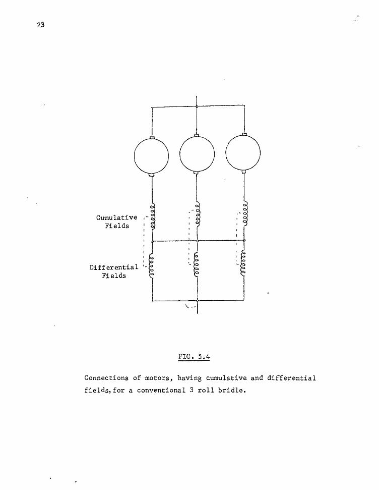
FIG. 5.4

Connections of motors, having cumulative and differential fields, for a conventional 3 roll bridle.

c) D i s a d v a n t a g e s of S e p a r a t e E l e c t r i c a l Dr ives ( C o n t . ) R e f e r r i n g t o f i g . 5 , 4 , each c i imu la t ive f i e l d can c o n t r i b u t e a 167o i n c r e a s e i n f i e l d s t r e n g t h a t f u l l l o a d , whereas t h e d i f f e r e n t i a l f i e l d i s 87o under t h e same c o n d i t i o n s . I f t h e s e b r i d l e s were s e t up t o s h a r e t h e l oad i n p r o p o r a t i o n t o t h e i r r a t i n g and sudden ly motor A l o a d i n c r e a s e d , t h e i n c r e a s e d a r m a t u r e c u r r e n t would f l o w i n motor A a r m a t u r e , b u t would d i v i d e up a t t h e d i f f e r e n t i a l f i e l d s i n i n v e r s e p r o p o r t i o n t o each m o t o r t s d i f f e r e n t i a l f i e l d r e s i s t a n c e . Consequen t ly motor A would have a r e l a t i v e l y s t r o n g e r f i e l d s t r e n g t h and s low down. The o t h e r mo to r s have i n c r e a s e d t h e i r d i f f e r e n t i a l f i e l d s t r e n g t h b u t n o t i n c r e a s e d t h e i r r e s p e c t i v e c u m u l a t i v e f i e l d s t r e n g t h s , so each of t h e s e motor s would have a r e l a t i v e l y lower o v e r a l l f i e l d s t r e n g t h . The r e s u l t b e i n g t h a t motofc A sheds i t s l o a d , w h i l s t t h e o t h e r moto r s speed up t o t a k e t h e i n c r e a s e d load f rom motor A.

Th is a r rangement i s u s e d on t h e e x i s i t i n g d u a l 3 r o l l b r i d l e on t h e Cont inuous G a l v a n i z i n g L i n e and i s s u c c e s s f u l . I t s h o u l d be c a p a b l e of b e i n g ex t ended t o dua l 5 r o l l b r i d l e s w i t h o u t g r e a t problems a r i s i n g .

c) Disadvantages of Separate Electrical Drives (Cont.)

2. The speed differential will not be mechanically locked in

and so the system accuracy will not be as good. On this

point a compromise must be reached in that if a 1% extension

is required, then an extension between 0.9% to 1.17o should

be permissible (refer Chapter 3). At this stage it is

impossible to say whether this accuracy would suffice, but

the digital system should allow the accuracy to be lowered

another decade if necessary.

3. During periods of acceleration and deceleration the

separate drives may not respond identically because of the

inertia ratios. This can be overcome by using flywheels

or oversize brake drums on the drives with relatively low

inertia ratios.

Conclusion

Based on the discussion in Chapter 3 on controlled extension

for quality improvements, and in particular in regard to the

stress versus strain curves, the assumption that an error of

up to 10% on the set extension should be reasonable. If this

were the case then matched analogue tachoes of good quality

could be used to reach this accuracy. These tachos particularly

if loaded can be relied upon to give the system a long term

accuracy of 0 . 1 7 o and a short term accuracy approaching 0 . 3 7 o .

(These are typical figures for tacho servos as applied to the

paper industry.)

Greater system accuracies would dictate the use of a digital

system which would be more expensive.

CHAPTER 6. ECONOMICS OF ELECTRICAL VERSUS MECHMICAL DRIVES

The gearbox associated with a mechanically driven anti-fluting

mill has been estimated to cost $300,000. For a comparison

purpose the gearbox cost will be compared with the additional

cost of individual motors, and gearboxes together with the

additional cost arising from

increased generator capacity

increased control panels and desks

increased foundations

increased conduits, cables and racks

increased installation

plus appropriate control gear to set and maintain extension,

i.e» Items such as work rolls, etc, which are common to both

arrangements have been neglected and basically the mechanical

drive gearbox cost will be compared with the cost of the electrics

to replace the gearbox.

FIG. 6.1

A 4 roll bridle having a large total angle of strip contact

with a consequent higher tension multiplication factor.

a) Calculation of Motor Horsepowers

Assume separately driven dual five roll bridle system with the

same roll configuration as a C.A.F.L. Mill. On a 200 degree

wrap assume tension multiplication factor of 2 (i.e. co-efficient

of friction of 0.2). The maximium tension that can be transmit-

ted between a single roll and strip without slippage is T_ - T-

where ^ = e "" (6.1)

T 2 = outgoing tension

T 1 = incoming tension

e = 2.718

u = co-efficient of friction

4> = angle of wrap in radians

This 5 roll configuration is not an efficient utilization as

much greater angle of wraps can be obtained. In fact the 4

roll configuration shown in fig. 6.1 has a multiplication factor

of 2.3 on each roll (based on co-efficient of friction of 0.2).

However, for the purpose of a comparison the 5 roll bridles

will be compared.

a) Calculation of Motor Horsepowers (Cont.)

The horsepower to be applied to or absorbed from the strip

is calculable from

H.P. = (F.P.M.) X (^2 .. ^1) (6.2)

33,000

where F.P.M.= Ft./min.

on Continuous Galvanizing Line F.P.M. = 550

H.P. = 550 X (^2 - "^D

33,000

on first roll ^2 - = 2 x 1000 - 1000 = 1000 lb,

H.P. = 16.65

on second roll " ^ 2 - ^ 1 = 2 x 2000 - 2000 = 2000 lb.

• • H.P. = 33•3

on third roll - = 2 x 4000 - 4000 = 4000 lb.

H.P. = 66.7

T T

on fourth roll 2 - 1 = 2 x 8000 - 8000 = 8000 lb.

H.P. = 133

on fifth roll ^ 2 - ^ 1 = 2 x 16000 - 16000 = 16000 lb.

H.P. = 266

a) Calculation of Motor Horsepowers (Cont.)

Using standard H.P. drives by adjusting angle of wrap

let No. 1 roll H.P. = 15

No. 2 roll H.P. = 50

No. 3 roll H.P. = 75

No. 4 roll H.P. = 100

No. 5 roll H.P. = 200

Total H.P. = 440

tension developed = 33,000 x 440 (from equation 6.2)

550

= 26,400 lbs.

b) Costing

C.A.F.L. Mill Gearbox $300,000 (Estimated)

Separately Driven Alternative

I t e m C o s t

2 X 15 H.P. motors 3,220

2 gearboxes to suit 15 H.P. drives 2,640

2 X 50 H.P. motors 4,460

2 gearboxes to suit 50 H.P. drives . 4,700

2 X 75 H.P. motors 4,640

2 gearboxes to suit 75 H.P, drives 6,100

2 X 100 H.P. motors 8,400

2 gearboxes to suit 100 H.P. drives 6,100

2 X 200 H.P. motors 10,600

2 gearboxes to suit 200 H.P. drives 11,000

increased conduits and racks 8,000

increased generator 12,000

increased control panels and desks 18,000

increased foundations 1,000

increased installation 15,000

generator voltage control scheme 1,000

booster 9,000

booster control scheme 20,000

Total: $136,000

Allowance 20% for incidentals gives total = $165,000

I elivery Bridle Entry Bridle

u o nJ ^ 0) g o o H

FIG. 6.2 Ward Leonard diagram of propssed system with booster being replaced by an S.C.R, converter.

Delivery Bridle Entry Bridle

FIG. 6.3

Diagram showing converter being used for complete supply to the entry bridle.

b) Costing (Cont.)

All other gear including work rolls would be common to both

proposals, thus a price differential of $135,000 should be

achieved. Note that even with this cost differential the

separately driven alternative has a pulling capacity of

26,400 lbs, whereas the C.A,F.L. Mill is rated as 15,000 lb.

system. The 15,000 pounds developed in the 5 roll bridle of the

C.A.F.L, Mill could easily be extended to greater tensions by

greater use of bridle configurations, but this would increase

the cost because greater torques would need to be transmitted.

c) Static Versus Rotating Generators

An alternative to using a booster, in the separate electrical

drive may be a converter based on silicon controlled rectifiers.

The booster could either be replaced as shown in fig. 6 .2 , or use

the converter to supply the entry bridle as shown in fig. 6.3,

The disadvantage of the latter would be that the delivery bridle

would need to be powered by a generator capable of supplying the

full bridle load, whereas the previous rating was based on it

supplying only system losses. However, if a converter were.to

replace the booster then it seems logical that it be taken one

step further and the generator replaced with a static converter.

c) Static Versus Rotating Generators (Cont.)

Converters have the advantages over rotating machinery of:-

1. Rapid response particularly with the deletion of the

booster and generator field time constants.

2. Lower maintenance costs.

3. Improved efficiency with resulting power savings because

the S.G.R. converter may be up to 107o more efficient

than an M.G. Set.

These advantages can be offset to some extent by:-

1. An S.G.R. installation cost is usually 10% to 15% more.

On the basis of driving each bridle with an S.G.R. converter

the approximate cost would be:

from previous calculations the load = 1,600 amps at 230 V.

Using a safety factor of 2.5 times the peak working volts then 800 volt P.I.V. rated S.G.R«s are required.

c) Static Versus Rotating Generators (Cont.)

If 350 amp average current rated S.C.R-Js are used in a 3 phase

6 pulse bridge then the bridge rating would be

each S.C.R. conducts for 120° in each cycle

bridge rating = 3 x 350 = 1,050 amps av.

Hence 2 bridges in parallel would be required and a reasonable

safety factor would be obtained.

Possibly some regenerative capacity would be required during

speed changing conditions and possibly for jogging. Here

allow for 507o capacity.

Thus a total of 3 bridges would be required in the converter.

total number of S.C.R*s = 3 x 6 = 18

cost of S.C.R. bridges = 18 x $264

= $4,750

to this must be added a transformer to step the voltage down

to 230 V. Cost = $3,000

c) Static Versus Rotating Generators (Cont.)

A D.C. circuit breaker would be required to protect the bridges

from "shoot through" conditions and other overload dangers.

Cost $900

total = $8,650

Other necessary accessories would include firing circuits,

blocking and logic, fast acting fuses, current -transformers,

etc.

Other requirements such as an A.C. circuit breaker are required

for both the M.G. and the converter and can be neglected.

One other aspect which must be considered would be inductors.

Depending on motor design, these may be necessary to limit

current build-up rates, reduce ripple voltage and reduce the

possibility of S.C.R. firing from high rate of change of volts.

The inductors also have the inherent advantage that in reducing

the ripple voltage they minimize discontinuous conduction and

the reduction in gain associated with it.

c) Static Versus Rotating Generators (Cont.)

Overall the converter cost would approach the nominal 10% to

157o increase in cost over the M.G. Set. It is difficult to

have a close comparison because of the many unknowns. Some

savings may result by using a different voltage D.C. machine

e.g. 440 volts. This may allow a cheaper bridge to be built

because of the relationship between voltage rating and current

rating in the cost of S.C.Rfs. It may also be possible to use

only 1 transformer for both converters. The rating of 1

transformer would be adequate, but special precautions may be

necessary to prevent interaction between the converters.

Conclusion

Separately driven rolls used in multi roll bridles for the

controlled extension of steel strip could be a very attractive

proposition from capital cost savings and reduced running and

Toaintenance costs when compared with the mechanical drive.

This separate driven alternative could only be worthwhile if

there is no strip slippage through the bridle and secondly

if the necessary speed accuracies can be attained.

Whilst the S.C.R. converter may be a slightly more expensive

proposition, its inclusion may be necessary to obtain the

accuracies, but even if a booster would suffice the converter

would need to be seriously considered because of its longer term

savings.

An allowance of $20,000 has been made for the control scheme

associated with obtaining the extension or speed difference

signal. This would be a digital arrangement with appropriate

digital to analogue conversion. This aspect will be investigated

further in a later chapter.

CHAPTER 7. BRIDLES IN PROCESS LINES

a) Mechanical Considerations

The tension multiplication factor relationship

= e " ^

where T^ = outgoing tension

T

1 = incoming tension

e = 2.718

u = coeff. of friction

4 — angle of wrap in radians

is derived in almost any engineering mechanics text and it

defines the theoretical ability of a roll to modify strip

tension without slipping. This equation gives the theoretical

limit, but in practice it must be modified by the centrifugal

force of the material and the power requirements in material

bending.

The first of these effects can be considered acedemic for the

speeds and gauges involved in this project. The horsepower

involved in material bending may be derived from equation 7.1 .

H.P. = BT^YF (7,1)

165,000R

a) Mechanical Considerations (Gont.)

where B = number of bends

T = material thickness in inches

W = material width in inches

Y = yield strength in pounds/square inch

F = speed in ft./min.

R = roll radius in inches.

e.g. 36" wide by 0.050" thick material with a yield strength

of 30,00 P.S.I, at 550 F.P.M. with 1 bend over a 36" dia. roll

required the following bending horsepower.

H.P. = 1 X (0.050)^ X 36 X 30,000 x 550

165,000 X 18

0.5 H.P.

Consequently this effect may also be considered negligible when

compared with the horsepower involved in the dual 5 roll bridle.

In any case, this effect can bB considerably reduced by correct

design. It can be shown that the minimum roll diameter that will

not result in the outer fibres of the material being stressed

beyond the yield point can be expressed by equation 7.2.

a) Mechanical Considerations (Cont.)

D = ^ (7.2)

Y

where D = roll diameter in inches

T = material thickness

E = Youngs Modulus

Y = material yield stress

e.g. on steel where E = 30 x 10^

and Y . = 30 X 10^

then from equation 7.2

D = 100 T

The roll diameter should be 1000 times the maximum strip

thickness being processed,

b) Electrical Consideratidns

. The main electrical considerations in any separately driven

multi roll bridle relate to load sharing of the motors under

both steady state and speed changing conditions. It is

desirable to split the load into the corieect ratio, otherwise

the bridle may slip on the strip, and once this happens it

causes many problems and is difficult to stop.

b) Electrical Considerations (Cont.)

Nominally the bridle is designed for steady state operation and

usually the basic bridle is available in standard configurations

and economics generally dictate that these standards be used.

The motor horsepower requirements are then usually calculated.

It would be most unlikely that the theoretical horsepowers

required line up with the standard sized motors. Consequently

the next highest standard motor is chosen above the calculated

value and hopefully the ratio of actual horsepower requirement

to the motor nameplate horsepower are the same for each roll

within the bridle. This ratio should be the same so that each

motor shares the total load in proportion to its horsepower.

Any discrepancy in this regard could be overcome by either

adjusting the angle of wraps within the bridle, or it may be

possible to adjust the load sharing in the differential fields

so that the bridle load is shared in proportion to the

calculated horsepowers.

During acceleration and deceleration the same basic ratio must

be maintained to avoid slip. Each roll within a bridle will

only accelerate at the same rate if the ratio of the motor

horsepower to motor inertia is equal for each drive. Motor

inertia in this case would be actual motor inertia plus brake

b) Electrical Consideration (Cent.)

inertia, roll inertia and gearbox inertia (all referred to the

motor shaft). Possibly a better ratio would be motor horsepower

to the horsepower required for acceleration.

If the actual horsepower requirements for the static condition

are some percentage other than 100% of the motor nameplate

rating then the same percentage should be obtained for the

acceleration horsepower to the motor nameplate rating.

Acceleration horsepower may be calculated from

H.B. = I N ^ (7.3)

1.6 X 10^ X T

2 I = total inertia in pound ft.

N change in speed in R.P.M.

T = time for speed change in seconds

If the acceleration ratio is not the same for each roll then

consideration could be given to the possibility of using a

b) Electrical Considerations (Cont.)

safety factor in the value of the coefficient of friction

used. This would be helpful, particularly if applied to the

larger drives which could then safely do some of the work of

the smaller drives without slipping being induced. This

method would be wasteful of a bridle's potential capabilities.

The remaining possibility of correcting the acceleration

ratios would be to add extra inertia to the drives with low "

ratios. In most conventional bridles, rolls would normally be

identical and hence each have the same inertia. Thus it is most

unlikely that the acceleration ratio is constant and obviously

the larger drives generally have the smaller ratio. As suggested,

extra inertia, on these larger motors, in the form of oversize

brake drums or even a flywheel, would restore equal ratios and

result in a bridle which will not slip under either static or

dynamic conditions.

Decoder Driver

Coincidence Detector

Delay

Counter

Memory

Decoder Driver

Nixie Read Out

FIG. 8.1

Block diagram of digital differential speed transducer.

CHAPTER 8, DEVELOPMENT OF A DIGITAL DIFFERENTIAL SPEED TRANSDUUER

a) General

Since this investigation is based on controlled extension using

speed control rather than a differential gearbox it is most

important that there be no slip around the rolls under all loads

and all types of strip. It was decided to conduct slippage tests

on the existing dual 3 roll bridle to determine the extent of any

slip. Thus some accurate form of measuring roll speed against

strip speed was needed. Since accuracies of better than 0.1% are

required and, as this is difficult to achieve using analogue

methods, a digital system was used.

The accuracies required indicated that the two measurements to be

compared be taken concurrently, so two separate counters based on

Fairchild Integrated circuit elements were built and logic elements

necessary for the purpose were included. Figure 8.1 shows the

block diagram arrangement of the scheme.

A "zero" is defined by zero volts.

A "one" is defined by 1.6 volts approximately.

The 9958 unit is a decade counter capable of frequencies to 2

megacycles with inputs consisting of a counting signal and a

reset signal. The outputs are binary coded decimal of relative

weight 1 - 2 - 4 - 8 . A detailed explanation of this unit is

given in appendix.

General (Cont.)

The memory units (9959) act as buffer storage elements. Each element

has basically an input, an output and a gate signal and the element is

capable of sampling the counter element output and storing this output

indefinitely. This sampling action is achieved by opening the gate with

a "zero" logic signal. Whilst this "zero" is applied the information

at the counter output will be stored in the memory unit and be also

transferred to the memory output. When the gate is switched to a

logic "one" the information in the counter just prior to the gate

signal is stored in the memory but the memory input opens and so no

further signals are received from the counter. The information in

the memory is continuously available at the memory output and hence

that count is maintained and can be decoded and read out on Nixie

Tubes. This particular count is maintained on the output until the

memory gate is again opened to sample the counter output. An equivalent

circuit and detailed write-up is appended.

The 9960 unit acts as a combination decoder driver. It facilitates

the conversion of the 8 - 4 - 2 - 1 binary coded decimal number

from the counter to a ten digit decimal number.

Counter

Decoder Driver

Reset

Counter

— (.J Decoder Driver

i.i.iii

Counter

Decoder Driver

! ! TT|-f ) I

I

Pulse Input

Pulse Amplifier

Y Input

Counter

Decoder Driver 1 : I I ! ;

+ 60 V.

1 r

To Reset Logic

— + 60 V.

To Reset Logic

1 r + 60 V.

9

To Reset Logic

. — + 60 V.

To Reset Logic

FIG. 8,2

Layout of counter 1 or master counter.

Counter (9958)

Memory

Counter (9958)

Memory

Decoder Driver ; J •

Nixie Tube

Pulse Amplifier

Count Input

Counter (9958)

Memory

P Decoder 1 Driver

Nixie Tube

"•High Tension

FIG. 8.3

Layout of counter 2 or readout,

b) Circuit Design and Operation

Fig. 8.2 is a detailed layout of counter 1, the master count, which

consists of a four stage counter feeding directly into decoder driver

units which feed a resistance network via selector switches. The

100 K load resistances replace the Nixie Tube, and the diode in each

of the decimal output leads are used to clamp the output to + 60 volts.

This means that the voltage at the various selector switches is either

at + 60 volts or zero volts. It goes to the low level when that

particular count is being registered. The signal to the reset logic

is attenuated to a "one" (1.6 volts) from the + 60 volt level. This

means that the reset logic signals only go to logic zeroes when the

decimal number selected on the selector switch coincides with that

particular number on the 9960 decimal decoder. The driver can be

simply considered as 10 pass transistors to the zero volt line and

a transistor is switched from an open circuit to short circuit when

that particular count has been decoded.

Counter 2, as detailed in fig. 8.3, consists of three counting stages

(9958) feeding decoder driver units (9960) via memory units (9959).

The load of the driver units on this counter is three Nixie Tubes.

In a similar manner to the previous counter the decoder ouputs were

clamped to + 60 volts. In this case this was necessary to prevent

inconsistent counting and two counts being registered simultaneously

on the Nixie Tubes.

Counter

Decoder Driver

Units

Tens ^ Hundreds

Thousands

Reset Line \_

L2

CI

Gate

FIG. 8.4

Counter

Memory

'Decoder Driver

Detailed arrangement of counter logic.

b) Circuit Design and Operation (Cont.)

Referring to fig. 8.4, the circuit description of operation is as

follows:

Assume both counters have just been reset, then each one will

commence counting the pulses received from the rotating discs.

(Say counter 1 has been set to a count of 999 with the selector

switches.) When 999 has been reached on counter 1 all inputs to

9914 unit LI will be logic "zeroes" and the 9914 unit LI acts as

a nand gate to then produce a logic "one" output.

This immediately appears at the input of the next 9914 unit L2

and thus its output goes from logic 1 to zero.

This "zero" signal appears on the "gate of the memory units and

opens the memory unit so that the infonnation stored in the counter

at that instant is relayed to the Nixie Tubes via the decoder driver.

If the gate were to be left open then the counter would continue to

count and thus alter the information stored on the Nixie c.ontinuously.

So after a delay of two micro seconds (2K x 800 P.F.) (approximately)

capacitor CI has charged sufficiently to make the input to the 9914

unit L2 a "zero" and thus the output is "one" and so the gate is shut.

b) Circuit Design and Operation (Cont.) Up to this stage then we have counted to -999 on counter 1 and in same

period the count reached on counter 2 has been transferred to the Nixie

Tubes and remains there until the gates have been re-opened.

Whilst the gate is opened with a "zero", capacitor C2 discharges but

the direction of the discharge merely biases off 9914 unit L3 and

thus it does not trigger. When the gate is re-closed with a "one"

capacitor G2 charges and now the direction of charge is such as to

trigger the 9914 L3 and 9900 L4 unit (connected as monostable vibrator)

and place a "one" on the output. The 9900 unit L4 has sufficient

power to drive all units and thus a reset or "one" appears on the

reset line.

After a set period determined by the time constant C3 capacitor

charges and switches the reset output line back to a "zero". By this

time capacitor C2 has charged sufficiently so that its contribution

to the input to 9914 unit L3 is a "zero".

The delay sequence is necessary to ensure that the counters are not

reset until the memory gate has been re-closed otherwise the Nixie

count will be destroyed.

b) Circuit Design and Operation (Cont.)

Once the reset pulse has been removed both counters then _r_ecycle

again and up-date the information stored in the Nixie Tubes if

slippage occurs.

The units and layout used for the logic_operations were not

derived in one go, but rather consisted in trial and correction.

The main difficuLty-was in connection with the gate pulses to

the memory, but the final set-up proved to be satisfactory.

Details on the logic modules used are appended. The driving

capacity input load factors, output drive factors were taken

into account and these details are included in the appendix.

The counter design was straightforward because of the use of

integrated circuits. As is probably generally the case when

using high speed counters, it proved a slow job to remove

multiple counting on the Nixies, spurious counts and other stray

pulses. The main solution arose from the use of printed circuit

boards with a layout s'uch that .it included as much earthing as

possible. Regulated power supplies were used for both the high

tension and logic voltages and this proved to be_important in

preventing simultaneous miltiple counting on the Nixie Tubes.

..mr

FIG. 8.5 Photograph of the Extensometer

Master Counters Pulse Inputs

Count Selector Switches

Logic Board

CI Pulse Amplifier

Readout Coimters

Nixie Readout Tubes

Output to Digital to Analogue Converter

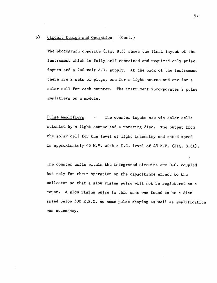
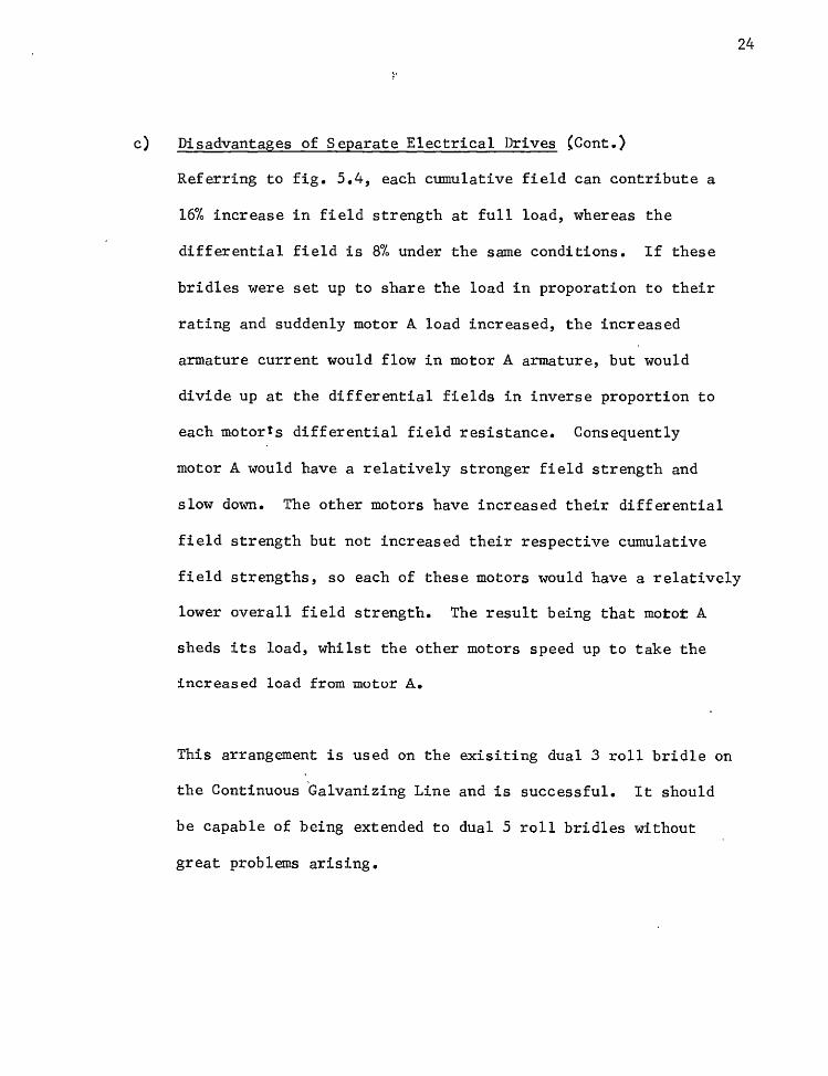
b) Circuit Design and Operation (Cont.)

The photograph opposite (fig. 8.5) shows the final layout of the

instrument which is fully self contained and required only pulse

inputs and a 240 volt A.C. supply. At the back of the instrument

there are 2 sets of plugs, one for a light source and one for a

solar cell for each counter. The instrument incorporates 2 pulse

amplifiers on a module.

Pulse Amplifiers - The counter inputs are via solar cells

actuated by a light source and a rotating disc. The output from

the solar cell for the level of light intensity and rated speed

is approximately 45 M.V. with a D.C. level of 45 M.V. (Fig. 8.6A).

The counter units within the integrated circuits are D.C. coupled

but rely for their operation on the capacitance effect to the

collector so that a slow rising pulse will not be registered as a

count. A slow rising pulse in this case was found to be a disc

speed below 500 R.P.M. so some pulse shaping as well as amplification

was necessary.

<u 00 CIS 4-» I-i o >

Time

tn a. I o u o

4J c 0) u u

u

a. 4J P o

1000

100

10

FIG. 8,6A Waveforms derived from Solar Cells«

^ VlAVVs'v-

>

> I ? > <

+ 9 V,

-A

0 V.

FIG. 8.6B Circuit used to amplify pulses from the Solar Cells.

100 Footcandles.

10 Footcandles.

1 Footcandle.

Output current versus- load resistance characteristic of a selenium photovoltaic cell (Solar cell).

10 100 1,000 10,000 Load Resistance (Ohms.)

FIG. 8.7

b) Circuit Design and Operation (Cont.)

Consequently a 2 stage D.C. coupled amplifier was used to

decouple and amplify the solar cell signal. The circuit used

is shown in fig, 8.6B, The output impedance of the solar cell

was loaded at 1 K because at this level it is essentially a

constant current souE-ce. At higher impedances it acts as a

constant voltage source. (Fig. 8.7)

The pulse shaping was achieved by joining the two emitters

through a suitable resistance. The value of this resistance was

found by trial and error and set to the optimum value without

allowing the system to oscillate. This resistance gives positive

feedback and so allows the output to switch faster and produce

a steeper pulse. This type of pulse shaping allowed accurate

pulse counting, however, in more critical applications it would

be necessary to go to more elaborate means e.g. (Schmitt trigger)

c) Testing

The circuit used proved difficult to check its accuracy because of its

rapid speed of operation. Placing the same signal on to each input

gives the same count but it was not known whether the counter was

actually counting or just locked in at that count. It was very

difficult to pick up the reset and gate pulses because of their short

duration and long period in between, A storage C.R.O. capable of

rapid writing rates could have proved valuable but was not available.

A 50 cycle input from the mains frequency to each channel of the dual

counter gave a reasonable indication of accuracy but still did not

check the instrument to the accuracy required until the test was

performed with same inputs to a batch counter over the same period.

A test to manually move a disc, operating a solar cell, through a

fixed number of holes did not prove satisfactory because it was found

that the counter registered nearly twice as many counts as expected.

Eventually the instrument was checked against another electronic

batch counter and proved to be accurate. The batch counter also

registered the same number of counts as the dual counter when used

to measure the manual movement of a disc and the error was found

to result from the unsteady manual motion of the disc.

FIG. 8.8

Layout of the dual 3 roll bridle.

Strip

Disc

Disc

FIG. 8.9

Location of the disc between motor and gearbox.

d) Measurement Technique

The extensometer was used to compare motor speed against the speed

of the anti-fluting roll which is not powered by a motor but driven

by the strip, so it is reasonable to assiame that roll speed is

directly proportional to line speed. Each counter receives pulses

from a solar cell and a rotating disc. One disc was attached to

the motor under test whilst the other was attached to the anti-

fluting roll. (Fig. 8.8) The disc had approximately 80 holes

so that the motor disc had a count rate of approximately 1,200 per

second (motor speed of 905 R.P.M. at top line speed) whereas the

second disc was connected directly to a one foot diameter work roll

so at 550 ft./minute line speed, the count rate approximates 240

pulses/second.

If the relationship between motor count and anti-fluting roll count

read out on the extensometer is maintained over the complete load

range of the motor then no slippage occurs. It is known from the

tensions developed and material processed that no extension takes

place (less than 0.025%). Thus a consistent extensometer count over

the motor full load range means no slippage.

On motors A, B and C a disc was inserted on the coupling between

motor and the gearbox. Fig 8.9) Another disc was attached to the

anti-fluting roll. Each disc had a known but different number of holes.

d) Measurement Technique (Cont,)

The purpose of this being to have a maximum count per revolution but

keeping the disc size to a reasonable value. As a first step the

output from the 75 H .P . disc was connected to the master input which

was then set to a count of 500, The output from anti-fluting roll

was used as the other input to the extensometer.

At maximum motor speed of 905 R.P.M. the first counter takes approx-

imately 0 ,5 seconds to reach the preselected count of 500, In this

interval of time the anti-fluting roll count was stored and at the

end of this period was read out on the Nixie Tubes. Because of roll

diameter ratios and the gearbox the ISIixie reading was only about 100,

but consistent over the full load range of the motor. This test was

to ensure there was no slippage occurring on a short term basis.

Obviously at such a low count only large slippages will show.

Greater accuracies in the slip measurement were obtained by connecting

the master count input to the anti-fluting roll and setting the count

to 999. The motor disc output was used to supply the second counter.

Since the anti-fluting roll is twelve (12) inches in diameter and

75 H .P . motor drives a thirty-six (36) inch roll through a 15.5 : 1

gearbox readings will now be taken over approximately every five (5)

seconds and the Nixie readout will be above 4,000 counts, thus an

accuracy of one part in 4,000 is obtainable.

d) Measurement Technique (Cont.)

The error of one part is due to the fact that digital systems have

an inherent error of up to one count over any number of counts

because it takes a finite time to transfer the information to the

readout (another count could be added in this period), and secondly

because the holes in each disc are not synchronised, so that the

instant counting commences, a count may be registered in either

counter immediately due to a disc hole being in front of the light

source*

Information stored in the Nixie Tubes record the number of counts

from the motor disc for 999 counts on the anti-fluting disc. Since

negligible extension actually takes place, then a consistent reading

over the motor load range should mean zero slippage. This reading

should be independent of line speed and product, but line speed will

have the slight affect that the slower the speed the slower will be

the counting cycle.

This method was used on 75 H . P , , 50 H . P . , and 15 H .P . motors.

e) Measurements

Count readings were taken over one minute. The reason f o r

the d i f ferent niomber of readings over each minute is due to

the fact that the Nixie tubes only changed reading when a

d i f ferent count was stored.

Results obtained were found to be independent of material

gauge, width or type of product. Also the results were

found to be independent of l ine speed, as expected, and

following results are tabulations of motor count versus 7o

motor load for a 999 count on the ant i - f lut ing r o l l .

e) Measurements (Cont.)

75 H.P. MOTOR

Count for 999 count on anti-fluting roll disc.

Count _

4767

4768

4767

4768

4767

4768

4767

4769

4768

4767

4768

4769

4767.6 Av.

7o Load Count

4767

4768

4767

4769

4768

4767

4768

4767 •

7o Load

18 Count

4767

4768

4767

4768

4767

4768

4767

4768

4767

7o Load

34

4767.6 Av. 4767.4 Av.

Count 7o Load Count 7o Load Count

4768 44 4768 67 4769

4767 4769 II 4770

4768 4768 II 4769

4767 4769 II 4771

4769 4768 II 4770

4768 4767 If 4769

4767 4768 II 4770

4768 4769 IT 4769

4767.7 Av. 4768.2 Av. 4769.6

7o Load

95

Measurements (Cont . )

50 H.P. MOTOR (4381)

Count 7o Load Count % Load Count

4372

4375

4374

4373

4377

4372

4373

4374

4373.7 Av.

11 4373

4375

4380

4377

4372

4374

4373

4374

4374.9 Av.

22

7o Load

4373

4374

4376

4374

4375

4372

4374

4373

4373.9 Av.

57

Count

4374

4375

4379

4376

4374

4375

7o Load

74

Count

4374

4375

4377

4376

4377

4378

7o Load

96

Count 7o Load

4375.5 Av. 4376.1 Av.

e) Measurements (Cont.)

Count _

3960

3961

3963

3958

3960

3962

3961

3960

3960.6 Av.

7o Load

13

15 H.P. MOTOR

Count

3962

3960

3962

3961

3964

3958

3961

3960

3961

7o Load

26

Av.

Count

3961

3964

3959

3961

3962

3961

3963

3962

3961.6 Av.

7o Load

48

Count

3963

3962

3965

3959

3961

3962

3961

% Load

69

Count

3962

3967

3964

3965

3963

3965

3964

% Load

74

Count

3963

3964

3967

3966

3965

3967

3964

°L Load

96

3961.6. Av. 3964.3 Av. 3965.1 Av.

f) Correlation of Measurements

This is a check to ensure that the counts obtained tie-up

approximately with the mechanics of the system. The

correlation is not expected to be exact because the

calculations rely on nominal roll diameters and gearbox

ratios.

For 75 H.P> Motor

999 counts on anti-fluting roll gave 4767 counts on Nixie tube

75 H.P. motor disc has 78 holes = HI

anti-fluting roll disc has 83 holes = H

anti-fluting roll dia« = 1 ft- (nominal) = D1

motor work roll dia. = 3 ft. (nominal) = D2

gearbox ratio = 15,5 : 1 = N

assinne line speed = Y F.P.M.

for anti-fluting roll time to count 999

999 h X H X

3.14

999 X X 3.14 H X Y

f) Correlation of Measurements (Cont*)

999 X 1 X 3.14

83 X Y

let the count on 75 H.P, motor in same time be Z

time to count Z = Z x x 3.14

H^ X Y X N

Y X 3 X 3.14

78 X Y X 15.5

time to count Z = time to count 999 on anti-fluting roll

999 X 1 X 3.14 ^ Z X 3 X 3.14

83 X Y 78 X Y X 15.5

Z = 999 X 1 X 3.14 X 78 X Y X 15.5

83 X Y X 3 X 3.14

= 999 X 78 X 15.5

83 X 3

Z = 4840

This compares well with actual count of 4767. The slightly

lower count could be due to the gearbox ratio being slightly

less than 15.5 : 1 or that the roll diameters are not quite

the 3 ft. and 1 ft. Note that Z is independent of line

speed Y.

f) Correlation of Measurements (Cont.)

For 50 H.P. Motor

time to count 999 on anti-fluting roll is same as in previous

calculation

999 X 1 X 3.14 83 X Y

again let Z = count on 50 H.P. motor in this time,

time to count Z

H^ in this case

N in this case

Z X 2 X 3,14 H^ X Y X N

74

15.49 : 1

time to count Z

Z X 3 X 3.14 74 X Y X 15.49

Z X 3 X 3.14 74 X Y X 15.49

999 X 3.14 83 X Y

999 X 3.14 X 74 X 15.49 3 X 3.14 X 83

999 X ' 74 X 15.49 3 X 83

4590

This compares with actual count of 4381 and again falls well

VTithin accuracy of above calculation.

f) Correlation of Measurements (Cont.)

For 15 H.P. Motor

let Z = count on 50 H.P. motor in the time 999 x 3,14 83 X Y

time to count Z = Z x x 3.14 H^ X Y X N

H^ in this case = 65

N in this case = 15.48 : 1

time to count Z = Z x 3 x 3.14 65 X Y X 15.48

999 X 3.14 ^ Z X 3 X 3.14 83 X Y 65 X Y X 15.48

Z = 999 X 3.14 X 65 X 15.48 83 X 3 X 3.14

Z = 4040

\

Actual count recorded of 3978 compares well with above

calculated value.

g) Conclusions

The results show generally that the count is maintained fairly

consistently over the load range, but results show a definite

pattern of increasing count as the load is increased. This

increase over the test range is of the order of 0,1% (4 counts in 4000)

and may be attributable to several factors.

The increased count may be explained to some extent by the

change in roll radius as tension is increased. . This should be

quite feasible as the rolls are rubber covered. Information on

this effect appears scant in journals and could well be worth

further investigation.

On the other hand the increase may be slip, but for the purposes

of this investigation this effect is known and limited and thus

could be compensated for or neglected.

CHAPTER 9 PILOT SPEED CONTROL SYSTEM USING DIGITAL SIGNALS

a) General

It has been shown that strip slip under static conditions is

negligible in a bridle and that under dynamic conditions a

properly designed bridle will also maintain a zero slip

condition. On this basis, separately driven bridles to attain

set extensions should be feasible if the required extension

accuracies can be met. An accuracy of 0.1% of the set speed

has been suggested as a minimum.

This order of accuracy could be obtained and maintained with

conventional tacho generators in a servo system, but any

greater accuracies would only be produced on a short term

basis. Greater accuracies would necessitate the use of

digital signals to generate a speed difference signal.

Basically the extensions required in an electrically driven

bridle rely on accurately controlling the speed of 1 set of

bridles with repect to the speed of the other bridle and the

servo system being capable of fine adjustments to attain the

desired extension.

o <

o •nJ-CM

S.C.R. Rect i f ier

FIG. 9.1

Pilot speed control system including inner current loop<

a) General (Cont.)

Consequently a pilot speed control system was built to control

the speed of a motor using digital signals. A fixed frequency

from an oscillator was used to simulate the speed of 1 bridle

and the speed of the motor was controlled at some fixed speed

above this frequency.

b) Servo Circuit and Description of Operation

Basically the control system consisted of controlling the

armature voltage of a D.C. machine via an S.C.R. bridge.

The S.C.R. gates are controlled from the output of a pulse

transformer in a unijunction emitter base circuit. Referring

to fig. 9.1, capacitor CI and resistor R1 are used so as to

delay the voltage build-up on CI so that in each half cycle

the capacitor voltage just fails to reach the emitter peak

point voltage. This means that, with no other inputs, the

U.J.T. emitter is reverse biassed and only a small reverse

leakage current flows so there is no output from the pulse

transformer.

Control is achieved by inserting a further signal into the

U.J.T. emitter and obviously the greater this additional

IR From Motor A2V

R, R, T" T" •^VWV-T—

R1

15 V.

FIG. 9.2

Current Amplifier.

b) Servo Circuit and Description of Operation (Cont.)

voltage the faster will CI capacitor charge to emitter peak

point voltage within each half cycle. The earlier the

capacitor charges the earlier in each cycle will the S.C.R^s

conduct and so produce a higher output voltage.

The system has several control lo,Dps. The most inner loop

was an armature feedback and this was incorporated for several

reasons.

1. It acts as a current limit if the input resistance

values are scaled appropriately. The gain of the

operational amplifiers is in excess of 10,000 and

capable of 15 volts output.

The series resistance in the armature circuit was

such that, when 2 times full load current was flowing,

2 volts were developed across it. The armature

current feedback resistor is scaled such that with

maximum output volts from preceeding amplifier the

current amplifier total input current is zero.

Referring to fig. 9,2.

b). Servo Circuit and Description of Operation (Cont.)

L5 =

15

(this neglects F/B current from current amplifier.)

2- Armature current feedback acts as a stabilizing signal

when controlling motor speed. The reason for this stems

from the fact that the transfer function between armature

current and speed is essentially an integration (neglecting

addition of load torque). This would not be a pure

integration in practice as some friction would be inherent

in the system, so the transfer function would be modified

to:

= K

W JS + F

where J = inertia

S = Laplace operator

F = friction

K = constant depending on the machine

b) Servo Circuit and Description of Operation (Cont.)

Normally, however, the inertia term J is considerably

larger than the friction term F and consequently armature

current leads the speed by nearly 90°. It is this leading

nature which makes it an excellent stabilizing signal but

this is only on the basis that any necessary filtering of

this signal wil-1 not introduce large phase lags in the

feedback. Some filtering will generally always be

necessary and, it is important, for the above reasons, to

ensure that this is minimized.

Since the armature voltage is being derived from a single

phase 50 cycle bridge then current feedback will contain 100

cycle ripple. A. time constant of 37.5 ms (5 uF x 7.5 K) was

inserted. The two 15 K resistances appear to act in parallel

for filtering because the operational amplifier has such a

high gain that its input is virtually zero and the centre point

of the feedback resistance is tied to earth through a 5 uF

capacitor. At 100 cycles the capacitor impedance can be

neglected and thus each half of the feedback resistor can be

considered as being in parallel.

FIG. 9.3

Pilot speed control system incorporating current and speed lops.

b) Servo Circuit and Description of Operation (Cont.)

The e f f e c t of this f i l t e r time constant corresponding to

27-radians i s that the r ipple of 100 cycles (314 rads.)

i s reduced by a factor of 12 approximately.

I

With the armature current feedback res i s tor being 2 x 15 K =

30 K and the input resistance from preceeding amp = 150 K,

the current amplifier F/B resistance of 330 K was the largest

value that could be placed in without causing overshoot during

step inputs on the current amplif ier.

The series capacitor in the current amplifier was inserted

so as to operate the system as an integrating one, i . e . with-

out error. A l l th is , of course, means, i s that during steady

state there i s no feedback current on current amplifier so

the f u l l gain of the amplifier i s used, but during transient

condition the capacitor allows current to pass and so limits

the amplifier gain to the resistance ra t i o s .

Referring to Fig. 9.3 the next loop consists of a speed reference

and a speed feedback into a speed amplif ier . Generally the

speed reference would come from the other br id le , but to

b) Servo Circuit and Description of Operation (Cont.)

simulate this a variable voltage was used. This is not a

good simulation, but it will be seen later that variations in

this voltage,up to a point, are not important in the steady

state response.

The speed feedback signal, instead of being from a conventional

tacho generator was derived from a digital tacho. The digital

tacho was used because a digital speed system was required for

the next or most outer loop and secondly, because a suitable

machine to generate an analogue signal was unavailable.

The pulse generator circuit and operation is discussed in

the next section.

The speed amplifier was set up in the same manner as the

current amplifier in that gains were kept as high as possible

without too much overshoot and filter time constants kept to

a minimum. Again the integrating capacitor on the speed

amplifier was chosen as small as possible so as not to affect

transient response, but not too small that integration

commences at such a low frequency as to affect stability.

Gain Control

+ 18 V.

-AA^WW

Speed

Reference

- 18 V.

-AWvW

Extension

Reference

FIG. 9 . 4

Complete speed control system incorporating an outer extension loop,

b) Servo Circuit and Description of Operation (Cont. )

Referring to fig. 9.4 the outer loop, called extension amplifier

or loop, is a 2 signal arrangement. The reference signal is

an analogue reference extension signal which simulates the

extension desired by the operator. The feedback signal is the

difference in speed between the motor and a frequency from a

signal generator. The motor signal is derived from a disc

driven by the motor. Holes in the disc actuate a photo diode

from a light source to be the signal into 1 slide of the

extensometer (instriiment detailed in Chapter 8 and used for

slip measurements). The other input to the extensometer came

from a signal generator which simulates the speed of the other

bridle. The output from extensometer is fed into a form of

digital to analogue converter. The circuit and description of

operation is detailed in section d) of this chapter.

The full circuit shown in fig. 9.4 operates such that the speed

amplifier sets the speed of the motor to the level set by the

speed reference potentiometer. The speed amplifier signal is

then modified by an over-riding extension signal from the

extension amplifier. The level of this extension signal is set

by the extension reference potentiometer.

Sigaal Generator

ExtouioDttter

Pov«r Supply

Disc Digital to Analogue S.C.&. Comrcrter Firing S.C.R. Bridge

Unit

Operational Ai^tUfier Modules

FIC. 9.5

Compcmimta used in pilot'speed control systec*

w w • • »

b) Servo Circuit and Description of Operation (Cont.)

Fig. 9.5 details the various components used in the scheme. All

amplifiers have proportional plus integral control. When only

proportional control is used there is a larger error when motor

is loaded than when not loaded or alternatively the speed is

dependent to some extent on the load. When integral control is

included then any error is integrated up until it is corrected.

This means that the steady state error is theoretically zero,

but in practice the system oscillates slightly about the zero

error. This arises from the fact that the integrating capacitor

does not allow any feedback on the amplifier during steady state

so the full gain of the operational amplifier is used.

c) Digital Tacho

The digital tacho used was an electronic version of an analogue

tacho and was used because pulses were necessary to be generated

from a disc on the motor for 1 input to the extensometer. Since

a suitable machine was not available for use as a conventional

tacho the electronic version was used.

The circuit is shown in fig. 9.6. The pulses from the motor disc

are detected by photo diode Dl and fed to the gate of a field

effect transistor (F.E.T.). The F.E.T. has the principle

feature of having an extremely high input impedance and

consequently the large resistance changing range of the photo

Photo Diode

To Pulse Integrator

Y A W A — ^

CD 00

+ 18 V,

To Extensometer ^

OV

- 18 V.

?^plifier Schmitt Trigger

Multi-Vibrator Emitter Followers Power Supply

FIG. 9.6

Outline of digital tacho.

c> Digital Tacho (Cont.)

diode at the illumination being used meant that the voltage

at the source of the F .E .T . reflected the voltage changes at

the gate. In this instance the resistance change in the

diode was of the order of 5 to 1,

The pulses from the F .E .T . source terminal were shaped in

the next 2 transistor stages which were connected as a

Schmitt trigger. The output pulses from the Schmitt trigger

were then fed into a multi-vibrator. The vibrator was

connected as a mono-stable multi-vibrator which triggered

from the front end of the shaped pulses.

The multi-vibrator had an on time of 0 .16 milli seconds when

triggered. This on time could be selected at any value, but

for this scheme 0 .16 milli seconds was sufficient because

this means that the device will operate up to a pulse rate

of 6,000 cycles/second. The motor was rated at 4,000 R .P .M . ,

and the disc had 60 holes, so the maximum pulse rate for this

would be 4,000 cycles/second.

The output of the digital tacho was taken from the collector

of the first transistor in the multi-vibrator and by referring

4 K.C .

0.16 M.S. 0.09 0.16 M.S. M.S.

0.25 M.S. —Per iod ^

2 K.C. 0.16 M.S< 0.34 M.S. ^ 0.16 M.S.

^ ^

0.5 M.S. Period

0.16 M.S.

1 K.C

0.84 M.S

1.0 M.S. Period

FIG. 9.7

Variable mark space rat io achieved with d ig i ta l tacho by having a f ixed on time of 0.16 m.s.

c) Digital Tacho (Cont.)

to fig. 9,7 it can be seen that the output always consists of

a pulse with a duration of 0,16 milli-seconds. From fig.-9.7,

it is the off time which is the variable, and is dependent on

motor speed. If the area of the pulse output is averaged over

the full interval, then average output is directly proportional

to pulse speed

at 4,000 R.P.M, overall pulse duration = 0.25 M.S.

pulse area = 0.16 P

where P = pulse height which is a constant voltage

averaged output = 0.16 P .25

= 0.64 P

at 2,000 R.P.M. overall pulse duration = 0.5 M.S.

pulse area = 0.16 P

Averaged output = 0.16 P 0.5

= 0.32 P

This is exactly half the value at 4,000 R.P.M.

u 0 4J 2 3 tJO a; C

H

1 M iw £ 2 t-H o > u p a 4J p o .

Digital Tacho Linearity Test

1,000 2,000 3,000

Speed (R.P.M.) 4,000

c) Digital Tacho (Cont.)

at 1,000 R.P.M. overall pulse duration = 1.0 M.S.

pulse area = 0.16 P

averaged output = 0.16 P

1

= 0.16 P

This is exactly half the value at 2,000 R.P.M.

These calculations verify that with the pulse width

modulation from the shaped pulses to the multi-vibrator

the average output voltage is directly proportional to

speed. The digital tacho output voltage was averaged by

using an integrator.

A linearity check was conducted on the digital tacho and

the result is fig. 9.8 which verifies the linearity.

The full circuit detailed in fig. 9.6 includes a further

2 transistor stages connected as emitter followers. As

mentioned, this pulse signal was necessary to also feed

the extensometer so it was taken from the digital tacho.

c) Digital Tacho (Cont.)

However, because of the very low input impedance (IK) of

the pulse amplifier associated with the extensometer the

two emitter fol lower stages were necessary so as not to

load down the multi -vibrator. The extensometer signal

could not be taken direct ly from the photo diode for the

same reason.

vO -P-

N

Inputs from

Nixie Tube

Grids

-<—AAAWW-Output

— w w w v -Output

V

—VvvWV-Output Output to Summer

> 10 V. Clamp

— + 18 V.

FIG. 9.9

Inversion stage in the digital to analogue converter, i.e.high input voltage gives low output voltage.

d) Digital To Analogue Converter

The voltage appearing on each grid of the Nixie Tube has 1 of

2 states. It is either 0 volts when that particular number is

up or alternatively it is at + 60 volts because of the clamping

voltage. Since the output at this point is a two level signal

then this fact can be used for conversion.

Each of the 10 output leads on a Nixie were connected to the base

of an N.P.N, transistor (refer fig. 9.9).' When a particular

number is not up on the Nixie then there is a + 60 volts applied

to the base through a series resistor. Thus every transitor

will be fully conducting and the collector voltage to N will be

zero. Only 1 number in any 1 tube can conduct at any time and

thus that particular output will be at zero volts and hence

there will be no signal applied to the base of that transistor.

The transistor will be turned off and the collector voltage to

zero would go up. Generally it would go to + 18 volts, but it

was limited through clamping diodes to a 10 volt maximum signal.

Thus on any Nixie there will be 9 signals at + 60 volts producing

9 zero volt signals at their respective transistor collectors and

1 signal at 0 volts giving a 10 volt collector voltage.

Input Number from Nixie

1

2 3

4

5

6

7

8

9

10

20

etc.

R R 2 R 3 R % R 5 R 6 R 7 R 8 R 9 R

10 R

•AMAMA-

-AAAWV-

-AAAAAAA-

-AAAAAAV-

-MAAMV-

•AAaaam/-

- A W W W -

-AAAAAA^-

-AAAANi--AAAAAA-

R

100 -WVW\A-

FIG. 9.10

Scaled adder in D/A converter with inputs from transistor inverter.

- 18 V .

+ 18 V.-*—/VVWSA-. y

Inputs from

Nixies ^-A/WV-

- n '

N

Output Outyut —^ Outjjut 0

4

•V/ 4 Output

10 V . Clamp

+ 18 V<

FIG. 9.11

An extra series transistor to remove error from inversion transistors collector to emitter saturation voltage.

d) Digital to Analogue Converter (Cont.)

Each of these collector output signals were fed into

approximately scaled resistors of an adder. As shown in fig.

9.10 the input resistances were scaled so that the gain of

each input was proportional to its equivalent digit. That is

digit 7 input has a gain of 7 times that of digit 1.

The adder was actually scaled so that a unit input produced

an adder output of 100 M.V. Despite the fact that the bases

were driven hard with + 60 volts the collector emitter

saturation voltage was 40 to 50 M.V. So instead of obtaining

a zero output a 40 to 50 M.V. signal was given and this is

half a unit output.

This was overcome by interposing a similar transistor between

N and a - 18 volt supply. The collector of this transistor

was connected to the zero voltage line (fig. 9.11) and its

emitter to - 18 volts through a load.

This particular transistor was kept saturated by a + 18 volts

to its base through a base resistance. This base resistance

was adjusted until the collector emitter voltage of this

transistor was reduced to 45 M.V. The higher the base current

the lower the saturation voltage.

d) Digital to Analogue Converter (Cent.)

The output voltages were then taken between N* the emitter of

the series transistor, and 0, Ot, 0" etc.

This solution means that errors arising from the collector to

emitter saturation voltage were reduced to + 5 M.V. because

45 M.V. were subtracted from each signal. The error was

reduced to 10% of a unit count.

e) Results

The main experiment for the control system consisted in

adjusting the extension reference potentiometer so as to

achieve a count on the motor disc that corresponded to

the oscillator frequency plus a 2 digit extension. As

an example, if the extension reference was set to 15 and '

the oscillator was set at 1 K.C. then the motor speed

should be 1015 on the Nixie display of the extensometer.

In the circuit shown in fig. 9.4 an actual extension

signal cannot be monitored except visually. The output

of the extension amplifier would give a reasonable

indication, but because of the integration in the amplifier

feedback, the output, rather than consisting of step pulses,

would be integrated and smoothed out.

A measure of the actual extensometer reading was taken by

installing another operational amplifier to sum the signals

from the digital to analogue converter. The gain of this

amplifier was set so that a unit pulse produced 100 milli-volts

c 0 Ex tendon

Set ~ '••Extension

/ 1 Armature Current

0 Armatur^ Current rr. fj 1 Second I

o o

Response of the system to a step input to top speed.

Armature Volts

0 Armature Volts /speed

0 Speed •• Ace. -•cSc Dec.

>-0- '•w-.'V-svi-rM.'-T.-r-ff • -'i.V-.aM Ti--.*-:'-FIG. 9.12

e) Results (Cont.)

and the output was not used in the control loop but was

connected directly to a high speed recorder. Armature volts,

armature current and motor speed were also monitored on the

recorder. The motor speed was taken from the output of the

integrator on the digital tacho.

In fig. 9.12 the motor was accelerated to set speed plus

extension by applying step signals. Steps were necessary

because insufficient operational amplifiers were available to

ramp the speed reference signal as would normally be the case.

Consequently the motor was accelerated to 3,000 R.P.M. under the

set maximum armature current. ,The drive attained this speed in

less than 1 second. As can be seen, the motor took about 3

seconds to reach the set speed plus set extension.

U rjXtension

O . ro

\ Step Load

On ^ • 0

Off

- I A, • I - - - —

1 - .i: ^ - — .

Armature Current

1 Sec,

H h -

System' response to the application of step loads on the motor,

, i

r . \

A Armature Volts

Speed

FIG. 9.13

0 Extension (Corresponds to 1,000 Pulses/Sampling Period) Set Extension

o t"ij-i—i-" rr- r_«-i_i——t-f—— — — — —

•i.- 0 Armature Current

Results of the system running under steady state conditions if no — disturbances purposely being induced. - -

FIG. 9.14

e) Results (Cont.)

The other test consisted in gauging the systems response to

large step loads on the motor. The results are shown in

fig, 9.13, The extension loop regains control again in about

1 second. Note that with integral contcol the error again

reduces, to zero, despite a large increase in armature current.

In fig. 9.14 the extension can be seen to be maintained within

a count for long periods. This was conducted without inducing

disturbances such as step loads.

f) Limitations and Improvements

The pilot servo demonstrated the ease with which digital

systems can be incorporated into a speed control system

and the possible scales of accuracy that can be obtained.

The pilot scheme achieved an accuracy approaching 0 . 1 7 o .

Greater accuracies could be attained if a 3 phase 6 pulse

system were used instead of single phase. This would mean

that the ripple in the current feedback would be at 300

cycles/second, rather than 100 cycles/second. Consequently

the filter time constants could be made lower with a

corresponding reduction in the phase lag of this signal

through the filter.

The main limitation with the existing system was that the

extensometer had an accuracy of plus or minus 1 count

because of the lack of synchronism between pulses whenever

the count period commenced. This in itself is not a large

barrier if the count rate of the motor could be lifted. In

this context it was not possible to accurately drill more

than 60 holes on the motor disc and at a nominal motor

speed of 3,000 R.P.M. the maximum pulse rate was 3 K.C. per

f ) Limitations and Improvements (Cont.)

second. Thus the greatest count in 1 second was 3,000 and

in fact i t was found that the system response and accuracy

rapidly deteriorated above a 1 second counting period. In

f a c t , the best results were obtained when the count period

was set at one third of a second. This was done by inject ing

a 1 K.C. signal from the signal generator into the master

counter which was preselected to a count of 333,

At this setting the motor disc would generate only 1,000

counts, but at this i t was found that the accuracy obtained

was only limited by the extensometer. I t appeared that a

faster counting rate from the motor disc would have allowed

a corresponding improvement in accuracy.

The S.C.R. bridge used was unidirectional and did not allow

regeneration. The system response had to be set up so that

i t did not overshoot, otherwise the motor would have to d r i f t

down to the correct speed on i t s losses and the work being

done. A converter with regenerative capacity could mean that

the response time of the loops could have been increased to

the extent of even having a s l ight overshoot.

CHAPTER 10 METHODS OF OBTAINING DIGITAL SPEED DIFFERENCE SIGNALS

An accuracy of 0.17o or 1 part in 1,000 has been discussed as the

starting point in separately driven rolls for the extension of

steel strip. This would be the maximum tolerable error and more

stringent control may be necessary.

If identical motors, with similar gear in speeds to that existing

on the dual 3 roll bridle were used, then top line speed corresponds

to 1,000 R.P.M. approximately. The speed range of the line is 10

to 1. This line always operates at 80% to 85% of its top speed, so

it is feasible to examine this set up.

A pulse generator could be geared up by a factor of 5 : 1 and so

have a top speed of 5,000 R.P.M., but with the line speed being

80% of top speed, the tacho speed would be 4,000 R.P.M.

Pulse generators are available commercially that can produce 360

pulses/second, so, the pulse speed would be40,000 pulses/second.

Methods of Obtaining Digital Speed Difference Signals (Cont.)

The next consideration would be the sampling period. Obviously the

longer this period then the greater should be the accuracy, but this

would not be so in practice as the drive wouH drift during long

samples. It is difficult to set down what would be a typically

suitable sampling period, but it would be reasonable to assume that

100 miHi-seconds or greater would be alright. By greater, it is

understood that it would not exceed 1 second. The actual period

would depend on the cross-over frequency of the servo system and it

would be desirable to keep this sampling period away from the cross-

over by a decade.

On the basis of 100 milli-seconds the count would be taken to 4,000

in each interval. With the plus or minus 1 count error that is

inherent in the extensometer of Chapter 8, then the minimum requisite

accuracy of 1 part in a 1,000 is feasible.

The disadvantage of such a system is that greater improvements could

not be made unless the sampling interval were increased and accuracy

would deteriorate whan line speed were below 8 0 7 o . Another limitation

on accuracy normally associated with pulse generators is that of the

accuracy associated with hole spacings on the discs.

109

Reset

Count Input

Counter 1

Count Input

Reset

Decoder Driver

360 Detector

R

R - S Flip Flop

360 Unit Detector Detector

R - S Flip Flop

Extension Readout

FIG, 10.1

Block diagram of a proposed method to obtain high accuracy speed difference signals.

\

Output

Methods of Obtainjing Digital Speed Difference Signals (Gont.)

Greater accuracies could not be obtained by frequency multiplication

because the resolution, remains the same and the system cannot count

part of 1 hole.

An alternative which would require more hardware but which may give

excellent results is shown diagramatically in fig. 10.1. It would

operate as follows with 1 disc on each motor and each disc capable

of 360 pulses/rev:-

Assume counter 1 has a reset signal and holds it until there is no

hole in front of the light source on the disc. The reset could be

removed and counter 1 commence counting. As soon as counter 1

receives its first pulse it would be detected and fed into the set

line of an R-S flip flop. The output from the flip flop would be

used as an input to an "and" gate. The other input would be a high

frequency signal from a crystal (say 100 K.C.). This high frequency

signal would pass through the "and" gate until the R-S flip has been

reset. The reset signal would be generated when the disc has counted

360 pulses or gone through exactly 1 revolution.

In this way frequency multiplication has taken place through the

"and" gate and the usual limitations of hole spacing and counting

part of a hole have been overcome.

Ill

Methods of Obtaining Digital Speed Difference Signals (Cont.)

A similar set-up could be built for the other side and eventually

both high frequency counts could be subtracted in a reversible

counter. The reversible counter would be set at some mid position

count when reset and move from that position. In this way it is

possible to count positive and negative, and by simply employing

a digital to analogue converter and a bias signal to compensate

for the mid count, an accurate extension signal has been generated.

A good deal of logic would be necessary to reset both counters and

the reversible counter, and also to hold the reset on the counters

until a hole has just passed by. Actually it is not necessary

that both counters have their reset lines lifted simultaneously

as they would almost certainly be going at different speeds and

one would finish before the other. In any case, if the system

were to operate on the basis that the discs be in exact synchronism

before their resets are lifted, then considerable delays would

occur between sampling intervals.

CHAPTER 11 PARAMETER IDENTIFICATION OF EXISTING DUAL 3 ROLL BRIDLE SYSTEM

a) General

The nfext step toward the implementation of separate drives for the

control led extension of steel s t r ip , would be to determine the

parameters and place the system into block diagram form. Most

parameters are generally available from the manufacturer, however,

in the case of the existing 3 r o l l br id le , certain key parameters

were unavailable. Consequently measurements and tests were

conducted on the existing machines to f ind a l l the parameters and

then these wi l l be compared with the information available from the

manufacturers. This w i l l also check the confidence with which

information from the manufacturers can be u t i l i z ed .

E - K W (Eqn. 11.1) T = K ^ I (Eqn. 11.2)

E = Generated Volts 5} = Flux (Weber) W = Speed (Radians/Second) T = Torque (Newton Metre) I = Armature Current

where K = P Z (Eqn. 11.3) 2 T r a

P = Number of Poles Z = Number of Armature Conductors a = Number of Parallel Paths

l) General (Cont.)

The machines involved are

1 Generator

1 Booster Generator

6 Motors

1 Amplidyne

Ni3mber

1

1

2

2

2

1

Size

150 K.W.

30 K.W.

75 H.P.

50 H.P.

15 H.P.

2.5 K.W,

Voltage

230

50

230

230

230

230

Speed (R.P.M.)

1460

1460

850/1750

850/1750

850/1750

1420

Frame Maker

DS13N A.E.I,

DY4829 A.E.I.

XF582C Laurence Scott

XF552C Laurence Scott

XF352C Laurence Scott

GXX4124A A.E.I.

b) Parameters of Motors

A visual inspection of the motors yielded the following information:

1. Number of poles

2. Lap or wave winding.

3. Number of armature slots.

4. Number of commutator segments.

5. Probable number of conductors in top half of each slot.

b) Parameters of Motors (Cont.)

In the case of step 2 the brushes were removed and a resistance check

made between adjacent terminals to determine whether the winding was

simplex or duplex. A tr ip lex xd.nding check was made by measuring

resistance between f i r s t and third segments. A c i r cu i t between

adjacent segments means that the winding i s simplex. I f duplex then

there i s no c i r cu i t between odd and even segments. These comments

assume that the duplex windings, etc . are double re-entrant. Single

re-entrant are used only in high current low voltage applications.

In any case, s ingle re-entrant duplex windings are easily detected

by the fact that there would be a smaller resistance between odd

segments than between adjacent segments.

M O T O R

15 H.P. 50 H.P. 75 H.P.

Number of poles 4 4 4

Lap or wave wave wave lap

Number of armature s lo ts 37 40 48

Number of commutator segments 147 159 192

Number of conductors in top 4 4 4 half of each s l o t

The number of commutator segments equals the number of armature c o i l s

and since there are four c o i l s per s lot f or each machine then each

c o i l has one turn. Thus there are eight conductors per s l o t , -there-

fore the number of armature conductors equals eight times the

number of armature s l o t s . Alternatively the total number of armature

conductors equals twice the turns per c o i l times the number of c o i l s .

b) Parameters of Motors (Cont.) NO. OF ARMATURE COISIDUCTORS

15 H.P. 50 H.P. 75 H.P. 8 times number of armature slots 8 x 37 = 296 8 x 40 = 320 8 x 48 = 384

2 times number of coils 2 X 147 = 294 2 x 159 = 318 2 x 192 = 384

In the case of the 15 H.P. and 50 H.P. there is one dummy coil.

It was not possible to determine whether these coils were

connected but the correct answer will be obtained if they are

assumed not connected. This is due to the fact that if they

are connected they are in parallel with another conductor and

share the current. The overall effect then being that the 2

conductors produce an equivalent excitation of 1 conductor.

From the information derived in steps 1 to 5, the machine constant

K was calculated utilising equation 11.3. This value of K may not

be correct because of the uncertainty of step 5, but it should be

a multiple of the actual value,

15 H.P. K = P Z = 4 X 294 = 94.3 x 2

50 H.P. K = P Z = 4 X 318 = 101 X 2

75 H.P. K = P Z = 4 x 384 = 61.1 2 TT a 2 X 4 '

vyvwv-

200 Volts D.C.

-AVvVV-

Motor Shunt Field

Search Turn

o

Ballistic Galvanometer

FIG. 11.1

Circuit used to obtain the flux excitation curve of the machines.

b) Parameters of Motors (Cont.)

The derived value of K was checked by utilising equation 11,1.

The open circuit characteristic of each motor was plotted by

driving them at some known speed and tabulating voltage versus

field current. (Graphs are tabulated in appendix.)

Flux measurements were made by utilising a ballistic galvanometer

in conjunction with a search turn around a field pole. Increased

steps of field current were measured and recorded against fluxmeter

readings. The field current was then reduced in steps and more

readings taken. The circuit shown in Fig. 11.1 was used for this

test. (Graphs are tabulated in appendix.)

from equation 11.2 E = K ^ W

•Since the E versus Ip slope was plotted in the open circuit test

and the flux ^ versus field current was plotted with the ballistic

galvanometer then equation 11.2 may be modified to:-

K W

where E and ^ are assumed linear

then K = E W ^ (Eqn. 11.4)

200 Volts D.C o

Ultra Violet High Speed Recorder

-^vwwyw-R 1

R 2 Motor Shunt Field

o X

FIG. 11.2

Method of obtaining the current response of the machine field to a voltage step input.

b) Parameters of Motors (Cont.)

Equation 11.4 was used to derive a value of K for each motor and

served as a check on the previously calculated value.

15 H.P. 50 H.P. 75 H.P.

^ (volts/amp.) 115 121 94

W (radians/second) 1000 x 2 IT 1000 x 2 TT 1000 x 2 "0" 60 60 60

(Weber/amp.) 126 x 10"^ 118 x 10"^ 162 x 10"^ S

K 87.2 98 55.6 Ip 0 w

The field inductance of each motor was found by using a high speed

recorder to find the field current response to a voltage step input,

Figure 11.2 details the circuit used for this test. The circuit

time constant was derived from the recording by measuring the time

taken for the current to reach 6 3 7 o of its final value. (Traces in

appendix.)

L since T = R (Eqn. 11.5)

where T = circuit time constant

R = circuit resistance

L = field inductance

b) Parameters of Motors (Cont.)

field circuit resistance R equals known resistance R1 plus field

resistance R2. The field resistance was measured with a bridge megger.

Thus equation 11.5 was used to find the field inductance L.

15 H.P. 50 H.P. 75 H.P.

Circuit time constant T 0.4 sees. 0.7 sees. 0.45 sees.

Field resistance R2 141.3 ohms. 76.1 ohms. 84 ohms.

Load resistance R1 102.1 ohms. 15.9 ohms. 100 ohms.

S inductance R^) T 243.4 X 0.4 92 X 0.7 184 X 0.45

= 97.2H = 64.2H - 82.7H

Field time constant ^F 0.68 sees. 0.84 sees. 0.99 sees.

(at 20° C) ^

For 50° C rise S 0.58 sees. 0.7 sees. 0.83 sees.

The time constants of the field were based on the measured field

resistance taken at 20° C but the machines are rated for a 50° C

rise at full load and thus the resistance will change with temperature

according to

R = Ro (1 + a T)

R = final resistance

Ro = initial resistance

T = change in temperature

a = temperature co-efficient of resistance

= 0,004 for copper

b) Parameters of Motors (Cont.)

1 + aT = 1 + 0.004 X 50 = 1 + 0.2 = 1.2

R = 1.2 Ro for 50° C r i s e .

The f i e l d turns per pole was found by using

L = P N ^ (Eqn. 11.6)

where L = tota l f i e l d inductance (from previous step)

P = number of poles

ISI = number of turns/pole

= l inearised slope of the fliix versus f i e l d I current measurements

15 H.P. N = S X ^ P ^

= 97.2 X 10 ^ 4 126

= 1930 turns/pole

50 H.P. N = ^ X ^ P

= 6 ^ X 10 ^

4 118

= 1362 tums /po le

b) Parameters of Motors (Cont.)

75 H.P. N = S X ^ P 5?

= 82.7 X 10^ 4 162

= 1274 turns/pole

Armature c i r cu i t resistance was found by measuring the resistance

between adjacent commutator segments with the brushes l i f t e d . A

Ducter Set which i s an instrument used for measuring low resistances

proved useful in determining these resistance values.

The actual armature resistance was then calculated using

f o r simplex lap winding

R ^S X No. of Coils (Eqn. 11.7)

where S = resistance between adjacent segments

P = number of poles

and number of c o i l s = number of armature s l o t s .

f or simplex wave winding

""2 R = ^S X 2 (No. of Coi ls ) (Eqn. 11.8)

P a

where a — 2.

Note: A l l these motors were simplex machines.

b) Parameters of Motors (Cont.)

Both equations 11.7 and 11.8 are not exact, because in each case,

the coils in parallel are being neglected. In a lap machine there

is 1 coil between adjacent segments in parallel with all other

coils in series (when brushes are lifted). The error would be

100 7o. In both lap wound motors the number of no. of arm. coils coils is approximately 150, so the accuracy is better than 1%.

In wave machines the same argiiment can be extended except the

accuracy is not quite as high as the lap formulae. This is due

to the fact that between adjacent segments in a wave machine P

with all brushes lifted there are 2 coils in series, in

parallel with all remaining coils in series. The error in this

case would be 100 %. 2 X No. of coils

P

For the 75 H.P. motor there are 192 coils and 4 poles

error = 100 % = 1% approximately. 2 X 192

b) Parameters of Motors (Cont.)

Hence both equations, whilst not exact, give an error of 1%,

which would be on the low side. The actual armature resistance

should include the brushes, but these measurements are made

difficult by their non-linearity and their almost constant

voltage effect. Overall the equations should give an excellent

measurement of total armature resistance.

The resistances of interpole, cumulative and differential

fields were also measured with the Ducter Set.

15 H.P. 50 H.P. 75 H.P.

0.0060 0.00162 0.00141

Winding Wave Wave Lap

Armature Resistance using Eqns. 11.7 and 11.8 0.11 0.0324 0.0169

Interpole Resistance 0.051 0.014 0.0098

Ciamulative Field Resistance 0.015 0.0028 0.00207

Differential Field Resistance 0.0055 0.00128 0.00128

Total Arm. Resistance (20°C) 0.181 0.0505 0.0297

(All measurements in ohms.)

FIG. lL.3a

Adjacent segment injection of an armature to determine whether lap or wave woundo

Effect of Adjacent Segment Current Injection

4 Pole Wave Winding

4 Slots with High Current

4 Pole Lap Winding

2 Slots with High Current

c ) Parameters of Booster and Generator

A visual inspection of these 2 machines gave a l l the same

winding information as that for the motors except whether

the machines were lap or wave wound. This point could not

be determined visually because an internal fan on one end of

each machine hid the winding. This was overcome by removing

a l l the brushes and injecting a current from some high capacity

batteries into adjacent segments via 2 point contact brushes

as shown in Fig. 11.3A, Provided a machine has at least 4

poles then a lap winding would mean that most of the current

would flow through 1 c o i l ( a l l other co i l s are in series and

then in parallel with this c o i l ) and thus a strong f i e l d wi l l

occur in only 2 armature slots irrespective of the number of

poles. These 2 segments wi l l be spaced a pole pitch apart and

are easily detected by the force of attraction on a hacksaw

blade. (Fig. 11.3B)

P A wave wound machine d i f f ers in that there are 2 co i l s in series

between adjacent segments. (P = no. of poles) This means

that adjacent segment inject ion of current produces a strong

f i e l d at P equally spaced segments around the armature. The injected current in a wave machine divides up into 2 paths, one

P path consists of the 2 co i l s in series whilst the other path is

the remaining co i l s in ser ies . Since most machines have a

c ) Parameters of Booster and Generator (Cont.)

large number of armature co i l s the di f ference in f i e l d strengths

between the 2 paths i s readily detected. Both machines were

lap wound.

30 K.W. 150 K.W.

Booster Generator

Number of poles 4 6

Lap or wave Lap Lap

Number of armature s lo ts 37 54

Number of commutator segments 74 216

Number of conductors in top 2 4 half of each s lo t

From above information and using same method as that for the

motors K was calculated using Eqn. 11.3.

c) Parameters of Booster and Generator (Cont.)

30 K.W. 150 K.W.

Number of arm. c o i l s 74 216

Co i l s / s l o t 2 4

Turns/coil 1 1

Z = 2 X No. of c o i l s 2 X 74 = 148 2 x 216 - 432

Z = 2 X c o i l s / s l o t X No.

of s lots 2 X 2 X 37 = 148 2 x 4 x 54 = 432

There are no dummy c o i l s in either of these machines.

Machine constant K was then calculated using Eqn. 11.3.

30 K.W. Booster K = P Z = 4 x 148 = 23.6 2 TT a 2 TT x 4

150 K.W. Generator K = P Z = 6 x 432 = 68.9 2 TT a 2 ^ x 6

These values of 'K were then checked in the same manner as the

motor f igure by plott ing the open c i r cu i t characterist ics and

the f i e l d f lux versus f i e l d current u t i l i s ing a b a l l i s t i c

galvanometer. (Graphs in appendix)

c) Parameters of Booster and Generator (Cont.)

Equation 11,4 was then used to calculate K.

30 K.W. 150 K.W.

(Volts/amp.) 19.5 124

W (Radians/second) 1460 x 2 "H" 1460 x 2 "TT

60 60

(Weber/amp.) 57 x 10 " 121 x 10 "

K - E X ^F X W 22.4 67.1

The booster and generator field resistance inductance and time

constant were found in the same manner as the motors. (Traces

in appendix)

30 K.W. 150 K.W.

Circuit time constant 0.087 sees. 0 .45 sees.

Field resistance 26.7 38 .7

Load resistance R^ 100.1 100.1

Lp field inductance 126.8 x .087 138.7 x 0.45

= (R^ + R2) T = 11 H = 61 H

Field time constant = ^ 0 .41 sees. 1.57 sees,

(at 20° C) ^2

For 50° C rise S 0 .34 sees. 1.32 sees.

o — •mvwu

Motor Shunt Field Search

^ Turn

Ultra Violet High Speed Recorder

FIG. 11.4

Method used to determine the number of turns in the machine main field.

c) Parameters of Booster and Generator (Cont.)

Field turns/pole was calculated using equation 11.6

30 K.W. Booster N = ^ x ^ F P

= n X w 4 57

= 483 turns/pole

150 K.W. Generator N = S x ^ P 0

= 61 X 10 ^ 6 121

= 840 turns/pole

The manufacturer did not give the turns/pole for either of these

two machines, so as a check on these calculations, the circuit

shown in Fig. 11.4 was used to determine the tums/pole. The

test consisted of winding a search turn around a pole of the

field and applying a step input to the field winding. A high

speed recorder was used to monitor the voltage developed in the

search turn. .The ratio of the field applied voltage to the

voltage across the search turn at the instant of turn on equals

the ratio of the turns in the pole to the search turns. (Traces

in appendix)

c ) Parameters of Booster and Generator (Cont.)

30 K.W. Test

galvanometer sensi t iv i ty = 12.2 micro amps/inch

series resistance

induced voltage e

10

def lect ion = 2-5 /8"

. ' • e = 0.114 volts

since search turn i s a s ingle turn

= 35% of 10 K

12.2 X X 10^ X (deflectioiO

^ 100

N

for 150 K.W. Generator

pen sens i t iv i ty

series resistance R

def lect ion

induced voltage

N

= 57

.114

= 501 turns/pole

= 12.2 micro amps/inch

= 157o of 10 K

= 2-3 /4"

= 12.2 X J ^ X 10 ^ X 2.75

10 ^ 100

= 0.0507 vo l ts

= 40

.0507

= 811 turns/pole

c) Parameters of Booster and Generator (Cont.)

Aimature circuit resistance was measured with the Ducter Set

in the same manner as the motor measurements and using equation

11.7.

Winding

Armature resistance

Interpole resistance

Total armature resistance (20° C)

30 K.W.

0.000303

Lap

0.0028

0.00068

0.0035

150 K.W.

0.00104

Lap

0.0063

0.00302

0.0093

( All measurements in otmis. )

The 30 K.W. machine had 74 armature coils in a lap winding,

thus the armature resistance measurement would be 100 % 74 (1.47o) low, which is a reasonable accuracy.

100

The 150 K.W. generator would have an error of 216 % (0.57o)

low. Again brush resistance has been neglected.

A

Ultra Violet High Speed Recorder

FIG. 11.5 Circuit used to find the control field time constant of the amplidyne.

Step Response

Time 1 Time Constant

Response of a system with 1 time constant.

Step Response

Time 2 Time Constants

FIG. 11.6

. Response of a system with 2 time constants.

d) Parameters of Amplidynes

The amplidyne control field time constant was found by monitoring

the quadrature open circuit voltage response to a step input on

the control field. The time taken for the voltage to reach 63% of

its final value equals the field time constant. Fig. 11.5 shows

the method used. (Trace in appendix)

Control field time constant = 0.095 sees.

The control field resistance was measured with a bridge megger. 137 ohms

Field inductance was calculated using L = RT

L = 137 X 0.095

13.1 H

Next the quadrature axis brushes were shorted and the direct axis

voltage response to a control field step input was recorded. Then

assuming that the effects of the two time constants were additive,

the circuit time constant was found to be 0.28 sees, from the trace.

(Trace in appendix)

Referring to Fig. 11.6 which shows the effect of 1 time constant

response and then 2 time constants of approximately the same

magnitude. .The trace derived was similar to a single time constant

response thus assumption was feasible. Alternatively, since the

first time constant was only 3 0 7 o of tlie total, then it produces

a higher frequency term.

d) Parameters of Amplidyne (Cont.)

( 1 ) ( 1 ) ( 1 )

( ) ( ) = ( 5 ) ( 1 + PT^) (1 + PT^ ) ( 1 + P (T^ + T^) + P^ T^ T^ )

at low frequencies this can be approximated by

1

1 + P (T^ + T^)

Thus time constant of quadrature axis = 0.18 sees.

Quadrature axis resistance was measured with a bridge megger

at 8.05 ohms.

Quadrature axis inductance can be calculated from

L = R T

8.05 X 0.18

1.49 H

Direct axis resistance was found to be 3 .05 ohms when measured

with a bridge megger.

Direct axis inductance was assimied to be the same as the quadrature

axis. This is a reasonable assumption for an amplidyne.

d) Parameters of Amplidyne (Cont.)

The amplidyne gain was found by plotting the open circuit

characteristic curve of direct axis voltage against input voltage

and input current. This test was done with the demagnetising

winding out and then repeated with it energized. The latter test

reduced hysterisis considerably. (Graph in appendix)

overall gain = 41 .4 volts/input volt

(this assumes linear excitation curve)

This result was checked by conducting a further test to plot input

volts and current against quadrature axis amps and direct axis volts.

(Tabulated in appendix)

Kp = direct axis gain = change in direct axis volts

change in quad, axis amps.

180.5

KQ = change in quad, axis volts = quad, axis gain

change in input amps.

257

amplidyne gain = ^ K,

R,

d) Parameters of Amplidyne (Cont.)

where ^ = control field resistance R — Q quad, axis resistance

gain = 180.5 x 257 137 X 8.05

42.2

e) Comparison of Manufacturers Results with Measurements

Machine Parameters

Parameter 15 H.P. 50 H.P. 75 H.P. 30 K.W. 150 K.W.

K.

1. From Winding Details 94.3 101 61.1 23.6 68.9 2. From Equation 11-2 87.2 98 55.6 22.4 67.1 3. Manufacturer - - - - -

FIELD INDUCTANCE.

1. Manufacturer 99.3 65.4 83.2 15.5 83.4 2. Step Test 97.2 64.2 82.7 11.0 61

TURNS/POLE.

1, Manufacturer 2050 1400 1300 - -

2. Calculated 1930 1362 1274 483 841 3. Step Test 501 811

FIELD RESISTANCE.

1. Manufacturer 140 78.0 84.5 31.0 38.5 2. Measured (20° C) 141.3 76.1 84.0 26.8 38.7

ARMATURE RESISTANCE.

1. Manufacturer 0.113 0.033 0.0175 0.0025 0.0095

2. Measured (20° C) 0.11 0.0324 0.0169 0.0028 0.0063

e) Comparison of Manufacturers Results with Measurements (Cont.)

Parameter 15 H.P. 50 H.P. 75 H.P. 30 K.W., 150 K.W,

COMPOLE RESISTANCE.

1, Manufacturer

2. Measured (20° C)

0.0445 0.0139 0.0099 0.0007 0.00346

0.0510 0.014 0.0098 0.00068 0.00302

CUM. SERIES FIELD.

1. Manufacturer

2. Measured

0.0138 0.0033 0.00146

0.0150 0.0028 0.00185

DIFF. SERIES FIELD.

1. Manufacturer

2. Measured

0.00435 0.00138 0.00073

0.0055 0.00128 0.00112

Al l Resistances in Otims.

Al l Inductances in Henries

e) Comparison of Manufacturers Results with Measurements (Cont.)

U n i t

Parameter 15 H.P. 50 H.P. 75 H.P. 30 K.W. 150 K.W.

Armature Circuit Resistance

Measured 20° C 0.181 0.0505 0.0297 0.0035 0.013

Manufacturer 0.176 0.0537 0.0296 0.0032 0.0093

Armature Inductance

Manufacturer 11.6 MH 5.9 MH 3.6 MH 0.16 MH 0.55 MH

*Armature Circuit 0.066 0.11 0.121 0.05 0.042

Time Constant 20° C

**Field Time Constant

Measured 20° C 0.69 0.84 0.99 0.41 1.58

Maniifacturer 20° C 0.71 0,84 0.99 0.50 2.17

* Armature circuit time constant calculations based on the manufacturer's

inductance and the actual measurements of resistance taken on the

machines at 20^ C,

**Field time constants based on the measured resistances and inductances.

Time constants have been calculated at 20° C but these would not be

actual constants as machines are generally rated for a 50* C rise at

full load and thus the resistances will change with temperature.

Comparison of Manufacturers Results with Measurements (Cent,)

Parameter

Control Field Resistance

Control Field Inductance

Quad. Axis Resistance

Quad, Axis Inductance

Direct Axis Resistance

Direct Axis Inductance

Quad. Axis Gain

Direct Axis Gain

Amplidyne Gain

A m p l i d y n e

Measured Manufacturer

137

13.1 H

8 .05

1.49 H

3 .05

1.49 H

257

180.5

42.2

157

9 .3 H

13

1.67 H

3 . 4

35 .7

f) Resume

Generally the comparison of relevant parameters reveals a good

correspondence. The two values of the calculated basic machine

constant K are close and in all instances the value derived using

equation 11.4 are marginally below the theoretical value. This is

due in part to the inclusion of some leakage flux in the flux

measurements which does not generate voltage. Consequently we

can deduce that this leakage flux is approximately 3% and that

the theoretical, value of K was accurate.

Most other measurements agree within accuracies of measurement

with following possible exceptions.

1. Field inductances of the 30 K.W. and 150 K.¥. machines were

found to be some 307o below the manufacturers stated figure.

In both cases this discrepancy may have occurred because of

methods of measurement and degree of excitation at which

the measurement is made. Also field measurements are based

on linearised curves but correlation between results suggests

the inaccuracy is considerably less than 30% because the

calculated value of inductance was used to find the turns/pole

and this agreed closely with the turns/pole calculated by

another method.

f ) Resume (Cont.)

2 . Cumulative and differential series field resistances deviate

by some 15% on the manufacturers. However, these resistances

are extremely small and the largest deviation is of the order

of 0.001 ohms and may arise from the large number of bolted

connections. The manufacturers resistance values are possibly

theoretical values whereas the field measurements were taken

for a particular machine.

3 . The amplidyne gain was approximately 25% above the manufacturers

figure but this is entirely dependent upon the settings of •

the quadrature axis resistance and divert resistance.

Consequently information on machine parameters from the manufacturers

can be confidently utilized. This data, along with control system

time constants, could be used to formulate a block diagram of the

system. Obviously a short cut to this would be to find the frequency

response of the system, but if it is the first to be built, then a

simulation would be necessary rather than the full scale model.

The dual 3 roll bridle will be used as a full scale model to firstly

conduct a frequency response and then to compare the results with

calculations based on the derived block diagram. This comparison

will be conducted to determine the value of a block diagram which

has been derived from linearizations and approximations.

- 18 + 18

FIG. 12.1

Diagram of the 3 roll bridle unit and the method of finding the frequency response.

CHAPTER 12 FREQUENCY RESPONSE AND BLOCK DIAGRAM

a) Frequency Response of Dual 3 Bridle System

A frequency response test was conducted on the generator speed

control servo of the dual 3 bridle system. Because of maintenance

reasons at the time of running the test, it was only possible to

include one bridle as load. The test was set up as shown in Fig.

12.1 and consisted of breaking the tacho speed feedback loop to

the transistor amplifier and inserting a variable frequency input

into the feedback input.

Input was derived from ultra low frequency oscillator (Airmec).

The output was the tacho generator voltage. A phase shifting

facility on the oscillator allowed an additional output from the

oscillator whose phase with respect to a fixed reference could be

varied manually.

The variable phase output was connected to the Y input of the

storage C.R.O. whilst tacho generator voltage was coupled directly

to the X input.

An additional test on the system was performed to see if there

were any problems and it was found that at low frequencies the

input level could be raised sufficiently to obtain a high output.

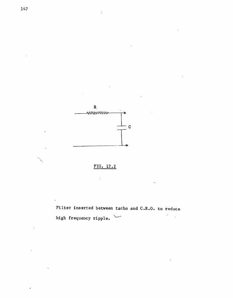
R ->vwvvvvww^

FIG. 12.2

Filter inserted between tacho and C.R.O. to reduce

high frequency ripple.

a) Frequency Response of Dual 3 Bridle System (Cont.)

but at the higher frequencies (around 1 cycle/second) the output

response became very low and it became difficult to determine

which was response and which was ripple from the tacho generator.

The actual test was conducted around a generator voltage of 60

volts for two reasons:

1. Operation should be in linear range.

2. It was found that the system tended to drift considerably

and so a bias signal was inserted into the amplifier to

correct for drift and ensure that all readings were taken

about the same generator voltage.

A simple filter (Fig. 12.2) was inserted between tacho and C.R.O.

to reduce the ripple and this improved results significantly.

R = 4.7 K

C = 0.47 micro farads

W = RG

= 450 radians

i.e. T = 2.2 M.S.

Tacho Voltaee

Generator Voltage

Nominal 0.8 cycles/second

Referenc

Voltage

1 Sec.

V

0 .1 Sees.

Tacho Voltage

Generator Voltage

Notninal 0 .4 cycles/sec,

A A

W / \j V

Reference Voltage

FIG. 12.3

Oscillographs of oscillator reference voltage, generator voltage and

tacho voltage.

a) Frequency Response of Dual 3 Bridle System (Cont.)

The tests were taken from the lowest frequency available (nominally

0.03 cycles/second) to 1 cycle/second. The upper limit was set by

the armature currents which were approaching full load whilst speed

was changing very little. In any case at 1 cycle/second the loop -

gain had dropped below unity. The filter inclusion thus did not

affect results to any significant extent.

The input voltage during the test was taken by recording the

amplitude dial reading on the signal generator whilst output voltage

was measured with the C.R.O. As a check on the input voltage and

frequency and phase shift between input and output a high speed

recorder was used to monitor input volts, generator volts and tacho

generator volts.

The test consisted of keeping generator voltage biased to 50 volts

and then superimposing a variable frequency input. The input level

was adjusted to obtain a reasonable output response and then the

variable phase input to the C.R.O. was adjusted until the trace on

the C.R.O. changed from an ellipse to a straight line. The input

level, phase angle on the dial and output voltage were recorded for

each frequency in addition to the high speed recorder traces.

(Typical traces are shown in Fig. 12.3)

14

12 ^

g. 10 p o

4J cU k

«J U

10 20 30 40 Oscillator Output Dial Reading

FIG. 12.4

Calibration curve for oscillator output voltage.

a) ^Frequency Response of Dual 3 Bridle System (Cont.)

Nominal Freq. Nominal Osc. Dial Output Volts C/S. Phase Shift Input Setting P - P

.03 73 7.5 56

• 05 78 12.5 56

.075 84 23 56

0.1 86 32 56

0.15 92 44 54

0.2 96 45 40

0.25 99 45 32.5

0.3 102 45 27

0.4 106 45 20

0.6 115 45 12.7

0.8 125 45 9.5

1.0 137 45 7.1

At the conclusion of the test the phase angle dial was calibrated

With the C.R.O, by using the reference and variable phase outputs

from the oscillator as the X and Y inputs respectively to the C.R.O.

The dial was found to have a constant error of 2°.

The C.R.O. calibration was checked and found to be correct so no

modifications were necessary to the output readings. The amplitude

dial readings on the signal generator were calibrated using the

C.R.O. with the high speed recorder still coupled as this was found

to have a considerable loading effect, (fig. 1^.4)

c o O (U CO

<n (U 1-4 o o o c ID cr 0) u

(U •u cd M

cd u

1.0

0.8

0.6

0.4

0.2

0.2 0.4 0.6 0.8 1.0 Oscillator Nominal Frequency (Cycles/Second)

FIG. 12.5

Calibration of oscillator dial frequency,

Frequency Response of Dual 3 Bridle System (Cent.)

Nominal frequency readings taken on tlie o s c i l l a t o r were compared

with those measured on the high speed recorder (which was subsequently

checked against 50 cyc le mains and found to be correct ) and were found

to be reading high. A cal ibration checked showed that the readings

had to be multiplied by 0.83. ( f i g . :12.5)

Actual F Actual Input 20 Log Frequency (Cycles /Sec . ) Phase Shi f t Volts Gain Gain Radians

P - P (d b)

.024 75 2.0 28 28.9 .0753

.041 80 3.6 15.5 23.8 .154

.063 86 7.0 8.0 18.0 .198

.084 90 9.6 5.8 15.2 .264

0.125 94 13.3 4.1 12.2 .394

0.165 98 13.6 2.9 9.2 .509

.208 101 13.6 2.4 7.9 .652

.25 104 13.6 2.0 6.0 .785

.33 108 13.6 1.5 • 3.6 1.035

0.5 117 13.6 0.94 - 0.6 1.57

0.66 127 13.6^ 0.70 ~ 3.2 2.07

0.83 139 13.6 0.54 - 5.4 2.61

25

20

15

n) O 10

0 db

- 5

0.1 0.2 0.4 0,6 0.8 1.0 Frequency (Radians/Second)

FIG. 12.6 150

Frequency response plot for 3 bridle speed control system.

a) Frequency Response of a Dual 3 Bridle System (Cont.)

The results are plotted in Fig, 12.6 in the form of a Bode Plot

of gain and phase shift with respect to frequency. The plot

shows the system to have a cross-over frequency of 1.5 radians/

second and a phase margin of 65°.

It is interesting to note that the phase shift between generator

voltage and tacho voltage is only 25° at 1 radian/second.

(Refer Fig. 12.3) A comparison of these results with calculations

from a transfer function and block diagram representation will

indicate whether or not linearizations and approximations, which

were made in the measurements of system parameters, are justifiable

and give reliable results.

Ampli dyne I Generator

v.-

1 Rp + Rp + P (Lp + Lp)

FIG. 12.7

Block diagram and transfer function of the generator.

b) Transfer Function of Generator

The generator block diagram can be expressed in form shown in

Fig. 12 .7 . Since the generator field is excited by the armature

of the amplidyne the whole circuit time constant must be taken

into account.

V

i . e . Generator field current is the amplidyne output voltage D

divided by the sum of the impedances of the amplidyne direct axis

and the generator field. The total impedance equals

^ + ^D + P ( S + S )

where ^ = generator field resistance

D = amplidyne direct axis resistance

^F = generator field inductance

^D = amplidyne direct axis inductance

Assuming the generator runs at maximum excitation then the field

resistance should be based on a

50 C rise.

^F - 4 6 . 4 ohms ( from Ch . 11)

but the amplidyne is rated at 11 amps and since the generator

requires only 2 amps at its maximum rated volts then the

losses in the machine would only be 37o so the temperature rise

should be negligible. The same argument can be applied to the

other time constants of the amplidyne.

thus generator transfer function is ^ = '^G ^D + S ) + P (^F + S )

b) Transfer Function of Generator (Cont.)

where G = generator armature voltage/field amp. from

Chapter 11.

124 ^ = 49.4 V D 1 + P 62.5

49.4

2.51 1 + 1.26 P

c) Transfer Function of Booster

By the same reasoning as in Section b) the booster transfer

function equals

^ + ^D + P ( S + ^D)

where ^B = booster armature volts/field amp. (Ch. 11) R PL D + D = amplidyne direct axis impedance

J) PL ^ + F = booster field impedance

In this case the value of the field resistance is again dependent

on t^perature but the booster excitation in this application

requires only half excitation to produce-maximum tension, but the 2

armature I R loss would be at maximum rating and this would be much

larger than the field losses so the machine temperature would still

approach the 50° C rise.

^ = 1.2 X field resistance at 20° C.

= 1.2 X 26.8 (from Ch. 11)

= 32.2 ohms.

booster transfer function

= 19 32.2 + 3.05 + P (11 + 1.49)

0.54 1 + 0.35 P

1 ^in 1 ^Q + PI-Q

Rp 1 + PLp 1 + PLq

FIG. 12.8

Block diagram and transfer function of an amplidyne.

d) Transfer Function of Amplidyne

Figure 12.8 is a block diagram of the amplidyne<

E in = control field input volts

^ + ^^F = control field impedance

^F = control field current

Q = quadrature axis gain V Q = quadrature axis volts R" PL

Q + Q = quadrature axis impedance

^Q = quadrature axis current

^ = direct axis gain V D = direct axis volts L„ r T — 1 = control field time constant R^

T L 2 = quadrature axis time constant

The amplidyne parameters were measured in Chapter 11 and the

amplidyne transfer function can be expressed as

= S 1 I S \ ( (1 + PT^ (1 + PTp ) In

41.4 (1 + 0.095 P) (1 + 0.185 P)

=§

ca o

10 20 30 Frequency

3 db.

FIG. 12.9

Frequency response plot for a transistor amplifier.

e) Transfer Fuic tion of Summating Amplifier

The calculations associated with the operational amplifier have

been calculated on the basis that the amplifier time constant

has negligible effect. This appears to be a reasonable assiimption

but a frequency response was conducted to find the actual time

constant.

The test consisted of injecting a variable frequency sinusoidal

signal from a signal generator to the input of the amplifier and

the input and output signals were displayed on a twin beam C.R.O,

The relative magnitudes of the input and output signals were

measured on the C.R.O , as the frequency was varied. The frequency

at which the output dropped to 707o of its low frequency level

represents a 3 db drop in gain. This frequency, when converted

to time, is the amplifier time constant and the resulting plot

in Fig, 12,9 shows the time constant to be 3 . 5 milli-seconds

(45 eyeles/s econd).

It was found necessary to use the twin beam C.R.O. because the

oscillator output voltage varied with frequency. Another advantage

was that approximate phase shift measurements could be taken in

conjunction with gain. The phase shift was achieved by utilizing

a facility on the C .R .O . whereby one trace was triggered by the

oth er.

- / w w v w

R.

^ W W v A A

FIG. 12.10

Transistor amplifier used as an adder but with

only one input E, shown.

e) Transfer Function of Summating Amplifier (Cont.)

If independent time bases were used for each trace then the phase

shift was destroyed.

This method of measuring frequency response does not approach the

accuracy of the method used in Ch. 11 a) but the aim in this case

was to find the approximate time constant. This time constant may

seem to be appreciable but the amplifier equivalent time constant

is modified when the amplifier is used as a summer.

Consider Fig. 12.10 where amplifier is used as an adder, and to

simplify,only 1 input will be considered:

E^ = input volts

R^ = input resistance

Eo == output voltage

= feedback resistance

e = amplifier input voltage G = amplifier transfer function = 1 + PT

where A = amplifier gain

T = amplifier time constant

- ^ + ^o - ^ = 0

El E J. _1 = - o + e + e

e) Transfer Function of Summating Amplifier (Cont.)

E, E 1 = " o R, R

1 - 1 G C-'

from Ge = E

R 2 E, = - E - 1 o 1 - 1 + 1

G /

• E R transfer function = o = - 2 E. R, 1 - 1

G R R, 2 + 1

/ looking at the denominator term in the square brackets

R, 1 - 1 -

G

since G =

11 GR

1 + PT

then denominator = 1 • 1

A

= 1 - 1 _

A

since A is much greater than 1

in this case A = 300 approx.

5R,

- PT A

R

R 2 -AR.

2 - PT AR,

R2PT

AR,

1 + ^ A AR,

and if ^2

then denominator = 1 -

50

= 1

300

- PT

300

\ 50

PT A 1 + _5_ 300 300

e) Transfer Function of S-ummating Amplifier (Cont.)

i.e. the transfer function = R,

1 - PT 49

hence the amplifier time constant has been effectively reduced

by a factor of 49. This means that when this amplifier is being

used as an adder with a nominal gain of 5 the amplifier time

constant is effectively 0,07 mi Hi-seconds.

On this basis the omission of the amplifier time constant should

not introduce large errors. Note that even if the nominal

amplifier gain is 10 the time constant is reduced by a factor of

26. As a check on these calculations a frequency response was

conducted on the amplifier when used with a nominal gain of 10.

From theoretical considerations the time constant should have

been reduced by a factor of 26 but it was found that the time

constant was reduced by a factor of 29 to 0.12 mi Hi-seconds•

This is a good correlation considering the method of measurement

which is apparently only accurate to about 107o.

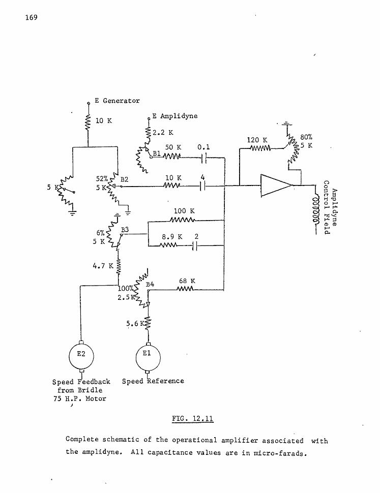
E Generator

10 K

52% B2

p E Amplidyne

2 .2 K

50 K 0 .1

Speed Feedback Speed Reference

from Bridle

75 H .P . Motor }

FIG. 12.11

Complete schematic of the operational amplifier associated with

the amplidyne. All capacitance values are in micro-farads.

e) Transfer Function of Siunmating Amplifier (Cont.)

Fig. 12.11 i s a detailed layout of the components associated with

the operational ampli f ier . Al l values and potentiometer settings

are as shown, but some c ircui try including jogging and suiciding

have been omitted because they do not enter into the normal running

mode.

Bl, B2, B3 and B4 are the attenuations for the amplidyne v o l t s ,

generator v o l t s , tacho-generator feedback vol ts and reference

tacho-generator vo l ts respect ively .

Bl = _93 X 5K - 0.647 100 (5 + 2.2) K

B2 = _52 X 5K = 0.208 100 lOK + ^

2

B3 - _94 X 5K = 0.485 100 5K + 4.7K

= 2.5K =

2.5K + 5.6K

Calculation of Path Impedances and Transfer Functions

1 + PRC input impedance = pc

R C AWvM I j_

50K 0.1 UF

Transfer Function of Summating Amplifier (Cont.)

Path 1 (Cont.)

Amplifier feedback impedance is 120K but there i s a 5K ohm potential

dividerx^ich i s set to 807o which means only 20% of the output voltage

i s fed back

equivalent feedback impedance i s : -

= (120K + 80 X 5K) X 100 ( 100 ) 20

= 620K

This i s the feedback impedance for a l l signals

path 1 transfer impedance i s : -

620K X PC 1 + PRC

= 620K X 0.1 X I P ' S 1 + 50K X 0.1 X 10"^P

= 0.062 P 1 + 0.005P

f o r Path 2 R

-MVA/t lOK

input impedance

transfer impedance i s : -

== 620K X P X 4 X 10 -6

4 UF

1 + PRC PC

- 6

1 + lOK X 4 X 10 X P

2.48 P 1 + 0.04P

0.65 Q.062P

1 + 0.005P

0 .2 2.48P

1 + 0.04P

6.2 (1 + 0.22P) 0.49

6.2 (1 + 0.22P) 0.49

1 + 0.18P 1 + 0.18P

0.31 9.13

FIG. 12.12

BLOCK DIAGRAM OF TRANSISTOR AMPLIFIER

AND ASSOCIATED COMPONENTS

Transfer Function of Sttngnating Amplifier (Cont.)

f o r Path 3 R1

W W W lOOK

R2 WVVV 8.9K

input impedance

where G

transfer impedance =

2UF

R1 (1 + PGT) 1 + PT

R2 R1 + R2

(R1 + R2) C

620K "(1 + PT) R1 (1 + PGT)

620K (1 + P 108.9K x 2 x 10"^) lOOK (1 + P 8.9K X 2 X 10

6.2 Cl + Q.218P) Cl + 0.0178P)

- 6

• f o r Path 4 R

-/WVW

.transfer impedance = 62QK R

62QK 68K

9.13

The amplifier and associated components can now be placed in

block diagram form of f i g . 12.12.

f) Overall Block Diagram

The tacho generator in use on the bridle has a gain of 100 volts/

1,000 R.P.M.

line top speed = 550 F.P.M.

work roll diameter = 36 inches

roll R.P.M. at top line speed = 58.3

gearbox ratio = 15.5 : 1

motor R.P.M. at top line speed = 905 R.P.M.

tacho voltage at top line speed = 90.5 volts

90.5 tacho gain = 94.6 volts/radian/sec.

(905 R,P.M. = 94.5 radians)

tacho gain = 0.96 volts/radian/sec.

The machine manufacturers supplied the inertias of the various

drive motors and gearboxes and is tabulated below.

15 H.P. 50 H.P. 75 H.P.

Motor inertia 18.4 84.6 119

Gearbox inertia 35.2 46.3 69

Total inertia 53.6 131 188

( all figures in lb. ft.^ )

Block Diagram of Voltage Control Scheme

and Delivery Bridle.

2 s •

ZR S o H ' r IS n r .

XA , -75*

c-UfCrtfcw"

U , ST rt f

X^ , i s n f

1 , r y * / " o t » f » * i

l e S o K / "

11 l y H / * " "

V

A/ , = Ni^mutft OF curout«7'.vl StC't? '"ift-D Tt^t^i V •• RirrlHuiiAi ••

' ^ f l f • nr-ir. - rum s

(/ y o-ottr) — » o -

k - 8

n = IS HP

j s i .

(47,«)

(M 0.097^)

N p l , (5300)

J H u n t f ' f t C Vit'^'i "V SP t e r ;

(l-fo-isip)

t :

i i n - t .

L . " " c f '

Aplr.

f) Overall Block Diagram (Cont.)

The motor manufacturer also supplied the number of turns in

the cumulative and differential series fields in each motor.

With this information and the measurements taken, the complete

block diagram of the system has been drawn in Fig, 12.13. The

block diagram includes the effects of the series fields by

summating the amp turns of the main field and cumulative field

and subtracting the amp turns of the differential field. ,The

current flowing in the cumulative fields is the actual motor

armature current, whereas the differential field current is the

sum of the 3 armature currents divided in inverse proportion to

the differential field impedances. »

The division of armature current was calculated as follows by

referring to Fig. 12.14.

1370 Y 1 = admittance of 75 H.P. differential field = 1 + 0.0807P

724 Y 2 ^ admittance of 50 H.P. differential field = 1 + 0.097P

230 ,Y 3 admittance of 15 H.P. differential field = 1 + 0.0732P

These figures are based on measurements tabulated in Chapter 11

and neglect the mutual coupling between the series fields and

between the shunt field.

o Cumulative Fields

yX,

Differential Fields

1

Y, ^ 2 = 1 Y, Z = 1

Y

FIG. 12.14

DIAGRAM OF 3 ROLL BRIDLE MOTORS SHOWING SERIES FIELDS AND

DIVISION OF CURRENT (NEGLECTS MUTUAL COUPLING BETWEEN FIELDS)

f) Overall Block Diagram (Cont.) Y = Y 1 + Y 2 + Y 2

1 5 . + 386P + 2325 0.00057P^ + 0.021P^ + 0.25P + 1

Z = 1=0.000437 C1+0.083P) - 0.0000068 (1 + Q.Q93P) Y (1+0.074P) (H-0.092P)

in the second tern a numerator and denominator term may be

cancelled.

.*. 2 = 0.000437 (1 + 0.083P) - 0.0000068 (1+0.074P)

The second term in this last expression represents only 2%

of the first term and could be neglected

thus Z = 0.000437 (1 + 0.083P)

If I is the total armature currents then current in 75 H.P.

differential field is

where = IZ

Zj = impedance of 75 H.P. differential field

I = T7 1 — = I 0.000437 (1 + 0.Q83P) 0.00073 (1 + 0.08P)

0.6 I

KD

V R Turns 11.6H

500 uF \AAAAAAAM

3,000 ohms |500 uF

To Entry Bridle Motors

Booster

] 0.024 ohms

To Generator

FIG. 12.15

SCHEMATIC DIAGRAM OF THE BOOSTER VOLTAGE CONTROL SERVO,

f ) Overall Block Diagram (Cont.)

T = T 7 2 ~ where Z = impedance of 50 H.P. d i f f e rent ia l f i e l d

- I 0.317 (1 + 0.083P) (1 + 0.097P)

"" where Z„ = impedance of 15 H.P. d i f f e rent ia l f i e l d Z3 3

- I 0.1 (1 + 0.083P) (1 + 0.073P)

The br id le containing the booster i s shown in Fig. 12.15 with the

appropriate values marked. In this case i t i s best to summate the

amp fums of each of the control windings and then express as a

transfer function.

The booster armature voltage feedback path transfer function can

be expressed as •

A/T = 0.047 P ^B 1 + 1.5P + 0.3 X 10"^ P^

The amplidyne armature voltage feedback path transfer function i s 0.17 P A/T =

\ 1 + 0.94P + 4.7 X 10"^ P^

Complete Block Diagram of Booster Control

Scheme and Entry Bridle.

y ' (/-ta-n (/-t a-nsp) (M o.^SP)

( u = : o 5 P )

S E M t s u T O K r E R w i N f j i -

o S ^ S —

V r 5 7 /<(<i

l M I a'nf)

( . - . O . U N O

x V

- ^.-jtiaasMJi j < £ .

" ' - T O R 5^-f5t>

f) Overall Block Diagram (Cont.)

Booster current feedback path transfer function is

A/T = 0.126 I 1 + 0.9 X 10'^ P

The reference voltage path transfer function is

A/T = 5.3

\ 1 + 0.16 P

The block diagram for this bridle is as shown in Fig. 12.16,

g) Frequency Response Versus Block Diagram

The dual 3 roll bridle system block diagram has now been drawn,

and the transfer functions calculated. These transfer functions have

been found by using some approximations. Referring to Fig.

12.13 the transfer function between the speed reference and the

generator terminal voltage is:-

41 .4 (1 + 0.005P> 2.51 (0.508P)

(1 + 0 .04P) (1 + 1.26P) (1 + 0.095P) (1 + 0.185P) (1 -fO.OOSP) +1.65P

This can be reduced further by neglecting the high order terms

which are negligible around 1 radian/second (near the cross-over

frequency).

Vt = 54.6 (1 + 0.0Q5P)

Vref (1 + 0.04P) (l + 1.26P) <1.2P> (1 + 0.0098P)

54.6

(1 + 1.26P) (1 + 2P)

g) Frequency Response Versus Block Diagram (Cont.)

The transfer function of 75 H.P. motor will now be calculated

by neglecting load torque and series field effects.

It can be shown that on the above basis the transfer function

between speed and generator volts is

^ Kd - ^ ^ Eqn. 12.1 E K 5) + JRP + JLP

2 where J = System inertia in Kg - M

R^ = Arm. resistance

L. = Arm. inductance A K = Basic machine constant

^ = Flux

W = Speed in radians/second

by substitution 0.55 E (1 + 0.69P) (1 + 0.013P)

W By calculating the frequency response of E around 1 rad./second

and adding the result to the phase shift of — at the same REF

frequency a comparison can be made to the frequency response

plot of Ch. 12.1. The results are tabulated below and compare

Frequency Response Versus Block Diagram (Cont.)

with the frequency response results .

W Freq. Response

Freq. (Rads. /Sec.) ^REF E Total Results

0 .5 - 78 19 - 97 98

1.0 - 117 35 - 152 107

1.5 - 137 47 - 184 118

2 . 149 - 55 - 204 125

All readings in

degrees of phase shift

The results indicate that, the assumptions made in the block

diagram derivation, and the further simplifications made in the

phase shift calculations have resulted in large differences to

that from the frequency response test. This means that a more

rigorous method must be used in the block diagram derivation to

achieve more realistic results.

The frequency response test indicated that considerable non-

linearities were present in the bridle system (Fig. 12.3) and

these may account for some part of the differences. These

results also highlight the fact that simulations can only serve

to pinpoint possible problem areas and may not give a true

indication of system response.

Conclusion

The principle factors necessary for the implementation of separately

powered rolls for the extension of steel strip are:-

1. Economic proposition

2» Load sharing of motors

3. Zero strip slippage

4. Digital control system

5. Extension accuracies capable of being attained and

maintained over long periods.

These five factors have been investigated and the economics leave

nothing to be desired whilst the load sharing of the motors will

present no problems with adequate design.

The extensometer, built up to measure strip slippage, proved an

accurate instrument which showed that there was negligible slippage

on the existing dual 3 roll bridle. This bridle was designed on a

reasonable co-efficient of friction factor and it would be feasible

to assume that the same results would be obtained on a similarly

designed multi-roll bridle. With zero strip slippage motor speed

equals strip speed and so motor speed can be controlled to obtain

the desired extension or speed difference signal.

Conclusion (Cont.)

Digital signals can be easily incorporated into control systems as was

shown in Chapter 9. The accuracy or resolution of these dig i ta l signals

i s normally limited, but this can be overcome by the adoption of the

proposed method of obtaining more accurate d ig i ta l speed di f ference

signals .

Measurements were conducted on the existing 3 r o l l br id le to determine

control system parameters. The results are a good correlation with

the information supplied by the manufacturers and allows their supplied

information to be used with confidence.

These parameters were used to formulate the 3 r o l l br id le into block

diagram form. Some phase sh i f t calculations were done on the block

diagrams at several frequencies and the results compared with a

frequency response test conducted on the 3 r o l l b r id le . The comparisons

indicated that assumptions and l inearisations made in the derivation of

the block diagram caused large errors near the c r i t i c a l frequency area

( i . e . crossover frequency). At lower frequencies the error reduced.

This error at the higher frequencies could have been due to the severe

non- l inear i t ies present in the system.

Conclusion (Cont.)

Overall separately powered multi roll bridles for the controlled

extension of steel strip are feasible. Simulations conducted on

any block diagram representation can only be used as a guide to

system performance unless transfer functions are rigorously

determined.

R E F E R E N C E S

"Mechanical Metallurgy," G.E. Dieter (McGraw-Hill) 1961.

"Fundamentals of Mechanical Design," R. Phelan (McGraw-Hill) 1962.

"Electrical Circuits and Machinery," F. Hehre & G. Harness (Wiley) 1944,

"Industrial Electricity," J. Nadon & B. Gelmine (Van Nostrand) 1942.

"Rotating Amplifiers," M.G. Say (Newnes) 1954.

"Electric Machinery," A.E. Fitzgerald & C. Kings ley (McGraw-Hill) 1952.

"Engineering Electronics," J.D. Ryder (McGraw-Hill) 1957.

"S.C.R. Manual," General Electric, 3rd ed. 1964.

"Transistor Manual," General Electric, 1964.

A.R. Foreman, "Application of Rubber Covered Rolls to Pinch Rolls

and Bridles," Iron & Steel Engineer, August, 1964.

G.C. Turner, "The Design and Application of Bridles for Process

Lines," Iron & Steel Engineer, February, 1965.

R E F E R E N C E S (Cont.)

Bell and Vassily "Continuous Strip Stretcher Levelling Process,"

Iron 6c Steel Engineer, May, 1967.

Hindley "Control of Process Line Tensions," Iron & Steel Engineer,

February, 1966.

W.D. Sinclair, "Thyristor Power Converters for D.C. Machine Drives,"

A.E.I. Engineering (Reprint).

FIG.A1

Typical layout of a Continuous Galvanizing Line

WTUDER.

SIDE Tr /A^A^ER

UNCOIL-ER.

EKJTKY

b

FURNF)CE.5

"O D O D O o O O O Os. C D CIL\LVFLN\2.MC,

P^R

C o o t i A / a A n d THERTMEUT

L£\/EULER PRIME PILING

( ) ( ) 8 8 8 8 ( ) O .

APPENDIX 1 CONTINUOUS GALVMIZING LINE OPERATION AND LAYOUT

The layout of a typical Galvanizing Line is shown in sketch Al.

The line consists of 4 main sections, but for recoiling only 3

are in use. The sections are the entry section, furnace or

process section, delivery section and the cut-up section.

The entry section includes a side trimmer, a welder and storage

facilities in the entry tower which is kept full at all times

except when the entry section stops to join coils together with

the welding. During this period there is sufficient strip stored

in the tower to allow the process to continue at top speed. When

the entry section is restarted it is oversped up to 207o of the

process section until the entry loop is full once again.

The process section consists of many distinct operations and these

include heating and soaking (annealing) in the furnaces followed

by dipping in the galvanizing pots, cooling, chemical treatment

and tension levelling. The storage tower after the process section

is kept in an empty condition so that when the delivery section

stops to unload, the process section can continue at top speed by

storing in the tower until the delivery section is ready to run.

APPENDIX 1 CONTINUOUS GALVANIZING LINE OPERATION AND LAYOUT (Cont.)

The delivery section basically consists of recoiling the galvanized

strip. If sheets are required instead of coil then the recoiler is

bypassed and the strip is fed into the cut-up section. In this

section there are flying shears, inspection belt tables, automatic

sheet rejection and sheet piling facilities. In the cut-up mode

the delivery and cut-up sections are stopped and started

simultaneously during stacking operations. Both these sections

can also be run up to 20% above the maximum process section speed

to empty the delivery tower.

Both towers on the line are operated by torque motors and they

have variable height modulation.

Within the process section there are many operations, and included,

is the tension levelling section which is the area under investigation,

Although the term levelling section has its own generator it is speed

matched to the rest of the process section. The process section has

a speed range of 1 0 : 1 but generally runs between 8 5 7 c , to 1 0 0 % top

speed. Speed changing within this section is done very slowly

because of strip temperature in the furnace. Reject material results

if the process speed is adjusted rapidly and of course if the process

section stops then all material within the furnace is scrap (0.5 tons).

200

APPENDIX A. 2

S PM rt o o o

t\ .-I

0) 00 CIS +J I-H o > 0) u •p

u

160

120

80

40

75 H.P. Motor Open Circuit Voltage Excitation

0.4 0.8 1.2 1.6 Field Current (Amps.)

2.0

APPENDIX A. 2

o o o

280

240

200

160

120

80

40

75 H.P. Motor

Flux Excitation

0.4 0.8 1.2

Field Current (Amps.)

1.6 2.0

140

120

rt o o o 1-1 cSj

100

<1) {JO CO 4-1 i-i o > OJ u •p

APPENDIX A. 2

50 H.P. Motor Open Circuit Voltage Excitation

0.8 1.2 1.6 Field Current (Amps.)

APPENDIX A. 2

240

200

160

o o o

' 120

50 H.P. Motor Flux Excitation

0.4 0.8 1.2 1.6 Field Current (Amps.)

APPENDIX A.2

160

*

o o o

CS; 120

0) iiO cfl +J t-H o > 0) n p +J

80

40

15 H.P. Motor Open Circuit Voltage Excitation

0 , 8 1.2

Field Current (Amps.)

APENDIX A. 2

200

o o o

X p 1 - 1

15 H.P. Motor Flux Excitation

160

120

80

40

0.4 0.8 1.2 Field Current (Amps.)

1.6

Motor Field Time Constant

R Circuit' = 243.4 ohms (102.1 + 141.._3) Time Constant = 0.4 Sees,

L =' RT =: 0.4 X 243.4- = :97.2 H.

APPENDIX A 2.

Motor Field Time Constant

Circuit Time Constant — 0.7 K Circuit E Field + 15.9 ohms 92.0 L = RT = 0.7 X 92 = 64.2 H.

75 H.P. MOTOR •• . , ! : I ; HT := 26 Divisions Time Lines = 10 Sec.

: .*. I Circuit Time Constant ••= 0.45 Sees. L = RT = .45 X 'l84i= 82.7 H. ' R = R Field + lOO' ohms.

APPENDIX A. 2

30 K.W. Booster

Open Circuit Voltage

Excitation

2 3

Field Current (Amps.)

APPENDIX A. 2

0.5 1.0 1.5 2.0

Field Current (Amps.)

2.5 3.0

240

APPENDIX A. 2

200

160 Pd o vj-

ca

<u GO Cti •P 1-4 o > 0) J-l p +J

120

80

40

150 K.W. Generator Open Circuit Voltage Excitation

0.5 1.0 1.5 Field Current (Amps.)

2.0

APPENDIX A. 2

120

150 K.W. Generator Flux Excitation Curve

0.25 0.5 0.75 Field Current (amps)

Generator Field Time Constant

30 K.H. BOOSTER ' ••

E Circuit = 126.8 ohms (26.8 + 100) \ Time Constant = 0.087 \ L = .087 X 126.8 = 11 H.

150 K.W. GEMERATOR R Circuit = 138.7 oteia (38.7 + 100) Time Constant = 0.44

L = 61 H.

APPENDIX A. 2 207 Step Test to Determine Turns/Pole

30 K.W. BOOSTER

Pen Sensitivity = 12.2<^A/Inch Pot Setting = 35% of 10 K Input Volts = 214

150 K.W. BOOSTER

Pen Sensitivity = 12.2c^A/Inch Pot Setting = 15% of 10 K Input Volts = 242

APPENDIX A. 2

Direct Axis Voltage Response to a Control Field Step Input Time Lines 0 Q.Ol Sees.

Final Height

Quadrature Axis Voltage Response to a Control Field Step Input Timing Lines 0 0.1 Sees.

APPENDIX A. 2

175

150

2 P h

o vO

125

100

<u 00 CO jj .-I o >

OJ u

•4-1 nJ

10 20 30 40

X^ X^ Field Current (MiHi-Amps)

APPENDIX A. 2 210

KQ == Slope

200

10 20 30

Control Field Input Current (MA)

150

cn 4J I—1 >100 •H X < 1 4J O (U u • H P

= Slope

50

0.2 0.4 0.6 Quadrature Axis Amps

0.8 1.0

The C/iL953 Decade Counter

The Fairchild C/iL 958 is a monolithic decade counter designed to operate at frequencies up'to 2 megacycles over a temperature range of 0°C to 75®C. Inputs consist of a count signal and a reset signal. Outputs are binary-coded decimal having 1 -2 -4 -8 relative weighting. Individual outputs maybe pulled to ground after resetting to establish any of the nine non-zero states in the normal decade sequence. Units may be cascaded to commodate multi-digit applications.

The 958 Deci.de Counter consists of four flip-flops and an input amplifiei as shown in Fig. 1. The flip-flops are interconnected in such a way that an ordinary modulo-16 binary count Is curtailed at the end of ten counts, returning to the first count rather than the eleventh. This action is accomplished by inhibiting an input to 7F2 at the ninth and tenth counts, and by resetting FF4 at the end of every even-number count.

The feedback loop from FF4 to FF2 inhibits the response of FF2 to the carry pulse from FFl during the ninth and tenth counts. At this time FF2 and FF3 are in the "zero" state and FF4 is in the "one" state. FF4 is reset at the end of counts 2, 4, 6, 8, and 10 by the signal from FFl . How-ever, since FF4 is in the "one" state only during counts 9

9 9 5 8 and 10, only the reset after count 10 has any effect. As FFl returns to "zero" at the end of every even-numbered pulse,

COUNTER the entire Counter is set to "zero" for the first count of the next cycle.

The flip-flops of the Decade Counter are similar in . principle to the Fairchi ld / iL9l6j -K flip-flop(see Fig. 2).

Transistors Qj and Q2 form a simple latch circuit through the cross coupling of resistors R ^ and Rg. Pulse steering transistors Q^ and Q^ direct a pulse of current to the base of either Qj or Qg to cause a change of the flip-flop's state. The diodes connected from the collectors of Q^ and Q^ to the bases of Qg and Q^ select the transistor through which a count pulse may pass. Note that either Q^ or Q^ can be active at any particular instant, but not both, because of the comple-mentary nature of the voltages at the collectors of Q^ and Qg.

FIG. 1. CmL958 decade counter block diagram.

RESET o

oOUTPUT

COUNT INPUTS

> T)

Z O M ><!

ro

FIG. 2. Decade counter flip-flop schematic.

.'I

J In FFl, FF2, and FF3, both collectors of the steering transistors are connected to the output of the previous stage (the amplifier has output characteristics similar to theflip-I flop). When an output is at its low potential (less than 0.4 volt), the \u.se-collector junction of one of the attached steering transistor^Js-forward biased. The resulting cur-

_ .rent is responsible for a quantity of charge being present in the associated collector-base region. If the collector voltage of the pulse-steering transistors is abruptly raised (to at least 1.0 volt), the charge in the collector-base region is trapped by the diode in the base circuit. The only available

^ exit is t / - emitter. The charge stored in the collector-base region exiis rapidly through the emitter creating a pulse of current adequate to trigger the flip-flop exactly once.

9958

COUNTER

( C o n t . )

In FF4, the collectors of the steering transistors are connected separately: one to the output of FF3, the other to the output of FFl. Thus, FF3 is responsible for setting FF4 and FFl is responsible for clearingit. Otherwise, FF4-operates in the manner just described.

The feedback loop from FF4 output to FF2 input includes an additional transistor, which provides a discharge path from the base of Q^ to ground when FF4 is in the "one" state. FF2 is thereby prevented from assuming the "one" state while FF4 is in the "one" state.

Each of the flip-flops contains a reset transistor, Qg. The base resistors of all Q^'s are connected to the reset in-put. A reset level of at least 1.4 volts and 3 mA will drive all outputs to the "zero" condition (greater than 1.5 volts).

t

The input amplifier is non-inverting and designed to produce an output similar to that of a binary. It can also accept an output from another Decade Counter, imposing minimal loading upon it.

> hd hd M «

> U)

N3 N)

FAIRCHILD COUNTING MICROLOGIC®INTEGRATED CIRCUITS CmL9958

RESET/PRESET

The circuit is reset to count 0 (all outputs high) with a high level at the reset input pin.

To preset an arbitrary count:

1. Reset to count 0 and then return the reset pin to a low level.

2. Ground (below 0.45 V) the appropriate outputs.

ELECTRICAL CHARACTERISTICS (25 'C Free Air Temperature unless otherwise noted)

Parameter Min, . Typ. Max. Units Conditions

Supply Voltage 3.3 5.5

Count Input-Low 0.45 V "

Count Input-High 1.2 V ^

Count Input Pulse Width-High 150 • ns _ •

Count Input Slope-Positive Going 1.0 V//1B ^

Maximum Count Input Frequency 2.0 MHa^

. -Reset Input-Low 0.45 V

Reset Input-High 1.2 V

Output-Low 0.35 V = 0.4 mA = 4.0 V

Output-High :1.4 V I^^^ = -0.7 mA V^^ = 3.6 V

Power Consumption \ 140

Count Input Impedance 2kC2 in series with a transistor base-emitter diode

Reset Input Impedance 300 n in series with a transistor base-emitter diode

Maximum Delay from Count Input 300 ns (Load: 2 parallel with 50pF from each to Zg Output. (Count 7 to 8)

' <

output to ground)

TYPICAL DUAL IN-UNE PACKAGE

T l

J—"-

(PRODUCT CODE. U6A995e7M)

hd W

a

><i > to

K)

CO

v_ •*tianar is a patented Fairchild process.

FAIRCHILD COUNTING iVilCtoLOGIC®INTEGRATED CIRCUITS C m L 9 9 5 8

O RESET O"

F.F.

COUNT U

BLOCK DIAGRAM

Z2 24 O

L r ^

/ A N D \

4 3

28 Q

L O O

SCHEMATIC DIAGRAM OF DECADE FLIP-FLOP

, *cc

I tooo:;

l U 1 Ik

rROMVi

-w—< sooo

< -oJnowmiT

O s I> U>

N>

LOADING RULES

DRIVIKG DEVICE AT OF CAN DRIVE

C/IL9958: - . - •

3.3 Mln. 1CML9959

3.3 Min. 1 CML9959P1us 1 C/iL 9958 Count Input

Zj, Zg, 4.0 Mln. 2CML9959

4.0 Mln. 2 CML9959PIUS 1 C^xL 9958 Count Input

Zg, 4.0 V Mln. and one 390 n current limiting resistor in series with each output

4 CML 9959

1 4.0 V Min. and one 330 n current limiting

resistor in series with Zg output

4 C/iL9959pIus 1 C^iL9958 Count Input

3.3 Min. - 1 C^L9960

3.3 Min. 1 C;iL9960pIu8 1 CptL9958 Count Input

' 4.0 Mln. 2 C/1L9960

4.0 Min. 2 C^iL9960plu5 1 CpiL 9958 Count Input

Z^, Zg, z^ 4.0 Min. and one 330 n current limiting resistor in series with each output

5C;iL9960

^8 4.0 Min. and one 270 n current limiting

resistor in series with Zg output

5 C/iL9960plus 1 C/XL9958 Count Inputs'

Industrial Range Milliwatt R T L : 3.6 V ±10% 1 C/iL99SBCount Input

Industrial Range RTL : 3.6 V ±10% 6 C/iL9958Count Inputs, or 1 C/iL9958 Reset Input

Industrial Range DTL 6k Family:

4.5 Mln. 1 C/iL9958Count Input

Industrial Range DTL 2k Family:

4.5 Min. 3 C/j.L9958Count Inputs, or 1 C/xL9958

Reset Input

>

§

o M X

> CO

M »-» Ln

The Ca<L959 Buffer Storage

The C ; iL959 Buffer Storage unit consists of four gated

latch circuits (Fig. 3) whose input characteristics match the

CmL958 Decade Counter output characteristics. The buffer

storage unit serves several vital functions ina C/xL system:

it allows the state of the counter outputs to be sampled and

held for an indefinite amount of time, it provides both true

and complement signals, and it furnishes a convenient meth-

od of signal level conversion when dissimilar circuitry is to

be driven.

Z2 Zz Z3 Z3 24

1 0 1 0 1 0 1 0

FL FL FL FL

i i i >2 '3 M

FIG. 3. C/IL959 buffer storage logic diagram.

The circuit of the latch used in the C/iL959 Is shown In

Fig. 4. Information is entered into each latch in a novel

manner. The gate signal is amplified and distributed to the

four latch circuits as illustrated in Fig. 3. Depending on

the state of the information applied to each latch, the ampli-

fied gate signal can cause two different-actions. If the

information signal is high, both Q3 and Q^are saturated and

the base voltage at Q^ is sufficiently low to turn Q^ off.

9959

BUFFER

MEMORY

Transistor Qg starts to conduct as the collector voltage of

Q^ rises, and the latch assumes a new state If the infor-

mation input is low, Q^ does not conduct and consequently

the gate current into the base of Q^ exits through the col-

lector and enters the base of Q^. Should Q^ be off, this

current turns Q^ on, causing, the latch to assume a new

state. This mechanism allows a single Input to saUsfy both

set and clear requirements in a very simple way.

+V

1 - v w

- Wv-

AMPLIFIED GATE o

W r — ^ ^ — W V

INPUT O — W V — t r Q 4

FIG. 4. Buffer storage latch circuit.

The latches of the Buffer Storage unit are isolated from

the load by transistors Qg and Qg. These transistors will

handle approximately 10 mA , permitting one to match the unit

to many other circuits, both digital and analog.

The gate amplifier is inverting, and will enable the latch

Inputs when low. An open gate input has the same effect. To

disable the latch inputs, the gate input must be raised to

1.5 volts or more.

F A I R C H I L D C O U N T I N G M I C R O L O G I C ® I N T E G R A T E D C I R C U I T S - C t i L 9 9 5 9 ELECTRICAL CHARACTERISTICS (25'C Free Air Temperature unless otherwise noted)

Characteristic Min. Typ, Max. Units Conditions

Supply Voltage 3.3 3.8 5.0 V . _ j Power Consumption . 115 . mW = 3 . 8 V Gate High Power Consumption 135 mW V c c = 3 . 8 V Gate Low [ Gate Input High LI V

V c c = 3 . 8 i

Gate Input Low 0.5 V 1 1 1

Data Input High 1.0 V -t

Data Input Low 0.5 V Output Low 0.4 V •OUT = mA , = 5.0 V : Output Low Load Current -0.4

o . o ; V mA

'OUT = mA - • V = 3.3 V i

Max. Sampling Rate >5.0 MHz

mA - • V = 3.3 V i

Sampling Pulse Width (Gate) 100 ns • ^ ^ •

LOADING RULES FOR CPL9959 '7 \

Driving Device AtV^^of 1

Can Drive:

9959 3 3 to 5.0 V 2 9960 inputs ts 9959 3.3;to 5.0 V 4 Low Power RT/xL loads 9959 3.3 to 5.0.V 1 RT/iL load

1 1

9959 3.3 to 5.0 V 2 DT/iL loads 1

9958 3.6 to 4.0 V 2 9959 data inputs Full Range Low Power RT^L 4.0 V Min.*

at -55°C 3 9959 data inputs or 1 9959 gate input

Industrial Range Low Power RT/iL 3.6 V±10% 2 9959 data inputs Full Range RT^L 3.0 ±10% 10 9959 data inputs or 3 9959 gate inputs Industrial Range RT^iL 3.6 ±10% 13 9959 data inputs or 5 9959 gate inputs Full Range DTML 6 K Family

2 9959 data inputs or 1 9959 gate input

Full Range DT/iL 2 K Family

4.5 V Min. 6 9959 data inputs or 2 9959 gate inputs

hd

><! >

05

M

FAIRCHILD C O U N T I N G M i C k O L O G l C ® I N T E G R A T E D CIRCUITS • Ct>L995,9

SCHEMATIC DIAGRAM OF BUFFER STORAGE UNiT ,. A ,

Zb Zb

I >

ro I - ' 00

The C;iL960 Decimal Decoder

This unit facilitates the conversion of an 8-4-2-1 binary-coded decimal uumber to a true ten-digit decimal number. The input characteristics of the Decimal Decoder are adapted to the output characteristics of the C/iL 958Decade Counter. Low signal levels are accepted as logic "ones" and high sig-nal levels as logic " zeros . " As complement values are needed in the decoding matrix, and as they are not furnished by the C/iL958, inverters are includedfor all input signals. The outputs of the C/1L960 have voltage breakdown charac-teristics adequate for controlling most types of neon-filled indicator tubes. '

The schematic diagram of the C/xL 960 Decimal Decoder is shown in Fig. 5. The decoding matrix consists of PNP transistors used as diodes. Advantage is taken of the fact that a "one" in the most-significant position never occurs unless -the two successive positions are "zeros." This reduces by five the number of transistors needed in the matrix. The actual decoding process is accomplished in two steps. The first step consists of forming five new signals from the three most significant bits of the input information. In the second step, one of each pair is selected by the least significant input signal. Only one of the ten output transistors can have the proper turn-on voltages applied simultaneously to both base and emitter when a valid BCD code is.used;~ However, because of the simplified decoding matrix, a binary code greater than nine causes two outputs to turn on simultaneously.

9960

DECODER

DRIVER

FIG. 5. C/1L960 decimal decoder schematic.

The output transistors can withstand voltages in excess of 60 volts and are thus quite adequate for the purpose .of

holding off series neon indicating devices. However, to

achieve the high voltage characteristics, it is necessary to

accept fairly high saturation voltages; consequently, the low-voltage current-sinking qualities are such that the Decoder is not recommended for driving incandescent lamps or other integrated devices.

ES hd a a M X! >

ro

FAIRCHILD COUNTING MICROLOGIC® INTEGRATED C I R C U I T - C / a L 9 9 6 0

ELECTRICAL .CHARACTERISTICS (25° C Free Air Temperature unless otherwise noted) ; •

Symbol Characteristic -Min. Typ. ' Max. Units Test Cqnc^tions

Vcc Power Supply (Note 4) 3.3 5.5 V •

PD Power Consumption 45 , , mW Vcc = 4.0 V Input High ViH Input High 1.0 V Va Input Low 0.4 ' V Vol o n Output Voltage (Note 2) V Vm = 1.0 V, loL = 3 mA VoH OFF Output Voltage V loH = 0.2 mA Ico OFF Output Leakage Current 50 MA VouT = 0.2 mA

; " * - ;

LOADING RULES FOR C;:L9960

Driving Device At Vcc of C/1L9959 . 3.3 to 5.5 V 2 C/iL9960 inputs C/xL9958 3.3 to 5.5 V 1 C/iL9960 plus 1 C/iL9958 .

Count Input Industrial Range Milliwatt RTL 3.6 V ±10% ,

1 1 C^L9960

Industrial Range RTL 3.6 ±10% 6 C/iL9960 Industrial Range DT/tL 6K Family

. 4.5 V Min. 1 C/iL9960

Industrial Range DT/iL 2K Family

4 .5VMin. / 3 C,fL9960

@ O M ><J

> U)

to N3 O

RESISTOR-TRANSISTOR MICROLOGIC® INTEGRATED CIRCUITS

PART NUMBER 9900

ELEMENT TYPE Buffer

NOISE IMMUNITY (TYP., 25'C)

300 mV

PROPAGATION DELAY (TYP.. 25"C)

16 nsec

POWER DISSIPATION (TYP., 25»C)

30 mW

DRIVE FACTOR.

25

DESCRIPTION Low impedance Inverting driver circuit for use as a line driver, an astable or monostable multivibrator, or pulse differentiator. Valuable for driving heavily loaded circuits or minimiz-ing rise-time deterioration due to capacitive loading. •

Logic Diagram

SUPPLY VOLTAGE 3.0 volts ±10%

3.6 volts ±10%

TEMPERATURE RANGE - 5 5 ' C to +125''C (21)

O'C to +100'C (22)

+15»C to + 55-C (28) O'C to + 70»C (29)

-vw-

- v w 5 Schematic

PACKAGE Flat-Pack (3F) TO-5 (50)

Epoxy (8B)

hd

O M X > L>9

PART ELEMENT NUMBER TYPE 9914 Dual Two-Input Gate

NOISE IMMUNITY (TYP.. 25''C)

300 mV

PROPAGATION DELAY (TYP., 25"O

12 nsec

POWER DISSIPATION (TYP., 25 »C)

24 mW

FAN-OUT

DESCRIPTION Dual two-input gate capable of generating any logic functio'n. Element circuits may be cross-connected to form a flip-flop, or con-nected in tandem to form non-inverting gates.

SUPPLY VOLTAGE 3.0 volts ±10%

3.6 volts ±10%

TEMPERATURE RANGE -\-55'C to +^25''C (21) / O'C to -t-IOO-C (22)

O'C to -I- 70*C (29) +15°C to + SS'C (28)

PACKAGE Flat-Pack (3F) TO-5 (5B)

Epoxy (8A)

fo ro

Logic Diagram Schematic

>008934975