
My title - UNSWorks
175
Novel Approach for Analyzing Interconnected Power Systems using Complex Network Theory A. B. M. Nasiruzzaman A thesis submitted in fulfilment of the requirements of the degree of Doctor of Philosophy SCIENTIA MANU E T MENTE School of Engineering and Information Technology The University of New South Wales Canberra November 2013
-
Upload
khangminh22 -
Category
Documents
-
view
0 -
download
0
Transcript of My title - UNSWorks

Novel Approach for Analyzing
Interconnected Power Systems using
Complex Network Theory
A. B. M. Nasiruzzaman
A thesis submitted in fulfilment
of the requirements of the degree of
Doctor of Philosophy
SCIENTIA
MANU E T MENTE
School of Engineering and Information Technology
The University of New South Wales Canberra
November 2013

Copyright Statement
‘I hereby grant the University of New South Wales or its agents the right to archive
and to make available my thesis or dissertation in whole or part in the University
libraries in all forms of media, now or here after known, subject to the provisions of
the Copyright Act 1968. I retain all proprietary rights, such as patent rights. I also
retain the right to use in future works (such as articles or books) all or part of this
thesis or dissertation.
I also authorise University Microfilms to use the 350 word abstract of my thesis
in Dissertation Abstract International (this is applicable to doctoral theses only).
I have either used no substantial portions of copyright material in my thesis or I
have obtained permission to use copyright material; where permission has not been
granted I have applied/will apply for a partial restriction of the digital copy of my
thesis or dissertation.’
A. B. M. Nasiruzzaman
28 Oct. 2013
i

Authenticity Statement
‘I certify that the Library deposit digital copy is a direct equivalent of the final
officially approved version of my thesis. No emendation of content has occurred and
if there are any minor variations in formatting, they are the result of the conversion
to digital format.’
A. B. M. Nasiruzzaman
28 Oct. 2013
ii

Originality Statement
‘I hereby declare that this submission is my own work and to the best of my knowl-
edge it contains no materials previously published or written by another person,
or substantial proportions of material which have been accepted for the award of
any other degree or diploma at UNSW or any other educational institution, except
where due acknowledgement is made in the thesis. Any contribution made to the
research by others, with whom I have worked at UNSW or elsewhere, is explicitly
acknowledged in the thesis. I also declare that the intellectual content of this thesis
is the product of my own work, except to the extent that assistance from others in
the project’s design and conception or in style, presentation and linguistic expression
is acknowledged.’
A. B. M. Nasiruzzaman
28 Oct. 2013
iii

Abstract
The first contribution of this dissertation is the use of complex network theory for the
vulnerability analysis of power systems, taking into considerations various electrical
parameters of the power grid into forming a graph corresponding to the power grid.
An algorithm is presented to find critical elements from any power grid once the load
flow analysis data is available on the system. A relation between the vulnerability
and stability is found to exist, i.e., removal of important components found from
proposed methodology shows transient behavior in the power angle oscillations.
Various standard IEEE test systems have been used to demonstrate the utility of the
proposed method. The proposed betweenness centrality based method is novel than
previously existing ones employing complex network framework in better capturing
several electrical characteristics of the electricity grid as well in finding stable and
unstable regions within the grid.
Secondly, this thesis develops a modified flow based betweenness centrality mea-
sure to identify critical elements of a power system. The proposed method overcomes
the limitation of concentrating on shortest paths in calculating centrality indices;
instead the method considers all possible paths through which the power can flow
from source nodes to load nodes, giving a more realistic modeling choice of the power
grid. Standard IEEE test systems have been used to exhibit the utilization of the
method in finding critical components of the grid.
iv

Abstract v
Finally, various centrality measures like degree centrality, closeness centrality,
and betweenness centrality used in complex network framework based analysis are
applied for the power grid application. New definitions of these measures are pro-
posed to capture the realistic power flow scenario of the grid. A new matrix, which
contains the information of dependency of bus pairs in a power system, is also
presented. An algorithm of finding the bus dependency matrix from the system
is demonstrated with real power grid examples. Several characteristics, e.g., the
correlation between bus dependency matrix with the electrical closeness centrality
and the electrical betweenness centrality; non-symmetric property, are analyzed in
detail.

Acknowledgements
All praise is due to Allah, the Entirely Merciful, and the Especially Merciful. Thanks
to the Almighty for giving me a chance to fulfil my parent’s dream of completing
the Ph.D. degree.
I would like to express my deepest appreciation and regards to the person without
whom I wouldn’t be able to reach at this stage of life, Associate Professor Hemanshu
Roy Pota, for his trust, dedication and guidance all through my life after starting
the Ph.D. He has been a great mentor both for my academic problems as well as
family concerns. Indeed the journey has been a research training opportunity for
me with his grand professionalism, demanding nature, and analytical insights.
I wish to acknowledge the continuing contribution of Dr. Md. Jahangir Hossain
towards the power system research group in UNSW Canberra, Australia, which gave
me a great opportunity to work closely with future geniuses of the power system
research. I missed a nice opportunity to collaborate with him, but his reputation
and expertise were always there for me to control my trajectory back on track.
Our champ, Dr. Md. Apel Mahmud, has been a great counselor of my daily life
in Australia. His attentiveness to little details, keen professional eye on every aspect
of research, immense drive and huge success, I wish I could strive to emulate!
Special thanks go to Dr. F. M. Rabiul Islam and Adnan Anwar for their daily
commitments to sit and collaborate over a cup of tea, special thanks to the school
vi

Acknowledgements vii
for continuing to provide milk and tea for refreshments in spite of huge budget
cuts. Insights that I achieved during our regular jaunts were vital for completing
the work. Your insightful stories and discussions have spurred me on throughout
the entire candidature.
Thanks to all group mates for all the red ink. All co-authors please accept my
sincere gratitude for your support in preparing, submitting, and publishing papers.
I would like to extend my appreciation towards table tennis partners whose active
participation in the game, keeping works aside, gave me a relief from mundane
routine work of searching and bug-fixing.
Presence of Md. Abdul Barik, Dr. Md. Shamim Anower, Dr. S. M. Shahidul
Islam, Dr. Abu Barkat Ullah, Dr. Naruttam Kumar Roy, Md. Sohel Rana, Habibul-
lah, Md. Asikuzaman, Md. Sawkat Ali, and Dr. Md. Jahangir Alam made my life
much easier in Canberra with their steadfast support, suggestion and guidance. My
deepest regards to UNSW Canberra Bangladeshi Community, whose unparalleled
socialism helped me turning each of my many spectacular failures into the butt of
a joke.
Furthermore, I would like to thank all staffs of UNSW Canberra for contributing
to such an inspiring and pleasant atmosphere. I would like to thank Elvira Berra,
Christa Cordes, Elizabeth Carey for the all the supports they provided to me for
continuing my research. I would like to thank ICTS, ETS for their support during
the candidature.

Acknowledgements viii
Specially, I would like to thank Australian government and UNSW Canberra for
providing me with the scholarship to support my research. I would also like to be
grateful for the contribution of colleagues of Rajshahi University of Engineering &
Technology for giving me a chance to continue my higher education abroad. My
sincere thanks go to Dr. M. G. Rabbani, and Dr. M. R. I. Sheikh, for introducing
me to the research of the power system. Thanks to the reviewers and editors of all
my papers and this thesis, for their insightful comments and suggestions.
Eunice has been very kind in proving me housing so close to work in a reasonable
price. I would like to thank McDonalds Queanbeyan and McDonalds Dickson for
providing casual jobs, which was essential to maintain recreational activities. Special
thanks to sisters and brothers for preparing enticing recipes on various occasions,
the journey would not be as enjoyable without them.
Even an epic cannot capture the depth of my love and gratitude for my parents
A. K. M. Nuruzzaman and Nasrin Begum, who have set the standards early and
always inspired me to go beyond. I really appreciate my gregarious brother A. B.
M. Shakeruzzaman, and my ever intrepid A. B. M. Karimuzzaman for taking care
of parents during my absence. Thanks to my in-laws, grandparents, uncles, aunts,
cousins, neighbors, and friends for providing a nice environment for me to grow up
and mature.
I just have written the manuscript, but the contributions behind it are even more
complex than the power grid itself, as I reckon. It’s time to zip now, but not without

Acknowledgements ix
acknowledging the most important factor of this thesis, Most. Nahida Akter, the
love of my life. Her dedication and sacrifice for this thesis is beyond description, but
it is her achievement that she provided an atmosphere where I could get out of bed
in the middle of the night and drive towards university with her in the passenger sit
to investigate an idea, which has evolved to be this dissertation, that stroke in my
dream.

Dedicated to my family, my wife, Most. Nahida Akter,
&
ADFA Banladeshi Community

List of Publications
Refereed Book Chapters
1. A. B. M. Nasiruzzaman and H. R. Pota, “ Resiliency analysis of large-scale
renewable enriched power grid – a network percolation based approach,” in
Large Scale Renewable Power Generation: Advances in Technologies for Gen-
eration, Transmission and Storage, M. J. Hossain and M. A. Mahmud, Eds.
Springer-Verlag: Berlin Heidelberg, November 2013, In Press.
2. A. B. M. Nasiruzzaman, M. N. Akter and H. R. Pota, “ Impediments and
model for network centrality analysis of a renewable integrated electricity
grid,” in Renewable Energy Integration: Challenges and Solutions, M. J. Hos-
sain and M. A. Mahmud, Eds. Springer-Verlag: Berlin Heidelberg, November
2013, In Press.
Refereed Journal Papers
3. A. B. M. Nasiruzzaman and H. R. Pota, “ Bus dependency matrix of electrical
power systems,” International Journal of Electrical Power & Energy Systems,
Volume 56, March 2014, Pages 33-41.
Refereed Conference Papers
4. A. B. M. Nasiruzzaman and H. R. Pota, “Transient stability assessment of
xi

xii
smart power system using complex networks framework,” Power and Energy
Society General Meeting (PESGM 2011), pp.1–7, Detroit, MI, USA, 24–29
July 2011.
5. A. B. M. Nasiruzzaman and H. R. Pota, “Critical node identification of smart
power system using complex network framework based centrality approach,”
North American Power Symposium (NAPS 2011), pp.1–6, Boston, MA, USA,
4–6 August 2011.
6. A. B. M. Nasiruzzaman, H. R. Pota and F. R. Islam, “Complex network frame-
work based dependency matrix of electric power grid,” 2011 21st Australasian
Universities Power Engineering Conference (AUPEC 2011), pp.1–6, Brisbane,
QLD, Australia, 25–28 September 2011.
7. A. B. M. Nasiruzzaman, H. R. Pota and M. A. Mahmud, “Application of
centrality measures of complex network framework in power grid,” 37th Annual
Conference on IEEE Industrial Electronics Society (IECON 2011), pp.4660–
4665, Melbourne, VIC, Australia, 7–10 November 2011.
8. A. B. M. Nasiruzzaman and H. R. Pota, “A new model of centrality mea-
sure based on bidirectional power flow for smart and bulk power transmission
grid,” 11th International Conference on Environment and Electrical Engineer-
ing (EEEIC 2012), pp.155–160, Venice, Italy, 18–25 May 2012.
9. A. B. M. Nasiruzzaman, H. R. Pota and F. R. Islam, “Method, impact and
rank similarity of modified centrality measures of power grid to identify critical

xiii
components,” 11th International Conference on Environment and Electrical
Engineering (EEEIC 2012), pp.223–228, Venice, Italy, 18–25 May 2012.
10. A. B. M. Nasiruzzaman, H. R. Pota and M. A. Barik, “Implementation of
bidirectional power flow based centrality measure in bulk and smart power
transmission systems,” IEEE PES Innovative Smart Grid Technology Asia
(ISGT Asia 2012), pp.1–6, Tianjin, China, 21–24 May 2012.
11. A. B. M. Nasiruzzaman, H. R. Pota and A. Anwar, “Comparative study of
power grid centrality measures using complex network framework,” IEEE In-
ternational Power Engineering and Optimization Conference (PEOCO 2012),
pp.176–181, Melaka, Malaysia, 6–7 June 2012.
12. A. B. M. Nasiruzzaman, H. R. Pota, A. Anwar and F. R. Islam, “Modified
centrality measure based on bidirectional power flow for smart and bulk power
transmission grid,” IEEE International Power Engineering and Optimization
Conference (PEOCO 2012), pp.159–164, Melaka, Malaysia, 6–7 June 2012.
13. A. B. M. Nasiruzzaman and H. R. Pota, “Modified Centrality Measures of
Power Grid to Identify Critical Components: Method, Impact, and Rank Sim-
ilarity, ” Power and Energy Society General Meeting (PESGM 2012), pp.1–8,
San Diego, CA, USA, 22–26 July 2012.
Others Group Works
14. F. R. Isman, H. R. Pota and A. B. M. Nasiruzzaman, “PHEV′s park as a
virtual active filter for HVDC networks,” 11th International Conference on

xiv
Environment and Electrical Engineering (EEEIC 2012), pp.885–890, Venice,
Italy, 18–25 May 2012.
15. F. R. Islam, H. R. Pota, A. Anwar and A. B. M. Nasiruzzaman, “Design a Uni-
fied Power Quality Conditioner using V2G technology,” IEEE International
Power Engineering and Optimization Conference (PEOCO 2012), pp.521–526,
Melaka, Malaysia, 6–7 June 2012.

Contents
Copyright Statement i
Authenticity Statement ii
Originality Statement iii
Abstract iv
Acknowledgements vi
List of Publications xi
Chapter 1 Introduction 1
1.1 Background . . . . . . . . . . . . . . . . . . . . . . . . . . . . . . . . 1
1.2 Motivation of Current Research . . . . . . . . . . . . . . . . . . . . . 7
1.3 Contribution of this Thesis . . . . . . . . . . . . . . . . . . . . . . . . 11
1.4 Thesis Outline . . . . . . . . . . . . . . . . . . . . . . . . . . . . . . . 14
Chapter 2 Centrality Analysis and Transient Stability Assessment 18
2.1 Introduction . . . . . . . . . . . . . . . . . . . . . . . . . . . . . . . . 18
2.2 Power System as a Complex Network . . . . . . . . . . . . . . . . . . 21
2.3 Topological Statistics Parameter in the Power Grid . . . . . . . . . . 27
2.3.1 Degree . . . . . . . . . . . . . . . . . . . . . . . . . . . . . . . 27
xv

Contents xvi
2.3.2 Clustering Coefficient . . . . . . . . . . . . . . . . . . . . . . . 29
2.3.3 Characteristic Path Length . . . . . . . . . . . . . . . . . . . 32
2.4 Stability Assessment of the Micro Grid . . . . . . . . . . . . . . . . . 33
2.5 Chapter Summary . . . . . . . . . . . . . . . . . . . . . . . . . . . . 40
Chapter 3 Maximal-Flow Based Critical Node Identification Approach 42
3.1 Introduction . . . . . . . . . . . . . . . . . . . . . . . . . . . . . . . . 42
3.2 Modeling of a Power System for Critical Node Identification . . . . . 45
3.3 Critical Node Identification of the Power Grid . . . . . . . . . . . . . 49
3.3.1 Shortest Electrical Path . . . . . . . . . . . . . . . . . . . . . 49
3.3.2 Node Removal and Network Efficiency of Power Grid . . . . . 50
3.3.3 Maximum Flow Based Critical Node Analysis . . . . . . . . . 52
3.3.4 Definition . . . . . . . . . . . . . . . . . . . . . . . . . . . . . 53
3.3.5 Example . . . . . . . . . . . . . . . . . . . . . . . . . . . . . . 56
3.3.6 Simulation of Various Standard Test System . . . . . . . . . . 58
3.4 Chapter Summary . . . . . . . . . . . . . . . . . . . . . . . . . . . . 58
Chapter 4 Electrical Centrality Measures and Bus Dependency Matrix 60
4.1 Introduction . . . . . . . . . . . . . . . . . . . . . . . . . . . . . . . . 60
4.2 System Model . . . . . . . . . . . . . . . . . . . . . . . . . . . . . . . 65
4.3 Measure of Connectivity-Degree Centrality . . . . . . . . . . . . . . 67
4.4 Measure of Independence-Closeness Centrality . . . . . . . . . . . . . 69
4.5 Measure of Control of Communication-Betweenness Centrality . . . . 72

Contents xvii
4.6 Simulation of Various Standard IEEE Test Systems . . . . . . . . . . 74
4.7 Measure of Pair Dependence of Various Buses . . . . . . . . . . . . . 78
4.7.1 Shortest Path . . . . . . . . . . . . . . . . . . . . . . . . . . . 80
4.7.2 Bus Dependency Matrix . . . . . . . . . . . . . . . . . . . . . 81
4.7.3 Example . . . . . . . . . . . . . . . . . . . . . . . . . . . . . . 83
4.7.4 Steps to Find Bus Dependency Matrix from System Data . . . 87
4.8 Characteristics of Bus Dependency Matrix . . . . . . . . . . . . . . . 87
4.8.1 Relationship with Other Centrality Measures . . . . . . . . . . 87
4.8.2 Several Observations . . . . . . . . . . . . . . . . . . . . . . . 89
4.9 Chapter Summary . . . . . . . . . . . . . . . . . . . . . . . . . . . . 89
Chapter 5 Bidirectional Power Flow Based Criticality Assessment 91
5.1 Introduction . . . . . . . . . . . . . . . . . . . . . . . . . . . . . . . . 91
5.2 System Model and Methodology . . . . . . . . . . . . . . . . . . . . . 96
5.3 Measure of Impact . . . . . . . . . . . . . . . . . . . . . . . . . . . . 100
5.3.1 Path Length . . . . . . . . . . . . . . . . . . . . . . . . . . . . 100
5.3.2 Connectivity Loss . . . . . . . . . . . . . . . . . . . . . . . . . 102
5.3.3 Load Loss . . . . . . . . . . . . . . . . . . . . . . . . . . . . . 103
5.4 Rank Similarity of Critical Nodes . . . . . . . . . . . . . . . . . . . . 107
5.5 Chapter Summary . . . . . . . . . . . . . . . . . . . . . . . . . . . . 114
Chapter 6 Conclusions 116
6.1 Directions for Future Research . . . . . . . . . . . . . . . . . . . . . . 119

List of Tables
2.1 Elements of Weight Matrix for IEEE 30 Bus System . . . . . . . . . . 29
2.2 Degree of Various Nodes of IEEE 30 Bus System . . . . . . . . . . . . 30
2.3 In-Degree and Out-Degree of Various Nodes of IEEE 30 Bus System . 30
2.4 Statistical Parameters of Standard IEEE Test Systems . . . . . . . . 32
2.5 Comparison of Betweenness Index . . . . . . . . . . . . . . . . . . . . 37
2.6 Sensitivity of Betweenness Index for IEEE 30 Bus System . . . . . . . 38
2.7 Top Ten Critical Lines of Various Standard Test Systems . . . . . . . 41
3.1 System Data for the Network in Fig. 3.1 . . . . . . . . . . . . . . . . 47
3.2 Various Power in Maximum Flow Network of Fig. 3.1 . . . . . . . . . 55
3.3 Betweenness of Simple 5 Bus System . . . . . . . . . . . . . . . . . . 58
3.4 Critical Nodes of IEEE 30 Bus System . . . . . . . . . . . . . . . . . 58
4.1 System Data for Network in Fig. 4.1 . . . . . . . . . . . . . . . . . . 67
4.2 Degree Centrality for Network in Fig. 4.1 . . . . . . . . . . . . . . . . 68
4.3 Closeness Centrality for Network in Fig. 4.1 . . . . . . . . . . . . . . 71
4.4 Betweenness Centrality for Network in Fig. 4.1 . . . . . . . . . . . . . 76
4.5 Top Ten Critical Nodes According to Degree Centrality of Various
Standard IEEE Test Systems. . . . . . . . . . . . . . . . . . . . . . . 76
4.6 Top Ten Critical Nodes According to Closeness Centrality of Various
Standard IEEE Test Systems. . . . . . . . . . . . . . . . . . . . . . . 76
xviii

List of Tables xix
4.7 Top Ten Critical Nodes According to Betweenness Centrality of Var-
ious Standard IEEE Test Systems. . . . . . . . . . . . . . . . . . . . 77
4.8 System Data for Network in Fig. 4.6 . . . . . . . . . . . . . . . . . . 79
4.9 Various Possible Connection Between Buses 1 and 4 of the System of
Fig. 4.6 . . . . . . . . . . . . . . . . . . . . . . . . . . . . . . . . . . 81
4.10 Maximum Power Flowing in Various Electrical Shortest Path Sets of
the Network in Fig. 4.6 . . . . . . . . . . . . . . . . . . . . . . . . . . 85
4.11 Maximum of In and Out Flow at Various Buses within Various Elec-
trical Shortest Path Sets of the Network in Fig. 4.6 . . . . . . . . . . 86
5.1 Top Ten Nodes in Nondirectional & Bidirectional Power Flow Models 99
5.2 Top Ten Critical Nodes in the Bidirectional Power Flow Model for
IEEE 30 Bus System Under Various Changed Topological Conditions 109
5.3 Six Normal Steady-State Operating Conditions of the Australian Power
Grid . . . . . . . . . . . . . . . . . . . . . . . . . . . . . . . . . . . . 111
5.4 Ranks of Various Buses of Australian Test System Based on Closeness
Centrality . . . . . . . . . . . . . . . . . . . . . . . . . . . . . . . . . 112
5.5 Variation of Ranks of Several Buses of Australian Test System Based
on Betweenness Centrality . . . . . . . . . . . . . . . . . . . . . . . . 114

List of Figures
2.1 The IEEE-30 bus system. . . . . . . . . . . . . . . . . . . . . . . . . 23
2.2 Physical topology graph of IEEE 30 bus system. . . . . . . . . . . . . 24
2.3 Power flow diagram of IEEE 30 bus system. . . . . . . . . . . . . . . 28
2.4 Degree sequence distribution of IEEE 30 bus system. . . . . . . . . . 31
2.5 Transient stability analysis of the IEEE 30 bus system with fault in
line 1-2 cleared at 1 sec. Unstable. . . . . . . . . . . . . . . . . . . . 38
2.6 Transient stability analysis of the IEEE 30 bus system with fault in
line 1-3 cleared at 1 sec. Unstable. . . . . . . . . . . . . . . . . . . . 39
2.7 Transient stability analysis of the IEEE 30 bus system with fault in
line 6-7 cleared at 1 sec. Stable. . . . . . . . . . . . . . . . . . . . . . 40
2.8 Normalized betweenness for IEEE 57 bus system. . . . . . . . . . . . 41
3.1 Simple 5 bus test system. . . . . . . . . . . . . . . . . . . . . . . . . . 46
3.2 Physical topology graph of simple 5 bus system. . . . . . . . . . . . . 48
3.3 Several possible paths between nodes 2 and 3 of the simple 5 bus
system. . . . . . . . . . . . . . . . . . . . . . . . . . . . . . . . . . . . 51
3.4 Network efficiency deterioration of IEEE 30 bus system with targeted
node and line removal. . . . . . . . . . . . . . . . . . . . . . . . . . . 52
3.5 Maximal flow in the simple 5 bus test system. . . . . . . . . . . . . . 54
4.1 Simple 5 bus system. . . . . . . . . . . . . . . . . . . . . . . . . . . . 66
xx

List of Figures xxi
4.2 Classical closeness of various nodes of the simple 5 bus system in
Fig. 4.1. . . . . . . . . . . . . . . . . . . . . . . . . . . . . . . . . . . 69
4.3 Electrical closeness based on line impedance of various nodes of simple
5 bus system. . . . . . . . . . . . . . . . . . . . . . . . . . . . . . . . 71
4.4 Illustration of betweenness in 10 possible shortest path set of the test
system. . . . . . . . . . . . . . . . . . . . . . . . . . . . . . . . . . . . 73
4.5 Ten possible shortest path set in terms of electrical distance in simple
5 bus system. . . . . . . . . . . . . . . . . . . . . . . . . . . . . . . . 75
4.6 Modified simple 5 bus system. . . . . . . . . . . . . . . . . . . . . . . 78
4.7 Power flow diagram of modified simple 5 bus system. . . . . . . . . . 79
4.8 Shortest path set for the network of Fig. 4.6. . . . . . . . . . . . . . . 84
5.1 Nominal unidirectional flow in IEEE 30 bus test system. . . . . . . . 97
5.2 Reverse unidirectional flow in IEEE 30 bus test system. . . . . . . . . 98
5.3 Change in path length in IEEE 57 bus test system for removal of
critical nodes based on two different measures. . . . . . . . . . . . . . 102
5.4 Connectivity loss of IEEE 118 bus test system as a function of removal
of critical nodes from two different point of views. . . . . . . . . . . . 103
5.5 Two different effects on load loss due to loss of functionality of im-
portant nodes in IEEE 300 bus test system. . . . . . . . . . . . . . . 106
5.6 Simple cascading failure model. . . . . . . . . . . . . . . . . . . . . . 108

List of Figures xxii
5.7 Variation of ranks of nodes in unidirectional model of IEEE 30 bus
test system when the network is modified slightly. . . . . . . . . . . . 110
5.8 Rank similarity of nodes in the bidirectional power flow model is
better than that of unidirectional one. . . . . . . . . . . . . . . . . . 111
5.9 Rank similarity of nodes in the bidirectional power flow model is
better than that of unidirectional one. . . . . . . . . . . . . . . . . . 112
5.10 Rank similarity of nodes in the bidirectional power flow model is
better than that of unidirectional one. . . . . . . . . . . . . . . . . . 113

Chapter 1
Introduction
1.1 Background
Power grid is one of the most complex networked systems that the human race has
ever made. The individual components of the grid are interconnected, operated
and controlled in such a way that they behave collectively in an orderly way, but
sometimes small initial failures lead to very complicated chain of events and the
grid behaves destructively and finally when situations go out of control large scale
blackouts occur. This chaotic behavior of the grid often costs up to billions of
dollars without considering social implications and effects on other infrastructural
systems (telephone, internet, computer, traffic, water, gas etc.) where the cascade
may propagate. The power system is intertwined with modern society in a way that
the issue of cascading failure leading to infrequent but large-scale blackouts requires
serious attention of researchers, system operators and policy makers to maintain
grid reliability and to develop new methods to manage the risks of blackouts.
Cascading failures may be considered as sequences of dependent failures, which
generally initiates from a single event of random failure within the grid and weakens
the grid progressively as the cascade propagate through the grid. The definition of
the power system might have a wide area. Power system components may include
1

Section 1.1 Background 2
software, method, group, and organizations involved with the power grid planning,
operating, and regulating the grid. Generally, the cascade initializes from a random
failure of the power grid components, but there exists a connecting link with suc-
ceeding failures. The failure may also cause due to inappropriate response of human
operators to control the event due to lack of necessary global information, or poor
training or experience to handle transient situations. These reasons do not manifest
themselves until it is very late to take action to avoid the cascading; hence these are
considered hidden.
Blackout in a power system can be triggered anywhere in the system initiating
various cascading damages of several components within the grid, which can propa-
gate to any place in the system and costs up to billions of dollars. It is initiated as a
sequence of dependent failures of various components that successively deteriorates
the ability of the power grid to continue its intended functionality [1]. Technology is
progressing day by day and there have been huge investments in system reliability
and security. But blackout is still occurring all over the world. The latest reported
large-scale blackout is found to be California blackout in the early September of
2011 [2].
Several researchers have come forward for the risk assessment of cascading out-
ages. Various attempts have been made by the researchers in improving the under-
standing of cascading outages, which can be broadly categorized [3] as Monte-Carlo
simulation methods and analytical techniques. Examples of these methods and

Section 1.1 Background 3
techniques include several probabilistic, deterministic method as well as approxi-
mate and heuristic techniques. Pros and cons of these methods along with their
limitations are addressed in [4].
ASSESS [5], CAT (Cascade Analysis Tool) [6], POM-PCM (Physical and Oper-
ational Margins - Potential Cascading Models) [7] are deterministic tools used by
industries to analyze and simulate cascading events. There is a huge number of rare,
unforeseeable phenomena that could trigger cascading which could lead to blackout.
Some events are so complicated that cannot be analyzed deterministically [8]. So,
several researchers have taken the probabilistic approach of determining vulnerabil-
ity.
Some methods are starting to emerge based on statistical analysis of cascading
failure. Hidden relay failures are modeled probabilistically and some countermea-
sures are proposed to prevent cascading effect [9]. Short-circuit analysis together
with reactive reserve calculations are used to identify vulnerable regions in a power
grid [10]. Since cascading is a complicated phenomenon and a complete enumeration
of all possibilities is computationally prohibitive, there are limitations in modeling
techniques or methods while assessing the cascading risk. Since it is not feasible to
include all possibilities in a model, there are significant limitations in the methods
based on probabilistic approach of cascading outages [8].
In recent years, there have been significant involvement of researchers in ana-
lyzing the power grid from the perspective of complex network theory. Power grid

Section 1.1 Background 4
topology is shown to possess the characteristic of small-world network in the seminal
paper [11–13]. The power grid is also shown to inherit the ability to cope with ran-
dom attacks but it is very vulnerable to targeted attacks since the abstract network
model of the grid shows scale-free distribution [14–19].
These preliminary results intrigued the interest of the scientific community to
analyze the power grid from a holistic point of view. Debate is going on whether
the purely topological approach of analysis is sufficient or does it provide useful
information about the vulnerability of the power grid [20]. Several researchers have
considered both topological and electrical characteristics of the network when using
complex network based analysis to model the cascading effect in power system [21,
22].
It is well established that the power grid functionality can be significantly re-
duced by removing a small number of components. So, it is necessary to identify
those critical components that can cause severe cascading effect in power system
which could lead to blackout and cost billions of dollars. Identification of critical
components is one of several directions of research in power system based on com-
plex network theory. The identification process takes a system level approach rather
than a component based method to find a set of critical nodes or lines for cascad-
ing failure. This set of nodes or lines have been named critical components, attack
vectors, vulnerable components etc. in various literature. To show the effectiveness
of the proposed methods, several measures of impact are adopted. These measures

Section 1.1 Background 5
show the degradation of network functionality as cascading progresses.
Centrality indices are used in social network literature to quantify an intuitive
feeling that in most networks some vertices or edges are more central than oth-
ers [23]. Several centrality indices namely degree centrality, betweenness centrality
and closeness centrality are proposed to find out influential person within a social
network [24]. In degree centrality, the most central node is the one which has highest
links. Betweenness centrality measures how often a node comes in the shortest path
connecting two different nodes in the system. Closeness centrality quantifies how
close a node is to all other nodes within the system.
Removing node with the highest degree damages the connectivity of the system.
Betweenness central node has the ability to control flow among all other nodes
since it comes in the transmission path many more times than other nodes. The
node which has the shortest distance with the other remaining nodes than all the
other nodes is the closeness central. Sometimes these set of centrality measures
are adopted directly in power system literature and sometime they are modified to
include electrical parameters.
Maximum-flow, minimum-flow, degree and betweenness based attack vectors are
used in [20] to judge the effectiveness of topology based critical component analysis
methods. Results are quite unsatisfactory in the sense that they produce different
types of impact on the grid in terms of connectivity loss, characteristic path length
and blackout size from a simple model of cascading failure.

Section 1.1 Background 6
Critical transmission line analysis is carried out to find which lines show the most
impact when removed from the system [25]. Complex network theory based shortest
path algorithm [26] is used find influential lines in terms of triggering cascading
events in power grid. It is argued that power does not necessarily flow over the
shortest path and utilizing maximal possible flow that a network can sustain under
different conditions the model of cascading failure is revised and new model based
on maximal flow approach [23] is proposed in [27]. This approach takes huge time
to execute and the method is used to find out critical lines in standard IEEE test
systems [21]. A more realistic approach based of Power Transfer Distribution Factor
(PTDF) is used to simulate cascading event in an attempt to identify correlated
lines [28].
Network efficiency loss and amount of load shedding due to removal of critical
components are used by some researchers as a measure of impact. Bus admittance
matrix is used to model the power system as a graph [29] and DC load flow is used
to find flows in different lines which comes with its inherent limitation of finding
real power only. A hybrid approach combining DC load flow with hidden failures in
relays is considered for improving the previous method [30].
Several new measures like net-ability, path redundancy and survivability is de-
fined and used to assess the vulnerability of the system [31]. Various lines in the
system are removed and change in these parameters are observed which gives a set of
critical lines whose removal would cause maximum impact. An extended topological

Section 1.2 Motivation of Current Research 7
method is proposed which incorporate electrical distance, power transfer distribution
factors and line flow limits to find out critical lines in the system [32].
There is no accepted standards on which set of critical components can result in
maximal efficiency loss in the system and research is ongoing on this issue. The main
reason why we can not be certain of the results is that the blackout model which
is used to quantify the impact is an approximate assumption. It is not possible to
capture all the real-world dynamics into mathematical or simulation methods. The
dissertation focuses on the complex network theory to develop tools and methods in
order to analyze the vulnerability of the power grid to prevent cascading outages.
1.2 Motivation of Current Research
We can summarize the issues relating to analyses of power system vulnerability using
complex network framework as follows:
• In case of the power system, the number of contingencies to analyze is very
huge, and the computational burden is more than ultra-modern computers
can handle. Complex network theory may be helpful, in such cases, to quickly
assess various contingency scenarios during emergency situations where small
preventive measures could stop spreading of large-scale cascade.
• Complex network framework based analysis of the power grid provides an
elegant, alternative approach to identify vulnerability of the power grid which
requires increased attention as the system is being stressed regularly with
augmented loads and generations to match the inflated demands.

Section 1.2 Motivation of Current Research 8
• It is necessary to model the power grid properly considering both the topologi-
cal and several electrical characteristics under the complex network framework.
• Alternative modeling approaches have a considerable effect on simulation out-
comes. So a comprehensive analysis of effects of different modeling choices
upon the results should be investigated properly. Under complex network
framework, the power grid has been modeled mainly as abstract network. An-
alytical strategies should be developed considering the electrical structure of
the grid.
• In order to make the best out of the limited resources, critical nodes and
lines should be identified properly and monitored regularly to prevent large-
scale outages. The effects of removing critical elements from the system on
the structure and functionality of the grid should also be analyzed. Results
obtained from such analysis provide useful information to rank large-scale
critical infrastructures.
• Degree distribution, frequency distribution of node degrees, is one of the most
fundamental properties of networks. Degree distributions of various electricity
transmission networks need to be investigated deeply since it is a defining
characteristic of network structure and provides valuable information about
local properties of a network.
• Network scientists have categorized various networks into three groups accord-
ing to their distinctive natures and features e.g., random network, scale-free

Section 1.2 Motivation of Current Research 9
network and small-world network. The topological, as well as functional char-
acterization of the power grid within the subclasses of networks, provides a
better understanding of system dynamics like cascading failures and blackouts.
• Analysis of network percolation leads to the realization of cascading phe-
nomenon in the power grid making connections between network structures
and functionality. Proper investigation in percolation behavior of the power
grid leads to an elegant theory of robustness of the interconnected systems to
either random or targeted failure of their constituents e.g., buses or transmis-
sion lines.
• Power grid has shown substantial robustness against random failures, but the
same grid becomes very much vulnerable when critical components are made
dysfunctional. Further exploration of this robust yet fragile nature of the
power grid is needed in terms of topological structure and functionality of the
power grid, which provides valuable insights into cascading failure mechanism.
• Effects of different attack strategies on the power grid should be simulated
in order to find out the consequence of various intentional and unintentional
faults occurring throughout the system on a daily basis which helps better
understanding of the power grid resilience as well as vulnerability to random
or targeted node or link removal.
• Identification of critical elements (typically nodes and sometimes links) of the
power grid has gained considerable attention in the literature. In case of the

Section 1.2 Motivation of Current Research 10
power system nodes are typically transmission or distribution buses that are
well protected within closed enclosure and with continual supervision. On the
other hand transmission lines, represented by links in graphical models of the
power grid, runs thousands of if not hundreds of thousands of kilometers in
open air under the influence of wind, snow, vegetation etc. Moreover, history
of large scale cascading failure shows us that most of the events initiated from
small disturbance caused by removal of a single transmission system. So,
critical link analysis needs to be performed in great details.
• Identification of closeness central nodes spans a considerable portion of liter-
ature from social science since it identifies cohesiveness of components within
the network, but this property has lacked the interest of the power system
researchers which could have important implication in defining system’s ro-
bustness. So closeness centrality in terms of the electrical distance needs to
be defined and analyzed within the complex network framework.
• Over the past few years, betweenness centrality has become very popular strat-
egy to identify key nodes within a network. Of course, there is another link
version of this centrality measures. Both of these quantities need to be explored
further in order to achieve comprehension about central factors initiating cas-
cading failures in a large extent.
• Australia, being populated mainly in the coastal regions and due to the lack
of interconnection between the western and eastern part of the grid shows

Section 1.3 Contribution of this Thesis 11
an unique radial topology. Difference in radial and meshed grid structure
should be properly modeled and analyzed which has not been addressed in
any previous literature.
• In a grid the power flows from generators through various intermediate trans-
mission nodes towards load nodes. The directionality of the power flow from
source nodes to load nodes should be taken into consideration while modeling
the grid under complex network framework. Effect of choice of bidirectional
flow pattern in the future smart power grid should also be taken into consid-
erations.
1.3 Contribution of this Thesis
This thesis provides a novel complex network framework based investigation into
the structural and functional vulnerability of the power grid to cascading failures.
This research work is aimed at identifying critical components of the dynamically
evolving power grid in a computationally efficient and fast manner using complex
network based approach. This dissertation intends to improve the power system vul-
nerability analysis methodology which implements graph theory based approach by
incorporating various electrical characteristics of the power grid into the traditional
abstraction of connectivity and DC load flow based model. The methodologies, al-
gorithms and simulations provided in this thesis are focused on providing deeper
insights into fragility of the power grid as well as improving the existing dynamic se-
curity analysis and management system. The main contributions of this dissertation

Section 1.3 Contribution of this Thesis 12
in this direction are as follows:
• modeling the power grid as a graph to analyze the topological and functional
vulnerability of the system using complex network framework and investigating
the effect of various modeling choices on the robustness or fragility of the
electrical power transmission network;
• establishing an elegant complex network theory based vulnerability analysis
framework for the power system network which provides alternative contin-
gency analysis mechanism for planning purpose or helps fast and reliable de-
cision taking, during emergency situations, to prevent large-scale cascades;
• identifying important elements (transmission lines or buses) of the power grid,
which cause significant damages in system performance when removed ei-
ther intentionally or by accident and can initiate devastating cascading failure
mechanism;
• studying relationships between transient stability and vulnerability of the
power grid upon intentional removal of important transmission lines and an-
alyzing the consequence of random removal of links between buses due to
unintentional causes on the power-angle oscillations of the generators of the
system;
• analyzing the effect of dynamic behavior of the power flow on centrality mea-
sures of the power system and implementing a maximal flow based criticality
analysis approach to take into considerations continual changing nature of

Section 1.3 Contribution of this Thesis 13
generations and loads;
• proposing an electrical power grid counterpart of degree centrality based on
the power flow through the grid and empirically explaining the scale-free char-
acteristics of the power grid and the effect of this characteristic on the power
grid vulnerability;
• conducting studies on the electrical closeness centrality measure of the power
grid by quantifying this metric with the electrical impedance of the transmis-
sion lines, which limits the flow of the electricity throughout the grid and an
inherent property of transmission lines;
• establishing a betweenness index for the electrical power grid based on the
power flow characteristics as well as exploring its strengths and limitations to
analyze the vulnerability of the system;
• summarizing the importance of various buses of a power transmission network
in a matrix form which can be used to find information regarding vulnerability
of various nodes in a given operating condition, in determining the dependence
of various buses for transmitting electricity and providing closeness and be-
tweenness centrality of various buses in a condensed way;
• providing a bidirectional power flow based model, which is used to capture the
changed pattern of the power flow in the future smart power grid in order to
analyze the robustness and fragility of the electricity grid when various large
scale renewable sources will be integrated in distribution levels and the grid

Section 1.4 Thesis Outline 14
will encounter a whole paradigm shift in the power flow pattern;
• proposing and analyzing various topological and functional measures of im-
pacts of removal of components from the functioning electricity grid and de-
veloping fast and efficient algorithms to calculate these impact matrices;
• understanding and thoroughly investigating percolation behavior of various
test case power grids under random and intentional removal of nodes and
edges;
• conducting case studies on various standard test cases to develop and analyze
algorithms and then applying on a practical power grid dataset to validate the
results obtained from simulations; and
• focusing results under various operating conditions of the power grid to show
the robustness of proposed algorithms under continual loads and generations
growth, as well as system parameter fluctuations and to find super stable
nodes.
Various proposed algorithms and methods are simulated in various flagship com-
mercial packages like MATLAB, PSS/E and Power World Simulator etc.
1.4 Thesis Outline
Motivated by the limitations of current works several achievements have been made
in the field of the power system vulnerability assessment employing complex net-
work based framework for vulnerability assessment, which is demonstrated in this
dissertation as outlined below:

Section 1.4 Thesis Outline 15
Chapter 1 provides a brief introduction to the field of complex network based
analysis of the power grid, motivations behind the current research as well as a sum-
mary of contributions made. A brief overview of all the chapters in the dissertation
is also presented at the end of this chapter.
Chapter 2 demonstrates the use of complex network theory for vulnerability
analysis of power systems after taking into considerations various electrical param-
eters of the power grid into modeling a graph corresponding to the power grid. A
betweenness centrality based approach of finding critical elements from a social net-
work have been adopted and extended to capture the true power flow scenario within
the grid. An algorithm is presented to find critical elements from any power grid
once the load flow analysis data is available on the system. A relation between the
vulnerability and stability is found to exist i.e., removal of important components
found from proposed methodology shows transient behavior in the power angle os-
cillations. Various standard IEEE test systems have been used to demonstrate the
utility of the proposed method. The proposed betweenness based method is novel
than previously existing ones employing complex network framework in better cap-
turing several electrical characteristics of the electricity grid as well as it finds stable
and unstable regions within the grid. Although, the proposed approach is a simple
extension of previous abstract network based model, however, it provides a plausible
new direction for complex system network research in the power system.
Chapter 3 deals with the vulnerability analysis of the power grid concentrating

Section 1.4 Thesis Outline 16
on maximal-flow of the system. This approach also uses a modified betweenness
centrality based measure to identify critical elements of a power system. The Floyd-
Warshall algorithm has been used to calculate maximal-flow of a network in a given
operating condition. The proposed method overcomes the limitation of concentrat-
ing on shortest paths in calculating centrality indices; instead the method considers
all possible paths through which the power can flow from source nodes to load
nodes, giving a more realistic modeling choice of the power grid. Several standard
IEEE test systems have been used to exhibit the utilization of the method in finding
critical components of the grid.
Chapter 4 explores various centrality measures like degree centrality, closeness
centrality, and betweenness centrality used in complex network framework based
analysis; and adopts them for various power system applications. New definitions
of these measures have been proposed to capture the realistic power flow scenario of
the grid. A new matrix, which contains the information of dependency of bus pairs
in a power system is also presented. The correlation between bus dependency matrix
with the electrical closeness centrality and the electrical betweenness centrality has
been explored in detail. A step-by-step procedure is demonstrated, with an example,
to evaluate the matrix from the power flow data of the grid. Several characteristics
of the bus dependency matrix have been explored.
Chapter 5 addresses a critical node analysis procedure based on complex net-
work theory. Credibility of the proposed modified centrality index, i.e., the electrical

Section 1.4 Thesis Outline 17
closeness and the betweenness centrality measures has also been investigated. It is
found that, impact of removing critical nodes found from proposed analysis is seri-
ous and hampers system’s ability to maintain intended function since connectivity is
lost and the amount of load need to be shedded increases. Rank similarity analysis
of critical nodes has also been carried out to demonstrate that the proposed method
is fairly stable, although numerical stability is not achieved. Various measures of
impact have been proposed.
Chapter 6 concludes the dissertation focusing on the current research and pro-
viding future research direction.

Chapter 2
Centrality Analysis and Transient
Stability Assessment
2.1 Introduction
Many of the public infrastructures like the electric power network are subject to two
types of threats: intentional and accidental [33]. Intentional attack can be subdi-
vided into physical or cyber attacks. According to US government accountability
office, in 2002, 70 percent of power companies experienced some kind of severe cyber
attack to their computing or energy management systems [34]. Whether it is going
to be a physical or cyber attack, the modern smart grid must resist. The designers
of the modern grid should plan for a dedicated, well planned attack prevention strat-
egy. For the modern grid to resist attack it must reduce the vulnerability of the grid
to attack by protecting key assets from cyber, physical, or accidental attacks. The
complex networks approach to the electric power network security would identify
key vulnerabilities, assess the likelihood of threats, and determine the consequences
of attacks. One of the particular goals of the security program is to identify critical
sites and systems.
18

Section 2.1 Introduction 19
Complex networks, which had been the main research area of graph theory,
have drawn interest of researchers from various disciplines as graph theory began
to focus on statistics and analytics [35]. A complex random network model was
proposed in [36]. There are other networks whose behaviour falls in between regular
and random, and these are classified as small-world networks [11, 37–39]. A power
system usually falls into the small-world network category [40].
Complex network theory has been used to model the power system and analyze
its several aspects [25, 40–42]. The structural vulnerability of the North Ameri-
can power grid was studied after the August 2003 blackout affecting the United
States [43]. Similarly, the large scale blackouts and cascading failures motivated
analysis of the Italian power grid based on the model for cascading failures [1,44–92].
The effect of the redistribution of loads on nodes due to failure of certain important
nodes on the cascading failure was also demonstrated in [93–96].
A model of cascading failure is introduced in [97], which is different from be-
tweenness based approach in that the cascading failure is considered as the process
of organization, infusion, and relaxation of congestion effect in the network. A com-
plex network based qualitative analysis about the Indian blackout [98] is carried out
in [99], where it is assumed that a node fails, if either of the real (P ) or reactive
(Q) power capacity of the node becomes lower than the actual load, distributing the
power to adjacent nodes while initiating cascade through the network. Cascading
failure in Watts-Strogatz small-world network is analyzed in [100]. Results from

Section 2.1 Introduction 20
the cascading failure model suggests that, small-world networks have homogeneous
degree distribution, but the betweenness distribution is heterogeneous. Cascade in
the power grid is modeled as load redistribution of broken nodes, where the dispatch
of load follows local preferential rule, in [101].
A simple probabilistic model of line outage is integrated with the hidden failure
model of the power grid in order to model the cascading phenomenon in a power
system in [102]. A simple probabilistic model considering variation and uncertainty
of the motor load is considered to model the cascading failure in [103–105], where an
estimate of parameters of cascading failure model is obtained from system data. An
statistical estimator, based on a series of simulated blackouts, is provided in [106].
The propagation of load shed, as estimated by the estimator, is consistent with the
estimate of line outage.
Vulnerability analysis models [11, 25, 37–42] were initially proposed for com-
plex abstract networks and were then used in power systems [14, 33, 43–46, 48, 107,
108]. However, those physicists’ work neglected some concrete engineering features.
Therefore, there are good prospects for researchers, further, to investigate the com-
plex problems by considering various power system characteristics and complex net-
work theory together. Electric power networks are different from these abstract
networks. Electric networks are governed by Ohm’s and Kirchhoff’s Laws which are
used to form the bus admittance matrix. These special characteristics result in a
unique pattern of interaction between nodes in power grids. Therefore, for better

Section 2.2 Power System as a Complex Network 21
explaining complex blackouts of power systems, an improved model which is based
on the system bus admittance matrix is proposed, representing the special electrical
topological structure [29, 30].
Till now the power system research based on complex network theory has been
mainly on fault study or vulnerability studies [104, 109–148, 148, 149, 149]. Since
the nodes and edges of the power grid increase as the human race develops, and the
interaction of the components in the power system becomes more and more complex,
attention must be paid in new research approaches to solve load flow, fault analysis,
and stability analysis problems [35]. Since smart grids add a new dimension and
complexity in the power system, a method for addressing transient stability issue
in the smart grids based on topographical information of the power grid has been
proposed in this chapter.
The rest of the chapter is organized as follows. Section 2.2 describes a model for
analyzing the power system within the context of complex networks. Section 2.3 de-
scribes some statistic parameter for complex network. Section 2.4 gives an index for
assessing the stability of the complex power system network using complex network
framework. Some concluding remarks are given in Section 2.5.
2.2 Power System as a Complex Network
To analyze the power system within the context of complex network theory, the first
step is to model the system as a graph [30]. From the perspective of network theory, a
graph is an abstract representation of a set of objects, called nodes or vertices, where

Section 2.2 Power System as a Complex Network 22
some pairs of objects are connected via links or edges. The power system of today
is a complex interconnected network which can be subdivided into four major parts:
generation, transmission, distribution and loads [150]. To portray the assemblage of
various components of power system, engineers use single-line or one-line diagrams
provide significant information about the system in a concise form [151]. Power is
supplied form generator nodes to load nodes via transmission and/or distribution
lines. Since, for a given operating condition, power flows only in one direction, a
directed graph can be easily constructed from the single-line representation of the
power system considering various generators, bus bars, substations, or loads of the
system as nodes or vertices and transmission lines and transformers as edges or
links between various nodes of the system. The principle of mapping is described as
follows:
a) all impedances between a bus and neutral are neglected,
b) all transmission and/or distribution lines are modeled except for the local
lines in plants and substations,
c) all transmission lines and transformers are modeled as weighted lines, the
weight is equal to the admittance between the buses, and
d) parallel lines between buses are modeled as an equivalent single line.
To illustrate mapping of a single-line diagram to a directed graph, a simple ex-
ample of the IEEE 30 bus system [152] is used here. Fig. 2.1 depicts the IEEE 30

Section 2.2 Power System as a Complex Network 23
Figure 2.1. The IEEE-30 bus system.

Section 2.2 Power System as a Complex Network 24
Figure 2.2. Physical topology graph of IEEE 30 bus system.

Section 2.2 Power System as a Complex Network 25
bus system with 30 bus bars, and 41 links connecting them. Fig. 2.2 is the cor-
responding mapped graph from the original IEEE 30 bus system. It contains 30
nodes/vertices, which correspond to the slack, voltage-controlled, and load bus bars
of the original system. The transmission lines are represented by the 41 links/edges
which connects various nodes. Now, the weight matrix from the graph has to be
formulated. The traditional modeling approach only considers the physical connec-
tion [30, 35, 45, 48, 96, 153], the weight matrix, W, (also called adjacency matrix or
Boolean matrix) is calculated by considering only the physical topology of the graph.
If there is a connection between node i and node j then the corresponding element
of the weight matrix wij = 1, otherwise wij = 0. The weight matrix found in tradi-
tional models has no sense of directionality, i.e., when nodes i and j are connected
wij = wji = 1. This model does not capture the electrical power system’s most
important trait like impedance which plays a significant role in the flow of power,
losses, stability of the system. Several researchers have considered the reactance of
the line [25, 154], neglecting the line resistance which is very small for transmission
systems, but, in order to generalize the model for both the transmission and the dis-
tribution system, the impedance, (i.e., both the reactance and resistance) needs to
be taken into consideration. This approach based on bus admittance matrix is well
adopted by various research in the power system [27, 29]. In this case, the weight
matrix can be found from the off-diagonal elements of the bus admittance matrix.
For an n bus system the node-voltage equation is written in the matrix form as:

Section 2.2 Power System as a Complex Network 26
I1
I2
.
Ii
.
In
=
Y11 Y12 . Y1i . Y1n
Y21 Y22 . Y2i . Y2n
. . . . . .
Yi1 Yi2 . Yii . Yin
. . . . . .
Yn1 Yn2 . Yni . Ynn
V1
V2
.
Vi
.
Vn
(2.1)
or
Ibus = YbusVbus (2.2)
where, Ybus is the bus admittance matrix. The diagonal elements of the bus
admittance matrix correspond to the sum of the impedances of the lines connected
to each bus of the system. Since diagonal elements are not included in weight
matrix, in effect, the role of various impedances connected from the bus to the
neutral is not considered here. The off-diagonal elements are equal to the negative
of the equivalent admittance between the nodes. They are known as the mutual or
transfer admittances. So, in this case the ij-th element of the weight matrix can
be found from wij = Yij. Here, it is obvious that Ybus is a symmetric matrix, i.e.,
Yij = Yji, except when there are phase-shifting or tap-changing transformers in the
system. So, the directionality of the power flow is not considered in this model. The
information of the direction of power flow within a network can be found from load

Section 2.3 Topological Statistics Parameter in the Power Grid 27
flow analysis. By conducting power flow, we can find the voltage magnitudes and
angles of all the buses within the system. If there is a link between bus i and bus j,
if voltage angle of bus i is higher than that of bus j, then power flows from bus i to
bus j, otherwise power flows in the reverse direction, i.e., from bus j to bus i. The
weight matrix is constructed using the following rule:
wij =
Yij if Pij > 0
∞ if Pij ≤ 0
(2.3)
where, Pij indicates the flow of power from node i to node j. Fig. 2.3 shows the
directionality of the IEEE 30 bus system in steady-state. Table 2.1 summarizes the
elements of the weight matrix for IEEE 30 bus system.
2.3 Topological Statistics Parameter in the Power Grid
This section describes some basic statistic parameter of the power grid within a
complex network framework. All of these parameters come from graph theory, the
branch of mathematics that deals with networks [155].
2.3.1 Degree
The number of links, directed or undirected, connected with a node i in a graph is
called the degree of the node, di. For the IEEE 30 bus system, in Fig. 2.1, the degree
of various nodes is given in Table 2.2. When the graph is directed, the out-degree of
a node is equal to the number of outward-directed links, and the in-degree is equal
to the number of inward-directed links. The in-degree and out-degree of the IEEE

Section 2.3 Topological Statistics Parameter in the Power Grid 28
Figure 2.3. Power flow diagram of IEEE 30 bus system.

Section 2.3 Topological Statistics Parameter in the Power Grid 29
Table 2.1. Elements of Weight Matrix for IEEE 30 Bus System
Element Weight Element Weight
w1−2 0.0192 + 0.0575i w12−15 0.0662 + 0.1304iw1−3 0.0452 + 0.1852i w12−16 0.0945 + 0.1987iw2−4 0.0570 + 0.1737i w13−12 0.0000 + 0.1400iw2−5 0.0472 + 0.1983i w14−15 0.2210 + 0.1997iw2−6 0.0581 + 0.1763i w15−18 0.1073 + 0.2185iw3−4 0.0132 + 0.0379i w15−23 0.1000 + 0.2020iw4−6 0.0119 + 0.0414i w16−17 0.0824 + 0.1923iw4−12 0.0000 + 0.2560i w18−19 0.0639 + 0.1292iw6−7 0.0267 + 0.0820i w20−19 0.0340 + 0.0680iw6−8 0.0120 + 0.0420i w22−21 0.0116 + 0.0236iw6−9 0.0000 + 0.2080i w22−24 0.1150 + 0.1790iw6−10 0.0000 + 0.5560i w23−24 0.1320 + 0.2700iw6−28 0.0169 + 0.0599i w25−24 0.1885 + 0.3292iw7−5 0.0460 + 0.1160i w25−26 0.2544 + 0.3800iw9−11 0.0000 + 0.2080i w27−25 0.1093 + 0.2087iw9−10 0.0000 + 0.1100i w27−29 0.2198 + 0.4153iw10−20 0.0936 + 0.2090i w27−30 0.3202 + 0.6027iw10−17 0.0324 + 0.0845i w28−27 0.0000 + 0.3960iw10−21 0.0348 + 0.0749i w27−8 0.0636 + 0.2000iw10−22 0.0727 + 0.1499i w29−30 0.2399 + 0.4533iw12−14 0.1231 + 0.2559i other ∞
30 bus system is given in Table 2.3. The hub of a graph is the node with the largest
degree. So node 6 with degree 7 is the hub of IEEE 30 bus system. The degree
sequence distribution of nodes of the IEEE 30 bus system is shown in Fig. 2.4.
2.3.2 Clustering Coefficient
Every node directly connected with a given node is called the neighbor of that node.
If there are di such neighbors of a node i, it means that there may be [di(di − 1)]/2
potential links among the neighbors of the node i. Suppose that the neighbors share
c links; then the clustering coefficient of node i, Cc(i), is the ratio between the actual

Section 2.3 Topological Statistics Parameter in the Power Grid 30
Table 2.2. Degree of Various Nodes of IEEE 30 Bus System
Node Degree Node Degree Node Degree
1 2 11 1 21 22 4 12 5 22 33 2 13 1 23 24 4 14 2 24 35 2 15 4 25 36 7 16 2 26 17 2 17 2 27 48 2 18 2 28 39 3 19 2 29 210 6 20 2 30 2
Table 2.3. In-Degree and Out-Degree of Various Nodes of IEEE 30 Bus System
NodeDegree
NodeDegree
NodeDegree
In Out In Out In Out
1 0 2 11 1 0 21 2 02 1 3 12 2 3 22 1 23 1 1 13 0 1 23 1 14 2 2 14 1 1 24 3 05 2 0 15 2 2 25 1 26 2 5 16 1 1 26 1 07 1 1 17 2 0 27 1 38 2 0 18 1 1 28 1 29 1 2 19 2 0 29 1 110 2 4 20 1 1 30 2 0

Section 2.3 Topological Statistics Parameter in the Power Grid 31
1 2 3 4 5 6 70
5
10
15
20
25
30
35
40
45
50
Figure 2.4. Degree sequence distribution of IEEE 30 bus system.
number of links and maximum possible links.
Cc(i) =2c
di(di − 1)(2.4)
The clustering coefficient of an entire graph is the average over all node clustering
coefficients. If there are n nodes in the whole system the clustering coefficient of the
whole system or graph G, CC(G), is
CC(G) =1
N
N∑
i=1
Cc(i) (2.5)
The clustering coefficient of IEEE 30 bus system is 0.2348.

Section 2.3 Topological Statistics Parameter in the Power Grid 32
Table 2.4. Statistical Parameters of Standard IEEE Test Systems
Parameters 30 Bus 57 Bus 118 Bus 300 Bus
Node 30 57 118 300Edge 41 80 186 411Average Degree of Node 2.73 2.81 3.15 2.74Clustering Coefficient 0.2348 0.1211 0.1592 0.0851Characteristic Path Length 3.43 5.12 2.95 5.95Diameter 7 13 9 17Number of Maximum Shortest Path 3 4 3 1
2.3.3 Characteristic Path Length
The length of a path is equal to the number of links between starting and ending
nodes of the path. Path length is measured in hops-the number of links along the
path. The distance between two nodes along a path is equal to the number of hops
that separate them. It is possible for a graph to contain multiple paths connecting
nodes. Generally, the shortest path is used to calculate the distance between nodes
i and j. This is also known as the direct path between two nodes. The average
path length of a graph is equal to the average over all direct paths. This metric
is also known as the characteristic path length of the graph. The diameter of the
graph is the maximum distance between any pairs of nodes [37, 39, 155–158]. The
characteristic path length and diameter of the IEEE 30 bus system is 3.43 and 7
hops respectively.
Table 2.4 summarizes various statistic parameters of several IEEE test systems.

Section 2.4 Stability Assessment of the Micro Grid 33
2.4 Stability Assessment of the Micro Grid
A small power system that includes self-contained generation, transmission, distri-
bution, sensors, energy storage, and energy management software is called a micro
smart grid [159]. This micro grid has a seamless and synchronized connection to a
utility power system but can operate independently as an island from that system.
Interconnections are required within several micro smart grids or between today’s
regional grid layouts and planned renewable energy generators to form future mega
grids [159] to transmit the electricity to any region where needed. The vision of the
grid is, also, to eliminate congestion problems and balance loads from intermittent
energy sources across regions. It is also known as super grid or national grid.
When multiple micro smart grids will be interconnected, they could have a sub-
stantial influence on grid stability. Undesirable dynamic interactions could cause key,
heavily loaded transmission lines to trip, interrupting power exports and imports
between areas. However, if micro grids are designed with their dynamic impact on
the transmission system taken into account, i.e., analyzing transient stability before-
hand, they can enhance the stability of the transmission lines, which could permit
the transmission power limits to increase. The transient stability of the system de-
pends on the transfer reactance which is heavily reliant on the topological structure
of the power network. Hence some of the complex network concepts and techniques
may be applicable to help analyze the stability of smart grid systems. Ideas from
the complex network theory have been used, in this chapter, to find whether a smart

Section 2.4 Stability Assessment of the Micro Grid 34
power system will be stable or not when subjected to transmission line removal from
the system due to fault or overloading.
Research is ongoing on the power system vulnerability analysis using complex
network theory. There are some critical links in every network which can make
the system very vulnerable to attacks. Complex network theory has been used to
explain some phenomenon like cascading effects in a power system and identification
of vulnerable line. In this chapter, we address the stability or synchronization issue
which is an immediate consequence of random or intentional attack on a network
by introducing a new vulnerability index called line betweenness, which relates to
the system stability. Betweenness measures the extent to which a line or edge lies
in the shortest paths between various sets of nodes [44]. In order to calculate the
betweenness we follow the following steps:
(a) Model the power system as a directed graph from the power flow solution
according the mapping procedure described earlier.
(b) Calculate the weight matrix from the mapped-directed graph according
to (2.3).
(c) Form a shortest path set including all possible shortest paths from all (source)
nodes containing generators to all other nodes using Floyd-Warshall algorithm [160].
(d) Find the betweenness of every line of the directed graph from the shortest
path set. If any line is included in the shortest path between generator node i and
other node j, then the real power flowing in the line is called the betweenness of that

Section 2.4 Stability Assessment of the Micro Grid 35
line. For the lines that are in multiple shortest paths, add up all the betweenness
indices.
(e) Sort and rank the lines according to the betweenness in descending order.
IEEE 30 bus system is analyzed, in this manner, to find the vulnerability of
the system. Table 2.5 gives critical lines of the system. To test our hypothesis we
performed the multimachine stability analysis of the system. The system is faulted
initially and to clear the fault a line is removed from the system at 1 second, and the
relative swing of the generators with respect to the slack bus is observed to check
whether the machines are swinging back to the equilibrium position or going out of
sync. It is found that if the lines with high vulnerability are removed the machines
cannot maintain synchronism. The lower the vulnerability, the higher is the chance
for the post-fault system to be stable.
Table 2.5 also compares two different approach of calculating betweenness. In
past approach researchers ignored the load of the system [154]. It can be seen
from the Fig. 2.1 of the IEEE 30 bus system that this system consists of only two
generators one at bus 1 and other at bus 2. So the impact of removing line 1-3
should be higher than removing lines 6-7, or 6-8. The past approach gives priority
to lines 6-7 or 6-8 than the line 1-3 in terms of betweenness index. This is clearly a
shortcoming of the past approach since removing line 1-3 would leave only one path
to flow the power from source to the rest of the system via bus 1 making the system
more susceptible to collapse. The proposed approach improves the betweenness of

Section 2.4 Stability Assessment of the Micro Grid 36
line 1-3 and gives it priority that line 6-7.
To verify our assumption, we simulated the swing equations for this multimachine
system and the results are depicted in Figs. 2.5–2.7. The simulation results are
also tabulated in the third column of the present and past approach of Table 2.5.
Transient stability analysis of the network was performed [150, 151, 161–163]. We
can remove any line of the interconnections and see the effect on the relative swings
of the machines. The swing equation is the very basic form that we used as given
in (2.6), (2.7)
dδ
dt= ∆ω (2.6)
d∆ω
dt=
πf0H
(Pm − Pmax sin δ) (2.7)
Next, in order to find the sensitivity of the proposed betweenness index with
topology the generator of bus 1 of IEEE 30 bus system is shifted to other buses.
This causes change in network topology since changing the generator bus causes a
redistribution of the power flow. Hence, critical lines of the system change, as well.
Table 2.6 lists top ten critical lines of the IEEE 30 bus system with generation of
bus 1 shifted to buses 3, and 23 respectively.
The simulation is repeated for IEEE 57, 118, and 300 bus test system. Table 2.7
summarizes top fifteen critical lines in IEEE 57, 118, and 300 bus systems. From

Section 2.4 Stability Assessment of the Micro Grid 37
Table 2.5. Comparison of Betweenness Index
Proposed Approach Past Approach
LineNormalized
BetweennessStability Line
Normalized
BetweennessStability
L1−2 1.0000 Unstable L1−2 1.0000 UnstableL1−3 1.0000 Unstable L2−4 1.0000 UnstableL2−4 1.0000 Unstable L2−5 1.0000 UnstableL2−5 1.0000 Unstable L2−6 1.0000 UnstableL2−6 1.0000 Unstable L6−7 1.0000 StableL6−7 0.9621 Stable L6−8 1.0000 StableL6−8 0.9621 Stable L6−9 1.0000 StableL6−9 0.9621 Stable L6−28 1.0000 StableL6−28 0.9621 Stable L1−3 0.9635 UnstableL9−10 0.4810 Stable L9−10 0.5000 StableL9−11 0.4810 Stable L9−11 0.5000 StableL3−4 0.4000 Stable L10−17 0.3889 StableL10−17 0.3741 Stable L10−20 0.3889 StableL10−20 0.3741 Stable L10−21 0.3889 StableL10−21 0.3741 Stable L10−22 0.3889 StableL10−22 0.3741 Stable L3−4 0.3854 StableL4−12 0.3500 Stable L4−12 0.3372 StableL12−14 0.3207 Stable L12−14 0.3333 StableL12−15 0.3207 Stable L12−15 0.3333 StableL12−16 0.3207 Stable L12−16 0.3333 StableL28−27 0.3207 Stable L28−27 0.3333 StableL27−25 0.2672 Stable L27−25 0.2778 StableL27−29 0.2672 Stable L27−29 0.2778 StableL27−30 0.2672 Stable L27−30 0.2778 StableL15−18 0.1603 Stable L15−18 0.1667 StableL15−23 0.1603 Stable L15−23 0.1667 StableL20−19 0.1069 Stable L20−19 0.1111 StableL22−24 0.1069 Stable L22−24 0.1111 StableL25−26 0.1069 Stable L25−26 0.1111 Stable
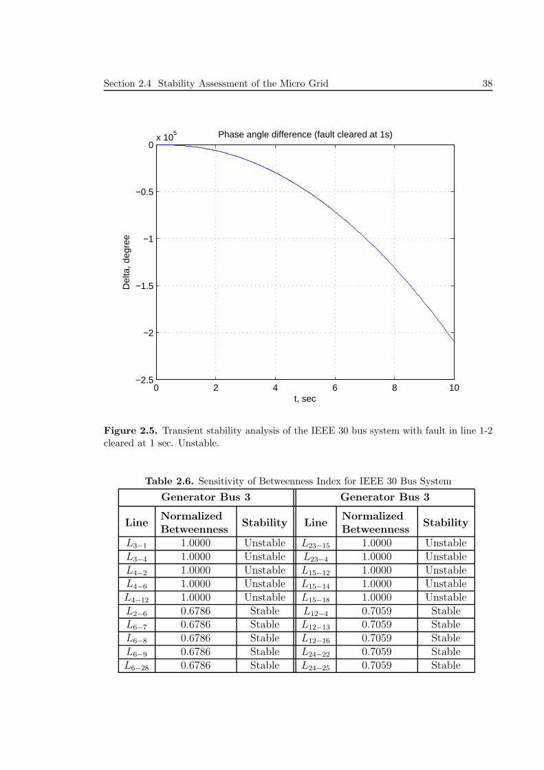
Section 2.4 Stability Assessment of the Micro Grid 38
0 2 4 6 8 10−2.5
−2
−1.5
−1
−0.5
0x 10
5 Phase angle difference (fault cleared at 1s)
t, sec
Del
ta, d
egre
e
Figure 2.5. Transient stability analysis of the IEEE 30 bus system with fault in line 1-2
cleared at 1 sec. Unstable.
Table 2.6. Sensitivity of Betweenness Index for IEEE 30 Bus System
Generator Bus 3 Generator Bus 3
LineNormalized
BetweennessStability Line
Normalized
BetweennessStability
L3−1 1.0000 Unstable L23−15 1.0000 UnstableL3−4 1.0000 Unstable L23−4 1.0000 UnstableL4−2 1.0000 Unstable L15−12 1.0000 UnstableL4−6 1.0000 Unstable L15−14 1.0000 UnstableL4−12 1.0000 Unstable L15−18 1.0000 UnstableL2−6 0.6786 Stable L12−4 0.7059 StableL6−7 0.6786 Stable L12−13 0.7059 StableL6−8 0.6786 Stable L12−16 0.7059 StableL6−9 0.6786 Stable L24−22 0.7059 StableL6−28 0.6786 Stable L24−25 0.7059 Stable

Section 2.4 Stability Assessment of the Micro Grid 39
0 2 4 6 8 10−18
−16
−14
−12
−10
−8
−6
−4
−2
0x 10
4 Phase angle difference (fault cleared at 1s)
t, sec
Del
ta, d
egre
e
Figure 2.6. Transient stability analysis of the IEEE 30 bus system with fault in line 1-3
cleared at 1 sec. Unstable.
simulation, it can be concluded that there exists a margin in the proposed normalized
betweenness index. It can be said that lines with normalized betweenness higher
than 0.5 is most critical and can cause stability problem when subject to fault.
So, special attention must be given to these critical lines. Again, a line whose
normalized betweenness index falls below 0.5 requires less care and maintenance.
The normalized betweenness of various IEEE 57 bus test systems is shown in Fig. 2.8
which also a margin of stability.

Section 2.5 Chapter Summary 40
0 2 4 6 8 10−55
−50
−45
−40
−35
−30
−25
−20Phase angle difference (fault cleared at 1s)
t, sec
Del
ta, d
egre
e
Figure 2.7. Transient stability analysis of the IEEE 30 bus system with fault in line 6-7
cleared at 1 sec. Stable.
2.5 Chapter Summary
In this chapter, we demonstrated the use of complex network theory for vulnerability
analysis of power systems after taking actual electrical parameters into considera-
tions. Various IEEE test systems were used to find critical transmission lines using
the proposed method. Other methods used by earlier researchers show clearly that
the proposed method is more realistic and draws a margin between stable and unsta-
ble region. Although, the proposed approach is simple, it provides a new direction
for complex system network research.

Section 2.5 Chapter Summary 41
Table 2.7. Top Ten Critical Lines of Various Standard Test Systems
IEEE 57 Bus System IEEE 118 Bus System IEEE 300 Bus System
LineNormalized
BetweennessLine
Normalized
BetweennessLine
Normalized
Betweenness
L1−2 1.0000 L9−8 1.0000 L2−3 1.0000L1−15 1.0000 L10−9 1.0000 L3−1 1.0000L1−16 1.0000 L8−5 0.9697 L3−4 1.0000L1−17 1.0000 L8−30 0.9697 L3−7 1.0000L3−15 1.0000 L89−85 0.8175 L3−129 1.0000L15−13 1.0000 L89−88 0.8175 L249−3 1.0000L15−14 1.0000 L89−90 0.8175 L4−16 0.9877L15−45 1.0000 L89−92 0.8175 L16−15 0.9768L14−46 0.5820 L92−91 0.8175 L16−36 0.9768L46−47 0.5542 L92−93 0.8175 L33−36 0.9441L47−48 0.5265 L92−94 0.8175 L36−28 0.9441L48−38 0.4988 L92−102 0.8175 L36−35 0.9441L38−22 0.4711 L49−42 0.7676 L36−40 0.9441L38−37 0.4711 L49−45 0.7676 L15−31 0.6840L9−13 0.3325 L49−47 0.7676 L31−32 0.6840
0
0.1
0.2
0.3
0.4
0.5
0.6
0.7
0.8
0.9
1
Line →
Nor
mal
ized
bet
wee
nnes
s →
Figure 2.8. Normalized betweenness for IEEE 57 bus system.

Chapter 3
Maximal-Flow Based Critical Node
Identification Approach
3.1 Introduction
There are some critical components in networks which when removed either acci-
dentally or deliberately, make the system vulnerable to failures or hazards. In the
case of a power system, either a link or a node removal can have a serious impact on
the normal system operation. Removal of a transmission line from the system shifts
the load of that line to other intact lines in order to match the load demand of the
network, but this may overload other portions of the network which can trigger relay
operation to disconnect some more links from the system. As a result, a cascading
effect can occur, and eventually a large portion or the whole network may suffer
from total power loss. In the case of a node removal much more serious and fast
network loss may occur. Generally, nodes, i.e., generating stations or substations
are connected to other nodes via several links. Malfunction of one node can cause
removal of some lines resulting in a cascading failure.
Complex network theory has been used to model and analyze several aspects of
power system networks. The structural vulnerability of the North American power
42

Section 3.1 Introduction 43
grid was studied after the August 2003 blackout affecting the United States [43].
Similarly, the large scale blackouts and cascading failures motivated the analysis of
Italian power grid based on the model for cascading failures in [48]. Vulnerability
analysis models [11, 37, 38, 44] were initially proposed for complex abstract network
analysis and were then used in power systems [40, 42, 43, 48, 107]. The application
of the ideas in [11, 37, 44] did not capture essential power system characteristics
since the ideas were based on abstract networks. There is a good motivation to
investigate further the complex problems of the grid by considering power system
characteristics and complex network theory together. Particularly, electric power
networks have additional features which are not captured by the prevalent abstract
networks. Power networks are governed by Ohm’s and Kirchhoff’s laws, as well as
flow limits imposed on companies. These special characteristics result in a unique
pattern of interaction between nodes in power grids.
In order to measure the performance of the power grid globally and locally,
the concept of network efficiency was introduced in [37] while discussing the model
of cascading failure in the power grid. In it the power system was modeled as a
Boolean network. A weighted line betweenness,which considered only generations
and neglected loads of the system, was used to find out critical links in [154]. A
betweenness index based on the position and power flowing in the line was proposed
to identify critical lines in a power system [25], where the reactance was considered
as the weight of the network and the resistance was neglected. It was observed
Section 3.1 Introduction 44
that the system is quite robust to random attacks, and there is hardly any effect
on the efficiency if lines are randomly selected and removed, but it was fragile to
targeted attacks. A hybrid approach for structural vulnerability analysis of power
transmission networks, in which a DC power flow model considering overloading
of lines is embedded into the traditional methodology, was proposed in [30]. The
admittance of the transmission line was considered as the weight matrix.
The redistribution of load on nodes due to cascading failure of certain important
nodes was demonstrated in [94]. A simple model was introduced to explain why
large but rare cascades triggered by small initial shocks are present in most of the
complex communication or transportation networks [44]. It was shown that it is
only the breakdown of a selected minority of nodes that can trigger the collapse
of the system. A vulnerability index was proposed based on power flowing in the
connecting lines of a node [107]. These models are initial attempts to explain and
model the cascading event in a power system. Power flow may vary from time to
time depending on load demand and generations available. So instead of using a
fixed power flow model we can use a dynamic one. Also, power does not always flow
via the shortest path from source node to sink node which was the main assumptions
of previous researchers. This limitation was identified, and a new maximum-flow
based centrality approach was proposed to identify critical lines in a power system
in [27]. In this chapter, we apply this concept to find critical nodes of the power
system [164].

Section 3.2 Modeling of a Power System for Critical Node Identification 45
3.2 Modeling of a Power System for Critical Node
Identification
To analyze the power system within the context of complex network theory, the
first step is to model the system as a graph [29]. From the perspective of network
theory, a graph is an abstract representation of a set of objects, called nodes or
vertices. Some pairs of the objects are connected via links or edges in the graph.
The power system is a complex interconnected network which can be subdivided
into four major parts of generation, transmission, distribution and loads [150]. To
portray the assemblage of various components of power system, engineers use single-
line or one-line diagrams, which provide significant information about the system
in a concise form [163]. Power is supplied from the generator nodes to the load
nodes via transmission and/or distribution lines. For a given operating condition
power flows only in one direction, a directed graph can be easily constructed from
the single-line representation of the power system considering various generators,
bus bars, substations, or loads of the system as nodes or vertices and transmission
lines and transformers as edges or links between various nodes of the system. The
principle of mapping is described as follows:
• all impedances between a bus and neutral are neglected,
• all transmission and/or distribution lines are modeled except for the local lines
in plants and substations,

Section 3.2 Modeling of a Power System for Critical Node Identification 46
0.0
2+
j0.0
6
0.08+j0.24 0.01+j0.03
0.04+j0.12
0.0
8+
j0.2
4
20 MW
15 Mvar 50 MW
30 Mvar
60 MW
40 Mvar
20 MW
10 Mvar
30 MW, V=1.03 pu
40 MW, V=1.045 pu
V=1.06 pu
Figure 3.1. Simple 5 bus test system.
• all transmission lines and transformers are modeled as weighted lines, the
weight is equal to the optimum power flowing in the network, and
• parallel lines between buses are modeled as equivalent single lines.
A single-line diagram to a graph, a simple 5 bus test system [150] is used to
illustrate the mapping of a single-line diagram to a graph. Fig. 3.1 depicts the the
test system with 5 bus bars and 7 links connecting them. Columns 1–5 of Table 3.1
gives the system data for the network of Fig. 3.1. Fig. 3.2 is the corresponding
mapped graph for the original 5 bus system. It contains 5 nodes/vertices, which
correspond to the slack, voltage-controlled, and load bus bars of the original system.
The transmission lines are represented by the 7 links/edges which connects various
nodes.
The weight of the lines in Fig. 3.2 is the optimum power flowing in the lines.
The fuel cost functions for three thermal power plants in buses 1, 2, and 3 in $/h
required for optimal power flow solution are given by:

Section 3.2 Modeling of a Power System for Critical Node Identification 47
Table 3.1. System Data for the Network in Fig. 3.1
From To R X 12B Optimum
Bus Bus in pu in pu in pu Power
1 2 0.02 0.06 0.030 16.131 3 0.08 0.24 0.025 7.522 3 0.06 0.18 0.020 4.612 4 0.06 0.18 0.020 13.212 5 0.04 0.12 0.015 47.703 4 0.01 0.03 0.010 50.954 5 0.08 0.24 0.025 13.71
C1 = 200 + 7.0P1 + 0.008P 21
C2 = 180 + 6.3P2 + 0.009P 22 (3.1)
C3 = 140 + 6.8P3 + 0.007P 23
The real power limits of these generators are:
10MW ≤ P1 ≤ 85MW
10MW ≤ P2 ≤ 80MW (3.2)
10MW ≤ P3 ≤ 70MW
The optimum power flow calculation for this network is continued until the ab-
solute value of difference between the scheduled slack generation, determined from

Section 3.2 Modeling of a Power System for Critical Node Identification 48
16.1
3 M
W
7.52 MW 50.95 MW
47.70 MW
13.7
1 M
W
Figure 3.2. Physical topology graph of simple 5 bus system.
the coordination equation, and the slack generation, obtained from the power flow
solution, is within a pre-specified limit. In this case, we have taken this limit as
0.001 MW. The optimum power flowing in different lines is taken as the weight of
the directed transmission lines, which, in this case, represents the maximum power
flow limits of various lines. The maximum power flow limits for various lines in this
network is given in column 6 of Table 3.1.
Any power network can be represented by a graph G = (V,E,W ) comprising
of a set V , whose elements are called vertices or nodes, a set E of ordered pairs of
vertices, called edges or lines, and a set W , whose elements are weights of the edge
set elements. From the node set V , we can find two subsets S and L; where, s ∈ S
represents source nodes in the power network, and l ∈ L is the set of load nodes in
the system. An element e = (x, y) of the edge set E, is considered to be directed
from x to y, where, y is called the head, and x is called the tail of the edge. A
one-to-one correspondence exists between set E and set W .
Networks can have weights on their edges, which indicate that some edges are
stronger or more prominent than others. In some cases, these weights can represent

Section 3.3 Critical Node Identification of the Power Grid 49
capacities of the edges to conduct a flow of some kind [155]. In the case of a power
network, the edge weights can represent the strength of the lines to aid in power
flow through the network. Alternatively, every line has some maximum capacity of
power flow, which can act as a weight of edges if needed. In our current modeling
in this chapter, the maximum power transfer capacity of a line is considered as the
weight of the lines.
For the network in Fig. 3.1, V = {1, 2, 3, 4, 5}, E = {(1, 2), (1, 3), (2, 3), (2, 4),
(2, 5), (3, 4), (4, 5)}, and W = {16.13, 7.52, 4.61, 13.21, 47.70, 50.95, 13.71}. Also,
S = {1, 2, 3} and L = {2, 3, 4, 5}.
3.3 Critical Node Identification of the Power Grid
This section explains maximum flow based critical node identification procedure of
the electrical power grid.
3.3.1 Shortest Electrical Path
In a power grid with n buses represented as a graph G = (V,E,W ), the shortest
electrical path between any two buses is the path which has minimum electrical
distance between them. The distance can be measured in various ways. Power
World Simulator [165] provides several important distance measure options like per
unit series reactance, magnitude of series impedance, length of the transmission
lines, number of nodes in the path, etc. In this chapter, we have used absolute
measure of impedance, |Z|, as the weight of the line. For example, if we want to

Section 3.3 Critical Node Identification of the Power Grid 50
find shortest electrical path between buses 2 and 3, several paths are possible as
given in Fig. 3.3. We can clearly see that the shortest path between buses 2 and 3
is 2− 3 whose weight is 0.19 pu. Several efficient algorithms are available to find all
possible shortest path in a network. In this chapter, we have used bioinformatics
toolbox of MATLAB to find shortest electrical path between various buses which
uses Johnson’s algorithm that has a time complexity of O(Nlog(N) +NE), where
N and E are the number of nodes and edges respectively.
3.3.2 Node Removal and Network Efficiency of Power Grid
Removal of nodes with a high degree, i.e., nodes which have more connections than
nodes with low degree causes more damages in the network. In addition, targeted
links removal also can cause significant deterioration of performance of a network.
A targeted node and link removal from IEEE 30 bus system and the calculated
network efficiency, E, given in is shown in Fig. 3.4, which suggests in our case node
removal have much serious consequence.
E =1
n(n− 1)
∑
i 6=j∈V
1
|Zij|(3.3)
where, |Zij| is the absolute value of the series impedance of the shortest electrical
path between buses i and j.
An alternative formulation of the network efficiency, considering line reactance
and voltages at the two ends of the transmission lines, is given in [166], as follows:

Sectio
n3.3
Critica
lNodeIdentifi
catio
nofthePower
Grid
51
1
2
3
5
0.0
6
0.25 0.03
0.13
0.2
50.190.19
4 1
2
3
5
0.0
6
0.25 0.03
0.13
0.190.19
4
1
2
3
5
0.0
6
0.25 0.03
0.13
0.2
50.190.19
4 1
2
3
50
.06
0.25 0.03
0.13
0.190.19
4
0.2
50
.25
Figure 3.3. Several possible paths between nodes 2 and 3 of the simple 5 bus system.

Section 3.3 Critical Node Identification of the Power Grid 52
Figure 3.4. Network efficiency deterioration of IEEE 30 bus system with targeted node
and line removal.
E =1
NLNG
∑
i∈NL
∑
j∈NG
ViVj
Xij
(3.4)
where, NL and NG are the number of load and generator nodes, respectively. Vi
and Vj are voltages of nodes i and j, respectively, and Xij is the reactance of the
transmission line between nodes i and j.
3.3.3 Maximum Flow Based Critical Node Analysis
Given a power grid, we can find how much maximum power can be transferred
through the network from a source node s ∈ S to a load node l ∈ L, where s 6=
l ∈ V from the solution of the maximum-flow problem [167]. There are many
algorithms to solve this problem, and in this chapter we have used MATLAB’s
bioinformatics toolbox which uses Goldberg’s algorithm [168] to solve maximum
flow problem. The idea behind this problem is to push power as much possible
to transfer from the source node s to load node l within the network modeled as

Section 3.3 Critical Node Identification of the Power Grid 53
a graph G = (V,E,W ). Various extremities in the network are explored with all
source and load combinations.
Solutions of maximum flow problem for various source-load combinations are
given in Fig. 3.5. For example, in the network of Fig. 3.5(b) to transfer power from
source bus 1 to load bus 3 two possible paths are 1 − 3 and 1 − 2 − 3. The path
1− 3 has a capacity of 7.52 MW. In the path 1− 2− 3, path 1− 3 has a capacity of
16.13 MW, but the maximum limit of path 2− 3 is 4.61 MW. So, only 4.61 MW of
power is transferred via path 1 − 2 − 3. So, the maximum possible power transfer
in the network of Fig. 3.5 (b) is 7.52 + 4.61 = 12.13 MW. In this maximum flow of
12.13, node 2 carries power 4.51 MW. There is no possible flow from node 3 to 2.
This case is illustrated in Fig. 3.5(h). Similar data for the simple 5 bus system is
given in Table 3.2.
Now, the importance of a node has within a network can be quantified by how
much power is transferred via the node within various possible maximum flow net-
works. This gives us a measure of centrality, called betweenness in social science,
which can be used to identify critical lines in the network.
3.3.4 Definition
Let, Fk be the net maximum power flowing through intermediate node k in net-
works with source node s ∈ S and load node l ∈ L. Then Fk could be defined
mathematically as:

Sectio
n3.3
Critica
lNodeIdentifi
catio
nofthePower
Grid
54
1
2
3
5
4
16
.13
MW
7.52 MW 50.95 MW
47.70 MW
13
.71 M
W
4.61 MW
13.21 MW
1
2
3
5
4
4.6
1 M
W
7.52 MW 50.95 MW
47.70 MW
13
.71 M
W
4.61 MW
13.21 MW
1
2
3
5
4
16
.13
MW
7.52 MW 10.44 MW
47.70 MW
13
.71
MW
2.92 MW
13.21 MW
1
2
3
5
4
16
.13
MW
7.52 MW 7.52 MW
16.13 MW
7.5
2 M
W
4.61 MW
13.21 MW
1
2
3
5
4
16
.13
MW
7.52 MW 50.95 MW
47.70 MW
13
.71
MW
4.61 MW
13.21 MW
1
2
3
5
4
16
.13
MW
7.52 MW 4.61 MW
47.70 MW
13
.71
MW
4.61 MW
13.21 MW
1
2
3
5
41
6.1
3 M
W
7.52 MW 0.50 MW
47.70 MW
13
.71
MW
0.50 MW
13.21 MW
1
2
3
5
4
16
.13
MW
7.52 MW 50.95 MW
47.70 MW
13
.71
MW
4.61 MW
13.21 MW
1
2
3
5
4
16
.13
MW
7.52 MW 50.95 MW
47.70 MW
13
.71 M
W
4.61 MW
13.21 MW
1
2
3
5
41
6.1
3 M
W7.52 MW 13.71 MW
47.70 MW
13
.71 M
W
4.61 MW
13.21 MW
a) 1-2 b) 1-3
c) 1-4 d) 1-5 e) 2-3
f) 2-4 g) 2-5 h) 3-2
i) 3-4 j) 3-5
Figure 3.5. Maximal flow in the simple 5 bus test system.

Section 3.3 Critical Node Identification of the Power Grid 55
Table 3.2. Various Power in Maximum Flow Network of Fig. 3.1
From To Maximum Intermediate Bus PowersBus Bus Power Bus 1 Bus 2 Bus 3 Bus 4 Bus 5
1 2 16.13 0.00 0.00 0.00 0.00 0.001 3 12.13 0.00 4.61 0.00 0.00 0.001 4 23.65 0.00 16.13 10.44 0.00 0.001 5 23.65 0.00 16.13 7.52 7.52 0.002 3 4.61 0.00 0.00 0.00 0.00 0.002 4 17.83 0.00 0.00 4.61 0.00 0.002 5 61.41 0.00 0.00 0.50 13.71 0.003 2 0.00 0.00 0.00 0.00 0.00 0.003 4 50.95 0.00 0.00 0.00 0.00 0.003 5 13.71 0.00 0.00 0.00 13.71 0.00
Fk =∑
s∈S
∑
l∈L
F slk (3.5)
where, s 6= l 6= k.
Also, let, FG be the net maximum power flowing in networks with source node
s ∈ S and load node l ∈ L, which is defined mathematically as:
FG =∑
s∈S
∑
l∈L
F slG (3.6)
The ratio of these two power could be used as a measure of importance, called
betweenness, of various nodes of the system. The betweenness of node k is defined
as:
CB(k) =Fk
FG
(3.7)

Section 3.3 Critical Node Identification of the Power Grid 56
F slk is the maximum possible flow through node k in the network G = (V,E,W )
with source node s and load node l. F slG is the maximum flow in the network
G = (V,E,W ) with source node s and load node l.
The numerator of the centrality equation is the sum of the maximum possible
flow through vertex k in various source-node combinations of the network where k
is neither source nor load The denominator is the maximum flow in the network for
various source-node combinations where k is neither source nor load. This gives us
a normalized measure of betweenness for vertex k, which was originally proposed
in [21] for unidirectional networks, but now since bi-directional power flow is a vision
of modern smart power system we have modified the equations for our use.
3.3.5 Example
For the network in Fig. 3.1 the betweenness of node 2 is:
CB(2) =F2
FG
(3.8)
where, F2, the summation of maximum powers flowing through intermediate
node 2 in networks with source node s ∈ {1, 2, 3} and load node l ∈ {2, 3, 4, 5} can
be found as:

Section 3.3 Critical Node Identification of the Power Grid 57
F2 =∑
s∈{1,2,3}
∑
l∈{2,3,4,5}
F sl2
= F 132 + F 14
2 + F 152 + F 34
2 + F 352
= (4.61 + 16.13 + 16.13 + 0.00 + 0.00)MW
= 36.87MW
(3.9)
and FG for the overall network in Fig. 3.1 can be found as follows:
FG =∑
s∈{1,2,3}
∑
l∈{2,3,4,5}
F slG
=F 12G + F 13
G + F 14G + F 15
G
+ F 23G + F 24
G + F 25G
+ F 32G + F 34
G + F 35G
=16.13 + 12.13 + 23.65 + 23.65 + 4.61
+ 17.83 + 61.41 + 0.00 + 50.95 + 13.71
=224.07
(3.10)
So, the betweenness of node 2, CB(2), is 36.87/224.07 = 0.16. Similarly, be-
tweennesses for other buses could be found which is given in Table 3.3.

Section 3.4 Chapter Summary 58
Table 3.3. Betweenness of Simple 5 Bus System
Bus Betweennessk CB(k)
1 0.002 0.163 0.104 0.165 0.00
Table 3.4. Critical Nodes of IEEE 30 Bus System
Node Betweenness Node Betweenness
4 0.6851 15 0.16996 0.4177 10 0.14822 0.3587 28 0.14093 0.3381 27 0.097412 0.3276 9 0.0948
3.3.6 Simulation of Various Standard Test System
Various standard test systems [152] are simulated to identify critical lines in the
system. The top ten critical lines for IEEE 30 bus system are tabulated in Table 3.4.
3.4 Chapter Summary
Complex network theory is utilized for analyzing vulnerability of the power grid
in this chapter. Critical nodes are identified using the maximum-flow algorithm.
Resource can be allocated, regularly, to monitor and service the critical nodes of the
system and large scale blackouts can be prevented. The method is applicable for
bi-directional power flow in modern smart grid system, and used to identify critical
nodes rather than links which have prominent influence in network vulnerability.

Section 3.4 Chapter Summary 59
The vulnerability analysis framework presented in this chapter identifies critical
nodes in a power grid when subjected to maximum possible flow of power. Since
the actual power flow scenario might be quite different depending on the system
operating characteristics, and capturing all the uncertainties is beyond the capacity
of available computing packages or instruments, the work is a step of identifying
worst case scenario. It is a matter of continuing research to develop and modify the
metrics and tools presented in this chapter in order to capture the true vulnerability
of the interconnected power system.

Chapter 4
Electrical Centrality Measures and Bus
Dependency Matrix
4.1 Introduction
The power grid is one of the most complex man-made infrastructures; for example,
the Australian power grid, commonly known as the National Electricity Market
(NEM), operated under the Australian Energy Market Operator (AEMO) is the
worlds longest interconnected power system that runs for more than 5, 000 kilometers
from Port Douglas in Queensland to Port Lincoln in South Australia and supplies
more than $10 billion worth of electricity annually to meet the demand of more
than 8 million end users [169]. NEM interconnects five regional market jurisdictions
including Queensland, New South Wales, Victoria, South Australia and Tasmania.
Power systems play an indispensable role in modern society. However, there have
been several large-scale blackouts in recent years, in spite of technological progress
and huge investments in system reliability and security. For instance, in August
1996, more than 4 million people in several western states of the USA were out of
the power service [170].
60

Section 4.1 Introduction 61
In August 2003, a historic blackout was triggered in the power grid of the United
States and Canada, which disconnected 61, 800 MW of power to an area spanning
most of the north-eastern states of the USA and two provinces of Canada, totally
containing more than 50 million people [171]. Besides, in the summer and autumn
of the year 2003, several large-scale blackouts happened, such as London blackout
in the UK, Sweden-Denmark blackout and Italy blackout, etc. [171].
A severe blackout occurred in India on two consecutive days [99]. On 30 July
2012, overloading of one of the Northern regional grid initiated a cascading failure
event affecting more than 370 million people in India. Although the system was
brought to normal condition around 7 PM, the next day, the cascade was propagated
to Eastern and Northeastern grids due to another grid station failure. Twenty
states out of 28 were affected by this event; more than 700 million were left without
electricity
Prevention of large scale outages is attributed to the security assessment and
monitoring system. Recent series of blackouts occurring all over the world shows
that the system designated for prevention of blackouts is not working well, which
stimulates researchers to seek solutions from alternative means. Recently advances
of research in complex network field have attracted the interest of researchers of
the power grid to model and analyze the century old power grid under the complex
network framework.
In case of a power system, the number of possibilities to be analyzed is huge.

Section 4.1 Introduction 62
Suppose we want to analyze the consequence of every line getting tripped with
faults in several locations in the Australian power grid. It is just too complicated,
time consuming and does not make any sense [172]. So, first of all, from some the
topological characteristics of the network we have to find few cases which we should
study in depth. The number of contingency is too large, somehow we have to decide
which contingencies are important and which are not. Complex network framework
can be used for this purpose.
If the network structure is known, several measures or matrices could be devel-
oped, which can identify particular features of the network. Social scientists have
used several centrality measures [24,173–175] to explain a person’s influence within
a network. Among these centralities most widely used measures are degree central-
ity, betweenness centrality, and closeness centrality. To analyze the vulnerability
of the power grid or to measure which nodes are more important within a power
network these centrality approaches were used by researchers [176–179]. Some of
these research considered the power grid as an abstract network and neglected con-
crete engineering features, whereas some literatures considered various features like
impedance or admittance of various lines.
Based only on the topological information of the power grid, [180] proposed an
evolutionary algorithm based approach to find critical lines in groups by formulating
a variant of betweenness centrality, the group betweenness centrality, as defined

Section 4.1 Introduction 63
in (4.1):
CB(g) =
∑
i,j∈G,i<j
si,j(g)
si,j
(N − dim(g)− 1)(N − dim(g))(4.1)
where, g is the subset of edges of the graph,and si,j represents the number of the
shortest paths connecting nodes i to j that pass through g. Implementation of the
proposed algorithm on the Italian high-voltage electrical transmission network shows
the utility of the genetic algorithm based approach in identifying critical links, but
the vulnerability due to operational parameters is not reflected by this simple net-
work structure dependent algorithm. Also, the huge computational burden required
for the optimum convergence of the method limits its applicability for the dynamic
network vulnerability assessment and monitoring system.
Traditional betweenness centrality approaches [24, 173, 175] rely on the assump-
tion that flow occurs using the shortest possible paths between source and load
nodes, which is not the case always, specially for the power system. This inherent
shortcoming is the definition of the centrality measure is taken into consideration,
and current flow betweenness centrality, somewhat overcoming this limitation, is
proposed in [174] for the electrical system where the flow quantity is current, as
in (4.2):
CB(CF ) =
∑N
i=1,s<t Isti
12N(N − 1)
(4.2)
where, Isti is the current flowing from source node, s, to load node, t, within an
electrical circuit. This measure is based on random walks between source and load

Section 4.1 Introduction 64
nodes, and essentially includes contributions from all paths between nodes, not just
the shortest one, but giving the shortest path more weights than the other paths.
This centrality measure is utilized in [181], as random-walk centrality, to show its
implementation in case of power system, with a typical example of IEEE 14 bus test
system.
Essentially, the quantity of interest for a power grid is real power. To include this
quantity as a measure of importance, [182] modified the current flow betweenness
centrality as in (4.3):
CB(PF ) =
∑N
i=1,s<t Psti
12N(N − 1)
(4.3)
where, P sti is the power flowing from source node, s, to load node, t, within a power
system. This centrality, known as power flow centrality, takes a global approach of
computation rather than the random sampling proposed in [174], and computation-
ally more efficient, but there is an inherent problem of convergence of the load flow
analysis.
In this chapter, various electrical centrality measures based on the power flow in
the transmission system is proposed [183]. A new matrix which captures the infor-
mation of pair dependency of various buses is also developed [184,185]. This matrix,
the bus dependency matrix, is used to find two centrality measures (betweenness
and closeness) of buses of the grid. A generalized methodology is developed to find
out bus dependency matrix for an n-bus system.
The rest of the chapter is organized as follows. Section 4.2 describes a model

Section 4.2 System Model 65
for analyzing the power system within the context of complex networks. Section 4.3
– 4.5 gives various centrality measures as applied to the power system. Section 4.6
deals with simulation of standard IEEE test systems, which finds out various cen-
trality measures in those systems. Section 4.7 introduces the bus dependency matrix
and gives an example to construct it from the system data. Section 4.8 compares
and relates two previously defined centrality measures with bus dependency matrix.
Some concluding remarks are given in Section 4.9.
4.2 System Model
In order to develop a dependency matrix of the electric power grid based on the
complex network framework, the first thing to do is to construct a graph from the
system model [29, 186–195]. From the perspective of network theory, a graph is an
abstract representation of a set of objects, called nodes or vertices, where some pairs
of the objects are connected via links or edges.
To portray the assemblage of various components of the power system, engineers
use single-line or one-line diagrams, which provide significant information about the
system in a concise form [162]. Power is supplied form the generator nodes to the
load nodes via transmission and/or distribution lines. The principle of constructing
a graph from the single-line diagram of the power grid is described as follows [196]:
• all impedances between a bus and neutral are neglected,
• all transmission and/or distribution lines are modeled except for the local lines
in plants and substations,

Section 4.2 System Model 66
Figure 4.1. Simple 5 bus system.
• all transmission lines and transformers are modeled as weighted lines, the
weight is equal to the optimum power flowing in the network, and
• parallel lines between buses are modeled as equivalent single lines.
A power system network is represented by a graph G = (V,E,W ) comprising
of a set V , whose elements are called vertices or nodes, a set E of ordered pairs of
vertices, called edges or lines. An element e = (x, y) of the edge set E, is considered
to be directed from x to y; where y is called the head, and x is called the tail of the
edge. A set W , whose elements are weights of the edge set elements. There exists
a one-to-one correspondence between set E and set W . In this model, we consider
the transmission line impedances in pu as weights of the edges between nodes.
A simple example of 5 bus system [150] is used in this chapter to illustrate various
concepts of complex network in the power system. Fig. 4.1 depicts the system with
5 bus bars, and 7 links connecting them. We can model the system as a graph

Section 4.3 Measure of Connectivity-Degree Centrality 67
Table 4.1. System Data for Network in Fig. 4.1
From To R X 12B
Bus Bus in pu in pu in pu
1 2 0.20 0.6110 0.0301 3 0.08 0.1123 0.0252 3 0.60 0.5139 0.0202 4 0.06 0.5663 0.0202 5 0.04 0.1155 0.0153 4 0.10 0.5727 0.0104 5 0.08 0.2725 0.025
which contains 5 nodes/vertices, which correspond to the slack, voltage-controlled,
and load bus bars of the original system. The transmission lines can be represented
by the 7 links/edges which connects various nodes. The system data is given in
Table 4.1.
For the network in Fig. 4.1, V = {1, 2, 3, 4, 5} , E = {(1, 2), (1, 3), (2, 3), (2, 4), (2, 5),
(3, 4), (4, 5)} , and W = {0.20+ j0.61, 0.08+ j0.11, 0.60+ j0.51, 0.06+ j0.57, 0.04+
j0.12, 0.10 + j0.57, 0.08 + j0.27}.
4.3 Measure of Connectivity-Degree Centrality
Degree centrality is the simplest form of centrality measures for networks. Although
it is very simple, it has a great significance. It represents the connectivity of a
node to the network [156]. Individuals who have more links with other persons are
more connected to the network in the sense that they have more resource, access of
information than others. A non-social network example is the use of citation counts
in the evaluation of scientific papers. The number of citations of a paper can be
regarded as its impact on research [155].

Section 4.3 Measure of Connectivity-Degree Centrality 68
Table 4.2. Degree Centrality for Network in Fig. 4.1
Bus CD(k) CED(k)
1 0.50 21.582 1.00 42.333 0.75 16.134 0.75 40.135 0.50 15.80
For example, node 2 in Fig. 4.1 is adjacent to four other nodes, it’s degree is
four. In a 5 node graph, any node can be adjacent to only remaining four nodes. So,
this node has the highest connectivity. In the literature degree centrality is defined
as:
CD(k) =deg(k)
n− 1(4.4)
where, deg(k) is the degree of node k.
In case of electrical network, the power flowing in the adjacent links of the node
in concern can be regarded as a degree of the node and the definition of the electrical
degree centrality can be given as:
CED(k) =
∑
k∼t
Pkt
n− 1(4.5)
where, k ∼ t indicates that node k are t are connected. Pkt indicates the power
flowing in line connected in between nodes k and t.
Table 4.2 shows the degree centrality of simple 5 bus system in Fig. 4.1 using
classical and proposed approach.

Section 4.4 Measure of Independence-Closeness Centrality 69
Figure 4.2. Classical closeness of various nodes of the simple 5 bus system in Fig. 4.1.
4.4 Measure of Independence-Closeness Centrality
This approach of centrality measure is based upon the degree to which a node is
close to all other nodes in the network [24]. Fig. 4.2 shows closeness in a classical
sense and to illustrate the idea of electrical closeness centrality Fig. 4.3 is drawn to
show the closeness of various nodes of the simple 5 bus system in Fig. 4.1 in terms of
electrical distance found in Table 4.1. It is clear from Fig. 4.3 that node 2 is adjacent
to three other nodes (nodes 1, 3, and 4) in terms of electrical distance, while nodes
1, 3, and 4 being adjacent to two nodes. Node 5 is adjacent to one node only. So
node 2 is the closest to other nodes than the rest of the nodes in the network.
In social network theory, closeness is a sophisticated measure of centrality. It is
defined as the mean geodesic distance (i.e., the shortest path) between a vertex k
and all other vertices reachable from it [197]. In mathematical form, the closeness
centrality of a vertex k, CC(k) in a network of n vertices is given by:

Section 4.4 Measure of Independence-Closeness Centrality 70
CC(k) =
∑
t∈V \k
d(k, t)
n− 1(4.6)
where, d(k, t) being the shortest path length between vertices k and t. This definition
of closeness centrality gives a measure of distance of particular vertex from other
vertices. So, some researchers have used the reciprocal of the shortest path to
quantify closeness centrality as follows:
CC(k) =1
∑
t∈V \k
d(k, t)(4.7)
The electrical closeness centrality was defined in [179] as:
CCz(k) =n− 1
∑
t∈V \k
dz(k, t)(4.8)
where, dz(k, t) is taken as the shortest electrical distance between nodes k and t.
Resistance was neglected since they considered only transmission systems; but in
order to generalize the concept to both transmission and distribution systems we
cannot neglect resistance of the network lines, which is a significant portion of the
line impedance in case of distribution lines. The numerator was taken as n−1. This
was adopted in (4.6) to average the distance, but when it comes in the numerator
it just scales the parameter. So, in this chapter we propose our electrical closeness
centrality as:

Section 4.4 Measure of Independence-Closeness Centrality 71
Figure 4.3. Electrical closeness based on line impedance of various nodes of simple 5 bus
system.
Table 4.3. Closeness Centrality for Network in Fig. 4.1
Bus CC(k) CEC (k)
1 0.17 1.282 0.25 2.133 0.20 1.234 0.20 1.925 0.17 1.14
CEC (k) =
1∑
t∈V \k
d(k, t)(4.9)
where, d(k, t) is the weight of the shortest electrical path from node k to all other
nodes t reachable from k.
Table 4.3 shows the closeness centrality of simple 5 bus system in Fig. 4.1 in
classical as in (4.7) and proposed approach.
The independence of a node is determined by the closeness centrality of the
node [24]. In Fig. 4.1, node 2 is in direct contact with nodes 1, 3, and 4. It must

Section 4.5 Measure of Control of Communication-Betweenness Centrality 72
depend upon node 4 to communicate with node 5. So, node 5 needs only one relayer
to communicate with all other nodes of the network. On the other hand, node 1
needs node 2 to communicate with node 4 and both need 2 and 4 to communicate
with node 5. So we can say that node 2 is more independent than node 1. So
closeness centrality can be used to quantify independence of various nodes within
an electrical power grid.
4.5 Measure of Control of Communication-Betweenness
Centrality
This type of centrality is based upon the frequency with which a node falls between
pairs of other nodes on the shortest or geodesic paths connecting them [24]. This
idea is illustrated by ten possible shortest paths in the network of Fig. 4.1 as shown
in Fig. 4.4. Node 2 comes four times between other points in the six geodesics. Node
4 comes three times. So node 2 is more central in terms of betweenness.
The betweenness centrality CB(k) for vertex k is computed as follows [197]:
1. Find the shortest path set of the network.
2. Find out the fraction of the shortest path containing node k for each pair of
vertices.
3. Sum this fraction over all pairs.
Mathematically,

Section 4.5 Measure of Control of Communication-Betweenness Centrality 73
Figure 4.4. Illustration of betweenness in 10 possible shortest path set of the test system.

Section 4.6 Simulation of Various Standard IEEE Test Systems 74
CB(k) =
n∑
s=1
n∑
t=1
σst(k)
σst
, s 6= t 6= k ∈ V (4.10)
where, σst is the number of shortest paths from s to t, and σst(k) is the number of
shortest paths from s to t that pass through a vertex k.
As in closeness centrality the shortest paths for an electrical network can be
calculated from the line impedance, and the power flowing in the line is taken as a
measure of betweenness [196]. The electrical betweenness centrality of a node k in
a network of n nodes is defined as:
CEB (k) =
n∑
s=1
n∑
t=1
Pst(k)
Pst
, s 6= t 6= k ∈ V (4.11)
where, Pst is the maximum power flowing in the shortest electrical path between
buses s and t , and Pst(k) is the maximum of inflow and outflow at bus k within
the shortest electrical path between buses s and t. Fig. 4.5 illustrates the concept
of electrical shortest path and shows ten possible geodesics in the simple 5 bus test
system.
Table 4.4 shows the betweenness centrality of the simple 5 bus system in Fig. 4.1
using classical and proposed approach.
4.6 Simulation of Various Standard IEEE Test Systems
There are some critical nodes in every network which when removed from the system
can make the system very vulnerable to attack. Previously researchers used complex

Section 4.6 Simulation of Various Standard IEEE Test Systems 75
Figure 4.5. Ten possible shortest path set in terms of electrical distance in simple 5 bus
system.

Section 4.6 Simulation of Various Standard IEEE Test Systems 76
Table 4.4. Betweenness Centrality for Network in Fig. 4.1
Bus CB(k) CEB (k)
1 010
0670
2 110
192670
3 110
0670
4 110
93.3670
5 010
0670
Table 4.5. Top Ten Critical Nodes According to Degree Centrality of Various Standard
IEEE Test Systems.
30 Bus CEB (k) 57 Bus CE
B (k) 118 Bus CEB (k)
2 12.5841 1 7.9668 12 12.21146 9.2330 4 5.3512 69 5.63721 9.0528 2 4.9898 70 5.19164 7.0180 3 4.4910 80 4.82333 5.7375 15 3.9604 7 4.72275 3.7382 6 3.5725 11 4.720010 2.4665 17 3.4561 32 4.41569 2.3013 24 2.9787 46 4.15327 2.2122 23 2.0769 75 3.816012 2.1811 13 2.0628 34 3.2639
Table 4.6. Top Ten Critical Nodes According to Closeness Centrality of Various Standard
IEEE Test Systems.
30 Bus CEC (k) 57 Bus CE
C (k) 118 Bus CEC (k)
6 2.2366 14 1.7785 65 3.05534 2.1676 13 1.7596 68 3.024928 2.0587 46 1.7399 116 2.98848 2.0438 47 1.7120 81 2.93663 2.0108 48 1.7042 38 2.87739 2.0029 15 1.6993 64 2.835310 1.9662 38 1.6775 69 2.82987 1.9069 11 1.6663 80 2.815812 1.8110 3 1.6167 66 2.811921 1.7877 12 1.6149 30 2.7189

Section 4.6 Simulation of Various Standard IEEE Test Systems 77
Table 4.7. Top Ten Critical Nodes According to Betweenness Centrality of Various
Standard IEEE Test Systems.
30 Bus CEB (k) 57 Bus CE
B (k) 118 Bus CEB (k)
2 0.6117 1 0.6117 12 0.70301 0.5546 2 0.4862 7 0.43316 0.3114 17 0.4142 11 0.43104 0.3103 3 0.3380 2 0.34313 0.2972 15 0.2271 3 0.07805 0.1668 16 0.1427 6 0.06297 0.0547 4 0.1398 14 0.03508 0.0490 6 0.0566 117 0.03409 0.0420 14 0.0544 13 0.028610 0.0406 5 0.0498 4 0.0219
network theory to explain blackouts or cascading effects in the power system. Very
few works were done to identify critical nodes of the system. System reliability can
be improved a lot if these critical nodes can be identified beforehand by monitoring
them regularly and servicing them when subjected to deterioration. Critical nodes
can be found from calculating various centrality measures as outlined in previous
sections.
IEEE 30, 57, and 118 bus systems were used to simulate various centrality mea-
sures and results are given in Tables 4.2 – 4.4. Results in Tables 4.2 – 4.4 show
that different approaches give different nodes as critical in order of priority. This
is expected because these three centrality measures are based on three different ap-
proaches. So if we are dealing with connectivity, degree based centrality is the one
to consider. If some cases required the criticality measure based on independence
on the node, closeness centrality would be the best option to consider. However, the

Section 4.7 Measure of Pair Dependence of Various Buses 78
Figure 4.6. Modified simple 5 bus system.
last option – control of communication can be measured using betweenness central-
ity. Since the future smart grid will rely on control of communication along with
the power transfer, the third measure of centrality could be very useful for future
control room engineers and planners to take necessary action in critical events.
4.7 Measure of Pair Dependence of Various Buses
To illustrate the idea of pair dependency, we slightly modified the system parameters
in order to accommodate various flows within the system as given in Fig. 4.6. Various
data for the system in given in Table 4.8. The simultaneous nonlinear algebraic
equations for the power flow problem of this network are solved using standard
Gauss-Seidel method [150]. Power flowing in various lines, line losses, generations
and loads in various buses in a steady-state of the network are given in Fig. 4.7.

Section 4.7 Measure of Pair Dependence of Various Buses 79
Figure 4.7. Power flow diagram of modified simple 5 bus system.
Table 4.8. System Data for Network in Fig. 4.6
From To R X 12B
Bus Bus in pu in pu in pu
1 2 0.20 0.6110 0.0301 3 0.08 0.1123 0.0252 3 0.60 0.5139 0.0202 4 0.06 0.5663 0.0202 5 0.04 0.1155 0.0153 4 0.10 0.5727 0.0104 5 0.08 0.2725 0.025

Section 4.7 Measure of Pair Dependence of Various Buses 80
4.7.1 Shortest Path
The concept of the shortest path is used by the researchers of the power system who
use complex network framework for network vulnerability analysis [25,30,153,154].
In order to assess the vulnerability of a power grid, the researchers used a dynamic
power system model where the concept of network flow is introduced [30]. The flow
between two nodes, s and t, takes on the shortest path between them. If there are
two or more paths between two buses then the path that has less weight is regarded
as the shortest path between those two buses.
Only the physical connection is considered in traditional modeling approach by
the complex network researchers. The weight of the line between nodes simply
reflects the topology of the network. If there is a connection between node s and
node t then the weight of the corresponding line is taken as 1, otherwise it is 0 in
the traditional approach [30, 153]. In case of a power system, the main parameter
of a transmission line, which has a significant effect in the power flow in the line
between buses, is its impedance which is not considered in this model.
Several researchers have considered the reactance of the line [154], neglecting the
line resistance which is very small for transmission systems. In order to generalize
the model for both the transmission and the distribution system, the impedance,
(i.e., both the reactance and resistance) needs to be taken into consideration [25,196].
In this chapter, we have used absolute measure of impedance, |Z|, as the weight
of the line. If we want to find the shortest electrical path between buses 1 and 4,

Section 4.7 Measure of Pair Dependence of Various Buses 81
Table 4.9. Various Possible Connection Between Buses 1 and 4 of the System of Fig. 4.6
Connection Weight (pu)
1–2–4 1.211–2–3–4 2.011–2–5–4 1.041–3–4 0.721–3–2–4 1.501–3–2–5–4 1.33
several paths are possible as given in Table 4.9. We can clearly see that the shortest
path between buses 1 and 4 is 1− 3− 4 whose weight is 0.72 pu. This approach of
measuring shortest path by combining absolute values of complex numbers |Z| may
appear theoretically troublesome, but the rationale here is to find shortest possible
paths for the power to flow from various source nodes to target nodes in an electric
circuit. Using both resistance and reactance in the calculation of line weights provide
a better way of modelling electricity grid under complex network framework than
to use resistance or reactance alone.
Finding the shortest path set for a network is a problem of graph theory and
several efficient algorithms are available.
4.7.2 Bus Dependency Matrix
In the context of complex network theory, when a pair of buses in the power system
are connected via a transmission line without any other buses in between (interme-
diaries), they are said to be adjacent [156]. A bus s adjacent to bus k, another bus
t adjacent to bus k, creates a transmission path between buses s and t via bus k.
The shortest electrical path linking a pair of buses is called a geodesic [155].

Section 4.7 Measure of Pair Dependence of Various Buses 82
Let, Pst be the maximum power flowing in the shortest electrical path between
buses s and t , and Pst(k) be the maximum of inflow and outflow at bus k within the
shortest electrical path between buses s and t. Then, let their fraction is represented
by rst(k) as in:
rst(k) =Pst(k)
Pst
(4.12)
where, the ratio rst(k) is an index of the degree to which buses s and t needs bus k
to transmit the power between them along the shortest electrical path.
The pair dependency of nodes in a network is defined in [198]. The concept of pair
dependency in [198] is used here in case of an electrical power grid. The dependency
of bus pairs can be regarded as the degree to which a bus s must depend upon
another bus k to transmit its power along the shortest electrical path or geodesic
to and from all other reachable buses t’s in the network. For a power grid with n
buses, the dependency of bus s upon bus k to transmit power on any other buses in
the network can be represented as follows:
dsk =
n∑
t=1s 6=t6=k∈V
rst(k) =
n∑
t=1s 6=t6=k∈V
Pst(k)
Pst
(4.13)
The dependency of bus pairs for the whole system can be calculated and the result
can be summarized in a matrix D as follows:

Section 4.7 Measure of Pair Dependence of Various Buses 83
D =
d11 d12 · · · · · · d1n
d21 d22 · · · · · · d2n
......
. . ....
...
dn1 dn2 · · · · · · dnn
(4.14)
Each element of D is an index of the degree to which a bus designated by row
number must depend upon another bus designated by column number to transmit its
power along the shortest electrical path or geodesic to and from all other reachable
buses in the network. Thus, this matrix captures the information of importance of
a bus as an intermediary with respect to other buses in the network. So we can call
the matrix D as bus dependency matrix.
4.7.3 Example
The shortest electrical path set is found here using Johnson’s algorithm for sparse
network [199]. Fig. 4.8 portrays the power flowing in various shortest electrical
paths within the network of Fig. 4.6. For example, the shortest 2 − 5 − 4 is the
shortest electrical path between buses 2 and 4. 81.02 MW of power is injected into
line 2 and 76.97 MW of power reaches at bus 5 via line 2 − 5. Similarly, for line
5 − 4, 16.97 MW of power is injected at bus 5 and 16.59 MW reaches at bus 4.
This situation is illustrated in Fig. 4.8(f). So, the maximum power in this shortest
electrical path between buses 2 − 4 is 81.02 MW. Table 4.10 lists maximum power
in various shortest paths within the simple 5 bus test system.

Section 4.7 Measure of Pair Dependence of Various Buses 84
Figure4.8.Shortestpath
setforthenetwork
ofFig.4.6.

Section 4.7 Measure of Pair Dependence of Various Buses 85
Table 4.10. Maximum Power Flowing in Various Electrical Shortest Path Sets of the
Network in Fig. 4.6
Bus Bus Shortest Pst
s t Path Set MW
1 2 1–2 69.821 3 1–3 94.491 4 1–3–4 94.491 5 1–2–5 81.022 1 2–1 69.822 3 2–1–3 94.492 4 2–5–4 81.022 5 2–5 81.023 1 3–1 94.493 2 3–1–2 94.493 4 3–4 67.693 5 3–4–5 67.694 1 4–3–1 94.494 2 4–5–2 81.024 3 4–3 67.694 5 4–5 16.975 1 5–2–1 81.025 2 5–2 81.025 3 5–4–3 67.695 4 5–4 16.97
Now, P24(5) is 76.97 MW since in the shortest electrical path between buses
2 and 4 inflow at bus 5 is 76.97 and outflow is 16.97. So, maximum of inflow
and outflow is 76.97. Since no other buses fall within this shortest electrical path
P24(1) = P24(3) = 0 MW. Most of these values are zero for this specific network.
Only non-zero elements of Pst(k) are given in Table 4.11.
An example of evaluating a component of the dependency matrixD, for example,
the element d13 is given in (4.15):

Section 4.7 Measure of Pair Dependence of Various Buses 86
Table 4.11. Maximum of In and Out Flow at Various Buses within Various Electrical
Shortest Path Sets of the Network in Fig. 4.6
Pst(k) Power (MW)
P23(1) 94.49P32(1) 94.49P15(2) 81.02P51(2) 81.02P14(3) 87.99P41(3) 87.99P35(4) 62.33P53(4) 62.33P24(5) 76.97P42(5) 76.97
d13 =∑
t∈{2,4,5}
r1t(3)
=∑
t∈{2,4,5}
P1t(3)
P1t
=P12(3)
P12+
P14(3)
P14+
P15(3)
P15
=0
69.82+
87.99
94.49+
0
81.02
= 0 + 0.93 + 0
= 0.93
(4.15)
Similarly, other elements of the matrix could be found, and the resulting bus
dependency matrix for the simple 5 bus system is given in (4.16):

Section 4.8 Characteristics of Bus Dependency Matrix 87
D =
0.00 1.00 0.93 0.00 0.00
1.00 0.00 0.00 0.00 0.95
1.00 0.00 0.00 0.92 0.00
0.00 0.00 0.93 0.00 0.95
0.00 1.00 0.00 0.92 0.00
(4.16)
4.7.4 Steps to Find Bus Dependency Matrix from System Data
The procedural steps to find bus dependency matrix from the system data is as
follows:
1. Model the system as a graph as described in Section 4.2.
2. Find a shortest path set for the graph using Johnson’s algorithm.
3. Find flow in various lines of the system solving load flow problem.
4. Find the maximum power flowing in the shortest electrical path between buses
s and t, Pst, for the shortest path set.
5. Find Pst(k), the maximum of inflow and outflow at bus k within the shortest
electrical path between buses s and t.
6. Evaluate bus dependency matrix D from Pst and Pst(k).
4.8 Characteristics of Bus Dependency Matrix
4.8.1 Relationship with Other Centrality Measures
If we take a column sum of the k-th column of the bus dependency matrix:

Section 4.8 Characteristics of Bus Dependency Matrix 88
n∑
s=1
dsk =
n∑
s=1
n∑
t=1
rst(k), s 6= t 6= k ∈ V
=n
∑
s=1
n∑
t=1
Pst(k)
Pst
, s 6= t 6= k ∈ V
= CEB (k)
(4.17)
So, it is clear that the sum of the elements of the k-th column of bus dependency
matrix is the electrical betweenness of the k-th bus of the system. So, the column
sum of (4.16)
[
2.00 2.00 1.86 1.84 1.90
]
represents electrical betweenness centrality
of 1, 2, ..., 5 bus respectively of the simple 5 bus system.
Similarly, if we take a row sum of the s-st row of the bus dependency matrix:
n∑
k=1
dsk =n
∑
k=1
n∑
t=1
rst(k), s 6= t 6= k ∈ V
=
n∑
k=1
n∑
t=1
Pst(k)
Pst
, s 6= t 6= k ∈ V
(4.18)
This summation represents the power ratio of all available paths starting from
bus s.
So, we can say that, the s-th row sum of the bus dependency matrix represents
the closeness centrality of s-th bus of the network. where the weight of the path
is taken as the power ratio instead of electrical impedance or admittance. The row
sum of (4.16)
[
1.93 1.95 1.92 1.88 1.92
]T
represents electrical closeness centrality

Section 4.9 Chapter Summary 89
of 1, 2, ..., 5 bus respectively of the simple 5 bus system.
4.8.2 Several Observations
Several observations about the bus dependency matrix is enumerated as follows:
• The (s, t)-th element of the matrix represents the dependency of bus s on bus
t.
• Diagonal elements of the bus dependency matrix is zero.
• This matrix is non-symmetric.
• The row sum of the matrix could be used as a electrical closeness centrality
measure.
• The column sum of the matrix is electrical betweenness centrality measure.
4.9 Chapter Summary
This chapter presents a new matrix which contains the information of dependency
of bus pairs in a power system. The correlation between bus dependency matrix
and electrical closeness centrality and electrical betweenness centrality is explored
in this chapter. A step by step procedure for evaluating the matrix is also given.
The example of simple 5 bus system clarifies the concept of bus dependency matrix
and its relation with other centrality measures is also investigated.
Several characteristics of the bus dependency matrices are explored. The matrix
described in this chapter could have various implementation in the future smart
power grid, where both information and power are transmitted via the transmission

Section 4.9 Chapter Summary 90
lines. Since there will be communication, there will be control of communication.
Bus dependency matrix, in fact, represents how much control a bus can exert on
another bus since it is a measure of one bus’s dependency on another in case of
transmitting the information or the power through transmission lines. Bus depen-
dency matrix could be used as a measure of how independently a bus can transmit
the power or the information through the lines in the grid.

Chapter 5
Bidirectional Power Flow Based
Criticality Assessment
5.1 Introduction
Existing power transmission grids around the world are being made much smarter
by integrating smart and new technologies by utilities [200]. The smart grid can
manage various generation sources efficiently, primarily in the distribution side –
near consumers. Engagement of customers with the energy management systems is
the most lucrative part of smart grid from the point of view of regulating energy
usage. Excess of generation after local use can be transmitted long distances to
meet the energy shortage of the destination area, which introduces a new concept of
the power flowing from customer end towards the grid. The bidirectional power flow
changes the whole power flow pattern of the existing grid [161]. Analytical methods,
technical strategies, control system and protecting devices need to be changed along
with, to mention a few. Metering and protecting equipments will experience flows
coming from the reverse side. Proper operation of the equipments used earlier can
be ensured either by changing the instruments themselves or by incorporating new
measurement techniques.
91

Section 5.1 Introduction 92
From the frequent events of large scale-blackouts [98, 99, 170, 171], it is clear
that the existing dynamics security assessment and monitoring system has not been
working well [29]. The motivation of complex network framework based analysis
approach comes from the necessity of new, alternative and improved methodologies
to assess the risk associated with cascading events in the power system. Degree
centrality, betweenness centrality and closeness centrality measures are commonly
used in the social network research to find a person with the most influence. [24].
The research on the power grid from a system point of view has been triggered
after the publications of the preliminary topology based analytical results. Since
results from pure topological approach is quite misleading [20], several researchers
have a mix of both topological and electrical characteristics based complex network
analysis of the power system to find reasonably improved results [21, 22].
Motivated by the topology based analytical result [14], that found the power grid
robust against random failure but vulnerable to targeted attacks [20], critical node
and link analysis of the power grid have been carried out to explore the criticality
of the power grid. If critical components, which can initiate cascading effect, can
be spotted out, special preventive actions could be exercised to prevent large scale
blackouts from happening.
Network efficiency, a topological measure of performance change after the inclu-
sion or removal of nodes or lines from a grid, is analyzed in [35]. A weighted line

Section 5.1 Introduction 93
betweenness based approach is utilized to find critical lines responsible for spread-
ing of large scale blackouts from small initial shock [154]. Vulnerable regions of the
power system are identified employing complex network theory based qualitative
simulation in [41]. Transmission line reactance is incorporated to compute a new
vulnerability index to identify critical lines [25].
A link is explored between the power system reliability and small world ef-
fect [153]. Maximum flow based centrality approach is used to find out critical lines,
which removes the shortcoming of the assumption of the power flowing through the
shortest path between source and load nodes [27]. The flow based method has slow
convergence, but can be useful when used in conjunction of planning issues. A DC
power flow model is used, and hidden failure of protective equipment is considered to
model the structural vulnerability of the power grid [30]. Electrical parameters are
incorporated extensively to improve the centrality indices for the power system [179].
An extended topological approach proposed in [31] takes into consideration tra-
ditional topological metrics as well as operational behavior of the power grid like
the real power flow allocation and the line flow limits. The power transfer distri-
bution factor (PTDF) is used to simulate cascading event in an attempt to identify
correlated lines [32].
Purely topological analysis cannot capture many important features of the power
grid, so a weighted directed model is considered in [201]. The power grid is modeled
into two directional graphs one containing real power flow (P ) information, and

Section 5.1 Introduction 94
another signifying reactive power flow (Q) within the network. The vulnerability
of a node is defined to be dependent on the betweenness value and an operational
state parameter, ε, of the node. The vulnerability of a node i, M , is given by:
Mi =√
εiCB(i) (5.1)
where, εi is the operational state vulnerability parameter, and CB(i) is the between-
ness centrality of node i, respectively. εi is given as:
εi =1
|xi(t)− xcri |
(5.2)
where, xi(t) is the state value at time t, and xcri is the critical value of the state.
Either voltage or phase angle of nodes can be considered as the state value. Due
to natural cohesion, phase angle is considered as state value in case of real power
(P ) graph, while voltage is taken as state when reactive power (Q) is taken into
consideration.
All these analyses are carried out mainly on nondirectional models where the
direction of the power flow has not been considered, but since with the inclusion of
distributed generations the power flow pattern is going to change, new methodolo-
gies have to be proposed, which take into account bidirectional power flow. Since
communication is an important factor in smart grid; identifying those nodes,which
are important for communication in the system, would be very much useful.

Section 5.1 Introduction 95
In this chapter, a comparison of the bidirectional flow based method has been
made with a nondirectional flow based method. This method is a modification of
closeness centrality, which takes into account the power flow distribution among
various transmission lines during steady state [202–204]. This work is a reason-
able extension of previous work carried out by the researchers since it captures the
power flow in smart grid environment. The power flow pattern in traditional power
grid and the envisioned smart electricity grid are different. Generally the power
flows from generation nodes throughout the network towards the destination nodes
or distribution systems. Recently, more and more renewable generations has been
included in the distribution systems and the excess of the generation in the distri-
bution system will flow back to the transmission grid which will be utilized in a
different area of need, or will be stored in a battery for future use. Hence, the power
flow pattern is different in traditional power systems and future smart power grid.
The impact of removing critical components is identified using well known impact
metrics like path length, connectivity loss, and load loss.
The organization of the rest of the chapter is as follows. Section 5.2 provides a
model for the analysis of the smart power grid under complex network framework.
A new model based on the bidirectional power flow is considered, and a method is
discussed to find critical nodes in the power grid. Effects of removal of critical nodes
on various topological and electrical measures are addressed in Section 5.3. Rank
similarity analysis is carried out is Section 5.4. Conclusion is drawn, and future

Section 5.2 System Model and Methodology 96
research direction is provided in Section 5.5.
5.2 System Model and Methodology
The power flow analysis is conducted for the given test system during nominal
condition. Newton-Raphson method is used to solve the simultaneous nonlinear
algebraic power flow equations [150]. The direction of the real power flowing through
the lines is taken as the direction of edges in the modeled graph as shown in Fig. 5.1.
From this point, this graph will be known as nominal unidirectional flow graph. In
order to consider the bidirectional flow in smart grid, a backward unidirectional
flow graph is also modeled. The direction of edges in the reverse unidirectional
flow graph is exactly opposite to the nominal unidirectional flow graph as shown
in Fig. 5.2. Superposition of the two models gives bidirectional model. Here, we
show the difference of two modeling approaches: (a) nondirectional model and (b)
bidirectional model.
Assume that, k represents the intermediate bus within the shortest path origi-
nating from bus s and ends at bus t. Let Pst represents the maximum power flowing
in the shortest electrical path between buses s and t , and Pst(k) is the maximum
of inflow and outflow at bus k within the shortest electrical path between buses s
and t. Then, let their fraction is represented by rst(k) as in:
rst(k) =Pst(k)
Pst
(5.3)

Section 5.2 System Model and Methodology 97
Bus 1
Bus 2 Bus 3
Bus 4Bus 5
Bus 6
Bus 7
Bus 8
Bus 9
Bus 10Bus 11
Bus 12
Bus 13 Bus 14
Bus 15Bus 16
Bus 17 Bus 18
Bus 19
Bus 20
Bus 21
Bus 22 Bus 23
Bus 24
Bus 25
Bus 26 Bus 27
Bus 28 Bus 29
Bus 30
Figure 5.1. Nominal unidirectional flow in IEEE 30 bus test system.

Section 5.2 System Model and Methodology 98
Bus 1
Bus 2Bus 3
Bus 4 Bus 5
Bus 6
Bus 7
Bus 8
Bus 9
Bus 10Bus 11
Bus 12
Bus 13Bus 14
Bus 15
Bus 16
Bus 17
Bus 18
Bus 19
Bus 20
Bus 21
Bus 22Bus 23
Bus 24
Bus 25
Bus 26Bus 27
Bus 28Bus 29
Bus 30
Figure 5.2. Reverse unidirectional flow in IEEE 30 bus test system.

Section 5.2 System Model and Methodology 99
Table 5.1. Top Ten Nodes in Nondirectional & Bidirectional Power Flow Models
Nondirectional Bidirectional
1 53 82 74 66 413 2412 199 1314 1228 14
where the ratio rst(k) is an index of the degree to which buses s and t need bus k
to transmit the power between them along the shortest electrical path. If a double
sum is taken of (5.3) over all intermediate buses k and all destination buses t for
the source buses s,
CEC (s) =
n∑
k=1
n∑
t=1
Pst(k)
Pst
, s 6= t 6= k ∈ V (5.4)
a centrality measure for bus s within the grid is obtained. This measure (5.4) adds
up the real power of the lines originating at bus s and terminating at all other buses.
This quantity takes high values if the difference between numerator and denominator
term is low. This fact represents that a very small amount of the power is lost in
the shortest path. Such buses might have direct influence on other buses since a
small amount of the power is lost. Table 5.1 lists top ten critical nodes in IEEE 30
bus test system [150] found from nominal and backward unidirectional as well as
bidirectional model.

Section 5.3 Measure of Impact 100
In summary, the method to identify can be summarized as:
1. Model a power system as a directed graph.
2. Calculate power flowing through various lines.
3. Construct a reverse directional graph.
4. Find the shortest path set of the graph from source nodes to load nodes.
5. Find rst(k) and calculate CEC (k).
6. Sort and rank in the descending value of CEC (k).
5.3 Measure of Impact
At first, the nominal network is solved, and nodes are removed from the system one
by one in the descending order of centrality measure. In order to measure the impact
of removing critical nodes from the system various measures are being used [205].
In this chapter, four measures are considered. The first two of them, path length
and connectivity loss, are purely topological. The last measure is the percentage of
load lost due to the removal of critical nodes.
5.3.1 Path Length
The path length is used by researchers as a measure of network connectedness. It is
the average length of the shortest paths between any two nodes in the network [108].
It is found that if a node is removed from a system, it generally increases the
distance between other nodes. So, the increase in network characteristic path length

Section 5.3 Measure of Impact 101
is considered as a measure of impact analysis of removing critical nodes from the
system.
Distance between two vertices can be computed as:
d(u, v) = min|P | (5.5)
where P is a path from u to v. Path length can be defined as:
d =1
k
∑
u 6=v∈V
d(u, v) (5.6)
where 0 ≤ d(u, v) ≤ ∞. k is the number of connected pairs.
This is topological path length. Another electrical path length is also measured
where the distance is computed in terms of the impedance of transmission lines. A
simple IEEE 57 bus test system is used to simulate the consequence of node removal
on path length and the result is depicted in Fig. 5.3. It is clear that the impact
of removing critical nodes based on the bidirectional flow rather than bidirectional
flow model is comparatively higher. Initially the impact is higher in nondirectional
measure but after four nodes removal the bidirectional model shows the impact in
a large scale. Electrical path length based measure shows similar characteristic. In
the later measure the impact is always higher than the topological path length in
bidirectional flow model.

Section 5.3 Measure of Impact 102
0
1
2
3
4
5
6
7
8
9
10
1 2 3 4 5
Pat
h L
eng
th
Number of Removed Node
Nondirectional (Topological) Bidirectional (Topological)
Nondirectional (Electrical) Bidirectional (Electrical)
Figure 5.3. Change in path length in IEEE 57 bus test system for removal of critical
nodes based on two different measures.
5.3.2 Connectivity Loss
This is a purely topological measure of impact a power grid encounters when some
nodes are removed from the system. In this measure, we calculate how much con-
nectivity is lost in terms of how many generators a transmission or distribution node
can access due to effect of removing a node from the system. The less is the number
of generators a node is connected with; the less is the redundancy and the more is
the vulnerability of the node. It is given as (5.7) originally proposed in [43].
C = 1−
⟨
N ig
Ng
⟩
i
(5.7)
where the averaging is done over each intermediate nodes, i.e., substations. Ng is
the total number of generators and N ig is the number of generators that a node i can

Section 5.3 Measure of Impact 103
0
1
2
3
4
5
6
1 2 3 4 5 6 7 8 9 10
Co
nn
ecti
vit
y L
oss
Number of Removed Node
Nondirectional Bidirectional
Figure 5.4. Connectivity loss of IEEE 118 bus test system as a function of removal of
critical nodes from two different point of views.
reach. Impact on connectivity loss for two different models is presented in Fig. 5.4
for IEEE 157 bus test system.
It is found that connectivity is lost to a great extent in both cases, although the
effect is higher in case of bidirectional flow model than the unidirectional counter-
part.
In case of bidirectional flow model, almost 50% connectivity is lost after six nodes
removal while if we remove nodes according to nondirectional model even after 10
nodes removal the connectivity is very high. It takes 17 nodes removal according to
nondirectional model to decrease the connectivity loss to 50%.
5.3.3 Load Loss
Last measure of impact is found from a simple model of cascading failure that
is presented here. Since it is not possible to exactly model the blackout, various

Section 5.3 Measure of Impact 104
approximate measures have been taken, by several researchers, to mimic the situa-
tion [20, 206–208].
The power system is a very much complex interconnected system whose exact
modeling would require consideration of dynamics of rotating machines and devices
within the system, discrete dynamics of switchgear elements, non-linear algebraic
equations that govern line flows and social dynamics of governing and operating
bodies.
In this chapter, a fairly simple model of cascading failure of the power grid is
proposed by incorporating important electrical features ignoring those which are too
complicated but have little effects. The detail of the model is described here.
At first, the AC power flow is used to calculate the steady state condition of the
network. The real and reactive power of transmission lines are found from numerical
solution of line flow equations given in (5.8) and (5.9)
Pi =
n∑
j=1
|Vi||Vj||Yij|cos(θij − δi + δj) (5.8)
Qi = −n
∑
j=1
|Vi||Vj||Yij|sin(θij − δi + δj) (5.9)
where the symbols have their usual meanings as found in the power system literature.
During the analysis, generator and load dynamics are not included. Although
the limitation of not using dynamics of generators and loads are well understood, but

Section 5.3 Measure of Impact 105
it is at least useful for modeling one mechanism of cascading failure that is cascad-
ing overload. Also, Generation Shift Factors (GSF) and Line Outage Distribution
Factors (LODF) [163] are used to recalculate flows in lines after disturbance. This
helps achieving fast results without using actual load flow after each disturbance.
The transmission lines are removed if overloaded. Also, time delayed over current
relays are used in every line so if there is a lot of overload it trips fast and if there
is a little bit of overload it trips slowly. Another thing that is added to the model
is ramping up of generators. As the system separates into sub grids, generators are
allowed to ramp up or ramp down to rebalance a little bit.
So, if a component failure disturbs the supply-demand balance, through genera-
tor set-point adjustment this balance is achieved, but if there is not enough ramping
ability, then the ultimate choice is to trip lowest possible system load. The total
amount of load lost during the successive removal of nodes is used as a measure of
impact.
Fig. 5.5 shows load loss as a percentage of total system load. Up to six node
removal the load loss is nearly equal and does not increase much for both unidirec-
tional models. After five node removal, more than 50% loads of the system need to
be shedded to ensure secure and reliable operation of the remaining system.
The overall steps are summarized below while the flowchart in Fig. 5.6 represents
the same.

Section 5.3 Measure of Impact 106
0
10
20
30
40
50
60
1 2 3 4 5 6 7 8 9 10
Load L
oss
Number of Removed Node
Unidirectional
Bidirectional
Figure 5.5. Two different effects on load loss due to loss of functionality of important
nodes in IEEE 300 bus test system.
Step 1 The AC power flow is solved to find out the steady-state condition of the
network.
Step 2 Find out if the power flow is converged or not.
Step 3 If the power flow is not converged, reduce some load from the system and
go to Step 1.
Step 4 If the power flow is converged, initialize counter i.
Step 5 Increment counter i by 1.
Step 6 Record total load shedded during the process.
Step 7 Remove i -th critical node from the critical list.
Step 8 Line Outage Distribution Factor (LODF) [163] is used to calculate redis-
tribution of the power flow without actually solving the load flow problem
again.
Step 9 Check for system load-generation balance. If the balance is not achieved,
ramp-up or ramp-down generators accordingly to adjust generator set-point

Section 5.4 Rank Similarity of Critical Nodes 107
in order to achieve the balance. Generation Shift Factor (GSF) is used to
calculate redistribution of the power flowing among lines.
Step 10 Check if there is any overloaded line.
Step 11 If any overloaded line is found trip the line and go to step 8. Time-
delayed overcurrent relays are used in every line so if there is a lot of overload
they trip faster and if there is a little bit of overload they trip slowly.
Step 12 If there is no overloaded line, go to Step 5.
5.4 Rank Similarity of Critical Nodes
From the results of Section 5.3, it is clear that, the nodes found from bidirectional
flow model has much more impact than nominal and backward unidirectional mod-
els. In order to analyze the effect of system change on ranks of critical nodes a
rank similarity analysis is performed [209–212]. A structural change like change in
the direction of the power flow is incorporated in the model, and critical nodes are
found out for the modified system. This change in network corresponds to a situa-
tion when there is a pushback of power from low voltage network via transmission
system to meet energy needs in other area.
Table 5.2 compares the changes in the top ten critical nodes in IEEE 30 bus
test system. This analysis is carried out for the bidirectional power flow model.
Top row of Table 5.2 corresponds to the topological state of the system. The first
column gives the top ten critical nodes from the bidirectional model. The rest of the
columns list changes in critical nodes for changed topology. For example, the third

Section 5.4 Rank Similarity of Critical Nodes 108
Solve AC Power Flow
Problem for the
Nominal Case
Shed Load
Power Flow
Converges?
Calculate
Total Load
Shedded
Remove i-th
Critical Node
from Critical List
Update Flows of
Lines using
LODF
Overloaded
Line?
Match Supply
Demand Balance
using GSF
Trip Line
i = 0
i = i+1
No
Yes
NoYes
Figure 5.6. Simple cascading failure model.

Section 5.4 Rank Similarity of Critical Nodes 109
Table 5.2. Top Ten Critical Nodes in the Bidirectional Power Flow Model for IEEE 30
Bus System Under Various Changed Topological Conditions
Nominal Line Line Line Line Line Line Line Line LineCase 24–25 29–27 6–2 17–10 4–3 10–6 18–15 30–29 15–141 1 1 1 1 1 1 1 1 13 3 3 2 3 2 2 3 3 32 2 2 3 2 4 4 2 2 24 4 4 6 4 6 6 4 4 46 24 24 4 13 24 24 6 6 624 13 6 24 12 19 19 24 24 2419 6 19 19 24 13 13 19 19 1913 12 29 13 6 12 12 18 13 912 19 13 12 16 14 14 9 12 2614 14 12 14 19 9 9 26 14 139 9 14 9 17 26 26 23 9 18
column represents the top ten critical nodes when the nominal direction of flow is
changed through line 29–27. It is clear that, changed topology does not affect much
the node criticality.
On the other hand, slightly more change is observed in criticality for the unidi-
rectional model as shown in Fig. 5.7. Each color represents different nodes of the
system in Figs. 5.7 - 5.10. When the power flow pattern through the grid is uni-
directional, nominal unidirectional method is effective, but, in order to model the
situation in the future smart grid, bidirectional model gives better result in terms
of rank similarity as given in Fig. 5.8.
In a typical power system, load varies from time to time and generation have to
match the load and line loss. For this reason, various power flow profiles are found
in the system during various seasons of the year. Even the scenario is different at

Section 5.4 Rank Similarity of Critical Nodes 110
1 2 3 4 5Node 1
Node 5
Node 10
Node 15
Node 20
Node 25
Node 30
No. of observations →
Ran
k c
han
ge
of
var
iou
s n
od
es →
Figure 5.7. Variation of ranks of nodes in unidirectional model of IEEE 30 bus test
system when the network is modified slightly.
different times in a day. To demonstrate that the proposed power flow based cen-
trality method gives critical nodes which is insensitive to system load and generation
change, an Australian test system is considered which provides six test cases from
heavy to light load conditions [213].
Table 5.3 gives the six normal steady-state operating conditions for the system.
Betweenness and closeness centrality of the test system is measured for various test
cases.

Section 5.4 Rank Similarity of Critical Nodes 111
1 2 3 4 5 6 7 8 9 10
Node 1
Node 5
Node 10
Node 15
Node 20
Node 25
Node 30
No. of observations →
Ran
k c
han
ge
of
var
iou
s n
od
es →
Figure 5.8. Rank similarity of nodes in the bidirectional power flow model is better than
that of unidirectional one.
Table 5.3. Six Normal Steady-State Operating Conditions of the Australian Power Grid
Case 1 Case 2 Case 3 Case 4 Case 5 Case 6
Load Condition Heavy Medium Heavy Peak Light Medium LightestGeneration (MW) 23030 21590 25430 15050 19060 14840
Load (MW) 22300 21000 24800 14810 18600 14630

Section 5.4 Rank Similarity of Critical Nodes 112
1 2 3 4 5 6rank 5
rank 4
rank 3
rank 2
rank 1
Test Case →
Ran
k→
Figure 5.9. Rank similarity of nodes in the bidirectional power flow model is better than
that of unidirectional one.
Table 5.4. Ranks of Various Buses of Australian Test System Based on Closeness Cen-
trality
Case 1 Case 2 Case 3 Case 4 Case 5 Case 6
Bus 13 44 44 44 44 44 44Bus 8 5 4 3 7 3 8Bus 14 45 45 45 45 45 45Bus 44 46 46 46 46 46 46Bus 2 2 3 1 2 1 4Bus 24 24 23 23 26 26 27Bus 57 17 18 19 19 18 18Bus 47 37 37 38 39 39 38Bus 28 56 56 53 56 55 56Bus 48 8 9 9 7 8 10

Section 5.4 Rank Similarity of Critical Nodes 113
1 2 3 4 5 6rank 5
rank 4
rank 3
rank 2
rank 1
Test Case →
Ran
k→
Figure 5.10. Rank similarity of nodes in the bidirectional power flow model is better
than that of unidirectional one.
Variation of ranks of the Australian test system in six test cases are shown
in Fig. 5.9 and presented in Table 5.4 for closeness centrality measures and for
betweenness centrality measures in Fig. 5.10 as well as in Table 5.5. From the figures,
it is clear that betweenness based measure is more rank stable than the closeness
one. In case of betweenness based measure, first three rank positions do not change
in six different operating conditions, whereas in case of closeness centrality there are
small variations in ranks two to four positions. In case of rank five there is a large

Section 5.5 Chapter Summary 114
Table 5.5. Variation of Ranks of Several Buses of Australian Test System Based on
Betweenness Centrality
Case 1 Case 2 Case 3 Case 4 Case 5 Case 6
Bus 41 58 59 58 59 59 57Bus 43 56 57 57 55 57 53Bus 46 1 4 2 5 1 4Bus 45 59 58 59 58 58 59Bus 42 49 51 46 46 47 46Bus 44 51 46 49 50 50 47Bus 15 16 17 18 18 15 18Bus 32 32 30 31 29 30 32Bus 59 45 44 45 43 46 44Bus 34 11 11 11 10 11 10
variation of two ranks.
5.5 Chapter Summary
The changing power flow pattern demands for improved analytical techniques to
solve the global problem of cascading failure. This issue has been addressed under
complex network framework. An improved model of closeness centrality measure
has been proposed. The bidirectional power flow pattern of the future smart power
system have been taken into consideration while modeling the system. Three dif-
ferent measures of impact have been evaluated to observe the effect of removal of
critical nodes found from centrality measures.
Closeness centrality based critical node analysis has been carried out and re-
sults from nondirectional and bidirectional flow based methods have been compared.
Large changes in path length, connectivity and load loss implies the efficacy of the
proposed method. IEEE 30 bus, 57 bus, 118 bus and 300 bus test systems has been

Section 5.5 Chapter Summary 115
used to demonstrate the applicability of proposed modified centrality measures in
critical node analysis of the power system. The analysis of a real Polish transmission
system based on the proposed methodology is our future work.

Chapter 6
Conclusions
This chapter summarizes key facts and findings of this research work, presents con-
clusions drawn and discusses future areas of exploration. In this work the emphasis
was on to identify the vulnerability of the power system, specially the topological
weakness of the transmission system. Various criticality assessment methods have
been proposed to identify important elements of the power transmission grid. Effect
of removal of the elements (nodes or lines) on the performance of the system has
also been analyzed.
The results presented in this thesis are based on the formulation of various cen-
trality measures for the power system to overcome the limitations of current topology
based criticality measures to assess the vulnerability of the system. However, before
designing new measures, an overview of the shortcomings of the existing measures
has been provided.
Complex network theory has been used for the vulnerability analysis of power
systems, taking into consideration critical electrical parameters which affect stability
of the power grid. Various simplified mapping techniques have been used without
neglecting key parameters. In order to capture the true power flow scenario within
the grid, a novel centrality analysis approach has been provided. The result of
116

Section Conclusions 117
the centrality analysis provides critical transmission lines of the grid, which when
removed from the system have found to affect the transient stability.
Another criticality assessment procedure has been provided, considering the max-
imum possible flow within the grid. Power flow solution technique has been com-
bined with the maximum flow finding algorithms to demonstrate the applicability
of complex network based analysis techniques into power systems in order to as-
sess vulnerability of the system. This criticality analysis procedure provides critical
nodes of the system. Network efficiency is greatly affected when top critical nodes
are removed from the system. This explores the vulnerability of the power system
on targeted node removal.
Motivated from social network based centrality analysis procedures, various cen-
trality based analysis procedures have been modified to use in case of the power
system. Electrical degree centrality, closeness centrality, and betweenness centrality
measures have been analyzed. Comparisons are carried out between pure topology
based centrality measures and the proposed electrical centrality measures. Bus de-
pendency matrix have been developed, which provides a succinct representation of
the closeness and betweenness centrality of the power grid. An algorithm is provided
to illustrate the step-by-step procedure of formulating centrality measures from the
system data.
Considering the bidirectional flow of the future smart power system, a new frame-
work has been established within the context of the complex network to identify

Section Conclusions 118
vulnerability of the power system. The bidirectional power flow model is a superpo-
sition of the generic power flow situation of the grid with the backward flow model.
The superiority of the bidirectional flow based model in finding the critical elements
of the smart power system has been demonstrated with examples.
From this work, the following conclusions can be drawn:
• Critical element analysis of the power system is crucial for system planning as
well as dynamic security assessment and monitoring system.
• Both nodes and links play important roles in criticality analysis.
• Although rare, but the node removal causes much more significant loss of
system’s performance than the link removal.
• Targeted removal of components cause more damage to the system than the
random removal.
• System reliability and security could be enhanced by regularly monitoring and
servicing the most critical components of the grid.
• Large scale blackouts could be prevented if actions are taken immediately in
case of a fault or overloading of high betweenness lines.
• The betweenness index could also be used as a measure of transient stability
of the system.
• The criticality analysis provides a margin between unstable and stable oper-
ating region.
• Removal of flow central nodes affects network efficiency.

Section 6.1 Directions for Future Research 119
• Power doesn’t flow only through the shortest path between two nodes, it flows
through all possible combination of originating at source node and terminating
in load nodes.
• The degree centrality is a measure of connectivity.
• The independence of a node is determined by the closeness centrality of the
node.
• The betweenness centrality provides a measure of control of communication.
• The bus dependency matrix contains the information of dependency of bus
pairs in a power system.
• The bidirectional power flow based model captures the changed topological
and pattern of power flow in smart grid.
• The rank similarity analysis shows the robustness of the proposed methods
under system parameter changes.
• The proposed methods of vulnerability analysis are proven to be computation-
ally efficient, improve system reliability and security, help dispatchers to take
prompt corrective action, and reduce the probability of large-scale cascading
failure leading to blackouts.
6.1 Directions for Future Research
Although this research achieved promising results in analyzing the vulnerability of
the power grid, and identifying critical components of the system, the work does not

Section 6.1 Directions for Future Research 120
end here. The proposed power system mapping, and criticality analysis procedure
may be further improved and consolidated by the following processes,
1. Considering both real and reactive power flow when measuring centrality of
the system.
2. Identifying how system robustness can be improved by simply adding links
while cascading is in progress.
3. Extending the vulnerability analysis into practical power systems.
4. Analyzing the effect of loop flow on vulnerability of power grid.
5. Conducting a detailed study to ascertain the impacts and possible benefits of
the inherent variability of renewable sources, particularly wind and solar, and
their correlations with load profiles.
6. Investigating into the network functional vulnerability.
7. Exploring the concept of network percolation in power system analysis.
8. Conducting case studies on electrical distribution networks.
This dissertation focuses on developing complex network based system metrics to
identify electrical power grid vulnerability. However, there are many other metrics
available which focus on contingency ranking. Although, this thesis does not address
contingency ranking [134], but it will be interesting to compare the performance of
complex network based metrics with conventional approaches to critical component
detection.”

References
[1] R. Baldick, B. Chowdhury, I. Dobson, Z. Dong, B. Gou, D. Hawkins, H. Huang,
M. Joung, D. Kirschen, F. Li, J. Li, Z. Li, C.-C. Liu, L. Mili, S. Miller,
R. Podmore, K. Schneider, K. Sun, D. Wang, Z. Wu, P. Zhang, W. Zhang, and
X. Zhang, “Initial review of methods for cascading failure analysis in electric
power transmission systems IEEE PES CAMS task force on understanding,
prediction, mitigation and restoration of cascading failures,” in Proc. IEEE
PESGM’08, Pittsburgh, PA, Jul. 20–24, 2008, pp. 1–8.
[2] P. Fairley. Notorious grid bottleneck spawns west-
ern blackout. Retrieved 23 Aug 2013. [Online]. Avail-
able: http://spectrum.ieee.org/energywise/energy/the-smarter-grid/
west-coast-blackout-emanates-from-notorious-grid-bottleneck
[3] M. Vaiman, K. Bell, Y. Chen, B. Chowdhury, I. Dobson, P. Hines, M. Pa-
pic, S. Miller, and P. Zhang, “Risk assessment of cascading outages: Part
I; overview of methodologies,” in Proc. IEEE PESGM’11, Detroit, MI, Jul.
24–29, 2011, pp. 1–10.
[4] M. Papic, K. Bell, Y. Chen, I. Dobson, L. Fonte, E. Haq, P. Hines, D. Kirschen,
X. Luo, S. Miller, N.Samaan, M. Vaiman, M. Varghese, and P. Zhang, “Survey
of tools for risk assessment of cascading outages,” in Proc. IEEE PESGM’11,
Detroit, MI, Jul. 24–29, 2011, pp. 1–9.
121

References 122
[5] J. P. Paul and K. R. W. Bell, “A flexible and comprehensive approach to
the assessment of large-scale power system security under uncertainty,” In-
ternational Journal of Electrical Power & Energy Systems, vol. 26, no. 4, pp.
265–272, May 2004.
[6] S. S. Miller, “Extending traditional planning methods to evaluate the poten-
tial for cascading failures in electric power grids,” in Proc. IEEE PESGM’08,
Pittsburgh, PA, Jul. 20–24, 2008, pp. 1–7.
[7] N. Bhatt, S. Sarawgi, R. O’Keefe, P. Duggan, M. Koenig, M. Leschuk, S. Lee,
K. Sun, V. Kolluri, S. Mandal, M. Peterson, D. Brotzman, S. Hedden, E. Litvi-
nov, S. Maslennikov, X. Luo, E. Uzunovic, B. Fardanesh, L. Hopkins, A. Man-
der, K. Carman, M. Y. Vaiman, M. M. Vaiman, and M. Povolotskiy, “Assess-
ing vulnerability to cascading outages,” in Proc. IEEE PSCE’09, Seattle, WA,
Mar. 15–18, 2009, pp. 1–9.
[8] M. Vaiman, K. Bell, Y. Chen, B. Chowdhury, I. Dobson, P. Hines, M. Papic,
S. Miller, and P. Zhang, “Risk assessment of cascading outages: Methodologies
and challenges,” IEEE Transactions on Power Systems, vol. 27, no. 2, pp. 631–
641, 2012.
[9] J. D. L. Ree, Y. Liu, L. Mili, A. G. Phadke, and L. Dasilva, “Catastrophic fail-
ures in power systems: Causes, analyses, and countermeasures,” Proceedings
of the IEEE, vol. 93, no. 5, pp. 956–964, May 2005.
[10] J. Chen, J. S. Thorp, and I. Dobson, “Cascading dynamics and mitigation

References 123
assessment in power system disturbances via a hidden failure model,” Inter-
national Journal of Electrical Power & Energy Systems, vol. 27, no. 4, pp.
318–326, May 2005.
[11] D. J. Watts and S. H. Strogatz, “Collective dynamics of ‘small-world’ net-
works,” Nature, vol. 393, pp. 440–442, Jun. 1998.
[12] L. A. N. Amaral, A. Scala, M. Barthelemy, and H. E. Stanley, “Classes of
small-world networks,” Proceedings of the National Academy of Sciences of
the United States of America, vol. 97, no. 21, pp. 11 149–11 152, Oct. 2000.
[13] X. F. Wang and G. Chen, “Complex networks: Small-world, scale-free and
beyond,” IEEE Circuits and Systems Magazine, vol. 3, no. 1, pp. 6–20, 2003.
[14] R. Albert and A.-L. Barabasi, “Statistical mechanics of complex networks,”
Reviews of Modern Physics, vol. 74, no. 1, pp. 47–97, Jan. 2002.
[15] A. Clauset, C. R. Shalizi, and M. E. J. Newman, “Power-law distributions in
empirical data,” SIAM Review, vol. 51, no. 4, pp. 661–703, 2009.
[16] G. J. Correa and J. M. Yusta, “Grid vulnerability analysis based on scale-free
graphs versus power flow models,” Electric Power Systems Research, vol. 101,
pp. 71–79, 2013.
[17] A. L. Barabasi, Linked: The new science of networks. Perseus Pub., 2002.
[18] D. P. Chassin and C. Posse, “Evaluating North American electric grid relia-
bility using the Barabasi-Albert network model,” Physica A: Statistical Me-
chanics and its Applications, vol. 355, pp. 667–677, 2005.
References 124
[19] P. Mahadevan, D. Krioukov, M. Fomenkov, B. Huffaker, X. Dimitropoulos,
K. claffy, and A. Vahdat, “The internet AS-level topology: Three data sources
and one definitive metric,” SIGCOMM Comput. Commun. Rev., vol. 36, no. 1,
pp. 17–26, Jan. 2006.
[20] P. Hines, E. Cotilla-Sanchez, and S. Blumsack, “Do topological models provide
good information about electricity infrastructure vulnerability?” Chaos: An
Interdisciplinary Journal of Nonlinear Science, vol. 20, no. 3, pp. 033 122–1–
033 122–5, 2010.
[21] A. Dwivedi and X. Yu, “A maximum flow based complex network approach
for power system vulnerability analysis,” IEEE Transactions on Industrial
Informatics, vol. 9, no. 1, pp. 81–88, 2013.
[22] G. Chen, Z. Y. Dong, D. J. Hill, and Y. S. Xue, “Exploring reliable strategies
for defending power systems against targeted attacks,” IEEE Transactions on
Power Systems, vol. 26, no. 3, pp. 1000–1009, Aug. 2011.
[23] U. Brandes and T. Erlebach, Network Analysis: Methodological Foundations,
ser. Lecture Notes in Computer Science / Theoretical Computer Science and
General Issues. Springer, 2005.
[24] L. C. Freeman, “Centrality in social networks: I. Conceptual clarification,”
Social Networks, vol. 1, no. 3, pp. 215–239, 1979.
[25] A. Dwivedi, X. Yu, and P. Sokolowski, “Identifying vulnerable lines in a power
network using complex network theory,” in Proc. IEEE ISIE’09, Seoul, Korea,

References 125
Jul. 5–8, 2009, pp. 18–23.
[26] R. Lempel and S. Moran, “Rank-stability and rank-similarity of link-based web
ranking algorithms in authority-connected graphs,” Information Retrieval,
vol. 8, no. 2, pp. 245–264, 2005.
[27] A. Dwivedi, X. Yu, and P. Sokolowski, “Analyzing power network vulnerability
with maximum flow based centrality approach,” in Proc. IEEE INDIN’10,
Osaka, Japan, Jul. 13–16, 2010, pp. 336–341.
[28] X. Li, A. Dwivedi, and X. Yu, “Assessing cascading failure in power networks
based on power line correlations,” in Proc. IEEE POWERENG’11, Malaga,
Spain, Mar. 11–13, 2011, pp. 1–6.
[29] G. Chen, Z. Y. Dong, D. J. Hill, and G. H. Zhang, “An improved model
for structural vulnerability analysis of power networks,” Physica A: Statistical
Mechanics and its Applications, vol. 388, no. 19, pp. 4259–4266, 2009.
[30] G. Chen, Z. Y. Dong, D. J. Hill, G. H. Zhang, and K. Q. Hua, “Attack
structural vulnerability of power grids: A hybrid approach based on complex
networks,” Physica A: Statistical Mechanics and its Applications, vol. 389,
no. 3, pp. 595–603, 2010.
[31] E. Bompard, R. Napoli, and F. Xue, “Extended topological approach for the
assessment of structural vulnerability in transmission networks,” IET Gener-
ation Transmission And Distribution, vol. 4, no. 6, pp. 716–724, Jun. 2010.
[32] E. Bompard, D. Wu, and F. Xue, “Structural vulnerability of power systems:

References 126
A topological approach,” Electric Power Systems Research, vol. 81, no. 7, pp.
1334–1340, 2011.
[33] E. Bompard, R. Napoli, and F. Xue, “Analysis of structural vulnerabilities
in power transmission grids,” International Journal of Critical Infrastructure
Protection, vol. 2, pp. 5–12, 2009.
[34] S. M. Kaplan, Smart Grid: Modernizing Electric Power Transmission and
Distribution; Energy Independence, Storage and Security; Energy Indepen-
dence and Security Act of 2007 (EISA); Improving Electrical Grid Efficiency,
Communication, Reliability, and Resiliency; Integrating New and Renewable
Energy Sources, ser. Government series. TheCapitol.Net, 2009.
[35] K. Sun, “Complex networks theory: A new method of research in power grid,”
in 2005 IEEE/PES Transmission and Distribution Conference and Exhibition:
Asia and Pacific, 2005, pp. 1–6.
[36] P. Erdos and A. Renyi, “On random graphs I,” Publicationes Mathematicae–
Debrecen, vol. 6, pp. 290–297, 1959.
[37] D. J. Watts, Small Worlds: The Dynamics of Networks Between Order and
Randomness, ser. Princeton Studies in Complexity. Princeton University
Press, 1999.
[38] V. Latora and M. Marchiori, “Efficient behavior of small-world networks,”
Physics Review Letters, vol. 87, pp. 198 701–1–198 701–4, Oct 2001.
[39] D. J. Watts, Six degrees: the science of a connected age. Norton, 2003.

References 127
[40] M. Ding and P. Han, “Reliability assessment to large-scale power grid based on
small-world topological model,” in International Conference on Power System
Technology, 2006. PowerCon 2006., 2006, pp. 1–5.
[41] H. Zhao, C. Zhang, and H. Ren, “Power transmission network vulnerable re-
gion identifying based on complex network theory,” in Third International
Conference on Electric Utility Deregulation and Restructuring and Power
Technologies, 2008. DRPT 2008., 2008, pp. 1082–1085.
[42] L. Zongxiang, M. Zhongwei, and Z. Shuangxi, “Cascading failure analysis of
bulk power system using small-world network model,” in 2004 International
Conference on Probabilistic Methods Applied to Power Systems, 2004, pp. 635–
640.
[43] R. Albert, I. Albert, and G. L. Nakarado, “Structural vulnerability of the
North American power grid,” Physical Review E, vol. 69, pp. 025 103–1–
025 103–4, Feb. 2004.
[44] P. Crucitti, V. Latora, and M. Marchiori, “Model for cascading failures in
complex networks,” Physical Review E, vol. 69, pp. 045 104–1–045 104–4, Apr
2004.
[45] R. Kinney, P. Crucitti, R. Albert, and V. Latora, “Modeling cascading fail-
ures in the North American power grid,” The European Physical Journal B -
Condensed Matter and Complex Systems, vol. 46, no. 1, pp. 101–107, 2005.

References 128
[46] P. Crucitti, V. Latora, and M. Marchiori, “Locating critical lines in high-
voltage electrical power grids,” Fluctuation and Noise Letters, vol. 05, no. 02,
pp. L201–L208, 2005.
[47] B. A. Carreras, V. E. Lynch, I. Dobson, and D. E. Newman, “Critical points
and transitions in an electric power transmission model for cascading failure
blackouts,” Chaos: An Interdisciplinary Journal of Nonlinear Science, vol. 12,
no. 4, pp. 985–994, 2002.
[48] P. Crucitti, V. Latora, and M. Marchiori, “A topological analysis of the italian
electric power grid,” Physica A: Statistical Mechanics and its Applications, vol.
338, pp. 92–97, Jul. 2004.
[49] J. Ash and D. Newth, “Optimizing complex networks for resilience against
cascading failure,” Physica A: Statistical Mechanics and its Applications, vol.
380, no. 0, pp. 673–683, 2007.
[50] Z. Bao, Y. Cao, L. Ding, and G. Wang, “Comparison of cascading failures
in small-world and scale-free networks subject to vertex and edge attacks,”
Physica A: Statistical Mechanics and its Applications, vol. 388, no. 20, pp.
4491–4498, 2009.
[51] I. Dobson, B. A. Carreras, and D. E. Newman, “A branching process approxi-
mation to cascading load-dependent system failure,” in Proceedings of the 37th
Annual Hawaii International Conference on System Sciences, 2004., 2004.
[52] Z. J. Bao, Y. J. Cao, G. Z. Wang, and L. J. Ding, “Analysis of cascading

References 129
failure in electric grid based on power flow entropy,” Physics Letters A, vol.
373, no. 34, pp. 3032–3040, 2009.
[53] L. Chang and Z. Wu, “Performance and reliability of electrical power grids
under cascading failures,” International Journal of Electrical Power & Energy
Systems, vol. 33, no. 8, pp. 1410–1419, 2011.
[54] V. Cupac, J. T. Lizier, and M. Prokopenko, “Comparing dynamics of cascad-
ing failures between network-centric and power flow models,” International
Journal of Electrical Power & Energy Systems, vol. 49, pp. 369–379, 2013.
[55] I. Dobson, B. A. Carreras, and D. E. Newman, “Probabilistic load-dependent
cascading failure with limited component interactions,” in Proceedings of the
2004 International Symposium on Circuits and Systems, 2004. ISCAS ’04.,
vol. 5, 2004.
[56] B.-L. Dou, X.-G. Wang, and S.-Y. Zhang, “Robustness of networks against
cascading failures,” Physica A: Statistical Mechanics and its Applications, vol.
389, no. 11, pp. 2310–2317, 2010.
[57] I. Dobson, B. A. Carreras, and D. E. Newman, “A criticality approach to
monitoring cascading failure risk and failure propagation in transmission sys-
tems,” in Proceedings of the Electricity Transmission in Deregulated Markets,
2004.
[58] P. Han and M. Ding, “Analysis of cascading failures in small-world power
grid,” International Journal of Energy Science, vol. 1, no. 2, pp. 99–104, 2011.

References 130
[59] I. Dobson, B. A. Carreras, and D. E. Newman, “Branching process models
for the exponentially increasing portions of cascading failure blackouts,” in
Proceedings of the 38th Annual Hawaii International Conference on System
Sciences, 2005. HICSS ’05., 2005.
[60] P. Hines and S. Talukdar, “Reciprocally altruistic agents for the mitigation of
cascading failures in electrical power networks,” in 2008 First International
Conference on Infrastructure Systems and Services: Building Networks for a
Brighter Future (INFRA), 2008.
[61] I. Dobson, B. A. Carreras, and D. E. Newman, “A loading-dependent model
of probabilistic cascading failure,” Probability in the Engineering and Infor-
mational Sciences, vol. 19, no. 1, pp. 15–32, Jan. 2005.
[62] S. Pahwa, M. Youssef, C. Scoglio, and N. Schulz, “Mitigating cascading fail-
ures in power grids: Targeted load reduction and islanding,” presented at the
Networks Of Networks: Systemic Risk and Infrastructural Interdependencies
(NETONETS), Budapest, Hungary, Jun. 7, 2011.
[63] I. Dobson, B. A. Carreras, V. E. Lynch, B. Nkei, and D. E. Newman, “Esti-
mating failure propagation in models of cascading blackouts,” Probability in
the Engineering and Informational Sciences, vol. 19, pp. 475–488, 2005.

References 131
[64] S. Pahwa, M. Youssef, P. Schumm, C. Scoglio, and N. Schulz, “Island-
ing in power systems to mitigate cascading failures,” presented at the Net-
works Of Networks: Systemic Risk and Infrastructural Interdependencies (NE-
TONETS), Chicago, IL, Jun. 19, 2012.
[65] I. Dobson, K. R. Wierzbickin, B. A. Carreras, V. E. Lynch, and D. E. Newman,
“An estimator of propagation of cascading failure,” in Proceedings of the 39th
Annual Hawaii International Conference on System Sciences, 2006. HICSS
’06., vol. 10, 2006.
[66] H. Sun, H. Zhao, and J. Wu, “A robust matching model of capacity to defense
cascading failure on complex networks,” Physica A: Statistical Mechanics and
its Applications, vol. 387, no. 25, pp. 6431–6435, 2008.
[67] I. Dobson, K. R. Wierzbicki, J. Kim, and H. Ren, “Towards quantifying cas-
cading blackout risk,” in Bulk Power System Dynamics and Control - VII.
Revitalizing Operational Reliability, 2007 iREP Symposium, 2007, pp. 1–12.
[68] S. Pahwa, A. Hodges, C. Scoglio, and S. Wood, “Topological analysis of the
power grid and mitigation strategies against cascading failures,” in Proc. 4th
Annu. IEEE Systems Conf., San Diego, CA, Apr. 5–8, 2010, pp. 272–276.
[69] I. Dobson, “Where is the edge for cascading failure?: challenges and oppor-
tunities for quantifying blackout risk,” in IEEE Power Engineering Society
General Meeting, 2007.

References 132
[70] J. Kim, K. R. Wierzbicki, I. Dobson, and R. C. Hardiman, “Estimating prop-
agation and distribution of load shed in simulations of cascading blackouts,”
IEEE Systems Journal, vol. 6, no. 3, pp. 548–557, 2012.
[71] I. Dobson, “Analysis of cascading infrastructure failures,” in Wiley Handbook
of Science and Technology for Homeland Security, J. G. Voeller, Ed. John
Wiley & Sons, Inc., 2008.
[72] S. Li, L. Li, Y. Yang, and Q. Luo, “Revealing the process of edge-based-attack
cascading failures,” Nonlinear Dynamics, vol. 69, no. 3, pp. 837–845, 2012.
[73] I. Dobson and B. A. Carreras, “Number and propagation of line outages in
cascading events in electric power transmission systems,” in 2010 48th Annual
Allerton Conference on Communication, Control, and Computing (Allerton),
2010, pp. 1645–1650.
[74] D. P. Nedic, I. Dobson, D. S. Kirschen, B. A. Carreras, and V. E. Lynch,
“Criticality in a cascading failure blackout model,” International Journal of
Electrical Power & Energy Systems, vol. 28, no. 9, pp. 627–633, 2006.
[75] I. Dobson, J. Kim, and K. R. Wierzbicki, “Testing branching process esti-
mators of cascading failure with data from a simulation of transmission line
outages,” Risk Analysis, vol. 30, no. 4, pp. 650–662, 2010.
[76] J. Kim and I. Dobson, “Propagation of load shed in cascading line outages
simulated by opa,” in Complexity in Engineering, 2010. COMPENG ’10.,
2010.

References 133
[77] I. Dobson, “Estimating the propagation and extent of cascading line outages
from utility data with a branching process,” IEEE Transactions on Power
Systems, vol. 27, no. 4, pp. 2146–2155, 2012.
[78] J. Kim and I. Dobson, “Approximating a loading-dependent cascading failure
model with a branching process,” IEEE Transactions on Reliability, vol. 59,
no. 4, pp. 691–699, 2010.
[79] Y. Koc, M. Warnier, R. E. Kooij, and F. M. Brazier, “An entropy-based metric
to quantify the robustness of power grids against cascading failures,” Safety
Science, vol. 59, pp. 126–134, 2013.
[80] S. Pahwa, “Topological analysis and mitigation strategies for cascading failures
in power grid networks,” M. Eng. thesis, Kansas State Univ., Manhattan, KS,
Aug. 2010.
[81] D. L. Pepyne, “Topology and cascading line outages in power grids,” Journal
of Systems Science and Systems Engineering, vol. 16, no. 2, pp. 202–221, 2007.
[82] H. Ren and I. Dobson, “Using transmission line outage data to estimate cas-
cading failure propagation in an electric power system,” IEEE Transactions
on Circuits and Systems II: Express Briefs, vol. 55, no. 9, pp. 927–931, 2008.
[83] K. Sun and Z.-X. Han, “Analysis and comparison on several kinds of models
of cascading failure in power system,” in 2005 IEEE/PES Transmission and
Distribution Conference and Exhibition: Asia and Pacific, 2005, pp. 1–7.
[84] J. Wang, L. Rong, L. Zhang, and Z. Zhang, “Attack vulnerability of scale-free

References 134
networks due to cascading failures,” Physica A: Statistical Mechanics and its
Applications, vol. 387, no. 26, pp. 6671–6678, 2008.
[85] S. N. Talukdar, J. Apt, M. Ilic, L. B. Lave, and M. Morgan, “Cascading
failures: Survival versus prevention,” The Electricity Journal, vol. 16, no. 9,
pp. 25–31, Nov. 2003.
[86] J.-W. Wang and L.-L. Rong, “A model for cascading failures in scale-free
networks with a breakdown probability,” Physica A: Statistical Mechanics and
its Applications, vol. 388, no. 7, pp. 1289–1298, 2009.
[87] P. Hines, K. Balasubramaniam, and E. C. Sanchez, “Cascading failures in
power grids,” IEEE Potentials, vol. 28, no. 5, pp. 24–30, 2009.
[88] J.-W. Wang and L.-L. Rong, “Edge-based-attack induced cascading failures
on scale-free networks,” Physica A: Statistical Mechanics and its Applications,
vol. 388, no. 8, pp. 1731–1737, 2009.
[89] J. Kim, J. A. Bucklew, and I. Dobson, “Splitting method for speedy simulation
of cascading blackouts,” IEEE Transactions on Power Systems, 2013, to be
published.
[90] J.-W. Wang and L.-L. Rong, “Robustness of the western United States power
grid under edge attack strategies due to cascading failures,” Safety Science,
vol. 49, no. 6, pp. 807–812, 2011.
[91] H. Ren, I. Dobson, and B. A. Carreras, “Long-term effect of the n-1 crite-
rion on cascading line outages in an evolving power transmission grid,” IEEE

References 135
Transactions on Power Systems, vol. 23, no. 3, pp. 1217–1225, 2008.
[92] J. Wang, “Mitigation of cascading failures on complex networks,” Nonlinear
Dynamics, vol. 70, pp. 1959–1967, 2012.
[93] A. E. Motter, T. Nishikawa, and Y.-C. Lai, “Range-based attack on links
in scale-free networks: Are long-range links responsible for the small-world
phenomenon?” Physical Review E, vol. 66, pp. 065 103–1–065 103–4, Dec 2002.
[94] A. E. Motter and Y.-C. Lai, “Cascade-based attacks on complex networks,”
Physical Review E, vol. 66, pp. 065 102–1–065 102–4, Dec 2002.
[95] Y.-C. Lai, A. E.Motter, and T. Nishikawa, “Attacks and cascades in complex
networks,” in Complex Networks, ser. Lecture Notes in Physics, E. Ben-Naim,
H. Frauenfelder, and Z. Toroczkai, Eds. Springer Berlin Heidelberg, 2004,
vol. 650, pp. 299–310.
[96] X. Yu, A. Dwivedi, and P. Sokolowski, “On complex network approach for
fault detection in power grids,” in IEEE International Conference on Control
and Automation, 2009. ICCA 2009., 2009, pp. 13–16.
[97] J.-F. Zheng, Z.-Y. Gao, and X.-M. Zhao, “Modeling cascading failures in con-
gested complex networks,” Physica A: Statistical Mechanics and its Applica-
tions, vol. 385, no. 2, pp. 700–706, Nov. 2007.
[98] List of major power outages. Wikipedia. Retrieved 28 Nov 2013. [Online].
Available: http://en.wikipedia.org/wiki/List of major power outages
[99] G. Zhang, Z. Li, B. Zhang, and W. A. Halang, “Understanding the cascading

References 136
failures in indian power grids with complex networks theory,” Physica A: Sta-
tistical Mechanics and its Applications, vol. 392, no. 15, pp. 3273–3280, Aug.
2013.
[100] Y. Xia, J. Fan, and D. Hill, “Cascading failure in Watts-Strogatz small-world
networks,” Physica A: Statistical Mechanics and its Applications, vol. 389,
no. 6, pp. 1281–1285, 2010.
[101] D. Q. Wei, X. S. Luo, and B. Zhang, “Analysis of cascading failure in complex
power networks under the load local preferential redistribution rule,” Physica
A: Statistical Mechanics and its Applications, vol. 391, no. 8, pp. 2771–2777,
2012.
[102] W. Xu, Z. Jianhua, W. Linwei, and Z. Xingyang, “Power system key lines
identification based on cascading failure and vulnerability evaluation,” in 2012
China International Conference on Electricity Distribution (CICED), 2012,
pp. 1–4.
[103] H. Wu and I. Dobson, “Cascading stall of many induction motors in a simple
system,” IEEE Transactions on Power Systems, vol. 27, no. 4, pp. 2116–2126,
2012.
[104] I. Dobson, B. A. Carreras, and D. E. Newman, “How many occurrences of rare
blackout events are needed to estimate event probability?” IEEE Transactions
on Power Systems, 2013, to be published.
[105] H. Wu and I. Dobson, “Analysis of induction motor cascading stall in a simple

References 137
system based on the cascade model,” IEEE Transactions on Power Systems,
2013, to be published.
[106] K. R. Wierzbickin and I. Dobson, “An approach to statistical estimation of
cascading failure propagation in blackouts,” in Proceedings of the Third Inter-
national Conference on Critical Infrastructures., vol. 10, 2006.
[107] Z. Guohua, W. Ce, Z. Jianhua, Y. Jingyan, Z. Yin, and D. Manyin, “Vulner-
ability assessment of bulk power grid based on complex network theory,” in
Third International Conference on Electric Utility Deregulation and Restruc-
turing and Power Technologies, 2008. DRPT 2008., 2008, pp. 1554–1558.
[108] R. Albert, H. Jeong, and A.-L. Barabasi, “Error and attack tolerance of com-
plex networks,” Nature, vol. 406, pp. 378–382, Jul. 2000.
[109] G. Fenu and P. L. P. Marco Nitti, “A complex network approach for a regional
power grid analysis,” in Digital Information Processing and Communications
(ICDIPC), 2012 Second International Conference on, 2012, pp. 45–50.
[110] M. Rosas-Casals and R. Sole, “Analysis of major failures in Europe’s power
grid,” International Journal of Electrical Power & Energy Systems, vol. 33,
no. 3, pp. 805–808, 2011.
[111] D. Hansen, B. Shneiderman, and M. Smith, Analyzing Social Media Networks
with NodeXL: Insights from a Connected World. Elsevier Science, 2010.
[112] B. A. Carreras, D. E. Newman, I. Dobson, and M. Zeidenberg, “A simple
model for the reliability of an infrastructure system controlled by agents,” in

References 138
42nd Hawaii International Conference on System Sciences, 2009. HICSS ’09.,
2009.
[113] M. Rosas-Casals and B. Corominas-Murtra, “Assessing European power grid
reliability by means of topological measures,” WIT Transactions on Ecology
and the Environment, vol. 121, pp. 515–525, 2009.
[114] E. Bompard, M. Masera, R. Napoli, and F. Xue, “Assessment of structural
vulnerability for power grids by network performance based on complex net-
works,” in Critical Information Infrastructure Security, ser. Lecture Notes in
Computer Science, R. Setola and S. Geretshuber, Eds. Springer Berlin Hei-
delberg, 2009, vol. 5508, pp. 144–154.
[115] B. A. Carreras, V. E. Lynch, D. E. Newman, and I. Dobson, “Blackout miti-
gation assessment in power transmission systems,” in Proceedings of the 36th
Annual Hawaii International Conference on System Sciences, 2003, 2003.
[116] M. Ouyang, “Comparisons of purely topological model, betweenness based
model and direct current power flow model to analyze power grid vulnerabil-
ity,” Chaos: An Interdisciplinary Journal of Nonlinear Science, vol. 23, no. 2,
pp. 023 114–1–023 114–9, 2013.
[117] B. A. Carreras, V. E. Lynch, I. Dobson, and D. E. Newman, “Complex dynam-
ics of blackouts in power transmission systems,” Chaos: An Interdisciplinary
Journal of Nonlinear Science, vol. 14, no. 3, pp. 643–652, 2004.
[118] D. E. Newman, B. A. Carreras, V. E. Lynch, and I. Dobson, “Evaluating the

References 139
effect of upgrade, control and development strategies on robustness and failure
risk of the power transmission grid,” in Proceedings of the 41st Annual Hawaii
International Conference on System Sciences, 2008.
[119] B. A. Carreras, D. E. Newman, and I. Dobson, “Determining the vulnerabil-
ities of the power transmission system,” in 2012 45th Hawaii International
Conference on System Science (HICSS), 2012, pp. 2044–2053.
[120] D. E. Newman, B. A. Carreras, V. E. Lynch, and I. Dobson, “Exploring
complex systems aspects of blackout risk and mitigation,” IEEE Transactions
on Reliability, vol. 60, no. 1, pp. 134–143, 2011.
[121] B. A. Carreras, V. E. Lynch, I. Dobson, and D. E. Newman, “Dynamical and
probabilistic approaches to the study of blackout vulnerability of the power
transmission grid,” in Proceedings of the 37th Annual Hawaii International
Conference on System Sciences, 2004., 2004.
[122] Z. Wang, A. Scaglione, and R. J. Thomas, “Generating statistically correct
random topologies for testing smart grid communication and control net-
works,” IEEE Transactions on Smart Grid, vol. 1, no. 1, pp. 28–39, 2010.
[123] B. A. Carreras, D. E. Newman, M. Zeidenberg, and I. Dobson, “Dynamics
of an economics model for generation coupled to the opa power transmission
model,” in 2010 43rd Hawaii International Conference on System Sciences
(HICSS), 2010.
[124] D. L. Turcotte, S. G. Abaimov, I. Dobson, and J. B. Rundle, “Implications of

References 140
an inverse branching aftershock sequence model,” Physical Review E, vol. 79,
pp. 016 101–1–016 101–8, Jan. 2009.
[125] J. W. Bialek, A. Germond, and R. Cherkaoui, “Improving NERC transmission
loading relief procedures,” The Electricity Journal, vol. 13, no. 5, pp. 11–19,
2000.
[126] B. A. Carreras, D. E. Newman, P. Gradney, V. E. Lynch, and I. Dobson,
“Interdependent risk in interacting infrastructure systems,” in 40th Annual
Hawaii International Conference on System Sciences, 2007. HICSS 2007.,
2007.
[127] N. Romero, N. Xu, L. K. Nozick, I. Dobson, and D. Jones, “Investment plan-
ning for electric power systems under terrorist threat,” IEEE Transactions on
Power Systems, vol. 27, no. 1, pp. 108–116, 2012.
[128] P. Hines, J. Apt, and S. Talukdar, “Large blackouts in North America: His-
torical trends and policy implications,” Energy Policy, vol. 37, no. 12, pp.
5249–5259, 2009.
[129] M. Youssef, “Measure of robustness for complex networks,” Ph.D. dissertation,
Kansas State Univ., Manhattan, KS, May 2012.
[130] S. Arianos, E. Bompard, A. Carbone, and F. Xue, “Power grid vulnerability: A
complex network approach,” Chaos: An Interdisciplinary Journal of Nonlinear
Science, vol. 19, no. 1, pp. 013 119–1–013 119–6, 2009.

References 141
[131] D. E. Newman, B. Nkei, B. A. Carreras, I. Dobson, V. E. Lynch, and P. Grad-
ney, “Risk assessment in complex interacting infrastructure systems,” in Pro-
ceedings of the 38th Annual Hawaii International Conference on System Sci-
ences, 2005. HICSS ’05., 2005.
[132] R. V. Sole, M. Rosas-Casals, B. Corominas-Murtra, and S. Valverde, “Robust-
ness of the European power grids under intentional attack,” Physical Review
E, vol. 77, pp. 026 102–1–026 102–7, Feb 2008.
[133] D. E. Newman, B. A. Carreras, N. S. Degala, and I. Dobson, “Risk metrics for
dynamic complex infrastructure systems such as the power transmission grid,”
in 2012 45th Hawaii International Conference on System Science (HICSS),
2012, pp. 2082–2090.
[134] V. Donde, V. Lopez, B. Lesieutre, A. Pinar, C. Yang, and J. Meza, “Severe
multiple contingency screening in electric power systems,” IEEE Transactions
on Power Systems, vol. 23, no. 2, pp. 406–417, 2008.
[135] C. D. Brummitt, R. M. DSouza, and E. A. Leicht, “Suppressing cascades
of load in interdependent networks,” Proceedings of the National Academy of
Sciences of the United States of America, vol. 109, no. 12, pp. E680–E689,
2012.
[136] E. Bompard, D. Wu, and F. Xue, “The concept of betweenness in the analysis
of power grid vulnerability,” in Complexity in Engineering, 2010. COMPENG
’10., 2010, pp. 52–54.

References 142
[137] D. E. Newman, B. A. Carreras, M. Kirchner, and I. Dobson, “The impact
of distributed generation on power transmission grid dynamics,” in 2011 44th
Hawaii International Conference on System Sciences (HICSS), 2011.
[138] B. A. Carreras, D. E. Newman, I. Dobson, and M. Zeidenberg, “The impact
of risk-averse operation on the likelihood of extreme events in a simple model
of infrastructure,” Chaos: An Interdisciplinary Journal of Nonlinear Science,
vol. 19, no. 4, pp. 043 107–1–043 107–8, 2009.
[139] G. A. Pagani and M. Aiello, “The power gridas a complex network: A survey,”
Physica A: Statistical Mechanics and its Applications, vol. 392, no. 11, pp.
2688–2700, 2013.
[140] B. A. Carreras, V. E. Lynch, D. E. Newman, and I. Dobson, “The impact of
various upgrade strategies on the long-term dynamics and robustness of the
transmission grid,” in Proceedings of the Electricity Transmission in Deregu-
lated Markets Conference, 2004.
[141] X. Fang, Q. Yang, and W. Yan, “Topological characterization and modeling of
dynamic evolving power distribution networks,” Simulation Modelling Practice
and Theory, vol. 31, pp. 186–196, 2013.
[142] M. Rosas-Casals, S. Valverde, and R. V. Sole, “Topological vulnerability of
the European power grid under errors and attacks,” International Journal of
Bifurcation and Chaos, vol. 17, no. 07, pp. 2465–2475, 2007.

References 143
[143] G. A. Pagani and M. Aiello, “Towards decentralization: A topological inves-
tigation of the medium and low voltage grids,” IEEE Transactions on Smart
Grid, vol. 2, no. 3, pp. 538–547, 2011.
[144] J. Qi, I. Dobson, and S. Mei, “Towards estimating the statistics of simulated
cascades of outages with branching processes,” IEEE Transactions on Power
Systems, 2013, to be published.
[145] T. Niimura, S. Niioka, and R. Yokoyama, “Transmission loading relief solutions
for congestion management,” Electric Power Systems Research, vol. 67, no. 2,
pp. 73–78, 2003.
[146] U. S. Bhatt, D. E. Newman, B. A. Carreras, and I. Dobson, “Understanding
the effect of risk aversion on risk,” in System Sciences, 2005. HICSS ’05.
Proceedings of the 38th Annual Hawaii International Conference on, 2005.
[147] B. A. Carreras, D. E. Newman, I. Dobson, and N. S. Degala, “Validating opa
with wecc data,” in 2013 46th Hawaii International Conference on System
Sciences (HICSS), 2013, pp. 2197–2204.
[148] F. Gutierrez, E. Barocio, F. Uribe, and P. Zuniga, “Vulnerability analysis of
power grids using modified centrality measures,” Discrete Dynamics in Nature
and Society, vol. 2013, pp. 1–11, 2013.
[149] C. J. Kim and O. B. Obah, “Vulnerability assessment of power grid using
graph topological indices,” International Journal of Emerging Electric Power
Systems, vol. 8, no. 6, pp. 1–15, 2007.

References 144
[150] H. Saadat, Power Systems Analysis, ser. McGraw-Hill series in electrical and
computer engineering. McGraw-Hill, 2002.
[151] J. J. Grainger and W. D. Stevenson, Power system analysis. McGraw-Hill,
1994.
[152] IEEE power system test case archieve. University of Washington Electrical
Engineering. Retrieved 28 Nov 2013. [Online]. Available: http://www.ee.
washington.edu/research/pstca
[153] S. Xu, H. Zhou, C. Li, and X. Yang, “Vulnerability assessment of power grid
based on complex network theory,” in Asia-Pacific Power and Energy Engi-
neering Conference, 2009. APPEEC 2009., 2009, pp. 1–4.
[154] X. Chen, K. Sun, Y. Cao, and S. Wang, “Identification of vulnerable lines in
power grid based on complex network theory,” in IEEE Power Engineering
Society General Meeting, 2007., 2007, pp. 1–6.
[155] M. Newman, Networks: An Introduction. OUP Oxford, 2009.
[156] T. Lewis, Network Science: Theory and Applications. Wiley, 2011.
[157] S. Mei, X. Zhang, and M. Cao, Power Grid Complexity. Tsinghua University
Press, 2011.
[158] S. Strogatz, Sync: The Emerging Science of Spontaneous Order. Penguin
Books Limited, 2004.
[159] C. Hertzog, Smart Grid Dictionary. Greenspring Marketing LLC, 2011.
[160] T. H. Cormen, C. E. Leiserson, R. L. Rivest, and C. Stein, Introduction To

References 145
Algorithms. MIT Press, 2001.
[161] J. D. Glover, M. S. Sarma, and T. J. Overbye, Power System Analysis &
Design. Cengage Learning, 2011.
[162] W. D. Stevenson, Elements of Power System Analysis. Mcgraw-Hill Book
Company, 1982.
[163] A. J. Wood and B. F. Wollenberg., Power Generation Operation & Control,.
John Wiley & Sons., 2006.
[164] A. B. M. Nasiruzzaman and H. R. Pota, “Critical node identification of smart
power system using complex network framework based centrality approach,”
in Proc. North American Power Symposium (NAPS), Boston, MA, Aug. 4–6,
2011, pp. 1–6.
[165] PowerWorld. Simulator user’s guide. Retrieved 28 Nov 2013. [Online]. Avail-
able: http://www.powerworld.com/download-purchase/download-help-files
[166] X. Zhu, W. Zhang, B. Yu, and W. Gong, “Identification of vulnerable lines
in power grid based on complex network theory,” in 2011 International Con-
ference on Mechatronic Science, Electric Engineering and Computer (MEC),
2011, pp. 118–121.
[167] L. R. Ford and D. R. Fulkerson, “Maximal flow through a network,” Canadian
Journal of Mathematics, vol. 8, pp. 399–404, 1956.
[168] A. V. Goldberg and R. E. Tarjan, “A new approach to the maximum-flow
problem,” Journal of the Association for Computing Machinery, vol. 35, no. 4,

References 146
pp. 921–940, Oct. 1988.
[169] National transmission network development plan. Australian Energy Market
Operator. Retrieved 28 Nov 2013. [Online]. Available: http://www.aemo.com.
au/Electricity/Planning/National-Transmission-Network-Development-Plan
[170] D. N. Kosterev, C. W. Taylor, and W. A. Mittelstadt, “Model validation for
the august 10, 1996 WSCC system outage,” IEEE Transactions on Power
Systems, vol. 14, no. 3, pp. 967–979, 1999.
[171] G. Andersson, P. Donalek, R. Farmer, N. Hatziargyriou, I. Kamwa, P. Kun-
dur, N. Martins, J. Paserba, P. Pourbeik, J. Sanchez-Gasca, A. S. R. Schulz,
C. Taylor, and V. Vittal, “Causes of the 2003 major grid blackouts in North
America and Europe, and recommended means to improve system dynamic
performance,” IEEE Transactions on Power Systems, vol. 20, no. 4, pp. 1922–
1928, 2005.
[172] P. Fairley, “The unruly power grid,” IEEE Spectrum, vol. 41, no. 8, pp. 22–27,
2004.
[173] M. Girvan and M. E. J. Newman, “Community structure in social and biolog-
ical networks,” Proceedings of the National Academy of Sciences of the United
States of America, vol. 99, no. 12, pp. 7821–7826, Jun. 2002.
[174] M. E. J. Newman, “A measure of betweenness centrality based on random
walks,” Social Networks, vol. 27, no. 1, pp. 39–54, Sep. 2005.
[175] I. Rajasingh, B. Rajan, and F. I. D, “Betweeness-centrality of grid networks,”

References 147
in Proc. IEEE ICCTD’09, vol. 1, Kota Kinabalu, Malaysia, Nov. 13–15, 2009,
pp. 407–410.
[176] P. Hines and S. Blumsack, “A centrality measure for electrical networks,”
in Proc. IEEE Hawaii International Conference on System Sciences’08,
Waikoloa, HI, Jan. 7–10, 2008, pp. 1–8.
[177] A. Torres and G. Anders, “Spectral graph theory and network dependabil-
ity,” in Proc. IEEE DepCos-RELCOMEX’09, Brunow, Poland, Jun. 30–Jul.
2, 2009, pp. 356–363.
[178] I. Gorton, Z. Huang, Y. Chen, B. Kalahar, S. Jin, D. Chavarrıa-Miranda,
D. Baxter, and J. Feo, “A high-performance hybrid computing approach to
massive contingency analysis in the power grid,” in Proc. IEEE e-Science’09,
Oxford, UK, Dec. 9–11, 2009, pp. 277–283.
[179] Z. Wang, A. Scaglione, and R. J. Thomas, “Electrical centrality measures for
electric power grid vulnerability analysis,” in Proc. IEEE CDC’10, Atlanta,
GA, Dec. 15–17, 2010, pp. 5792–5797.
[180] E. Zio, L. Golea, and C. R. S., “Identifying groups of critical edges in a
realistic electrical network by multi-objective genetic algorithms,” Reliability
Engineering and System Safety, vol. 99, pp. 172–177, Mar. 2012.
[181] E. Zio and R. Piccinelli, “Randomized flow model and centrality measure for
electrical power transmission network analysis,” Reliability Engineering and
System Safety, vol. 95, no. 4, pp. 379–385, Apr. 2010.

References 148
[182] E. Zio, R. Piccinelli, M. Delfanti, V. Olivieri, and M. Pozzi, “Application of
the load flow and random flow models for the analysis of power transmission
networks,” Reliability Engineering and System Safety, vol. 103, pp. 102–109,
Jul. 2012.
[183] A. B. M. Nasiruzzaman, H. R. Pota, and M. A. Mahmud, “Application of
centrality measures of complex network framework in power grid,” in Proc.
IEEE IECON’11, Melbourne, VIC, Australia, Nov. 7–10, 2011, pp. 4660–4665.
[184] A. B. M. Nasiruzzaman, H. R. Pota, and F. R. Islam, “Complex network
framework based dependency matrix of electric power grid,” in Proc. IEEE
AUPEC’11, Brisbane, QLD, Australia, Sep. 25–28, 2011, pp. 1–6.
[185] A. B. M. Nasiruzzaman and H. R. Pota, “Bus dependency matrix of electrical
power systems,” International Journal of Electrical Power & Energy Systems,
vol. 56, pp. 33–41, 2014.
[186] L. Cui, S. Kumara, and R. Albert, “Complex networks: An engineering view,”
IEEE Circuits and Systems Magazine, vol. 10, no. 3, pp. 10–25, 2010.
[187] E. Cotilla-Sanchez, P. D. H. Hines, and S. Blumsack, “Comparing the topo-
logical and electrical structure of the North American electric power infras-
tructure,” IEEE Systems Journal, vol. 6, no. 4, pp. 616–626, 2012.
[188] V. Rosato, S. Bologna, and F. Tiriticco, “Topological properties of high-
voltage electrical transmission networks,” Electric Power Systems Research,
vol. 77, no. 2, pp. 99–105, 2007.

References 149
[189] E. Cotilla-Sanchez, P. D. H. Hines, C. Barrows, and S. Blumsack, “Multi-
attribute partitioning of power networks based on electrical distance,” IEEE
Transactions on Power Systems, 2013, to be published.
[190] K. Wang, B. han Zhang, Z. Zhang, X. gen Yin, and B. Wang, “An electrical
betweenness approach for vulnerability assessment of power grids considering
the capacity of generators and load,” Physica A: Statistical Mechanics and its
Applications, vol. 390, no. 2324, pp. 4692–4701, 2011.
[191] A. J. Holmgren, “Using graph models to analyze the vulnerability of electric
power networks,” Risk Analysis, vol. 26, no. 4, pp. 955–969, 2006.
[192] J.-W. Wang and L.-L. Rong, “Cascade-based attack vulnerability on the US
power grid,” Safety Science, vol. 47, no. 10, pp. 1332–1336, 2009.
[193] P. Hines, J. Apt, and S. Talukdar, “Trends in the history of large blackouts in
the united states,” in 2008 IEEE Power and Energy Society General Meeting
- Conversion and Delivery of Electrical Energy in the 21st Century, 2008.
[194] M. Rosas-Casals, “Power grids as complex networks: Topology and fragility,”
in Complexity in Engineering, 2010. COMPENG ’10., 2010, pp. 21–26.
[195] P. Hines, S. Blumsack, E. C. Sanchez, and C. Barrows, “The topological and
electrical structure of power grids,” in 2010 43rd Hawaii International Con-
ference on System Sciences (HICSS), 2010, pp. 1–10.
[196] A. B. M. Nasiruzzaman and H. R. Pota, “Transient stability assessment
of smart power system using complex networks framework,” in Proc. IEEE

References 150
PESGM’11, Detroit, MI, Jul. 24–29, 2011, pp. 1–7.
[197] Centrality. Wikipedia. Retrieved 28 Nov 2013. [Online]. Available: http://en.
wikipedia.org/wiki/Centrality
[198] L. C. Freeman, “The gatekeeper, pair-dependency and structural centrality,”
Quality & Quantity, vol. 14, no. 4, pp. 585–592, 1980.
[199] D. B. Johnson, “Efficient algorithms for shortest paths in sparse networks,”
Journal of the Association for Computing Machinery, vol. 24, no. 1, pp. 1–13,
Jan. 1977.
[200] H. Farhangi, “The path of the smart grid,” IEEE Power and Energy Magazine,
vol. 8, no. 1, pp. 18–28, 2010.
[201] Z. Wei and J. Liu, “Research on the electric power grid vulnerability under
the directed-weighted topological model based on complex network theory,”
in 2010 International Conference on Mechanic Automation and Control En-
gineering (MACE), 2010, pp. 3927–3930.
[202] A. B. M. Nasiruzzaman and H. R. Pota, “A new model of centrality measure
based on bidirectional power flow for smart and bulk power transmission grid,”
in 11th Int. Conf. Environment and Electrical Engineering (EEEIC), Venice,
Italy, May 18–25, 2012, pp. 155–160.
[203] A. B. M. Nasiruzzaman, H. R. Pota, and M. A. Barik, “Implementation of
bidirectional power flow based centrality measure in bulk and smart power
transmission systems,” in Proc. IEEE PES Innovative Smart Grid Technology

References 151
Asia. (ISGT ASIA), Tianjin, China, May 21–24, 2012, pp. 1–6.
[204] A. B. M. Nasiruzzaman, H. R. Pota, A. Anwar, and F. R. Islam, “Modified
centrality measure based on bidirectional power flow for smart and bulk power
transmission grid,” in IEEE Int. Power Engineering and Optimization Conf.
(PEOCO), Melaka, Malaysia, Jun. 6–7, 2012, pp. 159–164.
[205] A. B. M. Nasiruzzaman, M. N. Akter, and H. R. Pota, “Impediments and
model for network centrality analysis of a renewable integrated electricity
grid,” in Renewable Energy Integration: Challenges and Solutions, M. J. Hos-
sain and M. A. Mahmud, Eds. SpringerVerlag: Berlin Heidelberg, Nov. 2013,
ch. 18, in Press.
[206] B. A. Carreras, D. E. Newman, I. Dobson, , and A. B. Poole, “Evidence for
self-organized criticality in a time series of electric power system blackouts,”
IEEE Transactions on Circuits and Systems I: Regular Papers, vol. 51, no. 9,
pp. 1733–1740, Sep. 2004.
[207] I. Dobson, B. A. Carreras, V. E. Lynch, and D. E. Newman, “Complex sys-
tems analysis of series of blackouts: Cascading failure, critical points, and
self-organization,” Chaos: An Interdisciplinary Journal of Nonlinear Science,
vol. 17, no. 2, pp. 026 103–1–026 103–13, 2007.
[208] S. Mei, F. He, X. Zhang, S. Wu, and G. Wang, “An improved OPA model
and blackout risk assessment,” IEEE Transactions on Power Systems, vol. 24,
no. 2, pp. 814–823, May 2009.

References 152
[209] G. Ghoshal and A.-L. Barabasi, “Ranking stability and super-stable nodes
in complex networks,” Nature Communications, vol. 2, no. 394, pp. 1–7, Jul.
2011.
[210] A. B. M. Nasiruzzaman and H. R. Pota, “Modified centrality measures of
power grid to identify critical components: Method, impact, and rank similar-
ity,” in Proc. IEEE Power and Energy Society General Meet. (PESGM), San
Diego, CA, Jul. 22–26, 2012, pp. 1–8.
[211] A. B. M. Nasiruzzaman, H. R. Pota, and F. R. Islam, “Method, impact and
rank similarity of modified centrality measures of power grid to identify crit-
ical components,” in 11th Int. Conf. Environment and Electrical Engineering
(EEEIC), Venice, Italy, May 18–25, 2012, pp. 223–228.
[212] A. B. M. Nasiruzzaman, H. R. Pota, and A. Anwar, “Comparative study of
power grid centrality measures using complex network framework,” in IEEE
Int. Power Engineering and Optimization Conf. (PEOCO), Melaka, Malaysia,
Jun. 6–7, 2012, pp. 176–181.
[213] M. Gibbard and D. Vowles. Simplified 14-generator model of the se australian
power system. Retrieved 28 Nov 2013. [Online]. Available: http://www.sel.
eesc.usp.br/ieee/webpage20121105/TestCaseWeb