Applications of Bayesian mixed effects models - Unsworks ...
174
Applications of Bayesian mixed effects models Vincent Chin Supervisors: Prof. Scott A. Sisson and Prof. Robert Kohn A thesis in fulfilment of the requirements for the degree of Doctor of Philosophy School of Mathematics and Statistics Faculty of Science October 2019
-
Upload
khangminh22 -
Category
Documents
-
view
0 -
download
0
Transcript of Applications of Bayesian mixed effects models - Unsworks ...

Applications ofBayesian mixed effects models
Vincent Chin
Supervisors: Prof. Scott A. Sisson and Prof. Robert Kohn
A thesis in fulfilment of the requirements for the degree ofDoctor of Philosophy
School of Mathematics and StatisticsFaculty of Science
October 2019


Thesis/Dissertation Sheet
Surname/Family Name : Chin Given Name/s : Vincent Abbreviation for degree as give in the University calendar : PhD Faculty : Faculty of Science School : School of Mathematics and Statistics Thesis Title : Applications of Bayesian mixed effects models
Abstract 350 words maximum: (PLEASE TYPE)
Longitudinal study is an experimental design which takes repeated measurements of some variables from a study cohort over a specified time period. Collected data is most often modelled using a mixed effects model, which permits heterogeneity analysis of the variables over time. In this thesis, we apply the linear mixed effects models to applications that cover different domains of research. First, we consider the problem of estimating a multivariate probit model in a longitudinal data setting with emphasis on sampling a high-dimensional correlation matrix, and improving the overall efficiency of the posterior sampling approach via a dynamic variance reduction technique. The proposed method is used to analyse stated preference of female contraceptive products by Australian general practitioners, and hence provide insights to their behaviour in decision-making. Additionally, we introduced a multiclass classification model for growth trajectory that flexibly extends a piecewise linear model popular in the literature by allowing the number of classes to be data driven. Individual-specific random change points are introduced to model heterogeneity in growth phases realistically. The model is then applied on a birth cohort from the Healthy Birth, Growth and Development knowledge integration (HBGDki) project funded by the Bill and Melinda Gates Foundation. Finally, we investigate the evolution of unobserved executive functions of male soccer players representing a professional German Bundesliga club using a latent variable model, where cognitive outcomes from a test battery of neuropsychological assessments undergone by the players are manifestation of some underlying curves representing executive functions. This is the first study of its kind in soccer research that permits a longitudinal analysis of domain-generic and domain-specific executive functions.
Declaration relating to disposition of project thesis/dissertation I hereby grant to the University of New South Wales or its agents a non-exclusive licence to archive and to make available (including to members of the public) my thesis or dissertation in whole or in part in the University libraries in all forms of media, now or here after known. I acknowledge that I retain all intellectual property rights which subsist in my thesis or dissertation, such as copyright and patent rights, subject to applicable law. I also retain the right to use all or part of my thesis or dissertation in future works (such as articles or books). …………………………………………………………… Signature
……….……………………...…….… Date
The University recognises that there may be exceptional circumstances requiring restrictions on copying or conditions on use. Requests for restriction for a period of up to 2 years can be made when submitting the final copies of your thesis to the UNSW Library. Requests for a longer period of restriction may be considered in exceptional circumstances and require the approval of the Dean of Graduate Research.

ORIGINALITY STATEMENT ‘I hereby declare that this submission is my own work and to the best of my knowledge it contains no materials previously published or written by another person, or substantial proportions of material which have been accepted for the award of any other degree or diploma at UNSW or any other educational institution, except where due acknowledgement is made in the thesis. Any contribution made to the research by others, with whom I have worked at UNSW or elsewhere, is explicitly acknowledged in the thesis. I also declare that the intellectual content of this thesis is the product of my own work, except to the extent that assistance from others in the project's design and conception or in style, presentation and linguistic expression is acknowledged.’ Signed …………………………………………….............. Date ……………………………………………..............

INCLUSION OF PUBLICATIONS STATEMENT
UNSW is supportive of candidates publishing their research results during their candidature as detailed in the UNSW Thesis Examination Procedure. Publications can be used in their thesis in lieu of a Chapter if: • The candidate contributed greater than 50% of the content in the publication and is the
“primary author”, ie. the candidate was responsible primarily for the planning, execution and preparation of the work for publication
• The candidate has approval to include the publication in their thesis in lieu of a Chapter from their supervisor and Postgraduate Coordinator.
• The publication is not subject to any obligations or contractual agreements with a third party that would constrain its inclusion in the thesis
Please indicate whether this thesis contains published material or not:
☐ This thesis contains no publications, either published or submitted for publication
☐ Some of the work described in this thesis has been published and it has been documented in the relevant Chapters with acknowledgement
☒ This thesis has publications (either published or submitted for publication) incorporated into it in lieu of a chapter and the details are presented below
CANDIDATE’S DECLARATION I declare that:
• I have complied with the UNSW Thesis Examination Procedure
• where I have used a publication in lieu of a Chapter, the listed publication(s) below meet(s) the requirements to be included in the thesis.
Candidate’s Name Signature Date (dd/mm/yy)

ii
POSTGRADUATE COORDINATOR’S DECLARATION
I declare that: • the information below is accurate • where listed publication(s) have been used in lieu of Chapter(s), their use complies
with the UNSW Thesis Examination Procedure • the minimum requirements for the format of the thesis have been met.
PGC’s Name PGC’s Signature Date (dd/mm/yy)
For each publication incorporated into the thesis in lieu of a Chapter, provide all of the requested details and signatures required
Details of publication #1: Full title: Efficient data augmentation for multivariate probit models with panel data: An application to general practitioner decision making about contraceptives Authors: Vincent Chin, David Gunawan, Denzil G. Fiebig, Robert Kohn and Scott A. Sisson Journal or book name: Journal of the Royal Statistical Society: Series C (Applied Statistics) Volume/page numbers: Volume 69, pp. 277-300 Status Published X Accepted and In
press In progress
(submitted)
The Candidate’s Contribution to the Work Formulating concept of the paper, performing data analysis, writing the paper and addressing reviewers’ comments Location of the work in the thesis and/or how the work is incorporated in the thesis: Chapter 3 PRIMARY SUPERVISOR’S DECLARATION I declare that: • the information above is accurate • this has been discussed with the PGC and it is agreed that this publication can be
included in this thesis in lieu of a Chapter • All of the co-authors of the publication have reviewed the above information and have
agreed to its veracity by signing a ‘Co-Author Authorisation’ form. Primary Supervisor’s name Primary Supervisor’s signature Date (dd/mm/yy)

COPYRIGHT STATEMENT ‘I hereby grant the University of New South Wales or its agents a non-exclusive licence to archive and to make available (including to members of the public) my thesis or dissertation in whole or part in the University libraries in all forms of media, now or here after known. I acknowledge that I retain all intellectual property rights which subsist in my thesis or dissertation, such as copyright and patent rights, subject to applicable law. I also retain the right to use all or part of my thesis or dissertation in future works (such as articles or books).’ ‘For any substantial portions of copyright material used in this thesis, written permission for use has been obtained, or the copyright material is removed from the final public version of the thesis.’ Signed ……………………………………………...........................
Date ……………………………………………..............................
AUTHENTICITY STATEMENT ‘I certify that the Library deposit digital copy is a direct equivalent of the final officially approved version of my thesis.’
Signed ……………………………………………...........................
Date ……………………………………………..............................

8

Acknowledgements
First of all, I would like to express my very profound gratitude to my supervisors,
Professor Scott Sisson and Professor Robert Kohn, for their continuous guidance and
support throughout my PhD study, and for putting up with my frequent ineptitude.
The doors to their offices were always open whenever I ran into an issue, either
personal or research related. Without their great insights and immense knowledge of
Bayesian computation, I could not have completed this research work.
I am thankful to have had constructive collaborations with great researchers
along my PhD journey. In particular, I am indebted to Professor Louise Ryan for the
privilege to contribute to a project funded by the Bill and Melinda Gates Foundation
in Chapter 4. Also, special thanks to Professor Denzil Fiebig, Dr. Job Fransen and
Adam Beavan for sharing the data for Chapters 3 and 5, as well as providing subject
matter expertise in the analyses.
I would like to acknowledge the Australian Research Council Centre of Excellence
for Mathematical and Statistical Frontiers (ACEMS) for providing generous financial
funding that supported my research. My sincere gratitude also goes to my fellow
colleagues – Dr. Jarod Lee, Dr. David Gunawan, Dr. Boris Beranger and Yu Yang
for their encouragement and valuable suggestions.
Last but not the least, I am grateful to my family for the unfailing support
throughout this challenging journey. My accomplishment would have meant nothing
without the unconditional love and care from them. To my friends (in no particular
order!) – Ritchie, Chee Han, Aron and Firdaus, thank you for keeping me sane!

10

11
To mum & dad.

12

Contents
Nomenclature 15
List of Figures 21
List of Tables 27
1 Introduction 29
2 Literature review 35
2.1 Longitudinal data analysis . . . . . . . . . . . . . . . . . . . . . . . . 36
2.1.1 Multivariate probit models . . . . . . . . . . . . . . . . . . . . 36
2.1.2 Growth mixture models . . . . . . . . . . . . . . . . . . . . . 39
2.1.3 Latent growth curve models . . . . . . . . . . . . . . . . . . . 41
2.2 Monte Carlo integration . . . . . . . . . . . . . . . . . . . . . . . . . 42
2.2.1 Rao-Blackwellisation . . . . . . . . . . . . . . . . . . . . . . . 43
2.2.2 Control variates . . . . . . . . . . . . . . . . . . . . . . . . . . 44
2.2.3 Antithetic variables . . . . . . . . . . . . . . . . . . . . . . . . 44
2.3 Markov chain simulation . . . . . . . . . . . . . . . . . . . . . . . . . 45
2.3.1 Gibbs sampling . . . . . . . . . . . . . . . . . . . . . . . . . . 45
2.3.2 Metropolis-Hastings algorithm . . . . . . . . . . . . . . . . . . 46
2.3.3 Hamiltonian Monte Carlo . . . . . . . . . . . . . . . . . . . . 47
2.3.4 Assessing convergence . . . . . . . . . . . . . . . . . . . . . . 50
2.3.5 Effective number of simulation draws . . . . . . . . . . . . . . 51
2.4 Bayesian non-parametric methods . . . . . . . . . . . . . . . . . . . . 51

14 CONTENTS
2.4.1 Dirichlet processes . . . . . . . . . . . . . . . . . . . . . . . . 52
3 Efficient data augmentation for multivariate probit models with
panel data: An application to general practitioner decision-making
about contraceptives 59
3.1 Introduction . . . . . . . . . . . . . . . . . . . . . . . . . . . . . . . . 59
3.2 Multivariate probit model with random effects . . . . . . . . . . . . . 62
3.3 Efficient sampling for Rε . . . . . . . . . . . . . . . . . . . . . . . . . 64
3.3.1 An unconstrained parameterisation . . . . . . . . . . . . . . . 65
3.3.2 Sampling the Cholesky factor using HMC . . . . . . . . . . . 66
3.4 A deterministic proposal distribution . . . . . . . . . . . . . . . . . . 67
3.5 Simulation studies . . . . . . . . . . . . . . . . . . . . . . . . . . . . 70
3.6 Application to contraceptive products by Australian GPs . . . . . . . 76
3.6.1 Background and aims of study . . . . . . . . . . . . . . . . . . 76
3.6.2 Analysis and results . . . . . . . . . . . . . . . . . . . . . . . 79
3.6.3 Comparing sampling schemes . . . . . . . . . . . . . . . . . . 84
3.7 Conclusion . . . . . . . . . . . . . . . . . . . . . . . . . . . . . . . . . 86
3.8 Appendices . . . . . . . . . . . . . . . . . . . . . . . . . . . . . . . . 87
3.8.1 Sampling scheme for the MVP model with random effects . . 87
3.8.2 Attributes of the patient in the Australian GP data . . . . . . 90
3.8.3 Posterior means of the patient and GP fixed effects in the
Australian GP data based on Model 2 . . . . . . . . . . . . . 91
3.8.4 Posterior mean of Rε in the Australian GP data based on
Model 2 . . . . . . . . . . . . . . . . . . . . . . . . . . . . . . 92
3.8.5 Posterior mean of Σα in the Australian GP data based on
Model 2 . . . . . . . . . . . . . . . . . . . . . . . . . . . . . . 92
4 Multiclass classification of growth curves using random change
points and heterogeneous random effects 93
4.1 Introduction . . . . . . . . . . . . . . . . . . . . . . . . . . . . . . . . 93

CONTENTS 15
4.2 Methods . . . . . . . . . . . . . . . . . . . . . . . . . . . . . . . . . . 97
4.2.1 A broken stick model with mixture distributed random slopes 97
4.2.2 Bayesian non-parametric mixture modelling . . . . . . . . . . 99
4.2.3 Knot locations as random effects . . . . . . . . . . . . . . . . 100
4.2.4 Posterior inference and cluster analysis . . . . . . . . . . . . . 101
4.3 Simulation study . . . . . . . . . . . . . . . . . . . . . . . . . . . . . 104
4.4 Application: Longitudinal birth cohort in India . . . . . . . . . . . . 108
4.5 Conclusion . . . . . . . . . . . . . . . . . . . . . . . . . . . . . . . . . 115
5 Modelling age-related changes in executive functions of soccer play-
ers 117
5.1 Introduction . . . . . . . . . . . . . . . . . . . . . . . . . . . . . . . . 117
5.2 Background of study . . . . . . . . . . . . . . . . . . . . . . . . . . . 119
5.2.1 Determination test . . . . . . . . . . . . . . . . . . . . . . . . 120
5.2.2 Response inhibition test . . . . . . . . . . . . . . . . . . . . . 120
5.2.3 Pre-cued choice response time task . . . . . . . . . . . . . . . 122
5.2.4 Helix test . . . . . . . . . . . . . . . . . . . . . . . . . . . . . 122
5.2.5 Footbonaut test . . . . . . . . . . . . . . . . . . . . . . . . . . 123
5.2.6 Description of data . . . . . . . . . . . . . . . . . . . . . . . . 124
5.3 Methods . . . . . . . . . . . . . . . . . . . . . . . . . . . . . . . . . . 128
5.3.1 The structural model . . . . . . . . . . . . . . . . . . . . . . . 129
5.3.2 The measurement model . . . . . . . . . . . . . . . . . . . . . 130
5.4 Analysis and results . . . . . . . . . . . . . . . . . . . . . . . . . . . . 132
5.5 Conclusion . . . . . . . . . . . . . . . . . . . . . . . . . . . . . . . . . 136
6 Summary and discussion 139
References 145

16 CONTENTS

Nomenclature
Parameter
θ Multidimensional parameter
θ[i] i-th iterate of θ in a Markov chain
θi i-th sample of θ
Θ Parameter space of θ
θi i-th margin of θ
Probability and Distribution Functions
Cov Covariance
E Expected value
HIW Hierarchical inverse-Wishart distribution
IG Inverse-Gamma distribution
IW Inverse-Wishart distribution
T N Truncated normal distribution
N Normal distribution
P Probability
V Variance

18 NOMENCLATURE
Matrices
I Identity matrix
K−1 Inverse of matrix K
R Correlation matrix
diag(K) Diagonal entries of matrix K
|K| Determinant of matrix K
Σ Covariance matrix
Dirichlet Process
DP Dirichlet process
G Realisation from a Dirichlet process
G0 Base distribution of a Dirichlet process
Hamiltonian Monte Carlo
M Mass matrix
u Momentum
H Hamiltonian
L Number of leapfrog updates
ε Stepsize
Other Symbols
M Space of all statistical models
R Space of all correlation matrices
R Real numbers

NOMENCLATURE 19
M Statistical model
ν Degrees of freedom
D Dimension of an observation
f A scalar function
G Number of mixture components
N Number of individuals
n Number of simulated samples or iterates
P Dimension of θ
T Number of repeated measurements

20 NOMENCLATURE

List of Figures
2.1 Bivariate density plots showing the dependence structures associated
with the marginally uniform prior (2.4) on Rε with ν = D + 1, for
pairs of parameters sharing common indices (top panels) and without
a common index (bottom panels). . . . . . . . . . . . . . . . . . . . . 38
2.2 Realisations (top panel) resulting from a random draw from the DP
prior DP(λ,G0) with λ = 1, 10, 100 and G0 is a standard normal
distribution. Empirical CDFs (bottom panel) of 50 samples generated
from DP(λ,G0) for each value of λ are plotted against the CDF of G0
(black curve). . . . . . . . . . . . . . . . . . . . . . . . . . . . . . . . 54
3.1 Trajectories of the first 50 samples generated from the independent
sampler (left), the over-relaxation algorithm with κ = 0.9 (middle),
and the over-relaxation algorithm coupled with the antithetic sampler
(right). The blue solid lines represent the 95% confidence region of
the bivariate normal distribution. . . . . . . . . . . . . . . . . . . . . 71
3.2 Marginal posterior densities of a randomly selected random effects
term α3,80 (top panel) and regression coefficient β182 (bottom panel),
and their sample autocorrelation plots under independent sampling
(IS) and antithetic sampling (AS). Rightmost column gives the dis-
tributions of the log IACT values and the element-wise log IACT
ratios of IS to AS for all random effects α1:N (1 296 parameters) and
regression coefficients β (216 parameters). . . . . . . . . . . . . . . . 72

22 LIST OF FIGURES
3.3 Distributions of the average posterior RMSE ratio of all parameters in
(a) Σα or (b) β, based on 1 000 replicate analyses, under different prior
choices. (a) Standard deviations, correlations and partial correlations
for parameters in Σα for the hierarchical inverse-Wishart prior versus
the inverse-Wishart prior on Σα. (b) Sparse regression coefficients
βk = 0 and non-sparse coefficients βk 6= 0 for the horseshoe prior
versus the N (0, 100I) prior on β. . . . . . . . . . . . . . . . . . . . 75
3.4 Graphical model illustrating estimated dependence structure of the
latent variables y∗ conditional on the random effects and the covariates
in both Model 1 and 2. Edges between y∗i and y∗j are included if the
95% credible interval of the marginal posterior distribution of the
(i, j)-th entry of R−1ε does not contain 0. Blue edges represent positive
dependence while red edges represent negative dependence. The
thickness of the edges is proportional to the strength of the dependence. 81
3.5 Graphical models illustrating estimated dependence structure of the
GP-specific random effects α in each model. Edges between αi and
αj are included if the 95% credible interval of the marginal posterior
distribution of the (i, j)-th entry of Σ−1α does not contain 0. Blue
edges represent positive dependence while red edges represent negative
dependence. The thickness of the edges is proportional to the strength
of the dependence. . . . . . . . . . . . . . . . . . . . . . . . . . . . . 81
3.6 Predicted probability of a GP discussing each product for a base-case
patient for each of the 162 Australian GPs. . . . . . . . . . . . . . . . 83
3.7 Distributions of the R of all model parameters (left) and the p-value of
the non-parametric multi-sample E-statistic test (right) comparing the
distribution of realised continuous residuals to a multivariate normal
distribution with mean vector 0 and covariance matrix Rε. . . . . . . 84

LIST OF FIGURES 23
3.8 Marginal posterior density estimates of those Model 2 parameters with
the greatest visual differences between using independent sampling
(IS) and antithetic sampling (AS) for α1:N and β. . . . . . . . . . . . 85
4.1 Scatterplots illustrating the bivariate marginal distributions of the
generated N = 400 growth trajectory vectors βi, i = 1, . . . , N . The
realised vectors are coloured by subgroup membership. . . . . . . . . 104
4.2 HAZ score versus age (from birth until year 1) of representative
simulated individuals from each of the four distinct growth trajectory
groups (columns) under the broken stick model. Growth curve knot
points are indicated by vertical dashed lines; the top panels showing
equally spaced fixed knots (Dfixed) and the bottom panels showing
the same individuals but with random knot points (Drandom). The
observed data (×) is generated using the same random errors around
each growth curve for each individual (top versus bottom panel in
each column). . . . . . . . . . . . . . . . . . . . . . . . . . . . . . . 105
4.3 Scatterplots comparing the true and estimated mean values of βi
when fitting fixed knot location model Mfixed to random knot location
dataset Drandom. The true group allocations strue are represented by
different colours, i.e. strue = 1 (black), strue = 2 (red), strue = 3 (blue)
and strue = 4 (green), while the estimated optimal clusterings s are
represented by different symbols. . . . . . . . . . . . . . . . . . . . . 108
4.4 Subgroups of children from the Vellore cohort based on the broken
stick model with random change points. Individual raw trajectories,
obtained by connecting the observations with straight lines, are shown
for a sample of children from each subgroup. The number of children
in each subgroup is given in parentheses. . . . . . . . . . . . . . . . . 111
4.5 Estimated posterior mean trajectories for the same sample and group-
ings of children in Figure 4.4. . . . . . . . . . . . . . . . . . . . . . . 111

24 LIST OF FIGURES
4.6 Subgroups of children from the Vellore cohort based on the broken
stick model with fixed change points. Individual raw trajectories,
obtained by connecting the observations with straight lines, are shown
for a sample of children from each subgroup. The number of children
in each subgroup is given in parentheses. . . . . . . . . . . . . . . . . 112
4.7 Estimated posterior mean trajectories for the same sample and group-
ings of children in Figure 4.6. . . . . . . . . . . . . . . . . . . . . . . 112
4.8 Bar charts illustrating the proportion of children in terms of gender
and maternal education levels in different subgroups (left panels),
and boxplots showing the distributions of IQ scores types (general
intelligence, verbal and performance) for children in different subgroups
(center and right panels). Raw data (×) for IQ scores are shown for
subgroups 6–9 which have a small number of observations. Not all
children are represented in each boxplot due to missing data. . . . . . 114
5.1 Graphical illustrations for some of the neuropsychological assessments
used in the study. (a) The test equipment used for the determination
test in which a participant is required to respond to different types
of stimuli by pressing the appropriate buttons on the keyboard panel
and foot pedal. The response inhibition test uses the same equipment,
but with a simpler keyboard design and without the foot pedal. (b) A
congruent trial (the pre-cue appears in the same circle as the stimulus)
in the pre-cued choice reaction time task. (c) A participant in the
midst of identifying the players whom he is assigned to track in the
Helix test while being monitored by a staff member. (d) A design plan
of the Footbonaut in which a participant (a solid circle) is required
to pass the soccer ball from one of the dispenser gates (square panels
with a solid square within) to the illuminated target gate (an empty
square panel partially surrounded by a striped band.) . . . . . . . . . 121

LIST OF FIGURES 25
5.2 Spearman’s rho correlation coefficients between the measurement vari-
ables collected from the 2017–18 pre-season assessment session. Circle
size is proportional to correlation magnitude, with darker blue/red in-
dicating stronger positive/negative correlation. Variables are ordered
such that the first four (y1, y5, y8, y9) report accuracy components
while the remainder (y2, y3, y4, y6, y7, y10) report speed components. . 125
5.3 Bar charts showing the distribution of players by age group and playing
position across the 3-year, pre- and post-season study period. . . . . . 126
5.4 Exploratory data analysis to examine performance variation between
players that is due to assessment session, playing position and age. . . 127
5.5 Domain-generic (left) and domain-specific (right) executive functions
for a sample of players plotted against the posterior mean trajectories
of the population, based on the accuracy of the determination test
and the Helix test respectively. 95% HPD credible intervals of the
population mean trajectories are given by the grey shaded regions. . . 133

26 LIST OF FIGURES

List of Tables
3.1 Correspondence of parameter subscripts to each female contraceptive
product. Long acting reversible contraceptive methods are shown in
grey. . . . . . . . . . . . . . . . . . . . . . . . . . . . . . . . . . . . . 79
3.2 Comparison of the performance between independent sampling (IS)
and antithetic sampling (AS) in the contraceptive products preference
data in terms of the speed (seconds per iteration), the mean IACT
and the IACT ratio for each block of parameter. . . . . . . . . . . . . 85
3.3 Categorical variables in the contraceptive discussion data with a text
description for each level of attribute. Levels in grey define the
attributes of a base-case patient. . . . . . . . . . . . . . . . . . . . . . 90
3.4 Regression coefficient posterior mean estimates for the attributes of
a female patient and the characteristics of a GP based on Model 2
for various products in the contraceptive discussion data. Parameters
whose 90% credible interval does not include 0 are shown in grey. . . 91
4.1 Performance summary when fitting fixed and random knot location
models (Mfixed and Mrandom) to fixed and random knot location
datasets (Dfixed and Drandom). For each dataset/model pair, columns
indicate minimum, maximum and mode of the posterior of the number
of mixture components (Gmin, Gmax, Gmode); the number of groups
G in the optimal clustering s; the value of the posterior expectation
Es [ARI(s, s)]) evaluated at s; and the ARI score comparing the
estimated s to the true group structure strue. . . . . . . . . . . . . . . 107

28 LIST OF TABLES
4.2 Contingency table comparing the true group allocations strue to those
in the estimated optimal clusterings s. Results are shown when fitting
fixed and random knot location models (Mfixed and Mrandom) to fixed
and random knot location datasets (Dfixed and Drandom). . . . . . . . 107
4.3 Comparison of the estimated optimal clusterings (srandom and sfixed)
based on the broken stick model with random change points Mrandom
and fixed knot location Mfixed. . . . . . . . . . . . . . . . . . . . . . 113
5.1 The mean number of observations per player and the proportion of
missing observations for each outcome variable of the neuropsycholog-
ical assessments in the executive functions test battery. . . . . . . . . 124
5.2 Estimated posterior means of regression coefficients γd for the covari-
ates for each outcome variable. Parameters whose 95% HPD credible
interval does not include 0 are highlighted in grey. . . . . . . . . . . . 135

Chapter 1
Introduction
A longitudinal study is an experimental design which takes repeated measurements
of some variables from a study cohort over a specified time period. This induces
a correlation structure between observations collected on the same measurement
subject, and hence special care is required when performing statistical analyses on the
data. One of the most dominant methods used in longitudinal analysis of continuous
outcomes is the linear mixed effects model proposed by Laird and Ware (1982).
Let yit = (y1,it, . . . , yD,it)> be a vector of D correlated continuous outcomes
collected from individual i = 1, . . . , N at time period t = 1, . . . , Ti. The linear mixed
effects model is formulated as
yit = Bxit +Aizit + εit, (1.1)
where xit = (1, x1,it, . . . , xKf−1,it)> and zit = (1, z1,it, . . . , zKr−1,it)
> are both a set of
exogenous variables assumed to be the same for all margins of yit, B is a D ×Kf
matrix of fixed-effects regression coefficients, Ai is a D×Kr matrix of random effects
and εit = (ε1,it, . . . , εD,it)> is a D-vector of N (0,Σε) distributed correlated error term
which models the dependence structure between the outcomes yit. The variable xit
is assumed to be uncorrelated with both Ai and εit. The fixed effects are constant
across all subjects, whereas the random effects α = vec(A) which are distributed

30 CHAPTER 1. INTRODUCTION
as N (0,Σα) account for heterogeneity between subjects, thereby permitting an
investigation of the evolution of individual-specific processes over time. Using the
linear mixed effects model as a basis for model formulation, we analyse longitudinal
data from three different domains of research – health economics, epidemiology and
sports science, and introduce novel statistical methodologies in this thesis. Chapter 2
reviews the modelling approaches for these applications and provides an outline of
the Bayesian framework used throughout the thesis for model estimation. The rest
of the thesis is organised as follows.
Chapter 3 models the longitudinal stated preference survey described in Fiebig
et al. (2017), whereby a study is designed to mimic the choice problem faced by
general practitioners in a consultation where they need to match alternative female
contraceptive products with a particular patient whose socio-economic and clinical
characteristics are varied as part of the experimental design to cover a range of
different life cycle and fertility stages. An analysis of the decision-making of these
general practitioners can be performed using a multivariate probit model with mixed
effects by extending the formulation in (1.1) to accommodate for binary responses.
This is done by introducing normally distributed latent variables y∗it following the
data augmentation approach given in Chib and Greenberg (1998) such that the
value of each margin in the observed binary outcomes yit is determined by the
sign of the corresponding margin in y∗it. Additionally, the covariance matrix Σε
of these latent normal random variates must be restricted to a correlation matrix
Rε so that the model parameters are uniquely identified (Chib and Greenberg,
1998). In a Bayesian context, Markov chain Monte Carlo (MCMC) sampling from
the posterior distribution of Rε is challenging as a result of the restrictions on the
diagonal entries and the positive definiteness property of the matrix (Chib and
Greenberg, 1998; Edwards and Allenby, 2003; Smith, 2013). Common sampling
approaches for Rε include the random walk Metropolis-Hastings algorithm (Chib
and Greenberg, 1998; Gunawan et al., 2017) and the Griddy-Gibbs sampler (Barnard
et al., 2000), which suffer from poor exploration of the parameter space (Sherlock

31
et al., 2010) in addition to being computationally expensive when the dimension
of Rε is large. To overcome this, we reparameterise Rε in a principled way and
then carry out efficient Bayesian inference using Hamiltonian Monte Carlo (Duane
et al., 1987; Neal, 2011) due to its ability to generate credible but distant candidate
parameters for the Metropolis-Hastings algorithm, thereby reducing autocorrelation
in the posterior samples. Motivated by variance reduction techniques, we also propose
a novel method which integrates an antithetic variable (Hammersley and Morton,
1956) dynamically within the MCMC sampling algorithm to improve the mixing
properties of the Markov chain associated with the regression parameter B and
the random effects α, thereby increasing their effective sample size. Our analysis
result of the motivating discrete choice experiment suggests that the joint probability
of discussing combinations of contraceptive products with a patient shows medical
practice variation (Wennberg et al., 1982; Scott and Shiell, 1997; Davis et al., 2000)
among the general practitioners.
While it is well established that having access to professional reproductive health
advice improves the general well-being of women (Darroch et al., 2011; Sundstrom
et al., 2019), it is also equally important to address nutritional problems among
young children which is prevalent in low to medium income countries (Onofiok and
Nnanyelugo, 1998; Martorell, 1999; Lartey, 2008; Kirby and Danner, 2009; Keino et al.,
2014). In Chapter 4, we propose a multiclass classification model for growth curves
so that children with similar growth structures can be identified and appropriate
targeted treatments or interventions can be designed and administered. Current
approaches in the literature can be categorised as functional models (Abraham
et al., 2003; James and Sugar, 2003; Ramsay and Silverman, 2005; Heard et al.,
2006; Tokushige et al., 2007) or growth mixture models (Muthén and Shedden, 1999;
Nagin, 1999; Muthén and Muthén, 2000; Li et al., 2001; Muthén, 2008). Functional
approaches intrinsically assume that the data are infinite dimensional and defined
over a continuum of time, which makes them a less attractive option in applications
with sparse observations, especially so when analysing health data from low to

32 CHAPTER 1. INTRODUCTION
medium income countries. On the other hand, growth mixture models are popular
regression models in the epidemiological literature which extend naturally from
the general formulation of the linear mixed effects models in (1.1) by replacing
the exogenous variable zit with basis function of time. Greater flexibility is also
achieved by relaxing the distribution assumption on α from a normal distribution to
a more structured normal mixture distribution with G components. This allows each
mixture component to characterise subgroup-specific growth trajectories. However,
choosing a suitable value of G in a mixture distribution is a non-trivial problem.
Most methods require the need to fit multiple models with different values of G,
and then select the “best” model by performing a likelihood ratio test (Titterington
et al., 1985), or considering a goodness-of-fit test (Verbeke and Lesaffre, 1996) or
information criterion (Dasgupta and Raftery, 1998), among others. In order to
circumvent this kind of model selection procedure, we model the mixture distribution
non-parametrically using a Dirichlet process prior (Ferguson, 1973), which avoids
the need to specify G by allowing its value to be driven by the complexity of the
data (Teh, 2011). Because children have individual differences in the onset of growth
stages, we introduce individual-specific random knot change points whose prior
distribution follow the even-numbered order statistics distribution in Green (1995)
to probabilistically encourage consecutive change points to be uniformly spaced.
Simulation results show that the random change point model outperforms the fixed
change point model because it has fewer restrictions on knot locations. We apply
the proposed model to analyse a longitudinal birth cohort from the Healthy Birth,
Growth and Development knowledge integration project. Our result suggests that
child growth may be influenced by gender and maternal education levels, and that
children who experience severe faltering during their first year of life have lower IQ
scores compared to their peers.
Unlike anthropometric measurements such as height, weight and body mass
index which can be collected physically, executive functions, which are higher order
cognitive functioning underpinning other cognitive processes such as problem solving,

33
planning and reasoning (Diamond, 2013), are usually examined using a test battery
of neuropsychological assessments. Chapter 5 presents one of the first population-
specific studies in the field of sports science research by analysing the developmental
changes in executive functions of elite German soccer players aged between 10 and
21 years old participating in a longitudinal study. Previous research investigating
this problem in an athlete population are based on cross-sectional data (see e.g.
Verburgh et al., 2014; Huijgen et al., 2015; Sakamoto et al., 2018), which ignores
potential heterogeneity between players that are due to unobservables such as the
number of training hours and familiarity with the test. Furthermore, existing results
from longitudinal studies are based on a general population (Zelazo et al., 2004;
Huizinga and Smidts, 2010; Zelazo and Carlson, 2012) and the generalisation of
these results to an athlete population is limited given that active participation in
sports has shown to improve executive functioning (Jacobson and Matthaeus, 2014).
The common factor theories (Birren and Fisher, 1995; Salthouse, 1996; Baltes and
Lindenberger, 1997; Lindenberger and Baltes, 1997) argue that the evolutionary
changes in cognitive functioning are shared among various types of cognitive variables
(Salthouse et al., 1998). Therefore, it is instructive to assume that measurements of
these cognitive variables reflect properties of a common latent cognitive process. To
model the unobserved latent cognitive process, we consider a latent growth curve
model (Meredith and Tisak, 1990; Dunson, 2000; Muthén, 2002; Proust et al., 2006)
which introduces a two-level hierarchical structure to the formulation in (1.1) such
that the first level given by a measurement model links the measured cognitive
outcomes to the latent variable representing the executive functions in a linear
fashion. The executive functions are, in turn, modelled by a structural model with
random effects in the second level of the hierarchical model so that each individual
has its own rate of growth centered around a population mean. Estimation results
show that executive functions of these players which are responsible for excellence
in soccer performance demonstrate a sharp increase from late childhood (10–12
years old) until early adolescence (12–15 years old), and then their increase remains

34 CHAPTER 1. INTRODUCTION
very minimal. This developmental pattern implies that executive functions do not
correlate with good performance in soccer, as claimed in the literature (Verburgh
et al., 2014; Vestberg et al., 2012; Sakamoto et al., 2018). Finally, we provide some
concluding remarks and discussion of potential future research work in Chapter 6.

Chapter 2
Literature review
Bayesian estimation methods for any general statistical modelM requires computing
the posterior distribution π(θ) (or π(θ|M,y) in a more precise notation) of model
parameter θ upon observing the data y = {yit; i = 1, . . . , N, t = 1, . . . , Ti} according
to the Bayes’ theorem,
π(θ) = π(θ|M,y) =p(y|θ,M)p(θ|M)
p(y|M), (2.1)
where p(y|θ,M) is the likelihood function of the modelM and p(θ|M) is the prior
distribution on the parameter θ. The marginal likelihood p(y|M), which can be
expressed as:
p(y|M) =
∫Θ
p(y|θ,M)p(θ|M)dθ, (2.2)
provides a measure of the average fit of the model to the data, and is therefore used
extensively for Bayesian model selection.
A fundamental problem in statistical computing is estimating the expectation
Eπ[f(θ)] of a scalar function f of θ∈ Θ with respect to its posterior distribution π(θ)
in (2.1), i.e. evaluating the integral
∫Θ
f(θ)π(θ)dθ. (2.3)

36 CHAPTER 2. LITERATURE REVIEW
A tractable closed form expression for (2.3) rarely exist for a high dimensional θ,
but it can be approximated if samples from π(θ) can be drawn easily.
This chapter begins by introducing three different models for the analysis of
longitudinal data that will be used in subsequent chapters, i.e. multivariate probit
models, growth mixture models and latent growth curve models. We then review
variance reduction techniques for Monte Carlo estimation of (2.3), as well as Markov
chain Monte Carlo algorithms when π(θ) is challenging to sample directly. Finally, we
address how model selection procedures can be circumvented, and model uncertainty
can be accounted for when using Bayesian non-parametric models.
2.1 Longitudinal data analysis
2.1.1 Multivariate probit models
A multivariate probit model (MVP; Ashford and Sowden, 1970) is used commonly
in situations where multiple correlated binary responses are observed. For example,
the outcome yit may represent an individual’s preference for each of the D different
products. To accommodate for binary outcomes in (1.1), the MVP model can be
written as:
y∗it = Bxit +Aizit + εit,
using the latent variable formulation introduced in Chib and Greenberg (1998) so that
each margin of yit takes the value of 0 or 1 depending on the sign of the corresponding
margin of the latent variable y∗it:
yd,it = 1(y∗d,it > 0), d = 1, . . . , D,
where 1(E) denotes an indicator function of the event E. Additionally, the covariance
matrix Σε must be restricted to a correlation matrix Rε so that all model parameters
are identifiable (Chib and Greenberg, 1998).

2.1. LONGITUDINAL DATA ANALYSIS 37
We now discuss related work on priors for Rε. Let RD be the space of all valid
correlation matrices. Barnard et al. (2000) suggest a uniform prior over all correlation
matrices in RD, which is equivalent to the LKJ prior (Lewandowski et al., 2009) with
unit shape, as suggested by the Stan Development Team (2017). The LKJ prior with
unit shape is a regularising prior (McElreath, 2020) since each off-diagonal elements
rij, i 6= j of Rε is marginally distributed according to a Beta(D2, D
2) distribution
over (−1, 1) with both shape parameters D2, which is informative in high dimensions
because the Beta density increasingly concentrates around zero. Chib and Greenberg
(1998) propose using a multivariate normal prior on the rij, with the support of the
prior restricted to values of rij which give a correlation matrix in RD, while Liechty
et al. (2004) introduce a mixture of normal distributions prior on rij to express a
priori knowledge of blocked structure in Rε. However, these choices of normal priors
do not imply that all marginal densities of the rij are the same due to the constraints
imposed on the rij for the resulting Rε to be in RD.
Barnard et al. (2000) also propose decomposing a covariance matrix Σε as SRεS,
where S is a diagonal matrix of standard deviations and Rε is a correlation matrix.
They show that if Σε ∼ IW(ν, I), i.e. an inverse-Wishart distribution with degrees
of freedom ν and the D ×D identity matrix I as scale matrix, then the density of
Rε is
p(Rε) ∝ |Rε|12
(ν−1)(D−1)−1
(D∏d=1
|Rε(−d;−d)|
)− ν2
, (2.4)
where Rε(−d;−d) denotes the d-th principal submatrix of Rε, that is Rε with its
d-th row and column removed. The prior distribution in (2.4) induces a modified
Beta distribution on each rij. In particular, the marginal densities of the rij are
uniform on (−1, 1) when ν = D+ 1, which means that posterior inference is invariant
to the ordering of the binary outcomes y. Furthermore, recent results in Wang et al.
(2018) establish that for such a choice of ν, the corresponding matrix of partial
correlations ρkl has the LKJ distribution with unit shape parameter. This means
that the prior weights on all ρkl are greater around zero as the dimension D increases,
using the property of the LKJ distribution mentioned earlier. The informativity of

38 CHAPTER 2. LITERATURE REVIEW
ρkl is useful in practical applications, where more often than not a sparse structure
on the partial correlation matrix is desirable to suggest conditional independence.
The dependence structures imposed by the marginally uniform prior on rij when
ν = D+ 1 in (2.4) are less studied in the literature. Since analytical results for these
properties are limited (Tokuda et al., 2011), we briefly illustrate these graphically
instead. The results obtained are based on correlation matrices of dimension D = 4
but they can be generalised to higher dimensions. We generate 107 samples from (2.4)
with ν = D+ 1 by normalising the covariance matrices drawn from an IW(D+ 1, I)
distribution. Figure 2.1 illustrates the pairwise dependence structures among the
correlations rij and the partial correlations ρkl when the pairs share (top panels) or
do not share (bottom panels) common indices. When there is a shared index, the
density on (r12, r13) tends to support similar values in absolute terms (the visible
cross pattern), which is less apparent when there is no common index in (r12, r34).
However, both distributions have most of their density on the vertices corresponding
to |rij| ≈ 1. This means that inference for all pairs of rij is skewed towards jointly
extreme values a priori (the univariate margin for each rij is still uniform on (−1, 1)),
although this effect diminishes with an increase in the number of observations. In
contrast, pairs of partial correlations ρkl exhibit no dependence structure regardless
-1 0 1-1
0
1
0
5
10-3
-1 0 1-1
0
1
0
2
410-3
-1 0 1-1
0
1
0
0.5
1
1.510-3
-1 0 1-1
0
1
0
0.5
1
1.510-3
-1 0 1-1
0
1
0
0.5
110-3
-1 0 1-1
0
1
0
0.5
110-3
-1 0 1-1
0
1
0
1
210-3
Figure 2.1: Bivariate density plots showing the dependence structures associatedwith the marginally uniform prior (2.4) on Rε with ν = D+1, for pairs of parameterssharing common indices (top panels) and without a common index (bottom panels).

2.1. LONGITUDINAL DATA ANALYSIS 39
of whether or not there is a common index. Independence is also observed between
rij and ρkl, except when both indices of parameters are the same (r12, ρ12) in which
case they are strongly positively correlated; see Figure 2.1, top row, rightmost.
2.1.2 Growth mixture models
The linear mixed effects model in (1.1) can also be used to study how growth curves
of measurement subjects are shaped and change over time (Ghisletta et al., 2015). A
univariate formulation of (1.1) that forms the basis of more complex growth models
is the random intercept and slopes model given by:
yit = αi + βiωit + εit, (2.5)αiβi
∼ N (µ,Σ), with µ =
µαµβ
,Σ =
σ2α σαβ
σαβ σ2β
, (2.6)
εit ∼ N (0, σ2ε ), (2.7)
where αi and βi are the normally distributed random intercept and slope whose
variance-covariance is (σ2α, σ
2β, σαβ); ωit is the age of individual i on the t-th measure-
ment occasion; εit is the random error term assumed to be uncorrelated with αi and
has variance σ2ε . The growth model described in (2.5)–(2.7) allows the growth trajec-
tory of each individual to have its own intercept and rate of growth. Acknowledging
the potential of non-linear trends in growth structures, some applications consider
more flexible construction of the growth trajectory using latent basis coefficients
(McArdle and Epstein, 1987; Meredith and Tisak, 1990; Ram and Grimm, 2009;
Grimm et al., 2011), linear splines (Pan and Goldstein, 1998; Tilling et al., 2014;
Crozier et al., 2019) and fractional polynomials (Long and Ryoo, 2010; Tan et al.,
2011), among others.
Equation (2.6) assumes that the study population is homogeneous such that
individual growth profiles follow closely the trend of a population trajectory whose
intercept-slope parameter is given by µ = (µα, µβ)>. However, this is rarely the case

40 CHAPTER 2. LITERATURE REVIEW
in most practical applications where multiple subgroups are hypothesised to present
in a population. This restriction motivates the utilisation of finite mixture models
(Gelman et al., 2013, Chapter 22) in the context of growth mixture models (Muthén
and Shedden, 1999; Nagin, 1999; Muthén and Muthén, 2000; Li et al., 2001; Muthén,
2008), which allow greater flexibility by permitting different sets of intercept-slope
parameter to capture group-specific growth trajectories. Formally, the distributional
assumption on (αi, βi)> is relaxed to a normal mixture distribution:
αiβi
∼ G∑g=1
wgN (µg,Σg), (2.8)
with positive weights wg > 0 such that∑G
g=1 wg = 1. Each component g in the
mixture distribution therefore represents a particular class of growth trajectory as
characterised by µg, and each child belongs to one of these G subgroups probabilis-
tically. The heterogeneous model assumed in (2.8) is used extensively for cluster
analysis. For example, Verbeke and Lesaffre (1996) divided a schoolgirl population
into “slow” growers and “fast” growers, Lin et al. (2002) identified different trajecto-
ries of prostate-specific antigen for the onset of prostate cancer, and Muthén (2004)
studied mathematics achievement of students in U.S. public schools.
Equation (2.8) requires specifying the “correct” number of subgroups G, which is
non-trivial. Under a classical statistical approach, a likelihood ratio test (Titterington
et al., 1985) is performed, but the asymptotic distribution of the test statistic
under the null hypothesis is unknown (Ghosh and Sen, 1985), as opposed to the
conventional χ2 distribution. Verbeke and Lesaffre (1996) consider a goodness-of-fit
test by comparing the probability distribution of random variables derived from linear
combinations of the observations against a uniform distribution using the Kolmogorov-
Smirnov test. From the Bayesian perspective, Richardson and Green (1997) adapt the
reversible jump MCMC (Green and Han, 1992), which permits dimension-changing
moves between the parameter subspaces corresponding to different values of G in
the Metropolis-Hastings algorithm. Dasgupta and Raftery (1998) use the Bayesian

2.1. LONGITUDINAL DATA ANALYSIS 41
information criterion (BIC) approximation to the Bayes factor as a basis for the
selection of G, from which there is strong evidence to prefer the model with a larger
value of G if the BIC value increases by more than 10 upon an increase of one
additional mixture component. Sugar and James (2003) propose computing the
average Mahalanobis distance between the observations and their respective subgroup
means for a range of values G. They show theoretically that the “true” value of G
contributes to the largest drop in the distance. More recently, Fúquene et al. (2019)
develop a family of repulsive prior distributions to penalise recurring components
so that each subgroup is well distinguished. An extensive review of other trans-
dimensional MCMC methods and likelihood-based approaches for finite mixture
models under model specification uncertainty of G is described in Frühwirth-Schnatter
(2006).
2.1.3 Latent growth curve models
An extension of the linear mixed effects model in (1.1) to latent variable models can
be formalised in a latent growth curve model (McArdle, 1986; Meredith and Tisak,
1990; Muthén, 1991; Duncan et al., 1994; Stoolmiller, 1995; Bollen and Curran, 2006;
Duncan et al., 2013), which can be described by a two-level hierarchical structure:
Measurement model: yd,it = ηd,i + x>itγd + cdζi(ωit) + εd,it, (2.9)
Structural model: ζi(ωit) = αi + βiωit + eit. (2.10)
The first level of the hierarchical structure in (2.9) is a measurement model that relates
the observed outcome yd,it to the latent construct ζi scaled by cd; ηd,i ∼ N (0, σ2ηd
) is
the random effects and γd is a Kf -vector of contrasts for the d-th outcome margin
associated with the exogenous variables xit. The second level of the structure shown
in (2.10) is a structural model having the same formulation as the random intercept
and slopes model in (2.5) to describe the evolutionary process of the latent construct
ζi over time ωit. Sammel and Ryan (1996) proposed a structural model in which fixed

42 CHAPTER 2. LITERATURE REVIEW
effect covariates are allowed to affecting ζi directly. In order for all model parameters
to be identifiable, the random error eit is assumed to have a N (0, 1) distribution and
c1 is a constant taking a value of 1.
An important feature of the latent growth curve model is that the time variable
ωit acts on the latent construct ζi directly, which in turn influences the D-dimensional
observation yit = (y1,it, . . . , yD,it)> such that the cross-sectional correlation structure
in yit is due to ζi (Roy and Lin, 2000). In other words, the model estimates a
common growth trajectory shared between the marginal outcomes to characterise
their observed variability across time (Rolfe, 2010; Wolf, 2016). Other possible
extensions of latent growth curve modelling include accommodating a mixture of
binary, ordinal, count and continuous data (Dunson, 2003), relaxing linear relationship
between the observed outcomes and the latent construct (Proust et al., 2006; Proust-
Lima et al., 2009), allowing individually varying measurement occasions (Sterba,
2014) and using a semi-parametric smooth function (Jacqmin-Gadda et al., 2010) or
a finite mixture model in the structural model (Berlin et al., 2014; Lai et al., 2016).
2.2 Monte Carlo integration
Monte Carlo methods, which date back to the work of Metropolis and Ulam (1949),
use stochastic simulation to approximate (2.3) via
fMCn =
1
n
n∑i=1
f(θi), θiiid∼ π(θ), (2.11)
with θi being independent and identically distributed samples drawn from π(θ). The
strong law of large numbers (Loève, 1977, Chapter 17) guarantees that the unbiased
Monte Carlo estimate fMCn converges almost surely to the expectation Eπ[f(θ)] as
n→∞. Moreover, the variance (and the mean squared error) of fMCn is given by
V(fMCn ) =
1
nV(f(θ)),

2.2. MONTE CARLO INTEGRATION 43
for Eπ[f 2(θ)] < ∞. It is possible in certain cases to construct an estimator that
is more efficient than fMCn . To produce estimates of (2.3) with a lower variance
for the same amount of simulation effort, or equivalently, achieve the same level of
variability as fMCn , but use fewer than n samples, we discuss a few variance reduction
techniques (Robert and Casella, 2004; Kroese et al., 2013; Rubinstein and Kroese,
2017) in the following sections.
2.2.1 Rao-Blackwellisation
A Rao-Blackwellised estimator (Gelfand and Smith, 1990; Casella and Robert, 1996)
is based on the principle that analytical computation should be carried out as much
as possible (Liu, 2001). Suppose that θ = (θ1, θ2)> has two margins for simplicity and
the conditional expectation Eπ[f(θ)|θ2] is analytically tractable, then given random
samples {θ2,1, . . . , θ2,n} of θ2,
fRBn =1
n
n∑i=1
Eπ[f(θ)|θ2 = θ2,i],
is an unbiased estimator of Eπ[f(θ)] by the law of total expectations, and additionally
by the law of total variance,
V(fRBn ) =1
nV(Eπ[f(θ)|θ2]) ≤ V(fMC
n ).
Variance reduction is achieved by replacing the random samples of f(θ) in (2.11) with
exact values of its conditional expectation Eπ[f(θ)|θ2]. Integrating out θ1 eliminates
some of the randomness in the naive estimator and in turn, this marginalisation
procedure means lower computational costs since only the simulation of θ2 is required
for the approximation of Eπ[f(θ)] in (2.3). The Rao-Blackwellisation method has
been used to estimate, for example, posterior model probabilities in Bayesian variable
selection for regression models (Ghosh and Clyde, 2011) and to compute smoothed
expectations in a general state space model (Olsson and Ryden, 2011).

44 CHAPTER 2. LITERATURE REVIEW
2.2.2 Control variates
The construction of a control variate estimator relies on the availability of an exact
solution to the expectation Eπ[h(θ)] for some proxy function h. A common choice
of h is the Taylor expansion of f , which is used extensively in a class of scalable
Bayesian computational methods (Giles et al., 2016; Bardenet et al., 2017; Bierkens
et al., 2019). A control variate estimator of Eπ[f(θ)] is then defined by
fCVn =1
n
n∑i=1
f(θi)− w(h(θi)− Eπ[h(θ)]),
where w is some weighting constant. Denote the correlation coefficient between
f(θ) and h(θ) by ρ and the covariance between the pair by Cov(f(θ), h(θ)), it is
straightforward to show that
V(fCVn ) =1
n
(V(f(θ))− 2wCov(f(θ), h(θ)) + w2V(h(θ))
)
attains its minimum value of (1− ρ2)V(fMCn ) at the optimal weighing constant
w∗ =Cov(f(θ), h(θ))
V(h(θ)), (2.12)
hence fCVn has lower variability the more highly correlated the samples of f(θ) and
h(θ) are. However, achieving the optimal condition in (2.12) is infeasible in practice
because computing w∗ requires knowing Eπ[f(θ)]. One possible solution is estimating
w∗ using the sample moments of f(θ) and h(θ), see e.g. Glynn and Szechtman (2002).
Alternatively, a more sophisticated approach based on the score function in Brooks
and Gelman (1998) and Philippe and Robert (2001) can be implemented.
2.2.3 Antithetic variables
An estimator constructed from independent samples may not always be desirable.
The formulation of an antithetic variable estimator is in fact similar to that of fMCn ,

2.3. MARKOV CHAIN SIMULATION 45
but with potentially correlated samples of f(θ). Suppose that both θ and θ are
distributed according to π(θ), then the antithetic variable estimator of Eπ[f(θ)] is
fAVn =1
n
n/2∑i=1
(f(θi) + f(θi)),
with its variance given by
V(fAVn ) =1
n
(V(f(θ)) + Cov(f(θ), f(θ))
).
Therefore, fAVn will have a lower variance compared to fMCn provided that the joint
distribution for (θ, θ) is chosen so that Cov(f(θ), f(θ)) < 0. In some cases, the
construction of the dependence structure is simple, for example letting θ be the
corresponding values of θ reflected about the mean of a symmetric π(θ) (Geweke,
1988), while others require careful designs (see Robert and Casella (2004) for a
discussion). The intuition behind this style of variance reduction is that if one of
a pair in (f(θi), f(θi)) overestimates Eπ[f(θ)] then the other provides a natural
correction and vice versa.
2.3 Markov chain simulation
So far, our discussion assumes that it is trivial to simulate from π(θ). However, this is
usually not the case as π(θ) is often a non-standard probability density function even
for a simple model. This section describes a Bayesian posterior sampling approach
known as Markov chain Monte Carlo (MCMC) methods, which produce approximate
samples from π(θ) without having to sample directly from π(θ). Technically, MCMC
methods generate a Markov chain whose invariant distribution is π(θ).
2.3.1 Gibbs sampling
The Gibbs sampler was formalised by Geman and Geman (1984) as an MCMC tool
for simulating from high-dimensional distributions arising in image restoration, and

46 CHAPTER 2. LITERATURE REVIEW
subsequently developed further in the statistics literature by Gelfand and Smith
(1990) to compute estimates of marginal probability distributions. Suppose that
it is impossible to sample directly from the joint posterior distribution π(θ) where
θ = (θ1, . . . , θP )>, but that sampling from the full conditional distribution of each
margin πp(θp|θ1, . . . , θp−1, θp+1, . . . , θP ) for p = 1, . . . , P is straightforward. The Gibbs
sampler proceeds by updating the margins systematically, one at a time, conditional
on the current values of the other margins (see Algorithm 1). Under relatively
general conditions, it can be shown that the generated Markov chain {θ[1], . . . ,θ[n]},
where θ[i] = (θ[i]1 , . . . , θ
[i]P )> is the sample generated in the i-th iteration, has invariant
distribution π(θ) (Robert and Casella, 2004). However, the Gibbs sampler is limited
since it requires the ability to sample from all P full conditional distributions.
Algorithm 1 Gibbs samplingInitialise θ[1] with a random value such that π(θ[1]) > 0. For i = 2, . . . , n,
1. Sample θ[i]1 ∼ π1(θ1|θ[i−1]
2 , . . . , θ[i−1]P ).
...
p. Sample θ[i]p ∼ πp(θp|θ[i]
1 , . . . , θ[i]p−1, θ
[i−1]p+1 . . . , θ
[i−1]P ).
...
P . Sample θ[i]P ∼ πP (θP |θ[i]
1 , . . . , θ[i]P−1).
2.3.2 Metropolis-Hastings algorithm
The Metropolis-Hastings (MH) algorithm, which is due to the work of Metropolis
et al. (1953) and Hastings (1970), is a powerful Bayesian inference tool for generating
samples of model parameters θ from their posterior distribution π(θ) for more
general problems compared to the Gibbs sampler as it only requires the likelihood
function of the model of interest to be analytically tractable. Each iteration of the
scheme involves sampling a proposed state θ′ from an arbitrary proposal distribution
q(θ′|θ). The proposed value θ′ is then accepted or rejected with a certain probability
according to the MH acceptance ratio to reflect how likely it is to move from the
current state of θ[i−1] to the new state θ′ under the target distribution π(θ) (see

2.3. MARKOV CHAIN SIMULATION 47
Algorithm 2). The posterior density π(θ) only needs to be known up to a normalising
constant (marginal likelihood) because the normalising constant is cancelled out in
the acceptance ratio. A rejection of θ′ implies that there is no change in the state
between successive iterations. Note that the Gibbs sampler is a special instance of
the MH algorithm with the full conditional distribution as the proposal distribution,
for which the acceptance probability is always 1. Furthermore, the Markov chain
generated will also yield the invariant distribution π(θ) when some of the Gibbs
steps in the Gibbs sampler are replaced by the equivalent MH step updates (Johnson
et al., 2013). Despite being a universal method for sampling difficult π(θ), the MH
sampler is known to be very inefficient for high dimensional θ as it performs local
updates which then generate highly correlated samples (Sherlock et al., 2010; Neal,
2011).
Algorithm 2 Metropolis-Hastings algorithmInitialise θ[1] with a random value such that π(θ[1]) > 0. For i = 2, . . . , n,
1. Sample θ′ ∼ q(·|θ[i−1]).
2. Calculate the MH acceptance ratio given by
a[i−1] = a(θ′|θ[i−1]) = min
{1,
π(θ′)q(θ[i−1]|θ′)π(θ[i−1])q(θ′|θ[i−1])
}.
3. Sample u ∼ Uniform(0, 1).
4. Set θ[i] ← θ′ if a[i−1] > u, otherwise set θ[i] ← θ[i−1].
2.3.3 Hamiltonian Monte Carlo
Hamiltonian Monte Carlo (HMC; Neal, 2011; Betancourt, 2017) was initially intro-
duced in the physics literature by Duane et al. (1987) and first used for statistical
applications in Neal (1996). The widespread use of HMC is attributed to its ability
to sample credible but distant proposal parameters for the MH algorithm, relying on
the gradient information of the posterior density π(θ), and often its Hessian as well.

48 CHAPTER 2. LITERATURE REVIEW
Instead of generating a Markov chain whose invariant distribution is π(θ), HMC
introduces an auxiliary momentum variable u and targets the augmented distribution
π(θ,u) ∝ exp(−H(θ,u)),
where
H(θ,u) = − log π(θ) +1
2u>M−1u,
is known as the Hamiltonian which is made up of potential energy and kinetic energy
components. The potential energy is defined as minus the log density of θ under
the target distribution π(θ), while the kinetic energy is due to the movement of
the momentum variable u which is assumed to follow a N (0,M ) pseudo-prior with
mass matrix M . The Hamiltonian system is used to describe the evolution of θ and
u over time t via the differential equations
dθ
dt=∂H∂u
anddu
dt= −∂H
∂θ. (2.13)
Essentially, the loss in the kinetic energy of u is used to drive θ to a region of higher
density, and vice versa. An inherent property of the Hamiltonian is that it conserves
energy, i.e. dH/dt = 0 so that the proposed state (θ′,u′) obtained by solving (2.13) is
always accepted. However, solution to the dynamics in (2.13) is typically intractable
for complex π(θ) and requires implementing the leapfrog integrator (Neal, 2011),
which discretises continuous time by a stepsize ε so that
u(t+ ε/2) = u(t)− (ε/2)∂H∂θ
(θ(t))
θ(t+ ε) = θ(t) + ε∂H∂u
(u(t+ ε/2))
u(t+ ε) = u(t+ ε/2)− (ε/2)∂H∂θ
(θ(t+ ε)).
(2.14)
Proposed values θ′ and u′ obtained after a trajectory of length T = Lε by iterating
the procedures in (2.14) L times are then accepted with probability
min{1, exp(H(θ,u)−H(θ′,u′))}. (2.15)

2.3. MARKOV CHAIN SIMULATION 49
Since the leapfrog integrator introduces approximation error, the MH accept-reject
step in (2.15) is necessary in order to preserve the invariant distribution of the Markov
chain generated as π(θ,u). Samples from π(θ) are obtained by retaining the margins
associated with θ. A summary description of HMC is provided in Algorithm 3.
Despite providing an approximate solution to the differential equations in (2.13), the
leapfrog integrator still largely conserves the energy in the Hamiltonian (Neal, 2011).
This translates to a high sampler acceptance probability even when the proposal
is distant, thereby suppressing the random walk behaviour observed in typical MH
algorithms. Note that the updates performed in the leapfrog integrator are entirely
deterministic, and the stochasticity of HMC is due to the random sampling of the
momentum variable u.
There are three tuning parameters which affect the performance of HMC sampling:
the choice of the covariance matrix M of the momentum u, the number of leapfrog
updates L and the stepsize ε. Betancourt (2017) suggest settingM to be the precision
matrix of the variable θ in order to achieve uniform energy level sets which lead to
efficient exploration of the scaled target space. For a small value of L, exploration of
the parameter space is reduced to a random walk. On the other hand, the simulated
trajectory reverses direction and the proposed value θ′ is close to the initial value θ
if L is chosen to be too large. To automate the tuning of this parameter, Hoffman
Algorithm 3 Hamiltonian Monte CarloInitialise θ[1] with a random value such that π(θ[1]) > 0. For i = 2, . . . , n,
1. Sample u[i−1] ∼ N (0,M).
2. Sample (θ′,u′) using the leapfrog integrator in (2.14).
3. Set u′ ← −u′.
4. Calculate the MH acceptance ratio given by
a[i−1] = a((θ′,u′)|(θ[i−1],u[i−1])) = min{1, exp(H(θ[i−1],u[i−1])−H(θ′,u′))}.
5. Sample u ∼ Uniform(0, 1).
6. Set (θ[i],u[i])← (θ′,u′) if a[i−1] > u, otherwise set (θ[i],u[i])← (θ[i−1],u[i−1]).

50 CHAPTER 2. LITERATURE REVIEW
and Gelman (2014) develop the No-U-Turn Sampler (NUTS) which determines an
optimal value of L using a tree building algorithm. The tree building algorithm
can be briefly described as follows: a single leapfrog update is performed from the
current state of θ, followed by two more updates and then four more, with the
doubling process being terminated when the simulated trajectory of θ first retraces
its steps back to its initialised value. The number of doubling procedure undertaken
is known as the tree depth. In the same paper, the authors also provide a heuristic
for setting ε based on the dual averaging method of Nesterov (2009), which is used
predominantly for non-smooth and stochastic convex optimisation, to target a desired
level of acceptance probability.
2.3.4 Assessing convergence
It is crucial to monitor the convergence of all parameters drawn using the algorithms
described in Sections 2.3.1–2.3.3 in order to ensure that the samples are representative
of the posterior distribution π(θ). For simplicity, suppose that we have a univariate
parameter θ and we simulate m parallel chains, each of length n after discarding the
burn in. Defining θ[i,j], i = 1, . . . , n, j = 1, . . . ,m as the i-th iterate of θ in the j-th
chain, the between- and within-chain variances are given, respectively, by
B =n
m− 1
m∑j=1
(θ[·,j] − θ[·,·])2, where θ[·,j] =1
n
n∑i=1
θ[i,j], θ[·,·] =1
m
m∑j=1
θ[·,j]
W =1
m
m∑j=1
s2j , where s2
j =1
n− 1
n∑i=1
(θ[i,j] − θ[·,j])2.
Convergence can be assessed by computing the factor by which the scale of the
current distribution for θ is reduced in the limit of n → ∞ (Gelman and Rubin,
1992), which can be estimated from
R =
√n− 1
n+
B
nW, (2.16)
which approaches 1 as n→∞.

2.4. BAYESIAN NON-PARAMETRIC METHODS 51
2.3.5 Effective number of simulation draws
The inefficiency of an MCMC sampler in estimating Eπ[f(θ)] is usually measured by
the integrated autocorrelation time (Roberts and Rosenthal, 2009), which is defined
as
IACTf = 1 +∞∑j=1
ρj,f ,
where ρj,f is the lag j autocorrelation function of the MCMC iterates of f(θ)
after convergence. Alternatively, one can measure the efficiency of the sampler by
computing the effective sample size per MCMC iteration, which by definition is the
reciprocal of the IACT (Kass et al., 1998; Robert and Casella, 2004), i.e.
ESS =1
IACTf
.
A small value of the IACT, under the assumptions that the invariant distribution of
the generated Markov chain is π(θ), is desirable in practice as it indicates that the
Markov chain mixes well (Pitt et al., 2012; Doucet et al., 2015).
2.4 Bayesian non-parametric methods
With advances in the computing technology, it has now become a common practice
for practitioners to consider various models of differing complexity {M1, . . . ,MQ},
and obtain the predictive distribution p(y?|y) of a future observation y? from the
same stochastic process that generated y via Bayesian model averaging (e.g. Draper,
1995; Hoeting et al., 1999; Clyde and George, 2004), i.e.
p(y?|y) =
Q∑q=1
p(y?|Mq)π(Mq|y),
where p(y?|Mq) is the predictive distribution of y? conditional on the modelMq
whose parameter is θMq and given prior model probabilities p(Mq), π(Mq|y) is the

52 CHAPTER 2. LITERATURE REVIEW
posterior model probability upon observing y computed from
π(Mq|y) =p(y|Mq)p(Mq)∑Qq=1 p(y|Mq)p(Mq)
. (2.17)
An important quantity required for the analysis in (2.17) is the marginal likelihood
of modelMq whose expression is given in (2.2). However, computation for (2.2) is
notoriously challenging and {M1, . . . ,MQ} only represents a finite subset of models
in the space M of all possible models (Ghahramani, 2013).
This section describes a special class of methods known as Bayesian non-parametric
(BNP) methods (Hjort et al., 2010; Gershman and Blei, 2012) which adopt a model
M∞ ∈M whose parameter θ lies in an infinite-dimensional space Θ. BNP models
account for model uncertainty by using a finite number of parameters in Θ to describe
the generating mechanism of y in such a way that the complexity of the modelM∞
is entirely data-driven (Orbanz and Teh, 2010), rather than comparing multiple
models that vary in complexity (Gershman and Blei, 2012). Common examples of
BNP methods used in statistical applications include Gaussian processes (Rasmussen
and Williams, 2006) and Dirichlet processes (Ferguson, 1973).
2.4.1 Dirichlet processes
The Dirichlet process (DP) belongs to a family of stochastic processes which is used
extensively in Bayesian mixture modelling (Rasmussen, 2000; Zhang et al., 2005;
da Silva, 2007) when the number of components G in a mixture distribution, i.e.
G∑g=1
wgpK(y|θg) withG∑g=1
wg = 1, (2.18)
where each component density pK(y|θg) comes from the same family of distribution
K(θ) weighted by wg ≥ 0, is unknown a priori. Let G0 be a probability measure on
the measurable space (Θ,F), where Θ is a non-empty set and F is the σ-algebra on
Θ. A realisation, G, from a Dirichlet process DP(λ,G0) with concentration parameter

2.4. BAYESIAN NON-PARAMETRIC METHODS 53
λ > 0 and base distribution G0 is a discrete probability distribution, taking the form
G =∞∑g=1
wgδθg , (2.19)
where {wg}∞g=1 is an infinite sequence of non-negative weights which sum to 1, {θg}∞g=1
are independent random samples (also known as atoms) drawn from G0 and δθ is
a point mass located at θ. The base distribution G0 determines the support of the
(almost surely) discrete distribution G in (2.19), whereas the concentration parameter
λ controls the variability of G around G0.
While the sampling of the atoms is straightforward, the construction of {wg}∞g=1
is non-trivial. Sethuraman (1994) provides a constructive definition of the infinite
sequence of weights in the DP using the stick-breaking process whereby metaphorically,
a stick, initially of unit length, is repeatedly broken at a random lengths, as determined
by a Beta random variable γ. In such a manner, the weights are constructed as
wg = γg
g−1∏h=1
(1− γh), γg ∼ Beta(1, λ). (2.20)
Note that the weight decreases stochastically so that wg is almost negligible for a
large value of G (which depends on λ).
We now discuss some theoretical properties of a DP. For any finite measurable
partition S1, . . . , SJ of Θ such that Sj ∩ Sj′ = ∅ for j 6= j′ andJ⋃j=1
Sj = Θ, the
marginal distribution of a DP is distributed according to a Dirichlet distribution by
definition (Ferguson, 1973), so that
(G(S1), . . . ,G(SJ)) ∼ Dirichlet(λG0(S1), . . . , λG0(SJ)).
Using properties of the Dirichlet distribution, the mean and variance of a DP can be
easily obtained as
E[G(S)] = G0(S), and V(G(S)) =G0(S)(1− G0(S))
1 + λ,

54 CHAPTER 2. LITERATURE REVIEW
for any measurable set S of Θ. The concentration parameter λ dictates the variability
of G around G0: G converges to G0 pointwise in the limit as λ → ∞, whereas G
collapses to a point distribution in the limit as λ → 0. Figure 2.2 illustrates this,
where realisations from a DP with G0 being a standard normal distribution and
different values of λ are shown. For small λ, G has large masses concentrated on
a few atoms, and its empirical cumulative distribution function (CDF) is highly
variable. As λ increases, more atoms have non-negligible weights, and the empirical
CDF of G converges to the CDF of the base distribution (shown by the solid black
line).
Suppose that G ∼ DP(λ,G0), and that θ1:N = {θ1, . . . ,θN} are independent and
identically distributed samples generated from the atomic distribution G. Define
nj := |i : θi ∈ Sj| to be the number of samples observed in the measurable set
Sj, j = 1, . . . , J such that∑J
j=1 nj = N . Using the conjugacy property of a Dirichlet
0.8
0.6
+-'
.c
0)
·m 0.4
s
0.2
0 -5
1
0.8
u.. 0.60 U
0.4
0.2
0 -5
0
θ
0
θ
0.15
+-' 0.1
.c
0)
(1)
s 0.05
0 5 -5
1
0.8
u.. 0.60 U
0.4
0.2
0 5 -5
0.025
0.02
:E 0.0150)
(1)
s 0.01
0.005
I 11IUI� 0
0 5 -5 0 5
θ θ
1
0.8
u.. 0.60 U
0.4
0.2
0 0 5 -5 0 5
θ θ
λ=1
λ=1
λ=10
λ=10 λ=100
λ=100
Figure 2.2: Realisations (top panel) resulting from a random draw from the DP priorDP(λ,G0) with λ = 1, 10, 100 and G0 is a standard normal distribution. EmpiricalCDFs (bottom panel) of 50 samples generated from DP(λ,G0) for each value of λare plotted against the CDF of G0 (black curve).

2.4. BAYESIAN NON-PARAMETRIC METHODS 55
prior distribution to a multinomial likelihood function (Wade et al., 2011), we obtain
(G(S1), . . . ,G(SJ))|θ1:N ∼ Dirichlet(λG0(S1) + n1, . . . , λG0(SJ) + nJ). (2.21)
Equation (2.21) holds for any finite measurable partition {S1, . . . , SJ} of Θ, and thus
by definition the posterior distribution of G is itself another DP with concentration
parameter λ = λ+N and base distribution
G0 =λ
λ+NG0 +
N
λ+N
N∑i=1
δθiN.
This shows that the DP is a conjugate prior for the random distribution G, and that
the posterior base distribution G0 is a weighted average of the prior base distribution
(whose informativity is given by λ) and the empirical distribution resulting from the
samples θ1:N .
The DP induces a clustering effect and this makes it a powerful tool in classification
problems when the actual number of classes G is unknown. To illustrate this property,
consider the following DP mixture model (Antoniak, 1974) in which
yi|θi ∼ pK(y|θi), θi|G ∼ G, G ∼ DP(λ,G0), (2.22)
for i = 1, . . . , N, where θi is the parameter of the density pK(y|θi) responsible for
generating the observation yi. Integrating out the discrete distribution G from (2.22),
Blackwell and MacQueen (1973) show that the conditional prior distribution induced
on θi follows a Pólya urn scheme where
θi|θ1, . . . , θi−1 ∼1
λ+ i− 1
i−1∑j=1
δθj +λ
λ+ i− 1G0. (2.23)
Equation (2.23) suggests that the first parameter θ1 is initialised by drawing a
random sample from the base distribution G0 of the DP. Conditional on the set of
previous samples drawn {θ1, . . . , θi−1}, the following parameter, θi, is determined

56 CHAPTER 2. LITERATURE REVIEW
probabilistically. With probability proportional to the concentration parameter λ, θi
is set to be a new random draw from G0, and with probability proportional to i− 1,
θi is sampled uniformly from {θ1, . . . , θi−1}. The former introduces a new distinct
value, while the latter induces clustering effect so that the generated parameters
{θ1, . . . , θN} concentrate on a set of unique values {θ1, . . . ,θG}, with G � N . A
larger value of λ increases the probability of generating θi from G0, which in turn
gives rise to a larger value of G. In fact, Teh (2011) show that for N, λ� 0,
E[G] ' λ log
(1 +
N
λ
),
indicating that the mean of G scales logarithmically with the size of the dataset, N .
Note that the value of G is bounded above by N , and its (random) value can be
determined via posterior inference.
Bayesian inference for mixture models often suffers from the label switching
problem (Celeux et al., 2000; Jasra et al., 2005) due to the invariance of the like-
lihood function in (2.18) to permutations of the labels of the mixture components.
This makes identification of and inference for each component (i.e. the clusters of
individuals) challenging. Identification of each component is further complicated
in a DP mixture model since G is variable. Fritsch and Ickstadt (2009) proposed
addressing this issue using Bayesian decision theory, where the best decision rule (for
component membership) satisfies certain optimality conditions. A popular measure
used for comparing competing membership clusterings s and s, with G and G clusters
respectively, is the adjusted Rand index (ARI; Hubert and Arabie, 1985) defined as
ARI(s, s) =
∑Gg=1
∑Gh=1
(Ngh
2
)−∑G
g=1
(Ng+
2
)∑Gh=1
(N+h
2
)/(N2
)12
(∑Gg=1
(Ng+
2
)+∑G
h=1
(N+h
2
))−∑G
g=1
(Ng+
2
)∑Gh=1
(N+h
2
)/(N2
) .Here Ngh is the number of individuals in group g of membership clustering s that are
also in group h of membership clustering s, Ng+ =∑G
h=1Ngh, N+h =∑G
g=1Ngh and(n2
)= n(n−1)/2 is the Binomial coefficient. The ARI measures the similarity between
the two clusterings, mostly taking values between 0 (for completely random clustering)

2.4. BAYESIAN NON-PARAMETRIC METHODS 57
and 1 (for identical clusterings). Thus, values closer to 1 indicate clusterings that
are more consistent. Negative values of the ARI are possible but they have no
substantive use. In the current context, the optimal clustering s maximises the
posterior expected adjusted Rand (PEAR) index. That is,
s = arg maxs
Es[ARI(s, s)],
where the expectation Es is taken with respect to the posterior distribution of s.

58 CHAPTER 2. LITERATURE REVIEW

Chapter 3
Efficient data augmentation for
multivariate probit models with
panel data: An application to
general practitioner decision-making
about contraceptives
3.1 Introduction
Bayesian inference for the multivariate probit (MVP) model is usually performed
using the data augmentation representation of Chib and Greenberg (1998), whereby
the latent variables indicating the observed outcomes are normally distributed. For
unique identification of the regression parameters, the covariance matrix of these
latent normal random variates is assumed to be a correlation matrix Rε. However,
Monte Carlo sampling for Rε in a Bayesian context is difficult due to the restrictions
on the diagonal entries and the requirement that the matrix Rε must be positive
definite (Chib and Greenberg, 1998; Edwards and Allenby, 2003; Smith, 2013).

60
CHAPTER 3. EFFICIENT DATA AUGMENTATION FOR MULTIVARIATE PROBITMODELS WITH PANEL DATA: AN APPLICATION TO GENERAL PRACTITIONER
DECISION-MAKING ABOUT CONTRACEPTIVES
This chapter presents three contributions, two methodological and the third a
subject matter one. The first methodological contribution provides an improved
method for sampling the potentially high dimensional correlation matrix Rε within a
Markov chain Monte Carlo (MCMC) algorithm. Chib and Greenberg (1998) suggest
sampling the correlation coefficients in blocks using a random walk Metropolis-
Hastings (RWMH) algorithm with a multivariate t proposal density whose degree of
freedom is specified arbitrarily as 10, or some similar values. However, the resulting
matrix obtained after each proposal is not guaranteed to be a valid correlation
matrix and such proposals are rejected with certainty in the MH algorithm, in
addition to the RWMH algorithm being notorious for its slow exploration of the
parameter space (Sherlock et al., 2010; Neal, 2011). Tuning the parameters of this
proposal distribution also requires finding an approximate mode of the log posterior
distribution and the observed Fisher information for every iteration, resulting in
high computational overheads. On the other hand, Barnard et al. (2000) adopt the
Griddy-Gibbs sampler of Ritter and Tanner (1992) to sample Rε in hierarchical
regression models. Here, prior to the Gibbs step, one needs to solve a quadratic
equation to determine the support for a single correlation coefficient (while keeping
the rest fixed) which results in a valid correlation matrix. The design of drawing
one correlation coefficient at a time becomes computationally prohibitive when the
dimension of Rε is large. In order to circumvent the positive definiteness restriction
imposed on a correlation matrix, we adopt the reparameterisation strategy of Smith
(2013) which re-expresses Rε as an unconstrained Cholesky factor Lε. This maps
the manifold space of a correlation matrix to a Euclidean space, which improves the
efficiency of posterior simulation while keeping the number of unknown parameters
the same. We employ the Hamiltonian Monte Carlo (HMC) algorithm (Neal, 2011)
to sample the high dimensional Lε efficiently, thereby avoiding the slow exploration
of parameter space by random walk updates.
The second methodological contribution is to introduce antithetic sampling, based
on the work of Hammersley and Morton (1956), into the Metropolis-Hastings (MH)

3.1. INTRODUCTION 61
literature in the context of MVP. In order to implement this idea, we specify the
proposal distribution of parameter update as a deterministic function. Here, the
generated samples will be super-efficient in terms of the reduction in variance of the
Monte Carlo estimates compared to the same estimates constructed from uncorrelated
samples. Although the proposal chain update is deterministic, the convergence prop-
erties are not compromised when this is embedded within a larger system of MCMC
sampling based on our empirical results. Our proposed methodology is motivated by
the over-relaxation algorithm (Adler, 1981; Barone and Frigessi, 1990), and is similar
to the idea built within the framework of HMC in Pakman and Paninski (2014).
However, our proposed sampler is different from these methods in two main aspects.
First, there is no randomness in the proposal distribution for parameter updates in
our method, whereas theirs still retain a certain degree of stochasticity. Second, we
introduce perfect negative correlation between successive MCMC samples via the
deterministic proposal, while they suggest partial or zero dependence between the
samples. Results based on our real data application investigating the decision-making
of general practitioners about contraceptives document a significant improvement
of up to a 16 times performance gain in the mixing behaviour of the Markov chain,
thereby lowering the autocorrelation between the iterates. The computing time of
the algorithm is also marginally reduced due to the deterministic sampling.
Our third contribution is a methodological development is motivated by the
staged stated preference panel data collection described in Fiebig et al. (2017), which
is used to study the decision-making of Australian general practitioners (GPs) about
female contraceptive products. Here, the authors used the data from the final stage
of the three-stage decision process, whereas we explore outcomes from the second
stage. This second stage relates to the question of which particular contraceptive
products GPs would discuss with a female patient, defined by a vignette that is part
of the experimental design. Separate univariate analyses on each product would
ignore possible complex dependence structures that are useful in exploring which
particular bundles of products are discussed with patients. This is important here

62
CHAPTER 3. EFFICIENT DATA AUGMENTATION FOR MULTIVARIATE PROBITMODELS WITH PANEL DATA: AN APPLICATION TO GENERAL PRACTITIONER
DECISION-MAKING ABOUT CONTRACEPTIVES
because in any correlated choice problem there may be multiple close substitutes,
which makes joint rather than marginal probabilities more relevant. Therefore, we
model the GPs’ choices by an MVP model, and employ our proposed methods to
improve the sampling efficiency of the correlation matrix Rε and the regression
coefficients of covariates in the model. Inspection of the resulting graphical model
describing this interaction between products lends support to the suitability of a
multivariate approach. By using the MVP model, we are able to compute the joint
probability of specific product bundles being discussed with a patient. Posterior
estimation of this probability, based on a patient with certain socio-economic and
clinical characteristics for which there is strong clinical evidence on the suitability
of long acting contraceptive choices, reveals differing views among the GPs in the
sample. This variability is known as medical practice variation in the health industry;
see for example Wennberg et al. (1982), Scott and Shiell (1997) and Davis et al.
(2000), whereby the decision making of GPs is influenced by both their personal
characteristics such as gender, age and qualifications, as well as other unobservables
that we model as random effects.
The rest of the chapter is organised as follows. Section 3.2 describes the MVP
model with random effects. Section 3.3 presents our proposed methodology of
sampling Rε, and Section 3.4 outlines the antithetic sampling technique whose
efficiency is illustrated via simulation studies in Section 3.5. Section 3.6 provides our
analysis of the discussion preference data of contraceptive products by Australian
GPs, and Section 3.7 concludes. Appendices 3.8.1–3.8.5 provide further details on
the contraceptive product data analysis.
3.2 Multivariate probit model with random effects
The MVP model has been used extensively to model correlated binary data (Gibbons
and Wilcox-Gök, 1998; Buchmueller et al., 2013). Let yit = (y1,it, . . . , yD,it)> be a
vector of D correlated binary outcomes for individual i = 1, . . . , N at time period t,
for t = 1, . . . , T . The latent variable representation of the MVP model, using the

3.2. MULTIVARIATE PROBIT MODEL WITH RANDOM EFFECTS 63
data augmentation approach of Albert and Chib (1993), is given by
y∗it = αi +Bxit + εit, (3.1)
αi = (α1,i, . . . , αD,i)> iid∼ N (0,Σα), (3.2)
εit = (ε1,it, . . . , εD,it)> iid∼ N (0,Rε), (3.3)
for i = 1, . . . , N, t = 1, . . . , T, where y∗it = (y∗1,it, . . . , y∗D,it)
> is a continuous latent
variable, αi is a D-vector of outcome-specific random intercepts for individual i
allowing for heterogeneity between individuals, xit = (1, x1,it, . . . , xK−1,it)> is a set
of exogenous variables, B is a D × K matrix of regression coefficients and εit is
a D-vector correlated error term which models the dependence structure between
outcomes. The variable xit is assumed to be uncorrelated with both αi and εit.
This is entirely appropriate in the stated preference case that is our motivating
analysis but relaxing the assumption of exogenous xit represents a useful extension.
In order for B to be uniquely identified (Chib and Greenberg, 1998), Rε is set to be
a correlation matrix. The observed outcome yit is defined to be dependent on the
latent variable y∗it via the relationship
yd,it = 1(y∗d,it > 0), d = 1, . . . , D, (3.4)
where 1(E) is an indicator function which takes value 1 if the event E occurs and 0
otherwise. Let y = {yit; i = 1, . . . , N, t = 1, . . . , T} be the set of observed discrete
outcomes. The density of the latent continuous variables y∗ conditional on the
random effects α1:N = (α1, . . . ,αN) is given by
p(y∗|α1:N ,θ) =N∏i=1
T∏t=1
φ(y∗it;µit,Rε),
where θ := (B,Rε,Σα) denotes the vector of model parameters, µit = αi +Bxit
and φ is the multivariate normal density function in D dimensions.

64
CHAPTER 3. EFFICIENT DATA AUGMENTATION FOR MULTIVARIATE PROBITMODELS WITH PANEL DATA: AN APPLICATION TO GENERAL PRACTITIONER
DECISION-MAKING ABOUT CONTRACEPTIVES
Following the specification of the MVP model in (3.1)–(3.4), the posterior density
is
π(y∗,α1:N ,θ|y) =p(y|y∗,α1:N ,θ)p(y∗|α1:N ,θ)p(α1:N |θ)p(θ)
p(y), (3.5)
where p(y) =∫p(y|y∗,α1:N ,θ)p(y∗|α1:N ,θ)p(α1:N |θ)p(θ)dθ is the marginal likeli-
hood, p(θ) is the prior on all of the model parameters θ and
p(y|y∗,α1:N ,θ) =N∏i=1
T∏t=1
D∏d=1
(1(yd,it = 0)1(y∗d,it ≤ 0) + 1(yd,it = 1)1(y∗d,it > 0)
),
is the distribution of the data conditional on the unobserved latent variables y∗.
3.3 Efficient sampling for Rε when using a
marginally uniform prior
This section describes an efficient way of sampling Rε by utilising Hamiltonian
dynamics (Duane et al., 1987). This involves reparameterising Rε to enable sampling
of parameters in an unconstrained space rather than RD. Due to the attractive
properties of the marginally uniform prior in (2.4) with ν = D + 1 being invariant
to different ordering of the outcome variables y and induces a shrinkage prior on
the partial correlation (detailed discussion in Section 2.1.1), we will use this prior
hereafter. Inference for the posterior distribution of (B,α1:N ,Σα) in (3.5) can be
performed using a Gibbs sampler (see Chapter 10 of Greenberg (2012) for details).
Our focus here is on the following non-standard conditional posterior distribution
π(Rε|y,y∗,α1:N ,θ−Rε) ∝N∏i=1
T∏t=1
φ(y∗it;µit,Rε) · p(Rε), (3.6)
where θ−Rε is defined as θ, but excluding the parameters Rε.

3.3. EFFICIENT SAMPLING FOR Rε 65
3.3.1 An unconstrained parameterisation
Because of the restrictions on sampling correlation coefficients on a confined space,
we adopt the reparameterisation strategy in Smith (2013) which re-expresses Rε via
a positive definite matrix Σε as
Rε = Λ−1/2ε ΣεΛ
−1/2ε , (3.7)
where Λε is a diagonal matrix made up from the diagonal elements of Σε. The
covariance matrix Σε can then be written in terms of its Cholesky factorisation
Σε = LεL>ε , where Lε is a lower triangular matrix. The diagonal elements of Lε
are set to 1 so that the transformation of Rε to Lε is one-to-one (Smith, 2013). We
define an operator vechL which vectorises the strict lower triangle of a matrix by row.
The unknown parameter vechL(Lε) = {Lij; i = 2, . . . , D, j < i} lies in RD(D−1)/2
and is therefore unconstrained. Lindstrom and Bates (1988) also implement the
Cholesky factorisation on a covariance matrix to optimise the log-likelihood function
of a linear mixed effects model. Other possible reparameterisation methods for Rε
include using polar coordinates (Rapisarda et al., 2007) and partial autocorrelations
(Daniels and Pourahmadi, 2009), but we adopt the representation in (3.7) due to its
computational tractability.
By using a change of variables, we can rewrite (3.6) in terms of Lε as
π(Lε|y,y∗,α1:N ,θ−Lε) ∝ π(Rε|y,y∗,α1:N ,θ−Rε) · |J|, (3.8)
where |J| = |∂vechL(Rε)/∂vechL(Lε)>| is the determinant of the Jacobian for the
transformation. We now note that for the transformation from Rε to Lε, the prior
on lower triangular Cholesky factor Lε whose diagonal entries are all fixed as ones,
given by
p(Lε) ∝ p(Rε) · |J|, (3.9)
induces a marginally uniform prior on all correlation coefficients for ν = D + 1.

66
CHAPTER 3. EFFICIENT DATA AUGMENTATION FOR MULTIVARIATE PROBITMODELS WITH PANEL DATA: AN APPLICATION TO GENERAL PRACTITIONER
DECISION-MAKING ABOUT CONTRACEPTIVES
3.3.2 Sampling the Cholesky factor using HMC
HMC, popularised by Neal (2011), has enjoyed considerable recent interest within
the statistical literature due to its ability to generate credible but distant candidate
parameters for the MH algorithm, thereby reducing autocorrelation in the posterior
samples. It does so by exploiting gradient information of the log posterior density to
simulate a trajectory according to physical dynamics.
HMC has an intuitive physical interpretation whereby the state of the system
consists of the position of the variable of interest θ and its momentum u, which is
assumed to follow a N (0,M) pseudo-prior with mass matrix M . The momentum
of θ allows it to move over surfaces of varying gradients in the physical system, and
hence changing the position of θ. As a result of the introduction of the auxiliary
momentum variable u, the HMC targets the augmented distribution
π(θ,u) ∝ exp(−H(θ,u)),
where H(θ,u) = − log π(θ) + 12u>M−1u is termed the Hamiltonian. As shown by
Neal (2011), the invariant distribution of the Markov chain generated from the HMC
algorithm is π(θ,u) and samples from π(θ) can be obtained by marginalising out
the momentum u.
In order to implement the HMC algorithm as described in Section 2.3.3, compu-
tation of the derivatives of (3.8) with respect to the Lij is required for the leapfrog
update. Lemma 1 derives the expressions for these gradients for the marginally
uniform prior in (2.4) based on the Cholesky reparameterisation in (3.7).
Lemma 1. Let Ed denote the matrix obtained by removing column d from an identity
matrix I. For the parameterisation of Rε in (3.7),
(i)∂R−1
ε
∂Lij= −Λ1/2
ε
(Σ−1ε
∂Σε
∂LijΣ−1ε +
∂Λ−1/2ε
∂LijΛ1/2ε Σ−1
ε + Σ−1ε Λ1/2
ε
∂Λ−1/2ε
∂Lij
)Λ1/2ε .
(ii)∂ log |Rε(−d;−d)|
∂Lij= tr
(R−1ε (−d;−d)E>d
∂Rε
∂LijEd
).

3.4. A DETERMINISTIC PROPOSAL DISTRIBUTION 67
(iii)∂ log |Rε|∂Lij
= − 2Lij∑ik=1 L
2ik
.
Proof.
(i) Using the chain rule and the reparameterisation in (3.7), we obtain
∂Σ−1ε
∂Lij=∂Λ−1/2ε
∂LijΛ1/2ε Σ−1
ε + Λ−1/2ε
∂R−1ε
∂LijΛ−1/2ε + Σ−1
ε Λ1/2ε
∂Λ1/2ε
∂Lij
and the result follows from Theorem 3 in Chapter 8 of Magnus and Neudecker
(1999).
(ii) We express Rε(−d;−d) as E>d RεEd and the result follows from Theorem 2 in
Chapter 8 of Magnus and Neudecker (1999).
(iii) We note that |Rε| = |Λε|−1 since |Σε| = 1 from the reparameterisation in
(3.7) and that |Λε| =∏D
i=1
∑ik=1 L
2ik. The result is straightforward from simple
calculus.
3.4 A deterministic proposal distribution
Various strategies have been proposed to reduce the variability in the Monte Carlo
estimate of the expectation Eπ[f(θ)] of a scalar function f of parameter θ with respect
to some posterior distribution π(θ), including the Rao-Blackwellisation (Robert and
Casella, 2004) and the control variates (Dellaportas and Kontoyiannis, 2012; Oates
et al., 2017). These techniques produce an efficient estimator of Eπ[f(θ)] based on
sampled θ generated from an MCMC sampler.
Here, we focus on a particular class of methods which integrate variance reduction
techniques dynamically within an MCMC sampling algorithm. Let θ = (θ1, . . . , θP )>
be a parameter vector that has P univariate parameter with normal full conditional
distributions θp|θ−p ∼ N (µp, σ2p), where the conditional mean µp and the conditional
variance σ2p may depend on θ−p = {θq : q = 1, . . . , P , q 6= p}. Adler (1981) and

68
CHAPTER 3. EFFICIENT DATA AUGMENTATION FOR MULTIVARIATE PROBITMODELS WITH PANEL DATA: AN APPLICATION TO GENERAL PRACTITIONER
DECISION-MAKING ABOUT CONTRACEPTIVES
Barone and Frigessi (1990) introduce an over-relaxation method where the update
on θ is performed using Gibbs sampling, and where the new value θ′p for each margin
of θ is generated as
θ′p = (1 + κ)µp − κθp + δσp√
1− κ2, p = 1, . . . , P , (3.10)
with δ ∼ N (0, 1) being a standard normal random variable. Equation (3.10) allows
for the introduction of dependence between successive samples via the constant
antithetic parameter κ, which is required to be in the open interval (−1, 1) so that
the Markov chain is ergodic and produces π(θ) as its invariant distribution. This
scheme is exactly the conventional Gibbs sampler when κ = 0. Variance reduction in
estimating Eπ[f(θ)] is achieved through the antithetic variable method (Hammersley
and Morton, 1956) by setting κ > 0 so that the estimation bias in the previous sample
is corrected in the opposite direction. The rate of convergence for the over-relaxation
method in (3.10) is studied in Barone and Frigessi (1990), while Green and Han
(1992) establish that the asymptotic variance of the estimator for Eπ[f(θ)] using this
strategy for linear f is proportional to (1− κ)/(1 + κ).
Motivated by the over-relaxation sampler (Adler, 1981; Barone and Frigessi, 1990)
discussed previously and noting that the IACT can be less than 1 if some of the
autocorrelations are negative, in which case a Monte Carlo estimator constructed is
super-efficient in terms of the reduction in variance of the Monte Carlo estimates
compared to the same estimates constructed from uncorrelated samples, we introduce
into the MH literature a deterministic design of the proposal distribution for θ
q(θ′|θ) = δψ(θ)(θ′),
where ψ is a mapping function which introduces negative correlation between samples
and δψ(θ) is the Dirac delta function at ψ(θ) so that θ′ = ψ(θ). In this case, the MH
acceptance probability reduces to the ratio of π(θ) evaluated at θ′ and θ.

3.4. A DETERMINISTIC PROPOSAL DISTRIBUTION 69
When π(θ) is a normal distribution, we propose setting
ψ(θ) = 2µθ − θ, (3.11)
where µθ is the mean of π(θ). It is clear that (3.11) represents an example of the
antithetic variable with perfect negative correlation, and also an instance of the over-
relaxation method in (3.10) with κ = 1, which is outside the range of values for which
the Markov chain is ergodic. Symmetry of the normal density gives π(θ′) = π(θ),
which in turn translates to an acceptance probability of one. Clearly, our proposed
antithetic sampling will only yield an ergodic Markov chain when it is coupled with
stochastic simulation of additional parameters that affect the value of the determin-
istic proposal ψ(θ), in particular µθ. Under this condition, the value of µθ changes
in every iteration of the update and this drives the exploration of θ in the parameter
space. Furthermore, the dependence between θ and other model parameters prevents
exact periodicity from occurring, and thus the Markov chain is aperiodic.
The conditional posterior distribution of the random effects α1:N in our MVP
model is normal and likewise for the regression parameters β = vec(B) when using
a conjugate normal prior. Therefore, we can employ the antithetic sampling method
in (3.11) to improve the IACTs of both the random effects α1:N and regression
coefficients β. In fact, antithetic sampling of normal random variables can also be
understood in terms of a HMC update. Suppose that θ ∼ N (µθ,Σθ), and the prior
on the momentum variable u is chosen as N (0,Σ−1θ ). Pakman and Paninski (2014)
show that the resulting Hamiltonian system can be solved analytically, with solution
given by
θ(t) = µθ + Σθu(0) sin(t) + (θ(0)− µθ) cos(t), (3.12)
which is a linear combination of µθ, the initial value θ(0) of θ and the initial
momentum u(0). Note that (3.12) is a multivariate generalisation of (3.10) with
t = cos−1(−κ). Equation (3.12) is thus equivalent to the antithetic sampler in
(3.11) when setting t = π radians. Since there is no approximation error in the

70
CHAPTER 3. EFFICIENT DATA AUGMENTATION FOR MULTIVARIATE PROBITMODELS WITH PANEL DATA: AN APPLICATION TO GENERAL PRACTITIONER
DECISION-MAKING ABOUT CONTRACEPTIVES
Hamiltonian dynamics for a normal distribution, an MH accept-reject step is not
required in the HMC sampler, and the proposed value of θ will always be accepted.
This equivalence relation was first observed by Pakman and Paninski (2014), but was
not particularly useful in their framework of sampling from a truncated multivariate
normal distribution. Our proposal for antithetic sampling is different from theirs in
the sense that it is entirely deterministic, and we choose t = π radians to induce a
perfect negative proposal correlation. Pakman and Paninski (2014), on the other
hand, suggest setting t = π2radians, which is equivalent to drawing a fresh sample
from a random number generator when it is applied to the setting of a normal
distribution. We refer to this approach as the independent sampler hereafter.
So far, our discussion has mainly focused on normal π(θ). This is because an
analytic solution to the Hamiltonian system is only available for a normal distribution.
It is possible to extend the proposed antithetic sampler to more general distributions
by obtaining an approximation of µθ in order to propose a new value of θ, and
then accept or reject the proposal in an MH algorithm to target the true π(θ), as
suggested in Green and Han (1992). However, the application of this generalisation
and its variants (e.g. Creutz (1987)) is somewhat limited due to high rejection rates
in the accept-reject step (Neal, 1998). In this case, we consider the HMC algorithm
as it provides a way to overcome this shortcoming.
3.5 Simulation studies
We now study the efficiency of the antithetic variable technique described in Sec-
tion 3.4. Two examples are presented. The first examines the antithetic sampler in a
more general setting, while the second is specific to the application in Section 3.6.
Reported IACT values of the parameters are computed using the coda package
version 0.19–3 (Plummer et al., 2006) in R version 3.6.2 (R Core Team, 2019).
Example 1. The invariant distribution π(θ) is specified as a bivariate normal
distribution with high correlation (0.99) between the variables. For such a strong

3.5. SIMULATION STUDIES 71
dependence between the variables, the Gibbs sampler is known to converge slowly to
π(θ) (Gilks et al., 1994). We investigate the performance of three sampling schemes –
the independent sampler, the over-relaxation algorithm with κ = 0.9, and a coupling
of the over-relaxation algorithm (on the first margin) with the antithetic sampler
(on the second margin). Note that this coupling strategy introduces stochasticity
into the antithetic sampler, which is essential to produce an ergodic Markov chain.
The three samplers are each run for 10 000 iterations from the same initialised
value (2, 2), and the update on each margin is performed conditional on the other.
Figure 3.1 illustrates the trajectories of the first 50 samples generated for each
of the three samplers. Exploration of the target space is reduced to a random
walk under the independent sampler (Figure 3.1 (left)). In contrast, the other two
samplers move between different contours of the density and explore the full support
of the distribution in an elliptical manner, thereby reducing the IACT significantly
(Figure 3.1 (middle)). The IACT decreases further (Figure 3.1 (right)) when the
over-relaxation algorithm on the second margin is replaced by antithetic sampling.
In this analysis, the mixing of both margins is improved by a factor of 1.75.
-2 0 2
-2
-1
0
1
2
-2 0 2
-2
-1
0
1
2
-2 0 2
-2
-1
0
1
2
Figure 3.1: Trajectories of the first 50 samples generated from the independentsampler (left), the over-relaxation algorithm with κ = 0.9 (middle), and the over-relaxation algorithm coupled with the antithetic sampler (right). The blue solid linesrepresent the 95% confidence region of the bivariate normal distribution.
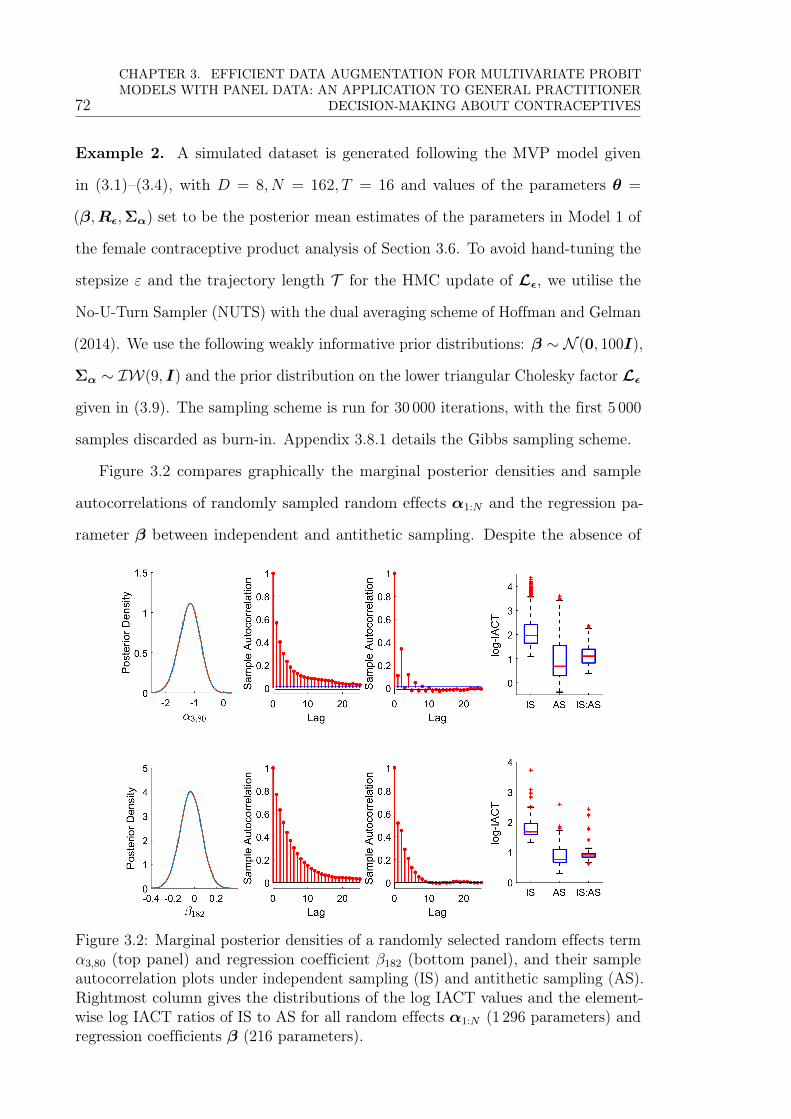
72
CHAPTER 3. EFFICIENT DATA AUGMENTATION FOR MULTIVARIATE PROBITMODELS WITH PANEL DATA: AN APPLICATION TO GENERAL PRACTITIONER
DECISION-MAKING ABOUT CONTRACEPTIVES
Example 2. A simulated dataset is generated following the MVP model given
in (3.1)–(3.4), with D = 8, N = 162, T = 16 and values of the parameters θ =
(β,Rε,Σα) set to be the posterior mean estimates of the parameters in Model 1 of
the female contraceptive product analysis of Section 3.6. To avoid hand-tuning the
stepsize ε and the trajectory length T for the HMC update of Lε, we utilise the
No-U-Turn Sampler (NUTS) with the dual averaging scheme of Hoffman and Gelman
(2014). We use the following weakly informative prior distributions: β ∼ N (0, 100I),
Σα ∼ IW(9, I) and the prior distribution on the lower triangular Cholesky factor Lε
given in (3.9). The sampling scheme is run for 30 000 iterations, with the first 5 000
samples discarded as burn-in. Appendix 3.8.1 details the Gibbs sampling scheme.
Figure 3.2 compares graphically the marginal posterior densities and sample
autocorrelations of randomly sampled random effects α1:N and the regression pa-
rameter β between independent and antithetic sampling. Despite the absence of
Figure 3.2: Marginal posterior densities of a randomly selected random effects termα3,80 (top panel) and regression coefficient β182 (bottom panel), and their sampleautocorrelation plots under independent sampling (IS) and antithetic sampling (AS).Rightmost column gives the distributions of the log IACT values and the element-wise log IACT ratios of IS to AS for all random effects α1:N (1 296 parameters) andregression coefficients β (216 parameters).

3.5. SIMULATION STUDIES 73
a stochastic component in the updates of α1:N and β, the kernel density plots of
these parameters indicate that the coupling of a stochastic MCMC scheme for the
remaining parameters with the antithetic variable technique gives the same posterior
distributions as those under independent sampling. The autocorrelation plots show
that the samples generated from antithetic sampling have positive dependence that
has a higher rate of decay over the number of lags, thereby reflecting the superior mix-
ing of the Markov chain. The IACT values of the randomly sampled parameters are
significantly lower, with improvement factors of 3.72 and 2.10 observed for α3,80 and
β182 respectively. The box plot showing the distribution of the IACT values across
all α1:N also indicates that some of these parameters are super-efficient (i.e. IACT
less than 1). Furthermore, the log IACT ratios of the independent sampler compared
to the antithetic sampler are well above 0, suggesting that all α1:N and β parameters
experience efficiency gains (see rightmost boxplots in Figure 3.2. Although perfect
negative correlation is induced between successive samples by the deterministic
proposal, this does not necessarily translate to an equivalent autocorrelation in the
posterior samples. Rather, the negative relationship is used to reduce the magnitude
of positive autocorrelation present in the MCMC samples. Note that convergence to
the posterior distribution might be slow for poorly initialised values under antithetic
sampling so we suggest using independent sampling during the burn-in period and
later switching to the deterministic proposal.
The remaining simulation experiments investigate the performance of the MVP
model in the context of recovering the true parameters of the data generating
process under different specifications of prior distribution on θ. We use the posterior
root-mean-square error (RMSE) defined by
RMSE(θp) =
√√√√ 1
n
n∑j=1
(θp[j] − θp,true)2, (3.13)
as the performance measure, where θp[j] is the j-th iterate from the n posterior
samples and θp,true is the true value of θp. The measure in (3.13) is defined for

74
CHAPTER 3. EFFICIENT DATA AUGMENTATION FOR MULTIVARIATE PROBITMODELS WITH PANEL DATA: AN APPLICATION TO GENERAL PRACTITIONER
DECISION-MAKING ABOUT CONTRACEPTIVES
univariate θp. For a multivariate θ, the posterior RMSE is calculated for each margin
of θ. All the results shown are based on 1 000 different replicate sets of simulated
data with the same true parameter values. The use of RMSE is valid here as a
measure of fit since weakly informative priors are used.
We first consider the conditionally conjugate hierarchical inverse-WishartHIW(ν0,
A) prior of Huang and Wand (2013) with degrees of freedom ν0 and positive scale
parameter A = (A1, . . . , AD)> as an alternative to the inverse-Wishart prior on the
D ×D covariance matrix Σα,
Σα|a1, . . . , aD ∼ IW
(ν0 +D − 1, 2ν0 diag
(1
a1
, . . . ,1
aD
)),
adiid∼ IG(0.5, A−2
d ), d = 1, . . . , D,
where IG(a, b) is an inverse-Gamma distribution with shape a and scale b. The
marginal prior of the standard deviation in Σα is a half-t(ν0, Ad) distribution, as
suggested in Gelman (2006). In the simulation, we select ν0 = 2 and choose a weakly
informative scale parameter whereby A1 = A2 = 0.23 and A3 = · · · = A8 = 0.46 so
that approximately 95% of the half-t density is below 1 and 2 respectively. This
specification is relevant to the real data application in Section 3.6, where our prior
belief is that the variability in the tendency of GPs to discuss pill contraceptives
is lower compared to non-pill alternatives. In contrast, the inverse-Wishart prior
assumes the same variability for all variance parameters σ2αi
in Σα.
Figure 3.3a shows the distribution of the average RMSE ratio of each type of
parameter in Σα, i.e.1
P
P∑p=1
RMSEHIW(θp)
RMSEIW(θp)
based on 1 000 replicate simulations, for the hierarchical inverse-Wishart prior versus
the inverse-Wishart prior. Although the hierarchical inverse-Wishart prior is flexible
enough to specify different strengths of prior on each σ2αi, Figure 3.3a shows that in
this case its performance is similar to the more restrictive inverse-Wishart prior. This
result is somewhat unsurprising considering that the estimated σ2αi
in the application

3.5. SIMULATION STUDIES 75
Standard Deviation Correlation Partial Correlation
0.96
0.98
1
1.02
1.04
1.06
Ave
rage
RM
SE
Rat
io
(a) Hierarchical inverse-Wishart prior versus inverse-Wishart prior on Σα.
Sparse Signal Non-sparse Signal
0.6
0.8
1
1.2
Ave
rage
RM
SE
Rat
io
(b) Horseshoe shrinkage prior versus normal prior on β.
Figure 3.3: Distributions of the average posterior RMSE ratio of all parameters in(a) Σα or (b) β, based on 1 000 replicate analyses, under different prior choices.(a) Standard deviations, correlations and partial correlations for parameters in Σα
for the hierarchical inverse-Wishart prior versus the inverse-Wishart prior on Σα.(b) Sparse regression coefficients βk = 0 and non-sparse coefficients βk 6= 0 for thehorseshoe prior versus the N (0, 100I) prior on β.
example are more or less similar across the different contraceptive products (see
Appendix 3.8.5). The distributions for the posterior RMSE ratio of the correlation
coefficients and the partial correlations are concentrated around 1 since both the
hierarchical inverse-Wishart prior with ν0 = 2 and the inverse-Wishart prior with
D + 1 degrees of freedom and scale matrix I induce the same marginally uniform
prior, i.e. (2.4) with ν = D + 1, on the resulting correlation matrix Rα, which in
turn gives the same implied LKJ distribution on the partial correlations.
To identify sparse signals (coefficients which are significant) in the regression
parameter β, we employ the horseshoe shrinkage prior (Carvalho et al., 2010) given

76
CHAPTER 3. EFFICIENT DATA AUGMENTATION FOR MULTIVARIATE PROBITMODELS WITH PANEL DATA: AN APPLICATION TO GENERAL PRACTITIONER
DECISION-MAKING ABOUT CONTRACEPTIVES
by
βk|λk, τ ∼ N (0, τ 2λ2k), λk ∼ C+(0, 1), τ ∼ C+(0, 1),
where C+(0, 1) is a half-Cauchy distribution with location 0 and scale 1 restricted
to positive support. The simulation is carried out by setting 75% of the smallest
non-intercept posterior mean regression coefficients (in absolute value) in β to
0, from which we generate the simulated datasets. We model the prior on each
intercept separately by a weakly informative N (0, 100) distribution to avoid heavily
penalising these parameters. Gibbs sampling from the posterior distribution of β is
implemented by adopting the latent variable formulation in Makalic and Schmidt
(2016). Figure 3.3b displays the results of comparing this prior specification for β
to a N (0, 100I) prior, again in terms of the average RMSE ratio over all regression
parameters. The horseshoe prior performs as well as the N (0, 100I) prior on non-zero
entries of β, although the variability in the RMSE ratio is large. On the other hand,
the horseshoe prior outperforms the normal prior for those parameters whose true
values are zero, reducing the RMSE by half. This occurs as the horseshoe prior
places a greater density around zero, which results in a more concentrated posterior
distribution for parameters which are truly zero. Therefore, it is an attractive default
option when we expect sparsity in the regression parameters, as is the case for our
analysis of the characteristics affecting the decision-making behaviour of GPs in the
next section.
3.6 Application to female contraceptive products
by Australian GPs
3.6.1 Background and aims of study
In order to study the decision-making behaviour of Australian GPs, we obtain data
from Fiebig et al. (2017) who design a stated preference experiment in which GPs
are asked to select the contraceptive products that they would consider discussing

3.6. APPLICATION TO CONTRACEPTIVE PRODUCTS BY AUSTRALIAN GPS 77
with hypothetical female patients. The GPs evaluate a sequence of vignettes where
patients are defined in terms of socio-economic and clinical characteristics that are
varied as part of the experimental design to cover a range of different life cycle and
fertility stages. Table 3.3 in Appendix 3.8.2 contains the attributes of the patients
with a description for each level of the categorical variables. The GPs choose from a
set of 9 products that they would discuss with the patient before deciding upon their
most preferred product to be subsequently prescribed to the patient. A sample of 162
GPs from a list of 14 816 GPs from all states and territories of Australia volunteered
to participate in the experiment between December 2008 and June 2009 where each
subject makes choices for 16 different patients, resulting in 2 592 observations. The
following covariate information is collected on the GPs themselves: age, gender,
whether they are registered as a Fellow of the Royal Australian College of GPs,
whether they have a certificate in family planning, whether they are an Australian
medical graduate, whether their location of practice is in an urban area and whether
they bulk-bill patients. Analysis of this panel data is based on the set of binary
outcomes as to whether or not to discuss each of the contraceptive products. Due
to low occurrences for the prescription of the hormonal patch which was yet to be
released in the Australian market, we removed this product from the dataset leaving
observations on the 8 remaining products.
The experiment is designed to mimic the choice problem faced by GPs in a
consultation where they need to match a product with a particular patient. In
characterising such a decision problem, Frank and Zeckhauser (2007) distinguish
between “custom-made” and “ready-to-wear” (or norm-based) choices. A custom-
made choice involves the GP undertaking a careful evaluation of the patient and then
matching her to an appropriate product. However, as new products are introduced,
GPs face considerable costs in the process of gaining the knowledge and expertise
required to discuss and prescribe these products (Hauser and Wernerfelt, 1990;
Roberts and Lattin, 1991; Gilbride and Allenby, 2004). This is particularly the
case when more familiar products are available even though they may be somewhat

78
CHAPTER 3. EFFICIENT DATA AUGMENTATION FOR MULTIVARIATE PROBITMODELS WITH PANEL DATA: AN APPLICATION TO GENERAL PRACTITIONER
DECISION-MAKING ABOUT CONTRACEPTIVES
inferior to the new products (Wellings et al., 2007); an especially salient situation in
the market for contraceptive products. In such cases, some GPs will tend to adopt
norms (here particular products) that work well for a broad class of patients and to
place less weight on certain patient attributes that would indicate a different product
that is potentially a better match.
Particular interest is in the dependence in recommendations among the products.
That is, which products tend to be discussed together and which tend to form distinct
clusters. If GPs pursue custom-made strategies, then a considerable portion of the
dependence between products will be explained by the attributes of the patient.
Conditional on the observable features of the patient and characteristics of the GPs,
remaining dependencies will reflect the relationship between unobservables related to
evaluations of the suitability of certain products for a particular patient, and how for
individual GP’s their product effects are correlated across products. The proposed
model is designed to capture these forms of heterogeneity and will permit a detailed
analysis of the choices.
The prevalence of ready-to-wear choices is one possible explanation for the rela-
tively low uptake of long acting reversible contraceptive (LARC) methods in Australia
(Black et al., 2013). LARC methods are contraceptives that are administered less
frequently than monthly and include hormonal implants, intrauterine contraception
(IUC), both hormonal and copper-bearing, and contraceptive injections. There is
increasing support for the greater use of these more effective methods to reduce
unintended pregnancies and abortion rates (Stevens-Simon et al., 2001; Blumenthal
et al., 2011; Secura, 2013). In our analysis below, we will use the model to explore
a case where there is no clinical reason why at least one of these LARC methods
should not be considered for discussion by GPs. For ease of presentation, we will use
the subscripts in Table 3.1 to denote the products.

3.6. APPLICATION TO CONTRACEPTIVE PRODUCTS BY AUSTRALIAN GPS 79
Subscript Product1 Combined pill2 Mini-pill3 Hormonal injection4 Hormonal implant5 Hormonal IUD6 Vaginal ring7 Copper IUD8 Condom
Table 3.1: Correspondence of parameter subscripts to each female contraceptiveproduct. Long acting reversible contraceptive methods are shown in grey.
3.6.2 Analysis and results
We consider two different models for the data:
Model 1: y∗it = αi +Bxit + εit, (3.14)
Model 2: y∗it = αi +Bxit +Czi + εit, (3.15)
for i = 1, . . . , N = 162 GPs and t = 1, . . . , T = 16 patients, where y∗ is the latent
normal random variables underlying the observed binary outcomes y described in
(3.4). Here αi and Czi respectively represent GP-specific random and fixed effects
with zi being a vector of GP characteristics, and Bxit represents fixed effects of
the patient. We select a horseshoe prior on β = vec(B) and model the covariance
matrix Σα of the random effects by the HIW(2,A) prior in Section 3.5 where
A = (0.23, 0.23, 0.46, . . . , 0.46)>. The scale is chosen to express the prior information
that the variances of the random effects are expected to be small, with those for the
pill products being less variable compared to the non-pill alternatives. The difference
between these two models is the presence of the GP-specific fixed effects in Model
2, which explain some of the relationships in the random effects of Model 1. Let
X = (X1, . . . , XK)> be a vector of normal random variables with covariance matrix
given by ΣX . Recall that Xi and Xj are conditionally independent given the other
random variables if the (i, j)-th entry of the precision matrix Σ−1X is zero.

80
CHAPTER 3. EFFICIENT DATA AUGMENTATION FOR MULTIVARIATE PROBITMODELS WITH PANEL DATA: AN APPLICATION TO GENERAL PRACTITIONER
DECISION-MAKING ABOUT CONTRACEPTIVES
Figures 3.4 and 3.5 give graphical summaries of the posterior distribution of the
dependence structures of the latent variable y∗it conditional on αi and xit (as well as
zi for Model 2), and the random effects αi respectively. All graphs are obtained by
computing the 95% credible interval of the posterior distribution for each entry of
R−1ε and Σ−1
α , where an edge is formed between two nodes if the credible interval
does not include 0. The absence of an edge between any two nodes indicates a
plausible conditional independence between the two variables given the rest. The
dependence structures associated with the latent variables are the same for both
Model 1 and 2. This supports the use of the MVP model in order to capture the
complex dependencies between different products that would otherwise be ignored
in separate univariate analyses on each product.
Figure 3.4 is also instrumental in explaining the suitability of the contraceptive
products for a patient in terms of substitute goods, which are products with similar
functions that can be used in place of each other. For conciseness, we only focus on
some important relationships illustrated in the graphical model. The propensity to
discuss pill products (y∗1, y∗2) is independent of each other given whether the hormonal
IUD and the vaginal ring (y∗5, y∗6) are discussed, by the Markov property since all paths
from y∗1 to y∗2 pass through (y∗5, y∗6), reflecting the use of these non-pill contraceptives
as pill alternatives dictated by particular clinical conditions. The clique formed
between (y∗5, y∗7, y∗8) suggests dependence in the propensity to discuss the hormonal
IUD, the copper IUD and condoms. In fact, the posterior correlation between the
propensity scores for both the IUD methods (y∗5, y∗7) is around 0.52 on average (see
Appendix 3.8.4), suggesting a high tendency for these products to be discussed
together. This also suggests that these IUD methods are substitutes. Noticeably,
the propensity to discuss the hormonal injection and the hormonal implant (y∗4, y∗5)
exhibit the highest level of association, as indicated by our model, with a mean
posterior correlation of 0.59. This indicates the likelihood of these two prominent
LARC products being included together in discussions, and it is consistent with
them being moderately close substitutes for many patients.

3.6. APPLICATION TO CONTRACEPTIVE PRODUCTS BY AUSTRALIAN GPS 81
y∗1
y∗2
y∗3
y∗4y∗5
y∗6
y∗7
y∗8
Figure 3.4: Graphical model illustrating estimated dependence structure of the latentvariables y∗ conditional on the random effects and the covariates in both Model1 and 2. Edges between y∗i and y∗j are included if the 95% credible interval of themarginal posterior distribution of the (i, j)-th entry of R−1
ε does not contain 0. Blueedges represent positive dependence while red edges represent negative dependence.The thickness of the edges is proportional to the strength of the dependence.
α1
α2
α3
α4α5
α6
α7
α8
(a) Model 1.
α1
α2
α3
α4α5
α6
α7
α8
(b) Model 2.
Figure 3.5: Graphical models illustrating estimated dependence structure of theGP-specific random effects α in each model. Edges between αi and αj are includedif the 95% credible interval of the marginal posterior distribution of the (i, j)-thentry of Σ−1
α does not contain 0. Blue edges represent positive dependence while rededges represent negative dependence. The thickness of the edges is proportional tothe strength of the dependence.
Figure 3.5 can be interpreted in the same way as Figure 3.4, regarding the
substitution of different products but in the context of ready-to-wear choices. This
is because the random effects in (3.14) characterise the consistency of GPs in
discussing a particular product after observing the patient’s attributes. There
are clear differences in the graphical structure when comparing Models 1 and 2
(Figures 3.5a and 3.5b). The changes in the dependence structure of the GP random

82
CHAPTER 3. EFFICIENT DATA AUGMENTATION FOR MULTIVARIATE PROBITMODELS WITH PANEL DATA: AN APPLICATION TO GENERAL PRACTITIONER
DECISION-MAKING ABOUT CONTRACEPTIVES
effects arise because some of the consistency in product choices can be explained by
GP characteristics. For example, the tendency of GPs to include both the hormonal
injection and the copper IUD (α3, α7) as ready-to-wear choices is due to their age
(see significance of GP characteristics in Appendix 3.8.3). The posterior structure
also provides some confidence that the random effects specification is useful in
capturing important GP characteristics that are not directly observed. Three clusters
of products with substantial dependence in ready-to-wear choices are identified from
the model after accounting for the observed GP characteristics. Particularly relevant
is the dependence between the hormonal IUD and the implant (α4, α5). There
is positive correlation between these two LARCs, indicating the tendency for GP
attitudes (either positive or negative) to be aligned. A second cluster includes both of
the pills (α1, α2) which is consistent with these products being used as a ready-to-wear
choice. GPs who are more likely to discuss the combined pill after conditioning on the
patient’s attributes behave similarly when considering the mini-pill. Contraceptives
that are not pill- nor hormone-based form the final bundle.
Our models allow us to examine posterior predictions for a range of patients.
Since we are interested in the uptake of LARC products, we specify a particular
female patient where there is no clinical reason why a LARC should not be considered
for discussion. Table 3.3 of Appendix 3.8.2 gives the attributes of this base-case
patient. Figure 3.6 summarises the estimate of the predictive probability of a GP
discussing a particular product, where the range of predictions shown is generated
for all GPs in the sample based on Model 2. For this particular base-case patient,
there is considerable agreement amongst all GPs in the sample that the combined
pill (product 1) is one of the most suitable products to be discussed, but they have
much more variable views on the other products. Amongst the LARCs (products
3, 4, 5 and 7), the hormonal injection (product 3) and the implant (product 4) are
the products which are the most likely to be discussed, with the variability across
GPs perhaps simply reflecting a view that they are good substitutes to each other,
which is in fact what we find in Figure 3.4. GPs could indeed have consistent views
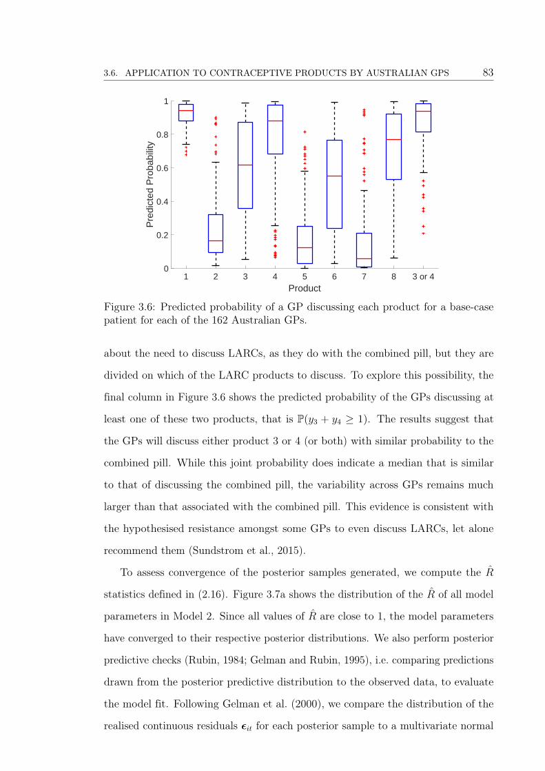
3.6. APPLICATION TO CONTRACEPTIVE PRODUCTS BY AUSTRALIAN GPS 83
1 2 3 4 5 6 7 8 3 or 4Product
0
0.2
0.4
0.6
0.8
1
Pre
dict
ed P
roba
bilit
y
Figure 3.6: Predicted probability of a GP discussing each product for a base-casepatient for each of the 162 Australian GPs.
about the need to discuss LARCs, as they do with the combined pill, but they are
divided on which of the LARC products to discuss. To explore this possibility, the
final column in Figure 3.6 shows the predicted probability of the GPs discussing at
least one of these two products, that is P(y3 + y4 ≥ 1). The results suggest that
the GPs will discuss either product 3 or 4 (or both) with similar probability to the
combined pill. While this joint probability does indicate a median that is similar
to that of discussing the combined pill, the variability across GPs remains much
larger than that associated with the combined pill. This evidence is consistent with
the hypothesised resistance amongst some GPs to even discuss LARCs, let alone
recommend them (Sundstrom et al., 2015).
To assess convergence of the posterior samples generated, we compute the R
statistics defined in (2.16). Figure 3.7a shows the distribution of the R of all model
parameters in Model 2. Since all values of R are close to 1, the model parameters
have converged to their respective posterior distributions. We also perform posterior
predictive checks (Rubin, 1984; Gelman and Rubin, 1995), i.e. comparing predictions
drawn from the posterior predictive distribution to the observed data, to evaluate
the model fit. Following Gelman et al. (2000), we compare the distribution of the
realised continuous residuals εit for each posterior sample to a multivariate normal
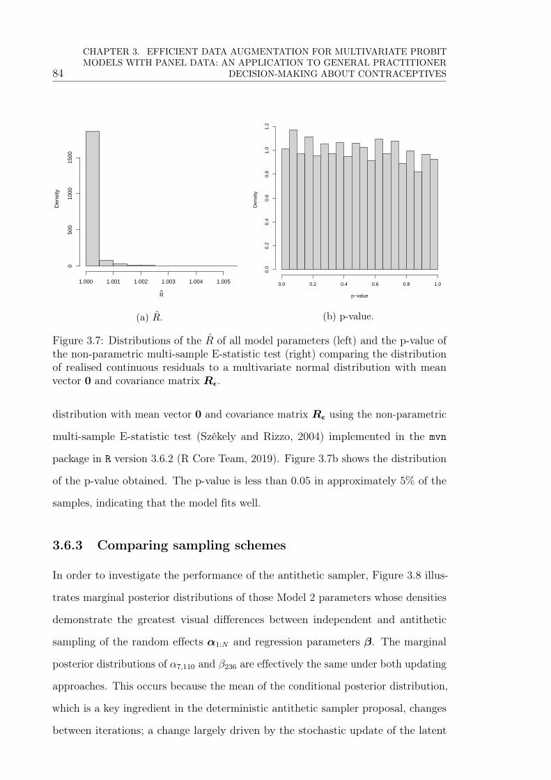
84
CHAPTER 3. EFFICIENT DATA AUGMENTATION FOR MULTIVARIATE PROBITMODELS WITH PANEL DATA: AN APPLICATION TO GENERAL PRACTITIONER
DECISION-MAKING ABOUT CONTRACEPTIVES
R
Den
sity
1.000 1.001 1.002 1.003 1.004 1.005
050
010
0015
00
(a) R.
p−value
Den
sity
0.0 0.2 0.4 0.6 0.8 1.0
0.0
0.2
0.4
0.6
0.8
1.0
1.2
(b) p-value.
Figure 3.7: Distributions of the R of all model parameters (left) and the p-value ofthe non-parametric multi-sample E-statistic test (right) comparing the distributionof realised continuous residuals to a multivariate normal distribution with meanvector 0 and covariance matrix Rε.
distribution with mean vector 0 and covariance matrix Rε using the non-parametric
multi-sample E-statistic test (Székely and Rizzo, 2004) implemented in the mvn
package in R version 3.6.2 (R Core Team, 2019). Figure 3.7b shows the distribution
of the p-value obtained. The p-value is less than 0.05 in approximately 5% of the
samples, indicating that the model fits well.
3.6.3 Comparing sampling schemes
In order to investigate the performance of the antithetic sampler, Figure 3.8 illus-
trates marginal posterior distributions of those Model 2 parameters whose densities
demonstrate the greatest visual differences between independent and antithetic
sampling of the random effects α1:N and regression parameters β. The marginal
posterior distributions of α7,110 and β236 are effectively the same under both updating
approaches. This occurs because the mean of the conditional posterior distribution,
which is a key ingredient in the deterministic antithetic sampler proposal, changes
between iterations; a change largely driven by the stochastic update of the latent

3.6. APPLICATION TO CONTRACEPTIVE PRODUCTS BY AUSTRALIAN GPS 85
2 40
0.2
0.4
0.6
0.8
1P
oste
rior
Den
sity
-0.05 0 0.050
10
20
30
40
Pos
terio
r D
ensi
ty
-0.2 0 0.2 0.40
2
4
6
Pos
terio
r D
ensi
ty
IS AS
0 0.50
2
4
6
8
10
Pos
terio
r D
ensi
ty
1 2 3 40
0.5
1
1.5
Pos
terio
r D
ensi
ty
Figure 3.8: Marginal posterior density estimates of those Model 2 parameters withthe greatest visual differences between using independent sampling (IS) and antitheticsampling (AS) for α1:N and β.
variable y∗. This outcome suggests that the posterior distribution of the other
parameters remains adequately explored by the antithetic sampler.
Table 3.2 compares the performance between independent and antithetic sampling
schemes when estimating Model 2. The antithetic variable method generates samples
marginally faster than independent sampling because it is deterministic. Based on
the results shown, we observe an improvement of 4.86 and 3.31 times performance
gain on average in the mixing of α1:N and β respectively. As a result of this, the
mean IACT of y∗ is also improved.
ParameterMean IACT IACT RatioIS AS Min Max Mean
y∗ 3.6387 2.6686 0.8242 3.1419 1.2127α1:N 16.8872 4.6456 1.4857 13.3424 4.8632β 15.0446 4.0105 1.4566 16.0173 3.3111
vechL(Lε) 14.8292 14.5422 0.9338 1.1737 1.0191vechL(Rε) 12.7311 12.5170 0.9147 1.1509 1.0180diag(Σα) 24.8056 14.6929 1.3130 2.0651 1.7222vechL(Rα) 9.5025 5.1716 1.4599 2.3336 1.8424
Time per iteration 0.0243 0.0239 - - -
Table 3.2: Comparison of the performance between independent sampling (IS) andantithetic sampling (AS) in the contraceptive products preference data in terms ofthe speed (seconds per iteration), the mean IACT and the IACT ratio for each blockof parameter.

86
CHAPTER 3. EFFICIENT DATA AUGMENTATION FOR MULTIVARIATE PROBITMODELS WITH PANEL DATA: AN APPLICATION TO GENERAL PRACTITIONER
DECISION-MAKING ABOUT CONTRACEPTIVES
3.7 Conclusion
Many methods exist for fitting a multinomial logit model with random effects, such
as simulated maximum likelihood (Gong et al., 2004), quadrature (Hartzel et al.,
2001; Hedeker, 2003), multinomial-Poisson transformation (Lee et al., 2017), and
moment-based estimation (Perry, 2017), among others. Computational strategies for
the MVP model, in contrast, are less well studied and computationally expensive to
implement. For instance, the random walk Metropolis-Hastings algorithm used in
Chib and Greenberg (1998) does not guarantee positive definiteness of the correlation
matrix in each proposal step, while at the same time not being able to explore the
parameter space efficiently (Sherlock et al., 2010). In this chapter, we introduce a
Hamiltonian Monte Carlo (Neal, 2011) sampling approach to generate the posterior
samples of correlation matrix Rε, which requires reparameterising Rε into an un-
constrained Cholesky factor to circumvent the restrictive properties of a correlation
matrix having diagonal entries of 1 and being positive definite. Credible but distant
candidate parameters for the Cholesky factor can be generated from the Hamilto-
nian dynamics by exploiting gradient information of the posterior density, thereby
reducing autocorrelation in the posterior samples. Furthermore, we propose a novel
antithetic variable technique, motivated by the over-relaxation algorithm (Adler,
1981; Barone and Frigessi, 1990), to accelerate the mixing of the random effects and
the regression parameters, where significant gains in efficiency are observed in our
application. Although our antithetic sampling regime deterministically specifies the
proposal distribution within the Metropolis-Hastings update, the ergodicity of the
Markov chain is unaffected when it is embedded within a larger system of stochastic
updates based on our empirical results.
Our methodology is applied to a longitudinal study of the discussion of female
contraceptive products by Australian GPs, where the (binary) outcomes are obtained
from the second stage of the stated preference data in Fiebig et al. (2017). An
examination of the correlation matrix underlying the choices revealed a complex

3.8. APPENDICES 87
dependence structure between the products, hence indicating the plausibility of our
formulation to model these choices in a multivariate setting. By using a multivariate
model, we are able to make inference about conditional independence of the products
using a graphical model, as well as computing the probability of the GPs discussing
a set of contraceptive products which is not possible in univariate analyses. Our
empirical study provided evidence of medical practice variation among the GPs,
which is in line with the findings of earlier studies (Wennberg et al., 1982; Scott and
Shiell, 1997; Davis et al., 2000). We found that the disparities in medical practice was
especially more pronounced with regard to the inclusion of LARCs in the discussion
with patients, and this result is also reported in Sundstrom et al. (2015). Our analysis
indicated that the combined pill was the most popular contraceptive choice among
the patients, and it represented a likely ready-to-wear option for many GPs. Without
GPs even discussing LARCs, their uptake was likely to remain relatively constrained
in such a context (Wellings et al., 2007).
3.8 Appendices
3.8.1 Sampling scheme for the MVP model with random
effects
Suppose that we choose the following prior distributions: β ∼ N (0,Ψβ),Σα ∼
IW(ν0,ΨΣ) and the prior distribution on the lower triangular Cholesky factor Lε
in (3.9) with ν = D + 1. Let θ = (β,Lε,Σα). Equation (3.5) gives the posterior
distribution of interest under the data augmentation approach where we update
y∗,α1:N and each component of θ using Gibbs sampling. For notational clarity, we
will drop the superscript which indicates the sequence of the samples in a Markov
chain where necessary.

88
CHAPTER 3. EFFICIENT DATA AUGMENTATION FOR MULTIVARIATE PROBITMODELS WITH PANEL DATA: AN APPLICATION TO GENERAL PRACTITIONER
DECISION-MAKING ABOUT CONTRACEPTIVES
Step 1: Updating y∗
For d = 1, . . . , D, sample y∗ conditionally one-at-a-time following Geweke (1991),
i.e.
y∗d,it|α1:N ,θ,y∗−d,it, yd,it ∼
T N (−∞,0](µ
(d|−d)d,it , σ
(d|−d)d,it ) if yd,it = 0
T N (0,∞)(µ(d|−d)d,it , σ
(d|−d)d,it ) if yd,it = 1
where y∗−d,it = (y1,it, . . . , yd−1,it, yd+1,it, . . . , yD,it)>, µ(d|−d)
d,it and σ(d|−d)d,it are the univari-
ate d-th dimension conditional mean and conditional standard deviation respectively
for the N (µit,Rε) distribution and T N (a,b) is a univariate normal distribution
truncated to the interval (a, b).
Step 2: Updating β
Compute the posterior mean µβ and the posterior covariance matrix Σβ for β as
Σβ =
(N∑i=1
T∑t=1
(I ⊗ xit)R−1ε (I ⊗ xit)> + Ψ−1
β
)−1
,
µβ = Σβ
(N∑i=1
T∑t=1
(I ⊗ xit)R−1ε (y∗it −αi)
),
where ⊗ denotes the Kronecker product and set β[j+1] = 2µβ −β[j] deterministically.
If a horseshoe prior is specified on β instead, its update is the same by first sampling
diag(Ψβ) conditional on the local shrinkage parameters λk and global shrinkage
parameter τ (see Makalic and Schmidt (2016) for details).
Step 3: Updating Lε
Sample Lε using the NUTS algorithm and obtain the correlation matrix Rε from
the relationship in (3.7).
Step 4: Updating α1:N
For i = 1, . . . , N , compute the posterior mean µαi and the posterior covariance

3.8. APPENDICES 89
matrix Σα for the random effects αi as
Σα =(TR−1
ε + Σ−1α
)−1,
µαi = Σα
(R−1ε
T∑t=1
y∗it −Bxit
),
and set α[j+1]i = 2µαi −α
[j]i deterministically.
Step 5: Updating Σα
Sample
Σα ∼ IW
(ν0 +N,
N∑i=1
αiα>i + ΨΣ
).
Suppose that a HIW(ν0,A) prior with scales A is used for Σα. Sample
ad ∼ IG(ν0 +D
2, ν0Σ
−1α (d; d) +
1
A2d
),
Σα ∼ IW
(ν0 +N +D − 1,
N∑i=1
αiα>i + 2ν0diag
(1
a1
, . . . ,1
aD
)),
where Σ−1α (d; d) is the d-th diagonal entry of the precision matrix Σ−1
α .

90
CHAPTER 3. EFFICIENT DATA AUGMENTATION FOR MULTIVARIATE PROBITMODELS WITH PANEL DATA: AN APPLICATION TO GENERAL PRACTITIONER
DECISION-MAKING ABOUT CONTRACEPTIVES
3.8.2 Attributes of the patient in the Australian GP data
Attribute Variable Description
Age
dagegp1 Aged 16-19 yearsdagegp2 Aged 20-29 yearsdagegp3 Aged 30-39 yearsdagegp4 Aged 40 years or more
Reason for encounter
drfe1 Starting prescribed contraception for first timedrfe2 Recommencing prescribed contraceptiondrfe3 On pill but dissatisfieddrfe4 Using non-pill method but dissatisfied
Periodsdbleed1 Heavy and/or painful periodsdbleed2 Irregular periodsdbleed3 No problems with periods
Blood pressuredbp1 Has low blood pressuredbp2 Has normal blood pressuredbp3 Elevated blood pressure
Relationship
drel1 In long-standing relationshipdrel2 In new relationshipdrel3 Has no steady relationshipdrel4 No information about relationship
Childrendchild1 Is currently breastfeedingdchild2 Has children but is not breastfeedingdchild3 Has no children
Fertility plans
dfut1 Does not want to have children in futuredfut2 Plans to have children in next 2 yearsdfut3 Plans to have children but not in next 2 yearsdfut4 Unsure about future fertility plans
Pill preferencedpil1 Prefer pill to other methodsdpil2 Has no strong opinion about pilldpil3 Prefers methods other than pill
Weight concern dwt1 Is concerned about gaining weightdwt2 Is not concerned about gaining weight
Compliance dcomp1 Has no difficulty with compliancedcomp2 Has difficulty with compliance
Incomedpay1 Has a low to middle household incomedpay2 Has a health care carddpay3 Has a high household income
Smokingdsmk1 Is a non-smokerdsmk2 Smokes less than 10 cigarettes per daydsmk3 Smokes 10 or more cigarettes per day
Table 3.3: Categorical variables in the contraceptive discussion data with a textdescription for each level of attribute. Levels in grey define the attributes of a base-case patient.

3.8. APPENDICES 91
3.8.3 Posterior means of the patient and GP fixed effects in
the Australian GP data based on Model 2
Variable Product1 2 3 4 5 6 7 8
Patient
Intercept 1.4161 −1.2576 −0.3964 1.0991 −2.3943 −0.1142 −1.7657 0.6918dagegp1 0.1949 −0.1329 0.0104 0.0744 −0.5063 −0.0205 −0.2880 0.0637dagegp3 −0.1326 0.0621 −0.0624 −0.0002 0.3173 −0.0037 0.0906 0.0108dagegp4 −0.3936 0.1851 −0.2406 −0.1041 0.8095 −0.0270 0.3849 0.0013drfe2 −0.0426 0.0008 −0.0388 −0.0144 0.0441 −0.0188 −0.0449 0.0068drfe3 −0.2464 −0.0541 0.0270 0.0788 0.0940 0.1069 −0.0248 0.1364drfe4 −0.0206 0.1042 −0.0099 0.0516 0.0678 0.0719 −0.0702 0.0056
dbleed1 0.0493 −0.1363 0.0615 −0.0869 0.4000 −0.0256 −0.5274 −0.2311dbleed2 0.0160 −0.0763 0.0213 −0.0222 0.0070 0.0408 −0.0869 −0.0254dbp1 −0.0599 −0.0011 −0.0300 0.0292 0.0040 0.0317 −0.0221 −0.1433dbp3 −0.9956 0.2444 0.0070 0.0135 0.2375 −0.2959 0.2561 0.0347drel1 0.0436 −0.0102 −0.0963 −0.0020 0.1570 0.0314 0.0282 −0.3971drel3 −0.0141 0.0269 −0.0208 0.0002 −0.0271 0.0090 −0.0186 0.0198drel4 −0.0914 0.0879 0.0667 −0.0009 −0.0101 0.0294 0.0029 −0.2035dchild1 −1.7437 1.3074 −0.0082 −0.0889 0.9236 −0.9909 0.5354 −0.0371dchild2 −0.0458 0.0344 −0.0632 −0.0403 0.9850 −0.0498 0.6007 −0.0543dfut1 −0.3206 −0.0043 0.1978 0.0245 0.6323 −0.0786 0.2120 −0.1143dfut2 −0.2861 0.1936 −0.2169 −0.1996 −0.0068 0.0359 −0.1438 0.0116dfut4 −0.3591 0.0485 0.0470 0.0099 0.2882 0.0067 0.0150 0.0323dpil1 0.4724 0.3662 −0.0948 −0.2629 −0.0120 −0.0331 −0.0430 −0.0287dpil3 −0.1878 −0.2417 0.0289 0.0618 0.0538 0.0329 0.0457 0.0814dwt1 0.0831 0.0374 −0.2582 −0.0624 0.0318 0.0652 −0.0130 0.0815
dcomp2 −0.3401 −0.1988 0.2152 0.0642 0.2321 −0.0033 0.3133 −0.0162dpay2 −0.0253 −0.0558 −0.0204 −0.0026 0.0084 0.0595 0.0082 0.0074dpay3 0.0317 −0.0639 −0.0697 −0.0177 −0.0373 0.2896 −0.0177 −0.0044dsmk2 −0.2665 −0.0117 −0.0266 −0.0126 −0.0038 0.0444 0.0892 0.0320dsmk3 −0.5218 −0.0133 0.0132 0.0255 0.0148 −0.0546 0.0467 0.0333
GP
Female −0.0662 0.0248 −0.4417 0.0732 0.0368 0.5999 −0.4474 −0.0260Fellow −0.0183 −0.0958 0.0709 0.0418 0.2067 0.1019 −0.1456 −0.0108
Family planning −0.0002 −0.0154 −0.1203 0.2229 0.0434 0.0360 −0.0324 −0.0118Bulk-bill −0.0210 −0.0349 0.0416 −0.0372 −0.0617 0.0036 0.0509 0.0038
Age 0.0086 0.0080 0.0207 −0.0061 0.0175 −0.0044 0.0093 −0.0100Australian graduate 0.0839 0.0564 −0.0087 0.3466 0.0911 −0.2385 −0.0965 0.5515
Urban −0.0888 0.0065 0.0706 −0.0078 0.0099 0.0048 −0.0222 0.1774
Table 3.4: Regression coefficient posterior mean estimates for the attributes of afemale patient and the characteristics of a GP based on Model 2 for various productsin the contraceptive discussion data. Parameters whose 90% credible interval doesnot include 0 are shown in grey.
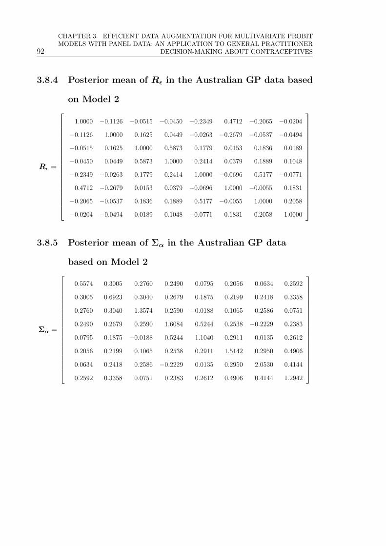
92
CHAPTER 3. EFFICIENT DATA AUGMENTATION FOR MULTIVARIATE PROBITMODELS WITH PANEL DATA: AN APPLICATION TO GENERAL PRACTITIONER
DECISION-MAKING ABOUT CONTRACEPTIVES
3.8.4 Posterior mean of Rε in the Australian GP data based
on Model 2
Rε =
1.0000 −0.1126 −0.0515 −0.0450 −0.2349 0.4712 −0.2065 −0.0204
−0.1126 1.0000 0.1625 0.0449 −0.0263 −0.2679 −0.0537 −0.0494
−0.0515 0.1625 1.0000 0.5873 0.1779 0.0153 0.1836 0.0189
−0.0450 0.0449 0.5873 1.0000 0.2414 0.0379 0.1889 0.1048
−0.2349 −0.0263 0.1779 0.2414 1.0000 −0.0696 0.5177 −0.0771
0.4712 −0.2679 0.0153 0.0379 −0.0696 1.0000 −0.0055 0.1831
−0.2065 −0.0537 0.1836 0.1889 0.5177 −0.0055 1.0000 0.2058
−0.0204 −0.0494 0.0189 0.1048 −0.0771 0.1831 0.2058 1.0000
3.8.5 Posterior mean of Σα in the Australian GP data
based on Model 2
Σα =
0.5574 0.3005 0.2760 0.2490 0.0795 0.2056 0.0634 0.2592
0.3005 0.6923 0.3040 0.2679 0.1875 0.2199 0.2418 0.3358
0.2760 0.3040 1.3574 0.2590 −0.0188 0.1065 0.2586 0.0751
0.2490 0.2679 0.2590 1.6084 0.5244 0.2538 −0.2229 0.2383
0.0795 0.1875 −0.0188 0.5244 1.1040 0.2911 0.0135 0.2612
0.2056 0.2199 0.1065 0.2538 0.2911 1.5142 0.2950 0.4906
0.0634 0.2418 0.2586 −0.2229 0.0135 0.2950 2.0530 0.4144
0.2592 0.3358 0.0751 0.2383 0.2612 0.4906 0.4144 1.2942

Chapter 4
Multiclass classification of growth
curves using random change points
and heterogeneous random effects
4.1 Introduction
According to the latest joint malnutrition estimates by the United Nations Children’s
Fund, World Health Organization (WHO), and World Bank Group (2018), it is
estimated that in 2017, stunted growth is prevalent in 22.2% of the global population
under the age of 5, or over 150 million children worldwide. This is particularly
serious in low to medium income countries where the rate of stunting is 35.0%.
A major contributor to stunted growth is prolonged faltering, defined as a slower
rate of growth compared to a reference healthy population of the same age and
gender, which comes with adverse consequences such as increased susceptibility of
individuals to diarrhoea and respiratory infections (Kossmann et al., 2000), abnormal
neurointegrative development (Benítez-Bribiesca et al., 1999) and at a population
scale, a capital loss to the labour market (Hoddinott et al., 2013). Therefore, it is
imperative to take early preventive measures to minimise these impacts. In order

94CHAPTER 4. MULTICLASS CLASSIFICATION OF GROWTH CURVES USING RANDOM
CHANGE POINTS AND HETEROGENEOUS RANDOM EFFECTS
to implement preventive measures, faltered children must first be identified in the
population. It is additionally important to distinguish between different growth
patterns, as each type represents a particular growth behaviour and so merits a
different response (Collins et al., 2006). For example, children who caught up on
growth after having faltered may have benefited from the intake of better diets or
nutritional supplements. Such strategies can then be extended to other children in
the cohort to improve their growth.
In the functional data analysis (Ramsay and Silverman, 2005) literature, several
clustering methods are proposed. One of these methods first reduces the dimension of
the inherently infinite-dimensional functional data using a finite basis expansion (see
e.g. Abraham et al. (2003) and Rossi et al. (2004) for such approximation using a B-
spline) or a functional principal component analysis, for example in Peng and Müller
(2008) and Xiao et al. (2016), and then clusters the basis coefficients or the functional
principal component scores using classical classification algorithms (see Chapter 14
in Hastie et al., 2009). Another related classification approach that is proposed in
Tarpey and Kinateder (2003), Ferraty and Vieu (2006) and Tokushige et al. (2007)
computes the pairwise Euclidean norm between curves, which is used as a similarity
measure for k-means clustering. On the other hand, model-based clustering methods
are presented in Shi et al. (1996), James and Sugar (2003), Heard et al. (2006) and
Giacofci et al. (2013), whereby the basis coefficients are typically assumed to be
distributed according to a mixture of normal distributions, with each component
determining the classification memberships. Model-based techniques using principal
components modelling are considered in Bouveyron et al. (2007) and Bouveyron and
Jacques (2011), whereby the data are fitted in group-specific functional subspaces
using the notion of functional probability density defined in Delaigle and Hall
(2010). However, functional methods are not suitable for sparse observations. This is
particularly relevant when studying the growth development of children in low to
medium income countries, where the number of height-related measurements per
child is small and they are taken at irregular intervals (see e.g. Anderson et al. (2019)

4.1. INTRODUCTION 95
for a summary of these statistics for the datasets used in their study). This has made
regression-based methods a more popular approach in modelling growth curves.
Similarly, both multi-stage and model-based methods are proposed for growth
curve regression models. Leung et al. (2017) suggests classifying children with the
lowest 10% of values of random velocity estimates extracted from a linear mixed
effects model (Laird and Ware, 1982) as having experienced an “abnormal” growth,
whereas Lee et al. (2018) classifies children into two groups based on their minimum
random random velocity estimates obtained from a broken stick model (Ruppert
et al., 2003), which is a piecewise linear model with breaks at several knots. Here, the
velocity refers to the rate of change in the measurements used for growth modelling
(Cole, 1998), which in practice includes the raw height and other suitable metrics such
as z-scores. Z-scores, such as the height-for-age z-score (HAZ), is a measure defined
by the WHO Multicentre Growth Reference Study Group (2006) that compares the
anthropometric measurements of a child matched against a reference population
of healthy children of the same age and gender. These staged methods rely on an
arbitrary threshold and the resulting classifications are not necessarily comparable
between different populations. As such, growth mixture models (Muthén and Shedden,
1999; Nagin, 1999; Muthén and Muthén, 2000; Li et al., 2001; Muthén, 2008) are
considered for analysing the change of growth patterns in longitudinal measurement
data. These models assume that the population is heterogeneous and comprises of
multiple smaller subgroups (Berlin et al., 2014). Unobserved heterogeneity between
children is modelled using random effects and finite mixture distribution (McLachlan
and Peel, 2000), thereby allowing different sets of velocities to capture group-specific
growth trajectories. Despite its extensive use, one unresolved issue in the application
of a growth mixture model is how to determine the “correct” number of mixture
components G (Nylund et al., 2007). Most approaches choose G based on information
criterion (Dasgupta and Raftery, 1998; Magidson and Vermunt, 2004), likelihood
ratio test (Titterington et al., 1985), goodness-of-fit test (Verbeke and Lesaffre, 1996),
among others, which requires fitting multiple models with different values of G.

96CHAPTER 4. MULTICLASS CLASSIFICATION OF GROWTH CURVES USING RANDOM
CHANGE POINTS AND HETEROGENEOUS RANDOM EFFECTS
This chapter adopts a different strategy in choosing G: modelling the mixture
distribution of growth velocities within a Bayesian framework using the Dirichlet
process (DP; Ferguson, 1973) prior, with G being inferred as part of the posterior
sampling algorithm. We note that the concept of using a DP prior for classification
is not new. In the context of functional data, Scarpa and Dunson (2014) cluster body
temperature curves of women during menstrual cycle using a functional DP prior,
Ray and Mallick (2006) and Suarez and Ghosal (2016) use a wavelet representation
of the functional data with a DP prior on the coefficients to classify precipitation
curves, while Rodriguez et al. (2008) propose a nested DP model to study differences
in health care quality. A DP prior is particularly convenient in our present framework
of growth curve modelling as it circumvents model selection procedure by modelling
the mixture distribution non-parametrically and adapting the complexity of the
model, i.e. the value of G, to the amount of data available. Furthermore, Teh (2011)
show that G scales logarithmically in the number of observations so that the number
of subgroups is bounded above.
Anderson et al. (2019) compare the most common growth modelling approaches
and find that the broken stick model, when used in conjunction with the z-scores
has superior performance in terms of out-of-sample prediction. As such, we use the
broken stick model as the underlying growth curves model. The locations of the
knots in the broken stick model are generally assumed to be equally spaced (Lee
et al., 2018; Anderson et al., 2019). A further contribution of this chapter is to
introduce random change points for the knots into the broken stick model, rather
than their locations being arbitrarily fixed, and simultaneously modelling the growth
velocities of each child as random slopes. These change points are modelled as
random effects so that the difference in the timing of growth phases between children
can be accommodated within the model and the classification process. Probabilistic
inference for these change points is straightforward and can be implemented using
Markov chain Monte Carlo (MCMC) algorithms. Our simulation studies demonstrate
the superior performance of the random change points model compared to the broken

4.2. METHODS 97
stick model with fixed knots in terms of the agreement to the true component
membership. Due to the limited flexibility of the broken stick model with fixed knot
locations in capturing change point heterogeneity, the number of clusters tends to
be overestimated. This occurs as a result of the bias in the estimation of growth
velocity.
This chapter is organised as follows: Section 4.2 describes the extension of the
broken stick model to include mixture distributed random effects using a DP prior. It
also introduces individual-specific random change points into the model, and provides
implementation details. Section 4.3 investigates the performance of the proposed
model via simulation studies. Section 4.4 provides an analysis of the Vellore growth
curve dataset, and Section 4.5 concludes.
4.2 Methods
4.2.1 A broken stick model with mixture distributed
random slopes
A popular method for modelling longitudinal growth data in the epidemiological
literature is the broken stick model (Ruppert et al., 2003). This may be defined as
yit = αi+β0i(ωit−(ωit−ξ1)+)+βKi(ωit−ξK)++K−1∑k=1
βki((ωit−ξk)+−(ωit−ξk+1)+)+εit,
(4.1)
αi ∼ N (µα, σ2α), εit ∼ N (0, σ2
ε ), (4.2)
for i = 1, . . . , N, t = 1, . . . , T i, where yit ∈ R denotes the height-for-age z-score (HAZ)
for child i on the t-th measurement occasion at age ωit, (a)+ = max{0, a} is the
positive part of a and ξ = (ξ1, . . . , ξK)> is an ordered vector ofK predetermined knots,
or change points, such that ξ1 < · · · < ξK . The individual-specific random intercept
αi and error εit are both assumed to be independent and normally distributed with
parameter vectors given by (µα, σ2α) and (0, σ2
ε ) respectively. The child-specific and

98CHAPTER 4. MULTICLASS CLASSIFICATION OF GROWTH CURVES USING RANDOM
CHANGE POINTS AND HETEROGENEOUS RANDOM EFFECTS
time invariant random intercept αi controls for heterogeneity in the HAZ at birth,
centred around the population mean µα, and is assumed to be uncorrelated with the
error term εit. The broken stick model fits K + 1 piecewise linear segments with
breaks at ξ to model the growth trajectory calibrated in terms of the HAZ. The
formulation in (4.1) enables an individual child’s growth velocity to be obtained
directly from the regression coefficients since βki represents the rate of change in
the HAZ between years ξk and ξk+1. This model could be extended to higher order
polynomials but this would complicate direct interpretation of the parameters as a
measure of change.
We now consider distributional assumptions on the individual-specific growth
velocity vector βi = (β0i, . . . βKi)>. Anderson et al. (2019) and Lee et al. (2018)
model βi as realisations from a multivariate normal distribution with mean vector
µβ and covariance matrix Σβ, i.e.
βi ∼ N (µβ,Σβ).
This signifies a homogeneous population model where individual growth profiles
largely follow the trend of a global trajectory, with the variability of deviations across
individuals from this mean curve determined by Σβ. Under this assumption the
growth rate is, on average, the same for all children in the population at each knot.
However, this is rarely the case in practice. For example, Goode et al. (2014) find
that higher socio-economic status has a positive impact on the HAZ through greater
health consciousness and better household sanitation systems in their analysis of
child health data from the China Health and Nutrition Survey, which is a household
survey conducted in nine Chinese provinces: Guangxi, Guizhou, Heilongjiang, Henan,
Hubei, Hunan, Jiangsu, Liaoning, and Shandong. Studies have also found evidence
of correlation between growth velocity during childhood and biological factors such
as maternal height (see e.g. Ramakrishnan et al. (1999) for a related study in rural
eastern Guatemala). Therefore, we alternatively consider a more structured normal

4.2. METHODS 99
mixture distribution
βi ∼G∑g=1
wgN (µg,Σg), (4.3)
for positive weights wg > 0 with∑G
g=1 wg = 1, in order to accommodate a more
complex composition of the population. Each mixture component g in (4.3) therefore
corresponds to a particular type of growth pattern as characterised by the set of mean
growth velocities µg, and each child belongs (probabilistically) to one of these G
subgroups. By clustering the children into different subgroups, subsequent analyses
can then identify risk factors which are associated with the manifestation of certain
growth behaviours. Equation (4.3) requires specifying the number of subgroups G,
which is typically unknown a priori in practice. Common methods for choosing G
are discussed in Section 2.1.2. In the next section, we describe a Bayesian approach
that incorporates the estimation of G via a Dirichlet process prior.
4.2.2 Bayesian non-parametric mixture modelling
Choosing a suitable value for the number of components G in a mixture distribution
is a non-trivial problem. Most of the methods described in Section 2.1.2 are ad-hoc,
requiring the need to fit multiple models of differing complexity, and selecting the
“best” model based on certain criteria. In order to circumvent this kind of model
selection procedure, we employ a Bayesian non-parametric approach to fit a model
which allows its complexity to be parameterized within the model. In general, such
flexibility is achieved by assuming an infinite dimensional parameter space Θ, on
which a prior distribution is then developed. In our present context, subscribing to
this framework leads to an infinite mixture model.
Specifically, we consider a DP mixture model (Antoniak, 1974) for βi for which
βi|(µi,Σi) ∼ N (µi,Σi), (µi,Σi)|G ∼ G, G ∼ DP(λ,G0), (4.4)
for i = 1, . . . , N , where θi = (µi,Σi) are the parameters of a normal distribution
specifying the mixture component from which the growth velocity βi of child i is

100CHAPTER 4. MULTICLASS CLASSIFICATION OF GROWTH CURVES USING RANDOM
CHANGE POINTS AND HETEROGENEOUS RANDOM EFFECTS
generated and DP(λ,G0) denotes a Dirichlet process with concentration parameter
λ > 0 and base distribution G0. Since the parameter of interest is a mean vector
and covariance matrix pair, one common choice of G0 is the normal-inverse-Wishart
distribution with parameters (m, c, ν,Ψ), having density function
p(θ) ∝ |Σ|−1/2 exp
(− c
2(µ−m)>Σ−1(µ−m)
)×|Σ|−(ν+K+2)/2 exp
(−1
2tr(ΨΣ−1)
).
Integrating out G from (4.4), Blackwell and MacQueen (1973) show that the con-
ditional prior distribution induced on θi follows a Pólya urn scheme, constructed
as
θi|θ1, . . . , θi−1 ∼1
λ+ i− 1
i−1∑j=1
δθj +λ
λ+ i− 1G0. (4.5)
From (4.5), the generating mechanism of the first parameter θ1 involves drawing an
independent sample from the base distribution G0. Subsequent samples, θi, are then
obtained by setting θi to be a random draw from the previous samples {θ1, . . . , θi−1}
with probability proportional to i− 1 (thereby directly introducing a clustering effect
within the mixture model) or a new sample from G0 (i.e. a new mixture component)
with probability proportional to λ. Accordingly, the generated samples {θ1, . . . , θN}
concentrate on a set of unique values {θ1, . . . ,θG}, with a larger value of λ giving
rise to a larger (random) value of G.
4.2.3 Knot locations as random effects
So far, the knot location vector ξ in (4.1) has been treated as predetermined and
fixed across all children in the population. However, this is unrealistic in the current
context as individual children react differently to treatment interventions such as
the administration of vitamins or to negative experiences such as infections, which
will likely occur at individual-specific time points. The heterogeneity in the timing
of such events is likely to cause individual trajectories to change course at different
time points. Furthermore, erroneously fixing ξ in the broken stick model, will result
in a biased estimate of the growth velocity βi as the regression lines between two

4.2. METHODS 101
neighbouring segments are connected at the knot. This then affects the classification
of each child because their growth patterns are summarised by βi. Therefore, a
sensible approach is to model the knot locations within the interval of [0, I] as a
child-specific ordered vector of knot random effects ξi = (ξi1, . . . , ξiK)>. We construct
the prior distribution of each ξi as
p(ξi) ∝K+1∏k=1
(ξik − ξi,k−1)×K∏k=1
1
(ξik ∈
((k − 1)I
K,kIK
)), (4.6)
for i = 1, . . . , N , where ξi0 = 0 and ξi,K+1 = I for convenience and 1(E) is an
indicator function which takes value 1 if the event E occurs and 0 otherwise. The
first product term in (4.6) is the distribution of the even-numbered order statistics
from 2K + 1 points uniformly distributed on [0, I], as used in Green (1995), which
probabilistically encourages consecutive knot points to be uniformly spaced such
that each random knot ξik is centered around (k − 0.5)I/K a priori. Although the
even-numbered order statistics distribution usefully penalises short subintervals, it
would still be possible for the knots ξi to be concentrated in regions where there is
an abundance of informative data. As such, we additionally impose a hard constraint
via the second product term in (4.6), which ensures that there is exactly one knot
within each of the K subintervals of equal length on [0, I] (see e.g. Fan et al. (2010)
for a similar construction).
4.2.4 Posterior inference and cluster analysis
Posterior simulation for the DP mixture model defined in (4.4) is straightforward to
implement using MCMC methods (Gelman et al., 2013). However, naive sampling
schemes based on the Pólya urn construction of the DP prior in (4.5) can be
highly inefficient due to the resulting numerical approximations of high dimensional
integrals when the dimension of βi is large. Let s = (s1, . . . , sN)>, si ∈ {1, 2, . . .}
be the vector of cluster allocation variables determining which subgroup each child
belongs to. Here we focus on the MCMC sampling of s, the weight of each mixture

102CHAPTER 4. MULTICLASS CLASSIFICATION OF GROWTH CURVES USING RANDOM
CHANGE POINTS AND HETEROGENEOUS RANDOM EFFECTS
component wg, the concentration parameter λ of the DP prior, and the knot random
effects ξi, as MCMC updates for other model parameters are straightforward. We
implement the slice sampler proposed by Walker (2007) which is based on the stick-
breaking representation. The slice sampling algorithm introduces auxiliary variables
ui, i = 1, . . . , N , whose distribution conditional on the label si is uniform on [0, wsi ].
This parameter augmentation strategy gives the conditional posterior distribution
P(si = g| · · · ) of si as
P(si = g| · · · ) =
∏Tit=1 p(yit|θg, αi,xit(ξi), σ2
ε )1(wg > ui)∑h:wh>ui
∏Tit=1 p(yit|θh, αi,xit(ξi), σ2
ε ), (4.7)
where xit(ξi) is the regressor in (4.1) by replacing the fixed knots ξ with individual-
specific random knots ξi, and given the univariate normal density φ
p(yit|θg, αi,xit(ξi), σ2ε ) = φ(yit;αi + x>it(ξi)µg,x
>it(ξi)Σgxit(ξi) + σ2
ε ),
is the likelihood function for the t-th measurement from child i under mixture group
g. Conditional on the other model parameters, (4.7) indicates that the possible
subgroups to which any child belongs are restricted to a finite set of components
in the infinite dimensional parameter space Θ whose weights are greater than ui.
Given this, the probability of child i belonging to any of these subgroups is then
proportional to the appropriate likelihood term for each group.
Denoting the number of children in the g-th occupied mixture component by
Ng, g = 1, . . . , G, where each child is assigned to one of the mixture components
probabilistically according to (4.7), the conditional posterior distribution of the
weights can be shown to be Dirichlet distributed (Ge et al., 2015), i.e.
(w1, . . . , wG, w′)| · · · ∼ Dirichlet(N1, . . . , NG, λ),
where w′ = 1−∑G
g=1 wg is the weight on Θ′ = Θ\{θ1, . . . ,θG}. The stick-breaking
process in (2.20) is then applied to w′ until the length of the stick is less than
min{u1, . . . , uN}. For each additional break of the stick with initial length w′, a new

4.2. METHODS 103
sample θ′ ∈ Θ′ is drawn from the base distribution, G0. The rationale behind this is
to ensure that Θ′ has zero probability of being sampled in (4.7). The generation of
additional empty mixture components and the removal of unoccupied components
after sampling s changes the value of G between MCMC iterations.
Escobar and West (1995) show that likelihood function of the hyperparameter λ
is given by
p(λ| · · · ) ∝ λGΓ(λ)
Γ(λ+N)∝ λG
∫ 1
0
cλ−1(1− c)N−1dc,
where Γ(λ) =∫∞
0xλ−1 exp(−x)dx denotes the gamma function and c is a latent
variable. Under a Gamma(aλ, bλ) prior for λ, the joint posterior distribution of (λ, c)
can be written as
π(λ, c| · · · ) ∝ λaλ+G−1 exp(−bλλ) cλ−1(1− c)N−1. (4.8)
Equation (4.8) simplifies posterior sampling of the hyperparameter λ since the
conditional posterior distributions of λ and c are now standard probability dis-
tributions. Therefore, the MCMC update for (λ, c) can be performed by Gibbs
sampling, whereby c is generated from a Beta(λ,N) distribution and then λ from a
Gamma(aλ +G, bλ − log c) distribution.
The individual-specific knots, ξi, can be updated one knot component, k =
1, . . . , K, at a time using a Metropolis-Hastings update. Writing ξ(k)i = (ξi1, . . . , ξi,k−1,
ξik, ξi,k+1, . . . , ξiK)> as the proposed vector of knot locations with ξik sampled uni-
formly from the subinterval ((k − 1)I/K, kI/K) and all other ξi components set at
their previous values, the probability of accepting the proposal is given by
min
{1,
Ti∏t=1
p(yit|βi, αi,xit(ξ(k)i ), σ2
ε )
p(yit|βi, αi,xit(ξi), σ2ε )× (ξi,k+1 − ξik)(ξik − ξi,k−1)
(ξi,k+1 − ξik)(ξik − ξi,k−1)
},
where p(yit|βi, αi,xit(·), σ2ε ) = φ(yit;αi + x>it(·)βi, σ2
ε ). For improved efficiency, the
update for ξi can be performed in parallel for each child.

104CHAPTER 4. MULTICLASS CLASSIFICATION OF GROWTH CURVES USING RANDOM
CHANGE POINTS AND HETEROGENEOUS RANDOM EFFECTS
4.3 Simulation study
We now examine how the above model and inferential procedure performs in a
controlled setting. A population of N = 400 children was generated under the broken
stick model in (4.1). The child-specific random intercepts αi were chosen to follow
a N (0.75, 0.5) distribution and the error variance σ2ε is set as 0.15. The individual
growth velocity vectors βi are generated from a normal mixture distribution with
G = 4 components with equal weights. The number of knots is specified as K = 2
so that the growth trajectories are constructed from three piecewise linear segments.
The mean velocities for each subgroup, µg, g = 1, . . . , 4, are given by
[µ1 µ2 µ3 µ4
]=
−3.0 −7.5 −3.0 4.0
−3.0 −5.0 −1.0 1.0
−3.0 0.0 3.0 −3.0
,
and the covariance matrix for each subgroup, Σg = 0.2I, where I is the identity
matrix. Figure 4.1 shows three scatterplots, with each plot illustrating the bivariate
marginal distributions of the generated βi. Using the same βi, we construct two sets
of data to examine different designs on the knot locations. The first dataset (Dfixed)
-10 -5 0 5-6
-4
-2
0
2
-10 -5 0 5-6
-4
-2
0
2
4
Subgroup 1 Subgroup 2 Subgroup 3 Subgroup 4
-6 -4 -2 0 2-6
-4
-2
0
2
4
Figure 4.1: Scatterplots illustrating the bivariate marginal distributions of thegenerated N = 400 growth trajectory vectors βi, i = 1, . . . , N . The realised vectorsare coloured by subgroup membership.

4.3. SIMULATION STUDY 105
has fixed and equally spaced knots within the interval [0, 1] so that (ξ1, ξ2) = (13, 2
3)>,
while the second dataset (Drandom) generates random knots for each child, with
the first and second knots drawn uniformly from the intervals [0, 0.5] and [0.5, 1]
respectively. Figure 4.2 illustrates growth profiles for one representative individual
from each subgroup (columns) and also compares their differences between Dfixed
(top panels) and Drandom (bottom panels) for the same βi. The first three subgroups
exhibit a faltering pattern with different rates during the first two time periods.
This faltering then either continues (subgroup 1), plateaus (subgroup 2) or growth
improves (subgroup 3) in the third time period. In contrast, subgroup 4 is qualitatively
different, whereby the children experience accelerated growth over time before a
decline in the HAZ score is observed closer to age 1.
For each child, a random number (uniformly between 10 and 20) of HAZ observa-
tions was generated, with the measurement time of each observation being uniformly
0 0.5 1-6
-4
-2
0
2
4
HA
Z
Subgroup 1
0 0.5 1-6
-4
-2
0
2
4
HA
Z
Subgroup 1
0 0.5 1-6
-4
-2
0
2
4
HA
Z
Subgroup 2
0 0.5 1-6
-4
-2
0
2
4
HA
Z
Subgroup 2
0 0.5 1-6
-4
-2
0
2
4
HA
Z
Subgroup 3
0 0.5 1-6
-4
-2
0
2
4
HA
Z
Subgroup 3
0 0.5 1-6
-4
-2
0
2
4
HA
ZSubgroup 4
0 0.5 1-6
-4
-2
0
2
4
HA
Z
Subgroup 4
ω ω ω ω
ω ω ω ω
Figure 4.2: HAZ score versus age (from birth until year 1) of representative simulatedindividuals from each of the four distinct growth trajectory groups (columns) underthe broken stick model. Growth curve knot points are indicated by vertical dashedlines; the top panels showing equally spaced fixed knots (Dfixed) and the bottompanels showing the same individuals but with random knot points (Drandom). Theobserved data (×) is generated using the same random errors around each growthcurve for each individual (top versus bottom panel in each column).

106CHAPTER 4. MULTICLASS CLASSIFICATION OF GROWTH CURVES USING RANDOM
CHANGE POINTS AND HETEROGENEOUS RANDOM EFFECTS
distributed between birth and age 1. To reduce variability in the comparison be-
tween Dfixed and Drandom, the two datasets were generated using the same number,
measurement time of observations and random deviations around the two growth
trajectories for each individual child. In this manner, the empirical residuals around
each growth trajectory are identical between the two datasets for each child, and the
knot locations are the only component which varies between Dfixed and Drandom.
For inference we adopted weakly informative conjugate prior distributions. In
particular we specified µα ∼ N (0, 25), σα, σε ∼ half-Cauchy(5), λ ∼ Gamma(2, 4),
and the base distribution G0 has a normal-inverse-Wishart distribution with parame-
ters (m, c, ν,Ψ) = (0, 10−3, K + 2, I). Posterior sampling is achieved using MCMC
following the details in Section 4.2.4 with a chain of 100 000 iterations, with the
first 50 000 iterations discarded as burn in and retaining every 20th of the remaining
samples, yielding 2 500 thinned iterates for analysis. We fit two model variants to
each dataset: Mfixed is the model with K = 2 fixed and equally spaced knots at ω = 13
and ω = 23, whereas Mrandom is the model where the two knot points are allowed
to vary for each individual. The optimal clustering s is obtained by optimising
the PEAR (or Es [ARI(s, s)]) described in Section 2.4.1 using the mcclust package
version 1.0 (Fritsch, 2012) in R version 3.6.2 (R Core Team, 2019).
Table 4.1 presents a summary of the performance of models Mfixed and Mrandom
for both datasets, in terms of the final group classification outcome. For the fixed
knot dataset Dfixed both models perform similarly well by correctly identifying
the true number of groups. This largely occurs as the Mfixed model is contained
within the Mrandom model, and so the latter has the capacity to achieve the same
performance as the former when the data have the knot structure assumed in Mfixed.
Of course, here model Mfixed is slightly outperforming Mrandom in terms of the
Es [ARI(s, s)] because the latter needs to estimate the knot locations based on a
small number of observed datapoints, which introduces some variability into the
final classification. As the number of observations per individual increases, we can
expect these two models to perform similarly. Although model Mrandom produces

4.3. SIMULATION STUDY 107
Dataset Model Gmin Gmax Gmode G Es [ARI(s, s)] ARI(s, strue)
Dfixed
Mfixed 4 6 4 4 0.9674 0.9734Mrandom 4 5 4 4 0.9096 0.9606
Drandom
Mfixed 6 9 7 7 0.7096 0.6102Mrandom 4 5 4 4 0.8245 0.7756
Table 4.1: Performance summary when fitting fixed and random knot locationmodels (Mfixed and Mrandom) to fixed and random knot location datasets (Dfixed andDrandom). For each dataset/model pair, columns indicate minimum, maximum andmode of the posterior of the number of mixture components (Gmin, Gmax, Gmode); thenumber of groups G in the optimal clustering s; the value of the posterior expectationEs [ARI(s, s)]) evaluated at s; and the ARI score comparing the estimated s to thetrue group structure strue.
lower agreement with the true clustering strue, the realised classification obtained
from the optimisation of PEAR is very much comparable to that of model Mfixed as
shown in Table 4.2: most children are allocated to their respective true groups, with
a 1.5% misclassification rate.
In contrast, when modelling the more heterogeneous (and realistic) dataset
Drandom, which is more realistic in practice, the fixed knot model performs significantly
worse (measured by PEAR) than the random knot model. TheMfixed model gives an
ARI score which indicates poor concurrence with strue. This arises as the fixed knots
lead to biased estimates of each child’s growth velocities βi, which then results in a
much larger estimated number of groups as the estimated growth curves are forced
to be more dissimilar. Figure 4.3 shows the discrepancy between the estimated βi
and their true values. True subgroup 1 has the same average velocity (−3.0) across
Dfixed Drandom
Mfixed Mrandom Mfixed Mrandom
strue\s 1 2 3 4 1 2 3 4 1 2 3 4 5 6 7 1 2 3 41 99 0 1 0 96 0 4 0 97 0 1 2 0 0 0 96 0 4 02 1 99 0 0 0 100 0 0 10 50 40 0 0 0 0 12 88 0 03 2 0 98 0 0 0 98 2 7 0 0 51 42 0 0 14 0 82 44 0 0 0 100 0 0 0 100 0 0 0 0 0 56 44 0 0 2 98
Table 4.2: Contingency table comparing the true group allocations strue to thosein the estimated optimal clusterings s. Results are shown when fitting fixed andrandom knot location models (Mfixed andMrandom) to fixed and random knot locationdatasets (Dfixed and Drandom).

108CHAPTER 4. MULTICLASS CLASSIFICATION OF GROWTH CURVES USING RANDOM
CHANGE POINTS AND HETEROGENEOUS RANDOM EFFECTS
-0.5 0 0.5 1 1.5-0.5
0
0.5
1
1.5
Figure 4.3: Scatterplots comparing the true and estimated mean values of βi whenfitting fixed knot location model Mfixed to random knot location dataset Drandom.The true group allocations strue are represented by different colours, i.e. strue = 1(black), strue = 2 (red), strue = 3 (blue) and strue = 4 (green), while the estimatedoptimal clusterings s are represented by different symbols.
all broken stick segments. As a result, the location of the knots is not critical, and
so any bias in βi for members in this group is relatively small. Therefore, this group
can largely be identified correctly under the fixed knot model. This is not the case
for the other true clusters: the individuals in these clusters tend to be split into
smaller subgroups, and this is largely due to the biases in the estimation of β1i and
β2i. Fitting the random knot model Mrandom naturally performs well, as expected.
Overall, it is clear that unless the true knot points for any growth curve are known
(which will not be the case in practice) and so can be fixed in the model, the random
knot location model, which allows for the heterogeneity between each individual
child’s growth stages, will outperform the fixed knot location model.
4.4 Application: Longitudinal birth cohort in India
The Healthy Birth, Growth and Development knowledge integration (HBGDki)
project is an initiative supported by the Bill and Melinda Gates Foundation to

4.4. APPLICATION: LONGITUDINAL BIRTH COHORT IN INDIA 109
combine and standardise information from various epidemiological studies into a
single knowledge base (Jumbe et al., 2016). The principal objective of this project
is to facilitate interdisciplinary collaboration among experts across different fields
to gain insights into global child growth and development issues. The life quality
of children, particularly those in low to medium income countries, can be greatly
improved by the development of appropriate and timely health solutions. To date
the project has amassed data sets from 192 studies, involving close to 11.5 million
children and spanning 36 countries.
Our focus is on the classification of growth curves for a longitudinal study from
the HBGDki project, examining the prevalence of rotavirus infections in a birth
cohort in Vellore, India (Paul et al., 2014). The sample population of N = 373
children were followed up for three years from birth and had their anthropometric
measurements recorded. For the present analysis, we only analyse the HAZ scores
from birth to year 1 as this is the period of fastest growth in mental development
(Olusanya and Renner, 2013). We remove outliers (HAZ < −6 or HAZ > 6) based on
WHO recommendations (WHO Multicentre Growth Reference Study Group, 2006).
This results in 5 to 15 observations for each child, with the first measurement taken
between days 1 and 225. The time scale is represented as age in years (between 0
and 1) whereby age 1 is equivalent to day 365, and the number of knot points on the
growth curve is specified as K = 3. Here, we fix the value of K = 3 which provides
sufficient flexibility in the shape of the individual growth curves as the number of
observed measurements for each child is relatively small. Two broken stick models
with mixture distributed random slopes are fitted, one has random change points
while the other has fixed knot locations. Further sensitivity analyses using K > 3
did not result in noticeably different analysis outcomes (results not shown). Prior
distributions on model parameters follow those in Section 4.3. The MCMC algorithm
is run for 300 000 iterations, with the first 100 000 iterations discarded as burn in,
retaining every 50th of the remaining samples, yielding 4 000 MCMC iterates for
cluster analysis.

110CHAPTER 4. MULTICLASS CLASSIFICATION OF GROWTH CURVES USING RANDOM
CHANGE POINTS AND HETEROGENEOUS RANDOM EFFECTS
Figure 4.4 shows empirical growth curves obtained from the estimated groupings
of children using the broken stick model with random change points Mrandom, and
Figure 4.5 shows the associated fitted posterior mean growth curves. The optimal
clustering srandom identifies 9 unique subgroups, which coincides with the posterior
mode for the number of groups in the posterior distribution for G. Children in
the two largest subgroups (1 and 2) show faltering growth where the distinction
between them is the slight improvement in the HAZ score from birth in subgroup 1.
Subgroup 3 (51 children) experiences severe early stage faltering which persists for
approximately 6 months, after which the HAZ scores subsequently improve. This
growth pattern is also observed in subgroup 7 (only 4 children), but the changes are
milder. Subgroups 4 and 6 (43 and 5 children respectively) each alternate between
growth and faltering, with the amplitude of each change differentiating between the
two groups. Children in subgroups 5 and 8 exhibit a steep decline in the HAZ score
before a short interval of significant recovery is observed, and which is then followed
by another onset of faltered growth. The difference between these two subgroups
lies in the times at which catch-up growth occurs (ω ∈ [0.25, 0.5] for subgroup 5,
ω ∈ [0.5, 0.8] for subgroup 8). Subgroup 9 consists of a small number of children
with severe and continued faltering growth between birth and age 1.
Figure 4.6 shows a sample of empirical growth curves obtained from the estimated
groupings of children using the broken stick model with fixed knot locations Mfixed,
and Figure 4.7 shows the corresponding fitted posterior mean growth curves for
these children. The optimal clustering sfixed now identifies 11 subgroups of children
from the birth cohort, but the patterns of growth trajectories obtained are relatively
similar to those in srandom. It is unsurprising that the number of distinct subgroups
in sfixed is higher compared to srandom, which corroborates with the results presented
in Section 4.3. The limited flexibility of Mfixed in capturing the heterogeneity in the
timing of growth phases between children leads to biased estimates of the growth
velocities – a key metric that determines the membership classification. This in turn
causes the splitting of a larger subgroup into multiple smaller subgroups. Table 4.3

4.4. APPLICATION: LONGITUDINAL BIRTH COHORT IN INDIA 111
0 1-6
-4
-2
0
2H
AZ
Subgroup 1 (117)
0 1-6
-4
-2
0
2
HA
Z
Subgroup 2 (108)
0 1-6
-4
-2
0
2
HA
Z
Subgroup 3 (51)
0 1-6
-4
-2
0
2
HA
Z
0 1-6
-4
-2
0
2
HA
Z
0 1-6
-4
-2
0
2
HA
Z0 0.5 1
-6
-4
-2
0
2
HA
Z
0 0.5 1-6
-4
-2
0
2
HA
Z
0 0.5 1-6
-4
-2
0
2
HA
Z
0.5ω
Subgroup 4 (43)
0.5ω
Subgroup 5 (38)
0.5ω
Subgroup 6 (5)
0.5ω
Subgroup 7 (4)
0.5ω
Subgroup 8 (4)
0.5ω
Subgroup 9 (3)
ω ω ω
Figure 4.4: Subgroups of children from the Vellore cohort based on the brokenstick model with random change points. Individual raw trajectories, obtained byconnecting the observations with straight lines, are shown for a sample of childrenfrom each subgroup. The number of children in each subgroup is given in parentheses.
Subgroup 1 (117) Subgroup 2 (108) Subgroup 3 (51)
2 2 2f
N 0 N 0 N 0
<( I -2 <(
I -2 <( I -2
-4 -4 -4
-6 -6 -6
0 1 0 1 0 1 0.5
ω
Subgroup 4 (43)
0.5
ω
Subgroup 5 (38)
0.5
ω
Subgroup 6 (5)
2 2 2
N 0
N 0
N 0
<( I -2 <(
I -2 <( I -2
-4 -4 -4
-6 -6 -6
0 1 0 1 0 1 0.5
ω
Subgroup 7 (4)
0.5
ω
Subgroup 8 (4)
0.5
ω
Subgroup 9 (3)
2 2 2
N 0
N 0
N 0
<( I -2 <(
I -2 <( I -2
-4 -4 -4
-6 -6 -6
0 0.5 1 0 0.5 1 0 0.5 1 ω ω ω
Figure 4.5: Estimated posterior mean trajectories for the same sample and groupingsof children in Figure 4.4.

112CHAPTER 4. MULTICLASS CLASSIFICATION OF GROWTH CURVES USING RANDOM
CHANGE POINTS AND HETEROGENEOUS RANDOM EFFECTS
0 1-6-4-202
HA
Z
Subgroup 1 (116)
0 1-6-4-202
HA
Z
Subgroup 2 (93)
0 1-6-4-202
HA
Z
Subgroup 3 (52)
0 1-6-4-202
HA
Z
0 0.5 1-6-4-202
HA
Z
0 1-6-4-202
HA
Z
0 1-6-4-202
HA
Z
0 1-6-4-202
HA
Z
Subgroup 8 (6)
0 0.5 1-6-4-202
HA
Z
0 0.5 1-6-4-202
HA
Z
0 0.5 1-6-4-202
HA
Z
0.5ω
Subgroup 4 (50)
0.5ω
Subgroup 5 (24)
0.5ω
Subgroup 6 (15)
0.5ω
Subgroup 7 (9)
ω0.5ω
Subgroup 9 (5)
0.5ω
Subgroup 10 (2)
0.5ω
Subgroup 11 (1)
ω
ω ω
Figure 4.6: Subgroups of children from the Vellore cohort based on the broken stickmodel with fixed change points. Individual raw trajectories, obtained by connectingthe observations with straight lines, are shown for a sample of children from eachsubgroup. The number of children in each subgroup is given in parentheses.
0 1-6-4-202
HA
Z
Subgroup 1 (116)
0 1-6-4-202
HA
Z
Subgroup 2 (93)
0 1-6-4-202
HA
Z
Subgroup 3 (52)
0 1-6-4-202
HA
Z
0 0.5 1-6-4-202
HA
Z
0 1-6-4-202
HA
Z
0 1-6-4-202
HA
Z
0 1-6-4-202
HA
Z
Subgroup 8 (6)
0 0.5 1-6-4-202
HA
Z
0 0.5 1-6-4-202
HA
Z
0 0.5 1-6-4-202
HA
Z
0.5ω
Subgroup 4 (50)
0.5ω
Subgroup 5 (24)
0.5ω
Subgroup 6 (15)
0.5ω
Subgroup 7 (9)
ω0.5ω
Subgroup 9 (5)
0.5ω
Subgroup 10 (2)
0.5ω
Subgroup 11 (1)
ω
ω ω
Figure 4.7: Estimated posterior mean trajectories for the same sample and groupingsof children in Figure 4.6.

4.4. APPLICATION: LONGITUDINAL BIRTH COHORT IN INDIA 113
compares the allocated subgroup membership between srandom and sfixed. Children
from subgroup 2 in srandom, which exhibit a faltering trend with a constant negative
slope, are assigned almost equally in numbers between three different subgroups (1,
2 and 4) in sfixed. Similarly, children from subgroup 5 in srandom are separated into
two distinct subgroups (2 and 6) in sfixed. While subgroup 3 in srandom has a more
heterogeneous composition of children in terms of their growth curves in the second
half of the first year, these children are classified into two different subgroups in
sfixed, i.e. subgroup 3 which shows a steep decline in the HAZ and subgroup 5 which
also shows a similar faltering pattern but with a recovery period between ω = 0.5
and ω = 0.75.
Using srandom as the benchmark due to its parsimony, we conduct a further analysis
to explore whether there is any relationship between various covariates recorded on
each individual and the classification of children into the subgroups illustrated in
Figure 4.4. Figure 4.8 shows the results. In terms of gender composition, subgroup
1 comprises mostly females (59.0%), whereas subgroup 3 has a disproportionately
large number of males (68.6%). These subgroups deviate significantly from the
composition of the full sample which has approximately equal proportions for each
sfixed\srandom 1 2 3 4 5 6 7 8 91 78 33 0 1 2 0 0 0 22 10 32 0 27 18 4 2 0 03 27 4 18 3 0 0 0 0 04 2 38 1 5 2 0 2 0 05 0 0 18 6 0 0 0 0 06 0 1 0 0 14 0 0 0 07 0 0 8 0 0 0 0 0 18 0 0 6 0 0 0 0 0 09 0 0 0 0 0 1 0 4 010 0 0 0 0 2 0 0 0 011 0 0 0 1 0 0 0 0 0
Table 4.3: Comparison of the estimated optimal clusterings (srandom and sfixed)based on the broken stick model with random change points Mrandom and fixed knotlocation Mfixed.

114CHAPTER 4. MULTICLASS CLASSIFICATION OF GROWTH CURVES USING RANDOM
CHANGE POINTS AND HETEROGENEOUS RANDOM EFFECTS
Gender
Pop.1 2 3 4 5 6 7 8 90
0.2
0.4
0.6
0.8
1
Male Female
Mother's Education (Years)
Pop.1 2 3 4 5 6 7 8 90
0.2
0.4
0.6
0.8
1
0 5 >=8
1 2 3 4 5 6 7 8 940
60
80
100
Performance IQ
1 2 3 4 5 6 7 8 9
50
60
70
80
90
100
110
Verbal IQ
1 2 3 4 5 6 7 8 950
60
70
80
90
100
110
General Intelligence IQ
Figure 4.8: Bar charts illustrating the proportion of children in terms of gender andmaternal education levels in different subgroups (left panels), and boxplots showingthe distributions of IQ scores types (general intelligence, verbal and performance)for children in different subgroups (center and right panels). Raw data (×) for IQscores are shown for subgroups 6–9 which have a small number of observations. Notall children are represented in each boxplot due to missing data.
gender. Mothers who received no formal education are more likely to give birth
to children that exhibit the growth patterns in subgroups 3 and 4. Children are
also more likely to experience severe faltering in their early childhood (subgroups 3
and 5) if they are birthed by mothers who completed 5 years (a moderate amount)
of education. Moreover, these children have lower IQ scores (general intelligence,
performance and verbal) compared to their peers, as indicated by the lower median
scores for these tests in subgroups 3 and 5. On the other hand, children in subgroup
4, which exhibits the mildest faltering of all subgroups, have the highest median
IQ scores for all tests and this is in line with the results in Emond et al. (2007).
For children in the smaller subgroups (i.e. subgroups 6–9), subgroups 7 and 9 are
dominated by male children (75% and 100% respectively), while those in subgroups

4.5. CONCLUSION 115
6 and 8 are mostly borne by mothers who are highly educated. There are no obvious
covariate patterns to account for those children who experienced severe faltering in
the first year (subgroup 9). However, these conclusions are unreliable due to the
small number of children in these subgroups.
4.5 Conclusion
This chapter proposes a new model to classify growth patterns in longitudinal child
growth studies where the number of classes is not known in advance. We model the
evolution of growth in terms of the HAZ scores by piecewise linear segments (i.e. the
broken stick model) whereby an individual child’s rates of growth are characterised
by the slopes of these segments. Accordingly, it is plausible to use these slope
parameters as a proxy for the growth pattern and so model their similarities via a
mixture distribution. A mixture distribution requires specifying a suitable number of
components to prevent over- and under-fitting. It is a common practice in the growth
mixture modelling literature (Muthén and Shedden, 1999; Muthén and Muthén, 2000;
Magidson and Vermunt, 2004; Nylund et al., 2007) to select the number of mixture
components based on model selection information criteria and likelihood ratio test,
which requires fitting multiple models of differing complexity. To overcome this issue,
a Bayesian non-parametric approach is adopted using the DP prior (Ferguson, 1973),
so that the number of mixture components is driven by the complexity of the data
and inferred as part of the posterior sampling algorithm.
In order to extend the flexibility of the broken stick model, and ensure that
it can be a viable model in practice given the heterogeneity inherent in observed
datasets, we incorporated random knot locations into the model. The location of
the knots varies between children and follows the even-numbered order statistics
distribution in Green (1995) a priori. In addition, we impose a structural restriction
which ensures that there is a knot within each of several equally divided segments
of the observational period. This is because we regard two growth curves, where
one has the same shape as the other but lags by one period, as being different.

116CHAPTER 4. MULTICLASS CLASSIFICATION OF GROWTH CURVES USING RANDOM
CHANGE POINTS AND HETEROGENEOUS RANDOM EFFECTS
Our simulation studies suggest that overall the random knot point model performs
well: the fixed knot points model overestimates the number of components when the
true data generating process has random change points due to the resulting biased
estimation of the velocity vectors.
Our methodology is applied to a longitudinal study of birth cohort in Vellore,
India from the Healthy Birth, Growth and Development knowledge integration
(HBGDki) project funded by the Bill and Melinda Gates Foundation. Analysis of the
posterior distribution indicated that there are 9 different types of growth profiles in
the population, with a majority exhibiting improved growth followed by a faltering
trend. We note that the granularity of the classification can be increased if we are
willing to impose stronger assumptions in the model, for example by having a shared
covariance matrix across all subgroups, or by restricting the covariance matrices to be
diagonal. More sophisticated analyses could treat the number of knots in the broken
stick model as unknown with some prior specification, which could be implemented
via reversible-jump style MCMC algorithms (Green, 1995; Sisson, 2005).

Chapter 5
Modelling age-related changes in
executive functions of soccer players
5.1 Introduction
Sports activity has long been an integral part of everyday life, and is synonymous
with a healthy lifestyle due to well-established relationships between an adequate
level of physical exercise and physiological benefits such as reduced risk of developing
coronary heart disease (Bassuk and Manson, 2005; Sofi et al., 2008) and improved
cognitive performance (Kramer and Erickson, 2007; Hillman et al., 2008). One of the
most popular sports in the world is soccer (also known as football), which is evident
from the over 3.5 billion total viewerships (Fédération Internationale de Football
Association (FIFA), 2018) it garnered for the quadrennial World Cup tournament in
2018. Due to its ubiquitous global presence, the sport has grown into a multi-billion
dollar industry over the last few decades, with soccer clubs investing heavily in talent
identification programmes guided by measures of executive functioning. Formally,
executive functions are cognitive processes that facilitate decision-making (Best and
Miller, 2010; Furley and Wood, 2016) and goal-oriented behaviours (Zelazo et al.,
2004) based on information within the context of the task (Alvarez and Emory, 2006).

118CHAPTER 5. MODELLING AGE-RELATED CHANGES IN EXECUTIVE FUNCTIONS OF
SOCCER PLAYERS
Some examples of these processes are problem-solving, sustained attention, resistance
to interference, utilisation of feedback and multi-tasking (Grafman and Litvan, 1999;
Burgess et al., 2000; Chan et al., 2008).
The proposition advocating for the use of executive functions testing within the
talent identification process is based on considerable amount of evidence indicating
that neuropsychological evaluations provide a useful indicator for performance success
in young soccer player. For example, Verburgh et al. (2014) revealed that elite players
show superior motor inhibition as measured by a stop signal task compared to amateur
players of the same age, and this finding has been further reaffirmed in other similar
experiments (Huijgen et al., 2015; Sakamoto et al., 2018). However, longitudinal
studies of the developmental trajectories of executive functions across different stages
of life in an athlete population are lacking in the literature as previous examinations
focus on a general population (Zelazo et al., 2004; Huizinga and Smidts, 2010; Zelazo
and Carlson, 2012). Since Jacobson and Matthaeus (2014) argued that executive
functions can be improved by active participation in sports, the generalisation of
existing results to an athlete population is therefore limited. Nevertheless, general
studies conducted so far establish that executive functions are attributed to the
frontal lobes of the brain (Stuss and Alexander, 2000) which undergo protracted
maturation from childhood to early adulthood (Lebel et al., 2008; Taylor et al., 2013),
and this is followed by cognitive declines (Dempster, 1992; Jurado and Rosselli, 2007)
due to the attrition of dendrites during the ageing process. These developments give
rise to an inverted U-shaped executive functions trajectory across the lifespan of
an individual (Kail and Salthouse, 1994; Cepeda et al., 2001; Zelazo et al., 2004).
Huizinga et al. (2006) and Zelazo and Müller (2011) documented that improvements
in executive functions occur the most rapidly from late childhood into adolescence.
In fact, Diamond (2002) reported that children between the age of 12 and 15 years
old attain adult levels of performance in neuropsychological assessments.
This chapter analyses the age-related architecture of executive functions in a
sample of male elite soccer players representing a professional German club, and

5.2. BACKGROUND OF STUDY 119
compares our findings with existing theories. A gender- and sport-specific study
is necessary here as evidence has shown that the impact of athletic participation
varies significantly between gender (Habacha et al., 2014) and sport type (Krenn
et al., 2018). Particular emphasis is given to examining the developmental changes
in executive functions trajectories between late childhood (10–12 years old) and early
adulthood (18–21 years old) since these periods are of relevance to talent identification
and development. Contrary to previous investigations in the sport science literature
which are based on cross-sectional data (see e.g. Verburgh et al., 2014; Huijgen
et al., 2015; Sakamoto et al., 2018), our analysis uses longitudinal cognitive data
collected from a test battery of soccer and non-soccer related neuropsychological
assessments performed by the players over a period of three years. These outcomes are
modelled using a latent variable model (Dunson, 2000; Muthén, 2002; Proust et al.,
2006), which relates speed and accuracy observables to latent variables representing
executive functions. Furthermore, we make a distinction between domain-generic
and domain-specific executive functions, in accordance with the two-component
intellectual development model introduced by Li et al. (2004). Indeed, Furley and
Wood (2016) recommended longitudinal studies that assess both domain-generic and
domain-specific executive functions jointly, rather than examining them independently.
This is done by modelling parameters of the underlying latent variables using a
multivariate formulation.
This chapter is organised as follows. Section 5.2 describes the data and the
neuropsychological assessments performed by the players. Section 5.3 describes the
latent variable model used in our analysis. Section 5.4 presents the results, and
Section 5.5 concludes.
5.2 Background of study
The study collects the outcome variables from a test battery of neuropsychological
assessments undergone by elite soccer players. The assessments measuring executive
functions used in the study include a determination test to measure general perceptual

120CHAPTER 5. MODELLING AGE-RELATED CHANGES IN EXECUTIVE FUNCTIONS OF
SOCCER PLAYERS
abilities, a response inhibition test to measure motor impulsivity, a pre-cued choice
response time task to measure vigilance under interference, a Helix test to measure
soccer-specific perceptual abilities and a Footbonaut test to measure soccer-specific
technical abilities. Figure 5.1 graphically illustrates these assessments, while the
following subsections give further details on each assessment.
5.2.1 Determination test
The determination test (Schuhfried GmbH, Mödling, Austria) is a multi-stimuli
assessment used in sports such as motor racing (Baur et al., 2006) to analyse the
perceptual-motor abilities of a participant. The participant is presented with a
combination of two audio tones (2 000 Hz and 100 Hz) and five coloured signals on a
computer screen in the assessment, to which the participant must react by choosing
the appropriate buttons on the keyboard panels via hand and foot responses. The
number of correct answers to the stimuli within the four-minute assessment session
and the median response time based on correct responses are recorded. Since the
participants are required to respond correctly to as many stimuli as possible within
the stipulated time, the assessment provides a good evaluation of the reactive stress
tolerance and receptivity of the participants. The validity and reliability of the
determination test in measuring executive functions have been confirmed by several
studies (Whiteside et al., 2003; Ljac et al., 2012; Beavan et al., 2019).
5.2.2 Response inhibition test
The response inhibition test (Schuhfried GmbH, Mödling, Austria) uses a stop signal
paradigm, and has been widely established to provide a good assessment of impulse
control (see e.g. Alderson et al., 2007; Zhong et al., 2014; Cox et al., 2016). The
assessment is made up of 100 trials, with each presenting a left- or right-pointing
arrow to which the participant must respond by pressing the corresponding button
on the keyboard panel. Each signal is displayed on the computer screen for a period
of one second, followed by a one-second lapse before the subsequent signal appears.

5.2. BACKGROUND OF STUDY 121
(a) Determination test. (b) Pre-cued choice response time task.
(c) Helix test. (d) Footbonaut.
Figure 5.1: Graphical illustrations for some of the neuropsychological assessmentsused in the study. (a) The test equipment used for the determination test in whicha participant is required to respond to different types of stimuli by pressing theappropriate buttons on the keyboard panel and foot pedal. The response inhibitiontest uses the same equipment, but with a simpler keyboard design and withoutthe foot pedal. (b) A congruent trial (the pre-cue appears in the same circle asthe stimulus) in the pre-cued choice reaction time task. (c) A participant in themidst of identifying the players whom he is assigned to track in the Helix test whilebeing monitored by a staff member. (d) A design plan of the Footbonaut in which aparticipant (a solid circle) is required to pass the soccer ball from one of the dispensergates (square panels with a solid square within) to the illuminated target gate (anempty square panel partially surrounded by a striped band.)

122CHAPTER 5. MODELLING AGE-RELATED CHANGES IN EXECUTIVE FUNCTIONS OF
SOCCER PLAYERS
There are two types of signals: go signal (around three quarters of the total trials)
which requires instant reaction from the participant, and stop signal (usually appears
after a go signal) to which the participant must refrain themselves from responding.
The stop signal is indicated by a tone at a pitch of 1 000 Hz for 100 milliseconds.
The difficulty of the assessment is adaptive, i.e. a correct response to a stop signal
will increase the visual-audio delay between the appearance of the arrow and the
tone in the next stop trial by 50 milliseconds (up to a maximum of 350 milliseconds),
and vice versa. The variable of interest that reflects the ability to override prepotent
actions (Logan, 1994) is the stop signal reaction time (SSRT), which is calculated by
deducting the mean stop signal delay from the mean reaction time. Measurements
recorded are the SSRT, the mean reaction time and the number of correct responses.
5.2.3 Pre-cued choice response time task
In a pre-cued choice response time task, the participant is required to press the
correct button on a joystick panel as fast as possible in response to a visual stimulus.
Four blank circles are arranged side by side and presented on the screen after a
three-second countdown timer is shown. One of them turns yellow after a randomised
interval of between 2 to 4 seconds. Prior to the colour change, a small dot appears
in the center of one circle. A total of 24 trials are conducted in the assessment,
half of which has the dot in the same circle that turns yellow (congruent trials;
see Figure 5.1b), and the rest in a different circle (incongruent trials). The mean
response time for correct answers is recorded. This task has been previously used to
assess psycho-motor vigilance under interference in both general population (Barela
et al., 2019) and professional athletes (Beavan et al., 2019), thereby validating its
use as a measure of executive functions.
5.2.4 Helix test
The Helix test (SAP SE, Walldorf, Germany) is designed to train various aspects of
a participant’s perceptual abilities including sustained attention, decision-making,

5.2. BACKGROUND OF STUDY 123
multiple object tracking, and peripheral vision using a soccer-relevant stimulus.
A participant stands facing a 180-degree curved screen where a soccer stadium is
reproduced. Eight soccer players, with equal representation from two teams, are
depicted as human-size avatars differing in the jersey colour, but otherwise having
the same physical features and jersey number. During the assessment, the animated
avatars run randomly across the virtual pitch away from the participant for eight
seconds before lining up across the screen in a different order to the initial line-up.
The participant must then identify four of the avatars that he is assigned to track
before the start of the trial (see Figure 5.1c). Ten trials are conducted and each
correct identification earns a point to a maximum score of 40 points. Although the
Helix test is a newly developed assessment tool, Beavan et al. (2020) found that it
distinguishes executive functions of professional soccer players based on their playing
experience.
5.2.5 Footbonaut test
The Footbonaut (CGoal GmbH, Berlin, Germany) is an innovative tool which aims
to measure a participant’s soccer-specific skill performance such as dribbling, passing
and shooting (Beavan et al., 2019), as well as perceptual-motor abilities. The
assessment system is made up of a square artificial turf surrounded by four walls.
Each wall contains 18 square panels arranged side by side in two rows, where the two
panels in the middle serve as the ball dispenser gates while the rest are the target
gates. All gates measure 1.5 meters × 1.5 meters in dimension and are fitted with
light barriers and light-emitting diodes (LEDs). During the assessment, a ball is
dispensed from one of the eight possible dispenser gates at a speed of 50 kilometers
per hour. Immediately before the dispense of the ball, the LEDs along the perimeter
of the gate light up and an audio signal is given to the participant. This is followed
by the same stimuli 0.8 seconds later from the target gate, to which the participant is
required to pass the ball. Thirty-two trials are conducted and the mean reaction time
for successful passes that enter the target gate is measured using the light barriers.

124CHAPTER 5. MODELLING AGE-RELATED CHANGES IN EXECUTIVE FUNCTIONS OF
SOCCER PLAYERS
Saal et al. (2018) investigated the validity of the passing test in the Footbonaut,
and concluded that it offers a reliable method to differentiate between skilled and
less-skilled soccer players.
5.2.6 Description of data
Table 5.1 summarises the measurement variables for each of the neuropsychological
assessments that were collected on 304 male soccer players, aged between 10 and 21
years old, who represented a professional German club in the Bundesliga. Repeated
measurements on the players were recorded over a study period of three years
from the 2016–17 season to the 2018–19 season, whereby an assessment session
was conducted twice in a year – pre-season (between July and August) and post-
season (between January and February). The number of assessment sessions that an
individual participated in varied, due to player mobility between soccer clubs through
the transfer market or player dropout from the soccer academy. Additionally, the
pre-cued choice response time task was only integrated into the test battery from
the start of the 2017–18 season, whereas the Helix test was excluded from the test
battery throughout the entire 2018–19 season. These changes in the test battery
setup resulted in an increased proportion of missing data, as well as a reduction in
the mean number of observations per player for measurements under both of these
NeuropsychologicalVariable Outcome
Mean number of Proportion ofassessment observations per player missing observations∗
Determinationy1 Number of correct answers 2.98 0.03y2 log median response time 2.98 0.03
Response inhibitiony3 log SSRT 2.98 0.03y4 log mean response time 2.87 0.07y5 Number of correct answers 2.98 0.03
Choice responsey6 log mean response time (congruent) 1.61 0.48y7 log mean response time (incongruent) 1.61 0.48
Helix y8 Number of correct answers 1.73 0.44
Footbonauty9 Number of correct answers 2.39 0.22y10 log mean response time 2.39 0.22
∗ Complete data have one observation per participated assessment session.
Table 5.1: The mean number of observations per player and the proportion of missingobservations for each outcome variable of the neuropsychological assessments in theexecutive functions test battery.

5.2. BACKGROUND OF STUDY 125
assessments. More missing data were also present in the measured outcomes as a
result of data mismanagement.
Table 5.1 shows the variables collected, which measure players’ performance in
accuracy and speed. Figure 5.2 illustrates the pairwise dependence structure between
these variables by computing their Spearman’s rho correlation coefficients using
complete observations from the 2017–18 pre-season assessment session (the only test
battery that contains all five assessments). Although the assessments are very dis-
similar in terms of their design and domain of cognitive abilities evaluated, the speed
components (y2, y3, y4, y6, y7, y10) are noticeably strongly positively correlated among
themselves. This suggests that players’ speed is measured relatively consistently
across different assessments. In contrast, the negative dependence observed in the
speed-accuracy pairs from the determination test (y1, y2) and the Footbonaut test
(y9, y10) implies that higher-scoring players also tend to have shorter response time.
This trend is in contrast to the speed-accuracy trade-off (longer response time for
●
●
●
●
●
●
●
●
●
●
●
●
●
●●
●
●
●
●
●
●
●
●
●
●
●
●
●
●
●
●
●
●
●
●
●
●
●
●
●
●
●
●
●
●
●
●
●
●
●
−1
−0.8
−0.6
−0.4
−0.2
0
0.2
0.4
0.6
0.8
1
y1 y5 y8 y9 y2 y3 y4 y6 y7 y10
y1
y5
y8
y9
y2
y3
y4
y6
y7
y10
Figure 5.2: Spearman’s rho correlation coefficients between the measurement variablescollected from the 2017–18 pre-season assessment session. Circle size is proportionalto correlation magnitude, with darker blue/red indicating stronger positive/negativecorrelation. Variables are ordered such that the first four (y1, y5, y8, y9) report accu-racy components while the remainder (y2, y3, y4, y6, y7, y10) report speed components.
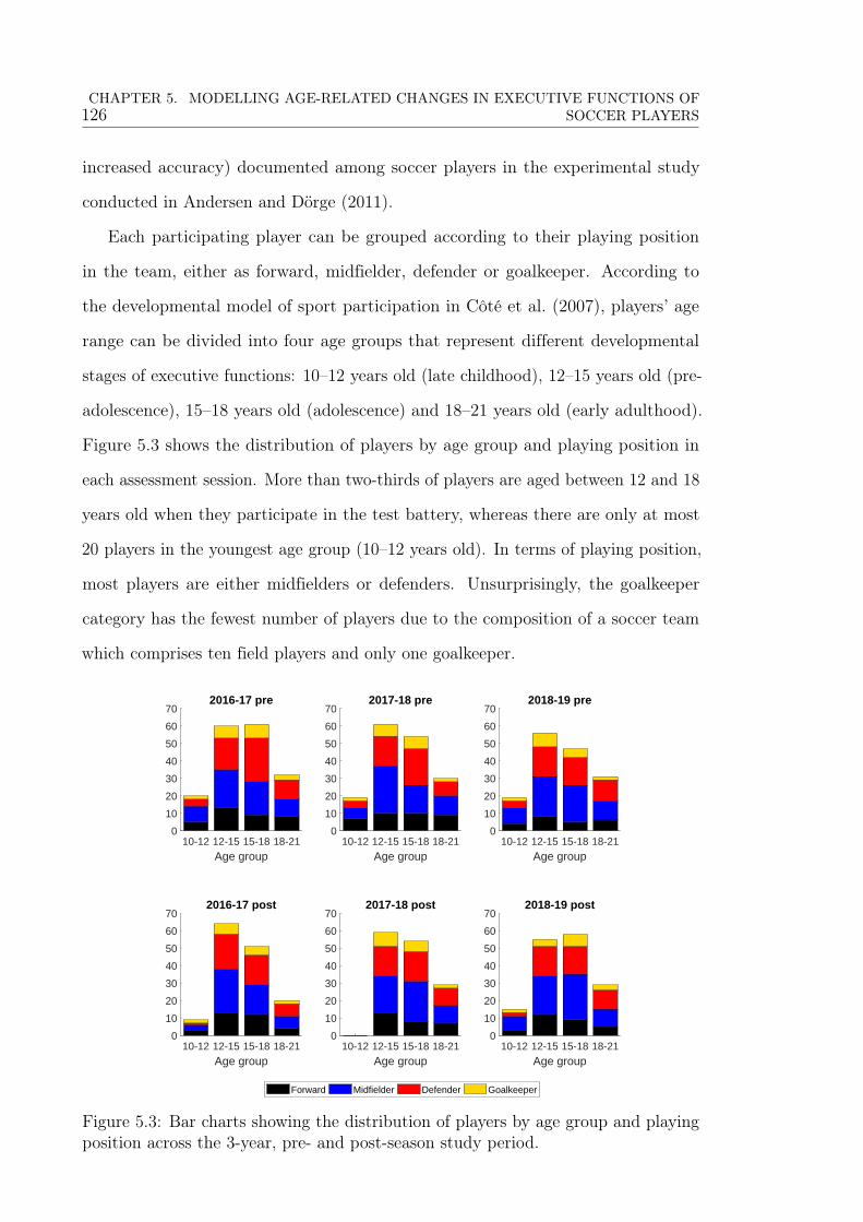
126CHAPTER 5. MODELLING AGE-RELATED CHANGES IN EXECUTIVE FUNCTIONS OF
SOCCER PLAYERS
increased accuracy) documented among soccer players in the experimental study
conducted in Andersen and Dörge (2011).
Each participating player can be grouped according to their playing position
in the team, either as forward, midfielder, defender or goalkeeper. According to
the developmental model of sport participation in Côté et al. (2007), players’ age
range can be divided into four age groups that represent different developmental
stages of executive functions: 10–12 years old (late childhood), 12–15 years old (pre-
adolescence), 15–18 years old (adolescence) and 18–21 years old (early adulthood).
Figure 5.3 shows the distribution of players by age group and playing position in
each assessment session. More than two-thirds of players are aged between 12 and 18
years old when they participate in the test battery, whereas there are only at most
20 players in the youngest age group (10–12 years old). In terms of playing position,
most players are either midfielders or defenders. Unsurprisingly, the goalkeeper
category has the fewest number of players due to the composition of a soccer team
which comprises ten field players and only one goalkeeper.
2016-17 pre
10-12 12-15 15-18 18-21Age group
0
10
20
30
40
50
60
70
2016-17 post
10-12 12-15 15-18 18-21Age group
0
10
20
30
40
50
60
70
2017-18 pre
10-12 12-15 15-18 18-21Age group
0
10
20
30
40
50
60
70
2017-18 post
10-12 12-15 15-18 18-21Age group
0
10
20
30
40
50
60
70
Forward Midfielder Defender Goalkeeper
2018-19 pre
10-12 12-15 15-18 18-21Age group
0
10
20
30
40
50
60
70
2018-19 post
10-12 12-15 15-18 18-21Age group
0
10
20
30
40
50
60
70
Figure 5.3: Bar charts showing the distribution of players by age group and playingposition across the 3-year, pre- and post-season study period.

5.2. BACKGROUND OF STUDY 127
Using the covariates available (assessment session and playing position), we
perform an exploratory analysis to examine whether there are systematic differences
in cognitive abilities between different groups of players. We demonstrate the general
underlying pattern with the example of log response time measurement y10 from
the Footbonaut test. Figure 5.4a shows the changes in mean value of y10 grouped
by playing position across the study period. The goalkeepers consistently improve
on their response time in the first four sessions, whereas the other field players’
performance fluctuates considerably. Goalkeepers also take the longest time to react
to the stimuli in the Footbonaut test. Visually, and on average, players react faster
in post-season assessment sessions within the same season, with a possible exception
of defenders in the 2016–17 season. This improvement in post-season cognitive
functioning can be attributed to the effect of active athletic participation (Jacobson
and Matthaeus, 2014). Overall, there is a general improvement in the response time
as the study progresses. However, it must be recognised that this positive shift in
performance level is likely to be confounded by the age of the players.
Figure 5.4b explores this age effect by showing differences in log response time
as a function of age, based on observations from the 2016–17 pre-season assess-
ment session (observations from other sessions produced similar graphs). The clear
16-17 pre 16-17 post 17-18 pre 17-18 post 18-19 pre 18-19 postAssessment session
0.75
0.8
0.85
0.9
0.95Forward Midfielder Defender Goalkeeper
(a) Changes in the grouped mean log re-sponse time measurement from the Footbo-naut test across the study period. Error barsindicate two standard errors of the mean.
10 15 20Age
0.7
0.8
0.9
1
(b) Scatterplot showing the relationship be-tween the log response time measurementfrom the Footbonaut test and the player age,in the 2016–17 pre-season assessment session.
Figure 5.4: Exploratory data analysis to examine performance variation betweenplayers that is due to assessment session, playing position and age.

128CHAPTER 5. MODELLING AGE-RELATED CHANGES IN EXECUTIVE FUNCTIONS OF
SOCCER PLAYERS
negative correlation underlines that performance heterogeneity between players is
age-dependent. Response time decreases significantly between ages 10 and 15, with a
reduced rate of improvement as players age further. The age effect also offers possible
explanation of two anomalies observed in Figure 5.4a: (i) post-season deterioration
in the defenders performance in the 2016–17 season and, (ii) a sharp reduction in
post-season response time for all players in the 2017–18 season. For the former, the
session effect is offset because there are fewer defenders in the older 15–18 and 18–21
age groups (see Figure 5.3) who tend to perform better and are able to improve
the group mean. For the latter, the age effect is amplified as there is no player
below 12 years old (see Figure 5.3), resulting in the mean response time values being
significantly lower.
5.3 Methods
Formal statistical modelling of the evolution of the players’ executive functions
requires consideration of the longitudinal nature of the study, as well as the fact
that cognitive performance is determined by a battery of different but correlated
neuropsychological assessments. Analysis of test outcomes is typically carried out
using a multivariate linear mixed effects model (e.g. Hall et al., 2001; Sliwinski et al.,
2003) whereby a unique mean latent growth trajectory that is representative of
the entire population is estimated for each measured outcome. However, Salthouse
et al. (1996) establish in an experimental study that age-related differences in the
observed psychometric outcomes are not exclusively attributable to assessment-
specific cognitive processes, but instead are the manifestation of a common cognitive
factor. Furthermore, the two-component characterisation of lifespan intellectual
development (Li et al., 2004) distinguishes between two distinct facets of cognitive
processes, namely fluid and crystallised abilities. The fluid abilities refer to biological
and genetically pre-disposed intelligence in information processing, whereas the
crystallised abilities relate to the normative and pragmatic aspects of expertise
acquired through contextualised personal experiences and socio-cultural influences.

5.3. METHODS 129
In the current context, the determination test, the response inhibition test and
the pre-cued choice response time task examine general intelligence, and thus can be
categorised as assessments that measure fluid (domain-generic) executive functions.
In contrast, the Helix and the Footbonaut are specialised test systems designed to
evaluate soccer-related skills that are developed through active participation in the
sport, thereby demonstrating their roles in measuring crystallised (domain-specific)
executive functions. Using this two-class grouping of neuropsychological assess-
ments, we introduce two latent curves, one shared between domain-generic variables
(y1, . . . , y7) and another shared between domain-specific variables (y8, y9, y10), within
a latent variable model (Dunson, 2000; Muthén, 2002; Proust et al., 2006). In the
following we describe a latent process representing age-related changes in executive
functions in a structural model. This model is then related to recorded outcomes of
the corresponding neuropsychological assessments through a measurement model.
5.3.1 The structural model
We model the latent curve underlying either of the two facets of executive func-
tions (domain-specific and domain-generic) according to a piecewise linear spline
model, which is a commonly used method in the epidemiological literature to model
longitudinal growth curves (e.g. Werner and Bodin, 2006; De Kroon et al., 2011;
Anderson et al., 2019; Chin et al., 2019). In the current setting, this models ζi ∈ R,
the unobserved executive functions for player i at age ωit, as
ζi(ωit) = β0i(ωit − (ωit − ξ1)+) + βKi(ωit − ξK)+ +K−1∑k=1
βki((ωit − ξk)+ − (ωit − ξk+1)+) + eit,
(5.1)
βi = (β0i, . . . , βKi)> ∼ N (µβ,Σβ), (5.2)
for i = 1, . . . , 304, where (a)+ = max{0, a} is the positive part of a, and ξ =
(ξ1, . . . , ξK)> is an ordered vector of K knots such that ξ1 < . . . < ξK . Here, t
measures time on the scale of the age of each individual, so that e.g. ζi(ωit) with

130CHAPTER 5. MODELLING AGE-RELATED CHANGES IN EXECUTIVE FUNCTIONS OF
SOCCER PLAYERS
ωit = 10 refers to executive functions of individual i when the individual is 10 years
old. In this way, (5.1) models the evolution of a player’s executive functions over time
(age) by K + 1 piecewise linear segments with breaks at ξ. Greater flexibility can be
achieved by introducing player-specific random change points, but here we fix ξ due to
the sparsity of the data. The vector of random slope coefficients βi = (β0i, . . . , βKi)>,
where βki represents the rate of change in ζi between knots ξk and ξk+1, allows for
the heterogeneity between players that is due to unobservables such as the number
of training hours and familiarity with the test. By assuming a Gaussian distribution
on the vector of random effects βi in (5.2), we postulate that the mean rate of
developmental growth in executive functions in the population is µβ, and that the
variability of player-specific deviations from this global trend is characterised by Σβ.
5.3.2 The measurement model
Write yd,it as the observed test outcome d for player i, on the t-th measurement
occasion, where i = 1, . . . , 304, t = 1, . . . , Ti and d = 1, . . . , 10. Assume for the
moment that each yd,it is a continuous measurement (this is relaxed below). Using a
latent variable model (e.g. Dunson, 2000; Muthén, 2002; Proust et al., 2006), we link
the unobserved executive functions to the outcome variable by
yd,it = αd + x>itγd + cd`ζi`(ωit) + εd,it, εit = (ε1,it, . . . , εD,it)> ∼ N (0,Σε), (5.3)
where αd is an intercept for test outcome d and xit is a vector of time-dependent
player-specific covariates associated with a vector of fixed effects γd for test d. The
recorded covariates for this study include a player’s playing position (forward, midfield,
defence or goalkeeper) and an indicator for post-season assessment measurements. In
this way, the covariates can vary in their effects on each test outcome d. The error
term εd,it is assumed to be uncorrelated with the exogenous variables xit and the
latent executive functions ζi. To incorporate the distinction between the two facets of
cognitive processes, we introduce an additional index ` ∈ {1, 2} on executive functions

5.3. METHODS 131
in (5.3) such that ` = 1 when d = 1, . . . , 7 refers to domain-generic functions, and
` = 2 when d = 8, . . . , 10 refers to domain-specific functions. As a result, the term
αd + cd`ζi`(ωit) stipulates a test-level linear rescaling (to account for scale differences
in the outcome variables) of either the domain-generic or domain-specific executive
functions, which is itself an individual-specific random effect around a population
mean as detailed in Section 5.3.1. In order for all model parameters to be identifiable,
one of the cd` = 1 for each value of `, i.e. cd1 = 1 for one d ∈ {1, . . . , 7} and cd2 = 1
for one d ∈ {8, . . . , 10}, and eit is restricted to a standard normal distribution N (0, 1).
Typically, the value of d for which cd` = 1 is chosen to be the measurement with the
largest scale so that the magnitude of cd` is less than 1 for other measurements.
Some of the measured outcomes are count variables, e.g. the number of correct
answers in the determination test. As a result, the assumption of normality on the
errors for these outcomes in (5.3) may be unsuitable. To account for this, we follow
Gelman et al. (2013) and transform the count variables into continuous outcomes
using the Gaussian kernel. In particular,
yd,it = h(y∗d,it), d ∈ {1, 5, 8, 9},
where h(·) is a rounding function such that h(y∗) = p if y∗ ∈ (ap, ap+1] for p =
0, . . . ,∞, a0 = −∞, and ap = p− 1, p = 1, . . . ,∞. The latent continuous variable
y∗d,it is then modelled following the measurement model in (5.3). As mentioned in
Section 5.2.6, the non-availability of certain neuropsychological assessments and data
management practices have resulted in the outcome vectors yit = (y1,it, . . . , yD,it)>
being partially observed. We overcome the missingness by fitting the model assuming
full data, and the missing values are sampled from their full conditional distributions
(which are the posterior predictive distributions) in the Bayesian sampling scheme.

132CHAPTER 5. MODELLING AGE-RELATED CHANGES IN EXECUTIVE FUNCTIONS OF
SOCCER PLAYERS
5.4 Analysis and results
We analyse the elite soccer player performance data through the above model
in the Bayesian framework, implemented via Markov chain Monte Carlo (Robert
and Casella, 2004). Following Côté et al. (2007), we consider the development of
executive functions in the four different stages of growth: late childhood (10–12
years old), pre-adolescence (12–15 years old), adolescence (15–18 years old) and
early adulthood (18–21 years old). Accordingly, the three knot locations (K = 3)
in the piecewise linear spline model in (5.1) are specified as ξ = (12, 15, 18)>. For
prior distributions, we specify a horseshoe prior (Makalic and Schmidt, 2016) on µβ
and γd, d = 1, . . . , 10, which is designed to have concentration at zero and to shrink
small coefficients towards zero, while having heavy tails to avoid over-shrinkage of
larger coefficients, a hierarchical inverse-Wishart prior (Huang and Wand, 2013)
with 2 degrees of freedom and scale parameter 25 on Σβ and Σε to induce a sparse
structure on the partial correlation matrices (Chin et al., 2020), and a standard
diffuse N (0, 103) prior on each αd.
For parameter identifiability, we set the scale coefficients for the number of correct
answers in the determination test and the Helix test equal to one (i.e. c11 = c81 = 1).
These were chosen as y1 and y8 have the largest scales among the variables measuring
the two facets of executive functions, and so this ensures that each of the other
cd` will typically scale around or less than 1 in magnitude. We expect a priori
that assessment tasks associated with the same type of assessment type (speed or
accuracy) are likely to be positively correlated, but that tasks are likely negatively
correlated between these two groups. This is largely in evidence in Figure 5.2. Since
both y1 and y8 are accuracy components, we specify an informative N (0.5, 0.25) prior
on cd` if measurement d also relates to an accuracy component of the assessment
(y5, y9) to express the prior belief that cd` is likely to be a value between 0 and 1.
Conversely, a N (−0.5, 0.25) prior is used if the measurement relates to log speed
(y2, y3, y4, y6, y7, y10).

5.4. ANALYSIS AND RESULTS 133
Figure 5.5 shows the estimated mean trajectories of domain-generic and domain-
specific executive functions for a chosen sample of players, and compares them to
the population mean whose 95% highest posterior density (HPD) credible levels
are represented by shaded regions. For simplicity, these trajectories are based on
the number of correct answers scored in the determination test (domain-generic)
and the Helix test (domain-specific) whereby the scale factor cd` is assumed a fixed
value of 1. Our estimation results indicate that changes in executive functions of
the elite soccer player population occur mainly between 10 to 15 years old since the
magnitudes of the slopes within this age range are the largest. In particular, the most
rapid increase happens during late childhood (10–12 years old) for domain-generic
executive functions (an average rate of 28.59, which is marginally higher than the
value of 24.86 in the next period), whereas the most rapid increase happens during
pre-adolescence (12–15 years old) for domain-specific executive functions (an average
rate of 0.95, which is nearly twice as large as the value of 0.48 in late childhood).
Domain-generic executive functions continue to develop, albeit at a much slower
Figure 5.5: Domain-generic (left) and domain-specific (right) executive functions fora sample of players plotted against the posterior mean trajectories of the population,based on the accuracy of the determination test and the Helix test respectively. 95%HPD credible intervals of the population mean trajectories are given by the greyshaded regions.

134CHAPTER 5. MODELLING AGE-RELATED CHANGES IN EXECUTIVE FUNCTIONS OF
SOCCER PLAYERS
pace, during adolescence (an average rate of 6.51) and early adulthood (an average
rate of 8.52). This observation is consistent with the findings in Diamond (2002),
which argues that performance in domain-generic executive functions reaches adult
performance levels between 12 to 15 years old.
Given that maturation in domain-specific executive functions is largely conditioned
by occupational expertise (Li et al., 2004), it could be hypothesised that improvements
in soccer-related abilities will be reflected in the trajectory across all developmental
stages as players are continuously challenged to refine their skills in order to remain
competitive (Mann et al., 2007). However, our results show that the increase in
domain-specific executive functions is almost negligible after 15 years old (average
rates of 0.11 and 0.07 during adolescence and early adulthood respectively). A
possible explanation for the observed plateau is that both domain-generic and
domain-specific assessments used in our study do not necessarily represent the way
in which perception and action of competition are coupled in soccer (Pinder et al.,
2011). For example, while the Footbonaut test has some validity for measuring
soccer skills, it requires players to use passing actions to react to visual and auditory
stimuli that are unrelated to soccer (Beavan et al., 2019). Meanwhile, the Helix
test measures high-level perceptual abilities specific to soccer but its design lacks an
action component. Therefore, it is unsurprising that the expected positive association
between domain-specific executive functions and age as a proxy for soccer experience
is not observed.
When inspecting the posterior distribution of the dependence structures in Σβ
(results not shown), we find that the slopes of the piecewise linear spline model
are independent of each other and across both facets of executive functions. This
suggests that previous studies which are based on cross-sectional data (Verburgh
et al., 2014; Huijgen et al., 2015; Vestberg et al., 2017; Sakamoto et al., 2018) may
have overstated the usefulness of domain-generic executive functions in soccer talent
identification. This is because a strong relationship between both types of executive
functions should exist if domain-generic executive functions are a prognostic tool for

5.4. ANALYSIS AND RESULTS 135
soccer performance. A sample of four players are chosen and shown in Figure 5.5 to
illustrate this argument. We observe that players A and B demonstrate an above-
average level of domain-generic executive functions but fail to reproduce similar
level of superiority in soccer-specific assessments. On the other hand, player D who
has less developed domain-generic executive functions compared to the population
mean outperforms his peers in terms of soccer expertise. Player D also achieve a
comparable level of domain-specific executive functions to that of player C although
the latter performs better in the generic abilities test battery.
We now examine the impact of the covariates on each outcome variable in the test
battery. Table 5.2 shows the regression coefficient posterior mean estimates for the
assessment session and playing position. The players tend to have better response
times (y2, y3, y6, y7) in domain-generic tasks during post-season assessment sessions,
indicating that there is an acute effect of soccer participation on performance in these
assessments. The absence of positional effects in the Helix test further reinforces
our previous argument that its design may not have adequately coupled perceptual
information with soccer-specific actions. We also observe that goalkeepers generally
perform the worst in the Footbonaut test in terms of the response time y10 (i.e. players
in the other positions respond much faster). This is because as part of their training,
Variable Intercept Post-season Forward Midfielder Defendery1 141.08 1.43 0.00 0.00 −0.01
y2 0.01 −0.03 0.00 0.00 0.00
y3 −1.26 −0.09 0.00 −0.04 0.00y4 −0.64 −0.02 0.00 0.00 0.00
y5 81.85 −0.22 0.06 0.02 −0.34
y6 −0.49 −0.04 0.00 0.00 0.00y7 −0.44 −0.04 0.00 0.00 0.00
y8 28.44 0.01 −0.02 0.02 0.00
y9 22.93 0.15 −0.60 0.23 0.27y10 1.03 −0.01 −0.05 −0.06 −0.04
Table 5.2: Estimated posterior means of regression coefficients γd for the covariatesfor each outcome variable. Parameters whose 95% HPD credible interval does notinclude 0 are highlighted in grey.

136CHAPTER 5. MODELLING AGE-RELATED CHANGES IN EXECUTIVE FUNCTIONS OF
SOCCER PLAYERS
goalkeepers tend not to train receiving, control and passing of the ball to the same
extent as players in other positions. As a result, we can conclude that the Footbonaut
test represents a more useful measure of performance for field players rather than for
goalkeepers.
5.5 Conclusion
This chapter has explored the relationship between age and executive functions in
an athlete population by modelling the cognitive outcomes from a test battery of
neuropsychological assessments performed by elite soccer players in a longitudinal
study using a latent variable model (Dunson, 2000; Muthén, 2002; Proust et al., 2006).
The findings of previous research on the developmental trajectories of executive
functions were drawn from cross-sectional studies (Verburgh et al., 2014; Huijgen
et al., 2015; Sakamoto et al., 2018), and to the best of our knowledge, this is the
first study of its kind in the sport science literature that is based on longitudinal
data. The latent growth curve representing the unobserved executive functions is
modelled to evolve in a piecewise linear fashion across time using a random effects
model, and is linked to the observed outcomes via a measurement model. Following
the argument in Li et al. (2004), we differentiate between fluid (domain-generic)
and crystallised (domain-specific) executive functions, where the former develops
biologically while the latter is acquired through occupational experience. This allows
us to make a comparison between their trajectories across different stages of growth
development (Côté et al., 2007). Rather than examining both types of executive
functions independently as what is commonly done in the literature (Furley and
Wood, 2016), we model them jointly in a multivariate formulation to investigate
if the claims made on the importance of domain-generic executive functions as a
prognostic tool for excellence in soccer can be substantiated.
Our analysis shows that both facets of executive functions exhibit a rapid increase
between 10 to 15 years old, and while domain-generic executive functions continue to
develop at a much slower rate, domain-specific executive functions begin to plateau

5.5. CONCLUSION 137
after that. The latter observation is in contrary to popular belief that soccer players
who excel in competitive settings tend to possess more developed technical abilities
shaped by their playing experience. However, the lack of evidence supporting this
expectation in our study could possibly be due to the failure of the assessment
design to reproduce the perception-action couplings experienced by players during
an actual match (Pinder et al., 2011). We also find no substantial dependencies
in the rate of developmental growth between domain-generic and domain-specific
executive functions, thereby contradicting the findings of earlier studies (Vestberg
et al., 2012; Verburgh et al., 2014; Sakamoto et al., 2018) and weakening the argument
that domain-generic executive functions provide useful information for soccer talent
identification. The longitudinal nature of the study allows our modelling approach to
control for unobserved heterogeneity such as the number of training hours (Huijgen
et al., 2015), and hence providing a closer representation of the underlying mechanistic
development in cognitive abilities.
Considering the results that we have presented, it is clear to conclude that
integrating neuropsychological test battery in soccer talent identification programmes
is likely a debatable topic given that no interaction is established between domain-
generic and domain-specific executive functions. Furthermore, a comprehensive study
on the reliability of each neuropsychological assessment in the test battery should be
undertaken to validate their use (Dicks et al., 2009), especially if the results of these
tests are used pervasively.

138CHAPTER 5. MODELLING AGE-RELATED CHANGES IN EXECUTIVE FUNCTIONS OF
SOCCER PLAYERS

Chapter 6
Summary and discussion
Chapter 3 presents an analysis of the decision-making of Australian general practition-
ers (GPs) in an experiment which is designed to mimic the choice problem faced in a
medical consultation, where the GPs need to match a set of contraceptive products
with a particular female patient. A graphical model representing the dependence
structure of the latent variables indicating the observed binary outcomes, identifies
products which are perceived to be substitutes and can be used in place of one
another. Conditional on the observable characteristics of the patient, the remaining
dependencies captured by the GP-specific random effects characterise the persistence
of GPs in discussing a particular product in ready-to-wear choices (norms that work
well for a broad class of patients). The latter dependence structure suggests evidence
of medical practice variation (Wennberg et al., 1982; Scott and Shiell, 1997; Davis
et al., 2000) among the GPs which is largely attributed to their age, gender and
qualifications. This phenomenon is likely to be one of the contributing factors to the
low uptake of long acting reversible contraceptive methods in Australia (Black et al.,
2013), as demonstrated by the varied views among the GPs on the suitability of long
acting contraceptive choices in a simulated case.
Motivated by the application example which is modelled using a multivariate
probit model, we provide an efficient method for sampling the potentially high
dimensional correlation matrix Rε for the dependence structure of the variables.

140 CHAPTER 6. SUMMARY AND DISCUSSION
The correlation matrix Rε is reparameterised as an unconstrained lower triangular
Cholesky factor which is then sampled using the Hamiltonian Monte Carlo algorithm
(Duane et al., 1987; Neal, 2011). Bayesian inference often relies on Markov chain
Monte Carlo algorithms to generate samples from the posterior distribution. However,
these samples tend to be positively correlated and in turn increase the variability of
Monte-Carlo based estimators. To address this issue, we propose an antithetic sampler,
which generates proposals in the Metropolis-Hastings algorithm deterministically. In
order to obtain an ergodic Markov chain, the antithetic sampler must be coupled
with a stochastic update of the other parameters. Our results show that significant
improvement is observed in the performance measure and some parameters achieve
super-efficiency. While we illustrate the efficiency of the antithetic sampler on an
example of a highly correlated bivariate normal distribution and the multivariate
probit model, an extension to more general settings or models is worth future research.
In addition, establishing the convergence properties of the antithetic sampler would
certainly enhance our empirical results.
Chapter 4 investigates faltering growth among young children that is endemic in
low to medium income countries. Faltered growth is generally defined as a slower
rate of growth compared to a reference healthy population of the same age and
gender. As faltering is closely associated with reduced physical, intellectual (Benítez-
Bribiesca et al., 1999) and economic productivity potential (Hoddinott et al., 2013),
it is important to identify faltered children and be able to characterise different
growth patterns, as each type represents a particular growth behaviour and so
merits a target-specific medical treatment (Collins et al., 2006). We use a multiclass
classification approach by approximating the smooth growth curves by piecewise
linear segments with random slopes using the broken stick model (Ruppert et al.,
2003). The heterogeneity in the growth velocity between children is captured by
allowing the random slopes of the broken stick model to be distributed according to
a mixture distribution. Therefore, the mixture component from which the vector of
random slopes is generated dictates the clustering of growth profiles into different

141
classes, as in the formulation of a Gaussian mixture model. However, specifying the
number of mixture components G is non-trivial, and fitting separate models with
different values of G is ad-hoc and ignores uncertainty in the model. This is overcome
by adopting a Bayesian non-parametric approach using the Dirichlet process (DP;
Ferguson, 1973) prior. Subscribing to this framework allows the complexity of the
model, i.e. the value of G, to be entirely data-driven since the DP prior exhibits
clustering a priori. Furthermore, we flexibly extend the broken stick model to ensure
that the model remains a sensible approach in practice where children are likely to
react differently to treatment interventions. In this extension, we relax the fixed knot
locations of the broken stick model to allow for child-specific random change points.
The change points are modelled probabilistically using a modified even-numbered
order statistics distribution (Green, 1995) so that there is exactly one knot in each
subinterval of equal length over the observational period. Simulation results show
that the broken stick model with fixed knots produces a biased estimate of the
random slopes, which subsequently leads to an overestimation of G.
In our work, classification performed on 373 children aged between 0 and 1 from
a longitudinal study from the Healthy Birth, Growth and Development knowledge
integration (HBGDki) project suggests 9 different growth trajectory patterns. A
majority of the children experience faltering growth between birth and age one.
Further exploratory analysis suggests that certain growth patterns are more likely
to be dominated by a particular gender or maternal education level. Children
who experience severe faltering are also found to have lower IQ scores. It would
be interesting to investigate whether such patterns are observed in other studies
in the HBGDki project. Although the broken stick model provides a reasonable
approximation of the growth curves, it requires specifying the number of (fixed or
random) knots in advance, which is often unknown in practical applications. One
possible extension is to consider an infinite mixture of Gaussian processes by unifying
the DP and Gaussian processes. Conceptually, the Gaussian process models each
curve non-parametrically without having to pre-specify the number of knots, while the
142 CHAPTER 6. SUMMARY AND DISCUSSION
DP classifies the functionals generated from the Gaussian process. This extends the
present framework of DP to functional data setting, whereby a probability measure
is now defined on a function space so that a random draw from the functional DP is
a smooth function that provides a better approximation to growth curves.
Finally, Chapter 5 aims to gain further insights into the developmental trajectories
of executive functions over the playing time of a soccer player. Executive functions
are complex cognitive abilities which allow an individual to reason, plan actions
and execute strategies to achieve a goal (Grafman and Litvan, 1999; Burgess et al.,
2000; Chan et al., 2008). Contemporary research based on cross-sectional data
has generally supported the hypothesis that executive functions can be used as a
variable in predicting the prospective performance of a soccer player (Verburgh et al.,
2014; Huijgen et al., 2015; Sakamoto et al., 2018), and thus they serve as good
measures in identifying young talented players. However, longitudinal studies of the
developmental trajectories of executive functions across different stages of life in an
athlete population are lacking in the literature and previous results were established
for a general population (Zelazo et al., 2004; Huizinga and Smidts, 2010; Zelazo and
Carlson, 2012). Recent research has shown that active participation in sports has
a positive impact on executive functioning (Jacobson and Matthaeus, 2014), and
therefore the generalisation of existing results to an athlete population is limited. We
address this problem by analysing longitudinal data that examines executive functions
of male soccer players representing a professional German Bundesliga club through
a series of neuropsychological assessments, which to the best of our knowledge, is
the most comprehensive set of data available in the sport science literature. These
assessments can be broadly classified into two different categories depending on the
facet of executive functions that they measure. Domain-generic assessments measure
the level of general intelligence, whereas domain-specific assessments measure the
skilfulness of the players acquired through active participation in the sport (Li et al.,
2004). Using a latent variable model (Dunson, 2000; Proust et al., 2006), these two
facets of executive functions are modelled as unobservable curves to reflect their

143
latency, and their manifestation is related to the corresponding cognitive outcome
through a measurement model.
The analysis results show that domain-specific executive functions of the players
do not change significantly between the age of 15 and 21 years old. This suggests
that the design of the domain-specific assessments may not be specialised enough to
test soccer-related skills (Pinder et al., 2011) or that these skills may be irrelevant
for soccer expertise (Beavan et al., 2019). Furthermore, no dependence structure is
observed between both facets of executive functions, which disproves earlier findings
on the usefulness of domain-generic executive functions in soccer talent identification
(Verburgh et al., 2014; Huijgen et al., 2015; Vestberg et al., 2017; Sakamoto et al.,
2018). The findings that we obtained can be further reinforced if more data is
available or the study is carried out over a longer time period. It would also be
interesting to investigate the relationship between executive functions and career
attainment by having more delineated variables recorded. Additionally, an extensive
examination on the reliability and accuracy of each neuropsychological assessment
in the test battery should be undertaken to validate their use (Dicks et al., 2009),
especially if the results of these tests are used in any major decision-making process.

144 CHAPTER 6. SUMMARY AND DISCUSSION

Bibliography
Abraham, C., P.-A. Cornillon, E. Matzner-Løber, and N. Molinari (2003). Unsuper-
vised curve clustering using B-splines. Scandinavian Journal of Statistics 30 (3),
581–595.
Adler, S. L. (1981). Over-relaxation method for the Monte Carlo evaluation of
the partition function for multiquadratic actions. Physical Review D 23 (12),
2901–2904.
Albert, J. H. and S. Chib (1993). Bayesian analysis of binary and polychotomous
response data. Journal of the American Statistical Association 88 (422), 669–679.
Alderson, R. M., M. D. Rapport, and M. J. Kofler (2007). Attention-
deficit/hyperactivity disorder and behavioral inhibition: a meta-analytic review of
the stop-signal paradigm. Journal of Abnormal Child Psychology 35 (5), 745–758.
Alvarez, J. A. and E. Emory (2006). Executive function and the frontal lobes: A
meta-analytic review. Neuropsychology Review 16 (1), 17–42.
Andersen, T. B. and H. C. Dörge (2011). The influence of speed of approach and
accuracy constraint on the maximal speed of the ball in soccer kicking. Scandinavian
Journal of Medicine & Science in Sports 21 (1), 79–84.
Anderson, C., R. Hafen, O. Sofrygin, L. Ryan, and HBGDki Community (2019).
Comparing predictive abilities of longitudinal child growth models. Statistics in
Medicine 38 (19), 3555–3570.

146 BIBLIOGRAPHY
Antoniak, C. E. (1974). Mixtures of Dirichlet processes with applications to Bayesian
nonparametric problems. Annals of Statistics 2 (6), 1152–1174.
Ashford, J. and R. Sowden (1970). Multivariate probit analysis. Biometrics 26 (3),
535–546.
Baltes, P. B. and U. Lindenberger (1997). Emergence of a powerful connection
between sensory and cognitive functions across the adult life span: A new window
to the study of cognitive aging? Psychology and Aging 12 (1), 12–21.
Bardenet, R., A. Doucet, and C. Holmes (2017). On Markov chain Monte Carlo
methods for tall data. Journal of Machine Learning Research 18 (1), 1515–1557.
Barela, J. A., A. A. Rocha, A. R. Novak, J. Fransen, and G. A. Figueiredo (2019).
Age differences in the use of implicit visual cues in a response time task. Brazilian
Journal of Motor Behavior 13 (2), 86–93.
Barnard, J., R. McCulloch, and X.-L. Meng (2000). Modeling covariance matrices
in terms of standard deviations and correlations, with application to shrinkage.
Statistica Sinica 10 (4), 1281–1311.
Barone, P. and A. Frigessi (1990). Improving stochastic relaxation for Gaussian
random fields. Probability in the Engineering and Informational Sciences 4 (3),
369–389.
Bassuk, S. S. and J. E. Manson (2005). Epidemiological evidence for the role of
physical activity in reducing risk of type 2 diabetes and cardiovascular disease.
Journal of Applied Physiology 99 (3), 1193–1204.
Baur, H., S. Müller, A. Hirschmüller, G. Huber, and F. Mayer (2006). Reactivity,
stability, and strength performance capacity in motor sports. British Journal of
Sports Medicine 40 (11), 906–911.

BIBLIOGRAPHY 147
Beavan, A., J. Fransen, J. Spielmann, J. Mayer, S. Skorski, and T. Meyer (2019). The
Footbonaut as a new football-specific skills test: Reproducibility and age-related
differences in highly trained youth players. Science and Medicine in Football 3 (3),
177–182.
Beavan, A., J. Spielmann, J. Mayer, S. Skorski, T. Meyer, and J. Fransen (2020).
The rise and fall of executive functions in high-level football players. Psychology
of Sport and Exercise 49, 101677.
Beavan, A. F., J. Spielmann, J. Mayer, S. Skorski, T. Meyer, and J. Fransen (2019).
Age-related differences in executive functions within high-level youth soccer players.
Brazilian Journal of Motor Behavior 13 (2), 64–75.
Benítez-Bribiesca, L., I. De la Rosa-Alvarez, and A. Mansilla-Olivares (1999). Den-
dritic spine pathology in infants with severe protein-calorie malnutrition. Pedi-
atrics 104 (2), e21.
Berlin, K. S., G. R. Parra, and N. A. Williams (2014). An introduction to latent
variable mixture modeling (part 2): Longitudinal latent class growth analysis and
growth mixture models. Journal of Pediatric Psychology 39 (2), 188–203.
Best, J. R. and P. H. Miller (2010). A developmental perspective on executive
function. Child Development 81 (6), 1641–1660.
Betancourt, M. (2017). A conceptual introduction to Hamiltonian Monte Carlo.
arXiv preprint arXiv:1701.02434.
Bierkens, J., P. Fearnhead, and G. Roberts (2019). The zig-zag process and super-
efficient sampling for Bayesian analysis of big data. Annals of Statistics 47 (3),
1288–1320.
Birren, J. E. and L. M. Fisher (1995). Aging and speed of behavior: Possible
consequences for psychological functioning. Annual Review of Psychology 46 (1),
329–353.

148 BIBLIOGRAPHY
Black, K. I., D. Bateson, and C. Harvey (2013). Australian women need increased
access to long-acting reversible contraception. Medical Journal of Australia 199 (5),
317–318.
Blackwell, D. and J. B. MacQueen (1973). Ferguson distributions via Pólya urn
schemes. Annals of Statistics 1 (2), 353–355.
Blumenthal, P., A. Voedisch, and K. Gemzell-Danielsson (2011). Strategies to prevent
unintended pregnancy: Increasing use of long-acting reversible contraception.
Human Reproduction Update 17 (1), 121–137.
Bollen, K. A. and P. J. Curran (2006). Latent Curve Models: A Structural Equation
Perspective. John Wiley & Sons.
Bouveyron, C., S. Girard, and C. Schmid (2007). High-dimensional data clustering.
Computational Statistics & Data Analysis 52 (1), 502–519.
Bouveyron, C. and J. Jacques (2011). Model-based clustering of time series in group-
specific functional subspaces. Advances in Data Analysis and Classification 5 (4),
281–300.
Brooks, S. and A. Gelman (1998). Some issues in monitoring convergence of iterative
simulations. In Proceedings of the Section on Statistical Computing, pp. 148–188.
Buchmueller, T. C., D. G. Fiebig, G. Jones, and E. Savage (2013). Preference
heterogeneity and selection in private health insurance: The case of Australia.
Journal of Health Economics 32 (5), 757–767.
Burgess, P. W., E. Veitch, A. de Lacy Costello, and T. Shallice (2000). The cognitive
and neuroanatomical correlates of multitasking. Neuropsychologia 38 (6), 848–863.
Carvalho, C. M., N. G. Polson, and J. G. Scott (2010). The horseshoe estimator for
sparse signals. Biometrika 97 (2), 465–480.
Casella, G. and C. P. Robert (1996). Rao-Blackwellisation of Sampling Schemes.
Biometrika 83 (1), 81–94.

BIBLIOGRAPHY 149
Celeux, G., M. Hurn, and C. P. Robert (2000). Computational and inferential
difficulties with mixture posterior distributions. Journal of the American Statistical
Association 95 (451), 957–970.
Cepeda, N. J., A. F. Kramer, and J. Gonzalez de Sather (2001). Changes in
executive control across the life span: Examination of task-switching performance.
Developmental Psychology 37 (5), 715–730.
Chan, R. C., D. Shum, T. Toulopoulou, and E. Y. Chen (2008). Assessment of
executive functions: Review of instruments and identification of critical issues.
Archives of Clinical Neuropsychology 23 (2), 201–216.
Chib, S. and E. Greenberg (1998). Analysis of multivariate probit models.
Biometrika 85 (2), 347–361.
Chin, V., D. Gunawan, D. G. Fiebig, R. Kohn, and S. A. Sisson (2020). Efficient
data augmentation for multivariate probit models with panel data: An application
to general practitioner decision making about contraceptives. Journal of the Royal
Statistical Society: Series C (Applied Statistics) 69 (2), 277–300.
Chin, V., J. Y. L. Lee, L. M. Ryan, R. Kohn, and S. A. Sisson (2019). Multiclass
classification of growth curves using random change points and heterogeneous
random effects. arXiv preprint arXiv:1909.07550.
Clyde, M. and E. I. George (2004). Model uncertainty. Statistical Science 19 (1),
81–94.
Cole, T. (1998). Presenting information on growth distance and conditional velocity
in one chart: Practical issues of chart design. Statistics in Medicine 17 (23),
2697–2707.
Collins, S., N. Dent, P. Binns, P. Bahwere, K. Sadler, and A. Hallam (2006).
Management of severe acute malnutrition in children. The Lancet 368 (9551),
1992–2000.

150 BIBLIOGRAPHY
Côté, J., J. Baker, and B. Abernethy (2007). Practice and play in the development
of sport expertise. In G. Tenenbaum and R. C. Eklund (Eds.), Handbook of Sport
Psychology (3rd ed.)., Chapter 8, pp. 184–202. John Wiley & Sons.
Cox, S. M., D. J. Cox, M. J. Kofler, M. A. Moncrief, R. J. Johnson, A. E. Lambert,
S. A. Cain, and R. E. Reeve (2016). Driving simulator performance in novice
drivers with autism spectrum disorder: The role of executive functions and basic
motor skills. Journal of Autism and Developmental Disorders 46 (4), 1379–1391.
Creutz, M. (1987). Overrelaxation and Monte Carlo simulation. Physical Review
D 36 (2), 515–519.
Crozier, S. R., W. Johnson, T. J. Cole, C. Macdonald-Wallis, G. Muniz-Terrera, H. M.
Inskip, and K. Tilling (2019). A discussion of statistical methods to characterise
early growth and its impact on bone mineral content later in childhood. Annals of
Human Biology 46 (1), 17–26.
da Silva, A. R. F. (2007). A Dirichlet process mixture model for brain MRI tissue
classification. Medical Image Analysis 11 (2), 169–182.
Daniels, M. J. and M. Pourahmadi (2009). Modeling covariance matrices via partial
autocorrelations. Journal of Multivariate Analysis 100 (10), 2352–2363.
Darroch, J. E., G. Sedgh, and H. Ball (2011). Contraceptive technologies: Responding
to women’s needs. New York: Guttmacher Institute.
Dasgupta, A. and A. E. Raftery (1998). Detecting features in spatial point processes
with clutter via model-based clustering. Journal of the American Statistical
Association 93 (441), 294–302.
Davis, P., B. Gribben, A. Scott, and R. Lay-Yee (2000). The “supply hypothesis” and
medical practice variation in primary care: Testing economic and clinical models
of inter-practitioner variation. Social Science & Medicine 50 (3), 407–418.

BIBLIOGRAPHY 151
De Kroon, M. L., C. M. Renders, J. P. Van Wouwe, R. A. Hirasing, and S. Van Buuren
(2011). Identifying young children without overweight at high risk for adult
overweight: The Terneuzen Birth Cohort. International Journal of Pediatric
Obesity 6, e187–e195.
Delaigle, A. and P. Hall (2010). Defining probability density for a distribution of
random functions. Annals of Statistics 38 (2), 1171–1193.
Dellaportas, P. and I. Kontoyiannis (2012). Control variates for estimation based on
reversible Markov chain Monte Carlo samplers. Journal of the Royal Statistical
Society: Series B (Statistical Methodology) 74 (1), 133–161.
Dempster, F. N. (1992). The rise and fall of the inhibitory mechanism: Toward a
unified theory of cognitive development and aging. Developmental Review 12 (1),
45–75.
Diamond, A. (2002). Normal development of prefrontal cortex from birth to young
adulthood: Cognitive functions, anatomy, and biochemistry. In D. T. Stuss and
R. T. Knight (Eds.), Principles of Frontal Lobe Function, pp. 466–503. Oxford
University Press.
Diamond, A. (2013). Executive functions. Annual Review of Psychology 64, 135–168.
Dicks, M., K. Davids, and C. Button (2009). Representative task design for the study
of perception and action in sport. International Journal of Sport Psychology 40 (4),
506.
Doucet, A., M. K. Pitt, G. Deligiannidis, and R. Kohn (2015). Efficient implementa-
tion of Markov chain Monte Carlo when using an unbiased likelihood estimator.
Biometrika 102 (2), 295–313.
Draper, D. (1995). Assessment and propagation of model uncertainty. Journal of
the Royal Statistical Society: Series B (Statistical Methodology) 57 (1), 45–70.

152 BIBLIOGRAPHY
Duane, S., A. D. Kennedy, B. J. Pendleton, and D. Roweth (1987). Hybrid Monte
Carlo. Physics Letters B 195 (2), 216–222.
Duncan, T. E., S. C. Duncan, and M. Stoolmiller (1994). Modeling developmental pro-
cesses using latent growth structural equation methodology. Applied Psychological
Measurement 18 (4), 343–354.
Duncan, T. E., S. C. Duncan, and L. A. Strycker (2013). An Introduction to Latent
Variable Growth Curve Modeling: Concepts, Issues, and Application (2nd ed.).
Quantitative Methodology. Routledge Academic.
Dunson, D. B. (2000). Bayesian latent variable models for clustered mixed outcomes.
Journal of the Royal Statistical Society: Series B (Statistical Methodology) 62 (2),
355–366.
Dunson, D. B. (2003). Dynamic latent trait models for multidimensional longitudinal
data. Journal of the American Statistical Association 98 (463), 555–563.
Edwards, Y. D. and G. M. Allenby (2003). Multivariate analysis of multiple response
data. Journal of Marketing Research 40 (3), 321–334.
Emond, A. M., P. S. Blair, P. M. Emmett, and R. F. Drewett (2007). Weight faltering
in infancy and IQ levels at 8 years in the Avon Longitudinal Study of Parents and
Children. Pediatrics 120 (4), e1051–e1058.
Escobar, M. D. and M. West (1995). Bayesian density estimation and inference using
mixtures. Journal of the American Statistical Association 90 (430), 577–588.
Fan, Y., J.-L. Dortet-Bernadet, and S. Sisson (2010). On Bayesian curve fitting
via auxiliary variables. Journal of Computational and Graphical Statistics 19 (3),
626–644.
Fédération Internationale de Football Association (FIFA) (2018). FIFA Activity
Report 2018. Retrieved from: https://resources.fifa.com/image/upload/
yjibhdqzfwwz5onqszo0.pdf.

BIBLIOGRAPHY 153
Ferguson, T. S. (1973). A Bayesian analysis of some nonparametric problems. Annals
of Statistics 1 (2), 209–230.
Ferraty, F. and P. Vieu (2006). Nonparametric Functional Data Analysis: Theory
and Practice. Springer Series in Statistics. Springer Science & Business Media.
Fiebig, D. G., R. Viney, S. Knox, M. Haas, D. J. Street, A. R. Hole, E. Weisberg,
and D. Bateson (2017). Consideration sets and their role in modelling doctor
recommendations about contraceptives. Health Economics 26 (1), 54–73.
Frank, R. G. and R. J. Zeckhauser (2007). Custom-made versus ready-to-wear
treatments: Behavioral propensities in physicians’ choices. Journal of Health
Economics 26 (6), 1101–1127.
Fritsch, A. (2012). mcclust: Process an MCMC Sample of Clusterings. R package
version 1.0.
Fritsch, A. and K. Ickstadt (2009). Improved criteria for clustering based on the
posterior similarity matrix. Bayesian Analysis 4 (2), 367–391.
Frühwirth-Schnatter, S. (2006). Finite Mixture and Markov Switching Models.
Springer Series in Statistics. Springer Science & Business Media.
Fúquene, J., M. Steel, and D. Rossell (2019). On choosing mixture components via
non-local priors. Journal of the Royal Statistical Society: Series B (Statistical
Methodology) 81 (5), 809–837.
Furley, P. and G. Wood (2016). Working memory, attentional control, and expertise
in sports: A review of current literature and directions for future research. Journal
of Applied Research in Memory and Cognition 5 (4), 415–425.
Ge, H., Y. Chen, M. Wan, and Z. Ghahramani (2015). Distributed inference for
Dirichlet process mixture models. In F. Bach and D. Blei (Eds.), International
Conference on Machine Learning, pp. 2276–2284.

154 BIBLIOGRAPHY
Gelfand, A. E. and A. F. Smith (1990). Sampling-based approaches to calculating
marginal densities. Journal of the American Statistical Association 85 (410),
398–409.
Gelman, A. (2006). Prior distributions for variance parameters in hierarchical models.
Bayesian Analysis 1 (3), 515–534.
Gelman, A., J. B. Carlin, H. S. Stern, D. B. Dunson, A. Vehtari, and D. B. Rubin
(2013). Bayesian Data Analysis (3rd ed.). Texts in Statistical Science Series. CRC
Press.
Gelman, A., Y. Goegebeur, F. Tuerlinckx, and I. Van Mechelen (2000). Diagnostic
checks for discrete data regression models using posterior predictive simulations.
Journal of the Royal Statistical Society: Series C (Applied Statistics) 49 (2), 247–
268.
Gelman, A. and D. B. Rubin (1992). Inference from iterative simulation using
multiple sequences. Statistical Science 7 (4), 457–472.
Gelman, A. and D. B. Rubin (1995). Avoiding model selection in Bayesian social
research. Sociological Methodology 25, 165–173.
Geman, S. and D. Geman (1984). Stochastic relaxation, Gibbs distributions, and
the Bayesian restoration of images. IEEE Transactions on Pattern Analysis and
Machine Intelligence 6 (6), 721–741.
Gershman, S. J. and D. M. Blei (2012). A tutorial on Bayesian nonparametric models.
Journal of Mathematical Psychology 56 (1), 1–12.
Geweke, J. (1988). Antithetic acceleration of Monte Carlo integration in Bayesian
inference. Journal of Econometrics 38 (1-2), 73–89.

BIBLIOGRAPHY 155
Geweke, J. (1991). Efficient simulation from the multivariate normal and Student-t
distributions subject to linear constraints and the evaluation of constraint proba-
bilities. In E. M. Keramidas and S. M. Kaufman (Eds.), Computing Science and
Statistics: Proceedings of the 23rd Symposium on the Interface, pp. 571–578.
Ghahramani, Z. (2013). Bayesian non-parametrics and the probabilistic approach
to modelling. Philosophical Transactions of the Royal Society A: Mathematical,
Physical and Engineering Sciences 371 (1984), 20110553.
Ghisletta, P., O. Renaud, N. Jacot, and D. Courvoisier (2015). Linear mixed-effects
and latent curve models for longitudinal life course analyses. In S. Cullati, A. Sacker,
C. Burton-Jeangros, and D. Blane (Eds.), A Life Course Perspective on Health
Trajectories and Transitions, pp. 155–178. Springer, Cham.
Ghosh, J. and M. A. Clyde (2011). Rao-Blackwellization for Bayesian variable
selection and model averaging in linear and binary regression: A novel data
augmentation approach. Journal of the American Statistical Association 106 (495),
1041–1052.
Ghosh, J. K. and P. K. Sen (1985). On the asymptotic performance of the log
likelihood ratio statistic for the mixture model and related results. In Proceedings
of the Berkeley conference in honor of Jerzy Neyman and Jack Kiefer, pp. 789–806.
Giacofci, M., S. Lambert-Lacroix, G. Marot, and F. Picard (2013). Wavelet-based
clustering for mixed-effects functional models in high dimension. Biometrics 69 (1),
31–40.
Gibbons, R. D. and V. Wilcox-Gök (1998). Health service utilization and insurance
coverage: A multivariate probit analysis. Journal of the American Statistical
Association 93 (441), 63–72.
Gilbride, T. J. and G. M. Allenby (2004). A choice model with conjunctive, disjunctive,
and compensatory screening rules. Marketing Science 23 (3), 391–406.

156 BIBLIOGRAPHY
Giles, M., T. Nagapetyan, L. Szpruch, S. Vollmer, and K. Zygalakis (2016). Multilevel
Monte Carlo for scalable Bayesian computations. arXiv preprint arXiv:1609.06144.
Gilks, W. R., G. O. Roberts, and E. I. George (1994). Adaptive direction sampling.
Journal of the Royal Statistical Society: Series D (The Statistician) 43 (1), 179–189.
Glynn, P. W. and R. Szechtman (2002). Some new perspectives on the method of
control variates. In K.-T. Fang, F. J. Hickernell, and H. Niederreiter (Eds.), Monte
Carlo and Quasi-Monte Carlo Methods, pp. 27–49. Springer.
Gong, X., A. van Soest, and E. Villagomez (2004). Mobility in the urban labor
market: A panel data analysis for Mexico. Economic Development and Cultural
Change 53 (1), 1–36.
Goode, A., K. Mavromaras, and R. Zhu (2014). Family income and child health in
China. China Economic Review 29, 152–165.
Grafman, J. and I. Litvan (1999). Importance of deficits in executive functions. The
Lancet 354 (9194), 1921–1923.
Green, P. J. (1995). Reversible jump Markov chain Monte Carlo computation and
Bayesian model determination. Biometrika 82 (4), 711–732.
Green, P. J. and X.-l. Han (1992). Metropolis methods, Gaussian proposals and
antithetic variables. In P. Barone, A. Frigessi, and M. Piccioni (Eds.), Stochastic
Models, Statistical Methods, and Algorithms in Image Analysis, Lecture Notes in
Statistics, pp. 142–164. Springer-Verlag New York.
Greenberg, E. (2012). Introduction to Bayesian Econometrics (2nd ed.). Cambridge
University Press.
Grimm, K. J., N. Ram, and F. Hamagami (2011). Nonlinear growth curves in
developmental research. Child Development 82 (5), 1357–1371.

BIBLIOGRAPHY 157
Gunawan, D., D. Fiebig, R. Kohn, et al. (2017). Efficient Bayesian estimation for
flexible panel models for multivariate outcomes: Impact of life events on mental
health and excessive alcohol consumption. arXiv preprint arXiv:1706.03953.
Habacha, H., C. Molinaro, and F. Dosseville (2014). Effects of gender, imagery
ability, and sports practice on the performance of a mental rotation task. The
American Journal of Psychology 127 (3), 313–323.
Hall, C. B., J. Ying, L. Kuo, M. Sliwinski, H. Buschke, M. Katz, and R. B. Lipton
(2001). Estimation of bivariate measurements having different change points, with
application to cognitive ageing. Statistics in Medicine 20 (24), 3695–3714.
Hammersley, J. and K. Morton (1956). A new Monte Carlo technique: Antithetic
variates. In Mathematical Proceedings of the Cambridge Philosophical Society,
Volume 52, pp. 449–475.
Hartzel, J., A. Agresti, and B. Caffo (2001). Multinomial logit random effects models.
Statistical Modelling 1 (2), 81–102.
Hastie, T., R. Tibshirani, and J. Friedman (2009). The Elements of Statistical
Learning (2nd ed.). Springer Series in Statistics. Springer Science & Business
Media.
Hastings, W. K. (1970). Monte Carlo sampling methods using Markov chains and
their applications. Biometrika 57 (1), 97–109.
Hauser, J. R. and B. Wernerfelt (1990). An evaluation cost model of consideration
sets. Journal of Consumer Research 16 (4), 393–408.
Heard, N. A., C. C. Holmes, and D. A. Stephens (2006). A quantitative study of
gene regulation involved in the immune response of anopheline mosquitoes: An
application of Bayesian hierarchical clustering of curves. Journal of the American
Statistical Association 101 (473), 18–29.

158 BIBLIOGRAPHY
Hedeker, D. (2003). A mixed-effects multinomial logistic regression model. Statistics
in Medicine 22 (9), 1433–1446.
Hillman, C. H., K. I. Erickson, and A. F. Kramer (2008). Be smart, exercise your
heart: Exercise effects on brain and cognition. Nature Reviews Neuroscience 9 (1),
58–65.
Hjort, N. L., C. Holmes, P. Müller, and S. G. Walker (2010). Bayesian Nonparamet-
rics. Cambridge Series in Statistical and Probabilistic Mathematics. Cambridge
University Press.
Hoddinott, J., H. Alderman, J. R. Behrman, L. Haddad, and S. Horton (2013).
The economic rationale for investing in stunting reduction. Maternal & Child
Nutrition 9 (2), 69–82.
Hoeting, J. A., D. Madigan, A. E. Raftery, and C. T. Volinsky (1999). Bayesian
model averaging: A tutorial. Statistical Science 14 (4), 382–401.
Hoffman, M. D. and A. Gelman (2014). The No-U-Turn sampler: Adaptively
setting path lengths in Hamiltonian Monte Carlo. Journal of Machine Learning
Research 15 (1), 1593–1623.
Huang, A. and M. P. Wand (2013). Simple marginally noninformative prior distribu-
tions for covariance matrices. Bayesian Analysis 8 (2), 439–452.
Hubert, L. and P. Arabie (1985). Comparing partitions. Journal of Classification 2 (1),
193–218.
Huijgen, B. C., S. Leemhuis, N. M. Kok, L. Verburgh, J. Oosterlaan, M. T. Elferink-
Gemser, and C. Visscher (2015). Cognitive functions in elite and sub-elite youth
soccer players aged 13 to 17 years. PLoS ONE 10 (12), e0144580.
Huizinga, M., C. V. Dolan, and M. W. van der Molen (2006). Age-related change
in executive function: Developmental trends and a latent variable analysis. Neu-
ropsychologia 44 (11), 2017–2036.

BIBLIOGRAPHY 159
Huizinga, M. and D. P. Smidts (2010). Age-related changes in executive function:
A normative study with the Dutch version of the Behavior Rating Inventory of
Executive Function (BRIEF). Child Neuropsychology 17 (1), 51–66.
Jacobson, J. and L. Matthaeus (2014). Athletics and executive functioning: How ath-
letic participation and sport type correlate with cognitive performance. Psychology
of Sport and Exercise 15 (5), 521–527.
Jacqmin-Gadda, H., C. Proust-Lima, and H. Amiéva (2010). Semi-parametric latent
process model for longitudinal ordinal data: Application to cognitive decline.
Statistics in Medicine 29 (26), 2723–2731.
James, G. M. and C. A. Sugar (2003). Clustering for sparsely sampled functional
data. Journal of the American Statistical Association 98 (462), 397–408.
Jasra, A., C. C. Holmes, and D. A. Stephens (2005). Markov chain Monte Carlo
methods and the label switching problem in Bayesian mixture modeling. Statistical
Science 20 (1), 50–67.
Johnson, A. A., G. L. Jones, and R. C. Neath (2013). Component-wise Markov chain
Monte Carlo: Uniform and geometric ergodicity under mixing and composition.
Statistical Science 28 (3), 360–375.
Jumbe, N. L., J. C. Murray, and S. Kern (2016). Data sharing and inductive
learning – Toward healthy birth, growth, and development. New England Journal
of Medicine 374 (25), 2415–2417.
Jurado, M. B. and M. Rosselli (2007). The elusive nature of executive functions: A
review of our current understanding. Neuropsychology Review 17 (3), 213–233.
Kail, R. and T. A. Salthouse (1994). Processing speed as a mental capacity. Acta
Psychologica 86 (2-3), 199–225.
Kass, R. E., B. P. Carlin, A. Gelman, and R. M. Neal (1998). Markov chain Monte
Carlo in practice: A roundtable discussion. American Statistician 52 (2), 93–100.

160 BIBLIOGRAPHY
Keino, S., G. Plasqui, G. Ettyang, and B. van den Borne (2014). Determinants of
stunting and overweight among young children and adolescents in sub-Saharan
Africa. Food and Nutrition Bulletin 35 (2), 167–178.
Kirby, M. and E. Danner (2009). Nutritional deficiencies in children on restricted
diets. Pediatric Clinics 56 (5), 1085–1103.
Kossmann, J., P. Nestel, M. Herrera, A. Amin, and W. Fawzi (2000). Undernutrition
in relation to childhood infections: A prospective study in the Sudan. European
Journal of Clinical Nutrition 54 (6), 463–472.
Kramer, A. F. and K. I. Erickson (2007). Capitalizing on cortical plasticity: influ-
ence of physical activity on cognition and brain function. Trends in Cognitive
Sciences 11 (8), 342–348.
Krenn, B., T. Finkenzeller, S. Würth, and G. Amesberger (2018). Sport type
determines differences in executive functions in elite athletes. Psychology of Sport
and Exercise 38, 72–79.
Kroese, D. P., T. Taimre, and Z. I. Botev (2013). Handbook of Monte Carlo Methods.
Wiley Series in Probability and Statistics. John Wiley & Sons.
Lai, D., H. Xu, D. Koller, T. Foroud, and S. Gao (2016). A multivariate finite
mixture latent trajectory model with application to dementia studies. Journal of
Applied Statistics 43 (14), 2503–2523.
Laird, N. M. and J. H. Ware (1982). Random-effects models for longitudinal data.
Biometrics 38 (4), 963–974.
Lartey, A. (2008). Maternal and child nutrition in Sub-Saharan Africa: Challenges
and interventions. Proceedings of the Nutrition Society 67 (1), 105–108.
Lebel, C., L. Walker, A. Leemans, L. Phillips, and C. Beaulieu (2008). Microstructural
maturation of the human brain from childhood to adulthood. Neuroimage 40 (3),
1044–1055.

BIBLIOGRAPHY 161
Lee, J. Y., P. J. Green, and L. M. Ryan (2017). On the “Poisson Trick” and its exten-
sions for fitting multinomial regression models. arXiv preprint arXiv:1707.08538.
Lee, J. Y. L., C. Anderson, W. T. Hung, H. Hwang, and L. M. Ryan (2018).
Detecting faltering growth in children via minimum random slopes. arXiv preprint
arXiv:1812.05903.
Leung, M., D. G. Bassani, A. Racine-Poon, A. Goldenberg, S. A. Ali, G. Kang,
P. S. Premkumar, and D. E. Roth (2017). Conditional random slope: A new
approach for estimating individual child growth velocity in epidemiological research.
American Journal of Human Biology 29 (5), e23009.
Lewandowski, D., D. Kurowicka, and H. Joe (2009). Generating random correlation
matrices based on vines and extended onion method. Journal of Multivariate
Analysis 100 (9), 1989–2001.
Li, F., T. E. Duncan, S. C. Duncan, and A. Acock (2001). Latent growth modeling of
longitudinal data: A finite growth mixture modeling approach. Structural Equation
Modeling 8 (4), 493–530.
Li, S.-C., U. Lindenberger, B. Hommel, G. Aschersleben, W. Prinz, and P. B.
Baltes (2004). Transformations in the couplings among intellectual abilities and
constituent cognitive processes across the life span. Psychological Science 15 (3),
155–163.
Liechty, J. C., M. W. Liechty, and P. Müller (2004). Bayesian correlation estimation.
Biometrika 91 (1), 1–14.
Lin, H., B. W. Turnbull, C. E. McCulloch, and E. H. Slate (2002). Latent class models
for joint analysis of longitudinal biomarker and event process data: Application to
longitudinal prostate-specific antigen readings and prostate cancer. Journal of the
American Statistical Association 97 (457), 53–65.

162 BIBLIOGRAPHY
Lindenberger, U. and P. B. Baltes (1997). Intellectual functioning in old and very
old age: Cross-sectional results from the Berlin Aging Study. Psychology and
Aging 12 (3), 410–432.
Lindstrom, M. J. and D. M. Bates (1988). Newton-Raphson and EM algorithms for
linear mixed-effects models for repeated-measures data. Journal of the American
Statistical Association 83 (404), 1014–1022.
Liu, J. S. (2001). Monte Carlo Strategies in Scientific Computing. Springer Series in
Statistics. Springer-Verlag New York.
Ljac, V., Z. Witkowski, B. Gutni, A. Samovarov, and D. Nash (2012). Toward
effective forecast of professionally important sensorimotor cognitive abilities of
young soccer players. Perceptual and Motor Skills 114 (2), 485–506.
Loève, M. (1977). Probability Theory I (4th ed.). Graduate Texts in Mathematics.
Springer-Verlag New York.
Logan, G. D. (1994). On the ability to inhibit thought and action: A users’ guide
to the stop signal paradigm. In D. Dagenbach and T. Carr (Eds.), Inhibitory
Processes in Attention, Memory, and Language, Chapter 5, pp. 189–239. Academic
Press.
Long, J. and J. Ryoo (2010). Using fractional polynomials to model non-linear
trends in longitudinal data. British Journal of Mathematical and Statistical
Psychology 63 (1), 177–203.
Magidson, J. and J. K. Vermunt (2004). Latent class models. In D. Kaplan (Ed.),
Handbook of Quantitative Methodology for the Social Sciences, pp. 175–198. Sage
Publications.
Magnus, J. R. and H. Neudecker (1999). Matrix Differential Calculus with Applications
in Statistics and Econometrics (Revised ed.). Wiley Series in Probability and
Statistics. John Wiley & Sons.

BIBLIOGRAPHY 163
Makalic, E. and D. F. Schmidt (2016). A simple sampler for the horseshoe estimator.
IEEE Signal Processing Letters 23 (1), 179–182.
Mann, D. T., A. M. Williams, P. Ward, and C. M. Janelle (2007). Perceptual-
cognitive expertise in sport: A meta-analysis. Journal of Sport and Exercise
Psychology 29 (4), 457–478.
Martorell, R. (1999). The nature of child malnutrition and its long-term implications.
Food and Nutrition Bulletin 20 (3), 288–292.
McArdle, J. J. (1986). Latent variable growth within behavior genetic models.
Behavior Genetics 16 (1), 163–200.
McArdle, J. J. and D. Epstein (1987). Latent growth curves within developmental
structural equation models. Child Development 58 (1), 110–133.
McElreath, R. (2020). Statistical Rethinking: A Bayesian Course with Examples in
R and Stan. CRC press.
McLachlan, G. J. and D. Peel (2000). Finite Mixture Models. Wiley Series in
Probability and Statistics. John Wiley & Sons.
Meredith, W. and J. Tisak (1990). Latent curve analysis. Psychometrika 55 (1),
107–122.
Metropolis, N., A. W. Rosenbluth, M. N. Rosenbluth, A. H. Teller, and E. Teller
(1953). Equation of state calculations by fast computing machines. Journal of
Chemical Physics 21 (6), 1087–1092.
Metropolis, N. and S. Ulam (1949). The Monte Carlo method. Journal of the
American Statistical Association 44 (247), 335–341.
Muthén, B. (2008). Latent variable hybrids: Overview of old and new models. In
G. R. H. Karen M. Samuelsen (Ed.), Advances in Latent Variable Mixture Models,
pp. 1–24. Information Age Publishing.

164 BIBLIOGRAPHY
Muthén, B. and L. K. Muthén (2000). Integrating person-centered and variable-
centered analyses: Growth mixture modeling with latent trajectory classes. Alco-
holism: Clinical and experimental Research 24 (6), 882–891.
Muthén, B. and K. Shedden (1999). Finite mixture modeling with mixture outcomes
using the EM algorithm. Biometrics 55 (2), 463–469.
Muthén, B. O. (1991). Multilevel factor analysis of class and student achievement
components. Journal of Educational Measurement 28 (4), 338–354.
Muthén, B. O. (2002). Beyond SEM: General latent variable modeling. Behav-
iormetrika 29 (1), 81–117.
Muthén, B. O. (2004). Latent variable analysis: Growth mixture modeling and related
techniques for longitudinal data. In D. Kaplan (Ed.), Handbook of Quantitative
Methodology for the Social Sciences, pp. 345–368. Sage Publications.
Nagin, D. S. (1999). Analyzing developmental trajectories: A semiparametric,
group-based approach. Psychological Methods 4 (2), 139–157.
Neal, R. M. (1996). Bayesian Learning for Neural Networks. Lecture Notes in
Statistics. Springer-Verlag New York.
Neal, R. M. (1998). Suppressing random walks in Markov chain Monte Carlo using
ordered overrelaxation. In M. I. Jordan (Ed.), Learning in Graphical Models,
Nato Science Series D: Behavioural and Social Sciences, pp. 205–228. Springer
Netherlands.
Neal, R. M. (2011). MCMC using Hamiltonian dynamics. In S. Brooks, A. Gelman,
G. Jones, and X.-L. Meng (Eds.), Handbook of Markov Chain Monte Carlo,
Chapter 5, pp. 113–162. Chapman & Hall.
Nesterov, Y. (2009). Primal-dual subgradient methods for convex problems. Mathe-
matical Programming 120 (1), 221–259.

BIBLIOGRAPHY 165
Nylund, K. L., T. Asparouhov, and B. O. Muthén (2007). Deciding on the number
of classes in latent class analysis and growth mixture modeling: A Monte Carlo
simulation study. Structural Equation Modeling 14 (4), 535–569.
Oates, C. J., M. Girolami, and N. Chopin (2017). Control functionals for Monte
Carlo integration. Journal of the Royal Statistical Society: Series B (Statistical
Methodology) 79 (3), 695–718.
Olsson, J. and T. Ryden (2011). Rao-Blackwellization of particle Markov chain Monte
Carlo methods using forward filtering backward sampling. IEEE Transactions on
Signal Processing 59 (10), 4606–4619.
Olusanya, B. O. and J. K. Renner (2013). Pattern and characteristics of growth
faltering in early infancy in an urban sub-Saharan African setting. Pediatrics &
Neonatology 54 (2), 119–127.
Onofiok, N. and D. Nnanyelugo (1998). Weaning foods in West Africa: Nutritional
problems and possible solutions. Food and Nutrition Bulletin 19 (1), 27–33.
Orbanz, P. and Y. W. Teh (2010). Bayesian nonparametric models. In C. Sammut and
G. I. Webb (Eds.), Encyclopedia of Machine Learning, pp. 81–89. Springer-Verlag
New York.
Pakman, A. and L. Paninski (2014). Exact Hamiltonian Monte Carlo for truncated
multivariate Gaussians. Journal of Computational and Graphical Statistics 23 (2),
518–542.
Pan, H. and H. Goldstein (1998). Multi-level repeated measures growth modelling
using extended spline functions. Statistics in Medicine 17 (23), 2755–2770.
Paul, A., B. P. Gladstone, I. Mukhopadhya, and G. Kang (2014). Rotavirus infections
in a community based cohort in Vellore, India. Vaccine 32 (11), A49–A54.
166 BIBLIOGRAPHY
Peng, J. and H.-G. Müller (2008). Distance-based clustering of sparsely observed
stochastic processes, with applications to online auctions. Annals of Applied
Statistics 2 (3), 1056–1077.
Perry, P. O. (2017). Fast moment-based estimation for hierarchical models. Journal
of the Royal Statistical Society: Series B (Statistical Methodology) 79 (1), 267–291.
Philippe, A. and C. P. Robert (2001). Riemann sums for MCMC estimation and
convergence monitoring. Statistics and Computing 11 (2), 103–115.
Pinder, R. A., K. Davids, I. Renshaw, and D. Araújo (2011). Manipulating in-
formational constraints shapes movement reorganization in interceptive actions.
Attention, Perception, & Psychophysics 73 (4), 1242–1254.
Pitt, M. K., R. dos Santos Silva, P. Giordani, and R. Kohn (2012). On some
properties of Markov chain Monte Carlo simulation methods based on the particle
filter. Journal of Econometrics 171 (2), 134–151.
Plummer, M., N. Best, K. Cowles, and K. Vines (2006). CODA: Convergence
diagnosis and output analysis for MCMC. R News 6 (1), 7–11.
Proust, C., H. Jacqmin-Gadda, J. M. Taylor, J. Ganiayre, and D. Commenges (2006).
A nonlinear model with latent process for cognitive evolution using multivariate
longitudinal data. Biometrics 62 (4), 1014–1024.
Proust-Lima, C., P. Joly, J.-F. Dartigues, and H. Jacqmin-Gadda (2009). Joint
modelling of multivariate longitudinal outcomes and a time-to-event: A nonlinear
latent class approach. Computational Statistics & Data Analysis 53 (4), 1142–1154.
R Core Team (2019). R: A Language and Environment for Statistical Computing.
Vienna, Austria: R Foundation for Statistical Computing.
Ram, N. and K. J. Grimm (2009). Methods and measures: Growth mixture modeling:
A method for identifying differences in longitudinal change among unobserved
groups. International Journal of Behavioral Development 33 (6), 565–576.

BIBLIOGRAPHY 167
Ramakrishnan, U., R. Martorell, D. G. Schroeder, and R. Flores (1999). Role of
intergenerational effects on linear growth. Journal of Nutrition 129 (2), 544S–549S.
Ramsay, J. and B. Silverman (2005). Functional Data Analysis (2nd ed.). Springer
Series in Statistics. Springer-Verlag New York.
Rapisarda, F., D. Brigo, and F. Mercurio (2007). Parameterizing correlations: A
geometric interpretation. IMA Journal of Management Mathematics 18 (1), 55–73.
Rasmussen, C. E. (2000). The infinite Gaussian mixture model. In S. Solla, T. Leen,
and K. Müller (Eds.), Advances in Neural Information Processing Systems, pp.
554–560.
Rasmussen, C. E. and C. K. I. Williams (2006). Gaussian Processes for Machine
Learning. MIT Press.
Ray, S. and B. Mallick (2006). Functional clustering by Bayesian wavelet methods.
Journal of the Royal Statistical Society: Series B (Statistical Methodology) 68 (2),
305–332.
Richardson, S. and P. J. Green (1997). On Bayesian analysis of mixtures with an
unknown number of components (with discussion). Journal of the Royal Statistical
Society: Series B (Statistical Methodology) 59 (4), 731–792.
Ritter, C. and M. A. Tanner (1992). Facilitating the Gibbs sampler: The Gibbs
stopper and the Griddy-Gibbs sampler. Journal of the American Statistical
Association 87 (419), 861–868.
Robert, C. P. and G. Casella (2004). Monte Carlo Statistical Methods (2nd ed.).
Springer Texts in Statistics. Springer-Verlag New York.
Roberts, G. O. and J. S. Rosenthal (2009). Examples of adaptive MCMC. Journal
of Computational and Graphical Statistics 18 (2), 349–367.
Roberts, J. H. and J. M. Lattin (1991). Development and testing of a model of
consideration set composition. Journal of Marketing Research 28 (4), 429–440.

168 BIBLIOGRAPHY
Rodriguez, A., D. B. Dunson, and A. E. Gelfand (2008). The nested Dirichlet process.
Journal of the American Statistical Association 103 (483), 1131–1154.
Rolfe, M. I. (2010). Bayesian models for longitudinal data. Ph. D. thesis, Queensland
University of Technology.
Rossi, F., B. Conan-Guez, and A. El Golli (2004). Clustering functional data with
the SOM algorithm. In Proceedings of the 12th European Symposium on Artificial
Neural Networks, pp. 305–312.
Roy, J. and X. Lin (2000). Latent variable models for longitudinal data with multiple
continuous outcomes. Biometrics 56 (4), 1047–1054.
Rubin, D. B. (1984). Bayesianly justifiable and relevant frequency calculations for
the applies statistician. Annals of Statistics 12 (4), 1151–1172.
Rubinstein, R. Y. and D. P. Kroese (2017). Simulation and the Monte Carlo Method.
Wiley Series in Probability and Statistics. John Wiley & Sons.
Ruppert, D., M. P. Wand, and R. J. Carroll (2003). Semiparametric Regression.
Cambridge University Press.
Saal, C., J. Zinner, H. Fiedler, R. Lanwehr, and J. Krug (2018). Reliability and
validity of a soccer passing test using the Footbonaut. German Journal Of Exercise
And Sport Research 48 (3), 334–340.
Sakamoto, S., H. Takeuchi, N. Ihara, B. Ligao, and K. Suzukawa (2018). Possible
requirement of executive functions for high performance in soccer. PLoS ONE 13 (8),
e0201871.
Salthouse, T. A. (1996). The processing-speed theory of adult age differences in
cognition. Psychological Review 103 (3), 403–428.
Salthouse, T. A., D. Z. Hambrick, and K. E. McGuthry (1998). Shared age-related
influences on cognitive and noncognitive variables. Psychology and Aging 13 (3),
486–500.

BIBLIOGRAPHY 169
Salthouse, T. A., H. E. Hancock, E. J. Meinz, and D. Z. Hambrick (1996). Interrela-
tions of age, visual acuity, and cognitive functioning. The Journals of Gerontology
Series B: Psychological Sciences and Social Sciences 51 (6), 317–330.
Sammel, M. D. and L. M. Ryan (1996). Latent variable models with fixed effects.
Biometrics 52 (2), 650–663.
Scarpa, B. and D. B. Dunson (2014). Enriched stick-breaking processes for functional
data. Journal of the American Statistical Association 109 (506), 647–660.
Scott, A. and A. Shiell (1997). Analysing the effect of competition on general practi-
tioners’ behaviour using a multilevel modelling framework. Health Economics 6 (6),
577–588.
Secura, G. (2013). Long-acting reversible contraception: A practical solution to
reduce unintended pregnancy. Minerva Ginecologica 65 (3), 271–277.
Sethuraman, J. (1994). A constructive definition of Dirichlet priors. Statistica
Sinica 4 (2), 639–650.
Sherlock, C., P. Fearnhead, and G. O. Roberts (2010). The random walk Metropolis:
Linking theory and practice through a case study. Statistical Science 25 (2),
172–190.
Shi, M., R. E. Weiss, and J. M. Taylor (1996). An analysis of paediatric CD4 counts
for acquired immune deficiency syndrome using flexible random curves. Journal
of the Royal Statistical Society: Series C (Applied Statistics) 45 (2), 151–163.
Sisson, S. A. (2005). Trans-dimensional Markov chains: A decade of progress and
future perspectives. Journal of the American Statistical Association 100 (471),
1077–1089.
Sliwinski, M. J., S. M. Hofer, and C. Hall (2003). Correlated and coupled cognitive
change in older adults with and without preclinical dementia. Psychology and
Aging 18 (4), 672.

170 BIBLIOGRAPHY
Smith, M. S. (2013). Bayesian approaches to copula modelling. In P. Damien,
P. Dellaportas, N. G. Polson, and D. A. Stephens (Eds.), Bayesian Theory and
Applications, Chapter 17, pp. 336–358. Oxford University Press.
Sofi, F., A. Capalbo, F. Cesari, R. Abbate, and G. F. Gensini (2008). Physical
activity during leisure time and primary prevention of coronary heart disease:
An updated meta-analysis of cohort studies. European Journal of Cardiovascular
Prevention & Rehabilitation 15 (3), 247–257.
Stan Development Team (2017). Stan Modeling Language Users Guide and Reference
Manual. Version 2.17.0.
Sterba, S. K. (2014). Fitting nonlinear latent growth curve models with individ-
ually varying time points. Structural Equation Modeling: A Multidisciplinary
Journal 21 (4), 630–647.
Stevens-Simon, C., L. Kelly, and R. Kulick (2001). A village would be nice but. . .:
It takes a long-acting contraceptive to prevent repeat adolescent pregnancies.
American Journal of Preventive Medicine 21 (1), 60–65.
Stoolmiller, M. (1995). Using latent growth curve models to study developmental
processes. In J. M. Gottman (Ed.), The Analysis of Change, pp. 103–138. Lawrence
Erlbaum Associates.
Stuss, D. T. and M. P. Alexander (2000). Executive functions and the frontal lobes:
a conceptual view. Psychological Research 63 (3-4), 289–298.
Suarez, A. J. and S. Ghosal (2016). Bayesian clustering of functional data using
local features. Bayesian Analysis 11 (1), 71–98.
Sugar, C. A. and G. M. James (2003). Finding the number of clusters in a dataset:
An information-theoretic approach. Journal of the American Statistical Associa-
tion 98 (463), 750–763.

BIBLIOGRAPHY 171
Sundstrom, B., A. Baker-Whitcomb, and A. L. DeMaria (2015). A qualitative analysis
of long-acting reversible contraception. Maternal and Child Health Journal 19 (7),
1507–1514.
Sundstrom, B., A. L. DeMaria, M. Ferrara, S. Meier, and D. Billings (2019). “The
Closer, the Better:” The role of telehealth in increasing contraceptive access
among women in rural South Carolina. Maternal and Child Health Journal 23 (9),
1196–1205.
Székely, G. J. and M. L. Rizzo (2004). Testing for equal distributions in high
dimension. InterStat 5 (16.10), 1249–1272.
Tan, Q., M. Thomassen, J. v. B. Hjelmborg, A. Clemmensen, K. E. Andersen, T. K.
Petersen, M. McGue, K. Christensen, and T. A. Kruse (2011). A growth curve
model with fractional polynomials for analysing incomplete time-course data in
microarray gene expression studies. Advances in Bioinformatics 2011, 1–6.
Tarpey, T. and K. K. Kinateder (2003). Clustering functional data. Journal of
Classification 20 (1), 093–114.
Taylor, S. J., L. A. Barker, L. Heavey, and S. McHale (2013). The typical develop-
mental trajectory of social and executive functions in late adolescence and early
adulthood. Developmental Psychology 49 (7), 1253.
Teh, Y. W. (2011). Dirichlet process. In C. Sammut and G. I. Webb (Eds.),
Encyclopedia of Machine Learning, pp. 280–287. Springer-Verlag New York.
Tilling, K., C. Macdonald-Wallis, D. A. Lawlor, R. A. Hughes, and L. D. Howe
(2014). Modelling childhood growth using fractional polynomials and linear splines.
Annals of Nutrition and Metabolism 65 (2-3), 129–138.
Titterington, D. M., A. F. Smith, and U. E. Makov (1985). Statistical Analysis of
Finite Mixture Distributions. John Wiley & Son.

172 BIBLIOGRAPHY
Tokuda, T., B. Goodrich, I. Van Mechelen, A. Gelman, and F. Tuerlinckx (2011).
Visualizing distributions of covariance matrices. Technical report, Columbia
University.
Tokushige, S., H. Yadohisa, and K. Inada (2007). Crisp and fuzzy k-means clustering
algorithms for multivariate functional data. Computational Statistics 22 (1), 1–16.
United Nations Children’s Fund, World Health Organization (WHO), and World
Bank Group (2018). Levels and trends in child malnutrition: Key findings of the
2018 Edition of the Joint Child Malnutrition Estimates. Geneva: World Health
Organization.
Verbeke, G. and E. Lesaffre (1996). A linear mixed-effects model with hetero-
geneity in the random-effects population. Journal of the American Statistical
Association 91 (433), 217–221.
Verburgh, L., E. J. Scherder, P. A. van Lange, and J. Oosterlaan (2014). Executive
functioning in highly talented soccer players. PLoS ONE 9 (3), e91254.
Vestberg, T., R. Gustafson, L. Maurex, M. Ingvar, and P. Petrovic (2012). Executive
functions predict the success of top-soccer players. PLoS ONE 7 (4), e34731.
Vestberg, T., G. Reinebo, L. Maurex, M. Ingvar, and P. Petrovic (2017). Core
executive functions are associated with success in young elite soccer players. PLoS
ONE 12 (2), e0170845.
Wade, S., S. Mongelluzzo, and S. Petrone (2011). An enriched conjugate prior for
Bayesian nonparametric inference. Bayesian Analysis 6 (3), 359–385.
Walker, S. G. (2007). Sampling the Dirichlet mixture model with slices. Communi-
cations in Statistics-Simulation and Computation 36 (1), 45–54.
Wang, Z., Y. Wu, and H. Chu (2018). On equivalence of the LKJ distribution and
the restricted Wishart distribution. arXiv preprint arXiv:1809.04746.

BIBLIOGRAPHY 173
Wellings, K., Z. Zhihong, A. Krentel, G. Barrett, and A. Glasier (2007). Attitudes
towards long-acting reversible methods of contraception in general practice in the
UK. Contraception 76 (3), 208–214.
Wennberg, J. E., B. A. Barnes, and M. Zubkoff (1982). Professional uncertainty
and the problem of supplier-induced demand. Social Science & Medicine 16 (7),
811–824.
Werner, B. and L. Bodin (2006). Growth from birth to age 19 for children in Sweden
born in 1981: Descriptive values. Acta Paediatrica 95 (5), 600–613.
Whiteside, A., G. Parker, and R. Snodgrass (2003). A review of selected tests from
the Vienna Test System. Selection and Development Review 19 (4), 7–11.
WHO Multicentre Growth Reference Study Group (2006). WHO Child Growth
Standards: Length/height-for-age, weight-for-age, weight-for-length, weight-for-
height and body mass index-for-age: Methods and development. Geneva: World
Health Organization.
Wolf, A. P. (2016). Identification and prediction of inter-individual differences in
cognitive training trajectories: A growth mixture modelling approach. Ph. D. thesis,
University of Tasmania.
Xiao, L., V. Zipunnikov, D. Ruppert, and C. Crainiceanu (2016). Fast covariance
estimation for high-dimensional functional data. Statistics and Computing 26 (1-2),
409–421.
Zelazo, P. D. and S. M. Carlson (2012). Hot and cool executive function in childhood
and adolescence: Development and plasticity. Child Development Perspectives 6 (4),
354–360.
Zelazo, P. D., F. I. Craik, and L. Booth (2004). Executive function across the life
span. Acta Psychologica 115 (2-3), 167–183.

174 BIBLIOGRAPHY
Zelazo, P. D. and U. Müller (2011). Executive function in typical and atypical
development. In U. Goswami (Ed.), The Wiley-Blackwell Handbook of Childhood
Cognitive Development (2nd ed.)., Chapter 22, pp. 574–603. Wiley-Blackwell.
Zhang, J., Z. Ghahramani, and Y. Yang (2005). A probabilistic model for online
document clustering with application to novelty detection. In Advances in Neural
Information Processing Systems, pp. 1617–1624.
Zhong, J., A. Rifkin-Graboi, A. T. Ta, K. L. Yap, K.-H. Chuang, M. J. Meaney, and
A. Qiu (2014). Functional networks in parallel with cortical development associate
with executive functions in children. Cerebral Cortex 24 (7), 1937–1947.