Bayesian filtering methods for target tracking in

mixed indoor/outdoor environments

Katrin Achutegui1, Javier Rodas2, Carlos J. Escudero2 and Joaquın Mıguez1

Department of Signal Theory and Communications, Universidad Carlos III deMadrid, Spain,

{kachutegui,jmiguez}@tsc.uc3m.es,Department of Electronics and Systems, Universidade da Coruna, Spain,

{jrodas,escudero}@udc.es

Abstract. We propose a stochastic filtering algorithm capable of inte-grating radio signal strength (RSS) data coming from a wireless sensornetwork (WSN) and location data coming from the global positioningsystem (GPS) in order to provide seamless tracking of a target thatmoves over mixed indoor and outdoor scenarios. We adopt the sequen-tial Monte Carlo (SMC) methodology (also known as particle filtering)as a general framework, but also exploit the conventional Kalman filter inorder to reduce the variance of the Monte Carlo estimates and to designan efficient importance sampling scheme when GPS data are available.The superior performance of the proposed technique, when comparedto outdoor GPS-only trackers, is demonstrated using experimental data.Synthetic observations are also generated in order to study, by way ofsimulations, the performance in mixed indoor/outdoor environments.

Key words: Bayesian filtering; indoor/outdoor tracking; Kalman filter;particle filter; switching models

1 Introduction

The existing outdoor and indoor systems for target positioning and/or trackinghave evolved in rather different ways. The global positioning system (GPS) isthe most common technology in outdoor scenarios. It provides broad coverage,essentially ubiquitous except for a few “tough” environments, such as urbancanyons [11], yet it has a poor accuracy, in the order of 10 meters [8, 17]. Po-sitioning based on cellular networks yields a similar precision and the coverage,even if not global [16], can include urban areas where GPS fails. Combinationsof both technologies [16] are attractive but do not resolve the accuracy prob-lem. During recent years, localization systems based on wireless sensor networks(WSNs) have gained momentum, specially for indoor applications [16, 13]. Inoutdoors environments, WSNs providing radio signal strength (RSS), time ofarrival (ToA) or angle of arrival (AoA) data can potentially beat GPS and cel-lular networks in terms of accuracy, but they are ad hoc systems to be deployedonly in small areas [16].

2 K. Achutegui et al.

Another major difference between positioning in outdoor and indoor environ-ments is the need to model very different kind of signals. Let us focus hereafterin systems that use RSS observations, although similar arguments could be putforward for ToA and AoA measurements. In an “open” outdoor area, with noobstacles, it is relatively easy to extract range information (i.e., estimate the dis-tance between the transmitter and the receiver of the signal) which can then beused for positioning. Unfortunately, such information is much harder to extractin indoor environments, due to the multipath propagation of the radio signals[16]. As a consequence the kind of models that are needed outdoors, with a di-rect line of sight (LOS) between the transmitter and receiver, and indoors, withstrong multipath and non LOS transmission, can be very different.

In order to deal with the nonlinearities inherent to RSS (but also AoA andToA) observations, sequential Monte Carlo (SMC) methods, also known as parti-cle filters (PFs) [9, 6, 5], have been proposed as tools for positioning and tracking,both outdoors and (specially) indoors [10]. These methods rely on the simula-tion of candidate positions and tracks for the target of interest, which are laterweighted and combined using a statistical procedure, and differ substantiallyfrom the (much simpler) Kalman filtering methods that are often used withGPS data [15].

In this paper, we tackle the design of a tracking algorithm that can workboth indoors and outdoors, using GPS and/or RSS data collected from a WSN.The basic methodology that we adopt is particle filtering, which enables us todeal with variety of different models (representing various indoor and outdoorscenarios) both for the observations and for the target motion, possibly switch-ing among them using the general scheme of [1]. However, we also exploit theavailability of GPS data and the ability to process them using Kalman filter-ing in order to (a) simplify the complexity of the tracker (when GPS alone isavailable) and (b) design efficient particle filtering algorithms for the online fu-sion of GPS and RSS observations. The superior performance of the resultingmethods, when compared to outdoor GPS-only trackers, is demonstrated usingexperimental data. Synthetic observations are also generated in order to study,by way of simulations, the performance in mixed indoor/outdoor environments.

The rest of the paper is organized as follows. In Section 2 we describe threeenvironment-specific tracking models. The proposed algorithms are introducedin Section 3. In Section 4 we describe the experimental setup used to collect GPSand RSS data in an outdoor environment and we illustrate the performance ofthe proposed tracker, both with synthetic and experimental data.

2 System model

2.1 Outdoor linear model

The dynamics of the target can be described using a linear and Gaussian state-space system [10]. Let x4,t = [r⊤t v⊤

t ]⊤ ∈ R4 be the state of the system. The state

vector contains the position, rt ∈ R2 and the velocity, vt ∈ R

2, of the object

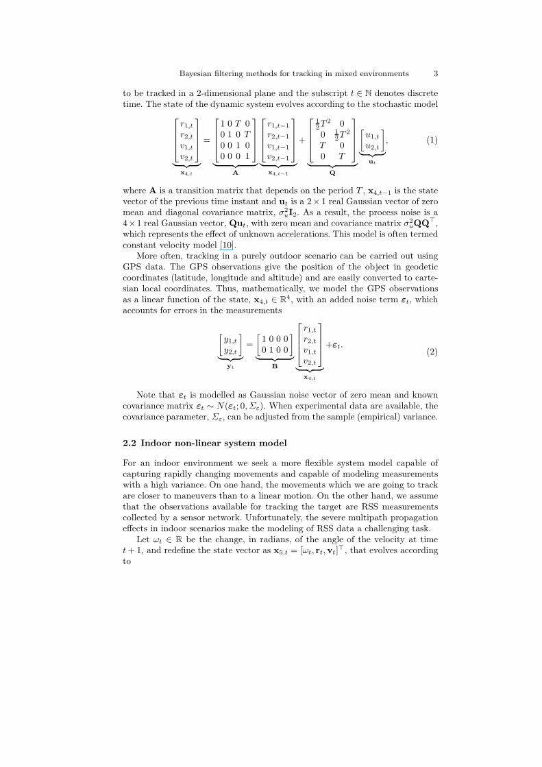
Bayesian filtering methods for tracking in mixed environments 3

to be tracked in a 2-dimensional plane and the subscript t ∈ N denotes discretetime. The state of the dynamic system evolves according to the stochastic model

r1,t

r2,t

v1,t

v2,t

︸ ︷︷ ︸

x4,t

=

1 0 T 00 1 0 T

0 0 1 00 0 0 1

︸ ︷︷ ︸

A

r1,t−1

r2,t−1

v1,t−1

v2,t−1

︸ ︷︷ ︸

x4,t−1

+

12T 2 00 1

2T 2

T 00 T

︸ ︷︷ ︸

Q

[u1,t

u2,t

]

︸ ︷︷ ︸

ut

, (1)

where A is a transition matrix that depends on the period T , x4,t−1 is the statevector of the previous time instant and ut is a 2× 1 real Gaussian vector of zeromean and diagonal covariance matrix, σ2

uI2. As a result, the process noise is a4×1 real Gaussian vector, Qut, with zero mean and covariance matrix σ2

uQQ⊤,which represents the effect of unknown accelerations. This model is often termedconstant velocity model [10].

More often, tracking in a purely outdoor scenario can be carried out usingGPS data. The GPS observations give the position of the object in geodeticcoordinates (latitude, longitude and altitude) and are easily converted to carte-sian local coordinates. Thus, mathematically, we model the GPS observationsas a linear function of the state, x4,t ∈ R

4, with an added noise term εt, whichaccounts for errors in the measurements

[y1,t

y2,t

]

︸ ︷︷ ︸

yt

=

[1 0 0 00 1 0 0

]

︸ ︷︷ ︸

B

r1,t

r2,t

v1,t

v2,t

︸ ︷︷ ︸

x4,t

+εt.(2)

Note that εt is modelled as Gaussian noise vector of zero mean and knowncovariance matrix εt ∼ N(εt; 0, Σε). When experimental data are available, thecovariance parameter, Σε, can be adjusted from the sample (empirical) variance.

2.2 Indoor non-linear system model

For an indoor environment we seek a more flexible system model capable ofcapturing rapidly changing movements and capable of modeling measurementswith a high variance. On one hand, the movements which we are going to trackare closer to maneuvers than to a linear motion. On the other hand, we assumethat the observations available for tracking the target are RSS measurementscollected by a sensor network. Unfortunately, the severe multipath propagationeffects in indoor scenarios make the modeling of RSS data a challenging task.

Let ωt ∈ R be the change, in radians, of the angle of the velocity at timet + 1, and redefine the state vector as x5,t = [ωt, rt,vt]

⊤, that evolves accordingto

4 K. Achutegui et al.

ωt ∼ p(ωt|ωt−1)

r1,t

r2,t

v1,t

v2,t

︸ ︷︷ ︸

x4,t

=

1 0 sin(ωt−1T )ωt−1

− cos(ωt−1T )−1ωt−1

0 1 1−cos(ωt−1T )ωt−1

sin(ωt−1T )ωt−1

0 0 cos(ωt−1T ) − sin(ωt−1T )0 0 sin(ωt−1T ) cos(ωt−1T )

︸ ︷︷ ︸

A(ωt−1)

r1,t−1

r2,t−1

v1,t−1

v2,t−1

︸ ︷︷ ︸

x4,t−1

+Qut, (3)

where the transition matrix A(ωt−1) is now a function of the angle ωt−1 as wellas the period T and the conditional probability density function (pdf) p(ωt|ωt−1)is known. If we select different distributions for ωt, we can create different motionmodels. Note also that in the extreme case where ωt = 0 for all t, (3) becomesthe constant velocity model (1).

Let us assume that, the objective can move according to one out of L modelsof motion, identified by the indices {1, 2, . . . , L}. Each one of the motion mod-els corresponds to a different transition pdf for the Markovian process {ωt}t∈N.Thus, to identify the different densities, we introduce a new state variable, de-noted at. This is a discrete random indicator, at ∈ {1, . . . , L}, so that at−1 = l

implies that ωt is generated according to the l-th model. Therefore we need towrite ωt ∼ p(ωt|ωt−1, at−1) to make the dependence explicit. The probabilitymass function (pmf) p(at|at−1) is part of the model and therefore is assumedknown. This type of dynamic model description, where the are various sub-models to describe different type of motion, is often denoted interacting multiplemodels (IMM) [10]. Incorporating the indicator at to the state, we obtain a 6×1vector, x6,t = [at, ωt, rt,vt]

⊤ which evolves in time according to the equations

at ∼ p(at|at−1), ωt ∼ p(ωt|ωt−1, at−1), x4,t = A(ωt−1)x4,t−1 + Qut. (4)

For the observation model, we assume that at time t we obtain J RSS mea-surements. The datum obtained from sensor j at time t is denoted as yj,t. Therelationship between the received observation, yj,t, and the position of the tar-get, rt, depends on the environment in which the measurement is taken and canchange with time [14]. In order to model this uncertainty in the observationswe are going to use an interacting multiple model (IMM) approach the same asfor the dynamic model. Specifically, we represent the observation yj,t using oneout of K different models that describe the different environments. Finally, wemodel the observations as

yj,t = fmj,t(rt) + εmj,t

, (5)

where mj,t ∈ {1, ..., K} is a random index with a known probability mass func-tion (pmf), p(mj,t), which identifies the observation model at time t for eachsensor j, fmj,t

is the function that describes the propagation conditions in modelmj,t, and εmj,t

∼ N(εmj; 0, σ2

mj,t) is Gaussian noise with zero mean and a known

variance σ2mj,t

, which is also associated with the model mj,t. The form of the

functions {f1, f2, . . . , fK} and variances {σ21 , σ

22 , . . . , σ2

K} should be determined

Bayesian filtering methods for tracking in mixed environments 5

from a bank of empirical observations collected in the scenarios in which thetracking will be performed. In [1] we give full details of the functions and vari-ances obtained when the RSS is measured using a network of ZigBee models. Weassume the same indoor environment and hardware setup in the present paper.

We write the measurement-model indicators together in a J × 1 vectormt = [m1,t, . . . , mJ,t]

⊤, hence the full target state has J + 6 components,xJ+6,t = [mt, at, ωt, rt,vt]

⊤. The observations are put together in a J ×1 vectoryt = [y1,t, . . . , yJ,t]

⊤. The indices in mt are assumed independent, but not neces-sarily identically distributed. The probability mass functions p(mj,t), j = 1, . . . , J

are assumed known and independent of time.

2.3 Outdoor nonlinear model

In this section we describe an outdoor system model that includes ZigBee obser-vations as well as GPS observations. The dynamic model is the same as describedin Section 2.1.

The observation vector is composed of J measurements received from ZigBeesensors and S GPS measurements, that is

yt = [y1,t, . . . , yJ,t, yJ+1,t, . . . , yS+J,t]. (6)

The GPS observation model is the same as described in Section 2.1.The outdoor ZigBee observation models we propose are based on the log

distance path-loss model described in [14]

yj,t = fj(rt) + εj = Lj,0 + γj10 log10

(dj,0

dj,t

)

+ εj, (7)

where dj,t is the distance between sensor j and the target at time instant t,dj,0 is a reference distance for sensor j, Lj,0 is the path loss corresponding tothe reference distance, γj is the path loss exponent and εj ∼ N(εj ; 0, σ2

εj) has a

normal distribution with zero mean and variance σ2εj

. The parameters Lj,0, γj ,

dj,0 and σ2εj

should be adjusted using experimental data.In particular, assume that we collect k RSS measurements for a sensor-to-

target distance di and this is repeated for l different distances, d1, . . . , dl. Then,the parameters L0 and γ are selected as the solution to the optimization problem

(L0,j, γj) = argminL0,γ

=

{l∑

i=1

k∑

n=1

(

yn,i − L0 − γ10 log10

(d0

di

))2}

,

where yn,i is the n-th observation measured at distance di in the experiments,k is the number of measurements we have at distance di and l is the number ofdistances at which we have measurements.

The variance parameter is fitted as

σ2ε,j =

1

l

1

k

l∑

i=1

k∑

n=1

(

yn,i − L0,j − γj10 log10

(d0

di

))2

.

Note that L0,j, γj and σ2ε,j are adjusted for each sensor separately.

6 K. Achutegui et al.

3 Tracking algorithms

3.1 Kalman filter

When both the dynamic and observation models are linear and Gaussian, thedensity p(xt|y1:t), t = 1, 2, . . . is also Gaussian and can be exactly computedusing the Kalman filter [15]. Specifically if we assume

Specifically, p(xt|y1:t) is Gaussian if we assume that

– ut y εt are independent and have known Gaussian distributions,– the dynamic model is a linear function of xt−1 and ut, and– the observation model is a linear function of xt and εt.

Obviously these requirements are satisfied by the outdoor linear model of Section2.1.

Assume that at time t = 0 the prior distribution of xt is Gaussian with meanx0|0 and covariance matrix P0|0 denoted x0 ∼ N(x0; x0|0,P0|0). The Kalmanfilter consists on the set of recursive equations [15]

xt|t−1 = Axt−1|t−1

Pt|t−1 = Qu,t−1 + APt−1|t−1A⊤

xt|t = xt|t−1 + Kt(yt − Bxt|t−1)

Pt|t = Pt|t−1 − KtStK⊤t

(8)

where Qu,t = σ2uQQ⊤ is the covariance matrix of the process noise,

St = Bt−1Pt|t−1B⊤t−1 + Qv,t (9)

is the covariance matrix of the innovation νt = yt − Btxt|t−1, Qv,t = Σε is thecovariance matrix of the observation noise and

Kt = Pt|t−1B⊤t S−1

t (10)

is the Kalman gain. The recursive application of these equations gives us themean and covariance matrix of the posterior probability distribution functionp(xt|y1:t), namely p(xt|y1:t) = N(xt; xt|t,Pt|t).

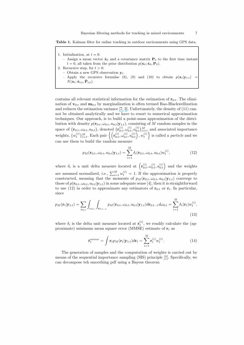
Table 1 summarizes the Kalman filter algorithm for outdoor tracking usingGPS observation data.

3.2 Particle filter for the indoor nonlinear model

Sequential Monte Carlo approximation From a Bayesian point of view,the smoothing pdf

p(r0:t, ω0:t, a0:t|y1:t) =∑

m0:t

∫

v0:t

p(xJ+4,0:t|y1:t)dv0:t (11)

Bayesian filtering methods for tracking in mixed environments 7

Table 1. Kalman filter for online tracking in outdoor environments using GPS data.

1. Initialization, at t = 0:– Assign a mean vector x0 and a covariance matrix P0 to the first time instant

t = 0, all taken from the prior distribution p(x0; x0, P0).2. Recursive step, for t > 0:

– Obtain a new GPS observation yt.– Apply the recursive formulae (8), (9) and (10) to obtain p(xt|y1:t) =

N(xt; xt|t, Pt|t).

contains all relevant statistical information for the estimation of r0:t. The elimi-nation of v0:t and m0:t by marginalization is often termed Rao-Blackwellizationand reduces the estimation variance [7, 3]. Unfortunately, the density of (11) can-not be obtained analytically and we have to resort to numerical approximationtechniques. Our approach, is to build a point-mass approximation of the distri-bution with density p(r0:t, ω0:t, a0:t|y1:t), consisting of M random samples in the

space of {r0:t, ω0:t, a0:t}, denoted {r(i)0:t, ω

(i)0:t, a

(i)0:t}

Mi=1, and associated importance

weights, {w(i)t }M

i=1. Each pair{(

r(i)0:t, ω

(i)0:t, a

(i)0:t

)

, w(i)t

}

is called a particle and we

can use them to build the random measure

pM (r0:t, ω0:t, a0:t|y1:t) =

M∑

i=1

δi(r0:t, ω0:t, a0:t)w(i)t , (12)

where δi is a unit delta measure located at(

r(i)0:t, ω

(i)0:t, a

(i)0:t

)

and the weights

are assumed normalized, i.e.,∑M

i=1 w(i)t = 1. If the approximation is properly

constructed, meaning that the moments of pM (r0:t, ω0:t, a0:t|y1:t) converge tothose of p(r0:t, ω0:t, a0:t|y1:t) in some adequate sense [4], then it is straightforwardto use (12) in order to approximate any estimators of r0:t or rt. In particular,since

pM (rt|y1:t) =∑

a0:t

∫

ω0:t

∫

r0:t−1

pM (r0:t, ω0:t, a0:t|y1:t)dr0:t−1dω0:t =

M∑

i=1

δi(rt)w(i)t ,

(13)

where δi is the delta unit measure located at r(i)t , we readily calculate the (ap-

proximate) minimum mean square error (MMSE) estimate of rt as

rmmset =

∫

rtpM (rt|y1:t)drt =

M∑

i=1

r(i)t w

(i)t . (14)

The generation of samples and the computation of weights is carried out bymeans of the sequential importance sampling (SIS) principle [7]. Specifically, wecan decompose teh smoothing pdf using a Bayess theorem

8 K. Achutegui et al.

p(r0:t, ω0:t, a0:t|y1:t) ∝ p(yt|rt)p(rt|r0:t−1, ω0:t−1)p(at|at−1)

× p(ωt|ωt−1, at−1)p(r0:t−1, ω0:t−1, a0:t−1|y1:t−1), (15)

and, if we draw the particles using the transition pdf’s

a(i)t ∼ p(at|a

(i)t−1)

ω(i)t ∼ p(ωt|ω

(i)t−1, a

(i)t−1)

r(i)t ∼ p(rt|r

(i)0:t−1, ω

(i)0:t−1,y1:t−1) (16)

then the importance weight becomes

w(i)t ∝ w

(i)t−1p(yt|r

(i)t ). (17)

Eqs. (16) and (17) together yield a sequential IS (SIS) type of algorithm for theconstruction of pM (r0:t, ω0:t, a0:t|y1:t) [7].

It is well known, however, that the sequential application of (16) and (17)with a finite number of samples, M < ∞, quickly leads to a degenerate set ofparticles [7]. Indeed, the variance of the weights increases stochastically with timeand, after a few time steps, one single particle tends to accumulate all the weightand the approximation pM (r0:t, ω0:t, a0:t|y1:t) becomes useless. This difficulty iscommonly overcome by adding a resampling step [7, 2] which, intuitively, consistsin stochastically discarding the particles with low weights while the particles withhigher weights are replicated. Although several resampling schemes exist (and allof them can be plugged into the tracking algorithm without any added difficulty),in this paper we adopt the conceptually simple multinomial resampling method[7, 4]. A resampling step can be taken every time the approximate effectivesample size [7] Meff = 1

P

Mi=1 w

(i)2

t

falls below a user-defined threshold. Since

Meff ≤ M , typical threshold values are λM for some 0 < λ < 1.

Evaluation of the weights In order to ensure that the weights of (17) canbe computed, we must be able to draw from p(rt|r0:t−1, ω0:t−1) and to evalu-ate the factors p(at|at−1), p(ωt|ωt−1, at−1) and p(yt|rt). The transition densitiesp(at|at−1) and p(ωt|ωt−1, at−1) are part of the model, hence known by assump-tion. The prior density of the position at time t, p(rt|r0:t−1, ω0:t−1), is Gaussian

and can be obtained in closed form for each particle. Indeed, given r(i)0:t−1 and

ω(i)0:t−1, the system

v1,t

v2,t

r(i)1,t

r(i)2,t

=

cos(ω(i)t−1T ) − sin(ω

(i)t−1T ) 0 0

sin(ω(i)t−1T ) cos(ω

(i)t−1T ) 0 0

sin(ω(i)t−1T )

ω(i)t−1

−cos(ω

(i)t−1T )−1

ω(i)t−1

1 0

1−cos(ω(i)t−1T )

ω(i)t−1

sin(ω(i)t−1T )

ω(i)t−1

0 1

v1,t−1

v2,t−1

r(i)1,t−1

r(i)2,t−1

+

T 0 0 00 T 0 00 0 1

2T 2 00 0 0 1

2T 2

u3,t

u4,t

u1,t

u2,t

(18)

Bayesian filtering methods for tracking in mixed environments 9

is linear and Gaussian, with known parameters, and all posterior pdf’s, including

p(rt|r(i)0:t−1, ω

(i)0:t−1), are Gaussian and can be computed exactly using a Kalman

filter [3, 10]. In the sequel, we denote

p(rt|r(i)0:t−1, ω

(i)0:t−1) = N(rt; r

(i)t|t−1, Σ

(i)

t|t−1). (19)

The pdf p(yt|rt) is usually referred to as the likelihood of rt. If we writep(yj,t|rt) as a marginal of the joint density p(yj,t, mj,t|rt), then it is straightfor-ward to obtain the expression

p(yt|rt) =

J∏

j=1

p(yj,t|rt) =

J∏

j=1

∑

mj,t

p(yj,t|rt, mj,t)p(mj,t), (20)

(note that the observations are conditionally independent given the position rt)where both

p(yj,t|rt, mj,t) = N(yj,t; fmj,t(rt), σ

2mj,t

) (21)

and p(mj,t) are known from the model, for all j = 1, ..., J .Table 2 summarizes the proposed SIS algorithm for the system model de-

scribed in Section 2.2.

Table 2. SIS for indoor tracking with RSS data.

1. Initialization, at t = 0:– For i = 1, . . . , M , sample r0, v0, ω0 and a0 from the priors p(r0), p(v0), p(ω0)

and p(a0). Initialize weights to w(i)0 = 1

M.

2. Recursive step, for t > 0:– For i = 1, . . . , M , sample a

(i)t ∼ p(at|a

(i)t−1), ω

(i)t ∼ p(ωt|ω

(i)t−1, a

(i)t−1) and ob-

tain r(i)t from the distribution p(rt|r

(i)0:t−1, a

(i)0:t−1, ω

(i)0:t−1) = N(rt; r

(i)t|t−1, Σ

(i)t|t−1)

obtained with the Kalman filter.– For i = 1, . . . , M , update weights, w

(i)t ∝ w

(i)t−1p(yt|r

(i)t )

– Compute the particle effective size Meff = 1/PM

k=1 w(k)2

t . If Meff < λM per-

form resampling and set w(i)t = 1

M∀i.

3.3 Particle filter for the outdoor nonlinear model

The algorithm that we are going to use for outdoor tracking with GPS and RSSdata is a particle filter similar to the one used for indoor tracking. The maindifference is the use of a different proposal pdf for the generation of particlesand the subsequent change in the computation of the weights. Recall that thestate vector for our nonlinear outdoor model is defined as x4,t = [r⊤t v⊤

t ]⊤ and,as a consequence, the probability density function of interest is

10 K. Achutegui et al.

p(r0:t|y1:t) =

∫

v0:t

p(x0:t|y1:t)dv0:t ,

where the velocity is integrated to reduce the variance in the estimation.In order to obtain an efficient proposal pdf, we note that even though the

complete vector of observations is not linear, the part of the vector that corre-sponds to the GPS observations is linear, therefore if we take only this part ofthe vector we can construct a posterior Gaussian pdf of rt given partial data.To be specific, if we define the vector of GPS observations as

yS,t = rt + εS,t,

then we can derive an analytic expression for the posterior density p(rt|r0:t−1,yS,t),namely

p(rt|r0:t−1,yS,t) ∝ p(yS,t|rt)p(rt|r0:t−1) =

1

2π|Σt|t−1|12 |Σε|

12

exp{−1

2[(yS,t − rt)

⊤Σ

−1ε (yS,t − rt) +

(rt − rt|t−1)⊤

Σ−1t|t−1(rt − rt|t−1)]}, (22)

where Σε is the covariance matrix of yS,t and p(rt|r0:t−1) = N(rt|rt|t−1, Σt|t−1).Equations 22 can be written in a more compact form if we use the equality

(y − Br)⊤V(y − Br) + (r − ra)⊤U(r − ra) = (r − rp)⊤C(r − rp) +

+(y⊤Vy + r⊤a Ura) − (B⊤Vy + Ura)⊤C−1(B⊤Vy + Ura) (23)

where all vectors have compatible dimensions, C = B⊤VB + U and rp =C−1(B⊤Vy + Ura). if we identify y = yS,t, V = Σ

−1ε , B = I, r = rt,

U = Σ−1t|t−1, ra = rt|t−1, Σt = C−1 and rt = rp, then we can see that sub-

stitution of (23) into (22) gives a Gaussian density

p(rt|r0:t−1,yt) ∝1

2π|Σ−1|1/2exp{−

1

2

[

(rt − rt)⊤Σ−1

t (rt − rt)]

}.

Therefore, the proposed pdf that incorporates GPS observations can be char-acterized as a Gaussian density, N(rt; rt, Σt), where the vector of means and thecovariance matrix are computed as

Σ−1t = Σ

−1ε + Σ

−1t|t−1 and rt = Σt(Σ

−1ε yS,t + Σ

−1t|t−1rt|t−1), (24)

respectively. The weight update equation becomes

w(i)t ∝ w

(i)t−1

p(yt|r(i)t )p(r

(i)t |r

(i)0:t−1)

N(rt; r(i)t , Σ

(i)t )

. (25)

Note that the pdf p(yt|rt) incorporates both GPS and RSS data as

Bayesian filtering methods for tracking in mixed environments 11

p(yt|rt) =

J+S∏

n=1

p(yn,t|rt) =

S∏

s=1

p(ys,t|rt)

J∏

j=1

p(yj,t|rt), (26)

where both p(ys,t|rt) = N(ys,t; rt, σ2vI2) and p(yj,t|rt) = N(yj,t; fj(rt), σ

2εj

) areknown, for j = 1, . . . , J y s = 1, . . . , S.

Table 3 shows a summary of the SIS algorithm for the nonlinear outdoormodel.

Table 3. SIS algorithm with a more efficient proposal function for tracking in anoutdoor environment with GPS and RSS data.

1. Initialization, at t = 0:– For i = 1, . . . , M , sample r0 and v0 from the prior functions p(r0) and p(v0).

Initialize weights w(i)0 = 1

M.

2. Recursive step, for t > 0:– For i = 1, . . . , M , compute the vector of means r

(i)t|t−1 and the covariance matrices

Σ(i)t|t−1 with the Kalman filter.

– With the current GPS observation, yS,t, compute the vector of means r(i)t and

the covariance matrices Σ(i)t of the proposal pdf as defined in (24).

– For i = 1, . . . , M , draw r(i)t from the distribution p(rt|r

(i)0:t−1,yS,t) =

N(rt; r(i)t , Σ

(i)t ).

– For i = 1, . . . , M , update the weights, w(i)t ∝ w

(i)t−1

p(yt|r(i)t )p(r

(i)t |r

(i)0:t−1)

N(rt ;r(i)t ,Σt)

with the

complete vector of observations of the current time instant yt.

– Compute the effective sample size Meff = 1/PM

k=1 w(k)2

t . If Meff < λM re-

sample and set w(i)t = 1

M∀i.

3.4 Switching between algorithms

As the targets move from an indoor environment to an outdoor environment, orvice versa, we have to switch between different tracking algorithms. There areessentially three cases. If the target moves form indoors to outdoors, or outdoorsto indoors, but RSS data are available in both environments, then the trackingalgorithms are particle filters and it is straightforward to go from one to another.

In order to switch from an outdoor environment with GPS data alone to anindoor environment with RSS data, we have to generate a collection of parti-cles from the Gaussian distribution computed by the Kalman filter immediatelybefore the transition, which plays the role of a prior pdf for the particle filter.Specifically if p(xt−1|y1:t−1) = N(xt−1; xt−1|t−1,Pt−1|t−1) then we can draw M

samples with equal weights,

x(i)t−1 ∼ N(xt;xt−1|t−1,Pt−1|t−1), w

(i)t−1 =

1

Mi = 1, . . . , M, (27)

from which the positions of the particles, r(i)t−1, i = 1, . . . , M , are extracted.

12 K. Achutegui et al.

The prior p(vt−1|y1:t−1) is a Gaussian marginal of N(xt−1; xt−1|t−1,Pt−1|t−1)that is straightforward to compute.

xt−1|t−1 =

M∑

i=1

w(i)t−1x

(i)t−1

Pt−1|t−1 =M∑

i=1

w(i)t−1(x

(i)t−1 − xt−1|t−1)(x

(i)t−1 − xt−1|t−1)

⊤. (28)

where x(i)t = [r

(i)t

⊤v

(i)t

⊤]⊤ and v

(i)t is the mean of p(vt|r

(i)0:t) which is obtained

from a Kalman filter for the i-th particle (this is the same Kalman filter that is

used to compute p(rt|r(i)0:t−1, ω

(i)0:t−1).

The algorithms require of a variable that will indicate them the availabletechnology at each instant t. To do so, we introduce a new variable Kt ∈ {0, 1, 2}that can take 3 values: Kt = 0 indicates that we only have ZIgbee observationsand that we must use particle filters for indoor tracking, Kt = 1 indicates usthat we only have GPS observations available and that we must use the Kalmanfilter, and lastly Kt = 2 indicates that we have GPS and ZigBee observationsand we therefore use the data fusion particle filter for outdoor.

4 Experimental setup and results

4.1 Experimental setup

We have developed two kind of hardware nodes using standard parts. For the col-lection of RSS data, we have set up J= 8 anchors, acting as ZigBee transmitters,built using Arduino boards and XBee (series 1) modules (IEEE 802.15.4 com-pliant). The mobile device, that acts as a target, uses an Arduino Mega board,a XBee (series 1) module, and adds an small OEM GPS receiver. The antennasfor 2.4 GHz band were all equal, 2 dBi monopole omnidirectional antennas. Forthe GPS receiver we used a RHCP external antenna. Each node was mountedinside a plastic enclosure and attached to a 2 m long non-metal pole. This wasdone to minimize the interferences caused by the person who carries the device.Figure 1 shows the setup of the mobile device. The anchors look really similar,with a smaller Arduino inside and without the GPS receiver (and its antenna).

The ZigBee and GPS measurements were taken in an outdoor scenario, inthe middle of a clear area (without walls or trees) of about 600 m2. We deployedan 8 ZigBee node network (anchors) covering a 6× 10 m area and, on the otherhand, another mobile node, with ZigBee and GPS receivers. This mobile nodeacted as a gateway, receiving both the ZigBee packets (from the 8 anchors) andthe GPS signal every 1 s. The measurement were tagged by this node and sentto a small laptop using the USB port, where they were stored for future off lineprocess.

In order to test the performance of the proposed algorithms and to be able tobuild realistic observation models we collected a large number of RSS and GPS

Bayesian filtering methods for tracking in mixed environments 13

Fig. 1. Mobile device setup, with ZigBee and GPS receivers.

observations in the mentioned area. The GPS observations are modelled as theposition of the target with an added Gaussian noise. Therefore once known thetrue position where the GPS data are being taken, xn,real, we may translate theGPS global coordinates onto ENU coordinates (east north up) [15] and we maycompute the covariance matrix applying a maximum likelihood criteria

Σε =1

N

N∑

n=1

(xn − xn,real)(xn − xn,real)⊤, (29)

where N is the total number of GPS observations taken in the experiment, n isthe index of a unique observation and xn,real is the true position where the n-thobservation has been taken. The resulting covariance matrix is

Σε =

[7.5 −0.58

−0.58 11.3

]

. (30)

For the modeling of the ZigBee observation functions we have followed thecriteria described in 2.2 to fit the real data taken in the experiments. Figure 2shows experimental data taken from sensors 1 and 8 and the log-distance pathloss models adjusted to them. Note we have fitted one model for each sensor.

The details of the hardware and experiments performed for the indoor modelconstruction can be found in [1].

0 1 2 3 4 5 6 7 8 9 10 11 12−55

−50

−45

−40

−35

−30

−25

−20

Distance [ m ]

RSS [ dB ]

Sensor 1 (0,0)

0 1 2 3 4 5 6 7 8 9 10 11 12−60

−55

−50

−45

−40

−35

−30

−25

−20

Distance [ m ]

RSS [ dB ]

Sensor 8 (6,10)

Fig. 2. Real ZigBee outdoor measurements taken in an outdoor environment for Sen-sors 1 and 8 and the observation functions adjusted to them.

14 K. Achutegui et al.

4.2 Results

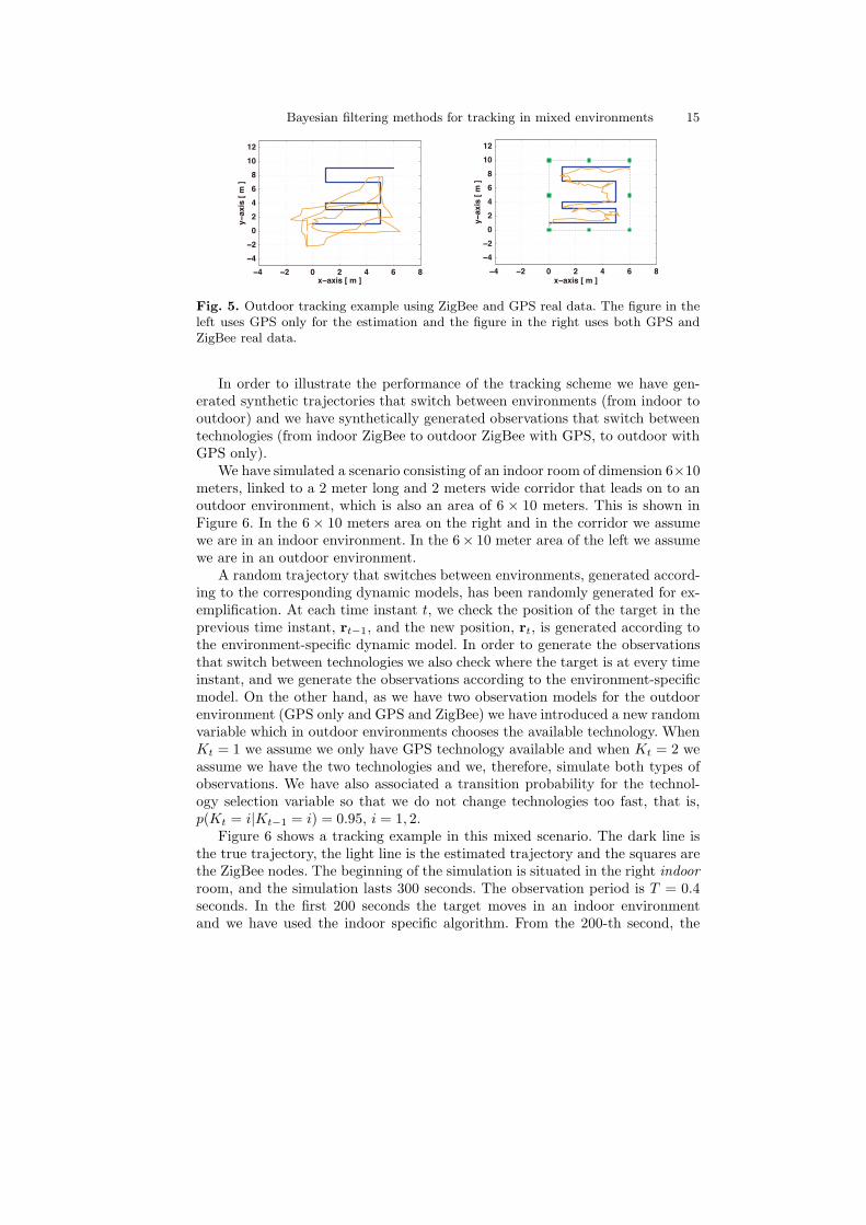
In order to illustrate the performance of the outdoor algorithms we have takenexperimental data of 8 ZigBee sensors and experimental GPS data from a movingtarget following three specific trajectories (see Figures 3, 4 and 5).

Figures 3, 4 and 5 show a tracking example of the two outdoor algorithms:the Kalman filter with GPS data alone and SIS algorithm. The figures in theleft show the estimation of the target trajectory with the Kalman filter and theGPS observations and the figures in the right show the estimated trajectorieswith the SIS filter that uses GPS and RSS data. The true trajectory is drawnwith a dark colored line, the estimated trajectory is drawn in a light colored lineand the ZigBee nodes are depicted with squares.

−4 −2 0 2 4 6 8

−4

−2

0

2

4

6

8

10

12

x−axis [ m ]

y−

ax

is [

m ]

−4 −2 0 2 4 6 8

−4

−2

0

2

4

6

8

10

12

x−axis [ m ]

y−

ax

is [

m ]

Fig. 3. Outdoor tracking example using ZigBee and GPS real data. The figure in theleft uses GPS only for the estimation (via de Kalman filter) and the figure in the rightuses both GPS and ZigBee data (vis de SIS algorithm).

−4 −2 0 2 4 6 8

−4

−2

0

2

4

6

8

10

12

x−axis [ m ]

y−

ax

is [

m ]

−4 −2 0 2 4 6 8

−4

−2

0

2

4

6

8

10

12

x−axis [ m ]

y−

ax

is [

m ]

Fig. 4. Outdoor tracking example using ZigBee and GPS real data. The figure in theleft uses GPS only for the estimation (via de Kalman filter) and the figure in the rightuses both GPS and ZigBee data (vis de SIS algorithm).

As we can observe the trajectories with GPS data have a greater error and theimprovement we obtain by incorporating RSS data is high. This is as expected,because the precision that the civil GPS system can obtain is from 5 to 10 metersand depends on open sky conditions [17, 8]. The area in which we perform thetracking is, therefore, too small for the precision that the technology provides.The ZigBee technology, on the other hand, has a much lower range but achievesa greater precision.

Bayesian filtering methods for tracking in mixed environments 15

−4 −2 0 2 4 6 8

−4

−2

0

2

4

6

8

10

12

x−axis [ m ]

y−

ax

is [

m ]

−4 −2 0 2 4 6 8

−4

−2

0

2

4

6

8

10

12

x−axis [ m ]

y−

ax

is [

m ]

Fig. 5. Outdoor tracking example using ZigBee and GPS real data. The figure in theleft uses GPS only for the estimation and the figure in the right uses both GPS andZigBee real data.

In order to illustrate the performance of the tracking scheme we have gen-erated synthetic trajectories that switch between environments (from indoor tooutdoor) and we have synthetically generated observations that switch betweentechnologies (from indoor ZigBee to outdoor ZigBee with GPS, to outdoor withGPS only).

We have simulated a scenario consisting of an indoor room of dimension 6×10meters, linked to a 2 meter long and 2 meters wide corridor that leads on to anoutdoor environment, which is also an area of 6 × 10 meters. This is shown inFigure 6. In the 6 × 10 meters area on the right and in the corridor we assumewe are in an indoor environment. In the 6× 10 meter area of the left we assumewe are in an outdoor environment.

A random trajectory that switches between environments, generated accord-ing to the corresponding dynamic models, has been randomly generated for ex-emplification. At each time instant t, we check the position of the target in theprevious time instant, rt−1, and the new position, rt, is generated according tothe environment-specific dynamic model. In order to generate the observationsthat switch between technologies we also check where the target is at every timeinstant, and we generate the observations according to the environment-specificmodel. On the other hand, as we have two observation models for the outdoorenvironment (GPS only and GPS and ZigBee) we have introduced a new randomvariable which in outdoor environments chooses the available technology. WhenKt = 1 we assume we only have GPS technology available and when Kt = 2 weassume we have the two technologies and we, therefore, simulate both types ofobservations. We have also associated a transition probability for the technol-ogy selection variable so that we do not change technologies too fast, that is,p(Kt = i|Kt−1 = i) = 0.95, i = 1, 2.

Figure 6 shows a tracking example in this mixed scenario. The dark line isthe true trajectory, the light line is the estimated trajectory and the squares arethe ZigBee nodes. The beginning of the simulation is situated in the right indoor

room, and the simulation lasts 300 seconds. The observation period is T = 0.4seconds. In the first 200 seconds the target moves in an indoor environmentand we have used the indoor specific algorithm. From the 200-th second, the

16 K. Achutegui et al.

target has moved on to the corridor and then on to the outdoor environment. Inthe corridor we assume we have both GPS and outdoor ZigBee measurementsavailable. Then, in the left outdoor environment we have allowed variable Kt tochoose which technology is available in each time instant.

−10 −8 −6 −4 −2 0 2 4 6 8−2

0

2

4

6

8

10

12

x−axis [ m ]

y−

ax

is [

m ]

Fig. 6. Example of tracking a simulated trajectory using different technologies indifferent time instants and commuting between environment and technology specificalgorithms. The beginning of the trajectory is situated in the right indoor room andthe trajectory end in an outdoor environment (in the left area). For the indoor environ-ment we have used ZigBee measurements to perform the tracking and for the outdoorenvironment we have used for some instant GPS measurements only and others GPSand ZigBee outdoor measurements.

4.3 Conclusions

We have introduced a target tracking algorithm for mixed indoor and outdoorscenarios based on the particle filtering methodology and a class of generalized in-teracting multiple-model state-space systems. The resulting method enables thefusion of GPS and RSS data in such a way that a target moving between indoorand outdoor environments, and therefore switching between different availabledata (GPS alone, RSS alone or both), can be seamlessly tracked. Within the par-ticle filter, we use Kalman filtering techniques to reduce the variance of MonteCarlo estimates and to design efficient importance sampling schemes when GPSdata are available. The performance improvement, compared to outdoor track-ers that use only GPS data, is demonstrated using experimental data. Computersimulation results are presented to illustrate the application of the method inmixed indoor/outdoor scenarios.

Acknowledgments

The authors acknowledge the support of Centro para el Desarrollo Tecnologico e Indus-

trial (CDTI) through project CEN-2002-2007 TIMI. K. A. and J. M. acknowledge the

support of Ministerio de Ciencia e Innovacion (program CONSOLIDER-INGENIO

Bayesian filtering methods for tracking in mixed environments 17

2010 CSD2008-00010 COMONSENS, and project TEC2009-14504-C02-01 DEIPRO)

and Ministerio de Industria, Turismo y Comercio (project TSI-020400-2009-103 uSer-

vice). J. R. and C. J. E. acknowledge the support of Ministerio de Ciencia e Innovacion

(project IPT-020000-2010-35).

References

1. K. Achutegui, L.Martino, J. Rodas, Carlos J. Escudero, and J. Mıguez. A Multi-Model Particle Filtering algorithm for indoor tracking of mobile terminals usingRSS data. In 18th IEEE International Conference on Control Applications, pages1702–1707, July 2009.

2. J. Carpenter, P. Clifford, and P. Fearnhead. Improved particle filter for nonlinearproblems. IEE Proceedings - Radar, Sonar and Navigation, 146(1):2–7, February1999.

3. R. Chen and J. S. Liu. Mixture Kalman filters. Journal of the Royal StatisticsSociety B, 62:493–508, 2000.

4. D. Crisan. Particle filters - a theoretical perspective. In A. Doucet, N. de Freitas,and N. Gordon, editors, Sequential Monte Carlo Methods in Practice, chapter 2,pages 17–42. Springer, 2001.

5. P. M. Djuric, J. H. Kotecha, J. Zhang, Y. Huang, T. Ghirmai, M. F. Bugallo,and J. Mıguez. Particle filtering. IEEE Signal Processing Magazine, 20(5):19–38,September 2003.

6. A. Doucet, N. de Freitas, and N. Gordon, editors. Sequential Monte Carlo Methodsin Practice. Springer, New York (USA), 2001.

7. A. Doucet, S. Godsill, and C. Andrieu. On sequential Monte Carlo Samplingmethods for Bayesian filtering. Statistics and Computing, 10(3):197–208, 2000.

8. M. Reza Ehsani, Matthew D. Sullivan, Tommy L. Zimmerman, and TimothyStombaugh. Evaluating the dynamic accuracy of low-cost gps receivers. Amer-ican Society of Agricultural and Biological Engineers, ASAE Meeting Paper No.031014. St. Joseph, Mich.: ASAE, 2003.

9. N. Gordon, D. Salmond, and A. F. M. Smith. Novel approach to nonlinear andnon-Gaussian Bayesian state estimation. IEE Proceedings-F, 140:107–113, 1993.

10. F. Gustafsson, F. Gunnarsson, N. Bergman, U. Forssell, J. Jansson, R. Karlsson,and P.-J. Nordlund. Particle filters for positioning, navigation and tracking. IEEETransactions Signal Processing, 50(2):425–437, February 2002.

11. E. D. Kaplan. Understanding GPS: Principles and Applications. Artech HousePublishers; 2 edition, 2005.

12. H. R. Kunsch. Recursive Monte Carlo filters: Algorithms and theoretical bounds.The Annals of Statistics, 33(5):1983–2021, 2005.

13. N. Patwari, J. N. Ash, S. Kyperountas, A. O. Hero III, R. L. Moses, and N. S.Correal. Locating the nodes. IEEE Signal Processing Magazine, 22(4):54–69, July2005.

14. T. S. Rappaport. Wireless Communications: Principles and Practice (2nd edition).Prentice-Hall, Upper Saddle River, NJ (USA), 2001.

15. B. Ristic, S. Arulampalam, and N. Gordon. Beyond the Kalman Filter. ArtechHouse, Boston, 2004.

16. G. Sun, J. Chen, W. Guo, and K. J. R. Liu. Signal processing techniques innetwork-aided positioning. IEEE Signal Processing Magazine, 22(4):12–23, July2005.

17. M. G. Wing, A. Eklund, and Loren D. Kellogg. Consumer-Grade Global PositioningSystem (GPS) Accuracy and Reliability. Society of American Foresters, 2005.