Adaptive finite element methods for elliptic problems: Abstract framework and applications

IMIPreprint Series

INDUSTRIAL

MATHEMATICS

INSTITUTE

Department of Mathematics

University of South Carolina

2005:16 Adaptive finite element methods for elliptic PDEs based on conforming centroidal Voronoi Delaunay triangulations

L. Ju, M. Gunzburger and W.D. Zhao

ADAPTIVE FINITE ELEMENT METHODS FOR ELLIPTIC PDESBASED ON CONFORMING CENTROIDAL VORONOI

DELAUNAY TRIANGULATIONS

LILI JU∗, MAX GUNZBURGER† , AND WEIDONG ZHAO‡

Abstract. A new triangular mesh adaptivity algorithm for elliptic PDEs that combines a pos-teriori error estimation with centroidal Voronoi/Delaunay tessellations of domains in two dimensionsis proposed and tested. The ability of the first ingredient to detect local regions of large error andthe ability of the second ingredient to generate superior unstructured grids results in an mesh adap-tivity algorithm that has several very desirable features, including the following. Errors are very wellequidistributed over the triangles; at all levels of refinement, the triangles remain very well shaped,even if the grid size at any particular refinement level, when viewed globally, varies by several ordersof magnitude; and the convergence rates achieved are the best obtainable using piecewise linear finiteelements. This methodology can be easily extended to higher-order finite element approximations ormixed finite element formulations although only the linear approximation is considered in this paper.

Key words. Adaptive methods, finite element methods, centroidal Voronoi tessellation, Delau-nay triangulation

AMS subject classifications. 65N50, 65N15

1. Introduction. Adaptive grid generation techniques play an increasingly im-portant role in the numerical solution of partial differential equations (PDEs). Anessential ingredient of adaptive meshing techniques is a posteriori error estimatorswhich are quantities that are computable once an approximate solution of the PDEhas been determined. The key objectives in designing reliable and efficient a posteriorierror estimators and mesh adaptivity techniques are that an existing mesh is refinedin such a way that the errors in the approximate solution of the PDE on the new meshare distributed as uniformly as possible, that those approximate solutions converge, asthe mesh size decreases, to the exact solution as well as can be expected, and that thefirst two objectives are met with a relatively simple complexity. Both mesh adaptivityand a posteriori error estimators have been extensively studied, beginning in the late70s [4–7] and followed by a vast literature. Here, we refer to [2, 31] for references ona posteriori error estimation and mesh adaptivity for elliptic PDEs.

The performance of adaptive methods for PDEs depends not only on the errorestimators, but also on the techniques used for adaptively refining and generatingmeshes. In [14], a convergent adaptive algorithm was proposed for the linear finiteelement methods applied to the Poisson equation in two dimensions; a sequence ofrefined triangulations is defined based on an a posteriori error estimator and theconvergence is proved. Another new family of adaptive algorithms was given in [25–27]and the convergence of the algorithms was also proved.

In many if not most adaptive methods for PDEs, the meshes are refined locallywhenever some criterion based on a local error estimator is not satisfied on someelements; the mesh elsewhere in the domain is not changed. However, in an unrefined

∗Department of Mathematics, University of South Carolina, Columbia, SC 29208.([email protected]). This work is partially supported by the University of South Carolina Researchand Productive Scholarship Fund under the grant number RPS 13060-06-12306.

†School of Computational Science, Florida State University, Tallahassee, FL 32306-4120([email protected]).

‡School of Mathematics and System Sciences, Shandong University, Jinan, Shandong 250100,P.R. China ([email protected]).

1

2 Lili Ju, Max Gunzburger and Weidong Zhao

region, the errors could be so small that, because one has too many grid nodes there,computational resources are wasted. Thus, to achieve some sort of mesh optimality, itis more reasonable to coarsen the meshes in regions where errors are relatively smallin addition to refining in regions where the errors are relatively large. For example,in [8], by introducing a coarsening step to the algorithm proposed in [25], an adaptivemethod is defined that results in certain optimal convergence rates in the energy norm.

In this paper, we propose an adaptive algorithm for linear finite element methodsthat can distribute the nodes in some optimal way according to a posterior errorestimates, so that the error of the resulting approximate solution is distributed equallyover the elements. To some extent, it is close to the mesh smoothing scheme proposedin [3]. We also would like to point out the techniques described in this paper can beeasily extended to higher-order finite element approximations or mixed finite elementformulations. The plan of the rest of the paper is as follows. In Sections 2 and 3,we respectively discuss the specific a posteriori error estimators and mesh generationand optimization methods that are used to define our mesh adaptivity algorithm.The mesh generation algorithm we use requires the definition of a density functionwhich that algorithm uses to decide how grid points should be distributed. In Section4, we first show how that density function can be related to the a posteriori errorestimators and then we provide the description of our mesh adaptation algorithm. InSection 5, we use several computational experiments to demonstrate the effectivenessand efficiency of our mesh adaptation approach.

2. Error estimators for linear finite element methods. Let Ω ⊂ R2 be a

bounded domain with a Lipschitz boundary ∂Ω. Consider the model elliptic partialdifferential equation with homogeneous boundary condition

−∇ · (a∇u) = f in Ω,

u = 0 on ∂Ω,(2.1)

where f ∈ L2(Ω) and a ∈ C1(Ω) with a(x) ≥ a > 0.There are several types of a posteriori error estimators used in adaptive finite

element methods, e.g., explicit error estimators, implicit error estimators, multilevelestimators, and averaging estimators. In this paper, we only use explicit a posteriorierror estimators for adaptive mesh generation and refinement because they can becomputed directly from the finite element approximate solution and the data of theproblem. In the following, we first review some results about explicit a posteriorierror estimators in the context of finite element methods for the model problem (2.1).

2.1. Finite element spaces and a priori error estimates. Assume that Ω isa polygonal domain with boundary ∂Ω and T is a conforming triangulation of Ω [13].Denote by hT the diameter of the triangle T ∈ T and by rT the diameter of thelargest circle that can be inscribed in T . Define the regularity ratio of the triangle Tby κT = hT /rT . If there is a constant κ such that κT ≤ κ for all T ∈ T , then we saythat the triangulation T of Ω is regular. It is worth noting that the assumption ofregularity permits partitions of the domain Ω into meshes that may contain elementsof quite different sizes. This observation is very important for adaptive refinement.In the following, we will assume that T is regular.

Let p denote a nonnegative integer and Pp the space of polynomials of degreeless than or equal to p. The finite element space of degree p associated with thetriangulation T is defined by Vh = v ∈ C(Ω) | v|T ∈ Pp(T ) ∀ T ∈ T . In this paper,for simplicity, we consider the case p = 1, i.e., Vh is the continuous piecewise linear

Adaptive FEMs for Elliptic PDEs based on CfCVDTs 3

finite element space with respect to T . But the techniques described in the remainingsections can be easily extended to other higher-order approximations.

In the a posteriori error analysis, it is also worthwhile to consider properties ofcertain patches of elements. Let the patch T ∈ Ω be the union of the triangle T andthe other triangles in T that share at least one common vertex with T . We define

hT = maxT ′⊂T

hT ′ and rT = maxT ′⊂T

rT ′ ;

then, the regularity of the patch T is measured by κT = hT /rT . It is easy to see that

the regularity of the triangulation T is inherited by each patch T ; see, e.g., [2].Let V be the Hilbert space H1

0 (Ω). The weak form of problem (2.1) is to findu ∈ V such that

B(u, v) = L(v) ∀ v ∈ V,

where B is the bilinear form and L is the linear functional respectively defined by

B(u, v) =

∫

Ω

a∇u · ∇v dx and L(v) =

∫

Ω

fv dx ∀ u, v ∈ V.

It is clear that Vh ⊂ V . Then, the finite element approximation uh ∈ Vh of theproblem (2.1) is determined from the problem

B(uh, vh) = L(vh) ∀ vh ∈ Vh.

For any u ∈ V , we define its energy norm ‖ · ‖E by ‖u‖E =(B(u, u)

)1/2. We

denote by h the piecewise linear function with respect to T satisfying

h(x) = maxT∈T and x∈T

hT

for each vertex x of T . We also assume that the exact solution u ∈ H2(Ω). Leteh = u− uh be the error of the approximate solution uh, we then have the followingclassic results about a priori error estimates [13].

Theorem 1. There exist constants C1 and C2 independent of a and h such that

‖eh‖E ≤ C1‖√

ahk−1|∇ku|‖L2(Ω), k = 1, 2, (2.2)

and

‖eh‖L2(Ω) ≤ C2‖√

ah2|∇2u|‖L2(Ω). (2.3)

2.2. An explicit H1-type a posteriori error estimator. Let v ∈ V be chosenarbitrarily, then writing the integral over the whole domain Ω as a sum of integralsover individual triangles gives

B(eh, v) =∑

T∈T

∫

T

fv dx−∫

T

(a∇uh) · ∇v dx

.

Let EI denote the set of interior edges of T . If T and T ′ share the common edgeγ ∈ EI , define the jump in the normal flux across the edge γ by

[(a∇uh) · nγ ] = (a∇uh)|T · nT + (a∇uh)|T ′ · nT ′


where nT is the unit outward normal vector to ∂T . Applying integration by partsand rearranging terms, we then can get

B(eh, v) =∑

T∈T

∫

T

rv dx +∑

γ∈EI

∫

γ

Rv ds, (2.4)

where r = f +∇ · (a∇uh) and R = − [(a∇uh) · nγ ].For given v ∈ V , let Ihv be the interpolant of v in Vh. Then, by the orthogonality

property B(eh, Ihv) = 0 and (2.4), we have

B(eh, v) =∑

T∈T

∫

T

r(v − Ihv) dx +∑

γ∈EI

∫

γ

R(v − Ihv) ds ∀ v ∈ V. (2.5)

The identity (2.5) plays an important role, indirectly or directly, throughout ana posteriori error analysis of finite element approximations. Due to the coercivity ofthe bilinear form B on V , the approximation theory, and some norm equivalences, bychoosing v = eh, we can obtain the first a posteriori error estimate

‖eh‖2E ≤ C

∑T∈T

h2T ‖r‖2L2(T ) +

∑γ∈EI

hT ‖R‖2L2(γ)

= C∑

T∈T

h2

T ‖r‖2L2(T ) +1

2hT ‖R‖2L2(∂T )

.

(2.6)

Except for the constant C, all of the quantities on the right-hand side of (2.6) can becomputed explicitly from the finite element solution uh. Then we obtain an H1-typelocal error estimator ηT,H1 associated with the element T ∈ T defined by

η2T,H1 = h2

T ‖r‖2L2(T ) +1

2hT ‖R‖2L2(∂T ). (2.7)

The inequality (2.6) shows that the true error eh can be bounded from above in termsof the local error estimator ηT,H1 , i.e. when ηT,H1 is small, the true error eh must alsobe small. This property is referred to as the reliability of the error estimator ηT,H1 .However, we cannot discern anything about the true error eh on any particular triangleT ∈ T from the stability estimate (2.6). Adaptive numerical methods generally alsoneed the fact that the true error eh is also locally bounded from below by the localerror estimator ηT,H1 . This type of property is referred to as the efficiency of the errorestimator. By using properly chosen bubble functions, the efficiency of the explicit aposteriori error estimator ηT,H1 can also be proved. Details can be found in [2] andthe references cited therein. We collect the the stability and efficiency results for theerror estimator ηT,H1 in the following theorem.

Theorem 2. Let ηT,H1 be defined in (2.7) and let η2H1 =

∑T∈T

η2T,H1 . Then, there

exist constants C1 and C2 depending only on the domain Ω, the coefficient functiona, and the regularity of T such that

C1

‖eh‖2E +

∑

T∈T

h2T ‖f − f‖2L2(T )

≤ ‖eh‖2E ≤ C2η

2H1 , (2.8)

where f denotes the mean value of f over T . Moreover, let Tγ denote the union ofthe triangles having γ as one of their edges; then, the local bound

η2T,H1 ≤ C2

‖eh‖E,Tγ

+ h2T ‖f − f‖L2(Tγ )

also holds.


2.3. An explicit L2-type a posteriori error estimator. Duality argumentscan be used to derive L2-type a posteriori error estimators. The starting point for theapplication of this technique is the adjoint of the model problem: find φg ∈ V suchthat

B(v, φg) = (g, v) ∀v ∈ V (2.9)

with g ∈ L2(Ω) and where (·, ·) denotes the L2(Ω) inner product. It is assumed thatthis problem is regular in the sense that the solution φg ∈ H2(Ω)∩V and there existsa constant C such that

‖φg‖H2(Ω) ≤ C‖g‖L2(Ω). (2.10)

This assumption is known to hold, in particular, if the domain Ω is convex. Thespecific choice g = eh in (2.9) then gives

‖eh‖2L2(Ω) = B(eh, φeh).

Then, we have

‖eh‖2L2(Ω) ≤∑

T∈T

‖r‖L2(T )‖φeh− Ihφeh

‖L2(T ) +∑

γ∈EI

‖R‖L2(γ)‖φeh− Ihφeh

‖L2(γ).

(2.11)By the approximation theory again, combining the inequalities (2.10) with g = eh

and (2.11), we obtain

‖eh‖2L2(Ω) ≤ C∑

T∈T

h4

T ‖r‖2L2(T ) + h3T ‖R‖2L2(∂T )

which is similar to (2.6), the only difference being a higher-order scaling in the meshsize; this reflects the expectation of a high-order rate of convergence with respect tothe L2 norm. Let ηT,L2 denote the L2-type local error estimator defined by

η2T,L2 = h4

T ‖r‖2L2(T ) + h3T ‖R‖2L2(∂T ). (2.12)

We summarize the results about this local error estimator in the following theorem [2].Theorem 3. Suppose that the domain Ω is convex. Let ηT,L2 be defined in (2.12)

and let η2L2 =

∑T∈T

η2T,L2 . Then, there exists a constant C depending on the domain

Ω, the coefficient function a, and the regularity of T such that

‖eh‖2L2(Ω) ≤ Cη2L2 . (2.13)

3. Mesh generation and mesh optimization. There have been many goodalgorithms developed for mesh generation and mesh optimization; e.g., see [12, 16,19, 21, 28, 29]. In this paper, we focus on centroidal Voronoi tessellation based meshgeneration as proposed in [15, 16, 19].

3.1. Conforming centroidal Voronoi-Delaunay triangulation. Given anopen convex domain Ω ∈ R

d and a set of distinct points xini=1 ⊂ Ω, define for eachpoint xi, i = 1, . . . , n, the corresponding Voronoi region Vi, i = 1, . . . , n, by

Vi =x ∈ Ω | ‖x− xi‖ < ‖x− xj‖ for j = 1, . . . , n and j 6= i

.


Clearly, we have xi ∈ Vi, Vi ∩ Vj = ∅ for i 6= j, and ∪ni=1V i = Ω so that Vini=1 is a

tessellation of Ω. We refer to Vini=1 as the Voronoi tessellation (VT) of Ω associatedwith the point set xini=1. A point xi is called a generator and a subdomain Vi ⊂ Ωis referred to as the Voronoi region corresponding to the generator xi.

It is well known that the dual tessellation (in a graph-theoretical sense) to aVoronoi tessellation of Ω is a Delaunay triangulation (DT). It is easy to show thatthe vertices of the Voronoi regions Vi’s are the circumcenters of the correspondingDelaunay triangles.

Given a density function ρ(x) defined on Ω, for any region V ⊂ Ω, we define themass centroid x∗ of V by

x∗ =

∫

V

yρ(y) dy∫

V

ρ(y) dy

.

Definition 1. We refer to a Voronoi tessellation (xi, Vi)ni=1 of Ω as a cen-troidal Voronoi tessellation (CVT) [15] if and only if the points xini=1 which serveas the generators of the associated Voronoi tessellation Vini=1 are also the masscentroids of those regions, i.e., if and only if we have that

xi = x∗i for i = 1, . . . , n.

The corresponding Delaunay triangulation is referred to as a centroidal Voronoi-Delaunay triangulations (CVDT).

It is worth noting that a CVT/CVDT may not be unique; see [15]. The extensionof CVTs and CVDTs to general surfaces is discussed in [17].

Given any set of points xini=1 on Ω and any tessellation Vini=1 of Ω, we definethe corresponding energy by

K((xi, Vi)ni=1

)=

n∑

i=1

∫

Vi

ρ(y)‖y − xi‖2 dy .

It has be shown that K is minimized only if (xi, Vi)ni=1 forms a centroidal Voronoitessellation [15]. Although K may not be directly identified with an energy of somephysical system, it is often naturally associated with quantities such as error distor-tion, variance, and cost in many practical applications.

An important and very useful property of CVTs is that the energy is equallydistributed over the Voronoi regions Vi’s in an asymptotic way. For example, it wasshown in [15] that, in the one-dimensional case,

KVi≈ K/n for i = 1, . . . , n,

where KVi=

∫Vi

ρ(x)‖x− xi‖2 dx and K =∑n

i=1 KVi. For higher-dimensional cases,

this property is only a conjecture but its validity has been verified through exten-sive numerical studies and is widely assumed in practical applications such as vectorquantization. As a consequence of this equipartition property, CVTs have importantgeometric features, including the following.

• For a constant density function, the generators xini=1 are uniformly dis-tributed; the Voronoi regions Vini=1 are all almost of the same size and,in the two-dimensional case, most of them are (nearly) congruent convexhexagons [15].


• For a non-constant density function, the generators xini=1 are still locallyuniformly distributed, and it is conjectured [15] that, asymptotically, for someconstant C,

KVi= Cρ(xi)h

d+2Vi

andhVi

hVj

≈(ρ(xj)

ρ(xi)

) 1d+2

, (3.1)

where hVidenotes the diameter of Vi and d is the dimension of Ω.

Thus, in principle, one could control the distribution of generators to obtain an equaldistribution of the error by connecting the density function ρ(x) to an a posteriorierror estimator.

An often used algorithm for constructing CVT/CVDT is the Lloyd’s method [15].Algorithm 1. (Lloyd’s Method for CVT) Given a domain Ω, a density

function ρ(x) defined on Ω, and a positive integer n,0. select an initial set of n points xini=1 in Ω;1. construct the Voronoi regions Vini=1 of Ω associated with xini=1;2. determine the mass centroids of the Voronoi regions Vini=1; these centroids form

the new set of points xini=1;3. if the new points meet some convergence criterion, return (xi, Vi)ni=1 and ter-

minate; otherwise, go to step 1.An important property of Lloyd’s algorithm is that the energy K of the Voronoi

tessellation (xi, Vi)ni=1 decreases after each iteration [15]. A probabilistic version ofLloyd’s method and its parallel implementation were suggested in [24].

If a CVDT mesh is to be used within a discretization method for a PDE, e.g.,in a finite element method, some modifications are needed. An obvious one is thatthe CVDT mesh must conform with the boundary of the domain Ω, i.e., some ofthe CVDT nodes should be constrained to lie on the boundary so that the boundaryconditions of the PDE problem can be enforced.1

One can, of course, pre-define a set of boundary mesh points and then determinean interior mesh that in some sense “conforms” with the boundary mesh. We chooseto instead amend the CVT definition and construction algorithm so that the boundarymesh points are automatically selected in conjunction with the interior mesh points.This results in a better “fit” of the boundary and interior meshes.

First, we generalize the CVT definition. Assume that Ω is compact and thedomain boundary ∂Ω is piecewise smooth; the set of singular points, e.g., corners, isdenoted by PS = ziki=1. Denote by Proj(x) the process that projects x ∈ Ω to theclosest point to x on the boundary ∂Ω. Let

PI = xi | V i ∩ ∂Ω = ∅ and PB = xi | V i ∩ ∂Ω 6= ∅

so that PI , the set of interior Voronoi generators, denotes the set of generators thathave Voronoi regions that do not intersect the boundary and PB , the set of boundaryVoronoi generators denotes the set of generators that have Voronoi regions that dointersect the boundary.

Definition 2. A Voronoi Tessellation (xi, Vi)ni=1 of Ω is called a conformingcentroidal Voronoi tessellation (CfCVT) if and only if the following properties aresatisfied:

• PS ⊂ xini=1;

1If ∂Ω = ∅, e.g., if Ω is the surface of a sphere, Voronoi-based discretizations of PDEs have beendiscussed in [18].


• xi = x∗i for xi ∈ PI ;

• xi = Proj(x∗i ) for xi ∈ PB − PS.

The corresponding dual triangulation is then called a conforming centroidal VoronoiDelaunay triangulation (CfCVDT). It is noted that the meaning of singular (corner)points is trivial in two-dimensional space but may need to be more rigorously definedin spaces higher than two dimensions.

An algorithm for constructing a CfCVT/CfCVDT was given in [16, 19] and canbe described as follows.2 We follow Algorithm 1 except that in step 2 the new set ofgenerators are given by–the centers of mass of the interior Voronoi regions;–the projections onto the boundary of the centers of mass of the boundary Voronoi

regions except if the boundary Voronoi region contains a point in PS , in whichcase the new generator is that point.

For this approach, both the number of mesh points on the boundary and their locationare not pre-determined. However, it is not difficult to show that the number ofgenerators lying on the boundary will never decrease after the first iteration of Lloyd’smethod. The reason for this is that the nodes on the boundary cannot return to theinterior of the domain since their Voronoi regions are obviously always boundaryVoronoi regions. Thus, for this approach, the initial position of generators must bechosen well according to the density function ρ; for example, one could determinean ordinary CVT (with no points lying on the boundary) to use as an initial set ofgenerators for the CfCVT construction algorithm.

In practical applications, the domain Ω is often non-convex and is possibly verycomplicated [19], so that a main difficulty associated with Lloyd’s method for con-structing CfCVDTs is the construction of the Voronoi regions. For this reason, wenext propose an algorithm for constructing approximate CfCVDTs in two dimensionsthat does not require the construction of exact Voronoi tessellations.

3.2. Approximate CfCVDT construction. In this section, we propose an al-gorithm to construct approximate CfCVDTs; we will later use this algorithm withinour adaptive methods for mesh generation and optimization. We describe our ap-proach for the two-dimensional case in detail; the generalization to higher dimensionsfollows similar lines.

Currently, for mesh generation with conforming boundary requirements, con-strained Delaunay triangulations (CDTs) have been widely used; see, e.g., [29, 30].The main difference between CDT and standard DT is that some geometric con-straints such as predetermined node position and node connectivities are added andstrictly enforced during the CDT process. For example, the boundary of the domaincan be triangulated first, and the resulting boundary triangulation is then used asa constraint on the conforming triangulation of the whole domain using CDT. It isworth noting that the dual tessellations of CDT generally is not an exact Voronoitessellation, especially near the boundary.

Our algorithm for constructing approximate CfCVDTs is based on the CDT pro-cess. Assume that Ω ∈ R

2 is a domain with a polygonal boundary.3 Denote byPS = zki=1 its corner vertex set as before. An initial conforming triangulationT0 = Timi=1 of Ω is generated using the “TRIANGLE” software package [29] thatuses the CDT process with a boundary mesh as a constraint and interior Delaunay

2Other modified techniques for constructing CfCVTs are given in [16].3For domains with curved boundaries, the projection process Proj can be easily effected by a

damped Newton’s method, see [28].


refinement techniques, or by some other means. Denote by P = xini=1 the set of ver-tices of T0, by PB the set of boundary vertices, and by PI the set of interior vertices.The CDT process guarantees that PS ⊂ PB .

For each triangle Ti = (xi1 ,xi2 ,xi3 ) ∈ T0, we define

xTi=

circumcenter of Ti if Ti is an acute triangle;the middle point of the longest edge of Ti otherwise.

Clearly, xTi∈ T i. For each vertex xi, we denote by Tik

mi

k=1 ⊂ T0 the set of trianglesfor which xi is a vertex, counting in the counterclockwise direction.

Interior vertices. First, consider the case xi ∈ PI , i.e., xi is an interior vertex.Define Ui by

Ui = the polygon formed by xTikmi

k=1;

see Fig. 3.1. The polygon Ui can be regarded as an approximation to the Voronoiregion Vi associated with xi. Let xi denote the center of mass of the Ui with re-spect to the density function ρ. Denote by αik

mi

k=1 the associated angles around xi

corresponding to Tikmi

k=1. Define

α =

maxαik

| T ik∩ ∂Ω 6= ∅ if T ik

∩ ∂Ω 6= ∅ for some ik;0 otherwise

and ei denote the corresponding boundary edge opposite to the angle αiksuch that

αik= α; see Fig. 3.1 for illustrations of some cases.Now, select a parameter θmax (π > θmax > π/2). Then, define

yi =

xi if α < θmax;Proj

eixi otherwise

(3.2)

where Projei

xi denotes the projection of xi onto the boundary edge ei. It is clearthat yi is still an interior vertex if α < θmax; otherwise, it is a boundary vertexalthough xi is an interior node.

Boundary vertices. Next, consider the case xi ∈ PB , i.e., xi is a boundary vertex.Let e1 and e2 denote the two boundary edges having xi as the common end point,and let z1 and z2 denote the midpoints of e1 and e2, respectively; see Fig. 3.2. Theapproximate Voronoi region Ui of xi is defined by

Ui = the polygon formed by z1, xTikmi

k=1, and z2;

see Fig. 3.2. Let xi denote the center of mass of the Ui associated with the densityfunction ρ.

If xi ∈ PB − PS , denote by β1 and β2 the angles facing the boundary edges e1

and e2, respectively, in Tikmi

k=1; see Fig. 3.2 (right). Let

β = max(β1, β2)

and select a parameter θmin (π/3 > θmin > 0). Then, define

yi =

xi if xi ∈ PS ;Proj

z1z2xi if xi ∈ PB − PS and β > θmin;

xi if xi ∈ PB − PS and β ≤ θmin

(3.3)

where Projz1z2

xi denotes the projection of xi onto the segment z1z2. It is clear thatyi is also a boundary vertex if xi is a corner vertex, or xi is a non-corner vertex butβ > θmin; otherwise, yi becomes an interior vertex although xi is on the boundary(We also call it a lifting process).


xix i

i

e e

e e

i i

ii

U

ix xi

Fig. 3.1: The approximate Voronoi region Ui for the interior vertex xi.

ie e

i

ix 1

U

11

2

2z zz

z

2e

1e 2 x

Fig. 3.2: The approximate Voronoi region Ui for the boundary vertex xi; left: cornervertex; right: non-corner vertex.

The approximate CfCVDT construction algorithm. We can now describe an al-gorithm for constructing an approximate CfCVDT of the domain Ω.

Algorithm 2. (Modified Lloyd’s method for approximate CfCVDT)Given a domain Ω, a density function ρ(x) defined on Ω, and an initial triangulationT0 of Ω with vertices xini=1 generated using CDT,

1. determine yini=1 from xini=1 according to (3.2) and (3.3);2. set xini=1 = yini=1 and reconstruct the boundary segments EB from the new

xini=1;3. re-triangulate the domain Ω using CDT with xini=1 as the vertices and EB as

the boundary edges; the resulting triangulation is the new T ;4. if the triangulation T meets some convergence criterion, return T and terminate;

otherwise, go to step 1.

In the remainder of this paper, we will use the notation T =CfCVDT(T0,Ω,ρ) torepresent the output of Algorithm 2.

Remark 1. To prevent some vertices from frequently jumping back and forthbetween the boundary and the interior of the domain, more sophisticated controls areneeded; for the sake of simplicity, we omit some details in Algorithm 2.

Remark 2. Two user-defined parameters θmax and θmin corresponding respec-


tively to the projection process and the lifting process are used to avoid bad-shapedtriangles in the region close to the boundary. In our computational experiments, weset θmax = 5π/9 and θmin = π/6. These are only empirical values, but many experi-ments lead us to believe they are good choices.

4. CfCVDT-based adaptive finite element methods. Adaptive meshingmethods for solving PDEs often takes the following standard form:

0. generate a coarse mesh T (0) of the domain Ω and set ` = 0;1. solve the system produced by discretizing the PDE based on T (`) and calculate

the local error estimators;2. if some convergence criteria is satisfied, terminate; otherwise, go to step 3;3. refine the mesh T (`) based on the local error estimators to get the next level of

mesh T (`+1) and set ` = ` + 1, then go to step 1.

In our adaptive method, we use CfCVDTs to refine and optimize the mesh at eachlevel, but first we need to determine, from the error estimators, the density functionused in the CfCVDT algorithm.

4.1. Determination of the density function. Let T (`) denote the triangu-

lation of Ω with vertices x(`)i n

(`)

i=1 at the refinement level `. Let η(`)T,H1 and η

(`)T,L2

represent the corresponding local H1-type and L2-type error estimators on T ∈ T (`)

at level ` defined by (2.7) and (2.12), respectively. A comparison of (2.2) and (2.8)

and of (2.3) and (2.13) reveals that it is reasonable to divide both η(`)T,H1 and η

(`)T,L2

by√

a in order to reflect the local variations of true error more accurately. Thus, wedefine

(ξ(`)T,H1 )

2 =(η

(`)T,H1 )

2

aTand (ξ

(`)T,L2)

2 =(η

(`)T,L2)

2

aT, (4.1)

where aT is the mean value of a(x) on the triangle T , i.e., aT =∫

Ta(x) dx/Area(T ).

In order to minimize

(ξ(`)H1 )

2 =∑

T∈T (`)

(ξ(`)T,H1 )

2 or (ξ(`)L2 )2 =

∑

T∈T (`)

(ξ(`)T,H1 )

2,

we need to distribute (ξ(`)T,H1 )

2 or (ξ(`)T,L2)

2 equally over all triangles of T (`).

Set

ρ(`)T,H1 =

(ξ(`)T,H1 )

2

h4T

and ρ(`)T,L2 =

(ξ(`)T,L2)

4/3

h4T

. (4.2)

We then uniquely determine two piecewise linear functions (with respect to T (`))

ρ(`+1)H1 and ρ

(`+1)L2 on Ω such that for any vertex x

(`)i of T (`),

ρ(`+1)H1 (x

(`)i ) =

∑T∈Si

ρ(`)T,H1

card(Si)and ρ

(`+1)L2 (x

(`)i ) =

∑T∈Si

ρ(`)T,L2

card(Si), (4.3)

where

Si = T ∈ T (`) | x(`)i ∈ T.


Note that, in some sense, if the solution u ∈ H2(Ω), we have

(ξ(`)T,H1 )

2 ≈ aT |∇2u|2h4T and (ξ

(`)T,L2)

2 ≈ aT |∇2u|2h6T . (4.4)

Combining (4.4) with the CVT/CVDT property (3.1) for d = 2, i.e.,

hVi

hVj

≈(ρ(xj)

ρ(xi)

)1/4

for a CVT (xi, Vi)ni=1 of Ω with respect to the density function ρ, it is then notdifficult to verify that the CfCVDT mesh T (`+1) generated by the density function

ρ(`+1)H1 or ρ

(`+1)H1 will approximately have the property that

(ξ(`+1)Ti,H1)

2 ≈ (ξ(`+1)Tj ,H1)

2 or (ξ(`+1)Ti,L2)

2 ≈ (ξ(`+1)Tj ,L2)

2,

respectively, for any triangles Ti, Tj ∈ T (`+1).

We will refer to the density functions ρ(`+1)H1 and ρ

(`+1)L2 as the H1-based and L2-

based density functions, respectively. From their defining formulas, it is easy to see

that ρ(`+1)H1 varies more rapidly than does ρ

(`+1)L2 . We expect that CCDVT meshes

generated using ρ(`+1)H1 will produce a finite element approximation with smaller H1

norm or energy error while those generated using ρ(`+1)L2 will tend to have smaller L2

norm error.The most time consuming step in the calculations of ρ

(`+1)H1 (x) and ρ

(`+1)L2 (x) for

any x ∈ Ω is the nearest neighbor search operation since they are defined by inter-polation with respect to an unstructured mesh. However, this task can be effectedefficiently using the software package “ANN” [1] that is based on the K-D tree algo-rithm.

Remark 3. In many practical applications, the coefficient in the model equation(2.1) is often a tensor product, i.e., a symmetric, positive definite matrix

A(x) =

(a11(x) a12(x)a21(x) a22(x)

)

rather than a scalar-valued function a(x). Under this situation, if the difference be-tween a11(x) and a22(x) is not large locally, then it is still reasonable to scale theseestimators by

(ξ(`)T,H1 )

2 =(η

(`)T,H1 )

2

ATand (ξ

(`)T,L2)

2 =(η

(`)T,L2)

2

AT, (4.5)

where AT =∫

T

√det(A(x)) dx/Area(T ); If A(x) is strongly anisotropic, then it could

not be handled correctly in this framework; the anisotropic CVT meshes proposedin [20], perhaps with some variations, may be able to deal with this case.

Remark 4. If a higher-order finite element approximation is used, for example,Vh = v ∈ C(Ω) | v|T ∈ Pk(T ) ∀ T ∈ T where k > 2, then the discrete solution uh

is of k-th order convergence in H1 norm and (k + 1)-th order in L2 norm. Let η(`)T,H1

and η(`)T,L2 be the accordingly derived local H1 and L2 type error estimators for this

approximation; then by similar analysis, it is better to replace (4.2) by

ρ(`)T,H1 =

(ξ(`)T,H1 )

4k+1

h4T

and ρ(`)T,L2 =

(ξ(`)T,L2)

4k+2

h4T

. (4.6)


Remark 5. If the mixed finite element method is used, the density fucntion canbe determined similar to the standard finite element approximation since all we needare just explicit a posterior local error estimators and their orders with respect to thelocal mesh size hT .

4.2. Adaptive algorithms based on CfCVDT. Let Eik(`)

i=1 denote the setof edges of the `-th level triangulation T (`). Set ρEi

= ρ(zi) for any density functionρ, where zi denotes the midpoint of the edge Ei. We can now define our adaptivefinite element method as follows.

Algorithm 3. (CfCVDT-based adaptive finite element method) Givena domain Ω, an integer Nmax > 0 (the maximum allowable number of mesh vertices),an integer Lmax (the maximum allowable levels of refinements), and a parameter0 < θ ≤ 1.0. Preprocessing: generate an initial coarse triangulation T of Ω using CDT or some

other means, solve the PDE using a finite element method (FEM) on T , andthen determine the local error estimators ηT,H1 (or ηT,L2) for all T ∈ T .Construct the density function ρH1 (or ρL2) using (4.3) and optimize T toobtain T (0) = CfCV DT (T , Ω, ρH1) (or T (0) = CfCV DT (T , Ω, ρL2)) thatbecomes the new initial coarse mesh; let n(0) denote the number of vertices ofT (0) and set ` = 0.

1. Solve the PDE using the FEM on T (`). If ` > Lmax or n(`) > Nmax, terminate;otherwise, go to step 2.

2. Determine the local error estimator η(`)T,H1 (or η

(`)T,L2) for all T ∈ T (`).

3. Construct ρ(`+1)H1 (or ρ

(`+1)L2 ) using (4.3) and set the density function ρ = ρ

(`+1)H1

(or ρ = ρ(`+1)L2 ).

4. Determine ρEik(`)

i=1 and sort them in decreasing order.5. Add zikθ

i=1 into the triangulation T (`), where

kθ = maxk∗

∣∣∣k∗∑

i=1

ρEi< θ

k(l)∑

i=1

ρEi

,

and then form, using CDT, the new intermediate triangulation T (`+1) withn(`+1) = n(`) + kθ vertices.

6. Optimize T (`+1) to obtain T (`+1) = CfCV DT (T (`+1), Ω, ρ), set ` ← ` + 1, thengo to step 1.

The parameter θ in Algorithm 3 is used here to control the refinement process [26].The sorting procedure in step 4 can be implemented efficiently using a quick sortingalgorithm.

5. Computational experiments. In this section, using computational experi-ments, we illustrate the effectiveness of CfCVDT-based adaptive finite element meth-ods. Consider the problem

−∇ · (a∇u) + bu = f in Ω,

u = g on ∂Ω,(5.1)

where b ∈ L∞(Ω) with b ≥ 0. Correspondingly, r = f in (2.7) and (2.12) is changedto r = f − buh. Initial coarse meshes are either chosen to be a uniform Cartesian gridor are produced using the “TRIANGLE” package and are subsequently repeatedly


refined by our adaptive methods, i.e., Algorithm 3. For the sake of having somethingto compare to, we also find finite element approximations of the problem (5.1) usinguniform refinements of the initial meshes. We set Lmax = 15, Nmax =20,000, andθ = 0.4 for Algorithm 3. For our adaptive methods, the convergence rate CR withrespect to the norm ‖ · ‖ at the refinement level ` is roughly computed by

CR =2 log(‖eh,`‖/‖eh,`−1‖)

log(n`−1/n`), (5.2)

where n` denotes the number of nodes and eh,` denotes the error u − uh at therefinement level `.

We apply the commonly used q measure [22] to evaluate the quality of triangularmeshes, where, for any triangle T , q is defined to be twice the ratio of the radius RT

of the largest inscribed circle and the radius rT of the smallest circumscribed circle,i.e.,

q(T ) = 2RT

rT=

(b + c− a)(c + a− b) + a + b− c)

abc,

where a, b, and c are side lengths of T . For a given triangulation T , we define

qmin = minT∈T

q(T ) and qavg =1

card(T )

∑

T∈T

q(T ); (5.3)

qmin measures the quality of the worst triangle and qavg measures the average qualityof the mesh T .

5.1. Smooth solution with large gradients. The first illustrative problem isgiven as follows.

Example 1. Set Ω = [−1, 1]×[−1, 1], a(x, y) = 10.0 cos(y), and b(x, y) = x2+y2.The exact solution u is chosen to be

u(x, y) =1.0

(x − 0.5)2 + (y − 0.5)2 + 0.01− 1.0

(x + 0.5)2 + (y + 0.5)2 + 0.01(5.4)

and f and g are determined from u so that (5.1) is satisfied.It is easy to see that the exact solution u given in (5.4) is a smooth function, i.e.,

certainly, u ∈ C2(Ω). Note that u achieves its maximum value 99 101201 at the point

(0.5, 0.5) and its minimum value −99 101201 at the point (−0.5,−0.5), but decays very

quickly away from its extrema and thus has large gradients near these two points.Note also that a(x, y) and f(x, y) also have relatively rapid variations over Ω.

The initial coarse mesh (the input for step 0 of Algorithm 3) used for the solu-tion of Example 1 is a uniform Cartesian grid consisting of 81 nodes; see Fig. 5.1.The corresponding CfCVDT meshes (the output of step 0) with the same number ofnodes produced using the density functions ρH1 and ρL2 are also given in Fig. 5.1.Fig. 5.2 presents repeatedly refined meshes at some levels generated using Algorithm3. The distributions of nodes in the CfCVDT-based adaptive meshes clearly show theaccumulation of nodes in the vicinity of the two points near which large gradients inthe solution occur. The CfCVDT-based adaptive meshes are “optimal” in the sensethat all triangles remain well-shaped at all refinement levels, an observation whichis supported by the values of qmin and qavg given in Table 5.1. It is also clear thatthe CfCVDT meshes generated using the density function ρH1 tend to distribute the


Fig. 5.1: Initial meshes for Example 1; left: a uniform Cartesian grid with 81 nodes;middle and right: the corresponding CfCVDT meshes with the same number of nodesgenerated using the density functions ρH1 and ρL2 , respectively.

Fig. 5.2: Repeatedly refined adaptive meshes at some levels generated by theCfCVDT-based adaptive method for Example 1; top: 394, 1287, 4644 nodes usingthe density function ρH1 ; bottom: 370, 1280, 4629 nodes using the density functionρL2 .

nodes in a slightly less uniform manner than those generated using the density func-tion ρL2 ; this observation which is also verified by the values of hmax/hmin in Table5.1, can be explained by the fact that ρH1 has larger variations than does ρL2 .

Table 5.1 contains information about mesh quality, solution errors, and conver-gence rates at all refinement levels for different refinement strategies for Example 1;the corresponding plots of the error norms (‖eh‖L2(Ω) and |eh|H1(Ω)) vs. the numberof nodes are given in Fig. 5.3 where |eh|H1(Ω) denotes the semi-H1 norm defined by‖∇eh‖L2(Ω). One observes that the two CfCVDT-based adaptive methods and theuniform refinement strategy achieve almost perfect convergence rates, i.e., 2 and 1


for ‖eh‖L2(Ω) and |eh|H1(Ω), respectively.4 These, of course, are the expected ratessince the exact solution u of Example 1 belongs to H2(Ω). The values of qmin andqavg given in Table 5.1 demonstrate that the shape quality of the meshes resultingfrom the CfCVDT-based adaptive strategy is always very good at all levels for bothdensity functions ρL2 and ρH1 , although the mesh sizes vary a lot over the Ω, e.g.,hmax/hmin reaches 176.3 at the last level when ρH1 is used. Note that hmax/hmin

tends to converge for our adaptive methods since u is smooth. Also, as expected, theadaptive method using ρL2 as the density function generated approximate solutionsuh having smaller ‖eh‖L2(Ω) relative to those obtained using ρH1 ; on the other hand,the latter generated approximate solutions with (slightly) smaller |eh|H1(Ω).

` n` qmin qavg hmax/hmin ‖eh‖L2(Ω) CR |eh|H1(Ω) CR

Uniform refinement0 81 0.828 0.828 1.0 2.3260e+01 1.8187e+021 289 0.828 0.828 1.0 2.2931e+00 3.34 1.0422e+02 0.802 1089 0.828 0.828 1.0 9.6260e-01 1.25 6.5176e+01 0.683 4225 0.828 0.828 1.0 2.7745e-01 1.80 3.5677e+01 0.874 16441 0.828 0.828 1.0 7.1278e-02 1.96 1.8242e+01 0.975 66409 0.828 0.828 1.0 1.8071e-02 1.98 9.2255e+00 0.98

Adaptive refinement using ρH1

0 81 0.280 0.805 6.6 7.6651e+00 1.5021e+021 114 0.541 0.916 8.8 2.9722e+00 5.54 9.0709e+01 2.952 143 0.459 0.876 20.8 2.2858e+00 2.31 6.1156e+01 3.473 229 0.579 0.919 22.5 1.1666e+00 2.86 4.5971e+01 1.214 394 0.618 0.926 40.7 7.5734e-01 1.59 3.3524e+01 1.165 703 0.574 0.936 45.9 4.6479e-01 1.69 2.4081e+01 1.146 1287 0.611 0.941 59.5 2.9602e-01 1.49 1.7575e+01 1.047 2426 0.622 0.942 80.9 1.8046e-01 1.56 1.2760e+01 1.018 4644 0.651 0.944 114.5 9.7005e-02 1.91 9.2654e+00 0.999 8921 0.621 0.945 130.9 5.6155e-02 1.68 6.7420e+00 0.97

10 17095 0.598 0.944 164.5 3.1818e-02 1.75 4.8327e+00 1.0211 33192 0.610 0.944 176.3 1.6909e-02 1.91 3.4671e+00 1.00

Adaptive refinement using ρL2

0 81 0.563 0.898 5.7 5.7395e+00 1.3966e+021 127 0.679 0.931 7.1 2.1686e+00 4.33 9.0681e+01 1.922 211 0.579 0.924 13.4 1.0831e+00 2.74 5.9141e+01 1.683 370 0.638 0.938 11.9 5.8917e-01 2.17 4.0737e+01 1.334 681 0.675 0.941 17.7 3.2326e-01 1.97 2.9245e+01 1.095 1280 0.679 0.940 20.6 1.7163e-01 2.01 2.1150e+01 1.036 2412 0.601 0.944 23.5 9.4164e-02 1.90 1.4562e+01 1.187 4629 0.680 0.944 27.7 4.8922e-02 2.01 1.0621e+01 0.978 8883 0.649 0.944 34.9 2.6327e-02 1.90 7.4636e+00 1.089 17099 0.602 0.944 37.4 1.3566e-02 2.03 5.4503e+00 0.96

10 32875 0.609 0.944 41.5 7.2308e-03 1.93 3.8497e+00 1.06

Table 5.1: Mesh quality, solution errors, and convergence rates for different refinementstrategies for Example 1.

From Table 5.1 and Fig. 5.3, one also observes that the CfCVDT-based adaptivemethods are much more efficient relative to the uniform refinement strategy. Forexample, for the uniform refinement method, we have that ‖eh‖L2(Ω) =1.8071e-02and |eh|H1(Ω) =9.2255e+00 on the refined mesh with 66, 049 nodes. However, forthe adaptive methods, the values of these norms are 5.6155e-02 and 6.7420e+00,

4The convergence rate for ‖eh‖L2(Ω) for the adaptive method using ρH1 being a little erraticand slightly lower than 2.


101

102

103

104

105

10−3

10−2

10−1

100

101

102

Number of Nodes

||u−

u h|| L2

Adaptive refinement using ρL

2

Adaptive refinement using ρH

1

Uniform refinement

101

102

103

104

105

100

101

102

103

Number of Nodes

|u−

u h| H1


2


1

Uniform refinement

Fig. 5.3: Error norms vs. number of nodes for different refinement strategies forExample 1; left: ‖eh‖L2(Ω); right: |eh|H1(Ω).

respectively, on the mesh with only 8, 921 nodes when ρH1 is used as the densityfunction, and 2.6327e-02 and 7.4636e+00, respectively, on the mesh with only 8, 883nodes when ρL2 is used as the density function. This means that, in the case ofthe |eh|H1(Ω) norm, the CfCVDT-based adaptive methods are more than 8 timesmore efficient than the uniform refinement method if only considering the size of theresulting system.

An important optimal property of CfCVDT-based adaptive methods is the equi-distribution of the errors over Ω. In order to verify this, we plot, in Fig. 5.4, a repre-sentative approximate solution uh and the errors eh for different refinement methods.It is obvious that the adaptive methods do indeed distribute the errors much moreequally than does the uniform refinement method; note that the same scale is usedfor eh in Fig. 5.4 for all the refinement methods.

5.2. Geometric singularity. The second illustrative problem is given as fol-lows.

Example 2. Let Ω = ΩR1 ∪ ΩR2 where ΩR1 = [−1, 0] × [0, 1] and ΩR2 =[0, 1] × [−1, 1] so that Ω is a non-convex, Γ-shaped region which induces a geomet-rically based singularity in the solution of the PDE at the origin (0, 0). In (5.1), weset a(x, y) = 1 and b(x, y) = 0. We use the polar coordinates (r, θ) instead of theCartesian coordinates (x, y) = (r cos θ, r sin θ) to describe the exact solution u whichis chosen to be

u(r, θ) = s

(r − δ1

δ2 − δ1

)r2/3 sin

(2

3θ)

+ w(r cos θ, r sin θ) (5.5)

with δ1 = 0.02 and δ2 = 0.25, where s is the cut-off function

s(t) =

1, t < 0,

− 6t5 + 15t4 − 10t3 + 1, 0 ≤ t ≤ 1,

0, t > 1,

and w(x, y) = (x − x3)(y2 − y4). Note that w is a smooth function with w|∂Ω = 0.Then, f and g are again determined from u so that (5.1) is satisfied.

The exponent and angle factor 2/3 in the exact solution (5.5) emulates the typicalsingular behavior of solutions of (5.1) in the Γ-shaped domain that has an interior


−1

−0.5

0

0.5

1 −1

−0.5

0

0.5

1−100

−50

0

50

100

−1

−0.5

0

0.5

1 −1

−0.5

0

0.5

1−1

−0.5

0

0.5

1

−1

−0.5

0

0.5

1 −1

−0.5

0

0.5

1−1

−0.5

0

0.5

1

−1

−0.5

0

0.5

1 −1

−0.5

0

0.5

1−1

−0.5

0

0.5

1

Fig. 5.4: Plots of an approximate solution and error distributions for different re-finement methods for Example 1; top-left: a representative approximate solution uh;top-right: the error eh on the mesh with 4225 nodes obtained using the uniform re-finement method; bottom-left: eh on the mesh with 4644 nodes obtained using theCfCVDT-based adaptive method using ρH1 ; bottom-right: eh on the mesh with 4629nodes obtained using the CfCVDT-based adaptive method using ρL2 .

angle equal to 3π/2; see [23]. It is then easy to show that the exact solution u given

in (5.5) only belongs to H53−ε(Ω) for any ε > 0 and has a strong singularity at the

origin. Again, this is the typical regularity one can expect for solutions of (5.1) in anΓ-shaped domain. Note that, in particular, u 6∈ H2(Ω).

The initial coarse mesh (the input for step 0 of Algorithm 3) used for the solu-tion of Example 2 is a uniform Cartesian grid consisting of 65 nodes; see Fig. 5.5.The corresponding CfCVDT meshes (the output of step 0) with the same number ofnodes produced using the density functions ρH1 and ρL2 are also given in Fig. 5.5.Fig. 5.6 presents repeatedly refined meshes at some levels generated using Algorithm3. The distributions of nodes in the CfCVDT-based adaptive meshes clearly show theaccumulation of nodes near the origin where the singularity in the solution occurs.In order to better visualize the extent of the accumulation, 16-fold magnifications ofthe meshes near the origin are also included in Fig. 5.6. It is easy to see that againCfCVDT meshes generated using the density function ρH1 have a little higher con-


centration of nodes near the singular point than the ones generated using ρL2 . Also,once again, all triangles remain well-shaped at all refinement levels, an observationthat is supported by the values of qmin and qavg listed in Table 5.2.

Fig. 5.5: Initial meshes for Example 2; left: a uniform Cartesian grid with 65 nodes;middle and right: the corresponding CfCVDT meshes with the same number of nodesgenerated using the density functions ρH1 and ρL2 , respectively.

Table 5.2 contains information about mesh quality, solution errors, and conver-gence rates at all refinement levels for different refinement strategies for Example 2;the corresponding plots of the error norms (‖eh‖L2(Ω) and |eh|H1(Ω)) vs. the num-ber of nodes are given in Fig. 5.7. The convergence rates for the uniform refinementmethod are about 1.48 and 0.85 for ‖eh‖L2(Ω) and |eh|H1(Ω), respectively. These ratesare a little better than the values 4/3 and 2/3, respectively, that finite element theory

predicts for an exact solution u ∈ H53−ε(Ω); this behavior can possibly be explained

by the superconvergence property of piecewise linear finite element approximations onuniform grids and by the fact that the mesh resolution may still not be fine enough toachieve asymptotic convergence rates; see [9]. However, one sees that the CfCVDT-based adaptive methods still achieve almost perfect convergence rates, i.e., 2 and 1 for‖eh‖L2(Ω) and |eh|H1(Ω), respectively. The values of qmin and qavg given in Table 5.2demonstrate that the quality of the meshes produced by the CfCVDT-based adaptivemethods is always very good for both density functions ρH1 and ρL2 , even thoughthe mesh sizes vary greatly over the Ω, e.g., hmax/hmin reaches 194.7 at the last levelwhen the density function ρH1 is used. It is interesting to observe that, since u doesnot belong to H2(Ω), hmax/hmin tends to monotonically increase for the adaptivemethods. The CfCVDT adaptive method using the density function ρL2 generatedapproximate solutions with almost the same values of ‖eh‖L2(Ω) as that obtained us-ing the density function ρH1 ; on the other hand, the latter generated approximatesolutions with (slightly) smaller values of |eh|H1(Ω).

From Table 5.2 and Fig. 5.7, one also observes that the CfCVDT-based adaptivemethods are much more efficient relative to the uniform refinement strategy. For ex-ample, for the uniform refinement method, we have that ‖eh‖L2(Ω) =1.9910e-04 and|eh|H1(Ω) =2.8144e-02 on the refined mesh with 49, 665 nodes. However, for the adap-tive methods, the values of these norms are 1.9454e-04 and 2.8889e-02, respectively,on the mesh with only 4, 455 nodes when ρH1 is used as the density function, and1.2593e-04 and 2.6637e-02, respectively, on the mesh with only 6, 847 nodes when ρL2

is used as the density function. This means that, in the case of the ‖eh‖H1(Ω) norm,the CfCVDT-based adaptive methods are more than 10 times more efficient than theuniform refinement method if only considering the size of the resulting system.


Fig. 5.6: Refined adaptive meshes at some levels generated by the CfCVDT-basedadaptive method for Example 2; top, left to right: for the density function ρH1 , 400and 2379 node meshes and the 2379 node case near the singular point magnified 16times; bottom, left to right: for the density function ρL2 , 565 and 3617 nodes and the3617 node case near the singular point magnified 16 times.

101

102

103

104

105

10−5

10−4

10−3

10−2

10−1

Number of Nodes

||u−

u h|| L2


2


1

Uniform refinement

101

102

103

104

105

10−2

10−1

100

Number of Nodes

|u−

u h| H1


2


1

Uniform refinement


We display a representative approximate solution uh and the errors eh for differentrefinement methods in Fig. 5.8. It is again obvious that the CfCVDT-based adaptivemethods distribute the errors much more equally over the triangles than does theuniform refinement method.

5.3. Interface singularity. The third illustrative problem is given as follows.



Uniform refinement

0 65 0.828 0.828 1.0 7.3322e-02 4.5081e-011 225 0.828 0.828 1.0 1.4759e-02 2.31 3.2282e-01 0.482 833 0.828 0.828 1.0 4.4383e-03 1.73 1.7465e-01 0.883 3201 0.828 0.828 1.0 1.4867e-03 1.58 9.3882e-02 0.894 12545 0.828 0.828 1.0 5.5462e-04 1.42 5.0745e-02 0.895 49665 0.828 0.828 1.0 1.9910e-04 1.48 2.8144e-02 0.85


0 65 0.745 0.929 2.1 3.8000e-02 3.9914e-011 91 0.653 0.915 3.9 1.5791e-02 5.22 3.0636e-01 1.572 141 0.602 0.911 6.2 8.8165e-03 2.66 2.0079e-01 1.933 232 0.536 0.915 9.2 5.4002e-03 1.97 1.4655e-01 1.274 400 0.505 0.923 10.3 2.6396e-03 2.63 1.0745e-01 1.145 711 0.579 0.934 15.2 1.3676e-03 2.29 7.7155e-02 1.156 1293 0.477 0.934 19.0 6.9433e-04 2.27 5.5410e-02 1.117 2379 0.442 0.937 32.2 3.5445e-04 2.21 3.9999e-02 1.078 4455 0.490 0.940 67.4 1.9454e-04 1.91 2.8889e-02 1.049 8419 0.480 0.941 86.7 9.3771e-05 2.29 2.0725e-02 1.04

10 16005 0.595 0.944 196.6 5.1481e-05 1.87 1.4871e-02 1.0311 30576 0.517 0.943 294.7 2.5224e-05 2.20 1.0716e-02 1.01



10 24933 0.579 0.945 28.4 3.5607e-05 2.00 1.3835e-02 1.09


Example 3. Let Ω = [−1, 1]× [−1, 1], b(x, y) = 0, and

a(x, y) =

1 (x, y) ∈ Ω1 ∪ Ω3

5 (x, y) ∈ Ω2 ∪ Ω4,

where Ω1 = (0, 1) × (0, 1), Ω2 = (−1, 0) × (0, 1), Ω3 = (−1, 0) × (−1, 0) and Ω4 =(0, 1) × (−1, 0); see the top-left image in Fig. 5.9. Note that the coefficient a isdiscontinuous across the two lines x = 0 and y = 0. This problem is thus an interfaceproblem [10]. The exact solution u is chosen to be

u(r, θ) = rα(pi cos(αθ) + qi sin(αθ)

)in Ωi, (5.6)

with 0 < α < 1 and for i = 1, 2, 3, 4. With a normalization condition such as

4∑

i=1

(pi + qi) = 1,


−1−0.5

00.5

1 −1

−0.5

0

0.5

1

−0.1

−0.05

0

0.05

0.1

0.15

0.2

0.25

−1−0.5

00.5

1 −1

−0.5

0

0.5

1

−1

0

1

2

3

4

5

6

7

8

x 10−3

−1−0.5

00.5

1 −1

−0.5

0

0.5

1

−8

−6

−4

−2

0

2

4

6

8

x 10−3

−1−0.5

00.5

1 −1

−0.5

0

0.5

1

−8

−6

−4

−2

0

2

4

6

8

x 10−3


we can easily solve a Sturm-Liouville problem to find that if α ≈ 0.53544094560 and

(pi, qi)4i=1 ≈(14.535673,−0.839562), (0.429608, 1.621108),

(−13.043759, 6.469236), (−0.478922,−0.693383),

then u given by (5.6) satisfies

∇ · (a∇u) = 0 in Ωi,

and the interface conditions

limθ→(iπ/2)+

u(r, θ) = limθ→(iπ/2)−

u(r, θ)

and

limθ→(iπ/2)+

a∂u(r, θ)

∂θ= lim

θ→(iπ/2)−a∂u(r, θ)

∂θ


for i = 1, 2, 3, 4. Note that u ∈ H1+α−ε(Ω) for any ε > 0 and has a strong singularityat the origin.

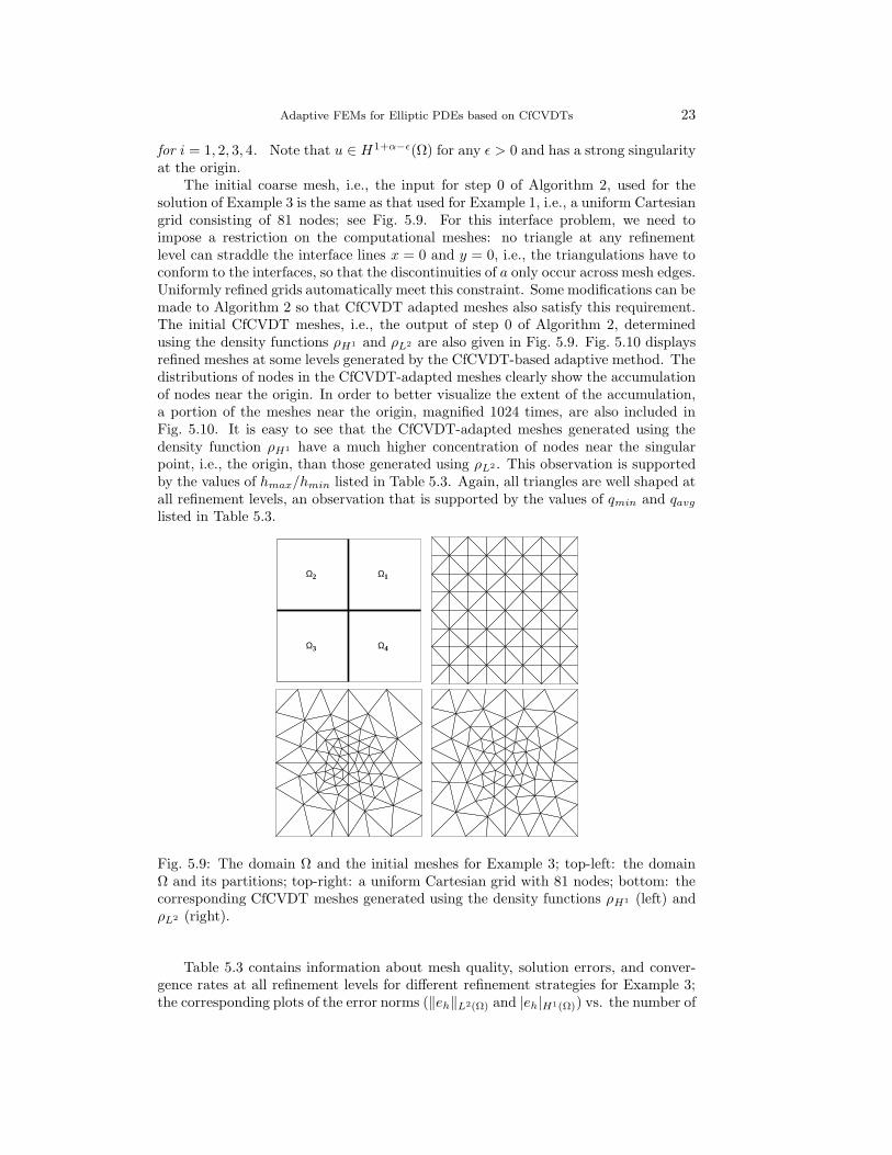
The initial coarse mesh, i.e., the input for step 0 of Algorithm 2, used for thesolution of Example 3 is the same as that used for Example 1, i.e., a uniform Cartesiangrid consisting of 81 nodes; see Fig. 5.9. For this interface problem, we need toimpose a restriction on the computational meshes: no triangle at any refinementlevel can straddle the interface lines x = 0 and y = 0, i.e., the triangulations have toconform to the interfaces, so that the discontinuities of a only occur across mesh edges.Uniformly refined grids automatically meet this constraint. Some modifications can bemade to Algorithm 2 so that CfCVDT adapted meshes also satisfy this requirement.The initial CfCVDT meshes, i.e., the output of step 0 of Algorithm 2, determinedusing the density functions ρH1 and ρL2 are also given in Fig. 5.9. Fig. 5.10 displaysrefined meshes at some levels generated by the CfCVDT-based adaptive method. Thedistributions of nodes in the CfCVDT-adapted meshes clearly show the accumulationof nodes near the origin. In order to better visualize the extent of the accumulation,a portion of the meshes near the origin, magnified 1024 times, are also included inFig. 5.10. It is easy to see that the CfCVDT-adapted meshes generated using thedensity function ρH1 have a much higher concentration of nodes near the singularpoint, i.e., the origin, than those generated using ρL2 . This observation is supportedby the values of hmax/hmin listed in Table 5.3. Again, all triangles are well shaped atall refinement levels, an observation that is supported by the values of qmin and qavg

listed in Table 5.3.

Ω

Ω Ω

Ω

3 4

12

Fig. 5.9: The domain Ω and the initial meshes for Example 3; top-left: the domainΩ and its partitions; top-right: a uniform Cartesian grid with 81 nodes; bottom: thecorresponding CfCVDT meshes generated using the density functions ρH1 (left) andρL2 (right).

Table 5.3 contains information about mesh quality, solution errors, and conver-gence rates at all refinement levels for different refinement strategies for Example 3;the corresponding plots of the error norms (‖eh‖L2(Ω) and |eh|H1(Ω)) vs. the number of


Fig. 5.10: Refined adaptive meshes at some levels generated by the CfCVDT-basedadaptive method for Example 3; top, left to right: for the density function ρH1 , 476and 2910 node meshes and the 2910 node case near the singular point magnified 1024times; bottom, left to right: for the density function ρL2 , 436 and 2868 nodes and the2868 node case near the singular point magnified 1024 times.

nodes are given in Fig. 5.11. The convergence rates for the uniform refinement methodare about 1.08 and 0.53 for ‖eh‖L2(Ω) and |eh|H1(Ω), respectively. These match verywell with those predicted by finite element theory, i.e., 2α and α, respectively, foru ∈ Hα−ε(Ω)). However, one sees that the CfCVDT-based adaptive methods stillachieve almost perfect convergence rates, i.e., 1.0 and 1.8 for |eh|H1(Ω) and |eh|L2(Ω),respectively. The values of qmin and qavg given in Table 5.3 demonstrate that thequality of the meshes produced by the CfCVDT-based adaptive methods is alwaysvery good at all refinement levels and for both density functions ρH1 and ρL2 , al-though the mesh sizes vary greatly over the Ω, e.g., hmax/hmin reaches 53393.1 at thelast level when the density function ρH1 is used. Again, since u is not in H2(Ω), wesee that hmax/hmin tends to monotonically increase for the adaptive methods. Notethat in this case, the CfCVDT-based adaptive method using the density function ρH1

generated approximate solutions having both smaller ‖eh‖L2(Ω) and ‖eh‖H1(Ω) thanusing ρL2 . We believe this phenomenon is due to the strong singularity of the exactsolution u while the density functions are constructed based on the assumption thatu ∈ H2(Ω).

From Table 5.3 and Fig. 5.11, one also observes that the CfCVDT-based adap-tive methods are much more efficient relative to the uniform refinement strategy. Forexample, for the uniform refinement method, we have that ‖eh‖L2(Ω) =1.4193e-03and |eh|H1(Ω) =1.0975e-01 on the refined mesh with 66, 409 nodes. However, for theadaptive methods, the values of these norms are 1.3335e-03 and 1.1379e-01, respec-tively, on the mesh with only 853 nodes when ρH1 is used as the density function, and1.2532e-03 and 1.1830e-01, respectively, on the mesh with only 1, 512 nodes when ρL2

is used as the density function. This means that, in the case of the |eh|H1(Ω) norm,



Uniform refinement0 81 0.828 0.828 1.0 6.1349e-02 6.5596e-011 289 0.828 0.828 1.0 2.9422e-02 1.06 4.7058e-01 0.482 1089 0.828 0.828 1.0 1.3654e-02 1.11 3.2931e-01 0.523 4225 0.828 0.828 1.0 6.3877e-03 1.09 2.2900e-01 0.524 16441 0.828 0.828 1.0 3.0046e-03 1.09 1.5869e-01 0.535 66409 0.828 0.828 1.0 1.4193e-03 1.08 1.0975e-01 0.53



10 19935 0.521 0.943 30373.2 6.3599e-05 1.71 2.2651e-02 1.1011 38024 0.596 0.944 53393.1 3.5049e-05 1.85 1.6798e-02 0.93




101

102

103

104

105

10−5

10−4

10−3

10−2

10−1

Number of Nodes

||u−

u h|| L2


2


1

Uniform refinement

101

102

103

104

105

10−2

10−1

100

Number of Nodes

|u−

u h| H1


2


1

Uniform refinement


the CfCVDT-based adaptive methods are more than 60 times more efficient than theuniform refinement method if only considering the size of the resulting system.

We display a representative approximate solution uh and the errors eh for different


refinement methods in Fig. 5.12. It is again obvious that the CfCVDT-based adaptivemethods distribute the errors much more equally over the triangles than does theuniform refinement method.

−1−0.5

00.5

1−1

−0.5

0

0.5

1

−2

−1.5

−1

−0.5

0

0.5

1

1.5

2

−1−0.5

00.5

1−1

−0.5

0

0.5

1

−0.04

−0.03

−0.02

−0.01

0

0.01

0.02

0.03

0.04

−1−0.5

00.5

1−1

−0.5

0

0.5

1

−0.04

−0.03

−0.02

−0.01

0

0.01

0.02

0.03

0.04

−1−0.5

00.5

1−1

−0.5

0

0.5

1

−0.04

−0.03

−0.02

−0.01

0

0.01

0.02

0.03

0.04


5.4. More complicated geometries. Our last two examples involve more com-plicated geometries and serve to illustrate the robustness and effectiveness of ouradaptive CfCVDT-based mesh generation algorithm.

Example 4. Let Ω = ΩS − ΩH1 ∪ ΩH2 , where ΩS = [0, 1]× [0, 1] and ΩH1 andΩH2 are two open hexagons formed by the set of vertices 0.25+0.1 cos(j−1)θ, 0.75+0.1 sin(j−1)θ)6j=1 and 0.6+0.1 cos(j−1)θ, 0.4+0.1 sin(j−1)θ)6j=1 with θ = π/3,respectively. Clearly, Ω is a square domain having two hexagonal holes; see Fig. 5.13.In general, solutions of (5.1) possess large geometric singularities at the vertices ofthe two interior hexagons. Set

a(x, y) = 1 + 10x2 + y2, b(x, y) = 1 + x2, f(x, y) = 1, and g(x, y) = 0. (5.7)


Although an analytic form of the exact solution u of (5.1) with the data (5.7) is not

known, it is known that u only belongs to H74−ε(Ω) for any ε > 0 and not to H2(Ω).

Example 5. Let Ω = ΩS1−ΩS2 , where ΩS1 = [0, 1]×[0, 1] and ΩS2 = [−0.5, 0.5]×[−0.5, 0.5]. Set

b(x, y) = 0, f(x, y) = 1, g(x, y) = 0 (5.8)

and

a(x, y) =

1 (x, y) ∈ Ω1

20 (x, y) ∈ Ω2

20 (x, y) ∈ Ω3

400 (x, y) ∈ Ω4,

(5.9)

where Ωi for i = 1, 2, 3, 4 are defined in Fig. 5.13. Note that a is discontinuous inΩ. We again do not know an analytic form of the exact solution u of (5.1) with thedata (5.8) and (5.9), but we do know that globally u only belongs to H1(Ω) (and notH2(Ω)), but u|Ωi

∈ H2(Ωi) for i = 1, 2, 3, 4.The initial coarse meshes used for the solution of Examples 4 and 5 are displayed in

Fig. 5.13. Fig. 5.14 and Fig. 5.15 present repeatedly refined meshes at different levelsgenerated by the CfCVDT-based adaptive methods for Examples 4 and 5, respectivelyfor both density functions ρH1 and ρL2 . Information about mesh quality is given inTables 5.4 and 5.5, respectively. Fig. 5.16 displays approximate solutions uh computedby our adaptive methods for the two examples.

Ω2Ω1

Ω4Ω3

Fig. 5.13: Top: the domain Ω for Examples 4 (left) and 5 (right); bottom: initialmeshes for Examples 4 (left) and 5 (right).

6. Conclusions. In this paper, we presented an efficient adaptive mesh refiningalgorithm for elliptic PDEs that combines a posteriori error estimation with centroidalVoronoi/Delaunay tessellations of domains in two dimensions. The two ingredients


Fig. 5.14: Repeatedly refined meshes at different levels generated by the CfCVDT-based adaptive methods for Example 4; top: 94, 507, and 3096 nodes using the densityfunction ρH1 ; bottom: 94, 524, and 3373 nodes using the density function ρL2 .

Fig. 5.15: Repeatedly refined meshes at different levels generated by the CfCVDT-based adaptive methods for Example 5. top: 70, 408, and 2474 nodes using the densityfunction ρH1 ; bottom: 70, 492, and 3020 nodes using the density function ρL2 .

are well linked together by the fact that the density function required by the secondone is defined and computed from the first one with standard interpolations. Variousnumerical experiments were carried out and showed that our techniques always ob-


Uniform refinement` 0 1 2 3 4 5nl 94 336 1261 4875 19159 75951qmin 0.467 0.467 0.467 0.467 0.467 0.467qavg 0.862 0.862 0.862 0.862 0.862 0.862hmax/hmin 2.4 2.4 2.4 2.4 2.4 2.4


` 0 1 2 3 4 5nl 94 146 280 507 921 1680qmin 0.721 0.727 0.614 0.715 0.636 0.649qavg 0.919 0.936 0.941 0.942 0.936 0.941hmax/hmin 1.7 2.5 2.7 3.2 3.9 5.8` 6 7 8 9nl 3096 5770 10838 20506qmin 0.538 0.556 0.567 0.529qavg 0.940 0.941 0.941 0.945hmax/hmin 9.4 10.9 18.8 30.7


` 0 1 2 3 4 5nl 94 160 287 524 968 1797qmin 0.721 0.661 0.628 0.655 0.663 0.620qavg 0.918 0.935 0.939 0.942 0.938 0.941hmax/hmin 1.6 2.1 2.2 2.7 3.0 3.8` 6 7 8 9nl 3373 6384 12168 23237qmin 0.625 0.465 0.608 0.571qavg 0.942 0.944 0.943 0.944hmax/hmin 4.0 5.9 6.5 8.6

Table 5.4: Mesh quality by different refinement methods for Example 4.

0

0.2

0.4

0.6

0.8

1 0

0.2

0.4

0.6

0.8

1

0

0.005

0.01

0.015

−1

−0.5

0

0.5

1 −1

−0.5

0

0.5

1

0

0.01

0.02

0.03

0.04

Fig. 5.16: Plots of the approximate solutions uh obtained using the CfCVDT-basedadaptive methods. Left: uh for Example 4 on the mesh with 3096 nodes generatedusing ρH1 ; right: uh for Example 5 on the mesh with 2474 nodes generated using ρH1 .

tained optimal convergence rates for the piecewise linear finite elements with respectto both H1 and L2 norms and worked pretty robust. This mesh adaptation strategycan be easily generalized and applied to higher-order finite element approximations ormixed finite element formulations. We also would like to remark that we are currently


Uniform Refinement` 0 1 2 3 4 5nl 70 232 832 3136 12160 47872qmin 0.828 0.828 0.828 0.828 0.828 0.828qavg 0.845 0.845 0.845 0.845 0.845 0.845hmax/hmin 1.3 1.3 1.3 1.3 1.3 1.3


` 0 1 2 3 4 5nl 70 90 137 233 409 734qmin 0.548 0.653 0.681 0.583 0.518 0.541qavg 0.903 0.917 0.931 0.930 0.929 0.38hmax/hmin 1.5 2.4 3.9 5.8 9.6 15.1` 6 7 8 9 10 11nl 1344 2474 4608 8685 16519 31555qmin 0.524 0.540 0.493 0.531 0.472 0.419qavg 0.935 0.939 0.942 0.943 0.944 0.942hmax/hmin 19.9 33.6 86.4 170.0 288.1 381.9


` 0 1 2 3 4 5nl 94 141 276 492 888 1625qmin 0.747 0.720 0.697 0.690 0.534 0.612qavg 0.921 0.931 0.936 0.935 0.935 0.943hmax/hmin 1.38 2.2 4.8 4.5 6.8 6.6` 6 7 8 9 10nl 3020 5612 10477 19611 38354qmin 0.635 0.502 0.567 0.595 0.582qavg 0.941 0.944 0.945 0.945 0.944hmax/hmin 9.1 11.9 13.9 15.5 25.2

Table 5.5: Mesh quality by different refinement methods for Example 5.

studying the extension of this methodology to problems in three dimensions and totime dependent problems.

Acknowledgments. The authors would like to thank the referees for their valu-able suggestions which improved the paper a lot.

REFERENCES

[1] S. Arya and D. Mount, Approximate nearest neighbor searching, Proceedings of 4th Ann.ACM-SIAM Symposium on Discrete Algorithms (SODA’93), 1993, pp. 271-280.

[2] M. Ainsworth and J. Oden, A Posteriori Error Estimation in Finite Element Analysis,Wiley, 2002.

[3] R.E. Bank and R.K. Smith, Mesh smoothing using a posterior error estimates, SIAM J.Numer. Anal. 34, 1997, pp. 979-997.

[4] I. Babuska and A. Miller, A feedback finite element method with a posteriori error estimationPart I, Comput. Meth. Appl. Mech. Engrg 61, 1987, pp. 1-40.

[5] I. Babuska and W.C. Rheinboldt, Error estimates for adaptive finite element computations,SIAM J. Numer. Anal. 18, 1978, pp. 736–754.

[6] I. Babuska and W.C. Rheinboldt, A posteriori error estimates for the finite element method,Int. J. Numer. Meth. Engrg. 12, 1978, pp. 1597-1615.

[7] I. Babuska and W.C. Rheinboldt, A posteriori error analysis of finite element solutions forone dimensional problems, SIAM J. Numer. Anal. 18, 1981, pp. 565-589.

[8] P. Binev, W. Dahmen, and R. DeVore, Adaptive finite element methods with convergencerates, Numer. Math. 97, 2004, pp. 219-268.

[9] S. Brenner, Multigrid methods for the computation of singular solutions and stress intensityfactors I: Corner singularities, Math. Comp. 68, 2003, pp. 559-583.


[10] S. Brenner and L.-Y. Sung, Multigrid methods for the computation of singular solutions andstress intensity factors III: Interface singularities, Comp. Meth. Appl. Mech. Engrg. 192,2003, pp. 4687-4702.

[11] C. Carstensen, All first-order averaging techiniques for a posteriori finite element error controlon unstructured grids are efficient and reliable, Math. Comp. 73, 2003, pp. 1153-1165.

[12] L. Chen and J. Xu, Optimal Delaunay triangulation, J. Comp. Math. 22, 2004, pp. 299-308.[13] P.G. Ciarlet, The Finite Element Method for Elliptic Problems, North-Holland, 1978.[14] W. Dorfler, A Convergent adaptive algorithm for Poisson’s equation, SIAM J Numer. Anal.

33, 1996, pp. 1106-1124.[15] Q. Du, V. Faber, and M. Gunzburger, Centroidal Voronoi tessellations: Applications and

algorithms, SIAM Review 41, 1999, pp. 637-676.[16] Q. Du and M. Gunzburger, Grid generation and optimization based on centroidal Voronoi

tessellations, Appl. Math. Comptut. 133, 2002, pp. 591-607.[17] Q. Du, M. Gunzburger, and L. Ju, Constrained centroidal Voronoi tessellations on general

surfaces, SIAM J. Sci. Comput. 24, 2003, pp. 1488-1506.[18] Q. Du, M. Gunzburger, and L. Ju, Voronoi-based finite volume methods, optimal Voronoi

meshes and PDEs on the sphere, Comp. Meth. Appl. Mech. Engrg. 192, 2003, pp. 3933-3957.

[19] Q. Du and D. Wang, Tetrahedral mesh generation and optimization based on centroidalVoronoi tessellations, Int. J. Numer. Methods Engrg. 56, 2003, pp. 1355-1373.

[20] Q. Du and D. Wang, Anisotropic centroidal Voronoi tessellations and their applications, SIAM.J. Sci. Comput. 26, 2005, pp. 737-761.

[21] D. Field, Laplacian smoothing and Delaunay triangulation, Comm. Appl. Numer. Methods 4,1988, pp. 709-712.

[22] D. Field, Quantitative measures for initial meshes, Int. J. Numer. Methods Engrg. 47, 2000,pp. 887-906.

[23] P. Grisvard, Elliptic Problems in Nonsmooth Domains, Pitman, Boston, 1985.[24] L. Ju, Q. Du, and M. Gunzburger, Probabilistic methods for centroidal Voronoi tessellations

and their parallel implementations, Parallel Comput. 28, 2002, pp. 1477-1500.[25] P. Morin, R. Nochetto, and K. Siebert, Data oscillation and convergence of adaptive FEM,

SIAM J. Numer. Anal. 38, 2000, pp. 466-488.[26] P. Morin, R. Nochetto, and K. Siebert, Convergence of adaptive finite element methods,

SIAM Review 44, 2002, pp. 631-658.[27] P. Morin, R. Nochetto, and K. Siebert, Local problems on stars: A posteriori error esti-

mators, convergence, and performance, Math. Comp. 72, 2003, pp. 1067-1097.[28] P.-O. Persson and G. Strang, A simple mesh generator in Matlab, SIAM Review 46, 2004,

pp.329-345.[29] J. Shewchuk, Triangle: Engineering a 2D quality mesh generator and Delaunay triangulator,

Lecture Notes in Comput. Sci. 1148, Springer, New York, 1996, pp. 203-222.[30] J. Shewchuk, What is a good linear element? Interpolation, conditioning and quality measures,

Proceedings of the 11th International Meshing Roundtable, Sandia National Laboratories,Albuquerque, 2002, pp. 115-126.

[31] R. Verfurth, A Review of A Posteriori Error Estimation and Adaptive Mesh-RefinementTechniques, Wiley-Teubner, Chichester, 1996.

Adaptive finite element methods for elliptic problems: Abstract framework and applications

Documents

Transcript of Adaptive finite element methods for elliptic problems: Abstract framework and applications