An International Journal

computers & mathematics with applkations

PERGAMON Computers and Mathematics with Applications 42 (2001) 1043-1053 www.elsevier.nl/locate/camwa

The Gradient-Finite Element for Elliptic Problems

Method

I. FARAG~ AND J. KARATSON E&&is LorAnd University, Department of Applied Analysis

H-1088 Budapest, Mtizeum krt. 6-8, Hungary <faragoisXkaratson>Qludens.elte.hu

Abstract-The coupling of the Sobolev space gradient method and the finite element method is developed. The Sobolev space gradient method reduces the solution of a quasilinear elliptic problem to a sequence of linear Poisson equations. These equations can be solved numerically by an appropriate finite element method. This coupling of the two methods will be called the gradient-finite element method (GFEM). Linear convergence of the GFEM is proved via suitable error control in the steps of the iteration. The GFEM defines an already preconditioned iteration in the sense that the theoretical ratio of convergence of the Sobolev space GM is preserved. Finally, a numerical example illustrates the method. @ 2001 Elsevier Science Ltd. All rights reserved.

Keywords-Sobolev space gradient method, Finite element method, Quasilinear elliptic boundary value problems, Preconditioned iteration.

1. INTRODUCTION

This paper is devoted to the numerical solution of uniformly elliptic quasilinear boundary value

problems of the form P(U) = -divg(z, Vu) + q(z, u) = f(z),

upn = 0. (1.1)

(The exact conditions on the domain 52 and the functions g, q, f are given in Section 2.) This type

of problem arises, among other fields, in elastoplasticity theory or in connection with magnetic

potential. We note that one is usually looking for the derivative Vu of the solution.

The usual ways of the numerical solution to (1.1) are the widespread finite difference and

finite element methods, which reduce the BVP to finite-dimensional nonlinear algebraic systems

of equations (see, e.g., [1,2]). Th e condition number of the Jacobians of these systems can

be arbitrarily large when discretization is refined. Hence, a suitable nonlinear preconditioning

technique has to be developed [3].

One of the methods which, besides Newton’s method, is most widely applied to these nonlinear

algebraic systems is the gradient method (together with its versions, e.g., the conjugate gradient,

This research was supported by Hungarian National Research Fund OTKA Nos. TO19460 and F022228. We are grateful for the keen help of T. Unyi and G. VGrb, who provided information for the physical model problem, and of L. Lhzl6, who helped us in using MATLAB to realize the FEM program. Further, we are thankful for the valuable suggestions of the unknown referee who has called our attention to important aspects of the topic.

0898-1221/01/g - see front matter @ 2001 Elsevier Science Ltd. All rights reserved. PII: SO898-1221(01)00220-6

Typeset by .%+%X

1044 I. FARA& AND J. I<AH.~TSON

method). Its main advantages are easy slgorithmization and linear convergence under uniform

ellipticity assumptions. In this context, the gradient method (henceforth referred to as GM) is

used in a finite-dimensional setting.

In contrast, the approach of our paper involves the infinite-dimensional generalization of the

GM. This was first developed in Hilbert spaces by Kantorovich [4,5], giving way to a lot of new

investigations. However, the continuity assumptions of these results make application to differen-

tial operators impossible. Getting around this difficulty in theory was achieved by applying the

infinite-dimensional GM to the (nonconstructively defined) generalized differential operators; this

Sobolev space method becomes constructive by the observation that, under suitable conditions,

the generalized operator is expressed as (-A)-‘P, where A stands for the Laplacian (see [5,6]).

We have investigated a setting which ensures that this decomposition holds throughout the iter-

ation [7]. The Sobolev space GM reduces the solution of the nonlinear equation to the sequence

of linear (Poisson) equations.

This paper suggests an approach for a numerical method based on the Sobolev space GM. The

application of the GM is determined only by the way in which the linear Poisson equations are

solved. In this paper, the application of the finite element method is proposed for the solution

of these linear problems. This coupling of the gradient and the finite element methods will be

called the gradient-finite element method (GFEM).

The GFEM approach has different advantages. The GM in this case not only yields conver-

gence, but it also linearizes in the sense that the original nonlinear problem is reduced to the

sequence of linear problems. This also means that the numerical questions of the GFEM coin-

cide with those arising for the FEM for the linear Poisson problems. The numerical handling of

the latter is well known and has wide literature involving several different approaches (adaptive,

mixed, multilevel, multigrid methods, domain decomposition, etc.), which exhibit good algorith-

mization and have standard error estimates. The choice of one of the above versions of the FEM,

which determines the efficiency of the whole GFEM algorithm, depends on the problem to be

solved.

The choice of the infinite-dimensional version of the GM preserves the ellipticity bounds of the

differential operator in the ratio of convergence (in contrast to the finite-dimensional GM for the

discretized problem). This means that the GFEM defines an already preconditioned iteration;

i.e., we need not face the sometimes cumbersome work of preconditioning. Further, choosing the

(suitable) FEM for the solution of the Poisson equations yields that the numerically constructed

sequence runs in the same function space as that in which the theoretical solution lies.

The aim of this paper is to achieve convergence of the coupled method, to which end our task

is to provide appropriate error control for the FEM in the steps of the GM iteration. Finally,

a numerical example with a suitable choice of FEM illustrates the feasibility of the proposed

method.

2. THEORETICAL BACKGROUND

In this section, we first deal with the BVP, and then the corresponding results on the Sobolev

space GM are formulated. We consider the BVP (1.1)

P(U) = -divg(z, VU) + q(z, u) = f(z), yan = 0,

on a bounded domain fl c RN with the following conditions:

(i) dR E C2 or R is convex; g E Cl@ x RN;RN), q E Cl@ x R), f E L2(s2). (ii) The matrix g(~,p) y is s mmetric, uniformly bounded, and positive definite; i.e., there

exist m’ > m > 0 such that its eigenvalues are between m and m’ for all (2, p) E fi x RN. (iii) There exist constants yr,yz > 0 such that 0 5 $$(x, U) 5 yr for all (2, U) E n x R and

]$$(z,p)) I y2lpl for all (z,P) E 2 x RN.

We define D(P) E H2(fl) n HA(R) as the domain of the operator P.

Gradient-Finite Element Method 1045

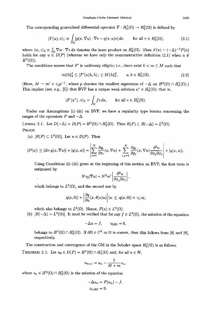
The corresponding generalized differential operator F : Hi(a) + Hi((52) is defined by

(F(u), 41 = s,[g(x, Vu) . Vv + dz, 44 dx, for all v E H:(R), (2.1)

where (w, z)r E so VW. Vzdx denotes the inner product on H;(0). Then F(u) = (-A)-‘P(u)

holds for any ‘11 E D(P) ( w h ereas we have only the nonconstructive definition (2.1) when u 4

H2(W The conditions ensure that F’ is uniformly elliptic; i.e., there exist 0 < m 2 M such that

4lhll:: I (F’(uP, WI I W4:, u, h E H;(a).

(Here, 1M = m’ + yrp-l, where p denotes the smallest eigenvalue of -A on

This implies (see, e.g., [5]) that BVP has a unique weak solution u* E Hi(a);

(2.2)

H2(s2) n H;(a).)

that is,

(F (u*) ,v)l = / fvdx, for all v E Hi(R). R

Under our Assumptions (i)-(“‘) m on BVP, we have a regularity type lemma concerning the

ranges of the operators P and -A.

LEMMA 2.1. Let D(-A) = D(P) = H2(R) fl H,-j((R). Then R(P) c R(-A) = L2(s2).

PROOF.

(a) [R(P) c L2(fl)]. Let u E D(P). Then

N ag, N dg. IP( I Idivgb, Vu)1 + lq(~,u)l = c 2(x,Vu) + c L(x7Vu)&

i=l dxi i,j=l +j 3 z + lq(x’u)l’

Using Conditions (i)-(iii) g iven at the beginning of this section on BVP, the first term is

estimated by

N-Y2lW +N2m’ & 1 I I 3 a

which belongs to L2(s2), and the second one by

Ic7cG0)l+ ~~z,ew4~ 1% 5 IdGO)l +nl4,

which also belongs to L2(s2). Hence, P(u) E L2(s2).

(b) [R(-A) = L2(s2)]. It must be verified that for any f E L2(r;2), the solution of the equation

-Au = f, u1as-r = 0,

belongs to H2(s2) n Ho(Q). If 6% E C2 or fl is convex, then this follows from [8] and [9],

respectively.

The construction and convergence of the GM in the Sobolev space HA(R) is as follows.

THEOREM 2.1. Let ug E D(P) = H2(n) n Hi(Q) and, for all n E N,

2 %+1 = un - jyjqq-p’

where z, E H2(s2) n H,j(Ck) is the solution of the equation

-AZ, = P(u,) - f,

kpn = 0.

1046 I. FAHAC,~ AND .J. KAR.~TSON

Then

(where p denotes the smallest eigenvalue of’-A on H2(s2) n Hi(R)).

PROOF. In order to apply Theorem 2 of [7] to BVP in the case D(P) = o(-A) = H2(Q)nH~(Cl),

it suffices that the inclusion R(P) c R(-A) holds. This has just been proved in Lemma 2.1.

The algorithmic form of the GM in Hi(R) is the following:

(1) uo E H2(s2) n H,‘(O); for any n E N,

(2a) r, = P(%) - f,

(GM) (2b) Z, = (-A)-%,, Z, E H2(fl) n H;(O), (2.3)

(2c) %I+1 = % - &zn.

REMARK 2.1. The definition D(-A) = H2(s2) n Hi(R), w rc remains valid throughout this h’ h paper, means that the Poisson equations (2b) in (2.3) are automatically understood with homo-

geneous Dirichlet boundary conditions.

The summary of this section is that the GM (2.3) gives a theoretically well-defined sequence which converges linearly, such that the solution of equation P(U) = f is reduced to a sequence of linear Poisson equations.

To turn this theoretical algorithm into a numerical one, we must specify the way in which z, is computed numerically.

3. THE GRADIENT-FINITE ELEMENT METHOD

3.1. Construction

The crucial point of realizing the GM algorithm (2.3) is the solution of the auxiliary Poisson equations (2b). We are going to investigate the process in which these auxiliary equations are computed numerically by the finite element method. This method is the gradient-finite element method (GFEM).

The FEM is able to yield that the numerical solutions of the auxiliary equations belong to H2(s2) n H;(R) in which the exact solutions Z, are. Therefore, in the next step, we can apply the operator P directly to the numerically computed u,+i. Thus, the method is determined only by the accuracy of the numerical computation of the functions 2,.

These considerations give the following algorithm: let (6,) C R+ be a sequence such that 6, + 0. Then

(z: = (-a)-‘~, denotes the exact solution of the auxiliary equation);

(GFEM) (2b) zn zz 2: using FEM such that (3.1)

F, E H2(n) n Hi(R) and ]]f --F,]]r 5 6,, I

(1) ?&, E H2(fl) n HA(R); for any n E N,

(2a) Tn = P(?&) - f,

I (2c) &+1 = iin - +_%.

In other words, F, is the numerically computed solution of the auxiliary equation

in H2(s2) with accuracy 6, in Hi(R) norm.

Gradient-Finite Element Method 1047

3.2. Convergence

The convergence estimates on (En) are obtained from the investigation of

where (u,) is defined by the theoretical GM (2.3) with uo = Ec.

LEMMA 3.1. Let J : H;(R) + H;(R), J(u) = u - (2/(M + m))F(u). Then

PROOF. It relies on the idea of the proof of convergence of the GM (see [5]). We remark that we

have

J’(u)h = h - &F’(u)h, u, h E H;(R).

Let U, ‘u E H,(O) be fixed. Then

s 1

J(u) -J(v) = 0

J’(v+t(u-v))(u-v)dt = u-u-& s

1

F’(v+t(u-v))(u-v)dt. (3.2) 0

Let A : HJ(R) + HJ(R),

2 J 1

Ar=r-p 1M+m 0

F’(v + t(u - u))r dt.

Then A is a bounded self-adjoint linear operator since F’(w) has these properties for all w E

HA(a). Further, using (2.2),

-~llrllT = llrllf - &~llrll~

5 (Ar,r) < Ilrll? - j&n’ll# = ~II~IIL r E H;(R).

Hence, llAl/l I (A4 -m)/(M+m). S ince by (3.2) J(u) - J(v) = A(u - w), the lemma is proved.

LEMMA 3.2. For all n E N, there holds the estimate

E n+l 2 &r+m n M-mE + +&.

PROOF. We have

2 21,+1 -Gin+1 = U, - -.z

2

M+m n- ;ii, - -

M+mzn >

= I& - i& - & (z, - z;) - j-j& (z; -q .

Here z, - zz = (-A)-l(P(un) - P(&)) = F(u,) - F(?&). Hence (using Lemma 3.1 and (3.1)),

u,+i - %z+i = J(un) - J(G) - g--&G%),

lb,+1 -G+& I IIJ(4 - J@in)ll~ + <M-m - M+m Ibn - Gzll, + &--$“.

1048 I. FARA& AND J. KARATSON

THEOREM 3.1. Let 0 < q < 1 be fixed, cl > 0, and 6, 5 clq” (n E N). Then (with a suitable

constant cz > 0), the following estimates hold for all n.

(a) If q > (M - m)/(M + m), then IIT& - u*[/I 5 c2qn.

(b) If q < (111 - m)/(M + m), then 11% - u*lji I cz((M - m)/(M + m))“.

PROOF. Since Theorem 2.1 yields

Il% - 2L*JIl 5 II% - %(I1 + II% - u*lll I IIGI - %I11 + c3

it suffices to verify our estimates (a),(b) for E, = II& - u,IIr instead of 11% - U* II 1.

We use notations Q = (M - m)/(M + m) and cy = 2/(M + m). Then Lemma 3.2 asserts

(a) Let c2 = crcl/(q - Q). We prove by induction

J% I c2qn, n E N.

Since Eo = II&, - UO((~ = 0, equation (3.3) is trivial for n = 0.

If (3.3) holds for fixed n E N, then

E n+l I &En + a& 2 c2Qqn + ClmP

WQ = _ + cla

> qn = sqn+l = czqn+l,

q-Q

(b) Let r = q/Q, c2 = crclr/q(l - r). We prove by induction

E, I c2 (I- rn) Q”, n E N.

For n = 0, this is again trivial.

If (3.4) holds for fixed n E N, then

E n+l 5 QE, + a& 5 c2 (1 - rn) Qn+’ + claqn

(3.3)

(3.4)

= aclr (1 - r”)

41 - r)

Qn+l+ y,n+lQn+'_ a;, (:_:" I rn) Qn+l

= 3 (1 - rn+‘) Qn+l = c2 (1 _ rn+l) ~n+l.

The hereby verified inequality (3.4) yields the desired estimate

& 5 c2Qn, n E N.

REMARK 3.1. The formula c:! = acl/(q - Q) in Part (a) of the proof shows that c2 -+ co as

q -+ Q = (M - m)/(M + m) f rom above in Part (a) of the theorem. This suggests that in the

case q = (M - m)/(M + m), convergence is faster than sn for any s > (M - m)/(M + m), but

is slower than ((M - m)/(M + m))“.

REMARK 3.2. Denoting by h, the width of the mesh used in (2b) in (3.1), we have the estimate

with suitable constants C, C’ > 0. The obtained expression on the right side plays the role of 6,.

If (hn) -+ 0 is chosen a geometric sequence and sup{ IIP(E~) - fll~s(o) : TZ E N} < +CXJ (which

can be assumed since &) is constructed to converge to the solution of equation P(U) = f), then

the condition of Theorem 3.1 on 6, is fulfilled; i.e. (instead of estimating S, in the steps), the

suitably prescribed refinement of the mesh yields the required order estimate of the convergence

of 6,.

Gradient-Finite Element Method 1049

4. NUMERICAL EXAMPLE

4.1. The Model Problem

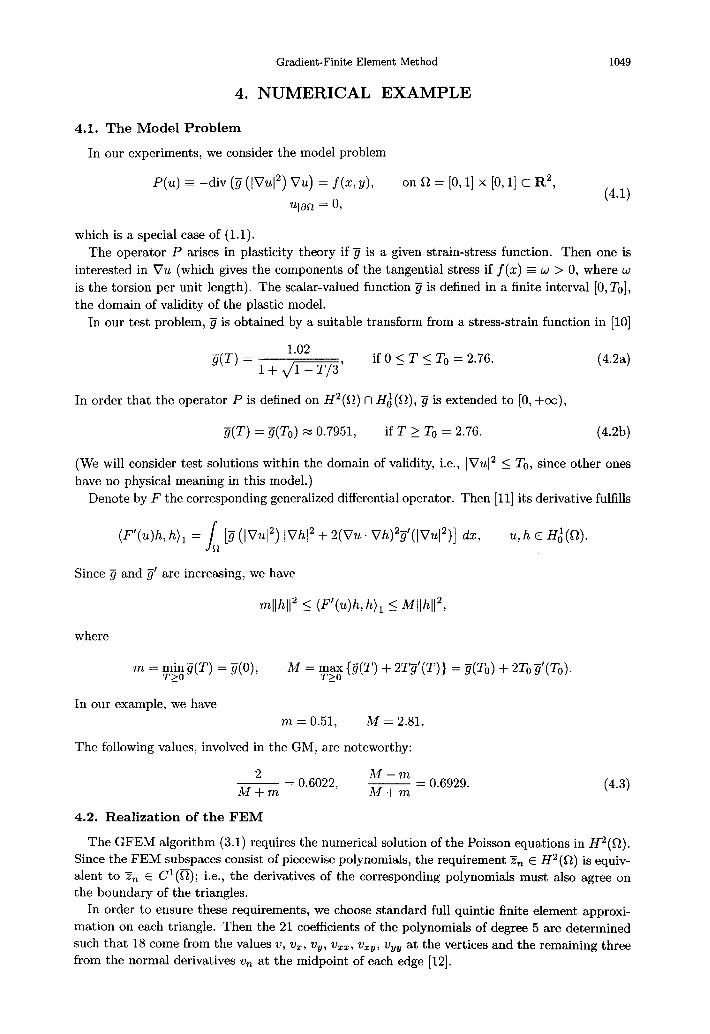
In our experiments, we consider the model problem

P(U) - -div (?j ([VU[~) VU) = f(z, y),

uian = 0,

on R = [O,l] x [0, l] c R2, (4.1)

which is a special case of (1.1).

The operator P arises in plasticity theory if ?j is a given strain-stress function. Then one is

interested in Vu (which gives the components of the tangential stress if f(o) = w > 0, where w

is the torsion per unit length). The scalar-valued function g is defined in a finite interval [0, To],

the domain of validity of the plastic model.

In our test problem, ?j is obtained by a suitable transform from a stress-strain function in [lo]

G(T) 1.02 = 1+J_’

if 0 5 T 5 To = 2.76. (4.2a)

In order that the operator P is defined on H2(s2) n Hi’(R), g is extended to [0, +co),

g(T) = g(To) x 0.7951, if T 2 To = 2.76. (4.2b)

(We will consider test solutions within the domain of validity, i.e., IVu12 5 To, since other ones

have no physical meaning in this model.)

Denote by F the corresponding generalized differential operator. Then [ll] its derivative fulfills

(F’(u)h, h), = / [jj(lV~1~) IVh12 + 2(Vu.. Vh)2$(IV~12)] ds, U, h E H;(a). R

Since g and 3’ are increasing, we have

W412 I P’W, h), 5 Nhl12,

where

m = ying(T) = g(O), M = y;; {g(T) + 2T$(T)} = g(To) + 2Tog’(To). - -

In our example, we have

m = 0.51, M = 2.81.

The following values, involved in the GM, are noteworthy:

2 ~ = 0.6022,

Al- m

Mfm - = 0.6929. Mtm

4.2. Realization of the FEM

The GFEM algorithm (3.1) requires the numerical solution of the Poisson equations in H2(s2). Since the FEM subspaces consist of piecewise polynomials, the requirement YZ, E H2(S1) is equiv-

alent to f, E C’(n); i.e., the derivatives of the corresponding polynomials must also agree on

the boundary of the triangles. In order to ensure these requirements, we choose standard full quintic finite element approxi-

mation on each triangle. Then the 21 coefficients of the polynomials of degree 5 are determined

such that 18 come from the values v, v,, 2ry, uZZ, vZy, vyy at the vertices and the remaining three from the normal derivatives v, at the midpoint of each edge [12].

1050 I. FARAG~ AND 3. KARATSON

For the case U* E H”(R) (Ic = 1, . . . ,6), the error estimate

element subspace is

]]u* - ~h]]r < con&. h”-l IIu*llk

[12] corresponding to this finite

(4.4)

It is worth underlining the case when u* happens to be in H6(s2),

IIu* - uhlll 5 const . h5 ~~2~~~~~. (4.5)

The use of higher-order FEM is not widespread, owing to the required number of arithmetic

operations. However, the reasonability of its usage is justified in literature (see, e.g., [13-15]), it is

also a basis for the &version [16]. Among the favourable properties, we recall the accuracy (4.4).

REMARK 4.1. To execute the numerical integration required for compiling the systems of linear

algebraic equations, we use a quadrature formula of order 5 [17]. This yields accuracy 0(h3),

whereas preserving the optimal order (4.5) would demand an even higher-order quadrature [18],

which would increase significantly the numerical cost of computation. Thus, our choice means a

compromise which will prove to be sufficient in the experiments.

A good property of the FEM within the GFEM iteration, as we mentioned in Section 3.1, is

that the operator P can be applied directly to i&, in the next step. In course of the realization,

this means that the functions ?iil, can be stored as

of P(?&) that are necessary in the next step for

directly.

vectors of coefficients. From this, the values the numerical integration can be calculated

4.3. Experiments

In this section, we illustrate the application of the GFEM in different test problems. The test

problems have been chosen to enable us to study the effect of two factors on the convergence

(namely, that of the widths h and the smoothness of the exact solution) until the prescribed

accuracy is reached.

In all the test problems, the right sides f in (4.1) were chosen such that the exact solution is

known. To realize the GFEM, we prepared a MATLAB program. We constructed the FEM part

of the program to represent the solution in a suitable way, i.e., in a form that can be used for the

calculations in the next step of the iteration of GM.

Throughout the experiments, the error is understood in the space H,(R). That is, let

en = IIu* - %111, (4.6)

where u* denotes the exact solution of (4.1). (The choice is motivated by the fact that we are

looking for VU*.)

TEST PROBLEM 1. The function U* is defined as follows:

- u*(& Y) P(S) (Y Y2> 0.2 + if where P(Z) (1 (22 1)“) , 0 < 3: 5 0.5, := - 9 :=

0.2 (1 - (22 - 1)“) , if 0.5 55 5 1.

Further, let f(z, y) = P(u*(x, y)). W e examine the test problem (4.1) with this f. Then the

exact solution U* belongs to C2(a) \ C3(St).

We make three numerical experiments of applying the GFEM such that in each experiment we

use a fixed mesh throughout the GM iteration. The widths of these meshes are h = 1, h = 0.5,

and h = 0.25, respectively. The computations are made up to accuracy of 10p4.

Tables l-3 contain the nodal errors sn of zi,, which we define as discrete Lz-norm of the

difference of the derivatives (those computed in the FEM approximation and the exact ones)

Gradient-Finite Element Method

Table 1. (h = 1).

1051

n 1 2 3 4 5 6 7 8 9 10

En 0.4381 0.3043 0.2167 0.1607 0.1250 0.1021 0.0873 0.0778 0.0716 0.0702

Table 2. (h = 0.5)

n 1 2 3 4 5 6 7 8 9 10

&II 0.3808 0.2364 0.1446 0.0886 0.0554 0.0354 0.0232 0.0155 0.0107 0.0077

71 11 12 13 14 15 16 17 18 19

En 0.0057 0.0045 0.0037 0.0033 0.0029 0.0027 0.0026 0.0025 0.0025

Table 3. (h = 0.25).

n 1 2 3 4 5 6 7 8 9 10

En 0.3334 0.2100 0.1305 0.0816 0.0518 0.0332 0.0215 0.0139 0.0091 0.0059

n 11 12 13 14 15 16 17 18 19 20 21

En 0.0039 0.0025 0.0017 0.0011 0.0007 0.0005 0.0003 0.0002 0.0002 0.0001 0.0001

Table 4.

I h=l I h = 0.5 1 h = 0.25 1

1 ~~ e1() = 0.0935 e1g = 0.0.0037 1 ezl = 0.0001 1

with respect to the mesh points. (Computing the nodal error requires no extra work since the

used values of derivatives appear during the FEM calculations.)

In each experiment, we compute the error e, defined in (4.6) for the last iteration. (It is

done by a numerical quadrature which, in contrast to the nodal error, ensures the corresponding

accuracy.) The results are given in Table 4.

The above tables show that the width h = 0.25 has been able to produce the required ac-

curacy lop4 for em. (W e note that therefore the use of the standard solver of MATLAB was

sufficient for the linear systems.)

It is apparent that after sufficiently many iterations, the nodal errors are stabilized around a

certain value which corresponds to the approximation order of the applied finite element subspace.

Since our aim is to preserve the linear convergence of the theoretical GM, it is worth computing

the ratios En+1

qn=-. GZ

The results are given in Tables 5-7.

Table 5. (h = 1).

?l 1 2 3 4 5 6 7 8 9

4n 0.69 0.71 0.74 0.78 0.82 0.86 0.89 0.92 0.98

(4.7)

1052 I. FARAG~ AND J. KARATSON

Table 6. (h = 0.5).

n 1 2 3 4 5 6 7 8 9

Qn 0.62 0.61 0.61 0.63 0.64 0.66 0.67 0.69 0.72

n 10 11 12 13 14 15 16 17 18

Qn 0.74 0.79 0.82 0.89 0.88 0.93 0.96 0.96 1.00

Table 7. (h = 0.25).

12 1 2 3 4 5 6 7 8 9 10

4n 0.63 0.62 0.63 0.63 0.64 0.65 0.65 0.65 0.65 0.66

R 11 12 13 14 15 16 17 18 19 20

Qn 0.64 0.68 0.65 0.64 0.71 0.60 0.67 1.00 0.50 1.00

These tables show that for some time, the values of qn follow the ratio of the theoretical

GM (4.3), then this property is lost. The number of steps when qn rises over, e.g., 0.85 essentially

coincides with the above-mentioned stabilization of the error E,.

As seen above, for smaller values of h, the error is stabilized later and around a smaller value.

Before this stabilization takes place, the ratio of convergence on a given mesh has essentially the

same order as for the refined one. Since the cost of numerical computations is greater on a mesh

of half width, it is worth doing the iteration on a coarser mesh as long as possible.

TEST PROBLEM 2. The setting is the same as for Test Problem 1, now with

ull*(z, Y) := P(X) (!I - Y2> > where p(x) := 2n (0.75X - x3) , if 0 5 z 5 0.5,

27r (X - 22) ) if 0.5 < J: 5 1.

Then u* E Cl(a) \ C’(R).

TEST PROBLEM 3. For this problem, the solution is u*(z, y) = 0.5 sinrzsinny. Then u* E

CcQ(fi).

We summarize briefly the experiences of Test Problems 2 and 3, without giving the detailed

numerical results.

Similarly as for Test Problem 1, the errors are stabilized after some time around values which

depend on h in the same way. At the same time, these values are greater in Test Problem 2

(involving a solution u* of worse smoothness) than in Test Problem 1. However, they are not

significantly better in Test Problem 3 (with “maximally” smooth u*) than in Test Problem 1.

That is, the smoothness required for the classical solution is sufficient to produce the favourable

behaviour that can be provided by possible greater smoothness.

REMARK 4.2. Due to (4.4), the width h = 0.25 (which is far from sufficiently small in the case

of piecewise linear elements) has been able to produce accuracy 0(10e4) for e,.

REMARK 4.3. We only mention for brevity that the discrete norm IlEn - u*((~~(G~ followed the

behaviour of e, in the same order.

5. SUMMARY AND FURTHER DIRECTIONS

This paper has set the aim to turn the theoretical Sobolev space gradient method (GM)

a feasible type of numerical methods through coupling with the finite element method.

following results have been achieved.

l The algorithm of the gradient-finite element method (GFEM) has been constructed,

into

The

Gradient-Finite Element Method 1053

l Convergence has been proved via appropriate error control.

l We have observed that the GFEM inherits the main advantages of the Sobolev space GM.

Namely, the GM preserves the ellipticity bounds of the differential operator in the ratio

of convergence; i.e., it defines an already preconditioned iteration. Further, executing the

simple GM iteration yields that the numerical questions of the GFEM coincide with those

arising for the FEM for the linear Poisson equations. This means that the numerical

handling of the GFEM is reduced to that of linear problems.

l A numerical example has demonstrated the feasibility of the method. Since this example

was intended for illustration, we have chosen the possible simplest FEM subspace (primal

version and fixed grids) within the requirement I?& E C’(a).

The introduction and theoretical foundations of the GFEM in this paper open a number of

directions for further investigation and development.

1. 2.

3. 4. 5. 6.

7.

8.

9. 10.

11

Ph. Ciarlet, The Finite Element Method for Elliptic Problems, North Holland, Amsterdam, (1978). I.N. Molchanov and L.D. Nikolenko, Introduction to the Finite Element Method, (in Russian), Naukova

Dumka, Kiev, (1989). 0. Axelsson, Iterative Solution Methods, Cambridge Univ. Press, (1994). L.V. Kantorovich and G.P. Akilov, Functional Analysis, Pergamon Press, (1982).

.I. Necas, Introduction to the Theory of Elliptic Equations, J. Wiley and Sons, (1986). H. Gajewski, K. GrGger and K. Zacharias, Nichtlineare Operatorgleichungen und Operatordifferentialgleich- ungen, Akademie-Verlag, Berlin, (1974). J. KarAtson, The gradient method for a class of nonlinear operators in Hilbert space and applications to quasilinear differential equations, Pure Math. Appl. 6 (2), 191-201, (1995). L. Simon and E. Baderko, Linear Partial Diflerential Equations of Second Order, (in Hungarian), Tankijnyv- kiadb, Budapest, (1983). W. Hackbusch, Theorie und Numerik Elliptischer Differentialgleichungen, Teubner, Stuttgart, (1986). I. Kovtis, J. Lendvai and G. V6r6s, Effect of precipitation structure on the work hardening process, Materials Sci. Forum 217-222, 1275-1280, (1996).

__. S.G. Mikhlin, The Numerical Performance of Variational Methods, Walters-Noordhoff, (1971). 12. G. Strang and G.J. Fix, An Analysis of the Finite Element Method, Prentice Hall, Englewood Cliffs, NJ,

(1973).

Comparison to other methods belonging to the traditional ‘discretize first’ approach in-

volving FEM. Special attention should be paid to multigrid methods and different pre-

conditioning techniques for the discretized system.

Decreasing the smoothness of the FEM subspace in the steps of the GM iteration.

Using more subtle versions of FEM (adaptive, mixed, multilevel, multigrid, etc.) within

the GFEM approach.

Applying other iterative methods in the Sobolev space: gradient type (e.g., conjugate

gradients) or Newton’s method.

Analysis of computational aspects.

REFERENCES

13. F.A. Bornemann, B. Erdmann and R. Kornhuber, A posteriori error estimates for elliptic problems in two

and three space dimensions, SIAM J. Numer. Anal. 33 (3), 1188-1204, (1996). 14. F. Ihlenburg and I. BabuSka, Dispersion analysis and error estimation of Galerkin finite element methods for

the_Helmholtz equation, Internat. J. Numer. Methods Engrg. 38 (22), 3745-3774, (1995). 15. A. ZeniSek, Nonlinear elliptic and evolution problems and their finite element approximations, In Computa-

tional Mathematics and Applications, Academic Press, London, (1990). 16. B. Szab6 and I. BabuSka, Finite Element Analysis, J. Wiley and Sons, (1991). 17. I.P. Misovskych, Formulas of Interpolation Quadraturas, (in Russian), Nauka, Moscow, (1981). 18. Ph. Ciarlet, Basic error estimates for elliptic problems, In Handbook of Numerical Analysis, II, (Edited by

Ph. Ciarlet and J.L. Lions), North Holland, Amsterdam, (1991).