Singular integrals and boundary value problems for elliptic ...
363
Singular integrals and boundary value problems for elliptic systems Juan José Marín García A thesis submitted for the degree of Doctor of Philosophy Under the supervision of José María Martell and Marius Mitrea Madrid, 2019
-
Upload
khangminh22 -
Category
Documents
-
view
1 -
download
0
Transcript of Singular integrals and boundary value problems for elliptic ...
Singular integrals and boundary value problemsfor elliptic systems
Juan José Marín García
A thesis submitted for the degree of Doctor of Philosophy
Under the supervision ofJosé María Martell and Marius Mitrea
Madrid, 2019

Acknowledgements
Many people made this dissertation possible in one way or another. First, I wouldlike to express my gratitude to my advisors Chema Martell and Marius Mitrea. I amdeeply thankful to Chema, who gave me this opportunity in the first place, for hispatience in our countless meetings. I am also really grateful to Marius for our fruitfulconversations and his great ideas.
I would like to thank Dorina Mitrea and Irina Mitrea for the generous amount oftime and energy spent in our shared projects. I am also thankful to the HAPDEGMTgroup in ICMAT, especially to Cruz Prisuelos for her support. I acknowledge Olli Saarifor the nice math conversations and for inviting me to visit him in Bonn. I have alsoenjoyed the hospitality of the staff of ICMAT, Universidad Autónoma de Madrid andUniversity of Missouri, especially to deal with the paperwork.
En el ICMAT, el doctorado me ha permitido estar rodeado de personas cuyo apoyo hasido esencial para llegar hasta el final de la tesis. Siempre dije que el despacho 412 era lasegunda sala común del ICMAT. Gracias por ello a Jorge, Víctor y Tania, que me dierontantos buenos momentos dentro y fuera del despacho. Estoy en deuda con muchos otroscompañeros de la cuarta planta por convertir la rutina en algo menos rutinario: Cristina,Javi, Manuel, Dani y Ángel. Gracias al resto de compañeros del ICMAT que alguna veztuvieron palabras de ánimo o complicidad: Diego, Ma Ángeles, Carlos, Ángel D., etc.
Fuera de las paredes del ICMAT, otras muchas personas merecen un agradecimiento.Gracias a los de aquí y a los de allí. A los que siempre estuvieron, a los que me llamabanmatemático antes de serlo y a los increíbles, especialmente a Patricia, que me dejó escribircon ella y es la amiga que cualquiera querría tener.
Estoy tan agradecido con Ángela que cualquier cosa que escriba aquí no hará justiciacon la realidad. Gracias por hacerme mejor persona, por aguantarme tanto tiempo ypor sufrir conmigo los malos momentos de esta tesis, que en cierto modo también estuya aunque no entiendas ni una palabra.
Finalmente, gracias a mi familia por valorarme y por su apoyo incondicional. A mihermana, que siempre fue un referente para mí, y en especial a mis padres, a quien dedicoesta tesis, por su confianza y por enseñarme el valor del esfuerzo y de casi todo lo demás.

Contents
Abstract and conclusions 1
Resumen y conclusiones (Spanish) 11
1 Preliminaries 231.1 Classes of Euclidean sets of locally finite perimeter . . . . . . . . . . . . . 241.2 Elliptic operators . . . . . . . . . . . . . . . . . . . . . . . . . . . . . . . . 301.3 Growth functions and generalized Hölder spaces . . . . . . . . . . . . . . . 351.4 Clifford algebras . . . . . . . . . . . . . . . . . . . . . . . . . . . . . . . . 39
2 Singular integral operators and quantitative flatness 412.1 Introduction . . . . . . . . . . . . . . . . . . . . . . . . . . . . . . . . . . . 432.2 Geometric measure theory . . . . . . . . . . . . . . . . . . . . . . . . . . . 59
2.2.1 More on classes of Euclidean sets of locally finite perimeter . . . . 592.2.2 Chord-arc curves in the plane . . . . . . . . . . . . . . . . . . . . . 702.2.3 The class of δ-SKT domains . . . . . . . . . . . . . . . . . . . . . . 842.2.4 Chord-arc domains in the plane . . . . . . . . . . . . . . . . . . . . 1032.2.5 Dyadic grids and Muckenhoupt weights on Ahlfors regular sets . . 1102.2.6 Sobolev spaces on Ahlfors regular sets . . . . . . . . . . . . . . . . 121
2.3 Calderón-Zygmund theory for boundary layers in UR domains . . . . . . 1242.3.1 Boundary layer potentials: the setup . . . . . . . . . . . . . . . . . 1242.3.2 SIO’s on Muckenhoupt weighted Lebesgue and Sobolev spaces . . 1282.3.3 Distinguished coefficient tensors . . . . . . . . . . . . . . . . . . . 136
2.4 Boundedness and invertibility of double layer potentials . . . . . . . . . . 1542.4.1 Estimates for Euclidean singular integral operators . . . . . . . . . 1542.4.2 Estimates for certain classes of singular integrals on UR sets . . . 1682.4.3 Norm estimates and invertibility results for double layers . . . . . 190
vi Contents
2.4.4 Another look at double layers for the two-dimensional Lamé system 2032.5 Controlling the BMO semi-norm of the unit normal . . . . . . . . . . . . . 209
2.5.1 Cauchy-Clifford operators . . . . . . . . . . . . . . . . . . . . . . . 2092.5.2 Estimating the BMO semi-norm of the unit normal . . . . . . . . . 2122.5.3 Using Riesz transforms to quantify flatness . . . . . . . . . . . . . 2162.5.4 Using Riesz transforms to characterize Muckenhoupt weights . . . 219
2.6 Boundary value problems in Muckenhoupt weighted spaces . . . . . . . . 2252.6.1 The Dirichlet Problem in weighted Lebesgue spaces . . . . . . . . 2262.6.2 The Regularity Problem in weighted Sobolev spaces . . . . . . . . 2362.6.3 The Neumann Problem in weighted Lebesgue spaces . . . . . . . . 2392.6.4 The Transmission Problem in weighted Lebesgue spaces . . . . . . 241
2.7 Singular integrals and boundary problems in Morrey and block spaces . . 2442.7.1 Boundary layer potentials on Morrey and block spaces . . . . . . . 2442.7.2 Inverting double layer operators on Morrey and block spaces . . . 2532.7.3 Characterizing flatness in terms of Morrey and block spaces . . . . 2572.7.4 Boundary value problems in Morrey and block spaces . . . . . . . 263
3 A Fatou theorem and Poisson’s formula in Rn+ 2733.1 Introduction . . . . . . . . . . . . . . . . . . . . . . . . . . . . . . . . . . . 2733.2 Preliminary matters . . . . . . . . . . . . . . . . . . . . . . . . . . . . . . 2773.3 Proofs of main results . . . . . . . . . . . . . . . . . . . . . . . . . . . . . 281
4 Generalized Hölder and Morrey-Campanato Dirichlet problems in Rn+2874.1 Introduction . . . . . . . . . . . . . . . . . . . . . . . . . . . . . . . . . . . 2884.2 Growth functions, generalized Hölder and Morrey-Campanato spaces . . . 2924.3 Properties of elliptic systems and their solutions . . . . . . . . . . . . . . 2954.4 John-Nirenberg’s inequality adapted to growth functions . . . . . . . . . . 3004.5 Existence results . . . . . . . . . . . . . . . . . . . . . . . . . . . . . . . . 3054.6 A Fatou-type result and uniqueness of solutions . . . . . . . . . . . . . . . 3064.7 Well-posedness results . . . . . . . . . . . . . . . . . . . . . . . . . . . . . 309
5 Characterizations of Lyapunov domains 3175.1 Introduction . . . . . . . . . . . . . . . . . . . . . . . . . . . . . . . . . . . 3175.2 More on growth functions . . . . . . . . . . . . . . . . . . . . . . . . . . . 3225.3 Singular integrals on generalized Hölder spaces . . . . . . . . . . . . . . . 3255.4 Cauchy-Clifford operators on C ω(∂Ω)⊗ C n . . . . . . . . . . . . . . . . . 3315.5 Proof of Theorem 5.1.4 . . . . . . . . . . . . . . . . . . . . . . . . . . . . . 340
Bibliography 349

Abstract and conclusions
This dissertation is devoted to the study of several problems lying at the intersection ofharmonic analysis, partial differential equations and geometric measure theory. In generalterms, it is focused on how the geometry of a domain in Rn influences the boundednessproperties of certain operators defined in its boundary, and the applications of this inthe realm of boundary value problems. More specifically, the behavior of the measuretheoretic outward unit normal vector, which plays a central role in this work, is the keygeometric feature that will allow us to bound singular integral operators (such as Riesztransforms or layer potentials) in certain function spaces. In turn, this is a fundamentalstep for the study of boundary value problems. In the opposite direction, we extractinformation from these operators about the geometry of a domain in terms of the behaviorof its outward unit normal vector.
Some of the singular integral operators that will have a pivotal role in this work areharmonic double layer potentials, defined for each UR domain (cf. Definition 1.1.5) andeach function f ∈ L1(∂Ω, σ(x)
1+|x|n−1)according to
D∆f(x) := 1ωn−1
ˆ∂Ω
〈ν(y), y − x〉|x− y|n
f(y) dσ(y) x ∈ Ω,
K∆f(x) := limε→0+
1ωn−1
ˆ∂Ω\B(x,ε)
〈ν(y), y − x〉|x− y|n
f(y) dσ(y) for σ-a.e. x ∈ ∂Ω,
where ωn−1 is the surface area of the unit sphere in Rn, ν is the geometric measuretheoretic outward unit normal to Ω (cf. Section 1.1), and σ := Hn−1b∂Ω (where Hn−1
stands for the (n−1)-dimensional Hausdorff measure in Rn). If ∆ denotes the Laplacian,one can show that ∆D∆f = 0 and D∆f
∣∣κ−n.t.
∂Ω =(1
2I + K∆)f σ-a.e. in ∂Ω for every
f ∈ L1(∂Ω, σ(x)1+|x|n−1
), where I is the identity operator and the boundary trace is taken
non-tangentially (cf. Section 1.1). The classical method of layer potentials uses theboundedness and invertibility properties of layer potential operators to study boundaryvalue problems. For instance, if 1
2I+K∆ is invertible in some function space contained in
2 Abstract and conclusions
L1(∂Ω, σ(x)1+|x|n−1
)and f belongs to the said space then u := D∆
((1
2I +K∆)−1f)satisfies
u∣∣κ−n.t.
∂Ω =(1
2I +K∆)(1
2I +K∆)−1
f = f.
This scheme is used to show that the function u above is a solution for a DirichletProblem. The case of the upper-half space, Ω = Rn+, will be treated with a differentapproach, as in this case K∆ ≡ 0 (because ν(y) is perpendicular to y − x wheneverx, y ∈ ∂Ω) and hence 2D∆f
∣∣κ−n.t.
∂Ω = f . In fact, 2D∆f = P∆t ∗ f , where P∆
t is theharmonic Poisson kernel (cf. Theorem 1.2.4). This case highlights the importance ofthe behavior of the outward unit normal vector ν.
More than 25 years ago, in [60, Problem 3.2.2, p. 117], C. Kenig asked to “Provethat the layer potentials are invertible in appropriate [...] spaces in [suitable subclassesof uniformly rectifiable] domains.” Kenig’s main motivation in this regard stems fromthe desire of establishing solvability results for boundary value problems formulated in arather inclusive geometric setting. In the buildup to this open question on [60, p. 116],it is remarked that there are quite general classes of open sets Ω ⊆ Rn with the propertythat the said layer potentials are bounded operators on Lp(∂Ω, σ) for each exponentp ∈ (1,∞). Remarkably, this is the case whenever Ω ⊆ Rn is an open set with auniformly rectifiable boundary (cf. [33]).
The theory developed by S. Hofmann, M. Mitrea, and M. Taylor in [53] goes someway towards answering Kenig’s open question. The stated goal of [53] was to “find theoptimal geometric measure theoretic context in which Fredholm theory can be successfullyimplemented, along the lines of its original development, for solving boundary valueproblems with Lp data via the method of layer potentials [in domains with compactboundaries].” In particular, [53] may be regarded as a sharp version of the fundamentalwork of E. Fabes, M. Jodeit, and N. Rivière in [39], dealing with the method of boundarylayer potentials in bounded C 1 domains.
However, the insistence on ∂Ω being a compact set is prevalent in [53]. In particular,the classical fact that the Dirichlet Problem (cf. (2.1.7)) is uniquely solvable in the casewhen Ω = Rn+ does not fall under the tutelage of [53]. This leads one to speculate whetherthe treatment of layer potentials may be extended to a class of unbounded domains thatincludes the upper half-space. This is indeed the main goal of Chapter 2.
Specifically, we develop the theory of layer potentials to study boundary value prob-lems in unbounded δ-SKT domains (with SKT acronym for Semmes-Kenig-Toro), a classof domains whose key feature is that the BMO semi-norm (cf. (2.2.31)) of its outwardunit normal ν is controlled by δ ∈ (0, 1), which is assumed to be small. The class ofδ-SKT domains emerged from the earlier work of S. Semmes [107], [108], and C. Kenigand T. Toro [61], [62], [63], and is related to a class of domains introduced in [53]. Thelatter was designed to work well when the domains in question have compact boundaries.By way of contrast, the fact that we are now demanding ‖ν‖[BMO(∂Ω,σ)]n < δ < 1 hastopological and metric implications for Ω. Specifically, Ω is a connected unbounded openset, with a connected unbounded boundary and an unbounded connected complement.For example, in the two-dimensional setting we show that the class of δ-SKT with
Abstract and conclusions 3
δ ∈ (0, 1) small agrees with the category of chord-arc domains with small constant.In this context, we prove that if δ is sufficiently small then the operator norm of
Calderón-Zygmund singular integrals whose kernels exhibit a certain algebraic structureis O(δ) as δ → 0+ as in the Theorem 2.4.4, which we state next.
Theorem. Let Ω ⊆ Rn be an Ahlfors regular domain satisfying a two-sided local Johncondition (cf. Definitions 1.1.2 and 1.1.10). Abbreviate σ := Hn−1b∂Ω and denote by νthe geometric measure theoretic outward unit normal to Ω. Fix an integrability exponentp ∈ (1,∞) along with a Muckenhoupt weight w ∈ Ap(∂Ω, σ) (cf. (2.2.300)). Also,consider a sufficiently large integer N = N(n) ∈ N. Given a complex-valued functionk ∈ CN (Rn \ 0) which is even and positive homogeneous of degree −n, consider themaximal operator T∗ whose action on each given function f ∈ Lp(∂Ω, w) is defined as
T∗f(x) := supε>0
∣∣Tεf(x)∣∣ for each x ∈ ∂Ω,
where, for each ε > 0,
Tεf(x) :=ˆ
y∈∂Ω|x−y|>ε
〈x− y, ν(y)〉k(x− y)f(y) dσ(y) for all x ∈ ∂Ω.
Then there exists some C ∈ (0,∞), which depends only on n, p, [w]Ap, the local Johnconstants of Ω, and the Ahlfors regularity constant of ∂Ω, such that
‖T∗‖Lp(∂Ω,w)→Lp(∂Ω,w) ≤ C( ∑|α|≤N
supSn−1
|∂αk|)‖ν‖[BMO(∂Ω,σ)]n .
We also establish estimates in the opposite direction, quantifying the flatness of a“surface” by estimating the BMO semi-norm of its unit normal in terms of the operatornorms of certain singular integrals associated with the given surface. Ultimately, thisshows that the two-way bridge between geometry and analysis constructed here is inthe nature of best possible.
Significantly, the operator norm estimates above permit us to invert the bound-ary double layer potentials associated with certain class of second-order homogeneousconstant complex coefficient PDE. Fix n ∈ N with n ≥ 2, along with M ∈ N, andconsider a second-order, homogeneous, constant complex coefficient, weakly elliptic,M × M system in Rn
L =(aαβjk ∂j∂k
)1≤α,β≤M ,
where the summation convention over repeated indices is in effect (here and elsewhere inthe manuscript). The weak ellipticity of the system L amounts to demanding that
the characteristic matrix L(ξ) := −(aαβjk ξjξk
)1≤α,β≤M is
invertible for each vector ξ = (ξ1, . . . , ξn) ∈ Rn \ 0.
This should be contrasted with the more stringent strong (Legendre-Hadamard) ellipticitycondition which asks for the existence of some κ0 > 0 such that
−Re⟨L(ξ)ζ , ζ
⟩≥ κ0 |ξ|2 |ζ|2 for all ξ ∈ Rn and ζ ∈ CM .
4 Abstract and conclusions
Examples of strongly (and hence weakly) elliptic operators include scalar operators,such as the Laplacian ∆ =
n∑j=1
∂2j or, more generally, operators of the form divA∇ with
A = (ars)1≤r,s≤n an n×n matrix with complex entries satisfying the ellipticity condition
infξ∈Sn−1
Re[arsξrξs
]> 0,
(where Sn−1 denotes the unit sphere in Rn), as well as the complex version of the Lamésystem of elasticity in Rn,
L := µ∆ + (λ+ µ)∇div.
Above, the constants λ, µ ∈ C (typically called Lamé moduli), are assumed to satisfy
Reµ > 0 and Re (2µ+ λ) > 0,
a condition equivalent to the demand that the Lamé system satisfies the strong ellipticitycondition. While the Lamé system is symmetric, we stress that the results in this thesisrequire no symmetry for the systems involved.
The main result regarding invertibility of double layer potentials is the following(cf. Theorem 2.4.24).
Theorem. Let Ω ⊆ Rn be an open set satisfying a two-sided local John condition andwhose topological boundary is an Ahlfors regular set. Abbreviate σ := Hn−1b∂Ω anddenote by ν the geometric measure theoretic outward unit normal to Ω. Also, let L be ahomogeneous, second-order, constant complex coefficient, weakly elliptic M ×M systemin Rn for which Adis
L 6= ∅ (cf. (2.3.83)). Pick A ∈ AdisL and consider the boundary-to-
boundary double layer potential operators KA,K#A associated with Ω and the coefficient
tensor A as in (2.3.4) and (2.3.5), respectively. Finally, fix an integrability exponentp ∈ (1,∞), a Muckenhoupt weight w ∈ Ap(∂Ω, σ), and some number ε ∈ (0,∞).
Then there exists some small threshold δ0 ∈ (0, 1) which depends only on n, p, [w]Ap,A, ε, the local John constants of Ω, and the Ahlfors regularity constant of ∂Ω, with theproperty that if ‖ν‖[BMO(∂Ω,σ)]n < δ0 it follows that for each spectral parameter z ∈ Cwith |z| ≥ ε the following operators are invertible:
zI +KA :[Lp(∂Ω, w)
]M −→ [Lp(∂Ω, w)
]M,
zI +KA :[Lp1(∂Ω, w)
]M −→ [Lp1(∂Ω, w)
]M,
zI +K#A :
[Lp(∂Ω, w)
]M −→ [Lp(∂Ω, w)
]M,
where Lp1(∂Ω, w) is a certain brand of Lp-based weighted Sobolev space of order one on∂Ω (cf. Section 2.2.6).
The condition AdisL 6= ∅ above amounts to say that L =
(aαβjk ∂j∂k
)1≤α,β≤M for some
distinguished coefficient tensor A =(aαβjk
)1≤α,β≤M1≤j,k≤n
, that is, a coefficient tensor A for which
Abstract and conclusions 5
the integral kernel of KA contains the inner product to ν(y) with the ‘chord’ x− y. Thisalgebraic structure is neccesary to apply the operator norm estimates previously statedand obtain that ‖KA‖Lp(∂Ω,w)→Lp(∂Ω,w) ≤ C ‖ν‖[BMO(∂Ω,σ)]n , from where one deduces theinvertibility result for zI + KA in [Lp(∂Ω, w)]M if ‖ν‖[BMO(∂Ω,σ)]n is small enough.
Concisely put, in the previous theorem we are able to answer Kenig’s open question(formulated above) pertaining to any given weakly elliptic homogeneous constant complexcoefficient second-order system L in Rn with Adis
L 6= ∅, in the setting of δ-SKT domainsΩ ⊆ Rn with δ ∈ (0, 1) small (relative to the original geometric characteristics ofΩ), for ordinary Lebesgue spaces, Muckenhoupt weighted Lebesgue spaces, as well asSobolev spaces on ∂Ω suitably defined in relation to each of the aforementioned scales.Analogue results are proved for Lorentz spaces and Morrey spaces (see Remark 2.4.25,Theorem 2.4.29, Theorem 2.7.12, Theorem 2.7.13). As indicated in Remark 2.4.28, thesmallness condition imposed on the parameter δ is actually in the nature of best possibleas far as the aforementioned invertibility results are concerned.
The invertibility results in the previous theorem open the door for solving boundaryvalue problems of Dirichlet, Regularity, Neumann, and Transmission type in the class ofδ-SKT domains with δ ∈ (0, 1) small (relative to the original geometric characteristicsof Ω) for second-order weakly elliptic constant complex coefficient systems which (eitherthemselves and/or their transposed) possess distinguished coefficient tensors.
For example, in such a setting, we succeed in establishing the well-posedness of theMuckenhoupt weighted Dirichlet Problem and the Muckenhoupt weighted RegularityProblem, formulated using the nontangential maximal operator introduced in (1.1.2),and nontangential boundary traces defined as in (1.1.5):
(D)p,w
u ∈[C∞(Ω)
]M,
Lu = 0 in Ω,
Nκu ∈ Lp(∂Ω, w),
u∣∣κ−n.t.
∂Ω = f ∈[Lp(∂Ω, w)
]M,
(R)p,w
u ∈[C∞(Ω)
]M,
Lu = 0 in Ω,
Nκu ∈ Lp(∂Ω, w),
Nκ(∇u) ∈ Lp(∂Ω, w),
u∣∣κ−n.t.
∂Ω = f ∈[Lp1(∂Ω, w)
]M,
for each integrability exponent p ∈ (1,∞) and each Muckenhoupt weight w ∈ Ap(∂Ω, σ),under the assumption that both L and L> have a distinguished coefficient tensor (cf.Theorems 2.6.2 and 2.6.5). Moreover, we provide counterexamples which show that thewell-posedness result just described may fail if these assumptions on the existence ofdistinguished coefficient tensors are simply dropped. Our results are therefore optimalin this regard. We also establish solvability for boundary value results with boundarydata from Lorentz spaces, Morrey spaces, vanishing Morrey spaces, block spaces, andfrom Sobolev spaces naturally associated with these scales.
This extends previously known well-posedness results for boundary value problems inthe upper half-space, which is the simplest example of unbounded SKT domain. Indeed, ifΩ = Rn+, then the Dirichlet Problem (D)p,w is uniquely solvable by taking the convolutionof the boundary datum f with the Poisson kernel associated with L in the upper half-
6 Abstract and conclusions
space (cf. [8], [42], [82], [115], [117]). Poisson kernels for elliptic boundary value problemsin a half-space have been studied extensively in [1], [2], [69, §10.3], [112], [113], [114].
In this direction, in Chapter 3 we establish a Fatou-type theorem and a naturallyaccompanying Poisson integral representation formula for null-solutions in the upper-halfspace. The main result is the following (cf. Theorem 3.1.1).
Theorem. Consider a homogeneous, second-order, constant complex coefficient, stronglyelliptic M ×M system L and fix some aperture parameter κ > 0. Assume that
u ∈[C∞(Rn+)
]M, Lu = 0 in Rn+,ˆ
Rn−1
(Nκu
)(x′) dx′
1 + |x′|n−1 <∞,
where Nκ denotes the nontangential maximal operator (cf. (1.1.2)). Then,
u∣∣κ−n.t.
∂Rn+exists at L n−1-a.e. point in Rn−1,
u∣∣κ−n.t.
∂Rn+belongs to
[L1(Rn−1 ,
dx′
1 + |x′|n−1
)]M,
u(x′, t) =(PLt ∗
(u∣∣κ−n.t.
∂Rn+
))(x′) for each (x′, t) ∈ Rn+,
where PL =(PLβα
)1≤β,α≤M denotes the Poisson kernel for L in Rn+ from Theorem 1.2.4
and PLt (x′) := t1−nPL(x′/t) for each x′ ∈ Rn−1 and t > 0.
This refines [82, Theorem 6.1, p. 956], where a stronger integrability condition isassumed. We also wish to remark that even in the classical case when L := ∆, theLaplacian in Rn, the previous theorem is more general (in the sense that it allows fora larger class of functions) than the existing results in the literature. Indeed, the lattertypically assume an Lp integrability condition for the harmonic function which, in therange p ∈ (1,∞), implies our weighted L1 integrability condition for the nontangentialmaximal function demanded above. In this vein see, e.g., [42, Theorems 4.8-4.9, pp. 174-175], [115, Corollary, p. 200], [116, Proposition 1, p. 119].
Moreover, this Fatou theorem has a natural associated uniqueness result which allowsthe study of very general results regarding the well-posedness of boundary value problemsfor elliptic systems (cf. Corollaries 3.1.3 and 3.1.4).
Going on with the study of boundary value problems in the upper-half space, inChapter 4 we study the Dirichlet Problem for elliptic systems with data in generalizedHölder spaces and generalized Morrey-Campanato spaces. Furthermore, via PDE-basedtechniques, we prove that these two function spaces are actually equivalent.
Generalized Hölder spaces, denoted by C ω(∂Ω,CM ), quantify continuity in termsof the modulus, or “growth” function, ω. Specifically, given U ⊆ Rn, M ≥ 1, and anon-decreasing function ω : (0,∞) → (0,∞) whose limit at the origin vanishes, thehomogeneous space C ω(U,CM ) is the collection of functions u : U → CM with
[u]Cω(U,CM ) := supx,y∈Ux 6=y
|u(x)− u(y)|ω(|x− y|) <∞.

Abstract and conclusions 7
Similarly, for D ∈ (0,∞] and a non-decreasing function ω : (0, D) → (0,∞) whoselimit at the origin vanishes and which is bounded if D < ∞, the space C ω(U,CM )is defined by the norm
‖u‖Cω(U,CM ) := supU|u|+ [u]
C ω(U,CM ),
where ω(t) := ω(mint,D) for each t ∈ (0,∞).Given a non-decreasing function ω : (0,∞) → (0,∞) whose limit at the origin
vanishes, along with some integrability exponent p ∈ [1,∞), we define the semi-norm
‖f‖E ω,p(Rn−1,CM ) := supQ⊆Rn−1
1ω(`(Q))
( Q|f(x′)− fQ|p dx′
)1/p,
and we denote the associated function space by E ω,p(Rn−1,CM ), called the generalizedMorrey-Campanato space in Rn−1. The choice ω(t) := tα with α ∈ (0, 1) correspondsto the classical Morrey-Campanato spaces, while the special case ω(t) := 1 yields theusual space of functions of bounded mean oscillations (BMO). We also define, for everyu ∈
[C 1(Rn+)
]M and q ∈ (0,∞),
‖u‖(ω,q)∗∗ := supQ⊆Rn−1
1ω(`(Q))
( Q
( ˆ `(Q)
0|(∇u)(x′, t)|2 t dt
)q/2dx′)1/q
.
We next state our main result on this subject, which is included in Theorem 4.1.2 andgeneralizes work in [85] (where the case ω(t) = tα for α ∈ (0, 1) is studied) by allowingmore flexible scales to measure regularity in Hölder spaces and Morrey-Campanatospaces.
Theorem. Consider a homogeneous, second-order, constant complex coefficient, stronglyelliptic M ×M system L. Also, fix an aperture parameter κ > 0, p ∈ [1,∞) along withq ∈ (0,∞). Finally, let ω : (0,∞)→ (0,∞) be a non-decreasing function, whose limit atthe origin vanishes, and satisfying
supt>0
1ω(t)
( ˆ t
0ω(s)ds
s+ t
ˆ ∞t
ω(s)s
ds
s
)< +∞.
Then the following statements are true.
(a) The generalized Hölder Dirichlet Problem for the system L in Rn+, i.e.,
u ∈[C∞(Rn+)
]M,
Lu = 0 in Rn+,
[u]Cω(Rn+,CM ) <∞,
u|∂Rn+ = f ∈ C ω(Rn−1,CM ) on Rn−1,
is well-posed. More specifically, there is a unique solution which is given by
u(x′, t) = (PLt ∗ f)(x′), ∀ (x′, t) ∈ Rn+,
8 Abstract and conclusions
where PL denotes the Poisson kernel for L in Rn+ from Theorem 1.2.4. In addition,u belongs to the space C ω(Rn+,CM ), satisfies u|∂Rn+ = f , and there exists a finiteconstant C = C(n,L, ω) ≥ 1 such that
C−1[f ]Cω(Rn−1,CM ) ≤ [u]Cω(Rn+,CM ) ≤ C[f ]Cω(Rn−1,CM ).
(b) The generalized Morrey-Campanato Dirichlet Problem for L in Rn+, formulated as
u ∈[C∞(Rn+)
]M,
Lu = 0 in Rn+,
‖u‖(ω,q)∗∗ <∞,
u|κ−n.t.
∂Rn+= f ∈ E ω,p(Rn−1,CM ) a.e. on Rn−1,
is well-posed. More precisely, there is a unique solution which is given by
u(x′, t) = (PLt ∗ f)(x′), ∀ (x′, t) ∈ Rn+,
where PL denotes the Poisson kernel for L in Rn+ from Theorem 1.2.4. In addition,u belongs to C ω(Rn+,CM ), satisfies u|∂Rn+ = f a.e. on Rn−1, and there exists a finiteconstant C = C(n,L, ω, p, q) ≥ 1 such that
C−1 ‖f‖E ω,p(Rn−1,CM ) ≤ ‖u‖(ω,q)∗∗ ≤ C ‖f‖E ω,p(Rn−1,CM ) .
(c) The following equality between vector spaces holds
C ω(Rn−1,CM ) = E ω,p(Rn−1,CM )
with equivalent norms, where the right-to-left inclusion is understood in the sensethat for each f ∈ E ω,p(Rn−1,CM ) there exists a unique f ∈ C ω(Rn−1,CM ) withthe property that f = f a.e. in Rn−1.
As a result, the Hölder Dirichlet Problem in (a) and the Morrey-Campanato Dirich-let Problem in (b) are equivalent. Specifically, for any pair of boundary data whichmay be identified in the sense described in the previous paragraph, these problemshave the same unique solution.
We would like to notice that in Section 4.7 we are able to weaken the hypothesis onthe growth function and still prove well-posedness for the two Dirichlet problems. Themain difference is that in that case they are no longer equivalent (see Example 4.7.4).
The interplay between analysis and geometry described at the outset of this sectionallows us to give characterizations of certain class of domains based on purely analyticconditions. Specifically, in Chapter 5 we characterize Lyapunov C 1,ω-domains. Lya-punov C 1,ω-domains are open sets of locally finite perimeter whose geometric measuretheoretic outward unit normal ν belongs to C ω(∂Ω) (after possibly being redefined on aset of σ-measure zero). Here, to simplify the notation, we call C ω(U) := C ω(U,C).
Abstract and conclusions 9
Borrowing ideas from [52], the class of C 1,ω-domains can also be described as thecollection of all open subsets of Rn which locally coincide (up to a rigid transformationof the space) with the upper-graph of a real-valued continuously differentiable functiondefined in Rn−1 whose first-order partial derivatives belong to C ω(Rn−1).
The characterizations of the class of Lyapunov domains that we prove are in termsof the boundedness properties of certain classes of singular integral operators acting ongeneralized Hölder spaces on the boundary of an Ahlfors regular domain Ω ⊆ Rn withcompact boundary (cf. Definition 1.1.2). The most important examples of such singularintegral operators are the Riesz transforms Rj (cf. (5.1.3)-(5.1.4)).
Our present work adds further credence to the heuristic principle that the actionof the distributional Riesz transforms on the constant function 1 encapsulates muchinformation, both of analytic and geometric flavor, about the underlying Ahlfors regulardomain Ω ⊆ Rn (with compact boundary). At the most basic level, the main result ofF. Nazarov, X. Tolsa, and A. Volberg in [101] states that
∂Ω is a UR set ⇐⇒ Rj1 ∈ BMO(∂Ω, σ) for each j ∈ 1, . . . , n,
and it has been proved in [96] that
ν ∈ VMO(∂Ω, σ)
and ∂Ω is a UR set
⇐⇒ Rj1 ∈ VMO(∂Ω, σ) for all j ∈ 1, . . . , n,
where VMO(∂Ω, σ) stands for the Sarason space of functions with vanishing mean oscil-lation on ∂Ω, with respect to the measure σ. By further assigning additional regularityfor the functionals Rj11≤j≤n yields the following result (proved in [96])
Ω is a domain
of class C 1+α
⇐⇒ Rj1 ∈ C α(∂Ω) for all j ∈ 1, . . . , n,
where α ∈ (0, 1) and C α(∂Ω) is the classical Hölder space of order α on ∂Ω. Thisis generalized by the following result, contained in Theorem 5.1.4, which allows us toconsider more flexible scales of spaces measuring Hölder regularity (see the discussionin Example 1.3.4 in this regard).
Theorem. Suppose Ω ⊂ Rn is an Ahlfors regular domain whose boundary is compact.Abbreviate σ := Hn−1b∂Ω and denote by ν the geometric measure theoretic outward unitnormal to Ω. Also, define Ω+ := Ω and Ω− := Rn \ Ω. Finally, let ω :
(0, diam(∂Ω)
)→
(0,∞) be a bounded, non-decreasing function, whose limit at the origin vanishes, andsatisfying
sup0<t<diam(∂Ω)
1ω(t)
( ˆ t
0ω(s)ds
s+ t
ˆ diam(∂Ω)
t
ω(s)s
ds
s
)< +∞.
Then the following statements are equivalent:
(a) After possibly being altered on a set of σ-measure zero, the outward unit normal νto Ω belongs to the generalized Hölder space C ω(∂Ω).
10 Abstract and conclusions
(b) The Riesz transforms on ∂Ω satisfy
Rj1 ∈ C ω(∂Ω) for each j ∈ 1, . . . , n.
(c) The set Ω is a UR domain (in the sense of Definition 1.1.5), and given any oddhomogenous polynomial P of degree ` ≥ 1 in Rn the singular integral operator actingon each function f ∈ C ω(∂Ω) according to
(Tf)(x) :=ˆ
y∈∂Ω|x−y|>ε
P (x− y)|x− y|n−1+` f(y) dσ(y) for σ-a.e. x ∈ ∂Ω
is well-defined and maps the generalized Hölder space C ω(∂Ω) boundedly into itself.
(d) The set Ω is a UR domain, and the boundary-to-domain version of the Riesz trans-forms defined for each j ∈ 1, . . . , n and each f ∈ L1(∂Ω, σ) as(
R±j f)(x) := 1
$n−1
ˆ∂Ω
xj − yj|x− y|n
f(y) dσ(y), ∀x ∈ Ω±,
satisfyR±j 1 ∈ C ω(Ω±) for each j ∈ 1, . . . , n.
(e) The set Ω is a UR domain, and given any odd homogenous polynomial P of degree` ≥ 1 in Rn, the integral operators acting on each function f ∈ C ω(∂Ω) according to
T±f(x) :=ˆ∂Ω
P (x− y)|x− y|n−1+` f(y) dσ(y), ∀x ∈ Ω±,
map the generalized Hölder space C ω(∂Ω) continuously into C ω(Ω±).
This thesis has led to the following papers:
(a) Singular integral operators, quantitative flatness, and boundary problems, bookmanuscript, 2019 (joint work with J.M. Martell, D. Mitrea, I. Mitrea, andM. Mitrea).
(b) A Fatou theorem and Poisson’s integral representation formula for elliptic systemsin the upper-half space, to appear in “Topics in Clifford Analysis”, special volumein honor of Wolfgang Sprößig, Swanhild Bernstein editor, Birkhäuser, 2019 (jointwork with J.M. Martell, D. Mitrea, I. Mitrea, and M. Mitrea).
(c) The generalized Hölder and Morrey-Campanato Dirichlet problems for elliptic sys-tems in the upper-half space, to appear in Potential Anal., 2019 (joint work withJ.M. Martell and M. Mitrea).
(d) Characterizations of Lyapunov domains in terms of Riesz transforms and general-ized Hölder spaces, preprint, 2019 (joint work with J.M. Martell and M. Mitrea).
The material in (a) is elaborated in Chapter 2, (b) is contained in Chapter 3, (c) isdeveloped in Chapter 4, and (d) is discussed in Chapter 5. They correspond, respectively,to [77], [76], [79], and [78] in the bibliography.
Resumen y conclusiones (Spanish)
Esta tesis está dedicada al estudio de varios problemas que se encuentran en la intersec-ción del análisis armónico, las ecuaciones en derivadas parciales y la teoría geométricade la medida. En términos generales, se centra en analizar cómo la geometría de undominio en Rn influye en las propiedades de acotación de ciertos operadores definidosen su frontera y las aplicaciones que esto tiene en los problemas de valor en la frontera.Más específicamente, el comportamiento del vector normal unitario exterior, que juegaun papel central en este trabajo, es la característica geométrica clave que nos permitiráacotar operadores integrales singulares (como las transformadas de Riesz o los potencialesde capa) en ciertos espacios de funciones. A su vez, este es un paso fundamental parael estudio de los problemas de valor en la frontera. En la dirección contraria, usandoestos operadores extraemos información sobre la geometría del dominio, en función delcomportamiento de su vector normal unitario exterior.
Algunos de los operadores integrales singulares que tendrán un papel crucial en estetrabajo son los potenciales de doble capa armónicos, definidos para cada dominio UR (cf.Definición 1.1.5) y para cada función f ∈ L1(∂Ω, σ(x)
1+|x|n−1)como
D∆f(x) := 1ωn−1
ˆ∂Ω
〈ν(y), y − x〉|x− y|n
f(y) dσ(y) x ∈ Ω,
K∆f(x) := limε→0+
1ωn−1
ˆ∂Ω\B(x,ε)
〈ν(y), y − x〉|x− y|n
f(y) dσ(y) para σ-c.t.p. x ∈ ∂Ω,
donde ωn−1 es la medida de superficie de la esfera unidad en Rn, ν es el normal unitarioexterior a Ω (cf. Sección 1.1) y σ := Hn−1b∂Ω (donde Hn−1 denota la medida deHausdorff de dimensión n − 1 en Rn). Si ∆ denota el laplaciano, se puede probar que∆D∆f = 0 y D∆f
∣∣κ−n.t.
∂Ω =(1
2I + K∆)f en σ-casi todo punto de ∂Ω para cada f ∈
L1(∂Ω, σ(x)1+|x|n−1
), donde I es el operador identidad y la traza a la frontera se toma no
tangencialmente (cf. Sección 1.1). El método clásico de los potenciales de capa hace usode las propiedades de acotación e invertibilidad de los operadores de potencial de capa
12 Resumen y conclusiones (Spanish)
para estudiar problemas de valor en la frontera. Por ejemplo, si 12I +K∆ es invertible en
cierto espacio de funciones contenido en L1(∂Ω, σ(x)1+|x|n−1
)y f pertenece a dicho espacio
entonces u := D∆((1
2I + K∆)−1f)satisface
u∣∣κ−n.t.
∂Ω =(1
2I +K∆)(1
2I +K∆)−1
f = f.
Este esquema se usa para mostrar que la función u es una solución del problema deDirichlet. El caso del semiespacio superior, Ω = Rn+, será tratado con un enfoque distinto,ya que en este caso K∆ ≡ 0 (porque ν(y) es perpendicular a y−x siempre que x, y ∈ ∂Ω)y por tanto 2D∆f
∣∣κ−n.t.
∂Ω = f . De hecho, 2D∆f = P∆t ∗ f , donde P∆
t es el núcleode Poisson armónico (cf. Teorema 1.2.4). Esto pone de manifiesto la importancia delcomportamiento del vector normal unitario exterior ν.
Hace más de 25 años, en [60, Problema 3.2.2, p. 117], C. Kenig pidió probar que lospotenciales de capa son invertibles en espacios apropiados en subclases adecuadas dedominios uniformemente rectificables. La motivación principal de Kenig a este respectosurge del deseo de establecer resultados para resolver problemas de valor en la fronteraformulados en un escenario geométrico general. En el preámbulo de esta pregunta abierta,en [60, p. 116], se observa que hay clases generales de conjuntos abiertos Ω ⊆ Rn con lapropiedad de que los citados operadores de capa están acotados en Lp(∂Ω, σ) para cadaexponente p ∈ (1,∞). Notablemente, este es el caso siempre que Ω ⊆ Rn sea un conjuntoabierto con una frontera uniformemente rectificable (cf. [33]).
La teoría desarrollada por S. Hofmann, M. Mitrea y M. Taylor en [53] presenta unavance para responder a la pregunta abierta de Kenig. El objetivo de [53] era el deencontrar las condiciones óptimas en el contexto de la teoría geométrica de la medidapara las cuales la teoría de Fredholm pueda ser implementada de manera satisfactoria,en las líneas de su desarrollo original, para resolver problemas de valor en la fronteracon dato en Lp mediante el método de los potenciales de capa en dominios con fronteracompacta. En particular, [53] puede considerarse como una versión óptima del trabajofundamental de E. Fabes, M. Jodeit y N. Rivière en [39] sobre el método de los potencialesde capa en dominios C 1 acotados.
Sin embargo, la exigencia de que ∂Ω sea un conjunto compacto prevalece en [53]. Enparticular, el hecho clásico de que el problema de Dirichlet (cf. (2.1.7)) es únicamenteresoluble en el caso en que Ω = Rn+ no se encuentra dentro del alcance de [53]. Estolleva a especular si el tratamiento de los potenciales de capa puede extenderse a unaclase de dominios no acotados que incluya al semiespacio superior. Este es, de hecho,el objetivo principal del Capítulo 2.
Específicamente, desarrollamos la teoría de potenciales de capa para estudiar proble-mas de valor en la frontera en dominios δ-SKT no acotados (donde SKT son las siglas deSemmes-Kenig-Toro), una clase de dominios cuya característica clave es que la seminormaBMO (cf. (2.2.31)) de su normal unitario exterior ν está controlada por δ ∈ (0, 1), unparámetro que se asume pequeño. La clase de dominios δ-SKT emergió de trabajos deS. Semmes [107], [108] y C. Kenig y T. Toro [61], [62], [63] y está relacionada con laclase de dominios introducidos en [53]. Esta última fue diseñada para funcionar bien
Resumen y conclusiones (Spanish) 13
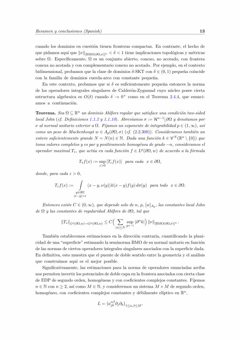
cuando los dominios en cuestión tienen fronteras compactas. En contraste, el hecho deque pidamos aquí que ‖ν‖[BMO(∂Ω,σ)]n < δ < 1 tiene implicaciones topológicas y métricassobre Ω. Específicamente, Ω es un conjunto abierto, conexo, no acotado, con fronteraconexa no acotada y con complementario conexo no acotado. Por ejemplo, en el contextobidimensional, probamos que la clase de dominios δ-SKT con δ ∈ (0, 1) pequeña coincidecon la familia de dominios cuerda-arco con constante pequeña.
En este contexto, probamos que si δ es suficientemente pequeña entonces la normade los operadores integrales singulares de Calderón-Zygmund cuyo núcleo posee ciertaestructura algebraica es O(δ) cuando δ → 0+ como en el Teorema 2.4.4, que enunci-amos a continuación.
Teorema. Sea Ω ⊆ Rn un dominio Ahlfors regular que satisface una condición two-sidedlocal John (cf. Definiciones 1.1.2 y 1.1.10). Abreviamos σ := Hn−1b∂Ω y denotamos porν al normal unitario exterior a Ω. Fijamos un exponente de integrabilidad p ∈ (1,∞), asícomo un peso de Muckenhoupt w ∈ Ap(∂Ω, σ) (cf. (2.2.300)). Consideramos también unentero suficientemente grande N = N(n) ∈ N. Dada una función k ∈ CN (Rn \ 0) quetoma valores completos y es par y positivamente homogénea de grado −n, consideramos eloperador maximal T∗, que actúa en cada función f ∈ Lp(∂Ω, w) de acuerdo a la fórmula
T∗f(x) := supε>0
∣∣Tεf(x)∣∣ para cada x ∈ ∂Ω,
donde, para cada ε > 0,
Tεf(x) :=ˆ
y∈∂Ω|x−y|>ε
〈x− y, ν(y)〉k(x− y)f(y) dσ(y) para todo x ∈ ∂Ω.
Entonces existe C ∈ (0,∞), que depende solo de n, p, [w]Ap, las constantes local Johnde Ω y las constantes de regularidad Ahlfors de ∂Ω, tal que
‖T∗‖Lp(∂Ω,w)→Lp(∂Ω,w) ≤ C( ∑|α|≤N
supSn−1
|∂αk|)‖ν‖[BMO(∂Ω,σ)]n .
También establecemos estimaciones en la dirección contraria, cuantificando la plani-cidad de una “superficie” estimando la seminorma BMO de su normal unitario en funciónde las normas de ciertos operadores integrales singulares asociados con la superficie dada.En definitiva, esto muestra que el puente de doble sentido entre la geometría y el análisisque construimos aquí es el mejor posible.
Significativamente, las estimaciones para la norma de operadores enunciadas arribanos permiten invertir los potenciales de doble capa en la frontera asociados con cierta clasede EDP de segundo orden, homogéneas y con coeficientes complejos constantes. Fijemosn ∈ N con n ≥ 2, así como M ∈ N, y consideremos un sistema M ×M de segundo orden,homogéneo, con coeficientes complejos constantes y débilmente elíptico en Rn,
L =(aαβjk ∂j∂k
)1≤α,β≤M ,
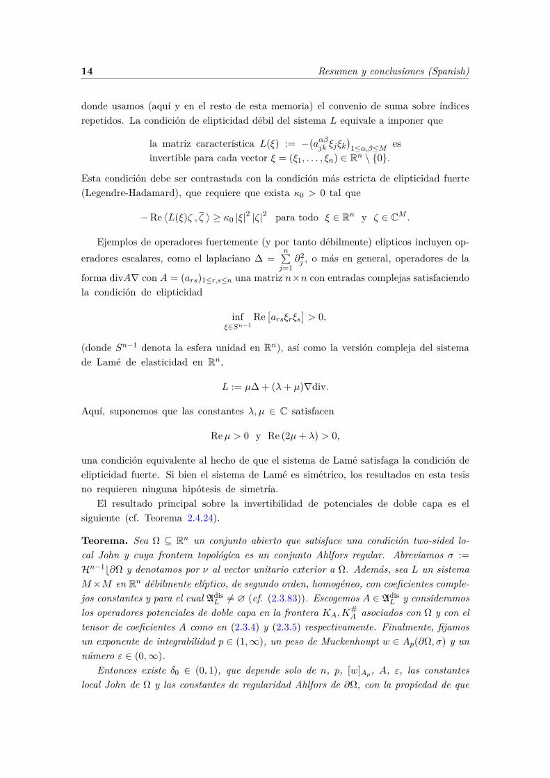
14 Resumen y conclusiones (Spanish)
donde usamos (aquí y en el resto de esta memoria) el convenio de suma sobre índicesrepetidos. La condición de elipticidad débil del sistema L equivale a imponer que
la matriz característica L(ξ) := −(aαβjk ξjξk
)1≤α,β≤M es
invertible para cada vector ξ = (ξ1, . . . , ξn) ∈ Rn \ 0.
Esta condición debe ser contrastada con la condición más estricta de elipticidad fuerte(Legendre-Hadamard), que requiere que exista κ0 > 0 tal que
−Re⟨L(ξ)ζ , ζ
⟩≥ κ0 |ξ|2 |ζ|2 para todo ξ ∈ Rn y ζ ∈ CM .
Ejemplos de operadores fuertemente (y por tanto débilmente) elípticos incluyen op-eradores escalares, como el laplaciano ∆ =
n∑j=1
∂2j , o más en general, operadores de la
forma divA∇ con A = (ars)1≤r,s≤n una matriz n×n con entradas complejas satisfaciendola condición de elipticidad
infξ∈Sn−1
Re[arsξrξs
]> 0,
(donde Sn−1 denota la esfera unidad en Rn), así como la versión compleja del sistemade Lamé de elasticidad en Rn,
L := µ∆ + (λ+ µ)∇div.
Aquí, suponemos que las constantes λ, µ ∈ C satisfacen
Reµ > 0 y Re (2µ+ λ) > 0,
una condición equivalente al hecho de que el sistema de Lamé satisfaga la condición deelipticidad fuerte. Si bien el sistema de Lamé es simétrico, los resultados en esta tesisno requieren ninguna hipótesis de simetría.
El resultado principal sobre la invertibilidad de potenciales de doble capa es elsiguiente (cf. Teorema 2.4.24).
Teorema. Sea Ω ⊆ Rn un conjunto abierto que satisface una condición two-sided lo-cal John y cuya frontera topológica es un conjunto Ahlfors regular. Abreviamos σ :=Hn−1b∂Ω y denotamos por ν al vector unitario exterior a Ω. Además, sea L un sistemaM×M en Rn débilmente elíptico, de segundo orden, homogéneo, con coeficientes comple-jos constantes y para el cual Adis
L 6= ∅ (cf. (2.3.83)). Escogemos A ∈ AdisL y consideramos
los operadores potenciales de doble capa en la frontera KA,K#A asociados con Ω y con el
tensor de coeficientes A como en (2.3.4) y (2.3.5) respectivamente. Finalmente, fijamosun exponente de integrabilidad p ∈ (1,∞), un peso de Muckenhoupt w ∈ Ap(∂Ω, σ) y unnúmero ε ∈ (0,∞).
Entonces existe δ0 ∈ (0, 1), que depende solo de n, p, [w]Ap, A, ε, las constanteslocal John de Ω y las constantes de regularidad Ahlfors de ∂Ω, con la propiedad de que
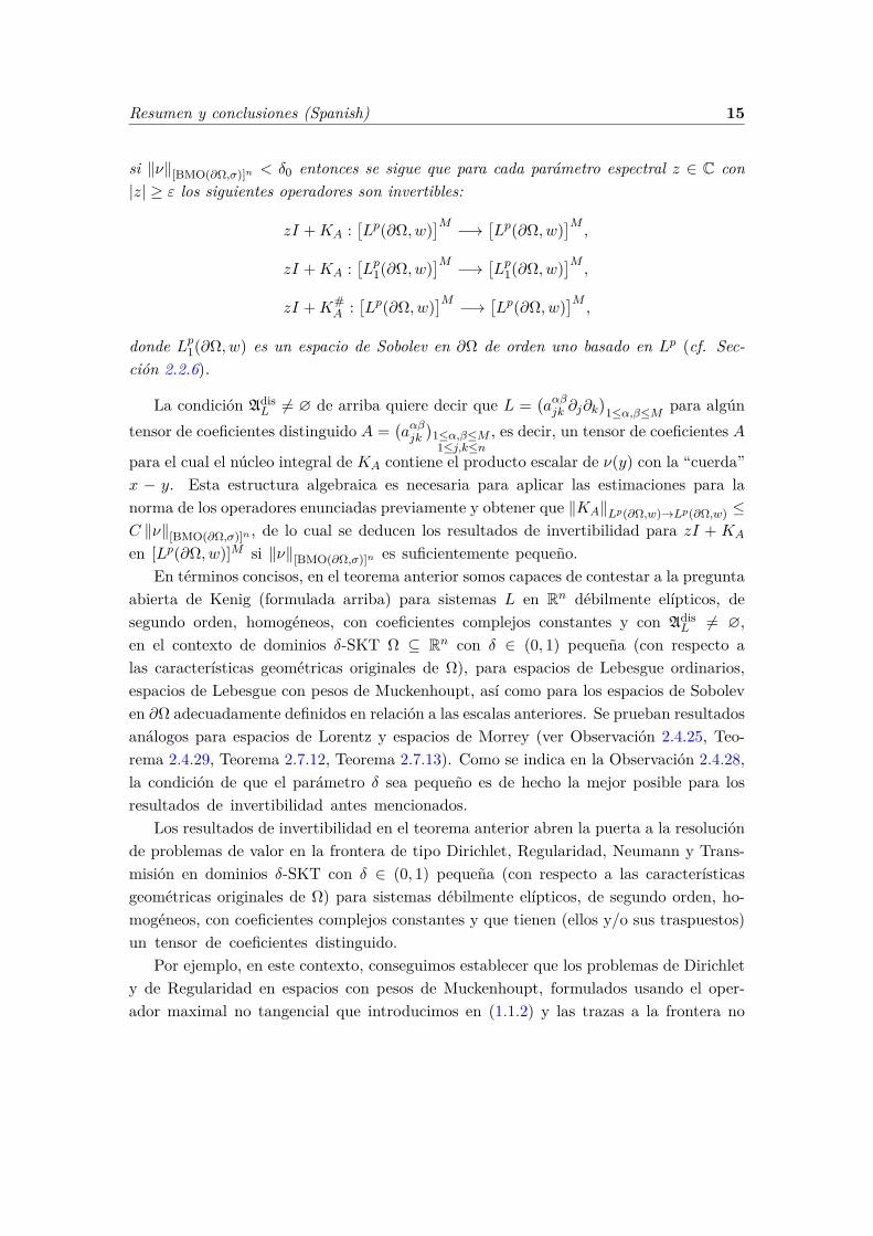
Resumen y conclusiones (Spanish) 15
si ‖ν‖[BMO(∂Ω,σ)]n < δ0 entonces se sigue que para cada parámetro espectral z ∈ C con|z| ≥ ε los siguientes operadores son invertibles:
zI +KA :[Lp(∂Ω, w)
]M −→ [Lp(∂Ω, w)
]M,
zI +KA :[Lp1(∂Ω, w)
]M −→ [Lp1(∂Ω, w)
]M,
zI +K#A :
[Lp(∂Ω, w)
]M −→ [Lp(∂Ω, w)
]M,
donde Lp1(∂Ω, w) es un espacio de Sobolev en ∂Ω de orden uno basado en Lp (cf. Sec-ción 2.2.6).
La condición AdisL 6= ∅ de arriba quiere decir que L =
(aαβjk ∂j∂k
)1≤α,β≤M para algún
tensor de coeficientes distinguido A =(aαβjk
)1≤α,β≤M1≤j,k≤n
, es decir, un tensor de coeficientes A
para el cual el núcleo integral de KA contiene el producto escalar de ν(y) con la “cuerda”x − y. Esta estructura algebraica es necesaria para aplicar las estimaciones para lanorma de los operadores enunciadas previamente y obtener que ‖KA‖Lp(∂Ω,w)→Lp(∂Ω,w) ≤C ‖ν‖[BMO(∂Ω,σ)]n , de lo cual se deducen los resultados de invertibilidad para zI + KA
en [Lp(∂Ω, w)]M si ‖ν‖[BMO(∂Ω,σ)]n es suficientemente pequeño.En términos concisos, en el teorema anterior somos capaces de contestar a la pregunta
abierta de Kenig (formulada arriba) para sistemas L en Rn débilmente elípticos, desegundo orden, homogéneos, con coeficientes complejos constantes y con Adis
L 6= ∅,en el contexto de dominios δ-SKT Ω ⊆ Rn con δ ∈ (0, 1) pequeña (con respecto alas características geométricas originales de Ω), para espacios de Lebesgue ordinarios,espacios de Lebesgue con pesos de Muckenhoupt, así como para los espacios de Soboleven ∂Ω adecuadamente definidos en relación a las escalas anteriores. Se prueban resultadosanálogos para espacios de Lorentz y espacios de Morrey (ver Observación 2.4.25, Teo-rema 2.4.29, Teorema 2.7.12, Teorema 2.7.13). Como se indica en la Observación 2.4.28,la condición de que el parámetro δ sea pequeño es de hecho la mejor posible para losresultados de invertibilidad antes mencionados.
Los resultados de invertibilidad en el teorema anterior abren la puerta a la resoluciónde problemas de valor en la frontera de tipo Dirichlet, Regularidad, Neumann y Trans-misión en dominios δ-SKT con δ ∈ (0, 1) pequeña (con respecto a las característicasgeométricas originales de Ω) para sistemas débilmente elípticos, de segundo orden, ho-mogéneos, con coeficientes complejos constantes y que tienen (ellos y/o sus traspuestos)un tensor de coeficientes distinguido.
Por ejemplo, en este contexto, conseguimos establecer que los problemas de Dirichlety de Regularidad en espacios con pesos de Muckenhoupt, formulados usando el oper-ador maximal no tangencial que introducimos en (1.1.2) y las trazas a la frontera no
16 Resumen y conclusiones (Spanish)
tangenciales definidas en (1.1.5), están bien propuestos:
(D)p,w
u ∈[C∞(Ω)
]M,
Lu = 0 en Ω,
Nκu ∈ Lp(∂Ω, w),
u∣∣κ−n.t.
∂Ω = f ∈[Lp(∂Ω, w)
]M,
(R)p,w
u ∈[C∞(Ω)
]M,
Lu = 0 en Ω,
Nκu ∈ Lp(∂Ω, w),
Nκ(∇u) ∈ Lp(∂Ω, w),
u∣∣κ−n.t.
∂Ω = f ∈[Lp1(∂Ω, w)
]M,
para cada exponente de integrabilidad p ∈ (1,∞) y cada peso de Muckenhoupt w ∈Ap(∂Ω, σ), ambos bajo la hipótesis de que L y L> tienen un tensor de coeficientesdistinguido (cf. Teoremas 2.6.2 y 2.6.5). Además, proporcionamos contraejemplos quemuestran que estos problemas pueden no estar bien propuestos si no asumimos la ex-istencia de un tensor de coeficientes distinguido. Nuestros resultados son por tantoóptimos a este respecto. Establecemos también resultados análogos para problemas devalor en la frontera con dato en la frontera en espacios de Lorentz, espacios de Morrey,espacios vanishing Morrey, espacios block y en los espacios de Sobolev asociados demanera natural a estas escalas.
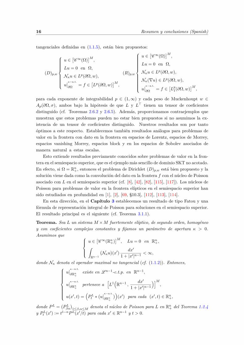
Esto extiende resultados previamente conocidos sobre problemas de valor en la fron-tera en el semiespacio superior, que es el ejemplo más sencillo de dominio SKT no acotado.En efecto, si Ω = Rn+, entonces el problema de Dirichlet (D)p,w está bien propuesto y lasolución viene dada como la convolución del dato en la frontera f con el núcleo de Poissonasociado con L en el semiespacio superior (cf. [8], [42], [82], [115], [117]). Los núcleos dePoisson para problemas de valor en la frontera elípticos en el semiespacio superior hansido estudiados en profundidad en [1], [2], [69, §10.3], [112], [113], [114].
En esta dirección, en el Capítulo 3 establecemos un resultado de tipo Fatou y unafórmula de representación integral de Poisson para soluciones en el semiespacio superior.El resultado principal es el siguiente (cf. Teorema 3.1.1).
Teorema. Sea L un sistema M ×M fuertemente elíptico, de segundo orden, homogéneoy con coeficientes complejos constantes y fijamos un parámetro de apertura κ > 0.Asumimos que
u ∈[C∞(Rn+)
]M, Lu = 0 en Rn+,ˆ
Rn−1
(Nκu
)(x′) dx′
1 + |x′|n−1 <∞,
donde Nκ denota el operador maximal no tangencial (cf. (1.1.2)). Entonces,
u∣∣κ−n.t.
∂Rn+existe en L n−1-c.t.p. en Rn−1,
u∣∣κ−n.t.
∂Rn+pertenece a
[L1(Rn−1 ,
dx′
1 + |x′|n−1
)]M,
u(x′, t) =(PLt ∗
(u∣∣κ−n.t.
∂Rn+
))(x′) para cada (x′, t) ∈ Rn+,
donde PL =(PLβα
)1≤β,α≤M denota el núcleo de Poisson para L en Rn+ del Teorema 1.2.4
y PLt (x′) := t1−nPL(x′/t) para cada x′ ∈ Rn−1 y t > 0.
Resumen y conclusiones (Spanish) 17
Este resultado refina [82, Teorema 6.1, p. 956], donde se asume una condición deintegrabilidad más restrictiva. Es conveniente notar que incluso en el caso clásico enque L := ∆ es el laplaciano en Rn, el teorema anterior es más general (en el sentidode que se puede aplicar sobre una clase más amplia de funciones) que los resultados queexisten en la literatura. En efecto, normalmente se asume una condición de integrabilidaden Lp para la función armónica que, en el rango p ∈ (1,∞), implica nuestra condiciónde integrabilidad sobre el espacio L1 con peso sobre la función maximal no tangencial.En este sentido, véase, por ejemplo, [42, Teorema 4.8-4.9, pp. 174-175], [115, Corolario,p. 200], [116, Proposición 1, p. 119].
Además, este teorema de Fatou tiene resultados de unicidad asociados de manera nat-ural, que permiten demostrar resultados muy generales que indican que ciertos problemasde valor en la frontera elípticos están bien propuestos (cf. Corolarios 3.1.3 y 3.1.4).
Continuando con el estudio de problemas de valor en la frontera en el semiespaciosuperior, en el Capítulo 4 estudiamos el problema de Dirichlet para sistemas elípticoscon dato en la frontera en espacios generalizados de Hölder y espacios generalizados deMorrey-Campanato. Además, mediante técnicas basadas en EDP, probamos que estosdos espacios de funciones son de hecho equivalentes.
Los espacios generalizados de Hölder, denotados por C ω(∂Ω,CM ), cuantifican lacontinuidad en términos de un módulo o función de crecimiento, ω. Específicamente,dado U ⊆ Rn, M ≥ 1 y una función no decreciente ω : (0,∞) → (0,∞) cuyo límiteen el origen se anula, el espacio homogéneo C ω(U,CM ) es la colección de funcionesu : U → CM tales que
[u]Cω(U,CM ) := supx,y∈Ux 6=y
|u(x)− u(y)|ω(|x− y|) <∞.
De forma similar, para D ∈ (0,∞] y una función no decreciente ω : (0, D) → (0,∞)cuyo límite en el origen se anula y que es acotada si D < ∞, el espacio C ω(U,CM )viene definido por la norma
‖u‖Cω(U,CM ) := supU|u|+ [u]
C ω(U,CM ),
donde ω(t) := ω(mint,D) para cada t ∈ (0,∞).Dada una función no decreciente ω : (0,∞) → (0,∞) cuyo límite en el origen se
anula, así como un exponente de integrabilidad p ∈ [1,∞), definimos la seminorma
‖f‖E ω,p(Rn−1,CM ) := supQ⊆Rn−1
1ω(`(Q))
( Q|f(x′)− fQ|p dx′
)1/p,
y denotamos el espacio de funciones asociado por E ω,p(Rn−1,CM ), llamado espaciogeneralizado de Morrey-Campanato en Rn−1. La elección ω(t) := tα con α ∈ (0, 1)corresponde con los espacios clásicos de Morrey-Campanato, mientras que el caso especialω(t) := 1 produce el espacio usual de oscilación media acotada (BMO). Tambiéndefinimos, para cada u ∈
[C 1(Rn+)
]M y q ∈ (0,∞),
‖u‖(ω,q)∗∗ := supQ⊆Rn−1
1ω(`(Q))
( Q
( ˆ `(Q)
0|(∇u)(x′, t)|2 t dt
)q/2dx′)1/q
.
18 Resumen y conclusiones (Spanish)
Enunciamos a continuación nuestro resultado principal a este respecto, que estáincluido en el Teorema 4.1.2 y que generaliza resultados de [85] (donde se estudia elcaso ω(t) = tα con α ∈ (0, 1)) permitiendo escalas más flexibles al medir la regularidaden los espacios de Hölder y Morrey-Campanato.
Teorema. Sea L un sistemaM×M fuertemente elíptico, de segundo orden, homogéneo ycon coeficientes complejos constantes. Fijamos además un parámetro de apertura κ > 0,p ∈ [1,∞), así como q ∈ (0,∞). Finalmente, sea ω : (0,∞) → (0,∞) una función nodecreciente cuyo límite en el origen se anula y que satisface
supt>0
1ω(t)
( ˆ t
0ω(s)ds
s+ t
ˆ ∞t
ω(s)s
ds
s
)< +∞.
Entonces las siguientes afirmaciones son ciertas.
(a) El problema de Dirichlet en el espacio generalizado de Hölder para el sistema L enRn+, es decir,
u ∈[C∞(Rn+)
]M,
Lu = 0 en Rn+,
[u]Cω(Rn+,CM ) <∞,
u|∂Rn+ = f ∈ C ω(Rn−1,CM ) en Rn−1,
está bien propuesto. Más específicamente, existe una única solución, que vienedada por
u(x′, t) = (PLt ∗ f)(x′), ∀ (x′, t) ∈ Rn+,
donde PL denota el núcleo de Poisson para L en Rn+ del Teorema 1.2.4. Además,u pertenece al espacio C ω(Rn+,CM ), satisface u|∂Rn+ = f y existe una constantefinita C = C(n,L, ω) ≥ 1 tal que
C−1[f ]Cω(Rn−1,CM ) ≤ [u]Cω(Rn+,CM ) ≤ C[f ]Cω(Rn−1,CM ).
(b) El problema de Dirichlet en el espacio generalizado de Morrey-Campanato para elsistema L en Rn+, formulado como
u ∈[C∞(Rn+)
]M,
Lu = 0 en Rn+,
‖u‖(ω,q)∗∗ <∞,
u|κ−n.t.
∂Rn+= f ∈ E ω,p(Rn−1,CM ) c.t.p. en Rn−1,
está bien propuesto. Concretamente, existe una única solución, que viene dada por
u(x′, t) = (PLt ∗ f)(x′), ∀ (x′, t) ∈ Rn+,
donde PL denota el núcleo de Poisson para L en Rn+ del Teorema 1.2.4. Además, upertenece a C ω(Rn+,CM ), satisface u|∂Rn+ = f en casi todo punto de Rn−1 y existeuna constante finita C = C(n,L, ω, p, q) ≥ 1 tal que
C−1 ‖f‖E ω,p(Rn−1,CM ) ≤ ‖u‖(ω,q)∗∗ ≤ C ‖f‖E ω,p(Rn−1,CM ) .
Resumen y conclusiones (Spanish) 19
(c) Se tiene la siguiente igualdad entre espacios vectoriales
C ω(Rn−1,CM ) = E ω,p(Rn−1,CM )
con normas equivalentes, donde la inclusión de derecha a izquierda se entiende en elsentido de que para cada f ∈ E ω,p(Rn−1,CM ) existe una única f ∈ C ω(Rn−1,CM )con la propiedad de que f = f en casi todo punto de Rn−1.
Como resultado, el problema de Dirichlet en el espacio generalizado de Hölder de(a) y el problema de Dirichlet en el espacio generalizado de Morrey-Campanatode (b) son equivalentes. Específicamente, para cada par de datos en la fronteraque puedan ser indentificados en el sentido descrito en el párrafo anterior, estosproblemas tienen la misma solución única.
Notemos que en la Sección 4.7 debilitamos las hipótesis sobre la función de crecimientoy probamos que los problemas de Dirichlet están bien propuestos. La diferencia principales que en este caso no son equivalentes (ver Ejemplo 4.7.4).
La interacción entre el análisis y la geometría descrita al comienzo de esta sección nospermite dar una caracterización de ciertas clases de dominios basándonos en condicionespuramente analíticas. Específicamente, en el Capítulo 5 caracterizamos dominios deLyapunov C 1,ω. Los dominios de Lyapunov C 1,ω son conjuntos abiertos con perímetrolocalmente finito cuyo normal unitario exterior ν pertenece a C ω(∂Ω) (después de,posiblemente, ser modificado en un conjunto de σ-medida cero). Aquí, para simplificarla notación, llamamos C ω(U) := C ω(U,C).
Usando ideas de [52], la clase de dominios C 1,ω puede ser descrita también comola colección de todos los subconjuntos abiertos de Rn que localmente coinciden (trasuna transformación rígida del espacio) con la región sobre el grafo de una funcióncontinuamente diferenciable que toma valores reales, definida en Rn−1, cuyas derivadasparciales de primer orden pertenecen a C ω(Rn−1).
Las caracterizaciones de la clase de dominios de Lyapunov que probamos vienen dadasen términos de las propiedades de acotación de ciertas clases de operadores integralessingulares actuando en espacios de Hölder generalizados en la frontera de un dominioAhlfors regular Ω ⊆ Rn con frontera compacta (cf. Definición 1.1.2). El ejemplo másimportante de estos operadores integrales singulares son las transformadas de RieszRj (cf. (5.1.3)-(5.1.4)).
Nuestro trabajo añade credibilidad al principio heurístico de que la acción de latransformada distribucional de Riesz sobre la función constante 1 encierra mucha in-formación, de tipo analítico y también geométrico, sobre el dominio Ahlfors regularsubyacente Ω ⊆ Rn (con frontera compacta). Al nivel más básico, el resultado principalde F. Nazarov, X. Tolsa y A. Volberg en [101] establece que
∂Ω es un conjunto UR ⇐⇒ Rj1 ∈ BMO(∂Ω, σ) para cada j ∈ 1, . . . , n
y se ha probado en [96] que
ν ∈ VMO(∂Ω, σ)
y ∂Ω es un conjunto UR
⇐⇒ Rj1 ∈ VMO(∂Ω, σ) para todo j ∈ 1, . . . , n,
20 Resumen y conclusiones (Spanish)
donde VMO(∂Ω, σ) denota el espacio de Sarason de funciones en ∂Ω con oscilación mediaque se anula, con respecto a la medida σ. Añadiendo más regularidad a los funcionalesRj11≤j≤n obtenemos el siguiente resultado (probado en [96])
Ω es un dominio
de clase C 1+α
⇐⇒ Rj1 ∈ C α(∂Ω) para todo j ∈ 1, . . . , n,
donde α ∈ (0, 1) y C α(∂Ω) es el espacio clásico de Hölder de orden α en ∂Ω. Esteresultado es generalizado por el siguiente, contenido en el Teorema 5.1.4, que nos permiteconsiderar escalas más flexibles para medir la regularidad Hölder (ver la exposición enel Ejemplo 1.3.4 a este respecto).
Teorema. Sea Ω ⊂ Rn un dominio Ahlfors regular cuya frontera es compacta. Abre-viamos σ := Hn−1b∂Ω y denotamos por ν al vector unitario exterior a Ω. Además,definimos Ω+ := Ω y Ω− := Rn \ Ω. Finalmente, sea ω :
(0, diam(∂Ω)
)→ (0,∞) una
función acotada, no decreciente, cuyo límite en el origen se anula y que satisface
sup0<t<diam(∂Ω)
1ω(t)
( ˆ t
0ω(s)ds
s+ t
ˆ diam(∂Ω)
t
ω(s)s
ds
s
)< +∞.
Entonces las siguientes afirmaciones son equivalentes:
(a) Después de ser posiblemente modificado en un conjunto de σ-medida cero, el normalunitario exterior ν a Ω pertenece al espacio generalizado de Hölder C ω(∂Ω).
(b) Las transformadas de Riesz en ∂Ω satisfacen
Rj1 ∈ C ω(∂Ω) para cada j ∈ 1, . . . , n.
(c) El conjunto Ω es un dominio UR (en el sentido de la Definición 1.1.5), y dado unpolinomio homogéneo e impar P de grado ` ≥ 1 en Rn el operador integral singularque actúa en cada función f ∈ C ω(∂Ω) de acuerdo a la fórmula
(Tf)(x) :=ˆ
y∈∂Ω|x−y|>ε
P (x− y)|x− y|n−1+` f(y) dσ(y) for σ-c.t.p. x ∈ ∂Ω
está bien definido y acotado del espacio generalizado de Hölder C ω(∂Ω) en sí mismo.
(d) El conjunto Ω es un dominio UR y la versión en la frontera de las transformadasde Riesz, definidas para cada j ∈ 1, . . . , n y cada f ∈ L1(∂Ω, σ) como
(R±j f
)(x) := 1
$n−1
ˆ∂Ω
xj − yj|x− y|n
f(y) dσ(y), ∀x ∈ Ω±,
satisfacenR±j 1 ∈ C ω(Ω±) para cada j ∈ 1, . . . , n.
Resumen y conclusiones (Spanish) 21
(e) El conjunto Ω es un dominio UR y dado un polinomio homogéneo e impar P de grado` ≥ 1 en Rn, los operadores integrales que actúan en cada función f ∈ C ω(∂Ω) deacuerdo a la fórmula
T±f(x) :=ˆ∂Ω
P (x− y)|x− y|n−1+` f(y) dσ(y), ∀x ∈ Ω±,
están acotados del espacio generalizado de Hölder C ω(∂Ω) al espacio C ω(Ω±).
Esta tesis ha dado lugar a los siguientes artículos:
(a) Singular integral operators, quantitative flatness, and boundary problems, bookmanuscript, 2019 (trabajo conjunto con J.M. Martell, D. Mitrea, I. Mitrea yM. Mitrea).
(b) A Fatou theorem and Poisson’s integral representation formula for elliptic systemsin the upper-half space, to appear in “Topics in Clifford Analysis”, special volume inhonor of Wolfgang Sprößig, Swanhild Bernstein editor, Birkhäuser, 2019 (trabajoconjunto con J.M. Martell, D. Mitrea, I. Mitrea y M. Mitrea).
(c) The generalized Hölder and Morrey-Campanato Dirichlet problems for elliptic sys-tems in the upper-half space, to appear in Potential Anal., 2019 (trabajo conjuntocon J.M. Martell y M. Mitrea).
(d) Characterizations of Lyapunov domains in terms of Riesz transforms and general-ized Hölder spaces, preprint, 2019 (trabajo conjunto con J.M. Martell y M. Mitrea).
El material en (a) está elaborado en el Capítulo 2, (b) está contenido en el Capítulo 3, (c)está desarrollado en el Capítulo 4 y (d) está expuesto en el Capítulo 5. Corresponden,respectivamente, a [77], [76], [79] y [78] en la bibliografía.

CHAPTER 1
Preliminaries
Contents
1.1 Classes of Euclidean sets of locally finite perimeter . . . . . . . . . . . . 241.2 Elliptic operators . . . . . . . . . . . . . . . . . . . . . . . . . . . . . . . . 301.3 Growth functions and generalized Hölder spaces . . . . . . . . . . . . . 351.4 Clifford algebras . . . . . . . . . . . . . . . . . . . . . . . . . . . . . . . . . 39
We begin with a quick review of notational conventions used in the dissertation.Throughout, N0 := N ∪ 0, n ∈ N with n ≥ 2, and Ln stands for the n-dimensionalLebesgue measure in Rn. For each k ∈ N, we denote by Nk0 the collection of all multi-indices α = (α1, . . . , αk) with αj ∈ N0 for 1 ≤ j ≤ k. Also, we let Hn−1 denotethe (n − 1)-dimensional Hausdorff measure in Rn. For each set E ⊆ Rn, we let 1Edenote the characteristic function of E (i.e., 1E(x) = 1 if x ∈ E and 1E(x) = 0 ifx ∈ Rn \ E). Also, δjk is the Kronecker symbol (i.e., δjk := 1 if j = k and δjk := 0if j 6= k). By ej1≤j≤n we shall denote the standard orthonormal basis in Rn, i.e.,ej := (δjk)1≤k≤n for each j ∈ 1, . . . , n. For each x ∈ Rn and r ∈ (0,∞) set B(x, r) :=y ∈ Rn : |x − y| < r. The dot product of two vectors u, v ∈ Rn is denoted byu · v = 〈u, v〉. Next, Rn± := x ∈ Rn : ±〈x, en〉 > 0 denote, respectively, the upper-space and lower half-space in Rn. For an arbitrary open set Ω ⊆ Rn we shall let D′(Ω)stand for the space of distributions in Ω and E ′(Ω) will denote the space of compactlysupported distributions in Ω. Given an integrability exponent p ∈ [1,∞] along withan integer k ∈ N, we shall define the local Lp-based Sobolev space of order k in Ω asW k,p
loc (Ω) :=u ∈ D′(Ω) : ∂αu ∈ Lploc(Ω,Ln), |α| ≤ k
. Next, Sn−1 := ∂B(0, 1) denotes
the unit sphere in Rn, and $n−1 = ωn−1 := Hn−1(Sn−1) is the surface area of Sn−1.In addition, we shall let υn−1 denote the volume of the unit ball in Rn−1. Given any
24 1.1. Classes of Euclidean sets of locally finite perimeter
x, y ∈ Rn, by [x, y] we shall denotes the line segment with endpoints x, y. We shall alsoneed dist(x,E) := inf|x − y| : y ∈ E, the distance from a given point x ∈ Rn to anonempty set E ⊆ Rn. If (X,µ) is a given measure space, for each p ∈ (0,∞] we shalldenote by Lp(X,µ) the Lebesgue space of µ-measurable functions which are p-th powerintegrable on X with respect to µ. Also, by Lp,q(X,µ) with p, q ∈ (0,∞] we shall denotethe scale of Lorentz spaces on X with respect to the measure µ. In the same setting,for each µ-measurable set E ⊆ X with 0 < µ(E) < ∞ and each function f which isabsolutely integrable on E we set
fflE f dµ := µ(E)−1 ´
E f dµ.Finally, we adopt the common convention of writing A ≈ B if there exists a constant
C ∈ (1,∞) with the property that A/C ≤ B ≤ CA for all values of the relevantparameters entering the definitions of A,B (something that is self evident in each contextwe employ this notation).
1.1 Classes of Euclidean sets of locally finite perimeter
Given an open set Ω ⊆ Rn and an aperture parameter κ ∈ (0,∞), define the non-tangential approach regions
Γκ(x) :=y ∈ Ω : |y − x| < (1 + κ) dist (y, ∂Ω)
for each x ∈ ∂Ω. (1.1.1)
In turn, these are used to define the nontangential maximal operator Nκ, acting on eachLn-measurable function u defined in Ω according to(
Nκu)(x) := ‖u‖L∞(Γκ(x),Ln) for each x ∈ ∂Ω, (1.1.2)
with the convention that(Nκu
)(x) := 0 whenever x ∈ ∂Ω is such that Γκ(x) = ∅. Note
that, if we work (as one usually does) with equivalence classes, obtained by identifyingfunctions which coincide Ln-a.e., the nontangential maximal operator is independentof the specific choice of a representative in a given equivalence class. It turns outthat Nκu : ∂Ω → [0,+∞] is a lower-semicontinuous function. Also, it is apparentfrom definitions that
whenever u ∈ C 0(Ω) one actually has(Nκu
)(x) = sup
y∈Γκ(x)|u(y)| for all x ∈ ∂Ω. (1.1.3)
More generally, if u : Ω → R is a Lebesgue measurable function and E ⊆ Ω isa Ln-measurable set, we denote by NE
κ u the non-tangential maximal function of urestricted to E, i.e.,
NEκ u : ∂Ω −→ [0,+∞] defined as
(NEκ u)(x) := ‖u‖L∞(Γκ(x)∩E,Ln) for each x ∈ ∂Ω.
(1.1.4)
Hence, NEκ u = Nκ(u · 1E). Throughout, we agree to use the simpler notation N δ
κ in thecase when E = x ∈ Ω : dist(x, ∂Ω) < δ for some δ ∈ (0,∞).
1. Preliminaries 25
Continue to assume that Ω is an arbitrary open, nonempty, proper subset of Rn
and suppose u is some vector-valued Ln-measurable function defined in Ω. Also, fix anaperture parameter κ > 0 and consider a point x ∈ ∂Ω such that x ∈ Γκ(x) (i.e., x isan accumulation point for the nontangential approach region Γκ(x)). In this context,we shall say that the nontangential limit of u at x from within Γκ(x) exists, and itsvalue is the vector a ∈ CM , provided
for every ε > 0 there exists some r > 0 such that |u(y)−a| < ε for Ln-a.e. point y ∈ Γκ(x) ∩B(x, r).
(1.1.5)
Whenever the nontangential limit of u at x from within Γκ(x) exists, we agree to denoteits value by the symbol
(u∣∣κ−n.t.
∂Ω)(x).
Moving on, recall that an Ln-measurable set Ω ⊆ Rn has locally finite perimeter ifits measure theoretic boundary, i.e.,
∂∗Ω :=x ∈ ∂Ω : lim sup
r→0+
Ln(B(x, r) ∩ Ω)rn
> 0, lim supr→0+
Ln(B(x, r) \ Ω)rn
> 0, (1.1.6)
satisfies
Hn−1(∂∗Ω ∩K) < +∞ for each compact K ⊆ Rn (1.1.7)
(cf. [38, Sections 5.7 and 5.11]). Alternatively, an Ln-measurable set Ω ⊆ Rn has locallyfinite perimeter if, with the gradient taken in the sense of distributions in Rn,
µΩ := ∇1Ω (1.1.8)
is an Rn-valued Borel measure in Rn of locally finite total variation. Fundamental workof De Giorgi-Federer (cf., e.g., [38]) then gives the following Polar Decomposition ofthe Radon measure µΩ:
µΩ = ∇1Ω = −ν |∇1Ω| (1.1.9)
where |∇1Ω|, the total variation measure of the measure ∇1Ω, is given by
|∇1Ω| = Hn−1b∂∗Ω, (1.1.10)
and where
ν ∈[L∞(∂∗Ω,Hn−1)
]n is an Rn-valued function
satisfying |ν(x)| = 1 at Hn−1-a.e. point x ∈ ∂∗Ω.(1.1.11)
We shall refer to ν above as the geometric measure theoretic outward unit normalto Ω. Note here that by simply eliminating the distribution theory jargon implicit inthe interpretation of (1.1.9) (and using a straightforward limiting argument involving amollifier) one already arrives at the formula
ˆΩ
div ~F dLn =ˆ∂∗Ω
ν ·(~F∣∣∂Ω)dHn−1
for each vector field ~F ∈[C 1
0 (Rn)]n. (1.1.12)
26 1.1. Classes of Euclidean sets of locally finite perimeter
For a set Ω ⊆ Rn of locally finite perimeter, we let ∂∗Ω denote the reduced boundaryof Ω, that is,
∂∗Ω consists of all points x ∈ ∂Ω satisfying the followingproperties: 0 < Hn−1(B(x, r) ∩ ∂∗Ω
)< +∞ for each r ∈
(0,∞), and limr→0+
fflB(x,r)∩∂∗Ω ν dH
n−1 = ν(x) ∈ Sn−1.(1.1.13)
For any set Ω ⊆ Rn of locally finite perimeter we then have (cf. [38, p. 208])
∂∗Ω ⊆ ∂∗Ω ⊆ ∂Ω and Hn−1(∂∗Ω \ ∂∗Ω) = 0. (1.1.14)
Definition 1.1.1. A closed set Σ ⊆ Rn is called an Ahlfors regular set (or an Ahlfors-David regular set) if there exists a constant C ∈ [1,∞) such that
rn−1/C ≤ Hn−1(B(x, r) ∩ Σ)≤ Crn−1, ∀ r ∈
(0 , 2 diam (Σ)
), ∀x ∈ Σ. (1.1.15)
We say that Σ is a lower Ahlfors regular set if it satisfies the first inequality in (1.1.15)and an upper Ahlfors regular set if it satisfies the second inequality in (1.1.15).
For a given closed set Σ ⊆ Rn, being Ahlfors regular is not a regularity condition ina traditional analytic sense, but rather a property guaranteeing that, at all locations, Σbehaves (in a quantitative, scale-invariant fashion) like an (n− 1)-dimensional “surface,”with respect to the Hausdorff measure Hn−1. For example, the classical four-cornerCantor set in the plane is an Ahlfors regular set (cf., e.g., [94, Proposition 4.79, p. 238]).
Definition 1.1.2. An open, nonempty, proper subset Ω of Rn is called an Ahlforsregular domain provided ∂Ω is an Ahlfors regular set and Hn−1(∂Ω \ ∂∗Ω
)= 0.
If Ω ⊆ Rn is an Ahlfors regular domain then the upper Ahlfors regularity conditionsatisfied by ∂Ω (i.e., the second inequality in (1.1.15) with Σ := ∂Ω) together with(1.1.7) guarantee that Ω is a set of locally finite perimeter. Also, the fact that themeasure theoretic boundary ∂∗Ω is presently assumed to have full measure (with respectto Hn−1) in the topological boundary ∂Ω, ensures that the geometric measure theoreticoutward unit normal ν to Ω (cf. (1.1.11)) is actually well defined at Hn−1-a.e. pointon ∂Ω. Ultimately,
if Ω ⊆ Rn is an Ahlfors regular domain then
ν ∈[L∞(∂Ω,Hn−1)
]n is an Rn-valued function
satisfying |ν(x)| = 1 at Hn−1-a.e. point x ∈ ∂Ω.
(1.1.16)
From [53, Proposition 2.9, p. 2588] we also know that
if Ω ⊆ Rn is an Ahlfors regular domain, and if κ > 0 is anarbitrary aperture parameter, then x ∈ Γκ(x) (i.e., x is anaccumulation point for the nontangential approach region Γκ(x))for Hn−1-a.e. point x in the topological boundary ∂Ω.
(1.1.17)

1. Preliminaries 27
In particular, if Ω ⊆ Rn is an Ahlfors regular domain and u is an Ln-measurable functionu defined in Ω, then for any fixed aperture parameter κ > 0 it is meaningful to attemptto define the nontangential boundary trace
(u∣∣κ−n.t.
∂Ω)(x) at Hn−1-a.e. point x ∈ ∂Ω. For
future endeavors, it is also useful to remark that (see [93] for a proof)
if Ω ⊂ Rn is an Ahlfors regular domain then Ω− := Rn \ Ω is alsoan Ahlfors regular domain, whose topological boundary coincideswith that of Ω, and whose geometric measure theoretic boundaryagrees with that of Ω, i.e., ∂(Ω−) = ∂Ω and ∂∗(Ω−) = ∂∗Ω.Moreover, the geometric measure theoretic outward unit normalto Ω− is −ν at σ-a.e. point on ∂Ω.
(1.1.18)
We continue by recalling the notion of countable rectifiability.
Definition 1.1.3. A closed set E ⊆ Rn is said to be countably rectifiable (ofdimension (n− 1)) provided
E =
∞⋃j=1
Sj
∪N, (1.1.19)
where N is a null-set for Hn−1 and each Sj is the image of a compact subset of Rn−1
under a Lipschitz map from Rn−1 to Rn.
The following definition is due to G. David and S. Semmes (cf. [34]).
Definition 1.1.4. A closed set Σ ⊆ Rn is said to be a uniformly rectifiable set (orsimply a UR set) if Σ is an Ahlfors regular set and there exist ε,M ∈ (0,∞) such that foreach location x ∈ Σ and each scale R ∈ (0 , 2 diam (Σ)
)it is possible to find a Lipschitz
map ϕ : Bn−1R → Rn (where Bn−1
R is a ball of radius R in Rn−1) with Lipschitz constant≤M and such that
Hn−1(Σ ∩B(x,R) ∩ ϕ(Bn−1R )
)≥ εRn−1. (1.1.20)
Uniformly rectifiability is a quantitative version of countable rectifiability. Any URset is countably rectifiable. We also remark that any Ahlfors regular domain in Rn hasa (n − 1)-dimensional countably rectifiable boundary (cf. [96, Section 2]). Following[53] we also make the following definition.
Definition 1.1.5. An open, nonempty, proper subset Ω of Rn is called a UR domain (shortfor uniformly rectifiable domain) provided ∂Ω is a UR set (in the sense of Definition 1.1.4)and Hn−1(∂Ω \ ∂∗Ω
)= 0.
By design, any UR domain is an Ahlfors regular domain. A basic subclass of URdomains has been identified by G. David and D. Jerison in [32]. To state (a version of)their result, we first recall the following definition.
Definition 1.1.6. Fix R ∈ (0,∞] and c ∈ (0, 1). A nonempty proper subset Ω of Rn
is said to satisfy the (R, c)-corkscrew condition (or, simply, a corkscrew condition
28 1.1. Classes of Euclidean sets of locally finite perimeter
if the particular values of R, c are not important) if for each location x ∈ ∂Ω and eachscale r ∈ (0, R) there exists a point z ∈ Ω (called a corkscrew point relative to x and r)with the property that B(z, c r) ⊆ B(x, r) ∩ Ω.
Also, a nonempty proper subset Ω of Rn is said to satisfy the (R, c)-two-sidedcorkscrew condition provided both Ω and Rn \Ω satisfy the (R, c)-corkscrew condition(with the same convention regarding the omission of R, c).
It is then clear from definitions that we have
∂∗Ω = ∂Ω for any Ln-measurable set Ω ⊆ Rn
satisfying a two-sided corkscrew condition.(1.1.21)
Also, [32, Theorem 1, p. 840] implies that
if Ω is a nonempty proper open subset of Rn satisfying a two-sided corkscrew condition and whose boundary is an Ahlforsregular set, then Ω is a UR domain.
(1.1.22)
Following [57], we define the class of nontangentially accessible domains as those opensets satisfying a two-sided corkscrew conditions and the following Harnack chain condi-tion.
Definition 1.1.7. Fix R ∈ (0,∞] and N ∈ N. An open set Ω ⊆ Rn is said to satisfythe (R,N)-Harnack chain condition (or, simply, a Harnack chain condition if theparticular values of R,N are irrelevant) provided whenever ε > 0, k ∈ N, z ∈ ∂Ω, r ∈(0, R), and x, y ∈ B(z, r/4)∩Ω satisfy |x−y| ≤ 2kε and min
dist (x, ∂Ω) , dist (y, ∂Ω)
≥
ε, one may find a chain of balls B1, B2, . . . , BK with K ≤ Nk, such that x ∈ B1, y ∈ BK ,Bi ∩Bi+1 6= ∅ for every i ∈ 1, . . . ,K − 1, and
N−1 · diam (Bi) ≤ dist (Bi, ∂Ω) ≤ N · diam (Bi), (1.1.23)
diam (Bi) ≥ N−1 ·mindist (x,Bi) , dist (y,Bi)
, (1.1.24)
for every i ∈ 1, . . . ,K.
Following [57, pp. 93-94] (cf. also [64, Definition 2.1, p. 3]), we introduce the class ofNTA domains.
Definition 1.1.8. Fix R ∈ (0,∞] andN ∈ N. An open, nonempty, proper subset Ω of Rn
is said to be a (R,N)-nontangentially accessible domain (or simply an NTA domainif the particular values of R,N are not important) if Ω satisfies both the (R,N−1)-two-sided corkscrew condition and the (R,N)-Harnack chain condition. Finally, an open,nonempty, proper subset Ω of Rn is said to be a (R,N)-two-sided nontangentiallyaccessible domain (or, simply, a two-sided NTA domain if the particular values ofR,N are not relevant) provided both Ω and Rn \Ω are (R,N)-nontangentially accessibledomains.
1. Preliminaries 29
There is also the related notion of (R,N)-one-sided NTA domain, i.e., an open setsatisfying a (R,N)-Harnack chain condition and a (R,N−1)-corkscrew condition (onceagain, we agree to drop the parameters R,N if theirs values are not relevant). Forexample, the complement of the classical four-corner Cantor set in the plane is a one-sided NTA domain with an Ahlfors regular boundary. We continue with the definitionof uniform domains.
Definition 1.1.9. A nonempty, proper, open subset Ω of Rn is called a uniform domainif there exist κ ∈ [1,∞) such that any two points x, y ∈ Ω may be joined in Ω by arectifiable path γ satisfying
length(γ) ≤ κ|x− y| and, for each z ∈ γ,
min
length(γx,z) , length(γy,z)≤ κ dist(z, ∂Ω),
(1.1.25)
where γx,z and γy,z are the sub-arcs of γ joining z with x and y, respectively.
The following definition of yet another brand of local path connectivity conditionfirst appeared in [53].
Definition 1.1.10. An open, nonempty, proper subset Ω of Rn is said to satisfy a localJohn condition if there exist θ ∈ (0, 1) and R > 0 (with the requirement that R =∞ if∂Ω is unbounded) such that for every x ∈ ∂Ω and r ∈ (0, R) one may find xr ∈ B(x, r)∩Ωsuch that B(xr, θr) ⊆ Ω and with the property that for each y ∈ B(x, r)∩∂Ω there existsa rectifiable path γy : [0, 1]→ Ω whose length is ≤ θ−1r and such that
γy(0) = y, γy(1) = xr, dist(γy(t) , ∂Ω
)> θ|γy(t)− y| for all t ∈ (0, 1]. (1.1.26)
Finally, a nonempty open set Ω ⊆ Rn which is not dense in Rn is said to satisfy atwo-sided local John condition if both Ω and Rn \ Ω satisfy a local John condition.
It is clear from the definitions that
any set satisfying a local John condition (respectively, a two-sided local John condition) also satisfies a corkscrew condition(respectively, a two-sided corkscrew condition).
(1.1.27)
Moreover, given any R ∈ (0,∞] and N ∈ N, from [53, Lemma 3.13, p. 2634] we know that
any (R,N)-nontangentially accessible domain satisfies a local Johncondition, and any (R,N)-two-sided nontangentially accessibledomain satisfies a two-sided local John condition (in all casesdemanding that R = ∞ if the said domain has an unboundedboundary).
(1.1.28)
30 1.2. Elliptic operators
1.2 Elliptic operators
Fix n ∈ N with n ≥ 2 along with M ∈ N, and denote by L the collection of allhomogeneous constant complex coefficient second-order M ×M systems L in Rn. Hence,any element L in L may be written as a matrix of differential operators of the formL =
(aαβjk ∂j∂k
)1≤α,β≤M
for some complex numbers aαβjk (here and elsewhere, we shall usethe usual convention of summation over repeated indices). In particular, the action of Lon any given vector-valued distribution u = (uβ)1≤β≤M may be described as
Lu =(aαβjk ∂j∂kuβ
)1≤α≤M
, (1.2.1)
and we denote by L> :=(aβαkj ∂j∂k
)1≤α,β≤M
the (real) transposed of L. We also definethe characteristic matrix of L as
L(ξ) := −[(aαβjk ξjξk
)1≤α,β≤M
]for each ξ = (ξi)1≤i≤n ∈ Rn, (1.2.2)
and introduce
L∗ :=L ∈ L : det[L(ξ)] 6= 0 for each ξ ∈ Rn \ 0
. (1.2.3)
We shall refer to a system L ∈ L as being weakly elliptic if actually L ∈ L∗.This is in contrast with the more stringent condition of Legendre-Hadamard (strong)ellipticity, asks for the existence of some κ0 > 0 such that
Re[aαβjk ξjξkζαζβ
]≥ κ0 |ξ|2 |ζ|2 for all
ξ = (ξj)1≤j≤n ∈ Rn and ζ = (ζα)1≤α≤M ∈ CM .(1.2.4)
Examples of strongly (and hence weakly) elliptic operators include scalar operators,such as the Laplacian ∆ =
n∑j=1
∂2j or, more generally, operators of the form divA∇ with
A = (ars)1≤r,s≤n an n×n matrix with complex entries satisfying the ellipticity condition
infξ∈Sn−1
Re[arsξrξs
]> 0, (1.2.5)
(where Sn−1 denotes the unit sphere in Rn), as well as the complex version of the Lamésystem of elasticity in Rn,
L := µ∆ + (λ+ µ)∇div. (1.2.6)
Above, the constants λ, µ ∈ C (typically called Lamé moduli), are assumed to satisfy
Reµ > 0 and Re (2µ+ λ) > 0, (1.2.7)
a condition equivalent to the demand that the Lamé system (1.2.6) satisfies the Legendre-Hadamard ellipticity condition (1.2.4). While the Lamé system is symmetric, we stressthat the results in this thesis require no symmetry for the systems involved.

1. Preliminaries 31
Next, let us consider
A :=A =
(aαβjk
)1≤α,β≤M1≤j,k≤n
: each aαβjk belongs to C, (1.2.8)
the collection of coefficient tensors with constant complex entries. Adopting naturaloperations (i.e., componentwise addition and multiplication by scalars), this becomes afinite dimensional vector space (over C) which we endow with the norm
‖A‖ :=∑
1≤α,β≤M1≤j,k≤n
∣∣aαβjk ∣∣ for each A =(aαβjk
)1≤α,β≤M1≤j,k≤n
∈ A. (1.2.9)
Hence, if the transposed of each given A =(aαβjk
)1≤α,β≤M1≤j,k≤n
∈ A is the coefficient tensor
A> :=(aβαkj
)1≤α,β≤M1≤j,k≤n
, then A 3 A 7→ A> ∈ A is an isometry. With each coefficient tensor
A =(aαβjk
)1≤α,β≤M1≤j,k≤n
∈ A associate the system LA ∈ L according to
LA :=(aαβjk ∂j∂k
)1≤α,β≤M
. (1.2.10)
Then the map
A 3 A 7−→ LA ∈ L (1.2.11)
is linear and surjective, though it fails to be injective. Specifically, if we introduce
Aant :=B =
(bαβjk
)1≤α,β≤M1≤j,k≤n
∈ A : bαβjk = −bαβkj whenever
1 ≤ j, k ≤ n and 1 ≤ α, β ≤M, (1.2.12)
the collection of all coefficient tensors which are antisymmetric in the lower indices, thenAant is a closed linear subspace of A and for each A, A ∈ A we have
LA = LA⇐⇒ A− A ∈ Aant. (1.2.13)
If we now define
AL :=A ∈ A : L = LA
for each L ∈ L, (1.2.14)
and for each L ∈ L we set (with the distance considered in the normed vector space A)
‖L‖ := dist(A,Aant) for each/some A ∈ AL, (1.2.15)
then L 3 L 7→ ‖L‖ is an unambiguously defined norm on the vector space L. In thetopology induced by this norm, L∗ from (1.2.3) is an open subset of L, the mapping(1.2.11) is continuous, and L 3 L 7→ L> ∈ L is an isometry.
Finally, we denote by AWE the collection of all coefficient tensors A with the propertythat the M × M homogeneous second-order system LA associated with A in Rn asin (1.2.10) is weakly elliptic, i.e.,
AWE :=A ∈ A : LA ∈ L∗
. (1.2.16)
32 1.2. Elliptic operators
Then AWE is an open subset of A.The following theorem, itself a special case of [92, Theorem 11.1, p. 393], summa-
rizes some of the main properties of a certain type of fundamental solution canonicallyassociated with any given homogeneous, constant complex coefficient, weakly ellipticsecond-order system in Rn.
Theorem 1.2.1. Let L be a homogeneous, second-order, constant complex coefficient,M ×M system in Rn, which is weakly elliptic (cf. (1.2.3)).Then there exists an M ×Mmatrix-valued function E =
(Eαβ
)1≤α,β≤M , canonically associated with the given system
L, such that the following properties are true.
(a) For each α, β ∈ 1, . . . ,M one has Eαβ ∈ C∞(Rn \ 0
)and Eαβ(x) = Eαβ(−x)
for every x ∈ Rn \ 0.
(b) For each fixed point y ∈ Rn one has L[E(· − y)
]= δyIM×M in the sense of
distributions in Rn, where IM×M is the M × M identity matrix and δy denotesthe Dirac distribution with mass at y in Rn. That is, using the standard Kroneckerdelta notation,
aαβjk ∂xj∂xk[Eβγ(x− y)
]= δαγδy(x), x ∈ Rn, (1.2.17)
in the sense of distributions, for every α, γ ∈ 1, . . . ,M.
(c) The transposed of E, i.e., E> = (Eβα)1≤α,β≤M , is a fundamental solution forthe transposed system L>. In other words, for each fixed point y ∈ Rn one hasL>[E>(· − y)
]= δyIM×M in the sense of distributions in Rn, i.e.,
aβαkj ∂xj∂xk[Eγβ(x− y)
]= δαγδy(x), x ∈ Rn, (1.2.18)
in the sense of distributions, for every α, γ ∈ 1, . . . ,M.
(d) For every multi-index α ∈ Nn0 with n + |α| > 2, the function ∂αE is positivehomogeneous of degree 2− n− |α| and there exists a constant Cα ∈ (0,∞) with theproperty that
∣∣(∂αE)(x)∣∣ ≤ Cα|x|2−n−|α| for all x ∈ Rn \ 0. (1.2.19)
Finally, corresponding to n = 2 and α = (0, . . . , 0), there exists C ∈ (0,∞) suchthat |E(x)| ≤ C
(1 +
∣∣ ln |x|∣∣) for every x ∈ R2 \ 0.
The following result is a particular case of more general interior estimates foundin [91, Theorem 11.9, p. 364].
Theorem 1.2.2. Let L be a constant complex coefficient system as in (1.2.1) satisfyingthe weak ellipticity condition in (1.2.3). Then for every p ∈ (0,∞), λ ∈ (0, 1), andm ∈ N0 there exists a finite constant C = C(L, p,m, λ, n) > 0 with the property that
1. Preliminaries 33
for every null-solution u of L in a ball B(x,R), where x ∈ Rn and R > 0, and everyr ∈ (0, R) one has
supz∈B(x,λr)
|(∇mu)(z)| ≤ C
rm
( B(x,r)
|u(x)|p dx)1/p
. (1.2.20)
The fundamental solution of L will be the matrix denoted by E := (Ejk)1≤j,k≤M . Thefollowing theorem from [91, Theorem 11.1] summarizes the properties of E in our context.
We now proceed to study the properties of solutions in the upper-half space Rn+ :=x = (x′, t) ∈ Rn : x′ ∈ Rn−1, t > 0. First, introduce
W 1,2bdd(Rn+) :=
u ∈ L2
loc(Rn+) : u, ∂ju ∈ L2(Rn+ ∩B(0, r))
for each j ∈ 1, . . . , n and r ∈ (0,∞), (1.2.21)
and define the Sobolev trace Tr, whenever meaningful, as
(Tr u)(x′) := limr→0+
B((x′,0),r)∩Rn+
u(y) dy, x′ ∈ Rn−1. (1.2.22)
The following result is taken from [90, Corollary 2.4].
Proposition 1.2.3. Let L be a constant complex coefficient system as in (1.2.1) satisfying(1.2.4), and suppose u ∈
[W 1,2
bdd(Rn+)]M satisfies Lu = 0 in Rn+ and Tr u = 0 on Rn−1.
Then u ∈[C∞(Rn+)
]M and there exists a finite constant C > 0, independent of u, suchthat for each x ∈ Rn+ and each r > 0,
supRn+∩B(x,r)
|∇u| ≤ C
rsup
Rn+∩B(x,2r)|u|. (1.2.23)
When dealing with the upper-half space, we agree to denote the (n− 1)-dimensionalLebesgue measure of given Lebesgue measurable set E ⊆ Rn−1 by |E|. Also, by a cubeQ in Rn−1 we shall understand a cube with sides parallel to the coordinate axes. Its side-length will be denoted by `(Q), and for each λ > 0 we shall denote by λQ the cube concen-tric with Q whose side-length is λ `(Q). For every function h ∈
[L1
loc(Rn−1)]M we write
hQ := Qh(x′) dx′ := 1
|Q|
ˆQh(x′) dx′ ∈ CM , (1.2.24)
with the integration performed componentwise. Moving on, for each given function f ∈[L1
loc(Rn−1)]M define the Lp-based mean oscillation of f at a scale r ∈ (0,∞) as
oscp(f ; r) := supQ⊆Rn−1
`(Q)≤r
( Q|f(x′)− fQ|p dx′
)1/p. (1.2.25)
Poisson kernels for elliptic boundary value problems in a half-space have been studiedextensively in [1], [2], [69, §10.3], [112], [113], [114]. The following theorem is containedin [85, Theorem 2.3 and Proposition 3.1], [82, Theorem 3.1, p. 934], and [2]. Here andelsewhere, the convolution between two functions, which are matrix-valued and vector-valued, respectively, takes into account the algebraic multiplication between a matrixand a vector in a natural fashion.
34 1.2. Elliptic operators
Theorem 1.2.4. Suppose L is a constant complex coefficient system as in (1.2.1),satisfying (1.2.4). Then the following statements are true.
(a) There exists a matrix-valued function PL = (PLαβ)1≤α,β≤M : Rn−1 → CM×M , calledthe Poisson kernel for L in Rn+, such that PL ∈
[C∞(Rn−1)
]M×M , there exists somefinite constant C > 0 such that
|PL(x′)| ≤ C
(1 + |x′|2)n/2, ∀x′ ∈ Rn−1, (1.2.26)
and ˆRn−1
PL(x′) dx′ = IM×M , (1.2.27)
where IM×M stands for the M ×M identity matrix.
(b) If for every x′ ∈ Rn−1 and t > 0 one defines
KL(x′, t) := PLt (x′) := t1−nPL(x′/t), (1.2.28)
then KL ∈[C∞
(Rn+ \ B(0, ε)
)]M×M for every ε > 0 and the function KL =(KLαβ
)1≤α,β≤M satisfies
LKL·β = 0 in Rn+ for each β ∈ 1, . . . ,M, (1.2.29)
where KL·β :=
(KLαβ
)1≤α≤M is the β-th column in KL. Moreover, for each multi-
index α ∈ Nn0 there exists Cα ∈ (0,∞) such that∣∣(∂αKL)(x)∣∣ ≤ Cα |x|1−n−|α|, for every x ∈ Rn+ \ 0. (1.2.30)
(c) For each function f = (fβ)1≤β≤M ∈[L1(Rn−1, dx′
1+|x′|n)]M define, with PL as above,
u(x′, t) := (PLt ∗ f)(x′), ∀ (x′, t) ∈ Rn+. (1.2.31)
Then u is meaningfully defined, via an absolutely convergent integral, and for everyaperture parameter κ > 0, it satisfies
u ∈[C∞(Rn+)
]M, Lu = 0 in Rn+, u|
κ−n.t.
∂Rn+= f a.e. on Rn−1 (1.2.32)
(with the last identity valid in the set of Lebesgue points of f), and there exists aconstant C = C(n,L, κ) ∈ (0,∞) with the property that(
Nκu)(x′) ≤ C
(Mf
)(x′), ∀x′ ∈ Rn−1 (1.2.33)
Furthermore, there exists a finite constant C > 0 such that
|(∇u)(x′, t)| ≤ C
t
ˆ ∞1
osc1(f ; st)dss2 , ∀ (x′, t) ∈ Rn+, (1.2.34)
and, for each cube Q ⊆ Rn−1,(ˆ `(Q)
0
Q|(∇u)(x′, t)|2 t dx′ dt
)1/2
≤ Cˆ ∞
1osc1(f ; s`(Q))ds
s2 . (1.2.35)
1. Preliminaries 35
1.3 Growth functions and generalized Hölder spaces
Definition 1.3.1. Given a number D ∈ (0,∞), a function ω : (0, D)→ (0,∞) is calleda growth function on (0, D) if ω is non-decreasing and
limt→0+
ω(t) = 0, ω(D) := limt→D−
ω(t) <∞. (1.3.1)
Corresponding to the case when D = ∞, a function ω : (0,∞) → (0,∞) is called agrowth function on (0,∞) if ω is non-decreasing and
limt→0+
ω(t) = 0. (1.3.2)
It turns out that any growth function on an interval extends to a growth function on(0,∞). For ease of reference, we state this formally in the remark below.Remark 1.3.2. Let D ∈ (0,∞]. If ω is a growth function on (0, D) then
ω(t) := ω(
mint,D)
for each t ∈ (0,∞) (1.3.3)
is a growth function on (0,∞) with the property that ω = ω on (0, D).We shall frequently impose additional conditions on the growth functions employed
in this work. First, if ω is a growth function on (0, D), with D ∈ (0,∞], we shallcall ω doubling provided
sup0<t<D/2
ω(2t)ω(t) <∞, (1.3.4)
and refer to the supremum in the left hand-side of (1.3.4) as the doubling constant ofω. It is then immediate from definitions that
if ω is a doubling growth function on (0, D), with D ∈ (0,∞], thenω is a doubling growth function on the interval (0,∞).
(1.3.5)
Another assumption (which plays a natural role in a variety of contexts) imposed ona given growth function ω : (0, D) → (0,∞), with D ∈ (0,∞], is that
Cω := sup0<t<D
1ω(t)
(ˆ t
0ω(s)ds
s+ t
ˆ D
t
ω(s)s
ds
s
)< +∞. (1.3.6)
Hence, whenever (1.3.6) holds it follows that Cω ∈ (0,∞) andˆ t
0ω(s)ds
s+ t
ˆ D
t
ω(s)s
ds
s≤ Cω · ω(t) for each t ∈ (0, D), (1.3.7)
with the added bonus that when D < ∞ this inequality also extends to t = D if ω(D)is interpreted as in (1.3.1).
Let us note that for any growth function ω on (0, D), with D ∈ (0,∞], the demandin (1.3.6) implies that ω is doubling. Indeed, for each t ∈ (0, D/4) we may write
(ln 2)ω(2t) ≤ˆ 4t
2tω(s)ds
s≤ 4t
ˆ D
t
ω(s)s
ds
s≤ 4Cω · ω(t) (1.3.8)
which already proves that ω is doubling in the case when D = ∞, whereas if D < ∞then for each t ∈ (D/4, D/2) we have ω(2t) ≤ Cω(t) with C := ω(D)/ω(D/4).
36 1.3. Growth functions and generalized Hölder spaces
Remark 1.3.3. Condition (1.3.6) is closely related to the dilation indices of Orlicz spacesstudied in [10], [40] (which are useful in the theory of interpolation of Orlicz spaces).Given a growth function ω : (0, D)→ (0,∞), where D ∈ (0,∞], we set
hω(s) := sup0<t<minD,D/s
ω(ts)ω(t) for each s ∈ (0,∞), (1.3.9)
and define the lower and upper dilation indices of ω, respectively, as
iω := lims→0+
ln hω(s)ln s = sup
0<s<1
ln hω(s)ln s , Iω := lim
s→∞ln hω(s)
ln s = infs>1
ln hω(s)ln s . (1.3.10)
Then one may check that (1.3.6) holds if 0 < iω ≤ Iω < 1. Indeed, from (1.3.10) wesee that whenever 0 < ε < miniω, 1 − Iω there exists some Cε ∈ (0,∞) such thathω(s) ≤ Cεs
iω−ε for every s ∈ (0, 1), and hω(s) ≤ CεsIω+ε for every s ∈ (1,∞). Hence,
there there exists C ∈ (0,∞) such that if 0 < t < D then
iω > 0 ⇒ˆ t
0
ω(s)ω(t)
ds
s=ˆ 1
0
ω(ts)ω(t)
ds
s≤ Cε
ˆ 1
0siω−ε
ds
s≤ C, (1.3.11)
Iω < 1 ⇒ t
ˆ D
t
ω(s)sω(t)
ds
s=ˆ D/t
1
ω(ts)sω(t)
ds
s≤ Cε
ˆ ∞1
sIω+ε−1ds
s≤ C. (1.3.12)
It is of interest to provide relevant examples of growth functions satisfying (1.3.6).
Example 1.3.4. Fix D ∈ (0,∞]. Given α ∈ (0, 1), if ω(t) := tα for each t ∈ (0, D) theniω = Iω = α, hence (1.3.6) holds. The particular version of Theorem 5.1.4 correspondingto this scenario has been established in [96]. There are many examples of interest thatare treated here for the first time. To elaborate, fix an arbitrary α ∈ (0, 1) along withθ ∈ R and, for each t ∈ (0,∞), define log+ t := max0, ln t. Then such examples include
ω(t) := tα (A+ log+ t)θ for all t ∈ (0, D), where A := max1,−θ/α, (1.3.13)
and
ω(t) := tα (B + log+(1/t))θ for all t ∈ (0, D), where B := max1, θ/α. (1.3.14)
In these situations iω = Iω = α which, as noted earlier, guarantees that (1.3.6) holds.Another relevant example is offered by
ω(t) := maxtα, tβ for all t ∈ (0, D), where 0 < α, β < 1. (1.3.15)
Indeed, in such a case we have iω = minα, β and Iω = maxα, β if D = ∞, andiω = Iω = minα, β if D <∞. Similarly, if
ω(t) := mintα, tβ for all t ∈ (0, D), where 0 < α, β < 1, (1.3.16)
then iω = minα, β and Iω = maxα, β if D =∞ and iω = Iω = maxα, β if D <∞.Hence, once again, condition (1.3.6) is verified.
1. Preliminaries 37
Next, we introduce generalized Hölder spaces, consisting of functions whose continuityis quantified using growth functions of the sort previously discussed.
Definition 1.3.5. Let U ⊆ Rn be an arbitrary set and M ≥ 1.
(a) Given a growth function ω on (0,∞), for each vector-valued function u : U → CM
consider [u]Cω(U,CM ) to be zero if U is a singleton, and
[u]Cω(U,CM ) := supx,y∈Ux 6=y
|u(x)− u(y)|ω(|x− y|) ∈ [0,∞] (1.3.17)
if the cardinality of the set U is at least two. Then the homogeneous ω-Hölderspace on U is introduced as
C ω(U,CM ) :=u : U → CM : [u]Cω(U,CM ) <∞
. (1.3.18)
(b) If D ∈ (0,∞] and ω is a growth function on (0, D), define the inhomogeneousω-Hölder space on U as
C ω(U,CM ) :=u ∈ C ω(U,CM ) : u bounded on U
, (1.3.19)
and is equipped with the norm
C ω(U,CM ) 3 u 7−→ ‖u‖Cω(U,CM ) := supU|u|+ [u]
C ω(U,CM ). (1.3.20)
In relation to Definition 1.3.5 a few comments are in order. First, in the contextof item (a), [·]Cω(U,CM ) is a semi-norm for the space C ω(U,CM ). Second, the fact thatω(t) → 0 as t → 0+ implies that if u ∈ C ω(U,CM ) then u is a uniformly continuousfunction on U . Finally, we note that the choice ω(t) := tα for each t ∈ (0,∞), withα ∈ (0, 1), yields the classical scale of Hölder spaces of order α on U .
Going further, it is clear from definitions that if ω is a growth function on (0,∞)and U ⊆ Rn is an arbitrary set, then
fg ∈ C ω(U,CM ) and ‖fg‖Cω(U,CM ) ≤ ‖f‖Cω(U,CM )‖g‖Cω(U,CM )
for any two functions f, g ∈ C ω(U,CM ).(1.3.21)
Also, for each subset V of U , the restriction operators
C ω(U,CM ) 3 u 7→ u∣∣V∈ C ω(V,CM ) and C ω(U,CM ) 3 u 7→ u
∣∣V∈ C ω(V,CM )
are well-defined, linear, and bounded.(1.3.22)
In the opposite direction, we have the following extension result.
38 1.3. Growth functions and generalized Hölder spaces
Lemma 1.3.6. Let U ⊆ Rn be an arbitrary set, M ≥ 1, and suppose ω is a doublinggrowth function on (0,∞). Then C ω(U,CM ) and C ω(U,CM ) coincide as vector spacesand have equivalent semi-norms. More specifically, the restriction map
C ω(U,CM ) 3 u 7−→ u∣∣U∈ C ω(U,CM ) (1.3.23)
is a linear bijection which, under the canonical identification of functions u ∈ C ω(U,CM )with their restrictions u
∣∣U∈ C ω(U,CM ), satisfies
[u]Cω(U,CM ) ≤ [u]Cω(U,CM ) ≤ C[u]Cω(U,CM )
for each function u ∈ C ω(U,CM ),(1.3.24)
where C ∈ [1,∞) is the doubling constant of ω.As a corollary of this, (1.3.5), and definitions, whenever U ⊆ Rn is an arbitrary set,
and ω is a doubling growth function on (0, D) for some D ∈ (0,∞], one may canonicallyidentify C ω(U,CM ) ≡ C ω(U,CM ) and there exists C ∈ [1,∞) such that
‖u‖Cω(U,CM ) ≤ ‖u‖Cω(U,CM ) ≤ C‖u‖Cω(U,CM )
for each function u ∈ C ω(U,CM ).(1.3.25)
Proof. Fix an arbitrary u ∈ C ω(U,CM ). As noted earlier, this membership ensures thatu is uniformly continuous, hence u extends uniquely to a continuous function v on U . Toshow that v actually belongs to C ω(U,CM ) pick two arbitrary distinct points x, y ∈ U .Then there exist two sequences xjj∈N, yjj∈N of points in U such that xj → x andyj → y as j → ∞. After discarding finitely many terms, there is no loss of generalityin assuming that 0 < |xj − yj | < 2|x − y| for each j ∈ N. Relying on the fact that ω isnon-decreasing we may then write
|v(x)− v(y)| = limj→∞
|u(xj)− u(yj)| ≤ [u]Cω(U,CM ) lim supj→∞
ω(|xj − yj |)
≤ [u]Cω(U,CM ) ω(2|x− y|) ≤ C[u]Cω(U,CM ) ω(|x− y|), (1.3.26)
where C ∈ [1,∞) is the doubling constant of ω. This ultimately proves that v ∈C ω(U,CM ) and [v]Cω(U,CM ) ≤ C[u]Cω(U,CM ). All desired conclusions now follow.
To simplify the notation, we call C ω(U) := C ω(U,C), and C ω(U) := C ω(U,C). Wecontinue by making the following definition.
Definition 1.3.7. Let Ω ⊆ Rn be a nonempty open set and denote by C 1(Ω) the spaceof continuously differentiable functions in Ω. Given a growth function ω on (0, D), withD ∈ (0,∞], for each u ∈ C 1(Ω) define
‖u‖C 1,ω(Ω) := supΩ|u|+ sup
Ω|∇u|+ [∇u]
C ω(Ω)∈ [0,∞], (1.3.27)
then introduceC 1,ω(Ω) :=
u ∈ C 1(Ω) : ‖u‖C 1,ω(Ω) <∞
. (1.3.28)
To close this section, we make the following convention. When simply speaking ofa growth function, we shall understand a growth function ω defined on some interval(0, D), with D ∈ (0,∞].
1. Preliminaries 39
1.4 Clifford algebras
This section is a brief tutorial about Clifford algebras, which are a non-commutativehigher-dimensional version of the field of complex numbers, where some of the magic can-cellations and algebraic miracles typically associated with the complex plane still occur.
The Clifford algebra with n imaginary units is the minimal enlargement of Rn to aunitary real algebra (C n,+,), which is not generated as an algebra by any propersubspace of Rn and such that
x x = −|x|2 for every x ∈ Rn → C n. (1.4.1)
In particular, with ej1≤j≤n denoting the standard orthonormal basis in Rn, we have
ej ej = −1 for all j ∈ 1, . . . , n and
ej ek = −ek ej for each distinct j, k ∈ 1, . . . , n.(1.4.2)
This allows us define an embedding Rn → C n by identifying
Rn 3 x = (x1, . . . , xn) ≡n∑j=1
xjej ∈ C n. (1.4.3)
In particular, ej1≤j≤n become n imaginary units in C n. Any element u ∈ C n hasa unique representation of the form
u =n∑`=0
∑′
|I|=`uIeI , uI ∈ R, (1.4.4)
where∑′ indicates that the sum is performed only over strictly increasing multi-indices
I, i.e., I = (i1, i2, . . . , i`) with 1 ≤ i1 < i2 < · · · < i` ≤ n, and eI denotes the Cliffordalgebra product eI := ei1 ei2 · · · ei` . Write e0 := e∅ := 1 for the multiplicativeunit in C n. For each u ∈ C n represented as in (1.4.4) define the projection
uproj :=n∑j=1
ujej ∈ Rn, (1.4.5)
and denote by
uscal := u∅e∅ = u∅ ∈ R, the scalar component of u. (1.4.6)
We endow C n with the natural Euclidean metric, hence
|u| :=
n∑`=0
∑′
|I|=`|uI |2
1/2
for each u =n∑`=0
∑′
|I|=`uIeI ∈ C n. (1.4.7)
Next, define the conjugate of each eI as the unique element eI ∈ C n with the propertythat eI eI = eI eI = 1. Thus, if I = (i1, . . . , i`) with 1 ≤ i1 < i2 < · · · < i` ≤ n,
40 1.4. Clifford algebras
then the conjugate of eI is given by eI = (−1)`ei` · · · e2 e1. More generally, foran arbitrary element u ∈ C n represented as in (1.4.4) we define
u :=n∑`=0
∑′
|I|=`uIeI . (1.4.8)
Note that x = −x for every x ∈ Rn → C n, and |u| = |u| for every u ∈ C n. One mayalso check that for any u, v ∈ C n we have
|u v| ≤ 2n/2|u||v|, u v = v u, (1.4.9)
and, in fact,
|u v| = |u||v| if either
u ∈ Rn → C n, or v ∈ Rn → C n,(1.4.10)
For further details on Clifford algebras, the reader is referred to [99].To study the boundedness of operators acting on Clifford algebra-valued functions, we
need appropriate norms on the spaces to which the said functions belong. If (X, ‖·‖X) is aBanach space thenX⊗C n will denote the Banach space consisting of elements of the form
u =n∑`=0
∑′
|I|=`uIeI , uI ∈ X, (1.4.11)
equipped with the norm
X ⊗ C n 3 u =n∑`=0
∑′
|I|=`uIeI 7→ ‖u‖X⊗C n :=
n∑`=0
∑′
|I|=`‖uI‖X . (1.4.12)
CHAPTER 2
Singular integral operators and quantitative flatness
We develop the theory of layer potentials in the context of δ-SKT domains in Rn (withSKT acronym for Semmes-Kenig-Toro) where the parameter δ ∈ (0, 1), regulating thesize of the BMO semi-norm of the outward unit normal ν to Ω, is assumed to be small.This category of two-sided NTA domains with Ahlfors regular boundaries, which emergedfrom the earlier work of S. Semmes, C. Kenig, and T. Toro, is related to a class of domainsintroduced in [53]. The latter was designed to work well when the domains in questionhave compact boundaries. By way of contrast, the fact that we are now demanding‖ν‖[BMO(∂Ω,σ)]n < 1 (where σ is the “surface measure” Hn−1b∂Ω) has topological andmetric implications for Ω, namely Ω is a connected unbounded open set, with a connectedunbounded boundary and an unbounded connected complement. For example, in thetwo-dimensional setting we show that the class of δ-SKT with δ ∈ (0, 1) small agreeswith the category of chord-arc domains with small constant.
Assuming Ω ⊆ Rn to be a δ-SKT with δ ∈ (0, 1) sufficiently small (relative to othergeometric characteristics of Ω) we prove that the operator norm of Calderón-Zygmundsingular integrals whose kernels exhibit a certain algebraic structure (specifically, theycontain the inner product to ν(y) with the “chord” x − y as a factor) is O(δ) as δ →0+ in the context of Muckenhoupt weighted Lebesgue spaces, Lorentz spaces, Morreyspaces, vanishing Morrey spaces, block spaces, as well as for the brands of Sobolev spacesnaturally associated with these scales. Simply put, the problem that we completely solveis that of determining when singular integral operators of double layer type have smalloperator norms. We also establish estimates in the opposite direction, quantifying theflatness of a “surface” by estimating the BMO semi-norm of its unit normal in terms of theoperator norms of certain singular integrals canonically associated with the given surface(such as the harmonic double layer, the family of Riesz transforms, and commutatorsbetween Riesz transforms and pointwise multiplication by the components of the unitnormal). Ultimately, this goes to show that the two-way bridge between geometry and
42 2. Singular integral operators and quantitative flatness
analysis constructed here is in the nature of best possible.Significantly, the operator norm estimates described in the previous paragraph permit
us to invert the boundary double layer potentials associated with certain classes of second-order PDE (such as the Laplacian, any scalar homogeneous constant complex coefficientsecond-order operator which is weakly elliptic when n ≥ 3 or strongly elliptic in anydimension, the Lamé system of elasticity and, most generally, any weakly elliptic homo-geneous constant complex coefficient second-order systems having a certain distinguishedcoefficient tensor), acting on a large variety of function spaces considered on the boundaryof a sufficiently flat domain (specifically, a δ-SKT domain with δ ∈ (0, 1) suitably smallrelative to other geometric characteristics of the said domain). In particular, this portionof our work goes in the direction of answering the question posed by C. Kenig in [60,Problem 3.2.2, p. 117] asking to invert layer potentials in appropriate spaces on certainuniformly rectifiable sets.
In turn, these invertibility results allow us to establish solvability results for boundaryvalue problems in the class of weakly elliptic second-order systems mentioned above,in a sufficiently flat δ-SKT domain, with boundary data from Muckenhoupt weightedLebesgue spaces, Lorentz spaces, Morrey spaces, vanishing Morrey spaces, block spaces,and from Sobolev spaces naturally associated with these scales.
In summary, a central theme in Geometric Measure Theory is understanding howgeometric properties translate into analytical ones, and here we explore the implicationsof demanding that Gauss’ map ∂Ω 3 x 7→ ν(x) ∈ Sn−1 has small BMO semi-norm, inthe realm of singular integral operators and boundary value problems. The sharp theorydeveloped here complements the results of S. Hofmann, M. Mitrea, and M. Taylor ob-tained for bounded domains in [53], and extends previously known well-posedness resultsfor elliptic PDE’s in the upper half-space (which is a δ-SKT domain for each δ ∈ (0, 1)).
The material in this chapter is based on joint work with J.M. Martell, D. Mitrea,I. Mitrea, and M. Mitrea (cf. [77]).
Contents
2.1 Introduction . . . . . . . . . . . . . . . . . . . . . . . . . . . . . . . . . . . 432.2 Geometric measure theory . . . . . . . . . . . . . . . . . . . . . . . . . . . 59
2.2.1 More on classes of Euclidean sets of locally finite perimeter . . . . . . . . . 592.2.2 Chord-arc curves in the plane . . . . . . . . . . . . . . . . . . . . . . . . . . 702.2.3 The class of δ-SKT domains . . . . . . . . . . . . . . . . . . . . . . . . . . . 842.2.4 Chord-arc domains in the plane . . . . . . . . . . . . . . . . . . . . . . . . . 1032.2.5 Dyadic grids and Muckenhoupt weights on Ahlfors regular sets . . . . . . . 1102.2.6 Sobolev spaces on Ahlfors regular sets . . . . . . . . . . . . . . . . . . . . . 121
2.3 Calderón-Zygmund theory for boundary layers in UR domains . . . . . 1242.3.1 Boundary layer potentials: the setup . . . . . . . . . . . . . . . . . . . . . . 1242.3.2 SIO’s on Muckenhoupt weighted Lebesgue and Sobolev spaces . . . . . . . 128
2. Singular integral operators and quantitative flatness 43
2.3.3 Distinguished coefficient tensors . . . . . . . . . . . . . . . . . . . . . . . . 1362.4 Boundedness and invertibility of double layer potentials . . . . . . . . . 154
2.4.1 Estimates for Euclidean singular integral operators . . . . . . . . . . . . . . 1542.4.2 Estimates for certain classes of singular integrals on UR sets . . . . . . . . 1682.4.3 Norm estimates and invertibility results for double layers . . . . . . . . . . 1902.4.4 Another look at double layers for the two-dimensional Lamé system . . . . 203
2.5 Controlling the BMO semi-norm of the unit normal . . . . . . . . . . . . 2092.5.1 Cauchy-Clifford operators . . . . . . . . . . . . . . . . . . . . . . . . . . . . 2092.5.2 Estimating the BMO semi-norm of the unit normal . . . . . . . . . . . . . . 2122.5.3 Using Riesz transforms to quantify flatness . . . . . . . . . . . . . . . . . . 2162.5.4 Using Riesz transforms to characterize Muckenhoupt weights . . . . . . . . 219
2.6 Boundary value problems in Muckenhoupt weighted spaces . . . . . . . 2252.6.1 The Dirichlet Problem in weighted Lebesgue spaces . . . . . . . . . . . . . 2262.6.2 The Regularity Problem in weighted Sobolev spaces . . . . . . . . . . . . . 2362.6.3 The Neumann Problem in weighted Lebesgue spaces . . . . . . . . . . . . . 2392.6.4 The Transmission Problem in weighted Lebesgue spaces . . . . . . . . . . . 241
2.7 Singular integrals and boundary problems in Morrey and block spaces 2442.7.1 Boundary layer potentials on Morrey and block spaces . . . . . . . . . . . . 2442.7.2 Inverting double layer operators on Morrey and block spaces . . . . . . . . 2532.7.3 Characterizing flatness in terms of Morrey and block spaces . . . . . . . . . 2572.7.4 Boundary value problems in Morrey and block spaces . . . . . . . . . . . . 263
2.1 Introduction
More than 25 years ago, in [60, Problem 3.2.2, p. 117], C. Kenig asked to “Prove thatthe layer potentials are invertible in appropriate [...] spaces in [suitable subclasses ofuniformly rectifiable] domains.” Kenig’s main motivation in this regard stems from thedesire of establishing solvability results for boundary value problems formulated in arather inclusive geometric setting. In the buildup to this open question on [60, p. 116], itis remarked that there are quite general classes of open sets Ω ⊆ Rn with the property thatif σ := Hn−1b∂Ω (where Hn−1 stands for the (n − 1)-dimensional Hausdorff measure inRn) then the said layer potentials are bounded operators on Lp(∂Ω, σ) for each exponentp ∈ (1,∞). Remarkably, this is the case whenever Ω ⊆ Rn is an open set with auniformly rectifiable boundary (cf. [33]).
To further elaborate on this issue, recall the terminology introduced in Section 1.2.In this context, note that the given system L in (1.2.1) does not determine uniquelythe coefficient tensor
A :=(aαβjk
)1≤j,k≤n
1≤α,β≤M(2.1.1)
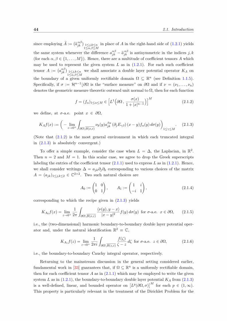
44 2.1. Introduction
since employing A :=(aαβjk
)1≤j,k≤n
1≤α,β≤Min place of A in the right-hand side of (1.2.1) yields
the same system whenever the difference aαβjk − aαβjk is antisymmetric in the indices j, k
(for each α, β ∈ 1, . . . ,M). Hence, there are a multitude of coefficient tensors A whichmay be used to represent the given system L as in (1.2.1). For each such coefficienttensor A :=
(aαβjk
)1≤j,k≤n
1≤α,β≤Mwe shall associate a double layer potential operator KA on
the boundary of a given uniformly rectifiable domain Ω ⊆ Rn (see Definition 1.1.5).Specifically, if σ := Hn−1b∂Ω is the “surface measure” on ∂Ω and if ν = (ν1, . . . , νn)denotes the geometric measure theoretic outward unit normal to Ω, then for each function
f = (fα)1≤α≤M ∈[L1(∂Ω ,
σ(x)1 + |x|n−1
)]M(2.1.2)
we define, at σ-a.e. point x ∈ ∂Ω,
KAf(x) :=(− limε→0+
ˆ∂Ω\B(x,ε)
νk(y)aβαjk (∂jEγβ) (x− y)fα(y) dσ(y))
1≤γ≤M. (2.1.3)
(Note that (2.1.2) is the most general environment in which each truncated integralin (2.1.3) is absolutely convergent.)
To offer a simple example, consider the case when L = ∆, the Laplacian, in R2.Then n = 2 and M = 1. In this scalar case, we agree to drop the Greek superscriptslabeling the entries of the coefficient tensor (2.1.1) used to express L as in (1.2.1). Hence,we shall consider writings ∆ = ajk∂j∂k corresponding to various choices of the matrixA = (ajk)1≤j,k≤2 ∈ C2×2. Two such natural choices are
A0 :=(
1 00 1
), A1 :=
(1 i
−i 1
), (2.1.4)
corresponding to which the recipe given in (2.1.3) yields
KA0f(x) = limε→0+
12π
ˆ∂Ω\B(x,ε)
〈ν(y), y − x〉|x− y|2
f(y) dσ(y) for σ-a.e. x ∈ ∂Ω, (2.1.5)
i.e., the (two-dimensional) harmonic boundary-to-boundary double layer potential oper-ator and, under the natural identification R2 ≡ C,
KA1f(z) = limε→0+
12πi
ˆ∂Ω\B(z,ε)
f(ζ)ζ − z
dζ for σ-a.e. z ∈ ∂Ω, (2.1.6)
i.e., the boundary-to-boundary Cauchy integral operator, respectively.
Returning to the mainstream discussion in the general setting considered earlier,fundamental work in [33] guarantees that, if Ω ⊆ Rn is a uniformly rectifiable domain,then for each coefficient tensor A as in (2.1.1) which may be employed to write the givensystem L as in (1.2.1), the boundary-to-boundary double layer potential KA from (2.1.3)is a well-defined, linear, and bounded operator on
[Lp(∂Ω, σ)
]M for each p ∈ (1,∞).This property is particularly relevant in the treatment of the Dirichlet Problem for the

2. Singular integral operators and quantitative flatness 45
system L in the uniformly rectifiable domain Ω when the boundary data are selectedfrom the space
[Lp(∂Ω, σ)
]M with p ∈ (1,∞), i.e.,
(D)p
u ∈
[C∞(Ω)
]M, Lu = 0 in Ω,
Nκu ∈ Lp(∂Ω, σ),
u∣∣κ−n.t.
∂Ω = g ∈[Lp(∂Ω, σ)
]M,
(2.1.7)
where Nκu is the nontangential maximal function, and u∣∣κ−n.t.
∂Ω is the nontangentialboundary trace, of the solution u (see the body of the manuscript for precise defini-tions). Indeed, the essence of the boundary layer method is to consider as a candidatefor the solution of the Dirichlet Problem (2.1.7) the CM -valued function u defined ateach point x ∈ Ω by
u(x) :=(−ˆ∂Ωνk(y)aβαjk (∂jEγβ) (x− y)fα(y) dσ(y)
)1≤γ≤M
, (2.1.8)
for some yet-to-be-determined function f = (fα)1≤α≤M ∈[Lp(∂Ω, σ)
]M . In light ofthe special format of u (in particular, thanks to the jump-formula (2.3.67)), this ul-timately reduces the entire aforementioned Dirichlet Problem to the issue of solvingthe boundary integral equation(1
2I +KA
)f = g on ∂Ω, (2.1.9)
where I is the identity operator (see Section 2.6 for the actual implementation of thisapproach). As such, having the operator KA well defined, linear, and bounded on[Lp(∂Ω, σ)
]M with p ∈ (1,∞) opens the door for bringing in functional analytic tech-niques for inverting 1
2I+KA on[Lp(∂Ω, σ)
]M and eventually expressing the solution f as(12I + KA
)−1g.
A breakthrough in this regard has been registered by S. Hofmann, M. Mitrea, andM. Taylor in [53], where they have employed Fredholm theory in order to solve theboundary integral equation (2.1.9). To describe one of their main results, supposeL = ∆, the Laplacian in Rn, is written as ∆ = ajk∂j∂k for the identity matrix A :=(δjk)1≤j,k≤n. The blueprint provided in (2.1.3) then presently produces the classicalharmonic double layer potential operator K∆, acting on each function f ∈ Lp(∂Ω, σ)with p ∈ (1,∞) according to
K∆f(x) := limε→0+
1ωn−1
ˆ∂Ω\B(x,ε)
〈ν(y), y − x〉|x− y|n
f(y) dσ(y) for σ-a.e. x ∈ ∂Ω, (2.1.10)
where ωn−1 is the surface area of the unit sphere in Rn. In regard to this operator,S. Hofmann, M. Mitrea, and M. Taylor have proved in [53, Theorem 4.36, pp. 2728-2729]that if Ω ⊆ Rn is a bounded open set satisfying a two-sided local John condition andwhose boundary is Ahlfors regular, then for every threshold ε > 0 there exists some δ > 0(which depends only on the said geometric characteristics of Ω, n, p, and ε) such that
dist(ν ,[VMO(∂Ω, σ)
]n)< δ =⇒ dist
(K∆ , Cp(Lp(∂Ω, σ))
)< ε. (2.1.11)

46 2.1. Introduction
The distance in the left-hand side of (2.1.11) is measured in the John-Nirenberg space[BMO(∂Ω, σ)
]n of vector-valued functions of bounded mean oscillations on ∂Ω (withrespect to the surface measure σ), from the unit vector ν ∈
[L∞(∂Ω, σ)
]n to the Sarasonspace
[VMO(∂Ω, σ)
]n of vector-valued functions of vanishing mean oscillations on ∂Ω(with respect to the surface measure σ), which is a closed subspace of
[BMO(∂Ω, σ)
]n.The distance in the right-hand side of (2.1.11) is considered from K∆ ∈ Bd(Lp(∂Ω, σ)),the Banach space of all linear and bounded operators on Lp(∂Ω, σ) equipped with theoperator norm, to Cp(Lp(∂Ω, σ)) which is the closed linear subspace of Bd(Lp(∂Ω, σ))consisting of all compact operators on Lp(∂Ω, σ). In particular, in the class of domainscurrently considered, K∆ is a compact operator on Lp(∂Ω, σ) whenever ν belongs to[VMO(∂Ω, σ)
]n. This is remarkable in as much that a purely geometric condition impliesa functional analytic property of a singular integral operator. Most importantly, (2.1.11)ensures the existence of some small threshold δ > 0 (which depends only on the saidgeometric characteristics of Ω, n, and p) with the property that
dist(ν ,[VMO(∂Ω, σ)
]n)< δ =⇒ dist
(K∆ , Cp(Lp(∂Ω, σ))
)< 1
2 (2.1.12)
=⇒ 12I +K∆ Fredholm operator with index zero on Lp(∂Ω, σ).
This is the main step in establishing that 12I +K∆ is actually an invertible operator on
Lp(∂Ω, σ) in the said geometric setting, under the additional assumption that Rn \ Ωis connected (see [53, Theorem 6.13, p. 2806]).
Another key result of a similar flavor to (2.1.11) proved in [53] pertains to thecommutators
[Mνk , Rj
]:= MνkRj−RjMνk , where j, k ∈ 1, . . . , n, between the operator
Mνk of pointwise multiplication by νk, the k-th scalar component of the geometricmeasure theoretic outward unit normal ν to Ω, and j-th Riesz transform Rj on ∂Ω,acting on any given function f ∈ L1(∂Ω, σ(x)
1+|x|n−1)according to
Rjf(x) := limε→0+
2ωn−1
ˆ∂Ω\B(x,ε)
xj − yj|x− y|n
f(y) dσ(y) for σ-a.e. x ∈ ∂Ω. (2.1.13)
Specifically, [53, Theorem 2.19, p. 2608] states that if Ω ⊆ Rn is a bounded open setsatisfying a two-sided local John condition and whose boundary is Ahlfors regular, andif some p ∈ (1,∞) has been fixed, then there exists some C ∈ (0,∞) (depending only onthe aforementioned geometric characteristics of Ω, n, and p) such that
n∑j,k=1
dist([Mνk , Rj
], Cp(Lp(∂Ω, σ))
)≤ C dist
(ν ,[VMO(∂Ω, σ)
]n). (2.1.14)
Estimates of this type (with the Riesz transforms replaced by more general singularintegral operators of the same nature) turned out to be a key ingredient in the proof ofthe fact that, if Ω is as above and p ∈ (1,∞), then for every threshold ε > 0 there existssome δ > 0 (of the same nature as before) such that
dist(ν ,[VMO(∂Ω, σ)
]n)< δ =⇒ dist
(K∆ , Cp(Lp1(∂Ω, σ))
)< ε, (2.1.15)
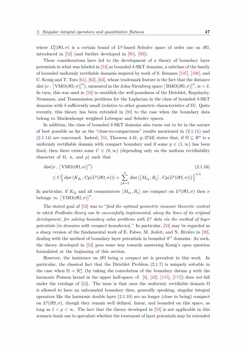
2. Singular integral operators and quantitative flatness 47
where Lp1(∂Ω, σ) is a certain brand of Lp-based Sobolev space of order one on ∂Ω,introduced in [53] (and further developed in [95], [93]).
These considerations have led to the development of a theory of boundary layerpotentials in what was labeled in [53] as bounded δ-SKT domains, a subclass of the familyof bounded uniformly rectifiable domains inspired by work of S. Semmes [107], [108], andC. Kenig and T. Toro [61], [62], [63], whose trademark feature is the fact that the distancedist
(ν ,[VMO(∂Ω, σ)
]n), measured in the John-Nirenberg space[BMO(∂Ω, σ)
]n, is < δ.In turn, this was used in [53] to establish the well-posedness of the Dirichlet, Regularity,Neumann, and Transmission problems for the Laplacian in the class of bounded δ-SKTdomains with δ sufficiently small (relative to other geometric characteristics of Ω). Quiterecently, this theory has been extended in [80] to the case when the boundary databelong to Muckenhoupt weighted Lebesgue and Sobolev spaces.
In addition, the class of bounded δ-SKT domains also turns out to be in the natureof best possible as far as the “close-to-compactness” results mentioned in (2.1.11) and(2.1.14) are concerned. Indeed, [53, Theorem 4.41, p. 2743] states that, if Ω ⊆ Rn is auniformly rectifiable domain with compact boundary and if some p ∈ (1,∞) has beenfixed, then there exists some C ∈ (0,∞) (depending only on the uniform rectifiabilitycharacter of Ω, n, and p) such that
dist(ν ,[VMO(∂Ω, σ)
]n) (2.1.16)
≤ C
dist(K∆ , Cp(Lp(∂Ω, σ))
)+
n∑j,k=1
dist([Mνk , Rj
], Cp(Lp(∂Ω, σ))
)1/n.
In particular, if K∆ and all commutators[Mνk , Rj
]are compact on Lp(∂Ω, σ) then ν
belongs to[VMO(∂Ω, σ)
]n.The stated goal of [53] was to “find the optimal geometric measure theoretic context
in which Fredholm theory can be successfully implemented, along the lines of its originaldevelopment, for solving boundary value problems with Lp data via the method of layerpotentials [in domains with compact boundaries].” In particular, [53] may be regarded asa sharp version of the fundamental work of E. Fabes, M. Jodeit, and N. Rivière in [39],dealing with the method of boundary layer potentials in bounded C 1 domains. As such,the theory developed in [53] goes some way towards answering Kenig’s open questionformulated at the beginning of this section.
However, the insistence on ∂Ω being a compact set is prevalent in this work. Inparticular, the classical fact that the Dirichlet Problem (2.1.7) is uniquely solvable inthe case when Ω = Rn+ (by taking the convolution of the boundary datum g with theharmonic Poisson kernel in the upper half-space; cf. [8], [42], [115], [117]) does not fallunder the tutelage of [53]. The issue is that once the uniformly rectifiable domain Ωis allowed to have an unbounded boundary then, generally speaking, singular integraloperators like the harmonic double layer (2.1.10) are no longer (close to being) compacton Lp(∂Ω, σ), though they remain well defined, linear, and bounded on this space, aslong as 1 < p < ∞. The fact that the theory developed in [53] is not applicable in thisscenario leads one to speculate whether the treatment of layer potentials may be extended
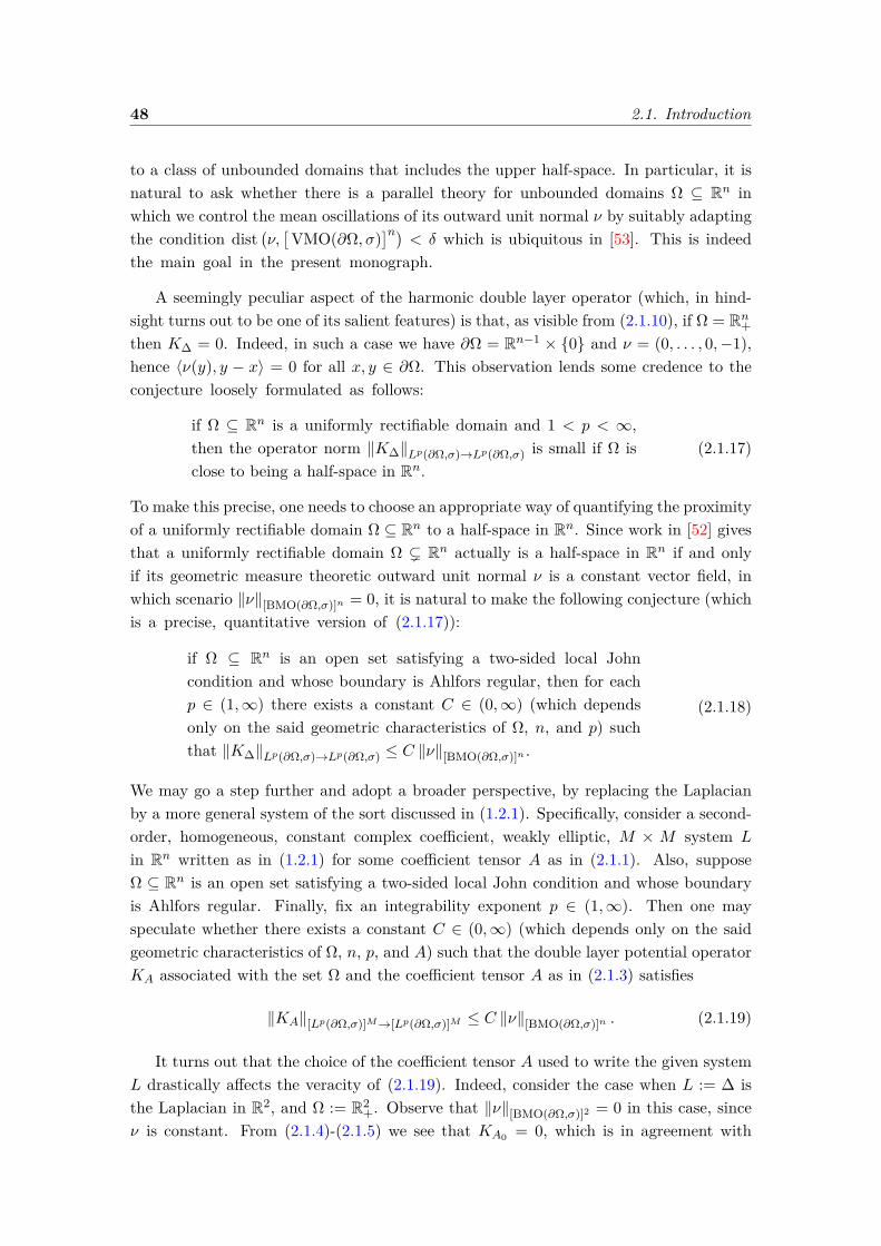
48 2.1. Introduction
to a class of unbounded domains that includes the upper half-space. In particular, it isnatural to ask whether there is a parallel theory for unbounded domains Ω ⊆ Rn inwhich we control the mean oscillations of its outward unit normal ν by suitably adaptingthe condition dist
(ν,[VMO(∂Ω, σ)
]n)< δ which is ubiquitous in [53]. This is indeed
the main goal in the present monograph.
A seemingly peculiar aspect of the harmonic double layer operator (which, in hind-sight turns out to be one of its salient features) is that, as visible from (2.1.10), if Ω = Rn+then K∆ = 0. Indeed, in such a case we have ∂Ω = Rn−1 × 0 and ν = (0, . . . , 0,−1),hence 〈ν(y), y − x〉 = 0 for all x, y ∈ ∂Ω. This observation lends some credence to theconjecture loosely formulated as follows:
if Ω ⊆ Rn is a uniformly rectifiable domain and 1 < p < ∞,then the operator norm ‖K∆‖Lp(∂Ω,σ)→Lp(∂Ω,σ) is small if Ω isclose to being a half-space in Rn.
(2.1.17)
To make this precise, one needs to choose an appropriate way of quantifying the proximityof a uniformly rectifiable domain Ω ⊆ Rn to a half-space in Rn. Since work in [52] givesthat a uniformly rectifiable domain Ω ( Rn actually is a half-space in Rn if and onlyif its geometric measure theoretic outward unit normal ν is a constant vector field, inwhich scenario ‖ν‖[BMO(∂Ω,σ)]n = 0, it is natural to make the following conjecture (whichis a precise, quantitative version of (2.1.17)):
if Ω ⊆ Rn is an open set satisfying a two-sided local Johncondition and whose boundary is Ahlfors regular, then for eachp ∈ (1,∞) there exists a constant C ∈ (0,∞) (which dependsonly on the said geometric characteristics of Ω, n, and p) suchthat ‖K∆‖Lp(∂Ω,σ)→Lp(∂Ω,σ) ≤ C ‖ν‖[BMO(∂Ω,σ)]n .
(2.1.18)
We may go a step further and adopt a broader perspective, by replacing the Laplacianby a more general system of the sort discussed in (1.2.1). Specifically, consider a second-order, homogeneous, constant complex coefficient, weakly elliptic, M × M system L
in Rn written as in (1.2.1) for some coefficient tensor A as in (2.1.1). Also, supposeΩ ⊆ Rn is an open set satisfying a two-sided local John condition and whose boundaryis Ahlfors regular. Finally, fix an integrability exponent p ∈ (1,∞). Then one mayspeculate whether there exists a constant C ∈ (0,∞) (which depends only on the saidgeometric characteristics of Ω, n, p, and A) such that the double layer potential operatorKA associated with the set Ω and the coefficient tensor A as in (2.1.3) satisfies
‖KA‖[Lp(∂Ω,σ)]M→[Lp(∂Ω,σ)]M ≤ C ‖ν‖[BMO(∂Ω,σ)]n . (2.1.19)
It turns out that the choice of the coefficient tensor A used to write the given systemL drastically affects the veracity of (2.1.19). Indeed, consider the case when L := ∆ isthe Laplacian in R2, and Ω := R2
+. Observe that ‖ν‖[BMO(∂Ω,σ)]2 = 0 in this case, sinceν is constant. From (2.1.4)-(2.1.5) we see that KA0 = 0, which is in agreement with
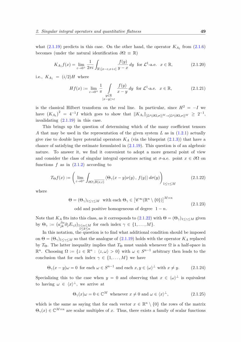
2. Singular integral operators and quantitative flatness 49
what (2.1.19) predicts in this case. On the other hand, the operator KA1 from (2.1.6)becomes (under the natural identification ∂Ω ≡ R)
KA1f(x) = limε→0+
12πi
ˆR\[x−ε,x+ε]
f(y)y − x
dy for L1-a.e. x ∈ R, (2.1.20)
i.e., KA1 = (i/2)H where
Hf(x) := limε→0+
1π
ˆ
y∈R|x−y|>ε
f(y)x− y
dy for L1-a.e. x ∈ R, (2.1.21)
is the classical Hilbert transform on the real line. In particular, since H2 = −I wehave
(KA1
)2 = 4−1I which goes to show that ‖KA1‖[Lp(∂Ω,σ)]M→[Lp(∂Ω,σ)]M ≥ 2−1,invalidating (2.1.19) in this case.
This brings up the question of determining which of the many coefficient tensorsA that may be used in the representation of the given system L as in (1.2.1) actuallygive rise to double layer potential operators KA (via the blueprint (2.1.3)) that have achance of satisfying the estimate formulated in (2.1.19). This question is of an algebraicnature. To answer it, we find it convenient to adopt a more general point of viewand consider the class of singular integral operators acting at σ-a.e. point x ∈ ∂Ω onfunctions f as in (2.1.2) according to
TΘf(x) :=(
limε→0+
ˆ∂Ω\B(x,ε)
⟨Θγ(x− y)ν(y) , f(y)
⟩dσ(y)
)1≤γ≤M
(2.1.22)
where
Θ = (Θγ)1≤γ≤M with each Θγ ∈[C∞(Rn \ 0)
]M×nodd and positive homogeneous of degree 1− n.
(2.1.23)
Note that KA fits into this class, as it corresponds to (2.1.22) with Θ = (Θγ)1≤γ≤M givenby Θγ :=
(aβαjk ∂jEγβ
)1≤α≤M1≤k≤n
for each index γ ∈ 1, . . . ,M.
In this notation, the question is to find what additional condition should be imposedon Θ = (Θγ)1≤γ≤M so that the analogue of (2.1.19) holds with the operator KA replacedby TΘ. The latter inequality implies that TΘ must vanish whenever Ω is a half-space inRn. Choosing Ω := z ∈ Rn : 〈z, ω〉 > 0 with ω ∈ Sn−1 arbitrary then leads to theconclusion that for each index γ ∈ 1, . . . ,M we have
Θγ(x− y)ω = 0 for each ω ∈ Sn−1 and each x, y ∈ 〈ω〉⊥ with x 6= y. (2.1.24)
Specializing this to the case when y = 0 and observing that x ∈ 〈ω〉⊥ is equivalentto having ω ∈ 〈x〉⊥, we arrive at
Θγ(x)ω = 0 ∈ CM whenever x 6= 0 and ω ∈ 〈x〉⊥, (2.1.25)
which is the same as saying that for each vector x ∈ Rn \ 0 the rows of the matrixΘγ(x) ∈ CM×n are scalar multiples of x. Thus, there exists a family of scalar functions
50 2.1. Introduction
kγ,1, . . . , kγ,M defined in Rn \ 0 such that the rows of Θγ(x) are kγ,1(x)x, . . . , kγ,M (x)xfor each x ∈ Rn \ 0. Ultimately, this implies that k :=
(kγ,α
)1≤γ≤M1≤α≤M
is a matrix-
valued function belonging to[C∞(Rn \ 0)
]M×M which is even, positive homogeneousof degree −n, and such that for each γ ∈ 1, . . . ,M we have
Θγ(x)ω = 〈x, ω〉kγ·(x) for each x ∈ Rn \ 0 and ω ∈ Rn. (2.1.26)
Consequently, TΘ from (2.1.22) may be simply re-cast as
Tf(x) = limε→0+
ˆ∂Ω\B(x,ε)
〈x− y, ν(y)〉k(x− y)f(y) dσ(y) for σ-a.e. x ∈ ∂Ω. (2.1.27)
In terms of the original double layer potential operator KA, the above argument provesthat
if (2.1.19) holds then the integral kernel of KA is necessarily ofthe form 〈x − y, ν(y)〉k(x − y) for some matrix-valued functionk ∈
[C∞(Rn\0)
]M×M which is even and positive homogeneousof degree −n.
(2.1.28)
An algebraic condition, formulated solely in terms of A, guaranteeing that the integralkernel of KA has the distinguished structure singled out in (2.1.28) has been identifiedin [86] (see (2.3.74)-(2.3.75) where the said algebraic condition is recalled). Henceforth,we shall refer to such a coefficient tensor A as being “distinguished”, and we shall denoteby Adis
L the collection of all distinguished coefficient tensors which may be employedin the writing of a given system L.
Examples of weakly elliptic second-order homogeneous constant coefficient systemsL in Rn which possess distinguished coefficient tensors (i.e., for which Adis
L 6= ∅) includeall scalar operators in dimension n ≥ 3. In particular, this is the case for the Laplacian∆ =
n∑j=1
∂2j or, more generally, for operators of the form L = divA∇ with the coefficient
matrix A = (ajk)1≤j,k≤n ∈ Cn×n satisfying the weak ellipticity condition
n∑j,k=1
ajkξjξk 6= 0, ∀ ξ = (ξ1, . . . , ξn) ∈ Rn \ 0. (2.1.29)
Other examples of weakly elliptic second-order homogeneous constant coefficient systemswhich possess distinguished coefficient tensors are obtained by considering the complexversion of the Lamé system of elasticity in Rn,
Lµ,λ := µ∆ + (λ+ µ)∇div, (2.1.30)
where the Lamé moduli λ, µ ∈ C are assumed to satisfy
µ 6= 0, 2µ+ λ 6= 0, 3µ+ λ 6= 0. (2.1.31)
The first two requirements in (2.1.31) are equivalent to having the system Lµ,λ weaklyelliptic (in the sense of (1.2.3)), while the last requirement in (2.1.31) ensures the
2. Singular integral operators and quantitative flatness 51
existence of a distinguished coefficient tensor for Lµ,λ. Recall from (1.2.7) that the(strong) Legendre-Hadamard ellipticity condition (1.2.4) holds for the complex Lamésystem Lµ,λ if and only if
Reµ > 0 and Re (2µ+ λ) > 0. (2.1.32)
As such, our results apply to certain classes of weakly elliptic second-order systems whichare not necessarily strongly elliptic (in the sense of Legendre-Hadamard). Also, whilethe Lamé system is symmetric, we stress that the results in this monograph require nosymmetry for the systems involved.
One of the main results in this work asserts that if L is a second-order, homogeneous,constant complex coefficient, weakly elliptic,M×M system in Rn, with the property thatAdisL 6= ∅, and if Ω ⊆ Rn is an open set satisfying a two-sided local John condition and
whose boundary is Ahlfors regular, then for each A ∈ AdisL and each p ∈ (1,∞) there exists
a constant C ∈ (0,∞) (which depends only on the said geometric characteristics of Ω, n,p, and A) such that estimate (2.1.19) actually holds (hence, in particular, the conjectureformulated in (2.1.18) is true). See Theorem 2.4.20 for a result of a more general flavor,formulated in terms of Muckenhoupt weighted Lebesgue spaces. Specifically, if the systemL, the coefficient tensor A, and the set Ω are as just described, then for each Muckenhouptweight w ∈ Ap(∂Ω, σ) with 1 < p < ∞ there exists a constant C ∈ (0,∞) (which nowalso depends on [w]Ap) with the property that
‖KA‖[Lp(∂Ω,w)]M→[Lp(∂Ω,w)]M ≤ C ‖ν‖[BMO(∂Ω,σ)]n . (2.1.33)
In turn, Theorem 2.4.20 is painlessly implied by the even more general result presentedin Theorem 2.4.4 which, de facto, is the central point of this monograph. The proof ofTheorem 2.4.4 uses a combination of tools of a purely geometric nature (such as Theo-rem 2.2.25 containing a versatile version of a decomposition result originally establishedby S. Semmes for smooth surfaces in [107] then subsequently strengthened as to applyto rough settings in [53], and the estimate from Proposition 2.2.24 controlling the innerproduct between the integral average of the outward unit normal and the “chord” in termsof the BMO semi-norm of the outward unit normal to a domain), and techniques of apurely harmonic analytic nature (like good-λ inequalities, maximal operator estimates,stopping time arguments, and Muckenhoupt weight theory).
These considerations lead us to adopt (as we do in Definition 2.2.14) the followingbasic piece of terminology. An open, nonempty, proper subset Ω of Rn is said to bea δ-SKT domain (for some δ > 0) if Ω satisfies a two-sided local John condition, ∂Ωis an Ahlfors regular set and, with σ := Hn−1b∂Ω, the geometric measure theoreticoutward unit normal ν to Ω satisfies
‖ν‖[BMO(∂Ω,σ)]n < δ. (2.1.34)
Remarkably, demanding that δ in (2.1.34) is small has topological and metric im-plications for the underlying domain, namely Ω is a connected unbounded open set,
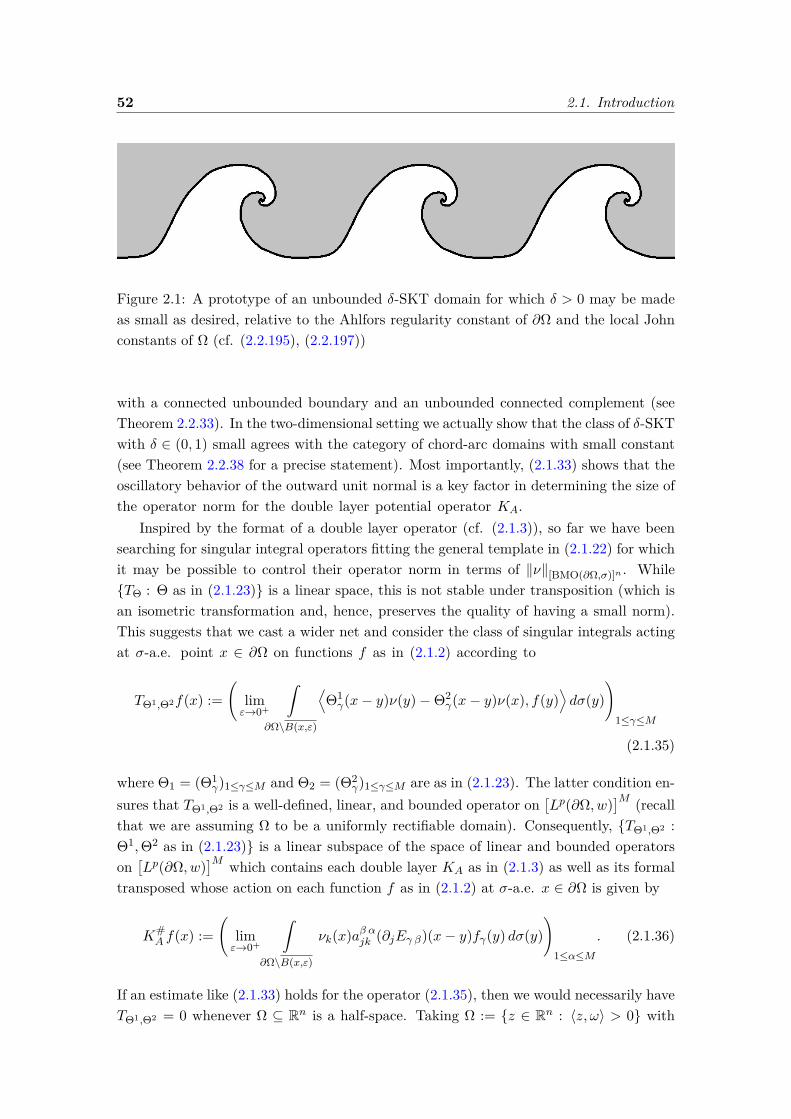
52 2.1. Introduction
Figure 2.1: A prototype of an unbounded δ-SKT domain for which δ > 0 may be madeas small as desired, relative to the Ahlfors regularity constant of ∂Ω and the local Johnconstants of Ω (cf. (2.2.195), (2.2.197))
with a connected unbounded boundary and an unbounded connected complement (seeTheorem 2.2.33). In the two-dimensional setting we actually show that the class of δ-SKTwith δ ∈ (0, 1) small agrees with the category of chord-arc domains with small constant(see Theorem 2.2.38 for a precise statement). Most importantly, (2.1.33) shows that theoscillatory behavior of the outward unit normal is a key factor in determining the size ofthe operator norm for the double layer potential operator KA.
Inspired by the format of a double layer operator (cf. (2.1.3)), so far we have beensearching for singular integral operators fitting the general template in (2.1.22) for whichit may be possible to control their operator norm in terms of ‖ν‖[BMO(∂Ω,σ)]n . WhileTΘ : Θ as in (2.1.23) is a linear space, this is not stable under transposition (which isan isometric transformation and, hence, preserves the quality of having a small norm).This suggests that we cast a wider net and consider the class of singular integrals actingat σ-a.e. point x ∈ ∂Ω on functions f as in (2.1.2) according to
TΘ1,Θ2f(x) :=(
limε→0+
ˆ
∂Ω\B(x,ε)
⟨Θ1γ(x− y)ν(y)−Θ2
γ(x− y)ν(x), f(y)⟩dσ(y)
)1≤γ≤M
(2.1.35)
where Θ1 = (Θ1γ)1≤γ≤M and Θ2 = (Θ2
γ)1≤γ≤M are as in (2.1.23). The latter condition en-sures that TΘ1,Θ2 is a well-defined, linear, and bounded operator on
[Lp(∂Ω, w)
]M (recallthat we are assuming Ω to be a uniformly rectifiable domain). Consequently, TΘ1,Θ2 :Θ1,Θ2 as in (2.1.23) is a linear subspace of the space of linear and bounded operatorson[Lp(∂Ω, w)
]M which contains each double layer KA as in (2.1.3) as well as its formaltransposed whose action on each function f as in (2.1.2) at σ-a.e. x ∈ ∂Ω is given by
K#A f(x) :=
(limε→0+
ˆ
∂Ω\B(x,ε)
νk(x)aβ αjk (∂jEγ β)(x− y)fγ(y) dσ(y))
1≤α≤M
. (2.1.36)
If an estimate like (2.1.33) holds for the operator (2.1.35), then we would necessarily haveTΘ1,Θ2 = 0 whenever Ω ⊆ Rn is a half-space. Taking Ω := z ∈ Rn : 〈z, ω〉 > 0 with
2. Singular integral operators and quantitative flatness 53
ω ∈ Sn−1 arbitrary then forces that for each index γ ∈ 1, . . . ,M we have[Θ1γ(x− y)−Θ2
γ(x− y)]ω = 0 for each ω ∈ Sn−1
and each x, y ∈ 〈ω〉⊥ with x 6= y.(2.1.37)
The same type of reasoning which, starting with (2.1.24), has produced (2.1.26) thenshows that there exists a matrix-valued function k ∈
[C∞(Rn \ 0)
]M×M , which is evenand positive homogeneous of degree −n, such that for each index γ ∈ 1, . . . ,M we have
[Θ1γ(z)−Θ2
γ(z)]ω = 〈x, ω〉kγ·(x) for each x ∈ Rn \ 0 and ω ∈ Rn. (2.1.38)
In turn, this implies that (2.1.35) may be re-cast as
TΘ1,Θ2f(x) = limε→0+
ˆ∂Ω\B(x,ε)
〈x− y, ν(y)〉k(x− y)f(y) dσ(y)
+(
limε→0+
ˆ∂Ω\B(x,ε)
〈Θ2γ(x− y)(ν(y)− ν(x)), f(y)〉 dσ(y)
)1≤γ≤M
(2.1.39)
for σ-a.e. x ∈ ∂Ω. The first principal-value integral in (2.1.39) has been encounteredearlier in (2.1.27), while the second one is of commutator type. Specifically, the secondprincipal-value integral in (2.1.39) may be thought of as a finite linear combination ofcommutators between singular integral operators of convolution type with kernels whichare odd and positive homogeneous of degree 1−n (like the entries in any of the matricesΘ2γ) and operators Mνj of pointwise multiplication with the scalar components νj , 1 ≤
j ≤ n, of the outward unit normal ν.The ultimate conclusion is that, in addition to the family of operators described in
(2.1.27), the class of commutators of the sort just described provides the only other viablecandidates for operators whose norms become small when the ambient surface on whichthey are defined becomes flatter. That such an eventuality actually materializes is impliedby [53, Theorem 2.16, p. 2603] which, in particular, gives (in the same setting as above)
n∑j,k=1
∥∥[Mνk , Rj]∥∥Lp(∂Ω,w)→Lp(∂Ω,w) ≤ C ‖ν‖[BMO(∂Ω,σ)]n . (2.1.40)
In the opposite direction, in Theorem 2.5.5 we prove that whenever Ω ⊆ Rn is auniformly rectifiable domain, 1 < p < ∞, and w ∈ Ap(∂Ω, σ), there exists someC ∈ (0,∞) which depends only on n, p, [w]Ap , and the Ahlfors regularity constantof ∂Ω with the property that
‖ν‖[BMO(∂Ω,σ)]n ≤ C‖K∆‖Lp(∂Ω,w)→Lp(∂Ω,w) (2.1.41)
+ max1≤j,k≤n
‖[Mνk , Rj ]‖Lp(∂Ω,w)→Lp(∂Ω,w)
1/(2n−1).
This is done using the Clifford algebra machinery (cf. Section 1.4) and exploiting therelationship between the Cauchy-Clifford operator (cf. (2.5.1)) and the operators K∆,
54 2.1. Introduction
[Mνk , Rj ] with 1 ≤ j, k ≤ n, intervening in (2.1.41). Collectively, these results pointto the optimality of the class of δ-SKT domains with δ ∈ (0, 1) small as the geometricenvironment in which ‖K∆‖[Lp(∂Ω,w)]M→[Lp(∂Ω,w)]M and
∥∥[Mνk , Rj]∥∥Lp(∂Ω,w)→Lp(∂Ω,w) for
1 ≤ j, k ≤ n can possibly be small (relative to n, p, [w]Ap , and the uniform rectifi-ability character of ∂Ω).
We also succeed in characterizing flatness solely in terms of the behavior of the Riesztransforms Rj1≤j≤n (defined in (2.1.13)). In one direction, in Theorem 2.5.7 we showthat if Ω ⊆ Rn is a uniformly rectifiable domain with an unbounded boundary andw ∈ Ap(∂Ω, σ) with p ∈ (1,∞), then there exists some C ∈ (0,∞) which depends onlyon n, p, [w]Ap , and the uniform rectifiability character of ∂Ω with the property that
‖ν‖[BMO(∂Ω,σ)]n ≤ C∥∥∥I +
n∑j=1
R2j
∥∥∥Lp(∂Ω,w)→Lp(∂Ω,w)
(2.1.42)
+ max1≤j,k≤n
∥∥[Rj , Rk]∥∥Lp(∂Ω,w)→Lp(∂Ω,w)
1/(2n−1).
Moreover, in the unweighted case (i.e., when w ≡ 1) the exponent 1/(2n − 1) may bereplaced by 1/n. In the opposite direction, in Theorem 2.5.8 we prove that if Ω ⊆ Rn isan open set satisfying a two-sided local John condition and whose topological boundary isan Ahlfors regular set, then for each Muckenhoupt weight w ∈ Ap(∂Ω, σ) with p ∈ (1,∞)there exists some constant C ∈ (0,∞) which depends only on n, p, [w]Ap , the local Johnconstants of Ω, and the Ahlfors regularity constant of ∂Ω, such that
∥∥∥I +n∑j=1
R2j
∥∥∥Lp(∂Ω,w)→Lp(∂Ω,w)
≤ C ‖ν‖[BMO(∂Ω,σ)]n , (2.1.43)
and
max1≤j<k≤n
∥∥[Rj , Rk]∥∥Lp(∂Ω,w)→Lp(∂Ω,w) ≤ C ‖ν‖[BMO(∂Ω,σ)]n . (2.1.44)
Collectively, (2.1.42)-(2.1.44) give a fully satisfactory answer to the question of quantify-ing flatness of a given “surface” Σ (thought of as the boundary of a uniformly rectifiabledomain Ω ⊆ Rn) in terms of the operator theoretic nature of the Riesz transforms on Σ.Informally, these estimates amount to saying that the flatter Σ is, the closer Rj1≤j≤nare to satisfying the “usual” Riesz transform identities
n∑j=1
R2j = −I and RjRk = RkRj for all j, k ∈ 1, . . . , n, (2.1.45)
when all operators are considered on Muckenhoupt weighted Lebesgue spaces on Σ, andvice versa. In the limit case when Σ is genuinely flat (manifested through the vanishingof the BMO semi-norm of its unit normal), all formulas in (2.1.45) become genuineidentities. The best know case is that when Σ is the hyperplane Rn−1 × 0 in Rn, ascenario in which (2.1.45) may be readily checked when p = 2 and w ≡ 1 based on thefact that each Rj is a Fourier multiplier corresponding to the symbol iξj/|ξ|.
2. Singular integral operators and quantitative flatness 55
The insistence on Muckenhoupt weights is justified by the fact that the boundednessof the Riesz transforms on a weighted Lebesgue space Lp with p ∈ (1,∞) actually forcesthe intervening weight to belong to the Muckenhoupt class Ap. See the discussion inSection 2.5.4 in this regard, where other related results may be found.
While estimate (2.1.33) is valid irrespective of whether ∂Ω is bounded or not, itsusefulness is most apparent when ‖ν‖[BMO(∂Ω,σ)]n is sufficiently small (relative to thegeometry of Ω and the weight w) since, in the context of (2.1.33),
‖ν‖[BMO(∂Ω,σ)]n < 1/(2C) implies that 12I + KA is invertible
on[Lp(∂Ω, w)
]M and (12I + KA)−1 may be expressed as the
Neumann series 2−1∑∞j=0(−2KA)j , which is convergent in the
operator norm,
(2.1.46)
and one can actually show that having ‖ν‖[BMO(∂Ω,σ)]n < 1 forces ∂Ω to be unbounded.We may therefore recast (2.1.46) as saying that we may invert 1
2I+KA on[Lp(∂Ω, w)
]Mwhenever Ω ⊆ Rn is a δ-SKT domain for some δ ∈ (0, 1) sufficiently small (relative tothe basic geometric features of Ω and the weight w), and the latter condition impliesthat ∂Ω is unbounded.
Estimate (2.1.33) then becomes a powerful tool in the proof of similar results on otherfunction spaces. First, in concert with the homogeneous space version of the commutatortheorem of Coifman et al., [27], proved in [53, Theorem 2.16, p. 2603], this implies ananalogous estimate on Muckenhoupt weighted Sobolev spaces (see (2.2.349)). That is,retaining the assumptions on the domain Ω and the system L made in the build-up to(2.1.33), whenever A ∈ Adis
L and w ∈ Ap(∂Ω, σ) with 1 < p < ∞ we have
‖KA‖[Lp1(∂Ω,w)]M→[Lp1(∂Ω,w)]M ≤ C ‖ν‖[BMO(∂Ω,σ)]n , (2.1.47)
for some constant C ∈ (0,∞) of the same nature as before. To elaborate on thiscrucial estimate, one should think of our Muckenhoupt weighted Sobolev space Lp1(∂Ω, w)as being naturally associated with a family
∂τjk
1≤j,k≤n of first-order “tangential”
differential operators along ∂Ω, which may loosely be described as ∂τjk = νj∂k − νk∂jfor each j, k ∈ 1, . . . , n. Specifically, Lp1(∂Ω, w) is the linear space consists of functionsf ∈ Lp(∂Ω, w) with ∂τjkf ∈ Lp(∂Ω, w) for each j, k ∈ 1, . . . , n (see the discussion inSection 2.2.6 in this regard). From this perspective it is then of paramount importanceto understand the manner in which a double layer operator KA commutes with a generictangential differential operators ∂τjk . It turns out that
each commutator [KA, ∂τjk ] acting on a function f belonging to aMuckenhoupt weighted Sobolev space may be expressed as a finitelinear combination of commutators of the form [Mν , R] acting onthe components of ∇tanf , the tangential gradient of f , where Mν
stands for the operator of pointwise multiplication by (genericcomponents of) the unit normal ν, and R is a convolution-typesingular integral operator on ∂Ω of similar nature as the Riesztransforms on ∂Ω (cf. (2.1.13)).
(2.1.48)
56 2.1. Introduction
Based on this, (2.1.33), and a suitable analogue of (2.1.40), we then conclude that thekey estimate stated in (2.1.47) holds. In turn, (2.1.47) permits us to invert 1
2I +KA onthe Muckenhoupt weighted Sobolev space
[Lp1(∂Ω, w)
]M , for each w ∈ Ap(∂Ω, σ) with1 < p < ∞, via a Neumann series converging in the operator norm, whenever Ω ⊆ Rn
is a δ-SKT domain for some δ ∈ (0, 1) sufficiently small (a condition that renders ∂Ωunbounded) relative to the geometry of Ω and the weight w.
Second, we use the operator norm estimate on Muckenhoupt weighted Lebesguespaces from (2.1.33) as a gateway to establishing similar estimates via extrapolationprocedures. One of the best known embodiments of this principle is Rubio de Fran-cia’s celebrated extrapolation theorem, according to which estimates on Muckenhouptweighted Lebesgue spaces for a fixed integrability exponent and all weights imply similarestimates for all integrability exponents (prompting Antonio Córdoba to famously declarethat “there are no Lp spaces, only weighted L2 spaces”). Here we use (2.1.33) togetherwith an extrapolation procedure from [93] (recalled in Proposition 2.7.5) to obtain normestimates for double layer operators on the scale of Morrey spaces on the boundary ofuniformly rectifiable domain Ω ⊆ Rn, i.e.,
Mp,λ(∂Ω, σ) :=f ∈ L1
loc(∂Ω, σ) : ‖f‖Mp,λ(∂Ω,σ) <∞
(2.1.49)
with p ∈ (1,∞) and λ ∈ (0, n − 1), where
‖f‖Mp,λ(∂Ω,σ) := supx∈∂Ω and
0<R<2 diam(∂Ω)
Rn−1−λ
p(
∂Ω∩B(x,R)|f |p dσ
) 1p
. (2.1.50)
(Note that the scale of ordinary Lebesgue spaces on ∂Ω corresponds to the end-pointcase λ = 0, while the end-point λ = n−1 corresponds to the space of essentially boundedfunctions on ∂Ω.) Retaining the same geometric context as before and assuming A ∈ Adis
L ,the extrapolation procedure alluded to above yields
‖KA‖[Mp,λ(∂Ω,σ)]M→[Mp,λ(∂Ω,σ)]M ≤ C ‖ν‖[BMO(∂Ω,σ)]n , (2.1.51)
for some constant C ∈ (0,∞) of the same nature as before (cf. Theorem 2.7.11 forthis, and other related results). We may take this a step further and establish a similaroperator norm estimate involving the Morrey-styled Sobolev space Mp,λ
1 (∂Ω, σ). These,in turn, allow us to us to invert 1
2I + KA both on the Morrey space[Mp,λ(∂Ω, σ)
]Mand on the Morrey-based Sobolev space
[Mp,λ
1 (∂Ω, σ)]M , under similar assumptions as
before. See Theorem 2.7.12 where this and other invertibility results on related spacesare proved. In addition, (2.1.33) implies (via real interpolation) norm estimates andinvertibility results for double layer potential operators on Lorentz spaces and Lorentz-based Sobolev spaces (cf. Remark 2.4.21 and Remark 2.4.25).
Concisely put, in this work we are able to answer Kenig’s open question (formulatedat the outset of this section) pertaining to any given weakly elliptic homogeneous constantcomplex coefficient second-order system L in Rn with Adis
L 6= ∅, in the setting of δ-SKTdomains Ω ⊆ Rn with δ ∈ (0, 1) small (relative to the original geometric characteristics
2. Singular integral operators and quantitative flatness 57
of Ω), for ordinary Lebesgue spaces, Lorentz spaces, Muckenhoupt weighted Lebesgue,Morrey spaces, as well as Sobolev spaces on ∂Ω suitably defined in relation to each ofthe aforementioned scales (see Theorem 2.4.24, Remark 2.4.25, Theorem 2.4.29, Theo-rem 2.7.12, Theorem 2.7.13). As indicated in Remark 2.4.28, the smallness conditionimposed on the parameter δ is actually in the nature of best possible as far as theaforementioned invertibility results are concerned.
In turn, the aforementioned invertibility results open the door for solving boundaryvalue problems of Dirichlet, Regularity, Neumann, and Transmission type in the class ofδ-SKT domains with δ ∈ (0, 1) small (relative to the original geometric characteristicsof Ω) for second-order weakly elliptic constant complex coefficient systems which (eitherthemselves and/or their transposed) possess distinguished coefficient tensors.
For example, in such a setting, we succeed in establishing the well-posedness ofthe Muckenhoupt weighted Dirichlet Problem and the Muckenhoupt weighted Regu-larity Problem (formulated using the nontangential maximal operator introduced in(1.1.2), and nontangential boundary traces defined as in (1.1.5), for some fixed apertureparameter κ > 0):
(D)p,w
u ∈[C∞(Ω)
]M,
Lu = 0 in Ω,
Nκu ∈ Lp(∂Ω, w),
u∣∣κ−n.t.
∂Ω = f ∈[Lp(∂Ω, w)
]M,
(R)p,w
u ∈[C∞(Ω)
]M,
Lu = 0 in Ω,
Nκu ∈ Lp(∂Ω, w),
Nκ(∇u) ∈ Lp(∂Ω, w),
u∣∣κ−n.t.
∂Ω = f ∈[Lp1(∂Ω, w)
]M,
(2.1.52)for each integrability exponent p ∈ (1,∞) and each Muckenhoupt weight w ∈ Ap(∂Ω, σ),under the assumption that both L and L> have a distinguished coefficient tensor. More-over, we provide counterexamples which show that the well-posedness result just de-scribed may fail if these assumptions on the existence of distinguished coefficient tensorsare simply dropped. See Theorem 2.6.2 and Theorem 2.6.5 for more nuanced statements.Our results are therefore optimal in this regard. We wish to note that even in the scalar(i.e.,M = 1), unweighted case (i.e., w ≡ 1), the well-posedness of the problems in (2.1.52)would still be new for such basic constant complex coefficient differential operators as
L = ∂21 + · · ·+ ∂2
n−1 + i∂2n. (2.1.53)
Existence for (D)p,w, (R)p,w is established by looking for a solution which is expressedas in (2.1.8), making use of the jump-formula (2.3.67), and the fact that 1
2I + KA isinvertible both on the Muckenhoupt weighted Lebesgue space
[Lp(∂Ω, w)
]M as well ason the Muckenhoupt weighted Sobolev space
[Lp1(∂Ω, w)
]M . The issue of uniquenessrequires a new set of techniques, and may be challenging even in the classical setting ofthe upper half-space Ω := Rn+. In the particular case when L = ∆, the Laplacian in Rn,the Dirichlet boundary value problem (D)p,w in Ω := Rn+ has been treated at length ina number of monographs in the unweighted case (i.e., when w = 1), including [8], [42],
58 2.1. Introduction
[115], [116], and [117]. In all these works, the existence part makes use of the explicitform of the harmonic Poisson kernel, while the uniqueness relies on either the MaximumPrinciple, or the Schwarz reflection principle for harmonic functions. Neither of thesetechniques may be adapted successfully to prove uniqueness in the case of general systemstreated here. Subsequently, the Dirichlet boundary value problem (D)p,w in Ω := Rn+for a general strongly elliptic, second-order, homogeneous, constant complex coefficient,system L, and for an arbitrary Muckenhoupt weight w has been treated in [82], whereexistence employs the Agmon-Douglis-Nirenberg Poisson kernel for L, while uniquenessrelies on special properties of the Green function for L in the upper half-space Rn+.
In the present setting, when Ω is merely a δ-SKT domain with δ ∈ (0, 1) small(relative to the original geometric characteristics of Ω), in order to deal with the issueof uniqueness for the Muckenhoupt weighted Dirichlet Problem (D)p,w we construct aGreen function G for L in Ω by correcting the fundamental solution E of L in Rn (asto ensure its boundary trace on ∂Ω vanishes) using the existence part for the RegularityProblem (R)p′,w′ (formulated for the transposed system L>, the conjugate exponent p′,and the dual weight w′) and then employ a rather general Poisson integral representationformula recently established in [93] (cf. Theorem 2.6.1 for a precise statement).
In the same geometric setting, of δ-SKT domains, we also discuss the solvability of theMuckenhoupt weighted Neumann Problem (in Theorem 2.6.10) and the Muckenhouptweighted Transmission Problem (in Theorem 2.6.14), i.e.,
u ∈[C∞(Ω)
]M,
Lu = 0 in Ω,
Nκ(∇u) ∈ Lp(∂Ω, w),
∂Aν u = f ∈[Lp(∂Ω, w)
]M,
u± ∈[C∞(Ω±)
]M,
Lu± = 0 in Ω±,
Nκ(∇u±) ∈ Lp(∂Ω, w),
u+∣∣κ−n.t.
∂Ω = u−∣∣κ−n.t.
∂Ω σ-a.e. on ∂Ω,
∂Aν u+ − µ · ∂Aν u− = f ∈
[Lp(∂Ω, w)
]M,
(2.1.54)
(where ∂Aν is the conormal derivative operator associated with the coefficient tensor Aused to represent the given system L, and µ ∈ C \ ±1 is a transmission parameter),as well as variants of those boundary value problems involving Lorentz spaces. In allcases, we show that the boundary layer method may be successfully implemented forany second-order homogeneous constant complex coefficient weakly elliptic system L inRn whose transposed possesses a distinguished coefficient tensor, assuming A ∈ Adis
L> .Moreover, in the two-dimensional setting we show that the Neumann and TransmissionProblems (2.1.54) remain solvable for a larger spectrum of choices of the coefficient tensorfor the Lamé system (see the results in Section 2.4.4, as well as Remark 2.6.12 andRemark 2.6.16, in this regard).
In [93], a robust Calderón-Zygmund theory for singular integral operators of boundarylayer type associated with weakly elliptic systems and uniformly rectifiable domainshas been developed. Here we use such a platform (consisting of results recalled inProposition 2.7.6, Theorem 2.7.7, and Theorem 2.7.8) to prove solvability results fora variety of boundary value problems of Dirichlet, Regularity, Neumann, and Transmis-
2. Singular integral operators and quantitative flatness 59
sion type (akin those formulated in (2.1.52) and (2.1.54)) with data in Morrey spaces,vanishing Morrey spaces, and block spaces (cf. Theorem 2.7.20, Theorem 2.7.22, The-orem 2.7.24, Theorem 2.7.25).
Lastly, we develop a perturbation theory to the effect that, in all cases discussedso far in this narrative, solvability of a boundary value problem for a certain systemLo implies solvability for any other system L which is sufficiently close to Lo (withproximity quantified using the norm introduced in (1.2.15)). For results of this na-ture, the reader is referred to Theorem 2.6.4, Theorem 2.6.9, Theorem 2.6.13, Theo-rem 2.6.18, Theorem 2.7.21.
2.2 Geometric measure theory
2.2.1 More on classes of Euclidean sets of locally finite perimeter
Recall the notion of Harnack chain condition in Definition 1.1.7. Note that, in the contextof Definition 1.1.7, consecutive balls must have comparable radii. The “notangentiality”condition (1.1.23) further implies that
λBi ⊆ Ω for each λ ∈ (0, 2N−1 + 1] and i ∈ 1, . . . ,K. (2.2.1)
The Harnack chain condition described in Definition 1.1.7 should be thought of as aquantitative local connectivity condition. In particular, any open set Ω ⊆ Rn satis-fying an (∞, N)-Harnack chain condition (for some N ∈ N) is pathwise connected ina quantitative fashion.
To elaborate on the latter aspect, we find it convenient to eliminate the parameterε > 0 in Definition 1.1.7. Assuming R =∞, this implies that for each k ≥ 2 there existsLk ∈ N (which is of the order of N · log2 k) with the property that for each
x1, x2 ∈ Ω with |x1 − x2| ≤ k ·mindist (x1, ∂Ω) , dist (x2, ∂Ω)
(2.2.2)
one can find a sequence of ballsB(yj , rj)
1≤j≤` with ` ∈ N satisfying ` ≤ Lk, such
that B(yj , (2N−1 + 1)rj
)⊆ Ω for every j ∈ 1, . . . , `,
x1 ∈ B(y1, r1), x2 ∈ B(y`, r`), and there exists somezj ∈ B(yj , rj) ∩B(yj+1, rj+1) for all j ∈ 1, . . . , `− 1.
(2.2.3)
The fact that Lk = O(log2 k) as k → ∞ quantifies the intuitive idea that the closer tothe boundary the points x1, x2 are, and the further apart for each other they happen tobe, the larger the numbers of balls in the Harnack chain joining them. To proceed,we agree to abbreviate
δ∂Ω(x) := dist (x, ∂Ω) for each x ∈ Ω. (2.2.4)
Then the first property in (2.2.3) implies that for each j ∈ 1, . . . , ` and a, b ∈ B(yj , rj)we have δ∂Ω(a) ≥ 2N−1rj and δ∂Ω(a) ≤ (N + 1) · δ∂Ω(b). In particular, for each index

60 2.2. Geometric measure theory
j ∈ 1, . . . , ` − 1 we have
(N + 1)−1 · δ∂Ω(zj) ≤ δ∂Ω(zj+1) ≤ (N + 1) · δ∂Ω(zj). (2.2.5)
Joining x1, y1, z1, y2, z2, y3, . . . , y`−1, z`−1, y`, x2 with line segments yields a polygonal arcγ joining x1 with x2 in Ω, whose length may be estimated as follows:
length(γ) ≤ N∑j=1
rj ≤ N∑j=1
δ∂Ω(zj) ≤ NLk∑j=1
(N + 1)j · δ∂Ω(x1)
≤ (N + 1)Lk+1 · δ∂Ω(x1). (2.2.6)
In a similar fashion, length(γ) ≤ (N + 1)Lk+1 · δ∂Ω(x2) hence, ultimately,
length(γ) ≤ (N + 1)Lk+1 ·minδ∂Ω(x1) , δ∂Ω(x2)
. (2.2.7)
In addition, for each x ∈ γ there exists jx ∈ 1, . . . , ` such that x ∈ B(yjx , rjx) so
δ∂Ω(x) ≥ (N + 1)−jx · δ∂Ω(x1) ≥ (N + 1)−Lk · δ∂Ω(x1). (2.2.8)
Analogously, δ∂Ω(x) ≥ (N + 1)−Lk · δ∂Ω(x2) which goes to show that
δ∂Ω(x) ≥ (N + 1)−Lk ·maxδ∂Ω(x1) , δ∂Ω(x2)
for each x ∈ γ. (2.2.9)
The existence of such a path γ is going to be used in Lemma 2.2.1 and Lemma 2.2.2which, in turn, play a significant role in the proof of Theorem 2.2.38.
Next, recall the notion of NTA domain in Definition 1.1.8. It turns out that fromany point in a given one-sided NTA domain one may proceed along a path towards tothe interior of said domain, which progressively distances itself from the boundary. Thisis made precise in the lemma below.
Lemma 2.2.1. Let Ω ⊂ Rn be an unbounded (∞, N)-one-sided NTA domain for someN ∈ N. Then there exists a constant CN ∈ (1,∞) with the following significance. Foreach location x ∈ Ω and each scale r ∈ (0,∞) there exist a point x∗ ∈ Ω and a polygonalarc γ joining x with x∗ in Ω such that
|x− x∗| < 2r, δ∂Ω(x∗) ≥ r/N2, length(γ) ≤ CN · r,
and length(γx,y) ≤ CN · δ∂Ω(y) for each point y ∈ γ,(2.2.10)
where γx,y is the sub-arc of γ joining x with y.
Proof. Without loss of generality assume N ≥ 2. If δ∂Ω(x) ≥ r/N , simply take x∗ := x
and γ := x. If δ∂Ω(x) < r/N , there exists m ∈ N such that r/Nm+1 ≤ δ∂Ω(x) < r/Nm.Pick some point z ∈ ∂Ω such that δ∂Ω(x) = |x−z| and define rj := N j ·δ∂Ω(x) ∈ (0,∞) foreach j ∈ 1, . . . ,m. The fact that Ω satisfies (∞, N−1)-corkscrew condition guaranteesthat for each j ∈ 1, . . . ,m there exists a corkscrew point xj ∈ Ω relative to the location
2. Singular integral operators and quantitative flatness 61
z and scale rj . Hence, for each j ∈ 1, . . . ,m we have B(xj , rj/N) ⊆ B(z, rj)∩Ω whichentails
N j · δ∂Ω(x) = rj > δ∂Ω(xj) > rj/N = N j−1 · δ∂Ω(x)
and |xj − z| < rj = N j · δ∂Ω(x) for each j ∈ 1, . . . ,m.(2.2.11)
Denote x0 := x and observe that for each j ∈ 1, . . . ,m we have xj−1, xj ∈ B(z, rj).Together with (2.2.11), for each j ∈ 1, . . . ,m this permits us to estimate
|xj−1 − xj | < 2rj = 2N j · δ∂Ω(x) ≤ 2N2 ·minδ∂Ω(xj−1) , δ∂Ω(xj)
. (2.2.12)
Hence, we are in the scenario described in (2.2.2) with xj−1, xj playing the roles of x1,x2, and k := 2N2. From (2.2.7)-(2.2.9) we then conclude that there exists CN ∈ (1,∞)with the property that for each j ∈ 1, . . . ,m we may find a polygonal arc γj joiningxj−1 with xj in Ω such that
length(γj) ≤ CN ·minδ∂Ω(xj−1) , δ∂Ω(xj)
≤ CN ·N j · δ∂Ω(x), (2.2.13)
and
CN · δ∂Ω(y) ≥ maxδ∂Ω(xj−1) , δ∂Ω(xj)
≥ N j−1 · δ∂Ω(x) for each y ∈ γj . (2.2.14)
If we now define x∗ := xm and take γ := γ1 ∪ γ2 ∪ · · · ∪ γm then γ is a polygonal arcjoining x = x0 with x∗ = xm in Ω whose length satisfies
length(γ) =m∑j=1
length(γj) ≤m∑j=1
CN ·N j · δ∂Ω(x)
≤ N · CNN − 1 N
m · δ∂Ω(x) ≤(N · CNN − 1
)r, (2.2.15)
thanks to (2.2.13) and our choice of m. Also, for each y ∈ γ there exists jy ∈ 1, . . . ,msuch that y ∈ γjy , hence we may use (2.2.14) to bound the length of the sub-arc γx,y ofγ joining x with y by
length(γx,y) ≤jy∑j=1
length(γj) ≤jy∑j=1
CN ·N j · δ∂Ω(x)
≤ N2 · CNN − 1 N jy−1 · δ∂Ω(x) ≤
(N2 · C2N
N − 1)δ∂Ω(y). (2.2.16)
Our choice of x∗, the first line in (2.2.11), and our choice of m also permit us to concludethat
δ∂Ω(x∗) = δ∂Ω(xm) > Nm−1 · δ∂Ω(x) ≥ r/N2. (2.2.17)
Finally, since x, x∗ ∈ B(z, rm) it follows that |x− x∗| < 2rm = 2Nm · δ∂Ω(x) < 2r, so allproperties claimed in (2.2.10) are verified.
Our next lemma shows that one-sided NTA domains satisfy a quantitative connec-tivity property of the sort considered by O. Martio and J. Sarvas in [87], where the classof uniform domains has been introduced.
62 2.2. Geometric measure theory
Lemma 2.2.2. Let Ω ⊂ Rn be an unbounded (∞, N)-one-sided NTA domain for someN ∈ N. Then there exists a constant CN ∈ (1,∞) with the following significance. Forany two points x, x ∈ Ω and any scale r ∈ (0,∞) with r ≥ |x− x| there exists a polygonalarc Γ joining x with x in Ω such that
length(Γ) ≤ CN · r, and for each point y ∈ Γ
minlength(Γx,y) , length(Γy,x)
≤ CN · δ∂Ω(y),
(2.2.18)
where Γx,y and Γy,x are the sub-arcs of Γ joining x with y and, respectively, y with x.
Proof. Fix two points x, x ∈ Ω and pick a scale r ∈ (0,∞) with r ≥ |x−x|. If δ∂Ω(x) > 2rthen x ∈ B(x, r) ⊆ B(x, 2r) ⊆ Ω. In such a scenario, take Γ to be the line segment withend-points x, x and all desired properties follow. There remains to treat the case when
δ∂Ω(x) ≤ 2r. (2.2.19)
To proceed, let x∗, x∗ be associated with the given points x, x as in Lemma 2.2.1,and denote by γ, γ the polygonal arcs joining x with x∗ and x with x∗ in Ω, having theproperties described in (2.2.10), for the current scale r. Specifically, for this choice of thescale, (2.2.10) gives
|x− x∗| < 2r, |x− x∗| < 2r,
δ∂Ω(x∗) ≥ r/N2, δ∂Ω(x∗) ≥ r/N2,
length(γ) ≤ CN · r, length(γ) ≤ CN · r,
length(γx,y) ≤ CN · δ∂Ω(y) for each y ∈ γ,
length(γx,y) ≤ CN · δ∂Ω(y) for each y ∈ γ.
(2.2.20)
Note that
|x∗ − x∗| ≤ |x∗ − x|+ |x− x|+ |x− x∗| < 2r + r + 2r = 5r. (2.2.21)
From (2.2.21) and the second line in (2.2.20) we then see that
|x∗ − x∗| < 5r ≤ 5N2 ·minδ∂Ω(x∗) , δ∂Ω(x∗)
. (2.2.22)
Thus, we are in the scenario described in (2.2.2) with x1 := x∗, x2 := x∗, and withk := 5N2. From (2.2.7)-(2.2.9) we then conclude that there exist a constant CN ∈ (1,∞)along with a polygonal arc γ joining x∗ with x∗ in Ω such that
length(γ) ≤ CN ·minδ∂Ω(x∗) , δ∂Ω(x∗)
≤ 2CN · r, (2.2.23)
where the last inequality comes from (2.2.19), and
CN · δ∂Ω(y) ≥ maxδ∂Ω(x∗) , δ∂Ω(x∗)
≥ r/N2 for each y ∈ γ, (2.2.24)
with the last inequality provided by the second line in (2.2.20).
2. Singular integral operators and quantitative flatness 63
If we now defineΓ := γ ∪ γ ∪ γ (2.2.25)
then Γ is a polygonal arc joining x with x in Ω. Also, (2.2.20) and (2.2.23) allow us toestimate
length(Γ) = length(γ) + length(γ) + length(γ) ≤ CN · r, (2.2.26)
proving the first estimate in (2.2.18). Fix now an arbitrary point y ∈ Γ. If y belongsto γ, then Γx,y = γx,y which further entails length(Γx,y) = length(γx,y) ≤ CN · δ∂Ω(y)by (2.2.20). Thus, the last estimate in (2.2.18) holds in this case. Similarly, if y ∈ γ,then length(Γy,x) = length(γx,y) ≤ CN · δ∂Ω(y) again by (2.2.20), so the last estimate in(2.2.18) holds in this case as well. Finally, in the case when y ∈ γ we may write
minlength(Γx,y) , length(Γy,x)
≤ length(Γ) ≤ CN · r ≤ CN · δ∂Ω(y), (2.2.27)
by (2.2.26) and (2.2.24).
When its end-points belong to a suitable neighborhood of infinity, the polygonalarc constructed in Lemma 2.2.2 may be made to avoid any given bounded set. Thisproperty, established in the next lemma, is going to be relevant later on, in the courseof the proof of Theorem 2.2.38.
Lemma 2.2.3. Let Ω ⊂ Rn be an unbounded (∞, N)-one-sided NTA domain for someN ∈ N such that Rn \ Ω 6= ∅. Fix some point z0 ∈ Rn \ Ω and some radius R ∈ (0,∞).Then there exist a large constant C = C(N) ∈ (0,∞) together with a small numberε = ε(N) ∈ (0, 1) with the property that for any two points x, x ∈ Ω \ B(z0, R) and anyscale r ∈ (0,∞) with r ≥ max
|x− x| , C ·R
the polygonal arc Γ joining x with x in Ω
as in Lemma 2.2.2 is disjoint from B(z0, εR).
Proof. Consider ε ∈ (0, 1) and C ∈ (0,∞) to be specified momentarily. Recall formula(2.2.25). Assume there exists a point y ∈ γ ∩ B(z0, εR). Then y ∈ γ ⊆ Ω so the linesegment with end-points y and z0 intersects ∂Ω. As such, δ∂Ω(y) ≤ εR. Also, γx,y joinsthe point x ∈ Rn \ B(z0, R) with the point y ∈ B(z0, εR), which forces length(γx,y) ≥(1− ε)R. In concert with the last line in (2.2.10) this permits us to write
(1− ε)R ≤ length(γx,y) ≤ CN · δ∂Ω(y) ≤ CN · εR, (2.2.28)
which leads to a contradiction if we choose ε := 1/[2(CN + 1)]. Thus, for this choice of εwe have γ∩B(z0, εR) = ∅. In a similar fashion, we also have γ∩B(z0, εR) = ∅. Finally,if there exists a point y ∈ γ ∩ B(z0, εR) then based on (2.2.24) and the nature of thescale r we may estimate
εR ≥ δ∂Ω(y) ≥ r/(N2 · CN ) ≥ (C ·R)/(N2 · CN ) (2.2.29)
which leads to a contradiction if C = C(N) ∈ (0,∞) is sufficiently large.

64 2.2. Geometric measure theory
To be able to define the class of Semmes-Kenig-Toro domains we have in mind wefirst need to formally introduce the John-Nirenberg space of functions of bounded meanoscillations on Ahlfors regular sets. Specifically, given a closed set Σ ⊆ Rn, for each x ∈ Σand r > 0 define the surface ball ∆ := ∆(x, r) := B(x, r) ∩ Σ. For any constant λ > 0we also agree to define λ∆ := ∆(x, λr) := B(x, λr) ∩ Σ. Make the assumption that Σ isAhlfors regular and abbreviate σ := Hn−1bΣ. For each f ∈ L1
loc(Σ, σ) introduce
f∆ :=
∆f dσ for each surface ball ∆ ⊆ Σ, (2.2.30)
then consider the semi-norm
‖f‖BMO(Σ,σ) := sup∆⊆Σ
∆
∣∣f − f∆∣∣ dσ, (2.2.31)
where the supremum in the right side of (2.2.31) is taken over all surface balls ∆ ⊆Σ. We shall then denote by BMO(Σ, σ) the space of all functions f ∈ L1
loc(Σ, σ) withthe property that ‖f‖BMO(Σ,σ) < ∞.
The above considerations may be naturally adapted to the case of vector-valuedfunctions. Specifically, given N ∈ N, for each f : Σ → CN with locally integrablescalar components, we define
‖f‖[BMO(Σ,σ)]N := sup∆⊆Σ
∆
∣∣f − f∆∣∣ dσ, (2.2.32)
where the supremum in the right side of (2.2.32) is taken over all surface balls ∆ ⊆ Σ,the integral average f∆ ∈ CN is taken componentwise, and | · | is the standard Euclideannorm in CN . In an analogous fashion, we then define
[BMO(Σ, σ)
]N as the space of allCN -valued functions f ∈
[L1
loc(Σ, σ)]N with the property that ‖f‖[BMO(Σ,σ)]N <∞.
A natural version of the classical John-Nirenberg inequality concerning exponentialintegrability of functions of bounded mean oscillations remains valid in this setting.Specifically, [75, Theorem 1.4, p. 2000] implies that there exist some small constantc ∈ (0,∞) along with some large constant C ∈ (0,∞), both of which depend onlyon the doubling character of σ, with the property that
∆
exp
c |f − f∆|‖f‖BMO(Σ,σ)
dσ ≤ C (2.2.33)
for each non-constant function f ∈ BMO(Σ, σ) and each surface ball ∆ ⊆ Σ. Note thatfor each surface ball ∆ ⊆ Σ and each λ ∈ (0,∞) we have
1 ≤ exp− cλ‖f‖BMO(Σ,σ)
· exp
c |f(x)−f∆|‖f‖BMO(Σ,σ)
for every x ∈ ∆ with |f(x)− f∆| > λ.
(2.2.34)
2. Singular integral operators and quantitative flatness 65
This shows that (2.2.33) implies the following level set estimate with exponential decay:
σ(x ∈ ∆ : |f(x)− f∆| > λ
)≤ exp
− cλ‖f‖BMO(Σ,σ)
ˆ∆
exp
c |f − f∆|‖f‖BMO(Σ,σ)
dσ
≤ C · exp− cλ‖f‖BMO(Σ,σ)
σ(∆) (2.2.35)
for each non-constant function f ∈ BMO(Σ, σ), each surface ball ∆ ⊆ Σ, and eachλ ∈ (0,∞). Conversely, (2.2.35) implies an estimate like (2.2.33), namely
∆
expco |f − f∆|‖f‖BMO(Σ,σ)
dσ ≤ 1 + C
c/co − 1 , (2.2.36)
for each non-constant function f ∈ BMO(Σ, σ) and each surface ball ∆ ⊆ Σ, as longas co ∈ (0, c). See also [14, Theorem 3.15], [37, Theorem 3.1, p. 1397], [65, Lemma 2.4,p. 409], [88], and [118, Theorem 2, p. 33] in this regard. Here we wish to emphasize thatonly the doubling property of the underlying measure plays a role. In turn, the John-Nirenberg level set estimate (2.2.35) has many notable consequences. For one thing,(2.2.33) implies that ef ∈ L1
loc(Σ, σ) if f is a σ-measurable function on Σ with ‖f‖BMO(Σ,σ)small enough (with ln | · | a representative example of this local exponential integrabilityphenomenon). Second, (2.2.35) guarantees that
BMO(Σ, σ) ⊆ Lploc(Σ, σ) for each p ∈ (0,∞). (2.2.37)
Third, (2.2.35) allows for more flexibility in describing the size of the BMO semi-norm.Specifically, for each p ∈ [1,∞) and f ∈ L1
loc(Σ, σ) define
‖f‖BMOp(Σ,σ) := sup∆⊆Σ
( ∆|f − f∆|p dσ
)1/p, (2.2.38)
where the supremum in (2.2.38) is taken over all surface balls ∆ ⊆ Σ. Then for eachintegrability exponent p ∈ [1,∞) there exists some constant CΣ,p ∈ (0,∞) with theproperty that for each function f ∈ L1
loc(Σ, σ) we have
‖f‖BMO(Σ,σ) ≤ ‖f‖BMOp(Σ,σ) ≤ CΣ,p‖f‖BMO(Σ,σ). (2.2.39)
Indeed, the first estimate in (2.2.39) is a direct consequence of definitions and Hölder’sinequality, while the second estimate in (2.2.39) relies on the John-Nirenberg inequality(2.2.35). Parenthetically, we wish to note that when Σ := R (hence σ = L1) andp := 2 the value of the optimal constant in (2.2.39) is known. Concretely, for eachf ∈ L1
loc(R,L1) we have
‖f‖BMO(R,L1) ≤ ‖f‖BMO2(R,L1) ≤ 12e
1+(2/e)‖f‖BMO(R,L1). (2.2.40)
The justification of the second estimate in (2.2.40) uses a sharp version of the one-dimensional version of the John-Nirenberg inequality (cf. [73]) according to which for

66 2.2. Geometric measure theory
each function f ∈ BMO(R,L1), each nonempty finite sub-interval I ⊂ R, and eachλ ∈ (0,∞) we have (with fI :=
fflI f dL
1)
L1(t ∈ I : |f(t)− fI | > λ
)≤ 1
2e4/eL1(I) · exp
− 2λ/e‖f‖BMO(R,L1)
. (2.2.41)
Specifically, for each nonempty finite sub-interval I ⊂ R we may write I|f(t)− fI |2 dt = 1
L1(I)
ˆ ∞0
2λ · L1(t ∈ I : |f(t)− fI | > λ
)dλ
≤ e4/eˆ ∞
0λ · exp
− 2λ/e‖f‖BMO(R,L1)
dλ
= e4/e(e/2)2 ‖f‖2BMO(R,L1)
ˆ ∞0
λ · e−λ dλ
= e4/e(e/2)2 ‖f‖2BMO(R,L1) , (2.2.42)
thanks to (2.2.41) and some natural changes of variables, so the second estimate in(2.2.40) readily follows from (2.2.42) and (2.2.38).
Returning to the mainstream discussion, observe that (2.2.39) implies that for eachintegrability exponent p ∈ [1,∞) we have
‖f‖BMO(Σ,σ) ≈ sup∆⊆Σ
( ∆
∣∣f − f∆∣∣p dσ) 1
p
≈ sup∆⊆Σ
infc∈R
( ∆
∣∣f − c∣∣p dσ) 1p
, (2.2.43)
uniformly for f ∈ L1loc(Σ, σ). For further use, let us also note here that if ∆ and ∆′ are
two concentric surface balls in Σ then for any f ∈ L1loc(Σ, σ) and any q ∈ [1,∞) we have
( ∆|f − f∆′ |q dσ
) 1q ≤ Cq,n
[1 +
(σ(∆ ∪∆′)σ(∆ ∩∆′)
) 1q]‖f‖BMO(Σ,σ) . (2.2.44)
In particular, (2.2.44) readily implies that there exists some constant C ∈ (0,∞) whichdepends only on n and the Ahlfors regular constant of Σ with the property that for eachfunction f ∈ L1
loc(Σ, σ) and each surface ball ∆ ⊆ Σ we have∣∣f2∆ − f∆∣∣ ≤ C ‖f‖BMO(Σ,σ) . (2.2.45)
In turn, (2.2.45) may be used to estimate
∣∣f2j∆ − f∆∣∣ ≤ j∑
k=1
∣∣f2k∆ − f2k−1∆∣∣ ≤ Cj ‖f‖BMO(Σ,σ) , (2.2.46)
for each function f ∈ L1loc(Σ, σ), each surface ball ∆ ⊆ Σ, and each integer j ∈ N.
More generally, suppose Σ ⊆ Rn is a closed set and assume µ is a doubling Borelmeasure on Σ. This means that there exists C ∈ (0,∞) with the property that foreach surface ball ∆ ⊆ Σ we have
0 < µ(2∆) ≤ Cµ(∆) < +∞. (2.2.47)
2. Singular integral operators and quantitative flatness 67
In this setting, we shall denote by BMO(Σ, µ) the space of all functions f ∈ L1loc(Σ, µ)
with the property that
‖f‖BMO(Σ,µ) := sup∆⊆Σ
∆
∣∣∣f − ∆f dµ
∣∣∣ dµ < +∞, (2.2.48)
where the supremum is once again taken over all surface balls ∆ ⊆ Σ. Much asbefore, since the John-Nirenberg inequality holds for generic Borel doubling measures (asnoted in the discussion pertaining to (2.2.33)-(2.2.35)), for each integrability exponentp ∈ [1,∞) we then have
‖f‖BMO(Σ,µ) ≈ ‖f‖BMOp(Σ,µ)
≈ sup∆⊆Σ
( ∆
∆|f(x)− f(y)|p dµ(x)dµ(y)
) 1p
≈ sup∆⊆Σ
infc∈R
( ∆
∣∣f − c∣∣p dµ) 1p
, (2.2.49)
uniformly for f ∈ L1loc(Σ, µ), where
‖f‖BMOp(Σ,µ) := sup∆⊆Σ
( ∆
∣∣∣f − ∆f dµ
∣∣∣p dµ)1/p, (2.2.50)
with the supremum taken over all surface balls ∆ ⊆ Σ. As before, for any giveninteger N ∈ N, we shall denote by
[BMO(Σ, µ)
]N the space of CN -valued functionsf ∈
[L1
loc(Σ, µ)]N with the property that ‖f‖[BMO(Σ,µ)]N < ∞, where the semi-norm
‖·‖[BMO(Σ,µ)]N is defined much as in (2.2.32). Finally, for each f ∈[L1
loc(Σ, µ)]N we
agree to define ‖f‖[BMOp(Σ,µ)]N as in (2.2.50), now interpreting | · | as the standardEucludean norm in CN .
Lemma 2.2.4. Let (X,µ) be a measure space with the property that 0 < µ(X) < ∞.Also, fix an integer N ∈ N and suppose f ∈
[L1(X,µ)
]N . Then X
∣∣∣f − Xf dµ
∣∣∣2 dµ = X|f |2 dµ−
∣∣∣ Xf dµ
∣∣∣2. (2.2.51)
In particular,
if |f(x)| = 1 for µ-a.e. x ∈ X then X
∣∣∣f − Xf dµ
∣∣∣2 dµ = 1−∣∣∣
Xf dµ
∣∣∣2 and
(1−
∣∣∣ Xf dµ
∣∣∣)2≤ X
∣∣∣f − Xf dµ
∣∣∣2 dµ ≤ 2(1−
∣∣∣ Xf dµ
∣∣∣),1−
∣∣∣ Xf dµ
∣∣∣ ≤ X
∣∣∣f − Xf dµ
∣∣∣ dµ ≤ √2√
1−∣∣∣
Xf dµ
∣∣∣.(2.2.52)
68 2.2. Geometric measure theory
Proof. Keeping in mind that |Z −W |2 = |Z|2− 2Re(Z ·W ) + |W |2 for each Z,W ∈ CN ,we may compute
X
∣∣∣f − Xf dµ
∣∣∣2 dµ = X
(|f |2 − 2Re
[f ·(
Xf dµ
)]+∣∣∣
Xf dµ
∣∣∣2) dµ= X|f |2 dµ− 2Re
Xf ·(
Xf dµ
)dµ+
∣∣∣ Xf dµ
∣∣∣2= X|f |2 dµ−
∣∣∣ Xf dµ
∣∣∣2, (2.2.53)
proving (2.2.51). Then (2.2.52) follows from this by observing that
1−∣∣∣
Xf dµ
∣∣∣2 =(1 +
∣∣∣ Xf dµ
∣∣∣)(1−∣∣∣
Xf dµ
∣∣∣) ≤ 2(1−
∣∣∣ Xf dµ
∣∣∣) (2.2.54)
and
1−∣∣∣
Xf dµ
∣∣∣ = X|f | dµ−
∣∣∣ Xf dµ
∣∣∣≤ X
∣∣∣f − Xf dµ
∣∣∣ dµ ≤ ( X
∣∣∣f − Xf dµ
∣∣∣2 dµ)1/2, (2.2.55)
by the reverse triangle inequality and the Cauchy-Schwarz inequality.
Given an Ahlfors regular domain Ω ⊆ Rn, Lemma 2.2.4 applies to the geometricmeasure theoretic outward unit normal ν to Ω, taking X := ∆, an arbitrary surface ballon ∂Ω, and µ := Hn−1b∆. As indicated below, this yields a better bound for the BMOsemi-norm of ν than directly estimating ‖ν‖[BMO(∂Ω,σ)]n ≤ 2 ‖ν‖[L∞(∂Ω,σ)]n = 2.
Lemma 2.2.5. Let Ω ⊆ Rn be an Ahlfors regular domain. Abbreviate σ := Hn−1b∂Ωand denote by ν the geometric measure theoretic outward unit normal to Ω. Then
‖ν‖[BMO(∂Ω,σ)]n ≤ ‖ν‖[BMO2(∂Ω,σ)]n ≤ 1, (2.2.56)
and
1− inf∆⊆∂Ω
∣∣∣ ∆ν dσ
∣∣∣ ≤ ‖ν‖[BMO(∂Ω,σ)]n ≤√
2√
1− inf∆⊆∂Ω
∣∣∣ ∆ν dσ
∣∣∣, (2.2.57)
where the two infima are taken over all surface balls ∆ ⊆ ∂Ω. Also,
if ∂Ω is bounded then ‖ν‖[BMO(∂Ω,σ)]n = ‖ν‖[BMO2(∂Ω,σ)]n = 1. (2.2.58)
As a consequence,
∂Ω is unbounded whenever ‖ν‖[BMO(∂Ω,σ)]n < 1. (2.2.59)
In relation to (2.2.58) we wish to note that, in the class of Ahlfors regular domains,having the BMO semi-norm of its geometric measure theoretic outward unit normal pre-cisely 1 is not an exclusive attribute of bounded domains. For example, a straightforwardcomputation shows that an infinite strip in Rn (i.e., the region in between two parallelhyperplanes in Rn) is an unbounded Ahlfors regular domain with the property that theBMO semi-norm of its outward unit normal is equal to 1.

2. Singular integral operators and quantitative flatness 69
Proof of Lemma 2.2.5. Hölder’s inequality and Lemma 2.2.4 imply that for each surfaceball ∆ ⊆ ∂Ω we have(
∆
∣∣ν − ν∆∣∣ dσ)2
≤
∆
∣∣ν − ν∆∣∣2 dσ = 1−
∣∣∣ ∆ν dσ
∣∣∣2 ≤ 1, (2.2.60)
from which (2.2.56) follows on account of (2.2.32), (2.2.38), and (2.2.39). Next, (2.2.57)follows from (2.2.52), used with X := ∆, arbitrary surface ball on ∂Ω, and µ := Hn−1b∆.
To justify the claim made in (2.2.58), assume first that the set Ω is bounded. In sucha case, fix some point x0 ∈ ∂Ω along with some real number r0 > diam (∂Ω) and notethat the latter choice entails ∆0 := B(x0, r0)∩∂Ω = ∂Ω. Also, since Hn−1(∂Ω\∂∗Ω
)= 0
(cf. Definition 1.1.2) the Divergence Formula (1.1.12) gives
ν∆0 =( 1σ(∂Ω)
ˆ∂Ων · ej dσ
)1≤j≤n
=( 1σ(∂Ω)
ˆΩ
div ej dLn)
1≤j≤n= 0. (2.2.61)
In concert with (1.1.11) this implies (again, bearing in mind that Hn−1(∂Ω \ ∂∗Ω)
= 0)
‖ν‖[BMO(∂Ω,σ)]n = sup∆⊆∂Ω
∆
∣∣ν − ν∆∣∣ dσ ≥
∂Ω
∣∣ν − ν∆0
∣∣ dσ = 1. (2.2.62)
In light of (2.2.56), we then conclude that ‖ν‖[BMO(∂Ω,σ)]n = ‖ν‖[BMO2(∂Ω,σ)]n = 1 in thiscase. When Ω is an unbounded Ahlfors regular domain with compact boundary in Rn,having n ≥ 2 implies that Rn \Ω is a bounded Ahlfors regular domain whose topologicalboundary coincides with that of Ω, whose geometric measure theoretic boundary agreeswith that of Ω, and whose geometric measure theoretic outward unit normal is −ν atσ-a.e. point on ∂Ω (cf. [93] for a proof). Granted these properties, we may run thesame argument as in (2.2.61)-(2.2.62) with Rn \ Ω in place of Ω and conclude that‖ν‖[BMO(∂Ω,σ)]n = 1 in this case as well. This finishes the proof of (2.2.58).
To close this section, recall for further use that CMO(Rn,Ln) is the closure of C∞0 (Rn)in BMO(Rn,Ln). As may be seen with the help of [17, Théorème 7, p. 198], the spaceCMO(Rn,Ln) may be alternatively described as the linear subspace of BMO(Rn,Ln)consisting of functions f satisfying the following three conditions:
limr→0+
[supx∈Rn
( B(x,r)
∣∣∣f − B(x,r)
f dLn∣∣∣ dLn)] = 0, (2.2.63)
limr→∞
[supx∈Rn
( B(x,r)
∣∣∣f − B(x,r)
f dLn∣∣∣ dLn)] = 0, (2.2.64)
and
lim|x|→∞
[sup
r∈[R0,R1]
( B(x,r)
∣∣∣f − B(x,r)
f dLn∣∣∣ dLn)] = 0
for each R0, R1 ∈ (0,∞) with R0 < R1.
(2.2.65)
This is going to be relevant later on, in Proposition 2.2.10.
70 2.2. Geometric measure theory
2.2.2 Chord-arc curves in the plane
Shifting gears, in this section we shall work in the two-dimensional setting. We beingby recalling some known results of topological flavor. First, for bounded sets, we knowfrom [9, Corollary 1, p. 352] that
an open bounded connected set Ω ⊆ R2 is simplyconnected if and only if R2 \ Ω is connected,
(2.2.66)
and
an open bounded connected set Ω ⊆ R2 is simplyconnected if and only if ∂Ω is connected.
(2.2.67)
For unbounded sets, [9, Corollary 2, p. 352] gives
an open unbounded connected set Ω ⊆ R2 is simply connected if andonly if every connected component of R2 \ Ω is unbounded,
(2.2.68)
and
an open unbounded connected set Ω ⊆ R2 is simply connected if andonly if every connected component Σ of ∂Ω is unbounded.
(2.2.69)
(Parenthetically, it is worth noting that the boundary of an open set Ω ⊆ R2 which isboth connected and simply connected is not necessarily connected: e.g., take Ω := R2 \Ewhere E := [0,∞) × 0, 1.) Finally, according to [9, Corollary 3, p. 352],
if E ⊆ R2 is a closed set such that each connected component ofE is unbounded, then R2 \ E is a simply connected set,
(2.2.70)
and according to [105, Theorem 13.11, p. 274]
an open connected set Ω ⊆ R2 ≡ C is simply connected if and only ifC\Ω is connected, where C := C∪∞ is the extended complex plane(i.e., the one-point compactification of C, aka Riemann’s sphere).
(2.2.71)
Next, recall that a (compact) curve in the Euclidean plane R2 (canonically identifiedwith C) is a set of the form Σ = γ([a, b]), where a, b ∈ R are two numbers satisfying a < b,and γ : [a, b]→ R2 is a continuous function, called a parametrization of Σ. Call the curveΣ simple if Σ has a parametrization γ : [a, b]→ R2 whose restriction to [a, b) is injective(hence, Σ is simple if it is non self-intersecting). Call the curve Σ closed if it has aparametrization γ : [a, b]→ R2 satisfying γ(a) = γ(b). Also, call Σ ⊂ C a Jordan curve,if Σ is a simple closed curve. Thus, a curve is Jordan if and only if it is the homeomorphicimage of the unit circle S1. The classical Jordan curve theorem asserts that
the complement of a Jordan curve Σ ⊂ C consists precisely of twoconnected components, one bounded Ω+, and one unbounded Ω−, calledthe inner and outer domains of Σ, satisfying ∂Ω± = Σ.
(2.2.72)
In light of (2.2.67), we also conclude that
the inner domain Ω+ of a Jordan curve Σ ⊂ C is simply connected. (2.2.73)
2. Singular integral operators and quantitative flatness 71
We are also going to be interested in Jordan curves passing through infinity inthe plane. This class consists of sets of the form Σ = γ(R), where γ : R → R2 is acontinuous injective function with the property that lim
t→±∞|γ(t)| = ∞. For this class of
curves a version of the Jordan separation theorem is also valid, namelyif Σ is a Jordan curve passing through infinity, then itscomplement in C consists precisely of two open connectedcomponents, called Ω±, which satisfy ∂Ω+ = Σ = ∂Ω−.
(2.2.74)
Once (2.2.74) has been established, we deduce from (2.2.69) that
in the context of (2.2.74), the sets Ω± are simply connected. (2.2.75)
To justify (2.2.74), let Σ be a Jordan curve passing through infinity. From definitions,it follows that Σ is a closed subset of C. Fix an arbitrary point zo ∈ C \ Σ andconsider the homeomorphisms
Φ : C \ zo −→ C \ 0, Φ(z) := (z − zo)−1 for all z ∈ C \ zo,
Φ−1 : C \ 0 −→ C \ zo, Φ−1(ζ) := zo + ζ−1 for all ζ ∈ C \ 0,(2.2.76)
which are inverse to each other. We then claim that
Σ := Φ(Σ) ∪ 0 (2.2.77)
is a simple closed curve which contains the origin in C. To see that this is indeed thecase, start by expressing Σ = γ(R) where γ : R → R2 is a continuous injective functionwith the property that lim
t→±∞|γ(t)| = ∞. Then γ :
[− π/2, π/2
]→ C defined for
each t ∈[− π/2, π/2
]as
γ(t) :=
(γ(tan t)− zo
)−1 if t ∈(− π/2, π/2
),
0 if t ∈± π/2
,
(2.2.78)
is a continuous function whose restriction to[−π/2, π/2
)is injective, and whose image is
precisely Σ. Also, 0 ∈ Σ by design. Hence, as claimed, Σ is a simple closed curve passingthrough 0 ∈ C. The classical Jordan curve theorem recalled in (2.2.72) then ensures thatC \ Σ consists precisely of two open connected components, one bounded Ω+, and oneunbounded Ω−, satisfying ∂Ω± = Σ. In particular,
C \ 0 = Ω+ t(Σ \ 0
)t Ω− (disjoint unions). (2.2.79)
Then O± := Φ−1(Ω±) are open connected subsets of C \ zo, and applying the home-omorphism Φ−1 to (2.2.79) yields
C \ zo = O+ t Σ tO− (disjoint unions). (2.2.80)
Let us also observe that since Ω− is unbounded, there exists a sequence ζjj∈N ⊆ Ω− with|ζj | → ∞ as j →∞. Consequently, the sequence zjj∈N defined for each j ∈ N as zj :=Φ−1(ζj) = zo + ζ−1
j is contained in Φ−1(Ω−) = O− and converges to zo. This shows that
zo ∈ O−. (2.2.81)
72 2.2. Geometric measure theory
Next, since Σ is a closed set, the fact that zo ∈ C \ Σ guarantees the existence ofsome r > 0 with the property that B(zo, r) ∩ Σ = ∅. In the context of (2.2.80) thisshows that the connected set B(zo, r) \ zo is covered by the open sets O±. As such,B(zo, r) \ zo is fully contained in either O+, or O−. In view of (2.2.81) we ultimatelyconclude that B(zo, r) \ zo ⊆ O−. Then Ω+ := O+ and Ω− := O− ∪ zo are open,connected, disjoint subsets of C, with
C = Ω+ t Σ t Ω− (disjoint unions), (2.2.82)
and
∂Ω± = ∂O± \ zo = Φ−1(∂Ω± \ 0)
= Φ−1(Σ \ 0) = Σ. (2.2.83)
This finishes the proof of (2.2.74).Moving on, the length L ∈ [0,+∞] of a given compact curve Σ = γ([a, b]) is defined as
L := supN∑j=1|γ(tj)− γ(tj−1)|, (2.2.84)
where the supremum is taken over all partitions a = t0 < t1 < · · · < tN−1 < tN = b ofthe interval [a, b]. As is well-known (cf., e.g., [72, Theorem 4.38, p. 135]), the length L ofany simple compact curve Σ may be expressed in terms of the Hausdorff measure by
L = H1(Σ), (2.2.85)
and|z1 − z2| ≤ H1(Σ) for any compact curve Σin the plane with endpoints z1, z2 ∈ C.
(2.2.86)
Call a curve Σ rectifiable provided its length is finite (i.e., L < +∞), and call Σlocally rectifiable if each of its compact sub-curves is rectifiable. The latter conditionis equivalent to demanding that γ(I) is a rectifiable curve for each compact sub-interval Iof the domain of definition of some (or any) parametrization on Σ. In particular, a Jordancurve Σ passing through infinity in the plane, with parametrization γ : R→ Σ, is locallyrectifiable if and only if γ(I) is a rectifiable curve for any compact sub-interval I of R.
Suppose Σ is a rectifiable, simple, compact curve in the plane, and denote by L itslength. Then there exists a unique parametrization [0, L] 3 s 7→ z(s) ∈ Σ of Σ, calledthe arc-length parametrization of Σ, with the property that for each s1, s2 ∈ [0, L]with s1 < s2 the length of the curve with end-points at z(s1) and z(s2) is s2 − s1. Itis well known (see, e.g., [72, Definition 4.21 and Theorem 4.22, pp. 128-129]) that thearch-length parametrization exists and satisfies
z(·) is differentiable at L1-a.e. point in [0, L]
and |z ′(s)| = 1 for L1-a.e. s ∈ [0, L].(2.2.87)
Also, (2.2.85)-(2.2.86) imply
|z(s1)− z(s2)| ≤ |s1 − s2|, ∀ s1, s2 ∈ [0, L]. (2.2.88)
2. Singular integral operators and quantitative flatness 73
Lemma 2.2.6. Let Σ be a rectifiable, simple, compact curve in the plane. Denote byL its length, and let [0, L] 3 s 7→ z(s) ∈ Σ be its arc-length parametrization. Givens1, s2 ∈ [0, L] with s1 < s2, abbreviate I := [s1, s2] and set z ′I :=
fflI z′(s) ds. Then
I|z ′(s)− z ′I |2 ds = 1−
∣∣∣z(s2)− z(s1)s2 − s1
∣∣∣2. (2.2.89)
Proof. Upon observing that
z ′I = Iz ′(s) ds = 1
s2 − s1
ˆ s2
s1
z ′(s) ds = z(s2)− z(s1)s2 − s1
, (2.2.90)
this is a direct consequence of the formula in the second line of (2.2.52).
Remark 2.2.7. The arch-length parametrization of a locally rectifiable Jordan curvepassing through infinity in the plane is defined similarly, with R now playing the role of theinterval [0, L], and satisfies properties analogous to (2.2.87), (2.2.88), and Lemma 2.2.6.
We continue by recalling an important category of curves, introduced in 1936 byMikhail A. Lavrentiev in [71] (also known as the class of Lavrentiev curves).
Definition 2.2.8. Given some number κ ∈ [0,∞), recall that a set Σ ⊂ C is said to be aκ-CAC, or simply CAC (acronym for chord-arc curve) if the parameter κ is de-emphasized,provided Σ is a locally rectifiable Jordan curve passing through infinity with the propertythat
`(z1, z2) ≤ (1 + κ)|z1 − z2| for all z1, z2 ∈ Σ, (2.2.91)
where `(z1, z2) denotes the length of the sub-arc of Σ joining z1 and z2.
In general, the presence of a cusp prevents a curve from being chord-arc. For example,Σ :=
(x,√|x|) : x ∈ R is a Jordan curve passing through infinity in R2 ≡ C which
nonetheless fails to be chord-arc. Indeed, if for x > 0 we set z1 := x + i√x ∈ Σ and
z2 := −x + i√x ∈ Σ then L’Hôspital’s Rule gives
limx→0+
`(z1, z2)|z1 − z2|
= limx→0+
2´ x
0
√1 + 1
4t dt
2x = limx→0+
√1 + 1
4x = +∞, (2.2.92)
which shows that condition (2.2.91) is violated for each κ ∈ [0,∞).There are fundamental links between chord-arc curves in the plane and the John-
Nirenberg space BMO on the real line. Such connections, along with other basic proper-ties of chord-arc curves, are brought to the forefront in Proposition 2.2.9 below. Tofacilitate stating and proving it, we first wish to recall the following version for bi-Lipschitz maps of the classical Kirszbraun extension theorem proved in [68, Theorem 1.2]with a linear bound on the distortion:
any function f : R→ C with the property that there exist C,C ′ ∈(0,∞) such that C|t1 − t2| ≤ |f(t1) − f(t2)| ≤ C ′|t1 − t2| forall t1, t2 ∈ R extends to a homeomorphism F : C → C with(C/120)|z1 − z2| ≤ |F (z1) − F (z2)| ≤ (2000C ′)|z1 − z2| for allz1, z2 ∈ C.
(2.2.93)
74 2.2. Geometric measure theory
Results of this nature have also been proved in [120], [121], [58, Proposition 1.13, p. 227](see also [104, Theorem 7.10, p. 166] and [29] in the case when the real line is replacedby the unit circle), though the quantitative aspect is less precise, or not explicitlymentioned, in these works.
Here is the proposition dealing with basic properties of chord-arc curves mentionedabove.
Proposition 2.2.9. Let Σ ⊂ C be a κ-CAC in the plane, for some κ ∈ [0,∞), andconsider its arc-length parametrization R 3 s 7→ z(s) ∈ Σ. Then the following statementsare true.
(i) For each s1, s2 ∈ R one has
|z(s1)− z(s2)| ≤ |s1 − s2| ≤ (1 + κ)|z(s1)− z(s2)|, (2.2.94)
andz(·) is differentiable at L1-a.e. point in R,
with |z ′(s)| = 1 for L1-a.e. s ∈ R.(2.2.95)
(ii) For each zo ∈ Σ and r ∈ (0,∞) abbreviate ∆(zo, r) := B(zo, r) ∩ Σ. Then for eachso ∈ R and r ∈ (0,∞) one has
(so − r, so + r) ⊆ z−1(∆(z(so), r))⊆(so − (1 + κ)r , so + (1 + κ)r
). (2.2.96)
(iii) For every Lebesgue measurable set A ⊆ R one has
H1(z(A))
= L1(A), (2.2.97)
and for each H1-measurable set E ⊆ Σ one has
H1(E) = L1(z−1(E)). (2.2.98)
(iv) With the arc-length measure σ on Σ defined as
σ := H1bΣ, (2.2.99)
for each σ-measurable set E ⊆ Σ and each non-negative σ-measurable function g
on E one has ˆEg dσ =
ˆz−1(E)
g(z(s)) ds. (2.2.100)
(v) Denote by Ω the region of the plane lying to the left of the curve Σ (relative to theorientation Σ inherits from its arc-length parametrization R 3 s 7→ z(s) ∈ Σ). ThenΩ is a set of locally finite perimeter and its geometric measure theoretic outwardunit normal ν is given by
ν(z(s)) = −i z ′(s) for L1-a.e. s ∈ R. (2.2.101)
As a consequence, for L1-a.e. number s ∈ R the line z(s) + t z ′(s) : t ∈ R isan approximate tangent line to Σ at the point z(s). Hence, Ω has an approximatetangent line at H1-almost every point on ∂Ω.

2. Singular integral operators and quantitative flatness 75
(vi) The set Ω introduced in item (v) is a connected, simply connected, unbounded, two-sided NTA domain with an Ahlfors regular boundary (hence also an Ahlfors regulardomain which satisfies a two-sided local John condition and, in particular, a URdomain) and whose topological boundary is precisely Σ, i.e., ∂Ω = Σ. In fact,
there exists a bi-Lipschitz homeomorphism F : R2 → R2 such that120−1(1 + κ)−1|z1 − z2| ≤ |F (z1) − F (z2)| ≤ 2000|z1 − z2| for allz1, z2 ∈ C, and with the property that Ω = F (R2
+), R2\Ω = F (R2−),
as well as ∂Ω = F (R× 0).
(2.2.102)
(vii) With the piece of notation introduced in (2.2.38) one has
12(1 + κ)‖ν‖BMO(Σ,σ) ≤ ‖z ′‖BMO(R,L1) ≤ ‖z ′‖BMO2(R,L1) ≤
√κ(2 + κ)1 + κ
< 1
(2.2.103)and
12(1 + κ)‖z
′‖BMO(R,L1) ≤ ‖ν‖BMO(Σ,σ) ≤ 2√κ(2 + κ). (2.2.104)
Moreover, Σ is a κ∗-CAC with κ∗ ∈ [0,κ] defined as
κ∗ := 1√1− ‖z ′‖2BMO2(R,L1)
− 1
=‖z ′‖2BMO2(R,L1)√
1− ‖z ′‖2BMO2(R,L1)(1 +
√1− ‖z ′‖2BMO2(R,L1)
) . (2.2.105)
Proof. The claims in item (i) are seen from definitions and Remark 2.2.7, while the claimin item (ii) is an elementary consequence of (2.2.94). Next, in view of (2.2.95), the areaformula (cf. [38, Theorem 1, p. 96]) gives (2.2.97), which may be equivalently recast as in(2.2.98). Also, the change of variable formula (cf. [38, Theorem 2, p. 99]) gives (2.2.100).This takes care of items (iii)-(iv).
To proceed, from the version of the Jordan curve theorem recorded in (2.2.74) weconclude that
the complement of the curve Σ in C consists precisely of twoopen connected components, namely Ω+ := Ω and Ω− :=C \ Ω, satisfying ∂Ω+ = Σ = ∂Ω−.
(2.2.106)
In addition, from (2.2.96) and (2.2.98) we see that for each so ∈ R and r ∈ (0,∞) wehave
H1(∆(z(so), r))
= L1(z−1(∆(z(so), r)
))≤ L1
((so − (1 + κ)r , so + (1 + κ)r
))= 2(1 + κ)r. (2.2.107)
76 2.2. Geometric measure theory
Based on this and the criterion for finite perimeter from [38, Theorem 1, p. 222] wethen conclude that Ω is a set of locally finite perimeter. Next, if so ∈ R is a point ofdifferentiability for the complex-valued function z(·), then for every ε > 0 there existsδ > 0 such that
z(so + s) ∈ B(z(so) + s z ′(so) , ε|s|
)for each s ∈ (−δ, δ). (2.2.108)
In turn, from this geometric property we deduce that for each angle θ ∈ (0, π) thereexists a height h = h(θ) > 0 such that if Γ±θ,h denote the open truncated plane sectorswith common vertex at z(so), common aperture θ, common height h, and symmetry axesalong the vectors ±i z′(so), then
Γ+θ,h ⊆ Ω = Ω+ and Γ−θ,h ⊆ C \ Ω = Ω−. (2.2.109)
To proceed, observe that that the measure-theoretic boundary of Ω (cf. (1.1.6)) may bepresently described as
∂∗Ω =z ∈ ∂Ω : lim sup
r→0+
L2(B(z, r) ∩ Ω±)
r2 > 0. (2.2.110)
Together, (2.2.109) and (2.2.110) imply that
A :=z(so) : so ∈ A
⊆ ∂∗Ω, where we have set
A :=so ∈ R : so differentiability point for z(·)
.
(2.2.111)
Meanwhile, from (2.2.97) and the fact that z(·) is differentiable at L1-a.e. point in R wededuce (also using ∂Ω = Σ) that
H1(∂Ω \ A) = H1(Σ \ A) = H1(z(R \A))
= L1(R \A) = 0. (2.2.112)
With this in hand, formulaH1(∂Ω \ ∂∗Ω) = 0 (2.2.113)
follows by combining (2.2.111) with (2.2.112). As a consequence of (2.2.112)-(2.2.113)and (1.1.14) we then conclude that
A ∩ ∂∗Ω has full H1-measure in ∂Ω. (2.2.114)
Next, pick an arbitrary point zo ∈ A and recall that (2.2.109) holds. From this and[52, Proposition 2.14, p. 606] it follows that if Γπ−θ is the infinite open plane sector withvertex at zo, aperture π − θ, and symmetry axis along the vector −i z ′(so), then thegeometric measure theoretic outward unit normal to Ω satisfies
ν(z(so)) ∈ Γπ−θ (2.2.115)
provided ν(z(so)) exists, i.e., if z(so) ∈ ∂∗Ω. The fact that the angle θ ∈ (0, π) maychosen arbitrarily close to π then forces ν(z(so)) = −i z ′(so) whenever z(so) ∈ ∂∗Ω, i.e.
2. Singular integral operators and quantitative flatness 77
for so ∈ z−1(A ∩ ∂∗Ω). Given that by (2.2.114) and (2.2.97) the latter set has full one-dimensional Lebesgue measure in R, the claim in (2.2.101) is established. This finishesthe treatment of item (v).
Turning our attention to item (vi), first observe that (2.2.94) implies
(1 + κ)−1|s1 − s2| ≤ |z(s1)− z(s2)| ≤ |s1 − s2| for all s1, s2 ∈ R, (2.2.116)
hence R 3 s 7→ z(s) ∈ C is a bi-Lipschitz map. When used in conjunction with (2.2.116),the extension result recalled in (2.2.93) gives that
R 3 s 7→ z(s) ∈ Σ extends to a bi-Lipschitz homeomorphismF : C → C with the property that for any points z1, z2 ∈ C onehas [120(1 + κ)]−1|z1 − z2| ≤ |F (z1)− F (z2)| ≤ 2000|z1 − z2|.
(2.2.117)
As a consequence, work in [52] implies that Ω is a connected two-sided NTA domainwith an Ahlfors regular boundary (hence also a connected Ahlfors regular domain whichsatisfies a two-sided local John condition; cf. (1.1.21) and (1.1.28)). As far as item (vi)is concerned, there remains to observe that ∂Ω = Σ has been noted earlier in (2.2.106).
Turning our attention to item (vii), fix s1, s2 ∈ R with s1 < s2, abbreviate I := [s1, s2]and set z ′I :=
fflI z′(s) ds. We may then use Lemma 2.2.6 and (2.2.94) to estimate
I|z ′(s)− z ′I |2 ds = 1−
∣∣∣z(s2)− z(s1)s2 − s1
∣∣∣2 ≤ 1−( 1
1 + κ
)2= κ(2 + κ)
(1 + κ)2 . (2.2.118)
In view of (2.2.38), this readily yields the penultimate inequality in (2.2.103). The secondinequality in (2.2.103) is seen directly from the first inequality in (2.2.40).
To prove the very first inequality in (2.2.103), fix an arbitrary point zo ∈ Σ alongwith a radius r ∈ (0,∞), and set ∆ := B(zo, r) ∩ Σ. Then there exists a unique numberso ∈ R such that zo = z(so) ∈ Σ, and we abbreviate I :=
(so − (1 + κ)r , so + (1 + κ)r
).
In particular, (2.2.96) and (2.2.98) imply
σ(∆) = H1(∆(z(so), r))
= L1(z−1(∆(z(so), r)
))≥ L1
((so − r , so + r
))= 2r = (1 + κ)−1L1(I). (2.2.119)
With c := −ifflI z′(s) ds ∈ C we may then write
∆|ν − c| dσ = 1
σ(∆)
ˆ∆|ν − c| dσ = 1
σ(∆)
ˆz−1(∆)
|ν(z(s))− c| ds
≤ 1σ(∆)
ˆI|ν(z(s))− c| ds = L
1(I)σ(∆)
I|ν(z(s))− c| ds
= L1(I)σ(∆)
I|z ′(s)− ic| ds ≤ (1 + κ)
I|z ′(s)− ic| ds
≤ (1 + κ)‖z ′‖BMO (R,L1), (2.2.120)
making use of (2.2.100), (2.2.96), (2.2.101), (2.2.119), and the choice of c. With (2.2.120)in hand, the first inequality in (2.2.103) readily follows. The last estimate in (2.2.104) is
78 2.2. Geometric measure theory
implicit in (2.2.103). To prove the first estimate in (2.2.104), retain notation introducedabove and, now with the choice c :=
ffl∆ ν dσ ∈ C, estimate
so+r
so−r|z ′(s)− ic| ds = 1
2r
ˆ so+r
so−r|z ′(s)− ic| ds ≤ 1
2r
ˆz−1(∆)
|z ′(s)− ic| ds
= 12r
ˆz−1(∆)
|ν(z(s))− c| ds = 12r
ˆ∆|ν − c| dσ
= σ(∆)2r
∆|ν − c| dσ ≤ (1 + κ)
∆|ν − c| dσ
≤ (1 + κ)‖ν‖BMO (Σ,σ), (2.2.121)
thanks to (2.2.96), (2.2.101), (2.2.100), and (2.2.107). This readily yields the firstestimate in (2.2.104).
To deal with the very last claim in item (vii), fix some s1, s2 ∈ R with s1 < s2, setI := [s1, s2] and abbreviate z ′I :=
fflI z′(s) ds. Lemma 2.2.6 then permits us to estimate
‖z ′‖2BMO2(R,L1) ≥ I|z ′(s)− z ′I |2 ds = 1−
∣∣∣z(s2)− z(s1)s2 − s1
∣∣∣2. (2.2.122)
In turn, this implies
|s1 − s2| ≤|z(s1)− z(s2)|√
1− ‖z ′‖2BMO2(R,L1)
= (1 + κ∗)|z(s1)− z(s2)|, (2.2.123)
provided κ∗ is defined as in (2.2.105). This goes to show that, indeed, Σ is a κ∗-CAC.
Having discussed a number of basic properties of chord-arc curves in Proposition 2.2.9,we now wish to elaborate on the manner on which concrete examples of chord-arc curvesmay be produced. To set the stage for the subsequent discussion orserve that, whenspecialized to the one-dimensional setting, (2.2.63)-(2.2.65) imply that for each functionf ∈ CMO(R,L1) we have
lim−∞<s1<s2<+∞|s1|+|s2|→∞
( s2
s1
∣∣∣f − s2
s1
f dL1∣∣∣ dL1
)= 0, (2.2.124)
and
lim−∞<s1<s2<+∞
s2−s1→0+
( s2
s1
∣∣∣f − s2
s1
f dL1∣∣∣ dL1
)= 0. (2.2.125)
These properties are relevant in the context of the next proposition, describing a wealthof examples of chord-arc curves in the plane.
Proposition 2.2.10. Suppose b ∈ CMO(R,L1) is a real-valued function and considerthe assignment
R 3 s 7−→ z(s) :=ˆ s
0eib(t) dt ∈ C. (2.2.126)
If the said assignment is injective then R 3 s 7→ z(s) ∈ C is, in fact, the arc-lengthparametrization of a chord-arc curve (which, in particular, passes through infinity in theplane).
2. Singular integral operators and quantitative flatness 79
Proof. Introduce
F (s1, s2) := z(s1)− z(s2)s1 − s2
for each s1, s2 ∈ R with s1 6= s2. (2.2.127)
Then, whenever −∞ < s1 < s2 < +∞ and with bI abbreviatingffl s2s1b(t) dt, we may write
F (s1, s2) = s2
s1
eib(t) dt = s2
s1
(eib(t) − eibI
)dt+ eibI . (2.2.128)
Recall that
|eiθ − 1| =∣∣∣ ˆ θ
0ieit dt
∣∣∣ ≤ ∣∣∣ ˆ θ
0
∣∣ieit∣∣ dt∣∣∣ = |θ| for each θ ∈ R. (2.2.129)
Then, since b is real-valued, we may use (2.2.129) to estimate∣∣∣ s2
s1
(eib(t) − eibI
)dt∣∣∣ =
∣∣∣ s2
s1
(ei(b(t)−bI) − 1
)dt∣∣∣
≤ s2
s1
∣∣ei(b(t)−bI) − 1∣∣ dt ≤ s2
s1
|b(t)− bI | dt. (2.2.130)
According to (2.2.124)-(2.2.125) (written for b in place of f), the last integral in (2.2.130)converges to zero as either |s1|+ |s2| → ∞, or s2−s1 → 0+. Since
∣∣eibI ∣∣ = 1, we concludethat
lim−∞<s1 6=s2<+∞|s1|+|s2|→∞
|F (s1, s2)| = 1 and lim−∞<s1 6=s2<+∞|s1−s2|→0+
|F (s1, s2)| = 1. (2.2.131)
Given that, by assumption, the assignment R 3 s 7→ z(s) ∈ C is injective, we also have
F (s1, s2) 6= 0 whenever −∞ < s1 6= s2 < +∞. (2.2.132)
From (2.2.131), (2.2.132), and the fact that F : (s1, s2) ∈ R2 : s1 6= s2 → C iscontinuous, we conclude that there exists c ∈ (0, 1) with the property that |F (s1, s2)| ≥ cfor each s1, s2 ∈ R with s1 6= s2. In view of (2.2.127), this implies
|s1 − s2| ≤ c−1|z(s1)− z(s2)| for each s1, s2 ∈ R. (2.2.133)
In particular, this entails lims→±∞
|z(s)| =∞. In addition, the mapping R 3 s 7→ z(s) ∈ C
is continuous, and it is assumed to be injective. Given that |z ′(s)| =∣∣eib(s)∣∣ = 1 for
L1-a.e. s ∈ R, since b is real-valued, it follows that R 3 s 7→ z(s) ∈ C is the arc-lengthparametrization of a Jordan curve in the plane which passes through infinity.
Here is a version of Proposition 2.2.10 in which the membership of b to CMO(R,L1)is replaced by the demand that ‖b‖L∞(R,L1) <
π2 . In an interesting twist, this forces
the image of (2.2.126) to be a Lipschitz graph.
Proposition 2.2.11. If b ∈ L∞(R,L1) is a real-valued function with ‖b‖L∞(R,L1) <π2
then the assignment (2.2.126) is actually the arc-length parametrization of a Lipschitzgraph in the plane (hence, in particular, a chord-arc curve).
80 2.2. Geometric measure theory
Proof. Suppose there exists θ ∈ (0, π/2) such that b(t) ∈ (−θ, θ) for L1-a.e. t ∈ R. Sincefor L1-a.e. t ∈ R we have z ′(t) = eib(t) = cos(b(t)) + i sin(b(t)) given that b is real-valued,it follows that
Re z ′(t) = cos(b(t)) ≥ cos θ > 0 for L1-a.e. t ∈ R. (2.2.134)
Granted this, whenever −∞ < s1 < s2 < +∞ we may estimate
|z(s2)− z(s1)| ≥ Re(z(s2)− z(s1)
)= Re
ˆ s2
s1
z ′(t) dt =ˆ s2
s1
Rez ′(t) dt
≥ˆ s2
s1
cos θ dt = (cos θ)(s2 − s1), (2.2.135)
which, in light of Proposition 2.2.10, implies that the image of z(·) is a chord-arc curveΣ in the plane. As such, Proposition 2.2.9 implies that if Ω denotes the region in Clying to the left of the curve Σ (relative to the orientation Σ inherits from its arc-length parametrization R 3 s 7→ z(s) ∈ Σ), then Ω is an Ahlfors regular domain whosetopological boundary is Σ, and whose geometric measure theoretic outward unit normalν is given at L1-a.e. s ∈ R by ν(z(s)) = −i z ′(s). Consider next the constant vector fieldh := (0,−1) ≡ −i in C and regard ν as a C2-valued function. Then, with 〈·, ·〉 denotingthe standard inner product in R2, we have⟨
ν(z(s)), h(z(s))⟩
= Re(iν(z(s))
)= Re z ′(s) ≥ cos θ > 0 for L1-a.e. s ∈ R. (2.2.136)
This goes to show that there exists a constant vector field which is transversal to Ω and,as a consequence of work in [52], we conclude that Ω is the upper-graph of a Lipschitzfunction ϕ : R→ R. The desired conclusion now follows.
Another sub-category of chord-arc curves is offered by graphs of real-valued BMO1
functions defined on the real line.
Proposition 2.2.12. Let ϕ ∈ W 1,1loc (R) be such that ϕ ′ ∈ BMO (R,L1) and consider its
graph Σ :=(x, ϕ(x)
): x ∈ R
⊆ R2. Then Σ is a κ-CAC with κ = ‖ϕ ′‖BMO (R,L1).
Proof. Throughout, identify R2 with C. Since functions inW 1,1loc (R) are locally absolutely
continuous (cf., e.g., [72, Corollary 7.14, p. 223]), we conclude that Σ is a curve in theplane, with parametrization R 3 x 7→ x + iϕ(x) ∈ Σ. Hence, Σ is a Jordan curve thatpasses through infinity in the plane. From [53, Proposition 2.25, p. 2616] we know thatΣ is an Ahlfors regular set which, in light of (2.2.85) implies that the curve Σ is alsolocally rectifiable. Consider two arbitrary points z1, z2 ∈ Σ, say z1 :=
(a, ϕ(a)
)and
z2 :=(b, ϕ(b)
)for some a, b ∈ R with a < b, and denote by Σz1,z2 the sub-arc of Σ with
end-points z1, z2. From [53, Proposition 2.25, p. 2616] we also know that the arc-lengthmeasure σ := H1bΣ on the curve Σ satisfies
`(z1, z2) = σ(Σz1,z2) =ˆ b
a
√1 + |ϕ ′(x)|2 dx. (2.2.137)
2. Singular integral operators and quantitative flatness 81
Observe that the function F : R → R defined as F (t) :=√
1 + t2 for each t ∈ R isLipschitz, with Lipschitz constant ≤ 1, since |F ′(t)| = |t|/
√1 + t2 ≤ 1 for each t ∈ R.
Consequently, if we set
ϕ ′I := b
aϕ ′ dL1 = ϕ(b)− ϕ(a)
b− a, (2.2.138)
then ˆ b
a
√1 + |ϕ ′(x)|2 dx =
ˆ b
aF (ϕ ′(x)) dx
≤ˆ b
a|F (ϕ ′(x))− F (ϕ ′I)| dx+ (b− a)F (ϕ ′I)
≤ˆ b
a|ϕ ′(x)− ϕ ′I | dx+ (b− a)
√1 + (ϕ ′I)2
≤ (b− a)‖ϕ ′‖BMO (R,L1) + (b− a)
√1 +
(ϕ(b)− ϕ(a)b− a
)2
≤ |z1 − z2|‖ϕ ′‖BMO (R,L1) + |z1 − z2|
=(1 + ‖ϕ ′‖BMO (R,L1)
)|z1 − z2|. (2.2.139)
From (2.2.137) and (2.2.139) we conclude that (2.2.91) holds with κ = ‖ϕ ′‖BMO (R,L1),and the desired conclusion follows.
Another basic link between chord-arc curves in the plane and the John-Nirenbergspace BMO on the real line has been noted by R. Coifman and Y. Meyer. Specifically,[25] contains the following result: if Σ ⊆ C is a chord-arc curve then its arc-lengthparametrization R 3 s 7→ z(s) ∈ Σ satisfies z ′(s) = eib(s) for L1-a.e. s ∈ R for somereal-valued function b ∈ BMO(R,L1) and, in the converse direction, for any given real-function b ∈ BMO(R,L1) whose BMO semi-norm is sufficiently small, the function R 3s 7→ z(s) :=
´ s0 e
ib(t) dt ∈ C is the arc-length parametrization of a chord-arc curve (cf. also[26] for related results). Below we further elaborate on this last part of Coifman-Meyer’sresult. In particular, the analysis contained in our next proposition (which may bethought of as a quantitative version of Proposition 2.2.10) is going to be instrumental inproducing a large variety of examples of δ-SKT domains a little later (see Example 2.2.20).
Proposition 2.2.13. Let b ∈ BMO (R,L1) be a real-valued function with
‖b‖BMO (R,L1) < 1 (2.2.140)
and introduceκ :=
‖b‖BMO (R,L1)1− ‖b‖BMO (R,L1)
∈ [0,∞). (2.2.141)
Define z : R→ C by setting
z(s) :=ˆ s
0ei b(t) dt for each s ∈ R. (2.2.142)
82 2.2. Geometric measure theory
Finally, consider Σ := z(R), the image of R under the mapping z(·). Then the followingstatements are true.
(i) The set Σ is a κ-CAC which contains the origin 0 ∈ C, and R 3 s 7−→ z(s) ∈ Σ isits arc-length parametrization. In addition,
‖z ′‖BMO (R,L1) ≤ 2‖b‖BMO (R,L1). (2.2.143)
(ii) Denote by Ω the region of the plane lying to the left of the curve Σ (relative tothe orientation Σ inherits from its arc-length parametrization R 3 s 7→ z(s) ∈ Σ).Then the set Ω is the image of the upper half-plane under a global bi-Lipschitzhomeomorphism of C, and
the Ahlfors regularity constant of ∂Ω and the local Johnconstants of Ω stay bounded as ‖b‖BMO (R,L1) −→ 0+. (2.2.144)
Furthermore, the geometric measure theoretic outward unit normal ν satisfies
‖ν‖BMO(Σ,σ) ≤ 4κ. (2.2.145)
(iii) With the piece of notation introduced in (2.2.38), if in place of (2.2.140) one nowassumes
‖b‖BMO2(R,L1) <√
2 (2.2.146)
then Σ is a κ2-CAC with
κ2 :=‖b‖2BMO2(R,L1)
2− ‖b‖2BMO2(R,L1)∈ [0,∞). (2.2.147)
As a consequence of this and (2.2.104), in such a scenario one has
‖ν‖BMO(Σ,σ) ≤ 2√κ2(2 + κ2). (2.2.148)
Proof. The fact that b is real-valued entails that ei b(·) ∈ L∞(R,L1). In turn, thismembership guarantees that z(·) in (2.2.142) is a well-defined Lipschitz function on R,with z(0) = 0 ∈ C, and such that z ′(s) = ei b(s) for L1-a.e. s ∈ R. In particular,
|z ′(s)| = 1 for L1-a.e. s ∈ R. (2.2.149)
We claim that the inequalities in (2.2.94) hold. To see this, for each s1, s2 ∈ R we write(keeping in mind that b is real-valued)
|z(s1)− z(s2)| =∣∣∣ ˆ s1
0ei b(t) dt−
ˆ s2
0ei b(t) dt
∣∣∣ =∣∣∣ ˆ s1
s2
ei b(t) dt∣∣∣
≤∣∣∣ ˆ s1
s2
∣∣ei b(t)∣∣ dt∣∣∣ = |s1 − s2|, (2.2.150)
2. Singular integral operators and quantitative flatness 83
justifying the first inequality in (2.2.94). To prove the second inequality in (2.2.94), foreach finite, non-trivial, sub-interval I of R introduce
bI := Ib(t) dt, mI := ei bI , (2.2.151)
and note that the fact that b is real-valued implies |mI | = 1. Also, m−1I = e−i bI . Assume
−∞ < s1 < s2 < +∞ and set I := [s1, s2]. We may then estimate
∣∣z(s1)− z(s2)−mI · (s1 − s2)∣∣ =
∣∣∣ ˆ s2
s1
(z ′(t)−mI) dt∣∣∣
=∣∣∣ ˆ s2
s1
(z ′(t)m−1
I − 1)dt∣∣∣ =
∣∣∣ ˆ s2
s1
(ei(b(t)−bI) − 1
)dt∣∣∣
≤ˆ s2
s1
∣∣ei(b(t)−bI) − 1∣∣ dt ≤ ˆ s2
s1
|b(t)− bI | dt
= |s1 − s2| I|b(t)− bI | dt ≤ |s1 − s2|‖b‖BMO (R,L1)
=( κ
1 + κ
)|s1 − s2|, (2.2.152)
where we have used the fact that Lipschitz functions are locally absolutely continuous(hence, the fundamental theorem of calculus applies), as well as the elementary inequalityfrom (2.2.129). From (2.2.152), we obtain
|s1 − s2| = |mI · (s1 − s2)| ≤ |z(s1)− z(s2)|+ |z(s1)− z(s2)−mI · (s1 − s2)|
≤ |z(s1)− z(s2)|+( κ
1 + κ
)|s1 − s2|, (2.2.153)
which then readily yields the second estimate in (2.2.94). In particular, (2.2.94) impliesthat R 3 s 7→ z(s) ∈ Σ is a bi-Lipschitz bijection. The argument so far shows that Σis a κ-CAC passing through the origin 0 ∈ C, and R 3 s 7−→ z(s) ∈ Σ is its arc-lengthparametrization. To finish the treatment of the claims in item (i), there remains tojustify (2.2.143). To this end, given any finite interval I ⊂ R, set bI :=
fflI b(t) dt ∈ R and
mI := ei bI ∈ S1 (the two memberships a consequence of the fact that b is real-valued).With z ′I :=
fflI z′(s) ds ∈ C we may then estimate (bearing in mind that m−1
I = e−i bI
and the inequality in (2.2.129)) I
∣∣z ′(s)− z ′I ∣∣ ds ≤ 2 I
∣∣z ′(s)−mI
∣∣ ds = 2 I
∣∣z ′(s)m−1I − 1
∣∣ ds= 2
I
∣∣ei(b(s)−bI) − 1∣∣ ds ≤ 2
I|b(s)− bI | ds
≤ 2‖b‖BMO (R,L1), (2.2.154)
and (2.2.143) readily follows from this. Next, all but the last claim in item (ii) areconsequences of (2.2.102). The estimate in (2.2.145) is obtain by combing the firstinequality in (2.2.103) with (2.2.143) and (2.2.141).
84 2.2. Geometric measure theory
To deal with the claims in item (iii), make the assumption that (2.2.146) holds anddefine κ2 as in (2.2.147). Whenever −∞ < s1 < s2 < +∞ and I := [s1, s2] we mayestimate
s2 − s1 ≤√
(s2 − s1)2 +∣∣∣ ˆ s2
s1
(b(t)− bI) dt∣∣∣2 =
∣∣∣(s2 − s1) + i
ˆ s2
s1
(b(t)− bI) dt∣∣∣
=∣∣∣mI · (s2 − s1) +mI ·
ˆ s2
s1
i(b(t)− bI) dt∣∣∣
≤ |z(s2)− z(s1)|
+∣∣∣z(s2)− z(s1)−mI · (s2 − s1)−mI ·
ˆ s2
s1
i(b(t)− bI) dt∣∣∣. (2.2.155)
Note that the last term above may be written as∣∣∣z(s2)− z(s1)−mI · (s2 − s1)−mI ·ˆ s2
s1
i(b(t)− bI) dt∣∣∣
=∣∣∣ ˆ s2
s1
(z ′(t)−mI −mI · i(b(t)− bI)
)dt∣∣∣
=∣∣∣ ˆ s2
s1
(z ′(t)m−1
I − 1− i(b(t)− bI))dt∣∣∣
=∣∣∣ ˆ s2
s1
(ei(b(t)−bI) − 1− i(b(t)− bI)
)dt∣∣∣. (2.2.156)
Also, for each θ ∈ R we may use (2.2.129) to write
|eiθ − 1− iθ| =∣∣∣ ˆ θ
0i(eit − 1) dt
∣∣∣ ≤ ∣∣∣ ˆ θ
0
∣∣i(eit − 1)∣∣ dt∣∣∣
≤∣∣∣ ˆ θ
0|t| dt
∣∣∣ = θ2/2. (2.2.157)
From (2.2.155), (2.2.156), (2.2.157), (2.2.38), and (2.2.147) we then conclude that
s2 − s1 ≤ |z(s2)− z(s1)|+ 12
ˆ s2
s1
|b(t)− bI |2 dt
≤ |z(s2)− z(s1)|+ 12(s2 − s1)‖b‖2BMO2(R,L1)
= |z(s2)− z(s1)|+( κ2
1 + κ2
)(s2 − s1). (2.2.158)
From (2.2.158) we conclude that the version of (2.2.94) with κ replaced by κ2 holds. Inparticular, Σ is a κ2-CAC. The proof of Proposition 2.2.13 is therefore complete.
2.2.3 The class of δ-SKT domains
We begin making the following definition which is central for the present work. Thisshould be compared with [53, Definitions 4.7-4.9, p. 2690] where related, yet distinct,
2. Singular integral operators and quantitative flatness 85
variants have been considered (the said definitions in [53] are designed to work particu-larly well when dealing with domains with compact boundaries, as opposed to the presetendeavors where we shall consider domains with unbounded boundaries).
Definition 2.2.14. Consider a parameter δ > 0. Call Ω a δ-SKT domain if Ω is anopen, nonempty, proper subset of Rn, which satisfies a two-sided local John condition,whose topological boundary ∂Ω is an Ahlfors regular set, and whose geometric measuretheoretic outward unit normal ν is such that
‖ν‖[BMO(∂Ω,σ)]n < δ, (2.2.159)
where σ := Hn−1b∂Ω.
Whenever Ω ⊆ Rn is an open set satisfying a two-sided local John condition and whosetopological boundary ∂Ω is an Ahlfors regular set, it follows from (1.1.27), (1.1.22), and(1.1.21) that Ω is a UR domain (hence, in particular, an Ahlfors regular domain). Sincein this class of domains we always have ‖ν‖[BMO(∂Ω,σ)]n ≤ 1 (cf. (2.2.56)), condition(2.2.159) is redundant when δ > 1. We will, however, be interested in the case when δ issmall. In particular, when δ ∈ (0, 1), Lemma 2.2.5 ensures that ∂Ω is an unbounded set.
Let us also note here that, as is visible from the first inequality in (2.2.57), wheneverΩ ⊆ Rn is a δ-SKT domain with δ ∈ (0, 1) then its geometric measure theoretic outwardunit normal ν satisfies (with the infimum taken over all surface balls ∆ ⊆ ∂Ω)
inf∆⊆∂Ω
∣∣∣ ∆ν dσ
∣∣∣ > 1− δ. (2.2.160)
Conversely, whenever Ω ⊆ Rn is an open set satisfying a two-sided local John conditionand whose topological boundary ∂Ω is an Ahlfors regular set, it follows from the secondinequality in (2.2.57) that Ω is a δ-SKT domain for each
δ >√
2√
1− inf∆⊆∂Ω
∣∣∣ ∆ν dσ
∣∣∣, (2.2.161)
where the infimum is taken over all surface balls ∆ ⊆ ∂Ω.Examples and counterexamples of δ-SKT domains in Rn are as follows.
Example 2.2.15. The set Ω := Rn+ is a δ-SKT domain for each δ > 0. Indeed, theoutward unit normal ν = −en = (0, . . . , 0,−1) to Ω is constant, hence its BMO semi-norm vanishes. More generally, any half-space in Rn, i.e., any set of the form
Ωxo,ξ :=x ∈ Rn : 〈x− xo, ξ〉 > 0
with xo ∈ Rn and ξ ∈ Sn−1,
(2.2.162)
is a δ-SKT domain for each δ > 0.Consider next a sector of aperture θ ∈ (0, 2π) in the two-dimensional space, i.e., a
planar set of the form
Ωθ :=x ∈ R2 \ xo : x−xo
|x−xo| · ξ > cos(θ/2)
with xo ∈ R2, θ ∈ (0, 2π), and ξ ∈ S1,(2.2.163)

86 2.2. Geometric measure theory
and abbreviate σθ := H1b∂Ωθ. Then a direct computation shows that the outward unitnormal vector ν to Ωθ, regarded as a complex-valued function, satisfies
‖ν‖BMO(∂Ωθ,σθ) = | cos(θ/2)|. (2.2.164)
Hence,Ωθ is a δ-SKT domain if and only if δ > | cos(θ/2)|. (2.2.165)
One last example in the same spirit is offered by the cone of aperture θ ∈ (0, 2π) inRn with vertex at the origin and axis along en, i.e.,
Ωθ :=x ∈ Rn \ 0 : xn
|x|> cos(θ/2)
=x = (x′, xn) ∈ Rn−1 × R : xn > φ(x′)
, (2.2.166)
where φ : Rn−1 → R is given by φ(x′) := |x′| cot(θ/2) for each x′ ∈ Rn−1. If we abbreviateσθ := Hn−1b∂Ωθ, then a direct computation (cf. (2.2.169) below) shows that the outwardunit normal vector ν to Ωθ satisfies
‖ν‖[BMO(∂Ωθ,σθ)]n = | cos(θ/2)|, hence once again
Ωθ is a δ-SKT domain if and only if δ > | cos(θ/2)|.(2.2.167)
Example 2.2.16. If Ω ⊆ Rn is a δ-SKT domain for some δ > 0, then Rn \ Ω is also aδ-SKT domain (having the same topological and measure theoretic boundaries as Ω, andwhose geometric measure theoretic outward unit normal is the opposite of the one forΩ). Also, any rigid transformation of Rn preserves the class of δ-SKT domains. One mayalso check from definitions that there exists a dimensional constant cn ∈ (0,∞) with theproperty that if Ω is a δ-SKT domain in Rn for some δ > 0 then Ω × R is a (cnδ)-SKTdomain in Rn+1.
Example 2.2.17. Given δ > 0, the region Ω :=(x′, t) ∈ Rn−1 × R : t > φ(x′)
above
the graph of a Lipschitz function φ : Rn−1 → R whose Lipschitz constant is < 2−3/2δ isa δ-SKT domain. To see this is indeed the case, it is relevant to note that
F : Rn → Rn defined for all x = (x′, xn) ∈ Rn−1 × R = Rn
as F (x′, xn) := x+ φ(x′)en =(x′, xn + φ(x′)
),
(2.2.168)
is a bijective function with inverse F−1 : Rn → Rn given at each point y = (y′, yn) inRn−1 × R = Rn by F−1(y′, yn) = y − φ(y′)en =
(y′, yn − φ(y′)
), and that both F, F−1
are Lipschitz functions with constant ≤ 1 + ‖∇φ‖[L∞(Rn−1,Ln−1)]n−1 . Hence, Ω is theimage of the upper half-space Rn+ under the bi-Lipschitz homeomorphism F , which alsomaps Rn− onto Rn \Ω and Rn−1 × 0 onto ∂Ω. This goes to show that Ω is a two-sidedNTA domain with an Ahlfors regular boundary, hence also an Ahlfors regular domainsatisfying a two-sided local John condition (cf. (1.1.21) and (1.1.28)). To conclude thatΩ is a δ-SKT domain we need to estimate the BMO semi-norm of its geometric measuretheoretic outward unit normal. Since this satisfies
ν(x′, φ(x′)
)= (∇φ(x′),−1)√
1 + |∇φ(x′)|2for Ln−1-a.e. x′ ∈ Rn−1, (2.2.169)

2. Singular integral operators and quantitative flatness 87
it follows that for Ln−1-a.e. point x′ ∈ Rn−1 we have
ν(x′, φ(x′)
)+ en =
(∇φ(x′)√
1 + |∇φ(x′)|2, 1− 1√
1 + |∇φ(x′)|2
)(2.2.170)
=(
∇φ(x′)√1 + |∇φ(x′)|2
,|∇φ(x′)|2√
1 + |∇φ(x′)|2(1 +√
1 + |∇φ(x′)|2)
).
Therefore, with σ := Hn−1b∂Ω, we may estimate
‖ν‖[BMO(∂Ω,σ)]n = ‖ν + en‖[BMO(∂Ω,σ)]n ≤ 2 ‖ν + en‖[L∞(∂Ω,σ)]n
= 23/2∥∥∥∥∥ |∇φ|
(1 + |∇φ|2)1/4(1 +√
1 + |∇φ|2)1/2
∥∥∥∥∥L∞(Rn−1,Ln−1)
≤ 23/2 ‖∇φ‖[L∞(Rn−1,Ln−1)]n−1 < δ. (2.2.171)
All things considered, the above analysis establishes that Ω ⊆ Rn is a δ-SKT domain,with δ = O
(‖∇φ‖[L∞(Rn−1,Ln−1)]n−1
)as ‖∇φ‖[L∞(Rn−1,Ln−1)]n−1 −→ 0+. In addition,
since the Lipschitz constants of the functions F, F−1 stay bounded when the Lipschitzconstant of φ, i.e., ‖∇φ‖[L∞(Rn−1,Ln−1)]n−1 , stays bounded, we ultimately conclude thatthat
by taking ‖∇φ‖[L∞(Rn−1,Ln−1)]n−1 sufficiently small, matters maybe arranged so that the above set Ω ⊆ Rn is a δ-SKT domainwith δ > 0 as small as desired, relative to the Ahlfors regularityconstant of ∂Ω and the local John constants of Ω.
(2.2.172)
Example 2.2.18. Given any δ > 0, the region Ω :=(x′, t) ∈ Rn−1 × R : t >
φ(x′)above the graph of some BMO1 function φ : Rn−1 → R, (i.e., a function φ ∈
L1loc(Rn−1,Ln−1) with ∇φ belonging to
[BMO(Rn−1,Ln−1)
]n−1), satisfying (for somepurely dimensional constant Cn ∈ (1,∞))
‖∇φ‖[BMO(Rn−1,Ln−1)]n−1 < min1, δ/Cn
(2.2.173)
is a δ-SKT domain. Indeed, BMO1 domains are contained in the class of Zygmunddomains (cf. [53, Proposition 3.15, p. 2637]) which, in turn, are NTA domains (cf. [57,Proposition 3.6, p. 94]). Since the set Rn \ Ω happens to be a reflection across theorigin of Ω :=
(x′, t) ∈ Rn−1 × R : t > φ(x′)
where φ(x′) := −φ(−x′) for each
x′ ∈ Rn−1, we also conclude that Rn \Ω is an NTA domain. Thus, Ω is a two-sided NTAdomain. In particular, Ω satisfies a two-sided local John condition (cf. (1.1.28)). From[53, Corollary 2.26, p. 2622] we also know that ∂Ω is an Ahlfors regular set. Finally,[53, Proposition 2.27, p. 2622] guarantees the existence of a purely dimensional constantC ∈ (0,∞) such that
‖ν‖[BMO(∂Ω,σ)]n (2.2.174)
≤ C ‖∇φ‖[BMO(Rn−1,Ln−1)]n−1
(1 + ‖∇φ‖[BMO(Rn−1,Ln−1)]n−1
).
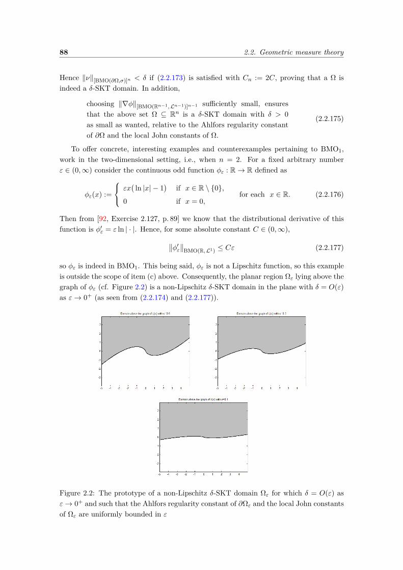
88 2.2. Geometric measure theory
Hence ‖ν‖[BMO(∂Ω,σ)]n < δ if (2.2.173) is satisfied with Cn := 2C, proving that a Ω isindeed a δ-SKT domain. In addition,
choosing ‖∇φ‖[BMO(Rn−1,Ln−1)]n−1 sufficiently small, ensuresthat the above set Ω ⊆ Rn is a δ-SKT domain with δ > 0as small as wanted, relative to the Ahlfors regularity constantof ∂Ω and the local John constants of Ω.
(2.2.175)
To offer concrete, interesting examples and counterexamples pertaining to BMO1,work in the two-dimensional setting, i.e., when n = 2. For a fixed arbitrary numberε ∈ (0,∞) consider the continuous odd function φε : R→ R defined as
φε(x) :=
εx(
ln |x| − 1)
if x ∈ R \ 0,
0 if x = 0,for each x ∈ R. (2.2.176)
Then from [92, Exercise 2.127, p. 89] we know that the distributional derivative of thisfunction is φ′ε = ε ln | · |. Hence, for some absolute constant C ∈ (0,∞),∥∥φ′ε∥∥BMO(R,L1) ≤ Cε (2.2.177)
so φε is indeed in BMO1. This being said, φε is not a Lipschitz function, so this exampleis outside the scope of item (c) above. Consequently, the planar region Ωε lying above thegraph of φε (cf. Figure 2.2) is a non-Lipschitz δ-SKT domain in the plane with δ = O(ε)as ε→ 0+ (as seen from (2.2.174) and (2.2.177)).
Figure 2.2: The prototype of a non-Lipschitz δ-SKT domain Ωε for which δ = O(ε) asε→ 0+ and such that the Ahlfors regularity constant of ∂Ωε and the local John constantsof Ωε are uniformly bounded in ε
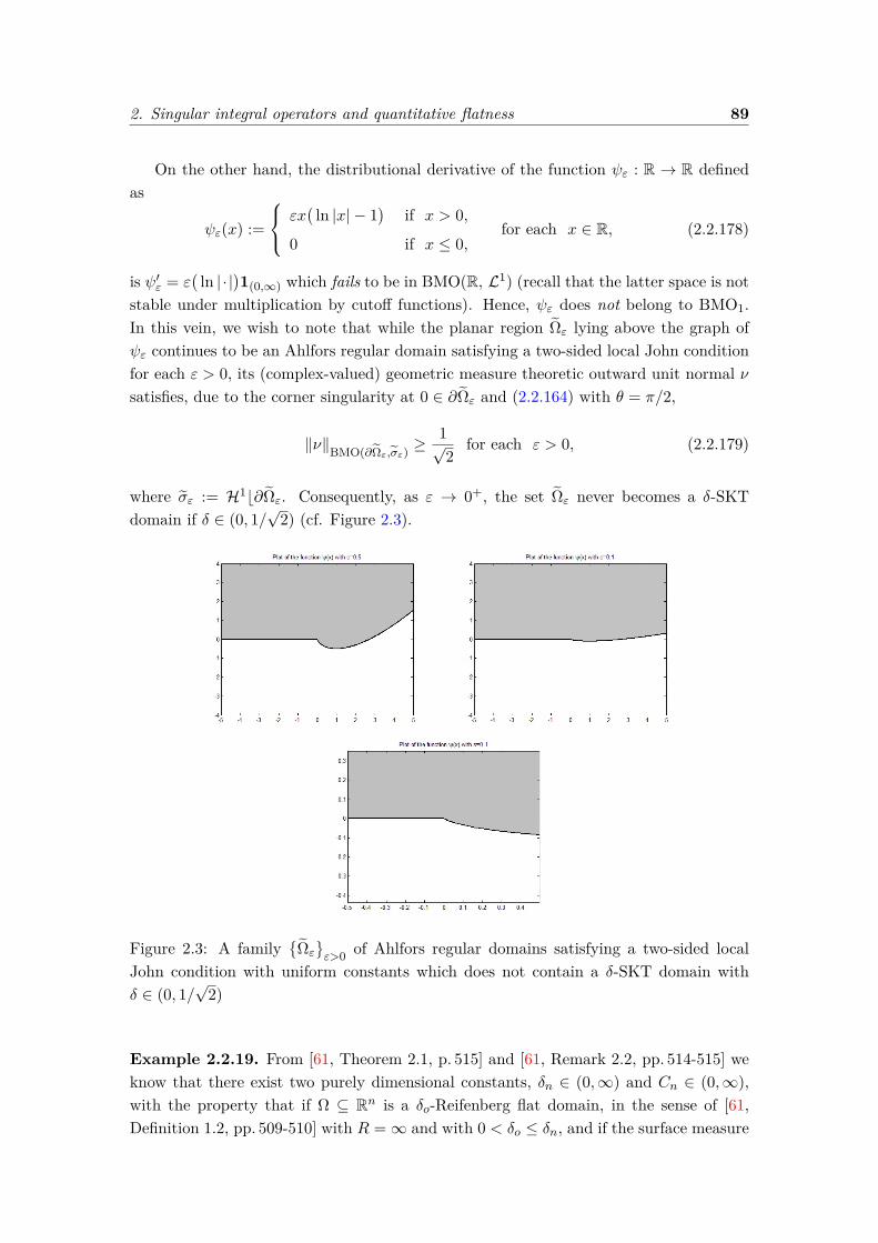
2. Singular integral operators and quantitative flatness 89
On the other hand, the distributional derivative of the function ψε : R → R definedas
ψε(x) :=
εx(
ln |x| − 1)
if x > 0,
0 if x ≤ 0,for each x ∈ R, (2.2.178)
is ψ′ε = ε(
ln | · |)1(0,∞) which fails to be in BMO(R, L1) (recall that the latter space is not
stable under multiplication by cutoff functions). Hence, ψε does not belong to BMO1.In this vein, we wish to note that while the planar region Ωε lying above the graph ofψε continues to be an Ahlfors regular domain satisfying a two-sided local John conditionfor each ε > 0, its (complex-valued) geometric measure theoretic outward unit normal νsatisfies, due to the corner singularity at 0 ∈ ∂Ωε and (2.2.164) with θ = π/2,
‖ν‖BMO(∂Ωε,σε)≥ 1√
2for each ε > 0, (2.2.179)
where σε := H1b∂Ωε. Consequently, as ε → 0+, the set Ωε never becomes a δ-SKTdomain if δ ∈ (0, 1/
√2) (cf. Figure 2.3).
Figure 2.3: A familyΩεε>0 of Ahlfors regular domains satisfying a two-sided local
John condition with uniform constants which does not contain a δ-SKT domain withδ ∈ (0, 1/
√2)
Example 2.2.19. From [61, Theorem 2.1, p. 515] and [61, Remark 2.2, pp. 514-515] weknow that there exist two purely dimensional constants, δn ∈ (0,∞) and Cn ∈ (0,∞),with the property that if Ω ⊆ Rn is a δo-Reifenberg flat domain, in the sense of [61,Definition 1.2, pp. 509-510] with R =∞ and with 0 < δo ≤ δn, and if the surface measure

90 2.2. Geometric measure theory
σ := Hn−1b∂Ω satisfies
σ(B(x, r) ∩ ∂Ω
)≤ (1 + δo)υn−1r
n−1
for each x ∈ ∂Ω and r > 0,(2.2.180)
(with υn−1 denoting the volume of the unit ball in Rn−1), then Ω is an Ahlfors regulardomain whose geometric measure theoretic outward unit normal ν to Ω satisfies
‖ν‖[BMO(∂Ω,σ)]n ≤ Cn√δo. (2.2.181)
See also [20, p. 11] and [107] in this regard. Consequently, given any number δ > 0, anyδo-Reifenberg flat domain with 0 < δo < min
δn , (δ/Cn)2 which satisfies (2.2.180) as
well as a two-sided local John condition is a δ-SKT domain.
Example 2.2.20. Denote by Ω the region of the plane lying to one side of a κ-CAC Σ ⊂C. Then Proposition 2.2.9 implies that Ω is a δ-SKT domain for any δ > 2
√κ(2 + κ).
To offer a concrete example, consider a real-valued function b ∈ BMO (R,L1) with‖b‖BMO (R,L1) < 1 and define z : R→ C by setting
z(s) :=ˆ s
0ei b(t) dt for each s ∈ R. (2.2.182)
If Ω ⊆ C ≡ R2 is the region of the plane to one side of the curve Σ := z(R), thenProposition 2.2.9 implies that Ω is a connected Ahlfors regular domain which satisfiesa two-sided local John condition, and ∂Ω = Σ, and whose geometric measure theoreticoutward unit normal ν to Ω is given by
ν(z(s)) = −i ei b(s) for L1-a.e. s ∈ R. (2.2.183)
In addition, if we set σ := H1b∂Ω then (2.2.145) gives
‖ν‖BMO(∂Ω,σ) ≤4‖b‖BMO (R,L1)
1− ‖b‖BMO (R,L1). (2.2.184)
As a consequence, Ω is a δ-SKT domain in R2 for each δ ∈ (0,∞) bigger than the numberin the right hand-side of (2.2.184).
For instance, we may take b to be a small multiple of the logarithm on the real line,i.e.,
b(s) := ε ln |s| for each s ∈ R \ 0,
with 0 < ε <∥∥ ln | · |
∥∥−1BMO (R,L1)
(2.2.185)
(e.g., the computation on [45, p. 520] shows that∥∥ ln | · |
∥∥BMO (R,L1) ≤ 3 ln(3/2), so taking
0 < ε < [3 ln(3/2)]−1 ≈ 0.8221 will do). Such a choice makes b a real-valued functionwith small BMO semi-norm which nonetheless maps R \ 0 onto R. In view of theformula given in (2.2.183), this goes to show that Gauss’ map Σ 3 z 7→ ν(z) ∈ S1 issurjective, which may be interpreted as saying that the unit normal rotates arbitrarilymuch along the boundary. In particular, the chord-arc curve Σ produced in this fashion,
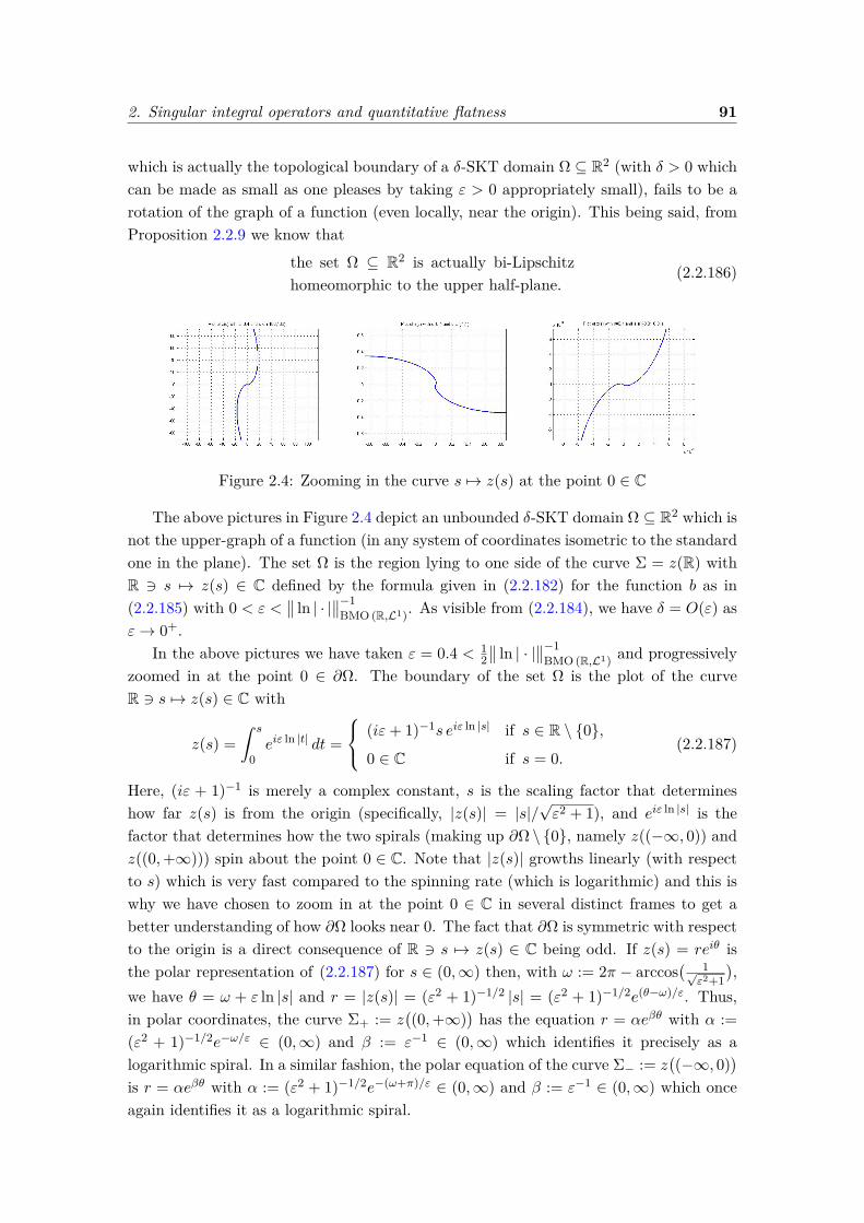
2. Singular integral operators and quantitative flatness 91
which is actually the topological boundary of a δ-SKT domain Ω ⊆ R2 (with δ > 0 whichcan be made as small as one pleases by taking ε > 0 appropriately small), fails to be arotation of the graph of a function (even locally, near the origin). This being said, fromProposition 2.2.9 we know that
the set Ω ⊆ R2 is actually bi-Lipschitzhomeomorphic to the upper half-plane.
(2.2.186)
Figure 2.4: Zooming in the curve s 7→ z(s) at the point 0 ∈ C
The above pictures in Figure 2.4 depict an unbounded δ-SKT domain Ω ⊆ R2 which isnot the upper-graph of a function (in any system of coordinates isometric to the standardone in the plane). The set Ω is the region lying to one side of the curve Σ = z(R) withR 3 s 7→ z(s) ∈ C defined by the formula given in (2.2.182) for the function b as in(2.2.185) with 0 < ε <
∥∥ ln | · |∥∥−1
BMO (R,L1). As visible from (2.2.184), we have δ = O(ε) asε→ 0+.
In the above pictures we have taken ε = 0.4 < 12∥∥ ln | · |
∥∥−1BMO (R,L1) and progressively
zoomed in at the point 0 ∈ ∂Ω. The boundary of the set Ω is the plot of the curveR 3 s 7→ z(s) ∈ C with
z(s) =ˆ s
0eiε ln |t| dt =
(iε+ 1)−1s eiε ln |s| if s ∈ R \ 0,
0 ∈ C if s = 0.(2.2.187)
Here, (iε + 1)−1 is merely a complex constant, s is the scaling factor that determineshow far z(s) is from the origin (specifically, |z(s)| = |s|/
√ε2 + 1), and eiε ln |s| is the
factor that determines how the two spirals (making up ∂Ω \ 0, namely z((−∞, 0)) andz((0,+∞))) spin about the point 0 ∈ C. Note that |z(s)| growths linearly (with respectto s) which is very fast compared to the spinning rate (which is logarithmic) and this iswhy we have chosen to zoom in at the point 0 ∈ C in several distinct frames to get abetter understanding of how ∂Ω looks near 0. The fact that ∂Ω is symmetric with respectto the origin is a direct consequence of R 3 s 7→ z(s) ∈ C being odd. If z(s) = reiθ isthe polar representation of (2.2.187) for s ∈ (0,∞) then, with ω := 2π − arccos
( 1√ε2+1
),
we have θ = ω + ε ln |s| and r = |z(s)| = (ε2 + 1)−1/2 |s| = (ε2 + 1)−1/2e(θ−ω)/ε. Thus,in polar coordinates, the curve Σ+ := z
((0,+∞)
)has the equation r = αeβθ with α :=
(ε2 + 1)−1/2e−ω/ε ∈ (0,∞) and β := ε−1 ∈ (0,∞) which identifies it precisely as alogarithmic spiral. In a similar fashion, the polar equation of the curve Σ− := z
((−∞, 0)
)is r = αeβθ with α := (ε2 + 1)−1/2e−(ω+π)/ε ∈ (0,∞) and β := ε−1 ∈ (0,∞) which onceagain identifies it as a logarithmic spiral.
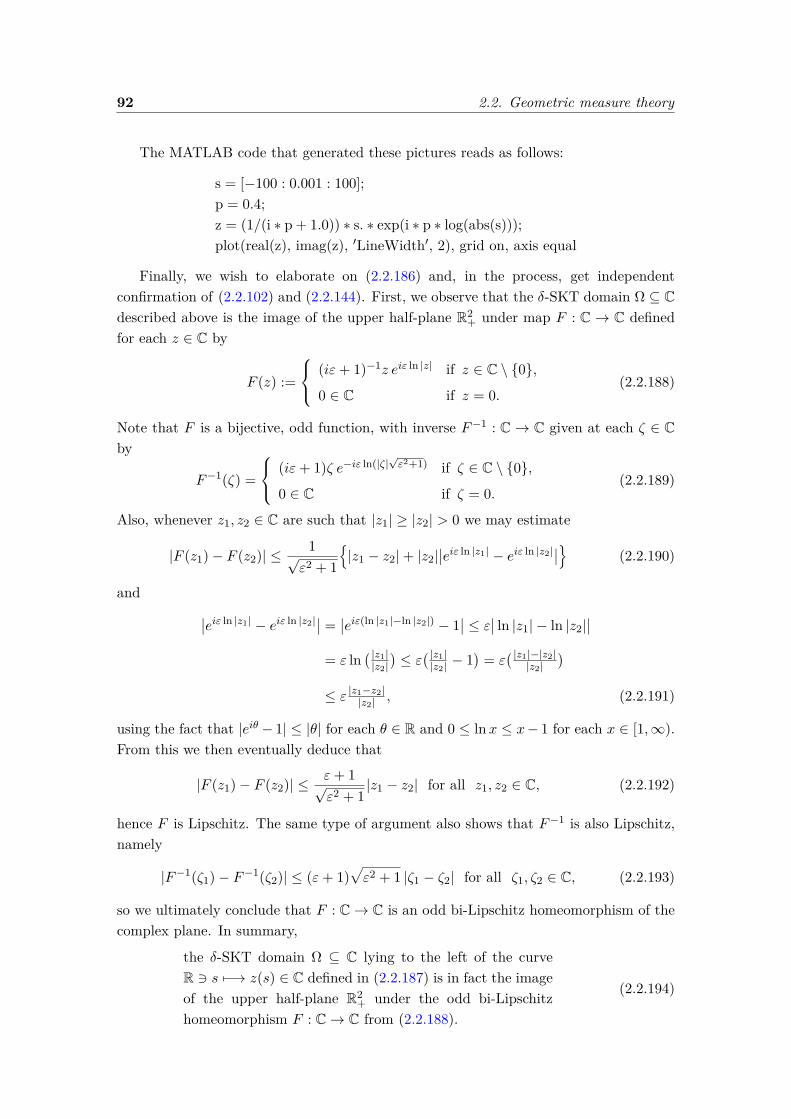
92 2.2. Geometric measure theory
The MATLAB code that generated these pictures reads as follows:
s = [−100 : 0.001 : 100];p = 0.4;z = (1/(i ∗ p + 1.0)) ∗ s. ∗ exp(i ∗ p ∗ log(abs(s)));plot(real(z), imag(z), ′LineWidth′, 2), grid on, axis equal
Finally, we wish to elaborate on (2.2.186) and, in the process, get independentconfirmation of (2.2.102) and (2.2.144). First, we observe that the δ-SKT domain Ω ⊆ Cdescribed above is the image of the upper half-plane R2
+ under map F : C → C definedfor each z ∈ C by
F (z) :=
(iε+ 1)−1z eiε ln |z| if z ∈ C \ 0,
0 ∈ C if z = 0.(2.2.188)
Note that F is a bijective, odd function, with inverse F−1 : C → C given at each ζ ∈ Cby
F−1(ζ) =
(iε+ 1)ζ e−iε ln(|ζ|√ε2+1) if ζ ∈ C \ 0,
0 ∈ C if ζ = 0.(2.2.189)
Also, whenever z1, z2 ∈ C are such that |z1| ≥ |z2| > 0 we may estimate
|F (z1)− F (z2)| ≤ 1√ε2 + 1
|z1 − z2|+ |z2|
∣∣eiε ln |z1| − eiε ln |z2|∣∣ (2.2.190)
and ∣∣eiε ln |z1| − eiε ln |z2|∣∣ =∣∣eiε(ln |z1|−ln |z2|) − 1
∣∣ ≤ ε∣∣ ln |z1| − ln |z2|∣∣
= ε ln( |z1||z2|)≤ ε
( |z1||z2| − 1
)= ε
( |z1|−|z2||z2|
)≤ ε |z1−z2||z2| , (2.2.191)
using the fact that |eiθ − 1| ≤ |θ| for each θ ∈ R and 0 ≤ ln x ≤ x− 1 for each x ∈ [1,∞).From this we then eventually deduce that
|F (z1)− F (z2)| ≤ ε+ 1√ε2 + 1
|z1 − z2| for all z1, z2 ∈ C, (2.2.192)
hence F is Lipschitz. The same type of argument also shows that F−1 is also Lipschitz,namely
|F−1(ζ1)− F−1(ζ2)| ≤ (ε+ 1)√ε2 + 1 |ζ1 − ζ2| for all ζ1, ζ2 ∈ C, (2.2.193)
so we ultimately conclude that F : C→ C is an odd bi-Lipschitz homeomorphism of thecomplex plane. In summary,
the δ-SKT domain Ω ⊆ C lying to the left of the curveR 3 s 7−→ z(s) ∈ C defined in (2.2.187) is in fact the imageof the upper half-plane R2
+ under the odd bi-Lipschitzhomeomorphism F : C→ C from (2.2.188).
(2.2.194)
2. Singular integral operators and quantitative flatness 93
Note that F also maps the lower half-plane R2− onto R2 \Ω, and R× 0 onto ∂Ω. This
is in agreement with (2.2.102). Moreover, since the Lipschitz constants of F, F−1 staybounded uniformly in ε ∈ (0, 1) (as is clear from (2.2.192), (2.2.193)) while, as notedearlier, δ = O(ε) as ε→ 0+, we see that (as predicted in (2.2.144))
by taking ε ∈ (0, 1) sufficiently small, matters may bearranged so that the above set Ω ⊆ R2 is a δ-SKT domainwith δ > 0 as small as one wishes, relative to the Ahlforsregularity constant of ∂Ω and the local John constants ofΩ.
(2.2.195)
Example 2.2.21. Wemay also construct examples of δ-SKT domains exhibitingmultiplespiral points (cf. Figure 2.1). Specifically, suppose −∞ < t1 < t2 < · · · < tN−1 < tN <
+∞, for some N ∈ N, and consider
b(t) := εN∑j=1
ln |t− tj | for each t ∈ R \ t1, . . . , tN, (2.2.196)
for some sufficiently small ε > 0. Next, define z : R → C as in (2.2.182) for this choiceof the function b. Then Proposition 2.2.13 and Proposition 2.2.9 imply that the regionΩ in R2 lying to one side of the curve Σ := z(R) is indeed a δ-SKT domain and, infact, δ = O(ε) as ε → 0+. Moreover, from (2.2.183) and (2.2.196) we see that ∂Ω = Σlooks like a spiral at each of the points z(t1), . . . , z(tN ). Yet, once again, there exists abi-Lipschitz homeomorphism F : R2 → R2 such that Ω = F (R2
+), R2 \ Ω = F (R2−), and
∂Ω = F (R× 0) (cf. (2.2.102)). Also, (2.2.144) presently entails
by choosing ε ∈ (0, 1) appropriately small, we mayensure that Ω is a δ-SKT domain in R2 with δ > 0as small as desired, relative to the Ahlfors regularityconstant of ∂Ω and the local John constants of Ω.
(2.2.197)
Example 2.2.22. We wish to note that the construction in Example 2.2.21 may bemodified as to allow infinitely many spiral points. Specifically, assume tjj∈N ⊆ R is agiven sequence of real numbers and consider
0 < λj < 2−j min
1 ,∥∥ ln | · −tj |
∥∥−1L1([−j,j],L1)
for each j ∈ N. (2.2.198)
Also, suppose 0 < ε <∥∥ ln | · |
∥∥−1BMO(R,L1) and define
b(t) := ε∞∑j=1
λj ln |t− tj | for each t ∈ R \ tjj∈N. (2.2.199)
The choice in (2.2.198) ensures that the above series converges absolutely in L1(K,L1)for any compact subset K of R. This has two notable consequences. First, the series in(2.2.199) converges absolutely in a pointwise sense L1-a.e. in R; in particular, b is well
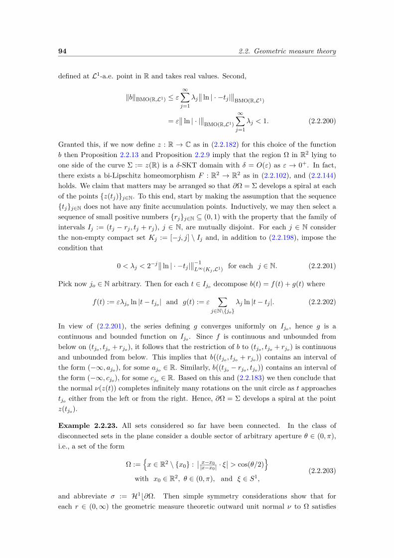
94 2.2. Geometric measure theory
defined at L1-a.e. point in R and takes real values. Second,
‖b‖BMO(R,L1) ≤ ε∞∑j=1
λj∥∥ ln | · −tj |
∥∥BMO(R,L1)
= ε∥∥ ln | · |
∥∥BMO(R,L1)
∞∑j=1
λj < 1. (2.2.200)
Granted this, if we now define z : R → C as in (2.2.182) for this choice of the functionb then Proposition 2.2.13 and Proposition 2.2.9 imply that the region Ω in R2 lying toone side of the curve Σ := z(R) is a δ-SKT domain with δ = O(ε) as ε → 0+. In fact,there exists a bi-Lipschitz homeomorphism F : R2 → R2 as in (2.2.102), and (2.2.144)holds. We claim that matters may be arranged so that ∂Ω = Σ develops a spiral at eachof the points z(tj)j∈N. To this end, start by making the assumption that the sequencetjj∈N does not have any finite accumulation points. Inductively, we may then select asequence of small positive numbers rjj∈N ⊆ (0, 1) with the property that the family ofintervals Ij := (tj − rj , tj + rj), j ∈ N, are mutually disjoint. For each j ∈ N considerthe non-empty compact set Kj := [−j, j] \ Ij and, in addition to (2.2.198), impose thecondition that
0 < λj < 2−j∥∥ ln | · −tj |
∥∥−1L∞(Kj ,L1) for each j ∈ N. (2.2.201)
Pick now jo ∈ N arbitrary. Then for each t ∈ Ijo decompose b(t) = f(t) + g(t) where
f(t) := ελjo ln |t− tjo | and g(t) := ε∑
j∈N\joλj ln |t− tj |. (2.2.202)
In view of (2.2.201), the series defining g converges uniformly on Ijo , hence g is acontinuous and bounded function on Ijo . Since f is continuous and unbounded frombelow on (tjo , tjo + rjo), it follows that the restriction of b to (tjo , tjo + rjo) is continuousand unbounded from below. This implies that b
((tjo , tjo + rjo)
)contains an interval of
the form (−∞, ajo), for some ajo ∈ R. Similarly, b((tjo − rjo , tjo)
)contains an interval of
the form (−∞, cjo), for some cjo ∈ R. Based on this and (2.2.183) we then conclude thatthe normal ν(z(t)) completes infinitely many rotations on the unit circle as t approachestjo either from the left or from the right. Hence, ∂Ω = Σ develops a spiral at the pointz(tjo).
Example 2.2.23. All sets considered so far have been connected. In the class ofdisconnected sets in the plane consider a double sector of arbitrary aperture θ ∈ (0, π),i.e., a set of the form
Ω :=x ∈ R2 \ x0 :
∣∣ x−x0|x−x0| · ξ
∣∣ > cos(θ/2)
with x0 ∈ R2, θ ∈ (0, π), and ξ ∈ S1,(2.2.203)
and abbreviate σ := H1b∂Ω. Then simple symmetry considerations show that foreach r ∈ (0,∞) the geometric measure theoretic outward unit normal ν to Ω satisfies
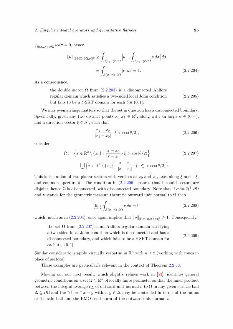
2. Singular integral operators and quantitative flatness 95
fflB(xo,r)∩∂Ω ν dσ = 0, hence
‖ν‖[BMO(∂Ω,σ)]2 ≥ B(xo,r)∩∂Ω
∣∣∣ν − B(xo,r)∩∂Ω
ν dσ∣∣∣ dσ
= B(xo,r)∩∂Ω
|ν| dσ = 1. (2.2.204)
As a consequence,
the double sector Ω from (2.2.203) is a disconnected Ahlforsregular domain which satisfies a two-sided local John conditionbut fails to be a δ-SKT domain for each δ ∈ (0, 1].
(2.2.205)
We may even arrange matters so that the set in question has a disconnected boundary.Specifically, given any two distinct points x0, x1 ∈ R2, along with an angle θ ∈ (0, π),and a direction vector ξ ∈ S1, such that
x1 − x0|x1 − x0|
· ξ < cos(θ/2), (2.2.206)
consider
Ω :=x ∈ R2 \ x0 : x− x0
|x− x0|· ξ > cos(θ/2)
(2.2.207)
⋃x ∈ R2 \ x1 : x− x1
|x− x1|· (−ξ) > cos(θ/2)
.
This is the union of two planar sectors with vertices at x0 and x1, axes along ξ and −ξ,and common aperture θ. The condition in (2.2.206) ensures that the said sectors aredisjoint, hence Ω is disconnected, with disconnected boundary. Note that if σ := H1b∂Ωand ν stands for the geometric measure theoretic outward unit normal to Ω then
limr→∞
B(xo,r)∩∂Ω
ν dσ = 0 (2.2.208)
which, much as in (2.2.204), once again implies that ‖ν‖[BMO(∂Ω,σ)]2 ≥ 1. Consequently,
the set Ω from (2.2.207) is an Ahlfors regular domain satisfyinga two-sided local John condition which is disconnected and has adisconnected boundary, and which fails to be a δ-SKT domain foreach δ ∈ (0, 1].
(2.2.209)
Similar considerations apply virtually verbatim in Rn with n ≥ 2 (working with cones inplace of sectors).
These examples are particularly relevant in the context of Theorem 2.2.33.
Moving on, our next result, which slightly refines work in [53], identifies generalgeometric conditions on a set Ω ⊆ Rn of locally finite perimeter so that the inner productbetween the integral average ν∆ of outward unit normal ν to Ω in any given surface ball∆ ⊆ ∂Ω and the “chord” x − y with x, y ∈ ∆ may be controlled in terms of the radiusof the said ball and the BMO semi-norm of the outward unit normal ν.
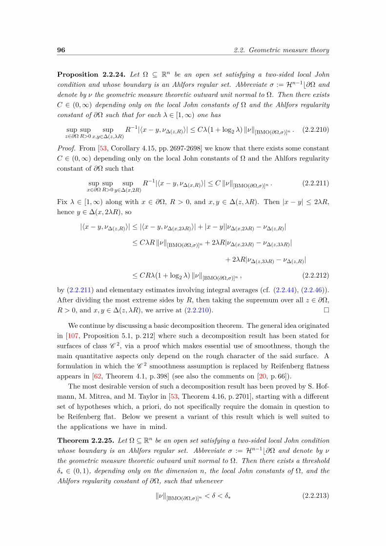
96 2.2. Geometric measure theory
Proposition 2.2.24. Let Ω ⊆ Rn be an open set satisfying a two-sided local Johncondition and whose boundary is an Ahlfors regular set. Abbreviate σ := Hn−1b∂Ω anddenote by ν the geometric measure theoretic outward unit normal to Ω. Then there existsC ∈ (0,∞) depending only on the local John constants of Ω and the Ahlfors regularityconstant of ∂Ω such that for each λ ∈ [1,∞) one has
supz∈∂Ω
supR>0
supx,y∈∆(z,λR)
R−1|〈x− y, ν∆(z,R)〉| ≤ Cλ(1 + log2 λ) ‖ν‖[BMO(∂Ω,σ)]n . (2.2.210)
Proof. From [53, Corollary 4.15, pp. 2697-2698] we know that there exists some constantC ∈ (0,∞) depending only on the local John constants of Ω and the Ahlfors regularityconstant of ∂Ω such that
supx∈∂Ω
supR>0
supy∈∆(x,2R)
R−1|〈x− y, ν∆(x,R)〉| ≤ C ‖ν‖[BMO(∂Ω,σ)]n . (2.2.211)
Fix λ ∈ [1,∞) along with x ∈ ∂Ω, R > 0, and x, y ∈ ∆(z, λR). Then |x − y| ≤ 2λR,hence y ∈ ∆(x, 2λR), so
|〈x− y, ν∆(z,R)〉| ≤ |〈x− y, ν∆(x,2λR)〉|+ |x− y||ν∆(x,2λR) − ν∆(z,R)|
≤ CλR ‖ν‖[BMO(∂Ω,σ)]n + 2λR|ν∆(x,2λR) − ν∆(z,3λR)|
+ 2λR|ν∆(z,3λR) − ν∆(z,R)|
≤ CRλ(1 + log2 λ) ‖ν‖[BMO(∂Ω,σ)]n , (2.2.212)
by (2.2.211) and elementary estimates involving integral averages (cf. (2.2.44), (2.2.46)).After dividing the most extreme sides by R, then taking the supremum over all z ∈ ∂Ω,R > 0, and x, y ∈ ∆(z, λR), we arrive at (2.2.210).
We continue by discussing a basic decomposition theorem. The general idea originatedin [107, Proposition 5.1, p. 212] where such a decomposition result has been stated forsurfaces of class C 2, via a proof which makes essential use of smoothness, though themain quantitative aspects only depend on the rough character of the said surface. Aformulation in which the C 2 smoothness assumption is replaced by Reifenberg flatnessappears in [62, Theorem 4.1, p. 398] (see also the comments on [20, p. 66]).
The most desirable version of such a decomposition result has been proved by S. Hof-mann, M. Mitrea, and M. Taylor in [53, Theorem 4.16, p. 2701], starting with a differentset of hypotheses which, a priori, do not specifically require the domain in question tobe Reifenberg flat. Below we present a variant of this result which is well suited tothe applications we have in mind.
Theorem 2.2.25. Let Ω ⊆ Rn be an open set satisfying a two-sided local John conditionwhose boundary is an Ahlfors regular set. Abbreviate σ := Hn−1b∂Ω and denote by νthe geometric measure theoretic outward unit normal to Ω. Then there exists a thresholdδ∗ ∈ (0, 1), depending only on the dimension n, the local John constants of Ω, and theAhlfors regularity constant of ∂Ω, such that whenever
‖ν‖[BMO(∂Ω,σ)]n < δ < δ∗ (2.2.213)
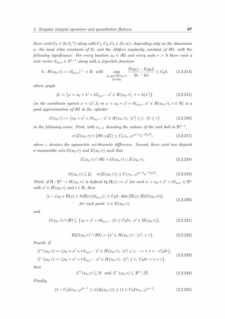
2. Singular integral operators and quantitative flatness 97
there exist C0 ∈ (0, δ−1∗ ) along with C1, C2, C3 ∈ (0,∞), depending only on the dimension
n, the local John constants of Ω, and the Ahlfors regularity constant of ∂Ω, with thefollowing significance. For every location x0 ∈ ∂Ω and every scale r > 0 there exist aunit vector ~nx0,r ∈ Sn−1 along with a Lipschitz function
h : H(x0, r) := 〈~nx0,r〉⊥ → R with supy1,y2∈H(x0,r)
y1 6=y2
|h(y1)− h(y2)||y1 − y2|
≤ C0δ, (2.2.214)
whose graph
G :=x = x0 + x′ + t~nx0,r : x′ ∈ H(x0, r), t = h(x′)
(2.2.215)
(in the coordinate system x = (x′, t) ⇔ x = x0 + x′ + t~nx0,r, x′ ∈ H(x0, r), t ∈ R) is agood approximation of ∂Ω in the cylinder
C(x0, r) :=x0 + x′ + t~nx0,r : x′ ∈ H(x0, r), |x′| ≤ r, |t| ≤ r
(2.2.216)
in the following sense. First, with υn−1 denoting the volume of the unit ball in Rn−1,
σ(C(x0, r) ∩
(∂Ω4G
))≤ C1υn−1r
n−1e−C2/δ, (2.2.217)
where 4 denotes the symmetric set-theoretic difference. Second, there exist two disjointσ-measurable sets G(x0, r) and E(x0, r) such that
C(x0, r) ∩ ∂Ω = G(x0, r) ∪ E(x0, r), (2.2.218)
G(x0, r) ⊆ G, σ(E(x0, r)
)≤ C1υn−1r
n−1e−C2/δ. (2.2.219)
Third, if Π : Rn → H(x0, r) is defined by Π(x) := x′ for each x = x0 + x′ + t~nx0,r ∈ Rn
with x′ ∈ H(x0, r) and t ∈ R, then∣∣x− (x0 + Π(x) + h(Π(x))~nx0,r)∣∣ ≤ C0δ · dist
(Π(x),Π(G(x0, r))
)for each point x ∈ E(x0, r),
(2.2.220)
and
C(x0, r) ∩ ∂Ω ⊆x0 + x′ + t~nx0,r : |t| ≤ C0δr, x
′ ∈ H(x0, r), (2.2.221)
Π(C(x0, r) ∩ ∂Ω
)=x′ ∈ H(x0, r) : |x′| < r
. (2.2.222)
Fourth, if
C+(x0, r) :=x0 + x′ + t ~nx0,r : x′ ∈ H(x0, r), |x′| ≤ r, −r < t < −C0δr
,
C−(x0, r) :=x0 + x′ + t ~nx0,r : x′ ∈ H(x0, r), |x′| ≤ r, C0δr < t < r
,
(2.2.223)
thenC+(x0, r) ⊆ Ω and C−(x0, r) ⊆ Rn \ Ω. (2.2.224)
Finally,
(1− C3δ)υn−1rn−1 ≤ σ
(∆(x0, r)
)≤ (1 + C3δ)υn−1r
n−1. (2.2.225)

98 2.2. Geometric measure theory
Proof. This is established by reasoning as in [53, pp. 2703-2709] with (2.2.213) replacingthe small local BMO assumption (which, in particular, frees us from having to restrictx0 to a compact subset of ∂Ω). The key observation is that in the present context, theparameter R∗ from [53, Theorem 4.16, p. 2701] (which limits the size of the scale r) maybe taken to be +∞. In turn, this is seen by a careful inspection of the proof of [53,Theorem 4.16, p. 2701], in which we now rely on [53, Corollary 4.15, p. 2697] in place of[53, Theorem 4.14, p. 2697].
Finally, since the claim pertaining to (2.2.223)-(2.2.224) does not explicitly appear inthe statement of [53, Theorem 4.16, p. 2701], we provide a proof here. From (2.2.221)-(2.2.222) it follows that the connected sets C±(x0, r) introduced in (2.2.223) do notintersect ∂Ω. As such, Ω+ := Ω and Ω− := Rn \ Ω form a disjoint, open cover ofC±(x0, r), hence
C+(x0, r) is fully contained in either Ω+ or Ω−, andalso C−(x0, r) is fully contained in either Ω+ or Ω−.
(2.2.226)
Denote by x±r ∈ Ω± the two corkscrew points corresponding to the location x0 and scaler. In particular,
|x±r − x0| < r and B(x±r , θr
)⊆ Ω± (2.2.227)
where the parameter θ ∈ (0, 1) is as in Definition 1.1.10. Assume 0 < δ < θ/C0 to beginwith. This makes it impossible to contain either of the balls B
(x+r , θr
), B(x−r , θr
)in the
stripx0 + x′ + t~nx0,r : |t| ≤ C0δr, x
′ ∈ H(x0, r). Since, as seen from (2.2.227), their
centers x±r belong to B(x0, r) ⊂ C(x0, r), in turn this forces one of the following fouralternatives to be true:
B(x+r , θr
)∩ C+(x0, r) 6= ∅ and B
(x−r , θr
)∩ C+(x0, r) 6= ∅, (2.2.228)
B(x+r , θr
)∩ C−(x0, r) 6= ∅ and B
(x−r , θr
)∩ C−(x0, r) 6= ∅, (2.2.229)
B(x+r , θr
)∩ C+(x0, r) 6= ∅ and B
(x−r , θr
)∩ C−(x0, r) 6= ∅, (2.2.230)
B(x+r , θr
)∩ C−(x0, r) 6= ∅ and B
(x−r , θr
)∩ C+(x0, r) 6= ∅. (2.2.231)
Note that the alternative described in (2.2.228) cannot possibly hold. Indeed, theexistence of two points z1 ∈ B
(x+r , θr
)∩ C+(x0, r) and z2 ∈ B
(x−r , θr
)∩ C+(x0, r) would
imply that, on the one hand, the line segment [z1, z2] lies in the convex set C+(x0, r), hencealso either in Ω+ or in Ω− by (2.2.226). However, the fact that z1 ∈ B
(x+r , θr
)⊆ Ω+ and
z2 ∈ B(x−r , θr
)⊆ Ω− prevents either one of these eventualities form materializing. This
contradiction therefore excludes (2.2.228). Reasoning in a similar fashion we may ruleout (2.2.229). When (2.2.230) holds, from (2.2.226) and the fact that B
(x±r , θr
)⊆ Ω±
(cf. (2.2.227)) we conclude that the inclusions in (2.2.224) hold as stated. Finally,when (2.2.231) holds, from (2.2.226) and (2.2.227) we deduce that C+(x0, r) ⊆ Ω− andC−(x0, r) ⊆ Ω+. In such a scenario, we may ensure that the inclusions in (2.2.224)are valid simply by re-denoting ~nx0,r as −~nx0,r which amounts to reversing the roles ofC+(x0, r) and C−(x0, r). This concludes the proof of (2.2.224).
2. Singular integral operators and quantitative flatness 99
In the final portion of this section we explore the implications of the quality of being aδ-SKT domain with δ > 0 small in terms of flatness (in the Reifenberg sense) and topology(cf. Theorem 2.2.33). To facilitate the subsequent discussion, the reader is reminded thatthe Hausdorff distance between two arbitrary nonempty sets A,B ⊂ Rn is defined as
Dist[A,B] := max
supdist (a,B) : a ∈ A , supdist (b, A) : b ∈ B. (2.2.232)
We also recall the following definitions from [61].
Definition 2.2.26. Fix R ∈ (0,∞] along with δ ∈ (0,∞) and let Σ ⊂ Rn be a closedset. Then Σ is said to be a (R, δ)-Reifenberg flat set if for each for each x ∈ Σ andeach r ∈ (0, R) there exists an (n− 1)-dimensional plane π(x, r) in Rn which contains xand satisfies
Dist[Σ ∩B(x, r) , π(x, r) ∩B(x, r)
]≤ δ r. (2.2.233)
For example, given δ > 0, the graph of a real-valued Lipschitz function defined in Rn−1
with a sufficiently small Lipschitz constant is a (∞, δ)-Reifenberg flat set.
Definition 2.2.27. Fix R ∈ (0,∞] along with δ ∈ (0,∞). A nonempty, proper subset Ωof Rn is said to satisfy the (R, δ)-separation property if for each x ∈ ∂Ω and r ∈ (0, R)there exist an (n− 1)-dimensional plane π(x, r) in Rn passing through x and a choice ofunit normal vector ~nx,r to π(x, r) such that
y + t ~nx,r ∈ B(x, r) : y ∈ π(x, r), t > 2δr⊂ Ω and
y + t ~nx,r ∈ B(x, r) : y ∈ π(x, r), t < −2δr⊂ Rn \ Ω.
(2.2.234)
Definition 2.2.28. Fix R ∈ (0,∞] along with δ ∈ (0,∞). A nonempty, proper subset Ωof Rn is called an (R, δ)-Reifenberg flat domain (or simply a Reifenberg flat domainif the particular values ofR, δ are not important) provided Ω satisfies the (R, δ)-separationproperty and ∂Ω is an (R, δ)-Reifenberg flat set.
Recall the two-sided corkscrew condition from Definition 1.1.6.
Proposition 2.2.29. Let Ω be a nonempty proper subset of Rn satisfying the (R, c)-two-sided corkscrew condition for some R ∈ (0,∞] and c ∈ (0, 1). In addition, suppose ∂Ωis a (R, δ)-Reifenberg flat set for some δ ∈ (0, c/2). Then Ω is an (R, δ)-Reifenberg flatdomain.
Proof. Pick a location x ∈ ∂Ω and a scale r ∈ (0, R). Definition 2.2.26 ensures theexistence of of an (n−1)-dimensional plane π(x, r) in Rn passing through x which satisfies(2.2.233). Make a choice of a unit normal vector ~nx,r to π(x, r) and abbreviate
C+(x, r) :=y + t ~nx,r ∈ B(x, r) : y ∈ π(x, r), t > 2δr
,
C−(x, r) :=y + t ~nx,r ∈ B(x, r) : y ∈ π(x, r), t < −2δr
.
(2.2.235)
We claim that matters may be arranged (by taking δ sufficiently small to begin with,and by making a judicious choice of the orientation of ~nx,r) so that
C+(x, r) ⊂ Ω and C−(x, r) ⊂ Rn \ Ω. (2.2.236)
100 2.2. Geometric measure theory
With this goal in mind, first observe that (2.2.233) guarantees that the connected setsC±(x, r) do not intersect ∂Ω. As such, Ω+ := Ω and Ω− := Rn \ Ω form a disjoint, opencover of C±(x, r), hence
C+(x, r) is entirely contained in either Ω+ or Ω−, andalso C−(x, r) is entirely contained in either Ω+ or Ω−.
(2.2.237)
To proceed, denote by x±r ∈ Ω± the two corkscrew points corresponding to the locationx and scale r. In particular,
|x±r − x| < r and B(x±r , cr
)⊆ Ω± (2.2.238)
where the constant c ∈ (0, 1) is as in Definition 1.1.6. Hence, if we consider the ballsB(x+r , cr
), B(x−r , cr
), their centers x±r belong to B(x, r). The fact that we are presently
assuming 0 < δ < c/2 with c ∈ (0, 1) ensures that δ < (c/2)√
4− c2 which, as someelementary geometry shows, forces each of the balls B
(x+r , cr
), B(x−r , cr
)to intersect one
of the sets C+(x, r), C−(x, r). As such, one of the following four alternatives is true:
B(x+r , cr
)∩ C+(x, r) 6= ∅ and B
(x−r , cr
)∩ C+(x, r) 6= ∅, (2.2.239)
B(x+r , cr
)∩ C−(x, r) 6= ∅ and B
(x−r , cr
)∩ C−(x, r) 6= ∅, (2.2.240)
B(x+r , cr
)∩ C+(x, r) 6= ∅ and B
(x−r , cr
)∩ C−(x, r) 6= ∅, (2.2.241)
B(x+r , cr
)∩ C−(x, r) 6= ∅ and B
(x−r , cr
)∩ C+(x, r) 6= ∅. (2.2.242)
Observe that the alternative described in (2.2.239) cannot possibly hold. Otherwise, theexistence of two points z1 ∈ B
(x+r , cr
)∩C+(x, r) and z2 ∈ B
(x−r , cr
)∩C+(x, r) would imply
that, on the one hand, the line segment [z1, z2] lies in the convex set C+(x, r), hence alsoeither in Ω+ or in Ω− by (2.2.237). This being said, the fact that z1 ∈ B
(x+r , cr
)⊆ Ω+ and
z2 ∈ B(x−r , cr
)⊆ Ω− prevents either one of these eventualities form materializing. This
contradiction therefore excludes (2.2.239). Reasoning in a similar fashion we may ruleout (2.2.240). When (2.2.241) holds, from (2.2.237) and the fact that B
(x±r , cr
)⊆ Ω±
(cf. (2.2.238)) we conclude that the inclusions in (2.2.236) hold as stated. Finally,when (2.2.242) holds, from (2.2.226) and (2.2.238) we deduce that C+(x, r) ⊆ Ω− andC−(x, r) ⊆ Ω+. In such a scenario, we may ensure that the inclusions in (2.2.236) arevalid simply by re-denoting ~nx,r as −~nx,r which amounts to reversing the roles of C+(x, r)and C−(x, r). This concludes the proof of (2.2.236). In turn, from (2.2.236) and (2.2.235)we conclude that (2.2.234) holds with π(x, r) := π(x, r). Definition 2.2.27 then impliesthat Ω is, indeed, an (R, δ)-Reifenberg flat domain.
Any δ-SKT domain with δ > 0 sufficiently small is a Reifenberg flat domain. Specif-ically, we have the following result.
Proposition 2.2.30. Suppose Ω ⊆ Rn is an open set satisfying a two-sided local Johncondition and whose boundary is Ahlfors regular. Abbreviate σ := Hn−1b∂Ω and denoteby ν the geometric measure theoretic outward unit normal to Ω.
2. Singular integral operators and quantitative flatness 101
Then there exists some threshold δ∗ ∈ (0, 1) along with some constant C ∈ (0,∞),both depending only on the dimension n, the local John constants of Ω, and the Ahlforsregularity constant of ∂Ω, such that if ‖ν‖[BMO(∂Ω,σ)]n < δ with δ ∈ (0, δ∗) then Ω is an(∞, Cδ)-Reifenberg flat domain.
A version of this result continues to hold with the two-sided local John conditionrelaxed to a two-sided corkscrew condition, in which scenario one concludes that ∂Ω isa Reifenberg flat set but only at small scales (see [15, Theorem 2.1] for details).
Proof of Proposition 2.2.30. Choose the parameter δ∗ ∈ (0, 1) as in Theorem 2.2.25 andmake the assumption that ‖ν‖[BMO(∂Ω,σ)]n < δ with δ ∈ (0, δ∗). Then from (2.2.221) itfollows that there exists some C ∈ (0,∞) which depends only on the dimension n, thelocal John constants of Ω, and the Ahlfors regularity constant of ∂Ω, such that ∂Ω isan (∞, Cδ)-Reifenberg flat set. Also, (2.2.223)-(2.2.224) guarantee that, for a constantC ∈ (0,∞) of the same nature as before, Ω satisfies the (∞, Cδ)-separation property.Alternatively, we may invoke Proposition 2.2.29 (keeping in mind that the two-sidedlocal John condition implies the two-sided corkscrew condition). Granted these qualities,Definition 2.2.28 then implies that Ω is an (∞, Cδ)-Reifenberg flat domain.
It turns out that sufficiently flat Reifenberg domains are NTA domains. More specif-ically, from [61, Theorem 3.1, p. 524] and its proof we see that
there exists a purely dimensional constant δn ∈ (0,∞) with theproperty that for each δ ∈ (0, δn) and R ∈ (0,∞] one may find anumber N = N(δ,R) ∈ N with the property that that any (R, δ)-Reifenberg flat domain Ω ⊆ Rn is also an (R,N)-nontangentiallyaccessible domain (in the sense of Definition 1.1.8).
(2.2.243)
This has a number of useful consequences. For example, it allows us to conclude thatany open set satisfying a two-sided corkscrew condition and whose topological boundaryis a sufficiently flat Reifenberg set is actually an NTA domain.
Proposition 2.2.31. Let Ω be a nonempty proper subset of Rn satisfying the (R, c)-two-sided corkscrew condition for some R ∈ (0,∞] and c ∈ (0, 1). In addition, suppose∂Ω is a (R, δ)-Reifenberg flat set with 0 < δ < minc/2, δn, where δn ∈ (0,∞) is thepurely dimensional constant from (2.2.243). Then there exist N = N(δ,R) ∈ N with theproperty that Ω is an (R,N)-nontangentially accessible domain.
Proof. The desired conclusion is a direct consequence of Proposition 2.2.29, (2.2.243),and Definition 1.1.8.
In concert with Proposition 2.2.30, the result recalled in (2.2.243) also shows thatany δ-SKT domain with δ > 0 sufficiently small is a two-sided NTA domain. Hereis a precise statement.
102 2.2. Geometric measure theory
Proposition 2.2.32. Let Ω ⊆ Rn be an open set satisfying a two-sided local Johncondition and whose boundary is Ahlfors regular. Abbreviate σ := Hn−1b∂Ω and denoteby ν the geometric measure theoretic outward unit normal to Ω.
Then there exists a threshold δ0 ∈ (0, 1) and a number N ∈ N, both depending onlyon the dimension n, the local John constants of Ω, and the Ahlfors regularity constantof ∂Ω, such that if ‖ν‖[BMO(∂Ω,σ)]n < δ0 then Ω is an (∞, N)-two-sided nontangentiallyaccessible domain (in the sense of Definition 1.1.8).
In the converse direction, fix δ ∈ (0,∞), N ∈ N, R ∈ (0,∞], and suppose Ω ⊆ Rn is an(R,N)-two-sided nontangentially accessible domain (with the requirement that R = ∞if ∂Ω is unbounded) whose boundary is an Ahlfors regular set. Then from (1.1.28) anddefinitions we see that Ω is a δ-SKT domain whenever its geometric measure theoreticoutward unit normal ν satisfies ‖ν‖[BMO(∂Ω,σ)]n < δ (where, as usual, σ := Hn−1b∂Ω).
Proof of Proposition 2.2.32. Let δ∗ ∈ (0, 1) and C ∈ (0,∞) be as in Proposition 2.2.30,and recall the purely dimensional constant δn ∈ (0,∞) from (2.2.243). Take
δ0 := minδ∗ , δn/C
∈ (0, 1) (2.2.244)
and assume that ‖ν‖[BMO(∂Ω,σ)]n < δ0. Also, fix some δ ∈(‖ν‖[BMO(∂Ω,σ)]n , δ0
). Propo-
sition 2.2.30 then guarantees that Ω is an (∞, Cδ)-Reifenberg flat domain. Given thatCδ < δn, from (2.2.243) we conclude that there exists some N ∈ N such that Ω is an(∞, N)-nontangentially accessible domain in the sense of Definition 1.1.8.
Going further, observe that the set Rn\Ω satisfies a two-sided local John condition andrecall from Example 2.2.16 that its topological and measure theoretic boundaries coincidewith those of Ω. Also, the geometric measure theoretic outward unit normal to Rn \Ω is−ν at σ-a.e. point on ∂Ω. In particular, the BMO semi-norm of the geometric measuretheoretic outward unit normal to Rn \Ω is < δ. As such, the argument in the first part ofthe proof applies and gives that Rn \Ω is an (∞, N)-nontangentially accessible domain aswell. All together, this makes Ω an (∞, N)-two-sided nontangentially accessible domain.
We are now in a position to show that for a δ-SKT domain Ω ⊆ Rn the demandthat the parameter δ ∈ (0, 1) is suitably small relative to the geometry of Ω has astring of remarkable topological and metric consequences for the set Ω. To set thestage, from [70, Theorem 2 in 49.VI, 57.I.9(i), 57.III.1] (cf. also [67, Lemma 4(1) andLemma 5, p. 1702]) we first note that
if O ⊆ Rn is some arbitrary connected open set, then anyconnected component of Rn \ O has a connected boundary. (2.2.245)
Theorem 2.2.33. Let Ω ⊆ Rn be an open set satisfying a two-sided local John conditionand whose boundary is Ahlfors regular. Abbreviate σ := Hn−1b∂Ω and denote by ν thegeometric measure theoretic outward unit normal to Ω.
Then there exists a threshold δ0 ∈ (0, 1) depending only on the ambient dimensionn, the local John constants of Ω, and the Ahlfors regularity constant of ∂Ω, such that if
2. Singular integral operators and quantitative flatness 103
‖ν‖[BMO(∂Ω,σ)]n < δ0 it follows that Ω is an unbounded connected set, Ω is an unboundedconnected set, ∂Ω is an unbounded connected set, Rn \Ω is an unbounded connected set,Rn \Ω is an unbounded connected set, and ∂(Ω ) = ∂Ω, ∂(Rn \Ω ) = ∂Ω, ∂(Rn \Ω) = ∂Ω.
As is apparent from Example 2.2.23, the demand that the parameter δ > 0 issufficiently small cannot be dispense with in the context of Theorem 2.2.33.
Proof of Theorem 2.2.33. Bring in the threshold δ0 ∈ (0, 1) from Proposition 2.2.32and assume that ‖ν‖[BMO(∂Ω,σ)]n < δ0. From Proposition 2.2.32, Definition 1.1.8, andDefinition 1.1.7 we then conclude that both Ω and Rn \ Ω are pathwise connected opensets (hence, connected open sets). Having established this, from (2.2.245) we then seethat ∂
(Rn \ Ω
)= ∂(Ω ) is connected. The fact that Ω satisfies an exterior corkscrew
condition further implies ∂(Ω ) = ∂Ω. Since δ < 1, Lemma 2.2.5 ensures that ∂Ω isunbounded, and this forces both Ω and Rn \ Ω to be unbounded (given that they have∂Ω as their topological boundary). Also, the fact that Rn \ Ω is connected implies thatits closure is connected. However, Rn \ Ω = Rn \ Ω and
Ω = Ω \ ∂(Ω ) = Ω \ ∂Ω = Ω = Ω, (2.2.246)
so Rn \ Ω = Rn \ Ω is connected.
In the two-dimensional setting, it turns out that having an outward unit normal withsmall BMO semi-norm implies (under certain background assumptions) that the domainin question is actually simply connected. This makes the object of Corollary 2.2.34,which augments Theorem 2.2.33.
Corollary 2.2.34. Let Ω ⊆ R2 be an open set satisfying a two-sided local John conditionand whose boundary is Ahlfors regular. Abbreviate σ := H1b∂Ω and denote by ν thegeometric measure theoretic outward unit normal to Ω. Then there exists a thresholdδ0 ∈ (0, 1), depending only on the local John constants of Ω and the Ahlfors regularityconstant of ∂Ω, such that if ‖ν‖[BMO(∂Ω,σ)]2 < δ0 it follows that Ω is an unboundedconnected set which is simply connected, ∂Ω is an unbounded connected set, R2 \Ω is anunbounded connected set which is simply connected, and ∂(R2 \ Ω ) = ∂Ω.
Proof. All claims are consequences of Theorem 2.2.33 and either (2.2.68), or (2.2.69), or(2.2.70).
2.2.4 Chord-arc domains in the plane
In the two-dimensional setting, an important category of sets is the class of chord-arcdomains, discussed next.
Definition 2.2.35. Given a nonempty, proper, open subset Ω of R2 and κ ∈ [0,∞), onecalls Ω a κ-CAD (or simply chord-arc domain, if the value of κ is not important) provided∂Ω is a locally rectifiable simple curve, which is either a closed curve or a Jordan curvepassing through infinity in C ≡ R2, with the property that
`(z1, z2) ≤ (1 + κ)|z1 − z2| for all z1, z2 ∈ ∂Ω, (2.2.247)
104 2.2. Geometric measure theory
where `(z1, z2) denotes the length of the shortest arc of ∂Ω joining z1 and z2.
For example, a planar sector Ωθ of aperture θ ∈ (0, 2π) (cf. (2.2.163)) is a κ-CADwith constant κ := [sin(θ/2)]−1 − 1. While Proposition 2.2.12 shows that the upper-graph of any real-valued BMO1 function defined on the real line is a chord-arc domain(hence, in particular, any Lipschitz domain in the plane is a chord-arc domain), from ourearlier discussion (see, e.g., Example 2.2.20) we know that the boundaries of chord-arcdomains may actually contain spiral points. There are also subtle connections betweenthe quality of being a chord-arc domain and the behavior of the conformal mapping(see, e.g., [20] and the references therein).
Our next major goal is to establish, in the two-dimensional setting, the coincidenceof the class of κ-CAD domains with κ ≥ 0 small constant with that of δ-SKT domainswith δ > 0 small. This is accomplished in Theorem 2.2.38. For now recall the conceptof UR domain from Definition 1.1.5.
Proposition 2.2.36. Assume Ω ⊆ R2 ≡ C is a chord-arc domain. Then Ω is a connectedUR domain, satisfying a two-sided local John condition. Moreover, ∂Ω = ∂( Ω ) and ifeither ∂Ω is unbounded, or Ω is bounded, then Ω is also simply connected.
Proof. If ∂Ω is a Jordan curve passing through infinity in C then the desired conclu-sions follow from item (vi) of Proposition 2.2.9 and (2.2.69). If ∂Ω is bounded, thenthere exists a bi-Lipschitz homeomorphism F of the complex plane onto itself suchthat F
(∂B(0, 1)
)= ∂Ω (cf. [104, Theorem 7.9, p. 165]). This implies that each of
the connected sets F(B(0, 1)
), F(C\B(0, 1)
)is contained in the disjoint union of Ω with
C \ Ω. Since F is surjective, this forces that either
F(B(0, 1)
)= Ω and F
(C \B(0, 1)
)= C \ Ω, (2.2.248)
orF(B(0, 1)
)= C \ Ω and F
(C \B(0, 1)
)= Ω. (2.2.249)
All desired conclusions readily follow from this and the transformational properties underbi-Lipschitz maps established in [52].
A chord-arc domain with a sufficiently small constant is necessarily unbounded (and,in fact, has an unbounded boundary).
Proposition 2.2.37. If Ω ⊆ R2 is a κ-CAD with κ ∈[0 ,√
2− 1)then ∂Ω is unbounded.
Proof. Seeking a contradiction, assume Ω ⊆ R2 is a κ-CAD with κ ∈[0 ,√
2 − 1)and
such that ∂Ω is a bounded set. In particular, ∂Ω is a rectifiable closed curve. AbbreviateL := H1(∂Ω) ∈ (0,∞) and let [0, L] 3 s 7→ z(s) ∈ ∂Ω be the arc-length parametrizationof ∂Ω. Define z0 := z(0), z1/4 := z(L/4), z1/2 := z(L/2), z3/4 := z(3L/4). Since
|z0 − z1/4| ≤ `(z0, z1/4) = L/4, |z3/4 − z0| ≤ `(z3/4, z0) = L/4,
|z1/2 − z3/4| ≤ `(z1/2, z3/4) = L/4, |z1/4 − z1/2| ≤ `(z1/4, z1/2) = L/4,(2.2.250)

2. Singular integral operators and quantitative flatness 105
it follows thatz1/4, z3/4 ∈ D := B(z0, L/4) ∩B(z1/2, L/4), (2.2.251)
hence|z1/4 − z3/4| ≤ diam(D). (2.2.252)
On the one hand, with R := |z0 − z1/2|, elementary geometry gives that
diam(D) = 2√
(L/4)2 − (R/2)2 =√L2/4−R2. (2.2.253)
On the other hand, L/2 = `(z0, z1/2) ≤ (1 + κ)|z0 − z1/2| = (1 + κ)R so
diam(D) ≤√L2/4− (L/(2 + 2κ))2 = L
2
√1−
( 11 + κ
)2. (2.2.254)
Based on the chord-arc property, (2.2.252), and (2.2.254) we then conclude that
L
2 = `(z1/4, z3/4) ≤ (1 + κ)|z1/4 − z3/4|
≤ (1 + κ)diam(D) ≤ L
2
√(1 + κ)2 − 1, (2.2.255)
which further implies that κ ≥√
2− 1, a contradiction.
By design, the boundary of any chord-arc domain is a simple curve, and this bringsinto focus the question: when is the boundary of an open, connected, simply connectedplanar set a Jordan curve? According to the classical Carathéodory theorem, this is thecase if and only if some (or any) conformal mapping ϕ : D → Ω (where D is the unitdisk in C) extends to a homeomorphism ϕ : D → Ω (see, e.g., [43, Theorem 3.1, p. 13]).A characterization of bounded planar Jordan regions in terms of properties having noreference to their boundaries has been given by R.L.Moore in 1918. According to [100],
given an open, bounded, connected, simply connected set Ω ⊆ R2,in order for ∂Ω to be a simple closed curve it is necessary andsufficient that Ω is uniformly connected im kleinen (i.e., if for everyεo > 0 there exists δo > 0 such that any two points P, P ∈ Ω with|P−P | < δo lie in a connected subset Γ of Ω satisfying |P−Q| < εo
for each point Q ∈ Γ).
(2.2.256)
A moment’s reflection shows that the uniform connectivity condition (im kleinen) for-mulated above is equivalent to the demand that for every εo > 0 there exists δo > 0such that any two points P, P ∈ Ω with |P − P | < δo lie in a connected subset Γ of Ωwith diam (Γ) < εo. This condition is meant to prevent the boundary of Ω to “branchout” (like in the case of a partially slit disk).
We are now in a position to establish the coincidence of the class of κ-CAD domainswith κ ≥ 0 small constant with that of δ-SKT domains with δ > 0 small, in the two-dimensional Euclidean setting.
106 2.2. Geometric measure theory
Theorem 2.2.38. If Ω ⊂ R2 is a κ-CAD with κ ∈[0 ,√
2−1)then Ω is a δ-SKT domain
for any δ > 2√κ(2 + κ). In particular, Ω is a δ-SKT domain for, say, δ := 4
√κ(2 + κ)
a choice which satisfies δ = O(√κ ) as κ → 0+.
Conversely, given any M ∈ (0,∞) there exists δ∗ ∈ (0, 1) with the property thatwhenever δ ∈ (0, δ∗) it follows that any δ-SKT domain Ω ⊂ R2 whose Ahlfors regularityconstant as well as local John constants are ≤M is a κ-CAD with κ = O(δ) as δ → 0+.
Proof. Suppose Ω ⊂ R2 is a κ-CAD with κ ∈[0 ,√
2 − 1). Proposition 2.2.37 then
ensures that ∂Ω is an unbounded set. Keeping this in mind, from Definition 2.2.35 wethen conclude that ∂Ω is a Jordan curve passing through infinity in C ≡ R2. Granted(2.2.247), it follows that ∂Ω is a κ-CAC. From Proposition 2.2.9 and (2.2.74) we then seethat Ω satisfies a two-sided local John condition and has an Ahlfors regular boundary.Moreover, if σ := H1b∂Ω and ν is the geometric measure theoretic outward unit normalto Ω, from (2.2.103) we deduce that
‖ν‖BMO(∂Ω,σ) ≤ 2√κ(2 + κ). (2.2.257)
It follows from this Definition 2.2.14 that Ω is a δ-SKT whenever δ > 2√κ(2 + κ). This
completes the proof of the claim in the first part of the statement of the theorem.In the converse direction, let Ω ⊆ R2 be a δ-SKT domain with δ is sufficiently
small relative to the Ahlfors regularity constant and the local John constants of Ω.Then Proposition 2.2.32 implies that Ω is an (∞, N)-two-sided nontangentially accessibledomain (in the sense of Definition 1.1.8), for some N ∈ N. From Corollary 2.2.34 wealso know that Ω is an unbounded connected set which is simply connected, and whosetopological boundary is an unbounded connected set.
The first order of business is to show that actually ∂Ω is a simple curve. To establishthis, we intend to make use of Moore’s criterion recalled in (2.2.256). Since this pertainsto bounded sets, as a preliminary step we fix a point z0 ∈ C \ Ω and consider
Ω := Φ(Ω) ⊆ C, (2.2.258)
whereΦ : C \ z0 −→ C \ 0
Φ(z) := (z − z0)−1 for each z ∈ C \ z0.(2.2.259)
Note that, when restricted to Ω, the function Φ satisfies a Lipschitz condition. Specifi-cally, if r0 := dist (z0, ∂Ω) then r0 ∈ (0,∞) and we may estimate
∣∣Φ(z1)− Φ(z2)∣∣ = |z1 − z2||z1 − z0||z2 − z0|
≤ r−20 |z1 − z2| for all z1, z2 ∈ Ω. (2.2.260)
Also, since Φ is a homeomorphism and Ω ⊆ C\z0 it follows that Ω = Φ(Ω) is an open,connected, simply connected subset of C \ 0. Moreover, Ω ⊆ C \B(z0, r0) and since Φmaps C\B(z0, r0) into B(0, 1/r0) it follows that Ω ⊆ B(0, 1/r0), hence Ω is also bounded.The idea is then to check Moore’s criterion (cf. (2.2.256)) for Ω, conclude that ∂Ω is asimple curve, then use Φ−1 to reach a similar conclusion for ∂Ω. Since Φ−1 is singular
2. Singular integral operators and quantitative flatness 107
at 0 ∈ ∂Ω, special care is required when checking the uniform connectivity condition (imkleinen) near the origin. This requires some preparations.
To proceed, fix some large number R ∈ (0,∞), to be specified later in the proof.Pick two points P, P ∈ Ω ∩ B(0, 1/R) then define x := Φ−1(P ) and x := Φ−1(P ). Itfollows that x, x ∈ Ω \B(z0, R). Bring in the polygonal arc Γ joining x with x in Ω as inLemma 2.2.2. As noted in Lemma 2.2.3, there exists ε = ε(N) ∈ (0, 1) with the propertythat this curve is disjoint from B(z0, εR). Next, abbreviate L := length(Γ) ∈ (0,∞)and let [0, L] 3 s 7→ Γ(s) ∈ Γ be the arc-length parametrization of Γ. In particular,∣∣Γ′(s)∣∣ = 1 for L1-a.e. s ∈ (0, L). If we define
Γ(s) := Φ(Γ(s)) = 1Γ(s)− z0
for each s ∈ [0, L], (2.2.261)
then the image of Γ is a rectifiable curve joining P with P in Ω. In particular, this curveis a connected subset of Ω containing P, P and, with (2.2.256) in mind, the immediategoal is to estimate the length of this curve. Retaining the symbol Γ for the said curve,we have
length(Γ) =ˆ L
0
∣∣Γ′(s)∣∣ ds =ˆ L
0
∣∣Φ′(Γ(s))∣∣ · ∣∣Γ′(s)∣∣ ds
=ˆ L
0
ds
|Γ(s)− z0|2. (2.2.262)
For each s ∈ [0, L] we have Γ(s) ∈ Ω. Given that z0 /∈ Ω, the line segment joiningΓ(s) with z0 intersects ∂Ω, hence |Γ(s) − z0| ≥ δ∂Ω(Γ(s)). On the other hand, for eachs ∈ [0, L] the last line in (2.2.18) implies that CN ·δ∂Ω(Γ(s)) ≥ mins, L−s. All together,CN · |Γ(s)− z0| ≥ mins, L− s for each s ∈ [0, L]. Upon recalling that the polygonal arcΓ is disjoint from B(z0, εR), we also have |Γ(s)−z0| ≥ εR for each s ∈ [0, L]. Ultimately,this proves that there exists some cN ∈ (0,∞) with the property that
|Γ(s)− z0| ≥ cN ·(R+ mins, L− s
)for each s ∈ [0, L]. (2.2.263)
Combining (2.2.262) with (2.2.263) then gives
length(Γ) =ˆ L
0
ds
|Γ(s)− z0|2≤ CN
ˆ L
0
ds(R+ mins, L− s
)2= CN
ˆ L/2
0
ds(R+ mins, L− s
)2 + CN
ˆ L
L/2
ds(R+ mins, L− s
)2= 2CN
ˆ L/2
0
ds
(R+ s)2 ≤ 2CNˆ ∞
0
ds
(R+ s)2 = 2CNR
. (2.2.264)
Armed with (2.2.264), we now proceed to check that the set Ω is uniformly connectedim kleinen (in the sense made precise in (2.2.256)). To get started, suppose somethreshold εo > 0 has been given. Make the assumption that
R > maxr0 ,
2CNεo
and pick δo ∈
(0, 1/(2R)
), (2.2.265)
108 2.2. Geometric measure theory
reserving the right to make further specifications regarding the size of δo. Consider twopoints P, P ∈ Ω with |P − P | < δo. The goal is to find a connected subset of Ω whoseevery point is at distance ≤ εo from P . To this end, we distinguish two cases.
Case I: Assume P, P ∈ Ω ∩ B(0, 1/R). Then Γ, the curve introduced in (2.2.261), is aconnected subset of Ω containing P, P , and (2.2.264) implies (in view of (2.2.265)) thatlength(Γ) < εo. In particular, for any point Q ∈ Γ we have |P −Q| ≤ length(Γ) < εo, aswanted.
Case II: Assume either P /∈ Ω ∩ B(0, 1/R), or P /∈ Ω ∩ B(0, 1/R). Since we know that|P − P | < δo < 1/(2R) to begin with, this forces P, P ∈ Ω \ B(0, 1/(2R)). To proceed,observe that the restriction of Φ : Ω→ Ω to Ω ∩B(z0, 2R), i.e., the function
Φ : Ω ∩B(z0, 2R) −→ Ω \B(0, 1/(2R)),
Φ(z) := (z − z0)−1 for each z ∈ Ω ∩B(z0, 2R),(2.2.266)
is a bijection, whose inverse
Φ−1 : Ω \B(0, 1/(2R)) −→ Ω ∩B(z0, 2R),
Φ−1(ζ) := ζ−1 + z0 for each ζ ∈ Ω \B(0, 1/(2R)),(2.2.267)
is Lipschitz since for each ζ1, ζ2 ∈ Ω \B(0, 1/(2R)) we may estimate
∣∣Φ−1(ζ1)− Φ−1(ζ2)∣∣ = |ζ1 − ζ2|
|ζ1||ζ2|≤ (2R)2|ζ1 − ζ2|. (2.2.268)
In particular, if we set x := Φ−1(P ) ∈ Ω and x := Φ−1(P ) ∈ Ω, it follows that
|x− x| =∣∣Φ−1(P )− Φ−1(P )
∣∣ ≤ (2R)2|P − P | ≤ (2R)2δo. (2.2.269)
Let Γ be the polygonal arc joining x with x in Ω as in Lemma 2.2.2 with the scaler := |x− x|. Then the first inequality in (2.2.18) tells us that length(Γ) ≤ CN · |x− x|, soL := length(Γ) ≤ CN ·(2R)2δo by (2.2.269). Let [a, b] 3 t 7→ γ(t) ∈ Γ be a parametrizationof the curve Γ and define Γ := Φ γ. Then the image of Γ is a rectifiable curve joiningP with P in Ω. Indeed, Φ(Γ) ⊆ Φ(Ω) = Ω and
Φ(γ(a)) = Φ(x) = Φ(Φ−1(P )
)= Φ
(Φ−1(P )
)= P,
Φ(γ(b)) = Φ(x) = Φ(Φ−1(P )
)= Φ
(Φ−1(P )
)= P ,
(2.2.270)
given that Φ−1(P ), Φ−1(P ) belong to Ω ∩ B(z0, 2R) where Φ agrees with Φ. Retainingthe symbol Γ for the the said curve, we may estimate
length(Γ) ≤ r−20 · length(Γ) = L/r2
0 ≤ CN · (2R)2δo/r20, (2.2.271)
where the first inequality is a consequence of (2.2.84) and the fact that Φ : Ω → Ω is aLipschitz function with constant ≤ r−2
0 (cf. (2.2.260)). Choosing δo > 0 sufficiently small,to begin with, so that CN · (2R)2δo/r
20 < εo, we ultimately conclude that length(Γ) < εo.
2. Singular integral operators and quantitative flatness 109
Hence, once again, Γ is a connected subset of Ω containing P, P , and with the propertythat |P −Q| ≤ length(Γ) < εo for each point Q ∈ Γ.
Let us summarize our progress. In view of (2.2.256), the proof so far gives that
∂Ω a simple closed curve in the plane. (2.2.272)
Moreover, since Φ(∂Ω) ⊆ ∂Ω, the origin 0 ∈ C is an accumulation point for Φ(∂Ω) (as isvisible from (2.2.259), keeping in mind that ∂Ω is unbounded), and ∂Ω is a closed set,we conclude that 0 ∈ ∂Ω. In turn, this implies that ∂Ω \ 0 is a simple curve, and thatthe function (2.2.259) induces a homeomorphism Φ : ∂Ω→ ∂Ω \ 0. As a consequence,∂Ω = Φ−1(∂Ω \ 0) is a simple curve in the plane. In addition, the (upper) Ahlforsregularity property of ∂Ω ensures that the curve ∂Ω is locally rectifiable, hence
∂Ω = Φ−1(∂Ω \ 0) is a locally rectifiable simple curve in the plane. (2.2.273)
Next, if γ :[− π
2 ,π2]→ ∂Ω is a parametrization of ∂Ω with γ(±π/2) = 0, then
γ : R→ ∂Ω, γ(t) := Φ−1(γ(arctan t))
for each t ∈ R, (2.2.274)
becomes a parametrization of the curve ∂Ω. Given that limt→±∞
|γ(t)| = 0, we ultimatelyconclude that
∂Ω is a Jordan curve passing through infinity in the plane. (2.2.275)
At this stage, there remains to prove that ∂Ω satisfies the chord-arc condition (2.2.247)with a constant κ = O(δ) as δ → 0+. In this regard, we note that Theorem 2.2.25gives (cf. (2.2.225) with n = 2) that there exists a finite geometrical constant Co > 1,independent of δ, with the property that∣∣∣∣∣H1(B(z, r) ∩ ∂Ω
)2r − 1
∣∣∣∣∣ ≤ Co δ, ∀ z ∈ ∂Ω, ∀ r ∈ (0,∞). (2.2.276)
Without loss of generality, henceforth assume 0 < δ < 1/(4Co). Consider now two pointsz1, z2 ∈ ∂Ω. Abbreviate r := `(z1, z2) and denote by z3 the first exit point of the curve∂Ω out of B(z1, r). Hence, |z1 − z3| = r and the ordering z1, z2, z3 conforms with thepositive orientation of ∂Ω. Moreover,
the portion of ∂Ω between z1 and z3 is contained inside B(z1, r). (2.2.277)
To proceed, introduce ∆ := B(z1, r)∩∂Ω and decompose ∆ = ∆+∪∆− (disjoint union),where ∆± denote the sets of points in ∆ lying, respectively, to the left and to the rightof z1. Also, denote by `(∆±) the arc-lengths of ∆±. Then
H1(B(z1, r) ∩ ∂Ω)
= `(∆−) + `(∆+) and `(∆±) ≥ r. (2.2.278)
Making use of (2.2.276) and (2.2.278) we may therefore estimate
Co δ ≥∣∣∣∣∣H1(B(z, r) ∩ ∂Ω
)2r − 1
∣∣∣∣∣ =∣∣∣∣∣`(∆−)− r
2r + `(∆+)− r2r
∣∣∣∣∣= `(∆−)− r
2r + `(∆+)− r2r ≥ `(∆+)− r
2r . (2.2.279)
110 2.2. Geometric measure theory
Hence, by (2.2.277) and (2.2.279),
|z2 − z3| ≤ `(∆+)− r ≤ 2rCo δ (2.2.280)
which further implies
|z1 − z2| ≥ |z1 − z3| − |z2 − z3| ≥ r − 2rCo δ = (1− 2Co δ)`(z1, z2). (2.2.281)
This proves that
`(z1, z2) ≤ (1 + κ)|z1 − z2| with κ := 2Co δ1− 2Co δ
, (2.2.282)
which goes to show that ∂Ω is a chord-arc curve. Moreover, the fact that we have assumed0 < δ < 1/(4Co) implies 0 < κ < 4Coδ, so in particular κ = O(δ) as δ → 0+. Hence, Ωis a κ-CAD with κ = O(δ) as δ → 0+, finishing the proof of Theorem 2.2.38.
2.2.5 Dyadic grids and Muckenhoupt weights on Ahlfors regular sets
The following result, pertaining to the existence of a dyadic grid structure on a givenAhlfors regular set, is essentially due to M. Christ [22] (cf. also [33], [34]), with somerefinements worked out in [51, Proposition 2.11, pp. 19-20].
Proposition 2.2.39. Let Σ ⊆ Rn be a closed, unbounded, Ahlfors regular set, andabbreviate σ := Hn−1bΣ. Then there are finite constants a1 ≥ a0 > 0 such that foreach m ∈ Z there exists a collection
Dm(Σ) := Qmα α∈Im (2.2.283)
of subsets of Σ indexed by a nonempty, at most countable set of indices Im, as well as afamily xmα α∈Im of points in Σ, for which the collection of all dyadic cubes in Σ, i.e.,
D(Σ) :=⋃m∈Z
Dm(Σ), (2.2.284)
has the following properties:
(1) [All dyadic cubes are open] For each m ∈ Z and each α ∈ Im the set Qmα is relativelyopen in Σ.
(2) [Dyadic cubes are mutually disjoint within the same generation] For each m ∈ Zand each α, β ∈ Im with α 6= β there holds Qmα ∩Qmβ = ∅;
(3) [No partial overlap across generations] For each m, ` ∈ Z with ` > m and eachα ∈ Im, β ∈ I`, either Q`β ⊆ Qmα or Qmα ∩Q`β = ∅.
(4) [Any dyadic cube has a unique ancestor in any earlier generation] For each integersm, ` ∈ Z with m > ` and each α ∈ Im there is a unique β ∈ I` such that Qmα ⊆ Q`β.In particular, for each m ∈ Z and each α ∈ Im there exists a unique β ∈ Im−1 suchthat Qmα ⊆ Qm−1
β (a scenario in which Qm−1β is referred to as the parent of Qmα ).
2. Singular integral operators and quantitative flatness 111
(5) [The size is dyadically related to the generation] For each m ∈ Z and each α ∈ Imone has
∆(xmα , a02−m) ⊆ Qmα ⊆ ∆Qmα := ∆(xmα , a12−m). (2.2.285)
(6) [Control of the number of children] There exists an integer M ∈ N with the propertythat for each m ∈ Z and each α ∈ Im one has
#β ∈ Im+1 : Qm+1
β ⊆ Qmα≤M. (2.2.286)
Also, this integer may be chosen such that for each m ∈ Z, each x ∈ Σ, and eachr ∈ (0, 2−m) the number of Q’s in Dm(Σ) that intersect ∆(x, r) is at most M .
(7) [Each generation covers the space σ-a.e.] For each m ∈ Z one has
σ(Σ \
⋃α∈Im
Qmα
)= 0. (2.2.287)
In particular,N :=
⋃m∈Z
(Σ \
⋃α∈Im
Qmα
)=⇒ σ(N) = 0, (2.2.288)
and for each m ∈ Z and each α ∈ Im one has
σ(Qmα \
⋃β∈Im+1, Q
m+1β⊆Qmα
Qm+1β
)= 0. (2.2.289)
(8) [Dyadic cubes have thin boundaries] There exist constants, some small ϑ ∈ (0, 1)along with some large C ∈ (0,∞), such that for each m ∈ Z, each α ∈ Im, andeach t > 0 one has
σ(x ∈ Qmα : dist(x,Σ \Qmα ) ≤ t · 2−k
)≤ Ctϑ · σ(Qmα ). (2.2.290)
Moving on, assume Σ ⊆ Rn is a closed set and abbreviate σ := Hn−1bΣ. It hasbeen noted in [93] that
if Hn−1(K ∩ Σ) < +∞ for each compact subset K of Rn then σ isa complete, locally finite (hence also sigma-finite), separable, Borel-regular measure on Σ, where the latter set is endowed with thetopology canonically inherited from the ambient space.
(2.2.291)
Let w be a weight on Σ, i.e., a σ-measurable function satisfying 0 < w(x) <∞ for σ-a.e.point x ∈ Σ. We agree to also use the symbol w for the weighted measure w σ, i.e., define
w(E) :=ˆEw dσ for each σ-measurable set E ⊆ Σ. (2.2.292)
Then the measures w and σ have the same sigma-algebra of measurable sets, and aremutually absolutely continuous with each other. Recall that, for a generic measure space(X,µ), the measure µ is said to be semi-finite if for each µ-measurable set E ⊆ X
with µ(E) = ∞ there exists some µ-measurable set F ⊆ E such that 0 < µ(F ) < ∞(cf., e.g., [41, p. 25]).
112 2.2. Geometric measure theory
Lemma 2.2.40. Suppose Σ ⊆ Rn is a closed set and abbreviate σ := Hn−1bΣ. Letw be an arbitrary weight on Σ and pick an arbitrary σ-measurable set ∆ ⊆ Σ withσ(∆) <∞. Then the measure wb∆ is semi-finite and, whenever p, p ′ ∈ (1,∞) are suchthat 1/p+ 1/p ′ = 1, it follows that
‖w−1‖Lp ′ (∆,w) = supf∈Lp(∆,w)‖f‖Lp(∆,w)=1
ˆ∆|f | dσ. (2.2.293)
Proof. Consider a w-measurable set E ⊆ ∆ with w(E) = ∞. In particular, the set Eis σ-measurable. If for each N ∈ N we set EN := x ∈ E : w(x) < N then EN is aσ-measurable subset of ∆ and EN ⊆ EN+1. Also,
⋃N∈NEN = x ∈ E : w(x) < ∞
hence σ(E \
⋃N∈NEN
)= 0. Consequently,
limN→∞
w(EN ) = limN→∞
ˆEN
w dσ =ˆEw dσ = w(E) =∞, (2.2.294)
by Lebesgue’s Monotone Convergence Theorem. In turn, (2.2.294) implies that thereexists No ∈ N such that w(ENo) > 0. Since we also have
w(ENo) =ˆENo
w dσ ≤ No · σ(ENo) ≤ No · σ(∆) <∞, (2.2.295)
we conclude that ENo is a w-measurable subset of E with 0 < w(ENo) <∞. This impliesthat wb∆ is indeed a semi-finite measure.
With an eye on (2.2.293), let Sfin(∆, w) be the vector space of all complex-valuedfunctions defined on ∆ which may be expressed as f =
∑Nj=1 λj1Ej where N ∈ N, each
λj is a complex number, the family Ej1≤j≤N consists of w-measurable mutually disjointsubset of ∆, and w
(⋃Nj=1Ej
)< +∞. Note that each such function f happens to be σ-
measurable and, for each q ∈ (0,∞), satisfies´
∆ |f |q ≤
∑Nj=1 |λj |q · σ(∆) < ∞. Hence,
Sfin(∆, w) ⊆⋂
0<q<∞Lq(∆, σ) (2.2.296)
and, in particular,
fw−1 ∈ L1(∆, w) for each f ∈ Sfin(∆, w). (2.2.297)
Having picked p, p ′ ∈ (1,∞) with 1/p+ 1/p ′ = 1, we may then write
‖w−1‖Lp ′ (∆,w) = supf∈Sfin(∆,w)‖f‖Lp(∆,w)=1
∣∣∣ ˆ∆fw−1 dw
∣∣∣ = supf∈Sfin(∆,w)‖f‖Lp(∆,w)=1
∣∣∣ ˆ∆f dσ
∣∣∣
≤ supf∈Lp(∆,w)‖f‖Lp(∆,w)=1
ˆ∆|f | dσ. (2.2.298)
The first equality above is a consequence of [41, Theorem 6.14, p. 189], whose applicabilityin the present setting is ensured by (2.2.297) and the fact that the measure wb∆ is semi-finite. The second equality in (2.2.298) is justified upon recalling that dw = wdσ, and
2. Singular integral operators and quantitative flatness 113
the inequality in (2.2.298) is trivial. There remains to observe that for each f ∈ Lp(∆, w)with ‖f‖Lp(∆,w) = 1 Hölder’s inequality gives
ˆ∆|f | dσ =
ˆ∆|f |w−1 dw ≤ ‖w−1‖Lp ′ (∆,w). (2.2.299)
At this stage, (2.2.293) becomes a consequence of (2.2.298) and (2.2.299).
Next, assume that Σ ⊆ Rn, where n ∈ N with n ≥ 2, is a closed set which is Ahlforsregular, and abbreviate σ := Hn−1bΣ. Given p ∈ (1,∞), we say that a weight w onΣ belongs to the Muckenhoupt class Ap(Σ, σ) if
[w]Ap := sup∆⊆Σ
( ∆w(x) dσ(x)
)( ∆w(x)1−p ′ dσ(x)
)p−1<∞, (2.2.300)
where p ′ is the Hölder conjugate exponent of p (i.e., p ′ ∈ (1,∞) satisfies 1/p+ 1/p ′ = 1)and the supremum runs over all surface balls ∆ in Σ. Corresponding to p = 1, wesay that w ∈ A1(Σ, σ) if
[w]A1 := sup∆⊆Σ
(ess infx∈∆
w(x))−1 (
∆w dσ
)<∞. (2.2.301)
Recall that the (non-centered) Hardy-Littlewood maximal operatorM on Σ acts on eachσ-measurable function f on Σ according to
Mf(x) := sup∆3x
∆|f | dσ, ∀x ∈ Σ, (2.2.302)
where the supremum is taken over all surface balls ∆ in Σ which contain the point x.In particular, a weight w on Σ belongs to A1(Σ, σ) if and only if there exists a constantC ∈ (0,∞) with the property that Mw(x) ≤ Cw(x) at σ-a.e. point x ∈ Σ, and the bestconstant is actually [w]A1 . Corresponding to the end-point p = ∞,
the class A∞(Σ, σ) is defined as theunion of all Ap(Σ, σ) with p ∈ [1,∞).
(2.2.303)
Lemma 2.2.41. Suppose Σ ⊆ Rn is a closed set which is Ahlfors regular, and abbreviateσ := Hn−1bΣ. Then for each p ∈ (1,∞), each Muckenhoupt weight w ∈ Ap(Σ, σ), andeach σ-measurable function f on Σ one has
∆|f | dσ ≤ [w]1/pAp
( ∆|f |p dw
)1/p,
for each surface ball ∆ ⊆ Σ.(2.2.304)
Conversely, if p ∈ (1,∞) and w is a weight on Σ with the property that there existsa constant C ∈ (0,∞) such that
∆|f | dσ ≤ C
( ∆|f |p dw
)1/pfor each
function f ∈ Lploc(Σ, w) and surface ball ∆ ⊆ Σ,(2.2.305)
then actually w ∈ Ap(Σ, σ) and [w]Ap ≤ Cp.
114 2.2. Geometric measure theory
Proof. Let p ′ ∈ (1,∞) denote the Hölder conjugate exponent of p and fix an arbitraryσ-measurable function f on Σ. Then for each surface ball ∆ ⊆ Σ we may estimate
∆|f | dσ = 1
σ(∆)
ˆ∆|f |w1/pw−1/p dσ
≤ 1σ(∆)
( ˆ∆|f |pw dσ
)1/p(ˆ∆w−p
′/p dσ)1/p ′
=(
∆w1−p ′ dσ
)1/p ′( ∆w dσ
)1/p( ∆|f |p dw
)1/p
≤ [w]1/pAp
( ∆|f |p dw
)1/p, (2.2.306)
by Hölder’s inequality and (2.2.300). This proves (2.2.304).As for the converse, fix p ∈ (1,∞) and suppose w is a generic weight function on
Σ for which there exists a constant C ∈ (0,∞) such that (2.2.305) holds. Once again,denote p ′ ∈ (1,∞) the Hölder conjugate exponent of p and fix an arbitrary surface ball∆ ⊆ Σ. Then, with tilde denoting the extension by zero of a function originally definedon ∆ to the entire set Σ, we may write
‖w−1‖Lp ′ (∆,w) = supf∈Lp(∆,w)‖f‖Lp(∆,w)=1
ˆ∆|f | dσ = σ(∆) · sup
f∈Lp(∆,w)‖f‖Lp(∆,w)=1
∆|f | dσ
≤ Cσ(∆) · supf∈Lp(∆,w)‖f‖Lp(∆,w)=1
( ∆|f |p dw
)1/p≤ C σ(∆)
w(∆)1/p , (2.2.307)
where the first equality comes from Lemma 2.2.40, and the first inequality is implied by(2.2.305). This proves that ‖w−1‖Lp ′ (∆,w) ≤ C · σ(∆)/w(∆)1/p which, after unravelingnotation, yields (
∆w dσ
)( ∆w1−p ′ dσ
)p−1≤ Cp. (2.2.308)
Ultimately, in view of the arbitrariness of the surface ball ∆ ⊆ Σ, this implies thatw ∈ Ap(Σ, σ) and [w]Ap ≤ Cp.
In this work we are particularly interested in the scale of weighted Lebesgue spaceLp(Σ, w) := Lp(Σ, wσ) with p ∈ (1,∞) and w ∈ Ap(Σ, σ). As in the Euclidean setting,given a weight w on Σ along with an integrability exponent p ∈ (1,∞), the Hardy-Littlewood maximal operator M is bounded on Lp(Σ, w) if and only if w ∈ Ap(Σ, σ), inwhich case there exists C = C(p,Σ) ∈ (0,∞) with the property that
‖Mf‖Lp(Σ,w) ≤ C[w]1/(p−1)Ap
‖f‖Lp(Σ,w) for each f ∈ Lp(Σ, w) (2.2.309)
(see, e.g., [55, Proposition 7.13]). Also, corresponding to p = 1, the operator M satisfiesthe weak-(1, 1) inequality
sup0<λ<∞ λ · w(x ∈ Σ : Mf(x) > λ
)≤ C‖f‖L1(Σ,w)
for all f ∈ L1(Σ, w), with C ∈ (0,∞) independent of f,(2.2.310)
2. Singular integral operators and quantitative flatness 115
if and only if w ∈ A1(Σ, σ). For the reader’s convenience, other useful properties ofMuckenhoupt weights are summarized in the proposition below (for a more extensivediscussion pertaining to the theory of weights in the general context of spaces of homo-geneous type the reader is referred to [4], [44], [56], [66], [118]).
Proposition 2.2.42. Let Σ ⊆ Rn be a closed Ahlfors regular set and define σ := Hn−1bΣ.Then the following properties hold.
(1) [Openness/Self-Improving] If w ∈ Ap(Σ, σ) with p ∈ (1,∞) then there exist someτ ∈ (1,∞) and some ε ∈ (0, p− 1) (both of which depend only on p, [w]Ap, n, andthe Ahlfors regularity constant of Σ) such that
wτ ∈ Ap(Σ, σ) and w ∈ Ap−ε(Σ, σ). (2.2.311)
In addition, both[wτ]Ap
and [w]Ap−ε are controlled in terms of p, [w]Ap, n, andthe Ahlfors regularity constant of Σ. In fact, matters may be arranged so that, ina quantitative fashion,
wθ ∈ Aq(Σ, σ) for each θ ∈ (τ−1, τ) and q ∈ (p− ε,∞). (2.2.312)
(2) [Monotonicity] If 1 ≤ p ≤ q ≤ ∞ then Ap(Σ, σ) ⊆ Aq(Σ, σ) and [w]Aq ≤ [w]Ap foreach w ∈ Ap(Σ, σ).
(3) [Dual Weights] Given any w ∈ Ap(Σ, σ) with p ∈ (1,∞), it follows that w1−p′
belongs to Ap′(Σ, σ) and [w1−p ′ ]Ap ′ = [w]1/(p−1)Ap
, where p′ ∈ (1,∞) is the Hölderconjugate exponent of p.
(4) [Products/Factorization] If w1, w2 ∈ A1(Σ, σ) then for every exponent p ∈ (1,∞)one has w1 ·w1−p
2 ∈ Ap(Σ, σ) and [w1 ·w1−p2 ]Ap ≤ [w1]A1 · [w2]p−1
A1. Also, given any
two weights w1, w2 ∈ Ap(Σ, σ) with p ∈ (1,∞) along with some α ∈ [0, 1], it followsthat wα1 · w1−α
2 ∈ Ap(Σ, σ) and [wα1 · w1−α2 ]Ap ≤ [w1]αAp · [w2]1−αAp
.
(5) [Doubling] If w ∈ Ap(Σ, σ) with p ∈ (1,∞) then for every surface ball ∆ ⊆ Σ andevery σ-measurable set E ⊆ ∆ one has(
σ(E)σ(∆)
)p≤ [w]Ap ·
w(E)w(∆) (2.2.313)
In particular, the measure w is doubling, that is, there exists some C ∈ (0,∞)which depends only on p, n, and the Ahlfors regularity constant of Σ, such thatw(2∆) ≤ C[w]Ap · w(∆) for every surface ball ∆ ⊆ Σ. More generally, with theconstant C ∈ (0,∞) of the same nature as above, one has the inequality w(λ∆) ≤C[w]Ap · λp(n−1) ·w(∆) for each λ ∈ (1,∞) and each surface ball ∆ ⊆ Σ (where, asin the past, λ∆ denotes the concentric dilate of ∆ by a factor of λ).
(6) [Reverse Hölder Inequalities] For every w ∈ A∞(Σ, σ) there exist some q ∈ (1,∞)and some C ∈ (0,∞) (which both depend only on p, [w]Ap, n, and the Ahlfors
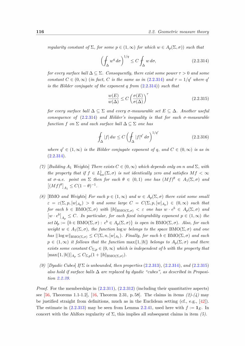
116 2.2. Geometric measure theory
regularity constant of Σ, for some p ∈ (1,∞) for which w ∈ Ap(Σ, σ)) such that(
∆wq dσ
)1/q≤ C
∆w dσ, (2.2.314)
for every surface ball ∆ ⊆ Σ. Consequently, there exist some power τ > 0 and someconstant C ∈ (0,∞) (in fact, C is the same as in (2.2.314) and τ = 1/q′ where q′
is the Hölder conjugate of the exponent q from (2.2.314)) such that
w(E)w(∆) ≤ C
(σ(E)σ(∆)
)τ(2.2.315)
for every surface ball ∆ ⊆ Σ and every σ-measurable set E ⊆ ∆. Another usefulconsequence of (2.2.314) and Hölder’s inequality is that for each σ-measurablefunction f on Σ and each surface ball ∆ ⊆ Σ one has
∆|f | dw ≤ C
( ∆|f |q′ dσ
)1/q′
(2.2.316)
where q′ ∈ (1,∞) is the Hölder conjugate exponent of q, and C ∈ (0,∞) is as in(2.2.314).
(7) [Building A1 Weights] There exists C ∈ (0,∞) which depends only on n and Σ, withthe property that if f ∈ L1
loc(Σ, σ) is not identically zero and satisfies Mf < ∞at σ-a.e. point on Σ then for each θ ∈ (0, 1) one has (Mf)θ ∈ A1(Σ, σ) and[(Mf)θ
]A1≤ C(1− θ)−1.
(8) [BMO and Weights] For each p ∈ (1,∞) and w ∈ Ap(Σ, σ) there exist some smallε = ε(Σ, p, [w]Ap) > 0 and some large C = C(Σ, p, [w]Ap) ∈ (0,∞) such thatfor each b ∈ BMO(Σ, σ) with ‖b‖BMO(Σ,σ) < ε one has w · eb ∈ Ap(Σ, σ) and[w · eb
]Ap≤ C. In particular, for each fixed integrability exponent p ∈ (1,∞) the
set Up :=b ∈ BMO(Σ, σ) : eb ∈ Ap(Σ, σ)
is open in BMO(Σ, σ). Also, for each
weight w ∈ A1(Σ, σ), the function logw belongs to the space BMO(Σ, σ) and onehas ‖ logw‖BMO(Σ,σ) ≤ C(Σ, n, [w]A1). Finally, for each b ∈ BMO(Σ, σ) and eachp ∈ (1,∞) it follows that the function max1, |b| belongs to Ap(Σ, σ) and thereexists some constant CΣ,p ∈ (0,∞) which is independent of b with the property that[max1, |b|]Ap ≤ CΣ,p(1 + ‖b‖BMO(Σ,σ)).
(9) [Dyadic Cubes] If Σ is unbounded, then properties (2.2.313), (2.2.314), and (2.2.315)also hold if surface balls ∆ are replaced by dyadic “cubes”, as described in Proposi-tion 2.2.39.
Proof. For the memberships in (2.2.311), (2.2.312) (including their quantitative aspects)see [56, Theorems 1.1-1.2], [16, Theorem 2.31, p. 58]. The claims in items (2)-(4) maybe justified straight from definitions, much as in the Euclidean setting (cf., e.g., [42]).The estimate in (2.2.313) may be seen from Lemma 2.2.41, used here with f := 1E . Inconcert with the Ahlfors regularity of Σ, this implies all subsequent claims in item (5).
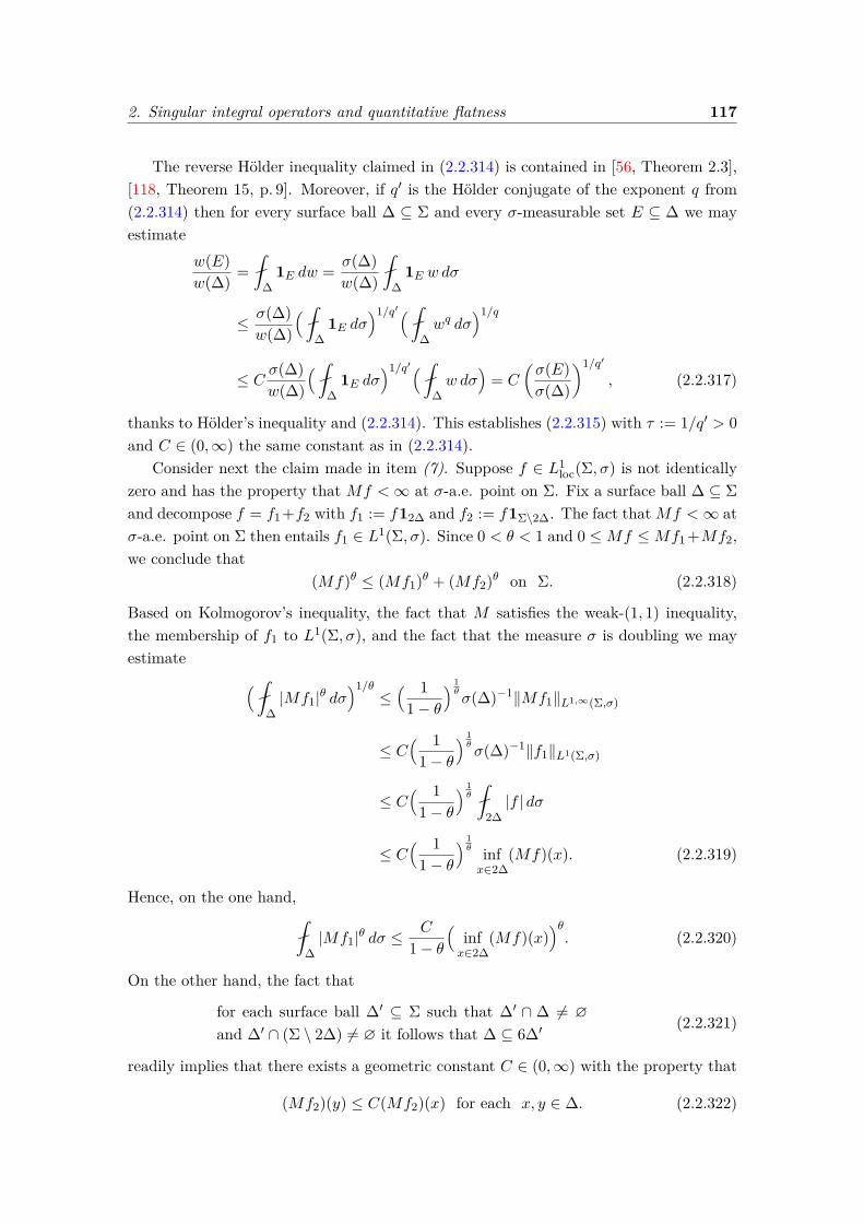
2. Singular integral operators and quantitative flatness 117
The reverse Hölder inequality claimed in (2.2.314) is contained in [56, Theorem 2.3],[118, Theorem 15, p. 9]. Moreover, if q′ is the Hölder conjugate of the exponent q from(2.2.314) then for every surface ball ∆ ⊆ Σ and every σ-measurable set E ⊆ ∆ we mayestimate
w(E)w(∆) =
∆
1E dw = σ(∆)w(∆)
∆
1E w dσ
≤ σ(∆)w(∆)
( ∆
1E dσ)1/q′(
∆wq dσ
)1/q
≤ C σ(∆)w(∆)
( ∆
1E dσ)1/q′(
∆w dσ
)= C
(σ(E)σ(∆)
)1/q′
, (2.2.317)
thanks to Hölder’s inequality and (2.2.314). This establishes (2.2.315) with τ := 1/q′ > 0and C ∈ (0,∞) the same constant as in (2.2.314).
Consider next the claim made in item (7). Suppose f ∈ L1loc(Σ, σ) is not identically
zero and has the property that Mf <∞ at σ-a.e. point on Σ. Fix a surface ball ∆ ⊆ Σand decompose f = f1+f2 with f1 := f12∆ and f2 := f1Σ\2∆. The fact thatMf <∞ atσ-a.e. point on Σ then entails f1 ∈ L1(Σ, σ). Since 0 < θ < 1 and 0 ≤Mf ≤Mf1 +Mf2,we conclude that
(Mf)θ ≤ (Mf1)θ + (Mf2)θ on Σ. (2.2.318)
Based on Kolmogorov’s inequality, the fact that M satisfies the weak-(1, 1) inequality,the membership of f1 to L1(Σ, σ), and the fact that the measure σ is doubling we mayestimate (
∆|Mf1|θ dσ
)1/θ≤( 1
1− θ) 1θσ(∆)−1‖Mf1‖L1,∞(Σ,σ)
≤ C( 1
1− θ) 1θσ(∆)−1‖f1‖L1(Σ,σ)
≤ C( 1
1− θ) 1θ
2∆|f | dσ
≤ C( 1
1− θ) 1θ infx∈2∆
(Mf)(x). (2.2.319)
Hence, on the one hand,
∆|Mf1|θ dσ ≤
C
1− θ(
infx∈2∆
(Mf)(x))θ. (2.2.320)
On the other hand, the fact that
for each surface ball ∆′ ⊆ Σ such that ∆′ ∩ ∆ 6= ∅and ∆′ ∩ (Σ \ 2∆) 6= ∅ it follows that ∆ ⊆ 6∆′
(2.2.321)
readily implies that there exists a geometric constant C ∈ (0,∞) with the property that
(Mf2)(y) ≤ C(Mf2)(x) for each x, y ∈ ∆. (2.2.322)
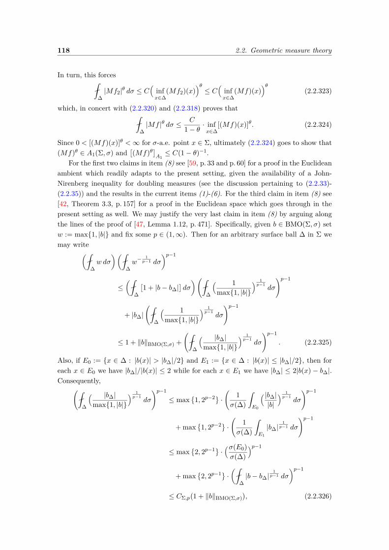
118 2.2. Geometric measure theory
In turn, this forces ∆|Mf2|θ dσ ≤ C
(infx∈∆
(Mf2)(x))θ≤ C
(infx∈∆
(Mf)(x))θ
(2.2.323)
which, in concert with (2.2.320) and (2.2.318) proves that ∆|Mf |θ dσ ≤ C
1− θ · infx∈∆
[(Mf)(x)]θ. (2.2.324)
Since 0 < [(Mf)(x)]θ <∞ for σ-a.e. point x ∈ Σ, ultimately (2.2.324) goes to show that(Mf)θ ∈ A1(Σ, σ) and
[(Mf)θ
]A1≤ C(1− θ)−1.
For the first two claims in item (8) see [59, p. 33 and p. 60] for a proof in the Euclideanambient which readily adapts to the present setting, given the availability of a John-Nirenberg inequality for doubling measures (see the discussion pertaining to (2.2.33)-(2.2.35)) and the results in the current items (1)-(6). For the third claim in item (8) see[42, Theorem 3.3, p. 157] for a proof in the Euclidean space which goes through in thepresent setting as well. We may justify the very last claim in item (8) by arguing alongthe lines of the proof of [47, Lemma 1.12, p. 471]. Specifically, given b ∈ BMO(Σ, σ) setw := max1, |b| and fix some p ∈ (1,∞). Then for an arbitrary surface ball ∆ in Σ wemay write(
∆w dσ
)( ∆w− 1p−1 dσ
)p−1
≤(
∆
[1 + |b− b∆|
]dσ
)( ∆
( 1max1, |b|
) 1p−1
dσ
)p−1
+ |b∆|(
∆
( 1max1, |b|
) 1p−1
dσ
)p−1
≤ 1 + ‖b‖BMO(Σ,σ) +(
∆
( |b∆|max1, |b|
) 1p−1
dσ
)p−1
. (2.2.325)
Also, if E0 := x ∈ ∆ : |b(x)| > |b∆|/2 and E1 := x ∈ ∆ : |b(x)| ≤ |b∆|/2, then foreach x ∈ E0 we have |b∆|/|b(x)| ≤ 2 while for each x ∈ E1 we have |b∆| ≤ 2|b(x) − b∆|.Consequently,(
∆
( |b∆|max1, |b|
) 1p−1
dσ
)p−1
≤ max1, 2p−2 · ( 1
σ(∆)
ˆE0
( |b∆||b|
) 1p−1
dσ
)p−1
+ max1, 2p−2 · ( 1
σ(∆)
ˆE1
|b∆|1p−1 dσ
)p−1
≤ max2, 2p−1 · (σ(E0)
σ(∆))p−1
+ max2, 2p−1 · (
∆|b− b∆|
1p−1 dσ
)p−1
≤ CΣ,p(1 + ‖b‖BMO(Σ,σ)
), (2.2.326)
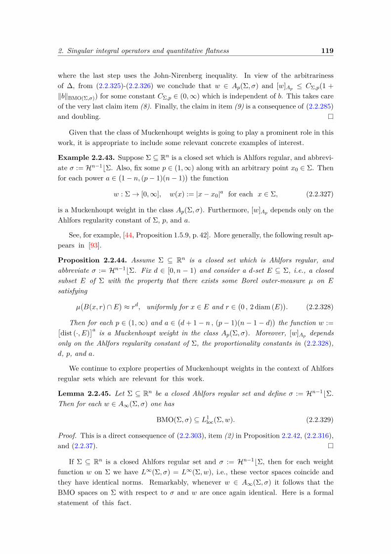
2. Singular integral operators and quantitative flatness 119
where the last step uses the John-Nirenberg inequality. In view of the arbitrarinessof ∆, from (2.2.325)-(2.2.326) we conclude that w ∈ Ap(Σ, σ) and [w]Ap ≤ CΣ,p(1 +‖b‖BMO(Σ,σ)) for some constant CΣ,p ∈ (0,∞) which is independent of b. This takes careof the very last claim item (8). Finally, the claim in item (9) is a consequence of (2.2.285)and doubling.
Given that the class of Muckenhoupt weights is going to play a prominent role in thiswork, it is appropriate to include some relevant concrete examples of interest.
Example 2.2.43. Suppose Σ ⊆ Rn is a closed set which is Ahlfors regular, and abbrevi-ate σ := Hn−1bΣ. Also, fix some p ∈ (1,∞) along with an arbitrary point x0 ∈ Σ. Thenfor each power a ∈
(1− n, (p− 1)(n− 1)
)the function
w : Σ→ [0,∞], w(x) := |x− x0|a for each x ∈ Σ, (2.2.327)
is a Muckenhoupt weight in the class Ap(Σ, σ). Furthermore, [w]Ap depends only on theAhlfors regularity constant of Σ, p, and a.
See, for example, [44, Proposition 1.5.9, p. 42]. More generally, the following result ap-pears in [93].
Proposition 2.2.44. Assume Σ ⊆ Rn is a closed set which is Ahlfors regular, andabbreviate σ := Hn−1bΣ. Fix d ∈ [0, n − 1) and consider a d-set E ⊆ Σ, i.e., a closedsubset E of Σ with the property that there exists some Borel outer-measure µ on E
satisfying
µ(B(x, r) ∩ E
)≈ rd, uniformly for x ∈ E and r ∈
(0 , 2 diam (E)
). (2.2.328)
Then for each p ∈ (1,∞) and a ∈(d + 1 − n , (p − 1)(n − 1 − d)
)the function w :=[
dist (·, E)]a is a Muckenhoupt weight in the class Ap(Σ, σ). Moreover, [w]Ap depends
only on the Ahlfors regularity constant of Σ, the proportionality constants in (2.2.328),d, p, and a.
We continue to explore properties of Muckenhoupt weights in the context of Ahlforsregular sets which are relevant for this work.
Lemma 2.2.45. Let Σ ⊆ Rn be a closed Ahlfors regular set and define σ := Hn−1bΣ.Then for each w ∈ A∞(Σ, σ) one has
BMO(Σ, σ) ⊆ L1loc(Σ, w). (2.2.329)
Proof. This is a direct consequence of (2.2.303), item (2) in Proposition 2.2.42, (2.2.316),and (2.2.37).
If Σ ⊆ Rn is a closed Ahlfors regular set and σ := Hn−1bΣ, then for each weightfunction w on Σ we have L∞(Σ, σ) = L∞(Σ, w), i.e., these vector spaces coincide andthey have identical norms. Remarkably, whenever w ∈ A∞(Σ, σ) it follows that theBMO spaces on Σ with respect to σ and w are once again identical. Here is a formalstatement of this fact.
120 2.2. Geometric measure theory
Lemma 2.2.46. Suppose Σ ⊆ Rn is a closed set which is Ahlfors regular, and abbreviateσ := Hn−1bΣ. Also, fix some weight w ∈ A∞(Σ, σ) (hence, there exists some p ∈ (1,∞)for which w ∈ Ap(Σ, σ)). Then there exists a constant C ∈ [1,∞) which depends only onp, [w]Ap, n, and the Ahlfors regularity constant of Σ such that
C−1 ‖f‖BMO(Σ,σ) ≤ ‖f‖BMO(Σ,w) ≤ C ‖f‖BMO(Σ,σ) (2.2.330)
for each function f ∈ L1loc(Σ, σ) ∩ L1
loc(Σ, w).Moreover, for each σ-measurable function f on Σ one has the equivalence
f ∈ BMO(Σ, σ)⇐⇒ f ∈ BMO(Σ, w) (2.2.331)
and if either of these memberships materializes then ‖f‖BMO(Σ,σ) ≈ ‖f‖BMO(Σ,w) wherethe implicit proportionality constants depend only on p, [w]Ap, n, and the Ahlfors regu-larity constant of Σ. Succinctly put,
the spaces BMO(Σ, σ) and BMO(Σ, w) coincide as sets
and have equivalent semi-norms.(2.2.332)
Proof. Pick a function f ∈ L1loc(Σ, σ) ∩ L1
loc(Σ, w). To prove the first inequality in(2.2.330), start by writing (2.2.304) with f replaced by f −
ffl∆ f dw for some arbitrary
surface ball ∆ ⊆ Σ, then invoke (2.2.43) to obtain
‖f‖BMO(Σ,σ) ≤ 2 sup∆⊆Σ
infc∈R
( ∆
∣∣f − c∣∣ dσ) ≤ 2 sup∆⊆Σ
∆
∣∣∣f − ∆f dw
∣∣∣ dσ≤ 2[w]1/pAp
· sup∆⊆Σ
( ∆
∣∣∣f − ∆f dw
∣∣∣p dw)1/p
≤ C ‖f‖BMO(Σ,w) , (2.2.333)
for some constant C ∈ (0,∞) as in the statement. To prove the second inequality in(2.2.330), observe first that w belongs to some Reverse Hölder class, say w ∈ RHq(Σ, σ)for some q ∈ (1,∞). if q′ ∈ (1,∞) denoting the Hölder conjugate exponent of q, then(2.2.316) allows to estimate
infc∈R
( ∆
∣∣f − c∣∣ dw) ≤ ∆
∣∣∣f − ∆f dσ
∣∣∣ dw≤ C
( ∆
∣∣∣f − ∆f dσ
∣∣∣q′ dσ)1/q′
, (2.2.334)
for some constant C ∈ (0,∞) of the same nature as before. Taking the supremum overall surface balls ∆ ⊆ Σ and then using John-Nirenberg’s inequality, we ultimately obtain‖f‖BMO(Σ,w) ≤ C ‖f‖BMO(Σ,σ), as desired.
As regards the equivalence in (2.2.331), assume first that f ∈ BMO(Σ, σ). Then(2.2.329) implies that f ∈ L1
loc(Σ, σ)∩L1loc(Σ, w), so (2.2.330) holds. Conversely, assume
the function f belongs to BMO(Σ, w). In particular, f ∈ L1loc(Σ, w) and the John-
Nirenberg inequality (for the doubling measure w) guarantees that we also have f ∈Lploc(Σ, w). In concert with (2.2.304) the latter membership implies that f ∈ L1
loc(Σ, σ),hence once again (2.2.330) applies.
2. Singular integral operators and quantitative flatness 121
The doubling and self-improving properties of Muckenhoupt weights yield the fol-lowing result (see [93] for a proof).
Lemma 2.2.47. Suppose Σ ⊆ Rn, where n ∈ N with n ≥ 2, is a closed set which isAhlfors regular, and abbreviate σ := Hn−1bΣ. In this setting, fix some p ∈ (1,∞) alongwith a Muckenhoupt weight w ∈ Ap(Σ, σ). Then
ˆΣ
w(x)(1 + |x|n−1)p dσ(x) < +∞. (2.2.335)
Also, there exists an exponent po ∈ (1, p] with the property that
Lp(Σ, w) → Lq(Σ ,
σ(x)1 + |x|n−1
)continuously, for each fixed q ∈ (0, po).
(2.2.336)
As a consequence,
Lp(Σ, w) → L1(Σ ,
σ(x)1 + |x|n−1
)continuously, (2.2.337)
andLp(Σ, w) ⊆
⋃1<q<p
Lqloc(Σ, σ). (2.2.338)
2.2.6 Sobolev spaces on Ahlfors regular sets
Consider an Ahlfors regular domain Ω ⊆ Rn. Denote by ν = (ν1, . . . , νn) the geomet-ric measure theoretic outward unit normal to Ω, and abbreviate σ := Hn−1b∂Ω. Inparticular, (2.2.291) implies that
σ is a complete, locally finite (hence also sigma-finite), sep-arable, Borel-regular measure on ∂Ω, where the latter set isendowed with the topology canonically inherited from Rn.
(2.2.339)
Among other things, this implies (cf. [93]) that for every f ∈ L1loc(∂Ω, σ) we have
f = 0 at σ-a.e. point on ∂Ω ⇐⇒ˆ∂Ωfφ dσ = 0 for every φ ∈ C∞0 (Rn). (2.2.340)
In this context, define the family of first-order tangential derivative operators, ∂τjk withj, k ∈ 1, . . . , n, acting on functions ϕ ∈ C∞0 (Rn) according to
∂τjkϕ := νj(∂kϕ)∣∣∂Ω − νk(∂jϕ)
∣∣∂Ω for all j, k ∈ 1, . . . , n. (2.2.341)
The starting point in the development of a brand of first-order Sobolev spaces on ∂Ωis the observation that for any two functions ϕ,ψ ∈ C∞0 (Rn) and every pair of indicesj, k ∈ 1, . . . , n one has the boundary integration by parts formula
ˆ∂Ω
(∂τjkϕ)ψ dσ = −ˆ∂Ωϕ(∂τjkψ) dσ. (2.2.342)
122 2.2. Geometric measure theory
Indeed, identity (2.2.342) is a consequence of the Divergence Formula (1.1.12) applied toa suitable vector field, namely ~F := ∂k(ϕψ)ej−∂j(ϕψ)ek (where ei1≤i≤n is the standardorthonormal basis in Rn), which is smooth, compactly supported, divergence-free, andsatisfies ν · ~F = (∂τjkϕ)ψ + ϕ(∂τjkψ) at σ-a.e. point on ∂Ω.
Next, given a function f ∈ L1loc(∂Ω, σ) along with two indices j, k ∈ 1, . . . , n, we
shall say that ∂τjkf exists in (or, belongs to) the space L1loc(∂Ω, σ) if there exists a
function fjk ∈ L1loc(∂Ω, σ) such that
ˆ∂Ω
(∂τjkϕ)f dσ = −ˆ∂Ωϕfjk dσ for all ϕ ∈ C∞0 (Rn). (2.2.343)
In view of (2.2.340), we conclude that the function fjk is unambiguously defined by thedemand in (2.2.343). Henceforth we shall favor the notation
∂τjkf := fjk (2.2.344)
which, in particular, allows us to recast (2.2.343) more in line with (2.2.342), namely asˆ∂Ωf(∂τjkϕ) dσ = −
ˆ∂Ω
(∂τjkf)ϕdσ for all ϕ ∈ C∞0 (Rn). (2.2.345)
In analogy with the classical flat, Euclidean case, it is natural to regard ∂τjkf as a weak(tangential) derivative of the function f . The developments so far allow us to definea convenient functional analytic environment within which is possible to consider suchweak (tangential) derivatives of functions in L1
loc(∂Ω, σ). Specifically, for each p ∈ [1,∞]we introduce the local Sobolev space Lp1,loc(∂Ω, σ) as
Lp1,loc(∂Ω, σ) :=f ∈ Lploc(∂Ω, σ) : ∂τjkf ∈ L
ploc(∂Ω, σ), 1 ≤ j, k ≤ n
. (2.2.346)
In such a context, we define the tangential gradient operator as
Lp1,loc(∂Ω, σ) 3 f 7→ ∇tanf :=(
n∑k=1
νk∂τkjf
)1≤j≤n
. (2.2.347)
If Ω is actually a UR domain, we may recover the weak tangential derivatives from thecomponents of the tangential gradient operator via (cf. [93], [53, Lemma 3.40])
∂τjkf = νj(∇tanf)k − νk(∇tanf)j , 1 ≤ j, k ≤ n,
for every f ∈ Lp1,loc(∂Ω, σ) with p ∈ (1,∞).(2.2.348)
Going further, having fixed an integrability exponent p ∈ (1,∞) along with a Muck-enhoupt weight w ∈ Ap(∂Ω, σ), define the (boundary) weighted Sobolev space
Lp1(∂Ω, w) :=f ∈ Lp(∂Ω, w) : ∂τjkf ∈ L
p(∂Ω, w), 1 ≤ j, k ≤ n
(2.2.349)
which is a Banach space when equipped with the norm
Lp1(∂Ω, w) 3 f 7→ ‖f‖Lp1(∂Ω,w) := ‖f‖Lp(∂Ω,w) +n∑
j,k=1
∥∥∥∂τjkf∥∥∥Lp(∂Ω,w). (2.2.350)
2. Singular integral operators and quantitative flatness 123
Since there exists q ∈ (1,∞) such that Lp(∂Ω, w) → Lqloc(∂Ω, σ) (cf. Lemma 2.2.47), wesee that Lp1(∂Ω, w) → Lq1,loc(∂Ω, σ) for such an exponent q. In particular, the equalityin (2.2.348) holds for every function f ∈ Lp1(∂Ω, w).
In the same geometric setting, recall that Lp,q(∂Ω, σ) with p, q ∈ (0,∞] stands for thescale of Lorentz spaces on ∂Ω, with respect to the measure σ. These are quasi-Banachspaces which arise naturally as intermediate spaces for the real interpolation methodused within the scale of ordinary Lebesgue spaces. In particular, this implies that
Lp,q(∂Ω, σ) → L1(∂Ω, σ(x)1+|x|n−1
)∩(⋂
1<s<p Lsloc(∂Ω, σ)
)whenever p ∈ (1,∞) and q ∈ (0,∞].
(2.2.351)
In relation to this scale of spaces, it is also of interest to consider (boundary) Lorentz-based Sobolev spaces. Specifically, following [93], for each p ∈ (1,∞) and q ∈ (0,∞] we set
Lp,q1 (∂Ω, w) :=f ∈ Lp,q(∂Ω, σ) : ∂τjkf ∈ L
p,q(∂Ω, σ), 1 ≤ j, k ≤ n
(2.2.352)
which is a quasi-Banach space when equipped with the quasi-norm
Lp,q1 (∂Ω, σ) 3 f 7→ ‖f‖Lp,q1 (∂Ω,σ) := ‖f‖Lp,q(∂Ω,σ) +n∑
j,k=1
∥∥∥∂τjkf∥∥∥Lp,q(∂Ω,σ). (2.2.353)
In the proposition below, which refines [53, Lemma 3.36, p. 2678], we study themanner in which weak tangential derivatives interact with pointwise nontangential traces.See [93] for a proof.
Proposition 2.2.48. Let Ω ⊆ Rn be an Ahlfors regular domain. Set σ := Hn−1b∂Ω anddenote by ν = (ν1, . . . , νn) the geometric measure theoretic outward unit normal to Ω.Also, fix an integrability exponent p ∈ [1,∞] and an aperture parameter κ ∈ (0,∞). Inthis context, assume the function u ∈W 1,1
loc (Ω) satisfies
Nκu ∈ Lploc(∂Ω, σ), Nκ(∇u) ∈ Lploc(∂Ω, σ), (2.2.354)
and the nontangential traces
u∣∣κ−n.t.
∂Ω and (∂ju)∣∣κ−n.t.
∂Ω for j ∈ 1, . . . , n
exist at σ-a.e. point on ∂Ω.(2.2.355)
Then u∣∣κ−n.t.
∂Ω belongs to Lp1,loc(∂Ω, σ), the functions (∂1u)∣∣κ−n.t.
∂Ω , . . . , (∂nu)∣∣κ−n.t.
∂Ω belongto Lploc(∂Ω, σ) and, for each j, k ∈ 1, . . . , n and for σ-a.e. point on ∂Ω, one has
∂τjk
(u∣∣κ−n.t.
∂Ω
)= νj
((∂ku)
∣∣κ−n.t.
∂Ω
)− νk
((∂ju)
∣∣κ−n.t.
∂Ω
). (2.2.356)
In particular, for each j, k ∈ 1, . . . , n one has∣∣∣∂τjk(u∣∣κ−n.t.
∂Ω
)∣∣∣ ≤ 2Nκ(∇u) at σ-a.e. point on ∂Ω. (2.2.357)
The following result from [93] may be regarded as a weighted counterpart of Proposi-tion 2.2.48.
124 2.3. Calderón-Zygmund theory for boundary layers in UR domains
Proposition 2.2.49. Let Ω ⊆ Rn be an Ahlfors regular domain and abbreviate σ :=Hn−1b∂Ω. Fix an aperture parameter κ ∈ (0,∞) and an integrability exponent p ∈ (1,∞).Also, assume w : ∂Ω→ [0,+∞] is a σ-measurable function satisfying 0 < w(x) < +∞ forσ-a.e. x ∈ ∂Ω and w−1/p ∈ Lp
′
loc(∂Ω, σ), where p ′ ∈ (1,∞) denotes the Hölder conjugateexponent of p; in particular, Lp(∂Ω, wσ) → L1
loc(∂Ω, σ). In this setting, suppose thatsome complex-valued function u ∈ W 1,1
loc (Ω) has been given which satisfies the followingconditions:
u∣∣κ−n.t.
∂Ω exists at σ-a.e. point on ∂Ω and
Nκu ∈ L1loc(∂Ω, σ), Nκ(∇u) ∈ Lp(∂Ω, wσ).
(2.2.358)
Then the nontangential trace u∣∣κ−n.t.
∂Ω belongs to L11,loc(∂Ω, σ) and satisfies
∂τjk
(u∣∣κ−n.t.
∂Ω
)∈ Lp(∂Ω, wσ) for each j, k ∈ 1, . . . , n
andn∑
j,k=1
∥∥∥∂τjk(u∣∣κ−n.t.
∂Ω
)∥∥∥Lp(∂Ω,wσ)
≤ C∥∥Nκ(∇u)
∥∥Lp(∂Ω,wσ)
(2.2.359)
for some constant C ∈ (0,∞) independent of u.
2.3 Calderón-Zygmund theory for boundary layers in URdomains
In [18], A.P. Calderón has initiated a breakthrough by proving the Lp-boundedness ofthe principal-value Cauchy integral operator on Lipschitz curves with small Lipschitzconstant. Subsequently, R. Coifman, A. McIntosh, and Y. Meyer have successfullyextended Calderón’s estimate on Cauchy integrals to general Lipschitz curves in [24], andused this to establish the boundedness of higher-dimensional singular integral operators(such as the harmonic double layerK∆) on Lebesgue spaces Lp(Σ,Hn−1) with p ∈ (1,∞),whenever Σ is a strongly Lipschitz surface in Rn. This gave the impetus for studyingsuch singular integral operators on surfaces more general than the boundaries of Lipschitzdomains. Works of G. David [30], [31], G. David and D. Jerison [32], G. David andS. Semmes [33], [34], and of S. Semmes [106] yield such boundedness when the Σ ⊆ Rn
is a UR set, i.e., Σ is a closed Ahlfors regular set which contains “big pieces” of Lipschitzimages in a quantitative, uniform, scale-invariant fashion (cf. Definition 1.1.4).
This body of results, which interfaced tightly with geometric measure theory, hasbeen applied to problems in PDE’s for the first time by S. Hofmann, M. Mitrea, andM. Taylor in [53] (see also [95] for PDE’s in the setting of Riemannian manifolds). Herewe continue this line of work with two specific goals in mind. First, we consider singularintegral operators (SIO’s) acting on a larger variety of function spaces and, second, weseek finer bounds on the operator norm of the singular integrals of double layer type.We begin by discussing the general setup.
2.3.1 Boundary layer potentials: the setup

2. Singular integral operators and quantitative flatness 125
First, assume Ω ⊆ Rn is a given UR domain. Abbreviate σ := Hn−1b∂Ω and denoteby ν = (ν1, . . . , νn) the geometric measure theoretic outward unit normal to Ω. Inaddition, consider a homogeneous, second-order, constant complex coefficient, weaklyelliptic M ×M system L in Rn and recall the matrix-valued fundamental solution E =(Eαβ)1≤α,β≤M associated with L as in Theorem 1.2.1. Finally, fix a coefficient tensorA =
(aαβjk
)1≤α,β≤M1≤j,k≤n
∈ AL, and pick an arbitrary function
f = (fα)1≤α≤M ∈[L1(∂Ω , σ(x)
1+|x|n−1)]M
. (2.3.1)
In this setting, define the action of the boundary-to-domain double layer potential opera-tor DA on f as
DAf(x) :=(−ˆ∂Ωνk(y)aβαjk (∂jEγβ) (x− y)fα(y) dσ(y)
)1≤γ≤M
, (2.3.2)
at each point x ∈ Ω. From (1.2.19) we see that (2.3.1) is the most general functionalanalytic setting in which the integral in (2.3.2) is absolutely convergent. The double layeroperator D may be regarded as a mechanism for generating lots of null-solutions for thegiven system L in Ω since, as is apparent from (2.3.2) and Theorem 1.2.1,
for each function f as in (2.3.1) we have
DAf ∈[C ∞(Ω)
]M and L(DAf) = 0 in Ω.(2.3.3)
Going further, let us define the action of the boundary-to-boundary double layer potentialoperator KA on f as in (2.3.1) by setting
KAf(x) :=(− limε→0+
ˆ
y∈∂Ω|x−y|>ε
νk(y)aβαjk (∂jEγβ) (x− y)fα(y) dσ(y))
1≤γ≤M, (2.3.4)
at σ-a.e. point x ∈ ∂Ω. Another singular integral operator which is closely related to(2.3.4) is the so-called “transposed” double layer operator K#
A defined by setting
K#A f(x) :=
(limε→0+
ˆ
y∈∂Ω|x−y|>ε
νk(x)aβ αjk (∂jEγ β)(x− y)fγ(y) dσ(y))
1≤α≤M
(2.3.5)
at σ-a.e. x ∈ ∂Ω, for each function f as in (2.3.1). Since we are presently assuming thatΩ is a UR domain, work in [93] guarantees that the above singular integral operators arewell-defined in a σ-a.e. pointwise fashion for each function as in (2.3.1).
Example 2.3.1. The standard fundamental solution for the Laplacian in Rn is definedfor x ∈ Rn \ 0 by
E(x) :=
1
ωn−1(2− n)1
|x|n−2 , if n ≥ 3,
12π ln |x|, if n = 2,
(2.3.6)
126 2.3. Calderón-Zygmund theory for boundary layers in UR domains
where, as usual, ωn−1 denotes the surface area of the unit sphere in Rn (cf. [92,Section 7.1]). Given an Ahlfors regular domain Ω ⊆ Rn, abbreviate σ := Hn−1b∂Ωand denote by ν the geometric measure theoretic outward unit normal to Ω. Set aαβjk :=ajk := δjk in (1.2.1) so that L = ∆, and refer to D∆, K∆ (constructed as in (2.3.2),(2.3.4)) for this choice of coefficient tensor, i.e., for A := In×n, the identity matrix)as being the (classical) harmonic double layer potentials. Concretely, for each func-tion f ∈ L1(∂Ω , σ(x)
1+|x|n−1)we have (writing, in this case, D∆,K∆,K
#∆ in place of
DIn×n ,KIn×n ,K#In×n
)
D∆f(x) = 1ωn−1
ˆ∂Ω
〈ν(y), y − x〉|x− y|n
f(y) dσ(y), ∀x ∈ Ω, (2.3.7)
and, at σ-a.e. point x ∈ ∂Ω,
K∆f(x) = limε→0+
1ωn−1
ˆ
y∈∂Ω|x−y|>ε
〈ν(y), y − x〉|x− y|n
f(y) dσ(y), (2.3.8)
K#∆f(x) = lim
ε→0+
1ωn−1
ˆ
y∈∂Ω|x−y|>ε
〈ν(x), x− y〉|x− y|n
f(y) dσ(y). (2.3.9)
Returning to the mainstream discussion, continue to assume that Ω ⊆ Rn is aUR domain and set σ := Hn−1b∂Ω. Also, as before, continue to assume that L is ahomogeneous constant complex coefficient weakly elliptic second-order M ×M systemin Rn. Then, for each coefficient tensor A ∈ AL, a basic identity relating the boundary-to-domain double layer potential operator DA to the boundary-to-boundary double layerpotential operator KA is the jump-formula (proved in [93]), to the effect that for eachaperture parameter κ > 0 and each function f ∈
[L1(∂Ω, σ(x)
1+|x|n−1)]M
we have (withI denoting the identity operator)
DAf∣∣κ−n.t.
∂Ω =(1
2I +KA
)f at σ-a.e. point on ∂Ω. (2.3.10)
Another fundamental property of the boundary-to-domain double layer potentialoperator is the ability of absorbing an arbitrary spacial derivative and eventually re-locate it, via integration by parts on the boundary, all the way to the function onwhich this was applied to begin with. This is made precise in the following basicproposition, proved in [93].
Proposition 2.3.2. Let Ω ⊆ Rn be an Ahlfors regular domain. Define σ := Hn−1b∂Ω,and denote by ν = (ν1, . . . , νn) the geometric measure theoretic outward unit normal toΩ. Also, for some M ∈ N, consider a weakly elliptic, homogeneous, constant (complex)coefficient, second-order, M ×M system L in Rn, written as in (1.2.1) for some choiceof a coefficient tensor A =
(aαβrs
)1≤r,s≤n
1≤α,β≤M. Finally, associate with A and Ω the double
2. Singular integral operators and quantitative flatness 127
layer potential operator DA as in (2.3.2), and consider a function
f = (fα)1≤α≤M ∈[L1(∂Ω ,
σ(x)1 + |x|n−1
)]Mwith the property that
∂τjkfα ∈ L1(∂Ω ,
σ(x)1 + |x|n−1
)for 1 ≤ j, k ≤ n and 1 ≤ α ≤M.
(2.3.11)
Then for each index ` ∈ 1, . . . , n and each point x ∈ Ω one has
∂`(DAf
)(x) =
( ˆ∂Ωaβαrs (∂rEγβ)(x− y)(∂τ`sfα)(y) dσ(y)
)1≤γ≤M
. (2.3.12)
In particular, for each aperture parameter κ > 0, the nontangential boundary trace(∇DAf
)∣∣κ−n.t.
∂Ω exists (in Cn·M ) at σ-a.e. point on ∂Ω. (2.3.13)
Once again, assume that Ω ⊆ Rn is a UR domain and set σ := Hn−1b∂Ω. Also, asbefore, continue to assume that L is a homogeneous constant complex coefficient weaklyelliptic second-order M ×M system in Rn. In general, different choices of the coefficienttensor A ∈ AL yield different double layer potential operators, so it makes sense to usethe subscript A to highlight the dependence on the choice of the coefficient tensor A.One integral operator of layer potential variety which is intrinsically associated with thegiven system L is the so-called single layer potential operator S , whose integral kernelis the matrix-valued function E(x− y), x, y ∈ ∂Ω. In order to make sense of the actionof such an operator on any function as in (2.3.1), it is necessary to alter the said integralkernel and consider the following modified single layer potential operator
Smodf(x) :=ˆ∂Ω
E(x− y)− E∗(−y)
f(y) dσ(y) for each x ∈ Ω,
for each f ∈[L1(∂Ω, σ(x)
1+|x|n−1)]M
, where E∗ := E · 1Rn\B(0,1).
(2.3.14)
In this regard, it is worth noting that for each f ∈[L1(∂Ω, σ(x)
1+|x|n−1)]M
the function
Smodf is well defined, belongs to the space[C ∞(Ω)
]M , and for each multi-index α ∈ Nn0with |α| ≥ 1 one has
∂α(Smodf)(x) =ˆ∂Ω
(∂αE)(x− y)f(y) dσ(y) for each x ∈ Ω. (2.3.15)
In particular,
L(Smodf
)= 0 in Ω for each f ∈
[L1(∂Ω, σ(x)
1+|x|n−1)]M
. (2.3.16)
Analogously to (2.3.14), we define the following modified version of the boundary-to-boundary single layer operator
Smodf(x) :=ˆ∂Ω
E(x− y)− E∗(−y)
f(y) dσ(y) at σ-a.e. x ∈ ∂Ω,
for each f ∈[L1(∂Ω, σ(x)
1+|x|n−1)]M
, where E∗ := E · 1Rn\B(0,1).
(2.3.17)
128 2.3. Calderón-Zygmund theory for boundary layers in UR domains
Then this operator is meaningfully defined, via an absolutely convergent integral, atσ-a.e. point in ∂Ω, and
Smod :[L1(∂Ω, σ(x)
1+|x|n−1)]M−→
[L1
loc(∂Ω, σ)]M (2.3.18)
is a well-defined, linear and continuous mapping. Also, with the modified boundary-to-domain single layer operator Smod as in (2.3.14), for each aperture parameter κ > 0and each f ∈
[L1(∂Ω, σ(x)
1+|x|n−1)]M one has
((Smodf
)∣∣∣κ−n.t.
∂Ω
)(x) = (Smodf)(x) at σ-a.e. point x ∈ ∂Ω. (2.3.19)
See [93] for a more in-depth discussion on this topic.To close this section, we define the conormal derivative operator associated with a
given Ahlfors regular domain and a given coefficient tensor. Specifically, suppose Ω ⊆ Rn
is an Ahlfors regular domain and abbreviate σ := Hn−1b∂Ω. In particular, Ω is a setof locally finite perimeter, and its geometric measure theoretic outward unit normalν = (ν1, . . . , νn) is defined σ-a.e. on ∂Ω. Also, fix a coefficient tensor A =
(aαβrs
)1≤r,s≤n
1≤α,β≤Malong with some aperture parameter κ > 0. In such a setting, define the conormalderivative of a given function u = (uβ)1≤β≤M ∈
[W 1,1
loc(Ω)]M as the CM -valued function
∂Aν u :=(νra
αβrs
(∂suβ
)∣∣κ−n.t.
∂Ω
)1≤α≤M
at σ-a.e. point on ∂Ω. (2.3.20)
It has been proved in [93] that if Ω ⊆ Rn is a UR domain and σ := Hn−1b∂Ω thenfor each function f ∈
[L1(∂Ω, σ(x)
1+|x|n−1)]M
, the conormal derivative ∂Aν Smodf may bemeaningfully considered in the sense of (2.3.20), and
∂Aν Smodf =(− 1
2I +K #A>
)f at σ-a.e. point in ∂Ω, (2.3.21)
where I is the identity, and K #A>
is the operator associated as in (2.3.5) with the URdomain Ω and the transposed coefficient tensor A>.
2.3.2 SIO’s on Muckenhoupt weighted Lebesgue and Sobolev spaces
We begin by considering garden variety Calderón-Zygmund singular integral operators(SIO’s), i.e., operators of convolution-type with odd, homogeneous, sufficiently smoothkernels, which otherwise lack any particular algebraic characteristics. The goal is toobtain estimates in Muckenhoupt weighted Lebesgue spaces on UR sets in Rn.
Proposition 2.3.3. Let Σ ⊆ Rn be a closed UR set and abbreviate σ := Hn−1bΣ.Assume N = N(n) ∈ N is a sufficiently large integer and consider a complex-valuedfunction k ∈ CN
(Rn \ 0
)which is odd and positive homogeneous of degree 1−n. Also,
fix an integrability exponent p ∈ (1,∞), along with a Muckenhoupt weight w ∈ Ap(Σ, σ).In this setting, for each f ∈ L1(Σ, σ(x)
1+|x|n−1)define
Tεf(x) :=ˆ
y∈Σ|x−y|>ε
k(x− y)f(y) dσ(y) for each x ∈ Σ, (2.3.22)
2. Singular integral operators and quantitative flatness 129
T∗f(x) := supε>0|Tεf(x)| for each x ∈ Σ, (2.3.23)
Tf(x) := limε→0+
Tεf(x) for σ-a.e. x ∈ Σ. (2.3.24)
Then there exists a constant C ∈ (0,∞) which depends exclusively on n, p, [w]Ap,and the UR constants of Σ with the property that for each f ∈ Lp(Σ, w) one has
‖T∗f‖Lp(Σ,w) ≤ C( ∑|α|≤N
supSn−1
|∂αk|)‖f‖Lp(Σ,w) , (2.3.25)
In particular,
the truncated integral operators Tε : Lp(Σ, w)→ Lp(Σ, w) arewell defined, linear, and bounded in a uniform fashion withrespect to the truncation parameter ε > 0.
(2.3.26)
Moreover, for each function f ∈ L1(Σ, σ(x)1+|x|n−1
)the limit defining Tf(x) in (2.3.24) exists
at σ-a.e. x ∈ Σ and the operator
T : Lp(Σ, w) −→ Lp(Σ, w) (2.3.27)
is well defined, linear, and bounded. Let p′ ∈ (1,∞) denote the Hölder conjugate exponentof p and, with w′ := w1−p′ ∈ Ap′(Σ, σ), consider the natural identification(
Lp(Σ, w))∗ = Lp
′(Σ, w′). (2.3.28)
Then, under the canonical integral pairing (f, g) 7→´
Σ fg dσ, it follows that
the (real) transposed of the operator (2.3.27) isthe operator −T : Lp′(Σ, w′)→ Lp
′(Σ, w′).(2.3.29)
Finally, assume Ω ⊆ Rn be an open set such that ∂Ω is a UR set and abbreviateσ := Hn−1b∂Ω. Fix some p ∈ (1,∞) along with a Muckenhoupt weight w ∈ Ap(∂Ω, σ),and pick an aperture parameter κ > 0. With the integral kernel k as before, for eachf ∈ Lp(∂Ω, w) define
T f(x) :=ˆ∂Ωk(x− y)f(y)dσ(y) for each x ∈ Ω. (2.3.30)
Then there exists a constant C ∈ (0,∞) which depends exclusively on n, p, [w]Ap, andthe UR constants of ∂Ω with the property that for each f ∈ Lp(∂Ω, w) one has
‖Nκ(T f)‖Lp(∂Ω,w) ≤ C( ∑|α|≤N
supSn−1
|∂αk|)‖f‖Lp(∂Ω,w) . (2.3.31)
The above proposition points to uniform rectifiability as being intimately connectedwith the boundedness of a large class of Calderón-Zygmund like operators on Mucken-houpt weighted Lebesgue spaces. From the work of G. David and S. Semmes (cf. [33],[34]) we know that UR sets make up the most general context in which Calderón-Zygmund
130 2.3. Calderón-Zygmund theory for boundary layers in UR domains
like operators are bounded on ordinary Lebesgue spaces. David and Semmes have alsoproved that, under the background assumption of Ahlfors regularity, uniform rectifiabilityis implied by the simultaneous L2 boundedness of all truncated integral convolution typeoperators on Σ (uniformly with respect to the truncation), whose kernels are smooth, odd,and satisfy standard growth conditions, i.e., odd functions k ∈ C∞(Rn \ 0) satisfying
supx∈Rn\0
[|x|(n−1)+|α|∣∣(∂αk)(x)
∣∣] < +∞, ∀α ∈ Nn0 . (2.3.32)
In fact, a remarkable result proved by F. Nazarov, X. Tolsa, and A. Volberg in [101]states that the L2-boundedness of the truncated Riesz transforms on Σ alone (uniformlywith respect to the truncation) yields uniform rectifiability. The corresponding result inthe plane was proved earlier in [89]. In light of (2.3.26), the above discussion highlightsthe optimality of demanding that Σ is a UR set in the context of Proposition 2.3.3.
Results like Proposition 2.3.3 have been recently established in [93]. Here we presentan alternative approach which makes essential use of the Fefferman-Stein sharp maximalfunction, considered in the setting of spaces of homogeneous type (for the Euclideancontext, see [59, p. 52], [42, Theorem 3.6, p. 161]).
Proof of Proposition 2.3.3. To set the stage, recall the Fefferman-Stein sharp maximaloperator M# on Σ, acting on each function f ∈ L1
loc(Σ, σ) according to
M#f(x) := sup∆3x
∆
∣∣∣∣f − ∆f dσ
∣∣∣∣ dσ, ∀x ∈ Σ, (2.3.33)
where the supremum is taken over all surface balls ∆ ⊆ Σ containing the point x ∈ Σ.Clearly, for each f ∈ L1
loc(Σ, σ) and each x ∈ Σ we have
sup∆3x
infa∈C
∆|f − a| dσ ≤M#f(x) ≤ 2 sup
∆3xinfa∈C
∆|f − a| dσ. (2.3.34)
Also, given α ∈ (0, 1), for each f ∈ L1loc(Σ, σ) set
M#α f(x) := M#(|f |α)(x)1/α for all x ∈ Σ. (2.3.35)
Since having 0 < α < 1 ensures that |Xα − Y α| ≤ |X − Y |α for all X,Y ∈ [0,∞), from(2.3.35) and the last inequality in (2.3.34) one may readily check that
M#α f(x) ≤ 21/α sup
∆3xinfa∈C
( ∆|f − a|α dσ
)1/α(2.3.36)
for each f ∈ L1loc(Σ, σ) and each x ∈ Σ. Finally, recall from (2.2.302) the (non-centered)
Hardy-Littlewood maximal operator M on Σ.From (2.3.22)-(2.3.24) it is clear that the maximal operator T∗ and the principal-value
singular integral operator T depend in a homogeneous fashion on the kernel function k.In view of this observation, by working with k/K (in the case when k is not identicallyzero) where K :=
∑|α|≤N supSn−1 |∂αk|, there is no loss of generality in assuming that∑
|α|≤NsupSn−1
|∂αk| = 1. (2.3.37)
2. Singular integral operators and quantitative flatness 131
The fact that for each function f ∈ L1(Σ, σ(x)1+|x|n−1
)the limit defining Tf(x) in (2.3.24)
exists at σ-a.e. x ∈ Σ has been proved in [93]. To proceed, denote by L∞comp(Σ, σ) thesubspace of L∞(Σ, σ) consisting of functions with compact support. Also, fix a powerα ∈ (0, 1). We will first show that there exists a constant C = C(Σ, n, α) ∈ (0,∞) suchthat
M#α (Tf)(x) ≤ C ·Mf(x)
for all f ∈ L∞comp(Σ, σ) and x ∈ Σ.(2.3.38)
To this end, fix a function f ∈ L∞comp(Σ, σ) along with a point x ∈ Σ, and consider anarbitrary surface ball ∆ = ∆(x0, r0), with center at x0 ∈ Σ and radius r0 > 0, containingthe point x. Decompose f = f1 + f2, where f1 := f12∆ and f2 := f1Σ\2∆. Then∣∣Tf2(x0)
∣∣ < +∞ and we abbreviate a := Tf2(x0) ∈ C. Note that
∆|Tf − a|α dσ ≤
∆|Tf1|α dσ +
∆|Tf2 − a|α dσ. (2.3.39)
For the first term in the right-hand side of (2.3.39), using Kolmogorov’s inequality, thefact that T is bounded from L1(Σ, σ) to L1,∞(Σ, σ) (cf. [93], [53, Proposition 3.19]) andthe fact that Σ is an Ahlfors regular set to write
∆|Tf1|α dσ ≤
Cασ(∆)α ‖Tf1‖αL1,∞(Σ,σ) ≤
Cασ(∆)α ‖f1‖αL1(Σ,σ)
≤ Cα(
2∆|f | dσ
)α≤ Cα ·Mf(x)α. (2.3.40)
For the second term in the right-hand side of (2.3.39), note that the properties of k and(2.3.37) entail
|(∇k)(z)| =∣∣∣(∇k)
( z|z||z|)∣∣∣ ≤ |z|−n sup
|ω|=1|(∇k)(ω)| = Cn|z|−n, (2.3.41)
for each z ∈ Rn \0, where Cn ∈ (0,∞) is a purely dimensional constant. On account of(2.3.41) and the Mean Value Theorem, we see that there exists a dimensional constantCn ∈ (0,∞) with the property that for each y ∈ ∆ and z ∈ Σ \ 2∆ we have
|k(y − z)− k(x0 − z)| ≤ Cn|y − x0||x0 − z|n
≤ Cnr0|x0 − z|n
. (2.3.42)
Using this, for every y ∈ ∆ we may write
|Tf2(y)− a| = |Tf2(y)− Tf2(x0)|
≤ˆ
Σ\2∆|k(y − z)− k(x0 − z)||f(z)| dσ(z)
≤ Cr0
∞∑j=1
ˆ2jr0≤|x0−z|<2j+1r0
|f(z)||x0 − z|n
dσ(z)
≤ C∞∑j=1
2−j
2j+1∆|f(z)| dσ(z)
≤ C ·Mf(x), (2.3.43)
132 2.3. Calderón-Zygmund theory for boundary layers in UR domains
where C ∈ (0,∞) depends only on dimension and the Ahlfors regularity constant of Σ.At this stage, the claim in (2.3.38) follows by combining (2.3.36), (2.3.39), (2.3.40), and(2.3.43).
We shall now analyze two cases, depending on whether Σ is bounded or not. Considerfirst the latter case, in which Σ is unbounded. In such a setting, the A∞-weighted versionof the Fefferman-Stein inequality for spaces of homogeneous type (cf., e.g. [7, Sections 3.2and 5]) gives that for every q ∈ (0,∞) there exists a constant Cw ∈ (0,∞), which dependson the weight w ∈ Ap(Σ, σ) ⊆ A∞(Σ, σ) only through its characteristic [w]Ap (indeed, itcan be expressed as an increasing function of [w]Ap), such that
‖Mg‖Lq(Σ,w) ≤ Cw∥∥∥M#g
∥∥∥Lq(Σ,w)
for each
g ∈ L1loc(Σ, σ) such that Mg ∈ Lq(Σ, w).
(2.3.44)
To proceed, fix α ∈ (0, 1) and f ∈ L∞comp(Σ, σ). Let us momentarily work under theadditional assumption that the weight w belongs to L∞(Σ, σ). This permits us toestimate
‖M(|Tf |α)‖Lp/α(Σ,w) ≤ ‖w‖α/pL∞(Σ,σ) ‖M(|Tf |α)‖Lp/α(Σ,σ)
≤ C ‖w‖α/pL∞(Σ,σ) ‖Tf‖αLp(Σ,σ)
≤ C ‖w‖α/pL∞(Σ,σ) ‖f‖αLp(Σ,σ) < +∞, (2.3.45)
where we have used the boundedness of M on Lp/α(Σ, σ) and the boundedness of T onLp(Σ, σ) (cf. [53, Proposition 3.18]). This allows us to use (2.3.44) (with g := |Tf |α andq := p/α) to obtain, for some constant Cw ∈ (0,∞) (again, depending in an increasingfashion on [w]Ap),
‖Tf‖Lp(Σ,w) ≤∥∥∥M(|Tf |α)1/α
∥∥∥Lp(Σ,w)
= ‖M(|Tf |α)‖1/αLp/α(Σ,w)
≤ Cw∥∥∥M#(|Tf |α)
∥∥∥1/α
Lp/α(Σ,w)= Cw
∥∥∥M#α (Tf)
∥∥∥Lp(Σ,w)
≤ Cw ‖Mf‖Lp(Σ,w) ≤ Cw ‖f‖Lp(Σ,w) , (2.3.46)
where the first inequality follows from Lebesgue Differentiation Theorem (cf. [6]), thelast equality is a consequence of (2.3.35), the penultimate inequality comes from (2.3.38),the last inequality is implied by the boundedness of the Hardy-Littlewood operator Mon Lp(Σ, w).
To remove the restriction w ∈ L∞(Σ, σ), we proceed as follows. For each j ∈ N, letwj := minw, j ∈ L∞(Σ, σ). Moreover, as in [46, Ex. 9.1.9], we have
[wj ]Ap ≤ Cp(1 + [w]Ap) (2.3.47)
for some Cp ∈ (0,∞) independent of j ∈ N. As such, we may invoke (2.3.46) written foreach wj (which now involves a constant whose dependence in wj may be expressed interms of a non-decreasing function of [wj ]Ap) to conclude that
‖Tf‖Lp(Σ,wj) ≤ C ‖f‖Lp(Σ,wj) ≤ C ‖f‖Lp(Σ,w) , (2.3.48)

2. Singular integral operators and quantitative flatness 133
for some constant C ∈ (0,∞) independent of j ∈ N. Upon letting j → ∞ andrelying on Lebesgue’s Monotone Convergence Theorem, we arrive at the conclusion that‖Tf‖Lp(Σ,w) ≤ C ‖f‖Lp(Σ,w) for every f ∈ L∞comp(Σ, σ). Given that L∞comp(Σ, σ) is densein Lp(Σ, w), this ultimately establishes the boundedness of the operator T in the contextof (2.3.27) when Σ is unbounded.
Let us now consider the case when Σ is bounded. In this case, compared to (2.3.44),the A∞-weighted version of the Fefferman-Stein inequality includes an extra term, namelyit now reads (cf. [7, Sections 3.2 and 5])
‖Mg‖Lq(Σ,w) ≤ Cw∥∥∥M#g
∥∥∥Lq(Σ,w)
+ Cσ(Σ)−1(ˆ
Σw dσ
)1/q‖g‖L1(Σ,σ) (2.3.49)
for all g ∈ L1(Σ, σ) with Mg ∈ Lq(Σ, w),
where Cw ∈ (0,∞) is as before and C ∈ (0,∞) is a purely geometric constant. Fixα ∈ (0, 1) and f ∈ L∞comp(Σ, σ). Assume first that w ∈ L∞(Σ, σ) and note that (2.3.45)holds in the same way. This permits us to invoke (2.3.49) (with g := |Tf |α and q := p/α),so in place of (2.3.46) we now get
‖Tf‖Lp(Σ,w) ≤∥∥M(|Tf |α)
∥∥1/αLp/α(Σ,w)
≤ Cw∥∥M#(|Tf |α)
∥∥1/αLp/α(Σ,w)
+ Cσ(Σ)−1/α(ˆ
Σw dσ
)1/p∥∥|Tf |α∥∥1/αL1(Σ,σ)
≤ Cw ‖f‖Lp(Σ,w) + Cσ(Σ)−1/α(ˆ
Σw dσ
)1/p‖Tf‖Lα(Σ,σ) , (2.3.50)
where the first and last estimates follow as before. Here, the constant Cw ∈ (0,∞)depends on w only through its characteristic [w]Ap (again, this may be expressed as anincreasing function of [w]Ap), while C ∈ (0,∞) depends just on p, α, n and the Ahlforsregularity constant of Σ.
It remains to estimate ‖Tf‖Lα(Σ,σ) in a satisfactory manner. Using Kolmogorov’sinequality and the fact that T is bounded from L1(Σ, σ) into L1,∞(Σ, σ) (cf. [93], [53,Proposition 3.19]) and Hölder’s inequality we obtain
‖Tf‖Lα(Σ,σ) ≤ (1− α)−1/ασ(Σ)(1−α)/α ‖Tf‖L1,∞(Σ,σ)
≤ Cσ(Σ)(1−α)/α ‖f‖L1(Σ,σ)
= Cσ(Σ)(1−α)/α(ˆ
Σw1−p′ dσ
)1/p′‖f‖Lp(Σ,w) . (2.3.51)
Let us record our progress. The argument so far proves that, if Σ is bounded, then for
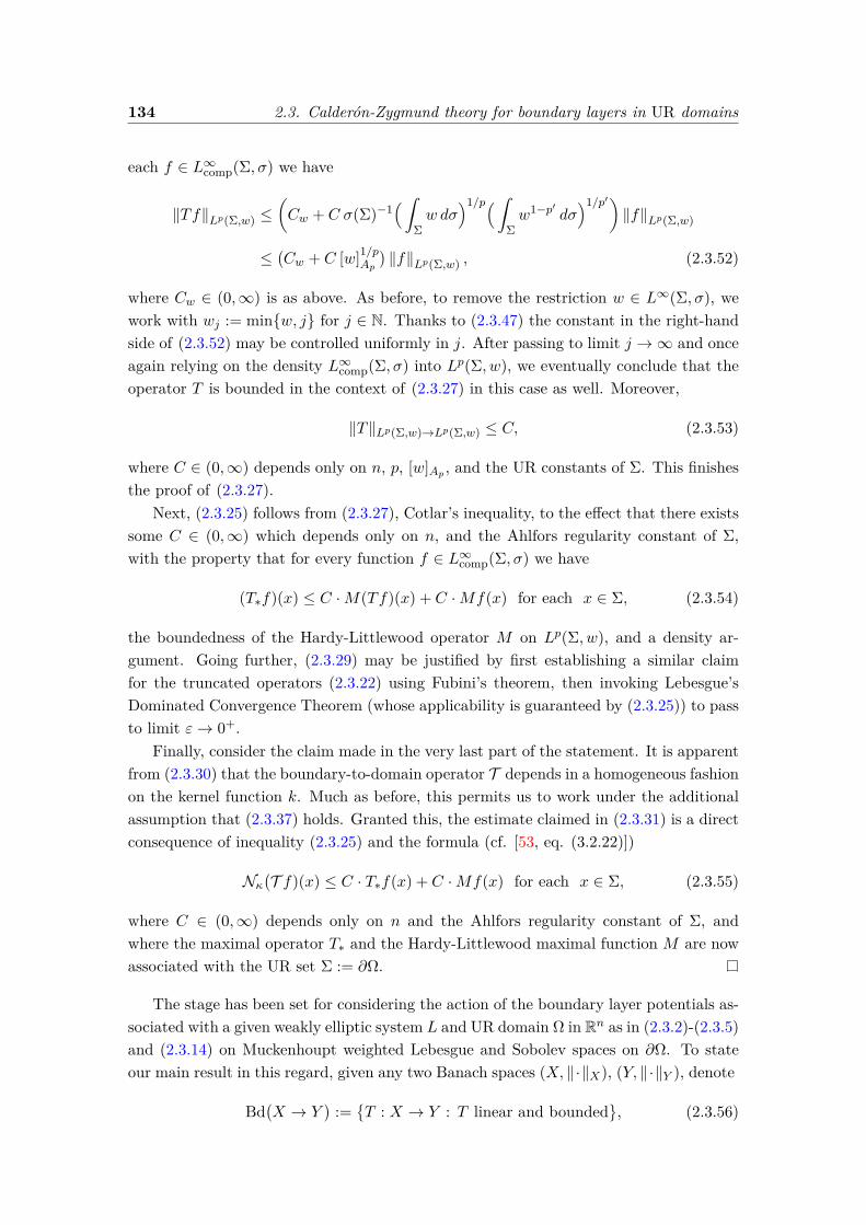
134 2.3. Calderón-Zygmund theory for boundary layers in UR domains
each f ∈ L∞comp(Σ, σ) we have
‖Tf‖Lp(Σ,w) ≤(Cw + C σ(Σ)−1
(ˆΣw dσ
)1/p(ˆΣw1−p′ dσ
)1/p′)‖f‖Lp(Σ,w)
≤(Cw + C [w]1/pAp
)‖f‖Lp(Σ,w) , (2.3.52)
where Cw ∈ (0,∞) is as above. As before, to remove the restriction w ∈ L∞(Σ, σ), wework with wj := minw, j for j ∈ N. Thanks to (2.3.47) the constant in the right-handside of (2.3.52) may be controlled uniformly in j. After passing to limit j →∞ and onceagain relying on the density L∞comp(Σ, σ) into Lp(Σ, w), we eventually conclude that theoperator T is bounded in the context of (2.3.27) in this case as well. Moreover,
‖T‖Lp(Σ,w)→Lp(Σ,w) ≤ C, (2.3.53)
where C ∈ (0,∞) depends only on n, p, [w]Ap , and the UR constants of Σ. This finishesthe proof of (2.3.27).
Next, (2.3.25) follows from (2.3.27), Cotlar’s inequality, to the effect that there existssome C ∈ (0,∞) which depends only on n, and the Ahlfors regularity constant of Σ,with the property that for every function f ∈ L∞comp(Σ, σ) we have
(T∗f)(x) ≤ C ·M(Tf)(x) + C ·Mf(x) for each x ∈ Σ, (2.3.54)
the boundedness of the Hardy-Littlewood operator M on Lp(Σ, w), and a density ar-gument. Going further, (2.3.29) may be justified by first establishing a similar claimfor the truncated operators (2.3.22) using Fubini’s theorem, then invoking Lebesgue’sDominated Convergence Theorem (whose applicability is guaranteed by (2.3.25)) to passto limit ε→ 0+.
Finally, consider the claim made in the very last part of the statement. It is apparentfrom (2.3.30) that the boundary-to-domain operator T depends in a homogeneous fashionon the kernel function k. Much as before, this permits us to work under the additionalassumption that (2.3.37) holds. Granted this, the estimate claimed in (2.3.31) is a directconsequence of inequality (2.3.25) and the formula (cf. [53, eq. (3.2.22)])
Nκ(T f)(x) ≤ C · T∗f(x) + C ·Mf(x) for each x ∈ Σ, (2.3.55)
where C ∈ (0,∞) depends only on n and the Ahlfors regularity constant of Σ, andwhere the maximal operator T∗ and the Hardy-Littlewood maximal function M are nowassociated with the UR set Σ := ∂Ω.
The stage has been set for considering the action of the boundary layer potentials as-sociated with a given weakly elliptic system L and UR domain Ω in Rn as in (2.3.2)-(2.3.5)and (2.3.14) on Muckenhoupt weighted Lebesgue and Sobolev spaces on ∂Ω. To stateour main result in this regard, given any two Banach spaces (X, ‖·‖X), (Y, ‖·‖Y ), denote
Bd(X → Y
):=T : X → Y : T linear and bounded
, (2.3.56)
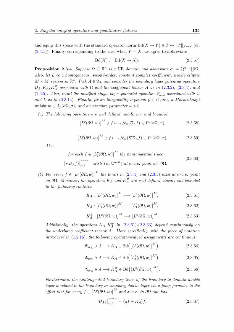
2. Singular integral operators and quantitative flatness 135
and equip this space with the standard operator norm Bd(X → Y
)3 T 7→ ‖T‖X→Y (cf.
(2.4.1)). Finally, corresponding to the case when Y = X, we agree to abbreviate
Bd(X) := Bd(X → X
). (2.3.57)
Proposition 2.3.4. Suppose Ω ⊆ Rn is a UR domain and abbreviate σ := Hn−1b∂Ω.Also, let L be a homogeneous, second-order, constant complex coefficient, weakly ellipticM ×M system in Rn. Pick A ∈ AL and consider the boundary layer potential operatorsDA,KA,K
#A associated with Ω and the coefficient tensor A as in (2.3.2), (2.3.4), and
(2.3.5). Also, recall the modified single layer potential operator Smod associated with Ωand L as in (2.3.14). Finally, fix an integrability exponent p ∈ (1,∞), a Muckenhouptweight w ∈ Ap(∂Ω, σ), and an aperture parameter κ > 0.
(a) The following operators are well defined, sub-linear, and bounded:[Lp(∂Ω, w)
]M 3 f 7−→ Nκ(DAf) ∈ Lp(∂Ω, w), (2.3.58)
[Lp1(∂Ω, w)
]M 3 f 7−→ Nκ (∇DAf) ∈ Lp(∂Ω, w). (2.3.59)
Also,
for each f ∈[Lp1(∂Ω, w)
]M the nontangential trace(∇DAf
)∣∣κ−n.t.
∂Ω exists (in Cn·M ) at σ-a.e. point on ∂Ω.(2.3.60)
(b) For every f ∈[Lp(∂Ω, w)
]M the limits in (2.3.4) and (2.3.5) exist at σ-a.e. pointon ∂Ω. Moreover, the operators KA and K#
A are well defined, linear, and boundedin the following contexts:
KA :[Lp(∂Ω, w)
]M −→ [Lp(∂Ω, w)
]M, (2.3.61)
KA :[Lp1(∂Ω, w)
]M −→ [Lp1(∂Ω, w)
]M, (2.3.62)
K#A :
[Lp(∂Ω, w)
]M −→ [Lp(∂Ω, w)
]M. (2.3.63)
Additionally, the operators KA,K#A in (2.3.61)-(2.3.63) depend continuously on
the underlying coefficient tensor A. More specifically, with the piece of notationintroduced in (1.2.16), the following operator-valued assignments are continuous:
AWE 3 A 7−→ KA ∈ Bd([Lp(∂Ω, w)
]M), (2.3.64)
AWE 3 A 7−→ KA ∈ Bd([Lp1(∂Ω, w)
]M), (2.3.65)
AWE 3 A 7−→ K#A ∈ Bd
([Lp(∂Ω, w)
]M). (2.3.66)
Furthermore, the nontangential boundary trace of the boundary-to-domain doublelayer is related to the boundary-to-boundary double layer via a jump-formula, to theeffect that for every f ∈
[Lp(∂Ω, w)
]M and σ-a.e. in ∂Ω one has
DAf∣∣κ−n.t.
∂Ω =(1
2I +KA
)f, (2.3.67)
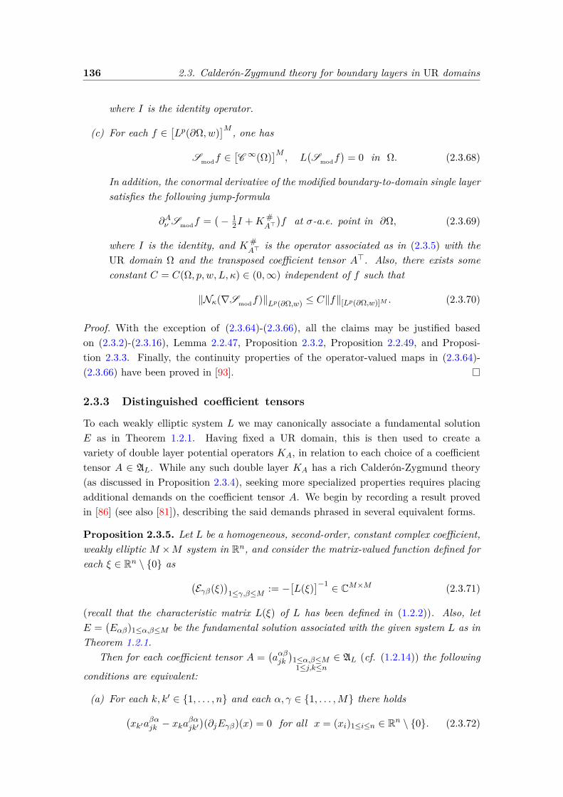
136 2.3. Calderón-Zygmund theory for boundary layers in UR domains
where I is the identity operator.
(c) For each f ∈[Lp(∂Ω, w)
]M , one has
Smodf ∈[C ∞(Ω)
]M, L
(Smodf
)= 0 in Ω. (2.3.68)
In addition, the conormal derivative of the modified boundary-to-domain single layersatisfies the following jump-formula
∂Aν Smodf =(− 1
2I +K #A>
)f at σ-a.e. point in ∂Ω, (2.3.69)
where I is the identity, and K #A>
is the operator associated as in (2.3.5) with theUR domain Ω and the transposed coefficient tensor A>. Also, there exists someconstant C = C(Ω, p, w, L, κ) ∈ (0,∞) independent of f such that
‖Nκ(∇Smodf)‖Lp(∂Ω,w) ≤ C‖f‖[Lp(∂Ω,w)]M . (2.3.70)
Proof. With the exception of (2.3.64)-(2.3.66), all the claims may be justified basedon (2.3.2)-(2.3.16), Lemma 2.2.47, Proposition 2.3.2, Proposition 2.2.49, and Proposi-tion 2.3.3. Finally, the continuity properties of the operator-valued maps in (2.3.64)-(2.3.66) have been proved in [93].
2.3.3 Distinguished coefficient tensors
To each weakly elliptic system L we may canonically associate a fundamental solutionE as in Theorem 1.2.1. Having fixed a UR domain, this is then used to create avariety of double layer potential operators KA, in relation to each choice of a coefficienttensor A ∈ AL. While any such double layer KA has a rich Calderón-Zygmund theory(as discussed in Proposition 2.3.4), seeking more specialized properties requires placingadditional demands on the coefficient tensor A. We begin by recording a result provedin [86] (see also [81]), describing the said demands phrased in several equivalent forms.
Proposition 2.3.5. Let L be a homogeneous, second-order, constant complex coefficient,weakly elliptic M ×M system in Rn, and consider the matrix-valued function defined foreach ξ ∈ Rn \ 0 as (
Eγβ(ξ))1≤γ,β≤M := −
[L(ξ)
]−1 ∈ CM×M (2.3.71)
(recall that the characteristic matrix L(ξ) of L has been defined in (1.2.2)). Also, letE =
(Eαβ)1≤α,β≤M be the fundamental solution associated with the given system L as in
Theorem 1.2.1.Then for each coefficient tensor A =
(aαβjk
)1≤α,β≤M1≤j,k≤n
∈ AL (cf. (1.2.14)) the following
conditions are equivalent:
(a) For each k, k′ ∈ 1, . . . , n and each α, γ ∈ 1, . . . ,M there holds(xk′a
βαjk − xka
βαjk′)(∂jEγβ)(x) = 0 for all x = (xi)1≤i≤n ∈ Rn \ 0. (2.3.72)
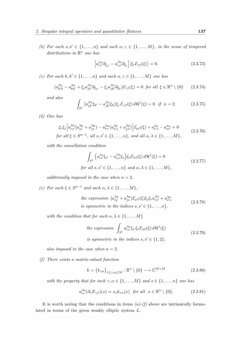
2. Singular integral operators and quantitative flatness 137
(b) For each s, s′ ∈ 1, . . . , n and each α, γ ∈ 1, . . . ,M, in the sense of tempereddistributions in Rn one has[
aβαrs ∂ξs′ − aβαrs′∂ξs
][ξrEγβ(ξ)
]= 0. (2.3.73)
(c) For each k, k′ ∈ 1, . . . , n and each α, γ ∈ 1, . . . ,M one has(aβαk′k − a
βαkk′ + ξja
βαjk ∂ξk′ − ξja
βαjk′∂ξk
)Eγβ(ξ) = 0 for all ξ ∈ Rn \ 0 (2.3.74)
and also ˆS1
(aβαjk ξk′ − a
βαjk′ξk
)ξj Eγβ(ξ) dH1(ξ) = 0 if n = 2. (2.3.75)
(d) One has
ξrξj[aβαrs′
(aλµsj + aλµjs
)− aβαrs
(aλµs′j + aλµjs′
)]Eµβ(ξ) + aλαs′s − aλαss′ = 0
for all ξ ∈ Sn−1, all s, s′ ∈ 1, . . . , n, and all α, λ ∈ 1, . . . ,M,(2.3.76)
with the cancellation conditionˆS1
(aβαrs ξs′ − a
βαrs′ξs
)ξrEλβ(ξ) dH1(ξ) = 0
for all s, s′ ∈ 1, . . . , n and α, λ ∈ 1, . . . ,M,(2.3.77)
additionally imposed in the case when n = 2.
(e) For each ξ ∈ Sn−1 and each α, λ ∈ 1, . . . ,M,
the expression(aλµsj + aλµjs
)Eµβ(ξ)ξjξraβαrs′ + aλαs′s
is symmetric in the indices s, s′ ∈ 1, . . . , n,(2.3.78)
with the condition that for each α, λ ∈ 1, . . . ,M
the expressionˆS1aβαrs ξs′ξrEλβ(ξ) dH1(ξ)
is symmetric in the indices s, s′ ∈ 1, 2,(2.3.79)
also imposed in the case when n = 2.
(f) There exists a matrix-valued function
k =kγα
1≤γ,α≤M : Rn \ 0 −→ CM×M (2.3.80)
with the property that for each γ, α ∈ 1, . . . ,M and s ∈ 1, . . . , n one has
aβαrs (∂rEγβ)(x) = xskγα(x) for all x ∈ Rn \ 0. (2.3.81)
It is worth noting that the conditions in items (a)-(f) above are intrinsically formu-lated in terms of the given weakly elliptic system L.
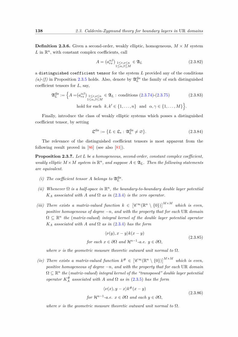
138 2.3. Calderón-Zygmund theory for boundary layers in UR domains
Definition 2.3.6. Given a second-order, weakly elliptic, homogeneous, M ×M systemL in Rn, with constant complex coefficients, call
A =(aαβrs
)1≤r,s≤n
1≤α,β≤M∈ AL (2.3.82)
a distinguished coefficient tensor for the system L provided any of the conditions(a)-(f) in Proposition 2.3.5 holds. Also, denote by Adis
L the family of such distinguishedcoefficient tensors for L, say,
AdisL :=
A =
(aαβrs
)1≤r,s≤n
1≤α,β≤M∈ AL : conditions (2.3.74)-(2.3.75) (2.3.83)
hold for each k, k′ ∈ 1, . . . , n and α, γ ∈ 1, . . . ,M.
Finally, introduce the class of weakly elliptic systems which posses a distinguishedcoefficient tensor, by setting
Ldis :=L ∈ L∗ : Adis
L 6= ∅. (2.3.84)
The relevance of the distinguished coefficient tensors is most apparent from thefollowing result proved in [86] (see also [81]).
Proposition 2.3.7. Let L be a homogeneous, second-order, constant complex coefficient,weakly elliptic M×M system in Rn, and suppose A ∈ AL. Then the following statementsare equivalent.
(i) The coefficient tensor A belongs to AdisL .
(ii) Whenever Ω is a half-space in Rn, the boundary-to-boundary double layer potentialKA associated with A and Ω as in (2.3.4) is the zero operator.
(iii) There exists a matrix-valued function k ∈[C∞(Rn \ 0)
]M×M which is even,positive homogeneous of degree −n, and with the property that for each UR domainΩ ⊆ Rn the (matrix-valued) integral kernel of the double layer potential operatorKA associated with A and Ω as in (2.3.4) has the form
〈ν(y), x− y〉k(x− y)
for each x ∈ ∂Ω and Hn−1-a.e. y ∈ ∂Ω,(2.3.85)
where ν is the geometric measure theoretic outward unit normal to Ω.
(iv) There exists a matrix-valued function k# ∈[C∞(Rn \ 0)
]M×M which is even,positive homogeneous of degree −n, and with the property that for each UR domainΩ ⊆ Rn the (matrix-valued) integral kernel of the “transposed” double layer potentialoperator K#
A associated with A and Ω as in (2.3.5) has the form
〈ν(x), y − x〉k#(x− y)
for Hn−1-a.e. x ∈ ∂Ω and each y ∈ ∂Ω,(2.3.86)
where ν is the geometric measure theoretic outward unit normal to Ω.
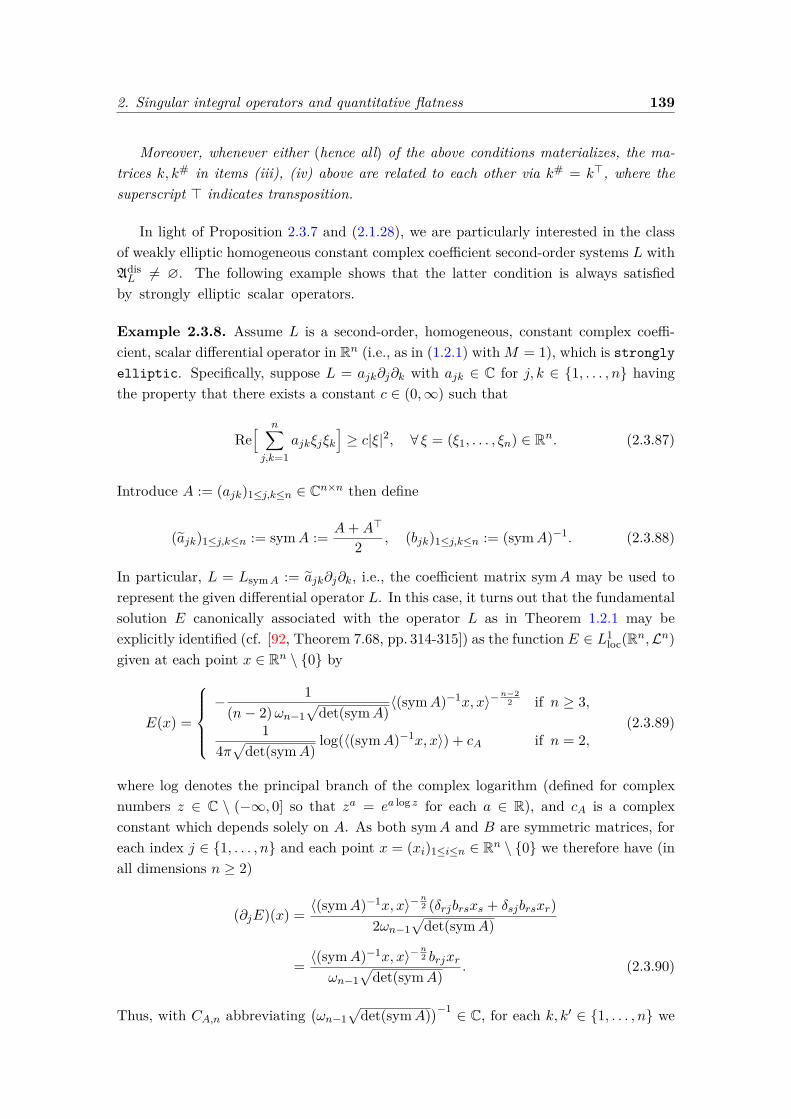
2. Singular integral operators and quantitative flatness 139
Moreover, whenever either (hence all) of the above conditions materializes, the ma-trices k, k# in items (iii), (iv) above are related to each other via k# = k>, where thesuperscript > indicates transposition.
In light of Proposition 2.3.7 and (2.1.28), we are particularly interested in the classof weakly elliptic homogeneous constant complex coefficient second-order systems L withAdisL 6= ∅. The following example shows that the latter condition is always satisfied
by strongly elliptic scalar operators.
Example 2.3.8. Assume L is a second-order, homogeneous, constant complex coeffi-cient, scalar differential operator in Rn (i.e., as in (1.2.1) withM = 1), which is stronglyelliptic. Specifically, suppose L = ajk∂j∂k with ajk ∈ C for j, k ∈ 1, . . . , n havingthe property that there exists a constant c ∈ (0,∞) such that
Re[ n∑j,k=1
ajkξjξk]≥ c|ξ|2, ∀ ξ = (ξ1, . . . , ξn) ∈ Rn. (2.3.87)
Introduce A := (ajk)1≤j,k≤n ∈ Cn×n then define
(ajk)1≤j,k≤n := symA := A+A>
2 , (bjk)1≤j,k≤n := (symA)−1. (2.3.88)
In particular, L = LsymA := ajk∂j∂k, i.e., the coefficient matrix symA may be used torepresent the given differential operator L. In this case, it turns out that the fundamentalsolution E canonically associated with the operator L as in Theorem 1.2.1 may beexplicitly identified (cf. [92, Theorem 7.68, pp. 314-315]) as the function E ∈ L1
loc(Rn,Ln)given at each point x ∈ Rn \ 0 by
E(x) =
− 1
(n− 2)ωn−1√
det(symA)〈(symA)−1x, x〉−
n−22 if n ≥ 3,
14π√
det(symA)log(〈(symA)−1x, x〉) + cA if n = 2,
(2.3.89)
where log denotes the principal branch of the complex logarithm (defined for complexnumbers z ∈ C \ (−∞, 0] so that za = ea log z for each a ∈ R), and cA is a complexconstant which depends solely on A. As both symA and B are symmetric matrices, foreach index j ∈ 1, . . . , n and each point x = (xi)1≤i≤n ∈ Rn \ 0 we therefore have (inall dimensions n ≥ 2)
(∂jE)(x) = 〈(symA)−1x, x〉−n2 (δrjbrsxs + δsjbrsxr)
2ωn−1√
det(symA)
= 〈(symA)−1x, x〉−n2 brjxr
ωn−1√
det(symA). (2.3.90)
Thus, with CA,n abbreviating(ωn−1
√det(symA)
)−1 ∈ C, for each k, k′ ∈ 1, . . . , n we
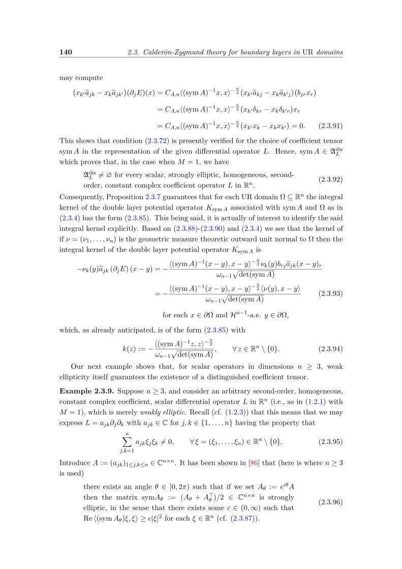
140 2.3. Calderón-Zygmund theory for boundary layers in UR domains
may compute(xk′ ajk − xkajk′
)(∂jE)(x) = CA,n〈(symA)−1x, x〉−
n2(xk′ akj − xkak′j
)(bjrxr
)= CA,n〈(symA)−1x, x〉−
n2(xk′δkr − xkδk′r
)xr
= CA,n〈(symA)−1x, x〉−n2(xk′xk − xkxk′
)= 0. (2.3.91)
This shows that condition (2.3.72) is presently verified for the choice of coefficient tensorsymA in the representation of the given differential operator L. Hence, symA ∈ Adis
L
which proves that, in the case when M = 1, we have
AdisL 6= ∅ for every scalar, strongly elliptic, homogeneous, second-
order, constant complex coefficient operator L in Rn.(2.3.92)
Consequently, Proposition 2.3.7 guarantees that for each UR domain Ω ⊆ Rn the integralkernel of the double layer potential operator KsymA associated with symA and Ω as in(2.3.4) has the form (2.3.85). This being said, it is actually of interest to identify the saidintegral kernel explicitly. Based on (2.3.88)-(2.3.90) and (2.3.4) we see that the kernel ofif ν = (ν1, . . . , νn) is the geometric measure theoretic outward unit normal to Ω then theintegral kernel of the double layer potential operator KsymA is
−νk(y)ajk (∂jE) (x− y) = −〈(symA)−1(x− y), x− y〉−n2 νk(y)brj ajk(x− y)r
ωn−1√
det(symA)
= −〈(symA)−1(x− y), x− y〉−n2 〈ν(y), x− y〉
ωn−1√
det(symA)(2.3.93)
for each x ∈ ∂Ω and Hn−1-a.e. y ∈ ∂Ω,
which, as already anticipated, is of the form (2.3.85) with
k(z) := −〈(symA)−1z, z〉−n2
ωn−1√
det(symA), ∀ z ∈ Rn \ 0. (2.3.94)
Our next example shows that, for scalar operators in dimensions n ≥ 3, weakellipticity itself guarantees the existence of a distinguished coefficient tensor.
Example 2.3.9. Suppose n ≥ 3, and consider an arbitrary second-order, homogeneous,constant complex coefficient, scalar differential operator L in Rn (i.e., as in (1.2.1) withM = 1), which is merely weakly elliptic. Recall (cf. (1.2.3)) that this means that we mayexpress L = ajk∂j∂k with ajk ∈ C for j, k ∈ 1, . . . , n having the property that
n∑j,k=1
ajkξjξk 6= 0, ∀ ξ = (ξ1, . . . , ξn) ∈ Rn \ 0. (2.3.95)
Introduce A := (ajk)1≤j,k≤n ∈ Cn×n. It has been shown in [86] that (here is where n ≥ 3is used)
there exists an angle θ ∈ [0, 2π) such that if we set Aθ := eiθA
then the matrix symAθ := (Aθ + A>θ )/2 ∈ Cn×n is stronglyelliptic, in the sense that there exists some c ∈ (0,∞) such thatRe 〈(symAθ)ξ, ξ〉 ≥ c|ξ|2 for each ξ ∈ Rn (cf. (2.3.87)).
(2.3.96)
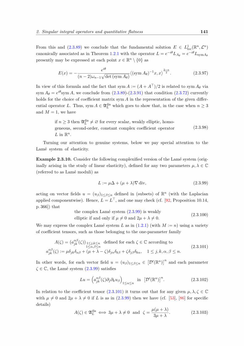
2. Singular integral operators and quantitative flatness 141
From this and (2.3.89) we conclude that the fundamental solution E ∈ L1loc(Rn,Ln)
canonically associated as in Theorem 1.2.1 with the operator L = e−iθLAθ = e−iθLsymAθpresently may be expressed at each point x ∈ Rn \ 0 as
E(x) = − eiθ
(n− 2)ωn−1√
det (symAθ)⟨(symAθ)−1x, x
⟩ 2−n2 . (2.3.97)
In view of this formula and the fact that symA := (A+ A>)/2 is related to symAθ viasymAθ = eiθsymA, we conclude from (2.3.89)-(2.3.91) that condition (2.3.72) currentlyholds for the choice of coefficient matrix symA in the representation of the given differ-ential operator L. Thus, symA ∈ Adis
L which goes to show that, in the case when n ≥ 3and M = 1, we have
if n ≥ 3 then AdisL 6= ∅ for every scalar, weakly elliptic, homo-
geneous, second-order, constant complex coefficient operatorL in Rn.
(2.3.98)
Turning our attention to genuine systems, below we pay special attention to theLamé system of elasticity.
Example 2.3.10. Consider the following complexified version of the Lamé system (orig-inally arising in the study of linear elasticity), defined for any two parameters µ, λ ∈ C(referred to as Lamé moduli) as
L := µ∆ + (µ+ λ)∇ div, (2.3.99)
acting on vector fields u = (uβ)1≤β≤n defined in (subsets) of Rn (with the Laplacianapplied componentwise). Hence, L = L>, and one may check (cf. [92, Proposition 10.14,p. 366]) that
the complex Lamé system (2.3.99) is weaklyelliptic if and only if µ 6= 0 and 2µ+ λ 6= 0.
(2.3.100)
We may express the complex Lamé system L as in (1.2.1) (with M := n) using a varietyof coefficient tensors, such as those belonging to the one-parameter family
A(ζ) =(aαβjk (ζ)
)1≤j,k≤n1≤α,β≤n
defined for each ζ ∈ C according to
aαβjk (ζ) := µδjkδαβ + (µ+ λ− ζ)δjαδkβ + ζδjβδkα, 1 ≤ j, k, α, β ≤ n.(2.3.101)
In other words, for each vector field u = (uβ)1≤β≤n ∈[D′(Rn)
]n and each parameterζ ∈ C, the Lamé system (2.3.99) satisfies
Lu =(aαβjk (ζ)∂j∂kuβ
)1≤α≤n
in[D′(Rn)
]n. (2.3.102)
In relation to the coefficient tensor (2.3.101) it turns out that for any given µ, λ, ζ ∈ Cwith µ 6= 0 and 2µ + λ 6= 0 if L is as in (2.3.99) then we have (cf. [53], [86] for specificdetails)
A(ζ) ∈ AdisL ⇐⇒ 3µ+ λ 6= 0 and ζ = µ(µ+ λ)
3µ+ λ. (2.3.103)
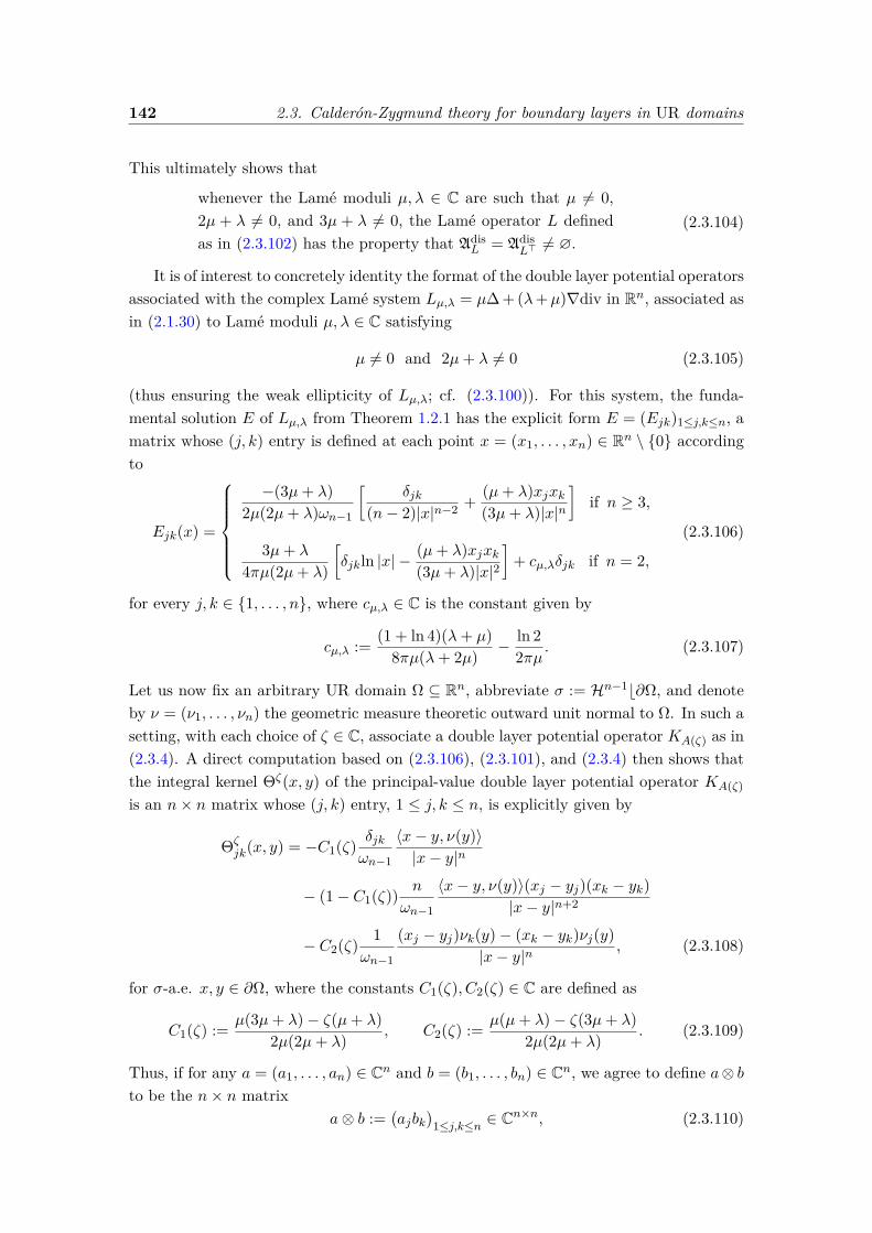
142 2.3. Calderón-Zygmund theory for boundary layers in UR domains
This ultimately shows that
whenever the Lamé moduli µ, λ ∈ C are such that µ 6= 0,2µ + λ 6= 0, and 3µ + λ 6= 0, the Lamé operator L definedas in (2.3.102) has the property that Adis
L = AdisL> 6= ∅.
(2.3.104)
It is of interest to concretely identity the format of the double layer potential operatorsassociated with the complex Lamé system Lµ,λ = µ∆ + (λ+µ)∇div in Rn, associated asin (2.1.30) to Lamé moduli µ, λ ∈ C satisfying
µ 6= 0 and 2µ+ λ 6= 0 (2.3.105)
(thus ensuring the weak ellipticity of Lµ,λ; cf. (2.3.100)). For this system, the funda-mental solution E of Lµ,λ from Theorem 1.2.1 has the explicit form E = (Ejk)1≤j,k≤n, amatrix whose (j, k) entry is defined at each point x = (x1, . . . , xn) ∈ Rn \ 0 accordingto
Ejk(x) =
−(3µ+ λ)2µ(2µ+ λ)ωn−1
[δjk
(n− 2)|x|n−2 + (µ+ λ)xjxk(3µ+ λ)|x|n
]if n ≥ 3,
3µ+ λ
4πµ(2µ+ λ)
[δjkln |x| −
(µ+ λ)xjxk(3µ+ λ)|x|2
]+ cµ,λδjk if n = 2,
(2.3.106)
for every j, k ∈ 1, . . . , n, where cµ,λ ∈ C is the constant given by
cµ,λ := (1 + ln 4)(λ+ µ)8πµ(λ+ 2µ) − ln 2
2πµ. (2.3.107)
Let us now fix an arbitrary UR domain Ω ⊆ Rn, abbreviate σ := Hn−1b∂Ω, and denoteby ν = (ν1, . . . , νn) the geometric measure theoretic outward unit normal to Ω. In such asetting, with each choice of ζ ∈ C, associate a double layer potential operator KA(ζ) as in(2.3.4). A direct computation based on (2.3.106), (2.3.101), and (2.3.4) then shows thatthe integral kernel Θζ(x, y) of the principal-value double layer potential operator KA(ζ)is an n× n matrix whose (j, k) entry, 1 ≤ j, k ≤ n, is explicitly given by
Θζjk(x, y) = −C1(ζ) δjk
ωn−1
〈x− y, ν(y)〉|x− y|n
− (1− C1(ζ)) n
ωn−1
〈x− y, ν(y)〉(xj − yj)(xk − yk)|x− y|n+2
− C2(ζ) 1ωn−1
(xj − yj)νk(y)− (xk − yk)νj(y)|x− y|n
, (2.3.108)
for σ-a.e. x, y ∈ ∂Ω, where the constants C1(ζ), C2(ζ) ∈ C are defined as
C1(ζ) := µ(3µ+ λ)− ζ(µ+ λ)2µ(2µ+ λ) , C2(ζ) := µ(µ+ λ)− ζ(3µ+ λ)
2µ(2µ+ λ) . (2.3.109)
Thus, if for any a = (a1, . . . , an) ∈ Cn and b = (b1, . . . , bn) ∈ Cn, we agree to define a⊗ bto be the n× n matrix
a⊗ b :=(ajbk
)1≤j,k≤n ∈ Cn×n, (2.3.110)
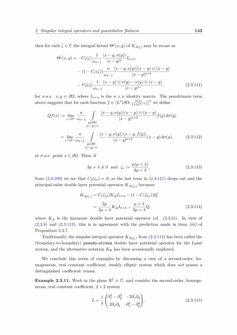
2. Singular integral operators and quantitative flatness 143
then for each ζ ∈ C the integral kernel Θζ(x, y) of KA(ζ) may be recast as
Θζ(x, y) = −C1(ζ) 1ωn−1
〈x− y, ν(y)〉|x− y|n
In×n
− (1− C1(ζ)) n
ωn−1
〈x− y, ν(y)〉(x− y)⊗ (x− y)|x− y|n+2
− C2(ζ) 1ωn−1
(x− y)⊗ ν(y)− ν(y)⊗ (x− y)|x− y|n
, (2.3.111)
for σ-a.e. x, y ∈ ∂Ω, where In×n is the n × n identity matrix. The penultimate termabove suggests that for each function f ∈
[L1(∂Ω, σ(x)
1+|x|n−1)]n we define
Qf(x) := limε→0+
n
ωn−1
ˆ
y∈∂Ω|x−y|>ε
〈x− y, ν(y)〉(x− y)⊗ (x− y)|x− y|n+2 f(y) dσ(y)
= limε→0+
n
ωn−1
ˆ
y∈∂Ω|x−y|>ε
〈x− y, ν(y)〉〈x− y, f(y)〉|x− y|n+2 (x− y) dσ(y), (2.3.112)
at σ-a.e. point x ∈ ∂Ω. Then, if
3µ+ λ 6= 0 and ζ∗ := µ(µ+ λ)3µ+ λ
, (2.3.113)
from (2.3.109) we see that C2(ζ∗) = 0, so the last term in (2.3.111) drops out and theprincipal-value double layer potential operator KA(ζ∗) becomes
KA(ζ∗) = C1(ζ∗)K∆In×n − (1− C1(ζ∗))Q
= 2µ3µ+ λ
K∆In×n −µ+ λ
3µ+ λQ, (2.3.114)
where K∆ is the harmonic double layer potential operator (cf. (2.3.8)). In view of(2.3.8) and (2.3.112), this is in agreement with the prediction made in item (iii) ofProposition 2.3.7.
Traditionally, the singular integral operator KA(ζ∗) from (2.3.114) has been called the(boundary-to-boundary) pseudo-stress double layer potential operator for the Lamésystem, and the alternative notation KΨ has been occasionally employed.
We conclude this series of examples by discussing a case of a second-order, ho-mogeneous, real constant coefficient, weakly elliptic system which does not posses adistinguished coefficient tensor.
Example 2.3.11. Work in the plane R2 ≡ C, and consider the second-order, homoge-neous, real constant coefficient, 2× 2 system
L = 14
∂2x − ∂2
y −2∂x∂y2∂x∂y ∂2
x − ∂2y
. (2.3.115)
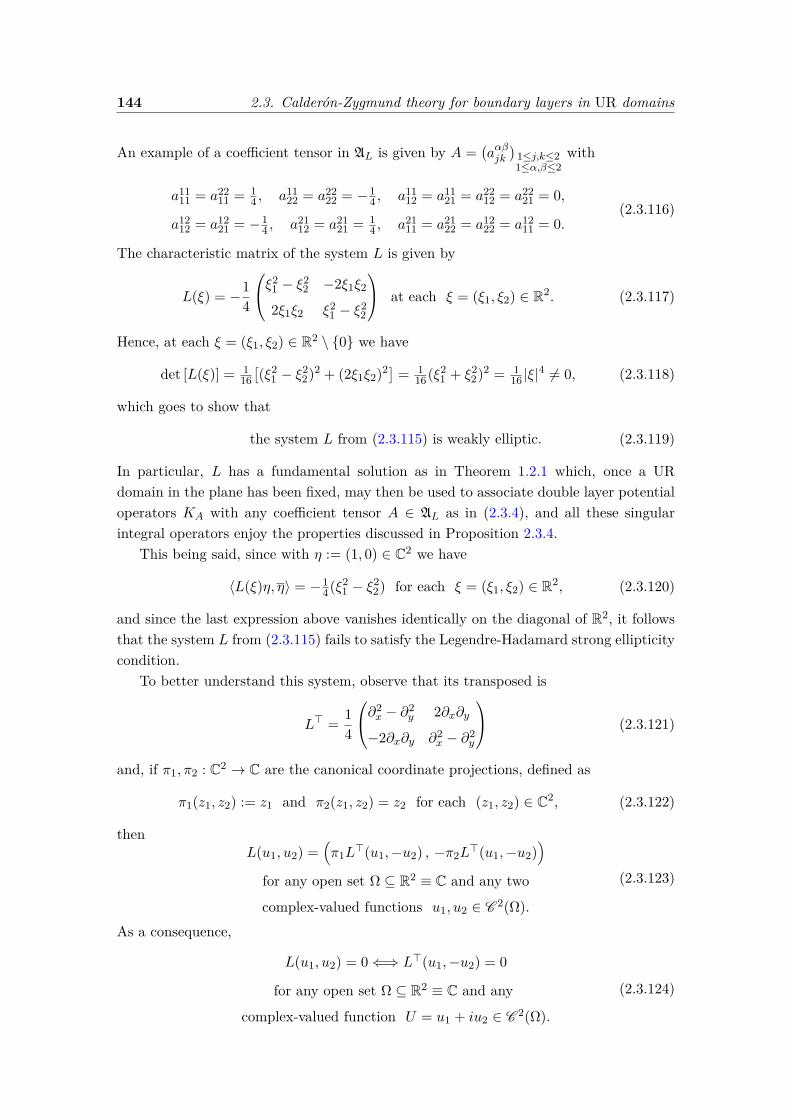
144 2.3. Calderón-Zygmund theory for boundary layers in UR domains
An example of a coefficient tensor in AL is given by A =(aαβjk
)1≤j,k≤21≤α,β≤2
with
a1111 = a22
11 = 14 , a11
22 = a2222 = −1
4 , a1112 = a11
21 = a2212 = a22
21 = 0,
a1212 = a12
21 = −14 , a21
12 = a2121 = 1
4 , a2111 = a21
22 = a1222 = a12
11 = 0.(2.3.116)
The characteristic matrix of the system L is given by
L(ξ) = −14
ξ21 − ξ2
2 −2ξ1ξ2
2ξ1ξ2 ξ21 − ξ2
2
at each ξ = (ξ1, ξ2) ∈ R2. (2.3.117)
Hence, at each ξ = (ξ1, ξ2) ∈ R2 \ 0 we have
det [L(ξ)] = 116[(ξ2
1 − ξ22)2 + (2ξ1ξ2)2] = 1
16(ξ21 + ξ2
2)2 = 116 |ξ|
4 6= 0, (2.3.118)
which goes to show that
the system L from (2.3.115) is weakly elliptic. (2.3.119)
In particular, L has a fundamental solution as in Theorem 1.2.1 which, once a URdomain in the plane has been fixed, may then be used to associate double layer potentialoperators KA with any coefficient tensor A ∈ AL as in (2.3.4), and all these singularintegral operators enjoy the properties discussed in Proposition 2.3.4.
This being said, since with η := (1, 0) ∈ C2 we have
〈L(ξ)η, η〉 = −14(ξ2
1 − ξ22) for each ξ = (ξ1, ξ2) ∈ R2, (2.3.120)
and since the last expression above vanishes identically on the diagonal of R2, it followsthat the system L from (2.3.115) fails to satisfy the Legendre-Hadamard strong ellipticitycondition.
To better understand this system, observe that its transposed is
L> = 14
∂2x − ∂2
y 2∂x∂y−2∂x∂y ∂2
x − ∂2y
(2.3.121)
and, if π1, π2 : C2 → C are the canonical coordinate projections, defined as
π1(z1, z2) := z1 and π2(z1, z2) = z2 for each (z1, z2) ∈ C2, (2.3.122)
thenL(u1, u2) =
(π1L
>(u1,−u2) , −π2L>(u1,−u2)
)for any open set Ω ⊆ R2 ≡ C and any two
complex-valued functions u1, u2 ∈ C 2(Ω).
(2.3.123)
As a consequence,
L(u1, u2) = 0⇐⇒ L>(u1,−u2) = 0
for any open set Ω ⊆ R2 ≡ C and any
complex-valued function U = u1 + iu2 ∈ C 2(Ω).
(2.3.124)

2. Singular integral operators and quantitative flatness 145
Pressing on, recall the Cauchy-Riemann operator and its conjugate
∂z := 12(∂x + i∂y
), ∂z := 1
2(∂x − i∂y
), where z = x+ iy, (2.3.125)
then bring in Bitsadze’s operator (cf. [12], [13]), which is simply the square of ∂z, i.e,
L := ∂2z = 1
4∂2x + i
2∂x∂y −14∂
2y , z = x+ iy. (2.3.126)
To place things into a broader perspective, there are three basic prototypes of scalar,constant coefficient, second-order, elliptic operators in the plane: the Laplacian 4∂z∂z,plus Bitsadze’s operator ∂2
z and its complex conjugate ∂2z . With π1, π2 : C2 → C the
canonical coordinate projections from (2.3.122), the system L introduced in (2.3.115) isrelated to Bitsadze’s operator L = ∂2
z via
L(u1 + iu2) = π1L(u1, u2) + iπ2L(u1, u2)
for any open set Ω ⊆ R2 ≡ C and any two
complex-valued functions u1, u2 ∈ C 2(Ω).
(2.3.127)
In particular,L(ReU , ImU
)=(Re (LU) , Im (LU)
)for any open set Ω ⊆ R2 ≡ C and any
complex-valued function U ∈ C 2(Ω).
(2.3.128)
On the other hand, given any open set Ω ⊆ R2 ≡ C along with any complex-valuedfunction U ∈ C 2(Ω), we have ∂2
zU = 0 if and only if f := −∂zU is holomorphic in Ω,and the latter condition further implies that the function g(z) := U(z) + zf(z) for eachz ∈ Ω is holomorphic in Ω. As such, the general format of null-solution of ∂2
z in an openset Ω ⊆ R2 ≡ C is
U(z) = g(z)− zf(z) for all z ∈ Ω, where
f and g are holomorphic functions in Ω.(2.3.129)
This is akin to the description of affine functions on the real line as null-solutions ofthe one-dimensional Laplacian d2/dx2, with the role of d/dx now played by the Cauchy-Riemann operator ∂z, with z now playing the role of the variable x, and with holomorphicfunctions playing the role of constants.
Specializing the expression of U in (2.3.129) to the case when g(z) := zf(z) for eachz ∈ Ω, we obtain the following particular family of null-solutions for Bitsadze’s operatorL in any given open set Ω ⊆ R2 ≡ C:
U(z) = (z − z)f(z), where f
is any holomorphic function in Ω.(2.3.130)
From this and (2.3.128) we then conclude thatgiven any holomorphic function f in an open set Ω ⊆ C,the vector-valued function u = (u1, u2) with componentsu1(z) := Re
[(z − z)f(z)
]and u2(z) := Im
[(z − z)f(z)
]for
z ∈ Ω is a null-solution of the system L from (2.3.115).
(2.3.131)
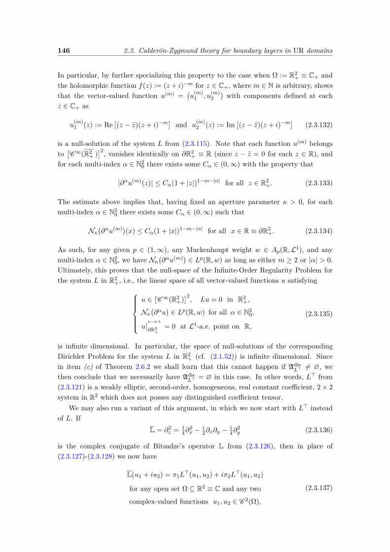
146 2.3. Calderón-Zygmund theory for boundary layers in UR domains
In particular, by further specializing this property to the case when Ω := R2+ ≡ C+ and
the holomorphic function f(z) := (z + i)−m for z ∈ C+, where m ∈ N is arbitrary, showsthat the vector-valued function u(m) =
(u
(m)1 , u
(m)2)with components defined at each
z ∈ C+ as
u(m)1 (z) := Re
[(z − z)(z + i)−m
]and u
(m)2 (z) := Im
[(z − z)(z + i)−m
](2.3.132)
is a null-solution of the system L from (2.3.115). Note that each function u(m) belongsto[C∞(R2
+ )]2, vanishes identically on ∂R2
+ ≡ R (since z − z = 0 for each z ∈ R), andfor each multi-index α ∈ N2
0 there exists some Cα ∈ (0,∞) with the property that
∣∣∂αu(m)(z)∣∣ ≤ Cα(1 + |z|)1−m−|α| for all z ∈ R2
+. (2.3.133)
The estimate above implies that, having fixed an aperture parameter κ > 0, for eachmulti-index α ∈ N2
0 there exists some Cα ∈ (0,∞) such that
Nκ(∂αu(m))(x) ≤ Cα(1 + |x|)1−m−|α| for all x ∈ R ≡ ∂R2
+. (2.3.134)
As such, for any given p ∈ (1,∞), any Muckenhoupt weight w ∈ Ap(R,L1), and anymulti-index α ∈ N2
0, we have Nκ(∂αu(m)) ∈ Lp(R, w) as long as either m ≥ 2 or |α| > 0.
Ultimately, this proves that the null-space of the Infinite-Order Regularity Problem forthe system L in R2
+, i.e., the linear space of all vector-valued functions u satisfyingu ∈
[C∞(R2
+)]2, Lu = 0 in R2
+,
Nκ(∂αu
)∈ Lp(R, w) for all α ∈ N2
0,
u∣∣κ−n.t.
∂R2+
= 0 at L1-a.e. point on R,
(2.3.135)
is infinite dimensional. In particular, the space of null-solutions of the correspondingDirichlet Problem for the system L in R2
+ (cf. (2.1.52)) is infinite dimensional. Sincein item (c) of Theorem 2.6.2 we shall learn that this cannot happen if Adis
L> 6= ∅, wethen conclude that we necessarily have Adis
L> = ∅ in this case. In other words, L> from(2.3.121) is a weakly elliptic, second-order, homogeneous, real constant coefficient, 2× 2system in R2 which does not posses any distinguished coefficient tensor.
We may also run a variant of this argument, in which we now start with L> insteadof L. If
L = ∂2z = 1
4∂2x − i
2∂x∂y −14∂
2y (2.3.136)
is the complex conjugate of Bitsadze’s operator L from (2.3.126), then in place of(2.3.127)-(2.3.128) we now have
L(u1 + iu2) = π1L>(u1, u2) + iπ2L
>(u1, u2)
for any open set Ω ⊆ R2 ≡ C and any two
complex-valued functions u1, u2 ∈ C 2(Ω),
(2.3.137)
2. Singular integral operators and quantitative flatness 147
and, respectively,L>(ReU , ImU
)=(Re (LU) , Im (LU)
)for any open set Ω ⊆ R2 ≡ C and any
complex-valued function U ∈ C 2(Ω).
(2.3.138)
Keeping in mind that U is a null-solution of L if and only if U is a null-solution of Land reasoning as before, we conclude that, for each m ∈ N, the vector-valued functionv(m) =
(v
(m)1 , v
(m)2)with components defined at each z ∈ C+ as
v(m)1 (z) := Re
[(z − z)(z − i)−m
]and v
(m)2 (z) := Im
[(z − z)(z − i)−m
](2.3.139)
is a null-solution of the system L> from (2.3.121). In turn, this goes to show that thenull-space of the Infinite-Order Regularity Problem for the system L> in R2
+ (formulatedas in (2.3.135) with L> now replacing L) is infinite dimensional. Once this has beenestablished, from item (c) in Theorem 2.6.2 we then conclude that Adis
L = ∅. Thebottom line is that
L in (2.3.115) is an example of a weakly elliptic, second-order,homogeneous, real constant coefficient, 2× 2 system in R2, withthe property that Adis
L = ∅ and AdisL> = ∅.
(2.3.140)
In particular, this goes to show that not every weakly elliptic, second-order, homogeneous,real constant coefficient, system has a distinguished coefficient tensor.
In relation to the system L from (2.3.115) it is also of interest to identify the spaceof boundary traces of its null-solutions whose nontangential maximal function belongsto a Muckenhoupt weighted Lebesgue space.
Proposition 2.3.12. Fix an integrability index p ∈ (1,∞) along with a Muckenhouptweight w ∈ Ap(R,L1), and choose an aperture parameter κ > 0. Also, recall the 2 × 2system L defined in the plane as in (2.3.115).
Then if u ∈[C∞(R2
+)]2 is a vector-valued function satisfying
Lu = 0 in R2+, Nκu ∈ Lp(R, w), (2.3.141)
and such that the nontangential boundary trace
f := u∣∣κ−n.t.
∂R2+
exists (in C2) at L1-a.e. point on R, (2.3.142)
it follows that the function f belongs to[Lp(R, w)
]2 and, if f1, f2 ∈ Lp(R, w) are thescalar components of f (i.e., f = (f1, f2)), then with H denoting the Hilbert transformon the real line (cf. (2.1.21)) one has
Hf1 = f2 at L1-a.e. point on R. (2.3.143)
In the converse direction, for any given f ∈ Lp(R, w) there exists a vector-valuedfunction u ∈
[C∞(R2
+)]2 satisfying
Lu = 0 in R2+, Nκu ∈ Lp(R, w), and
u∣∣κ−n.t.
∂R2+
= (f,Hf) at L1-a.e. point on R.(2.3.144)
148 2.3. Calderón-Zygmund theory for boundary layers in UR domains
All together, the space of admissible boundary data for the Dirichlet Problem formu-lated in terms of Muckenhoupt weighted Lebesgue spaces for the system L in the upperhalf-plane, i.e.,
u∣∣κ−n.t.
∂R2+
: u ∈[C∞(R2
+)]2, Lu = 0 in R2
+, Nκu ∈ Lp(R, w), (2.3.145)
and u∣∣κ−n.t.
∂R2+
exists at L1-a.e. point on R,
is precisely (f,Hf) : f ∈ Lp(R, w)
. (2.3.146)
As a consequence of this and (2.3.124), one also hasu∣∣κ−n.t.
∂R2+
: u ∈[C∞(R2
+)]2, L>u = 0 in R2
+, Nκu ∈ Lp(R, w),
and u∣∣κ−n.t.
∂R2+
exists at L1-a.e. point on R
=(f,−Hf) : f ∈ Lp(R, w)
. (2.3.147)
Proof. That the function f belongs to[Lp(R, w)
]2 is clear from∣∣u∣∣κ−n.t.
∂R2+
∣∣ ≤ Nκu, the factthat u
∣∣κ−n.t.
∂R2+
is L1-measurable (cf. [93]), and the last property in (2.3.141).
To proceed, fix a function u ∈[C∞(R2
+)]2 satisfying (2.3.141)-(2.3.142) and denote
by u1, u2 ∈ C∞(R2+) its scalar components. Hence, u = (u1, u2) in R2
+. Also, pick anarbitrary ε > 0 and define
Uε(z) := u1(z + εi) + iu2(z + εi) for each z ∈(R2
+ − εi). (2.3.148)
Then Uε ∈ C∞(R2+−εi) and, as seen from (2.3.127), the fact that Lu = 0 in R2
+ translatesinto ∂2
zUε = 0 in R2+ − εi. Granted this, (2.3.129) then guarantees the existence of two
holomorphic functions fε, gε in R2+ − εi with the property that
Uε(z) = gε(z)− zfε(z) for each z ∈(R2
+ − εi). (2.3.149)
More specifically, the unique holomorphic functions f, g which do the job in (2.3.149) are
fε(z) := −∂zUε(z) and gε(z) := Uε(z) + zfε(z) for each z ∈(R2
+ − εi). (2.3.150)
Henceforth, we agree to restrict Uε, fε, gε to R2+. With this interpretation, introduce
Wε(z) := gε(z)− zfε(z) for each z ∈ R2+. (2.3.151)
Hence, Wε is holomorphic in R2+, extends continuously to R2
+, and
Uε(z)−Wε(z) = 2iyfε(z) = −2iy(∂zUε
)(z)
for each z = x+ iy ∈ R2+.
(2.3.152)
2. Singular integral operators and quantitative flatness 149
From the fact that ∂2zUε = 0 in R2
+ we also conclude that 0 = ∂2z∂
2zUε = 1
16∆2Uε, i.e., thefunction Uε is bi-harmonic in R2
+. Select θ ∈ (0, 1) and κ ∈ (0, κ) both small so that
1 + θ + κ
1− θ < 1 + κ. (2.3.153)
Fix an arbitrary point x ∈ R ≡ ∂R2+ and pick some zo = xo+ iyo ∈ Γκ(x). The inequality
demanded in (2.3.153) ensures that
B(zo, θyo) ⊆ Γκ(x). (2.3.154)
Based on interior estimates for bi-harmonic functions (cf. [92, Theorem 11.12, p. 415]),(2.3.152), and (2.3.154) we may then estimate, for some constant C = C(θ) ∈ (0,∞),∣∣Uε(zo)−Wε(zo)
∣∣ = 2yo∣∣(∂zUε)(zo)∣∣ ≤ √2yo|(∇Uε)(zo)|
≤ C B(zo,θyo)
|Uε| dL2 ≤ C(NκUε
)(x). (2.3.155)
Taking the supremum over all zo ∈ Γκ(x) this ultimately yields(Nκ(Uε −Wε)
)(x) ≤ C
(NκUε
)(x) for each x ∈ R ≡ ∂R2
+. (2.3.156)
In turn, (2.3.156) implies
NκWε ≤ NκUε +Nκ(Uε −Wε) ≤ NκUε + CNκUε
= (1 + C)NκUε ≤ (1 + C)Nκu on R ≡ ∂R2+. (2.3.157)
Upon recalling that the nontangential maximal function NκWε is non-negative and lower-semicontinuous, we then conclude from (2.3.157), the last property in (2.3.141), and(2.2.337) that
NκWε ∈ L1(R , L
1(x)1+|x|
). (2.3.158)
Let us record our progress. The argument so far shows that the function Wε is holo-morphic in R2
+, extends continuously to R2+, and there exists some aperture parameter
κ > 0 such that NκWε belongs to L1(R , L
1(x)1+|x|
). These properties allow us to invoke the
Cauchy reproducing formula (proved in [93] in much more general geometric settings)which asserts that
Wε(z) = 12πi
ˆR
(Wε
∣∣R)(y)
y − zdy, for each z ∈ R2
+. (2.3.159)
Since fε, gε extend continuously to R2+, from (2.3.149), (2.3.151), and the fact that z = z
on R ≡ ∂R2+, we conclude that
Wε
∣∣R = Uε
∣∣R on R ≡ ∂R2
+. (2.3.160)
Hence, if we abbreviatehε := Uε
∣∣R on R ≡ ∂R2
+, (2.3.161)
150 2.3. Calderón-Zygmund theory for boundary layers in UR domains
after taking the nontangential boundary traces of both sides in (2.3.159) and using thePlemelj jump-formula for the Cauchy operator (which continues to be valid in this setting;see [93]) we arrive at
hε =(1
2I + i2H)hε at L1-a.e. point on R, (2.3.162)
where I is the identity and H is the Hilbert transform on R. Hence, on the one hand,we may rewrite (2.3.162) simply as
Hhε = −ihε at L1-a.e. point on R. (2.3.163)
On the other hand, from (2.3.161) and (2.3.148) we see that
hε(x) = u1(x+ εi) + iu2(x+ εi) for L1-a.e. x ∈ R. (2.3.164)
In turn, this implies
|hε(x)| ≤√
2(Nκu
)(x) for L1-a.e. x ∈ R, (2.3.165)
and, when used in concert with (2.3.142), that
limε→0+
hε(x) =(u1∣∣κ−n.t.
∂R2+
)(x) + i
(u2∣∣κ−n.t.
∂R2+
)(x)
= f1(x) + if2(x) for L1-a.e. x ∈ R. (2.3.166)
Thanks to (2.3.165)-(2.3.166) and the last property in (2.3.141), we may now invokeLebesgue’s Dominated Convergence Theorem to conclude that
limε→0+
hε = f1 + if2 in Lp(R, w). (2.3.167)
Having established this, on account of (2.3.163) and the continuity of the Hilbert trans-form H on the Muckenhoupt weighted Lebesgue space Lp(R, w) we obtain
H(f1 + if2) = −i(f1 + if2) at L1-a.e. point on R. (2.3.168)
The idea is now write u = Reu + i Im u and observe that, since the coefficientsof the system L are real, Reu ∈
[C∞(R2
+)]2 and Im u ∈
[C∞(R2
+)]2 enjoy the same
properties as the function u in (2.3.141)-(2.3.142). Granted what we have proved already,it follows that if φ1, φ2 are the scalar components of (Reu)
∣∣κ−n.t.
∂R2+
and if ψ1, ψ2 are the
scalar components of (Im u)∣∣κ−n.t.
∂R2+
then φ1, φ2, ψ1, ψ2 are real-valued functions belongingto Lp(R, w), and the conclusion in (2.3.168) written separately for Reu and Im u gives
H(φ1 + iφ2) = −i(φ1 + iφ2) at L1-a.e. point on R, (2.3.169)
and, respectively,
H(ψ1 + iψ2) = −i(ψ1 + iψ2) at L1-a.e. point on R. (2.3.170)
2. Singular integral operators and quantitative flatness 151
In particular, taking the real parts in (2.3.169)-(2.3.170) (keeping in mind that H mapsreal-valued functions into real-valued functions) leads to the conclusion that
Hφ1 = φ2 and Hψ1 = ψ2. (2.3.171)
Upon observing that u∣∣κ−n.t.
∂R2+
= (Reu)∣∣κ−n.t.
∂R2+
+ i (Im u)∣∣κ−n.t.
∂R2+
implies f1 = φ1 + iψ1 andf2 = φ2 + iψ2, from (2.3.171) we readily obtain the formula claimed in (2.3.143).
In the converse direction, suppose first that the function f ∈ Lp(R, w) is real-valued.Then Hf ∈ Lp(R, w) and work in [93] then ensures that
U(z) := 12πi
ˆR
(f + iHf)(y)y − z
dy, for each z ∈ R2+, (2.3.172)
is a holomorphic function in R2+ satisfying NκU ∈ Lp(R, w) and
U∣∣κ−n.t.
∂R2+
=(1
2I + i2H)(f + iHf) = f + iHf at L1-a.e. point on R, (2.3.173)
since the Hilbert transform satisfies H2 = −I on Lp(R, w). If we now set u1 := ReU andu2 := ImU , then u := (u1, u2) ∈
[C∞(R2
+)]2 is a vector-valued function with real-valued
scalar components. Thanks to (2.3.128), we have
Lu = L(ReU , ImU
)=(Re (∂2
zU) , Im (∂2zU)
)= 0 ∈ C2 in R2
+, (2.3.174)
since ∂zU = 0 in R2+ by the Cauchy-Riemann equations. Also, Nκu = NκU ∈ Lp(R, w)
given that, by design, |u| = |U |. Finally, at L1-a.e. point on R we have
u∣∣κ−n.t.
∂R2+
=(ReU
∣∣κ−n.t.
∂R2+, ImU
∣∣κ−n.t.
∂R2+
)= (f,Hf), (2.3.175)
by virtue of (2.3.173) and the fact that f is real-valued. Thus, u satisfies all requirementsin (2.3.144).
To deal with an arbitrary function f ∈ Lp(R, w) which is not necessarily real-valued,denote by φ, ψ the real and imaginary parts of f . In particular, f = φ + iψ. Fromwhat we have proved so far, there exist v, w ∈
[C∞(R2
+)]2 as in (2.3.144) such that
v∣∣κ−n.t.
∂R2+
= (φ,Hφ) and w∣∣κ−n.t.
∂R2+
= (ψ,Hψ). Then the function u := v + iw ∈[C∞(R2
+)]2
is as in (2.3.144) and satisfies u∣∣κ−n.t.
∂R2+
= (f,Hf), as wanted.
Remark 2.3.13. Suppose w ∈ Ap(R,L1) for some p ∈ (1,∞) and choose an apertureparameter κ > 0. Also, let L be the 2×2 system from (2.3.115) and assume u : R2
+ → C2
is a function satisfying
u ∈[C∞(R2
+)]2, Lu = 0 in R2
+, Nκu ∈ Lp(R, w),
and u∣∣κ−n.t.
∂R2+
= 0 at L1-a.e. point on R.(2.3.176)
In particular, u satisfies (2.3.141)-(2.3.142) with f = (f1, f2) = (0, 0). Retaining notationfrom the proof of Proposition 2.3.12, from (2.3.159), (2.3.160), and (2.3.161) we see that
Wε(z) = 12πi
ˆR
hε(y)y − z
dy, for each z ∈ R2+. (2.3.177)
152 2.3. Calderón-Zygmund theory for boundary layers in UR domains
Let U := u1 + iu2, where u1, u2 are the two scalar components of the C2-valued functionu. On the one hand, from (2.3.148)-(2.3.150) it is clear that
limε→0+
Wε(z) = U(z) + (z − z)(∂zU
)(z) for fixed each z ∈ R2
+. (2.3.178)
On the other hand, for each fixed z ∈ R2+, on account of (2.3.167) and the fact that
we currently have f1 + if2 = 0, we conclude that the limit as ε → 0+ of the integral in(2.3.177) is zero. Based on these observations and (2.3.177), we ultimately conclude that
if u is as in (2.3.176) then the C-valued function U := u1 + iu2
(where u1, u2 are the two scalar components of the C2-valuedfunction u) satisfies U(z) = (z − z)
(∂zU
)(z) for each z ∈ R2
+.(2.3.179)
The same type of argument also shows that
U ∈ C∞(R2+)
∂2zU = 0 in R2
+
NκU ∈ Lp(R, w)
U∣∣κ−n.t.
∂R2+
= 0 on R
=⇒ U(z) = (z − z)
(∂zU
)(z) for all z ∈ R2
+. (2.3.180)
Bearing in mind that for any U as in the left side of (2.3.180) the function f := −∂zU isholomorphic in R2
+, we may recast the conclusion in (2.3.180) as saying that there existssome holomorphic function f in R2
+ such that U(z) = (z − z)f(z) for each z ∈ R2+. In
particular, this shows that that the choice g(z) := zf(z) which has led to the conclusionin (2.3.130) is actually canonical in the case when Ω = R2
+, the nontangential trace ofU vanishes, and the nontangential maximal function of U belongs to a Muckenhouptweighted Lebesgue space.
By further building on Proposition 2.3.12, below we identify the space of admissibleboundary data for the Muckenhoupt weighted version of the Regularity Problem for thesystem L from (2.3.115) in the upper half-plane.
Proposition 2.3.14. Fix an integrability index p ∈ (1,∞) along with a Muckenhouptweight w ∈ Ap(R,L1), and choose an aperture parameter κ > 0. Also, recall the 2 × 2system L defined in the plane as in (2.3.115). Then the space of admissible boundarydata for the Muckenhoupt weighted version of the Regularity Problem for the system L
in the upper half-plane, i.e.,u∣∣κ−n.t.
∂R2+
: u ∈[C∞(R2
+)]2, Lu = 0 in R2
+, Nκu,Nκ(∇u) ∈ Lp(R, w),
and u∣∣κ−n.t.
∂R2+
exists at L1-a.e. point on R, (2.3.181)
coincides with (f,Hf) : f ∈ Lp1(R, w)
. (2.3.182)
2. Singular integral operators and quantitative flatness 153
As a consequence of this and (2.3.124), one also hasu∣∣κ−n.t.
∂R2+
: u ∈[C∞(R2
+)]2, L>u = 0 in R2
+, Nκu,Nκ(∇u) ∈ Lp(R, w),
and u∣∣κ−n.t.
∂R2+
exists at L1-a.e. point on R
=(f,−Hf) : f ∈ Lp1(R, w)
. (2.3.183)
Proof. Consider some function u = (u1, u2) ∈[C∞(R2
+)]2 satisfying Lu = 0 in R2
+,with Nκu,Nκ(∇u) ∈ Lp(R, w), and such that u
∣∣κ−n.t.
∂R2+
exists at L1-a.e. point on R. In
particular, Proposition 2.3.12 guarantees that u∣∣κ−n.t.
∂R2+
= (f,Hf) for some f ∈ Lp(R, w).
Then actually f = u1∣∣κ−n.t.
∂R2+∈ Lp1(R, w), thanks to Proposition 2.2.49 (used with u1 in
place of u and with Ω := R2+). This proves that the nontangential boundary trace u
∣∣κ−n.t.
∂R2+
belongs to the space in (2.3.182).Conversely, start with a function f ∈ Lp1(R, w), which is first assumed to be real-
valued. Work in [93] ensures that Hf ∈ Lp1(R, w) and
U(z) := 12πi
ˆR
(f + iHf)(y)y − z
dy, for each z ∈ R2+, (2.3.184)
is a holomorphic function in R2+ satisfying NκU, Nκ(∇U) ∈ Lp(R, w) and, much as in
(2.3.173), U∣∣κ−n.t.
∂R2+
= f + iHf . Then u :=(ReU, ImU) ∈
[C∞(R2
+)]2 is a vector-valued
function with real-valued scalar components, satisfying Nκu, Nκ(∇u) ∈ Lp(R, w) and
u∣∣κ−n.t.
∂R2+
=(ReU
∣∣κ−n.t.
∂R2+, ImU
∣∣κ−n.t.
∂R2+
)= (f,Hf), (2.3.185)
since f is real-valued. Given that, much as in (2.3.174) we also have Lu = 0 in R2+, it
follows that (f,Hf) belongs to the space in (2.3.181). Finally, the general case whenf ∈ Lp1(R, w) is not necessarily real-valued is dealt with based on what we have justproved, decomposing f into its real and imaginary parts. This eventually shows that thespace from (2.3.182) is contained in the space from (2.3.181). By double inclusion, wemay therefore conclude that the said spaces are in fact equal.
In the last part of this section we elaborate on connections with Poisson kernels,introduced in Theorem 1.2.4. We wish to augment Theorem 1.2.4 with the followingresult proved in [84], which identifies yet another scenario when a Poisson kernel exists.
Proposition 2.3.15. Let L be an M × M homogeneous constant complex coefficientsecond-order system in Rn which is weakly elliptic and satisfies Adis
L 6= ∅. Fix a coefficienttensor A ∈ Adis
L and bring in the function k : Rn \0 → CM×M from (2.3.80), associatedwith A as in item (f) of Proposition 2.3.5. Then the matrix-valued function
P : Rn−1 −→ CM×M defined by
P (x′) := 2k(x′, 1) for each x′ ∈ Rn−1(2.3.186)
is a Poisson kernel for L in Rn+ (in the sense that it satisfies the properties in Theo-rem 1.2.4).
154 2.4. Boundedness and invertibility of double layer potentials
Based on the mere knowledge that the system L ∈ L∗ has a Poisson kernel in Rn+,the Muckenhoupt weighted Dirichlet Problem for L in the upper half-space (formulatedas in (2.1.52) with Ω := Rn+) has been shown in [82] to be always solvable. In concertwith Proposition 2.3.12, this solvability result offers an alternative proof of (2.3.140).
2.4 Boundedness and invertibility of double layer poten-tials
The key result in this work is Theorem 2.4.4 which elaborates on the nature of theoperator-norm of a singular integral operator T defined on the boundary of a UR domainΩ whose integral kernel has a special algebraic format, through the presence of the innerproduct between the outward unit normal ν to Ω and the chord, as a factor. Proving thistheorem requires extensive preparations and takes quite a bit of effort, but the redeemingfeature of Theorem 2.4.4 is that the said operator-norm estimate involves the BMO semi-norm of ν as a factor. This trademark attribute (which is shared by the double layeroperator KA associated with a distinguished coefficient tensor A) entails that the flatter∂Ω is, the smaller ‖T‖ is. In particular, having ∂Ω sufficiently flat ultimately allows usto invert 1
2I+KA on Muckenhoupt weighted Lebesgue spaces via a Neumann series, andthis is of paramount importance later on, when dealing with boundary value problemsvia the method of boundary layer potentials.
2.4.1 Estimates for Euclidean singular integral operators
We begin with a few generalities of functional analytic nature. Given two normed vectorspaces
(X, ‖·‖X
)and
(Y, ‖·‖Y
), consider a positively homogeneous mapping T : X → Y ,
i.e., a function T sending X into Y and satisfying T (λu) = λT (u) for each u ∈ X andeach λ ∈ (0,∞) (note that taking u := 0 ∈ X and λ := 2 implies T (0) = 0 ∈ Y ).We shall denote by
‖T‖X→Y := sup‖Tu‖Y : u ∈ X, ‖u‖X = 1
∈ [0,∞] (2.4.1)
the operator norm of such a mapping T ; in particular,
‖Tu‖Y ≤ ‖T‖X→Y ‖u‖X for each u ∈ X. (2.4.2)
It is then straightforward to check that a positively homogeneous mapping T : X → Y
is continuous at 0 ∈ X if and only if T is bounded (i.e., it maps bounded subsets of Xinto bounded subsets of Y ) if and only if ‖T‖X→Y < +∞.
Consider now the special case when X,Y are Lebesgue spaces (associated with ageneric measure space) and T is a sub-linear mapping of X into Y (i.e., T : X → Y
satisfies T (λu) = |λ|T (u) for each u ∈ X and each scalar λ, as well as T (u+w) ≤ Tu+Twat a.e. point, for each u,w ∈ X). Then, for each u,w ∈ X we have |Tu−Tw| ≤ T (u−w)at a.e. point, hence ‖Tu− Tw‖Y ≤ ‖T (u− w)‖Y ≤ ‖T‖X→Y ‖u− w‖X . Consequently,
a sub-linear map T : X → Y is continuous
if and only if ‖T‖X→Y < +∞.(2.4.3)
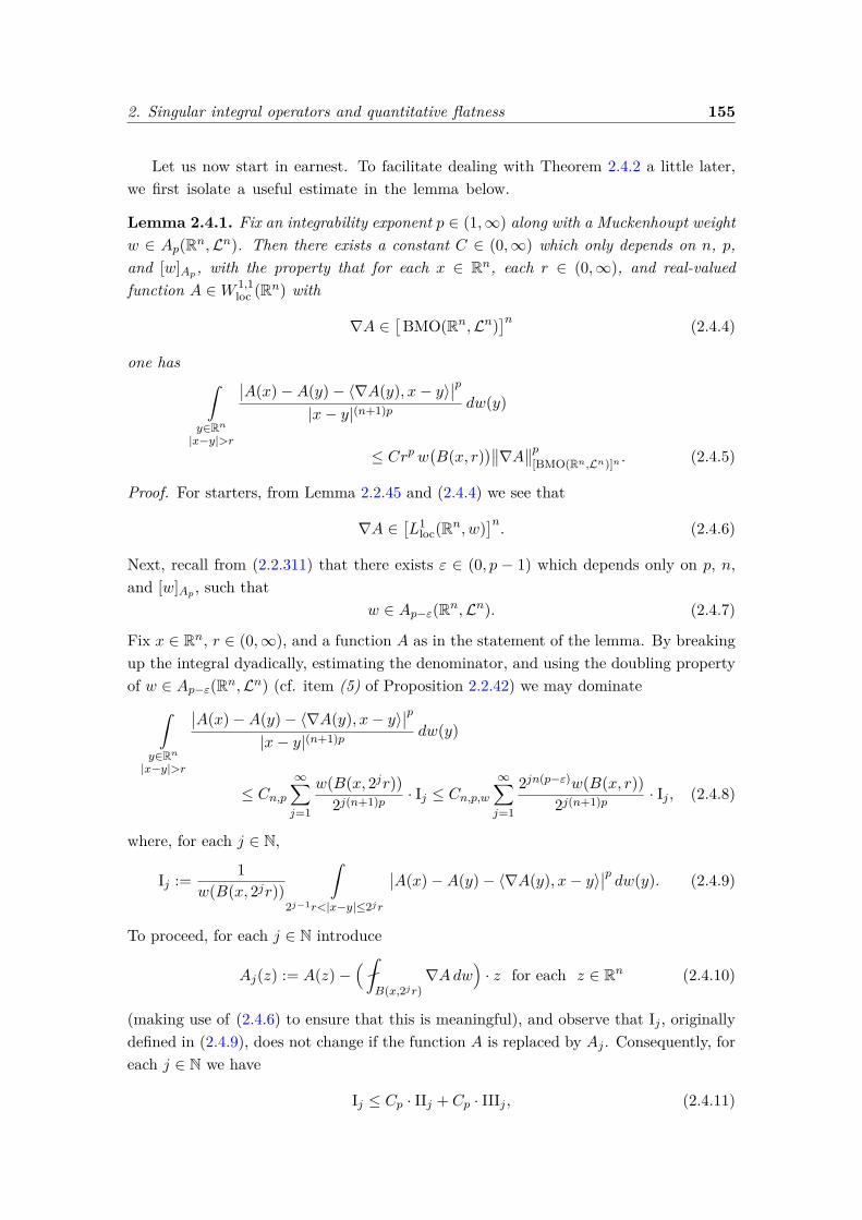
2. Singular integral operators and quantitative flatness 155
Let us now start in earnest. To facilitate dealing with Theorem 2.4.2 a little later,we first isolate a useful estimate in the lemma below.
Lemma 2.4.1. Fix an integrability exponent p ∈ (1,∞) along with a Muckenhoupt weightw ∈ Ap(Rn,Ln). Then there exists a constant C ∈ (0,∞) which only depends on n, p,and [w]Ap, with the property that for each x ∈ Rn, each r ∈ (0,∞), and real-valuedfunction A ∈W 1,1
loc (Rn) with
∇A ∈[BMO(Rn,Ln)
]n (2.4.4)
one hasˆ
y∈Rn|x−y|>r
∣∣A(x)−A(y)− 〈∇A(y), x− y〉∣∣p
|x− y|(n+1)p dw(y)
≤ Crpw(B(x, r)
)∥∥∇A∥∥p[BMO(Rn,Ln)]n . (2.4.5)
Proof. For starters, from Lemma 2.2.45 and (2.4.4) we see that
∇A ∈[L1
loc(Rn, w)]n. (2.4.6)
Next, recall from (2.2.311) that there exists ε ∈ (0, p − 1) which depends only on p, n,and [w]Ap , such that
w ∈ Ap−ε(Rn,Ln). (2.4.7)
Fix x ∈ Rn, r ∈ (0,∞), and a function A as in the statement of the lemma. By breakingup the integral dyadically, estimating the denominator, and using the doubling propertyof w ∈ Ap−ε(Rn,Ln) (cf. item (5) of Proposition 2.2.42) we may dominate
ˆ
y∈Rn|x−y|>r
∣∣A(x)−A(y)− 〈∇A(y), x− y〉∣∣p
|x− y|(n+1)p dw(y)
≤ Cn,p∞∑j=1
w(B(x, 2jr))2j(n+1)p · Ij ≤ Cn,p,w
∞∑j=1
2jn(p−ε)w(B(x, r))2j(n+1)p · Ij , (2.4.8)
where, for each j ∈ N,
Ij := 1w(B(x, 2jr))
ˆ
2j−1r<|x−y|≤2jr
∣∣A(x)−A(y)− 〈∇A(y), x− y〉∣∣p dw(y). (2.4.9)
To proceed, for each j ∈ N introduce
Aj(z) := A(z)−(
B(x,2jr)∇Adw
)· z for each z ∈ Rn (2.4.10)
(making use of (2.4.6) to ensure that this is meaningful), and observe that Ij , originallydefined in (2.4.9), does not change if the function A is replaced by Aj . Consequently, foreach j ∈ N we have
Ij ≤ Cp · IIj + Cp · IIIj , (2.4.11)
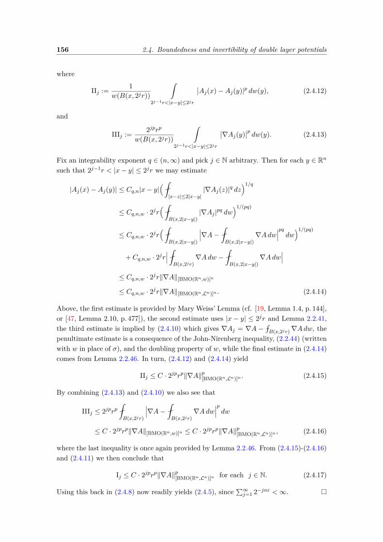
156 2.4. Boundedness and invertibility of double layer potentials
where
IIj := 1w(B(x, 2jr))
ˆ
2j−1r<|x−y|≤2jr
∣∣Aj(x)−Aj(y)|p dw(y), (2.4.12)
and
IIIj := 2jprp
w(B(x, 2jr))
ˆ
2j−1r<|x−y|≤2jr
∣∣∇Aj(y)∣∣p dw(y). (2.4.13)
Fix an integrability exponent q ∈ (n,∞) and pick j ∈ N arbitrary. Then for each y ∈ Rn
such that 2j−1r < |x− y| ≤ 2jr we may estimate
|Aj(x)−Aj(y)| ≤ Cq,n|x− y|( |x−z|≤2|x−y|
|∇Aj(z)|q dz)1/q
≤ Cq,n,w · 2jr(
B(x,2|x−y|)|∇Aj |pq dw
)1/(pq)
≤ Cq,n,w · 2jr(
B(x,2|x−y|)
∣∣∣∇A− B(x,2|x−y|)
∇Adw∣∣∣pq dw)1/(pq)
+ Cq,n,w · 2jr∣∣∣
B(x,2jr)∇Adw −
B(x,2|x−y|)
∇Adw∣∣∣
≤ Cq,n,w · 2jr‖∇A‖[BMO(Rn,w)]n
≤ Cq,n,w · 2jr‖∇A‖[BMO(Rn,Ln)]n . (2.4.14)
Above, the first estimate is provided by Mary Weiss’ Lemma (cf. [19, Lemma 1.4, p. 144],or [47, Lemma 2.10, p. 477]), the second estimate uses |x− y| ≤ 2jr and Lemma 2.2.41,the third estimate is implied by (2.4.10) which gives ∇Aj = ∇A −
fflB(x,2jr)∇Adw, the
penultimate estimate is a consequence of the John-Nirenberg inequality, (2.2.44) (writtenwith w in place of σ), and the doubling property of w, while the final estimate in (2.4.14)comes from Lemma 2.2.46. In turn, (2.4.12) and (2.4.14) yield
IIj ≤ C · 2jprp‖∇A‖p[BMO(Rn,Ln)]n . (2.4.15)
By combining (2.4.13) and (2.4.10) we also see that
IIIj ≤ 2jprp B(x,2jr)
∣∣∣∇A− B(x,2jr)
∇Adw∣∣∣p dw
≤ C · 2jprp‖∇A‖[BMO(Rn,w)]n ≤ C · 2jprp‖∇A‖p[BMO(Rn,Ln)]n , (2.4.16)
where the last inequality is once again provided by Lemma 2.2.46. From (2.4.15)-(2.4.16)and (2.4.11) we then conclude that
Ij ≤ C · 2jprp‖∇A‖p[BMO(Rn,Ln)]n for each j ∈ N. (2.4.17)
Using this back in (2.4.8) now readily yields (2.4.5), since∑∞j=1 2−jnε <∞.
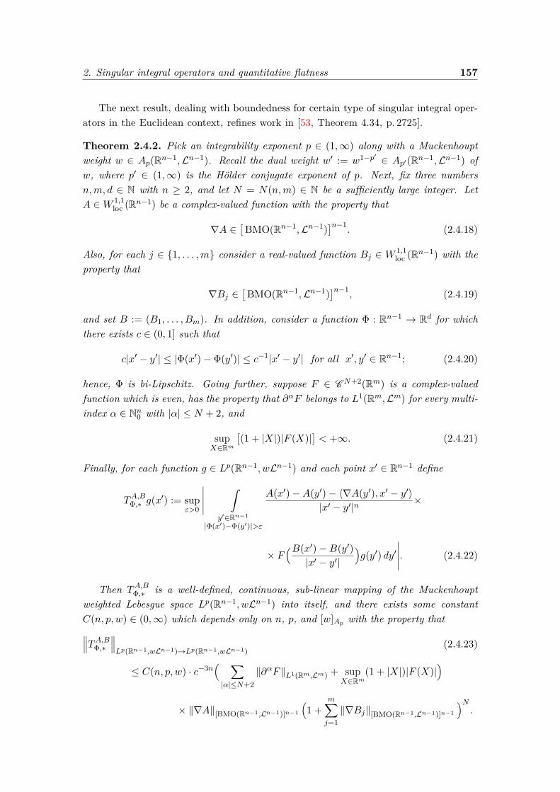
2. Singular integral operators and quantitative flatness 157
The next result, dealing with boundedness for certain type of singular integral oper-ators in the Euclidean context, refines work in [53, Theorem 4.34, p. 2725].
Theorem 2.4.2. Pick an integrability exponent p ∈ (1,∞) along with a Muckenhouptweight w ∈ Ap(Rn−1,Ln−1). Recall the dual weight w′ := w1−p′ ∈ Ap′(Rn−1,Ln−1) ofw, where p′ ∈ (1,∞) is the Hölder conjugate exponent of p. Next, fix three numbersn,m, d ∈ N with n ≥ 2, and let N = N(n,m) ∈ N be a sufficiently large integer. LetA ∈W 1,1
loc (Rn−1) be a complex-valued function with the property that
∇A ∈[BMO(Rn−1,Ln−1)
]n−1. (2.4.18)
Also, for each j ∈ 1, . . . ,m consider a real-valued function Bj ∈ W 1,1loc (Rn−1) with the
property that
∇Bj ∈[BMO(Rn−1,Ln−1)
]n−1, (2.4.19)
and set B := (B1, . . . , Bm). In addition, consider a function Φ : Rn−1 → Rd for whichthere exists c ∈ (0, 1] such that
c|x′ − y′| ≤ |Φ(x′)− Φ(y′)| ≤ c−1|x′ − y′| for all x′, y′ ∈ Rn−1; (2.4.20)
hence, Φ is bi-Lipschitz. Going further, suppose F ∈ CN+2(Rm) is a complex-valuedfunction which is even, has the property that ∂αF belongs to L1(Rm,Lm) for every multi-index α ∈ Nn0 with |α| ≤ N + 2, and
supX∈Rm
[(1 + |X|)|F (X)|
]< +∞. (2.4.21)
Finally, for each function g ∈ Lp(Rn−1, wLn−1) and each point x′ ∈ Rn−1 define
TA,BΦ,∗ g(x′) := supε>0
∣∣∣∣∣ˆ
y′∈Rn−1
|Φ(x′)−Φ(y′)|>ε
A(x′)−A(y′)− 〈∇A(y′), x′ − y′〉|x′ − y′|n
×
× F(B(x′)−B(y′)|x′ − y′|
)g(y′) dy′
∣∣∣∣∣. (2.4.22)
Then TA,BΦ,∗ is a well-defined, continuous, sub-linear mapping of the Muckenhouptweighted Lebesgue space Lp(Rn−1, wLn−1) into itself, and there exists some constantC(n, p, w) ∈ (0,∞) which depends only on n, p, and [w]Ap with the property that∥∥∥TA,BΦ,∗
∥∥∥Lp(Rn−1,wLn−1)→Lp(Rn−1,wLn−1)
(2.4.23)
≤ C(n, p, w) · c−3n( ∑|α|≤N+2
‖∂αF‖L1(Rm,Lm) + supX∈Rm
(1 + |X|)|F (X)|)
× ‖∇A‖[BMO(Rn−1,Ln−1)]n−1
(1 +
m∑j=1‖∇Bj‖[BMO(Rn−1,Ln−1)]n−1
)N.
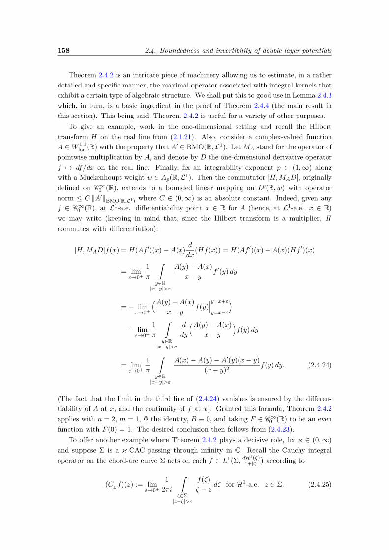
158 2.4. Boundedness and invertibility of double layer potentials
Theorem 2.4.2 is an intricate piece of machinery allowing us to estimate, in a ratherdetailed and specific manner, the maximal operator associated with integral kernels thatexhibit a certain type of algebraic structure. We shall put this to good use in Lemma 2.4.3which, in turn, is a basic ingredient in the proof of Theorem 2.4.4 (the main result inthis section). This being said, Theorem 2.4.2 is useful for a variety of other purposes.
To give an example, work in the one-dimensional setting and recall the Hilberttransform H on the real line from (2.1.21). Also, consider a complex-valued functionA ∈W 1,1
loc (R) with the property that A′ ∈ BMO(R,L1). LetMA stand for the operator ofpointwise multiplication by A, and denote by D the one-dimensional derivative operatorf 7→ df/dx on the real line. Finally, fix an integrability exponent p ∈ (1,∞) alongwith a Muckenhoupt weight w ∈ Ap(R,L1). Then the commutator [H,MAD], originallydefined on C∞0 (R), extends to a bounded linear mapping on Lp(R, w) with operatornorm ≤ C ‖A′‖BMO(R,L1) where C ∈ (0,∞) is an absolute constant. Indeed, given anyf ∈ C∞0 (R), at L1-a.e. differentiability point x ∈ R for A (hence, at L1-a.e. x ∈ R)we may write (keeping in mind that, since the Hilbert transform is a multiplier, Hcommutes with differentiation):
[H,MAD]f(x) = H(Af ′)(x)−A(x) ddx
(Hf(x)) = H(Af ′)(x)−A(x)(Hf ′)(x)
= limε→0+
1π
ˆ
y∈R|x−y|>ε
A(y)−A(x)x− y
f ′(y) dy
= − limε→0+
(A(y)−A(x)x− y
f(y)∣∣∣y=x+ε
y=x−ε
)− limε→0+
1π
ˆ
y∈R|x−y|>ε
d
dy
(A(y)−A(x)x− y
)f(y) dy
= limε→0+
1π
ˆ
y∈R|x−y|>ε
A(x)−A(y)−A′(y)(x− y)(x− y)2 f(y) dy. (2.4.24)
(The fact that the limit in the third line of (2.4.24) vanishes is ensured by the differen-tiability of A at x, and the continuity of f at x). Granted this formula, Theorem 2.4.2applies with n = 2, m = 1, Φ the identity, B ≡ 0, and taking F ∈ C∞0 (R) to be an evenfunction with F (0) = 1. The desired conclusion then follows from (2.4.23).
To offer another example where Theorem 2.4.2 plays a decisive role, fix κ ∈ (0,∞)and suppose Σ is a κ-CAC passing through infinity in C. Recall the Cauchy integraloperator on the chord-arc curve Σ acts on each f ∈ L1(Σ, dH1(ζ)
1+|ζ|)according to
(CΣf)(z) := limε→0+
12πi
ˆ
ζ∈Σ|z−ζ|>ε
f(ζ)ζ − z
dζ for H1-a.e. z ∈ Σ. (2.4.25)
2. Singular integral operators and quantitative flatness 159
Since from Proposition 2.2.9 we know that Σ is the topological boundary of a UR domain,Proposition 2.3.3 guarantees that CΣ is a well-defined, linear, and bounded operator onLp(Σ, w) whenever p ∈ (1,∞) and w ∈ Ap(Σ, σ), where σ := H1bΣ. Let us indicatehow Theorem 2.4.2 may be used to show that
the flatter the chord-arc curve Σ becomes, the closer the corre-sponding Cauchy operator becomes (with proximity measured in theoperator norm on Muckenhoupt weighted Lebesgue spaces) to the(suitably normalized) Hilbert transform on the real line.
(2.4.26)
A brief discussion on this topic may be found in [23, pp. 138-139]. In order to facilitatea direct comparison between the two singular integral operators mentioned in (2.4.26),it is natural to consider the pull-back of CΣ to R under the arc-length parametrizationR 3 s 7→ z(s) ∈ C of Σ. After natural adjustments in notation, this corresponds tothe mapping sending each f ∈ Lp(R, w) into
(CRf)(t) := limε→0+
i
2π
ˆ
s∈R|z(t)−z(s)|>ε
z ′(s)z(t)− z(s)f(s) ds for L1-a.e. t ∈ R, (2.4.27)
where p ∈ (1,∞) and w ∈ Ap(R,L1). Recall from (2.2.94) that the function z(·) isbi-Lipschitz, specifically,
(1 + κ)−1|t− s| ≤ |z(t)− z(s)| ≤ |t− s| for all t, s ∈ R. (2.4.28)
Keeping this in mind, a suitable application1 of [54, Proposition B.2] allows to changethe truncation in (2.4.27) to
(CRf)(t) = limε→0+
i
2π
ˆ
s∈R|t−s|>ε
z ′(s)z(t)− z(s)f(s) ds for L1-a.e. t ∈ R, (2.4.29)
for each f ∈ Lp(R, w) with p ∈ (1,∞) and w ∈ Ap(R,L1). We wish to compare theoperator written in this form with the (suitably normalized) Hilbert transform on the realline, acting on functions f ∈ Lp(R, w), where p ∈ (1,∞) and w ∈ Ap(R,L1), according to
(Hf)(t) := limε→0+
1π
ˆ
s∈R|t−s|>ε
f(s)t− s
ds for L1-a.e. t ∈ R. (2.4.30)
Fix p ∈ (1,∞), w ∈ Ap(R,L1), and f ∈ Lp(R, w). Then at L1-a.e. t ∈ R we may express(CR − (i/2)H
)f(t) = lim
ε→0+
i
2π
ˆ
s∈R|t−s|>ε
( z ′(s)z(t)− z(s) −
1t− s
)f(s) ds
= limε→0+
12πi
ˆ
s∈R|t−s|>ε
z(t)− z(s)− z ′(s)(t− s)(z(t)− z(s))(t− s) f(s) ds. (2.4.31)
1While [54, Proposition B.2] is stated for ordinary Lebesgue spaces, the same type of result holds inthe class of Muckenhoupt weighted Lebesgue spaces (thanks to the fact that the phenomenon in questionis local in nature, and (2.2.338)).
160 2.4. Boundedness and invertibility of double layer potentials
Pick an even function φ ∈ C∞0 (C) satisfying (with κ as in (2.4.28))
0 ≤ φ ≤ 1, φ ≡ 0 near 0 ∈ C, suppφ ⊆ B(0, 2),
φ ≡ 1 on B(0, 1) \B(0, (1 + κ)−1), (2.4.32)
along with a function ψ ∈ C∞0 (R) which is even and satisfies
0 ≤ ψ ≤ 1, suppψ ⊆ [−4, 4], and ψ ≡ 1 on [−2, 2] \[− 1
2 ,12]. (2.4.33)
We may then invoke Theorem 2.4.2 with n := 2, m := 3, and
Φ(t) := t, A(t) := z(t), B(t) :=(Re z(t), Im z(t), t
)for all t ∈ R,
F (a, b, c) := c
a+ ibφ(a+ ib)ψ(c) for all (a, b, c) ∈ R3,
(2.4.34)
and conclude from (2.4.23) and (2.2.103) that there exist some integer N ∈ N and someconstant Cp,w ∈ (0,∞) such that, with κ as in (2.4.28), we have
∥∥CR − (i/2)H∥∥Lp(R,w)→Lp(R,w) ≤ Cp,w(1 + κ)N
√κ. (2.4.35)
This lends credence to (2.4.26) since it implies
∥∥CR − (i/2)H∥∥Lp(R,w)→Lp(R,w) = O(
√κ ) as κ → 0+. (2.4.36)
After this preamble, we are ready to present the proof of Theorem 2.4.2.
Proof of Theorem 2.4.2. Throughout, let us abbreviate
K(x′, y′) := A(x′)−A(y′)− 〈∇A(y′), x′ − y′〉|x′ − y′|n
F(B(x′)−B(y′)|x′ − y′|
), (2.4.37)
for each x′ ∈ Rn−1 and Ln−1-a.e. y′ ∈ Rn−1. That, to begin with, TA,B∗ g(x′) in (2.4.56)is well-defined for each g ∈ Lp(Rn−1, wLn−1) and each x′ ∈ Rn−1 is ensured by observingthat
K(·, ·) is an Ln−1 ⊗ Ln−1-measurable function on Rn−1 × Rn−1, (2.4.38)
which is clear from (2.4.37), and that
for each g ∈ Lp(Rn−1, wLn−1), ε > 0, x′ ∈ Rn−1,
one hasˆ
y′∈Rn−1
|x′−y′|>ε
|K(x′, y′)||g(y′)| dy′ < +∞. (2.4.39)
The finiteness property in (2.4.39) is a consequence of Hölder’s inequality, (2.4.37), thefact that F is bounded, and Lemma 2.4.1 (used with n replaced by n− 1, p ′ in place of
2. Singular integral operators and quantitative flatness 161
p, and with w′ in place of w). In concert, these give that for each g ∈ Lp(Rn−1, wLn−1),each ε > 0, and each x′ ∈ Rn−1 we have
ˆ
y′∈Rn−1
|x′−y′|>ε
|K(x′, y′)||g(y′)| dy′ ≤ Cε[w′(B(x′, ε)
)]1/p′( supX∈Rm
|F (X)|)× (2.4.40)
× ‖g‖Lp(Rn−1,wLn−1)∥∥∇A∥∥[BMO(Rn−1,Ln−1)]n−1 <∞.
To proceed, for each function function g ∈ Lp(Rn−1, wLn−1), each truncation parameterε > 0, and each point x′ ∈ Rn−1 define
TA,BΦ,ε g(x′) :=ˆ
y′∈Rn−1
|Φ(x′)−Φ(y′)|>ε
K(x′, y′)g(y′) dy′. (2.4.41)
Thanks to (2.4.20) and (2.4.38)-(2.4.39), the above integral is absolutely convergent,which means that TA,BΦ,ε g(x′) is a well-defined number. If Q+ denotes the collection of allpositive rational numbers, we claim that for each function g ∈ Lp(Rn−1, wLn−1) we have
(TA,BΦ,∗ g
)(x′) = sup
ε∈Q+
∣∣(TA,BΦ,ε g)(x′)
∣∣ for every x′ ∈ Rn−1. (2.4.42)
To justify this, pick some g ∈ Lp(Rn−1, wLn−1). The idea is to show that if x′ ∈ Rn−1
is arbitrary and fixed then for each ε ∈ (0,∞) and each sequence εjj∈N ⊆ (0,∞) suchthat εj ε as j →∞ we have
limj→∞
(TA,BΦ,εj g
)(x′) =
(TA,BΦ,ε g
)(x′). (2.4.43)
To justify (2.4.43) note that
y′ ∈ Rn−1 : |Φ(x′)− Φ(y′)| > εj y′ ∈ Rn−1 : |Φ(x′)− Φ(y′)| > ε (2.4.44)
as j →∞, in the sense that
y′ ∈ Rn−1 : |Φ(x′)− Φ(y′)| > ε =⋃j∈Ny′ ∈ Rn−1 : |Φ(x′)− Φ(y′)| > εj (2.4.45)
and
y′ ∈ Rn−1 : |Φ(x′)− Φ(y′)| > εj ⊆ y′ ∈ Rn−1 : |Φ(x′)− Φ(y′)| > εj+1 (2.4.46)
for every j ∈ N. Then (2.4.43) follows from (2.4.44) and Lebesgue’s Dominated Conver-gence Theorem (whose applicability is ensured by (2.4.38)-(2.4.39)). Having establishedthis, (2.4.42) readily follows on account of the density of Q+ in (0,∞).
Moving on, we claim that
for each fixed threshold ε > 0, the function
Rn−1 × Rn−1 3 (x′, y′) 7−→(1y′∈Rn−1, |Φ(x′)−Φ(y′)|>ε
)(y′) ∈ R
is lower-semicontinuous, hence Ln−1 ⊗ Ln−1-measurable.
(2.4.47)
162 2.4. Boundedness and invertibility of double layer potentials
To justify this claim, observe that for every number λ ∈ R the set of points in Rn−1×Rn−1
where the given function is > λ may be described as∅ if λ ≥ 1,(x′, y′) ∈ Rn−1 × Rn−1 : |Φ(x′)− Φ(y′)| > ε
if λ ∈ [0, 1),
Rn−1 × Rn−1 if λ < 0.
(2.4.48)
Thanks to the fact that Φ is a continuous function, all sets appearing in (2.4.48) are openin Rn−1 × Rn−1. This proves that the function (2.4.47) is indeed lower-semicontinuous.
We next claim that
given any g ∈ Lp(Rn−1, wLn−1), thefunction TA,BΦ,∗ g is Ln−1-measurable. (2.4.49)
To see that this is the case, granted (2.4.42) and since the supremum of some countablefamily of Ln−1-measurable functions is itself a Ln−1-measurable function, it suffices toshow that
TA,BΦ,ε g is a Ln−1-measurable function, for each fixed
ε ∈ (0,∞) and each fixed g ∈ Lp(Rn−1, wLn−1).(2.4.50)
With this goal in mind, fix ε ∈ (0,∞) along with g ∈ Lp(Rn−1, wLn−1), and for eachj ∈ N define
Gj : Rn−1 × Rn−1 −→ R given at every (x′, y′) ∈ Rn−1 × Rn−1 by
Gj(x′, y′) :=(1B(0′,j)
)(x′)K(x′, y′)g(y′)
(1y′∈Rn−1, |Φ(x′)−Φ(y′)|>ε
)(y′).
(2.4.51)
Then, thanks to (2.4.38) and (2.4.47), it follows that Gj is an Ln−1 ⊗ Ln−1-measurablefunction for each j ∈ N. In addition, from (2.4.51), (2.4.39), and since balls have finitemeasure, we see that
ˆRn−1×Rn−1
|Gj(x′, y′)| dx′dy′ < +∞. (2.4.52)
Granted these properties, Fubini’s Theorem (whose applicability is ensured by the factthat
(Rn−1,Ln−1) is a sigma-finite measure space) then guarantees that
gj : Rn−1 → R, gj(x′) :=ˆRn−1
Gj(x′, y′) dy′, ∀x′ ∈ Rn−1,
is an Ln−1-measurable function, for each integer j ∈ N.(2.4.53)
On the other hand, from (2.4.51), (2.4.53), and (2.4.41) it is apparent that for each j ∈ Nwe have
gj = 1B(0′,j) TA,BΦ,ε g everywhere in Rn−1. (2.4.54)
In particular, this implies
limj→∞
gj = TA,BΦ,ε g pointwise everywhere in Rn−1. (2.4.55)
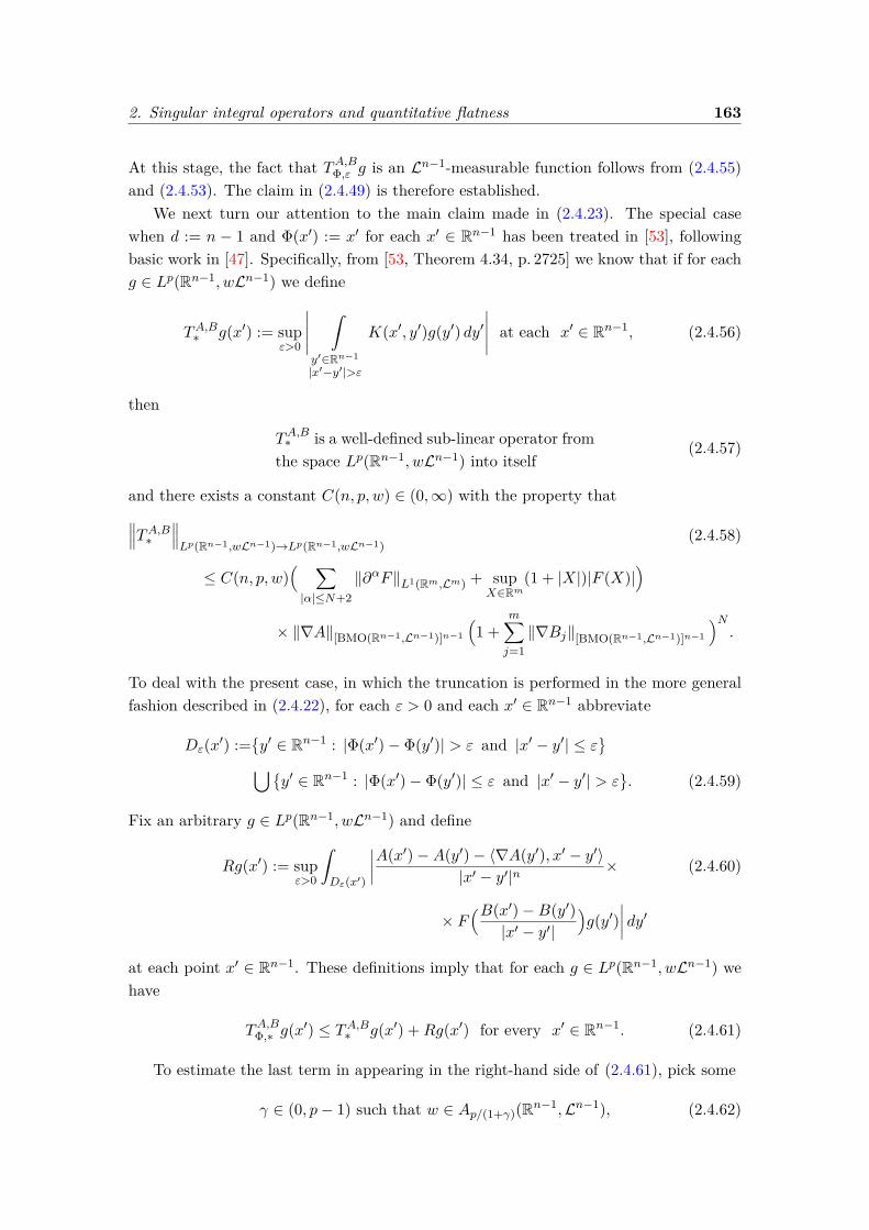
2. Singular integral operators and quantitative flatness 163
At this stage, the fact that TA,BΦ,ε g is an Ln−1-measurable function follows from (2.4.55)and (2.4.53). The claim in (2.4.49) is therefore established.
We next turn our attention to the main claim made in (2.4.23). The special casewhen d := n − 1 and Φ(x′) := x′ for each x′ ∈ Rn−1 has been treated in [53], followingbasic work in [47]. Specifically, from [53, Theorem 4.34, p. 2725] we know that if for eachg ∈ Lp(Rn−1, wLn−1) we define
TA,B∗ g(x′) := supε>0
∣∣∣∣∣ˆ
y′∈Rn−1
|x′−y′|>ε
K(x′, y′)g(y′) dy′∣∣∣∣∣ at each x′ ∈ Rn−1, (2.4.56)
then
TA,B∗ is a well-defined sub-linear operator fromthe space Lp(Rn−1, wLn−1) into itself
(2.4.57)
and there exists a constant C(n, p, w) ∈ (0,∞) with the property that∥∥∥TA,B∗ ∥∥∥Lp(Rn−1,wLn−1)→Lp(Rn−1,wLn−1)
(2.4.58)
≤ C(n, p, w)( ∑|α|≤N+2
‖∂αF‖L1(Rm,Lm) + supX∈Rm
(1 + |X|)|F (X)|)
× ‖∇A‖[BMO(Rn−1,Ln−1)]n−1
(1 +
m∑j=1‖∇Bj‖[BMO(Rn−1,Ln−1)]n−1
)N.
To deal with the present case, in which the truncation is performed in the more generalfashion described in (2.4.22), for each ε > 0 and each x′ ∈ Rn−1 abbreviate
Dε(x′) :=y′ ∈ Rn−1 : |Φ(x′)− Φ(y′)| > ε and |x′ − y′| ≤ ε
⋃
y′ ∈ Rn−1 : |Φ(x′)− Φ(y′)| ≤ ε and |x′ − y′| > ε. (2.4.59)
Fix an arbitrary g ∈ Lp(Rn−1, wLn−1) and define
Rg(x′) := supε>0
ˆDε(x′)
∣∣∣∣A(x′)−A(y′)− 〈∇A(y′), x′ − y′〉|x′ − y′|n
× (2.4.60)
× F(B(x′)−B(y′)|x′ − y′|
)g(y′)
∣∣∣∣ dy′at each point x′ ∈ Rn−1. These definitions imply that for each g ∈ Lp(Rn−1, wLn−1) wehave
TA,BΦ,∗ g(x′) ≤ TA,B∗ g(x′) +Rg(x′) for every x′ ∈ Rn−1. (2.4.61)
To estimate the last term in appearing in the right-hand side of (2.4.61), pick some
γ ∈ (0, p− 1) such that w ∈ Ap/(1+γ)(Rn−1,Ln−1), (2.4.62)
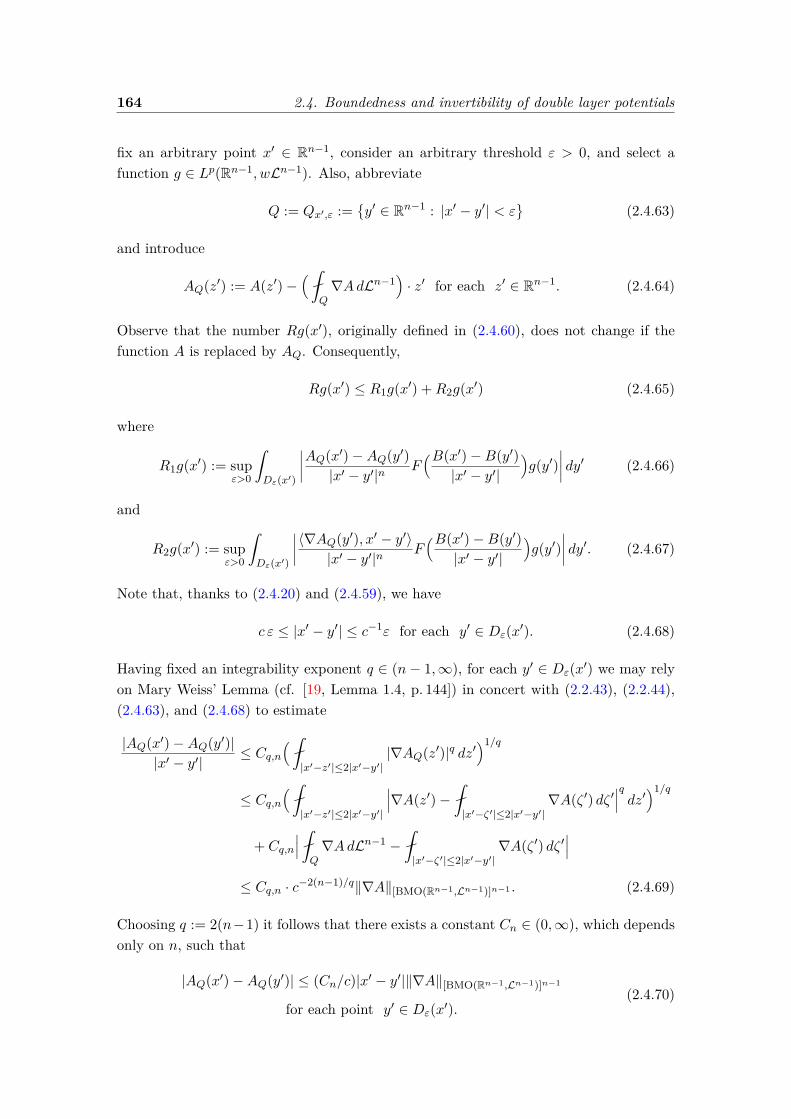
164 2.4. Boundedness and invertibility of double layer potentials
fix an arbitrary point x′ ∈ Rn−1, consider an arbitrary threshold ε > 0, and select afunction g ∈ Lp(Rn−1, wLn−1). Also, abbreviate
Q := Qx′,ε :=y′ ∈ Rn−1 : |x′ − y′| < ε
(2.4.63)
and introduce
AQ(z′) := A(z′)−(
Q∇AdLn−1
)· z′ for each z′ ∈ Rn−1. (2.4.64)
Observe that the number Rg(x′), originally defined in (2.4.60), does not change if thefunction A is replaced by AQ. Consequently,
Rg(x′) ≤ R1g(x′) +R2g(x′) (2.4.65)
where
R1g(x′) := supε>0
ˆDε(x′)
∣∣∣∣AQ(x′)−AQ(y′)|x′ − y′|n
F(B(x′)−B(y′)|x′ − y′|
)g(y′)
∣∣∣∣ dy′ (2.4.66)
and
R2g(x′) := supε>0
ˆDε(x′)
∣∣∣∣〈∇AQ(y′), x′ − y′〉|x′ − y′|n
F(B(x′)−B(y′)|x′ − y′|
)g(y′)
∣∣∣∣ dy′. (2.4.67)
Note that, thanks to (2.4.20) and (2.4.59), we have
c ε ≤ |x′ − y′| ≤ c−1ε for each y′ ∈ Dε(x′). (2.4.68)
Having fixed an integrability exponent q ∈ (n− 1,∞), for each y′ ∈ Dε(x′) we may relyon Mary Weiss’ Lemma (cf. [19, Lemma 1.4, p. 144]) in concert with (2.2.43), (2.2.44),(2.4.63), and (2.4.68) to estimate
|AQ(x′)−AQ(y′)||x′ − y′|
≤ Cq,n( |x′−z′|≤2|x′−y′|
|∇AQ(z′)|q dz′)1/q
≤ Cq,n( |x′−z′|≤2|x′−y′|
∣∣∣∇A(z′)− |x′−ζ′|≤2|x′−y′|
∇A(ζ ′) dζ ′∣∣∣q dz′)1/q
+ Cq,n∣∣∣
Q∇AdLn−1 −
|x′−ζ′|≤2|x′−y′|
∇A(ζ ′) dζ ′∣∣∣
≤ Cq,n · c−2(n−1)/q‖∇A‖[BMO(Rn−1,Ln−1)]n−1 . (2.4.69)
Choosing q := 2(n−1) it follows that there exists a constant Cn ∈ (0,∞), which dependsonly on n, such that
|AQ(x′)−AQ(y′)| ≤ (Cn/c)|x′ − y′|‖∇A‖[BMO(Rn−1,Ln−1)]n−1
for each point y′ ∈ Dε(x′).(2.4.70)
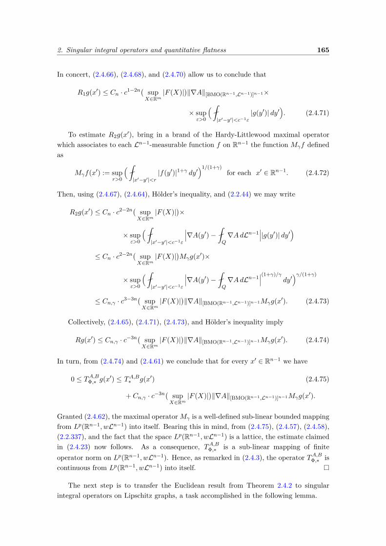
2. Singular integral operators and quantitative flatness 165
In concert, (2.4.66), (2.4.68), and (2.4.70) allow us to conclude that
R1g(x′) ≤ Cn · c1−2n( supX∈Rm
|F (X)|)‖∇A‖[BMO(Rn−1,Ln−1)]n−1×
× supε>0
( |x′−y′|<c−1ε
|g(y′)| dy′). (2.4.71)
To estimate R2g(x′), bring in a brand of the Hardy-Littlewood maximal operatorwhich associates to each Ln−1-measurable function f on Rn−1 the function Mγf definedas
Mγf(x′) := supr>0
( |x′−y′|<r
|f(y′)|1+γ dy′)1/(1+γ)
for each x′ ∈ Rn−1. (2.4.72)
Then, using (2.4.67), (2.4.64), Hölder’s inequality, and (2.2.44) we may write
R2g(x′) ≤ Cn · c2−2n( supX∈Rm
|F (X)|)×
× supε>0
( |x′−y′|<c−1ε
∣∣∣∇A(y′)− Q∇AdLn−1
∣∣∣|g(y′)| dy′)
≤ Cn · c2−2n( supX∈Rm
|F (X)|)Mγg(x′)×
× supε>0
( |x′−y′|<c−1ε
∣∣∣∇A(y′)− Q∇AdLn−1
∣∣∣(1+γ)/γdy′)γ/(1+γ)
≤ Cn,γ · c3−3n( supX∈Rm
|F (X)|)‖∇A‖[BMO(Rn−1,Ln−1)]n−1Mγg(x′). (2.4.73)
Collectively, (2.4.65), (2.4.71), (2.4.73), and Hölder’s inequality imply
Rg(x′) ≤ Cn,γ · c−3n( supX∈Rm
|F (X)|)‖∇A‖[BMO(Rn−1,Ln−1)]n−1Mγg(x′). (2.4.74)
In turn, from (2.4.74) and (2.4.61) we conclude that for every x′ ∈ Rn−1 we have
0 ≤ TA,BΦ,∗ g(x′) ≤ TA,B∗ g(x′) (2.4.75)
+ Cn,γ · c−3n( supX∈Rm
|F (X)|)‖∇A‖[BMO(Rn−1,Ln−1)]n−1Mγg(x′).
Granted (2.4.62), the maximal operatorMγ is a well-defined sub-linear bounded mappingfrom Lp(Rn−1, wLn−1) into itself. Bearing this in mind, from (2.4.75), (2.4.57), (2.4.58),(2.2.337), and the fact that the space Lp(Rn−1, wLn−1) is a lattice, the estimate claimedin (2.4.23) now follows. As a consequence, TA,BΦ,∗ is a sub-linear mapping of finiteoperator norm on Lp(Rn−1, wLn−1). Hence, as remarked in (2.4.3), the operator TA,BΦ,∗ iscontinuous from Lp(Rn−1, wLn−1) into itself.
The next step is to transfer the Euclidean result from Theorem 2.4.2 to singularintegral operators on Lipschitz graphs, a task accomplished in the following lemma.
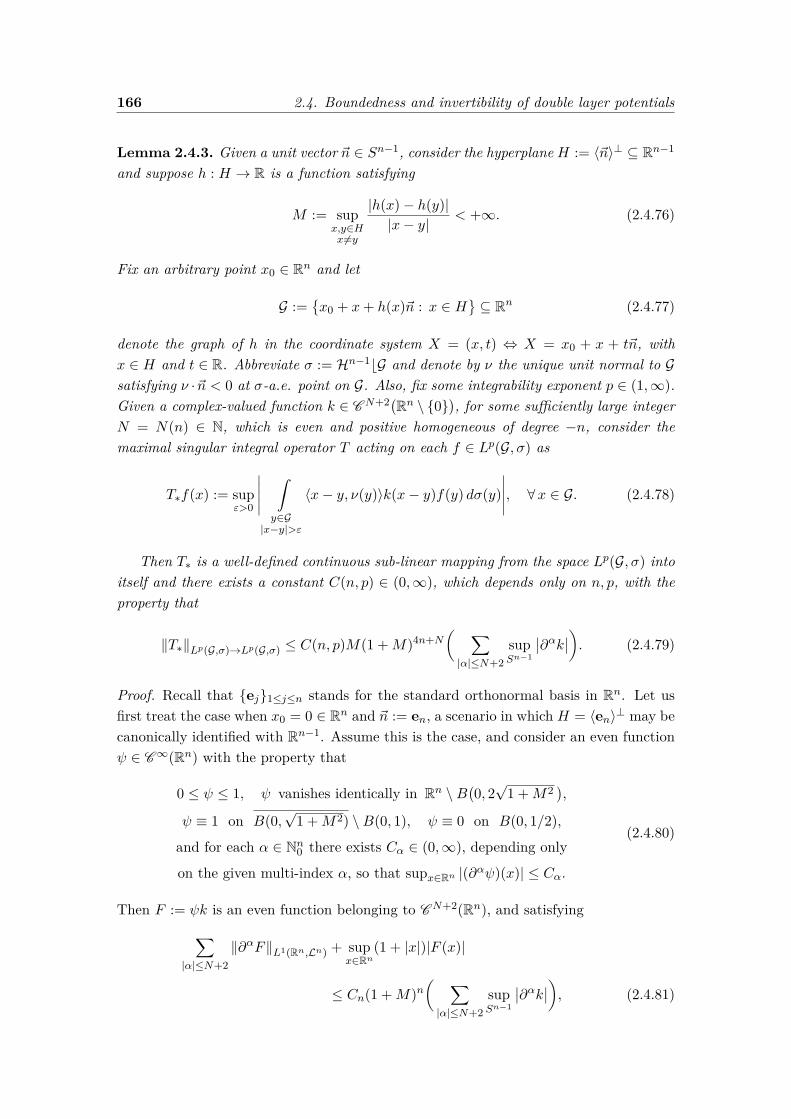
166 2.4. Boundedness and invertibility of double layer potentials
Lemma 2.4.3. Given a unit vector ~n ∈ Sn−1, consider the hyperplane H := 〈~n〉⊥ ⊆ Rn−1
and suppose h : H → R is a function satisfying
M := supx,y∈Hx 6=y
|h(x)− h(y)||x− y|
< +∞. (2.4.76)
Fix an arbitrary point x0 ∈ Rn and let
G :=x0 + x+ h(x)~n : x ∈ H
⊆ Rn (2.4.77)
denote the graph of h in the coordinate system X = (x, t) ⇔ X = x0 + x + t~n, withx ∈ H and t ∈ R. Abbreviate σ := Hn−1bG and denote by ν the unique unit normal to Gsatisfying ν ·~n < 0 at σ-a.e. point on G. Also, fix some integrability exponent p ∈ (1,∞).Given a complex-valued function k ∈ CN+2(Rn \ 0), for some sufficiently large integerN = N(n) ∈ N, which is even and positive homogeneous of degree −n, consider themaximal singular integral operator T acting on each f ∈ Lp(G, σ) as
T∗f(x) := supε>0
∣∣∣∣∣ˆ
y∈G|x−y|>ε
〈x− y, ν(y)〉k(x− y)f(y) dσ(y)∣∣∣∣∣, ∀x ∈ G. (2.4.78)
Then T∗ is a well-defined continuous sub-linear mapping from the space Lp(G, σ) intoitself and there exists a constant C(n, p) ∈ (0,∞), which depends only on n, p, with theproperty that
‖T∗‖Lp(G,σ)→Lp(G,σ) ≤ C(n, p)M(1 +M)4n+N( ∑|α|≤N+2
supSn−1
∣∣∂αk∣∣). (2.4.79)
Proof. Recall that ej1≤j≤n stands for the standard orthonormal basis in Rn. Let usfirst treat the case when x0 = 0 ∈ Rn and ~n := en, a scenario in which H = 〈en〉⊥ may becanonically identified with Rn−1. Assume this is the case, and consider an even functionψ ∈ C∞(Rn) with the property that
0 ≤ ψ ≤ 1, ψ vanishes identically in Rn \B(0, 2√
1 +M2 ),ψ ≡ 1 on B(0,
√1 +M2) \B(0, 1), ψ ≡ 0 on B(0, 1/2),
and for each α ∈ Nn0 there exists Cα ∈ (0,∞), depending only
on the given multi-index α, so that supx∈Rn |(∂αψ)(x)| ≤ Cα.
(2.4.80)
Then F := ψk is an even function belonging to CN+2(Rn), and satisfying∑|α|≤N+2
‖∂αF‖L1(Rn,Ln) + supx∈Rn
(1 + |x|)|F (x)|
≤ Cn(1 +M)n( ∑|α|≤N+2
supSn−1
∣∣∂αk∣∣), (2.4.81)
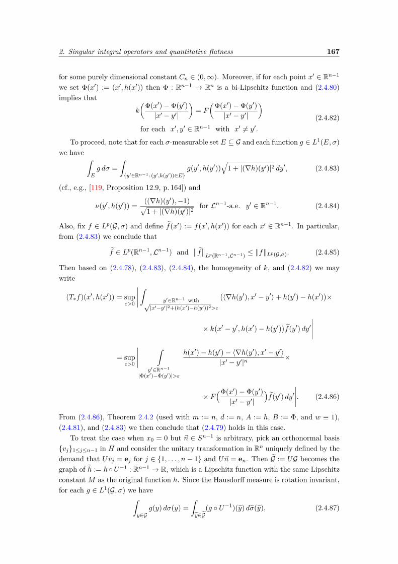
2. Singular integral operators and quantitative flatness 167
for some purely dimensional constant Cn ∈ (0,∞). Moreover, if for each point x′ ∈ Rn−1
we set Φ(x′) := (x′, h(x′)) then Φ : Rn−1 → Rn is a bi-Lipschitz function and (2.4.80)implies that
k
(Φ(x′)− Φ(y′)|x′ − y′|
)= F
(Φ(x′)− Φ(y′)|x′ − y′|
)for each x′, y′ ∈ Rn−1 with x′ 6= y′.
(2.4.82)
To proceed, note that for each σ-measurable set E ⊆ G and each function g ∈ L1(E, σ)we have ˆ
Eg dσ =
ˆy′∈Rn−1: (y′,h(y′))∈E
g(y′, h(y′))√
1 + |(∇h)(y′)|2 dy′, (2.4.83)
(cf., e.g., [119, Proposition 12.9, p. 164]) and
ν(y′, h(y′)) = ((∇h)(y′),−1)√1 + |(∇h)(y′)|2
for Ln−1-a.e. y′ ∈ Rn−1. (2.4.84)
Also, fix f ∈ Lp(G, σ) and define f(x′) := f(x′, h(x′)) for each x′ ∈ Rn−1. In particular,from (2.4.83) we conclude that
f ∈ Lp(Rn−1,Ln−1) and∥∥f∥∥
Lp(Rn−1,Ln−1) ≤ ‖f‖Lp(G,σ). (2.4.85)
Then based on (2.4.78), (2.4.83), (2.4.84), the homogeneity of k, and (2.4.82) we maywrite
(T∗f)(x′, h(x′)) = supε>0
∣∣∣∣∣ˆ
y′∈Rn−1 with√|x′−y′|2+(h(x′)−h(y′))2>ε
(〈∇h(y′), x′ − y′〉+ h(y′)− h(x′)
)×
× k(x′ − y′, h(x′)− h(y′)
)f(y′) dy′
∣∣∣∣∣= sup
ε>0
∣∣∣∣∣ˆ
y′∈Rn−1
|Φ(x′)−Φ(y′)|>ε
h(x′)− h(y′)− 〈∇h(y′), x′ − y′〉|x′ − y′|n
×
× F(Φ(x′)− Φ(y′)|x′ − y′|
)f(y′) dy′
∣∣∣∣∣. (2.4.86)
From (2.4.86), Theorem 2.4.2 (used with m := n, d := n, A := h, B := Φ, and w ≡ 1),(2.4.81), and (2.4.83) we then conclude that (2.4.79) holds in this case.
To treat the case when x0 = 0 but ~n ∈ Sn−1 is arbitrary, pick an orthonormal basisvj1≤j≤n−1 in H and consider the unitary transformation in Rn uniquely defined by thedemand that Uvj = ej for j ∈ 1, . . . , n− 1 and U~n = en. Then G := UG becomes thegraph of h := h U−1 : Rn−1 → R, which is a Lipschitz function with the same Lipschitzconstant M as the original function h. Since the Hausdorff measure is rotation invariant,for each g ∈ L1(G, σ) we haveˆ
y∈Gg(y) dσ(y) =
ˆy∈G
(g U−1)(y) dσ(y), (2.4.87)
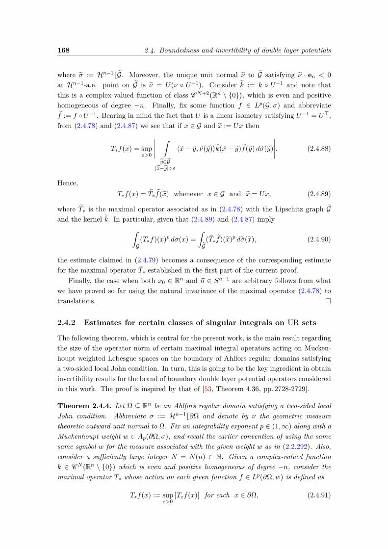
168 2.4. Boundedness and invertibility of double layer potentials
where σ := Hn−1bG. Moreover, the unique unit normal ν to G satisfying ν · en < 0at Hn−1-a.e. point on G is ν = U(ν U−1). Consider k := k U−1 and note thatthis is a complex-valued function of class CN+2(Rn \ 0), which is even and positivehomogeneous of degree −n. Finally, fix some function f ∈ Lp(G, σ) and abbreviatef := f U−1. Bearing in mind the fact that U is a linear isometry satisfying U−1 = U>,from (2.4.78) and (2.4.87) we see that if x ∈ G and x := Ux then
T∗f(x) = supε>0
∣∣∣∣∣ˆ
y∈G|x−y|>ε
〈x− y, ν(y)〉k(x− y)f(y) dσ(y)∣∣∣∣∣. (2.4.88)
Hence,T∗f(x) = T∗f(x) whenever x ∈ G and x = Ux, (2.4.89)
where T∗ is the maximal operator associated as in (2.4.78) with the Lipschitz graph Gand the kernel k. In particular, given that (2.4.89) and (2.4.87) imply
ˆG(T∗f)(x)p dσ(x) =
ˆG(T∗f)(x)p dσ(x), (2.4.90)
the estimate claimed in (2.4.79) becomes a consequence of the corresponding estimatefor the maximal operator T∗ established in the first part of the current proof.
Finally, the case when both x0 ∈ Rn and ~n ∈ Sn−1 are arbitrary follows from whatwe have proved so far using the natural invariance of the maximal operator (2.4.78) totranslations.
2.4.2 Estimates for certain classes of singular integrals on UR sets
The following theorem, which is central for the present work, is the main result regardingthe size of the operator norm of certain maximal integral operators acting on Mucken-houpt weighted Lebesgue spaces on the boundary of Ahlfors regular domains satisfyinga two-sided local John condition. In turn, this is going to be the key ingredient in obtaininvertibility results for the brand of boundary double layer potential operators consideredin this work. The proof is inspired by that of [53, Theorem 4.36, pp. 2728-2729].
Theorem 2.4.4. Let Ω ⊆ Rn be an Ahlfors regular domain satisfying a two-sided localJohn condition. Abbreviate σ := Hn−1b∂Ω and denote by ν the geometric measuretheoretic outward unit normal to Ω. Fix an integrability exponent p ∈ (1,∞) along with aMuckenhoupt weight w ∈ Ap(∂Ω, σ), and recall the earlier convention of using the samesame symbol w for the measure associated with the given weight w as in (2.2.292). Also,consider a sufficiently large integer N = N(n) ∈ N. Given a complex-valued functionk ∈ CN (Rn \ 0) which is even and positive homogeneous of degree −n, consider themaximal operator T∗ whose action on each given function f ∈ Lp(∂Ω, w) is defined as
T∗f(x) := supε>0
∣∣Tεf(x)∣∣ for each x ∈ ∂Ω, (2.4.91)
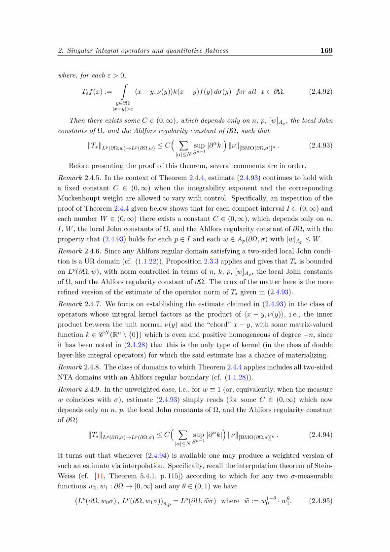
2. Singular integral operators and quantitative flatness 169
where, for each ε > 0,
Tεf(x) :=ˆ
y∈∂Ω|x−y|>ε
〈x− y, ν(y)〉k(x− y)f(y) dσ(y) for all x ∈ ∂Ω. (2.4.92)
Then there exists some C ∈ (0,∞), which depends only on n, p, [w]Ap, the local Johnconstants of Ω, and the Ahlfors regularity constant of ∂Ω, such that
‖T∗‖Lp(∂Ω,w)→Lp(∂Ω,w) ≤ C( ∑|α|≤N
supSn−1
|∂αk|)‖ν‖[BMO(∂Ω,σ)]n . (2.4.93)
Before presenting the proof of this theorem, several comments are in order.Remark 2.4.5. In the context of Theorem 2.4.4, estimate (2.4.93) continues to hold witha fixed constant C ∈ (0,∞) when the integrability exponent and the correspondingMuckenhoupt weight are allowed to vary with control. Specifically, an inspection of theproof of Theorem 2.4.4 given below shows that for each compact interval I ⊂ (0,∞) andeach number W ∈ (0,∞) there exists a constant C ∈ (0,∞), which depends only on n,I, W , the local John constants of Ω, and the Ahlfors regularity constant of ∂Ω, with theproperty that (2.4.93) holds for each p ∈ I and each w ∈ Ap(∂Ω, σ) with [w]Ap ≤W .Remark 2.4.6. Since any Ahlfors regular domain satisfying a two-sided local John condi-tion is a UR domain (cf. (1.1.22)), Proposition 2.3.3 applies and gives that T∗ is boundedon Lp(∂Ω, w), with norm controlled in terms of n, k, p, [w]Ap , the local John constantsof Ω, and the Ahlfors regularity constant of ∂Ω. The crux of the matter here is the morerefined version of the estimate of the operator norm of T∗ given in (2.4.93).Remark 2.4.7. We focus on establishing the estimate claimed in (2.4.93) in the class ofoperators whose integral kernel factors as the product of 〈x − y, ν(y)〉, i.e., the innerproduct between the unit normal ν(y) and the “chord” x − y, with some matrix-valuedfunction k ∈ CN (Rn \ 0) which is even and positive homogeneous of degree −n, sinceit has been noted in (2.1.28) that this is the only type of kernel (in the class of doublelayer-like integral operators) for which the said estimate has a chance of materializing.Remark 2.4.8. The class of domains to which Theorem 2.4.4 applies includes all two-sidedNTA domains with an Ahlfors regular boundary (cf. (1.1.28)).Remark 2.4.9. In the unweighted case, i.e., for w ≡ 1 (or, equivalently, when the measurew coincides with σ), estimate (2.4.93) simply reads (for some C ∈ (0,∞) which nowdepends only on n, p, the local John constants of Ω, and the Ahlfors regularity constantof ∂Ω)
‖T∗‖Lp(∂Ω,σ)→Lp(∂Ω,σ) ≤ C( ∑|α|≤N
supSn−1
|∂αk|)‖ν‖[BMO(∂Ω,σ)]n . (2.4.94)
It turns out that whenever (2.4.94) is available one may produce a weighted version ofsuch an estimate via interpolation. Specifically, recall the interpolation theorem of Stein-Weiss (cf. [11, Theorem 5.4.1, p. 115]) according to which for any two σ-measurablefunctions w0, w1 : ∂Ω→ [0,∞] and any θ ∈ (0, 1) we have(
Lp(∂Ω, w0σ) , Lp(∂Ω, w1σ))θ,p
= Lp(∂Ω, wσ) where w := w1−θ0 · wθ1. (2.4.95)
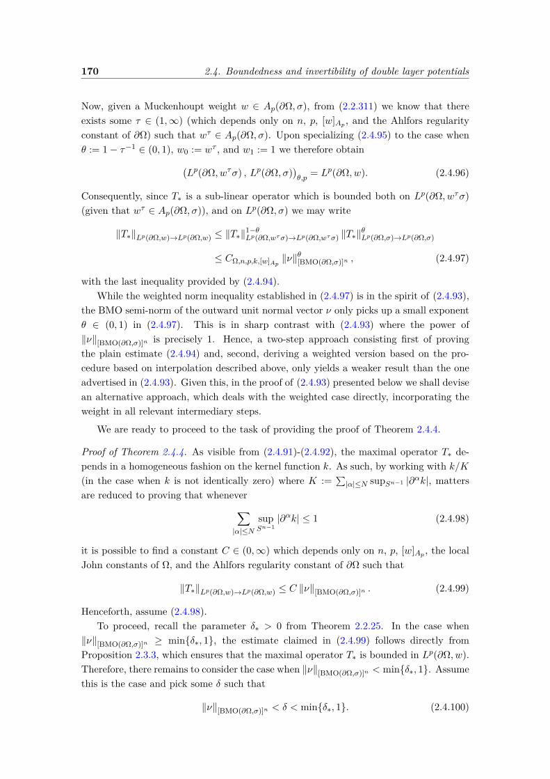
170 2.4. Boundedness and invertibility of double layer potentials
Now, given a Muckenhoupt weight w ∈ Ap(∂Ω, σ), from (2.2.311) we know that thereexists some τ ∈ (1,∞) (which depends only on n, p, [w]Ap , and the Ahlfors regularityconstant of ∂Ω) such that wτ ∈ Ap(∂Ω, σ). Upon specializing (2.4.95) to the case whenθ := 1− τ−1 ∈ (0, 1), w0 := wτ , and w1 := 1 we therefore obtain(
Lp(∂Ω, wτσ) , Lp(∂Ω, σ))θ,p
= Lp(∂Ω, w). (2.4.96)
Consequently, since T∗ is a sub-linear operator which is bounded both on Lp(∂Ω, wτσ)(given that wτ ∈ Ap(∂Ω, σ)), and on Lp(∂Ω, σ) we may write
‖T∗‖Lp(∂Ω,w)→Lp(∂Ω,w) ≤ ‖T∗‖1−θLp(∂Ω,wτσ)→Lp(∂Ω,wτσ) ‖T∗‖
θLp(∂Ω,σ)→Lp(∂Ω,σ)
≤ CΩ,n,p,k,[w]Ap ‖ν‖θ[BMO(∂Ω,σ)]n , (2.4.97)
with the last inequality provided by (2.4.94).While the weighted norm inequality established in (2.4.97) is in the spirit of (2.4.93),
the BMO semi-norm of the outward unit normal vector ν only picks up a small exponentθ ∈ (0, 1) in (2.4.97). This is in sharp contrast with (2.4.93) where the power of‖ν‖[BMO(∂Ω,σ)]n is precisely 1. Hence, a two-step approach consisting first of provingthe plain estimate (2.4.94) and, second, deriving a weighted version based on the pro-cedure based on interpolation described above, only yields a weaker result than the oneadvertised in (2.4.93). Given this, in the proof of (2.4.93) presented below we shall devisean alternative approach, which deals with the weighted case directly, incorporating theweight in all relevant intermediary steps.
We are ready to proceed to the task of providing the proof of Theorem 2.4.4.
Proof of Theorem 2.4.4. As visible from (2.4.91)-(2.4.92), the maximal operator T∗ de-pends in a homogeneous fashion on the kernel function k. As such, by working with k/K(in the case when k is not identically zero) where K :=
∑|α|≤N supSn−1 |∂αk|, matters
are reduced to proving that whenever∑|α|≤N
supSn−1
|∂αk| ≤ 1 (2.4.98)
it is possible to find a constant C ∈ (0,∞) which depends only on n, p, [w]Ap , the localJohn constants of Ω, and the Ahlfors regularity constant of ∂Ω such that
‖T∗‖Lp(∂Ω,w)→Lp(∂Ω,w) ≤ C ‖ν‖[BMO(∂Ω,σ)]n . (2.4.99)
Henceforth, assume (2.4.98).To proceed, recall the parameter δ∗ > 0 from Theorem 2.2.25. In the case when
‖ν‖[BMO(∂Ω,σ)]n ≥ minδ∗, 1, the estimate claimed in (2.4.99) follows directly fromProposition 2.3.3, which ensures that the maximal operator T∗ is bounded in Lp(∂Ω, w).Therefore, there remains to consider the case when ‖ν‖[BMO(∂Ω,σ)]n < minδ∗, 1. Assumethis is the case and pick some δ such that
‖ν‖[BMO(∂Ω,σ)]n < δ < minδ∗, 1. (2.4.100)
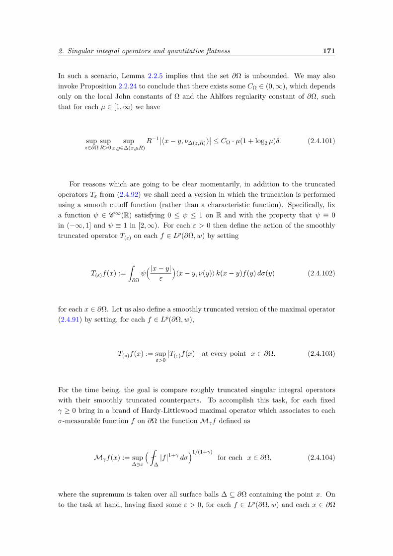
2. Singular integral operators and quantitative flatness 171
In such a scenario, Lemma 2.2.5 implies that the set ∂Ω is unbounded. We may alsoinvoke Proposition 2.2.24 to conclude that there exists some CΩ ∈ (0,∞), which dependsonly on the local John constants of Ω and the Ahlfors regularity constant of ∂Ω, suchthat for each µ ∈ [1,∞) we have
supz∈∂Ω
supR>0
supx,y∈∆(x,µR)
R−1∣∣⟨x− y, ν∆(z,R)⟩∣∣ ≤ CΩ · µ(1 + log2 µ)δ. (2.4.101)
For reasons which are going to be clear momentarily, in addition to the truncatedoperators Tε from (2.4.92) we shall need a version in which the truncation is performedusing a smooth cutoff function (rather than a characteristic function). Specifically, fixa function ψ ∈ C∞(R) satisfying 0 ≤ ψ ≤ 1 on R and with the property that ψ ≡ 0in (−∞, 1] and ψ ≡ 1 in [2,∞). For each ε > 0 then define the action of the smoothlytruncated operator T(ε) on each f ∈ Lp(∂Ω, w) by setting
T(ε)f(x) :=ˆ∂Ωψ( |x− y|
ε
)〈x− y, ν(y)〉 k(x− y)f(y) dσ(y) (2.4.102)
for each x ∈ ∂Ω. Let us also define a smoothly truncated version of the maximal operator(2.4.91) by setting, for each f ∈ Lp(∂Ω, w),
T(∗)f(x) := supε>0
∣∣T(ε)f(x)∣∣ at every point x ∈ ∂Ω. (2.4.103)
For the time being, the goal is compare roughly truncated singular integral operatorswith their smoothly truncated counterparts. To accomplish this task, for each fixedγ ≥ 0 bring in a brand of Hardy-Littlewood maximal operator which associates to eachσ-measurable function f on ∂Ω the functionMγf defined as
Mγf(x) := sup∆3x
( ∆|f |1+γ dσ
)1/(1+γ)for each x ∈ ∂Ω, (2.4.104)
where the supremum is taken over all surface balls ∆ ⊆ ∂Ω containing the point x. Onto the task at hand, having fixed some ε > 0, for each f ∈ Lp(∂Ω, w) and each x ∈ ∂Ω
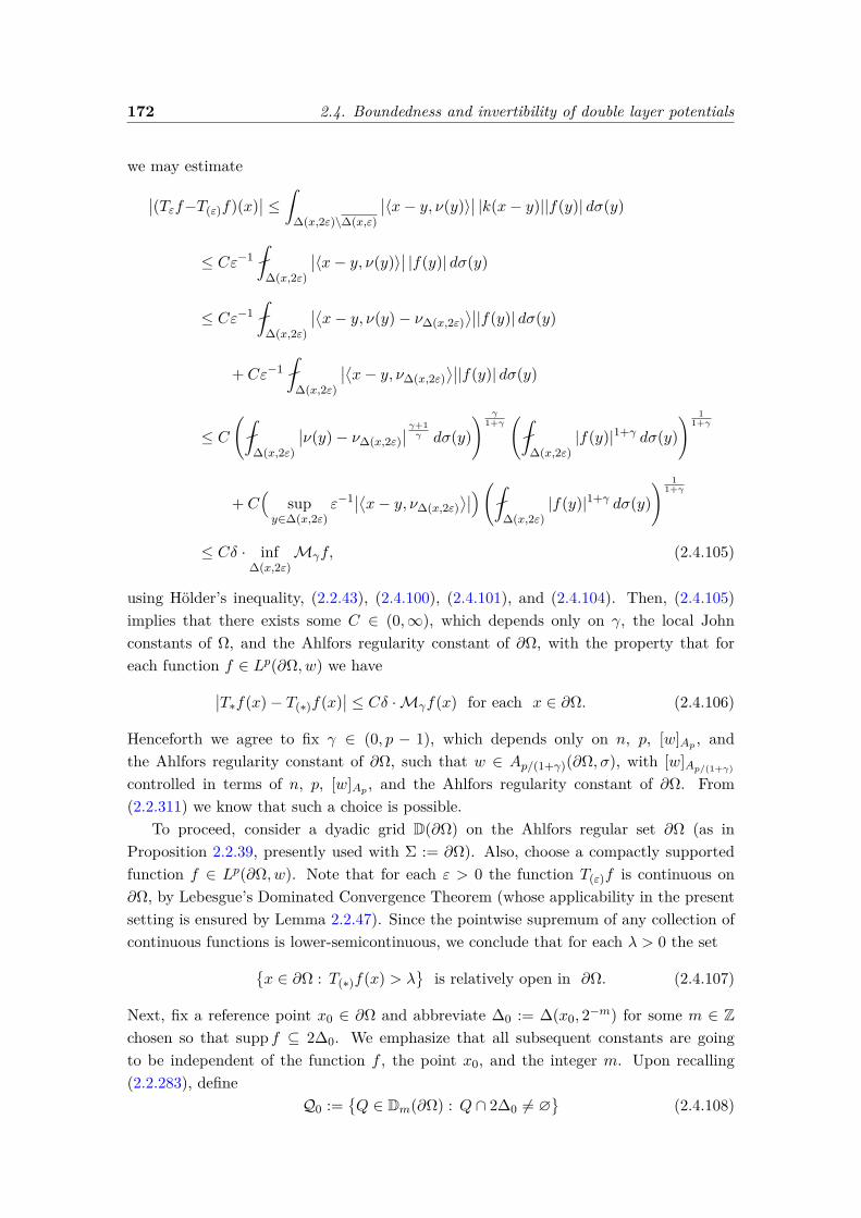
172 2.4. Boundedness and invertibility of double layer potentials
we may estimate
∣∣(Tεf−T(ε)f)(x)∣∣ ≤ ˆ
∆(x,2ε)\∆(x,ε)
∣∣〈x− y, ν(y)〉∣∣ |k(x− y)||f(y)| dσ(y)
≤ Cε−1
∆(x,2ε)
∣∣〈x− y, ν(y)〉∣∣ |f(y)| dσ(y)
≤ Cε−1
∆(x,2ε)
∣∣⟨x− y, ν(y)− ν∆(x,2ε)⟩∣∣|f(y)| dσ(y)
+ Cε−1
∆(x,2ε)
∣∣⟨x− y, ν∆(x,2ε)⟩∣∣|f(y)| dσ(y)
≤ C(
∆(x,2ε)
∣∣ν(y)− ν∆(x,2ε)∣∣ γ+1γ dσ(y)
) γ1+γ
( ∆(x,2ε)
|f(y)|1+γ dσ(y)) 1
1+γ
+ C(
supy∈∆(x,2ε)
ε−1∣∣⟨x− y, ν∆(x,2ε)⟩∣∣)(
∆(x,2ε)|f(y)|1+γ dσ(y)
) 11+γ
≤ Cδ · inf∆(x,2ε)
Mγf, (2.4.105)
using Hölder’s inequality, (2.2.43), (2.4.100), (2.4.101), and (2.4.104). Then, (2.4.105)implies that there exists some C ∈ (0,∞), which depends only on γ, the local Johnconstants of Ω, and the Ahlfors regularity constant of ∂Ω, with the property that foreach function f ∈ Lp(∂Ω, w) we have∣∣T∗f(x)− T(∗)f(x)
∣∣ ≤ Cδ · Mγf(x) for each x ∈ ∂Ω. (2.4.106)
Henceforth we agree to fix γ ∈ (0, p − 1), which depends only on n, p, [w]Ap , andthe Ahlfors regularity constant of ∂Ω, such that w ∈ Ap/(1+γ)(∂Ω, σ), with [w]Ap/(1+γ)
controlled in terms of n, p, [w]Ap , and the Ahlfors regularity constant of ∂Ω. From(2.2.311) we know that such a choice is possible.
To proceed, consider a dyadic grid D(∂Ω) on the Ahlfors regular set ∂Ω (as inProposition 2.2.39, presently used with Σ := ∂Ω). Also, choose a compactly supportedfunction f ∈ Lp(∂Ω, w). Note that for each ε > 0 the function T(ε)f is continuous on∂Ω, by Lebesgue’s Dominated Convergence Theorem (whose applicability in the presentsetting is ensured by Lemma 2.2.47). Since the pointwise supremum of any collection ofcontinuous functions is lower-semicontinuous, we conclude that for each λ > 0 the set
x ∈ ∂Ω : T(∗)f(x) > λ
is relatively open in ∂Ω. (2.4.107)
Next, fix a reference point x0 ∈ ∂Ω and abbreviate ∆0 := ∆(x0, 2−m) for some m ∈ Zchosen so that supp f ⊆ 2∆0. We emphasize that all subsequent constants are goingto be independent of the function f , the point x0, and the integer m. Upon recalling(2.2.283), define
Q0 :=Q ∈ Dm(∂Ω) : Q ∩ 2∆0 6= ∅
(2.4.108)
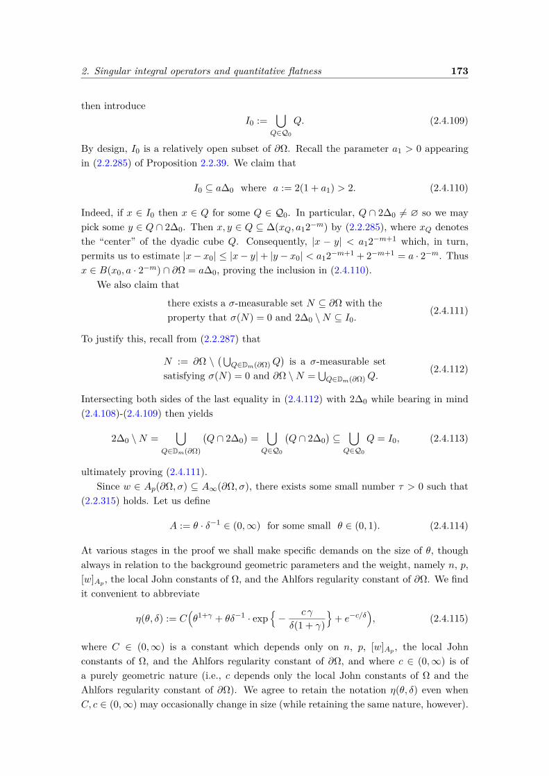
2. Singular integral operators and quantitative flatness 173
then introduceI0 :=
⋃Q∈Q0
Q. (2.4.109)
By design, I0 is a relatively open subset of ∂Ω. Recall the parameter a1 > 0 appearingin (2.2.285) of Proposition 2.2.39. We claim that
I0 ⊆ a∆0 where a := 2(1 + a1) > 2. (2.4.110)
Indeed, if x ∈ I0 then x ∈ Q for some Q ∈ Q0. In particular, Q ∩ 2∆0 6= ∅ so we maypick some y ∈ Q ∩ 2∆0. Then x, y ∈ Q ⊆ ∆(xQ, a12−m) by (2.2.285), where xQ denotesthe “center” of the dyadic cube Q. Consequently, |x − y| < a12−m+1 which, in turn,permits us to estimate |x− x0| ≤ |x− y|+ |y − x0| < a12−m+1 + 2−m+1 = a · 2−m. Thusx ∈ B(x0, a · 2−m) ∩ ∂Ω = a∆0, proving the inclusion in (2.4.110).
We also claim that
there exists a σ-measurable set N ⊆ ∂Ω with theproperty that σ(N) = 0 and 2∆0 \N ⊆ I0.
(2.4.111)
To justify this, recall from (2.2.287) that
N := ∂Ω \(⋃
Q∈Dm(∂Ω)Q)is a σ-measurable set
satisfying σ(N) = 0 and ∂Ω \N =⋃Q∈Dm(∂Ω)Q. (2.4.112)
Intersecting both sides of the last equality in (2.4.112) with 2∆0 while bearing in mind(2.4.108)-(2.4.109) then yields
2∆0 \N =⋃
Q∈Dm(∂Ω)
(Q ∩ 2∆0
)=
⋃Q∈Q0
(Q ∩ 2∆0
)⊆
⋃Q∈Q0
Q = I0, (2.4.113)
ultimately proving (2.4.111).Since w ∈ Ap(∂Ω, σ) ⊆ A∞(∂Ω, σ), there exists some small number τ > 0 such that
(2.2.315) holds. Let us define
A := θ · δ−1 ∈ (0,∞) for some small θ ∈ (0, 1). (2.4.114)
At various stages in the proof we shall make specific demands on the size of θ, thoughalways in relation to the background geometric parameters and the weight, namely n, p,[w]Ap , the local John constants of Ω, and the Ahlfors regularity constant of ∂Ω. We findit convenient to abbreviate
η(θ, δ) := C(θ1+γ + θδ−1 · exp
− c γ
δ(1 + γ)
+ e−c/δ), (2.4.115)
where C ∈ (0,∞) is a constant which depends only on n, p, [w]Ap , the local Johnconstants of Ω, and the Ahlfors regularity constant of ∂Ω, and where c ∈ (0,∞) is ofa purely geometric nature (i.e., c depends only the local John constants of Ω and theAhlfors regularity constant of ∂Ω). We agree to retain the notation η(θ, δ) even whenC, c ∈ (0,∞) may occasionally change in size (while retaining the same nature, however).
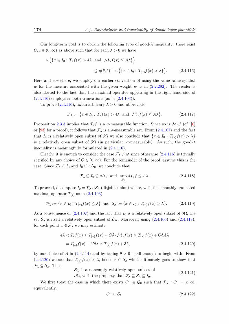
174 2.4. Boundedness and invertibility of double layer potentials
Our long-term goal is to obtain the following type of good-λ inequality: there existC, c ∈ (0,∞) as above such that for each λ > 0 we have
w(x ∈ I0 : T∗f(x) > 4λ and Mγf(x) ≤ Aλ
)≤ η(θ, δ)τ · w
(x ∈ I0 : T(∗)f(x) > λ
). (2.4.116)
Here and elsewhere, we employ our earlier convention of using the same same symbolw for the measure associated with the given weight w as in (2.2.292). The reader isalso alerted to the fact that the maximal operator appearing in the right-hand side of(2.4.116) employs smooth truncations (as in (2.4.103)).
To prove (2.4.116), fix an arbitrary λ > 0 and abbreviate
Fλ :=x ∈ I0 : T∗f(x) > 4λ and Mγf(x) ≤ Aλ
. (2.4.117)
Proposition 2.3.3 implies that T∗f is a σ-measurable function. Since so isMγf (cf. [6]or [93] for a proof), it follows that Fλ is a σ-measurable set. From (2.4.107) and the factthat I0 is a relatively open subset of ∂Ω we also conclude that
x ∈ I0 : T(∗)f(x) > λ
is a relatively open subset of ∂Ω (in particular, σ-measurable). As such, the good-λinequality is meaningfully formulated in (2.4.116).
Clearly, it is enough to consider the case Fλ 6= ∅ since otherwise (2.4.116) is triviallysatisfied by any choice of C ∈ (0,∞). For the remainder of the proof, assume this is thecase. Since Fλ ⊆ I0 and I0 ⊆ a∆0, we conclude that
Fλ ⊆ I0 ⊆ a∆0 and supFλMγf ≤ Aλ. (2.4.118)
To proceed, decompose I0 = Pλ∪Sλ (disjoint union) where, with the smoothly truncatedmaximal operator T(∗) as in (2.4.103),
Pλ :=x ∈ I0 : T(∗)f(x) ≤ λ
and Sλ :=
x ∈ I0 : T(∗)f(x) > λ
. (2.4.119)
As a consequence of (2.4.107) and the fact that I0 is a relatively open subset of ∂Ω, theset Sλ is itself a relatively open subset of ∂Ω. Moreover, using (2.4.106) and (2.4.118),for each point x ∈ Fλ we may estimate
4λ < T∗f(x) ≤ T(∗)f(x) + Cδ · Mγf(x) ≤ T(∗)f(x) + CδAλ
= T(∗)f(x) + Cθλ < T(∗)f(x) + 3λ, (2.4.120)
by our choice of A in (2.4.114) and by taking θ > 0 small enough to begin with. From(2.4.120) we see that T(∗)f(x) > λ, hence x ∈ Sλ which ultimately goes to show thatFλ ⊆ Sλ. Thus,
Sλ is a nonempty relatively open subset of∂Ω, with the property that Fλ ⊆ Sλ ⊆ I0.
(2.4.121)
We first treat the case in which there exists Q0 ∈ Q0 such that Pλ ∩ Q0 = ∅ or,equivalently,
Q0 ⊆ Sλ. (2.4.122)
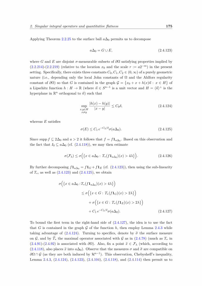
2. Singular integral operators and quantitative flatness 175
Applying Theorem 2.2.25 to the surface ball a∆0 permits us to decompose
a∆0 = G ∪ E, (2.4.123)
where G and E are disjoint σ-measurable subsets of ∂Ω satisfying properties implied by(2.2.214)-(2.2.219) (relative to the location x0 and the scale r := a2−m) in the presentsetting. Specifically, there exists three constants C0, C1, C2 ∈ (0,∞) of a purely geometricnature (i.e., depending only the local John constants of Ω and the Ahlfors regularityconstant of ∂Ω) so that G is contained in the graph G =
x0 + x + h(x)~n : x ∈ H
of
a Lipschitz function h : H → R (where ~n ∈ Sn−1 is a unit vector and H = 〈~n〉⊥ is thehyperplane in Rn orthogonal to ~n) such that
supx,y∈Hx 6=y
|h(x)− h(y)||x− y|
≤ C0δ, (2.4.124)
whereas E satisfies
σ(E) ≤ C1 e−C2/δσ(a∆0). (2.4.125)
Since supp f ⊆ 2∆0 and a > 2 it follows that f = f1a∆0 . Based on this observation andthe fact that I0 ⊆ a∆0 (cf. (2.4.118)), we may then estimate
σ(Fλ) ≤ σ(x ∈ a∆0 : T∗
(f1a∆0
)(x) > 4λ
). (2.4.126)
By further decomposing f1a∆0 = f1G + f1E (cf. (2.4.123)), then using the sub-linearityof T∗, as well as (2.4.123) and (2.4.125), we obtain
σ(x ∈ a∆0 :T∗
(f1a∆0
)(x) > 4λ
)≤ σ
(x ∈ G : T∗
(f1G
)(x) > 2λ
)+ σ
(x ∈ G : T∗
(f1E
)(x) > 2λ
)+ C1 e
−C2/δσ(a∆0). (2.4.127)
To bound the first term in the right-hand side of (2.4.127), the idea is to use the factthat G is contained in the graph G of the function h, then employ Lemma 2.4.3 whiletaking advantage of (2.4.124). Turning to specifics, denote by σ the surface measureon G, and by T∗ the maximal operator associated with G as in (2.4.78) (much as T∗ in(2.4.91)-(2.4.92) is associated with ∂Ω). Also, fix a point x ∈ Fλ (which, according to(2.4.118), also places x into a∆0). Observe that the measures σ and σ are compatible on∂Ω ∩ G (as they are both induced by Hn−1). This observation, Chebysheff’s inequality,Lemma 2.4.3, (2.4.124), (2.4.123), (2.4.104), (2.4.118), and (2.4.114) then permit us to

176 2.4. Boundedness and invertibility of double layer potentials
estimate
σ(x ∈ G :T∗
(f1G
)(x) > 2λ
)≤ σ
(x ∈ G : T∗
(f1G
)(x) > 2λ
)≤ 1
(2λ)1+γ
ˆG|T∗(f1G)|1+γ dσ ≤ C δ
1+γ
λ1+γ
ˆG|f1G|1+γ dσ
= Cδ1+γ
λ1+γ
ˆG|f |1+γ dσ ≤ Cδ1+γ σ(a∆0)
λ1+γ
a∆0
|f |1+γ dσ
≤ Cδ1+γ σ(a∆0)λ1+γ
[Mγf(x)
]1+γ≤ C (Aδ)1+γ σ(a∆0)
= C θ1+γ σ(a∆0), (2.4.128)
for some constant C ∈ (0,∞) which depends only on n, p, [w]Ap , and C0. As for thesecond term in the right-hand side of (2.4.127), once again fix a point x ∈ Fλ (whichthen also belongs to a∆0). We may then use the fact that T∗ is bounded from L1(∂Ω, σ)into the weak Lebesgue space L1,∞(∂Ω, σ) (cf. [53, Proposition 3.19]), (2.4.123), Hölder’sinequality, (2.4.125), (2.4.104), (2.4.118), and (2.4.114) to obtain
σ(x ∈ G : T∗
(f1E
)(x) > 2λ
)≤ σ
(x ∈ ∂Ω : T∗
(f1E
)(x) > 2λ
)≤ C
λ
ˆ∂Ω|f |1E dσ = C
λ
ˆa∆0
|f |1E dσ
≤ C
λσ(E)
γ1+γ
(ˆa∆0
|f |1+γ dσ
) 11+γ
= C
λ
( σ(E)σ(a∆0)
) γ1+γ
( a∆0
|f |1+γ dσ
) 11+γ
σ(a∆0)
≤ C
λexp
− C2 γ
δ(1 + γ)Mγf(x)σ(a∆0)
≤ CA · exp− C2 γ
δ(1 + γ)σ(a∆0)
= Cθδ−1 · exp− C2 γ
δ(1 + γ)σ(a∆0), (2.4.129)
where C ∈ (0,∞) depends only n, the local John constants of Ω, and the Ahlforsregularity constant of ∂Ω. Gathering (2.4.127), (2.4.128), and (2.4.129) then yields
σ(x ∈ a∆0 :T∗
(f1a∆0
)(x) > 4λ
)≤ C
(θ1+γ + θδ−1 · exp
− C2 γ
δ(1 + γ)
+ e−C2/δ)σ(a∆0)
= η(θ, δ)σ(a∆0), (2.4.130)
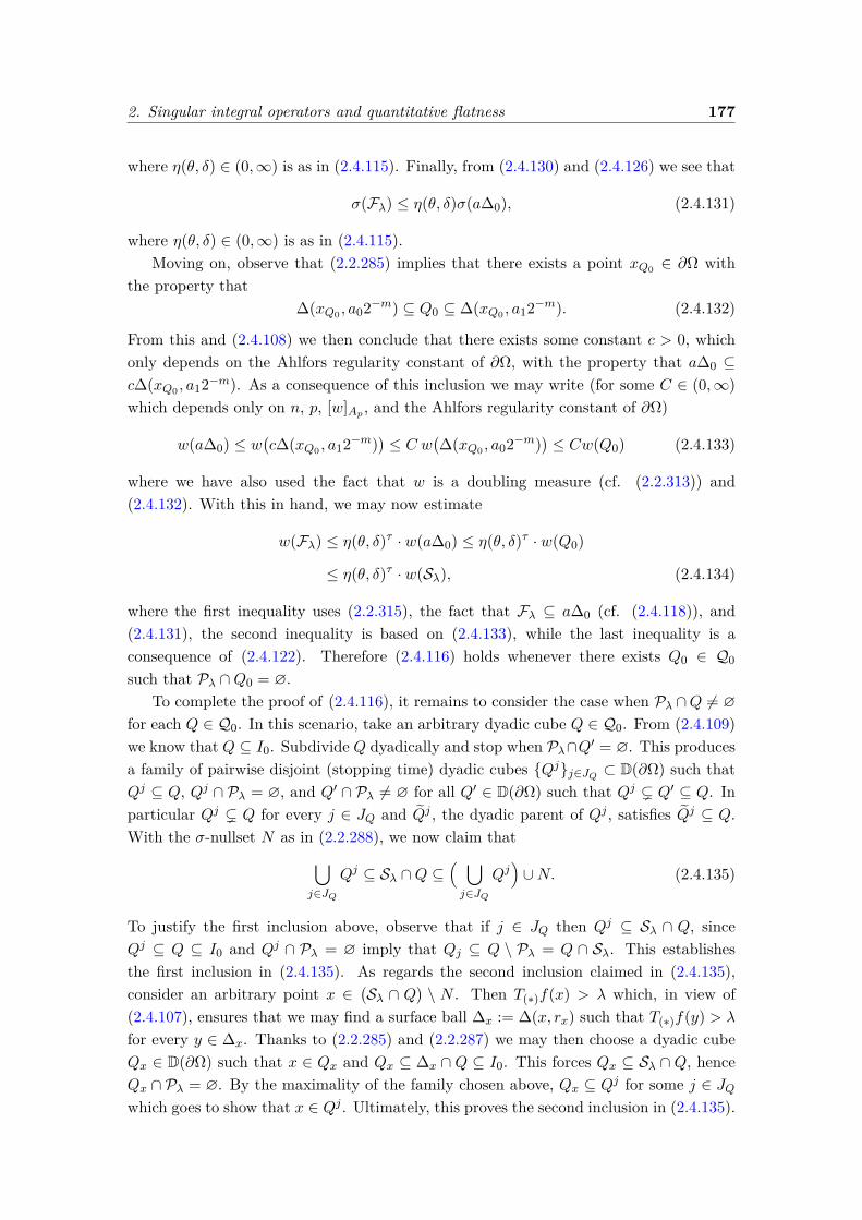
2. Singular integral operators and quantitative flatness 177
where η(θ, δ) ∈ (0,∞) is as in (2.4.115). Finally, from (2.4.130) and (2.4.126) we see that
σ(Fλ) ≤ η(θ, δ)σ(a∆0), (2.4.131)
where η(θ, δ) ∈ (0,∞) is as in (2.4.115).Moving on, observe that (2.2.285) implies that there exists a point xQ0 ∈ ∂Ω with
the property that∆(xQ0 , a02−m) ⊆ Q0 ⊆ ∆(xQ0 , a12−m). (2.4.132)
From this and (2.4.108) we then conclude that there exists some constant c > 0, whichonly depends on the Ahlfors regularity constant of ∂Ω, with the property that a∆0 ⊆c∆(xQ0 , a12−m). As a consequence of this inclusion we may write (for some C ∈ (0,∞)which depends only on n, p, [w]Ap , and the Ahlfors regularity constant of ∂Ω)
w(a∆0) ≤ w(c∆(xQ0 , a12−m)
)≤ C w
(∆(xQ0 , a02−m)
)≤ Cw(Q0) (2.4.133)
where we have also used the fact that w is a doubling measure (cf. (2.2.313)) and(2.4.132). With this in hand, we may now estimate
w(Fλ) ≤ η(θ, δ)τ · w(a∆0) ≤ η(θ, δ)τ · w(Q0)
≤ η(θ, δ)τ · w(Sλ), (2.4.134)
where the first inequality uses (2.2.315), the fact that Fλ ⊆ a∆0 (cf. (2.4.118)), and(2.4.131), the second inequality is based on (2.4.133), while the last inequality is aconsequence of (2.4.122). Therefore (2.4.116) holds whenever there exists Q0 ∈ Q0
such that Pλ ∩Q0 = ∅.To complete the proof of (2.4.116), it remains to consider the case when Pλ ∩Q 6= ∅
for each Q ∈ Q0. In this scenario, take an arbitrary dyadic cube Q ∈ Q0. From (2.4.109)we know that Q ⊆ I0. Subdivide Q dyadically and stop when Pλ∩Q′ = ∅. This producesa family of pairwise disjoint (stopping time) dyadic cubes Qjj∈JQ ⊂ D(∂Ω) such thatQj ⊆ Q, Qj ∩ Pλ = ∅, and Q′ ∩ Pλ 6= ∅ for all Q′ ∈ D(∂Ω) such that Qj ( Q′ ⊆ Q. Inparticular Qj ( Q for every j ∈ JQ and Qj , the dyadic parent of Qj , satisfies Qj ⊆ Q.With the σ-nullset N as in (2.2.288), we now claim that⋃
j∈JQ
Qj ⊆ Sλ ∩Q ⊆( ⋃j∈JQ
Qj)∪N. (2.4.135)
To justify the first inclusion above, observe that if j ∈ JQ then Qj ⊆ Sλ ∩ Q, sinceQj ⊆ Q ⊆ I0 and Qj ∩ Pλ = ∅ imply that Qj ⊆ Q \ Pλ = Q ∩ Sλ. This establishesthe first inclusion in (2.4.135). As regards the second inclusion claimed in (2.4.135),consider an arbitrary point x ∈
(Sλ ∩ Q
)\ N . Then T(∗)f(x) > λ which, in view of
(2.4.107), ensures that we may find a surface ball ∆x := ∆(x, rx) such that T(∗)f(y) > λ
for every y ∈ ∆x. Thanks to (2.2.285) and (2.2.287) we may then choose a dyadic cubeQx ∈ D(∂Ω) such that x ∈ Qx and Qx ⊆ ∆x ∩Q ⊆ I0. This forces Qx ⊆ Sλ ∩Q, henceQx ∩ Pλ = ∅. By the maximality of the family chosen above, Qx ⊆ Qj for some j ∈ JQwhich goes to show that x ∈ Qj . Ultimately, this proves the second inclusion in (2.4.135).

178 2.4. Boundedness and invertibility of double layer potentials
Going further, the idea is to carry out the stopping-time argument just describedfor each dyadic cube Q ∈ Q0. For ease of reference, organize the resulting collectionof dyadic cubes
Qj : Q ∈ Q0 and j ∈ JQ
(which is an at most countable set) as a
single-index familyQ``∈I of mutually disjoint dyadic cubes; in particular,⋃
Q∈Q0
⋃j∈JQ
Qj =⋃`∈I
Q`, (2.4.136)
with the latter union comprised of pairwise disjoint dyadic cubes in ∂Ω. Note thatSλ ∩ Q might be empty for some Q ∈ Q0 and in this case JQ = ∅ (i.e., the family ofcubes Qjj∈JQ is empty, since there are no stopping time dyadic cubes produced in thiscase). However, (2.4.109) and (2.4.121) imply that Sλ ∩ Q cannot be empty for everyQ ∈ Q0 and, as a consequence, I 6= ∅. Going further, using (2.4.109) and the fact thatSλ ⊆ I0 (cf. (2.4.119)) we may write⋃
Q∈Q0
(Sλ ∩Q) = Sλ (2.4.137)
which further entails, on account of (2.4.136) and (2.4.135), that⋃`∈I
Q` ⊆ Sλ ⊆( ⋃`∈I
Q`)∪N. (2.4.138)
By construction, for each index ` ∈ I there exists a point x∗` such that
x∗` ∈ Q` ∩ Pλ = Q` ∩(I0 \ Sλ
), (2.4.139)
where Q` denotes the dyadic parent of Q` (cf. item (4) in Proposition 2.2.39). For each` ∈ I we let ∆` := ∆Q` and ∆` := ∆
Q`be as in (2.2.285). Pressing on, split the collection
∆``∈I into two sub-classes. Specifically, bring in
I1 :=` ∈ I : there exists x∗∗` ∈ ∆` such that Mγf(x∗∗` ) ≤ Aλ
and I2 := I \ I1.
(2.4.140)
Hence, by design, Fλ ∩∆` = ∅ for each ` ∈ I2. Recall now from (2.4.121) that Fλ ⊆ Sλ.From this, (2.4.138), and (2.2.285) we then obtain (bearing in mind that σ(N) = 0; cf.(2.2.288))
w(Fλ) =∑`∈I
w(Fλ ∩Q`) ≤∑`∈I1
w(Fλ ∩∆`). (2.4.141)
Let us also consider
F` :=x ∈ ∆` : T∗f(x) > 4λ
for each ` ∈ I1, (2.4.142)
and observe that this entails
Fλ ∩∆` ⊆ F` for each ` ∈ I1, (2.4.143)
Our next goal is to prove that
σ(F`) ≤ η(θ, δ) · σ(∆`) for each ` ∈ I1. (2.4.144)
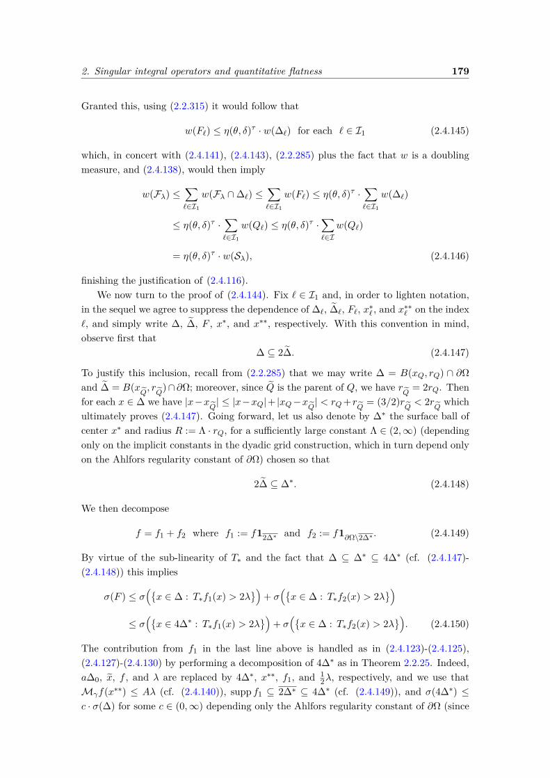
2. Singular integral operators and quantitative flatness 179
Granted this, using (2.2.315) it would follow that
w(F`) ≤ η(θ, δ)τ · w(∆`) for each ` ∈ I1 (2.4.145)
which, in concert with (2.4.141), (2.4.143), (2.2.285) plus the fact that w is a doublingmeasure, and (2.4.138), would then imply
w(Fλ) ≤∑`∈I1
w(Fλ ∩∆`) ≤∑`∈I1
w(F`) ≤ η(θ, δ)τ ·∑`∈I1
w(∆`)
≤ η(θ, δ)τ ·∑`∈I1
w(Q`) ≤ η(θ, δ)τ ·∑`∈I
w(Q`)
= η(θ, δ)τ · w(Sλ), (2.4.146)
finishing the justification of (2.4.116).We now turn to the proof of (2.4.144). Fix ` ∈ I1 and, in order to lighten notation,
in the sequel we agree to suppress the dependence of ∆`, ∆`, F`, x∗` , and x∗∗` on the index`, and simply write ∆, ∆, F , x∗, and x∗∗, respectively. With this convention in mind,observe first that
∆ ⊆ 2∆. (2.4.147)
To justify this inclusion, recall from (2.2.285) that we may write ∆ = B(xQ, rQ) ∩ ∂Ωand ∆ = B(x
Q, rQ
)∩ ∂Ω; moreover, since Q is the parent of Q, we have rQ
= 2rQ. Thenfor each x ∈ ∆ we have |x−x
Q| ≤ |x−xQ|+ |xQ−xQ| < rQ+r
Q= (3/2)r
Q< 2r
Qwhich
ultimately proves (2.4.147). Going forward, let us also denote by ∆∗ the surface ball ofcenter x∗ and radius R := Λ · rQ, for a sufficiently large constant Λ ∈ (2,∞) (dependingonly on the implicit constants in the dyadic grid construction, which in turn depend onlyon the Ahlfors regularity constant of ∂Ω) chosen so that
2∆ ⊆ ∆∗. (2.4.148)
We then decompose
f = f1 + f2 where f1 := f12∆∗ and f2 := f1∂Ω\2∆∗ . (2.4.149)
By virtue of the sub-linearity of T∗ and the fact that ∆ ⊆ ∆∗ ⊆ 4∆∗ (cf. (2.4.147)-(2.4.148)) this implies
σ(F ) ≤ σ(x ∈ ∆ : T∗f1(x) > 2λ
)+ σ
(x ∈ ∆ : T∗f2(x) > 2λ
)≤ σ
(x ∈ 4∆∗ : T∗f1(x) > 2λ
)+ σ
(x ∈ ∆ : T∗f2(x) > 2λ
). (2.4.150)
The contribution from f1 in the last line above is handled as in (2.4.123)-(2.4.125),(2.4.127)-(2.4.130) by performing a decomposition of 4∆∗ as in Theorem 2.2.25. Indeed,a∆0, x, f , and λ are replaced by 4∆∗, x∗∗, f1, and 1
2λ, respectively, and we use thatMγf(x∗∗) ≤ Aλ (cf. (2.4.140)), supp f1 ⊆ 2∆∗ ⊆ 4∆∗ (cf. (2.4.149)), and σ(4∆∗) ≤c · σ(∆) for some c ∈ (0,∞) depending only the Ahlfors regularity constant of ∂Ω (since
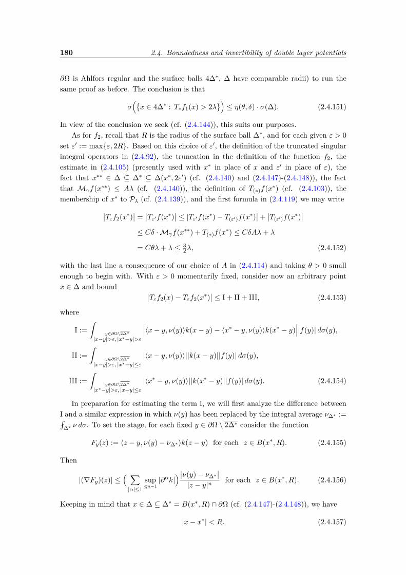
180 2.4. Boundedness and invertibility of double layer potentials
∂Ω is Ahlfors regular and the surface balls 4∆∗, ∆ have comparable radii) to run thesame proof as before. The conclusion is that
σ(x ∈ 4∆∗ : T∗f1(x) > 2λ
)≤ η(θ, δ) · σ(∆). (2.4.151)
In view of the conclusion we seek (cf. (2.4.144)), this suits our purposes.As for f2, recall that R is the radius of the surface ball ∆∗, and for each given ε > 0
set ε′ := maxε, 2R. Based on this choice of ε′, the definition of the truncated singularintegral operators in (2.4.92), the truncation in the definition of the function f2, theestimate in (2.4.105) (presently used with x∗ in place of x and ε′ in place of ε), thefact that x∗∗ ∈ ∆ ⊆ ∆∗ ⊆ ∆(x∗, 2ε′) (cf. (2.4.140) and (2.4.147)-(2.4.148)), the factthat Mγf(x∗∗) ≤ Aλ (cf. (2.4.140)), the definition of T(∗)f(x∗) (cf. (2.4.103)), themembership of x∗ to Pλ (cf. (2.4.139)), and the first formula in (2.4.119) we may write∣∣Tεf2(x∗)
∣∣ =∣∣Tε′f(x∗)
∣∣ ≤ |Tε′f(x∗)− T(ε′)f(x∗)∣∣+ ∣∣T(ε′)f(x∗)
∣∣≤ Cδ · Mγf(x∗∗) + T(∗)f(x∗) ≤ CδAλ+ λ
= Cθλ+ λ ≤ 32λ, (2.4.152)
with the last line a consequence of our choice of A in (2.4.114) and taking θ > 0 smallenough to begin with. With ε > 0 momentarily fixed, consider now an arbitrary pointx ∈ ∆ and bound ∣∣Tεf2(x)− Tεf2(x∗)
∣∣ ≤ I + II + III, (2.4.153)
where
I :=ˆ
y∈∂Ω\2∆∗|x−y|>ε, |x∗−y|>ε
∣∣∣〈x− y, ν(y)〉k(x− y)− 〈x∗ − y, ν(y)〉k(x∗ − y)∣∣∣|f(y)| dσ(y),
II :=ˆ
y∈∂Ω\2∆∗|x−y|>ε, |x∗−y|≤ε
|〈x− y, ν(y)〉||k(x− y)||f(y)| dσ(y),
III :=ˆ
y∈∂Ω\2∆∗|x∗−y|>ε, |x−y|≤ε
|〈x∗ − y, ν(y)〉||k(x∗ − y)||f(y)| dσ(y). (2.4.154)
In preparation for estimating the term I, we will first analyze the difference betweenI and a similar expression in which ν(y) has been replaced by the integral average ν∆∗ :=ffl
∆∗ ν dσ. To set the stage, for each fixed y ∈ ∂Ω \ 2∆∗ consider the function
Fy(z) := 〈z − y, ν(y)− ν∆∗〉k(z − y) for each z ∈ B(x∗, R). (2.4.155)
Then
|(∇Fy)(z)| ≤( ∑|α|≤1
supSn−1
|∂αk|)∣∣ν(y)− ν∆∗
∣∣|z − y|n
for each z ∈ B(x∗, R). (2.4.156)
Keeping in mind that x ∈ ∆ ⊆ ∆∗ = B(x∗, R) ∩ ∂Ω (cf. (2.4.147)-(2.4.148)), we have
|x− x∗| < R. (2.4.157)

2. Singular integral operators and quantitative flatness 181
Also, (recall that [x, x∗] denotes the line segment with endpoints x, x∗),
|x∗ − y| ≤ 2|ξ − y| for each y ∈ ∂Ω \ 2∆∗ and each ξ ∈ [x, x∗]. (2.4.158)
Hence, by (2.4.155)-(2.4.156), the Mean Value Theorem (bearing in mind (2.4.98)),(2.4.157)-(2.4.158), and Hölder’s inequality it follows that
ˆ∂Ω\2∆∗
∣∣∣〈x− y, ν(y)− ν∆∗〉k(x− y)− 〈x∗ − y, ν(y)− ν∆∗〉k(x∗ − y)∣∣∣|f(y)| dσ(y)
=ˆ∂Ω\2∆∗
∣∣Fy(x)− Fy(x∗)∣∣|f(y)| dσ(y)
≤ˆ∂Ω\2∆∗
|x− x∗| · supξ∈[x,x∗]
∣∣(∇Fy)(ξ)∣∣|f(y)| dσ(y)
≤ Cˆ∂Ω\2∆∗
R
|x∗ − y|n∣∣ν(y)− ν∆∗
∣∣|f(y)| dσ(y)
≤ C∞∑j=1
2−j
2j+1∆∗\2j∆∗
∣∣ν(y)− ν∆∗∣∣|f(y)| dσ(y)
≤ C∞∑j=1
2−j(
2j+1∆∗
(∣∣ν(y)− ν2j+1∆∗∣∣+ ∣∣ν2j+1∆∗ − ν∆∗
∣∣) 1+γγ dσ(y)
) γ1+γ×
×(
2j+1∆∗|f(y)|1+γ dσ(y)
) 11+γ
≤ C( ∞∑j=1
(j + 2) 2−j)‖ν‖[BMO(∂Ω,σ)]nMγf(x∗∗)
≤ CAδλ, (2.4.159)
for some C ∈ (0,∞) which depends only on n, p, [w]Ap , and the Ahlfors regularityconstant of ∂Ω. Above, the fifth inequality relies on (2.2.43) and the fact that
∣∣ν2j+1∆∗ − ν∆∗∣∣ ≤ C (j + 1) ‖ν‖[BMO(∂Ω,σ)]n for each j ∈ N (2.4.160)
for some C ∈ (0,∞) depending only on n and the Ahlfors regular constant of ∂Ω, whichis a direct consequence of (2.2.46). The fifth inequality in (2.4.159) also uses the factthat x∗∗ ∈ ∆ ⊆ ∆∗ ⊆ 2j+1∆∗ for each integer j ∈ N. The last inequality in (2.4.159) isa consequence of the fact thatMγf(x∗∗) ≤ Aλ (cf. (2.4.140)).
On the other hand, from the properties of the kernel k and the Mean Value Theorem

182 2.4. Boundedness and invertibility of double layer potentials
we obtainˆ∂Ω\2∆∗
∣∣∣〈x− y, ν∆∗〉k(x− y)− 〈x∗ − y, ν∆∗〉k(x∗ − y)∣∣∣|f(y)| dσ(y)
=ˆ∂Ω\2∆∗
∣∣∣ (〈x− y, ν∆∗〉 − 〈x∗ − y, ν∆∗〉) k(x∗ − y)
+ 〈x− y, ν∆∗〉 (k(x− y)− k(x∗ − y))∣∣∣|f(y)| dσ(y)
≤ Cn∞∑j=1
ˆ2j+1∆∗\2j∆∗
( |〈x− x∗, ν∆∗〉||x∗ − y|n
+R|〈x− y, ν∆∗〉||x∗ − y|n+1
)|f(y)| dσ(y)
≤ Cn∞∑j=1
ˆ2j+1∆∗\2j∆∗
|〈x− x∗, ν∆∗〉||x∗ − y|n
|f(y)| dσ(y)
+ CnR∞∑j=1
ˆ2j+1∆∗\2j∆∗
|〈x− y, ν∆∗ − ν2j+1∆∗〉||x∗ − y|n+1 |f(y)| dσ(y)
+ CnR∞∑j=1
ˆ2j+1∆∗\2j∆∗
|〈x− y, ν2j+1∆∗〉||x∗ − y|n+1 |f(y)| dσ(y)
=: I1 + I2 + I3. (2.4.161)
To estimate I1, write
I1 ≤ CnR−1|〈x− x∗, ν∆∗〉|∞∑j=1
2−j
2j+1∆∗|f(y)| dσ(y)
≤ Cδ∞∑j=1
2−jMγf(x∗∗) ≤ CδMγf(x∗∗)
≤ CAδλ, (2.4.162)
where C ∈ (0,∞) depends only on n, the local John constants of Ω, and the Ahlforsregularity constant of ∂Ω. The second inequality above is a consequence of (2.4.101)used here with z := x∗, y := x∗, µ := 2 (a valid choice given that x ∈ ∆(x∗, 2R)since, as seen from (2.4.147)-(2.4.148), we have x ∈ ∆ ⊆ ∆∗ = ∆(x∗, R)), as well as thefact that x∗∗ ∈ ∆ ⊆ ∆∗ ⊆ 2j+1∆∗ for each j ∈ N. The last inequality (2.4.162) usesMγf(x∗∗) ≤ Aλ (cf. (2.4.140)).
To treat I2, we write (for some C ∈ (0,∞) which depends only on n, the local Johnconstants of Ω, and the Ahlfors regularity constant of ∂Ω),
I2 ≤ CR∞∑j=1
ˆ2j+1∆∗\2j∆∗
|ν∆∗ − ν2j+1∆∗ ||x∗ − y|n
|f(y)| dσ(y)
≤ C∞∑j=1
(j + 1) ‖ν‖[BMO(∂Ω,σ)]n 2−j
2j+1∆∗|f(y)| dσ(y)
≤ CδMγf(x∗∗) ≤ CAδλ, (2.4.163)
2. Singular integral operators and quantitative flatness 183
where the first inequality uses the definition of I2 and the estimate |x−y| ≤ (3/2)|x∗−y|for each y ∈ ∂Ω\2∆∗, the second inequality takes into account (2.4.160) and the Ahlforsregularity of ∂Ω, while the remaining inequalities are justified as in (2.4.162).
As regards I3, write (again, with C ∈ (0,∞) depending only on n, the local Johnconstants of Ω, and the Ahlfors regularity constant of ∂Ω)
I3 ≤ C∞∑j=1
2−j
2j+1∆∗
|〈x− y, ν2j+1∆∗〉|2j+1R
|f(y)| dσ(y)
≤ Cδ∞∑j=1
2−j
2j+1∆∗|f(y)| dσ(y) ≤ CδMγf(x∗∗)
≤ CAδλ. (2.4.164)
The second inequality in (2.4.164) is based on (2.4.101) used with z := x∗ and R replacedby 2j+1R. The remaining inequalities in (2.4.164) are then justified much as in (2.4.162).
At this stage, by combining (2.4.159) and (2.4.161)-(2.4.164) we conclude that thereexists some C ∈ (0,∞) which depends only on n, the local John constants of Ω, and theAhlfors regularity constant of ∂Ω, such that
I ≤ CAδλ. (2.4.165)
To bound II in (2.4.154), recall that x, x∗∗ ∈ ∆ and assume y ∈ ∂Ω \ 2∆∗ is such that|x∗ − y| ≤ ε and |x− y| > ε. Then, 2R < |x∗ − y| ≤ ε and since x, x∗∗ ∈ ∆ ⊆ B(xQ, rQ)(where xQ and rQ are, respectively, the center and radius of the surface ball ∆) andR = Λ · rQ with Λ > 2, we have |x − x∗∗| < 2rQ < R < ε/2. Hence, the pointx∗∗ belongs to the surface ball ∆(x, ε/2). Moreover, on account of (2.4.157) we maywrite |x − y| ≤ |x − x∗| + |x∗ − y| < R + ε < (3/2)ε which, in particular, guaranteesthat y ∈ ∆(x, 2ε). Consequently, ε < |x− y| < 2ε hence |k(x− y)| ≤ ε−n and (for someC ∈ (0,∞) which depends only on depends only on n and the Ahlfors regularity constantof ∂Ω),
II ≤ Cε−1
∆(x,2ε)|〈x− y, ν(y)〉| |f(y)| dσ(y)
≤ Cε−1
∆(x,2ε)|〈x− y, ν(y)− ν∆(x,2ε)〉| |f(y)| dσ(y)
+ Cε−1
∆(x,2ε)|〈x− y, ν∆(x,2ε)〉| |f(y)| dσ(y)
=: II1 + II2. (2.4.166)
Using Hölder’s inequality, (2.2.43), (2.4.140), and (2.4.100) we obtain that there existssome C ∈ (0,∞) which depends only on n, p, [w]Ap , the local John constants of Ω, and
184 2.4. Boundedness and invertibility of double layer potentials
the Ahlfors regularity constant of ∂Ω, such that
II1 ≤ C(
∆(x,2ε)|ν(y)− ν∆(x,2ε)|
1+γγ dσ(y)
) γ1+γ
( ∆(x,2ε)
|f(y)|1+γ dσ(y)) 1
1+γ
≤ C ‖ν‖[BMO(∂Ω,σ)]nMγf(x∗∗) ≤ CAδλ, (2.4.167)
since x∗∗ is contained in ∆(x, ε/2) ⊆ ∆(x, 2ε) and Mγf(x∗∗) ≤ CAλ, as already notedearlier. As for II2, invoking (2.4.101), Hölder’s inequality, and (2.4.140), it follows that(with C ∈ (0,∞) as above)
II2 ≤ C(
supy∈∆(x,2ε)
ε−1|〈x− y, ν∆(x,2ε)〉|)
∆(x,2ε)|f(y)| dσ(y)
≤ Cδ(
∆(x,2ε)|f(y)|1+γ dσ(y)
) 11+γ
≤ Cδ · Mγf(x∗∗) ≤ CAδλ. (2.4.168)
From (2.4.166)-(2.4.168) we see that there exists C ∈ (0,∞) which depends only on n,p, [w]Ap , the local John constants of Ω, and the Ahlfors regularity constant of ∂Ω, suchthat
II ≤ CAδλ. (2.4.169)
Turning our attention to III, recall that x, x∗∗ ∈ ∆ and suppose y ∈ ∂Ω \ 2∆∗ is suchthat |x∗ − y| > ε and |x− y| ≤ ε. Then |x∗ − y| > 2R > R+ |x− x∗| by (2.4.157) whichfurther entails ε ≥ |x − y| ≥ |x∗ − y| − |x − x∗| > R. In particular, R < ε. If we nowabbreviate R := R+ε then, on the one hand, |x∗−y| ≤ |x∗−x|+|x−y| < R+ε = R, whileon the other hand having |x∗−y| > ε and |x∗−y| > 2R implies |x∗−y| > R+(ε/2) > 1
2R.As such, |k(x∗ − y)| ≤ R−n and
III ≤ CnR−1
∆(x∗,R)|〈x∗ − y, ν(y)〉| |f(y)| dσ(y). (2.4.170)
Granted this, the same type of argument which, starting with the first line in (2.4.166)has produced (2.4.169) (reasoning with R/2 replacing ε and with x∗ replacing x) will nowyield (for some C ∈ (0,∞) which depends only on n, p, [w]Ap , the local John constantsof Ω, and the Ahlfors regularity constant of ∂Ω)
III ≤ CAδλ, (2.4.171)
as soon as we show that x∗∗ ∈ ∆(x∗, R). To justify this membership, start by recallingthat |x − x∗∗| < 2rQ < R and then use (2.4.157), the triangle inequality, and the factthat R < ε to estimate |x∗−x∗∗| ≤ |x−x∗|+ |x−x∗∗| < 2R < R. The proof of (2.4.171)is therefore complete.
Let us summarize our progress. From (2.4.153), (2.4.165), (2.4.169), and (2.4.171) weconclude that there exists some C ∈ (0,∞), which depends only on θ, n, p, [w]Ap , thelocal John constants of Ω, and the Ahlfors regularity constant of ∂Ω, such that∣∣∣Tεf2(x)− Tεf2(x∗)
∣∣∣ ≤ C Aδλ, ∀x ∈ ∆, ∀ ε > 0. (2.4.172)
2. Singular integral operators and quantitative flatness 185
In view of the fact that A = θ · δ−1 this entails∣∣∣Tεf2(x)− Tεf2(x∗)∣∣∣ ≤ 1
2λ, ∀x ∈ ∆, ∀ ε > 0, (2.4.173)
provided we pick θ > 0 small to begin with. From (2.4.152), (2.4.173), and (2.4.91) wethen obtain
T∗f2(x) ≤ 2λ for all x ∈ ∆, (2.4.174)
whenever θ > 0 is small enough. Therefore, for this choice of θ, we conclude that
σ(x ∈ ∆ : T∗f2(x) > 2λ
)= 0 (2.4.175)
which, in concert with (2.4.150) and (2.4.151), establishes (2.4.144). This finishes theproof of the good-λ inequality (2.4.116).
Once (2.4.116) has been established, we proceed to prove (2.4.99). First, using(2.4.106), by our definition of A, and by possibly choosing a smaller θ > 0, for eachpoint x ∈ I0 with T(∗)f(x) > λ andMγf(x) ≤ Aλ we may write
λ < T(∗)f(x) ≤ T∗f(x) + Cδ · Mγf(x)
≤ T∗f(x) + CδAλ = T∗f(x) + Cθλ
< T∗f(x) + 12λ. (2.4.176)
Hence, for such a choice of θ we have
12λ < T∗f(x) whenever the point x ∈ I0 is suchthat T(∗)f(x) > λ andMγf(x) ≤ Aλ.
(2.4.177)
Consequently,
x ∈ I0 : T(∗)f(x) > λ and Mγf(x) ≤ Aλ
⊆x ∈ I0 : T∗f(x) > λ
2
(2.4.178)
which, in turn, permits us to estimate
w(x ∈ I0 : T(∗)f(x) > λ
)≤ w
(x ∈ I0 : T(∗)f(x) > λ and Mγf(x) ≤ Aλ
)+ w
(x ∈ I0 : Mγf(x) > Aλ
)≤ w
(x ∈ I0 : T∗f(x) > λ
2)
+ w(x ∈ I0 : Mγf(x) > Aλ
). (2.4.179)
From (2.4.115) it is clear that
limθ→0+
limδ→0+
η(θ, δ) = 0 (2.4.180)
186 2.4. Boundedness and invertibility of double layer potentials
so it is possible to choose the threshold δ0 > 0 and the coefficient θ > 0 small enoughdepending only on n, p, [w]Ap , the local John constants of Ω, and the Ahlfors regularityconstant of ∂Ω, so that
η(θ, δ)τ < (2 · 8p)−1. (2.4.181)
This is the last demand imposed on δ, θ, and the totality of the such size specificationsimply that the final choice of the said parameters ultimately depends only on n, p, [w]Ap ,the local John constants of Ω, and the Ahlfors regularity constant of ∂Ω. Combining(2.4.179) with (2.4.116) and keeping (2.4.181) in mind we then get
w(x ∈ I0 :T∗f(x) > 4λ
)≤ w
(x ∈ I0 : T∗f(x) > 4λ and Mγf(x) ≤ Aλ
)+ w
(x ∈ I0 : Mγf(x) > Aλ
)≤ η(θ, δ)τ · w
(x ∈ I0 : T(∗)f(x) > λ
)+ w
(x ∈ I0 : Mγf(x) > Aλ
)< (2 · 8p)−1w
(x ∈ I0 : T∗f(x) > λ
2)
+(1 + (2 · 8p)−1)w(x ∈ I0 : Mγf(x) > Aλ
). (2.4.182)
Recall that γ ∈ (0, p − 1) has been chosen so that w ∈ Ap/(1+γ)(∂Ω, σ), hence Mγ
is bounded on Lp(∂Ω, w). Multiply the most extreme sides of (2.4.182) by pλp−1 andintegrate over λ ∈ (0,∞). Bearing in mind that A = θ · δ−1, after three natural changesof variables (namely, λ := 4λ in the first integral, λ := 1
2λ in the second integral, andλ := θδ−1λ in the third integral) we therefore obtainˆ
I0
|T∗f |pw dσ ≤12
ˆI0
|T∗f |pw dσ + δpθ−p(22p + 2−p−1)ˆ
I0
(Mγf)pw dσ
≤ 12
ˆI0
|T∗f |pw dσ + C δpˆ∂Ω|f |pw dσ, (2.4.183)
for some constant C ∈ (0,∞) which depends only on n, p, [w]Ap , the local John constantsof Ω, and the Ahlfors regularity constant of ∂Ω (hence, in particular, independent ofthe function f , the quantity δ, as well as the parameters x0,m defining the set I0).Since f ∈ Lp(∂Ω, w) and the operator T∗ maps the space Lp(∂Ω, w) into itself (cf.Proposition 2.3.3), it follows that
´I0|T∗f |pw dσ ≤ ‖T∗f‖pLp(∂Ω,w) < ∞. Hence, the
first integral in the right-most side of (2.4.183) may be absorbed in the left-most side.By also taking into account (2.4.111), we therefore obtainˆ
2∆0
|T∗f |pw dσ ≤ˆI0
|T∗f |pw dσ ≤ Cδpˆ∂Ω|f |pw dσ. (2.4.184)
Recall that 2∆0 = ∆(x0, 2−m+1) and the only constraint on the integer m ∈ Z hasbeen that supp f ⊆ 2∆0. Upon letting m → −∞ and invoking Lebesgue’s Monotone
2. Singular integral operators and quantitative flatness 187
Convergence Theorem we arrive at the conclusion that, for some C ∈ (0,∞) whichdepends only on n, p, [w]Ap , and the Ahlfors regularity constant of ∂Ω, we have theestimate ˆ
∂Ω|T∗f |pw dσ ≤ Cδp
ˆ∂Ω|f |pw dσ,
for every f ∈ Lp(∂Ω, w) with compact support.(2.4.185)
To treat the case when the function f ∈ Lp(∂Ω, w) is now arbitrary, for each j ∈ Ndefine fj := 1∆(x0,j)f . Then Lebesgue’s Dominated Convergence Theorem implies thatfj → f in Lp(∂Ω, w) as j → ∞, and since T∗ is continuous on Lp(∂Ω, w) we also haveT∗fj → T∗f in Lp(∂Ω, w) as j →∞. Writing the estimate in (2.4.185) for fj in place off and passing to limit j →∞ then yields
ˆ∂Ω|T∗f |pw dσ ≤ Cδp
ˆ∂Ω|f |pw dσ for each f ∈ Lp(∂Ω, w), (2.4.186)
where C ∈ (0,∞) depends only on n, p, [w]Ap , and the Ahlfors regularity constantof ∂Ω. Finally, sending δ ‖ν‖[BMO(∂Ω,σ)]n (cf. (2.4.100)), this finishes the proof of(2.4.99).
Recall the notion of chord-arc domain introduced, in the two-dimensional setting, inDefinition 2.2.35.
Corollary 2.4.10. Fix κ∗ ∈ (0,∞) and let Ω ⊆ R2 be a κ-CAD for some κ ∈ [0,κ∗).Abbreviate σ := H1b∂Ω and denote by ν the geometric measure theoretic outward unitnormal to Ω. Also, fix an integrability exponent p ∈ (1,∞) along with a Muckenhouptweight w ∈ Ap(∂Ω, σ). Consider a complex-valued function k ∈ CN (R2 \ 0), for asufficiently large integer N ∈ N, which is even and positive homogeneous of degree −2,and define the maximal operator T∗ acting on each function f ∈ Lp(∂Ω, w) according to
T∗f(x) := supε>0
∣∣Tεf(x)∣∣ for each x ∈ ∂Ω, (2.4.187)
where, for each ε > 0,
Tεf(x) :=ˆ
y∈∂Ω|x−y|>ε
〈x− y, ν(y)〉k(x− y)f(y) dσ(y) for all x ∈ ∂Ω. (2.4.188)
Then there exists some C ∈ (0,∞), which depends only on κ∗, p, [w]Ap such that
‖T∗‖Lp(∂Ω,w)→Lp(∂Ω,w) ≤ C( ∑|α|≤N
supS1|∂αk|
)√κ. (2.4.189)
Of course, the crux of the matter is the presence of√κ as a multiplicative factor in the
right hand-side of (2.4.189). As a consequence, ‖T∗‖Lp(∂Ω,w)→Lp(∂Ω,w) is small if Ω ⊆ R2
is a κ-CAD whose constant κ > 0 is sufficiently small (relative to the integral exponentp, the characteristic [w]Ap of the Muckenhoupt weight, and the integral kernel k).
188 2.4. Boundedness and invertibility of double layer potentials
Proof of Corollary 2.4.10. From Proposition 2.2.36 and Proposition 2.3.3 it follows thatT∗ is bounded on Lp(∂Ω, w), with norm controlled in terms of
∑|α|≤N supS1 |∂αk|, and
κ∗, p, [w]Ap . This trivially implies (2.4.189) when κ stays away from zero, say whenκ ≥
√2− 1, simply by adjusting constants. When κ ∈
[0 ,√
2− 1)the estimate claimed
in (2.4.189) is implied by (2.4.93) and (2.2.257).
Theorem 2.4.4 then readily implies similar operator norm estimates for principal-value singular integral operators whose integral kernel has a special algebraic format, inthat it involves the inner product between the outward unit normal and the chord, as afactor. This is made precise in the corollary below. In turn, for a given second-order,homogeneous, constant complex coefficient system L with Adis
L 6= ∅, and a given Ahlforsregular domain Ω ⊆ Rn satisfying a two-sided local John condition, Corollary 2.4.11 willbe used for T being either the boundary-to-boundary double layer potential operator KA
associated with a coefficient tensor A ∈ AdisL , or its “transposed” version K#
A , acting onMuckenhoupt weighted Lebesgue spaces on ∂Ω.
Corollary 2.4.11. Let Ω ⊆ Rn be an Ahlfors regular domain satisfying a two-sidedlocal John condition. Abbreviate σ := Hn−1b∂Ω and denote by ν the geometric measuretheoretic outward unit normal to Ω. Fix an integrability exponent p ∈ (1,∞) along witha Muckenhoupt weight w ∈ Ap(∂Ω, σ), and recall the earlier convention of using thesame same symbol w for the measure associated with the given weight w as in (2.2.292).Also, consider a sufficiently large integer N = N(n) ∈ N and suppose k ∈ CN (Rn \ 0)is a complex-valued function which is even and positive homogeneous of degree −n. Inthis setting consider the principal-value singular integral operators T, T# acting on eachfunction f ∈ Lp(∂Ω, w) according to
Tf(x) := limε→0+
ˆ
y∈∂Ω|x−y|>ε
〈x− y, ν(y)〉k(x− y)f(y) dσ(y), (2.4.190)
andT#f(x) := lim
ε→0+
ˆ
y∈∂Ω|x−y|>ε
〈y − x, ν(x)〉k(x− y)f(y) dσ(y), (2.4.191)
at σ-a.e. point x ∈ ∂Ω. Then there exists a constant C ∈ (0,∞), which depends onlyon n, p, [w]Ap, the local John constants of Ω, and the Ahlfors regularity constant of ∂Ω,with the property that
‖T‖Lp(∂Ω,w)→Lp(∂Ω,w) ≤ C( ∑|α|≤N
supSn−1
|∂αk|)‖ν‖[BMO(∂Ω,σ)]n (2.4.192)
and ∥∥∥T#∥∥∥Lp(∂Ω,w)→Lp(∂Ω,w)
≤ C( ∑|α|≤N
supSn−1
|∂αk|)‖ν‖[BMO(∂Ω,σ)]n . (2.4.193)
2. Singular integral operators and quantitative flatness 189
Furthermore, with p′ ∈ (1,∞) denoting the Hölder conjugate exponent of p and withw′ := w1−p′ ∈ Ap′(∂Ω, σ), it follows that
the (real) transposed of T : Lp(∂Ω, w) → Lp(∂Ω, w) isthe operator T# : Lp′(∂Ω, w′)→ Lp
′(∂Ω, w′).(2.4.194)
Proof. In view of the fact that
‖T‖Lp(∂Ω,w)→Lp(∂Ω,w) ≤ ‖T∗‖Lp(∂Ω,w)→Lp(∂Ω,w) , (2.4.195)
the estimate claimed in (2.4.192) follows directly from (2.4.93). As regards the claimmade in (2.4.193), first observe that (2.4.194) holds, thanks to (2.4.190)-(2.4.191) and(2.3.29). As such,∥∥∥T#
∥∥∥Lp(∂Ω,w)→Lp(∂Ω,w)
= ‖T‖Lp′ (∂Ω,w′)→Lp′ (∂Ω,w′)
≤ C( ∑|α|≤N
supSn−1
|∂αk|)‖ν‖[BMO(∂Ω,σ)]n , (2.4.196)
thanks to (2.4.192) used with p′, w′ in place of p, w.
Remark 2.4.12. Of course, in the special case when w ≡ 1, Theorem 2.4.4 and Corol-lary 2.4.11 yield estimates on ordinary Lebesgue spaces, Lp(∂Ω, σ) with p ∈ (1,∞). Viareal interpolation, these further imply similar estimates on the scale of Lorentz spaces on∂Ω. Specifically, from (2.4.93), (2.4.192)-(2.4.193), and real interpolation (for sub-linearoperators) we conclude that for each p ∈ (1,∞) and q ∈ (0,∞] there exists a constantC ∈ (0,∞), which depends only on n, p, q, the local John constants of Ω, and the Ahlforsregularity constant of ∂Ω, with the property that
‖T∗‖Lp,q(∂Ω,σ)→Lp,q(∂Ω,σ) ≤ C( ∑|α|≤N
supSn−1
|∂αk|)‖ν‖[BMO(∂Ω,σ)]n , (2.4.197)
‖T‖Lp,q(∂Ω,σ)→Lp,q(∂Ω,σ) ≤ C( ∑|α|≤N
supSn−1
|∂αk|)‖ν‖[BMO(∂Ω,σ)]n , (2.4.198)
and ∥∥∥T#∥∥∥Lp,q(∂Ω,σ)→Lp,q(∂Ω,σ)
≤ C( ∑|α|≤N
supSn−1
|∂αk|)‖ν‖[BMO(∂Ω,σ)]n . (2.4.199)
Remark 2.4.13. In the context of Corollary 2.4.11, estimates (2.4.192)-(2.4.193) remainvalid with a fixed constant C ∈ (0,∞) when the integrability exponent and the corre-sponding Muckenhoupt weight are allowed to vary while retaining control. Concretely,Remark 2.4.5 implies that for each compact interval I ⊂ (0,∞) and each numberW ∈ (0,∞) there exists a constant C ∈ (0,∞), which depends only on n, I, W , thelocal John constants of Ω, and the Ahlfors regularity constant of ∂Ω, with the propertythat (2.4.192)-(2.4.193) hold for each p ∈ I and each w ∈ Ap(∂Ω, σ) with [w]Ap ≤W .
Similar considerations apply to the estimates in (2.4.197)-(2.4.199).
190 2.4. Boundedness and invertibility of double layer potentials
2.4.3 Norm estimates and invertibility results for double layers
We first recall a result (cf. [53, Theorem 2.16, p. 2603]) which is a combination of theextrapolation theorem of Rubio de Francia with the commutator theorem of Coifman etal., [27], suitably adapted to setting of spaces of homogeneous type.
Theorem 2.4.14. Let Σ ⊆ Rn be a closed Ahlfors regular set, and abbreviate σ :=Hn−1bΣ. Fix p0 ∈ (1,∞) along with some non-decreasing function Φ : (0,∞) → (0,∞)and let T be a linear operator which is bounded on Lp0(Σ, w) for every w ∈ Ap0(Σ, σ),with operator norm ≤ Φ
([w]Ap0
).
Then for each integrability exponent p ∈ (1,∞) there exist C1, C2 ∈ (0,∞) whichdepend exclusively on the dimension n, the exponents p0, p, and the Ahlfors regularityconstant of Σ, with the property that for any Muckenhoupt weight w ∈ Ap(Σ, σ) theoperator
T : Lp(Σ, w) −→ Lp(Σ, w) (2.4.200)
is well defined, linear, and bounded, with operator norm
‖T‖Lp(Σ,w)→Lp(Σ,w) ≤ C1 · Φ(C2 · [w]max1,(p0−1)/(p−1)
Ap
). (2.4.201)
In addition, given any p ∈ (1,∞) along with some w ∈ Ap(Σ, σ), there exists a con-stant C = C(Σ, n, p0, p, [w]Ap) ∈ (0,∞) with the property that for every complex-valuedfunction b ∈ L∞(Σ, σ) one has (with C1 as before)
‖[Mb, T ]‖Lp(Σ,w)→Lp(Σ,w) ≤ C1 · Φ(C) ‖b‖BMO(Σ,σ) , (2.4.202)
where [Mb, T ] is the commutator of T considered as in (2.4.200) and the operator Mb ofpointwise multiplication on Lp(Σ, w) by the function b, i.e.,
[Mb, T ]f := bT (f)− T (bf) for each f ∈ Lp(Σ, w). (2.4.203)
In particular, from (2.4.202) with w ≡ 1 and real interpolation it follows that, for anygiven p ∈ (1,∞) and q ∈ (0,∞], there exists a constant C = C(Σ, n, p, q) ∈ (0,∞) withthe property that for every complex-valued function b ∈ L∞(Σ, σ) one has
‖[Mb, T ]‖Lp,q(Σ,σ)→Lp,q(Σ,σ) ≤ C1 · Φ(C) ‖b‖BMO(Σ,σ) . (2.4.204)
Theorem 2.4.14 is a particular case of a more general result proved in Theorem 2.4.16,stated just after the following remark.
Remark 2.4.15. Even though Theorem 2.4.14 suffices for the purposes we have in mind,it is worth noting that there is a version of (2.4.202) in which the pointwise multiplierb is allowed to belong to the larger space BMO(Σ, σ). The price to pay is that we nowno longer may regard [Mb, T ] as in (2.4.203) and, instead, have to interpret this as anabstract extension (by density) of a genuine commutator. Specifically, given a real-valuedfunction b ∈ BMO(Σ, σ), for each N ∈ N define
bN := min
maxb,−N , N
= max
minb,N , −N, (2.4.205)
2. Singular integral operators and quantitative flatness 191
and note that there exists C ∈ (0,∞) such that
bN ∈ L∞(Σ, σ), thus bN ∈ BMO(Σ, σ), and
‖bN‖BMO(Σ,σ) ≤ 2‖b‖BMO(Σ,σ) for all N ∈ N,
|bN (x)| ≤ |b(x)| for all x ∈ Σ and N ∈ N,
limN→∞
bN (x) = b(x) for each x belonging to Σ.
(2.4.206)
Keeping in mind that BMO(Σ, σ) ⊆ Lp0loc(Σ, σ), Lebesgue’s Dominated Convergence
Theorem then implies bN → b in Lp0loc(Σ, σ) as N → ∞, hence bNf → bf in Lp0(Σ, σ)
as N → ∞ for any f in L∞comp(Σ, σ) (the space of essentially bounded functions withcompact support in Σ). For each such function f the hypotheses on T then imply thatT (bNf) → T (bf) in Lp0(Σ, σ) as N → ∞. Since we also have bNT (f) → bT (f) at eachpoint in Σ as N →∞, we ultimately conclude that
for each function f ∈ L∞comp(Σ, σ) there exists a strictlyincreasing sequence Njj∈N ⊆ N with the property that[MbNj
, T]f →
[Mb, T
]f at σ-a.e. point in Σ as j →∞.
(2.4.207)
Having fix p ∈ (1,∞) along with w ∈ Ap(Σ, σ), for each such function f in L∞comp(Σ, σ)we may now writeˆ
Σ
∣∣[Mb, T ]f∣∣p dw =
ˆΣ
lim infj→∞
∣∣∣[MbNj, T]f∣∣∣p dw
≤ lim infj→∞
ˆΣ
∣∣∣[MbNj, T]f∣∣∣p dw
≤ lim infj→∞
(C1 · Φ(C)
∥∥∥bNj∥∥∥BMO(Σ,σ)
)p‖f‖Lp(Σ,w)
≤(C1 · Φ(C) ‖b‖BMO(Σ,σ)
)p‖f‖Lp(Σ,w), (2.4.208)
where the equality comes from (2.4.207), the first inequality is implies by Fatou’s Lemma,the second inequality is a consequence of (2.4.202) (bearing in mind the first propertyin (2.4.206)), and the last inequality follows from the second line of (2.4.206). In turn,(2.4.208) proves that [Mb, T ] maps L∞comp(Σ, σ), regarded as a subspace of Lp(Σ, w),boundedly into Lp(Σ, w). Given that L∞comp(Σ, σ) is dense in Lp(Σ, w), we finally concludethat [Mb, T ], acting as a commutator on L∞comp(Σ, σ), extends by density to a linear andbounded mapping on Lp(Σ, w).
Here is a generalization of Theorem 2.4.14, involving the “maximal commutator”associated with a given family of linear and bounded operators.
Theorem 2.4.16. Let Σ ⊆ Rn be a closed Ahlfors regular set, and abbreviate σ :=Hn−1bΣ. Fix p0 ∈ (1,∞) and let Tjj∈N be a family of linear operators which arebounded on Lp0(Σ, w) for every w ∈ Ap0(Σ, σ). Define the action of the maximal operatorassociated with this family on each function f ∈ Lp0(Σ, w) with w ∈ Ap0(Σ, σ) as
Tmaxf(x) := supj∈N|Tjf(x)| for each x ∈ Σ. (2.4.209)
192 2.4. Boundedness and invertibility of double layer potentials
Assume that for each w ∈ Ap0(Σ, σ) the sub-linear operator Tmax maps Lp0(Σ, w) intoitself, and that there exists some non-decreasing function Φ : (0,∞) → (0,∞) with theproperty that
‖Tmax‖Lp0 (Σ,w)→Lp0 (Σ,w) ≤ Φ([w]Ap0
)for each w ∈ Ap0(Σ, σ). (2.4.210)
Then the following statements are true.
(i) For each integrability exponent p ∈ (1,∞) there exist C1, C2 ∈ (0,∞) which dependexclusively on the dimension n, the exponents p0, p, and the Ahlfors regularityconstant of Σ, with the property that for any Muckenhoupt weight w ∈ Ap(Σ, σ)the operator
Tmax : Lp(Σ, w) −→ Lp(Σ, w) (2.4.211)
is well defined, sub-linear, and bounded, with operator norm
‖Tmax‖Lp(Σ,w)→Lp(Σ,w) ≤ C1 · Φ(C2 · [w]max1,(p0−1)/(p−1)
Ap
). (2.4.212)
In particular, for each j ∈ N the operator Tj is a well-defined, linear, and boundedmapping on Lp(Σ, w) with operator norm satisfying a similar estimate to (2.4.212).
(ii) Pick an arbitrary p ∈ (1,∞) along with some w ∈ Ap(Σ, σ), and fix an arbitrarycomplex-valued function b ∈ L∞(Σ, σ). Define the action of the “maximal com-mutator” (associated with the given function b and the family Tjj∈N) on eachfunction f ∈ Lp(Σ, w) as
Cmaxf(x) := supj∈N
∣∣[Mb, Tj ]f(x)∣∣ for each x ∈ Σ, (2.4.213)
where, as in the past, Mb denotes the operator of pointwise multiplication by thefunction b. Then there exist two constants Ci = Ci(Σ, n, p0, p, [w]Ap) ∈ (0,∞),i ∈ 1, 2, independent of the function b and the family Tjj∈N, with the propertythat
‖Cmax‖Lp(Σ,w)→Lp(Σ,w) ≤ C1 · Φ(C2) ‖b‖BMO(Σ,σ) . (2.4.214)
The particular case when all operators in the family Tjj∈N are identical to oneanother corresponds to Theorem 2.4.14.
Proof of Theorem 2.4.16. The fact that for each p ∈ (1,∞) and w ∈ Ap(Σ, σ) the sub-linear operator Tmax induces a bounded mapping on Lp(Σ, w) whose operator norm maybe estimated as in (2.4.212) follows from Rubio de Francia’s extrapolation theorem. Thespecific format of the constant in (2.4.212) is seen from a straightforward adaptation tothe setting of measure metric spaces of the Euclidean argument in [35, Theorem 3.2], [28,Theorem 3.22, p.40] (making use of (2.2.309)). This takes care of item (i).
To deal with item (ii), we shall adapt the argument in [27], [59], [53]. First, fromsimple linearity and homogeneity considerations, there is no loss of generality in assuming
2. Singular integral operators and quantitative flatness 193
that b ∈ L∞(Σ, σ) is actually real-valued and satisfies ‖b‖BMO (Σ,σ) = 1 (the case whenb is constant is trivial). Fix now p ∈ (1,∞) and w ∈ Ap(Σ, σ). From item (8) ofProposition 2.2.42 we know that there exists some small ε = ε(Σ, p, [w]Ap) > 0 with theproperty that for each complex number z with |z| ≤ ε we have
w · e(Re z)b ∈ Ap(Σ, σ) with[w · e(Re z)b]
Ap≤ C, (2.4.215)
where the constant C = C(Σ, p, [w]Ap) ∈ (0,∞) is independent of z.To proceed, denote by L (Lpw) the space of all linear and bounded operators from
Lp(Σ, w) into itself, equipped with the operator norm ‖ · ‖Lp(Σ,w)→Lp(Σ,w). The idea isnow to observe that, for each j ∈ N,
Φj :z ∈ C : |z| < ε/2
−→ L (Lpw) defined as
Φj(z) := MezbTjMe−zb for each z ∈ C with |z| < ε/2,(2.4.216)
is an analytic map which, for each z ∈ C with |z| < ε/2 and each f ∈ Lp(Σ, w), satisfiesˆ
Σ
supj∈N
∣∣Φj(z)f(x)∣∣pw(x) dσ(x)
=ˆ
Σ
supj∈N
∣∣Tj(e−zbf)(x)∣∣pw(x) · e(Re z)b(x) dσ(x)
=ˆ
Σ
∣∣Tmax(e−zbf)(x)∣∣pw(x) · e(Re z)b(x) dσ(x)
≤ ‖Tmax‖pLp(Σ,w·e(Re z)b)→Lp(Σ,w·e(Re z)b)×
׈
Σ
∣∣e−zb(x)f(x)∣∣pw(x) · e(Re z)b(x) dσ(x)
≤ Cp1 · Φ(C2 · C max1,(p0−1)/(p−1)
)p‖f‖pLp(Σ,w), (2.4.217)
thanks to (2.4.216), (2.4.209), (2.4.215), and (2.4.212). In addition, from (2.4.216) andCauchy’s reproducing formula for analytic functions we see that for each j ∈ N we have
[Mb, Tj ] = Φ′j(0) = 12πi
ˆ|z|=ε/4
Φj(z)z2 dz. (2.4.218)
Consequently, for each f ∈ Lp(Σ, w) and x ∈ Σ, we have
Cmaxf(x) = supj∈N
∣∣[Mb, Tj ]f(x)∣∣ ≤ 8
πε2
ˆ|z|=ε/4
supj∈N
∣∣Φj(z)f(x)∣∣ dH1(z), (2.4.219)
hence ∣∣Cmaxf(x)∣∣p ≤ ( 8
πε2
)p ˆ|z|=ε/4
supj∈N
∣∣Φj(z)f(x)∣∣p dH1(z). (2.4.220)
From the last property in item (i) and (2.4.213) we see that for each f ∈ Lp(Σ, w) thefunction Cmaxf is σ-measurable. In concert with (2.4.220) and (2.4.217), this permits us
194 2.4. Boundedness and invertibility of double layer potentials
to estimateˆ
Σ
∣∣Cmaxf(x)∣∣p dw(x)
≤( 8πε2
)p ˆΣ
( ˆ
|z|=ε/4
supj∈N
∣∣Φj(z)f(x)∣∣p dH1(z)
)dw(x)
=( 8πε2
)p ˆ
|z|=ε/4
( ˆ
Σ
supj∈N
∣∣Φj(z)f(x)∣∣p dw(x)
)dH1(z)
≤( 23p−1
πp−1ε2p−1
)Cp1 · Φ
(C2 · C max1,(p0−1)/(p−1)
)p‖f‖pLp(Σ,w), (2.4.221)
and (2.4.214) readily follows from this.
We next discuss a companion result to Theorem 2.4.4, the novelty being the consid-eration of a maximal “transposed” operator as defined below in (2.4.222).
Theorem 2.4.17. Let Ω ⊆ Rn be an Ahlfors regular domain satisfying a two-sidedlocal John condition. Abbreviate σ := Hn−1b∂Ω and denote by ν the geometric measuretheoretic outward unit normal to Ω. Fix an integrability exponent p ∈ (1,∞) along with aMuckenhoupt weight w ∈ Ap(∂Ω, σ), and recall the earlier convention of using the samesame symbol w for the measure associated with the given weight w as in (2.2.292). Also,consider a sufficiently large integer N = N(n) ∈ N. Given a complex-valued functionk ∈ CN (Rn \ 0) which is even and positive homogeneous of degree −n, consider themaximal operator T#
∗ whose action on each given function f ∈ Lp(∂Ω, w) is defined as
T#∗ f(x) := sup
ε>0
∣∣T#ε f(x)
∣∣ for σ-a.e. x ∈ ∂Ω, (2.4.222)
where, for each ε > 0,
T#ε f(x) :=
ˆ
y∈∂Ω|x−y|>ε
〈y − x, ν(x)〉k(x− y)f(y) dσ(y) for σ-a.e. x ∈ ∂Ω. (2.4.223)
Then there exists some C ∈ (0,∞), which depends only on n, p, [w]Ap, the local Johnconstants of Ω, and the Ahlfors regularity constant of ∂Ω, such that∥∥∥T#
∗
∥∥∥Lp(∂Ω,w)→Lp(∂Ω,w)
≤ C( ∑|α|≤N
supSn−1
|∂αk|)‖ν‖[BMO(∂Ω,σ)]n . (2.4.224)
In particular, Theorem 2.4.17 may be used to give a direct proof of (2.4.193), withouthaving to rely on duality.
Proof of Theorem 2.4.17. To get started, we make the observation that if Q+ denotes thecollection of all positive rational numbers, then for each function f ∈ L1(∂Ω , σ(x)
1+|x|n−1)
we have(T#∗ f)(x) = sup
ε∈Q+
∣∣(T#ε f)(x)
∣∣ for every x ∈ ∂∗Ω. (2.4.225)
2. Singular integral operators and quantitative flatness 195
To justify this, pick some f ∈ L1(∂Ω , σ(x)1+|x|n−1
). We claim that if x ∈ ∂∗Ω is arbitrary
and fixed then for each ε ∈ (0,∞) and each sequence εjj∈N ⊆ (0,∞) such that εj ε
as j →∞ we have
limj→∞
ˆ
y∈∂Ω|x−y|>εj
〈y − x, ν(x)〉k(x− y)f(y) dσ(y)
=ˆ
y∈∂Ω|x−y|>ε
〈y − x, ν(x)〉k(x− y)f(y) dσ(y). (2.4.226)
To justify (2.4.226) note that
y ∈ ∂Ω : |x− y| > εj y ∈ ∂Ω : |x− y| > ε as j →∞, (2.4.227)
in the sense that
y ∈ ∂Ω : |x− y| > ε =⋃j∈Ny ∈ ∂Ω : |x− y| > εj and
y ∈ ∂Ω : |x− y| > εj ⊆ y ∈ ∂Ω : |x− y| > εj+1 for every j ∈ N.(2.4.228)
Then (2.4.226) follows from (2.4.227), the properties of k, and Lebesgue’s DominatedConvergence Theorem. What we have just proved amounts to saying that for everyfunction f ∈ L1(∂Ω , σ(x)
1+|x|n−1)we have
limj→∞
(T#εj f)(x) = (T#
ε f)(x) for every x ∈ ∂∗Ω, (2.4.229)
whenever ε ∈ (0,∞) and εjj∈N ⊆ (0,∞) are such that εj ε as j → ∞. Havingestablished this, (2.4.225) readily follows on account of the density of Q+ in (0,∞).
To proceed, let εjj∈N be an enumeration of Q+. Also, bring back the operators(2.4.92) and observe that for each j ∈ N, each f ∈ Lp(∂Ω, w), and each x ∈ ∂∗Ω we have
T#εj f(x) + Tεjf(x) =
ˆ
y∈∂Ω|x−y|>εj
〈y − x, ν(x)− ν(y)〉k(x− y)f(y) dσ(y). (2.4.230)
Write (νi)1≤i≤n for the scalar components of the geometric measure theoretic outwardunit normal ν to Ω and, for every i ∈ 1, . . . , n, every j ∈ N, and every f ∈ Lp(∂Ω, w)set
T(i)j f(x) :=
ˆ
y∈∂Ω|x−y|>εj
(yi − xi)k(x− y)f(y) dσ(y) for each x ∈ ∂Ω. (2.4.231)
Then, for each j ∈ N and each f ∈ Lp(∂Ω, w) we may recast (2.4.230) as
T#εj f(x) + Tεjf(x) =
n∑i=1
[Mνi , T
(i)j
]f(x) for each x ∈ ∂∗Ω. (2.4.232)
196 2.4. Boundedness and invertibility of double layer potentials
If for each i ∈ 1, . . . , n and each f ∈ Lp(∂Ω, w) we now define
C(i)maxf(x) := sup
j∈N
∣∣∣[Mνi , T(i)j
]f(x)
∣∣∣ for each x ∈ ∂∗Ω, (2.4.233)
then, thanks to Proposition 2.3.3, for each i ∈ 1, . . . , n we may invoke Theorem 2.4.16for the family
T(i)j
j∈N to conclude that∥∥∥C(i)
max
∥∥∥Lp(∂Ω,w)→Lp(∂Ω,w)
≤ C( ∑|α|≤N
supSn−1
|∂αk|)‖ν‖[BMO(∂Ω,σ)]n , (2.4.234)
where C ∈ (0,∞), which depends only on n, p, [w]Ap , the local John constants of Ω,and the Ahlfors regularity constant of ∂Ω. Also, from (2.4.232), (2.4.233), (2.4.225), and(2.4.91) we deduce that for each f ∈ Lp(∂Ω, w) we have
T#∗ f(x) ≤ T∗f(x) +
n∑i=1
C(i)maxf(x) for each x ∈ ∂∗Ω. (2.4.235)
At this stage, the estimate claimed in (2.4.224) becomes a consequence of (2.4.235),(2.4.93), and (2.4.234), keeping in mind that, as is apparent from (2.4.225), the functionT#∗ f is σ-measurable, and that we currently have σ
(∂Ω \ ∂∗Ω
)= 0 (cf. Definition 1.1.2
and (1.1.14)).
To discuss a significant application of Theorem 2.4.14 let us first formally introducethe family of Riesz transforms Rj1≤j≤n on the boundary a UR domain Ω ⊆ Rn.Specifically, with σ := Hn−1b∂Ω, for each j ∈ 1, . . . , n the j-th Riesz transform Rj
acts on any given function f ∈ L1(∂Ω, σ(x)1+|x|n−1
)according to
Rjf(x) := limε→0+
2ωn−1
ˆ
y∈∂Ω|x−y|>ε
xj − yj|x− y|n
f(y) dσ(y) (2.4.236)
at σ-a.e. point x ∈ ∂Ω.
Theorem 2.4.18. Let Ω ⊆ Rn be an open set satisfying a two-sided local John conditionand whose topological boundary is an Ahlfors regular set. Abbreviate σ := Hn−1b∂Ω anddenote by ν = (νk)1≤k≤n the geometric measure theoretic outward unit normal to Ω.Also, fix an integrability exponent p ∈ (1,∞) and a Muckenhoupt weight w ∈ Ap(∂Ω, σ).Finally, recall the boundary-to-boundary harmonic double layer potential operator K∆from (2.3.8), the Riesz transforms Rj1≤j≤n from (2.4.236), and for each k ∈ 1, . . . , ndenote by Mνk the operator of pointwise multiplication by the k-th scalar component ofν.
Then there exists some C ∈ (0,∞) which depends only on n, p, [w]Ap, the local Johnconstants of Ω, and the Ahlfors regularity constant of ∂Ω, such that
‖K∆‖Lp(∂Ω,w)→Lp(∂Ω,w)
+ max1≤j,k≤n
∥∥[Mνk , Rj ]∥∥Lp(∂Ω,w)→Lp(∂Ω,w) ≤ C ‖ν‖[BMO(∂Ω,σ)]n . (2.4.237)
2. Singular integral operators and quantitative flatness 197
Proof. The estimate claimed in (2.4.237) is implied by (2.3.8), Corollary 2.4.11, (2.4.236),Proposition 2.3.3, and Theorem 2.4.14.
We shall, once again, see Theorem 2.4.14 in action shortly, in the proof of Theo-rem 2.4.20 stated a little later. As a preamble, we recall the following lemma from [93],which identifies the commutator between the double layer potential operator KA from(2.3.4) and the first-order tangential derivative operators ∂τjk from (2.2.344) as beingyet another commutator, of the sort considered in Theorem 2.4.14 (with the function ba scalar component of the outward unit normal ν).
Lemma 2.4.19. Suppose Ω ⊆ Rn is a UR domain. Abbreviate σ := Hn−1b∂Ω and denoteby ν = (ν1, . . . , νn) the geometric measure theoretic outward unit normal to Ω. Let L be ahomogeneous, second-order, constant complex coefficient, weakly ellipticM×M system inRn and consider the matrix-valued fundamental solution E = (Eαβ)1≤α,β≤M associatedwith L as in Theorem 1.2.1. Also, pick a coefficient tensor A =
(aαβjk
)1≤α,β≤M1≤j,k≤n
∈ AL
and bring in KA, the boundary-to-boundary double layer potential operator associatedwith Ω and A as in (2.3.4). In addition, for each j, k ∈ 1, . . . , n define the singularintegral operator Ujk acting on each given matrix-valued function F = (Fαs)1≤α≤M
1≤s≤nwith
entries belonging to L1(∂Ω, σ(x)1+|x|n−1
)as UjkF =
((UjkF )γ
)1≤γ≤M where, for each index
γ ∈ 1, . . . ,M,
(UjkF )γ(x) := − limε→0+
ˆ
y∈∂Ω|x−y|>ε
[νk(x)− νk(y)]νj(y)aβαrs (∂rEγβ)(x− y)Fαs(y) dσ(y)
+ limε→0+
ˆ
y∈∂Ω|x−y|>ε
[νj(x)− νj(y)]νk(y)aβαrs (∂rEγβ)(x− y)Fαs(y) dσ(y)
+ limε→0+
ˆ
y∈∂Ω|x−y|>ε
[νk(y)− νk(x)]νs(y)aβαrs (∂rEγβ)(x− y)Fαj(y) dσ(y)
− limε→0+
ˆ
y∈∂Ω|x−y|>ε
[νj(y)− νj(x)]νs(y)aβαrs (∂rEγβ)(x− y)Fαk(y) dσ(y)
(2.4.238)
at σ-a.e. point x ∈ ∂Ω. Finally, fix some integrability exponents p, q ∈ (1,∞] andconsider a function
f ∈[L1(∂Ω, σ(x)
1+|x|n−1)∩ Lploc(∂Ω, σ)
]Mwith the property that
∂τjkf ∈[L1(∂Ω, σ(x)
1+|x|n−1)∩ Lqloc(∂Ω, σ)
]Mfor all j, k ∈ 1, . . . , n.
(2.4.239)
Then for each j, k,∈ 1, . . . , n one has
∂τjk(KAf) = KA(∂τjkf) + Ujk(∇tanf) at σ-a.e. point on ∂Ω, (2.4.240)
198 2.4. Boundedness and invertibility of double layer potentials
where ∇tanf is regarded as the M × n matrix-valued function F = (Fαs)1≤α≤M1≤s≤n
whose
entry Fαs is the s-th component of ∇tanfα.
In Theorem 2.4.20 below the focus is obtaining operator norm estimates for dou-ble layer potentials associated with distinguished coefficient tensors on Muckenhouptweighted Lebesgue and Sobolev spaces, involving the BMO semi-norm of the unit normalto the boundary of the underlying domain as a factor.
Theorem 2.4.20. Let Ω ⊆ Rn be an open set satisfying a two-sided local John conditionand whose topological boundary is an Ahlfors regular set. Abbreviate σ := Hn−1b∂Ω anddenote by ν the geometric measure theoretic outward unit normal to Ω. Also, let L be ahomogeneous, second-order, constant complex coefficient, weakly elliptic M ×M systemin Rn for which Adis
L 6= ∅. Pick A ∈ AdisL and consider the boundary-to-boundary double
layer potential operators KA,K#A associated with Ω and the coefficient tensor A as in
(2.3.4) and (2.3.5), respectively. Finally, fix an integrability exponent p ∈ (1,∞) and aMuckenhoupt weight w ∈ Ap(∂Ω, σ).
Then there exists some C ∈ (0,∞) which depends only on n, A, p, [w]Ap, the localJohn constants of Ω, and the Ahlfors regularity constant of ∂Ω, such that
‖KA‖[Lp(∂Ω,w)]M→[Lp(∂Ω,w)]M ≤ C ‖ν‖[BMO(∂Ω,σ)]n , (2.4.241)
‖KA‖[Lp1(∂Ω,w)]M→[Lp1(∂Ω,w)]M ≤ C ‖ν‖[BMO(∂Ω,σ)]n , (2.4.242)
and ∥∥∥K#A
∥∥∥[Lp(∂Ω,w)]M→[Lp(∂Ω,w)]M
≤ C ‖ν‖[BMO(∂Ω,σ)]n . (2.4.243)
Note that the estimate in (2.4.241) implies that the operator KA becomes identicallyzero whenever Ω is a half-space in Rn. From (i)⇔ (ii) in Proposition 2.3.7 we know thatthis may only occur if A ∈ Adis
L . Hence, the assumption AdisL 6= ∅ is actually necessary
in light of the conclusion in Theorem 2.4.20.
Proof of Theorem 2.4.20. The estimates claimed in (2.4.241) and (2.4.243) are directconsequences of Corollary 2.4.11 and Proposition 2.3.7, bearing in mind (2.3.4) and(2.3.5).
Turning to the task of proving (2.4.242), it is apparent from (2.4.238) that each Ujkis a sum of operators of commutator type. Then, given any f ∈
[Lp1(∂Ω, w)
]M , based on
2. Singular integral operators and quantitative flatness 199
(2.4.240), (2.4.241), and Theorem 2.4.14 we may write
‖KAf‖[Lp1(∂Ω,w)]M = ‖KAf‖[Lp(∂Ω,w)]M +n∑
j,k=1
∥∥∥∂τjk(KAf)∥∥∥
[Lp(∂Ω,w)]M
= ‖KAf‖[Lp(∂Ω,w)]M +n∑
j,k=1
(∥∥∥KA(∂τjkf)∥∥∥
[Lp(∂Ω,w)]M+ ‖Ujk(∇tanf)‖[Lp(∂Ω,w)]M
)
≤ C ‖ν‖[BMO(∂Ω,σ)]n ‖f‖[Lp(∂Ω,w)]M + C ‖ν‖[BMO(∂Ω,σ)]nn∑
j,k=1
∥∥∥∂τjkf∥∥∥[Lp(∂Ω,w)]M
+ C ‖ν‖[BMO(∂Ω,σ)]n ‖∇tanf‖[Lp(∂Ω,w)]M
≤ C ‖ν‖[BMO(∂Ω,σ)]n ‖f‖[Lp1(∂Ω,w)]M , (2.4.244)
which finishes the proof.
Remark 2.4.21. The unweighted case (i.e., the scenario in which w ≡ 1) of Theorem 2.4.20gives norm estimates for the double layer operator and its formal transposed on ordinaryLebesgue and Sobolev spaces. By relying on (2.4.198)-(2.4.199), Lemma 2.4.19, (2.4.204),and (2.2.351) we may also obtain similar estimates on Lorentz spaces and Lorentz-based Sobolev spaces (cf. (2.2.352)-(2.2.353)). Specifically, in the same setting asTheorem 2.4.20, the aforementioned result imply that for each p ∈ (1,∞) and q ∈ (0,∞]there exists some C ∈ (0,∞) which depends only on n, A, p, q, the local John constantsof Ω, and the Ahlfors regularity constant of ∂Ω, such that
‖KA‖[Lp,q(∂Ω,σ)]M→[Lp,q(∂Ω,σ)]M ≤ C ‖ν‖[BMO(∂Ω,σ)]n , (2.4.245)
‖KA‖[Lp,q1 (∂Ω,σ)]M→[Lp,q1 (∂Ω,σ)]M ≤ C ‖ν‖[BMO(∂Ω,σ)]n , (2.4.246)
and ∥∥∥K#A
∥∥∥[Lp,q(∂Ω,σ)]M→[Lp,q(∂Ω,σ)]M
≤ C ‖ν‖[BMO(∂Ω,σ)]n . (2.4.247)
Remark 2.4.22. By reasoning much as in the proof of Theorem 2.4.20, we may also obtainoperator norm estimates for the double layer KA with A ∈ Adis
L on off-diagonal weightedSobolev spaces, i.e., when the integrability exponents and the weights for the Lebesguespaces to which the actual function and its tangential derivatives belong to are allowedto be different. Specifically, given two integrability exponents p1, p2 ∈ (1,∞) along withtwo Muckenhoupt weights w1 ∈ Ap1(∂Ω, σ) and w2 ∈ Ap2(∂Ω, σ), define the off-diagonalweighted Sobolev space
Lp1;p21 (∂Ω, w1;w2) :=
f ∈ Lp1(∂Ω, w1) : ∂τjkf ∈ L
p2(∂Ω, w2), 1 ≤ j, k ≤ n, (2.4.248)
equipped with the natural norm defined for each f ∈ Lp1;p21 (∂Ω, w1;w2) as
‖f‖Lp1;p21 (∂Ω,w1;w2) := ‖f‖Lp1 (∂Ω,w1) +
n∑j,k=1
∥∥∥∂τjkf∥∥∥Lp2 (∂Ω,w2). (2.4.249)
200 2.4. Boundedness and invertibility of double layer potentials
Then much as in (2.4.244) we now obtain
‖KA‖[Lp1;p21 (∂Ω,w1;w2)]M→[Lp1;p2
1 (∂Ω,w1;w2)]M ≤ C ‖ν‖[BMO(∂Ω,σ)]n , (2.4.250)
for some C ∈ (0,∞) which depends only on n, A, p1, p2, [w1]Ap1 , [w2]Ap2 , the local Johnconstants of Ω, and the Ahlfors regularity constant of ∂Ω.
Remark 2.4.23. In the setting of Theorem 2.4.20, estimates (2.4.241)-(2.4.243) continueto hold with a fixed constant C ∈ (0,∞) when the integrability exponent and thecorresponding Muckenhoupt weight are permitted to vary with control. Specifically, fromRemark 2.4.13 and the proof of Theorem 2.4.20 we see that for each compact intervalI ⊂ (0,∞) and each number W ∈ (0,∞) there exists a constant C ∈ (0,∞), whichdepends only on n, I, W , the local John constants of Ω, and the Ahlfors regularityconstant of ∂Ω, with the property that (2.4.241)-(2.4.243) hold for each p ∈ I and eachw ∈ Ap(∂Ω, σ) with [w]Ap ≤W .
Having proved Theorem 2.4.20, we may now establish invertibility results for certaintypes of boundary layer potentials assuming Ω is a δ-SKT domain with δ suitablysmall relative to the local John constants of Ω and the Ahlfors regularity constant of∂Ω. As explained a little later, in Remark 2.4.28, the latter smallness condition isactually in the nature of best possible as far as the invertibility results from Theo-rem 2.4.24 are concerned.
Theorem 2.4.24. Let Ω ⊆ Rn be an open set satisfying a two-sided local John conditionand whose topological boundary is an Ahlfors regular set. Abbreviate σ := Hn−1b∂Ωand denote by ν the geometric measure theoretic outward unit normal to Ω. Also, letL be a homogeneous, second-order, constant complex coefficient, weakly elliptic M ×Msystem in Rn for which Adis
L 6= ∅. Pick A ∈ AdisL and consider the boundary-to-boundary
double layer potential operators KA,K#A associated with Ω and the coefficient tensor A
as in (2.3.4) and (2.3.5), respectively. Finally, fix an integrability exponent p ∈ (1,∞),a Muckenhoupt weight w ∈ Ap(∂Ω, σ), and some number ε ∈ (0,∞).
Then there exists some small threshold δ0 ∈ (0, 1) which depends only on n, p, [w]Ap,A, ε, the local John constants of Ω, and the Ahlfors regularity constant of ∂Ω, with theproperty that if ‖ν‖[BMO(∂Ω,σ)]n < δ0 it follows that for each spectral parameter z ∈ Cwith |z| ≥ ε the following operators are invertible:
zI +KA :[Lp(∂Ω, w)
]M −→ [Lp(∂Ω, w)
]M, (2.4.251)
zI +KA :[Lp1(∂Ω, w)
]M −→ [Lp1(∂Ω, w)
]M, (2.4.252)
zI +K#A :
[Lp(∂Ω, w)
]M −→ [Lp(∂Ω, w)
]M, (2.4.253)
Proof. If we pick δ0 := min1 , ε/C
where C is the constant appearing in the estimates
2. Singular integral operators and quantitative flatness 201
(2.4.241)-(2.4.243), then Theorem 2.4.20 ensures that
‖KA‖[Lp(∂Ω,w)]M→[Lp(∂Ω,w)]M < ε, (2.4.254)
‖KA‖[Lp1(∂Ω,w)]M→[Lp1(∂Ω,w)]M < ε, (2.4.255)∥∥∥K#A
∥∥∥[Lp(∂Ω,w)]M→[Lp(∂Ω,w)]M
< ε. (2.4.256)
In particular, the operators in (2.4.251)-(2.4.253) are invertible for each given z ∈ C with|z| ≥ ε using a Neumann series, i.e.,
(zI +KA
)−1 = z−1∞∑m=0
(− z−1KA
)m (2.4.257)
with convergence in the space of linear and bounded operators on[Lp(∂Ω, w)
]M as wellas on
[Lp1(∂Ω, w)
]M , and
(zI +K#
A
)−1 = z−1∞∑m=0
(− z−1K#
A
)m (2.4.258)
with convergence in the space of linear and bounded operators on[Lp(∂Ω, w)
]M .
Remark 2.4.25. In view of (2.4.245)-(2.4.247), and (2.4.250), invertibility results whichare similar to those proved in Theorem 2.4.24 may be established on Lorentz spacesand Lorentz-based Sobolev spaces, as well as on the brand of off-diagonal Muckenhouptweighted Sobolev spaces defined as in (2.4.248)-(2.4.249).Remark 2.4.26. It is of interest to contrast Theorem 2.4.24 with the precise invertibilityresults known in the particular case when Ω is an infinite sector in the plane, with openingangle θ ∈ (0, 2π) and when L = ∆ (the two-dimensional Laplacian). In such a setting, itis known (cf. [109, Theorem 5, p. 192]) that
given p ∈ (1,∞), the operators ±12I +K∆ are invertible on
Lp(∂Ω, σ) if and only if p 6= 1 + |π − θ|/π (which amountsto saying that p 6= 2π−θ
π for θ ∈ (0, π) and p 6= θπ for θ ∈
(π, 2π)).
(2.4.259)
When θ = π (i.e., when Ω is a half-plane) then, of course, any p ∈ (1,∞) will do. In thisvein, see also [97, Lemma 4.5, p. 2042]. Consider next the case of the two-dimensionalLamé system in an infinite sector of aperture θ ∈ (0, 2π), and recall from the discussionat the end of Example 2.3.10 that pseudo-stress double layer potential operator for theLamé system is denoted by KΨ. Then there are two critical values of the integrabilityexponent p ∈ (1,∞), which depend on θ and a specific combination of the Lamé moduli,for which the invertibility of the operators ±1
2I + KΨ on[Lp(∂Ω, σ)
]2 fails. See [98,Theorem 1.1(A.2) on pp. 153-154, and Theorem 1.3 on pp. 157-158] for more preciseinformation in this regard (including the location of these critical values, which are nolonger as explicit as in the case of the Laplacian, and certain monotonicity propertieswith respect to the angle θ and the Lamé moduli). We shall revisit the case of thetwo-dimensional Lamé system in Section 2.4.4.
202 2.4. Boundedness and invertibility of double layer potentials
Remark 2.4.27. In the context of Theorem 2.4.24, the operators in (2.4.251)-(2.4.253)continue to be invertible when the integrability exponent and the corresponding Muck-enhoupt weight are permitted to vary while retaining control. More specifically, fromRemark 2.4.23 and the proof of Theorem 2.4.24 it follows that for each compact intervalI ⊂ (0,∞) and each number W ∈ (0,∞) there exists a threshold δ0 ∈ (0, 1), whichdepends only on n, I, W , the local John constants of Ω, and the Ahlfors regularityconstant of ∂Ω, with the property that if
‖ν‖[BMO(∂Ω,σ)]n < δ0 (2.4.260)
then the operators (2.4.251)-(2.4.253) are invertible for each p ∈ I and each w ∈ Ap(∂Ω, σ)with [w]Ap ≤W .
Remark 2.4.28. The more general version of Theorem 2.4.24 from Remark 2.4.27 is in thenature of best possible, in the sense that the simultaneous invertibility result describedin Remark 2.4.27 forces ‖ν‖[BMO(∂Ω,σ)]n to be small (relative to the other geometriccharacteristics of Ω). To illustrate this, consider the case when Ω = Ωθ, an infinitesector in the plane with opening angle θ ∈ (0, 2π) (cf. (2.2.163)), and when L = ∆, thetwo-dimensional Laplacian. We are interested in the geometric implications of havingthe operators ±1
2I + K∆ are invertible on Lp(∂Ωθ, σθ) (where σθ := H1b∂Ωθ) for all p’sbelonging to a compact sub-interval of (1,∞).
Specifically, suppose the said operators are invertible whenever p ∈ Iη := [1 + η, 2]for some fixed η ∈ (0, 1). From (2.4.259) we see that this forces θ 6= π(2− p) if θ ∈ (0, π)and θ 6= πp if θ ∈ (π, 2π). As p swipes the interval [1 + η, 2], the set of prohibited valuesfor the aperture θ becomes
(0, (1 − η)π
]∪[(1 + η)π, 2π
). Hence, we necessarily have
θ ∈((1− η)π, (1 + η)π
)which further entails
− sin(η π2)
= cos((1 + η)π2
)< cos(θ/2) < cos
((1− η)π2
)= sin
(η π2). (2.4.261)
If ν denotes the outward unit normal vector to Ωθ, then from (2.4.261) and (2.2.164) weconclude that
‖ν‖[BMO(∂Ωθ,σθ)]2 = | cos(θ/2)| < sin(η π2)−→ 0+ as η → 0+. (2.4.262)
This goes to show that, in general, the smallness of the BMO semi-norm of the geometricmeasure theoretic outward unit normal stipulated in (2.4.260) cannot be dispensed with,as far as the invertibility of the operator in (2.4.251) (in this case, with z ∈ ±1
2, L = ∆,A the identity matrix, M = 1, and w ≡ 1) for each p ∈ Iη is concerned.
The invertibility results from Theorem 2.4.24 may be further enhanced by allowingthe coefficient tensor to be a small perturbation of any distinguished coefficient tensor ofthe given system. Concretely, by combining Theorem 2.4.20 with the continuity of theoperator-valued assignments in (2.3.64)-(2.3.66), we obtain the following result.
Theorem 2.4.29. Retain the original background assumptions on the set Ω from Theo-rem 2.4.24 and, as before, fix an integrability exponent p ∈ (1,∞), a Muckenhoupt weight
2. Singular integral operators and quantitative flatness 203
w ∈ Ap(∂Ω, σ), and some number ε ∈ (0,∞). Consider L ∈ Ldis (cf. (2.3.84)) and pickan arbitrary Ao ∈ Adis
L . Then there exist some small threshold δ0 ∈ (0, 1) along with someopen neighborhood O of Ao in AWE, both of which depend only on n, p, [w]Ap, Ao, ε, thelocal John constants of Ω, and the Ahlfors regularity constant of ∂Ω, with the propertythat if ‖ν‖[BMO(∂Ω,σ)]n < δ0 then for each A ∈ O and each spectral parameter z ∈ C with|z| ≥ ε, the operators (2.4.251)-(2.4.253) are invertible.
2.4.4 Another look at double layers for the two-dimensional Lamé sys-tem
Throughout this section, we shall work in the two-dimensional case, i.e., when n = 2.As a preamble, we introduce a singular integral operator which is going to be relevantshortly. To set the stage, suppose Ω ⊆ R2 is a UR domain, abbreviate σ := H1b∂Ω,and denote by ν = (ν1, ν2) the geometric measure theoretic outward unit normal to Ω.Then for each function f ∈ L1(∂Ω, σ(x)
1+|x|)define
R∆f(x) := limε→0+
12π
ˆ
y∈∂Ω|x−y|>ε
ν1(y)(y2 − x2)− ν2(y)(y1 − x1)|x− y|2
f(y) dσ(y), (2.4.263)
at σ-a.e. point x ∈ ∂Ω. Let us fix an integrability exponent p ∈ (1,∞) along with aMuckenhoupt weight w ∈ Ap(∂Ω, σ). It has been proved in [93] that the singular integraloperator R∆ introduced in (2.4.263) is bounded on Lp(∂Ω, w) and satisfies
(R∆)2 =(1
2I +K∆)(− 1
2I +K∆)
on Lp(∂Ω, w), (2.4.264)
K∆R∆ +R∆K∆ = 0 on Lp(∂Ω, w), (2.4.265)
where K∆ is the harmonic double layer potential operator in this setting (i.e., K∆ isas in (2.3.8) with n := 2).
Our main result in this section is Theorem 2.4.30 below, which elaborates on thespectra of double layer potential operators, associated with the two-dimensional complexLamé system, when acting on Muckenhoupt weighted Lebesgue and Sobolev spaces onthe boundary of a δ-SKT unbounded domains in the plane.
Theorem 2.4.30. Let Ω ⊆ R2 be an open set satisfying a two-sided local John conditionand whose topological boundary is an Ahlfors regular set. Abbreviate σ := H1b∂Ω anddenote by ν the geometric measure theoretic outward unit normal to Ω. Fix two Lamémoduli µ, λ ∈ C satisfying
µ 6= 0, 2µ+ λ 6= 0, (2.4.266)
and bring back the one-parameter family coefficient tensors from (2.3.101) (with n = 2),i.e.,
A(ζ) =(aαβjk (ζ)
)1≤j,k≤21≤α,β≤2
defined for each ζ ∈ C according to
aαβjk (ζ) := µδjkδαβ + (µ+ λ− ζ)δjαδkβ + ζδjβδkα, 1 ≤ j, k, α, β ≤ 2,(2.4.267)
204 2.4. Boundedness and invertibility of double layer potentials
which allows to represent the 2× 2 Lamé system Lµ,λ = µ∆ + (λ+ µ)∇div in R2 as
Lµ,λ =(aαβjk (ζ)∂j∂k
)1≤α,β≤2
for each ζ ∈ C. (2.4.268)
Fix an integrability exponent p ∈ (1,∞) along with a Muckenhoupt weight w ∈ Ap(∂Ω, σ).Finally, suppose z, ζ ∈ C are such that
z 6= ±µ(µ+ λ)− ζ(3µ+ λ)4µ(2µ+ λ) , (2.4.269)
and associate the double layer potential operator KA(ζ) with the coefficient tensor A(ζ)and the domain Ω as in (2.3.4).
Then there exists some small threshold δ ∈ (0, 1) which depends only on µ, λ, p,[w]Ap, z, ζ, the local John constants of Ω, and the Ahlfors regularity constant of ∂Ω, withthe property that if ‖ν‖[BMO(∂Ω,σ)]2 < δ it follows that
the operator zI2×2 +KA(ζ) is invertible
both on[Lp(∂Ω, w)
]2 and on[Lp1(∂Ω, w)
]2.
(2.4.270)
Before presenting the proof of this theorem, a few clarifications are in order. From(2.4.251)-(2.4.252) in Theorem 2.4.24 and (2.3.103)-(2.3.104) we already know that, undersuitable geometric assumptions, the conclusion in (2.4.270) holds (and this is true inall dimensions n ≥ 2) when
3µ+ λ 6= 0 and ζ = µ(µ+ λ)3µ+ λ
. (2.4.271)
The point of Theorem 2.4.30 is that, for the two-dimensional Lamé system, the invertibil-ity results from (2.4.251)-(2.4.252) holds with A = A(ζ) as in (2.3.101) for a much largerrange of ζ’s than the singleton in (2.4.271). (Parenthetically we wish to note that what isspecial about the scenario described in (2.4.271) is that this makes ±µ(µ+λ)−ζ(3µ+λ)
4µ(2µ+λ) zero,so (2.4.269) simply reads z ∈ C \ 0 in this case, as was assumed in Theorem 2.4.24.) Itshould be also remarked that, in the setting on Theorem 2.4.30, the double layer KA(ζ)does not necessarily have small operator norm, and this is in stark contrast with the caseof the double layer operators considered in Theorem 2.4.24.
We are now ready to present the proof of Theorem 2.4.30.
Proof of Theorem 2.4.30. Recall the numbers C1(ζ), C2(ζ) ∈ C associated with ζ, µ, λ asin (2.3.109). From (2.3.8), (2.3.111), (2.3.112), and (2.4.263) we see that for each ζ ∈ Cwe have
KA(ζ) = C1(ζ)K∆I2×2 − (1− C1(ζ))Q+ C2(ζ)
0 R∆
−R∆ 0
(2.4.272)
as operators on[Lp(∂Ω, w)
]2. Note that (2.4.264) implies 0 R∆
−R∆ 0
2
=(1
4I − (K∆)2)I2×2 on[Lp(∂Ω, w)
]2. (2.4.273)

2. Singular integral operators and quantitative flatness 205
Staring with (2.4.272) and then using (2.4.273), (2.4.265) we may write, with all operatorsacting on the space
[Lp(∂Ω, w)
]2,(zI2×2 +KA(ζ)
)(− zI2×2 +KA(ζ)
)= (KA(ζ))2 − z2I2×2
=[1
4C2(ζ)2 − z2]I2×2 + Tζ , (2.4.274)
for all z, ζ ∈ C, where Tζ is the operator
Tζ =(C1(ζ)2 − C2(ζ)2)K2
∆I2×2 + (1− C1(ζ))2Q2 (2.4.275)
− C1(ζ)(1− C1(ζ))(K∆I2×2)Q− C1(ζ)(1− C1(ζ))Q(K∆I2×2)
− C2(ζ)(1− C1(ζ))Q
0 R∆
−R∆ 0
− C2(ζ)(1− C1(ζ))
0 R∆
−R∆ 0
Q.Fix now ζ ∈ C along with ε > 0 arbitrary. Note that Tζ in (2.4.275) is a finite linearcombination of compositions of pairs of singular integral operators such that, in eachcase, at least one of them falls under the scope of Corollary 2.4.11. As a consequence ofthis and Proposition 2.3.3, it follows that there exists δ ∈ (0, 1) small enough (relative toµ, λ, ζ, ε, p, [w]Ap , the local John constants of Ω, and the Ahlfors regularity constant of∂Ω), matters may be arranged so that, under the additional assumption that
‖ν‖[BMO(∂Ω,σ)]2 < δ, (2.4.276)
we have
‖Tζ‖[Lp(∂Ω,w)]2→[Lp(∂Ω,w)]2 ≤ ε2/2. (2.4.277)
Consider now
z ∈ C \B(1
2C2(ζ) , ε)∪B
(− 1
2C2(ζ) , ε), (2.4.278)
which entails
∣∣14C2(ζ)2 − z2∣∣ =
∣∣12C2(ζ)− z
∣∣∣∣12C2(ζ) + z
∣∣ ≥ ε2. (2.4.279)
Then from (2.4.279), (2.4.277) it follows that[1
4C2(ζ)2 − z2]I2×2 + Tζ is invertible on[Lp(∂Ω, w)
]2for each z as in (2.4.278),
(2.4.280)
and ∥∥∥([14C2(ζ)2 − z2]I2×2 + Tζ
)−1∥∥∥
[Lp(∂Ω,w)]2→[Lp(∂Ω,w)]2≤ (ε2/2)−1
for each z as in (2.4.278).(2.4.281)
206 2.4. Boundedness and invertibility of double layer potentials
Since the operators zI2×2 +KA(ζ) and −zI2×2 +KA(ζ) commute with one another, from(2.4.274) and (2.4.280) we ultimately conclude that
zI2×2 +KA(ζ) is invertible on[Lp(∂Ω, w)
]2 for each z as in (2.4.278). (2.4.282)
In relation to (2.4.282) we also claim that there exists some small number
c := c(Ω, ε, ζ, p, w) ∈ (0, 1] (2.4.283)
where the dependence of c on Ω manifests itself only through the local John constants ofΩ and the Ahlfors regularity constant of ∂Ω, with the property that
c‖f‖[Lp(∂Ω,w)]2 ≤∥∥(zI2×2 +KA(ζ)
)f∥∥
[Lp(∂Ω,w)]2
for each z as in (2.4.278) and each f ∈[Lp(∂Ω, w)
]2.
(2.4.284)
To prove this, first observe that
whenever |z| > 1 +∥∥KA(ζ)
∥∥[Lp(∂Ω,w)]2→[Lp(∂Ω,w)]2 then
zI2×2 +KA(ζ) is invertible on[Lp(∂Ω, w)
]2 and∥∥∥(zI2×2 +KA(ζ))−1
∥∥∥[Lp(∂Ω,w)]2→[Lp(∂Ω,w)]2
< 1.
(2.4.285)
Hence, as long as |z| > 1+∥∥KA(ζ)
∥∥[Lp(∂Ω,w)]2→[Lp(∂Ω,w)]2 , the estimate in (2.4.284) is true
for any choice of c ∈ (0, 1]. As such, there remains to study the case in which
z is as in (2.4.278) and also satisfies
|z| ≤ 1 +∥∥KA(ζ)
∥∥[Lp(∂Ω,w)]2→[Lp(∂Ω,w)]2 .
(2.4.286)
Henceforth assume z is as in (2.4.286). From (2.4.274) and (2.4.281) we know that∥∥∥(zI2×2 +KA(ζ))−1(− zI2×2 +KA(ζ)
)−1∥∥∥
[Lp(∂Ω,w)]2→[Lp(∂Ω,w)]2≤ (ε2/2)−1. (2.4.287)
Write(zI2×2 +KA(ζ)
)−1 as[(zI2×2 +KA(ζ)
)−1(− zI2×2 +KA(ζ))−1](− zI2×2 +KA(ζ)
), (2.4.288)
then use this formula and (2.4.287) to estimate∥∥∥(zI2×2 +KA(ζ))−1
∥∥∥[Lp(∂Ω,w)]2→[Lp(∂Ω,w)]2
≤ (ε2/2)−1∥∥− zI2×2 +KA(ζ)∥∥
[Lp(∂Ω,w)]2→[Lp(∂Ω,w)]2
≤ (ε2/2)−1(|z|+
∥∥KA(ζ)∥∥
[Lp(∂Ω,w)]2→[Lp(∂Ω,w)]2)
≤ C(Ω, ε, ζ, p, w), (2.4.289)
where the last inequality comes from (2.4.286), and
C(Ω, ε, ζ, p, w) := 2ε−2 + 4ε−2∥∥KA(ζ)∥∥
[Lp(∂Ω,w)]2→[Lp(∂Ω,w)]2 . (2.4.290)
2. Singular integral operators and quantitative flatness 207
Hence, if we define
c := c(Ω, ε, ζ, p, w) := min
1 ,[C(Ω, ε, ζ, p, w)
]−1 ∈ (0, 1], (2.4.291)
we may rely on (2.4.289) to write
c‖f‖[Lp(∂Ω,w)]2 ≤∥∥(zI2×2 +KA(ζ)
)f∥∥
[Lp(∂Ω,w)]2 , ∀ f ∈[Lp(∂Ω, w)
]2, (2.4.292)
finishing the proof of (2.4.284).We next claim that, if the threshold δ ∈ (0, 1) appearing in (2.4.276) is taken
sufficiently small to begin with, we also have
zI2×2 +KA(ζ) invertible on[Lp1(∂Ω, w)
]2for each z as in (2.4.278).
(2.4.293)
For starters, observe that for each z ∈ C, and each f ∈[Lp1(∂Ω, w)
]2, Lemma 2.4.19 gives
∂τ12
[(zI2×2 +KA(ζ)
)f]
=(zI2×2 +KA(ζ)
)(∂τ12f) + U ζ12(∇tanf) (2.4.294)
where the commutator U ζ12 is defined as in (2.4.238) with n = 2, j = 1, k = 2, andthe coefficient tensor A(ζ) as in (2.4.267). If z as in (2.4.278) then, on account of(2.4.294), (2.4.284), and Theorem 2.4.14 (also keeping in mind Proposition 2.3.3) foreach f ∈
[Lp1(∂Ω, w)
]2 we may estimate
c‖∂τ12f‖[Lp(∂Ω,w)]2 ≤∥∥(zI2×2 +KA(ζ)
)(∂τ12f)
∥∥[Lp(∂Ω,w)]2
≤∥∥∂τ12
[(zI2×2 +KA(ζ)
)f]∥∥
[Lp(∂Ω,w)]2 +∥∥U ζ12(∇tanf)
∥∥[Lp(∂Ω,w)]2
≤∥∥(zI2×2 +KA(ζ)
)f∥∥
[Lp1(∂Ω,w)]2 + Cδ‖∂τ12f‖[Lp(∂Ω,w)]2 , (2.4.295)
(since we presently have ∂τ11 = ∂τ22 = 0 and ∂τ12 = −∂τ21), where C ∈ (0,∞) dependsonly on µ, λ, ζ, p, [w]Ap , the local John constants of Ω, and the Ahlfors regularityconstant of ∂Ω. Assuming δ < c/(2C) to begin with, the very last term above may beabsorbed in the left-most side of (2.4.295). By combing the resulting inequality with(2.4.284) we therefore arrive at the conclusion that if δ in (2.4.276) is small enough thenwe may find some small η > 0 with the property that
η‖f‖[Lp1(∂Ω,w)]2 ≤∥∥(zI2×2 +KA(ζ)
)f∥∥
[Lp1(∂Ω,w)]2
for each z as in (2.4.278) and each f ∈[Lp1(∂Ω, w)
]2.
(2.4.296)
In this scenario, (2.4.296) implies that the operator zI2×2 +KA(ζ) acting on[Lp1(∂Ω, w)
]2is injective and has closed range for each z as in (2.4.278). Consequently, the operatorzI2×2 +KA(ζ) acting on
[Lp1(∂Ω, w)
]2 is semi-Fredholm for each z as in (2.4.278). Sincethis depends continuously on z, the homotopic invariance of the index on connected setsthen ensures that the index of zI2×2 +KA(ζ) on
[Lp1(∂Ω, w)
]2 is independent of z in thesaid range. Given that, via a Neumann series argument,
zI2×2 +KA(ζ) is invertible on[Lp1(∂Ω, w)
]2if |z| >
∥∥KA(ζ)∥∥
[Lp1(∂Ω,w)]2→[Lp1(∂Ω,w)]2 ,(2.4.297)
208 2.4. Boundedness and invertibility of double layer potentials
we may therefore conclude that the index of zI2×2+KA(ζ) on[Lp1(∂Ω, w)
]2 is zero for eachz as in (2.4.278). In view of the fact that, as already noted from (2.4.296), the operatorzI2×2 +KA(ζ) is injective on
[Lp1(∂Ω, w)
]2 for each z as in (2.4.278), this ultimately provesthat zI2×2 + KA(ζ) is invertible on
[Lp1(∂Ω, w)
]2 for each z as in (2.4.278). Hence, theclaim made in (2.4.293) is true. At this stage, the claim made in (2.4.270) readily followsfrom (2.4.282) and (2.4.293).
It is of interest to single out the case z = ±12 in (2.4.270), and in Corollary 2.4.31
stated next we do just that.
Corollary 2.4.31. Let Ω ⊆ R2 be an open set satisfying a two-sided local John conditionand whose topological boundary is an Ahlfors regular set. Abbreviate σ := H1b∂Ω anddenote by ν the geometric measure theoretic outward unit normal to Ω. Fix two Lamémoduli µ, λ ∈ C satisfying
µ 6= 0, 2µ+ λ 6= 0, 3µ+ λ 6= 0, (2.4.298)
and recall the one-parameter family coefficient tensors A(ζ) defined for each ζ ∈ C asin (2.4.267). Fix an integrability exponent p ∈ (1,∞) along with a Muckenhoupt weightw ∈ Ap(∂Ω, σ). Finally, pick some
ζ ∈ C \− µ , µ(5µ+3λ)
3µ+λ
(2.4.299)
and associate double layer potential operator KA(ζ) with the coefficient tensor A(ζ) andthe domain Ω as in (2.3.4).
Then there exists some small threshold δ ∈ (0, 1) which depends only on µ, λ, p,[w]Ap, ζ, the local John constants of Ω, and the Ahlfors regularity constant of ∂Ω, withthe property that if ‖ν‖[BMO(∂Ω,σ)]2 < δ it follows that
the operators ± 12I2×2 +KA(ζ) are invertible
both on[Lp(∂Ω, w)
]2 and on[Lp1(∂Ω, w)
]2,
(2.4.300)
and
the operators ± 12I2×2 +K#
A(ζ) are invertible on[Lp(∂Ω, w)
]2. (2.4.301)
As seen from (2.4.299) (also keeping in mind (2.4.298)), under the additional as-sumption that µ + λ 6= 0 the value ζ := µ becomes acceptable in the formulation ofthe conclusions in (2.4.300)-(2.4.301). This special choice leads to the conclusion that,if Ω is sufficiently flat (relative to µ, λ, p, [w]Ap , the local John constants of Ω, and theAhlfors regularity constant of ∂Ω) then the operators
± 12I2×2 +KA(µ) :
[Lp(∂Ω, w)
]2 −→ [Lp(∂Ω, w)
]2, (2.4.302)
± 12I2×2 +KA(µ) :
[Lp1(∂Ω, w)
]2 −→ [Lp1(∂Ω, w)
]2, (2.4.303)
± 12I2×2 +K#
A(µ) :[Lp(∂Ω, w)
]2 −→ [Lp(∂Ω, w)
]2, (2.4.304)
2. Singular integral operators and quantitative flatness 209
are all invertible whenever
µ 6= 0, µ+ λ 6= 0, 2µ+ λ 6= 0, 3µ+ λ 6= 0. (2.4.305)
This is relevant in the context of Remark 2.6.12.
Proof of Corollary 2.4.31. The claim in (2.4.300) follows at once from Theorem 2.4.30,upon observing that when z = ±1/2 the demand in (2.4.269) becomes equivalent to thecondition stipulated in (2.4.299). The claim in (2.4.301) then follows from (2.4.300) andduality.
2.5 Controlling the BMO semi-norm of the unit normal
In the previous chapter we have succeeded in estimating the size of a certain brandof singular integrals operators (which includes the harmonic double layer operator; cf.Theorem 2.4.20) in terms of the geometry of the underlying “surface.” A key characteristicof these estimates (originating with Theorem 2.4.4) is the presence of the BMO semi-norm of the unit normal to the surface as a factor in the right side. In particular,the flatter the said surface, the smaller the norm of the singular integral operators inquestion. Similar results are also valid for a specific type of commutators, of the sortdescribed in Theorem 2.4.14.
By way of contrast, the principal goal in this chapter is to proceed in the oppositedirection, and control geometry in terms of analysis. More specifically, we seek to quantifyflatness of a given “surface” (by estimating the BMO semi-norm of its unit normal) interms of analytic entities, such as the operator norms of the harmonic double layer andthe commutators of Riesz transforms with the operator of pointwise multiplication bythe (scalar components of the) unit normals, or various natural algebraic combinationsof the said Riesz transforms (where all singular integral operators just mentioned areintrinsically defined on the given “surface”).
In this endeavor, the catalyst is the language of Clifford algebras which allows usto glue together singular integral operators of the sort described above into a single,Cauchy-like, singular integral which exhibits excellent non-degeneracy properties (i.e.,up to normalization, such a Cauchy-Clifford operator is its own inverse; cf. (2.5.9)). Wetherefore begin with a brief review about Cauchy-Clifford operators. This chapter endswith Section 2.5.4 which contains results characterizing Muckenhoupt weights in terms ofthe boundedness Riesz transforms. The Clifford algebra formalism turns out to be usefulin this regard, both as tool and as a mean to bring into play other types of operators,like the Cauchy-Clifford singular integral operator alluded to above.
2.5.1 Cauchy-Clifford operators
Recall the Clifford algebras machinery introduced in Section 1.4 and consider an arbitraryUR domain Ω ⊆ Rn. Abbreviate σ := Hn−1b∂Ω and denote by ν = (ν1, . . . , νn) itsgeometric measure theoretic outward unit normal. For the goals we have in mind, it
210 2.5. Controlling the BMO semi-norm of the unit normal
is natural to identify ν with the Clifford algebra-valued function ν = ν1e1 + · · · + νnen.Bearing this identification in mind, we then recall the action of the boundary-to-boundaryCauchy-Clifford operator of any given C n-valued function f ∈ L1(∂Ω, σ(x)
1+|x|n−1)⊗ C n as
Cf(x) := limε→0+
1ωn−1
ˆ
y∈∂Ω|x−y|>ε
x− y|x− y|n
ν(y) f(y) dσ(y), (2.5.1)
for σ-a.e. point x ∈ ∂Ω (cf. (5.4.21)). In particular, with Riesz transforms Rj1≤j≤non ∂Ω defined as in (2.4.236), for each function f ∈ L1(∂Ω, σ(x)
1+|x|n−1)⊗ C n we have
Cf = 12
∑1≤j,k≤n
ej ek Rj(νkf) at σ-a.e. point on ∂Ω. (2.5.2)
Another closely related integral operator which is of interest to us acts on each givenfunction f ∈ L1(∂Ω, σ(x)
1+|x|n−1)⊗ C n according to
C#f(x) := − limε→0+
1ωn−1
ˆ
y∈∂Ω|x−y|>ε
ν(x) x− y|x− y|n
f(y) dσ(y) (2.5.3)
for σ-a.e. x ∈ ∂Ω. Analogously to (2.5.2), for each function f ∈ L1(∂Ω, σ(x)1+|x|n−1
)⊗C n we
have
C#f = −12
∑1≤j,k≤n
ek ej νkRjf at σ-a.e. point on ∂Ω. (2.5.4)
As is apparent from (2.5.2), (2.5.4), both C and C# are amenable to Proposition 2.3.3.Hence, whenever p ∈ (1,∞) and w ∈ Ap(∂Ω, σ),
C : Lp(∂Ω, w)⊗ C n −→ Lp(∂Ω, w)⊗ C n (2.5.5)
and
C# : Lp(∂Ω, w)⊗ C n −→ Lp(∂Ω, w)⊗ C n (2.5.6)
are well defined, linear and bounded operators, with
‖C‖Lp(∂Ω,w)⊗C n→Lp(∂Ω,w)⊗C n , ‖C#‖Lp(∂Ω,w)⊗C n→Lp(∂Ω,w)⊗C n
controlled in terms of n, p, [w]Ap , and the UR character of ∂Ω.(2.5.7)
In fact (see [53, Sections 4.6-4.7] and [93]),
the transposed of C from (2.5.5) is the operator C#
acting in the context of (2.5.6) with the exponent preplaced by its Hölder conjugate p′ ∈ (1,∞) and theweight w replaced by w1−p′ ∈ Ap′(∂Ω, σ).
(2.5.8)
2. Singular integral operators and quantitative flatness 211
For this reason, it is natural to refer to C# as the “transposed” Cauchy-Clifford operator.Moreover, with I denoting the identity operator, we have
C2 = 14I and
(C#)2 = 1
4I, (2.5.9)
on Lp(∂Ω, σ) ⊗ C n with p ∈ (1,∞) (cf. [53, Sections 4.6-4.7]). In view of (2.5.5)-(2.5.7), a standard density argument then shows that these formulas remain valid onLp(∂Ω, w) ⊗ C n whenever p ∈ (1,∞) and w ∈ Ap(∂Ω, σ).
Here we are interested in the difference C−C# which, up to multiplication by 2−1,may be thought of as the antisymmetric part of the Cauchy-Clifford operator C. Thefollowing lemma elaborates on the relationship between the antisymmetric part of theCauchy-Clifford operator, i.e., C−C#, and the harmonic boundary double layer potential(cf. (2.3.8)) together with commutators between Riesz transforms (cf. (2.4.236)) andoperators of pointwise multiplication by scalar components of the unit vector. For aproof see [53, Lemma 4.45].
Lemma 2.5.1. Let Ω ⊆ Rn be a UR domain. Abbreviate σ := Hn−1b∂Ω and denoteby ν = (ν1, . . . , νn) the geometric measure theoretic outward unit normal to Ω. For eachindex j ∈ 1, . . . , n, denote by Mνj the operator of pointwise multiplication by νj. Also,recall the boundary-to-boundary harmonic double layer potential operator K∆ from (2.3.8)and the family of Riesz transforms Rj1≤j≤n from (2.4.236). Then
(C−C#)f = −2n∑`=0
∑′
|I|=`(K∆fI)eI
−n∑`=0
∑′
|I|=`
n∑j,k=1
([Mνj , Rk]fI
)ej ek eI (2.5.10)
for each C n-valued function f =∑n`=0
∑′|I|=` fI eI belonging to the weighted Lebesgue
space L1(∂Ω, σ(x)1+|x|n−1
)⊗ C n.
In turn, the structural result from Lemma 2.5.1 is a basic ingredient in the proofof the following corollary.
Corollary 2.5.2. Let Ω ⊆ Rn be an open set satisfying a two-sided local John conditionand whose topological boundary is an Ahlfors regular set. Abbreviate σ := Hn−1b∂Ωand denote by ν the geometric measure theoretic outward unit normal to Ω. Also, fixan integrability exponent p ∈ (1,∞) and a Muckenhoupt weight w ∈ Ap(∂Ω, σ). Thenthere exists some constant C ∈ (0,∞) which depends only on n, p, [w]Ap, the local Johnconstants of Ω, and the Ahlfors regularity constant of ∂Ω, such that∥∥∥C−C#
∥∥∥Lp(∂Ω,w)⊗C n→Lp(∂Ω,w)⊗C n
≤ C ‖ν‖[BMO(∂Ω,σ)]n . (2.5.11)
Proof. This is a consequence of Lemma 2.5.1, Lemma 2.2.47, (2.3.8), Corollary 2.4.11,(2.4.236), Proposition 2.3.3, and Theorem 2.4.14.

212 2.5. Controlling the BMO semi-norm of the unit normal
2.5.2 Estimating the BMO semi-norm of the unit normal
The next goal is to establish a bound from below for the operator norm of C − C#
on Muckenhoupt weighted Lebesgue spaces on the boundary of a UR domain in termsof the BMO semi-norm of the geometric measure theoretic outward unit normal vec-tor to the said domain.
Proposition 2.5.3. Let Ω ⊆ Rn be a UR domain such that ∂Ω is unbounded. Abbreviateσ := Hn−1b∂Ω and denote by ν the geometric measure theoretic outward unit normalto Ω. Also, fix an integrability exponent p ∈ (1,∞) along with a Muckenhoupt weightw ∈ Ap(∂Ω, σ). Then there exists some C ∈ (0,∞) which depends only on n, p, [w]Ap,and the Ahlfors regularity constant of ∂Ω with the property that
‖ν‖[BMO(∂Ω,σ)]n ≤ C∥∥∥C−C#
∥∥∥1/(2n−1)
Lp(∂Ω,w)⊗C n→Lp(∂Ω,w)⊗C n. (2.5.12)
A couple of comments are in order. First, as a consequence of (2.5.12) and work in [52]we see that
given a UR domain Ω ⊆ Rn such that ∂Ω is unbounded, and givenp ∈ (1,∞) together with w ∈ Ap(∂Ω, σ), we have C = C# asoperators on Lp(∂Ω, w)⊗ C n if and only if Ω is a half-space.
(2.5.13)
Second, estimate (2.5.12) may fail without the assumption that ∂Ω is unbounded. Indeed,from (2.5.1)-(2.5.3) one may easily check that C = C# if Ω is an open ball, or thecomplement of a closed ball, in Rn and yet ‖ν‖[BMO(∂Ω,σ)]n > 0 in either case. In fact,open balls, complements of closed balls, and half-spaces in Rn are the only UR domainsfor which C = C# (see [48] for more on this).
Proof of Proposition 2.5.3. If∥∥∥C−C#
∥∥∥Lp(∂Ω,w)⊗C n→Lp(∂Ω,w)⊗C n
≥ 41−2n then (2.2.56)implies
‖ν‖[BMO(∂Ω,σ)]n ≤ 1 ≤ 4∥∥∥C−C#
∥∥∥1/(2n−1)
Lp(∂Ω,w)⊗C n→Lp(∂Ω,w)⊗C n, (2.5.14)
so the estimate claimed in (2.5.12) holds in this case if C ≥ 4. Hence, there remains toconsider the scenario in which
∥∥∥C−C#∥∥∥Lp(∂Ω,w)⊗C n→Lp(∂Ω,w)⊗C n
< 41−2n. Assume thisis the case and pick a real number η > 0 such that∥∥∥C−C#
∥∥∥Lp(∂Ω,w)⊗C n→Lp(∂Ω,w)⊗C n
< η < 41−2n. (2.5.15)
Fix a location x0 ∈ ∂Ω along with a scale R > 0, and define r := R · η−1/(2n−1) > 0.If C ∈ [1,∞) is the Ahlfors regularity constant of ∂Ω (cf. (1.1.15)) then choosing someλ ≥ 1 sufficiently large relative to C it follows that (here we make use of the fact that nosmallness condition on r is necessary since ∂Ω is unbounded)
σ(∆(x0, λr) \∆(x0, r)
)= σ
(∆(x0, λr)
)− σ
(∆(x0, r)
)≥( 1Cλn−1 − C
)rn−1 > 0. (2.5.16)
2. Singular integral operators and quantitative flatness 213
In turn, this guarantees that ∆(x0, λr) \∆(x0, r) 6= ∅, hence we may choose some pointy0 ∈ ∆(x0, λr) \∆(x0, r). Define
δ := |x0 − y0| ∈ [r, λr) (2.5.17)
then set
r∗ := δ η1/(2n−1). (2.5.18)
In particular, the last estimate in (2.5.15) implies
r∗ < δ/4. (2.5.19)
Also,
R = r η1/(2n−1) ≤ δ η1/(2n−1) = r∗ < λrη1/(2n−1) = λR. (2.5.20)
Next, define
A := δn−2(
∆(y0,r∗)
x0 − y|x0 − y|n
ν(y) dσ(y)) (x0 − y0) ∈ C n. (2.5.21)
In relation to this we claim that
( ∆(x0,r∗)
|ν(y)−A|p dw(y))1/p
≤ C η1/(2n−1) (2.5.22)
for some C ∈ (0,∞) which depends only on n, p, [w]Ap , and the Ahlfors regularityconstant of ∂Ω. Assuming this momentarily, we use (1.4.5), (2.5.20), and the fact thatw is a doubling measure to conclude that
( ∆(x0,R)
|ν(y)−Aproj|p dw(y))1/p
≤(
∆(x0,R)|ν(y)−A|p dw(y)
)1/p
≤ C(
∆(x0,r∗)|ν(y)−A|p dw(y)
)1/p
≤ C η1/(2n−1), (2.5.23)
for some C ∈ (0,∞) which depends only on n, p, [w]Ap , and the Ahlfors regularityconstant of ∂Ω. As x0 ∈ ∂Ω and R > 0 are arbitrary, the estimate claimed in (2.5.12) isobtained from (2.5.23) by recalling (2.2.49), Lemma 2.2.46, and passing to limit
η ∥∥∥C−C#
∥∥∥Lp(∂Ω,w)⊗C n→Lp(∂Ω,w)⊗C n
. (2.5.24)
It remains to prove (2.5.22). To this end, observe that for each point x ∈ ∆(x0, r∗)
214 2.5. Controlling the BMO semi-norm of the unit normal
we haveˆ
∆(y0,r∗)
x0 − y|x0 − y|n
ν(y) + ν(x) x0 − y0|x0 − y0|n
dσ(y)
=ˆ
∆(y0,r∗)
x0 − y|x0 − y|n
ν(y)− x− y|x− y|n
ν(y)dσ(y)
+ˆ
∆(y0,r∗)
x− y|x− y|n
ν(y) + ν(x) x− y|x− y|n
dσ(y)
−ˆ
∆(y0,r∗)
ν(x) x− y
|x− y|n− ν(x) x0 − y
|x0 − y|ndσ(y)
−ˆ
∆(y0,r∗)
ν(x) x0 − y
|x0 − y|n− ν(x) x0 − y0
|x0 − y0|ndσ(y)
=: I + II− III− IV. (2.5.25)
Based on definitions, the second term above may be re-cast as
II = ωn−1 (C−C#)1∆(y0,r∗)(x). (2.5.26)
For the remaining terms in (2.5.25) we use (2.5.19) and the Mean Value Theorem toestimate
|I|+ |III|+ |IV| ≤ C r∗δnrn−1∗ = C
(r∗δ
)n, (2.5.27)
for some C ∈ (0,∞) which depends only on the Ahlfors regularity constant of ∂Ω. Onaccount of (2.5.25)-(2.5.27), (2.2.313), (2.5.19), and (2.5.18) we conclude that
∆(x0,r∗)
∣∣∣∣ ˆ∆(y0,r∗)
x0 − y|x0 − y|n
ν(y) + ν(x) x0 − y0|x0 − y0|n
dσ(y)
∣∣∣∣p dw(x)
≤ C(r∗δ
)np+ Cn,p
∆(x0,r∗)
|(C−C#)1∆(y0,r∗)(x)|p dw(x)
< C(r∗δ
)np+ Cn,p · w
(∆(x0, r∗)
)−1 · ηp ·∥∥∥1∆(y0,r∗)
∥∥∥pLp(∂Ω,w)
= C(r∗δ
)np+ Cn,p · ηp ·
w(∆(y0, r∗)
)w(∆(x0, r∗)
)≤ C
(r∗δ
)np+ Cn,p · ηp ·
w(∆(x0, r∗ + δ)
)w(∆(x0, r∗)
)≤ C
(r∗δ
)np+ Cn,p,w · ηp ·
(σ(∆(x0, r∗ + δ)
)σ(∆(x0, r∗)
) )p
≤ C(r∗δ
)np+ C ηp
(δ
r∗
)(n−1)p= C η(np)/(2n−1), (2.5.28)
for some C ∈ (0,∞) which depends only on n, p, [w]Ap , and the Ahlfors regularityconstant of ∂Ω. Based on (1.4.1), (2.5.17), (1.4.10), (2.5.21), (2.5.28), and (2.5.18) we
2. Singular integral operators and quantitative flatness 215
may then write ∆(x0,r∗)
|ν(x)−A|p dw(x)
= δ(n−2)p
∆(x0,r∗)
∣∣∣∣(ν(x)−A) x0 − y0|x0 − y0|n
(x0 − y0)∣∣∣∣p dw(x)
= δ(n−2)p
∆(x0,r∗)
∣∣∣∣(ν(x)−A) x0 − y0|x0 − y0|n
∣∣∣∣p |x0 − y0|p dw(x)
= δ(n−1)p
∆(x0,r∗)
∣∣∣∣ν(x) x0 − y0|x0 − y0|n
−A x0 − y0|x0 − y0|n
∣∣∣∣p dw(x)
= δ(n−1)p
∆(x0,r∗)
∣∣∣∣∣
∆(y0,r∗)
ν(x) x0 − y0
|x0 − y0|n
+ x0 − y|x0 − y|n
ν(y)dσ(y)
∣∣∣∣∣p
dw(x)
≤ C( δr∗
)(n−1)p ∆(x0,r∗)
∣∣∣∣∣ˆ
∆(y0,r∗)
ν(x) x0 − y0
|x0 − y0|n
+ x0 − y|x0 − y|n
ν(y)dσ(y)
∣∣∣∣∣p
dw(x)
≤ Cη−(np−p)/(2n−1) · η(np)/(2n−1) = C ηp/(2n−1), (2.5.29)
for some C ∈ (0,∞) which depends only on n, p, [w]Ap , and the Ahlfors regularityconstant of ∂Ω. From this (2.5.22) follows, completing the proof of the proposition.
Remark 2.5.4. In the unweighted case (i.e., for w ≡ 1 or, equivalently, when the measurew coincides with σ) a slight variant of the above proof gives that, in the geometric contextof Proposition 2.5.3, one actually has
‖ν‖[BMO(∂Ω,σ)]n ≤ C∥∥∥C−C#
∥∥∥1/n
Lp(∂Ω,σ)⊗C n→Lp(∂Ω,σ)⊗C n. (2.5.30)
Specifically, the idea is to take r∗ := δ η1/n in place of (2.5.18) and run the same argumentas above bearing in mind that we now have w
(∆(y0, r∗)
)/w(∆(x0, r∗)
)≤ C in the fourth
line of (2.5.28).
Our next result contains estimates in the opposite direction to those given in Theo-rem 2.4.18.
Theorem 2.5.5. Let Ω ⊆ Rn be a UR domain. Abbreviate σ := Hn−1b∂Ω and denoteby ν = (νk)1≤k≤n the geometric measure theoretic outward unit normal to Ω. Also, fixan integrability exponent p ∈ (1,∞) along with a Muckenhoupt weight w ∈ Ap(∂Ω, σ).Finally, recall the boundary-to-boundary harmonic double layer potential operator K∆from (2.3.8), the Riesz transforms Rj1≤j≤n on ∂Ω from (2.4.236), and for each indexk ∈ 1, . . . , n denote by Mνk the operator of pointwise multiplication by the k-th scalarcomponent of ν.
216 2.5. Controlling the BMO semi-norm of the unit normal
Then there exists some C ∈ (0,∞) which depends only on n, p, [w]Ap, and the Ahlforsregularity constant of ∂Ω with the property that
‖ν‖[BMO(∂Ω,σ)]n ≤ C‖K∆‖Lp(∂Ω,w)→Lp(∂Ω,w) (2.5.31)
+ max1≤j,k≤n
‖[Mνk , Rj ]‖Lp(∂Ω,w)→Lp(∂Ω,w)
1/(2n−1).
Moreover, in the unweighted case the exponent 1/(2n− 1) may be replaced by 1/n.
Proof. If ∂Ω is unbounded, then the estimate claimed in (2.5.31) is a direct consequenceof Proposition 2.5.3 and Lemma 2.5.1 (also bearing in mind Lemma 2.2.47). In thecase when ∂Ω is bounded, we have K∆1 = ±1
2 (cf. [93]) with the sign plus if Ω isbounded, and the sign minus if Ω is unbounded, hence ‖K∆‖Lp(∂Ω,w)→Lp(∂Ω,w) ≥
12 in
such a scenario. Since from (2.2.56) we know that we always have ‖ν‖[BMO(∂Ω,σ)]n ≤ 1,the estimate claimed in (2.5.31) holds in this case if we take C ≥ 21/(2n−1). Finally, thatin the unweighted case the exponent 1/(2n − 1) may be replaced by 1/n is seen fromRemark 2.5.4.
We conclude this section by presenting a characterization of δ-SKT domains interms of the size of the operator norms of the classical harmonic double layer andcommutators of Riesz transforms with pointwise multiplication by the scalar compo-nents of the unit normal.
Corollary 2.5.6. Let Ω ⊆ Rn be an open set satisfying a two-sided local John conditionand whose topological boundary is an Ahlfors regular set. Abbreviate σ := Hn−1b∂Ω anddenote by ν = (νk)1≤j≤n the geometric measure theoretic outward unit normal to Ω. Also,fix an integrability exponent p ∈ (1,∞) along with a Muckenhoupt weight w ∈ Ap(∂Ω, σ).Finally, recall the boundary-to-boundary harmonic double layer potential operator K∆ on∂Ω from (2.3.8), the Riesz transforms Rj1≤j≤n on ∂Ω from (2.4.236), and for eachk ∈ 1, . . . , n denote by Mνk the operator of pointwise multiplication by the k-th scalarcomponent of ν.
Then there exists some C ∈ (0,∞) which depends only on n, p, [w]Ap, and the Ahlforsregularity constant of ∂Ω with the property that if
‖K∆‖Lp(∂Ω,w)→Lp(∂Ω,w) + max1≤j,k≤n
∥∥[Mνk , Rj ]∥∥Lp(∂Ω,w)→Lp(∂Ω,w) < δ (2.5.32)
then Ω is a (Cδ1/(2n−1))-SKT domain. Moreover, in the unweighted case the exponent1/(2n− 1) may be replaced by 1/n.
Proof. Since the current hypotheses imply that Ω is a UR domain, all desired conclusionsfollow from Theorem 2.5.5 and Definition 2.2.14.
2.5.3 Using Riesz transforms to quantify flatness
Recall from (2.1.13) that for each j ∈ 1, . . . , n the j-th Riesz transform Rj associatedwith a UR domain Ω ⊆ Rn is the formal convolution operator on ∂Ω with the kernel
2. Singular integral operators and quantitative flatness 217
kj(x) := 2ωn−1
xj|x|n for x ∈ Rn \ 0. From Proposition 2.3.3 we know that these are
bounded operators on Lp(∂Ω, w) for each p ∈ (1,∞) and w ∈ Ap(∂Ω, σ). The mostfamiliar setting is when Ω = Rn+, in which case it is well known that
n∑j=1
R2j = −I and RjRk = RkRj for all j, k ∈ 1, . . . , n, (2.5.33)
when all operators are considered on Muckenhoupt weighted Lebesgue spaces. Indeed,in such a setting, for the integrability exponent p = 2 and the weight w = 1 these areimmediate consequences of the fact that each Rj is a Fourier multiplier in ∂Ω ≡ Rn−1
corresponding to the symbol iξj/|ξ|, then the said identities extend to Lp(∂Ω, w) via adensity argument. For ease of reference, we shall refer to the formulas in (2.5.33) asbeing URTI, i.e., the usual Riesz transform identities.
Remarkably, Theorem 2.5.7 below provides a stability result to the affect that ifΩ ⊆ Rn is a UR domain with an unbounded boundary for which the URTI are “almost”true in the context of a Muckenhoupt weighted Lebesgue space, then ∂Ω is “almost” flat,in that the BMO semi-norm of the outward unit normal to Ω is small.
Theorem 2.5.7. Let Ω ⊆ Rn be a UR domain with an unbounded boundary. Abbreviateσ := Hn−1b∂Ω and denote by ν the geometric measure theoretic outward unit normalto Ω. Also, fix an integrability exponent p ∈ (1,∞) along with a Muckenhoupt weightw ∈ Ap(∂Ω, σ), and recall the Riesz transforms Rj1≤j≤n on ∂Ω from (2.4.236). Thenthere exists some C ∈ (0,∞) which depends only on n, p, [w]Ap, and the UR characterof ∂Ω with the property that
‖ν‖[BMO(∂Ω,σ)]n ≤ C∥∥∥I +
n∑j=1
R2j
∥∥∥Lp(∂Ω,w)→Lp(∂Ω,w)
(2.5.34)
+ max1≤j,k≤n
∥∥[Rj , Rk]∥∥Lp(∂Ω,w)→Lp(∂Ω,w)
1/(2n−1).
Moreover, in the unweighted case the exponent 1/(2n− 1) may be replaced by 1/n.
It is perhaps surprising (but nonetheless true; cf. [48]) that URTI are also valid inthe context of Muckenhoupt weighted Lebesgue spaces when Ω is an open ball, or thecomplement of a closed ball in Rn. This shows that, in the context of Theorem 2.5.7, ourassumption that ∂Ω is unbounded is warranted, since otherwise (2.5.34) may fail.
Proof of Theorem 2.5.7. Formula [53, (4.6.46), p. 2752] (which is valid in any UR do-main, irrespective of whether its boundary is compact or not) tells us that for eachf ∈ Lp(∂Ω, σ)⊗ C n we have
(C−C#)f = C(I +
n∑j=1
R2j
)f +
∑1≤j<k≤n
C(([Rj , Rk]f)ej ek
). (2.5.35)
Since(Lp(∂Ω, σ)∩Lp(∂Ω, w)
)⊗ C n is a dense subspace of Lp(∂Ω, w)⊗ C n and since all
operators involved are continuous on Lp(∂Ω, w)⊗ C n, we conclude that formula (2.5.35)

218 2.5. Controlling the BMO semi-norm of the unit normal
continues to hold for each f ∈ Lp(∂Ω, w) ⊗ C n. From this version of (2.5.35) we thenconclude that
C−C# = C(I +
n∑j=1
R2j
)+
∑1≤j<k≤n
C[Rj , Rk]ej ek (2.5.36)
as operators on Lp(∂Ω, w)⊗ C n. In concert with (2.5.7), this implies
‖C−C#‖Lp(∂Ω,w)⊗C n→Lp(∂Ω,w)⊗C n
≤ C∥∥∥I +
n∑j=1
R2j
∥∥∥Lp(∂Ω,w)→Lp(∂Ω,w)
+ C∑
1≤j<k≤n
∥∥[Rj , Rk]∥∥Lp(∂Ω,w)→Lp(∂Ω,w) (2.5.37)
Then (2.5.34) becomes a consequence of (2.5.37) and Proposition 2.5.3. Finally, the verylast claim in the statement of the theorem follows from Remark 2.5.4.
Our next result contains estimates in the opposite direction to those from Theo-rem 2.5.7. Collectively, Theorem 2.5.8 and Theorem 2.5.7 amount to saying that, undernatural background geometric assumptions on the set Ω, the URTI are “almost” true inthe context of a Muckenhoupt weighted Lebesgue space if and only if ∂Ω is “almost” flat(in that the BMO semi-norm of the outward unit normal to Ω is small).
Theorem 2.5.8. Let Ω ⊆ Rn be an open set satisfying a two-sided local John conditionand whose topological boundary is an Ahlfors regular set. Abbreviate σ := Hn−1b∂Ω anddenote by ν the geometric measure theoretic outward unit normal to Ω. Also, fix anintegrability exponent p ∈ (1,∞) along with a Muckenhoupt weight w ∈ Ap(∂Ω, σ), andrecall the Riesz transforms Rj1≤j≤n on ∂Ω from (2.4.236).
Then there exists some constant C ∈ (0,∞) which depends only on n, p, [w]Ap, thelocal John constants of Ω, and the Ahlfors regularity constant of ∂Ω, such that
∥∥∥I +n∑j=1
R2j
∥∥∥Lp(∂Ω,w)→Lp(∂Ω,w)
≤ C ‖ν‖[BMO(∂Ω,σ)]n , (2.5.38)
and
max1≤j<k≤n
∥∥[Rj , Rk]∥∥Lp(∂Ω,w)→Lp(∂Ω,w) ≤ C ‖ν‖[BMO(∂Ω,σ)]n . (2.5.39)
Proof. From the Muckenhoupt version of (2.5.9) and (2.5.36) we see that for each f ∈Lp(∂Ω, σ)⊗ C n we have
C(C# −C)f = −14
(I +
n∑j=1
R2j
)f − 1
4∑
1≤j<k≤n([Rj , Rk]f)ej ek. (2.5.40)
Fix an arbitrary scalar function f ∈ Lp(∂Ω, w) normalized so that ‖f‖Lp(∂Ω,w) = 1. Inparticular, this entails f ∈ Lp(∂Ω, w) ⊗ C n and ‖f‖Lp(∂Ω,w)⊗C n = 1. Bearing this in
2. Singular integral operators and quantitative flatness 219
mind, we may then write
max∥∥∥1
4
(I +
n∑j=1
R2j
)f∥∥∥Lp(∂Ω,w)
, max1≤j<k≤n
∥∥∥14 [Rj , Rk]f
∥∥∥Lp(∂Ω,w)
≤∥∥∥∥∥∣∣∣14(I +
n∑j=1
R2j
)f∣∣∣2 +
∑1≤j<k≤n
∣∣∣14 [Rj , Rk]f∣∣∣2
1/2 ∥∥∥∥∥Lp(∂Ω,w)
=∥∥∥1
4
(I +
n∑j=1
R2j
)f + 1
4∑
1≤j<k≤n([Rj , Rk]f)ej ek
∥∥∥Lp(∂Ω,w)⊗C n
= ‖C(C# −C)f‖Lp(∂Ω,w)⊗C n
≤ ‖C‖Lp(∂Ω,w)⊗C n→Lp(∂Ω,w)⊗C n
∥∥∥C−C#∥∥∥Lp(∂Ω,w)⊗C n→Lp(∂Ω,w)⊗C n
≤ C ‖ν‖[BMO(∂Ω,σ)]n , (2.5.41)
where the first inequality is trivial, the subsequent equality is implied by (1.4.7), thesecond equality is seen from formula (2.5.40), the penultimate estimate uses the normal-ization of f , while the last inequality is provided by (2.5.7) and (2.5.11). With (2.5.41)in hand, the claims in (2.5.38)-(2.5.39) readily follow (in view of the arbitrariness of thescalar-valued function f ∈ Lp(∂Ω, w) with ‖f‖Lp(∂Ω,w) = 1).
2.5.4 Using Riesz transforms to characterize Muckenhoupt weights
Assume Σ ⊆ Rn, where n ∈ N with n ≥ 2, is a closed UR set and abbreviate σ := Hn−1bΣ.For j ∈ 1, . . . , n, the j-th Riesz transform Rj on Σ is defined as the operator actingon each f ∈ L1(Σ, σ(x)
1+|x|n−1)according to
Rjf(x) := limε→0+
2ωn−1
ˆ
y∈Σ|x−y|>ε
xj − yj|x− y|n
f(y) dσ(y) for σ-a.e. x ∈ Σ. (2.5.42)
From Proposition 2.3.3 we know that these Riesz transforms are well-defined in thiscontext, and that for each integrability exponent p ∈ (1,∞) and Muckenhoupt weightw ∈ Ap(Σ, σ) they induce linear and bounded mappings on Lp(Σ, w). The goal in thissection is to show that the class of Muckenhoupt weights is the largest class of weightsfor which the latter boundedness properties hold.
As a preamble, we note that for a variety of purposes it is convenient to glue togetherall Riesz transforms Rj1≤j≤n from (2.5.42) into a unique operator now acting onClifford algebra-valued functions f ∈ L1(Σ, σ(x)
1+|x|n−1)⊗ C n according to
Rf(x) := limε→0+
2ωn−1
ˆ
y∈Σ|x−y|>ε
x− y|x− y|n
f(y) dσ(y)
= e1 R1f(x) + · · ·+ en Rnf(x) for σ-a.e. x ∈ Σ. (2.5.43)
220 2.5. Controlling the BMO semi-norm of the unit normal
Theorem 2.5.9. Suppose Σ ⊆ Rn is a closed UR set and abbreviate σ := Hn−1bΣ. Fixp ∈ (1,∞) and consider a weight w on Σ which belongs to L1
loc(Σ, σ) and has the propertythat, for j ∈ 1, . . . , n, the j-th Riesz transform Rj on Σ originally defined as in (2.5.42)extends to a linear and bounded operator on Lp(Σ, w). Then necessarily w ∈ Ap(Σ, σ).
From assumptions and (2.2.291) we know that σ is a complete, locally finite (hencealso sigma-finite), separable, Borel-regular measure on Σ. Since the weight w belongsto L1
loc(Σ, σ), it follows that
the measure dw := w dσ is complete, locally finite (hencealso sigma-finite), separable, and Borel-regular on Σ.
(2.5.44)
Granted this, results in [6], [93] then guarantee that the natural inclusion
X :=φ∣∣Σ : φ ∈ C∞0 (Rn)
→ Lp(Σ, w) has dense range. (2.5.45)
From the preamble to Theorem 2.5.9 we know that the Riesz transforms (2.5.42) actin a meaningful fashion on X , and this is the manner in which the Rj ’s are originallyconsidered in the context of Theorem 2.5.9. The point of the latter theorem is that ifthe Rj ’s originally defined on X extend via density (cf. (2.5.45)) to linear and boundedoperators on Lp(Σ, w) then necessarily w ∈ Ap(Σ, σ).
Proof of Theorem 2.5.9. The fact that all Riesz transforms on Σ originally defined as in(2.5.42) on functions f ∈ X :=
φ∣∣Σ : φ ∈ C∞0 (Rn)
induce (via density; cf. (2.5.45))
linear and bounded mappings on Lp(Σ, w), implies that the operator R from (2.5.43),originally defined on functions f ∈ X ⊗ C n induces (via density) a linear and boundedmapping on Lp(Σ, w)⊗ C n.
To proceed in earnest, fix a number λ ∈ (1,∞) which is sufficiently large relative tothe Ahlfors regularity constant of Σ. Much as in (2.5.16), this may be done as to ensurethat
∆(x, λR) \∆(x,R) 6= ∅ for each x ∈ Σ and R ∈(0 , diam (Σ)
/λ). (2.5.46)
Fix r ∈(0 , diam (Σ)
/(10λ)
)and suppose x1, x2 ∈ Σ are such that
10 r < |x1 − x2| < 10λr. (2.5.47)
Abbreviate∆1 := ∆(x1, r) and ∆2 := ∆(x2, r). (2.5.48)
Next, select a real-valued function f ∈ X and set f± := max±f, 0. We then have0 ≤ f± ≤ |f | = f+ + f− on Σ, and f± ∈ Lp(Σ, w) since X ⊆ Lp(Σ, w). To proceed,define
g±(y) :=
− x2 − y|x2 − y|
f±(y) for y ∈ ∆1,
0 for y ∈ Σ \∆1,
(2.5.49)
2. Singular integral operators and quantitative flatness 221
so g± belong to Lp(Σ, w)⊗ C n and are supported in ∆1. Consequently,
Rg±(x) = 2ωn−1
ˆ∆1
x− y|x− y|n
−(x2 − y)|x2 − y|
f±(y) dσ(y) for each x ∈ ∆2. (2.5.50)
Recall that the scalar component uscal of a Clifford algebra element u ∈ C n is defined asin (1.4.6). For each x ∈ ∆2 and y ∈ ∆1 we may use (1.4.1), (1.4.7), (1.4.10), as well as(2.5.47) to compute
( x− y|x− y|n
−(x2 − y)|x2 − y|
)scal
=( x− y|x− y|n
−(x− y)|x2 − y|
)scal
+( x− y|x− y|n
x− x2|x2 − y|
)scal
= 1|x− y|n−2 · |x2 − y|
+( x− y|x− y|n
x− x2|x2 − y|
)scal
≥ 1|x− y|n−2 · |x2 − y|
− |x− x2||x− y|n−1 · |x2 − y|
= |x− y| − |x− x2||x− y|n−1 · |x2 − y|
≥ 7r(10λr + 2r)n−1(10λr + r) = cn,λ · r1−n. (2.5.51)
Based on (2.5.50), (2.5.51), and the Ahlfors regularity of Σ we conclude that
∣∣Rg±∣∣ ≥ (Rg±)scal ≥ cn,λ
∆1
f± dσ on ∆2. (2.5.52)
In concert with the boundedness of R on Lp(Σ, w) ⊗ C n (mentioned in the first part ofthe proof), this permits us to estimate
cpn,λ
( ∆1
f± dσ)p≤ 1w(∆2)
ˆ∆2
∣∣Rg±∣∣p dw ≤ 1w(∆2)
ˆΣ
∣∣Rg±∣∣p dw≤ C
w(∆2)
ˆΣ
∣∣g±∣∣p dw ≤ C
w(∆2)
ˆ∆1
|f |p dw, (2.5.53)
for some constant C ∈ (0,∞) independent of f , x1, x2, and r. Combining the twoversions of (2.5.53), corresponding to f+ and f−, yields
cpn,λ
( ∆1
|f | dσ)p≤ C
w(∆2)
ˆ∆1
|f |p dw, (2.5.54)
for some constant C ∈ (0,∞) independent of f , x1, x2, and r. Specializing (2.5.54) tothe case when the real-valued function f ∈X is chosen such that f ≡ 1 on ∆1∪∆2 thenyields
cpn,λ ≤ Cw(∆1)w(∆2) . (2.5.55)
222 2.5. Controlling the BMO semi-norm of the unit normal
Running the same type of argument as above but with the roles of x1 and x2 (which areinterchangeable) reversed then produces, in place of (2.5.55),
cpn,λ ≤ Cw(∆2)w(∆1) . (2.5.56)
From (2.5.56) and (2.5.54) we then conclude that for each real-valued function f ∈ X
we have ∆1
|f | dσ ≤ C(
∆1
|f |p dw)1/p
(2.5.57)
for some constant C ∈ (0,∞) independent of f , x1, and r.Consider now an arbitrary function h ∈ Lploc(Σ, w). In particular, the extension of
h∣∣∆1
by zero to the rest of Σ belongs to Lp(Σ, w). Granted this, (2.5.45) guarantees theexistence of a sequence of functions fjj∈N ⊆X such that
fj∣∣∆1→ h
∣∣∆1
in Lp(∆1, w) as j →∞. (2.5.58)
By eventually passing to sub-sequences there is no loss of generality in also assumingthat lim
j→∞fj(x) = h(x) for σ-a.e. x ∈ ∆1. Based on this, Fatou’s lemma, and (2.5.57) we
may then write
∆1
|h| dσ ≤ lim infj→∞
∆1
|fj | dσ ≤ C · lim infj→∞
( ∆1
|fj |p dw)1/p
≤ C(
∆1
|h|p dw)1/p
. (2.5.59)
Ultimately, this goes to show that for each h ∈ Lploc(Σ, w) we have
∆1
|h| dσ ≤ C(
∆1
|h|p dw)1/p
, (2.5.60)
with C ∈ (0,∞) independent of h, x1, and r.Start now with an arbitrary point x ∈ Σ, and continue to assume that the scale r
belongs to(0 , diam (Σ)
/(10λ)
). We may then employ (2.5.46) with R := 10 r to conclude
that there exists some x ∈ ∆(x, 10λr) \∆(x, 10 r). We then have 10 r < |x − x| < 10λrwhich, in light of (2.5.47), shows that we may run the argument so far with x1 := x andx2 := x. In place of (2.5.60) we then arrive at the conclusion that there exists C ∈ (0,∞)with the property that
∆(x,r)
|h| dσ ≤ C(
∆(x,r)|h|p dw
)1/pfor each
h ∈ Lploc(Σ, w), x ∈ Σ, r ∈(0 , diam (Σ)
/(10λ)
).
(2.5.61)
In the case when Σ is unbounded, from (2.5.61) (which now hold with no restrictionon the size of the scale r since diam (Σ) =∞) and the second part of Lemma 2.2.41 weconclude that w ∈ Ap(Σ, σ) and [w]Ap ≤ Cp.
2. Singular integral operators and quantitative flatness 223
As such, there remains to treat the case when Σ is bounded. When is the case,starting with (2.5.61), the argument in the proof of Lemma 2.2.41 that has led to (2.2.308)presently gives (with p ′ denoting the Hölder conjugate exponent of p)(
∆(x,r)w dσ
)( ∆(x,r)
w1−p ′ dσ
)p−1
≤ Cp
for each x ∈ Σ and r ∈(0 , diam (Σ)
/(10λ)
).
(2.5.62)
To treat the case when
diam (Σ)/(10λ) ≤ r ≤ diam (Σ), (2.5.63)
observe that for each x ∈ Σ we may estimate, using the Ahlfors regularity of Σ and thefact that r is comparable with diam (Σ),(
∆(x,r)w dσ
)( ∆(x,r)
w1−p ′ dσ
)p−1
≤ CΣ,p
( Σw dσ
)( Σw1−p ′ dσ
)p−1, (2.5.64)
for some constant CΣ,p ∈ (0,∞) which depends only on Σ and p. At this stage, thereremains to show that the right hand-side of (2.5.64) is finite. To this end, introducer0 := diam (Σ)
/(20λ) and cover the compact set Σ with finitely surface balls of radius
r0, say Σ ⊆⋃Nj=1 ∆(xj , r0) for some N ∈ N and xj1≤j≤N ⊆ Σ. Also, define
c∗ := inf1≤j≤N
w(∆(xj , r0))w(Σ) > 0. (2.5.65)
From (2.5.65) and (2.5.61) used with r := r0 ∈(0 , diam (Σ)
/(10λ)
)we then obtain that
for each h ∈ Lploc(Σ, w) we have
∆(xj ,r0)|h| dσ ≤ C · c−1/p
∗(
Σ|h|p dw
)1/pfor j ∈ 1, . . . , N. (2.5.66)
Using the Ahlfors regularity of Σ and summing up in j further yields
Σ|h| dσ ≤ CΣ · C · c
−1/p∗
( Σ|h|p dw
)1/pfor each h ∈ Lploc(Σ, w), (2.5.67)
where CΣ ∈ (0,∞) depends only on Σ. Having established (2.5.67), the argument in theproof of Lemma 2.2.41 that has produced (2.2.308) then currently gives(
Σw dσ
)( Σw1−p ′ dσ
)p−1≤ (CΣ · C)p/c∗. (2.5.68)
In concert with (2.5.64) this finally proves that w ∈ Ap(Σ, σ).
In concert with earlier results, Theorem 2.5.9 yields the following remarkable char-acterization of Muckenhoupt weights.
224 2.5. Controlling the BMO semi-norm of the unit normal
Theorem 2.5.10. Let Ω ⊆ Rn be a UR domain and abbreviate σ := Hn−1b∂Ω. Fixa function w ∈ L1
loc(∂Ω, σ) which is strictly positive σ-a.e. on ∂Ω, along with anintegrability exponent p ∈ (1,∞). Then the following statements are equivalent.
(1) The weight w belongs to the Muckenhoupt class Ap(∂Ω, σ).
(2) For each j ∈ 1, . . . , n, the j-th Riesz transform Rj on ∂Ω (cf. (2.4.236)) inducesa linear and bounded operator on Lp(∂Ω, w).
(3) The Cauchy-Clifford operator C from (2.5.1) induces a linear and bounded mappingon Lp(∂Ω, w)⊗ C n.
(4) The “transposed” Cauchy-Clifford operator C# from (2.5.3) induces a linear andbounded mapping on Lp(∂Ω, w)⊗ C n.
(5) For each complex-valued function k ∈ C∞(Rn \ 0
)which is odd and positive ho-
mogeneous of degree 1−n, the integral operator originally defined for each functionf ∈ L1(∂Ω, σ(x)
1+|x|n−1)as
Tf(x) := limε→0+
ˆ
y∈∂Ω|x−y|>ε
k(x− y)f(y) dσ(y) for σ-a.e. x ∈ ∂Ω, (2.5.69)
induces a linear and bounded mapping on Lp(∂Ω, w).
Proof. The implications (1)⇒ (2) and (1)⇒ (5) are direct consequences of Proposi-tion 2.3.3 and (2.4.236). From (2.4.236) it is also clear that (5)⇒ (2). To proceed,let ν = (ν1, . . . , νn) denote the geometric measure theoretic outward unit normal to Ω.Then (2.5.2) and (2.5.4) imply that the Cauchy-Clifford operator C from (2.5.1) as wellas the “transposed” Cauchy-Clifford operator C# from (2.5.3) induce linear and boundedmappings on Lp(∂Ω, w)⊗C n whenever all Riesz transforms on ∂Ω, i.e., Rj as in (2.4.236)with 1 ≤ j ≤ n, induce linear and bounded operators on Lp(∂Ω, w). This takes care ofthe implications (2)⇒ (3) and (2)⇒ (4).
Going further, bring in the integral operator R defined as in (2.5.43) for Σ := ∂Ω, i.e.,Rf = e1R1f+ · · ·+enRnf for each f ∈ L1(∂Ω, σ(x)
1+|x|n−1)⊗C n, where Rj1≤j≤n are
Riesz transforms on ∂Ω defined in (2.4.236). From definitions and the fact that νν = −1at σ-a.e. point of ∂Ω (cf. (1.4.1)) we then see that for each f ∈ L1(∂Ω, σ(x)
1+|x|n−1)⊗ C n
we have
ν C#f = 12Rf, −C(ν f) = 1
2Rf, Cf = ν C#(ν f),
C#f = −12ν Rf, Cf = 1
2R(ν f), C#f = ν C(ν f).(2.5.70)
It is also clear that the statement in item (2) is equivalent to the demand that R induces alinear and bounded operator on Lp(∂Ω, w)⊗C n. On account of this and (2.5.70) we thenconclude that the implications (3)⇒ (2) and (4)⇒ (2) are valid. Finally, Theorem 2.5.9gives the implication (2)⇒ (1). The proof of Theorem 2.5.10 is therefore complete.
2. Singular integral operators and quantitative flatness 225
2.6 Boundary value problems in Muckenhoupt weightedspaces
This section is devoted to studying the Dirichlet, Regularity, Neumann, and Transmissionboundary value problems in unbounded δ-SKT domains with boundary data in Mucken-houpt weighted Lebesgue and Sobolev spaces. The technology that we bring to bear onsuch problems also allows us to deal with similar boundary value problems formulatedin terms of ordinary Lorentz spaces and Lorentz-based Sobolev spaces.
As a preamble, in Theorem 2.6.1 below we recall from [93] a Poisson integral rep-resentation formula for solutions of the Dirichlet Problem for a given weakly ellipticsecond-order system L, in domains of a very general geometric nature, which involves theconormal derivative of the Green function for the transposed system L> as integral kernel.Stating this requires that we review a definition and a couple of related results. Specif-ically, following [93] we shall say that a set Ω is globally pathwise nontangentiallyaccessible provided Ω is an open nonempty proper subset of Rn such that:
given any κ > 0 there exist κ ≥ κ along with c ∈ [1,∞)such that σ-a.e. point x ∈ ∂Ω has the property that anyy ∈ Γκ(x) may be joined by a rectifiable curve γx,y such thatγx,y \ x ⊂ Γκ(x) and whose length is ≤ c|x− y|.
(2.6.1)
It has been noted in [93] that
any one-sided NTA domain with unbounded boundary isa globally pathwise nontangentially accessible set,
(2.6.2)
and that
any semi-uniform set (in the sense of Aikawa-Hirata; cf. [3])is a globally pathwise nontangentially accessible set.
(2.6.3)
We are now ready to state the Poisson integral representation formula advertisedearlier (for a proof see [93]).
Theorem 2.6.1. Let Ω be an open nonempty proper subset of Rn (where n ∈ N withn ≥ 2) which is globally pathwise nontangentially accessible (in the sense of (2.6.1)), andsuch that ∂Ω is unbounded and Ahlfors regular. Abbreviate σ := Hn−1b∂Ω and denote byν = (ν1, . . . , νn) the geometric measure theoretic outward unit normal to Ω. Next, supposeL is a weakly elliptic, homogeneous, constant (complex) coefficient, second-order, M×Msystem in Rn. Fix an aperture parameter κ ∈ (0,∞), along with an arbitrary pointx0 ∈ Ω, and suppose 0 < ρ < 1
4 dist (x0, ∂Ω). Finally, define K := B(x0, ρ).Then there exists some κ > 0, which depends only on Ω and κ, with the following
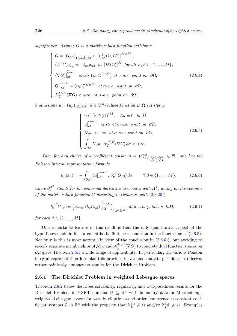
226 2.6. Boundary value problems in Muckenhoupt weighted spaces
significance. Assume G is a matrix-valued function satisfying
G =(Gαβ
)1≤α,β≤M ∈
[L1
loc(Ω,Ln)]M×M
,(L>G.β
)α
= −δx0δαβ in[D′(Ω)
]M for all α, β ∈ 1, . . . ,M,(∇G
)∣∣κ−n.t.
∂Ω exists (in Cn·M2) at σ-a.e. point on ∂Ω,
G∣∣κ−n.t.
∂Ω = 0 ∈ CM×M at σ-a.e. point on ∂Ω,
NΩ\Kκ
(∇G) < +∞ at σ-a.e. point on ∂Ω,
(2.6.4)
and assume u = (uβ)1≤β≤M is a CM -valued function in Ω satisfying
u ∈[C ∞(Ω)
]M, Lu = 0 in Ω,
u∣∣κ−n.t.
∂Ω exists at σ-a.e. point on ∂Ω,
Nκu < +∞ at σ-a.e. point on ∂Ω,ˆ∂ΩNκu · NΩ\K
κ(∇G) dσ < +∞.
(2.6.5)
Then for any choice of a coefficient tensor A =(aαβrs
)1≤r,s≤n
1≤α,β≤M∈ AL one has the
Poisson integral representation formula
uβ(x0) = −ˆ∂∗Ω
⟨u∣∣κ−n.t.
∂Ω , ∂A>
ν G.β⟩dσ, ∀β ∈ 1, . . . ,M, (2.6.6)
where ∂A>ν stands for the conormal derivative associated with A>, acting on the columnsof the matrix-valued function G according to (compare with (2.3.20))
∂A>
ν G.β :=(νra
γαsr
(∂sGγβ
)∣∣κ−n.t.
∂Ω
)1≤α≤M
at σ-a.e. point on ∂∗Ω, (2.6.7)
for each β ∈ 1, . . . ,M.
One remarkable feature of this result is that the only quantitative aspect of thehypotheses made in its statement is the finiteness condition in the fourth line of (2.6.5).Not only is this is most natural (in view of the conclusion in (2.6.6)), but avoiding tospecify separate memberships of Nκu and NΩ\K
κ(∇G) to concrete dual function spaces on
∂Ω gives Theorem 2.6.1 a wide range of applicability. In particular, the various Poissonintegral representation formulas this provides in various contexts permits us to derive,rather painlessly, uniqueness results for the Dirichlet Problem.
2.6.1 The Dirichlet Problem in weighted Lebesgue spaces
Theorem 2.6.2 below describes solvability, regularity, and well-posedness results for theDirichlet Problem in δ-SKT domains Ω ⊆ Rn with boundary data in Muckenhouptweighted Lebesgue spaces for weakly elliptic second-order homogeneous constant coef-ficient systems L in Rn with the property that Adis
L 6= ∅ and/or AdisL> 6= ∅. Examples
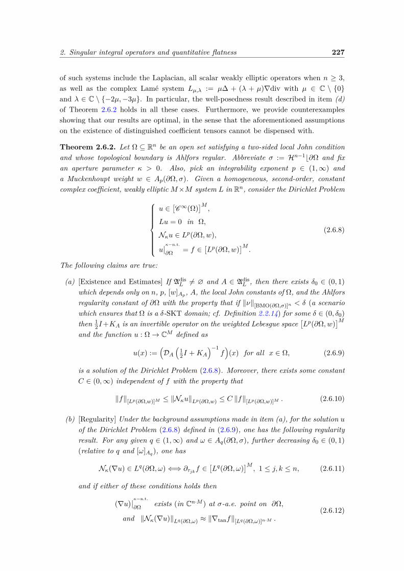
2. Singular integral operators and quantitative flatness 227
of such systems include the Laplacian, all scalar weakly elliptic operators when n ≥ 3,as well as the complex Lamé system Lµ,λ := µ∆ + (λ + µ)∇div with µ ∈ C \ 0and λ ∈ C \ −2µ,−3µ. In particular, the well-posedness result described in item (d)of Theorem 2.6.2 holds in all these cases. Furthermore, we provide counterexamplesshowing that our results are optimal, in the sense that the aforementioned assumptionson the existence of distinguished coefficient tensors cannot be dispensed with.
Theorem 2.6.2. Let Ω ⊆ Rn be an open set satisfying a two-sided local John conditionand whose topological boundary is Ahlfors regular. Abbreviate σ := Hn−1b∂Ω and fixan aperture parameter κ > 0. Also, pick an integrability exponent p ∈ (1,∞) anda Muckenhoupt weight w ∈ Ap(∂Ω, σ). Given a homogeneous, second-order, constantcomplex coefficient, weakly ellipticM×M system L in Rn, consider the Dirichlet Problem
u ∈[C∞(Ω)
]M,
Lu = 0 in Ω,
Nκu ∈ Lp(∂Ω, w),
u∣∣κ−n.t.
∂Ω = f ∈[Lp(∂Ω, w)
]M.
(2.6.8)
The following claims are true:
(a) [Existence and Estimates] If AdisL 6= ∅ and A ∈ Adis
L , then there exists δ0 ∈ (0, 1)which depends only on n, p, [w]Ap, A, the local John constants of Ω, and the Ahlforsregularity constant of ∂Ω with the property that if ‖ν‖[BMO(∂Ω,σ)]n < δ (a scenariowhich ensures that Ω is a δ-SKT domain; cf. Definition 2.2.14) for some δ ∈ (0, δ0)then 1
2I+KA is an invertible operator on the weighted Lebesgue space[Lp(∂Ω, w)
]Mand the function u : Ω→ CM defined as
u(x) :=(DA
(12I +KA
)−1f)(x) for all x ∈ Ω, (2.6.9)
is a solution of the Dirichlet Problem (2.6.8). Moreover, there exists some constantC ∈ (0,∞) independent of f with the property that
‖f‖[Lp(∂Ω,w)]M ≤ ‖Nκu‖Lp(∂Ω,w) ≤ C ‖f‖[Lp(∂Ω,w)]M . (2.6.10)
(b) [Regularity] Under the background assumptions made in item (a), for the solution uof the Dirichlet Problem (2.6.8) defined in (2.6.9), one has the following regularityresult. For any given q ∈ (1,∞) and ω ∈ Aq(∂Ω, σ), further decreasing δ0 ∈ (0, 1)(relative to q and [ω]Aq), one has
Nκ(∇u) ∈ Lq(∂Ω, ω)⇐⇒ ∂τjkf ∈[Lq(∂Ω, ω)
]M, 1 ≤ j, k ≤ n, (2.6.11)
and if either of these conditions holds then
(∇u)∣∣κ−n.t.
∂Ω exists (in Cn·M ) at σ-a.e. point on ∂Ω,
and ‖Nκ(∇u)‖Lq(∂Ω,ω) ≈ ‖∇tanf‖[Lq(∂Ω,ω)]n·M .(2.6.12)
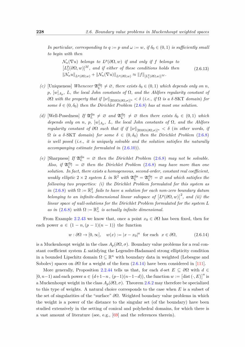
228 2.6. Boundary value problems in Muckenhoupt weighted spaces
In particular, corresponding to q := p and ω := w, if δ0 ∈ (0, 1) is sufficiently smallto begin with then
Nκ(∇u) belongs to Lp(∂Ω, w) if and only if f belongs to[Lp1(∂Ω, w)]M , and if either of these conditions holds then‖Nκu‖Lp(∂Ω,w) + ‖Nκ(∇u)‖Lp(∂Ω,w) ≈ ‖f‖[Lp1(∂Ω,w)]M .
(2.6.13)
(c) [Uniqueness] Whenever AdisL> 6= ∅, there exists δ0 ∈ (0, 1) which depends only on n,
p, [w]Ap, L, the local John constants of Ω, and the Ahlfors regularity constant of∂Ω with the property that if ‖ν‖[BMO(∂Ω,σ)]n < δ (i.e., if Ω is a δ-SKT domain) forsome δ ∈ (0, δ0) then the Dirichlet Problem (2.6.8) has at most one solution.
(d) [Well-Posedness] If AdisL 6= ∅ and Adis
L> 6= ∅ then there exists δ0 ∈ (0, 1) whichdepends only on n, p, [w]Ap, L, the local John constants of Ω, and the Ahlforsregularity constant of ∂Ω such that if if ‖ν‖[BMO(∂Ω,σ)]n < δ (in other words, ifΩ is a δ-SKT domain) for some δ ∈ (0, δ0) then the Dirichlet Problem (2.6.8)is well posed (i.e., it is uniquely solvable and the solution satisfies the naturallyaccompanying estimate formulated in (2.6.10)).
(e) [Sharpness] If AdisL = ∅ then the Dirichlet Problem (2.6.8) may not be solvable.
Also, if AdisL> = ∅ then the Dirichlet Problem (2.6.8) may have more than one
solution. In fact, there exists a homogeneous, second-order, constant real coefficient,weakly elliptic 2 × 2 system L in R2 with Adis
L = AdisL> = ∅ and which satisfies the
following two properties: (i) the Dirichlet Problem formulated for this system asin (2.6.8) with Ω := R2
+ fails to have a solution for each non-zero boundary datumbelonging to an infinite-dimensional linear subspace of
[Lp(∂Ω, w)
]2, and (ii) thelinear space of null-solutions for the Dirichlet Problem formulated for the system L
as in (2.6.8) with Ω := R2+ is actually infinite dimensional.
From Example 2.2.43 we know that, once a point x0 ∈ ∂Ω has been fixed, then foreach power a ∈
(1 − n, (p − 1)(n − 1)
)the function
w : ∂Ω→ [0,∞], w(x) := |x− x0|a for each x ∈ ∂Ω, (2.6.14)
is a Muckenhoupt weight in the class Ap(∂Ω, σ). Boundary value problems for a real con-stant coefficient system L satisfying the Legendre-Hadamard strong ellipticity conditionin a bounded Lipschitz domain Ω ⊆ Rn with boundary data in weighted (Lebesgue andSobolev) spaces on ∂Ω for a weight of the form (2.6.14) have been considered in [111].
More generally, Proposition 2.2.44 tells us that, for each d-set E ⊆ ∂Ω with d ∈[0, n−1) and each power a ∈
(d+1−n , (p−1)(n−1−d)
), the function w :=
[dist (·, E)
]a isa Muckenhoupt weight in the class Ap(∂Ω, σ). Theorem 2.6.2 may therefore be specializedto this type of weights. A natural choice corresponds to the case when E is a subset ofthe set of singularities of the “surface” ∂Ω. Weighted boundary value problems in whichthe weight is a power of the distance to the singular set (of the boundary) have beenstudied extensively in the setting of conical and polyhedral domains, for which there isa vast amount of literature (see, e.g., [69] and the references therein).
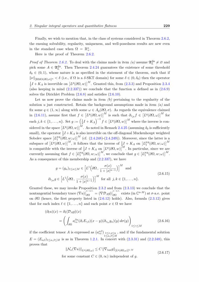
2. Singular integral operators and quantitative flatness 229
Finally, we wish to mention that, in the class of systems considered in Theorem 2.6.2,the ensuing solvability, regularity, uniqueness, and well-posedness results are new evenin the standard case when Ω = Rn+.
Here is the proof of Theorem 2.6.2.
Proof of Theorem 2.6.2. To deal with the claims made in item (a) assume AdisL 6= ∅ and
pick some A ∈ AdisL . Then Theorem 2.4.24 guarantees the existence of some threshold
δ0 ∈ (0, 1), whose nature is as specified in the statement of the theorem, such that if‖ν‖[BMO(∂Ω,σ)]n < δ (i.e., if Ω is a δ-SKT domain) for some δ ∈ (0, δ0) then the operator12I +KA is invertible on
[Lp(∂Ω, w)
]M . Granted this, from (2.3.3) and Proposition 2.3.4(also keeping in mind (2.2.337)) we conclude that the function u defined as in (2.6.9)solves the Dirichlet Problem (2.6.8) and satisfies (2.6.10).
Let us now prove the claims made in item (b) pertaining to the regularity of thesolution u just constructed. Retain the background assumptions made in item (a) andfix some q ∈ (1,∞) along with some ω ∈ Aq(∂Ω, σ). As regards the equivalence claimedin (2.6.11), assume first that f ∈
[Lp(∂Ω, w)
]M is such that ∂τjkf ∈[Lq(∂Ω, ω)
]M for
each j, k ∈ 1, . . . , n. Set g :=(
12I +KA
)−1f ∈
[Lp(∂Ω, w)
]M where the inverse is con-
sidered in the space[Lp(∂Ω, w)
]M . As noted in Remark 2.4.25 (assuming δ0 is sufficientlysmall), the operator 1
2I+KA is also invertible on the off-diagonal Muckenhoupt weightedSobolev space
[Lp;q1 (∂Ω, w;ω)
]M (cf. (2.4.248)-(2.4.249)). Moreover, since the latter is asubspace of
[Lp(∂Ω, w)
]M , it follows that the inverse of 12I + KA on
[Lp;q1 (∂Ω, w;ω)
]Mis compatible with the inverse of 1
2I +KA on[Lp(∂Ω, w)
]M . In particular, since we arecurrently assuming that f ∈
[Lp;q1 (∂Ω, w;ω)
]M , we conclude that g ∈[Lp;q1 (∂Ω, w;ω)
]M .As a consequence of this membership and (2.2.337), we have
g = (gα)1≤α≤M ∈[L1(∂Ω ,
σ(x)1 + |x|n−1
)]Mand
∂τjkg ∈[L1(∂Ω ,
σ(x)1 + |x|n−1
)]Mfor all j, k ∈ 1, . . . , n.
(2.6.15)
Granted these, we may invoke Proposition 2.3.2 and from (2.3.13) we conclude that thenontangential boundary trace (∇u
)∣∣κ−n.t.
∂Ω =(∇DAg
)∣∣κ−n.t.
∂Ω exists (in Cn·M ) at σ-a.e. pointon ∂Ω (hence, the first property listed in (2.6.12) holds). Also, formula (2.3.12) givesthat for each index ` ∈ 1, . . . , n and each point x ∈ Ω we have
(∂`u)(x) = ∂`(DAg
)(x)
=(ˆ
∂Ωaβαrs (∂rEγβ)(x− y)(∂τ`sgα)(y) dσ(y)
)1≤γ≤M
(2.6.16)
if the coefficient tensor A is expressed as(aαβrs
)1≤r,s≤n
1≤α,β≤M, and if the fundamental solution
E = (Eαβ)1≤α,β≤M is as in Theorem 1.2.1. In concert with (2.3.31) and (2.2.348), thisproves that
‖Nκ(∇u)‖Lq(∂Ω,ω) ≤ C ‖∇tang‖[Lq(∂Ω,ω)]n·M
for some constant C ∈ (0,∞) independent of g.(2.6.17)
230 2.6. Boundary value problems in Muckenhoupt weighted spaces
In particular, Nκ(∇u) belongs to Lq(∂Ω, ω), which finishes the justification of the right-to-left implication in (2.6.11). Also, in light of (2.6.17), to justify the left-pointinginequality in the equivalence claimed in (2.6.12), there remains to show that, for someconstant C ∈ (0,∞) independent of f ,
‖∇tang‖[Lq(∂Ω,ω)]n·M ≤ C ‖∇tanf‖[Lq(∂Ω,ω)]n·M . (2.6.18)
To this end, use (2.4.240) to write, for each j, k ∈ 1, . . . , n,
∂τjkf = ∂τjk[(1
2I +KA
)g]
=(1
2I +KA
)(∂τjkg) + Ujk(∇tang)
=(1
2I +KA
)(∂τjkg) + Ujk
((νr∂τrsgα
)1≤α≤M1≤s≤n
)(2.6.19)
at σ-a.e. point on ∂Ω, where ν = (νr)1≤r≤n is the geometric measure theoretic outwardunit normal to Ω. Using the abbreviations
∇τf :=(∂τjkf
)1≤j,k≤n, ∇τg :=
(∂τjkg
)1≤j,k≤n, (2.6.20)
we find it convenient to recast the collection of all formulas as in (2.6.19), correspondingto all indices j, k ∈ 1, . . . , n, simply as
∇τf =(1
2I +R)(∇τg), (2.6.21)
where I is the identity and R is the operator acting from[Lq(∂Ω, ω)
]M ·n2into itself
according toR := KA +
(Ujk
(Mνr παrs
)1≤α≤M1≤s≤n
)1≤j,k≤n
. (2.6.22)
Above, we let KA act on each F =(Fαrs)
1≤α≤M1≤r,s≤n
∈[Lq(∂Ω, ω)
]M ·n2by setting
KAF :=(KA
(Fαrs)1≤α≤M
)1≤r,s≤n
. (2.6.23)
Also, recall that each Mνr denotes the operator of pointwise multiplication by νr, ther-th scalar component of ν. Finally, in (2.6.22) we let each παrs be the “coordinate-projection” operator which acts as παrs(X) := Xα
rs for every X =(Xαrs
)1≤α≤M1≤r,s≤n
∈ CM ·n2 .
From (2.6.22), (2.4.241), (2.4.238), Theorem 2.4.14, and (2.3.27), we then conclude that
‖R‖[Lq(∂Ω,ω)]M·n2→[Lq(∂Ω,ω)]M·n2 ≤ C ‖ν‖[BMO(∂Ω,σ)]n (2.6.24)
for some C ∈ (0,∞) which depends only on n, A, q, [ω]Aq , the local John constants of Ω,and the Ahlfors regularity constant of ∂Ω. As a consequence of this, if we assume δ0 > 0to be sufficiently small to begin with, a Neumann series argument gives that
12I +R is invertible on
[Lq(∂Ω, ω)
]M ·n2, (2.6.25)
and provides an estimate for the norm on the inverse. At this stage, the estimate claimedin (2.6.18) follows from (2.6.21), (2.6.25), (2.6.20), and (2.2.347)-(2.2.348). As noted
2. Singular integral operators and quantitative flatness 231
earlier, this concludes the proof of the left-pointing inequality in the equivalence claimedin (2.6.12). To complete the treatment of item (b), there remains to observe that theright-pointing implication in (2.6.11) together with the right-pointing inequality in theequivalence claimed in (2.6.12) are consequences of Proposition 2.2.49 (bearing in mind(2.2.347)).
Consider next the uniqueness result claimed in item (c). Suppose AdisL> 6= ∅ and pick
some A ∈ AL such that A> ∈ AdisL> . Also, denote by p′ ∈ (1,∞) the Hölder conjugate
exponent of p, and set w′ := w1−p′ ∈ Ap′(∂Ω, σ). From Theorem 2.4.24, presently usedwith L replaced by L>, p′ in place of p, and w′ in place of w, we know that there existsδ0 ∈ (0, 1), which depends only on n, p, [w]Ap , A, the local John constants of Ω, and theAhlfors regularity constant of ∂Ω, such that if Ω is a δ-SKT domain with 0 < δ < δ0
then12I +KA> :
[Lp′
1 (∂Ω, w′)]M −→ [
Lp′
1 (∂Ω, w′)]M (2.6.26)
is an invertible operator.By eventually decreasing the value of δ0 ∈ (0, 1) if necessary, we may ensure that Ω
is an NTA domain with unbounded boundary (cf. Proposition 2.2.32 and Lemma 2.2.5).In such a case, (2.6.2) guarantees that Ω is globally pathwise nontangentially accessible.
To proceed, let E =(Eαβ
)1≤α,β≤M be the fundamental solution associated with the
system L as in Theorem 1.2.1. Fix x? ∈ Rn \ Ω along with x0 ∈ Ω, arbitrary. Also, pickρ ∈
(0 , 1
4 dist (x0, ∂Ω))and define K := B(x0, ρ). Finally, recall the aperture parameter
κ > 0 associated with Ω and κ as in Theorem 2.6.1. Next, for each fixed β ∈ 1, . . . ,M,consider the CM -valued function
f (β)(x) :=(Eβα(x− x0)− Eβα(x− x?)
)1≤α≤M , ∀x ∈ ∂Ω. (2.6.27)
From (2.6.27), (2.2.349), (2.2.341), (2.2.335), (1.2.19), and the Mean Value Theorem wethen conclude that
f (β) ∈[Lp′
1 (∂Ω, w′)]M. (2.6.28)
As a consequence, with(
12I +KA>
)−1denoting the inverse of the operator in (2.6.26),
vβ :=(vβα
)1≤α≤M := DA>
( (12I +KA>
)−1f (β)
)(2.6.29)
is a well-defined CM -valued function in Ω which, thanks to Proposition 2.3.4, satisfies
vβ ∈[C∞(Ω)
]M, L>vβ = 0 in Ω,
Nκvβ ∈ Lp′(∂Ω, w′), Nκ(∇vβ) ∈ Lp′(∂Ω, w′),
and vβ∣∣κ−n.t.
∂Ω = f (β) at σ-a.e. point on ∂Ω.
(2.6.30)
Moreover, from (2.6.28)-(2.6.29) and (2.3.60) we see that
(∇vβ)∣∣κ−n.t.
∂Ω exists (in Cn·M ) at σ-a.e. point on ∂Ω. (2.6.31)
232 2.6. Boundary value problems in Muckenhoupt weighted spaces
Subsequently, for each pair of indices α, β ∈ 1, . . . ,M define
Gαβ(x) := vβα(x)−(Eβα(x− x0)− Eβα(x− x?)
), ∀x ∈ Ω \ x0. (2.6.32)
If we now consider G :=(Gαβ
)1≤α,β≤M as a CM×M -valued function defined Ln-a.e. in
Ω, then from (2.6.32) and Theorem 1.2.1 we see that G ∈[L1
loc(Ω,Ln)]M×M . Also, by
design,L>G = −δx0IM×M in
[D′(Ω)
]M×M and
G∣∣κ−n.t.
∂Ω = 0 at σ-a.e. point on ∂Ω,(∇G
)∣∣κ−n.t.
∂Ω exists at σ-a.e. point on ∂Ω,
(2.6.33)
while if v :=(vβα
)1≤α,β≤M then from (1.1.4), (1.2.19), and the Mean Value Theorem it
follows that at each point x ∈ ∂Ω we have(NΩ\Kκ
G)(x) ≤
(Nκv
)(x) + Cx0,ρ(1 + |x|)1−n and(
NΩ\Kκ
(∇G))(x) ≤
(Nκ(∇v)
)(x) + Cx0,ρ(1 + |x|)−n,
(2.6.34)
where Cx0,ρ ∈ (0,∞) is independent of x. In view of (2.6.30), (2.6.34), and (2.2.335) wesee that the conditions listed in (2.6.4) are presently satisfied and, in fact,
NΩ\Kκ
(∇G) ∈ Lp′(∂Ω, w′) =(Lp(∂Ω, w)
)∗. (2.6.35)
Suppose now that u = (uβ)1≤β≤M is a CM -valued function in Ω satisfying
u ∈[C ∞(Ω)
]M, Lu = 0 in Ω,
u∣∣κ−n.t.
∂Ω exists at σ-a.e. point on ∂Ω,
and Nκu belongs to the space Lp(∂Ω, w).
(2.6.36)
Since (2.6.35) implies ˆ∂ΩNκu · NΩ\K
κ(∇G) dσ < +∞, (2.6.37)
we may then invoke Theorem 2.6.1 to conclude that the Poisson integral representationformula (2.6.6) holds. In particular, this proves that whenever u
∣∣κ−n.t.
∂Ω = 0 at σ-a.e. pointon ∂Ω we necessarily have u(x0) = 0. Given that x0 has been arbitrarily chosen in Ω,this ultimately shows such a function u is actually identically zero in Ω. This finishes theproof of the claim made in item (c).
Next, the well-posedness claim in item (d) is a consequence of what we have provedin items (a) and (c). Finally, the two optimality results formulated in item (e) are seenfrom Proposition 2.3.12, and from Example 2.3.11, respectively.
Remark 2.6.3. The approach used to prove Theorem 2.6.2 relies on mapping propertiesand invertibility results for boundary layer potentials on Muckenhoupt weighted Lebesgueand Sobolev spaces. Given that analogous of these results are also valid on Lorentzspaces and Lorentz-based Sobolev spaces (cf. Remark 2.4.25, and the Lorentz space
2. Singular integral operators and quantitative flatness 233
version of (2.3.31) obtained via real interpolation), the type of argument used to establishTheorem 2.6.2 produces similar results for the Dirichlet Problem with data in Lorentzspaces, i.e., for
u ∈[C∞(Ω)
]M,
Lu = 0 in Ω,
Nκu ∈ Lp,q(∂Ω, σ),
u∣∣κ−n.t.
∂Ω = f ∈[Lp,q(∂Ω, σ)
]M.
(2.6.38)
More specifically, for this boundary problem existence holds in the setting of item (a)of Theorem 2.6.2 whenever p ∈ (1,∞) and q ∈ (0,∞], whereas uniqueness holds inthe setting of item (c) of Theorem 2.6.2 provided p ∈ (1,∞) and q ∈ (0,∞] (see [45,Theorem 1.4.17, p. 52] for duality results for Lorentz spaces).
In particular, corresponding to q = ∞, whenever AdisL 6= ∅ and Adis
L> 6= ∅ it followsthat for each p ∈ (1,∞) the weak-Lp Dirichlet Problem
u ∈[C∞(Ω)
]M,
Lu = 0 in Ω,
Nκu ∈ Lp,∞(∂Ω, σ),
u∣∣κ−n.t.
∂Ω = f ∈[Lp,∞(∂Ω, σ)
]M,
(2.6.39)
is well posed assuming Ω is a δ-SKT domain for a sufficiently small δ > 0, relative to n,p, L, the local John constants of Ω, and the Ahlfors regularity constant of ∂Ω. As in theproof of Theorem 2.6.2, uniqueness is obtained relying on the Poisson integral represen-tation formula from Theorem 2.6.1. This requires checking that the Green function withcomponents as in (2.6.32) is well defined and satisfies NΩ\K
κ(∇G) ∈ Lp′,1(∂Ω, σ), where
p′ is the Hölder conjugate exponents of p. Once this task is accomplished, the fact thatNκu ∈ Lp,∞(∂Ω, σ) =
(Lp′,1(∂Ω, σ)
)∗ (cf. [45, Theorem 1.4.17(v), p. 52]) guarantees thatthe finiteness condition (2.6.37) presently holds, and the desired conclusion follows. Inturn, the membership of NΩ\K
κ(∇G) to Lp′,1(∂Ω, σ) is seen from (2.6.34) and (2.6.29),
keeping in mind that the operator 12I +KA> (where A ∈ AL is such that A> ∈ Adis
L>) isinvertible on the Lorentz-based Sobolev space
[Lp′,1
1 (∂Ω, σ)]M and, as seen from standard
real interpolation inclusions, (1 + |x|)−N ∈ Lp,q(∂Ω, σ) whenever N ≥ n− 1, p ∈ (1,∞),and q ∈ (0,∞].
To offer an example, assume Ω ⊆ Rn is a δ-SKT domain and fix an arbitrary apertureparameter κ > 0 along with some power a ∈ (0, n − 1). Set p := (n − 1)/a ∈ (1,∞).Then, if δ ∈ (0, 1) is sufficiently small (relative to n, a, the Ahlfors regularity constantof ∂Ω, and the local John constants of Ω), it follows that for each point xo ∈ ∂Ωthe Dirichlet Problem u ∈ C∞(Ω), ∆u = 0 in Ω, Nκu ∈ Lp,∞(∂Ω, σ),(
u∣∣κ−n.t.
∂Ω
)(x) = |x− xo|−a at σ-a.e. point on ∂Ω,
(2.6.40)
234 2.6. Boundary value problems in Muckenhoupt weighted spaces
is uniquely solvable. In addition, there exists a constant C(Ω, n, κ, a) ∈ (0,∞) withthe property that if uxo denotes the unique solution of (2.6.40) then we have the esti-mate ‖Nκuxo‖Lp,∞(∂Ω,σ) ≤ C(Ω, n, κ, a) for each xo ∈ ∂Ω. Indeed, since the functionfxo(x) := |x − xo|−a for σ-a.e. point x ∈ ∂Ω belongs to the Lorentz space Lp,∞(∂Ω, σ)and supxo∈∂Ω ‖fxo‖Lp,∞(∂Ω,σ) < ∞, the solvability result in Remark 2.6.3 applies. Thisexample is particularly relevant in view of the fact that the boundary datum |·−xo|−a doesnot belong to any ordinary Lebesgue space on ∂Ω with respect to the “surface measure”σ. In addition, since for each j, k ∈ 1, . . . , n the boundary datum fxo satisfies
∂τjkfxo ∈ Lq,∞(∂Ω, σ) and supxo∈∂Ω∥∥∂τjkfxo∥∥Lq,∞(∂Ω,σ) <∞,
where q := (n− 1)/(a+ 1) ∈ (1,∞),(2.6.41)
given that, if (νi)1≤i≤n are the components of the geometric outward unit normal vector toΩ,
(∂τjkfxo
)(x) = a
(x− xo)jνk(x)− (x− xo)kνj(x)|x− xo|a+2 for σ-a.e. x ∈ ∂Ω, (2.6.42)
then the analogues of (2.6.11)-(2.6.12) in the current setting imply that the uniquesolution uxo of the Dirichlet Problem (2.6.40) enjoys additional regularity. Specifically,if δ ∈ (0, 1) is sufficiently small to begin with, then
for each xo ∈ ∂Ω, the nontangential boundary trace
(∇uxo)∣∣κ−n.t.
∂Ω exists (in Rn) at σ-a.e. point on ∂Ω,
and supxo∈∂Ω
‖Nκ(∇uxo)‖Lq,∞(∂Ω,σ) < +∞ if q := n−1a+1 .
(2.6.43)
In relation to the Dirichlet Problem with data in weak-Lebesgue spaces formulated in(2.6.39), we also wish to note that, in contrast to the well-posedness result in the range p ∈(1,∞), uniqueness no longer holds in the limiting case when p = 1. Indeed, if we take Ω :=Rn+ and u(x) := xn/|x|n for each x = (x1, . . . , xn) ∈ Ω then, since under the identification∂Ω ≡ Rn−1 we have
(Nκu
)(x′) ≈ |x′|1−n uniformly for x′ ∈ Rn−1 \ 0, wee see that
u ∈ C∞(Ω),
∆u = 0 in Ω,
Nκu ∈ L1,∞(∂Ω, σ),
u∣∣κ−n.t.
∂Ω = 0 at σ-a.e. point x ∈ ∂Ω,
(2.6.44)
and yet, obviously, u 6≡ 0 in Ω.
Moving on, it is remarkable that the solvability results described in Theorem 2.6.2are also stable under small perturbations. This is made precise in the theorem below.
Theorem 2.6.4. Retain the original background assumptions on the set Ω from Theo-rem 2.6.2 and, as before, fix an integrability exponent p ∈ (1,∞) along with a Mucken-houpt weight w ∈ Ap(∂Ω, σ). Then the following statements are true.
2. Singular integral operators and quantitative flatness 235
(a) [Existence] For each given system Lo ∈ Ldis (cf. (2.3.84)) there exist some smallthreshold δ0 ∈ (0, 1) and some open neighborhood U of Lo in L, both of which dependonly on n, p, [w]Ap, Lo, the local John constants of Ω, and the Ahlfors regularityconstant of ∂Ω, with the property that if ‖ν‖[BMO(∂Ω,σ)]n < δ (i.e., if Ω is a δ-SKTdomain) for some δ ∈ (0, δ0) then for each system L ∈ U the Dirichlet Problem(2.6.8) formulated for L is solvable.
(b) [Uniqueness] For each given system Lo ∈ L with L>o ∈ Ldis there exist some smallthreshold δ0 ∈ (0, 1) and some open neighborhood U of Lo in L, both of which dependonly on n, p, [w]Ap, Lo, the local John constants of Ω, and the Ahlfors regularityconstant of ∂Ω, with the property that if ‖ν‖[BMO(∂Ω,σ)]n < δ (i.e., if Ω is a δ-SKTdomain) for some δ ∈ (0, δ0) then for each system L ∈ U the Dirichlet Problem(2.6.8) formulated for L has at most one solution.
(c) [Well-Posedness] For each given system Lo ∈ Ldis with L>o ∈ Ldis there exist somesmall threshold δ0 ∈ (0, 1) and some open neighborhood U of Lo in L, both of whichdepend only on n, p, [w]Ap, Lo, the local John constants of Ω, and the Ahlforsregularity constant of ∂Ω, with the property that if ‖ν‖[BMO(∂Ω,σ)]n < δ (i.e., if Ωis a δ-SKT domain) for some δ ∈ (0, δ0) then for each system L ∈ U the DirichletProblem (2.6.8) formulated for L is well posed.
Proof. To deal with the claim made in item (a), start by observing that the assumptionLo ∈ Ldis guarantees the existence of some Ao ∈ Adis
Lo. By Theorem 2.4.29 (used with,
say, ε := 1/4) then ensures the existence of some small threshold δ0 ∈ (0, 1) along withsome open neighborhood O of Ao in AWE , both of which depend only on n, p, [w]Ap ,Ao, the local John constants of Ω, and the Ahlfors regularity constant of ∂Ω, with theproperty that if ‖ν‖[BMO(∂Ω,σ)]n < δ0 then for each A ∈ O the operator 1
2I + KA
isinvertible on
[Lp(∂Ω, w)
]M . Pick ε > 0 such that A ∈ A : ‖A − Ao‖ < ε ⊆ O, anddefine U := L ∈ L : ‖L − Lo‖ < ε. Choose now an arbitrary system L ∈ U . Bydesign, there exists A ∈ AL and B ∈ Aant such that ‖A − Ao − B‖ < ε. Hence, if wenow introduce A := A − B, then A ∈ AL and the fact that ‖A − Ao‖ < ε implies thatA ∈ O. In particular, the latter property permits us to conclude (in light of our earlierdiscussion) that the operator 1
2I + KA
is invertible on[Lp(∂Ω, w)
]M . Given that wealso have A ∈ AL, it follows (much as in the proof of Theorem 2.6.2) that the functionu : Ω→ CM defined as
u(x) :=(DA
(12I +K
A
)−1f)(x) for all x ∈ Ω, (2.6.45)
is a solution of the Dirichlet Problem (2.6.8) formulated for the current system L. Thisfinishes the proof of the claim made in item (a).
On to the claim in item (b), pick some Ao ∈ ALo with A>o ∈ AdisL>o
. Running thesame argument as above (with L>o playing the role of Lo, A>o playing the role of Ao, andkeeping in mind that transposition is an isometry) yields some small threshold δ0 ∈ (0, 1)along with some open neighborhood U of Lo in L, both of which depend only on n, p,
236 2.6. Boundary value problems in Muckenhoupt weighted spaces
[w]Ap , Ao, the local John constants of Ω, and the Ahlfors regularity constant of ∂Ω, withthe property that if ‖ν‖[BMO(∂Ω,σ)]n < δ0 then for each system L ∈ U we may find acoefficient tensor A ∈ AL with the property that the operator 1
2I+K(A)> is invertible on
the Muckenhoupt weighted Sobolev space[Lp′
1 (∂Ω, w′)]M . This is a perturbation of the
invertibility result in (2.6.26) and, once this has been established, the same argument asin the proof of item (b) of Theorem 2.6.2 applies and gives the conclusion we presentlyseek.
Finally, the claim in item (c) is a direct consequence of what we have proved in items(a)-(b).
2.6.2 The Regularity Problem in weighted Sobolev spaces
Traditionally, the label “Regularity Problem” is intended for a version of the DirichletProblem in which both the boundary datum and the solution sought are more “regular”than in the standard formulation of the Dirichlet Problem. For us here, this means thatwe shall now select boundary data from Muckenhoupt weighted Sobolev spaces and alsodemand control of the nontangential maximal operator of the gradient of the solution.This being said, the specific manner in which we have formulated the solvability resultfor the Dirichlet Problem in Theorem 2.6.2, in particular, having already elaborated onhow extra regularity of the boundary datum affects the regularity of the solution (cf.(2.6.11)), renders the Regularity Problem a “sub-problem” of the Dirichlet Problem. Asseen below, this makes light work of the treatment of the Regularity Problem.
Theorem 2.6.5. Let Ω ⊆ Rn be an open set satisfying a two-sided local John conditionand whose topological boundary is Ahlfors regular. Abbreviate σ := Hn−1b∂Ω and fixan aperture parameter κ > 0. Also, pick an integrability exponent p ∈ (1,∞) anda Muckenhoupt weight w ∈ Ap(∂Ω, σ). Given a homogeneous, second-order, constantcomplex coefficient, weakly elliptic M × M system L in Rn, consider the RegularityProblem
u ∈[C∞(Ω)
]M,
Lu = 0 in Ω,
Nκu, Nκ(∇u) ∈ Lp(∂Ω, w),
u∣∣κ−n.t.
∂Ω = f ∈[Lp1(∂Ω, w)
]M.
(2.6.46)
The following statements are true:
(a) [Existence and Estimates] If AdisL 6= ∅ and A ∈ Adis
L , then there exists δ0 ∈ (0, 1)which depends only on n, p, [w]Ap, A, the local John constants of Ω, and theAhlfors regularity constant of ∂Ω such that if Ω is a δ-SKT domain with 0 < δ < δ0
then 12I +KA is an invertible operator on the Muckenhoupt weighted Sobolev space[
Lp1(∂Ω, w)]M and the function
u(x) :=(DA
(12I +KA
)−1f)(x), ∀x ∈ Ω, (2.6.47)
2. Singular integral operators and quantitative flatness 237
is a solution of the Regularity Problem (2.6.46). In addition,
‖Nκu‖Lp(∂Ω,w) ≈ ‖f‖[Lp(∂Ω,w)]M , (2.6.48)
and‖Nκ(∇u)‖Lp(∂Ω,w) ≈ ‖∇tanf‖[Lp(∂Ω,w)]n·M . (2.6.49)
In particular,
‖Nκu‖Lp(∂Ω,w) + ‖Nκ(∇u)‖Lp(∂Ω,w) ≈ ‖f‖[Lp1(∂Ω,w)]M . (2.6.50)
(b) [Uniqueness] Whenever AdisL> 6= ∅, there exists δ0 ∈ (0, 1) which depends only on n,
p, [w]Ap, L, the local John constants of Ω, and the Ahlfors regularity constant of∂Ω such that if Ω is a δ-SKT domain with 0 < δ < δ0 then the Regularity Problem(2.6.46) has at most one solution.
(c) [Well-Posedness] If AdisL 6= ∅ and Adis
L> 6= ∅ then there exists δ0 ∈ (0, 1) whichdepends only on n, p, [w]Ap, L, the local John constants of Ω, and the Ahlforsregularity constant of ∂Ω such that if Ω is a δ-SKT domain with 0 < δ < δ0
then the Regularity Problem (2.6.46) is uniquely solvable and the solution satisfies(2.6.48)-(2.6.50).
(d) [Sharpness] If AdisL = ∅ the Regularity Problem (2.6.46) may fail to be solvable, and
if AdisL> = ∅ the Regularity Problem (2.6.46) may posses more than one solution. In
particular, if either AdisL = ∅, or Adis
L> = ∅, then the Regularity Problem (2.6.46)may fail to be well posed.
Proof. All claims in items (a)-(c) are direct consequences of Theorem 2.4.24 and The-orem 2.6.2. As regards the sharpness results formulated in item (d), the fact thatthe Regularity Problem (2.6.46) may fail to be solvable when Adis
L = ∅ is seen fromProposition 2.3.14 and (2.3.140). Finally, that the Regularity Problem (2.6.46) for Lmay have more than one solution if Adis
L> = ∅ is seen from Example 2.3.11.
Remark 2.6.6. From Remark 2.6.3 we see that the Regularity Problem with data inLorentz-based Sobolev spaces, i.e.,
u ∈[C∞(Ω)
]M,
Lu = 0 in Ω,
Nκu, Nκ(∇u) ∈ Lp,q(∂Ω, σ),
u∣∣κ−n.t.
∂Ω = f ∈[Lp,q1 (∂Ω, σ)
]M,
(2.6.51)
enjoys similar solvability and well-posedness results to those described in Theorem 2.6.5.Concretely, for this boundary problem we have existence in the setting of item (a) ofTheorem 2.6.5 whenever p ∈ (1,∞) and q ∈ (0,∞], and we have uniqueness in thesetting of item (b) of Theorem 2.6.5 whenever p, q ∈ (1,∞).
238 2.6. Boundary value problems in Muckenhoupt weighted spaces
Remark 2.6.7. An inspection of the proof of Theorem 2.6.5 reveals that similar solvabilityand well-posedness results are valid in the case when the boundary data belong to the off-diagonal Muckenhoupt weighted Sobolev spaces discussed in (2.4.248)-(2.4.249). Morespecifically, given two integrability exponents p1, p2 ∈ (1,∞) along with two Mucken-houpt weights w1 ∈ Ap1(∂Ω, σ) and w2 ∈ Ap2(∂Ω, σ), the off-diagonal Regularity Problem
u ∈[C∞(Ω)
]M,
Lu = 0 in Ω,
Nκu ∈ Lp1(∂Ω, w1),
Nκ(∇u) ∈ Lp2(∂Ω, w2),
u∣∣κ−n.t.
∂Ω = f ∈[Lp1;p2
1 (∂Ω, w1;w2)]M,
(2.6.52)
continues to enjoy similar solvability and well-posedness results to those described inTheorem 2.6.5. Of course, this time, the a priori estimates (2.6.48)-(2.6.49) read
‖Nκu‖Lp1 (∂Ω,w1) ≈ ‖f‖[Lp1 (∂Ω,w1)]M , (2.6.53)
and‖Nκ(∇u)‖Lp2 (∂Ω,w2) ≈ ‖∇tanf‖[Lp2 (∂Ω,w2)]n·M . (2.6.54)
Remark 2.6.8. Once again, in the class of systems considered in Theorem 2.6.5, thesolvability, uniqueness, and well-posedness results for the Regularity Problem (2.6.46)are new even in the standard case when Ω = Rn+.
As in the case of the Dirichlet Problem, it turns out that the solvability results pre-sented in Theorem 2.6.5 are stable under small perturbations, of the sort described below.
Theorem 2.6.9. Retain the original background assumptions on the set Ω from Theo-rem 2.6.5 and, as before, fix an integrability exponent p ∈ (1,∞) along with a Mucken-houpt weight w ∈ Ap(∂Ω, σ). Then the following statements are true.
(a) [Existence] Given any system Lo ∈ Ldis (cf. (2.3.84)), there exist a threshold δ0 ∈(0, 1) and an open neighborhood U of Lo in L, both of which depend only on n,p, [w]Ap, Lo, the local John constants of Ω, and the Ahlfors regularity constant of∂Ω, with the property that if ‖ν‖[BMO(∂Ω,σ)]n < δ (i.e., if Ω is a δ-SKT domain)for some δ ∈ (0, δ0) then for each system L ∈ U the Regularity Problem (2.6.46)formulated for L is solvable.
(b) [Uniqueness] Given any system Lo ∈ L with L>o ∈ Ldis there exist a thresholdδ0 ∈ (0, 1) and an open neighborhood U of Lo in L, both of which depend only onn, p, [w]Ap, Lo, the local John constants of Ω, and the Ahlfors regularity constantof ∂Ω, with the property that if ‖ν‖[BMO(∂Ω,σ)]n < δ (i.e., if Ω is a δ-SKT domain)for some δ ∈ (0, δ0) then for each system L ∈ U the Regularity Problem (2.6.46)formulated for L has at most one solution.
2. Singular integral operators and quantitative flatness 239
(c) [Well-Posedness] Given any system Lo ∈ Ldis with L>o ∈ Ldis there exist a thresholdδ0 ∈ (0, 1) and an open neighborhood U of Lo in L, both of which depend only onn, p, [w]Ap, Lo, the local John constants of Ω, and the Ahlfors regularity constantof ∂Ω, with the property that if ‖ν‖[BMO(∂Ω,σ)]n < δ (i.e., if Ω is a δ-SKT domain)for some δ ∈ (0, δ0) then for each system L ∈ U the Regularity Problem (2.6.46)formulated for L is well posed.
Proof. The same type of argument used in the proof of Theorem 2.6.4 continues to workin this setting.
2.6.3 The Neumann Problem in weighted Lebesgue spaces
To set the stage, recall the definition of the conormal derivative operator from (2.3.20).
Theorem 2.6.10. Let Ω ⊆ Rn be an open set satisfying a two-sided local John conditionand whose topological boundary is Ahlfors regular. Denote by ν the geometric measuretheoretic outward unit normal ν to Ω, abbreviate σ := Hn−1b∂Ω, and fix an apertureparameter κ > 0. Also, pick an integrability exponent p ∈ (1,∞) and a Muckenhouptweight w ∈ Ap(∂Ω, σ).
Suppose L is a homogeneous, second-order, constant complex coefficient, weakly el-liptic M ×M system in Rn, with the property that Adis
L> 6= ∅. Select A ∈ AL such thatA> ∈ Adis
L> and consider the Neumann Problem
u ∈[C∞(Ω)
]M,
Lu = 0 in Ω,
Nκ(∇u) ∈ Lp(∂Ω, w),
∂Aν u = f ∈[Lp(∂Ω, w)
]M.
(2.6.55)
Then there exists δ0 ∈ (0, 1) which depends only on n, p, [w]Ap, A, the local Johnconstants of Ω, and the Ahlfors regularity constant of ∂Ω such that if Ω is a δ-SKTdomain with 0 < δ < δ0 then −1
2I + K#A>
is an invertible operator on the Muckenhouptweighted Lebesgue space
[Lp(∂Ω, w)
]M and the function u : Ω→ CM defined as
u(x) :=(Smod
(−1
2I +K#A>
)−1f)(x) for all x ∈ Ω, (2.6.56)
is a solution of the Neumann Problem (2.6.55) which satisfies
‖Nκ(∇u)‖Lp(∂Ω,w) ≤ C ‖f‖[Lp(∂Ω,w)]M . (2.6.57)
for some constant C ∈ (0,∞) independent of f .
Proof. From the current assumptions and Theorem 2.4.24 we know that there exists somethreshold δ0 ∈ (0, 1), whose nature is as specified in the statement of the theorem, suchthat if Ω is a δ-SKT domain with 0 < δ < δ0 then the operator −1
2I +K#A>
is invertibleon[Lp(∂Ω, w)
]M . Granted this, item (c) in Proposition 2.3.4 then guarantees that thefunction (2.6.56) solves the Neumann Problem (2.6.55) and satisfies (2.6.57).
240 2.6. Boundary value problems in Muckenhoupt weighted spaces
Remark 2.6.11. For similar reasons as in past situations, a solvability result which isanalogous to the one described in Theorem 2.6.10 also holds for the Neumann Problemwith data in Lorentz spaces, i.e., for
u ∈[C∞(Ω)
]M,
Lu = 0 in Ω,
Nκ(∇u) ∈ Lp,q(∂Ω, σ),
∂Aν u = f ∈[Lp,q(∂Ω, σ)
]M,
(2.6.58)
with p ∈ (1,∞) and q ∈ (0,∞].
Remark 2.6.12. In light of the remarks made in (2.3.103)-(2.3.104), Theorem 2.6.10applies in the case of the Lamé system Lµ,λ = µ∆ + (λ + µ)∇div in Rn with n ≥ 2,assuming µ 6= 0, 2µ+ λ 6= 0, and 3µ+ λ 6= 0. Specifically, if Ω ⊆ Rn is a δ-SKT domain,and w ∈ Ap(∂Ω, σ) with p ∈ (1,∞), then if δ ∈ (0, 1) sufficiently small (relative to µ, λ,p, [w]Ap , the local John constants of Ω, and the Ahlfors regularity constant of ∂Ω) theNeumann Problem (2.6.55), which in this case reads
u ∈[C∞(Ω)
]n,
µ∆u+ (λ+ µ)∇divu = 0 in Ω,
Nκ(∇u) ∈ Lp(∂Ω, w),
∂A(ζ)ν u =
[µ(∇u)> + ζ(∇u)
]∣∣∣κ−n.t.
∂Ων + (µ+ λ− ζ)(divu)
∣∣κ−n.t.
∂Ω ν = f
(2.6.59)
is solvable (in the manner described in (2.6.56)) for each given function f ∈[Lp(∂Ω, w)
]n,provided
ζ = µ(µ+ λ)3µ+ λ
. (2.6.60)
By way of contrast, in the two-dimensional case, Corollary 2.4.31 ensures that the Neu-mann Problem (2.6.59) is actually solvable (again, in the manner described in (2.6.56))for each given function f ∈
[Lp(∂Ω, w)
]2, in the much larger range
ζ ∈ C \− µ , µ(5µ+3λ)
3µ+λ
. (2.6.61)
In particular, if we also demand that µ+λ 6= 0 then ζ := µ becomes an admissible value,as far as (2.6.61) is concerned, and from (2.4.304), (2.6.56) we see that the NeumannProblem (2.6.59) with ζ := µ is solvable for each given function f ∈
[Lp(∂Ω, w)
]2. This isof interest since the said problem involves the so-called traction conormal derivative,i.e.,
∂A(µ)ν u = µ
[(∇u)> + (∇u)
]∣∣∣κ−n.t.
∂Ων + λ(divu)
∣∣κ−n.t.
∂Ω ν, (2.6.62)
which is particularly relevant in physics and engineering.
It is also of interest to note that the solvability result from Theorem 2.6.10 is sta-ble under small perturbations. Specifically, by reasoning similarly as in the proof ofTheorem 2.6.4 yields the following theorem.
2. Singular integral operators and quantitative flatness 241
Theorem 2.6.13. Retain the original background assumptions on the set Ω from The-orem 2.6.10 and, as before, fix an integrability exponent p ∈ (1,∞) along with a Muck-enhoupt weight w ∈ Ap(∂Ω, σ). Also, consider a system Lo ∈ L with L>o ∈ Ldis (cf.(2.3.84)). Then for any Ao ∈ ALo with A>o ∈ Adis
L>othere exist a threshold δ0 ∈ (0, 1) and
an open neighborhood U of Ao in A, both of which depend only on n, p, [w]Ap, Ao, thelocal John constants of Ω, and the Ahlfors regularity constant of ∂Ω, with the propertythat if ‖ν‖[BMO(∂Ω,σ)]n < δ (i.e., if Ω is a δ-SKT domain) for some δ ∈ (0, δ0) then foreach coefficient tensor A ∈ U the Neumann Problem (2.6.55) formulated for the systemLA (cf. (1.2.10)) and the conormal derivative associated with A (cf. (2.3.20)) is actuallysolvable.
2.6.4 The Transmission Problem in weighted Lebesgue spaces
The trademark characteristic of a Transmission problem is the fact that one now seeks twofunctions, defined on either side of an interface, whose traces and conormal derivativescouple in a specific fashion along the common interface.
Theorem 2.6.14. Let Ω ⊆ Rn be an open set satisfying a two-sided local John conditionand whose topological boundary is Ahlfors regular. Denote by ν the geometric measuretheoretic outward unit normal to Ω, abbreviate σ := Hn−1b∂Ω, and set
Ω+ := Ω, Ω− := Rn \ Ω. (2.6.63)
Also, pick an integrability exponent p ∈ (1,∞), a Muckenhoupt weight w ∈ Ap(∂Ω, σ),an aperture parameter κ > 0, and a transmission parameter η ∈ C \ ±1.
Assume L is a homogeneous, second-order, constant complex coefficient, weakly el-liptic M ×M system in Rn, with the property that Adis
L> 6= ∅. Select A ∈ AL such thatA> ∈ Adis
L> and consider the Transmission Problem
u± ∈[C∞(Ω±)
]M,
Lu± = 0 in Ω±,
Nκ(∇u±) ∈ Lp(∂Ω, w),
u+∣∣κ−n.t.
∂Ω = u−∣∣κ−n.t.
∂Ω at σ-a.e. point on ∂Ω,
∂Aν u+ − η · ∂Aν u− = f ∈
[Lp(∂Ω, w)
]M.
(2.6.64)
Then there exists δ0 ∈ (0, 1) which depends only on n, η, p, [w]Ap, A, the localJohn constants of Ω, and the Ahlfors regularity constant of ∂Ω such that if Ω is a δ-SKTdomain with 0 < δ < δ0 then η+1
2(η−1)I+K#A>
is an invertible operator on the Muckenhouptweighted Lebesgue space
[Lp(∂Ω, w)
]M and the functions u± : Ω± → CM defined as
u±(x) := (1− η)−1(Smod
(η+1
2(η−1)I +K#A>
)−1f)(x) for all x ∈ Ω± (2.6.65)
solve the Transmission Problem (2.6.64) and satisfy∥∥Nκ(∇u±)∥∥Lp(∂Ω,w) ≤ C ‖f‖[Lp(∂Ω,w)]M . (2.6.66)
for some constant C ∈ (0,∞) independent of f .
242 2.6. Boundary value problems in Muckenhoupt weighted spaces
A few clarifications are in order here. First, work in [93] shows that
Ω− is an open set in Rn satisfying a two-sided local John condi-tion, whose topological boundary is Ahlfors regular and actuallycoincides ∂Ω, and whose geometric measure theoretic boundaryagrees with that of Ω (hence, ∂(Ω−) = ∂Ω and ∂∗(Ω−) = ∂∗Ω); inaddition, the geometric measure theoretic outward unit normal toΩ− is −ν at σ-a.e. point on ∂Ω.
(2.6.67)
In particular, this makes it meaningful to talk about the nontangential boundary traceu−∣∣κ−n.t.
∂Ω , here understood as u−∣∣κ−n.t.
∂(Ω−). Second, the existence of u±∣∣κ−n.t.
∂Ω at σ-a.e. pointon ∂Ω is an implicit demand in the formulation of the Transmission Problem (2.6.64).Third, the conormal derivative ∂Aν u+ is defined as in (2.3.20), while in light of the lastproperty in (2.6.67) we take ∂Aν u− to be the opposite of (i.e.,−1 times) the conormalderivative operator from (2.3.20) for the domain Ω− acting on the function u−, i.e.,
∂Aν u− := −∂A(−ν)u
−. (2.6.68)
We now turn to the task of giving the proof of Theorem 2.6.14.
Proof of Theorem 2.6.14. The present assumptions and Theorem 2.4.24 (currently usedfor the spectral parameter z := η+1
2(η−1) ∈ C \ 0) ensure the existence of some thresholdδ0 ∈ (0, 1), whose nature is as specified in the statement of the theorem, such that ifΩ is a δ-SKT domain with 0 < δ < δ0 then the operator η+1
2(η−1)I + K#A>
is invertibleon[Lp(∂Ω, w)
]M . In particular, it is meaningful to define u± as in (2.6.65). In view of(2.6.67) and item (c) in Proposition 2.3.4 (used both for Ω+ and Ω−), these functionssatisfy the first three conditions in (2.6.64), the estimates claimed in (2.6.66), and wehave (keeping (2.6.68) and (2.6.67) in mind)
∂Aν u+ − η · ∂Aν u− = (1− η)−1(− 1
2I +K#A>
) ( η+12(η−1)I +K#
A>
)−1f
− η(1− η)−1(−1)(− 1
2I −K#A>
) ( η+12(η−1)I +K#
A>
)−1f
=(
η+12(η−1)I +K#
A>
) (η+1
2(η−1)I +K#A>
)−1f
= f at σ-a.e. point on ∂Ω. (2.6.69)
Finally, thanks to (2.3.17)-(2.3.19), (2.2.337), and (2.6.67), we see that
u+∣∣κ−n.t.
∂Ω = (1− η)−1Smod
(η+1
2(η−1)I +K#A>
)−1f = u−
∣∣κ−n.t.
∂Ω
at σ-a.e. point on ∂Ω.(2.6.70)
Hence, the functions u± defined as in (2.6.65) solve the Transmission Problem (2.6.64)and satisfy the estimates demanded in (2.6.66).
2. Singular integral operators and quantitative flatness 243
Remark 2.6.15. Once again, for familiar reasons, a similar solvability result to the oneestablished in Theorem 2.6.14 turns out to be true for the Transmission Problem withdata in Lorentz spaces, i.e., for
u± ∈[C∞(Ω±)
]M,
Lu± = 0 in Ω±,
Nκ(∇u±) ∈ Lp,q(∂Ω, σ),
u+∣∣κ−n.t.
∂Ω = u−∣∣κ−n.t.
∂Ω at σ-a.e. point on ∂Ω,
∂Aν u+ − η · ∂Aν u− = f ∈
[Lp,q(∂Ω, σ)
]M,
(2.6.71)
with p ∈ (1,∞) and q ∈ (0,∞].
Remark 2.6.16. Thanks to (2.3.103)-(2.3.104), Theorem 2.6.14 is applicable to the Lamésystem Lµ,λ = µ∆ + (λ + µ)∇div in Rn with n ≥ 2, assuming µ 6= 0, 2µ + λ 6= 0,3µ+ λ 6= 0, provided we work with the coefficient tensor A(ζ) defined as in (2.3.101) forthe choice ζ = µ(µ+λ)
3µ+λ . In addition, when n = 2, we may rely on the invertibility resultfrom Theorem 2.4.30 (and duality) to conclude that the transmission boundary problemfor the two-dimensional Lamé system in sufficiently flat δ-SKT domains in the plane issolvable when formulated in a similar fashion to (2.6.64) with A := A(ζ), for a muchlarger range of ζ’s, namely
ζ ∈ C \± η + 1η − 1
[2µ(2µ+ λ)3µ+ λ
]+ µ(µ+ λ)
3µ+ λ
. (2.6.72)
Remark 2.6.17. In the two-dimensional setting, for L = ∆ the Laplacian and Ω aninfinite sector in the plane, counterexamples to the well-posedness of the TransmissionProblem (2.6.64) for certain values of p (related to the aperture of Ω and the transmissionparameter appearing in the formulation of the problem) have been given in [97].
Finally, it is possible to enhance the solvability result from Theorem 2.6.14 viaperturbations, and our next theorem elaborates on this aspect.
Theorem 2.6.18. Retain the original background assumptions on the set Ω from Theo-rem 2.6.14 and, as before, fix an integrability exponent p ∈ (1,∞) along with a Mucken-houpt weight w ∈ Ap(∂Ω, σ) and a transmission parameter η ∈ C\±1. Also, consider asystem Lo ∈ L with L>o ∈ Ldis (cf. (2.3.84)). Then for any Ao ∈ ALo with A>o ∈ Adis
L>othere
exist a threshold δ0 ∈ (0, 1) and an open neighborhood U of Ao in A, both of which dependonly on n, η, p, [w]Ap, Ao, the local John constants of Ω, and the Ahlfors regularityconstant of ∂Ω, with the property that if ‖ν‖[BMO(∂Ω,σ)]n < δ (i.e., if Ω is a δ-SKTdomain) for some δ ∈ (0, δ0) then for each coefficient tensor A ∈ U the TransmissionProblem (2.6.64) formulated for the system LA (cf. (1.2.10)) and the conormal derivativeassociated with A (cf. (2.3.20)) is actually solvable.
Proof. This is seen by reasoning as in the proofs of Theorem 2.6.4 and Theorem 2.6.14.
244 2.7. Singular integrals and boundary problems in Morrey and block spaces
2.7 Singular integrals and boundary problems in Morreyand block spaces
The spaces which bear the name of Morrey have been introduced by C. Morrey in 1930’sin relation to regularity problems for solutions to partial differential equations in theEuclidean setting. Membership of a function to a Morrey space amounts to a bound onthe size of the Lp-integral average of the said function over an arbitrary ball in terms of afixed power of its radius. Since these are all measure-metric considerations, this brand ofspace naturally adapts to the more general setting of spaces of homogeneous type. Herewe are concerned with the space of Morrey spaces when the ambient is the boundary of auniformly rectifiable domain Ω ⊆ Rn. We make use of the Calderón-Zygmund theory forsingular integral operators acting on Morrey spaces in such a setting as a platform thatallows us to build in the direction of solving boundary value problems for weakly ellipticsystems in δ-SKT domains with boundary data in Morrey spaces (and their pre-duals).
2.7.1 Boundary layer potentials on Morrey and block spaces
The material in this section closely follows [93]. We begin by discussing the scale ofMorrey spaces on Ahlfors regular sets. To set the stage, assume Σ ⊆ Rn (where, as inthe past, n ∈ N with n ≥ 2) is a closed Ahlfors regular set, and abbreviate σ := Hn−1bΣ.Given p ∈ (0,∞) and λ ∈ (0, n− 1), we then define the Morrey space Mp,λ(Σ, σ) as
Mp,λ(Σ, σ) :=f : Σ→ C : f is σ-measurable and ‖f‖Mp,λ(Σ,σ) < +∞
(2.7.1)
where, for each σ-measurable function f on Σ, we have set
‖f‖Mp,λ(Σ,σ) := supx∈Σ and
0<R<2 diam(Σ)
Rn−1−λ
p(
Σ∩B(x,R)|f |p dσ
) 1p
. (2.7.2)
The space Mp,λ(Σ, σ) is complete, hence Banach (though not separable) when equippedwith the norm (2.7.2), and (cf. [93] for a proof)
Mp,λ(Σ, σ) → Lploc(Σ, σ) ∩ L1(Σ ,
σ(x)1 + |x|n−1
)whenever p ∈ [1,∞) and λ ∈ (0, n− 1).
(2.7.3)
As may be seen from (2.7.1)-(2.7.2), we also have
Ls(Σ, σ) →Mp,λ(Σ, σ) continuously, with s := p(n−1)n−1−λ ∈ (p,∞). (2.7.4)
In particular, there exists some C ∈ (0,∞) which depends only on n, p, λ, and the Ahlforsregularity constant of Σ, with the property that for each σ-measurable set E ⊆ Σ we have∥∥1E∥∥Mp,λ(Σ,σ) ≤ C
∥∥1E∥∥Ls(Σ,σ) = C · σ(E)(n−1−λ)/[p(n−1)]. (2.7.5)
As a consequence, 1E belongs to Mp,λ(Σ, σ) whenever E ⊆ Σ is a σ-measurable setwith σ(E) < +∞. Other examples of functions belonging to Morrey spaces are pre-sented below (see [93]).
2. Singular integral operators and quantitative flatness 245
Example 2.7.1. Let Σ, σ be as above, and for each fixed point xo ∈ Σ consider thefunction fxo : Σ→ R defined for each x ∈ Σ \ xo as fxo(x) := |x−xo|−(n−1−λ)/p. Theneach fxo belongs to the Morrey space Mp,λ(Σ, σ) and, in fact,
supxo∈Σ
‖fxo‖Mp,λ(Σ,σ) < +∞. (2.7.6)
This being said, each fxo fails to be in Ls(Σ, σ) with s := p(n−1)n−1−λ , so the inclusion in
(2.7.4) is strict.
In view of (2.7.4) it is of interest to define the space
Mp,λ(Σ, σ) := the closure of Ls(Σ, σ) with s := p(n−1)n−1−λ in Mp,λ(Σ, σ). (2.7.7)
Hence, by design,
Mp,λ(Σ, σ) is a closed linear subspace of Mp,λ(Σ, σ) withthe property that Ls(Σ, σ) → Mp,λ(Σ, σ) continuouslyand densely.
(2.7.8)
Thus, when equipped with the norm inherited from the larger ambient Mp,λ(Σ, σ),the space Mp,λ(Σ, σ) is complete (hence Banach). As a consequence of (2.7.8) and(2.2.291) we also see that
the space Mp,λ(Σ, σ) is separable. (2.7.9)
As noted in [93],
the operator of pointwise multiplication by a function b ∈L∞(Σ, σ) is a bounded mapping from the space Mp,λ(Σ, σ)into itself, with operator norm ≤ ‖b‖L∞(Σ,σ).
(2.7.10)
and
if f, g : Σ → C are two σ-measurable functions withthe property that |g| ≤ |f | at σ-a.e. point on Σ andf ∈ Mp,λ(Σ, σ), then g also belongs to Mp,λ(Σ, σ).
(2.7.11)
In relation to the space introduced in (2.7.7), we also wish to remark that since Lipcomp(Σ)(the space of Lipschitz functions with compact support on Σ) is dense in Ls(Σ, σ) andsince, according to (2.7.4), the latter space embeds continuously intoMp,λ(Σ, σ), we have
Mp,λ(Σ, σ) = the closure of Lipcomp(Σ) in Mp,λ(Σ, σ). (2.7.12)
An immediate corollary of the latter description of the space Mp,λ(Σ, σ) worth mentioningis that functions f belonging to Mp,λ(Σ, σ) enjoy the “vanishing” property
limρ→0+
supx∈Σ andR∈(0,ρ)
Rn−1−λ
p(
Σ∩B(x,R)|f |p dσ
) 1p
= 0. (2.7.13)
246 2.7. Singular integrals and boundary problems in Morrey and block spaces
As such, it is natural to refer to Mp,λ(Σ, σ) as being a vanishing Morrey space.The topic addressed next pertains to the pre-duals of Morrey spaces, and the duals
of vanishing Morrey spaces. Continue to assume that Σ ⊆ Rn is a closed Ahlfors regularset and define σ := Hn−1bΣ. To set the stage, given an integrability exponent q ∈(1,∞) and a parameter λ ∈ (0, n − 1), a function b ∈ Lq(Σ, σ) is said to be a Bq,λ-block on Σ (or, simply, a block) provided there exist some point xo ∈ Σ and someradius R ∈
(0, 2 diam (Σ)
)such that
supp b ⊆ B(xo, R) ∩ Σ and ‖b‖Lq(Σ,σ) ≤ Rλ(1q−1
). (2.7.14)
With r := q(n−1)n−1+λ(q−1) ∈ (1, q) we then define the block space
Bq,λ(Σ, σ) :=f ∈ Lr(Σ, σ) : there exist a numerical sequence λjj∈N ∈ `1(N)
and a family bjj∈N of Bq,λ-blocks on Σ with
f =∞∑j=1
λjbj in Lr(Σ, σ), (2.7.15)
and for each f ∈ Bq,λ(Σ, σ) define
‖f‖Bq,λ(Σ,σ) := inf ∞∑j=1|λj | : f =
∞∑j=1
λjbj in Lr(Σ, σ) with (2.7.16)
λjj∈N ∈ `1(N) and each bj a Bq,λ-block on Σ.
Work in [93] gives that(Bq,λ(Σ, σ) , ‖ · ‖Bq,λ(Σ,σ)
)is a separable Banach space,
and Bq,λ(Σ, σ) → Lr(Σ, σ) with r := q(n−1)n−1+λ(q−1) ∈ (1, q).
(2.7.17)
andthe operator of pointwise multiplication by a function b ∈L∞(Σ, σ) is a bounded mapping from the space Bq,λ(Σ, σ)into itself, with operator norm ≤ ‖b‖L∞(Σ,σ).
(2.7.18)
Note that the latter property further implies that
if f, g : Σ −→ C are two σ-measurable functions such that|g| ≤ |f | at σ-a.e. point on Σ and f ∈ Bq,λ(Σ, σ), then wehave g ∈ Bq,λ(Σ, σ) and ‖g‖Bq,λ(Σ,σ) ≤ ‖f‖Bq,λ(Σ,σ).
(2.7.19)
Examples of functions in the block space (2.7.15) may be produced using the following re-sult from [93].
Proposition 2.7.2. Let Σ ⊆ Rn be a closed Ahlfors regular set and define σ := Hn−1bΣ.Also, fix q ∈ (1,∞) along with λ ∈ (0, n−1). Then for each a > λ one has the continuousand dense embedding
Lq(Σ , (1 + |x|)a(q−1)σ(x)
)→ Bq,λ(Σ, σ). (2.7.20)
2. Singular integral operators and quantitative flatness 247
In particular,
if N > λ(q−1)+n−1q and fN (x) := (1 + |x|)−N for x ∈ Σ,
then the function fN belongs to the space Bq,λ(Σ, σ).(2.7.21)
Our primary interest in the space (2.7.15) stems from the fact that this turns out tobe the pre-dual of a Morrey space. In turn, vanishing Morrey spaces are pre-duals ofblock spaces. Specifically, we have the following result proved in [93].
Proposition 2.7.3. Let Σ ⊆ Rn be a closed Ahlfors regular set and define σ := Hn−1bΣ.Fix two integrability exponents p, q ∈ (1,∞) satisfying 1/p + 1/q = 1, along with aparameter λ ∈ (0, n−1). Then there exists C ∈ (0,∞) which depends only on the Ahlforsregularity constant of Σ, n, p, and λ, with the property that
ˆΣ|f ||g| dσ ≤ C‖f‖Mp,λ(Σ,σ)‖g‖Bq,λ(Σ,σ)
for all f ∈Mp,λ(Σ, σ) and g ∈ Bq,λ(Σ, σ).(2.7.22)
In addition, the mapping
Mp,λ(Σ, σ) 3 f 7−→ Λf ∈(Bq,λ(Σ, σ)
)∗ given by
Λf (g) :=ˆ
Σfg dσ for each g ∈ Bq,λ(Σ, σ)
(2.7.23)
is a well-defined, linear, bounded isomorphism, with bounded inverse. Simply put, theintegral paring yields the quantitative identification
(Bq,λ(Σ, σ)
)∗ = Mp,λ(Σ, σ). (2.7.24)
Furthermore, regarding Mp,λ(Σ, σ) as a Banach space equipped with the norm inher-ited from Mp,λ(Σ, σ), the mapping
Bq,λ(Σ, σ) 3 g 7−→ Λg ∈(Mp,λ(Σ, σ)
)∗ given by
Λg(f) :=ˆ
Σfg dσ for each f ∈ Mp,λ(Σ, σ)
(2.7.25)
is a well-defined, linear, bounded isomorphism, with bounded inverse. As such, theintegral paring yields the identification
(Mp,λ(Σ, σ)
)∗ = Bq,λ(Σ, σ). (2.7.26)
In the setting of Proposition 2.7.3, from (2.7.24), (2.7.17), and the Sequential Banach-Alaoglu Theorem we conclude that any bounded sequence in Mp,λ(Σ, σ) has a sub-sequence which is weak-∗ convergent. A result in this spirit in which a stronger conclusionis reached, provided one assumes more than mere boundedness for the said sequence,has been proved in [93].

248 2.7. Singular integrals and boundary problems in Morrey and block spaces
Proposition 2.7.4. Let Σ ⊆ Rn be a closed Ahlfors regular set and define σ := Hn−1bΣ.Fix two integrability exponents p, q ∈ (1,∞) satisfying 1/p + 1/q = 1, along with aparameter λ ∈ (0, n− 1). In this setting, suppose fjj∈N ⊆Mp,λ(Σ, σ) is a sequence offunctions with the property that
f(x) := limj→∞
fj(x) exists for σ-a.e. x ∈ Σ, and
there exists some g ∈Mp,λ(Σ, σ) such that for each
j ∈ N one has |fj(x)| ≤ |g(x)| for σ-a.e. x ∈ Σ.
(2.7.27)
Then f ∈Mp,λ(Σ, σ) and fj → f as j →∞ weak-∗ in Mp,λ(Σ, σ), i.e.,
limj→∞
ˆΣfjh dσ =
ˆΣfh dσ for each h ∈ Bq,λ(Σ, σ). (2.7.28)
Remarkably, certain types of estimates on Muckenhoupt weighted Lebesgue spaceimply estimates on Morrey spaces. Here is a basic result of this flavor from [93] (cf. also[36] for related results in the Euclidean setting).
Proposition 2.7.5. Let Σ be a closed Ahlfors regular set in Rn and define σ := Hn−1bΣ.Fix an integrability exponent p ∈ (1,∞) along with some parameter λ ∈ (0, n − 1), andassume that some assignment (not necessarily linear) f 7→ Θ(f), mapping functionsf ∈ L1(Σ, σ(x)
1+|x|n−1)into σ-measurable functions on Σ has been given, with the property
that
for each Muckenhoupt weight w ∈ A1(Σ, σ) one may findsome constant Cw = C([w]A1) ∈ (0,∞) (which depends in anon-decreasing fashion on the characteristic [w]A1) such that‖Θ(f)‖Lp(Σ,w) ≤ Cw‖f‖Lp(Σ,w) for each function f belonging tothe weighted Lebesgue space Lp(Σ, w).
(2.7.29)
Then there exist two constants CΣ,p ∈ (0,∞) (which depends only on the Ahlforsregularity constant of Σ and p), and Wn,λ ∈ (0,∞) (which depends only on n and λ) withthe property that if one abbreviates
CΘ := CΣ,p · supw∈A1(Σ,σ)
[w]A1≤Wn,λ
Cw (2.7.30)
then‖Θ(f)‖Mp,λ(Σ,σ) ≤ CΘ‖f‖Mp,λ(Σ,σ) for each f
belonging to the Morrey space Mp,λ(Σ, σ).(2.7.31)
Based on Proposition 2.7.5, Proposition 2.3.3, Proposition 2.7.3 (as well as Coltar’sinequality and boundedness results for the Hardy-Littlewood maximal operator on Mor-rey and block spaces), the following result has been established in [93].
Proposition 2.7.6. Let Ω ⊆ Rn be an open set such that ∂Ω is a UR set and abbreviateσ := Hn−1b∂Ω. Assume N = N(n) ∈ N is a sufficiently large integer and consider acomplex-valued function k ∈ CN
(Rn \ 0
)which is odd and positive homogeneous of
2. Singular integral operators and quantitative flatness 249
degree 1−n. Also, fix two integrability exponents p, q ∈ (1,∞) with 1/p+ 1/q = 1, alongwith a parameter λ ∈ (0, n − 1), and pick an aperture parameter κ > 0. In this setting,for each f belonging to either Mp,λ(∂Ω, σ), Mp,λ(∂Ω, σ), Bq,λ(∂Ω, σ) define
Tεf(x) :=ˆ
y∈∂Ω|x−y|>ε
k(x− y)f(y) dσ(y) for each x ∈ ∂Ω, (2.7.32)
T∗f(x) := supε>0|Tεf(x)| for each x ∈ ∂Ω, (2.7.33)
Tf(x) := limε→0+
Tεf(x) for σ-a.e. x ∈ ∂Ω, (2.7.34)
T f(x) :=ˆ∂Ωk(x− y)f(y)dσ(y) for each x ∈ Ω. (2.7.35)
Then there exists a constant C ∈ (0,∞) which depends exclusively on n, p, λ, andthe UR constants of ∂Ω with the property that for each f ∈Mp,λ(∂Ω, σ) one has
‖T∗f‖Mp,λ(∂Ω,σ) ≤ C( ∑|α|≤N
supSn−1
|∂αk|)‖f‖Mp,λ(∂Ω,σ) , (2.7.36)
‖Nκ(T f)‖Mp,λ(∂Ω,σ) ≤ C( ∑|α|≤N
supSn−1
|∂αk|)‖f‖Mp,λ(∂Ω,σ) , (2.7.37)
for each f ∈ Mp,λ(∂Ω, σ) one has
‖T∗f‖Mp,λ(∂Ω,σ) ≤ C( ∑|α|≤N
supSn−1
|∂αk|)‖f‖Mp,λ(∂Ω,σ) , (2.7.38)
‖Nκ(T f)‖Mp,λ(∂Ω,σ) ≤ C( ∑|α|≤N
supSn−1
|∂αk|)‖f‖Mp,λ(∂Ω,σ) , (2.7.39)
and for each f ∈ Bq,λ(∂Ω, σ) one has
‖T∗f‖Bq,λ(∂Ω,σ) ≤ C( ∑|α|≤N
supSn−1
|∂αk|)‖f‖Bq,λ(∂Ω,σ) , (2.7.40)
‖Nκ(T f)‖Bq,λ(∂Ω,σ) ≤ C( ∑|α|≤N
supSn−1
|∂αk|)‖f‖Bq,λ(∂Ω,σ) . (2.7.41)
Furthermore, for each function f belonging to either Mp,λ(∂Ω, σ), Mp,λ(∂Ω, σ), orMp,λ(∂Ω, σ) the limit defining Tf(x) in (2.7.34) exists at σ-a.e. x ∈ ∂Ω and the operators
T : Mp,λ(∂Ω, σ) −→Mp,λ(∂Ω, σ), (2.7.42)
T : Mp,λ(∂Ω, σ) −→ Mp,λ(∂Ω, σ), (2.7.43)
T : Bq,λ(∂Ω, σ) −→ Bq,λ(∂Ω, σ), (2.7.44)
are well defined, linear, and bounded. In addition,the (real) transposed of the operator (2.7.43) is the operator −Twith T as in (2.7.44), and the (real) transposed of the operator(2.7.44) is the operator −T with T as in (2.7.42).
(2.7.45)
250 2.7. Singular integrals and boundary problems in Morrey and block spaces
In particular, the results from Proposition 2.7.6 are directly applicable to the Riesztransforms Rj1≤j≤n defined as in (2.4.236) on the boundary of a UR domain Ω ⊆ Rn.This proves that, in such a setting, for each p, q ∈ (1,∞) and λ ∈ (0, n − 1)
the operators Rj1≤j≤n are well defined, linear, andbounded on Mp,λ(∂Ω, σ), Mp,λ(∂Ω, σ), and Bq,λ(∂Ω, σ).
(2.7.46)
In concert with Theorem 2.4.14, (2.7.7), and duality (cf. Proposition 2.7.3), Propo-sition 2.7.5 also yields the following version of the commutator theorem from [27], inMorrey and block spaces.
Theorem 2.7.7. Let Σ ⊆ Rn be a closed Ahlfors regular set, and abbreviate σ :=Hn−1bΣ. Fix p0 ∈ (1,∞) along with some non-decreasing function Φ : (0,∞) → (0,∞)and let T be a linear operator which is bounded on Lp0(Σ, w) for every w ∈ Ap0(Σ, σ),with operator norm ≤ Φ
([w]Ap0
).
Then for each integrability exponent p ∈ (1,∞) and each parameter λ ∈ (0, n− 1) theoperator T induces well-defined, linear, and bounded mappings in the contexts
T : Mp,λ(Σ, σ) −→Mp,λ(Σ, σ), (2.7.47)
T : Mp,λ(Σ, σ) −→ Mp,λ(Σ, σ). (2.7.48)
In addition, given any p ∈ (1,∞) along with some λ ∈ (0, n−1), there exist two constants,C1 = C1(Σ, n, p0, p, λ) ∈ (0,∞) and C2 = C2(Σ, n, p0, p) ∈ (0,∞), with the property thatfor every complex-valued function b ∈ L∞(Σ, σ) one has
‖[Mb, T ]‖Mp,λ(Σ,σ)→Mp,λ(Σ,σ) ≤ ‖[Mb, T ]‖Mp,λ(Σ,σ)→Mp,λ(Σ,σ)
≤ C1Φ(C2) ‖b‖BMO(Σ,σ) , (2.7.49)
where [Mb, T ] := bT (·)− T (b ·) is the commutator of T (considered either as in (2.7.47),or as in (2.7.48)) and the operator Mb of pointwise multiplication (either on Mp,λ(Σ, σ),or on Mp,λ(Σ, σ)) by the function b.
Moreover, if T> is the (real) transposed of the original operator T , then for eachq ∈ (1,∞) and λ ∈ (0, n−1) the operator T> induces a well-defined, linear, and boundedmapping
T> : Bq,λ(Σ, σ) −→ Bq,λ(Σ, σ). (2.7.50)
Finally, for each q ∈ (1,∞) and λ ∈ (0, n−1) there exist two positive finite constants,C1 = C1(Σ, n, p0, q, λ) and C2 = C2(Σ, n, p0, q), with the property that for every complex-valued function b ∈ L∞(Σ, σ) one has∥∥∥[Mb, T
>]∥∥∥Bq,λ(Σ,σ)→Bq,λ(Σ,σ)
≤ C1Φ(C2) ‖b‖BMO(Σ,σ) . (2.7.51)
For example, if Ω ⊆ Rn is a UR domain then, for each complex-valued functionk ∈ CN
(Rn \ 0
)(where N = N(n) ∈ N is sufficiently large) which is odd and positive
2. Singular integral operators and quantitative flatness 251
homogeneous of degree 1−n, Theorem 2.7.7 applies with Σ := ∂Ω and T as in (2.7.34). Insuch a scenario, from (2.7.51) and (2.7.45) we see that for each b ∈ L∞(∂Ω, σ), q ∈ (1,∞),and λ ∈ (0, n − 1), the following commutator estimate holds:
‖[Mb, T ]‖Bq,λ(∂Ω,σ)→Bq,λ(∂Ω,σ) ≤ C( ∑|α|≤N
supSn−1
|∂αk|)‖b‖BMO(∂Ω,σ) , (2.7.52)
where C ∈ (0,∞) depends exclusively on n, q, λ, and the UR character of ∂Ω.Following [93], we may also consider Morrey-based Sobolev spaces on the boundaries
of Ahlfors regular domains. Specifically, if Ω ⊆ Rn is an Ahlfors regular domain andσ := Hn−1b∂Ω, then for each p ∈ (1,∞) and λ ∈ (0, n − 1) we define
Mp,λ1 (∂Ω, σ) :=
f ∈Mp,λ(∂Ω, σ) ∩ L1
1,loc(∂Ω, σ) : ∂τjkf ∈Mp,λ(∂Ω, σ) (2.7.53)
for each j, k ∈ 1, . . . , n,
equipped with the natural norm
Mp,λ1 (∂Ω, σ) 3 f 7−→ ‖f‖Mp,λ(∂Ω,σ) +
n∑j,k=1
∥∥∂τjkf∥∥Mp,λ(∂Ω,σ). (2.7.54)
A significant closed subspace of Mp,λ1 (∂Ω, σ) is the vanishing Morrey-based Sobolev
space
Mp,λ1 (∂Ω, σ) :=
f ∈ Mp,λ
1 (∂Ω, σ) : for each j, k ∈ 1, . . . , n (2.7.55)
one has ∂τjkf ∈ Mp,λ(∂Ω, σ)
.
In the same vein, for each q ∈ (1,∞) let us also define the block-based Sobolev space
Bq,λ1 (∂Ω, σ) :=f ∈ Bq,λ(∂Ω, σ) : for each j, k ∈ 1, . . . , n (2.7.56)
one has ∂τjkf ∈ Bq,λ(∂Ω, σ)
,
and endowed with the norm
Bq,λ1 (∂Ω, σ) 3 f 7−→ ‖f‖Bq,λ(∂Ω,σ) +n∑
j,k=1
∥∥∂τjkf∥∥Bq,λ(∂Ω,σ). (2.7.57)
It has been noted in [93] that by combining Proposition 2.7.5 with Proposition 2.3.4(while also keeping in mind Lemma 2.4.19, (2.7.3), (2.7.8), (2.7.17), (2.7.18), (2.7.52))one obtains the following result pertaining to the action of boundary layer potentialsassociated with weakly elliptic second-order systems in UR domains, on the scales ofspaces discussed earlier.
Theorem 2.7.8. Suppose Ω ⊆ Rn is a UR domain. Define σ := Hn−1b∂Ω and denoteby ν the geometric measure theoretic outward unit normal to Ω. Let L be a homogeneous,weakly elliptic, constant complex coefficient, second-order M×M system in Rn (for someM ∈ N) and recall the modified single layer potential operator Smod associated with L
252 2.7. Singular integrals and boundary problems in Morrey and block spaces
and Ω as in (2.3.14). Also, pick a coefficient tensor A ∈ AL and consider the doublelayer potential operators DA, KA, K#
A associated with the coefficient tensor A and theset Ω as in (2.3.2), (2.3.4), and (2.3.5), respectively. Finally, select p ∈ (1,∞) along withλ ∈ (0, n− 1) and some aperture parameter κ > 0.
Then the operators
KA,K#A :
[Mp,λ(∂Ω, σ)
]M −→ [Mp,λ(∂Ω, σ)
]M (2.7.58)
are well defined, linear, and bounded. Additionally, the operators KA,K#A in the context
of (2.7.58) depend continuously on the underlying coefficient tensor A. Specifically, withthe piece of notation introduced in (1.2.16), the following operator-valued assignmentsare continuous:
AWE 3 A 7−→ KA ∈ Bd([Mp,λ(∂Ω, σ)
]M), (2.7.59)
AWE 3 A 7−→ K#A ∈ Bd
([Mp,λ(∂Ω, σ)
]M). (2.7.60)
Furthermore, there exists a constant C ∈ (0,∞), depending only on the UR characterof ∂Ω, L, n, κ, p, and λ, with the property that∥∥Nκ(DAf)∥∥Mp,λ(∂Ω,σ) +
∥∥Nκ(∇(Smodf))∥∥Mp,λ(∂Ω,σ) ≤ C‖f‖[Mp,λ(∂Ω,σ)]M
for each function f ∈[Mp,λ(∂Ω, σ)
]M .(2.7.61)
Moreover, for each given function f in the Morrey space[Mp,λ(∂Ω, σ)
]M the followingnontangential boundary trace formulas hold (with I denoting the identity operator)
DAf∣∣∣κ−n.t.
∂Ω=(1
2I +KA
)f at σ-a.e. point on ∂Ω, (2.7.62)
and
∂Aν Smodf =(− 1
2I +K#A>
)f at σ-a.e. point in ∂Ω, (2.7.63)
where K#A>
is the singular integral operator associated as in (2.3.5) with the set Ω andthe transposed coefficient tensor A>.
In addition, for each function f in the Morrey-based Sobolev space[Mp,λ
1 (∂Ω, σ)]M
it follows that
the nontangential boundary trace(∂`DAf
)∣∣κ−n.t.
∂Ω exists (inCM ) at σ-a.e. point on ∂Ω, for each ` ∈ 1, . . . , n,
(2.7.64)
and there exits some finite constant C > 0, depending only on ∂Ω, L, n, κ, p, λ, suchthat ∥∥Nκ(DAf)
∥∥Mp,λ(∂Ω,σ) +
∥∥Nκ(∇DAf)∥∥Mp,λ(∂Ω,σ) ≤ C‖f‖[Mp,λ
1 (∂Ω,σ)]M . (2.7.65)
In fact, similar results are valid with the Morrey space Mp,λ(∂Ω, σ) replaced throughoutby the vanishing Morrey space Mp,λ(∂Ω, σ) (defined as in (2.7.7) with Σ := ∂Ω), or bythe block space Bq,λ(Σ, σ) with q ∈ (1,∞) (defined as in (2.7.15)-(2.7.16) with Σ := ∂Ω).
2. Singular integral operators and quantitative flatness 253
Finally, the operators
KA :[Mp,λ
1 (∂Ω, σ)]M −→ [
Mp,λ1 (∂Ω, σ)
]M, (2.7.66)
KA :[Mp,λ
1 (∂Ω, σ)]M −→ [
Mp,λ1 (∂Ω, σ)
]M, (2.7.67)
are well defined, linear, bounded and, for each q ∈ (1,∞), so is
KA :[Bq,λ1 (∂Ω, σ)
]M −→ [Bq,λ1 (∂Ω, σ)
]M. (2.7.68)
Also, much as in (2.7.59)-(2.7.60), the operator KA in the context of (2.7.66)-(2.7.68)depends in a continuous fashion on the underlying coefficient tensor A.
2.7.2 Inverting double layer operators on Morrey and block spaces
The starting point is deriving estimates for the operator norms of singular integraloperators whose integral kernels contain, as a factor, the crucial inner product betweenthe unit normal and the “chord” (cf. (2.7.69), (2.7.70)), of the sort obtained earlier inTheorem 2.4.4 and Corollary 2.4.11 in the context of Muckenhoupt weighted Lebesguespaces, but now working in the framework of Morrey spaces, vanishing Morrey spaces,and block spaces. We carry out this task in Theorem 2.7.9 below.
Theorem 2.7.9. Let Ω ⊆ Rn be an Ahlfors regular domain satisfying a two-sided localJohn condition. Abbreviate σ := Hn−1b∂Ω and denote by ν the geometric measuretheoretic outward unit normal to Ω. Fix an integrability exponent p ∈ (1,∞) along with aparameter λ ∈ (0, n−1). Also, consider a complex-valued function k ∈ CN (Rn \0) (fora sufficiently large integer N = N(n) ∈ N) which is even and positive homogeneous ofdegree −n. In this setting consider the principal-value singular integral operators T, T#
acting on each function f ∈Mp,λ(∂Ω, σ) according to
Tf(x) := limε→0+
ˆ
y∈∂Ω|x−y|>ε
〈x− y, ν(y)〉k(x− y)f(y) dσ(y), (2.7.69)
andT#f(x) := lim
ε→0+
ˆ
y∈∂Ω|x−y|>ε
〈y − x, ν(x)〉k(x− y)f(y) dσ(y), (2.7.70)
at σ-a.e. point x ∈ ∂Ω. Also, define the action of the maximal operator T∗ on each givenfunction f ∈Mp,λ(∂Ω, σ) as
T∗f(x) := supε>0
∣∣∣∣∣ˆ
y∈∂Ω|x−y|>ε
〈x− y, ν(y)〉k(x− y)f(y) dσ(y)∣∣∣∣∣ for each x ∈ ∂Ω. (2.7.71)
Then the following are well-defined, bounded operators
T∗, T, T# : Mp,λ(∂Ω, σ) −→Mp,λ(∂Ω, σ), (2.7.72)
T∗, T, T# : Mp,λ(∂Ω, σ) −→ Mp,λ(∂Ω, σ), (2.7.73)
254 2.7. Singular integrals and boundary problems in Morrey and block spaces
and there exists some C ∈ (0,∞), which depends only on n, p, λ, the local John constantsof Ω, and the Ahlfors regularity constant of ∂Ω, such that
max‖T∗‖Mp,λ(∂Ω,σ)→Mp,λ(∂Ω,σ) , ‖T∗‖Mp,λ(∂Ω,σ)→Mp,λ(∂Ω,σ)
≤ C
( ∑|α|≤N
supSn−1
|∂αk|)‖ν‖[BMO(∂Ω,σ)]n , (2.7.74)
max‖T‖Mp,λ(∂Ω,σ)→Mp,λ(∂Ω,σ) , ‖T‖Mp,λ(∂Ω,σ)→Mp,λ(∂Ω,σ)
≤ C
( ∑|α|≤N
supSn−1
|∂αk|)‖ν‖[BMO(∂Ω,σ)]n , (2.7.75)
max∥∥∥T#
∥∥∥Mp,λ(∂Ω,σ)→Mp,λ(∂Ω,σ)
,∥∥∥T#
∥∥∥Mp,λ(∂Ω,σ)→Mp,λ(∂Ω,σ)
≤ C
( ∑|α|≤N
supSn−1
|∂αk|)‖ν‖[BMO(∂Ω,σ)]n . (2.7.76)
Furthermore, for each q ∈ (1,∞) the operators
T, T# : Bq,λ(∂Ω, σ) −→ Bq,λ(∂Ω, σ) (2.7.77)
are well defined, linear, bounded, and there exists some C ∈ (0,∞), which depends onlyon n, q, λ, the local John constants of Ω, and the Ahlfors regularity constant of ∂Ω, suchthat
max‖T‖Bq,λ(∂Ω,σ)→Bq,λ(∂Ω,σ) ,
∥∥∥T#∥∥∥Bq,λ(∂Ω,σ)→Bq,λ(∂Ω,σ)
≤ C
( ∑|α|≤N
supSn−1
|∂αk|)‖ν‖[BMO(∂Ω,σ)]n . (2.7.78)
Proof. The claims made in (2.7.72)-(2.7.76) follow from Theorem 2.4.4, Corollary 2.4.11,and Proposition 2.7.5 (also keeping in mind (2.7.3) and (2.7.7)). Then the claims in(2.7.77)-(2.7.78) become consequences of what we have just proved and duality (cf.Proposition 2.7.3 and (2.7.45)).
In concert with the commutator estimates discussed earlier (cf. Theorem 2.7.7),Theorem 2.7.9 implies the following result, which is the Morrey space (respectively,vanishing Morrey space, and block space) counterpart of Theorem 2.4.18.
Corollary 2.7.10. Let Ω ⊆ Rn be an open set satisfying a two-sided local John conditionand whose topological boundary is an Ahlfors regular set. Abbreviate σ := Hn−1b∂Ω anddenote by ν = (νk)1≤k≤n the geometric measure theoretic outward unit normal to Ω. Also,fix two integrability exponents p, q ∈ (1,∞) and a parameter λ ∈ (0, n−1). Finally, recallthe boundary-to-boundary harmonic double layer potential operator K∆ from (2.3.8), the
2. Singular integral operators and quantitative flatness 255
Riesz transforms Rj1≤j≤n from (2.4.236), and for each k ∈ 1, . . . , n denote by Mνk
the operator of pointwise multiplication by the k-th scalar component of ν.Then there exists some C ∈ (0,∞) which depends only on n, p, q, λ, the local John
constants of Ω, and the Ahlfors regularity constant of ∂Ω, such that
‖K∆‖Mp,λ(∂Ω,σ)→Mp,λ(∂Ω,σ)
+ max1≤j,k≤n
‖[Mνk , Rj ]‖Mp,λ(∂Ω,σ)→Mp,λ(∂Ω,σ) ≤ C ‖ν‖[BMO(∂Ω,σ)]n , (2.7.79)
‖K∆‖Mp,λ(∂Ω,σ)→Mp,λ(∂Ω,σ)
+ max1≤j,k≤n
‖[Mνk , Rj ]‖Mp,λ(∂Ω,σ)→Mp,λ(∂Ω,σ) ≤ C ‖ν‖[BMO(∂Ω,σ)]n , (2.7.80)
and
‖K∆‖Bq,λ(∂Ω,σ)→Bq,λ(∂Ω,σ)
+ max1≤j,k≤n
‖[Mνk , Rj ]‖Bq,λ(∂Ω,σ)→Bq,λ(∂Ω,σ) ≤ C ‖ν‖[BMO(∂Ω,σ)]n . (2.7.81)
Proof. The estimates claimed in (2.7.79)-(2.7.81) are implied by (2.3.8), Theorem 2.7.9,(2.4.236), Proposition 2.3.3, and Theorem 2.7.7.
We shall revisit Corollary 2.7.10 later, in Theorem 2.7.17, which contains estimatesin the opposite direction to those obtained in (2.7.79)-(2.7.81).
For the time being, we take up the task of establishing estimates akin to those obtainedin Theorem 2.4.20 for Muckenhoupt weighted Lebesgue and Sobolev spaces, now workingin the setting of Morrey spaces, vanishing Morrey spaces, block spaces, as well as thebrands of Sobolev spaces naturally associated with these scales.
Theorem 2.7.11. Let Ω ⊆ Rn be an open set satisfying a two-sided local John conditionand whose topological boundary is an Ahlfors regular set. Abbreviate σ := Hn−1b∂Ω anddenote by ν the geometric measure theoretic outward unit normal to Ω. Also, let L be ahomogeneous, second-order, constant complex coefficient, weakly elliptic M ×M systemin Rn for which Adis
L 6= ∅. Pick A ∈ AdisL and consider the boundary-to-boundary double
layer potential operators KA,K#A associated with Ω and the coefficient tensor A as in
(2.3.4) and (2.3.5), respectively. Finally, fix two integrability exponents p, q ∈ (1,∞) anda parameter λ ∈ (0, n− 1).
Then there exists some constant C ∈ (0,∞) which depends only on n, A, p, q, λ, thelocal John constants of Ω, and the Ahlfors regularity constant of ∂Ω, such that
‖KA‖[Mp,λ(∂Ω,σ)]M→[Mp,λ(∂Ω,σ)]M ≤ C ‖ν‖[BMO(∂Ω,σ)]n , (2.7.82)
‖KA‖[Mp,λ(∂Ω,σ)]M→[Mp,λ(∂Ω,σ)]M ≤ C ‖ν‖[BMO(∂Ω,σ)]n , (2.7.83)
‖KA‖[Bq,λ(∂Ω,σ)]M→[Bq,λ(∂Ω,σ)]M ≤ C ‖ν‖[BMO(∂Ω,σ)]n , (2.7.84)
256 2.7. Singular integrals and boundary problems in Morrey and block spaces
‖KA‖[Mp,λ1 (∂Ω,σ)]M→[Mp,λ
1 (∂Ω,σ)]M ≤ C ‖ν‖[BMO(∂Ω,σ)]n , (2.7.85)
‖KA‖[Mp,λ1 (∂Ω,σ)]M→[Mp,λ
1 (∂Ω,σ)]M ≤ C ‖ν‖[BMO(∂Ω,σ)]n , (2.7.86)
‖KA‖[Bq,λ1 (∂Ω,σ)]M→[Bq,λ1 (∂Ω,σ)]M ≤ C ‖ν‖[BMO(∂Ω,σ)]n , (2.7.87)
as well as ∥∥∥K#A
∥∥∥[Mp,λ(∂Ω,σ)]M→[Mp,λ(∂Ω,σ)]M
≤ C ‖ν‖[BMO(∂Ω,σ)]n , (2.7.88)
∥∥∥K#A
∥∥∥[Mp,λ(∂Ω,σ)]M→[Mp,λ(∂Ω,σ)]M
≤ C ‖ν‖[BMO(∂Ω,σ)]n , (2.7.89)
∥∥∥K#A
∥∥∥[Bq,λ(∂Ω,σ)]M→[Bq,λ(∂Ω,σ)]M
≤ C ‖ν‖[BMO(∂Ω,σ)]n . (2.7.90)
Proof. All claims are justified as in the proof of Theorem 2.4.20, now making use of The-orem 2.7.9, Lemma 2.4.19, Theorem 2.7.7, (2.7.53)-(2.7.54), (2.7.55), (2.7.56)-(2.7.57), aswell as (2.7.3), (2.7.8), (2.7.10), (2.7.17), (2.7.18).
The stage is now set for obtaining invertibility results for certain types of double layerpotential operators acting on Morrey spaces, vanishing Morrey spaces, block spaces, aswell as on the brands of Sobolev spaces naturally associated with these scales.
Theorem 2.7.12. Let Ω ⊆ Rn be an open set satisfying a two-sided local John conditionand whose topological boundary is an Ahlfors regular set. Abbreviate σ := Hn−1b∂Ω anddenote by ν the geometric measure theoretic outward unit normal to Ω. Also, let L be ahomogeneous, second-order, constant complex coefficient, weakly elliptic M ×M systemin Rn for which Adis
L 6= ∅. Pick A ∈ AdisL and consider the boundary-to-boundary double
layer potential operators KA,K#A associated with Ω and the coefficient tensor A as in
(2.3.4) and (2.3.5), respectively. Finally, fix two integrability exponents p, q ∈ (1,∞)along with a parameter λ ∈ (0, n− 1), and some number ε ∈ (0,∞).
Then there exists some small threshold δ0 ∈ (0, 1) which depends only on n, p, q, λ,A, ε, the local John constants of Ω, and the Ahlfors regularity constant of ∂Ω, with theproperty that if ‖ν‖[BMO(∂Ω,σ)]n < δ0 it follows that for each spectral parameter z ∈ C
2. Singular integral operators and quantitative flatness 257
with |z| ≥ ε the following operators are invertible:
zI +KA :[Mp,λ(∂Ω, σ)
]M −→ [Mp,λ(∂Ω, σ)
]M, (2.7.91)
zI +KA :[Mp,λ(∂Ω, σ)
]M −→ [Mp,λ(∂Ω, σ)
]M, (2.7.92)
zI +KA :[Bq,λ(∂Ω, σ)
]M −→ [Bq,λ(∂Ω, σ)
]M, (2.7.93)
zI +KA :[Mp,λ
1 (∂Ω, σ)]M −→ [
Mp,λ1 (∂Ω, σ)
]M, (2.7.94)
zI +KA :[Mp,λ
1 (∂Ω, σ)]M −→ [
Mp,λ1 (∂Ω, σ)
]M, (2.7.95)
zI +KA :[Bq,λ1 (∂Ω, σ)
]M −→ [Bq,λ1 (∂Ω, σ)
]M, (2.7.96)
zI +K#A :
[Mp,λ(∂Ω, σ)
]M −→ [Mp,λ(∂Ω, σ)
]M, (2.7.97)
zI +K#A :
[Mp,λ(∂Ω, σ)
]M −→ [Mp,λ(∂Ω, σ)
]M, (2.7.98)
zI +K#A :
[Bq,λ(∂Ω, σ)
]M −→ [Bq,λ(∂Ω, σ)
]M. (2.7.99)
Proof. This is a direct consequence of Theorem 2.7.11, reasoning as in the proof ofTheorem 2.4.24.
We may be further enhance the invertibility results from Theorem 2.7.12 by allowingthe coefficient tensor to be a small perturbation of any distinguished coefficient tensorof the given system. Specifically, Theorem 2.7.11 in concert with the continuity of theoperator-valued assignments AWE 3 A 7→ KA and AWE 3 A 7→ K#
A , considered in allcontexts discussed in Theorem 2.7.8, yield the following result.
Theorem 2.7.13. Retain the original background assumptions on the set Ω from The-orem 2.7.12 and, as before, fix some integrability exponents p, q ∈ (1,∞), a parameterλ ∈ (0, n−1), and some number ε ∈ (0,∞). Consider L ∈ Ldis (cf. (2.3.84)) and pick anarbitrary Ao ∈ Adis
L . Then there exist some small threshold δ0 ∈ (0, 1) along with someopen neighborhood O of Ao in AWE, both of which depend only on n, p, q, λ, Ao, ε, thelocal John constants of Ω, and the Ahlfors regularity constant of ∂Ω, with the propertythat if ‖ν‖[BMO(∂Ω,σ)]n < δ0 then for each A ∈ O and each spectral parameter z ∈ C with|z| ≥ ε, the operators (2.7.91)-(2.7.99) are invertible.
We close this section with the following remark.Remark 2.7.14. In the two-dimensional setting, more can be said about the Lamé system.Specifically, the versions of Theorem 2.4.30 and Corollary 2.4.31 naturally formulated interms of Morrey spaces, vanishing Morrey spaces, block spaces, as well as their associatedSobolev spaces, continue to hold, virtually with the same proofs (now making use ofProposition 2.7.6, Theorem 2.7.7, Theorem 2.7.8, and Theorem 2.7.9).
2.7.3 Characterizing flatness in terms of Morrey and block spaces
How do the quantitative aspects of the analysis of a certain geometric environment affectthe very geometric features of the said environment? Here we address a specific aspect
258 2.7. Singular integrals and boundary problems in Morrey and block spaces
of this general question by characterizing the flatness of a “surface” in terms of thesize of the norms of certain singular integral operators acting on Morrey and blockspaces considered on this surface.
In order be able to elaborate on this topic, we need some notation. Given a URdomain Ω ⊆ Rn, denote by ν its geometric measure theoretic outward unit normal andabbreviate σ := Hn−1b∂Ω. From Proposition 2.7.5 (more specifically, from a version ofit using the formalism of pairs of functions as in [28, p. 30]) and (2.5.5)-(2.5.7) we thenconclude that whenever p ∈ (1,∞) and λ ∈ (0, n − 1), the operators
C : Mp,λ(∂Ω, σ)⊗ C n −→Mp,λ(∂Ω, σ)⊗ C n, (2.7.100)
C : Mp,λ(∂Ω, σ)⊗ C n −→ Mp,λ(∂Ω, σ)⊗ C n, (2.7.101)
and
C# : Mp,λ(∂Ω, σ)⊗ C n −→Mp,λ(∂Ω, σ)⊗ C n, (2.7.102)
C# : Mp,λ(∂Ω, σ)⊗ C n −→ Mp,λ(∂Ω, σ)⊗ C n, (2.7.103)
are all well defined, linear, and continuous, with
‖C‖Mp,λ(∂Ω,σ)⊗C n→Mp,λ(∂Ω,σ)⊗C n , ‖C#‖Mp,λ(∂Ω,σ)⊗C n→Mp,λ(∂Ω,σ)⊗C n ,
‖C‖Mp,λ(∂Ω,σ)⊗C n→Mp,λ(∂Ω,σ)⊗C n , ‖C#‖Mp,λ(∂Ω,σ)⊗C n→Mp,λ(∂Ω,σ)⊗C n ,
bounded exclusively in terms of n, p, λ, and the UR character of ∂Ω.
(2.7.104)
Granted these, via duality (cf. (2.5.8) and Proposition 2.7.3) we also obtain that foreach q ∈ (1,∞) and λ ∈ (0, n − 1) the operators
C : Bq,λ(∂Ω, σ)⊗ C n −→ Bq,λ(∂Ω, σ)⊗ C n, (2.7.105)
C# : Bq,λ(∂Ω, σ)⊗ C n −→ Bp,λ(∂Ω, σ)⊗ C n (2.7.106)
are all well defined, linear, and bounded, with
‖C‖Bq,λ(∂Ω,σ)⊗C n→Bp,λ(∂Ω,σ)⊗C n , ‖C#‖Bq,λ(∂Ω,σ)⊗C n→Bq,λ(∂Ω,σ)⊗C n
controlled only in terms of n, q, λ, and the UR character of ∂Ω.(2.7.107)
In addition, from (2.5.9) and duality (cf. (2.5.8) and Proposition 2.7.3) we concludethat, for each p, q ∈ (1,∞) and λ ∈ (0, n − 1),
the operator identities C2 = 14I and
(C#)2 = 1
4I
are valid on either of the spaces Mp,λ(∂Ω, σ) ⊗ C n,Mp,λ(∂Ω, σ)⊗ C n, and Bq,λ(∂Ω, σ)⊗ C n.
(2.7.108)
More delicate estimates than (2.7.104), (2.7.107) turn out to hold for the antisym-metric part of the Cauchy-Clifford operator, i.e., for the difference C −C#, of the sortdescribed in the proposition below.
2. Singular integral operators and quantitative flatness 259
Proposition 2.7.15. Let Ω ⊆ Rn be an open set satisfying a two-sided local John condi-tion and whose topological boundary is an Ahlfors regular set. Abbreviate σ := Hn−1b∂Ωand denote by ν the geometric measure theoretic outward unit normal to Ω. Also, fix twointegrability exponents p, q ∈ (1,∞) and a parameter λ ∈ (0, n − 1). Then there existssome constant C ∈ (0,∞) which depends only on n, p, q, λ, the local John constants ofΩ, and the Ahlfors regularity constant of ∂Ω, such that∥∥∥C−C#
∥∥∥Mp,λ(∂Ω,σ)⊗C n→Mp,λ(∂Ω,σ)⊗C n
≤ C ‖ν‖[BMO(∂Ω,σ)]n , (2.7.109)∥∥∥C−C#
∥∥∥Mp,λ(∂Ω,σ)⊗C n→Mp,λ(∂Ω,σ)⊗C n
≤ C ‖ν‖[BMO(∂Ω,σ)]n , (2.7.110)∥∥∥C−C#
∥∥∥Bq,λ(∂Ω,σ)⊗C n→Bq,λ(∂Ω,σ)⊗C n
≤ C ‖ν‖[BMO(∂Ω,σ)]n . (2.7.111)
Proof. This is implied by the structural result from Lemma 2.5.1 (bearing in mind (2.7.3),(2.7.8), (2.7.17)), together with Theorem 2.7.7, Theorem 2.7.9, and (2.3.8).
Remarkably, it is also possible to establish bounds from below for the operator normof C −C# on Morrey spaces and their pre-duals, considered on the boundary of a URdomain, in terms of the BMO semi-norm of the geometric measure theoretic outwardunit normal vector to the said domain.
Proposition 2.7.16. Let Ω ⊆ Rn be a UR domain such that ∂Ω is unbounded. Abbreviateσ := Hn−1b∂Ω and denote by ν the geometric measure theoretic outward unit normal toΩ. Also, fix an integrability exponent p ∈ (1,∞) along with a parameter λ ∈ (0, n − 1).Then there exists some C ∈ (0,∞) which depends only on n, p, λ, and the Ahlforsregularity constant of ∂Ω with the property that
‖ν‖[BMO(∂Ω,σ)]n ≤ C∥∥∥C−C#
∥∥∥1/n
Mp,λ(∂Ω,σ)⊗C n→Mp,λ(∂Ω,σ)⊗C n
≤ C∥∥∥C−C#
∥∥∥1/n
Mp,λ(∂Ω,σ)⊗C n→Mp,λ(∂Ω,σ)⊗C n. (2.7.112)
Furthermore, for each q ∈ (1,∞) and λ ∈ (0, n − 1) there exists some C ∈ (0,∞)which depends only on n, q, λ, and the Ahlfors regularity constant of ∂Ω with the propertythat
‖ν‖[BMO(∂Ω,σ)]n ≤ C∥∥∥C−C#
∥∥∥1/n
Bq,λ(∂Ω,σ)⊗C n→Bq,λ(∂Ω,σ)⊗C n. (2.7.113)
Proof. The argument largely follows the proof of the unweighted version of Proposi-tion 2.5.3 (i.e., when w ≡ 1), so we will only indicate the main changes. First, in placeof (2.5.15) we now consider∥∥∥C−C#
∥∥∥Mp,λ(∂Ω,σ)⊗C n→Mp,λ(∂Ω,σ)⊗C n
< η < 4−n. (2.7.114)
Second, we now take r∗ := δ η1/n in place of (2.5.18). Lastly, in place of (2.5.28) wenow write (making use of (2.5.25)-(2.5.27), (2.7.2), (2.7.114), the fact that 1∆(y0,r∗) ∈
260 2.7. Singular integrals and boundary problems in Morrey and block spaces
Mp,λ(∂Ω, σ), and (2.7.5))
∆(x0,r∗)
∣∣∣∣ ˆ∆(y0,r∗)
x0 − y|x0 − y|n
ν(y) + ν(x) x0 − y0|x0 − y0|n
dσ(y)
∣∣∣∣p dσ(x)
≤ C(r∗δ
)np+ Cn,p
∆(x0,r∗)
|(C−C#)1∆(y0,r∗)(x)|p dσ(x)
≤ C(r∗δ
)np+ Cn,p · r−(n−1−λ)
∗∥∥(C−C#)1∆(y0,r∗)
∥∥pMp,λ(∂Ω,σ)
< C(r∗δ
)np+ Cn,p · ηp · r−(n−1−λ)
∗∥∥∥1∆(y0,r∗)
∥∥∥pMp,λ(∂Ω,σ)
≤ C(r∗δ
)np+ C · ηp · r−(n−1−λ)
∗ σ(∆(y0, r∗)
)(n−1−λ)/(n−1)
≤ C(r∗δ
)np+ C · ηp = C · ηp, (2.7.115)
for some C ∈ (0,∞) which depends only on n, p, λ, and the Ahlfors regularity constantof ∂Ω. Having established this, after running the same argument as in (2.5.29), in placeof (2.5.22) we presently arrive at the conclusion that
( ∆(x0,r∗)
|ν(y)−A|p dσ(y))1/p
≤ C · η1/n, (2.7.116)
for some C ∈ (0,∞) which depends only on n, p, λ, and the Ahlfors regularity constant of∂Ω. With this in hand, the first estimate claimed in (2.7.112) now follows upon passingto limit η
∥∥∥C−C#∥∥∥Mp,λ(∂Ω,σ)⊗C n→Mp,λ(∂Ω,σ)⊗C n
and reasoning as in (2.5.23). Thesecond estimate in (2.7.112) is a direct consequence of (2.7.8).
Finally, the estimate claimed in (2.7.113) follows from the first inequality in (2.7.112),plus the fact that whenever p, q ∈ (1,∞) are such that 1/p + 1/q = 1 then the (real)transposed of
C−C# : Mp,λ(∂Ω, σ)⊗ C n −→ Mp,λ(∂Ω, σ)⊗ C n (2.7.117)
is the operator
C# −C : Bq,λ(∂Ω, σ)⊗ C n −→ Bq,λ(∂Ω, σ)⊗ C n. (2.7.118)
See (2.5.8) and Proposition 2.7.3 in this regard.
The next result contains estimates in the opposite direction to those presented inCorollary 2.7.10.
Theorem 2.7.17. Let Ω ⊆ Rn be a UR domain. Abbreviate σ := Hn−1b∂Ω and denoteby ν = (νk)1≤j≤n the geometric measure theoretic outward unit normal to Ω. Also, fix twointegrability exponent p, q ∈ (1,∞) along with a parameter λ ∈ (0, n− 1). Finally, recallthe boundary-to-boundary harmonic double layer potential operator K∆ from (2.3.8), theRiesz transforms Rj1≤j≤n on ∂Ω from (2.4.236), and for each index k ∈ 1, . . . , ndenote by Mνk the operator of pointwise multiplication by the k-th scalar component of
2. Singular integral operators and quantitative flatness 261
ν. Then there exists some C ∈ (0,∞) which depends only on n, p, q, λ, and the Ahlforsregularity constant of ∂Ω with the property that
‖ν‖[BMO(∂Ω,σ)]n ≤ C‖K∆‖Mp,λ(∂Ω,σ)→Mp,λ(∂Ω,σ) (2.7.119)
+ max1≤j,k≤n
‖[Mνk , Rj ]‖Mp,λ(∂Ω,σ)→Mp,λ(∂Ω,σ)
1/n,
‖ν‖[BMO(∂Ω,σ)]n ≤ C‖K∆‖Mp,λ(∂Ω,σ)→Mp,λ(∂Ω,σ) (2.7.120)
+ max1≤j,k≤n
‖[Mνk , Rj ]‖Mp,λ(∂Ω,σ)→Mp,λ(∂Ω,σ)
1/n,
and
‖ν‖[BMO(∂Ω,σ)]n ≤ C‖K∆‖Bq,λ(∂Ω,σ)→Bq,λ(∂Ω,σ) (2.7.121)
+ max1≤j,k≤n
‖[Mνk , Rj ]‖Bq,λ(∂Ω,σ)→Bq,λ(∂Ω,σ)
1/n.
Proof. If ∂Ω is unbounded then all estimates are implied by Proposition 2.7.16 and thestructural result from Lemma 2.5.1 (keeping in mind (2.7.3), (2.7.8), (2.7.17)). When ∂Ωis bounded, we have K∆1 = ±1
2 (cf. [93]) with the sign plus if Ω is bounded, and thesign minus if Ω is unbounded, hence the norm of K∆ on eitherMp,λ(∂Ω, σ), Mp,λ(∂Ω, σ),or Bq,λ(∂Ω, σ) is ≥ 1
2 in such a case. Given that ‖ν‖[BMO(∂Ω,σ)]n ≤ 1 (cf. (2.2.56)), theestimates claimed in (2.7.119)-(2.7.121) are valid in this case if we take C ≥ 21/n.
In turn, the results established in Theorem 2.7.17 may be used to characterize the classof δ-SKT domains in Rn, in the spirit of Corollary 2.5.6, using Morrey spaces and theirpre-duals.
By way of contrast, Theorem 2.7.18 discussed next is a stability result stating that ifΩ ⊆ Rn is a UR domain with an unbounded boundary for which the URTI (cf. (2.5.33))are “almost” true in the context of either Morrey or block spaces, then ∂Ω is “almost”flat, in that the BMO semi-norm of the outward unit normal to Ω is small.
Theorem 2.7.18. Let Ω ⊆ Rn be a UR domain with an unbounded boundary. Abbreviateσ := Hn−1b∂Ω and denote by ν the geometric measure theoretic outward unit normal toΩ. Also, fix p, q ∈ (1,∞) along with λ ∈ (0, n − 1), and recall the Riesz transformsRj1≤j≤n on ∂Ω from (2.4.236). Then there exists some C ∈ (0,∞) which depends onlyon n, p, q, λ, and the UR character of ∂Ω with the property that
‖ν‖[BMO(∂Ω,σ)]n ≤ C∥∥∥I +
n∑j=1
R2j
∥∥∥Mp,λ(∂Ω,σ)→Mp,λ(∂Ω,σ)
(2.7.122)
+ max1≤j,k≤n
‖[Rj , Rk]‖Mp,λ(∂Ω,σ)→Mp,λ(∂Ω,σ)
1/n,
plus similar estimates with the Morrey space Mp,λ(∂Ω, σ) replaced by the vanishing Mor-rey space Mp,λ(∂Ω, σ), or the block space Bq,λ(∂Ω, σ).
262 2.7. Singular integrals and boundary problems in Morrey and block spaces
Proof. A key ingredient is the fact that we have the operator identities
C−C# = C(I +
n∑j=1
R2j
)+
∑1≤j<k≤n
C[Rj , Rk]ej ek
on Mp,λ(∂Ω, σ)⊗ C n, Mp,λ(∂Ω, σ)⊗ C n, Bq,λ(∂Ω, σ)⊗ C n.(2.7.123)
These are proved much like formula [53, (4.6.46), p. 2752], now making use of (2.7.108).Once (2.7.123) has been established, Proposition 2.7.16 and (2.7.100)-(2.7.107) to con-clude (much as in the proof of Theorem 2.5.7) that the estimate claimed in (2.7.122) aswell as its related versions on vanishing Morrey spaces and block spaces are all true.
The last result in this section contains estimates in the opposite direction to those fromTheorem 2.7.18. Together, Theorem 2.7.19 and Theorem 2.7.18 amount to saying that,under natural background geometric assumptions on the set Ω, the URTI are “almost”true on Morrey spaces or block spaces if and only if ∂Ω is “almost” flat (in that the BMOsemi-norm of the outward unit normal to Ω is small).
Theorem 2.7.19. Let Ω ⊆ Rn be an open set satisfying a two-sided local John conditionand whose topological boundary is an Ahlfors regular set. Abbreviate σ := Hn−1b∂Ωand denote by ν the geometric measure theoretic outward unit normal to Ω. Also, fixp, q ∈ (1,∞) along with λ ∈ (0, n− 1), and recall the Riesz transforms Rj1≤j≤n on ∂Ωfrom (2.4.236).
Then there exists some constant C ∈ (0,∞) which depends only on n, p, q, λ, thelocal John constants of Ω, and the Ahlfors regularity constant of ∂Ω, such that
∥∥∥I +n∑j=1
R2j
∥∥∥Mp,λ(∂Ω,σ)→Mp,λ(∂Ω,σ)
≤ C ‖ν‖[BMO(∂Ω,σ)]n , (2.7.124)
max1≤j<k≤n
∥∥[Rj , Rk]∥∥Mp,λ(∂Ω,σ)→Mp,λ(∂Ω,σ) ≤ C ‖ν‖[BMO(∂Ω,σ)]n , (2.7.125)
plus similar estimates with the Morrey space Mp,λ(∂Ω, σ) replaced by the vanishing Mor-rey space Mp,λ(∂Ω, σ), or the block space Bq,λ(∂Ω, σ).
Proof. The starting point is to observe that we have the operator identities
C(C# −C) = −14
(I +
n∑j=1
R2j
)− 1
4∑
1≤j<k≤n[Rj , Rk]ej ek,
on Mp,λ(∂Ω, σ)⊗ C n, Mp,λ(∂Ω, σ)⊗ C n, Bq,λ(∂Ω, σ)⊗ C n,(2.7.126)
which are themselves consequences of (2.7.123) and (2.7.108). With (2.7.126) in hand, theestimates claimed in the statement of the theorem may then be justified via an estimatesimilar in spirit to (2.5.41), and also invoking Proposition 2.7.15 (as well as (2.7.104),(2.7.107)) in the process.
2. Singular integral operators and quantitative flatness 263
2.7.4 Boundary value problems in Morrey and block spaces
We begin by discussing the Dirichlet Problem for weakly elliptic systems in δ-SKT do-mains with boundary data in ordinary Morrey spaces, vanishing Morrey spaces, and blockspaces.
Theorem 2.7.20. Let Ω ⊆ Rn be an open set satisfying a two-sided local John conditionand whose topological boundary is Ahlfors regular. Abbreviate σ := Hn−1b∂Ω and fix anaperture parameter κ > 0. Also, pick an integrability exponent p ∈ (1,∞) and a parameterλ ∈ (0, n− 1). Given a homogeneous, second-order, constant complex coefficient, weaklyelliptic M ×M system L in Rn, consider the Dirichlet Problem
u ∈[C∞(Ω)
]M,
Lu = 0 in Ω,
Nκu ∈Mp,λ(∂Ω, σ),
u∣∣κ−n.t.
∂Ω = f ∈[Mp,λ(∂Ω, σ)
]M.
(2.7.127)
The following claims are true:
(a) [Existence, Regularity, and Estimates] If AdisL 6= ∅ and A ∈ Adis
L , then there existsδ0 ∈ (0, 1) which depends only on n, p, λ, A, the local John constants of Ω, and theAhlfors regularity constant of ∂Ω such that if Ω is a δ-SKT domain with 0 < δ < δ0
then 12I + KA is an invertible operator on the Morrey space
[Mp,λ(∂Ω, σ)
]M andthe function u : Ω→ CM defined as
u(x) :=(DA
(12I +KA
)−1f)(x) for all x ∈ Ω, (2.7.128)
is a solution of the Dirichlet Problem (2.7.127). Moreover,
‖Nκu‖Mp,λ(∂Ω,σ) ≈ ‖f‖[Mp,λ(∂Ω,σ)]M . (2.7.129)
Furthermore, the function u defined in (2.7.128) satisfies the following regularityresult
Nκ(∇u) ∈Mp,λ(∂Ω, σ)⇐⇒ f ∈[Mp,λ
1 (∂Ω, σ)]M, (2.7.130)
and if either of these conditions holds then
(∇u)∣∣κ−n.t.
∂Ω exists (in Cn·M ) at σ-a.e. point on ∂Ω and
‖Nκu‖Mp,λ(∂Ω,σ) + ‖Nκ(∇u)‖Mp,λ(∂Ω,σ) ≈ ‖f‖[Mp,λ1 (∂Ω,σ)]M .
(2.7.131)
(b) [Uniqueness] Whenever AdisL> 6= ∅, there exists δ0 ∈ (0, 1) which depends only on
n, p, λ, L, the local John constants of Ω, and the Ahlfors regularity constant of∂Ω such that if Ω is a δ-SKT domain with 0 < δ < δ0 then the Dirichlet Problem(2.7.127) has at most one solution.
264 2.7. Singular integrals and boundary problems in Morrey and block spaces
(c) [Well-Posedness] If AdisL 6= ∅ and Adis
L> 6= ∅ then there exists δ0 ∈ (0, 1) whichdepends only on n, p, λ, L, the local John constants of Ω, and the Ahlfors regularityconstant of ∂Ω such that if Ω is a δ-SKT domain with 0 < δ < δ0 then the DirichletProblem (2.7.127) is uniquely solvable and the solution satisfies (2.7.129).
(d) [Sharpness] If AdisL = ∅ then the Dirichlet Problem (2.7.127) may fail to be solvable
(actually for boundary data belonging to an infinite dimensional subspace of the cor-responding Morrey space). Also, if Adis
L> = ∅ then the Dirichlet Problem (2.7.127)may have more than one solution (in fact, the linear space of null-solutions mayactually be infinite dimensional).
(e) [Other Spaces of Boundary Data] Similar results to those described in items (a)-(d)above hold with the Morrey space Mp,λ(∂Ω, σ) replaced by the vanishing Morreyspace Mp,λ(∂Ω, σ), or the block space Bq,λ(∂Ω, σ) with q ∈ (1,∞).
To give an example, suppose Ω ⊆ Rn is a δ-SKT domain and fix an arbitrary apertureparameter κ > 0 along with some power a ∈ (0, n − 1). In addition, choose a numberλ ∈ (0, n−1−a) and define p := (n−1−λ)/a ∈ (1,∞). Then, if δ > 0 is sufficiently small(relative to n, a, λ, the Ahlfors regularity constant of ∂Ω, and the local John constantsof Ω), it follows that for each point xo ∈ ∂Ω the Dirichlet Problem u ∈ C∞(Ω), ∆u = 0 in Ω, Nκu ∈Mp,λ(∂Ω, σ),(
u∣∣κ−n.t.
∂Ω
)(x) = |x− xo|−a at σ-a.e. point on ∂Ω,
(2.7.132)
has a unique solution. Moreover, there exists a constant C(Ω, n, κ, a, λ) ∈ (0,∞) with theproperty that the said solution satisfies ‖Nκu‖Mp,λ(∂Ω,σ) ≤ C(Ω, n, κ, a, λ). The reason isthat, as seen from Example 2.7.1, the function fxo(x) := |x−xo|−a for σ-a.e. point x ∈ ∂Ωbelongs to the Morrey spaceMp,λ(∂Ω, σ) and we have supxo∈∂Ω ‖fxo‖Mp,λ(∂Ω,σ) <∞. Assuch, the result in item (c) of Theorem 2.7.20 applies and yields the desired conclusion.
In addition, there is a naturally accompanying regularity result. To formulate it,assume q ∈ (1,∞) and µ ∈ (0, n − 1) are such that a + 1 = (n − 1 − µ)/q. Startingfrom the realization that the boundary datum fxo actually actually belongs to a suitablydefined off-diagonal Morrey-based Sobolev space on ∂Ω, from (2.6.42) and Example 2.7.1we see that actually there exists C(Ω, n, κ, a, q, µ) ∈ (0,∞) independent of xo ∈ ∂Ω suchthat, if δ > 0 is sufficiently small to begin with, then the unique solution of the DirichletProblem (2.7.132) satisfies the following additional regularity properties
(∇u)∣∣κ−n.t.
∂Ω exists (in Rn) at σ-a.e. point on ∂Ω,
and ‖Nκ(∇u)‖Mq,µ(∂Ω,σ) ≤ C(Ω, n, κ, a, q, µ).(2.7.133)
In closing, let us also mention that boundary value problems in a bounded Lipschitzdomain Ω ⊆ Rn with boundary data with components in the Morrey spaces M2,λ(∂Ω, σ)(with λ belonging to a certain sub-interval of (0, n − 1)) for symmetric, homogeneous,second-order, systems with constant real coefficients satisfying the Legendre-Hadamardstrong ellipticity condition have been considered in [110].
2. Singular integral operators and quantitative flatness 265
After this digression we turn to the task of giving the proof of Theorem 2.7.20.
Proof of Theorem 2.7.20. The argument parallels the proof of Theorem 2.6.2. First,Theorem 2.7.12 shows that there exists some δ0 ∈ (0, 1), whose nature is as specified in thestatement of the theorem, with the property that if Ω is a δ-SKT domain with 0 < δ < δ0
then the operator 12I + KA is invertible on the Morrey space
[Mp,λ(∂Ω, σ)
]M . Hence,the function u in (2.7.128) is meaningfully defined, and according to (2.3.3), (2.7.3),and Theorem 2.7.8, we have u ∈
[C∞(Ω)
]M , Lu = 0 in Ω, Nκu ∈ Mp,λ(∂Ω, σ), and(2.7.129) holds. Concerning the equivalence claimed in (2.7.130), if f ∈
[Mp,λ
1 (∂Ω, σ)]M
then Theorem 2.7.12 gives (assuming δ0 is sufficiently small) that(
12I +KA
)−1f ∈[
Mp,λ1 (∂Ω, σ)
]M . With this in hand, (2.7.64)-(2.7.65) then imply that the function u
defined as in (2.7.128) satisfies Nκ(∇u) ∈Mp,λ(∂Ω, σ), the nontangential boundary trace(∇u
)∣∣κ−n.t.
∂Ω exists σ-a.e. on ∂Ω, and the left-pointing inequality in the equivalence claimedin (2.7.131) holds. In particular, this justifies the left-pointing implication in (2.7.130).The right-pointing implication in (2.7.130) together with the right-pointing inequality inthe equivalence claimed in (2.7.131) are consequences of (2.7.3) and Proposition 2.2.48.
Turning our attention to the uniqueness result claimed in item (b), suppose AdisL> 6= ∅
and pick some A ∈ AL such that A> ∈ AdisL> . Also, denote by q ∈ (1,∞) the Hölder
conjugate exponent of p. From Theorem 2.7.12, presently used with L replaced by L>,we know that there exists δ0 ∈ (0, 1), which depends only on n, p, λ, A, the local Johnconstants of Ω, and the Ahlfors regularity constant of ∂Ω, such that if Ω is a δ-SKTdomain with 0 < δ < δ0 then the following operator is invertible:
12I +KA> :
[Bq,λ1 (∂Ω, σ)
]M −→ [Bq,λ1 (∂Ω, σ)
]M. (2.7.134)
Also, decreasing the value of δ0 ∈ (0, 1) if necessary guarantees that Ω is an NTA domainwith unbounded boundary (cf. Proposition 2.2.32 and Lemma 2.2.5). In such a case,(2.6.2) ensures that Ω is globally pathwise nontangentially accessible.
Moving on, recall the fundamental solution E =(Eαβ
)1≤α,β≤M associated with the
system L as in Theorem 1.2.1. Pick x? ∈ Rn \ Ω along with x0 ∈ Ω, arbitrary. Also, fixρ ∈
(0 , 1
4 dist (x0, ∂Ω))and define K := B(x0, ρ). Finally, recall the aperture parameter
κ > 0 associated with Ω and κ as in Theorem 2.6.1. To proceed, for each fixed indexβ ∈ 1, . . . ,M, consider the CM -valued function
f (β)(x) :=(Eβα(x− x0)− Eβα(x− x?)
)1≤α≤M , ∀x ∈ ∂Ω. (2.7.135)
Based on (2.7.19), (2.7.135), (2.7.56), (2.2.341), (2.7.21), (1.2.19), and the Mean ValueTheorem we then conclude that
f (β) ∈[Bq,λ1 (∂Ω, σ)
]M. (2.7.136)
Consequently, with(
12I +KA>
)−1denoting the inverse of the operator in (2.7.134),
vβ :=(vβα
)1≤α≤M := DA>
( (12I +KA>
)−1f (β)
)(2.7.137)
266 2.7. Singular integrals and boundary problems in Morrey and block spaces
is a well-defined CM -valued function in Ω which, by virtue of Theorem 2.7.8, satisfies
vβ ∈[C∞(Ω)
]M, L>vβ = 0 in Ω,
Nκvβ ∈ Bq,λ(∂Ω, σ), Nκ(∇vβ) ∈ Bq,λ(∂Ω, σ),
and vβ∣∣κ−n.t.
∂Ω = f (β) at σ-a.e. point on ∂Ω.
(2.7.138)
In addition, from (2.7.136)-(2.7.137) and (2.7.64) we see that
(∇vβ)∣∣κ−n.t.
∂Ω exists (in Cn·M ) at σ-a.e. point on ∂Ω. (2.7.139)
For each pair of indices α, β ∈ 1, . . . ,M let us now define
Gαβ(x) := vβα(x)−(Eβα(x− x0)− Eβα(x− x?)
), ∀x ∈ Ω \ x0. (2.7.140)
Regarding G :=(Gαβ
)1≤α,β≤M as a CM×M -valued function defined Ln-a.e. in Ω, from
(2.7.140) and Theorem 1.2.1 we then see that G ∈[L1
loc(Ω,Ln)]M×M . Furthermore, by
design,L>G = −δx0IM×M in
[D′(Ω)
]M×M and
G∣∣κ−n.t.
∂Ω = 0 at σ-a.e. point on ∂Ω,(∇G
)∣∣κ−n.t.
∂Ω exists at σ-a.e. point on ∂Ω,
(2.7.141)
while if v :=(vβα
)1≤α,β≤M then from (1.1.4), (1.2.19), and the Mean Value Theorem it
follows that at each point x ∈ ∂Ω we have(NΩ\Kκ
G)(x) ≤
(Nκv
)(x) + Cx0,ρ(1 + |x|)1−n and(
NΩ\Kκ
(∇G))(x) ≤
(Nκ(∇v)
)(x) + Cx0,ρ(1 + |x|)−n,
(2.7.142)
where Cx0,ρ ∈ (0,∞) is independent of x. From (2.7.138), (2.7.142), (2.7.21), and (2.7.19)we see that the conditions listed in (2.6.4) are presently satisfied and, in fact,
NΩ\Kκ
(∇G) ∈ Bq,λ(∂Ω, σ). (2.7.143)
Assume now that u = (uβ)1≤β≤M is a CM -valued function in Ω satisfying
u ∈[C ∞(Ω)
]M, Lu = 0 in Ω,
u∣∣κ−n.t.
∂Ω exists at σ-a.e. point on ∂Ω,
and Nκu belongs to the space Mp,λ(∂Ω, σ).
(2.7.144)
Since (2.7.143) and (2.7.22) implyˆ∂ΩNκu·NΩ\K
κ(∇G) dσ
≤ C∥∥Nκu∥∥Mp,λ(∂Ω,σ)
∥∥NΩ\Kκ
(∇G)∥∥Bq,λ(∂Ω,σ) <∞, (2.7.145)
2. Singular integral operators and quantitative flatness 267
we may rely on Theorem 2.6.1 to conclude that the Poisson integral representationformula (2.6.6) holds. In particular, the said formula proves that whenever u
∣∣κ−n.t.
∂Ω = 0at σ-a.e. point on ∂Ω we necessarily have u(x0) = 0. Given that x0 has been arbitrarilychosen in Ω, this ultimately shows such a function u is actually identically zero in Ω.This finishes the proof of the uniqueness claim made in item (b). The well-posednessclaim in item (c) is a consequence of what we have already proved in items (a)-(b).
Going further, the first claim in item (d), regarding the potential failure of solvabilityof the Dirichlet Problem (2.7.127), is a consequence of Proposition 2.3.12 formulated forMorrey spaces. Its proof goes through virtually unchanged, with one caveat. Specifically,to justify (2.3.167), instead of Lebesgue’s Dominated Convergence Theorem on Mucken-houpt weighted Lebesgue spaces we now use the weak-∗ convergence on Morrey spacesfrom Proposition 2.7.4 (bearing in mind the continuity and skew-symmetry of the Hilberttransform on Morrey and block spaces on the real line). Also, the second claim in item(d), regarding the potential failure of uniqueness for the Dirichlet Problem (2.7.127), isa consequence of Example 2.3.11 (keeping in mind (2.3.134) and (2.7.4)).
Consider next the claim made in item (e). When the Morrey space Mp,λ(∂Ω, σ)is replaced by the vanishing Morrey space Mp,λ(∂Ω, σ), virtually the same proof goesthrough, given that matters may be arranged (by taking δ0 sufficiently small) so thatthe operator 1
2I + KA is invertible on[Mp,λ(∂Ω, σ)
]M and[Mp,λ
1 (∂Ω, σ)]M (cf. Theo-
rem 2.7.12). Finally, in the scenario in which the Morrey space Mp,λ(∂Ω, σ) is replacedby the block space Bq,λ(∂Ω, σ) for some given q ∈ (1,∞), the same line of reasoningapplies, with a few notable changes. First, if p is the Hölder conjugate exponent of q,then taking δ0 sufficiently small we may ensure that the operator 1
2I + KA is invertibleon[Bq,λ(∂Ω, σ)
]M ,[Bq,λ1 (∂Ω, σ)
]M , and[Mp,λ
1 (∂Ω, σ)]M (cf. Theorem 2.7.12). Second,
with f (β) as in (2.7.135), thanks to (2.7.4) in place of (2.7.136) we now have
f (β) ∈[Mp,λ
1 (∂Ω, σ)]M. (2.7.146)
In place of (2.7.143), this eventually implies
NΩ\Kκ
(∇G) ∈Mp,λ(∂Ω, σ), (2.7.147)
so in place of (2.7.145) we now have (again, thanks to (2.7.22))ˆ∂ΩNκu·NΩ\K
κ(∇G) dσ
≤ C∥∥Nκu∥∥Bq,λ(∂Ω,σ)
∥∥NΩ\Kκ
(∇G)∥∥Mp,λ(∂Ω,σ) <∞. (2.7.148)
As before, this allows us to invoke Theorem 2.6.1 to conclude that the Poisson integralrepresentation formula (2.6.6) holds. Ultimately, this readily implies the uniquenessresult we presently seek. Finally, the versions of the claims in item (d) for vanishingMorrey spaces and block spaces are dealt with much as before (for the former scale, use(2.7.8); in the case of block spaces, it is useful to observe that (2.7.17) and Lebesgue’sDominated Convergence Theorem yield, in place of (2.3.167), that lim
ε→0+hε = f1 + if2 in
Lr(R,L1) where r is as in (2.7.17), and this suffices to conclude that (2.3.168) holds inthis case). The proof of Theorem 2.7.20 is therefore complete.
268 2.7. Singular integrals and boundary problems in Morrey and block spaces
It turns out that the solvability results established in Theorem 2.7.20 may be furtherenhanced, via perturbation arguments, as described in our next theorem.
Theorem 2.7.21. Retain the original background assumptions on the set Ω from The-orem 2.7.20 and, as before, fix two integrability exponents p, q ∈ (1,∞) along with aparameter λ ∈ (0, n− 1). Then the following statements are true.
(a) [Existence] For each given system Lo ∈ Ldis (cf. (2.3.84)) there exist some smallthreshold δ0 ∈ (0, 1) and some open neighborhood U of Lo in L, both of whichdepend only on n, p, q, λ, Lo, the local John constants of Ω, and the Ahlforsregularity constant of ∂Ω, with the property that if ‖ν‖[BMO(∂Ω,σ)]n < δ (i.e., if Ωis a δ-SKT domain) for some δ ∈ (0, δ0) then for each system L ∈ U the DirichletProblem (2.7.127), along with its versions in which the Morrey spaceMp,λ(∂Ω, σ) isreplaced by the vanishing Morrey space Mp,λ(∂Ω, σ) or the block space Bq,λ(∂Ω, σ),are all solvable.
(a) [Uniqueness] For each given system Lo ∈ L with L>o ∈ Ldis there exist some smallthreshold δ0 ∈ (0, 1) and some open neighborhood U of Lo in L, both of which dependonly on n, p, q, λ, Lo, the local John constants of Ω, and the Ahlfors regularityconstant of ∂Ω, with the property that if ‖ν‖[BMO(∂Ω,σ)]n < δ (i.e., if Ω is a δ-SKTdomain) for some δ ∈ (0, δ0) then for each system L ∈ U the Dirichlet Problem(2.7.127) along with its versions in which the Morrey space Mp,λ(∂Ω, σ) is replacedby the vanishing Morrey space Mp,λ(∂Ω, σ) or the block space Bq,λ(∂Ω, σ), have atmost one solution.
(c) [Well-Posedness] For each given system Lo ∈ Ldis with L>o ∈ Ldis there exist somesmall threshold δ0 ∈ (0, 1) and some open neighborhood U of Lo in L, both of whichdepend only on n, p, q, λ, Lo, the local John constants of Ω, and the Ahlforsregularity constant of ∂Ω, with the property that if ‖ν‖[BMO(∂Ω,σ)]n < δ (i.e., if Ωis a δ-SKT domain) for some δ ∈ (0, δ0) then for each system L ∈ U the DirichletProblem (2.7.127) along with its versions in which the Morrey space Mp,λ(∂Ω, σ) isreplaced by the vanishing Morrey space Mp,λ(∂Ω, σ) or the block space Bq,λ(∂Ω, σ),are all well posed.
Proof. This may be justified by reasoning as in the proof of Theorem 2.6.4, now makinguse of the invertibility results from Theorem 2.7.13.
We continue by discussing the Regularity Problem for weakly elliptic systems inδ-SKT domains with boundary data in Morrey-based Sobolev spaces, vanishing Morrey-based Sobolev spaces, as well as block-based Sobolev spaces.
Theorem 2.7.22. Let Ω ⊆ Rn be an open set satisfying a two-sided local John conditionand whose topological boundary is Ahlfors regular. Abbreviate σ := Hn−1b∂Ω and fix anaperture parameter κ > 0. Also, pick an integrability exponent p ∈ (1,∞) and a parameter
2. Singular integral operators and quantitative flatness 269
λ ∈ (0, n− 1). Given a homogeneous, second-order, constant complex coefficient, weaklyelliptic M ×M system L in Rn, consider the Regularity Problem
u ∈[C∞(Ω)
]M,
Lu = 0 in Ω,
Nκu, Nκ(∇u) ∈Mp,λ(∂Ω, σ),
u∣∣κ−n.t.
∂Ω = f ∈[Mp,λ
1 (∂Ω, σ)]M.
(2.7.149)
The following statements are true:
(a) [Existence and Estimates] If AdisL 6= ∅ and A ∈ Adis
L , then there exists some δ0 ∈(0, 1) which depends only on n, p, λ, A, the local John constants of Ω, and theAhlfors regularity constant of ∂Ω such that if Ω is a δ-SKT domain with 0 <
δ < δ0 then 12I + KA is an invertible operator on the Morrey-based Sobolev space[
Mp,λ1 (∂Ω, σ)
]M and the function
u(x) :=(DA
(12I +KA
)−1f)(x), ∀x ∈ Ω, (2.7.150)
is a solution of the Regularity Problem (2.7.149). In addition,
‖Nκu‖Mp,λ(∂Ω,σ) ≈ ‖f‖[Mp,λ(∂Ω,σ)]M and
‖Nκu‖Mp,λ(∂Ω,σ) + ‖Nκ(∇u)‖Mp,λ(∂Ω,σ) ≈ ‖f‖[Mp,λ1 (∂Ω,σ)]M .
(2.7.151)
(b) [Uniqueness] Whenever AdisL> 6= ∅, there exists δ0 ∈ (0, 1) which depends only on n,
p, λ, L, the local John constants of Ω, and the Ahlfors regularity constant of ∂Ωsuch that if Ω is a δ-SKT domain with 0 < δ < δ0 then the Regularity Problem(2.7.149) has at most one solution.
(c) [Well-Posedness] If AdisL 6= ∅ and Adis
L> 6= ∅ then there exists δ0 ∈ (0, 1) whichdepends only on n, p, λ, L, the local John constants of Ω, and the Ahlfors regularityconstant of ∂Ω such that if Ω is a δ-SKT domain with 0 < δ < δ0 then the RegularityProblem (2.7.149) is uniquely solvable and the solution satisfies (2.7.151).
(d) [Other Spaces of Boundary Data] Analogous results to those described in items (a)-(c) above are also valid for the Regularity Problem formulated with boundary datain the vanishing Morrey-based Sobolev space
[Mp,λ
1 (∂Ω, σ)]M , or the block-based
Sobolev space[Bq,λ1 (∂Ω, σ)
]M with q ∈ (1,∞).
(e) [Perturbation Results] In each of the cases considered in items (a)-(d), there arenaturally accompanying perturbation results of the sort described in Theorem 2.7.21.
(f) [Sharpness] If AdisL = ∅ the Regularity Problem (2.7.149) (and its variants involving
vanishing Morrey-based Sobolev spaces, or block-based Sobolev spaces) may failto be solvable, and if Adis
L> = ∅ the Regularity Problem (2.7.149) (along with itsaforementioned variants) may posses more than one solution.
270 2.7. Singular integrals and boundary problems in Morrey and block spaces
Proof. The claims in items (a)-(d) are implied by Theorem 2.7.12 and Theorem 2.7.20,while the claim in item (e) may be justified by reasoning as in the proof of Theorem 2.6.4,now making use of the invertibility results from Theorem 2.7.13. Finally, the claimsin item (f) are consequences of the versions of Example 2.3.11 and Proposition 2.3.14formulated for Morrey spaces, as well as vanishing Morrey spaces and block spaces (whoseproofs naturally adapt to these spaces; see the discussion in the proof of item (d) inTheorem 2.7.20).
Remark 2.7.23. Much as in discussed in Remark 2.6.7, similar solvability and well-posedness results as in Theorem 2.7.22 hold for the versions of the Regularity Prob-lem (2.7.149) formulated with boundary data belonging to suitably defined off-diagonalMorrey-based Sobolev spaces (as well as off-diagonal vanishing Morrey-based Sobolevspaces, and off-diagonal block-based Sobolev spaces).
We next treat the Neumann Problem for weakly elliptic systems in δ-SKT domainswith boundary data in Morrey spaces, vanishing Morrey spaces, and block spaces.
Theorem 2.7.24. Let Ω ⊆ Rn be an open set satisfying a two-sided local John conditionand whose topological boundary is Ahlfors regular. Denote by ν the geometric measuretheoretic outward unit normal ν to Ω, abbreviate σ := Hn−1b∂Ω, and fix an apertureparameter κ > 0. Also, pick an integrability exponent p ∈ (1,∞) and a parameterλ ∈ (0, n− 1).
Suppose L is a homogeneous, second-order, constant complex coefficient, weakly el-liptic M ×M system in Rn, with the property that Adis
L> 6= ∅. Select A ∈ AL such thatA> ∈ Adis
L> and consider the Neumann Problem
u ∈[C∞(Ω)
]M,
Lu = 0 in Ω,
Nκ(∇u) ∈Mp,λ(∂Ω, σ),
∂Aν u = f ∈[Mp,λ(∂Ω, σ)
]M.
(2.7.152)
Then there exists δ0 ∈ (0, 1) which depends only on n, p, λ, A, the local John constantsof Ω, and the Ahlfors regularity constant of ∂Ω such that if Ω is a δ-SKT domain with0 < δ < δ0 then −1
2I+K#A>
is an invertible operator on the Morrey space[Mp,λ(∂Ω, σ)
]Mand the function u : Ω→ CM defined as
u(x) :=(Smod
(−1
2I +K#A>
)−1f)(x) for all x ∈ Ω, (2.7.153)
is a solution of the Neumann Problem (2.7.152) which satisfies
‖Nκ(∇u)‖Mp,λ(∂Ω,σ) ≤ C ‖f‖[Mp,λ(∂Ω,σ)]M . (2.7.154)
for some constant C ∈ (0,∞) independent of f .Moreover, similar results are valid with the Morrey space Mp,λ(∂Ω, σ) replaced by the
vanishing Morrey space Mp,λ(∂Ω, σ), or the block space Bq,λ(∂Ω, σ) with q ∈ (1,∞).Finally, in each of these cases there are naturally accompanying perturbation results
of the sort described in Theorem 2.7.21.
2. Singular integral operators and quantitative flatness 271
Proof. Theorem 2.7.12 guarantees the existence of some threshold δ0 ∈ (0, 1), whosenature is as specified in the statement of the theorem, with the property that if Ωis a δ-SKT domain with 0 < δ < δ0 then the operator −1
2I + K#A>
is invertible on[Mp,λ(∂Ω, σ)
]M ,[Mp,λ(∂Ω, σ)
]M , and[Bq,λ(∂Ω, σ)
]M (assuming q ∈ (1,∞) has beenfixed to begin with). Granted this, all desired conclusions follow from Theorem 2.7.8 andTheorem 2.7.13.
In relation to Theorem 2.7.24, we wish to note that in the formulation of the Neu-mann Problem (2.7.152) for the two-dimensional Lamé system we may allow conormalderivatives associated with coefficient tensors of the form A = A(ζ) as in (2.4.267) forany ζ as in (2.6.61) (see Remark 2.7.14 and Remark 2.6.12 in this regard).
Finally, we formulate and solve the Transmission Problem for weakly elliptic systemsin δ-SKT domains with boundary data in Morrey spaces, vanishing Morrey spaces, andblock spaces. In the formulation on this problem, the clarifications made right after thestatement of Theorem 2.6.14 continue to remain relevant.
Theorem 2.7.25. Let Ω ⊆ Rn be an open set satisfying a two-sided local John conditionand whose topological boundary is Ahlfors regular. Denote by ν the geometric measuretheoretic outward unit normal to Ω, abbreviate σ := Hn−1b∂Ω, and set
Ω+ := Ω, Ω− := Rn \ Ω. (2.7.155)
Also, pick an integrability exponent p ∈ (1,∞) along with a parameter λ ∈ (0, n− 1), anaperture parameter κ > 0, and a transmission parameter µ ∈ C \ ±1.
Assume L is a homogeneous, second-order, constant complex coefficient, weakly el-liptic M ×M system in Rn, with the property that Adis
L> 6= ∅. Select A ∈ AL such thatA> ∈ Adis
L> and consider the Transmission Problem
u± ∈[C∞(Ω±)
]M,
Lu± = 0 in Ω±,
Nκ(∇u±) ∈Mp,λ(∂Ω, σ),
u+∣∣κ−n.t.
∂Ω = u−∣∣κ−n.t.
∂Ω at σ-a.e. point on ∂Ω,
∂Aν u+ − µ · ∂Aν u− = f ∈
[Mp,λ(∂Ω, σ)
]M.
(2.7.156)
Then there exists some number δ0 ∈ (0, 1) which depends only on n, µ, p, λ, A, thelocal John constants of Ω, and the Ahlfors regularity constant of ∂Ω such that if the setΩ is a δ-SKT domain with 0 < δ < δ0 then µ+1
2(µ−1)I + K#A>
is an invertible operator onthe Morrey space
[Mp,λ(∂Ω, σ)
]M and the functions u± : Ω± → CM defined as
u±(x) := (1− µ)−1(Smod
(µ+1
2(µ−1)I +K#A>
)−1f)(x) for all x ∈ Ω± (2.7.157)
solve the Transmission Problem (2.7.156) and satisfy∥∥Nκ(∇u±)∥∥Mp,λ(∂Ω,σ) ≤ C ‖f‖[Mp,λ(∂Ω,σ)]M . (2.7.158)

272 2.7. Singular integrals and boundary problems in Morrey and block spaces
for some constant C ∈ (0,∞) independent of f .Furthermore, analogous results hold with the Morrey space Mp,λ(∂Ω, σ) replaced by
the vanishing Morrey space Mp,λ(∂Ω, σ), or the block space Bq,λ(∂Ω, σ) with q ∈ (1,∞).In addition, in each of these cases there are naturally accompanying perturbation resultsof the sort described in Theorem 2.7.21.
Proof. From the current assumptions and Theorem 2.7.12 (used for the spectral param-eter z := µ+1
2(µ−1) ∈ C \ 0) we conclude that there exists some threshold δ0 ∈ (0, 1),whose nature is as specified in the statement of the theorem, with the property that ifΩ is a δ-SKT domain with 0 < δ < δ0 then the operator µ+1
2(µ−1)I + K#A>
is invertibleon[Mp,λ(∂Ω, σ)
]M ,[Mp,λ(∂Ω, σ)
]M , and[Bq,λ(∂Ω, σ)
]M (assuming q ∈ (1,∞) has beenfixed to begin with). With this in hand, the same type of argument as in the proof ofTheorem 2.6.14 (which now relies on Theorem 2.7.8) and the proof of Theorem 2.6.4(which now makes use of Theorem 2.7.13) yields all desired conclusions.
We close by noting that, in the formulation of the Transmission Problem (2.7.156) forthe two-dimensional Lamé system, we may allow conormal derivatives associated withcoefficient tensors of the form A = A(ζ) as in (2.4.267) for any ζ as in (2.6.72) (seeRemark 2.7.14 and Remark 2.6.16 in this regard).
CHAPTER 3
A Fatou theorem and Poisson’s integral representationformula in the upper-half space
Let L be a second-order, homogeneous, constant (complex) coefficient elliptic system inRn. The goal of this chapter is to prove a Fatou-type result, regarding the a.e. existenceof the nontangential boundary limits of any null-solution u of L in the upper-half space,whose nontangential maximal function satisfies an integrability condition with respectto the weighted Lebesgue measure (1 + |x′|n−1)−1dx′ in Rn−1 ≡ ∂Rn+. This is the bestresult of its kind in the literature. In addition, we establish a naturally accompanyingintegral representation formula involving the Agmon-Douglis-Nirenberg Poisson kernelfor the system L. Finally, we use this machinery to derive well-posedness results for theDirichlet boundary value problem for L in Rn+ formulated in a manner which allows forthe simultaneous treatment of a variety of function spaces.
The material in this chapter is based on joint work with J.M. Martell, D. Mitrea,I. Mitrea, and M. Mitrea (cf. [76]).
Contents
3.1 Introduction . . . . . . . . . . . . . . . . . . . . . . . . . . . . . . . . . . . 273
3.2 Preliminary matters . . . . . . . . . . . . . . . . . . . . . . . . . . . . . . . 277
3.3 Proofs of main results . . . . . . . . . . . . . . . . . . . . . . . . . . . . . . 281
3.1 Introduction
As is known from the classical work of S.Agmon, A.Douglis, and L.Nirenberg in [1]and [2], every operator L as in (1.2.1) satisfying (1.2.4) has a Poisson kernel, denoted
274 3.1. Introduction
by PL (an object whose properties mirror the most basic characteristics of the classicalharmonic Poisson kernel). For details, see Theorem 1.2.4 above.
The main goal of this chapter is to establish a Fatou-type theorem and a naturallyaccompanying Poisson integral representation formula for null-solutions of an ellipticsystem L in the upper-half space. Among other things, this is going to yield versatilewell-posedness results for the Dirichlet Problem in Rn+ for such systems.
Theorem 3.1.1 (A Fatou-Type Theorem and Poisson’s Integral Formula). Let L be anM ×M system with constant complex coefficients as in (1.2.1) satisfying (1.2.4), and fixsome aperture parameter κ > 0. Then
u ∈[C∞(Rn+)
]M, Lu = 0 in Rn+,ˆ
Rn−1
(Nκu
)(x′) dx′
1 + |x′|n−1 <∞,(3.1.1)
implies that
u∣∣κ−n.t.
∂Rn+exists at Ln−1-a.e. point in Rn−1,
u∣∣κ−n.t.
∂Rn+belongs to
[L1(Rn−1 ,
dx′
1 + |x′|n−1
)]M,
u(x′, t) =(PLt ∗
(u∣∣κ−n.t.
∂Rn+
))(x′) for each (x′, t) ∈ Rn+,
(3.1.2)
where PL =(PLβα
)1≤β,α≤M is the Agmon-Douglis-Nirenberg Poisson kernel for the system
L in Rn+ and PLt (x′) := t1−nPL(x′/t) for each x′ ∈ Rn−1 and t > 0.
This refines [82, Theorem 6.1, p. 956]. We also wish to remark that even in the classicalcase when L := ∆, the Laplacian in Rn, Theorem 3.1.1 is more general (in the sense that itallows for a larger class of functions) than the existing results in the literature. Indeed, thelatter typically assume an Lp integrability condition for the harmonic function which, inthe range p ∈ (1,∞), implies our weighted L1 integrability condition for the nontangentialmaximal function demanded in (3.1.1). In this vein see, e.g., [42, Theorems 4.8-4.9,pp. 174-175], [115, Corollary, p. 200], [116, Proposition 1, p. 119].
A special case of Theorem 3.1.1 worth singling out is as follows. Recall the Agmon-Douglis-Nirenberg kernel function
KL ∈⋂ε>0
[C∞
(Rn+ \B(0, ε)
)]M×M,
KL(x) := PLt (x′) for all x = (x′, t) ∈ Rn+,(3.1.3)
associated with the elliptic system L as in Theorem 1.2.4. Fix some to > 0 and define
u(x) := KL(x′, t+ to) = PLt+to(x′) for all x = (x′, t) ∈ Rn+. (3.1.4)
Then
u ∈[C∞
(Rn+
)]M×M, Lu = 0 in Rn+, u
∣∣∂Rn+
= PLto on Rn−1. (3.1.5)
3. A Fatou theorem and Poisson’s formula in Rn+ 275
In addition, (1.2.30) ensures that there exists a finite constant Cto > 0 with the propertythat |u(x)| ≤ Cto(1 + |x|)1−n for each x ∈ Rn+. For each fixed κ > 0 this readily entails
(Nκu
)(x′) ≤ C
1 + |x′|n−1 , ∀x′ ∈ Rn−1. (3.1.6)
This, in turn, guarantees that the finiteness condition demanded in (3.1.6) is presentlysatisfied. Having verified all hypotheses of Theorem 3.1.1, from the Poisson integralrepresentation formula in the last line of (3.1.2) and (3.1.4)-(3.1.5) we conclude that
PLt+to(x′) = u(x′, t) =
(PLt ∗ PLto
)(x′) for all (x′, t) ∈ Rn+, (3.1.7)
where the convolution between the two matrix-valued functions in (3.1.7) is understoodin a natural fashion, taking into account the algebraic multiplication of matrices. Ul-timately, this provides an elegant proof of the following result (first established in [82,Theorem 5.1] via a conceptually different argument):
the Agmon-Douglis-Nirenberg Poisson kernel PL associatedwith any given elliptic system L as in Theorem 1.2.4 satisfiesthe semi-group property PLt0+t1 = PLt0 ∗ P
Lt1 for all t0, t1 > 0.
(3.1.8)
Here is another important corollary of Theorem 3.1.1, which refines [82, Theorem 3.2,p. 935].
Corollary 3.1.2 (A General Uniqueness Result). Let L be an M × M system withconstant complex coefficients as in (1.2.1) satisfying (1.2.4), and fix an aperture parameterκ > 0. Then
u ∈[C∞(Rn+)
]M, Lu = 0 in Rn+,ˆ
Rn−1
(Nκu
)(x′) dx′
1 + |x′|n−1 < +∞,
u∣∣κ−n.t.
∂Rn+= 0 at Ln−1-a.e. point on Rn−1,
=⇒ u = 0 in Rn+. (3.1.9)
Theorem 3.1.1 also interfaces tightly with the topic of boundary value problems.To elaborate on this aspect, we need more notation. Denote by M the collection ofall (equivalence classes of) Lebesgue measurable functions f : Rn−1 → [−∞,∞] suchthat |f | < ∞ at Ln−1-a.e. point in Rn−1. Also, call a subset Y of M a functionlattice if the following properties hold:
(i) whenever f, g ∈ M satisfy 0 ≤ f ≤ g at Ln−1-a.e. point in Rn−1 and g ∈ Y thennecessarily f ∈ Y;
(ii) 0 ≤ f ∈ Y implies λf ∈ Y for every λ ∈ (0,∞);
(iii) 0 ≤ f, g ∈ Y implies maxf, g ∈ Y.
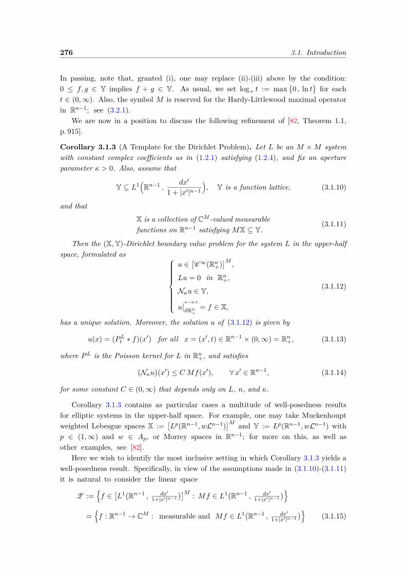
276 3.1. Introduction
In passing, note that, granted (i), one may replace (ii)-(iii) above by the condition:0 ≤ f, g ∈ Y implies f + g ∈ Y. As usual, we set log+ t := max
0 , ln t
for each
t ∈ (0,∞). Also, the symbol M is reserved for the Hardy-Littlewood maximal operatorin Rn−1; see (3.2.1).
We are now in a position to discuss the following refinement of [82, Theorem 1.1,p. 915].
Corollary 3.1.3 (A Template for the Dirichlet Problem). Let L be an M ×M systemwith constant complex coefficients as in (1.2.1) satisfying (1.2.4), and fix an apertureparameter κ > 0. Also, assume that
Y ⊆ L1(Rn−1 ,
dx′
1 + |x′|n−1
), Y is a function lattice, (3.1.10)
and that
X is a collection of CM -valued measurablefunctions on Rn−1 satisfying MX ⊆ Y.
(3.1.11)
Then the (X,Y)-Dirichlet boundary value problem for the system L in the upper-halfspace, formulated as
u ∈[C∞(Rn+)
]M,
Lu = 0 in Rn+,
Nκu ∈ Y,
u∣∣κ−n.t.
∂Rn+= f ∈ X,
(3.1.12)
has a unique solution. Moreover, the solution u of (3.1.12) is given by
u(x) = (PLt ∗ f)(x′) for all x = (x′, t) ∈ Rn−1 × (0,∞) = Rn+, (3.1.13)
where PL is the Poisson kernel for L in Rn+, and satisfies(Nκu
)(x′) ≤ CMf(x′), ∀x′ ∈ Rn−1, (3.1.14)
for some constant C ∈ (0,∞) that depends only on L, n, and κ.
Corollary 3.1.3 contains as particular cases a multitude of well-posedness resultsfor elliptic systems in the upper-half space. For example, one may take Muckenhouptweighted Lebesgue spaces X :=
[Lp(Rn−1, wLn−1)
]M and Y := Lp(Rn−1, wLn−1) withp ∈ (1,∞) and w ∈ Ap, or Morrey spaces in Rn−1; for more on this, as well asother examples, see [82].
Here we wish to identify the most inclusive setting in which Corollary 3.1.3 yields awell-posedness result. Specifically, in view of the assumptions made in (3.1.10)-(3.1.11)it is natural to consider the linear space
Z :=f ∈
[L1(Rn−1 , dx′
1+|x′|n−1)]M : Mf ∈ L1(Rn−1 , dx′
1+|x′|n−1)
=f : Rn−1 → CM : measurable and Mf ∈ L1(Rn−1 , dx′
1+|x′|n−1)
(3.1.15)
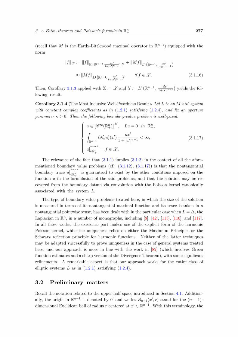
3. A Fatou theorem and Poisson’s formula in Rn+ 277
(recall that M is the Hardy-Littlewood maximal operator in Rn−1) equipped with thenorm
‖f‖Z := ‖f‖[L1(Rn−1, dx′1+|x′|n−1 )]M + ‖Mf‖
L1(Rn−1, dx′
1+|x′|n−1
)≈ ‖Mf‖
L1(Rn−1, dx′
1+|x′|n−1
), ∀ f ∈ Z . (3.1.16)
Then, Corollary 3.1.3 applied with X := Z and Y := L1(Rn−1 , dx′|1+|x′|n−1
)yields the fol-
lowing result.
Corollary 3.1.4 (The Most Inclusive Well-Posedness Result). Let L be anM×M systemwith constant complex coefficients as in (1.2.1) satisfying (1.2.4), and fix an apertureparameter κ > 0. Then the following boundary-value problem is well-posed:
u ∈[C∞(Rn+)
]M, Lu = 0 in Rn+,ˆ
Rn−1
(Nκu
)(x′) dx′
1 + |x′|n−1 <∞,
u∣∣κ−n.t.
∂Rn+= f ∈ Z .
(3.1.17)
The relevance of the fact that (3.1.1) implies (3.1.2) in the context of all the afore-mentioned boundary value problems (cf. (3.1.12), (3.1.17)) is that the nontangentialboundary trace u
∣∣κ−n.t.
∂Rn+is guaranteed to exist by the other conditions imposed on the
function u in the formulation of the said problems, and that the solution may be re-covered from the boundary datum via convolution with the Poisson kernel canonicallyassociated with the system L.
The type of boundary value problems treated here, in which the size of the solutionis measured in terms of its nontangential maximal function and its trace is taken in anontangential pointwise sense, has been dealt with in the particular case when L = ∆, theLaplacian in Rn, in a number of monographs, including [8], [42], [115], [116], and [117].In all these works, the existence part makes use of the explicit form of the harmonicPoisson kernel, while the uniqueness relies on either the Maximum Principle, or theSchwarz reflection principle for harmonic functions. Neither of the latter techniquesmay be adapted successfully to prove uniqueness in the case of general systems treatedhere, and our approach is more in line with the work in [82] (which involves Greenfunction estimates and a sharp version of the Divergence Theorem), with some significantrefinements. A remarkable aspect is that our approach works for the entire class ofelliptic systems L as in (1.2.1) satisfying (1.2.4).
3.2 Preliminary matters
Recall the notation related to the upper-half space introduced in Section 4.1. Addition-ally, the origin in Rn−1 is denoted by 0′ and we let Bn−1(x′, r) stand for the (n − 1)-dimensional Euclidean ball of radius r centered at x′ ∈ Rn−1. With this terminology, the
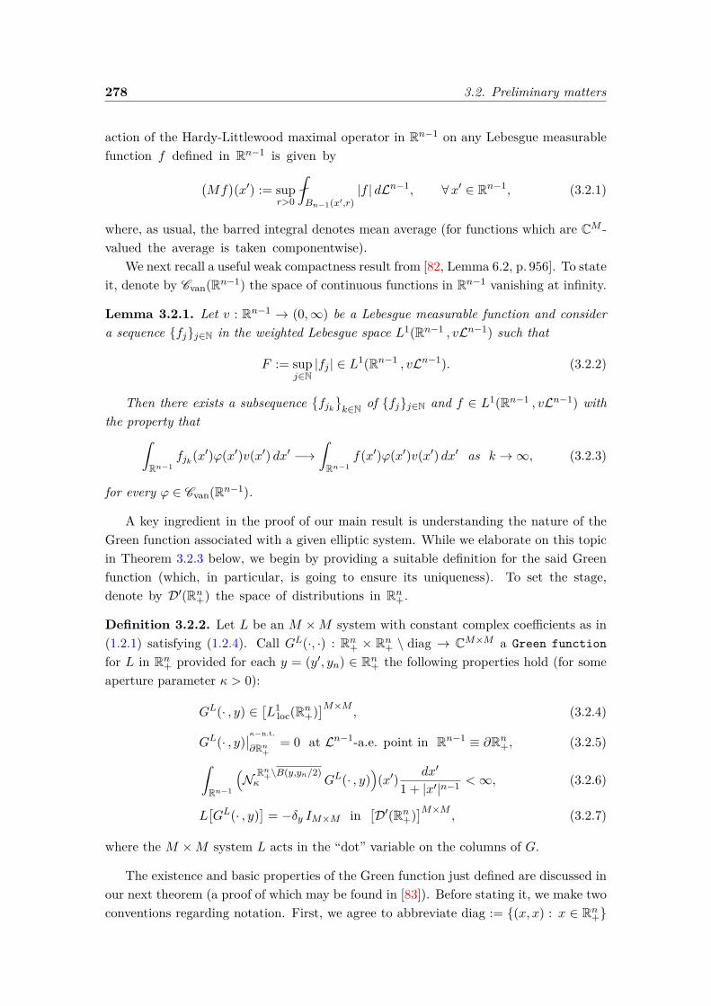
278 3.2. Preliminary matters
action of the Hardy-Littlewood maximal operator in Rn−1 on any Lebesgue measurablefunction f defined in Rn−1 is given by
(Mf
)(x′) := sup
r>0
Bn−1(x′,r)
|f | dLn−1, ∀x′ ∈ Rn−1, (3.2.1)
where, as usual, the barred integral denotes mean average (for functions which are CM -valued the average is taken componentwise).
We next recall a useful weak compactness result from [82, Lemma 6.2, p. 956]. To stateit, denote by Cvan(Rn−1) the space of continuous functions in Rn−1 vanishing at infinity.
Lemma 3.2.1. Let v : Rn−1 → (0,∞) be a Lebesgue measurable function and considera sequence fjj∈N in the weighted Lebesgue space L1(Rn−1 , vLn−1) such that
F := supj∈N|fj | ∈ L1(Rn−1 , vLn−1). (3.2.2)
Then there exists a subsequencefjkk∈N of fjj∈N and f ∈ L1(Rn−1 , vLn−1) with
the property thatˆRn−1
fjk(x′)ϕ(x′)v(x′) dx′ −→ˆRn−1
f(x′)ϕ(x′)v(x′) dx′ as k →∞, (3.2.3)
for every ϕ ∈ Cvan(Rn−1).
A key ingredient in the proof of our main result is understanding the nature of theGreen function associated with a given elliptic system. While we elaborate on this topicin Theorem 3.2.3 below, we begin by providing a suitable definition for the said Greenfunction (which, in particular, is going to ensure its uniqueness). To set the stage,denote by D′(Rn+) the space of distributions in Rn+.
Definition 3.2.2. Let L be an M ×M system with constant complex coefficients as in(1.2.1) satisfying (1.2.4). Call GL(·, ·) : Rn+ × Rn+ \ diag → CM×M a Green functionfor L in Rn+ provided for each y = (y′, yn) ∈ Rn+ the following properties hold (for someaperture parameter κ > 0):
GL(· , y) ∈[L1
loc(Rn+)]M×M
, (3.2.4)
GL(· , y)∣∣κ−n.t.
∂Rn+= 0 at Ln−1-a.e. point in Rn−1 ≡ ∂Rn+, (3.2.5)
ˆRn−1
(N Rn+\B(y,yn/2)κ GL(· , y)
)(x′) dx′
1 + |x′|n−1 <∞, (3.2.6)
L[GL(· , y)
]= −δy IM×M in
[D′(Rn+)
]M×M, (3.2.7)
where the M ×M system L acts in the “dot” variable on the columns of G.
The existence and basic properties of the Green function just defined are discussed inour next theorem (a proof of which may be found in [83]). Before stating it, we make twoconventions regarding notation. First, we agree to abbreviate diag := (x, x) : x ∈ Rn+

3. A Fatou theorem and Poisson’s formula in Rn+ 279
for the diagonal in the Cartesian product Rn+ × Rn+. Second, given a function G(·, ·) oftwo vector variables, (x, y) ∈ Rn+ × Rn+ \ diag, for each k ∈ 1, . . . , n we agree to write∂XkG and ∂YkG, respectively, for the partial derivative of G with respect to xk, and yk.This convention may be iterated, lending a natural meaning to ∂αX∂
βYG, for each pair of
multi-indices α, β ∈ Nn0 . We are now ready to present the result alluded to above.
Theorem 3.2.3. Assume that L is an M ×M system with constant complex coefficientas in (1.2.1) satisfying (1.2.4). Then there exists a unique Green function GL(·, ·) for Lin Rn+, in the sense of Definition 3.2.2. Moreover, this Green function also satisfies thefollowing additional properties:
(1) Given κ > 0, for each y ∈ Rn+ and each compact neighborhood K of y in Rn+ thereexists a finite constant Cy = C(n,L, κ,K, y) > 0 such that for every x′ ∈ Rn−1
there holdsN
Rn+\K
κ
(GL(·, y)
)(x′) ≤ Cy
1 + log+ |x′|1 + |x′|n−1 . (3.2.8)
Moreover, for any multi-indices α, β ∈ Nn0 such that |α|+ |β| > 0, there exists someconstant Cy = C(n,L, κ, α, β,K, y) ∈ (0,∞) such that
N Rn+\Kκ
((∂αX∂
βYG
L)(·, y))(x′) ≤ Cy
1 + |x′|n−2+|α|+|β| . (3.2.9)
(2) For each fixed y ∈ Rn+, there holds
GL(· , y) ∈[C∞
(Rn+ \B(y, ε)
)]M×M for every ε > 0. (3.2.10)
As a consequence of (3.2.10) and (3.2.5), for each fixed y ∈ Rn+ one has
GL(·, y)∣∣∣∂Rn+
= 0 everywhere on Rn−1. (3.2.11)
(3) For each α, β ∈ Nn0 the function ∂αX∂βYG
L is translation invariant in the tangentialvariables, in the sense that(
∂αX∂βYG
L)(x− (z′, 0), y − (z′, 0)
)=(∂αX∂
βYG
L)(x, y)
for each (x, y) ∈ Rn+ × Rn+ \ diag and z′ ∈ Rn−1,(3.2.12)
and is positive homogeneous, in the sense that(∂αX∂
βYG
L)(λx, λy) = λ2−n−|α|−|β|(∂αX∂βYGL)(x, y)
for each x, y ∈ Rn+ with x 6= y and λ ∈ (0,∞),
provided either n ≥ 3, or |α|+ |β| > 0.
(3.2.13)
(4) If GL>(·, ·) denotes the (unique, by the first part of the statement) Green functionfor L> (the transposed of L) in Rn+, then
GL(x, y) =[GL>(y, x)
]>, ∀ (x, y) ∈ Rn+ × Rn+ \ diag. (3.2.14)
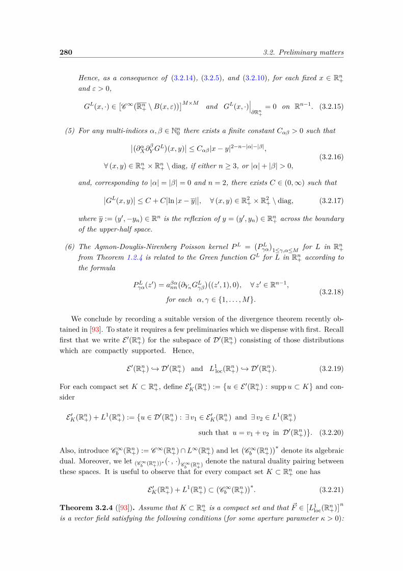
280 3.2. Preliminary matters
Hence, as a consequence of (3.2.14), (3.2.5), and (3.2.10), for each fixed x ∈ Rn+and ε > 0,
GL(x, ·) ∈[C∞
(Rn+ \B(x, ε)
)]M×M and GL(x, ·)∣∣∣∂Rn+
= 0 on Rn−1. (3.2.15)
(5) For any multi-indices α, β ∈ Nn0 there exists a finite constant Cαβ > 0 such that∣∣(∂αX∂βYGL)(x, y)∣∣ ≤ Cαβ|x− y|2−n−|α|−|β|,
∀ (x, y) ∈ Rn+ × Rn+ \ diag, if either n ≥ 3, or |α|+ |β| > 0,(3.2.16)
and, corresponding to |α| = |β| = 0 and n = 2, there exists C ∈ (0,∞) such that∣∣GL(x, y)∣∣ ≤ C + C
∣∣ln |x− y|∣∣, ∀ (x, y) ∈ R2+ × R2
+ \ diag, (3.2.17)
where y := (y′,−yn) ∈ Rn is the reflexion of y = (y′, yn) ∈ Rn+ across the boundaryof the upper-half space.
(6) The Agmon-Douglis-Nirenberg Poisson kernel PL =(PLγα
)1≤γ,α≤M for L in Rn+
from Theorem 1.2.4 is related to the Green function GL for L in Rn+ according tothe formula
PLγα(z′) = aβαnn(∂YnG
Lγβ
)((z′, 1), 0
), ∀ z′ ∈ Rn−1,
for each α, γ ∈ 1, . . . ,M.(3.2.18)
We conclude by recording a suitable version of the divergence theorem recently ob-tained in [93]. To state it requires a few preliminaries which we dispense with first. Recallfirst that we write E ′(Rn+) for the subspace of D′(Rn+) consisting of those distributionswhich are compactly supported. Hence,
E ′(Rn+) → D′(Rn+) and L1loc(Rn+) → D′(Rn+). (3.2.19)
For each compact set K ⊂ Rn+, define E ′K(Rn+) :=u ∈ E ′(Rn+) : suppu ⊂ K
and con-
sider
E ′K(Rn+) + L1(Rn+) :=u ∈ D′(Rn+) : ∃ v1 ∈ E ′K(Rn+) and ∃ v2 ∈ L1(Rn+)
such that u = v1 + v2 in D′(Rn+). (3.2.20)
Also, introduce C∞b (Rn+) := C∞(Rn+)∩L∞(Rn+) and let(C∞b (Rn+)
)∗ denote its algebraicdual. Moreover, we let (C∞
b(Rn+))∗
(· , ·)C∞b
(Rn+) denote the natural duality pairing betweenthese spaces. It is useful to observe that for every compact set K ⊂ Rn+ one has
E ′K(Rn+) + L1(Rn+) ⊂(C∞b (Rn+)
)∗. (3.2.21)
Theorem 3.2.4 ([93]). Assume that K ⊂ Rn+ is a compact set and that ~F ∈[L1
loc(Rn+)]n
is a vector field satisfying the following conditions (for some aperture parameter κ > 0):
3. A Fatou theorem and Poisson’s formula in Rn+ 281
(a) div ~F ∈ E ′K(Rn+) + L1(Rn+), where the divergence is taken in the sense of distribu-tions;
(b) the nontangential maximal function N Rn+\Kκ
~F belongs to L1(Rn−1);
(c) the nontangential boundary trace ~F∣∣κ−n.t.
∂Rn+exists (in Cn) at Ln−1-a.e. point in Rn−1.
Then, with en := (0, . . . , 0, 1) ∈ Rn and “dot" denoting the standard inner product in Rn,
(C∞b
(Rn+))∗(div ~F, 1
)C∞b
(Rn+) = −ˆRn−1
en ·(~F∣∣κ−n.t.
∂Rn+
)dLn−1. (3.2.22)
3.3 Proofs of main results
We take on the task of presenting the proof of Theorem 3.1.1.
Proof of Theorem 3.1.1. Fix an arbitrary point x? ∈ Rn+ and bring in GL>( · , x?), the
Green function with pole at x? for L>, the transposed of the operator L (cf. Defini-tion 3.2.2 and Theorem 3.2.3 for details on this matter). For ease of notation, abbreviate
G(·) := GL>( · , x?) in Rn+ \ x?. (3.3.1)
By design, this is a matrix-valued function, say G = (Gαγ)1≤α,γ≤M . We shall applyTheorem 3.2.4 to a suitably chosen vector field. To set the stage, consider the compactset
K? := B(x?, r) ⊂ Rn+, where r := dist (x?, ∂Rn+) · κ2√
4+κ2 . (3.3.2)
For each ε > 0 consider the function uε : Rn+ → CM given by
uε(x) := u(x′, xn + ε) for all x = (x′, xn) ∈ Rn+. (3.3.3)
Then
uε ∈[C ∞(Rn+ )
]M, Luε = 0 in Rn+, and Nκuε ≤ Nκu on Rn−1. (3.3.4)
Fix ε > 0 along with some β ∈ 1, . . . ,M and, using the summation convention overrepeated indices, define the vector field
~F :=(uεα a
γαkj ∂kGγβ −Gαβ a
αγjk ∂ku
εγ
)1≤j≤n
at Ln-a.e. point in Rn+. (3.3.5)
From (3.3.5), Theorem 3.2.3, and the fact that uε ∈[C ∞(Rn+ )
]M it follows that
~F ∈[L1
loc(Rn+)]n ∩ [C∞(Rn+ \K?)
]n (3.3.6)
and, on account of (3.2.11) (used for L> in place of L), we have
~F∣∣∣∂Rn+
=((uεα∣∣∂Rn+
)aγαkj
(∂kGγβ
)∣∣∂Rn+
)1≤j≤n
. (3.3.7)
282 3.3. Proofs of main results
Next, in the sense of distributions in Rn+, we may compute
div ~F = (∂juεα) aγαkj (∂kGγβ) + uεα aγαkj (∂j∂kGγβ)
− (∂jGαβ) aαγjk (∂kuεγ)−Gαβ aαγjk (∂j∂kuεγ)
=: I1 + I2 + I3 + I4, (3.3.8)
where the last equality defines the Ii’s. Changing variables j′ = k, k′ = j, α′ = γ, andγ′ = α in I3 yields
I3 = −(∂k′Gγ′β) aγ′α′
k′j′ (∂j′uεα′) = −I1. (3.3.9)
As regards I4, we haveI4 = −Gαβ (Luε)α = 0, (3.3.10)
by (3.3.4). Finally,
I2 = uεα(LA>G·β)α = uεα(L>G·β)α
= −uεαδαβδx? = −uεβ δx? = −uεβ(x?) δx? . (3.3.11)
Collectively, these equalities permit us to conclude that, in the sense of distributions inRn+,
div ~F = −uεβ(x?) δx? ∈ E ′(Rn+). (3.3.12)
In particular,
div ~F ∈ D′(Rn+) induces a continuous functional in(C∞b (Rn+)
)∗. (3.3.13)
Moving on, fix x′ ∈ Rn−1 ≡ ∂Rn+ and pick an arbitrary point
y = (y′, yn) ∈ Γκ/2(x′) \K?. (3.3.14)
Choose a rectifiable path γ : [0, 1]→ Rn+ joining (x′, 0) with y in Γκ/2(x′)\K? and whoselength is ≤ Cyn. Then, for some constant C ∈ (0,∞) independent of x′ and y, we mayestimate
|G(y)| = |G(y)−G(x′, 0)| =∣∣∣ ˆ 1
0
d
dt[G(γ(t))] dt
∣∣∣=∣∣∣ ˆ 1
0(∇G)(γ(t)) · γ′(t) dt
∣∣∣ ≤ ( supξ∈γ((0,1))
|(∇G)(ξ)|)ˆ 1
0|γ′(t)| dt
≤ Cyn · NRn+\K?κ/2 (∇G)(x′), (3.3.15)
using the fact that G vanishes on ∂Rn+, the Fundamental Theorem of Calculus, ChainRule, and (1.1.4). Next, define
a := κ
2(κ+ 1) ∈(0, 1
2)
(3.3.16)
3. A Fatou theorem and Poisson’s formula in Rn+ 283
and write, using interior estimates (cf. Theorem 1.2.2) for the function uε,
|(∇uε)(y)| ≤ C
yn
B(y,a·yn)
|uε(z)| dz
≤ Cy−1n · sup
z∈Γκ(x′)|uε(z)| ≤ Cy−1
n ·(Nκuε
)(x′), (3.3.17)
since having z = (z′, zn) ∈ B(y, a · yn) entails
yn ≤ zn + |z − y| < zn + a · yn =⇒ yn < (1− a)−1zn, (3.3.18)
which, bearing in mind that y is as in (3.3.14), permits us to conclude that
|z′ − x′| ≤ |z′ − y′|+ |y′ − x′| ≤ |z − y|+ (κ/2)yn < a · yn + (κ/2)yn
= (κ/2 + a)yn <κ/2 + a
1− a zn = κzn, hence z ∈ Γκ(x′). (3.3.19)
Then combining (3.3.15) with (3.3.17) gives, on account of (3.2.9),
N Rn+\K?κ/2
(|G||∇uε|
)(x′) ≤ C
(N Rn+\K?κ/2 (∇G)
)(x′)
(Nκuε
)(x′)
≤ C(Nκu
)(x′) 1
1 + |x′|n−1 at each point x′ ∈ Rn−1. (3.3.20)
Since we also have
N Rn+\K?κ/2
(|∇G||uε|
)(x′) ≤
(N Rn+\K?κ/2 (∇G)
)(x′)
(Nκuε
)(x′)
≤ C(Nκu
)(x′) 1
1 + |x′|n−1 at each point x′ ∈ Rn−1, (3.3.21)
we conclude from (3.3.5), (3.3.20), (3.3.21), and the second line in (3.1.1) that
N Rn+\K?κ/2
~F ∈ L1(Rn−1). (3.3.22)
Having established (3.3.6), (3.3.7), (3.3.13), and (3.3.22), Theorem 3.2.4 applies. Towrite the Divergence Formula (3.2.22) in this case, express x? as (x′, t) ∈ Rn−1 × (0,∞).
284 3.3. Proofs of main results
Then, in view of (3.3.12) and (3.3.7) we may write
uβ(x? + εen) = uεβ(x?) = −(C∞b
(Rn+))∗(div ~F , 1
)C∞b
(Rn+)
=ˆRn−1
en ·(~F∣∣∂Rn+
)dLn−1
=ˆRn−1
uα(y′, ε)aγαkn(∂kGγβ
)(y′, 0) dy′
=ˆRn−1
uα(y′, ε)aγαnn(∂nGγβ
)(y′, 0) dy′
=ˆRn−1
uα(y′, ε)aγαnn(∂XnGL>
γβ )((y′, 0), x?
)dy′
=ˆRn−1
uα(y′, ε)aγαnn(∂YnGLβγ)(x?, (y′, 0)
)dy′
=ˆRn−1
uα(y′, ε)aγαnn(∂YnGLβγ)((x′ − y′, t), 0
)dy′
=ˆRn−1
uα(y′, ε)t1−naγ αnn (∂YnGLβγ)(((x′ − y′)/t, 1), 0
)dy′
=ˆRn−1
uα(y′, ε)(PLβα)t(x′ − y′) dy′, (3.3.23)
where the fifth equality uses the observation that (∂kG)(y′, 0) = 0 whenever k < n sinceG vanishes (in a smooth fashion) on Rn−1 × 0, the sixth equality is a consequenceof (3.3.1), the seventh equality is implied by (3.2.14), the eighth equality makes use of(3.2.12) (bearing in mind that x? = (x′, t)), the ninth equality is seen from (3.2.13), andthe last equality comes from (3.2.18).
Since β ∈ 1, . . . ,M and x? = (x′, t) ∈ Rn+ have been arbitrarily chosen, theargument so far shows that
u(x′, t+ ε) =ˆRn−1
PLt (x′ − y′)fε(y′) dy′ for each x = (x′, t) ∈ Rn+, (3.3.24)
where we have abbreviated
fε := u(·, ε) : Rn−1 −→ CM for each ε > 0. (3.3.25)
If we also consider the weight υ : Rn−1 → (0,∞) defined as v(x′) := (1 + |x′|n−1)−1 foreach x′ ∈ Rn−1, then the last condition in (3.1.1) entails
supε>0|fε| ≤ Nκu ∈ L1(Rn−1 , vLn−1). (3.3.26)
Granted this, the weak-∗ convergence result in Lemma 3.2.1 may be used for the sequencefεε>0 ⊂ L1(Rn−1 , vLn−1) to conclude that there is some f ∈ L1(Rn−1 , vLn−1) and
some sequence εjj∈N ⊂ (0,∞) which converges to zero with the property that
limj→∞
ˆRn−1
ϕ(y′)fεj (y′)dy′
1 + |y′|n−1 =ˆRn−1
ϕ(y′)f(y′) dy′
1 + |y′|n−1 (3.3.27)
3. A Fatou theorem and Poisson’s formula in Rn+ 285
for every continuous function ϕ ∈ Cvan(Rn−1). The fact that there exists a constantC ∈ (0,∞) for which
|PL(z′)| ≤ C
(1 + |z′|2)n/2for each z′ ∈ Rn−1 (3.3.28)
(see (1.2.26)) ensures for each fixed point (x′, t) ∈ Rn+ the assignment
Rn−1 3 y′ 7→ ϕ(y′) := (1 + |y′|n−1)PLt (x′ − y′) ∈ CM×M
is a continuous function which vanishes at infinity.(3.3.29)
At this stage, from (3.3.24) and (3.3.27) used for the function ϕ defined in (3.3.29) weobtain (bearing in mind that u is continuous in Rn+) that
u(x′, t) =ˆRn−1
PLt (x′ − y′)f(y′) dy′ for each x = (x′, t) ∈ Rn+. (3.3.30)
With this in hand, and since L1(Rn−1 , vLn−1) ⊆ L1(Rn−1 ,
dx′
1 + |x′|n), we may invoke
Theorem 1.2.4(c) to conclude that
u∣∣κ−n.t.
∂Rn+exists and equals f at Ln−1-a.e. point in Rn−1. (3.3.31)
Once this has been established, all conclusions in (3.1.2) are implied by (3.3.30)-(3.3.31).
We close by presenting the proof of Corollary 3.1.3.
Proof of Corollary 3.1.3. As a preamble, let us first show that
X ⊆[L1(Rn−1 ,
dx′
1 + |x′|n)]M
. (3.3.32)
To justify this, pick some arbitrary f ∈ X. Then the inclusion in (3.1.11) gives thatMf ∈ Y, hence Mf is not identically +∞. This implies that f ∈ [L1
loc(Rn−1)]M which,in concert with Lebesgue’s Differentiation Theorem, implies that |f | ≤Mf at Ln−1-a.e.point in Rn−1. Since Y is a function lattice, it follows that |f | ∈ Y. Thus, ultimately,(3.3.32) holds by virtue of the inclusion in (3.1.10).
To prove the existence of a solution for (3.1.12), given any f ∈ X define u as in(3.1.13). Note that (3.3.32) ensures that Theorem 1.2.4(c) is applicable. In turn, thisguarantees that u is a well-defined null-solution of L belonging to
[C∞(Rn+)
]M , satisfyingthe boundary condition u
∣∣κ−n.t.
∂Rn+= f at Ln−1-a.e. point in Rn−1, as well as the pointwise
estimate in (3.1.14). The latter property, together with the last conditions imposed in(3.1.11) and (3.1.10), guarantees Nκu ∈ Y. Thus, u is indeed a solution for (3.1.12).
At this stage, there remains to establish that the boundary value problem (3.1.12)can have at most one solution. To this end, assume that both u1 and u2 solve (3.1.12)for the same datum f ∈ X and set u := u1 − u2 ∈
[C∞(Rn+)
]M . Then Lu = 0 in Rn+
286 3.3. Proofs of main results
and u∣∣κ−n.t.
∂Rn+= 0 at Ln−1-a.e. point in Rn−1. Since we also have Nκu1,Nκu2 ∈ Y, the
pointwise estimate
0 ≤ Nκu ≤ Nκu1 +Nκu2 ≤ 2 maxNκu1 , Nκu2
on Rn−1 (3.3.33)
forces Nκu ∈ Y by the properties of the function lattice Y. Granted this, Corollary 3.1.2applies (thanks to the first condition in (3.1.10)) and gives that u ≡ 0 in Rn+. Henceu1 = u2, as wanted.
CHAPTER 4
The generalized Hölder and Morrey-Campanato Dirichletproblems for elliptic systems in the upper-half space
We prove well-posedness results for the Dirichlet Problem in the upper-half space Rn+ forhomogeneous, second-order, constant complex coefficient elliptic systems with boundarydata in generalized Hölder spaces C ω(Rn−1,CM ) and in generalized Morrey-Campanatospaces E ω,p(Rn−1,CM ) under certain assumptions on the growth function ω. We alsoidentify a class of growth functions ω for which C ω(Rn−1,CM ) = E ω,p(Rn−1,CM ) andfor which the aforementioned well-posedness results are equivalent, in the sense that theyhave the same unique solution, satisfying natural regularity properties and estimates.
The material in this chapter is based on joint work with J.M. Martell and M. Mitrea(cf. [79]).
Contents
4.1 Introduction . . . . . . . . . . . . . . . . . . . . . . . . . . . . . . . . . . . 288
4.2 Growth functions, generalized Hölder and Morrey-Campanato spaces . 292
4.3 Properties of elliptic systems and their solutions . . . . . . . . . . . . . 295
4.4 John-Nirenberg’s inequality adapted to growth functions . . . . . . . . 300
4.5 Existence results . . . . . . . . . . . . . . . . . . . . . . . . . . . . . . . . . 305
4.6 A Fatou-type result and uniqueness of solutions . . . . . . . . . . . . . . 306
4.7 Well-posedness results . . . . . . . . . . . . . . . . . . . . . . . . . . . . . 309
288 4.1. Introduction
4.1 Introduction
This chapter is devoted to studying the Dirichlet Problem for elliptic systems in theupper-half space with data in generalized Hölder and generalized Morrey-Campanatospaces. As a byproduct of the PDE-based techniques developed here, we are ableto establish the equivalence of these function spaces. To be more specific requiresintroducing some notation.
With each system L as in (1.2.1) satisfying (1.2.4) one may associate a Poissonkernel, PL, which is a CM×M -valued function defined in Rn−1 described in detail inTheorem 1.2.4. This Poisson kernel has played a pivotal role in the treatment of theDirichlet Problem with data in Lp, BMO, VMO and Hölder spaces (see [82, 85]). Fornow, we make the observation that the Poisson kernel gives rise to a nice approximationto the identity in Rn−1 by setting PLt (x′) = t1−nPL(x′/t) for every x′ ∈ Rn−1 and t > 0.
For every point x ∈ Rn write x = (x′, t), where x′ ∈ Rn−1 corresponds to the firstn − 1 coordinates of x, and t ∈ R is the last coordinate of x. As is customary, we shalllet Rn+ := x = (x′, t) ∈ Rn : x′ ∈ Rn−1, t > 0 denote the upper-half space in Rn,and typically identify its boundary with (n− 1)-dimensional Euclidean space, via ∂Rn+ 3(x′, 0) ≡ x′ ∈ Rn−1. In this case, the nontangential approach regions defined in (1.1.1) arecones and we agree to denote the cone with vertex at x′ ∈ Rn−1 and aperture κ > 0 as
Γκ(x′) := y = (y′, t) ∈ Rn+ : |x′ − y′| < κt. (4.1.1)
The nontangential limit of u at x′ ∈ Rn−1 (that is, the limit from within the cone Γκ(x′)defined as in (4.1.1)) is denoted by
(u∣∣κ−n.t.
∂Ω)(x′) following the terminology introduced
in Section 1.1. The unrestricted pointwise trace of a vector-valued function u definedin Rn+ at each x′ ∈ ∂Rn+ ≡ Rn−1 is taken to be
(u|∂Rn+)(x′) := limRn+3y→(x′,0)
u(y), x′ ∈ Rn−1, (4.1.2)
whenever such a limit exists exists.Remember the definitions of growth function and generalized Hölder space in Defini-
tions 1.3.1 and 1.3.5. Growth functions are always defined on (0,∞) throughout this chap-ter.
Definition 4.1.1. Given a growth function ω along with some integrability exponentp ∈ [1,∞), the associated generalized Morrey-Campanato space in Rn−1 is defined as
E ω,p(Rn−1,CM ) :=f ∈
[L1
loc(Rn−1)]M : ‖f‖E ω,p(Rn−1,CM ) <∞
, (4.1.3)
where ‖f‖E ω,p(Rn−1,CM ) stands for the semi-norm
‖f‖E ω,p(Rn−1,CM ) := supQ⊆Rn−1
1ω(`(Q))
( Q|f(x′)− fQ|p dx′
)1/p. (4.1.4)
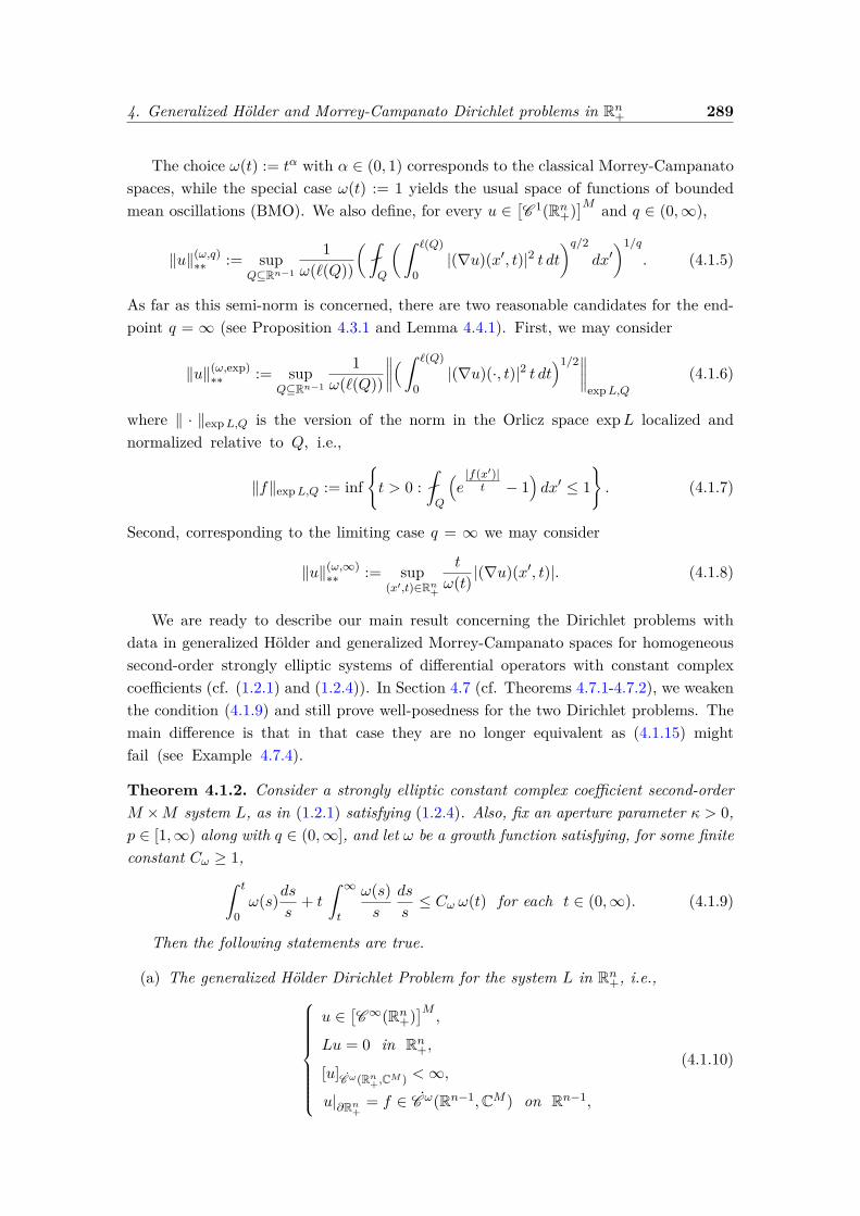
4. Generalized Hölder and Morrey-Campanato Dirichlet problems in Rn+ 289
The choice ω(t) := tα with α ∈ (0, 1) corresponds to the classical Morrey-Campanatospaces, while the special case ω(t) := 1 yields the usual space of functions of boundedmean oscillations (BMO). We also define, for every u ∈
[C 1(Rn+)
]M and q ∈ (0,∞),
‖u‖(ω,q)∗∗ := supQ⊆Rn−1
1ω(`(Q))
( Q
( ˆ `(Q)
0|(∇u)(x′, t)|2 t dt
)q/2dx′)1/q
. (4.1.5)
As far as this semi-norm is concerned, there are two reasonable candidates for the end-point q = ∞ (see Proposition 4.3.1 and Lemma 4.4.1). First, we may consider
‖u‖(ω,exp)∗∗ := sup
Q⊆Rn−1
1ω(`(Q))
∥∥∥∥(ˆ `(Q)
0|(∇u)(·, t)|2 t dt
)1/2∥∥∥∥expL,Q
(4.1.6)
where ‖ · ‖expL,Q is the version of the norm in the Orlicz space expL localized andnormalized relative to Q, i.e.,
‖f‖expL,Q := inft > 0 :
Q
(e|f(x′)|t − 1
)dx′ ≤ 1
. (4.1.7)
Second, corresponding to the limiting case q = ∞ we may consider
‖u‖(ω,∞)∗∗ := sup
(x′,t)∈Rn+
t
ω(t) |(∇u)(x′, t)|. (4.1.8)
We are ready to describe our main result concerning the Dirichlet problems withdata in generalized Hölder and generalized Morrey-Campanato spaces for homogeneoussecond-order strongly elliptic systems of differential operators with constant complexcoefficients (cf. (1.2.1) and (1.2.4)). In Section 4.7 (cf. Theorems 4.7.1-4.7.2), we weakenthe condition (4.1.9) and still prove well-posedness for the two Dirichlet problems. Themain difference is that in that case they are no longer equivalent as (4.1.15) mightfail (see Example 4.7.4).
Theorem 4.1.2. Consider a strongly elliptic constant complex coefficient second-orderM ×M system L, as in (1.2.1) satisfying (1.2.4). Also, fix an aperture parameter κ > 0,p ∈ [1,∞) along with q ∈ (0,∞], and let ω be a growth function satisfying, for some finiteconstant Cω ≥ 1,
ˆ t
0ω(s)ds
s+ t
ˆ ∞t
ω(s)s
ds
s≤ Cω ω(t) for each t ∈ (0,∞). (4.1.9)
Then the following statements are true.
(a) The generalized Hölder Dirichlet Problem for the system L in Rn+, i.e.,
u ∈[C∞(Rn+)
]M,
Lu = 0 in Rn+,
[u]Cω(Rn+,CM ) <∞,
u|∂Rn+ = f ∈ C ω(Rn−1,CM ) on Rn−1,
(4.1.10)
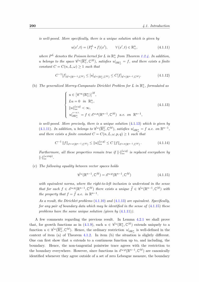
290 4.1. Introduction
is well-posed. More specifically, there is a unique solution which is given by
u(x′, t) = (PLt ∗ f)(x′), ∀ (x′, t) ∈ Rn+, (4.1.11)
where PL denotes the Poisson kernel for L in Rn+ from Theorem 1.2.4. In addition,u belongs to the space C ω(Rn+,CM ), satisfies u|∂Rn+ = f , and there exists a finiteconstant C = C(n,L, ω) ≥ 1 such that
C−1[f ]Cω(Rn−1,CM ) ≤ [u]Cω(Rn+,CM ) ≤ C[f ]Cω(Rn−1,CM ). (4.1.12)
(b) The generalized Morrey-Campanato Dirichlet Problem for L in Rn+, formulated as
u ∈[C∞(Rn+)
]M,
Lu = 0 in Rn+,
‖u‖(ω,q)∗∗ <∞,
u|κ−n.t.
∂Rn+= f ∈ E ω,p(Rn−1,CM ) a.e. on Rn−1,
(4.1.13)
is well-posed. More precisely, there is a unique solution (4.1.13) which is given by(4.1.11). In addition, u belongs to C ω(Rn+,CM ), satisfies u|∂Rn+ = f a.e. on Rn−1,and there exists a finite constant C = C(n,L, ω, p, q) ≥ 1 such that
C−1 ‖f‖E ω,p(Rn−1,CM ) ≤ ‖u‖(ω,q)∗∗ ≤ C ‖f‖E ω,p(Rn−1,CM ) . (4.1.14)
Furthermore, all these properties remain true if ‖·‖(ω,q)∗∗ is replaced everywhere by‖·‖(ω,exp)∗∗ .
(c) The following equality between vector spaces holds
C ω(Rn−1,CM ) = E ω,p(Rn−1,CM ) (4.1.15)
with equivalent norms, where the right-to-left inclusion is understood in the sensethat for each f ∈ E ω,p(Rn−1,CM ) there exists a unique f ∈ C ω(Rn−1,CM ) withthe property that f = f a.e. in Rn−1.
As a result, the Dirichlet problems (4.1.10) and (4.1.13) are equivalent. Specifically,for any pair of boundary data which may be identified in the sense of (4.1.15) theseproblems have the same unique solution (given by (4.1.11)).
A few comments regarding the previous result. In Lemma 4.2.1 we shall provethat, for growth functions as in (4.1.9), each u ∈ C ω(Rn+,CM ) extends uniquely to afunction u ∈ C ω(Rn+,CM ). Hence, the ordinary restriction u|∂Rn+ is well-defined in thecontext of item (a) of Theorem 4.1.2. In item (b) the situation is slightly different.One can first show that u extends to a continuous function up to, and including, theboundary. Hence, the non-tangential pointwise trace agrees with the restriction tothe boundary everywhere. However, since functions in E ω,p(Rn−1,CM ) are canonicallyidentified whenever they agree outside of a set of zero Lebesgue measure, the boundary
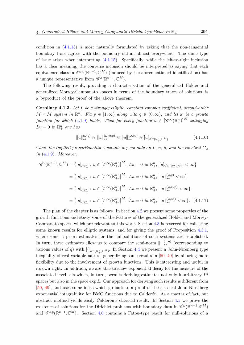
4. Generalized Hölder and Morrey-Campanato Dirichlet problems in Rn+ 291
condition in (4.1.13) is most naturally formulated by asking that the non-tangentialboundary trace agrees with the boundary datum almost everywhere. The same typeof issue arises when interpreting (4.1.15). Specifically, while the left-to-right inclusionhas a clear meaning, the converse inclusion should be interpreted as saying that eachequivalence class in E ω,p(Rn−1,CM ) (induced by the aforementioned identification) hasa unique representative from C ω(Rn−1,CM ).
The following result, providing a characterization of the generalized Hölder andgeneralized Morrey-Campanato spaces in terms of the boundary traces of solutions, isa byproduct of the proof of the above theorem.
Corollary 4.1.3. Let L be a strongly elliptic, constant complex coefficient, second-orderM × M system in Rn. Fix p ∈ [1,∞) along with q ∈ (0,∞), and let ω be a growthfunction for which (4.1.9) holds. Then for every function u ∈
[C∞(Rn+)
]M satisfyingLu = 0 in Rn+ one has
‖u‖(ω,q)∗∗ ≈ ‖u‖(ω,exp)∗∗ ≈ ‖u‖(ω,∞)
∗∗ ≈ [u]Cω(Rn+,CM ) (4.1.16)
where the implicit proportionality constants depend only on L, n, q, and the constant Cωin (4.1.9). Moreover,
C ω(Rn−1,CM ) =u|∂Rn+ : u ∈
[C∞(Rn+)
]M, Lu = 0 in Rn+, [u]Cω(Rn+,CM ) <∞
=u|∂Rn+ : u ∈
[C∞(Rn+)
]M, Lu = 0 in Rn+, ‖u‖
(ω,q)∗∗ <∞
=u|∂Rn+ : u ∈
[C∞(Rn+)
]M, Lu = 0 in Rn+, ‖u‖
(ω,exp)∗∗ <∞
=u|∂Rn+ : u ∈
[C∞(Rn+)
]M, Lu = 0 in Rn+, ‖u‖
(ω,∞)∗∗ <∞
. (4.1.17)
The plan of the chapter is as follows. In Section 4.2 we present some properties of thegrowth functions and study some of the features of the generalized Hölder and Morrey-Campanato spaces which are relevant to this work. Section 4.3 is reserved for collectingsome known results for elliptic systems, and for giving the proof of Proposition 4.3.1,where some a priori estimates for the null-solutions of such systems are established.In turn, these estimates allow us to compare the semi-norm ‖·‖(ω,q)∗∗ (corresponding tovarious values of q) with [·]Cω(Rn+,CM ). In Section 4.4 we present a John-Nirenberg typeinequality of real-variable nature, generalizing some results in [50, 49] by allowing moreflexibility due to the involvement of growth functions. This is interesting and useful inits own right. In addition, we are able to show exponential decay for the measure of theassociated level sets which, in turn, permits deriving estimates not only in arbitrary Lq
spaces but also in the space expL. Our approach for deriving such results is different from[50, 49], and uses some ideas which go back to a proof of the classical John-Nirenbergexponential integrability for BMO functions due to Calderón. As a matter of fact, ourabstract method yields easily Calderón’s classical result. In Section 4.5 we prove theexistence of solutions for the Dirichlet problems with boundary data in C ω(Rn−1,CM )and E ω,p(Rn−1,CM ). Section 4.6 contains a Fatou-type result for null-solutions of a
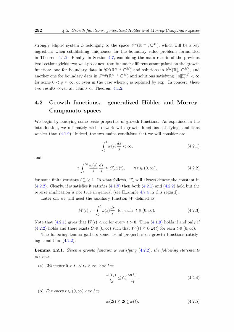
292 4.2. Growth functions, generalized Hölder and Morrey-Campanato spaces
strongly elliptic system L belonging to the space C ω(Rn−1,CM ), which will be a keyingredient when establishing uniqueness for the boundary value problems formulatedin Theorem 4.1.2. Finally, in Section 4.7, combining the main results of the previoustwo sections yields two well-posedness results under different assumptions on the growthfunction: one for boundary data in C ω(Rn−1,CM ) and solutions in C ω(Rn+,CM ), andanother one for boundary data in E ω,p(Rn−1,CM ) and solutions satisfying ‖u‖(ω,q)∗∗ <∞for some 0 < q ≤ ∞, or even in the case where q is replaced by exp. In concert, thesetwo results cover all claims of Theorem 4.1.2.
4.2 Growth functions, generalized Hölder and Morrey-Campanato spaces
We begin by studying some basic properties of growth functions. As explained in theintroduction, we ultimately wish to work with growth functions satisfying conditionsweaker than (4.1.9). Indeed, the two mains conditions that we will consider are
ˆ 1
0ω(s)ds
s<∞, (4.2.1)
and
t
ˆ ∞t
ω(s)s
ds
s≤ C ′ω ω(t), ∀ t ∈ (0,∞), (4.2.2)
for some finite constant C ′ω ≥ 1. In what follows, C ′ω will always denote the constant in(4.2.2). Clearly, if ω satisfies it satisfies (4.1.9) then both (4.2.1) and (4.2.2) hold but thereverse implication is not true in general (see Example 4.7.4 in this regard).
Later on, we will need the auxiliary function W defined as
W (t) :=ˆ t
0ω(s)ds
sfor each t ∈ (0,∞). (4.2.3)
Note that (4.2.1) gives that W (t) <∞ for every t > 0. Then (4.1.9) holds if and only if(4.2.2) holds and there exists C ∈ (0,∞) such that W (t) ≤ C ω(t) for each t ∈ (0,∞).
The following lemma gathers some useful properties on growth functions satisfy-ing condition (4.2.2).
Lemma 4.2.1. Given a growth function ω satisfying (4.2.2), the following statementsare true.
(a) Whenever 0 < t1 ≤ t2 <∞, one has
ω(t2)t2≤ C ′ω
ω(t1)t1
. (4.2.4)
(b) For every t ∈ (0,∞) one has
ω(2t) ≤ 2C ′ω ω(t). (4.2.5)
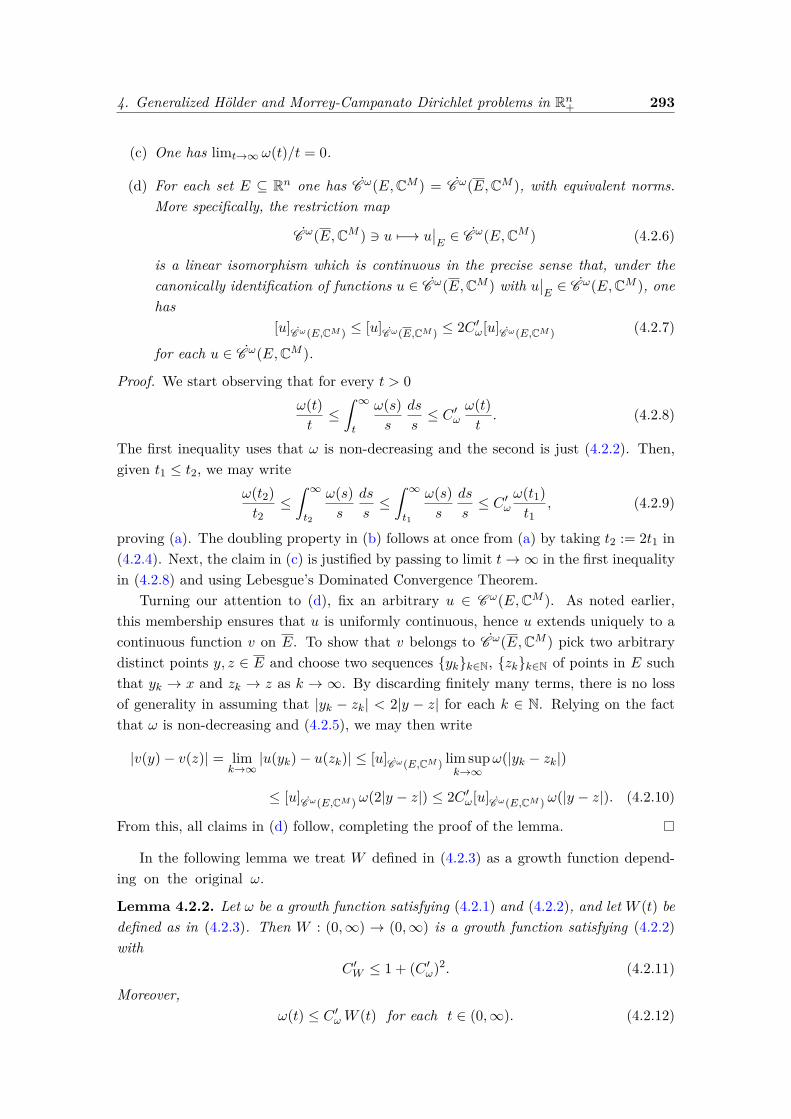
4. Generalized Hölder and Morrey-Campanato Dirichlet problems in Rn+ 293
(c) One has limt→∞ ω(t)/t = 0.
(d) For each set E ⊆ Rn one has C ω(E,CM ) = C ω(E,CM ), with equivalent norms.More specifically, the restriction map
C ω(E,CM ) 3 u 7−→ u∣∣E∈ C ω(E,CM ) (4.2.6)
is a linear isomorphism which is continuous in the precise sense that, under thecanonically identification of functions u ∈ C ω(E,CM ) with u
∣∣E∈ C ω(E,CM ), one
has[u]Cω(E,CM ) ≤ [u]Cω(E,CM ) ≤ 2C ′ω[u]Cω(E,CM ) (4.2.7)
for each u ∈ C ω(E,CM ).
Proof. We start observing that for every t > 0ω(t)t≤ˆ ∞t
ω(s)s
ds
s≤ C ′ω
ω(t)t. (4.2.8)
The first inequality uses that ω is non-decreasing and the second is just (4.2.2). Then,given t1 ≤ t2, we may write
ω(t2)t2≤ˆ ∞t2
ω(s)s
ds
s≤ˆ ∞t1
ω(s)s
ds
s≤ C ′ω
ω(t1)t1
, (4.2.9)
proving (a). The doubling property in (b) follows at once from (a) by taking t2 := 2t1 in(4.2.4). Next, the claim in (c) is justified by passing to limit t→∞ in the first inequalityin (4.2.8) and using Lebesgue’s Dominated Convergence Theorem.
Turning our attention to (d), fix an arbitrary u ∈ C ω(E,CM ). As noted earlier,this membership ensures that u is uniformly continuous, hence u extends uniquely to acontinuous function v on E. To show that v belongs to C ω(E,CM ) pick two arbitrarydistinct points y, z ∈ E and choose two sequences ykk∈N, zkk∈N of points in E suchthat yk → x and zk → z as k → ∞. By discarding finitely many terms, there is no lossof generality in assuming that |yk − zk| < 2|y − z| for each k ∈ N. Relying on the factthat ω is non-decreasing and (4.2.5), we may then write
|v(y)− v(z)| = limk→∞
|u(yk)− u(zk)| ≤ [u]Cω(E,CM ) lim supk→∞
ω(|yk − zk|)
≤ [u]Cω(E,CM ) ω(2|y − z|) ≤ 2C ′ω[u]Cω(E,CM ) ω(|y − z|). (4.2.10)
From this, all claims in (d) follow, completing the proof of the lemma.
In the following lemma we treat W defined in (4.2.3) as a growth function depend-ing on the original ω.
Lemma 4.2.2. Let ω be a growth function satisfying (4.2.1) and (4.2.2), and let W (t) bedefined as in (4.2.3). Then W : (0,∞) → (0,∞) is a growth function satisfying (4.2.2)with
C ′W ≤ 1 + (C ′ω)2. (4.2.11)
Moreover,ω(t) ≤ C ′ωW (t) for each t ∈ (0,∞). (4.2.12)
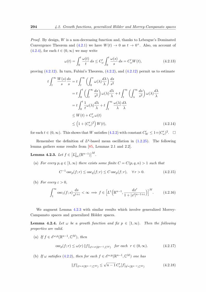
294 4.2. Growth functions, generalized Hölder and Morrey-Campanato spaces
Proof. By design, W is a non-decreasing function and, thanks to Lebesgue’s DominatedConvergence Theorem and (4.2.1) we have W (t) → 0 as t → 0+. Also, on account of(4.2.4), for each t ∈ (0,∞) we may write
ω(t) =ˆ t
0
ω(t)t
ds ≤ C ′ωˆ t
0
ω(s)s
ds = C ′ωW (t), (4.2.13)
proving (4.2.12). In turn, Fubini’s Theorem, (4.2.2), and (4.2.12) permit us to estimate
t
ˆ ∞t
W (s)s
ds
s= t
ˆ ∞t
(ˆ s
0ω(λ)dλ
λ
)ds
s2
= t
ˆ t
0
(ˆ ∞t
ds
s2
)ω(λ)dλ
λ+ t
ˆ ∞t
(ˆ ∞λ
ds
s2
)ω(λ)dλ
λ
= t
ˆ t
0
1tω(λ)dλ
λ+ t
ˆ ∞t
ω(λ)λ
dλ
λ
≤W (t) + C ′ω ω(t)
≤(1 + (C ′ω)2
)W (t), (4.2.14)
for each t ∈ (0,∞). This shows thatW satisfies (4.2.2) with constant C ′W ≤ 1+(C ′ω)2.
Remember the definition of Lp-based mean oscillation in (1.2.25). The followinglemma gathers some results from [85, Lemmas 2.1 and 2.2].
Lemma 4.2.3. Let f ∈[L1
loc(Rn−1)]M .
(a) For every p, q ∈ [1,∞) there exists some finite C = C(p, q, n) > 1 such that
C−1 oscp(f ; r) ≤ oscq(f ; r) ≤ C oscp(f ; r), ∀ r > 0. (4.2.15)
(b) For every ε > 0,ˆ ∞
1osc1(f ; s) ds
s1+ε <∞ =⇒ f ∈[L1(Rn−1,
dx′
1 + |x′|n−1+ε
)]M. (4.2.16)
We augment Lemma 4.2.3 with similar results which involve generalized Morrey-Campanato spaces and generalized Hölder spaces.
Lemma 4.2.4. Let ω be a growth function and fix p ∈ [1,∞). Then the followingproperties are valid.
(a) If f ∈ E ω,p(Rn−1,CM ), then
oscp(f ; r) ≤ ω(r) ‖f‖E ω,p(Rn−1,CM ) for each r ∈ (0,∞). (4.2.17)
(b) If ω satisfies (4.2.2), then for each f ∈ E ω,p(Rn−1,CM ) one has
‖f‖E ω,p(Rn−1,CM ) ≤√n− 1C ′ω[f ]Cω(Rn−1,CM ) (4.2.18)

4. Generalized Hölder and Morrey-Campanato Dirichlet problems in Rn+ 295
and
C ω(Rn−1,CM ) ⊆ E ω,p(Rn−1,CM ) ⊆[L1(Rn−1,
dx′
1 + |x′|n)]M
. (4.2.19)
Proof. Note that given any f ∈ E ω,p(Rn−1,CM ) and r > 0, based on (1.2.25), the factthat ω is non-decreasing, and (4.1.4) we may write
oscp(f ; r) = supQ⊆Rn−1
`(Q)≤r
ω(`(Q)) 1ω(`(Q))
( Q|f(x′)− fQ|p dx′
)1/p
≤ ω(r) ‖f‖E ω,p(Rn−1,CM ) , (4.2.20)
proving (a). Consider next the claims in (b). Given any f ∈ C ω(Rn−1,CM ), a combina-tion of (4.1.4), (1.3.17), and (4.2.4) yields
‖f‖E ω,p(Rn−1,CM ) ≤ supQ⊆Rn−1
( Q
Q
( |f(x′)− f(y′)|ω(`(Q))
)pdx′ dy′
)1/p
≤ supQ⊆Rn−1
ω(√n− 1`(Q))ω(`(Q)) [f ] ˙Cω(Rn−1,CM )
≤√n− 1C ′ω[f ] ˙Cω(Rn−1,CM ). (4.2.21)
This establishes (4.2.18), hence also the first inclusion in (4.2.19). For the second inclusionin (4.2.19), using Jensen’s inequality, (4.2.17), and (4.2.2) we may write
ˆ ∞1
osc1(f ; s)dss2 ≤ ‖f‖E ω,p(Rn−1,CM )
ˆ ∞1
ω(s)dss2
≤ C ′ω ω(1) ‖f‖E ω,p(Rn−1,CM ) <∞. (4.2.22)
The desired inclusion now follows from this and (4.2.16) with ε := 1.
4.3 Properties of elliptic systems and their solutions
Our next proposition contains a number of a priori estimates comparing ‖u‖(ω,q)∗∗ , corre-sponding to different values of q, for solutions of Lu = 0 in Rn+. To set the stage, we firststate some simple estimates which are true for any function u ∈
[C 1(Rn+)
]M :
‖u‖(ω,p)∗∗ ≤ ‖u‖(ω,q)∗∗ ≤ C ‖u‖(ω,exp)∗∗ , 0 < p ≤ q <∞, (4.3.1)
where C = C(q) ≥ 1. Indeed, the first estimate follows at once from Jensen’s inequality.The second estimate is a consequence of the fact that tmax1,q ≤ C(et − 1) (with C > 0depending on max1, q) for each t ∈ (0,∞) and the definition of ‖ · ‖expL,Q (cf. (4.1.6)).
Proposition 4.3.1. Let L be a constant complex coefficient system as in (1.2.1) satisfyingthe strong ellipticity condition (1.2.4), and let u ∈
[C∞(Rn+)
]M be such that Lu = 0 inRn+. Then the following statements hold.

296 4.3. Properties of elliptic systems and their solutions
(a) For every q ∈ (0,∞) there there exists a finite constant C = C(L, n, q) ≥ 1 suchthat for each (x′, t) ∈ Rn+ one has
t |(∇u)(x′, t)| ≤ C( |x′−y′|< t
2
( ˆ 3t/2
t/2|(∇u)(y′, s)|2 s ds
)q/2dy′)1/q
. (4.3.2)
(b) There exists a finite constant C = C(L, n) ≥ 1 such that for each cube Q ⊆ Rn−1
and each x′ ∈ Rn−1 one has( ˆ `(Q)
0|(∇u)(x′, t)|2 t dt
)1/2≤ C
( ˆ 2`(Q)
0
ˆ|x′−y′|<s
|(∇u)(y′, s) s|2 dy′dssn
)1/2.
(4.3.3)
Furthermore, whenever 2 ≤ q <∞ there exists a finite constant C = C(L, n, q) ≥ 1such that for each cube Q ⊆ Rn−1 and each x′ ∈ Rn−1 one has(
Q
( ˆ `(Q)
0
ˆ|x′−y′|<s
|(∇u)(y′, s) s|2 dy′dssn
)q/2dx′)1/q
≤ C(
3Q
( ˆ 3`(Q)
0|(∇u)(x′, t)|2 t dt
)q/2dx′)1/q
. (4.3.4)
(c) There exists a finite constant C = C(L, n) ≥ 1 such that for each growth functionω one has
‖u‖(ω,∞)∗∗ ≤ C[u] ˙Cω(Rn+,CM ). (4.3.5)
(d) For every q ∈ (0,∞) there exists a finite constant C = C(L, n, q) ≥ 1 such that foreach growth function ω satisfying (4.2.2) one has
‖u‖(ω,∞)∗∗ ≤ C C ′ω ‖u‖
(ω,q)∗∗ . (4.3.6)
(e) There exists a finite constant C = C(L, n) ≥ 1 such that for each growth functionω satisfying (4.2.2) one has
‖u‖(ω,exp)∗∗ ≤ C(C ′ω)2 ‖u‖(ω,2)
∗∗ . (4.3.7)
(f) Let ω be a growth function satisfying (4.2.1) as well as (4.2.2), and define W (t) asin (4.2.3). Then
[u]CW (Rn+,CM ) ≤ C′ω(2 + C ′ω) ‖u‖(ω,∞)
∗∗ , (4.3.8)
and, if the latter quantity is finite, u ∈ CW (Rn+,CM ) in the sense described inLemma 4.2.1(d).
(g) Let ω be a growth function satisfyingˆ t
0ω(s)ds
s≤ C ′′ω ω(t), ∀ t ∈ (0,∞), (4.3.9)
for some finite constant C ′′ω > 1. Then
‖u‖(ω,exp)∗∗ ≤ (C ′′ω)1/2 ‖u‖(ω,∞)
∗∗ . (4.3.10)

4. Generalized Hölder and Morrey-Campanato Dirichlet problems in Rn+ 297
(h) Let ω be a growth function satisfying (4.1.9). Then for every q ∈ (0,∞)
‖u‖(ω,q)∗∗ ≈ ‖u‖(ω,exp)∗∗ ≈ ‖u‖(ω,∞)
∗∗ ≈ [u]Cω(Rn+,CM ) (4.3.11)
where the implicit constants depend only on L, n, q, and the constant Cω in (4.1.9).In particular, if ‖u‖(ω,q)∗∗ < ∞ for some q ∈ (0,∞], or ‖u‖(ω,exp)
∗∗ < ∞, then u ∈C ω(Rn+,CM ) in the sense of Lemma 4.2.1(d).
Proof. We start by proving (a). Fix (x′, t) ∈ Rn+ and let Qx′,t be the cube in Rn−1
centered at x′ with side-length t. Then from Theorem 1.2.2 (presently used with m := 0and p := minq, 2) and Jensen’s inequality we obtain
|(∇u)(x′, t)| ≤ C( |(y′,s)−(x′,t)|< t
2
|(∇u)(y′, s)|p dy′ ds)1/p
≤ C( |x′−y′|< t
2
( (t/2,3t/2)
|(∇u)(y′, s)|2 ds)p/2
dy′)1/p
≤ C( |x′−y′|< t
2
( (t/2,3t/2)
|(∇u)(y′, s)|2 ds)q/2
dy′)1/q
= Ct−1( |x′−y′|< t
2
( ˆ 3t/2
t/2|(∇u)(y′, s)|2 s ds
)q/2dy′)1/q
, (4.3.12)
proving (4.3.2). Turning our attention to (b), fix a cube Q ⊆ Rn−1 along with a pointx′ ∈ Rn−1. First, integrating (4.3.2) written for q := 2 yields
ˆ `(Q)
0|(∇u)(x′, t)|2 t dt ≤ C
ˆ `(Q)
0
1tn+1
ˆ 3t/2
t/2
ˆ|x′−y′|<s
|(∇u)(y′, s)|2 s dy′ ds t dt
≤ Cˆ 2`(Q)
0
ˆ|x′−y′|<s
|(∇u)(y′, s)|2ˆ 2s
2s/3t−n dt dy′ s ds
= C
ˆ 2`(Q)
0
ˆ|x′−y′|<s
|(∇u)(y′, s) s|2 dy′ dssn, (4.3.13)
and this readily leads to the estimate in (4.3.3). To justify (4.3.4), observe that for eachnonnegative function h ∈ L1
loc(Rn−1) we have Q
( ˆ `(Q)
0
ˆ|x′−y′|<s
|(∇u)(y′, s) s|2 dy′dssn
)h(x′) dx′
≤ 3n
3Q
ˆ `(Q)
0
( 1sn−1
ˆ|y′−x′|<s
h(x′) dx′)|(∇u)(y′, s)|2 s ds dy′
≤ Cn
3Q
( ˆ 3`(Q)
0|(∇u)(y′, s)|2 s ds
)(Mh)(x′) dx′, (4.3.14)
where M is the Hardy-Littlewood maximal operator in Rn−1. Note that if q = 2 then(4.3.14) gives at once (4.3.4) by taking h = 1 in Q and using that Mh ≤ 1. On the other
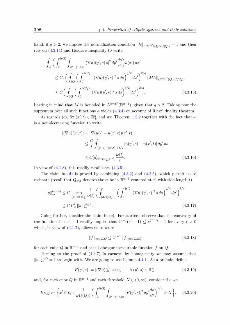
298 4.3. Properties of elliptic systems and their solutions
hand, if q > 2, we impose the normalization condition ‖h‖L(q/2)′ (Q,dx′/|Q|) = 1 and thenrely on (4.3.14) and Hölder’s inequality to write
Q
( ˆ `(Q)
0
ˆ|x′−y′|<s
|(∇u)(y′, s) s|2 dy′dssn
)h(x′) dx′
≤ Cn(
3Q
( ˆ 3`(Q)
0|(∇u)(y′, s)|2 s ds
)q/2dx′)2/q
‖Mh‖L(q/2)′ (Q,dx′/|Q|)
≤ C(
3Q
( ˆ 3`(Q)
0|(∇u)(y′, s)|2 s ds
)q/2dx′)2/q
, (4.3.15)
bearing in mind that M is bounded in L(q/2)′(Rn−1), given that q > 2. Taking now thesupremum over all such functions h yields (4.3.4) on account of Riesz’ duality theorem.
As regards (c), fix (x′, t) ∈ Rn+ and use Theorem 1.2.2 together with the fact that ωis a non-decreasing function to write
|(∇u)(x′, t)| =∣∣∇(u(·)− u(x′, t))(x′, t)
∣∣≤ C
t
|(y′,s)−(x′,t)|<t/2
|u(y′, s)− u(x′, t)| dy′ ds
≤ C[u] ˙Cω(Rn+,CM )ω(t)t. (4.3.16)
In view of (4.1.8), this readily establishes (4.3.5).The claim in (d) is proved by combining (4.3.2) and (4.2.5), which permit us to
estimate (recall that Qx′,t denotes the cube in Rn−1 centered at x′ with side-length t)
‖u‖(ω,∞)∗∗ ≤ C sup
(x′,t)∈Rn+
1ω(t)
( (3/2)Qx′,t
( ˆ 3t/2
0|(∇u)(y′, s)|2 s ds
)q/2dy′)1/q
≤ C C ′ω ‖u‖(ω,q)∗∗ . (4.3.17)
Going further, consider the claim in (e). For starters, observe that the convexity ofthe function t 7→ et − 1 readily implies that 2n−1(et − 1) ≤ e2n−1t − 1 for every t > 0which, in view of (4.1.7), allows us to write
‖f‖expL,Q ≤ 2n−1 ‖f‖expL,2Q (4.3.18)
for each cube Q in Rn−1 and each Lebesgue measurable function f on Q.Turning to the proof of (4.3.7) in earnest, by homogeneity we may assume that
‖u‖(ω,2)∗∗ = 1 to begin with. We are going to use Lemma 4.4.1. As a prelude, define
F (y′, s) := |(∇u)(y′, s) s|, ∀ (y′, s) ∈ Rn+, (4.3.19)
and, for each cube Q in Rn−1 and each threshold N ∈ (0,∞), consider the set
EN,Q :=x′ ∈ Q : 1
ω(`(Q))
( ˆ `(Q)
0
ˆ|x′−y′|<κs
|F (y′, s)|2 dy′dssn
)1/2> N
. (4.3.20)
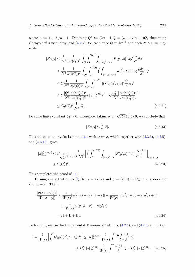
4. Generalized Hölder and Morrey-Campanato Dirichlet problems in Rn+ 299
where κ := 1 + 2√n− 1. Denoting Q∗ := (2κ + 1)Q = (3 + 4
√n− 1)Q, then using
Chebytcheff’s inequality, and (4.2.4), for each cube Q in Rn−1 and each N > 0 we maywrite
|EN,Q| ≤1N2
1ω(`(Q))2
ˆQ
ˆ `(Q)
0
ˆ|x′−y′|<κs
|F (y′, s)|2 dy′dssndx′
≤ 1N2
1ω(`(Q))2
ˆQ∗
ˆ `(Q)
0
(ˆ|y′−x′|<κs
dx′)|F (y′, s)|2ds
sndy′
≤ C 1N2
1ω(`(Q))2
ˆQ∗
ˆ `(Q∗)
0|(∇u)(y′, s) s|2ds
sdy′
≤ C |Q∗|
N2ω(`(Q∗))2
ω(`(Q))2(‖u‖(ω,2)
∗∗)2 = C
|Q∗|N2
[ω(`(Q∗))ω(`(Q))
]2≤ C0(C ′ω)2 1
N2 |Q|, (4.3.21)
for some finite constant C0 > 0. Therefore, taking N :=√
2C0C′ω > 0, we conclude that
|EN,Q| ≤12 |Q|. (4.3.22)
This allows us to invoke Lemma 4.4.1 with ϕ := ω, which together with (4.3.3), (4.2.5),and (4.3.18), gives
‖u‖(ω,exp)∗∗ ≤ C sup
Q⊆Rn−1
1ω(`(Q))
∥∥∥∥( ˆ `(2Q)
0
ˆ| · −y′|<s
|F (y′, s)|2 dy′dssn
)1/2∥∥∥∥expL,Q
≤ C(C ′ω)2. (4.3.23)
This completes the proof of (e).Turning our attention to (f), fix x = (x′, t) and y = (y′, s) in Rn+, and abbreviate
r := |x− y|. Then,
|u(x)− u(y)|W (|x− y|) ≤
1W (r) |u(x′, t)− u(x′, t+ r)|+ 1
W (r) |u(x′, t+ r)− u(y′, s+ r)|
+ 1W (r) |u(y′, s+ r)− u(y′, s)|
=: I + II + III. (4.3.24)
To bound I, we use the Fundamental Theorem of Calculus, (4.2.4), and (4.2.3) and obtain
I = 1W (r)
∣∣∣∣ˆ r
0(∂nu)(x′, t+ ξ) dξ
∣∣∣∣ ≤ ‖u‖(ω,∞)∗∗
1W (r)
ˆ r
0
ω(t+ ξ)t+ ξ
dξ
≤ C ′ω ‖u‖(ω,∞)∗∗
1W (r)
ˆ r
0
ω(ξ)ξ
dξ = C ′ω ‖u‖(ω,∞)∗∗ . (4.3.25)
300 4.4. John-Nirenberg’s inequality adapted to growth functions
Note that III is bounded analogously replacing x′ by y′ and t by s. For II, we use againthe Fundamental Theorem of Calculus, together with (4.2.4) and (4.2.12), to write
II = 1W (r)
∣∣∣∣∣ˆ 1
0
d
dθ[u(θ(x′, t+ r) + (1− θ)(y′, s+ r))] dθ
∣∣∣∣∣= 1W (r)
∣∣∣∣∣ˆ 1
0(x′ − y′, t− s) · (∇u)
(θ(x′, t+ r) + (1− θ)(y′, s+ r)
)dθ
∣∣∣∣∣≤ ‖u‖(ω,∞)
∗∗r
W (r)
ˆ 1
0
ω((1− θ)s+ θt+ r
)(1− θ)s+ θt+ r
dθ
≤ C ′ω ‖u‖(ω,∞)∗∗
r
W (r)
ˆ 1
0
ω(r)r
dθ
≤ (C ′ω)2 ‖u‖(ω,∞)∗∗ . (4.3.26)
As x and y were chosen arbitrarily, (4.3.24), (4.3.25), and (4.3.26) collectively justify(4.3.8).
To justify (g), observe that since ω is non-decreasing and satisfies (4.3.9) we maywrite(
Q
( ˆ `(Q)
0|(∇u)(x′, t)|2 t dt
)q/2dx′)1/q
≤( ˆ `(Q)
0ω(t)2dt
t
)1/2‖u‖(ω,∞)
∗∗
≤ (C ′′ω)1/2ω(`(Q)) ‖u‖(ω,∞)∗∗ , (4.3.27)
which readily leads to the desired inequality.As regards (h), the idea is to combine (4.3.1), (g), and (d) for the first three equiv-
alences. In concert, (c), the fact that (4.1.9) gives W ≤ Cω ω, and (f) also give the lastequivalence in (h). The proof of Proposition 4.3.1 is therefore complete.
4.4 John-Nirenberg’s inequality adapted to growth func-tions
In what follows we assume that all cubes are half-open, that is, they can be written inthe form Q = [a1, a1 + `(Q)) × · · · × [an−1, an−1 + `(Q)) with ai ∈ Rn−1 and `(Q) > 0.Notice that since ∂Q has Lebesgue measure zero the half-open assumption is harmless.Subdividing dydically yields the collection of (half-open) dyadic-subcubes of a givencube Q, which we shall denote by DQ. For the following statement, and with the aim ofconsidering global results, it is also convenient to consider the case Q = Rn−1 in whichscenario we take DQ to be the classical dyadic grid generated by [0, 1)n−1, or any otherdyadic grid. Let us also recall the definition of the dyadic Hardy-Littlewood maximalfunction localized to a given cube Q, i.e.,
(MdQf)(x) := sup
x∈Q′∈DQ
Q′|f(y′)| dy′, x ∈ Q, (4.4.1)
4. Generalized Hölder and Morrey-Campanato Dirichlet problems in Rn+ 301
for each f ∈ L1(Q). The following result is an extension of the John-Nirenberg inequalityobtained in [50], [49] (when ω ≡ 1) adapted to our growth function.
Lemma 4.4.1. Let F ∈ L2loc(Rn+) and let ϕ : [0,∞) → [0,∞) be a non-decreasing
function. Let Q0 ⊆ Rn−1 be an arbitrary half-open cube, or Q0 = Rn−1. Assume thatthere are numbers α ∈ (0, 1) and N ∈ (0,∞) such that∣∣∣∣x′ ∈ Q : 1
ϕ(`(Q))
( ˆ `(Q)
0
ˆ|x′−y′|<κs
|F (y′, s)|2 dy′dssn
)1/2> N
∣∣∣∣ ≤ α|Q| (4.4.2)
for every cube Q ∈ DQ0 and κ := 1 + 2√n− 1. Then, for every t > 0
supQ∈DQ0
1|Q|
∣∣∣∣x′ ∈ Q : 1ϕ(`(Q))
( ˆ `(Q)
0
ˆ|x′−y′|<κs
|F (y′, s)|2 dy′dssn
)1/2> t
∣∣∣∣≤ 1αe−
log(α−1)N t. (4.4.3)
Hence, for each q ∈ (0,∞) there exists a finite constant C = C(α, q) ≥ 1 such that
supQ∈DQ0
1ϕ(`(Q))
( Q
( ˆ `(Q)
0
ˆ|x′−y′|<s
|F (y′, s)|2 dy′dssn
)q/2dx′)1/q
≤ CN. (4.4.4)
Moreover, there exists some finite C = C(α) ≥ 1 such that
supQ∈DQ0
1ϕ(`(Q))
∥∥∥∥( ˆ `(Q)
0
ˆ| · −y′|<s
|F (y′, s)|2 dy′dssn
)1/2∥∥∥∥expL,Q
≤ CN. (4.4.5)
The previous result can be proved using the arguments in [50], [49] with appropriatemodifications. Here we present an alternative abstract argument based on ideas thatgo back to Calderón, as presented in [102] (see also [103], [74]). This also containsas a particular case the classical John-Nirenberg result concerning the exponential in-tegrability of BMO functions.
Proposition 4.4.2. Let Q0 ⊆ Rn−1 be an arbitrary half-open cube, or Q0 = Rn−1. Forevery Q ∈ DQ0 assume that there exist two non-negative functions GQ, HQ ∈ L1
loc(Rn−1)such that
GQ(x′) ≤ HQ(x′) for almost every x′ ∈ Q, (4.4.6)
and, for every Q′ ∈ DQ \ Q,
GQ(x′) ≤ GQ′(x′) +HQ(y′) for a.e. x ∈ Q′ and for a.e. y′ ∈ Q′, (4.4.7)
where Q′ is the dyadic parent of Q′. For each α ∈ (0, 1) define
mα := supQ∈DQ0
infλ > 0 : |x′ ∈ Q : HQ(x′) > λ| ≤ α|Q|
. (4.4.8)
Then, for every α ∈ (0, 1) one has
supQ∈DQ0
|x ∈ Q : GQ(x′) > t||Q|
≤ 1αe− log(α−1) t
mα , ∀ t > 0. (4.4.9)
302 4.4. John-Nirenberg’s inequality adapted to growth functions
As a consequence,
supQ∈DQ0
‖GQ‖expL,Q ≤1 + α−1
log(α−1) mα (4.4.10)
and for every q ∈ (0,∞) there exists a finite constant C = C(q) > 0 such that
supQ∈DQ0
( QGQ(x′)q dx′
)1/q≤ Cq
1α1/q log(α−1)
mα. (4.4.11)
Before proving this result and Lemma 4.4.1, let us illustrate how Proposition 4.4.2yields the classical John-Nirenberg result regarding the exponential integrability of BMOfunctions. Concretely, pick f ∈ BMO(Rn−1). Fix an arbitrary cube Q0 and for everyQ ∈ DQ0 define GQ := |f − fQ| and HQ := 2n−1Md
Q
(|f − fQ|
)(cf. (4.4.1)). Clearly,
(4.4.6) holds by Lebesgue’s Differentiation Theorem. Moreover, for every Q′ ∈ DQ \Q, x′ ∈ Q′, and y′ ∈ Q′ we have
GQ(x′) ≤ |f(x′)− fQ′ |+ |f ′Q − fQ| ≤ GQ′(x′) + Q′|f(z′)− fQ| dz′
≤ GQ′(x′) + 2n−1 Q′|f(z′)− fQ| dz′ ≤ GQ′(x′) +HQ′(y′), (4.4.12)
and (4.4.7) follows. Going further, by the weak-type (1, 1) of the dyadic Hardy-Littlewoodmaximal function, for every λ > 0 we may write
|x′ ∈ Q : HQ(x′) > λ| ≤ 2n−1
λ
ˆQ|f(y′)− fQ| dy′ ≤
2n−1‖f‖BMO(Rn−1)λ
|Q|. (4.4.13)
In particular, choosing for instance α := e−1, if we use the previous estimate with λ :=2n−1‖f‖BMO(Rn−1)/α we obtain mα ≤ 2n−1‖f‖BMO(Rn−1)/α. Thus, (4.4.9) yields
|x ∈ Q0 : |f(x′)− fQ0 | > t||Q0|
≤ 1αe−α log(α−1)
2n−1t
‖f‖BMO(Rn−1)
= e · e− 1
2n−1et
‖f‖BMO(Rn−1) (4.4.14)
while (4.4.10) gives
‖f − fQ0‖expL,Q0 ≤ (1 + e) e 2n−1‖f‖BMO(Rn−1) (4.4.15)
which are the well-known John-Nirenberg inequalities.We now turn to the proof of Lemma 4.4.1.
Proof of Lemma 4.4.1. Let F , α, and N be fixed as in the statement of the lemma. Forevery Q ∈ DQ0 and x′ ∈ Rn−1, define
GQ(x′) := 1ϕ(`(Q))
(ˆ `(Q)
0
ˆ|x′−z′|<s
|F (z′, s)|2 dz′dssn
)1/2(4.4.16)
4. Generalized Hölder and Morrey-Campanato Dirichlet problems in Rn+ 303
andHQ(x′) = 1
ϕ(`(Q))(ˆ `(Q)
0
ˆ|x′−z′|<κs
|F (z′, s)|2 dz′dssn
)1/2. (4.4.17)
Note that (4.4.6) is trivially verified since κ > 1. To proceed, fix Q′ ∈ DQ along withx′ ∈ Q′ and y′ ∈ Q′. If |x′ − z′| < s with `(Q′) ≤ s ≤ `(Q) then
|y′ − z′| ≤ |y′ − x′|+ |x′ − z′| < 2√n− 1 `(Q′) + s ≤ κs. (4.4.18)
Therefore, since ϕ is non-decreasing,
GQ(x′) ≤ ϕ(`(Q′))ϕ(`(Q)) GQ
′(x′) + 1ϕ(`(Q))
(ˆ `(Q)
`(Q′)
ˆ|x′−z′|<s
|F (z′, s)|2 dz′dssn
)1/2
≤ GQ′(x′) +HQ(y′), (4.4.19)
establishing (4.4.7). Moreover, (4.4.2) gives immediately that mα ≤ N . Granted this,(4.4.9), (4.4.11), and (4.4.10), (with α ∈ (0, 1) given by (4.4.2)) prove, respectively (4.4.3),(4.4.4), and (4.4.5).
Finally, we give the proof of Proposition 4.4.2.
Proof of Proposition 4.4.2. We start by introducing some notation. Set
Ξ(t) := supQ∈DQ0
|EQ(t)||Q|
:= supQ∈DQ0
|x′ ∈ Q : GQ(x′) > t||Q|
, 0 < t <∞. (4.4.20)
Fix α ∈ (0, 1), let ε > 0 be arbitrary, and write λε = mα + ε. From (4.4.8) it follows that
|FQ,ε| := |x′ ∈ Q : HQ(x′) > λε| ≤ α|Q|, ∀Q ∈ DQ0 . (4.4.21)
Fix now Q ∈ DQ0 , β ∈ (α, 1) (we will eventually let β → 1+) and set
ΩQ := x′ ∈ Q : MdQ(1FQ,ε)(x
′) > β. (4.4.22)
Note that (4.4.21) ensures that Q
1FQ,ε(y′) dy′ = |FQ,ε|
|Q|≤ α < β, (4.4.23)
hence we can extract a family of pairwise disjoint stopping-time cubes Qjj ⊆ DQ \Qso that ΩQ = ∪jQj and for every j
|FQ,ε ∩Qj ||Qj |
> β,|FQ,ε ∩Q′||Q′|
≤ β, Qj ( Q′ ∈ DQ. (4.4.24)
Let t > λε and note that (4.4.6) gives
λε < t < GQ(x′) ≤ HQ(x′) for a.e. x′ ∈ EQ(t). (4.4.25)
which implies that
β < 1 = 1FQ,ε(x′) ≤Md
Q
(1FQ,ε
)(x′) for a.e. x′ ∈ EQ(t). (4.4.26)
304 4.4. John-Nirenberg’s inequality adapted to growth functions
Hence,|EQ(t)| = |EQ(t) ∩ ΩQ| =
∑j
|EQ(t) ∩Qj |. (4.4.27)
For every j, by the second estimate in (4.4.24) applied to Qj , the dyadic parent of Qj ,we have |FQ,ε ∩ Qj |/|Qj | ≤ β < 1, therefore |Qj \ FQ,ε|/|Qj | > 1− β > 0. In particular,(4.4.7) guarantees that we can find x′j ∈ Qj \ FQ,ε, such that for a.e. x′ ∈ Qj we have
GQ(x′) ≤ GQj (x′) +HQ(x′j) ≤ GQj (x′) + λε. (4.4.28)
Consequently, GQj (x′) > t− λε for a.e. x′ ∈ EQ(t) ∩Qj which further implies
|EQ(t) ∩Qj | ≤ |x′ ∈ Qj : GQj (x′) > t− λε| ≤ Ξ(t− λε)|Qj |. (4.4.29)
In turn, this permits us to estimate
|EQ(t)| =∑j
|EQ(t) ∩Qj | ≤ Ξ(t− λε)∑j
|Qj | ≤ Ξ(t− λε)1β
∑j
|FQ,ε ∩Qj |
≤ Ξ(t− λε)1β|FQ,ε| ≤ Ξ(t− λε)
α
β|Q|, (4.4.30)
where we have used (4.4.24), that the cubes Qjj are pairwise disjoint and, finally,(4.4.21). Dividing by |Q| and taking the supremum over all Q ∈ DQ0 we arrive at
Ξ(t) ≤ α
βΞ(t− λε), t > λε. (4.4.31)
Since this is valid for all β ∈ (α, 1), we can now let β → 1+, iterate the previousexpression, and use the fact that Ξ(t) ≤ 1 to conclude that
Ξ(t) ≤ 1αα
tλε = 1
αe− log(α−1) t
λε , t > 0. (4.4.32)
Recalling that λε = mα + ε and letting ε→ 0+ establishes (4.4.9).We shall next indicate how (4.4.9) implies (4.4.10). Concretely, if we take t :=
1+α−1
log(α−1) mα we see that (4.4.9) gives
Q
(eGQ(x′)
t − 1)dx′ =
ˆ ∞0
|x′ ∈ Q : GQ(x′)/t > λ||Q|
eλ dλ
≤ 1α
ˆ ∞0
e− log(α−1) λtmα eλ dλ = 1
α
ˆ ∞0
e−α−1λ dλ = 1. (4.4.33)
With this in hand, (4.4.10) follows with the help of (4.1.7).At this stage, there remains to justify (4.4.11). This can be done invoking again
(4.4.9): QGQ(x′)q dx′ =
ˆ ∞0
|x′ ∈ Q : GQ(x′) > λ||Q|
q λqdλ
λ≤ 1α
ˆ ∞0
e− log(α−1) λmα q λq
dλ
λ
= 1α
(mα
log(α−1)
)q ˆ ∞0
e−λ q λqdλ
λ= Cq
1α
(mα
log(α−1)
)q. (4.4.34)
This completes the proof of Proposition 4.4.2.
4. Generalized Hölder and Morrey-Campanato Dirichlet problems in Rn+ 305
4.5 Existence results
In this section we develop the main tools used to establish the existence of solutions forthe boundary value problems formulated in the statement of Theorem 4.1.2. We startwith the generalized Hölder Dirichlet Problem.
Proposition 4.5.1. Let L be a constant complex coefficient system as in (1.2.1) satisfyingthe strong ellipticity condition formulated in (1.2.4), fix an aperture parameter κ > 0and let ω be a growth function satisfying (4.2.2). Given f ∈ C ω(Rn−1,CM ), defineu(x′, t) := (PLt ∗ f)(x′) for every (x′, t) ∈ Rn+. Then u is meaningfully defined via anabsolutely convergent integral and satisfies
u ∈[C∞(Rn+)
]M, Lu = 0 in Rn+, u|
κ−n.t.
∂Rn+= f a.e. on Rn−1. (4.5.1)
Moreover, there exists a finite constant C = C(L, n) > 0 such that
[u]Cω(Rn+,CM ) ≤ C C′ω(1 + C ′ω)[f ]Cω(Rn−1,CM ), (4.5.2)
and u ∈ C ω(Rn+,CM ) with u|∂Rn+ = f .
Proof. Let f ∈ C ω(Rn−1,CM ) and define u(x′, t) := (PLt ∗ f)(x′) for every (x′, t) ∈ Rn+.By (4.2.19) and Theorem 1.2.4(c), u satisfies all properties listed in (4.5.1). To prove theestimate in (4.5.2), we first notice that for any (x′, t) ∈ Rn+, we can write
(PLt ∗ f)(x′) =ˆRn−1
PLt (x′ − y′)f(y′) dy′ =ˆRn−1
t1−nPL(x′ − y′
t
)f(y′) dy′
=ˆRn−1
PL(z′)f(x′ − tz′) dz′. (4.5.3)
Fix now x = (x′, t) and y = (y′, s) arbitrary in Rn+, and set r := |x− y|. By (1.2.26) andthe fact that ω is non-decreasing we obtain
|u(x′, t)− u(y′, s)| = |(PLt ∗ f)(x′)− (PLs ∗ f)(y′)|
≤ CˆRn−1
1(1 + |z′|2)n/2
|f(x′ − tz′)− f(y′ − sz′)| dz′
≤ C[f ]Cω(Rn−1,CM )
ˆRn−1
1(1 + |z′|2)n/2
ω((1 + |z′|)r) dz′
≤ C[f ]Cω(Rn−1,CM )
ˆ ∞0
1(1 + λ2)n/2
ω((1 + λ)r
)λn−1dλ
λ
≤ C[f ]Cω(Rn−1,CM )
( ˆ 1
0ω(2r)λn−1dλ
λ+ˆ ∞
1
ω(2λr)λ
dλ
λ
)
= C[f ]Cω(Rn−1,CM )
(ω(2r) + 2r
ˆ ∞2r
ω(λ)λ
dλ
λ
)≤ C C ′ω(1 + C ′ω)ω(r)[f ]Cω(Rn−1,CM ), (4.5.4)
306 4.6. A Fatou-type result and uniqueness of solutions
where in the last inequality we have used (4.2.2) and (4.2.5). Hence, (4.5.2) holds. Inparticular, u ∈ C ω(Rn+,CM ) by Lemma 4.2.1(d). This and the fact that u|
κ−n.t.
∂Rn+= f a.e.
in Rn−1 with f ∈ C ω(Rn−1,CM ) then prove that, indeed, u|∂Rn+ = f .
The result below is the main tool in the proof of existence of solutions for thegeneralized Morrey-Campanato Dirichlet Problem.
Proposition 4.5.2. Let L be a constant complex coefficient system as in (1.2.1) satisfyingthe strong ellipticity condition stated in (1.2.4), fix an aperture parameter κ > 0, and letω be a growth function satisfying (4.2.2). Given 1 ≤ p <∞, let f ∈ E ω,p(Rn−1,CM ) anddefine u(x′, t) := (PLt ∗ f)(x′) for every (x′, t) ∈ Rn+. Then u is meaningfully defined viaan absolutely convergent integral and satisfies
u ∈[C∞(Rn+)
]M, Lu = 0 in Rn+, u|
κ−n.t.
∂Rn+= f a.e. on Rn−1. (4.5.5)
Moreover, for every q ∈ (0,∞] there exists a finite constant C = C(L, n, p, q) > 0 suchthat
‖u‖(ω,q)∗∗ ≤ C(C ′ω)4 ‖f‖E ω,p(Rn−1,CM ) . (4.5.6)
Furthermore, the same is true if ‖·‖(ω,q)∗∗ is replaced by ‖·‖(ω,exp)∗∗ .
Proof. Given f ∈ E ω,p(Rn−1,CM ), if u(x′, t) := (PLt ∗ f)(x′) for every (x′, t) ∈ Rn+, from(4.2.19) and Theorem 1.2.4(c) we see that u satisfies all properties listed in (4.5.5).
Next, having fixed an arbitrary exponent q ∈ (0,∞), based on Proposition 4.3.1(d),(4.3.1), Proposition 4.3.1(e), (1.2.35), (4.2.15), (4.2.17) and (4.2.2) we may write
‖u‖(ω,∞)∗∗ ≤ C C ′ω ‖u‖
(ω,q)∗∗ ≤ C C ′ω ‖u‖
(ω,exp)∗∗
≤ C(C ′ω)3 ‖u‖(ω,2)∗∗ ≤ C(C ′ω)3 sup
t>0
1ω(t)
ˆ ∞1
osc1(f, st)dss2
= C(C ′ω)3 ‖f‖E ω,p(Rn−1,CM ) supt>0
t
ω(t)
ˆ ∞t
ω(s)dss2
≤ C(C ′ω)4 ‖f‖E ω,p(Rn−1,CM ) , (4.5.7)
which proves (4.5.6) and the corresponding estimate for ‖u‖(ω,exp)∗∗ .
4.6 A Fatou-type result and uniqueness of solutions
We shall now prove a Fatou-type result which is going to be the main ingredient in estab-lishing the uniqueness of solutions for the boundary value problems we are presently con-sidering. More precisely, the following result establishes that any solution in C ω(Rn+,CM )can be obtained as a convolution of its trace with the associated Poisson kernel.
Proposition 4.6.1. Let L be a constant complex coefficient system as in (1.2.1) satisfyingthe strong ellipticity condition stated in (1.2.4), and let ω be a growth function satisfying
4. Generalized Hölder and Morrey-Campanato Dirichlet problems in Rn+ 307
(4.2.2). If u ∈[C∞(Rn+)
]M ∩ C ω(Rn+,CM ) is a function satisfying Lu = 0 in Rn+, thenu|∂Rn+ ∈ C ω(Rn−1,CM ) and
u(x′, t) =(PLt ∗ (u|∂Rn+)
)(x′), ∀ (x′, t) ∈ Rn+. (4.6.1)
Proof. Let u ∈[C∞(Rn+)
]M ∩ C ω(Rn+,CM ) satisfy Lu = 0 in Rn+. By Lemma 4.2.1(d),it follows that u can be continuously extended to a function (which we call again u)u ∈ C ω(Rn+,CM ). In particular, the trace u|∂Rn+ is well-defined and belongs to the spaceC ω(Rn−1,CM ). To proceed, fix an arbitrary ε > 0 and define uε = u(·+εen) in Rn+, whereen = (0, . . . , 0, 1) ∈ Rn. Then, by design, uε ∈
[C∞(Rn+)
]M ∩ C ω(Rn+,CM ), Luε = 0 inRn+, and [uε] ˙Cω(Rn+,CM ) ≤ [u] ˙Cω(Rn+,CM ). Moreover, using Proposition 4.3.1(c) and (4.2.4)we obtain
sup(x′,t)∈Rn+
|(∇uε)(x′, t)| = sup(x′,t)∈Rn+
|(∇u)(x′, t+ ε)|
≤ C[u] ˙Cω(Rn+,CM ) sup(x′,t)∈Rn+
ω(t+ ε)t+ ε
≤ C C ′ω[u] ˙Cω(Rn+,CM )ω(ε)ε. (4.6.2)
This implies that ∇uε is bounded in Rn+, hence uε ∈[W 1,2
bdd(Rn+)]M .
Define next fε(x′) := u(x′, ε) ∈ C ω(Rn−1,CM ) and wε(x′, t) := (PLt ∗ fε)(x′) for each(x′, t) ∈ Rn+. Then, Proposition 4.5.1 implies that that wε ∈
[C∞(Rn+)
]M ∩ C ω(Rn+,CM ),Lwε = 0 in Rn+ and wε|∂Rn+ = fε. Moreover, for every pair of points x′, y′ ∈ Rn−1 wehave, on the one hand,
|fε(x′)− fε(y′)| = |u(x′, ε)− u(y′, ε)| ≤ [u] ˙Cω(Rn+,CM ) ω(|x′ − y′|), (4.6.3)
and, on the other hand, using the Mean Value Theorem and Proposition 4.3.1(c),
|fε(x′)− fε(y′)| = |u(x′, ε)− u(y′, ε)|
≤ |x′ − y′| supz′∈[x′,y′]
|(∇u)(z′, ε)|
≤ C |x′ − y′| [u] ˙Cω(Rn+,CM )ω(ε)ε. (4.6.4)
Therefore, we conclude that fε ∈ C Ψ(Rn−1,CM ), with norm depending (unfavorably) onthe parameter ε, where the growth function Ψ is given by
Ψ(t) := mint,ω(t)ω(1)
=
t if t ≤ 1,
ω(t)/ω(1) if t > 1.(4.6.5)
For every R > 1 and x = (x′, t), let us now invoke (1.2.34), (4.2.15) and (4.2.17), with Ψ
308 4.6. A Fatou-type result and uniqueness of solutions
in place of ω, to writeˆB(0,R)∩Rn+
|(∇wε)(x)|2 dx ≤ˆB(0,R)∩Rn+
(C
t
ˆ ∞1
osc1(fε; st)ds
s2
)2dx
≤ C ‖fε‖E Ψ,p(Rn−1,CM )
ˆB(0,R)∩Rn+
(ˆ ∞1
Ψ(st)st
ds
s
)2dx
≤ C ‖fε‖E Ψ,p(Rn−1,CM )Rn−1
ˆ R
0
(ˆ ∞t
Ψ(s)s
ds
s
)2dt, (4.6.6)
and then use (4.2.2) to observe thatˆ R
0
(ˆ ∞t
Ψ(s)s
ds
s
)2dt ≤
ˆ 1
0
(ˆ 1
t
ds
s+ 1ω(1)
ˆ ∞1
ω(s)s
ds
s
)2
dt
+ˆ R
1
( 1ω(1)
ˆ ∞1
ω(s)s
ds
s
)2dt
≤ˆ 1
0
(log(1/t) + C ′ω
)2dt+ (R− 1)(C ′ω)2 <∞, (4.6.7)
Collectively, (4.6.6) and (4.6.7) show that wε ∈[W 1,2
bdd(Rn+)]M .
We now consider vε := uε−wε ∈[C∞(Rn+)
]M ∩ C ω(Rn+,CM )∩[W 1,2
bdd(Rn+)]M , which
satisfies Lvε = 0 in Rn+ and vε|∂Rn+ = 0. Hence, Tr vε = 0 on Rn−1 (see (1.2.22)) and foreach x ∈ Rn we have
|vε(x)| ≤ |vε(x)− vε(0)|+ |vε(0)|
≤ max[vε] ˙Cω(Rn+,CM ) , |vε(0)|
(1 + ω(|x|)). (4.6.8)
From this and Proposition 1.2.3 we then conclude that
supRn+∩B(0,r)
|∇vε| ≤C
rsup
Rn+∩B(0,2r)|vε| ≤ Cε
1 + ω(2r)r
, (4.6.9)
and from Lemma 4.2.1(c) we see that the right side of (4.6.9) tends to 0 as r →∞. Thisforces ∇vε ≡ 0, and since vε ∈
[C∞(Rn+)
]M ∩C ω(Rn+,CM ) with vε|∂Rn+ = 0 we ultimatelyconclude that vε ≡ 0. Consequently,
u(x′, t+ ε) = (PLt ∗ fε)(x′), ∀ (x′, t) ∈ Rn+. (4.6.10)
Since, as noted earlier, u|∂Rn+ ∈ C ω(Rn−1,CM ), for every x′ ∈ Rn−1 and ε > 0 we maynow write∣∣u(x′, t+ ε)−
(PLt ∗ (u|∂Rn+)
)(x′)
∣∣ =∣∣(PLt ∗ (fε − u|∂Rn+)
)(x′)
∣∣≤ ‖PLt ‖L1(Rn−1) sup
y′∈Rn−1
∣∣fε(y′)− u|∂Rn+ (y′)∣∣
= ‖PL‖L1(Rn−1) supy′∈Rn−1
∣∣u(y′, ε)− u|∂Rn+ (y′)∣∣
≤ ‖PL‖L1(Rn−1)[u] ˙Cω(Rn+,CM ) ω(ε). (4.6.11)
4. Generalized Hölder and Morrey-Campanato Dirichlet problems in Rn+ 309
From (1.2.26) we know that ‖PL‖L1(Rn−1) < ∞. Upon letting ε → 0+ and using that ωvanishes in the limit at the origin, we see that (4.6.11) implies (4.6.1). This finishes theproof of Proposition 4.6.1.
4.7 Well-posedness results
We are now ready to prove well-posedness results. We first consider the case in which theboundary data belong to generalized Hölder spaces and we note that, in such a scenario,the only requirement on the growth function is (4.2.2).
Theorem 4.7.1. Let L be a constant complex coefficient M ×M system as in (1.2.1)satisfying the strong ellipticity condition (1.2.4). Also, let ω be a growth function satis-fying (4.2.2). Then the generalized Hölder Dirichlet Problem for L in Rn+, formulated as
u ∈[C∞(Rn+)
]M,
Lu = 0 in Rn+,
[u]Cω(Rn+,CM ) <∞,
u|∂Rn+ = f ∈ C ω(Rn−1,CM ) on Rn−1,
(4.7.1)
is well-posed. More specifically, there exists a unique solution which is given by
u(x′, t) = (PLt ∗ f)(x′), ∀ (x′, t) ∈ Rn+, (4.7.2)
where PL denotes the Poisson kernel for the system L in Rn+ from Theorem 1.2.4. Inaddition, u extends to a function in C ω(Rn+,CM ) with u|∂Rn+ = f , and there exists afinite constant C = C(n,L, ω) ≥ 1 such that
C−1[f ]Cω(Rn−1,CM ) ≤ [u]Cω(Rn+,CM ) ≤ C[f ]Cω(Rn−1,CM ). (4.7.3)
Proof. Given f ∈ C ω(Rn−1,CM ), define u as in (4.7.2). Proposition 4.5.1 then impliesthat u satisfies all conditions in (4.7.1). Also, u extends to a function in C ω(Rn+,CM )with u|∂Rn+ = f , and the second inequality in (4.7.3) holds. Moreover, (4.2.7) yields
[f ]Cω(Rn−1,CM ) = [u|∂Rn+ ]Cω(Rn−1,CM ) ≤ [u]Cω(Rn+,CM ) ≤ 2C ′ω[u]Cω(Rn+,CM ), (4.7.4)
so that the first inequality in (4.7.3) follows.It remains to prove that the solution is unique. However, this follows at once from
Proposition 4.6.1. Indeed, the first three conditions in (4.7.1) imply (4.6.1) and sinceu|∂Rn+ = f we conclude that necessarily u(x′, t) =
(PLt ∗ f
)(x′) for every (x′, t) ∈ Rn+.
Here is the well-posedness for the generalized Morrey-Campanato Dirichlet Problem.In this case, the growth function is assumed to satisfy both (4.2.1) and (4.2.2).
Theorem 4.7.2. Let L be a constant complex coefficient M ×M system as in (1.2.1)satisfying the strong ellipticity condition (1.2.4). Fix an aperture parameter κ > 0,
310 4.7. Well-posedness results
p ∈ [1,∞) along with q ∈ (0,∞], and let ω be a growth function satisfying (4.2.1) and(4.2.2). Then the generalized Morrey-Campanato Dirichlet Problem for L in Rn+, namely
u ∈[C∞(Rn+)
]M,
Lu = 0 in Rn+,
‖u‖(ω,q)∗∗ <∞,
u|κ−n.t.
∂Rn+= f ∈ E ω,p(Rn−1,CM ) a.e. on Rn−1,
(4.7.5)
is well-posed. More specifically, there exists a unique solution which is given by
u(x′, t) = (PLt ∗ f)(x′), ∀ (x′, t) ∈ Rn+, (4.7.6)
where PL denotes the Poisson kernel for the system L in Rn+ from Theorem 1.2.4. More-over, with W defined as in (4.2.3), the solution u extends to a function in CW (Rn+,CM )with u|∂Rn+ = f a.e. on Rn−1, and there exists a finite constant C = C(n,L, ω, p, q) ≥ 1for which
C−1 ‖f‖EW,p(Rn−1,CM ) ≤ ‖u‖(ω,q)∗∗ ≤ C ‖f‖E ω,p(Rn−1,CM ) . (4.7.7)
Furthermore, all results remain valid if ‖·‖(ω,q)∗∗ is replaced everywhere by ‖·‖(ω,exp)∗∗ .
Proof. Having fixed f ∈ E ω,p(Rn−1,CM ), if u is defined as in (4.7.6) then Proposi-tion 4.5.2 implies the validity of all conditions in (4.7.5) and also of the second inequalityin (4.7.7) (even replacing q by exp). In the case q =∞ we invoke Proposition 4.3.1(f) toobtain that u ∈ CW (Rn+,CM ) in the sense of Lemma 4.2.1(d). Note that we also have
[u|∂Rn+ ]CW (Rn−1,CM ) ≤ [u]CW (Rn+,CM ) ≤ 2C ′W [u]CW (Rn+,CM ) ≤ C(C ′ω)4 ‖u‖(ω,∞)∗∗ (4.7.8)
thanks to (4.2.7) (for the growth function W ), Lemma 4.2.2, and (4.3.8).Given that, on the one hand, u|∂Rn+ = u|
κ−n.t.
∂Rn+everywhere in Rn−1 because u ∈
CW (Rn+,CM ), and that, on the other hand, u|κ−n.t.
∂Rn+= f a.e. in Rn−1, we conclude that
u|∂Rn+ = f a.e. in Rn−1. In addition, (4.2.18) (applied to W ), Lemma 4.2.2, and (4.7.8)permit us to estimate
‖f‖EW,p(Rn−1,CM ) = ‖ u|∂Rn+ ‖EW,p(Rn−1,CM ) ≤√n− 1C ′W [u|∂Rn+ ] ˙C W (Rn−1,CM )
≤ C(C ′ω)6 ‖u‖(ω,∞)∗∗ ≤ C(C ′ω)7 ‖u‖(ω,q)∗∗ ≤ C(C ′ω)7 ‖u‖(ω,exp)
∗∗ , (4.7.9)
where 0 < q <∞ and where we have also used Proposition 4.3.1(d) and (4.3.1).To prove that the solution is unique, we note that having ‖u‖(ω,q)∗∗ < ∞ for a given
q ∈ (0,∞], or even ‖u‖(ω,exp)∗∗ < ∞, implies that ‖u‖(ω,∞)
∗∗ < ∞ by Proposition 4.3.1(d)and (4.3.1). Having established this, Proposition 4.3.1(f) applies and yields that u ∈CW (Rn+,CM ). Consequently, u|∂Rn+ = u|
κ−n.t.
∂Rn+everywhere in Rn−1, and if we also take
into account the boundary condition from (4.7.5), we conclude that u|∂Rn+ = f a.e. on
4. Generalized Hölder and Morrey-Campanato Dirichlet problems in Rn+ 311
Rn−1. Moreover, since Lemma 4.2.2 ensures that W is a growth function satisfying(4.2.2), we may invoke Proposition 4.6.1 to write
u(x′, t) =(PLt ∗ (u|∂Rn+)
)(x′) =
(PLt ∗ f
)(x′), ∀ (x′, t) ∈ Rn+. (4.7.10)
The proof of the theorem is therefore finished.
Remark 4.7.3. Theorems 4.7.1 and 4.7.2 are closely related. To elaborate in this, fix agrowth function ω satisfying (4.2.1) and (4.2.2). From (4.2.18) and Proposition 4.5.2 itfollows that, given any f ∈ C ω(Rn−1,CM ), the unique solution of the boundary valueproblem (4.7.1), i.e., u(x′, t) = (PLt ∗ f)(x′) for (x′, t) ∈ Rn+, also solves (4.7.5), regardingnow f as a function in E ω,p(Rn−1,CM ) (cf. (4.2.19)) with p ∈ [1,∞) and q ∈ (0,∞]arbitrary (and even with ‖·‖(ω,q)∗∗ replaced by ‖·‖(ω,exp)
∗∗ ). As such, u satisfies (4.7.7)whenever (4.2.1) holds.
This being said, the fact that f ∈ E ω,p(Rn−1,CM ) does not guarantee, in general, thatthe corresponding solution satisfies u ∈ C ω(Rn+,CM ), even though we have establishedabove that the solution to the boundary value problem (4.7.5) belongs to CW (Rn+,CM ).Note that, as seen from (1.3.17)-(1.3.18) and (4.2.12), the space CW (Rn+,CM ) containsC ω(Rn+,CM ).
This aspect is fully clarified with the help of Example 4.7.4 discussed further below,where we construct some growth function ω satisfying (4.2.1), (4.2.2), and for which thespace E ω,1(Rn−1,C) is strictly bigger than C ω(Rn−1,C). Its relevance for the issue athand is as follows. Consider the boundary problem (4.7.5) formulated with L being theLaplacian in Rn and with f ∈ E ω,1(Rn−1,C) \ C ω(Rn−1,C) as boundary datum. Itssolution u then necessarily satisfies u /∈ C ω(Rn+,C), for otherwise Lemma 4.2.1(d) wouldimply u ∈ C ω(Rn+,CM ) and since u|∂Rn+ = u|
κ−n.t.
∂Rn+= f a.e. on Rn−1 and f is continuous
in Rn−1 we would conclude that f coincides everywhere with u|∂Rn+ ∈ C ω(Rn−1,C), acontradiction.
In spite of the previous remark, Theorem 4.1.2 states that the boundary problems(4.7.1) and (4.7.5) are actually equivalent under the stronger assumption (4.1.9) on thegrowth function. Here is the proof of Theorem 4.1.2.
Proof of Theorem 4.1.2. We start with the observation that (4.1.9) and Lemma 4.2.2yield C−1
ω W (t) ≤ ω(t) ≤ CωW (t) for each t ∈ (0,∞). Therefore,
C ω(Rn+,CM ) = CW (Rn+,CM ), C ω(Rn+,CM ) = CW (Rn+,CM ), (4.7.11)
andE ω,p(Rn−1,CM ) = EW,p(Rn−1,CM ), (4.7.12)
as vector spaces, with equivalent norms.Having made these identifications, we now proceed to observe that (a) follows directly
from Theorem 4.7.1, while (b) is implied by Theorem 4.7.2 with the help of (4.7.11) and(4.7.12). To deal with (c), we first observe that the left-to-right inclusion follows fromLemma 4.2.4(b), whereas (4.2.18) provides the accompanying estimate for the norms.
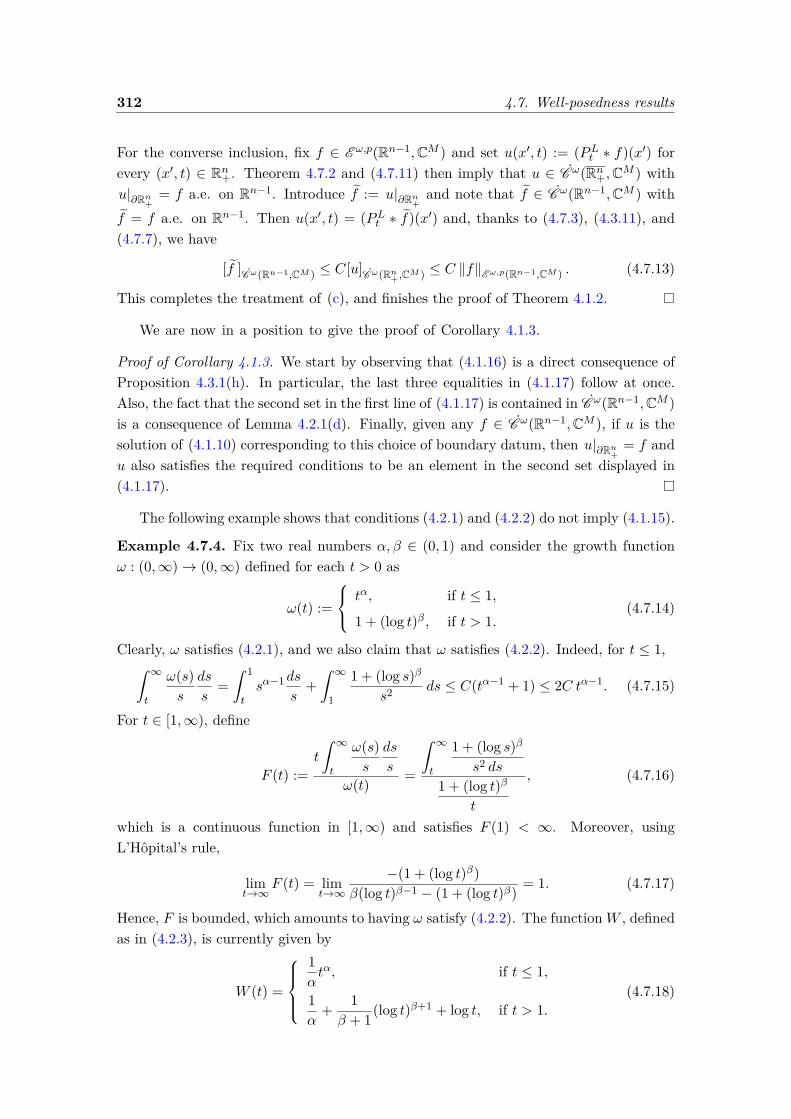
312 4.7. Well-posedness results
For the converse inclusion, fix f ∈ E ω,p(Rn−1,CM ) and set u(x′, t) := (PLt ∗ f)(x′) forevery (x′, t) ∈ Rn+. Theorem 4.7.2 and (4.7.11) then imply that u ∈ C ω(Rn+,CM ) withu|∂Rn+ = f a.e. on Rn−1. Introduce f := u|∂Rn+ and note that f ∈ C ω(Rn−1,CM ) withf = f a.e. on Rn−1. Then u(x′, t) = (PLt ∗ f)(x′) and, thanks to (4.7.3), (4.3.11), and(4.7.7), we have
[f ]Cω(Rn−1,CM ) ≤ C[u]Cω(Rn+,CM ) ≤ C ‖f‖E ω,p(Rn−1,CM ) . (4.7.13)
This completes the treatment of (c), and finishes the proof of Theorem 4.1.2.
We are now in a position to give the proof of Corollary 4.1.3.
Proof of Corollary 4.1.3. We start by observing that (4.1.16) is a direct consequence ofProposition 4.3.1(h). In particular, the last three equalities in (4.1.17) follow at once.Also, the fact that the second set in the first line of (4.1.17) is contained in C ω(Rn−1,CM )is a consequence of Lemma 4.2.1(d). Finally, given any f ∈ C ω(Rn−1,CM ), if u is thesolution of (4.1.10) corresponding to this choice of boundary datum, then u|∂Rn+ = f andu also satisfies the required conditions to be an element in the second set displayed in(4.1.17).
The following example shows that conditions (4.2.1) and (4.2.2) do not imply (4.1.15).
Example 4.7.4. Fix two real numbers α, β ∈ (0, 1) and consider the growth functionω : (0,∞)→ (0,∞) defined for each t > 0 as
ω(t) :=
tα, if t ≤ 1,
1 + (log t)β, if t > 1.(4.7.14)
Clearly, ω satisfies (4.2.1), and we also claim that ω satisfies (4.2.2). Indeed, for t ≤ 1,ˆ ∞t
ω(s)s
ds
s=ˆ 1
tsα−1ds
s+ˆ ∞
1
1 + (log s)β
s2 ds ≤ C(tα−1 + 1) ≤ 2C tα−1. (4.7.15)
For t ∈ [1,∞), define
F (t) :=t
ˆ ∞t
ω(s)s
ds
s
ω(t) =
ˆ ∞t
1 + (log s)β
s2 ds
1 + (log t)β
t
, (4.7.16)
which is a continuous function in [1,∞) and satisfies F (1) < ∞. Moreover, usingL’Hôpital’s rule,
limt→∞
F (t) = limt→∞
−(1 + (log t)β)β(log t)β−1 − (1 + (log t)β) = 1. (4.7.17)
Hence, F is bounded, which amounts to having ω satisfy (4.2.2). The functionW , definedas in (4.2.3), is currently given by
W (t) =
1αtα, if t ≤ 1,
1α
+ 1β + 1(log t)β+1 + log t, if t > 1.
(4.7.18)
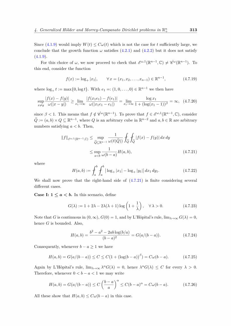
4. Generalized Hölder and Morrey-Campanato Dirichlet problems in Rn+ 313
Since (4.1.9) would imply W (t) ≤ Cω(t) which is not the case for t sufficiently large, weconclude that the growth function ω satisfies (4.2.1) and (4.2.2) but it does not satisfy(4.1.9).
For this choice of ω, we now proceed to check that E ω,1(Rn−1,C) 6= C ω(Rn−1). Tothis end, consider the function
f(x) := log+ |x1|, ∀x = (x1, x2, . . . , xn−1) ∈ Rn−1, (4.7.19)
where log+ t := max0, log t. With e1 =: (1, 0, . . . , 0) ∈ Rn−1 we then have
supx 6=y
|f(x)− f(y)|ω(|x− y|) ≥ lim
x1→∞|f(x1e1)− f(e1)|ω(|x1e1 − e1|)
= limx1→∞
log x11 + (log(x1 − 1))β =∞, (4.7.20)
since β < 1. This means that f /∈ C ω(Rn−1). To prove that f ∈ E ω,1(Rn−1,C), considerQ := (a, b)×Q ⊆ Rn−1, where Q is an arbitrary cube in Rn−2 and a, b ∈ R are arbitrarynumbers satisfying a < b. Then,
‖f‖E ω,1(Rn−1,C) ≤ supQ⊆Rn−1
1ω(`(Q))
Q
Q|f(x)− f(y)| dx dy
≤ supa<b
1ω(b− a)H(a, b), (4.7.21)
whereH(a, b) :=
b
a
b
a
∣∣ log+ |x1| − log+ |y1|∣∣ dx1 dy1. (4.7.22)
We shall now prove that the right-hand side of (4.7.21) is finite considering severaldifferent cases.
Case I: 1 ≤ a < b. In this scenario, define
G(λ) := 1 + 2λ− 2λ(λ+ 1) log(
1 + 1λ
), ∀λ > 0. (4.7.23)
Note that G is continuous in (0,∞), G(0) = 1, and by L’Hôpital’s rule, limλ→∞G(λ) = 0,hence G is bounded. Also,
H(a, b) = b2 − a2 − 2ab log(b/a)(b− a)2 = G
(a/(b− a)
). (4.7.24)
Consequently, whenever b− a ≥ 1 we have
H(a, b) = G(a/(b− a)
)≤ C ≤ C
(1 + (log(b− a)
)β) = Cω(b− a). (4.7.25)
Again by L’Hôpital’s rule, limλ→∞ λαG(λ) = 0, hence λαG(λ) ≤ C for every λ > 0.
Therefore, whenever 0 < b− a < 1 we may write
H(a, b) = G(a/(b− a)
)≤ C
(b− aa
)α≤ C(b− a)α = Cω(b− a). (4.7.26)
All these show that H(a, b) ≤ Cω(b− a) in this case.
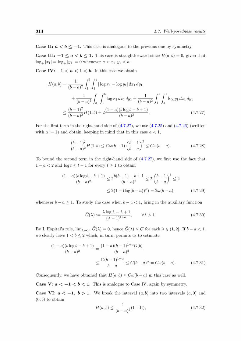
314 4.7. Well-posedness results
Case II: a < b ≤ −1. This case is analogous to the previous one by symmetry.
Case III: −1 ≤ a < b ≤ 1. This case is straightforward since H(a, b) = 0, given thatlog+ |x1| = log+ |y1| = 0 whenever a < x1, y1 < b.
Case IV: −1 < a < 1 < b. In this case we obtain
H(a, b) = 1(b− a)2
ˆ b
1
ˆ b
1| log x1 − log y1| dx1 dy1
+ 1(b− a)2
ˆ 1
a
ˆ b
1log x1 dx1 dy1 + 1
(b− a)2
ˆ b
1
ˆ 1
alog y1 dx1 dy1
≤ (b− 1)2
(b− a)2H(1, b) + 2(1− a)(b log b− b+ 1)(b− a)2 . (4.7.27)
For the first term in the right-hand side of (4.7.27), we use (4.7.25) and (4.7.26) (writtenwith a := 1) and obtain, keeping in mind that in this case a < 1,
(b− 1)2
(b− a)2H(1, b) ≤ Cω(b− 1)(b− 1b− a
)2≤ Cω(b− a). (4.7.28)
To bound the second term in the right-hand side of (4.7.27), we first use the fact that1− a < 2 and log t ≤ t− 1 for every t ≥ 1 to obtain
(1− a)(b log b− b+ 1)(b− a)2 ≤ 2b(b− 1)− b+ 1
(b− a)2 ≤ 2(b− 1b− a
)2≤ 2
≤ 2(1 + (log(b− a))β
)= 2ω(b− a), (4.7.29)
whenever b− a ≥ 1. To study the case when b− a < 1, bring in the auxiliary function
G(λ) := λ log λ− λ+ 1(λ− 1)1+α , ∀λ > 1. (4.7.30)
By L’Hôpital’s rule, limλ→1+ G(λ) = 0, hence G(λ) ≤ C for each λ ∈ (1, 2]. If b− a < 1,we clearly have 1 < b ≤ 2 which, in turn, permits us to estimate
(1− a)(b log b− b+ 1)(b− a)2 = (1− a)(b− 1)1+αG(b)
(b− a)2
≤ C(b− 1)1+α
b− a≤ C(b− a)α = Cω(b− a). (4.7.31)
Consequently, we have obtained that H(a, b) ≤ Cω(b− a) in this case as well.
Case V: a < −1 < b < 1. This is analogue to Case IV, again by symmetry.
Case VI: a < −1, b > 1. We break the interval (a, b) into two intervals (a, 0) and(0, b) to obtain
H(a, b) ≤ 1(b− a)2 (I + II), (4.7.32)
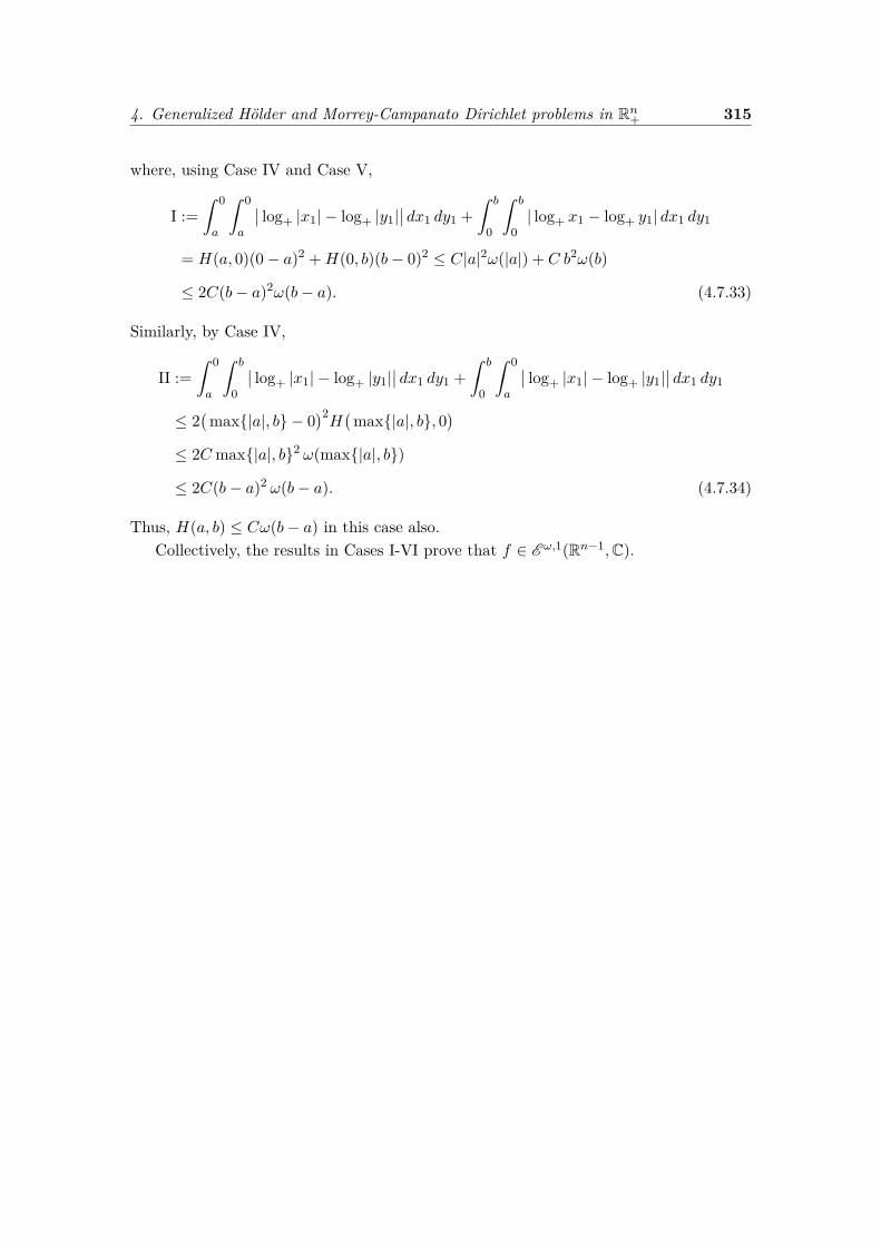
4. Generalized Hölder and Morrey-Campanato Dirichlet problems in Rn+ 315
where, using Case IV and Case V,
I :=ˆ 0
a
ˆ 0
a
∣∣ log+ |x1| − log+ |y1|∣∣ dx1 dy1 +
ˆ b
0
ˆ b
0| log+ x1 − log+ y1| dx1 dy1
= H(a, 0)(0− a)2 +H(0, b)(b− 0)2 ≤ C|a|2ω(|a|) + C b2ω(b)
≤ 2C(b− a)2ω(b− a). (4.7.33)
Similarly, by Case IV,
II :=ˆ 0
a
ˆ b
0
∣∣ log+ |x1| − log+ |y1|∣∣ dx1 dy1 +
ˆ b
0
ˆ 0
a
∣∣ log+ |x1| − log+ |y1|∣∣ dx1 dy1
≤ 2(
max|a|, b − 0)2H(
max|a|, b, 0)
≤ 2C max|a|, b2 ω(max|a|, b)
≤ 2C(b− a)2 ω(b− a). (4.7.34)
Thus, H(a, b) ≤ Cω(b− a) in this case also.Collectively, the results in Cases I-VI prove that f ∈ E ω,1(Rn−1,C).

316
CHAPTER 5
Characterizations of Lyapunov domains in terms of Riesztransforms and generalized Hölder spaces
We prove several characterizations of C 1,ω-domains (aka Lyapunov domains), where ωis a growth function satisfying natural assumptions. For example, given an Ahlforsregular domain Ω ⊆ Rn, we show that the modulus of continuity of the geometricmeasure theoretic outward unit normal ν to Ω is dominated by (a multiple of) ω ifand only if the action of each Riesz transform Rj associated with ∂Ω on the constantfunction 1 has a modulus of continuity dominated by (a multiple of) ω. We also establishestimates for certain classes of singular integral operators on generalized Hölder spaceon Lyapunov domains.
The material in this chapter is based on joint work with J.M. Martell and M. Mitrea(cf. [78]).
Contents
5.1 Introduction . . . . . . . . . . . . . . . . . . . . . . . . . . . . . . . . . . . 3175.2 More on growth functions . . . . . . . . . . . . . . . . . . . . . . . . . . . 3225.3 Singular integrals on generalized Hölder spaces . . . . . . . . . . . . . . 3255.4 Cauchy-Clifford operators on C ω(∂Ω)⊗ C n . . . . . . . . . . . . . . . . . 3315.5 Proof of Theorem 5.1.4 . . . . . . . . . . . . . . . . . . . . . . . . . . . . . 340
5.1 Introduction
The principal aim of this chapter is to characterize Lyapunov C 1,ω-domains in Rn, n ≥2. One way to think of such a domain Ω ⊆ Rn is as an open set of locally finite
318 5.1. Introduction
perimeter whose geometric measure theoretic outward unit normal ν, after possibly beingredefined on a set of σ-measure zero, belongs to C ω(∂Ω). Here, C ω(∂Ω) is a generalizedHölder space, quantifying continuity in terms of the modulus, or “growth” function, ω(cf. Definition 1.3.5), and σ := Hn−1b∂Ω is the “surface measure” on ∂Ω (with Hn−1
denoting the (n − 1)-dimensional Hausdorff measure in Rn). Thanks to work in [52],the above class of domains may be equivalently described as the collection of all opensubsets of Rn which locally coincide (up to a rigid transformation of the space) with theupper-graph of a real-valued continuously differentiable function defined in Rn−1 whosefirst-order partial derivatives belong to C ω(Rn−1).
Definition 5.1.1. Let ω be a growth function. A nonempty, proper, open subset Ω of Rn
is called a Lyapunov C 1,ω-domain (or simply a C 1,ω-domain) if there exist r, h > 0 suchthat for every point x0 ∈ ∂Ω there exists a coordinate system (x′, xn) ∈ Rn−1 ×R whichis isometric to the canonical one and has x0 as its origin, and a function ϕ ∈ C 1,ω(Rn−1)such that
Ω ∩ C(r, h) =x = (x′, xn) ∈ Rn−1 × R : |x′| < r, ϕ(x′) < xn < h
, (5.1.1)
where C(r, h) is the cylinder defined as
C(r, h) =x = (x′, xn) ∈ Rn−1 × R : |x′| < r, −h < xn < h
. (5.1.2)
Remark 5.1.2. Any C 1,ω-domain with compact boundary is, in particular, simultaneouslya UR domain and a uniform domain.
Remark 5.1.3. Analogously to the characterization of C 1 domains given in [52], one canprove that C 1,ω-domain are those open sets of locally finite perimeter with the propertythat the geometric measure theoretic outward unit normal ν to Ω, after possibly beingaltered on a set of σ-measure zero, belongs to C ω(∂Ω). See [52, Theorem 2.19] for theproof in the case ω(t) = tα for each t ∈ (0,∞) with α ∈ (0, 1), which is easily adapted toour scenario.
The characterizations of the class of Lyapunov domains we presently seek are in termsof the boundedness properties of certain classes of singular integral operators actingon generalized Hölder spaces. The most prominent examples of such singular integraloperators are offered by the Riesz transforms on the boundary of an Ahlfors regulardomain Ω ⊆ Rn with compact boundary (cf. Definition 1.1.2). Specifically, for eachj ∈ 1, . . . , n we define the j-th distributional Riesz transform on ∂Ω as the operator
Rj : C ω(∂Ω) −→(C ω(∂Ω)
)∗ satisfying, for every f, g ∈ C ω(∂Ω),
〈Rjf, g〉 = 12$n−1
ˆ∂Ω
ˆ∂Ω
xj − yj|x− y|n
(f(y)g(x)− f(x)g(y)
)dσ(y) dσ(x),
(5.1.3)
where $n−1 stands for the area of the unit sphere Sn−1 in Rn, and 〈·, ·〉 denotes thenatural duality pairing between
(C ω(∂Ω)
)∗ and C ω(∂Ω). From the T (1) theorem forspaces of homogeneous type (cf., e.g., [21]) we know that for each j ∈ 1, . . . , n the
5. Characterizations of Lyapunov domains 319
operator Rj extends to a bounded linear mapping on L2(∂Ω, σ) if and only if Rj1 belongsto BMO(∂Ω, σ), the John-Nirenberg space of functions with bounded mean oscillationon ∂Ω (with respect to the measure σ). Moreover, having Rj1 ∈ BMO(∂Ω, σ) is actuallyequivalent to ∂Ω being uniformly rectifiable (cf. [101]). Ultimately this goes to show thatthe aforementioned extension of Rj from (5.1.3) to a bounded mapping on L2(∂Ω, σ) isgiven by the principal-value integral operator acting on each f ∈ L2(∂Ω, σ) according to
(Rjf)(x) := limε→0+
1$n−1
ˆ
y∈∂Ω|x−y|>ε
xj − yj|x− y|n
f(y) dσ(y) for σ-a.e. x ∈ ∂Ω. (5.1.4)
In this chapter, we find it convenient to make two terminology changes with respect tothe previous chapters: the area of the unit sphere is denoted by $n−1 (in place of ωn−1),and the definition of the Riesz transform Rjf above differs from the Riesz transformdefined in Chapter 2 by a constant).
Our main result in this regard is the following theorem. For all relevant definitions,the reader is referred to Sections 1.1, 1.3, and 5.2.
Theorem 5.1.4. Suppose Ω ⊆ Rn is an Ahlfors regular domain whose boundary iscompact. Abbreviate σ := Hn−1b∂Ω and denote by ν the geometric measure theoreticoutward unit normal to Ω. Also, define Ω+ := Ω and Ω− := Rn \ Ω. Finally, letω :
(0, diam(∂Ω)
)→ (0,∞) be a bounded, non-decreasing function, whose limit at the
origin vanishes, and satisfying
sup0<t<diam(∂Ω)
1ω(t)
( ˆ t
0ω(s)ds
s+ t
ˆ diam(∂Ω)
t
ω(s)s
ds
s
)< +∞. (5.1.5)
Then the following statements are equivalent:
(a) After possibly being altered on a set of σ-measure zero, the outward unit normal ν toΩ belongs to the generalized Hölder space C ω(∂Ω) (i.e. the set Ω is a C 1,ω-domain;cf. Remark 5.1.3).
(b) The Riesz transforms on ∂Ω satisfy
Rj1 ∈ C ω(∂Ω) for each j ∈ 1, . . . , n. (5.1.6)
(c) The set Ω is a UR domain (in the sense of Definition 1.1.5), and given any oddhomogenous polynomial P of degree ` ≥ 1 in Rn the singular integral operator actingon each function f ∈ C ω(∂Ω) according to
(Tf)(x) :=ˆ
y∈∂Ω|x−y|>ε
P (x− y)|x− y|n−1+` f(y) dσ(y) for σ-a.e. x ∈ ∂Ω (5.1.7)
is well-defined and maps the generalized Hölder space C ω(∂Ω) boundedly into itself.

320 5.1. Introduction
(d) The set Ω is a UR domain, and the boundary-to-domain version of the Riesz trans-forms defined for each j ∈ 1, . . . , n and each f ∈ L1(∂Ω, σ) as
(R±j f
)(x) := 1
$n−1
ˆ∂Ω
xj − yj|x− y|n
f(y) dσ(y), ∀x ∈ Ω±, (5.1.8)
satisfyR±j 1 ∈ C ω(Ω±) for each j ∈ 1, . . . , n. (5.1.9)
(e) The set Ω is a UR domain, and given any odd homogenous polynomial P of degree` ≥ 1 in Rn, the integral operators acting on each function f ∈ C ω(∂Ω) accordingto
T±f(x) :=ˆ∂Ω
P (x− y)|x− y|n−1+` f(y) dσ(y), ∀x ∈ Ω±, (5.1.10)
map the generalized Hölder space C ω(∂Ω) continuously into C ω(Ω±).
In addition, if Ω is a C 1,ω-domain, there exists a constant C ∈ (0,∞), dependingonly on n, ω, and Ω, with the property that
‖T±f‖Cω(Ω±) ≤ C` 2`2‖P‖L2(Sn−1,Hn−1)‖f‖Cω(∂Ω), ∀ f ∈ C ω(∂Ω), (5.1.11)
and
‖Tf‖Cω(∂Ω) ≤ C` 2`2‖P‖L2(Sn−1,Hn−1)‖f‖Cω(∂Ω), ∀ f ∈ C ω(∂Ω). (5.1.12)
This generalizes earlier work in [96] where similar characterizations for domains ofclass C 1+α, with α ∈ (0, 1), have been obtained. The latter scenario presently correspondsto the particular choice ω(t) := tα for each t > 0 in Theorem 5.1.4. Our present workadds further credence to the heuristic principle that the action of the distributional Riesztransforms (5.1.3) on the constant function 1 encapsulates much information, both ofanalytic and geometric flavor, about the underlying Ahlfors regular domain Ω ⊆ Rn (withcompact boundary). At the most basic level, the main result of F. Nazarov, X. Tolsa,and A. Volberg in [101] states that
∂Ω is a UR set ⇐⇒ Rj1 ∈ BMO(∂Ω, σ) for each j ∈ 1, . . . , n, (5.1.13)
and it has been noted in [96] that
ν ∈ VMO(∂Ω, σ)
and ∂Ω is a UR set
⇐⇒ Rj1 ∈ VMO(∂Ω, σ) for all j ∈ 1, . . . , n, (5.1.14)
where VMO(∂Ω, σ) stands for the Sarason space of functions with vanishing mean oscil-lation on ∂Ω, with respect to the measure σ. By further assigning additional regularityfor the functionals Rj11≤j≤n yields the following result (proved in [96])
Ω is a domain
of class C 1+α
⇐⇒ Rj1 ∈ C α(∂Ω) for all j ∈ 1, . . . , n, (5.1.15)
5. Characterizations of Lyapunov domains 321
where α ∈ (0, 1) and C α(∂Ω) is the classical Hölder space of order α on ∂Ω.Theorem 5.1.4 provides a satisfactory generalization of (5.1.15) by allowing consid-
erably more flexible scales of spaces measuring Hölder regularity (see the discussion inExample 1.3.4 in this regard). To place this in perspective, observe that the opera-tors described in (5.1.7) may be thought of as generalized Riesz transforms since theycorrespond to (5.1.4) in the case when
P (x) := xj/$n−1 for x = (x1, . . . , xn) ∈ Rn, j ∈ 1, . . . , n. (5.1.16)
As such, our result may be interpreted as roughly saying that the classical Riesz trans-forms are bounded on a generalized Hölder space if and only if all generalized Riesztransforms are bounded on a generalized Hölder space if and only if the underlyingdomain is Lyapunov.
Due to their significant role in Partial Differential Equations, Lyapunov domainshave received a good deal of attention in the literature, and a number of alternativecharacterizations have been discovered. For example, Theorem 5.1.4 should be comparedwith the following purely geometric characterization of Lyapunov domains obtained in[5], which amounts to the ability of threading the boundary of the said domain in betweenthe two rounded components of an “hour-glass” shaped solid.
Proposition 5.1.5. Fix D ∈ (0,∞) and let ω : (0, D]→ [0,∞) be a continuous, strictlyincreasing function, with the property that
limλ→0+
(sup
t∈(0,minD,D/λ]
ω(λ t)ω(t)
)= 0. (5.1.17)
Define the pseudo-ball associated with ω having apex at a point x ∈ Rn, axis of symmetryalong some vector h ∈ Sn−1, height b > 0, and aperture a > 0, as the set
G ωa,b(x, h) :=
y ∈ B(x,D) \ x : a|y − x|ω(|y − x|) < h · (y − x) < b
. (5.1.18)
Then a nonempty, open, proper subset Ω of Rn, with compact boundary is a C 1,ω-domain if and only if there exist a > 0, b > 0 and a function h : ∂Ω → Sn−1 with theproperty that
G ωa,b(x, h(x)) ⊆ Ω and G ω
a,b(x,−h(x)) ⊆ Rn \ Ω for each x ∈ ∂Ω. (5.1.19)
In [5] this was used to prove a sharper version of the Hopf-Oleinik Boundary PointPrinciple in domains satisfying an “pseudo-ball condition” (in place of the classicalinterior ball condition).
The layout of the chapter is as follows. In Section 5.2 we study growth functionsand generalized Hölder spaces, extending the results in Section 1.3. We then proceedto study singular integrals on generalized Hölder spaces in Section 5.3. Following [96],our approach relies on Clifford algebra techniques. In Section 5.4 we prove some basicestimates for the Cauchy-Clifford operators acting on generalized Hölder spaces. Finally,Section 5.5 contains the proof of our main result, Theorem 5.1.4, which proceeds byinduction on the degree ` of the polynomial P involved in (5.1.7) and (5.1.10).
322 5.2. More on growth functions
5.2 More on growth functions
Given a growth function ω, in the lemma below we study some of the implications of(1.3.6) for the function ω associated with ω as in Remark 1.3.2.
Lemma 5.2.1. Suppose D ∈ (0,∞] and let ω be a growth function on (0, D) satisfying(1.3.6). If ω is associated with ω as in Remark 1.3.2, then the following statements aretrue.
(a) For each N ∈ [1,∞) one hasˆ t
0ω(s)ds
s≤ C1ω(t) for all t ∈ (0, ND), (5.2.1)
with C1 := Cω + lnN if D <∞ and C1 := Cω if D =∞.
(b) One has
t
ˆ ∞t
ω(s)s
ds
s≤ C2ω(t) for all t ∈ (0,∞), (5.2.2)
with C2 := Cω + max1, Cω ω(D)ω(D/2) if D <∞ and C2 := Cω if D =∞.
(c) As a consequence of Remark 1.3.2 and (a)-(b), one concludes that ω is growthfunction on (0,∞) which satisfies (1.3.6) with
Cω ≤ C1 + C2, (5.2.3)
where C1, C2 ∈ (0,∞) are as above.
(d) Whenever 0 < t1 ≤ t2 <∞ one has
ω(t2)t2≤ C2
ω(t1)t1
, (5.2.4)
with C2 as in part (b). In particular, ω is doubling with constant
sup0<t<∞
ω(2t)ω(t) ≤ 2C2. (5.2.5)
Proof. If D =∞, then the claims in (a) and (b) are direct consequences of (1.3.7), sinceω = ω on (0,∞) in this case. Henceforth assume D <∞. In such a scenario, if t ∈ (0, D)then the claim in (a) follows at once from (1.3.7) since ω = ω on (0, D). On the otherhand, if t ∈ [D,ND) for some N ∈ [1,∞), then
ˆ t
0ω(s)ds
s=ˆ D
0ω(s)ds
s+ˆ ND
Dω(D)ds
s≤ Cωω(D) + ω(D) lnN
= (Cω + lnN)ω(t), (5.2.6)
keeping in mind that, as noted earlier, (1.3.7) extends to t = D in this case.
5. Characterizations of Lyapunov domains 323
As regards item (b), we first claim that
t ≤ max1, CωDω(D/2) ω(t) for each t ∈ (0, D). (5.2.7)
Indeed, if t ∈ (0, D/2] we may estimate
tω(D/2)D
≤ tˆ D
D/2
ω(s)s
ds
s≤ t
ˆ D
t
ω(s)s
ds
s≤ Cωω(t), (5.2.8)
which suits our purposes. If t ∈ (D/2, D), the fact hat ω is a non-decreasing functionentails ω(D/2)/D ≤ ω(t)/t, finishing the proof of (5.2.7). In turn, on account of (5.2.7)we see that for each t ∈ (0, D) we have
t
ˆ ∞t
ω(s)s
ds
s= t
ˆ D
t
ω(s)s
ds
s+ t
ˆ ∞D
ω(D)s
ds
s≤ Cωω(t) + t
ω(D)D
≤(Cω + max1, Cω
ω(D)ω(D/2)
)ω(t). (5.2.9)
To finish the proof of (5.2.2) there remains to observe that, if t ≥ D,
t
ˆ ∞t
ω(s)s
ds
s= ω(D) = ω(t). (5.2.10)
Next, the claims in item (c) are direct consequences of Remark 1.3.2 and parts (a)-(b).Turning our attention to item (d), if 0 < t1 ≤ t2 <∞ then (5.2.2) implies
ω(t2)t2≤ˆ ∞t2
ω(s)s
ds
s≤ˆ ∞t1
ω(s)s
ds
s≤ C2
ω(t1)t1
, (5.2.11)
and the assertion in (5.2.5) follows by specializing this to the case when t1 := t andt2 := 2t.
In the classical case when, for some α ∈ (0, 1), the growth function is defined asω(t) := tα for each t ∈ (0,∞), the function V (t) := tα−1 for each t ∈ (0,∞) plays asignificant role in ensuing analysis. Below we identify the general format of the latterfunction associated with general growth functions.
Lemma 5.2.2. Given D ∈ (0,∞], let ω be a growth function on (0, D) and recall thefunction ω from Remark 1.3.2, defined as ω(t) := ω(mint,D) for each t ∈ (0,∞). Set
V (t) :=ˆ ∞t
ω(s)s
ds
sfor each t ∈ (0,∞). (5.2.12)
Then V : (0,∞)→ (0,∞] is a non-increasing function which satisfies
ω(t)t≤ V (t) for each t ∈ (0,∞). (5.2.13)
Moreover, if D <∞ then V takes only finite values.
324 5.2. More on growth functions
Proof. By design, V is a non-increasing function. Bearing in mind that ω is non-decreasing, for every t ∈ (0,∞) we may write
ω(t)t
=ˆ ∞t
ω(t)s
ds
s≤ˆ ∞t
ω(s)s
ds
s= V (t), (5.2.14)
proving (5.2.13). Also, when D ∈ (0,∞), for each t ∈ (0, D) we have
V (t) =ˆ ∞D
ω(s)s
ds
s+ˆ D
t
ω(s)s
ds
s= ω(D)
D+ˆ D
t
ω(s)s
ds
s
≤ ω(D)D
+ ω(D)(1t− 1D
). (5.2.15)
As V (t) is non-increasing, this proves that V only takes finite values.
We close this section by proving some useful integral estimates on upper Ahlforsregular sets involving growth functions. Here and elsewhere, for each number a ∈ Rwe agree to abbreviate (a)+ := maxa, 0.
Lemma 5.2.3. Suppose Σ is closed subset of Rn satisfying an upper Ahlfors regularitycondition with constant C ∈ (0,∞). Define σ := Hn−1bΣ. Also, assume ω is a growthfunction on (0,∞). Then for each x ∈ Σ, r ∈
(0 , diam(Σ)
), and d ∈ R one has
ˆΣ∩B(x,r)
ω(|x− y|)|x− y|n−1+d dσ(y) ≤ C 2n−1+d · 2d+ · 2(1−n−d)+
ln 2
ˆ 2 r
0
ω(s)sd
ds
s, (5.2.16)
ˆΣ\B(x,r)
ω(|x− y|)|x− y|n−1+d dσ(y) ≤ C 2n−1+d · 2d+ · 2(1−n−d)+
ln 2
ˆ 4 diam(Σ)
2 r
ω(s)sd
ds
s. (5.2.17)
Proof. Fix x ∈ Σ and r ∈(0 , diam(Σ)
)then abbreviate B := B(x, r). Using the fact
that ω is non-decreasing and the upper Ahlfors regularity of Σ we may estimateˆ
Σ∩B
ω(|x− y|)|x− y|n−1+d dσ(y) =
∞∑k=0
ˆΣ∩(2−kB\2−k−1B)
ω(|x− y|)|x− y|n−1+d dσ(y)
≤∞∑k=0
2(1−n−d)+ ω(2−kr)(2−k−1 r)n−1+d σ(Σ ∩ 2−kB)
≤ C 2n−1+d · 2(d)+ · 2(1−n−d)+
ln 2
∞∑k=0
ˆ 2−k+1 r
2−k r
ω(s)sd
ds
s
= C2n−1+d · 2d+ · 2(1−n−d)+
ln 2
ˆ 2 r
0
ω(s)sd
ds
s, (5.2.18)
proving (5.2.16).Let us now turn to (5.2.17). We may assume that Σ \ B 6= ∅, otherwise there is
nothing to prove. Set N := [log2 (diam(Σ)/r)] ∈ N0 ∪ ∞, so that ∂Ω \ 2kB = ∅
5. Characterizations of Lyapunov domains 325
for every integer k > N . Then, using that ω is non-decreasing and the upper Ahlforsregularity of Σ we may write
ˆΣ\B
ω(|x− y|)|x− y|n−1+d dσ(y) ≤
N∑k=0
ˆΣ∩(2k+1B\2kB)
ω(|x− y|)|x− y|n−1+d dσ(y)
≤N∑k=0
2(1−n−d)+ ω(2k+1 r)(2k r)n−1+d σ(Σ ∩ 2k+1B)
≤ C 2n−1+d · 2(d)+ · 2(1−n−d)+
ln 2
N∑k=0
ˆ 2k+2 r
2k+1 r
ω(s)sd
ds
s
≤ C 2n−1+d · 2(d)+ · 2(1−n−d)+
ln 2
ˆ 4 diam(Σ)
2 r
ω(s)sd
ds
s, (5.2.19)
proving (5.2.17).
5.3 Singular integrals on generalized Hölder spaces
We first recall a basic result pertaining to the behavior of singular integral operators onUR sets, which is a direct consequence of Proposition 2.3.3 with w ≡ 1 (except for theformula in (5.3.3), which is proved in [93]).
Theorem 5.3.1. Suppose Ω ⊆ Rn is an open set such that ∂Ω is a UR set. Abbreviateσ := Hn−1b∂Ω and denote by ν the geometric measure theoretic outward unit normal to Ω.Also, assume N = N(n) ∈ N is a sufficiently large integer and consider a complex-valuedfunction k ∈ CN
(Rn\0
)which is odd and positive homogeneous of degree 1−n. Finally,
fix an aperture parameter κ > 0. In this setting, for each function f ∈ L1(∂Ω, σ(x)1+|x|n−1
)define
T f(x) :=ˆ∂Ωk(x− y)f(y) dσ(y) for each x ∈ Ω, (5.3.1)
Tf(x) := limε→0+
ˆ
y∈∂Ω|x−y|>ε
k(x− y)f(y) dσ(y) for σ-a.e. x ∈ ∂Ω. (5.3.2)
Then for each f ∈ L1(∂Ω, σ(x)1+|x|n−1
)the limit in (5.3.2) exists σ-a.e. and one has the
jump-formula(T f)
∣∣κ−n.t.
∂Ω (x) = 12i k(ν(x))f(x) + Tf(x), (5.3.3)
for σ-a.e. x ∈ ∂∗Ω, where k denotes the Fourier transform of k in Rn and i :=√−1 ∈ C.
Also, for each integrability exponent p ∈ (1,∞) there exists a finite constant C > 0such that for each function f ∈ Lp(∂Ω, σ) one has
‖Nκ(T f)‖Lp(∂Ω,σ) ≤ C ‖f‖Lp(∂Ω,σ) , (5.3.4)
‖Tf‖Lp(∂Ω,σ) ≤ C ‖f‖Lp(∂Ω,σ) . (5.3.5)
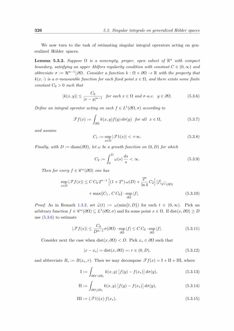
326 5.3. Singular integrals on generalized Hölder spaces
We now turn to the task of estimating singular integral operators acting on gen-eralized Hölder spaces.
Lemma 5.3.2. Suppose Ω is a nonempty, proper, open subset of Rn with compactboundary, satisfying an upper Ahlfors regularity condition with constant C ∈ (0,∞) andabbreviate σ := Hn−1b∂Ω. Consider a function k : Ω × ∂Ω → R with the property thatk(x, ·) is a σ-measurable function for each fixed point x ∈ Ω, and there exists some finiteconstant C0 > 0 such that
|k(x, y)| ≤ C0|x− y|n−1 for each x ∈ Ω and σ-a.e. y ∈ ∂Ω. (5.3.6)
Define an integral operator acting on each f ∈ L1(∂Ω, σ) according to
T f(x) :=ˆ∂Ωk(x, y)f(y) dσ(y) for all x ∈ Ω, (5.3.7)
and assumeC1 := sup
x∈Ω|T 1(x)| < +∞. (5.3.8)
Finally, with D := diam(∂Ω), let ω be a growth function on (0, D) for which
C2 :=ˆ D
0ω(s) ds
s<∞. (5.3.9)
Then for every f ∈ C ω(∂Ω) one has
supx∈Ω|T f(x)| ≤ C C0 2n−1
[(1 + 2n)ω(D) + 2n
ln 4 C2]
[f ]C ω(∂Ω)
+ maxC1 , C C0 · sup∂Ω|f |. (5.3.10)
Proof. As in Remark 1.3.2, set ω(t) := ω(mint,D) for each t ∈ (0,∞). Pick anarbitrary function f ∈ C ω(∂Ω) ⊆ L1(∂Ω, σ) and fix some point x ∈ Ω. If dist(x, ∂Ω) ≥ Duse (5.3.6) to estimate
|T f(x)| ≤ C0Dn−1σ(∂Ω) · sup
∂Ω|f | ≤ C C0 · sup
∂Ω|f |. (5.3.11)
Consider next the case when dist(x, ∂Ω) < D. Pick x∗ ∈ ∂Ω such that
|x− x∗| = dist(x, ∂Ω) =: r ∈ (0, D), (5.3.12)
and abbreviate B∗ := B(x∗, r). Then we may decompose T f(x) = I + II + III, where
I :=ˆ∂Ω∩ 2B∗
k(x, y)[f(y)− f(x∗)
]dσ(y), (5.3.13)
II :=ˆ∂Ω\2B∗
k(x, y)[f(y)− f(x∗)
]dσ(y), (5.3.14)
III := (T 1)(x) f(x∗). (5.3.15)
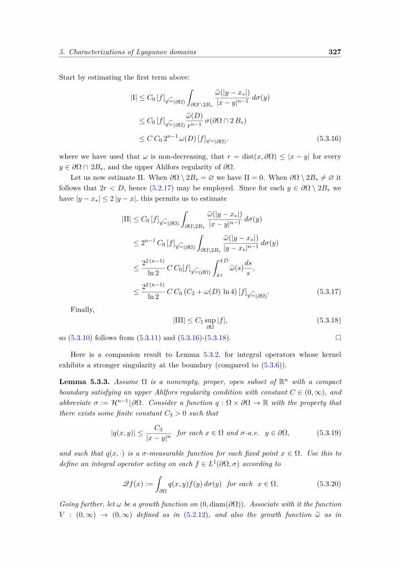
5. Characterizations of Lyapunov domains 327
Start by estimating the first term above:
|I| ≤ C0 [f ]C ω(∂Ω)
ˆ∂Ω∩ 2B∗
ω(|y − x∗|)|x− y|n−1 dσ(y)
≤ C0 [f ]C ω(∂Ω)
ω(D)rn−1 σ(∂Ω ∩ 2B∗)
≤ C C0 2n−1 ω(D) [f ]Cω(∂Ω). (5.3.16)
where we have used that ω is non-decreasing, that r = dist(x, ∂Ω) ≤ |x − y| for everyy ∈ ∂Ω ∩ 2B∗, and the upper Ahlfors regularity of ∂Ω.
Let us now estimate II. When ∂Ω \ 2B∗ = ∅ we have II = 0. When ∂Ω \ 2B∗ 6= ∅ itfollows that 2r < D, hence (5.2.17) may be employed. Since for each y ∈ ∂Ω \ 2B∗ wehave |y − x∗| ≤ 2 |y − x|, this permits us to estimate
|II| ≤ C0 [f ]C ω(∂Ω)
ˆ∂Ω\2B∗
ω(|y − x∗|)|x− y|n−1 dσ(y)
≤ 2n−1C0 [f ]C ω(∂Ω)
ˆ∂Ω\2B∗
ω(|y − x∗|)|y − x∗|n−1 dσ(y)
≤ 22 (n−1)
ln 2 C C0[f ]C ω(∂Ω)
ˆ 4D
4 rω(s)ds
s,
≤ 22 (n−1)
ln 2 C C0(C2 + ω(D) ln 4
)[f ]
C ω(∂Ω). (5.3.17)
Finally,|III| ≤ C1 sup
∂Ω|f |, (5.3.18)
so (5.3.10) follows from (5.3.11) and (5.3.16)-(5.3.18).
Here is a companion result to Lemma 5.3.2, for integral operators whose kernelexhibits a stronger singularity at the boundary (compared to (5.3.6)).
Lemma 5.3.3. Assume Ω is a nonempty, proper, open subset of Rn with a compactboundary satisfying an upper Ahlfors regularity condition with constant C ∈ (0,∞), andabbreviate σ := Hn−1b∂Ω. Consider a function q : Ω × ∂Ω → R with the property thatthere exists some finite constant C3 > 0 such that
|q(x, y)| ≤ C3|x− y|n
for each x ∈ Ω and σ-a.e. y ∈ ∂Ω, (5.3.19)
and such that q(x, ·) is a σ-measurable function for each fixed point x ∈ Ω. Use this todefine an integral operator acting on each f ∈ L1(∂Ω, σ) according to
Qf(x) :=ˆ∂Ωq(x, y)f(y) dσ(y) for each x ∈ Ω. (5.3.20)
Going further, let ω be a growth function on (0,diam(∂Ω)). Associate with it the functionV : (0,∞) → (0,∞) defined as in (5.2.12), and also the growth function ω as in
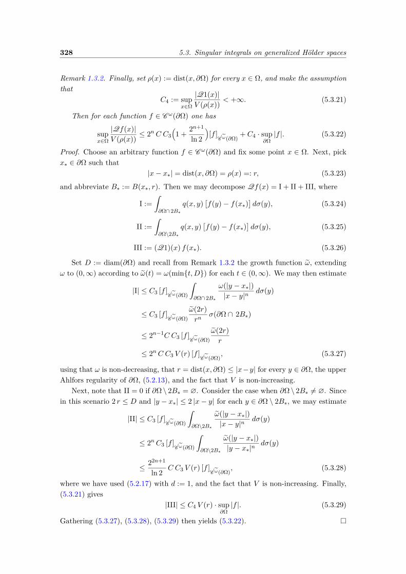
328 5.3. Singular integrals on generalized Hölder spaces
Remark 1.3.2. Finally, set ρ(x) := dist(x, ∂Ω) for every x ∈ Ω, and make the assumptionthat
C4 := supx∈Ω
|Q1(x)|V (ρ(x)) < +∞. (5.3.21)
Then for each function f ∈ C ω(∂Ω) one has
supx∈Ω
|Qf(x)|V (ρ(x)) ≤ 2nC C3
(1 + 2n+1
ln 2)[f ]
C ω(∂Ω)+ C4 · sup
∂Ω|f |. (5.3.22)
Proof. Choose an arbitrary function f ∈ C ω(∂Ω) and fix some point x ∈ Ω. Next, pickx∗ ∈ ∂Ω such that
|x− x∗| = dist(x, ∂Ω) = ρ(x) =: r, (5.3.23)
and abbreviate B∗ := B(x∗, r). Then we may decompose Qf(x) = I + II + III, where
I :=ˆ∂Ω∩ 2B∗
q(x, y)[f(y)− f(x∗)
]dσ(y), (5.3.24)
II :=ˆ∂Ω\2B∗
q(x, y)[f(y)− f(x∗)
]dσ(y), (5.3.25)
III := (Q1)(x) f(x∗). (5.3.26)
Set D := diam(∂Ω) and recall from Remark 1.3.2 the growth function ω, extendingω to (0,∞) according to ω(t) = ω(mint,D) for each t ∈ (0,∞). We may then estimate
|I| ≤ C3 [f ]C ω(∂Ω)
ˆ∂Ω∩ 2B∗
ω(|y − x∗|)|x− y|n
dσ(y)
≤ C3 [f ]C ω(∂Ω)
ω(2r)rn
σ(∂Ω ∩ 2B∗)
≤ 2n−1C C3 [f ]C ω(∂Ω)
ω(2r)r
≤ 2nC C3 V (r) [f ]C ω(∂Ω)
, (5.3.27)
using that ω is non-decreasing, that r = dist(x, ∂Ω) ≤ |x−y| for every y ∈ ∂Ω, the upperAhlfors regularity of ∂Ω, (5.2.13), and the fact that V is non-increasing.
Next, note that II = 0 if ∂Ω \ 2B∗ = ∅. Consider the case when ∂Ω \ 2B∗ 6= ∅. Sincein this scenario 2 r ≤ D and |y − x∗| ≤ 2 |x− y| for each y ∈ ∂Ω \ 2B∗, we may estimate
|II| ≤ C3 [f ]C ω(∂Ω)
ˆ∂Ω\2B∗
ω(|y − x∗|)|x− y|n
dσ(y)
≤ 2nC3 [f ]C ω(∂Ω)
ˆ∂Ω\2B∗
ω(|y − x∗|)|y − x∗|n
dσ(y)
≤ 22n+1
ln 2 C C3 V (r) [f ]C ω(∂Ω)
, (5.3.28)
where we have used (5.2.17) with d := 1, and the fact that V is non-increasing. Finally,(5.3.21) gives
|III| ≤ C4 V (r) · sup∂Ω|f |. (5.3.29)
Gathering (5.3.27), (5.3.28), (5.3.29) then yields (5.3.22).

5. Characterizations of Lyapunov domains 329
From Lemmas 5.3.2-5.3.3 we then immediately derive the following result.
Lemma 5.3.4. Let Ω be a nonempty, proper, open subset of Rn with a compact boundarysatisfying an upper Ahlfors regularity condition with constant C ∈ (0,∞), and abbreviateσ := Hn−1b∂Ω. Consider function K : Ω× ∂Ω→ R, which is continuously differentiablein the first argument, with the property that there exists some finite constant A0 > 0 suchthat
|K(x, y)|+ |x− y| |∇xK(x, y)| ≤ A0|x− y|1−n
for each x ∈ Ω and σ-a.e. y ∈ ∂Ω,(5.3.30)
and such that K(x, ·) is a σ-measurable function for each fixed point x ∈ Ω. Define anintegral operator acting on each function f ∈ L1(∂Ω, σ) according to
T f(x) :=ˆ∂ΩK(x, y)f(y) dσ(y) for each x ∈ Ω. (5.3.31)
With D := diam(∂Ω), let ω be a growth function on (0, D). Bring in the function V
associated with ω as in (5.2.12), and the growth function ω associated with ω as inRemark 1.3.2. In relation to these, assume
A1 :=ˆ D
0ω(s) ds
s< +∞, (5.3.32)
and, if ρ(x) := dist(x, ∂Ω) for each x ∈ Ω,
A2 := supx∈Ω|(T 1)(x)|+ sup
x∈Ω
|∇(T 1)(x)|V (ρ(x)) < +∞. (5.3.33)
Then for every f ∈ C ω(∂Ω) one has
supx∈Ω|(T f)(x)|+ sup
x∈Ω
|∇(T f)(x)|V (ρ(x))
≤ C A0 2n−1[(1 + 2n)ω(D) + 2n
ln 4 A1 + 2 + 2n+2
ln 2]
[f ]C ω(∂Ω)
+(2A2 + C A0
)sup∂Ω|f |. (5.3.34)
As a consequence, there exists a finite constant CΩ,n,ω > 0 with the property that foreach function f ∈ C ω(∂Ω) one has
supx∈Ω|(T f)(x)|+ sup
x∈Ω
|∇(T f)(x)|V (ρ(x)) ≤ CΩ,n,ω
(A0 (1 +A1) +A2
)‖f‖Cω(∂Ω). (5.3.35)
We conclude this section by estimating the generalized Hölder norm of a C 1 functiondefined in a uniform domain (cf. Definition 1.1.9).
Lemma 5.3.5. Let Ω ⊆ Rn be a uniform domain. Recall the constant κ ∈ [1,∞) ap-pearing in (1.1.25) and abbreviate D := diam(∂Ω) ∈ (0,∞]. Also, set ρ(x) := dist(x, ∂Ω)for each x ∈ Ω. In addition, consider a growth function ω on (0, D) satisfying (1.3.6)and associate with it the function V as in (5.2.12).
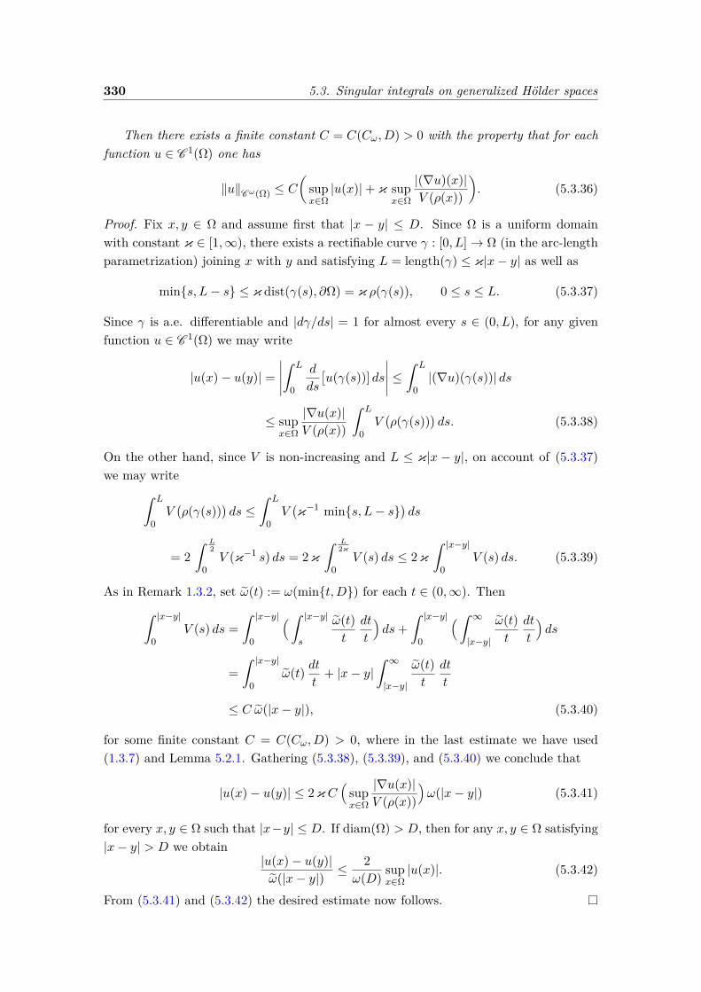
330 5.3. Singular integrals on generalized Hölder spaces
Then there exists a finite constant C = C(Cω, D) > 0 with the property that for eachfunction u ∈ C 1(Ω) one has
‖u‖Cω(Ω) ≤ C(
supx∈Ω|u(x)|+ κ sup
x∈Ω
|(∇u)(x)|V (ρ(x))
). (5.3.36)
Proof. Fix x, y ∈ Ω and assume first that |x − y| ≤ D. Since Ω is a uniform domainwith constant κ ∈ [1,∞), there exists a rectifiable curve γ : [0, L]→ Ω (in the arc-lengthparametrization) joining x with y and satisfying L = length(γ) ≤ κ|x− y| as well as
mins, L− s ≤ κ dist(γ(s), ∂Ω) = κ ρ(γ(s)), 0 ≤ s ≤ L. (5.3.37)
Since γ is a.e. differentiable and |dγ/ds| = 1 for almost every s ∈ (0, L), for any givenfunction u ∈ C 1(Ω) we may write
|u(x)− u(y)| =∣∣∣∣∣ˆ L
0
d
ds
[u(γ(s))] ds
∣∣∣∣∣ ≤ˆ L
0|(∇u)(γ(s))| ds
≤ supx∈Ω
|∇u(x)|V (ρ(x))
ˆ L
0V(ρ(γ(s))
)ds. (5.3.38)
On the other hand, since V is non-increasing and L ≤ κ|x − y|, on account of (5.3.37)we may write
ˆ L
0V(ρ(γ(s))
)ds ≤
ˆ L
0V(κ−1 mins, L− s
)ds
= 2ˆ L
2
0V (κ−1 s) ds = 2κ
ˆ L2κ
0V (s) ds ≤ 2κ
ˆ |x−y|0
V (s) ds. (5.3.39)
As in Remark 1.3.2, set ω(t) := ω(mint,D) for each t ∈ (0,∞). Thenˆ |x−y|
0V (s) ds =
ˆ |x−y|0
( ˆ |x−y|s
ω(t)t
dt
t
)ds+
ˆ |x−y|0
(ˆ ∞|x−y|
ω(t)t
dt
t
)ds
=ˆ |x−y|
0ω(t) dt
t+ |x− y|
ˆ ∞|x−y|
ω(t)t
dt
t
≤ C ω(|x− y|), (5.3.40)
for some finite constant C = C(Cω, D) > 0, where in the last estimate we have used(1.3.7) and Lemma 5.2.1. Gathering (5.3.38), (5.3.39), and (5.3.40) we conclude that
|u(x)− u(y)| ≤ 2κC(
supx∈Ω
|∇u(x)|V (ρ(x))
)ω(|x− y|) (5.3.41)
for every x, y ∈ Ω such that |x−y| ≤ D. If diam(Ω) > D, then for any x, y ∈ Ω satisfying|x− y| > D we obtain
|u(x)− u(y)|ω(|x− y|) ≤ 2
ω(D) supx∈Ω|u(x)|. (5.3.42)
From (5.3.41) and (5.3.42) the desired estimate now follows.
5. Characterizations of Lyapunov domains 331
5.4 Cauchy-Clifford operators on C ω(∂Ω) ⊗ C n
The last part of our auxiliary results deals with Clifford algebras and the properties ofCauchy-Clifford operators. This complements the preliminary results and terminologyintroduced in Section 1.4. We recall the definition of the Dirac operator D :=
∑nj=1 ej∂j .
Given an open set Ω ⊆ Rn, we shall denote by DL and DR the action of D on functionsu ∈ C 1(Ω) ⊗ C n from the left and from the right, respectively. More precisely, if uis written as in (1.4.4) then
DLu :=n∑`=0
∑′
|I|=`
n∑j=1
∂uI∂xj
ej eI , DRu :=n∑`=0
∑′
|I|=`
n∑j=1
∂uI∂xj
eI ej . (5.4.1)
If Ω ⊆ Rn is an Ahlfors regular domain, σ := Hn−1b∂Ω, and ν = (ν1, . . . , νn) is thegeometric measure theoretic outward unit normal to Ω, we agree to identify the lattervector field with the Clifford algebra valued function defined at σ-a.e. point x ∈ ∂Ω asν(x) = ν1(x)e1 + · · ·+νn(x)en ∈ C n. In this context, for any u, v ∈ C 1
0 (Rn)⊗C n formula(1.1.12) implies the following integration by parts holds:ˆ∂Ωu(x) ν(x) v(x) dσ(x) =
ˆΩ
((DRu)(x) v(x) + u(x) (DLv)(x)
)dx. (5.4.2)
The following lemma is proved in [96, Lemma 4.2]. To state it, we set
[x]s := xs for each x = (x1, . . . , xn) ∈ Rn and s ∈ 1, . . . , n. (5.4.3)
Lemma 5.4.1. Fix n ≥ 2 and consider an odd, harmonic, homogeneous polynomial P (x),with x ∈ Rn, of degree ` ≥ 3. Associate with it the family Prs(x) with r, s ∈ 1, . . . , n ofharmonic homogeneous polynomials of degree `− 2 given by the formula
Prs(x) := 1`(`− 1)(∂r∂sP )(x), x ∈ Rn. (5.4.4)
Then there exists a family of odd, C∞ functions
krs : Rn \ 0 → Rn → C n, r, s ∈ 1, . . . , n, (5.4.5)
which are homogeneous of degree 1 − n, such that for each r, s ∈ 1, . . . , n and eachx ∈ R \ 0 one has
P (x)|x|n−1+` =
n∑r,s=1
[krs(x)
]s
(cf. (5.4.3)), (5.4.6)
(DRkrs)(x) = `− 1n+ `− 3
∂
∂xr
(Prs(x)|x|n+`−3
). (5.4.7)
Moreover, there exists a finite dimensional constant cn > 0 such that
max1≤r,s≤n
supSn−1
|krs|+ max1≤r,s≤n
supSn−1
|∇krs| ≤ cn2` ‖P‖L1(Sn−1,Hn−1) . (5.4.8)
332 5.4. Cauchy-Clifford operators on C ω(∂Ω)⊗ C n
Remark 5.4.2. Let P be an odd, harmonic homogeneous polynomial of degree ` ≥ 1.Then for each multi-index γ ∈ Nn0 there exists a finite constant cn,γ > 0 such that
‖∂γP‖L∞(Sn−1,Hn−1) ≤ cn,γˆB(0,2)
|P (x)| dx
= cn,γ
ˆSn−1
|P (υ)|(ˆ 2
0rn−1+` dr
)dHn−1(υ)
= cn,γ2`
n+ `‖P‖L1(Sn−1,Hn−1) , (5.4.9)
where we have used interior estimates for the harmonic function P and its homogeneityof degree `.
We continue to assume that Ω ⊆ Rn is an Ahlfors regular domain, and abbreviateσ := Hn−1b∂Ω. As before, we identify the geometric measure theoretic outward unitnormal ν = (ν1, . . . , νn) to Ω with the Clifford algebra valued function defined at σ-a.e. point x ∈ ∂Ω as ν(x) = ν1(x)e1 + · · · + νn(x)en ∈ C n. With $n−1 denotingthe surface area of the unit sphere in Rn, define the action of the boundary-to-domainCauchy-Clifford operator on any function f ∈ L1(∂Ω, σ(x)
1+|x|n−1)⊗ C n as
(Cf)(x) := 1$n−1
ˆ∂Ω
x− y|x− y|n
ν(y) f(y) dσ(y) for each x ∈ Ω. (5.4.10)
There is a remarkable Cauchy Reproducing Formula involving the above integral op-erator. Specifically, with Ω as above, if the function u ∈ C∞(Ω) ⊗ C n satisfies (forsome fixed aperture parameter κ > 0)
Du = 0 in Ω, Nκu ∈ L1(∂Ω, σ(x)1+|x|n−1
), and
u∣∣κ−n.t.
∂Ω exists at σ-a.e. point on ∂Ω,(5.4.11)
then (cf. [93])
u = C(u∣∣κ−n.t.
∂Ω)
in Ω. (5.4.12)
Before proving boundedness properties for the Cauchy-Clifford integral operator in-troduced above, we need two lemmas. Their proofs may be found in [96, Lemmas 2.5, 5.2,and 5.3].
Lemma 5.4.3. Let Ω ⊆ Rn be an Ahlfors regular domain whose boundary is compact.Abbreviate σ := Hn−1b∂Ω and denote by ν the geometric measure theoretic outward unitnormal to Ω. Also, fix an aperture parameter κ > 0. Then for each x ∈ ∂∗Ω there existsa Lebesgue measurable set Ox ⊆ (0, 1) satisfying
limε→0+
L1(Ox ∩ (0, ε))ε
= 1, (5.4.13)
5. Characterizations of Lyapunov domains 333
with the property that
limOx3ε→0+
limΓκ(x)3z→x
1$n−1
ˆ
y∈∂Ω|x−y|<ε
z − y|z − y|n
ν(y) dσ(y)
= limOx3ε→0+
Hn−1(∂B(x, ε) \ Ω)$n−1εn−1 = 1
2 . (5.4.14)
Here is the second lemma from [96] alluded to above.
Lemma 5.4.4. Let Ω ⊆ Rn be a set of locally finite perimeter whose boundary is compactand upper Ahlfors regular. Abbreviate σ := Hn−1b∂Ω and denote by ν the geometricmeasure theoretic outward unit normal to Ω. Then there exists some finite constantC∂Ω,n > 0, depending only on the dimension n and the upper Ahlfors regularity constantof ∂Ω, such that ∣∣∣∣∣
ˆ∂∗Ω\B(x,r)
x− y|x− y|n
ν(y) dσ(y)∣∣∣∣∣ ≤ C∂Ω,n (5.4.15)
for every x ∈ Rn and r > 0. Moreover, if Ω is bounded,ˆ∂∗Ω\B(x,r)
x− y|x− y|n
ν(y) dσ(y) = Hn−1(Ω ∩ ∂B(x, r))
rn−1 (5.4.16)
for every x ∈ Rn and L1-a.e. r > 0.As a consequence, if Ω ⊆ Rn is an Ahlfors regular domain whose boundary is compact,
then for each x ∈ Rn one has
C1(x) =
1 if Ω is bounded,
0 if Ω is unbounded.(5.4.17)
At this point, we have enough foundation material to conclude the following result.
Proposition 5.4.5. Let Ω ⊆ Rn be an Ahlfors regular domain whose boundary iscompact. Suppose ω is a growth function on (0,diam(∂Ω)) satisfying (1.3.6), and foreach x ∈ Ω set ρ(x) := dist(x, ∂Ω). Then there exists some finite constant CΩ,n,ω > 0with the property that
supx∈Ω|(Cf)(x)|+ sup
x∈Ω
|∇(Cf)(x)|V (ρ(x)) ≤ CΩ,n,ω ‖f‖Cω(∂Ω) (5.4.18)
for each function f ∈ C ω(∂Ω).
Proof. It is a consequence of Lemma 5.3.4, whose applicability is ensured by (5.4.17) and(1.3.6).
Proposition 5.4.6. Suppose Ω ⊆ Rn is simultaneously a uniform domain and an Ahlforsregular domain with compact boundary. Let ω be a growth function on (0,diam(∂Ω))satisfying (1.3.6). Then the boundary-to-domain Cauchy-Clifford operator defined in(5.4.10) is well-defined, and bounded in the context
C : C ω(∂Ω)⊗ C n −→ C ω(Ω)⊗ C n, (5.4.19)
with operator norm controlled in terms of n, ω, and Ω.

334 5.4. Cauchy-Clifford operators on C ω(∂Ω)⊗ C n
Proof. For each x ∈ Ω set ρ(x) := dist(x, ∂Ω). Also, recall the constant κ ∈ [1,∞) asso-ciated with the uniform domain Ω as in (1.1.25). Then from (5.4.18) and Lemma 5.3.5,whose applicability is ensured by (1.3.6), we obtain
‖Cf‖Cω(Ω)⊗C n ≤ C(
supx∈Ω|Cf(x)|+ κ sup
x∈Ω
|∇(Cf)(x)|V (ρ(x))
)≤ CΩ,n,ω ‖f‖Cω(∂Ω)⊗C n , (5.4.20)
and the desired result follows on account of Lemma 1.3.6.
The following result can be found in [96, Proposition 5.1]
Proposition 5.4.7. Let Ω ⊆ Rn be a UR domain. Abbreviate σ := Hn−1b∂Ω and denoteby ν the geometric measure theoretic outward unit normal to Ω. Also, fix an apertureparameter κ > 0. Then for each function f ∈ L1(∂Ω, σ(x)
1+|x|n−1)⊗ C n the limit
Cf(x) := limε→0+
1$n−1
ˆ
y∈∂Ω|x−y|>ε
x− y|x− y|n
ν(y) f(y) dσ(y) (5.4.21)
exists exists at σ-a.e. point x ∈ ∂Ω and, with I denoting the identity operator, thefollowing jump-formula holds(
Cf∣∣κ−n.t.
∂Ω
)(x) =
(12I + C
)f(x) for σ-a.e. x ∈ ∂Ω. (5.4.22)
Moreover, for each p ∈ (1,∞) there exists a finite constant C > 0 such that
‖Nκ(Cf)‖Lp(∂Ω,σ) ≤ C ‖f‖Lp(∂Ω,σ)⊗C n
for each f ∈ Lp(∂Ω, σ)⊗ C n,(5.4.23)
the operator C is well-defined and bounded on Lp(∂Ω, σ)⊗ C n, and
C2 = 14 I on Lp(∂Ω, σ)⊗ C n. (5.4.24)
We next arrive at a central result in this section, regarding the action of the Cauchy-Clifford operator on generalized Hölder spaces in Ahlfors regular domains with compactboundaries.
Theorem 5.4.8. Let Ω ⊆ Rn be an Ahlfors regular domain whose boundary is compact.Set σ := Hn−1b∂Ω and fix an aperture parameter κ > 0. Also, suppose ω is a growthfunction on (0,diam(∂Ω)) satisfying (1.3.6).
Then for every function f ∈ C ω(∂Ω) ⊗ C n the limit in (5.4.21) exists for σ-a.e.x ∈ ∂Ω, and the operator C thus defined induces a well-defined, linear, and boundedmapping
C : C ω(∂Ω)⊗ C n −→ C ω(∂Ω)⊗ C n, (5.4.25)
with operator norm controlled in terms of n, ω, diam(∂Ω), and the upper Ahlfors regu-larity constant of ∂Ω.
5. Characterizations of Lyapunov domains 335
Furthermore, for each f ∈ C ω(∂Ω)⊗ C n the following jump-formula holds(Cf∣∣κ−n.t.
∂Ω
)(x) =
(12I + C
)f(x) for σ-a.e. x ∈ ∂Ω, (5.4.26)
where I denotes the identity operator. Finally, one has
C2 = 14 I on C ω(∂Ω)⊗ C n. (5.4.27)
Proof. Denote by ν the geometric measure theoretic outward unit normal to Ω. From[96, Lemma 5.5] we know that, at σ-a.e. x ∈ ∂Ω,
limε→0+
1$n−1
ˆ
y∈∂Ω|x−y|>ε
x− y|x− y|n
ν(y) dσ(y) =
+12 if Ω is bounded,
−12 if Ω is unbounded.
(5.4.28)
Set D := diam(∂Ω) ∈ (0,∞) and let ω be associated with ω as in Remark 1.3.2. Also,fix some f ∈ C ω(∂Ω)⊗C n. Then from (1.4.9), (5.2.17), (1.3.7), and Lemma 5.2.1 we seethat there exists some C ∈ (0,∞), which depends only on the upper Ahlfors regularityconstant of ∂Ω and ω, such that for every x ∈ ∂Ω we have
ˆ∂Ω
∣∣∣∣ x− y|x− y|n ν(y) (f(y)− f(x))
∣∣∣∣ dσ(y)
≤ 2n/2 [f ]C ω(∂Ω)⊗C n
ˆ∂Ω
ω(|x− y|)|x− y|n−1 dσ(y)
≤ 23n2 −1
ln 2 C [f ]C ω(∂Ω)⊗C n
ˆ 4D
0ω(s) ds
s
≤ 23n2 −1
ln 2 C ω(4D) [f ]C ω(∂Ω)⊗C n
< +∞. (5.4.29)
Granted this, for every x ∈ ∂Ω we may write (based on (5.4.28) and Lebesgue’s Domi-nated Convergence Theorem)
limε→0+
1$n−1
ˆ
y∈∂Ω|x−y|>ε
x− y|x− y|n
ν(y) f(y) dσ(y),
= limε→0+
1$n−1
ˆ
y∈∂Ω|x−y|>ε
x− y|x− y|n
ν(y) (f(y)− f(x)) dσ(y)± 12 f(x)
= 1$n−1
ˆ
∂Ω
x− y|x− y|n
ν(y) (f(y)− f(x)) dσ(y)± 12 f(x), (5.4.30)
where the sign of 12 f(x) is plus if Ω is bounded and minus if Ω is unbounded. This
implies that the limit in the second line of (5.4.30) exists and thus for every x ∈ ∂Ω,
Cf(x) = ±12 f(x) + 1
$n−1
ˆ∂Ω
x− y|x− y|n
ν(y) (f(y)− f(x)) dσ(y), (5.4.31)
336 5.4. Cauchy-Clifford operators on C ω(∂Ω)⊗ C n
where ± depends on Ω being bounded or unbounded, as explained above.Our next goal is to show that the operator (5.4.31) is well-defined and bounded on
C ω(∂Ω) ⊗ C n. To this end, fix two distinct points x1, x2 ∈ ∂Ω and use (5.4.31) todecompose
Cf(x1)−Cf(x2) = I + II, (5.4.32)
whereI := ±1
2 (f(x1)− f(x2)), (5.4.33)
and
II := 1$n−1
ˆ∂Ω
( x1 − y|x1 − y|n
ν(y) (f(y)− f(x1))
− x2 − y|x2 − y|n
ν(y) (f(y)− f(x2)))dσ(y). (5.4.34)
Set r := |x1 − x2| ∈ (0, D) and note that this entails
|I| ≤ 12 [f ]
C ω(∂Ω)⊗C nω(r). (5.4.35)
Also, we may bound|II| ≤ II1 + II2 + III3, (5.4.36)
where
II1 := 1$n−1
∣∣∣∣ ˆ
y∈∂Ω|x1−y|≥2r
( x1 − y|x1 − y|n
ν(y) (f(y)− f(x1))
− x2 − y|x2 − y|n
ν(y) (f(y)− f(x2)))dσ(y)
∣∣∣∣, (5.4.37)
II2 := 1$n−1
[f ]C ω(∂Ω)⊗C n
ˆ
y∈∂Ω|x1−y|<2r
ω(|x1 − y|)|x1 − y|n−1 dσ(y), (5.4.38)
and
II3 := 1$n−1
[f ]C ω(∂Ω)⊗C n
ˆ
y∈∂Ω|x1−y|<2r
ω(|x2 − y|)|x2 − y|n−1 dσ(y)
≤ 1$n−1
[f ]C ω(∂Ω)⊗C n
ˆ
y∈∂Ω|x2−y|<3r
ω(|x2 − y|)|x2 − y|n−1 dσ(y), (5.4.39)
with the last inequality a consequence of the fact that |x2−y| ≤ |x2−x1|+ |x1−y| < 3 rwhenever |x1 − y| < 2r. We may then use (5.2.16), (5.2.1), and (5.2.4) to conclude that
II2 + II3 ≤ C2n
$n−1 ln 2[f ]C ω(∂Ω)⊗C n
ˆ 6r
0ω(s)ds
s
≤ C 6 · 2n
$n−1 ln 2[f ]C ω(∂Ω)⊗C n
ω(r). (5.4.40)
5. Characterizations of Lyapunov domains 337
for C ∈ (0,∞) which depends only on Cω, D, and the upper Ahlfors regularity constantof ∂Ω. Let us turn our attention to II1 which we further decompose as
II1 ≤ II11 + II12, (5.4.41)
with
II11 := 1$n−1
∣∣∣∣ ˆ∂Ω\B(x1,2r)
x1 − y|x1 − y|n
ν(y)(f(x2)− f(x1)
)dσ(y)
∣∣∣∣≤ 2n/2
$n−1[f ]
C ω(∂Ω)⊗C nω(r)
∣∣∣∣ ˆ∂Ω\B(x1,2r)
x1 − y|x1 − y|n
ν(y) dσ(y)∣∣∣∣
≤ C 2n/2
$n−1[f ]
C ω(∂Ω)⊗C nω(r), (5.4.42)
for some C ∈ (0,∞) which depends only on n and the upper Ahlfors regularity constantof ∂Ω (here we have used (1.4.9) and (5.4.15)), and
II12 := 1$n−1
∣∣∣∣ ˆ∂Ω\B(x1,2r)
( x1 − y|x1 − y|n
− x2 − y|x2 − y|n
) ν(y)
(f(y)− f(x2)
)dσ(y)
∣∣∣∣≤ 2n/2
$n−1
ˆ∂Ω\B(x1,2r)
∣∣∣ x1 − y|x1 − y|n
− x2 − y|x2 − y|n
∣∣∣ ∣∣f(y)− f(x2)∣∣ dσ(y)
≤ C [f ]C ω(∂Ω)⊗C n
r
ˆ∂Ω\B(x2,r)
ω(|x2 − y|)|x2 − y|n
dσ(y)
≤ C [f ]C ω(∂Ω)⊗C n
r
ˆ ∞2r
ω(s)s
ds
s
≤ C [f ]C ω(∂Ω)⊗C n
ω(r), (5.4.43)
for some C ∈ (0,∞), which depends only on n, the upper Ahlfors regularity constantof ∂Ω, ω, and D (here we have used (1.4.9), the Mean Value Theorem, the fact thatr ≤ |y−x1|/2 ≤ |y−x2| ≤ 3 |y−x1|/2 for every y ∈ ∂Ω \B(x1, 2r), (5.2.17), (1.3.7), andLemma 5.2.1).
After gathering (5.4.32), (5.4.35), (5.4.36), (5.4.40), (5.4.41), (5.4.42), and (5.4.43),and recalling that r = |x1−x2|, we may now conclude that there exists some C ∈ (0,∞),depending only on n, ω, D, and the upper regularity constant of ∂Ω with the propertythat ∣∣Cf(x1)−Cf(x2)
∣∣ ≤ C [f ]C ω(∂Ω)⊗C n
ω(|x1 − x2|)
for all distinct points x1, x2 ∈ ∂Ω.(5.4.44)
Since (5.4.31) and (5.4.29) also imply
sup∂Ω|Cf | ≤ 2
3n2 −1
ln 2 C ω(4D) [f ]C ω(∂Ω)⊗C n
+ 12 sup
∂Ω|f |, (5.4.45)
we ultimately obtain
‖Cf‖Cω(∂Ω)⊗C n ≤ C(
sup∂Ω|f |+ [f ]
C ω(∂Ω)⊗C n
)= C‖f‖Cω(∂Ω)⊗C n , (5.4.46)
338 5.4. Cauchy-Clifford operators on C ω(∂Ω)⊗ C n
where C ∈ (0,∞) depends on n, ω, D, and the upper regularity constant of ∂Ω. Thisfinishes the proof of (5.4.25).
We continue by observing that our current assumptions guarantee that (5.4.18) holdsand therefore Cf is a well-defined function for each f ∈ C ω(∂Ω) ⊗ C n. Also (1.1.17)ensures that it is meaningful to consider the limit in (5.4.26) given that Ω is an Ahlforsregular domain. Assume now that f ∈ C ω(∂Ω) ⊗ C n is given and fix x ∈ ∂∗Ω. Let Oxbe the associated with the point x as in Lemma 5.4.3. In particular, (5.4.14) holds. Forevery ε > 0 we may then write(
Cf∣∣κ−n.t.
∂Ω
)(x) = lim
Γκ(x)3z→xCf(z)
= limΓκ(x)3z→x
1$n−1
ˆ∂Ω\B(x,ε)
z − y|z − y|n
ν(y) f(y) dσ(y)
+ limΓκ(x)3z→x
1$n−1
ˆ∂Ω∩B(x,ε)
z − y|z − y|n
ν(y) (f(y)− f(x)) dσ(y)
+(
limΓκ(x)3z→x
1$n−1
ˆ∂Ω∩B(x,ε)
z − y|z − y|n
ν(y) dσ(y)) f(x)
=: I1 + I2 + I3. (5.4.47)
For each fixed ε > 0, Lebesgue’s Dominated Convergence Theorem applies to thelimit Γκ(x) 3 z → x in I1. This allows us to compute
limOx3ε→0+
I1 = limOx3ε→0+
1$n−1
ˆ∂Ω\B(x,ε)
x− y|x− y|n
ν(y) f(y) dσ(y) = Cf(x), (5.4.48)
given that that the latter limit exists in view of (5.4.30). To handle I2, first notice thatfor every x, y ∈ ∂Ω and z ∈ Γκ(x)
|x− y| ≤ |z − y|+ |z − x| ≤ |z − y|+ (1 + κ) ρ(z) ≤ (2 + κ) |z − y|, (5.4.49)
therefore∣∣∣ z − y|z − y|n ν(y)
∣∣∣ |f(y)− f(x)| ≤ (2 + κ)n−1 [f ]C ω(∂Ω)⊗C n
ω(|x− y|)|x− y|n−1 . (5.4.50)
This, (5.2.16), (5.2.17), (1.3.7) and Lemma 5.2.1 then permit us to employ Lebesgue’sDominated Convergence Theorem to conclude that
limOx3ε→0+
I2 = 0. (5.4.51)
Finally, from (5.4.14),
limOx3ε→0+
I3 = 12 f(x). (5.4.52)
All together, the above argument implies that (5.4.26) holds for every x ∈ ∂∗Ω, hencealso for σ-a.e. point x ∈ ∂Ω, by (1.1.14) and the fact that Ω is an Ahlfors regular domain.
5. Characterizations of Lyapunov domains 339
To complete the proof of the theorem there remains to justify (5.4.27). Given anyf ∈ C ω(∂Ω)⊗C n, define u := Cf . By design, u ∈ C∞(Ω)⊗C n and DLu = 0 in Ω. Also,(5.4.18) yields
supx∈Ω|u(x)| ≤ CΩ,n,ω‖f‖Cω(∂Ω)⊗C n < +∞. (5.4.53)
Keeping in mind that Nκu is a lower-semicontinuous function, from (5.4.53) we concludethat Nκu ∈ L∞(∂Ω, σ) ⊆ L1(∂Ω, σ) since ∂Ω is compact and therefore has finite measure.Also, the jump-formula (5.4.26) gives
u∣∣κ−n.t.
∂Ω =(Cf∣∣κ−n.t.
∂Ω)
=(1
2 I + C)f at σ-a.e. point in ∂Ω. (5.4.54)
From this and (5.4.11)-(5.4.12) we then obtain
u = C(u∣∣κ−n.t.
∂Ω)
= C((1
2 I + C)f)
in Ω. (5.4.55)
Notice that(1
2 I + C)f ∈ C ω(∂Ω)⊗ C n by (5.4.25). As such, we may once again employ
the jump-formula (5.4.26) for this function. Together with (5.4.54) and (5.4.55) thisyields
(12 I + C
)f = u
∣∣κ−n.t.
∂Ω = C((1
2 I + C)f)∣∣∣κ−n.t.
∂Ω=(1
2 I + C)(1
2 I + C)f, (5.4.56)
at σ-a.e. point on ∂Ω. Now (5.4.27) follows from this and simple algebra, completingthe proof of Theorem 5.4.8.
In the last portion of this section we briefly review the harmonic single potentialoperator and highlight its relationship to the Cauchy-Clifford integral operator. To setthe stage, assume Ω ⊆ Rn is an Ahlfors regular domain whose boundary is compact.Abbreviate σ := Hn−1b∂Ω and denote by ν the geometric measure theoretic outwardunit normal to Ω. In this setting, define action of the harmonic single layer operatoron each f ∈ L1(∂Ω, σ) ⊗ C n as
Sf(x) :=ˆ∂ΩE(x− y)f(y) dσ(y) for each x ∈ Ω, (5.4.57)
where E denotes the standard fundamental solution for the Laplacian (cf. (2.3.6)). Fromdefinitions and the fact that ν ν = −1 at σ-a.e. point on ∂Ω, it follows that foreach f ∈ L1(∂Ω, σ) ⊗ C n we have
DLSf = −C(ν f) in Ω. (5.4.58)
In particular, in light of the identification in (1.4.3),
∇(S1) ≡ DLS1 = −Cν in Ω. (5.4.59)
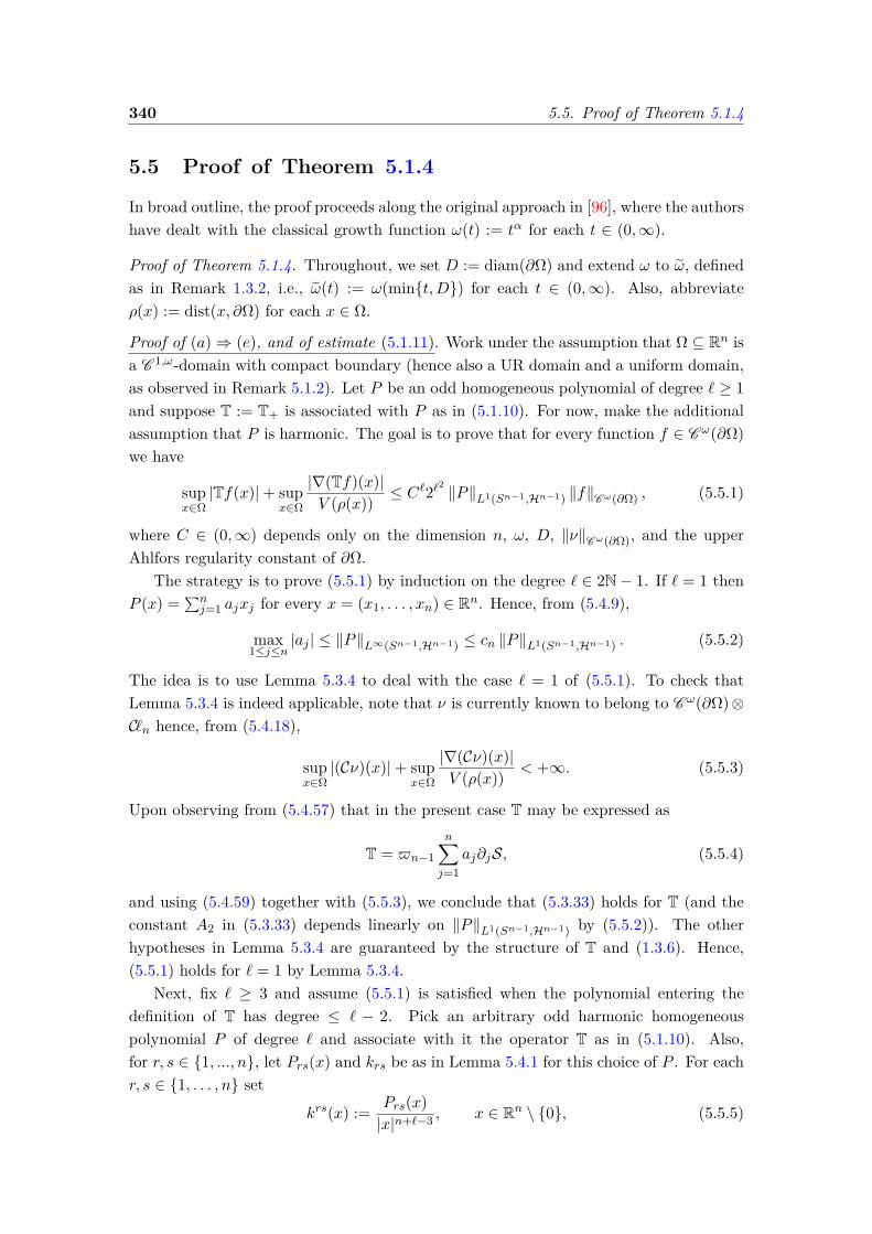
340 5.5. Proof of Theorem 5.1.4
5.5 Proof of Theorem 5.1.4
In broad outline, the proof proceeds along the original approach in [96], where the authorshave dealt with the classical growth function ω(t) := tα for each t ∈ (0,∞).
Proof of Theorem 5.1.4. Throughout, we set D := diam(∂Ω) and extend ω to ω, definedas in Remark 1.3.2, i.e., ω(t) := ω(mint,D) for each t ∈ (0,∞). Also, abbreviateρ(x) := dist(x, ∂Ω) for each x ∈ Ω.
Proof of (a)⇒ (e), and of estimate (5.1.11). Work under the assumption that Ω ⊆ Rn isa C 1,ω-domain with compact boundary (hence also a UR domain and a uniform domain,as observed in Remark 5.1.2). Let P be an odd homogeneous polynomial of degree ` ≥ 1and suppose T := T+ is associated with P as in (5.1.10). For now, make the additionalassumption that P is harmonic. The goal is to prove that for every function f ∈ C ω(∂Ω)we have
supx∈Ω|Tf(x)|+ sup
x∈Ω
|∇(Tf)(x)|V (ρ(x)) ≤ C`2`2 ‖P‖L1(Sn−1,Hn−1) ‖f‖Cω(∂Ω) , (5.5.1)
where C ∈ (0,∞) depends only on the dimension n, ω, D, ‖ν‖Cω(∂Ω), and the upperAhlfors regularity constant of ∂Ω.
The strategy is to prove (5.5.1) by induction on the degree ` ∈ 2N− 1. If ` = 1 thenP (x) =
∑nj=1 ajxj for every x = (x1, . . . , xn) ∈ Rn. Hence, from (5.4.9),
max1≤j≤n
|aj | ≤ ‖P‖L∞(Sn−1,Hn−1) ≤ cn ‖P‖L1(Sn−1,Hn−1) . (5.5.2)
The idea is to use Lemma 5.3.4 to deal with the case ` = 1 of (5.5.1). To check thatLemma 5.3.4 is indeed applicable, note that ν is currently known to belong to C ω(∂Ω)⊗C n hence, from (5.4.18),
supx∈Ω|(Cν)(x)|+ sup
x∈Ω
|∇(Cν)(x)|V (ρ(x)) < +∞. (5.5.3)
Upon observing from (5.4.57) that in the present case T may be expressed as
T = $n−1
n∑j=1
aj∂jS, (5.5.4)
and using (5.4.59) together with (5.5.3), we conclude that (5.3.33) holds for T (and theconstant A2 in (5.3.33) depends linearly on ‖P‖L1(Sn−1,Hn−1) by (5.5.2)). The otherhypotheses in Lemma 5.3.4 are guaranteed by the structure of T and (1.3.6). Hence,(5.5.1) holds for ` = 1 by Lemma 5.3.4.
Next, fix ` ≥ 3 and assume (5.5.1) is satisfied when the polynomial entering thedefinition of T has degree ≤ ` − 2. Pick an arbitrary odd harmonic homogeneouspolynomial P of degree ` and associate with it the operator T as in (5.1.10). Also,for r, s ∈ 1, ..., n, let Prs(x) and krs be as in Lemma 5.4.1 for this choice of P . For eachr, s ∈ 1, . . . , n set
krs(x) := Prs(x)|x|n+`−3 , x ∈ Rn \ 0, (5.5.5)
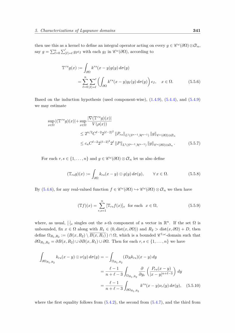
5. Characterizations of Lyapunov domains 341
then use this as a kernel to define an integral operator acting on every g ∈ C ω(∂Ω)⊗C n,say g =
∑n`=0
∑′|I|=` gIeI with each gI in C ω(∂Ω), according to
T rsg(x) :=ˆ∂Ωkrs(x− y)g(y) dσ(y)
=n∑`=0
∑′
|I|=`
(ˆ∂Ωkrs(x− y)gI(y) dσ(y)
)eI , x ∈ Ω. (5.5.6)
Based on the induction hypothesis (used component-wise), (1.4.9), (5.4.4), and (5.4.9)we may estimate
supx∈Ω|(T rsg)(x)|+ sup
x∈Ω
|∇(T rsg)(x)|V (ρ(x))
≤ 2n/2C`−22(`−2)2 ‖Prs‖L1(Sn−1,Hn−1) ‖g‖Cω(∂Ω)⊗C n
≤ cnC`−22(`−2)22` ‖P‖L1(Sn−1,Hn−1) ‖g‖Cω(∂Ω)⊗C n . (5.5.7)
For each r, s ∈ 1, . . . , n and g ∈ C ω(∂Ω)⊗ C n let us also define
(Trsg)(x) :=ˆ∂Ωkrs(x− y) g(y) dσ(y), ∀x ∈ Ω. (5.5.8)
By (5.4.6), for any real-valued function f ∈ C ω(∂Ω) → C ω(∂Ω)⊗ C n we then have
(Tf)(x) =n∑
r,s=1[Trsf(x)]s for each x ∈ Ω, (5.5.9)
where, as usual, [·]s singles out the s-th component of a vector in Rn. If the set Ω isunbounded, fix x ∈ Ω along with R1 ∈ (0, dist(x, ∂Ω)) and R2 > dist(x, ∂Ω) + D, thendefine ΩR1,R2 :=
(B(x,R2) \ B(x,R1)
)∩ Ω, which is a bounded C 1,ω-domain such that
∂ΩR1,R2 = ∂B(x,R2) ∪ ∂B(x,R1) ∪ ∂Ω. Then for each r, s ∈ 1, . . . , n we have
ˆ∂ΩR1,R2
krs(x− y) ν(y) dσ(y) = −ˆ
ΩR1,R2
(DRkrs)(x− y) dy
= `− 1n+ `− 3
ˆΩR1,R2
∂
∂yr
(Prs(x− y)|x− y|n+`−3
)dy
= `− 1n+ `− 3
ˆ∂ΩR1,R2
krs(x− y)νr(y) dσ(y), (5.5.10)
where the first equality follows from (5.4.2), the second from (5.4.7), and the third from
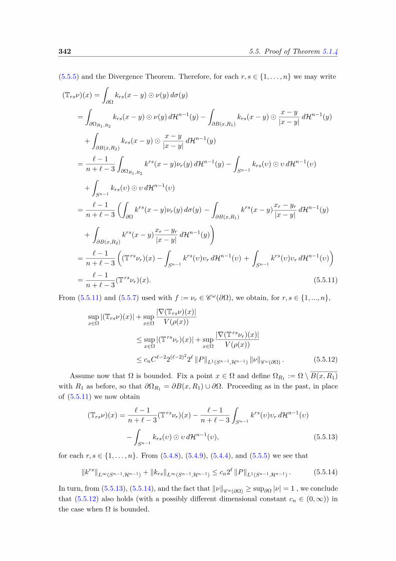
342 5.5. Proof of Theorem 5.1.4
(5.5.5) and the Divergence Theorem. Therefore, for each r, s ∈ 1, . . . , n we may write
(Trsν)(x) =ˆ∂Ωkrs(x− y) ν(y) dσ(y)
=ˆ∂ΩR1,R2
krs(x− y) ν(y) dHn−1(y)−ˆ∂B(x,R1)
krs(x− y) x− y|x− y|
dHn−1(y)
+ˆ∂B(x,R2)
krs(x− y) x− y|x− y|
dHn−1(y)
= `− 1n+ `− 3
ˆ∂ΩR1,R2
krs(x− y)νr(y) dHn−1(y)−ˆSn−1
krs(υ) υ dHn−1(υ)
+ˆSn−1
krs(υ) υ dHn−1(υ)
= `− 1n+ `− 3
(ˆ∂Ωkrs(x− y)νr(y) dσ(y) −
ˆ∂B(x,R1)
krs(x− y)xr − yr|x− y|
dHn−1(y)
+ˆ∂B(x,R2)
krs(x− y)xr − yr|x− y|
dHn−1(y))
= `− 1n+ `− 3
((T rsνr)(x)−
ˆSn−1
krs(υ)υr dHn−1(υ) +ˆSn−1
krs(υ)υr dHn−1(υ))
= `− 1n+ `− 3(T rsνr)(x). (5.5.11)
From (5.5.11) and (5.5.7) used with f := νr ∈ C ω(∂Ω), we obtain, for r, s ∈ 1, ..., n,
supx∈Ω|(Trsν)(x)|+ sup
x∈Ω
|∇(Trsν)(x)|V (ρ(x))
≤ supx∈Ω|(T rsνr)(x)|+ sup
x∈Ω
|∇(T rsνr)(x)|V (ρ(x))
≤ cnC`−22(`−2)22` ‖P‖L1(Sn−1,Hn−1) ‖ν‖Cω(∂Ω) . (5.5.12)
Assume now that Ω is bounded. Fix a point x ∈ Ω and define ΩR1 := Ω \ B(x,R1)with R1 as before, so that ∂ΩR1 = ∂B(x,R1) ∪ ∂Ω. Proceeding as in the past, in placeof (5.5.11) we now obtain
(Trsν)(x) = `− 1n+ `− 3(T rsνr)(x)− `− 1
n+ `− 3
ˆSn−1
krs(υ)υr dHn−1(υ)
−ˆSn−1
krs(υ) υ dHn−1(υ), (5.5.13)
for each r, s ∈ 1, . . . , n. From (5.4.8), (5.4.9), (5.4.4), and (5.5.5) we see that
‖krs‖L∞(Sn−1,Hn−1) + ‖krs‖L∞(Sn−1,Hn−1) ≤ cn2` ‖P‖L1(Sn−1,Hn−1) . (5.5.14)
In turn, from (5.5.13), (5.5.14), and the fact that ‖ν‖Cω(∂Ω) ≥ sup∂Ω |ν| = 1 , we concludethat (5.5.12) also holds (with a possibly different dimensional constant cn ∈ (0,∞)) inthe case when Ω is bounded.
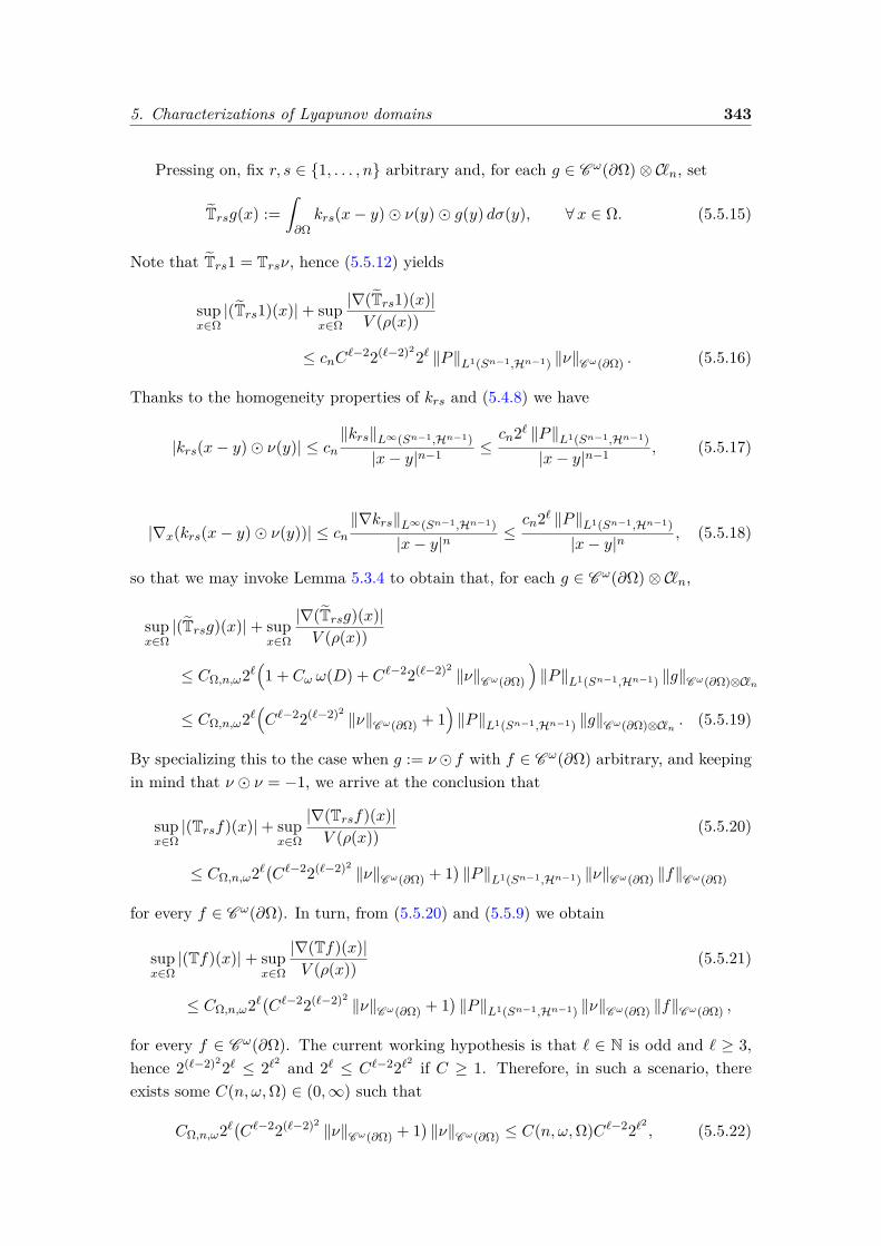
5. Characterizations of Lyapunov domains 343
Pressing on, fix r, s ∈ 1, . . . , n arbitrary and, for each g ∈ C ω(∂Ω)⊗ C n, set
Trsg(x) :=ˆ∂Ωkrs(x− y) ν(y) g(y) dσ(y), ∀x ∈ Ω. (5.5.15)
Note that Trs1 = Trsν, hence (5.5.12) yields
supx∈Ω|(Trs1)(x)|+ sup
x∈Ω
|∇(Trs1)(x)|V (ρ(x))
≤ cnC`−22(`−2)22` ‖P‖L1(Sn−1,Hn−1) ‖ν‖Cω(∂Ω) . (5.5.16)
Thanks to the homogeneity properties of krs and (5.4.8) we have
|krs(x− y) ν(y)| ≤ cn‖krs‖L∞(Sn−1,Hn−1)|x− y|n−1 ≤
cn2` ‖P‖L1(Sn−1,Hn−1)|x− y|n−1 , (5.5.17)
|∇x(krs(x− y) ν(y))| ≤ cn‖∇krs‖L∞(Sn−1,Hn−1)
|x− y|n≤cn2` ‖P‖L1(Sn−1,Hn−1)
|x− y|n, (5.5.18)
so that we may invoke Lemma 5.3.4 to obtain that, for each g ∈ C ω(∂Ω)⊗ C n,
supx∈Ω|(Trsg)(x)|+ sup
x∈Ω
|∇(Trsg)(x)|V (ρ(x))
≤ CΩ,n,ω2`(1 + Cω ω(D) + C`−22(`−2)2 ‖ν‖Cω(∂Ω)
)‖P‖L1(Sn−1,Hn−1) ‖g‖Cω(∂Ω)⊗C n
≤ CΩ,n,ω2`(C`−22(`−2)2 ‖ν‖Cω(∂Ω) + 1
)‖P‖L1(Sn−1,Hn−1) ‖g‖Cω(∂Ω)⊗C n . (5.5.19)
By specializing this to the case when g := ν f with f ∈ C ω(∂Ω) arbitrary, and keepingin mind that ν ν = −1, we arrive at the conclusion that
supx∈Ω|(Trsf)(x)|+ sup
x∈Ω
|∇(Trsf)(x)|V (ρ(x)) (5.5.20)
≤ CΩ,n,ω2`(C`−22(`−2)2 ‖ν‖Cω(∂Ω) + 1
)‖P‖L1(Sn−1,Hn−1) ‖ν‖Cω(∂Ω) ‖f‖Cω(∂Ω)
for every f ∈ C ω(∂Ω). In turn, from (5.5.20) and (5.5.9) we obtain
supx∈Ω|(Tf)(x)|+ sup
x∈Ω
|∇(Tf)(x)|V (ρ(x)) (5.5.21)
≤ CΩ,n,ω2`(C`−22(`−2)2 ‖ν‖Cω(∂Ω) + 1
)‖P‖L1(Sn−1,Hn−1) ‖ν‖Cω(∂Ω) ‖f‖Cω(∂Ω) ,
for every f ∈ C ω(∂Ω). The current working hypothesis is that ` ∈ N is odd and ` ≥ 3,hence 2(`−2)22` ≤ 2`2 and 2` ≤ C`−22`2 if C ≥ 1. Therefore, in such a scenario, thereexists some C(n, ω,Ω) ∈ (0,∞) such that
CΩ,n,ω2`(C`−22(`−2)2 ‖ν‖Cω(∂Ω) + 1
)‖ν‖Cω(∂Ω) ≤ C(n, ω,Ω)C`−22`2 , (5.5.22)
344 5.5. Proof of Theorem 5.1.4
where Cn,ω,Ω is the constant appearing in (5.5.21). This suggests that, to begin with,we take C ≥ max
1 ,√C(n, ω,Ω)
which then ensures both that C ≥ 1 and that
C(n, ω,Ω)C`−22`2 ≤ C`2`2 . Ultimately, this choice, together with (5.5.21) and (5.5.22),proves (5.5.1) and therefore the induction is complete.
Moving on, we claim that the additional assumption that P is harmonic may beeliminated. The starting point in the justification of this claim is the observation thatany homogeneous polynomial P in Rn may be written as P (x) = P0(x) + |x|2Q0(x) forevery x ∈ Rn, where P0 and Q0 are homogeneous polynomials in Rn, and P0 is harmonic(cf. [115, p. 69]). If P has degree ` = 2N + 1 for some N ∈ N0, by iterating this processfinitely many steps we conclude that for each j ∈ 0, 1, . . . , N there exists a harmonichomogeneous polynomial Pj of degree `− 2j such that
P (x) =N∑j=0|x|2jPj(x), ∀x ∈ Rn. (5.5.23)
Since the restrictions to the unit sphere of any two homogeneous harmonic polynomialsof different degrees are orthogonal in L2(Sn−1,Hn−1) (cf. [115, p. 69]), we have
‖P‖2L2(Sn−1,Hn−1) =N∑j=0‖Pj‖2L2(Sn−1,Hn−1) . (5.5.24)
Thus, for every j ∈ 0, 1, . . . , N,
‖Pj‖L1(Sn−1,Hn−1) ≤ cn ‖Pj‖L2(Sn−1,Hn−1) ≤ cn ‖P‖L2(Sn−1,Hn−1) . (5.5.25)
The upshot of (5.5.23) is that we may now express the action of the operator T on anyfunction f ∈ C ω(∂Ω) as
Tf(x) =N∑j=0
ˆ∂Ω
Pj(x− y)|x− y|n−1+(`−2j) f(y) dσ(y), ∀x ∈ Ω. (5.5.26)
and an estimate like (5.5.1) is valid for each integral operator in the above sum sinceeach polynomial Pj is odd, homogeneous, and harmonic. From this and (5.5.25) we thenconclude that, in the current general case, for each function f ∈ C ω(∂Ω) we have
supx∈Ω|Tf(x)|+ sup
x∈Ω
|∇(Tf)(x)|V (ρ(x)) ≤ cn`C`2`
2 ‖P‖L2(Sn−1,Hn−1) ‖f‖Cω(∂Ω) . (5.5.27)
By choosing again C big enough to begin with, matters may be arranged so that cn` ≤ C`
for ` ≥ 1. Assume this is the case and rename C2 as C. From (5.5.27) and Lemma 5.3.5we then conclude that the operator T+ from (5.1.10) maps C ω(∂Ω) continuously intoC ω(Ω+), and that the corresponding estimate claimed in (5.1.11) holds. Finally, Ω−is also a C 1,ω-domain with compact boundary, so the same argument applies for theoperator T−.
Proof of (e)⇒ (d). This is a direct consequence of the observation that the operatorsR±j considered in item (d) are particular cases of those considered in item (e).
5. Characterizations of Lyapunov domains 345
Proof of (d)⇒ (a). Since Ω is a UR domain, the jump-formulas from Theorem 5.3.1hold. In view of (1.1.18) this implies that for each f ∈ L1(∂Ω, σ), each j ∈ 1, . . . , n,and σ-a.e. x ∈ ∂Ω, we have(
R±j f∣∣κ−n.t.
∂Ω±
)(x) = ∓1
2νj(x)f(x) + limε→0+
ˆ∂Ω\B(x,ε)
(∂jE)(x− y)f(y) dσ(y), (5.5.28)
where E is the fundamental solution for the Laplacian defined in (2.3.6). From this,(5.1.9), Lemma 1.3.6, and (1.3.22) we then see that for j ∈ 1, . . . , n we have
νj = R−j 1∣∣∂Ω− −R+
j 1∣∣∂Ω+∈ C ω(∂Ω), (5.5.29)
where the first equality holds σ-a.e. on ∂Ω. Thus, ν ∈ C ω(∂Ω) which ultimately goes toshow that Ω is a C 1,ω-domain.
Proof of (a)⇒ (c), and of estimate (5.1.12). Suppose Ω ⊆ Rn is a C 1,ω-domain withcompact boundary and fix an odd homogenous polynomial P of degree ` ≥ 1 in Rn.Under these hypotheses, we have already proved (in the implication (a) ⇒ (e)) thatthe integral operators associated with P as in (5.1.10) map C ω(∂Ω) continuously intoC ω(Ω±) and that the estimates in (5.1.11) hold. Assume first that P is harmonic anddefine
k(x) := P (x)|x|n−1+` , ∀x ∈ Rn \ 0. (5.5.30)
From [115, p. 73] we know that its Fourier transform is given by
k(ξ) = γn,`P (ξ)|ξ|`+1 , ∀ ξ ∈ Rn \ 0, (5.5.31)
where γn,` = O(`−(n−2)/2) if n is even, and γn,` = O(`−(n−4)/2) if n is odd as `→∞.Fix two arbitrary distinct points x, y ∈ ∂Ω. In the case when |ν(x)− ν(y)| ≥ 1/2 we
have ω(|x− y|) ≥ (2 ‖ν‖Cω(∂Ω))−1, hence
|P (ν(x))− P (ν(y))|ω(|x− y|) ≤ 4 ‖ν‖Cω(∂Ω) ‖P‖L∞(Sn−1,Hn−1)
≤ cn2` ‖ν‖Cω(∂Ω) ‖P‖L1(Sn−1,Hn−1) , (5.5.32)
where the last inequality above is a consequence of (5.4.9). Consider next the case when|ν(x)− ν(y)| ≤ 1/2. In such a scenario, the line segment [ν(x), ν(y)] is contained in theannulus B(0, 1) \ B(0, 1/2). Based on this, the Mean Value Theorem, the homogeneityof P , and (5.4.9), we obtain
|P (ν(x))− P (ν(y))|ω(|x− y|) ≤
(sup
z∈[ν(x),ν(y)]|(∇P )(z)|
)‖ν‖Cω(∂Ω)
≤ ‖∇P‖L∞(Sn−1,Hn−1) ‖ν‖Cω(∂Ω)
≤ cn2` ‖P‖L1(Sn−1,Hn−1) ‖ν‖Cω(∂Ω) . (5.5.33)
346 5.5. Proof of Theorem 5.1.4
Moreover, using (5.4.9) and the fact that ‖ν‖Cω(∂Ω) ≥ sup∂Ω |ν| = 1,
supx∈∂Ω
|P (ν(x))| ≤ ‖P‖L∞(Sn−1,Hn−1) ≤ cn2` ‖P‖L1(Sn−1,Hn−1)
≤ cn2` ‖P‖L1(Sn−1,Hn−1) ‖ν‖Cω(∂Ω) . (5.5.34)
From (5.5.32), (5.5.33), (5.5.34), and the fact that k(ν(x)) = γn,`P (ν(x)) for each x ∈ ∂Ω(as seen from (5.5.31)), we can conclude that the mapping ∂Ω 3 x 7→ k(ν(x)) ∈ C belongsto C ω(∂Ω) and
‖k(ν(·))‖Cω(∂Ω) = γn,` ‖P (ν(·))‖Cω(∂Ω) ≤ cn2` ‖ν‖Cω(∂Ω) ‖P‖L1(Sn−1,Hn−1) , (5.5.35)
where the last inequality is based on the decay properties of γn,` in the parameter `.Given that Ω is a UR domain (cf. Remark 5.1.2), Theorem 5.3.1 is applicable. Fixan aperture parameter κ > 0. Based the jump-formula (5.3.3), (5.1.11), Lemma 1.3.6,(1.3.22), (5.5.35), and (1.3.21) we may then estimate
‖Tf‖Cω(∂Ω) ≤∥∥∥ 1
2i k(ν(·))f + Tf∥∥∥
Cω(∂Ω)+∥∥∥ 1
2i k(ν(·))f∥∥∥
Cω(∂Ω)
≤∥∥∥Tf ∣∣κ−n.t.
∂Ω
∥∥∥Cω(∂Ω)
+ 12‖k(ν(·))‖Cω(∂Ω) ‖f‖Cω(∂Ω)
≤ ‖Tf‖Cω(Ω) + cn2` ‖ν‖Cω(∂Ω) ‖P‖L1(Sn−1,Hn−1) ‖f‖Cω(∂Ω)
≤ ‖Tf‖Cω(Ω) + cn2` ‖ν‖Cω(∂Ω) ‖P‖L2(Sn−1,Hn−1) ‖f‖Cω(∂Ω)
≤(C`2`2 + cn2` ‖ν‖Cω(∂Ω)
)‖P‖L2(Sn−1,Hn−1) ‖f‖Cω(∂Ω)
≤ (2C)`2`2 ‖P‖L2(Sn−1,Hn−1) ‖f‖Cω(∂Ω) , (5.5.36)
assuming, without loss of generality, that C ≥ max1 , cn ‖ν‖Cω(∂Ω)
. This ultimately
proves that the singular integral operator T associated with the polynomial P as in (5.1.7)maps C ω(∂Ω) boundedly into itself in the case when P is harmonic.
In the case when the polynomial P is not necessarily harmonic, we decompose P asin (5.5.23) and for each f ∈ C ω(∂Ω) write
Tf(x) =N∑j=0
limε→0+
ˆ
y∈∂Ω|x−y|>ε
Pj(x− y)|x− y|n−1+(`−2j) f(y) dσ(y) for σ-a.e. x ∈ ∂Ω. (5.5.37)
Each term in the above sum may be regarded as the action of an integral operator onthe function f , of the sort described in (5.1.7), though now associated with a harmonichomogeneous odd polynomial. As such, what we have proved up to this point appliesand, on account of (5.5.25), gives that
‖Tf‖Cω(∂Ω) ≤ `(2C)`2`2 ‖P‖L2(Sn−1,Hn−1) ‖f‖Cω(∂Ω) . (5.5.38)
By choosing again C big enough so that `(2C)` ≤ C`(2C)` for ` ≥ 1 and renaming 2C2
as C, the claim in item (c) and the estimate in (5.1.12) follow.
5. Characterizations of Lyapunov domains 347
Proof of (c)⇒ (b). Since Ω is a UR domain and 1 ∈ L2(∂Ω, σ) since ∂Ω is bounded, thefunctional Rj1 ∈
(C ω(∂Ω)
)∗, originally defined as in (5.1.3), is given by the principal-value integral (5.1.4) with f = 1, for each j ∈ 1, . . . , n. Indeed, for each g ∈ C ω(∂Ω)we may write
〈Rj1, g〉 = 12$n−1
ˆ∂Ω
ˆ∂Ω
xj − yj|x− y|n
(g(x)− g(y)
)dσ(y) dσ(x)
= limε→0+
12$n−1
ˆ ˆ
(x,y)∈∂Ω×∂Ω|x−y|>ε
xj − yj|x− y|n
(g(x)− g(y)
)dσ(y) dσ(x)
=⟨
limε→0+
1$n−1
ˆ
y∈∂Ω|·−y|>ε
(· − y)j| · −y|n
dσ(y) , g⟩, (5.5.39)
as wanted. As such, (5.1.6) is a direct consequence of item (c).
Proof of (b)⇒ (a). Assume Rj1 ∈ C ω(∂Ω) for every j ∈ 1, . . . , n. Since we triviallyhave C ω(∂Ω) ⊆ L∞(∂Ω, σ) ⊆ BMO(∂Ω, σ), from the discussion in Section 5.1 it followsthat each distributional Riesz transform Rj extends to a bounded linear operator onL2(∂Ω, σ), given by (5.1.4). Then at σ-a.e. point on ∂Ω we may write
14ν = C(Cν) = −C
( n∑j=1
(Rj1)ej). (5.5.40)
The first equality above uses (5.4.24). The second equality in (5.5.40) uses the fact thatat σ-a.e. point on ∂Ω we have Cν = −
∑nj=1(Rj1)ej , itself a consequence of the definition
of C plus the fact that νν = −1 and x−y =∑nj=1(xj−yj)ej for each x, y ∈ Rn. Thanks
to (5.1.6) and Theorem 5.4.8, the function in the right hand-side of (5.5.40) belongs toC ω(∂Ω)⊗ C n, so ultimately ν ∈ C ω(∂Ω) (hence Ω is a C 1,ω-domain, by Remark 5.1.3).
This concludes the proof of Theorem 5.1.4.

348
Bibliography
[1] S. Agmon, A. Douglis, and L. Nirenberg, Estimates near the boundary for solutionsof elliptic partial differential equations satisfying general boundary conditions. I,Comm. Pure Appl. Math. 12 (1959), 623–727.
[2] , Estimates near the boundary for solutions of elliptic partial differentialequations satisfying general boundary conditions. II, Comm. Pure Appl. Math. 17(1964), 35–92.
[3] H. Aikawa and K. Hirata, Doubling conditions for harmonic measure in Johndomains, Ann. Inst. Fourier (Grenoble) 58 (2008), no. 2, 429–445.
[4] H. Aimar, A. Bernardis, and B. Iaffei, Comparison of Hardy-Littlewood and dyadicmaximal functions on spaces of homogeneous type, J. Math. Anal. Appl. 312 (2005),no. 1, 105–120.
[5] R. Alvarado, D. Brigham, V. Maz’ya, M. Mitrea, and E. Ziadé, On the regularityof domains satisfying a uniform hour-glass condition and a sharp version of theHopf-Oleinik boundary point principle, J. Math. Sci. 176 (2011), no. 3, 281–360.
[6] R. Alvarado and M. Mitrea, Hardy spaces on Ahlfors-regular quasi metric spaces.A sharp theory, Lecture Notes in Mathematics, vol. 2142, Springer, 2015.
[7] P. Auscher and J.M. Martell, Weighted norm inequalities, off-diagonal estimatesand elliptic operators. I. General operator theory and weights, Adv. Math. 212(2007), no. 1, 225–276.
[8] S. Axler, P. Bourdon, and W. Ramey, Harmonic function theory, second ed.,Graduate Texts in Mathematics, vol. 137, Springer-Verlag, New York, 2001.
[9] R.E. Basye, Simply connected sets, Trans. Amer. Math. Soc. 38 (1935), no. 2,341–356.
350 Bibliography
[10] C. Bennett and R. Sharpley, Interpolation of operators, Pure and Applied Mathe-matics, vol. 129, Academic Press Inc., Boston, MA, 1988.
[11] J. Bergh and J. Löfström, Interpolation spaces. An introduction, Springer-Verlag,Berlin-New York, 1976.
[12] A.V. Bitsadze, Ob edinstvennosti resheniya zadachi dirichlet dlya ellipticheskikhuravnenii s chastnymi proizvodnymi, Uspekhi Matem. Nauk 3 (1948), no. 6, 211–212.
[13] , Boundary value problems for second order elliptic equations, North-Holland Publishing Co., Amsterdam, 1968.
[14] A. Björn and J. Björn, Nonlinear potential theory on metric spaces, EMS Tracts inMathematics, vol. 17, European Mathematical Society (EMS), Zürich, 2011.
[15] S. Bortz and M. Engelstein, Reifenberg flatness and oscillation of the unit normalvector, preprint, arXiv:1708.05331, 2017.
[16] A. Böttcher and Yu.I. Karlovich, Carleson curves, Muckenhoupt weights, andToeplitz operators, Progress in Mathematics, vol. 154, Birkhäuser Verlag, Basel,1997.
[17] G. Bourdaud, Remarques sur certains sous-espaces de BMO(Rn) et de bmo(Rn),Ann. Inst. Fourier (Grenoble) 52 (2002), no. 4, 1187–1218.
[18] A.P. Calderón, Cauchy integrals on Lipschitz curves and related operators, Proc.Nat. Acad. Sci. U.S.A. 74 (1977), no. 4, 1324–1327.
[19] C.P. Calderón, On commutators of singular integrals, Studia Math. 53 (1975),no. 2, 139–174.
[20] L. Capogna, C. Kenig, and L. Lanzani, Harmonic measure. Geometric and analyticpoints of view, University Lecture Series, vol. 35, American Mathematical Society,Providence, RI, 2005.
[21] M. Christ, Lectures on singular integral operators, CBMS Regional ConferenceSeries in Mathematics, vol. 77, American Mathematical Society, Providence, RI,1990.
[22] , A T (b) theorem with remarks on analytic capacity and the Cauchy integral,Colloq. Math. 60/61 (1990), no. 2, 601–628.
[23] R.R. Coifman, G. David, Y. Meyer, and S.W. Semmes, ω-Calderón-Zygmundoperators, Harmonic analysis and partial differential equations (El Escorial, 1987),Lecture Notes in Math., vol. 1384, Springer, Berlin, 1989, pp. 132–145.
Bibliography 351
[24] R.R. Coifman, A. McIntosh, and Y. Meyer, L’intégrale de Cauchy définit unopérateur borné sur L2 pour les courbes lipschitziennes, Ann. of Math. (2) 116(1982), no. 2, 361–387.
[25] R.R. Coifman and Y. Meyer, Le théorème de Calderón par les “méthodes de variableréelle”, C. R. Acad. Sci. Paris Sér. A-B 289 (1979), no. 7, A425–A428.
[26] , Une généralisation du théorème de Calderón sur l’intégrale de Cauchy,Fourier analysis (Proc. Sem., El Escorial, 1979), vol. 1, Asoc. Mat. Española,Madrid, 1980, pp. 87–116.
[27] R.R. Coifman, R. Rochberg, and G. Weiss, Factorization theorems for Hardy spacesin several variables, Ann. of Math. (2) 103 (1976), no. 3, 611–635.
[28] D. Cruz-Uribe, J.M. Martell, and C. Pérez, Weights, extrapolation and thetheory of Rubio de Francia, Operator Theory: Advances and Applications,Birkhäuser/Springer Basel AG, Basel, 2011.
[29] S. Daneri and A. Pratelli, A planar bi-Lipschitz extension theorem, Adv. Calc. Var.8 (2015), no. 3, 221–266.
[30] G. David, Opérateurs d’intégrale singulière sur les surfaces régulières, Ann. Sci.École Norm. Sup. (4) 21 (1988), no. 2, 225–258.
[31] , Wavelets and singular integrals on curves and surfaces, Lecture Notes inMathematics, vol. 1465, Springer-Verlag, Berlin, 1991.
[32] G. David and D. Jerison, Lipschitz approximation to hypersurfaces, harmonicmeasure, and singular integrals, Indiana Univ. Math. J. 39 (1990), no. 3, 831–845.
[33] G. David and S. Semmes, Singular integrals and rectifiable sets in Rn: BeyondLipschitz graphs, Astérisque (1991), no. 193, 152.
[34] , Analysis of and on uniformly rectifiable sets, Mathematical Surveys andMonographs, vol. 38, American Mathematical Society, Providence, RI, 1993.
[35] J. Duoandikoetxea, Forty years of Muckenhoupt weights, “Function Spaces andInequalities,” Lecture Notes Paseky nad Jizerou 2013, J. Lukes, L. Pick ed.,Matfyzpress, Praga, 2013, pp. 23–75.
[36] J. Duoandikoetxea and M. Rosenthal, Extension and boundedness of operators onMorrey spaces from extrapolation techniques and embeddings, J. Geom. Anal. 28(2018), no. 4, 3081–3108.
[37] X.T. Duong and L. Yan, New function spaces of BMO type, the John-Nirenberginequality, interpolation, and applications, Comm. Pure Appl. Math. 58 (2005),no. 10, 1375–1420.
352 Bibliography
[38] L. Evans and R. Gariepy, Measure theory and fine properties of functions, Studiesin Advanced Mathematics, CRC Press, Boca Raton, FL, 1992.
[39] E.B. Fabes, M. Jodeit Jr., and N.M. Rivière, Potential techniques for boundaryvalue problems on C1-domains, Acta Math. 141 (1978), no. 3-4, 165–186.
[40] A. Fiorenza and M. Krbec, Indices of Orlicz spaces and some applications, Com-ment. Math. Univ. Carolin. 38 (1997), no. 3, 433–451.
[41] G.B. Folland, Real analysis. Modern techniques and their applications, second ed.,Pure and Applied Mathematics (New York), John Wiley & Sons, Inc., New York,1999.
[42] J. García-Cuerva and J.L. Rubio de Francia, Weighted norm inequalities and relatedtopics, North-Holland Mathematics Studies, vol. 116, North-Holland PublishingCo., Amsterdam, 1985.
[43] J.B. Garnett and D.E. Marshall, Harmonic measure, New Mathematical Mono-graphs, vol. 2, Cambridge University Press, Cambridge, 2005.
[44] I. Genebashvili, A. Gogatishvili, V. Kokilashvili, and M. Krbec, Weight theoryfor integral transforms on spaces of homogeneous type, Pitman Monographs andSurveys in Pure and Applied Mathematics, vol. 92, Longman, Harlow, 1998.
[45] L. Grafakos, Classical and modern Fourier analysis, Pearson Education, Inc.,Upper Saddle River, NJ, 2004.
[46] , Modern Fourier analysis, 2nd ed., Graduate Texts in Mathematics 250,Springer New York, 2009.
[47] S. Hofmann, On singular integrals of Calderón-type in Rn, and BMO, Rev. Mat.Iberoamericana 10 (1994), no. 3, 467–505.
[48] S. Hofmann, E. Marmolejo-Olea, M. Mitrea, S. Pérez-Esteva, and M. Taylor, Hardyspaces, singular integrals and the geometry of Euclidean domains of locally finiteperimeter, Geom. Funct. Anal. 19 (2009), no. 3, 842–882.
[49] S. Hofmann, J.M. Martell, and S. Mayboroda, Transference of scale-invariant esti-mates from lipschitz to non-tangentially accessible to uniformly rectifiable domains,preprint, 2016.
[50] S. Hofmann and S. Mayboroda, Hardy and BMO spaces associated to divergenceform elliptic operators, Math. Ann. 344 (2009), no. 1, 37–116.
[51] S. Hofmann, D. Mitrea, M. Mitrea, and A. Morris, Lp-square function estimates onspaces of homogeneous type and on uniformly rectifiable sets, Mem. Amer. Math.Soc. 245 (2017), no. 1159.

Bibliography 353
[52] S. Hofmann, M. Mitrea, and M. Taylor, Geometric and transformational propertiesof Lipschitz domains, Semmes-Kenig-Toro domains, and other classes of finiteperimeter domains, J. Geom. Anal. 17 (2007), no. 4, 593–647.
[53] , Singular integrals and elliptic boundary problems on regular Semmes-Kenig-Toro domains, Int. Math. Res. Not. IMRN (2010), no. 14, 2567–2865.
[54] , Symbol calculus for operators of layer potential type on Lipschitz surfaceswith VMO normals, and related pseudodifferential operator calculus, Anal. PDE 8(2015), no. 1, 115–181.
[55] T. Hytönen and A. Kairema, Systems of dyadic cubes in a doubling metric space,Colloq. Math. 126 (2012), no. 1, 1–33.
[56] T. Hytönen, C. Pérez, and E. Rela, Sharp reverse Hölder property for A∞ weightson spaces of homogeneous type, J. Funct. Anal. 263 (2012), no. 12, 3883–3899.
[57] D. Jerison and C. Kenig, Boundary behavior of harmonic functions in nontangen-tially accessible domains, Adv. in Math. 46 (1982), no. 1, 80–147.
[58] , Hardy spaces, A∞, and singular integrals on chord-arc domains, Math.Scand. 50 (1982), no. 2, 221–247.
[59] J.-L. Journé, Calderón-Zygmund operators, pseudodifferential operators and theCauchy integral of Calderón, Lecture Notes in Mathematics, vol. 994, Springer-Verlag, Berlin, 1983.
[60] C. Kenig, Harmonic analysis techniques for second order elliptic boundary valueproblems, CBMS Regional Conference Series in Mathematics, vol. 83, AMS,Providence, RI, 1994.
[61] C. Kenig and T. Toro, Harmonic measure on locally flat domains, Duke Math. J.87 (1997), no. 3, 509–551.
[62] , Free boundary regularity for harmonic measures and Poisson kernels, Ann.of Math. (2) 150 (1999), no. 2, 369–454.
[63] , Poisson kernel characterization of Reifenberg flat chord arc domains, Ann.Sci. École Norm. Sup. (4) 36 (2003), no. 3, 323–401.
[64] , Free boundary regularity below the continuous threshold: 2-phase problems,J. Reine Angew. Math. 596 (2006), 1–44.
[65] J. Kinnunen, R. Korte, N. Marola, and N. Shanmugalingam, A characterizationof BMO self-maps of a metric measure space, Collect. Math. 66 (2015), no. 3,405–421.
[66] J. Kinnunen and P. Shukla, The structure of reverse Hölder classes on metricmeasure spaces, Nonlinear Anal. 95 (2014), 666–675.
354 Bibliography
[67] J. Kolář and J. Kristensen, Gradient ranges of bumps on the plane, Proc. Amer.Math. Soc. 133 (2005), no. 6, 1699–1706.
[68] L.V. Kovalev, Sharp distortion growth for bilipschitz extension of planar maps,Conform. Geom. Dyn. 16 (2012), 124–131.
[69] V. Kozlov, V. Maz′ya, and J. Rossmann, Spectral problems associated with cornersingularities of solutions to elliptic equations, Mathematical Surveys and Mono-graphs, vol. 85, American Mathematical Society, Providence, RI, 2001.
[70] K. Kuratowski, Topology. Vol. II, Academic Press and PWN-Polish ScientificPublishers, 1966.
[71] M.A. Lavrentiev, Boundary problems in the theory of univalent functions, Math.Sbornik, N.S. 1(43) (1936), no. 6, 815–845.
[72] G. Leoni, A first course in Sobolev spaces, Graduate Studies in Mathematics, vol.105, American Mathematical Society, Providence, RI, 2009.
[73] A.K. Lerner, The John-Nirenberg inequality with sharp constants, C. R. Math.Acad. Sci. Paris 351 (2013), no. 11-12, 463–466.
[74] A.K. Lerner and C. Pérez, Self-improving properties of generalized Poincaré typeinequalities through rearrangements, Math. Scand. 97 (2005), no. 2, 217–234.
[75] P. MacManus and C. Pérez, Trudinger inequalities without derivatives, Trans.Amer. Math. Soc. 354 (2002), no. 5, 1997–2012.
[76] J.J. Marín, J.M. Martell, D. Mitrea, I. Mitrea, and M. Mitrea, A Fatou theorem andPoisson’s integral representation formula for elliptic systems in the upper-half space,to appear in “Topics in Clifford Analysis”, special volume in honor of WolfgangSprößig, Swanhild Bernstein editor, Birkhäuser, 2019.
[77] , Singular integral operators, quantitative flatness, and boundary problems,book manuscript, 2019.
[78] J.J. Marín, J.M. Martell, and M. Mitrea, Characterizations of Lyapunov domainsin terms of Riesz transforms and generalized Hölder spaces, preprint, 2019.
[79] , The generalized Hölder and Morrey-Campanato Dirichlet problems forelliptic systems in the upper-half space, to appear in Potential Anal., 2019.
[80] , The weighted theory for layer potentials and elliptic boundary valueproblems on Semmes-Kenig-Toro domains, preprint, 2019.
[81] J.M. Martell, D. Mitrea, I. Mitrea, and M. Mitrea, The higher order regularityDirichlet problem for elliptic systems in the upper-half space, Harmonic analysisand partial differential equations, Contemp. Math., vol. 612, Amer. Math. Soc.,Providence, RI, 2014, pp. 123–141.
Bibliography 355
[82] , The Dirichlet problem for elliptic systems with data in Köthe functionspaces, Rev. Mat. Iberoam. 32 (2016), no. 3, 913–970.
[83] , The Green function for elliptic systems in the upper-half space, preprint,2018.
[84] , Poisson kernels and boundary problems for elliptic systems in the upper-half space, book manuscript, 2018.
[85] , The BMO-Dirichlet problem for elliptic systems in the upper half-spaceand quantitative characterizations of VMO, Anal. PDE 12 (2019), no. 3, 605–720.
[86] J.M. Martell, D. Mitrea, and M. Mitrea, Higher order regularity for ellipticboundary value problems, preprint, 2018.
[87] O. Martio and J. Sarvas, Injectivity theorems in plane and space, Ann. Acad. Sci.Fenn. Ser. A I Math. 4 (1979), no. 2, 383–401.
[88] J. Mateu, P. Mattila, A. Nicolau, and J. Orobitg, BMO for nondoubling measures,Duke Math. J. 102 (2000), no. 3, 533–565.
[89] P. Mattila, M.S. Melnikov, and J. Verdera, The Cauchy integral, analytic capacity,and uniform rectifiability, Ann. of Math. (2) 144 (1996), no. 1, 127–136.
[90] V. Maz′ya, M. Mitrea, and T. Shaposhnikova, The Dirichlet problem in Lipschitzdomains with boundary data in Besov spaces for higher order elliptic systems withrough coefficients, Journal d’Analyse Mathématique 110 (2010), no. 1, 167–239.
[91] D. Mitrea, Distributions, partial differential equations, and harmonic analysis,Universitext, Springer, New York, NY, 2013.
[92] , Distributions, partial differential equations, and harmonic analysis, Uni-versitext, Springer, New York, NY, 2019, second edition.
[93] D. Mitrea, I. Mitrea, and M. Mitrea, A sharp divergence theorem with non-tangential pointwise traces and applications to singular integral operators, bookmanuscript, 2018.
[94] D. Mitrea, I. Mitrea, M. Mitrea, and S. Monniaux, Groupoid metrization theory withapplications to analysis on quasi-metric spaces and functional analysis, Applied andNumerical Harmonic Analysis, Birkhäuser/Springer, New York, 2013.
[95] D. Mitrea, I. Mitrea, M. Mitrea, and M. Taylor, The Hodge-Laplacian: Boundaryvalue problems on riemannian manifolds, Studies in Mathematics, vol. 64, DeGruyter, Berlin, 2016.
[96] D. Mitrea, M. Mitrea, and J. Verdera, Characterizing regularity of domains via theRiesz transforms on their boundaries, Anal. PDE 9 (2016), no. 4, 955–1018.
356 Bibliography
[97] I. Mitrea and K. Ott, Counterexamples to the well-posedness of Lp transmissionboundary value problems for the Laplacian, Proc. Amer. Math. Soc. 135 (2007),no. 7, 2037–2043.
[98] I. Mitrea, K. Ott, and W. Tucker, Invertibility properties of singular integraloperators associated with the Lamé and Stokes systems on infinite sectors in twodimensions, Integr. Equ. Oper. Theory 89 (2017), no. 2, 151–207.
[99] M. Mitrea, Clifford wavelets, singular integrals, and Hardy spaces, Lecture Notesin Mathematics, vol. 1575, Springer-Verlag, Berlin, 1994.
[100] R.L. Moore, A characterization of Jordan regions by properties having no referenceto their boundaries, Proc. Nat. Acad. Sci. USA. 4 (1918), no. 12, 364–370.
[101] F. Nazarov, X. Tolsa, and A. Volberg, On the uniform rectifiability of AD-regularmeasures with bounded Riesz transform operator: the case of codimension 1, ActaMath. 213 (2014), no. 2, 237–321.
[102] U. Neri, Some properties of functions with bounded mean oscillation, Studia Math.61 (1977), no. 1, 63–75.
[103] C. Pérez, Calderón-Zygmund theory related to Poincaré-Sobolev inequalities, frac-tional integrals and singular integral operators, Function Spaces, Nonlinear Analysisand Applications, Lecture notes of the Spring Lectures in analysis. Editors: J.Lukes and L. Pick, Charles University and Academy of Sciences, 1999, pp. 31–94.Available at http://grupo.us.es/anaresba/trabajos/carlosperez/31.pdf.
[104] Ch. Pommerenke, Boundary behaviour of conformal maps, Grundlehren der Math-ematischen Wissenschaften, vol. 299, Springer-Verlag, Berlin, 1992.
[105] W. Rudin, Real and complex analysis, third ed., McGraw-Hill Book Co., New York,1987.
[106] S.W. Semmes, A criterion for the boundedness of singular integrals on hypersur-faces, Trans. Amer. Math. Soc. 311 (1989), no. 2, 501–513.
[107] , Chord-arc surfaces with small constant. I, Adv. Math. 85 (1991), no. 2,198–223.
[108] , Chord-arc surfaces with small constant. II. Good parameterizations, Adv.Math. 88 (1991), no. 2, 170–199.
[109] V.Yu. Shelepov, On the index and spectrum of integral operators of potential typealong Radon curves, Math. USSR Sbornik 70 (1991), no. 1, 175–203.
[110] Z. Shen, Boundary value problems in Morrey spaces for elliptic systems on Lipschitzdomains, Amer. J. Math. 125 (2003), no. 5, 1079–1115.
Bibliography 357
[111] , Weighted estimates for elliptic systems on Lipschitz domains, IndianaUniv. Math. J. 55 (2006), no. 3, 1135–1154.
[112] V. A. Solonnikov, Estimates for solutions of general boundary value problemsfor elliptic systems, Doklady Akad. Nauk. SSSR 151 (1963), 783–785 (Russian),English translation in Soviet Math., 4 (1963), 1089–1091.
[113] , General boundary value problems for systems elliptic in the sense of A.Douglis and L. Nirenberg. I, Izv. Akad. Nauk SSSR Ser. Mat. 28 (1964), 665–706(Russian).
[114] , General boundary value problems for systems elliptic in the sense ofA. Douglis and L. Nirenberg. II, Trudy Mat. Inst. Steklov. 92 (1966), 233–297(Russian).
[115] E.M. Stein, Singular integrals and differentiability properties of functions, PrincetonMathematical Series, No. 30, Princeton University Press, Princeton, N.J., 1970.
[116] , Harmonic analysis: real-variable methods, orthogonality, and oscillatoryintegrals, Princeton Mathematical Series, vol. 43, Princeton University Press,Princeton, NJ, 1993, With the assistance of Timothy S. Murphy, Monographs inHarmonic Analysis, III.
[117] E.M. Stein and G. Weiss, Introduction to Fourier analysis on Euclidean spaces,Princeton University Press, Princeton, N.J., 1971, Princeton Mathematical Series,No. 32.
[118] J.-O. Strömberg and A. Torchinsky, Weighted Hardy spaces, Lecture Notes inMathematics, vol. 1381, Springer-Verlag, Berlin, 1989.
[119] M. Taylor, Measure theory and integration, Graduate Studies in Mathematics,vol. 76, American Mathematical Society, Providence, RI, 2006.
[120] P. Tukia, The planar Schönflies theorem for Lipschitz maps, Ann. Acad. Sci. Fenn.Ser. A I Math. 5 (1980), no. 1, 49–72.
[121] , Extension of quasisymmetric and Lipschitz embeddings of the real line intothe plane, Ann. Acad. Sci. Fenn. Ser. A I Math. 6 (1981), no. 1, 89–94.