Efficiency improvement of the polar coordinate transformation forevaluating BEM singular integrals on curved elements

Junjie Rong, Lihua Wen n, Jinyou XiaoCollege of Astronautics, Northwestern Polytechnical University, Xi'an 710072, PR China

a r t i c l e i n f o

Article history:Received 4 June 2013Accepted 17 October 2013Available online 12 November 2013

Keywords:Singular integralsBoundary element methodNyström methodAcoustics

a b s t r a c t

The polar coordinate transformation (PCT) method has been extensively used to treat various singularintegrals in the boundary element method (BEM). However, the resultant integrands tend to becomenearly singular when (1) the aspect ratio of the element is large or (2) the field point is closed to theelement boundary. In this paper, the first problem is circumvented by using a conformal transformationso that the geometry of the curved physical element is preserved in the transformed domain. The secondproblem is alleviated by using a sigmoidal transformation, which makes the quadrature points moreconcentrated around the near singularity.

By combining the proposed two transformations with the Guiggiani method in Guiggiani et al. (1992)[8], one obtains an efficient and robust numerical method for computing the weakly, strongly and hyper-singular integrals in high-order BEM. Numerical integration results show that, compared with theoriginal PCT, the present method can reduce the number of quadrature points considerably, for givenaccuracy. For further verification, the method is incorporated into a 2-order Nystrom BEM code forsolving acoustic Burton–Miller boundary integral equation. It is shown that the method can retain theconvergence rate of the BEM with much less quadrature points than the existing PCT.

& 2013 Elsevier Ltd. All rights reserved.

1. Introduction

The boundary element method (BEM) has been a most impor-tant numerical method in science and engineering. Its uniqueadvantages include the highly accurate solution on the boundary,the reduction of dimensionality, and the incomparable superior insolving infinite or semi-infinite field problems, etc. Historically,relatively low-order discretizations have been used with geome-tries modeled using first order elements and surface variablesmodeled to zero or first order on those elements. Recently,however, there has been increasing interest in the use of highorder methods, in order to obtain extra digits of precision withcomparatively small additional effort. Successful usage are seen inacoustics [1], electromagnetics [2,3], elasticity [4], aerodynamics[5], to name a few. One of the main difficulties in using high orderBEM is the lack of efficient methods for accurately evaluatingvarious singular integrals over curved elements. For the well-developed low order methods, there is no great difficulty sincerobust analytical and numerical integration schemes are generallyavailable for planar elements [6,7,9]. When concerned with highorder elements, however, a fully numerical method is required;

various techniques have been proposed, for example, the singu-larity subtraction [8], special purpose quadrature [3,10–12] andthe variable transformation methods [13–16].

In [8], Guiggiani et al. proposed a unified formula (Guiggiani'smethod for short) for treating various order of singular integralson curved elements. It is a singularity subtraction method, and hasfound extensive use in BEM. In this method the singular parts areextracted from the integrand and treated analytically. The remain-ing parts are regular so that conventional Gaussian quadrature canbe employed, but the number of quadrature points needed wouldbe large, depending on the regularity of the associated integrands.The special purpose quadrature can be used to substantiallyreduce the number of quadrature points, besides it is more robustand highly accurate. Most recently, Bremer [3] proposed such amethod which can achieve machine precision. The problem withthe special purpose quadrature is that its construction is some-what complicated and time-consuming. Variable transformationmethod, also known as singularity cancelation, eliminates thesingularity of the integrand by the null Jacobian at the field pointthrough a proper change of variables. Although simple to imple-ment, it is generally hard to be used in handling hypersingularintegrals. See the review papers [17,18] for further description ofthese techniques.

In most existing integration methods, including those men-tioned above, polar coordinates transformation (PCT) always servesas a common base [3,8,12,13,16,19]. It converses the surface

Contents lists available at ScienceDirect

journal homepage: www.elsevier.com/locate/enganabound

Engineering Analysis with Boundary Elements

0955-7997/$ - see front matter & 2013 Elsevier Ltd. All rights reserved.http://dx.doi.org/10.1016/j.enganabound.2013.10.014

n Corresponding author. Tel.: þ86 18629023355.E-mail addresses: rxrjj@126.com (J. Rong), lhwen@nwpu.edu.cn (L. Wen),

xiaojy@nwpu.edu.cn (J. Xiao).

Engineering Analysis with Boundary Elements 38 (2014) 83–93

integral into a double integral in radial and angular directions.Many works have been done on dealing with the singularity in theradial direction; numerical integration on the angular direction,however, still deserves more attention. In fact, after singularitycancelation or subtraction, although the integrand may behavesvery well in the radial direction, its behavior in the angulardirection would be much worst, so that too many quadraturepoints are needed. Especially when the field point lies close to theboundary of the element, one can clearly observe near singularityof the integrand in the angular direction. Unfortunately, this case isfrequently encountered in using high order elements, especiallyfor non-conform elements as will be demonstrated by a NyströmBEM in this paper. Similar problems have been considered in workabout the nearly singular BEM integrals. Effective methods alongthis line are the subdivision method [20], the Hayami transforma-tion [21], the sigmoidal transformation [22], etc. For the singularBEM integrals, the angular transformation has been used forcomputing weakly singular integrals over planar element [13].

Another problem of the PCT is how to find a proper planar domainto establish the polar coordinates. In usual practice, the integral iscarried out over standard reference domain (i.e., triangle in this paper)in intrinsic coordinates. However, the reference triangle is indepen-dent of the shape of the curved element, and thus the distortion of theelement is brought into the integrand, which can cause near singu-larity in the angular direction. Consequently, the performance ofquadratures is highly sensitive to the shape of element. The abovetwo problems in the angular direction were considered and resolvedby special purpose quadrature rule in [3]; whereas, as mentionedbefore, the algorithm has its own overhead.

In this paper, two strategies are proposed to overcome twoproblems in the angular direction, respectively. First, a conformaltransformation is carried out to map the curved physical element ontoa planar integration domain. Since it is conformal at the field point,the resultant integration domain perseveres the shape of the curvedelement. Second, a new sigmoidal transformation is introduced toalleviate the near singularity caused by the closeness of the field pointto the element boundary. The two proposed techniques, whencombined with Guiggiani's method, lead to a unified, efficient androbust numerical integration methods for various singular integrals inhigh order BEM. As a byproduct of the conformal transformation, theline integral in Guiggiani's method can be evaluated in close form.

The paper is organized as follows. The Nyström BEM for acousticsand singular integrals encountered are reviewed in Section 2. Section 3describes the Guiggiani's unified framework for treating various orderof singular integrals, with emphasis on the two reasons which renderthe poor performance of polar coordinates methods. Two efficienttransformations which represent the main contribution of this paperare proposed in Section 4. Numerical examples are given in Section 5to validate the efficiency and accuracy of the present methods. Section6 concludes the paper with some discussions.

2. Model problem: acoustic BIEs and Nyström discretization

The method presented in this paper will be used in solving theacoustic Burton–Miller BIE, which is briefly recalled here. The BIE issolved by using the Nyströmmethodwith the domain boundary beingpartitioned into curved quadratic elements. Various singular integralsthat will be treated in the following sections are summarized.

2.1. Acoustic Burton–Miller formulation

The time harmonic acoustic waves in a homogenous and isotropicacoustic mediumΩ is described by the following Helmholtz equation:

∇2uðxÞþk2uðxÞ ¼ 0; 8xAΩ; ð1Þ

where, ∇2 is the Laplace operator, uðxÞ is the sound pressure at thepoint x¼ ðx1; x2; x3Þ in the physical coordinate system, k¼ω=c isthe wavenumber, with ω being the angular frequency and c being thesound speed. For static case k¼0, (1) becomes the Laplace equation.By using Green's second theorem, the solution of Eq. (1) can beexpressed by integral representation

uðxÞþZS

∂Gðx; yÞ∂nðyÞ uðyÞ dSðyÞ ¼

ZSGðx; yÞqðyÞ dSðyÞþuIðxÞ; 8xAΩ;

ð2Þwhere x is a field point and y is a source point on boundary S;qðyÞ ¼ ∂uðyÞ=∂nðyÞ is the normal gradient of sound pressure; nðyÞdenotes the unit normal vector at the source point y. The incidentwave uIðxÞ will not be presented for radiation problems. The threedimensional fundamental solution G is given as

Gðx; yÞ ¼ eikr

4πr; ð3Þ

with r¼ jx�yj denoting the distance between the source and thefield points.

Before presenting the BIEs it is convenient to introduce theassociated single, double, adjoint and hypersingular layer opera-tors which are denoted by S, D, M and H, respectively; that is,

SqðyÞ ¼ZSGðx; yÞqðyÞ dSðyÞ; ð4aÞ

DuðyÞ ¼ZS

∂Gðx; yÞ∂nðyÞ uðyÞ dSðyÞ; ð4bÞ

MqðyÞ ¼ZS

∂Gðx; yÞ∂nðxÞ qðyÞ dSðyÞ; ð4cÞ

HuðyÞ ¼ZS

∂2Gðx; yÞ∂nðxÞ∂nðyÞuðyÞ dSðyÞ: ð4dÞ

The operator S is weakly singular and the integral is well-defined,while the operators D andM are defined in Cauchy principal valuesense (CPV). The operator H, on the other hand, is hypersingularand unbounded as a map from the space of smooth functions on Sto itself. It should be interpreted in the Hadamard finite part sense(HFP). Denoting a vanishing neighbourhood surrounding x by sɛ ,the CPV and HFP integrals are those after extracting free termsfrom a limiting process to make sɛ tends to zero in deriving BIEs[8]. Letting the field point x approach the boundary S in Eq. (2)leads to the CBIE [23]

CðxÞuðxÞþDuðxÞ ¼ SqðxÞþuIðxÞ; xAS; ð5Þwhere, CðxÞ is the free term coefficient which equals to 1/2 onsmooth boundary. By taking the normal derivative of Eq. (2)and letting the field point x go to boundary S, one obtains thehypersingular BIE (HBIE)

CðxÞqðxÞþHuðxÞ ¼MqðxÞþqIðxÞ; xAS: ð6ÞBoth CBIE and HBIE can be applied to calculate the unknownboundary values of interior acoustic problems. For an exteriorproblem, they have a different set of fictitious frequencies at whicha unique solution cannot be obtained. However, Eqs. (5) and (6)will always have only one solution in common. Given this fact,the Burton–Miller formulation which is a linear combination ofEqs. (5) and (6) (CHBIE) should yield a unique solution for allfrequencies [23]

CðxÞuðxÞþðDþαHÞuðyÞ�uIðxÞ¼ ðSþαMÞqðyÞ�α½cðxÞqðxÞ�qIðxÞ�; xAS; ð7Þ

where, α is a coupling constant that can be chosen as i=k.

J. Rong et al. / Engineering Analysis with Boundary Elements 38 (2014) 83–9384

2.2. Nyström method and the singular integrals

In this paper, the Nyströmmethod is used to discretize the BIEs.Let K be one of the integral operators in (4) and K be theassociated kernel function. Divide the problem into two regions,a region near and far from the field point x. If the element locatesin far field, Nyström method replaces the integral operator K witha summation under a quadrature rule [1]

ZΔS

Kðxi; yÞuðyÞ dSðyÞffi∑jωjKðxi; yjÞuðyjÞ; ΔSAS\Di; ð8Þ

where, xi and yj are quadrature points, Di is the near field of xi, ωj

is the jth weight over element ΔS. Such quadrature rules canbe obtained by mapping the Gaussian quadrature rules onto theparameterization of ΔS.

If the element locates in near field, however, the kernels exhibitsingularities or even hypersingularities. As a result, conventionalquadratures fail to give correct results. In order to maintain high-order properties, the quadrature weights are adjusted by a localcorrection procedure. Thus (8) becomes

ZΔS

Kðxi; yÞuðyÞ dSðyÞffi∑jωjðxiÞuðyjÞ; ΔSADi; ð9Þ

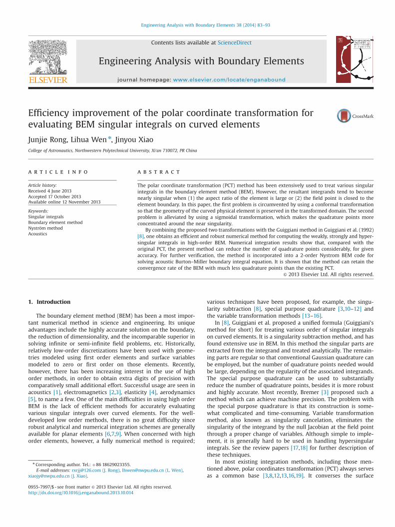
where ω jðxiÞ represents the modified quadrature weights for specia-lized rule at the singularity. The local corrected procedure is performedby approximating the unknown quantities using linear combination ofpolynomial basis functions which are defined on intrinsic coordinates(Fig. 1). Modified weights are obtained by solving the linear system

∑jωjϕ

ðnÞðyjÞ ¼ZΔS

Kðxi; yÞϕðnÞðyÞ dSðyÞ; ΔSADi; ð10Þ

where ϕðnÞ are polynomial basis functions. For the Nyström methodbased on quadratic elements, ϕðnÞ are given by

ϕðnÞðξ1; ξ2Þ ¼ ξp1ξq2; pþqr2; ð11Þ

where, p and q are integers, ξ1 and ξ2 denote local intrinsiccoordinates.

The right hand side integrals in Eq. (10) are of crucial impor-tance to the accuracy of the Nyström method. They are referred toas singular integrals when xi lies on the element, and nearlysingular integrals when xi is closed to but not on the element. Thispaper deals with the integrals in the first case, the nearly singularintegrals are treated via an recursive subdivision quadrature.When concerned with the first three operators in Eq. (4), theintegrals have a weak singularity of r�1, while the other operatorH is hypersingular of order r�3, as r-0.

3. An unified framework for singular integrals

Since various order of singularities appear in Eq. (7) or manyother BIEs, it is advantage to find a unified formula to treat theseintegrals in the same framework. In such a way, these integrals canbe implement in just one program so that the computational costwill be reduced. By expansion of the singular integrands in polarcoordinates, the three types of singular integrals considered in thispaper can be handled in a unified manner by using the formulaproposed by Guiggiani [8]. Despite of this advantage the methodcan be of low efficiency in practical usage; the very reasons arethen explained.

3.1. Polar coordinates transformation

Following a common practice in the BEM, the curved element isfirst mapped onto a region Δ of standard shape in the parameterplane (Fig. 1). In this case, the integral must be evaluated inEq. (10) and are of the form

I¼ZΔKðx; yðξÞÞϕðξÞjJðξÞj dξ1 dξ2; ð12Þ

where jJj is the transformation Jacobian from global coordinates tothe intrinsic coordinates,

J¼ ∂y∂ξ1

∂y∂ξ2

� �; jJðξÞj ¼ ∂y

∂ξ1� ∂y

∂ξ2

����:����

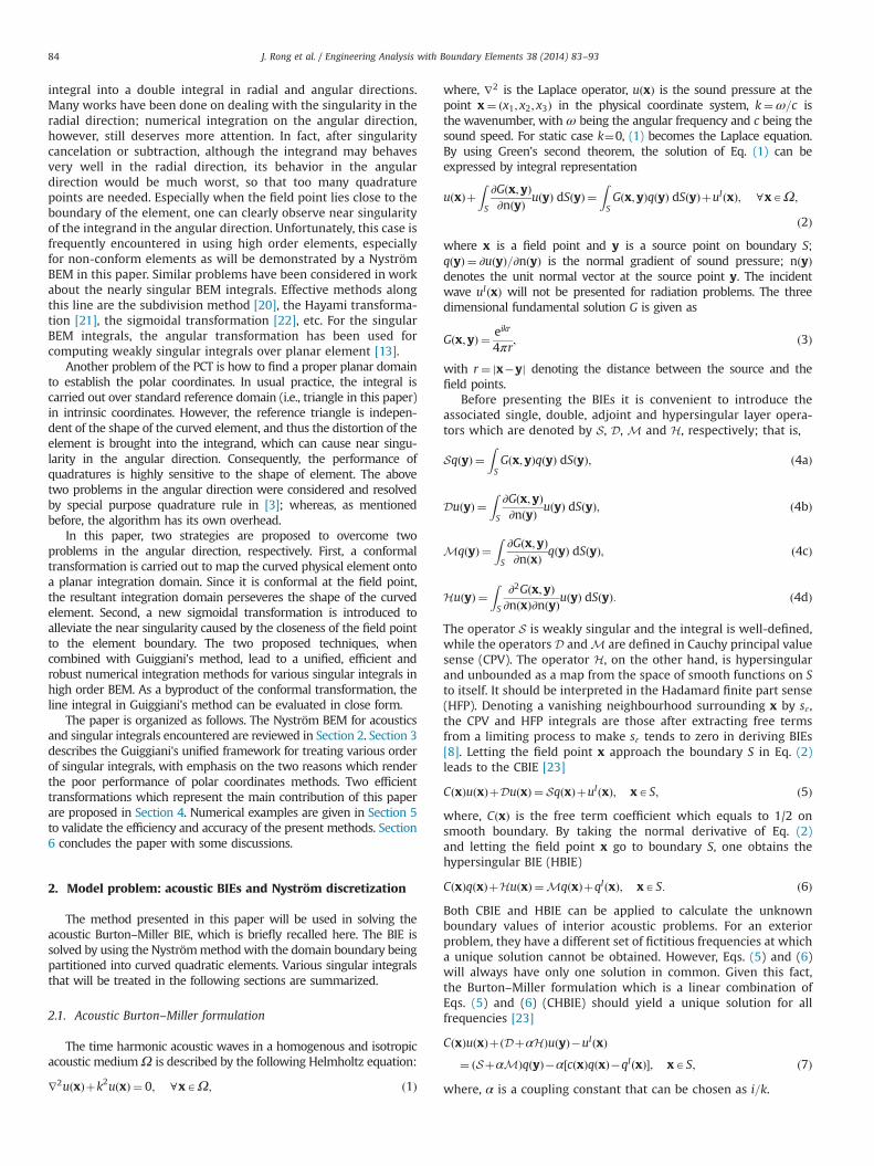
Then, polar coordinates ðρ;θÞ centered at ξs (the image of x onintrinsic plane) are defined in the parameter space (Fig. 2)

ξ1 ¼ ξðsÞ1 þρ cos θ

ξ2 ¼ ξðsÞ2 þρ sin θ

8<:so that dξ1 dξ2 ¼ ρ dρ dθ. Due to piecewise smooth property ofthe boundary of Δ, the triangle is split into three sub-triangles. Theassociated integral of Eq. (12) now becomes

I¼ limρðɛÞ-0

∑3

j ¼ 1

Z θj

θj� 1

Z ρ̂ðθÞ

ρðɛÞKðρ;θÞϕðρ;θÞjJðρ;θÞjρ dρ dθ; ð13Þ

where ρ̂ðθÞ gives a parametrization of the boundary of Δ in polarcoordinates, ðθj�1;θjÞ are three intervals on which ρ̂ðθÞ is smooth.The limiting process means CPV or HFP integral mentioned before,although for well-defined integral operator S, the limiting is notnecessary. According to the geometrical relationship in Fig. 2

ρ̂ðθÞ ¼ hjcos θ

: ð14Þ

where hj is the perpendicular distance from ξs to jth side ofthe planar triangle and θ is the angle from the perpendicular to

Fig. 1. Description of curved triangle. Left hand image: curved triangle and a fieldpoint; right hand image:the reference triangle and typical field points (interiorpoints) distribution of the second order Nyström method in intrinsic coordinatesystem. (For interpretation of the references to color in this figure caption, thereader is referred to the web version of this article.)

Fig. 2. Integration under polar coordinates. Left: polar coordinates transformation;right: near singularity as the field point approaches the boundary.

J. Rong et al. / Engineering Analysis with Boundary Elements 38 (2014) 83–93 85

a point ξ (Fig. 2). In each sub-triangle, θ equals to θ minus aconstant.

For singularity of order not more than 3, the integrand of (13),denoted by Fðρ;θÞ, can be expressed as series expansion underpolar coordinate [25,8]

Fðρ;θÞ ¼ Kðρ;θÞϕðρ;θÞ J ρ dρ����

¼ f �2ðθÞρ2 þ f �1ðθÞ

ρþ f 0ðθÞþρf 1ðθÞþρ2f 2ðθÞþ⋯¼ ∑

1

i ¼ pρif iðθÞ;

ð15Þ

where, fi are just functions of θ, integer p is determined by theorder of singularity,

p¼0; weakly singular;�1; strongly singular;�2; hyper� singular:

8><>:First, let us consider the hypersingular integrals. Due to the

appearance of the two terms with ði¼ �2; �1Þ, the integration ofFðρ;θÞ must be performed in the HFP sense; for more detailssee Guiggiani's work [8]. The resultant formula for hypersingularintegrals is given by

I¼ I1þ I2 ¼ ∑3

j ¼ 1

Z θj

θj� 1

Z ρ̂ðθÞ

0Fðρ;θÞ� f �2ðθÞ

ρ2 þ f �1ðθÞρ

� �� �dρ dθ|fflfflfflfflfflfflfflfflfflfflfflfflfflfflfflfflfflfflfflfflfflfflfflfflfflfflfflfflfflfflfflfflfflfflfflfflfflfflfflfflfflfflfflfflfflfflfflfflfflfflffl{zfflfflfflfflfflfflfflfflfflfflfflfflfflfflfflfflfflfflfflfflfflfflfflfflfflfflfflfflfflfflfflfflfflfflfflfflfflfflfflfflfflfflfflfflfflfflfflfflfflfflffl}

I1

þ ∑3

j ¼ 1

Z θj

θj� 1

f �1ðθÞ ln ρ̂ðθÞ� f �2ðθÞ1

ρ̂ðθÞ

� �dθ|fflfflfflfflfflfflfflfflfflfflfflfflfflfflfflfflfflfflfflfflfflfflfflfflfflfflfflfflfflfflfflfflfflfflfflfflfflfflfflfflfflffl{zfflfflfflfflfflfflfflfflfflfflfflfflfflfflfflfflfflfflfflfflfflfflfflfflfflfflfflfflfflfflfflfflfflfflfflfflfflfflfflfflfflffl}

I2

: ð16Þ

The strongly and weak singular integrals can be treated in asimilar manner based on expansion (15). The resultant computingformulas can also be written in the above form except that forstrongly singular integrals f �2 ¼ 0, and for weak singular integralsf �2 ¼ f �1 ¼ 0 (thus I2 ¼ 0). Therefore, formula (16) actually pro-vide an unified approach to evaluate singular integrals in BEM.

In (16) the double integral I1 and line integral I2 are all regular,thus one may conclude that it is sufficient to guarantee numericalaccuracy in evaluating these two integrals, it would be never-theless too expensive in practical usage, especially when used inhigh order Nyström method considered in this paper. The diffi-culties and the corresponding solutions will be presented in thefollowing sections.

3.2. Difficulties in evaluating I1

It is the computation of I1 that accounts for the main cost forevaluating the various singular integrals. The integrand of I1 can beapproximated by polynomials in ρ; that is,

I1 ¼ ∑3

j ¼ 1

Z θj

θj� 1

Z ρ̂ðθÞ

0ðf 0ðθÞþρf 1ðθÞþρ2f 2ðθÞþ⋯Þ dρ dθ: ð17Þ

The number of terms in this approximation is determined by thekernel function, the order of basis function and the flatness of theassociated element. The relative flatness of element is a basicrequirement in BEM in order to guarantee the accuracy. Conse-quently, it appears that the integrand of I1 can be well approxi-mated by low order polynomials in ρ in solving many problemsincluding Laplace, Helmholtz, elasticity and so forth, using quad-ratic elements. This implies that low order Gaussian quadraturesare sufficient for numerical integration in ρ.

In angular θ direction, however, two difficulties are frequ-ently encountered which severely retard the convergence rateof Gaussian quadratures. To show this, preforming integration

in ρ in (17) one obtains

I1 ¼ ∑3

j ¼ 1

Z θj

θj� 1

ρ̂ðθÞf 0ðθÞþ12ρ̂2ðθÞf 1ðθÞþ⋯

� �dθ: ð18Þ

The difficulties in computation of I1 are caused by the nearsingularities of f iðθÞ and ρ̂ðθÞ.

3.2.1. Near singularity in f iðθÞFunctions f iðθÞ can be expressed as (Appendix A)

f iðθÞ ¼~f iðθÞAαðθÞ; ð19Þ

where ~f i are regular trigonometric functions and α is integerdetermined by the subscript i. Function AðθÞ depends on the shapeof the element and parametric coordinate system (see [8] for adefinition of AðθÞ). Specifically, let u1, u2 be the two columnvectors of the Jacobian matrix J which spans the space tangentto the element at the point x, i.e.

u1 ¼∂y∂ξ1

�����y ¼ x

and u2 ¼∂y∂ξ2

�����y ¼ x

: ð20Þ

Then AðθÞ is given by

AðθÞ ¼ffiffiffiffiffiffiffiffiffiffiffiffiffiffiffiffiffiffiffiffiffiffiffiffiffiffiffiffiffiffiffiffiffiffiffiffiffiffiffiffiffiffiffiffiffiffiffiffiffiffiffiffiffiffiffiffiffiffiffiffiffiffiffiffiffiffiffiffiffiffiffiffiffiffiffiffiffiffiffiffiffiffiffiffiffiffiffiffiffiffiffiffiju1j2 cos 2 θþu1 � u2 sin 2θþju2j2 sin 2 θ

q¼

ffiffiffiffiffiffiffiffiffiffiffiffiffiffiffiffiffiffiffiffiffiffiffiffiffiffiffiffiffiffiffiffiffiffiffiffiffiffiffiffiffiffiffiffiffiffiffiffiffiffiffiffiffiffiffiffiffiffiffiffiffiffiffiffiffiffiffiffiffiffiffiffiffiffiffiffiffiffiffiffiffiffiffiffiffiffiffiffiffiffiffiffiffiffiffiffiffiffiffiffiffiffiffiffiffiffiffiffiffiffiffiffiffiffiffiffiffiffiffiffiu1 � u2 sin 2θþ1

2 ð u1j2� u2j2Þ cos 2θþ12 ð u1j2þ u2j2Þ

��������q¼

ffiffiffiffiffiffiffiffiffiffiffiffiffiffiffiffiffiffiffiffiffiffiffiffiffiffiffiffiffiffiffiffiffiffiffiffiffiffiffiffiffiffiffiffiffiffiffiffiffiffiffiffiffiffiffiffiffiffiffiffiffiffiffiffiffiffiffiffiffiffiffiffiffi12 ð u1j2þ u2j2Þ½μ sin ð2θþφÞþ1�:

����qð21Þ

If we let λ¼ ju1j=ju2j and cos γ ¼ ðu1 � u2Þ=ju1jju2j, then

φ¼ arctanλ2�1

2λ cos γ;

and

μ¼

ffiffiffiffiffiffiffiffiffiffiffiffiffiffiffiffiffiffiffiffiffiffiffiffiffiffiffiffiffi1� 4 sin 2 γ

ðλþλ�1Þ2

vuut o1: ð22Þ

It can be seen from (21) that, if μ-1, there exist two pointsθA ½0;2π� such that AðθÞ-0. Thus function fi tends to be nearlysingular. The circumstance μ-1 occurs in two cases accordingto Eq. (22): (1) the aspect ratio of the element is large, i.e., λapproaches 0 or 1; (2) peak or big obtuse corner appear in theelement which lead to sin γ-0. Both of these two cases indicate adistorted shape of the element.

To illustrate the influence of the element aspect ratio on thebehavior of function 1=AðθÞ which represents the smoothness of fi,consider the curved element in Fig. 7; see Section 5.1 for more detaileddescriptions. The aspect ratio of the element is controlled by s; larger simplies more distorted shape. Let b be the singular point. The plots of1=AðθÞ in the interval corresponding to the sub-triangle (2-b-3) inFig. 7 with various s are exhibited in Fig. 3. It is clear that 1=AðθÞ variesmore acutely as the increase of the aspect ratio.

The above analysis shows how element shape affects fi and thusthe integrand in (18). In an intuitionistic manner, the nearsingularity in fi is induced by the fact that the integration planeΔ in intrinsic coordinate system is independent on the shape ofelement, as a result the distortion is brought into the integrand.One can suppose that if the integration is performed over anotherplanar triangle which reflects the distortion of the element, thenear singularity should be eliminated. This is the main idea of theour new method in Section 4.1.

3.2.2. Near singularity in ρ̂ðθÞIn addition to the near singularity in fi, another obstacle retards

the convergence of the numerical quadrature for (18) is the near

J. Rong et al. / Engineering Analysis with Boundary Elements 38 (2014) 83–9386

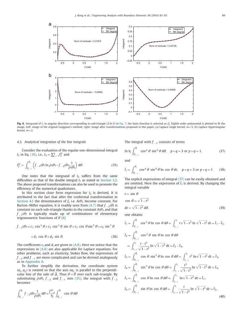
singularity in ρ̂ðθÞ, which can be clearly seen from (14). When thefield point x lies near to the boundary of the element, the restrictof θ approaches 7π=2, thus the denominator cos θ is close to 0 atthe two ends of the interval ðθj�1;θjÞ (see Fig. 2). The effect of thenear singularity in ρ̂ðθÞ on the total behavior of the integrandFðρ;θÞ is demonstrated by the left plots of Fig. 6(a) and (b), wherethe integrand have large peaks near the two ends of the interval.

Unfortunately, the situation that causes the near singularity inρ̂ðθÞ is ubiquitous in using the high order Nyström method. SeeFig. 1 for a typical distribution of field points in the second orderNyström method.

4. Efficient transformation methods

How to effectively resolve the above mentioned two difficultiesis crucial to the accurate evaluation of the BEM singular integrals.More recently, special quadratures are constructed for this pur-pose in [3]. Although accurate and robust numerical results arereported, it is noticed that the abscissas and weights of the specialquadratures are depend on the singular (field) point as well as theelement on which the integral is defined. The construction ofthe quadrature for integral can be rather complicated and time-consuming.

In this section, however, we propose a more simple yet efficientmethod. First, the intrinsic coordinates ðξ1; ξ2Þ are transformedonto a new system which results in constant AðθÞ. An additionalbenefit of constant AðθÞ is that the line integral I2 can be evaluatedin closed form; see Section 4.3. Then the sigmoidal transformationis introduced to alleviate the near singularity caused by ρ̂ðθÞ.

4.1. Conformal transformation

First, the near singularity caused by AðθÞ in fi is consideredand resolved. The idea is to introduce a new transformation underwhich AðθÞ becomes constant. It can be seen from (21) that if

u1 � u2 ¼ 0 and ju1j ¼ ju2j; ð23Þthen AðθÞ will be constant, i.e. AðθÞ ¼ ju1j ¼ ju2j.

Relations (23) indicate a conformal mapping from the elementto the plane at field point x, i.e., both angle and the shape ofthe infinitesimal neighborhood at x are preserved. However, thiscondition generally cannot be satisfied under intrinsic coordinates.In [21] Hayami proposed to connect the three corners of the

curved element to establish a planar triangle which preserves theshape of the element. This operation, nevertheless, cannot satisfycondition (23) exactly.

Here, we propose a transformation in which the curved physicalelement is mapped to a triangle Δ in plane ðη1;η2Þ as shown inFig. 4. The coordinates of the three corners of Δ are ð0;0Þ, ðηð2Þ1 ;ηð2Þ2 Þand ð1;0Þ, with ηð2Þ2 40. The transformation from system ðξ1; ξ2Þ toðη1;η2Þ can be realized by linear interpolation

η¼ ∑3

i ¼ 1ϕiðξ1; ξ2ÞηðiÞ; ð24Þ

where, ηðiÞ are coordinates of the three corners of Δ, ϕ i are linearinterpolating functions

ϕ1 ¼ 1�ξ1�ξ2;

ϕ2 ¼ ξ2;

ϕ3 ¼ ξ1: ð25Þ

Plugging (25) into (24) yields

η¼ Tξ; ð26Þ

where, T is the transformation matrix

T¼1 ηð2Þ1

0 ηð2Þ2

24

35 and T�1 ¼

1 �ηð2Þ1

ηð2Þ2

0 1ηð2Þ2

264

375: ð27Þ

The Jacobian matrix at x from physical coordinates to ðη1;η2Þcoordinates, denoted by ½u1u2�, can be written as

½u1 u2� ¼ ½u1 u2�T�1 ¼ u1�ηð2Þ1 u1

ηð2Þ2

þ u2

ηð2Þ2

" #: ð28Þ

In order to obtain constant AðθÞ, u1 and u2 have to satisfycondition (23), thus one has

ηð2Þ1 ¼ cos γλ

; ηð2Þ2 ¼ sin γλ

; ð29Þ

where, λ and γ are defined in Section 3.2.By using relation (26) the integral (12) can be transformed onto

ðη1;η2Þ plane. One can then employ the polar coordinate transformin Section 3.1. The origin of the polar system is set as the image of

Fig. 4. Transformations between coordinate systems. Left: curved element in globalcoordinates; top right: intrinsic coordinates and the reference element; bottomright: the parametric plane to perform integral.

−0.5 0 0.5 1 1.5 20

0.5

1

1.5

θ (rad)

1/A

(θ)

s=0.5s=2.0s=4.0s=10

Fig. 3. The plot of 1=AðθÞ for various value of s. The aspect ratio of the associatedelement increased with s. The curved element is described in Section 5.1, with fieldpoint ðbÞ.

J. Rong et al. / Engineering Analysis with Boundary Elements 38 (2014) 83–93 87

x on ðη1;η2Þ plane. Then integral I1 becomes

I1 ¼ ∑3

j ¼ 1

Z θj

θj� 1

Z ρ̂ðθÞ

0Fðρ;θÞ� f �2ðθÞ

ρ2 þ f �1ðθÞρ

� �� �jT�1jρ dρ dθ;

ð30Þin which the near singularity caused by AðθÞ has been successfullyremoved.

Numerical results show that the above transformation canalways improve the numerical integration regardless the shapesof the elements being regular or irregular.

4.2. Sigmoidal transformation

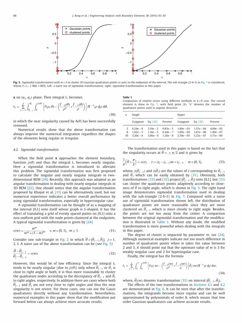
When the field point x approaches the element boundary,function ρ̂ðθÞ and thus the integral I1 becomes nearly singular.Here a sigmoidal transformation is introduced to alleviatethis problem. The sigmoidal transformation was first proposedto calculate the singular and nearly singular integrals in two-dimensional BEM [24]. Recently, this approach was adopted as anangular transformation in dealing with nearly singular integrals in3D BEM [22]. One should notice that the angular transformationproposed by Khayat et al. [13] can be alternatively used, but ournumerical experience indicates a better overall performance byusing sigmoidal transformation, especially in hypersingular case.

A sigmoidal transformation can be thought of as a mapping ofthe interval [0,1] onto itself whose graph is S-shaped. It has theeffect of translating a grid of evenly spaced points on [0,1] onto anon-uniform grid with the node points clustered at the endpoints.A typical sigmoidal transformation is given by [24]

sðwÞ ¼ wm

wmþð1�wÞm; s;wA ½0;1�; mZ1: ð31Þ

Consider one sub-triangle in Fig. 2 in which θA ½θ j�1;θ j�; j¼ 1;2;3. A naive use of the above transformation can be (see Fig. 5)

θ�θ j�1

θ j�θ j�1

¼ sðwÞ: ð32Þ

However, this would be of low efficiency. Since the integral I1tends to be nearly singular (due to ρ̂ðθÞ) only when θ j�1 or θ j isclose to right angle or both, it is thus more reasonable to clusterthe quadrature nodes according to the discrepancy of θ j�1 and θ j

to right angles, respectively. In addition there are cases where bothθ j�1 and θ j are not very close to right angles and thus the nearsingularity is not severe. For these cases, one can use the Gaussquadratures directly without any transformation. Nevertheless,numerical examples in this paper show that the modification putforward below can always achieve more accurate results.

The transformation used in this paper is based on the fact thatthe singularity occurs at θ ¼ 7π=2 and is given by

1π

θþπ2

¼ sðzÞ; z¼ ðzj�zj�1Þwþzj�1; wA ½0;1�; ð33Þ

where, zðθ j�1Þ and zðθ jÞ are the values of z corresponding to θ j�1

and θ j which can be easily obtained by (31). Obviously, bothtransformations (33) and (32) project ½θ j�1;θ j� onto [0,1], but (33)can cluster the quadrature points adaptively according to close-ness of θ to right angle, which is shown in Fig. 5. The right handimage demonstrates sigmoidal transformation used in dealingwith the sub-triangle (2-b-3) in Fig. 7. Compared with a naiveuse of sigmoidal transformation shown left, the distribution ofquadrature points are more reasonable since they are moreclustered on θ j�1 which is more closely to right angle. Besides,the points are not too away from the center. A comparisonbetween the original sigmoidal transformation and the modifica-tion is illustrated in Table 1. Without any doubt, the modifiedtransformation is more powerful when dealing with the integralsin this paper.

The degree of cluster is impacted by parameter m, see [24].Although numerical examples indicate not too much difference innumber of quadrature points when m takes the value between2 and 3, it should point out that the optimum value of m is 3 forweakly singular case and 2 for hypesingular case.

Finally, the integral has the formula

I1 ¼ ∑3

j ¼ 1

Z 1

0

Z ρ̂ðθÞ

0Fðρ;wÞ� f �2ðwÞ

ρ2 þ f �1ðwÞρ

� �� �θ j′ðwÞjT�1jρ dρ dw;

ð34Þ

where, θ jðwÞ denotes transformation (33) on interval ½θ j�1;θ j�.The effects of the two transformations in Sections 4.1 and 4.2

are demonstrated in Fig. 6. It can be seen that after the transfor-mations, the integrands become more regular and can be wellapproximated by polynomials of order 8, which means that loworder Gaussian quadratures can achieve accurate results.

Fig. 5. Sigmoidal transformation with m¼3 to cluster 10 Gaussian quadrature points (x-axis) to the endpoints of the interval. The sub-triangle (2-b-3) in Fig. 7 is considered,whose θA ½�1:466;1:005�. Left: a naive use of sigmoidal transformation; right: sigmoidal transformation in this paper.

Table 1Comparison of relative errors using different methods in k¼0 case. The curvedelement is show in Fig. 7, with field point (b). “n” denotes the number ofquadrature points used in angular direction.

n Single Hyper

Guiggiani Eq. (32) Present Guiggiani Eq. (32) Present

5 6.24e�4 3.19e�3 9.83e�5 1.80e�03 1.57e�04 4.09e�058 1.02e�3 1.16e�5 6.44e�7 1.69e�04 1.87e�06 1.49e�07

10 3.20e�4 3.06e�6 1.26e�8 2.39e�05 5.22e�07 3.71e�09

J. Rong et al. / Engineering Analysis with Boundary Elements 38 (2014) 83–9388

4.3. Analytical integration of the line integrals

Consider the evaluation of the regular one-dimensional integralI2 in Eq. (16), i.e., I2 ¼∑3

j ¼ 1IðjÞ2 and

IðjÞ2 ¼Z θj

θj� 1

f �1ðθÞ ln ρ̂ðθÞ� f �2ðθÞ1

ρ̂ðθÞ

� �dθ: ð35Þ

One notes that the integrand of I2 suffers from the samedifficulties as that of the double integral I1 as stated in Section 3.2.The above proposed transformations can also be used to promote theefficiency of the numerical quadratures.

In this section close form expression for I2 is derived. It isattributed to the fact that after the conformal transformation inSection 4.1 the denominators of fi, i.e. AðθÞ, become constant. ForBurton–Miller equation, it is readily seen from (A.7) that f �2ðθÞ isconstant on each sub-triangle thanks to the constant AðθÞ, and thatf �1ðθÞ is typically made up of combinations of elementarytrigonometric functions of θ [8]

f �1ðθÞ ¼ c1 cos 3 θþc2 cos 2 θ sin θþc3 cos θ sin 2 θþc4 sin 3 θ

þd1 cos θþd2 sin θ: ð36Þ

The coefficients ci and di are given in (A.8). Here we notice that theexpressions in (A.8) are also applicable for Laplace equations. Forother problems, such as elasticity, Stokes flow, the expressions off �2 and f �1 are more complicated and can be derived analogouslyas in Appendix A.

To further simplify the derivation, the coordinate systemðη1;η2Þ is rotated so that the axis oη1 is parallel to the perpendi-cular line of the side of Δ. Thus θ¼ θ over each sub-triangle. Bysubstituting ρ̂ðθÞ, f �2 and f �1 into (35), the integral with f �2becomes

Z θj

θj� 1

f �2ðθÞ1

ρ̂ðθÞ dθ¼ f ðjÞ�2

hj

Z θj

θj� 1

cos θ dθ:

The integral with f �1 consists of terms

ln hj

Z θj

θj� 1

cos p θ sin q θ dθ; pþq¼ 3 or pþq¼ 1; ð37Þ

and

I i ¼Z θj

θj� 1

cos p θ sin q θ ln cos θ dt; pþq¼ 3 or pþq¼ 1: ð38Þ

The explicit expressions of integral (37) can be easily obtained andare omitted. Here the expression of I i is derived. By changing theintegral variable

t ¼ sin θ

cos θ¼ffiffiffiffiffiffiffiffiffiffiffiffi1�t2

pdt ¼

ffiffiffiffiffiffiffiffiffiffiffiffi1�t2

pdθ; ð39Þ

one obtains

I1 ¼Z θj

θj� 1

cos 3 θ ln cos θ dθ¼Z tj

tj� 1

tffiffiffiffiffiffiffiffiffiffiffiffi1�t2

pln

ffiffiffiffiffiffiffiffiffiffiffiffi1� t2

pdt ¼ ~I1� ~I3;

I2 ¼Z θj

θj� 1

cos 2 θ sin θ ln cos θ dθ

¼Z tj

tj� 1

t�t3ffiffiffiffiffiffiffiffiffiffiffiffi1�t2

p lnffiffiffiffiffiffiffiffiffiffiffiffi1�t2

pdt ¼ ~I2� ~I4;

I3 ¼Z θj

θj� 1

cos θ sin 2 θ ln cos θ dθ¼Z tj

tj� 1

t2 lnffiffiffiffiffiffiffiffiffiffiffiffi1�t2

pdt ¼ ~I3;

I4 ¼Z θj

θj� 1

sin 3 θ ln cos θ dθ¼Z tj

tj� 1

t3ffiffiffiffiffiffiffiffiffiffiffiffi1�t2

p lnffiffiffiffiffiffiffiffiffiffiffiffi1�t2

pdt ¼ ~I4;

I5 ¼Z θj

θj� 1

cos θ ln cos θ dθ¼Z tj

tj� 1

lnffiffiffiffiffiffiffiffiffiffiffiffi1�t2

pdt ¼ ~I1;

I6 ¼Z θj

θj� 1

sin θ ln cos θ dθ¼Z tj

tj� 1

tffiffiffiffiffiffiffiffiffiffiffiffi1�t2

p lnffiffiffiffiffiffiffiffiffiffiffiffi1�t2

pdt ¼ ~I2;

ð40Þ

Fig. 6. Integrand of I1 in angular direction corresponding to sub-triangle (2-b-3) in Fig. 7; the basis function is selected as ξ22. Eighth order polynomial is plotted to fit theimage. Left: image of the original Guiggiani's method; right: image after transformations proposed in this paper. (a) Laplace single kernel, m¼3. (b) Laplace hypersingularkernel, m¼2.

J. Rong et al. / Engineering Analysis with Boundary Elements 38 (2014) 83–93 89

where

~I1 ¼Z tj

tj� 1

lnffiffiffiffiffiffiffiffiffiffiffiffi1�t2

pdt ¼ tðln

ffiffiffiffiffiffiffiffiffiffiffiffi1�t2

p�1þ ln

tþ1ffiffiffiffiffiffiffiffiffiffiffiffi1�t2

p�����tj

tj� 1

;

~I2 ¼Z tj

tj� 1

t lnffiffiffiffiffiffiffiffiffiffiffiffi1�t2

pffiffiffiffiffiffiffiffiffiffiffiffi1�t2

p dt ¼ffiffiffiffiffiffiffiffiffiffiffiffi1�t2

pð1� ln

ffiffiffiffiffiffiffiffiffiffiffiffi1�t2

p�����tj

tj� 1

;

~I3 ¼Z tj

tj� 1

t2 lnffiffiffiffiffiffiffiffiffiffiffiffi1�t2

pdt ¼ 1

9t3ð3 ln

ffiffiffiffiffiffiffiffiffiffiffiffi1�t2

p�1Þ�1

3tþ1

6ln

1þt1�t

�����tj

tj� 1

;

~I4 ¼Z tj

tj� 1

t3 lnffiffiffiffiffiffiffiffiffiffiffiffi1�t2

pffiffiffiffiffiffiffiffiffiffiffiffi1�t2

p dt

¼ffiffiffiffiffiffiffiffiffiffiffiffi1�t2

p 19ð8þt2Þ�1

3ð2þt2Þ ln

ffiffiffiffiffiffiffiffiffiffiffiffi1�t2

p� ������tj

tj� 1

: ð41Þ

5. Numerical examples

Two numerical examples are provided to demonstrate theefficiency and robustness of the method in this paper. The firstone is used to illustrate the superior of the method in this paperto the method in Section 3.1, i.e., the classic polar coordinatestransformation and Guiggiani's method [8], using a sample curvedelement. The second one is used to verify the accuracy andconvergence of the method when employed in solving Burton–Miller equation. The method is implemented in C language. Thenumerical integration code are freely available.

The focus of this paper is to improve the performance of thequadrature in angular direction, while in radial direction, asexplained in Section 3.2, the integrand behaves well so that onlya small number of quadrature points are sufficient. In Section 5.16 points are used in every test in radial direction. However, whenimplemented in BEM programs, fewer points are needed becauseas the subdivision of the model the diameter of each element willdecrease so that fewer terms are needed in expansion (15) toapproximate the integrand. As a result, the rate of convergence ofBEM will not be affected. For the 2th order Nyström BEM inSection 5.2, we use 3 points in polar direction.

5.1. Accuracy of the method on a curved element

The accuracy, effectiveness and robustness of the method inthis paper are investigated. The integrals is performed over acurved element extracted from a cylinder surface. The size of thecylinder and the element are given in Fig. 7. Distance s in Fig. 7is designed to change the aspect ratio of the element. s¼0.5represents a quite regular element; the quality of the elementbecomes bad as the increase of s. Four positions for the fieldpoint x are considered, which correspond to intrinsic coordi-nates (a) ξ¼ ð0:3;0:3Þ, (b) ξ¼ ð0:1;0:8Þ, (c) ξ¼ ð0:45;0:45Þ, (d) ξ¼ð0:64;0:31Þ, respectively. One should note that points (b) and (c)match approximately with the nodes of the 2th order Nyströmdiscretization, while (d) match with that of the 3th order.In addition, for the rather centered point (a) the original Guiggiani'smethod in Section 3.1 are believed to work well.

Since no analytical solutions are available, the (relative) error,given by

relative error¼ jIcalc� Iref jjIref j

is evaluated by comparison with the results Iref of the Guiggiani'smethods using Gauss quadratures with 256 quadrature points inangular direction and 32 points in radial direction. Icalc denotes theresult calculated by the various methods. The single layer operator

S and the hypersingular operator H are tested. The parameter m insigmoidal transformation takes the value of 3 in weakly singularcase and 2 in hypersingular case. The basis function ϕ is selectedas the second order monomial ξ22.

A description of the methods tested are listed in Table 2. Themethod in this paper are indicated by “Present” in which the lineintegral I2 in (16) is computed by Gauss quadratures; while in“Presentþa” the line integral is computed by using the closedformulations in Section 4.3. Note that “Presentþa” only validatesfor hypersingular integrals.

5.1.1. Results for regular elementFirst the performance of the present method for regular

element are verified; for this purpose, we let s¼0.5. The wave-number k is selected as 2.0 so that the wavelength is about 3 timessize of the triangular element. In practical BEM implementationsuch a mesh is rather coarse.

Convergence behavior of the original methods and the presentmethod for the four field points are illustrated in Fig. 8. The resultsof the present method are marked by triangles or circles. Theresults for single layer kernel are plotted with dashed line, whilereal lines are for hypersingular integrals. A comparison betweencase (a) and the other three cases shows that the originalGuiggiani's method tends to converge slowly when the field pointis closed to the element boundary; while the present method canachieve almost the same fast convergence. Even in regular case(a) in which the Guiggiani's method performs better than otherthree cases, the benefit of the present method is also obvious.

The effect of each transformation scheme in Section 4 is studiedand exhibited in Table 3. The hypersingular operator with fieldpoint (d) is tested. It is readily to see that the accuracy can beimproved by only using the sigmoidal transformation; whereas

Fig. 7. Curved element and the field points in Example 1.

Table 2Methods to compare.

Methods Description

Guiggiani Guiggiani's method in Section 3.1Guiþsig Guiggiani's method with a sigmoidal

transformation applied in angular directionPresent Method in this paper, i.e. Guiggiani's method

with the two transformations in Section 4Presentþa Similar to “Present”, except that the line integral

is calculated analytically

J. Rong et al. / Engineering Analysis with Boundary Elements 38 (2014) 83–9390

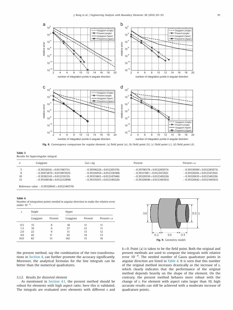
the present method, say the combination of the two transforma-tions in Section 4, can further promote the accuracy significantly.Moreover, the analytical formulas for the line integrals can bebetter than the numerical quadratures.

5.1.2. Results for distorted elementAs mentioned in Section 4.1, the present method should be

robust for elements with high aspect ratio; here this is validated.The integrals are evaluated over elements with different s and

k¼0. Point (a) is taken to be the field point. Both the original andpresent methods are used to compute the integrals with relativeerror 10�8. The needed number of Gauss quadrature points inangular direction are listed in Table 4. It is seen that this numberof the original method increases drastically as the increase of s,which clearly indicates that the performance of the originalmethod depends heavily on the shape of the element. On thecontrary, the present method behaves more robust with thechange of s. For element with aspect ratio larger than 10, highaccurate results can still be achieved with a moderate increase ofquadrature points.

Fig. 8. Convergence comparison for regular element. (a) field point (a). (b) field point (b). (c) field point (c). (d) field point (d).

Table 3Results for hypersingular integral.

n Guiggiani Guiþsig Present Presentþa

5 �0.39218541þ0.011746751i �0.39596226þ0.012205176i �0.39798378þ0.012285073i �0.39330589þ0.012285073i8 �0.39472870þ0.011987825i �0.39326954þ0.012338188i �0.39317481þ0.012347202i �0.39320416þ0.012347202i

10 �0.39382143þ0.012119135i �0.39331863þ0.012347940i �0.39320550þ0.012349226i �0.39320619þ0.012349226i12 �0.39348546þ0.012212898i �0.39319293þ0.012349226i �0.39320640þ0.012349363i �0.39320642þ0.012349363i

Reference value �0.39320643þ0.012349370i

Table 4Number of integration points needed in angular direction to make the relative errorunder 10�8.

s Single Hyper

Guiggiani Present Guiggiani Present Presentþa

0.5 15 8 18 11 111.5 19 9 27 12 112.0 22 9 31 13 124.0 42 11 62 14 13

10.0 82 13 142 15 16 Fig. 9. Geometry model.

J. Rong et al. / Engineering Analysis with Boundary Elements 38 (2014) 83–93 91

5.2. An exterior sound radiation problems

The overall performance of the present integration method istested by incorporating it into a Nyström BEM code for solving theBurton–Miller equation. The geometry of the problem consistsof three sections of cylinders, as shown in Fig. 9. The origin ofcoordinate system lies on the middle point of the symmetry axis ofthe cylinder. All the surfaces of the cylinder vibrate with givenvelocity qðxÞ ¼ ∂u=∂x (Neumann problem), where u is chosen to bethe fundamental solution uðxÞ ¼ Gðx; yÞ in (3) with y¼ ð0;0;0Þ.

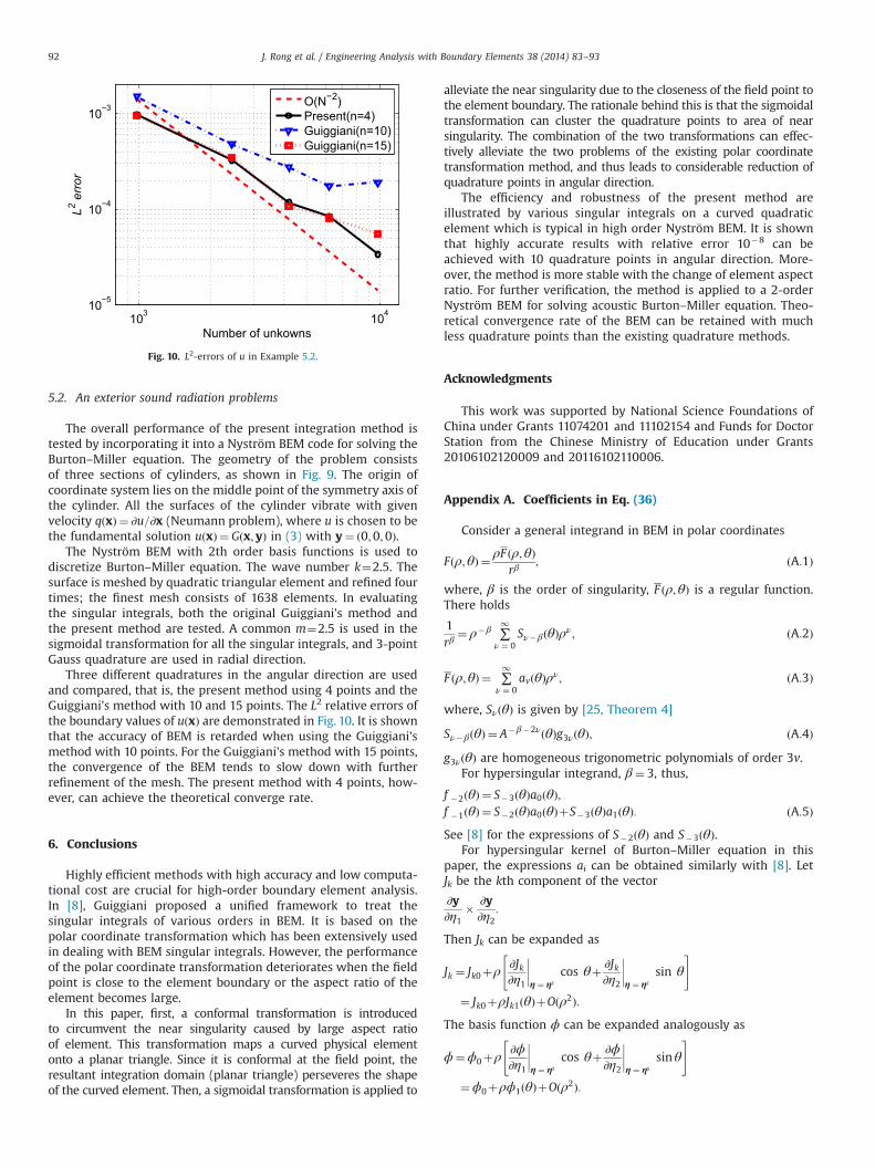
The Nyström BEM with 2th order basis functions is used todiscretize Burton–Miller equation. The wave number k¼2.5. Thesurface is meshed by quadratic triangular element and refined fourtimes; the finest mesh consists of 1638 elements. In evaluatingthe singular integrals, both the original Guiggiani's method andthe present method are tested. A common m¼2.5 is used in thesigmoidal transformation for all the singular integrals, and 3-pointGauss quadrature are used in radial direction.

Three different quadratures in the angular direction are usedand compared, that is, the present method using 4 points and theGuiggiani's method with 10 and 15 points. The L2 relative errors ofthe boundary values of uðxÞ are demonstrated in Fig. 10. It is shownthat the accuracy of BEM is retarded when using the Guiggiani'smethod with 10 points. For the Guiggiani's method with 15 points,the convergence of the BEM tends to slow down with furtherrefinement of the mesh. The present method with 4 points, how-ever, can achieve the theoretical converge rate.

6. Conclusions

Highly efficient methods with high accuracy and low computa-tional cost are crucial for high-order boundary element analysis.In [8], Guiggiani proposed a unified framework to treat thesingular integrals of various orders in BEM. It is based on thepolar coordinate transformation which has been extensively usedin dealing with BEM singular integrals. However, the performanceof the polar coordinate transformation deteriorates when the fieldpoint is close to the element boundary or the aspect ratio of theelement becomes large.

In this paper, first, a conformal transformation is introducedto circumvent the near singularity caused by large aspect ratioof element. This transformation maps a curved physical elementonto a planar triangle. Since it is conformal at the field point, theresultant integration domain (planar triangle) perseveres the shapeof the curved element. Then, a sigmoidal transformation is applied to

alleviate the near singularity due to the closeness of the field point tothe element boundary. The rationale behind this is that the sigmoidaltransformation can cluster the quadrature points to area of nearsingularity. The combination of the two transformations can effec-tively alleviate the two problems of the existing polar coordinatetransformation method, and thus leads to considerable reduction ofquadrature points in angular direction.

The efficiency and robustness of the present method areillustrated by various singular integrals on a curved quadraticelement which is typical in high order Nyström BEM. It is shownthat highly accurate results with relative error 10�8 can beachieved with 10 quadrature points in angular direction. More-over, the method is more stable with the change of element aspectratio. For further verification, the method is applied to a 2-orderNyström BEM for solving acoustic Burton–Miller equation. Theo-retical convergence rate of the BEM can be retained with muchless quadrature points than the existing quadrature methods.

Acknowledgments

This work was supported by National Science Foundations ofChina under Grants 11074201 and 11102154 and Funds for DoctorStation from the Chinese Ministry of Education under Grants20106102120009 and 20116102110006.

Appendix A. Coefficients in Eq. (36)

Consider a general integrand in BEM in polar coordinates

Fðρ;θÞ ¼ ρF ðρ;θÞrβ

; ðA:1Þ

where, β is the order of singularity, F ðρ;θÞ is a regular function.There holds

1rβ

¼ ρ�β ∑1

ν ¼ 0Sν�βðθÞρν; ðA:2Þ

F ðρ;θÞ ¼ ∑1

ν ¼ 0avðθÞρν; ðA:3Þ

where, SνðθÞ is given by [25, Theorem 4]

Sν�βðθÞ ¼ A�β�2νðθÞg3νðθÞ; ðA:4Þg3νðθÞ are homogeneous trigonometric polynomials of order 3v.

For hypersingular integrand, β¼ 3, thus,

f �2ðθÞ ¼ S�3ðθÞa0ðθÞ;f �1ðθÞ ¼ S�2ðθÞa0ðθÞþS�3ðθÞa1ðθÞ: ðA:5ÞSee [8] for the expressions of S�2ðθÞ and S�3ðθÞ.

For hypersingular kernel of Burton–Miller equation in thispaper, the expressions ai can be obtained similarly with [8]. LetJk be the kth component of the vector

∂y∂η1

� ∂y∂η2

:

Then Jk can be expanded as

Jk ¼ Jk0þρ∂Jk∂η1

����η ¼ ηs

cos θþ ∂Jk∂η2

����η ¼ ηs

sin θ

#"

¼ Jk0þρJk1ðθÞþOðρ2Þ:The basis function ϕ can be expanded analogously as

ϕ¼ϕ0þρ∂ϕ∂η1

����η ¼ ηs

cos θþ ∂ϕ∂η2

����η ¼ ηs

sinθ

#"

¼ϕ0þρϕ1ðθÞþOðρ2Þ:

103 10410−5

10−4

10−3

Number of unkowns

L2 err

or

O(N−2)Present(n=4)Guiggiani(n=10)Guiggiani(n=15)

Fig. 10. L2-errors of u in Example 5.2.

J. Rong et al. / Engineering Analysis with Boundary Elements 38 (2014) 83–9392

Then, a0 and a1ðθÞ in Eq. (A.5) can be expressed as (repeatedindices imply summation)

a0 ¼niðxÞ4π

Ji0ϕ0;

a1ðθÞ ¼niðxÞ4π

½Ji1ðθÞϕ0þ Ji0ϕ1ðθÞ�: ðA:6Þ

Substituting Eq. (A.6) into Eq. (A.5), yields

f �1ðθÞ ¼ c1 cos 3 θþc2 cos 2 θ sin θþc3 cos θ sin 2 θþc4 sin 3 θ

þd1 cos θþd2 sin θ;

f �2ðθÞ ¼niðxÞ4πA3Ji0ϕ0: ðA:7Þ

with

c1 ¼ �3niðxÞJi0ϕ0

8πA5

∂yk∂η1

∂2yk∂η21

;

c2 ¼ �3niðxÞJi0ϕ0

4πA5

∂yk∂η1

∂2yk∂η1∂η2

þ12∂yk∂η2

∂2yk∂η21

!;

c3 ¼ �3niðxÞJi0ϕ0

4πA5

∂yk∂η2

∂2yk∂η1∂η2

þ12∂yk∂η1

∂2yk∂η22

!;

c4 ¼ �3niðxÞJi0ϕ0

8πA5

∂yk∂η2

∂2yk∂η22

;

d1 ¼niðxÞ4πA3

∂Ji∂η1

ϕ0þ Ji0∂ϕ∂η1

� �;

d2 ¼niðxÞ4πA3

∂Ji∂η2

ϕ0þ Ji0∂ϕ∂η2

� �: ðA:8Þ

Note that all the derivatives are evaluated at the field point x.

References

[1] Canino LF, Ottusch JJ, Stalzer MA, Visher JL, Wandzurz SM. Numerical solutionof the Helmhotz equation in 2D and 3D using a high-order Nyströmdiscretization. J Comput Phys 1998;146:627–33.

[2] Rjasanow S, Weggler L. ACA accelerated high order BEM for Maxwellproblems. Comput Mech 2013;51:431–41.

[3] Bremer J, Gimbutas Z. A Nyström method for weakly singular integraloperators on surfaces. J Comput Phys 2012;231:4885–903.

[4] Gao XW, Davies TG. Boundary element programming in mechanics.Cambridge University Press; 2002 (ISBN: 052177359-8).

[5] Willis DJ, Peraire J, White JK. A quadratic basis function, quadratic geometry,high order panel method. In: 44th AIAA aerospace sciences meeting, numberAIAA-2006-1253; 2006.

[6] Wu HJ, Liu YJ, Jiang WK. A low frequency fast multiploe boundary elementmethod based on analytical integration of the hypersingular integral for 3Dacoustic problems. Eng Anal Boundary Elem 2013;37:309–18.

[7] Fata SN. Explicit expressions for 3D boundary integrals in potential theory. IntJ Numer Methods Eng 2009;78:32–47.

[8] Guiggiani M, Krishnasamy G, Rudolphi TJ, Rizzo FJ. A general algorithm for thenumerical solution of hypersingular boundary integral equations. ASME J ApplMech 1992;59:604–14.

[9] Järvenpää S, Taskinen M, Ylä-Oijala P. Singularity extraction technique forintegral equation methods with higher order basis functions on planetriangles and tetrahedra. Int J Numer Methods Eng 2003;58:1149–65.

[10] Kolm P, Rokhlin V. Numerical quadratures for singular and hypersingularintegrals. Comput Math Appl 2001;41:327–52.

[11] Graglia RD, Lombardi G. Machine precision evaluation of singular and nearlysingular potential integrals by use of Gauss quadrature formulas for rationalfunctions. IEEE Trans Antennas Propag 2008;56:981–98.

[12] Carley M. Numeriacl quadratures for singular and hypersingular integrals inboundary element methods. SIAM J Sci Comput 2007;29:1207–16.

[13] Khayat MA, Wilton DR, Fink PW. An improved transformation and optimizedsampling scheme for the numberical evaluation of singular and near-singularpotentials. IEEE Trans Antennas Propag 2008;7:377–80.

[14] Khayat MA, Wilton DR. Numerical evaluation of singular and near-singularpotential integrals. IEEE Trans Antennas Propag 2005;53:3180–90.

[15] Duffy MG. Quadrature over a pyramid or cube of integrands with a singularityat a vertex. SIAM J Numer Anal 1982;19(6):1260–2.

[16] Johnston BM, Johnston PR. A comparsion of transformation methods forevaluating two-dimensional weakly singular integrals. Int J Numer MethodsEng 2003;56:589–607.

[17] Huang Q, Cruse TA. Some notes on singular integral techniques in boundaryelement analysis. Int J Numer Methods Eng 1993;36:2643–59.

[18] Chen JT, Hong HK. Review of dual boundary element methods with emphasison hypersingular integrals and divergent series. ASME Appl Mech Rev1999;52:17–33.

[19] Gao XW. An effective method for numerical evaluation of gneral 2D and 3Dhigh order singular boundary integrals. Comput Methods Appl Mech Eng2010;199:2856–64.

[20] Scuderi L. On the compuation of nearly singular integrals in 3D BEMcollocation. Int J Numer Methods Eng 2008;74:1733–70.

[21] Hayami K. Variable transformation for nearly singular integrals in the boun-dary element method. Res Inst Math Sci 2005;41:821–42 Kyoto University.

[22] Johnston BM, Johnston PR, Elliott D. A new method for the numericalevaluation of nearly singular integrals on triangular elements in the 3Dboundary element method. J Comput Appl Math 2013;245:148–61.

[23] Burton AJ, Miller GF. The application of integral equation methods to thenumerical solution of some exterior boundary-value problems. Proc R SocLondon Ser A 1971;323:201–10.

[24] Johnston PR. Application of sigmoidal transformations to weakly singularand near-singular boundary element integrals. Int J Numer Methods Eng1999;45:1333–48.

[25] Schwab C, Wendland WL. Kernel properties and representations of boundaryintegral operators. Math Nachr 1992;156:187–218.

J. Rong et al. / Engineering Analysis with Boundary Elements 38 (2014) 83–93 93