Finite element modeling of erosive wear

Finite element modeling of erosive wear

M.S. ElTobgy*, E. Ng, M.A. Elbestawi

McMaster Manufacturing Research Institute, McMaster University JHE 316, 1280 Main St. W, Hamilton, ON, Canada L8S 4L7

Received 3 June 2004; accepted 13 January 2005

Available online 3 March 2005

Abstract

Material damage caused by the attack of particles entrained in a fluid system impacting a surface at high speed is called ‘Erosion’. Erosion

is a phenomenon that takes place in several engineering applications. It also can be used in several manufacturing process such as abrasive

waterjet machining. Erosion is a complex process dependent on particle speed, size, angle of attack as well as the behavior of the eroded

material. Extensive experimental results have been reported in the literature on the erosion of different materials. Simulating the erosion

process through finite element enables the prediction of erosion behavior of materials under different conditions, which will substitute the

need of experimentation, and will enable the identification of constants required for existing analytical models.

In this paper, an elasto-plastic finite element (FE) model is presented to simulate the erosion process in 3D configuration. The FE model takes

into account numerical and material damping, thermal elastic–plastic material behavior and the effect of multiple particle impacts as well as

material removal. The workpiece material modeled was Ti–6Al–4V. The effects of strain hardening, strain rate and temperature were considered

in the non-linear material model. Comparison against results reported in literature and erosion models by Finnie, Bitter and Hashish are made. It

is shown that the predicted results are in agreement with published results obtained experimentally and from analytical erosion models.

q 2005 Elsevier Ltd. All rights reserved.

Keywords: Erosion; Finite element modeling; Elastic–plastic

1. Introduction

The erosion of materials caused by impact of hard

particles is one of several forms of material degradation

generally classified as wear. Bitter [1] defined erosion as

“Material damage caused by the attack of particles entrained

in a fluid system impacting the surface at high speed” while

Hutchings [2] wrote “Erosion is an abrasive wear process in

which the repeated impact of small particles entrained in a

moving fluid against a surface results in the removal of

material from that surface”. Solid particle erosion is a

serious problem in gas turbines, rocket nozzles, cyclone

separators, valves, pumps and boiler tubes. However, solid

particle erosion can be utilized in manufacturing processes

such as abrasive waterjet cutting.

Removal of material occurs through the processes of

micro-plastic deformation and/or brittle fracture. For ductile

0890-6955/$ - see front matter q 2005 Elsevier Ltd. All rights reserved.

doi:10.1016/j.ijmachtools.2005.01.007

* Corresponding author. Tel.: C1 905 525 9140x24058; fax: C1 905 572

7944.

E-mail address: [email protected] (M.S. ElTobgy).

materials such as pure metals and alloys, the impact of the

hard particles causes severe, localized plastic strain at the

impact site on the surface. Material is removed when

the strain exceeds the material’s strain-to-failure. For brittle

materials, such as ceramic and intermetallic compounds, the

force of the impacting particle causes localized cracking at

the surface. With subsequent impact events, these cracks

propagate and eventually link together, and as a result,

material becomes detached from the surface [3]. As a

consequence, the particle impingement angle on the surface

affects each material in a different manner. Material loss for

ductile metals tends to peak at an oblique angle of

impact, typically between 20 and 308. However, material

loss for brittle materials tends to increase with increasing

impingement angle with maximum material loss occurring

at 908 [4]. Alman’s [3] studies on both ceramics and

metals suggest that the attack angle is the best indicator

for the erosion mechanism. Ductile materials exhibit

maximum erosion rates at attack angles of about 20–408

while brittle materials exhibit a maximum erosion rate at an

angle of 908.

No external forces act on the impacting particle other

than the contact forces exerted by the work piece material

International Journal of Machine Tools & Manufacture 45 (2005) 1337–1346

www.elsevier.com/locate/ijmactool

http://www.elsevier.com/locate/ijmactool

M.S. ElTobgy et al. / International Journal of Machine Tools & Manufacture 45 (2005) 1337–13461338

surface. The contact forces are responsible for the

deceleration of the impacting particle [2].

Variables affecting the erosion can be broadly classified

into three types [5]:

(1)
impingement variables describing the particle flow:
† particle velocity

† angle of impact

† particle concentration

(2)
particle variables:
† particle shape

† particle density

† particle size

(3)
material variables (workpiece and particles):
† Young’s modulus

† Poisson’s ratio

† plastic behavior

† failure behavior

A literature review on erosion theoretical models indicates

that various models, if supported by an appropriate tuning of

certain parameters, can be made to perform well. However, a

continuous tuning of these parameters is required.

Experimentally, one may measure volume loss or weight

loss of a material and investigate the erosion mechanism by

analyzing the worn surface and the erosion conditions.

However, erosion is a complex process, affected by many

factors. The interaction of these factors makes it difficult to

explain all information obtained experimentally. Computer

modeling allows ‘computational experiments’ under con-

trolled conditions to be performed. The effect of each

parameter on an erosion process can thus be studied

separately. Therefore, computer modeling provides an

effective method, complementary to experimental tech-

niques, for fundamental understanding of solid particle

erosion and for predicting material performance during

erosion processes. Several attempts have been made

previously to model the erosion using the finite element

method, Elalem and Li [6] presented a dynamic simulation

model (MSDM) in which they used an algorithm similar to

that used in the explicit formulation in FEM. The model

included strain hardening and material failure. However,

they simplified the erosion problem to a 2D configuration

which neglected the effect of the third component of strain

on the strain hardening and fracture strain. An axisymmetric

model would have been more accurate in this case (where

no dependency on impact angle is studied).

Chen et al. [7] extended the work on the MSDM. They

studied the effect of impact angle, velocity and shape of the

particle on erosion of ductile and brittle materials. The

predicted trends using the MSDM model are the same as

reported in literature both experimentally and analytically.

However, no comparisons were made for the magnitudes of

the erosion rates.

Shimizu et al. [8] studied the erosion of a structural mild

steel, SS400, and a ferritic spherical-graphite cast iron, FDI,

experimentally and through simulation. They simulated the

impact of a single particle and concluded that there should be

an intimate relationship between the erosion rate and the

protrusions at theedge ofan impressiondue toasingleparticle

impact. The FE simulation model did not include any failure

criteria and they made the assumption of plane strain. No

direct relation was established between the edge protrusion

and the erosion rate. The authors believe that this conclusion

is valid only for a small range of particles speeds where

material is removed by accumulation of plastic deformations.

Aquaro and Fontani [5] presented a comprehensive study

on erosion modeling; they used FE simulations to predict

the constant in the equations of some analytical models.

They used an Eulerian model for ductile behavior and a

Lagrangian model for brittle behavior. However, ductile and

brittle behavior should not be modeled separately, as it is

believed by most researchers that both ductile and brittle

behavior occur simultaneously in proportions depending on

the material properties and the impact stress states. Further

details on the modeling approach and the results obtained

are discussed in the following sections.

2. Erosion modeling

2.1. Finnie model for ductile erosion

Finnie [9,10] was the first to derive a single-particle

erosive cutting model. This model sets the main concepts

and assumptions for many subsequent single-particle

erosion models. The model assumes a hard particle with

velocity V impacting a surface at an angle a. The material of

the surface is assumed to be a rigid plastic one. The final

expression and boundary conditions for the volume of

material removed from the workpiece material due to the

impact of a single particle can be obtained from Eq. (1) by

Finnie [10]

W Z

mV2

Jpksinð2aÞK

6

ksin2ðaÞ

� �; tan a%

k

6

mV2

Jpk

k cos2ðaÞ

6

� �; tan aO

k

6

8>><>>: (1)

where a is the attack angle, k is the ratio of vertical to

horizontal force components, and J is the ratio of the depth

of contact l to the depth of the cut (Yt) as shown in Fig. 1, V

is the abrasive particle velocity, p is the flow stress of the

eroded workpiece material and W is the total volume of

target material removed.

The total volume removed by multiple particles having a

total mass M can be obtained from Eq. (2) [10]:

W Zc

MV2

Jpksinð2aÞK

6

ksin2ðaÞ

� �; tan a%

k

6

cMV2

Jpk

k cos2ðaÞ

6

� �; tan aO

k

6

8>><>>: (2)

Fig. 1. Depth of cut length of contact as given in [10].

M.S. ElTobgy et al. / International Journal of Machine Tools & Manufacture 45 (2005) 1337–1346 1339

The constant c is used to compensate for the particles that

do not follow the ideal model (some particles impact with

each other, or fracture during erosion), M is the total mass of

abrasive particles. Although, Finnie model for erosion is

oversimplified and very old, it is considered as the milestone

of erosion modeling and provides the basis for future

modeling of the process. It is only valid for ductile

materials, and does not include any brittle fracture behavior

of the material.

2.2. Bitter model for erosion

The Bitter model [1,4] makes the hypothesis that the

loss of material is the sum of material lost due to plastic

deformation WD (during the impact the material elastic

limit is exceed, the surface layer is destroyed and

fragments of it are removed) and material lost due to

cutting WC (the particle strikes the body scratching out

some material from the surface). Bitter used an approach

based on the Hertzian contact theory and making use of

the energy balance equation. In his analysis Bitter

assumed that deformation and cutting erosion occur

simultaneously and their effects can be superimposed.

Bitter introduces the concept of threshold velocity where a

particle cannot erode the workpiece if its velocity is less

than a threshold velocity Vel.

The particle velocity V can be resolved in two

components, one normal to the body surface and another

tangential to it. The normal component is responsible for the

particle penetration in the body while the tangential

component induces the particle scratching action. Depend-

ing on whether the particle velocity tangential to the body

becomes zero during the collision, two expressions of the

volume of material removed by cutting wear can be

evaluated.

Total wear is a summation of brittle wear and ductile

wear. The brittle wear (deformation wear) is calculated

using Eq. (3)

Wd ZM½V sin a KVel�

2

23b

; V sinðaÞOVel

0; V sinðaÞ!Vel

8<: (3)

where a is the attack angle, 3b is the deformation wear factor

(obtained experimentally), and Vel is the threshold velocity

(velocity at collision at which the elastic limit of the

workpiece material is just reached). Vel can be calculated

from the Hertzian contact theory using Eq. (4)

Vel Z1:54s5=2

yffiffiffiffiffirp

p1 Kn2

p

Ep

C1 Kn2

t

Et

� �(4)

where sy is the elastic load limit, rp is the particle density, np

and nt are the Poission’s ratios, and Ep and Et are the moduli

of elasticity of the particle and target workpiece respect-

ively. The threshold velocity Vel can be computed from the

approach velocity V and the rebound velocity V2 as shown in

Eq. (5), given in [1]:

V2 Zffiffiffiffiffiffiffiffiffiffiffiffiffiffiffiffiffiffiffiffiffiffiffi2VVel KV2

el

q(5)

For the ductile erosion mode (cutting wear mode), Bitter

calculates the volume removed as shown in Eq. (6)

Wc Z

2MC 0½V sin a KVel�2ffiffiffiffiffiffiffiffiffiffiffiffiffiffiffi

V sin ap

! V cos a KC 0½V sin a KVel�

2ffiffiffiffiffiffiffiffiffiffiffiffiffiffiffiV sin a

p fc

� �; a%a0

MfV2 cos2 a KK1½V sin a KVel�3=2g

2fc

; aRa0

8>>>>>>><>>>>>>>:

(6)

where fc is a material dependant wear factor obtained

experimentally and C 0, K1 are constants obtained from Eqs.

(7) and (8):

C 0 Z0:288

sy

ffiffiffiffiffiffirp

sy

4

r(7)

K1 Z 0:82s2y

ffiffiffiffiffiffisy

rp

4

s1 Kn2

p

Ep

C1 Kn2

t

Et

� �(8)

The angle a0 is estimated using Eq. (2).

Applying Bitter model requires the knowledge of the two

wear factors fc, 3b which have to be determined exper-

imentally. However, those two factors are dependant on

other parameters such as particle speed, size, as well as the

erodent, thus experimental identification of those factors for

each set of process parameters is required.

Bitter was the first to address the brittle behavior of

materials, several models followed the same foundations

laid by Bitter. However, all of them still require the

experimentally determined constants.

Table 1

Constants for Eq. (12)

A (MPa) B (MPa) n C m

1098 1092 0.93 0.014 1.1


2.3. Neilson and Gilchrist’s erosion model

Neilson and Gilchrist’s [11] simplified Bitter’s combined

model by assuming a simplified ductile erosion model while

retaining Bitter model for brittle erosion. Their model is

given in Eq. (9):

W Z

MV2 cos2ðaÞ

2fc

CM½V sinðaÞKVel�

2

23b

; aRa0

MV2 cos2ðaÞsinðnaÞ

2fc

CM½V sinðaÞKVel�

2

23b

; a%a0

8>><>>:

(9)

However, the simplification made still did not provide

any mean of eliminating or reducing the experimental work

required to determine the erosion constants.

2.4. Hashish modified model for erosion

Hashish [12] modified Finnie model for erosion to

include the effect of the particle shape as well as modify the

velocity exponent predicted by Finnie. The final form of his

model, which is more suitable for shallow angles of impact

is given in Eq. (10)

W Z7

p

M

rp

V

Ck

� �2:5

sinð2aÞffiffiffiffiffiffiffiffiffiffisin a

p(10)

where Ck can be computed from Eq. (11)

Ck Z

ffiffiffiffiffiffiffiffiffiffiffiffiffiffiffi3sfR

3=5f

rp

s(11)

where Rf is the particle roundness factor.

One of the main advantages of this model is that it does

not require any experimental constants, in addition, it is the

only model that accounts for the shape of particles.

However, in [12], the author did not perform any validation

or experimental investigation to investigate the accuracy of

the model and its boundaries. This model is only based on

the ductile behavior of material, so it is only suitable for

shallow impact angles for ductile materials.

A new model based on finite element method is presented

in this paper. This model includes only the basic mechanical

properties of the workpiece and the particles materials.

Table 2

Constants for Eq. (13)

d1 d2 d3 d4 d5

K0.09 0.27 0.48 0.014 3.870

3. Finite element modeling

3.1. Material modeling

The workpiece material modelled was Ti–6Al–4V with a

hardness of 35 HRcG2 HRc. The Johnson Cook [13]

material model was employed to model the flow stress

behavior of the target workpiece material. In the Johnson-

Cook model, as detailed in Eq. (12), the flow stress is

expressed as a function of the strain 3, strain hardening

index n, strain rate _3, reference strain rate _30, work piece

temperature T, room temperature Tr, melting temperature

Tm and strain-rate sensitivity index m.

sf Z ðA CB3nÞ 1 CC ln_3

30

� �� 1 K

T KTr

Tm KTr

� �� (12)

A, B, and C are constants acquired experimentally by

Leseur [14] from compressive split Hopkinson bar tests in

punching shear configuration on Ti–6Al–4V. The Johnson-

Cook materials constants for Ti–6Al–4V are detailed in

Table 1.

3.1.1. Failure model

A shear failure criterion was incorporated in the material

model to simulate material removal during the erosion

process. The material failure strain 3f is detailed in Eq. (13),

as a function of non-dimensional plastic strain _3p=_30, a

dimensionless deviatoric-pressure stress ratio sp/se (where

sp is the pressure stress and se is the Von-Mises stress),

computed or modelled work piece temperature T, room

temperature Tr, and melting temperature Tm. The constants

d1, d2, d3 and d4 are acquired from Kay [15] and listed in

Table 2

3f Zðd1 Cd2 ed3ðsp=seÞÞ 1 Cd4 ln3p

30

� ��

! 1 Cd5

T KTr

Tm KTr

� �� ð13Þ

3.1.2. Impacting-particle material

The impacting-particle material simulated was a steel

ball with a density of 7870 kg/m3. In the finite element

model, the impacting-particle material was modeled as a

rigid body (stresses and strains are assumed to be zero in the

impacting particle material.)

3.2. Explicit formulation

Modeling of the erosion process was performed using a

general purpose, commercially available, finite element

solver; ABAQUS/EXPLICIT (version 6.3). The analysis

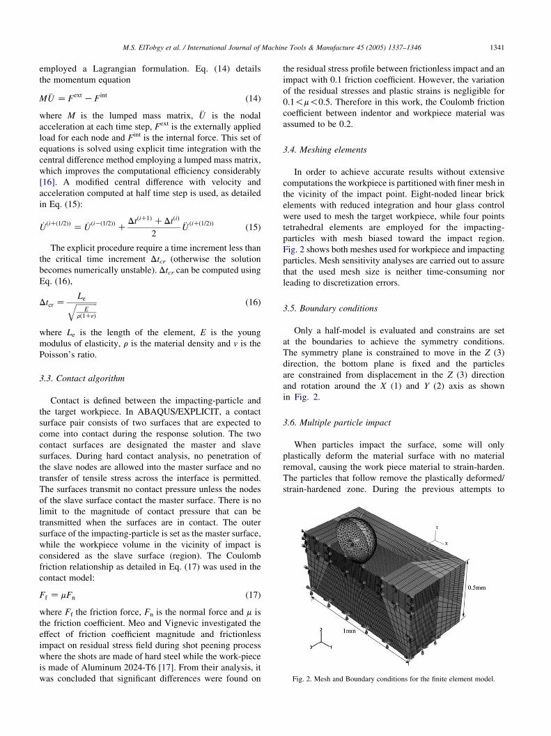
Fig. 2. Mesh and Boundary conditions for the finite element model.


employed a Lagrangian formulation. Eq. (14) details

the momentum equation

M €U Z Fext KFint (14)

where M is the lumped mass matrix, €U is the nodal

acceleration at each time step, Fext is the externally applied

load for each node and Fint is the internal force. This set of

equations is solved using explicit time integration with the

central difference method employing a lumped mass matrix,

which improves the computational efficiency considerably

[16]. A modified central difference with velocity and

acceleration computed at half time step is used, as detailed

in Eq. (15):

_UðiCð1=2ÞÞ Z _UðiKð1=2ÞÞC

DtðiC1Þ CDtðiÞ

2€U ðiCð1=2ÞÞ

(15)

The explicit procedure require a time increment less than

the critical time increment Dtcr (otherwise the solution

becomes numerically unstable). Dtcr can be computed using

Eq. (16),

Dtcr ZLeffiffiffiffiffiffiffiffiffiffiffi

Erð1CnÞ

q (16)

where Le is the length of the element, E is the young

modulus of elasticity, r is the material density and v is the

Poisson’s ratio.

3.3. Contact algorithm

Contact is defined between the impacting-particle and

the target workpiece. In ABAQUS/EXPLICIT, a contact

surface pair consists of two surfaces that are expected to

come into contact during the response solution. The two

contact surfaces are designated the master and slave

surfaces. During hard contact analysis, no penetration of

the slave nodes are allowed into the master surface and no

transfer of tensile stress across the interface is permitted.

The surfaces transmit no contact pressure unless the nodes

of the slave surface contact the master surface. There is no

limit to the magnitude of contact pressure that can be

transmitted when the surfaces are in contact. The outer

surface of the impacting-particle is set as the master surface,

while the workpiece volume in the vicinity of impact is

considered as the slave surface (region). The Coulomb

friction relationship as detailed in Eq. (17) was used in the

contact model:

Ff Z mFn (17)

where Ff the friction force, Fn is the normal force and m is

the friction coefficient. Meo and Vignevic investigated the

effect of friction coefficient magnitude and frictionless

impact on residual stress field during shot peening process

where the shots are made of hard steel while the work-piece

is made of Aluminum 2024-T6 [17]. From their analysis, it

was concluded that significant differences were found on

the residual stress profile between frictionless impact and an

impact with 0.1 friction coefficient. However, the variation

of the residual stresses and plastic strains is negligible for

0.1!m!0.5. Therefore in this work, the Coulomb friction

coefficient between indentor and workpiece material was

assumed to be 0.2.

3.4. Meshing elements

In order to achieve accurate results without extensive

computations the workpiece is partitioned with finer mesh in

the vicinity of the impact point. Eight-noded linear brick

elements with reduced integration and hour glass control

were used to mesh the target workpiece, while four points

tetrahedral elements are employed for the impacting-

particles with mesh biased toward the impact region.

Fig. 2 shows both meshes used for workpiece and impacting

particles. Mesh sensitivity analyses are carried out to assure

that the used mesh size is neither time-consuming nor

leading to discretization errors.

3.5. Boundary conditions

Only a half-model is evaluated and constrains are set

at the boundaries to achieve the symmetry conditions.

The symmetry plane is constrained to move in the Z (3)

direction, the bottom plane is fixed and the particles

are constrained from displacement in the Z (3) direction

and rotation around the X (1) and Y (2) axis as shown

in Fig. 2.

3.6. Multiple particle impact

When particles impact the surface, some will only

plastically deform the material surface with no material

removal, causing the work piece material to strain-harden.

The particles that follow remove the plastically deformed/

strain-hardened zone. During the previous attempts to

Fig. 3. Material removed for several particles impact and plastic strain after impact.


simulate the erosion wear using finite element, only the

effect of a single particle is simulated, which does not

consider the effect of previous particles. In this model,

multiple particles are simulated, with the erosion rate

calculated after each particle impact to take into account the

effect of strain-hardening. After the impact of the first

particle the erosion rate (volume removed per impacting

mass) is very small compared with the effect of the second,

third and fourth particles, respectively. Fig. 3 shows the

volume removed after the impact of one, two and three

particles, respectively. Fig. 4 gives the values of the

cumulative and individual volume removed per particle

and the erosion rate calculated after the impact of one, two,

three and four particles. The erosion rate was very small

after the impact of the first particle and then increased and

stabilized after impacting with three particles. It can be

concluded that simulating a single particle is not sufficient,

three or more particles are needed to simulate the erosion

process.

3.7. Test matrix

Table 3 gives an overview for the three different cases

studied in this work after the number of impacting particles

Fig. 4. Effect of number of simulated particle

has been identified. The first case studies the effect of

particle velocity on the erosion rate for five different

velocities selected in the range of 40–100 m/s

which considers a good range of erosion problems. The

second case is a study on the effect of impact angle on the

erosion rate; seven models are used with impact angles,

ranging from 15 to 808. The third case examines the effect of

particles size on the erosion rate with four size values,

ranging from 300 to 600 mm.

4. Results discussion

4.1. Effect of particle speed on volume removed

Particles impacting the workpiece at different speeds were

simulated using the Finite element model with an impact

angle of 458 for the same workpiece and abrasive materials.

Fig. 5 shows the relation between the erosion rate and the

impact speed plotted on a log–log scale. The relation follows

an exponential form with an exponent of 2.2525. An exponent

of 2 was proposed by Finnie [9] as given in Eq. (2) and 2.5 by

Hashish [12] as given in Eq. (10). Sheldon [18] determined

experimentally the velocity exponent to be in the range of

s on erosion rate and volume removed.

Table 3

Model test parameters

Parameter Phase I effect of

particle velocity

Phase II effect

of impact angle

Phase III effect

of particle size

Velocity (m/s) 40–100 75 75

Impact angle

(degrees)

45 15–80 45

Diameter (mm) 500 500 300–600

3 3 3

Fig. 6. Material removed by a single particle impact at different impacting

angles.


2–3. Yerramareddy [19] performed experiments on the

erosion of Ti–6Al–4V and found that the velocity exponent

is 2.35. Although the finite element simulation does not use

any experimentally determined constants, it was able to

predict the velocity exponent within the same range

proposed and found by other researchers [9,12,18,19]. The

erosion rate increase with the increase of the velocity can be

explained by the increase of the energy content of

the particles. This leads to more erosion of the workpiece

material at the same mass of impacting particles.

4.2. Effect of impact angle on erosion rate

Results shown in Fig. 6 represent volume removed

versus angle of impact. The simulation results show a peak

erosion rate at a 408 angle as shown in Fig. 7, which is a

typical behavior of ductile materials as mentioned in [4,9,

10,19]. The angle at which the peak erosion occur is

material dependant. Yerramareddy [19] performed

experiments on Ti–6Al–4V and found that the maximum

erosion occurs at an angle of 30–358.

Fig. 7 presents the results obtained from the finite

element simulation models compared with results obtained

from Finnie model for erosion given in Eq. (2) and Hashish

model for erosion in Eq. (10). The constants for Finnie

model are KZ4, CZ1 and jZ1, while material constant P

1098 MPa. The FE model agreed with Hashish model for

shallow impact angles and has better agreement for Finnie

model for angles in the mid range (O508). The erosion rates

values predicted from the Finite element model are within

the same order of magnitude when compared with the

values obtained experimentally. Further details about

Fig. 5. Impacting particles velocity vs. erosion rate.

the explanation of the parabolic behavior of ductile

materials can be found in [4,9,10,12]. Comparison with

the Bitter [1,4] and Neilson and Gilchrist [11] models

discussed earlier model are shown in Fig. 8. The FE

simulation results are in a good agreement with the pattern

predicted by Bitter and Neilson and Gilchrist models.

Fig. 9 shows the relation between the penetration depth

and the impact angle. The increasing trend of the

penetration depth can be explained by the increasing normal

component of the velocity. With higher impacting angles,

higher normal component of the velocity exists, causing

deeper penetration with lower material removal. This has

also been also observed by Shimuzu [8].

4.3. Effect of particles size on eroded volume

The simulation results given in Fig. 10 show a

slight increasing trend at the lower range of particle size

(!300 mm) and then a constant trend. A similar trend has

been observed by Tilly [20]; he found through experimental

measurements that the erosion rate tends to increase

considerably at particle size values below 200 mm and

then tends to remain constant. This trend has also been

observed by Yerramareddy [19] during his experimental

investigation.

The erosion rate tends to be constant for the higher

particle size range, because increasing the particle diameter

Fig. 7. Results obtained from Finnie and Hashish Models vs. Finite Element

simulation.

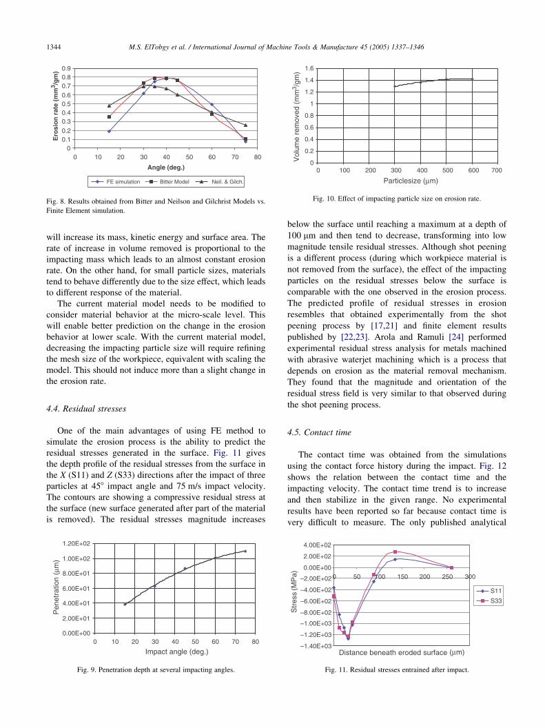
Fig. 8. Results obtained from Bitter and Neilson and Gilchrist Models vs.

Finite Element simulation.

Fig. 10. Effect of impacting particle size on erosion rate.


will increase its mass, kinetic energy and surface area. The

rate of increase in volume removed is proportional to the

impacting mass which leads to an almost constant erosion

rate. On the other hand, for small particle sizes, materials

tend to behave differently due to the size effect, which leads

to different response of the material.

The current material model needs to be modified to

consider material behavior at the micro-scale level. This

will enable better prediction on the change in the erosion

behavior at lower scale. With the current material model,

decreasing the impacting particle size will require refining

the mesh size of the workpiece, equivalent with scaling the

model. This should not induce more than a slight change in

the erosion rate.

4.4. Residual stresses

One of the main advantages of using FE method to

simulate the erosion process is the ability to predict the

residual stresses generated in the surface. Fig. 11 gives

the depth profile of the residual stresses from the surface in

the X (S11) and Z (S33) directions after the impact of three

particles at 458 impact angle and 75 m/s impact velocity.

The contours are showing a compressive residual stress at

the surface (new surface generated after part of the material

is removed). The residual stresses magnitude increases

Fig. 9. Penetration depth at several impacting angles.

below the surface until reaching a maximum at a depth of

100 mm and then tend to decrease, transforming into low

magnitude tensile residual stresses. Although shot peening

is a different process (during which workpiece material is

not removed from the surface), the effect of the impacting

particles on the residual stresses below the surface is

comparable with the one observed in the erosion process.

The predicted profile of residual stresses in erosion

resembles that obtained experimentally from the shot

peening process by [17,21] and finite element results

published by [22,23]. Arola and Ramuli [24] performed

experimental residual stress analysis for metals machined

with abrasive waterjet machining which is a process that

depends on erosion as the material removal mechanism.

They found that the magnitude and orientation of the

residual stress field is very similar to that observed during

the shot peening process.

4.5. Contact time

The contact time was obtained from the simulations

using the contact force history during the impact. Fig. 12

shows the relation between the contact time and the

impacting velocity. The contact time trend is to increase

and then stabilize in the given range. No experimental

results have been reported so far because contact time is

very difficult to measure. The only published analytical

Fig. 11. Residual stresses entrained after impact.

Fig. 12. Effect of impacting-particle velocity on contact time. Fig. 14. Effect of particle size on contact time.


expression for the contact time is given by Tabor [25]

dt Zp

2

ffiffiffiffiffiffiffiffiffiffiffim

2ppr

r(18)

where m is the impacting-particle mass, p is the elastic load

limit and r is the impacting particle radius. The equation

gives the contact time from the time of impact until the

velocity in the normal direction reaches zero. Applied to the

simulation conditions it results in a value of 3eK6 s. Tabor

equation does not include the effect of the impact angle or

the particle velocity, however, it gives a value for contact

time within the same range as that obtained from the finite

element simulation. No previous reports of the effect of

impact angle on the contact time were found in literature.

The effect of the impact angle on the contact time is

shown in Fig. 13. This behavior can be explained by two

opposing effects of the impact angle on the contact time.

The first effect shows higher contact time with lower impact

angle due to ploughing action of the abrasive particles

(decreasing trend). The second effect would be the increase

of contact time with increasing impact angle due to deeper

penetration (increasing trend) as shown in Fig. 9. The

summation of both effects will produce the trend shown in

Fig. 13.

Fig. 14 shows the relation between the particle diameter

and the contact time. The contact time is believed to

Fig. 13. Effect of attack angle on contact time.

increase with particle diameter due to the increase in the

energy with larger particle size.

5. Conclusions

A finite element method to simulate the 3D erosion

process is presented in this paper. The material model

employed was elasto-plastic with material failure criteria

capabilities. This model can help in limiting the number of

experiments required to determine the experimental

constants used in analytical erosion models.

Multiple particles consideration is required to model the

erosion process accurately. This is because the erosion rate

only stabilized after three particles. The erosion rate

displayed an exponential relationship with particle velocity.

The exponent magnitude of 2.25 acquired from the model is

very close to those reported in other literature. The erosion

rate showed a parabolic trend with the attack angle. This

trend was also observed by both analytical models and

results acquired experimentally.

The present finite element model offers the unique

advantage of modeling the residual stresses generated

during the erosion process, which were found to follow a

profile similar to that observed in a shot peening process.

This model also offers the opportunity to study the effects

of the particles size, velocity and impact angle on

contact time.

Future research will include the application of the model

to brittle materials as well as the enhancement of the

model to incorporate material softening effects (Thermo-

mechanical analysis) with the emphasis on multiple particle

simulation rather than single particle simulation.

Acknowledgements

The authors are grateful for the financial support from

Materials and Manufacturing Ontario (MMO).


References

[1] J. Bitter, A study of erosion phenomena, part 1, Wear 6 (1963) 5–21.

[2] I.M. Hutchings, Particle erosion of ductile metals: a mechanism of

material removal, Wear 27 (1974) 121.

[3] D. Alman, J. Tylczak, J. Hawk, M. Hebsur, Solid particle erosion

behavior of an Si3N4–MoSi2, Mater. Sci. Eng. A261 (1999) 245–251.

[4] J. Bitter, A study of erosion phenomena, part 2, Wear 8 (1963)

161–190.

[5] D. Aquaro, E. Fontani, Erosion of ductile and brittle materials,

Mecanica 36 (2001) 651–661.

[6] K. Elalem, Dynamical simulation of an abrasive wear process,

J. Comput-Aided Mater. Des. 6 (1999) 185–193.

[7] Q. Chen, D.Y. Li, Computer simulation of solid particle erosion, Wear

254 (2003) 203–210.

[8] K. Shimizu, T. Noguchi, H. Seitoh, M. Okadab, Y. Matsubara, FEM

analysis of erosive wear, Wear 250 (2001) 779–784.

[9] I. Finnie, The mechanism of erosion of ductile metals, Proceedings of

the Third National Congress on Applied Mechanics, New York, 1958

pp. 527–532.

[10] I. Finnie, Erosion of surfaces by solid particles, Wear 3 (1960)

87–103.

[11] J. Neilson, A. Gilchrist, Erosion by a stream of solid particles, Wear

11 (1968) 111–122.

[12] M. Hashish, Modified model for erosion, Seventh International

Conference on Erosion by Liquid and Solid Impact, Cambridge,

England, 1987 pp. 461–480.

[13] G.R. Johnson, W. Cook, Fracture characteristics of three metals

subjected to various strains, strain rates, temperatures and pressures,

Eng. Fract. Mech. 21 (1) (1985) 31–48.

[14] D.R. Leseur, Experimental investigations of material models for

Ti–6Al–4V titanium and 2024-T3 aluminum. Tech. Rep. DOT/

FAA/AR-00/25, US department of Transportation, Federal Aviation

Administration, September, 2000.

[15] G. Kay, Failure modeling of titanium 6Al–4V and aluminum 2024-T3

with the Johnson-Cook material model. Tech. Rep. DOT/FAA/AR-

03/57, US department of Transportation, Federal Aviation Adminis-

tration, September, 2003.

[16] T. Belytschko, W.K. Liu, B. Moran, Nonlinear Finite Elements for

Continua and Structures, Wiley, New York, 2001.

[17] M. Meo, R. Vignevic, Finite element analysis of residual stress

induced by shot peening process, Adv. Eng. Software 34 (2003) 569–575.

[18] G.L. Scheldon, A. Kanhere, An investigation of impingement erosion

using single particles, Wear 21 (1972) 195–209.

[19] S. Yerramareddy, S. Bahadur, Effect of operational variables,

microstructure and mechanical properties on the erosion of Ti–

6Al–4V, Wear 142 (1991) 253–263.

[20] G.P. Tilly, A two stage mechanism of ductile erosion, Wear 23 (1973)

87–96.

[21] M. Torres, H. Voorwald, An evaluation of shot peening, residual

stress and stress relaxation on the fatigue life of AISI 4340 steel, Int.

J. Fatigue 24 (2002) 877–886.

[22] K. Schiffner, C. Helling, Simulation of residual stresses by shot

peening, Comput. Struct. 72 (1999) 329–340.

[23] S. Meguid, G. Shagal, J. Stranart, Finite element modeling of shot-

peening residual stresses, J. Mater. Proc. Tech. 92-93 (1999) 401–404.

[24] D. Arola, M. Ramuli, A residual stress analysis of metals machined

with the abrasive waterjet, Jetting Technology, Mechanical

Engineering Publications, London, 1996.

[25] D. Tabor, The Hardness of Metals, Clarendon Press, Oxford, 1951.

p. 132.

Finite element modeling of erosive wear

Documents

Transcript of Finite element modeling of erosive wear