DRILL BIT WEAR MONITORING AND

FAILURE PREDICTION

by

Hamed Rafezi

Department of Mining and Materials Engineering McGill University, Montreal, Quebec, Canada

May 2019

A thesis submitted to McGill University in partial fulfillment of the requirements of the degree of

Doctor of Philosophy

© Hamed Rafezi 2019

II

Dedication

To my loving family.

III

Abstract

Drilling and blasting are two primary tasks in surface mining. As the mining industry

moves toward automation and increasing production efficiency, effective drill condition

monitoring is vital. Bit condition significantly affects drilling performance and

consequently the total operation cost; determining the time to change the bit is a

challenging issue. Bit failure during the operation as a result of progressive wear will

impose subsequent costs on the mining company. Thus, the present study develops a novel

approach to monitor the wear state and predict catastrophic failure of tricone bits, which

are preferred in most rotary drilling applications for blasthole drilling.

In the first phase of this project, the application of ground penetrating radar (GPR)

in surface mining was investigated. The capabilities and limitations of GPR are discussed

for mine subsurface identification based on field trials.

To develop an indirect wear monitoring approach, a deep understanding of the

relationship between bit wear and drilling signals is required. Therefore, an extensive

measurement while drilling (MWD) was done on equipped drill rigs in two participating

mines in Canada to collect real-world, full-scale drilling data in a variety of geological

conditions. The drill bit wear condition was visually inspected during the entire field

measurement period to label the collected data accordingly. In addition, a new wear grading

method for tricone bits is proposed. The MWD data were analyzed in time, frequency, and

time-frequency domains. The rotary motor current and vertical vibration signals were

determined to be bit wear sensitive. Bit vibration fault frequencies were mathematically

IV

and experimentally investigated. Signal features from wavelet decomposed vibration and

statistical features from rotary motor current were selected for bit wear monitoring.

A sensor-fusion artificial neural network model was designed and trained based on

the selected signal features to classify bit wear condition into five classes and predict

failure. Finally, the performance of the developed model was examined using empirical

drilling data collected from two mines.

V

Résumé

Le forage et le dynamitage sont deux tâches principales dans les mines à ciel ouvert.

À l'heure où l'industrie minière s'automatise et augmente l'efficacité de sa production, une

surveillance efficace de l'état des forages est essentielle. La condition du bit affecte de

manière significative les performances de forage, et par conséquent le coût total

d'exploitation. Déterminer le temps nécessaire pour changer le bit est une question difficile.

Une panne de bit au cours de l'opération à la suite d'une usure progressive entraînera des

coûts ultérieurs pour la société minière. Ainsi, la présente étude développe une nouvelle

approche pour surveiller l’état d’usure et prédire les défaillances catastrophiques des

trépans tricones, qui sont préférés dans la plupart des applications de forage rotatif pour le

forage en trous de mine.

Au cours de la première phase de ce projet, l’utilisation du radar à pénétration de sol

(GPR) dans les mines à ciel ouvert a été étudiée. Les capacités et les limites du GPR sont

discutées pour l’identification du sous-sol de la mine sur la base d’essais sur le terrain.

Pour développer une approche de surveillance de l'usure indirecte, une compréhension

approfondie de la relation entre l'usure des trépans et les signaux de forage est nécessaire.

Par conséquent, des mesures exhaustives en cours de forage (MWD) ont été effectuées sur

des appareils de forage équipés dans deux mines participantes au Canada afin de recueillir

des données de forage à grande échelle dans le monde réel, dans diverses conditions

géologiques. La condition d'usure du foret a été inspectée visuellement pendant toute la

période de mesure sur le terrain pour étiqueter les données collectées en conséquence. En

outre, une nouvelle méthode de classement de l'usure des tricones est proposée. Les

VI

données de la MWD ont été analysées à l'aide des méthodes de temps, de fréquence et

temps-fréquence. Le courant du moteur rotatif et les signaux de vibration verticale ont été

déterminés comme étant sensibles à l’usure des trépans. Les fréquences de défaut de

vibration des trépans ont été étudiées mathématiquement et expérimentalement. Les

caractéristiques du signal provenant des vibrations décomposées par ondelettes et les

caractéristiques statistiques du courant du moteur rotatif ont été sélectionnées pour la

surveillance de l'usure des trépans.

Un modèle de réseau de neurones artificiels à fusion de capteurs a été conçu et entraîné

sur la base des caractéristiques de signal sélectionnées afin de classer l'état d'usure des

trépans en cinq classes et de prévoir les défaillances. Enfin, la performance du modèle

développé a été examinée à l'aide de données de forage empiriques recueillies sur le terrain.

VII

Acknowledgements

I would like to express my sincere appreciation to my research supervisor Professor

Ferri Hassani. The goals of this research could have never been achieved without his

invaluable support and continuous guidance.

This research was generously supported by the Natural Sciences and Engineering

Research Council of Canada (NSERC) through Collaborative Research and Development

(CRD) and Idea to Innovation (I2I) Grants, the Fonds de recherche du Québec – Nature et

technologies (FRQNT), the McGill Engineering Doctoral Award (MEDA), McGill’s

William and Rhea Seath Award (WRSA) in engineering innovation, Teck Resources,

ArcelorMittal, Peck Tech Consulting, and Rotacan.

I am grateful to Mr. Mark Richards and Mr. Glenn Johnson for facilitating the drilling

fieldwork and all support staff at Highland Valley Copper Mine. I would like to extend my

sincere thanks to IDS GeoRadar and Dr. Alex Novo for their support in ground penetrating

radar tests.

I was very fortunate to work with highly knowledgeable members of my supervisor’s

research group, as well as the students who completed their co-op program with us. I would

especially like to thank Daniel Lucifora, Ali Ghoreishi Madiseh, Pejman Nekoovaght,

Elijah Saragosa, Mehrdad Kermani, Hoang Trung, Jeffrey Templeton, Farzaan Abbasy,

Mohammed Hefni, Nima Gharib, Arash Zarassi, Leyla Amiri, and Amir Arash Rafiei.

I am indebted to the staff in the Mining and Materials Engineering Department offices,

especially Mrs. Barbara Hanley and Mrs. Marina Rosati, for their administrative support.

VIII

Contributions of the Author

A novel tricone bit wear monitoring and failure prediction approach is developed

using an extensive measurement while drilling dataset collected from instrumented drill

rigs at two participating mine sites in Canada. High-frequency vibration signals at several

spots of each drill rig were collected along with the corresponding bit wear grade, the latter

based on a novel qualitative method for tricone bit wear grading proposed as part of this

thesis research.

The effect of bit wear on vibration and electric current signals is investigated. Bit

wear-sensitive signal features and frequency components are introduced and bit vibration

fault frequencies are experimentally and mathematically investigated. In the time-

frequency domain, the vibration signal energy distribution pattern in wavelet packets

during the bit life cycle is studied. A sensor-fusion artificial neural network model is

developed to classify bit wear condition and predict bit failure in a variety of geological

conditions. Model performance is tested using empirical field drilling data.

The outcome of this research is being patented by McGill University (application

number PCT/CA2018/051236).

IX

Table of Contents

Dedication ........................................................................................................................... II

Abstract ............................................................................................................................. III

Résumé ............................................................................................................................... V

Acknowledgements .......................................................................................................... VII

Contributions of the Author ........................................................................................... VIII

Table of Contents .............................................................................................................. IX

List of Figures .................................................................................................................. XII

List of Tables ................................................................................................................. XVI

Nomenclature ................................................................................................................ XVII

Chapter 1 – Introduction ..................................................................................................... 1

Surface Mining ..................................................................................................... 1

Projected Surface Mining Extraction and Future Markets ................................... 3

Drilling Methods .................................................................................................. 4

Drill Bit ................................................................................................................ 6

Objectives ............................................................................................................. 8

Methodology ...................................................................................................... 10

Thesis Overview ................................................................................................. 11

Chapter 2 – Literature Review .......................................................................................... 12

Condition Monitoring ......................................................................................... 12

Geological Recognition ...................................................................................... 14

Electric Blasthole Drills and Drill Bits .............................................................. 15

Rock Drilling Tools ............................................................................................ 19

Tricone Bits ........................................................................................................ 21

Bit-Rock Interaction ........................................................................................... 28

Rock Specific Energy ......................................................................................... 31

Drillability and Rate of Penetration ................................................................... 31

X

Bit Wear ............................................................................................................. 34

Total Drilling Cost .......................................................................................... 38

Drilling Vibration ........................................................................................... 39

2.11.1 Torsional vibration ...................................................................................... 40

2.11.2 Lateral vibration .......................................................................................... 40

2.11.3 Axial vibration ............................................................................................ 41

2.11.4 Other sources of vibration ........................................................................... 44

Tricone Bit Wear Detection ............................................................................ 44

Artificial Intelligence in Mining ..................................................................... 48

Chapter 3 – Ground Penetrating Radar ............................................................................. 50

Ground Penetrating Radar Concept.................................................................... 50

Ground Penetration Radar Tests ........................................................................ 50

Framework and Instruments ............................................................................... 51

3.3.1 Low-frequency systems: 25 and 80 MHz ................................................... 51

3.3.2 Dual frequency system: Hi-MOD system (200 and 600 MHz) .................. 52

3.3.3 Multi-channel array system......................................................................... 53

Data Analysis ..................................................................................................... 54

Survey Results .................................................................................................... 55

3.5.1 Limestone quarry ........................................................................................ 55

3.5.2 Coal mine .................................................................................................... 56

Conclusions ........................................................................................................ 57

Chapter 4 – Drilling Fieldwork ......................................................................................... 58

Bit Condition Monitoring System ...................................................................... 58

Preliminary fieldwork ........................................................................................ 58

4.2.1 Drill rig........................................................................................................ 59

4.2.2 Standalone sensors ...................................................................................... 61

4.2.3 X-ray imaging ............................................................................................. 63

4.2.4 Bits .............................................................................................................. 65

4.2.5 Experimental design.................................................................................... 66

Comprehensive Fieldwork ................................................................................. 67

XI

4.3.1 Equipment and instrumentation .................................................................. 67

4.3.2 Drilling operations ...................................................................................... 70

Proposed Tricone Bit Wear Grading Method .................................................... 74

Chapter 5 – Drilling Signal Analysis and Results ............................................................ 76

MWD Analysis ................................................................................................... 76

Statistical Analysis of Signals ............................................................................ 77

5.2.1 Probability distributions for random discrete variables .............................. 77

5.2.2 Moments of a random signal....................................................................... 77

Rate of Penetration Analysis .............................................................................. 79

Motor Electric Current Analysis ........................................................................ 84

Vibration Analysis.............................................................................................. 87

5.5.1 Drill pipe natural frequency ........................................................................ 88

5.5.2 Drilling vibration frequency spectrum analysis .......................................... 90

5.5.3 Tricone bit vibration frequencies ................................................................ 92

5.5.4 Wavelet packet decomposition (time-frequency analysis) ......................... 98

Chapter 6 – Artificial Intelligence Model for Drill Bit Wear Pattern Recognition ........ 106

Bit Wear Pattern Recognition .......................................................................... 106

Neural Network Model..................................................................................... 106

6.2.1 Feedforward neural network classifier ...................................................... 108

6.2.2 The loss function and learning algorithm ................................................. 109

Bit Wear Classification Models ....................................................................... 110

6.3.1 Model configuration.................................................................................. 110

Model Performance Evaluation ........................................................................ 115

Chapter 7 – Conclusions and Recommendations............................................................ 119

7.1 Conclusions ...................................................................................................... 119

7.2 Recommendations ............................................................................................ 121

References ....................................................................................................................... 122

XII

List of Figures

Figure 1.1- Orebodies surrounded by waste material (AtlasCopco 2012) .......................... 1

Figure 1.2- Break energy requirement versus mean fragmentation size (Gokhale 2011) .. 2

Figure 1.3- Blasthole terminology for an open pit mine bench (Gokhale 2011) ................ 3

Figure 1.4- Past and projected U.S. surface mining equipment market size (Global

Market Insights 2016) ......................................................................................................... 4

Figure 1.5- Rotary drilling (Left), DTH Drilling (Right) (AtlasCopco 2012) .................... 5

Figure 1.6- Drilling methods based on hole size and formation type (AtlasCopco 2012) . 6

Figure 1.7- A new tricone bit installed on a drill pipe ........................................................ 7

Figure 1.8- Failed tricone bit with one missing cone .......................................................... 8

Figure 2.1- Condition monitoring diagram ....................................................................... 12

Figure 2.2- CAT MD6640 dimensions (Caterpillar 2016) ............................................... 17

Figure 2.3- CAT MD6640 main components (Caterpillar 2016) ..................................... 18

Figure 2.4- Drag bits with three (left) and four (right) cutting edges ............................... 20

Figure 2.5- Button bits, from left to right: concave, convex and flat face design (Mincon

2016) ................................................................................................................................. 20

Figure 2.6- Two-cone roller bit patented in 1909 (Cobb et al. 2014) ............................... 21

Figure 2.7- Tricone bit components (AtlasCopco 2012) .................................................. 22

Figure 2.8- Insert rows on a cone (Cobb et al. 2014) ....................................................... 23

Figure 2.9- Roller and ball bearings in a tricone bit (Sandvik 2015) ............................... 23

Figure 2.10- Tricone bit lug design (AtlasCopco 2012) ................................................... 23

Figure 2.11- The cone offset (left) and Journal angle (right) (Cobb et al. 2014) ............. 25

Figure 2.12- IADC bit classification based on rock UCS (AtlasCopco 2012) ................. 26

Figure 2.13- The interaction between a single bit insert and rock in rotary drilling

(Gokhale 2011) ................................................................................................................. 29

Figure 2.14- ROP vs. WOB at 79 rpm rotational speed (Gokhale 2011) ......................... 30

Figure 2.15- IADC bit tooth wear grading (Halliburton 2009) ........................................ 34

Figure 2.16- Eight factor bit wear recording (Cobb et al. 2014) ...................................... 36

Figure 2.17- TDC versus bit life and production rate (AtlasCopco 2012) ....................... 39

XIII

Figure 2.18- DOP versus revolutions of bit (Ma and Azar 1985) .................................... 42

Figure 2.19- Dynamic model of a tricone bit (Naganawa 2012) ...................................... 44

Figure 2.20- Axial vibration spectra for tricone at different tooth wear grades in a

constant rock type (Naganawa 2012) ................................................................................ 45

Figure 2.21- Rock strength from geological logs and drill logs versus depth (Cooper

2002) ................................................................................................................................. 47

Figure 3.1- The 25 MHz GPR antenna ............................................................................. 52

Figure 3.2- The 80 MHz GPR antenna ............................................................................. 52

Figure 3.3- The dual-frequency antenna ........................................................................... 53

Figure 3.4- The multi-channel array system ..................................................................... 54

Figure 3.5- Left: 3D subsurface map generated with 200 MHz antenna, Right: 3D

subsurface image with layer boundaries ........................................................................... 55

Figure 3.6- 3D subsurface map generated with 200 MHz antenna array ......................... 56

Figure 3.7- 3D representation of three main coal seams (in blue) using the single channel

antenna at 200 MHz frequency ......................................................................................... 57

Figure 4.1- Bit CM block diagram .................................................................................... 58

Figure 4.2- The Bucyrus 49 HR drill rig at Bloom Lake Mine, Quebec .......................... 59

Figure 4.3- DATAQ Model DI-718Bx-S unit installed inside the control cabinet of a

Bucyrus 49 HR rig ............................................................................................................ 60

Figure 4.4- Standalone Sensor package ............................................................................ 61

Figure 4.5- Frequency responses of the piezoelectric sensor on three axes (Mide 2017) 62

Figure 4.6- Sensor mounting for the drill pipe. Left: SolidWorks design. Right: After

installation on the pipe ...................................................................................................... 62

Figure 4.7- Left: Mast sensor, Right: Chassis sensor ....................................................... 63

Figure 4.8- Portable X-ray setup ....................................................................................... 64

Figure 4.9- X-ray cart design ............................................................................................ 64

Figure 4.10- X-ray image of milled tooth tricone bit........................................................ 65

Figure 4.11- Tricone bits used for the field test ................................................................ 65

Figure 4.12- Instrumented Bucyrus 49 HR drill rig .......................................................... 69

Figure 4.13- Two installed data acquisition units ............................................................. 69

XIV

Figure 4.14- Left: Accelerometer on the drill mast base, Right: Accelerometer on the

mast base with the protection ............................................................................................ 69

Figure 4.15- Sandvik sealed-bearing tricone bit installed on drill pipe ............................ 71

Figure 4.16- Sandvik T and B it with missing center rows .............................................. 71

Figure 4.17- Failed tricone bit with three missing cones .................................................. 72

Figure 4.18- Bit with failed bearings at one cone ............................................................. 73

Figure 4.19- Loose bearings with worn rolling elements ................................................. 73

Figure 4.20- Tricone bit with two failed bearings and missing gauge row inserts ........... 74

Figure 5.1- Time domain sample of MWD signals recorded using a DATAQ unit in

WinDaq software .............................................................................................................. 76

Figure 5.2- ROP at different setpoints .............................................................................. 80

Figure 5.3- ROP as a function of WOB and rotational speed ........................................... 81

Figure 5.4- Measured ROP at maximum setpoint values (WOB = 420 kN, N = 80 rpm)

for new (Class 1), half-worn (Class 3), and worn (Class 5) bits assuming homogeneous

geology in the bench ......................................................................................................... 81

Figure 5.5- The ROP trend during the lifecycle of first Rotacan bit ................................ 82

Figure 5.6- The ROP trend during the lifecycle of second Rotacan bit ............................ 83

Figure 5.7- The ROP trend during the lifecycle of third Rotacan bit ............................... 83

Figure 5.8- Time domain signal of the rotary motor current signal for a new (A) and a

half-worn bit (B) ............................................................................................................... 84

Figure 5.9- Rotary motor current RMS for new (Class 1), half-worn (Class 3), and worn

(Class 5) bits ..................................................................................................................... 85

Figure 5.10- Rotary motor current variance for the three bit classes ................................ 86

Figure 5.11- Pearson correlation coefficients for vibration statistical features ................ 88

Figure 5.12- Drill string 3D model imported to ANSYS.................................................. 89

Figure 5.13- Top: Bit with worn bearings (Class 3),

Bottom: Worn bearings before failure (Class 5) ............................................................... 92

Figure 5.14- Bit 3D model, one third section showing the outer and roller bearing and

ball bearing........................................................................................................................ 94

XV

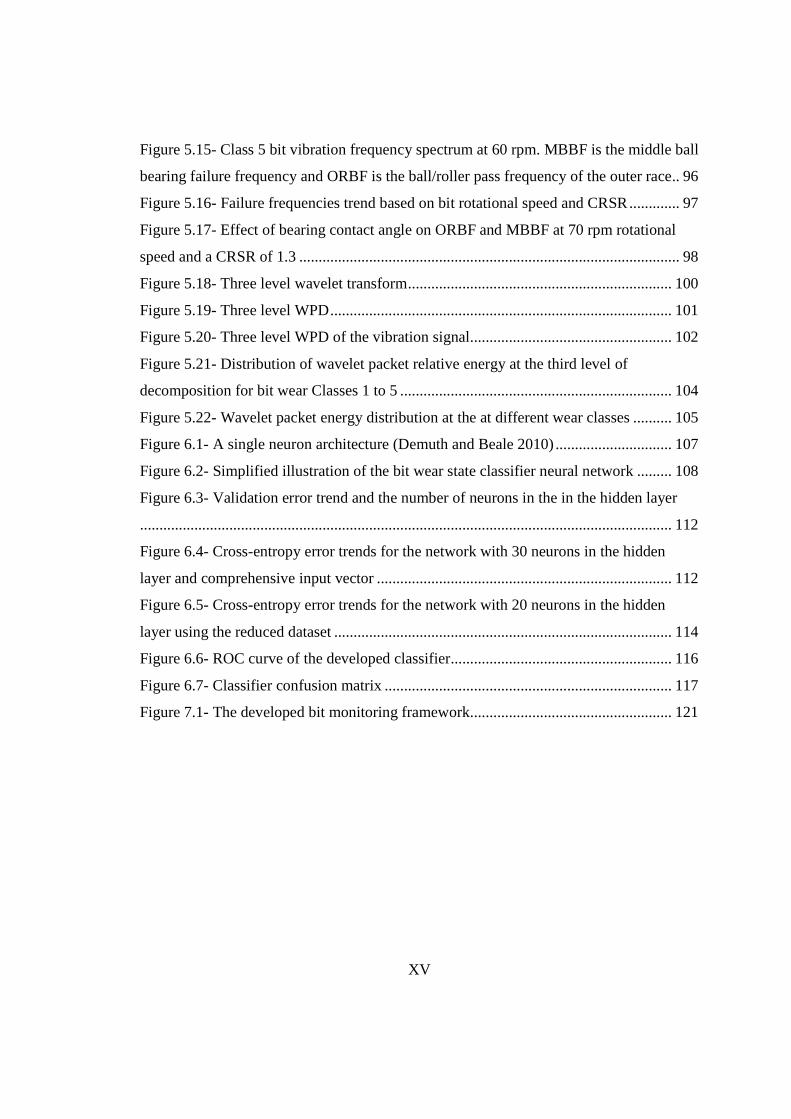
Figure 5.15- Class 5 bit vibration frequency spectrum at 60 rpm. MBBF is the middle ball

bearing failure frequency and ORBF is the ball/roller pass frequency of the outer race .. 96

Figure 5.16- Failure frequencies trend based on bit rotational speed and CRSR ............. 97

Figure 5.17- Effect of bearing contact angle on ORBF and MBBF at 70 rpm rotational

speed and a CRSR of 1.3 .................................................................................................. 98

Figure 5.18- Three level wavelet transform .................................................................... 100

Figure 5.19- Three level WPD ........................................................................................ 101

Figure 5.20- Three level WPD of the vibration signal .................................................... 102

Figure 5.21- Distribution of wavelet packet relative energy at the third level of

decomposition for bit wear Classes 1 to 5 ...................................................................... 104

Figure 5.22- Wavelet packet energy distribution at the at different wear classes .......... 105

Figure 6.1- A single neuron architecture (Demuth and Beale 2010) .............................. 107

Figure 6.2- Simplified illustration of the bit wear state classifier neural network ......... 108

Figure 6.3- Validation error trend and the number of neurons in the in the hidden layer

......................................................................................................................................... 112

Figure 6.4- Cross-entropy error trends for the network with 30 neurons in the hidden

layer and comprehensive input vector ............................................................................ 112

Figure 6.5- Cross-entropy error trends for the network with 20 neurons in the hidden

layer using the reduced dataset ....................................................................................... 114

Figure 6.6- ROC curve of the developed classifier ......................................................... 116

Figure 6.7- Classifier confusion matrix .......................................................................... 117

Figure 7.1- The developed bit monitoring framework .................................................... 121

XVI

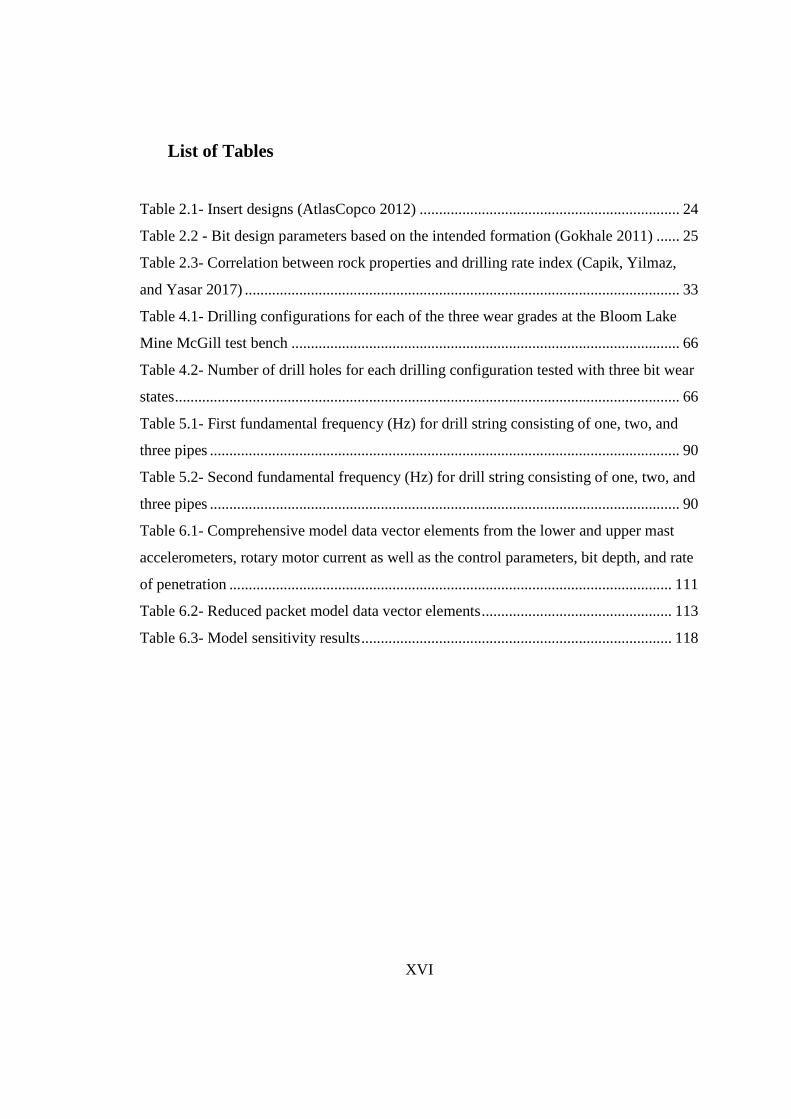
List of Tables

Table 2.1- Insert designs (AtlasCopco 2012) ................................................................... 24

Table 2.2 - Bit design parameters based on the intended formation (Gokhale 2011) ...... 25

Table 2.3- Correlation between rock properties and drilling rate index (Capik, Yilmaz,

and Yasar 2017) ................................................................................................................ 33

Table 4.1- Drilling configurations for each of the three wear grades at the Bloom Lake

Mine McGill test bench .................................................................................................... 66

Table 4.2- Number of drill holes for each drilling configuration tested with three bit wear

states .................................................................................................................................. 66

Table 5.1- First fundamental frequency (Hz) for drill string consisting of one, two, and

three pipes ......................................................................................................................... 90

Table 5.2- Second fundamental frequency (Hz) for drill string consisting of one, two, and

three pipes ......................................................................................................................... 90

Table 6.1- Comprehensive model data vector elements from the lower and upper mast

accelerometers, rotary motor current as well as the control parameters, bit depth, and rate

of penetration .................................................................................................................. 111

Table 6.2- Reduced packet model data vector elements ................................................. 113

Table 6.3- Model sensitivity results ................................................................................ 118

XVII

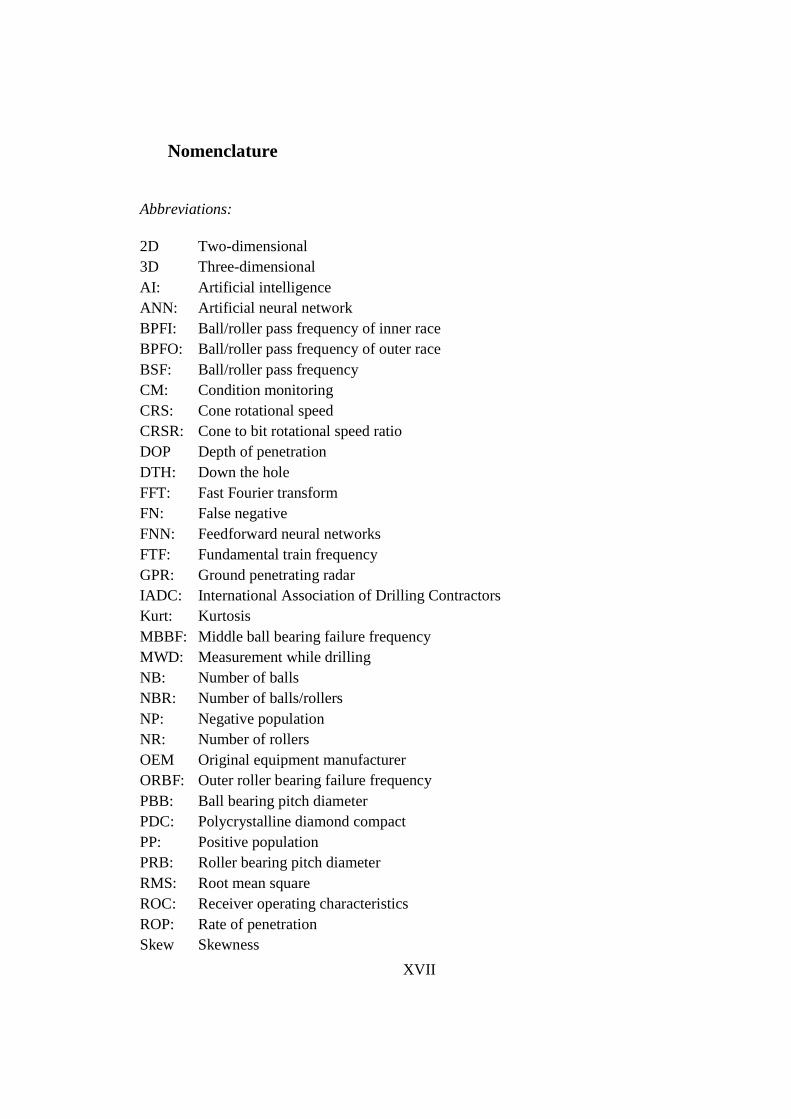
Nomenclature

Abbreviations:

2D Two-dimensional 3D Three-dimensional AI: Artificial intelligence ANN: Artificial neural network BPFI: Ball/roller pass frequency of inner race BPFO: Ball/roller pass frequency of outer race BSF: Ball/roller pass frequency CM: Condition monitoring CRS: Cone rotational speed CRSR: Cone to bit rotational speed ratio DOP Depth of penetration DTH: Down the hole FFT: Fast Fourier transform FN: False negative FNN: Feedforward neural networks FTF: Fundamental train frequency GPR: Ground penetrating radar IADC: International Association of Drilling Contractors Kurt: Kurtosis MBBF: Middle ball bearing failure frequency MWD: Measurement while drilling NB: Number of balls NBR: Number of balls/rollers NP: Negative population NR: Number of rollers OEM Original equipment manufacturer ORBF: Outer roller bearing failure frequency PBB: Ball bearing pitch diameter PDC: Polycrystalline diamond compact PP: Positive population PRB: Roller bearing pitch diameter RMS: Root mean square ROC: Receiver operating characteristics ROP: Rate of penetration Skew Skewness

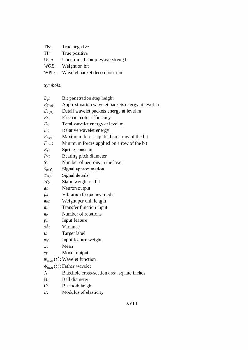
XVIII

TN: True negative TP: True positive UCS: Unconfined compressive strength WOB: Weight on bit WPD: Wavelet packet decomposition Symbols: Dp: Bit penetration step height ES(m): Approximation wavelet packets energy at level m ET(m): Detail wavelet packets energy at level m Ef: Electric motor efficiency Em: Total wavelet energy at level m Er: Relative wavelet energy Fmax: Maximum forces applied on a row of the bit Fmin: Minimum forces applied on a row of the bit Ks: Spring constant Pd: Bearing pitch diameter Si: Number of neurons in the layer Sm,n: Signal approximation Tm,n: Signal details W0: Static weight on bit ai: Neuron output fn: Vibration frequency mode m0: Weight per unit length ni: Transfer function input nx Number of rotations pi: Input feature ���: Variance ti: Target label wi: Input feature weight �̅: Mean yi: Model output ��,��: Wavelet function

�,��: Father wavelet

A: Blasthole cross-section area, square inches B: Ball diameter C: Bit tooth height E: Modulus of elasticity

XIX

f: Frequency F: Rotational speed difference between outer and inner race g: Acceleration due to gravity, 9.8 m/s2 I: Polar moment of inertia L: Length N: Bit rotational speed N: Number of data points n: Wavelet packet number Q: Volume of compressed air R: Number of inputs to the neuron R: Roller diameter X: Random discrete signal xi: Random discrete signal data point Z: Model parameter vector F(t): Axial forces on the teeth rows H: Loss function I: Electric current T: Torque V: Electric voltage e: Specific energy l: Iteration number m: Wavelet level θ: Bearing contact angle λ: Frequency factor, dimensionless

µ: Learning rate

1

Chapter 1 – Introduction

Surface Mining

Commercially important minerals are called ores. Target ores are usually surrounded

by other non-commercially important material known as waste (Fig.1.1).

Figure 1.1- Orebodies surrounded by waste material (AtlasCopco 2012)

When an orebody is located at shallow depth, surface mining techniques are used for

rock extraction. More than 95% of non-metallic and 90% of metallic minerals, and more

than 60% of coal is excavated using surface mining (Ramani 2012). Most surface mines

are large and are mass producers of minerals (Hartman and Mutmansky 2002).

When a large amount of hard rock must be excavated to reach ores, mechanical

cutting methods are not efficient and drilling and blasting must be used. Blasting releases

enough energy to fragment even the hardest rock formations and is thus the most

2

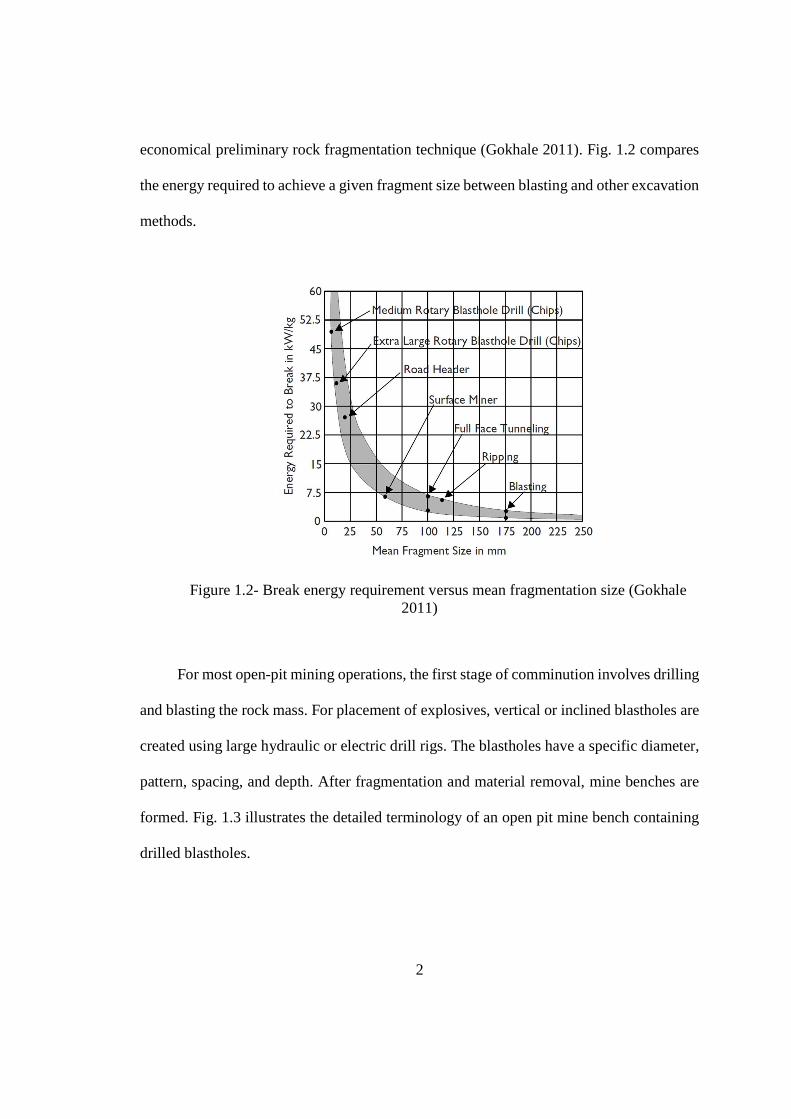
economical preliminary rock fragmentation technique (Gokhale 2011). Fig. 1.2 compares

the energy required to achieve a given fragment size between blasting and other excavation

methods.

Figure 1.2- Break energy requirement versus mean fragmentation size (Gokhale 2011)

For most open-pit mining operations, the first stage of comminution involves drilling

and blasting the rock mass. For placement of explosives, vertical or inclined blastholes are

created using large hydraulic or electric drill rigs. The blastholes have a specific diameter,

pattern, spacing, and depth. After fragmentation and material removal, mine benches are

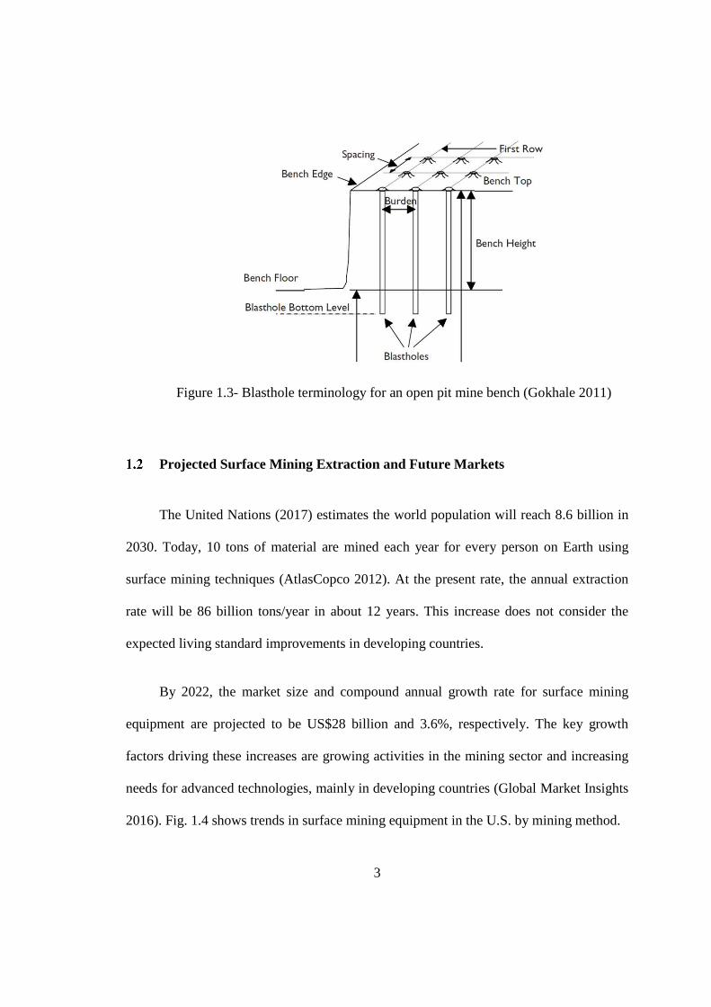
formed. Fig. 1.3 illustrates the detailed terminology of an open pit mine bench containing

drilled blastholes.

3

Figure 1.3- Blasthole terminology for an open pit mine bench (Gokhale 2011)

Projected Surface Mining Extraction and Future Markets

The United Nations (2017) estimates the world population will reach 8.6 billion in

2030. Today, 10 tons of material are mined each year for every person on Earth using

surface mining techniques (AtlasCopco 2012). At the present rate, the annual extraction

rate will be 86 billion tons/year in about 12 years. This increase does not consider the

expected living standard improvements in developing countries.

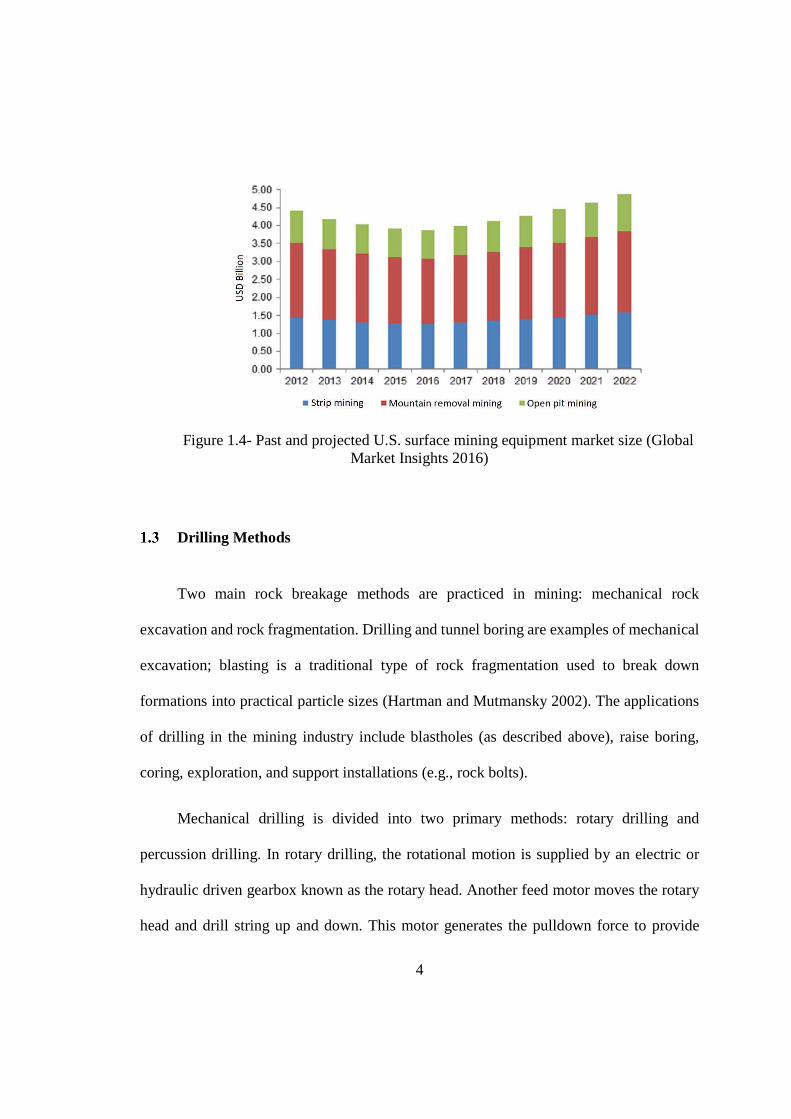
By 2022, the market size and compound annual growth rate for surface mining

equipment are projected to be US$28 billion and 3.6%, respectively. The key growth

factors driving these increases are growing activities in the mining sector and increasing

needs for advanced technologies, mainly in developing countries (Global Market Insights

2016). Fig. 1.4 shows trends in surface mining equipment in the U.S. by mining method.

4

Figure 1.4- Past and projected U.S. surface mining equipment market size (Global Market Insights 2016)

Drilling Methods

Two main rock breakage methods are practiced in mining: mechanical rock

excavation and rock fragmentation. Drilling and tunnel boring are examples of mechanical

excavation; blasting is a traditional type of rock fragmentation used to break down

formations into practical particle sizes (Hartman and Mutmansky 2002). The applications

of drilling in the mining industry include blastholes (as described above), raise boring,

coring, exploration, and support installations (e.g., rock bolts).

Mechanical drilling is divided into two primary methods: rotary drilling and

percussion drilling. In rotary drilling, the rotational motion is supplied by an electric or

hydraulic driven gearbox known as the rotary head. Another feed motor moves the rotary

head and drill string up and down. This motor generates the pulldown force to provide

5

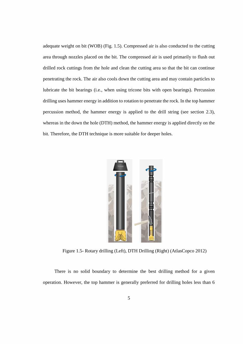
adequate weight on bit (WOB) (Fig. 1.5). Compressed air is also conducted to the cutting

area through nozzles placed on the bit. The compressed air is used primarily to flush out

drilled rock cuttings from the hole and clean the cutting area so that the bit can continue

penetrating the rock. The air also cools down the cutting area and may contain particles to

lubricate the bit bearings (i.e., when using tricone bits with open bearings). Percussion

drilling uses hammer energy in addition to rotation to penetrate the rock. In the top hammer

percussion method, the hammer energy is applied to the drill string (see section 2.3),

whereas in the down the hole (DTH) method, the hammer energy is applied directly on the

bit. Therefore, the DTH technique is more suitable for deeper holes.

Figure 1.5- Rotary drilling (Left), DTH Drilling (Right) (AtlasCopco 2012)

There is no solid boundary to determine the best drilling method for a given

operation. However, the top hammer is generally preferred for drilling holes less than 6

6

inches in diameter (Fig. 1.6). For hard formations (unconfined compressive strength >100

MPa), DTH drilling usually provides a better rate of penetration. DTH drilling is limited

by the volume of pressurized air supply. For example, an 8” DTH bit is designed to receive

25 bar air pressure to provide enough impact energy. Therefore, rotary drilling with tricone

bits is the most cost-effective method for larger hole diameters and generally suits a wider

range of applications and hole sizes in terms of diameter and depth (AtlasCopco 2012).

Figure 1.6- Drilling methods based on hole size and formation type (AtlasCopco 2012)

Drill Bit

Drill bits are divided into two main categories: fixed bits and roller bits. Fixed bits

include drag bits and button bits and are primarily used for percussion drilling. In rotary

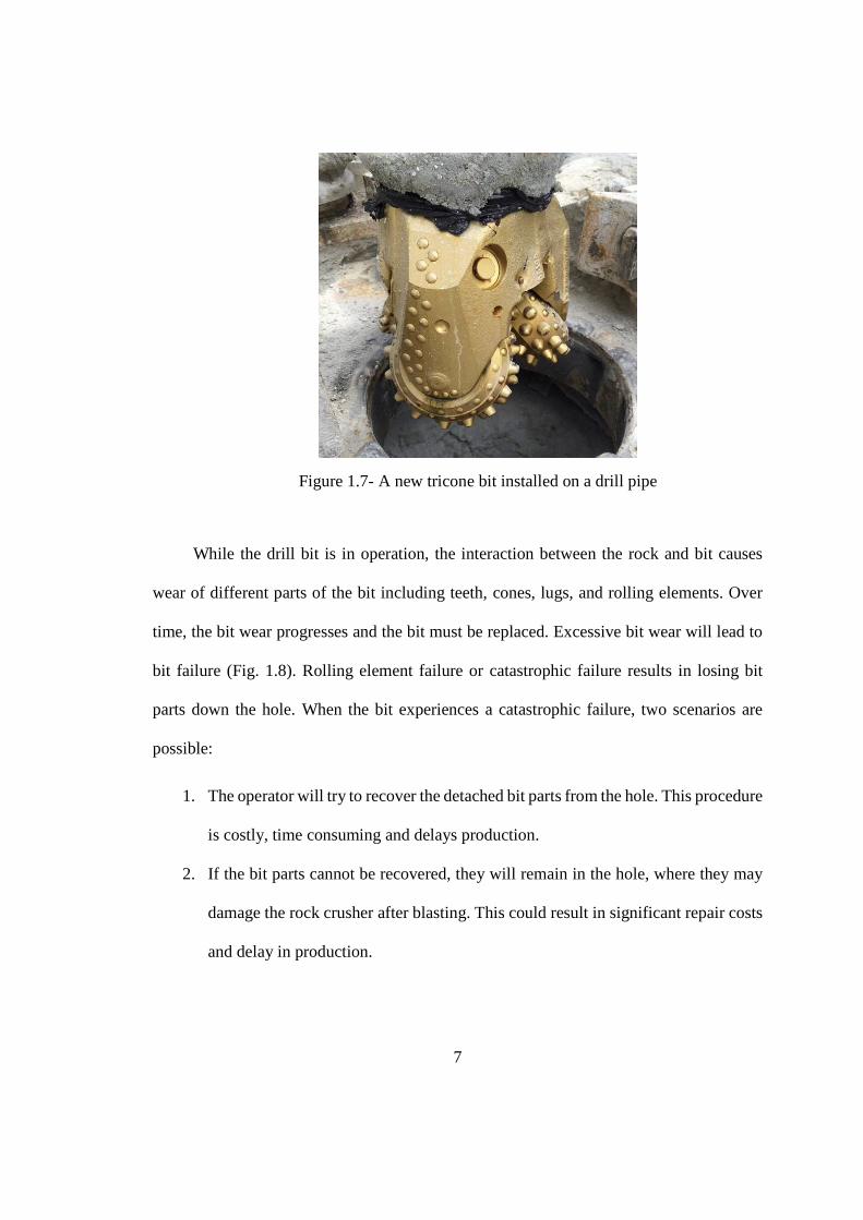
blasthole drilling, the most preferred bit type is the tricone roller bit. Tricone bits penetrate

rock by crushing and spalling it (AtlasCopco 2012). The bit comprises three cones, each

installed on a lug support structure (Fig. 1.7). The connection between the lug and cone

contains roller and ball bearings.

7

Figure 1.7- A new tricone bit installed on a drill pipe

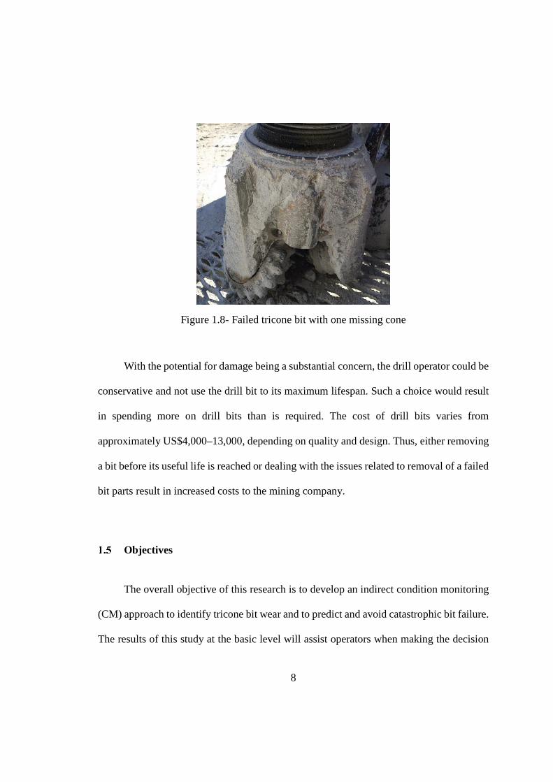
While the drill bit is in operation, the interaction between the rock and bit causes

wear of different parts of the bit including teeth, cones, lugs, and rolling elements. Over

time, the bit wear progresses and the bit must be replaced. Excessive bit wear will lead to

bit failure (Fig. 1.8). Rolling element failure or catastrophic failure results in losing bit

parts down the hole. When the bit experiences a catastrophic failure, two scenarios are

possible:

1. The operator will try to recover the detached bit parts from the hole. This procedure

is costly, time consuming and delays production.

2. If the bit parts cannot be recovered, they will remain in the hole, where they may

damage the rock crusher after blasting. This could result in significant repair costs

and delay in production.

8

Figure 1.8- Failed tricone bit with one missing cone

With the potential for damage being a substantial concern, the drill operator could be

conservative and not use the drill bit to its maximum lifespan. Such a choice would result

in spending more on drill bits than is required. The cost of drill bits varies from

approximately US$4,000–13,000, depending on quality and design. Thus, either removing

a bit before its useful life is reached or dealing with the issues related to removal of a failed

bit parts result in increased costs to the mining company.

Objectives

The overall objective of this research is to develop an indirect condition monitoring

(CM) approach to identify tricone bit wear and to predict and avoid catastrophic bit failure.

The results of this study at the basic level will assist operators when making the decision

9

to change the bit. Furthermore, a bit CM system is an integral component of an autonomous

drilling operation. The objectives of this research are to:

• Investigate the application of ground penetrating radar (GPR) for geological

identification and for detection of subsurface layer variations with the capability of

real-time implementation

• Design the data acquisition and sensor configuration needed to collect blasthole

drilling field data at two Canadian surface mines

• Perform preliminary fieldwork and data analysis at a surface mine

• Plan and implement blasthole drill instrumentation and a comprehensive field work

based on preliminary results

• Visually inspect and record bit wear state during the entire field tests in various

working conditions and geological formations for data labeling

• Assess the professional opinions of bit manufacturers and experienced operators

regarding drilling conditions, geology, bit wear state and bit replacement strategy

• Establish a new qualitative wear grading technique for tricone bits

• Analyze data in time, frequency, and time-frequency domains to identify and

introduce signal signatures that are sensitive to bit wear condition and carry related

information

• Mathematically calculate and experimentally investigate tricone bit failure

frequencies

• Design, train, and evaluate sensor-fusion artificial intelligence (AI) models based

on full-scale field data and identified signal features

10

• Introduce the data vector for the purpose of tricone wear monitoring

• Test AI model ability to classify bit condition and predict bit failure using unseen

field data

Methodology

This research develops a novel approach to monitor tricone bit condition and predict

bit failure for blasthole drilling in surface mining. The CM solution is established through

extensive field data collection and analysis, bit wear related signal signature identification,

and AI modeling. Signal analysis and modeling are conducted using MATLAB software

(MathWorks), which is broadly used by academic and industrial engineers and scientists.

A blasthole drill was instrumented with several accelerometers and two data

acquisition units for a comprehensive measurement while drilling, including drilling

vibration at various locations on the machine. The data were collected during the life cycles

of tricone bits working in a variety of geological conditions on different benches of the

surface mines.

Drilling vibration was first analyzed in the frequency domain to identify the

frequency component trends that carry bit wear information and are sensitive to bit wear

state with consideration of geological variations. Mathematical equations were introduced

to calculate the failure frequencies of tricone bits based on the design parameters.

Wavelet packet decomposition was applied as a time-frequency analysis approach to

focus on desired frequency bands and finally for statistical feature extraction. Features were

11

analyzed to introduce a signal feature vector for tricone bit wear monitoring and failure

prediction.

Based on experience gained during the fieldwork, discussions with operators, and

inspections of bit scrap yards at the mines, a new qualitative tricone bit wear grading

method was defined to describe tricone bit wear in its life cycle.

AI models were developed using artificial neural networks (ANN) for bit wear

pattern recognition and classification. The models were trained and their performance was

evaluated using real field data. Finally, the signal feature vector and model architecture

were suggested for tricone bit wear monitoring and failure prediction in surface mining.

Thesis Overview

Chapter 2 reviews published literature on drilling and attempts to conduct drilling

monitoring. Chapter 3 investigates the application of GPR for surface mining. Chapter 4

discusses experimental work including drill rig instrumentation, data collection, and data

labeling. Data analysis is detailed in chapter 5, including time, frequency, and time-

frequency approaches and identification of the wear-sensitive signal information. Chapter

6 presents the developed sensor-fusion ANN model to classify bit wear state. Finally,

concluding remarks and suggested future works constitute Chapter 7.

12

Chapter 2 – Literature Review

Condition Monitoring

Automation and unmanned production are growing trends in many industries,

including mining. Thus, condition monitoring (CM) of system components is required to

understand the status of devices, machines, and ultimately the overall operation.

Monitoring is also necessary to identify system anomalies. An anomaly could be removed

by stopping the process or by adjusting operating parameters (Wang and Gao 2006).

Understanding the system status in real-time provides the ability to predict faults and avoid

further consequences of failure during the operation. This approach is known as predictive

maintenance.

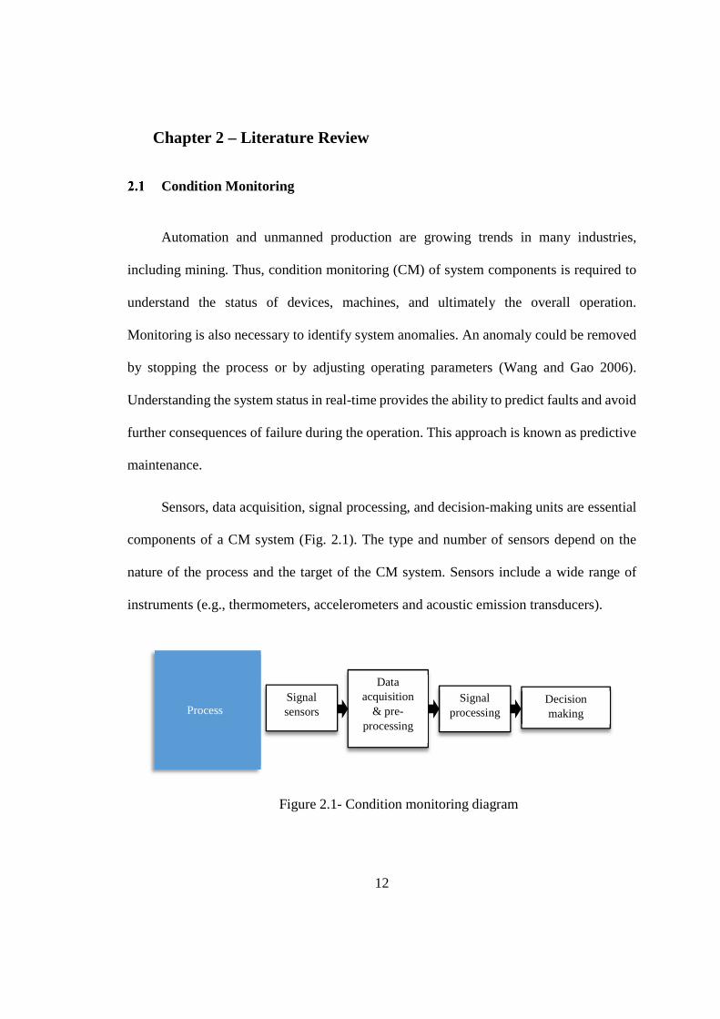
Sensors, data acquisition, signal processing, and decision-making units are essential

components of a CM system (Fig. 2.1). The type and number of sensors depend on the

nature of the process and the target of the CM system. Sensors include a wide range of

instruments (e.g., thermometers, accelerometers and acoustic emission transducers).

Figure 2.1- Condition monitoring diagram

Process Signal sensors

Data acquisition

& pre-processing

Signal processing

Decision making

13

In a direct CM system, sensors directly measure the desired parameter (e.g.,

processing images taken from a cutting tool to detect the amount of wear). However, in

many industrial applications, it is not feasible to directly measure the desired parameter.

Instead, the effects of variations in the desired parameter on the behavior of the system or

on other parameters are measured. Using this indirect CM approach, variations in the

desired parameter are estimated indirectly (e.g., measuring the cutting forces to estimate

the cutting tool wear state) (Zhu, San Wong, and Hong 2009). CM approaches are being

widely developed in different sectors of the mining industry, from the earliest stages of

excavation rigs to structures and processing equipment.

Stenström, Carlson, and Lundberg (2012) investigated wear monitoring of a rotary

mining mill by using a waterjet ultrasound scanning system. Due to the nature of the

milling process, these mills are always subject to wear, fatigue, and crack progress in the

mill steel shell. The authors performed laboratory-scale experiments on a mill with a shell

thickness of 15 mm. They used an ultrasound transducer with 5 MHz of central frequency

and reported the detection of artificially created defects in the mill internal wall.

Pang, Zhang, Fu, and Zhu (2011) developed a remote CM approach for coal mine

fan system based on the ethernet. Monitoring of ventilation fans is crucial to ensure mine

air quality and worker safety. Their CM system relied on analysis of vibration and

temperature signals from the fans. It was able to detect a fault in the fan running state and

produce an early warning of the issue.

14

Geological Recognition

The interaction between the drill bit and rock causes bit wear; therefore, identifying

the geological formation is an important issue in rock and tool interaction analysis. A

serious challenge with automating mining machinery is detecting and measuring geological

layers at the mine site. A non-destructive and non-invasive approach for subsurface

recognition is GPR. This technique uses electromagnetic wave reflections to collect

information from underground or from within structures such as buried pipes, underground

cavities, subsurface cracks, voids, and stratifications. GPR has a wide range of

applications; the appropriate wavelength is selected depending on the application. For

example, the GPR systems used in security applications to search for small items at a

shallow depth use high-frequency (3–6 GHz) antennas (Utsi 2017). GPR is also effective

in quality control and CM of infrastructure, including railways, buildings, roads, and

bridges. Depending on the desired depth of penetration (DOP), mid- to high-frequency

antennas (400–500 MHz) are often used (Utsi 2017). Lower frequencies provide an

overview of the subsurface, while high frequencies give a detailed local representation.

In mining applications, geological materials can be considered as semiconductors.

And their electromagnetic properties can be difined by: dielectric permittivity (ε), electrical

conductivity (σ), and magnetic permeability. The capability of material to transmit a direct

current is known as electrical conductivity. Relative dielectric permittivity is a geological

medium resistance degree to the flow of an electrical charge divided by the resistance

degree of vacuum space to that amount of charge; this characteristic is an essential

parameter for GPR application (Francke and Utsi 2009).

15

Ground formations are usually a combination of materials with different dielectric

properties. When the electrical conductivity increases, the GPR signal penetration

decreases. Other than the electrical conductivity and dielectric permittivity, the DOP is

affected by the complexity of subsurface interfaces that scatter the signal.

Patterson (2003) and Kampf, Gochenour, and Clanin (2003) applied GPR at the

Cryo-Genie pegmatite mine in San Diego County, USA to discover a major gem

tourmaline pocket. They were able to map a pocket type zone at a depth of 5 m. In the coal

mining field, Strange, Ralston, and Chandran (2005) applied high-frequency GPR at the

laboratory scale reaching depths of less than 80 cm. Ralston and Hainsworth (2000) studied

the capability of GPR to identify the coal-rock interface and they were able to detect the

coal-tuff boundary. Other research works have investigated the application of GPR to map

the barrier thickness and also to assess the penetration of polyurethane grout into the mine

roof in underground coal mining (Jha et al. 2004; Monaghan and Trevits 2004).

Electric Blasthole Drills and Drill Bits

As mentioned in Chapter 1, drilling methods include down the hole (DTH), top

hammer, and rotary approaches; drill rigs are designed and constructed accordingly. When

drills are used to make holes in the ground in surface mining to be filled with explosive

material, they are called blasthole drills.

Several companies manufacture rotary blasthole drills; Atlas Copco, Caterpillar,

Sandvik, and P&H are among the major manufacturers. In 2016, Atlas Copco was the

industry leader, followed by Caterpillar, with 39% and 36% of worldwide drill market,

16

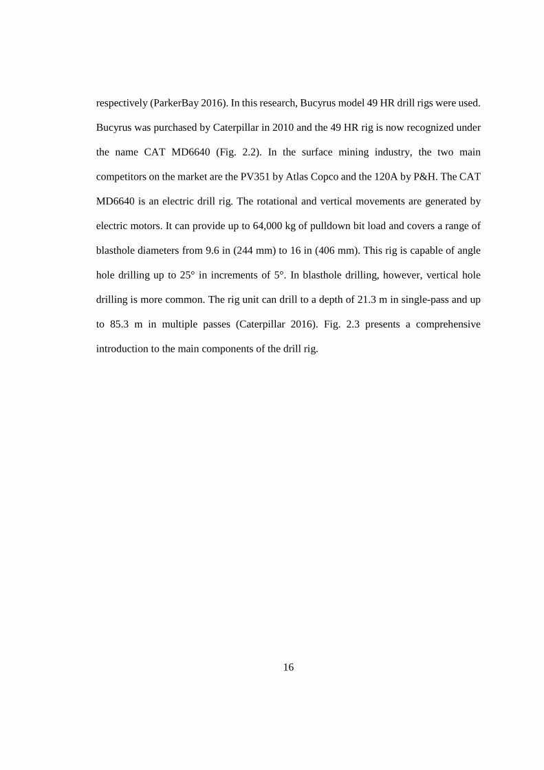
respectively (ParkerBay 2016). In this research, Bucyrus model 49 HR drill rigs were used.

Bucyrus was purchased by Caterpillar in 2010 and the 49 HR rig is now recognized under

the name CAT MD6640 (Fig. 2.2). In the surface mining industry, the two main

competitors on the market are the PV351 by Atlas Copco and the 120A by P&H. The CAT

MD6640 is an electric drill rig. The rotational and vertical movements are generated by

electric motors. It can provide up to 64,000 kg of pulldown bit load and covers a range of

blasthole diameters from 9.6 in (244 mm) to 16 in (406 mm). This rig is capable of angle

hole drilling up to 25° in increments of 5°. In blasthole drilling, however, vertical hole

drilling is more common. The rig unit can drill to a depth of 21.3 m in single-pass and up

to 85.3 m in multiple passes (Caterpillar 2016). Fig. 2.3 presents a comprehensive

introduction to the main components of the drill rig.

17

Figure 2.2- CAT MD6640 dimensions (Caterpillar 2016)

18

Figure 2.3- CAT MD6640 main components (Caterpillar 2016)

19

When drilling is completed by a unit piece of drill pipe, it is called single-pass

drilling. Large drills are capable of accommodating additional drill pipes to increase the

depth of drilling; this is called multi-pass drilling. One or more connected drill pipes are

known as a drill string. Note that the single pass drill depth mast in the rest position

increases the overall length of the CAT MD6640 drill rig from 14.73 to 31.24 m (Fig. 2.2).

Rock Drilling Tools

The type of bit used depends on the drilling method and application specifications.

In surface mining, fixed and rotary bits are used. Fixed bits include drag bits and button

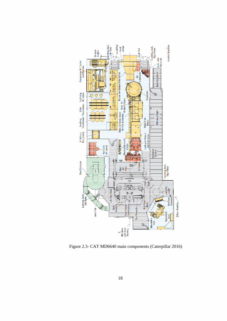
bits. Drag bits (also known as cross bits) have a relatively simple design, usually consisting

of four straight cutting edges mounted on the bit body (Fig. 2.4 right), but the number of

cutting edges can be less than four (Fig. 2.4 left). Application of drag bits is limited to soft

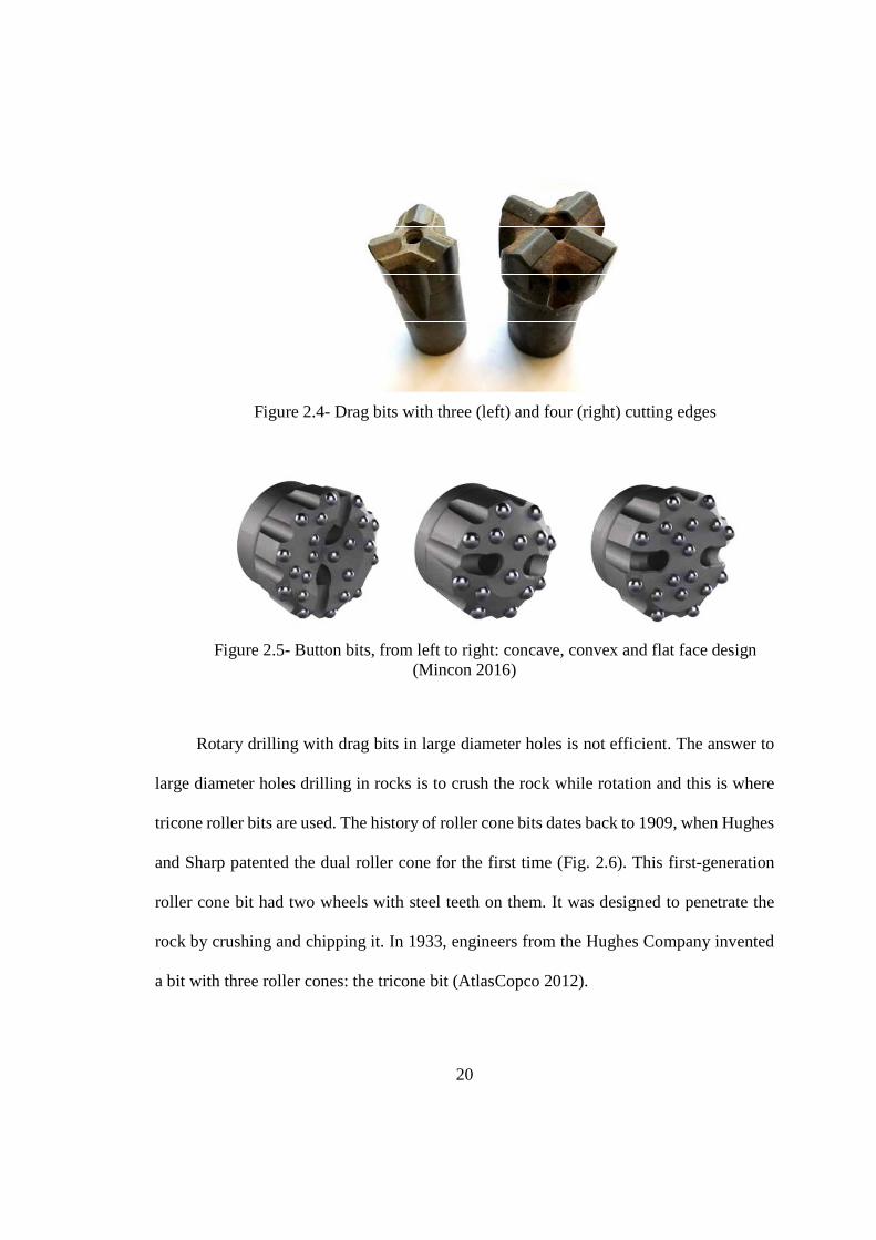
formation drilling (AtlasCopco 2012). By comparison, button bits are designed to suit the

geological formation and operating conditions. Design parameters include the number of

carbon buttons (also known as inserts) and the bit face profile (concave, convex, or flat;

Fig. 2.5). A concave surface improves drilling stability to achieve a straighter hole; a

convex surface is designed for hard and abrasive rock conditions; and a flat face is meant

for general purpose drilling. A flat face is also most effective for softer formations that tend

to over drill (Mincon 2016).

20

Figure 2.4- Drag bits with three (left) and four (right) cutting edges

Figure 2.5- Button bits, from left to right: concave, convex and flat face design (Mincon 2016)

Rotary drilling with drag bits in large diameter holes is not efficient. The answer to

large diameter holes drilling in rocks is to crush the rock while rotation and this is where

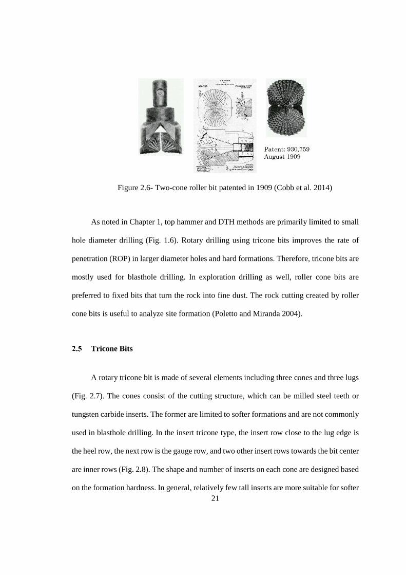
tricone roller bits are used. The history of roller cone bits dates back to 1909, when Hughes

and Sharp patented the dual roller cone for the first time (Fig. 2.6). This first-generation

roller cone bit had two wheels with steel teeth on them. It was designed to penetrate the

rock by crushing and chipping it. In 1933, engineers from the Hughes Company invented

a bit with three roller cones: the tricone bit (AtlasCopco 2012).

21

Figure 2.6- Two-cone roller bit patented in 1909 (Cobb et al. 2014)

As noted in Chapter 1, top hammer and DTH methods are primarily limited to small

hole diameter drilling (Fig. 1.6). Rotary drilling using tricone bits improves the rate of

penetration (ROP) in larger diameter holes and hard formations. Therefore, tricone bits are

mostly used for blasthole drilling. In exploration drilling as well, roller cone bits are

preferred to fixed bits that turn the rock into fine dust. The rock cutting created by roller

cone bits is useful to analyze site formation (Poletto and Miranda 2004).

Tricone Bits

A rotary tricone bit is made of several elements including three cones and three lugs

(Fig. 2.7). The cones consist of the cutting structure, which can be milled steel teeth or

tungsten carbide inserts. The former are limited to softer formations and are not commonly

used in blasthole drilling. In the insert tricone type, the insert row close to the lug edge is

the heel row, the next row is the gauge row, and two other insert rows towards the bit center

are inner rows (Fig. 2.8). The shape and number of inserts on each cone are designed based

on the formation hardness. In general, relatively few tall inserts are more suitable for softer

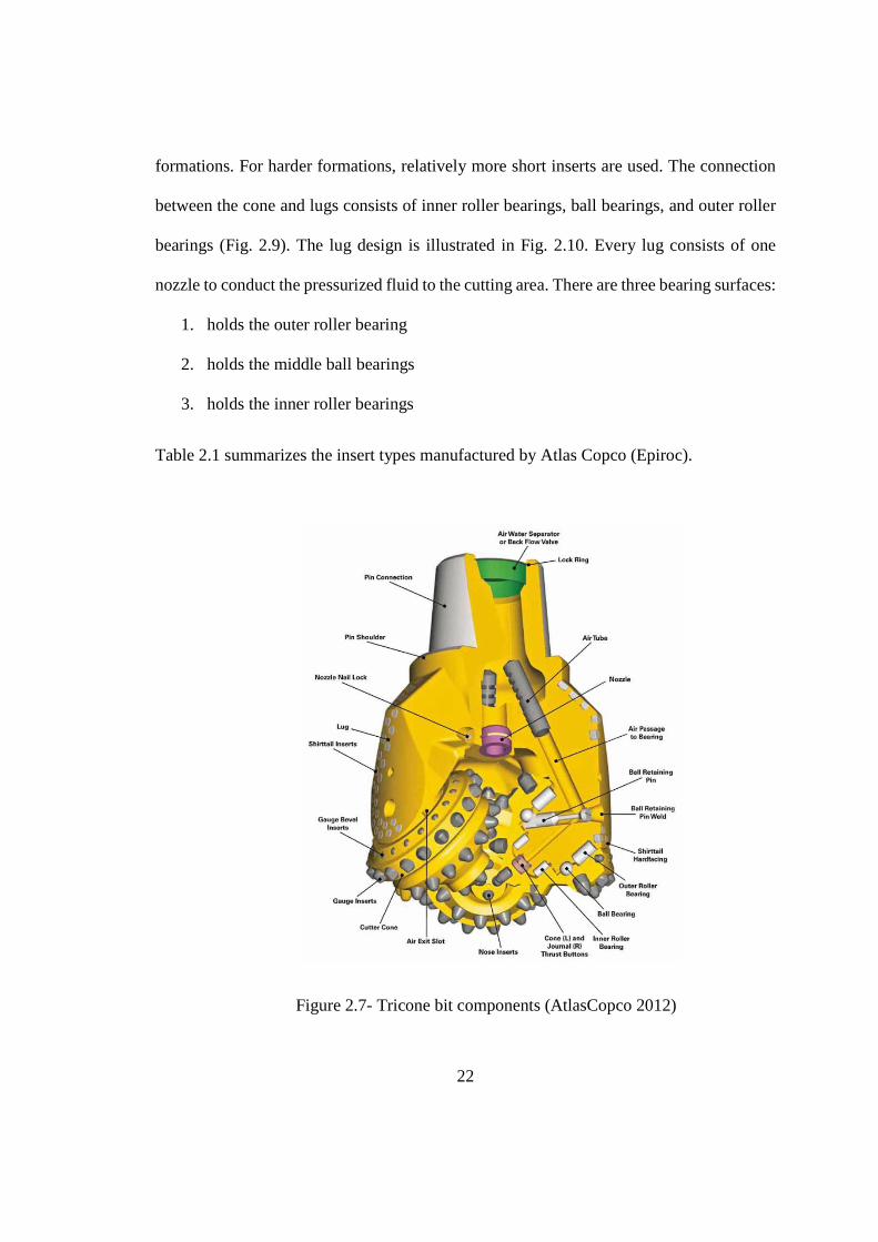
22

formations. For harder formations, relatively more short inserts are used. The connection

between the cone and lugs consists of inner roller bearings, ball bearings, and outer roller

bearings (Fig. 2.9). The lug design is illustrated in Fig. 2.10. Every lug consists of one

nozzle to conduct the pressurized fluid to the cutting area. There are three bearing surfaces:

1. holds the outer roller bearing

2. holds the middle ball bearings

3. holds the inner roller bearings

Table 2.1 summarizes the insert types manufactured by Atlas Copco (Epiroc).

Figure 2.7- Tricone bit components (AtlasCopco 2012)

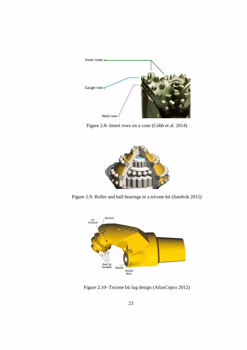
23

Figure 2.8- Insert rows on a cone (Cobb et al. 2014)

Figure 2.9- Roller and ball bearings in a tricone bit (Sandvik 2015)

Figure 2.10- Tricone bit lug design (AtlasCopco 2012)

24

Table 2.1- Insert designs (AtlasCopco 2012)

In addition to the material, shape, and quantity of the cutting structures, other design

parameters influence bit performance in hard and soft formations. In application-specific

design, cone offset and journal angle are key parameters related to formation hardness. The

bit cone offset is the distance between the bit axes and a vertical plane through the journal

axis (Fig. 2.11 left). The angle formed between the axis of the journal and a line

perpendicular to the bit rotation axis is the journal angle (Fig. 2.11 right). Table 2.2

summarizes the bit design parameter relative values based on the intended geological

formation condition. Journal angles range between 30° and 39°. Higher angles (34–39°)

and lower offset boost the crushing mechanism. Therefore, the bit will have an enhanced

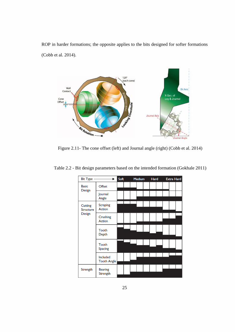
25

ROP in harder formations; the opposite applies to the bits designed for softer formations

(Cobb et al. 2014).

Figure 2.11- The cone offset (left) and Journal angle (right) (Cobb et al. 2014)

Table 2.2 - Bit design parameters based on the intended formation (Gokhale 2011)

26

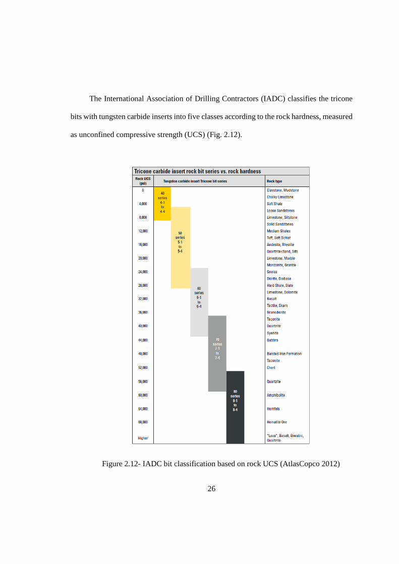
The International Association of Drilling Contractors (IADC) classifies the tricone

bits with tungsten carbide inserts into five classes according to the rock hardness, measured

as unconfined compressive strength (UCS) (Fig. 2.12).

Figure 2.12- IADC bit classification based on rock UCS (AtlasCopco 2012)

27

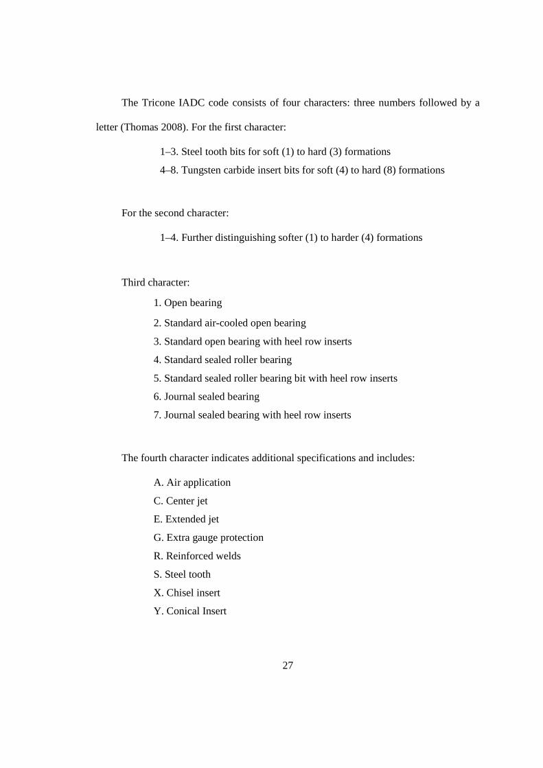
The Tricone IADC code consists of four characters: three numbers followed by a

letter (Thomas 2008). For the first character:

1–3. Steel tooth bits for soft (1) to hard (3) formations

4–8. Tungsten carbide insert bits for soft (4) to hard (8) formations

For the second character:

1–4. Further distinguishing softer (1) to harder (4) formations

Third character:

1. Open bearing

2. Standard air-cooled open bearing

3. Standard open bearing with heel row inserts

4. Standard sealed roller bearing

5. Standard sealed roller bearing bit with heel row inserts

6. Journal sealed bearing

7. Journal sealed bearing with heel row inserts

The fourth character indicates additional specifications and includes:

A. Air application

C. Center jet

E. Extended jet

G. Extra gauge protection

R. Reinforced welds

S. Steel tooth

X. Chisel insert

Y. Conical Insert

28

Bit-Rock Interaction

To better illustrate the events at the bit-rock interface, it is helpful to simplify the

interaction to that of a single insert acting on a rock; this represents the interactions between

a tricone rotary bit consisting of many inserts and a rock formation. Maurer (1962)

introduced a model to show the basis of interaction between rock and bit in rotary drilling

for a single bit insert. Fig. 2.13a shows a single insert (wedge in the diagram) impacting

the rock and causing the elastic deformation of rock. The process continues until the

crushing strength of the rock is exceeded, and crushed rock is created below the insert

(Hartman 1959). More applied force causes the crushed material to compress and exert

high lateral forces on the solid. As the lateral forces exceed the UCS of the rock mass,

fractures propagate at the free surface of the rock (Fig. 2.13c) (Clausing 1959; Maurer

1959). Eventually, rock cuttings (chips) are formed, which separate (Fig. 2.13e) and must

be removed from the cutting area. Because of moving position of the insert and resulting

rock fragmentation described, high amounts of torque are required to rotate tricone bits.

29

Figure 2.13- The interaction between a single bit insert and rock in rotary drilling (Gokhale 2011)

In the literature, the ROP of a tricone bit at the drill side is considered a function of

four factors that can be expressed as (Gokhale 2011):

ROP = ����, �, �, �� (2.1)

Where

ROP: Rate of penetration

WOB: Weight on bit (feed force)

N: Bit rotation speed

C: Bit tooth height

Q: Volume of compressed air

Increasing the WOB at a fixed rotational speed increases the ROP, but this effect is

lessened at high WOB values due to overload (Fig. 2.14) (Gokhale 2011). Based on the

30

crushing mechanism of the bit tooth (Fig. 2.13), the bit ROP is limited by the tooth length.

In addition, bearings are other important limiting factors in tricone drilling. An excessive

amount of force can damage the bearing elements.

Figure 2.14- ROP vs. WOB at 79 rpm rotational speed (Gokhale 2011)

“Q” does not participate in rock fracturing, but compressed air is necessary to flush

the cuttings from the hole. As noted in Chapter 1, if cuttings remain in the hole, the bit will

be eroded by abrasive rock chips, and the teeth will quickly wear. In blasthole drilling, the

compressed air usually lifts cuttings between the wall of the hole and the drill rods. To let

the cuttings pass, there must be enough clearance— annular space—between drill string

and the hole wall. Field studies have shown that the approximate annular space should be

17% of the cross-sectional area of the drilled blasthole (AtlasCopco 2012).

31

Rock Specific Energy

Drilling is an excavation act and in rotary tricone drilling, this task is accomplished

by applying the energy in forms of feed force (WOB) and rotation. The work needed to

excavate a unit volume of rock is known as rock specific energy. Teale’s equation sums

two parts to calculate the energy transfer by a rotary tricone bit (Teale 1965):

� = ����� ! �2 ∗ $

� � %&'�( (2.2)

Where

e: Specific energy (lb/in3)

WOB: Drill bit feed force (lb)

A: Blasthole cross-section area (in2)

N: Rotational speed (rpm)

T: Drill bit torque (lb-in)

ROP: Rate of penetration (in/min)

The first part of the equation mostly contributes to the creation of cracks and crushing

the rock and the second term contributes to loosening and moving cracked fragments.

Because the hole cross section area is fixed, the term �2 ∗ $� is a constant (Gokhale 2011).

Drillability and Rate of Penetration

Rock drillability is the projected ROP in a rock formation. Many aspects of a drilling

operation influence rock drillability, including (Gokhale 2011):

32

• Rock uniaxial compressive (i.e., UCS at rock failure under uniaxial compression

conditions), tensile, and shear strength

• Rock abrasiveness

• Rock density

• Joint spacing and orientation in the rock mass

• WOB

• Rotatory speed and torque

• Air flush pressure and volume

• Vibration

• Bit tooth height, quantity and type

• Bit lug and cone design

Scientists have attempted to correlate the ROP with rock properties. In 1926,

Protodyakonov introduced the empirical “Protodyakonov number” to represent the

dynamic strength of rock against impacts. A more advanced equation to calculate the ROP

was later developed by Paone and Bruce (1969) by accounting for more parameters. The

specific energy approach is also reported in the literature to calculate the projected ROP.

In 1971, Bauer modified an earlier empirical equation to predict the ROP of blasthole

tricone drilling in hard iron ores (Eq. 2.3). In 1994, Calder introduced a modified version

of the equation that was applicable to blasthole drilling in low-UCS formations (Gokhale

2011).

ROP = 61 − 28 -./ 0�1)(���∅ )( %

344) (2.3)

33

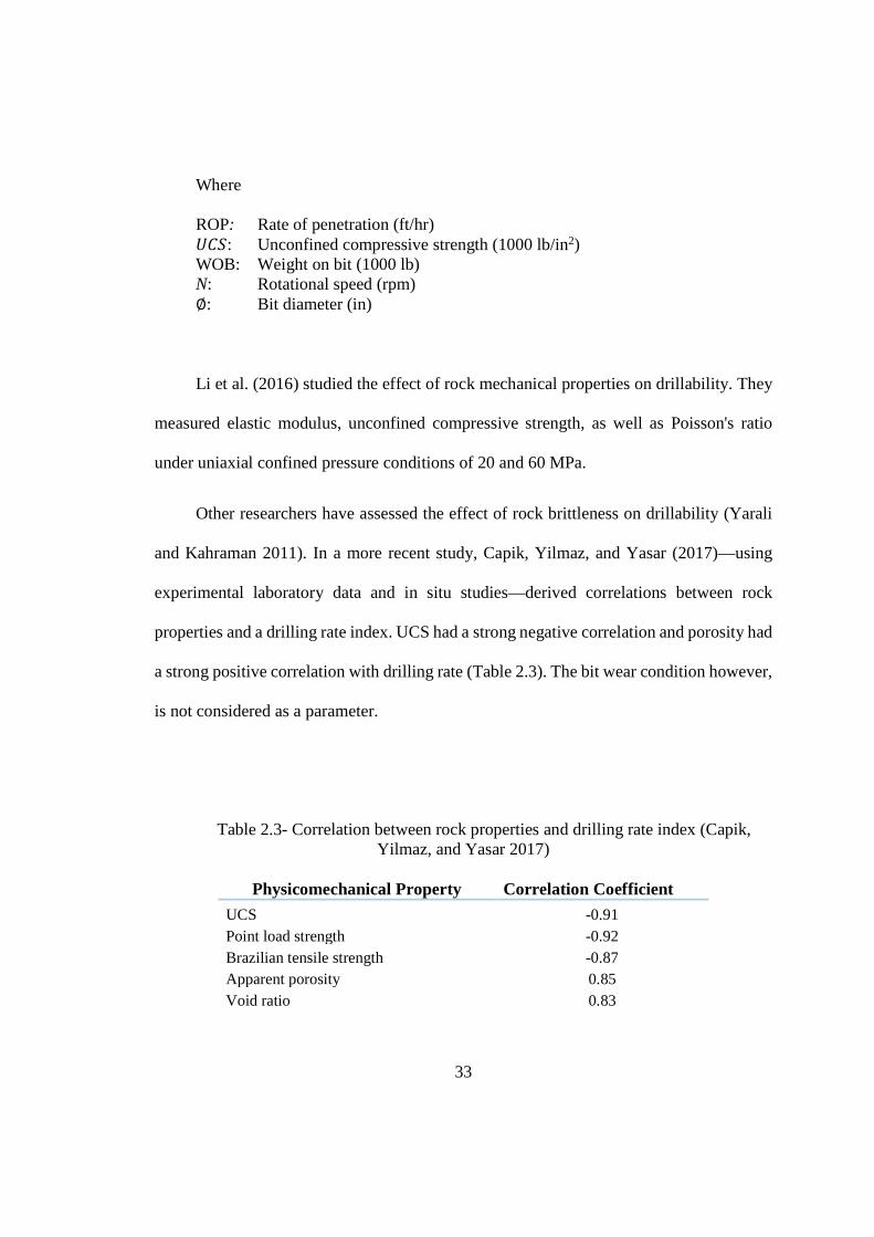
Where ROP: Rate of penetration (ft/hr) 0�1: Unconfined compressive strength (1000 lb/in2) WOB: Weight on bit (1000 lb) N: Rotational speed (rpm) ∅: Bit diameter (in)

Li et al. (2016) studied the effect of rock mechanical properties on drillability. They

measured elastic modulus, unconfined compressive strength, as well as Poisson's ratio

under uniaxial confined pressure conditions of 20 and 60 MPa.

Other researchers have assessed the effect of rock brittleness on drillability (Yarali

and Kahraman 2011). In a more recent study, Capik, Yilmaz, and Yasar (2017)—using

experimental laboratory data and in situ studies—derived correlations between rock

properties and a drilling rate index. UCS had a strong negative correlation and porosity had

a strong positive correlation with drilling rate (Table 2.3). The bit wear condition however,

is not considered as a parameter.

Table 2.3- Correlation between rock properties and drilling rate index (Capik, Yilmaz, and Yasar 2017)

Physicomechanical Property Correlation Coefficient

UCS -0.91 Point load strength -0.92 Brazilian tensile strength -0.87 Apparent porosity 0.85 Void ratio 0.83

34

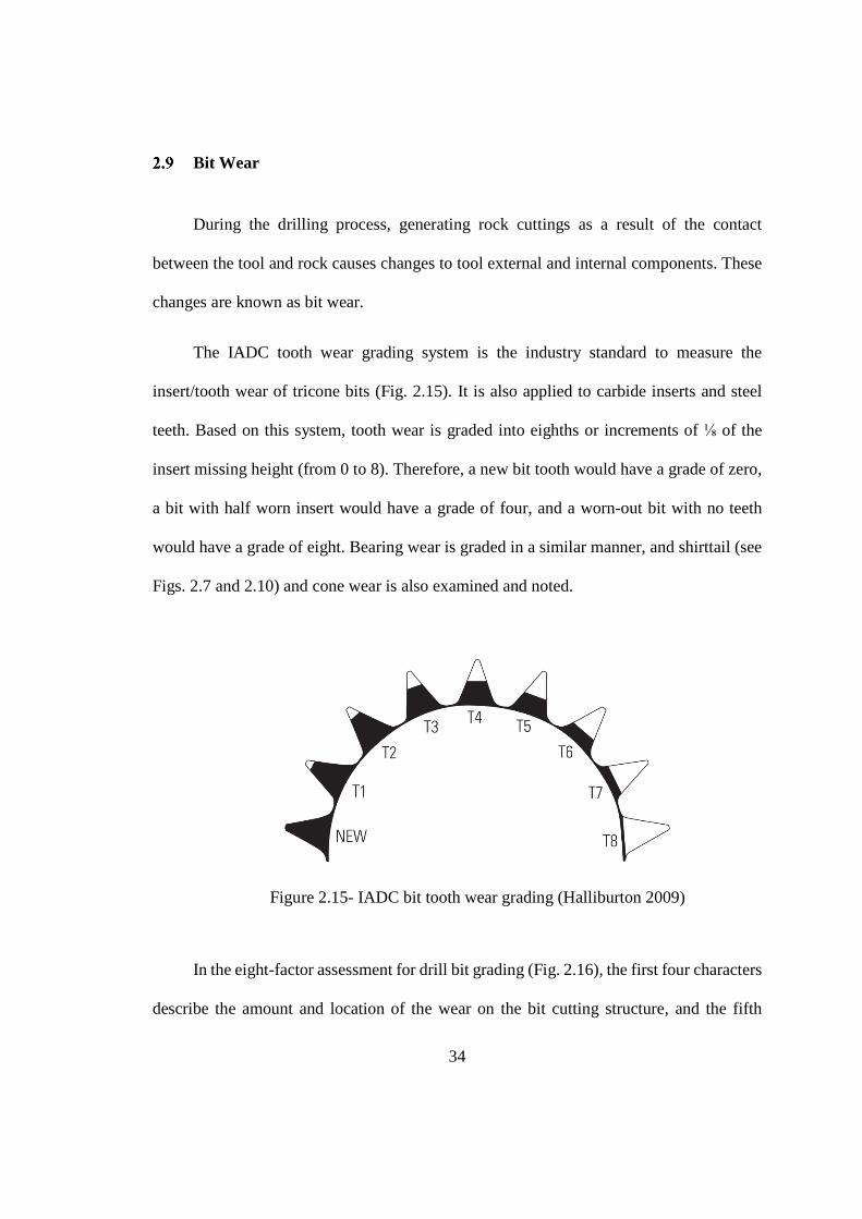
Bit Wear

During the drilling process, generating rock cuttings as a result of the contact

between the tool and rock causes changes to tool external and internal components. These

changes are known as bit wear.

The IADC tooth wear grading system is the industry standard to measure the

insert/tooth wear of tricone bits (Fig. 2.15). It is also applied to carbide inserts and steel

teeth. Based on this system, tooth wear is graded into eighths or increments of ⅛ of the

insert missing height (from 0 to 8). Therefore, a new bit tooth would have a grade of zero,

a bit with half worn insert would have a grade of four, and a worn-out bit with no teeth

would have a grade of eight. Bearing wear is graded in a similar manner, and shirttail (see

Figs. 2.7 and 2.10) and cone wear is also examined and noted.

Figure 2.15- IADC bit tooth wear grading (Halliburton 2009)

In the eight-factor assessment for drill bit grading (Fig. 2.16), the first four characters

describe the amount and location of the wear on the bit cutting structure, and the fifth

35

represents the bearing wear condition and applies only to the tricone bits. The sixth

character describes the gauge measurement. The seventh space is reserved for adding

additional information from the bit inspection and last space describes the reason for

pulling the bit (Cobb et al. 2014).

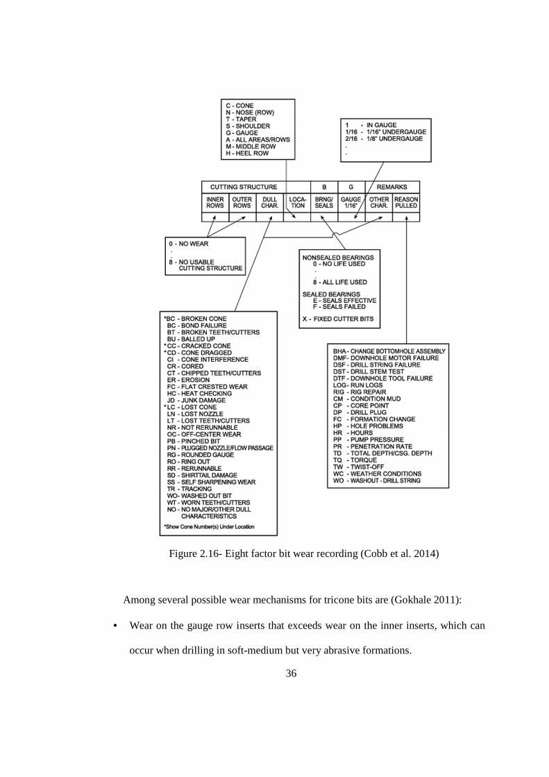
36

Figure 2.16- Eight factor bit wear recording (Cobb et al. 2014)

Among several possible wear mechanisms for tricone bits are (Gokhale 2011):

• Wear on the gauge row inserts that exceeds wear on the inner inserts, which can

occur when drilling in soft-medium but very abrasive formations.

37

• Uniform wear on all teeth of the cones

• Heavy wear on the bit shirttail, which can occur if drilling with a bent pipe that

results in very high side thrust on the bit and consequent wear.

• More broken inserts on the gauge row than the inner rows; this type of wear is

observed when a bit designed for soft geological condition is applied in hard

formations.

• A broken bit lug, which results when the bit is dropped and hits a ledge in the hole

• Worn out teeth on the surface of cone(s) that touched the bottom of the drilled hole

often due to locked cone(s)

• Broken and lost inner part of cone(s) from bearing failure

• Loss of one or more cones in the blasthole due to bearing failure

The IADC recognizes bearing failure as the dominant failure mode for tricone bits.

The bit must be pulled when there is a good reason to suspect bearing failure. Premature

bearing failure (before the anticipated bit end-of-life) can occur due to unsuitable operation

setpoints, incorrect cutting structure selection, and excessive axial or torsional vibrations

(Cobb et al. 2014). If the bearing failure is not detected in time, the chance of cone

detachment is high. Risks associated with leaving detached bit cones in the hole are serious

and will lead to the costly “fishing” efforts.

The lifetimes and wear mechanisms of tricone bits differ depending on bit design and

working conditions. For example, a tricone with sealed bearings will last much longer than

the open bearing type in hard formations. The seal does not allow dust and rock particles

to enter the rotational structure, which extends the bearing life significantly. In soft ground

38

conditions, however, bearing type does not make the same significant difference. Sealed

bearing tricone bits usually experience cone wear when working in hard formations.

Continued drilling with a bit with worn cones exerts excessive forces on the bearing

elements and ultimately results in bearing failure.

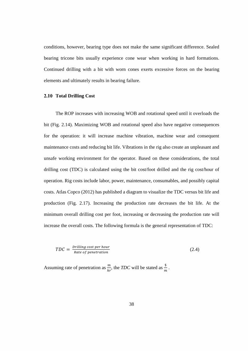
Total Drilling Cost

The ROP increases with increasing WOB and rotational speed until it overloads the

bit (Fig. 2.14). Maximizing WOB and rotational speed also have negative consequences

for the operation: it will increase machine vibration, machine wear and consequent

maintenance costs and reducing bit life. Vibrations in the rig also create an unpleasant and

unsafe working environment for the operator. Based on these considerations, the total

drilling cost (TDC) is calculated using the bit cost/foot drilled and the rig cost/hour of

operation. Rig costs include labor, power, maintenance, consumables, and possibly capital

costs. Atlas Copco (2012) has published a diagram to visualize the TDC versus bit life and

production (Fig. 2.17). Increasing the production rate decreases the bit life. At the

minimum overall drilling cost per foot, increasing or decreasing the production rate will

increase the overall costs. The following formula is the general representation of TDC:

56� = 789::9; <=>? @A8 B=C8'D?A =E @AA?8D?9= (2.4)

Assuming rate of penetration as �B8, the TDC will be stated as

$� .

39

Figure 2.17- TDC versus bit life and production rate (AtlasCopco 2012)

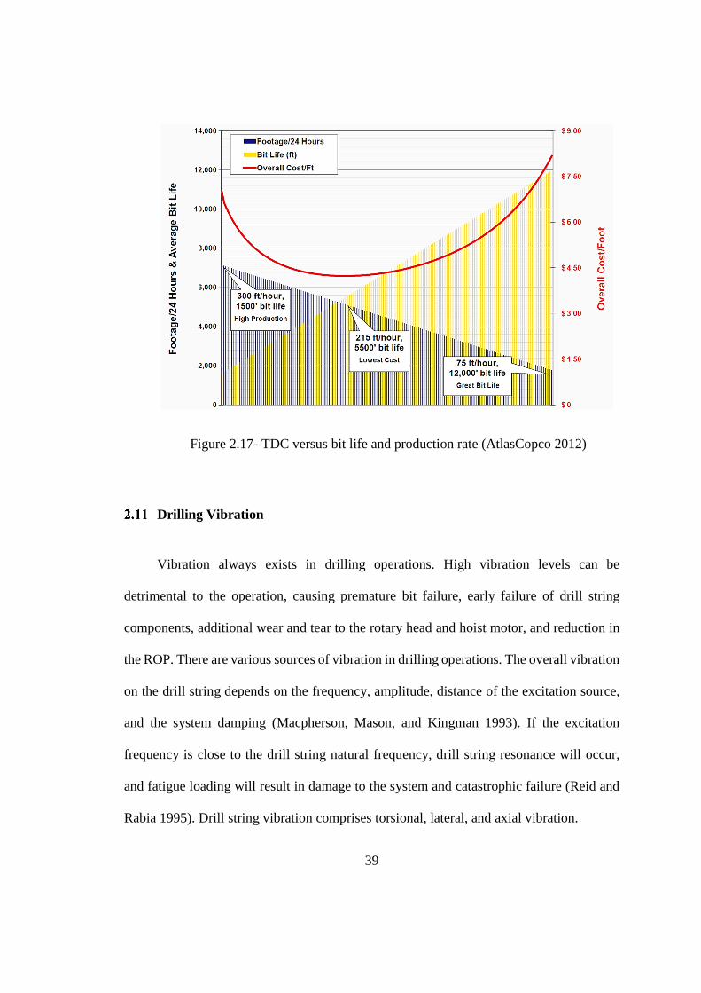
Drilling Vibration

Vibration always exists in drilling operations. High vibration levels can be

detrimental to the operation, causing premature bit failure, early failure of drill string

components, additional wear and tear to the rotary head and hoist motor, and reduction in

the ROP. There are various sources of vibration in drilling operations. The overall vibration

on the drill string depends on the frequency, amplitude, distance of the excitation source,

and the system damping (Macpherson, Mason, and Kingman 1993). If the excitation

frequency is close to the drill string natural frequency, drill string resonance will occur,

and fatigue loading will result in damage to the system and catastrophic failure (Reid and

Rabia 1995). Drill string vibration comprises torsional, lateral, and axial vibration.

40

2.11.1 Torsional vibration

Torsional vibration is excited by the frictional torque applied on the bit and possibly

drill string inside the hole. It will manifest as accelerations and decelerations in string rotary

motion, resulting in a non-uniform rotation of the bit down the hole. The stick-slip

phenomenon is an extreme case of torsional vibration and is usually a concern in long drill

strings used in the oil and gas industry.

Early models to investigate the torsional behavior of drill strings used a torsional

pendulum and assumed the pipe inertia to be negligible (Lin and Wang 1991). Later studies

investigated the effect of the bit-rock interaction on the stick-slip phenomenon—a jerking

motion when two objects slide against each other (Besselink, van de Wouw, and Nijmeijer

2011), but are limited by simplifications and assumptions (Ghasemloonia, Rideout, and

Butt 2015). Stick-slip vibration frequency in the drill string is usually between 0.05 to 0.5

Hz (Aadnoy et al. 2009).

2.11.2 Lateral vibration

Lateral vibration will cause the bit and drill string to rotate around an axis other than

the string geometrical center, causing the bit to repeatedly strike the hole wall. The extreme

case of lateral vibration is bit whirling or walk of the bit around the hole. Whirling mostly

occurs with polycrystalline diamond compact (PDC) drill bits, which are broadly applied

in the oil and gas drilling industry. Lateral vibration is usually damped along the drill pipe

41

and would not be seen on the surface. However, due to interactions with the hole wall, high

amounts of whirling will cause surface detectable torsional and axial vibration

(Christoforou and Yigit 2001). Depending on the string rotational speed and the number of

cutters on the PDC bit, whirling ranges between 5 and 100 Hz (Aadnoy et al. 2009).

2.11.3 Axial vibration

Axial vibration occurs as a result of bit-rock interactions. Bit bouncing occurs when

the WOB lifts the bit off the hole bottom and then the bit drops repeatedly. This

phenomenon is usually is associated with tricone bit drilling. Bit bouncing can generate an

excitation three times the tricone bit rotational speed. The frequency of axial vibration is

usually 1–10 Hz. Bit bouncing can be sensed at the surface when drilling at shallow depths

(Aadnoy et al. 2009). This interaction adds a dynamic part to the axial load and causes

fluctuations in the actual WOB (Dunayevsky, Abbassian, and Judzis 1993).

Indentions formed in the rock by bit teeth are also a source of axial vibration.

Laboratory tests by Ma and Azar (1985) to determine the contact condition on roller cone

bit teeth down the hole and tooth velocity and position showed that the relationship

between DOP and bit rotation exhibits a repeated step shape (Fig. 2.18). A series of craters

are formed under the bit after a given number of rotations, then the bit suddenly drops and

begins creating a new series of indentions.

42

Figure 2.18- DOP versus revolutions of bit (Ma and Azar 1985)

The step height (Dp) is the mean depth of the craters down the hole and is calculated

as (Ma and Azar 1985):

6@ = G�H I J�/� (2.5)

Where

ROP: Rate of penetration in m/min

nx: Number of rotations

N: Bit rotational speed in rpm

In a simplified model of tricone bit-rock interactions, Sheppard and Lesage (1988)

assumed that at an instant, only one tooth from each row of a cone is in contact with the

rock and the bit load is equally distributed among all rows of the cone. Their laboratory

tests measuring the torque and forces on every row of an instrumented tricone bit showed

that the rotational speed of the cones around the bearing axis is 1.25–1.31 times that of the

bit. Hardage (1992) used these results to define a periodic behavior for tricone bits.

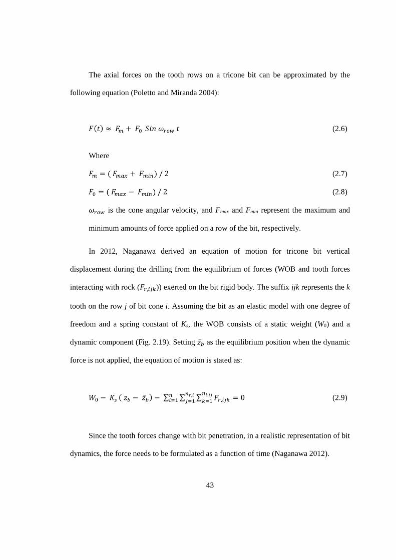
43

The axial forces on the tooth rows on a tricone bit can be approximated by the

following equation (Poletto and Miranda 2004):

L�� ≈ L� + L4 1NJ O8=P � (2.6)

Where

L� = ( L�D� + L�9) / 2 (2.7)

L4 = ( L�D� − L�9) / 2 (2.8)

O8=P is the cone angular velocity, and Fmax and Fmin represent the maximum and

minimum amounts of force applied on a row of the bit, respectively.

In 2012, Naganawa derived an equation of motion for tricone bit vertical

displacement during the drilling from the equilibrium of forces (WOB and tooth forces

interacting with rock (L8,9QR)) exerted on the bit rigid body. The suffix ijk represents the k

tooth on the row j of bit cone i. Assuming the bit as an elastic model with one degree of

freedom and a spring constant of Ks, the WOB consists of a static weight (W0) and a

dynamic component (Fig. 2.19). Setting ST̅ as the equilibrium position when the dynamic

force is not applied, the equation of motion is stated as:

�4 − U> ( ST − ST̅) − ∑ ∑ ∑ L8,9QR = 0X,YZR[\

],YQ[\9[\ (2.9)

Since the tooth forces change with bit penetration, in a realistic representation of bit

dynamics, the force needs to be formulated as a function of time (Naganawa 2012).

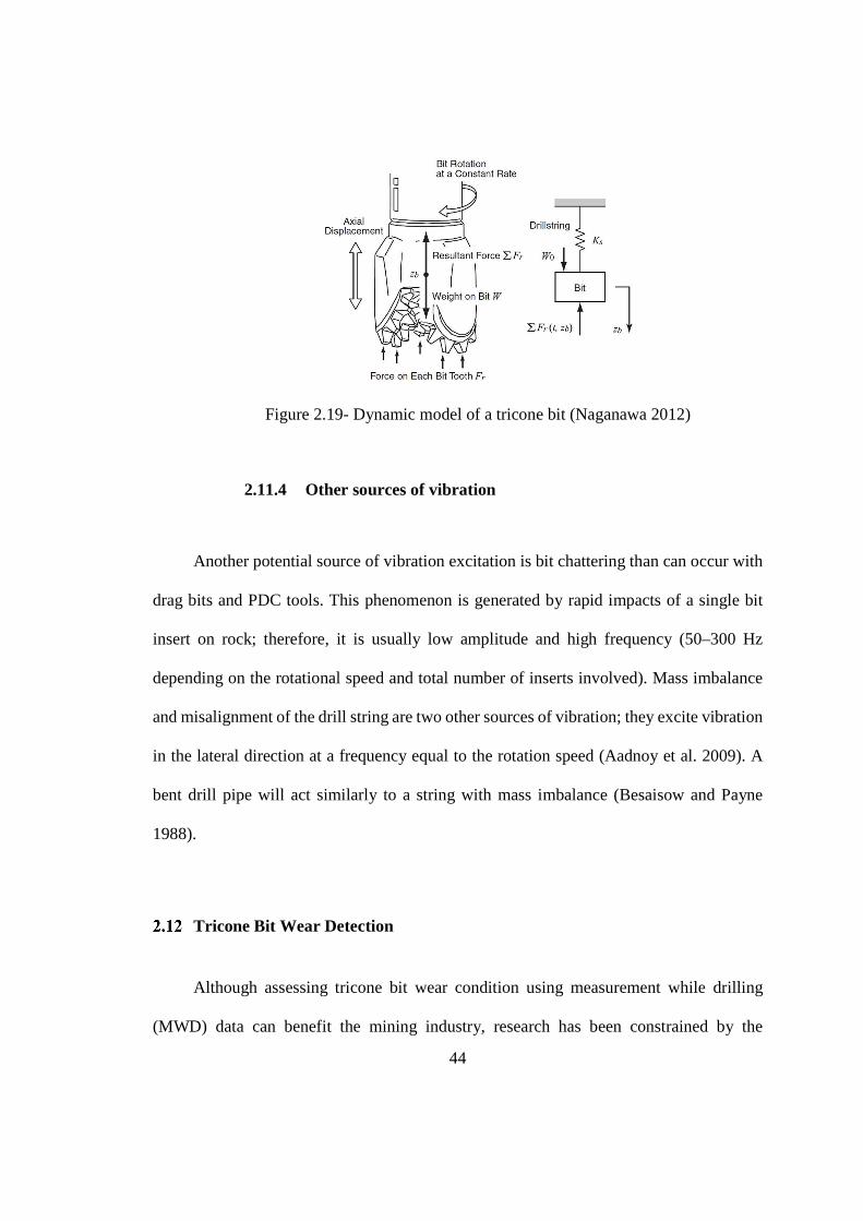
44

Figure 2.19- Dynamic model of a tricone bit (Naganawa 2012)

2.11.4 Other sources of vibration

Another potential source of vibration excitation is bit chattering than can occur with

drag bits and PDC tools. This phenomenon is generated by rapid impacts of a single bit

insert on rock; therefore, it is usually low amplitude and high frequency (50–300 Hz

depending on the rotational speed and total number of inserts involved). Mass imbalance

and misalignment of the drill string are two other sources of vibration; they excite vibration

in the lateral direction at a frequency equal to the rotation speed (Aadnoy et al. 2009). A

bent drill pipe will act similarly to a string with mass imbalance (Besaisow and Payne

1988).

Tricone Bit Wear Detection

Although assessing tricone bit wear condition using measurement while drilling

(MWD) data can benefit the mining industry, research has been constrained by the

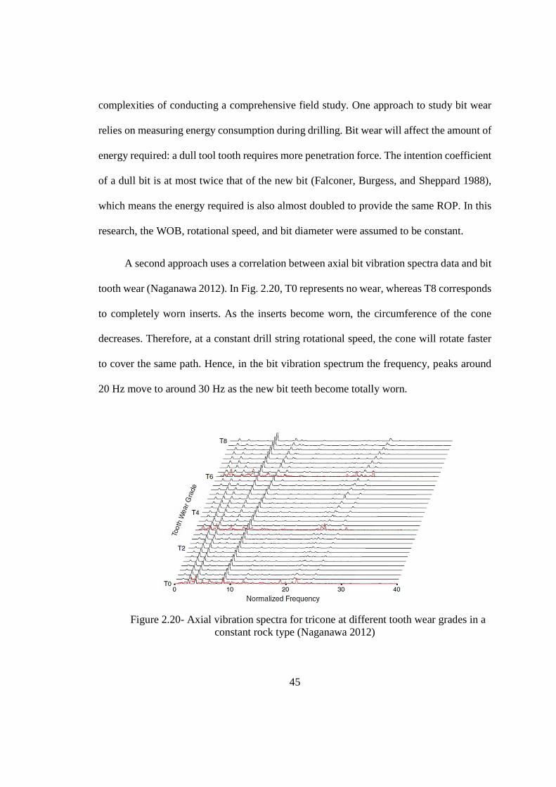
45

complexities of conducting a comprehensive field study. One approach to study bit wear

relies on measuring energy consumption during drilling. Bit wear will affect the amount of

energy required: a dull tool tooth requires more penetration force. The intention coefficient

of a dull bit is at most twice that of the new bit (Falconer, Burgess, and Sheppard 1988),

which means the energy required is also almost doubled to provide the same ROP. In this

research, the WOB, rotational speed, and bit diameter were assumed to be constant.

A second approach uses a correlation between axial bit vibration spectra data and bit

tooth wear (Naganawa 2012). In Fig. 2.20, T0 represents no wear, whereas T8 corresponds

to completely worn inserts. As the inserts become worn, the circumference of the cone

decreases. Therefore, at a constant drill string rotational speed, the cone will rotate faster

to cover the same path. Hence, in the bit vibration spectrum the frequency, peaks around

20 Hz move to around 30 Hz as the new bit teeth become totally worn.

Figure 2.20- Axial vibration spectra for tricone at different tooth wear grades in a constant rock type (Naganawa 2012)

46

Drilling vibration has also been offered as an input for the control system of a drill

rig to keep the vibration levels in an acceptable level by adjusting drilling parameters

(Aboujaoude 1997).

Cooper (2002) proposed detecting bit tooth wear by comparing measured drilling

performance with theoretical bit performance. In this approach, which requires knowledge

of geological information, a model estimates a theoretical ROP from drilling parameters

and rock strength data. The theoretical values are then compared with the ROP measured

in the laboratory; any difference between the two indicates the bit wear state.

Cooper (2002) proposed a similar approach for rock strength measurement, assuming

the driller has an access to rock strength data from the drill log. As shown in Fig. 2.21, the

drill log estimation follows an incremental trend compared to the geological log

estimations. The rock strength estimated from drill logs erroneously increases due to

increasing wear on the bit teeth. Cooper’s research from 1987 is based on laboratory

experiments, whereas his more recent work is based on real lithological data and synthetic

drilling data. The author emphasizes that precise estimation of ROP based on rock type—

or vice versa—is very challenging in practice because of the large number of parameters

involved (Cooper 1987; Cooper 2002).

47

Figure 2.21- Rock strength from geological logs and drill logs versus depth (Cooper 2002)

Sheppard and Lesage (1988) measured the load distribution between the rows of new

and half-worn bits (T0 and T3 states) in controlled laboratory tests and concluded that the

load distribution is sensitive to tooth wear. A total force of 8 kN was distributed between

the outer and inner rows as 6 and 2 kN, respectively, for the T0 bit and 5 and 3 kN,

respectively, for the T3 bit (i.e. for T0: outer/inner = 3 and for T3: outer/inner = 1.66).

Therefore, the outer/inner row force distribution ratio decreased as the bit wear increased

to the T3 level. Applying these results to actual operations is limited by the fact that tooth

wear is not uniform within the same row or among different rows.

Other research has suggested a method for tricone bit performance evaluation using

MWD data. For example, the degradation of production and the initial and final ROP

(before the bit change) was studied in an operating mine in Sweden by (Ghosh,

48

Schunnesson, and Kumar 2016). Production degradation was assumed to be caused by

wear progress on the bit. The rock strength variations in the mine were assumed to be

negligible.

Researchers have also implemented image processing techniques for tricone bit wear

detection. Images of the bit taken at specific time intervals are processed and image features

are extracted for analysis (Saeidi et al. 2014). An advantage to this approach is that it is not

influenced by geological conditions or working parameters. Drawbacks related to vision-

based wear monitoring methods based on image analysis include:

• a portion of each cone is invisible in each image

• frequent bit cleaning is required before each image is captured

• most importantly,

o bit bearings cannot be assessed

o real-time monitoring while drilling is not feasible

Artificial Intelligence in Mining

Application of artificial intelligence (AI) approaches has become beneficial to

address real-world problems including regression, clustering, and classification. In the

mining industry, researchers are working to implement AI models in a variety of

applications to increase the safety and efficiency of operations. Putting an effective AI

model into practice plays a crucial role in automation problems. For example, Dadhich et

al. (2019) presented a supervised machine learning algorithm for automation of loaders

49

bucket filling. They used an artificial neural network (ANN) model that was trained by

data generated from an expert operator and tested and verified the model in field trials.

Siami-Irdemoosa and Dindarloo (2015) constructed a feedforward backpropagation

neural network to predict fuel consumption by mine dump trucks, in an attempt to assess

energy costs and greenhouse gas generation. Descriptive features in the model included

payload, loading time, travel time, and idle time. The model was able to predict fuel

efficiency with only 10% error.

In the context of drilling, Fattahi and Bazdar (2017) evaluated the performance of

ANN models to determine the rock drilling rate index. Rock properties were the model

inputs, and data from the literature were used to train and test the models. The performance

of different ANN architectures in predicting the drillability rate index was evaluated.

However, the dataset presented in this work does not include controllable drilling

parameters (e.g., thrust force, rotational speed) and bit condition was not analyzed.

ANN models have also been developed to predict the drilling ROP in the oilfield

environment. For example, Ashrafi et al. (2019) collected 1,000 data points from the field

as input features, including the operational parameters of WOB and bit rotational speed.

Although the researchers acknowledged the effect of bit type on the results, bit

characteristics were not among the input vector of features. It needs to be emphasized that

bit wear condition is a significant parameter in drilling performance and needs to be taken

into account for an accurate and practical analysis of the ROP.

50

Chapter 3 – Ground Penetrating Radar

Ground Penetrating Radar Concept

A ground penetrating radar (GPR) system consists of at least one transmission

antenna that generates high-frequency electromagnetic waves into the subsurface. Changes

in the electrical properties of ground material result in partial reflection of the signal. The

reflected signal is captured by the GPR receiver antenna; these reflection data are stored

for post-processing. Wave propagation is largely described by velocity and attenuation,

which correspond to the material dielectric permittivity and electrical conductivity,

respectively (Davis and Annan 1989; Utsi 2017).

Ground Penetration Radar Tests

In the initial phases of the current bit wear monitoring project, the need for geological

data led to investigating the applicability of GPR to extract subsurface geological

information. This chapter presents the results of several GPR surveys conducted to map

stratification and fractures at a Lafarge limestone quarry in Quebec and to detect coal seams

at the Teck Fording River coal mine in southeastern British Columbia, which produces coal

for steel making. The annual production capacity is about 8.5 million tonnes of clean coal

(TeckResources 2018).

The motivation behind this study is to support the movement of the surface mining

industry towards automation and to optimize exploration, mine planning, and reducing

extraction costs by investigating the application of GPR for geological mapping. Since the

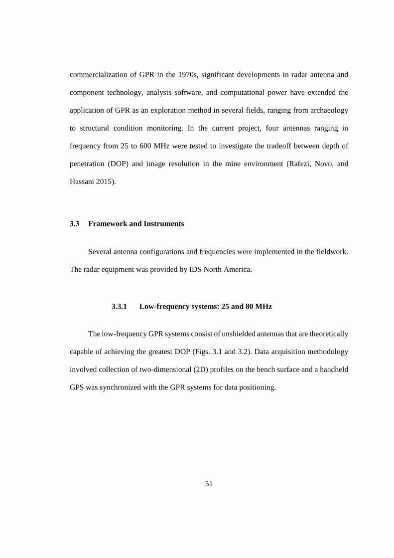
51

commercialization of GPR in the 1970s, significant developments in radar antenna and

component technology, analysis software, and computational power have extended the

application of GPR as an exploration method in several fields, ranging from archaeology

to structural condition monitoring. In the current project, four antennas ranging in

frequency from 25 to 600 MHz were tested to investigate the tradeoff between depth of

penetration (DOP) and image resolution in the mine environment (Rafezi, Novo, and

Hassani 2015).

Framework and Instruments

Several antenna configurations and frequencies were implemented in the fieldwork.

The radar equipment was provided by IDS North America.

3.3.1 Low-frequency systems: 25 and 80 MHz

The low-frequency GPR systems consist of unshielded antennas that are theoretically

capable of achieving the greatest DOP (Figs. 3.1 and 3.2). Data acquisition methodology

involved collection of two-dimensional (2D) profiles on the bench surface and a handheld

GPS was synchronized with the GPR systems for data positioning.

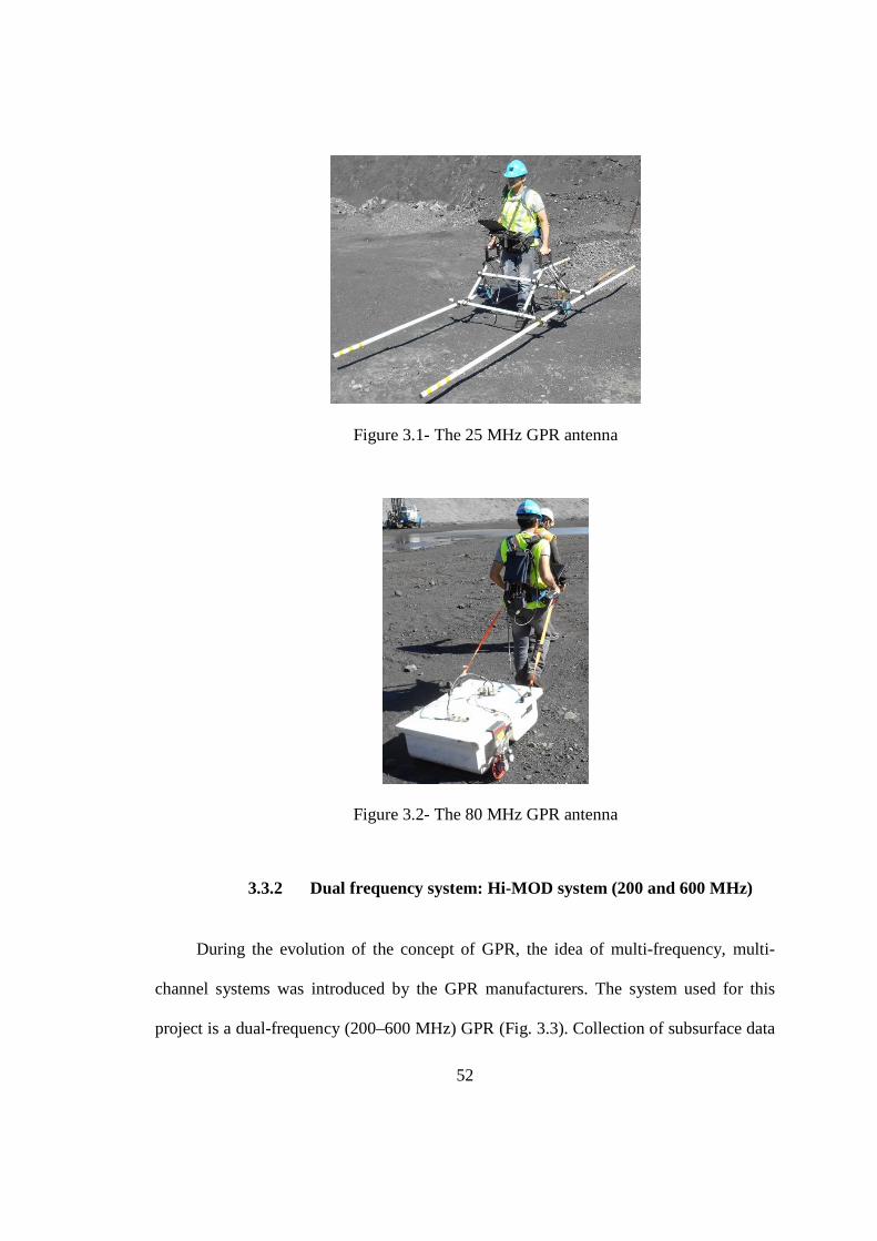
52

Figure 3.1- The 25 MHz GPR antenna

Figure 3.2- The 80 MHz GPR antenna

3.3.2 Dual frequency system: Hi-MOD system (200 and 600 MHz)

During the evolution of the concept of GPR, the idea of multi-frequency, multi-

channel systems was introduced by the GPR manufacturers. The system used for this

project is a dual-frequency (200–600 MHz) GPR (Fig. 3.3). Collection of subsurface data

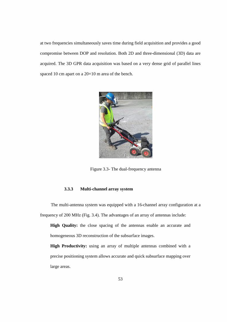
53

at two frequencies simultaneously saves time during field acquisition and provides a good

compromise between DOP and resolution. Both 2D and three-dimensional (3D) data are

acquired. The 3D GPR data acquisition was based on a very dense grid of parallel lines

spaced 10 cm apart on a 20×10 m area of the bench.

Figure 3.3- The dual-frequency antenna

3.3.3 Multi-channel array system

The multi-antenna system was equipped with a 16-channel array configuration at a

frequency of 200 MHz (Fig. 3.4). The advantages of an array of antennas include:

High Quality: the close spacing of the antennas enable an accurate and

homogeneous 3D reconstruction of the subsurface images.

High Productivity: using an array of multiple antennas combined with a

precise positioning system allows accurate and quick subsurface mapping over

large areas.

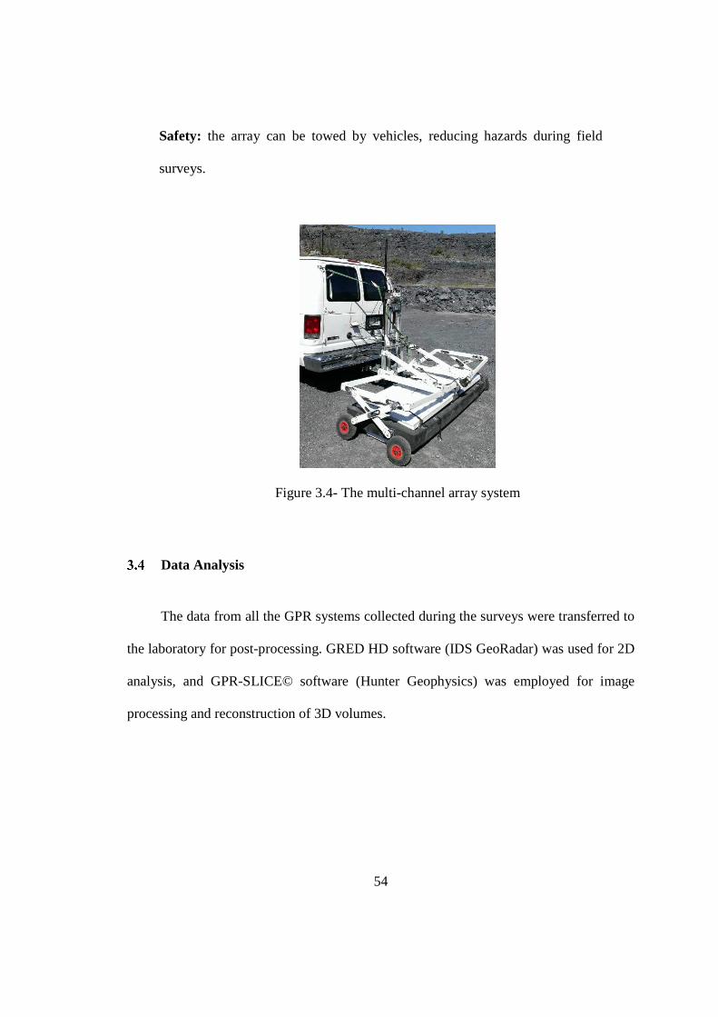
54

Safety: the array can be towed by vehicles, reducing hazards during field

surveys.

Figure 3.4- The multi-channel array system

Data Analysis

The data from all the GPR systems collected during the surveys were transferred to

the laboratory for post-processing. GRED HD software (IDS GeoRadar) was used for 2D

analysis, and GPR-SLICE© software (Hunter Geophysics) was employed for image

processing and reconstruction of 3D volumes.

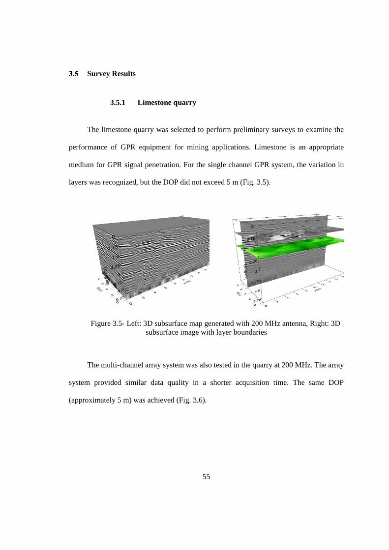
55

Survey Results

3.5.1 Limestone quarry

The limestone quarry was selected to perform preliminary surveys to examine the

performance of GPR equipment for mining applications. Limestone is an appropriate

medium for GPR signal penetration. For the single channel GPR system, the variation in

layers was recognized, but the DOP did not exceed 5 m (Fig. 3.5).

Figure 3.5- Left: 3D subsurface map generated with 200 MHz antenna, Right: 3D subsurface image with layer boundaries

The multi-channel array system was also tested in the quarry at 200 MHz. The array

system provided similar data quality in a shorter acquisition time. The same DOP

(approximately 5 m) was achieved (Fig. 3.6).

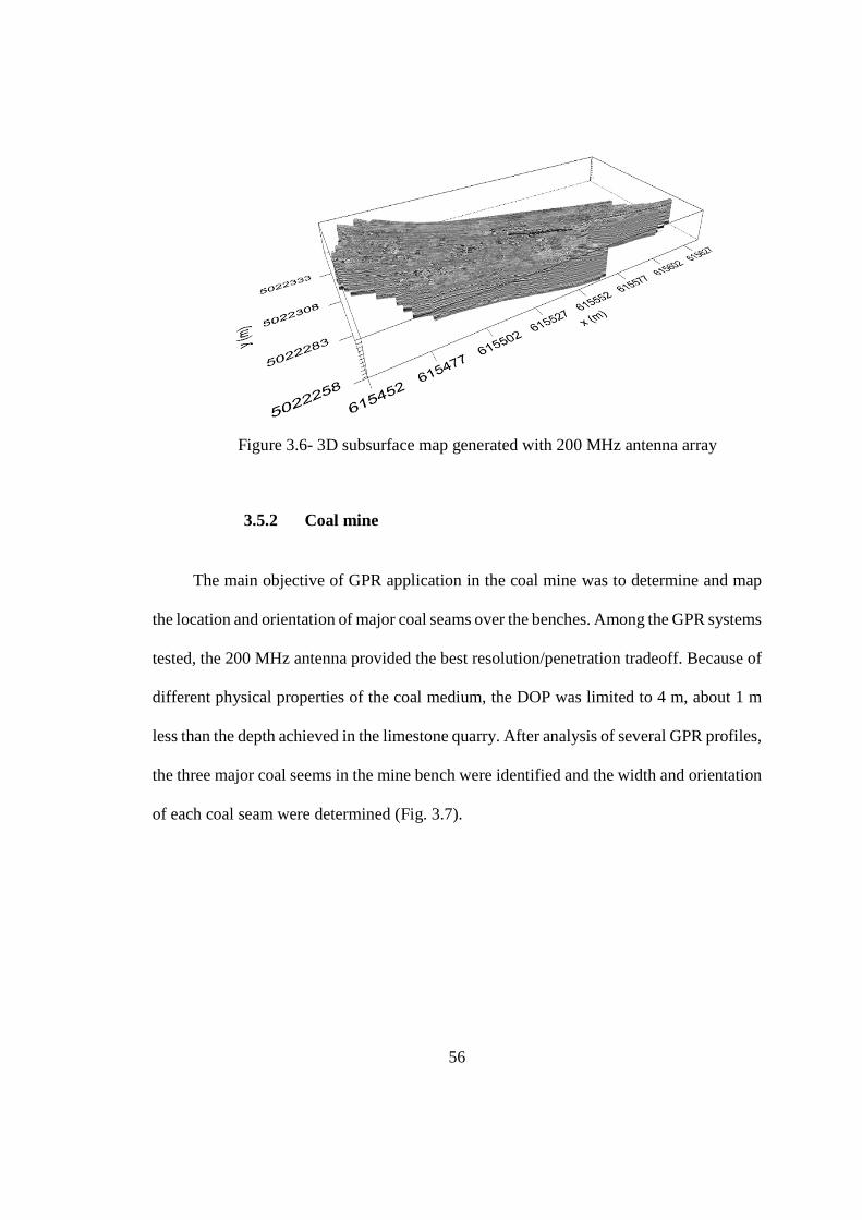
56

Figure 3.6- 3D subsurface map generated with 200 MHz antenna array

3.5.2 Coal mine

The main objective of GPR application in the coal mine was to determine and map

the location and orientation of major coal seams over the benches. Among the GPR systems

tested, the 200 MHz antenna provided the best resolution/penetration tradeoff. Because of

different physical properties of the coal medium, the DOP was limited to 4 m, about 1 m

less than the depth achieved in the limestone quarry. After analysis of several GPR profiles,

the three major coal seems in the mine bench were identified and the width and orientation

of each coal seam were determined (Fig. 3.7).

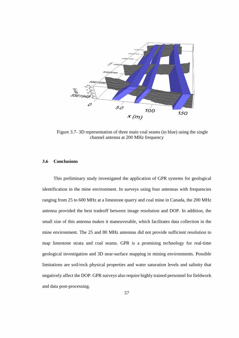
57

Figure 3.7- 3D representation of three main coal seams (in blue) using the single channel antenna at 200 MHz frequency

Conclusions

This preliminary study investigated the application of GPR systems for geological

identification in the mine environment. In surveys using four antennas with frequencies

ranging from 25 to 600 MHz at a limestone quarry and coal mine in Canada, the 200 MHz

antenna provided the best tradeoff between image resolution and DOP. In addition, the

small size of this antenna makes it maneuverable, which facilitates data collection in the

mine environment. The 25 and 80 MHz antennas did not provide sufficient resolution to

map limestone strata and coal seams. GPR is a promising technology for real-time

geological investigation and 3D near-surface mapping in mining environments. Possible

limitations are soil/rock physical properties and water saturation levels and salinity that

negatively affect the DOP. GPR surveys also require highly trained personnel for fieldwork

and data post-processing.

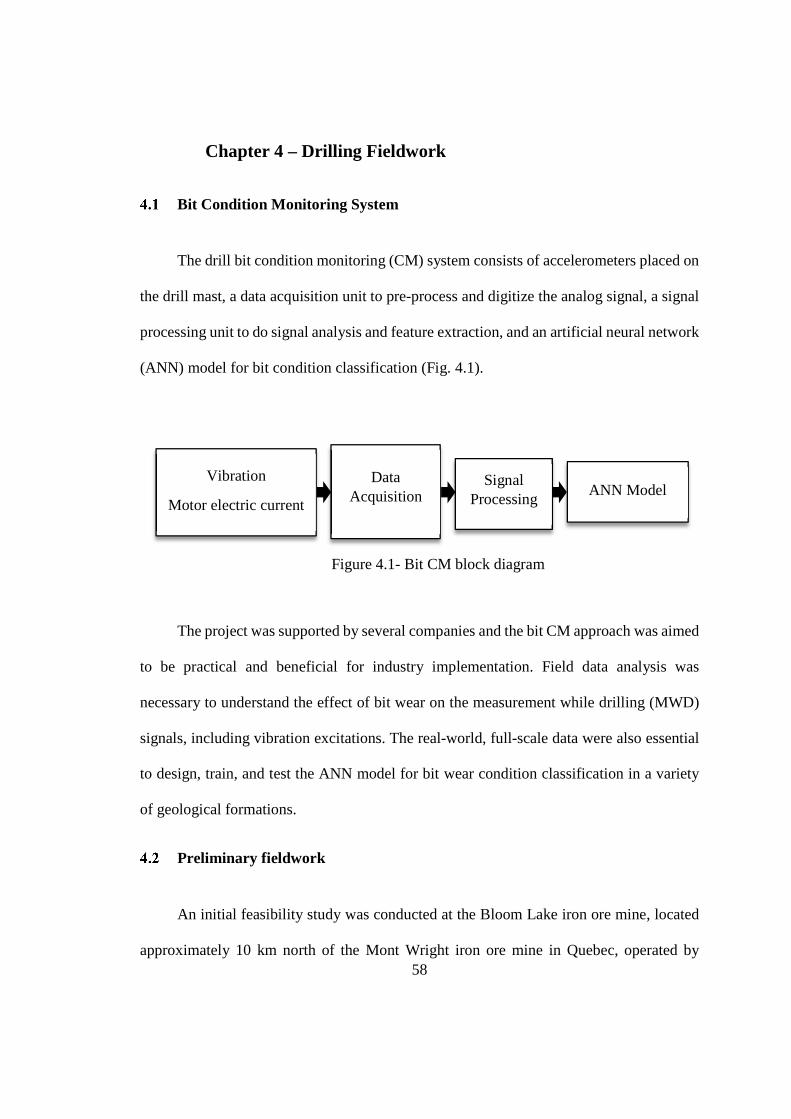
58

Chapter 4 – Drilling Fieldwork

Bit Condition Monitoring System

The drill bit condition monitoring (CM) system consists of accelerometers placed on

the drill mast, a data acquisition unit to pre-process and digitize the analog signal, a signal

processing unit to do signal analysis and feature extraction, and an artificial neural network

(ANN) model for bit condition classification (Fig. 4.1).

Figure 4.1- Bit CM block diagram

The project was supported by several companies and the bit CM approach was aimed

to be practical and beneficial for industry implementation. Field data analysis was

necessary to understand the effect of bit wear on the measurement while drilling (MWD)

signals, including vibration excitations. The real-world, full-scale data were also essential

to design, train, and test the ANN model for bit wear condition classification in a variety

of geological formations.

Preliminary fieldwork

An initial feasibility study was conducted at the Bloom Lake iron ore mine, located

approximately 10 km north of the Mont Wright iron ore mine in Quebec, operated by

Vibration

Motor electric current

Data Acquisition

Signal Processing

ANN Model

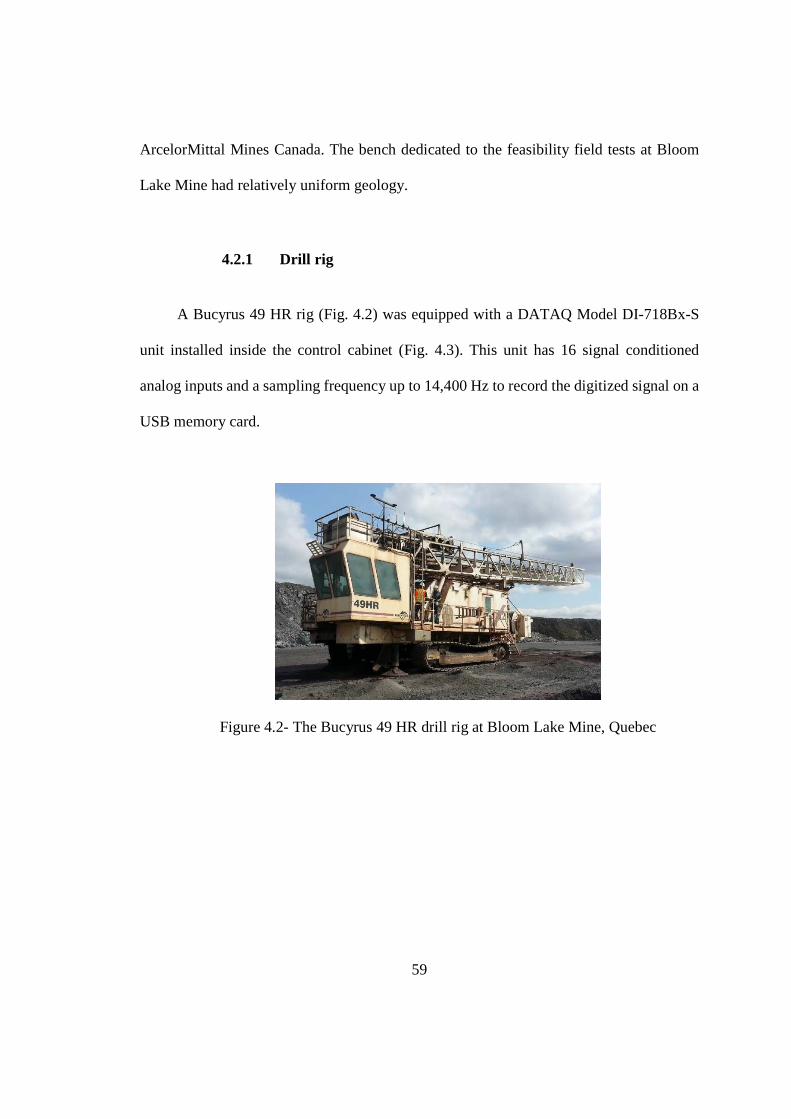
59

ArcelorMittal Mines Canada. The bench dedicated to the feasibility field tests at Bloom

Lake Mine had relatively uniform geology.

4.2.1 Drill rig

A Bucyrus 49 HR rig (Fig. 4.2) was equipped with a DATAQ Model DI-718Bx-S

unit installed inside the control cabinet (Fig. 4.3). This unit has 16 signal conditioned

analog inputs and a sampling frequency up to 14,400 Hz to record the digitized signal on a

USB memory card.

Figure 4.2- The Bucyrus 49 HR drill rig at Bloom Lake Mine, Quebec

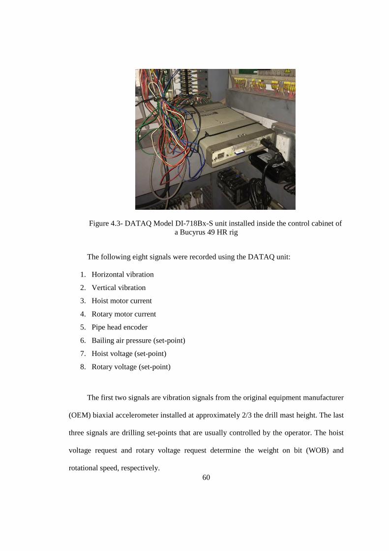
60

Figure 4.3- DATAQ Model DI-718Bx-S unit installed inside the control cabinet of a Bucyrus 49 HR rig

The following eight signals were recorded using the DATAQ unit:

1. Horizontal vibration

2. Vertical vibration

3. Hoist motor current

4. Rotary motor current

5. Pipe head encoder

6. Bailing air pressure (set-point)

7. Hoist voltage (set-point)

8. Rotary voltage (set-point)

The first two signals are vibration signals from the original equipment manufacturer

(OEM) biaxial accelerometer installed at approximately 2/3 the drill mast height. The last

three signals are drilling set-points that are usually controlled by the operator. The hoist

voltage request and rotary voltage request determine the weight on bit (WOB) and

rotational speed, respectively.

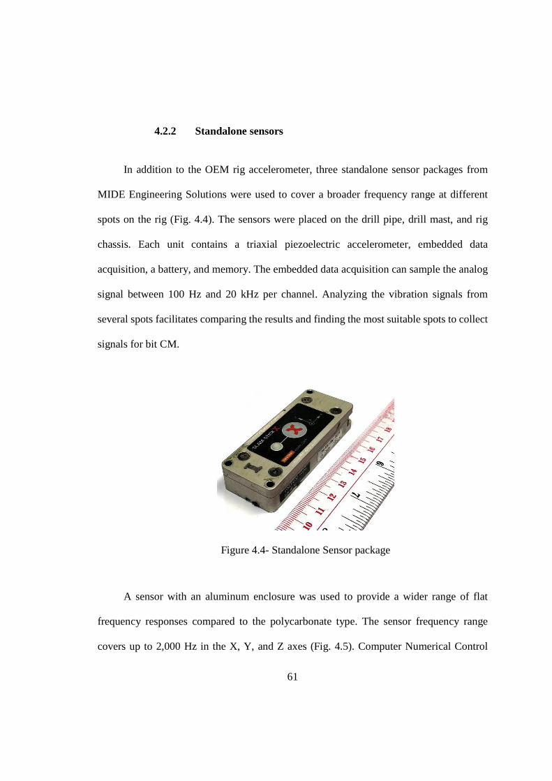
61

4.2.2 Standalone sensors

In addition to the OEM rig accelerometer, three standalone sensor packages from

MIDE Engineering Solutions were used to cover a broader frequency range at different

spots on the rig (Fig. 4.4). The sensors were placed on the drill pipe, drill mast, and rig

chassis. Each unit contains a triaxial piezoelectric accelerometer, embedded data

acquisition, a battery, and memory. The embedded data acquisition can sample the analog

signal between 100 Hz and 20 kHz per channel. Analyzing the vibration signals from

several spots facilitates comparing the results and finding the most suitable spots to collect

signals for bit CM.

Figure 4.4- Standalone Sensor package

A sensor with an aluminum enclosure was used to provide a wider range of flat

frequency responses compared to the polycarbonate type. The sensor frequency range

covers up to 2,000 Hz in the X, Y, and Z axes (Fig. 4.5). Computer Numerical Control

62

machined mountings were designed in SolidWorks software to accommodate sensors on

the desired spots on the rig (Fig. 4.6). Another sensor package was installed on the drill

mast. The vibration on the rig chassis was also measured (Fig 4.7).

Figure 4.5- Frequency responses of the piezoelectric sensor on three axes (Mide 2017)

Figure 4.6- Sensor mounting for the drill pipe. Left: SolidWorks design. Right: After installation on the pipe

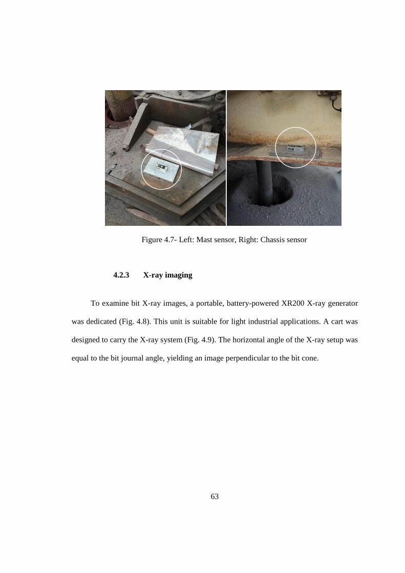
63

Figure 4.7- Left: Mast sensor, Right: Chassis sensor

4.2.3 X-ray imaging

To examine bit X-ray images, a portable, battery-powered XR200 X-ray generator

was dedicated (Fig. 4.8). This unit is suitable for light industrial applications. A cart was

designed to carry the X-ray system (Fig. 4.9). The horizontal angle of the X-ray setup was

equal to the bit journal angle, yielding an image perpendicular to the bit cone.

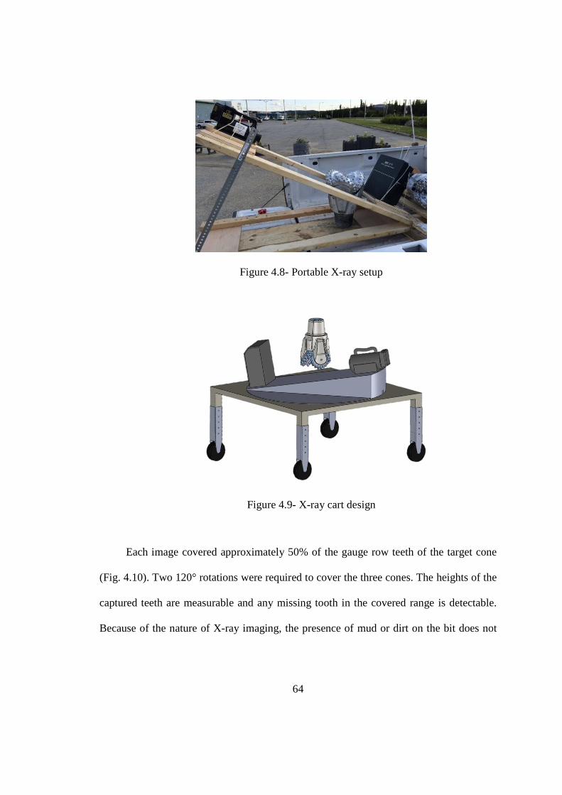
64

Figure 4.8- Portable X-ray setup

Figure 4.9- X-ray cart design

Each image covered approximately 50% of the gauge row teeth of the target cone

(Fig. 4.10). Two 120° rotations were required to cover the three cones. The heights of the

captured teeth are measurable and any missing tooth in the covered range is detectable.

Because of the nature of X-ray imaging, the presence of mud or dirt on the bit does not

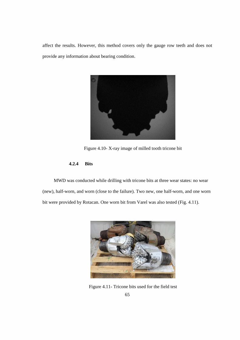
65

affect the results. However, this method covers only the gauge row teeth and does not

provide any information about bearing condition.

Figure 4.10- X-ray image of milled tooth tricone bit

4.2.4 Bits

MWD was conducted while drilling with tricone bits at three wear states: no wear

(new), half-worn, and worn (close to the failure). Two new, one half-worn, and one worn

bit were provided by Rotacan. One worn bit from Varel was also tested (Fig. 4.11).

Figure 4.11- Tricone bits used for the field test

66

4.2.5 Experimental design

Two WOBs and rotational speeds were considered for each of the three wear grades

(Table 4.1). Five blastholes were drilled for each configuration and bit to a depth of

approximately 6 m or until bit failure in the case of the worn bits (Table 4.2).

Table 4.1- Drilling configurations for each of the three wear grades at the Bloom Lake Mine McGill test bench

Configuration WOB (kN) Rotational speed (rpm)

1 415 60

2 415 80

3 300 60

4 300 80

Table 4.2- Number of drill holes for each drilling configuration tested with three bit wear states

Configuration Bit condition

New Half-worn Worn

1 10 5 10

2 10 5 10

3 10 5 10

4 10 5 10

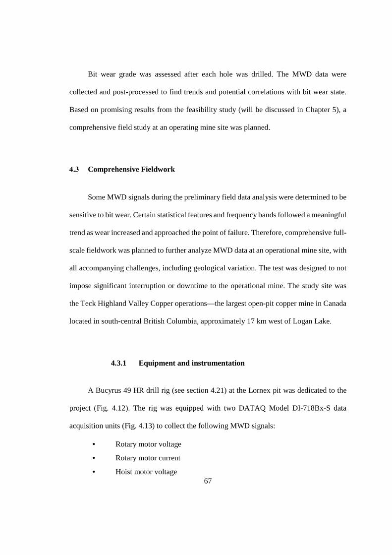
67

Bit wear grade was assessed after each hole was drilled. The MWD data were

collected and post-processed to find trends and potential correlations with bit wear state.

Based on promising results from the feasibility study (will be discussed in Chapter 5), a

comprehensive field study at an operating mine site was planned.

Comprehensive Fieldwork

Some MWD signals during the preliminary field data analysis were determined to be

sensitive to bit wear. Certain statistical features and frequency bands followed a meaningful

trend as wear increased and approached the point of failure. Therefore, comprehensive full-

scale fieldwork was planned to further analyze MWD data at an operational mine site, with

all accompanying challenges, including geological variation. The test was designed to not

impose significant interruption or downtime to the operational mine. The study site was

the Teck Highland Valley Copper operations—the largest open-pit copper mine in Canada

located in south-central British Columbia, approximately 17 km west of Logan Lake.

4.3.1 Equipment and instrumentation

A Bucyrus 49 HR drill rig (see section 4.21) at the Lornex pit was dedicated to the

project (Fig. 4.12). The rig was equipped with two DATAQ Model DI-718Bx-S data

acquisition units (Fig. 4.13) to collect the following MWD signals:

• Rotary motor voltage

• Rotary motor current

• Hoist motor voltage

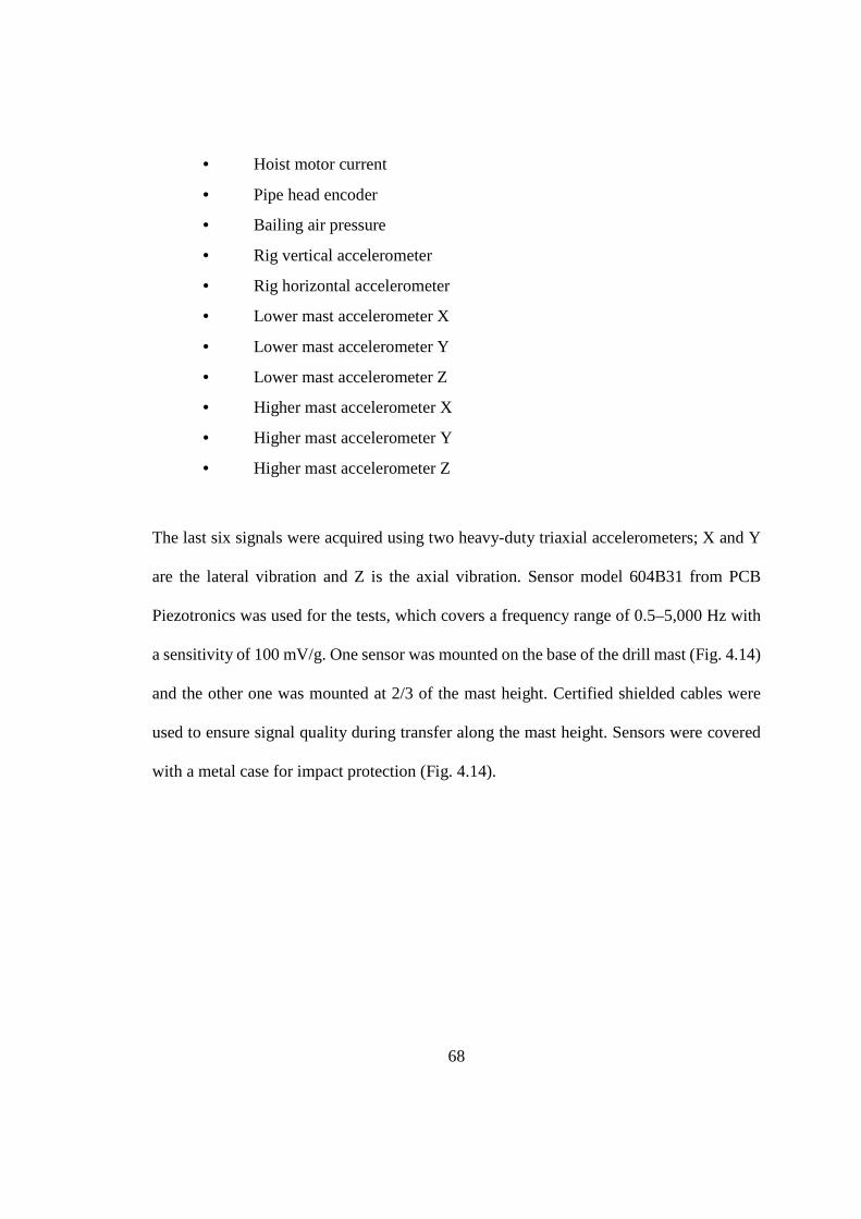
68

• Hoist motor current

• Pipe head encoder

• Bailing air pressure

• Rig vertical accelerometer

• Rig horizontal accelerometer

• Lower mast accelerometer X

• Lower mast accelerometer Y

• Lower mast accelerometer Z

• Higher mast accelerometer X

• Higher mast accelerometer Y

• Higher mast accelerometer Z

The last six signals were acquired using two heavy-duty triaxial accelerometers; X and Y

are the lateral vibration and Z is the axial vibration. Sensor model 604B31 from PCB

Piezotronics was used for the tests, which covers a frequency range of 0.5–5,000 Hz with

a sensitivity of 100 mV/g. One sensor was mounted on the base of the drill mast (Fig. 4.14)

and the other one was mounted at 2/3 of the mast height. Certified shielded cables were

used to ensure signal quality during transfer along the mast height. Sensors were covered

with a metal case for impact protection (Fig. 4.14).

69

Figure 4.12- Instrumented Bucyrus 49 HR drill rig

Figure 4.13- Two installed data acquisition units

Figure 4.14- Left: Accelerometer on the drill mast base, Right: Accelerometer on the mast base with the protection

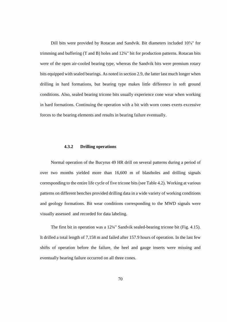
70

Dill bits were provided by Rotacan and Sandvik. Bit diameters included 10⅝" for

trimming and buffering (T and B) holes and 12¼" bit for production patterns. Rotacan bits

were of the open air-cooled bearing type, whereas the Sandvik bits were premium rotary

bits equipped with sealed bearings. As noted in section 2.9, the latter last much longer when

drilling in hard formations, but bearing type makes little difference in soft ground

conditions. Also, sealed bearing tricone bits usually experience cone wear when working

in hard formations. Continuing the operation with a bit with worn cones exerts excessive

forces to the bearing elements and results in bearing failure eventually.

4.3.2 Drilling operations

Normal operation of the Bucyrus 49 HR drill on several patterns during a period of

over two months yielded more than 16,600 m of blastholes and drilling signals

corresponding to the entire life cycle of five tricone bits (see Table 4.2). Working at various

patterns on different benches provided drilling data in a wide variety of working conditions

and geology formations. Bit wear conditions corresponding to the MWD signals were

visually assessed and recorded for data labeling.

The first bit in operation was a 12¼" Sandvik sealed-bearing tricone bit (Fig. 4.15).

It drilled a total length of 7,158 m and failed after 157.9 hours of operation. In the last few

shifts of operation before the failure, the heel and gauge inserts were missing and

eventually bearing failure occurred on all three cones.

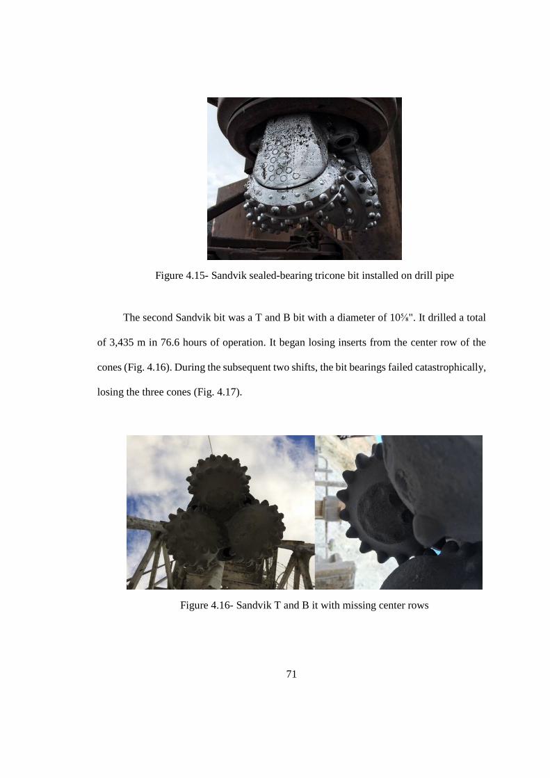
71

Figure 4.15- Sandvik sealed-bearing tricone bit installed on drill pipe

The second Sandvik bit was a T and B bit with a diameter of 10⅝". It drilled a total

of 3,435 m in 76.6 hours of operation. It began losing inserts from the center row of the

cones (Fig. 4.16). During the subsequent two shifts, the bit bearings failed catastrophically,

losing the three cones (Fig. 4.17).

Figure 4.16- Sandvik T and B it with missing center rows

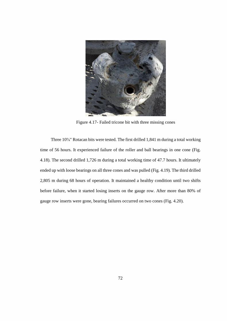
72

Figure 4.17- Failed tricone bit with three missing cones

Three 10⅝" Rotacan bits were tested. The first drilled 1,841 m during a total working

time of 56 hours. It experienced failure of the roller and ball bearings in one cone (Fig.

4.18). The second drilled 1,726 m during a total working time of 47.7 hours. It ultimately

ended up with loose bearings on all three cones and was pulled (Fig. 4.19). The third drilled

2,805 m during 68 hours of operation. It maintained a healthy condition until two shifts

before failure, when it started losing inserts on the gauge row. After more than 80% of

gauge row inserts were gone, bearing failures occurred on two cones (Fig. 4.20).

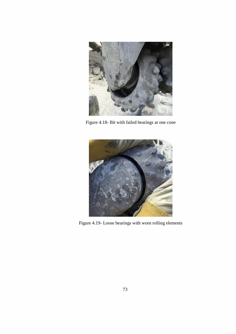
73

Figure 4.18- Bit with failed bearings at one cone

Figure 4.19- Loose bearings with worn rolling elements

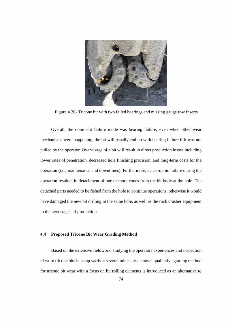
74

Figure 4.20- Tricone bit with two failed bearings and missing gauge row inserts

Overall, the dominant failure mode was bearing failure; even when other wear

mechanisms were happening, the bit will usually end up with bearing failure if it was not

pulled by the operator. Over-usage of a bit will result in direct production losses including

lower rates of penetration, decreased hole finishing precision, and long-term costs for the

operation (i.e., maintenance and downtimes). Furthermore, catastrophic failure during the

operation resulted in detachment of one or more cones from the bit body at the hole. The

detached parts needed to be fished from the hole to continue operations, otherwise it would

have damaged the new bit drilling in the same hole, as well as the rock crusher equipment

in the next stages of production.

Proposed Tricone Bit Wear Grading Method

Based on the extensive fieldwork, studying the operators experiences and inspection

of worn tricone bits in scrap yards at several mine sites, a novel qualitative grading method

for tricone bit wear with a focus on bit rolling elements is introduced as an alternative to

75

the T0 to T8 method. The classification method divides the bit lifespan into five stages as

follows:

Class 1: New bit

Class 2: Appearance of slight wear on tooth tips and cone edges

Class 3: Bearing(s) beginning to loosen because of damaged outer roller bearing;

progressive tooth wear and missing teeth

Class 4: Deterioration stage: Loose bearings because of the damaged outer roller and

ball bearing; accelerated bearing and tooth wear

Class 5: Failure stage: Excessive bearing looseness because of severe damage to the

ball bearing; bit change is required to avoid catastrophic failure

The field data are labeled according to this grading strategy. These labels are also used as

output of the artificial intelligence classifier model.

76

Chapter 5 – Drilling Signal Analysis and Results

MWD Analysis

The goal of this study component was to determine if a relationship existed between

drilling signal behavior and bit wear by analyzing the vast measurement while drilling

(MWD) dataset from two mines. Labeled data obtained from frequent visual inspection of

bit wear grade during the operation (Chapter 4) was used to correlate signal trends with bit

changes over the time. To achieve a deeper understanding of the signals and obtain signal

features to support the development of the artificial intelligence model (Chapter 6), time

domain statistical analysis, frequency spectrum analysis, and the time-frequency approach

were applied to the signals (e.g., Fig. 5.1). Signals were exported to MATLAB software

for analysis.

Figure 5.1- Time domain sample of MWD signals recorded using a DATAQ unit in WinDaq software

77

Statistical Analysis of Signals

MWD signals were preliminarily studied in the time domain. To analyze MWD data

as random signals statistically, moments of the random variable were extracted, and their

trends were assessed during the bit lifespan.

5.2.1 Probability distributions for random discrete variables

The probability distribution of X as a random discrete signal is characterized by

determining the probabilities that random variable X = �^ for every �^. The probability

distribution of a random discrete variable X is described by P[X = �^] and satisfies equation

5.1 (Shin and Hammond 2008):

∑ H_X = �^a = 1^ (5.1)

By defining L(�) = H _b c �a, the probability density function d�� is defined by

Equation 5.2:

d�� = limh�→4

( _ �jk l�mh�ah� = n o��

n� (5.2)

5.2.2 Moments of a random signal

To extract numerical parameters from the probability density function of the random

signal, a set of data (x1, x2, . . . , xN ) are collected from N measurements of signal X. These

78

numerical features, known as moments of a random variable, are introduced in equations

5.3 to 5.7 (Shin and Hammond 2008).

The first moment or the mean value is:

�̅ = \% ∑ �%[\ (5.3)

The second moment about the mean measures the variance or the dispersion and is

calculated using:

��� = \%p\ ∑ (� − �̅)�%[\ (5.4)

The third moment about the mean is to quantify the asymmetry of a probability distribution,

and is called the skewness. It is calculated by:

Skew = \% ∑ (� − �̅)3 ��3⁄%[\ (5.5)

The fourth moment about the mean measures the degree of flattening known as Kurtosis

and is calculated using:

Kurt = �\% ∑ (� − �̅)z ��z⁄%[\ − 3 (5.6)

The root mean square (RMS) value of a set of datapoints is calculated as the square root of

the arithmetic mean of the squares of the original data, given in equation 5.7.

79

RMS � �\% ∑ ��%

[\ � \/�

(5.7)

Rate of Penetration Analysis

The effect of weight on bit (WOB) and rotational speed on the rate of penetration

(ROP) was evaluated based on the test configurations used and data collected in the

preliminary field program (section 4.2). The ROP trends presented correspond to a new

12¼" Rotacan tricone bit drilling on a relatively homogeneous bench. Therefore, the ROP

variation is assumed to wholly result from WOB and rotation speed. By having healthy bit

nozzles and enough air bailing pressure and volume, the perfect cleaning condition is

assumed to be valid.

As expected, increasing the WOB and rotation speed increased the ROP (Fig. 5.2).

Increasing the WOB from 310 to 410 kN at 60 rpm increased the mean ROP by 32%. By

comparison, increasing the rotational speed from 60 to 80 rpm at 310 kN increased the

mean ROP by < 15%.

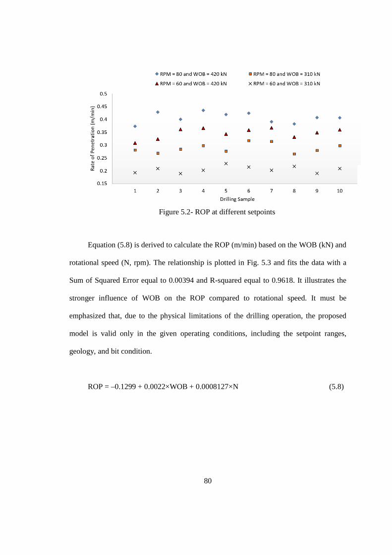
80

Figure 5.2- ROP at different setpoints

Equation (5.8) is derived to calculate the ROP (m/min) based on the WOB (kN) and

rotational speed (N, rpm). The relationship is plotted in Fig. 5.3 and fits the data with a

Sum of Squared Error equal to 0.00394 and R-squared equal to 0.9618. It illustrates the

stronger influence of WOB on the ROP compared to rotational speed. It must be

emphasized that, due to the physical limitations of the drilling operation, the proposed

model is valid only in the given operating conditions, including the setpoint ranges,

geology, and bit condition.

ROP = –0.1299 + 0.0022×WOB + 0.0008127×N (5.8)

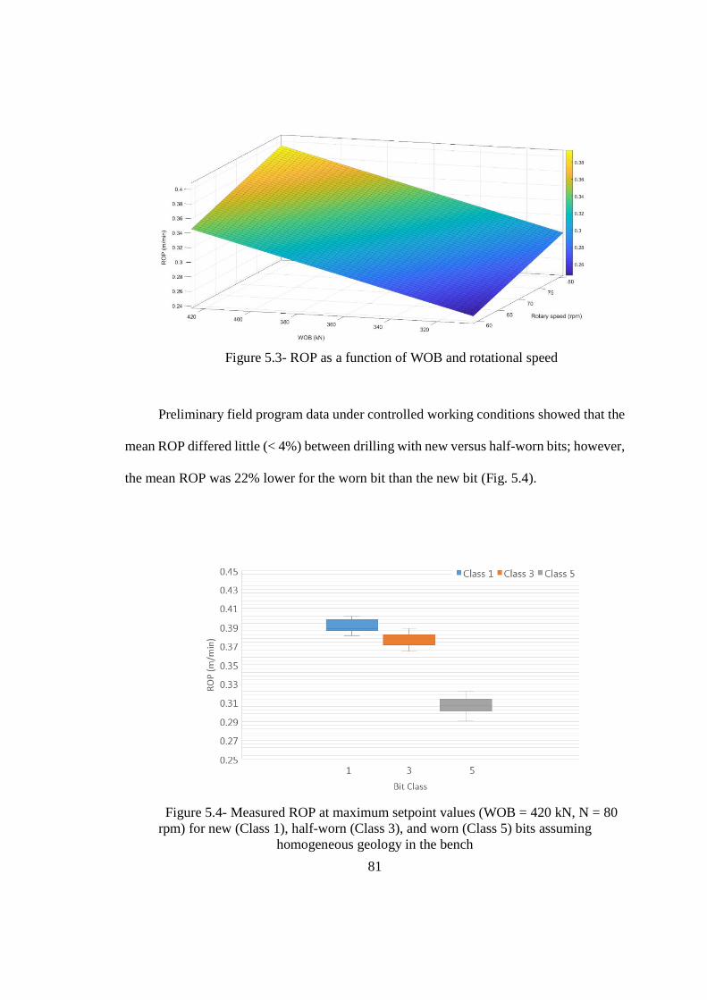
81

Figure 5.3- ROP as a function of WOB and rotational speed

Preliminary field program data under controlled working conditions showed that the

mean ROP differed little (< 4%) between drilling with new versus half-worn bits; however,

the mean ROP was 22% lower for the worn bit than the new bit (Fig. 5.4).

Figure 5.4- Measured ROP at maximum setpoint values (WOB = 420 kN, N = 80 rpm) for new (Class 1), half-worn (Class 3), and worn (Class 5) bits assuming

homogeneous geology in the bench

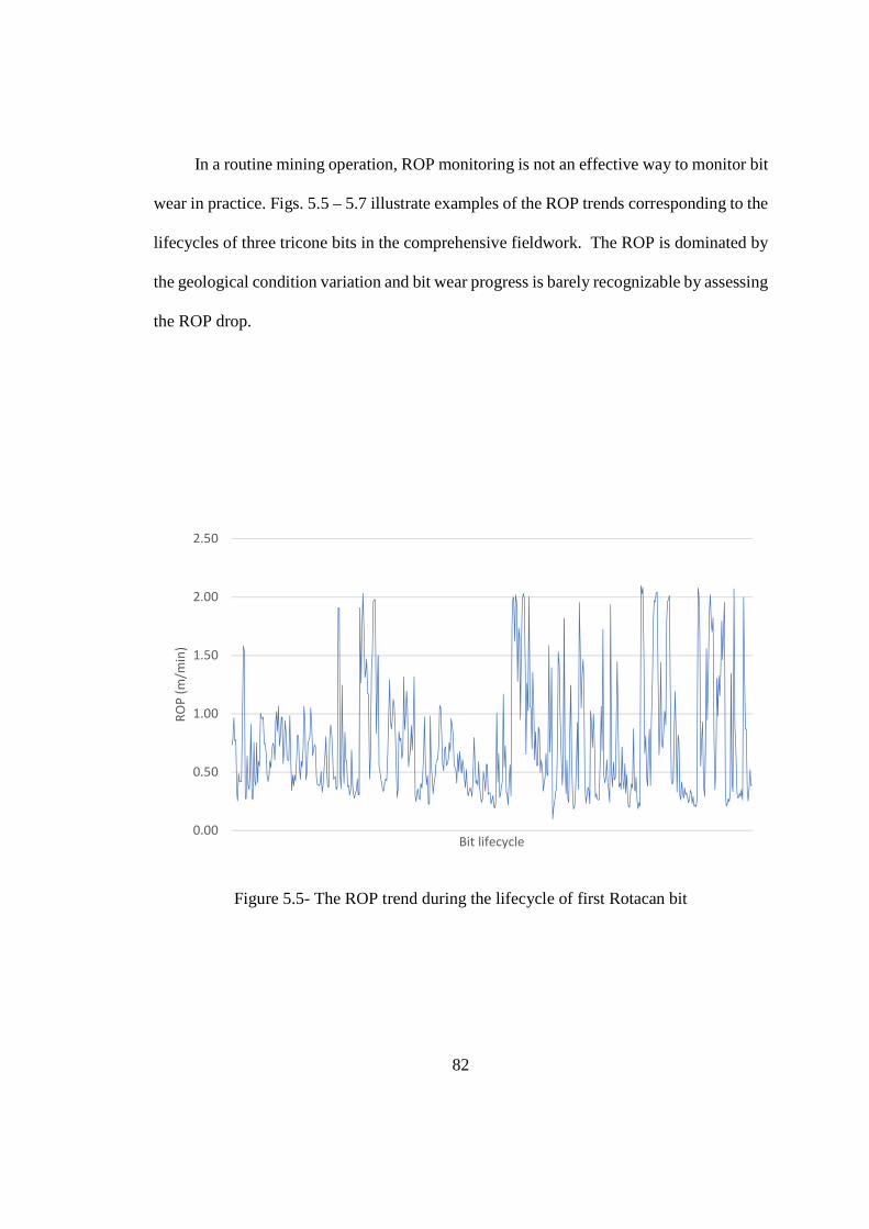
82

In a routine mining operation, ROP monitoring is not an effective way to monitor bit

wear in practice. Figs. 5.5 – 5.7 illustrate examples of the ROP trends corresponding to the

lifecycles of three tricone bits in the comprehensive fieldwork. The ROP is dominated by

the geological condition variation and bit wear progress is barely recognizable by assessing

the ROP drop.

Figure 5.5- The ROP trend during the lifecycle of first Rotacan bit

0.00

0.50

1.00

1.50

2.00

2.50

RO

P (

m/m

in)

Bit lifecycle

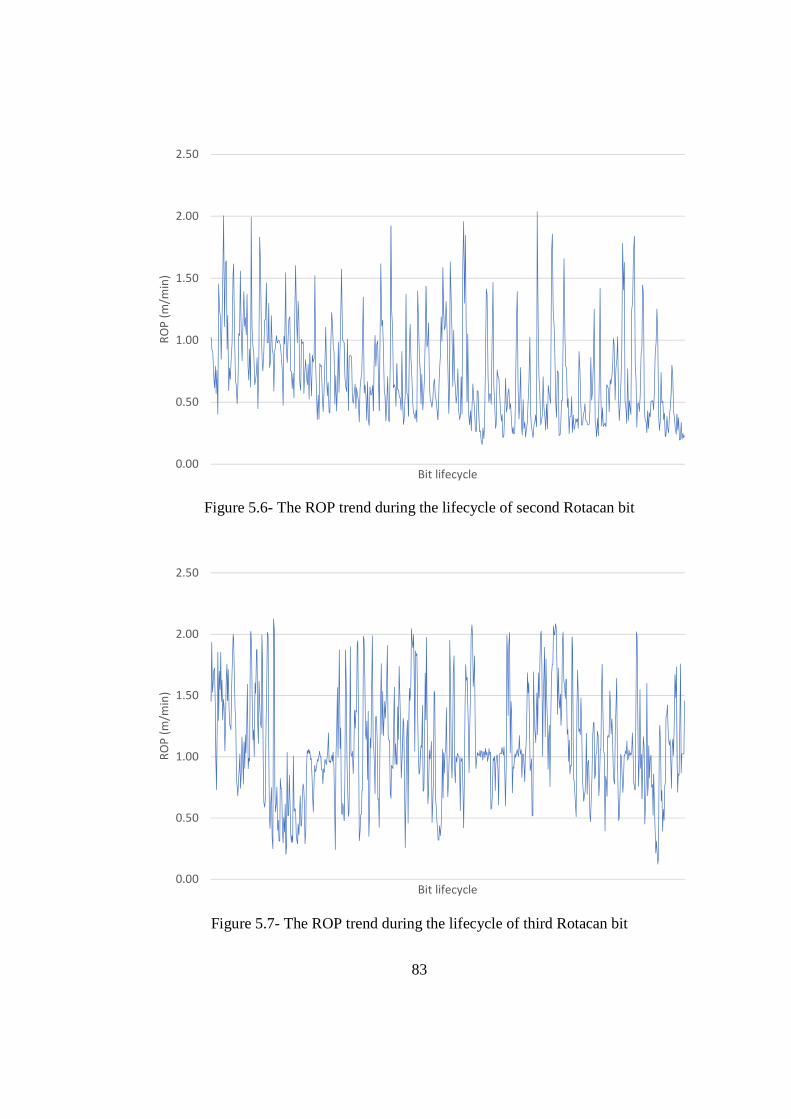
83

Figure 5.6- The ROP trend during the lifecycle of second Rotacan bit

Figure 5.7- The ROP trend during the lifecycle of third Rotacan bit

0.00

0.50

1.00

1.50

2.00

2.50R

OP

(m

/min

)

Bit lifecycle

0.00

0.50

1.00

1.50

2.00

2.50

RO

P (

m/m

in)

Bit lifecycle

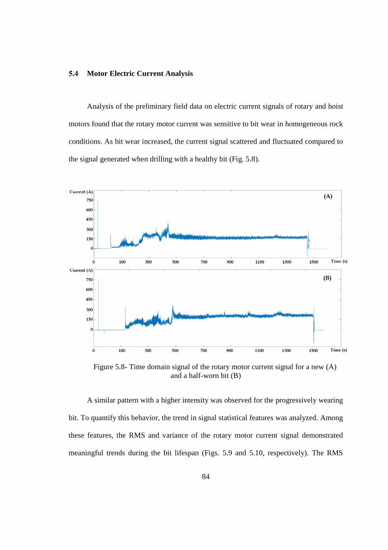
84

Motor Electric Current Analysis

Analysis of the preliminary field data on electric current signals of rotary and hoist

motors found that the rotary motor current was sensitive to bit wear in homogeneous rock

conditions. As bit wear increased, the current signal scattered and fluctuated compared to

the signal generated when drilling with a healthy bit (Fig. 5.8).

Figure 5.8- Time domain signal of the rotary motor current signal for a new (A) and a half-worn bit (B)

A similar pattern with a higher intensity was observed for the progressively wearing

bit. To quantify this behavior, the trend in signal statistical features was analyzed. Among

these features, the RMS and variance of the rotary motor current signal demonstrated

meaningful trends during the bit lifespan (Figs. 5.9 and 5.10, respectively). The RMS

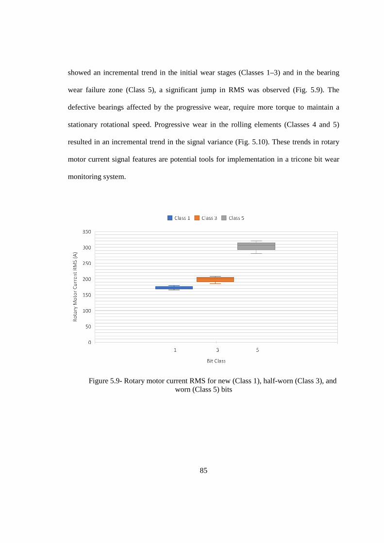
85

showed an incremental trend in the initial wear stages (Classes 1–3) and in the bearing

wear failure zone (Class 5), a significant jump in RMS was observed (Fig. 5.9). The

defective bearings affected by the progressive wear, require more torque to maintain a

stationary rotational speed. Progressive wear in the rolling elements (Classes 4 and 5)

resulted in an incremental trend in the signal variance (Fig. 5.10). These trends in rotary

motor current signal features are potential tools for implementation in a tricone bit wear

monitoring system.

Figure 5.9- Rotary motor current RMS for new (Class 1), half-worn (Class 3), and worn (Class 5) bits

86

Figure 5.10- Rotary motor current variance for the three bit classes

Equation 5.9 explains the relationship between electric current and torque in the

electric rotary motor: more current is required to maintain a constant rotational speed at a

higher torque.

5 = 30}~�E πN⁄ (5.9)

Where

5: Torque in Newton meters (N.m)

}: Current in amperes (A)

~: Applied voltage in volts (V)

�E: Motor efficiency

N: Rotational speed (rpm)

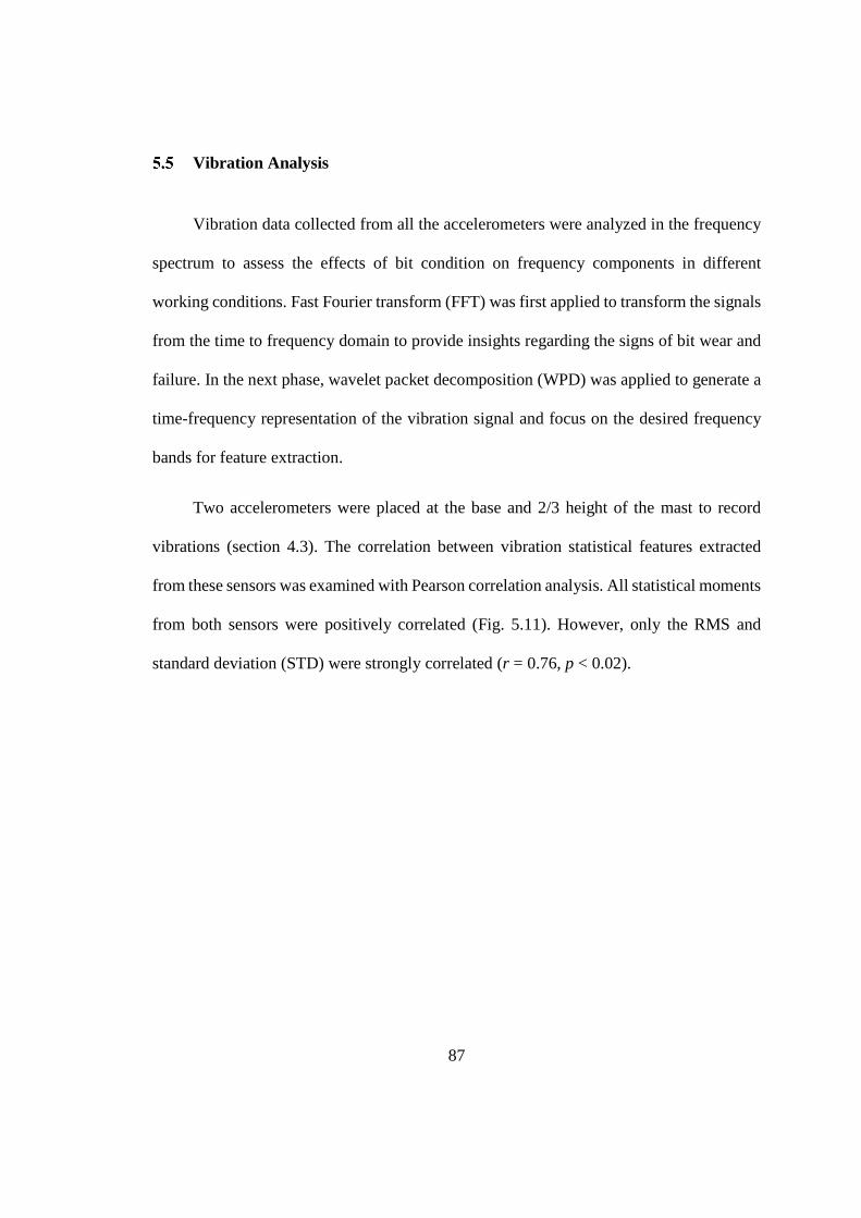
87

Vibration Analysis

Vibration data collected from all the accelerometers were analyzed in the frequency

spectrum to assess the effects of bit condition on frequency components in different

working conditions. Fast Fourier transform (FFT) was first applied to transform the signals

from the time to frequency domain to provide insights regarding the signs of bit wear and

failure. In the next phase, wavelet packet decomposition (WPD) was applied to generate a

time-frequency representation of the vibration signal and focus on the desired frequency

bands for feature extraction.

Two accelerometers were placed at the base and 2/3 height of the mast to record

vibrations (section 4.3). The correlation between vibration statistical features extracted

from these sensors was examined with Pearson correlation analysis. All statistical moments

from both sensors were positively correlated (Fig. 5.11). However, only the RMS and

standard deviation (STD) were strongly correlated (r = 0.76, p < 0.02).

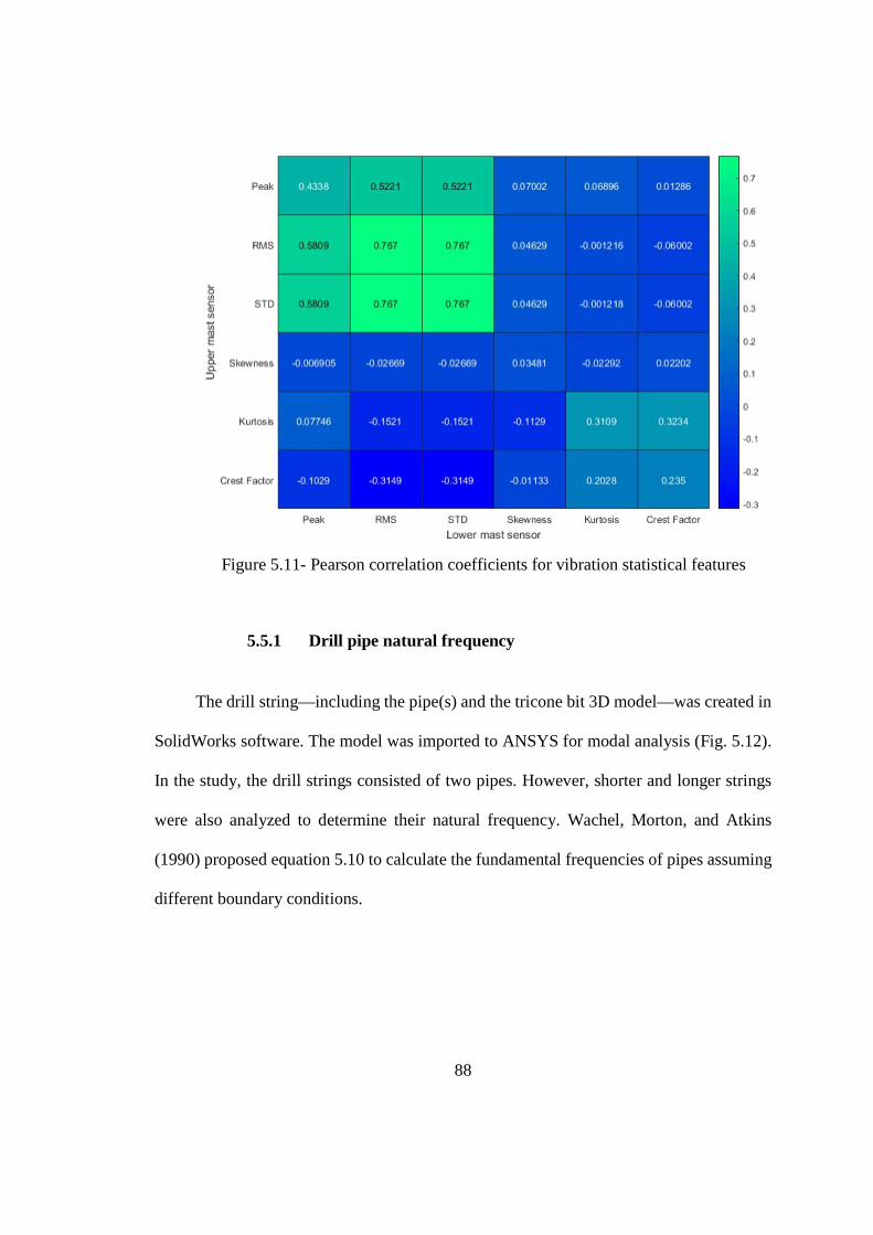
88

Figure 5.11- Pearson correlation coefficients for vibration statistical features

5.5.1 Drill pipe natural frequency

The drill string—including the pipe(s) and the tricone bit 3D model—was created in

SolidWorks software. The model was imported to ANSYS for modal analysis (Fig. 5.12).

In the study, the drill strings consisted of two pipes. However, shorter and longer strings

were also analyzed to determine their natural frequency. Wachel, Morton, and Atkins

(1990) proposed equation 5.10 to calculate the fundamental frequencies of pipes assuming

different boundary conditions.

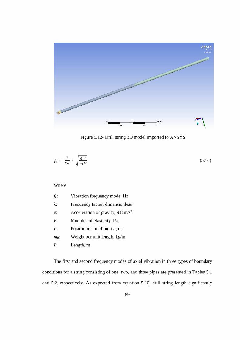
89

Figure 5.12- Drill string 3D model imported to ANSYS

� = ��$ ∙ � ;��

���� (5.10)

Where

fn: Vibration frequency mode, Hz

λ: Frequency factor, dimensionless

g: Acceleration of gravity, 9.8 m/s2

E: Modulus of elasticity, Pa

I: Polar moment of inertia, m4

m0: Weight per unit length, kg/m

L: Length, m

The first and second frequency modes of axial vibration in three types of boundary

conditions for a string consisting of one, two, and three pipes are presented in Tables 5.1

and 5.2, respectively. As expected from equation 5.10, drill string length significantly

90

influenced the string fundamental frequencies. For a drilling depth of approximately 15 m,

two drill pipes are required. The rotational speed range is 60 rpm to 120 rpm which is equal

to 1–2 Hz. Therefore, the axial vibration fundamental frequencies of the drill string in all

the three boundary conditions are well above the pipe rotation frequency.

Table 5.1- First fundamental frequency (Hz) for drill string consisting of one, two, and three pipes

Boundary condition One pipe Two pipes Three pipes

Fixed top – fixed bit 104.09 29.57 13.74

Fixed top – supported bit 71.56 20.33 9.44

Fixed top – free bit 16.36 4.65 2.16

Table 5.2- Second fundamental frequency (Hz) for drill string consisting of one, two, and three pipes

Boundary condition One pipe Two pipes Three pipes

Fixed top – fixed bit 286.72 81.44 37.84

Fixed top – supported bit 232.35 66.00 30.66

Fixed top – free bit 104.09 29.57 13.74

5.5.2 Drilling vibration frequency spectrum analysis

Analysis of vibration signals collected during the lifespans of bits in the frequency

domain using FFT showed that the amplitudes of some frequency bands were affected by

bit wear condition changes. These vibration excitations occurred as bit wear approached

91

the worn condition (or potential catastrophic failure), regardless of changes in geology and

working conditions. In addition, low-frequency vibration was sensitive to geology and

working condition.

Vibration signals in the X, Y (lateral), and Z (axial) directions from all

accelerometers in different spots were analyzed in the frequency domain to locate the signal

frequency bands sensitive to bit wear. Results from the preliminary fieldwork (section 4.2)

showed that tooth wear, which is geometrical changes on the teeth and tooth breakage result

in a non-uniform distribution of cutting forces exerted on each cone. This phenomenon

unbalances the rotation and excites the 1x rpm in the axial vibration frequency spectrum.

Therefore, the wear progresses to Class 2 and increases this frequency component. This

conclusion, however, is based on a uniform contact force distribution, which cannot be

generalized to geological conditions in blasthole drilling. Therefore, application of this

frequency component to wear detection is not practical.

Based on the comprehensive field data collected in a variety of geology conditions

(section 4.3), the axial vibration 3x rpm frequency peak or tricone bit bouncing frequency

was determined to be the formation drillability indicator. At a constant bit wear level and

the same drilling setpoints (WOB and rpm), a decrease in the ROP resulted from hitting

harder rock formations. It was observed that drilling in harder formations would excite the

3x rpm component in the axial vibration spectrum.

A series of harmonics of the cone rotational speed (CRS) was found in the axial

vibration frequency as the bit reached Class 3 wear. These peaks start from 2x CRS and

were detectable up to approximately 70 Hz. In addition, the frequency band ranging from

40 to 60 Hz was strongly excited by a worn bit starting at Class 3 (Fig. 5.13 top). This

92

frequency range followed an incremental trend as the bit reached Class 4 wear and

increased up to 300% when the bit reached Class 5 wear (Fig. 5.13 bottom).

Figure 5.13- Top: Bit with worn bearings (Class 3),

Bottom: Worn bearings before failure (Class 5)

5.5.3 Tricone bit vibration frequencies

As discussed in section 2.5, bearings comprise the connection between cones and

lugs in tricone bits (Fig. 5.14). Each bearing has unique fundamental frequencies based on

its design, geometry, and speed of operation. These frequencies are calculated using

equations 5.11 to 5.14 (Graney and Starry 2012):

93

�HL} = %�'� × L × �1 ! �

(� × cos � (5.11)

�HL� = %�'� × L × �1 − �

(� × cos � (5.12)

L5L = o� × �1 − �

(� × cos � (5.13)

�1L = (��� × L × �1 − �

(� × cos �) � (5.14)

Where

BPFI = Ball/roller pass frequency of inner race (Hz)

NBR = Number of balls / roller

F = Rotational speed difference between outer and inner race (Hz)

B = Ball diameter (mm)

Pd = Pitch diameter (mm)

θ = Bearing contact angle

BPFO = Ball/roller pass frequency of outer race (Hz)

FTF = Fundamental train frequency (Hz)

BSF = Ball / roller spin frequency (Hz)

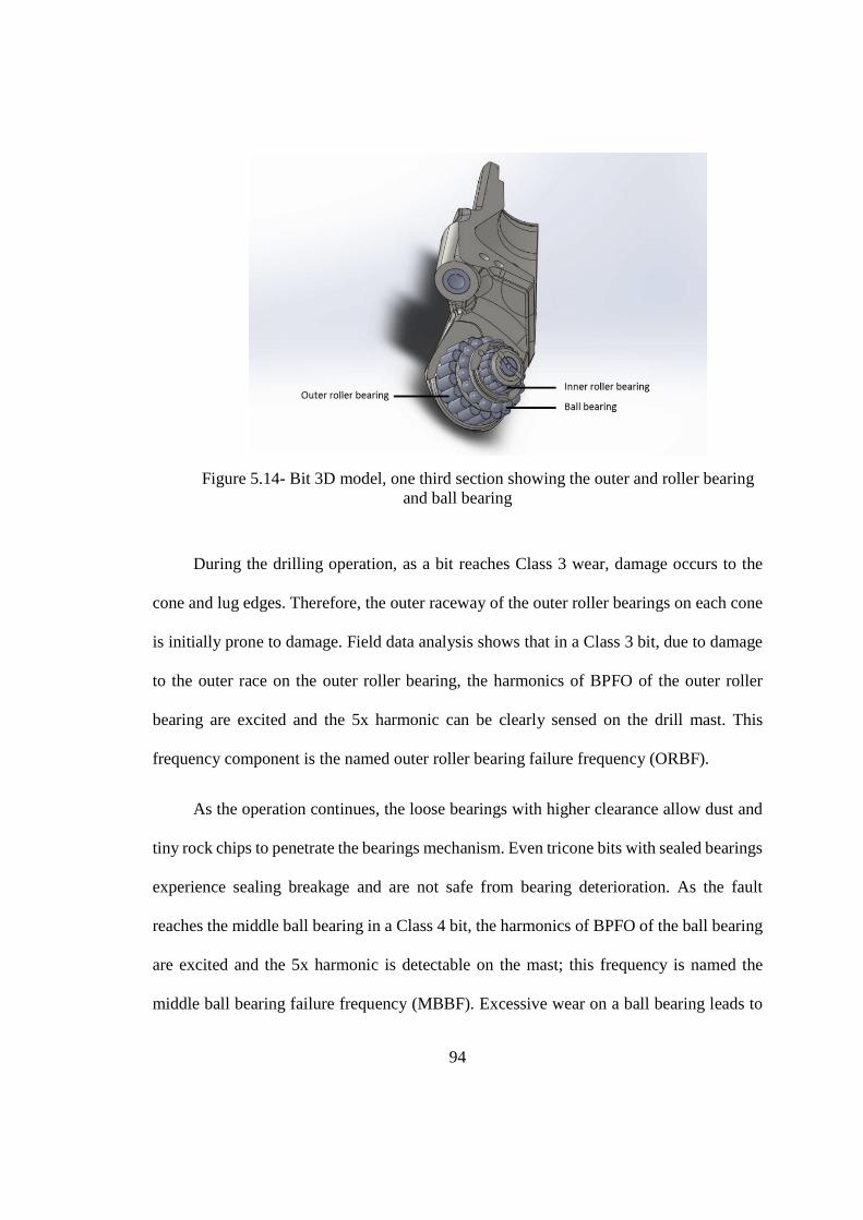
94

Figure 5.14- Bit 3D model, one third section showing the outer and roller bearing and ball bearing

During the drilling operation, as a bit reaches Class 3 wear, damage occurs to the

cone and lug edges. Therefore, the outer raceway of the outer roller bearings on each cone

is initially prone to damage. Field data analysis shows that in a Class 3 bit, due to damage

to the outer race on the outer roller bearing, the harmonics of BPFO of the outer roller

bearing are excited and the 5x harmonic can be clearly sensed on the drill mast. This

frequency component is the named outer roller bearing failure frequency (ORBF).

As the operation continues, the loose bearings with higher clearance allow dust and

tiny rock chips to penetrate the bearings mechanism. Even tricone bits with sealed bearings

experience sealing breakage and are not safe from bearing deterioration. As the fault

reaches the middle ball bearing in a Class 4 bit, the harmonics of BPFO of the ball bearing

are excited and the 5x harmonic is detectable on the mast; this frequency is named the

middle ball bearing failure frequency (MBBF). Excessive wear on a ball bearing leads to

95

Class 5 wear. Failure of the middle ball bearing will result in bit catastrophic failure and

possibly detachment of the cone.

Equations 5.15 and 5.16 are proposed to calculate tricone bit failure frequencies.

�G�L = %'�z × N × �G1G × �1 − '

('� × cos � (5.15)

���L = %��z × N × �G1G × �1 − �

(�� × cos � (5.16)

Where

ORBF: Outer roller bearing failure frequency (Hz)

NR: Number of rollers

N: Bit rotational speed (rpm)

CRSR: Cone to bit rotational speed ratio

R: Roller diameter (mm)

PRB: Roller bearing pitch diameter (mm)

θ: Bearing contact angle

MBBF: Middle ball bearing failure frequency (Hz)

NB: Number of balls

B: Ball diameter (mm)

PBB: Ball bearing pitch diameter (mm)

Failure frequencies of a class 5 bit at rotational speed of 60 rpm are illustrated in Fig.

5.15.

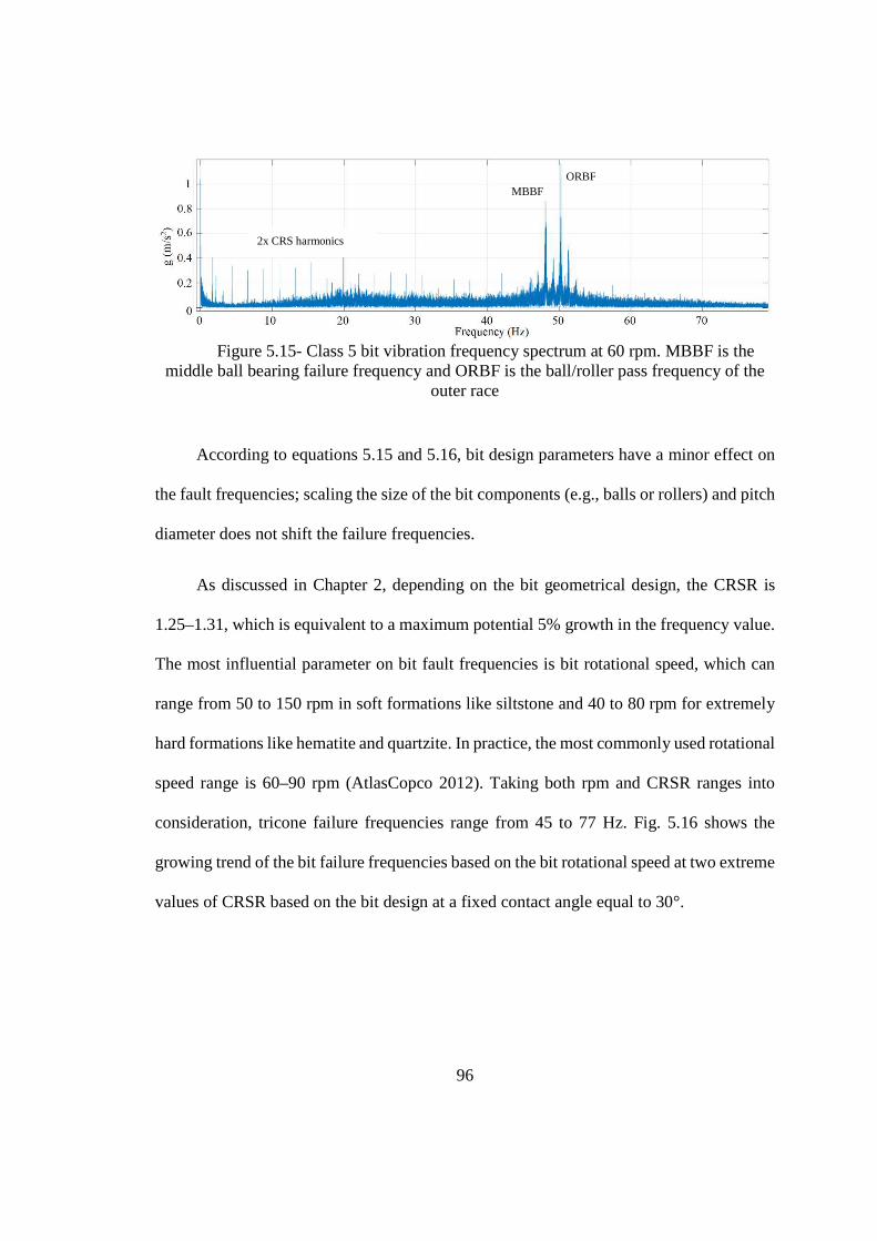
96

Figure 5.15- Class 5 bit vibration frequency spectrum at 60 rpm. MBBF is the

middle ball bearing failure frequency and ORBF is the ball/roller pass frequency of the outer race

According to equations 5.15 and 5.16, bit design parameters have a minor effect on

the fault frequencies; scaling the size of the bit components (e.g., balls or rollers) and pitch

diameter does not shift the failure frequencies.

As discussed in Chapter 2, depending on the bit geometrical design, the CRSR is

1.25–1.31, which is equivalent to a maximum potential 5% growth in the frequency value.

The most influential parameter on bit fault frequencies is bit rotational speed, which can

range from 50 to 150 rpm in soft formations like siltstone and 40 to 80 rpm for extremely

hard formations like hematite and quartzite. In practice, the most commonly used rotational

speed range is 60–90 rpm (AtlasCopco 2012). Taking both rpm and CRSR ranges into

consideration, tricone failure frequencies range from 45 to 77 Hz. Fig. 5.16 shows the

growing trend of the bit failure frequencies based on the bit rotational speed at two extreme

values of CRSR based on the bit design at a fixed contact angle equal to 30°.

2x CRS harmonics

MBBF ORBF

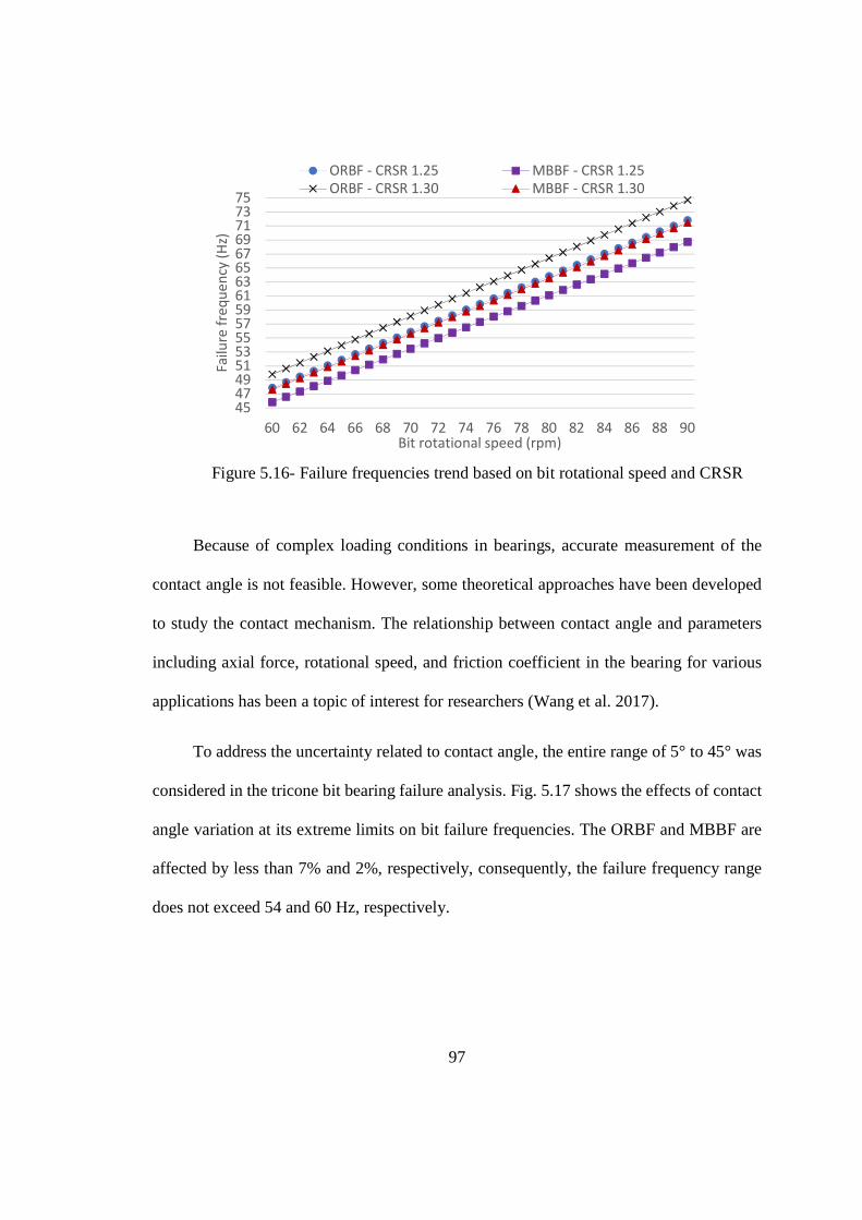
97

Figure 5.16- Failure frequencies trend based on bit rotational speed and CRSR

Because of complex loading conditions in bearings, accurate measurement of the

contact angle is not feasible. However, some theoretical approaches have been developed

to study the contact mechanism. The relationship between contact angle and parameters

including axial force, rotational speed, and friction coefficient in the bearing for various

applications has been a topic of interest for researchers (Wang et al. 2017).

To address the uncertainty related to contact angle, the entire range of 5° to 45° was

considered in the tricone bit bearing failure analysis. Fig. 5.17 shows the effects of contact

angle variation at its extreme limits on bit failure frequencies. The ORBF and MBBF are

affected by less than 7% and 2%, respectively, consequently, the failure frequency range

does not exceed 54 and 60 Hz, respectively.

45474951535557596163656769717375

60 62 64 66 68 70 72 74 76 78 80 82 84 86 88 90

Failu

re f

req

ue

ncy

(H

z)

Bit rotational speed (rpm)

ORBF - CRSR 1.25 MBBF - CRSR 1.25ORBF - CRSR 1.30 MBBF - CRSR 1.30

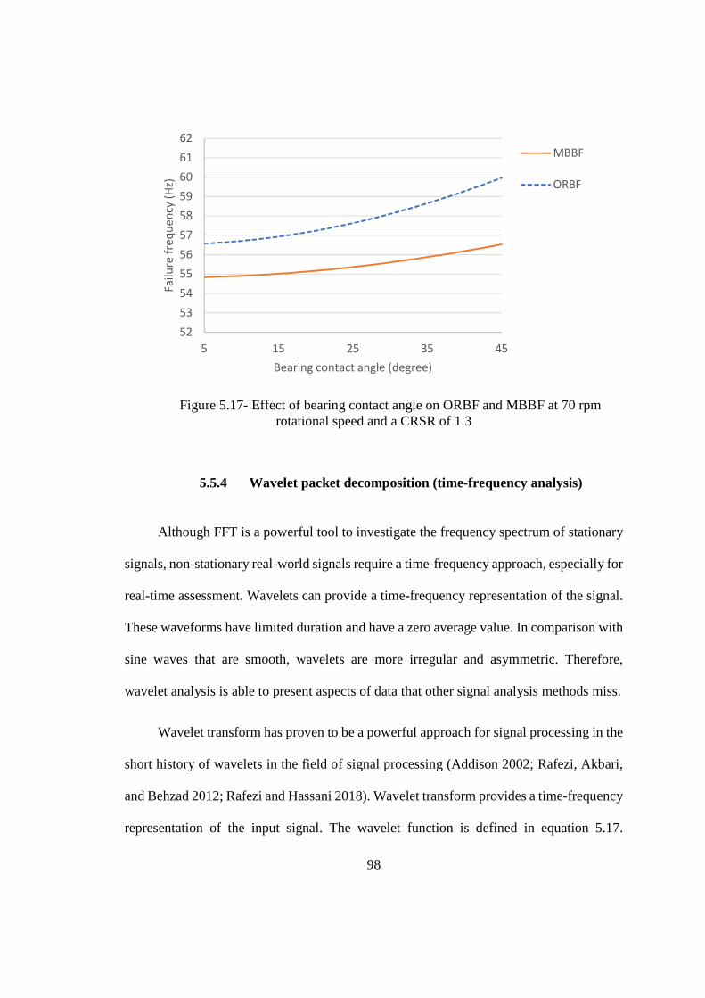
98

Figure 5.17- Effect of bearing contact angle on ORBF and MBBF at 70 rpm rotational speed and a CRSR of 1.3

5.5.4 Wavelet packet decomposition (time-frequency analysis)

Although FFT is a powerful tool to investigate the frequency spectrum of stationary

signals, non-stationary real-world signals require a time-frequency approach, especially for

real-time assessment. Wavelets can provide a time-frequency representation of the signal.

These waveforms have limited duration and have a zero average value. In comparison with

sine waves that are smooth, wavelets are more irregular and asymmetric. Therefore,

wavelet analysis is able to present aspects of data that other signal analysis methods miss.

Wavelet transform has proven to be a powerful approach for signal processing in the

short history of wavelets in the field of signal processing (Addison 2002; Rafezi, Akbari,

and Behzad 2012; Rafezi and Hassani 2018). Wavelet transform provides a time-frequency

representation of the input signal. The wavelet function is defined in equation 5.17.

52

53

54

55

56

57

58

59

60

61

62

5 15 25 35 45

Failu

re f

req

ue

ncy

(H

z)

Bearing contact angle (degree)

MBBF

ORBF

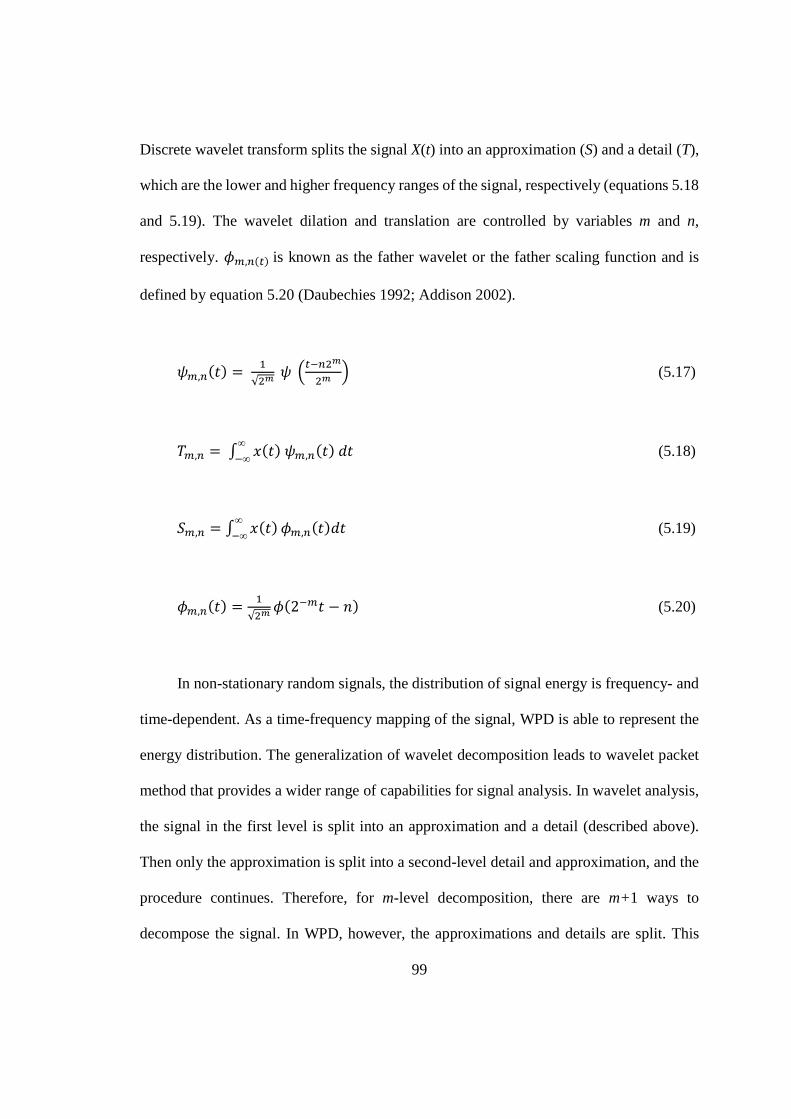
99

Discrete wavelet transform splits the signal X(t) into an approximation (S) and a detail (T),

which are the lower and higher frequency ranges of the signal, respectively (equations 5.18

and 5.19). The wavelet dilation and translation are controlled by variables m and n,

respectively. �,?� is known as the father wavelet or the father scaling function and is

defined by equation 5.20 (Daubechies 1992; Addison 2002).

��,(�) = \√�� � �?p��

�� (5.17)

5�, = � �(�) ��,(�) ��∞

p∞ (5.18)

1�, = � �(�)∞

p∞ �,(�)�� (5.19)

�,(�) = \√�� (2p�� − J) (5.20)

In non-stationary random signals, the distribution of signal energy is frequency- and

time-dependent. As a time-frequency mapping of the signal, WPD is able to represent the

energy distribution. The generalization of wavelet decomposition leads to wavelet packet

method that provides a wider range of capabilities for signal analysis. In wavelet analysis,

the signal in the first level is split into an approximation and a detail (described above).

Then only the approximation is split into a second-level detail and approximation, and the

procedure continues. Therefore, for m-level decomposition, there are m+1 ways to

decompose the signal. In WPD, however, the approximations and details are split. This

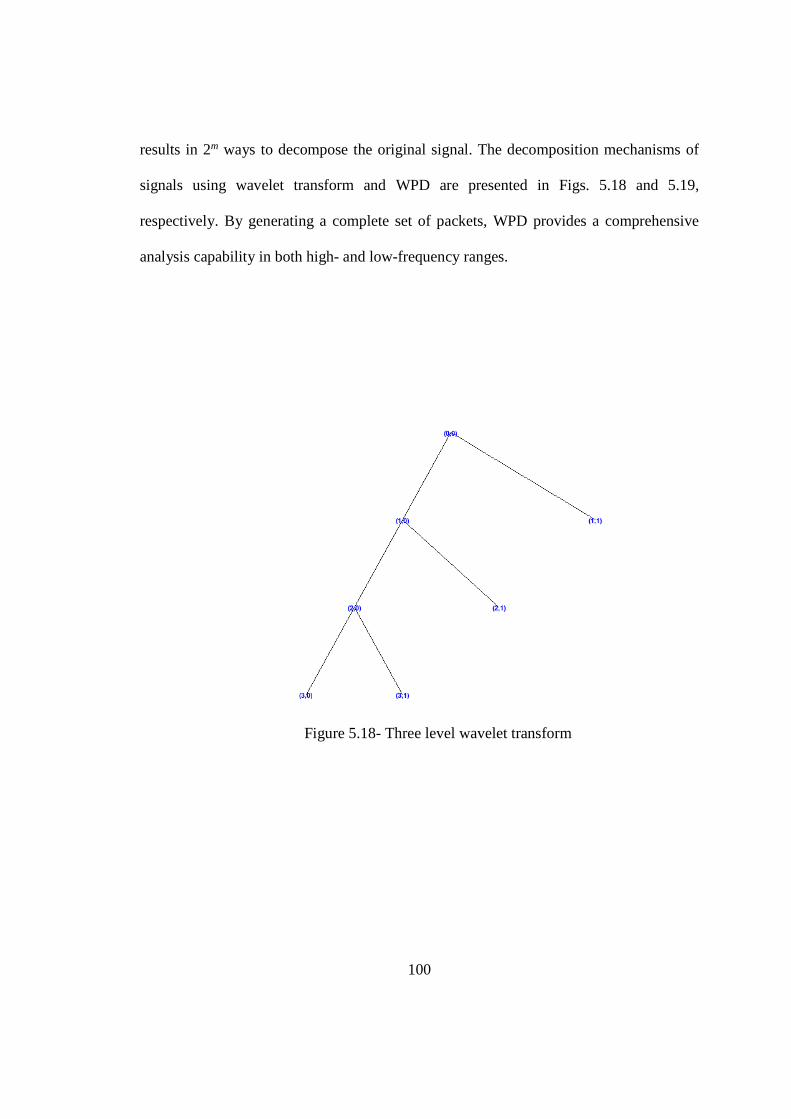
100

results in 2m ways to decompose the original signal. The decomposition mechanisms of

signals using wavelet transform and WPD are presented in Figs. 5.18 and 5.19,

respectively. By generating a complete set of packets, WPD provides a comprehensive

analysis capability in both high- and low-frequency ranges.

Figure 5.18- Three level wavelet transform

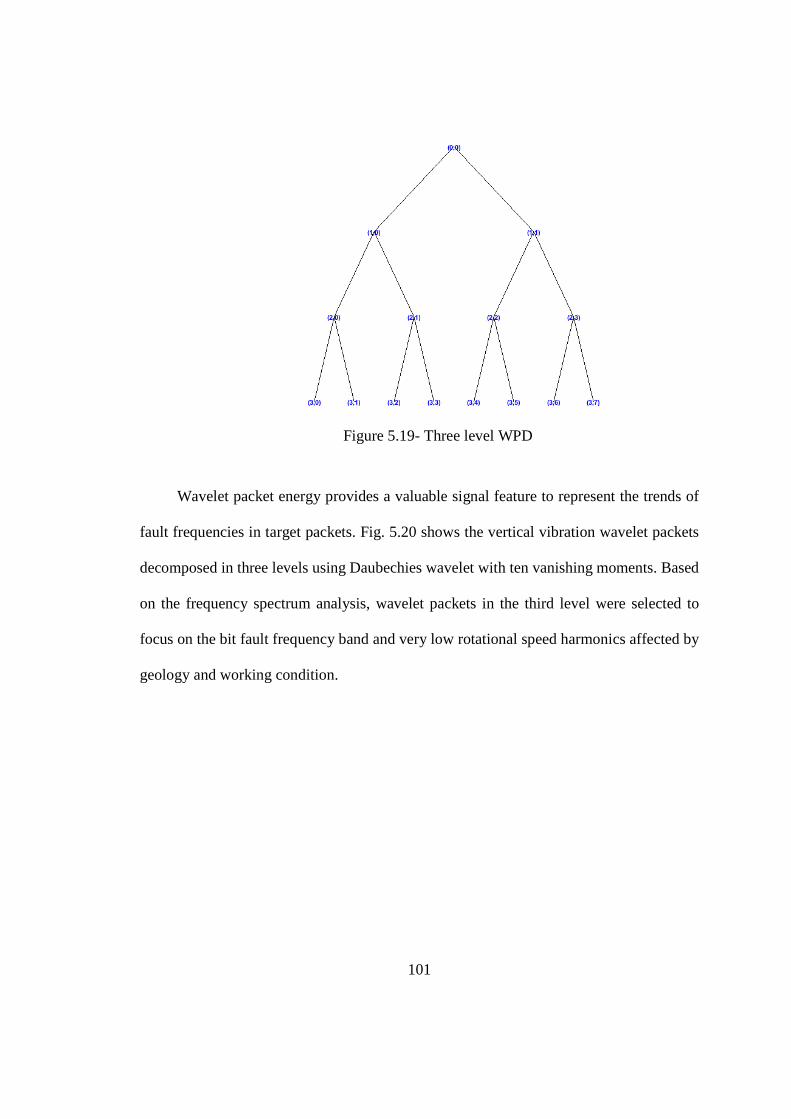
101

Figure 5.19- Three level WPD

Wavelet packet energy provides a valuable signal feature to represent the trends of

fault frequencies in target packets. Fig. 5.20 shows the vertical vibration wavelet packets

decomposed in three levels using Daubechies wavelet with ten vanishing moments. Based

on the frequency spectrum analysis, wavelet packets in the third level were selected to

focus on the bit fault frequency band and very low rotational speed harmonics affected by

geology and working condition.

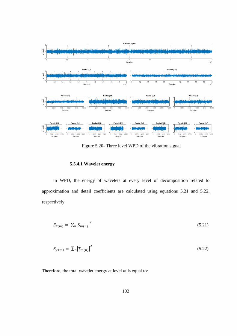
102

Figure 5.20- Three level WPD of the vibration signal

5.5.4.1 Wavelet energy

In WPD, the energy of wavelets at every level of decomposition related to

approximation and detail coefficients are calculated using equations 5.21 and 5.22,

respectively.

���� = ∑ �1���� (5.21)

�&�� = ∑ �5���� (5.22)

Therefore, the total wavelet energy at level m is equal to:

103

�� = ��(�) + �&(�) (5.23)

At each level, the ratio of every packet energy to the total energy of the level defines

the wavelet packet relative energy. The relative energy of approximation packet n at level

m is calculated as:

�8 = ��(�,�)��

(5.24)

Based on the bit fault frequency calculations, packets (3,2) and (3,3) correspond to

the bit fault frequency and packet (3,1) contains the CRS components. Application of WPD

provides the flexibility to analyze higher or lower frequency bands when changes in

working condition are significant. For example, by increasing the bit rotational speed

jumps to 110 rpm in a rare situation, the bit fault shifts to the packet (3,4). At the third

level, packet (3,0) consist of the low-frequency range, including the tricone bit bouncing

frequency (3x rpm) component. Therefore, it is considered as the drillability representative

in the bit classification model. With wear progress from Classes 1 to 5, the relative wavelet

energy distribution transits from the low-frequency packet (3,0) to the higher frequency

packets. Eventually, in a Class 5 bit condition, the highest relative energy value is related

to the packet (3,2), which is the bit fault frequency packet (Fig. 5.21).

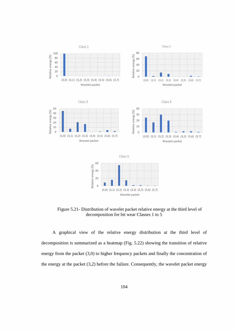
104

Figure 5.21- Distribution of wavelet packet relative energy at the third level of decomposition for bit wear Classes 1 to 5

A graphical view of the relative energy distribution at the third level of

decomposition is summarized as a heatmap (Fig. 5.22) showing the transition of relative

energy from the packet (3,0) to higher frequency packets and finally the concentration of

the energy at the packet (3,2) before the failure. Consequently, the wavelet packet energy

0

20

40

60

80

100

(3,0) (3,1) (3,2) (3,3) (3,4) (3,5) (3,6) (3,7)

Re

lati

ve e

ne

rgy

(%)

Wavelet packet

Class 1

0

20

40

60

80

(3,0) (3,1) (3,2) (3,3) (3,4) (3,5) (3,6) (3,7)

Re

lati

ve e

ne

rgy

(%)

Wavelet packet

Class 2

0

10

20

30

40

50

(3,0) (3,1) (3,2) (3,3) (3,4) (3,5) (3,6) (3,7)

Re

lati

ve e

ne

rgy

(%)

Wavelet packet

Class 3

0

10

20

30

40

(3,0) (3,1) (3,2) (3,3) (3,4) (3,5) (3,6) (3,7)R

ela

tive

en

erg

y (%

)

Wavelet packet

Class 4

0

20

40

60

(3,0) (3,1) (3,2) (3,3) (3,4) (3,5) (3,6) (3,7)

Re

lati

ve e

ne

rgy

(%)

Wavelet packet

Class 5

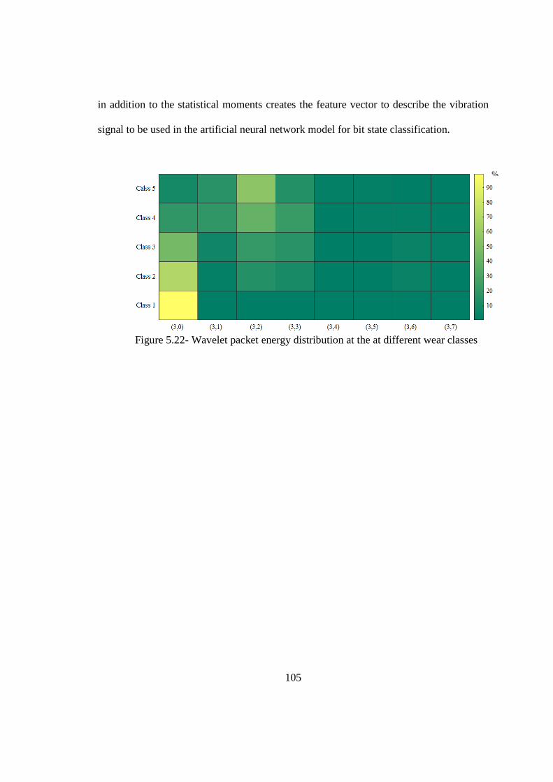
105

in addition to the statistical moments creates the feature vector to describe the vibration

signal to be used in the artificial neural network model for bit state classification.

Figure 5.22- Wavelet packet energy distribution at the at different wear classes

%

106

Chapter 6 – Artificial Intelligence Model for Drill Bit Wear Pattern Recognition

Bit Wear Pattern Recognition

In this research, the classification of bit wear state is considered a pattern recognition

problem. By the means of artificial intelligence (AI), the bit wear condition is determined

based on drilling signals, and bit catastrophic failure is predicted. Feedforward neural

network (FNN) models are designed and examined to classify the drill bit wear state as a

supervised learning approach. The final sensor-fusion model is trained, validated, and

tested using full-scale real-world drilling data acquired in the field. The model input is a

vector of signal features based on the analysis discussed in Chapter 5 and the outputs are

the bit wear classes introduced in Chapter 4.

Neural Network Model

The developed FNN model consists of three layers; One hidden layer connects the

input and ouput layers. The input layer contains nodes equivalent to the number of elements

in the signal feature vector and the output layer contains one neuron for each class of bit

wear state. At every neuron, the sum of weighted input features (pi) and the bias (bi)

provides the input to the neuron transfer function (f) and the transfer function generates the

neuron output (Fig. 6.1).

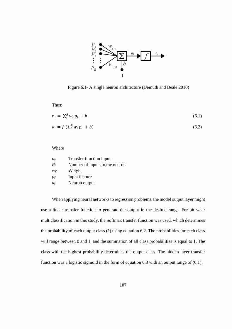
107

Figure 6.1- A single neuron architecture (Demuth and Beale 2010)

Thus:

J9 = ∑ �9'9 d9 + � (6.1)

�9 = � (∑ �9'9 d9 + �) (6.2)

Where

ni: Transfer function input R: Number of inputs to the neuron wi: Weight pi: Input feature ai: Neuron output

When applying neural networks to regression problems, the model output layer might

use a linear transfer function to generate the output in the desired range. For bit wear

multiclassification in this study, the Softmax transfer function was used, which determines

the probability of each output class (k) using equation 6.2. The probabilities for each class

will range between 0 and 1, and the summation of all class probabilities is equal to 1. The

class with the highest probability determines the output class. The hidden layer transfer

function was a logistic sigmoid in the form of equation 6.3 with an output range of (0,1).

108

�>=E?�D�� = A�∑ A��

(6.2)

�:=;>9;() = \\m A�� (6.3)

6.2.1 Feedforward neural network classifier

The neuron connections in FFNs go from input to output with no cycles and the

network may contain several layers. The network in Fig. 6.2 comprises two layers of

neurons with full interconnection. Passive nodes in the input layer distribute their single

input corresponding to a signal feature to multiple outputs to feed neurons in the hidden

layer. The number of the nodes and neurons in the hidden layer are discussed in section

6.3.1. Outputs of neurons in hidden layer generate the inputs to the output layer neurons.

In the output layer, there is one neuron corresponding to each bit wear class (i.e., total of 5

neurons).

Figure 6.2- Simplified illustration of the bit wear state classifier neural network

109

6.2.2 The loss function and learning algorithm

In neural networks, learning is the minimization of the global error function. The loss

or error function is defined over the network weights and biases. In this work, cross-entropy

was selected as the loss function (Eq. 6.4). Because of the logarithmic derivation of cross-

entropy, it strongly penalizes highly inaccurate model outputs (yi) in the training procedure,

where the target value label is (ti).

��, �� = ∑ �9 log \ Y9 (6.4)

A variety of learning algorithms for FFN training have been developed (e.g., (Hinton

1989; Rumelhart, Hinton, and Williams 1986)). A standard method of minimizing the error

is the gradient descent algorithm, where the gradient of the error function (G = ¡¢¡£¤

) is

calculated by the partial derivatives of error with respect to each model parameter vector

Z (i.e., weights and biases). The model parameters are updated in a short distance in the

direction of –G to decrease the error (Bishop 1995) and minimize the error function.

Therefore:

£:m\ = £: − ¥ ¡¢¡£¤

(6.5)

Where µ is the learning rate and determines the amount of change in the weights at

every step, and l is the iteration number in the training procedure. The algorithm converges

110

and ends the training process when the error function is at the minimum and G = 0. The

drawback of gradient descent is associated with fixed and user-dependent selection of µ

with no theoretical basis for the selection. This could result in an inefficient learning

process in terms of processing time and robustness.

In this research, the scaled conjugate gradient algorithm was selected, which is

similar to the gradient descent method but uses a scaled step size. Møller (1993) introduced

the scaled conjugate gradient algorithm and discussed the mathematics behind it in detail.

The approach has been an algorithm of interest for research on supervised classification

problems in a variety of applications (Rostami, Hemmati-Sarapardeh, and Shamshirband

2018; Nematinia and Mehdizadeh 2018; Karmakar et al. 2018; Sodhi and Chandra 2014).

Bit Wear Classification Models

The performance of neural network models on the basis of network shown in Fig.

6.2 was evaluated based on the feature vector configurations and the number of neurons in

the hidden layer. In the following section, the neural network data vectors derived from the

signal analysis results in Chapter 5 are presented.

6.3.1 Model configuration

The data vector configurations comprise signal features from wavelet packets and

time domain features. Table 6.1 presents the comprehensive set of the signal features

achieved from the lower mast and upper mast accelerometers, rotary motor current as well

111

as the control parameters, bit depth and the rate of penetration. Therefore, the

comprehensive input vector consists of 59 elements and the output vector contains 5

elements corresponding to the 5 classes of bit wear.

Table 6.1- Comprehensive model data vector elements from the lower and upper mast accelerometers, rotary motor current as well as the control parameters, bit depth,

and rate of penetration

Signal Model Input Vector Elements

Lower Mast Vibration

Wavelet Packets (3,0) (3,1) (3,2) (3,3) (3,4) Energy Peak Variance Skewness Kurtosis

Upper Mast Vibration

Wavelet Packets (3,0) (3,1) (3,2) (3,3) (3,4) Energy Peak Variance Skewness Kurtosis

Rotary Motor Current

Time Domain Peak RMS Variance Skewness Kurtosis

Control Signals Time Domain WOB Rotational speed Bit position

Bit Penetration Time Domain Rate of penetration

The model was initially designed for the comprehensive data vector. Examination of

the performance of classifiers containing 25–40 neurons showed that the classifier with 30

neurons in the hidden layer performed the best validation performance in classification of

bit condition (Fig. 6.3 and Appendix). The trend of cross entropy errors for the network

with thirty neurons in the hidden layer during the training is plotted in figure 6.4. The best

validation performance was achieved at iteration number 84 with a cross-entropy equal to

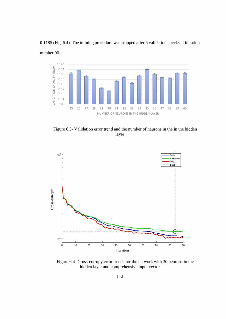
112

0.1185 (Fig. 6.4). The training procedure was stopped after 6 validation checks at iteration

number 90.

Figure 6.3- Validation error trend and the number of neurons in the in the hidden layer

Figure 6.4- Cross-entropy error trends for the network with 30 neurons in the hidden layer and comprehensive input vector

0.105

0.11

0.115

0.12

0.125

0.13

0.135

0.14

0.145

25 26 27 28 29 30 31 32 33 34 35 36 37 38 39 40

VA

LID

AT

ION

CR

OSS

-EN

TR

OP

Y

NUMBER OF NEURONS IN THE HIDDEN LAYER

Iteration

Cro

ss-e

ntro

py

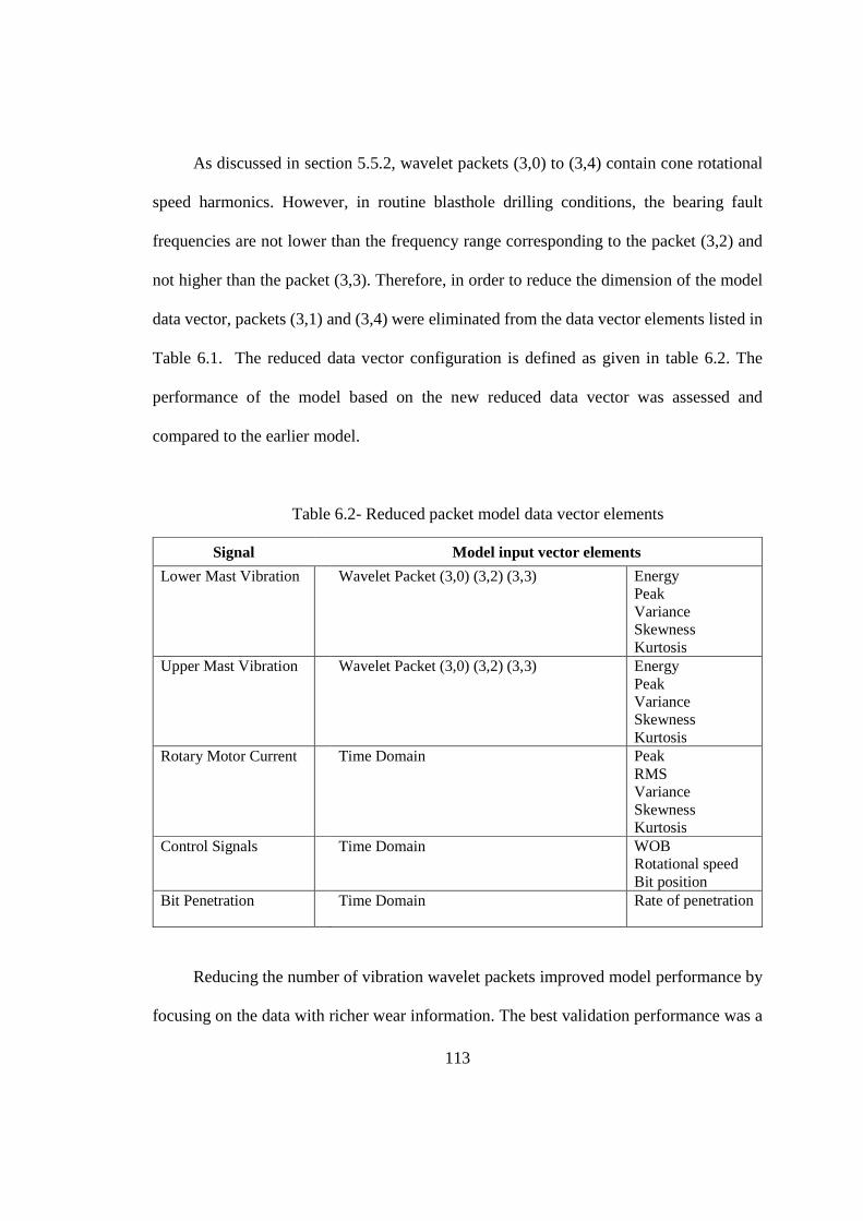
113

As discussed in section 5.5.2, wavelet packets (3,0) to (3,4) contain cone rotational

speed harmonics. However, in routine blasthole drilling conditions, the bearing fault

frequencies are not lower than the frequency range corresponding to the packet (3,2) and

not higher than the packet (3,3). Therefore, in order to reduce the dimension of the model

data vector, packets (3,1) and (3,4) were eliminated from the data vector elements listed in

Table 6.1. The reduced data vector configuration is defined as given in table 6.2. The

performance of the model based on the new reduced data vector was assessed and

compared to the earlier model.

Table 6.2- Reduced packet model data vector elements

Signal Model input vector elements

Lower Mast Vibration Wavelet Packet (3,0) (3,2) (3,3) Energy Peak Variance Skewness Kurtosis

Upper Mast Vibration Wavelet Packet (3,0) (3,2) (3,3) Energy Peak Variance Skewness Kurtosis

Rotary Motor Current Time Domain Peak RMS Variance Skewness Kurtosis

Control Signals Time Domain WOB Rotational speed Bit position

Bit Penetration Time Domain Rate of penetration

Reducing the number of vibration wavelet packets improved model performance by

focusing on the data with richer wear information. The best validation performance was a

114

cross-entropy equal to 0.0982 for the network with 20 neurons in the hidden layer at

iteration number 284 (Fig. 6.5). After this iteration, the validation error increased and the

network training process was stopped. Therefore, compared to the comprehensive network,

reducing network size resulted in a 54% reduction in the total number of connections in

the model, which corresponds to lower computational power requirement.

Figure 6.5- Cross-entropy error trends for the network with 20 neurons in the hidden layer using the reduced dataset

The potential benefits gained by fusion of multiple sensors, including the current

signal and the upper mast vibration signals were also assessed. Elimination of the current

Iteration

Cro

ss-e

ntro

py

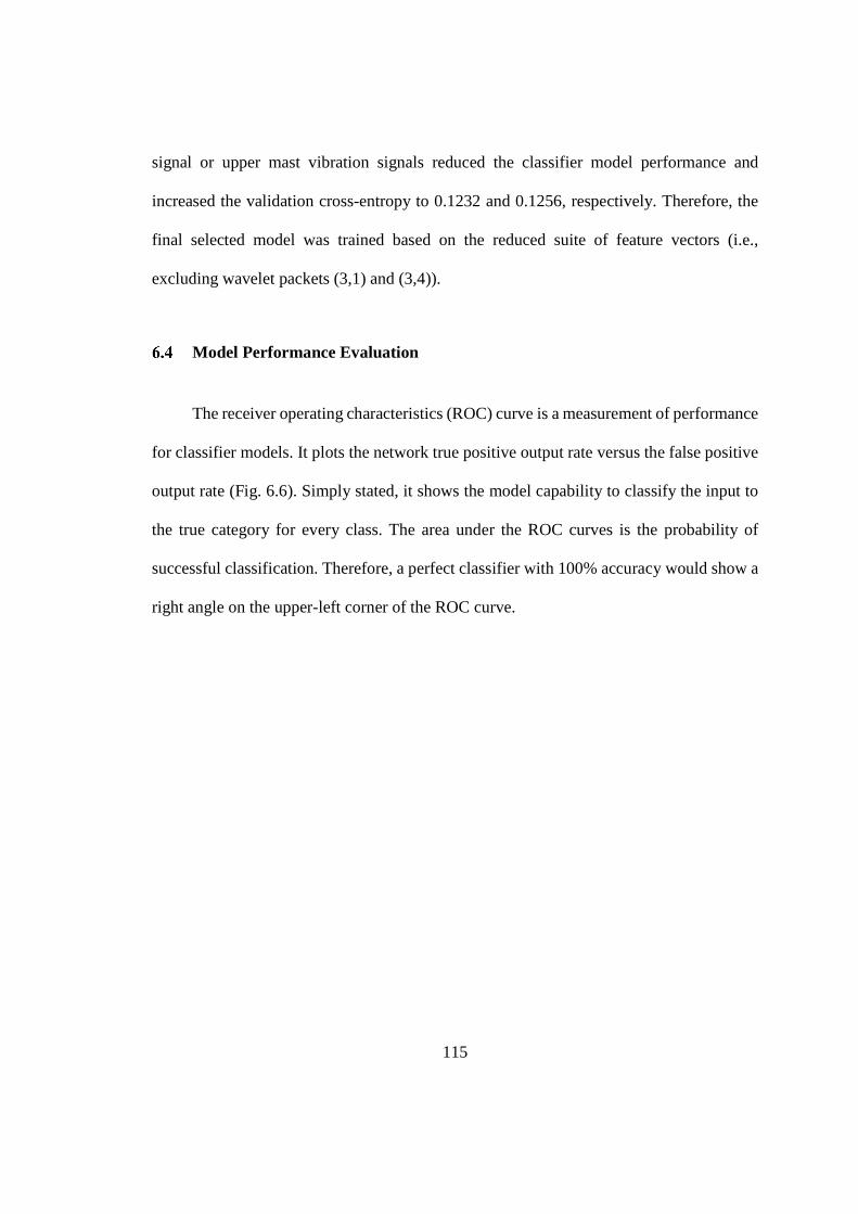
115

signal or upper mast vibration signals reduced the classifier model performance and

increased the validation cross-entropy to 0.1232 and 0.1256, respectively. Therefore, the

final selected model was trained based on the reduced suite of feature vectors (i.e.,

excluding wavelet packets (3,1) and (3,4)).

Model Performance Evaluation

The receiver operating characteristics (ROC) curve is a measurement of performance

for classifier models. It plots the network true positive output rate versus the false positive

output rate (Fig. 6.6). Simply stated, it shows the model capability to classify the input to

the true category for every class. The area under the ROC curves is the probability of

successful classification. Therefore, a perfect classifier with 100% accuracy would show a

right angle on the upper-left corner of the ROC curve.

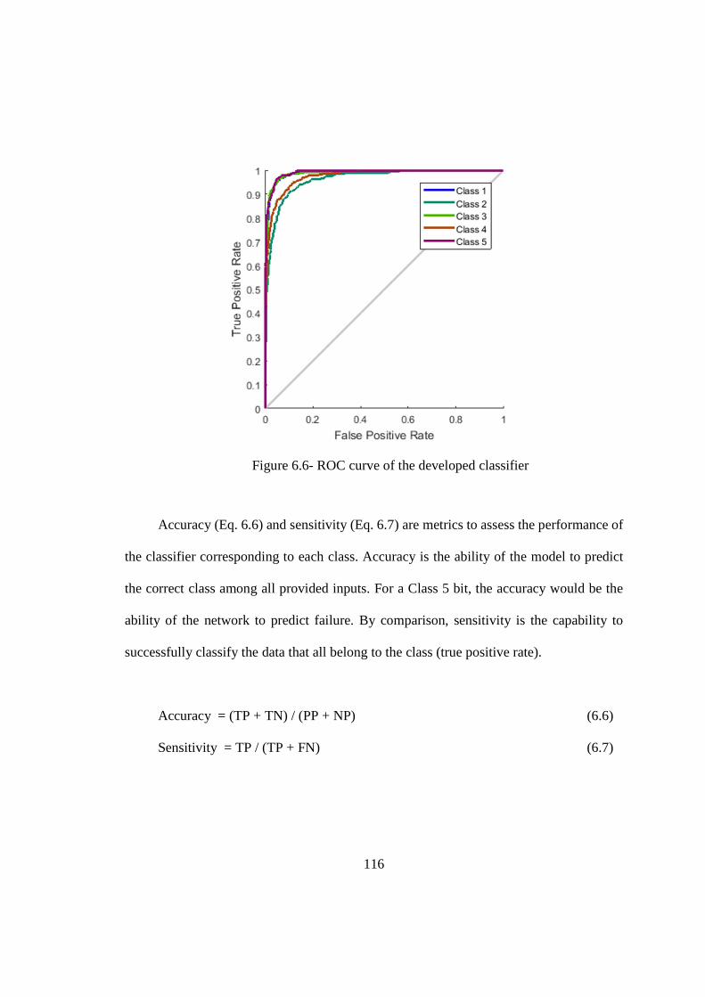
116

Figure 6.6- ROC curve of the developed classifier

Accuracy (Eq. 6.6) and sensitivity (Eq. 6.7) are metrics to assess the performance of

the classifier corresponding to each class. Accuracy is the ability of the model to predict

the correct class among all provided inputs. For a Class 5 bit, the accuracy would be the

ability of the network to predict failure. By comparison, sensitivity is the capability to

successfully classify the data that all belong to the class (true positive rate).

Accuracy = (TP + TN) / (PP + NP) (6.6)

Sensitivity = TP / (TP + FN) (6.7)

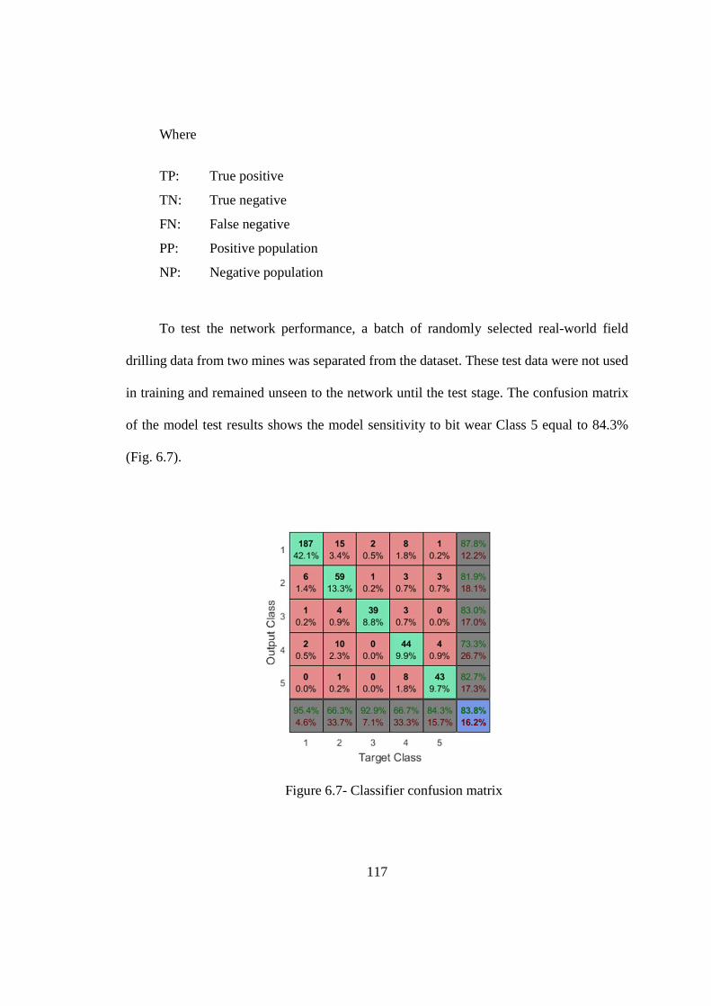
117

Where

TP: True positive

TN: True negative

FN: False negative

PP: Positive population

NP: Negative population

To test the network performance, a batch of randomly selected real-world field

drilling data from two mines was separated from the dataset. These test data were not used

in training and remained unseen to the network until the test stage. The confusion matrix

of the model test results shows the model sensitivity to bit wear Class 5 equal to 84.3%

(Fig. 6.7).

Figure 6.7- Classifier confusion matrix

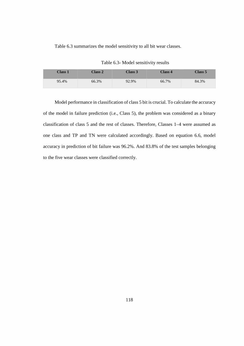
118

Table 6.3 summarizes the model sensitivity to all bit wear classes.

Table 6.3- Model sensitivity results

Class 1 Class 2 Class 3 Class 4 Class 5

95.4% 66.3% 92.9% 66.7% 84.3%

Model performance in classification of class 5 bit is crucial. To calculate the accuracy

of the model in failure prediction (i.e., Class 5), the problem was considered as a binary

classification of class 5 and the rest of classes. Therefore, Classes 1–4 were assumed as

one class and TP and TN were calculated accordingly. Based on equation 6.6, model

accuracy in prediction of bit failure was 96.2%. And 83.8% of the test samples belonging

to the five wear classes were classified correctly.

119

Chapter 7 – Conclusions and Recommendations

7.1 Conclusions

The primary goal of this thesis was to develop a practical condition monitoring (CM)

approach to monitor the wear and predict the failure of tricone bits for industrial

applications. The analysis and developed artificial intelligence model were based on real-

world drilling data. The accomplishments of this project are the following:

• A comprehensive literature review of drilling wear monitoring was presented.

• Application of Ground penetrating radar (GPR) for mine subsurface identification

was investigated. A variety of antennas were tested in limestone and coal mine

environments. The 200 MHz antenna provided the best penetration depth/resolution

tradeoff. GPR is a practical method for subsurface mapping. However, the depth of

penetration is limited, and the results are sensitive to the rock physical properties

and water saturation.

• In the preliminary fieldwork, a drill rig in an iron ore mine was equipped with a

data acquisition unit and accelerometers on several spots of the machine. Special

sensor mountings were designed. Drilling signals were measured during drilling

with tricone bits at three levels of wear condition.

• Based on promising preliminary results, comprehensive fieldwork was designed to

be conducted in a copper mine. Two heavy-duty high-frequency accelerometers

were installed on the drill rig mast to measure the vibration in line with the motor

signals, air pressure, and drill string head encoder signal in over 16 km of blasthole

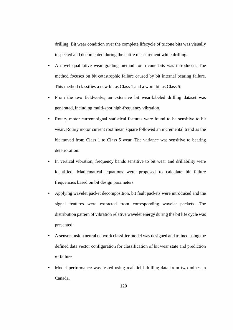
120

drilling. Bit wear condition over the complete lifecycle of tricone bits was visually

inspected and documented during the entire measurement while drilling.

• A novel qualitative wear grading method for tricone bits was introduced. The

method focuses on bit catastrophic failure caused by bit internal bearing failure.

This method classifies a new bit as Class 1 and a worn bit as Class 5.

• From the two fieldworks, an extensive bit wear-labeled drilling dataset was

generated, including multi-spot high-frequency vibration.

• Rotary motor current signal statistical features were found to be sensitive to bit

wear. Rotary motor current root mean square followed an incremental trend as the

bit moved from Class 1 to Class 5 wear. The variance was sensitive to bearing

deterioration.

• In vertical vibration, frequency bands sensitive to bit wear and drillability were

identified. Mathematical equations were proposed to calculate bit failure

frequencies based on bit design parameters.

• Applying wavelet packet decomposition, bit fault packets were introduced and the

signal features were extracted from corresponding wavelet packets. The

distribution pattern of vibration relative wavelet energy during the bit life cycle was

presented.

• A sensor-fusion neural network classifier model was designed and trained using the

defined data vector configuration for classification of bit wear state and prediction

of failure.

• Model performance was tested using real field drilling data from two mines in

Canada.

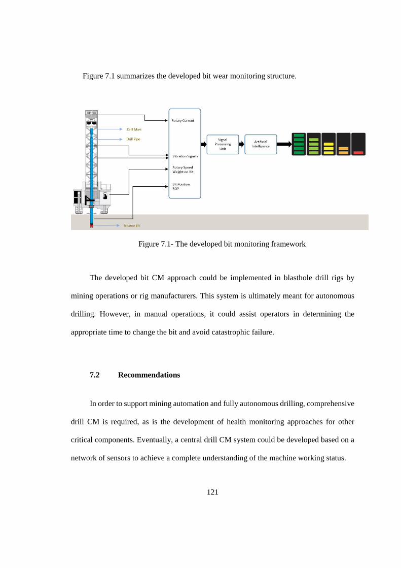
121

Figure 7.1 summarizes the developed bit wear monitoring structure.

Figure 7.1- The developed bit monitoring framework

The developed bit CM approach could be implemented in blasthole drill rigs by

mining operations or rig manufacturers. This system is ultimately meant for autonomous

drilling. However, in manual operations, it could assist operators in determining the

appropriate time to change the bit and avoid catastrophic failure.

7.2 Recommendations

In order to support mining automation and fully autonomous drilling, comprehensive

drill CM is required, as is the development of health monitoring approaches for other

critical components. Eventually, a central drill CM system could be developed based on a

network of sensors to achieve a complete understanding of the machine working status.

122

References

Aadnoy, B. S., Cooper, I., Miska, S. Z., Mitchell, R. F., & Payne, M. L. (2009). Advanced

drilling and well technology: Society of Petroleum Engineers, USA.

Aboujaoude, C. E. (1997). Feedback control of vibrations in surface rotary blasthole

drilling. (PhD), Department of Mining and Metallurgical Engineering McGill

University, Montreal, Canada.

Ashrafi, S. B., Anemangely, M., Sabah, M., & Ameri, M. J. (2019). Application of hybrid

artificial neural networks for predicting rate of penetration (ROP): A case study

from Marun oil field. Journal of Petroleum Science and Engineering, 175, 604-

623.

AtlasCopco (2012). Blasthole drilling in open pit mining. (3 ed.).

Besaisow, A. A., & Payne, M. (1988). A study of excitation mechanisms and resonances

inducing bottomhole-assembly vibrations. SPE drilling engineering, 3(01), 93-101.

Besselink, B., van de Wouw, N., & Nijmeijer, H. (2011). A semi-analytical of stickslip

oscillations in drilling systems. ASME Journal of Computational and Nonlinear

Dynamics, 6, 021006-021001.

Bishop, C. M. (1995). Neural networks for pattern recognition: Oxford university press.

Capik, M., Yilmaz, A. O., & Yasar, S. (2017). Relationships between the drilling rate index

and physicomechanical rock properties. Bulletin of Engineering Geology and the

Environment, 76(1), 253-261.

Caterpillar (2016). Cat ® MD6640 rotary blasthole drill 2016.

123

Christoforou, A. P., & Yigit, A. S. (2001). Active control of stick-slip vibrations: The role

of fully coupled dynamics. Paper presented at the SPE middle east oil show. 17-20

March, Manama, Bahrain, 2001.

Clausing, D. (1959). Comparison of Griffith's theory with Mohr's failure criteria. Paper

presented at the The 3rd US Symposium on Rock Mechanics (USRMS). 20-22

April, Golden, Colorado, USA, 1959.

Cobb, T., Scott, D., Dirksen, D., Dourfaye, A., Fleming, C., Rivera, R., & Silveus, J.

(2014). IADC Drilling Manual: Bits. (12 ed.).

Cooper, G. (1987). The interpretation of tricone drill bit vibrations for bit wear and rock

type. Paper presented at the Proc. Rapid Excavation and Tunneling Conference, 14-

18 June, New Orleans, Louisiana, USA, 1987.

Cooper, G. (2002). Proposal for the real-time measurement of drill bit tooth wear.

Geothermal Resources Council, 189-192.

Dadhich, S., Sandin, F., Bodin, U., Andersson, U., & Martinsson, T. (2019). Field test of

neural-network based automatic bucket-filling algorithm for wheel-loaders.

Automation in Construction, 97, 1-12.

Daubechies, I. (1992). Ten lectures on wavelets (Vol. 61). Society for Industrial and

Applied Mathematics Philadelphia, PA, USA.

Davis, J. L., & Annan, A. (1989). Ground-penetrating radar for high-resolution mapping

of soil and rock stratigraphy. Geophysical prospecting, 37(5), 531-551.

Demuth, H., & Beale, M. (2010). Neural Network Toolbox for use with MATLAB. The

mathworks, USA.

124

Dunayevsky, V., Abbassian, F., & Judzis, A. (1993). Dynamic stability of drillstrings under

fluctuating weight on bit. SPE drilling and completion, 8(02), 84-92.

Falconer, I., Burgess, T., & Sheppard, M. (1988). Separating bit and lithology effects from

drilling mechanics data. Paper presented at the SPE/IADC Drilling Conference, 28

February-2 March, Dallas, Texas, USA, 1988.

Fattahi, H., & Bazdar, H. (2017). Applying improved artificial neural network models to

evaluate drilling rate index. Tunnelling and Underground Space Technology, 70,

114-124.

Francke, J., & Utsi, V. (2009). Advances in long-range GPR systems and their applications

to mineral exploration, geotechnical and static correction problems. First break,

27(7).

Ghasemloonia, A., Rideout, D. G., & Butt, S. D. (2015). A review of drillstring vibration

modeling and suppression methods. J Journal of Petroleum Science and

Engineering, 131, 150-164.

Ghosh, R., Schunnesson, H., & Kumar, U. (2016). Evaluation of operating life length of

rotary tricone bits using Measurement While Drilling data. International Journal

of Rock Mechanics Mining Sciences(83), 41-48.

Global Market Insights. (2016). Surface mining market to reach US$28 billion by 2022.

Retrieved from http://www.mining.com/author/gminsights/

Gokhale, B. V. (2011). Rotary drilling and blasting in large surface mines: CRC Press.

Taylor & Francis Group, London, UK.

Graney, B. P., & Starry, K. (2012). Rolling element bearing analysis. Materials Evaluation,

70(1).

125

Halliburton. (2009). Drill bits; Roller Cone, IADC Dull Grading.

Hardage, B. A. (1992). Crosswell seismology & reverse VSP (Vol. 1), Seismic

Applications Series : Geophysical Press, London, UK.

Hartman, H. L. (1959). Basic studies of percussion drilling. Mining Engineering, 11, 68-

75.

Hartman, H. L., & Mutmansky, J. M. (2002). Introductory mining engineering: John Wiley

& Sons, New Jersey, USA.

Hinton, G. E. (1989). Connectionist learning procedures. Artificial Intelligence, 40(1), 185-

234.

Jha, P. C., Balasubramaniam, V., Sandeep, N., Sivaram, Y., & Gupta, R. (2004). GPR

applications in mapping barrier thickness in coal mines: Some case studies. Paper

presented at Tenth International Conference on Grounds Penetrating Radar, GPR

2004, 21-24 June, Delft, The Netherlands, 2004.

Kampf, A. R., Gochenour, K., & Clanin, J. (2003). Tourmaline Discovery at the Cryo-

Genie Mine, San Diego County, California. Rocks and Minerals, 78(3), 156-163.

Karmakar, M., Maiti, S., Singh, A., Ojha, M., & Maity, B. S. (2018). Mapping of rock

types using a joint approach by combining the multivariate statistics, self-

organizing map and Bayesian neural networks: an example from IODP 323 site.

Marine Geophysical Research, 39(3), 407-419.

Li, G., Yang, M., Meng, Y., Liu, H., Han, L., Zhou, F., & Zhang, H. (2016). The assessment

of correlation between rock drillability and mechanical properties in the laboratory

and in the field under different pressure conditions. Journal of Natural Gas Science

and Engineering, 30, 405-413.

126

Lin, Y.-Q., & Wang, Y.-H. (1991). Stick-slip vibration of drill strings. Journal of

Engineering for Industry, 113(1), 38-43.

Ma, D., & Azar, J. (1985). Dynamics of roller cone bits. Journal of Energy Resources

Technology, 107(4), 543-548.

Macpherson, J., Mason, J., & Kingman, J. (1993). Surface measurement and analysis of

drillstring vibrations while drilling. Paper presented at the SPE/IADC Drilling

Conference, 22-25 February, Amsterdam, Netherlands, 1993.

Maurer, W. (1962). The" perfect-cleaning" theory of rotary drilling. Journal of Petroleum

Technology, 14(11), 1,270-271,274.

Maurer, W. C. (1959). Impact crater formation in sandstone and granite. Colorado School

of Mines.

Mide (2017). Slam Stick Product Catalogue, (12 ed.).

Mincon (2016). DTH Tools Product Catalogue.

Møller, M. F. (1993). A scaled conjugate gradient algorithm for fast supervised learning.

Neural networks, 6(4), 525-533.

Monaghan, W. D., & Trevits, M. A. (2004). Application Of Ground Penetrating Radar To

Evaluate The Extent Of Polyurethane Grout Infiltration For Mine Roof Control-A

Case Study. Proceedings of the 23rd International Conference on Ground Control

in Mining, August 3-5, 2004, Morgantown, West Virginia.

Naganawa, S. (2012). Feasibility study on roller-cone bit wear detection from axial bit

vibration. J Journal of Petroleum Science and Engineering, 82, 140-150.

127

Nematinia, E., & Mehdizadeh, S. A. (2018). Assessment of egg freshness by prediction of

Haugh unit and albumen pH using an artificial neural network. Journal of Food

Measurement and Characterization, 1-11.

Pang, Y., Zhang, Y., Fu, S., & Zhu, Q. (2011). The condition monitoring system of mine

fan and analysis of condition based maintenance policy. Paper presented at the

Reliability, Maintainability and Safety (ICRMS), 12-15 June, Guiyang, China,

2011.

Parker Bay (2016). Surface mining equipment database, http://parkerbaymining.com.

Patterson, J. (2003). Application of ground penetrating radar (GPR) at the cryo-genie gem

pegmatite mine. Published by Mineralogical Society of America:

http://www.minsocam.org/

Poletto, F., & Miranda, F. (2004). Seismic while drilling: Fundamentals of drill-bit seismic

for exploration (Vol. 35): Elsevier Science, Amesterdam, The Netherlands.

Rafezi, H., Akbari, J., & Behzad, M. (2012). Tool Condition Monitoring based on sound

and vibration analysis and wavelet packet decomposition. Paper presented at the

2012 8th International Symposium on Mechatronics and its Applications, 10-12

April, Sharjah, United Arab Emirates, 2012.

Rafezi, H., & Hassani, F. (2018). Tricone bit health monitoring using wavelet packet

decomposed vibration signal. Paper presented at the 2018 5th International

Conference on Control, Decision and Information Technologies (CoDIT), 10-13

April, Thessaloniki, Greece, 2018.

Rafezi, H., Novo, A., & Hassani, F. P. (2015). An investigation into application of Ground

Penetrating Radar (GPR) in surface mining. Paper presented at the Symposium on

128

the Application of Geophysics to Engineering and Environmental Problems, 22-26

March, Texas, USA, 2015.

Ramani, R. V. (2012). Surface mining technology: progress and prospects. Procedia

Engineering, 46, 9-21.

Reid, D., & Rabia, H. (1995). Analysis of drillstring failures. Paper presented at the

SPE/IADC Drilling Conference, 28 February-2 March, Amsterdam, Netherlands,

1995.

Rostami, A., Hemmati-Sarapardeh, A., & Shamshirband, S. (2018). Rigorous

prognostication of natural gas viscosity: Smart modeling and comparative study.

Fuel, 222, 766-778.

Rumelhart, D. E., Hinton, G. E., & Williams, R. J. (1986). Learning representations by

back-propagating errors. Nature, 323(6088), 533-536.

Saeidi, O., Rostami, J., Ataei, M., & Torabi, S. R. (2014). Use of digital image processing

techniques for evaluating wear of cemented carbide bits in rotary drilling.

Automation in Construction, 44, 140-151.

Sandvik. (2013). Top hammer rock drilling tools, Sandvik Mining.

Sandvik. (2015). Rotary drilling bits and drill string tools, Sandvik Mining.

Sheppard, M., & Lesage, M. (1988). The forces at the teeth of a drilling rollercone bit:

Theory and experiment. Paper presented at the SPE Annual Technical Conference

and Exhibition, 2-5 October, Houston, Texas, 1988.

Shin, K., & Hammond, J. (2008). Fundamentals of signal processing for sound and

vibration engineers: John Wiley & Sons, Chichester, England.

129

Siami-Irdemoosa, E., & Dindarloo, S. R. (2015). Prediction of fuel consumption of mining

dump trucks: A neural networks approach. Applied Energy, 151, 77-84.

Sodhi, S. S., & Chandra, P. (2014). Bi-modal derivative activation function for sigmoidal

feedforward networks. Neurocomputing, 143, 182-196.

Stenström, C., Carlson, J. E., & Lundberg, J. (2012). Mining mill condition monitoring

using water jet ultrasonics. Paper presented at the IEEE International Ultrasonics

Symposium (IUS), October 7 - 10, Dresden, Germany, 2012.

Strange, A. D., Ralston, J. C., & Chandran, V. (2005). Application of ground penetrating

radar technology for near-surface interface determination in coal mining. Paper

presented at the Acoustics, Speech, and Signal Processing, 18-23 March,

Philadelphia, PA, USA, 2005.

Teale, R. (1965). The concept of specific energy in rock drilling. International journal of

rock mechanics and mining sciences & geomechanics abstracts, 2, 57-73.

Teck Resources (2018). Retrieved from

https://www.teck.com/operations/canada/operations/fording-river-5668/

Thomas, T. (2008). International Association of Drilling Contractors (IADC) codes.

Retrieved from https://www.bitbrokers.com/iadc.php

United Nations (2017). World Population Prospects: The 2017 Revision. Retrieved from

https://www.un.org/development/desa/publications/

Utsi, E. C. (2017). Ground penetrating radar theory and practice: Butterworth-Heinemann

Elsevier.

130

Wachel, J., Morton, S. J., & Atkins, K. E. (1990). Piping Vibration Analysis. Paper

presented at 19th turbomachinery symposium, September 18-20, Texas, USA,

1990.

Wang, F., Jing, M., Fan, H., Wei, Y., Zhao, Y., & Liu, H. (2017). Investigation on contact

angle of ball bearings. Proceedings of the Institution of Mechanical Engineers, Part

K: Journal of Multi-body Dynamics, 231(1), 230-251.

Wang, L., & Gao, R. X. (2006). Condition monitoring and control for intelligent

manufacturing: Springer-Verlag London.

Yarali, O., & Kahraman, S. (2011). The drillability assessment of rocks using the different

brittleness values. Tunnelling and Underground Space Technology, 26(2), 406-414.

Zhu, K., San Wong, Y., & Hong, G. S. (2009). Wavelet analysis of sensor signals for tool

condition monitoring: A review and some new results. International Journal of

Machine Tools Manufacture, 49(7-8), 537-553.

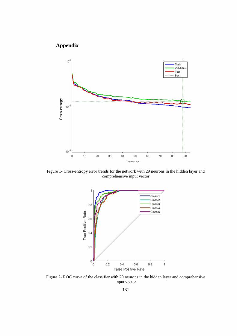
131

Appendix

Figure 1- Cross-entropy error trends for the network with 29 neurons in the hidden layer and comprehensive input vector

Figure 2- ROC curve of the classifier with 29 neurons in the hidden layer and comprehensive input vector

Cro

ss-e

ntro

py

Iteration

132

Figure 3- Cross-entropy error trends for the network with 31 neurons in the hidden layer and comprehensive input vector

Figure 4- ROC curve of the classifier with 31 neurons in the hidden layer and comprehensive input vector

Cro

ss-e

ntro

py

Iteration