Finite element method modeling of craniofacial growth

Finite element method modeling of craniofacial growth

Melvin L. Moss, Richard Skalak, Himanshu Patel, Kasturi Sen, Letty Moss-Salentijn, Masanobu Shinoiuka, and Henning Vilmann New York, N.Y., and Copenhagen, Denmark

The application of the concepts of continuum mechanics and of the numerical techniques of the finite element method permits the development of a new and potentially clinically useful method of describing craniofacial skeletal growth. This new method differs from those associated with customary roentgenographic cephalometry in that its descriptions and analyses are invariant; that is, they are independent of any method of registration and superimposition. Such invariance avoids the principal geometric constraint explicit in all analytical methods associated with conventional roentgenographic cephalometry. The conceptual and mathematical bases of the finite element method (FEM) are presented and illustrated by the numerical and graphic descriptions of the two- dimensional growth of the rat skull, for which two sets of longitudinal growth data are used. In practice, the FEM permits analysis of the skull at a scale significantly finer than previously possible, by considering cranial structure as consisting of a relatively large number of contiguous finite elements. For each such element, independently, it is then possible to describe and depict both the magnitude and the direction of temporal size and shape changes occurring in that element relative to itself at some initial time. It is emphasized that such descriptions are completely independent of any local reference frame.

Key words: Finite element, growth modeling, craniofacial

T he cranial skeleton is composed of a number of skeletal elements of complex shape. Cranial growth is characterized by numerous time-dependent changes of size, shape, and location of these cranial skeletal elements, resulting in marked geometric differences between homologous anatomic entities as growth progresses. It is the aim of this article to introduce a method (the finite element method) to describe and quantify mathematically the complex morphologic and skeletal changes that occur during growth. This is of theoretical and clinical significance.

Recently, it has been shown that, for a variety of reasons, the methods and techniques of customary roentgenographic cephalometry cannot satisfactorily serve these clinical and theoretical purposes.‘~2 Simul- taneously, alternative methods of analysis and description of cranial skeletal growth changes have been sug- gested. Skalak3 gave the general mathematical basis of the present analysis in three dimensions. Bookstein4-6 proposed a similar morphometric , biorthogonal method applicable in two dimensions. We initiated a systematic and comparative study of the ability of three other math-

From the Departments of Anatomy and Cell Biology, Civil Engineering and Engineering Mechanics, Bioengineering Institute, and Division of Orofacial Growth and Development, Columbia University, New York, N.Y., Department of Anatomy, Royal Dental College, Copenhagen, Denmark. This study was aided, in part, by Grants HD-14371 and DE-05145.

ematical models to most correctly describe and quantify cranial growth.3,7 Two of these models have been tested: (1) an allometric centered model’ and (2) a growth-network model.’ The third model, that of the finite element method, was introduced in this journal recently. ‘O In the present article the finite element method will be more fully presented.

CUSTOMARY ROENTGENOGRAPHIC CEPHALOMETRY (RCM)

It is useful to discuss here the two ways in which the methodologic and conceptual bases and content of “customary roentgenographic cephalometry” are used in this article. The first is related to the acquisition of radiologic data and the second to the methods of analysis of such data.

The primary requirement of any radiologic method of description, analysis, and/or comparison of cranial or cephalic size, shape, or growth is to provide the most accurate and repeatable determination of the coordinate locations of a number of anatomic or material points (defined below).

The most commonly used radiologic methods for such data acquisition in clinical orthodontics involved some sort of repeatable orientation of the patient’s head (for example, the use of a “cephalostat”). The finite element method (FEM), as used in this article, involves

453

454 Moss et al.

several variations of this same generic method of data acquisition. In sharing this procedural commonality, the FEM shares with all other such methods a similar set of constraints; that is, the errors of anatomic or material point imaging, detection, and representation are identical, whatever the method of their subsequent analysis.

It is in the second, analytical, use of RCM that the FEM differs significantly from customary roentgenographic cephalometry. For the reasons presented in this article, we suggest that the FEM offers significant analytical advantages over RCM. These are related to the demonstration that the FEM descriptions are invariant and independent of any local reference frame; that is, the descriptions and comparisons are independent of the well-known difference existing between many of the usual methods of superimposition and registration of different RCM analytical methods.

The data obtained from cephalic radiography fre- quently are used (1) to analyze statistically an appro- priate ensemble of many individual samples for the preparation of normative mean values; (2) to compare the size and/or shape of selected cranial skeletal elements of an individual with those of such a normative standard; or (3) to describe the size and shape changes of such cranial skeletal elements of an individual through time.

An intuitive comprehension of the advantages of- fered by the finite element method (FEM) relative to the customary methods of roentgenographic cephalometry (RCM) can be gained by considering the manner in which each method treats the cranial skeletal analyses noted above.

Let us consider first a pure longitudinal growth (seri- atim, time series) study of cranial growth. It is assumed that, for each individual, there exist a number of se- quential x-ray films taken in a standardized manner; that is, that we have a series of growth cross sections. In each such film it is assumed that a series of corresponding (homologous) points can be identified at each age. These points may be anatomic (for example, Na,Br,Ba) or material (for example, metallic implants). In principle, it would be desirable that a large number of material points be identified so that the local growth of the tissue could be evaluated on a fine spatial scale. In practice, it is convenient and usual to use anatomic points to a large extent, with fairly large spacings. This limits the interpretation of computed results to certain regional mean values. To be useful, we require only that any point used can be reliably identified and that the coordinates of its location can be determined in a two-dimensional plane, at least, or in three dimensions if possible.

In RCM, in each x-ray film or tracing it is customary to fix the location of one common point (for example,

S), and to fix the direction of one common line segment (for example, Na-S) in each cross section. Some variant methods use a common osseous contour (anterior cranial base). Then all growth cross sections may be stacked (superimposed) and the kinematic (growth) behavior of all other studied points can be observed. It is noted that the principal difficulty with RCM is that the observed growth behavior of any set of such points is specific for the registration method; that is, it is dependent on the choices of fixed point and fixed line. ” Regions with little growth may appear to translate and rotate significantly in this method. It is impossible to construct a model that is independent of the choices of fixed point and fixed line, and there is no objective way in which it can be determined that one method of registration of RCM analysis displays growth behavior more correctly than any other.*.”

Considering the methodologic constraints detailed above, it is clear that, with the use of any RCM, we can describe and depict only the relative growth behavior of a series of discrete anatomic or material points (that is, relative to the selected fixed point or arbitrary frame of reference); nothing is known of the growth behavior at the individual points in the continuum between the discrete points actually studied. In a technical sense, it may be said that RCM shows relative move- ments of individual points, such as studied in classic mechanics of particles (point masses). For example, in studying the orbits of planets, each planet may be represented by a single point. Accordingly, while it is usual in RCM to construct a line segment between pairs of such points (Na-Br; ANS-PNS), it must be realized that such line segments are arbitrary geometric constructs, and that the reported “growth changes” of such line segments are, in fact, only indirect reflections of the growth behavior of their intervening points. Some intervening points may not be growing at all, as in the case of points situated within osseous tissue. Further, in customary usage, the distances separating RCM points, relative to total skull size, often are large. Only anecdotal observation of the time-related changes in shape, or location of a skeletal element (for example, the “lowering” of the lower border of the mandible) is possible since it has been shown that RCM is incapable of correctly depicting in local detail either biologic shape or the shape changes.4,’ The same constraints exist when RCM are used to prepare normative standards and to compare a single film against such standards.

GROWTH STRAIN TENSORS AND FINITE ELEMENTS

The conceptual bases of the mathematical modeling of craniofacial skeletal growth presented in this article must be carefully described since they introduce most

Volume 81 Number 6

Finite element method modeling of craniofacial growth 455

readers to terms, concepts, and procedures that are not commonly used by students of growth. In a technical sense, two separate ideas are presented. The first is that the use of a growth strain tensor permits a fundamental description of growth; more specifically that a growth tensor is a fundamental descriptor of growth. The second idea is that the use of the finite element method makes possible a convenient and systematic approximation of the mean growth tensor within finite elements, using the data from a finite number of data points. It will be helpful to define and exemplify both concepts, first that of finite elements and then that of growth tensors.

THE FINITE ELEMENT METHOD (FEM)

This method differs fundamentally from RCM in several significant ways, some of which are outlined below. FEM is discussed, in depth, in a number of texts.‘2-‘7 This article will present only some conceptual attributes of the FEM that are useful to explain the ways in which the FEM differs from RCM and the advantages that the FEM offers in the study of craniofacial growth. The principal advantage of the finite element method is that it can provide an estimate of the growth behavior of all points of the body and in all directions at all points.

The particular FEM used in this study, and in that by Patel,” begins with a consideration of a two- or three-dimensional body (or structure) as consisting of a boundary and an internal continuum of particles, or points. A substantial amount of literature has shown convincingly that most biologic growth in general and craniofacial skeletal growth in particular often are both anisotropic and nonlinear. Growth is anisotropic because it must include shape changes as well as size changes, and it is nonlinear because the changes in lengths and angles are not small. Accordingly, the present study uses the concepts of nonlinear continuum mechanics” and the numerical methods of the FEM for their implementation.

For present purposes, it is useful to regard a growing continuum as subdivided by a series of imaginary lines (in a two-dimensional body) or plane surfaces (in a three-dimensional body). In either case, these lines and planes may be thought of as passing through tissue or air and are so chosen that each line is connected at one end to at least one other line. The points of connection are termed nodes. In the three-dimensional case, the planes are bounded by straight lines that extend from one node to another. These lines and planes concep- tually subdivide the body into a series of contiguous finite elements, a process termed discretization. The location of the node connecting two or more such lines is occupied by a single point whose coordinates are

A A

i ,’ ‘\ ,I’ ‘1

f!a J-- --- / Fig. 1. Three possible finite elements: a three-noded, two-dimensional element (a triangle), a four-noded element (a pyramid), and an eight-noded element (a box).

assumed to be known. Fig. 1 illustrates a three-noded, two-dimensional finite element (a triangle); an eight- noded, three-dimensional hexahedron (a box); and a four-noded tetrahedron (a pyramid); there are many other possible configurations.

Finite elements may also be constructed with curved lines or surfaces as boundaries. Such elements require one or more additional nodes between the comer nodes described above. Such elements are described in the references to the FEM cited above and may be advan- tageous if sufficient nodal data are available so that element boundaries can fit curved anatomic shapes closely. In the present article only straight-line and plane boundaries will be used to illustrate the principal attributes of the FEM most simply.

In practice, the mathematical subdivision of a body into a number of finite elements may be done either by arbitrarily selecting some of the particles of the body and allowing them to serve as nodes of a finite element or by using a set of anatomic points as such nodes. The later technique is used here and in Patel’s” study. Ide- ally, all nodes should be homologous material points; otherwise, the growth information that can be deduced is limited.

The FEM differs significantly from RCM in the method of analysis of growth behavior. Whereas in RCM only the behavior of a set of separate points (for example, Na,Ba) is studied, in the FEM the emphasis is on analysis of growth within each element. In the method presented here, the assumption is made that all the points within a given finite element share a common growth behavior. This will become more accurate as

456 Moss et al. Am. J. Orthod. Jtme 1985

the number of elements is increased and their size is decreased. Let us consider a two-dimensional, three- noded, triangular finite element (Fig. 1). At some initial time (b) the coordinates of each of the three nodes are assumed to be determined and, in time, as a result of growth, the location of these nodes is transformed, so that, at some later time (tJ the new coordinates of the three nodal points are again determined. In a common clinical vocabulary the triangular finite element is said to have “grown larger,” while in the more precise vocabulary of continuum mechanics it is said that the finite element has been deformed, strained, or transformed. The term strain may be understood in the sense that it is used in classical physics or mechanics. When a physical body is externally loaded, it tends to deform. For example, in vertical, axial, compressive loading, a physical body tends to shorten vertically and widen horizontally. The dimensional changes, expressed as fractions of the original lengths, are strains, and can be measured.

The force per unit area required to produce such strain is termed stress and is a measure of the internal resistance of the body to deformation. In growth the deformations are not due to stresses but are produced by cell division, cell growth, and production of extra- cellular matrices (that is, by adding mass). Accordingly, a growth strain is the measurable deformation of a biologic body resulting from its growth. With the use of the mathematical definitions introduced by Skalak and associates’ and the numerical methods detailed by Pa- tel,” a quantitative description of the values of the growth strains, or deformations or extensions, as well as a determination of the principal directions of these extensions, can be computed and graphically displayed. It is assumed that the growth description of any single element is valid for all of the points within the continuum of that same element in the present study of skulls. This may be a crude approximation of the biologic reality, for several reasons: No data on brain growth were considered in treating the neural skull, no data on the growth of the splanchnocranial viscera were in- cluded, and some points used were not material points. Nevertheless, the analyses given here are able to dem- onstrate the utility of the finite element method. The deficiencies can be remedied simply by supplying more detailed input data. While the FEM describes only the mean growth behavior in each element, in practice the finer the discretization of the body (that is, the smaller the individual finite elements and the more of them in a given body), the more closely the resulting numerical results will approximate the reality of the growth behavior at each point.

GROWTH TENSORS

While customary roentgenographic cephalometry (RCM) usually employs vectors to display and describe results, the FEM computes growth tensors. The difference between these two descriptions is related to the different basic viewpoints of the two descriptors of growth. Conventional RCM reports the results in terms of displacements or movement of points in time. The continuum viewpoint suggests that the fundamental effects in growth are the local extensions (growth strains) in the vicinity of any point. These growth strains are distributed throughout the growing body and are prop- erly described by the growth tensor at each point. This calls for a tensor description of growth extensions as opposed to a vector description of displacement, as given by RCM. In a technical sense, the tensor description of growth is derived from displacements via the theory of continuum mechanics. More precisely, the growth tensor is a function of the derivatives of displacements with respect to position (that is, the displacement gradient).20,2’ The tensor description provides an invariant (coordinate system independent) description of growth at each point. With the example of the deformation of a single three-noded, triangular finite element given above, it is possible to provide a two- dimensional elucidation of the term tensor as used here. This is a concept that is not in general use in physical anthropology or in orthodontics but is common in continuum mechanics.

Tensors, in general, are abstract mathematical entities that cannot be readily visualized. This lack of visualizability is the greatest stumbling block in comparison to the type of graphic representation customary with vectors. The general concept of a tensor involves a set of numbers that describe a three-dimensional field, such as a stress or strain (or a methematical operation, such as transformation or coordinates). The numbers that specify a tensor are called components. A tensor may also be specified by giving so-called principal directions and principal values that may be represented graphically. This will be the mode used in the present article for growth descriptions. Generally, the tensor is a descriptor. The numbers and figures are representa- tions of the tensor or the expression of the tensor in a particular coordinate system. As a tensor is a descriptor, so a growth tensor is a descriptor of growth. It may be regarded as specifying a transformation of coordinates from one stage of growth to another. A simple analogy of a tensor operation may be helpful. Arithmetic addition is a mathematical operation. The concepts of arithmetic, addition, subtraction, etc., per se, are with- out specific (dimensional or directional) content, and

Volume 87 Number 6


this is true also for the concept of a tensor operation. The addition of 3 and 5 to produce the sum of 8 is an arithmetic operation. The integers involved do not ex- press the concept of addition, but only the input and output of its operation. Addition, per se, is a concept in which the results of the operation are easily observed. A tensor is a more general concept than arithmetic but has rules analogous to arithmetic addition, multiplica- tion, etc. In the present context, tensor operations are involved with the transformations from one set of coordinates to another set, and the results may be expressed as the growth strain tensor.

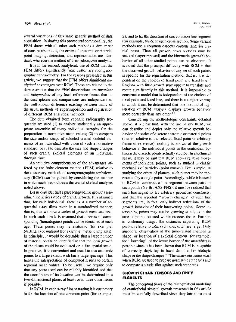
In the particular situation treated here, the significance of the growth tensor can be summarized in a physical way. The growth tensor describes the relative displacements of all points in the neighborhood of the given point (for example, displacements of the continuum of points within a given finite element relative to any selected point) (Fig. 2). It will be remembered that a vector quantity (a force, an acceleration) has the two attributes of magnitude and direction. In three dimensions, a growth tensor has attributes of six scalar components or three principal directions. In the present context, a growth tensor may be regarded as specifying the local transformation from one set of coordinates to another (from the initial to the final coordinates in the interval of growth considered). For example, it describes the transformation of a triangular finite element at time t,, in a Cartesian frame of reference to the location of the same triangular element after growth at time t,. Strictly speaking, the growth tensor allows determination of displacements only within a rigid body translation and/or rotation. This freedom is one aspect of the fact that the growth tensor is independent of any rigid body motions or displacements of the subject of study on radiographs representing it.

The analysis of a transformation by the finite element method requires the ability to locate each node before and after the transformation and to determine accurately the three-dimensional coordinates of each node both before and after the transformation. Tech- nically, this is the ability to “map” homologous points from one time frame to another. It may also be stated as the ability to identify end points of the path of a particular point in space-time.* It is precisely these re- lationships between homologous points that a growth tensor describes and quantifies. In principle, if the growth tensor is given at every point of a body (and it may vary continuously from point to point) it gives sufficient information to reconstruct final form (size and shape) in three dimensions, starting from the initial form; again, this is within an arbitrary rigid body mo-

Fig. 2. The deformation of the circle above to the ellipse below illustrates the general transformation of the neighborhood of any point during a two-dimensional growth. The lines through the point are shown in their corresponding initial and final po- sitions. The general line segment both stretches and rotates, but the principal axes are subject to stretching only.

tion. The difficulty with RCM is that it specifies the particular rigid body translation and rotation to be used and thus lacks independence of these choices.

There are, in general, various types of tensors of geometric interest: a metric tensor, a rotation tensor, a rate-of-growth tensor,3 etc. An additional example may be useful. Consider a human skull, in norma verticalis, in which the sagittal suture is marked by implants at points bregma and lambda and the location of the cor- onal and lambdoidal sutures is marked by implants at pterion and asterion, respectively. In the customary three-dimensional Euclidean space, all three sutures and the implants have a fixed vectorial (spatial) relationship to each other. Now, allow this skull to be rotated relative to the fixed three-dimensional reference frame, so that the lateral surface of the skull is now in view. With

458 MOSS et al.

4.Br

Am. J. Orrhod June 1985

‘1,ANS

13,APP

Fig. 3. The triangular elements used for finite element description of rat craniofacial growth in the analysis of the first (European) data set. The anatomic points lie in the midsagittal plane of the rat skull.

Age in days = 15 1

10

5 MM

0

Fig. 4. The triangular elements used for finite element description of rat craniofacial growth in the analysis of the second (Japanese) data set. The anatomic points lie in the midsaggital plane and are defined in the text.

respect to the fixed axes of the reference frame, the coordinates of all the implanted points of that skull have changed; however, within the skull, the relative rela- tionships of these points and of the vectors of the sutures to each other have remained constant. Such constancy of description of growth in the face of rigid body rotation is expressed by the growth tensor. This statement reiterates one of the chief advantages of the jnite element method over RCA!: that tensor descriptions are independent of external frames of reference. It is this attribute that permits the tensor descriptions of the FEM to overcome the principal geometric disadvantage of all RCM and to permit the FEM to be independent of any method of registration and orientation.

A further advantage is that growth is described in a local basis. In the vicinity of each point, the local changes due to growth are described independently of

what is taking place elsewhere. In RCM the displacements of any point may depend on the growth at distant points.

The finite element method was first introduced into the literature about 20 years ago to assist in solving certain problems in structural mechanics. A method able to subdivide structures into large numbers of contiguous two- or three-dimensional elements and to analyze the size and shape changes in each element individually and over all elements together was soon seen to be valuable in the analysis of a great variety of fields, including biologic problems at the supracellular level. I6 The extension of finite element methods to problems of plant growth** and to problems of vertebrate skeletal responses to external loadings23-25 proved useful.

In dentistry, the finite element method has been applied to stress analysis in recent years, in studies of two- and three-dimensional responses to loadings of teeth, dental restorations, and intraosseous implants.*6-30 Despite this extensive use, specific orthodontic applications have been rare. One Dutch-lan- guage3’ and one English-language article3* report finite element analyses of the responses of nonvital tooth and bone to the application of specific orthodontic loadings. The latter article has the additional virtue of demon- strating the application of finite element methods to the analysis of data obtained by holographic techniques, a matter of potentially great significance. 33

In the intervening years the use of the FEM has spread to such fields as geophysics, fluid mechanics, and, importantly, to biomechani&.‘6 In the past several years the method has been applied to problems of cranial form. Cheverud and associates” illustrated a three- dimensional analysis of comparative adult primate cra-

Volume 87 Number 6


Table I. Relative notation matrix

Element no. (degrees)

Days I 2 3 4 5 6 7 8 9 10 Sl s2

14 2.6 -0.4 -0.5 0.0 1.0 1.9 2.7 4.1 2.4 2.4 0.8 2.9 21 2.2 -3.1 -1.5 0.0 2.0 2.4 6.0 7.8 2.7 5.9 0.3 5.6 30 2.0 -6.2 -2.3 0.0 3.5 3.6 9.4 10.7 4.4 7.1 0.1 7.9 40 0.4 -9.4 -3.7 0.0 5.4 4.9 11.8 12.4 5.0 8.1 -0.4 9.3 60 1.5 -11.9 -4.4 0.0 7.7 6.9 14.6 14.6 7.1 11.0 -0.03 11.8 90 2.2 - 13.1 -5.1 0.0 8.7 7.5 15.1 14.8 7.1 14.5 0.03 12.9

150 3.1 - 15.4 -5.7 0.0 10.2 8.2 16.7 15.9 7.2 15.8 0.1 13.9

Negative sign indicates clockwise rotation. Relative rotations of elements used for the finite element description of the average male rat craniofacial growth as shown in Fig. 3. All rotations are relative to element 4. S 1 is the average relative rotation of the neural skull section (elements 1 to 6), while S2 is the average relative rotation of the facial skull section (elements 7 to 10).

nial form, and we have applied the FEM to problems of cranial growth.‘,” Patell’ presented a two-dimensional analysis of the growth of rat and human neuro- crania and provides a full three-dimensional discussion. The rodent data were used by Bookstein in a parallel and mutually corroborative study. The present article, to the best of our knowledge, is the first to describe and depict a two-dimensional finite element analysis of the growth of the complete rat cranium, neural skull, and facial skull, including the mandible.

MATERIALS AND METHODS Data

Two sets of longitudinal rat skull growth data (time series) were analyzed. The first are from a European strain, on whose growth behavior we have reported previously. 35-39 The data consist of the coordinates of a series of midsagittal anatomic points obtained at the ages of 7, 14, 21, 30, 40, 60, 90, and 150 days in 21 male and 25 female rats individually at each age.

With this close-bred strain, we used the calculated mean values for the following mid-sag&al anatomic points (Vilmann’s classification38.39): bregma (point 4); intersphenoidale (9); spheno-occipital synchondrosis (8); basion (7); opisthion (6); posterior lambdoidal suture (25); lambda (5); anterior palatal point (APP) (13); posterior nasal spine (12); nasion (27); presphenoidale (28); anterior nasal point (ANS) (1) (Fig. 3).

The second data set consisted of two groups of mean, two-dimensional, coordinate of 15 anatomic points of the neural and facial skulls as separately determined for 67 male and 52 female rats of a Japanese Wistar strain, as published by Hanada. These rats were studied at 15,20, 25, 30, 35,40,45,50,60,70, 80,90, 100, 110, 123, and 145 days of age. The points studied in Hanada’s classification are intersphenoidal synchrondrosis (1); basion (2); tip of the external oc-

cipital crest (3); bregma (4); anterior nasal point (5); prosthion (6); tip of the maxillary palatal alveolar crest (7); tip of the maxillary incisor tooth (8); tip of the mandibular incisor tooth (9); infradentale (tip of labial mandibular alveolar crest) (10); tip of lingual mandibular alveolar crest (11); menton (tip of mental protu- berance (12); gonion (14); and condylion (15) (Fig. 4). It should be noted that while point 13 is shown in that figure, it was not used in the present study.

Selection of finite elements

For each set of rat data, an arbitrary number of three- noded, triangular, finite elements was selected. For the first data set, ten two-dimensional elements were constructed (Fig. 3); this number permitted relatively fine discretization of the neural and upper facial skulls. With the second data set, twelve two-dimensional finite elements were used. This analyzed the neural and upper facial skulls less finely than the first set, while permit- ting, for the first time, a relatively discrete analysis of the lower facial skull and of the maxillary incisor region (Fig. 4).

Presentation of results

The mathematical concepts and the computer-as- sisted mathematical operations involved in finite element analysis are outlined in the appendix; these operations are detailed in the textbooks cited above and adapted by Patell* to the application of the FEM to growth studies. In essence, these computations treat the input data so that, for each finite element in turn, the program determines the direction and amount of maximal and minimal growth changes (strains) in relation to some initial state. In the present case the 7- or 15- day rat skull provides a set of initial values relative to which all subsequent growth changes are described. In a three-dimensional finite element analysis, the program

460 Moss et al. Am. J. Orthod. June 198.5

Table II. Analysis of the growth changes in twelve elements (column 2) of the rat skull, by the finite element method, during the period of 15 to 145 days

Finite Maximum Minimum Maximum Area Maximum extension Minimum extension element no. large strain large strain shear ratio ratio ratio

Age 20 days 1 2 3 4 5 6 I 8 9

10 11 12

Age 30 days 1 2 3 4 5 6 I 8 9

10 11 12

Age 50 days 1 2 3 4 5 6 7 8 9

IO 11 12

-

0.12 0.20** 0.60* 1.1 1.1 1.0 0.85* 0.39* 0.23* 1.1 1.1 1.0 0.14 0.38* 0.54* 1.2 1.1 1.0 0.11 0.65* 0.25* 1.2 1.1 1.1 0.56 0.55* 0.25 1.5 1.5 I.1 0.53 0.74* 0.23 1.5 1.4 1.1 0.54 0.79* 0.23 1.6 1.4 1.1 0.26 0.97* 0.79* 1.3 1.3 I.1 0.37 0.96* 0.14 1.4 1.3 1.1 0.37 -0.13* 0.25* 1.1 1.3 0.86 0.15 0.64* 0.41* 1.2 1.1 1.1 0.19 0.98* 0.48* 1.3 1.2 I.1

0.30 0.98* 0.98* 0.18 0.79* 0.52* 0.39 0.85* 0.15* 0.32 0.24 0.41* 9.0 0.28 4.3 1.7 0.28 0.73 1.5 0.18 0.67

0.51 0.23 0.14 1.4 0.31 0.53

0.70 -0.84** 0.35 0.45 0.16 0.14 0.53 0.24 0.14

0.62 0.19 0.21 0.33 0.12 0.10 0.74 0.14 0.30 0.61 0.57 0.19*

19.0 0.59 9.4 2.9 0.63 1.1 3.4 0.42 1.5 0.90 0.44 0.23 2.4 0.33 1.0 1.2 - 0.27* 0.60

0.88 0.31 0.29 1.1 0.46 0.33

-

1.4 1.3 1.1 1.3 1.2 1.1 1.4 1.3 1.1 1.6 1.3 1.2 5.4 4.4 1.2 2.6 2.1 1.2 2.3 2.0 1.2 1.7 1.4 1.2 2.5 1.9 1.3 1.5 1.5 0.99 1.6 1.4 1.2 1.7 1.4 1.2

1.8 1.5 1.2 1.4 1.3 1.1 1.8 1.6 1.1 2.2 1.5 1.5 9.3 6.3 1.5 3.9 2.6 1.5 3.8 2.8 1.4 2.3 1.7 I .4 3.1 2.4 1.3 1.8 1.8 0.97 2.1 1.7 1.3 2.5 1.8 1.4

The twelve finite elements are defined by the following points: (1) l-2-3; (2) l-3-4; (3) l-4-5; (4) l-5-7; (5) 5-6-7; (6) 6-7-8; (7) 9-11-15; (8) 10-11-15; (9) 9-10-11; (10) 10-11-12; (11) 11-12-14; (12) 11-14-15. For convenience, only the values for days 20, 30, 50, 90, and 145 days are shown. The parameters shown include (column 2) maximum extensional strain; (column 3) minimal extensional strain; (column 4) maximum shear strain; (column 5) area ratio; (column 6) maximum extension ratio; (column 7) minimum extension ratio. * = e-‘, ** = e-?,

determines the direction and magnitude of the principal I. Maximum strain. This is a tensor component growth strains. The first of these represents the direction describing the maximal growth of all directions within of maximal growth. The other two occur in mutually a given two-dimensional finite element, relative to the perpendicular directions, one of which is the minimal initial age that serves as a standard for comparison. The growth strain and the third one of intermediate (sta- mathematical bases for computing the several tensor tionary) value. The results (computer output) of such attributes shown in Table I are provided in the appendix. analyses may be presented in both numerical and 2. Minimal strain. This is a component describing graphic form, as follows: the amount of minimal increase of any direction within

Volume 87 Number 6


Table II. Cont’d

Finite element no.

Age 90 days 1 2 3 4 5 6 7 8 9

10 11 12

Age 145 days 1 2 3 4 5 6 7 8 9

10 11 12

Maximum Minimum Maximum Area Maximum extension Minimum extension large strain large strain shear ratio ratio ratio

0.94 0.25 0.35 2.1 1.7 1.2 0.44 0.17 0.14 1.6 1.4 1.2 1.1 0.18 0.44 2.1 1.8 1.2 0.92 0.80 0.62* 2.7 1.7 1.6

20.0 0.84 9.5 10.0 6.4 1.6 4.2 1.2 1.5 5.6 3.1 1.8 4.6 0.67 1.9 4.9 3.2 1.5 1.6 0.71 0.46 3.2 2.1 1.6 2.9 0.78 1.0 4.1 2.6 1.6 2.5 0.66* 1.3 2.3 2.4 6.93 1.3 0.52 0.38 2.7 1.9 1.4 1.6 0.72 0.43 3.2 2.0 1.6

1.1 0.29 0.39 2.2 1.8 1.3 0.49 0.19 0.15 1.6 1.4 1.2 1.2 0.19 0.50 2.2 1.8 1.2 1.1 0.91 0.85* 3.0 1.8 1.7

35.0 1.0 17.0 15.0 8.4 1.7 5.6 1.1 2.3 6.3 3.5 1.8 5.4 0.77 2.3 5.5 3.4 1.6 1.5 0.77 0.36 3.2 2.0 1.6 3.5 0.56 1.5 4.1 2.8 1.5 2.0 0.94* 0.94* 2.4 2.2 1.1 1.4 0.60 0.42 2.9 2.0 1.5 1.7 0.81 0.47 3.4 2.1 1.6

the finite element, relative to initial values. It may be shown that the directions of the maximal and minimal strains are always normal perpendicular to each other.

3. Manimum shear. The value of this tensor is determined, in twb dimensions, by the difference between the maximal and minimal strains. This difference represents the magnitude of the maximal shear that occurs at 45” to the direction of the maximal extensional strain. The shear strain is a measure of the change of angle between the two line segments that are initially perpendicular.

4. Area ratio. This is the ratio of the value of the area of the finite element being studied at a given age to the initial value of that area. In three dimensions one can also calculate a volume ratio.

5. Maximum and minimum extension ratios. As in the area ratio, these values represent the ratio between the initial and final lengths in the directions reported for maximal and minimal strains. The extension ratio is the length, at a given age, divided by the values at the initial age. The two extension ratios contain the same information as the maximum and minimum strains above and are related to them as indicated in the appendix .

6. Directions of principal axes. An arbitrary local

line segment is selected to serve as an x axis in two- dimensional Cartesian space. The directions in which maximal and minimal extension (growth, strain) occurs are defined in terms of direction cosines. The direction cosine of the line representing maximal strain with respect to the x axis is defined as the cosine of the angle formed by that line and the local x axis. There is also the complementary determination of the cosine of the angle that same line makes to the y axis. A similar pair of determinations is made of the direction cosines of the line representing the minimal extension (growth strain) to the x and y axes. These two principal axes are always mutually perpendicular to each other. In three dimensions there are three mutually perpendicular principal directions, each of which is specified by three direction cosines. This relationship is similar to the relationship that exists in a stressed solid between the directions of the principal trajectories of strain and/or stress. ‘Basically, the orientations of the principal axes are related to local landmarks (nodes and sides of elements) and in this sense are independent of the choice of global coordinates. A different choice of local axes will give different direction cosines, but the orientation of principal axes relative to the element will be the same.

462 Moss et al. Am. J. Orrhod Junr 19X.5

Table III. Analysis of growth changes in twelve elements of the rat skull, by the finite element method, during the period 15 to 145 days

20 days 1 2 3 4 5 6 7 8 9

10 11 12

30 days 1 2 3 4 5 6 7 8 9

10 11 12

50 days 1 2 3 4 5 6

8.1 32.9 34.9

0.0 28.4 74.3 42.2 47.9

8.1 60.7 62.0 71.3

14.1 62.6 29.5 14.1 57.3 57.3 36.9 74.3 14.1 73.7 60.7 56.6

18.2 60.7 27.1 64.5 52.4 60.7

82.5 82.5 171.9 55.6 55.6 147.1 55.3 55.3 145.1 90.0 90.0 180.0 62.0 62.0 151.6 16.3 16.3 105.7

47.9 47.9 137.7 42.3 42.3 132.1 84.3 84.3 171.9 29.5 29.5 119.3 28.4 28.4 118.0 18.2 18.2 108.7

76.7 76.7 165.9 27.1 27.1 117.4 60.0 60.0 150.5 75.5 75.5 165.9 32.9 32.9 122.7 32.9 32.9 122.7 53.1 53.1 143.1 16.3 16.3 105.7 76.7 76.7 165.9 16.3 16.3 106.3 29.5 29.5 119.3 32.9 32.9 123.4

72.5 72.5 161.8 29.5 29.5 119.3 62.6 62.6 152.9 25.8 25.8 115.5 37.8 37.8 127.6 29.5 29.5 119.3

Finite element no. (4 fB) CC) (0) -

7 8 9

10 11 12

90 days 1 2 3 4 5 6 7 8 9

10 I1 12

150 days 1 2 3 4 5 6 7 8 9

10 11 12

43.1 73.7

0.0 67.7 57.3 54.5

16.3 57.3 24.5 65.2 30.7 53.1 44.8 64.5

8.1 63.9 53.1 56.6

18.2 23.1 23.1 66.4 51.7 58.7 46.4 71.9

8.1 67.0 58.0 53.8

46.4 46.4 136.9 16.3 16.3 106.3 90.0 90.0 0.0 21.6 21.6 112.3 32.9 32.9 122.7 34.9 34.9 125.5

73.7 73.1 163.7 32.9 32.9 122.7 65.8 65.8 155.5 24.5 24.5 114.8 59.3 59.3 149.3 36.9 36.9 126.9 44.8 44.8 135.2 25.8 25.8 115.5 84.3 84.3 171.9 25.8 25.8 116.1 31.8 31.8 121.3 33.9 33.9 123.4

71.9 71.9 161.8 30.7 30.7 121.3 66.4 66.4 156.9 24.5 24.5 113.6 38.7 38.7 128.3 30.7 30.7 121.3 43.1 43.1 133.6 18.2 18.2 108.1 83.1 83.1 171.9 23.0 23.0 113.0 31.8 31.8 122.0 35.9 35.9 126.2

For convenience, only the values for 20, 30, 50, 90, and 145 days are shown, and the cosines of the angles have been converted to degrees. In this analysis the X axis is formed by a line originating at basion and passing through and beyond S-O-S, and the Y axis is a perpendicular passing through the point S-O-S. The parameters shown include: (A) the angle of the maximal principal strain axis with the X axis, (B) the angle of the minimal principal strain axis with the X axis, (C) the angle of the maximal principal strain axis with the Y axis, (D) the angle of the minimal principal strain axis with the Y axis.

The area and extension ratio values provided in Table II are to be understood in the customary, arithmetic manner. These ratios, together with the descriptions of the directions in which the maximal and minimal extensions occur (Table III), give a physical interpretation of the finite element method description of growth.

European rat strain. This description is derived from the doctoral thesis of Patel,” who used the rat skull growth data of Vilmann.35-39

Principal growth strains and directions are computed and located on each element of the average network. The results for male rat skull growth are shown in Fig. 5, A to G. The crosses drawn at the centroid of

each element are directions of principal growth strains, and the number at the end of each segment is the principal extension ratio in that direction. The length of each arm of the cross is proportional to the extension ratio in that direction. When the growth is nearly uniform in an element (that is, there is negligible shape change in it), then the principal extension ratios are nearly equal. On the other hand, when values of principal extension ratios in an element differ substantially, there is significant shape change associated with its growth. In this case, some or all of the interior angles of the triangular element change significantly. If the direction of maximum principal extension ratio nearly bisects an interior angle, then that angle will generally

volume 87

Number 6 Finite element method modeling of craniofacial growth 463

@ Principal extension ratios for rat .craniofacial growth from 7 to 14 days.

I

0

6

Fig. 5. A and 6, The results of the finite element method analysis of the European rat cranial growth data set. The values of the principal extension ratios and their directions are shown, relative to the 7-day-old rat, at 14, 21, 30, 40, 60, 90, and 150 days.

decrease with growth. If the direction of minimum principal extension ratio nearly bisects an interior angle, then that angle will generally increase with growth.

The kinematics of male rat neural skull growth in the period from 7 to 150 days can be described by means of the results shown in Fig. 5. The neural skull is the region enclosed by the anatomic points Ba, Op, PLS, L, Br, PSS, ISS, and SOS (that is, elements 1 to 6 in Fig. 3). It is observed in Fig. 5, A that the direction and magnitude of principal extension ratios are approximately the same in most of the neural skull for growth from 7 to 14 days and that maximum growth extension is roughly parallel to a line connecting PLS and ISS. After 14 days of growth, maximum principal extension ratios are significantly larger in elements 3, 5, and 6 along the base of the neural skull (Ba-SOS, SOS-ISS, and ISS-PSS). Growth extensions in direc-

tions parallel to line L-SOS are significantly smaller than in the base of the skull, and after 60 days of growth there is no further extension in this direction.

Consider the growth in elements 1 and 2 from 14 days to 150 days. It is observed that the direction of maximum extension ratio nearly bisects the angle at PLS in element 1 until 30 days and in element 2 until 150 days, so that these angles are decreasing. After 30 days, growth extension in element 1 occurs primarily along segment Op-PLS. Also, the direction of minimum extension ratio nearly bisects the angle at L in element 2, suggesting a significant increase in that angle of that element during the entire growth period. The growth extensions in elements 3 and 5 are similar at each age, as seen from the magnitudes and directions of principal extension ratios in those elements. Large growth extensions occur along segments Ba-SOS and SOS-ISS

464 Moss et al. Am. J. Orrhod. June IYXS

13

@ Prlnclpal extension ratios for rat craniofacial growth from 7 to 40 days.

Flg. 5 (Cont’d), C and D.

in these elements, with corresponding increases in angles at L and Br, respectively. The growth in element 4, on the other hand, is more nearly isotropic, so there are negligible shape changes. Element 4 grows into nearly similar triangles. After 60 days there is virtually no growth in that element. The growth in element 6 of the rat neural skull is similar to that of element 3. Large growth extensions occur in segments ISS-PSS, and the angle at PSS in that element decreases significantly.

The salient features of rat neural skull growth over the entire growth period are as follows: 1. Maximum growth extensions of about 2.0 occur in

segments Ba-SOS, SOS-ISS, ISS-PSS; small principal extensions of about 1.5 are found in segments PLS-L and L-Br.

2. Significant angular changes occur at L and PLS. 3. Minimal growth extensions of about 1.3 occur in

the L-SOS direction. The large growth extensions in segments Ba-SOS,

SOS-ISS, and ISS-PSS at the base of the neural skull, coupled with much smaller growth extensions in upper segments L-Br, cause significant counter-clockwise rotations of line segments Br-ISS and Br-PSS about Br, which corresponds to the orthocephalization of the rat facial skull.

In Fig. 5, A it is observed that rat facial growth (elements 7 to 10) from 7 to 14 days is uniform in elements 7, 8, and 10, with growth extensions primarily in directions parallel to segment Br-Na. In element 9, however, the magnitude of maximum extension ratio is somewhat larger and is not parallel to segment Br-Na. Also, the direction of maximum extension ratio nearly bisects the angle at ANS, signifying a decrease in it and an associated shape change in that element during growth from 7 to 14 days. Consider the growth in elements 7, 8, and 10 of the rat facial skull from 14 to 150 days. The growth in element 8 is very similar to element 10 as seen from the magnitudes and directions

Volume 87 Number 6


extension ratios for rat craniofacial growth from 7 to 60 days.

@

13

Prnc‘pal extension ratios for eat craniofacial growth from 7 to 150 days

Fig. 5 (Cont’d), E-G.

of principal extension ratios in those elements (Fig. 5, angle at APP in element 8, and thus it decreases with A to G). Maximum growth extension in elements 8 and growth. In element 10, however, the direction of max- 10 is in a direction parallel to segment Na-ANS. The imum extension ratio nearly bisects the angle at APP direction of maximum extension ratio nearly bisects the during growth from 7 to 21 days only, signifying a

466 Moss et al.

Age in days = 50 T I0

i

5 MM

Age in days = 20 1 10

5 MM

A&a In days = 30

Fig. 6. A and B, The results of the finite element method analysis of the second rat cranial growth data set. The directions of the principal extension ratios (and growth strains) are shown, relative to the 15day-old rat depicted in Fig. 4. The numerical values of these ratios, tensors, and dkctions are given in Tables II and Ill.

decrease in that angle during that time period. After 21 days, the maximum extension in element 10 is initially along PSS-APP and rotates progressively until 150 days, when it becomes parallel to the corresponding principal axis direction in element 8. This signifies that the growth in elements 8 and 120 is predominantly along a direction parallel to the line connecting Br with APP. The growth in element 7 is quite different from that in elements 8 and 10. After 14 days, the direction of maximum extension is no longer parallel to Br-Na but is rotated in a counter-clockwise direction so that it is parallel with L-Br. Thus, maximum growth extension in element 7 occurs in a direction parallel to L- Br. Also, the growth in this element is more nearly uniform than in elements 8 and 10, with the angle at Na decreasing somewhat in time. In element 9, maximum growth extension ratio nearly bisects the angle at ANS throughout the growth period, signifying large shape changes in this element with this angle decreasing in time. The magnitude of the principal extension ratio in element 9 is larger than those occurring in elements

5

0 72’10 -

Age in days = 90 T 10

16 \

‘4-Y’” 8

Age In days = 145

Fig. 6 (Cont’d), C-E.

7, 8, and 10 and is in a direction approximately parallel to L-Br.

The salient features of rat facial skull growth are as follows: 1. Maximum growth extensions of about 2.3 occur in

the central portion of the facial skull and are in a direction parallel to line Br-APP.

2. The posterior region of the facial skull grows primarily in a direction parallel to L-Br, with growth extension of 1.9.

3. Large growth extensions of about 3 .O and significant shape changes occur in the anterior portion of the facial skull (element 9).

4. Significant angular changes occur at ANS and APP.

Volume 81 Number 6


Rotation tensors are also calculated for each element of the rat skull at 14,21,30,40,60,90, and 150 days.

In the two-dimensional treatment given here, the rotation tensor is defined by the angle of rotation of the principal directions with respect to their initial directions. The initial directions of the principal axes can be shown also to be perpendicular. From the rotations of each element, the relative rotation of any pair of elements with respect to each other can be calculated. Table I shows the relative rotation of elements with respect to element 4 at each age from 15 to 150 days. The last two columns in Table I show the average rotation of neural and facial skulls with respect to element 4. The results show quite effectively the orthocephalization of the skull, that is, the large counter-clockwise growth (in this rotation) of the facial skull with respect to the neural skull.

Japanese rat strain. While two-dimensional finite element method studies were carried out separately for each sex, the results of the analysis of the female data for 20,30,50,90, and 145 days exhibit the kinematics of mandibular and anterior maxillary skeletal and dental growth behavior sufficiently for the purposes of this article (Tables II and III and Fig. 6, A.3). As with the first rat data set, examination of the maximum and minimum extension ratios and their directions (as well as the area ratios) provides an immediate and intuitive approach to the interpretation of finite element analysis.

Since the rat neurocranium and the upper facial skull were analyzed at finer scale in the first data set (Fig. 5)) elements 1 to 4 in the second data set may be ignored here. Maxillary elements 5 (points 5,6, and 7) 6 (points lO,ll, and 15), 9 (points 9,10, and ll), 10 (points lO,ll, and 12), 11 (points 11,12, and 14), and 12 (points 11,14, and 15) are of interest (Fig. 7).

Element 5, the region of the external nasal aperture, exhibits the greatest extension of all, and this in a vertical direction. This growth is closely related to the age changes of element 6, essentially the maxillary incisor tooth, whose maximum extension (constant eruption) occurs in a direction parallel to that of a chord of the lingual surface of the tooth, virtually the same principal direction as that of element 5, although of a somewhat lesser magnitude. Element 9, the mandibular incisor, exhibits maximal extension in a direction parallel to a similar dental chord shape. The magnitude of its extension, as expected, is less than that of its maxillary antagonist. For both of these dental elements, the directions of their maximum extensions are closely similar through time.

In the mandibular elements 7,8,11, and 12, after 30 days of age, the directions of maximal extension remain essentially vertical and quite similar; that is, the

15

\ \

\ \

\ 5 \

14 Qji&/ \ \

\ \ 7 6

\ 11 9 \

\ 6

12 10

Fig. 7. The two-dimensional finite elements of the rat mandible and of the maxillary incisor and nasal aperture region studied. The anatomic points shown are defined in the text. The finite elements studied are as follows: No. 5, points 5-6-7; No. 6, points 6-7-8; No. 7, points 9-11-15; No. 8, points 15-10-11 (line segment 10-15 shown as an interrupted line); No. 9, points 9- 10-11; No. 10, points 10-11-12; No. 11, points 11-12-14; No. 12, points 11-14-15.

mandibular corpus and ramus increase relatively more in height than in length. In the period from 20 to 30 days, the immediate postweaning period, element 12 has a different principal direction of maximal extension; that is, it is directed more vertically (posteriorly) in this period. These time-related differences reflect early ad- olescent growth changes in the location and size of the condylar and angular process.

Element 10 has two points related to the antero- posterior width of the mandibular incisor tooth at the alveolar crest, so that it and element 7 exhibit greater maximal extensions (and increases in area ratios) than the three mandibular elements considered above. This is to be expected since the mandibular incisor (element 9) exhibits the largest mandibular maximum extension.

The salient feature of skeletal growth in the anterior nasal aperture region and of maxillary incisor growth, at all ages, is that maximum growth extensions occur parallel to line 5-8, from the anterior tip of the nasal bone to the incisal edge of the maxillary incisor tooth.

The salient features of mandibular skeletal growth are as follows: 1. The shapes of the mandibular finite elements studied

remain closely similar at all ages. 2. Maximal growth extension of the mandibular incisor

occurs approximately parallel to a chord connecting the lingual curvature of the tooth.

3. The direction of maximal extension of all other, nondental mandibular finite elements remains essentially identical at all ages.

4. The direction of this maximal extension parallels the height of the mandibular ramus and approximates line 14-15.

466 Moss et al.

DISCUSSION

Finite element methods are able to provide, for the first time, absolute quantitative descriptions of cranial skeletal shape and shape change with local growth significance, independent of any external frame of reference, and, by so doing, eliminate the principal source of methodologic error in customary roentgenographic cephalometry.

Finite element methods uniquely describe growth locally. This is to be understood as stating that, given the coordinate information defining the location of the nodes of a series of individual finite elements at suc- cessive times, the FEM provides an invariant (unique) description of the time-related shape changes of each finite element of a given structure independently of the coordinate system used and referred to its own initial boundaries (that is, locally). While it is possible to integrate over the descriptions of all the individual finite elements so as to provide a summary (global) description of that same structure, as a whole, the utility of the FEM increases when the structures analyzed are subdivided into increasingly smaller and more numerous constituent elements.

This article is intended primarily to introduce the FEM to an orthodontic audience, and the present two- dimensional numerical and graphic descriptions of rat cranial growth are intended only to illustrate the method. A more useful extension of the FEM to the study of cranial growth, particularly in clinical situa- tions, requires the application of a three-dimensional grid of finite elements at a much finer scale than that currently employed. We are currently conducting such studies. The scale of our present descriptions, however, compares well with that used by Cheverud and as- sociates34, who reported on a three-dimensional finite element analysis of the variations in form of a series of adult male Macaca rhesus skulls.

Those accustomed to the superimpositions customary in the graphic display of RCM may be puzzled by their absence here. To assist such readers in this matter, it is helpful to recall (1) that no points or line segments are regarded as privileged in FEM (no point locations or line segment directions necessarily remain unaltered in time) and (2) that there are no “fixed centers” in the skull about which the rest of the cranial skeleton grows in an invariant manner.8 While we employ the centroid of each finite element to depict the intersection of the axes of maximal and minimal extension, these locations are not regarded as privileged either. Given these conditions, Figs. 4 and 6, E, for example, directly display both the magnitude and the direction of maximal and minimal growth changes for the period 15 to 150

days within each two-dimensional finite element of the rat skull studied.

While it is implicitly assumed in the present use of the concepts of continuum mechanics that the growth behavior of all of the points within each element is identical, it is explicitly acknowledged that this prob- ably does not correspond closely to biologic reality, particularly at the relatively gross scale of construction of finite elements presently employed, because, in their present state, these elements include tissues of greatly different histologic type and growth processes, including air and fluids. These deficiencies can be remedied by providing many more closely spaced nodal points and applying the same analysis to each of the many finite elements created. This article is intended to introduce a method, rather than to provide definitive descriptions of growth.

In this article we display the two-dimensional growth changes of the rat skull at various ages relative to the size and shape of the 7- or 15-day skull. It is possible, of course, to have the FEM computer program determine and display growth changes relative to any age we choose as an initial state. If the directions of principal growth do not change markedly, this may be accomplished approximately as follows: If it is desired to determine the extension ratio in the intermediate period of 30 to 50 days, this may be estimated as the ratio of the 15- to 50-day to the 15- to 30-day extension ratios, respectively.

Growth tensors and growth prediction

In an attempt to make the finite element method comprehensible to those unaccustomed to tensor descriptions, the interpretation of the numerical maximal and minimal extension ratios and of the graphic displays of their principal directions are stressed here. While it is true that all of the usual numeric and geometric information displayed by customary RCM are contained in, and may be derived from, the growth tensor descriptions, it is stressed that certain advantages accrue from the use of tensor descriptions directly. For example, as noted above, growth tensors are, by definition, independent of the body registration method and define growth deformations (“changes”) locally. If that growth process is prescribed by specifying growth tensors at every point of the body, then, assuming that the growth strains are compatible and that the initial shape of the body is given, the finite element method is capable of predicting the shape of the body at any subsequent time during its growth.

An additional, potential clinical significance of FEM is shown by an example in which, as a result of

Volume 8-l Number 6


some therapeutic intervention in the craniofacial skeleton, some geometric alteration (a strain) is produced. In this example, if the craniofacial skeleton is considered as spanned by tetrahedral elements whose initial dimensions are given, and if the growth tensor is given for each element, there exists a determinant system of equations that, in principle, can be solved for the geometry of the corresponding elements at a later time. Thus, the finite element method can also be used to study the size and shape changes in the craniofacial skeleton when it is subjected to hypothetical and/or actual growth strains (in other words, to model the effect of therapy).

Comparison of allometric centered and growth network models with the finite element model

Earlier we proposed to test three models of craniofacial skeletal growth’: the allometric centered model, the growth network model,’ and the finite element model. In this section, the centered and network models are first compared with each other and then are compared with the finite element model with respect to ability to describe the kinematics of craniofacial growth. It has been shown that a unique center of allometry cannot be defined for the human and rat skulls.8 Thus, it is not possible to describe the unique kinematics of skull growth by means of the allometric centered model. Also, the allometric centered model assumes strict allometric growth along fixed radial directions, and thus it cannot accurately model non-gnomonic growth in which each line segment grows allometrically with different growth rates. In other words, the allometric centered model is incapable of describing certain types of shape changes due to growth (that is, changes in certain angles between line segments). Further, it is not possible to analyze both the neural and facial skulls by means of a single center of allometry because the skeletal elements in these regions grow quite differently with respect to age and duration of growth and they rotate with respect to each other, in rat, in man, and in most other mammals. Hence, the allometric centered model cannot display the relative motions of the neural and facial skulls.

The network model is superior to the centered model for the following reasons: The network model is capable of modeling growth more accurately than the allometric centered model because it has a greater capacity for describing both size and shape changes in craniofacial growth. This is verified by performing a standard t test for differences between the two variables c and n. Vari- able c is defined as the mean of the differences between the centered model and the data nodes for each network

in position of best fit, while n is defined as the mean of the distances between the network model and the data nodes for the corresponding network in its position of best fit. It is found that the network model is significantly more accurate in modeling human and rat neural skull growth than the allometric centered model. (See Moss et a1.9 for details.)

An important advantage of the network model is that it can simultaneously model both the neural and the facial skull and consider them as a single skeletal structure. Thus, it can display the relative motions of these cranial skeletal regions during growth.

Both the centered and the network models are based on the law of allometry. It has been noted that the possibilities of allometric growth are limited.3.7-9 For example, it is possible that not all line segments of a network grow allometricahy and this limits the scope of both the centered and the network models. Also, the centered and network models do not quantify growth deformations in an invariant way; nor do they directly determine directions and values of maximal and minimal growth extensions. These parameters are most conveniently computed by the finite element method. Fur- ther, the finite element method can predict changes in growth size and shape if the basic data are in the form of specified growth tensors. The finite element method is more general than the allometric centered or network models because it can be used to describe the kinematics of other types of growth (for example, additive [accre- tionary] growth as well as the multiplicative growth that both the centered and network models describe).

For the aforementioned reasons, the finite element method is recommended over the allometric centered and network models for the kinematic description of general growth behavior and in particular for describing the kinematics of craniofacial growth. Clearly, the finite element method offers an exciting alternative to the analytical methods of customary roentgenographic cephalometry.

A final, cautionary, note seems useful. It is the primary purpose of this article to introduce the FEM to the orthodontic specialty. It is presented as a proposal for a program of future work, not as a report of definitive results obtained. As this method is but newly introduced into the biologic disciplines, it is not surprising that several matters remain to be resolved before this method may be recommended for general clinical use. One of these relates to the interpretation of the description of growth behavior of the large number of three-dimensional finite elements into which we believe the skull should be eventually discretized.

Although a definitive answer to this problem is not

470 Moss et al. Am. J. Onhod. June 1985

yet at hand, ongoing work of our group suggests that it is possible to provide the clinician, through the use of “worked examples,” with a “primer on tensor analysis” that will make the interpretation of such descriptions both clear and biologically meaningful; we will continue our efforts in this direction.

The next point is more difficult and concerns the probable discrepancies between the description of the growth behavior in any one element and biologic reality. This difficulty diminishes as the degree of discretion of the structure increases, as we go to a finer spatial scale. With the human skull, however, there is a finite limit to the number of points that can be obtained reliably. Clearly, in this case the FEM can never provide an absolute description of growth; it can and does, however, often provide one that is significantly finer than that of any RCM and, because of its intrinsic invariance, is always more biologically correct.

REFERENCES 1. Moyers RE, Bookstein FL: The inappropriateness of conven-

tional cephalometrics. AM J ORTHOD 75: 599-617, 1979. 2. Moss ML, Skalak R, Dasgupta G, Vilmann H: Space time and

space-time in craniofacial growth. AM J ORTHOD 77: 591-612, 1980.

3. Skalak R: Growth in finite displacement field. In Carlson D, Shields RT (editors): IUTAM symposium on finite elements, Den The Hague, Martinus Nijhoff Publisher, 1981, pp. 347-355.

4. Bookstein n: The measurement of biological shape and shape change: Lecture Notes in Biomathematics, v. 24, Berlin, 1978, Springer Verlag.

5. Bookstein FL: On the cephalometrics of skeletal change. AM J ORTHOD 82: 177-198, 1982.

6. Bookstein FL: Geometry of craniofacial growth invariants. AM J ORTHOD 83: 221-234, 1983.

7. Skalak R, Dasgupta G, Moss ML, Otten E, Dullemeijer P, Vil- mann H: Analytical description of growth. J Theor Bio194: 555 577, 1982.

8. Moss ML, Skalak R, Shinozuka M, Pate1 H, Moss-Salentijn L, Vilmann H, Mehta P: Statistical testing of an allometric centered model of craniofacial growth. AM J ORTHOD 83: 5-18, 1983.

9. Moss ML, Skalak R, Pate1 H, Moss-Salentijn L, Vilmann H: An allometric network model of craniofacial growth. AM J OR- THOD 85: 316-332, 1984.

10. Moss ML: Beyond roentgenographic cephalometry-What? AM J ORTHOD 84: 77-79, 1983.

11. Krogman WM, Sassouni V: Syllabus in roentgenographic cephalometry. Philadelphia, 1957, University of Pennsylvania, Cen- ter for the Study of Child Growth.

12. Desai CS, Abel JF: Introduction to the finite element method: a numerical method for engineering analysis, New York, 1972, Van Nostrand-Reinhold Company.

13. Bathe K, Wilson E: Numerical methods in finite element analysis. Prentice-Hall, Inc. Englewood, N.J., 1976.

14. Zienkiewicz OC: The finite element method, ed 3, London, 1977, McGraw-Hill Book Company (UK), Ltd.

15. Owen DRJ , Hinton E: A simple guide to finite elements, Swan- sea, 1980, Pineridge Press Ltd.

16. Gallagher RH, et al (editors): Finite elements in biomechanics, New York, 1982, John Wiley & Sons, Inc.

17. Husikes R, Chao EYS: A survey of finite element analysis in orthopedic biomechanics: the first decade. J Biomech 16: 385- 409, 1983.

18. Pate1 HC: Growth analysis by non-linear continuum theory, Doc- toral thesis, Columbia University, New York, 1983.

19. Calcote LR: Introduction to continuum mechanics. Princeton, N.J., 1968, D. Van Nostrand Company, Inc.

20. Fung YC: Foundations of solid mechanics, Englewood Cliffs, N.J., 1972, Prentice-Hall, Inc.

21. Green AE, Adkins JE: Large elastic deformations, ed 2, London, 1970, Oxford University Press.

22. Niklas KJ: Applications of finite element analyses to problems in plant morphology. Ann Botany 41: 133-153, 1977.

23. McPherson GK, Kriewall TJ: Fetal head mouldings: an inves- tigation utilizing a finite element of the human fetal parietal bone. J Biomech 13: 17-26, 1980.

24. Rohlmann A, Mossner U, Bergmann B, Kolbel R: Finite-element analysis and experimental investigations of stress in the femur. J Biomed Eng 4: 241-246, 1982.

25. Lewis JL, Lew WD, Zimmerman JR: A non-homogenous an- thropometric scaling method based on finite element principles. J Biomech 13: 815-824, 1980.

26. Reinhardt RA, Krejci RF, Pao YC, Stannard JG: Dentin stresses in post-reconstructed teeth with diminishing bone support. J Dent Res 62: 1002-1008, 1983.

27. Wright KWJ, Yettram AL: Finite element stress analysis of a Class I amalgam restoration subjected to setting and thermal expansion. J Dent Res 57: 715-723, 1978.

28. Cook SD, Klawitter JJ, Weinstein SM: A model for the implant- bone interface characteristic of porous dental implants. J Dent Res 61: 1006-1009, 1982.

29. Rubin C, Krishnamurthy N, Capiluoto E, Yi H: Stress analysis of the human tooth using a three-dimensional finite element model. J Dent Res 62: 82-86, 1983.

30. Borcher L, Richert P: Three-dimensional stress distributor around a dental implant at different stages of interface development. J Dent Res 62: 155-159, 1983.

3 1. Terlingen PJAM: Material and mathematical model experiments on orthodontic extraoral traction (in Dutch, with English summary), Doctoral thesis, University of Nijmegen, 1973.

32. Bowley WW, Burstone C, Koenig HA, Siatkowsky R: Prediction of tooth displacement using laser holography and finite element technique. Proc Symp Commission V Intemat. Sot. Photogram- metry, 1974.

33. Kragt G, Duterloo HS: The initial effects of orthopedic forces: a study of alterations in the craniofacial complex of a macerated skull owing to high-pull headgear traction. AM J ORTHOD 81: 57-64, 1982.

34. Cheverud J, Lewis J, Bachrach W, Lew WD: The measurement of form and variation in form: an application of three-dimensional quantitaive morphology by finite element methods. Am I Phys Anthropol 62: 151-165, 1983.

35. Vilmann H: The growth of the parietal bone in the albino rat studied by roentgencephalometry and vital staining. Arch Oral Biol 13: 887-901, 1968.

36. Vilmann H: The growth of the cranial base in the albino rat revealed by roentgencephalometry. J Zoo1 Lond 159: 283-291. 1969.

37. Moss ML, Vihnann H: Studies on orthocephalization of the rat head. 1. A model system for the study of adjustive cranial skeletal

Volume 87 Number 6


growth processes. Geganbaurs Morph01 Jahrh 124: 559-5’79, 1978.

38. Vilmann H, Moss ML: Studies on orthocephalization. 2. Plexion of the rat head in the period between 14 and 60 days. Gegenbaurs Morph01 Jahrh 125: 577-582, 1979.

39. Vilmann H, Moss M: Studies on orthocephalization. 7. Behavior of the rat cranial frame in the period between 1 day before birth and 14 days after birth. Acta Anat 109: 157-160, 1981.

40. Hanada K: A study of the growth and development of the den- tofacial complex of the living rat by means of longitudinal rcent- genographic cephalometrics. Bull Tokyo Med Dent Univ 34: 18- 14, 1967.

Reprint requests to: Dr. Melvin L. Moss Department of Anatomy College of Physicians and Surgeons Columbia University 630 W. 168th St. New York, NY 10032

Appendix

The finite element method has been extensively docu- mented and used for many purposes.‘z~‘7 In the context of a description of growth, the finite element method is being used only as a descriptor rather than for predicting, as usual in solid mechanics, the displacements due to a given loading. In relation to growth, the vocabulary of finite elements is used as a convenient way to describe the local deformations trans- forming one homologous form to another, both forms being given in advance as observed data. From the two sets of corresponding nodal points, the growth strain tensor that car- ries the first set into the second is computed by means of finite element formulations. This process can be carried out with many different shapes of elements and in either two or three dimensions.

The definition of the growth strain tensor advocated is given first below as it applies in three dimensions in order to identify the tensor clearly in the general case. Specific equations for computational purposes are given only for the sim- plest case (that is, for a triangular element under constant strain in two dimensions) because all the numerical results presented herein are computed on this basis. More complex elements and equations for three dimensions may be found in the references. 12-‘8

In three dimensions, let the Cartesian coordinate axes (x,, x,, x,) be used at a time to describe a body by specifying these coordinates at each point of the body. At some later time, t, the body is assumed to have changed size and form due to growth and is described by specifying Cartesian coordinates with respect to the axes (X,, X,, X,). The axes Xi can be the same set as x, but need not necessarily have tbe same origin or orientation.

The fact that the growth strain tensor is independent of these choices illustrates the convenience and invariance of

the tensor description. The growth of the body is considered to be completely known if the final coordinates X, of every homologous point at time t1 are known as functions of the initial coordinates x, of the same homologous point at t,,.

The displacement of any homologous point is defined as the vector u having components u, given by

u, = x, - x, (1)

In equation 1, and below, a free index i may, as usual, take on the values 1, 2, and 3 in turn. The displacements ui may be considered as known functions of x, since Xi is assumed to be known in terms of xi. Then the growth strain tensor is defined by

where i, j, and k have again the range 1, 2, and 3 and the repeated index k indicates summation over 1, 2, and 3. If u were the displacement field of the original body as a result of being deformed by external forces, rather than growth, then the tensor E,, would be the Green strain tensor used in continuum mechanics.20~ *’ Here it is called the growth strain tensor instead because there are no stresses involved and the deformation occurs by the growth process.

Since the tensor E, is symmetrical, it has three principal values El, I$, and Ej, which are the roots E, of the determinant:

IE,j - E&j1 = 0 (3)

where 6,, is the Kronecker delta. The roots E, and E, are the maximum and minimum values of the normal strain components, and E, is a stationary value. These principal strains occur in three mutually perpendicular directions given by

(6, - EA,) n: = 0 (4)

where t$ are the components of the unit vector nk in the direction of 6. The line elements in these principal directions remain mutually perpendicular after the deformation (growth) takes place. Hence a relative rotation in the neighborhood of one point with respect to another is conveniently computed as the change in the relative orientation of their principal axes. A convenient property of the principal strains is that they are related to the principal stretch ratios by”

A, = (1 + 2E,)‘4 (5)

The stretch (or extension) ratio A, is the ratio of line element at time t, to its corresponding length at time to.

All of the foregoing equations apply to a two-dimensional growth, such as the growth of a leaf considered to occur only in the plane of the leaf. In such cases the indices i, j, k, are limited to 1, 2 only. However, it is convenient to illustrate the specific equations for two dimensions by using x,y in place of x,, x2, X,Y in place of X,, X,, and u,v in place of u,, u2. Further, the indices 1, 2, and 3 are now used to indicate quantities related to the nodes 1,2, and 3 of the typical triangle

472 Moss et al.

Fig. Al. A triangular finite element in initial position with coordinates xi,y, and final coordinates X, Y,.

as shown in Fig. A 1. The coordinates of the nodal points are all assumed to be known as biologic input data. Then the displacements of the nodal points are as follows:

u, = x, - x, u, = x, - x, us = X, - x, (6)

VI = y, - YI v2 = y* - y2 V? = y, - Y3 (7)

The displacements u,v are assumed to be linear functions of coordinates x,y in this particular kind of finite element, and they are required to take on the nodal values given by equations 6 and 7 at the nodes. These requirements lead to the equations for the displacements at any point (x,y) in the element in the form (14):

u = [(a, + b,x + c,y)u, + (a, + b,x + c,y)u, + (a, + b,x + c,y)u,]/2A (8)

v = [(a, + b,x + c,y)v, + (a, + b,x + c,y)v, + (a, + b,x + c,y)v,]/2A (9)

where

a, = xzy3 - x3y2 (10)

b, = ~2 - Y% (11)

c, = x, - x, (12)

and

A = xzy, - X,Y, + X,Y, - X,Y, + X,Y, - X,Y, (13)

The coefficients a,, b,, c,, a,, b,, and c, are given by equations 1, 11, and 12 with cyclic rotation of the subscripts. The constant A is the area of the triangular element at to. For given nodal coordinates, all coefficients in equations 8 and 9 become known constants, and only x and y are variable. Then the growth strain tensor components are computed by

Since u and v are linear in x and y, the strain components E,,, E,Z, and E,, are constant throughout the element. The principal strains are the roots E,, E, of equation 3 with a range of 1, 2. In two dimensions the results may be expressed in closed form:

E,, E, = ;(EXX + E,,) 2

The orientations of the principal axes are given by equation 4 which leads to the result:

2E 8 = ; arctan ‘y

L - E,, (18)

where 8 is the angle between the principal axis and the x axis. Finally, the principal stretch ratios are given by

A, = (1 + 2E,)‘b A, = (1 + 2EJ”2 (19)

The above equations allow computation of the quantities of interest for plane triangular elements, with nodes at the corners only. The steps are the same for other finite elements, but the algebraic forms of the functions 8 and 9 particularly will be more complicated. In higher-order elements, the strains will not be constant throughout the element but will vary from point to point. In the biologic reality, a continuous variation is more likely. In any case, the constant strain in a triangular element may be regarded as representing an average over the element.

Finite element method modeling of craniofacial growth

Documents

Transcript of Finite element method modeling of craniofacial growth