A Hybrid Finite Element/Finite DifferenceAlgorithm for Compressible/IncompressibleViscoelastic LiquidsAmr Guaily* and Marcelo Epstein

Department of Mechanical and Manufacturing Engineering, University of Calgary, Calgary, AB, Canada T2N 1N4

A unified formulation is proposed for modelling compressible/incompressible viscoelastic liquids. The pure hyperbolic nature of the modelovercomes some of the drawbacks of available models. The most important of these drawbacks is the mixed nature of the resulting systems ofequations, with the subsequent consequence of having no general numerical algorithm for the solution. A new non-dimensionalisation procedureis adopted. A hybrid least-squares finite element/finite difference scheme coupled with a Newton-Raphson’s algorithm is used to solve theresulting system of equations. The method is used to predict the velocity and stress fields for different Weissenberg numbers for two benchmarkproblems.

Une formule unifiee est proposee pour la modelisation de liquides viscoelastiques compressibles/incompressibles. La nature hyperbolique pure dumodele compense pour certains des inconvenients des modeles disponibles. L’inconvenient le plus important est la nature mixte des systemesd’equations resultants, avec comme consequence de n’avoir aucun algorithme numerique general pour la solution. Une nouvelle procedure denon-dimensionalisation a ete adoptee. Un procede d’element fini et de difference finie de moindres carres hybride ajoute a un algorithme deNewton-Raphson est utilise pour regler le systeme d’equations resultant. La methode est utilisee pour predire les champs de vitesse et de tensionpour les differents nombres de Weissenberg pour deux problemes d’evaluation.

Keywords: viscoelastic liquid, boundary conditions, least squares, hyperbolic equations

LITERATURE REVIEW

Viscoelastic Flow Solvers

Aviscoelastic liquid is a fluid that exhibits a physicalbehaviour intermediate between that of a viscous liquidand an elastic solid. For this reason, both the mathemati-

cal formulation and the experimental techniques used to describethe response of viscoelastic liquids are substantially different fromtheir viscous liquid counterparts. In particular, the numericalimplementation of the governing system of equations containsimportant qualitative differences, such as the character of theequations, the choice of independent variables and the enforcingof boundary conditions. A comprehensive treatment of the asso-ciated problematic is presented in Joseph (1990). It is well knownthat the flow of Newtonian fluids presents a host of mathemati-cal difficulties. It turns out that all of these difficulties exist alsofor the flow of viscoelastic liquids especially at high Weissenberg

number besides other sources of numerical difficulties. One ofthe sources of difficulties in viscoelastic liquids is the presence ofstress boundary layers and singularities. Another source of diffi-culty stems from the convective behaviour and in the treatmentof the stress field as a primary unknown, we refer to Keunings(1990) for more details about challenges in viscoelastic fluidssimulations. To the best of our knowledge, this study is the firstattempt to formulate the governing equations of viscoelastic liq-

Contract grant sponsor: Natural Sciences and Engineering ResearchCouncil of Canada (NSERC).∗Author to whom correspondence may be addressed.E-mail address: agguaily@ucalgary.caCan. J. Chem. Eng. 88:959–974, 2010© 2010 Canadian Society for Chemical EngineeringDOI 10.1002/cjce.20361Published online 2 August 2010 in Wiley Online Library(wileyonlinelibrary.com).

| VOLUME 88, DECEMBER 2010 | | THE CANADIAN JOURNAL OF CHEMICAL ENGINEERING | 959 |

uids as a purely hyperbolic model describing the compressible andthe incompressible flow regimes in a unified way. Being a totallyhyperbolic system is of great importance for many reasons, themost important of which are: (i) the boundary conditions canbe determined without ambiguity, which may not be the situa-tion for other types of systems. (ii) A major source of difficulty innumerical simulation for viscoelastic liquids is the change of typeof the system of equations. Phelan et al. (1989) implemented ahyperbolic model for the incompressible flow regime only. Theirresults appear to be very sensitive to the grid discretisation andtheir solutions are limited to very coarse spatial discretisations.The mathematical and physical consequences of the elasticity ofliquids as well as the asymptotic theories of constitutive mod-els are well explained in Joseph (1990). In polymer processingoperations, such as injection moluding and high-speed extrusion,pressure and flow rate may be large. Hence, compressibility effectswithin the viscoelastic regime may become important and influ-ence resulting flow phenomena. Comprehensive literature reviewsfor viscoelastic incompressible flow may be found in Baaijens(1998). A variety of formulations have been applied over the lastdecade or so, such as finite volume (FV) methods (Oliveira andPinho, 1998; Phillips and Williams, 1999), finite element (FE)method (Marchal and Crochet, 1986; Baloch et al., 1995; Guenetteand Fortin, 1995; Matallah et al., 1998), spectral collocationmethods (Fietier and Deville, 2003), and hybrid FE/FV methods(Wapperom and Webster, 1998; Aboubacar and Webster, 2001).These would include time-marching and steady-state approaches,leading to various options for the state-of-the-art (e.g., DEVSS asshown by Guenette and Fortin, 1995; Discontinuous-Galerkin andGalerkin-Least-Squares as shown by Baaijens, 1998, and others).The compressible viscoelastic domain is relatively unshelteredin the literature. Georgiou (2003) has addressed non-Newtonianinelastic (Carreau) fluid modelling for compressible flows, withparticular interest in slip effects at the wall, relevant to time-dependent Poiseuille flow and extrudate-swell. Brujan (1999) hasderived an equation of motion for bubble dynamics, incorporat-ing the effects of compressibility and viscoelastic properties for anOldroyd-B model fluid. The objective there has been to analyse thephysics of cavitation. In Barrett and Gotts (2002), the equations ofmotion have been transformed into the Laplace domain to anal-yse a compressible dynamic viscoelastic hollow sphere problem.Hao and Pan (2007) proposed a finite element/operator-splittingmethod for simulating viscoelastic flow at high Weissenberg num-bers. This scheme is stable when simulating lid-driven cavityStokes flow at high-Weissenberg numbers. Guaily and Epstein(2010) proposed a unified purely hyperbolic model for Maxwellfluids. Misoulis and Hatzikiriakos (2009) re-examined the rhe-ological constitutive equation proposed by Patil et al. (2006)to model the flow of polytetrafluoroethylene (PTFE) paste tak-ing into account the significant compressibility of the paste andimplementing the slip law based on the consistent normal-to-the-surface unit vector. The proposed model by Patil et al. (2006) wassolved for different cases of extrusion rate and die geometry, withthe emphasis being on the relative effects of compressibility andslip. Both of them found to be important and alter significantly theresults for velocity, pressure, and other parameters, and of courseon the flow rate.

Least-Squares Finite Element Method (LSFEM)Least-squares schemes for approximating the solution to differ-ential equations were proposed some time ago as a particularvariant of the method of weighted residuals. The basic idea is quite

straightforward. Given a trial solution expansion with unknowncoefficients and satisfying the boundary conditions, construct thecorresponding residual for the differential equations. Next, min-imise the integral mean square residual to generate an algebraicsystem. Finally, solve this algebraic system to determine the coef-ficients and hence the approximation. This approach is appealingbecause the resulting algebraic system is symmetric and posi-tive definite for a first-order system of differential equations. Atheoretical analysis of a class of least-squares methods for theapproximate solution of elliptic differential equations was dis-cussed by Varga (1971). Baker (1973) obtained error estimatesfor the least-squares finite element approximation of the Dirich-let problem for the Laplacian. When compared with the Galerkinfinite element method, least-squares finite element methods gen-erally lead to more stringent continuity requirements for the trialfunctions. Lynn and Arya (1973); and Zienkiewicz et al. (1974)demonstrated that it is possible to reduce the order of continuityrequirements at the expense of introducing more unknowns, byfirst transforming the original differential equation into an equiv-alent system of first-order differential equations. Subsequently,least-squares finite element methods were applied to boundary-layer flow problems as shown by Lynn and Alani (1976). Fixand Gunzburger (1978) also studied a least-squares method forsystems of first-order equations and applied it to the Tricomiequation. A least-squares finite element formulation for the Eulerequations governing inviscid compressible flow was proposed byFletcher (1979). An important feature of his formulation is thedesignation of groups of variables rather than single variables.Jiang and Chai (1980) applied the least-squares finite elementmethod to a first-order quasi-linear system for compressible poten-tial flow. A least-squares collocation finite element method wasinvestigated by Kwok et al. (1977); and Carey et al. (1980).High-order elements were used for the second-order problemrather than a lower order system being introduced. More recently,least-squares finite element methods have received considerableattention in relation to transonic full potential flow calculationsand numerical solution of the Navier–Stokes equations for incom-pressible viscous flow (Bristeau et al., 1979, 1985). Carey andJiang (1987) developed a systematic procedure for construct-ing a least-squares finite element method for partial differentialequations. The problem is first recast as a first-order system andthe least-squares residual used to form a variational statement.Carey et al. (1998) described a least-squares mixed finite elementmethod and supporting error estimates and briefly summarisedsome computational results for linear elliptic (steady diffusion)problems. The extension to the stationary Navier–Stokes problemsfor Newtonian, generalised Newtonian and viscoelastic fluidsis then considered. Pontaza et al. (2004) used the approachdescribed by Carey and Jiang (1987) to solve both the Eulerand Navier–Stokes equations for the compressible regime. Boltonand Thatcher (2006) used the LSFEM to solve the Navier–Stokesequations in the form of stress and stream functions. Pontazaand Reddy (2006) have presented least-squares based finite ele-ment formulations, as an alternate approach to the well-knownweak form Galerkin finite element formulations. Gerritsma etal. (2008) described a least-squares spectral element formulationin which time stepping was used to reach steady-state solu-tions. The time integration method provides artificial diffusion,which suppresses the oscillations in the vicinity of discontinu-ities. Ahmadi et al. (2009) presented a framework and derivationsof 2D higher order global differentiability approximations for 2Ddistorted quadrilateral elements widely used by LSFEM. Guailyand Megahed (2010) used the LSFEM coupled with a direction-

| 960 | THE CANADIAN JOURNAL OF CHEMICAL ENGINEERING | | VOLUME 88, DECEMBER 2010 |

ally adaptive grid to capture shock waves in compressible inviscidflows.

The present article is organised as follows: the governingequations are presented in second section. In third section, thedisadvantage of the standard formulation is explained, followedby our proposed remedy for this disadvantage. In fourth section,we formulate the governing equations in a matrix form. Then,in fifth section, we classify the resulting system of equations. Insixth section, the time integration procedure is explained then theLSFEM formulation is presented in seventh section followed by adescription of the method used to describe the boundary condi-tions in eighth section. In nineth section, numerical results arepresented for the sake of validation. tenth section consists of asummary and conclusions.

GOVERNING EQUATIONS

Balance LawsConservation of mass yields the scalar equation:

D�

Dt+ �∇ · V = 0 (1)

where � denotes the spatial density, V is the velocity field, tdenotes time, and (D/Dt) is the material time-derivative.

Conservation of momentum yields the vector equation:

�∂V∂t

+ �(V · ∇V) = ∇ · � − ∇pL (2)

where � is the extra stress tensor and pL is the isotropic pressure.The separation of the total stress � into two parts according to:

� = � − pI (3)

is introduced for later convenience in the expression of the con-stitutive law. Notice that the extra stress tensor is not necessarilytraceless for viscoelastic liquids.

Constitutive EquationsThe conservation laws (1) and (2) are not sufficient to determinethe unknowns corresponding to the flow. Constitutive equationsare needed to relate the extra stress tensor to the velocity gradient.

Upper convected Maxwell (UCM) modelThe extra stress tensor is linked to the velocity gradient by:

�

(∂�

∂t+ (V · ∇)� − (∇V)� − �(∇V)T

)+ � = 2 � D (4)

with

D = 12

(∇V + (∇V)T) (5)

where � is the elastic viscosity and the quantity � has the dimen-sion of time and is known as the relaxation time. It is, roughlyspeaking, a measure of the time for which the fluid remembers theflow history (Renardy, 2000). And D is the rate of strain tensor.There are many reasons for analysing this particular constitutiveequation: elastic effects in a UCM fluid are modelled-albeit in avery simple way. The model only depends on two parameters,� and �. Other models can be obtained by simple extensions:

adding a quadratic lower order term (˛�/�)�2(1 > ˛ > 0), to theleft-hand side yields a Giesekus model; letting � and � dependon the velocity gradient ∇V yields a White–Metzner model, andso on. There is also a link to molecular theories, for example,the linear dumbbell model. What is important for our analysisis to note that many of the modified constitutive equations differessentially only in lower order terms, that is, in terms containingno derivative. Also the UCM is known to be the most challengingconstitutive equation for numerical analysis as it overestimatesstresses at higher shear rates as explained by Renardy (2000).

The Compressibility EquationThe compressibility effect is accounted for by considering themodified Tait equation (Thompson, 1972):

pL = B

((�

�0

)�

− 1

)(6)

where B is a weak function of the entropy (in practice usuallytaken as a constant), �0 is the liquid density extrapolated to zeropressure, that is, very nearly the density at 1 atm. Different valuesfor B, �0, and � are given in Thompson (1972).

To transform Equation (6) into a first-order partial differentialequation, we may define the pressure as:

p = pL + B (7)

with no loss of generality since the pressure term always appearsas a spatial derivative. Taking the time derivative for both sidesof Equation (6) and using the continuity equation, we get thefollowing non-dimensional equation:

Dp

Dt+ �p(∇ · V) = 0 (8)

which is surprisingly the same, in shape, as the energy equationfor a perfect gas in an isothermal flow.

FAILURE OF THE STANDARD FORMULATION INTHE INCOMPRESSIBLE LIMITFrom the mathematical point of view, the difficulty of numericaltreatment in the unification of compressible and incompressibleflows stems from two sources:

(i) The property of the equation of mass conservation, wherebyit behaves as a hyperbolic equation in the compressible case,but as a constraint equation for the velocity field in the incom-pressible case. To overcome this difficulty we propose to usethe modified Tait equation with � � 1 in the incompressiblelimit. Which in practice defines an incompressible fluid whilekeeping a real set of characteristics.

(ii) Another numerical difficulty arises from the standardnondimensionlisation procedure. Indeed, in the standardformulation, the free stream velocity is used to nondimen-sionalise the variables (Moussaoui, 2003), as u∗ = (u/U∞),and p∗ = (p/�∞U2

∞), where (∞) refers to free-stream values.With this scaling we see that:

u∗ = u

U∞= M

1M∞

, and p∗ = p

�∞U2∞= p

�∞C2∞

1M2∞

| VOLUME 88, DECEMBER 2010 | | THE CANADIAN JOURNAL OF CHEMICAL ENGINEERING | 961 |

where C∞ is the free-stream speed of sound and M is theMach number, For the incompressible limit M∞ goes to zero,which means that u* tends to unity while p* tends to infin-ity. In other words, the pressure term in the momentumequation is of order infinity while the advection term is oforder unity, which leads to a numerical failure due to round-off error in the momentum equation. This problem is morecomplicated for viscoelastic liquids, as the speed of soundfor air at room temperature is around 330 m/s. Therefore, atsay M∞ = 0.3, the speed of the fluid will be approximately100 m/s. Nevertheless, the speed of sound for compressibleliquids is much larger than the speed of sound in air (sayfive times). In applications such as polymer processing, veloc-ity levels are generally low (of the order of unity as shownby Keshtiban et al., 2005). This is why computation of com-pressible liquid flows is generally associated with much moresevere conditions than those for gas flows.To remedy thisproblem, in the present study we use the free-stream speedof sound instead of the free-stream velocity as a nondi-mensionlisation velocity. The nondimensionlised variablesbecome:

�∗ = �

�∞, u∗ = u

C∞, v∗ = v

C∞, p∗ = p

�∞C2∞= p

�p∞,

�∗ = �

�∞C2∞, t∗ = tC∞

Land C2

∞ = �p∞�∞

where L is a characteristic length. Henceforth, we will omitthe asterisk (*) for clarity. The proposed formulation is val-idated for the compressible and the incompressible flowregimes in Driven Cavity Flow Section.

FORMULATION OF THE GOVERNING EQUATIONSIN MATRIX FORMIn the present study, we consider Equations (1), (2), (4), and (8).Other models can be obtained by just adding lower order termsto Equation (6), a modification that does not affect the type of theequations.

In two-dimensional flow, the velocity vector has the formV = (u,v), and the extra stress tensor:

� =[

S Q

Q T

](9)

The system of equations can be written in non-dimensional vectorform as follows:

At

∂q

∂t+ Ax

∂q

∂x+ Ay

∂q

∂y= r (10)

We have two options regarding the vector of unknowns q; The firstoption (pressure-density based system of equations) is to considerthe vector of unknowns to be q = [ � u v p S Q T ]T. Thematrix At is the identity matrix and

Ax =

u � 0 0 0 0 00 u 0 1/� −1/� 0 00 0 u 0 0 −1/� 00 �p 0 u 0 0 00 −2S − 2/(Re We) 0 0 u 0 00 −Q −S − 1/(Re We) 0 0 u 00 0 −2Q 0 0 0 u

Ay =

v 0 � 0 0 0 00 v 0 0 0 −1/� 00 0 v 1/� 0 0 −1/�

0 0 �p v 0 0 00 −2Q 0 0 v 0 00 −T − 1/(Re We) −Q 0 0 v 00 0 −2T − 2/(Re We) 0 0 0 v

r = [ 0 0 0 0 − SWe

− QWe

− TWe

]T

The second option (pressure-based system of equations) is toadopt:

q = [ u v p S Q T ]T with :

Ax =

u 0 (�p)(−1/�) −(�p)(−1/�) 0 00 u 0 0 −(�p)(−1/�) 0�p 0 u 0 0 0

−2S − 2/(Re We) 0 0 u 0 0−Q −S − 1/(Re We) 0 0 u 00 −2Q 0 0 0 u

and

Ay =

v 0 0 0 −(�p)(−1/�) 00 v (�p)(−1/�) 0 0 −(�p)(−1/�)

0 �p v 0 0 0−2Q 0 0 v 0 0

−T − 1/(Re We) −Q 0 0 v 00 −2T − 2/(Re We) 0 0 0 v

| 962 | THE CANADIAN JOURNAL OF CHEMICAL ENGINEERING | | VOLUME 88, DECEMBER 2010 |

r = [ 0 0 0 − SWe

− QWe

− TWe

]T

The Reynolds number (based on the free stream speed of sound)is defined as Re = ((�∞C∞L)/�) and the Weissenberg number asWe = ((�C∞)/L), which can be related easily to the regular onesusing the Mach number as scaling factor.

CLASSIFICATION OF THE SYSTEM OF EQUATIONSEquation (10) represents a quasi-linear system of first-order partialdifferential equations. In order to treat such a system numerically,we must first classify it mathematically. The system of Equation(10) can be classified according to the eigenvalues of the matrix�1Ax + �2Ay, where �1 and �2 are arbitrary scalars as explainedin Courant and Hilbert (1962). The rigorous condition for hyper-bolicity requires the matrix �1Ax + �2Ay to have real eigenvaluesfor every �1 and �2. Equivalently, according to Brian and Antony(1990), the criterion for hyperbolicity for Equation (10) reducesto the requirement that the matrix Ax or Ay has a full set of realeigenvalues. The condition that the matrix Ax has a complete setof real eigenvalues (for arbitrary velocity and stress tensor fields)is both necessary and sufficient for the system of Equation (10) tobe fully hyperbolic. For our system of equations (pressure basedsystem of equations), the eigenvalues for Ax are:

�1 = u, �2 = u, �3 = u +√

k(�p)(−1/�), �4 = u −√

k(�p)(−1/�),

�5 = u +√

(�p)(−1/�)(2k + �p), �6 = u −√

(�p)(−1/�)(2k + �p)

k = S + 1Re We

One can easily show that all of the above eigenvalues are alwaysreal, and consequently, that the system of Equation (10) is alwayspurely hyperbolic under the conditions: S ≥ (−1/ReWe). Theseinequalities are easy to satisfy in practice, especially for viscoelas-tic flows since we have low Reynolds number in practical flows.

It is worth noting that being a totally hyperbolic system is ofgreat importance for many reasons, the most important of whichare:

• The boundary conditions can be determined without ambiguityfor all variables including the stresses, which may not be thesituation for other types of systems as discussed by Godlewskiand Raviart (1996). Marchal and Crochet (1987) proposed amixed type model, so they have to choose the geometry in sucha way that the flow is forced to be fully developed in entry andexit sections which is not consistent with the physics of theproblem. While in our model, we do not have this drawback.Since the boundary conditions is determined from the theoryof characteristics.

• A major source of difficulty, which doesn’t exist for our pro-posed model, in numerical simulation for viscoelastic liquids isthe change of type of the system of equations which needs a spe-cial numerical treatment to have a stable algorithm as explainedby Joseph (1990). Several investigators (Brown et al., 1986;Song and Yoo, 1987) have linked the occurrence of a changeof type in their numerical schemes to a subsequent loss of con-vergence. To overcome this issue, Marchal and Crochet (1987)divide the element into several bilinear sub-elements for thestresses, while streamline-upwinding is used for discretisingthe constitutive equation. By this approach, the computationalcomplexity of the descretised problem is increased significantly.

• In our proposed model, the stress field is treated as a primaryunknown without the need for a special treatment which is notthe case with the mixed systems (Marchal and Crochet, 1987).

TIME INTEGRATIONOne of the most important parameters in numerical analysis isthe size of the time step. This section aims to clarify the signifi-cance of using a fully implicit backward Euler scheme in iteratingtoward the steady state solution. To iterate toward a steady statesolution, the unsteady term is descritised using finite differencefully implicit backward Euler scheme:

∂q

∂t≈ q

t

Steady state is declared when q ≤ tol, for a given tolerance tol.To see the effect of time step and to have a closer look at thischoice, let’s apply it to one of our governing equations, say thecompressibility Equation (8) as it also represents the continuityequation by replacing the pressure by the density and for � = 1.

Recalling the compressibility Equation (8) in its non-conservative form

∂p

∂t+ u

∂p

∂x+ v

∂p

∂y+ �p

∂u

∂x+ �p

∂v

∂y= 0 (11)

After descritising the unsteady term using Euler backwardformula and doing some algebraic work using Taylor series expan-sion, the modified equation is:

∂p

∂t+ u

[1 − t

((1 + �)

∂u

∂x+ �

∂v

∂y

)]∂p

∂x

+ v

[1 − t

((1 + �)

∂v

∂y+ �

∂u

∂x

)]∂p

∂y

+ �p

[1 − t

2

(∂v

∂y+ ∂u

∂x(1 + �)

)]∂u

∂x

+ �p

[1 − t

2

(∂u

∂x+ ∂v

∂y(1 + �)

)]∂v

∂y

− t

2

{[u2 + (�p)((�−1)/�)]

∂2p

∂x2+ 2uv

∂2p

∂x∂y

+ [v2 + (�p)((�−1)/�)]∂2p

∂y2

+ 2�p

[u

∂2u

∂x2+ v

∂2v

∂y2+ u

∂2v

∂x∂y+ v

∂2u

∂x∂y

]

− (�p)((�−1)/�)

[∂2S

∂x2+ 2

∂2Q

∂x∂y+ ∂2T

∂y2

]}= 0 (12)

Since the numerical scheme implicitly deals with Equation (12)rather than Equation (11), it is important to see the modificationsoccurred to the original equation due to this choice of time inte-gration scheme. By inspection of Equation (12), one can concludethe following:

(1) The original advection speeds are changed.(2) A certain amount of dissipation is introduced.(3) The steady state solution is affected by the time step.

| VOLUME 88, DECEMBER 2010 | | THE CANADIAN JOURNAL OF CHEMICAL ENGINEERING | 963 |

In conclusion, we have to choose the time step tin a balancedway to suppress the oscillations and in the same time to minimiseboth the amount of dissipation added to the original equation andthe effect of the time step on the steady-state solution.

LEAST-SQUARES FINITE ELEMENT FORMULATIONViscoelastic flows remain a demanding class of problems forapproximate analysis, particularly at increasing Weissenbergnumbers. Part of the difficulty stems from the convectivebehaviour and in the treatment of the stress field as a primaryunknown. This latter aspect has led to the use of higher orderpiecewise approximations for the stress approximation spaces inrecent finite element research (Guenette and Fortin, 1995; Baai-jens, 1998). The computational complexity of the descretised

problem is increased significantly by this approach. On the otherhand the LSFEM appears to be the most viable technique forsolving these problems. In addition to the relative ease of itsimplementation, the LSFEM is a minimisation technique, thus isnot subject to the LBB (Ladyshenskaya–Babuska–Brezzi) condi-tion and allow us to use equal-order interpolation functions of allvariables, which greatly simplify the discretisation process.

The spatial part of the system given in Equation (10) may besolved iteratively using Newton–Raphson’s method, by setting:qn+1 = qn + q, neglecting the higher order terms; Equation (10)

can be rewritten as:

Lqn+1 = −f (13)

where:

L = Anx

∂

∂x+ An

y

∂

∂y+

(1

tI + An

)

f =(

Anx

∂qn

∂x+ An

y

∂qn

∂y+ fnewt

)

For the pressure-density based system of equations:

fnewt =[

0 0 0 0S

We

Q

We

T

We

]T

A =

∂u

∂x+ ∂v

∂y

∂�

∂x

∂�

∂y0 0 0 0

−1�2

(∂p

∂x− ∂S

∂x− ∂Q

∂y

)∂u

∂x

∂u

∂y0 0 0 0

−1�2

(∂p

∂y− ∂Q

∂x− ∂T

∂y

)∂v

∂x

∂v

∂y0 0 0 0

0∂p

∂x

∂p

∂y�

(∂u

∂x+ ∂v

∂y

)0 0 0

0∂S

∂x

∂S

∂y0

1We

− 2∂u

∂x−2

∂u

∂x0

0∂Q

∂x

∂Q

∂y0

∂v

∂x

1We

− ∂u

∂x+ ∂v

∂y−∂u

∂y

0∂T

∂x

∂T

∂y0 0 −2

∂v

∂x

1We

− 2∂v

∂y

while for the pressure based system of equations:

fnewt =[

0 0 0S

We

Q

We

T

Wee

]T

A =

∂u

∂x

∂u

∂y−� (−1/�)p(−(1+�)/�)

(∂p

∂x− ∂S

∂x− ∂Q

∂y

)0 0 0

∂v

∂x

∂v

∂y−�−1/�p(−(1+�)/�)

(∂p

∂y− ∂T

∂y− ∂Q

∂x

)0 0 0

∂p

∂x

∂p

∂y�

(∂u

∂x+ ∂v

∂y

)0 0 0

∂S

∂x

∂S

∂y0 1

We− 2

∂u

∂x−2

∂u

∂x0

∂Q

∂x

∂Q

∂y0

∂v

∂x

1We

− ∂u

∂x+ ∂v

∂y−∂u

∂y∂T

∂x

∂T

∂y0 0 −2

∂v

∂x

1We

− 2∂v

∂y

Defining the residual vector, for more details about the LSFEM(Carey and Jiang, 1987), as:

E = Lqn+1 + f (14)

the least-squares functional is given by:

J(qn+1) = 12

∫∫

(E)T(E) d (15)

| 964 | THE CANADIAN JOURNAL OF CHEMICAL ENGINEERING | | VOLUME 88, DECEMBER 2010 |

We can now introduce the finite element approximation:

qn+1 ≈ qn+1h =

ne∑j=1

Njqn+1j (16)

where ne is the number of nodes per element and Nj (j = 1, . . . ,ne) are the element shape functions. It is worth noting here thatthe LSFEM allows us to use the same shape functions Nj for allvariables, which greatly simplify the discretisation process. Whilefor other finite element techniques, we have to use different shapefunctions to have a stable scheme. Minimising the least-squaresfunctional Equation (15) yields the following weak form:∫∫

(LN)T(Lqn+1 + f ) d = 0 (17)

Introducing Equation (16) into Equation (17) results in the linearalgebraic system of equations:

[K]{q} = −{R} (18)

where

Keij =

∫∫e

(LNi)T(LNj) de

is the coefficient matrix which is symmetric and positive definite,as expected for a system of first-order partial differential equations.For higher order systems, this property is totally lost due to theintegration by parts. So, for a higher order system, one shouldbreak down the system of equations into the equivalent first orderone as suggested by Carey and Jiang (1987). Being symmetricand positive definite allows the use of simple and more efficientiterative solvers like the Jacobe-Conjugate gradient:

rei =

∫∫e

(LNi)Tf d (19)

which is the right-hand side for local elements. The integrationsare evaluated using Gauss–Legendre quadrature.

BOUNDARY CONDITIONSFor a hyperbolic system of equations, considerations on charac-teristics show that one must be cautious about prescribing thesolution on the boundary. In some particular cases, the bound-ary conditions can be found by physical considerations (such asa solid wall), but their derivation in general case is not obvi-ous. The problem of finding the “correct” boundary conditions,that is, which lead to a well-posed problem, is difficult in gen-eral from both the theoretical and practical points of view (proofof well-posedness, choice of the physical variables that can beprescribed). The implementation of these boundary conditions iscrucial in practice; however, it depends very much on the problemas shown in Godlewski and Raviart (1996). The number of bound-ary conditions to be imposed on a boundary is determined by thetheory of characteristics according to the incoming/outgoing char-acteristics. In the finite element method, the boundary conditionsare easily imposed, a fact that can be considered as one of themost important features of the finite element method.

It is worth noting that, as the Weissenberg number approacheszero, the Newtonian term dominates in the constitutive Equation(4) and one can consider it as an algebraic equation (neglectingthe upper convected derivative term). In this case, we are left withthe Navier–Stokes equations. In other words, we do not have tospecify boundary conditions for the stress since in the Newtoniancase the flow is completely determined by specifying the veloc-ities and the pressure. On the other hand, as the Weissenbergnumber increases, the upper convected part in the constitutivelaw becomes the dominant term and, consequently, the hyper-bolicity of the constitutive law becomes stronger so we have tospecify boundary conditions for the stress to be consistent withthe physics of the problem.

NUMERICAL RESULTSTo validate the present algorithm for both compressible andincompressible flow regimes. In this section, we analysed twoproblems; the first one is the very well-known test case, lid drivencavity, for the incompressible flows. For the compressible flows,we analysed the channel flow with a bump problem since it teststhe ability of the proposed scheme to capture high stress gradients.

Driven Cavity Flow

GeometryThe algorithm described above was used to calculate the flowinside a square cavity. The geometry, the grid, and the boundaryconditions are shown in Figure 1a. In order to capture the highgradients, we used a clustered grid as shown in Figure 1a. Theclustering equation is taken form Hoffmann and Chiang (1993).Another important feature of using the finite element method forthe spatial part of the equations is that we donot need to transformthe system of equations into generalised coordinates to be able touse a clustered grid, as would be the case in a pure finite differencescheme.

As far the Boundary conditions are concerned, for the upperboundary, we use a constant velocity, u = 0.001, v = 0.0, while theno-slip boundary condition is imposed over the rest of the domainand the pressure is set to p = 1/� at the lower left corner. Thereare no other boundary conditions to be imposed, to be consistentwith the physics of the problem.

Newtonian limitTo represent the incompressible, Newtonian limit, calculationswere performed with t = 0.05, Re = 0.001, We = 0.001 on a20 × 20 (bi-linear elements) clustered grid. These calculationswere undertaken to test the accuracy of the proposed schemeby comparing the results with other Newtonian calculations thatare available in the literature. The solution was considered toreach the steady state solution when the maximum error, defined

as the Euclidean norm L2(q) =(

nnodes∑i=0

|qi|2)1/2

, is of order

1E−4 or less for all the variables. We reached this tolerance usingabout 300 for this case. Note that all the variables plotted in thefollowing figures are nondimensionalised as u∗ = (u/U∞), v∗ =(v/U∞), p∗ = (p/(�p∞)), �∗ = (�/(�∞U2

∞)) but the solution wascarried out using the free stream speed of sound as the nondi-mensionalisation velocity as explained in Failure of the StandardFormulation in the Incompressible Limit Section. The stream-tracelines for this limiting case are shown in Figure 1b. The calculationsshow a vortex located at the point (x = 0.5, y = 0.76). This is in

| VOLUME 88, DECEMBER 2010 | | THE CANADIAN JOURNAL OF CHEMICAL ENGINEERING | 965 |

-500

-500

-500

0

0

0 0

0500

500500

500

1000

10001000

2000

20002000

30003000

3000

4000

50005000

Shear stress iso-contours

d0.132

0.134 0.13

6

0.138

0.13

8

0.1385

0.13

980

.139

8

0.13

98

0.140

.14

0.14

0.1404

0.1404

0.142

0.144

0.146 0.148

0.152

Pressureiso-contours

c

100

1a

Thephysical andthe computational domain0 0.25 0.5 0.75 1

0

0.25

0.5

0.75

1b

Stream-traceplot

Figure 1. Physical domain and the Newtonian solution.

very good agreement with the results of Phelan et al. (1989) whocalculated a vortex centre at (x = 0.5, y = 0.75) who solved thesteady problem in the lid driven cavity geometry using a split coef-ficient matrix (SCM) finite difference method. The pressure field isshown in Figure 1c, which is consistent with what is known fromthe Newtonian literature; the domain is divided into two parts,a lower pressure zone (left) and a higher pressure zone (right).Figure 1d shows the shear stress distribution, which is in a goodagreement with Phelan et al. (1989). A mesh convergence testwas carried out for different mesh sizes. Figure 2 shows the axialvelocity at the centreline of the cavity for different meshes, whichshows a mesh-independent solution as well as a very good agree-ment with the experimental work of Pakdel et al. (1997). Noticethat the finer the mesh, the closer the solution is to the experi-mental data. For quantitative comparison between our algorithmand mixed finite element techniques, Figure 2 shows the axialvelocity for Grillet et al. (1999). One has to mention that Grilletet al. (1999) uses a non-physical trick to obtain the solution asthey introduce leakage to relieve the corner singularities. To imple-ment this leakage, small rounded channels are included at thecorners where fluid can leak through and, by the use of peri-odic boundary conditions, reenter the cavity on the upstream side.While in the current work we donot need a special treatment forthe corner singularities. Also one has to mention that their algo-rithm is subject to LBB condition so they have to use differentshape functions to satisfy the LBB condition. By this approach, thecomputational complexity of the descretised problem is increasedsignificantly. Finally, we should mention that their mesh consists

of 6,312 elements while ours is only 400 elements which meansa huge saving in the required memory and faster processing.

Viscoelastic flowViscoelastic flow computations were performed with the sameflow conditions and for different Weissenberg numbers (We = 0.3,

Axial Velocity

Y

-0.2 00 .2 0.4 0.6 0. 180

0.1

0.2

0.3

0.4

0.5

0.6

0.7

0.8

0.9

1

60x60m esh40x40m esh20x20m eshAnne et al. yearPakdel et al. (1997)

Figure 2. Axial velocity comparison.

| 966 | THE CANADIAN JOURNAL OF CHEMICAL ENGINEERING | | VOLUME 88, DECEMBER 2010 |

a We=0.3

b We=1.0

c d We=5.0 We=20.0

Figure 3. Stream-trace lines for non-Newtonian flow.

1, 5, 20) to show the viscoelasticity effects on a 20 × 20 clus-tered grid. It is worth noting here that we didn’t encounter alimit for the Weissenberg number but we stopped the calcula-tions at We = 20 since most of the practical applications involvemuch lower values. Figure 3 shows the stream-trace lines for dif-ferent Weissenberg numbers. From this figure, one can see theviscoelastic effects as a distortion to the symmetry of the vortexstructure compared to the Newtonian case as reported by Bogerand Walter (1993). As well as for very high Weissenberg numbers(more energy and elasticity effects), a secondary vortex is formedas shown in Figure 3d.

Figure 4 shows the resulting shear stress isocontours. It is clearthat, the higher the Weissenberg number, the higher the shearstress gradient in the boundary layer, which is a well-knownfact about viscoelastic flows. Figure 5 shows the first principalstress difference defined as Np = [

(S − T)2 + 4Q2]1/2

for differentWeissenberg numbers. The effect of high-Weissenberg numbersis evident as the stress gradient becomes more severe for higherWeissenberg numbers.

Channel Flow With a bumpA challenging problem for this algorithm is the analysis of com-pressible flow past a parabolic arc bump of height-to-length ratio˛ = 10%. This problem creates high stress gradients, especially inthe vicinity of the bump. The main reason for considering thisproblem is to show the ability of the proposed algorithm to cap-ture the stress gradient especially in the vicinity of the bump.So the current work could be extended to include axisymmetriceffects to be able to simulate viscoelastic flows in a multi-passrheometer (Mackley and Spittler, 1996, which suffers from high

stress gradients). The curved lower wall for the circular arc isgiven by:

y ={

0 −L1 < x < −0.5√R2 − x2 + b −0.5 < x < 0.5

0 0.5 < x < L2

where b =(˛2 − 0.25)/2˛ and R = √0.25 + b2.

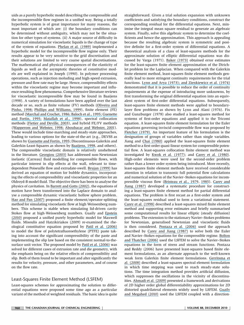
Figure 6 shows the physical domain as well as the grid used forthe solution.

Viscoelastic flow computations were performed with (t =0.15, � = 7.15, U∞ = 0.2, Re = 1.0, We = 0.1, L1 = 1.5, L2 = 1.5).We are simulating a relatively high-Mach number flow comparedto practical values just to show the capabilities of the proposedscheme to capture severe stress gradients. The grid consists of43 × 15 uniformly distributed bi-linear rectangular elements with15 elements in the y-direction, 15 elements on the bump, 13 ele-ments in the entrance section, and 15 for the exit section. Thepressure-density system of equation is used in the current testcase. The boundary conditions at the inlet are:

� = 1, u = 4U∞y(1 − y), v = 0, S = 32We

ReU2

∞(1 − 2y)2, T = 0

At the exit, the pressure is specified as p = 1/� and the shear stressas Q = 4(U∞/Re)(1 − 2y) while the no-slip boundary condition isimposed on the upper and lower boundaries.

Results for We = 0.1 are shown in the following figures.Figure 7 shows the axial velocity isocontours, while Figure 8shows the isocontours of the normal velocity. One easily noticesthe symmetry about x = 0. Figure 9 shows the first principal stress

| VOLUME 88, DECEMBER 2010 | | THE CANADIAN JOURNAL OF CHEMICAL ENGINEERING | 967 |

0

0

0

00

100

100

100

100

200

200

200

300

300

300

400

400 500500

600

600 700800 9001000 130

We=1.0

-100

-100

-100

00

0

0

0100

100

100

100

200

200300

400

400

500600 700

90012001300 140

We=5.0

-50

-50

0

0

0

0

00

0

50

50

50

100100

100

150150 250400

We=20.0

-500

0

0

500

500

10001000 1500

15002000

20002500

30003500

We=0.3

a b

c d

Figure 4. Shear stress isocontours for non-Newtonian flow.

1000

1000

10001000

1000

20002000

2000

3000

3000

3000 4000

4000 50005000 60006000 7000

7000

8000

8000

10000 100000000 12000

We=0.3

00 500

500

500500500

500

500

1000

10001000

1000

2000

2000000 40004000 6000

We=5.0

500

500500

500

1000

10001000

1000

200020002000 25002500 3003000

We=1.0

200

200

200

200

300

300

300 400

400

600600 700

700 900

900

1100 1200

1200140015001700

We=20.0

a

c d

b

Figure 5. First principal stress difference isocontours for non-Newtonian flow.

| 968 | THE CANADIAN JOURNAL OF CHEMICAL ENGINEERING | | VOLUME 88, DECEMBER 2010 |

-1.5 -1 -0.5 00 . 115 .50

1

Figure 6. Geometry and grid.

0.02

0.02

0.04

0.04

0.06

0.06

0.08

0.08

0.1

0.1

0.12

0.12

0.14

0.140.16

0.18

0.18

0.2

0.2

0.2

0.22

0.22

0.24

Figure 7. The axial velocity isocontours (We = 0.1).

-0.02

-0.015

-0.015

-0.01

-0.01-0

.01

-0.0

05

-0.005

-0.0

05

-0.005

00

0

0

0

0.005

0.005 0.005

0.005

0.01

0.01

0.01

0.01

5

0.01

50.02

Figure 8. The normal velocity isocontours (We = 0.1).

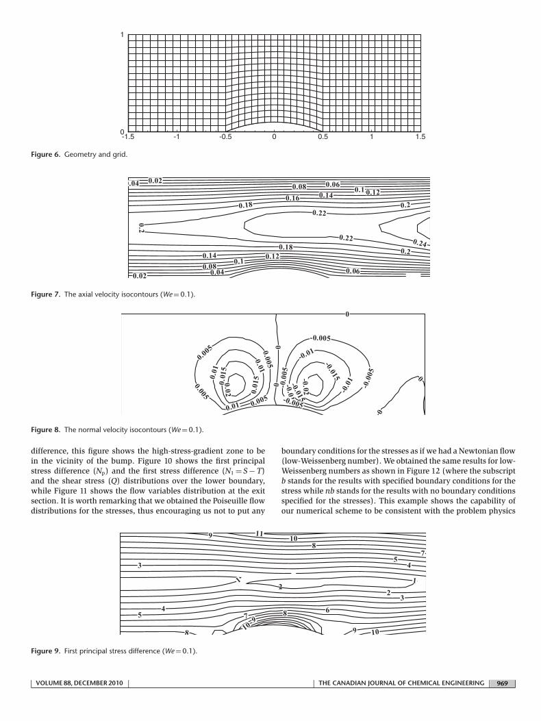
difference, this figure shows the high-stress-gradient zone to bein the vicinity of the bump. Figure 10 shows the first principalstress difference (Np) and the first stress difference (N1 = S − T)and the shear stress (Q) distributions over the lower boundary,while Figure 11 shows the flow variables distribution at the exitsection. It is worth remarking that we obtained the Poiseuille flowdistributions for the stresses, thus encouraging us not to put any

boundary conditions for the stresses as if we had a Newtonian flow(low-Weissenberg number). We obtained the same results for low-Weissenberg numbers as shown in Figure 12 (where the subscriptb stands for the results with specified boundary conditions for thestress while nb stands for the results with no boundary conditionsspecified for the stresses). This example shows the capability ofour numerical scheme to be consistent with the problem physics

1 12

23

3

4

4

5

5

67

7

8

8

8

99

9

1010

1011

Figure 9. First principal stress difference (We = 0.1).

| VOLUME 88, DECEMBER 2010 | | THE CANADIAN JOURNAL OF CHEMICAL ENGINEERING | 969 |

X-1.5 -1 -0.5 0 0.5 11 .5

0

2

4

6

8

10

12

14

Shear stressFirst Normal StressFirst principal stress difference

Figure 10. Stress distribution over the lower boundary (We = 0.1).

unlike the mixed type model proposed by Marchal and Crochet(1987) in which they have to choose the geometry in such a waythat the flow is forced to be fully developed in entry and exit sec-tions which is not consistent with the physics of the problem.The same calculations were carried out for a finer grid (65 × 20)to check for grid convergence. To save space, we show only thestress distribution over the lower boundary in Figure 13, whichassures the scheme convergence.

Another viscoelastic flow computations were performed with(t = 0.1, � = 7.15, U∞ = 0.1, Re = 1.0, L1 = 1.0, L2 = 1.5) and fordifferent Weissenberg numbers. The pressure system of equationis used in the current test case. The grid consists of 40 × 10 uni-formly distributed bi-linear rectangular elements with 10 elementsin the y-direction, 10 elements on the bump, 10 elements in theentrance section, and 20 for the exit section. To show the abil-ity of the proposed scheme to capture higher stress gradients, weincreased the Weissenberg from be 0.01 to 0.7. The solution wasconsidered to reach the steady state solution when the maximum

Y

-4 -2 0 8642 100

0.2

0.4

0.6

0.8

1

Axialv elocityNormal velocityShear stressFirst principal stress difference

Figure 11. Flow variables distribution at the exit section (We = 0.1).

A

A

A

A

A

A

A

A

A

A

A

A

A

A

A

A

B

B

B

B

B

B

B

B

B

B

B

B

B

B

B

B

C

C

C

C

C

C

C

C

C

C

C

C

C

C

C

C

D

D

D

D

D

D

D

D

D

D

D

D

D

D

D

D

E

E

E

E

E

E

E

E

E

E

E

E

E

E

E

E

F

F

F

F

F

F

F

F

F

F

F

F

F

F

F

F

-4 -2 20 40

0.2

0.4

0.6

0.8

1

Axials tressShears tressNormal stressAxials tress (withoutBCs.)Shears tress (withoutBCs.)Normal stress (withoutBCs.)

ABCDEF

Figure 12. Stress distribution at the inlet section (We = 0.1).

error, defined as the Euclidean norm L2(q) =(

nnodes∑i=0

|qi|2)1/2

,

is of order 1E−4 or less for all the variables. We reached thistolerance using about 1,200 for this case. Figure 14 shows thefirst principal stress difference for different Weissenberg numbers,from the figure, one can notice that the maximum nondimen-sional first principal stress difference obtained for We = 0.01 is10.0 compared to 45.0 for We = 0.7. Figure 15 shows the firststress difference N1 for different Weissenberg numbers, it is worthrecalling that N1 should be zero for Newtonian flows (We = 0.),which is consistent with the isocontours of Figure 15 (top). Againthe higher the Weissenberg number, the higher stress gradients.To show the importance of the compressibility, Figure 16 showsthe density isocontours for different Weissenberg numbers. Byinspection of this figure, we have about 20% variation in the liquiddensity for these conditions, which cannot be neglected. Figure 17shows the corresponding pressure isocontours. Finally, Figure 18shows the convergence history for this problem for We = 0.3.

Y

-4 -2 86420 100

0.2

0.4

0.6

0.8

1

Axialv elocityNormal velocityShear stressFirst principal stress difference

Figure 13. Flow variables distributions at the exit (finer grid).

| 970 | THE CANADIAN JOURNAL OF CHEMICAL ENGINEERING | | VOLUME 88, DECEMBER 2010 |

1 2

2

34 5

5

6

6

7

7

88

89

9

10 10

10

11

11

1212

12

13

13

1414

14

1515

16

W e=0.3

12

2

34 55

5

6

6

77

7

88

8

W e=0.01

5

5

10

10

10

15

15

1520

20

25

2530

35

W e=0.7

Figure 14. First principal stress difference for different We.

22

2

4

4

4

6

8

8

8

10

12

12

12

14

14

16

16

18

18

20

20

22

22

24

24

24

26

28

W e=0.7

01

1

2

2

3

3

3

4 4

4

5

5

6

6

78

8

910

10

11

11

12

1212

17

W e=0.3

-1

0

0

0

0.5

0.5

0.5

1

1.5

W e=0.01

Figure 15. First stress difference for different We.

| VOLUME 88, DECEMBER 2010 | | THE CANADIAN JOURNAL OF CHEMICAL ENGINEERING | 971 |

1.01

1.01

1.02

1.02

1.03

1.03

1.04

1 .041.04

1.05

1.051.05

1.06

1.0 61.06

1.071.07

1.07

1.0 8

1.08

1.09

1.09

1.09

1.1

1.1

1.11

1.11

1.12

1.12

1.13

1.13

1.14

1.14

1.15

1.15

1.16

1.16

1.17

1.17

1.17

1.18

1.18

We=0.01

1.01

1.01

1.02

1.0 21.02

1.03

1.03

1.04

1.04

1.04

1.05

1.05

1.06

1.06

1.06

.06

1.07

1.07

1.07

1.08

1.08

1.08

1.09

1.09

1.1

1.1

1.11

1.11

1.12

1.12

1.13

1.13

1.14

1.14

1.15

1.15

1.15

1.15

1.161.16

1.16

1.17

1.17

1.17

1.18

We=0.3

1

1

1.01

1.01

1.01

1.021.02

1.02

1.03

1.03

1.041.04

1.05 1.05

1.051.05

1.06

06

1.061.06

1.07

1.07

1.08

1.08

1.091.09

1.09

1.091.1

1.1

1.11

1.111.11

1.121.12

1.12

1.131.13

1.14

1.14

1.14

1.15

1.15

1.15

1.16

1.16

1.16

1.171.17

1.17

1.17

1.18

1.18

We=0.7

Figure 16. The density isocontours for different We.

0.16

0.1 60.16

0.1 8

0.18

0.2

0.2

0 .220.22

0.24

0.24

0.26

0.26

0.28

0.28

0.3

0.3

0.32

0.32

0.34

0.34

0.360.36

0.38

0.38

0.4

0.4

0.4

0.42

0.42

0.44

0.44

0.46

0.46

W e=0.010.

16

0.160.16

0.18

0.18

0.18

0.20.2

0 .220 .22

0.24

0.24

0.24

0.260.26

0.28

0.28

0.30.3

0.32

0.32

0 34

0.340.34

0.360.36

0.38

0.38

0.38

0.4

0.40.4

0.38

0.42

0.42

0.440.44

0.44

W e=0.3

0.160.16

0.16

0.18

0.18

0.18

0.2

0.2

0.2

0.2

0.22

0.22

0.22

0.240.24

0.24

0 26

0.26

0.26

0.28

0.28

0.3

0.3

0.3

0.32

0.32

0.32

0.34

0.34

0 360.36

0.36

0.38

0.38

0.36

0.40.

4

0.42

0.42

0.42

0.44

0.44

0.44

046W e=0.7

Figure 17. The pressure isocontours for different We.

| 972 | THE CANADIAN JOURNAL OF CHEMICAL ENGINEERING | | VOLUME 88, DECEMBER 2010 |

Iterations

L2R

esid

ual

200 400 600 80010-6

10-5

10-4

10-3

10-2

10-1

Figure 18. Convergence history for We = 0.3.

SUMMARY AND CONCLUSIONA hybrid least-squares finite element/finite difference based tech-nique was used to simulate the flow of viscoelastic fluids. In whichthe finite difference method was used to advance in time whilethe LSFEM was used to treat the spatial part of the system ofequations. For the first time; the theoretical formulation permitsthe governing equations to be cast in the form of a totally hyper-bolic system of first-order PDEs for both the compressible andthe incompressible regimes. Being totally hyperbolic avoids manyproblems exist in the traditional systems of mixed types. The qual-ity of the numerical results indicates the remarkable performanceof the proposed model, as is quite evident from the final resultseven when using a coarse mesh. The robustness of the techniqueallows one to use large time steps (t = 0.15) to reach the steadystate solution in relatively few iterations.

END NOTESWith no loss of generality, we used Poiseuille flow at the inlet to specify

the boundary conditions for the stresses.

REFERENCESAboubacar, M. and M. F. Webster, “A Cell-Vertex Finite

Volume/Element Method on Triangles for Abrupt ContractionViscoelastic Flows,” J. NonNewton. Fluid Mech. 98, 83–106(2001).

Ahmadi, A., K. S. Surana, R. K. M. Romkes and J. N. Reddy,“Higher Order Global Differentiability Local Approximationsfor 2D Distorted Quadrilateral Elements,” Int. J. Comput.Meth. Eng. Sci. Mech. 10, 1–19 (2009).

Baaijens, F. P. T., “Mixed Finite Element Methods for ViscoelasticFlow Analysis a Review,” J. Nonnewton. Fluid Mech. 79,361–385 (1998).

Baker, G., “Simplified Proofs of Error Estimates of the LeastSquares Method for Dirichlet’s Problem,” Math. Comp. 27,229–235 (1973).

Baloch, A., P. Townsend and M. F. Webster, “On the Simulationof Highly Elastic Complex Flows,” J. Nonnewton. FluidMech. 59(2–3), 111–128 (1995).

Barrett, K. E. and A. C. Gotts, “Finite Element Analysis of aCompressible Dynamic Viscoelastic Sphere Using FFT,”Comput. Struct. 80, 1615–1625 (2002).

Boger, D. V. and K. Walter, “Rheological Phenomena in Focus,”Rheology Series 4, Amsterdam; New York: Elsevier,(1993).

Bolton, P. and R. W. Thatcher, “A Least-Squares Finite ElementMethod for the Navier-Stokes Equations,” J. Comput. Phys.213, 174–183 (2006).

Brian, J. and N. Antony, “Remarks Concerning CompressibleViscoelastic Fluid Models,” J. Nonnewton. Fluid Mech. 36,411–417 (1990).

Bristeau, M. O., R. Glowinski, J. Periaux, P. Perrier and O.Pironneau, “On the Numerical Solution of NonlinearProblems in Fluid Dynamics by Least Squares and FiniteElement Methods. I—Least Square Formulations andConjugate Gradient Solution of the Continuous Problems,”Comp. Meth. Appl. Mech. Eng. 17(18), 619–657 (1979).

Bristeau, M. O., O. Pironneau, R. Glowinski, J. Periaux, P.Perrier and G. Poirier, “On the Numerical Solution ofNonlinear Problems in Fluid Dynamics by Least Squares andFinite Element Methods (II). Application to Transonic FlowSimulations,” Comp. Meth. Appl. Mech. Eng. 51, 363–394(1985).

Brown, R. A., R. C. Armstrong, A. N. Beris and P. W. Yeh,“Galerkin Finite Element Analysis of Complex ViscoelasticFlows,” Comput. Meth. Appl. Mech. Eng. 58, 201–226 (1986).

Brujan, E. A., “A First-Order Model for Bubble Dynamics in aCompressible Viscoelastic Liquid,” J. Nonnewton. FluidMech. 84, 83–103 (1999).

Carey, G. F. and B. N. Jiang, “Least-Squares Finite ElementMethod and Preconditioned Conjugate Gradient Solution,”Int. J. Numer. Meth. Eng. 24, 1283–1296 (1987).

Carey, G. F., A. I. Pehlivanov, Y. Shen, A. Bose and K. C. Wang,“Least-Squares Finite Elements for Fluid Flow and Transport,”Int. J. Numer. Meth. Fluids 27, 97–107 (1998).

Carey, G. F., Y. K. Cheung and S. L. Lau, “Mixed OperatorProblems Using Least Squares Finite Element Collocation,”Comp. Meth. Appl. Mech. Eng. 22, 121–130 (1980).

Courant, R. and D. Hilbert, “Methods of Mathematical Physics,”Vol. 2. Wiley, New York (1962).

Fietier, N. and M. O. Deville, “Time-Dependent Algorithms forthe Simulation of Viscoelastic Flows with Spectral ElementMethods: Applications and Stability,” J. Comp. Phys. 186,93–121 (2003).

Fix, G. J. and M. D. Gunzburger, “On Least SquaresApproximations to Indefinite Problems of the Mixed Type,”Int. J. Numer. Meth. Eng. 12, 453–469 (1978).

Fletcher, C. A. J., “A Primitive Variable Finite ElementFormulation for Inviscid Compressible Flow,” J. Comp. Phys.33, 301–312 (1979).

Georgiou, G. C., “The Time-Dependent Compressible Poiseuilleand Extrudate-Swell Flows of a Carreau Fluid With Slip at theWall,” J. Nonnewton. Fluid Mech. 109, 93–114 (2003).

Gerritsma, M., R. V. Bas, B. Maerschalck, B. Koren and H.Deconinck, “Least-Squares Spectral Element Method Appliedto the Euler Equations,” Int. J. Numer. Meth. Fluids 57,1371–1395 (2008).

Godlewski, E. and P. A. Raviart, “Numerical approximation ofthe Hyperbolic Systems of conservation Laws,” Appl. math.Sci. V.118. Springer-Verlag, New York (1996), Chapter VI.

Grillet, A. M., B. Yang, B. Khomami and E. S. G. Shaqfeh,“Modeling of Viscoelastic Lid Driven Cavity Flow Using Finite

| VOLUME 88, DECEMBER 2010 | | THE CANADIAN JOURNAL OF CHEMICAL ENGINEERING | 973 |

Element Simulations,” J. Nonnewton. Fluid Mech. 88, 99–131(1999).

Guaily, A. and M. Epstein, “A Unified Hyperbolic Model forViscoelastic Liquids,” Mech. Res. Comm. 37, 158–163 (2010).

Guaily, A. and M. Megahed, “An Adaptive Finite ElementMethod for Planar and Axisymmetric Compressible Flows,”Finite Elem. Anal. Des. 46, 613–624 (2010)dx.doi.org/10.1016/j.finel.2010.03.001.

Guenette, R. and M. Fortin, “A New Mixed Finite ElementMethod for Computing Viscoelastic Flows,” J. Nonnewton.Fluid Mech. 60, 27–52 (1995).

Hao, J. and T. Pan, “Simulation for high Weissenberg number:Viscoelastic flow by a finite element method,” Appl. Math.Lett. 20, 988–993 (2007).

Hoffmann, K. A. and S. T. Chiang, “Computational FluidDynamics for Engineers,” Engineering Education system,Wichita, Kansas, USA, (1993).

Jiang, B. N. and J. Chai, “Least Squares Finite Element Analysisof Steady High Subsonic Plane Potential Flows,” Acta Mech.Sinica 90–93 (1980).

Joseph, D., “Fluid Dynamics of Viscoelastic Liquids,”Springer-Verlag, Appl. Math. Sci, V. 84, New York (1990),Chapter V–VI.

Keshtiban, I. J., F. Belblidia and M. F. Webster, “Computation ofIncompressible and Weakly-Compressible ViscoelasticLiquids Flow: Finite Element/Volume Schemes,” J.Nonnewton. Fluid Mech. 126, 123–143 (2005).

Keunings, R., “Progress and Challenges in ComputationalRheology,” Rheol. Acta 29, 556–570 (1990).

Kwok, W. L., Y. K. Cheung and C. Delcourt, “Application ofLeast Squares Collocation Technique in Finite Element andFinite Strip Formulation,” Int. J. Numer. Meth. Eng. 11,1391–1404 (1977).

Lynn, P. P. and S. K. Arya, “Use of the Least Squares Criterion inthe Finite Element Formulation,” Int. J. Numer. Meth. Eng. 6,75–88 (1973).

Lynn, P. P. and K. Alani, “Efficient Least Squares Finite Elementsfor Two-Dimensional Laminar Boundary Layer Analysis,” Int.J. Numer. Meth. Eng. 10, 809–825 (1976).

Mackley, M. R. and P. Spittler, “Viscoelastic Characterisation ofPolyethylene Using a Multipass Rheometer,” Rheol. Acta 35,202–209 (1996).

Marchal, J. M. and M. J. Crochet, “Hermitian Finite Elements forCalculating Viscoelastic Flow,” J. Nonnewton. Fluid Mech.20, 187–207 (1986).

Marchal, J. M. and M. J. Crochet, “A New Mixed Finite Elementfor Calculating Viscoelastic Flow,” J. Nonnewton. FluidMech. 26, 77–114 (1987).

Matallah, H., P. Townsend and M. F. Webster, “Recovery andStress Splitting Schemes for Viscoelastic Flows,” J.Nonnewton. Fluid Mech. 75, 139–166 (1998).

Misoulis, E. and S. G. Hatzikiriakos, “Steady Flow Simulationsof Compressible PTFE Paste Extrusion Under Severe WallSlip,” J. Nonnewton. Fluid Mech. 157(1–2), 26–33 (2009).

Moussaoui, F., “A Unified Approach for Inviscid Compressibleand Nearly Incompressible Flow by Least-Squares FiniteElement Method,” Appl. Numer. Math. 44, 183–199 (2003).

Oliveira, P. J. and F. T. Pinho, “Pinto G. A. Numerical Simulationof Nonlinear Elastic Flows With a General Collocated FiniteVolume Method,” J. Nonnewton. Fluid Mech. 79, 1–43(1998).

Pakdel, P., S. Spiegelberg and G. McKinley, “Cavity Flows ofElastic Liquids Two-Dimensional Flows,” Phys. Fluids 9(11),3123–3140 (1997).

Patil, P. D., J. J. Feng and S. G. Hatzikiriakos, “ConstitutiveModelling and Flow Simulation of PolytetrafluoroethylenePaste Extrusion,” J. Nonnewton. Fluid Mech. 139, 44–53(2006).

Phelan, F. R., Jr., M. F. Malone and H. H. Winter, “A PurelyHyperbolic Model for Unsteady Viscoelastic Flow,” J.Nonnewton. Fluid Mech. 32, 197–224 (1989).

Phillips, T. N. and A. J. Williams, “Viscoelastic Flow through aPlanar Contraction Using a Semi-Lagrangian Finite VolumeMethod,” J. Non-newtonian Fluid Mech. 87, 215–246 (1999).

Pontaza, J. P., X. Diao, J. N. Reddy and K. S. Surana,“Least-Squares Finite Element Models of Two-DimensionalCompressible Flows,” Finit. Elem. Anal. Des. 40, 629–644(2004).

Pontaza, J. P. and J. N. Reddy, “Least-Squares Finite ElementFormulations for Viscous Incompressible and CompressibleFluid Flows,” Comput. Meth. Appl. Mech. Eng. 195,2454–2494 (2006).

Renardy, M., “Mathematical Analysis of viscoelastic Flows,”CBMS-NSF regional Conference Series in Appl. Math., No. 73(2000).

Song, J. H. and J. Y. Yoo, “Numerical Simulation of ViscoelasticFlow Through a Sudden Contraction Using a Type DependentDifference Method,” J. Nonnewton. Fluid Mech. 24, 221–243(1987).

Thompson, P. A., “Compressible Fluid Dynamics,” McGraw-Hill,New York (1972).

Varga, R. S., “Functional analysis and approximation theory innumerical analysis,” Regional Conference Series in Appl.Math., No. 3, SIAM, Philadelphia (1971).

Wapperom, P. and M. F. Webster, “A Second-Order Hybrid FiniteElement/Volume Method for Viscoelastic Flows,” J.Nonnewton. Fluid Mech. 79, 405–431 (1998).

Zienkiewicz, O. C., D. R. J. Owen and K. N. Lee, “Least SquaresFinite Element for Elasto-Static Problems-Use Of ReducedIntegration,” Int. J. Numer. Meth. Eng. 8, 341–358 (1974).

Manuscript received October 24, 2009; revised manuscriptreceived January 4, 2010; accepted for publication January 5,2010.

| 974 | THE CANADIAN JOURNAL OF CHEMICAL ENGINEERING | | VOLUME 88, DECEMBER 2010 |