Physicsof the Earth and PlanetaryInteriors, 59 (1990) 195—207 195ElsevierSciencePublishersBy., Amsterdam— Printed in The Netherlands

ConMan:vectorizinga finite elementcodefor incompressibletwo-dimensionalconvectionin theEarth’smantle

ScottD. King, Arthur RaefskyandBradford H. Hager*252-21 SeismologicalLaboratory, California Instituteof Technology,Pasadena,CA 91125(U. S.A.)

(ReceivedMay 23, 1989~acceptedAugust 2. 1989)

King, S.D., Raefsky, A. and Hager, B.H., 1990. ConMan: vectorizing a finite element code for incompressibletwo-dimensionalconvectionin theEarth’s mantle.Phys.Earth Planet. Inter., 59: 195—207.

We discuss somesimple conceptsfor vectorizingscientific codes,then apply theseconceptsto ConMan, a finiteelementcodefor simulationsof mantleconvection.We demonstratethat largespeed-ups,closeto the theoreticallimitof themachine,arepossiblefor entirecodes,notjust speciallyconstructedroutines.Although our specificcodeusesthefinite elementmethod, the vectorizingconceptsdiscussedarewidely applicable.

1 Introduction speedsof 50—200 MFLOPS are attainable formanycodes(DongarraandEisenstat,1984).

Many large computational projects in geo- It is often mistakenlybelievedthat for a gen-physics are now being run on vector supercom- eralcode, specialtricks are neededto obtain vec-puterssuchas the CrayX-MP, yet aftermorethan tor performance.However, although vectorizinga decadesince the introduction of the Cray-i, compilersare becomingmoresophisticated,a codemost geophysicistssimply compile their original that does not have data structuressuitable forcodes,makinguseof thefast clock, without taking vector operationswill not perform well on a vec-full advantageof the vectorhardwareor achieving tor computer. We show that ConMan (Convec-anywherenearsupercomputerspeed. tion, Mantle), a finite elementcode for two-di-

To illustrate, let us considerthe Cray X-MP mensional, incompressible, thermal convection,with a 9.5 ns clock. It takessix clock cycles to which usesthe simpleconceptswepresentandnocomputea floating point addition (7 clock cycles special tricks, runs up to 65 MFLOPS for thefor a floating pointmultiplication).This leadsto a entirecode on a Cray X-MP (including i/o andtheoreticalpeakscalarrateof 9.5 MFLOPS (mil- subroutineoverhead).lion floating point operationsper second).This is Understandingvectorization is becomingevenabout 25 times faster than a Sun 3/260 work- moreimportantbecauseof the recentintroductionstation (Dongarra, 1987). The theoretical maxi- of high-performancepipelined workstations.Themum for vector code on the Cray X-MP is 210 pipeline architectureis similar to a vectorregister.MFLOPS, over 20 times faster than the scalar and many of the sameconceptsfrom vector pro-codeand500 times fasterthan the Sun. In reality, gramming apply to obtaining the maximum per-the theoreticalspeedsare neverreached;however. formancefrom a pipelined computer.

In the next sectionwe discussthe basiccon-ceptsof vectorization, including the conceptsof

Presentaddress:Departmentof Earth. AtmosphencandPlanetary Sciences,MassachusettsInstitute of Technology, chaining and unrolling. Although we illustrateCambridge,MA 02139, U.S.A. vectorization with the finite elementcode Con-

0031-9201/90/$03.50 © 1990 ElsevierSciencePublishersB.V.

196 S.D. KING ETAL.

Man, theconceptswepresentare general.Because In FORTRAN (or C), vectorizationis imple-we usea generalformulationof the finite element mented in the innermost do ioop. Within themethod,it would be especiallyeasyto generalize innermost do loop there must be no subroutineConManto solve otherequationsor othergeome- calls or i/o statementsbecausethese inhibit vec-tries. We then review the equations for incom- torization of the loop (as compilersbecomemorepressiblethermal convectionand briefly describe sophisticatedthis statementwill no longerbe true).the techniquesused to solve them using the finite Because it is the innermost ioops which areelementmethod.Wepresentbenchmarksandtim- vectorized, theseshould be in generalthe longestings for several computersand we include an loops(the loop whose index runsover the largestexamplesubroutinefrom ConMan in the Appen- range)and they shouldnot have any dependentdix for illustration. statements,wherea newly computedresultis used

in the right-hand side of the same assignment

during a futurepassof the loop. A simpleexample

2. Vectorization isDO 10 I = 1, N

Considerthe simpleaddition A(I) = A(I) + A(I — 1)10 CONTINUE

c,=a1+b1 fori=l,2,...,Ncomp (1)

This causesa problem becausethe result A(I) ison a genericscalararchitecture.A new result c

1 is dependenton the previousvalueA(I — 1). In realavailable after N~dd,the total number of cycles codesthis problem is often hiddenin a statementneededfor oneaddition(on the CrayX-MP this is which usesindirectreferencing,as in the followingsix cycles).On a vector computer,after the sum- finite elementexample.This loop assemblesthemandsa1 and b1 move to the secondstep in the elementcontribution for the IELth elementintoaddition unit, the next summandsa2 and b2 can the global equations,LM(IEL, 1 — 4), for the fourenter the addition unit. The first result c1 is local nodes.availableafter Nadd cycles. Then, unlike a scalaroperation,after (Nadd+ 1) cycles c2 is available, DO 10 IEL = 1, NELand so on. After the start-upcost, a new result is A(LM(IEL, 1)) = A(LM(IEL, 1)) +

availableevery cycle. On the scalarmachine, the EL_LOCAL(IEL, 1)secondresult would not be available until after A(LM(IEL, 2)) = A(LM(IEL, 2)) +2Nadd cycles. For long vectors (i.e, Neomp large), EL_LOCAL(IEL, 2)the vector time is asymptotically reduced by A(LM(IEL, 3)) = A(LM(IEL, 3)) +I /Nadd relativeto scalarprocessing. EL ... LOCAL(IEL, 3)

In addition to increasing speedby vectoriza- A(LM(IEL, 4)) = A(LM(IEL, 4)) +tion, a vectorcomputercanchain operations.The EL_LOCAL(IEL, 4)classic example is the linear algebra operation 10 CONTINUESAXPY (SingleprecisionA timesX Plus Y) where LM(IEL, 1) is an integerarray of indices

= a~x1 +yi for i = 1, 2 Ncomp (2) with IEL the elementnumberandLM(IEL, 1) the

global equationnumber of the first node of the

Chainingallows the result from a x~to be added IELth element.Here, the compilercannotassumeto Yi while a x2 is being computed,and so on. that LM(IEL, 1) is not equal to LM(IEL — J, 1)As the CrayX-MP haseightvector registers,up to for some arbitraryJ.sevenvectorscould appearon the right-handside Many of the operationsin a finite elementcodeand be chained (one register is needed for the (or finite differencecode) havethis kind of struc-result vector c). In this way, an addition and a ture and the LM arrays usually have the unfor-multiplication can be computedeachclock cycle, tunateproperty that LM(IEL, 1) is not a uniqueleadingto the 210 MFLOP theoreticalrate. value (see Fig. 1 for an example).This is not a

INCOMPRESSIBLE TWO-DIMENSIONAL CONVECTION IN THE EARTH’S MANTLE 197

3 6 9

LM(Element number,loeal node number)

ED EDLM(4,1) = 2

2 N B LM(4,2)=5

LM(4,3) = 6

/ LM(4,4) = 3

ED ED1 4 7

Fig. 1. The four bilinear quadrilateralelements(1—4) all contributeto theglobal nodalequationatnodeN, which theyall share.Theelementnumbersarecircledand theglobal nodenumbersare not. TheLM array for element4 is listed at theright.

serious problem becausewe can rearrangethe elements in each group, which are independentelements(by shuffling the LM array) such that andwill safelyvectorize.thereis a small numberof groupsof elementsthat The final point illustrated here is that as wedo not share global nodes(Fig. 2). We can then want our innermostloop to be the loop over theloop over the total numberof groupsandover the elements, we do not want small loops over the

I I local node numbers(i.e., 1= 1, 4). We unroll theinnermostioop by writing out the expressionfour

__________ __________________________________ times, explicitly putting in the valueof the local

- nodein each line (seeAppendix for an example)~ II

- ~ 3 Equations and implementation

We now turn to the specific exampleprogram,ConMan, and discussin brief the equationsand

III W III themethod usedto implementtheir solutionson a

vectorcomputer.We give only a brief descriptionof the methodandrefer to otherwork for conver-- ii: genceproofs stability proofsanddetailedanalyses

I II U The equations for tncompressibleconvection- - -- (in dimensionless form) are the equations of

momentum

Fig. 2. The ‘four-color’ ordering schemeusedin ConMan. It V = — Vp + Ra 8~ (3)should be noted that the shadedelements(group I) do not continuitysharenodeswith anyothergroup I element.This group canbeoperatedon safelywith a vectoroperation. V u = 0 (4)

198 S.D. KING ET AL.

andenergy where F is theboundaryof the domain ~2.Fg and

2 Fh are the partsof the boundarywherevelocities= U~V&+ V 0 (5) andtractionsare specified.‘1 is the empty set.

Find u: —s R’1 and p: ~2— R

where u is the dimensionlessvelocity, 0 is thedimensionlesstemperature,p is the dimensionless t

11,1 +f, = 0 on (7)pressure,k is the unit vectorin the verticaldirec- u,, = 0 on (8)tion and t is the dimensionlesstime. In this form u = g on F (9)all the materialpropertiesare combinedinto one — h 10dimensionlessparameter, the Rayleigh number, t,1n1 — ongiven by with the constitutive equation for a Newtonian

A .,3 fluidgcsi.iTa / .,

Ra = ~6 ~ = —p6,J+ 2p.u~

11~ (11)

whereg is the accelerationdue to gravity, a is the where t,1 denotesthe Cauchystress tensor, p iscoefficient of thermal expansion, LXT is the tem- the pressure,~ is the Kroneckerdelta and U(, J)

peraturedrop acrossthe box, d is the depthof the = (u,,1 + u11)/2.

box, K is the thermal diffusivity, and p. is the In the penaltyformulation, (11) is replacedbydynamic viscosity. t~ = + 2p.u~> (12)

The momentumand energy equationsform a hsimple coupled systemof differential equations. w ereWe treat the incompressibilityequationas a con- ~( = — ~ (13)straint on the momentumequationand enforce and X is the penalty parameter(repeatedsub-incompressibilityin the solution of the momentum scriptsmeanssummationover all indices).equationusinga penaltyformulation.As the tem- This formulation automaticallyenforcesincom-peraturesprovide the buoyancy(body force) to pressibility (8) as the solution to (7), (12) and(13)drive the momentumequationand as thereis no convergesto the incompressibleStokesequationtime dependencein the momentumequation,the as A approachesinfinity (Temam,1977).Also, thealgorithm to solve the systemis a simple one: unknown pressurefield is eliminated.This is use-given an initial temperaturefield, calculate the ful not only becausethe amountof computationalresultingvelocity field. Usethe velocitiesto advect work is decreasedbecauseno pressureequationisthe temperaturesfor the next time step and solve solved,but also becauseit eliminatesthe needtofor a new temperaturefield. If the time stepping createartificial boundaryconditionsfor the pres-for the temperatureequationis stable, then this sure equation.There are no pressureboundarymethod is stableandconvergesas I~t—~ 0. conditionsin the formal specificationof the prob-

lem. By examiningthe equationwe see that the3.1. Momentumequation role of pressureis to balancethe system,sophysi-

cally the penaltyformulation makessense.The momentumequation is solved using the The equationis castin the weak form and the

penaltymethod to enforceincompressibility.The Galerkinformulation (i.e, the weighting functionsformal statementof the problemis as follows: are the sameas the basis functions) is used toGiven: solve the weak form of the equation.

R’~ body force vector Let

g: Fg~5R~imposedvelocityvector v= fwEH1Iw=oon Fg} (14)

h: F~—~ R” imposedtractionvector where V is the set of all weighting functions w

F UFh = F which vanish on the boundary.Similarly Vh is asubsetof V parameterizedby h, the meshparame-

FSflFh = ter. Let gh denotean approximationof g which

INCOMPRESSIBLE TWO-DIMENSIONAL CONVECTION IN THE EARTH~SMANTLE 199

= 1 2 3 4 j = ~ = ~NAuIA (16)1 2 4 7 11 16 22 29 / \ /

1 UAUI,XA) ~173 5 8 12 17 23 30

-— ~ i~ii~~T where NA is the shapefunction for nodeA for the

1, 10 14 19 25 32 2 element.[Kj = f~i7 26 33 Theelementstiffnessmatrix (Fig. 3) is madeup

— 21 2734 of the two terms from the left-hand side of the28 35 integral equation.The integration is done using

36 2 X 2 Gaussquadrature,which is exact when the

elementsare rectangularand bilinear shapefunc-[1K]’ = [K]~e + [JK]~’ tions are used. The A term is under-integrated

(one point rule) to keepthe large penalty valuefrom effectively locking the element(Malkus and

2N~(i)N~(i)+ N~(i)N~(i) N~(i)N~(i) Hughes,1978). Theright-handside is madeup of

[t] = u threeknown parts,the body force term (ft), theN~(i)N~(J) N~(i)N~(i)+ 2N~(i)N~(i) applied tractions (h

1) and the applied velocities(g1). The momentumequation is equivalent to anincompressibleelastic problem, and the resulting

N~,(i)N~(i) N~(i)N~(j) stiffness matrix will always be positive definite= X (Hughes,1987, pp. 84—89). This allows us to as-

N~(j)N~(i) N~(I)N~(J) sembleonly the uppertriangularpart of the stiff-

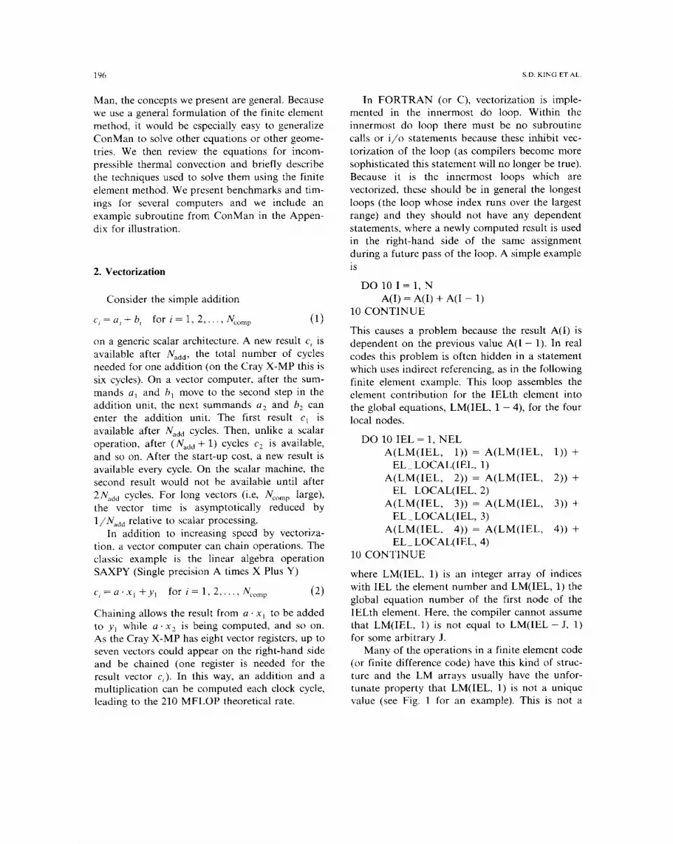
Fig. 3. (a) The location and numberingof the 8 x8 element nessmatrix andsavebothstorageand operationsstiffnessmatrix for the velocity equationusedin ConMan. It using Choleskyfactorization. More details of theshouldbenotedthat thematrixis madeup of 16 2 x2 matrices method anda formal error analysisweregiven bywith i~j indicesasshown.The i and I referto thelocal node Hugheset al. (1979).numberingof theelementand canbe thought of as the effectof node i as felt at node j. (b) The 8 x8 element stiffness 3.2. Energyequationmatrix is madeup of two terms: a viscositycontribution [K]~,and thepenaltycontribution [K ]~.(c) The 2 x2 submatrix for . . .

theviscouscontribution to the elementstiffnessmatrix. N (i) The energyequation is an advection—diffusionis thex derivativeof theshapefunction evaluatedatnodei (i, equation.The formal statementisj hererefer to the location of the 2 x2 matrix in the 8 x 8 Find T: ~ —‘ R suchthatelement stiffness matrix). (d) The 2 x2 submatrix for thepenaltycontribution to the elementstiffnessmatrix (i, J here T+ u1T1= KT,~ + H on (18)refer to the location of the 2x2 matrix in the 8x8 element T= b on F (19)stiffnessmatrix). b

T~n~=q on Fq (20)

where T is the temperature,u, is the velocity, ic is

the thermaldiffusivity and H is the internal heatsource.The weak form of (18) is given by

convergesto g as h —s 0. Find uh = + gh wh E f (w + p)f d~= — f (w + p)(u1T~)d~2V’~,such that for all w

5 E Vh 13 17

J(xw~ji~,+ 2ftw~1~i3~1)d~ _icfw1Te d~+ J wT1n1 dFq

= ff~d~+ J h,w~d~ (21)12 where I’ is the time derivativeof temperature,T,

— I (Xg’~ i~”1~+ 2p.gh .w—h ) d~ (15) is the gradient of temperature, w is the standard

-‘1_i ~ “ “~ “~ weighting function and (w + p) is the

200 S.D. KING ETAL.

Petrov—Galerkinweighting function with, p, the plemented in matrix form. The added cost ofdiscontinuousstreamlineupwind part of the Pet- calculating the Petrov—Galerkinweighting func-rov—Galerkinweightingfunction given by tions is much less than the cost of usinga refined

— — - w1 grid with the Galerkin method. The Galerkin

P — ~u VT—ku~H u 2 (22) method requires a finer grid than the

Petrov—Galerkinmethod to achieve stable solu-The energy equation is solved using . .

tions (Travis et al., in preparation).Petrov—Galerkinweighting functionson the inter-nal heatsourceand advectivetermsto correctfor 3.2.1. Time steppingthe under-diffusion and remove the oscillations Time steppingin the energy equationis donewhich would result from the standardGalerkin using an explicit predictor—correctoralgorithm.method for an advection-dommatedproblem The form of the predictor—correctoralgorithmis(Hughesand Brooks, 1979). The Petrov—Galerkin PredictSfunction canbe thoughtof asa standardGalerkin

(0)... / \~methodin which we counterbalancethe numerical ,~ — ,~ + ti, —

underdiffusionby adding an artificial diffusivity ~° = 0 (27

oftheform fl±I

~ (23) Solve:

with M i~2~= R~. (28)

(24) R~1=-[1~i+u•(7~21)~](w+p)

= 1 — ~ (25) + (boundaryconditionterms) (29)

where h~and hn are the element lengthsand u1 Correct:and un are the velocities in the local element U = J~I + t~stai~1 (30)

coordinate system(~system) evaluatedat the .11+1) — + 31elementcenter.This form of discretizationhas no n + I — n+ I n + I

crosswinddiffusion because(23) acts only in the where i is the iterationnumber(for the corrector),directionof theflow (i.e., it follows the streamline), n is the time-stepnumber,T is the temperature,Thence the name Streamline Upwind Petrov— is the derivativeof temperaturewith time, LS~TisGalerkin (SUPG). This makes it a better ap- the correction to the temperaturederivative forproximation than straight upwinding, and it has the iteration, M * is the lumped mass matrix,been demonstratedto be more accurate than R~1is theresidualterm, .~t is the time step andGalerkin or straight upwinding in advection- a is a convergenceparameter.It shouldbe noteddominatedproblems(Hughesand Brooks, 1979; that in the explicit formulation M * is diagonal.Brooks,1981).It hasrecentlybeenshownthat the The time stepis dynamicallychosen,andcorre-SUPGmethod is oneof a broaderclassof meth- spondsto the Courant time step (the largeststepods for advection—diffusionequationsreferredto thatcanbe takenexplicitly andmaintainstability).asGalerkin/least-squaresmethods(Hugheset al., With the appropriatechoice of variables, a = 0.51988). and two iterations, the method is second-order

The resultingmatrix equationis not symmetric, accurate(Hughes,1987,pp. 562—566).but as the energyequationonly hasonedegreeoffreedomper node, whereasthe momentumequa-tion has two or three, the storagefor the energy 4. Numerical benchmarks

equation is small compared with that for themomentumequation.As we use an explicit time- Two examplesare given,basedon benchmarkssteppingmethod,the energy equationis not im- for two-dimensional Cartesianconvectioncodes

INCOMPRESSIBLE TWO-DIMENSIONAL CONVECTION IN THE EARTH’S MANTLE 201

Table I Table2The parametersusedin thetwo benchmarks Executionspeedsnormalizedto the Cray X-MP scalarexecu-

tion speed for the two benchmark problems(CVBM andParameters Benchmark TDBM) on variouscomputers

CVBM TDBMComputer Benchmark

Rayleighnumber 77927 100000 CVBM TDBMTime steps 5000 1000 _____________________________________________________Tempdepviscosity no yes CrayY-MP V 31.18 26.07Velocity b.c. fs fs CrayX-MP V 18.73 15.29Tempb.c.—top T= 0 T= 0 Cray 2 V 15.92 10.62Tempb.c.—bottom T=1 T=1 ConvexC210V 4.27 3.10

ConvexC120V 1.40 1.42Tempdepviscosity meansthe global matrix hadto be factored CrayX-MP S 1.00 1.00at every step.fs meansfree slip boundaryconditionappliedat Sun4-330 0.42 0.79theboundaries(flow allowedalongthesidewalls aswell astop ConvexC1205 0.31 0.42and bottom). TDBM was not run to steady state,but for a _____________________________________________________fixed numberof time stepsfor timing purposes Where available, both scalar(S) and vector (V) speeds are

shown.The speed-up(the ratio of scalar to vector times) isgreateron theCrays thanon the Convexbecausetheslower

given by Traviset al. (in preparation).Theparam- memoryaccesson theConvexlimits vectorperformance

eters for thesebenchmarksare given in Table 1.Thereare two purposesfor thesebenchmarks:(1)to verify the codeagainststandardexistingcodes; trix is factoredat every time step.This allows usand (2) to demonstratethe speedof the vector to observethe differencebetweenthe speed-upincode on representative problems. Benchmark the finite element forms and assembliesand theCVBM has a constantviscosity, and the velocity matrix factorization and back-substitution.stiffness matrix is factored only once, whereas Vectorizing sparse matrix solvers is an area ofTDBM (not from Travis et al.) has temperature- activeresearch(e.g., Ashcraft et al., 1987; Lucas,dependentviscosity andthe velocity stiffnessma- 1988), and our implementationhas used a stan-

Table3Executiontimes (in seconds)for individual routines for benchmarksCVBM and TDBM in scalarand vectormode on variouscomputers

Subroutine ConvexC120 CrayX-MP CrayY-MP Cray2

Scalar Vector Scalar Vector Scalar Vector Scalar Vector

Times(s) for subroutinesfrom CVBMFactor 10.4 3.6 4.8 0.3 — 0.2 — 0.5Backsolve 3132.2 830.2 1341.5 80.0 — 52.8 — 100.1fvStf 1.6 0.4 0.6 0.1 — 0.0 — 0.1fvRes 531.0 92.9 154.4 6.6 — 3.8 9.5f.tRes 5272.3 948.7 1212.4 50.9 — 28.2 — 53.8Total 9383.2 2021.2 2869.3 153.2 — 92.0 -. 180.2

Times(s)for subroutinesfrom TDBMFactor 10883.4 3564.9 4870.0 297.1 — 199.4 — 507.7Backsolve 646.9 167.3 270.2 16.4 — 10.6 — 20.0f...vStf 1690.0 417.1 649.5 71.3 — 15.9 — 30.0fvRes 112.9 19.5 30.6 1.4 — 0.8 — 1.8ftRes 1088.5 188.0 242.4 9.8 — 5.5 — 10.6Total 14513.8 4383.2 6094.7 398.6 — 233.7 — 573.4

The assemblingroutines(f_vStf, fvRes, LtRes) showbettervectorperformancethando the factorandback-substitutionroutines.The performanceof thefactorizationandback-substitutionimprovesas thebandwidthof the matrix approachesthevectorregisterlength

202 S.D. KING ET AL.

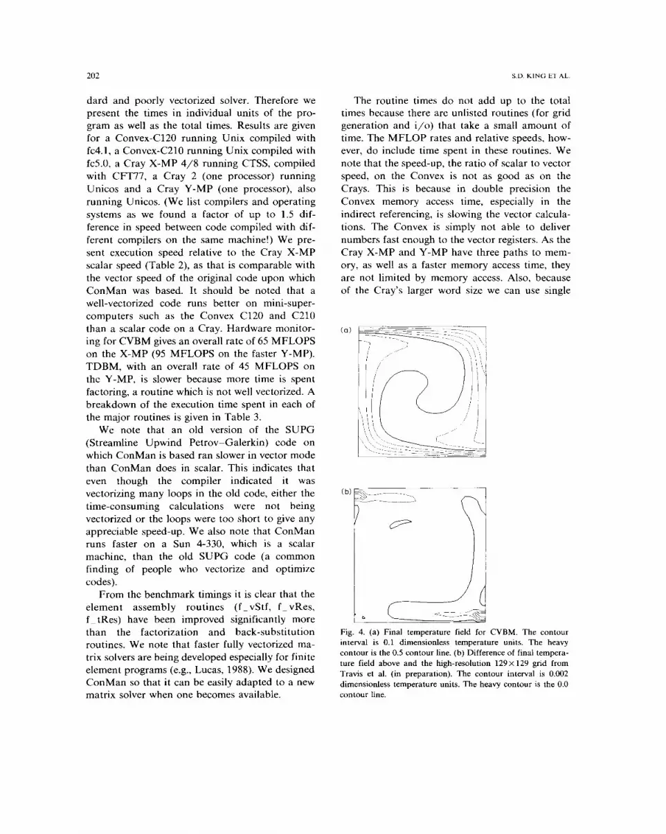
dard and poorly vectorized solver. Thereforewe The routine times do not add up to the totalpresentthe times in individual units of the pro- timesbecausethereare unlisted routines(for gridgram as well as the total times. Resultsare given generationand i/o) that take a small amount offor a Convex-C120running Unix compiled with time. The MFLOP ratesandrelativespeeds,how-fc4.1, a Convex-C210running Unix compiledwith ever, do include time spent in theseroutines.Wefc5.0, a Cray X-MP 4/8 running CTSS,compiled notethat the speed-up,the ratio of scalarto vectorwith CFT77, a Cray 2 (one processor)running speed,on the Convex is not as good as on theUnicos and a Cray Y-MP (one processor),also Crays. This is becausein double precision therunning Unicos. (We list compilersand operating Convex memory access time, especiallyin thesystemsas we found a factor of up to 1.5 dif- indirect referencing,is slowing the vectorcalcula-ferencein speedbetweencodecompiledwith dif- tions. The Convex is simply not able to deliverferent compilerson the samemachine!)We pre- numbersfast enoughto the vectorregisters.As thesent executionspeedrelative to the Cray X-MP Cray X-MP and Y-MP havethreepathsto mem-scalarspeed(Table 2), as that is comparablewith ory, as well as a fastermemory accesstime, theythe vector speedof the original codeupon which are not limited by memory access.Also, becauseConMan was based. It should be noted that a of the Cray’s larger word size we can use singlewell-vectorized code runs better on mini-super-computerssuch as the Convex C120 and C210than a scalarcodeon a Cray. Hardwaremonitor- (~) t~~=~-.~--- —~

ing for CVBM givesan overall rateof 65 MFLOPS -.~

on the X-MP (95 MFLOPSon the faster Y-MP). I1~ ~

TDBM, with an overall rate of 45 MFLOPS on / ‘I

the Y-MP, is slower becausemore time is spent /factoring,a routine which is notwell vectorized.A ( I!

breakdownof the executiontime spentin eachofthe major routinesis givenin Table3.

We note that an old version of the SUPG(Streamline Upwind Petrov—Galerktn) code on - I

which ConMan is basedranslowerin vectormodethan ConMan does in scalar.This indicatesthateven though the compiler indicated it wasvectorizingmany loopsin the old code, eitherthe (b)

time-consuming calculations were not beingvectorizedor the loopsweretoo short to give anyappreciablespeed-up.We also note that ConManruns faster on a Sun 4-330, which is a scalarmachine, than the old SUPG code (a commonfinding of people who vectorize and optimizecodes).

From the benchmarktimings it is clear that theelement assembly routines (fvStf, f_vRes,f_tRes) have been improved significantly more ±.~.

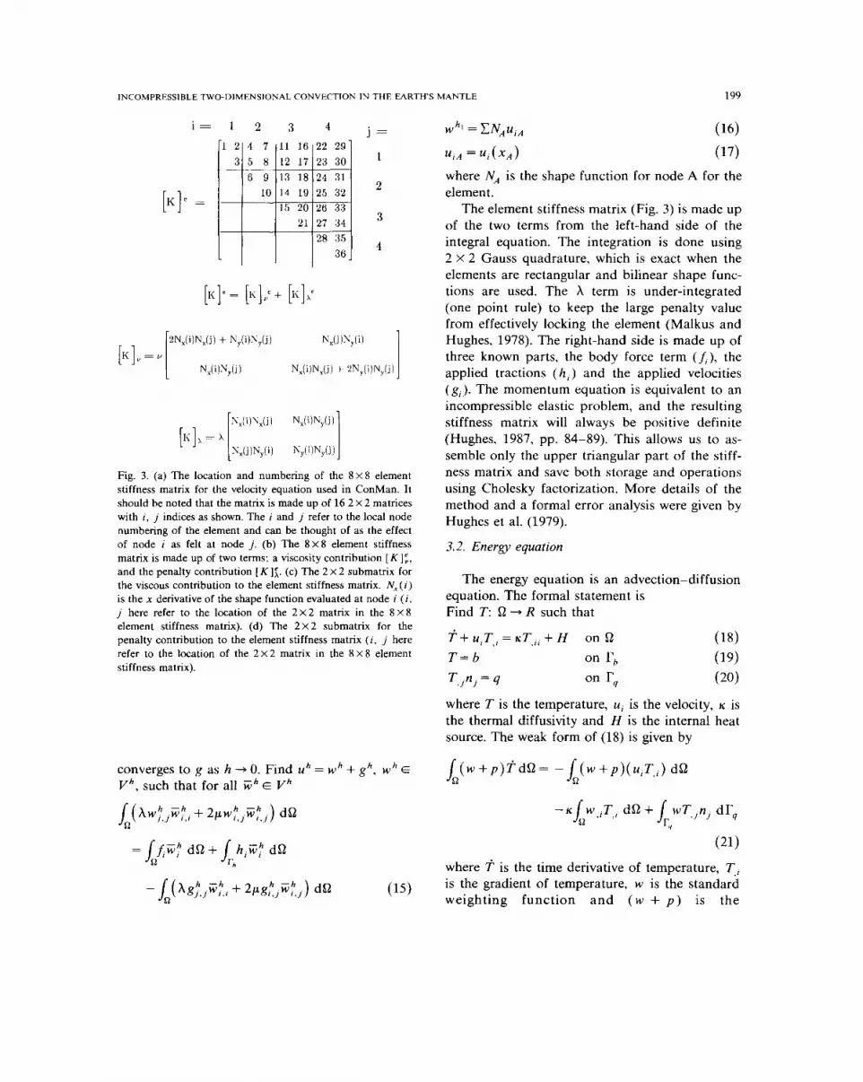
than the factorization and back-substitution Fig. 4. (a) Final temperaturefield for CVBM. The contour

routines.We note that faster fully vectorizedma- interval is 0.1 dimensionlesstemperatureunits. The heavy

trix solversare beingdevelopedespeciallyfor finite contouris the0.5 contour line. (b) Differenceof final tempera-ture field above and the high-resolution129x 129 gnd from

elementprograms(e.g., Lucas, 1988).We designed Travis et al. (in preparation). The contour interval is 0.002ConManso that it canbe easilyadaptedto a new dimensionlesstemperatureunits. Theheavycontour is the0.0

matrix solverwhenonebecomesavailable, contour line.

INCOMPRESSIBLE TWO-DIMENSIONAL CONVECTION IN THE EARTH’S MANTLE 203

precisionon the Cray with the same accuracyas the improvementof data structures.Theseideasdoubleprecisionon the Convex, work not only on small linearalgebraroutinesbut

Plots of the final temperaturefield and the can also be extendedto full-scale scientific pro-differencefrom a finite-differencecalculationon a gramsand still retain order of magnitudespeed-129 x 129 grid from Travis et al. (in preparation) ups. We have implementedtheseideasin a neware shownin Fig. 4. The solution for benchmark finite-element code, ConMan, designedto studyCVBM agreesreasonablywell with the Travis et problemsin mantle convection,which takesad-al. benchmark. The error from this method is Vantageof the speedavailableon current vectorsecond order O((~x)2),where L~x is the grid supercomputers.An unsupportedversion of thisspacing.The error associatedwith the highresolu- codeis availablefrom the authors.tion grid is more thanan order of magnitudelessthan the 33 x 33 grid used for CVBM. Taking the129x 129 result as the exact solution, the dif-ferenceplot (Fig. 4b) showstheerror in the SUPG Acknowledgementsmethod.The SUPG method has localized the er-ror in the corner regions where the flow is most Solutions for CVBM were provided by Brianadvective,and comparesexactlywith the sequen- Travis and were calculatedas part of the IGPPtial SUPG method codeused in the benchmark Mantle ConvectionWorkshopat Los AlamosNa-paper (see Travis et al. (in preparation)for more tional Laboratory. Helpful videotapelecturesondetails of the error associatedwith the method). vectorizingcode and Cray architecturewere ob-

tained at the Los Alamos National Laboratory.This researchwassupportedby NSF grant EAR-

5. Summary 86-18744,and is Caltechcontribution no. 4751.Cray X-MP calculationswere performed at the

In addition to the traditional modificationsfor San Diego SupercomputerCenter. Cray 2 andvectorization(removing subroutinecalls and i/o CrayY-MP calculationswereperformedat NASAstatementsfrom the inner loops, etc.), we believe Ames with the help of EugeneMiya. ConvexC210that datastructureis an importantconsideration calculationswereperformedby Ron Grayat Con-for codes used on vector computers. We have vex Computer Corporation.Sun 330 calculationspresentedsome simple ideasfor improving code wereperformedby Keith Biermanat Sun Micro-performanceon vector computers,specifically in systems,Inc.

Appendix

subroutineLvRes(shl , det , tl , lcblk& t ,vrhs ,mat ,ra& tq ,lmv ,lmt )

c

include ‘common.h’c

dimension shl(4,5) , det(numel,5) , tl(lvec,4)& lcblk(2, nEG) , t(numnp) , vrhs(nEGdf),& mat(numel) , ra(numat) , tq(lvec,5)& lmv(numel,8) , lmt(numel,4)

c

common/tempi/el rhs(lvec,8),blkra(lvec)c

204 S.D. KING i~r AL.

c

cc This routinecalculatesthe Right HandSidevelocity Residualcc Input:c lvec: max lengthof elementgroups(64 for Cray)c numnp: total numberof nodesc numel: total numberof elementsc nEGdf: numberof degreesof freedomfor velocityc equation(2* numnp)cc shl(4,5): shapefunctions (for mappingelement)c det(numel,5): determinantof element(for transformation)c lcblk(2,nEG): elementgroup infoc t(numnp): arrayof nodal temperaturesc mat(numel): materialnumberof elementc ra(numat): rayleighnumberof materialgroupsc lmv(numel,8) arraylinking elementandlocal node numberc to global equationnumberfor velocityc lmt(numel,8) arraylinking elementandlocal node numberc to global equationnumberfor temperaturec

c Temporary:c tl(lvec,4): temporaryspacefor temperaturearrayc tq(lvec,4): temporaryarrayfor temperaturesat integrationc pointsc el — rhs(lvec,8) temporaryspacefor elementcontributionc

c Output:c vrhs(nEGdf): right handside of velocity equationc

cinclude ‘common.h’

c

c... loop over the elementblocksc

do 1000 iblk = 1, nelblkc

c... set up the parameterscc iel: startingelementnumberof the groupc nenl: numberof elementnodes(4 for bilinear elements)c nvec: numberof elementsin ibik th groupc

iel = lcblk(1,iblk)nenl = lcblk(2,iblk)nvec = lcblk(1,iblk + 1) — iel

INCOMPRESSIBLE TWO-DIMENSIONAL CONVECTION IN THE EARTH’S MANTLE 205

cc... localize (gather)the temperaturefor the whole elementgroupc

do 150 iv = 1, nvecivel=iv+iel—1tl(iv,1) = t( lmt(ivel,1) )tl(iv,2) = t( lmt(ivel,2) )tl(iv,3) = t( lmt(ivel,3) )tl(iv,4) = t( lmt(ivel,4) )

150 continuecc... form the temperatureat integrationpointsc the temperature at each integration point (tq(iv,1 — 4)) is formedbyc adding contributions from all four nodes (tl(iv,1 — 4))c

do 200 iv = 1, nvectq(iv,1) = shl(1,1)* tl(iv,1) + shl(2,1) * tl(iv,2)

& + shl(3,1) * tl(iv,3) + shl(4,1)* tl(iv,4)tq(iv,2) = shl(1,2)* tl(iv,1) + shl(2,2) * tl(iv,2)

& + shl(3,2)* tl(iv,3) + shl(4,2) * tl(iv,4)tq(iv,3) = shl(1,3)* tl(iv,1) + shl(2,3) * tl(iv,2)

& + shl(3,3) * tl(iv,3) + shl(4,3)* tl(iv,4)tq(iv,4) = shl(1,4)* tl(iv,1) + shl(2,4)* tl(iv,2)

& + shl(3,4) * tl(iv,3) + shl(4,4)* tl(iv,4)200 continuecc... load the valueof the rayleighnumberinto temp arrayblkrac for each elementcc$dir no — recurrence

do 300 iv = 1, nvecivel = iv + iel — 1blkra(iv) = ra(mat(ivel))

300 continuecc... calculate the contribution to each local element right hand sidec due to the buoyancy (i.e. t * Ra)c

do 400 iv = I ,nvecivel = iv + iel — 1

el..rhs(iv,1)= zeroel_rhs(iv,3) = zeroel..rhs(iv,5)= zeroel — rhs(iv,7)= zeroel — rhs(iv,2)= blkra(iv)* (tq(iv,1) * det(ivel,1)* shl(1,1)

& + tq(iv,2) * det(ivel,2)* shl(1,2)& + tq(iv,3)*det(ivel,3)*shl(1,3)& + tq(iv,4)* det(ivel,4)* shl(1,4))

206 S.D. KING ET AL.

cel — rhs(iv,4)= blkra(iv) * (tq(iv,1) * det(ivel,1)* shl(2,1)

& + tq(iv,2) * det(ivel,2)* shl(2,2)& + tq(iv,3) * det(ivel,3)* shl(2,3)& + tq(iv,4)* det(ivel,4)* shl(2,4))

C

el — rhs(iv,6)= blkra(iv)* (tq(iv,1) * det(ivel,1)* shl(3,1)& + tq(iv,2) * det(ivel,2) * shl(3,2)& + tq(iv,3) * det(ivel,3)* shl(3,3)& + tq(iv,4) * det(ivel,4)* shl(3,4))

cel — rhs(iv,8) = blkra(iv)* (tq(iv,1) * det(ivel,1)* shl(4,1)

& + tq(iv,2) * det(ivel,2)* shl(4,2)& + tq(iv,3) * det(ivel,3)* shl(4,3)& + tq(iv,4) * det(ivel,4)* shl(4,4))

400 continuecc. . . assemble(scatter)the local elementright handsidesinto thec global right hand sideC

c$dirno— recurrencedo 500 iv = 1 , nvec

ivel = iv + iel — I

vrhs(lmv(ivel, 1)) = vrhs(lmv(ivel,1)) + el — rhs(iv, 1)vrhs(lmv(ivel,2))= vrhs(lmv(ivel,2)) + elrhs(iv,2)vrhs(lmv(ivel,3)) = vrhs(lmv(ivel,3)) + el— rhs(iv,3)vrhs(lmv(ivel,4))= vrhs(lmv(ivel,4)) + el_rhs(iv,4)vrhs(lmv(ivel,5)) = vrhs(lmv(ivel,5)) + el_rhs(iv,5)vrhs(lmv(ivel,6))= vrhs(lmv(ivel,6)) + el_rhs(iv,6)vrhs(lmv(ivel,7)) = vrhs(lmv(ivel,7)) + el_rhs(iv,7)vrhs(lmv(ivel,8)) = vrhs(lmv(ivel,8)) + el..rhs(iv,8)

500 continuecc... end loop over element blocksc1000 continueC

C... returnc

returnend

References Brooks, A., 1981. A Petrov—GalerkinFinite-elementFormula-

tion for ConvectionDominatedFlows. Ph.D. Thesis,Cah-Ashcraft,C.C., Grimes,R.G., Peyton,B.W. and Simon,H.D., fornia Instituteof Technology,Pasadena,CA.

1987. Progressin sparsematrix methods for large linear Dongarra,J.J., 1987. Performanceof various computersusingsystems on vector supercomputers.mt. J. Supercomput. standardlinear equationsoftwarein a FORTRAN environ-AppI., 1: 10—30. ment.ArgonneNational LaboratoryTech.Memo, 23.

INCOMPRESSIBLE TWO-DIMENSIONAL CONVECTION IN THE EARTH’S MANTLE 207

Dongarra, J.J. and Eisenstat,S.C., 1984. Squeezingthe most Lucas, R.F., 1988. Solving Planar Systemsof Equations onout of an algorithm in Cray FORTRAN. ACM Trans. Distributed Memory Multi-processors.Ph.D. Thesis,Stan-Math. Software,10: 219—230. ford University, Palo Alto, CA.

Hughes, T.J.R., 1987. The Finite Element Method. Malkus, D.S. andHughes,T.J.R., 1978. Mixed finite elementPrentice—Hall,EnglewoodCliffs, NJ, 631 pp. methods—reducedand selective integration teclmiques: a

Hughes, T.J.R., and Brooks, A., 1979. A multi-dimensional unificationof concepts.Comput.Meth. Appl. Mech, Eng.,upwind schemewith no crosswind diffusion. In: Finite 15: 63—81.ElementMethodsfor ConvectionDominatedFlows.ASME, Temam, R., 1977. Navier—Stokes Equations: Theory andNew York, Vol. 34 pp. 19—35. Numerical Analysis. North-Holland, Amsterdam, pp.

Hughes,T.J.R., Liu, W.K. and Brooks, A., 1979. Finite ele- 148—156.mentanalysisof incompressibleviscousflows by thepenalty Travis, B.J., Olson, P., Hager, B.H., Raefsky, A., O’Connell,function formulation, J. Comput.Phys.,30: 19—35. R.J., Gable, C., Anderson, C., Schubert, G. and Baum-

Hughes,T.J.R., Franca,L.P., Hulbert, G.M., Johan,Z. and gardner,J., in preparation.Comparisonof codes for in-Shakib, F., 1988. The Galerkin/ least-squaresmethodfor finite Prandtl numberconvection:2-D Cartesiancases,Losadvective—diffusionequations.In: T.E. Tezduyar(Editor), AlamosNational LaboratoryTech.Rep.Recent Developmentsin ComputationalFluid Dynamics.ASME, New York, Vol. 95, pp. 75—99.