INTRODUCTION TO THE PHYSICS OF THE EARTH'S ...

INTRODUCTION TO THE PHYSICS OF THE

EARTH'S INTERIOREdition 2

Cambridge University Press

JEAN-PAUL POIRIER

Introduction to the Physics of the Earth’s Interior describes the structure,composition and temperature of the deep Earth in one comprehensivevolume.The book begins with a succinct review of the fundamentals of continu-

um mechanics and thermodynamics of solids, and presents the theory oflattice vibration in solids. The author then introduces the various equationsof state,moving on to a discussion of melting laws and transport properties.The book closes with a discussion of current seismological, thermal andcompositional models of the Earth. No special knowledge of geophysics ormineral physics is required, but a background in elementary physics ishelpful. The new edition of this successful textbook has been enlarged andfully updated, taking into account the considerable experimental andtheoretical progress recently made in understanding the physics of deep-Earth materials and the inner structure of the Earth.Like the first edition, this will be a useful textbook for graduate and

advanced undergraduate students in geophysics and mineralogy. It willalso be of great value to researchers in Earth sciences, physics andmaterialssciences.

Jean-Paul Poirier is Professor of Geophysics at the Institut de Physique duGlobe de Paris, and a correspondingmember of the Academie des Sciences.He is the author of over one-hundred-and-thirty articles and six books ongeophysics and mineral physics, including Creep of Crystals (CambridgeUniversity Press, 1985) and Crystalline Plasticity and Solid-state flow ofMetamorphic Rocks with A. Nicolas (Wiley, 1976).

This Page Intentionally Left Blank

INTRODUCTION TO THEPHYSICS OF THE EARTH’S

INTERIORSECOND EDITION

JEAN-PAUL POIRIERInstitut de Physique du Globe de Paris

PUBLISHED BY CAMBRIDGE UNIVERSITY PRESS (VIRTUAL PUBLISHING) FOR AND ON BEHALF OF THE PRESS SYNDICATE OF THE UNIVERSITY OF CAMBRIDGE The Pitt Building, Trumpington Street, Cambridge CB2 IRP 40 West 20th Street, New York, NY 10011-4211, USA 477 Williamstown Road, Port Melbourne, VIC 3207, Australia http://www.cambridge.org © Cambridge University Press 2000 This edition © Cambridge University Press (Virtual Publishing) 2003 First published in printed format 1991 Second edition 2000 A catalogue record for the original printed book is available from the British Library and from the Library of Congress Original ISBN 0 521 66313 X hardback Original ISBN 0 521 66392 X paperback ISBN 0 511 01034 6 virtual (netLibrary Edition)

Contents

Preface to the first edition page ixPreface to the second edition xii

Introduction to the first edition 1

1 Background of thermodynamics of solids 41.1 Extensive and intensive conjugate quantities 41.2 Thermodynamic potentials 61.3 Maxwell’s relations. Stiffnesses and compliances 8

2 Elastic moduli 112.1 Background of linear elasticity 112.2 Elastic constants and moduli 132.3 Thermoelastic coupling 20

2.3.1 Generalities 202.3.2 Isothermal and adiabatic moduli 202.3.3 Thermal pressure 25

3 Lattice vibrations 273.1 Generalities 273.2 Vibrations of a monatomic lattice 27

3.2.1 Dispersion curve of an infinite lattice 273.2.2 Density of states of a finite lattice 33

3.3 Debye’s approximation 363.3.1 Debye’s frequency 363.3.2 Vibrational energy and Debye temperature 383.3.3 Specific heat 39

v

3.3.4 Validity of Debye’s approximation 413.4 Mie—Gruneisen equation of state 443.5 The Gruneisen parameters 463.6 Harmonicity, anharmonicity and quasi-harmonicity 57

3.6.1 Generalities 573.6.2 Thermal expansion 58

4 Equations of state 634.1 Generalities 634.2 Murnaghan’s integrated linear equation of state 644.3 Birch—Murnaghan equation of state 66

4.3.1 Finite strain 664.3.2 Second-order Birch—Murnaghan equation of state 704.3.3 Third-order Birch—Murnaghan equation of state 72

4.4 A logarithmic equation of state 744.4.1 The Hencky finite strain 744.4.2 The logarithmic EOS 76

4.5 Equations of state derived from interatomic potentials 774.5.1 EOS derived from the Mie potential 774.5.2 The Vinet equation of state 78

4.6 Birch’s law and velocity—density systematics 794.6.1 Generalities 794.6.2 Bulk-velocity—density systematics 82

4.7 Thermal equations of state 904.8 Shock-wave equations of state 94

4.8.1 Generalities 944.8.2 The Rankine—Hugoniot equations 964.8.3 Reduction of the Hugoniot data to isothermal

equation of state 1004.9 First principles equations of state 102

4.9.1 Thomas—Fermi equation of state 1024.9.2 Ab-initio quantum mechanical equations of state 107

5 Melting 1105.1 Generalities 1105.2 Thermodynamics of melting 115

5.2.1 Clausius—Clapeyron relation 1155.2.2 Volume and entropy of melting 1155.2.3 Metastable melting 118

vi Contents

5.3 Semi-empirical melting laws 1205.3.1 Simon equation 1205.3.2 Kraut—Kennedy equation 121

5.4 Theoretical melting models 1235.4.1 Shear instability models 1235.4.2 Vibrational instability: Lindemann law 1255.4.3 Lennard-Jones and Devonshire model 1325.4.4 Dislocation-mediated melting 1395.4.5 Summary 143

5.5 Melting of lower-mantle minerals 1445.5.1 Melting of MgSiO

�perovskite 145

5.5.2 Melting of MgO and magnesiowustite 1455.6 Phase diagram and melting of iron 146

6 Transport properties 1566.1 Generalities 1566.2 Mechanisms of diffusion in solids 1626.3 Viscosity of solids 1746.4 Diffusion and viscosity in liquid metals 1846.5 Electrical conduction 189

6.5.1 Generalities on the electronic structure of solids 1896.5.2 Mechanisms of electrical conduction 1946.5.3 Electrical conductivity of mantle minerals 2036.5.4 Electrical conductivity of the fluid core 212

6.6 Thermal conduction 213

7 Earth models 2217.1 Generalities 2217.2 Seismological models 223

7.2.1 Density distribution in the Earth 2237.2.2 The PREM model 227

7.3 Thermal models 2307.3.1 Sources of heat 2307.3.2 Heat transfer by convection 2317.3.3 Convection patterns in the mantle 2367.3.4 Geotherms 241

7.4 Mineralogical models 2447.4.1 Phase transitions of the mantle minerals 2447.4.2 Mantle and core models 259

viiContents

Appendix PREM model (1s) for the mantle and core 272

Bibliography 275

Index 309

viii Contents

Preface to the first edition

Not so long ago, Geophysics was a part of Meteorology and there was nosuch thing as Physics of the Earth’s interior. Then came Seismology and,with it, the realization that the elastic waves excited by earthquakes,refracted and reflected within the Earth, could be used to probe its depthsand gather information on the elastic structure and eventually the physicsand chemistry of inaccessible regions down to the center of the Earth.The basic ingredients are the travel times of various phases, on seismo-

grams recorded at stations all over the globe. Inversion of a considerableamount of data yields a seismological earth model, that is, essentially a setof values of the longitudinal and transverse elastic-wave velocities for alldepths. It is well known that the velocities depend on the elasticmoduli andthe density of the medium in which the waves propagate; the elastic moduliand the density, in turn, depend on the crystal structure and chemicalcompositionof the constitutiveminerals, and on pressure and temperature.To extract from velocity profiles self-consistent information on the Earth’sinterior such as pressure, temperature, and composition as a function ofdepth, one needs to know, or at least estimate, the values of the physicalparameters of the high-pressure and high-temperature phases of the candi-dateminerals, and relate them, in the framework of thermodynamics, to theEarth’s parameters.Physics of the Earth’s interior has expanded from there to become a

recognized discipline within solid earth geophysics, and an important partof the current geophysical literature can be found under such key words as‘‘equation of state’’, ‘‘Gruneisen parameter’’, ‘‘adiabaticity’’, ‘‘meltingcurve’’, ‘‘electrical conductivity’’, and so on.The problem, however, is that, although most geophysics textbooks

devote a few paragraphs, or even a few chapters, to the basic concepts of thephysics of solids and its applications, there still is no self-contained book

ix

that offers the background information needed by the graduate student orthe non-specialist geophysicist to understand an increasing portion of theliterature as well as to assess the weight of physical arguments from variousparties in current controversies about the structure, composition, or tem-perature of the deep Earth.The present book has the, admittedly unreasonable, ambition to fulfill

this role. Starting as a primer, and giving at length all the importantdemonstrations, it should lead the reader, step by step, to the most recentdevelopments in the literature. The book is primarily intended for graduateor senior undergraduate students in physical earth sciences but it is hopedthat it can also be useful to geophysicists interested in getting acquaintedwith the mineral physics foundations of the phenomena they study.In the first part, the necessary background in thermodynamics of solids

is succinctly given in the framework of linear relations between intensiveand extensive quantities. Elementary solid-state theory of vibrations insolids serves as a basis to introduce Debye’s theory of specific heat andanharmonicity. Many definitions of Gruneisen’s parameter are given andcompared.The background is used to explain the origin of the various equations of

state (Murnaghan, Birch—Murnaghan, etc.). Velocity—density systematicsand Birch’s law lead to seismic equations of state. Shock-wave equations ofstate are also briefly considered. Tables of recent values of thermodynamicand elastic parameters of the most important mantle minerals are given.The effect of pressure on melting is introduced in the framework of anhar-monicity, and various melting laws (Lindemann, Kraut—Kennedy, etc.) aregiven and discussed. Transport properties of materials — diffusion andviscosity of solids and of liquid metals, electrical and thermal conductivityof solids — are important in understanding the workings of the Earth; achapter is devoted to them.The last chapter deals with the application of the previous ones to the

determination of seismological, thermal, and compositional Earth models.An abundant bibliography, including the original papers and the most

recent contributions, experimental or theoretical, should help the reader togo further than the limited scope of the book.

It is a pleasure to thank all those who helped make this book come intobeing: First of all, Bob Liebermann, who persuaded me to write it andsuggested improvements in the manuscript; Joel Dyon, who did a splendidjob on the artwork; Claude Allegre, Vincent Courtillot, Francois Guyot,

x Preface to the first edition

Jean-Louis Le Mouel, and Jean-Paul Montagner, who read all or parts ofthe manuscript and provided invaluable comments and suggestions; andlast but not least, Carol, for everything.

1991 Jean-Paul Poirier

xiPreface to the first edition

Preface to the second edition

Almost ten years ago, I wrote in the introduction to the first edition of thisbook: ‘It will also probably become clear that the simplicity of the innerEarth is only apparent; with the progress of laboratory experimentaltechniques as well as observational seismology, geochemistry and geomag-netism, we may perhaps expect that someday ‘‘Physics of the Inner Earth’’will make as little sense as ‘‘Physics of the Crust’’ ’. We are not there yet, butwe have made significant steps in this direction in the last ten years. Nogeophysicist now would entertain the idea that the Earth is composed ofhomogeneous onion shells. The analysis of data provided by more andbetter seismographic nets has, not surprisingly, revealed the heterogeneousstructure of the depths of the Earth and made clear that the apparentsimplicity of the lower mantle was essentially due to its remoteness. Wealso know more about the core.Mineral physics has become an essential part of geophysics and the

progress of experimental high-pressure and high-temperature techniqueshas provided new results, solved old problems and created new ones.Samples of high-pressure phases prepared in laser-heated diamond-anvilcells or large-volume presses are now currently studied by X-ray diffrac-tion, using synchrotron beams, and by transmission electron microscopy.In ten years, we have thus considerably increased our knowledge of thedeep minerals, including iron at core pressures.We knowmore about theirthermoelastic properties, their phase transitions and their melting curves.Concurrently, quantum mechanical ab-initio computer methods havemade such progress as to be able to reproduce the values of physicalquantities in the temperature- and pressure-ranges that can be experimen-tally reached, and therefore predict with confidence their values at deep-Earth conditions.In this new edition, I have therefore expanded the chapters on equations

xii

of state, on melting, and the last chapter on Earth models. Close totwo-hundred-and-fifty new references have been added.I thank Dr Brian Watts of CUP, my copy editor, for a most thorough

review of the manuscript.

1999 Jean-Paul Poirier

xiiiPreface to the second edition

Introduction to the first edition

The interior of the Earth is a problem at once fascinating andbaffling, as one may easily judge from the vast literature and thefew established facts concerning it.

F. Birch, J. Geophys. Res., 57, 227 (1952)

This book is about the inaccessible interior of the Earth. Indeed, it isbecause it is inaccessible, hence known only indirectly and with a lowresolving power, that we can talk of the physics of the interior of the Earth.The Earth’s crust has been investigated for many years by geologists andgeophysicists of various persuasions; as a result, it is known with such awealth of detail that it is almost meaningless to speak of the crust as if itwere a homogeneous medium endowed with averaged physical properties,in a state defined by simple temperature and pressure distributions. Wehave the physics of earthquake sources, of sedimentation, of metamor-phism, of magnetic minerals, and so forth, but no physics of the crust.

Below the crust, however, begins the realm of inner earth, less wellknown and apparently simpler: a world of successive homogeneous spheri-cal shells, with a radially symmetrical distribution of density and under apredominantly hydrostatic pressure. To these vast regions, we can applymacroscopic phenomenologies such as thermodynamics or continuummechanics, deal with energy transfers using the tools of physics, and obtainEarth models — seismological, thermal, or compositional. These models,such as they were until, say, about 1950, accounted for the gross features ofthe interior of the Earth: a silicate mantle whose density increased withdepth as it was compressed, with a couple of seismological discontinuitiesinside, a liquid iron core where convection currents generated the Earth’smagnetic field, and a small solid inner core.

The physics of the interior of the Earth arguably came of age in the 1950s,

1

when, following Bridgman’s tracks, Birch at Harvard University and Ring-wood at the Australian National University started investigating the high-pressure properties and transformations of the silicate minerals. Large-volume multi-anvil presses were developed in Japan (see Akimoto 1987)and diamond-anvil cells were developed in the United States (see Bassett1977), allowing the synthesis of minerals at the static pressures of the lowermantle, while shock-wave techniques (see Ahrens 1980) produced highdynamic pressures. It turn out, fortunately, that the wealth of mineralarchitecture that we see in the crust and uppermost mantle reduces to a fewclose-packed structures at very high pressures.

It is now possible to use the arsenal of modern methods (e.g. spectros-copies from the infrared to the hard X-rays generated in synchrotrons) toinvestigate the physical properties of the materials of the Earth at very highpressures, thus giving a firm basis to the averaged physical properties of theinner regions of the Earth deduced from seismological or geomagneticobservations and allowing the setting of constraints on the energetics of theEarth.

It is the purpose of this book to introduce the groundwork of condensedmatter physics, which has allowed, and still allows, the improvement ofEarth models. Starting with the indispensable, if somewhat arid, phenom-enological background of thermodynamics of solids and continuum mech-anics, we will relate the macroscopic observables to crystalline physics; wewill then deal with melting, phase transitions, and transport propertiesbefore trying to synthetically present the Earth models of today.

The role of laboratory experimentation cannot be overestimated. It is,however, beyond the scope of this book to present the experimentaltechniques, but references to review articles will be given.

In a book such as this one, which topic to include or reject is largely amatter of personal, hence debatable, choice. I give only a brief account ofthe phase transitions of minerals in a paragraph that some readers maywell find somewhat skimpy; I chose to do so because this active field is inrapid expansion and I prefer outlining the important results and givingrecent references to running the risk of confusing the reader. Also, little isknown yet about the mineral reactions in the transition zone and the lowermantle, so I deal only with the polymorphic, isochemical transitions of themain mantle minerals, thus keeping well clear of the huge field of experi-mental petrology.

It is hoped that this book may help with the understanding of howcondensed matter physics may be of use in improving Earth models. It will

2 Introduction to the first edition

also probably become clear that the simplicity of the inner Earth is onlyapparent; with the progress of laboratory experimental techniques as wellas observational seismology, geochemistry, and geomagnetism, we mayperhaps expect that someday ‘‘physics of the interior of the Earth’’ willmake as little sense as ‘‘physics of the crust.’’

3Introduction to the first edition

1

Background of thermodynamics of solids

1.1 Extensive and intensive conjugate quantities

The physical quantities used to define the state of a system can be scalar(e.g. volume, hydrostatic pressure, number of moles of constituent), vec-torial (e.g. electric or magnetic field) or tensorial (e.g. stress or strain). In allcases, one may distinguish extensive and intensive quantities. The distinc-tion is most obvious for scalar quantities: extensive quantities are size-dependent (e.g. volume, entropy) and intensive quantities are not (e.g.pressure, temperature).Conjugate quantities are such that their product (scalar or contracted

product for vectorial and tensorial quantities) has the dimension of energy(or energy per unit volume, depending on the definition of the extensivequantities), (Table 1.1). By analogy with the expression of mechanical workas the product of a force by a displacement, the intensive quantities are alsocalled generalized forces and the extensive quantities, generalized displace-ments.If the state of a single-phase system is defined byN extensive quantities e

�and N intensive quantities i

�, the differential increase in energy per unit

volume of the system for a variation of e�is:

dU��

i�de

�(1.1)

The intensive quantities can therefore be defined as partial derivatives ofthe energy with respect to their conjugate quantities:

i��

�U�e

�

(1.2)

For the extensive quantities, we have to introduce the Gibbs potential

4

Table 1.1. Some examples of conjugate quantities

Intensive quantities i�

Extensive quantities e�

Temperature T Entropy SPressure P Volume VChemical potential � Number of moles nElectric field E Displacement DMagnetic field H Induction BStress � Strain �

(see below):

G�U��

i�e�

(1.3)

dG��

i�de

�� d�

�

i�e��

�

e�di

�(1.4)

and we have:

e��

�G�i

�

(1.5)

Conjugate quantities are linked by constitutive relations that express theresponse of the system in terms of one quantity, when its conjugate is madeto vary. The relations are usually taken to be linear and the proportionalitycoefficient is a material constant (e.g. elastic moduli in Hooke’s law).In general, starting from a given state of the system, if all the intensive

quantities are arbitrarily varied, the extensive quantities will vary (andvice-versa). As a first approximation, the variations are taken to be linearand systems of linear equations are written (Zwikker, 1954):

di��K

��de

��K

��de

�� · · ·�K

��de

�(1.6)

or

de��

��di

��

��di

�� · · ·��

��di

�(1.7)

The constants:

��

��e

��i

��

(1.8)

are called compliances, (e.g. compressibility), and the constants:

51.1 Extensive and intensive conjugate quantities

K��

��i

��e

��

(1.9)

are called stiffnesses (e.g. bulk modulus).Note that, in general,

K��

�1

��

The linear approximation, however, holds only locally for small valuesof the variations about the reference state, and we will see that, in manyinstances, it cannot be used. This is in particular true for the relationbetween pressure and volume, deep inside the Earth: very high pressurescreate finite strains and the linear relation (Hooke’s law) is not valid oversuch a wide range of pressure. One, then, has to use more sophisticatedequations of state (see below).

1.2 Thermodynamic potentials

The energy of a thermodynamic system is a state function, i.e. its variationdepends only on the initial and final states and not on the path from theone to the other. The energy can be expressed as various potentials accord-ing to which extensive or intensive quantities are chosen as independentvariables. The most currently used are: the internal energy E, for thevariables volume and entropy, the enthalpy H, for pressure and entropy,theHelmholtz free energy F, for volume and temperature and theGibbs freeenergy G, for pressure and temperature:

E (1.10)

H�E�PV (1.11)

F�E� TS (1.12)

G�H� TS (1.13)

The differentials of these potentials are total exact differentials:

dE� TdS�PdV (1.14)

dH� TdS� VdP (1.15)

dF�� SdT �PdV (1.16)

dG�� SdT � VdP (1.17)

6 1 Background of thermodynamics of solids

The extensive and intensive quantities can therefore be expressed aspartial differentials according to (1.2) and (1.5):

T ��E�S�

��H�S�

�

(1.18)

S��F�T�

� ��G�T�

�

(1.19)

P��E�V�

�

��F�V�

(1.20)

V ��H�P�

�

��G�P�

(1.21)

In accordance with the usual convention, a subscript is used to identifythe independent variable that stays fixed.From the first principle of thermodynamics, the differential of internal

energy dE of a closed system is the sum of a heat term dQ� TdS and amechanical work term dW ��PdV. The internal energy is therefore themost physically understandable thermodynamic potential; unfortunately,its differential is expressed in terms of the independent variables entropyand volume that are not the most convenient in many cases. The existenceof the other potentials H, F and G has no justification other than beingmore convenient in specific cases. Their expression is not gratuitous, nordoes it have some deep and hidden meaning. It is just the result of amathematical transformation (Legendre’s transformation), whereby afunction of one or more variables can be expressed in terms of its partialderivatives, which become independent variables (see Callen, 1985).

The idea can be easily understood, using as an example a function y of a variable x:y� f (x). The function is represented by a curve in the (x, y) plane (Fig. 1.1), and theslope of the tangent to the curve at point (x, y) is: p� dy/dx. The tangent cuts they-axis at the point of coordinates (0,�) and its equation is: �� y� px. Thisequation represents the curve defined as the envelope of its tangents, i.e. as afunction of the derivative p of y(x).In our case, we deal with a surface that can be represented as the envelope of its

tangent planes. Supposing we want to expressE (S,V ) in terms of T andP, we writethe equation of the tangent plane:

��E��E�V�

�

V ��E�S�

S�E�PV � TS�G

In geophysics, we are mostly interested in the variables T and P; we will thereforemostly use the Gibbs free energy.

71.2 Thermodynamic potentials

Figure 1.1 Legendre’s transformation: the curve y� f (x) is defined as the envelopeof its tangents of equation �� y� px.

1.3 Maxwell’s relations. Stiffnesses and compliances

The potentials are functions of state and their differentials are total exactdifferentials. The second derivatives of the potentials with respect to theindependent variables do not depend on the order in which the successivederivatives are taken. Starting from equations (1.18)—(1.21), we thereforeobtain Maxwell’s relations:

��S�P�

��V�T�

�

(1.22)

��S�V�

��P�T�

(1.23)

��T�P�

�

� ��V�S�

�

(1.24)

��T�V�

�

��P�S�

(1.25)

Other relationships between the second partial derivatives can be ob-tained, using the chain rule for the partial derivatives of a functionf (x, y, z)� 0:

��x�y�

�

·��y�z�

�

·��z�x�

�

�� 1 (1.26)

For instance, assuming a relation f (P,V,T )� 0, we have:


Table 1.2. Derivatives of extensive (S,V ) and intensive (T,P) quantities

��S

�T�

�C

T �

�S

�V�

� �K �

�S

�P�

�C

��K

�T

��S

�T��

�C

�T �

�S

�V��

�C

��VT �

�S

�P�

�� V

��T

�S�

�T

C

��T

�V��

��K

�T

C�

��T

�P�

�1

�P

��T

�S��

�T

C�

��T

�V��

�1

�V ��T

�P��

��VT

C�

��P

�T�

� �K �

�P

�V��

� �K

�V �

�P

�S�

��1

�V

��P

�T��

�C

��VT �

�P

�V�

� �K

V �

�P

�S�

��K

�T

C�

��V

�T��

��C

��K

�T �

�V

�P��

� �V

K�

��V

�S�

�1

�K

��V

�T��

� �V ��V

�P�

� �V

K

��V

�S��

��VT

C�

��V�T�

�

��V�P�

·��P�T�

(1.27)

With Maxwell’s relations, the chain rule yields relations between allderivatives of the intensive and extensive variables with respect to oneanother (Table 1.2). Second derivatives are given in Stacey (1995).We must be aware that Maxwell’s relations involved only conjugate

quantities, but that by using the chain rule, we introduce derivatives ofintensive or extensive quantities with respect to non-conjugate quantities.These will have a meaning only if we consider cross-couplings between

91.3 Maxwell’s relations. Stiffnesses and compliances

fields (e.g. thermoelastic coupling, see Section 2.3) and the material con-stants correspond to second-order effects (e.g. thermal expansion).In Zwikker’s notation, the second derivatives of the potentials are stiff-

nesses and compliances (Section 1.1):

K��

��i

��e

�

��U

�e��e

�

(1.28)

��

��e

��i

�

��G

�i��i

�

(1.29)

It follows, since the order of differentiations can be reversed, that:

K��

�K��

(1.30)

��

��

(1.31)

Inspection of Table 1.2 shows that, depending on which variables arekept constant when the derivative is taken, we define isothermal,K

, and

adiabatic, K�, bulk moduli and isobaric, C

�, and isochoric, C

, specific

heats. We must note here that the adiabatic bulk modulus is a stiffness,whereas the isothermal bulk modulus is the reciprocal of a compliance,hence they are not equal (Section 1.1); similarly, the isobaric specific heat isa compliance, whereas the isochoric specific heat is the reciprocal of astiffness.Table 1.2 contains extremely useful relations, involving the thermal and

mechanical material constants, which we will use throughout this book.Note that, here and throughout the book, V is the specific volume. We willalso use the specific mass , with V� 1. Often loosely called density, thespecific mass is numerically equal to density only in unit systems in whichthe specific mass of water is equal to unity.


2

Elastic moduli

2.1 Background of linear elasticity

We will rapidly review here the most important results and formulas oflinear (Hookean) elasticity. For a complete treatment of elasticity, thereader is referred to the classic books on the subject (Love, 1944; Brillouin,1960; Nye, 1957). See also Means (1976) for a clear treatment of stress andstrain at the beginner’s level.Let us start with the definition of infinitesimal strain (a general definition

of finite strain will be given in Chapter 4). We define the tensor of infinitesi-mal strain �

��, (i, j� 1, 2, 3), as the symmetrical part of the displacement

gradient tensor �u�/�x

�, where the u

�s are the components of the displace-

ment vector of a point of coordinates x�, (Fig. 2.1):

��

1

2��u

��x

�

��u

��x

�� (2.1)

The trace of the strain tensor is the dilatation (positive or negative):

Tr��

�

��

��u

��x

�

��u

��x

�

��u

��x

�

�div u��VV

(2.2)

The components ��of the stress tensor are defined in the following way:

Let us consider a volume element around a point in a solid submitted tosurface and/or body forces. If we cut the volume element by a plane normalto the coordinate axis i and remove the part of the solid on the side of thepositive axis, its action on the volume element can be replaced by a force,whose components along the axis j is �

��(Fig. 2.2). In the absence of body

torque, the stress tensor is symmetrical.The trace of the stress tensor is equal to three times the hydrostatic

pressure:

11

Figure 2.1 Components of the displacement gradient tensor in the case ofinfinitesimal plane strain. The components of the strain tensor are:

��

� �u�/�x

�, �

�� u

�/�x

�, �

��

�(�u

�/�x

�� u

�/�x

�)� �

��

Figure 2.2 Components of the stress tensor ��. The bold vectors represent the force

per unit area exerted on the volume element by the (removed) part of the solid on thepositive side of the normal to the corresponding plane.

12 2 Elastic moduli

Tr��

��

��

�� 3P (2.3)

Hence the hydrostatic pressure is:

P�1

3��

��

(2.4)

2.2 Elastic constants and moduli

For an isotropic, homogeneous solid and infinitesimal strains, there is alinear constitutive relation between the second order tensors of stress andstrain, that expresses the response of an elastic solid to the application ofstress or strain, starting from an initial, ‘‘natural’’, stress- and strain-freestate

��

��

c��

��

(2.5)

This is Hooke’s law. The fourth-order symmetrical tensor c��

is theelastic constants tensor. Due to the fact that the stress and strain tensors aresymmetrical, themost general elastic constants tensor has only 21 non-zeroindependent components. For crystals, the number of independent elasticconstants decreases as the symmetry of the crystalline system increases andit reduces to three for the cubic system *:

c��

� c��, c

�� c

��, c

�� c

��

* The elastic constants are usually expressed in contracted notation, pairs of indicesbeing replaced by one index according to the correspondence rule:

11� 1, 22� 2, 33� 3, 23� 32� 4, 13� 31� 5, 12� 21� 6.

In what follows, we will mostly give examples relative to cubic crystals, for thesake of simplicity and also because many of the most important minerals of thedeep Earth are cubic (spinel, garnet, magnesiowustite, ideal silicate perovskites).

For an isotropic system (e.g. an aggregate of crystals in various randomorientations), the number of independent elastic constants reduces to two.Hooke’s law is then conveniently expressed as:

��

��

��

� 2��

(2.6)

where ��is equal to 1 if i� j and to zero if i� j,

��

� �V/V is the trace ofthe strain tensor, � and � are the two independent Lame constants, definedby:


�� c��

(the shear modulus)

and:

� � 2�� c��

hence:

�� c��

� c��

� 2c��

Note that c��, c

��and c

��here are the three non-independent elastic

constants of the isotropic aggregate, not the three independent constants ofcubic crystals.The elastic properties of an isotropic material can be described by elastic

moduli, which consist of any two convenient functions of � and �.The elastic moduli most currently used in solid earth geophysics are (see

Weidner, 1987, for a review of the experimental methods of determinationof the elastic moduli):

• The shear modulus �.• The bulk modulus or incompressibility K, defined (Table 1.2) by:

K�� VdP

dV��

dP

d lnV(2.7)

In linear elasticity, when a pressure P is applied to a solid in thenatural state, the corresponding relative volume change is given by:

�VV

��P

K(2.8)

Hence, from (2.6):

K�3�� 2�

3(2.9)

• Poisson’s ratio , defined in a regime of uniaxial stress ��, as minus the

ratio of the strain normal to the stress axis, ��

� ��, to the strain along

the stress axis, ��

(i.e. ratio of thinning to elongation or thickening tocontraction, if � 0):

��

��

��

��

(2.10)

Poisson’s ratio, being dimensionless, is not strictly speaking amodulus, but it is a combination of elastic moduli and it can be used,

14 2 Elastic moduli

together with any one modulus to completely define the elastic proper-ties of a body. Indeed, using (2.6) and writing �

��

�� 0, we obtain:

��

2(�� )(2.11)

and, with (2.9):

�3K� 2�2(3K��)

�3(K/�)� 2

2[3(K/�)� 1](2.12)

In many cases, especially in the Earth’s crust, it so happens that � ��,i.e. there is only one independent elastic modulus (a Cauchy solid); then� 0.25.If the solid is incompressible (K��), then, from (2.12), � 0.5. The

same result can of course be obtained with the definition of , by writing�V/V � �

�� 2�

�� 0. Note that for a liquid � � 0, hence we also have

� 0.5, but that does not mean that the liquid is incompressible. Also, it isimportant to realize that Poisson’s ratio results from a complicated combi-nation of elastic constants and can take widely different values dependingon the material. A value of close to 0.5 does not mean that there is someproportion of fluid present: solid gold, for instance, at room temperature,has a Poisson’s ratio of about 0.42. Poisson’s ratio can be negative, if cracksare present in the body. For an infinitely compressible solid (K� 0), wewould have �� 1.We therefore have the bounds on Poisson’s ratio:

� 1�� 0.5 (2.13)

Poisson’s ratio is especially interesting in geophysics, since it can beexpressed as a function of the ratio v

�/v

of the velocities of the longitudinal

(P) and transverse (S) elastic waves only . We have:

v��

�� 2� �

��

K��

��

(2.14)

v��

� �

��(2.15)

hence:

v�v

� �� 2�

� ��

(2.16)

From (2.16) and (2.11), we have:


��v�v�� 2

2��v�v�� 1�

(2.17)

The condition � 0.25 corresponds to v�� v

�3, which is frequently

obtained in the crust.

Let us remind the reader here that (2.14) and (2.15) can be derived fromNewton’sequation of motion of a unit volume element of a continuum medium:

��u

�t�� F (2.18)

where u is the displacement vector, the specificmass and F the force that balancesthe stress on the volume element, given by:

F��

�

��

�x�

(2.19)

We will here write the equation of motion in the simple case of a longitudinalwave propagating in the x

�direction (u

�� u, u

�� u

�� 0, �u

�/�x

�� u/�x, �u

�/

�x�� u

�/�x

�� 0) and a shear wave polarized along x

�and propagating along x

�(u�� u, u

�� u

�� 0, �u

�/�x

�� u/�x, �u

�/�x

�� u

�/�x

�� 0).

From (2.1), (2.6), (2.18) and (2.19), we have for the longitudinal wave:

��

� (�� 2�)�u

��x

�

and:

��u

�t�� (�� 2�)

��u

�x�(2.20)

and for the shear wave (u�� u

�� 0, u

�� u):

��

��u

��x

�and:

��u

�t��

��u

�x�(2.21)

The wave equations (2.20) and (2.21) correspond to waves propagating withvelocities given by (2.14) and (2.15) respectively.

Here is a good opportunity to introduce the seismic parameter �, whichwe will frequently use later on:

��K

(2.22)

16 2 Elastic moduli

It is related to v�, the propagation velocity of the hydrostatic part of thestrain (dilatation), given by:

v��K

��

��3�� 2�

3 ��

(2.23)

Hence:

�� v��

�v�

(2.24)

Note that:

v�� v�in solids, for �� 2�/3�� 2�.

v�� v�in liquids, for �� 0 (the strain is purely dilatational)

We can find another useful expression for � from the definition of K,(2.7):

K� �dP

d lnV�

dP

d ln �

dP

d (2.25)

where � 1/V is the specific mass, hence:

� �dP

d (2.26)

The bulk modulus K is, by definition, isotropic. The average bulkmodulus of a single-phase aggregate of anisotropic crystals is therefore thesame as the bulk modulus of the single crystals and it can easily be foundfrom the experimentally determined elastic constants.For cubic crystals:

K�c��

� 2c��

3(2.27)

The problem of calculating the effective shear moduli of an aggregatefrom the single-crystal elastic constants is, however, much more difficultand, indeed, it has no exact solution; all we know is that the aggregate valuelies between two bounds (see Watt et al., 1976): a lower bound calculatedassuming that the stress is uniform in the aggregate and that the strain isthe total sum of all the strains of the individual grains in series (Reussbound), and an upper bound calculated assuming that the strain is uniformand that the stress is supported by the individual grains in parallel (Voigtbound). The arithmetic average of the two bounds is often used (Voigt—Reuss—Hill average).


Variational methods allow the calculation of the tighter Hashin—Shtrik-man bounds (Watt et al., 1976; Watt, 1988).For cubic crystals, with elastic constants c

��, c

��, c

��, there are two shear

moduli, c and c' corresponding to shear on the �100� and �110� planesrespectively:

c� c��

c' ��(c

�� c

��)

The effective Reuss and Voigt shear moduli of a single-phase aggregateare:

��

15

6/c' � 9/c(2.28a)

��

�1

5(2c' � 3c) (2.28b)

Expressions for the effective moduli of aggregates of crystals with lowersymmetry can be found in Sumino and Anderson (1984).The lower and upper Hashin—Shtrikman bounds are:

� � c' �

3

5(2c� c' � 4�) (2.29a)

�� c�

2

5(c' � c� 6�') (2.29b)

with:

� �3

5

K� 2c'c'(3K� 4c')

�' �3

5

K� 2c

c(3K� 4c)

A compilation of elastic constants and averaged aggregate moduli for anumber of mantle minerals as a function of temperature is given in Ander-son and Isaak (1995). The single-crystal elastic constants and aggregate(Hashin—Shtrikman) moduli of San Carlos olivine were measured up to1500K (Isaak, 1992), and at room temperature, for pressures up to 17GPa(Abramson et al., 1997) and up to 32GPa (Zha et al., 1998a, see Fig. 2.3).The elastic moduli of forsteriteMg

�SiO

�and its high-pressure polymorph,

wadsleyite, were measured up to the pressures of the transition zone (Li et

18 2 Elastic moduli

Figure 2.3 Aggregate bulk and shear moduli (Hashin—Shtrikman averages) of SanCarlos olivine as a function of density. Experimental points are fitted to a

third-order Birch—Murnaghan equation of state (after Zha et al., 1998a).

Figure 2.4 Schema of the coupling between thermal andmechanical variables (afterNye, 1957).


al., 1996; Zha et al., 1998b). Chen et al. (1998) measured the elastic con-stants of periclase (MgO) at simultaneous high temperature and pressure,up to 1600K and 8GPa.

2.3 Thermoelastic coupling

2.3.1 Generalities

All the extensive and intensive variables, conjugate or not, can be cross-coupled in many ways and the couplings are responsible for a variety offirst- and second-order physical effects, e.g. thermoelastic or piezoelectriceffects (see Nye, 1957).We will deal here only with thermoelastic coupling (Fig. 2.4) and derive

the expressions for the isothermal and adiabatic bulk moduli.

2.3.2 Isothermal and adiabatic moduli

Let us assume that the intensive variables ��and T depend only on the two

extensive variables ��and S and that we can write the coupled equations

for the differentials (Nye, 1957):

d��

��

��

d��

��

��S �� dS (2.30)

dT ��T��

��

d��

��T�S�� dS (2.31)

Let us consider only the simple scalar case (geophysically relevant) ofhydrostatic pressure: �

��

��P and isotropic compression ��V/V.

We can then write (2.30) and (2.31) as:

dP��P��

�

d��P�S�� dS (2.32)

dT ��T��

�

d��T�S�� dS (2.33)

Dividing both sides of (2.32) by d�:

dP

d��

�P��

�

��P�S��

dS

d�(2.34)

Let us consider the isothermal case, and assume dT � 0 in (2.33). Wefind:

20 2 Elastic moduli

dS

d��

��T��

�

��T�S��

(2.35)

Carrying (2.35) into (2.34), we get:

�dP

d��

��P��

�

� ��P�S��

�S�T��

�T��

�

�dP

d��

��P��

�

� ��P�T��

�T��

�

(2.36)

Now:

��P��

�

�K�

[isothermal bulk modulus]

��P��

�

�K�

[adiabatic bulk modulus]

and:

��T��

�

� ��T�V�

�

V

Hence:

K��K

��

�P�T��

�T�V�

�

V (2.37)

We find in Table 1.2 that:

��P�T�

�

� ��P�T�� K

�

��T�V�

�

��K

�T

C

hence:

K��K

�� K

�T�

�K�V

C� (2.38)

The dimensionless parameter in brackets is the thermodynamicGruneisen parameter (see Chapter 3):


��

�K

�V

C

(2.39)

Hence:

K�

K�

� 1� ��T (2.40)

Now, from Table 1.2, we see that:

��P�S�

�

��K

�T

C

(2.41)

We also see that:

��P�T�

�

� �K�

(2.42)

and:

��T�S�

�

�TC

�

(2.43)

Hence, from (2.41), (2.42) and (2.43):

��P�T�

��T�S�

�

� ��P�S�

�

��K

�T

C�

��K

�T

C

(2.44)

and:

CC

�

�K

�K

�

� 1� ��T (2.45)

Incidentally, we note that:

��

��K

�V

C

��K

�V

C�

(2.46)

Zwikker (1954) gives a general formulation for calculating the differencebetween a stiffness and the reciprocal of a compliance. Starting from thelinear equations (1.6) between intensive and extensive quantities:

di��K

��de

��K

��de

�(2.47)

di��K

��de

��K

��de

�(2.48)

and the definition:

22 2 Elastic moduli

K��

��i

��e

��

(2.49)

we can calculate 1/��

� (�i�/�e

�)��by putting di

�� 0 in (2.48), from which

we obtain:

de��

K��K

��

de�

(2.50)

Substituting in (2.47):

di��K��

�K�

��K

�� de� (2.51)

hence:

��i

��e

��

�1

��

�K��

�K�

��K

��

(2.52)

or:

K��

�1

��

�K�

��K

��

(2.53)

For thermoelastic coupling, if subscript 1 corresponds to the elasticvariables and subscript 2 to the thermal variables (i.e. i

��P, i

�� T,

e�� , e

��S):

K��

�K�,

1

��

�K�, K

��

�P�S�

�

, K��

��T�S�

�

For unit volume, (2.53) is equivalent to (2.38) if we take (2.45) intoaccount.The difference between the bulk modulus at constant temperature and

the bulk modulus at constant entropy (adiabatic) is not trivial since theelastic moduli measured in the laboratory by ultrasonic methods areadiabatic, as well as the ones derived from the seismic wave velocities (thetransit time of the waves is too short to allow exchange of heat); on theother hand, the elastic moduli relevant to geodynamic processes on thescale of millions of years are evidently isothermal. However, for values of �and �

��typical of Earth materials, the difference between K

�and K

at

room temperature is of the order of 1% only (Dewaele and Guyot, 1998).

It is interesting to remark that the adiabatic and isothermal shear moduli of anisotropic solid are identical to first order. The following hand-waving demonstra-


Figure 2.5 Variation of the entropy and free energy with elastic deformation: (a)extension—compression, and (b) shear (after Brillouin, 1940).

tion is borrowed from Brillouin (1940, p. 23).Let us consider a solid of unit volume, at equilibrium. Its free energy is a

minimum. Hence, if we impose a dilatation or a compression, the free energyincreases in both cases. The free-energy curve has a horizontal tangent (Fig. 2.5(a)).However, due to thermoelastic coupling, the variation of entropy S is not symmetri-cal: dilatation (�V/V � 0) absorbs heat (�S� 0), whereas compression (�V/V � 0)evolves heat (�S� 0). If the entropy is kept constant, the temperature increases oncompression and decreases on dilatation. The variation of pressure as a function of�V/V (bulk modulus) is therefore (as seen above) greater for constant entropy thanfor constant temperature.Let us now turn to the case of shear strain. For symmetry reasons, at constant

temperature, positive and negative shear are equivalent and correspond to anincrease in entropy. Free energy and entropy are represented by curves with aminimum and a horizontal tangent (Fig. 2.5(b)). Hence, a shear isothermal trans-formation is also adiabatic to first order and �

��

�.

The variation of temperature with reversible adiabatic compression ordilatation is easily found by simple inspection of Table 1.2:

��T�V�

�

��K

�T

C

��

TV

(2.54)

�� lnT� lnV�

�

��

(2.55)

or:

�� lnT� ln �

�

� ��

(2.56)

We may note that for an adiabatic compression or decompression wehave, from (2.55):

24 2 Elastic moduli

�T�

T��

��V

�V

�� (2.57)

This relation is known for perfect gases with ��C/C

�� 1. For solids,

we have from (2.45):

� � ��

�1

�T�C

C

�

� 1� (2.58)

With the definition K� dP/d ln , we find a useful expression for thevariation of temperature with pressure

��T�P�

�

� ��

TK

�

(2.59)

which, of course, we could have found from Table 1.2 and the definition of��.

2.3.3 Thermal pressure

Let us calculate the increase in internal pressure, �P��, caused by heating a

solid at constant volume (thermal pressure).Table 1.2 gives:

��P�T�

�

� �K��

��

C�

V(2.60)

Integrating at constant volume and supposing ��

� const, we obtain:

�P��

�P��P

��

��

V ��

��

C�dT �

��

V(E

��E

�)� �

��

�EV

(2.61)

where E is the internal energy. Hence:

�P��

� ��

�EV

(2.62)

This is the equation of state of Mie—Gruneisen, to which we will returnlater. The Gruneisen parameter is defined here as the coefficient relatingthe thermal pressure to the thermal energy per unit volume:

��

� V�P

��E

(2.63)

Integration of (2.60) at constant volume also yields:


�P��

��

��

�K�dT (2.64)

It is experimentally verified in many solids that �K�is approximately

independent of temperature (O. L. Anderson, 1995a). Equation (2.64) canthen be written:

�P��

� �K��T (2.65)

or:

�P��

K�

��VV

� ��T (2.66)

This is consistentwith the definition of the thermal expansion coefficient.It could be said that thermal pressure causes thermal expansion whenvolume is not constrained to remain constant.It is interesting to find the variation of �K

�with volume (Anderson et al.,

1995) and the conditions for which it is independent of volume, because inthis case the thermal pressure depends only on temperature (O. L. Ander-son, 1995b). The logarithmic derivative of �K

�:

�� ln(�K

�)

� lnV ��

�� ln �� lnV

�� lnK

�� lnV

(2.67)

can be written:

�� ln(�K

�)

� lnV ��

� ��

�K' (2.68)

where:

��

� ln �� lnV

��1

�� lnK

��T �

(2.69)

is the Anderson—Gruneisen parameter (see Section 3.6), and:

K' �K

��P

�� lnK

�� lnV

(2.70)

The condition ��K' � 0 is fulfilled for olivine between 300K and

1500K, and only above 1600K for MgO (O. L. Anderson, 1995b).

26 2 Elastic moduli

3

Lattice vibrations

3.1 Generalities

In a crystal at temperatures above the absolute zero, atoms vibrate abouttheir equilibrium positions. The crystal can therefore be considered as acollection of oscillators, whose global properties can be calculated. Inparticular, it will be interesting to determine:

(i) The normal modes of vibration of the crystal.(ii) The dispersion relation, i.e. the relation �� f (k) between the fre-

quency � and the wave vector k.(iii) The vibrational energy.

The vibrational approach is especially fruitful since it allows a synthesisbetween the thermal and elastic properties and gives a physical basis tothermoelastic coupling. This is due to the fact that the low-frequency,long-wavelength part of the vibrational spectrum corresponds to elasticwaves, whereas the high-frequency part corresponds to thermal vibrations.In finite crystals, the lattice vibrations are quantized and behave as quasi-particles: the phonons.

In the following section, we will give the elementary basis of the calcula-tions in the simple case of a monatomic lattice. This will be sufficient tointroduce the concepts and formulas needed for our purpose. For a morecomplete and still elementary treatment, the reader is referred to thestandard textbooks by Kittel (1967) and Ziman (1965).

3.2 Vibrations of a monatomic lattice

3.2.1 Dispersion curve of an infinite lattice

Let us consider an infinite crystalline lattice formed of only one kind ofatoms. Furthermore, let us assume that the lattice is a very simple one and

27

Figure 3.1 Parallel identical lattice planes of an infinite crystalline lattice. Thedisplacement of plane n� i with respect to plane n is u

�� u

�.

can be described as an infinite stacking of identical, equally spaced, latticeplanes. Each atomic plane, of mass M, is labeled by an index n and isconnected to all the other planes n� p (p positive or negative can becomeinfinite) by a symmetrical pair-interaction potential V

��(Fig. 3.1).

Let us now consider a longitudinal planar wave propagating normal tothe planes, (the reasoning would be the same for a shear wave). Thedisplacements u

��, . . ., u

��are counted from an arbitrary origin taken at

plane n and they are assumed to be infinitesimal.Plane n is in the potential of all the other planes �

�V

��, that can be

expanded to second order in powers of (u�� u

��):

��

V��

��

V��1

2��

��V��

�u��

(u��

� u�)�� · · · (3.1)

The potential is assumed to be symmetrical; this is an important con-straint that will be lifted later on.

The potential well corresponding to a symmetrical potential truncatedafter the second order is therefore parabolic. This is the harmonic approxi-mation, the vibrations of the planes are harmonic, like those of a mass—spring system, as we will see presently.

Plane n is subjected to a force F�

given by:

F��

��u

��

�

V��

�

��V��

�u��

(u��

� u�) (3.2)

or:

F��

�

K�(u

�� u

�) (3.3)

28 3 Lattice vibrations

with a force constant:

K��

��V��

�u��

� V��

(3.4)

The force is linear in displacement as in the case of a harmonic mass—spring system with a force constant K.

If we had only a pair of planes of mass M, Newton’s equation would give theequation for a harmonic oscillator:

Md�u

dt��Ku� 0

with a restoring force: F�� dE/du, which corresponds to a parabolic potentialwell:

E�Ku�

2� const

(i) Dispersion relations

Let us consider the motion of plane n of mass M in the potential of theother planes. The equation of motion is:

Md�u

�dt�

� ��

K�(u

�� u

�) (3.5)

Let us look for progressive plane wave solutions:

u�� u� exp i(nk·a��t) (3.6)

where a is the interplanar distance at rest, i.e. the period of the lattice (Fig.3.1).

Let us carry u�

into the equation of motion:

��Mu� exp i(nk·a��t)�

��

K�u�[exp i(n� p)k·a� exp ink·a] exp(� i�t)

or:

��M� ��

K�exp(ipk·a� 1) (3.7)

All planes being identical, we have K��K

��and we can write:

��M��

K�[exp(ipk·a)� exp(� ipk·a)� 2] (3.8)


Figure 3.2 Dispersion curve of the lattice of Fig. 3.1. In the center of the Brillouinzone, for long wavelengths, the frequency � is proportional to the wave number k,Hence, the group velocity of the lattice waves is equal to the phase velocity of sound.At the edge of the Brillouin zone, the group velocity is zero, that is, the waves do not

propagate.

and remembering (3.4) that K�� V�

�:

��2M

��

V��(1� cos pk·a) (3.9)

This is the dispersion relation for the infinite crystal. We will discuss it,without loss of generality, in the simple case where the interaction is limitedto the nearest-neighbor planes (p� 1). We have then:

��2M

V�(1� cosk·a)�4M

V� sin��k·a2 �

or:

�� 2�V�M�

��

� sin�k.a2 � � (3.10)

The dispersion curve is given in Fig. (3.2).We can make the following observations:

(i) � � f (k) is periodic with the period � g �� 2�/a � , equal by definitionto the period of the reciprocal lattice. The interval ��/a, ��/a definesthe first Brillouin zone.

(ii) � � f (k) is a symmetrical function. It is therefore sufficient to specify itin the interval 0,�/a.

(iii) At the edge of the Brillouin zone, i.e. for � k � � (2n� 1)�/a�


(n� 1/2) � g � , the frequency is a maximum:

� ��

� 2�V�M�

��(3.11)

(The maximum atomic vibrational frequency is of the order of10�Hz.)

At the maximum, d�/dk� 0, which means that the group velocity ofthe waves vanishes. The only permissible wave is a stationary wavethat does not propagate energy:

u�� u� exp i[(n��

�)k·a��t]�� u� exp(� i�t) (3.12)

The neighboring planes vibrate with opposite phases.(iv) Near the origin, at very low frequencies and long wavelengths, i.e. for

� ��

(in practice, � � 10�Hz), we have: �� a and �k �� 1/a.

The neighboring planes vibrate almost in phase and we can write:

� � ak�V�M�

��(3.13)

The frequency is proportional to the wave number. In other terms, in thelong-wavelength limit, the group velocity d�/dk is equal to the phasevelocity: there is no dispersion. The phase velocity is equal to the velocity v

of the longitudinal wave:

d�dk

� a�V�M�

��

�k

� v

(3.14)

Indeed, if the wave vector k is much smaller than the reciprocal latticeparameter, i.e. if the lattice parameter in real space is much smaller than thewavelength, it is reasonable to assimilate the lattice to an elastic continuumin which the wave equation for longitudinal waves is (2.20) and the velocityof the waves is given by (2.14):

v � �

�� 2 �

��

The reasoning would, of course, be the same for transverse waves.Indeed, there are three dispersion curves, one for the P-waves and one foreach polarization of the S-waves.

Comparing the classic expression (2.14) for the velocity of the P-waveswith (3.14), we see that the relevant elastic modulus is proportional to the


second derivative of the potential energy with respect to strain. Therefore,the elastic constants, introduced as phenomenological material constantsin the thermodynamic approach, can be physically interpreted in terms ofinteratomic potentials.

As an example, let us calculate the value of the bulk modulus K�

at 0K (nothermal energy), for a simple ionic crystal like NaCl (Kittel, 1967). The pair-interaction potentialE

��between neighboring ions of opposite charge consists of an

attractive Coulombic part and a short-range repulsive part due to the ion cores:

E��q�q�

r��

�ZB

r��

(3.15)

Here q�and q

�are the electric charges of ion i and its neighbor j, r

��is the distance

between the ions, Z is the coordination number and B and n are parameters of therepulsive part of the potential (Born potential).

The cohesive energy E�of the crystal is obtained by summing the attractive parts

of the potential (a somewhat complicated process) and assuming that the short-range repulsive part extends only to nearest neighbors:

E��N��

�q�R

�ZB

R�� (3.16)

where ��(�)R/r

��is theMadelung constant (�� 1.75 for the NaCl structure),R

is the nearest-neighbor distance, q� q�� q

�is the electric charge, and N is the

total number of ions of one sign.At equilibrium, the nearest-neighbor distance is R

�given by: (dE

�/dR)

�� 0

and we have then:

R��

�nZB

�q�(3.17)

Hence:

E��

N�q�R

��R

�R

�1

n�R

�R �

�

� (3.18)

We can now calculate K�� V�

dP

dV��

.

From P��E�V�

, we get ��P�V�

��E

�V��

and K�� V

��E

�V�.

For the NaCl structure, we haveN� 4 formula units per face centered cubic unitcell, each occupying a volume a/4 (a� 2R is the cell parameter), hence V � 2NR.

dE�

dV�dE

�dR

dR

dV�dE

dR

1

6NR�

d�E�

dV��d�E

�dR� �

dR

dV��dE

�dR

d�R

dV�

At equilibrium, dE/dR� 0 and R�R�, hence:


Figure 3.3 Dispersion curve (half of the first Brillouin zone) of an infinite lattice withp atoms per primitive unit cell. there are three acoustical modes (one P mode andtwo S modes polarized at right angles) and 3p� 3 optical modes. There is a gap of

forbidden energies at the edge of the Brillouin zone.

K�� V�

1

6NR��

�d�E

�dR��

��

�1

18NR��d�E

�dR��

��

(3.19)

From (3.16) , (3.17) and (3.19) we obtain:

K��

1

R�

�q�(n� 1)

18R�

(3.20)

In the general case of an infinite crystal, with p atoms per primitive unitcell (not necessarily of the same chemical nature), it can be shown (seeKittel, 1967) that for each value of the wave number k, there are 3pfrequencies, each corresponding to one normal mode. There are:

Three acoustical modes corresponding to one longitudinal (P) mode andtwo transverse (S) modes, if they are pure. The modes are orthogonalto one another.

3p � 3 optical modes corresponding to out-of-phase vibrations of neigh-boring planes for small wave numbers. The optical modes often havefrequencies in the range of that of infrared or visible light and cancause optical absorption, hence their name. Near the edge of theBrillouin zone, there is a forbidden gap (Fig. 3.3).

3.2.2 Density of states of a finite lattice

In the case of a finite lattice, the number of degrees of freedom, hence ofpossible normal modes, is finite and the vibrations are quantized: instead of


Figure 3.4 Dispersion ‘‘curve’’ of a finite unidimensional lattice of length L andperiod a; it consists of L/a discrete points, one for each allowed mode.

continuous dispersion curves, we have a succession of discrete points, onefor every one of the allowed wave numbers (Fig. 3.4).

We also need boundary conditions: For a crystal large enough com-pared with the interatomic distance a, the boundary conditions chosen donot matter much as long as there are boundary conditions. The onescurrently used are the Born—von Karman periodic boundary conditions:ForN parallel planes in the crystal, we impose that the vibrational state oftheN�� (last) plane be the same as that of the first, which amounts to ideallyclosing the crystal on itself (as a hypertorus in 4-D space), hence imposing aperiod N:

u��

� u�

We have therefore:

u� expi(nk·a��t)� u� expi[(n�N)k·a��t]

hence:

expiNk·a� 1

or:

Nk·a� 2m�

with m an integer (positive or negative).The length of the crystal is L �Na. The allowed modes therefore have

wave numbers given by:

k� 2m�/L (3.21)

and the number of allowed wave numbers is:


Table 3.1. Volume and mass of the various subunits in a polyatomic crystal

Unit Volume Mass Number of subunits

Mole V V Unit cells: V/V�Formulas: VZ/V

��N

�Atoms: nN�� VZn/V

�Unit cell V

�V

�Formulas: ZAtoms: Zn

Formula (‘‘molecule’’) V�/Z� V/N

�V

�/Z�M Atoms: n

Atoms V/nN�

M/n�M�

2�a �

2�L �

��

La

�N (3.22)

Let us now generalize this result to three-dimensional reciprocal space(k-space) and consider, for the sake of simplicity, the case of a crystal ofvolume V and primitive unit cell volume V

�, where subscript L stands for

‘‘lattice’’.The volume of the Brillouin zone is: (2�)/V

�, and the volume per

allowed wave number in k-space is: (2�)/V. There are, therefore, V/V�

allowed values of k in the Brillouin zone.The density of states g(�) is the number of modes per unit frequency

range. The number of vibrational states between � and �� d� is there-fore:

g(�)d��w(k)dk (3.23)

where w(k)dk is the number of states in k-space in a spherical shell ofthickness dk, between k and k� dk. If (Table 3.1) we take the volume of thecrystal equal to the molar volume V, and if the crystal has n atoms performula unit andZ unit cells per mole, there are nN

�atoms in the mole (N

�is Avogadro’s number) and 3nN

�modes in the volume of the Brillouin

zone (see Kieffer, 1979a). We have:

w(k)dk�3nN

�V

�(2�)

· 4�k�dk�3nZV(2�)

· 4�k�dk

We will now calculate the density of states in the case of the very usefulDebye approximation.


3.3 Debye’s approximation

3.3.1 Debye’s frequency

Debye’s approximation consists in assuming that the long wave or con-tinuum approximation, with a linear dispersion curve � � v k (where v is anaverage velocity of sound waves), holds for the whole vibrational spectrum.In other words, all the modes are considered to be acoustic, with the sameaverage value of the velocity. The allowed ks are assumed to be uniformlydistributed in the Brillouin zone. If we take for the volume V of the crystalthe molar volume, the crystal contains nN

�atoms, where n is the number of

atoms in the formula unit and N�

is Avogadro’s number.The density of states (3.23) is therefore given by:

g(�)�3nZV(2�)

· 4��

v

or

g(�)�A�� (3.24)

with

A�3nZV2��v

(3.25)

The curve of the density of states vs frequency is the vibrational spec-trum. We see that in Debye’s approximation it is parabolic (Fig. 3.5).

Debye’s calculation of the average sound velocity gives:

v ��3�1

v

�2

v��

(3.26)

O. L. Anderson (1963) showed that the Debye average sound velocity isaccurately estimated by using the Voigt—Reuss—Hill averaging method (seeSection 2.2) for calculating the longitudinal and transverse sound velocitiesv

and v�from single-crystal elastic constants.

The Brillouin zone is assumed to have the simple shape of a sphere withradius k

�given by:

4

3�k

��

(2�)

V�

The maximum radius k�

corresponds to a maximum cut-off frequency�

�, called Debye frequency: �

�� k

�v .


Figure 3.5 Dispersion curve (a) and vibrational spectrum (b) in the case of theDebye approximation. The vibrational spectrum is the curve of the density of statesg(�) vs frequency. �

�and k

�are the Debye frequency and wave numberrespectively.

�� v �

6��

V��

� v �6��N

�Z �

�V�� (3.27)

However, if we assume that all the different atoms play equivalentmechanical roles in the vibrations, it is then possible to consider theindividual atom (of any chemical nature) as the vibrational unit. In thatcase, we can take for V

�the average volume of one atom:

V��

�nN

�V

�nN

�

M

where M is the mass of the formula unit.Hence:

��

� v (6��nN�)�V�� (3.28)

Introducing the mean atomic mass M� �M

n, we find the expression of

Debye’s frequency in general use (O. L. Anderson, 1988; Robie and Ed-wards, 1966):

�� (6��N

�)��

M� �

�v (3.29)

Since this approach assumes that there is only one atom per unit cell, itfollows that all the modes are assumed to be acoustic, which is consistentwith Debye’s approximation.


3.3.2 Vibrational energy and Debye temperature

In the limit of the linear continuum approximation, the normal vibrationmodes are independent, hence the energy of one lattice mode (state) de-pends only on its frequency � and on the number of quanta of vibrationoccupying that state (phonon occupancy). In thermal equilibrium, thephonon occupancy is given by the Bose—Einstein distribution, (phononsare bosons):

n�� exp��k�T�� 1�

��(3.30)

where ��h

2�� 1.0546� 10�� J s (h� 6.626 08 � 10�� J s is Planck’s

constant) and k�� 1.380 66� 10�� J/K is Boltzmann’s constant.

The crystal, with all its modes of oscillation, can be considered as acollection of oscillators. Einstein’s approximation assumes that all theoscillators have the same frequency; neglecting the zero-point energy, theenergy of a crystal with N oscillators is therefore:

E� 3N n�� 3N��exp��k�T�� 1�

��

and the specific heat:

C�

��dE

dT��

� 3Nk��

��k�T�

�exp�

��k�T��exp�

��k�T�� 1�

��

In Debye’s approximation, we have various permissible frequencies:�(k)��

�. The energy per oscillator (per mode) is equal to ��; as we have

g(�)d� modes in the frequency range � to � � d�, the energy (neglectingthe zero-point energy) is:

E��

�

n(�, T )��g(�)d� (3.31)

With (3.24), (3.25) and (3.30) we have:

E�3�nZV2��v �

��

�

�d�

exp��k�T�� 1

(3.32)

It is convenient to change variables and express (3.32) in terms of thenon-dimensional variables x� ��/k

�T and x

��

�/T, where �

�is the

elastic Debye temperature, defined by:


��

��

�k�

(3.33)

With (3.27):

��

�k��6��N

�Z �

�V��v �

h

k��3N

�4�Z�

�V��v (3.34)

which, if Z� 1, gives:

�� 251.2V��v (3.35)

with V in cm/mol and v in km/s given by (3.26).With (3.28) and (3.29), i.e. if all the atoms play an equivalent mechanical

role:

��

�h

k��3nN

�4� �

�V��v �

h

k��3nN

�4� �

�

�M� �

�v (3.36)

or:

�� 251.2�

M� �

�v (3.37)

There are various more or less sophisticated ways of calculating Debye’stemperature from elastic constants (Alers, 1965) or from specific heats(Blackman, 1955) (see below) and the resulting numerical values are oftenquite different. When comparing and using Debye’s temperatures of vari-ous materials found in the literature, it is always advisable to checkwhether they have been calculated in the same way (e.g. using (3.35) or(3.37) see Table 3.2).

Using (3.34) we have:

E�3nZVk�

�T �

2��v ��

�

x

expx� 1dx (3.38)

or:

E� 9nN�k�Tx�

� ��

�

x

exp x� 1dx (3.39)

3.3.3 Specific heat

The specific heat or heat capacity at constant volume C�

is obtained bydifferentiating (3.39) with respect to temperature:


Tab

le3.

2.Physicalconstantsofsometypicalandimportantcrystals

Mat

eria

lFor

mula

M�

K

v

v �v

��

T�

Iron�

Fe

7.87

55.8

517

2.7

83.1

6.00

3.25

3.63

474

1808

Nic

kel

�N

i8.

9158

.69

185.

688

.25.

833.

153.

5147

117

26Lea

d�

Pb

11.3

420

7.20

39.9

9.0

2.14

0.89

1.00

9660

0C

opper

�C

u8.

9263

.55

144.

949

.44.

862.

352.

6434

513

56D

iam

ond�

C3.

5112

.01

584.

834

6.3

17.2

79.

9311

.03

1839

3823

Silic

on�

Si

2.33

28.0

997

.966

.78.

955.

355.

9264

916

83H

alite�

NaC

l2.

1629

.22

24.7

14.4

4.51

2.58

2.87

302

1075

Per

icla

se�

MgO

3.58

20.1

516

2.8

129.

49.

686.

016.

6393

631

25St

isho

vite

�Si

O�

4.29

20.0

327

7.4

232.

211

.70

7.36

8.10

1217

Coru

ndum

�A

l �O

3.99

20.3

925

1.9

162.

010

.83

6.37

7.06

1030

2345

For

ster

ite�

Mg �S

iO�

3.21

20.1

012

8.2

80.5

8.57

5.00

5.55

757

2183

�-phas

eM

g �SiO

�3.

4720

.10

174.

011

4.0

9.69

5.73

6.35

888

Spin

el�

Mg �S

iO�

3.56

20.1

018

4.0

119.

09.

815.

786.

4190

4Pyr

ope�

Mg A

l �Si O

��3.

5620

.16

176.

689

.69.

125.

025.

5978

8Ens

tatite

�M

gSiO

3.

2020

.08

107.

575

.48.

064.

855.

3773

1Ilm

enite�

MgS

iO

3.80

20.0

821

2.0

132.

010

.10

5.89

6.54

943

Per

ovs

kite�

MgS

iO

4.11

20.0

824

6.4

184.

210

.94

6.69

7.39

1094

Per

ovs

kite�

CaT

iO

4.04

27.1

917

7.0

104.

08.

845.

075.

6475

022

48

Notes

:Spe

cific

mas

s

ing/

cm,

mea

nat

om

icm

assM�

ing/

at.M

elting

tem

per

ature

T�

and

Deb

yete

mper

ature

��

calc

ula

ted

from

(3.3

7),i

nK

elvi

n.V

oig

t—R

euss—H

ill,a

tro

om

tem

per

ature

and

ambi

entpre

ssur

e,bulk

modulu

sK

an

dsh

earm

odulu

s

inG

Pa.

Vel

oci

tiesv ,v

andv �

inkm

/s.

Sources:

�Sim

mons

and

Wan

g(1

971)

;�Su

min

oan

dA

nder

son

(198

4);

Saw

amot

oetal

.(19

84);

�Wei

dneretal

.(19

84);

�Wei

dne

ran

dIt

o(1

985)

;�Y

egan

eh-H

aerietal

.(19

89).

Figure 3.6 Typical curve of the specific heat at constant volumeC�

vs temperatureT. At low temperatures,C

�varies as T and at high temperaturesC

�approaches the

classical Dulong and Petit value 3R.

C��

�E�T�

�

� 9nN�k�x��

��

�

x� exp x

(expx� 1)�dx (3.40)

or:

C�� 9nN

�k�D�

��

T � (3.41)

TheDebye functionD��

�T � is calculated and tabulated (e.g. in Landolt—

Bornstein tables).At T � �

�the heat capacity approaches the classical value given by the

Dulong and Petit law:

C�

� 3nNk�� 3nR (3.42)

with the gas constant R� 2 cal/molK.At low temperatures, the heat capacity is approximately equal to:

C�� 234nNk

��T�

��

(3.43)

(Debye’s T law).The values of C

�(T ), (Fig. 3.6), can be experimentally determined by

calorimetry and fitted to (3.41) by choosing the best value of the Debyetemperature. The Debye temperature determined in this fashion is calledthe calorimetric Debye temperature (at temperature T).

3.3.4 Validity of Debye’s approximation

Debye’s approximation is only as good as its basic assumptions. It is


Figure 3.7 Variation with temperature of the calorimetric Debye temperature for afew simple substances. Elastic Debye temperatures at 0K are shown by closed

circles (after Kieffer, 1979).

therefore valid if the actual vibrational spectrum can reasonably be ap-proximated by a parabolic curve g(�) and if most of the spectrum corre-sponds to frequencies lower than the cut-off Debye frequency �

�. If De-

bye’s model is valid, then the calorimetric Debye temperature ��

mustbe independent of temperature and equal to the elastic Debye temperature�

�(usually calculated with (3.37) and reasonably assuming that the

elastic constants, varying little with temperature, can be taken equal totheir values at room temperature). This is practically the case for elementsand simple close-packed substances, for which it can be reasonably as-sumed that all atoms are mechanically equivalent (Kieffer, 1979a) (Fig. 3.7).Plots of the ratio �

��/�

�as a function of temperature, for minerals with

open structures (Fig. 3.8) exhibit a dip at low temperatures correspondingto the actual presence of more low-frequency modes (optical modes) thanare taken into account in Debye’s model, and rise steadily at high tempera-tures, indicating an excess of modes near Debye’s frequency and a deficit athigher frequencies in the model (Kieffer, 1979a). O. L. Anderson (1988)finds that Debye’s model is satisfactory for close-packed minerals with avolume per atom V

��M� / smaller than about 5.8 cm/mol, like


Figure 3.8 Variation with temperature of the ratio of the calorimetric to the elasticDebye temperatures for quartz (Qz), olivine (Ol), stishovite (St), and periclase (Pe)

(after Kieffer, 1979).

Figure 3.9 Vibrational spectrum (density of states) for periclase compared with theDebye spectrum (dashed curve). The frequencies of the modes, including the opticalmodes, are nearly all below the Debye frequency and both spectra converge at low

frequencies (after O. L. Anderson, 1988).

stishovite, corundum and periclase (Fig. 3.9), since only a small fraction ofthe phonon spectrum has frequencies higher than the Debye cut-off fre-quency. This is also the case for the dense lower-mantle perovskite form ofMgSiO

(V

�� 4.8), whose thermoelastic properties are satisfactorily ac-

counted for by Debye’s theory (O. L. Anderson, 1998) (Fig. 3.10).


Figure 3.10 Calculated phonon density of states (two sets of calculations, A and B)for MgSiO

perovskite. The greater portion of the spectra is at frequencies lower

than the Debye cut-off frequency ��. The dashed curve is the Debye spectrum (after

O. L. Anderson, 1998).

Kieffer (1979a—c) developed a generalized model based on lattice dy-namics and observational vibrational data (infrared and Raman spectro-scopy, inelastic neutron scattering) that allows a better calculation ofthermodynamic data of minerals (specific heat and entropy) than Debye’smodel.

3.4 Mie–Gruneisen equation of state

We have calculated, in Debye’s approximation, the vibrational (i.e. ther-mal) energy of a solid. We are now in a position to calculate the total energyof the solid and its equation of state, i.e. the expression of pressure P as afunction of specific volume V and temperature T.

Since P�� (�F/�V )�, let us start with Helmholtz’ free energy F and

consider it as the sum of two terms:

F�E��F

�(3.44)


where E�is the cohesive energy at 0 K, calculated in Section 3.2 equation

(3.16), and F�

is the free energy of the phonon ‘‘gas’’ in Debye’s approxi-mation:

F��E

�� TS

��E

�� T�

�F�

�T ��

(3.45)

E�

is given by (3.39) and we will write it:

E�� Tf�

��

T �Now, from (3.45) we have:

E�

�F�

� T��F

��T �

�

�d(F

�/T )

d(1/T )(3.46)

It will be convenient to express F�

also as a function of T and ��/T:

F�� Tg�

��

T � (3.47)

which, with (3.46), gives:

E��

�

dg(��/T )

d(��/T )

(3.48)

Let us now write the expression of pressure:

P��F�V�

�

��dE

�dV

�dF

�d�

�

d��

dV(3.49)

Now:

dF�

d��

�dF

�d(�

�/T )

d(��/T )

d��

�1

Td(Tg(�

�/T ))

d(��/T )

and, with (3.48):

dF�

d��

�E�

��

(3.50)

We can therefore write:

P��dE

�dV

�E�

��

d��

dV(3.51)

We have thus expressed P in terms of known quantities and of the

453.4 Mie—Gruneisen equation of state

variation of Debye’s temperature with volume. It is convenient to intro-duce the Debye—Gruneisen parameter:

��

d ln��

d ln V��

d ln��

d ln V(3.52)

We have then:

P��dE

�dV

� ��

E�

V(3.53)

This is the complete Mie—Gruneisen equation of state, that we firstencountered in Section 2.3.3. The thermal pressure was then related to theincrease in thermal energy by the thermodynamicGruneisen parameter �

��.

Now we see that the thermal energy is the energy of the phonon gas and wehave introduced a more physical definition of the Gruneisen parameter,expressing the volume dependence of the Debye frequency.

We will now show that the two definitions are equivalent and that��

� ��.

Assuming that the mode frequencies are independent of temperature(quasi-harmonic approximation, see below), we can differentiate (3.53) withrespect to T and obtain:

�dP

dT��

��

V �dE

�dT �

�

��

VC

�

now, by definition of the coefficient of thermal expansion � and (1.27), wehave:

��1

V��V�T�

�

��1

V��V�P�

��P�T�

�

�1

K��P�T�

�

(3.54)

hence:

��

�VK�

C�

� ��

(3.55)

3.5 The Gruneisen parameters

So far we have introduced two definitions of the Gruneisen parameter, athermodynamic, i.e. macroscopic one: �

��and a microscopic one: �

�. Now,

there are many more ways of defining a Gruneisen parameter or ‘‘gamma’’and we will review here those that are the more important and currentlyencountered in the literature (see Stacey, 1977b).


We should indeed start with Gruneisen’s own definition: he consideredwhat we call the ‘‘mode gamma’’ �

�expressing the volume dependence of the

frequency of the i�� vibration mode of the lattice:

��

� ln��

� ln V�

� ln ��

� ln(3.56)

If all the ��s have the same volume dependence and there is only one

Debye cut-off frequency, all the mode gammas are equal to the Debyegamma �

�defined above. If, in addition, we make the assumption that the

mode frequencies are independent of temperature, it can be shown to beequivalent to the thermodynamic gamma (see Section 3.4).

Slater (1939) asserted that Debye’s theory implied that all mode frequen-cies varied in the same ratio as the cut-off frequency, hence that all themode gammas were equal. He also made the assumption that Poisson’sratio � was independent of the volume and derived another expression forGruneisen’s parameter in terms of the variation of the bulk modulus Kwith volume as follows.

From (3.28) we have:

�� v V�� v � (3.57)

we can show, from (2.12), (2.14) and (2.15) that the velocities of the longi-tudinal (P) and transverse (S) waves can be expressed as the square root ofK/ times a function of Poisson’s ratio:

v ��

K

��

�3(1� �)1� � �

��

(3.58)v��

K

��

�3(1� 2�)2(1� �) �

��

N.B.: We clearly see here that the assumption that Poisson’s ratio is independentof volume is, in fact, already included in Debye’s model stricto sensu, since adependence of � on volume would mean that the longitudinal and transversevelocities, hence the frequencies of the corresponding modes, would have differentvolume dependences. The modes would not all have the same gammas, in contra-diction with Debye’s assumptions.

The average Debye velocity can therefore be written:

v �K��V��f (�) (3.59)

It follows that:

ln��

�1

2lnK�

1

6ln V � ln f (�) (3.60)


and, since � is assumed to be independent of volume:

��

�� ln�

�� ln V

��1

6�

1

2

d lnK

d ln V(3.61)

or:

��

��1

6�

1

2

d lnK

d ln(3.62)

or:

��

��1

6�

1

2

dK

dP(3.63)

This defines the Slater gamma, which explicitly depends on the assump-tion that Poisson’s ratio is independent of volume (or pressure). Using thedefinition of the bulk modulus:

K�

�� V��P�V�

�

we can write:

��

��1

6�

1

2 �1 �

� ln ��P�V�

�� ln V �

which gives another expression of Slater’s gamma:

��

��2

3�

V2

��P

�V��

��P�V�

�

(3.64)

A full lattice dynamical computer simulation on a monatomic cubiclattice has confirmed the linear dependence of the Gruneisen parameter ondK/dP (Vocadlo and Price, 1994).

Conversely, knowing Slater’s gamma, we can obtain the variation withdensity or pressure of the bulk modulus:

d lnK

d ln�dK

dP� 2�

��

1

3(3.65)

Since the ratio K/ depends only on Poisson’s ratio, which is assumed


not to depend on volume, we also have:

d lnd ln

� 2��

�1

3(3.66)

and:

ddP

�K�2�

��

1

3� (3.67)

The assumption that Poisson’s ratio does not vary as specific volumedecreases is of course not strictly correct, as Slater perfectly knew; Pois-son’s ratio does, in fact, slightly increase with pressure. Slater’s gamma isnevertheless a rather good approximation for close-packed solids (O. L.Anderson, 1988) and formulas (3.64) to (3.67) are useful expressions of thepressure dependence of the elastic moduli.

The restriction that Poisson’s ratio be independent of volume can belifted by dealing separately with the longitudinal and transverse acousticbranches of the phonon spectrum and defining a transverse gamma �

�and a

longitudinal gamma �; this, of course, is in contradiction with the original

Debye’s assumptions (see N.B. above) and implies a modification of De-bye’s model (Stacey, 1977b). The weighted average of �

�and �

defines a new

gamma called acoustic gamma or high-temperature gamma (Vashchenkoand Zubarev, 1963; Stacey, 1977b):

��

��

1

3(�

� 2�

�) (3.68)

Defining �and �

�in the same way as �

�, but replacing v by v

and v

�respectively, and using (3.58), we obtain:

��

1

6�

1

2

d lnK

d ln�

1

3

5�� 4�(1� ��)(1� 2�)

d ln �d ln

(3.69)

We see that the acoustic gamma is equal to the Slater gamma plus a termwhich is a function only of Poisson’s ratio and its dependence on specificmass. Knopoff and Shapiro (1969) show that in the acoustic gamma thepressure derivative of the shear modulus plays a role significantly moreimportant than the pressure derivative of the bulk modulus.

The acoustic gamma is also called high-temperature gamma because itcan be derived from the expression for thermal pressure, assuming that athigh temperature the thermal energy E

�� 3RT is equally distributed

between the P-mode and the two S-modes. We have then:


P��

�RTV

(�� 2�

�)�

3RTV

��

and the definition (3.68) immediately follows.Quareni and Mulargia (1988) propose to use what they call the Debye—

Brillouin gamma:

��

�1

3� V�

dv

dV� 2

dv�

dV� (2v�� v

)�� (3.70)

To compare it with the other formulations, it is convenient to write:

��

�1

3�

d ln�2v

�� v

3 �

d ln(3.71)

Note that we could write the acoustic gamma as:

��

1

3�

1

3�d ln v

d ln

� 2d ln v

�d ln��

1

3�

d ln�v v��

3 �d ln

(3.72)

and, of course, Debye’s gamma is:

��

�1

3�

d ln��1

v

�2

v��/3�

��

d ln(3.73)

We see that in practice these formulations differ only in the way thevelocities are averaged; they can all be written:

��

1

3�d ln v

d ln(3.74)

with:

v �� 3�

1

v

�2

v��

for the Debye gamma

v �� (v

v��)� for the acoustic gamma (3.75)

v ��

�1

3(v

� 2v

�) for the Debye—Brillouin gamma.

The pressure dependence of Poisson’s ratio is obviously included in thelast two expressions and the cut-off frequencies for the longitudinal and


transverse branches may or may not be assumed equal without affectingtheir validity.

All these approaches use the same fundamental assumptions of theDebye approximation: the optical modes are not specifically taken intoaccount and all the modes are assumed to be independent and non-dispersive (i.e. the group velocity is equal to the phase velocity and does notdepend on the frequency), an approximation valid only at low frequencyand for acoustic modes only. Now, at high temperatures, the high-fre-quency modes carry an important proportion of the thermal energy andthey are dispersive. Furthermore, they interact and cannot be considered asindependent.

Irvine and Stacey (1975) proposed another way of calculating an expres-sion of the Gruneisen parameter in the high-temperature classical limit,still as a function of the pressure derivative of the bulk modulus, butavoiding consideration of lattice modes (see also Stacey, 1977b). Theexpression they found is identical with the one derived earlier by Vash-chenko and Zubarev (1963) from the free-volume theory. In view of the factthat the Vashchenko—Zubarev gamma or free-volume gamma is widelyquoted and used, I will reconstitute the derivation of formula (3.80) (seebelow), of which Vashchenko and Zubarev, in their original paper, only saythat it was ‘‘obtained by starting from the free-volume theory’’. I will thengive Irvine and Stacey’s derivation.

The free-volume theory was proposed by Lennard-Jones and Devon-shire (1937) to account for the properties of dense gases and liquids. Themain idea is that the atoms can be regarded as confined in cells and thattheir average environment is approximately the same as in a crystal. Theatoms are in potential wells resulting from the attractive and repulsiveparts of the pair-interaction potentials with their neighbors. This is in away similar to the Einstein approximation where the atoms are consideredas independent oscillators in harmonic, parabolic, potential wells, exceptthat here the wells do not have to be parabolic. (Interestingly enough,Vashchenko and Zubarev used for solids a theory that was devised fordense fluids, assuming they could be locally regarded as solid-like!) Due tothe fact that the energy is high near the cell boundaries, the atoms are ineffect confined to a ‘‘free volume’’ V

�smaller than the cell size:

V��

�

exp��(r)� �(0)

kT � dV (3.76)

where �(r) is the potential energy of the atom in its cell at the distance r from


its equilibrium position.The thermodynamic properties can be determined from the translation

partition function of the atoms of mass m, in their free volume, which isknown from statistical mechanics (see e.g. Gurney, 1966):

Z��2�mk

�T

h� ��

V�

(3.77)

Vashchenko and Zubarev start from the Mie—Gruneisen definition ofthe thermodynamic gamma (2.63):

��

�VP

��E��

whereP��

andE��

are the thermal pressure and thermal energy respectively,which can be expressed in terms of the partition function Z:

P��

� k�T�d lnZ

dV ��

E��

� k�T��

d lnZ

dT ��

Note, incidentally, another interesting formulation of the thermo-dynamic gamma:

��

�(d lnZ/dV )

�(d lnZ/dT )

�

·VT

(3.78)

Inserting (3.77) into (3.78), we obtain:

��

�� ln V

�� ln V �

��3

2��

� ln V�

� ln T ��

��(3.79)

From (3.76), expanding �(r) in powers of r for small displacements of theatoms, integrating and approximating the energy by the pair-interactionpotential, Vashchenko and Zubarev find:

��

��V2 �d�(PV�)

dV� ��d(PV�)

dV ��

(3.80)

to be compared with Slater’s gamma formulation (3.64).Irvine and Stacey (1975) start from an analysis of the three-dimensional

oscillations of atoms on a simple cubic lattice and calculate the thermalenergy and thermal pressure in the classical limit to obtain the Mie—


Gruneisen thermal gamma. The outline of their demonstration is givenhere:

Let us consider a pair of neighboring atoms vibrating independently in the threedirections x, y, z. At equilibrium (T � 0K), the atomic separation is r

in the x

direction and the force constant of the bond is F(r). At finite temperature, the

atoms vibrate and their interatomic separation is r� [(r��x)��y�� z�]��,

where �x, �y,�z are the components of the elongation of the bond; as they aresmall compared to r

, r�� can be expanded to second order in �x,�y,�z. The force

constant can be expanded to second order in (r� r), and its x-component

F��F(r)(r

��x)r�� is expressed to second order using the expansions of F(r) and

r��. Its time average �F�� must be balanced by the force created by the external

pressure P over the area r�

so that the specific volume remains constant; P is thenequal to the thermal pressure. In taking the time average of F

�, the time average

��x� is taken equal to zero since the external pressure prevents thermal expan-sion and in the classical limit the potential energy of each bond is equal to (1/2)k

�T.

The quadratic terms in the expansion of �F�� can therefore be written as

functions of r

and of F(r) and its derivatives with respect to r, taken at r

:

F�(r),F�(r

). The thermal pressure appears in a Mie—Gruneisen type equation,

using the high-temperature classical Dulong and Petit value for the specific heat atconstant volume: C

�� 3k

�per atom. The Gruneisen parameter is calculated as:

��1

3�1

2F�(r

) �

F�(r)

r

�F(r

)

r��F�(r

)

r

�2F(r

)

r��

��

SinceP��F(r

)/r�

, we can express r

, F(r

), F�(r

) and F�(r

) in terms of P and of the

bulk modulus K and its derivative dK/dP.The Gruneisen parameter can thus be written:

��

��1

2

dK

dP�

5

6�

2

9

P

K��1�4

3

P

K��

(3.81)

which is equivalent to (3.80) and can be easily derived from it by using the definitionof the bulk modulus: K�� V�P/�V. The calculation can be generalized to otherlattices than the simple cubic one; the expression (3.81) still holds, as long as theinteratomic forces are purely central.

A ‘‘modified free-volume’’ gamma, adapted to the high pressures of thelower mantle and core, is given in Stacey (1995).

Dugdale and MacDonald (1953) proposed another expression for theGruneisen parameter correcting the alleged error made by Slater in ne-glecting to take into account the effect of finite strain under appliedpressure:

��

��1

2

dK

dP� 1�

2

9

P

K��1 �2

3

P

K��

(3.82)

or:


Fig

ure

3.11

Rel

atio

nsam

ong

the

various

defi

nitio

nsoft

he

Gru

nei

sen

par

amet

er.

��

��1

3�

V2 �

��(PV�)

�V� ��(PV�)

�V ��

(3.83)

However, Gilvarry (1956d) showed that use of the formal theory of finitestrain also leads to Slater’s gamma and that no physical basis exists for themodification proposed by Dugdale and MacDonald. Irvine and Stacey(1975) found that their derivation of the free-volume gamma leads to theDugdale and MacDonald gamma if they assume one-dimensional atomicmotions, thus displaying the weakness of the model.

N.B. Incidentally, note that at P� 0, we have: ��

� (1/2)(��

� ��

)

The relations between the various gammas are summarized in Fig. 3.11.That Gruneisen’s parameter varies with pressure clearly appears from

the calculations, but the variation depends on how the sound velocities orthe elastic moduli vary with pressure and the data do not always exist or, ifthey exist, they are not always easy to extrapolate to high pressures.Depending on which equations of state (i.e. K� f (P)) are used, the resultsmay widely differ (Irvine & Stacey, 1975).

A useful empirical law relates the Gruneisen parameter to the density (O. L. Anderson, 1979):

�� const (3.84)

with values of q between 0.8 and 2.2 acceptable for the lower mantle.Boehler & Ramakrishnan (1980) determined the pressure dependence of

the thermodynamic gamma by measuring the temperature change asso-ciated with adiabatic compression up to 5 kbar, using the expression:

��

��K

C

�

�K

T �

�T�P�

they found values of q between 0.6 (for Fe) and 1.7, with an average value of1.3 for metals and alkali halides.

It is simpler, not necessarily more inaccurate in view of all the othersources of uncertainty, and often experimentally correct to assume thatq� 1. Indeed, O. L. Anderson (1998) finds that, for MgSiO

perovskite, q

varies from 1.12 to 0.82 between 800 and 1800K, and Fei et al. (1992) findthat q� 1.1 for magnesiowustite (Mg

��, Fe

��)O. From q� 1, it follows

that:

� � �� const (3.84)

The formula can be given some justification by considering the thermo-


Table 3.3. Gruneisen parameters of some typical crystals

Crystal ��

��

��

��

��

��

��

Source

MgO 1.52 1.41 A1.54 1.12 0.78 0.45 0.92 0.95 QM (a)1.54 1.89 1.55 1.22 1.40 1.48 QM (b)

Al�O

1.13 1.15 A1.28 1.92 1.59 1.25 1.25 1.39 QM (b)

MgAl�O

�1.40 0.67 A1.40 2.18 1.84 1.51 0.44 0.85 QM (b)

Mg�SiO

�1.16 1.49 A1.18 2.39 2.05 1.72 1.26 1.51 QM (b)

SrTiO

1.63 1.96 AFe 1.65 3.14 2.80 2.47 2.26 2.48 QM (a)

1.65 2.65 2.31 1.98 1.76 1.99 QM (b)

Notes: ��

� thermodynamic gamma; �� acoustic gamma; �

��Slater gamma;

��

�Dugdale—MacDonald gamma; ��

�Vashchenko—Zubarev gamma;��Debye gamma; �

��Debye—Brillouin gamma.

Sources: A: O. L. Anderson (1988). QM (a): Quareni and Mulargia (1988)(Hashin—Shtrickman). QM (b): Quareni and Mulargia (1988) (Voigt—Reuss—Hill).

dynamic gamma: ��

� �K�/C

�; at high temperature in the classical limit

C�� 3nR, and:

��K

�3nR

(3.86)

Now, there is reasonable experimental evidence that �K�

remains con-stant at high temperatures for a number of crystals (Birch, 1968; Brennan &Stacey, 1979; Steinberg, 1981).

The Gruneisen parameter can reasonably be considered as independentof temperature to a first approximation (Irvine & Stacey, 1975).

Table 3.3 gives values of the various gammas for a few important crystalsand mantle minerals, from Quareni and Mulargia (1988) and O. L. Ander-son (1988). Two observations can be made:

(i) For all materials, the values of gamma at ambient pressure roughly liebetween 0.5 and 3 and are generally close to 2.

(ii) For a given material the values of gamma vary widely, depending ofcourse on which gamma is calculated, but also on the origin of theexperimental data used and even on the way the elastic data areaveraged (Voigt—Reuss—Hill or Hashin—Shtrickman).


Figure 3.12 Harmonic curve of interatomic potential. The equilibrium interatomicdistance r

corresponds to the minimum of the parabolic curve.

3.6 Harmonicity, anharmonicity and quasi-harmonicity

3.6.1 Generalities

Let us come back to the schematic case of a lattice of atoms vibrating asharmonic oscillators about their equilibrium position. The restoring forceF� k(r� r

) is proportional to the elongation r� r

, and the symmetrical

interatomic pair potential is parabolic (Section 3.2.1) (Fig. 3.12). This casecorresponds to the linear infinitesimal elasticity, with elastic moduli inde-pendent of strain (or stress).

In reality, the equilibrium distance between atoms r

is determined bythe balance between a long-range attractive force and a short-range repul-sive force. The interatomic potential E(r) can be expressed as the sum of anattractive and a repulsive potential e.g. by Mie’s formula:

E(r)��a

r��b

r�(3.87)

with n�m, since the repulsive potential has a shorter range. A simple caseis that of ionic crystals, for which m� 1 (Coulombic attraction) and n� 9(Born potential). The curve of bond energy (Fig. 3.13) is therefore asymmet-rical, steeper towards small interatomic distances. This results in non-


Figure 3.13 Anharmonic curve of interatomic potential (bold curve). The potentialis the sum of the attractive Coulombic potential and a short-range repulsivepotential (thin curves). The osculatory parabola at r� r

(dashed curve) corre-

sponds to the harmonic approximation.

linear anharmonic oscillations. As the interatomic spacing decreases withincreasing applied pressure, the restoring force (i.e. the opposite of the slopeof the curve) increases more rapidly than in the harmonic case: compres-sion becomes more and more difficult, in other words the bulk modulusincreases with pressure.

Of course, near its minimum, the curve of bond energy can be assimilatedto its osculatory parabola (with the same curvature) and the linear approxi-mation is valid.

3.6.2 Thermal expansion

Another important consequence of the asymmetry of the potential curveappears when temperature is taken into consideration. At low tempera-tures, the quantized energy levels are near the bottom of the potential welland the vibrational amplitudes are small; the harmonic approximationholds. However, as temperature increases, the energy levels climb higher upin the well and the amplitudes increase. The asymmetry of the well cannotbe neglected any longer and causes the oscillations to become non-sinusoidal or, in other words, anharmonic.

The interatomic distance oscillates between r�

and r�, with r

�� r

�

r� r

�, i.e. the extension of the bond is greater than its compression (Fig.


Figure 3.14 Thermal expansion. At T � 0K, the interatomic potential is minimumfor the equilibrium distance r

. At a finite temperature, the potential E(T ) is higher

and due to the asymmetric shape of the anharmonic curve, the equilibrium distanceis the average between r

�and r

�, which is greater than r

.

3.14). In addition, the restoring force is smaller on the extension side, sothat, on average, the bond spends a longer time in extension than incompression. The mean value of the bond length becomes longer than theequilibrium value at low temperature: r

�� r

�� 2r

.

The asymmetry of the potential curve of anharmonic solids can be seenas the cause of thermal expansion. However, it does not follow that thecoefficient of thermal expansion of harmonic solids is zero (nor that theirbulk modulus is independent of pressure). Stacey (1993a) has shown that,for a 3-D harmonic lattice, K�

�� 1 and that the Gruneisen parameter is

necessarily negative, which implies that the coefficient of thermal expan-sion is negative.

We have already seen (Section 2.3.3) that we can relate thermal expan-sion to thermal pressure by considering that heating a solid at constantvolume increases the internal (negative) pressure, which, in turn, wouldcause the solid to expand if the constraint of constant volume were lifted:

��P�T�

�

� �K��

��C

�

The Gruneisen ratio is therefore a good parameter of anharmonicity andwe have seen in Section 3.5 that it can be related to dK/dP, which is also


linked to the bond asymmetry. It can also be expressed as a function of theexponents m and n of the bond potential in Mie’s formula (3.87) (Zwikker,1954). By expanding the potential E(r) in a series of powers of the vibra-tional elongations, the thermal energy can be expressed as a function of mand n and Gruneisen’s parameter is found to be (see also Section 4.4):

��

�1

2�m� n

6(3.88)

It is possible to introduce an intrinsic anharmonic parameter a�for every

vibration mode, that can be experimentally determined by measuringseparately the variation with temperature and pressure of the mode fre-quencies by infrared or Raman spectroscopy (Gillet et al., 1989). There aretherefore two mode Gruneisen parameters:

��

�� ln�

�� ln V�

�

and ��

�� ln�

�� ln V�

�

We can write:

d ln�� a

�dT � �

��d ln V � a

�

�T�PdP��a�

�T� ln V

� �� d ln V

(3.89)

Hence:

�� ln�

�� ln V�

�

��

� a�

�T� ln V

� ��

or:

a��

� ln ��

�T ��

� �(��

� ��

) (3.90)

We can also deal with the effect of temperature on the vibration modesand elastic moduli by considering that an increase in temperature causes anincrease in volume by thermal expansion and calculating the effect of theincrease in volume on the elastic properties through quantities such as� d lnK/d ln V � dK/dP. This is the so-called quasi-harmonic approxi-mation, which takes into account the effect of temperature through thevolume change due to thermal expansion only. In the quasi-harmonicapproximation, the vibrations are considered to be harmonic about thenew equilibrium positions of the atoms corresponding to the expandedstate.


Table 3.4. Typical values of thermal expansion coefficient

Mineral P (GPa) T (K) �(10��/K) Reference

MgO 0 298 3.1 (Suzuki, 1975)�-Mg

�SiO

�(forsterite) 0 1700 2.5 (Isaak et al., 1989)

�-Mg�SiO

�0 23 2.7 (Suzuki et al., 1979)

MgSiO

(perovskite) 0 298—381 2.2 (Ross & Hazen, 1989)MgSiO

(perovskite) 10.7 677—1024 1.9 (Wang et al., 1994)

MgSiO

(perovskite) 0—20 298—773 1.8—2.5 (Utsumi et al., 1995)MgSiO

(perovskite) 25 298—1473 2.0 (Kato et al., 1995)

MgSiO

(perovskite) 30 2000 2.1 (Funamori et al.,1996)

MgSiO

(perovskite) 0 300—1600 2.6 (Jackson & Rigden,1996)

Fe 243 4500 1.3 (Stacey, 1993)

However, we must not overlook the fact that there are anharmoniceffects due to temperature that are not accounted for by the quasi-har-monic approximation (e.g. changes in the electronic configuration of thebonds). D. L. Anderson (1987, 1988) distinguishes between the intrinsicderivatives of the elastic moduli expressing the effect of temperature orpressure at constant volume and the extrinsic, or volume-dependent de-rivatives. They are conveniently expressed as dimensionless logarithmicderivatives with respect to specific mass (Dimensionless LogarithmicAnharmonic or DLA parameters).

An often-used DLA parameter (D. L. Anderson, 1987a) is theAnderson—Gruneisen parameter (proposed by O. L. Anderson) �

�or �

:

��

� ln �� ln V�

�

��1

�� lnK

��T �

�

� �� lnK

�� ln �

�

(3.91)

��

� ln �� ln V�

��1

�� lnK

�T �

�

�� lnK

� ln �

�

(3.92)

The Anderson—Gruneisen parameter embodies the pressure dependenceof the thermal expansion coefficient. Chopelas and Boehler (1989) deter-mined the pressure dependence of the thermal expansion coefficient ofMgO and forsterite by putting experimentally determined values of ther-modynamic parameters in the equation:

� �K

C

�K

�VT�

�T�P�

They found values of �� (� ln �/� ln)

�equal to 6.5 and 6.1 respect-


ively. A systematics of (� ln �/� ln)�

for many minerals yields an averagevalue �

�� 5.5� 0.5. A more recent systematics has shown that �

�is

proportional to the compression V/V�

(Chopelas and Boehler, 1992). Thevalue of �

�therefore decreases at high pressure.

Typical values of the thermal expansion coefficient for minerals are givenin Table 3.4.


4

Equations of state

4.1 Generalities

The thermodynamic state of a system is usually defined by pressure P,temperature T and specific volume V (or specific mass �), linked by theequation of state (EOS) (see e.g. Eliezer et al., 1986). The best known EOS isthe one for ideal gases:

PV � RT

We are concerned here with the various possible EOSs for solids at highpressures and high temperatures (see Zharkov & Kalinin, 1971; O. L.Anderson, 1995a) because, in order to build compositional (mineralogical )Earth models, it is indispensable to have an EOS for the regions of theinterior of the Earth, as well as for the candidate minerals. Inversion ofseismic travel-times yields seismic velocities at all depths (pressures), and tocompare the velocities, or the inferred values of densities or elastic moduli,with those of mineral assemblages, one needs either to ‘‘compress’’ theassemblages to high pressures or ‘‘decompress’’ the Earth material toambient pressure. Hence the need for EOS.

Since in the case of solids the effect of temperature is much less than forgases, it is often introduced only as a thermal expansion correction to theisothermal EOS : V(P) or �(P), which is the one usually experimentallydetermined for minerals at high pressures (Stacey et al., 1981). We willtherefore start by considering isothermal equations of state (see reviews byBoschi and Caputo, 1969; Stacey et al., 1981; and Poirier, 1999).

The simplest isothermal EOS one can think of, for solids, is given by thedefinition of the bulk modulus K:

K ��dP

d lnV�

dP

d ln�(4.1)

63

If we consider infinitesimal strains resulting from the application ofhydrostatic pressure to an initially unstressed solid, we are in the case oflinear elasticity, with constant bulk modulus, and the EOS is obtained byintegrating (4.1) with K � K

�:

V � V�exp��

P

K�� (4.2)

This simple EOS is obviously not correct for high pressures since it doesnot take into account the fact that it is more andmore difficult to compressthe solid, i.e. that the bulk modulus increases with pressure. Seismic wavesin the Earth, as well as ultrasonic waves in laboratory experiments, propa-gate in media that have undergone a finite strain under high pressure, andeven though the strain corresponding to the propagation of the waves canbe considered infinitesimal and treated in the linear approximation, wemust not neglect the fact that the large finite strain has modified the elasticmoduli of the medium.

4.2 Murnaghan’s integrated linear equation of state

Let us consider infinitesimal strains resulting from the application ofhydrostatic pressure P to a solid initially compressed to a finite strain bypressure P

�.

Murnaghan (1967) demonstrated that the effective local bulk modulus is(see note, p. 71):

K �1

3(3�� 2� � P

�) (4.3)

In the case of isotropic solids, this is equivalent to having three elasticconstants: �, � and P

�. The constants � and � depend on the initial pressure

P�and are equal to �

�and �

�(Lame constants of the solid in the natural

state) for P � P�. If we make the assumption that � and � are linear

functions of P�, the local bulk modulus is also a linear function of P

�:

K �1

3(3�

�� 2�

�)� kP

�(4.4)

where k is a constant.Using (4.1), we have:

d ln� �dP

K�� kP

�

64 4 Equations of state

P�, being arbitrary, can be replaced by P and we obtain by integration:

P �K

�k ��

�� 1� (4.5)

If we made the drastic assumption that � and � do not depend on P�, we

would have k � 1/3. If, now, we assume that the dependence of K on thepre-applied pressure is the same as that of K

�on pressure about P � 0, i.e.

if we assimilate k to K�� (dK/dP)

��, we can write (4.5) as:

P �K

�K�

��

��

� 1� (4.6)

which can also be written as:

�� 1�

K��

K�

P��

(4.7)

This is Murnaghan’s integrated linear EOS, (Murnaghan, 1967), usuallysimply called Murnaghan’s EOS.

An equation formally identical to (4.6) could be derived by expanding Kto first order in P about P � 0:

K � K�� K�

�P (4.8)

inserting (4.1) into (4.8) and integrating, but this apparently simpler pro-cedure is not physically rigorous and hides the important role of the finitestrain.

The assumption that the bulk modulus is a linear function of pressure is also atthe basis of the polytropic equation of state used by astrophysicists (Eddington,1930), which links the pressure inside a star, considered as a self-gravitating sphereof perfect gas, to the density of the gas:

P � C��

where C and � are constants. We see that:

K � �dP

d�� C�� P

� is equivalent to K��, but K

�� 0, since density is zero for zero pressure in a gas.

Laplace (1825) also used the assumption that the bulk modulus is a linearfunction of pressure to calculate the density at the center of the Earth (see Section7.2.1).

654.2 Murnaghan’s integrated linear equation of state

Figure 4.1 The distance ds between two neighboring points P, P� becomes dS afterstraining, due to the nonuniformity of the displacement field u.

4.3 Birch–Murnaghan equation of state

4.3.1 Finite strain

The EOS most currently used, especially in the treatment of experimentalcompression data of minerals, is the Eulerian finite strain Birch—Mur-naghan EOS. In view of its importance, we will devote some space topresenting it here, first introducing the necessary background, starting withthe expression for finite strain.

Let us consider a solid in the coordinate axes Ox�x

x(Fig. 4.1), and let

ds be the distance between two neighboring points P of coordinates x�

(i � 1, 2, 3) and Q of coordinates x�� dx

�. We have:

ds��

(dx�) (4.9)

Let points P and Q be displaced to P' and Q' by a displacement vectoru(x

�), which is a function of the coordinates of the points:

P(x�)�P'(x

�� u

�)

Q(x�� dx

�)�Q'(x

�� dx

�� u

�� du

�)

Since u is not constant for all points, which would correspond to arigid-body translation, the distance dS between P' and Q' is different fromds: the solid undergoes a strain.

To define the notion of strain and perform all the necessary calculations,we can use either of two schemes.


• The Lagrangian scheme, in which one expresses the coordinates X�of a

point in the strained state as a function of its coordinates x�in the initial,

unstrained state:

X�� x

�� u

�(4.10)

• The Eulerian scheme, in which one expresses the coordinates x�of a

point in the initial unstrained state as a function of its coordinates X�in

the strained state:

x�� X

�� u

�(4.11)

The two schemes yield definitions of strain that are equivalent forinfinitesimal strain but not for finite strain. The Lagrangian scheme yields afinite strain for an infinite pressure (see below), and anyway, the Eulerianscheme is more physically meaningful for finite strain conditions, sinceevery quantity is expressed in terms of the coordinates of the points in thestrained solid, which are the experimentally accessible ones. As a conse-quence, the Eulerian scheme is commonly used to determine experimentalequations of state and we will adopt it in what follows.

We have:

dS� ds� ��

(dX�)��

�

(dx�)� 2�

�

dX�du

��

�

(du�) (4.12)

If the displacements u are continuous and differentiable functions of x�,

we have:

du��

�

du�

dX�

dX�

(4.13)

The Eulerian finite strain tensor ��is defined by:

dS� ds� 2��

��

dX�dX

�(4.14)

with:

��

12�

�u�

�X�

��u

��X

��

12��

�u�

�X�

�u�

�X�

(4.15)

For infinitesimal strains, we can neglect the quadratic term and weobtain the definition of strain given by (2.1).

The Eulerian strain is sometimes written:

674.3 Birch—Murnaghan equation of state

��

12��

��

�x�

�X�

�x�

�X�� (4.16)

where �� 1 if i � j and

�� 0 if i � j.

N.B. It is easy to show that (4.16) is equivalent to (4.15) by carrying x�� X

�� u

�into (4.16). We have then:

2��

��

��X

��X

�

�X�

�X�

��X

��X

�

�u�

�X�

��X

��X

�

�u�

�X�

��u

��X

�

�u�

�X��

2��

��

��

��

�u�

�X�

� ��

�u�

�X�

��

�u�

�X�

�u�

�X�

which can be immediately reduced to (4.15).N.B. The Lagrangian finite strain is:

��

1

2��

�X�

�x�

�X�

�x�

� �� (4.17)

Let us now focus our attention on the isotropic compressional straincaused by the application of hydrostatic pressure, and let us write:

�u�

�X�

��u

�X

��u

�X

�3

(4.18)

��

�u�

�x�

��VV

�

is the trace of the infinitesimal strain tensor.

From (4.15) and (4.18), we have:

��

��

with:

��3�

1

2

9(4.19)

An elementary cube of volume V � (dX�) in the strained state had a

volume equal to V��dX

��1��u

��X

��

in the unstrained state, hence:

V�

V�

��

� �1��u

��X

�� 1�

3�

Using the simple trick of writing:

�1�3�

��1�

3�

��


we see that:

��

��1�23

�

9 ��

��1� 2�3

�

18��

� (1� 2�)� (4.20)

As � (dilatation) is negative for positive pressures, we introduce the‘‘compression’’ f �� :

��

�V

�V

� (1� 2 f )� (4.21)

We see that for infinitesimal strains, we obtain the well-known result:

��

�V

�V

� 1� (4.22)

The isothermal bulk modulus at P � 0 is:

K��

�� lim��

PV�V�

�

�� lim��

P

��

(4.23)

and, since P �� F

�V��

:

K��

�� lim��1

�F

�V��

(4.24)

where F is the Helmholtz free energy.Now, to first order, we have:

VV

�

� (1� 2 f )�� 1� 3 f (4.25)

and:

dV �� 3V�

df

Since f tends toward zero with P, we can write:

9K��

V�� lim

��1

f

�F

�f ��

(4.26)

Let us now expand the free energy F in powers of f. If we take the energyof the unstrained state equal to zero and remembering that the elasticstrain energy is quadratic for infinitesimal strains, we have:

F � a(T ) f � b(T ) f � c(T ) f �� · · · (4.27)


4.3.2 Second-order Birch–Murnaghan equation of state

We will follow Bullen (1975) for the demonstration of the Birch—Murnaghan EOS. Let us consider only the expansion of F to second order:

F � af (4.28)

From (4.26) and (4.27), we obtain:

a �9

2K

��V

�(4.29)

The pressure is:

P ��F

�V��

��F

�f ��

df

dV(4.30)

Differentiating (4.21), we get:

dF

dV� �

1

3V�

(1� 2f ) � (4.31)

hence:

P � 3K��

f (1� 2 f ) � (4.32)

Using (4.21), we can express f in terms of �/��:

f �1

2 ��

� 1� (4.33)

and carrying it into (4.32), we obtain the second-order Birch—Murnaghanequation of state (Birch, 1938, 1947):

P �3K

��2 ��

��

��

� (4.34)

The bulk modulus can be calculated directly from (4.34):

K ��

dP

d��

(4.35)

K �K

��2 �7�

��

� 5��

� (4.36)

and, using (4.21) again:

K � K��

(1� 7f )(1� 2f ) � (4.37)


The seismic parameter � is, then, a simple polynomial in f:

� �K

��

K�

��

(1� 2f )(1� 7f )

or:

� ��(1� 9f � 14f ) (4.38)

The pressure derivative of the bulkmodulus is calculated from (4.37) and(4.31):

�dK

dP��

� K��

dK

df

df

dP

K��

12� 49f

3� 21f(4.39)

It is interesting to note that purely from finite strain theory, we obtainthe numerical value K�

�� 4, for the infinitesimal case f � 0. It turns out

that the experimental values of K��for many close-packed minerals are

usually close to 4 (see Table 4.1, below).Note also that K�

�� 4 corresponds to reasonable values of the

Gruneisen parameters:

��

� 1.8 ��

� 1.2

Introducing the value K�� 4 in Murnaghan’s equation of state (4.6), we

can compare the pressure P' it predicts with the pressure P predicted by theBirch—MurnaghanEOS (4.34) for the same values of �/�

�. We see (Fig. 4.2)

that P' is slightly greater than P, but for values of �/�� 1.25 given by the

seismological PREM model for the lower mantle, the relative difference isabout 3%.

N.B. Let us consider the results we obtain if, expanding the strain energy tosecond order in the finite strain f as we have done in (4.29), we calculate P, K and K�

�in the limit f � 0. We see from (4.32) that: P � 3f K��

, when f � 0; we have from(4.22): �/�

�� 1� 3f, hence:

P � K��

��

� 1�K ��

�P

�� K

��

��

� K��

� P

This physically corresponds to a situation, where, having applied pressure P andcompressed the solid to a finite compression f, we then increase the strain f by


Figure 4.2 Ratio R of the pressure given by the second-order Birch—Murnaghanequation of state to the pressure given byMurnaghan’s equation (with K�

�� 4) as a

function of �/��(ratio of the density to the density at zero pressure) for the material

of the lower mantle. At the core—mantle boundary (CMB) R � 0.968.

infinitesimal increments. The effective bulk modulus is then increased by P (see(4.3)).

4.3.3 Third-order Birch–Murnaghan equation of state

If we expand F to third order in f:

F � a(T ) f � b(T ) f (4.40)

we have:

P � 3K��

f (1� 2f ) ��1�3bf

2a� (4.41)

For P � 0 ( f � 0), K � K�and K� � K�

�. Expressing these conditions as

a function of the coefficients a and b yields the third-order Birch—Mur-naghan EOS, after a simple, but tedious, calculation:

P �3K

��2 ��

��

� ��

� �1�3

4(K�

�� 4)��

��

� 1�� (4.42)

usually written:

P �3K

��2 ��

��

��

��1� ��

� 1�� (4.43)


Table 4.1. Elastic moduli at room temperature of mantle materials, andtheir pressure derivatives

Mineral K�(GPa) K�

��(GPa) ��

�Reference

�-(Mg��

Fe��

)SiO

�131.1 3.8 Zha et al. (1998a)

�-(Mg��

Fe��

)SiO

�126.3 4.28 78 1.71 Abramson et al. (1997)

�-MgSiO

�129 4.2 79 1.4 Zha et al. (1998b)

�-MgSiO

�128 4.44 80 1.32 Li et al. (1998)

�-MgSiO

�125 4.45 77 1.79 Fujisawa (1998)

�-MgSiO

�170 4.24 108 1.49 Li et al. (1998)

�-MgSiO

�170 4.3 115 1.4 Zha et al. (1998b)

�-MgSiO

�166 6.04 111 2.15 Fujisawa (1998)

�-(Mg��

Fe��

)SiO

�183 5.38 Zerr et al. (1993)

MgSiO(Pv) 261 4 Funamori et al. (1996)

MgSiO(En) [�4.2GPa] 123 5.6 Angel & Ross (1996)

MgO 153 4 Utsumi et al. (1998)

Pv�perovskite; En� enstatite.

Note that if K�� 4, we obtain the second-order equation (4.34).

Static equations of state of minerals are currently obtained up to press-ures of several hundred kilobar (tens of GPa) (e.g.Will et al., 1986) and evensometimes above a megabar (100GPa) (Knittle and Jeanloz, 1987). Themethod consists in measuring the lattice parameters by X-ray diffraction insitu in a diamond-anvil cell at various pressures; the curve V/V

�� f (P) is

usually fitted by a third-order Birch—Murnaghan EOS. However, there is atrade-off between the values of K

�and K�

�and, in many cases, the accuracy

of the measurement is too low to obtain a good value of K��, so K�

�� 4 is

assumed (which, in fact, amounts to fitting the data by a second-orderBirch—Murnaghan EOS).

Knittle (1995) gives a review of the experimental techniques and thevalues of K

�and K�

�for a great number of minerals. Recent values for

mantle minerals are given in Table 4.1.The errors involved in parameter-fitting of the compression curves have

been analyzed by Bell et al. (1987). Angel and Ross (1996) point out thatfitting the compression curve with a unique equation of state may lead toerroneous results when the mineral undergoes a structural change, as is thecase for orthopyroxene at 4.2GPa.

More generally, Stacey et al. (1981) andO. L. Anderson (1995a) note thatthe Birch—Murnaghan equation is subject to a truncation problem due to


the fact that the coefficient of the term of degree 4 of the polynomialexpansion of the free energy is larger than that of the term of degree 3,leading to bad convergence for large strains . However, it turns out that thecoefficient of the term of degree 3 vanishes for K�

�� 4, which accounts for

the fact that, despite its shortcomings, the second-order Birch—Murnaghanequation works rather well in this case. Indeed, Stacey et al. (1981) writethat: ‘‘In spite of its apparently rigorous, classical origin, the Love—Murnaghan—Birch formalism has no more fundamental theoretical basisthan [ . . . ] other, mostly completely empirical, approaches . . .’’, andO. L.Anderson (1995a) remarks: ‘‘The long use and wide application of this[Birch—Murnaghan] EoS has engendered for it a certain authority in theliterature. Nevertheless, this EoS, like all other isothermal EoSs, is basedon an unproven assumption. In this case, the EoS rests on the assumptionof Eulerian strain.’’

Wewill now examine an equation of state, based on another definition offinite strain, that is free from many of the shortcomings of the Birch—Murnaghan EOS.

4.4 A logarithmic equation of state

4.4.1 The Hencky finite strain

When the finite strain is defined by the change in distance between twoneighboring points during deformation (Section 4.3.1), the problem arisesof choosing between the Eulerian and the Lagrangian schemes. Now, theLagrangian and Eulerian strains behave very differently for large exten-sions and compressions and are equivalent only for small strains.

As a function of V/V�or �/�

�, the Eulerian and Lagrangian strains are:

��

1

2 �1��V

�V �

�

��1

2�1� ��

� (4.44)

and:

��

1

2 ��VV

��

� 1��1

2��

�� 1� (4.45)

It is easily seen that for infinite extension (V ��) the Eulerian straintakes the finite value �

, while for infinite compression (V � 0) the Lagran-

gian strain takes the finite value ��. This obviouslymakes the Lagrangian

strain unsuitable for large compressions. However, the choice remainsfraught with an uncomfortable arbitrariness.


Figure 4.3 Eulerian, Lagrangian, and Hencky strains (see text).

Engineers and structural geologists, dealing with large finite strains,have taken a different approach (see e.g. Means, 1976; Poirier, 1985). Inuniaxial deformation (compression or extension), they do not take as areference state either the deformed or undeformed state. Instead, theydefine an increment of strain d� corresponding to the increase (or decrease)by dl of the current length l of a sample during deformation:

d��dl

l(4.46)

When the body undergoes a finite extension (or compression) from l�to

l, the total finite strain is:

��

��

�

d�� ln

l

l�

(4.47)

The finite strain thus defined is called the Hencky strain (Fig. 4.3). Forcompression under hydrostatic pressure, the Hencky strain has a simpleexpression (Reiner, 1969, p. 43):

��

1

3ln�

VV

��

1

3ln�

��

� � (4.48)

It is clear that the Hencky strain satisfactorily tends to � � for infinitecompression, and to �� for infinite extension.

754.4 A logarithmic equation of state

Figure 4.4 P/K�

as a function of �/��

for the logarithmic (Log) and Birch—Murnaghan EOS, for different values of K�

�(K�

�� 2, 3.5, 4, 5). BME: Birch—

Murnaghan Eulerian. BML: Birch—Murnaghan Lagrangian, V: Vinet.

4.4.2 The logarithmic EOS

An equation of state can be derived by expanding the free energy in powersof theHencky strain (exactly as the Birch—MurnaghanEOSwas derived byexpanding the free energy in powers of the Eulerian strain). In this case theconvergence of the expansion is better.

For the expansion to second order, we obtain the simple expression(Poirier and Tarantola, 1998):

P � K�

��

ln��

(4.49)

and to third order:

P � K�

��

ln��1��

K�� 2

2 � ln�� (4.50)

Fig. 4.4 shows the compression curves P/K�� f (�/�

�), for the logarith-


mic and the Birch—Murnaghan EOS, and different values of K��. We see

that, if the curves are very similar for K�� 3.5, they diverge for K�

�� 3.5

and K�� 3.5. In the latter case, the Birch—Murnaghan EOS would lead to

the unphysical result of negative pressures for very large compressions.

4.5 Equations of state derived from interatomic potentials

4.5.1 EOS derived from the Mie potential

Equations of state expressed as functions of (�/��) can be justified by the

choice of appropriate interatomic attractive and repulsive potentials (seeSection 3.6) (Gilvarry, 1957a; Stacey et al., 1981).

Let us, for example, consider Mie’s potential (3.87):

F(r)��a

r�

b

r�� aV�� bV�� (4.51)

Adjusting a and b to obtain r � r�and K � K

�for P � 0, we obtain:

F(V )�9K

�V

�n � m ��

1

m�VV

��

�1

n�VV

��

� (4.52)

and:

P �3K

�n � m��

V�

V ��

��V

�V �

��

�(4.53)

�3K

�n � m��

��

��

�K�

�has the simple expression (see D. L. Anderson, 1989b):

K��

1

3(m � n � 6) (4.54)

We see that the second-order Birch—Murnaghan equation is obtained form � 2 and n � 4 and that, as expected, we have K�

�� 4.

N.B.: Using Slater’s relation (3.65):

��

��1

6�

1

2

dK

dP

we find an expression for Slater’s Gruneisen parameter for P � 0:

��

�1

6(m � n � 5) (4.55)

774.5 Equations of state derived from interatomic potentials

For m � 2 and n � 4, Slater’s gamma is equal to 1.83.

In the case of ionic or ionocovalent crystals, it is physicallymore realistic totake m � 1, corresponding to a Coulombic attractive potential, we thenobtain a Born—Mie potential:

F(V )�9K

�V

�n � 1 ��

VV

��

�1

n�VV

��

� (4.56a)

which can be expressed in terms of the Hencky strain, given by (4.48)

F(��)�

9K�V

�n � 1 �� exp(� �

�)�

1

nexp(� n�

�)� (4.56b)

Expanding F in powers of the Hencky strain to third order, and followingthe same procedure as above, we find the logarithmic EOS (4.50).

Other equations of state, derived from various more or less empiricalinteratomic potentials are given in Stacey et al. (1981).

4.5.2 The Vinet equation of state

At very high pressures, i.e. for large compressions, it is understandable thatEOSs derived from expansions of a potential truncated to low ordersbecome invalid. The Vinet EOS (Vinet et al., 1987, 1989), derived from anempirical potential, has a special interest, since it gives good results for verycompressible solids, such as hydrogen (Hemley et al., 1990). It also givesgood results for MgSiO

perovskite (Hama and Suito, 1996, 1998).

Partly due to an unfortunate choice of notations, the derivation of theEOS in the original paper (Vinet et al., 1987) is unnecessarily complicated.It is, however, very simple to derive it, starting from the empirical potentialused by the authors, and following the same steps as above.

The empirical potential is:

F(a)� F�(1� a)exp(� a) (4.57)

where:

a �r � r

�l

(4.58)

and where r and r�have the same meaning as above and l is a scaling

length.Taking V � (4/3)�r, we find:


P ��F(V )

�V��

F�

4�lra exp(� a) (4.59)

and setting:

K��

F�

12�lr�

and:

K�� 1�

2r�

3l

yields the Vinet EOS:

P � 3K��

VV

��

�1� �VV

��

� exp�3

2(K�

�� 1)�1��

VV

��

�� (4.60)

The compression curves corresponding to the Birch—Murnaghan, logar-ithmic and Vinet equations of state, for several values of K�

�, are compared

in Fig. 4.4. We see that the curve for the Vinet EOS is situated between thecurves for the Birch—Murnaghan and logarithmic EOS, but closer to thecurve for the logarithmic EOS. It is remarkable that, for K�

�� 3.5, all three

curves are practically indistinguishable.

4.6 Birch’s law and velocity–density systematics

4.6.1 Generalities

Having measured the compressional wave velocities v�of some 250 speci-

mens of rocks by ultrasonic methods, up to 10 kbar (1GPa), Birch (1961a)found that at pressures above a few kilobars (whenmost cracks are closed),the principal factors determining velocity were the specific mass � and themean atomic mass M (usually, although improperly, called ‘‘density’’ andmean atomic ‘‘weight’’ respectively). The mean atomic mass is equal to thesum of the atomic masses of all atoms in a formula unit, divided by thenumber of atoms. The mean atomic mass of Mg

SiO

�for instance is equal

to: M � (2� 24.3� 28.3� 4� 16)/7� 20.13. It turns out that mostclose-packed mantle oxides and silicates have a value of M close to 20 (e.g.20.12 for MgSiO

; 20.15 for MgO). In most cases, an increase in M above

these values corresponds to the replacement of magnesium by the heavieriron. One can consider that, for the mantle M � 21.1 and for the coreM � 49.3.

794.6 Birch’s law and velocity—density systematics

Figure 4.5 Velocity of P-waves at 1GPa vs specific mass for silicates and oxides.The dashed lines show the trend for a constant mean atomic mass (after Birch,

1961a).

Birch (1961a) was able to fit the data corresponding to the same M by alinear law (Fig. 4.5) and, for values corresponding to the mantle(20� M � 22), he found:

v�� 1.87� 3.05� (4.61)

with v�in km/s and � in g/cm.

More generally, Birch (1961b) noted that: ‘‘The experimental data sug-gest that, regardless of crystal structure, the representative points on thevelocity—density diagram will move along a line of constant mean atomicweight,’’ and that, in general:

v�� a(M )� b� (4.62)

Also, isostructural compounds plot on lines roughly perpendicular tothe iso-M lines.

Birch further wrote: ‘‘As a provisional hypothesis, it will be postulated thatthe velocity—density relations, as expressed above, hold for all changes ofdensity in the Earth’s mantle, however produced.’’ In other words, thechanges in density produced by compression or by replacing a mineral byan ‘‘analog’’ compound of same M but of different chemical composition,


cause the same change in elastic wave velocity. Forty years later, the‘‘provisional hypothesis’’ still holds and relation (4.62), known as Birch’slaw, has given rise to the vast field of velocity—density systematics onanalog compounds.

Analog compounds of minerals relevant to geophysics (mostly silicates)are usually isostructural crystals (see below for the importance of structure)with different cations: in the perovskite structure, for instance, silicon canbe replaced by germanium, titanium or even aluminum, while magnesiumand iron can be replaced by other alkaline earths or transition elements(Liebermann et al., 1977). The replacement of divalent oxygen by theunivalent fluoride anion gives rise to another class of analogs: fluorides,with weaker ionic bonds, which are indeed rather good models of oxides(e.g. BeF

for SiO

) and have been used to infer their elastic or thermal

properties (Jones and Liebermann, 1974; Jackson, 1977).The velocity—density systematics are currently used for three main pur-

poses (Liebermann, 1973):

• Determining the density profiles from measured seismic velocities inregions of the mantle assumed to be chemically homogeneous.

• Assessing the chemical homogeneity of regions of the mantle and relat-ing the inhomogeneity to changes in chemical composition.

• Relating the velocity jump at seismic discontinuities to the densityincrease known to occur for certain phase transitions.

The contribution of this approach to geophysics has been immense, butspecific conclusions are usually not unique and must sometimes be takenwith a grain of salt. Indeed, Schreiber and Anderson (1970) found thatBirch’s curves for various rocks such as diabase, gabbro and eclogite, fittedthe data on various cheeses extremely well and that it was not possible toreject the hypothesis that the Moon is made of green cheese, on acousticgrounds.

As the elastic wave velocities depend on the elastic constants and den-sity, Birch’s law is indeed an equation of state, if the changes in density areassumed to be produced by hydrostatic pressure. Furthermore, if onejustifiably assumes that the velocities are insensitive to frequency at firstorder, i.e. that the velocity—density relationship established in the labora-tory at ultrasonic frequencies (� 1MHz) is valid for seismic frequencies(� 10Hz), we have then a seismic equation of state (D. L. Anderson, 1967).

In what follows, we will try to extract the most important results from aconsiderable amount of published literature and, for details, we will referthe reader to the original papers and review articles (e.g. Wang, 1978;


Figure 4.6 Bulk sound velocity vs specific mass for metals, from shock-wave data(solid curves). The corresponding atomic masses are indicated. The curves (dashed)for mantle and core materials, from seismic data, are also shown (after Birch, 1963).

Liebermann, 1973, 1982; O. L. Anderson, 1988). We will deal only withbulk-velocity—density systematics, since, despite some attempts (Davies,1976), the systematics on shear velocity are extremely unreliable, due to thegreat influence of the structure-sensitive non-central bonding forces inshear.

4.6.2 Bulk-velocity–density systematics

Using published values of the bulk (or hydrodynamical) velocity v� �

�� K/�, obtained by shock-wave experiments or isothermal com-pression on metals, Birch (1961b, 1963) found that the bulk-velocity—den-sity plots occurred in a sequence corresponding to the sequence of theatomic numbers of the metals (Fig. 4.6). Superimposing on the plots of themetals the plots corresponding to the mantle and to the core obtained fromseismic data, Birchwas led to the conclusion that themantle was composedof light elements and that the core was essentially made of iron. McQueenet al. (1964), using shock-wave data, obtained a bulk-velocity—densityBirch’s diagram for oxides and silicates (Fig. 4.7).

Wang (1968a) used an experimental shock-wave equation of state toshow that the bulk-velocity—density plot for MgO was indeed linear up to1.26Mbar (126GPa), in agreement with Birch’s postulate. He established a


Figure 4.7 Bulk sound velocity vs specificmass for minerals and rocks of themantleand crust. Themean atomicmass is indicated. The solid line is the locus of the pointscorresponding to material of mean atomic mass 20.1 (after McQueen et al., 1964).

systematics similar to that of McQueen et al. (1964) with an equation:

v�� a(M )� b� (4.63)

For the values 20� M � 22 corresponding to mantle minerals, Wangproposed:

v�� 1.75� 2.36� (4.64)

Wang (1970) compared the plots of �/��

vs �/��

corresponding tothe empirical relationship (4.64) with the plot derived from the Birch—Murnaghan expression of the seismic parameter:

��

�

� 7��

� 5 ��

(4.65)

He found that the values of �/��at given �/�

�, predicted by the linear

relation, with coefficients consistent with experimental data were only 1%higher than those predicted by the Birch—Murnaghan EOS.


Shankland (1972, 1977) and Chung (1972) showed that Birch’s law wasconsistent with Debye’s theory: The sound velocity is v�

��/k and we

have, from (3.28) and (3.56):

d ln v��

d ln ��

��

1

3(4.66)

As the values of Gruneisen’s ratio for most materials are in the range of 1to 2, the slopes of the constant mean atomic mass lines in Birch’s diagramare roughly identical as a consequence of the near constancy of �

�for the

‘‘isochemical’’ compounds. Integration of (4.66) would lead to a power law(see 4.68 below) and Chung (1972) showed that Birch’s law is a linearizationof the power law over a certain range of densities corresponding to those ofmost rocks and minerals.

Chung (1972) and Shankland (1972), using a reasoning based on in-teratomic potentials for ionic crystals, also proposed that the isostructuralvariation of the bulk velocity with M is given by:

�d ln v�d lnM �

��

��1

2

or

v��M � const (4.67)

This relation can be justified by considering the acoustic velocity:

v��

�k

��R�

where R�is the interatomic distance at equilibrium and remembering that

for harmonic atomic oscillations, the frequency � is given by:

��E��

m

where E��is the second derivative of the cohesive energy with respect to

interatomic distance and m is the mass (see Section 3.2.1). For interatomicpotentials appropriate for ionic crystals, such as (3.15), the cohesive energyis given by (3.18) and we have:

E��

N�q(n � 1)

R�

hence:

v��

N�q(n � 1)

mR�

��

(4.68)


The quantity �q(n � 1)/R�is practically constant for a given structure and

M is proportional to m. It follows that the logarithmic derivative of thevelocity with respect to the mean atomic mass is equal to � �

, hence

equation (4.67).The relation (4.67) has been verified for various oxides (Chung, 1972)

(Fig. 4.8) and also for the geophysically interesting compounds with il-menite (Liebermann, 1982) and perovskite (Liebermann et al., 1977) struc-tures (Fig. 4.9).

Birch’s postulate that, whatever the cause of the density change, therelation between v� and � can be represented by a straight line of constantslope, must be somewhat qualified, although it remains valid as a generalprinciple. It appears, for instance, that crystal structure has some effect onthe coefficient b of the linear relation (4.63): the slope of the iso-M linestends to be smaller (b � 3) for close-packed structures such as corundum,rocksalt and perovskite than for open structures such as olivine, pyroxeneor quartz (b � 4) (Liebermann, 1982). Furthermore, when the densitychange is caused by a phase transformation, b tends to be smaller whenthere is an increase in coordination than when the coordination remainsunchanged (Liebermann and Ringwood, 1973; Liebermann, 1982).

A power-law form of the bulk-velocity—density relation can indeed bederived from (4.66), which we can write:

v�� a(M )�� (4.69)

D. L. Anderson (1967, 1989b) proposed a power-law seismic equation ofstate, derived from the expression of pressure in terms of interatomicpotentials (see Section 4.5). Following Gilvarry (1957), Anderson writesequation (4.53) as:

P � (N � M)��K��

��

��

� (4.70)

with: N � 1� (n/3) and M � 1� (m/3). Taking the derivative of pressurewith respect to density and remembering that � � dP/d�, we have:

� ��(N � M)��N�

��

� M��

� (4.71)

and:

d ln�d ln �

��N(N � 1)�

��

� M(M � 1)��

�·�N�

��

� M��

��


Figure 4.8 Bulk sound velocity vs mean atomic mass for various minerals. Forminerals of the same structure and different chemical composition (e.g. Fe content),

the empirical relation v�� M �� is verified (after Chung, 1972).


Figure 4.9 Bulk sound velocity vs mean atomic mass for crystals with ilmenitestructure (a) and perovskite structure (b) (after Liebermann, 1982).


If �/�� 1, i.e. for small compressions, we have:

d ln�d ln �

� N � M � 1�1

3(n � m � 3) (4.72)

or:

��

��

��

(4.73)

Taking into account the expression for Slater’s gamma (4.55), we canwrite:

��

��

��

(4.74)

identical to (4.69). Note that (4.74) can be written:

d ln�d ln�

� 2 ��1

3� (4.75)

For N � 4� K��

and M � 0, equation (4.69) becomes Murnaghan’slinear integrated EOS and (4.73) becomes:

��

� ��

��

(4.76)

which, of course, can be directly obtained by taking the derivative of (4.6),with K�

�� 4:

��dP

d��

��

(4.77)

For N � 7/3 and M � 5/3 (n � 4, m � 2), equation (4.70) becomes theBirch—Murnaghan EOS and we also have:

��

� ��

��

(4.78)

which corresponds to a value of Slater’s gamma of 1.83.From an experimental correlation on 31 minerals and rocks, Anderson

(1967) gives:

�M

� 0.048�� (4.79)

in good agreement with the theoretical considerations (Fig. 4.10).


Figure 4.10 Seismic equation of state for selected rocks and minerals (afterAnderson, 1967).

Equation (4.78) can be written:

ln� �1

3ln�� const�

1

3(lnK � ln�)� const

or:

lnK � 4 ln�� const (4.80)

Relation (4.80) can be directly derived by setting dK/dP � 4 in

� �d ln K

d ln��

d lnK

d lnV�

dK

dP

Anderson and Nafe (1965) verified that in the case of oxides the slope ofthe �—V logarithmic plot takes values between � 4 and � 3, whether thechange in volume is due to compression or compositional variation. How-ever, alkali halides, fluorides, sulfides and covalent compounds behaveddifferently and obeyed a relation:

K�V

�� const (4.81)


Figure 4.11 The product KVof the bulk modulus by the molar volume is almost

constant for materials of the same crystal structure and independent of the meanatomic mass (after Chung, 1972).

where the bulk modulus and the specific molar volume are taken atambient pressure.

Anderson and Anderson (1970) and Chung (1972) showed that therelation (4.81) is indeed applicable to oxides, provided they have the samestructure (Fig. 4.11 ). This results from the near constancy of the quantity�q(n � 1)/R

�, in (4.68), which is equal to K

�V

�(or K

�R

�), (see (3.20)).

4.7 Thermal equations of state

So far, we have only dealt with isothermal equations of state, whosematerial parameters are experimentally determined at room temperature.We will now consider equations of state valid at high temperatures (aboveDebye temperature) or with explicit temperature dependence. For a recentreview see O. L. Anderson (1995a).


Figure 4.12 Experimentally determined thermal pressure (relative to the thermalpressure at room temperature) vs T/�

�(�

��Debye temperature). In most cases

the thermal pressure is proportional to temperature (after O.L. Anderson, 1984).

(i) At temperatures above the Debye temperature, we already know, ofcourse, one appropriate EOS: the Mie—Gruneisen equation of state (3.53).However, it has the important drawback of containing a thermal pressureterm: P

��

�E�/V, which is not directly accessible to experiment. O. L.

Anderson (1984) circumvented the difficulty by proposing for P�

an em-pirical expression, independent of volume and linear in temperature:P�

� a � bT. The coefficients a and b are given a physical meaning bywriting the thermal pressure along an isochore:

P�

��

��P

�T��

dT ��

�

�K�

dT (4.82)

Assuming that �K�

is a constant independent of temperature forT ��

�, an assumption valid in most cases (Birch, 1968; Brennan and

Stacey, 1979; O. L. Anderson, 1980), Anderson finds:

P�

� ��

�

�K�

dT � �K�(T ��

�) (4.83)


The Mie—Gruneisen EOS, thus modified, is claimed to be universal, asthe linear correlation (4.83) holds for most materials (Fig. 4.12). The bulkmodulus can be measured at high temperatures by resonance methods(Sumino et al., 1983) and the thermal expansion coefficient � can bemeasured by dilatometry.

(ii) Brennan and Stacey (1979) derived a high-temperature, ther-modynamically based EOS by equating the expression of the ther-modynamic gamma (3.55) with that of the Vaschenko—Zubarev gamma(3.81), both valid in the classical high-temperature range (T ��

�). If

C�� const and (dK

�/dT )

�� 0, �K

�is independent of T and P (or �) and

we can write:

� � ��x��

with x ��/��. Denoting the derivatives with respect to x by primes, we

have:

K � xP� (4.84)

dK

dP� 1�

xP�P�

(4.85)

Inserting (4.84) and (4.85) into the expression of the Vaschenko—Zubarevgamma (3.81), Breenan and Stacey obtain a differential equation:

9xP�� (6x� 18��x)P�� (4x � 24�

�)P � 0 (4.86)

whose solution is the EOS:

P �K

�2�

��

��

�exp�2��1�� 1� (4.87)

K �K

�3�

��

��

��2��

� 3�� exp�2�� 1�

��

� �� (4.88)

For P � 0, K�� 2�

�� 5/3 and for infinite pressure, K� asymptotically

tends to 4/3.

(iii) Gilvarry (1957a) started from the isothermal general form of equa-tions of state (4.53), which he wrote:

P � (N � M)��K��

V�

V ��

V�

V ��

� (4.89)

K � (N � M)��K��N�

V�

V �� M�

V�

V ��

� (4.90)


and he generalized it to arbitrary temperatures by replacing V�and K

�by

quantities V and K, functions only of temperature. The temperaturedependence of V and K is determined by considerations of ther-modynamic consistency, writing that the expressions of (�P/�T )

�and

(�K/�T )�obtained by differentiating (4.89) and (4.90) are equal to:

��P

�T��

� �K�

and:

��K

�T��

�� V��K

�V��

� K��P�

�

After various reasonable approximations, Gilvarry finds:

V(T )� V�exp��

�

�

��dT� (4.91)

K(T )� K�exp� �

�

�

��

dT� (4.92)

with � �� K��P�

�

.

V(T ) and K(T ) are thus the volume of the solid at temperature T andzero pressure and the bulk modulus at temperature T and zero pressurerespectively. The equation of state obtained by replacing V

�and K

�by

V(T ) andK(T ) in (4.89 and 4.90) can be approximated at high pressure byretaining only the first terms in the expansion of the exponentials:

P � P(T�)� (N � M)��K

� �N�V

�V �

�� M�

V�

V ��

��

�

��

dT (4.93)

Gilvarry found a very good agreement between the pressure as a func-tion of compression measured for potassium at 77K and the prediction ofhis EOS based on experimental results at 4.2K.

(iv) Recent progress in experimental techniques at high pressures andtemperatures, and the use of synchrotron radiation has made it possible toobtain thermal equations of state of mantle minerals in relevant pressuresand temperature ranges (see e.g. Jeanloz and Hemley, 1994). In more andmore cases, the derivatives of the bulk modulus and the thermal expansioncoefficient with respect to pressure and temperature are measured.


The P—V—T equation of state of magnesiowustite (Mg��

, Fe��

)O hasbeen determined up to 30GPa and 800K (Fei et al., 1992). The thermoelas-tic properties of (Mg, Fe)SiO

perovskite have been investigated by Wang

et al. (1994) up to 11GPa and 1300K, and those of MgSiOby Funamori

et al. (1996) up to 30GPa and 2000K and by Fiquet et al. (1998) up to57GPa and 2500K. Dubrovinsky et al. (1998), using X-ray diffraction athigh temperature and pressure, determined the equation of state of corun-dum (Al

O

) and �-iron up to 68GPa.

Experimental results have also been used in thermodynamicmodeling ofthe high-temperature, high-pressure thermoelastic properties of the silicateperovskite (O. L. Anderson, 1998; Hama and Suito, 1998).

A thorough critical analysis of the experimental data and of the con-straints on the P—V—T equations of state of mantle minerals has beenprovided by Jackson and Rigden (1996) and Jackson (1998), and in the caseof silicate perovskite by Bina (1995), who points out the importance ofmeasuring the thermoelastic properties in the stability field of the mineral.

4.8 Shock-wave equations of state

4.8.1 Generalities

Although pressures up to above 5Mbar (500GPa) have been obtained indiamond-anvil cells (Xu et al., 1986), in practice, equations of state ofminerals obtained by static compression using the diamond-anvil cellcover a pressure range seldom extending above 1Mbar (100GPa). For themeasure of density as a function of pressure from 1 bar (100 kPa) to3.7Mbar (370GPa) (pressure at the center of the Earth), the shock-wavetechnique still has no competitors. Shock waves are generated in targetsamples by a variety of methods, essentially using explosives or high-velocity projectiles launched by a light-gas (hydrogen) gun. The quantitiesmeasured are the shock-wave velocity and the ‘‘particle velocity’’ (i.e. thevelocity imparted to the particles of the sample by the shock wave) as wellas the temperature. Details on the experimental apparatus and methods ofmeasurement are given in review articles (Ahrens, 1980, 1987).

The results of the shock-wave experiments are embodied in Hugoniotcurves or ‘‘Hugoniots’’, loci of the peak shock states achieved from theinitial state by experiments with different impact velocities. The Hugoniotsare usually given as Pressure vs Density curves or sometimes as Pressure vsVolume curves. Typically, they exhibit several stages (Fig. 4.13).

(i) Up to the pressure of the Hugoniot Elastic Limit (HEL), which can


Figure 4.13 Typical Hugoniot curve showing theHugoniot elastic limit (HEL). Thehydrostatic compression curve (hydrostat) of the low-pressure phase is given for

comparison (after Ahrens, 1980).

vary from about 0.2GPa (for halite) to about 20GPa (for diamond),the regime is one of finite elastic strain, corresponding to the propaga-tion of the longitudinal shock wave.

(ii) Above the Hugoniot elastic limit, the material yields plastically at themicroscopic level and loses most or all of its shear strength, behavingin effect hydrostatically like a fluid. The Hugoniot then differs little, ifat all, from the theoretical hydrostatic Hugoniot or ‘‘hydrostat’’.

(iii) Most Earth materials at high pressure exhibit one or several phasetransitions toward higher-density phases, giving rise to new stages onthe Hugoniot corresponding to the behavior of the high-pressurephases. Between the low-pressure phase and the high-pressure phaseregimes (and between successive high-pressure phase regimes), a tran-sitional ‘‘mixed-phase regime’’ occurs.

It is important to note that the Hugoniot is just the locus of the finalshock state achieved, but that it is not the thermodynamic path followed bythe material. In other words, ‘‘successive shock states along the Hugoniotcannot be achieved one from another by the shock process’’ (Ahrens, 1987).The actual thermodynamic path followed is a straight line from the initial


Figure 4.14 Profile of a shock wave propagating with velocity U�in a material of

density ��and energy E

�at rest. Behind the front, the density, pressure, and energy

are �, P, and E, respectively, and the particle velocity is u�.

to the final state, called the Rayleigh line (see below). Similarly, the press-ure—density relation represented by the Hugoniot in the low- or high-pressure phase regimes does not correspond to an isothermal equation ofstate, any more than it is adiabatic. Isotherms or isentropes (adiabats) canhowever be derived from the Hugoniot (reduction of the Hugoniot toisothermal EOS) (see below).

We will now derive the Rankine—Hugoniot equations governing thethermodynamics of shock-wave experiments.

4.8.2 The Rankine–Hugoniot equations

Let us consider a steady planar shock front, with a rise time short com-pared to the characteristic decay time, propagating in a solid at rest (Fig.4.14). The shock front propagates with a velocity U

�with respect to the

frame of reference of the laboratory and imparts a velocity u�to the

particles of the solid. The specific mass and the internal energy per unitmass change from the values �

�and E

�at rest to � and E behind the shock

front.We will now perform the calculations in the frame of reference of the

shock front, considered as at rest.Let us assume that the sample is a cylinder of unit area cross-section at

rest in the frame of reference of the laboratory and that the shock wave goesthrough it from left to right with a velocity U

�(Fig. 4.15).

In the frame of reference of the shock front, the particles of matter arrivefrom the right with a velocity U

�(from right to left) and they acquire a

velocity u�(from left to right), the velocity with respect to the shock front

therefore becomes U�� u

�� 0 (the positive sense is taken from right to

left).Let us now write the conservation of mass, momentum and energy in a

slice containing the shock front.

(i) Per unit time, the mass entering the slice is equal to the mass leaving it:

��

U��(U

�� u

�)� m (4.94)


Figure 4.15 Velocities of the particles in the frame of reference of the shock front.

(ii) The sum of the forces exerted on the slice is equal to the rate of changeof momentum. The forces on the unit area cross-section ends of theslice are equal to the normal stresses �

�and �, i.e. to the pressures P

�and P in the hydrostatic case, above the HEL:

m[(U�� u

�)� U

�]��

��

or:

P � P�� mu

�(4.95)

and, with (4.94):

P � P��

�U

�u�

(4.96)

(iii) The work done by the forces is equal to the sum of the increments ofkinetic energy and internal energy per unit time:

P�U

�� P(U

�� u

�)� m�E � E

��

1

2(U

�� u

�)�

1

2U

��or, with (4.95):

� mu�U

�� P

�u�� mu

�� m�E � E

�� u

�U

��

1

2u��

and, with (4.94):

��

U��E � E

��

1

2u�� P

�u�

(4.97)

We can set P�� 0 in (4.94), (4.96) and (4.97) and we obtain the usual

form of the Rankine—Hugoniot equations:

��U

�U

�� u

�

(4.98)

P � ��

u�U

�(4.99)


�E � E � E��

1

2u�

(4.100)

We see that the increase in internal energy is equal to the kinetic energy(per unit mass).

If, now, we retain P�for symmetry and eliminate u

�between (4.94) and

(4.96), we obtain:

U�� (P � P

�)�

��

(� ��)�

or, in terms of the specific volumes:

U�� V

��P � P

�V

�� V�

��(4.101)

Eliminating U�between (4.96) and (4.101), we obtain:

u�� [(P � P

�)(V

�� V )]�� (4.102)

With (4.101) and (4.102), (4.97) gives:

E � E��

1

2(P � P

�)(V

�� V) (4.103)

For a final shock state characterized by u�and U

�, the energy is known,

since it is a function of the shock-wave and particle velocities only, and thepressure and specific volume are, from (4.101) and (4.102):

P � P��

u�U

�V

�

(4.104)

V � V�� V

�

u�

U�

(4.105)

The initial specific volume is that of the sample, equal to that of thematerial for non-porous samples only. If an artificially porous sample isused (V

�large), shock states of higher energy at higher pressures can be

reached for the same shock-wave velocity. For a given specific volume (ormass), one can achieve different energy states (at different pressures) bydriving shock waves into samples of different initial porosities. TheGruneisen parameter can then be obtained by carrying the finite differen-ces �P and �E obtained from (4.104) and (4.103) into the definition (2.60):��

� V(�P/�E)�.


Figure 4.16 Pressure—volumeHugoniots for periclase, iron, pyrrhotite, and quartz.Except periclase, these minerals exhibit phase changes (after Ahrens, 1987). hpp:

high-pressure phase.

The Hugoniot P(V ) (Fig. 4.16) or P(�) is, as seen above, the locus of thefinal shock states of given internal energy, which cannot be reached byfollowing the Hugoniot but a straight line, the Rayleigh line.

For a constant shock-wave velocity U�and starting from P

�� 0, we

have, from (4.104):

P �u�U

�V

�

and, from (4.105):

u��

U�

V�

(V�� V)

hence:

P �U

�V

�

(V�� V) (4.106)


Figure 4.17 Multiple shockwaves occur if the Rayleigh line from initial to final stateintersects the Hugoniot. Point 1 corresponds to a phase transition or to theHugoniot elastic limit. To obtain a final state between 1 and 3 (e.g. 2) two shockwaves will form, one leading to the intermediate shock state 1, followed by a slower

one leading from 1 to 2.

The slope of the Rayleigh line is equal to � U�/V

�, it depends on the

shock-wave velocity and the initial specific volume only.The Hugoniots generally exhibit a change in slope at the pressure

corresponding to the Hugoniot elastic limit (Fig. 4.17). The states betweenthe HEL and the intersection of the HEL Rayleigh line with the Hugoniotcan be reached only by a bifurcation of the shock wave: two successiveshockwaves form, the first one is an elastic wave that brings the material tothe HEL state, the second one is slower and brings the material to the finalstate (Ahrens, 1971, 1987).

After the passage of the shock wave, the shocked material is releasedfrom the high-pressure shock state to ambient pressure in a very short time(10�� to 10� s), following a release isentrope (Ahrens, 1987).

4.8.3 Reduction of the Hugoniot data to isothermal equation of state

For most materials, in a range of pressure where there is no phase transi-tion, there exists an empirical linear relation between U

�and u

�, usually

written (Takeuchi and Kanamori, 1966):

U�� C

�� u

�(4.107)

Although there is no satisfactory theoretical explanation for this rela-tion, Berger and Joigneau (1959) and, later, Ruoff (1967), have shown thatby combining the Rankine—Hugoniot equations, theMie—Gruneisen equa-tion of state and an expansion of the pressure in a series of powers of thecompression, it is possible to construct an expansion of U

�in a series of

powers of u�, whose first-order terms represent (4.107). The particle velocity


tends toward zero with pressure and the shock-wave velocity is then equalto the bulk sound velocity, hence:

C��

K

��

� �� (4.108)

The slope of the line is found to be:

��(dK/dP)

�� 1

4�

��

� 1

2(4.109)

With (4.107), (4.101) and (4.102), we obtain the Hugoniot centered at thezero-pressure state (metastable state, if relation (4.107) corresponds to ahigh-pressure phase) (McQueen et al., 1963):

P � P�� C

�

V � V�

[V�� (V

�� V )]

(4.110)

where P is the pressure at high temperature under the shock conditions.Raw Hugoniot data can also be fitted with a two-parameter Birch—

Murnaghan type equation constrained by choosing a zero-pressure densityrelated to the slope of the P(�) Hugoniot at zero pressure (dP/d��

�) by

the Anderson (1967) seismic equation of state (Anderson and Kanamori,1968; Ahrens et al., 1969).

It is then necessary to remove the thermal pressure to obtain an isother-mal equation of state at T � 0K.

Takeuchi and Kanamori (1966) use the Mie—Gruneisen equation ofstate:

P � P��

�

E � E�

V(4.111)

where P�is the pressure needed to compress thematerial at 0K to the same

specific volume as that obtained under shock and E�is the internal energy

corresponding to the isothermal compression at 0K. The isothermal equa-tion of state relates P

�to V and V

��(specific volume at 0 K and zero

pressure). It is found by integrating a system of differential equationsessentially obtained by carrying (4.103) into the expression of �

�from

(4.111) and identifying it with Slater’s or Dugdale—McDonald expressionsin terms of the derivatives of pressure and in using the definition:P�� (�E

�/�V )

�. The specific volume at 0K is estimated using the defini-

tion of the thermodynamic gamma in terms of the coefficient of thermalexpansion.


Shapiro and Knopoff (1969) proposed a method based on the sameprinciples, but which they claim to be mathematically simpler.

4.9 First principles equations of state

4.9.1 Thomas–Fermi equation of state

The Thomas—Fermi equation of state (TF EOS) is an EOS in which theatomic structure of the solid is not taken into consideration; the pressure isassumed to be entirely that of a degenerate electron gas and is calculatedusing the semi-classical Thomas—Fermi approximation. These assump-tions are justified for elements at extremely high pressures, inside stars forinstance. Even the pressure at the center of the Earth is much below thedomain of validity of the TF EOS, which does not extend below 1000GPa.This, apparently, should suffice to confine the interest in the TF EOS toastrophysics and exclude it from geophysics. It turns out however thatconsiderable attention was given in the geophysical literature to the TFEOS (see e.g. Boschi and Caputo, 1969), extrapolating it below its validityrange down to the range of shock-wave and static pressure experimentaldata. Although these attempts generally met with indifferent success, inter-polation between the TF EOS and experimental P—V curves is possible(Elsasser, 1951) and it provided a useful constraint on the composition ofthe core (Birch, 1952) (Fig. 4.18). It is therefore justified to devote somespace here to outlining the basic physics of the TF EOS.

(i) The Thomas–Fermi approximation

The Thomas—Fermi approximation is a method for finding the density ofelectrons in an atom of atomic number Z. It essentially rests on thefollowing assumptions (see Eliezer et al., 1986):

• The system as a whole is in its lowest quantum state.• In a volume so small that within it the change in the potential energy is

small comparedwith themean total energy of an electron, the number ofelectrons is large.

It is therefore possible to consider that the free electrons form a gas thatcan be treated classically rather than by quantum mechanical methods.The only contribution of quantum mechanics is that the electrons aresubject to the exclusion principle, hence obey Fermi—Dirac stastistics(Fermi—Dirac gas). The approximation works better for heavy metals.

Let the electrostatic potential due to the nucleus and electrons inside the


Figure 4.18 Estimated density of iron as a function of pressure. The dashed curve isinterpolated to pass through the data for the core (after Birch, 1952).

atom be V(r), r being the distance from the nucleus, and let the maximumenergy of an electron be E

�� eV

�, (e is the charge of the electron). At

any point, we have:

p

2m� eV � E

��

where p is the momentum of an electron, whose maximum value is:

p��

� (2me)��[V(r)� V�]�� (4.112)

According to Fermi—Dirac stastistics, each volume of phase space dpdrcontains (2/h)dpdr electrons and the volume of the momentum spacecorresponding to points which are occupied is (4�/3)p

��, hence the numb-

er of electrons per unit volume in real space is:

n(r)�8�3h

(2me)�[V(r)� V�]� (4.113)

The electrostatic potential V(r) and the density of charge n(r) are relatedby Poisson’s equation:


�V � 4�ne (4.114)

With spherical symmetry, the Laplacian is written:

�V �1

r

d

dr�rdVdr� (4.115)

As r � 0, the potential is due mostly to the nucleus and behaves as Ze/r,it is therefore convenient to introduce the dimensionless quantity:

�(r)� [V(r)� V�]�

Ze

r ��

(4.116)

with the boundary condition �(0)� 1. We have therefore:

�V �Ze

r

d�dr

(4.117)

With (4.117) and (4.113), we can write (4.114) as:

d�dr

�32�

3h(2me)�Z��(r)�r�� (4.118)

Introducing the dimensionless variable x � r/�, with � � Z�� (seeEliezer et al., 1986), we obtain the dimensionless Thomas—Fermi differen-tial equation, valid for any value of Z:

d�dx

��x�� (4.119)

The equation can be solved numerically (Feynman et al., 1949), with�(x)expanded in a series of powers of x:

�� 1� a

x � a

x�� a�

x�� · · · (4.120)

The coefficients are expressed as functions of a. The values of � are

tabulated as a function of x�� r

�/�(Z), where r

�is the atomic radius of the

element of atomic number Z.

(ii) Pressure–volume relation at T � 0K

From (4.113) and (4.116), the electronic density of an isolated atom is:

n �8�3h

(2me)��Ze

r��

�(4.121)


The solid is considered as a gas of atoms, each atom being surrounded bya sphere of atomic size; the pressure is due to the bombardment of the freeelectrons on the boundary of the atomic sphere and is given by the kinetictheory:

P �2

3

E

V�

�2

3

E�n

N(4.122)

n � N/V is the number of free electrons per unit volume and E�/N is the

internal energy (equal to the kinetic energy) per electron:

E�

N�

3h

10m�3

8��

n� (4.123)

Hence:

P �h

5m�3

8��

n � (4.124)

With (4.124) and (4.121) and remembering that r ��x, we have:

PV �2

15

Ze

�x��

[�(x�)] � (4.125)

where V is the atomic volume:

V � (4�/3)(�x�) (4.126)

The values of �(x�), for a given atomic number are found in tables

(Feynman et al., 1949).At high enough pressures, for an element of atomic number Z, the

pressure can be directly found from (4.124), by taking for n the number ofelectrons in the atomic volume, n � Z/V:

P �h

5m�3

8��

Z �V� � (4.127)

or:

PV �h

5m�3

8��

Z �V�� (4.128)

Brillouin (1954, p. 245) estimated the electronic pressure for metals bytaking one free electron per atom; he found values of the order of 10GPa.

Scaled pressure—volume curves, valid for all values of Z, are often givenas PZ�� vs ZV. This can be justified by writing (4.125) as:


Figure 4.19 Pressure—density isotherms for iron at 0K. TFD: Thomas—Fermi—Dirac approximation; BM: Birch—Murnaghan equation of state for ��

, 0, �

(after Boschi and Caputo, 1969).

P � Z��(x

�)

x��

�(4.129)

Remembering that �� Z��, we see from (4.126) that x�is a function

only of ZV and we can write:

PZ�� (x

�)

x��

�� f (ZV ) (4.130)

Dirac modified the Thomas—Fermi theory to include the quantum ex-change effects (TFD model). The resulting equation cannot be put in ascaled form and has to be solved for every value of Z (see Eliezer et al., 1986;


Boschi and Caputo, 1969). The results for iron, compared with the iso-therm derived from shock-wave experiments and the Birch—MurnaghanEOS (Takeuchi and Kanamori, 1966) are given Fig. 4.19.

Feynman et al. (1949) treated the more complicated case of the TF EOSat high temperature.

4.9.2 Ab-initio quantum mechanical equations of state

In recent years, progress in computer performance and in calculationmethods have led to considerable advances in the field of construction ofparameter-free, ab-initio equations of state for specific minerals, usingmolecular dynamics and quantummechanics. It is beyond the scope of thisbook to enter into the quantummechanical details of the methods.We willonly and very briefly give the physical basis of the more popular models.More information can be found in Vocadlo et al. (1995), Price and Vocadlo(1996) and Gillan (1997).

Isothermal equations of state at 0K (neglecting thermal vibrations) areusually calculated by two different approaches.

(i) The static binding energy of the crystal U(�), where � is the totalcharge-density, is considered as the sum of two contributions: a long-range attractive Culombic pair potential between ions, usually cal-culated by the Ewald summation method, and a term embodying theelectronic interactions. The pair potential can be given a priori or fittedto experimental values of somematerial parameter (e.g. elastic moduli).The electronic energy may also be fitted to experimental data or toab-initio data, obtained by using quantum mechanical simulationmethods.

It is also possible to neglect the long-range electronic interactionsand, using molecular orbital theory, to calculate the energy of a finitecluster of atoms in a vacuum over a range of bond lengths (see e.g.McCammon et al., 1991).

The energy of the infinite lattice (finite in the computer, with periodicboundary conditions), or of the cluster of atoms, is computed as afunction of interatomic distance, and minimized to obtain the equilib-rium volume at 0K. The pressure, hence the equation of state, isobtained by taking the derivative of the energy as a function of volume.

(ii) In the second, truly ab-initio, approach, the electronic energy is cal-culated from first principles, by solving the Schrodinger equation for amany-electron system. A popular formalism consists in describing the


Figure 4.20 Calculated isothermal compression curve for MgO at 298K. Thecircles represent experimental results (after Hemley et al., 1985).

ground state of the system in terms of a unique functional of charge-density alone (density functional theory). As the exact form of thisfunctional is unknown, approximations such as local density approxi-mation (LDA) (e.g. for MgSiO

perovskite, Stixrude and Cohen, 1993;

Karki et al., 1997) or generalized gradient approximation (GGA) areused.

Thermal equations of state are obtained by introducing atomic latticevibrations. This can be done in different ways.

(i) The phonon spectrum of the system can be described by lattice dy-namics in the quasi-harmonic approximation (below the Debye tem-perature). This has been done byHemley et al. (1985) forMgO at roomtemperature, yielding an ab-initio EOS in good agreement with theexperimental data of Mao and Bell (1979) (Fig. 4.20). Hemley et al.(1987b) and Wolf and Bukowinski (1985, 1987), using the samemethod, calculated the thermal EOS of MgSiO

and CaSiO

perov-

skites. Cohen (1987) calculated the EOS of MgSiOperovskite, using

the ‘‘potential induced breathing’’ model, in which the constraint onthe rigidity of ions is lifted. He found a very good agreement with theexperimental results of Yagi et al. (1982) and Knittle and Jeanloz(1987) (Fig. 4.21).


Figure 4.21 Calculated and experimental equation of state for MgSiOperovskite

at room temperature. WB: Wolf and Bukowinski (1987); H: Hemley et al. (1987b);PIB: potential induced breathing (Cohen, 1987). The experimental results of Yagi etal. (1982) and Knittle and Jeanloz (1987) are indicated by crosses and circles,

respectively (after Cohen, 1987).

(ii) Different configurations of the system can be drawn at random(Monte-Carlo simulation).

(iii) Each atommay wander in the potential field of the static lattice, but isconfined in its Wigner—Seitz cell. (see e.g. Wasserman et al., 1996).

(iv) In the molecular dynamics (MD) technique, each vibrating ion isassigned position and velocity in a potential field. The forces acting onthe ion are calculated from the derivative of the potential. Position andvelocity are calculated at each time step by solving Newton’s equationof motion (e.g. for MgSiO

perovskite, Patel et al., 1996).

(v) Finally, ab-initio quantummolecular dynamics (QMD), is independentof the choice of an arbitrary (or fitted) potential. The forces are directlycalculated by fully self-consistent electronic structure methods at everystep of the dynamics (e.g. for perovskites, Wentzcovitch et al., 1995).


5

Melting

5.1 Generalities

Melting (or fusion) is an extremely important phenomenon for solids sinceit causes them to cease being solids and to transform to the liquid state ofmatter, thereby losing crystalline long-range order and resistance to shear.Melting is a first-order phase transition, i.e. it exhibits discontinuities in thefirst derivatives of the free energy: volume and entropy.Pure metals (and more generally elements) have a fixedmelting point T

�at a given pressure. The equilibrium between solid and liquid is univariantand the variation of the melting point with pressure is represented by themelting curve: T

�(P).

The situation is more complicated for multicomponent systems such asalloys and mineral crystals. Several cases may arise and are best under-stood by referring to phase diagrams (see also Section 7.4.1). A phasediagram at constant pressure is a map of the stability domains of thevarious possible phases in the composition—temperature space. For thesake of simplicity, let us consider only binary systems, whose compositioncan be defined by the proportions (in atom or mole percents) of two simpleend-members. The end-members that will concern us here can be elements(e.g. Fe, S) or simple binary oxides (e.g. MgO, SiO

�) that exhibit congruent

melting like elements (i.e. the solid melts at fixed temperature, giving aliquid with the same chemical composition). For various definite propor-tions of the end-members, compounds may exist, e.g. FeS, FeS

�or

MgO,SiO�(MgSiO

�) or 2MgO, SiO

�(Mg

�SiO

�). The compounds may

sometimes in turn be used as end-members in other, more restricted phasediagrams, e.g. MgSiO

�—Mg

�SiO

�.

The most typical melting situations are schematically represented inFig. 5.1:

110

Figure 5.1 Typical phase diagram for compositions intermediate between � and �.(�,� in the cases that interest us are often simple oxides.) (a) For compositions suchas x

�, when temperatureT

�is reached during heating (cooling) the first (last) drop of

liquid of composition x�appears (disappears); when temperature T

�is reached

during heating (cooling) the last (first) crystal of composition x�disappears

(appears). (b) For the eutectic composition x�, the solid (liquid) melts (freezes) at the

fixed temperature T�of the eutectic point E. (c) For the definite composition �

��,

the solid melts congruently, yielding a liquid of the same composition. (d) For thedefinite composition �

��, the solid melts incongruently, decomposing into a liquid

in equilibrium with crystals of composition ��.

(i) Close to one end-member, (e.g. �), there usually is a region where thestable phase is a solid solution of � in �. For a composition x

�(Fig.

5.1(a)) melting occurs over a temperature interval, with a variablecomposition of the liquid: When the temperature reaches the value T

�,

the first drop of liquid of compositionx�appears, in equilibriumwith a

solid solution of composition x�; if the temperature is increased, the

proportion of liquid increases and its composition varies until thetemperature T

�is reached, at which the last crystal of composition x

�disappears.The locus of the points in the diagram corresponding to the appear-

ance of the first drop of liquid is called solidus and the locus of pointscorresponding to the disappearance of the last crystals (or appearanceof first crystals during cooling) is called liquidus.The situation in Fig. 5.1(a) corresponds to a rather usual case, where

the melting point of a crystal is lowered by impurity elements insolution. A geophysically important example is that of the lowering of

1115.1 Generalities

Figure 5.2 Phase diagram for the iron—sulfur system at ambient pressure (afterVerhoogen, 1980).

the melting point of iron by sulfur (Fig. 5.2). When end-members differonly by the chemical nature of atoms of comparable size on the samecrystalline sites (e.g. forsterite Mg

�SiO

�and fayalite Fe

�SiO

�), a con-

tinuous solid solution can exist and the spindle formed by the solidusand liquidus extends over the whole composition range (Fig. 5.3).

(ii) A common feature of phase diagrams is the existence of one or severalcompositions for which melting occurs at a fixed temperature. Forthese compositions, the liquidus exhibits an angular point correspond-ing to a deep minimum of the melting temperature (eutectic point), asshown in Fig. 5.1(b).

(iii) Intermediate compounds may melt congruently (Fig. 5.1(c)) and canbe considered as end-members, thus dividing the phase diagram intoindependent binary diagrams; such is for instance the case of forsteriteMg

�SiO

�in the MgO—SiO

�diagram (Fig. 5.4). Others melt, also at a

fixed temperature, but incongruently (Fig. 5.1(d)), decomposing into aliquid and another compound; such is the case of enstatite MgSiO

�at

atmospheric pressure, which gives forsterite and a silica-rich liquid(Fig. 5.4). At pressures higher than 0.5GPa, melting becomes congru-ent and a eutectic appears between forsterite and enstatite. The tem-

112 5 Melting

Figure 5.3 Phase diagram of the forsterite—fayalite system at ambient pressure.

Figure 5.4 Phase diagram of the MgO—SiO�system at ambient pressure (after

Levin et al., 1964). Fo: Forsterite, Cl: Clinopyroxene, Cr: Cristobalite, Pe: Periclase.

1135.1 Generalities

Figure 5.5 Phase diagramof the forsterite—enstatite system at pressures of 3GPa (a)and 7GPa (b) (after Kato and Kumazawa, 1985b).

perature of the eutectic point increases with pressure, in parallel withthe melting point of enstatite, and its composition shifts towards theMg-rich side (Kato and Kumazawa, 1985b) (Fig. 5.5).

Many minerals exhibit anomalous rapid variations of physical proper-ties (specific heat at constant pressure, thermal expansion, compressibility,etc.) a few hundred degrees below the nominal melting point. Thesepremelting effects, notably observed in diopside (Ca

�MgSi

�O

�), anorthite

(CaAl�Si

�O

) and (Ca,Mg)Ge

�O

�olivine, have been attributed to cation

disordering in the crystalline phases (Richet et al., 1994). In natural diop-side, containing some iron, very small droplets of a liquid consisting ofalmost pure silica start forming at 1150 °C (200 °C below the solidus). Thisincongruent early partial melting has been observed by transmission elec-tron microscopy (Doukhan, 1995).Melting of rocks is even more complicated: Minerals with the lowest

melting point melt first when temperature increases and the liquid reactswith other minerals. To a given temperature above the melting point of themost fusible mineral, corresponds a given degree of partial melting. Onestill can define a liquidus, on which the first fractions of melt are inequilibrium with the ‘‘liquidus phases’’; see e.g. Takahashi (1986) and Ito

114 5 Melting

and Takahashi (1987b), on the melting of peridotites at pressures of theupper and lower mantle.Melting in the Earth obviously concerns rocks, and melting of rocks is

an important research topic in experimental petrology; it is however acomplicated phenomenon, little amenable to physical extrapolations tohigh pressures. As a consequence, geophysicists generally use the meltingcurves of the mantle minerals and of iron to obtain constraints on thetemperature profile in the Earth. In what follows we will consider thephysics of melting of simple solids as a basis for studying the effect ofpressure on melting, and we will review the various melting laws giving T

�as a function of pressure.

5.2 Thermodynamics of melting

5.2.1 Clausius–Clapeyron relation

Let us express the equilibrium between solid and liquid at themelting pointby writing that the total differential change in Gibbs free energy G is equalto zero, when a small volume element of the solid changes to liquid:

dG (V�� V

�)dP� (S

��S

�)dT 0 (5.1)

V�, S

�andV

�,S

�are the specific volume and entropy per unit mass of the

liquid and solid respectively. The slope of the melting curve is given by theClausius—Clapeyron relation:

dT�

dP

�V�

�S�

(5.2)

where �V�

V�� V

�is the melting volume at pressure P, and

�S�

S�� S

�is the melting entropy at pressure P.

The latent heat of melting is:

L T��S

�(5.3)

5.2.2 Volume and entropy of melting

(i) The melting volume is usually positive, since in most cases the specificvolume of the liquid is greater than that of the solid. Formetals, the ratio ofthemelting volume to the specific volume of the solid is of the order of a fewpercent, whereas it is an order of magnitude greater for alkali halides; thesilicates have intermediate values (see Table 5.1). When the short-rangestructure of the liquid is very different from that of the solid, due to a


Table 5.1.Melting volume �V�in cm�/mol, melting entropy �S

�in

J/molK, and slope of the melting curve at 1 bar (100 kPa) for variouscrystals

Crystal �V�

�V�

V�S

� �dT

�dP �

�

Na 0.60 0.025 7.10 8.5Mg 0.46 0.041 9.43 7.2Al 0.64 0.060 11.3 5.9K 1.20 0.026 7.10 16.9Fe 0.28 0.036 8.32 3.5Cu 0.32 0.042 9.58 3.64Ag 0.42 0.038 9.27 6.04Pb 0.46 0.041 8.28 7.23LiF 3.47 0.327 24.12 11.2NaCl 7.01 0.238 26.04 23.8KCl 7.02 0.173 25.4 26.7KBr 7.72 0.165 25.3 38.0RbI 8.05 0.126 24.0 15.0Quartz 2.5 0.105 5.53 35.5Forsterite 3.8 0.081 70 4.8Fayalite 3.7 0.076 60.9 7.5Pyrope 18.3 0.158 162 5.5Enstatite 5.4 0.160 41.1 12.8Diopside 82.7 13.2

Sources: The values of �V�and �S

�are from Ubbelohde (1978) for metals and

from Jackson (1977) for alkali halides. The values of �V�for silicates and of �S

�for forsterite are from Bottinga (1985). The values (averaged) of �S�for the other

silicates are from Richet and Bottinga (1986). The values of the slopes of themelting curves are from Jackson (1977).

change in the type of bonding on melting, the liquid can be denser than thesolid (�V

�� 0). This is, for instance, the case for water, denser than ice I

�,

and silicon that becomes metallic on melting. Since the melting entropy isalways positive (the liquid is always more disordered than the solid), themelting curve of these substances has therefore a negative slope; themelting point decreases as pressure increases. In some cases (e.g. Rb, Ba,Eu), the melting curve may exhibit a maximum at high pressures (Kawaiand Inokuti, 1968).(ii) The entropy of melting is generally the sum of two terms:

�S�

��S�V�

�

�V�

�S�

(5.4)

The first term corresponds to the entropy change due to themodification

116 5 Melting

of the vibrational frequencies following the isothermal expansion atmelting, and the second term is the entropy of disorder due to the structuraldifferences between the solid and the less well-ordered liquid. The disorderis generally positional and can also be rotational if the structural units ofthe liquid have no spherical symmetry.Oriani (1951) calculated the expansion contribution to the entropy for

metals, starting from Maxwell’s relations:

��S�V�

�

��P�T�

�

� ��P�V�

�

·��V�T�

�

�K�

(5.5)

The first term in (5.4) can therefore be written:

�S� �K

��V

�(5.6)

or:

�S�

��C

�

�V�

V(5.7)

where ��is the thermodynamic gamma and V, the specific volume of the

solid.The existence of a linear relation between the entropy and the volume of

melting for various metals is implicit in Oriani’s analysis and directlyobtains if the entropy of disorder is independent of the metal and if it can beassumed that �K

�is a constant for a given solid (see Section 3.5). Indeed,

Stishov et al. (1973) noticed that the function �S�/(�V

�/V) is the same for

argon and for sodium and tends to Rln2 0.69R when �V�/V vanishes.

Lasocka (1975) further reported that, for a number of metals, the represen-tative points on a diagramof�S

�vs�V

�/Vwere scattered about a straight

line passing through the point with ordinate Rln2 for �V�

0. Tallon(1980), probably unaware of Oriani’s work, again justified the relationship:

�S�

Rln2 �K��V

�(5.8)

He also showed that the relationship is verified for sodium along itsmelting curve, but he did not provide an explanation for the fact that theentropy of disorder is close to Rln2.Rivier and Duffy (1982) showed that, for dense atomic liquids, the

configurational entropy of disorder is, indeed, equal toRln2, by identifyingthe configurations of the liquid to its topological degrees of freedom, linkedto the existence of line defects in the liquid that are absent in the solid.From statistical mechanical theories of the entropy of the liquid and


crystal, Wallace (1991) estimated the entropy of fusion for 25 elements. For19 ‘‘normal’’ elements, he found constant-density entropies of fusion�S

� (0.79� 0.11)R. The elements that did not fall into this group and

had larger entropies of fusion were those that had a change in electronicstructure between solid and liquid states (e.g. Si and Ge which go fromsemi-conducting solid to metallic liquid).The linear relationship between entropy and volume of melting is appar-

ently valid only for dense atomic liquids (metals, rare gases, etc.); it is notverified for alkali halides and silicates, probably due to unaccounted forcontributions. In the case of silicates, for instance, the entropy of meltingmust comprise a compositional (mixing) term that is larger for mineralswith isolated SiO

�tetrahedra like olivine and garnet than for chain silicates

like enstatite and is, of course, zero for quartz (Stebbins et al., 1984).Jackson (1977), searching for melting systematics, compared the melting

curves of fluorides and fluoroberyllates analogs of silicates (e.g. BeF�,

Li�BeF

�). He found that the entropy of melting is primarily a function of

the crystal structure, while the volume of melting is controlled by the molarvolume of the crystal within each isostructural series. The magnitude ofdT

�/dP is a function of the way in which the SiO

�and BeF

�tetrahedra are

linked. It is small for structures with isolated tetrahedra and large forstructures where the tetrahedra form a 3-D framework, themelting entropybeing low in this case due to the similarity between the solid and liquidphases.Experimental values of �S

�, �V

�and dT

�/dP are given in Table 5.1.

5.2.3 Metastable melting

For solids, such as ice, whichmelt with a decrease of volume (�V�

� 0), themelting curve has a negative slope and usually ends at a triple point at highpressure, where another phase becomes stable. However, the melting curveof the low-pressure phase can be extrapolated in the stability domain of thehigh-pressure phase. From this observation, Mishima et al. (1984) deducedthat, if a low-pressure phase were pressurized at temperatures low enoughto remain in a metastable state, it would melt when the trajectory of therepresentative point in the P,T plane crosses the extrapolated meltingcurve. Of course, for temperatures lower than the glass transition tempera-ture, ‘‘melting’’ would produce not a liquid, but an amorphous glass.Mishima et al. (1984) performed the experiment on ice I

�at 77K and

succeeded in ‘‘melting’’ it at 1GPa, producing a new high-density (1.31)amorphous phase of ice. In later experiments, (Mishima, 1996), the cross-

118 5 Melting

Figure 5.6 Phase diagram of SiO�. The horizontal arrow indicates the path of

pressure-induced amorphization (after Hemley et al., 1988).

over from equilibrium melting of ice to sluggish amorphization could befollowed during pressurization at about 140—165K.Hemley et al. (1988), compressing SiO

�quartz and coesite at 300K,

transformed them into glass at 25—35GPa, bypassing the stable higher-pressure phases, thus confirming that metastable melting can also occur inminerals (Fig. 5.6).Molecular dynamics simulation on the SiO

�system also

suggests that the amorphization curve and the metastable extension of themelting curve of quartz are identical (Badro et al., 1998).Richet (1988) observed that there is no reason why such ‘‘melting’’ (or

rather vitrification) should be restricted to solids with �V�

� 0 only;high-pressure phases with �V

�� 0 should be decompressed rather than

compressed to achieve vitrification. He gave a thermodynamic analysis ofdirect vitrification from the solid state and argued that the fact that


high-pressure CaSiO�perovskite cannot be quenched and immediately

vitrifies on release of pressure represents metastable melting.Reviews of the pressure-induced amorphization of materials and min-

erals, have been given by Sharma and Sikka (1996) and by Richet andGillet (1997).

5.3 Semi-empirical melting laws

5.3.1 Simon equation

The equation proposed by Simon and Glatzel (1929) satisfactorily de-scribes the melting curve of many substances: solidified gases, metals,organic crystals, silicates. It was originally proposed in the form:

log(a P) c logT�

b

and tested for alkali metals and organic molecular compounds. Nowadays,it is usually written:

P�P�

a�

T�

T�� 1 (5.9)

where P�and T

�are the pressure and temperature of the triple point and a

and c, parameters that depend on the substance (they do not have the samemeaning as in the original equation). For most substances, P

�is close to

zero and can be neglected. The slope at the triple point, close to the meltingpoint at ambient pressure, is: dT

�/dP T

�/ac.

Several authors have shown that a melting equation of the same form asSimon’s equation could be derived from physically based melting models:Domb (1951) started from the Lennard-Jones and Devonshire model (seebelow) and found that it led to a formula of the right type, at high enoughpressure and for solids with central forces, but that the melting tempera-tures predicted were too high. Salter (1954) derived Simon’s equation byeliminating the atomic volume between the Mie—Gruneisen equation ofstate and the Lindemann equation of melting, he found a relation betweenthe constant c and the Gruneisen parameter �: c (6� 1)/(6�� 2). Gil-varry (1956c) (see also Babb, 1963b) used Lindemann’s law and the Mur-naghan integrated linear equation of state to obtain an equation of thefusion curve similar to Simon’s equation.The Simon equation has been fitted to the melting curve of many

substances (mostly organic crystals) by Babb (1963a) and of silicates byBottinga (1985) (Table 5.2). It is convenient to analytically fit melting

120 5 Melting

Table 5.2. Parameters of Simon equation for a few substances

Substance T�(K) a (GPa) c

Fe 1805 107 1.76Hg 234.3 38.22 1.177Forsterite 2163 10.83 3.7Fayalite 1490 15.78 1.59Pyrope 2073 1.98 9.25Enstatite 1830 2.87 5.01Quartz 2003 1.60 3.34Albite 1373 6.10 2.38

Note: P� 0 for all substances, except for pyrope (P

� 4GPa).

Sources: The parameters for Fe and Hg are from Babb (1963a); those for silicatesare from Bottinga (1985).

curves but, even though it has been given some theoretical justification, itcannot be used to extrapolate the melting curve outside of the interval inwhich it has been experimentally determined.

5.3.2 Kraut–Kennedy equation

Kraut and Kennedy (1966a,b) found that, for many substances and in awide pressure range, the melting temperature varies linearly as a functionof the compression of the solid �V/V

�(� 0) or, in other terms, that the

melting curve is a straight line, if plotted against compression instead ofpressure:

T�

T ��1 C

�VV

�� (5.10)

They claimed that the linear relation can be safely extrapolated up to amaximum compression of 0.5. For iron (Fig. 5.7) Kraut and Kennedy find:

T�(°C) 1513�1 3.3209

�VV

�� (5.11)

The relation also holds for solids whose melting curve has a negativeslope (e.g. germanium).Gilvarry (1966) and Vaidya and Gopal (1966) independently showed

that the Kraut—Kennedy relation can be derived from Lindemann’s law(see Section 5.4.2) and that the constantC can be expressed as a function of

1215.3 Semi-empirical melting laws

Figure 5.7 Melting temperature vs isothermal compression of iron at roomtemperature (after Kraut and Kennedy, 1966a, b).

the Gruneisen parameter at P�,T

�: C 2(�

�� 1/3). The Kraut—Kennedy

law can also be derived from the Clausius—Clapeyron relation, as shown byLibby (1966) andMukherjee (1966). If the pressure dependence of the bulkmodulus is neglected and if �V

�/�S

�is assumed to remain constant along

themelting curve, integration of the Clausius—Clapeyron relation (5.2) thenyields:

T�

� T ��

�V

��S

�

(P�P�)

�V�

T��S

�

T ��K

�

�VV

�

(5.12)

the value of the Kraut—Kennedy constant is therefore: CK�(�V

�/L).

As pointed out by Gilvarry (1966), the Kraut—Kennedy relation is alinear approximation that, like Simon’s equation, should properly be usedas an interpolation formula only. While Kraut and Kennedy (1966b)dispute this conclusion, Kennedy and Vaidya (1970) indeed reported thatthe linear Kraut—Kennedy relation gives a good fit for the experimental

122 5 Melting

results on metals, but that the melting curves of van der Waals solids,concave toward the T axis, are best fitted by Simon’s law. The meltingcurves of ionic crystals and silicates are concave toward the (�V/V

�) axis.

Use of the Kraut—Kennedy relation and a fortiori Simon relation forextrapolation would therefore overestimate the melting temperature ofminerals.

5.4 Theoretical melting models

5.4.1 Shear instability models

Brillouin (1938, 1940) analyzed the thermal vibrations in strained solidbodies and gave a physical justification to the already old idea that, sinceliquids have no shear strength, the shear modulus of a solid should de-creasewith increasing temperature and vanish at themelting point (Suther-land, 1891; Brillouin, 1898). He remarked, however, that it would bedifficult to imagine that the shear modulus should decrease smoothly up tothemelting point, since this would meanmelting without heat of fusion, i.e.it would not account for the first-order character of melting.Durand (1936) in the course of an experimental study of the elastic

moduli of alkali halides andMgOhad earlier observed that c��(see Section

2.2) was almost independent of temperature while c��decreased linearly.

He extrapolated the data to the temperature at which c��

c��, assumed

to be the melting temperature (thus implicitly defining the melting point asthe temperature for which the modulus � (c

�� c

��)/2 vanishes) and

calculated values of the melting points quite close to the experimentalvalues (e.g. 1170K instead of 1077K for NaCl).Born (1939) unambiguously chose the loss of shear resistance as a

criterion for melting and stated that ‘‘a theory of melting should consist ofan investigation of the stability of a lattice under shearing stress’’. Hecalculated a second-order expansion of the free-energy density of a cubiccrystal as a function of finite strain and wrote the conditions for stabilitywhich guarantee that the energy is positive definite:

3K c��

2c��

� 0; c��

� c��

� 0; c��

� 0 (5.13)

Born considered (without offering much justification for it) that meltingoccurs when the modulus c

��, corresponding to shear along the �100

planes, vanishes first and that a gel would be produced if c��

� c��,

corresponding to shear along the �110 planes, vanished first. He thenproceeded to calculate explicit expressions for the coefficients in the expan-


sion of the free energy, using lattice dynamics within Debye’s quasi-har-monic approximation and determined the variation of the elastic moduliwith T/

�for different pressures and, finally, the melting curve T

�/

�vs

P. Born was quite aware that the latent heat of fusion could not becalculated from his theory by using the Clausius—Clapeyron relation, sincethe change of volume on melting depended on the properties of the liquidstate. It is also worth remarking that Born showed that his theory led to anexpression of vibrational frequencies as a function of T

�similar to Lin-

demann’s (see Section 5.4.2) with a slightly different numerical coefficient:

��CR��N��T��

�M��V�� (5.14)

May (1970), instead of plotting the shear moduli c' (c��

� c��)/2 and

c��

against temperature, plotted them for metals and argon, againstu (V � V

�)/V

�, whereV andV

�are the specific volume at temperatureT

and at 0 °C respectively.He found that the plots were straight lines and thatc' vanished for a value of u slightly higher than but quite close to that of themelt (e.g. for Al, c' 0 for u 0.125, while melting occurs with u 0.123).Jackson and Liebermann (1974) calculated the critical temperatures for

shear instability and their initial pressure dependences for alkali halidesand oxides. They used the instability criterion c' 0 for halides with NaClstructure (B1) and c

�� 0 for those with CsCl structure (B2). They found

that, although the critical temperatures were higher than the meltingtemperatures by 30 to 200K, the initial pressure dependence was the sameas for melting; also, the critical temperatures and the initial pressuredependences ordered in the same sense as the melting points and the initialslopes of the melting curves. There was an excellent correspondence be-tween these parameters for oxides and for their ‘‘weakened’’ fluoride ana-logues (Table 5.3).Tallon and co-workers (1977) modified the Born shear instability model

to account for the first-order character of melting. Plotting the logarithm ofthe isothermal bulk modulus against the true dilatation ln(V/V

�), for solid

alkali halides and for their melts, they found that the plot is linear over alarge temperature range including themelting point and that one canwrite:

� lnK�

� lnV� g

where gis analogous to aGruneisen parameter. Themain point is that the

variation of the bulk modulus with dilatation is continuous through themelting point. From similar plots for c

��and c' (Fig. 5.8), extrapolations

124 5 Melting

Table 5.3. Comparison of the critical temperatures for shear instability T�

and melting point T�and their initial pressure variation for oxides (OX) and

their fluoride (FL) analogs

Analogs T ��

T ��

T ��

T ��

dT ��

dP

dT ��

dP

dT ��

dP

LiF—MgO 2.8 2.8 12 10 11NaF—CaO 2.4 2.3 15.1—18 14 13KF—SrO 2.6 2.4 22.6 21 19

Source: From Jackson and Liebermann (1974).

show that, for B1 halides, c��is finite at the melting point and that c'

vanishes at the melting point on the melt side. Using these considerations,Tallon and co-workers proposed that the free energy of the system is aminimumwhen the elastic energy increase due to expansion is balanced bythe entropic term 2RT, where 2R is the ‘‘communal’’ entropy, correspond-ing to the fact that, when the shear modulus vanishes, the onset of fluidityallows the ions to have access to every part of the volume.

5.4.2 Vibrational instability: Lindemann law

(i) Sutherland relation

At the end of the last century, the idea of thermal vibrations of atoms insolids was well accepted. Sutherland (1890) thought that ‘‘at some charac-teristic temperature each solid ought to have a period of vibration charac-teristic of its molecule. The question is, at what temperature? At the meltingpoint in each case the vibratory motion just breaks down, so that we oughtto expect some simple relation amongst the periods of vibration of theelements at their melting points.’’ He then proceeded to calculate thevibrational period at the melting point for an element of molecular massMand specific heat C by writing that the kinetic energy of the molecule,(Mv �)/2 is proportional to the heat received from 0K to the melting point,MCT

�. The period was taken equal to the maximum amplitude possible

at the melting point, �T�

V�� (where � is the linear expansion coefficientand V, the molecular volume) divided by the mean velocity v .Assuming that MC const for elements and using an empirical rela-

tion �T�

V�� const, which he claimed to have verified for metals,Sutherland obtained an expression for the vibrational period p:


Figure 5.8 Evolution of shear modulus with dilatation for alkali halides. From topto bottom: NaF, LiF, NaCl, KCl, KBr (after Tallon et al., 1977).

p� V��M��T��

(5.15)

Using the data available in the literature, he concluded that ‘‘the periods ofvibration of themolecules of solids at their melting points show very simpleharmonic relations.’’We have devoted some attention to Sutherland’s paper to make it clear

that, despite some recent contentions (e.g. Mulargia and Quareni, 1988),Sutherland did not give a theory of melting and that the semi-empirical(and incorrect) relation (5.15) is not an earlier form of Lindemann’s law,which we will now examine.

(ii) Lindemann law

In point of fact, Lindemann (1910) did not propose a theory of meltingeither; his purpose was to calculate the Einstein vibrational frequency of asolid. He assumed a harmonic solid, whose atoms vibrate sinusoidally witha frequency:

��

�m�

��(5.16)

126 5 Melting

where � is the force constant and m, the mass of the atom.As a step in his calculations, Lindemann assumed that, at the melting

point, the amplitude of the vibration is so large that the atomic spherescollide, i.e. the parameter , expressing the ratio of the distance between thesurfaces of the spheres to the distance of their centers, vanishes. It is thenpossible to write that the integral of the work done on one atom by therestoring force �x (where x is the elongation), from the equilibriumpositionto the value x r/2, corresponding to the contact of two neighboringspheres of radius r, is equal to the thermal energy calculatedwith Einstein’smodel (Section 3.3.2):

� �r�

8 ��

��exp��

�k�T

�� 1�

�� T

��

��

2k�

(5.17)

Replacing � by its expression as a function of ��from (5.16), solving for

��and neglecting small terms, Lindemann finds:

�� 2��R��

T�

Mr��

(5.18)

The ratio is calculated from Clausius—Mossotti equation, relating thedielectric constant to the number of atoms per unit volume and it isassumed to be constant; hence, in c.g.s units:

�� 4.12·10��T��

�M��V�� (5.19)

where V is the atomic (molar) volume and MNm, the atomic (molar)mass.Lindemann used the melting points to calculate the frequencies and at

no point in the original paper did he suggest using relation (5.19) to predictmelting points.Gilvarry (1956a, 1957b) gave a firmer basis to the Lindemann equation.

Instead of assuming that melting occurs when neighboring spheres collide,he wrote that the root mean square amplitude of atomic vibrations atfusion is a critical fraction f of the distance r

�of separation of nearest-

neighbor atoms:

�u�� f �r��

(5.20)

(Strangely enough, the introduction of the critical ratio f, without whichLindemann’s law would not have been so successful, is usually attributedto Lindemann, although it is nowhere to be found in the original 1910paper and clearly belongs to Gilvarry.)


In Debye’s approximation, at high temperatures, for a monatomic solidof atomic mass M, we have (see Ziman, 1965):

�u��9k

�T

m��

9��Tmk

��

�

(5.21)

hence, with (5.20):

T�

f �k�

9��M�

�r��

(5.22)

which can be written in terms of the atomic volume V, assuming thatr�

(V/N)��:

T�

0.00321 f �MV��

(5.23)

Noting that Debye’s frequency can be expressed as a function of theelastic constants (see Section 3.3.1), Gilvarry (1956a) obtains an interestingexpression for Lindemann’s law:

RT�

�(�)KV (5.24)

where �(�) is a function of Poisson’s ratio at the melting point, propor-tional to f � and K and V are the bulk modulus and the atomic volume atthe melting point. The critical ratio f is calculated for a few metals fromexperimental data and found identical and equal to about 0.08, whichsupports the theory.Ross (1969) reformulated Lindemann’s law in terms of the statistical

mechanical partition function of a Lennard-Jones—Devonshire cell modelof a solid and found again that the Simon and Kraut—Kennedy relationscould be derived from it.Wolf and Jeanloz (1984) noted that in its usual form, Lindemann’s law is

derived using a quasi-harmonic Debye approximation valid only for mon-atomic solids. They found that the anharmonic contribution to the rootmean square atomic displacement can be quite large at the melting pointand they gave a lattice dynamics formulation of Lindemann’s criterion forpolyatomic, anharmonic crystals; in many cases, however, due to the lackof experimental data on the frequency spectra, the complete formulationcannot be used.Stacey and Irvine (1977a) starting from the definition of the ther-

modynamic gamma in the Mie—Gruneisen equation of state, equated thethermal pressure with the pressure increase that would obtain if meltingoccurred at constant volume:

128 5 Melting

2��T��S

�K��V

�

and, with the Clausius—Clapeyron equation, they obtained the relation:

d lnT�

dP2�K

that resembles equation (5.27) (see below) and, in these authors view, givesa sound thermodynamic basis to Lindemann’s law.Despite such attempts, the single-phase approach to melting, derived

from the Lindemann relation, has generally been criticized — and rightly so— on thermodynamic grounds:melting is defined as a vibrational instabilityof the solid and no acccount is taken of the liquid phase (the same criticismcan be leveled at the shear instability models). The only valid ther-modynamic criterion of melting should be the equality of the free energiesof the solid and liquid phases. However, in the absence of any good theoryof melting, Lindemann’s law represents a valuable tool. In fact, in therather common case where the structure and coordination of the liquid isclose to that of the solid and the free energies of both phases differ verylittle, one may find good justification for using Lindemann’s law.Martin and O’Connor (1977) experimentally determined the value of

�u�� near the melting point for Al, Cu and alkali halides (LiF, NaCl, KCl,KBr) by measuring the reduction in intensity of the elastically scatteredcomponent of a Bragg diffraction peak caused by thermal vibrations. Theyfound that the Gilvarry critical ratio f is equal to about 0.08 for metals (inagreementwith the value determined byGilvarry, 1956a) and to about 0.11for alkali halides. They concluded that the vibrational melting relationshipcan be applied to simple crystals of similar type but that the factor f varieswith the crystal structure and the nature of the interaction force law.Stern and Zhang (1988) determined �u�� in Pb using X-ray absorption

spectroscopy (EXAFS) with synchrotron radiation. They found a value ofthe critical ratio at melting f 0.068. They also showed that in solidsolutions of Hg in Pb, the Hg impurity atoms have a larger vibrationalamplitude than the Pb atoms and suggested that local premelting of theHg—Pb bonds occurs below the bulk melting temperature (this mayprovide a physical reason for the lowering of melting point by impurities).The case of polyatomic complex minerals is more difficult since the

Lindemann—Gilvarry approach is properly restricted to Debyemonatomicsolids. It is, however, possible to use Lindemann’s law (5.23) as a semi-empirical relation between melting temperature, acoustic Debye tempera-ture, molar volume andmean atomic massM� . Poirier (1989) found that for


Figure 5.9 Correlation between actual melting temperature and the temperaturepredicted by the Lindemann law (proportional to the quantity plotted as abscissa)for oxide and fluoride perovskites: ScAlO

�, GdAlO

�, SmAlO

�, EuAlO

�, YAlO

�,

CaTiO�, BaTiO

�(point in the middle), SrTiO

�, KMgF

�, KMnF

�, KZnF

�, KNiF

�,

KCoF�, RbMnF

�, and RbCoF

�(after Poirier, 1989).

15 crystals with perovskite structure (fluorides and oxides) whose meltingpoints and elastic moduli are known, there exists a good systematic corre-lation (Fig. 5.9) between T

�and M� V��

�where

�is calculated using

(3.37). For these crystals, the Gilvarry ratio is found to be f 0.11 forperovskite oxides and about f 0.13 for perovskite fluorides (Table 5.4).Lindemann’s law is, in most cases, used together with an equation of

state (Gilvarry, 1956c) to extrapolate melting points to high pressures, i.e.obtain an estimate of the melting curve T

�(P) or T

�(V ) when none is

experimentally available. Wolf and Jeanloz (1984) extrapolated the experi-mental melting data for a few minerals to the V,T plane, using availablethermodynamic data; they used the Mie—Gruneisen equation of state,taking into account anharmonicity and they found that the agreementbetween the predicted and experimentalmelting curves was poor or bad formost minerals (fayalite, diopside, pyrope, etc.), with the exception of for-sterite for which the agreement was excellent.Mulargia andQuareni (1988)avoided using an equation of state by directly calculating T

�as a function

of pressure from the values of the sound velocities at high pressures derivedfrom experimental data. They compared the predicted slopes of the meltingcurves with the experimental ones for five metals, three alkali halides, andtwo minerals: bronzite and ‘‘peridotite’’ (?!); they found that the agreementwas satisfactory and concluded that Lindemann’s law could profitably be

130 5 Melting

Table 5.4. Critical Gilvarry—Lindemann factor f for various fluorides andoxides with perovskite structure

ABX�

M� � v�

T�

�

f

KMgF�

24.08 3.15 4.29 1413 320 0.13KMnF

�30.21 3.42 3.43 1308 244 0.14

KZnF�

32.26 4.02 3.43 1143 252 0.12KNiF

�30.99 3.99 3.53 1403 262 0.13

KCoF�

31.00 3.82 3.38 1305 247 0.14RbMnF

�39.48 4.32 3.13 1259 221 0.13

RbCoF�

40.31 4.76 3.31 1148 239 0.11ScAlO

�24.00 4.28 6.19 2143 513 0.11

GdAlO�

46.45 7.44 4.43 2303 354 0.11SmAlO

�45.07 7.18 4.57 2373 364 0.11

EuAlO�

45.39 7.25 4.41 2213 353 0.11YAlO

�32.78 5.35 5.09 2223 410 0.11

CaTiO�

27.20 4.04 5.63 2248 438 0.11BaTiO

�46.25 6.04 3.77 1898 280 0.12

SrTiO�

27.70 5.12 5.29 2213 403 0.11

Note:M� is the mean atomic mass in g/at., � is the specific mass in g/cm�, v�is the

average Debye acoustic velocity in km/s, T�is the melting point in K, and

�is

the Debye temperature in K, calculated from (3.37).

used as a semi-empirical scaling law.Another interesting way of using Lindemann’s law to extrapolate

melting curves consists in starting from its differential form giving the slopeof the melting curve in terms of the Gruneisen parameter.Gilvarry (1956a) showed that at high temperature and in the limits of

Slater’s approximation (Poisson’s ratio constant along the melting curve),differentiation of (5.24) gives:

d lnT�

d lnV 1 �

d lnK

d lnV��

and, with Slater’s definition of gamma (at the melting temperature):

��

�1

6�1

2

d lnK

d lnV

we have:

d lnT�

d lnV� 2�

�� 2

3(5.25)

or:


d lnT�

d ln� 2��

1

3� (5.26)

or:

dT�

dP 2

T�K ��

1

3� (5.27)

The same relations can of course be obtained by taking the logarithmicderivative of (5.23) and using the definition: � � d ln

�/d lnV.

Note that:

d lnT�

d ln�

d ln�d ln�

where � K/� is the seismic parameter.Equation (5.26) is a useful differential form of Lindemann’s law, very

convenient for extrapolating melting curves. Its integrated form, takinginto account the variation of � with density (��

��) is:

T�

T ��exp�2��1�

��

2

3ln�

�� (5.28)

It can be used with a theoretical or an experimental EOS.Note that writing (5.25) as a finite difference equation (taking into

account the fact that �V � 0):

�T�

T ��

T�

� T ��

T ��

2��1

3��VV

�

one obtains the Kraut—Kennedy relation (5.10):

T�

T ��1 2��

1

3��VV

��

where the constant C is explicitly stated in terms of gamma (Vaidya andGopal, 1966; Gilvarry, 1966).We clearly see here that the Kraut—Kennedy relation replaces the

melting curve in the T,V plane by its tangent at the origin and generallycannot be used for extrapolations to very high pressures.

5.4.3 Lennard-Jones and Devonshire model

The two essential characteristics of the liquid state are that it has a

132 5 Melting

vanishing shear modulus and no long-range order, and indeed it can beshown that the loss of rigidity is a direct consequence of the loss oflong-range order (P. W. Anderson, 1984). We have seen that the problemwith the shear instability melting theories is that one defines melting by thevanishing of the shear modulus of the solid, without reference to the meltand that, consequently, these theories have no sound thermodynamicgrounding. No such inconvenience arises if one, instead, defines melting bythe transition from an ordered to a disordered state, which can be ther-modynamically defined. This is what Lennard-Jones and Devonshire(1939a,b) did in constructing what is probably the most rigorous theory ofmelting of simple solids.An atom of the solid or the liquid is regarded as vibrating in the available

space of a small cell (the free volume, defined in Section 3.5). Lennard-Jonesand Devonshire consider a crystal made up of identical atoms on regularlattice sites �; the interstitial sites � are positions of higher energy. Theproportion of atoms on interstitial sites (Fig. 5.10) is taken as a measure ofdisorder: The order parameter Q is defined as the ratio of the number ofatoms on �-sites, N� to the total number of atoms N:

QN�

N(5.29)

1�QN�

N

Q varies between ��for total disorder and 1 for perfect order.

In a first paper, Lennard-Jones and Devonshire (1939a) calculated theeffect of disorder on the partition function of atoms by determining theprobability of various configurations about atoms on �- and �-sites. Theyfound a critical temperature at which long-range order disappears and theydetermined the additional free energy and pressure due to disorder, interms of the extra energy W of a pair of atoms on neighboring �- and�-sites. To calculate the melting temperature, they expressedW in terms ofinteratomic potentials. This method gave good results for rare gases, butthe calculations were rather elaborate and Lennard-Jones and Devonshire(1939b) proposed a simpler method derived from the Bragg—Williamstheory for order—disorder transformations in binarymetallic alloys. Simul-taneously and independently, Frank (1939) published a paper developingexactly the same method, showing that a cooperative disorder of theBragg—Williams type leads to the right kind of two-phase, first-ordermelting transition. However, he did not go into detailed calculations and


Figure 5.10 Melting by atomic disordering (after Lennard-Jones and Devonshire,1939). (a) Local displacement of atoms, but long-range order preserved. (b) Long-range order broken: equal number of atoms on regular lattice sites (crosses) and

interstitial sites (dots).

we will now return to the Lennard-Jones and Devonshire (1939b) quanti-tative model.Instead of calculating the configurations about a given atom, they

assume that its environment is governed by the average state of orderthroughout the system. To change the position of a single atom from an�-site to a �-site when all the atoms are on �-sites requires much moreenergy, owing to the repulsive field of the neighbors, than when the changeis made simultaneously for several atoms. The phenomenon of interchangeis therefore regarded as a cooperative one.The partition function ofN atoms in perfect order is equal to f

�, where f

is the partition function of each atom of mass m vibrating in its cell, givenby:

f�2�mk

�T

h� ��

V�exp��

��

Nk�T� (5.30)

where V�, the free volume, is given by (3.76) and �

�is the potential energy

of the system when all the atoms are in their equilibrium positions. Thepartition function of the disordered system is:

Z f �D(Q) (5.31)

where D(Q) is a factor introduced to take account of the disorder, Q beingthe order parameter defined in (5.29).Assuming that the disorder is homogeneous, an atom on a �-site is

surrounded on average by zQ atoms on �-sites and an atom on an �-site issurrounded by z(1�Q) atoms on �-sites, z being the number of �-sites

134 5 Melting

adjacent to a �-site, equal to the number of �-sites adjacent to a �-site in thesystem considered by Lennard-Jones and Devonshire. Now, if the interac-tion energy of a pair of neighbors on �- and �-sites is W, the average extraenergy of an atom due to its neighbors is: W� Wz(1�Q) for an atom onan �-site and W� WzQ for an atom on a �-site. Hence, the energyrequired to transfer an atom from an �-site to a �-site is:

�W W� � W� Wz(2Q� 1) (5.32)

The total energy of interaction due to the disorder is:

N�W� N�W� zNWQ(1�Q) (5.33)

Note thatW is a function of the distance between two sites and thereforeof the volume of the solid as a whole; this is how the cooperative feature ofthe model is introduced.The number of configurations such that there are N� atoms on �-sites

and N� atoms on �-sites is:

�(Q)N!

(N�N�)!(N�)!�

N!

(N�N�)!(N�)!

N!

(NQ)!� [N(1�Q)]!

The disorder factor D(Q) is therefore:

D(Q) �(Q) exp��zNWQ(1�Q)

k�T � (5.34)

and the partition function of the system of atoms vibrating in disorderedcells is, from (5.31):

Z f ��(Q) exp��zNWQ(1�Q)

k�T � (5.35)

Themaxima of the partition function for given volume, temperature andW are found for dZ/dQ 0, which, if one uses Stirling’s approximation:ln(N!)�N lnN�N, can be written:

zW(2Q� 1)

2k�T

lnQ� ln(1�Q) (5.36)

and, if one remembers that:

arg tanh x1

2ln�

1 x

1� x�one can write (5.36) as:


2Q� 1 tanh�zW(2Q� 1)

4k�T � (5.37)

Equation (5.37) always has one root forQ��and, if zW/4k

�T � 1, it has

another root Q��

� ��, corresponding to a maximum of the partition

function Z and given in terms of W/k�T by (5.36). The Helmholtz free

energy, F � k�T lnZ

��, is then:

F �Nk�T ln f zNWQ

��(1�Q

��)

2Nk�T[Q

��lnQ

�� (1�Q

��) ln(1�Q

��)]

The free energy consists of two terms. The first one: F' �NkT ln f,corresponds to the perfectly ordered crystal and the second term:

F" zNWQ��(1�Q

��)

2Nk�T[Q

��lnQ

�� (1�Q

��) ln(1�Q

��)] (5.38)

corresponds to the extra contribution of the disorder of the centers aboutwhich the atoms vibrate.The internal energy, entropy and pressure can be similarly separated

into terms corresponding to the ordered crystal and extra terms due to thestate of positional disorder.Since F" U" � TS", the disorder contributions to the internal energy

and entropy are:

U" zNWQ��(1�Q

��) (5.39)

S" � 2[Q��

lnQ��

(1�Q��) ln(1�Q

��)] (5.40)

The extra pressure due to disorder P" � (�F"/�V )�is:

P" � zNQ��(1�Q

��)�dWdV�

�

��dF"dQ�

��dQ

dV��

(5.41)

Since F" is maximum for Q��, the last term vanishes and, as W is a

function of volume alone, we have:

P" � zNQ��(1�Q

��)dWdV

(5.42)

Denoting by n" zNQ��(1�Q

��), the number of atoms in adjacent �-

and �-sites, we have:

P" � n"dWdV

136 5 Melting

Figure 5.11 Lennard-Jones andDevonshire theory of melting (after Lennard-Jonesand Devonshire, 1939). (a) Pressure as a function of volume at a given temperature.The lower curve givesP', the pressure for a state of order, and the upper one gives thetotal pressure, the sum of P' and P", the disorder pressure. (b) Free energy as a

function of volume.


SinceQ��

is a function ofW/k�T only , as seen in equation (5.36), andW

is a function of volume only, it follows that, for a given temperature, n" is afunction of volume only and that P" rises from zero for small volumes to amaximum and decreases to zero again for large volumes.Owing to the existence of the term P" in the equation of state, the shape

of the isotherm is drastically modified from that of the ordered solid (Fig.5.11(a)). The curve of free energy F as a function of volume is shown in Fig.5.11(b) for solid argon. It displays a maximum B between two minima Aand C. The minimum A, for small volume, corresponds to a relativelyordered state (solid) and the other minimum C corresponds to nearly totaldisorder (liquid). Between A and C the system will have less free energy byfollowing the straight line AC corresponding to a two-phase mixture ofsolid and liquid in equilibrium. The volume of melting can be directly readas the difference of the abscissae of the twominima.Now, the total pressuredepends on volume and temperature ; if the interaction energy W varieswith volume as W W

�(V

�/V )� and if �

�� W

�, it can be shown that:

P f (V/V�, k

�T/�

�). Therefore, there exists a functional relationship be-

tween V/V�and k

�T/�

�at P 0.

As we have seen (Fig. 5.11), P goes to zero for three values of V/V�, the

smallest one corresponding to the volume of the solid at melting and it isfound that for many solid gases the corresponding value of k

�T/�

�is about

0.7. The melting temperature is therefore: T�

� 0.7��/k

�.

There is a good agreement between observed and calculated values ofthe temperature and volume of melting for solid gases.Lennard-Jones and Devonshire (1939b) calculated the vibrational fre-

quency of a solid with an interatomic potential (Lennard-Jones potential)given by:

� ��

r

r��

� 2�r

r��

� (5.43)

They were able to find a correlation between the vibrational frequency ofthe solid and the melting temperature calculated by their model, thusverifying Lindemann’s law: they found that for a number of solid gases,they had:

T�

�1

163��

�MV�� (5.44)

in good agreement with formula (5.23), if the Gilvarry factor f is takenequal to about 0.1.

138 5 Melting

5.4.4 Dislocation-mediated melting

The loss of long-range order is the fundamental feature of the meltingphenomenon and, as we have seen in the case of the Frank and Lennard-Jones andDevonshiremodels, the cooperative appearance of disorder ( theorder parameter being a function of the total volume) accounts for thefirst-order character of the melting transition.However, for energetic reasons, long-range order cannot be destroyed

simultaneously over the whole crystal and disorder must be caused by theproliferation of lattice defects that locally break the order. This is the originof defect-mediated theories of melting.The simplest defect is the vacancy, a vacant lattice site. The equilibrium

atomic fraction of vacancies in a crystal increases with temperature asexp(��G/k

�T), where �G is the free energy of formation of vacancies (see

e.g. Poirier, 1985, p. 40). It is therefore tempting to envision melting as dueto the increase in the number of vacancies up to a point where thevacancy-filled solid becomes so disordered that it can be considered as aliquid. However, the cooperative effects necessary to produce a first-ordertransition would appear only for unrealistically high vacancy concentra-tions.Dislocations (see e.g. Friedel, 1964; Nabarro, 1967) are linear lattice

defects that break the order along their cores. They also have a long-rangestress field and cause elastic energy to be stored in the volume of the crystal.Motion of dislocations in the lattice causes slip and plastic deformation. Itis easy to see how a crystal filled with dislocations can be so disordered andfluid as to be liquid-like. It probably was Shockley (1952) who first re-garded the liquid as being a solid densely packed with dislocations andcalculated its viscosity by consideration of the motion of dislocations.Dislocation-melting theories indeed rest on the assumption that a liquid

is a solid saturated with dislocation cores (Fig. 5.12) (Mizushima, 1960;Kuhlmann-Wilsdorf, 1965; Ninomiya, 1978; Cotterill, 1980; Suzuki, 1983;Poirier, 1986; Joos, 1996). The dislocation-melting models invoke acooperative effect: The free energy of the solid increases with dislocationdensity but the introduction of new dislocations becomes easier and easierand, for a finite density, the free energy of the solid saturated with disloca-tions (i.e. a liquid) is equal to that of the dislocation-free solid . A first-ordertransition is then thermodynamically possible between solid and liquid atequilibrium.The various dislocation-melting theories are reviewed by Poirier (1986)

and a model based on Ninomiya’s (1978) model is developed, giving the


Figure 5.12 Dislocationmelting (two-dimensional example): a disordered liquid (a)can be represented by a solid saturated with dislocations (b); the dislocation cores

are traditionally represented by ‘‘nails.’’

melting volume, entropy and temperature as a function of the elasticmoduli and the Gruneisen parameter. We will only give here the mainoutline of the model.The total elastic internal energy �E of one mole of crystal containing a

dislocation concentration C�consists of:

• The core energy:

�E��C

�b� (5.45)

C�is defined by: C

� LV/N

�b, where L is the dislocation length per

unit volume, V is the molar volume, N�is Avogadro’s number and b is

the Burgers vector of the dislocations (a vector of the Bravais lattice,expressing the strength of the dislocation).

• The elastic energy stored in the bulk of the crystal, which can be written,taking into account the interaction of dislocations (Poirier, 1986):

�E��C

��b� ln�

�r��N

�C

�b

V ��

(5.46)

140 5 Melting

where � is the shear modulus and r�is the core radius.

Now, the strain field of a dislocation has a dilatation component andthe concentrationC

�of dislocations introduces a dilatation �(C

�), which,

in turn, causes the shear modulus to decrease. Using Slater’s formula(3.66), we can write:

��1 �2��

1

3� �� (5.47)

where ��is Slater’s gamma, and carry the value of � into (5.46).

• A third energy term corresponds to the dilatation �:

�E� �K�� (5.48)

where K is the bulk modulus.

The total energy is therefore:

�E�E� �E

�E� (5.49)

The equilibrium value of � corresponding to C�is obtained by minimiz-

ing �E with respect to �. For C�C��

��

�at saturation, we have:

��A

2��K ��

1

3�C��

(5.50)

where A is a geometric factor depending on the crystal structure.The melting volume is then:

�V�

V�� (5.51)

The melting entropy can be written:

�SR[3��

2C��] (5.52)

The first term corresponds to the entropy increase due to the lowering oflattice frequencies caused by anharmonic dilatation and the second termcorresponds to the vibrational entropy of dislocation lines.The total extra free energy of the crystal with a dislocation concentration

C�, at temperature T is:

�F�E� T�S (5.53)

and the melting temperature is obtained by taking C�C��

�in (5.53)

and setting �F 0 (Fig. 5.13), since �F corresponds to the difference infree energy between the liquid (dislocation saturated crystal) and thedislocation-free solid. We have:


Figure 5.13 Extra free energy of a crystal containing a dislocation concentrationC�.

At the melting temperature, �F 0 for C�C��

�.

T�

KV2R

��1� ��

1

3��

1

3� (3�� 2C��)

(5.54)

Using (5.51), (5.52) and the Clausius—Clapeyron rule, we obtain the slopeof the melting curve:

dT�

dP

�V�

�S�

VR

��(3��

�� 2C��

�)

(5.55)

and:

d lnT�

d ln�

2��1

3�1 ��

1

3�(5.56)

We see that (5.56) differs from the differential Lindemann law (5.26) onlyby the coefficient [1 ��(�

�� 1/3)], slightly larger than 1 if �

��

�, which

is always the case.The melting parameters of iron were calculated using this model

142 5 Melting

Figure 5.14 Calculated vs experimental melting temperature of the metals potass-ium, sodium, rubidium, lead, cadmium, zinc, aluminum, gold and iron (after Poirier

and Price, 1992).

(Poirier, 1986) and found to be in good agreement with the experimentalvalues, as we will see in the next section. Poirier and Price (1992) found anagreement better than 90% between the calculated and experimentalmelting point of nine metals (Rb, K, Na, Cd, Pb, Zn, Al, Au, Fe) (Fig. 5.14).Stacey and Irvine (1977b) derived the differential Lindemann law from

what they claimed to be a dislocation theory of melting and the Clausius—Clapeyron rule. However, their model has no cooperative feature and theliquid state is not characterized by a saturation concentration of disloca-tions; instead, they assume that the latent heat of melting and the meltingvolume are, respectively, equal to the extra energy and the anharmonicdilatation corresponding to the removal of an atom from one of a pair oflinear mass-and-spring type chains — a system only very remotely connec-ted to a crystal dislocation.

5.4.5 Summary

All melting theories are imperfect because to construct a good theory forthe first-order melting transition, one must write that the free energies of


the solid and the liquid are equal at equilibrium. This would necessitate abetter description of the liquid state than the ones currently available —indeed, the structure of the liquid state is a standing problem in physics.Ab-initio calculations of the free energies of liquid and solid phases, usingdensity functional theory, are very promising and have recently given goodresults in the case of metals (Vocadlo et al., 1997; de Wijs et al., 1998), butthey do not constitute theories of melting.Such as they are, the disorder theories of melting of the Frank—Lennard-

Jones—Devonshire type or the dislocation theories of melting are closer tobeing acceptable theories. The main objection to these theories is that theylead to homogeneous melting kinetics in the bulk, while there is more andmore experimental evidence that melting is initiated from the surface, orgrain boundaries (see e.g. Joos, 1996).The shear instability theories, even though they provide some interesting

correlations, are not good theories of melting, nor are the vibrationaltheories in which, to quote Frank (1939), one assumes that ‘‘at the meltingpoint, the crystal shakes itself to pieces’’. We must, however, remark thatLindemann (1910) never claimed to have done anything else than find acorrelation between the melting point and the vibrational frequency, and itis no surprise that the Lindemann law can be found as a by-product of anytheory of melting worth its salt, even though that does not constitute ajustification of a ‘‘Lindemann theory of melting’’. As a correlation, andespecially in its differential form, in terms of the Gruneisen parameter,Lindemann’s law is very valuable and its status is not impaired by the factthat it does not embody a theory of melting.It remains that even the best theories of melting, developed for simple

solids like solid gases or metals, dismally fail in the case of minerals due tothe complexity of the structure of their liquids. The Lindemann correlation,however, if applied to crystals of the same structure, may be the base offruitful systematics and reasonable extrapolations of the melting curve.

5.5 Melting of lower-mantle minerals

The melting curve of the lower-mantle minerals provides an upper boundto the temperature profile in the deep Earth, except possibly near thecore—mantle boundary (CMB), where it has been suggested that partialmelting may occur in an ultra-low velocity zone (Williams and Garnero,1996; Holland and Ahrens, 1997). Also, as many transport phenomena(diffusion, viscosity, etc.) have been empirically shown to scale with meltingtemperature, it is important to obtain information on melting of mineralsat very high pressures.

144 5 Melting

5.5.1 Melting of MgSiO3 perovskite

Heinz and Jeanloz (1987) first determined the melting curve of(Mg

��Fe

��)SiO

�perovskite up to 65GPa in a YAG laser-heated dia-

mond-anvil cell. They found that the melting point was independent ofpressure (dT

�/dP� 0) and equal to 3000� 300K. Knittle and Jeanloz

(1989) pursued the experiments up to 96GPa, and found that above60GPa the melting curve had a small slope dT

�/dP� 20K/GPa; they

attributed the change of slope to a structural transition in the melt.Melting experiments on MgSiO

�between 22 and 25GPa in a multi-

anvil apparatus by Ito and Katsura (1992) gave a melting temperature ofabout 2800K at 23GPa, in agreement withHeinz and Jeanloz (1987), but afinite slope of the melting curve dT

�/dP� 30� 5K/GPa, close to that

estimated by Poirier (1989).Sweeney and Heinz (1993), using a diamond-anvil cell up to 94GPa,

found melting temperatures of (Mg��

Fe��

)SiO�slightly lower than

those reported by Heinz and Jeanloz (1987), and a small negative slopedT

�/dP� � 2.5� 0.6K/GPa, without any change in slope at 60GPa.

Zerr and Boehler (1993), using argon as the pressure medium in a CO�

laser-heated diamond-anvil cell up to 63GPa, found a much higher slopefor the melting curve of (Mg

��Fe

��)SiO

�, dT

�/dP� 60K/GPa at

22GPa, smoothly decreasing to 40K/GPa at 60GPa. This leads to anextrapolated melting temperature at the CMB higher than 7000K. Thewide discrepancy with the results of Heinz and Jeanloz (1987) and Sweeneyand Heinz (1993) was attributed to differences in experimental set-ups andmelting criteria; a heated controversy followed (Heinz et al., 1994; Boehlerand Zerr, 1994). The experiments of Shen and Lazor (1995) on MgSiO

�(Fig. 5.15) are in agreement with Zerr and Boehler (1993), while Sweeneyand Heinz (1998) find that the slope of the melting curve of(Mg

��Fe

��)SiO

�up to 85GPa is dT

�/dP� 5� 0.8K/GPa, leading to a

melting temperature at the CMB, extrapolated by Simon’s equation, ofabout 4500K.

5.5.2 Melting of MgO and magnesiowustite

Due to the fact that the melting temperature of MgO at atmosphericpressure is already very high (3060K), there have been fewer attempts atdetermining its pressure dependence by experiment than by calculation.Zerr and Boehler (1994) measured the melting point up to 31.5GPa. Fit ofthe experimental data to a Lindemann relation yields a slope dT

�/dP�

36K/GPa near 1 atm (smaller than the slope found by the same authors for

1455.5 Melting of lower-mantle minerals

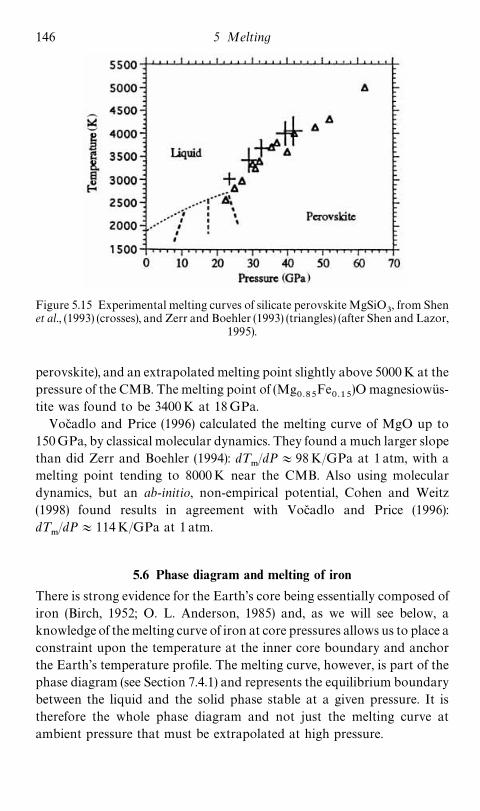
Figure 5.15 Experimental melting curves of silicate perovskiteMgSiO�, from Shen

et al., (1993) (crosses), and Zerr and Boehler (1993) (triangles) (after Shen and Lazor,1995).

perovskite), and an extrapolatedmelting point slightly above 5000K at thepressure of the CMB. The melting point of (Mg

��Fe

��)O magnesiowus-

tite was found to be 3400K at 18GPa.Vocadlo and Price (1996) calculated the melting curve of MgO up to

150GPa, by classical molecular dynamics. They found a much larger slopethan did Zerr and Boehler (1994): dT

�/dP� 98K/GPa at 1 atm, with a

melting point tending to 8000K near the CMB. Also using moleculardynamics, but an ab-initio, non-empirical potential, Cohen and Weitz(1998) found results in agreement with Vocadlo and Price (1996):dT

�/dP� 114K/GPa at 1 atm.

5.6 Phase diagram and melting of iron

There is strong evidence for the Earth’s core being essentially composed ofiron (Birch, 1952; O. L. Anderson, 1985) and, as we will see below, aknowledge of themelting curve of iron at core pressures allows us to place aconstraint upon the temperature at the inner core boundary and anchorthe Earth’s temperature profile. The melting curve, however, is part of thephase diagram (see Section 7.4.1) and represents the equilibrium boundarybetween the liquid and the solid phase stable at a given pressure. It istherefore the whole phase diagram and not just the melting curve atambient pressure that must be extrapolated at high pressure.

146 5 Melting

Figure 5.16 Phase diagram of iron up to 20GPa (after Guillermet and Gustafson,1984).

At pressures lower than about 20GPa, the phase diagram of iron isreasonably well known (Guillermet and Gustafson, 1984; Boehler, 1986)(Fig. 5.16): The phase stable at room temperature and ambient pressure is�-Fe with a body-centered-cubic (bcc) structure, at high temperature itchanges into face-centered-cubic (fcc) �-Fe, which reverts to a bcc �-Fephase below the melting point (Strong et al., 1973). At high pressure, �-Fetransforms into hexagonal-close-packed (hcp) �-Fe. The � � transform-ation has been studied in situ by X-ray diffraction, using synchrotronradiation and appears to take place by a diffusionless mechanism (Bassettand Huang, 1987). The experimental values of the triple point between the�, � and � phases are given in Table 5.5.At low and moderate pressures, the phase that melts is �-Fe and the

melting curve has been determined up to 20GPa (Liu & Bassett, 1975) and43GPa (Boehler, 1986) by resistive heating of an iron wire in a diamond-anvil cell.For more than ten years, the phase diagram of iron at high pressure has

been the subject of a controversy in the ‘‘iron workers’’ community, whichis not entirely over at the date of this writing. Whether the melting curveextrapolated to a melting point at the pressure of the inner core boundary


Table 5.5. Triple points in the Fe phase diagram. Pressure in GPa,temperature in K.

�—�—� �—�—L �—�—L �—�—L

Reference P T P T P T P T

Bundy (1965) 11 763Liu (1975b) 94 3243Guillermet & Gustafson(1984) 10.7 747Anderson (1986) 280 5760Boehler (1986) 11.6 810 75 2773Akimoto et al. (1987) 8.3 713Williams et al. (1991) 300 7500Saxena et al. (1993) 70 2700Boehler (1993) 100 2750Saxena et al. (1994) 76.5 2946 205 40Yoo et al. (1995) 50 2500Mao et al. (1998) 60 2800

L: liquid.

(330GPa) higher than 7000K or lower than 5000K was the main bone ofcontention. As more and more experiments were performed, the problemarose of the presence (or absence) of new high-pressure phases and of theircrystallographic structures, with obvious consequences as to the nature ofthe iron phase of the inner core.In shock-wave experiments, Brown and McQueen (1980, 1982, 1986)

found a first discontinuity in sound wave velocity near 200GPa, and asecond discontinuity at 243GPa, at a higher temperature, between 5000and 5700K; they attributed the first discontinuity to a solid—solid phasetransition, which they suggested might be � �, and the second discon-tinuity was considered as due to melting. Most later extrapolations ofexperimental data were forced to go through the (wide) error bar of theBrown and McQueen melting point at 243GPa.Williams et al. (1987b) combined shock-wave experiments and melting

experiments in a laser-heated diamond-anvil cell up to 100GPa, and founda very steep melting curve, extrapolating to a melting point of7600� 500K at 330GPa. The melting curve calculated ab initio by Haus-leitner and Hafner (1989) goes approximately through the Williams et al.experimental points at lower pressures, but extrapolates to 5200K at330GPa.Boehler et al. (1990), in Mainz, also from experiments in a laser-heated

148 5 Melting

Figure 5.17 Experimental melting curves of iron from Williams et al., (1987b)(triangles) and Boehler et al., (1990) (crosses and rectangles) (after Duba, 1992).

diamond-anvil cell, found that the melting point of �-Fe at 120GPa was3000K, more than 1000K lower than the value found by Williams et al.(1987b). Williams et al. (1991) then confirmed a melting point T

�

4300� 200K at 105GPa and the extrapolation of the melting curve to the�—�—liquid triple point at 300GPa and 7500K. Duba (1992) summarizedthe arguments from both sides (Fig. 5.17), pointing out that the determina-tion of melting in a diamond-anvil cell is very difficult and that thediscrepancy between experimentalists might come from the differentmelting criteria used. Boehler (1993) confirmed his previous results byextending his measurements up to a pressure of 200GPa, and found the�—�—liquid triple point at 100GPa and 2750K. The melting curve extrapo-lated to 4850K at 330GPa. At this point, a third team entered the fray:Shen et al. (1993) in Uppsala, also using a laser-heated diamond-anvil cell,measured the melting point of iron up to 60GPa. Below 20GPa, theirresults agreed with both those of Williams et al. (1987b) and Boehler et al.(1990), but above this pressure they were much closer to those of Boehler etal. New shock-wave measurements at Livermore National Laboratory,however, yielded melting temperatures of 6350K and 6720K at 235GPa


Figure 5.18 Phase diagram of iron. Dashed curves are extrapolations, for Pbetween 200 and 330GPa, using values of the Gruneisen parameter � 1.55, 1.4,1.3, 1.2. The dotted curve is the extrapolation from Boehler (1993). The full curvebetween 200 and 330GPa is from experiments by Yoo et al. (1993) (after Anderson

and Duba, 1997).

and 300GPa respectively, extrapolating to 6830� 500K at 330GPa (Yooet al., 1993).Chen and Ahrens (1995) calculated the phase diagram of iron from

equations of state and found that their calculations favored Boehler’smelting curve over that of Williams et al. (1987b).Ten years after the controversial paper of Williams et al. (1987b), it was

time again for an assessment of the situation. On the basis of X-raydiffraction identifications of the liquid phase in later work, and a more orless general consensus, Anderson and Duba (1997) removed the steepmelting curve of Williams et al. (1987b) from further consideration. Theyconstructed a phase diagram from the published diamond-anvil cell data,in reasonable agreement up to 200GPa, and extrapolated the meltingcurve to the pressure of the inner core boundary (ICB), using the Lin-demann law (5.28), for various values of the Gruneisen parameter (Fig.5.18). With their preferred value � 1.4, they find an extrapolated meltingtemperature at 330GPa between 5600 and 6500K, in rather good agree-ment with the calculated values of Poirier and Shankland (1994)(T

� 6060—6160K) and Chen and Ahrens (1995) (T

� 5800K). More

recent measurements by Mao et al. (1998) up to 84GPa agreed with thoseof Saxena et al. (1993) and Boehler (1993) below 60GPa and yieldedslightly higher melting points above 60GPa. They inferred a position of the�—�—liquid triple point at 60� 5GPa and 2800� 200K.From Boehler’s (1993) data, the triple point at about 2700K and

150 5 Melting

100GPa thought to be the �—�—liquid triple point would be at too low apressure to make it possible for the solid—solid transition observed byBrown and McQueen to be an � � transition. If a fifth phase of ironexisted, the transition could be explained. Boehler (1997) interpreted thetransition reported by Brown and McQueen as due to incomplete shockmelting, which eliminated the need for a fifth phase and extended the fieldof �-Fe to the temperature and pressure of the inner core.However, Saxena et al. (1993) at Uppsala claimed to have identified a

phase � between the � and � phases, with the �—�—� triple point near 30GPaand 1200K. A triple point near 70GPa and 2700K could then be the�—�—liquid triple point. A further study up to 150GPa led Saxena et al.(1994) to propose a phase diagram with the �—�—liquid triple point at2946� 100K and 76.5� 4GPa and the �—�—liquid triple point at 4015Kand 205GPa. The melting curve extrapolates to between 5980 and 6680Kat 330GPa.Another controversy was soon to appear. Yoo et al. (1995) used a

combined laser-heated diamond-anvil cell and X-ray diffraction techniqueto determine the structure of the high-pressure high-temperature phases upto 130GPa and 3500K. They observed that �-Fe was stable from 50 to atleast 110GPa, and found no evidence for the � phase. The triple point at2500� 200K and 50� 10GPa was identified as the �—�—liquid triplepoint. However, they found evidence for a double hcp phase (��) inside thestability field of the � phase. Saxena et al. (1995) and Saxena et al. (1996),using synchrotron X-ray diffraction, confirmed the transition from � to � at38GPa and temperatures between 1200 and 1500K. They indexed thestructure of the � phase as double hcp. In a technical comment in Science,Saxena and Dubrovinsky (1997) and Yoo et al. (1997) expounded theirrespective viewpoints. More recent determinations of structures by X-raydiffraction, while the sample is at high temperature and pressure (strangelycalled ‘‘in-situ’’ experiments) did not clarify the situation. Shen et al. (1998)still do not observe the � phase, while Saxena and Dubrovinsky (1998) andDubrovinsky et al. (1998) define its stability field and confirm a double hcpstructure, although Saxena and Dubrovinsky (1998) propose a positiveslope of the P,T boundary between � and � phases, while Dubrovinsky etal. (1998) find a negative slope (Fig. 5.19). Andrault et al. (1997) confirm theexistence of the � phase, and agree with the Uppsala team on its stabilityfield (with a positive slope of the �—� boundary) (Fig. 5.20), but assign to itan orthorhombic structure, that can be derived by small distortions from �and � phases. O. L. Anderson (1997) sums up the situation.Considering the controversy about the � phase, involving pressures of


Figure 5.19 Phase diagram of iron. Stability field of the � phase (after Dubrovinskyet al., 1998b).

the order of 50GPa, it is not surprising that the existence or non-existenceof a high-pressure phase above 200GPa (�� or �) is entirely hypothetical. Itwas suggested by Brown and McQueen (1986) from their shock-waveexperiments, and thought to be body-centered cubic, since this structurehad been predicted to be stable at very high pressures (Ross et al., 1990;Bassett and Weathers, 1990). However, Stixrude and Cohen (1995) per-formed ab-initio calculations of the energies of the various iron phases athigh pressure and found the bcc structure to be unstable with respect to abody-centered-tetragonal structure above 150GPa.At the time of writing, it is still impossible to guess whether the inner core

phase is hexagonal close packed (�), double hcp or orthorhombic (�), orsomething else (��). It seems however probable that it is not face-centeredcubic (�), as there is good evidence that the stability field of this phase doesnot extend to very high pressures.The seismologically determined density of the outer core is lower than

that of pure iron, at core pressure and temperature, deduced from equa-tions of state. Light elements (S, O, Si, etc.) must therefore be present insolution in the liquid metal. Besides decreasing the density of the core, theyalso decrease the melting (freezing) point of the alloy, with respect to that ofpure iron. As the inner core boundary corresponds to freezing of the liquidiron alloy, a knowledge of the freezing-point depression, together with thatof pure iron, would allow an estimation of the temperature at the inner coreboundary, thus providing an anchoring point for the geotherm. There is

152 5 Melting

Figure 5.20 Phase diagram of iron. Stability field of the � phase (after Andrault etal., 1997).

still much uncertainty about the nature and concentration of the lightelements in the core (Poirier, 1994a), although some progress has recentlybeenmade in estimates of the chemical composition of the core andmantle(Allegre et al., 1995). In addition, very little is known about the phasediagrams of iron alloys at core pressures.Sulfur is known to depress the melting point of iron at atmospheric

pressure and forms a eutectic, but it is not obvious that this effect persistsup to core pressures. Williams and Jeanloz (1990) investigated the meltingof iron—sulfur alloys up to 120GPa. They determined the melting curve ofFeS and of a 10wt% S alloy (Fig. 5.21), and they calculated the composi-tion and temperature of the eutectic as a function of pressure.Boehler (1992) measured the melting curve of FeS and FeS

�between 7

and 44GPa, as well as the melting point of a mixture of Fe with about10—20wt% FeS at several pressures. At 17.6GPa, the mixture begins tomelt at 1650� 50K, 600K below the melting point of iron and 300Kbelow that of FeS. Fei et al. (1997) report that the formation of the definitecompound Fe

�S�above 14GPa changes the melting relation in the Fe—

FeS system.Oxygen is another candidate as a light alloying element in the core.

Knittle and Jeanloz (1991) measured the melting curve of Fe��

O up to100GPa and found that it lies above that of pure Fe. The melting tempera-


Figure 5.21 Experimental (full) and calculated (dashed) melting curve of anFe—10wt% S alloy (after Williams and Jeanloz, 1990).

Figure 5.22 Experimental melting curve of Fe��

O. The melting curve of Knittleand Jeanloz (1991b) is given for comparison (dashed) (after Boehler, 1992).

154 5 Melting

ture of an alloy with 10wt% oxygen (Fe��

O��

) lies between that of Feand FeO at 83GPa. Boehler (1992) measured a melting curve of Fe

��O,

lying much below that measured by Knittle and Jeanloz (1991) (Fig. 5.22).Boehler (1993) found that alloys with 10wt% and 30wt% oxygen hadmelting temperatures lower than those of Fe and FeO, but that above60GPa the melting-point depression disappeared.


6

Transport properties

6.1 Generalities

All dynamic processes inside the Earth are governed by the transport ofcertain physical quantities, or at least depend on materials constants(conductivities or diffusivities) that express how easily those quantities aretransported in a given region of the Earth.

• Solid-state reactions between minerals and kinetics of phase transform-ations are controlled by transport of matter (atoms) by diffusion.

• Viscous flow of matter in the convecting mantle is controlled by diffu-sion of momentum (viscosity).

• Cooling of the Earth is controlled by heat transfer in the thermalboundary layers.

• The propagation of electromagnetic signals in the mantle depends on itselectrical conductivity.

Transport of a physical quantity (e.g. momentum or heat ) or of particles(e.g. atoms or electrically charged particles) always results from the appli-cation of a driving force F. In all cases it produces a flux J (measured perunit area and unit time).In the case of particles, the velocity v of the particle depends on the

driving force and in the linear approximation, we have:

v�MF (6.1)

whereM is the mobility of the particle, which depends on the nature of theparticle, on the properties of the medium in which it moves and ontemperature and pressure. The flux J is then equal to the number ofparticles per unit volume times the velocity.

156

In general, if the driving force derives from a potentialU, F� � gradU,the linear approximation gives:

J��C gradU (6.2)

where C is the kinetic coefficient expressing the ease of transport.The driving force may be external and imposed on the system (e.g. flow

due to a pressure gradient, electric current due to a difference of potential).It can also reflect the existence of heterogeneities in the system, which theresulting flow will tend to eliminate (e.g. diffusion of matter, diffusion ofmomentumor viscosity, diffusion of heat). In that case, as we will see below,equations of the type (6.2), together with conservation equations, yielddiffusion equations.Diffusion is an out-of-equilibrium, dissipative, irreversible process.

Steady state flow in such processes corresponds to a minimumof the rate ofentropy production dS/dt. It can be shown (Prigogine, 1962) that the rate ofentropy production can be written as the product of a generalized drivingforce F by the corresponding flux J.Let us now consider a few important cases of transport phenomena

mentioned above.

(i) Fluid flow through a porous medium

The external driving force is a pressure gradient. The flow of an incom-pressible fluid per unit area and second is given by Darcy’s equation:

J� �k

�gradP (6.3)

where k is the permeability of the medium, expressed in darcys (1darcy� 1 �m�) and � is the dynamical viscosity (see below).

(ii) Electrical conduction

The external force is an electric field E deriving from a potential:E�� gradV. The transport equation is Ohm’s law:

J��E��

��gradV (6.4)

where ��

is the electrical conductivity, expressed in siemens/m (1 S/m� 1��m��).The electric current density J is equal to the number of charge-carrying

particles per unit volume times the electric charge they carry times theirvelocity.

1576.1 Generalities

(iii) Diffusion of matter

Diffusion is an irreversible process and, as such, can be best treated in theframework of the thermodynamics of irreversible processes (TIP). For ashort and clear presentation of the formalism in the simpler case of metallicalloys, see Bocquet et al. (1983).The driving force for the diffusion of species A (atom or point defect) is

the gradient of its chemical potential ��. The flux of matter is given by:

J�� L

�grad�

�(6.5)

where J�is the flux of atoms A per second, and L

�is called the phenom-

enological coefficient. It is, however, more convenient to use Fick’s equa-tion, expressed in terms of the concentration c

�of atoms (number of atoms

per unit volume):

J��D

�grad c

�(6.6)

where D�is the diffusivity or diffusion coefficient of species A, expressed in

m�/s or cm�/s.Concentration c

�is defined as the number of atoms of speciesA per unit

volume. If n is the total number of atoms per unit volume in the mediumand N

�the atomic fraction of atoms A, we have:

nN�� c

�(6.7)

By definition, the chemical potential is:

��

��RT ln �

�N

�(6.8)

where ��is the chemical potential in the standard state and �

�the activity

coefficient of species A. In the simple case of ideal solutions, �� 1 and we

have:

grad��

��

�x�

��

�N�

�N�

�x�

RTnN

�

�c�

�x(6.9)

hence:

J�� L

�grad�

��

L�RTc�

grad c�

(6.10)

and, by comparison with (6.6):

D��

L�RTc�

(6.11)

158 6 Transport properties

Now, from (6.1), we have the velocity v�

��M�grad�

�and, since

J� c�v�, we have L

�� c

�M

�. Carrying into (6.11), we obtain Einstein’s

relation, linking the diffusivity with the mobility:

D��RTM

�(6.12)

The conservation equation for species A is written:

divJ��

�c�

�t� 0 (6.13)

hence, with (6.6):

�c�

�t� div(D

�grad c

�) (6.14)

if diffusivity is independent of concentration (an approximation generallyvalid only for dilute systems), we obtain the diffusion equation (Fick’ssecond equation):

�c�

�t�D

��c

�(6.15)

where �� div grad is the Laplacian operator in cartesian coordinates.The irreversibility of diffusion is clearly seen in the equation, since it is

not invariant under transformation of t into � t.

(iv) Diffusion of momentum

The viscosity of a flowing fluid is due to the diffusional transfer of momen-tum per unit volume �v (� is the specific mass and v, the velocity) down themomentum gradient, i.e. from regions of higher velocity to regions of lowervelocity in an incompressible fluid.The linear relation (6.2) can be written here:

�� grad (�v) (6.16)

� is the shear stress (force per unit area) equal to the flux of momentum(momentum transferred per unit area and second) and is the kinematicviscosity expressed in m�/s or cm�/s.Equation (6.16) can be written:

�� (6.17)

where � �� is the dynamic viscosity expressed in Pa s or poise(1Pa s� 10 poise) and � � d/dt�� grad v is the shear rate (Fig. 6.1). This

1596.1 Generalities

Figure 6.1 In laminar shear flow, the shear rate is given by � � v/h.

is Newton’s relation, which often serves as a definition of the viscosity.The corresponding diffusion equation of momentum is a simple form of

the Navier—Stokes equation for an incompressible fluid:

�(�v)�t

� ��(�v) (6.18)

(v) Diffusion of heat

The driving force here is (see Callen, 1985):

F�� grad��S�Q�� grad�

1

T� (6.19)

where S is the entropy, T the temperature and Q the internal energy (heat).The linear equation given by experiment:

J�� k gradT (6.20)

where k is the thermal conductivity, can be rewritten, as (6.2):

J� kT� grad�1

T�where kT� is the kinetic coefficient.The diffusion equation (conservation of heat) is Fourier’s equation:

�T�t

�k

�C�

��T (6.21)

where C�is the specific heat at constant pressure. It can also be written:

�T�t

� ��T (6.22)

where �� k/�C�is the thermal diffusivity , expressed in m�/s or cm�/s.

The solutions of the differential equation for the diffusion of heat have


been determined for a great variety of initial and boundary conditions byCarslaw and Jaeger (1959) and can, of course, be applied to the diffusion ofmatter.For the sake of example, let us give here the solution of Fourier’s

equation in the case of a semi-infinite medium bounded by the plane x� 0(extending to infinity in the direction of x� 0), whose initial temperature attime t� 0 is a constant T

�, the surface (x� 0) being kept at T � 0. The

temperature T of the medium at time t and depth x is given by:

T � T�erf�

x

2(�t)�� (6.23)

where erf is the (tabulated) error function defined by:

erf (y)�2

� ��

�

exp(� u�)du (6.24)

We see that since the temperature at a given time and depth dependsonly on the dimensionless parameter x/(�t)��, the time required for a pointto reach a given temperature is proportional to the square of its distance tothe surface, e.g. the time to reach T ��

�T�is:

t�1.099

�x� (6.25)

Incidentally, these are the simplified boundary conditions Kelvin used to esti-mate the age of the Earth (see Carslaw and Jaeger, 1959 and Burchfield, 1990). Thetemperature gradient, from (6.23) and (6.24), is

�T�x

� T�( �t)��exp��

x�

4�t� (6.26)

hence the geothermal gradient at the surface is:

G��T

�x��

� T�( �t)�� (6.27)

Taking T�� 1200 °C (for molten rock) and a typical value of � � 0.118 cm�/s,

Kelvin found that it took about nine million years for the geothermal gradient atthe surface to reach its present value taken to be equal to be 37 °C/km. Note thatKelvin did not calculate the time it would take the whole Earth to cool down to itspresent temperature and that, using the same numerical values and (6.25), we findthat it would take more than 10 years to reduce by half the temperature at a depthof 200 km. It is generally thought that Kelvin found an erroneous age of the Earthbecause he did not take into account the production of heat by radioactivity.However, Richter (1986) showed that it would not have been enough to obtain thecorrect value. Indeed, as noted by Perry (1895), if Kelvin had accepted that the

1616.1 Generalities

coefficient of thermal conduction could increase with depth (which is in effectequivalent to assuming the existence of convection), he could have found an age ofthe Earth greater than four billion (4� 10) years.

(vi) Dimensionless numbers

The diffusion coefficient D, the kinematic viscosity and the thermaldiffusivity � have the same dimensions and represent material properties .Dimensionless numbers characterizing a fluid can be constructed withthese parameters (see e.g. Tritton, 1977). Particularly interesting are thePrandtl number: P� /�, the Schmidt number: S� /D and the Lewisnumber L��/D.

6.2 Mechanisms of diffusion in solids

There are various definitions of diffusion coefficients, corresponding todifferent experimental conditions (see Bocquet et al., 1983). Let us inciden-tally mention here that the chemical diffusion coefficient (a term looselyused in earth sciences) only corresponds to the interdiffusion of two differ-ent solids A and B (A into B and B into A), as seen in the laboratoryreference frame (as opposed to the lattice frame). It generally depends onconcentration. For simplicity, we will only consider solute diffusion coeffi-cients at infinite dilution.It is a fact of experience that diffusivity in solids varies with temperature

according to an Arrhenius law (Fig. 6.2(a)):

D�D�exp��

�HRT� (6.28)

where �H is the activation enthalpy for diffusion, given by the slope of theArrhenius plot:

�H��R� lnD�(1/T)

(6.29)

The activation enthalpy is a function of pressure and the pressuredependence of the diffusion coefficient is expressed by an apparent activa-tion volume (Fig. 6.2(b); see p. 170 below):

�H��H��P�V (6.30)

�V��RT� lnD�P

(6.31)


Figure 6.2 (a) Typical Arrhenius plot for diffusion. The activation enthalpy �H isgiven by the slope of the straight line. (b) Typical variation of diffusion coefficientwith pressure. The activation volume is given by the slope of the straight line.

The linear expression (6.30) is of course valid only at relatively lowpressures; at pressures of the lower mantle, the pressure dependence of theactivation volume would have to be taken into account.In most cases relevant to geophysics, transport of atoms is effected by

exchange with vacant lattice sites or vacancies, that migrate through thecrystal.Let us consider the important case of self-diffusion, i.e. diffusion of an

atomA in a crystal constituted totally or partially of atomsA (e.g. diffusionof Fe in Fe or diffusion of O in MgO).The probability for an atom to exchange with a vacancy, i.e. to diffuse by

one jump, is equal to the probability of finding a vacancy in a neighboringsite multiplied by the probability of successfully jumping into it. Hence theself-diffusion coefficient is given by:

D��

�N�D

�(6.32)

whereN�is the equilibrium atomic fraction of vacancies at temperature T

and D�is the diffusion coefficient of vacancies.

It can be shown (see e.g. Poirier, 1985) that the equilibrium concentra-tion of (thermal) vacancies is:

N�� exp��

�G�

RT� (6.33)

with:

�G��H

�� T�S

�(6.34)

where �G�, �H

�, �S

�, are the Gibbs free energy of formation, the enthalpy

of formation and the entropy of formation of vacancies, respectively.Vacancies diffuse by a random walk process described by another of


Einstein’s relations (there are many Einstein’s relations!):

�R��t(�l)� (6.35)

where �R�� is the mean square distance covered by a vacancy during timet, � is the jump frequency and �l, the jump distance. The diffusion coeffi-cient of vacancies is defined by:

D��

�R��6t

�1

6�(�l)� (6.36)

Note that the root mean square distance covered in time t by vacancies (orany particle diffusing by randomwalk) is proportional to the square root oftime, as expected from (6.23):

x��Dt (6.37)

The jump frequency � is thermally activated, with an activation en-thalpy equal to the activation enthalpy for migration of vacancies �H

�.

Hence:

�H��

��H�� H

�(6.38)

In ionic compounds, each ionic species diffuses on its own sublattice andone can define the coefficients of self-diffusion of cations D

�and of anions

D. In the case of binary compounds, we have:

D��D

��N

��(6.39)

D�D

�N

�(6.40)

where D��and D

�are the diffusion coefficients of cationic and anionic

vacancies, respectively.Cationic vacancies are negatively charged and anionic vacancies are

positively charged; they are formed in electrically neutral pairs (Schottkypairs). In pure ionic crystals, at equilibrium, the product of the atomicfractions of cationic and anionic vacancies depends only on temperature:

NN

��N�

�� exp�

�S�

R � exp��H

�RT� (6.41)

with, for electrical neutrality:

N�N

�

The activation enthalpies for diffusion of cations and anions are then:

�H��

��H

��H

��(6.42)


�H��

��H

��H

�(6.43)

Now, there can be, and often are, aliovalent cationic impurities insolution (e.g. Ca�� replacing Na� ions in NaCl). If a Na� is replaced by aCa��, there is an excess of positive charge thatmust be compensated by thecreation of one negatively charged cationic vacancy. If the atomic fractionof impurities is C, electrical neutrality demands that:

N�C�N

�(6.44)

Hence, with (6.41):

N��N

(C�N

) (6.45)

and:

N�

C

2 ��1�4N�

�C �

�� 1� (6.46)

N��

C

2 ��1�4N�

�C �

�� 1� (6.47)

If C�N�, diffusion is controlled by the thermally activated formation

andmigration of vacancies and the activation enthalpies are given by (6.42)and (6.43). (It is the intrinsic regime.)IfC�N

�, the concentration of thermal vacancies is negligible compared

to that of the charge-compensating vacancies fixed by the concentration ofimpurities:

N��C (6.48)

The cationic vacancies are freely available for diffusion and no formationactivation enthalpy has to be spent:

�H��H

��(6.49)

Conversely, the concentration of anionic vacancies is reduced, N�

N��/C, thus reducing the diffusion coefficient of the anions. (It is the

extrinsic regime.) At lower temperatures, the charge-compensating va-cancies may remain associated with the aliovalent cations; the activationenthalpy for diffusion then includes the dissociation energy (equal to thebinding energy) of the complex (association regime).On an Arrhenius plot (Fig. 6.3), the intrinsic and extrinsic regimes are

represented by straight line segments with different slopes and the transi-tion temperature increases with impurity content:


Figure 6.3 Diffusion regimes for ionic crystals: At high temperature, the concentra-tion of vacancies is the thermal equilibrium concentration; below a temperature T

that depends on the concentration of aliovalent impurities, the concentration ofvacancies is imposed by charge balance requirements; at still lower temperatures,the charge-compensating vacancies remain associated to the impurities and have tobe dissociated to participate in diffusion. �H

�is the formation enthalpy, �H

�is the

migration enthalpy, and �H�is the binding enthalpy of the vacancies.

T�

�H�

�H�� 2k

�lnC

(6.50)

In the case of compounds where a cation can take several degrees ofoxidation (as often happens with transition-metal oxides and silicates), theconcentration of vacancies is sensitive to the oxygen partial pressure. Forinstance, in a binary oxide such as magnesiowustite (Mg, Fe)O,Fe�� ionscan be oxidized to Fe�� and we have (Chen and Peterson, 1980):

��(O

�)�� 2Fe��O�� V�

�� 2Fe�� (6.51)

V� �represents an Fe�� vacancy, with effective charge 2� ; an electron

hole h is associated with an Fe�� ion. The law of mass action gives:

[V� �][h]��

(p� )��

�K (6.52)

where K is called the reaction constant. Electrical neutrality imposes2[V�

�]� [h], hence, for a diffusion controlled mechanism:

D�

� [V� �]� (p

� )�� (6.53)

Nonstoichiometry, that in turn is often a function of oxygen partialpressure p

� , obviously considerably complicates the problem (see Kofstad,

1983; Dieckmann, 1984).The transport of matter by diffusion in a compound involves transport


of all cations and anions corresponding to the formula group. The case ofbinary ionic crystals A�B� has been treated by Ruoff (1965) (see Poirier,1985, for a summary), who defined an effective diffusion coefficient:

D��

�D

�D

�n�D

�� n

�D

�

(6.54)

where D�, n

�and D

�, n

�are the diffusion coefficients and atomic fractions

of species A and B respectively �n��

��, n

��

�� . The case of

multicomponent diffusion in silicates has been treated by Lasaga (1979)and by Jaoul (1990) in the case of olivine.Some values of the pre-exponential coefficient D

�and of the activation

enthalpies for self-diffusion of silicon and oxygen in olivine and quartz aregiven in Table 6.1. See also Freer (1980) for a review on oxides and Freer(1981) for a review on silicates. A compilation of diffusion data for silicateminerals, glasses and liquids can be found in Brady (1995). Experimentalmethods of determination of the diffusion coefficients are reviewed inRyerson (1987). For more details on the mechanisms of diffusion, thereader is referred to the book by Borg and Dienes (1988).

(i) Empirical relations

(i) A systematic empirical proportionality relation, the van Liempt relation,has been found between the activation enthalpy of self-diffusion and themelting point of metals (van Liempt, 1935; Bocquet et al., 1983):

�H��

� 34T�

(6.55)

with �H��in calories per mole and T

�in kelvin (Fig. 6.4). In other words,

the activation enthalpy of self-diffusion of metals scales with their meltingpoints, and the self-diffusion coefficient can be written:

D�D�exp��

g��

T�

RT � (6.56)

with g��

� 17, hence:

�H��

� g��RT

�(6.57)

The van Liempt relation does not hold for oxides and silicates: Plots ofpublished values of activation enthalpies for the self-diffusion of oxygen orcations (Freer, 1980, 1981) against the melting temperatures of oxides orsilicate minerals yield only a scattered cloud of points (Fig. 6.5 shows, for


Table 6.1. Pre-exponential factor and activation enthalpy for the diffusionof O and Si in olivine and quartz

System �T (°C) D�(cm�/s) �H (kJ/mol) Reference

��O in forsterite 1275—1625 3.5� 10�� 372� 13 Reddy et al. (1980)��O in forsterite 1300—1600 2.3� 10�� 293� 42 Jaoul et al. (1983)��O in forsterite 1472—1734 2.9� 10�� 416 Oishi & Ando (1984)��O in olivine 1636—2046 6.7� 10�� 318� 17 Gerard & Jaoul (1989)��Si in forsterite 1300—1700 1.5� 10�� 376� 42 Jaoul et al. (1981)Si in olivine 1130—1530 1.3� 10�� 291� 15 Houlier et al. (1990)Si in quartz 1400—1600 1.3� 10� 734� 96 Jaoul et al. (1995)

instance, all the measured activation enthalpies of ��O in binary oxides).This is obviously due to the fact that diffusion in these compounds is oftenextremely sensitive to the impurity content, the oxygen partial pressure andthe experimental temperature range; in most cases the published values arenot comparable.(ii) The compensation law or ‘‘isokinetic effect’’ was revived by Hart

(1981) and applied to diffusion in minerals. It is an empirical linear correla-tion between the logarithm of the pre-exponential factor D

�and the

activation enthalpy for the diffusion of various elements in the samemineral or rock (Fig. 6.6). For olivine, for instance, Hart (1981) found (with�H in kcal/mol and D

�in cm�/s) (Fig. 6.7):

�H� 78� 7.5 logD�

(6.58)

For silicon diffusion in silicates (quartz, olivine, diopside) Bejina andJaoul (1997) found (with �H in kJ/mol and D

�in cm�/s) (Fig. 6.8):

�H� 532.6� 30.4 logD�

(6.59)

This correlation implies that there exists an ‘‘isokinetic’’ temperature T*for which all coefficients of diffusion are equal to D*. Then:

�H�RT lnD��RT* lnD* (6.60)

and, asD�is proportional to exp (�S/R), this in fact is equivalent to having

a linear relation between activation enthalpy and entropy. The compensa-tion law, also applied to other thermally activated phenomena, like thethermal death of bacteria, has a long history of controversy (Exner, 1964;Banks et al., 1972; Kemeny and Rosenberg, 1973; Boon, 1973; Harris,1973). The case for the correlation being in most cases devoid of any


Figure 6.4 The van Liempt relation for some metals: There is a good correlationbetween the activation enthalpy for self-diffusion �H and the melting temperature

T�(after Bocquet et al., 1983).

physical significance has convincingly been made (Exner, 1964; Banks etal., 1972; Dosdale and Brooks, 1983; Kirchheim andHuang, 1987): It couldbe due to logarithmic compression in plotting logD, which varies in arather small range, since diffusion to be measurable has to be neither toorapid nor too slow. In other words, only those materials which apparentlyobey the compensation law are susceptible to investigation (Banks et al.,1972).Limoge and Grandjean (1996) have discussed the origin of the correla-

tion between activation enthalpy and entropy.


Figure 6.5 Activation enthalpy for the diffusion at high temperature of ��O inbinary oxides versus melting point (data fromFreer, 1980). The van Liempt relation

is not verified.

(ii) Effect of pressure

The pressure dependence of the diffusivity is expressed by the activationvolume, defined as:

�V ��G�P

(6.61)

�G is the Gibbs free energy of the activation process; the apparentactivation volume, defined by (6.31): �V ' ��RT (� lnD/�P)� (��H/�P),is equal to the real activation volume only if the pressure dependence of theentropic term is neglected.As diffusion experiments under pressure are difficult to realize, it is

interesting to calculate or estimate the activation volume, on theoreticalgrounds or from empirical relations.Keyes (1958, 1960, 1963) proposed a semi-empirical relation:

�V ' �4�HK

(6.62)

where �V ' is the apparent activation volume and K, the isothermal bulk


Figure 6.6 Compensation law for diffusion (after Hart, 1981).

modulus. He found it could be justified using several models of latticedefects. Assuming that the free energy of formation and migration of thedefect responsible for the diffusion is essentially represented by strainenergy in the crystal considered as a continuous medium, we can write:

�G��V (6.63)

or:

�G�KV (6.64)

depending on whether we assume the energy is entirely due to shear ordilatation. From the definition (6.61), we can write:

�V�G

�� ln�G

�P


Figure 6.7 Compensation law for diffusion in a few olivines (Mg—Fe, Co, Ni, Mn)(after Hart, 1981).

If we assume that the pressure dependence of the bulk and shear moduliare equal, we can write, using Slater’s relation (3.65 and 3.66):

� ln��P

�� lnK�P

�2�

��

�K

(6.65)

and, whether the energy is due to shear or dilatation:

�V ��2�

��

�K

�1

K��G

�V �2(�

��

�)

K�G (6.66)

which is almost equivalent to (6.62) if we take ��

� 1.83, corresponding toK�� 4 (see Section 4.3.2) and if we assume that �G��H.Sammis et al. (1981) have shown that strain-energy models assuming

pure shear and pure dilatation give upper and lower bounds on theactivation volume.


Figure 6.8 Linear relation between �H and logD�for silicon diffusion in quartz

(circles), forsterite (stars) and diopside (squares). The straight line is a fit to thecompensation law (after Bejina and Jaoul, 1997).

Keyes (1963) also considered the case where the activation enthalpy isexpressed in terms of the melting temperature (equation (6.57)): The appar-ent activation volume is then, using the Clausius—Clapeyron relation:

�V ' �dT

�T

�dP

�H��V

�T

��S

�

�H��V

��H

�

�H (6.67)

where T�, �V

�and �S

�are the melting temperature, volume and entropy

respectively. The relation can also be written:

�V ' �d lnT

�dP

�H�d lnT

�d ln �

1

K�H

and, using the differential Lindemann law (5.26), we obtain (Poirier andLiebermann, 1984):

�V ' �2(�

��

�)

K�H (6.68)

equivalent to (6.66) if �V ' ��V.At high pressures, the assumption that the activation volume is constant

does not hold any longer. The pressure dependence of the activation


volume has been calculated, using various assumptions, by O’Connell(1977), Karato (1981b), Sammis et al. (1981). It can be expressed as adimensionless parameter (Poirier and Liebermann, 1984):Differentiating (6.66) and using (6.61), we obtain:

� ln�V�P

�� ln[2(�

��

�)K��]

�P�

�V�G

and:

� ln�V�P

�� ln[2(�

��

�)K��]

�P�

2(��

��)

K(6.69)

which, with (6.65) gives:

� ln�V�P

�1

K�

1

��

��

��

�P(6.70)

Assuming �� const (3.85), one obtains:

� ln�V� ln �

� � 1� ��(�

��

�)�� (6.71)

Experimental and calculated values of activation volumes for self-diffusion can be found in Sammis et al. (1981).

6.3 Viscosity of solids

The viscosity of solids is defined, as for fluids, by (6.17), rewritten here:

��

(6.72)

where � is the applied shear stress and � (� d/dt) is the shear strain rate(see Fig. 6.1). The definition of viscosity as a material constant has ameaning only if it does not depend on time, i.e. if the shear strain rate isconstant. This is the case for high-temperature creep under constant stress,in the quasi-steady state regime. The problem of the viscosity of solids istherefore that of the high-temperature creep of crystals. A summary over-view of the principal physical mechanisms of creep is given in what followsand, for further information, the reader is referred to the monograph byPoirier (1985) (see also Poirier, 1995). If the viscosity depends only on thestructural properties of the material and on temperature, it is said to beNewtonian : the creep rate � then depends linearly on stress. In many cases,


however, the creep rate is an increasing non-linear function of stress,usually fitted by a power law: � ��, with 3� n� 5 for most solids(‘‘power-law creep’’).Creep of solids is a thermally activated phenomenon, with an activation

energy �H, and the creep rate can be put into the Arrhenian form:

� � �� exp��

�HRT� (6.73)

To define the viscosity in the non-Newtonian case, one must thereforespecify either the stress or the strain rate (see e.g. Poirier, 1988b).The viscosity at constant stress is given by:

��

� (�)� � ��

�� exp�

�HRT� (6.74)

and the viscosity at constant strain rate by:

�� (� )�

� � ��

�� exp��HRT� (6.75)

It is also interesting to consider the viscosity at constant dissipatedpower (�� const):

�� (�� )��

�� exp�2�H

(n� 1)RT�(6.76)

Note that the apparent activation energies (i.e. the sensitivity to tempera-ture) of the viscosity at constant strain rate or dissipated power are smallerthan that at constant stress unless, of course, n� 1 in which case all threeviscosities are equal.Creep deformation is due to a transport of matter by motion of lattice

defects. If the defects are vacancies, creep, then, directly results from thedirected diffusion of matter and vacancies in opposite directions, and it isNewtonian. If the defects are dislocations, creep is non-Newtonian and canbe controlled either by diffusion-controlled climb or by glide of disloca-tions (see below).

(i) Diffusion creep

Diffusion creep, orNabarro—Herring creep, is due to transport of matter byself-diffusion through the grains of a polycrystal.Let us consider a crystal of size d in the shape of a cube (for the sake of


Figure 6.9 Principle of Nabarro—Herring creep. Vacancies flow from the faces intension (concentration C�) to the faces in compression (concentration C��C�)

and matter flow in the opposite direction.

simplicity), subjected to a normal tensile stress on a pair of faces and tonormal compressive stresses on the four other faces (Fig. 6.9). The compres-sive normal stress hinders the formation of vacancies (to form vacancies,atoms are extracted from inside the crystal and deposited on the surface,which involves work against the stress), while the tensile stress facilitates it.The formation energy of vacancies is therefore increased by �V/k

�T at the

faces in compression and decreased by the same amount at the faces intension (V is the atomic volume) and the equilibrium concentrations ofvacancies at the faces in compression and tension are respectively:

C��C�exp��

�VRT� (6.77)


C��C�exp�

�VRT� (6.78)

There is a flow of vacancies from the faces in tension to the faces incompression and a flow of atoms in the opposite direction. The flux ofatoms is given by Fick’s law:

J� �D�gradC��

�D�(C��C�)

d(6.79)

where D�is the diffusion coefficient of vacancies and � is a geometrical

constant. In unit time, a number Jd� of atoms leave the faces in compres-sion and are added to the faces in tension; the crystal shortens by �d andwidens by the same quantity. We have:

�d�Jd�Vd�

�JV

hence:

� ��dd

�JVd

(6.80)

With (6.77) , (6.78) and (6.79), we obtain:

� ��D

�C

�V

d�sinh�

�VRT� (6.81)

or, remembering that D�C

�V �D

�N

��D

��, the coefficient of self-diffu-

sion, we obtain, for �V �RT:

� ��D

��V

d�RT(6.82)

The activation energy for viscosity is therefore obviously equal to theactivation energy of self-diffusion.

(ii) Dislocation creep

Dislocations (Fig. 6.10) are line defects bounding an area within the crystalwhere slip by an interatomic distance b has taken place , i.e. the crystal onone side of the slip plane has been rigidly displaced by b with respect to theother side (see Friedel, 1964 and, for a short summary, Poirier, 1985).Dislocations move under an applied stress, extending the slipped area.When a dislocation loop sweeps a whole crystal plane andmoves out of the


Figure 6.10 (a) Dislocation loop in a crystal represented as a stack of lattice planes(the front half is removed for clarity). The slipped area inside the dislocation isstippled. The extra half-plane above the edge portion (left) is seen to wind itself inhelicoidal fashion around the screw portion (back) until it ends up as the extrahalf-plane below the other edge portion (right). Each turn of the screw correspondsto a displacement by the Burgers vector b, parallel to the screw portion and normalto the edge portions. (b) Front view of the half loop. Flipping the bond OM to ONmakes the edge portion propagate toward the left. (c) Top view of the whole looporiented continuously (dashed arrows); opposite-sign extra half-planes correspondto Burgers vectors of edge portions that would point in the opposite direction if thedislocation segments were oriented in the same direction.


Figure 6.11 Slip by dislocation motion. (1) Undeformed crystal. (2) A dislocationline has been created at left andmoved inside the crystal, causing a slip by b behind it(stippled area). (3) The dislocation has swept the whole length of the crystal and left a

step of height b at the surface. The shear strain is � b/h.

crystal, it leaves at the surface a step of height b. The crystal has acquired apermanent shear deformation equal to b/h, where h is the dimension of thecrystal normal to the slip plane (Fig. 6.11). The motion of dislocations byprogressive breaking and re-establishment of atomic bonds is the energeti-cally economic way of deforming crystals. Dislocations are carriers ofplastic deformation in solids.For a mobile dislocation density � (total length of dislocation lines per

unit volume) moving an average distance �L, the shear strain is:

��b�L (6.83)

and, for constant dislocation density, the creep rate is:

� � �bv (6.84)

where v is the average dislocation velocity. This isOrowan’s equation, whichcan be seen as a transport equation, giving the creep rate as the product ofthe density of strain carriers (the dislocations), their strength (the Burgers


vector b, characteristic of the dislocation and equal to the elementary slipby an interatomic distance) and their velocity. The equation is analogousto the microscopic Ohm’s law (see below). The dependence of the viscosityon stress and temperature is found by expressing the dependence of dislo-cation density and velocity.For steady-state creep, the dislocation density is generally proportional

to �� (see Poirier, 1985) and depends little on temperature. The averagedislocation velocity depends, of course, on � and is controlled by the natureand distribution of obstacles to the motion of dislocation lines in thecrystal. Two cases are especially interesting:

(a) The principal obstacle to the dislocation motion lies in the intrinsicdifficulty in breaking the atomic bonds, the so-called ‘‘lattice friction’’.The material is said to have a high Peierls stress and the dislocationlines tend to be straight, lying in potential valleys. The lattice frictioncan be overcomewith the help of thermal vibrations and of the effectivestress (applied stress minus internal stress). The motion is directlythermally activated and the activation enthalpy is stress dependent,decreasing with increasing stress. The creep rate can be written:

� � �� exp��

�H(�)RT � (6.85)

The viscosity is said to be glide-controlled.(b) If the obstacles are discrete, with an average spacing �L, the average

velocity can be written in general:

v ��L

t�� t

�

(6.86)

where t�is the average time the dislocation takes in gliding over the

distance �L between obstacles and t�is the average time it takes in

overcoming the obstacles. If t�� t

�, the average velocity is v ��L/t

�.

Edge dislocations can overcome obstacles to glide by moving out oftheir glide plane by diffusion-controlled climb (Fig. 6.12) (Weertmancreep). If � is the distance a dislocation has to climb to escape theobstacle and v

�is the climb velocity, we have:

� ��b�Lv�� (6.87)

It can be shown (Friedel, 1964) that v�is proportional to the self-

diffusion coefficientD��and, in the linear approximation, to the applied


Figure 6.12 Climb of an edge dislocation. The dislocation climbs by an interatomicdistance when a jog travels down its length by absorbing (A) or emitting (E)

vacancies.

stress �. Remembering that � ��, we then obtain the general equationfor diffusion-controlled creep:

� � �� exp��

�H��

RT � (6.88)

We have here a physical justification for power-law creep with n� 3,but the experimental values usually range between 3 and 5. Diffusion-controlled power-law creep is often observed at high temperatures inmetals and minerals, although some caution is in order before issuinggeneral pronouncements (Poirier, 1978). It is currently thought to beresponsible for the viscosity of the Earth’s mantle (Weertman, 1970,1978; Poirier, 1988b). The viscosity profile of the mantle then dependson the temperature profile and on the pressure dependence of the creeprate.

In the case of diffusion-controlled creep of minerals containing iron,which can take several degrees of oxidation, the creep rate depends onoxygen partial pressure, and also on the activity of the components. Creepexperiments on olivine buffered against orthopyroxene or magnesiowus-tite, under various conditions of temperature, pressure and oxygen partialpressure, yield very different activation energies and oxygen partial press-ure dependence (Bai et al., 1991). Several creep laws are needed to accountfor the results, which makes extrapolation to mantle conditions difficult.


(iii) Effect of pressure

As for diffusion, the pressure dependence is expressed by an apparentactivation volume:

�V ' �RT� ln ��P

��H�P

(6.89)

which should, in principle, be equal to the activation volume for self-diffusion of the atomic species whose diffusion controls the creep rate.There is, however, some debate as to which species controls the creep rate,even in well-investigated minerals such as olivine (e.g. Jaoul et al., 1981)and, anyway, there are very few experimental determinations of the activa-tion volumes (Bejina et al., 1997, find an activation volume close to zero forthe diffusion of silicon in olivine). Onemust therefore resort to systematics.Weertman (1970) applied van Liempt’s relation (6.57) to the creep of

metals and ice and implicitly extended it to the creep of all substances,including the minerals of the Earth’s lower mantle. Weertman’s relation:

�H� gRT�

(6.90)

where �H is the activation enthalpy for viscosity (or creep rate) and T�is

the melting temperature, is valid for metals with a value of the constant gclose to 18. For compounds, however, things are obviously not so simplesince the creep mechanisms are not always clear and, even if creep isdiffusion-controlled, van Liempt’s relation does not hold. Besides, thepublished values of activation enthalpies for creep of ceramics (Cannonand Lang-don, 1983) correspond to widely differing experimental condi-tions, purity of materials, grain size, oxygen partial pressure, etc. Even if thedata are carefully selected, a plot of the activation energy against meltingtemperature for various materials exhibits a considerable scatter (Fig. 6.13shows, for instance, the data corresponding to compression creep of singlecrystals of oxides and alkali halides). By grouping the compounds accord-ing to their structure, it is, however, possible to improve the systematics(Frost and Ashby, 1982) (Fig.6.14). Nevertheless, there is little hope of everobtaining a systematics good enough to usefully predict the activationenthalpy of a compound from a knowledge of its melting temperaturebecause the scatter on g remains much too large. We find, for instance,that, from the data of Fig. 6.13, we have g� 27� 8 for oxides (in agree-ment with Frost and Ashby, 1982) but, as g appears in an exponential, thiscorresponds to an uncertainty of three orders of magnitude on the viscos-ity! Weertman’s relation, however, remains useful for the purpose orig-


Figure 6.13 Activation enthalpy for creep versusmelting point for oxides and alkalihalides (data fromCannon and Langdon, 1983). Straight lines are drawn for g� � 15

and g� � 30.

Figure 6.14 The ranges of the dimensionless quantity g� ��H�/RT�for classes of

solids (after Frost and Ashby, 1982).


inally assigned to it by Weertman (1970), i.e. to extrapolate the viscosity tohigh pressures, if the melting curve is known or inferred, but the value of gmust be the one experimentally determined for the specific compound oneis interested in.The activation volume for diffusion-controlled creep of solids (and the

Earth’s mantle) has been estimated by several authors (e.g. Sammis et al.,1981; Karato, 1981b; Ellsworth et al., 1985), using either Weertman’srelation (6.90), i.e. assuming that the pressure dependence of viscosity isequal to that of the melting point, or Keyes’ formulation with an elasticstrain model for the Gibbs free energy of activation. Poirier and Lieber-mann (1984) discussed these formulations and showed that they wereequivalent within the limits of validity of Slater’s relation and Lindemann’slaw. The discussion has already been presented for diffusion in Section 6.2.

6.4 Diffusion and viscosity in liquid metals

The Earth’s outer core (16% of the Earth’s volume) is constituted of liquidiron. Its diffusional and viscous transport properties must be placed in thewider framework of liquid metals which, being simple unassociated liquids,have been experimentally and theoretically well investigated. The reader isreferred to the book by Shimoji and Itami (1986) for a complete review ofthe field (see also Battezzati and Greer, 1989).There is an intimate connection in liquids between the self-diffusion

coefficient and the viscosity �. It is expressed by the Stokes—Einstein rela-tion:

D��k�T

2 a(6.91)

where a is an atomic-size parameter. The Stokes—Einstein relation has beenexperimentally verified for liquidmetals (Saxton and Sherby, 1962) and canbe theoretically justified (e.g. Zwanzig, 1983).Eyring (1936) considered a liquid as a collection of molecules bound to

their neighbors and ‘‘dissolved holes’’ (similar to vacancies in solids).Transport, either by diffusion or under the action of a shear stress (viscos-ity), was thought to occur by thermally activated jumps of the moleculesinto the holes. The diffusion coefficient then can be written, as for solids (see6.36):

D� ��k� (6.92)

where � is the jump distance, comparable to the average interatomic


spacing, and k� is the absolute reaction rate of the diffusion process. Eyringtherefore finds an expression of the diffusion coefficient that follows anArrhenius law, like the coefficient of diffusion of crystals:

D�D�exp��

Q

RT� (6.93)

whereQ is the activation energy corresponding to the potential barrier thatthe molecule must overcome to jump into the hole.To calculate the viscosity, Eyring assumed that the motion takes place

by individual molecules slipping by a distance � over the potential barrierwith a reaction rate k�. The viscosity is given by (6.17) with � � �

�/�v, where

�v is the difference in velocity of two neighboring parallel layers, which area distance �

�apart. The force acting on a molecule is ��

��, where �

�and

��are the distances between molecules in the parallel planes in the direc-

tion of motion and perpendicular to it respectively. The force acts to lessenthe work for overcoming the barrier in the forward direction and raises it inthe backward direction, so the velocity difference can be written:

�v� �k��exp��

��

2k�T �� exp��

��

2k�T �� (6.94)

Now, for �� 2k

�T, we have:

��k�T

��k�

(6.95)

With (6.92) and (6.95), we see that Eyring’s theory yields the Stokes—Einstein relation:

D��

��

k�T (6.96)

The ‘‘free volume’’ theory of diffusion of Cohen and Turnbull (1951)assumes that atoms are enclosed in cages formed by their neighbors andcan jump only when statistical fluctuations of the free volume V

�(total

volume minus the volume occupied by the atoms) create a hole of volumeV* sufficient to accept an atom. The diffusion coefficient is:

D� (k�T )�� exp��

�V*

V�� (6.97)


where 0�� 1 is a numerical constant and V�� (T � T

�), where � is the

coefficient of thermal expansion.Swalin (1959) starts from Einstein’s equation (6.36) but, instead of con-

sidering atoms jumping by a fixed distance into holes of a critical size, heassumes that local density fluctuations cause atoms to move small variabledistances and finds for the diffusion coefficient of liquid metals:

D� (1.29� 10��)��T�

�H�

(6.98)

where � (in Å��) is related to the curvature of the potential-vs-distancecurve and �H

�is the heat of vaporization. In this model, there is a

distribution of fluctuation sizes and most atoms participate in the diffusionprocess at a givenmoment. The process has no activation energy; however,a plot of lnD vs 1/T yields an apparent ‘‘activation energy’’ equal to 2RT,devoid of physical meaning.Indeed, the assumption that there are identifiable holes and that there is

a localized energy barrier to diffusion, inherent to Eyring’s ‘‘activatedstate’’ model and its variants, is not easily tenable in liquids.Nachtrieb (1967, 1977) found that the experimental results were best

fitted by a linear relation between D and T, based on the assumption thateach atom vibrates in the cage of its neighbors with a harmonic motion andthat with each oscillation, the center of oscillation moves by a distanceequal to the mean thermal amplitude:

D�k��

�h�

T (6.99)

where ��is the Debye temperature, h is Planck’s constant and � the force

constant of the harmonic vibrations. In a sense, the entire liquid is in anactivated state and the concept of activation energy has no meaning.However, and despite the fact that there is no convincing theoreticaljustification for it, the temperature dependence of the diffusion coefficient isstill currently displayed on Arrhenius plots and ‘‘activation energies’’ aredetermined, even by those who object to it (Nachtrieb, 1967; Shimoji andItami, 1986). Indeed, the fit of the data by an Arrhenius law is in most casesreasonably good and ‘‘activation energies’’ provide a convenient means ofsystematizing the data.The ‘‘activation energies’’ for self-diffusion and heterodiffusion in liquid

metals are, not surprisingly, much smaller than in the corresponding solids.As an example, average values for the heterodiffusion of H, C, N, O, S in �-,


Table 6.2. Apparent activation energies for diffusion of various elements in�-, �-, and liquid iron

Diffusing element Q� � (kJ/mol) Q� � (kJ/mol) Q��(kJ/mol)

Hydrogen 12.5 47.2 15.5Carbon 81.3 134.4 49Nitrogen 76.8 152.2 50.2Oxygen 96.3 168.5 50.2� 8.4Sulfur 207.2 222.4 35.6

Source: Bester and Lange (1972).

�- and liquid iron, from Bester and Lange (1972) are given in Table 6.2.As for diffusion, Eyring’s (1936) activated state theory of viscosity is

among the very few that predict an Arrhenian temperature dependence (seeBrush, 1962 and Shimoji and Itami, 1986, for a review).Andrade (1934, 1952) proposed a theory of the viscosity of unassociated

liquids at their melting points, based on the idea that their structure is closeto that of the solid and that their viscosity is due to the transfer ofmomentum by collision between parallel layers of atoms through theamplitude of thermal vibration. Andrade found an expression of the viscos-ity in terms of the massm of atoms, the mean interatomic spacing a and theLindemann vibrational frequency �

�(equation (5.19)):

� �2m�

�3 a

(6.100)

or, in c.g.s. units:

�� (5.7� 10��)(AT�)��V�� (6.101)

where A and V are the atomic mass and volume respectively. Viscosity isthought to decrease with increasing temperature because thermal agitationinterferes with the transfer of momentum at maximum amplitude. Thevariation of viscosity with temperature is then governed, according toAndrade (1934), by the fraction of atoms possessing the mutual potentialenergy at extreme amplitude, which varies according to the Boltzmanndistribution formula, hence:

� � exp�C

T� (6.102)

where C has the dimensions of an energy. Although it is not an activation


Figure 6.15 Correlation between the melting point and apparent activation energyfor self-diffusion of liquid metals (after Poirier, 1988a).

energy, it can be treated like an apparent ‘‘activation energy’’ for system-atization purposes.

(i) Empirical relations and effect of pressure

As for diffusion and viscosity in solids, there are systematic empiricalrelations between the apparent ‘‘activation energy’’ of diffusion and viscos-ity in liquid metals similar to (6.57) and (6.90), but the values of theconstants g

�and g� are much smaller (Saxton and Sherby, 1962; Grosse,

1963; Poirier, 1988a). This is to be expected since the activation energy fordiffusion (and diffusion-controlled creep) of solids consists mostly of theformation energy of point defects, whereas in liquids the apparent ‘‘activa-tion energy’’ reflects only the temperature dependence of the mobility ofatoms which does not necessitate the creation of localized defects.Poirier (1988a) found for a number of liquid metals:

Q�� 3.2RT

�(6.103)

for diffusion (Fig. 6.15) and:

Q� � 2.6RT�

(6.104)

for viscosity (Fig. 6.16). The value of g�� 3 is in good agreement with that

obtained by Saxton and Sherby (1962) and by Nachtrieb (1967), whosemodel for diffusion rests on the idea that the average energy of atomsvibrating in the cage of their neighbors is equal to 3RT.The extrapolation to high pressures of the viscosity of liquid metals

(especially interesting for iron in the Earth’s core) stands on a somewhat


Figure 6.16 Correlation between the melting point and apparent activation energyfor viscosity of liquid metals (after Poirier, 1988a).

safer ground than in the case of solids, despite the lack of theoreticaljustification for (6.104), because of the lesser scatter in the value of theconstant ( close to 3). There is an excellent agreement between the apparent‘‘activation volume’’ of the viscosity of mercury, calculated from the experi-mental results of Bridgman, using (6.89) (�V ' � 0.62 cm�/mol) and theempirical value, calculated from (6.104) and the slope of the melting curve(�V ' � 0.59 cm�/mol).It is interesting to consider the vicosity of a liquid metal right at its

melting point (T � T�). Since we have:

� � exp�g�T�

T � (6.105)

we immediately see that the viscosity stays constant along the meltingcurve and is equal to the viscosity at atmospheric pressure. The viscosity ofliquid iron at the inner core boundary should then be equal to 6 centipoise(Poirier, 1988a). Ab-initio electronic structure calculations, based on den-sity functional theory, yield a diffusion coefficient of liquid iron, atT � 6000K, ofD� 0.4—0.5� 10�� cm�/s, which, with the Stokes—Einsteinrelation (6.91), and a� 1Å, yields a viscosity of about 15 centipoise (deWijs et al., 1998).

6.5 Electrical conduction

6.5.1 Generalities on the electronic structure of solids

The theory of the electronic structure of solids is the corner stone of


solid-state physics and it is obviously beyond the scope of this book even togive a summary overview of it. However, since transport of electroniccharges is what electrical conduction is all about, it is impossible to avoidgiving some indispensable background, mostly at the hand-waving level.For an elementary or intermediate treatment, the reader is referred toKittel (1967), Ziman (1965), Honig (1970) or Animalu (1977). An essentialconcept in solid-state theory is that of electronic energy bands, separated byband gaps.Energy bands are ranges of allowed energy states for the electrons, the

gaps corresponding to forbidden states for which the Schrodinger equationhas no acceptable solution. They arise because of the existence of a periodiclattice potential: Electronwave functions represent running waves carryingmomentum p� �k (k is the wave number). At the boundaries of theBrillouin zones the waves cannot propagate and two standing waves areformed with energies differing by E

�the gap energy (Fig. 6.17).

It is also convenient to envision the formation of bands as due to thespreading of atomic energy levels (orbitals) when the many atoms con-stituting the crystal are brought together and the atomic orbitals overlap(Fig. 6.18). The degree of overlap also characterizes the type of atomicbonding.

• For ionic bonding, the electrons are transferred from one atomic speciesto the other, forming ions with an inert gas electronic shell configur-ation. There is very little overlap of orbitals and the band formalism isnot adequate. The electrons are bound to the ions and localized.

• For covalent bonding, the orbitals overlap and there is some degree ofdelocalization of electrons, shared between neighboring atoms.

• For metallic bonding, the overlap is large and the electrons belonging tothe outer shell are completely delocalized; there is a sea of nearly freeelectrons, bathing the ion core lattice.

The highest occupied band is the valence band, the lowest unoccupiedband is the conduction band. The gap width is given by:

E��E

��E

�(6.106)

where E�is the energy of the top level of the valence band and E

�is the

energy of the bottom level of the conduction band. The electronic levels arefilled up to the Fermi level E

�.

The electrical conduction properties of crystals essentially depend on theposition of the Fermi level with respect to the bands and on the gap width.


Figure 6.17 (a) Energy vs wave number curve for a free electron (parabola).(b) Energy vs wave number curve for a nearly free electron in a periodic potential

(first Brillouin zone). The energies in the gap of width E�are forbidden.

When an electrical field is applied to a crystal, the electrons are subjected toa force and are accelerated, thus acquiring energy. They must therefore bepromoted to higher-energy levels. This is possible only if the Fermi levellies within a partially filled conduction band with empty levels available(metal) or if the gap is narrow enough so that thermal agitation can allowelectrons to cross it, from the valence band into the empty conduction band(semi-conductor). If the valence band is completely filled and the gap iswide, the crystal is an insulator; the electric field cannot make the electronsmove since there are no accessible energy levels for them. However, thebands can be distorted, giving rise to polarization (dielectric). We can nowclassify the crystals according to their electronic structure and electricalproperties.

(i) Insulators (Fig. 6.19(a)). The valence band is completely filled at 0K


Figure 6.18 Widening of atomic levels into bands when atoms are brought closetogether.

Figure 6.19 Electronic band structure of various classes of materials. (a) Insulators.(b) Intrinsic semi-conductors at T � 0K. (c) Intrinsic semi-conductors at T � 0K.(d) Metals at T � 0K. (e) Semi-metals at T � 0K. The filled levels are stippled.


Figure 6.20 Localized levels introduced in the energy gap. (a) Shallow donor levels.(b) Deep levels. (c) Shallow acceptor levels.

and the gap is too wide for thermal agitation to allow promotion ofelectrons across it, even at high temperatures, i.e. (E

�� k

�T).

Typical insulators are, for instance, diamond (E�� 5.3 eV), for-

sterite (E�� 6.4 eV) and SiO

�(E

�� 8 eV). Incidentally, remember that

k�T � 1/40 eV at room temperature and that k

�T � 1 eV at 11 605K.

Ionic crystals generally are insulators at low temperatures. This is dueto the fact that the charges can move only by thermally activatedjumps from one site to another; conduction involves either diffusion ofthe whole ions (ionic conduction) or electronic charge transfer betweenions of different valence (hopping conduction). In both cases, if theactivation energy of the process is much higher than k

�T, the crystal

behaves as a dielectric with very low conductivity. Although the bandformalism is not the best suited to ionic crystals, a large value of theband gap width is associated with ionic crystals in the low-tempera-ture insulating regime. At high temperatures, ionocovalent com-pounds that are insulators at low temperatures, can simultaneouslyexhibit electronic semi-conduction or hopping conduction and ionicconduction.Impurity atoms in low concentrations may introduce deep energy

levels in the gap, far from the gap edges (Fig. 6.20), whichmay allow forsome electrical conductivity of the semi-conduction type if the gap isnot too wide (see, e.g. Morin et al., 1977, for forsterite).

(ii) Semi-conductors (Fig. 6.19(b,c)). Semi-conductors differ from insula-tors in that their gap is narrower, comparable to k

�T, thus allowing, in

pure crystals, thermal promotion of electrons in the conduction band,leaving positively charged holes at the top of the valence band (intrinsicsemi-conduction). Typical gap widths for semi-conductors are of the


order of 1 eV, e.g. E�� 1.14 eV for Si, E

�� 0.67 eV for Ge, E

�� 1.4 eV

for GaAs.Impurity atoms in solution, e.g. As in Ge, can introduce shallow

levels (donor levels) near the top of the gap, that can ‘‘donate’’ electronsto the conduction band and give rise to n-type conduction. If theimpurity can receive electrons, e.g. Ga in Ge, it introduces levels(acceptor levels) near the bottom of the gap and gives rise to p-typeconduction, by holes in the valence band. This is known as extrinsicsemi-conduction.

(iii) Metals (Fig. 6.19(d)). In metals, the Fermi level falls within the conduc-tion band, the remaining empty levels in the band are directly access-ible to the electrons and there is a good electrical conductivity at 0K.In some cases, the bottom of the conduction band is lower than the topof the valence band in certain directions of reciprocal space (k-space)and the electrons at the top of the valence band can spill over into theconduction band (Fig. 6.19(e)). There are conduction electrons andholes at 0K. Such crystals are known as semi-metals, not as goodconductors as metals; typical examples are the rare-earth metals.

It must be noted that the electrical properties of a given compound canchange with temperature or pressure. The change can be gradual and twoor more conduction mechanisms may coexist, as when an insulator at lowtemperatures becomes a semi-conductor and/or an ionic conductor at hightemperatures or a metallic conductor at high pressure (Samara, 1967); thechange may also be discontinuous, as when some oxides become metallicconductors above a critical temperature because, for a critical interatomicdistance, the electronic structure with localized electrons is less stable thanthe metallic one (Mott transition). Pressure may lower the critical tempera-ture (Mott, 1961).

6.5.2 Mechanisms of electrical conduction

(i) Generalities

Ohm’s law, I�R��V, relates the current intensity flowing in a conductorto the difference of potential driving it and to the resistance R (or conduc-tance R��) of the conductor.The resistivity is: ��RS/L, where S is the section of the conductor and

L its length. Ohm’s law can therefore be written:

J��E (6.107)


where J� I/S (in amperes/m�) is the current density, E� V/L (in volts/m)is the electric field and � �� (in ��/m or siemens/m) is the electricalconductivity.The current is equal to the rate of passage of electric charge through unit

area of the conductor, it can be written:

J� nqv�

(6.108)

where n is the number of mobile charge-carrying particles per unit volume,q is their electric charge and v

�their drift velocity in the direction of the

electric field.We will give here a microscopic expression of Ohm’s law in the case of

electronic conduction in a partially filled band (metal or semi-conductor).The electrons feel the periodic potential of the crystal (which accounts forthe existence of the bands in the first place), but for the sake of simplicityand without too much loss of generality, we will consider the conductionelectrons as free.Let us consider electrons moving freely in a band. The force exerted on

them by the electric field is:

F�� eE�dp

dt� �

dk

dt(6.109)

where e is the electron charge, p is the momentum and k, the wave vector.The electrons are accelerated by the force but their velocity does not

increase indefinitely, because of collisions and scattering of phonons orpoint defects, and it reaches a steady state drift velocity v

�. Let the relax-

ation time � be the average time between scattering events, the increase inmomentum between these events is:

��k�F� (6.110)

and the drift velocity is:

v��

�km

�F�m

(6.111)

where m is the mass of the electron, or with (6.109):

v�� eE

�m

(6.112)

and, with (6.108):

J� � nev��

ne��m

E


hence:

��ne��m

(6.113)

If � is the mean free path of electrons and v is the total average (rms)velocity (thermal velocity plus drift velocity), we have:

� �ne��mv

(6.114)

If the band is only slightly filled, as in extrinsic n-type semi-conductors,the average kinetic energy of an electron is:

��mv ��

�k�T (6.115)

hence:

� � ne��(3mk�T )�� (6.116)

(ii) Metallic conduction

All the conduction electrons gain energy when the electric field is appliedand most of them are shifted from the levels they occupied to those leftvacant by others, with no net contribution to the electrical current. It isonly the electrons near the Fermi level that are promoted to empty levelsand provide a net response to the field. To a first approximation we cantake for v in (6.114) the velocity at the Fermi level v

�given by:

��mev

��E

�(6.117)

and we obtain Drude’s formula:

� �ne��mv

�

(6.118)

The temperature dependence of the conductivity in T�� given by thefree-electron approximation does not agree with experimental results.Indeed at low temperatures (a few kelvin), the conductivity is controlled bythe collision of electrons with dilute impurities in the lattice; it depends onthe impurity concentration and is practically independent of temperature.At high temperatures (T ��

�), the conductivity is controlled by phonon

scattering and decreases as T��. The resistivity of metals can be written(Matthiessen’s rule) as:

��

��

(6.119)


where ��

is the impurity contribution and ��

� T at high temperaturesis the lattice-dependent part. The linear temperature dependence of theresistivity can be qualitatively explained in the following way (Mott andJones, 1958).The electrical resistance is due to the scattering of electrons by vibrating

atoms and it is proportional to the scattering probability, which, in turn, isproportional to the mean square of the displacement of atoms �u��. Athigh temperatures (T ��

�), the mean potential energy of vibrating atoms

is:

��f �u��

�k�T (6.120)

where f is the restoring force. From the equation of motion:

Md�u

dt�� fu� 0 (6.121)

we have:

f�M�� (6.122)

whereM is the mass of the atoms and � their vibrational frequency. With(6.120) and (6.122) and taking for� theDebye frequency�

�� (k

�/�)�

�, we

obtain:

��u��

�T

k�M

(6.123)

Since �u�� decreases with pressure, the conductivity of metals increaseswith pressure. We have, with the definition (3.52) of the Debye—Gruneisenparameter �

�:

�d ln�d lnV

�d ln�d ln�

� �2d ln�

�d lnV

� 2��

(6.124)

(iii) Semi-conduction

In the case of semi-conductors, where electron- or hole states are close tothe edge of a band, the free-electron approximation cannot be used and theinteraction of the electrons with the lattice and other electrons must betaken into account by introducing the effective mass m*, instead of the massm of the free electron. The expression of the effective mass can be found byconsidering the motion of a wave packet of states with frequencies andwave numbers near � and k respectively. Energy E� �� is propagatedwith group velocity v

�:


v��

d�dk

�1

�dE

dk(6.125)

hence:

dv�

dt�

1

�d�E

dk�

dk

dt

With �dk

dt�F, (6.109), it becomes:

F� ��d�E

dk�� dv

�dt

�dp

dt(6.126)

We see that the role of the mass is played by the effective mass:

m*� ��d�E

dk��

(6.127)

For free electrons E� �k�/2m, hence m*�m. Close to the edge of thebands, momentum transfer between the electrons and the lattice is thustaken into account by introducing the effective mass.For a semi-conductor with band gap width E

�and Fermi level E

�, if the

energy at the top of the valence band is taken as the zero of energy, thenumber of electrons in the conduction band (filled states) per unit volumeis:

n� ��

��

2D(E) f (E)dE (6.128)

whereD(E) is the density of states of electrons (the number of states per unitvolume with energy between E and E� dE) and f (E) is the Fermi—Diracdistribution function:

f (E)��exp�E�E

�k�T �� 1�

�� exp�

E��E

k�T � (6.129)

Calculating the value of the density of states (see e.g. Kittel, 1967;Animalu, 1977), it can be shown that:

n� 2�m*

�k�T

2 ��

exp�E

��E

�k�T � (6.130)

Similarly, the concentration of holes in the valence band is:

p� 2�m*

�k�T

2 ��

exp��E

�k�T � (6.131)


The law of mass action for the concentrations of electrons and holes iswritten as:

np� 4�k�T

2 ��(m*

�m*

�)�� exp�

�E�

k�T � (6.132)

wherem*�andm*

�are the effective masses of electrons and holes respective-

ly.

(i) Intrinsic conduction. For intrinsic conduction, we have n� p, since ahole is left in the valence band for every electron that is promoted to theconduction band. The number of intrinsic carriers is then found from(6.132):

n � p

� 2�

k�T

2 ��

(m*�m*

�)�� exp�

�E�

2k�T� (6.133)

and, setting (6.130) equal to (6.131):

E��

1

2E��

3

4k�T ln�

m*�

m*�� (6.134)

One then sees that, if m*��m*

�, the Fermi level lies in the middle of the

gap. The conductivity is given by the sum of the contributions of electronsand holes:

� � ne�� pe�

�� n

e(�

��

�) (6.135)

where ��and �

�are the mobility of electrons and holes respectively (drift

velocity per unit electric field). Comparison of (6.135) with (6.113) andreplacement of m by the effective masses yields:

�� e�

�m*

� (6.136)�� e�

�m*

�

where ��and �

�are the relaxation times for electrons and holes respectively.

From (6.133) and (6.135), we have therefore for intrinsic conductivity:

� � 2�k�T

2 ��

(m*�m*

�)�� exp�

�E�

2k�T� (��

� ��) (6.137)

Intrinsic conductivity is the conduction regime for pure crystals orcrystals with a low impurity concentration at high temperature, where theconcentration of intrinsic carriers, which grows exponentially with tem-perature, is much larger than the concentration of impurities.


Figure 6.21 Arrhenius plot of the electrical conductivity of semi-conductor showingthe intrinsic regime at high temperatures and the extrinsic regime at low tempera-tures; in the intermediate regime the conductivity may slightly decrease withincreasing temperature due to electron—photon scattering (after Animalu, 1977).

The mobility at high temperatures is mostly controlled by phononscattering and it can be shown that:

��

�� T�� (6.138)

The temperature dependence of the conductivity comes therefore essen-tially from the temperature dependence of the carrier concentration. Theslope of the Arrhenius plot directly gives the energy gap E

�(Fig. 6.21).

(ii) Extrinsic conduction. The electrons in the conduction band of n-typesemi-conductors (holes in the valence band of p-type semi-conductors)arise by thermal ionization of the donor (acceptor) impurities. The donorlevel (E

�below the conduction band) is atE

��E

�, referred to the top of the

valence band. The conduction electron concentration n is equal to theconcentration of ionized donors N�

�, given by the product of the total

dopant concentration by the Fermi—Dirac distribution:

n� 2 �m*

�k�T

2 ��

exp�E

��E

�k�T ��N

��exp�E

��E

��E

�k�T �� 1� (6.139)

In the low-temperature limit, E�� k

�T, we have:

exp 2�E��E

�k�T ��

1

2N

��m*

�k�T

2 ��

exp��E

�k�T �

and:


n� (2N�)��

m*�k�T

2 ��

exp��E

�k�T � (6.140)

The carrier concentration varies with the square root of the impurityconcentration and as T ��; the mobility, controlled by ionized impurityscattering, varies as T��. The temperature dependence of the conductiv-ity is therefore exponential, with the slope of the Arrhenius plot giving theionization energy of the impurity E

�(Fig. 6.20). The same results apply to

p-type semi-conductors.Between the intrinsic and the extrinsic regimes, there is an intermediate

temperature range where the concentration of intrinsic carriers is compar-able with that of the dopant impurity. The conductivity in this range mayslightly decrease as temperature increases because of electron—phononscattering (Fig. 6.21).Pressure affects the electrical conductivity of semi-conductors via the

mobility and concentration of the carriers. Mobility, controlled by phononscattering, depends on density, phonon velocity, effective mass, etc., all ofwhich depend on pressure (Paul and Warschauer, 1963). The overallpressure dependence of mobility, however, remains of second order com-pared to the pressure dependence of the carrier concentration: The carrierconcentration depends exponentially on the energy gap E

�which depends

in a complicated way on pressure. At pressures up to 10 kbar (1GPa), forinstance, the energy gap of germanium first increases with pressure(5� 10�� eV/bar), then tends to decrease, whereas the energy gap of silicondecreases as pressure increases (Paul and Warschauer, 1963). At very highpressures, anyway, one should expect that bands would eventually overlap,giving rise to metallic conduction (Drickamer, 1963).

(iii) Hopping conduction and ionic conduction. Let us now consider thecase of ionic crystals where the orbital overlap is so small that the bandformalism becomes inadequate. To a first approximation, the electrons arelocalized and bound to the ions; they cannot freely move as an electric fieldis applied and the crystal behaves as an insulator at low temperatures. Suchcompounds, for which the effective mass of the carriers is very large aresometimes called ‘‘low-mobility semi-conductors’’. The only way an electri-cal current can be created is by bodily motion of the ions by thermallyactivated diffusion through the crystal (ionic conduction) or by thermallyactivated charge-transfer between neighboring ions of different valence(hopping conduction): for instance, a hole hops from a cation with charge� 3 to a neighboring ion with charge � 2 or � 1. This occurs in the


so-called ‘‘mixed-valence compounds’’. The ions can be of different natures(e.g. Ni�� and Li� in lithium-doped NiO). They can also be of the samenature, as in the important case of transition metals, which can exist withseveral degrees of oxidation, e.g. Fe�� and Fe�� in magnetite Fe

�O

�(Kundig and Hargrove, 1969); see also Coey et al. (1989).There are also cases where the low-mobility carriers in narrow-band

materials, interacting strongly with optical phonons, polarize the latticeand distort it in their neighborhood. The lattice distortion moves with thecarrier (see Appel, 1968). The unit formed by the bound carrier and itsinduced lattice deformation, confined to a small region, is called a smallpolaron . The strain energy of the distorted latticeE

�is equal to the polaron

binding energy. Conduction by polarons has been found in the case ofoxides like NiO, CeO

�and FeO (Yamashita and Kurosawa, 1958; Austin

and Mott, 1969; Tuller and Nowick, 1977; Chen et al., 1982). At hightemperatures, small polarons move by thermally activated hopping (Emin,1975). We will limit ourselves to the discussion of hopping and ionicconduction, both of which proceed by thermally activated diffusion jumps.The Nernst—Einstein relation links the electrical conductivity to the

diffusion coefficient of electrons or ions, it is obtained by equating theexpression of Ohm’s law (6.107) with the diffusion flux of charges:

�E� �Dgrad(nq)�� qD�n�x

(6.141)

where q is the charge of the carrier (ion, electron or hole) diffusing under theaction of the electric field E. In steady state, the concentration n(x) ofcarriers at point x in the electric field follows a Boltzmann distribution law:

n(x)� exp��eEx

k�T� (6.142)

From (6.141) and (6.142), we have:

�D

�q�n

k�T

(6.143)

For the case of hopping, the electron (hole) transfer reaction can bewritten for instance:

M��

�M��

�M��

�M��

(6.144)

where M��

and M��

are cations of charge q in neighboring sites a and b.If � is the fraction of lattice sites occupied by electrons or holes suscep-


tible to jump (e.g. atomic fraction of M��), the probability of finding anempty site in the neighborhood is 1� � and the diffusion coefficient ofcharges (see Honig, 1970) is:

D��(�l)�(1� �) (6.145)

where � is the jump frequency and �l, the jump distance (see Section 6.2).The jump frequency is thermally activated:

� ��exp��

�Hk�T� (6.146)

The number of carriers per unit volume n is proportional to �, theconstant of proportionality depending on the crystal structure. With(6.145) and (6.146), the Nernst—Einstein relation gives:

� ��(1� �)k�T

exp��Hk�T� (6.147)

where ��is a constant and �H is the activation energy for hopping. If the

atomic fraction � of charge carriers is constant, the hopping conductivitydepends on temperature according to an Arrhenius law, like diffusion, andit is maximum for �� 0.5. Deviations from the Arrhenius law obviouslyoccur if � changes with temperature, e.g. if the concentration of Fe��increases due to oxidation of Fe�� as the oxygen partial pressure increases.The case of ionic conduction obviously reduces, via the Nernst—Einsteinrelation, to the case of ionic diffusion, treated in Section 6.2.The effect of pressure, however, is quite different for hopping and ionic

conductivity. In the case of ionic conductivity, we have seen in Section 6.2that the activation energy for diffusivity increases with pressure because itis more difficult to create vacancies under pressure. The ionic conductivitytherefore decreases as pressure increases. On the contrary, the activationenergy for hopping conductivity decreases as pressure increases becausethe jump distance between sites decreases under pressure. As there is noneed for vacancies, the hopping conductivity increases with pressure.

6.5.3 Electrical conductivity of mantle minerals

A review of the experimental measurements of the conductivity of variousminerals and rocks at high pressure was given by Parkhomenko (1982).Wewill only briefly summarize here the results concerning the main mantleminerals.


Figure 6.22 Arrhenius plot of the electrical conductivity of forsterite equilibratedwith MgO (after Cemic et al., 1980).

(i) Forsterite, olivines, fayalite

Pure forsteriteMg�SiO

�is an insulator at room temperatures (�� 10��S/

m). Its conductivity was studied by Bradley et al. (1964), who found that itsactivation energy between 300 and 700 °C increases with pressure, from1.1 eV at 11 kbar (1.1GPa) to about 3 eV at 35 kbar (3.5GPa). Measure-ments on single crystals in the three directions a, b and c (Morin et al., 1977,1979) showed a conductivity anisotropy, with the highest conductivity inthe a-direction and the lowest conductivity in the b-direction .These resultsare not confirmed by measurements between 1000 and 1500 °C by Schocket al. (1989), who find that the conductivity is greatest and independent ofoxygen partial pressure in the c-direction, intermediate in the a-directionand still least in the b-direction; they infer that conduction in forsterite isdominated by electronic conduction in the a- and b-directions and prob-ably by magnesium vacancy diffusion along the c-direction. Will et al.(1979) and Cemic et al. (1980) studied the electrical conductivity of for-sterite equilibrated with MgO, the thermodynamic conditions being thuswell defined. They found two regimes (Fig. 6.22):

� � 4.92 exp(� 0.98[eV]/k�T) for 520� T � 970 °C


Figure 6.23 Arrhenius plot of the electrical conductivity of San Carlos olivine. Thegas mixture (10 CO

�for 1 CO) buffers the oxygen partial pressure at the value of

10��Pa at 1200 °C (after Schock et al., 1989).

� � 4.69 · 10�� exp(� 2.46[eV]/k�T) for 970� T � 1075 °C

Olivines (Mg��

Fe�)�SiO

�and fayalite Fe

�SiO

�have been studied by

many authors. Schock et al. (1989) find that olivine appears to show mixedconduction from 1000 to 1500 °C, as evidenced by the curvature of theArrhenius plot (Fig. 6.23), with electron hole conduction by hoppingpredominant at lower temperatures andmagnesium vacancy ionic conduc-tion predominant above 1390 °C.Wanamaker and Duba (1993) measured the conductivity along [100] of

single-crystal San Carlos olivine, between 1100 and 1200 °C, as a functionof oxygen partial pressure, for ‘‘self-buffered’’ and ‘‘pyroxene-buffered’’crystals. They find that, depending on the oxygen partial pressure, conduc-tion is dominated by polarons or electrons in self-buffered samples and bypolarons and magnesium vacancies in pyroxene-buffered samples.The experimental results for temperatures up to about 1200 °C are

generally consistent with a conduction mechanism by electron transfer byhopping between Fe�� and Fe�� ions (Bradley et al., 1964, 1973; Hirsch etal., 1993).


Table 6.3. Parameters of the Arrhenius law �� exp(�E/k

�T ) for

olivines (Mg��

Fe�)�SiO

�

x (%Fe) T range (°C) P (GPa) ��(S/m) E (eV) Reference

10.4—17.5 560—1800 1.15—3.2 0.9 Hamilton (1965)1 300—1000 1.2 11 200 1 Bradley et al. (1964)1 300—1000 3.5 230 1 Bradley et al. (1964)10 300—1000 1.2 200 0.92 Bradley et al. (1964)10 300—1000 4.7 5 0.74 Bradley et al. (1964)50 300—1000 1.2 17 380 0.74 Bradley et al. (1964)100 300—1000 1.2 1900 0.72 Bradley et al. (1964)100 300—1000 4.7 370 0.53 Bradley et al. (1964)18 500—1200 0 29 0.86 Mizutani & Kanamori (1967)8.4 800—1200 0 160 0.79 Kobayashi & Maruyama

(1971)19� 560—1120 0.2—0.8 1.3 0.98 Duba et al. (1974)19� 1270—1440 0.2—0.8 53 700 2.33 Duba et al. (1974)10� 870—1210 1.0 2.7 0.78 Cemic et al. (1980)10� 820—1220 1.0 1.9 0.62 Cemic et al. (1980)20� 800—1210 1.0 13.8 0.68 Cemic et al. (1980)20� 875—1160 1.0 16.3 0.58 Cemic et al. (1980)100� 340—1100 1.0 0.52 Will et al. (1980)100� 340—1100 1.0 0.38 Will et al. (1980)9� 1200—1250 0 1.3 Schock et al. (1989)9� 1200—1250 0 1.6 Schock et al. (1989)10 1000—1300 4.0 955 1.73 Xu et al. (1998b)10 1000—1400 7.0 427 1.66 Xu et al. (1998b)10 1000—1400 10.0 513 1.69 Xu et al. (1998b)10� 1000—1400 10.0 1047 1.71 Xu et al. (1998b)

�Red Sea olivine with a low Fe��/Fe�� ratio.�Reducing conditions (Fe—FeO buffer).�Oxidizing conditions (Quartz—Magnetite—Fayalite buffer).�Reducing conditions (Quartz—Fe).�Oxidizing conditions (Quartz—Magnetite).�f

� � 10��Pa, a- and b-directions.

�f�

� 10��Pa, c-direction.�Single crystal, a-direction.

Even though results are somewhat scattered (Table 6.3), most investiga-tions on olivines lead to similar conclusions:

• Conductivity increases and activation energy decreases as the total ironcontent x increases (Bradley et al., 1964; Cemic et al., 1980; Hirsch et al.,1993).

• Conductivity increases and activation energy decreases as the ratio of


ferric to ferrous iron content increases, for instance, whenmeasurementsare made in an oxidizing atmosphere (Duba et al., 1973; Duba andNicholls, 1973; Cemic et al., 1980).

The effect of pressure is more disputed: Bradley et al. (1964, 1973) findthat conductivity increases with pressure, with an activation energydecreasing linearly as pressure increases (dE/dP�� 0.005 eV/kbar forolivine) from 10 to 60 kbar (1 to 6GPa). In shock-wave experiments(Mashimo et al., 1980), conductivity is found to increase by a factor of morethan 10�� between 0 and 40GPa. However, no systematic variation ofconductivity with pressure is observed up to 0.8GPa (Duba et al., 1974)and, in experiments at pressures up to 5GPa, Xu et al. (1998b) find anactivation volume not significantly different from zero.In general, a behavior similar to that of olivine is found for other

orthosilicates of transition metals such as manganese, cobalt or nickelolivines (Bradley et al., 1973), as well as for manganese germanate olivine(Yagi and Akimoto, 1974).The transition from olivine to its high-pressure polymorphs wadsleyite

and ringwoodite (occurring in the mantle transition zone below 400 km) isaccompanied by an increase in conductivity by about two orders of magni-tude (Akimoto and Fujisawa, 1965; Xu et al., 1998b). This is consistent withthe hopping mechanism, which is easier in the spinel structure (as, forinstance, in magnetite).

(ii) Periclase and magnesiowustite

Mitoff (1962) measured the conductivity of MgO single crystals at hightemperature and various oxygen partial pressures. He found that theconduction was predominantly ionic at 1000 °C and intermediate oxygenpartial pressures, whereas at 1500 °C and high (1 atm) or low (� 10��atm)pressures, the conduction was mostly electronic, deviation from stoichio-metry resulting in sources of electronic charge carriers. Periclase is, in mostcases, at high temperatures, a mixed electronic and ionic conductor.The behavior of the electrical conductivity of magnesiowustites

(Mg��

Fe�)O and wustite Fe

��O, as a function of pressure, total Fe

content and ferric/ferrous iron ratio is similar to that of olivines. It has alsogenerally been ascribed to hopping (Tannhauser, 1962; Hansen and Cutler,1966; Iyengar and Alcock, 1970; Mao, 1972; Bowen et al., 1975; Chen et al.,1982).The conductivity of magnesiowustites and wustite is much higher than

that of olivines and its activation energy is lower, ranging from 0.7 to 0.4 eV


for iron contents of 7.5 to 20mol% at ambient pressure (Iyengar andAlcock, 1970). Mao (1972) found that at 15GPa, the electrical conductivityof (Mg

��Fe

��)O is six orders of magnitude higher than that of olivines

with the same Fe/Mg ratio, with an activation energy equal to 0.37 eV. Liand Jeanloz (1990b) studied the conductivity of magnesiowustites with 9and 27.5mol% FeO at 30GPa in a laser-heated diamond-anvil cell; theyfound that the magnesiowustite with 27.5mol%FeOwasmore conductiveby three orders of magnitude than the more iron-poor magnesiowustite.The activation energy decreased from 0.38 eV for 27.5% FeO to 0.29 eV for9% FeO.Wood and Nell (1991) investigated the electrical conductivity of

(Mg��

Fe��

)O between 1173 and 1773K, under controlled oxygen par-tial pressure. They found that the variation of conductivity with p

� rough-

ly obeys the relation: �� p��

and that the highest conductivity isachieved for equal concentrations of ferric and ferrous ions, as expected forconduction by electron hopping. In experiments at 5 and 10GPa, Dobsonet al. (1997) find a curvature of the Arrhenius plot and suggest thatconduction is controlled by small polarons below about 1000K and bylarge polarons at higher temperatures.Shock-wave and diamond-anvil cell experiments at pressures above

70GPa and temperatures above 1000K have shown that wustite Fe��

Oundergoes an increase in conductivity by three orders of magnitude(Knittle and Jeanloz, 1986), which is interpreted as a transition to themetallic state (‘‘metallization’’). Sherman (1989) argued that the observed‘‘metallization’’ is not associated with metallic bonding, but with pressure-induced 4s—3d band overlap (Mott transition). Fei and Mao (1994) per-formed synchrotron X-ray diffraction measurements of FeO at high press-ure and temperature and found that FeO undergoes a transition to theNiAs structure above 96GPa; they suggested that the shorter Fe—Fedistance across shared FeO

�octahedra faces could lead to metallization by

electron delocalization.

(iii) Crystals with perovskite structure

Silicate perovskite (Mg,Fe)SiO�is thought to be an essential constituent of

the lower mantle but, so far, few experiments on its electrical conductivityhave been reported in the literature and they are conflicting.Li and Jeanloz (1987, 1990a) report on the results of measurements of the

conductivity of (Mg��, Fe

��)SiO

�perovskite in a laser-heated diamond-

anvil cell, up to 85GPa and 3500K; they claim that the conductivityremains below 0.001 S/m at lower-mantle conditions, with a very weak


Figure 6.24 Arrhenius plot of the electrical conductivity of lower-mantle material.(a) Perovskite and magnesiowustite assemblage obtained by decomposition ofSan Carlo olivine of various Fe contents. (b) Perovskite (Mg, Fe)SiO

�with 8 and

11 at.% Fe at 52GPa. (After Peyronneau and Poirier, 1989.)

dependence on temperature (activation energy: 0.1—0.2 eV). Li et al. (1993)found that conductivity increases with pressure and measured a negativeactivation volume of � 0.12 cm�/mol. Peyronneau and Poirier (1989),however, measured the conductivity of the same perovskite at 52GPa, in adiamond-anvil cell heated by an external furnace up to about 400 °C; theyfound that the conductivity is already 0.01 S/m at 400 °C and that itincreases with temperature and iron content in a way entirely consistentwith a hopping mechanism (Fig 6.24(b)). Shankland et al. (1993) confirmedthese results, finding an activation energy of 0.48 eV and an activationvolume of � 0.26 cm�/mol; the value of conductivity extrapolated to thelower-mantle conditions is of the order of 1 S/m. Katsura et al. (1998)


Figure 6.25 Electrical conductivity of perovskite, measured in amulti-anvil press ata pressure of 23GPa. Enstatite was brought up to temperatures above 1500K andtransformed to stable perovskite.Measurements were then performed on quenchedperovskite reheated up to 1500K. The results of Shankland et al., 1993 (dashed line)and of Li and Jeanloz, 1990a (dotted line) are shown for comparison (after Katsura

et al., 1998).

measured the conductivity of perovskite in a multi-anvil press, up to23GPa and 2000K; they found an excellent agreement with the results ofShankland et al. (1993) up to about 1000K (activation energy: 0.41 eV)(Fig. 6.25), but report another regime, close to 2000K, with an activationenergy of 0.92 eV.Values of the conductivity of the order of 1 S/m at lower-mantle condi-

tions, as extrapolated by Shankland et al. (1993) and Katsura et al. (1998),are in good agreement with geophysical determinations. It is probable thatthe discrepancy of more than four orders of magnitude between the resultsfound by Li and Jeanloz using laser-heating and by other teams usingexternal heating is due to the difference in experimental conditions.Some other perovskites have been investigated and are generally


thought to be electronic extrinsic semi-conductors up to the highest tem-peratures investigated (generally about 1000 °C). This is, in particular, thecase for SrTiO

�, with an activation energy of 0.4 eV above 1000K (Stumpe

et al., 1983). The conductivity of CaTiO�has also been investigated up to

1100 °C; it exhibits several regimes of conduction depending on the oxygenpartial pressure, which are interpreted in terms of small amounts of accep-tor impurities (Balachandran et al., 1982).Fluoride perovskites NaMgF

�(O’Keefe and Bovin, 1979) and KZnF

�(Poirier et al., 1983) were reported to exhibit a solid-electrolyte-like behav-ior close to the melting point, attributed to an abnormally high mobility ofquasi-delocalized fluorine anions, which gives a very high electrical con-ductivity comparable to that of a liquid. Kapusta and Guillope (1988) andWall and Price (1989) performed molecular dynamics simulations onMgSiO

�and found a very high mobility of the oxygen ions, which leads

them to the conclusion that the silicate perovskite might also behave as asolid electrolyte at high temperatures. There is, however, no experimentalsupport, so far, for this hypothesis.

(iv) Perovskite–magnesiowustite assemblage

There is reasonably good evidence that a perovskite—magnesiowustiteassemblage is representative of the composition of the lower mantle. Theelectrical conductivity of this assemblage resulting from the dispropor-tionation of olivine at high pressure was measured at Berkeley in a laser-heated diamond-anvil cell (Li and Jeanloz, 1987, 1991) and in Paris in anexternally heated diamond-anvil cell (Peyronneau and Poirier, 1989 (seeFig. 6.24(a)); Poirier and Peyronneau, 1992; Shankland et al., 1993; Poirieret al., 1996). As in the case of pure silicate perovskite, there is a discrepancyof about four orders of magnitude between the results, which can beascribed to differences in experimental conditions (Duba andWanamaker,1994). There is a reasonable agreement of the Paris extrapolated value ofthe conductivity at conditions of the lower mantle (of the order of 1 S/m)with geophysical determinations (Shankland et al., 1993).However, the experimental determination of the lower-mantle conduc-

tivity is fraught with many difficulties arising, in particular, from thepresence of impurities in the minerals, which may alter the oxidation stateand the conductivity. Thus, San Carlos olivine containing some nickel hasa higher conductivity than nickel-free synthetic olivine (Duba et al., 1997).More important, perhaps, is the fact that aluminum is present in the lowermantle, and it has been clearly shown that aluminum can not only dissolvein perovskite and extend its stability field (Kesson et al., 1995), but it also


modifies the partition coefficient of iron between perovskite and mag-nesiowustite (Wood and Rubie, 1996; Mao et al., 1997). In the absence ofaluminum, iron partitions mostly into magnesiowustite, whereas it maypartition equally between both phases when aluminum is present. Further-more, in perovskite containing some aluminum a high proportion of theiron becomes ferric (McCammon, 1997). Xu et al. (1998) have found thatthe conductivity of perovskite containing 2.9wt%Al

�O

�is about 3.5 times

greater than the conductivity of aluminum-free (Mg��

, Fe��

)SiO�

perovskite. It is, therefore, probable that the perovskite of the lower mantleis richer in Fe and in Fe�� than the perovskite obtained in diamond-anvilcells from the disproportionation of aluminum-free olivine (McCammon etal., 1997), and that it might contribute more to the conductivity of theassemblage (Poirier, 1997; Katsura et al., 1998).

6.5.4 Electrical conductivity of the fluid core

The fluid core is a liquid alloy of iron and nickel with about 10wt% lightelements (see Poirier, 1994a) at temperatures close to the melting point andpressures above 1.3Mbar.Measurements of the electrical conductivity of pure liquid iron at atmos-

pheric pressure yield a value of about 7� 10� S/m (Iida andGuthrie, 1988).Conductivity decreases with increasing temperature, since electrons arescattered by thermal vibrations of the atoms. One can write (Mott, 1934):

� �M��

�T

(6.148)

where��is Debye temperature andM, the mass of the atoms. Conductiv-

ity then must increase with pressure, as compression of the lattice restrictsthe thermal vibrations. From (6.148), one can derive:

� ln�� ln�

� 2� ln�

�� ln�

� 2��

(6.149)

where ��is the Gruneisen parameter.

Conversely, impurities in solution scatter the electrons and cause adecrease in conductivity. Estimates (Gardiner and Stacey, 1971) and simplefirst-principle calculations (Jain and Evans, 1972) of the conductivity of thecore fluid yielded values between 2� 10� and 10� S/m.Measurement, at atmospheric pressure and 1000 °C, of the conductivity

of a ‘‘core mix’’ composed of liquid (Fe��Ni

��)�S�alloyed with 2.6wt%


carbon gave an average value �� 2.7� 10�S/m (Johnston and Strens,1973), while direct measurement of the conductivity of pure liquid ironclose to the melting point gave �� 7� 10� S/m (Van Zytveld, 1980).Shock-wave measurements of Fe—10wt% Si alloys, at pressures between50 and 150GPa also yield a value of � � 7� 10�S/m (Matassov, 1977). Itseems that there is some compensation between the effects of temperatureand impurities on the one hand and pressure on the other hand.Secco and Schloessin (1989) have measured the electrical conductivity of

pure iron in the solid and liquid state as a function of temperature and atpressures up to 7GPa. Extrapolating their results to the P,T conditions ofthe outer core, they find it improbable that the conductivity of the impureouter core can differ much from that of pure liquid iron at pressures below7GPa and conclude that the most probable range of its value is 0.67—0.83� 10�S/m.

6.6 Thermal conduction

(i) Generalities

Heat is transferred through solids by essentially two processes: latticeconduction (or phonon conduction) and electronic conduction. In theformer case, the carriers are quantized lattice vibrations, i.e. phonons, andin the latter case, electrons. Both processes operate in some measure in allsolids, but it is obvious that, in electrical insulators, phonons are respon-sible for almost all of the conductivity whereas, in metals, electronicconduction plays a predominant role. In both cases, the principal featuresof the mechanisms of conduction can be accounted for by the classical (orsemi-classical) approach of the kinetic theory of gases, considering a gas ofelectrons or phonons. We will limit ourselves here to this elementaryoutlook, referring the reader to the book by Berman (1976) for a morerigorous treatment. Techniques of measurement are dealt with in Horaiand Shankland (1987) and values of the thermal conductivities of manyrock-forming minerals can be found in Horai (1971).The geophysical literature usually lumps together thermal conduction

and radiative heat transfer. This is somewhat misleading since thermalconduction refers to the transport of heat, the degraded form of energy,whereas radiative transfer concerns the propagation of energy, carried byelectromagnetic waves (photons) through a more or less transparent (i.e.non-absorbing) medium. A justification can be found in the fact that, athigh temperatures, most experimental methods for measuring the thermal


conductivity of solids yield an effective thermal conductivity, comprising aterm corresponding to radiative transfer (Kanamori et al., 1968). We willfollow the common usage and briefly deal with radiative transfer at the endof this section.

(ii) Lattice conduction

The carriers of heat are phonons. In an anharmonic crystal, phononsinteract (collide) and the thermal conductivity is controlled by the meanfree path� between collisions: the more collisions there are, the shorter themean free path and the smaller the conductivity. In a harmonic crystal,with no interactions between phonons, the mean free path, hence theconductivity, would be infinite.Let us consider the thermal conduction in a material along direction x.

The heat flux is given by:

J�� n(c� gradT)v�

(6.150)

where n is the number of carriers per unit volume, c, their specific heat(c� gradT is the amount of heat transferred over the length of themean freepath) and v

�is their average velocity in the x-direction. We can also write:

J��1

3Cv� gradT (6.151)

where C� cn is the lattice specific heat per unit volume and v� 3v�is the

root mean square velocity of the phonon gas, i.e. the sound velocity.Comparison with (6.20) gives the lattice heat conductivity:

k��

1

3Cv� (6.152)

At low temperatures (T � ��) the lattice specific heat varies as T� and

the mean free path � tends to become constant and controlled by defects,hence the thermal conductivity varies as T� (Fig. 6.26). At high tempera-tures (T ��

�) the specific heat tends towards 3R (R is the gas constant)

and it can be more or less empirically shown (Dugdale and McDonald,1955) that the mean free path varies as 1/T; thermal conductivity thereforedecreases as 1/T at high temperatures (Fig. 6.26). Minerals of geophysicalinterest should not depart markedly from this behavior (Roufosse andKlemens, 1974).As the lattice heat conductivity is linked to anharmonicity, it clearly

must be possible to express it in terms of the Gruneisen parameter. Let us


Figure 6.26 Temperature dependence of the lattice thermal conductivity.

start with (6.152) andwith the expression of Dugdale andMcDonald (1955)for the mean free path:

� �a

��T(6.153)

where a is an interatomic distance, � the thermal expansion coefficient and�, the Gruneisen parameter. Taking for � the thermodynamic gamma:

��

��KC

(6.154)

where C��C�is the specific heat per unit volume and K is the bulk

modulus, we obtain:

k��

avK

3��

T(6.155)

Taking for the average phonon velocity: v� v�� (K/�)��, we can write:

k��

av��3��

�T

(6.156)

and obtain the expression first given by Lawson (1957):

k��

aK��

3��T

(6.157)


The thermal conductivity can also be expressed in terms of the Debyetemperature �

�. Assuming the minimum wavelength of the vibrational

modes to be equal to 2a, the maximum frequency is:

��

� �va

�k��

��

(6.158)

Replacing v in (6.155) by its expression in terms of the Debye temperatureand writing

K� v�Ma��

where M is the average atomic weight, we obtain (Berman, 1976):

k��

Ma��

3��

T(6.159)

Horai and Simmons (1969, 1970) found empirical relations between thethermal conductivity and the compressional (P-wave) and shear (S-wave)velocities:

v�� 0.17k

�� 5.93

(6.160)v�� 0.09k

�� 3.31

and between thermal conductivity and Debye temperature:

��

� 25.6k�� 385 (6.161)

with k�in mcal/cmsK, v

�and v

�in km/s and �

�in K (Fig. 6.27).

Using D. L. Anderson’s (1967) seismic equation of state and introducingthe concept of mean atomic specific heat, Maj (1978) derived a relationbetween the lattice thermal conductivity and the seismic parameter forsilicate minerals:

k�� 0.43�� (6.162)

where k�is expressed in mcal/cmsK and � in km�/s�.

An order of magnitude value of the thermal conductivity of insulatorscan be found (Animalu, 1977) by setting in (6.152): � � 3� 10�� cm,v� 10� cm/s, C� 3R cal/mol. One obtains:

k��

0.3R

V��

with typical values of the molar volume V��

of a few tens of cm�, conduc-


Figure 6.27 Correlation of Debye temperature and lattice thermal conductivity forsilicates (after Horai and Simmons, 1970).

tivity values are found to lie in the range of about 5—30mcal/cm sK(0.8—12.5W/m).The effect of pressure on thermal conductivity can be found through the

theoretical or empirical relations between k�and the sound velocity: k

�obviously increases with pressure. For typical mantle minerals, thermalconductivity can undergo a tenfold increase between ambient conditionsand the pressure of the core—mantle boundary (Mao, 1972). From (6.157)we can also see that, along an adiabatic temperature gradient, we have:

d ln k�

d ln��

1

3�

3

2

d lnK

d ln��

1

2�

d lnTd ln�

� 2d ln �d ln�

or, using (d lnT/d ln�)�

� � and �� const:

d ln k�

d ln �� 2��

5

3(6.163)

Using interatomic potentials, Roufosse and Jeanloz (1983) predicted theeffect of phase transitions on the thermal conductivity of alkali halides;they suggested that the increase in coordination associated with a smallvolume change acts to reduce the thermal conductivity at high pressures.The thermal diffusivity �� k

�/�C

�of rock-forming minerals at high

temperatures and pressures have been measured by Kanamori et al. (1968)and Fujisawa et al. (1968) (Table 6.4). Chai et al. (1996) measured the


Table 6.4. Thermal diffusivity of some minerals

Mineral T (K) P (kbar)� �(10�� cm�/s) Reference

Quartz � [001] 1100 0.001 1.64 Kanamori et al. (1968)Quartz � [010] 1100 0.001 1.28 Kanamori et al. (1968)Olivine � [001] 1100 0.001 1.35 Kanamori et al. (1968)Forsterite 1100 30 0.94 Fujisawa et al. (1968)

1100 50 1.10 Fujisawa et al. (1968)NaCl 1000 29 1.20 Fujisawa et al. (1968)Periclase 1100 0.001 3.23 Kanamori et al. (1968)Jadeite 1100 0.001 0.96 Kanamori et al. (1968)Garnet 1100 0.001 0.83 Kanamori et al. (1968)Spinel 1100 0.001 2.13 Kanamori et al. (1968)

Note: �10 kbar� 1GPa.

thermal diffusivity of olivine and orthopyroxene along the three directionsa, b and c, at ambient pressure and temperature.We see that for most minerals (and rocks) � is of order 10�� cm�/s. The

pressure derivative d�/dP at 40 kbar (4GPa) for Mg�SiO

�has been found

to be 1.8� 10�� cm�/s kbar at 700K and 0.8� 10�� cm�/s kbar at 1100K(Fujisawa et al., 1968). Using the volume dependence of the Gruneisenparameter, Kieffer (1976) built a model for the lattice thermal conductivityof the mantle: she found it to be minimal at the depth of the olivine—spineltransition and reach the value k� 0.01 cal/cm s at the core—mantle bound-ary.

(iii) Electronic conduction

The carriers are electrons instead of phonons but the same general formula(6.152) applies:

k��

�Cv

�� (6.164)

where k�is the electronic conductivity,C� nc is the electronic specific heat

per unit volume (n is the number of electrons per unit volume and c is thespecific heat of an electron), v

�is the velocity of electrons at the Fermi level

and � is their mean free path between collisions. The electrons in a metalare also the carriers of electric current and the electrical conductivity �wasgiven in the free-electron approximation by the Drude formula (6.118):

� �ne��m

�v�

(6.165)

We therefore have:


k�

��

1

3

m�v��c

e�(6.166)

With c��k�, and �

�m

�v��

�k�T, we have:

k�

�T�

3

2�k�e �

�(6.167)

The rigorous quantum mechanical treatment (Ziman, 1965) would give:

k�

�T�

�

3 �k�e �

�� L

�� 2.45� 10�� [W�/K�] (6.168)

This is the Wiedemann—Franz law. L�is known as the Lorentz number.

The Wiedemann—Franz law is generally well verified for metals, withvalues of the ratio in rather good agreementwith the theoretical value ofL

�(2.47� 10�� for Fe and 2.23� 10�� for Cu at 0 °C).At low temperatures, the mean free path of electrons is constant and

determined by the distribution of defects and impurities; the electricalconductivity is constant and by theWiedemann—Franz law, we see that thethermal conductivity varies linearly with T.At high temperatures, the electrons are scattered by phonons and their

mean free path is proportional to 1/T, hence the electronic thermal conduc-tivity varies as 1/T.The order of magnitude of k

�can be calculated (Animalu, 1977), taking

typical values for v�� 10� cm/s, � � 10�� cm and C� 0.1R cal/mol. It is

found to be two orders of magnitude larger than for lattice conductivity:

k��

30R

V��

Metals are normally much better heat conductors than are electricalinsulators; however, if the maximum of lattice conductivity occurs atrelatively high temperature, the heat conductivity of an electrical insulatormay be quite large. This is the case for diamond, whose heat conductivity atroom temperature is about 2000W/mK, compared to 400W/mK for cop-per.

(iv) Radiative conductivity

In non-opaque media, a sizeable fraction of energy transfer at high tem-peratures may occur by thermal radiation (photon transfer). The opacity of a medium is defined by the decrease of the intensity, due to absorptionand scattering, of a pencil of radiation passing through a thickness x ofmaterial:


I� I�exp(� x) (6.169)

The opacity is the reciprocal of the mean free path of radiation.In the simplest case, in which the opacity is assumed to be independent of

the wavelength of the radiation, the radiative conductivity k�can be written

(Clark, 1957):

k��

16n�ST�

3(6.170)

where n is the refractive index and S the Stefan—Boltzmann constant. Withn� 1.7 (a typical value for ferromagnesian silicates), one gets:

k�� 9.2� 10�

T�

[W/mK] (6.171)

One of the important mechanisms responsible for opacity in the fer-romagnesian silicates is the absorption of photons causing the chargetransfer from Fe�� to Fe�� (or, equivalently, the excitation of electronsfrom one narrow band to another). We have seen that the same charge-transfer process can be thermally activated and is then responsible forhopping electrical conduction. High pressure, favoring overlapping of theelectronic orbitals of neighboring ions, increases the optical absorption dueto charge transfer and causes the absorption edge to shift from the ultravio-let to the visible and infrared regions of the spectrum. It is then possible forenergy transfer by radiation in the lower mantle to be effectively blocked,the increase of opacity with pressure overriding the T� dependence of theradiative conductivity (Mao, 1972, 1976).


7

Earth models

Inferences about the interior of the Earth, so far from being allinferior to those in the ‘exact’ sciences, range from those whichare indeed flimsily based to inferences that are now as wellestablished as commonly accepted results in standard physics.

K. E. Bullen, The Earth’s Density (1975)

7.1 Generalities

All the information we have about the inaccessible interior of the Earth isembodied in Earth models which, if they are well constrained by observa-tions and physical laws, are, at least in some respects, open to as little doubtas accepted tenets of, for instance, astronomy.The previous chapters were devoted to laying the groundwork of the

physics and thermodynamics that apply to the materials constituting thedeep Earth, emphasizing the contribution of laboratory experimentation.We are now in a position to summarily present the recent view of the innerEarth that results from the conjunction of these physical constraints with acorpus of ever-improving geophysical observations.We will follow the traditional, and convenient, habit of separately con-

sidering seismological, thermal and compositional (mineralogical) Earthmodels. It must, of course, be kept in mind that they strongly interact (Fig.7.1).The seismological models are based on velocity—depth profiles deter-

mined from the travel-time—distance curves for seismic waves and onperiods of free oscillations (see Bullen and Bolt, 1985 and, for a clearelementary presentation, Bolt, 1982). Due to the development of world-wide networks of three-component broad-band seismographs, there aremore and more data, of better and better quality. At the initiative of the

221

Figure 7.1 Interrelations between seismological, compositional, and thermal earthmodels.

International Association of Seismology and Physics of the Earth’s In-terior (IASPEI), a Preliminary Reference Earth Model (PREM) was set up(Dziewonski and Anderson, 1981). Although new global travel-time tablesand velocity models (iasp 91) have since been generated (Kennett andEngdahl, 1991), PREM is still, in practice, the most currently used globalseismological model.Seismological models yield pressure, density and elastic moduli as func-

tions of depth and, before introducing the PREMmodel, we will deal with

222 7 Earth models

the fundamentals of density-profile determination. Bolt (1991) gave a criti-cal analysis of the precision of density estimations from seismologicalmodels.Thermal models necessarily depend on experimentally determined ther-

modynamic parameters, as well as observations of heat flux and geomag-netic variations. The temperature—depth profile (geotherm) has a stronginfluence on the compositional models since we need to know the tempera-ture at a given pressure to infer from the experimentally determined phasediagrams which minerals are stable.The compositional models, constrained by the density and velocity

profiles from seismological models, in turn react on the thermal models byanchoring the geotherm and by allowing or forbidding convective layering,thus making the introduction of thermal boundary layers necessary or not.

7.2 Seismological models

7.2.1 Density distribution in the Earth

Knowing the mass of the EarthM� 5.974� 10��kg and its mean radiusR� 6371km, it is obvious that its mean density �� 5.515 is higher thanthe average density (2.7 to 3.3) of the rocks found at the surface of the Earth.Besides, the moment of inertia of the Earth about its rotation axis, deter-mined from flattening and precession measurements is I� 0.33MR�,smaller than the value 0.4MR� that would obtain for a homogeneoussphere of constant density, thus pointing to a concentration of mass nearthe center of the Earth. It could, of course, be entirely due to an increase indensity with depth as the rocks are compressed. It is therefore necessary toexamine the variation of density with depth, due to compression alone, ofan isochemical material; it will turn out that it is insufficient to account forall of the mass concentration toward the center.We assume that the compression is adiabatic, i.e. that there is no ex-

change of heat which could cause temperature variations and add a ther-mal expansion contribution to the density variations with pressure. Wealso assume that the Earth is in hydrostatic equilibrium and sphericallysymmetrical, hence:

dP�� gdr (7.1)

whereP is the pressure at radius r or depth z (r[km]� 6371� z) and � andg are the density and acceleration of gravity at radius r respectively, with:

g�Gmr�� 4�Gr��

�

�r�dr (7.2)


where m is the mass of the sphere of radius r and density � andG� 6.66� 10��SI is the gravitational constant. Hence:

dP

dr��4�G�r��

�

�

�r�dr (7.3)

By definition of the (adiabatic) bulk modulus K and of the seismicparameter �, we have:

d�dP

��K

�� (7.4)

Hence, with (7.3):

d�dr

�� 4�GK��r��

�

�r�dr (7.5)

or:

d

dr�r�K��d�dr�� 4�Gr�� (7.6)

N.B. Remembering that:

dU

dr�� g�

dP

dr��

where U is the gravitational potential, and with the definition of the Laplacian inspherical coordinates:

��U�1

r�

d

dr�r�dU

dr �we see that (7.6) is, in fact, Poisson’s equation:

��U� 4�G�

Using an equation of state of the form:

K�C�� (7.7)

where C and n are constants, we obtain Emden’s equation (first establishedto calculate the pressure inside stars):

d

dr�r��d�dr��A�r�� (7.8)

with A� � 4�G/C.We see, from (7.7), that:

224 7 Earth models

n�d lnK

d ln��dK

dP�K�

�(7.9)

As we have seen before, n� 4 for the second-order Birch—Murnaghanequation.Note that Laplace (1825), assuming that the derivative of the pressure

with respect to the density was proportional to the density:

dP

d��C� (7.10)

had directly obtained equation (7.8) with n� 2, as immediately followsfrom (7.10). In this case Emden’s equation (7.8) has a solution of the form:��

�(Ar)�� sin(Ar), but it has no simple solution in the general non-linear

case.Still assuming that the interior of the Earth is homogeneous and

adiabatic, Williamson and Adams (1923) did not introduce an a-prioriequation of state such as (7.7) into (7.5) to obtain a differential equationwhich turns out to be difficult to resolve for �(r). They kept (7.5) under theform known as Adams and Williamson’s equation:

d�dr

� � g��K��

�� g��

(7.11)

or:

ln��

�

��

g�K��dr��

�

��

g��dr (7.12)

where ��is the density at the surface of the Earth (r� r

�).

Equation (7.12) relating � and K for a given value of r is indeed anequation of state.Using P- and S-wave velocity profiles determined from travel-time

curves and starting from the surface with initial density 3 and 3.5, William-son and Adams obtained a density—depth profile by approximation andrepeated graphical integration, layer by layer. They find that the densityvariation due to compression alone accounts for the density profile in thelowermantle but that the density does not increase fast enough tomake themean density equal to 5.5. They conclude that: ‘‘It is therefore impossible toexplain the high density of the Earth on the basis of compression alone. Thedense interior cannot consist of ordinary rocks compressed to a smallvolume; we must therefore fall back on the only reasonable alternative,


namely, the presence of a heavier material, presumably some metal, which,to judge from its abundance in the Earth’s crust, in meteorites and in theSun, is probably iron.’’The pressure—depth profile follows immediately by integration of (7.1).

Williamson and Adams find the pressure at the center of the EarthP�� 318GPa, which can be compared to the values P

�� 308GPa found

by Laplace and P�� 364GPa of the PREM model. Departure from the

conditions of homogeneity and adiabaticity, hence from the conditions ofvalidity of the Adams and Williamson equation can be expressed by theBullen parameter � (Bullen, 1963), defined in the following fashion. TheAdams—Williamson equation (7.11) can be written:

� ��g��

d�dr

� 1 (7.13)

If the conditions of adiabaticity or homogeneity are not fulfilled, the Bullenparameter is defined as being the value of the left-hand side member of(7.13), no longer equal to 1, since � then corresponds to a non-homogene-ous or non-adiabatic region:

� ��g��

d�dr

� � (7.14)

The pressure derivative of the bulk modulus can be expressed in terms ofthe Bullen parameter; starting with the definition of the seismic parameter:K�� and taking the derivative ofK with respect to pressure, we obtain,with (7.14):

dK

dP��

d�dr

�d�dr�

dr

dP� � �

1

g

d�dr

(7.15)

which yields another expression for Bullen’s parameter:

��dK

dP

1

g

d�dr

(7.16)

Another interesting expression for � immediately results from (7.14), ifwe write, on the model of (7.13):

��g��d�dr

��

(7.17)

where � is the density of the non-homogeneous or non-adiabatic region; wethen have:

226 7 Earth models

��

d�dr

�d�dr�

�

(7.18)

The parameter � ‘‘gives the ratio of the actual density gradient to thegradient that would obtain if the composition remained uniform’’ (Bullen,1963).In the non-adiabatic, homogeneous, case, the Adams—Williamson equa-

tion can be corrected from the thermal expansion term, due to the super-adiabatic gradient:

d�dr

� � g��

� ��dTdr

�g�TC

�� (7.19)

With (7.18) and (7.17), we see that:

� � 1�

��dTdr

�g�TC

��

�g��

� 1 (7.20)

7.2.2 The PREM model

Seismological Earth models typically use the velocity—depth profiles andan equation of state relating � to K (or � or v

�) to obtain density, pressure

and elastic moduli profiles. We will deal here only with the PreliminaryReference Earth Model PREM (Dziewonski and Anderson, 1981).The Earth is divided into radially symmetrical shells separated by con-

venient seismological discontinuities, of which the principal are situated atdepths of 400, 670, 2890 and 5150km, corresponding to the seismic bound-aries between uppermost mantle and transition zone, upper and lowermantle, mantle and core, and outer and inner core, respectively.It is assumed that Adams and Williamson’s equation is justified in each

region from the center up to the 670km discontinuity and that Birch’s law�� a bv

�can be applied in the upper mantle. The Earth’s mass and its

moment of inertia are given.Starting values are assigned to the density below the crust (�� 3.32), at

the base of the mantle (�� 5.5) and to the density jump between inner andouter core (�� 0.5).The density at the center of the Earth and the jump in density at 670 km


Figure 7.2 PREM model: Seismic velocities and density profile (after Dziewonskiand Anderson, 1981).

are calculated and found to be �� 12.97 and �� 0.35 respectively.

The starting density distribution is then known.The observed values entering the model are the travel times of P and S

body waves with a period of 1s and the periods of free oscillations, togetherwith the attenuation factors. The starting model is defined by a set of fivefunctions of radius: the velocities v

�and v

; the density; and the attenuation

factors in shear and compression. The inverse problem is solved simulta-neously for elastic and anelastic parameters and perturbations are intro-duced into the starting model to satisfy the data. Elastic anisotropy isintroduced in the uppermost 200km of the upper mantle. The parametersof the final model are given as polynomials in r, or tabulated (see Appen-dix).The velocity, density and pressure profiles of the PREMmodel are given

in Figs. 7.2 and 7.3; the variation of the seismic parameter � and ofPoisson’s ratio with depth are given in Figs. 7.4 and 7.5.Note that the Poisson’s ratio of the outer core is equal to 0.5 as expected

for a liquid, but the Poisson’s ratio of the inner core is also quite high(� 0.44). Various explanations have been given, including the possibilityof liquid inclusions in the inner core. However, such conclusions areunnecessary, since a high Poisson’s ratio does not necessarily imply the

228 7 Earth models

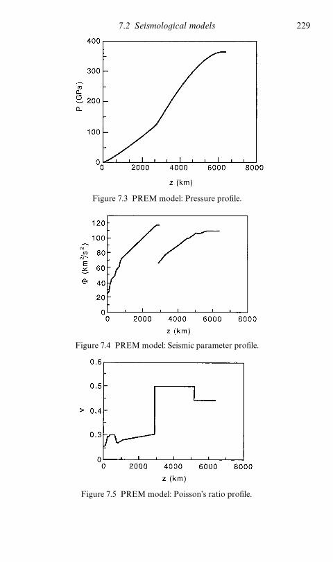
Figure 7.3 PREMmodel: Pressure profile.

Figure 7.4 PREMmodel: Seismic parameter profile.

Figure 7.5 PREMmodel: Poisson’s ratio profile.


presence of liquid: Some solidmetals, for instance, have very high Poisson’sratios, e.g. � 0.42 for gold and 0.45 for indium. Falzone and Stacey (1980)gave an explanation of the high Poisson’s ratio at high pressure in terms ofthe second-order theory of elasticity.

7.3 Thermal models

7.3.1 Sources of heat

For a discussion of the sources of heat and temperatures in the Earth, thereader will profitably refer to Verhoogen’s (1980) delightful and illumina-ting little book Energetics of the Earth.The heat flux coming from inside the Earth can be measured at the

surface; its mean value is about 80mW/m� or 4.2� 10��W (42TW) for thewhole Earth. This is, of course, a boundary condition for any thermalmodel but, to infer the temperature profile, onemust also have some idea ofthe sources of the heat that is transported through the mantle and finallyradiated out at the surface.Howmuch of the heat is original and howmuch is currently produced in

the Earth? In other words, is the Earth still cooling from an original hotstate, as was widely thought in the last century, or are there active sourcesof heat inside? We now know that radioactivity is the major heat source,but others may exist, and whether the Earth is still cooling is a matter ofcurrent debate. Let us briefly review the possible sources of heat.

(i) The original heat. This is the heat content of the Earth in the earlystages of its history. It is essentially accretional heat, due to the dissipationof the gravitational energy when planetesimals bombarded the surface ofthe growing Earth, which eventually partly melted. There was also acontribution of short-lived, now extinct, radioactive elements such as ��Al.During the differentiation stage that ensued, gravitational energy wasagain released when droplets of liquid iron or iron—sulfur eutectic trickleddown to form the core. It is generally thought that the core was formed in arelatively short time, ending about 0.5 billion (0.5� 10�) years after theformation of the Earth, the corresponding heat therefore can be said to be‘‘original’’. It is believed, although not universally, that the original heatcontributes little to the thermal budget, with the exception of the heatstored in the liquid core.

(ii) Radiogenic heat. Decay of the radioactive elements present in themantle is the main source of heat in the Earth. The principal radioactive

230 7 Earth models

elements are: ��U, ��U, ��Th whose decay eventually gives ��Pb,��Pb, ��Pb respectively, and ��K whose decay gives ��Ca and ��Ar. Theheat production per mass unit of each element is well known but theirconcentration in the Earth is much less certain. One estimate (Verhoogen,1980) leads to the approximate lower bound of 2.4� 10��W for the totalradiogenic production of heat in the mantle, i.e. about 60% at least of thetotal output of heat.

(iii) Other sources of heat. These include: tidal dissipation in the solidEarth, negligible at the present time, although it may have been importantin the past, when theMoonwas closer to the Earth; frictional dissipation inthe convecting mantle; and latent heat released in exothermal phase transi-tions (e.g. olivine—spinel). All these contributions are unimportant whencompared to that of radiogenic heat. However, in addition to the secularcooling of the core, a non-negligible contribution to the heat output of thecore is made by the latent heat released during crystallization of the innercore and by the gravitational energy released as the fluid enriched in lightelements by crystallization of the inner core rises.

N.B. The latent heat released during crystallization of the inner core isL � T

�S

�. With the values calculated by Poirier (1986) for the temperature of the

inner core boundary (T�

� 5000K) and the melting entropy (S�

� 5.83 J/molK)and taking a molar volume at the pressure of the inner core boundary of 4.38 cm�/mol and density of 12, we find: L � 5.55� 10� J/kg.

The heat flux from the core into the lower mantle is another boundarycondition of the convective problem. It is not known, but lower and upperbounds of its value can be estimated to be 1TWand 10TW, correspondingto 6mW/m� and 60mW/m�, respectively (see Buffett et al., 1992 andLabrosse et al., 1997). Verhoogen (1980) estimates that about 2.6TW comefrom the cooling of the whole core, 0.34TW come from the crystallizationof the inner core and 0.66TW correspond to the gravitational energy term.With these estimates, the total heat output of the core (input into the lowermantle) could be Q

�� 3.6TW, about 10% of the total heat output of the

Earth.

7.3.2 Heat transfer by convection

We have seen (Section 6.6) that, due to the opacity of the iron-bearingminerals under high pressure, radiative transfer of heat is most probablynegligible in the Earth’s mantle. The two remaining mechanisms for heattransfer are then conduction, consisting in heat transport by thermal

2317.3 Thermal models

Figure 7.6 Convective instability in a sheet of fluid heated from below. (a)Temperature profile. (b) The temperature profile is superadiabatic: a parcel of fluiddisplaced upward is lighter than the surrounding fluid and keeps going up(convective instability). (c) The temperature profile is subadiabatic: a parcel of fluiddisplaced upward is heavier than the surrounding fluid and falls back (stable

layering).

vibrations of the mineral lattices, and convection, in which the heat-containing matter is transported bodily in a fluid-like manner: On thetime-scale of the geophysical phenomena (e.g. plate tectonics) the mantlecan be considered as a fluid endowed with a very high viscosity (10��—10��Pa s).It is completely beyond the scope of this book to deal with the fluid

mechanics of convection. However, we will give the physical bases of theconvective phenomenon in the simpler case of a fluid heated from below ina gravity field (Rayleigh—Benard convection) (see Tritton, 1977; Turcotteand Schubert, 1982).Let us consider a laterally infinite layer of fluid of density � in the

gravitational field of the Earth, bounded by plane surfaces at r� 0 andr� h (Fig. 7.6(a)). The upper surface is maintained at a fixed temperatureT�, while the lower surface is maintained at T

�� T

�, thus establishing a

temperature gradient �T � (T�� T

�)/h through the fluid. Let us now

consider a small parcel of fluid at r� 0 and T � T�and let it rise rapidly by

�r. It undergoes an adiabatic decompression and its temperature is loweredby:

�T ��T��

�r (7.21)

where �T��

is the adiabatic gradient, given by (2.56). SincedP� �gdz��gdr, we have:

�T��

�dTdz

�g�TC

�

(7.22)

Note that we have:

232 7 Earth models

�T��

�g�

��

T (7.23)

where ��is the thermodynamic Gruneisen parameter and � the seismic

parameter; the adiabatic gradient in the lower mantle is about 0.3K/km.

• If the temperature gradient in the fluid is subadiabatic, i.e. �T � � T

�� (Fig. 7.6(c)), the parcel of fluid is cooler, hence denser, than the

surrounding fluid and sinks again. The fluid is stratified and stable withrespect to convection. Heat is transported by conduction and the heatflux (per unit time and area) is:

H�� k�T � k

T�� T

�h

(7.24)

where k is the thermal conductivity of the fluid.• If the temperature gradient in the fluid is superadiabatic, i.e. �T �

� T��

(Fig. 7.6(b)), the parcel of fluid is warmer and lighter than thesurrounding fluid, it is buoyant and will go on rising. The situation isunstable.

The criterion for the onset of convection is therefore that the tempera-ture gradient be superadiabatic, or that the Bullen parameter be smallerthan unity. The density of a fluid parcel displaced by �r upward is:� �r(d�/dr)

��, while the density of the surrounding fluid is � �r(d�/dr),

the gravitational force on the parcel is therefore:� g�r[(d�/dr)��

� (d�/dr)]and the equation of motion of the parcel is:

�d��r

dt� g�r��

d�dr�

��

�d�dr�� 0 (7.25)

The fluid parcel oscillates about its original position with the Brunt—Vaisala frequency N (see Tritton, 1977):

N��g

��d�dr�

��

�d�dr��

��(7.26)

The Brunt—Vaisala frequency can be related to the Bullen parameter �,by writing (7.26) as:

N��

g��

��

�g ��d�dr�

��

�d�dr�� 1 �

which yields:


N��g�

��

(�� 1) (7.27)

We see that, if the gradient is superadiabatic (�� 1), the frequency isimaginary and a convective instability sets in and can grow exponentially ifthe physical properties of the fluid (essentially its viscosity) are such as toallow convection. The condition �� 1 is necessary but not sufficient forconvection. A tighter criterion is given by the dimensionless Rayleighnumber Ra, defined, in the case of a fluid heated from below, by:

Ra�g�h�T

�(7.28)

In (7.28), � �/� is the kinematic viscosity of the fluid, � is its thermaldiffusivity, � its thermal expansion coefficient and T � T

�� T

�.

The Rayleigh number measures the relative importance of the buoyancyforce g�T, favoring convection, and the viscosity drag force ��V, hinder-ing convection:

Ra�g�T��V

(7.29)

If we scale velocity V to the value U, length to L and time to L/U, wehave: ��V �UL�� and � � L�(L/U)��UL, hence U��L�� and��V ��L��. Equation (7.29) is therefore equivalent to (7.28).In the case of a fluid heated from within, the Rayleigh number is (see

Turcotte and Schubert, 1982):

Ra�g��qh�

�k(7.30)

where k is the thermal conductivity of the fluid and q is the rate of internalheat production.A linear stability analysis shows that perturbations can grow exponen-

tially when the Rayleigh number is greater than the critical Rayleighnumber Ra

�. For fluids heated from below as well as from within,

Ra�� 2000.

N.B. Let us calculate an order of magnitude value for the Rayleigh number of theinternally heated Earth’s whole mantle, using values of the various parameters:

� � 4� 10�kgm��, �� 3� 10��K��, �� 0.01 cm� s��, �� 10��Pa s,g� 10ms��, � �/� � 3� 10��m� s��, h� 3000 km,

k� 4Wm��K��, q� 9� 10��Wkg��.

We find a Rayleigh number of about 2� 10�, considerably above the criticalvalue.

234 7 Earth models

TheNusselt numberNu, measures the thermal efficiency of heat transfer.It is equal to the ratio of the total heat fluxH to the heat flux that would betransported by conduction in the same conditions. With (7.24), we have:

Nu�Hh

kT(7.31)

For Ra�Ra�, we have Nu� 1.

In steady state, convection in a viscous fluid is controlled by the coupleddifferential equations for conservation of momentum and for transport ofheat:

�Dv

Dt��F (7.32)

DTDt

��T (7.33)

N.B. The symbol D/Dt represents the material (or convective) derivative, whichmust be used when considering the variation with time of a quantity y in a fluidmoving with a velocity v.

Dy

Dt�

�y�t

��

�y�x

�

�x�

�t�

�y�t

��

�y�x

�

v�

x�and v

�(i� 1, 2, 3) are the components of the position and velocity vectors

respectively. We can write:

Dy

Dt�

�y�t

v·�y

The term v·�y is called the advective term.

In the equation of conservation of momentum for a viscous fluid, theforces F to be taken into account are the force resulting from a pressuregradient and the force needed to overcome viscosity (see equation (6.18)).We can write (7.32) under the form known as Navier—Stokes equation:

�v

�t (v·�)v��

1

��P g ��v (7.34)

The heat transport equation in a convecting compressible fluid is foundby writing the continuity equation for heat:

�TdS

dT��·(k�T )H (7.35)


where S is the entropy and H the heat source.Using Table 1.2, we find:

dS

dT��

��dP

dTC

�TdTdt

(7.36)

and we can write:

�TdS

dT� � �T�

�P�t

v·�P��C��

�T�t

v·�T� (7.37)

Assuming �P/�t� 0, we have:

�TdS

dT��C

��T�t

v·��T ��T�C

�

�P�� (7.38)

and, with (7.35) and (7.22):

�C��

�T�t

v·(�T ��T��)�� ·(k�T )H (7.39)

In the case of vigorous convection, the term corresponding to thediffusion of heat, ��T, is negligible compared to the advective term,v·(�T ��T

��). The heat is transported with matter and has no time to

diffuse far. In the steady state, the temperature profile in the convectingfluid tends toward an adiabat.At the top and bottom of the convection cells, where heat is tranferred

into the convecting fluid or out of it, or between thermally coupled butisolated convecting systems, there must exist a thermal boundary layerthrough which heat is transferred by conduction and where the gradient ishighly superadiabatic.

7.3.3 Convection patterns in the mantle

Continental drift and plate tectonics are proof enough that the uppermantle convects. There is no direct evidence for convection in the lowermantle and it was thought for some time that the viscosity increase withpressure could be so high as to prevent convection (McKenzie, 1967). Thisview, which partly resulted from not taking into account the decrease ofactivation volume for creep with increasing pressure (see e.g. Poirier andLiebermann, 1984), is no longer currently entertained: TheRayleigh numb-er for the lower mantle is supercritical and the Bullen parameter is close to1 in most estimates. So, it is now generally agreed that the lower mantle is

236 7 Earth models

convecting, even though its viscosity may be one or two orders of magni-tude greater than that of the upper mantle.The controversy now centers, not on whether the lower mantle convects

or not, but on whether it convects together with the upper mantle (whole-mantle convection) or separately, with a thermal boundary layer at 670 km(two-layer convection).The arguments presented by each school of thought for their favorite

model and against the other one, are generally cogent and persuasive,which makes the question difficult to decide for an unprejudiced observer,all the more so since their proponents usually rely, perforce, on variousunverifiable assumptions and on the feeling that the opposite view wouldlead, in their opinion, to improbable values of parameters which are,anyway, very little constrained by observational data. Note also that manyof the arguments brought forward merely say that a given observation orcalculation is consistent with one style of convection but generally do notprove that another style is excluded.Reviewing the extant literature on convection, including the experimen-

tal and numerical models, could be the subject of a whole book. It willsuffice here to briefly present the pro and con arguments for the maincontending models and leave the reader to make up her or his own mind.Note that some authors use a temperature profile to defend a convectionstyle, while others posit a convection style to derive a temperature profile.Indeed, the two problems are so intimately linked that it is only for the sakeof convenience that we deal with them in different paragraphs.

(i) Two-layer convection. The principal arguments proposed are:

• The deepest earthquakes stop at 670 km and their focal mechanismsimply down-dip compression. It is therefore concluded that the subduct-ing plates cannot penetrate the lower mantle.

• The 670km discontinuity, in addition to being due to a phase transition,is also a compositional and/or chemical boundary (Liu, 1979). Thedensity and seismic velocities agree with a lower mantle richer in silica(Anderson and Bass, 1986; Duffy and Anderson, 1989) and/or richer iniron (D. L. Anderson, 1989a) than the upper mantle (see Section 7.4).

• The 670 km discontinuity is a sharp seismic reflector that cannot beproduced by a phase transition occurring over a wide depth interval,hence it must also be a chemical boundary (Lees et al., 1983).

• The mantle has the same composition throughout but the convectivesystems of the upper and lower mantle are isolated by the subductedlithosphere trapped between 600 and 700km (Ringwood and Irifune,


Figure

7.7Schem

atic

diagram

sof(a)whole-man

tlean

d(b)layeredconvectionmodels,withcorrespo

ndingtemperature

andviscosity

profi

les(after

Peltier

andJarvis,198

2).

1988; Ringwood, 1994). A chemically heterogeneous ‘‘mesosphereboundary layer’’ between upper and lower mantle could be the source ofthe Ocean Island Basalts (Allegre and Turcotte, 1987).

• The upper and lower mantle are two different geochemical reservoirsthat separately fractionated to produce the continental crust and thecore, respectively (Allegre, 1982, 1987).

• A thermal boundary layer inside the mantle is required in the thermalmodel, in order to avoid using an unreasonably high value of the heatflux from the core into the mantle (Jeanloz and Richter, 1979).

(ii) Whole-mantle convection. A number of arguments in favor of thismodel are negative, i.e. against the two-layer model: They contend eitherthat it is not required by the data (then, why not accept the simplersolution?) or that it would lead to unreasonable assumptions.

• A compositional difference between upper and lower mantle is notrequired (although not excluded) by the seismological data (Weidner,1986; Jackson, 1998).

• The analysis of travel-times of deep earthquakes shows that there arefast (colder) regions below 670km, in the prolongation of some subduct-ing slabs which are therefore thought to penetrate into the lower mantle(Creager and Jordan, 1986; Fischer et al., 1988). The seismically ob-served downward depressions of the 670 km discontinuity — ‘‘topogra-phy’’ of the discontinuity — (e.g. Wicks & Richards, 1993) can be inter-preted as resulting from horizontal deflection of the subducting plates(Shearer andMasters, 1992), inhibiting convection across the boundary,but they are too small to prevent whole-mantle convection (PhippsMorgan and Shearer, 1993).

• The seismic constraints on the sharpness of the 670 km discontinuity areweak (Muirhead, 1985).

• The post-spinel phase transition at 670km is sharp and could accountfor a good seismic reflectivity, a compositional difference between upperand lower mantle is not required (Ito and Takahashi, 1989).

• The existence of a thermal boundary layer at 670 km, where heat istransferred by conduction between the isolated convection cells, impliesa high temperature gradient, hence a temperature in the lower mantlehigher by about 800 °C than in the case of whole-mantle convection. Asthe lower-mantle viscosity is thermally activated, a higher temperatureimplies a viscosity of about 6� 10��Pa s for the lower mantle (Kenyonand Turcotte, 1983), whereas the viscosity deduced from post-glacialrebound is of the order of 10��Pa s (Peltier and Jarvis, 1982) (Fig. 7.7).


Note, however, that in the absence of experimental data on the high-temperature creep of the lower-mantle material, any kind of extrapo-lated or otherwise calculated viscosity of the lower mantle is largely amatter of personal choice.

• Three-dimensional spherical models of whole-mantle convection (Ber-covici et al., 1989) predict upwelling plumes and downwelling sheetsclosely resembling the circum-Pacific subduction ring (but so wouldpresumably 3-D models of two-layer mantle convection). Indeed, seis-mic tomography of the lower mantle shows a ring of high-velocitymaterial, which projects to the surface as a circum-Pacific ring andmight be the continuation of the subducting slabs (Olson et al., 1990;Fukao, 1992; van der Hilst et al., 1997).

Interesting observations of strong correlations between the geoid, thesurface topography and the seismic velocity anomalies in the lower mantlehave recently been presented (Hager et al., 1985; Cazenave et al., 1989); thegeoid anomalies observed at the surface result from interior density con-trasts (hot and cold matter) driving the convective flow and from thedeformation of the boundaries caused by the flow. The magnitude and signof the total effect depend on the viscosity profile and the style of convection.However, although the results of the analyses are compatible with one styleof convection, they are not incompatible with the other.

• Finally, the study of the nature and composition of inclusions in somediamonds suggests a deep origin, possibly from the lower mantle (Kes-son and Fitz Gerald, 1991; Kerr, 1993; McCammon et al., 1997).

(iii) ‘‘Middle of the road’’ convection. Christensen (1984, 1995) modeledseveral types of convection and showed that ‘‘with the present uncertaintiesabout the 670km discontinuity a variety of convection styles are possible’’.He noted in particular that a phase-transition boundary alone couldmarginally produce a kind of leaky two-layer convection for current valuesof the Clapeyron slope, not significantly different from the most recentexperimental value of � 3MPa/K (Ito and Takahashi, 1989). The influ-ence of an endothermic phase transition at 670km was further modeled byMachetel and Weber (1991) and Tackley et al. (1993), who found thatdownwelling cold material could accumulate above the discontinuity andbe discharged at intervals, as avalanches into the lower mantle (see alsoRingwood, 1991).The seismic evidence that some plates penetrate into the lower mantle is

now well accepted. Seismic tomography (see Montagner, 1994) provides a

240 7 Earth models

rather convincing picture of the lowermantle (e.g. van derHilst et al., 1997),and improved 3-D computer modeling points to avalanches through the670km discontinuity. As a result, the style of convection of the mantle isnow generally seen as intermediate between two-layer and whole-mantleconvection: spatially non-uniform and temporally intermittent (Kerr, 1992,1997). Some, but not all, plates, could sink down into the lower mantlethrough the 670km discontinuity. Some cold material could accumulateabove the discontinuity and intermittently go down in avalanches.To reconcile the geochemical and seismological view points, Allegre

(1997) proposes a time-dependent model of convection. Up to one billionyears ago, two-layer convection would have taken place, with little ex-change of matter between upper and lower mantle, then the convectionpatternwould have broken down, allowing some whole-mantle convectioncells.

7.3.4 Geotherms

Temperature profiles (geotherms) are usually anchored at the depths ofseismic discontinuities identified with phase transitions whose P,T bound-aries are experimentally known or extrapolated. The principal discontinui-ties used are: the inner-core boundary (ICB), identified with the freezing ofthe liquid core iron alloy; and the 670km discontinuity, identified with thepost-spinel transition. Starting from these anchoring points, the geothermsfollow an adiabat in the homogeneous regions where the Bullen parameteris close to 1 (lower mantle and outer core), the adiabatic gradient oftenbeing determined using a value of the acoustic Gruneisen parameter com-patible with a seismological Earth model. The uncertainty is seldom claim-ed to be less than a few hundred degrees and often is of the order of 1000K.The temperatures at various characteristic depths, determined in severalstudies, are given in Table 7.1 and the geotherms are shown in Fig. 7.8 (seealso Duffy and Hemley, 1995).In the lithosphere, the geotherm is often derived from pyroxene ther-

mobarometry measurements made on peridotite xenoliths (e.g. Mercier,1980).In the transition zone, themost recent estimates using the phase diagram

of the system Mg�SiO

�—Fe

�SiO

�(Ito and Katsura, 1989) give a tempera-

ture of 1400 °C at 350km and of 1600 °C at 655 km.In the lower mantle, Shankland and Brown (1985), starting from the

temperature at 670 km (1600 °C) and using a seismological adiabatic gradi-ent, arrive at a temperature of 3300 °C on the outer-core side of the


Table 7.1. Temperatures inside the Earth (in Kelvin)

z (km) W72 V80 BS81 A82 SS84 BM86 P86 W87 IK89

100 1273 1450150 1473350 1400371 1662655 1600671� 1873 1830 1970671 1980 23001300 28002571 3300 28142885� 2773 2937 30002886 3573 3637 3800 3800 38005156 4676 5000 5000 5000 66006371 4805 5000 6600

Source: W72: Wang (1972b). V80: Verhoogen (1980). BS81: Brown and Shankland(1981). A82: O. L. Anderson (1982). SS84: Spiliopoulos and Stacey (1984). BM:Brown and McQueen (1986). P86: Poirier (1986). W87: Williams et al. (1987a).IK89: Ito and Katsura (1989).

core—mantle boundary (CMB), in agreement with the temperature derivedfrom their measurements of shock melting in iron, provided one assumesthat the D" zone at the base of the mantle is a thermal boundary layer withT � 800K. Under these conditions, they do not find it necessary tointroduce a thermal boundary layer at 670 km.Spiliopoulos and Stacey (1984) start upward from the temperature at the

inner-core boundary, using T � 800K in the D" zone, and meet, at670 km, a profile extrapolated down from the Mg

�SiO

�phase transition.

The temperature misfit of 300K which they find is thought to be too smallfor a thermal boundary layer to be stable. They conclude that there isprobably no boundary layer at 670 km, although it cannot be ruled out.A temperature difference of 800K across the D" zone corresponds to a

gradient of 8K/km over 100km; this usually adopted value is derived fromFourier’s law assuming a heat flux from the core of 0.032W/m� and athermal conductivity of the lower mantle k� 4W/mK. Brown (1986),taking into account the variation of k with temperature and pressure, findsthat it could be three times larger than the currently adopted value at thecore—mantle boundary, and that the need for a thermal boundary layer atthe base of the mantle then disappears, unless one assumes an unrealisti-cally high value for the heat flux from the core (higher than the heat flux atthe surface of the Earth). Note, however, that there is a trade-off between

242 7 Earth models

Figure

7.8Geotherms.Forallthesetemperature

profiles,theerrorbar

isab

out�

800K.

the thermal boundary layers at 670 km and at the core—mantle boundaryand that the geotherms, estimated assuming a homogeneous mantle, can-not really be used as arguments for or against whole-mantle or two-layerconvection.Despite the large uncertainty on the temperatures, mostmodels, whether

based on theoretical calculations (Poirier, 1986; Poirier and Shankland,1993) or extrapolations of the melting temperature of iron at the inner-coreboundary (O. L. Anderson, 1982; Spiliopoulos and Stacey, 1984; Brownand McQueen, 1986; Anderson and Duba, 1997) generally agree on atemperature at the inner-core boundary between 5000K and 6000K (seeSection 5.6).

7.4 Mineralogical models

7.4.1 Phase transitions of the mantle minerals

(i) Generalities on phase transitions

Nature’s schemes for building up crystalline edifices from atoms are many,and compounds with a given crystal structure are generally stable only in alimited region of the temperature—pressure plane, where their Gibbs freeenergy is minimal. Even a simple element like iron has four known solidphases and the number of structures a polyatomic mineral can adopt atvarious pressures and temperatures can indeed be very large, especially ifone considers the additional degree of freedom afforded by the possibilityof partial replacement of one kind of atom by another (e.g. Mg by Fe, Si byAl, etc.). Descriptions of the atomic architecture of mineral structures canbe found in the specialized volumes of theReviews inMineralogy or in suchbooks as Wells (1984) or Muller and Roy (1974) for ternary oxides.The number of thermodynamic degrees of freedom of a system (or

variance) is the number of intensive parameters capable of independentvariation. It is given by the Gibbs phase rule (see Callen, 1985):

V� c 2�� (7.40)

whereV is the variance, c, the number of independent components, and �,the number of phases in equilibrium.In the simplest case of one-component systems, when the only intensive

variables are temperature and pressure, the equilibrium between twophases is univariant and the domains of stability of two phases in the P—Tplane are separated by a line boundary, i.e. the equilibrium pressure andtemperature cannot be varied independently. The map of the stability

244 7 Earth models

Figure 7.9 Lever rule: At T � T�and P�P

�and for a compositionC, for example

x mol% of component B, the mole fraction x� of high-pressure phase �, ofcomposition C�, and the mole fraction x� of low-pressure phase �, of composition

C�, are in the proportion x�/x� � bc/ab.

domains of the phases in the P—T plane is the phase diagram. For binary(two-component) systems, one usually considers sections of the three-dimensional phase diagram by planes of constant T or P. The phase-diagram boundaries are replaced by two-phase loops and at a given P (orT), for a given global composition, there are equilibrium mixtures of twophases. The proportion of the phases varies with T (or P) and is given bythe ‘‘lever rule’’ (see Callen, 1985) (Fig. 7.9). The case of ternary systems isobviously more complicated and one often uses ‘‘pseudo-binary diagrams’’(e.g.P, Fe%at constantT, between the compositionsMgSiO

�and FeSiO

�in the ternary systemMgO—FeO—SiO

�). One must of course beware not to

reason on pseudo-binary diagrams as if they were binary diagrams.Phase transitions can be usefully classified according to their order in

Ehrenfest’s sense (see Rao and Rao, 1978). For first-order transitions, thereis a discontinuity in the first derivatives of the Gibbs free energy: entropy Sand specific volume V. Hence, first-order transitions are accompanied by avolume change V and latent heat L � TS is absorbed (endothermaltransition) or evolved (exothermal transition).The slope of the phase boundary is given by the Clausius—Clapeyron

relation (5.2):

dT�

dP�

VS

(7.41)


already mentioned in the case of melting (melting is a first-order phasetransition). Here, T

�is the temperature of transition at pressure P.

The specific volume of the high-pressure phase is always smaller thanthat of the low-pressure phase, and the high-temperature phase always hasa higher entropy than the low-temperature phase. In many cases, thehigh-pressure phase has a lower entropy than the low-pressure phase andits stability field is wider at low temperatures, i.e. the slope of the Clapeyronis positive. However, at very high pressures, when the increase of thecoordinance of the small cations (e.g. silicon going from 4 to 6 coordinance)is accompanied by an increase in the length of certain bonds, the transitiontoward the high-pressure phase may be accompanied by an increase inentropy. The slope of the Clapeyron is then negative. This was predicted byNavrotsky (1980) and verified in the case of the very-high-pressure phasesof the mantle silicates (see below).In a first-order phase transition, the phases are physically separated by a

surface of discontinuity: the phase boundary. In many cases, the transform-ation operates by nucleation and growth of one phase at the expense of theother, growth being effected by diffusion-controlled displacement of thephase boundary.Martensitic transformations are rapid, diffusionless transformations

characterized by crystallographic orientation (topotactic) relations be-tween parent and daughter phase and corresponding to a shear of thelattice.For second-order phase transitions, the discontinuity in the derivatives

of the Gibbs free energy affects only the second derivatives (e.g. specificheat, incompressibility) and there is no coexistence of phases on each sideof a phase boundary. These transitions are often displacive transitions, thechange in crystal structure corresponding to a mere distortion of thebonds, whereas in reconstructive first-order transitions atoms have tochange places.For more information on the mechanisms and kinetics of phase transi-

tions inminerals, the reader is referred to Putnis andMcConnell (1980) andPutnis (1992). The phase diagrams of elements, oxides and silicates havebeen reviewed by Liu and Bassett (1986).In the following sections, we will summarize the state of the art concern-

ing the experimental data on the principal isochemical phase transitionsthought to occur in the Earth’s mantle, particularly focusing on the poly-morphic transitions of MgSiO

�and Mg

�SiO

�. Most of the progress in

recent years (see Akimoto, 1987) has been achieved using two high-pressuretechniques: the multi-anvil apparatus, up to about 25GPa and the laser-

246 7 Earth models

Figure 7.10 Principle of the diamond—anvil cell. The sample (stippled) is containedin a small hole (200—400�m) drilled in a metal gasket, compressed by the diamonds.

It can be heated by focusing a laser beam on it.

heated diamond-anvil cell (Fig. 7.10), up to 100GPa (Ming and Bas-sett,1974; Bassett, 1977; Hemley et al., 1987a).

(ii) The phase transitions of MgSiO3

The phase diagram of MgSiO�has been investigated by Ringwood (1967),

Liu (1976), Ito and Yamada (1982), Ito and Navrotsky (1985), Kato andKumazawa (1985a), Sawamoto (1987), Irifune (1987), Akaogi et al. (1987)and Ito and Takahashi (1989) among others. The resulting phase diagramin the P—T plane (D. L. Anderson, 1987b) is shown in Fig. 7.11, and thepseudo-binary diagram at 1000 °C (Jeanloz and Thompson, 1983) is givenin Fig. 7.12.The low-pressure phase with composition MgSiO

�is enstatite, an or-

thorhombic pyroxene with two formula units per unit cell (Mg�Si

�O

�); its


Figure 7.11 P—T phase diagram for MgSiO�composition. The approximate

velocity of P-waves (in km/s) is indicated below the names of themineral phases. Thearrows show the direction in which the phase boundaries are expected to move

when Al�O

�is added (after D. L. Anderson, 1987b).

structure can be described as consisting of chains of corner-sharing SiO�

tetrahedra, with Mg�� cations in the appropriate sites between the chains.Enstatite forms a continuous solid solution with the pyroxene ferrosiliteFeSiO

�. The upper-mantle material, found in peridotite xenoliths or in

ophiolites has a composition Mg��

FeSi

�O

�, with x� 0.1 in most cases.

At higher pressures, the orthorhombic enstatite changes to monoclinicclinoenstatite. At pressures between about 17 and 19GPa and above about2000K, the pyroxene transforms into a phase with a garnet structure(isolated tetrahedra) and 4 formula units per unit cell (Mg

�Si

�O

��). The

aluminous garnet pyrope has a formula (Mg�Al

�Si

�O

��) resulting from the

replacement of one Si�� ion by one Al�� ion and compensating the chargeimbalance by replacing oneMg�� by one Al��. At upper-mantle pressures,pyrope is soluble in the silicate garnet, giving the aluminous silicate garnetmajorite, first identified in shocked meteorites and later synthesized byRingwood and Major (1971). Alumina (Al

�O

�) widens the garnet stability

field (Fig. 7.11). At pressures above about 20GPa and temperatures lowerthan about 2000K, MgSiO

�garnet transforms into a phase with the

ilmenite structure (Liu, 1976), that can be described as a corundum (Al�O

�)

structure with Mg�� and Si�� located in an ordered alternate fashion inthe six-coordinated Al�� sites. At lower-mantle pressures, the silicate

248 7 Earth models

Figure 7.12 Isothermal (T � 1000 °C) phase diagram for the MgSiO�—FeSiO

�system. The crystalline structures are Cpx (clinopyroxene), � (�-phase), � (�-spinel),Mw (magnesiowustite), St (stishovite), Pv (perovskite) (after Jeanloz and Thompson,

1983).

ilmenite transforms into a phase with the perovskite structure (Fig. 7.13),that can be described as a 3-D framework of corner-sharing SiO

�oc-

tahedra, with Mg�� in the dodecahedral sites. The slope of the Clapeyron,in the range 1000—1600 °C for the ilmenite—perovskite transition is nega-tive, and is given (Ito and Takahashi, 1989) by: P[GPa]� 26.8�

0.0025T [°C].The existence of the perovskite phase was proved experimentally by Liu,

who synthesized it in the diamond-anvil cell, first from pyrope (Liu, 1974),then by decomposition of Mg

�SiO

�at high pressure (Liu, 1975a).

(Mg,Fe)SiO�perovskite is probably the most abundant mineral in the

Earth, since it constitutes possibly more than 80 vol.% of the lower mantle.It is orthorhombic, at least up to 100GPa at room temperature, with astructure derived from the ideal cubic perovskite by tilting of the octahedra


Figure 7.13 Structure of MgSiO�perovskite. The Mg cations are in dodecahedral

sites between tilted corner-sharing SiO�octahedra. (The oxygen ions at the corners

and the silicon ions at the centers of octahedra are not represented.)

(see Fig. 7.13) (GdFeO�distortion, see Muller and Roy, 1974). Measure-

ment of the evolution of the distortion of the analog oxide perovskitesSrZrO

�led to the suggestion that MgSiO

�perovskite might become cubic

at mantle pressures (Andrault and Poirier, 1991). The high density of twinsobserved by electron microscopy in (Mg,Fe)SiO

�perovskite quenched

from high temperature might also point to the existence of a cubic phase athigh temperature (Wang et al., 1992). However, X-ray observation ofMgSiO

�perovskite at 36GPa and 1900K showed that it remained orthor-

hombic (Funamori and Yagi, 1993), in agreement with ab-initio electronicstructure calculations (Stixrude and Cohen, 1993; Wentzcovitch et al.,1995). Meade et al. (1995) found experimentally that (Mg, Fe)SiO

�perov-

250 7 Earth models

skite at 1850K does indeed stay orthorhombic at 38GPa, but becomescubic at 64 and 70GPa.FeSiO

�cannot take the perovskite structure, and above a certain con-

centration of iron, depending on temperature (see Fig. 7.12), (Mg, Fe)SiO�

perovskite decomposes into stishovite SiO�

and magnesiowustite(Mg,Fe)O. Aluminum in solution in (Mg,Fe)SiO

�perovskite expands its

compositional stability field toward greater iron concentrations, up to90mol% of the ferrous end member for 25mol% Al

�O

�in solution (Kes-

son et al., 1995).The question arises whether perovskite remains stable in the lower

mantle or decomposes to mixed oxides (which, incidentally, was thecommonly accepted view before perovskite was identified as the high-pressure phase of enstatite). Indeed, (Mg,Fe)SiO

�perovskite heated for

more than one hour at 70GPa decomposes into stishovite and mag-nesiowustite (Meade et al., 1995). Saxena et al. (1996) found that, atpressures from 58 to 85GPa and temperatures from 1900 to 3200K, evenironless MgSiO

�perovskite breaks down to a mixture of periclase and

stishovite. However the consensus is far from being reached, as otherexperiments up to 135GPa and 3000K show that (Mg, Fe)SiO

�perovskite

remains stable (Serghiou et al., 1998; Kesson et al., 1998).The principal physical properties of silicate perovskite, insofar as they

have been experimentally determined, are listed in Table 7.2. The densityand the equation of state parameters K

�and K�

�are reasonably well

known, having been determined by several investigators. Values of thethermal expansion coefficient are given in Table 3.4. Melting of perovskitehas been discussed in Section 5.5.1.Phases with perovskite structure have also been found at high pressures

for CaSiO�(Liu and Ringwood, 1975), diopside CaMgSi

�O

�, and diop-

side—jadeite solid solutions (CaMgSi�O

�—NaAlSi

�O

�) (Liu, 1987). There is,

however, no high-pressure phase with perovskite structure for the compo-sition FeSiO

�, which decomposes into FeO and stishovite SiO

�(Fig. 7.12).

(iii) The phase transitions of Mg2SiO4

Olivine (Mg��

Fe)�SiO

�is an important, possibly dominant, mineral of

the upper mantle (with x� 0.1). The magnesian end member Mg�SiO

�,

forsterite forms a continuous series of solid solution with fayalite Fe�SiO

�.

The orthorhombic olivine structure can be described as a slightly distortedhexagonal close-packed (hcp) sublattice of oxygen ions, with the siliconions occupying one-eighth of the tetrahedral sites and forming isolatedSiO

�tetrahedra, and theMg or Fe ions occupying one-half of the octahed-


Table 7.2. Physical properties (experimental) of MgSiO�perovskite

ExperimentalPhysical property value Reference

Cell dimensions (Å) a� 4.7787 Ito & Matsui (1978)b� 4.9313 Ito & Matsui (1978)c� 6.9083 Ito & Matsui (1978)

Specific mass (g/cm�) 4.108 Ito & Matsui (1978)Mean atomic mass (g/atom) 20.08 Ito & Matsui (1978)Molar volume (cm�/mol) 24.4426 Ito & Matsui (1978)K

�(GPa) (Hill) 246.4 Yeganeh-Haeri et al. (1989)

K��

3.9 Knittle et al. (1987)��(GPa) (Hill) 184.2 Yeganeh-Haeri et al. (1989)

v�(km/s) 10.94 Yeganeh-Haeri et al. (1989)

v (km/s) 6.69 Yeganeh-Haeri et al. (1989)

��(spectro) 1.9 Williams et al. (1987)

T�(K) (at 22GPa) 3000 Heinz & Jeanloz (1987)

� (K��) (298—840K) 4� 10�� Knittle & Jeanloz (1986)(298—341K) 2.2� 10�� Ross & Hazen (1989)

ral sites. Alternatively, the structure can be considered as that of anintermetallic compound Mg

�Si (with the Ni

�In structure), stuffed with

oxygen ions (O’Keefe and Hyde, 1981).High-pressure phases of the ferromagnesian olivines were first syn-

thesized by Ringwood andMajor (1966, 1970) and Akimoto and Fujisawa(1966). Fayalite directly transforms into the spinel structure, still withisolated SiO

�tetrahedra, but with a face-centered-cubic packing of oxy-

gens. Forsterite and Mg-rich olivines first transform to an orthorhombicphase with face-centered-cubic (fcc) packing of oxygens, where the SiO

�tetrahedra are linked in pairs by a corner. This phase is called �-phase (� isolivine and � is spinel) or ‘‘modified spinel’’. The P—T phase diagram of theMg

�SiO

�polymorphs, constrained by thermochemical data (Akaogi et al.,

1984) is given in Fig. 7.14 and the pseudo-binary diagram of Mg�SiO

�—

Fe�SiO

�(Akaogi et al., 1989) in Fig. 7.15 (see also Katsura and Ito, 1989).

Natural high-pressure spinel phase or ringwoodite, was found in shockedchondritic meteorites (Binns et al., 1969) and unambiguously identified bytransmission electron microscopy by Putnis and Price (1979) and Poirierand Madon (1979). The high-pressure �-phase (wadsleyite) was also foundin shocked chondrites (Price et al., 1983; Madon & Poirier, 1983).The mechanism of the olivine—�-spinel transformation in silicates and

analog germanates has been much investigated in recent years. Since theoxygen sublattice goes from hexagonal close packed in olivine to face-centered cubic in spinel, Poirier (1981a,b) proposed that, by analogy with

252 7 Earth models

Figure 7.14 P—T phase diagram for the Mg�SiO

�polymorphs (�: olivine, �:

modified spinel phase, �: spinel). Solid lines from Akaogi et al. (1984), dashed linesfrom Suito (1977) (after Akaogi et al., 1984).

other hcp—fcc transformations, olivine could transform to �-spinel by shearrestacking of oxygen ions due to invasion of the grains by stacking faults,the cations falling simultaneously into their new sites by ‘‘synchroshear’’.This ‘‘martensitic-like’’ mechanism was indeed found to be operative inexperiments conducted in diamond-anvil cells (Lacam et al., 1980; Furnishand Bassett, 1983; Boland and Liu, 1983), although there exists an inter-mediate stage, where the cations are disordered, thus ruling out syn-chroshear (Furnish and Bassett, 1983). However, in experiments conductedin large-volume apparatus, the transformation was found to take place bynucleation and growth (Boland and Liebermann, 1983; Vaughan et al.,1982) with no cation disordering (Yagi et al., 1987), although disorderingwas found in experiments conducted in a belt-type apparatus (Lauterjungand Will, 1986).Using multi-anvil apparatus and transmission electron microscopy to

study the olivine—�-phase transition in forsterite, Fujino and Irifune (1992)found that it occurred by nucleation and growth, and Guyot et al. (1991)observed an intermediate phase filled with stacking faults destroying thecation long-range order. Brearley et al. (1992) and Rubie and Brearley


Figure 7.15 Isothermal (T � 1600 °C) calculated phase diagram for the Mg�SiO

�—

Fe�SiO

�system. The crystalline structures are � (olivine), � (�-phase), � (�-spinel).

The boundaries determined experimentally byKatsura and Ito (1989) are shown bydashed curves (after Akaogi et al., 1989).

(1994) showed that, although the �—� transition occurs by nucleation andgrowth, the reverse tranformation occurs by a shear mechanism. Kubo etal. (1998) directly studied the kinetics of the transformation by X-raydiffraction using synchrotron radiation.Kerschhofer et al. (1996) observed two competing mechanisms in the

transformation of (Mg��

Fe��

)�SiO

�olivine: incoherent nucleation on

olivine grain boundaries and coherent intracrystalline nucleation of ring-woodite lamellas on shear-induced stacking faults on (100) planes (inagreementwith Poirier, 1981b), followed by nucleation of wadsleyite on theringwoodite.Burnley and Green (1989) suggested that the ‘‘martensitic-like’’ mechan-

254 7 Earth models

ism for the olivine—spinel transition occurs only for experiments conductedunder large shear stresses, as is the case for the diamond-anvil cell. How-ever, experiments conducted in a large-volume press on the analogMgGeO

�showed that the transformation occurs by nucleation and

growth near the Clapeyron and by ‘‘martensitic-like’’ shear restacking ofthe oxygen ions at high overpressures (Burnley, 1995). Indeed, the fact thatthe ‘‘martensitic-like’’ mechanism is observed in experiments conducted indiamond-anvil cells but usually not in a multi-anvil apparatus may be dueto the fact that in the latter type of experiments, the pressure and tempera-ture paths make it easy to perform runs close to the Clapeyron, whereas inthe diamond-cell the high pressure must be applied before laser-heating,producing a very high overpressure and a high effective stress on thedislocations responsible for the shear of the lattice (Poirier, 1982).The seismic discontinuity at 670 km has been, for a long time, attributed

to the transformation of (Mg, Fe)�SiO

�to denser post-spinel phases. It was

first believed that spinel transformed to a mixture of magnesiowustite(Mg,Fe)O and stishovite, the high-pressure phase of quartz, where siliconis in SiO

�octahedra (‘‘mixed oxide’’ lower-mantle models). Ming and

Bassett (1975) indeed found that the X-ray diffraction patterns of thedisproportionated phase were consistent with the mixed-oxidemodels. Liu(1975a), however, conclusively showed that the post-spinel phases were amixture of magnesiowustite and the perovskite phase (Mg, Fe)SiO

�:

(Mg, Fe)�SiO

�� (Mg,Fe)O (Mg,Fe)SiO

�

Observations by analytical electron microscopy (Guyot et al., 1988b; Ma-don et al., 1989b) give direct evidence of the validity of this disproportiona-tion reaction. At high iron contents, however, (higher than those currentlyadmitted for the lower mantle) the perovskite is not stable and the dispro-portionation indeed leads to a mixture of magnesiowustite and stishovite.The pressure interval within which the decomposition takes place

(‘‘sharpness’’ of the transition) has long been a subject of controversy,bearing on the problem of the composition of the lower mantle (e.g. Lees etal., 1983). Ito and Takahashi (1989) found that magnesian spinel with lessthan 26 at.% Fe dissociates within a very narrow pressure interval(0.15GPa at 1600 °C), thus buttressing the view that the transition is quitesharp (Fig. 7.16). The negative Clapeyron is given by: P[GPa]�

27.6� 0.0028T [°C]. Calculation of the phase boundaries using thermo-dynamic data by Akaogi et al. (1998) confirms the results of Ito andTakahashi (Figs. 7.17 and 7.18). However, a determination of the post-spinel phase boundary by synchrotron X-ray diffraction under pressure


Figure 7.16 Isothermal (T � 1600 °C) phase diagram for the post-spinel transform-ation in the Mg

�SiO

�—Fe

�SiO

�system. Note that the spinel (Sp) transforms to

perovskite (Pv) and magnesiowustite (Mw) over a narrow pressure interval; Stindicates stishovite (after Ito and Takahashi, 1989).

and temperature (Irifune et al., 1998) yields a boundary located at 21.1GPaat 1600 °C, about 2GPa lower than previous estimates.Iron does not disproportionate equally between magnesiowustite and

perovskite and goes preferentially into magnesiowustite (Bell et al., 1979;Ito et al., 1984). The partition coefficient of iron can be written:

K��x��x��x��x��

where x is the Fe or Mg content of the phases, given in at.%. Guyot et al.(1988b) have measured the value of K as a function of pressure by analyti-cal transmission electron microscopy and found that it decreases withincreasing pressure and remains constant (K� 3.5) at pressures above40GPa (Fig. 7.19). For the starting material used, it corresponds to thereaction:

(Mg��

Fe��

)�SiO

��Mg

��Fe

��SiO

�Mg

��Fe

��O

More recent measurements by analytical transmission electron micro-

256 7 Earth models

Figure 7.17 Isothermal (T � 1600 °C) phase diagram of systemMg�SiO

�—Fe

�SiO

�system. The phase boundaries were calculated from experimental data (after Akaogiet al., 1998).

scopy (Martinez et al., 1997) yielded a value of K� 3.8� 0.3 at 26GPaand 1300 °C and K� 4.3� 0.4 at 26GPa and 1600 °C.The partitioning of iron between magnesiowustite and perovskite de-

pends on the alumina concentration in the perovskite. It as been shownthat in presence of alumina, iron enters perovskitemore readily (Wood andRubie, 1996). As a result of the dissolution of aluminous garnet intoperovskite, mantle perovskite can contain up to 9wt% Al

�O

�. The

measurements of Wood and Rubie suggest that, in the lower mantle,perovskite might contain as much iron as magnesiowustite. The stabilitylimit of Fe in perovskite increases as temperature and pressure increase(Mao et al., 1997) and perovskite can accept Fe�� in larger concentrationsthan Fe��. As a higher proportion of the iron in perovskite tends tobecome ferric in the presence of aluminum (McCammon, 1997), it seems


Figure 7.18 CalculatedP—T phase diagramof (Mg��

Fe��

)�SiO

�(after Akaogi et

al., 1998).

Figure 7.19 Variation with pressureP of the partition coefficientK of iron betweenmagnesiowustite and perovskite. The error bars on the measurements are shown in

the upper right-hand corner (after Guyot et al., 1988b).

258 7 Earth models

reasonable to believe that the perovskite of the lower mantle is richer iniron than the perovskite prepared experimentally by disproportionation ofolivine.The structure of the disproportionated mixture of magnesiowustite and

perovskite was investigated as a function of T and P by transmissionelectron microscopy of metastable quenched samples recovered from thediamond-anvil cell (Guyot et al., 1988b; Madon et al., 1989b). Wang et al.(1997) and Martinez et al. (1997) also used transmission electron micro-scopy to observe the resulting product of disproportionation of olivine;their observations led them to suggest a two-step mechanism for thetransformation, involving first the formation of ringwoodite by shear,followed by break-down to magnesiowustite and perovskite.

7.4.2 Mantle and core models

(i) Constraints and trade-offs

The compositional Earth models are usually patterned after the descrip-tion of rocks by petrographers: For each region of the mantle, one mustknow the ‘‘norm’’ i.e. the chemical composition expressed in weight % ofoxides and the ‘‘mode’’ i.e. the proportions of the various constituentminerals.Compositional models are bound by different types of constraints:

• They are required to agree as much as possible with the seismologicalmodels, i.e. they must account for the velocity and density profiles. Thisof course implies that the P—T phase diagrams for the candidate compo-sitions are known and that the equations of state, elastic moduli andthermal expansion coefficients, as well as their temperature and pressurederivatives, are known for the relevant minerals. A geotherm must bechosen.

• The starting normative composition is usually chosen on the basis ofassumptions about the primitive bulk Earth composition and the chemi-cal evolution of the Earth.

• Compositional models are often more or less openly tailored to fit othergeophysical requirements: e.g. whole-mantle convection (hence chemi-cally homogeneous mantle) or two-layer convection (hence possibilityfor the upper and lowermantle to be chemically different). Note that thisalso conditions the choice of the geotherm.

The construction of a compositional model usually follows one of twolines:


(i) The actual density and elastic moduli (often only the bulk modulus) atdepth are adiabatically extrapolated to zero pressure and broughtdown from the final temperature to room temperature. A mineralassemblage is devised so that its density and aggregate elastic proper-ties fit the decompressed material.

(ii) A mineral assemblage at room temperature and ambient pressure isdevised so that after heating and adiabatically compressing it, itsdensity and seismic velocities (often only the bulk velocity) fit theseismological model.

In both cases, the elastic moduli of the high-pressure phases and theirpressure and temperature derivatives, either have been measured at ambi-ent pressure in the metastable state, or, at any rate, have been estimatedfrom elastic systematics. The thermal expansion coefficients often areestimated.Most of the discrepancies between contending compositional Earth

models come from one of two sources.

(i) The models use different assumptions as to the primitive bulk Earthcomposition and its evolution. It is generally assumed that the primitivecomposition of the bulk Earth (and terrestrial planets) is that of thedevolatilized solar nebula (Hart and Zindler, 1986). Now, the problem is todecide what was the composition of the original solar nebula and to whatdegree it has lost volatile elements. It is currently thought that the solarabundance of refractory elements is well reflected in the composition of theCI chondrites, meteorites that have not been differentiated and are con-sidered as samples of the primitive nebular material (Anders and Grevesse,1989). The composition of the primitive upper mantle, however, derivedfrom the study of mantle peridotites, corresponds to a smaller Mg/Si ratiothan that of the chondrites; it has been proposed that theMg/Si ratio of theterrestrial planets is more representative of the solar nebula value than thatof the CI chondrites (Ringwood, 1989).If one believes that the bulk Earth is nevertheless chondritic, one is

drawn to the conclusion that themissing silicon is hidden away in the lowermantle and/or core and the resulting compositional models are calledchondritic Earth models (e.g. Liu, 1982; D. L. Anderson, 1984; Andersonand Bass, 1986). In these models, the lower mantle is more silica-rich thanthe upper mantle and can be composed almost entirely of (Mg, Fe)SiO

�perovskite, thus leading to a two-layer convection pattern.One can also solve the case of the missing silicon by assuming that this

260 7 Earth models

element, less refractory than calcium and aluminum, was partly volatilizedaway. The mantle then need not be chemically heterogeneous and whole-mantle convection is not precluded (although not required). The mostpopular model of a homogeneous mantle is the pyrolite model (see Ring-wood, 1979): The bulk composition of the mantle is that of ‘‘pyrolite’’, anon-specific olivine—pyroxene rock, capable of yielding a basaltic magmaand a peridotite residue upon partial melting in the uppermost mantle.Pyrolite is a fictitious rock in that it is defined by its chemical composition(norm) only and not by its mineralogy (mode).D. L. Anderson (1989a), using new estimates of the solar composition,

proposed that the Sun should be richer in iron and calcium than the CIchondrites. If the bulk Earth composition is solar, it then should be richerin iron and calcium than the chondritic model. Javoy (1995) presented amodel in which the Earth is essentially built from the material of enstatitechondrites (EH), resulting in a large difference in chemical compositionbetween upper and lower mantle.Allegre et al. (1995) did not a priori assume that the bulk Earth composi-

tion is that of any particular chondrite; they determined it from meteoritecorrelations and used the fact that the ratios of elements which do not enterthe core (e.g. Al and Mg) are the same in the mantle (assumed to behomogeneous) and in the bulk Earth. By difference, they found that thecore should contain silicon.The composition of the mantle corresponding to the various hypotheses

is given in Table 7.3.

(ii) The other source of discrepancy lies in the choice of the elastic andthermal parameters of the high-pressure candidate minerals. Most of themare, if not unknown, at least known with a high degree of uncertainty,stemming either from the inherent experimental errors and/or from the factthat we must often rely on only one measurement. Also, the elastic par-ameters are sensitive to the assumed iron content. As a consequence, manytrade-offs are possible and various mineral assemblages may be fitted tothe velocity and density profiles — themselves known within the resolutionof the seismological methods only, see Bolt (1991) — by choosing anappropriate geotherm and not unlikely combinations of elastic moduli,thermal expansion coefficient and P—T derivatives (see Jackson, 1983,1998).In recent years considerable progress has been made due to the improve-

ment of high-pressure apparatus and to the possibility of obtaining elastic


Table 7.3. Composition models for the Earth’s mantle, in wt%, for the fivemajor oxides

Oxide Pyrolite Chondritic� Chondritic� Chondritic Solar� �

SiO�

45.0 50.8 49.52 45.96 45 46.12MgO 38.8 36.6 35.68 37.78 32.7 37.77FeO 7.6 6.08 7.14 7.54 15.7 7.49Al

�O

�4.4 3.67 3.56 4.06 3.2 4.09

CaO 3.4 2.89 2.82 3.21 3.4 3.23

Jackson (1983); �Anderson & Bass (1986); �Hart & Zindler (1986); Hart &Zindler (1986): devolatilized chondritic (LOSIMAG); �Anderson (1989a); �Allegreet al. (1995).

and thermal parameters of mantle phases, as well as their pressure andtemperature derivatives, by simultaneous measurements at high tempera-ture and high pressure, using synchrotron radiation. However, it still mightbe submitted that, at the present time, there is no compelling evidence infavor of any one of the contending models, such evidence as is usuallypresented for one model never really ruling out other models.

(ii) Mantle models

We have some direct knowledge of the composition of the uppermostmantle from the produce of its partial melting (basalts) and from theperidotites found in ophiolitic complexes, massifs, and in xenoliths broughtup from as deep as 200 or 250 km by basalts or kimberlites. Ringwood(1979) drew the conclusion that the uppermost mantle is composed ofresidual peridotite strongly depleted in the lowmelting-pointminerals thatwent into basalt during partial melting. A typical peridotite is composed ofmostly olivine and orthopyroxene (enstatite) with some calcicclinopyroxene (diopside) and an aluminous phase (plagioclase, spinel orpyrope garnet, in that order with increasing depth). Below the lithosphere,there must exist a primitive source material: pyrolite, defined as we haveseen above by its capacity to produce basalt and residual peridotite. Thephase transitions of the relevant minerals, described above, are compatiblewith the following model (for a review, see Gillet, 1995):At about 350 km, pyroxene and aluminous garnet enter into solid sol-

ution, giving majorite with garnet structure and, at 400 km, olivine goes to�-phase; then, in the transition zone, �-phase goes to �-spinel, garnet goesto ilmenite, and the CaSiO

�component goes to calcic perovskite. Finally,

at 650 km, (Mg,Fe)SiO�

disproportionates to perovskite and mag-nesiowustite. Ringwood (1975) found that these transitions provided a

262 7 Earth models

satisfactory explanation of the position and magnitude of the seismicdiscontinuities and density jumps and that there was no need for changes inchemical composition and, in particular, no need for an enrichment in ironof the lowermantle. The 670km seismic discontinuity is then thought to bedue only to phase transitions, but it is seismically marked by the thinsubducted oceanic lithosphere trapped at the interface between upper andlower mantle (Ringwood and Irifune, 1988).D. L. Anderson (1984), Anderson and Bass (1986) and Duffy and Ander-

son (1989) account for the seismic velocity profiles by mineralogical assem-blages consistent with a chondritic mantle having melted (magma ocean)and differentiated at an early stage of the Earth’s history: low-densityolivine crystallizes first and concentrates into a peridotite uppermostmantle, the residual fluid freezes to a clinopyroxene garnet-rich assemblagewith less than 50% olivine, termed piclogite, which would constitute thetransition zone. The lower-mantle velocities are found to be consistent witha silica-rich composition of pure perovskite, as also proposed by Liu (1979).In a later (Anderson, 1989a) model, the lower mantle is also richer in ironand there is more diopside in the transition zone. Stixrude et al. (1992) findthat the seismological data are consistent with a lower mantle consisting ofnearly pure perovskite.The two major classes of upper mantle models are (see Fig. 7.20 and

Table 7.4):

• The ‘‘pyrolite’’ mantle models, with no chemical difference betweenupper and lower mantle.

• The ‘‘piclogite’’ mantle models, with a more silica- (and iron-) rich lowermantle.

Jackson (1983) showed that due to the trade-offs between composition,temperature and physical properties, pyrolite and chondritic models couldbe equally plausible. Experimental investigation of the phase relations ofthe MgO—FeO—SiO

�system (Ito et al., 1984) led the authors to the con-

clusion that a pyrolite lower mantle satisfied the density and bulk modulusconstraints, although a pure perovskite composition or a compositionclose to that of E enstatite chondrites could not be ruled out. Poirier (1987)investigated the variation of Poisson’s ratio of the perovskite—mag-nesiowustite assemblage with various perovskite and iron contents andfound that the Poisson’s ratio and the seismic parameter of the lowermantle were satisfied both by a pyrolite and a chondritic model. Weidner(1986), investigating the agreement between the upper-mantle models andthe seismological data, found that the phase transitions in the transition


Figure 7.20(a) The calculated volume fraction of mineral phases for a pyrolitemantle composition as a function of depth (after Weidner, 1986).

Figure 7.20(b) The calculated volume fraction of mineral phases for a piclogitemantle composition as a function of depth (after Weidner, 1986).

264 7 Earth models

Table 7.4.Upper mantle models

Oxide Pyrolite Piclogite

NormMgO 40.3 21.0FeO 7.9 5.7CaO 3.0 7.0SiO

�45.2 48.9

Al�O

�3.5 14.4

Na�O 0.0 3.0

ModeOlivine 61 16Orthopyroxene 15 3Clinopyroxene 10 45Garnet 14 36

Note: Norm in wt% oxides, mode in vol.% minerals.Source: Weidner (1986).

zone alone could satisfy the data without resorting to mineralogical strat-ification as in ‘‘piclogite’’ models. The latter, however, cannot be categori-cally ruled out.In conclusion, it is difficult to eliminate one of the models on the grounds

that it does not fit the seismological data and it is possible to say withWeidner (1986) that ‘‘within the uncertainty of the current data-base, weneed look no further than the pyrolite model to find a chemical composi-tion compatible with the data for the upper mantle’’; as for the lowermantle it is even less well constrained. Note again that a homogeneousmantle does not necessarily imply whole-mantle convection.

(iii) The core–mantle boundary and D" layer

The core—mantle boundary (CMB) is possibly the major discontinuity inthe Earth, with a specific mass contrast of 4.4 g/cm� between the core andthe mantle (compared to 2.7 g/cm� between the crust and the atmosphere)and a viscosity contrast of the order of 10�� poise. The CMB may bebumpy, with a ‘‘topography’’ of several kilometers amplitude at the scale ofthousands of kilometers (Morelli and Dziewonski, 1987), while it may besharp and flat in places (Vidale and Benz, 1992). The analysis of thecorrelations between the geoid and the surface topography show that theamplitude of the topography dynamically maintained by convection at theCMB should be of about 3 km (Hager et al., 1985). The core—mantleboundary region is the seat of energetic exchanges and couplings between


core and mantle that may be of extreme geodynamic importance and it isbecoming the object of a sustained interest. The progress in recent yearscan be assessed by reading the special issue ofGeophysical ResearchLetters(volume 13, no.13, 1986) and the successive reviews by Young and Lay(1987), Lay (1989), Loper and Lay (1995) and Lay et al. (1998).Global seismological Earth models exhibit a zone of reduced or even

negative velocity gradient (Lay, 1989, 1995), extending 200 to 300 kmabove the CMB, called the D" layer. As, from most estimates, there is afinite heat flux from the core into the mantle, it was natural to think of theD" zone as a thermal boundary layer. Numerical simulations lead to thepicture of the D" zone as an unstable thermal boundary layer over thedepth of which the temperature-dependent viscosity can decrease by sev-eral orders of magnitude, inducing the rise of convective instabilities, orplumes, (Loper, 1984; Zharkov et al., 1985; Olson et al., 1987). If, asconvincingly argued by Stevenson (1981), the core is not in equilibriumwith the mantle, the core—mantle boundary must indeed be a chemicallyactive and heterogeneous zone.Recent seismological investigations, using travel-time residuals of body

waves reflected from the core, transmitted through it, or diffracted near theboundary show that the structure of the D" layer is rather complicated.There is evidence of lateral heterogeneities of velocity up to 4% for P- andS-waves (Wysession et al., 1992; Vidale and Benz, 1993) and of seismicanisotropy (Kendall and Silver, 1993; Vinnik et al., 1998). The heterogene-ity and anisotropy can be interpreted as due to rafts of denser subductedplate material, unevenly distributed at the CMB, much like the continentsat the top of the mantle (Dornboos et al., 1986; Wysession, 1996).Chemically denser material (dregs) may lie at the bottom of the mantle,

in an uneven layer of variable thickness, interacting with the convectionandmodulating the heat flow from the core (Davies and Gurnis, 1986). Thenature of the dense material is still as speculative as its existence: litho-spheric plate material coming from above or core material coming frombelow. Indeed, there is good evidence that the molten iron alloy of the corecan react with the silicate perovskite and magnesiowustite (Williams et al.,1987b; Urakawa et al., 1987; Knittle and Jeanloz, 1989a; Goarant et al.,1992; Song and Ahrens, 1994). It has been proposed that the accumulationof infiltrated liquid iron or reaction products between iron and silicateslayer might make up an electrically conducting D" layer, possibly affectingthemagnetic field (Jeanloz, 1990;Knittle and Jeanloz, 1991a). However, theinfiltrated layer, likely to be extremely thin (a few hundred meters at most)and possibly re-equilibrated, cannot be identified with the D" layer; its

266 7 Earth models

effects on the magnetic field must be negligible (Poirier and Le Mouel,1992; Le Mouel et al., 1997).There is recent seismic evidence for a very thin ultra-low-velocity zone

(ULVZ) lying near the CMB. Its laterally varying thickness is probably ofthe order of a few tens of kilometers (Wen and Helmberger, 1998; Garneroet al., 1998). The ULVZ is unlikely to be caused by infiltration of iron fromthe core (Poirier et al., 1998) and it is currently thought to be due to partialmelting at the base of the mantle (Williams and Garnero, 1996; Vidale andHedlin, 1998; Wen and Helmberger, 1998). This view is supported byexperimental determinations of the solidus of the magnesiowustite—perov-skite assemblage of the lowermantle (Holland andAhrens, 1997; Zerr et al.,1998).

(iv) The outer core

The physical state and composition of the Earth’s core have been a matterof considerable controversy up to recent times (see Brush, 1979, 1982) andthere still is some debate as to exactly what elements it contains in additionto iron. That the core is made of iron is consistent with the large increase indensity at the core—mantle boundary and with the idea that ironmeteoritesconstitute the cores of small differentiated planetary bodies.The view had been entertained (Ramsey, 1949) that the core, like the

mantle, was composed of silicate phases, compressed to a very high densityand having undergone a transition to themetallic state. Birch (1952, 1961b,1963), using the bulk-velocity—density systematics he had established for anumber of elements and the Hugoniot compression curves obtained ex-perimentally for iron, conclusively showed that the core was indeed iron(see Section 4.6.2 and Fig. 4.6). His principal argument was that silicates,with a mean atomic mass close to 20, could never achieve the density of thecore given by seismological models, unless under pressures much largerthan the pressure at the center of the Earth (or that the bulk sound velocityof silicates at core pressure densities would be much too high); iron on thecontrary, gave good agreement with the density and seismic velocities, ifalloyed with a small quantity of light elements. Even though Ramsey’stheory is revived from time to time, it is clearly not tenable (O. L. Anderson,1985).By analogy with iron meteorites and from cosmic abundances consider-

ation, it is reasonable to assume that there is some nickel in the core. If theEarth is of cosmic composition, there should be about 4—5wt% nickel inthe Earth’s core (Brett, 1976; Allegre et al., 1995).A core of pure iron (and a fortiori a core containing some nickel) would


have a density about 10% higher than that deduced from seismologicalobservations (Birch, 1952). The density may be adjusted by assuming thatiron—nickel is alloyed with some proportion of light elements. What thelight elements are is an object of debate (for a review, see Poirier, 1994a). Itmust be noted that the arguments pro and con a given element often rely onassumptions about the bulk Earth composition and the mode of formationof the core.

• Silicon may be present in the core, although there are some difficultiesregarding core formation processes. Indeed, the presence of silicon in thecore was suggested a long time ago (MacDonald and Knopoff, 1958).

• Oxygen is little soluble in iron near its liquidus at atmospheric pressure,but its solubility increases with temperature and probably with pressure.Ringwood (1977, 1979) estimates the oxygen content of the core to be10� 4wt% (44� 16wt% FeO). The probability for oxygen to be pres-ent in the core is enhanced by experimental results showing that FeO,immiscible with Fe at ambient pressure, becomes metallic above 70GPaand can thus be incorporated in the iron core (Knittle and Jeanloz,1986). The metallization may be due to a Mott transition (Sherman,1989).

• Sulfur also remains a good candidate since it easily partitions into ironand can form a low melting-point eutectic with it (Rama Murthy andHall, 1970); 8 to 10wt% S would be enough to account for the coredensity (Stevenson, 1981).

• Hydrogen has been found to be highly soluble in iron at high pressureand to form hydrides (Badding et al., 1991). It has been suggested thathydrogen might be one of the light elements present in the core (Suzukiet al., 1984; Fukai and Suzuki, 1986).

• Carbon was suggested by Wood (1993).• Potassium might be present in the core, especially if there is sulfur. The

radioactive decay of ��Kmight then contribute to the heat flow from thecore (Stacey, 1972). Oversby and Ringwood (1972) found that potassiumdid not significantly partition into iron. However, later experimentaland theoretical investigations pointed to the still little understood effectsof pressure and oxygen partial pressure on the solubility of potassium iniron (Bukowinski, 1976; Ganguly and Kennedy, 1977; Murrell andBurnet, 1986; Sherman, 1990; Parker et al., 1996). The problem ofwhether there is potassium in the core is still not satisfactorily solved.

Of course, as pointed out by Stevenson (1981) there is no reason tobelieve that the core is a particularly ‘‘clean’’ system and that there is only

268 7 Earth models

one light element present in it. Allegre et al. (1995) find about 7.3%Si, 2.3%S and 4% O (in wt%).The light elements, whichever they are, partition into the liquid phase

during crystallization of the iron alloy at the inner-core boundary, thelighter liquid can then rise and the ensuing ‘‘compositional convection’’ isthought to be essential to the generation of the magnetic field (Braginsky,1964; Loper, 1978).The physical, thermal and elastic properties of the core have been

reviewed by Poirier (1994b) and Stacey (1995). Estimates of the dynamicviscosity of the outer core, from geodetic, seimological, and geomagneticstudies, as well as theoretical and experimental estimates are listed in Secco(1995). Extrapolations of experimental measurements of the viscosity ofFe—S liquids yield values or the order of 10��Pa s (LeBlanc and Secco,1996; Secco et al., 1998), consistent with estimates of Poirier (1988a) andab-initio calculations of de Wijs et al. (1998).

(v) The inner core

The inner core is the most remote region of the Earth and its compositionand structure have been (and sometimes still are) the object of unbridledand fanciful speculation, involving, for instance, the existence near itscenter of a subcore of uranium and thorium, seat of nuclear reactions(Nanda, 1989; Herndon, 1996).There is, however, little doubt that inner core freezes out of the outer

core (Jacobs, 1953). It is essentially iron, but the nature of the high-pressurephase of iron (perhaps �-Fe) is still debated (see Section 5.6). Crystallizationof a liquid alloy leads to a purer solid phase and a liquid enriched in lightelements. However, pure liquid iron is 3—6% denser than the inner core(Anderson and Ahrens, 1994), implying that several percent of the lightcomponentmust be present in the inner core, as proposed by Jephcoat andOlson (1987).The inner core is seismically anisotropic. The velocity of seismic waves

parallel to the Earth’s rotation axis is 3—4% faster than that of wavestraveling in the equatorial plane (Creager, 1992; Song, 1997). The attenu-ation is also anisotropic, the direction of strong attenuation coincidingwith the fast direction (Souriau and Romanowicz, 1996).The origin of the seismic anisotropy is debated. It has been assigned to

lattice preferred orientation of crystals induced by plastic flow duringconvection of the inner core (Jeanloz and Wenk, 1988; Romanowicz et al.,1996). This view rested on the assumption (Wenk et al., 1988) that the �-Feinner core deformed primarily on prism planes, like titanium. Poirier and


Price (1999), however, contend that the primary slip planes of �-Fe shouldbe basal, and would not lead to the observed anisotropy. Other mechan-isms were proposed: magnetic field-induced preferred orientation of ironcrystals (Karato, 1993), solidification texturing (Bergman, 1997), alignmentof crystals under the stress field produced by the flow resulting fromisostatic adjustment of the inner core (Yoshida et al., 1996).Grain size and viscosity of the inner core are parameters entering some

of the above models. Assuming the material of the inner core to be �-Feleads Stixrude and Cohen (1995b) to the conclusion that the observedanisotropy can be explained only if the alignment of the crystals is soperfect as to make the inner core equivalent to a single crystal. From theobserved seismic attenuation anisotropy, Bergman (1998) estimates thatthe smallest grain dimension must be of the order of hundreds of meters.Buffett (1997) discusses the mechanisms for the production of seismicanisotropy according to viscosity estimates.

270 7 Earth models

Appendix

Table A.1. PREM model (1s) for the mantle and core

z r P � v�

v�

� K � � g

24.4 6346 6 3.38 8.11 4.49 38.9 1315 682 0.28 98440 6331 11.2 3.38 8.11 4.48 38.8 1311 680 0.28 98460 6311 17.9 3.38 8.09 4.48 38.7 1307 677 0.28 98580 6291 24.5 3.37 8.08 4.47 38.6 1303 674 0.28 986

115 6256 36.2 3.37 8.03 4.44 38.2 1287 665 0.28 988185 6186 59.4 3.36 8.01 4.43 38.0 1278 660 0.28 989220 6151 71.1 3.36 7.99 4.42 37.8 1270 656 0.28 990220 6151 71.1 3.44 8.56 4.64 44.5 1529 741 0.29 990265 6106 86.5 3.42 8.65 4.68 45.6 1579 757 0.29 992310 6061 102 3.49 8.73 4.71 46.7 1630 773 0.30 994355 6016 118 3.52 8.81 4.74 47.8 1682 790 0.30 995400 5971 134 3.54 8.91 4.77 49.0 1735 806 0.30 997400 5971 134 3.72 9.13 4.93 51.0 1899 906 0.29 997450 5921 152 3.79 9.39 5.08 53.8 2037 977 0.29 998500 5871 171 3.85 9.65 5.22 56.7 2181 1051 0.29 999550 5821 191 3.91 9.90 5.37 59.6 2332 1128 0.29 1000600 5771 210 3.98 10.16 5.51 62.6 2489 1210 0.29 1000635 5736 224 3.98 10.21 5.54 63.3 2523 1224 0.29 1001670 5701 238 3.99 10.27 5.57 64.0 2556 1239 0.29 1001670 5701 238 4.38 10.75 5.95 68.5 2999 1548 0.28 1001721 5650 261 4.41 10.91 6.09 69.5 3067 1639 0.27 1001771 5600 283 4.44 11.07 6.24 70.5 3133 1730 0.27 1000871 5500 328 4.50 11.24 6.31 73.3 3303 1794 0.27 999971 5400 373 4.56 11.41 6.38 76.1 3471 1856 0.27 9971071 5300 419 4.62 11.58 6.44 78.7 3638 1918 0.28 9961171 5200 465 4.68 11.73 6.50 81.3 3803 1979 0.28 9951271 5100 512 4.73 11.88 6.56 83.8 3966 2039 0.28 9941371 5000 559 4.79 12.02 6.62 86.2 4128 2098 0.28 9931471 4900 607 4.84 12.16 6.67 88.5 4288 2157 0.28 9931571 4800 655 4.90 12.29 6.72 90.8 4448 2215 0.29 9931671 4700 704 4.95 12.42 6.77 93.1 4607 2273 0.29 9941771 4600 754 5.00 12.54 6.83 95.3 4766 2331 0.29 9951871 4500 804 5.05 12.67 6.87 97.4 4925 2388 0.29 9961971 4400 854 5.11 12.78 6.92 99.6 5085 2445 0.29 9992071 4300 906 5.16 12.90 6.97 101.7 5246 2502 0.29 10022171 4200 958 5.21 13.02 7.01 103.9 5409 2559 0.30 10052271 4100 1010 5.26 13.13 7.06 106.0 5575 2617 0.30 10102371 4000 1064 5.31 13.25 7.10 108.2 5744 2675 0.30 10162471 3900 1118 5.36 13.36 7.14 110.5 5917 2734 0.30 1023

272

Table A.1 (cont.)

z r P � v�

v�

� K � � g

2571 3800 1173 5.41 13.48 7.19 112.7 6095 2794 0.30 10312671 3700 1230 5.46 13.60 7.23 115.1 6279 2855 0.30 10412771 3600 1287 5.51 13.67 7.27 117.0 6440 2907 0.30 10522871 3500 1346 5.56 13.71 7.26 117.6 6537 2933 0.30 10652891 3480 1358 5.57 13.72 7.26 117.8 6556 2938 0.31 10682891 3480 1358 9.90 8.06 0 65.0 6441 0 0.5 10682971 3400 1442 10.02 8.19 0 67.2 6743 0 0.5 10513071 3300 1547 10.18 8.36 0 69.9 7116 0 0.5 10283171 3200 1651 10.33 8.51 0 72.5 7484 0 0.5 10053271 3100 1754 10.47 8.66 0 75.0 7846 0 0.5 9813371 3000 1856 10.60 8.80 0 77.4 8202 0 0.5 9563471 2900 1957 10.73 8.93 0 79.7 8550 0 0.5 9303571 2800 2056 10.85 9.05 0 81.9 8889 0 0.5 9043671 2700 2153 10.97 9.17 0 84.0 9220 0 0.5 8773771 2600 2248 11.08 9.28 0 86.1 9542 0 0.5 8503871 2500 2342 11.19 9.38 0 88.1 9855 0 0.5 8223971 2400 2342 11.29 9.48 0 90.0 10158 0 0.5 7944071 2300 2521 11.39 9.58 0 91.8 10451 0 0.5 7664171 2200 2607 11.48 9.67 0 93.5 10735 0 0.5 7364271 2100 2690 11.57 9.75 0 95.1 11009 0 0.5 7074371 2000 2770 11.65 9.83 0 96.7 11273 0 0.5 6774471 1900 2848 11.73 9.91 0 98.3 11529 0 0.5 6474571 1800 2922 11.81 9.99 0 99.1 11775 0 0.5 6174671 1700 2993 11.88 10.05 0 101.1 12013 0 0.5 5864771 1600 3061 11.95 10.12 0 102.5 12242 0 0.5 5554871 1500 3126 12.01 10.19 0 103.8 12464 0 0.5 5244971 1400 3187 12.07 10.25 0 105.1 12679 0 0.5 4945071 1300 3245 12.13 10.31 0 106.3 12888 0 0.5 4645150 1221 3289 12.17 10.36 0 107.2 13047 0 0.5 4405150 1221 3289 12.76 11.02 3.50 105.3 13434 1567 0.44 4405171 1200 3300 12.77 11.03 3.51 105.4 13462 1574 0.44 4325271 1100 3354 12.83 11.07 3.54 106.0 13586 1603 0.44 3975371 1000 3402 12.87 11.11 3.56 106.5 13701 1630 0.44 3625471 900 3447 12.91 11.14 3.58 106.9 13805 1654 0.44 3265571 800 3487 12.95 11.16 3.60 107.3 13898 1676 0.44 2915671 700 3522 12.98 11.18 3.61 107.7 13981 1696 0.44 2555771 600 3553 13.01 11.21 3.63 108.2 14053 1713 0.44 2175871 500 3579 13.03 11.22 3.64 108.3 14114 1727 0.44 1825971 400 3600 13.05 11.24 3.65 108.5 14164 1739 0.44 1466071 300 3617 13.07 11.25 3.66 108.7 14203 1749 0.44 1106171 200 3629 13.08 11.26 3.66 108.8 14231 1755 0.44 736271 100 3636 13.09 11.26 3.67 108.9 14248 1759 0.44 376371 0 3639 13.09 11.26 3.67 108.9 14253 1761 0.44 0

Note: z: depth, in km; r: radius, in km; P: pressure, in kbar; �: specific mass, ing/cm�; v

�: P-wave velocity, in km/s; v

�: S-wave velocity, in km/s; �: seismic

parameter, in km�/s�; K: bulk modulus, in kbar; �: shear modulus, in kbar;�: Poisson’s ratio; g: acceleration of gravity, in cm/s�. [10 kbar� 1GPa.]

273Appendix

Bibliography

Abramson, E. H., Brown, J. M., Slutsky, L. J. & Zaug, J. (1997). The elasticconstants of San Carlos olivine to 17GPa. J. Geophys. Res., 102,12 253—12 263.

Ahrens, T. J. (1971). Shock-wave equation of state of minerals. In Scuola Int. diFisica ‘‘E. Fermi’’: ‘‘Mantello e nucleo nella fisica planetaria’’, J. Coulomb &M. Caputo eds., Academic Press, New York, pp. 157—187.

Ahrens, T. J. (1980). Dynamic compression of Earth materials. Science, 207,1035—1041.

Ahrens, T. J. (1987). Shock wave techniques for geophysics and planetary physics.In Methods of Experimental Physics, C. G. Sammis & T. L. Henyey eds.,Academic Press, 24 A, 185—235.

Ahrens, T. J., Anderson, D. L. & Ringwood, A. E. (1969). Equations of state andcrystal structures of high-pressure phases of shocked silicates and oxides.Rev. Geophys., 7, 667—707.

Akaogi, M., Ito, E. & Navrotsky, A. (1989). Olivine-modified spinel—spineltransitions in the system Mg

�SiO

�—Fe

�SiO

�: Calorimetric measurements,

thermochemical calculation, and geophysical application. J. Geophys. Res.,94, 15 671—15 685.

Akaogi, M., Kojitani, H., Matsuzaka, K., Suzuki, T. & Ito, E. (1998). Post-spineltransformations in the system Mg

�SiO

�—Fe

�SiO

�: Element partitioning,

calorimetry and thermodynamic calculation. In Properties of Earth andPlanetary Materials at High Pressure and Temperature, M. H. Manghnani &T. Yagi eds., American Geophysical Union Monograph 101, AGU,Washington D.C., pp. 373—384.

Akaogi, M., Navrotsky, A., Yagi, T. & Akimoto, S. (1987). Pyroxene—garnettransformation: Thermochemistry and elasticity of garnet solid solutions andapplication to a pyrolite mantle. In High-Pressure Research in MineralPhysics, M. H. Manghnani & Y. Syono eds., American Geophysical Union,Washington, D.C., pp. 251—260.

Akaogi, M., Ross, N., McMillan, P. & Navrotsky, A. (1984). The Mg�SiO

�polymorphs (olivine, modified spinel and spinel) — Thermodynamicproperties from oxide melt solution calorimetry, phase relations and modelsof lattice vibrations. Amer. Mineral., 69, 499—512.

Akimoto, S. (1987). High-pressure research in geophysics: Past, present andfuture. In High-Pressure Research in Mineral Physics, M. H. Manghnani &Y. Syono eds., American Geophysical Union, Washington, D.C., pp. 1—13.

275

Akimoto, S. & Fujisawa, H. (1965). Demonstration of the electrical conductivityjump produced by the olivine—spinel transition. J. Geophys. Res., 70,443—449.

Akimoto, S. & Fujisawa, H. (1966). Olivine—spinel transition in the systemMg

�SiO

�—Fe

�SiO

�at 800 °C. Earth Planet. Sci. Lett., 1, 237—240.

Akimoto, S., Suzuki, T., Yagi, T. & Shimomura, O. (1987). Phase diagram of irondetermined by high pressure/temperature X-ray diffraction usingsynchrotron radiation. In High Pressure Research in Mineral Physics, M. H.Manghnani & Y. Syono eds., American Geophysical Union, Washington,D.C., pp. 149—154.

Alers, G. A. (1965). Use of sound velocity measurements in determining the Debyetemperature of solids. In Physical Acoustics, vol. III B, W. P. Mason & R. N.Thurston eds., Academic Press, New York, pp. 1—42.

Allegre, C. J. (1982). Chemical geodynamics. Tectonophysics, 81, 109—132.Allegre, C. J. (1987). Isotope geodynamics. Earth Planet. Sci. Lett., 86, 175—203.Allegre, C. J. (1997). Limitation on the mass exchange between the upper and

lower mantle: The evolving convection regime of the Earth. Earth Planet. Sci.Lett., 150, 1—6.

Allegre, C. J. & Turcotte, D. L. (1987). Geodynamic mixing in the mesospherelayer and the origin of oceanic islands. Geophys. Res. Lett., 12, 207—210.

Allegre, C. J., Poirier, J. P., Humler, E. & Hofmann, A. W. (1995). The chemicalcomposition of the Earth. Earth Planet. Sci. Lett., 134, 515—526.

Anders, E. & Grevesse, N. (1989). Abundance of the elements: Meteoritic andsolar. Geochim. Cosmochim. Acta, 35, 197—214.

Anderson, D. L. (1967). A seismic equation of state. Geophys. J. R. astr. Soc., 13,9—30.

Anderson, D. L. (1984). The Earth as a planet: Paradigms and paradoxes. Science,223, 347—355.

Anderson, D. L. (1987a). A seismic equation of state, II. Shear properties andthermodynamics of the lower mantle. Phys. Earth Planet. Interiors, 45,307—323.

Anderson, D. L. (1987b). Thermally induced phase changes, lateral heterogeneityof the mantle, continental roots and deep slab anomalies. J. Geophys. Res.,92, 13 968—13 980.

Anderson, D. L. (1988). Temperature and pressure derivatives of elastic constants,with application to the mantle. J. Geophys. Res., 93, 4668—4700.

Anderson, D. L. (1989a). Composition of the Earth. Science, 243, 367—370.Anderson, D. L. (1989b). Theory of the Earth, Blackwell, Oxford.Anderson, D. L. & Anderson, O. L. (1970). The bulk modulus—volume

relationship for oxides. J. Geophys. Res., 75, 3494—3500.Anderson, D. L. & Bass, J. D. (1986). Transition region of the Earth’s upper

mantle. Nature, 320, 321—328.Anderson, D. L. & Kanamori, H. (1968). Shock-wave equations of state for rocks

and minerals. J. Geophys. Res., 73, 6477—6502.Anderson, O. L. (1963). A simplified method for calculating the Debye

temperature from elastic constants. J. Phys. Chem. Solids, 24, 909—917.Anderson, O. L. (1979). Evidence supporting the approximation �� const for

the Gruneisen parameter of the Earth lower mantle. J. Geophys. Res., 84,3537—3542.

Anderson, O. L. (1980). An experimental high-temperature thermal equation ofstate bypassing the Gruneisen parameter. Phys. Earth Planet. Interiors, 22,

276 Bibliography

173—183.Anderson, O. L. (1982). The Earth’s core and the phase diagram of iron. Phil.

Trans. Roy. Soc. Lond., A306, 21—35.Anderson, O. L. (1984). A universal thermal equation of state. J. Geodynamics , 1,

185—214.Anderson, O. L. (1985). Ramsey’s silicate core revisited. Nature, 314, 407—408.Anderson, O. L. (1986). Properties of iron at the Earth’s core conditions. Geophys.

J. R. astr. Soc., 84, 561—579.Anderson, O. L. (1988). Simple solid-state equations for materials of terrestrial

planet interiors. In The Physics of Planets. S. K. Runcorn ed., J. Wiley,London, pp. 27—60.

Anderson, O. L. (1995a). Equations of State of Solids for Geophysics and CeramicScience. Oxford University Press, Oxford.

Anderson, O. L. (1995b). The volume dependence of thermal pressure in solids. J.Phys. Chem. Solids, 58, 335—343.

Anderson, O. L. (1997). Iron: beta phase frays. Science, 278, 821—822.Anderson, O. L. (1998). Thermoelastic properties of MgSiO

�perovskite using the

Debye approach. Amer. Mineralogist, 83, 23—35.Anderson, O. L. & Duba, A. (1997). Experimental melting curve of iron revisited.

J. Geophys. Res., 102, 22 659—22 669.Anderson, O. L. & Isaak, D. G. (1995). Elastic constants of mantle minerals at

high temperature. Mineral Physics and Crystallography, A Handbook ofPhysical Constants, T. J. Ahrens, ed., American Geophysical Union,Washington, D.C., pp. 64—97.

Anderson, O. L. & Nafe, J. E. (1965). The bulk modulus—volume relationship foroxide compounds and related geophysical problems. J. Geophys. Res., 70,3951—3963.

Anderson, O. L. & Sumino, Y. (1980). The thermodynamic properties of theEarth’s lower mantle. Phys. Earth Planet. Interiors, 23, 314—331.

Anderson, O. L. & Suzuki, I. (1983). Anharmonicity of three minerals at hightemperature: Forsterite, fayalite and periclase. J. Geophys. Res. , 88,3549—3556.

Anderson, O. L., Masuda, K. & Isaak, D. G. (1995). A new thermodynamicapproach for high-pressure physics. Phys. Earth Planet. Interiors, 91, 3—16.

Anderson, P. W. (1984). Basic Notions of Condensed Matter Physics. Benjamin,London, pp. 49—69.

Anderson, W. W. & Ahrens, T. J. (1994) An equation of state for liquid iron andimplications for the Earth’s core. J. Geophys. Res. , 99, 4273—4284.

Andrade, E. N. da C. (1934). A theory of the viscosity of liquids. Phil. Mag., 17,497—732.

Andrade, E. N. da C. (1952). Viscosity of liquids. Proc. Roy. Soc. Lond., 215A,36—43.

Andrault, D. & Poirier, J. P. (1991) Evolution of the distortion of perovskitesunder pressure: An EXAFS study of BaZrO

�, SrZrO

�and CaGeO

�. Phys.

Chem. Minerals, 18, 91—105.Andrault, D., Fiquet, G., Kunz, M., Visocekas, F. & Hausermann, D. (1997). The

orthorhombic structure of iron: An in-situ study at high temperature andhigh pressure. Science, 278, 831—834.

Angel, R. J. & Ross, N. L. (1996). Compression mechanisms and equations ofstate. Phil. Trans. Roy. Soc. Lond., A 354, 1449—1459.

Animalu, A. O. E. (1977). Intermediate Quantum Theory of Crystalline Solids,

277Bibliography

Prentice-Hall, New Jersey.Appel, J. (1968). Polarons. Sol. State Phys., 21, 193—391.Austin, I. G. & Mott, N. F. (1969). Polarons in crystalline and non-crystalline

materials. Adv. Phys., 18, 41—102.Babb, S. E. (1963a). Parameters in the Simon equation relating pressure and

melting temperature. Rev. Mod. Phys., 35, 400—413.Babb, S. E. (1963b). Values of the Simon constants. J. Chem. Phys., 38, 2743—2749.Badding, J. V., Hemley, R. J. & Mao, H. K. (1991). High-pressure chemistry of

hydrogen in metals: In-situ study of iron hydrides. Science, 253, 421—424.Badro, J., Gillet, P. & Barrat, J. L. (1998). Melting and pressure-induced

amorphization of quartz. Europhys. Lett., 42, 643—648.Bai, Q., Mackwell, S. J. & Kohlstedt, D. L. (1991). High-temperature creep of

olivine single crystals. 1. Mechanical results for buffered samples. J. Geophys.Res., 96, 2441—2463.

Balachandran, U., Odekirk, B. & Eror, N. G. (1982). Electrical conductivity ofcalcium titanate. J. Solid State Chem., 41, 185—194.

Banks, B. E. C., Damjanovic, V. & Vernon, C. A. (1972). The so-calledthermodynamic compensation law and thermal death. Nature, 240, 147—148.

Barin, I. & Knacke, O. (1973) Thermochemical properties of inorganic substances,Springer.

Bassett, W. A. (1977). The diamond cell and the nature of the Earth’s interior.Ann. Rev. Earth Planet. Sci., 7, 357—384.

Bassett, W. A. & Huang, E. (1987). Mechanism of the body-centeredcubic—hexagonal close-packed phase transition in iron. Science, 238, 780—783.

Bassett, W. A. & Weathers, M. S. (1990). Stability of the body-centered cubicphase of iron: A thermodynamic analysis. J. Geophys. Res., 95, 21709—21711.

Battezzati, L. & Greer, A. L. (1989). The viscosity of liquid metals and alloys. ActaMetall., 37, 1791—1802.

Bejina, F. & Jaoul, O. (1997). Silicon diffusion in silicate minerals. Earth Planet.Sci. Lett., 153, 229—238.

Bejina, F., Ratteron, P., Zhang, J., Jaoul, O. & Liebermann, R. C. (1997).Activation volume of silicon diffusion in San Carlos olivine. Geophys. Res.Lett., 24, 2597—2600.

Bell, P. M., Mao, H. K. & Xu, J. A. (1987). Error analysis in parameter-fitting inequations of state for mantle minerals. In High-Pressure Research in MineralPhysics, M. H. Manghnani & Y. Syono eds., American Geophysical Union,Washington, D.C., pp. 447—454.

Bell, P. M., Yagi, T. & Mao, H. K. (1979). Iron—magnesium distributioncoefficients between spinel (Mg,Fe)

�SiO

�, magnesiowustite (Mg, Fe)O and

perovskite (Mg,Fe)SiO�. Carnegie Inst. Washington Yearbook, 78, 618—621.

Bercovici, D., Schubert, G. & Glatzmaier, G. A. (1989). Three-dimensionalspherical models of convection in the Earth’s mantle. Science, 244, 950—955.

Berger, J. & Joigneau, S. (1959). Au sujet de la relation lineaire existant entre lavitesse materielle et la vitesse de l’onde de choc se propageant dans un metal.C. R. Acad. Sci. Paris, 249, 2506—2508.

Bergman, M. I. (1997). Measurements of elastic anisotropy due to solidificationtexturing and the implications for the Earth’s inner core. Nature, 389, 60—63.

Bergman, M. I. (1998). Estimates of the Earth’s inner core grain size. Geophys.Res. Lett., 25, 1593—1596.

Berman, R. (1976). Thermal Conduction in Solids, Oxford University Press,Oxford.

278 Bibliography

Bester, H. & Lange, K. W. (1972). Abschatzung mittlerer Werte fur die Diffusionvon Kohlenstoff, Sauerstoff, Wasserstoff, Stickstoff und Schwefel in festemund flussigen Eisen. Archiv fur das Eisenhuttenweisen, 3, 207—213.

Bina, C. R. (1995). Confidence limits for silicate perovskite equations of state.Phys. Chem. Minerals, 22, 375—382.

Binns, R. A., Davis, R. J., & Reed, S. J. B. (1969). Ringwoodite, natural Mg�SiO

�spinel in the Tenham meteorite. Nature, 221, 943—944.Birch, F. (1938). The effect of pressure upon the elastic parameters of isotropic

solids, according to Murnaghan’s theory of finite strain. J. Appl. Phys., 9,279—288.

Birch, F. (1947). Finite elastic strain of cubic crystals. Phys. Rev., 71, 809—924.Birch, F. (1952). Elasticity and constitution of the Earth’s interior. J. Geophys.

Res., 57, 227—286.Birch, F. (1961a). The velocity of compressional waves in rocks to 10 kilobars,

Part 2. J. Geophys. Res., 66, 2199—2224.Birch, F. (1961b). Composition of the Earth’s mantle. Geophys. J. R. astr. Soc., 4,

295—311.Birch, F. (1963). Some geophysical applications of high-pressure research. In

Solids under Pressure , W. Paul & D. M. Warschauer eds., McGraw Hill,New York, pp. 137—162.

Birch, F. (1964). Density and composition of mantle and core. J. Geophys. Res.,69, 4377—4388.

Birch, F. (1968). Thermal expansion at high pressures. J. Geophys. Res., 73,817—819.

Birch, F. (1972). The melting relations of iron and temperatures in the Earth’score. Geophys. J. R. astr. Soc., 29, 373—387.

Blackman, M. (1955). The specific heat of solids. In Handbuch der Physik, vol. VII.S. Flugge ed., Springer, pp. 325—382.

Bocquet, J. L., Brebec, G. & Limoge, Y. (1983). Diffusion in metals and alloys. InPhysical Metallurgy, R. W. Cahn and P. Haasen eds., North-Holland,Amsterdam, pp. 386—475.

Boehler, R. (1982). Adiabats of quartz, coesite, olivine and magnesium oxide to50 kbar and 100K, and the adiabatic gradient in the Earth’s mantle. J.Geophys. Res., 87, 5501—5506.

Boehler, R. (1986). The phase diagram of iron to 430 kbar. Geophys. Res. Lett., 13,1153—1156.

Boehler, R. (1992). Melting of Fe—FeO and Fe—FeS systems at high pressure:Constraints on core temperatures. Earth & Planet. Sci. Lett., 111, 217—227.

Boehler, R. (1993). Temperatures in the Earth’s core from melting pointmeasurements of iron at high static pressures. Nature, 363, 534—536.

Boehler, R. (1997). Melting curve of aluminum in a diamond anvil cell to0.8Mbar: Implications for iron. Earth & Planet. Sci. Lett., 153, 223—227.

Boehler, R. & Ramakrishnan, J. (1980). Experimental results on the pressuredependence of the Gruneisen parameter: A review. J. Geophys. Res., 85,6996—7002.

Boehler, R., von Bargen, N. & Chopelas, A. (1990) Melting, thermal expansionand phase transitions of iron at high pressures. J. Geophys. Res., 95,21 731—21 736.

Boehler, R. & Zerr, A. (1994). (Response to) High-pressure melting of(Mg,Fe)SiO

�perovskite [by Heinz, D. L. et al.]. Science, 264, 279—281.

Boland, J. N., & Liebermann, R. C. (1983). Mechanism of the olivine to spinel

279Bibliography

phase transformation in Ni�SiO

�. Geophys. Res. Lett., 10, 87—90.

Boland, J. N. & Liu, L. G. (1983). Olivine to spinel transformation in Mg�SiO

�via faulted structures. Nature, 303, 233—235.Bolt, B. A. (1982). Inside the Earth, W. H. Freeman & Co., San Francisco.Bolt, B. A. (1991). The precision of density estimation deep in the Earth. Q. J. R.

astr. Soc., 32, 367—388.Boon, M. R. (1973). Thermodynamic compensation rule. Nature, 243, 401.Borg, R. J., & Dienes, G. J. (1988). An Introduction to Solid State Diffusion,

Academic Press, New York.Born, M. (1939). Thermodynamics of crystals and melting. J. Chem. Phys., 7,

591—603.Boschi, E. & Caputo, M. (1969). Equations of state at high pressure and the

Earth’s interior. Riv. Nuovo Cimento, 1, 441—513.Bottinga, Y. (1985). On the isothermal compressibility of silicate liquids at high

pressure. Earth Planet. Sci. Lett., 74, 350—360.Bowen, H. K., Adler, D. & Auker, B. H. (1975). Electrical and optical properties of

FeO. J. Solid State Chem., 12, 355—359.Bradley, R. S., Jamil, A. K. & Munro, D. C. (1964). The electrical conductivity of

olivine at high temperature and pressure. Geochim. Cosmochim. Acta, 28,1669—1678.

Bradley, R. S., Milnes, G. J. & Munro, D. C. (1973). The electrical conductivitiesat elevated temperatures and pressures of polycrystalline manganese, cobaltand nickel orthosilicates. Geochim. Cosmochim. Acta, 37, 2379—2394.

Brady, J. B. (1995). Diffusion data for silicate minerals, glasses and liquids. InMineral Physics and Crystallography, A Handbook of Physical Constants, T.J. Ahrens, ed., American Geophysical Union, Washington, D.C., pp. 269—290.

Braginsky, S. I. (1964). Magnetohydrodynamics of the Earth’s core?Geomagnetism & Aeronomy, 4, 698—712.

Brearley, A. J., Rubie, D. C. & Ito, E. (1992). Mechanisms of the transformationsbetween the �, � and � polymorphs of Mg

�SiO

�at 15GPa. Phys. Chem.

Minerals, 18, 343—358.Brennan, B. J. & Stacey, F. D. (1979). A thermodynamically based equation of

state for the lower mantle. J. Geophys. Res., 84, 5535—5539.Brett, R. (1976). The current status of speculations on the composition of the core

of the Earth. Rev. Geophys. Space Phys., 14, 375—383.Brillouin, L. (1938). On the thermal dependence of elasticity in solids. Phys. Rev.,

54, 916—917.Brillouin, L. (1940). Influence de la temperature sur l’elasticite d’un solide.

Memorial des Sciences Mathematiques, 94, 1—65.Brillouin, L. (1960). Les Tenseurs en Mecanique et en Elasticite, Masson, Paris.Brillouin, M. (1898). Theorie de la fusion complete et de la fusion pateuse. Ann.

Chim. et Phys., 13, 264—275.Brown, J. M. (1986). Interpretation of the D� zone at the base of the mantle:

Dependence on assumed values of thermal conductivity. Geophys. Res. Lett.,13, 1509—1512.

Brown, J. M. & McQueen, R. G. (1980). Melting of iron under core conditions.Geophys. Res. Lett., 7, 533—536.

Brown, J. M. & McQueen, R. G. (1982). The equation of state for iron and theEarth’s core. In High Pressure Research in Geophysics , S. Akimoto & M. H.Manghnani eds., D. Reidel, Dordrecht, pp. 611—623.

Brown, J. M. & McQueen, R. G. (1986). Phase transitions, Gruneisen parameter

280 Bibliography

and elasticity for shocked iron between 77GPa and 400GPa. J. Geophys.Res., 91, 7485—7494.

Brown, J. M. & Shankland, T. J. (1981). Thermodynamic parameters in the Earthas determined from seismic profiles. Geophys. J. R. astr. Soc., 66, 579—596.

Brush, S. G. (1962). Theories of liquid viscosity. Chemical Reviews, 62, 513—548.Brush, S. G. (1979). Nineteenth century debates about the inside of the Earth:

Solid, liquid or gas? Annals of Science, 36, 225—254.Brush, S. G. (1982). Chemical history of the Earth’s core. EOS Trans. AGU, 63,

1185—1188.Buffett, B. A. (1997). Geodynamic estimates of the viscosity of the Earth’s inner

core. Nature, 388, 571—573.Buffett, B. A., Huppert, H. E., Lister, J. R. & Woods, A. W. (1992). Analytical

model for solidification of the Earth’s core. Nature, 356, 329—331.Bukowinski, M. S. T. (1976). The effect of pressure on the physics and chemistry

of potassium. Geophys. Res. Lett., 3, 491—494.Bullen, K. E. (1963). An index of degree of chemical inhomogeneity in the Earth.

Geophys. J. R. astr. Soc., 7, 584—592.Bullen, K. E. (1975). The Earth’s Density, Chapman & Hall, London.Bullen, K. E. & Bolt, B. A. (1985). An Introduction to the Theory of Seismology,

Cambridge University Press, Cambridge.Bundy, F. P. (1965). Pressure—temperature phase diagram of iron to 200kbar,

900 °C. J. Appl. Phys., 36, 616—620.Burchfield, J. D. (1990). Lord Kelvin and the Age of the Earth. University of

Chicago Press, Chicago.Burnley, P. C. (1995). The fate of olivine in subducting slabs: A reconnaissance

study. Amer. Mineralogist, 80, 1293—1301.Burnley, P. C. & Green, H. W. (1989). The olivine—spinel transformation: The

dependence of the nucleation mechanism on the level of stress. Nature, 338,753—756.

Butler, R. & Anderson, D. L. (1978). Equation of state fits to the lower mantle andouter core. Phys. Earth Planet. Interiors, 17, 147—162.

Callen, H. B. (1985). Thermodynamics, an Introduction to Thermostatistics, J.Wiley, New York.

Cannon, W. R. & Langdon, T. G. (1983). Creep of ceramics. J. Mat. Sci., 18, 1—50.Carslaw, H. S. & Jaeger, J. C. (1959). Conduction of Heat in Solids. Oxford

University Press, Oxford.Cazenave, A., Souriau, A. & Dominh, K. (1989). Global coupling of Earth surface

topography with hotspots, geoid and mantle heterogeneities. Nature, 340,54—57.

Cemic, L., Will, G. & Hinze, E. (1980). Electrical conductivity measurements onolivines Mg

�SiO

�—Fe

�SiO

�under defined thermodynamic conditions. Phys.

Chem. Minerals, 6, 95—107.Chai, M., Brown, J. M. & Slutsky, L. J. (1996). Thermal diffusivity of mantle

minerals. Phys. Chem. Minerals, 23, 470—475.Chen, G. & Ahrens, T. J. (1995). Equations of state of �, � and liquid iron and

iron’s melting curve — Thermodynamic calculations. Geophys. Res. Lett., 22,21—24.

Chen, G., Liebermann, R. C. & Weidner, D. J. (1998). Elasticity of single-crystalMgO to 8 gigapascals and 1600 kelvin, Science, 280, 1913—1916.

Chen, H. C., Gartstein, E. & Mason, T. O. (1982). Conduction mechanismanalysis for Fe

��O and Co��O. J. Phys. Chem. Solids, 43, 991—995.

281Bibliography

Chen, W. K. & Peterson, N. L. (1980). Iron diffusion and electrical conductivity inmagnesiowustite solid solutions (Mg,Fe)O. J. Phys. Chem. Solids, 41,335—339.

Chopelas, A. & Boehler, R. (1989). Thermal expansion measurements at very highpressures, systematics and a case for a chemically homogeneous mantle.Geophys. Res. Lett., 16, 1347—1350.

Chopelas, A. & Boehler, R. (1992). Thermal expansivity in the lower mantle.Geophys. Res. Lett., 19, 1983—1986.

Christensen, U. (1984). Large-scale mantle dynamics and the 670kmdiscontinuity. Terra Cognita, 4, 59—66.

Christensen, U. (1995). Effects of phase transitions on mantle convection. Ann.Rev. Earth Planet. Sci., 23, 65—87.

Chung, D. H. (1972). Birch’s law: Why is it so good? Science, 177, 261—263.Clark, S. P. (1957). Radiative transfer in the Earth’s mantle. Trans. AGU, 38,

931—938.Cohen, M. H. & Turnbull, D. S. (1959). Molecular transport in liquids and

glasses. J. Chem. Phys., 31, 1164—1169.Cohen, R. E. (1987). Elasticity and equation of state of MgSiO

�perovskite.

Geophys. Res. Lett., 14, 1053—1056.Cohen, R. E. & Weitz, J. S. (1998). The melting curve and premelting of MgO. In

Properties of Earth and Planetary Materials at High Pressure andTemperature, M. H. Manghnani & T. Yagi eds., American GeophysicalUnion Monograph 101, AGU, Washington D.C., pp. 185—196.

Cotterill, R. M. J. (1980). The physics of melting. J. Crystal Growth, 48, 582—588.Coey, J. M. D., Bakas, T., McDonagh, C. M. & Litterst, F. J. (1989). Electrical and

magnetic properties of cronstedtite. Phys. Chem. Minerals, 16, 394—400.Creager, K. C. (1992). Anisotropy of the inner core from differential travel times of

the phases PKP and PKIKP. Nature, 356, 309—314.Creager, K. C. & Jordan, T. H. (1986). Slab penetration into the lower mantle

beneath the Mariana and other island orcs of the northwest Pacific. J.Geophys. Res., 91, 3573—3589.

Davies, G. F. (1976). The estimation of elastic properties from analoguecompounds. Geophys. J. R. astr. Soc., 44, 625—647.

Davies, G. F. & Gurnis, M. (1986). Interaction of mantle dregs with convection:Lateral heterogeneity at the core—mantle boundary. Geophys. Res. Lett., 13,1517—1520.

Dewaele, A. & Guyot, F. (1998). Thermal parameters of the Earth’s lower mantle.Phys. Earth Planet. Interiors, 107, 261—267.

de Wijs, G. A., Kresse, G., Vocadlo, L. et al. (1998). The viscosity of liquid iron atthe physical conditions of the Earth’s core. Nature, 392, 805—807.

Dieckmann, R. (1984). Point defects and transport properties of binary andternary oxides. In Transport in Non-Stoichiometric Compounds, G.Petot-Ervas, H. J. Matzke, C. Monty eds., North-Holland, Amsterdam, pp.1—22.

Dobson, D. P., Richmond, N. C. & Brodholt, J. P. (1997). A high-temperatureelectrical conduction mechanism in the lower mantle phase (Mg,Fe)

��O.

Science, 275, 1779—1781.Domb, C. (1951). The melting curve at high pressures. Phil. Mag., 42, 1316—1324.Dornboos, D. J., Spiliopoulos, S. & Stacey, F. D. (1986). Seismological properties

of D� and the structure of a thermal boundary layer. Phys. Earth Planet.Interiors, 41, 225—239.

282 Bibliography

Dosdale, T. & Brook, R. J. (1983). Comparison of diffusion data and of activationenergies. J. Amer. Ceram. Soc., 66, 392—395.

Doukhan, J. C. (1995). The phenomenon of early partial melting. C. R. Acad. Sci.Paris IIa, 320, 1—8.

Drickamer, H. G. (1963). The electronic structure of solids under pressure. InSolids under Pressure, W. Paul & D. Warschauer eds., McGraw-Hill,357—384.

Duba, A. (1992). Earth’s core not so hot. Nature, 359, 197—198.Duba, A. & Nicholls, I. A. (1973). The influence of the oxidation state on the

electrical conductivity of olivine. Earth Planet. Sci. Lett., 18, 59—64.Duba, A., Heard, H. C. & Schock, R. N. (1974). Electrical conductivity of olivine

at high pressure and under controlled oxygen fugacity. J. Geophys. Res., 79,1667—1673.

Duba, A., Ito, J. & Jamieson, J. C. (1973). The effect of ferric iron on the electricalconductivity of olivine. Earth Planet. Sci. Lett., 18, 279—284.

Duba, A., Peyronneau, J., Visocekas, F. & Poirier, J. P. (1997). Electricalconductivity of magnesiowustite/perovskite produced by laser heating ofsynthetic olivine in the diamond anvil cell. J. Geophys. Res., 102,27 723—27 728.

Duba, A. G. & Wanamaker, B. J. (1994). DAC measurement of perovskiteconductivity and implications for the distribution of mineral phases in thelower mantle. Geophys. Res. Lett., 21, 1643—1646.

Dubrovinsky, L. S., Saxena, S. K. & Lazor, P. (1998a). High-pressure andhigh-temperature in-situ X-ray diffraction study of iron and corundum to68GPa using an internally heated diamond anvil cell. Phys. Chem. Minerals,25, 434—441.

Dubrovinsky, L. S., Saxena, S. K. & Lazor, P. (1998b). Stability of �-iron: a newsynchrotron X-ray study of heated iron at high pressure. Eur. J. Mineral, 10,43—47.

Duffy, T. S. & Anderson, D. L. (1989). Seismic velocities in mantle minerals andthe mineralogy of the upper mantle. J. Geophys. Res., 94, 1895—1912.

Duffy, T. S. & Hemley, R. J. (1995). Some like it hot: The temperature structure ofthe Earth. Rev. Geophys., Supplement (July), 5—9.

Dugdale, J. S. & MacDonald, D. K. C. (1953). The thermal expansion of solids.Phys. Rev., 89, 832—834.

Dugdale, J. S. & MacDonald, D. K. C. (1955). Lattice thermal conductivity. Phys.Rev., 98, 1751—1752.

Durand, M. A. (1936). The temperature variation of the elastic moduli of NaCl,KCl and MgO. Phys. Rev., 50, 449—455.

Dziewonski, A. M. & Anderson, D. L. (1981). Preliminary reference Earth model.Phys. Earth Planet. Interiors, 25, 297—356.

Eddington, A. S. (1930). The Internal Constitution of the Stars, CambridgeUniversity Press, Cambridge.

Eliezer, S., Ghatak, A. & Hora, H. (1986). An Introduction to Equations of State.Theory and Applications, Cambridge University Press, Cambridge.

Ellsworth, K., Schubert, G. & Sammis, C. G. (1985). Viscosity profile of the lowermantle. Geophys. J. R. astr. Soc., 83, 199—214.

Elsasser, W. M. (1951). Quantum-theoretical densities of solids at extremecompressions. Science, 113, 105—107.

Emin, D. (1975). Transport properties of small polarons. J. Sol. State Chem., 12,246—252.

283Bibliography

Exner, O. (1964). Concerning the isokinetic relation. Nature, 201, 488—490.Eyring, H. (1936). Viscosity, plasticity and diffusion as examples of absolute

reaction rates. J. Chem. Phys., 4, 283—291.Falzone, A. J. & Stacey, F. D. (1980). Second-order elasticity theory: Explanation

for the high Poisson’s ratio of the inner core. Phys. Earth Planet. Interiors,21, 371—377.

Fei, Y. & Mao, H. K. (1994). In-situ determination of the NiAs phase of FeO athigh pressure and temperature. Science, 266, 1678—1680.

Fei, Y., Bertka, C. M. & Finger, L. W. (1997). High-pressure iron—sulfurcompound Fe

�S�and melting relations in the Fe—FeS system. Science, 275,

1621—1623.Fei, Y., Mao, H. K., Shu, J. & Hu, J. (1992). P—V—T equation of state of

magnesiowustite (Mg��

, Fe��

)O. Phys. Chem. Minerals, 18, 416—422.Feynman, R. P., Metropolis, N. & Teller, E. (1949). Equations of state of elements

based on the generalized Fermi—Thomas theory. Phys. Rev., 75, 1561—1573.Fiquet, G., Andrault, D., Dewaele, A., Charpin, T., Kunz, M. & Hausermann, D.

(1998). P—V—T equation of state of MgSiO�perovskite. Phys. Earth Plant.

Interiors, 105, 21—31.Fischer, K. M., Jordan, T. H. & Creager, K. C. (1988). Seismic constraints on the

morphology of deep slabs. J. Geophys. Res., 93, 4773—4783.Frank, F. C. (1939). Melting as a disorder phenomenon. Proc. Roy. Soc. Lond., A

170, 182—189.Freer, R. (1980). Self-diffusion and impurity diffusion in oxides. J. Mat. Sci., 15,

803—824.Freer, R. (1981). Diffusion in silicate minerals and glasses: A data digest and guide

to the literature. Contrib. Mineral. Petrol., 76, 440—454.Friedel, J. (1964). Dislocations. Pergamon Press, Oxford.Frost, H. J. & Ashby, M. F. (1982). Deformation-mechanism Maps. Pergamon

Press, Oxford.Fujino, K. & Irifune, T. (1992). TEM studies on the olivine to modified spinel

transformation in Mg�SiO

�. In High-Pressure Research: Applications to

Earth and Planetary Sciences, Y. Syono & M. H. Manghnani eds., Terra pub,Tokyo, pp. 237—243.

Fujisawa, H. (1998). Elastic wave velocities of forsterite and its �-spinel form andchemical boundary hypothesis for the 410-km discontinuity. J. Geophys.Res., 103, 9591—9608.

Fujisawa, H., Fujii, N., Mizutani, H., Kanamori, H. & Akimoto, S. (1968).Thermal diffusivity of Mg

�SiO

�, Fe

�SiO

�and NaCl at high pressures and

temperatures. J. Geophys. Res., 73, 4727—4733.Fukai, Y. & Suzuki, T. (1986). Iron—water reaction under high pressure and its

implications in the evolution of the Earth. J. Geophys. Res., 91, 9222—9230.Fukao, Y. (1992). Seismic tomography of the Earth’s mantle: Geodynamic

implications. Science, 258, 625—630.Funamori, N. & Yagi, T. (1993) High pressure and high temperature in-situ X-ray

observation of MgSiO�perovskite under lower mantle conditions. Geophys.

Res. Lett., 20, 387—390.Funamori, N., Yagi, T., Utsumi, W., Kondo, T., Uchida, T. & Funamori, M.

(1996). Thermoelastic properties of MgSiO�perovskite determined by in situ

X-ray observations up to 30GPa and 2000K. J. Geophys. Res., 101,8257—8269.

Furnish, M. D. & Bassett, W. A. (1983). Investigation of the mechanism of the

284 Bibliography

olivine—spinel transition in fayalite by synchrotron radiation. J. Geophys.Res., 88, 10 333—10 341.

Ganguly, J. & Kennedy, G. C. (1977). Solubility of K in Fe—S liquid,silicate—K—(Fe—S)�� equilibria, and their planetary implications. Earth Planet.Sci. Lett., 35, 411—420.

Gardiner, R. B. & Stacey, F. D. (1971). Electrical resistivity of the core. Phys.Earth Planet. Interiors, 4, 406—410.

Garnero, E. J., Revenaugh, J., Williams, Q., Lay, T. & Kellogg, L. H. (1998).Ultralow velocity zone at the core—mantle boundary. In The Core—MantleBoundary Region, M. Gurnis et al. eds., American Geophysical Union,Washington, D.C., pp. 319—334.

Gerard, O. & Jaoul, O. (1989). Oxygen diffusion in San Carlos olivine. J. Geophys.Res., 94, 4119—4128.

Gillan, M. J. (1997). The virtual matter laboratory. Contemp. Phys., 38, 115—130.Gillet, P. (1995). Mineral physics, mantle mineralogy and mantle dynamics. C. R.

Acad. Sci. Paris IIa, 320, 341—356.Gillet, P., Guyot, F. & Malezieux, J. M. (1989). High pressure, high temperature

Raman spectroscopy of Ca�GeO

�(olivine form): Some insights on

anharmonicity. Phys. Earth Planet. Interiors, 58, 141—154.Gilvarry, J. J. (1956a). The Lindemann and Gruneisen laws. Phys. Rev., 102,

308—316.Gilvarry, J. J. (1956b). Gruneisen’s law and the fusion curve at high pressure.

Phys. Rev., 102, 317—325.Gilvarry, J. J. (1956c). Equation of the fusion curve. Phys. Rev., 102, 325—331.Gilvarry, J. J. (1956d). Gruneisen parameter for a solid under finite strain. Phys.

Rev., 102, 331—340.Gilvarry, J. J. (1957a). Temperature dependent equations of state of solids. J.

Appl. Phys., 28, 1253—1261.Gilvarry, J. J. (1957b). Temperatures in the Earth’s interior. J. Atm. Terrestr.

Phys., 10, 84—95.Gilvarry, J. J. (1966). Lindemann and Gruneisen laws and a melting law at high

pressures. Phys. Rev. Lett., 16, 1089—1091.Goarant, F., Guyot, F., Peyronneau, J. & Poirier, J. P. (1992). High-pressure and

high-temperature reactions between silicates and liquid iron alloys, in thediamond anvil cell, studied by analytical electron microscopy. J. Geophys.Res., 97, 4477—4487.

Graham, E. K. & Barsch, G. R. (1969). Elastic constants of single-crystal forsteriteas a function of temperature and pressure. J. Geophys. Res., 74, 5949—5960.

Graham, E. K. Schwab, J. A., Sopkin, S. M. & Takei, H. (1988). The pressure andtemperature dependence of the elastic properties of single-crystal fayaliteFe

�SiO

�. Phys. Chem. Minerals, 16, 186—198.

Grosse, A. V. (1963). The empirical relation between the activation energy ofviscosity of liquid metals and their melting points. J. Inorg. Nuclear Chem.,25, 317—318.

Guillermet, A. F. & Gustafson, P. (1984). An Assessment of the ThermodynamicProperties and Phase Diagram of Iron. Report Trita-Mac-0229, MaterialsCentre, Roy. Inst. Technology, Stockholm. 38 pp.

Gurney, R. W. (1966). Introduction to Statistical Mechanics. Dover, New York.Guyot, F., Gwanmesia, G. D. & Liebermann, R. C. (1991). An olivine to beta

phase transformation mechanism in Mg�SiO

�. Geophys. Res. Lett., 18, 89—92.

Guyot, F., Madon, M., Peyronneau, J. & Poirier, J. P. (1988a). X-ray micro-

285Bibliography

analysis of high-pressure/high-temperature phases synthesized from naturalolivine in a diamond anvil cell. Earth Planet. Sci. Lett., 90, 52—64.

Guyot, F., Peyronneau, J. & Poirier, J. P. (1988b). TEM study of high pressurereactions between iron and silicate perovskites. Chemical Geology, 70, 61.

Hager, B. H., Clayton, R. W., Richards, M. A., Comer, R. P. & Dziewonski, A.(1985). Lower mantle heterogeneity, dynamic topography and the geoid.Nature, 313, 541—545.

Hama, J. & Suito, K. (1996). The search for a universal equation of state correctup to very high pressures. J. Phys.: Condens. Matter, 8, 67—81.

Hama, J. & Suito, K. (1998) Equation of state of MgSiO�perovskite and its

thermoelastic properties under lower-mantle conditions, J. Geophys. Res.,103, 7443—7462.

Hamilton, R. M. (1965). Temperature variation at constant pressures of theelectrical conductivity of periclase and olivine. J. Geophys. Res., 70,5679—5692.

Hansen, K. W. & Cutler, I. B. (1966). Electrical conductivity in Fe��

O—MgOsolid solutions. J. Amer. Ceram. Soc., 49, 100—102.

Harris, P. S. (1973). Compensation effect and experimental error. Nature, 243,401—402.

Hart, S. R. (1981). Diffusion compensation in natural silicates. Geochim.Cosmochim. Acta, 45, 279—291.

Hart, S. R. & Zindler, A. (1986). In search of a bulk Earth composition. ChemicalGeology, 57, 247—267.

Hausleitner, C. & Hafner, J. (1989) A theoretical study of the melting curve of ironto very high pressure. J. Phys.: Condens. Matter, 1, 5243—5252.

Heinz, D. L. & Jeanloz, R. (1987). Measurement of the melting curve ofMg

��Fe

��SiO

�at lower-mantle conditions and its geophysical implications.

J. Geophys. Res., 92, 11 437—11 444.Heinz, D. L., Knittle, E., Sweeney, J. S., Williams, Q. & Jeanloz, R., and response

by Boehler, R. & Zerr, A. (1994). High-pressure melting of (Mg, Fe)SiO�perovskite. Science, 264, 279—281.

Hemley, R. J., Bell, P. M. &Mao, H. K. (1987a). Laser techniques in high-pressuregeophysics. Science, 237, 605—612.

Hemley, R. J., Jackson, M. D. & Gordon, R. G. (1985). First-principles theory forthe equations of state of minerals at high pressures and temperatures:application to MgO. Geophys. Res. Lett., 12, 247—250.

Hemley, R. J., Jackson, M. D. & Gordon, R. G. (1987b). Theoretical study of thestructure, lattice dynamics, and equation of state of perovskite-type MgSiO

�and CaSiO�. Phys. Chem. Minerals, 14, 2—12.

Hemley, R. J., Jephcoat, A. P., Mao, H. K., Ming, L. C. & Manghnani, M. H.(1988). Pressure-induced amorphization of silica. Nature, 334, 52—54.

Hemley, R. J., Mao, H. K., Finger, L. W., Jephcoat, A. P., Hazen, R. M. & Zha, C.S. (1990) Equation of state of solid hydrogen and deuterium from singlecrystal diffraction to 26.5GPa. Phys. Rev. B, 42, 6458—6470.

Herndon, J. M. (1996). Substructure of the inner core of the Earth. Proc. Natl.Acad. Sci. USA, 93, 646—648.

Hirsch, L. M., Shankland, T. J. & Duba, A. G. (1993). Electrical conduction andpolaron mobility in Fe-bearing olivine. Geophys. J. Int., 114, 36—44.

Holland, K. G. & Ahrens, T. J. (1997) Melting of (Mg,Fe)�SiO

�at the

core—mantle boundary of the Earth. Science, 275, 1623—1625.Honig, J. M. (1970). Band and transport theories in solids. In Modern Aspects of

286 Bibliography

Solid State Chemistry, C. N. R. Rao ed., Plenum Press, New York, pp.497—566.

Horai, K. (1971). Thermal conductivity of rock-forming minerals. J. Geophys.Res., 76, 1278—1308.

Horai, K. & Shankland, T. (1987). Thermal conductivity of rocks and minerals. InMethods of Experimental Physics, Geophysics, C. G. Sammis & T. L. Henyeyeds., Academic, New York, 24 A, pp. 271—302.

Horai, K. & Simmons, G. (1969). Thermal conductivity of rock-forming minerals.Earth Planet. Sci. Lett., 6, 359—368.

Horai, K. & Simmons, G. (1970). An empirical relationship between thermalconductivity and Debye temperature for silicates. J. Geophys. Res., 75,978—982.

Houlier, B., Cheraghmakani, M. & Jaoul, O. (1990). Silicon diffusion in SanCarlos olivine. Phys. Earth Planet. Interiors, 62, 329—340.

Iida, T. & Guthrie, R. I. L. (1988). The Physical Properties of Liquid Metals,Oxford University Press, Oxford.

Irifune, T. (1987). An experimental investigation of the pyroxene—garnettransformation in a pyrolite composition and its bearing on the compositionof the mantle. Phys. Earth Planet. Interiors., 45, 324—336.

Irifune, T., Nishiyama, N., Kuroda, K. et al. (1998). The postspinel phaseboundary in Mg

�SiO

�determined by in-situ X-ray diffraction. Science, 279,

1698—1700.Irvine, R. D. & Stacey, F. D. (1975). Pressure dependence of the thermal

Gruneisen parameter, with application to the lower mantle and outer core.Phys. Earth Planet. Interiors, 11, 157—165.

Isaak D. G. (1992). High-temperature elasticity of iron-bearing olivines. J.Geophys. Res., 97, 1871—1885.

Isaak, D. G., Anderson, O. L., Goto, T. & Suzuki, I. (1989). Elasticity of singlecrystal forsterite measured to 1700K. J. Geophys. Res., 94, 5895—5906.

Ito, E. & Katsura, T. (1989). A temperature profile of the mantle transition zone.Geophys. Res. Lett., 16, 425—428.

Ito, E. & Katsura, T. (1992). Melting of ferromagnesian silicates under the lowermantle conditions. In High-Pressure Research: Applications to Earth andPlanetary Sciences, Y. Syono & M. H. Manghnani eds., Terra pub., Tokyo,pp. 315—322.

Ito, E. & Matsui, Y. (1978). Synthesis and crystal-chemical characterization ofMgSiO

�perovskite. Earth Planet. Sci. Lett., 38, 443—450.

Ito, E. & Navrotsky, A. (1985). MgSiO�ilmenite: Calorimetry, phase equilibria,

and decomposition at atmospheric pressure. Amer. Mineral., 70, 1020—1026.Ito, E. & Takahashi, E. (1987a). Ultra-high pressure phase transformations and

the constitution of the deep mantle. In High Pressure Research in MineralPhysics, M. H. Manghnani & Y. Syono eds., American Geophysical Union,Washington, pp. 221—229.

Ito, E. & Takahashi, E. (1987b). Melting of peridotite at uppermost lower mantleconditions. Nature, 328, 514—517.

Ito, E. & Takahashi, E. (1989). Post-spinel transformations in the systemMg

�SiO

�—Fe

�SiO

�and some geophysical implications. J. Geophys. Res., 94,

10 637—10 646.Ito, E., Takahashi, E. & Matsui, Y. (1984). The mineralogy and chemistry of the

lower mantle: An implication of the ultra-high pressure phase relations in thesystem MgO—FeO—SiO

�. Earth Planet. Sci. Lett., 67, 238—248.

287Bibliography

Ito, E. & Yamada, H. (1982). Stability relations of silicate spinels, ilmenites andperovskites. In High-Pressure Research in Geophysics, S. Akimoto & M. H.Manghnani, eds., D. Reidel, Dordrecht, pp. 405—419.

Iyengar, G. N. K. & Alcock, C. B. (1970). A study of semiconduction in dilutemagnesiowustites. Phil. Mag., 21, 293—304.

Jackson, I. (1977). Melting of some alkaline-earth and transition-metal fluoridesand alkali fluoroberyllates at elevated pressures: a search for meltingsystematics. Phys. Earth Planet. Interiors, 14, 143—164.

Jackson, I. (1983). Some geophysical constraints on the chemical constitution ofthe Earth’s lower mantle. Earth Planet. Sci. Lett., 62, 91—103.

Jackson, I. (1998). Elasticity, composition and temperature of the Earth’s lowermantle: A reappraisal. Geophys. J. Int., 134, 291—311.

Jackson, I. N. S. & Liebermann, R. C. (1974). Melting and elastic shear instabilityof alkali halides. J. Phys. Chem. Solids, 35, 115—119.

Jackson, I. & Niesler, H. (1982). The elasticity of periclase to 3GPa and somegeophysical implications. Advances in Earth & Planet. Sci., 12, 93—113.

Jackson, I. & Rigden, S. M. (1996). Analysis of P—V—T data: constraints on thethermoelastic properties of high-pressure minerals. Phys. Earth Planet.Interiors, 96, 85—112.

Jacobs, J. A. (1953). The Earth’s inner core. Nature, 172, 297—298.Jacobs, J. A. (1986). The Earth’s Core, Academic Press, London.Jain, A. & Evans, R. (1972). Calculation of the electrical resistivity of liquid iron

and the Earth’s core. Nature (Phys. Sci.), 235, 165—167.Jaoul, O. (1990). Multicomponent diffusion and creep in olivine. J. Geophys. Res.,

95, 17 631—17 642.Jaoul, O., Houlier, B. & Abel, F. (1983). Study of ��O diffusion in magnesium

orthosilicate by nuclear microanalysis. J. Geophys. Res., 88, 613—624.Jaoul, O., Bejina, F., Elie, F. & Abel, F. (1995). Silicon self-diffusion in quartz.

Phys. Rev. Lett., 74, 2038—2041.Jaoul, O., Poumellec, M., Froidevaux, C. & Havette, A. (1981). Silicon diffusion in

forsterite: A new constraint for understanding mantle deformation. InAnelasticity in the Earth, F. D. Stacey, M. S. Paterson & A. Nicolas, eds.,American Geophysical Union, pp. 95—100.

Javoy, M. (1995). The integral enstatite chondrite model of the Earth. Geophys.Res. Lett., 22, 2219—2222.

Jeanloz, R. (1981). Majorite:Vibrational and compressional properties of ahigh-pressure phase. J. Geophys. Res., 86, 6171—6179.

Jeanloz, R. (1990). The nature of the Earth’s core. Ann. Rev. Earth Planet. Sci., 18,357—386.

Jeanloz, R. & Grover, R. (1988). Birch—Murnaghan and U�—u

�equations of state.

In Shock Waves in Condensed Matter 1987, S. C. Schmitt & N. C. Holmeseds., Elsevier, Amsterdam.

Jeanloz, R. & Hemley, R. J. (1994). Thermoelasticity of perovskite: an emergingconsensus. EOS Trans. AGU., 75, October 11, 476—477.

Jeanloz, R. & Richter, F. M. (1979). Convection, composition and the thermalstate of the lower mantle. J. Geophys. Res., 84, 5497—5503.

Jeanloz, R. & Thompson, A. B. (1983). Phase transitions and mantlediscontinuities. Rev. Geophys. Space Phys., 21, 51—74.

Jeanloz, R. & Wenk, H. R. (1988). Convection and anisotropy of the inner core.Geophys. Res. Lett., 15, 72—75.

Jephcoat, A. & Olson, P. (1987). Is the inner core of the Earth pure iron? Nature,

288 Bibliography

325, 332—335.Johnston, M. J. S. & Strens, R. G. J. (1973). Electrical conductivity of molten

Fe—Ni—S—C core mix. Phys. Earth Planet. Interiors, 7, 217—218.Jones, L. E. A. & Liebermann, R. C. (1974). Elastic and thermal properties of

fluoride and oxide analogues in the rocksalt, fluorite, rutile and perovskitestructures. Phys. Earth Planet. Interiors, 9, 101—107.

Joos, B. (1996). The role of dislocations in melting. In Dislocations in Solids, F. R.N. Nabarro & M. S. Duesberry eds., Elsevier, Amsterdam, pp. 505—587.

Kanamori, H., Fujii, N. & Mizutani, H. (1968). Thermal diffusivity measurementof rock-forming minerals from 300 to 1100K. J. Geophys. Res., 73, 595—605.

Kapusta, B. & Guillope, M. (1988). High ionic diffusivity in the perovskiteMgSiO

�: A molecular dynamics study. Phil. Mag., 58, 809—816.

Karato, S. (1981a). Rheology of the lower mantle. Phys. Earth Planet. Interiors,24, 1—14.

Karato, S. (1981b). Pressure dependence of diffusion in ionic solids. Phys. EarthPlanet. Interiors, 25, 38—51.

Karato, S. (1993). Inner core anisotropy due to the magnetic field-inducedpreferred orientation of iron. Science, 262, 1708—1711.

Karki, B. B., Stixrude, L., Clark, S. J., Warren, M. C., Ackland, G. J. & Crain, J.(1997). Elastic properties of orthorhombic MgSiO

�perovskite at

lower-mantle pressures. American Mineralogist, 82, 635—638.Kato, T. & Kumazawa, M. (1985a). Garnet phase of MgSiO

�filling the pyroxene

ilmenite gap at very high temperature. Nature, 316, 803—805.Kato, T. & Kumazawa, M. (1985b). Effect of high pressure on the melting relation

in the system Mg�SiO

�—MgSiO

�. J. Phys. Earth, 33, 513—524.

Kato, T., Ohtani, E., Morishima, H., et al. (1995). In-situ X-ray observation ofhigh-pressure phase transitions of MgSiO

�and thermal expansion of

MgSiO�perovskite at 25GPa by double-stage multianvil system. J. Geophys.

Res., 100, 20 475—20 481.Katsura, T. & Ito, E. (1989). The system Mg

�SiO

�—Fe

�SiO

�at high pressures and

temperatures: Precise determination of stabilities of olivine, modified spineland spinel. J. Geophys. Res., 94, 15 663—15 670.

Katsura, T., Sato, K. & Ito, E. (1998). Electrical conductivity of silicate perovskiteat lower mantle conditions. Nature, 395, 493—495.

Kawai, N. & Inokuti, Y. (1968). Low-temperature melting of elements under highpressure and its progression in the periodic table. Jap. J. Appl. Phys., 7,989—1004.

Kemeny, G. & Rosenberg, B. (1973). Compensation law in thermodynamics andthermal death. Nature, 243, 400.

Kendall, J. M. & Silver, P. G. (1996). Constraints from seismic anisotropy on thenature of the lowermost mantle. Nature, 381, 409—412.

Kennedy, G. C. & Vaidya, S. N. (1970). The effect of pressure on the meltingtemperature of solids. J. Geophys. Res., 75, 1019—1022.

Kennett, B. L. N. & Engdahl, E. R. (1991). Traveltimes for global earthquakelocation and phase identification. Geophys. J. Int., 105, 429—465.

Kenyon, P. M. & Turcotte, D. L. (1983). Convection in a two-layer mantle with astrongly temperature-dependent viscosity. J. Geophys. Res., 88, 6403—6414.

Kerr, R. A. (1992). Having it both ways in the mantle. Science, 258, 1576—1578.Kerr, R. A. (1993). Bits of the lower mantle found in Brazilian diamonds. Science,

261, 1391.Kerr, R. A. (1997). Deep-sinking slabs stir the mantle. Science, 275, 613—615.

289Bibliography

Kerschhofer, L., Sharp, T. G. & Rubie, D. C. (1996). Intracrystallinetransformation of olivine to wadsleyite and ringwoodite under subductionzone conditions. Science, 274, 79—81.

Kesson, S. E. & Fitz Gerald, J. D. (1991). Partitioning of MgO, NiO, MnO andCr

�O

�between magnesian silicate perovskite and magnesiowustite:

Implications for the origin of inclusions in diamond and the composition ofthe lower mantle. Earth Planet. Sci. Lett., 111, 229—240.

Kesson, S. E., Fitz Gerald, J. D., Shelley, J. M. G. & Withers, R. L. (1995). Phaserelations, structure and crystal chemistry of some aluminous silicateperovskites. Earth Planet. Sci. Lett., 134, 187—201.

Kesson, S. E., Fitz Gerald, J. D. & Shelley, J. M. G. (1998). Mineralogy anddynamics of a pyrolite lower mantle. Nature, 393, 252—255.

Keyes, R. W. (1958). Volumes of activation for diffusion in solids. J. Chem. Phys.,29, 467—475.

Keyes, R. W. (1960). Volumes of activation. II. Pressure dependence of activationparameters. J. Chem. Phys., 32, 1066—1067.

Keyes, R. W. (1963). Continuum model of the effect of pressure on activatedprocesses. In Solids under Pressure, W. Paul & D. Warschauer eds.,McGraw-Hill, New York, pp. 71—91.

Kieffer, S. W. (1976). Lattice thermal conductivity within the Earth andconsiderations of a relationship between the pressure dependence of thethermal diffusivity and the volume dependence of the Gruneisen parameter.J. Geophys. Res., 81, 3025—3030.

Kieffer, S. W. (1979a). Thermodynamics and lattice vibrations of minerals: 1.Mineral heat capacities and their relationships to simple lattice vibrationalmodels. Rev. Geophys. Space Phys., 17, 1—19.

Kieffer, S. W. (1979b). Thermodynamics and lattice vibrations of minerals: 2.Vibrational characteristics of silicates. Ibid., 17, 20—34.

Kieffer, S. W. (1979c). Thermodynamics and lattice vibrations of minerals: 3.Lattice dynamics and an approximation for minerals with application tosimple substances and framework silicates. Ibid., 17, 35—59.

Kieffer, S. W. (1985). Heat capacity and entropy: Systematic relations to latticevibrations. In Microscopic to Macroscopic , S. W. Kieffer & A. Navrotskyeds., Mineral. Soc. America, Washington, D.C., pp. 65—126.

Kirchheim, R. & Huang, X. Y. (1987). A relationship between prefactor andactivation energy for diffusion. Phys. stat. sol. (b), 144, 253—257.

Kittel, C. (1967). Introduction to Solid State Physics, J. Wiley, New York.Knittle, E. (1995). Static compression measurements of equations of state. In

Mineral Physics and Crystallography, A Handbook of Physical Constants, T.J. Ahrens ed., American Geophysical Union, Washington, D.C., pp. 98—142.

Knittle, E. & Jeanloz, R. (1986). High-pressure metallization of FeO andimplications for the Earth’s core. Geophys. Res. Lett., 13, 1541—1544.

Knittle, E. & Jeanloz, R. (1987). Synthesis and equation of state of (Mg, Fe)SiO�perovskite to over 100 gigapascals. Science, 235, 668—670.

Knittle, E. & Jeanloz, R. (1989a). Simulating the core—mantle boundary: Anexperimental study of high-pressure reactions between silicate and liquidiron. Geophys. Res. Lett., 16, 609—612.

Knittle, E. & Jeanloz, R. (1989b). Melting curve of (Mg,Fe)SiO�perovskite to

96GPa: Evidence for a structural transition in lower-mantle melts. Geophys.Res. Lett., 16, 421—424.

Knittle, E. & Jeanloz, R. (1991a). Earth’s core—mantle boundary: Results of

290 Bibliography

experiments at high pressures and temperatures. Science, 251, 1438—1443.Knittle, E. & Jeanloz, R. (1991b). The high-pressure phase diagram of Fe

��O: A

possible constituent if the Earth’s core. J. Geophys. Res., 96, 16 169—16 180.Knittle, E. Jeanloz, R. & Smith, G. L. (1987). Thermal expansion of silicate

perovskite and stratification of the Earth’s mantle. Nature, 319, 214—216.Knopoff, L. & Shapiro, J. N. (1969). Comments on the interrelationships between

Gruneisen’s parameter and shock and isothermal equations of state. J.Geophys. Res., 74, 1439—1450.

Kobayashi, Y. & Maruyama, H. (1971). Electrical conductivity of olivine singlecrystals at high temperature. Earth Planet. Sci. Lett., 11, 415—419.

Kofstad, P. (1983). Nonstoichiometry, Diffusion and Electrical Conductivity inBinary Metal Oxides, R. E. Krieger Publ. Co., Malabar, Florida.

Kraut, E. A. & Kennedy, G. C. (1966a). New melting law at high pressures. Phys.Rev. Lett., 16, 608—609.

Kraut, E. A. & Kennedy, G. C. (1966b). New melting law at high pressures. Phys.Rev., 151, 668—675.

Kubo, T., Ohtani, E., Kato, T., et al. (1998). An in-situ X-ray diffraction study ofthe �� transformation kinetics of Mg

�SiO

�. Geophys. Res. Lett., 25,

695—698.Kuhlmann-Wilsdorf, D. (1965). Theory of melting. Phys. Rev., A 140, 1599—1610.Kumazawa, M. & Anderson, O. L. (1969). Elastic moduli, pressure derivatives,

and temperature derivatives of single-crystal olivine and single-crystalforsterite. J. Geophys. Res., 74, 5961—5972.

Kundig, W. & Hargrove, R. S. (1969). Electron hopping in magnetite. Solid StateComm., 7, 223—227.

Labrosse, S., Poirier, J. P. & Le Mouel, J. L. (1997). On cooling of the Earth’score. Phys. Earth Planet. Interiors, 99, 1—17.

Lacam, A., Madon, M. & Poirier, J. P. (1980). Olivine glass and spinel formed in alaser-heated, diamond-anvil high pressure cell. Nature, 288, 155—157.

Laplace, M. le Marquis de (1825). Traite de Mecanique Celeste, V, Bachelier,Paris, pp. 48—50.

Lasaga, A. C. (1979). Multicomponent exchange and diffusion in silicates.Geochim. Cosmochim. Acta, 43, 455—469.

Lasocka, M. (1975). On the entropy of melting. Physics Lett., 51A, 137—138.Lauterjung, J. & Will, G. (1986). The kinetics of the olivine—spinel transformation

in Mg�GeO

�under high pressure and temperature. Physica, 139–140B,

343—346.Lawson, A. W. (1957). On the high temperature heat conductivity of insulators.

Phys. Chem. Solids, 3, 155.Lay, T. (1989). Structure of the core—mantle transition zone: A chemical and

thermal boundary layer. EOS Trans. AGU, 70, 49—59.Lay, T. (1995). Seismology of the lower mantle and core—mantle boundary. Rev.

Geophys. Supplement, (July), 325—328.Lay, T., Williams, Q. & Garnero, E. J. (1998). The core—mantle boundary layer

and deep Earth dynamics. Nature, 392, 461—468.LeBlanc, G. E. & Secco, A. R. (1996) Viscosity of an Fe—S liquid up to 1300 °C

and 5GPa. Geophys. Res. Lett., 23, 213—216.Lees, A. C., Bukowinski, M. S. T. & Jeanloz, R. (1983). Reflection properties of

phase transition and compositional change models of the 670 kmdiscontinuity. J. Geophys. Res., 88, 8145—8159.

Le Mouel, J. L., Hulot, G. & Poirier, J. P. (1997). Core—mantle interactions. In

291Bibliography

Earth’s Deep Interior (The Doornbos Memorial Volume), D. J. Crossley, ed.,Gordon & Breach, New York, pp. 197—221.

Lennard-Jones, J. E. & Devonshire, A. F. (1937). Critical phenomena in gases — I.Proc. Roy. Soc. Lond., A 163, 53—70.

Lennard-Jones, J. E. & Devonshire, A. F. (1939). Critical and cooperativephenomena. (a) III A theory of melting and the structure of liquids. Proc.Roy. Soc. Lond., A 169, 317—338. (b) IV A theory of disorder in solids andliquids and the process of melting. Proc. Roy. Soc. Lond., A 170, 464—484.

Levin, E. M., Robbins, C. R. & McMurdie, H. F. (1964). Phase Diagrams forCeramicists, American Ceramic Society.

Li, B., Chen, G., Gwanmesia, G. D. & Liebermann, R. C. (1998). Sound velocitymeasurements at mantle transition zone conditions of pressure andtemperature using ultrasonic interferometry in a multi anvil apparatus. InProperties of Earth and Planetary Materials at High Pressure andTemperature, M. H. Manghnani & T. Yagi eds., American GeophysicalUnion Monograph 101, AGU, Washington D.C., pp. 41—61.

Li, B., Gwanmesia, G. D. & Liebermann, R. C. (1996). Sound velocities of olivineand beta polymorphs of Mg

�SiO

�at Earth’s transition zone pressures,

Geophys. Res. Lett., 23, 2259—2262.Li, X. & Jeanloz, R. (1987). Measurement of the electrical conductivity of

(Mg,Fe)SiO�perovskite and a perovskite-dominated assemblage at lower

mantle conditions. Geophys. Res. Lett., 14, 1075—1078.Li, X. & Jeanloz, R. (1990a). Laboratory study of the electrical conductivity of

silicate perovskites at high pressures and temperatures. J. Geophys. Res., 95,5067—5078.

Li, X. & Jeanloz, R. (1990b). High-pressure—temperature electrical conductivity ofmagnesiowustite as a function of iron oxide concentration. J. Geophys. Res.,95, 21 609—21 612.

Li, X. & Jeanloz, R. (1991). Effect of iron content on the electrical conductivity ofperovskite and magnesiowustite assemblages at lower mantle conditions. J.Geophys. Res., 96, 6113—6120.

Li, X., Ming, L. C., Manghnani, M. H., Wang, Y. & Jeanloz, R. (1993). Pressuredependence of the electrical conductivity of (Mg

��, Fe

��)SiO

�perovskite. J.

Geophys. Res., 98, 501—508.Libby, W. F. (1966). Melting points at high compressions from zero compression

properties through the Kennedy relation. Phys. Rev. Lett., 17, 423—424.Liebermann, R. C. (1973). On velocity—density systematics, polymorphic phase

transformations and the transition zone of the Earth’s mantle. Comments onEarth Sciences: Geophysics, 3, 127—133.

Liebermann, R. C. (1982). Elasticity of minerals at high pressure and temperature.In High Pressure Researches in Geosciences, W. Schreyer ed.,Schweizerbart’sche Verlag, Stuttgart, pp. 1—14.

Liebermann, R. C. & Ringwood, A. E. (1973). Birch’s law and polymorphic phasetransformations. J. Geophys. Res., 78, 6926—6932.

Liebermann, R. C., Jones, L. E. A. & Ringwood, A. E. (1977). Elasticity ofaluminate, titanate, stannate and germanate compounds with the perovskitestructure. Phys. Earth Planet. Interiors, 14, 165—178.

Limoge, Y. & Grandjean, A. (1996). On the correlations between activationenthalpies and entropies of activated processes in the solid state. Proc.DIMAT 96, H. Mehrer et al. eds., Nordkirchen, Scitec Pub. pp. 747—752.

Lindemann, F. A. (1910). UU ber die Berechnung molekularer Eigenfrequenzen.

292 Bibliography

Physikalisches Zeitsch., 11, 609—612.Liu, L. G. (1974). Silicate perovskite from phase transformations of pyrope garnet

at high pressure and temperature. Geophys. Res. Lett., 1, 277—280.Liu, L. G. (1975a). Post-oxide phases of forsterite and enstatite. Geophys. Res.

Lett., 2, 417—419.Liu, L. G. (1975b). On the (�, �, l) triple point of iron and the Earth’s core. Geophys.

J. R. astr. Soc., 43, 697—705.Liu, L. G. (1976). The high-pressure phases of MgSiO

�. Earth Planet. Sci. Lett.,

31, 200—208.Liu, L. G. (1979). On the 650 km seismic discontinuity. Earth Planet. Sci. Lett., 42,

202—208.Liu, L. G. (1982). Chemical inhomogeneity of the mantle: Geochemical

considerations. Geophys. Res. Lett., 9, 124—126.Liu, L. G. (1987). New silicate perovskites. Geophys. Res. Lett., 14, 1077—1082.Liu, L. G. & Bassett, W. A. (1975). The melting of iron up to 200 kbar. J. Geophys.

Res., 80, 3777—3782.Liu, L. G. & Bassett, W. A. (1986). Elements, Oxides, Silicates, Oxford University

Press, Oxford.Liu, L. G. & Ringwood, A. E. (1975). Synthesis of a perovskite-type polymorph of

CaSiO�. Earth Planet. Sci. Lett., 28, 209—211.

Loper, D. E. (1978). The gravitationally powered dynamo. Geophys. J. R. astr.Soc., 54, 389—404.

Loper, D. E. (1984). The dynamical structure of D� and deep plumes in anon-Newtonian mantle. Phys. Earth Planet. Interiors, 34, 57—67.

Loper, D. E. & Lay, T. (1995). The core—mantle boundary region. J. Geophys.Res., 100, 6397—6420.

Love, A. E. H. (1944). A Treatise on the Mathematical Theory of Elasticity. Dover,New York.

Machetel, P. & Weber, P. (1991). Intermittent layered convection in a modelmantle with an endothermic phase change at 670 km. Nature, 350, 55—57.

MacDonald, G. F. J. & Knopoff, L. (1958). On the chemical composition of theouter core. Geophys. J. R. astr. Soc., 1, 284—297.

Madon, M. & Poirier, J. P. (1983). Transmission electron microscopeobservations of �, � and � (MgFe)

�SiO

�in shocked meteorites: Planar defects

and polymorphic transitions. Phys. Earth Planet. Interiors, 33, 31—44.Madon, M., Castex, J. & Peyronneau, J. (1989a). A new hollandite-type structure

as a possible host for calcium and aluminium in the lower mantle. Nature,342, 422—424.

Madon, M., Guyot, F., Peyronneau, J. & Poirier, J. P. (1989b). Electronmicroscopy of high-pressure phases synthesized from natural olivine indiamond anvil cell. Phys. Chem. Minerals, 16, 320—330.

Maj, S. (1978). A relationship between phonon conductivity and seismicparameter for silicate minerals. Pageoph, 116, 1225—1230.

Mao, H. K. (1972). Observations of optical absorption and electrical conductivityin magnesiowustite at high pressures. In Carnegie Institution of WashingtonAnnual Report, pp. 554—557.

Mao, H. K. (1976). Charge transfer processes at high pressure. In The Physics andChemistry of Minerals and Rocks, R. G. J. Strens ed., J. Wiley, London, pp.573—581.

Mao, H. K. & Bell, P. M. (1979). Equations of state of MgO and � Fe under staticpressure conditions. J. Geophys. Res., 84, 4533—4536.

293Bibliography

Mao, H. K., Bell, P. M. & Hadidiacos, C. (1987). Experimental phase relations ofiron to 360 kbar, 1400 °C, determined in an internally heated diamond-anvilapparatus. In High Pressure Research in Mineral Physics, M. H. Manghnani& Y. Syono eds., AGU, Washington, 135—138.

Mao, H. K., Shen, G. & Hemley, R. J. (1997). Multivariable dependence of Fe—Mgpartitioning in the lower mantle. Science, 278, 2098—2100.

Mao, H. K., Shen, G., Hemley, R. J. & Duffy, T. S. (1998). X-ray diffraction with adouble hot-plate laser-heated diamond cell. In Properties of Earth andPlanetary Materials at High Pressure and Temperature, M. H. Manghnani &T. Yagi eds., American Geophysical Union Monograph 101, AGU,Washington D.C., pp. 27—33.

Martin, C. J. & O’Connor, D. A. (1977). An experimental test of Lindemann law.J. Phys. C., 10, 3521—3526.

Martinez, I., Wang, Y., Guyot, F., Liebermann, R. C. & Doukhan, J. C. (1997).Microstructures and iron partitioning in (Mg,Fe)SiO

�perovskite—(Mg,Fe)O

magnesiowustite assemblages: An analytical transmission electronmicroscopy study. J. Geophys. Res., 102, 5265—5280.

Mashimo, T., Kondo, K., Sawaoka, A., Syono, Y., Takei, H. & Ahrens, T. J.(1980). Electrical conductivity measurement of fayalite under shockcompression up to 56GPa. J. Geophys. Res., 85, 1876—1881.

Masters, G. (1979). Observational constraints on the chemical and thermalstructure of the Earth’s deep interior. Geophys. J. R. astr. Soc., 57, 507—534.

Matassov, G. (1977). The Electrical Conductivity of Iron—Silicon Alloys at HighPressures and the Earth’s Core, Lawrence Livermore Laboratory ReportUCRL-52322, 180 pp.

May, A. N. (1970). Extrapolation of the shear elastic moduli of face-centred cubicsolids to the molten state. Nature, 228, 990—991.

McCammon, C. A. (1997). Perovskite as a possible sink for ferric iron in the lowermantle. Nature, 387, 694—696.

McCammon, C. A., Brown, T. H. & Meagher, E. P. (1991). Calculation of theequation of state and elastic moduli of MgO using molecular orbital theory,Phys. Chem. Minerals, 17, 622—628.

McCammon, C. A., Hutchison, M. & Harris, J. (1997). Ferric iron content inmineral inclusions in diamonds from Sa� o Luis: A view into the lower mantle.Science, 278, 434—436.

McKenzie, D. P. (1967). The viscosity of the mantle. Geophys. J. R. astr. Soc., 14,297—305.

McQueen, R. G., Fritz, J. N. & Marsh, S. P. (1963). On the equation of state ofstishovite. J. Geophys. Res., 68, 2319—2322.

McQueen, R. G., Fritz, J. N. & Marsh, S. P. (1964). On the composition of theEarth’s interior. J. Geophys. Res., 69, 2947—2965.

Meade, C., Mao, H. K. & Hu, J. (1995). High-temperature phase transition anddissociation of (MgFe)SiO

�perovskite at lower mantle pressures. Science,

268, 1743—1745.Means, W. D. (1976). Stress and Strain. Springer, New York.Mercier, J. C. C. (1980). Single pyroxene thermobarometry. Tectonophysics, 70,

1—37.Ming, L. C. & Bassett, W. A. (1974). Laser heating in the diamond anvil press up

to 2000 °C sustained and 3000 °C pulsed at pressures up to 260 kilobars. Rev.Sci. Instr., 45, 1115—1118.

Ming, L. C. & Bassett, W. A. (1975). The post-spinel phases in the

294 Bibliography

Mg�SiO

�—Fe

�SiO

�system. Science, 187, 66—68.

Mishima, O. (1996). Relationship between melting and amorphization of ice.Nature, 384, 546—549.

Mishima, O., Calvert, L. D. & Whalley, E. (1984). ‘‘Melting ice’’ at 77K and10 kbar: a new method of making amorphous solids. Nature, 310, 393—395.

Mitoff, S. P. (1962). Electronic and ionic conductivity in single crystals of MgO. J.Chem. Phys., 36, 1383—1389.

Mizushima, S. (1960). Dislocation models of liquid structure. J. Phys. Soc. Japan,15, 70—77.

Mizutani, H. & Kanamori, H. (1967). Electrical conductivities of rock-formingminerals at high temperatures. J. Phys. Earth, 15, 25—31.

Montagner, J. P. (1994). Can seismology tell us anything about convection in themantle? Rev. Geophys., 32, 115—137.

Morelli, A. & Dziewonski, A. M. (1987). Topography of the core—mantleboundary and lateral homogeneity of the liquid core. Nature, 325, 678—683.

Morin, F. J., Oliver, J. R. & Housley, R. M. (1977). Electrical properties offorsterite, Mg

�SiO

�, I. Phys. Rev., B16, 4434—4445.

Morin, F. J., Oliver, J. R. & Housley, R. M. (1979). Electrical properties offorsterite, Mg

�SiO

�, II. Phys. Rev., B19, 2886—2894.

Morishima, H., Ohtani, E., Kato, T., Shimomura, O. & Kikegawa, T. (1994).Thermal expansion of MgSiO

�perovskite at 20.5GPa. Geophys. Res. Lett.,

21, 899—902.Mott, N. F. (1934). The resistance of liquid metals. Proc. Roy. Soc. Lond., A 146,

465—472.Mott, N. F. & Jones, H. (1958). The Theory of the Properties of Metals and Alloys,

Dover, New York.Mott, N. F. (1961). The transition to the metallic state. Phil. Mag., 6, 287—309.Muirhead, K. (1985). Comments on ‘‘Reflection properties of phase transition and

compositional change models of the 670 km discontinuity’’ by Lees,Bukowinski and Jeanloz. J. Geophys. Res., 90, 2057—2059.

Mukherjee, K. (1966). Clapeyron’s equation and melting under high pressures.Phys. Rev. Lett., 17, 1252—1254.

Mulargia, F. (1986). The physics of melting and the temperatures in the Earth’souter core. Q. J. R. astr. Soc., 27, 383—402.

Mulargia, F. & Quareni, F. (1988). Validity of the Sutherland—Lindemann lawand melting temperatures in the Earth’s interior. Geophys. J., 92, 269—282.

Muller, O. & Roy, R. (1974). The Major Ternary Structural Families,Springer—Verlag, Berlin.

Murnaghan, F. D. (1967). Finite Deformation of an Elastic Solid, Dover, NewYork.

Murrell, M. T. & Burnet, D. S. (1986). Partitioning of K, U, and Th betweensulfide and silicate liquid: Implications for radioactive heating of planetarycores. J. Geophys. Res., 91, 8126—8136.

Nabarro, F. R. N. (1967). Theory of Crystal Dislocations, Oxford University Press,Oxford.

Nachtrieb, N. H. (1967). Self-diffusion in liquid metals. Adv. in Phys., 16, 309—323.Nachtrieb, N. H. (1977). Atomic transport properties in liquid metals. In The

Properties of Liquid Metals, S. Takeuchi, ed., Taylor & Francis, London, pp.521—535.

Nanda, J. N. (1989). The Earth’s inner core. Proc. Indian natn. Sci. Acad., 55,101—109.

295Bibliography

Navrotsky, A. (1980). Lower mantle phase transitions may generally havenegative pressure—temperature slopes. Geophys. Res. Lett., 7, 709—711.

Ninomiya, T. (1978). Theory of melting, dislocation model. J. Phys. Soc. Japan,44, 263—271.

Nye, J. F. (1957). Physical Properties of Crystals, Oxford University Press, Oxford.O’Connell, R. J. (1977). On the scale of mantle convection. Tectonophysics, 38,

119—136.Oishi, Y. & Ando, K. (1984). Oxygen self-diffusion coefficient in single crystal

forsterite. In Materials Science of the Earth’s Interior, I. Sunagawa ed., Terrapub., Tokyo, pp. 271—280.

O’Keefe, M. & Bovin, J. O. (1979). Solid electrolyte behaviour of NaMgF�:

Geophysical implications. Science, 206, 599—600.O’Keeffe, M. & Hyde, B. G. (1981). Why olivine transforms to spinel at high

pressure. Nature, 293, 727—728.Olson, P., Schubert, G. & Anderson, C. (1987). Plume formation in the D� layer

and the roughness of the core—mantle boundary. Nature, 327, 409—413.Olson, P., Silver, P. G. & Carlson, R. W. (1990). The large-scale structure of

convection in the Earth’s mantle. Nature, 344, 209—215.Oriani, R. A. (1951). The entropies of melting of metals. J. Chem. Phys., 19, 93—97.Oversby, V. M. & Ringwood, A. E. (1972). Potassium distribution between metal

and silicate and its bearing on the occurrence of potassium in the Earth’score. Earth Planet. Sci. Lett., 14, 345—347.

Parker, L. J., Atou, T. & Badding, J. V. (1996). Transition element-like chemistryfor potassium under pressure. Science, 273, 95—97.

Parkhomenko, E. I. (1982). Electrical resistivity of minerals and rocks at hightemperature and pressure. Rev. Geophys. Space Phys., 20, 193—218.

Patel, A., Price, G. D., Matsui, M., Brodholt, J. P. & Howarth, R. J. (1996). Acomputer simulation approach to the high pressure thermoelasticity ofMgSiO

�perovskite. Phys. Earth Planet. Interiors, 98, 55—63.

Paul, W. & Warschauer, D. M. (1963). The role of pressure in semiconductorresearch. In Solids under Pressure, W. Paul & D. Warschauer eds.,McGraw-Hill, 179—249.

Peltier, W. R. & Jarvis, G. T. (1982). Whole mantle convection and the thermalevolution of the Earth. Phys. Earth Planet. Interiors, 29, 281—304.

Perry, J. (1895). On the age of the Earth. Nature, 51, 224—227.Peyronneau, J. & Poirier, J. P. (1989). Electrical conductivity of the material of

the Earth’s lower mantle. Nature, 342, 537—539.Phipps Morgan, J. & Shearer, P. M. (1993). Seismic constraints on mantle flow

and topography of the 660-km discontinuity: evidence for whole-mantleconvection. Nature, 365, 506—511.

Poirier, J. P. (1978). Is power-law creep diffusion controlled? Acta Metall., 26,629—637.

Poirier, J. P. (1981a). Martensitic olivine—spinel transformation and plasticity ofthe mantle transition zone. In Anelastic Properties and Related Processes inthe Earth’s Mantle, F. D. Stacey, M. S. Paterson & A. Nicolas eds., AmericanGeophysical Union Monograph, AGU, pp. 113—117.

Poirier, J. P. (1981b). On the kinetics of the olivine spinel transition. Phys. EarthPlanet. Interiors, 26, 179—187.

Poirier, J. P. (1982). The kinetics of martensitic olivine �-spinel transition and itsdependence on material and experimental parameters. In High PressureResearch in Geophysics, S. Akimoto & M. H. Manghnani eds., D. Reidel,

296 Bibliography

Dordrecht, pp. 361—371.Poirier, J. P. (1985). Creep of Crystals, Cambridge University Press, Cambridge.Poirier, J. P. (1986). Dislocation-mediated melting of iron and the temperature of

the Earth’s core. Geophys. J. R. astr. Soc., 85, 315—328.Poirier, J. P. (1987). On Poisson’s ratio and the composition of the Earth’s lower

mantle. Phys. Earth Planet. Interiors, 46, 357—368.Poirier, J. P. (1988a). Transport properties of liquid metals and viscosity of the

Earth’s core. Geophys. J., 92, 99—105.Poirier, J. P. (1988b). The rheological approach to the viscosity of planetary

mantles: A critical assessment. In The Physics of Planets, S. K. Runcorn ed., J.Wiley & Sons, Chichester, pp. 161—171.

Poirier, J. P. (1989). Lindemann law and the melting temperature of perovskites.Phys. Earth Planet. Interiors, 54, 364—369.

Poirier, J. P. (1994a). Light elements in the Earth’s outer core: A critical review.Phys. Earth Planet. Interiors, 85, 319—337.

Poirier, J. P. (1994b). Physical properties of the Earth’s core. C. R. Acad. Sci.Paris, serie II, 318, 341—350.

Poirier, J. P. (1995). Plastic rheology of crystals. In Mineral Physics andCrystallography, A Handbook of Physical Constants, T. J. Ahrens, ed.,American Geophysical Union, Washington, D.C., pp. 237—247.

Poirier, J. P. (1997). Aluminium under the spotlight. Nature, 387, 653—654.Poirier, J. P. (1999). Equations of state. NATO ASI Summer School, Il Ciocco,

Sept. 1998.Poirier, J. P. & Le Mouel, J. L. (1992). Does infiltration of core material into the

lower mantle affect the observed magnetic field? Phys. Earth Planet. Interiors,73, 29—37.

Poirier, J. P. & Liebermann, R. C. (1984). On the activation volume for creep andits variation with depth in the Earth’s lower mantle. Phys. Earth Planet.Interiors, 35, 283—293.

Poirier, J. P. & Madon, M. (1979). Transmission electron microscopy of naturalMg

�� Fe

��SiO

�spinel. EOS Trans. AGU, 60, 370.

Poirier, J. P. & Peyronneau, J. (1992). Experimental determination of theelectrical conductivity of the material of the Earth’s lower mantle. InHigh-Pressure Research: Applications to Earth and Planetary Sciences, Y.Syono & M. H. Manghnani eds., Terra pub, Tokyo, pp. 77—87.

Poirier, J. P. & Price, G. D. (1992). Dislocation melting of metals. Phys. EarthPlanet. Interiors, 69, 153—162.

Poirier, J. P. & Price, G. D. (1999). Primary slip system of � iron and anisotropy ofthe Earth’s inner core. Phys. Earth Planet. Interiors, 110, 147—156.

Poirier, J. P. & Shankland, T. J. (1993). Dislocation melting of iron and thetemperature of the inner core, revisited. Geophys. J. Int., 115, 147—151.

Poirier, J. P. & Tarantola, A. (1998). A logarithmic equation of state. Phys. EarthPlanet. Interiors, 109, 1—8.

Poirier, J. P., Goddat, A. & Peyronneau, J. (1996). Ferric iron dependence of theelectrical conductivity of the Earth’s lower mantle material. Phil. Trans. Roy.Soc. Lond., A 354, 1361—1369.

Poirier, J. P., Malavergne, V. & Le Mouel, J. L. (1998). Is there a thin electricallyconducting layer at the base of the mantle? In The Core—Mantle BoundaryRegion, American Geophysical Union, Washington, D.C., pp. 131—137.

Poirier, J. P., Peyronneau, J., Madan, M., Guyot, F. & Revcoleschi, A. (1983).Viscosity and conductivity of the lower mantle; an experimental study on a

297Bibliography

MgSiO�perovskite analogue, KZnF

�. Phys. Earth Planet. Interiors, 32,

273—287.Price, G. D. & Vocadlo, L. (1996). Computational mineralogy, C. R. Acad. Sci.

Paris, 323 IIa, 357—371.Price, G. D., Putnis, A., Agrell, S. O. & Smith, D. G. W. (1983). Wadsleyite,

natural �-(MgFe)�SiO

�from the Peace River meteorite. Can. Mineralogist,

21, 29—35.Prigogine, I. (1962). Introduction to Thermodynamics of Irreversible Processes, J.

Wiley, London.Putnis, A. (1992). Introduction to Mineral Sciences, Cambridge University Press,

Cambridge.Putnis, A. & McConnell, J. D. C. (1980). Principles of Mineral Behaviour, Elsevier,

New York.Putnis, A. & Price, G. D. (1979). High-pressure Mg

�SiO

�phases in the Tenham

chondrite meteorite. Nature, 280, 217—218.Quareni, F. & Mulargia, F. (1988). The validity of the common approximate

expressions for the Gruneisen parameter. Geophys. J., 93, 505—519.Ramakrishnan, J., Boehler, R., Higgins, G. & Kennedy, G. (1978). Behavior of

Gruneisen’s parameter of some metals at high pressure. J. Geophys. Res., 83,3535—3538.

Rama Murthy, V. & Hall, H. T. (1970). The chemical composition of the Earth’score: Possibility of sulfur in the core. Phys. Earth Planet. Interiors, 2,276—282.

Ramsey, W. H. (1949). On the nature of the Earth’s core. Mon. not. R. astr. Soc.Geophys. Suppl., 5, 409—426.

Rao, C. N. R. & Rao, K. J. (1978). Phase Transitions in Solids, McGraw-Hill, NewYork.

Reddy, K. P. R., Oh, S. M., Major Jr, L. D. & Cooper, A. R. (1980). Oxygendiffusion in forsterite. J. Geophys. Res., 85, 322—326.

Reiner, M. (1969). Deformation, Strain and Flow. H. K. Lewis, London.Richet, P. (1988). Superheating, melting and vitrification through decompression

of high pressure minerals. Nature, 331, 56—58.Richet, P. & Bottinga, Y. (1986). Thermochemical properties of silicate glasses

and liquids. Rev. Geophys., 24, 1—25.Richet, P. & Gillet, P. (1997). Pressure-induced amorphization of minerals: A

review. Eur. J. Mineral., 9, 907—933.Richet, P., Ingrin, J., Mysen, B. O., Courtial, P. & Gillet, P. (1994). Premelting

effects in minerals. Earth Planet. Sci. Lett., 121, 589—600.Richet, P., Mao, H. K. & Bell, P. M., (1988). Static compression and equation of

state of CaO to 1.35Mbar. J. Geophys. Res., 93, 15 279—15 288.Richter, F. M. (1986). Kelvin and the age of the Earth. J. of Geology, 94, 395—401.Rigden, S. M., Jackson, I., Niesler, H., Ringwood, A. E. & Liebermann, R. C.

(1988). Pressure dependence of the elastic wave velocities for Mg�GeO

�spinel. Geophys. Res. Lett., 15, 605—608.Ringwood, A. E. (1967). The pyroxene—garnet transformation in the Earth’s

mantle. Earth Planet. Sci. Lett., 2, 255—263.Ringwood, A. E. (1970). Phase transformations and the constitution of the mantle.

Phys. Earth Planet. Interiors, 3, 109—155.Ringwood, A. E. (1975). Composition and Petrology of the Earth’s Mantle,

McGraw-Hill, New York.Ringwood, A. E. (1977). Composition of the core and implications for origin of

298 Bibliography

the Earth. Geochemical J., 11, 111—135.Ringwood, A. E. (1979). Composition and origin of the Earth. In The Earth, its

Origin, Structure and Evolution, M. W. McElhinny ed., Academic Press, NewYork, pp. 1—58.

Ringwood, A. E. (1989). Significance of the Mg/Si terrestrial ratio. Earth PlanetSci. Lett., 95, 1—7.

Ringwood, A. E. (1991). Phase transformations and their bearing on theconstitution and dynamics of the mantle. Geochim. Cosmochim. Acta, 55,2083—2110.

Ringwood, A. E. (1994). Role of the transition zone and 660km discontinuity inmantle dynamics. Earth Planet. Sci. Lett., 86, 5—24.

Ringwood, A. E. & Irifune, T. (1988). Nature of the 650-km seismic discontinuity:Implications for mantle dynamics and differentiation. Nature, 331, 131—136.

Ringwood, A. E. & Major, A. (1966). Synthesis of Mg�SiO

�—Fe

�SiO

�spinel solid

solutions. Earth Planet Sci. Lett., 1, 241—245.Ringwood, A. E. & Major, A. (1970). The system Mg

�SiO

�—Fe

�SiO

�at high

pressures and temperatures. Phys. Earth Planet. Interiors, 3, 89—108.Ringwood, A. E. & Major, A. (1971). Synthesis of majorite and other high

pressure garnets and perovskites. Earth Planet. Sci. Lett., 12, 411—418.Rivier, N. & Duffy, D. M. (1982). On the topological entropy of atomic liquids

and the latent heat of fusion. J. Phys. C, 15, 2867—2874.Robie, R. A. & Edwards, J. L. (1966). Some Debye temperatures from

single-crystal elastic constant data. J. Appl. Phys., 37, 2569—2663.Romanowicz, B., Li, X. & Durek, J. (1996). Anisotropy in the inner core: Could it

be due to low-order convection? Science, 274, 963—966.Ross, M. (1969). Generalized Lindemann melting law. Phys. Rev., 184, 233—242.Ross, M., Young, D. A. & Grover, R. (1990). Theory of the iron phase diagram at

Earth core conditions. J. Geophys. Res., 95, 21 713—21 716.Ross, N. L. & Hazen, R. M. (1989). Single crystal X-ray diffraction study of

MgSiO�perovskite from 77 to 400K. Phys. Chem. Minerals, 16, 415—420.

Roufosse, M. C. & Jeanloz, R. (1983). Thermal conductivity of minerals at highpressure: The effect of phase transitions. J. Geophys. Res., 88, 7399—7409.

Roufosse, M. C. & Klemens, P. G. (1974). Lattice thermal conductivity ofminerals at high temperatures. J. Geophys. Res., 79, 703—705.

Rubie, D. C. & Brearley, A. J. (1994). Phase transitions between � and �(Mg,Fe)

�SiO

�in the Earth’s mantle: Mechanisms and rheological

implications. Science, 264, 1445—1448.Ruoff, A. L. (1965). Mass transfer problems in ionic crystals with charge

neutrality. J. Appl. Phys., 36, 2903—2907.Ruoff, A. L. (1967). Linear shock-velocity—particle-velocity relationship. J. Appl.

Phys., 38, 4976—4980.Ryerson, F. J. (1987). Diffusion measurements: experimental methods. Methods of

Experimental Physics, Geophysics, C. G. Sammis & T. L. Henyey eds., 24 A,89—130.

Salter, L. (1954). The Simon melting equation. Phil. Mag., 54, 369—378.Samara, G. A. (1967). Insulator to metal transition at high pressure. J. Geophys.

Res., 72, 671—678.Sammis, C. G., Smith, J. C. & Schubert, G. (1981). A critical assessment of

estimation methods for activation volume. J. Geophys. Res., 86,10 707—10 718.

Sawamoto, H. (1987). Phase diagram of MgSiO�at pressures up to 24GPa and

299Bibliography

temperatures up to 2200 °C: Phase stability and properties of tetragonalgarnet. In High-Pressure Research in Mineral Physics, M. H. Manghnani &Y. Syono eds., American Geophysical Union, Washington, pp. 209—219.

Sawamoto, H., Weidner, D. J., Sasaki, S. & Kumazawa, M. (1984). Single crystalelastic properties of modified spinel (Beta) phase of magnesium orthosilicate.Science, 224, 749—751.

Saxena, S. K. & Dubrovinsky, L. S. (1997). Detecting phases of iron. Science, 275,94—96.

Saxena, S. K. & Dubrovinsky, L. S. (1998). Thermodynamics of iron phases athigh pressures and temperatures. In Properties of Earth and PlanetaryMaterials at High Pressure and Temperature, M. H. Manghnani & T. Yagieds., American Geophysical Union Monograph 101, AGU, WashingtonD.C., pp. 271—279.

Saxena, S. K., Dubrovinsky, L. S., Haggkvist, P., Cerenius, Y., Shen, G. & Mao,H. K. (1995). Synchrotron X-ray study of iron at high pressure and hightemperature. Science, 269, 1703—1704.

Saxena, S. K., Dubrovinsky, L. S., Lazor, P., et al. (1996). Stability of perovskite(MgSiO

�) in the Earth’s mantle. Science, 274, 1357—1359.

Saxena, S. K., Shen, G. & Lazor, P. (1993). Experimental evidence for a new ironphase and implications for the Earth’s core. Science, 260, 1312—1314.

Saxena, S. K., Shen, G. & Lazor, P. (1994). Temperatures in the Earth’s corebased on melting and phase transformation experiments on iron. Science,264, 405—407.

Saxton, H. J., & Sherby, O. D. (1962). Viscosity and atomic mobility in liquidmetals. Trans. ASM, 55, 826—843.

Schock, R. N., Duba, A. G. & Shankland, T. J. (1989). Electrical conduction inolivine. J. Geophys. Res., 94, 5829—5839.

Schreiber, E. & Anderson, O. L. (1970). Properties and composition of lunarmaterials: Earth analogies. Science, 168, 1579—1580.

Secco, A. R. (1995) Viscosity of the outer core. In Mineral Physics andCrystallography, A Handbook of Physical Constants, T. J. Ahrens, ed.,American Geophysical Union, Washington, D.C., pp. 218—226.

Secco, R. A. & Schloessin, H. H. (1989). The electrical resistivity of solid andliquid Fe at pressures up to 7 GPa. J. Geophys. Res., 94, 5887—5894.

Secco, A. R., LeBlanc, G. E., Yang, H. & Seibel, J. N. (1998) High-pressureviscosity of an Fe—S liquid: Experimentally derived estimate of the viscosityof Earth’s outer core. In Properties of Earth and Planetary Materials at HighPressure and Temperature, M. H. Manghnani & T. Yagi eds., AmericanGeophysical Union Monograph 101, AGU, Washington D.C., pp. 495—505.

Serghiou, G., Zerr, A. & Boehler, R. (1998). (MgFe)SiO�perovskite stability under

lower mantle conditions. Science, 280, 2093—2095.Shankland, T. J. (1972). Velocity—density systematics: Derivation from Debye

theory and the effect of ionic size. J. Geophys. Res., 77, 3750—3758.Shankland, T. J. (1977). Elastic properties, chemical composition and crystal

structure of minerals. Geophys. Surveys, 3, 69—100.Shankland, T. J. & Brown, J. M. (1985). Homogeneity and temperatures in the

lower mantle. Phys. Earth Planet. Interiors, 38, 51—58.Shankland, T. J., Nitsan, U. & Duba, A. G. (1979). Optical absorption and

radiative heat transport in olivine at high temperature. J. Geophys. Res., 84,1603—1610.

Shankland, T. J., Peyronneau, J. & Poirier, J. P. (1993). Electrical conductivity of

300 Bibliography

the lower mantle. Nature, 366, 453—455.Shapiro, J. N. & Knopoff, L. (1969). Reduction of shock-wave equations of state

to isothermal equations of state. J. Geophys. Res., 74, 1435—1438.Sharma, S. M. & Sikka, S. K. (1996). Pressure-induced amorphization of

materials. Progress in Materials Science, 40, 1—77.Shearer, P. M. & Masters, T. G. (1992). Global mapping of topography on the

660-km discontinuity. Nature, 355, 791—796.Shen, G. & Lazor, P. (1995). Measurement of melting temperatures of some

minerals under lower-mantle pressure. J. Geophys. Res., 100, 17 699—17 713.Shen, G., Lazor, P. & Saxena, S. K. (1993). Melting of wustite and iron up to

pressures of 600 kbar. Phys. Chem. Minerals, 20, 91—96.Shen, G., Mao, H. K., Hemley, R. F., Duffy, T. S. & Rivers, M. L. (1998). Melting

and crystal structure of iron at high pressures and temperatures. Geophys.Res. Lett., 25, 373—376.

Sherman, D. M. (1989). The nature of the pressure-induced metallization of FeOand its implication to the core—mantle boundary. Geophys. Res. Lett., 17,693—696.

Sherman, D. M. (1990). Chemical bonding and the incorporation of potassiuminto the Earth’s core. Geophys. Res. Lett., 16, 515—518.

Shimoji, M. & Itami, T. (1986). Atomic Transport in Liquid Metals, TransTechPublications, Switzerland.

Shockley, W. (1952). Dislocation models of grain boundaries. L’Etat Solide. 9eme

Conseil de Physique Solvay, Brussels.Simon, F. & Glatzel, G. (1929). Bemerkungen zur Schmelzdruckkurve. Z. Anorg.

Allg. Chem., 178, 309—316.Simmons, G. & Wang, H. (1971). Single Crystal Elastic Constants and Calculated

Aggregate Properties: A Handbook, MIT Press, Cambridge, MA.Slater, J. C. (1939). Introduction to Chemical Physics, McGraw-Hill, New York.Song, X. (1997). Anisotropy of the Earth’s inner core. Rev. Geophys., 35, 297—313.Song, X. & Ahrens, T. J. (1994). Pressure—temperature range of reactions between

the liquid iron in the outer core and mantle silicates. Geophys. Res. Lett., 21,153—156.

Souriau, A. & Romanowicz, B. (1996). Anisotropy in inner core attenuation: Anew type of data to constrain the nature of the inner core. Geophys. Res.Lett., 23, 1—4.

Spiliopoulos, S. & Stacey, F. D. (1984). The Earth’s thermal profile: Is there amid-mantle thermal boundary layer? J. Geodynamics, 1, 61—77.

Stacey, F. D. (1972). Physical properties of the Earth’s core. Geophys. Surveys, 1,99—119.

Stacey, F. D. (1977a). A thermal model of the Earth. Phys. Earth Planet. Interiors,15, 341—348.

Stacey, F. D. (1977b). Applications of thermodynamics to fundamental Earthphysics. Geophys. Surveys, 3, 175—204.

Stacey, F. D. (1993a) Properties of a harmonic lattic. Phys. Earth Planet. Interiors,78, 19—22.

Stacey, F. D. (1993b). Thermodynamic relationships and the properties of iron atEarth’s core conditions. In High-Pressure Science and Technology — 1993, S.C. Schmidt, J. W. Shaner, G. A. Samara & M. Ross, eds., American Instituteof Physics, New York, pp. 899—902.

Stacey, F. D. (1995). Theory of thermal and elastic properties of the lower mantleand core. Phys. Earth Planet. Interiors, 89, 219—245.

301Bibliography

Stacey, F. D. & Irvine, R. D. (1977a). Theory of melting: Thermodynamic basis ofLindemann law. Aust. J. Phys., 30, 631—640.

Stacey, F. D. & Irvine, R. D. (1977b). A simple dislocation theory of melting. Aust.J. Phys., 30, 641—646.

Stacey, F. D., Brennan, B. J. & Irvine, R. D. (1981). Finite strain theories andcomparison with seismological data. Geophys. Surveys, 4, 189—232.

Stebbins, J. F., Carmichael, I. S. E. & Moret, L. K. (1984). Heat capacities andentropies of silicate liquids and glasses. Contrib. Min. Petrol., 86, 131—148.

Steinberg, D. J. (1981). The temperature independence of Gruneisen’s gamma athigh temperature. J. Appl. Phys., 52, 6415—6417.

Stern, E. A. & Zhang, K. (1988). Local premelting about impurities. Phys. Rev.Lett., 60, 1872—1875.

Stevenson, D. J. (1981). Models of the Earth’s core. Science, 214, 611—619.Stishov, S. M., Makarenko, I. N., Ivanov, V. A. & Nikolaenko, A. M. (1973). On

the entropy of melting. Physics Lett., 45A, 18.Stixrude, L. & Cohen, R. E. (1993). Stability of orthorhombic MgSiO

�perovskite

in the Earth’s lower mantle. Nature, 364, 613—616.Stixrude, L. & Cohen, R. E. (1995a). Constraints on the crystalline structure of the

inner core: Mechanical instability of BCC iron at high pressure. Geophys.Res. Lett., 22, 125—128.

Stixrude, L. & Cohen, R. E. (1995b). High-pressure elasticity of iron andanisotropy of Earth’s inner core, Science, 267, 1972—1975.

Stixrude, L., Hemley, R. J., Fei, Y. & Mao, H. K. (1992). Thermoelasticity ofsilicate perovskite and magnesiowustite and stratification of the Earth’smantle. Science, 257, 1099—1101.

Strong, H. M., Tuft, R. E. & Hanneman, R. E. (1973). The iron fusion curve andthe �—�—l triple point. Metallurgical Trans., 4, 2657—2661.

Stumpe, R., Wagner, D. & Bauerle, D. (1983). Influence of bulk and interfaceproperties on the electric transport in ABO3 perovskites. Phys. Stat. Sol., 75,143—154.

Suito, K. (1977). Phase relations of pure Mg�SiO

�up to 200 kilobars. In High

Pressure Research, M. H. Manghnani & S. Akimoto, eds., Academic Press,New York, pp. 255—266.

Sumino, Y. & Anderson, O. L. (1984). Elastic constants of minerals. In Handbookof Physical Properties of Rocks, CRC press, Boca Raton, pp. 39—138.

Sumino, Y., Anderson, O. L. & Suzuki, I. (1983). Temperature coefficients ofelastic constants of single crystal MgO between 80 and 1300 K. Phys. Chem.Minerals , 9, 38—47.

Sutherland, W. (1890). A new periodic property of the elements. Phil. Mag., 30,318—323.

Sutherland, W. (1891). A kinetic theory of solids, with an experimentalintroduction. Phil. Mag., 32, 31—43.

Suzuki, H. (1983). Dislocation models of liquids. Basic concepts and phenomenarelated to atomic motions. In Topological Disorder in Condensed Matter, F.Yonegawa & T. Ninomiya, eds., Springer—Verlag, Berlin, pp. 222—233.

Suzuki, I. (1975). Thermal expansion of periclase and olivine and theiranharmonic properties. J. Phys. Earth, 23, 145—159.

Suzuki, I., Ohtani, E. & Kumazawa, M. (1979). Thermal expansion of � Mg�SiO

�.

J. Phys. Earth, 27, 53—61.Suzuki, T., Akimoto, S. & Fukai, Y. (1984). The system iron—enstatite—water at

high pressures and temperatures — formation of iron hydride and some

302 Bibliography

geophysical implications. Phys. Earth Planet. Interiors, 36, 135—144.Swalin, R. (1959). On the theory of self-diffusion in liquid metals. Acta Metall., 7,

736—740.Sweeney, J. S. & Heinz, D. L. (1993). Melting of iron—magnesium silicate

perovskite. Geophys. Res. Lett., 20, 855—858.Sweeney, J. S. & Heinz, D. L. (1998). Laser-heating through a diamond-anvil cell:

Melting at high pressures. In Properties of Earth and Planetary Materials atHigh Pressure and Temperature, M. H. Manghnani & T. Yagi eds., AmericanGeophysical Union Monograph 101, AGU, Washington D.C., pp. 197—213.

Tackley, P. J., Stevenson, D. J., Glatzmaier, G. A. & Schubert, G. (1993). Effects ofan endothermic phase transition in a spherical model of convection in theEarth’s mantle. Nature, 361, 699—704.

Takahashi, E. (1986). Melting of dry peridotite KLB-1 up to 14GPa: Implicationson the origin of the peridotitic upper mantle. J. Geophys. Res., 91, 9367—9382.

Takeuchi, H. & Kanamori, H. (1966). Equations of state of matter from shockwave experiments. J. Geophys. Res., 71, 3985—3994.

Tallon, J. L. (1980). The entropy change on melting of simple substances. PhysicsLett., 76A, 139—142.

Tallon, J. L., & Robinson, W. H. (1977). A mechanical instability hypothesis formelting in the alkali halides. Phil. Mag., 36, 741—751.

Tallon, J. L., Robinson, W. H. & Smedley, S. I. (1977). A melting criterion basedon the dilatation dependence of shear moduli. Nature, 266, 337—338.

Tannhauser, D. S. (1962). Conductivity in iron oxides. J. Phys. Chem. Solids, 23,25—34.

Tritton, D. J. (1977). Physical Fluid Dynamics, van Nostrand—Reinhold, NewYork.

Tuller, H. L. & Nowick, A. S. (1977). Small polaron electron transport in reducedCeO

�single crystals. J. Phys. Chem. Solids, 38, 859—867.

Turcotte, D. L. & Schubert, G. (1982). Geodynamics, J. Wiley & Sons, New York.Ubbelohde, A. R. (1978). The Molten State of Matter, Wiley, London.Urakawa, S., Kato, M. & Kumazawa, M. (1987). Experimental study on the phase

relations in the system Fe—Ni—O—S up to 15GPa. In High Pressure Researchin Mineral Physics, M. H. Manghnani & Y. Syono eds., AmericanGeophysical Union, Washington, D.C., pp. 95—111.

Utsumi, W., Funamori, N., Yagi, T., Ito, E., Kikegawa, T. & Shimomura, O.(1995). Thermal expansivity of MgSiO

�perovskite under high pressures up

to 20GPa. Geophys. Res. Lett., 22, 1005—1008.Utsumi, W., Weidner, D. J. & Liebermann, R. C. (1998). Volume measurement of

MgO at high pressures and high temperatures. In Properties of Earth andPlanetary Materials at High Pressure and Temperature, M. H. Manghnani &T. Yagi eds., American Geophysical Union Monograph 101, AGU,Washington D.C., pp. 327—333.

Vaidya, S. N., & Gopal, E. S. R. (1966). Melting law at high pressures. Phys. Rev.Lett., 17, 635—636.

van der Hilst, R. D., Widiyantoro, S. & Engdahl, E. R. (1997). Evidence for deepmantle circulation from global tomography. Nature, 386, 578—584.

van Liempt, J. (1935). Die Berechnung der Auflockerunswarme der Metalle ausRekristallisationsdaten. Z. Phys., 96, 534—541.

Van Zytveld, J. B. (1980). Electrical resistivity of liquid transition metals. J.Physique, 41, C8-504—C8-506).

Vashchenko, V. Ya. & Zubarev, V. N. (1963). Concerning the Gruneisen constant.

303Bibliography

Soviet Phys. Solid State, 5, 653—655.Vaughan, P. J., Green, H. W. & Coe, R. S (1982). Is the olivine—spinel phase

transformation martensitic? Nature, 298, 357—358.Verhoogen, J. (1980). Energetics of the Earth, Nat. Acad. Sci., Washington, D.C.Vidale, J. E. & Benz, H. M. (1992). A sharp and flat section of the core—mantle

boundary. Nature, 359, 627—629.Vidale, J. E. & Benz, H. M. (1993). Seismological mapping of fine structure near

the base of the Earth’s mantle. Nature, 361, 529—532.Vidale, J. E. & Hedlin, M. A. (1998). Evidence for partial melt at the core—mantle

boundary north of Tonga from the strong scattering of seismic waves.Nature, 391, 682—685.

Vinet, P., Ferrante, J., Rose, J. H. & Smith, J. R. (1987). Compressibility of solids.J. Geophys. Res., 92, 9319—9325.

Vinet, P., Rose, J. H., Ferrante, J. & Smith, J. R. (1989). Universal features of theequation of state of solids. J. Phys.:Condens. Matter, 1, 1941—1963.

Vinnik, L., Breger, L. & Romanowicz, B. (1998). Anisotropic structures at the baseof the Earth’s mantle. Nature, 393, 564—567.

Vocadlo, L. & Price, G. D. (1994). The Gruneisen parameter — computercalculations via lattice dynamics. Phys. Earth Planet. Interiors , 82, 261—270.

Vocadlo, L. & Price, G. D. (1996). The melting of MgO — computer calculationsvia molecular dynamics. Phys. Chem. Minerals, 23, 42—49.

Vocadlo, L., Patel, A. & Price, G. D. (1995). Molecular dynamics: some recentdevelopments in classical and quantum mechanical simulation of minerals.Mineralogical Magazine, 59, 597—605.

Vocadlo, L., de Wijs, G. A., Kresse, G., Gillan, M. J. & Price, G. D. (1997). Firstprinciple calculations of crystalline and liquid iron at Earth’s core conditions.In Solid State Chemistry — New Opportunities for Computer Simulation, W.Mackrodt & R. Catlow eds., Faraday Discussion No. 106, Royal Society ofChemistry, London, pp.

Wall, A., & Price, G. D. (1989). Electrical conductivity of the lower mantle; amolecular dynamics simulation of MgSiO


192—204.Wallace, D. C. (1991). Melting of elements. Proc. Roy. Soc. Lond., A 433, 631—661.Wanamaker, B. J. & Duba, A. G. (1993). Electrical conductivity of San Carlos

olivine along [100] under oxygen- and pyroxene-buffered conditions andimplications for defect equilibria. J. Geophys. Res., 98, 489—500.

Wang, C. Y. (1968a). Equation of state of periclase and Birch’s relationshipbetween velocity and density. Nature., 218, 74—76.

Wang, C. Y. (1968b). Constitution of the lower mantle as evidenced fromshock-wave data for some rocks. J. Geophys. Res., 73, 6459—6476.

Wang, C. Y. (1970). Density and constitution of the mantle. J. Geophys. Res., 75,3264—3284.

Wang, C. Y. (1978). Elastic constants systematics. Phys. Chem. Minerals, 3,251—261.

Wang, Y., Guyot, F. & Liebermann, R. C. (1992). Electron microscopy of(Mg,Fe)SiO

�perovskite: Evidence for structural phase transitions and

implications for the lower mantle. J. Geophys. Res., 97, 12 327—12 347.Wang, Y., Martinez, I., Guyot, F. & Liebermann, R. C. (1997). The breakdown of

olivine to perovskite and magnesiowustite. Science, 275, 510—513.Wang, Y., Weidner, D. J., Liebermann, R. C. & Zhao, Y. (1994). P—V—T equation

of state of (Mg, Fe)SiO�perovskite: Constraints on composition of the lower

304 Bibliography

mantle. Phys. Earth Planet. Interiors, 83, 13—40.Wasserman, E., Stixrude, L. & Cohen, R. E. (1996). Thermal properties of iron at

high pressures and temperatures. Phys. Rev. B, 53, 8296—8309.Watt, J. P. (1988). Elastic properties of polycrystalline minerals: Comparison of

theory and experiment. Phys. Chem. Minerals, 15, 579—587.Watt, J. P., Davies, G. F. & O’Connell, R. J. (1976). The elastic properties of

composite materials. Rev. Geophys. Space Phys., 14, 541—563.Weertman, J. (1970). The creep strength of the Earth’s mantle. Rev. Geophys.

Space Phys., 8, 145—168.Weertman, J. (1978). Creep laws for the mantle of the Earth. Phil. Trans. Roy. Soc.

Lond., A288, 9—26.Weidner, D. J. (1986). Mantle models based on measured physical properties of

minerals. In Chemistry and Physics of Terrestrial Planets, S. K. Saxena ed.,Springer, New York, pp. 251—274.

Weidner, D. J. (1987). Elastic properties of rocks and minerals. Methods ofExperimental Physics, Geophysics. C. G. Sammis, T. L. Henyey eds, 24 A,1—30.

Weidner, D. J. & Ito, E. (1985). Elasticity of MgSiO�in the ilmenite phase. Phys.

Earth Planet. Interiors, 40, 65—70.Weidner, D. J., Sawamoto, H., Sasaki, S. & Kumazawa, M. (1984). Single crystal

elastic properties of the spinel phase of Mg�SiO

�. J. Geophys. Res., 89,

7852—7860.Wells, A. F. (1984). Structural Inorganic Chemistry, 5th edn, Oxford University

Press, Oxford.Wen, L. & Helmberger, D. V. (1998). Ultra-low velocity zones near the

core—mantle boundary from broadband PKP precursors. Science, 279,1701—1703.

Wenk, H. R., Takeshita, T., Jeanloz, R. & Johnson, G. C. (1988). Development oftexture and elastic anisotropy during deformation of hcp metals. Geophys.Res. Lett., 15, 76—79.

Wentzcovitch, R. M., Ross, N. L. & Price, G. D. (1995) Ab-initio study of MgSiO�and CaSiO

�perovskites at lower mantle pressures. Phys. Earth Planet.

Interiors, 90, 101—112.White, G. K. & Anderson, O. L. (1966). Gruneisen parameter of magnesium

oxide. J. Appl. Phys., 37, 430—432.Wicks, C. W. & Richards, M. A. (1993). A detailed map of the 660 kilometer

discontinuity beneath the Izu-Bonin subduction zone. Science, 261,1424—1427.

Will, G., Cemic, L., Hinze, E., Seifert, K. F. & Voigt, R. (1979). Electricalconductivity measurements on olivines and pyroxenes under definedthermodynamic activities as a function of temperature and pressure. Phys.Chem. Minerals, 4, 189—197.

Will, G., Hoffbauer, W., Hinze, E. & Lauterjung, J. (1986). The compressibility offorsterite up to 300 kbar measured with synchrotron radiation. Physica,139–140B, 193—197.

Williams, Q. & Garnero, E. J. (1996). Seismic evidence for partial melt at the baseof the Earth’s mantle, Science, 273, 1528—1530.

Williams, Q. & Jeanloz, R. (1990). Melting relations in the iron—sulfur system atultra-high pressures: Implications for the thermal state of the Earth. J.Geophys. Res., 95, 19 299—19 310.

Williams, Q., Jeanloz, R., Bass, J., Svendsen, B. & Ahrens, T. J. (1987a). The

305Bibliography

melting curve of iron to 250 Gigapascals: A constraint on the temperature atthe Earth’s center. Science, 236, 181—182.

Williams, Q., Jeanloz, R. & McMillan, P. (1987b). Vibrational spectrum ofMgSiO

�perovskite: Zero-pressure Raman and mid-infrared spectra to

27GPa. J. Geophys. Res., 92, 8116—8128.Williams, Q., Knittle, E. & Jeanloz, R. (1987c). High temperature experiments on

liquid iron alloys: Applications to the Earth’s core. EOS Trans. AGU, 68,1493.

Williams, Q., Knittle, E. & Jeanloz, R. (1991). The high-pressure melting curve ofiron: A technical discussion. J. Geophys. Res., 96, 2171—2184.

Williamson, E. D. & Adams, L. H. (1923). Density distribution in the Earth. J.Washington Acad. Sci., 13, 413—428.

Wolf, G. H. & Bukowinski, M. S. T. (1985). Ab initio structural and thermoelasticproperties of orthorhombic MgSiO

�. Geophys. Res. Lett., 12, 809—812.

Wolf, G. H. & Bukowinski, M. S. T. (1987). Theoretical study of the structuralproperties and equation of state of MgSiO

�and CaSiO

�perovskites:

implications for lower-mantle composition. In High-Pressure Research inMineral Physics, M. H. Manghnani & Y. Syono eds., American GeophysicalUnion, Washington, D.C., pp. 313—331.

Wolf, G. H. & Jeanloz, R. (1984). Lindemann melting law: Anharmonic correctionand test of its validity for minerals. J. Geophys. Res., 89, 7821—7835.

Wood, B. J. (1993). Carbon in the core. Earth Planet. Sci. Lett., 117, 593—607.Wood, B. J. & Nell, J. (1991). High-temperature electrical conductivity of the

lower-mantle phase (Mg,Fe)O. Nature, 351, 309—311.Wood, B. J. & Rubie, D. C. (1996). The effect of alumina on phase

transformations at the 660 kilometer discontinuity from Fe—Mg partitioningexperiments. Science, 273, 1522—1524.

Wysession, M. E. (1996). Continents of the core. Nature, 381, 373—375Wysession, M. E., Okal, E. A. & Bina, C. R. (1992). The structure of the

core—mantle boundary from diffracted waves. J. Geophys. Res., 97,8749—8764.

Xu, J. A., Mao, H. K. & Bell, P. M. (1986). High-pressure ruby and diamondfluorescence: observations at 0.21 to 0.55 terapascal. Science, 232, 1404—1406.

Xu, Y., McCammon, C. & Poe, B. T. (1998a). Effect of alumina on the electricalconductivity of silicate perovskite. Science, 282, 922—924.

Xu, Y., Poe, B. T., Shankland, T. J. & Rubie, D. C. (1998b). Electrical conductivityof olivine, wadsleyite and ringwoodite under upper-mantle conditions.Science, 280, 1415—1418.

Yagi, T. & Akimoto, S. (1974). Electrical conductivity jump produced by the�—�—� transformations in Mn

�GeO


235—240.Yagi, T, Akaogi, M., Shimomura, O., Suzuki, T. & Akimoto, S. (1987). In-situ

observation of the olivine—spinel transformation in Fe�SiO

�using

synchrotron radiation. J. Geophys. Res., 92, 6207—6213.Yagi, T., Mao, H. K. & Bell, P. M. (1982). Hydrostatic compression of

perovskite-type MgSiO�. In Advances in Physical Geochemistry, S. K. Saxena

ed., Springer—Verlag, 2, 317—325.Yamashita, J. & Kurosawa, T. (1958). On electronic current in NiO. J. Phys.

Chem. Solids, 5, 34—43.Yeganeh-Haeri, A., Weidner, D. J. & Ito, E. (1989). Elasticity of MgSiO

�in the

perovskite structure. Science, 243, 787—789.

306 Bibliography

Yoo, C. S., Akella, J., Campbell, A. J., Mao, H. K. & Hemley, R. J. (1995). Phasediagram of iron by in-situ X-ray diffraction: Implications for the Earth’s core.Science, 270, 1473—1475.

Yoo, C. S., Akella, J., Campbell, A. J., Mao, H. K. & Hemley, R. J. (1997).Detecting phases of iron. Science, 275, 96.

Yoo, C. S., Holmes, N. C., Ross, M., Webb, D. J. & Pike, C. (1993). Shocktemperatures and melting of iron at Earth core conditions. Phys. Rev. Lett.,70, 3931—3934.

Young, C. J., & Lay, T. (1987). The core—mantle boundary. Ann. Rev. EarthPlanet. Sci., 15, 25—46.

Yoshida, S., Sumita, I. & Kumazawa, M. (1996). Growth model of the inner corecoupled with the outer core dynamics and the resulting elastic anisotropy. J.Geophys. Res., 101, 28 085—28 103.

Zerr, A. & Boehler, R. (1993). Melting of (Mg, Fe)SiO�perovskite to 625 kilobars:

Indication of a high melting temperature in the lower mantle. Science, 262,553—555.

Zerr, A. & Boehler, R. (1994). Constraints on the melting temperature of the lowermantle from high-pressure experiments on MgO and magnesiowustite.Nature, 371, 506—508.

Zerr, A., Diegeler, A. & Boehler, R. (1998). Solidus of Earth’s deep mantle. Science,281, 243—246.

Zerr, A., Reichmann, H., Euler, H., & Boehler, R. (1993). Hydrostatic compressionof � Mg

�SiO

�to 50.0GPa. Phys. Chem. Minerals, 19, 507—509.

Zha, C. S., Duffy, T. S., Downs, R. T., Mao, H. K. & Hemley, R. J. (1998a).Brillouin scattering and X-ray diffraction of San Carlos olivine: directpressure determination to 32GPa. Earth Planet. Sci. Lett., 159, 25—33.

Zha, C. S., Duffy, T. S., Downs, R. T., Mao, H. K., Hemley, R. J. & Weidner, D. J.(1998b). Single-crystal elasticity of the � and � Mg

�SiO

�polymorphs at high

pressure. In Properties of Earth and Planetary Materials at High Pressure andTemperature, M. H. Manghnani & T. Yagi eds., American GeophysicalUnion Monograph 101, AGU, Washington D.C., pp. 9—16.

Zharkov, V. N. & Kalinin, V. A. (1971). Equations of State for Solids at HighPressures and Temperatures, Consultants Bureau, New York.

Zharkov, V. N., Karpov, P. B. & Leontjeff, V. V. (1985). On the thermal regime ofthe boundary layer at the bottom of the mantle. Phys. Earth Planet. Interiors,41, 138—142.

Ziman, J. M. (1965). Principles of the Theory of Solids, Cambridge UniversityPress, Cambridge.

Zwanzig, R. (1983). On the relation between self-diffusion and viscosity of liquids.J. Chem. Phys., 79, 4507—4508.

Zwikker, C. (1954). Physical Properties of Solid Materials, Pergamon Press,Oxford.

307Bibliography

Index

activation enthalpyof creep, 180—3of diffusion, 162—73

activation volumeof creep, 182–4of diffusion, 170–4

Adams and Williamson equation, 225—7adiabatic gradient, 217, 232, 233, 241age of the Earth, 161—2aluminum, 82, 116, 129, 143, 211, 212, 230,

251, 257amorphization, 118—20Anderson—Gruneisen parameter, 26, 61anharmonicity, 58–59Arrheniuslaw, 162, 185, 203, 206plot, 162, 163, 165, 200, 204, 205, 208, 209

band, 190–4beta-phase (�-Mg

�SiO

�) see wadsleyite

Birch’s law, 79–82, 227Bragg—Williams theory, 133Brillouin zone, 30, 33, 35, 36, 190—1Brunt—Vaisala frequency, 233bulk Earth composition, 259–61bulk modulus, 6, 10, 14, 17, 19, 32, 47, 63,

64, 70, 72adiabatic, 10, 20–3, 224isothermal, 10, 20–3, 224of NaCl, 32

pressure derivative of the, 48, 71, 73, 77,79, 226

bulk sound velocity, 82, 84, 86, 87, 101Bullen parameter, 226–7, 233, 236, 241Burgers vector, 140, 179

Cauchy solid, 15cheese, 81chondrite, chondritic, 252, 260—2Clapeyron slope, 240, 246, 249, 255

Clausius—Clapeyron relation, 115, 122, 124,129, 142, 137, 245

climb, 180—1coesite (SiO

�), 119

compensation law, 168–70, 171, 172compliance, 5, 8, 10, 22convection, 231–6, 269in the mantle, 236–41

copper, 40, 116, 129, 219core, 82, 102, 103, 146, 148, 152, 153, 184,

189, 212, 228, 231, 241inner, 269–70outer, 267–9

core—mantle boundary, 72, 217, 218, 265–7corundum (Al

�O

�), 40, 43, 56, 94, 248

creep, 174–84dislocation, 177–81diffusion, 175—7power-law, 181

D" layer, 266Darcy’s equation, 157Debyeapproximation, 36–44, 45, 51, 127frequency, 36–7, 42, 43, 128, 197function, 41temperature, 38–9, 41, 42, 124, 129, 131,212, 216, 217

density, 10, 55, 79—85, 103in the Earth, 223–7, 228, 260of states, 33–235, 44

diamond, 40, 94, 219, 238anvil cell, 73, 94, 145, 147, 149, 208, 211,212, 219, 247, 253, 259

diffusion, 157coefficient, 158, 160in ionic crystals, 164—7in liquid metals, 184–9in solids, 162—74of heat, 160—1

309

of matter, 158–9of momentum, 159

diopside, 114, 116, 130, 168, 172, 251dislocation, 139, 177—81creep, 177–81mediated melting, 139–43

dispersion relation, 27–33Drude’s formula, 196, 218Dulong and Petit limit, 41, 53

earthquakes, 237Einsteinapproximation, 38, 51, 127frequency, 126relation, 159, 164, 189

elastic constants, 13–20, 36, 39, 64, 128elastic moduli, 5, 13–20, 23, 63, 227, 260electrical conductivity, 157, 189–203of metals, 196–7of mantle minerals, 203–12of the core, 212–13

electron, 102—6, 190–9, 212, 218, 219microscopy, 252, 253, 255, 259

Emden’s equation, 224enstatite (MgSiO

�), 40, 73, 114, 116, 247

equation of state (EOS), 6, 63–109, 224—5ab-initio quantum mechancial, 107–9Birch—Murnagan, 18, 66–74, 77, 79, 83,88, 101, 106, 107, 225

derived from interatomic potentials, 77—9isothermal, 63, 92, 100logarithmic, 74—7, 78Mie—Gruneisen, 25, 44–6, 91, 92, 100, 101,120, 130

polytropic, 65seismic, 81, 85, 88, 89, 101, 216shock wave, 94–102thermal, 90–4Thomas—Fermi, 102–7Vinet, 78—79

error function, 161

fayalite (Fe�SiO

�), 113, 116, 130, 204, 205,

251Fermi—Dirac statistics, 102, 103, 198, 200Fermi level, 190, 191, 194, 196, 197, 218Fick’s equation, 158, 159, 177fluorides, 81, 89, 118, 124, 125, 130, 131, 211forsterite (�-Mg

�SiO

�), 18, 40, 61, 73, 112,

114, 116, 130, 172, 204, 218, 251Fourier’s equation, 160free energyHelmholtz, 6, 44, 69, 136, 141Gibbs, 6, 115, 163, 170, 245, 246

free volume, 51, 185gamma, 51—3theory, 51, 185

fusion see melting

gamma see Gruneisen parametergap, 190—4geoid, 240, 265geotherm, 241–4, 259Gruneisen parameter, 25, 46–56, 71, 120,

122, 124, 131, 140, 150, 214, 217, 218acoustic, 49, 50, 54, 241Debye, 47, 50, 54, 84, 197, 212Debye—Brillouin, 50, 54Dugdale—McDonald, 53, 54, 67, 101high-temperature, 49, 54mode, 47, 54Slater, 48–9, 52, 54, 77, 78, 88, 101, 31,141, 172

thermodynamic, 21, 47, 52, 54, 55, 57, 92,98, 101, 117, 215, 233

Vaschenko—Zubarev (free-volume), 51–3,54, 92

halite (NaCl), 32, 40, 42, 91, 94, 126, 129,218

harmonic approximation, 28, 57Hashin—Shtrikman bounds, 18, 19, 56heat flux, 214, 230, 231, 233, 242hole, 193, 198, 199, 201, 202Hooke’s law, 5, 6, 13hopping conduction, 193, 201–3, 205, 207,

209Hugoniot, 94—101, 267elastic limit, 95, 100

hydrostatic pressure, 13, 19, 64, 71, 170—4,182—4, 188—9

ice, 116, 118, 119, 182ilmenite, 40, 248impurities, 165, 194, 199insulator, 191—3, 204, 216iron, 40, 56, 61, 82, 94, 99, 103, 106, 107, 112,

116, 143, 187, 189, 226, 244, 256, 257,266, 270

electrical conductivity of, 212—13melting of, 116, 121, 122, 146–51, 244phase diagram of, 146–55

isokinetic effect see compensation law

Kraut—Kennedy equation 121–3, 128, 132

Lame constants, 13, 64Laplace, 65, 225Legendre transformation, 7Lennard-Jones—Devonshire model, 120,

128, 132–8Lewis number, 162Lindemann law, 120, 121, 124, 126–32, 138,

142, 143, 144, 145, 150, 173

310 Index

Lorentz number, 219

Madelung constant, 32magnesiowustite, 55, 94, 145, 146, 166,

207—8, 251, 255, 257, 267magnetite (Fe

�O

�), 202, 207

majorite (MgSiO�), 64, 248, 262

mantle, 181, 227, 231, 234, 249convection, 236–41models, 259–65viscosity, 182, 237, 238, 239

Matthiessen’s rule, 196Maxwell’s relations, 8, 9, 117mean atomic mass, 79, 80, 83—7melting, 110–44curve, 110, 121, 184, 189entropy, 115–18, 141, 173, 231of lower-mantle minerals, 144—6of metals, 116, 143, 167latent heat of, 231partial, 114volume, 115–18, 141, 173metastable, 118—20

mercury, 121, 189Mie’s potential, 57, 77, 78Mott transition, 194, 208

Nabarro—Herring creep, 175—7Navier—Stokes equation, 160, 235Nernst—Einstein relation, 202—3Newton’s relation, 160nickel, 40, 211, 267Nusselt number, 235

Ohm’s law, 157, 180, 194—5olivine, 18, 19, 26, 43, 73, 113, 118, 167, 168,

172, 181, 182, 204—7, 211, 218, 251electrical conductivity of, 204–7—spinel transition, 231, 252–5

opacity, 219, 231Orowan’s equation, 179oxygen, 153, 269diffusion of, 167, 168, 170, 189partial pressure, 166, 181, 207, 208

partition function, 52, 133—5Peierls stress, 180periclase (MgO), 20, 40, 43, 56, 61, 73, 82,

99, 108, 145, 207, 218, 251peridotite, 115, 130, 241, 260, 262perovskite, 40, 94, 130, 131, 145CaSiO

�, 121, 251, 262

CaTiO�, 40, 211

SrTiO�, 56, 211

MgSiO�and (Mg,Fe)SiO

�, 40, 43, 44, 55,

61, 73, 87, 94, 108, 109, 208—11, 249–51,257, 260, 262, 267

structure, 81, 85 87, 130, 131, 208—11, 249phase diagram, 110–14, 241, 245of iron, 146–55of MgSiO

�, 247–51

of Mg�SiO

�, 251–9

phase rule, 244phase transition, 237, 239, 241, 242, 244–59phonon, 27, 38, 43, 44, 45, 201, 202, 214, 215piclogite, 263—5Poisson’s equation, 103, 224Poisson’s ratio, 14–15, 47—50, 128, 131, 228,

229, 263polaron, 202, 205, 208potassium, 93, 116, 143, 231, 268Prandtl number, 162PREM, 222, 227–30premelting, 114, 129pyrolite, 262—5pyrope, (Mg

�Al

�Si

�O

��), 40, 116, 248, 249

pyroxene, 73, 85, 241

quartz (SiO�), 43, 99, 116, 118, 119, 121, 167,

168, 173, 218quasi-harmonic approximation, 60, 124, 128

radiative transfer, 213, 214, 219—20, 231radioactive elements, 230random walk, 163—4Rankine—Hugoniot equations, 96–100Rayleigh line, 95, 100Rayleigh number, 234, 235, 237Reuss bound, 17, 18ringwoodite (�-Mg

�SiO

�), 207, 252, 254, 259

Schmidt number, 162seismic parameter, 16–17, 83, 88, 89, 132,

216, 224, 226, 228, 233seismic discontinuities, 227, 237, 239, 242,

263seismic velocities, 80—7, 228semi-conductor, 193, 194, 197–201semi-metal, 194shear instability, 123–5shear modulus, 14, 17, 19, 23, 24, 124, 141,

172shock wave, 82, 94–102, 207, 213silicon, 40, 116, 167, 168, 173, 201, 213, 260,

268Simon equation, 120–1, 123, 128slip, 178—80specific heat, 10, 39–41, 214, 216spinelMgAl

�O

�, 56, 218

�-Mg�SiO

�, 40, 61, 73, 252, 256

stiffness, 6, 8, 10, 22Stirling’s approximation, 135stishovite (SiO

�), 40, 43, 121, 251, 255

311Index

Stokes—Einstein relation, 184, 185, 189strainEulerian, 67, 68, 74, 75finite, 64, 66–9, 75, 124Hencky, 74—5infinitesimal, 11, 12, 67, 68Lagrangian, 67, 68, 74, 75

stress tensor, 12, 13sulfur, 112, 153, 187, 268Sutherland relation, 125, 126synchrotron radiation, 93, 129, 147, 151,

208, 262

thermal boundary layer, 236, 237, 239, 242,266

thermal conductivity, 160, 213–20, 233, 242thermal diffusivity, 160, 16thermal expansion, 10, 19, 26, 58–62, 227thermal pressure, 19, 25–26, 52, 59, 91

thermoelastic coupling, 10, 20–5, 27

vacancies, 139, 163—7, 175—7van Liempt relation, 167, 170, 182velocity—density systematics, 79–90, 267velocity of elastic waves, 15, 16, 31, 216viscosity, 156, 159, 160, 234, 237of liquid metals, 184–9of outer core, 269of solids, 174–84of the mantle, 182, 237, 238, 239

Voigt bound, 17, 18Voigt—Reuss—Hill average, 17, 36, 56

wadsleyite (�-Mg�SiO

�) 18, 40, 73, 207, 252,

254Weertman’s relation, 182Wiedemann—Franz law, 219wustite (Fe

��O), 207, 208

312 Index

INTRODUCTION TO THE PHYSICS OF THE EARTH'S ...

Documents

Transcript of INTRODUCTION TO THE PHYSICS OF THE EARTH'S ...