Finite Element Analysis of Composite Materials Using Abaqus

E v e r J . B a r b e r o

Finite Element Analysis

of Composite Materials

Using AbaqusTM

Ba

rbe

roFinite Elem

ent Analysis of Composite

Materials Using Abaqus

TM

ISBN: 978-1-4665-1661-8

9 781466 516618

9 0 0 0 0

K15072

MATERIALS SCIENCE/MECHANICAL ENGINEERING

“In my opinion, the book is very well written; it is easy to follow and includes topics that students, engineers, and researchers from different fields can find very interesting and useful. The examples are very well detailed and provide valuable guidance on how to implement and understand theoretical solutions when translated into finite element models of composite materials and structures. Overall, this is a great book if the reader is looking for a comprehensive treatment of composite materials covering detailed theoretical background followed by implementation of the concepts into practical problems using a powerful modeling tool such as Abaqus.” — EDUARDO M. SOSA , West Virginia University

“The book is essential for any academic in the area of solid mechanics. I use this book with my students, as the subject and the materials are very clear. Model files for the finite element examples in the book help students progress and make my guidance more productive. It has both theory and applications using the finite element method. This book is also essential for composite engineers as a quick reference of topics that can be of use in their field.” — GASSER ABDELAL , Queen’s University Belfast

“This book by Professor Barbero does an excellent job introducing the fundamentals of mechanics of composite materials and the finite element method in a concise way. Some of the most common problems that the practicing engineer has to face when designing with composites using finite element analysis are covered in detail. … a valuable asset for any reader dealing with modeling of composite structures using the finite element method.” — JOAQUIN GUTIERREZ , Blade Dynamics LLLP



Using AbaqusTM

K15072_Cover_mech.indd All Pages 3/19/13 10:09 AM



Using AbaqusTM

K15072_FM.indd 1 3/22/13 11:31 AM

Composite Materials: Design and Analysis

Series Editor

Ever J. Barbero

PUBLISHED

Finite Element Analysis of Composite Materials with Abaqus, Ever J. Barbero

FRP Deck and Steel Girder Bridge Systems: Analysis and Design, Julio F. Davalos, An Chen, Bin Zou, and Pizhong Qiao

Introduction to Composite Materials Design, Second Edition, Ever J. Barbero

Finite Element Analysis of Composite Materials, Ever J. Barbero

FORTHCOMING

Smart Composites: Mechanics and Design, Rani El-Hajjar, Valeria La Saponara, and Anastasia Muliana

K15072_FM.indd 2 3/22/13 11:31 AM

CRC Press is an imprint of theTaylor & Francis Group, an informa business

Boca Raton London New York




Using AbaqusTM

K15072_FM.indd 3 3/22/13 11:31 AM

MATLAB® is a trademark of The MathWorks, Inc. and is used with permission. The MathWorks does not warrant the accuracy of the text or exercises in this book. This book’s use or discussion of MATLAB® software or related products does not constitute endorsement or sponsorship by The MathWorks of a particular pedagogical approach or particular use of the MATLAB® software.

CRC PressTaylor & Francis Group6000 Broken Sound Parkway NW, Suite 300Boca Raton, FL 33487-2742

© 2013 by Taylor & Francis Group, LLCCRC Press is an imprint of Taylor & Francis Group, an Informa business

No claim to original U.S. Government worksVersion Date: 20130408

International Standard Book Number-13: 978-1-4665-1663-2 (eBook - PDF)

This book contains information obtained from authentic and highly regarded sources. Reasonable efforts have been made to publish reliable data and information, but the author and publisher cannot assume responsibility for the valid-ity of all materials or the consequences of their use. The authors and publishers have attempted to trace the copyright holders of all material reproduced in this publication and apologize to copyright holders if permission to publish in this form has not been obtained. If any copyright material has not been acknowledged please write and let us know so we may rectify in any future reprint.

Except as permitted under U.S. Copyright Law, no part of this book may be reprinted, reproduced, transmitted, or uti-lized in any form by any electronic, mechanical, or other means, now known or hereafter invented, including photocopy-ing, microfilming, and recording, or in any information storage or retrieval system, without written permission from the publishers.

For permission to photocopy or use material electronically from this work, please access www.copyright.com (http://www.copyright.com/) or contact the Copyright Clearance Center, Inc. (CCC), 222 Rosewood Drive, Danvers, MA 01923, 978-750-8400. CCC is a not-for-profit organization that provides licenses and registration for a variety of users. For organizations that have been granted a photocopy license by the CCC, a separate system of payment has been arranged.

Trademark Notice: Product or corporate names may be trademarks or registered trademarks, and are used only for identification and explanation without intent to infringe.

Visit the Taylor & Francis Web site athttp://www.taylorandfrancis.com

and the CRC Press Web site athttp://www.crcpress.com

�

�

“K15072” — 2013/3/21 — 10:58�

�

�

�

�

�

Dedicated to my graduate students, who taught me as much asI taught them.

�

�

“K15072” — 2013/3/21 — 10:58�

�

�

�

�

�

�

�

“K15072” — 2013/3/21 — 10:58�

�

�

�

�

�

Contents

Series Preface xiii

Preface xv

Acknowledgments xix

List of Symbols xxi

List of Examples xxix

1 Mechanics of Orthotropic Materials 1

1.1 Lamina Coordinate System . . . . . . . . . . . . . . . . . . . . . . . 1

1.2 Displacements . . . . . . . . . . . . . . . . . . . . . . . . . . . . . . . 1

1.3 Strain . . . . . . . . . . . . . . . . . . . . . . . . . . . . . . . . . . . 2

1.4 Stress . . . . . . . . . . . . . . . . . . . . . . . . . . . . . . . . . . . 3

1.5 Contracted Notation . . . . . . . . . . . . . . . . . . . . . . . . . . . 4

1.5.1 Alternate Contracted Notation . . . . . . . . . . . . . . . . . 5

1.6 Equilibrium and Virtual Work . . . . . . . . . . . . . . . . . . . . . 6

1.7 Boundary Conditions . . . . . . . . . . . . . . . . . . . . . . . . . . . 8

1.7.1 Traction Boundary Conditions . . . . . . . . . . . . . . . . . 8

1.7.2 Free Surface Boundary Conditions . . . . . . . . . . . . . . . 8

1.8 Continuity Conditions . . . . . . . . . . . . . . . . . . . . . . . . . . 8

1.8.1 Traction Continuity . . . . . . . . . . . . . . . . . . . . . . . 8

1.8.2 Displacement Continuity . . . . . . . . . . . . . . . . . . . . . 9

1.9 Compatibility . . . . . . . . . . . . . . . . . . . . . . . . . . . . . . . 9

1.10 Coordinate Transformations . . . . . . . . . . . . . . . . . . . . . . . 10

1.10.1 Stress Transformation . . . . . . . . . . . . . . . . . . . . . . 12

1.10.2 Strain Transformation . . . . . . . . . . . . . . . . . . . . . . 14

1.11 Transformation of Constitutive Equations . . . . . . . . . . . . . . . 15

1.12 3D Constitutive Equations . . . . . . . . . . . . . . . . . . . . . . . . 17

1.12.1 Anisotropic Material . . . . . . . . . . . . . . . . . . . . . . . 18

1.12.2 Monoclinic Material . . . . . . . . . . . . . . . . . . . . . . . 19

1.12.3 Orthotropic Material . . . . . . . . . . . . . . . . . . . . . . . 20

1.12.4 Transversely Isotropic Material . . . . . . . . . . . . . . . . . 21

1.12.5 Isotropic Material . . . . . . . . . . . . . . . . . . . . . . . . 23

vii

�

�

“K15072” — 2013/3/21 — 10:58�

�

�

�

�

�

viii Finite Element Analysis of Composite Materials

1.13 Engineering Constants . . . . . . . . . . . . . . . . . . . . . . . . . . 24

1.13.1 Restrictions on Engineering Constants . . . . . . . . . . . . . 27

1.14 From 3D to Plane Stress Equations . . . . . . . . . . . . . . . . . . . 29

1.15 Apparent Laminate Properties . . . . . . . . . . . . . . . . . . . . . 30

Suggested Problems . . . . . . . . . . . . . . . . . . . . . . . . . . . . . . 32

2 Introduction to Finite Element Analysis 35

2.1 Basic FEM Procedure . . . . . . . . . . . . . . . . . . . . . . . . . . 35

2.1.1 Discretization . . . . . . . . . . . . . . . . . . . . . . . . . . . 36

2.1.2 Element Equations . . . . . . . . . . . . . . . . . . . . . . . . 36

2.1.3 Approximation over an Element . . . . . . . . . . . . . . . . 37

2.1.4 Interpolation Functions . . . . . . . . . . . . . . . . . . . . . 38

2.1.5 Element Equations for a Specific Problem . . . . . . . . . . . 40

2.1.6 Assembly of Element Equations . . . . . . . . . . . . . . . . . 41

2.1.7 Boundary Conditions . . . . . . . . . . . . . . . . . . . . . . 42

2.1.8 Solution of the Equations . . . . . . . . . . . . . . . . . . . . 42

2.1.9 Solution Inside the Elements . . . . . . . . . . . . . . . . . . 42

2.1.10 Derived Results . . . . . . . . . . . . . . . . . . . . . . . . . . 43

2.2 General Finite Element Procedure . . . . . . . . . . . . . . . . . . . 43

2.3 Solid Modeling, Analysis, and Visualization . . . . . . . . . . . . . . 46

2.3.1 Model Geometry . . . . . . . . . . . . . . . . . . . . . . . . . 47

2.3.2 Material and Section Properties . . . . . . . . . . . . . . . . . 57

2.3.3 Assembly . . . . . . . . . . . . . . . . . . . . . . . . . . . . . 61

2.3.4 Solution Steps . . . . . . . . . . . . . . . . . . . . . . . . . . 63

2.3.5 Loads . . . . . . . . . . . . . . . . . . . . . . . . . . . . . . . 63

2.3.6 Boundary Conditions . . . . . . . . . . . . . . . . . . . . . . 65

2.3.7 Meshing and Element Type . . . . . . . . . . . . . . . . . . . 68

2.3.8 Solution Phase . . . . . . . . . . . . . . . . . . . . . . . . . . 70

2.3.9 Post-processing and Visualization . . . . . . . . . . . . . . . . 73


3 Elasticity and Strength of Laminates 91

3.1 Kinematic of Shells . . . . . . . . . . . . . . . . . . . . . . . . . . . . 92

3.1.1 First-Order Shear Deformation Theory . . . . . . . . . . . . . 93

3.1.2 Kirchhoff Theory . . . . . . . . . . . . . . . . . . . . . . . . . 97

3.1.3 Simply Supported Boundary Conditions . . . . . . . . . . . . 99

3.2 Finite Element Analysis of Laminates . . . . . . . . . . . . . . . . . 100

3.2.1 Element Types and Naming Convention . . . . . . . . . . . . 101

3.2.2 Thin (Kirchhoff) Shell Elements . . . . . . . . . . . . . . . . 104

3.2.3 Thick Shell Elements . . . . . . . . . . . . . . . . . . . . . . . 104

3.2.4 General-purpose (FSDT) Shell Elements . . . . . . . . . . . . 104

3.2.5 Continuum Shell Elements . . . . . . . . . . . . . . . . . . . . 105

3.2.6 Sandwich Shells . . . . . . . . . . . . . . . . . . . . . . . . . . 106

3.2.7 Nodes and Curvature . . . . . . . . . . . . . . . . . . . . . . 106

3.2.8 Drilling Rotation . . . . . . . . . . . . . . . . . . . . . . . . . 106

�

�

“K15072” — 2013/3/21 — 10:58�

�

�

�

�

�

Table of Contents ix

3.2.9 A, B, D, H Input Data for Laminate FEA . . . . . . . . . . . 107

3.2.10 Equivalent Orthotropic Input for Laminate FEA . . . . . . . 113

3.2.11 LSS for Multidirectional Laminate FEA . . . . . . . . . . . . 119

3.2.12 FEA of Ply Drop-Off Laminates . . . . . . . . . . . . . . . . 129

3.2.13 FEA of Sandwich Shells . . . . . . . . . . . . . . . . . . . . . 139

3.2.14 Element Coordinate System . . . . . . . . . . . . . . . . . . . 150

3.2.15 Constraints . . . . . . . . . . . . . . . . . . . . . . . . . . . . 159

3.3 Failure Criteria . . . . . . . . . . . . . . . . . . . . . . . . . . . . . . 163

3.3.1 2D Failure Criteria . . . . . . . . . . . . . . . . . . . . . . . . 163

3.3.2 3D Failure Criteria . . . . . . . . . . . . . . . . . . . . . . . . 166

3.4 Predefined Fields . . . . . . . . . . . . . . . . . . . . . . . . . . . . . 171


4 Buckling 177

4.1 Eigenvalue Buckling Analysis . . . . . . . . . . . . . . . . . . . . . . 177

4.1.1 Imperfection Sensitivity . . . . . . . . . . . . . . . . . . . . . 183

4.1.2 Asymmetric Bifurcation . . . . . . . . . . . . . . . . . . . . . 183

4.1.3 Post-critical Path . . . . . . . . . . . . . . . . . . . . . . . . . 184

4.2 Continuation Methods . . . . . . . . . . . . . . . . . . . . . . . . . . 187


5 Free Edge Stresses 195

5.1 Poisson’s Mismatch . . . . . . . . . . . . . . . . . . . . . . . . . . . . 196

5.1.1 Interlaminar Force . . . . . . . . . . . . . . . . . . . . . . . . 196

5.1.2 Interlaminar Moment . . . . . . . . . . . . . . . . . . . . . . 197

5.2 Coefficient of Mutual Influence . . . . . . . . . . . . . . . . . . . . . 204

5.2.1 Interlaminar Stress due to Mutual Influence . . . . . . . . . . 207


6 Computational Micromechanics 215

6.1 Analytical Homogenization . . . . . . . . . . . . . . . . . . . . . . . 216

6.1.1 Reuss Model . . . . . . . . . . . . . . . . . . . . . . . . . . . 216

6.1.2 Voigt Model . . . . . . . . . . . . . . . . . . . . . . . . . . . . 217

6.1.3 Periodic Microstructure Model . . . . . . . . . . . . . . . . . 217

6.1.4 Transversely Isotropic Averaging . . . . . . . . . . . . . . . . 218

6.2 Numerical Homogenization . . . . . . . . . . . . . . . . . . . . . . . 220

6.3 Local-Global Analysis . . . . . . . . . . . . . . . . . . . . . . . . . . 238

6.4 Laminated RVE . . . . . . . . . . . . . . . . . . . . . . . . . . . . . . 241


7 Viscoelasticity 249

7.1 Viscoelastic Models . . . . . . . . . . . . . . . . . . . . . . . . . . . . 251

7.1.1 Maxwell Model . . . . . . . . . . . . . . . . . . . . . . . . . . 251

7.1.2 Kelvin Model . . . . . . . . . . . . . . . . . . . . . . . . . . . 252

7.1.3 Standard Linear Solid . . . . . . . . . . . . . . . . . . . . . . 253

�

�

“K15072” — 2013/3/21 — 10:58�

�

�

�

�

�

x Finite Element Analysis of Composite Materials

7.1.4 Maxwell-Kelvin Model . . . . . . . . . . . . . . . . . . . . . . 253

7.1.5 Power Law . . . . . . . . . . . . . . . . . . . . . . . . . . . . 254

7.1.6 Prony Series . . . . . . . . . . . . . . . . . . . . . . . . . . . 254

7.1.7 Standard Nonlinear Solid . . . . . . . . . . . . . . . . . . . . 256

7.1.8 Nonlinear Power Law . . . . . . . . . . . . . . . . . . . . . . 256

7.2 Boltzmann Superposition . . . . . . . . . . . . . . . . . . . . . . . . 258

7.2.1 Linear Viscoelastic Material . . . . . . . . . . . . . . . . . . . 258

7.2.2 Unaging Viscoelastic Material . . . . . . . . . . . . . . . . . . 259

7.3 Correspondence Principle . . . . . . . . . . . . . . . . . . . . . . . . 260

7.4 Frequency Domain . . . . . . . . . . . . . . . . . . . . . . . . . . . . 261

7.5 Spectrum Representation . . . . . . . . . . . . . . . . . . . . . . . . 262

7.6 Micromechanics of Viscoelastic Composites . . . . . . . . . . . . . . 262

7.6.1 One-Dimensional Case . . . . . . . . . . . . . . . . . . . . . . 262

7.6.2 Three-Dimensional Case . . . . . . . . . . . . . . . . . . . . . 264

7.7 Macromechanics of Viscoelastic Composites . . . . . . . . . . . . . . 269

7.7.1 Balanced Symmetric Laminates . . . . . . . . . . . . . . . . . 269

7.7.2 General Laminates . . . . . . . . . . . . . . . . . . . . . . . . 269

7.8 FEA of Viscoelastic Composites . . . . . . . . . . . . . . . . . . . . . 269


8 Continuum Damage Mechanics 283

8.1 One-Dimensional Damage Mechanics . . . . . . . . . . . . . . . . . . 284

8.1.1 Damage Variable . . . . . . . . . . . . . . . . . . . . . . . . . 284

8.1.2 Damage Threshold and Activation Function . . . . . . . . . . 286

8.1.3 Kinetic Equation . . . . . . . . . . . . . . . . . . . . . . . . . 287

8.1.4 Statistical Interpretation of the Kinetic Equation . . . . . . . 288

8.1.5 One-Dimensional Random-Strength Model . . . . . . . . . . 289

8.1.6 Fiber-Direction, Tension Damage . . . . . . . . . . . . . . . . 294

8.1.7 Fiber-Direction, Compression Damage . . . . . . . . . . . . . 300

8.2 Multidimensional Damage and Effective Spaces . . . . . . . . . . . . 304

8.3 Thermodynamics Formulation . . . . . . . . . . . . . . . . . . . . . . 305

8.3.1 First Law . . . . . . . . . . . . . . . . . . . . . . . . . . . . . 306

8.3.2 Second Law . . . . . . . . . . . . . . . . . . . . . . . . . . . . 307

8.4 Kinetic Law in Three-Dimensional Space . . . . . . . . . . . . . . . . 313

8.4.1 Return-Mapping Algorithm . . . . . . . . . . . . . . . . . . . 316

8.5 Damage and Plasticity . . . . . . . . . . . . . . . . . . . . . . . . . . 322


9 Discrete Damage Mechanics 327

9.1 Overview . . . . . . . . . . . . . . . . . . . . . . . . . . . . . . . . . 328

9.2 Approximations . . . . . . . . . . . . . . . . . . . . . . . . . . . . . . 332

9.3 Lamina Constitutive Equation . . . . . . . . . . . . . . . . . . . . . 333

9.4 Displacement Field . . . . . . . . . . . . . . . . . . . . . . . . . . . . 334

9.4.1 Boundary Conditions for ΔT = 0 . . . . . . . . . . . . . . . . 335

9.4.2 Boundary Conditions for ΔT �= 0 . . . . . . . . . . . . . . . . 336

�

�

“K15072” — 2013/3/21 — 10:58�

�

�

�

�

�

Table of Contents xi

9.5 Degraded Laminate Stiffness and CTE . . . . . . . . . . . . . . . . . 3379.6 Degraded Lamina Stiffness . . . . . . . . . . . . . . . . . . . . . . . . 3389.7 Fracture Energy . . . . . . . . . . . . . . . . . . . . . . . . . . . . . 3399.8 Solution Algorithm . . . . . . . . . . . . . . . . . . . . . . . . . . . . 340

9.8.1 Lamina Iterations . . . . . . . . . . . . . . . . . . . . . . . . 3409.8.2 Laminate Iterations . . . . . . . . . . . . . . . . . . . . . . . 340


10 Delaminations 35310.1 Cohesive Zone Method . . . . . . . . . . . . . . . . . . . . . . . . . . 356

10.1.1 Single Mode Cohesive Model . . . . . . . . . . . . . . . . . . 35810.1.2 Mixed Mode Cohesive Model . . . . . . . . . . . . . . . . . . 361

10.2 Virtual Crack Closure Technique . . . . . . . . . . . . . . . . . . . . 371Suggested Problems . . . . . . . . . . . . . . . . . . . . . . . . . . . . . . 375

A Tensor Algebra 377A.1 Principal Directions of Stress and Strain . . . . . . . . . . . . . . . . 377A.2 Tensor Symmetry . . . . . . . . . . . . . . . . . . . . . . . . . . . . . 377A.3 Matrix Representation of a Tensor . . . . . . . . . . . . . . . . . . . 378A.4 Double Contraction . . . . . . . . . . . . . . . . . . . . . . . . . . . . 379A.5 Tensor Inversion . . . . . . . . . . . . . . . . . . . . . . . . . . . . . 379A.6 Tensor Differentiation . . . . . . . . . . . . . . . . . . . . . . . . . . 380

A.6.1 Derivative of a Tensor with Respect to Itself . . . . . . . . . 380A.6.2 Derivative of the Inverse of a Tensor with Respect to the Ten-

sor . . . . . . . . . . . . . . . . . . . . . . . . . . . . . . . . 381

B Second-Order Diagonal Damage Models 383B.1 Effective and Damaged Spaces . . . . . . . . . . . . . . . . . . . . . 383B.2 Thermodynamic Force Y . . . . . . . . . . . . . . . . . . . . . . . . 384B.3 Damage Surface . . . . . . . . . . . . . . . . . . . . . . . . . . . . . . 386B.4 Unrecoverable-Strain Surface . . . . . . . . . . . . . . . . . . . . . . 387

C Software Used 389C.1 Abaqus . . . . . . . . . . . . . . . . . . . . . . . . . . . . . . . . . . . 389

C.1.1 Abaqus Programmable Features . . . . . . . . . . . . . . . . . 391C.2 BMI3 . . . . . . . . . . . . . . . . . . . . . . . . . . . . . . . . . . . 393

References 395

Index 407

�

�

“K15072” — 2013/3/21 — 10:58�

�

�

�

�

�

�

�

“K15072” — 2013/3/21 — 10:58�

�

�

�

�

�

Series Preface

Half a century after their commercial introduction, composite materials are ofwidespread use in many industries. Applications such as aerospace, windmill blades,highway bridge retrofit, and many more require designs that assure safe and reli-able operation for twenty years or more. Using composite materials, virtually anyproperty, such as stiffness, strength, thermal conductivity, and fire resistance, canbe tailored to the users needs by selecting the constituent material, their proportionand geometrical arrangement, and so on. In other words, the engineer is able todesign the material concurrently with the structure. Also, modes of failure are muchmore complex in composites than in classical materials. Such demands for perfor-mance, safety, and reliability require that engineers consider a variety of phenomenaduring the design. Therefore, the aim of the Composite Materials: Analysis andDesign book series is to bring to the design engineer a collection of works writtenby experts on every aspect of composite materials that is relevant to their design.

Variety and sophistication of material systems and processing techniques hasgrown exponentially in response to an ever-increasing number and type of applica-tions. Given the variety of composite materials available as well as their continuouschange and improvement, understanding of composite materials is by no meanscomplete. Therefore, this book series serves not only the practicing engineer butalso the researcher and student who are looking to advance the state-of-the-artin understanding material and structural response and developing new engineeringtools for modeling and predicting such responses.

Thus, the series is focused on bringing to the public existing and developingknowledge about the material-property relationships, processing-property relation-ships, and structural response of composite materials and structures. The seriesscope includes analytical, experimental, and numerical methods that have a clearimpact on the design of composite structures.

Ever Barbero, book series editorWest Virginia University, Morgantown, WV

xiii

�

�

“K15072” — 2013/3/21 — 10:58�

�

�

�

�

�

�

�

“K15072” — 2013/3/21 — 10:58�

�

�

�

�

�

Preface

Finite Element Analysis of Composite Materials deals with the analysis of structuresmade of composite materials, also called composites. The analysis of compositestreated in this textbook includes the analysis of the material itself, at the micro-level,and the analysis of structures made of composite materials. This textbook evolvedfrom the class notes of MAE 646 Advanced Mechanics of Composite Materials thatI teach as a graduate course at West Virginia University. Although this is alsoa textbook on advanced mechanics of composite materials, the use of the finiteelement method is essential for the solution of the complex boundary value problemsencountered in the advanced analysis of composites, and thus the title of the book.

There are a number of good textbooks on advanced mechanics of composite ma-terials, but none carries the theory to a practical level by actually solving problems,as it is done in this textbook. Some books devoted exclusively to finite elementanalysis include some examples about modeling composites but fall quite short ofdealing with the actual analysis and design issues of composite materials and com-posite structures. This textbook includes an explanation of the concepts involved inthe detailed analysis of composites, a sound explanation of the mechanics needed totranslate those concepts into a mathematical representation of the physical reality,and a detailed explanation of the solution of the resulting boundary value problemsby using commercial Finite Element Analysis software such as AbaqusTM. Further-more, this textbook includes more than fifty fully developed examples interspersedwith the theory, as well as more than seventy-five exercises at the end of chapters,and more than fifty separate pieces of Abaqus pseudocode used to explain in detailthe solution of example problems. The reader will be able to reproduce the examplesand complete the exercises. When a finite element analysis is called for, the readerwill be able to do it with commercially or otherwise available software. A Web siteis set up with links to download the necessary software unless it is easily availablefrom Finite Element Analysis software vendors. Use of Abaqus and MATLABTMisexplained with numerous examples, and the relevant code can be downloaded fromthe Web site. Furthermore, the reader will be able to extend the capabilities ofAbaqus by use of user material subroutines and Python scripting, as demonstratedin the examples included in this textbook.

Chapters 1 through 7 can be covered in a one-semester graduate course. Chapter2 (Introduction to Finite Element Analysis) contains a brief introduction intendedfor those readers who have not had a formal course or prior knowledge about thefinite element method. Chapter 4 (Buckling) is not referenced in the remainder of

xv

�

�

“K15072” — 2013/3/21 — 10:58�

�

�

�

�

�

xvi Finite Element Analysis of Composite Materials

the textbook and thus it could be omitted in favor of more exhaustive coverage ofcontent in later chapters. Chapters 7 (Viscoelasticity), 8 (Continuum Damage Me-chanics), and 9 (Discrete Damage Mechanics) are placed consecutively to emphasizehereditary phenomena. However, Chapter 7 can be skipped if more emphasis ondamage and/or delaminations is desired in a one-semester course.

The inductive method is applied as much as possible in this textbook. That is,topics are introduced with examples of increasing complexity, until sufficient phys-ical understanding is reached to introduce the general theory without difficulty.This method will sometimes require that, at earlier stages of the presentation, cer-tain facts, models, and relationships be accepted as fact, until they are completelyproven later on. For example, in Chapter 7, viscoelastic models are introduced earlyto aid the reader in gaining an appreciation for the response of viscoelastic mate-rials. This is done simultaneously with a cursory introduction to the superpositionprinciple and the Laplace transform, which are formally introduced only later inthe chapter. For those readers accustomed to the deductive method, this may seemodd, but many years of teaching have convinced me that students acquire and retainknowledge more efficiently in this way.

It is assumed that the reader is familiar with basic mechanics of composites ascovered in introductory level textbooks such as my previous textbook, Introductionto Composite Material Design–Second Edition. Furthermore, it is assumed that thereader masters a body of knowledge that is commonly acquired as part of a bachelorof science degree in any of the following disciplines: Aerospace, Mechanical, Civil,or similar. References to books and to other sections in this textbook, as well asfootnotes, are used to assist the reader in refreshing those concepts and to clarify thenotation used. Prior knowledge of continuum mechanics, tensor analysis, and thefinite element method would enhance the learning experience but are not necessaryfor studying with this textbook. The finite element method is used as a tool tosolve practical problems. For the most part, Abaqus is used throughout the book.Computing programming using Fortran, Python c©, and MATLAB is limited toprogramming material models and post-processing algorithms. Basic knowledge ofthese programming languages is useful but not essential.

Only three software packages are used throughout the book. Abaqus is neededfor finite element solution of numerous examples and suggested problems. MAT-LAB is needed for both symbolic and numerical solution of examples and suggestedproblems. Additionally, BMI3 c©, which is available free of charge on the book’s Website, is used in Chapter 4. Several other programs such as ANSYS Mechanical R©,LS-DYNA R©, MSC-MARC R©, SolidWorksTM are cited, but not used in the ex-amples. Relevant code used in the examples is available in the book’s Web sitehttp://barbero.cadec-online.com/feacm-abaqus/.

Composite materials are now ubiquitous in the marketplace, including extensiveapplications in aerospace, automotive, civil infrastructure, sporting goods, and soon. Their design is especially challenging because, unlike conventional materialssuch as metals, the composite material itself is designed concurrently with the com-posite structure. Preliminary design of composites is based on the assumption of astate of plane stress in the laminate. Furthermore, rough approximations are made

�

�

“K15072” — 2013/3/21 — 10:58�

�

�

�

�

�

Preface xvii

about the geometry of the part, as well as the loading and support conditions. Inthis way, relatively simple analysis methods exist and computations can be carriedout simply using algebra. However, preliminary analysis methods have a number ofshortcomings that are remedied with advanced mechanics and finite element anal-ysis, as explained in this textbook. Recent advances in commercial finite elementanalysis packages, with user-friendly pre- and post-processing, as well as power-ful user-programmable features, have made detailed analysis of composites quiteaccessible to the designer. This textbook bridges the gap between powerful finiteelement tools and practical problems in structural analysis of composites. I expectthat many graduate students, practicing engineers, and instructors will find this tobe a useful and practical textbook on finite element analysis of composite materialsbased on sound understanding of advanced mechanics of composite materials.

Ever J. Barbero, 2013

AbaqusTM and SolidWorksTMare registered trademarks of Dassault Systemes. Abaqus is de-veloped by SIMULIA, the Dassault Systemes brand for Realistic Simulation. www.simulia.com.

ANSYS R© is a registered trademark of ANSYS Inc. www.ansys.com

LS-DYNA R© is a registered trademark of Livermore Software Technology Corporation. www.

lstc.com.

MATLAB R© is a registered trademark of The MathWorks, Inc. For product information, pleasecontact: The MathWorks, Inc. 3, Apple Hill Drive, Natick, MA 01760-2098 USA; Tel: 508 6477000; Fax: 508 647 7001; E-mail: [email protected]; Web: www.mathworks.com

MSC-MARC R© is a registered trademark of MSC Software. www.mscsoftware.com

Python c© 2001–2010 by the Python Software Foundation. python.org/psf

�

�

“K15072” — 2013/3/21 — 10:58�

�

�

�

�

�

�

�

“K15072” — 2013/3/21 — 10:58�

�

�

�

�

�

Acknowledgments

I wish to thank Elio Sacco, Raimondo Luciano, and Fritz Campo for their con-tributions to Chapter 6 and to Tom Damiani, Joan Andreu Mayugo, and XavierMartinez, who taught the course in 2004, 2006, and 2009, making many correctionsand additions to the course notes on which this textbook is based. Also, thanks toDr. Eduardo Sosa for helping set up the imperfection analysis in Chapter 4 andto Prof. Fabrizio Greco for reviewing Chapter 10. Acknowledgment is due also tothose who reviewed the manuscript including Enrique Barbero, Guillermo Creus,Luis Godoy, Paolo Lonetti, Severino Marques, Pizhong Qiao, Timothy Norman,Sonia Sanchez, and Eduardo Sosa. Furthermore, recognition is due to those whohelped me compile the solutions manual, including Hermann Alcazar, John SandroRivas, and Rajiv Dastane. Also, I wish to thank John Sandro Rivas for manuallychecking that the pseudo code of the examples translates into viable Abaqus/CAERelease 6.10 keystrokes and mouse clicks that accurately represent the problem athand. Also, many thanks to my colleagues and students for their valuable sugges-tions and contributions to this textbook. Lastly, my gratitude goes to my wife, AnaMaria, and to my children, Margaret and Daniel, who gave up many opportunitiesto bond with their dad so that I might write this book.

xix

�

�

“K15072” — 2013/3/21 — 10:58�

�

�

�

�

�

�

�

“K15072” — 2013/3/21 — 10:58�

�

�

�

�

�

List of Symbols

Symbols Related to Mechanics of Orthotropic Materials

ε Strain tensorεij Strain components in tensor notationεα Strain components in contracted notationεeα Elastic strainεpα Plastic strainλ Lame constantν Poisson’s ratioν12 In-plane Poisson’s ratioν23, ν13 Interlaminar Poisson’s ratiosνxy Apparent laminate Poisson’s ratio x-yσ Stress tensorσij Stress components in tensor notationσα Stress components in contracted notation[a] Transformation matrix for vectorsei Unit vector components in global coordinatese′i Unit vector components in materials coordinatesfi, fij Tsai-Wu coefficientsk Bulk modulusl,m, n Direction cosinesu(εij) Strain energy per unit volumeui Displacement vector componentsxi Global directions or axesx′i Materials directions or axesC Stiffness tensorCijkl Stiffness in index notationCα,β Stiffness in contracted notationE Young’s modulusE1 Longitudinal modulusE2 Transverse modulusE2 Transverse-thickness modulusEx Apparent laminate modulus in the global x-directionG = μ Shear modulusG12 In-plane shear modulusG23, G13 Interlaminar shear moduli

xxi

�

�

“K15072” — 2013/3/21 — 10:58�

�

�

�

�

�

xxii Finite Element Analysis of Composite Materials

Gxy Apparent laminate shear modulus x-yIij Second-order identity tensorIijkl Fourth-order identity tensorQ′

ij Lamina stiffness components in lamina coordinates

[R] Reuter matrixS Compliance tensorSijkl Compliance in index notationSα,β Compliance in contracted notation[T ] Coordinate transformation matrix for stress

[T ] Coordinate transformation matrix for strain

Symbols Related to Finite Element Analysis

∂ Strain-displacement equations in matrix form

ε Six-element array of strain componentsθx, θy, θz Rotation angles following the right-hand rule (Figure 2.19)σ Six-element array of stress componentsφx, φy Rotation angles used in plate and shell theorya Nodal displacement arrayuej Unknown parameters in the discretization

B Strain-displacement matrix

C Stiffness matrix

K Assembled global stiffness matrix

Ke Element stiffness matrix

N Interpolation function arrayN e

j Interpolation functions in the discretization

P e Element force arrayP Assembled global force array

Symbols Related to Elasticity and Strength of Laminates

γ0xy In-plane shear strain

γ4u Ultimate interlaminar shear strain in the 2-3 planeγ5u Ultimate interlaminar shear strain in the 1-3 planeγ6u Ultimate in-plane shear strainε0x, ε

0y In-plane strains

ε1t Ultimate longitudinal tensile strainε2t Ultimate transverse tensile strainε3t Ultimate transverse-thickness tensile strainε1c Ultimate longitudinal compressive strainε2c Ultimate transverse compressive strainε3c Ultimate transverse-thickness compressive strainκx, κy Bending curvaturesκxy Twisting curvature

�

�

“K15072” — 2013/3/21 — 10:58�

�

�

�

�

�

List of Symbols xxiii

φx, φy Rotations of the middle surface of the shell (Figure 2.19)c4, c5, c6 Tsai-Wu coupling coefficientstk Lamina thicknessu0, v0, w0 Displacements of the middle surface of the shellz Distance from the middle surface of the shellAij Components of the extensional stiffness matrix [A]Bij Components of the bending-extension coupling matrix [B]Dij Components of the bending stiffness matrix [D][E0] Extensional stiffness matrix [A], in ANSYS notation[E1] Bending-extension matrix [B], in ANSYS notation[E2] Bending stiffness matrix [D], in ANSYS notationF1t Longitudinal tensile strengthF2t Transverse tensile strengthF3t Transverse-thickness tensile strengthF1c Longitudinal compressive strengthF2c Transverse compressive strengthF3c Transverse-thickness compressive strengthF4 Interlaminar shear strength in the 2-3 planeF5 Interlaminar shear strength in the 1-3 planeF6 In-plane shear strengthHij Components of the interlaminar shear matrix [H]IF Failure indexMx,My,Mxy Moments per unit length (Figure 3.3)Mn Applied bending moment per unit lengthNx, Ny, Nxy In-plane forces per unit length (Figure 3.3)Nn Applied in-plane force per unit length, normal to the edgeNns Applied in-plane shear force per unit length, tangential(

Qij

)

kLamina stiffness components in laminate coordinates, layer k

Vx, Vy Shear forces per unit length (Figure 3.3)

Symbols Related to Buckling

λ, λi Eigenvaluess Perturbation parameterΛ Load multiplier

Λ(cr) Bifurcation multiplier or critical load multiplier

Λ(1) Slope of the post-critical path

Λ(2) Curvature of the post-critical pathv Eigenvectors (buckling modes)[K] Stiffness matrix[Ks] Stress stiffness matrixPCR Critical load

�

�

“K15072” — 2013/3/21 — 10:58�

�

�

�

�

�

xxiv Finite Element Analysis of Composite Materials

Symbols Related to Free Edge Stresses

ηxy,x, ηxy,y Coefficients of mutual influenceηx,xy, ηy,xy Alternate coefficients of mutual influenceFyz Interlaminar shear force y-zFxz Interlaminar shear force x-zMz Interlaminar moment

Symbols Related to Micromechanics

εα Average engineering strain componentsεij Average tensor strain componentsε0α, ε

0ij Far-field applied strain components

σα Average stress componentsAi Strain concentration tensor, i-th phase, contracted notation2a1, 2a2, 2a3 Dimensions of the RVEAijkl Components of the strain concentration tensorBi Stress concentration tensor, i-th phase, contracted notationBijkl Components of the stress concentration tensorI 6× 6 identity matrixPijkl Eshelby tensorVf Fiber volume fractionVm Matrix volume fraction

Symbols Related to Viscoelasticity

ε Stress rateη Viscosityθ Age or aging timeσ Stress rateτ Time constant of the material or systemΓ Gamma functions Laplace variablet TimeCα,β(t) Stiffness tensor in the time domainCα,β(s) Stiffness tensor in the Laplace domainCα,β(s) Stiffness tensor in the Carson domainD(t) ComplianceD0, (Di)0 Initial compliance valuesDc(t) Creep component of the total compliance D(t)D′,D′′ Storage and loss compliancesE0, (Ei)0 Initial moduliE∞ Equilibrium modulusE,E0, E1, E2 Parameters in the viscoelastic models (Figure 7.1)E(t) Relaxation

�

�

“K15072” — 2013/3/21 — 10:58�

�

�

�

�

�

List of Symbols xxv

E′, E′′ Storage and loss moduliF [] Fourier transform(Gij)0 Initial shear moduliH(t− t0) Heaviside step functionH(θ) Relaxation spectrumL[] Laplace transformL[]−1 Inverse Laplace transform

Symbols Related to Damage

α Laminate CTE

α(k) CTE of lamina kαcr Critical misalignment angle at longitudinal compression failureασ Standard deviation of fiber misalignmentγ(δ) Damage hardening functionγ0 Damage thresholdδij Kronecker deltaδ Damage hardening variableε Effective strainε Undamaged strainεp Plastic strainγ Heat dissipation rate per unit volumeγs Internal entropy production rateλ Crack densityλlim Saturation crack density

λ, λd Damage multiplier

λp Yield multiplierρ Densityσ Effective stressσ Undamaged stressτ13, τ23 Intralaminar shear stress componentsϕ,ϕ∗ Strain energy density, and complementary SEDχ Gibbs energy densityψ Helmholtz free energy densityΔT Change in temperatureΩ = Ωij Integrity tensor2a0 Representative crack sizedi Eigenvalues of the damage tensorfd Damage flow surfacefp Yield flow surfacef(x), F (x) Probability density, and its cumulative probabilityg Damage activation functiongd Damage surfacegp Yield surfaceh Laminate thickness

�

�

“K15072” — 2013/3/21 — 10:58�

�

�

�

�

�

xxvi Finite Element Analysis of Composite Materials

hk Thickness of lamina km Weibull modulusp Yield hardening variablep Thickness average of quantity pp Virgin value of quantity pp Volume average of quantity pq Hear flow vector per unit arear Radiation heat per unit masss Specific entropyu(εij) Internal energy densityA Crack area[A] Laminate in-plane stiffness matrixAijkl Tension-compression damage constitutive tensorBijkl Shear damage constitutive tensorBa Dimensionless number (8.57)

Cα,β Stiffness matrix in the undamaged configurationCed Tangent stiffness tensorDij Damage tensorDcr

1t Critical damage at longitudinal tensile failureDcr

1c Critical damage at longitudinal compression failureDcr

2t Critical damage at transverse tensile failureD2,D6 Damage variablesE(D) Effective modulus

E Undamaged (virgin) modulusGc = 2γc Surface energyGIc, GIIc Critical energy release rate in modes I and IIJijkl Normal damage constitutive tensorMijkl Damage effect tensorN Number of laminas in the laminate{N} Membrane stress resultant arrayQ Degraded 3x3 stiffness matrix of the laminateR(p) Yield hardening functionR0 Yield thresholdS Entropy or Laminate complinace matrix, depending on contextT TemperatureU Strain energyV Volume of the RVEYij Thermodynamic force tensor

Symbols Related to Delaminations

α Mixed mode crack propagation exponentβδ , βG Mixed mode ratiosδ CZM separation of the interfaceδm Mixed mode separation

�

�

“K15072” — 2013/3/21 — 10:58�

�

�

�

�

�

List of Symbols xxvii

δ0m Mixed mode separation at damage onsetδ0m Mixed mode separation at fractureσ0 CZM critical separation at damage onset� Delamination length for 2D delaminationsσ0 CZM strength of the interfaceψxi, ψyi Rotation of normals to the middle surface of the plateΩ Volume of the bodyΩD Delaminated regionΠe Potential energy, elasticΠr Potential energy, total

Γ Dissipation rateΛ Interface strain energy density per unit area∂Ω Boundary of the bodyd One-dimensional damage state variablekxy, kz Displacement continuity parameters[Ai], [Bi], [Di] Laminate stiffness sub-matricesDI ,DII ,DIII Damage variables for modes I, II, and III of CZMG(�) Energy release rate (ERR), total, in 2DG Energy release rate (ERR), total, in 3DGI , GII , GIII Energy release rate (ERR) of modes I, II, and IIIGc Critical energy release rate (ERR), total, in 3DGc

I Critical energy release rate mode I[Hi] Laminate interlaminar shear stiffness matrixK Penalty stiffness

K Virgin penalty stiffnessKI ,KII ,KIII Stress intensity factors (SIF) of modes I, II, and IIINi,Mi, Ti Stress resultantsU Internal energyW Work done by the body on its surroundingsWclosure Crack closure work

�

�

“K15072” — 2013/3/21 — 10:58�

�

�

�

�

�

�

�

“K15072” — 2013/3/21 — 10:58�

�

�

�

�

�

List of Examples

Example 1.1, 7Example 1.2, 11Example 1.3, 11Example 1.4, 28Example 1.5, 30Example 1.6, 31Example 2.1, 46Example 2.2, 47Example 2.3, 54Example 2.4, 75Example 2.5, 77Example 2.6, 79Example 3.1, 108Example 3.2, 113Example 3.3, 116Example 3.4, 121Example 3.5, 130Example 3.6, 136Example 3.7, 139

Example 3.8, 151Example 3.9, 153Example 3.10, 157Example 3.11, 159Example 3.12, 167Example 3.13, 168Example 3.14, 171Example 4.1, 179Example 4.2, 185Example 4.3, 188Example 4.4, 191Example 5.1, 199Example 5.2, 199Example 5.3, 207Example 5.4, 209Example 6.1, 219Example 6.2, 226Example 6.3, 236Example 6.4, 240

Example 6.5, 243

Example 7.1, 257

Example 7.2, 259

Example 7.3, 263

Example 7.4, 267

Example 7.5, 269

Example 7.6, 271

Example 7.7, 272

Example 7.8, 276

Example 8.1, 288

Example 8.2, 292

Example 8.3, 296

Example 8.4, 311

Example 8.5, 317

Example 9.1, 341

Example 10.1, 364

Example 10.2, 368

Example 10.3, 373

xxix

�

�

“K15072” — 2013/3/21 — 10:58�

�

�

�

�

�

�

�

“K15072” — 2013/3/21 — 10:58�

�

�

�

�

�

Chapter 1

Mechanics of OrthotropicMaterials

This chapter provides the foundation for the rest of the book. Basic concepts ofmechanics, tailored for composite materials, are presented, including coordinatetransformations, constitutive equations, and so on. Continuum mechanics is usedto describe deformation and stress in an orthotropic material. The basic equationsare reviewed in Sections 1.2 to 1.9. Tensor operations are reviewed in Section1.10 because they are used in the rest of the chapter. Coordinate transformationsare required to express quantities such as stress, strain, and stiffness in laminacoordinates, in laminate coordinates, and so on. They are reviewed in Sections 1.10to 1.11. This chapter is heavily referenced in the rest of the book, and thus readerswho are already versed in continuum mechanics may choose to come back to reviewthis material as needed.

1.1 Lamina Coordinate System

A single lamina of fiber reinforced composite behaves as an orthotropic material.That is, the material has three mutually perpendicular planes of symmetry. Theintersection of these three planes defines three axes that coincide with the fiberdirection (x′1), the thickness coordinate (x′3), and a third direction x′2 = x′3 × x′1perpendicular to the other two1 [1].

1.2 Displacements

Under the action of forces, every point in a body may translate and rotate as arigid body as well as deform to occupy a new region. The displacements ui of anypoint P in the body (Figure 1.1) are defined in terms of the three components ofthe vector ui (in a rectangular Cartesian coordinate system) as ui = (u1,u2,u3). An

1× denotes vector cross product.

1

�

�

“K15072” — 2013/3/21 — 10:58�

�

�

�

�

�

2 Finite Element Analysis of Composite Materials

Fig. 1.1: Notation for displacement components.

alternate notation for displacements is ui = (u, v, w). Displacement is a vector orfirst-order tensor quantity

u = ui = (u1,u2,u3) ; i = 1...3 (1.1)

where boldface (e.g., u) indicates a tensor written in tensor notation, in this casea vector (or first-order tensor). In this book, all tensors are boldfaced (e.g., σ),but their components are not (e.g., σij). The order of the tensor (i.e., first, second,fourth, etc.) must be inferred from context, or as in (1.1), by looking at the numberof subscripts of the same entity written in index notation (e.g., ui).

1.3 Strain

For geometric nonlinear analysis, the components of the Lagrangian strain tensorare [2]

Lij =1

2(ui,j + uj,i + ur,iur,j) (1.2)

where

ui,j =∂ui∂xj

(1.3)

If the gradients of the displacements are so small that products of partial deriva-tives of ui are negligible compared with linear (first-order) derivative terms, thenthe (infinitesimal) strain tensor εij is given by [2]

ε = εij =1

2(ui,j + uj,i) (1.4)

�

�

“K15072” — 2013/3/21 — 10:58�

�

�

�

�

�

Mechanics of Orthotropic Materials 3

Fig. 1.2: Normal strain.

Again, boldface indicates a tensor, the order of which is implied from the context.For example ε is a one-dimensional strain and ε is the second-order tensor of strain.Index notation (e.g., = εij) is used most of the time and the tensor character ofvariables (scalar, vector, second order, and so on) is easily understood from context.

From the definition (1.4), strain is a second-order, symmetric tensor (i.e., εij =εji). In expanded form the strains are defined by

ε11 =∂u1∂x1

= ε1 ; 2ε12 = 2ε21 =

(

∂u1∂x2

+∂u2∂x1

)

= γ6 = ε6

ε22 =∂u2∂x2

= ε2 ; 2ε13 = 2ε31 =

(

∂u1∂x3

+∂u3∂x1

)

= γ5 = ε5

ε33 =∂u3∂x3

= ε3 ; 2ε23 = 2ε32 =

(

∂u2∂x3

+∂u3∂x2

)

= γ4 = ε4 (1.5)

where εα with α = 1..6 are defined in Section 1.5. The normal components ofstrain (i = j) represent the change in length per unit length (Figure 1.2). Theshear components of strain (i �= j) represent one-half the change in an original rightangle (Figure 1.3). The engineering shear strain γα = 2εij , for i �= j, is oftenused instead of the tensor shear strain because the shear modulus G is defined byτ = Gγ in mechanics of materials [3]. The strain tensor, being of second order, canbe displayed as a matrix

[ε] =

⎡

⎣

ε11 ε12 ε13ε12 ε22 ε23ε13 ε23 ε33

⎤

⎦ =

⎡

⎣

ε1 ε6/2 ε5/2ε6/2 ε2 ε4/2ε5/2 ε4/2 ε3

⎤

⎦ (1.6)

where [ ] is used to denote matrices.

1.4 Stress

The stress vector associated to a plane passing through a point is the force per unitarea acting on the plane passing through the point. A second-order tensor, calledstress tensor, completely describes the state of stress at a point. The stress tensor

�

�

“K15072” — 2013/3/21 — 10:58�

�

�

�

�

�


Fig. 1.3: Engineering shear strain.

can be expressed in terms of the components acting on three mutually perpendicularplanes aligned with the orthogonal coordinate directions as indicated in Figure 1.4.The tensor notation for stress is σij with (i, j = 1, 2, 3), where the first subscriptcorresponds to the direction of the normal to the plane of interest and the secondsubscript corresponds to the direction of the stress. Tensile normal stresses (i = j)are defined to be positive when the normal to the plane and the stress component di-rections are either both positive or both negative. All components of stress depictedin Figure 1.4 have a positive sense. Force and moment equilibrium of the elementin Figure 1.4 requires that the stress tensor be symmetric (i.e., σij = σji) [3]. Thestress tensor, being of second order, can be displayed as a matrix

[σ] =

⎡

⎣

σ11 σ12 σ13σ12 σ22 σ23σ13 σ23 σ33

⎤

⎦ =

⎡

⎣

σ1 σ6 σ5σ6 σ2 σ4σ5 σ4 σ3

⎤

⎦ (1.7)

1.5 Contracted Notation

Since the stress is symmetric, it can be written in Voigt contracted notation as

σα = σij = σji (1.8)

with the contraction rule defined as follows

α = i if i = j

α = 9− i− j if i �= j (1.9)

�

�

“K15072” — 2013/3/21 — 10:58�

�

�

�

�

�


Fig. 1.4: Stress components.

Table 1.1: Contracted notation convention used by various FEA software packages.Standard LS-DYNA andConvention Abaqus/Standard Abaqus/Explicit ANSYS/Mechanical

11 −→ 1 11 −→ 1 11 −→ 1 11 −→ 122 −→ 2 22 −→ 2 22 −→ 2 22 −→ 233 −→ 3 33 −→ 3 33 −→ 3 33 −→ 323 −→ 4 12 −→ 4 12 −→ 4 12 −→ 413 −→ 5 13 −→ 5 23 −→ 5 23 −→ 512 −→ 6 23 −→ 6 13 −→ 6 13 −→ 6

resulting in the contracted version of stress components shown in (1.7). The sameapplies to the strain tensor, resulting in the contracted version of strain shown in(1.6). Note that the six components of stress σα with α = 1 . . . 6 can be arrangedinto a column array, denoted by curly brackets { } as in (1.10), but {σ} is nota vector, but just a convenient way to arrange the six unique components of asymmetric second-order tensor.

1.5.1 Alternate Contracted Notation

Some FEA software packages use different contracted notations, as shown in Table1.1. For example, to transform stresses or strains from standard notation to Abaqusnotation, a transformation matrix can be used as follows

�

�

“K15072” — 2013/3/21 — 10:58�

�

�

�

�

�


{σA} = [T ]{σ} (1.10)

where the subscript ()A denotes a quantity in ABAQUS notation. Also note that{ } denotes a column array, in this case of six elements, and [ ] denotes a matrix,in this case the 6× 6 rotation matrix given by

[T ] =

⎡

⎢

⎢

⎢

⎢

⎢

⎢

⎣

1 0 0 0 0 00 1 0 0 0 00 0 1 0 0 00 0 0 0 0 10 0 0 0 1 00 0 0 1 0 0

⎤

⎥

⎥

⎥

⎥

⎥

⎥

⎦

(1.11)

The stiffness matrix transforms as follows

[CA] = [T ]T [C][T ] (1.12)

For LS-DYNAand ANSYS, the transformation matrix is

[T ] =

⎡

⎢

⎢

⎢

⎢

⎢

⎢

⎣

1 0 0 0 0 00 1 0 0 0 00 0 1 0 0 00 0 0 0 0 10 0 0 1 0 00 0 0 0 1 0

⎤

⎥

⎥

⎥

⎥

⎥

⎥

⎦

(1.13)

1.6 Equilibrium and Virtual Work

The three equations of equilibrium at every point in a body are written in tensornotation as

σij,j + fi = 0 (1.14)

where fi is the body force per unit volume and ( ),j =∂

∂xj. When body forces are

negligible, the expanded form of the equilibrium equations, written in the laminatecoordinate system x-y-z, is

∂σxx∂x

+∂σxy∂y

+∂σxz∂z

= 0

∂σxy∂x

+∂σyy∂y

+∂σyz∂z

= 0

∂σxz∂x

+∂σyz∂y

+∂σzz∂z

= 0 (1.15)

�

�

“K15072” — 2013/3/21 — 10:58�

�

�

�

�

�


The principle of virtual work (PVW) provides an alternative to the equationsof equilibrium [4]. Since the PVW is an integral expression, it is more convenientthan (1.14) for finite element formulation. The PVW reads

∫

VσijδεijdV −

∫

StiδuidS −

∫

VfiδuidV = 0 (1.16)

where ti are the surface tractions per unit area acting on the surface S. The negativesign means that work is done by external forces (ti, fi) on the body. The forces andthe displacements follow the same sign convention; that is, a component is positivewhen it points in the positive direction of the respective axis. The first term in (1.16)is the virtual work performed by the internal stresses and it is positive following thesame sign convention.

Example 1.1 Find the displacement function u(x) for a slender rod of cross-sectional areaA, length L, modulus E, and density ρ, hanging from the top end and subjected to its ownweight. Use a coordinate x pointing downward with origin at the top end.

Solution to Example 1.1 We assume a quadratic displacement function

u(x) = C0 + C1x+ C2x2

Using the boundary condition (B.C.) at the top yields C0 = 0. The PVW (1.16) simpli-fies because the only non-zero strain is εx and there is no surface tractions. Using Hooke’slaw

∫ L

0

EεxδεxAdx−∫ L

0

ρgδuAdx = 0

From the assumed displacement

δu = xδC1 + x2δC2

εx =du

dx= C1 + 2xC2

δεx = δC1 + 2xδC2

Substituting

EA

∫ L

o

(C1 + 2xC2)(δC1 + 2xδC2)dx− ρgA

∫ L

0

(xδC1 + x2δC2)dx = 0

Integrating and collecting terms in δC1 and δC2 separately

(EC2L2 + EC1L− ρgL2

2)δC1 + (

4

3EC2L

3 + EC1L2 − ρgL3

3)δC2 = 0

Since δC1 and δC2 have arbitrary (virtual) values, two equations in two unknowns areobtained, one inside each parenthesis. Solving them we get

C1 =Lρg

E; C2 = − ρg

2ESubstituting back into u(x)

u(x) =ρg

2E(2L− x)x

which coincides with the exact solution from mechanics of materials.

�

�

“K15072” — 2013/3/21 — 10:58�

�

�

�

�

�


1.7 Boundary Conditions

1.7.1 Traction Boundary Conditions

The solution of problems in solid mechanics requires that boundary conditions bespecified. The boundary conditions may be specified in terms of components ofdisplacement, stress, or a combination of both. For any point on an arbitrarysurface, the traction Ti is defined as the vector consisting of the three componentsof stress acting on the surface at the point of interest. As indicated in Figure1.4 the traction vector consists of one component of normal stress, σnn, and twocomponents of shear stress, σnt and σns. The traction vector can be written usingCauchy’s law

Ti = σjinj =

3∑

j

σjinj (1.17)

where nj is the unit normal to the surface at the point under consideration.2 For aplane perpendicular to the x1 axis ni = (1, 0, 0) and the components of the tractionare T1 = σ11, T2 = σ12, and T3 = σ13.

1.7.2 Free Surface Boundary Conditions

The condition that a surface be free of stress is equivalent to all components oftraction being zero, i.e., Tn = σnn = 0, Tt = σnt = 0, and Ts = σns = 0. Itis possible that only selected components of the traction be zero while others arenon-zero. For example, pure pressure loading corresponds to non-zero normal stressand zero shear stresses.

1.8 Continuity Conditions

1.8.1 Traction Continuity

Equilibrium (action and reaction) requires that the traction components Ti must becontinuous across any surface. Mathematically this is stated as T+

i −T−i = 0. Using

(1.17), T+i = σ+jinj. Since n+j = −n−j , we have σ+ji = σ−ji. In terms of individual

stress components, σ+nn = σ−nn, σ+nt = σ−nt, and σ+ns = σ−ns (Figure 1.5). Thus, the

normal and shear components of stress acting on a surface must be continuous acrossthat surface. There are no continuity requirements on the other three componentsof stress. That is, it is possible that σ+tt �= σ−tt , σ+ss �= σ−ss, and σ+ts �= σ−ts. Lack ofcontinuity of the two normal and one shear components of stress is very commonbecause the material properties are discontinuous across layer boundaries.

2Einstein’s summation convention can be introduced with (1.17) as an example. Any pair ofrepeated indices implies a summation over all the values of the index in question. Furthermore,each pair of repeated indices represents a contraction. That is, the order of resulting tensor, in thiscase order one for Ti, is two less than the sum of the orders of the tensors involved in the operation.The resulting tensor keeps only the free indices that are not involved in the contraction–in thiscase only i remains.

�

�

“K15072” — 2013/3/21 — 10:58�

�

�

�

�

�


Fig. 1.5: Traction continuity across an interface.

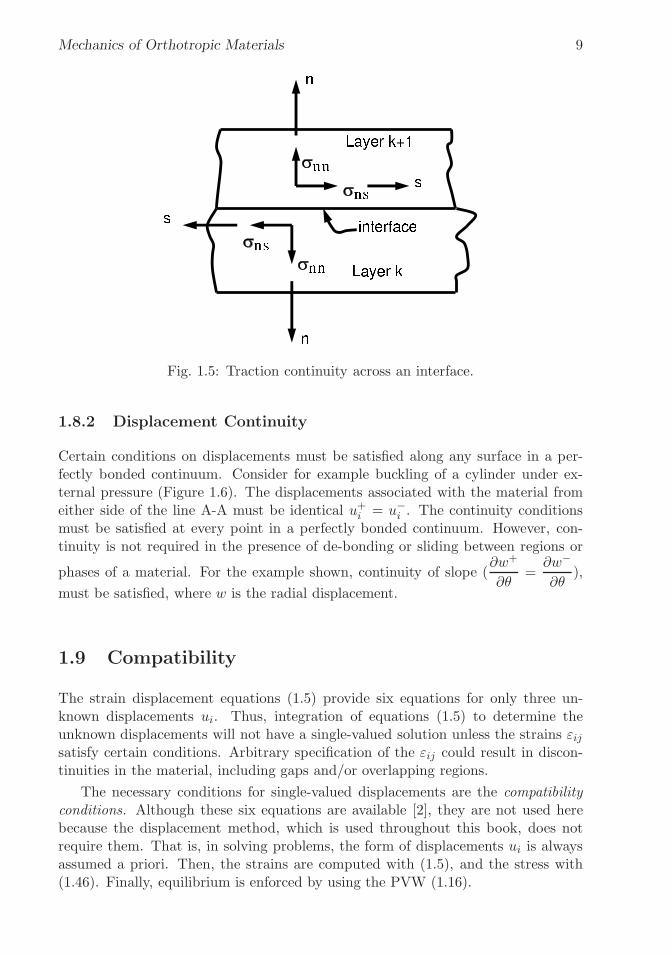
1.8.2 Displacement Continuity

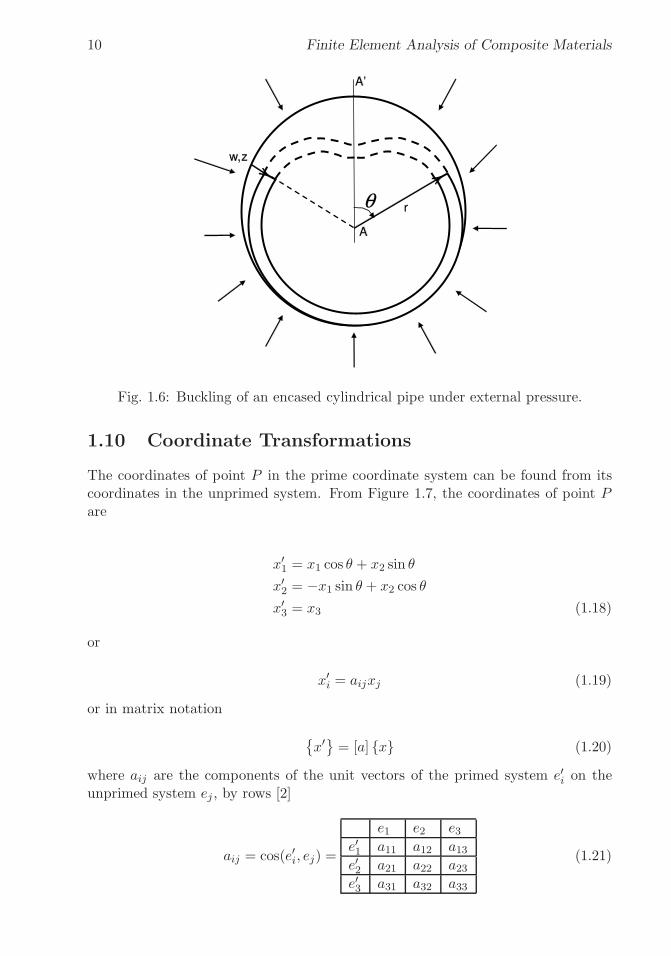
Certain conditions on displacements must be satisfied along any surface in a per-fectly bonded continuum. Consider for example buckling of a cylinder under ex-ternal pressure (Figure 1.6). The displacements associated with the material fromeither side of the line A-A must be identical u+i = u−i . The continuity conditionsmust be satisfied at every point in a perfectly bonded continuum. However, con-tinuity is not required in the presence of de-bonding or sliding between regions or

phases of a material. For the example shown, continuity of slope (∂w+

∂θ=∂w−

∂θ),

must be satisfied, where w is the radial displacement.

1.9 Compatibility

The strain displacement equations (1.5) provide six equations for only three un-known displacements ui. Thus, integration of equations (1.5) to determine theunknown displacements will not have a single-valued solution unless the strains εijsatisfy certain conditions. Arbitrary specification of the εij could result in discon-tinuities in the material, including gaps and/or overlapping regions.

The necessary conditions for single-valued displacements are the compatibilityconditions. Although these six equations are available [2], they are not used herebecause the displacement method, which is used throughout this book, does notrequire them. That is, in solving problems, the form of displacements ui is alwaysassumed a priori. Then, the strains are computed with (1.5), and the stress with(1.46). Finally, equilibrium is enforced by using the PVW (1.16).

�

�

“K15072” — 2013/3/21 — 10:58�

�

�

�

�

�


Fig. 1.6: Buckling of an encased cylindrical pipe under external pressure.

1.10 Coordinate Transformations

The coordinates of point P in the prime coordinate system can be found from itscoordinates in the unprimed system. From Figure 1.7, the coordinates of point Pare

x′1 = x1 cos θ + x2 sin θ

x′2 = −x1 sin θ + x2 cos θ

x′3 = x3 (1.18)

or

x′i = aijxj (1.19)

or in matrix notation

{

x′}

= [a] {x} (1.20)

where aij are the components of the unit vectors of the primed system e′i on theunprimed system ej , by rows [2]

aij = cos(e′i, ej) =

e1 e2 e3e′1 a11 a12 a13e′2 a21 a22 a23e′3 a31 a32 a33

(1.21)

�

�

“K15072” — 2013/3/21 — 10:58�

�

�

�

�

�


P

fibers

xcos

1

�

xsin

2

�

xco

s2

�

xsin

1

�

lamina

laminatex1

x2

x’1x’2

Fig. 1.7: Coordinate transformation.

If primed coordinates denote the lamina coordinates and unprimed denote thelaminate coordinates, then (1.19) transforms vectors from laminate to lamina coor-dinates. The inverse transformation simply uses the transpose matrix

{x} = [a]T{

x′}

(1.22)

Example 1.2 A composite layer has fiber orientation θ = 30◦. Construct the [a] matrixby calculating the direction cosines of the lamina system, i.e., the components of the unitvectors of the lamina system (x′i) on the laminate system (xj).

Solution to Example 1.2 From Figure 1.7 and (1.19) we have

a11 = cos θ =

√3

2

a12 = sin θ =1

2a13 = 0

a21 = − sin θ = −1

2

a22 = cos θ =

√3

2a23 = 0

a31 = 0

a32 = 0

a33 = 1

Example 1.3 A fiber reinforced composite tube is wound in the hoop direction (1-direction).Formulas for the stiffness values (E1, E2, etc.) are given in that system. However, whenanalyzing the cross-section of this material with generalized plane strain elements (CAX4 in

�

�

“K15072” — 2013/3/21 — 10:58�

�

�

�

�

�


Fig. 1.8: Coordinate transformation for axial-symmetric analysis.

Abaqus), the model is typically constructed in the structural X,Y, Z system. It is thereforenecessary to provide the stiffness values in the structural system as Ex, Ey, etc. Con-struct the transformation matrix [a]T to go from lamina coordinates (1-2-3) to structuralcoordinates in Figure 1.8.

Solution to Example 1.3 First, construct [a] using the definition (1.21). Taking eachunit vector (1-2-3) at a time we construct the matrix [a] by rows. The i-th row contains thecomponents of (i=1,2,3) along (X-Y-Z).

[a] X Y Z1 0 0 12 0 −1 03 1 0 0

The required transformation is just the transpose of the matrix above.

1.10.1 Stress Transformation

A second-order tensor σpq can be thought as the (un-contracted) outer product3 oftwo vectors Vp and Vq

σpq = Vp ⊗ Vq (1.23)

each of which transforms as (1.19)

σ′ij = aipVp ⊗ ajqVq (1.24)

Therefore,

3The outer product preserves all indices of the entities involved, thus creating a tensor of orderequal to the sum of the order of the entities involved.

�

�

“K15072” — 2013/3/21 — 10:58�

�

�

�

�

�


σ′ij = aipajqσpq (1.25)

or, in matrix notation

{σ′} = [a]{σ}[a]T (1.26)

For example, expand σ′11 in contracted notation

σ′1 = a211σ1 + a212σ2 + a213σ3 + 2a11a12σ6 + 2a11a13σ5 + 2a12a13σ4 (1.27)

Expanding σ′12 in contracted notation yields

σ′6 = a11a21σ1 + a12a22σ2 + a13a23σ3 + (a11a22 + a12a21)σ6 (1.28)

+ (a11a23 + a13a21)σ5 + (a12a23 + a13a22)σ4

The following algorithm is used to obtain a 6 × 6 coordinate transformationmatrix [T] such that (1.25) is rewritten in contracted notation as

σ′α = Tαβσβ (1.29)

If α ≤ 3 and β ≤ 3 then i = j and p = q, so

Tαβ = aipaip = a2ip no sum on i, p (1.30)

If α ≤ 3 and β > 3 then i = j but p �= q, and taking into account that switchingp by q yields the same value of β = 9− p− q as per (1.9) we have

Tαβ = aipaiq + aiqaip = 2aipaiq no sum on i, p (1.31)

If α > 3, then i �= j, but we want only one stress, say σij, not σji because theyare numerically equal. In fact σα = σij = σji with α = 9− i− j. If in addition β ≤ 3then p = q and we get

Tαβ = aipajp no sum on i, p (1.32)

When α > 3 and β > 3, i �= j and p �= q so we get

Tαβ = aipajq + aiqajp (1.33)

which completes the derivation of Tαβ . Expanding (1.30–1.33) and using (1.21) weget

[T ] =

⎡

⎢

⎢

⎢

⎢

⎢

⎢

⎣

a211 a212 a213 2 a12 a13 2 a11 a13 2 a11 a12a221 a22

2 a223 2 a22 a23 2 a21 a23 2 a21 a22a231 a232 a233 2 a32 a33 2 a31 a33 2 a31 a32

a21 a31 a22 a32 a23 a33 a22 a33 + a23 a32 a21 a33 + a23 a31 a21 a32 + a22 a31a11 a31 a12 a32 a13 a33 a12 a33 + a13 a32 a11 a33 + a13 a31 a11 a32 + a12 a31a11 a21 a12 a22 a13 a23 a12 a23 + a13 a22 a11 a23 + a13 a21 a11 a22 + a12 a21

⎤

⎥

⎥

⎥

⎥

⎥

⎥

⎦

(1.34)

�

�

“K15072” — 2013/3/21 — 10:58�

�

�

�

�

�


A MATLAB program that can be used to generate (1.34) is shown next (alsoavailable in [5]).

% Derivation of the transformation matrix [T]

clear all;

syms T alpha R

syms a a11 a12 a13 a21 a22 a23 a31 a32 a33

a = [a11,a12,a13;

a21,a22,a23;

a31,a32,a33];

T(1:6,1:6) = 0;

for i=1:1:3

for j=1:1:3

if i==j; alpha = j; else alpha = 9-i-j; end

for p=1:1:3

for q=1:1:3

if p==q beta = p; else beta = 9-p-q; end

T(alpha,beta) = 0;

if alpha<=3 & beta<= 3; T(alpha,beta)=a(i,p)*a(i,p); end

if alpha> 3 & beta<= 3; T(alpha,beta)=a(i,p)*a(j,p); end

if alpha<=3 & beta>3; T(alpha,beta)=a(i,q)*a(i,p)+a(i,p)*a(i,q);end

if alpha>3 & beta>3; T(alpha,beta)=a(i,p)*a(j,q)+a(i,q)*a(j,p);end

end

end

end

end

T

R = eye(6,6); R(4,4)=2; R(5,5)=2; R(6,6)=2; % Reuter matrix

Tbar = R*T*R^(-1)

1.10.2 Strain Transformation

The tensor components of strain εij transform in the same way as the stress com-ponents

ε′ij = aipajqεpq (1.35)

or

ε′α = Tαβεβ (1.36)

with Tαβ given by (1.34). However, the three engineering shear strains γxz, γyz, γxyare normally used instead of tensor shear strains εxz, εyz , εxy. The engineeringstrains (ε instead of ε) are defined in (1.5). They can be obtained from the tensorcomponents by the following relationship

εδ = Rδγεγ (1.37)

with the Reuter matrix given by

�

�

“K15072” — 2013/3/21 — 10:58�

�

�

�

�

�


[R] =

⎡

⎢

⎢

⎢

⎢

⎢

⎢

⎣

1 0 0 0 0 00 1 0 0 0 00 0 1 0 0 00 0 0 2 0 00 0 0 0 2 00 0 0 0 0 2

⎤

⎥

⎥

⎥

⎥

⎥

⎥

⎦

(1.38)

Then, the coordinate transformation of engineering strain results from (1.36)and (1.37) as

ε′α = Tαβεβ (1.39)

with

[

T]

= [R][T ][R]−1 (1.40)

used only to transform engineering strains. Explicitly we have

[

T]

=⎡

⎢

⎢

⎢

⎢

⎢

⎢

⎣

a211 a212 a213 a12 a13 a11 a13 a11 a12a221 a222 a223 a22 a23 a21 a23 a21 a22a231 a232 a233 a32 a33 a31 a33 a31 a32

2 a21 a31 2 a22 a32 2 a23 a33 a22 a33 + a23 a32 a21 a33 + a23 a31 a21 a32 + a22 a312 a11 a31 2 a12 a32 2 a13 a33 a12 a33 + a13 a32 a11 a33 + a13 a31 a11 a32 + a12 a312 a11 a21 2 a12 a22 2 a13 a23 a12 a23 + a13 a22 a11 a23 + a13 a21 a11 a22 + a12 a21

⎤

⎥

⎥

⎥

⎥

⎥

⎥

⎦

(1.41)

1.11 Transformation of Constitutive Equations

The constitutive equations that relate stress σ to strain ε are defined using tensorstrains (ε, not ε), as

σ′ = C′ : ε′

σ′ij = C ′ijklε

′kl (1.42)

where both tensor and index notations have been used.4

For simplicity consider an orthotropic material (Section 1.12.3). Then, it ispossible to write σ′11, and σ′12 as

σ′11 = C ′1111ε

′11 + C ′

1122ε′22 + C ′

1133ε′33

σ′12 = C ′1212ε

′12 + C ′

1221ε′21 = 2C ′

1212ε′12 (1.43)

4A double contraction involves contraction of two indices, in this case k and l, and it is denotedby : in tensor notation. Also note the use of boldface to indicate tensors in tensor notation.

�

�

“K15072” — 2013/3/21 — 10:58�

�

�

�

�

�


Rewriting (1.43) in contracted notation, it is clear that in contracted notationall the shear strains appear twice, as follows

σ′1 = C ′11ε

′1 + C ′

12ε′2 + C ′

13ε′3 (1.44)

σ′6 = 2C ′66ε

′6

The factor 2 in front of the tensor shear strains is caused by two facts, the minorsymmetry of the tensors C and ε (see (1.5,1.55-1.56)) and the contraction of the lasttwo indices of Cijkl with the strain εkl in (1.43). Therefore, any double contractionof tensors with minor symmetry needs to be corrected by a Reuter matrix (1.38)when written in the contracted notation. Next, (1.42) can be written as

σ′α = C ′αβRβδε

′δ (1.45)

Note that the Reuter matrix in (1.45) can be combined with the tensor strainsusing (1.37), to write

σ′α = C ′αβε

′β (1.46)

in terms of engineering strains. To obtain the stiffness matrix [C] in the laminatecoordinate system, introduce (1.29) and (1.39) into (1.46) so that

Tαδσδ = C ′αβT βγεγ (1.47)

It can be shown that

[T ]−1 = [T ]T (1.48)

Therefore

{σ} = [C]{ε} (1.49)

with

[C] = [T ]T [C ′][T ] (1.50)

and

[C ′] = [T ]−T [C][T ]−1 = [T ][C][T ]T (1.51)

The compliance matrix is the inverse of the stiffness matrix, not the inverse ofthe fourth order tensor Cijkl. Therefore,

[S′] = [C ′]−1 (1.52)

Taking into account (1.48) and (1.50), the compliance matrix transforms as

[S] = [T ]T [S′][T ] (1.53)

[S′] = [T ]−T [S][T ]−1 = [T ][S][T ]T (1.54)

�

�

“K15072” — 2013/3/21 — 10:58�

�

�

�

�

�


1.12 3D Constitutive Equations

Hooke’s law in three dimensions (3D) takes the form of (1.42). The 3D stiffnesstensor Cijkl is a fourth-order tensor with 81 components. For anisotropic materialsonly 21 components are independent. That is, the remaining 60 components canbe written in terms of the other 21. The one-dimensional case (1D), studied inmechanics of materials, is recovered when all the stress components are zero exceptσ11. Only for the 1D case, σ11 = σ, ε11 = ε, C1111 = E, and σ = Eε. All thederivations in this section are carried out in lamina coordinates but for simplicitythe prime symbol (′) is omitted, in this section only.

In (1.42), exchanging the dummy indexes i by j, and k by l we have

σji = Cjilkεlk (1.55)

Since the stress and strain tensors are symmetric, i.e, σij = σji and εkl = εkl, itfollows that

Cijkl = Cjikl = Cijlk = Cjilk (1.56)

which effectively reduces the number of independent components from 81 to 36. Forexample, C1213 = C2131 and so on. Then, the 36 independent components can bewritten as a 6×6 matrix.

Furthermore, an elastic material does not dissipate energy. All elastic energystored during loading is recovered during unloading. Therefore, the elastic energyat any point on the stress-strain curve is independent on the path that was followedto arrive at that point. A path independent function is called a potential function.In this case, the potential is the strain energy density u(εij). Expanding the strainenergy density in a Taylor power series

u = u0 +∂u

∂εij

∣

∣

∣

∣

0

εij +1

2

∂2u

∂εij∂εkl

∣

∣

∣

∣

0

εij εkl + ... (1.57)

Now take a derivative with respect to εij

∂u

∂εij= 0 + βij +

1

2(αijkl εkl + αklij εij) (1.58)

where βij and αijkl are constants. From here, one can write

σij − σ0ij = Cijkl εkl (1.59)

where σ0ij = βij is the residual stress and αijkl = 1/2(Cijkl + Cklik) = Cijkl is thesymmetric stiffness tensor (see (1.56)). Equation (1.59) is a generalization of (1.55)including residual stresses.

Using contracted notation, the generalized Hooke’s law becomes

�

�

“K15072” — 2013/3/21 — 10:58�

�

�

�

�

�


Fig. 1.9: Anisotropic material.

⎧

⎪

⎪

⎪

⎪

⎪

⎪

⎨

⎪

⎪

⎪

⎪

⎪

⎪

⎩

σ1σ2σ3σ4σ5σ6

⎫

⎪

⎪

⎪

⎪

⎪

⎪

⎬

⎪

⎪

⎪

⎪

⎪

⎪

⎭

=

⎡

⎢

⎢

⎢

⎢

⎢

⎢

⎣

C11 C12 C13 C14 C15 C16

C12 C22 C23 C24 C25 C26

C13 C23 C33 C34 C35 C36

C14 C24 C34 C44 C45 C46

C15 C25 C35 C45 C55 C56

C16 C26 C36 C46 C56 C66

⎤

⎥

⎥

⎥

⎥

⎥

⎥

⎦

⎧

⎪

⎪

⎪

⎪

⎪

⎪

⎨

⎪

⎪

⎪

⎪

⎪

⎪

⎩

ε1ε2ε3γ4γ5γ6

⎫

⎪

⎪

⎪

⎪

⎪

⎪

⎬

⎪

⎪

⎪

⎪

⎪

⎪

⎭

(1.60)

Once again, the 1D case is covered when σα = 0 if α �= 1. Then, σ1 = σ, ε1 =ε, C11 = E.

1.12.1 Anisotropic Material

Equation (1.60) represents a fully anisotropic material. Such a material has prop-erties that change with the orientation. For example, the material body depicted inFigure 1.9 deforms differently in the directions P, T, and Q, even if the forces ap-plied along the directions P, T, and Q are equal. The number of constants requiredto describe anisotropic materials is 21.

The inverse of the stiffness matrix is the compliance matrix [S] = [C]−1. Theconstitutive equation (3D Hooke’s law) is written in terms of compliances as follows

⎧

⎪

⎪

⎪

⎪

⎪

⎪

⎨

⎪

⎪

⎪

⎪

⎪

⎪

⎩

ε1ε2ε3γ4γ5γ6

⎫

⎪

⎪

⎪

⎪

⎪

⎪

⎬

⎪

⎪

⎪

⎪

⎪

⎪

⎭

=

⎡

⎢

⎢

⎢

⎢

⎢

⎢

⎣

S11 S12 S13 S14 S15 S16S12 S22 S23 S24 S25 S26S13 S23 S33 S34 S35 S36S14 S24 S34 S44 S45 S46S15 S25 S35 S45 S55 S56S16 S26 S36 S46 S56 S66

⎤

⎥

⎥

⎥

⎥

⎥

⎥

⎦

⎧

⎪

⎪

⎪

⎪

⎪

⎪

⎨

⎪

⎪

⎪

⎪

⎪

⎪

⎩

σ1σ2σ3σ4σ5σ6

⎫

⎪

⎪

⎪

⎪

⎪

⎪

⎬

⎪

⎪

⎪

⎪

⎪

⎪

⎭

(1.61)

The [S] matrix is also symmetric and it has 21 independent constants. For the1D case, σ = 0 if p �= 1. Then, σ1 = σ, ε1 = ε, S11 = 1/E.

�

�

“K15072” — 2013/3/21 — 10:58�

�

�

�

�

�


Fig. 1.10: Monoclinic material.

1.12.2 Monoclinic Material

If a material has one plane of symmetry (Figure 1.10) it is called monoclinic and13 constants are required to describe it. One plane of symmetry means that theproperties are the same at symmetric points (z and -z as in Figure 1.10).

When the material is symmetric about the 1-2 plane, the material propertiesare identical upon reflection with respect to the 1-2 plane. For such reflection thea-matrix (1.21) is

e′′1e′′2e′′3

x1 x2 x3⎡

⎣

1 0 00 1 00 0 −1

⎤

⎦

(1.62)

where ′′ has been used to avoid confusion with the lamina coordinate system that isdenoted without ()′ in this Section but with ()′ elsewhere in this book. From (1.40)we get

[

T]

=

⎡

⎢

⎢

⎢

⎢

⎢

⎢

⎣

1 0 0 0 0 00 1 0 0 0 00 0 1 0 0 00 0 0 −1 0 00 0 0 0 −1 00 0 0 0 0 1

⎤

⎥

⎥

⎥

⎥

⎥

⎥

⎦

(1.63)

The effect of[

T]

is to multiply rows and columns 4 and 5 in [C] by -1. Thediagonal terms C44 and C55 remain positive because they are multiplied twice.Therefore, C ′′

i4 = −Ci4 with i �= 4, 5, C ′′i5 = −Ci5 with i �= 4, 5, with everything else

unchanged. Since the material properties in a monoclinic material cannot changeby a reflection, it must be C4i = Ci4 = 0 with i �= 4, 5, C5i = Ci5 = 0 with

�

�

“K15072” — 2013/3/21 — 10:58�

�

�

�

�

�


Fig. 1.11: Orthotropic material.

i �= 4, 5. That is, 3D Hooke’s law reduces to⎧

⎪

⎪

⎪

⎪

⎪

⎪

⎨

⎪

⎪

⎪

⎪

⎪

⎪

⎩

σ1σ2σ3σ4σ5σ6

⎫

⎪

⎪

⎪

⎪

⎪

⎪

⎬

⎪

⎪

⎪

⎪

⎪

⎪

⎭

=

⎡

⎢

⎢

⎢

⎢

⎢

⎢

⎣

C11 C12 C13 0 0 C16

C12 C22 C23 0 0 C26

C13 C23 C33 0 0 C36

0 0 0 C44 C45 00 0 0 C45 C55 0C16 C26 C36 0 0 C66

⎤

⎥

⎥

⎥

⎥

⎥

⎥

⎦

⎧

⎪

⎪

⎪

⎪

⎪

⎪

⎨

⎪

⎪

⎪

⎪

⎪

⎪

⎩

ε1ε2ε3γ4γ5γ6

⎫

⎪

⎪

⎪

⎪

⎪

⎪

⎬

⎪

⎪

⎪

⎪

⎪

⎪

⎭

(1.64)

and in terms of the compliances to⎧

⎪

⎪

⎪

⎪

⎪

⎪

⎨

⎪

⎪

⎪

⎪

⎪

⎪

⎩

ε1ε2ε3γ4γ5γ6

⎫

⎪

⎪

⎪

⎪

⎪

⎪

⎬

⎪

⎪

⎪

⎪

⎪

⎪

⎭

=

⎡

⎢

⎢

⎢

⎢

⎢

⎢

⎣

S11 S12 S13 0 0 S16S12 S22 S23 0 0 S26S13 S23 S33 0 0 S360 0 0 S44 S45 00 0 0 S45 S55 0S16 S26 S36 0 0 S66

⎤

⎥

⎥

⎥

⎥

⎥

⎥

⎦

⎧

⎪

⎪

⎪

⎪

⎪

⎪

⎨

⎪

⎪

⎪

⎪

⎪

⎪

⎩

σ1σ2σ3σ4σ5σ6

⎫

⎪

⎪

⎪

⎪

⎪

⎪

⎬

⎪

⎪

⎪

⎪

⎪

⎪

⎭

(1.65)

1.12.3 Orthotropic Material

An orthotropic material has three planes of symmetry that coincide with the co-ordinate planes. It can be shown that if two orthogonal planes of symmetry exist,there is always a third orthogonal plane of symmetry. Nine constants are requiredto describe this type of material.

The symmetry planes can be Cartesian, as depicted in Figure 1.11, or they maycorrespond to any other coordinate representation (cylindrical, spherical, etc.). Forexample, the trunk of a tree has cylindrical orthotropy because of the growth rings.However, most practical materials exhibit Cartesian orthotropy. A unidirectionalfiber reinforced composite may be considered to be orthotropic. One plane of sym-metry is perpendicular to the fiber direction, and the other two are parallel to thefiber direction and orthogonal among themselves.

In addition to the reflection about the 1-2 plane discussed in Section 1.12.2,a second reflection about the 1-3 plane should not affect the properties of the or-thotropic materials. In this case the a-matrix is

�

�

“K15072” — 2013/3/21 — 10:58�

�

�

�

�

�


[a] =

⎡

⎣

1 0 00 −1 00 0 1

⎤

⎦ (1.66)

The T -matrix from (1.40) is

[

T]

=

⎡

⎢

⎢

⎢

⎢

⎢

⎢

⎣

1 0 0 0 0 00 1 0 0 0 00 0 1 0 0 00 0 0 −1 0 00 0 0 0 1 00 0 0 0 0 −1

⎤

⎥

⎥

⎥

⎥

⎥

⎥

⎦

(1.67)

This will make Ci6 = −Ci6 , i �= 4, 6 and Ci4 = −Ci4 , i �= 4, 6. Since thematerial has symmetry about the 1-3 plane, this means that Ci6 = C6i = 0 , i �= 6.In this case, 3D Hooke’s law reduces to

⎧

⎪

⎪

⎪

⎪

⎪

⎪

⎨

⎪

⎪

⎪

⎪

⎪

⎪

⎩

σ1σ2σ3σ4σ5σ6

⎫

⎪

⎪

⎪

⎪

⎪

⎪

⎬

⎪

⎪

⎪

⎪

⎪

⎪

⎭

=

⎡

⎢

⎢

⎢

⎢

⎢

⎢

⎣

C11 C12 C13 0 0 0C12 C22 C23 0 0 0C13 C23 C33 0 0 00 0 0 C44 0 00 0 0 0 C55 00 0 0 0 0 C66

⎤

⎥

⎥

⎥

⎥

⎥

⎥

⎦

⎧

⎪

⎪

⎪

⎪

⎪

⎪

⎨

⎪

⎪

⎪

⎪

⎪

⎪

⎩

ε1ε2ε3γ4γ5γ6

⎫

⎪

⎪

⎪

⎪

⎪

⎪

⎬

⎪

⎪

⎪

⎪

⎪

⎪

⎭

(1.68)

and in terms of the compliances to

⎧

⎪

⎪

⎪

⎪

⎪

⎪

⎨

⎪

⎪

⎪

⎪

⎪

⎪

⎩

ε1ε2ε3γ4γ5γ6

⎫

⎪

⎪

⎪

⎪

⎪

⎪

⎬

⎪

⎪

⎪

⎪

⎪

⎪

⎭

=

⎡

⎢

⎢

⎢

⎢

⎢

⎢

⎣

S11 S12 S13 0 0 0S12 S22 S23 0 0 0S13 S23 S33 0 0 00 0 0 S44 0 00 0 0 0 S55 00 0 0 0 0 S66

⎤

⎥

⎥

⎥

⎥

⎥

⎥

⎦

⎧

⎪

⎪

⎪

⎪

⎪

⎪

⎨

⎪

⎪

⎪

⎪

⎪

⎪

⎩

σ1σ2σ3σ4σ5σ6

⎫

⎪

⎪

⎪

⎪

⎪

⎪

⎬

⎪

⎪

⎪

⎪

⎪

⎪

⎭

(1.69)

Note that if the material has two planes of symmetry, it automatically has threebecause applying the procedure once more for a third plane (the 2-3 plane) will notchange (1.68-1.69).

1.12.4 Transversely Isotropic Material

A transversely isotropic material has one axis of symmetry. For example, the fiberdirection of a unidirectional fiber reinforced composite can be considered an axis ofsymmetry if the fibers are randomly distributed in the cross section (Figure 1.12).In this case, any plane containing the fiber direction is a plane of symmetry. Atransversely isotropic material is described by five constants. When the axis ofsymmetry is the fiber direction (1-direction), 3D Hooke’s law reduces to

�

�

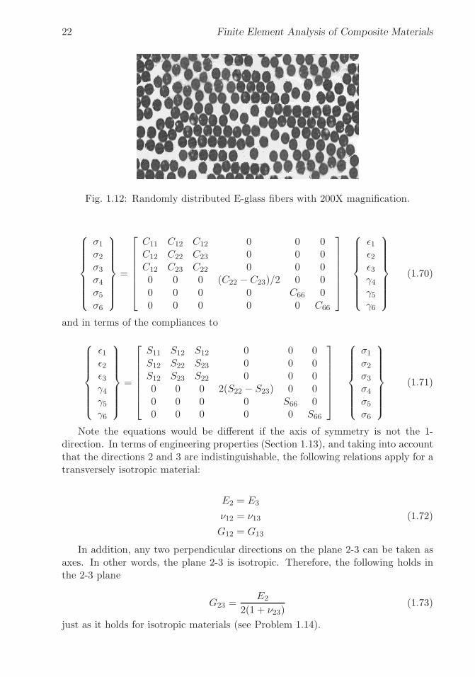
“K15072” — 2013/3/21 — 10:58�

�

�

�

�

�


Fig. 1.12: Randomly distributed E-glass fibers with 200X magnification.

⎧

⎪

⎪

⎪

⎪

⎪

⎪

⎨

⎪

⎪

⎪

⎪

⎪

⎪

⎩

σ1σ2σ3σ4σ5σ6

⎫

⎪

⎪

⎪

⎪

⎪

⎪

⎬

⎪

⎪

⎪

⎪

⎪

⎪

⎭

=

⎡

⎢

⎢

⎢

⎢

⎢

⎢

⎣

C11 C12 C12 0 0 0C12 C22 C23 0 0 0C12 C23 C22 0 0 00 0 0 (C22 − C23)/2 0 00 0 0 0 C66 00 0 0 0 0 C66

⎤

⎥

⎥

⎥

⎥

⎥

⎥

⎦

⎧

⎪

⎪

⎪

⎪

⎪

⎪

⎨

⎪

⎪

⎪

⎪

⎪

⎪

⎩

ε1ε2ε3γ4γ5γ6

⎫

⎪

⎪

⎪

⎪

⎪

⎪

⎬

⎪

⎪

⎪

⎪

⎪

⎪

⎭

(1.70)

and in terms of the compliances to

⎧

⎪

⎪

⎪

⎪

⎪

⎪

⎨

⎪

⎪

⎪

⎪

⎪

⎪

⎩

ε1ε2ε3γ4γ5γ6

⎫

⎪

⎪

⎪

⎪

⎪

⎪

⎬

⎪

⎪

⎪

⎪

⎪

⎪

⎭

=

⎡

⎢

⎢

⎢

⎢

⎢

⎢

⎣

S11 S12 S12 0 0 0S12 S22 S23 0 0 0S12 S23 S22 0 0 00 0 0 2(S22 − S23) 0 00 0 0 0 S66 00 0 0 0 0 S66

⎤

⎥

⎥

⎥

⎥

⎥

⎥

⎦

⎧

⎪

⎪

⎪

⎪

⎪

⎪

⎨

⎪

⎪

⎪

⎪

⎪

⎪

⎩

σ1σ2σ3σ4σ5σ6

⎫

⎪

⎪

⎪

⎪

⎪

⎪

⎬

⎪

⎪

⎪

⎪

⎪

⎪

⎭

(1.71)

Note the equations would be different if the axis of symmetry is not the 1-direction. In terms of engineering properties (Section 1.13), and taking into accountthat the directions 2 and 3 are indistinguishable, the following relations apply for atransversely isotropic material:

E2 = E3

ν12 = ν13 (1.72)

G12 = G13

In addition, any two perpendicular directions on the plane 2-3 can be taken asaxes. In other words, the plane 2-3 is isotropic. Therefore, the following holds inthe 2-3 plane

G23 =E2

2(1 + ν23)(1.73)

just as it holds for isotropic materials (see Problem 1.14).

�

�

“K15072” — 2013/3/21 — 10:58�

�

�

�

�

�


1.12.5 Isotropic Material

The most common materials of industrial use are isotropic, like aluminum, steel,etc. Isotropic materials have an infinite number of planes of symmetry, meaningthat the properties are independent of the orientation. Only two constants areneeded to represent the elastic properties. These two properties can be the Young’smodulus E and the Poisson’s ratio ν, but several other pairs of constants are usedwhenever it is convenient. However, any pair of properties has to be related to anyother pair. For example, you could describe isotropic materials by E and G, butthe shear modulus of isotropic materials is related to E and ν by

G =E

2(1 + ν)(1.74)

Also, the Lame constants are sometimes used for convenience, in this case thetwo constants are

λ =E

(1 + ν)(1− 2ν)(1.75)

μ = G

To form yet another pair, any of the above properties could be substituted bythe bulk modulus k, as follows

k =E

3(1− 2ν)(1.76)

which relates the hydrostatic pressure p to the volumetric strain as

p = k(ε1+ε2+ε3) (1.77)

For isotropic materials, the 3D Hooke’s law is written in terms of only twoconstants C11 and C12 as

⎧

⎪

⎪

⎪

⎪

⎪

⎪

⎨

⎪

⎪

⎪

⎪

⎪

⎪

⎩

σ1σ2σ3σ4σ5σ6

⎫

⎪

⎪

⎪

⎪

⎪

⎪

⎬

⎪

⎪

⎪

⎪

⎪

⎪

⎭

=

⎡

⎢

⎢

⎢

⎢

⎢

⎢

⎢

⎣

C11 C12 C12 0 0 0C12 C11 C12 0 0 0C12 C12 C11 0 0 0

0 0 0 (C11−C12)2 0 0

0 0 0 0 (C11−C12)2 0

0 0 0 0 0 (C11−C12)2

⎤

⎥

⎥

⎥

⎥

⎥

⎥

⎥

⎦

⎧

⎪

⎪

⎪

⎪

⎪

⎪

⎨

⎪

⎪

⎪

⎪

⎪

⎪

⎩

ε1ε2ε3γ4γ5γ6

⎫

⎪

⎪

⎪

⎪

⎪

⎪

⎬

⎪

⎪

⎪

⎪

⎪

⎪

⎭

(1.78)

In terms of compliances, once again, two constants are used, S11 and S12, asfollows

�

�

“K15072” — 2013/3/21 — 10:58�

�

�

�

�

�


⎧

⎪

⎪

⎪

⎪

⎪

⎪

⎨

⎪

⎪

⎪

⎪

⎪

⎪

⎩

ε1ε2ε3γ4γ5γ6

⎫

⎪

⎪

⎪

⎪

⎪

⎪

⎬

⎪

⎪

⎪

⎪

⎪

⎪

⎭

=

⎡

⎢

⎢

⎢

⎢

⎢

⎢

⎣

S11 S12 S12 0 0 0S12 S11 S12 0 0 0S12 S12 S11 0 0 00 0 0 2s 0 00 0 0 0 2s 00 0 0 0 0 2s

⎤

⎥

⎥

⎥

⎥

⎥

⎥

⎦

⎧

⎪

⎪

⎪

⎪

⎪

⎪

⎨

⎪

⎪

⎪

⎪

⎪

⎪

⎩

σ1σ2σ3σ4σ5σ6

⎫

⎪

⎪

⎪

⎪

⎪

⎪

⎬

⎪

⎪

⎪

⎪

⎪

⎪

⎭

(1.79)

s = S11 − S12

Not only are the various constants related in pairs, but also certain restrictionsapply on the values that these constants may have for real materials. Since theYoung and shear moduli must always be positive, the Poisson’s ratio must be ν >−1. Furthermore, since the bulk modulus must be positive, we have ν < 1

2 . Finally,the Poisson’s ratio of isotropic materials is constrained by −1 < ν < 1

2 .

1.13 Engineering Constants

Please note from here forward ()′ denotes the lamina coordinate system. Our nexttask is to write the components of the stiffness and compliance matrices in termsof engineering constants for orthotropic materials. For this purpose it is easier towork with the compliance matrix, which is defined as the inverse of the stiffnessmatrix. In lamina coordinates [S′] = [C ′]−1. The compliance matrix is used to writethe relationship between strains and stresses in (1.69) for an orthotropic material.Let’s rewrite the first of (1.69), which corresponds to the strain in the 1-direction(fiber direction)

ε′1 = S′11σ

′1 + S′

12σ′2 + S′

13σ′3 (1.80)

and let’s perform a thought experiment. Note that [S′] is used to emphasize the factthat we are working in the lamina coordinate system. First, apply a tensile stressalong the 1-direction (fiber direction) as in Figure 1.13, with all the other stressesequal to zero, and compute the strain produced in the 1-direction, which is

ε′1 =σ1

′

E1(1.81)

Then, apply a stress in the 2-direction only, and compute the strain in the1-direction using the appropriate Poisson’s ratio [1]

ε′1 = −ν21 σ′2

E2(1.82)

Now, apply a stress in the 3-direction only, and compute the strain in the 1-direction using the appropriate Poisson’s ratio,

ε′1 = −ν31 σ′3

E3(1.83)

�

�

“K15072” — 2013/3/21 — 10:58�

�

�

�

�

�


Fig. 1.13: Longitudinal loading.

The total strain ε′1 is the sum of equations (1.81), (1.82), and (1.83)

ε′1 =1

E1σ′1 −

ν21E2

σ′2 −ν31E3

σ′3 (1.84)

Comparing (1.84) with (1.80) we conclude that

S′11 =

1

E1;S′

12 = −ν21E2

;S′13 = −ν31

E3(1.85)

Repeat the same procedure for the equations corresponding to ε′2 and ε′3 toobtain the coefficients in the second and third rows of the compliance matrix (1.69).

For the shear terms use the 4th, 5th, and 6th rows of the compliance matrix(1.69). For example, from Figure 1.14 we write

σ′6 = ε′6G12 = 2ε′6G12 (1.86)

which compared to the 6th row of (1.69) leads to S66 = 1/G12.

For an orthotropic material, the compliance matrix [S′] is defined in the laminacoordinate system as

[S′] =

⎡

⎢

⎢

⎢

⎢

⎢

⎢

⎢

⎢

⎢

⎢

⎢

⎢

⎢

⎢

⎢

⎣

1

E1

−ν21E2

−ν31E3

0 0 0

−ν12E1

1

E2

−ν32E3

0 0 0

−ν13E1

−ν23E2

1

E30 0 0

0 0 01

G230 0

0 0 0 01

G130

0 0 0 0 01

G12

⎤

⎥

⎥

⎥

⎥

⎥

⎥

⎥

⎥

⎥

⎥

⎥

⎥

⎥

⎥

⎥

⎦

(1.87)

�

�

“K15072” — 2013/3/21 — 10:58�

�

�

�

�

�


Fig. 1.14: Shear loading.

where Ei, Gij , and νij are the elastic moduli, shear moduli, and Poisson’s ratios,respectively. Furthermore, the subscripts indicate lamina coordinates, i.e.,

νij = νx′ix

′jand Eii = Ex′

i(1.88)

Since [S′] is symmetric, the following must be satisfied

νijEii

=νjiEjj

, i, j = 1 . . . 3 (1.89)

Furthermore, Poisson’s ratios are defined so that the lateral strain is given by

νj = −νijεi (1.90)

In ANSYS, the Poisson’s ratios are defined differently than in this textbook.In fact, νxy, νxz, νyz are denoted PRXY, PRXZ, and PRYZ, while νyx, νzx, νzy aredenoted by NUXY, NUXZ, and NUYZ. On the contrary, Abaqus uses the standardnotation also used in this textbook. That is, the symbols NU12, NU13, NU23 followthe convention described by (1.90).

After computing Sij , the components of stress are obtained by using (1.46)or (1.49). This formulation predicts realistic behavior for finite displacement androtations as long as the strains are small. This formulation is expensive to usesince it needs 18 state variables: 12 components of the strain displacement matrixcomputed in the initial configuration (ui,j and ur,iur,j) plus 6 direction cosines [a]to account for finite rotations.

However, in (1.87) only nine constants are independent because the matrix [S′]must be symmetric (see 1.93), so

�

�

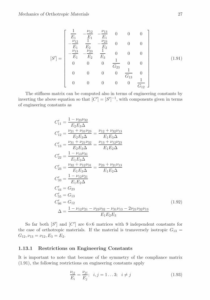
“K15072” — 2013/3/21 — 10:58�

�

�

�

�

�


[S′] =

⎡

⎢

⎢

⎢

⎢

⎢

⎢

⎢

⎢

⎢

⎢

⎢

⎢

⎢

⎢

⎢

⎣

1

E1−ν12E1

−ν13E1

0 0 0

−ν12E1

1

E2−ν23E2

0 0 0

−ν13E1

−ν23E2

1

E30 0 0

0 0 01

G230 0

0 0 0 01

G130

0 0 0 0 01

G12

⎤

⎥

⎥

⎥

⎥

⎥

⎥

⎥

⎥

⎥

⎥

⎥

⎥

⎥

⎥

⎥

⎦

(1.91)

The stiffness matrix can be computed also in terms of engineering constants byinverting the above equation so that [C ′] = [S′]−1, with components given in termsof engineering constants as

C ′11 =

1− ν23ν32E2E3Δ

C ′12 =

ν21 + ν31ν23E2E3Δ

=ν12 + ν32ν13E1E3Δ

C ′13 =

ν31 + ν21ν32E2E3Δ

=ν13 + ν12ν23E1E2Δ

C ′22 =

1− ν13ν31E1E3Δ

C ′23 =

ν32 + ν12ν31E1E3Δ

=ν23 + ν21ν13E1E2Δ

C ′33 =

1− ν12ν21E1E2Δ

C ′44 = G23

C ′55 = G13

C ′66 = G12 (1.92)

Δ =1− ν12ν21 − ν23ν32 − ν31ν13 − 2ν21ν32ν13

E1E2E3

So far both [S′] and [C ′] are 6×6 matrices with 9 independent constants forthe case of orthotropic materials. If the material is transversely isotropic G13 =G12, ν13 = ν12, E3 = E2.

1.13.1 Restrictions on Engineering Constants

It is important to note that because of the symmetry of the compliance matrix(1.91), the following restrictions on engineering constants apply

νijEi

=νjiEj

; i, j = 1 . . . 3; i �= j (1.93)

�

�

“K15072” — 2013/3/21 — 10:58�

�

�

�

�

�


Further restrictions on the values of the elastic constants can be derived fromthe fact that all diagonal terms in both the compliance and stiffness matricesmust be positive. Since all the engineering elastic constants must be positive(E1, E2, E3, G12, G23, G31 > 0), all the diagonal terms of the stiffness matrix (1.92)will be positive if the following two conditions are met. The first condition is that(1 − νijνji) > 0 for i, j = 1..3 and i �= j, which leads to the following restriction onthe values of the engineering constants

0 < νij <

√

Ei

Ej; i, j = 1 . . . 3; i �= j (1.94)

The second condition is that

Δ = 1− ν12ν21 − ν23ν32 − ν31ν13 − 2ν21ν32ν13 > 0 (1.95)

These restrictions can be used to check experimental data. For example, consideran experimental program in which if E1 and ν12 are measured in a longitudinal test(fibers in the direction of loading) by using two strain gages, one longitudinal andone transverse, and E2 and ν21 are measured in the transverse tensile tests (fibersperpendicular to loading). For the test procedure to be valid, all the four datavalues, E1,E2, ν12, and ν21, must conform to (1.93-1.95) within the margin allowedby experimental errors.

Example 1.4 Sonti et al. [6] performed a series of tests on pultruded glass-fiber reinforcedcomposites. From tensile tests along the longitudinal axis, the average of eight tests givesE1 = 19.981 GPa and ν12 = 0.274. The average of eight tests in the transverse directiongives E2 = 11.389 GPa and ν21 = 0.192. Do these data fall within the constraints on elasticconstants?

Solution to Example 1.4 First compute both sides of (1.93) for i, j = 1, 2 as

E1

ν12=

19.981

0.274= 72.9 GPa

E2

ν21=

11.389

0.192= 59.3 GPa

The transverse result is 23% lower than expected. Either E2 measured is too low or ν21measured is 23% higher than what it should be. In any case a 23% difference deserves somescrutiny.

Next check (1.94)

abs(ν12) <

√

E1

E2

0.274 < 1.32

abs(ν21) <

√

E2

E1

0.192 < 0.75

Finally, there are insufficient data to evaluate the last of the restrictions on elasticconstants from (1.95).

�

�

“K15072” — 2013/3/21 — 10:58�

�

�

�

�

�


1.14 From 3D to Plane Stress Equations

Setting σ3 = 0 in the compliance equations (1.69) of an orthotropic material impliesthat the third row and column of the compliance matrix are not used

⎧

⎪

⎪

⎪

⎪

⎪

⎪

⎨

⎪

⎪

⎪

⎪

⎪

⎪

⎩

ε′1ε′2ε′3γ′4γ′5γ′6

⎫

⎪

⎪

⎪

⎪

⎪

⎪

⎬

⎪

⎪

⎪

⎪

⎪

⎪

⎭

=

⎡

⎢

⎢

⎢

⎢

⎢

⎢

⎣

S′11 S′

12 S′13 0 0 0

S′12 S′

22 S′23 0 0 0

S′13 S′

23 S′33 0 0 0

0 0 0 S′44 0 0

0 0 0 0 S′55 0

0 0 0 0 0 S′66

⎤

⎥

⎥

⎥

⎥

⎥

⎥

⎦

⎧

⎪

⎪

⎪

⎪

⎪

⎪

⎨

⎪

⎪

⎪

⎪

⎪

⎪

⎩

σ′1σ′2

σ′3 = 0σ′4σ′5σ′6

⎫

⎪

⎪

⎪

⎪

⎪

⎪

⎬

⎪

⎪

⎪

⎪

⎪

⎪

⎭

(1.96)

So, the first two equations plus the last one can be written separately of theremaining, in terms of a 3×3 reduced compliance matrix [S] and using γ = 2ε, wehave

⎧

⎨

⎩

ε′1ε′2γ′6

⎫

⎬

⎭

=

⎡

⎣

S′11 S′

12 0S′12 S′

22 00 0 S′

66

⎤

⎦

⎧

⎨

⎩

σ′1σ′2σ′6

⎫

⎬

⎭

(1.97)

The third equation is seldom used

ε′3 = S′13σ

′1 + S′

23σ′2 (1.98)

and the remaining two equations can be written separately as

{

γ′4γ′5

}

=

[

S′44 00 S′

55

]{

σ′4σ′5

}

(1.99)

To compute stress components from strains, (1.97) can be inverted to get {σ} =[Q]{ε} or

⎧

⎨

⎩

σ′1σ′2σ′6

⎫

⎬

⎭

=

⎡

⎣

Q′11 Q′

12 0Q′

12 Q′22 0

0 0 Q′66

⎤

⎦

⎧

⎨

⎩

ε′1ε′2γ′6

⎫

⎬

⎭

(1.100)

where the matrix [Q′] = [S′3×3]

−1 is the reduced stiffness matrix for plane stress.Note that while the components of the reduced compliance matrix [S′

3×3] are nu-merically identical to the corresponding entries in the 6×6 compliance matrix, thecomponents of the reduced stiffness matrix [Q′] are not numerically equal to the cor-responding entries on the 6×6 stiffness matrix [C ′], thus the change in name. Thisis because the inverse of a 3×3 matrix produces different values than the inverse ofa 6×6 matrix. The set of equations is completed by writing

{

σ′4σ′5

}

=

[

C ′44 00 C ′

55

]{

γ′4γ′6

}

(1.101)

where the coefficient C ′44 and C ′

55 are numerically equal to the corresponding entriesin the 6× 6 stiffness matrix because the 2× 2 matrix in (1.101) is diagonal.

�

�

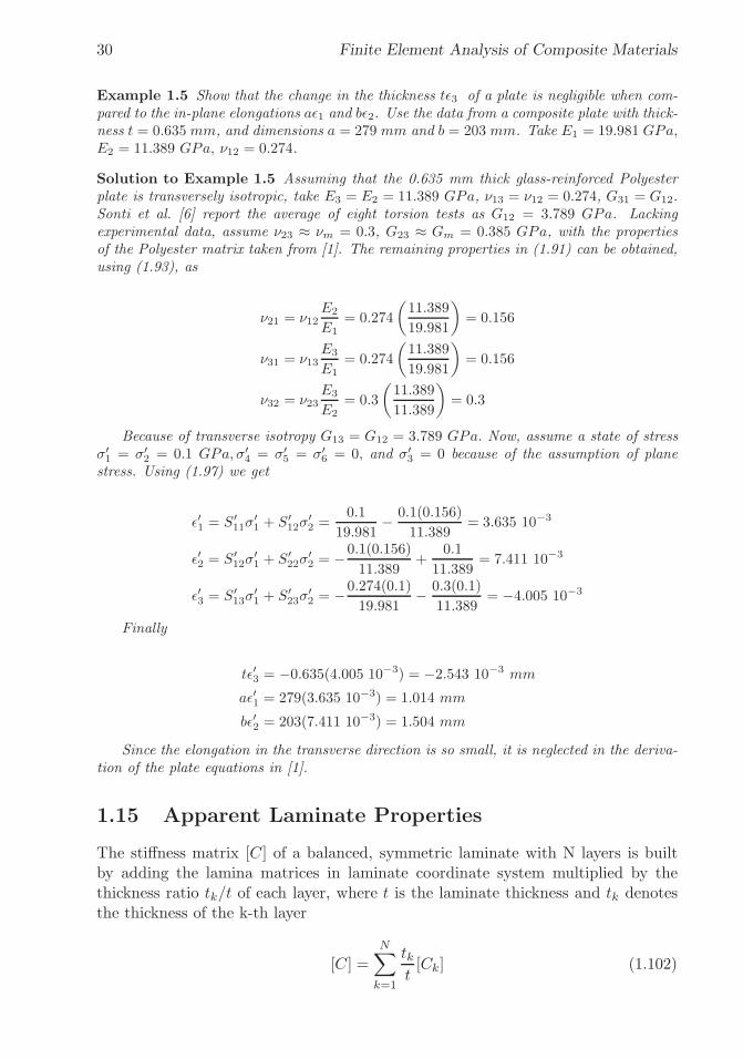
“K15072” — 2013/3/21 — 10:58�

�

�

�

�

�


Example 1.5 Show that the change in the thickness tε3 of a plate is negligible when com-pared to the in-plane elongations aε1 and bε2. Use the data from a composite plate with thick-ness t = 0.635mm, and dimensions a = 279 mm and b = 203 mm. Take E1 = 19.981 GPa,E2 = 11.389 GPa, ν12 = 0.274.

Solution to Example 1.5 Assuming that the 0.635 mm thick glass-reinforced Polyesterplate is transversely isotropic, take E3 = E2 = 11.389 GPa, ν13 = ν12 = 0.274, G31 = G12.Sonti et al. [6] report the average of eight torsion tests as G12 = 3.789 GPa. Lackingexperimental data, assume ν23 ≈ νm = 0.3, G23 ≈ Gm = 0.385 GPa, with the propertiesof the Polyester matrix taken from [1]. The remaining properties in (1.91) can be obtained,using (1.93), as

ν21 = ν12E2

E1= 0.274

(

11.389

19.981

)

= 0.156

ν31 = ν13E3

E1= 0.274

(

11.389

19.981

)

= 0.156

ν32 = ν23E3

E2= 0.3

(

11.389

11.389

)

= 0.3

Because of transverse isotropy G13 = G12 = 3.789 GPa. Now, assume a state of stressσ′1 = σ′

2 = 0.1 GPa, σ′4 = σ′

5 = σ′6 = 0, and σ′

3 = 0 because of the assumption of planestress. Using (1.97) we get

ε′1 = S′11σ

′1 + S′

12σ′2 =

0.1

19.981− 0.1(0.156)

11.389= 3.635 10−3

ε′2 = S′12σ

′1 + S′

22σ′2 = −0.1(0.156)

11.389+

0.1

11.389= 7.411 10−3

ε′3 = S′13σ

′1 + S′

23σ′2 = −0.274(0.1)

19.981− 0.3(0.1)

11.389= −4.005 10−3

Finally

tε′3 = −0.635(4.005 10−3) = −2.543 10−3 mm

aε′1 = 279(3.635 10−3) = 1.014 mm

bε′2 = 203(7.411 10−3) = 1.504 mm

Since the elongation in the transverse direction is so small, it is neglected in the deriva-tion of the plate equations in [1].

1.15 Apparent Laminate Properties

The stiffness matrix [C] of a balanced, symmetric laminate with N layers is builtby adding the lamina matrices in laminate coordinate system multiplied by thethickness ratio tk/t of each layer, where t is the laminate thickness and tk denotesthe thickness of the k-th layer

[C] =

N∑

k=1

tkt[Ck] (1.102)

�

�

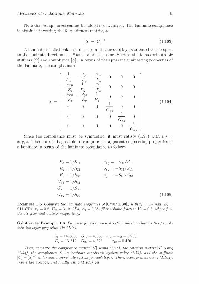
“K15072” — 2013/3/21 — 10:58�

�

�

�

�

�


Note that compliances cannot be added nor averaged. The laminate complianceis obtained inverting the 6×6 stiffness matrix, as

[S] = [C]−1 (1.103)

A laminate is called balanced if the total thickness of layers oriented with respectto the laminate direction at +θ and −θ are the same. Such laminate has orthotropicstiffness [C] and compliance [S]. In terms of the apparent engineering properties ofthe laminate, the compliance is

[S] =

⎡

⎢

⎢

⎢

⎢

⎢

⎢

⎢

⎢

⎢

⎢

⎢

⎢

⎢

⎢

⎢

⎢

⎣

1

Ex−νyxEy

−νzxEz

0 0 0

−νxyEx

1

Ey−νzyEz

0 0 0

−νxzEx

−νyzEy

1

Ez0 0 0

0 0 01

Gyz0 0

0 0 0 01

Gxz0

0 0 0 0 01

Gxy

⎤

⎥

⎥

⎥

⎥

⎥

⎥

⎥

⎥

⎥

⎥

⎥

⎥

⎥

⎥

⎥

⎥

⎦

(1.104)

Since the compliance must be symmetric, it must satisfy (1.93) with i, j =x, y, z. Therefore, it is possible to compute the apparent engineering properties ofa laminate in terms of the laminate compliance as follows

Ex = 1/S11 νxy = −S21/S11Ey = 1/S22 νxz = −S31/S11Ez = 1/S33 νyz = −S32/S22Gyz = 1/S44

Gxz = 1/S55

Gxy = 1/S66 (1.105)

Example 1.6 Compute the laminate properties of [0/90/± 30]S with tk = 1.5 mm, Ef =241 GPa, νf = 0.2, Em = 3.12 GPa, νm = 0.38, fiber volume fraction Vf = 0.6, where f,m,denote fiber and matrix, respectively.

Solution to Example 1.6 First use periodic microstructure micromechanics (6.8) to ob-tain the layer properties (in MPa).

E1 = 145, 880 G12 = 4, 386 ν12 = ν13 = 0.263E2 = 13, 312 G23 = 4, 528 ν23 = 0.470

Then, compute the compliance matrix [S′] using (1.91), the rotation matrix [T ] using(1.34), the compliance [S] in laminate coordinate system using (1.53), and the stiffness[C] = [S]−1 in laminate coordinate system for each layer. Then, average them using (1.102),invert the average, and finally using (1.105) get

�

�

“K15072” — 2013/3/21 — 10:58�

�

�

�

�

�


Ex = 78, 901 Gxy = 17, 114 νxy = 0.320Ey = 47, 604 Gyz = 4, 475 νyz = 0.364Ez = 16, 023 Gxz = 4, 439 νxz = 0.280

Suggested Problems

Problem 1.1 Using the principle of virtual work (PVW), find a quadratic displacementfunction u(x) in 0 < x < L of a tapered slender rod of length L, fixed at the origin andloaded axially in tension at the free end. The cross-section area changes lineally and theareas are A1 > A2 at the fixed and free ends, respectively. The material is homogeneousand isotropic with modulus E.

Problem 1.2 Using the principle of virtual work (PVW), find a quadratic rotation anglefunction θ(x) in 0 < x < L of a tapered slender shaft of circular cross section and length L,fixed at the origin and loaded by a torque T at the free end. The cross-section area changeslineally and the areas are A1 > A2 at the fixed and free ends, respectively. The material ishomogeneous and isotropic with shear modulus G.

Problem 1.3 Construct a rotation matrix [a] resulting from three consecutive reflectionsabout (a) the x-y plane, (b) the x-z plane, (c) the y-z plane. The resulting system does notfollow the right-hand rule.

Problem 1.4 Construct three rotation matrices [a] for rotations θ = π about (a) the x-axis,(b) the y-axis, (c) the z-axis.

Problem 1.5 Using

σ =

⎡

⎣

10 2 12 5 11 1 3

⎤

⎦

and [a] of Ex. 1.2, verify that (1.29) yields the same result as (1.26).

Problem 1.6 Write a computer program to evaluate the compliance and stiffness matricesin terms of engineering properties. Take the input from a file and the output to another file.Validate the program with your own examples. You may use material properties from [1,Tables 1.3–1.4] and assume the material is transversely isotropic as per Section 1.12.4.Show all work in a report.

Problem 1.7 Write a computer program to transform the stiffness and compliance matrixfrom lamina coordinates C ′, S′, to another coordinate system C, S, by a rotation −θ aroundthe z-axis (Figure 1.7). The data C′, S′, θ, should be read from a file. The output C, Sshould be written to another file. Validate your program with your own examples. You mayuse material properties from [1, Tables 1.3–1.4] and assume the material is transverselyisotropic as per Section 1.12.4. Show all work in a report.

Problem 1.8 Verify numerically (1.92) against [S]−1 for the material of your choice. Youmay use material properties from [1, Tables 1.3–1.4] and assume the material is transverselyisotropic as per Section 1.12.4.

�

�

“K15072” — 2013/3/21 — 10:58�

�

�

�

�

�


Problem 1.9 The following data has been obtained experimentally for a composite basedon a unidirectional carbon-epoxy prepreg (MR50 carbon fiber at 63% by volume in LTM25Epoxy). Determine if the restrictions on elastic constants are satisfied.

E1 = 156.403 GPa, E2 = 7.786 GPa

ν12 = 0.352, ν21 = 0.016

G12 = 3.762 GPa

σu1t = 1.826 GPa, σu

1c = 1.134 GPa

σu2t = 19 MPa, σu

2c = 131 MPa

σu6 = 75 MPa

εu1t = 11, 900 10−6, εu1c = 8, 180 10−6

εu2t = 2, 480 10−6, εu2c = 22, 100 10−6

γu12 = 20, 000 10−6

Problem 1.10 Explain contracted notation for stresses and strains.

Problem 1.11 What is an orthotropic material and how many constants are needed todescribe it?

Problem 1.12 What is a transversely isotropic material and how many constants areneeded to describe it?

Problem 1.13 Use the three rotation matrices in Problem 1.4 to verify (1.48) numerically.

Problem 1.14 Prove (1.73) using (1.71) and (1.91).

Problem 1.15 Demonstrate that a material having two perpendicular planes of symmetryalso has a third. Apply a reflection about the 2-3 plane to (1.68) using the procedure inSection 1.12.3.

Problem 1.16 What is a plane stress assumption?

Problem 1.17 Write a computer program to evaluate the laminate engineering propertiesfor symmetric balanced laminates. All layers are of the same material. Input data consistof all the engineering constants for a transversely isotropic material, number of layers N ,thickness and angle for all the layers tk, θk with k = 1...N . Use Section 1.15, 1.12.4, and1.13.

�

�

“K15072” — 2013/3/21 — 10:58�

�

�

�

�

�

�

�

“K15072” — 2013/3/21 — 10:58�

�

�

�

�

�

Chapter 2

Introduction to Finite ElementAnalysis

In this textbook, the finite element method (FEM) is used as a tool to solve practicalproblems. For the most part, commercial packages, mainly Abaqus, are used in theexamples. Computer programming is limited to implementing material models andpost processing algorithms. When commercial codes lack needed features, othercodes are used, which are provided in [5]. A basic understanding of the finite elementmethod is necessary for effective use of any finite element software. Therefore, thischapter contains a brief introduction intended for those readers who have not hada formal course or prior knowledge about the finite element method. Furthermore,an introduction to the Abaqus/CAE graphical user interface (GUI) is presented tofamiliarize the reader with the typical procedures used for finite element modelingusing any commercial software.

2.1 Basic FEM Procedure

Consider the axial deformation of a rod. The ordinary differential equation (ODE)describing the deformation of the rod is

− d

dx

(

EAdu

dx

)

− f = 0 ; 0 ≤ x ≤ L (2.1)

where E, A are the modulus and cross-section area of the rod, respectively, and fis the distributed force. The boundary conditions for the case illustrated in Figure2.1 are

u(0) = 0[(

EAdu

dx

)]

x=L

= P (2.2)

As it is customary in mechanics of materials textbooks, the real rod shown inFigure 2.1(a) is mathematically modeled as a line in Figure 2.1(b). The rod occupiesthe domain [0, L] along the real axis x.

35

�

�

“K15072” — 2013/3/21 — 10:58�

�

�

�

�

�


Fig. 2.1: Physical and mathematical (idealization) model.

2.1.1 Discretization

The next step is to divide the domain into discrete elements, as shown in Figure2.2.

2.1.2 Element Equations

To derive the element equations, an integral form of the ordinary differential equa-tion (ODE) is used, which is obtained by integrating the product of the ODE timesa weight function v as follows

0 =

∫ xB

xA

v

[

− d

dx

(

EAdu

dx

)

− f

]

dx (2.3)

This is called a weak form because the solution u(x) does not have to satisfy theODE (2.1) for all and every one of the infinite values of x in [0, L], in a strong sense.Instead, the solution u(x) only has to satisfy the ODE in (2.3) in a weighted averagesense. It is therefore easier to find a weak solution than a strong one. Although forthe case of the rod, the strong (exact) solution is known, most problems of compositemechanics do not have exact solutions. The governing equation is obtained byintegrating (2.3) by parts as follows

0 =

∫ xB

xA

EAdv

dx

du

dxdx−

∫ xB

xA

vfdx−[

v

(

EAdu

dx

)]xB

xA

(2.4)

where v(x) is a weight function, which is usually set equal to the primary variableu(x). From the boundary term, it is concluded that

– specifying v(x) at xA or xB is an essential boundary condition

– specifying(

EAdudx

)

at either end is the natural boundary condition

�

�

“K15072” — 2013/3/21 — 10:58�

�

�

�

�

�

Introduction to Finite Element Analysis 37

Fig. 2.2: Discretization into elements.

While u(x) is the primary variable,(

EAdudx

)

= EAεx = Aσx is the secondaryvariable. Let

u(xA) = ue1

u(xB) = ue2

−[(

EAdu

dx

)]

xA

= P e1

[(

EAdu

dx

)]

xB

= P e2 (2.5)

Then, the governing equation becomes

0 =

∫ xB

xA

(

EAdv

dx

du

dx− vf

)

dx− P e1 v(xA)− P e

2 v(xB) = B(v, u) − l(v) (2.6)

with

B(u, v) =

∫ xB

xA

EAdv

dx

du

dxdx

l(v) =

∫ xB

xA

vfdx+ P e1 v(xA) + P e

2 v(xB) (2.7)

2.1.3 Approximation over an Element

Now, the unknown u(x) is approximated as a linear combination (series expansion)of known functions N e

i (x) and unknown coefficients aej , as

�

�

“K15072” — 2013/3/21 — 10:58�

�

�

�

�

�


ue(x) =

n∑

j=1

aejNej (x)

where aej are the coefficients to be found and N ej (x) are the interpolation functions.

For the weight function v(x), the Ritz method can be used [4], in which v(x) =N e

j (x). Substituting in the governing equation (2.6) we get

n∑

j=1

(∫ xB

xA

EAdN e

i

dx

dN ej

dxdx

)

aej =

∫ xB

xA

N ei fdx+ P e

1Nei (xA) + P e

2Nei (xB) (2.8)

which can be written as

n∑

j=1

Keija

ej = F e

i (2.9)

or in matrix form

[Ke]{ae} = {F e} (2.10)

where [Ke] is the element stiffness matrix, {F e} is the element vector equivalentforce, and {ae} are the element unknown parameters.

2.1.4 Interpolation Functions

Although any complete set of linearly independent functions could be used as in-terpolation functions, it is convenient to choose the function in such a way that theunknown coefficients represent the nodal displacements, that is ai = ui. For a two-node element spanning the interval xe ≤ x ≤ xe+1, the following linear interpolationfunctions (Figure 2.3) can be used

N e1 =

xe+1 − x

he

N e2 =

x− xehe

(2.11)

where he = xe+1 − xe is the element length. These interpolation functions satisfythe following conditions

N ei (xj) =

{

0 if i �= j

1 if i = j

}

(2.12)

2∑

i=1

N ei (x) = 1 (2.13)

�

�

“K15072” — 2013/3/21 — 10:58�

�

�

�

�

�


Fig. 2.3: Linear interpolation functions for a two-node element rod.

Fig. 2.4: Two-dimensional interpolation functions.

which guarantees that the unknown coefficients represent the nodal displacements,i.e., ai = ui.

Many other interpolation functions can be used, each one with some advan-tages and disadvantages. The interpolation functions are intimately related to thenumber of nodes of the element. Figure 2.4 illustrates the shape of the interpola-tion functions N1 and N5 (corresponding to nodes 1 and 5) in an eight-node shellelement.

Broadly speaking, more nodes per element imply more accuracy and less needfor a fine mesh, but also imply higher cost in terms of computer time. Figure 2.5illustrates how the approximate solution converges to the exact one as the numberof elements increases from 2 to 4 or as the number of nodes in the element increasesfrom 2 for the linear element to 3 for the quadratic element.

�

�

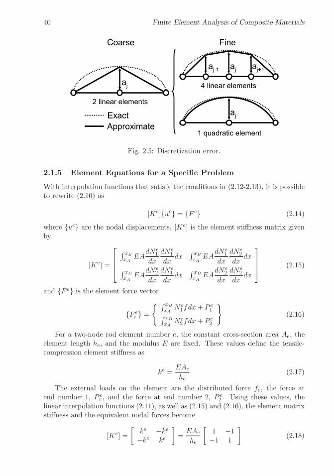
“K15072” — 2013/3/21 — 10:58�

�

�

�

�

�


Fig. 2.5: Discretization error.

2.1.5 Element Equations for a Specific Problem

With interpolation functions that satisfy the conditions in (2.12-2.13), it is possibleto rewrite (2.10) as

[Ke]{ue} = {F e} (2.14)

where {ue} are the nodal displacements, [Ke] is the element stiffness matrix givenby

[Ke] =

⎡

⎢

⎢

⎣

∫ xB

xAEA

dN e1

dx

dN e1

dxdx

∫ xB

xAEA

dN e1

dx

dN e2

dxdx

∫ xB

xAEA

dN e2

dx

dN e1

dxdx

∫ xB

xAEA

dN e2

dx

dN e2

dxdx

⎤

⎥

⎥

⎦

(2.15)

and {F e} is the element force vector

{F ei } =

{∫ xB

xAN e

1fdx+ P e1

∫ xB

xAN e

2fdx+ P e2

}

(2.16)

For a two-node rod element number e, the constant cross-section area Ae, theelement length he, and the modulus E are fixed. These values define the tensile-compression element stiffness as

ke =EAe

he(2.17)

The external loads on the element are the distributed force fe, the force atend number 1, P e

1 , and the force at end number 2, P e2 . Using these values, the

linear interpolation functions (2.11), as well as (2.15) and (2.16), the element matrixstiffness and the equivalent nodal forces become

[Ke] =

[

ke −ke−ke ke

]

=EAe

he

[

1 −1−1 1

]

(2.18)

�

�

“K15072” — 2013/3/21 — 10:58�

�

�

�

�

�


Fig. 2.6: Connectivity between three two-node elements.

{F e} =fehe2

{

11

}

+

{

P e1

P e2

}

(2.19)

2.1.6 Assembly of Element Equations

The element unknown parameters correspond to displacements at the element nodes.Since a node must have the same displacement on both adjacent elements, thevalue is unique. For example, using the connectivity of elements shown in Figure2.6, unique labels are assigned to the displacements, using capital letters. While asuperscript denotes an element number, a subscript indicates a nodal number, asfollows

u11 = U1

u12 = U2 = u21

u21 = U3 = u31

u32 = U4 (2.20)

Now, the element equations can be assembled into the global system. First, thecontribution of element #1 is

⎡

⎢

⎢

⎣

k1 −k1 0 0−k1 k1 0 00 0 0 00 0 0 0

⎤

⎥

⎥

⎦

⎧

⎪

⎪

⎨

⎪

⎪

⎩

U1

U2

U3

U4

⎫

⎪

⎪

⎬

⎪

⎪

⎭

=

⎧

⎪

⎪

⎨

⎪

⎪

⎩

f1h1/2f1h1/2

00

⎫

⎪

⎪

⎬

⎪

⎪

⎭

+

⎧

⎪

⎪

⎨

⎪

⎪

⎩

P 11

P 12

00

⎫

⎪

⎪

⎬

⎪

⎪

⎭

(2.21)

Add the contribution of element #2, as follows

⎡

⎢

⎢

⎣

k1 −k1 0 0−k1 k1 + k2 −k2 00 −k2 k2 00 0 0 0

⎤

⎥

⎥

⎦

⎧

⎪

⎪

⎨

⎪

⎪

⎩

U1

U2

U3

U4

⎫

⎪

⎪

⎬

⎪

⎪

⎭

=

⎧

⎪

⎪

⎨

⎪

⎪

⎩

f1h1/2f1h1/2 + f2h2/2

f2h2/20

⎫

⎪

⎪

⎬

⎪

⎪

⎭

+

⎧

⎪

⎪

⎨

⎪

⎪

⎩

P 11

P 12 + P 2

1

P 22

0

⎫

⎪

⎪

⎬

⎪

⎪

⎭

(2.22)

Finally, add element #3 to obtain the fully assembled system, as follows

�

�

“K15072” — 2013/3/21 — 10:58�

�

�

�

�

�


⎡

⎢

⎢

⎣

k1 −k1 0 0−k1 k1 + k2 −k2 00 −k2 k2 + k3 −k30 0 −k3 k3

⎤

⎥

⎥

⎦

⎧

⎪

⎪

⎨

⎪

⎪

⎩

U1

U2

U3

U4

⎫

⎪

⎪

⎬

⎪

⎪

⎭

=1

2

⎧

⎪

⎪

⎨

⎪

⎪

⎩

f1h1f1h1 + f2h2f2h2 + f3h3

f3h3

⎫

⎪

⎪

⎬

⎪

⎪

⎭

+

⎧

⎪

⎪

⎨

⎪

⎪

⎩

P 11

P 12 + P 2

1

P 22 + P 3

1

P 32

⎫

⎪

⎪

⎬

⎪

⎪

⎭

(2.23)

2.1.7 Boundary Conditions

By equilibrium (see Figure 2.2), the internal loads cancel whenever two elementsshare a node, or

P 12 + P 2

1 = 0

P 22 + P 3

1 = 0 (2.24)

The remaining P 11 and P 2

3 are the forces at the end of the rod. If either end ofthe rod is fixed, then the displacement must be set to zero at that end. Say the endat x = 0 is fixed, then U1 = 0. If the end at x = L is free, then P 2

3 must be specified,since U4 �= 0. If it is not specified, then it is assumed that the force is zero.

2.1.8 Solution of the Equations

Since U1 = 0, eliminating the first row and column of the stiffness matrix, a 3× 3system of algebraic equations is obtained, and solved for 3 unknowns: U2, U3, U4.Once a solution for U2 is found, the reaction P 1

1 is computed from the first equationof (2.23), as follows

−k1U2 =f1h12

+ P 11 (2.25)

2.1.9 Solution Inside the Elements

Now, the solution Ui at 4 points along the rod is available. Next, the solution atany location x can be computed by interpolating with the interpolation functions,as follows

U e(x) =

2∑

j=1

U ejN

ej (x) (2.26)

or

u(x) =

⎧

⎨

⎩

U1N11 (x) + U2N

12 (x) if 0 ≤ x ≤ h1

U2N21 (x) + U3N

22 (x) if h1 ≤ x ≤ h1 + h2

U3N31 (x) + U4N

32 (x) if h1 + h2 ≤ x ≤ h1 + h2 + h3

(2.27)

�

�

“K15072” — 2013/3/21 — 10:58�

�

�

�

�

�


2.1.10 Derived Results

Strains

Strains are computed using (1.5) directly from the known displacements inside theelement. For example,

εx =du

dx=

2∑

j=1

U ej

dN ej

dx(2.28)

Note that if N ej (x) are linear functions, the strains are constant over the element.

In general the quality of the strains is one order of magnitude poorer than theprimary variable (displacements).

Stresses

Stress values are usually computed from strains through the constitutive equations.In this example, with one-dimensional stress-strain behavior

σx = E εx (2.29)

Note that the quality of stresses is the same as that of the strains.

2.2 General Finite Element Procedure

The derivation of the element equations, assembly, and solution for any type ofelements is similar to that of the one-dimensional rod element described in Section2.1, with the exception that the principle of virtual work (PVW, 1.16) is used insteadof the governing equation (2.1). The PVW provides a weak form similar to that in(2.4). Expanding (1.16) for full 3D state of deformation, the internal virtual workis

δWI =

∫

(σxxδεxx + σyyδεyy + σzzδεzz + σyzδγyz + σxzδγxz + σxyδγxy) dV

=

∫

VσT δε dV (2.30)

where

σT = {σxx, σyy, σzz, σyz , σxz, σxy}δεT = {δεxx, δεyy , δεzz , δγyz , δγxz , δγxy} (2.31)

Next, the external work is

δWE =

∫

VfT δu dV +

∫

StT δu dS (2.32)

�

�

“K15072” — 2013/3/21 — 10:58�

�

�

�

�

�


where the volume forces per unit volume and surface forces per unit area are

fT = {fx, fy, fz}tT = {tx, ty,tz} (2.33)

Here, underline ( ) denotes a one-dimensional array, not necessarily a vector.For example, u is a vector but σ are the six components of stress arranged ina six-element array. The virtual strains are strains that would be produced byvirtual displacements δu (x). Therefore, virtual strains are computed from virtualdisplacements using the strain-displacement equations (1.5). In matrix notation

ε = ∂ u

δε = ∂ δu (2.34)

where

∂ =

⎡

⎢

⎢

⎢

⎢

⎢

⎣

∂

∂x0 0

∂

∂y0

∂

∂z

0∂

∂y0

∂

∂x

∂

∂z0

0 0∂

∂z0

∂

∂y

∂

∂x

⎤

⎥

⎥

⎥

⎥

⎥

⎦

T

(2.35)

Then, the PVW is written in matrix notation as

∫

VσT∂ δu dV =

∫

VfT δu dV +

∫

StT δu dS (2.36)

The integrals over the volume V and surface S of the body can be broken elementby element over m elements, as

m∑

e=1

[∫

Ve

σT∂ δu dV

]

=

m∑

e=1

[∫

Ve

fT δu dV +

∫

Se

tT δu dS

]

(2.37)

Whenever two elements share a surface, the contributions of the second inte-gral cancel out, just as the internal loads canceled in Section 2.1.7. The stresscomponents are given by the constitutive equations. For a linear material

σ = C ε (2.38)

with C given by (1.68). The internal virtual work over each element becomes

δW eI =

∫

Ve

σT δε dV =

∫

Ve

εTC δε dV (2.39)

The expansion of the displacements can be written in matrix form as

u = N a (2.40)

�

�

“K15072” — 2013/3/21 — 10:58�

�

�

�

�

�


whereN contains the element interpolation functions and a the nodal displacementsof the element, just as in Section 2.1.4. Therefore, the strains are

ε = ∂ u = ∂ N a = B a (2.41)

where B = ∂ N is the strain-displacement matrix. Now, the discretized form of theinternal virtual work over an element can be computed as

δW eI =

∫

Ve

aTBTC B δa dV = aT∫

Ve

BTC B dV δa = aTKe δa (2.42)

where the element stiffness matrix Ke is

Ke =

∫

Ve

BTC B dV (2.43)

The external virtual work becomes

δW eE =

∫

Ve

fT δu dV +

∫

Se

tT δu dS

=

(∫

Ve

fTN dV +

∫

Se

tTN dS

)

δa = (P e)T δa (2.44)

where the element force vector is

P e =

∫

Ve

NT f dV +

∫

Se

NT t dS (2.45)

The integrals over the element volume Ve and element surface Se are usuallyevaluated numerically by the Gauss integration procedure. For the volume integral,such a procedure needs evaluation of the integrand at a few points inside the volume.Such points, which are called Gauss points, are important for two reasons. First,the constitutive matrix C is evaluated at those locations. Second, the most accuratevalues of strains (and stresses) are obtained at those locations too.

The assembly of the element equations δW eI and δW e

E into the PVW for thewhole body is done similarly to the process in Section 2.1.6. Obviously the processis more complicated than for rod elements. The details of such process and itscomputer programming are part of finite element technology, which is outside thescope of this textbook. Eventually all the element stiffness matrices Ke and elementforce vectors P e are assembled into a global system for the whole body

K a = P (2.46)

Next, boundary conditions are applied on the system (2.46) in a systematic wayresembling the procedure in Section 2.1.6. Next, the algebraic system of equations(2.46) is solved to find the nodal displacement array a over the whole body. Sincethe nodal displacements results for every element can be found somewhere in a, itis possible to go back to (2.34) and to (2.38) to compute the strains and stressesanywhere inside the elements.

�

�

“K15072” — 2013/3/21 — 10:58�

�

�

�

�

�


Example 2.1 Compute the element stiffness matrix (2.43) and the equivalent force vector(2.45) of a rod discretized with one element. Use linear interpolation functions such as(2.11). Compare the result with (2.18-2.19).

Solution to Example 2.1 Let Ae be the transverse area of the rod and he the elementlength, with xe = 0 and xe+1 = he. Substituting these values in the linear interpolationfunctions from equation (2.11), the interpolation functions arrays are obtained as follows

NT =

[

Ne1

Ne2

]

=

⎡

⎢

⎣

xe+1 − x

hex− xehe

⎤

⎥

⎦=

[

1− x/he

x/he

]

The strain-displacement array is obtained as

BT = ∂ NT =

[

∂Ne1/∂x

∂Ne2/∂x

]

=

[ −1/he1/he

]

The rod element has a one-dimensional strain-stress state with linear elastic behavior.Therefore

C = E

Then, using equation (2.43) we can write

Ke =

∫

Ve

BTC B dV =

∫ he

0

[ −1/he 1/he]

E

[ −1/he1/he

]

Aedx

The element stiffness matrix is obtained by integration

[Ke] =EAe

he

[

1 −1−1 1

]

To calculate the equivalent vector force, fe is defined as the distributed force on element,P e1 is the force at end x = 0, and P e

2 is the force at end x = he. Substituting into equation(2.45) we obtain

P e =

∫

Ve

NT f dV +

∫

Se

NT t dS =

∫ he

0

[

1− x/hex/he

]

fedx+

[

P e1

P e2

]

The element equivalent force vector is obtained by integration

P e =fehe2

[

11

]

+

[

P e1

P e2

]

2.3 Solid Modeling, Analysis, and Visualization

Many commercial programs exist with finite element analysis capabilities for differ-ent engineering disciplines. They help solve a variety of problems from simple linearstatic analysis to nonlinear transient analysis. A few of these codes, such as AN-SYS and Abaqus, have special capabilities to analyze composite materials and theyaccept custom, user-programmed constitutive equations and element formulations.Since these software packages not only provide analysis tools, geometric modeling,and visualization of results, but also they can be integrated in the larger design,

�

�

“K15072” — 2013/3/21 — 10:58�

�

�

�

�

�


production, and product life-cycle process, they are often called complete analysisenvironments or computer aided engineering (CAE) systems.

Modern FEA software are commonly organized into three blocks: the pre-processor, the processor, and the post-processor. In the pre-processor, the modelis built defining the geometry, material properties, and element type. Also, loadsand boundary conditions are entered in the pre-processor, but they may also be en-tered during the solution phase. With this information, the processor can computethe stiffness matrix and the force vector. Next, the algebraic equations (2.46) aresolved and the solution is obtained in the form of displacement values. In the lastblock–the post-processor–derived results, such as stress, strain, and failure ratios,are computed. The solution can be reviewed using graphic tools.

In the remainder of this chapter, a general description of the procedures and thespecific steps for a basic finite element analysis (FEA) are presented using examplesexecuted with Abaqus [7]. Although the emphasis of this textbook is on mechanicsof composite materials, concepts are illustrated with examples that are solved usingAbaqus. Solutions to similar examples are available in [8], using ANSYS [9].

The first requirement of the model is the geometry. Then, material properties aregiven for the various parts that make up the geometry. Next, loads and boundaryconditions are applied on the geometry. Next, the geometry is discretized intoelements, which are defined in terms of the nodes and element connectivity. Theelement type is chosen to represent the type of problem to be solved. Next, themodel is solved. Finally, derived results are computed and visualized.

2.3.1 Model Geometry

The model geometry is obtained specifying all nodes, their position, and the elementconnectivity. The connectivity information allows the program to assemble theelement stiffness matrix and the element equivalent force vector to obtain the globalequilibrium equations, as shown in Section 2.1.6.

There are two ways to generate the model. The first is to manually create amesh. The second is to use solid modeling, and then mesh the solid to get the nodeand element distribution.

Manual Meshing

Manual mesh generation was the only method available before solid modeling be-came widespread among commercial packages. It is still the only option with someolder and custom software, although in those cases it is always possible to use ageneral purpose, solid modeling pre-processor to generate the mesh. With manualmeshing, the user creates nodes, then connects the nodes into elements. Afterward,the user applies boundary conditions and loads directly on nodes and/or elements.Manual meshing is used in Example 2.2.

Example 2.2 Use manual meshing to set up a finite element model of a two-dimensionalsquare sheet, in a state of plane stress, with dimensions 20 × 20 mm × 4 mm and mesh itwith a 2 × 2 mesh of continuum, plane stress, square, CPS4R elements in Abaqus. The

�

�

“K15072” — 2013/3/21 — 10:58�

�

�

�

�

�


Fig.2.7:

Squaremeshin

Ex.2.2.

�

�

“K15072” — 2013/3/21 — 10:58�

�

�

�

�

�


left edge (nodes 1, 4, 7 in Fig. 2.7) should be horizontally restrained. Also, node 1 shouldbe vertically restrained. A uniform surface load of −9.5MN/mm2 should be applied to theright edge (nodes 3, 6, 9). The material is steel with E = 210, 000MPa, ν = 0.3. Run themodel from the DOS shell window. Then, use Abaqus/CAE to visualize the results.

Solution to Example 2.2 The commands listed below define the model geometry by usingmanual meshing, and they are written into what is called an input file (Ex_2.2.inp). Theyare available on the Web site [5, file name: Ex 2.2.inp].

The *Node command line is followed by a list of nodes, each line containing the nodenumber, plus x, y, and possibly z coordinates of each node.

The *Element command line is followed by a list of elements, each line containing theelement number, and a sequence of node numbers going counterclockwise (ccw) around theboundary of the element (see Fig. 2.7).

The meaning of the remaining command lines is either obvious or can be researched inthe Abaqus Keywords Reference Manual [10].

*Heading

Example 2.2 FEA of Composite Materials: using Abaqus

*Part, name=Part1

*Node

1, 0., 0.

2, 10., 0.

3, 20., 0.

4, 0., 10.

5, 10., 10.

6, 20., 10.

7, 0., 20.

8, 10., 20.

9, 20., 20.

*Element, type=CPS4R

1, 1, 2, 5, 4

2, 2, 3, 6, 5

3, 4, 5, 8, 7

4, 5, 6, 9, 8

*Nset, nset=NamedSet, generate

1, 9, 1

*Elset, elset=NamedSet, generate

1, 4, 1

** Section: Section-1

*Solid Section, elset=NamedSet, material=Material-1

4.,

*End Part

*Assembly, name=Assembly

*Instance, name=Part1-1, part=Part1

*End Instance

*Nset, nset=Nodeset1, internal, instance=Part1-1

1

*Nset, nset=Nodeset2, internal, instance=Part1-1

4, 7

*Elset, elset=Elset1, internal, instance=Part1-1

2, 4

�

�

“K15072” — 2013/3/21 — 10:58�

�

�

�

�

�


*Surface, type=ELEMENT, name=Surface1, internal

Elset1, S2

*End Assembly

*Material, name=Material-1

*Elastic

210000., 0.3

*Step, name=Step-1

*Static

1., 1., 1e-05, 1.

*Boundary

Nodeset1, 1, 2

Nodeset2, 1, 1

*Dsload

Surface1, P, -9.5

*Restart, write, frequency=0

*Output, field, variable=PRESELECT

*Output, history, variable=PRESELECT

*End Step

To run Abaqus on a command line, first you have to get a DOS shell, as follows:On Windows 7 click Start, then on the Search Programs and Files window, type cmd,then hit Enter. Then, on the DOS shell, do this:

>cd c:\SIMULIA

>mkdir User

>cd User

where cd stands for change directory, and mkd creates a new folder (mkd stands for ‘makedirectory’).1

Next, copy the file Ex_2.2.inp from [5] to the folder c: \Simulia\User , or type thecommands listed above using Notepad or your favorite text editor.2 The command line torun Abaqus is:

>abaqus job=job1 input=Ex_2.2

Now to start CAE on Windows 7, click Start, then All Programs, then Abaqus 6.xx,then Abaqus/CAE. Once CAE starts, close the pop-up window. Then, on the Menu bar atthe top of the screen3 click File, Open, navigate to the c: \Simulia\User\ folder, changethe File Filter to *.odb, and select Job1.odb. At this point you should see the mesh, asshown in Fig. 2.7.

To display element and node numbers do this: On the top Menu, Options, Common,Labels (see Fig. 2.8), checkmark Show element labels and Show node labels. Also inthe same window, to increase the font of the labels do this: Set Font. For future reference,the instructions given in this paragraph are summarized below (see notation in Table 2.1).

1If your system administrator has restricted write access to c:\SIMULIA then make your userdirectory at some other unrestricted location such as c:\TEMP or see Appendix C for additionaldetails.

2We recommend Notepad++ available free at http://notepad-plus-plus.org/.3Also called display, monitor, or window.

�

�

“K15072” — 2013/3/21 — 10:58�

�

�

�

�

�


Fig. 2.8: To display element and node numbers in a larger font size.

Menu: File,

Open [c:\Simulia\User\], File Filter [*.odb], File Name [Job1.odb]

Menu: Options,

Common, Labels,

# checkmark [Show element labels]

# checkmark [Show node labels]

Set Font for All Model Labels, Size [24], OK

OK

Solid Modeling

With solid modeling, the user creates a geometric representation of the geometryusing solid model constructs, such as volumes, areas, lines, and points. Boundaryconditions, loads, and material properties can be assigned to parts of the solid modelbefore meshing. In this way, re-meshing can be done without losing, or having toremove, the loads and boundary conditions. The models are meshed just prior tothe solution. Solid modeling is used in Example 2.3, p. 54.

Abaqus/CAE has all the capabilities to construct the solid model, mesh, solvethe problem, and visualize the results within the same CAE environment. Moreadvanced solid modeling software, such as SolidWorks [11], can be used to generatethe solid model, then import into CAE for finalizing the boundary conditions andloads, invoking the solver, and finally visualizing the results. A brief description of

�

�

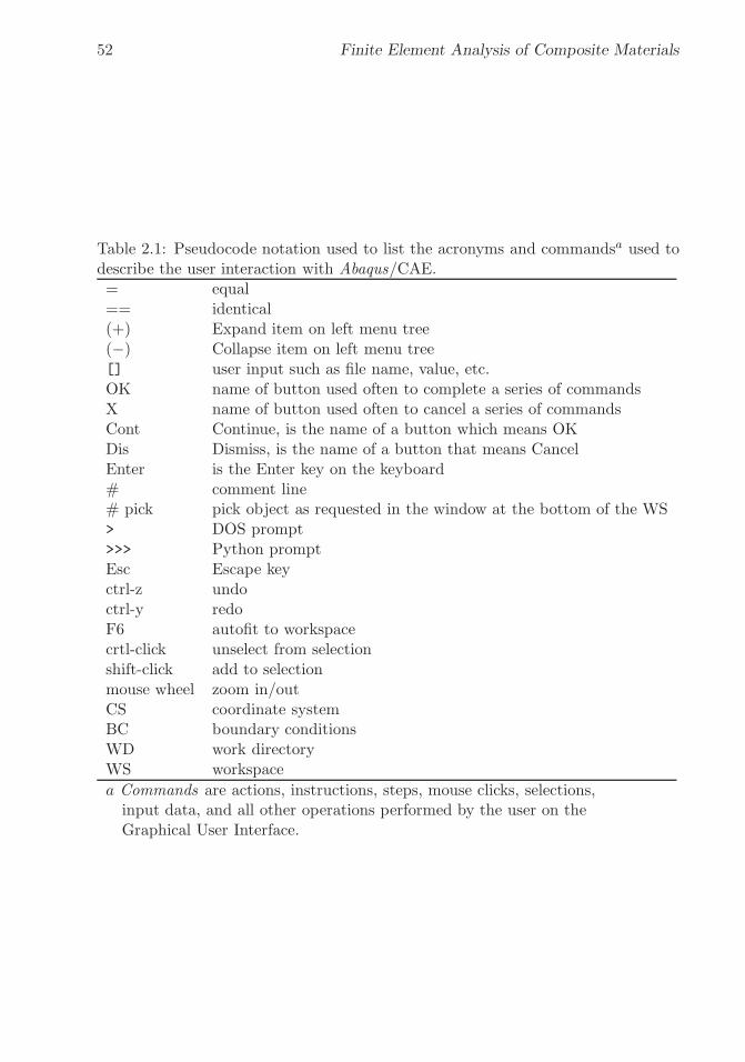
“K15072” — 2013/3/21 — 10:58�

�

�

�

�

�


Table 2.1: Pseudocode notation used to list the acronyms and commandsa used todescribe the user interaction with Abaqus/CAE.= equal== identical(+) Expand item on left menu tree(−) Collapse item on left menu tree[] user input such as file name, value, etc.OK name of button used often to complete a series of commandsX name of button used often to cancel a series of commandsCont Continue, is the name of a button which means OKDis Dismiss, is the name of a button that means CancelEnter is the Enter key on the keyboard# comment line# pick pick object as requested in the window at the bottom of the WS> DOS prompt>>> Python promptEsc Escape keyctrl-z undoctrl-y redoF6 autofit to workspacecrtl-click unselect from selectionshift-click add to selectionmouse wheel zoom in/outCS coordinate systemBC boundary conditionsWD work directoryWS workspace

a Commands are actions, instructions, steps, mouse clicks, selections,input data, and all other operations performed by the user on theGraphical User Interface.

�

�

“K15072” — 2013/3/21 — 10:58�

�

�

�

�

�


the CAE graphical user interface (GUI) is described next. The notation used todescribe the steps necessary to construct a model in CAE are listed in Table 2.1.

The CAE Window

The CAE window4 (see Fig. 2.7) is divided in regions as follows:

– Menu: The top menu bar (horizontally across the top of the window) is dy-namic, i.e., it changes depending on what we are doing. Specifically, it changesaccording to the selection in the drop-down list Module, which is explainedbelow.

– Toolbar: Under the menu bar, we have dynamic toolbars. You can un-dockthem, one at at a time, to learn their names. They are dynamic because theychange depending on what Module is selected.

– Trees: On the left you see two tabs, Model and Results; one for each of thetwo database trees. All the items in the trees can be right-clicked to accessactions to modify the information stored in each item. The trees correspondto the database files .mdb and .odb, as follows:

– Model: .mdb

– Results: .odb

– Drop-down menus: To the right of Model and Results tabs, we have severaldynamic drop-down menus, such as Module, Model, and Part.5 Module:

contains a number of selections, as follows:

– Module:

- Part

- Property

- Assembly

- Step

- Interaction

- Load

- Mesh

- Job

- Visualization

- Sketch

– Workspace: The workspace covers the most of the screen. It is located underthe drop-down menus, to the right of the Model/Results tabs.

4At this time, the user should have Abaqus/CAE open on a computer.5Since the drop-down menus are dynamic, only Module: and ODB: are shown in Fig. 2.7.

�

�

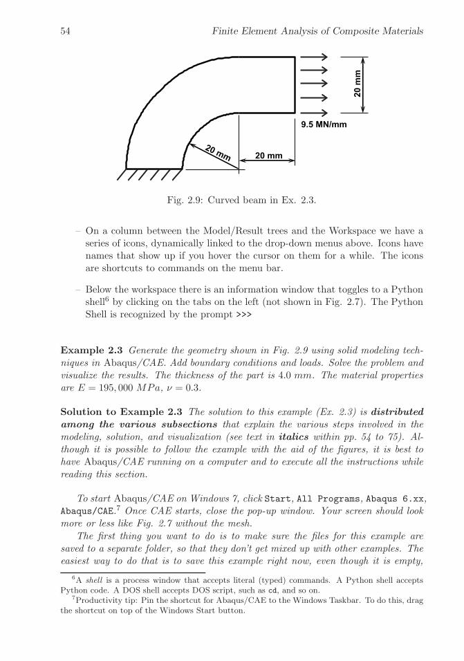
“K15072” — 2013/3/21 — 10:58�

�

�

�

�

�


20 mm20 mm

20

mm

9.5 MN/mm

Fig. 2.9: Curved beam in Ex. 2.3.

– On a column between the Model/Result trees and the Workspace we have aseries of icons, dynamically linked to the drop-down menus above. Icons havenames that show up if you hover the cursor on them for a while. The iconsare shortcuts to commands on the menu bar.

– Below the workspace there is an information window that toggles to a Pythonshell6 by clicking on the tabs on the left (not shown in Fig. 2.7). The PythonShell is recognized by the prompt >>>

Example 2.3 Generate the geometry shown in Fig. 2.9 using solid modeling tech-niques in Abaqus/CAE. Add boundary conditions and loads. Solve the problem andvisualize the results. The thickness of the part is 4.0 mm. The material propertiesare E = 195, 000 MPa, ν = 0.3.

Solution to Example 2.3 The solution to this example (Ex. 2.3) is distributedamong the various subsections that explain the various steps involved in themodeling, solution, and visualization (see text in italics within pp. 54 to 75). Al-though it is possible to follow the example with the aid of the figures, it is best tohave Abaqus/CAE running on a computer and to execute all the instructions whilereading this section.

To start Abaqus/CAE on Windows 7, click Start, All Programs, Abaqus 6.xx,Abaqus/CAE.7 Once CAE starts, close the pop-up window. Your screen should lookmore or less like Fig. 2.7 without the mesh.

The first thing you want to do is to make sure the files for this example aresaved to a separate folder, so that they don’t get mixed up with other examples. Theeasiest way to do that is to save this example right now, even though it is empty,

6A shell is a process window that accepts literal (typed) commands. A Python shell acceptsPython code. A DOS shell accepts DOS script, such as cd, and so on.

7Productivity tip: Pin the shortcut for Abaqus/CAE to the Windows Taskbar. To do this, dragthe shortcut on top of the Windows Start button.

�

�

“K15072” — 2013/3/21 — 10:58�

�

�

�

�

�


to a new folder, as follows. On the Menu bar at the top of the screen click File,Save As, navigate to a new folder of your choice, or create one if you need to; thenin the field File name enter Ex_2.3, OK. These steps are summarized below.

Menu: File, Save as, New directory [name of new directory],

Select new directory, [name of file], OK

The first modeling task is to create one or more Parts, which represent thegeometry of the model. Since this example is very simple, a single part will suffice,but more complex models will require several parts. There are many ways to definethe geometry of a part. In this first example we use Points connected by Arcs andLines. To work with parts, the Module has to be set to Part. Remember that

– Module: refers to the drop-down box immediately left of the Model/Result tabs(see Fig. 2.7), and

– Menu: refers to the top menu bar running across the top of the CAE window.

In this way, the selections described below will result in opening the dialog boxshown in Fig. 2.10:

Module: Part

Menu: Part, Create,

Name[Part-1], 2D, Deformable, Shell, Approx size [200], Cont

# sketch mode is now active

Next, we define Points and join them with Arcs, as summarized below. See Fig.2.11 in conjunction with the step-by-step instructions below.

Menu: Add, Point,

[0,0] # type in the input window below the WS, then [Enter]

[-20,0]

[-40,0]

[0,20]

[0,40]

[20,20]

[20,40]

F6 # zoom to fit

Menu: Add, Arc, Center/Endpoints,

# pick center point (see Fig. 2.11)

# pick point left of center point

# pick point above of center point, the arc is done

# again pick center point (see Fig. 2.11)

# pick point left-most of center point

# pick point above-most of center point, the outer arc is done

X # to finalize the Add feature (do not click Done)

At this point, the workspace should look like Fig. 2.11.Sketch mode is similar to SolidWorks [11]. Arcs, points, and other geometrical

constructs are called entities. When adding/editing entities, you must follow the

�

�

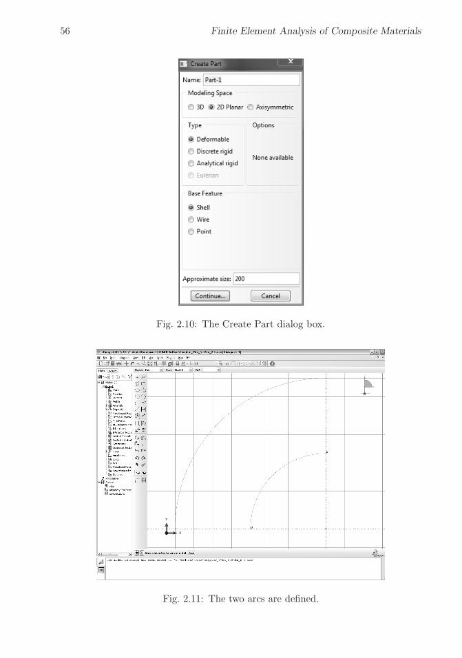
“K15072” — 2013/3/21 — 10:58�

�

�

�

�

�


Fig. 2.10: The Create Part dialog box.

Fig. 2.11: The two arcs are defined.

�

�

“K15072” — 2013/3/21 — 10:58�

�

�

�

�

�


Fig. 2.12: The Part is finalized.

instructions displayed immediately below the WS. The X situated to the left of theinstructions line allows you to finalize the current operation, i.e., the Add featurein the set of instructions above.

Still referring to Fig. 2.11, add lines to close the boundary of the figure, andonce the figure is closed, the part is created:

Menu: Add, Lines, Connected,

# pick two nodes to close bottom left of the part

X # to finalize the Line drawing

Menu: Add, Lines, Connected,

# pick 4 nodes in sequence to close rectangle at top right

X # to finalize the Line drawing

Done # to finish the sketch, thus creating the part

At this point, the workspace should look like Fig. 2.12.

2.3.2 Material and Section Properties

Parts must be associated to materials. Depending on the analysis, material prop-erties can be linear (linear elastic analysis) or nonlinear (e.g. damage mechanicsanalysis), isotropic or orthotropic, constant or temperature-dependent. Enteringthe correct materials properties is one of the most important aspects of a successfulanalysis of composite materials. A great deal of attention is devoted to materialproperties in the rest of the textbook. For now it will suffice to illustrate the process

�

�

“K15072” — 2013/3/21 — 10:58�

�

�

�

�

�


using a linear elastic, isotropic material. For structural analysis, elastic propertiesmust be defined according to Section (1.12). Other mechanical properties, such asstrength, density, and thermal expansion coefficients are optional and their defini-tion depends on the objectives of the analysis.

In Abaqus/CAE, materials are entered in Module: Property, Menu: Material.The instructions below will bring out a pop-up window as shown in Fig. 2.13, wherethe materials properties are entered, as follows:

Module: Property

Menu: Material, Create,

Name [Material-1], Mechanical, Elasticity, Elastic,

Type, Isotropic [195000, 0.3], OK

All elements need material properties, but structural elements need additionalparameters that vary with the type of element. These parameters result from an-alytical integration of the 3D governing equations while formulating the element.For example, the cross-section area A appears in (2.1) because the 3D partial dif-ferential equations have been integrated over the cross section of the rod to arriveat the ordinary differential equation (2.1).

Beam elements require cross-section area and moments of inertia. Laminatedshell elements require the laminate stacking sequence (LSS, see Figure 3.4, p. 96).Continuum elements such as 3D solid elements (see Table 2.2) do not require addi-tional parameters, only material properties, because the geometry is fully describedby the mesh. However, continuum elements representing laminated composites stillrequire the LSS.

Conventional shells and beams are typical structural elements. The word con-ventional is used also by Abaqus to emphasize shell elements that are not contin-uum. On the other hand, continuum shells are continuum elements with kinematicconstrains introduced in order to represent shell behavior.

Therefore, besides a Material, one needs to create a Section to provide theadditional parameters required by structural elements. In Abaqus, the additionalparameters are called section parameters; in ANSYS they are called section con-stants.8 Continuum elements do not require section parameters, but a Section hasto be created anyway.

In this simple example, section parameters are used to define the state of planestress for the part shown in Fig. 2.9. A complex model may have several differentsections. Sections are created in the same Module: Property, as follows:

Menu: Section, Create,

# plane stress/strain is considered solid even though

# pstres needs a thickness

# pstran does not

# shells are not solids, they need a thickness

# beams are not solids, they need area and moments of inertia

Name [Section-1], Solid, Homogeneous, Cont

8Section constants were called “real constants” in older versions of ANSYS.

�

�

“K15072” — 2013/3/21 — 10:58�

�

�

�

�

�


Fig. 2.13: Material properties window.

�

�

“K15072” — 2013/3/21 — 10:58�

�

�

�

�

�


Table 2.2: Some of the elements available in Abaqus and ANSYS.Abaqus ANSYS Nodes DOF Element Description

Structural elementsT2D2 LINK180 2 uX uY line bar/truss, 2D spaceT3D2 LINK180 2 uX uY uZ line bar/truss, 3D space- COMBIN14 2 uX uY uZ spring/damper, 3D spaceB21 BEAM188 2 uX uY line beam in 2D space

θX θYB31 BEAM188 2 uX uY uZ line beam in 3D space

θX θY θZCPE4R PLANE182 4 uX uY solid quadrilateral

in 2D spaceCPE8R PLANE183 8 uX uY solid quadrilateral

in 2D spaceS4R SHELL181 4 uX uY uZ shell quadrilateral

θX θY θZ in 3D space (conventional)S8R SHELL281 8 uX uY uZ shell quadrilateral

θX θY θZ in 3D space (conventional)S8R5 - 4 uX uY uZ thin shell quadrilateral

θX θY in 3D space (conventional)

Continuum elementsC3D8 SOLID185 8 uX uY uZ solid hexahedra

in 3D spaceC3D20 SOLID186 20 uX uY uZ solid hexahedra

in 3D spaceSC8R SOLSH190 8 uX uY uZ shell hexahedra

in 3D space (continuum)

�

�

“K15072” — 2013/3/21 — 10:58�

�

�

�

�

�


Fig. 2.14: The Create Section and Edit Section windows define the Section.

Material: Material-1,

Plane stress/strain thickness [4.0], OK

The Create Section and Edit Section windows, shown in Fig. 2.14, appear insequence. They are used to define the section.

Finally, we need to tell the software what are the section properties for eachpart. This is done by assigning Sections to Parts. In this simple model there is onlyone part and only one section, so the assignment is trivial, but it has to be doneanyway. Note that the assignment is done in the same module, i.e., the Propertymodule. The procedure is illustrated in Fig. 2.15 and summarized as follows:

Menu: Assign, Section

# pick all (click on part), Done

OK

2.3.3 Assembly

If more than one part exists, assembly is necessary to put the parts together intowhat is called an assembly, which represents the physical object you are trying toanalyze.

During assembly it is possible to specify how the mesh is related to the parts.That is, the mesh can be dependent or independent of the part. A dependent meshis tied to the part. So, if the part is used (i.e., instanced) multiple times in anassembly, all the instances of the part will be meshed identically. And independentmesh means that each instance of the part will have to be meshed independently.The latter provides flexibility to refine the mesh for some instances of the part atthe expense of more work when it comes the time to mesh. Since this example hasonly one part, the assembly process is trivial, as follows (see also Fig. 2.16):

Module: Assembly

Menu: Instance, Create,

Independent, OK

�

�

“K15072” — 2013/3/21 — 10:58�

�

�

�

�

�


Fig.2.15:Assigningasectionto

thepart.

�

�

“K15072” — 2013/3/21 — 10:58�

�

�

�

�

�


Fig. 2.16: Dialog box to create an instance of a part.

2.3.4 Solution Steps

Next, the analysis process is normally broken down into several steps, each repre-senting different loading and constraint conditions. The minimum number of stepsis two: an initial step and at least one additional step. No loads can be applied onthe initial step, only boundary conditions.

The current example uses just those two steps, as follows:

Module: Step

Menu: Step, Create,

Name [Step-1], General, Static/General, Cont

OK

The dialog box for Create Step is followed by one for Edit Step to complete thedata entry for this step, as shown in Fig. 2.17.

2.3.5 Loads

In structural analysis, loads are defined by forces, pressures, inertial forces (as grav-ity), and specified displacements, all applied to the model. Specification of differentkinds of loads for the FE model is explained in the following sections. The reac-tions obtained by fixing a nodal degree of freedom (displacements and rotations)are discussed also.

Loads can be applied on nodes by means of concentrated forces and moments,as shown in Example 2.4, p. 75. Also, loads can be distributed over the elements as:surface loads, body loads, inertia loads, or other coupled-field loads (for example,thermal strains). Surface loads are used in Example 2.5, p. 77.

�

�

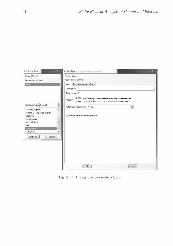
“K15072” — 2013/3/21 — 10:58�

�

�

�

�

�


Fig. 2.17: Dialog box to create a Step.

�

�

“K15072” — 2013/3/21 — 10:58�

�

�

�

�

�


A surface load is a distributed load applied over a surface, for example a pressure.A body load is a volumetric load, for example expansion of material by temperatureincrease in structural analysis. Inertia loads are those attributable to the inertia ofa body, such as gravitational acceleration, angular velocity, and acceleration.

A concentrated load applied on a node is directly added to the force vector.However, the element interpolation functions are used to compute the equivalentforces vector due to distributed loads.

In Abaqus/CAE, loads and boundary (support) conditions for the structure arespecified with the Loads module, as follows:

Module: Load

Menu: Load, Create,

Name [load-1], Mechanical, Pressure, Cont

# pick the vertical edge on the right, Done

Magnitude [-9.5], OK

The dialog box for Create Load (top left in Fig. 2.18) is followed by the selectionof the surfaces over which the load (or bc) are to be applied (note dialog box belowthe x-y-z triad in Fig. 2.18), then followed by the Edit Load box to enter the valuesfor the load (top right in Fig. 2.18).

2.3.6 Boundary Conditions

The boundary conditions are the known values of the degrees of freedom (DOF)on the boundary. In structural analysis, the DOF are displacements and rotations.With this information, the software knows which values of a in (2.46) are known orunknown.

Constrained Displacements and Rotations

In general, a node can have more than one DOF. For example, if the FE model usesbeam elements in 2D space, there are three DOF: the horizontal displacement, thevertical displacement, and the rotation around an axis perpendicular to the plane.Constraining different sets of DOF results in different boundary conditions beingapplied. In the 2D beam element case, constraining only the horizontal and verticaldisplacements results in a simple support, but constraining all the DOF results ina clamped condition.

Symmetry Conditions

Symmetry conditions can be applied to reduce the size of the model without loss ofaccuracy. Four types of symmetry must exist concurrently: symmetry of geometry,boundary conditions, material, and loads. Under these conditions the solution willalso be symmetric. For example, symmetry with respect to the y − z plane meansthat the nodes on the symmetry plane have the following constraints

ux = 0 ; θy = 0 ; θz = 0 (2.47)

�

�

“K15072” — 2013/3/21 — 10:58�

�

�

�

�

�


Fig. 2.18: Dialog box to create a Load.

Fig. 2.19: Convention for rotations of a plate or shell.

�

�

“K15072” — 2013/3/21 — 10:58�

�

�

�

�

�


where ux is the displacement along the x-direction, θy and θz are the rotationsaround the y− and z−axis, respectively (Figure 2.19). Note that the definitionof rotations used in shell theory (φi, see Section 3.1) is different than the usualdefinition of rotations θi that follows the right-hand rule. All rotations in Abaqus9

are described using right-hand-rule rotations θi. Symmetry boundary conditionson nodes in the symmetry plane involve the restriction of DOF translations out-of-plane with respect to the symmetry plane and restriction of the DOF rotationsin-plane with respect to the symmetry plane. Symmetry boundary conditions areused in Example 2.5, p. 77.

Antisymmetry Conditions

Antisymmetry conditions are similar to the symmetry conditions. They can beapplied when the model exhibits antisymmetry of loads but otherwise the modelexhibits symmetry of geometry, symmetry of boundary conditions, and symmetry ofmaterial. Antisymmetry boundary conditions on nodes in the antisymmetry planeinvolve restriction of DOF translations in the antisymmetry plane and restrictionof DOF rotations out-of-plane with respect to the antisymmetry plane.

Periodicity Conditions

When the material, load, boundary conditions, and geometry are periodic with pe-riod (x, y, z) = (2ai, 2bi, 2ci), only a portion of the structure needs to be modeled,with dimensions (2ai, 2bi, 2ci). The fact that the structure repeats itself periodi-cally means that the solution will also be periodic. Periodicity conditions can beimposed by different means. One possibility involves using constraint equations(CE) between DOF (see Section 6.2) or using Lagrange multipliers.

Boundary Conditions in Abaqus/CAE

In Abaqus/CAE, the dialog box for Create a Boundary Condition is followed by theEdit Boundary Condition dialog, as shown in Fig. 2.20. The dialog box is reachedas follows:

Module: Load

Menu: BC, Create,

Name [BC-1], Step: Initial, Mechanical, Displacement/Rot, Cont

# pick the horizontal edge on bottom, Done

# checkmark U1, U2, UR3, OK

Step: Step-1 # to see the load and BC together

9Quote “Except for axisymmetric elements, the degrees of freedom are always referred to asfollows: 1: x-displacement 2: y-displacement 3: z-displacement 4: Rotation about the x-axis, inradians 5: Rotation about the y-axis, in radians 6: Rotation about the z-axis, in radians ... Herethe x-, y-, and z-directions coincide with the global X-, Y-, and Z-directions, respectively; however,if a local transformation is defined at a node (see Transformed coordinate systems [7, Section2.1.5]), they coincide with the local directions defined by the transformation.” End quote [7].

�

�

“K15072” — 2013/3/21 — 10:58�

�

�

�

�

�


Fig. 2.20: Dialog box to create Boundary Conditions.

To see the loads together with the BC, one must change the visualized step toStep-1, because on Step: Initial, only the BC are present. To change the visualizedstep, look for the Step drop-down box to the right of the Module drop-down menu.Once the change is made, the WS should look like Fig. 2.21.

2.3.7 Meshing and Element Type

Next, the assembly needs to be meshed. There are many ways to mesh a model. Forthis example we use a very simple approach, called global seeding, as follows:

Module: Mesh

Menu: Seed, Instance,

Approx global size [5.0], Apply, OK

Menu: Mesh, Controls, Quad, Structured, OK

Global seeding, as shown in the left dialog box in Fig. 2.22, is perhaps the easiestapproach to specify mesh density. It is best to click Apply before OK. This providesan opportunity to see the seeded part, and thus to modify it, before committing to agiven seed pattern. Of course everything can be edited, but that is for later.

Then, on the right dialog box in Fig. 2.22, Mesh Control is used to specify theelement characteristics.

Finite Element Analysis (FEA) programs have an element library that containsmany different element types. The element type determines the element formulationused. For example, the degree of freedom set, the interpolation functions, whetherthe element is for 2D or 3D space, etc. The element type identifies the elementcategory: bar/rod tensile-compression, beam bending, solid, shell, laminate shell,etc. Each commercial code identifies element formulations with different labels.

�

�

“K15072” — 2013/3/21 — 10:58�

�

�

�

�

�


Fig.2.21:Displayingtheload

san

dbou

ndaryconditions.

�

�

“K15072” — 2013/3/21 — 10:58�

�

�

�

�

�


Fig. 2.22: Using Global Seeds (left dialog box) and Mesh Control (right dialog box).

Identification labels and basic characteristics of a few element formulations areshown in Table 2.2. Also, each element type has different options. For example,on a planar solid element, an option allows one to choose between plane strain andplane stress analysis.

The element type is selected in the Element Type dialog box shown in Fig. 2.23.The last step is to finalize (instance) the mesh. The procedure is summarized asfollows:

Menu: Mesh, Element type, Standard, Linear, Plane stress, OK

Menu: Mesh, Instance, Yes

Finally, your mesh should look like the one displayed in Fig. 2.24.

2.3.8 Solution Phase

In the solution phase of the analysis, the solver subroutine included in the finiteelement program solves the simultaneous set of equations (2.46) that the finiteelement method generates. Usually, the primary solution is obtained by solvingfor the nodal degree of freedom values, i.e., displacements and rotations. Then,derived results, such as stresses and strains, are calculated at the integration points.Primary results are called nodal solutions and derived results are called elementsolutions.

Several methods of solving the system of simultaneous equations are available.Some methods are better for larger models, others are faster for nonlinear analysis,others allow one to distribute the solution by parallel computation. Commercialfinite element programs solve these equations in batch mode. The frontal directsolution method is commonly used because it is rather efficient for FEA. When theanalysis is nonlinear, the equations must be solved repeatedly, thus increasing thecomputational time significantly.

To solve the model, one must create a Job. The job is then submitted from withinCAE for execution by the Abaqus processor. The CAE submit process is simply a

�

�

“K15072” — 2013/3/21 — 10:58�

�

�

�

�

�


Fig. 2.23: Element Type.

way to submit a job as in Ex. 2.2 but within CAE, thus obviating the use of a DOSshell. Note however that execution is a process done outside CAE. CAE maintainsa model database (.mdb), and on Submit, it generates an input file (.inp) that isread by the Abaqus processor. Although the processor checks the file for errors,it cannot find all possible modeling errors until actual execution. Since, the errorcheck capability of the processor is much less intensive than the solution itself, aData Check is normally requested from the Job Manager before requesting a solu-tion. The response is displayed in the information window located at the bottom ofthe CAE window. If the data check passes, one can submit the job. Again, progressis shown in the information window. Once the solution is completed, hopefully with-out errors, the results are written by the processor in the output database (.odb). Atthis point one can invoke the Visualization module directly from the Job window byclicking Results. This last step will change the module to Visualization, read the.odb, and display a preliminary visualization. The process is summarized as follows:

Module: Job

Menu: Job, Manager, # opens the Job Manager window

Create, Name [Job-1], Model: [Model-1],

Description: [User’s heading goes here], Cont, OK

Data check # watch the execution window below the WS

Submit # watch the execution window below the WS

Results

�

�

“K15072” — 2013/3/21 — 10:58�

�

�

�

�

�


Fig.2.24:Thepartis

meshed

.

�

�

“K15072” — 2013/3/21 — 10:58�

�

�

�

�

�


Fig. 2.25: The Job Manager and Create Job dialog boxes.

The Job Manager dialog and the Create Job dialog boxes are shown in Fig.2.25. On the Job Manager, note the buttons for Write Input, Data Check, Submit,Continue, Monitor, Results, and Kill. These allow the user to control the executionof the Abaqus processor, and with Results, to jump directly to the visualization modeafter the execution is done.

The Description field allows the user to enter a heading that will display onthe visualization module provided Viewport Annotation Options, General, Showtitle box is checked. The heading appears in the .inp file following the keyword*Heading, as shown in Example 2.2, p. 47.

2.3.9 Post-processing and Visualization

Once the solution has been calculated, the post-processor can be used to reviewand to analyze the results. Results can be reviewed graphically or by listing thevalues numerically. Since a model usually contains a considerable amount of re-sults, it may be better to use graphical tools. Post-processors of commercial codesproduce contour plots of stress and strain distributions, deformed shapes, etc. Thesoftware usually includes derived calculations such as error estimation, load casecombinations, or path operations.

The visualization module can be reached either from the Job Manager (button Re-sults in Fig. 2.25) or by changing the Module to Visualization using the drop-downModule menu, but the latter requires the user to further instruct CAE to read the.odb by executing File, Open, File Filter, [.odb], File Name, [job1.odb].Assuming you reached the visualization module by clicking Results in the Job Man-ager, a basic visualization can be done as follows:

Module: Visualization

Menu: Plot, Contours, On Deformed Shape

This will produce a contour plot of von Mises stress on the deformed shape, asshown in Fig. 2.26. The maximum value of stress is 65.78 MPa. Finally, before

�

�

“K15072” — 2013/3/21 — 10:58�

�

�

�

�

�


Fig.2.26:Visualizeacontourplotof

vonMises

stress

onthedeformed

shap

e.

�

�

“K15072” — 2013/3/21 — 10:58�

�

�

�

�

�


exiting the program, save the various files that contain the status of Abaqus/CAEat this point in the session; as follows:

Menu: File, Save # save the .cae and .mdb files

Menu: File, Exit # exit CAE

The .mdb file contains all the model information. The file .cae allows you toresume the session at a later time. A copy of Ex_ 2. 3. cae is available in the Website [5].

Examples 2.4 and 2.5 include commands to review the results by listing and bygraphic output, respectively.

Example 2.4 ( [8, Example 2.5])Use a commercial FE code to find the axial displacementat the axially loaded end of a rod clamped at the other end. The rod is made of steelE = 200, 000 MPa, diameter d = 9 mm, length L = 750 mm, and load P = 100, 000 N .Also find the stress and strain. Use three two-node (linear) truss elements (called linkelements in Ansys).

Solution to Example 2.4 The Abaqus/CAE procedure is listed below. The CAE file isavailable in [5, Ex 2.4.cae]. Poisson’s ratio should not be needed for a 1D analysis of a bar,but it is required in Abaqus/CAE for defining the isotropic material, so the value ν = 0.3is used.

i. Creating the geometry

Module: Part

Menu: Create, Name: [Part-1], 2D, Deformable, Wire,

Approx size: [2000], Cont

Menu: Add, Line, Connected Lines,

# enter coordinates in the dialog box below the WS

[0,0], Enter,

[750,0], Enter, X, Done

ii. Entering the material and section properties

Module: Property

Menu: Material, Create, Name [Material-1],

Mechanical, Elasticity, Elastic, Isotropic, [200E3, 0.3], OK

Menu: Section, Create, Name: [Section-1], Beam, Truss, Cont

Material-1, Cross-sectional area: [63.617], OK

Menu: Assign, Section, # pick the truss, Done, OK

iii. Creating an assembly, which is trivial in this case

Module: Assembly

Menu: Instance, Create, [Part-1], Independent, OK

iv. Creating a step as part of the solution strategy

Module: Step

Menu: Step, Create, Name [Step-1], Static, General, Cont, OK

v. Specifying loads and boundary conditions, as well as adjusting the display

�

�

“K15072” — 2013/3/21 — 10:58�

�

�

�

�

�


Module: Load

Menu: BC, Create, Name: [BC-1],

Step: Initial, Category: Mechanical, Types: Symm, Cont

# pick the origin, Done,

Encastre, OK

Menu: Load, Create, Name: [Load-1],

Step: Step-1, Category: Mechanical, Types: Concentrated, Cont

# pick the end @ x=750, Done,

CF1 [100E3], OK

Menu: View, Assembly display options,

Attribute, Symbol, Size: [24], Arrows: [24], Apply, OK

F6 # roll the mouse wheel forward to see the part smaller

vi. Meshing

Module: Mesh

Menu: Seed, Instance, Apply, # to see the proposed mesh seeds

# change it to get 3 elements

Approx global size [250], Apply, OK

Menu: Mesh, Element Type, Family: Truss, Linear, OK



Tab: Mesh, # checkmark Show node labels, Apply

# checkmark Show element labels, Apply, OK

# to save these options as default for the future

Menu: File, Save Options, Current, OK

vii. Defining a Job for the Abaqus processor to execute

Module: Job

Menu: Job, Manager,

Create, Name [Job-1], Cont, OK

Submit, # monitor the progress window below the WS

Results, # switches to Module: Visualization

viii. Visualizing the results is easier by invoking the Results from the Job Manager as inthe previous step. Once in the Visualization module


# to get arrows with magnitude proportional to the displacement

# max. value read on the color scale is 5.895 mm

Menu: Result, Field Output,

Tab: Symbol Variable, Name: U, Vector: Resultant, Apply, OK

# to get the stress

# max. value read on the color scale is 1572 MPa

Menu: Result, Field Output, Tab: Primary Variable,

Name: S, Component: S11, Apply, Contour, OK

# to get the strain

# max. value read on the color scale 7860E-3 (micro-strain)

Menu: Result, Field Output, Tab: Primary Variable,

Name: E, Component: E11, Apply, Contour, OK

# further modify the way things are seen on the screen

# and save the settings

�

�

“K15072” — 2013/3/21 — 10:58�

�

�

�

�

�


Fig. 2.27: Rectangular notched strap analyzed in Example 2.5.

Menu: View, ODB Display Options, Tab: Entity Display,

Symbol size [24]

Menu: File, Save Options, Current, OK

A convenient combination of units for this case is Newton, mm, and MPa = N/mm2.The analysis results can be easily verified by mechanics of material calculations, as follows

Ux =PL

AE=

(750)(100000)

(63.617)(200000)= 5.894 mm

σ =P

A=

100000

63.617= 1571.9 MPa

ε =σ

E= 7.859 · 10−3

Example 2.5 [8, Example 2.6]Use a commercial FE code to find the stress concentrationfactor of a rectangular notched strap. The dimensions and the load state are defined inFigure 2.27. Use eight node (quadratic) quadrilateral plane stress elements.

Solution to Example 2.5 The Abaqus/CAE procedure is listed below. The CAE file isavailable in [5, Ex 2.5.cae].

i. Creating the geometry

Module: Part,

Menu: Part, Create, Name: [Part-1],

2D, Deformable, Shell, Approx size [200], Cont

# a quarter model of the Figure in the textbook

Menu: Add, Point,

[0,0]

[50,18.5]

X,

Menu: Add, Line, Rectangle, #pick diagonal points, X

Add, Point,

[0,20] # center

[7.5,20] # radius

�

�

“K15072” — 2013/3/21 — 10:58�

�

�

�

�

�


X,

Menu: Add, Circle # select center and edge point

Edit, Auto trim # the unneeded lines/arches

X,

Done # with the sketch. finalize the part.

Menu: File, Save

ii. Entering the material and section properties

Module: Property

Menu: Material, Create, Name: [Material-1],

Mechanical, Elasticity, Elastic, [190E3, 0.3], OK

Menu: Section, Create, Name: [Section-1], Solid, Homogeneous, Cont

# checkmark Plane stress/strain thickness: [4], OK

Menu: Assign, Section, # pick the part, Done, OK

iii. Creating an assembly

Module: Assembly

Menu: Instance, Create, Name: [Part-1], Independent, OK

iv. Creating a step as part of the solution strategy

Module: Step

Menu: Step, Create, Name: [Step-1], Static, General, Cont, OK

v. Specifying loads and boundary conditions, as well as adjusting the display

Module: Load

Menu: BC, Create, Name: [BC-1], Step: Initial, Mechanical, Symm, Cont

# pick the horiz edge on bottom, Done, YSYMM, OK

Menu: BC, Create, Name: [BC-2], Step: Initial, Mechanical, Symm, Cont

# pick the vert edge on left, Done, XSYMM, OK

Menu: Load, Create, Name: [Load-1],

Step: Step-1, Mechanical, Types: Pressure, Cont

# pick the vertical edge on the right, Done,

Distribution: Uniform, Magnitude [-10], OK

# mouse wheel fwd to zoom out on the WS

vi. Meshing

Module: Mesh

# Above the WS, select Object: Assembly

Menu: Seed, Instance, Apply, #if you like it, OK,

# otherwise Approx global size: [1.0], Apply, OK

Menu: Mesh, Controls, Quadratic, Structured, OK

Menu: Mesh, Element type, Standard, Quadratic,

Family: Plane stress, Reduced Integration, OK

Menu: Mesh, Instance, Yes, # OK to mesh the part instance

vii. Defining a Job for the Abaqus processor to execute

�

�

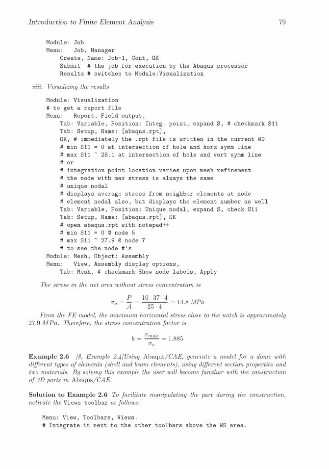
“K15072” — 2013/3/21 — 10:58�

�

�

�

�

�


Module: Job

Menu: Job, Manager

Create, Name: Job-1, Cont, OK

Submit # the job for execution by the Abaqus processor

Results # switches to Module:Visualization

viii. Visualizing the results


# to get a report file

Menu: Report, Field output,

Tab: Variable, Position: Integ. point, expand S, # checkmark S11

Tab: Setup, Name: [abaqus.rpt],

OK, # immediately the .rpt file is written in the current WD

# min S11 = 0 at intersection of hole and horz symm line

# max S11 ~ 28.1 at intersection of hole and vert symm line

# or

# integration point location varies upon mesh refinement

# the node with max stress is always the same

# unique nodal

# displays average stress from neighbor elements at node

# element nodal also, but displays the element number as well

Tab: Variable, Position: Unique nodal, expand S, check S11

Tab: Setup, Name: [abaqus.rpt], OK

# open abaqus.rpt with notepad++

# min S11 = 0 @ node 5

# max S11 ~ 27.9 @ node 7

# to see the node #’s

Module: Mesh, Object: Assembly


Tab: Mesh, # checkmark Show node labels, Apply

The stress in the net area without stress concentration is

σo =P

A=

10 · 37 · 425 · 4 = 14.8 MPa

From the FE model, the maximum horizontal stress close to the notch is approximately27.9MPa. Therefore, the stress concentration factor is

k =σmax

σo= 1.885

Example 2.6 [8, Example 2.4]Using Abaqus/CAE, generate a model for a dome withdifferent types of elements (shell and beam elements), using different section properties andtwo materials. By solving this example the user will become familiar with the constructionof 3D parts in Abaqus/CAE.

Solution to Example 2.6 To facilitate manipulating the part during the construction,activate the Views toolbar as follows:

Menu: View, Toolbars, Views.

# Integrate it next to the other toolbars above the WS area.

�

�

“K15072” — 2013/3/21 — 10:58�

�

�

�

�

�


Creating the 3D dome

i. Creating a solid semi-sphere:

Module: Part

Menu: Part, Create, Name [Part-1], 3D, Deformable, Solid,

Revolution, Approximate size [2000], Cont,

Menu: Add, Arc, Center/Endpoint,

# in the dialog box below the WS enter the coordinates

[0,0], [0,500], [500,0], X # to end the Arc command, F6 # zoom/fit


# enter the coordinates

[0,500], [0,0], [500,0], X # to end the Line command, Done,

Angle [360], OK

A 3D semi-sphere should have been created.

ii. Creating the side-walls:

# Rotate the part so you can see the base of the semi-sphere,

Menu: View, Rotate, X # to end the Rotate command,

# roll the mouse-wheel backward to zoom in,

# save this view-point for use in future procedures,

# click the ’Save View’ icon from the ’Views toolbar’,

# in the pop-up window select [User 1], Save Current, OK,

Menu: Shape, Cut, Extrude, # pick the base of the semi-sphere,

# pick the edge of the base of the semi-sphere,

# Sketch mode is now active,

Menu: Add, Line, Rectangle, # enter the coordinates

[300,300], [-300,-300],

# create a new rectangle entering the coordinates

[600,600], [-600,-600], X # to end the Line command, Done,

Type: [Through All], OK

The semi-sphere should have been cut creating four identical side-walls as shown inFigure 2.28.

iii. Reducing the height of the side-walls:

Menu: Shape, Cut, Extrude, # pick one of the side-walls,

# in the dialog box below the WS select [horizontal on bottom],

# pick the longest straight edge of the side-wall selected,


# roll the mouse-wheel forward to see the figure smaller,

# Draw a rectangle in an area away from the figure,

Menu: Add, Line, Rectangle, # pick any two point on the screen,

X # to end Line command

Your construction should look similar to Figure 2.29.

Menu: Add, Dimension, # pick a vertical line of the rectangle

# may need to move pointer and right-click to create dimension

�

�

“K15072” — 2013/3/21 — 10:58�

�

�

�

�

�


# enter the height of the rectangle [200],

# pick a horizontal line of the rectangle,

# enter the width of the rectangle [600],

X # to end the Dimension command

Your construction should look similar to Figure 2.30.

Menu: Edit, Transform, Translate,

# in the notification area below the WS select [Move],

# pick the four lines forming the rectangle

# hold the ’shift-key’ to individually select the lines, Done,

# pick the lower-left point of the rectangle,

# pick the lower-left point of the figure,

X # to end the Translate command, Done

The rectangle should have been moved as shown in Figure 2.31.

Type: [Through All], OK

The height of the part should have been reduced as shown in Figure 2.32.

iv. Converting the solid part to a shell part:

Menu: Shape, Shell, From Solid,

# pick the part, Done, X # to end the shell command,

Menu: Tools, Geometry Edit, Face, Remove,

# pick the surface at the base of the part,

Done, X # to end the command, # close the pop-up window

The part should look like the one shown in Figure 2.33.

v. Creating the supporting columns:

Menu: Shape, Wire, Sketch, # pick one of the side-walls,

# in the dialog box below the WS select [horizontal on bottom],

# pick the longest straight edge of the side-wall selected,


# roll the mouse-wheel forward to see the figure smaller,


# pick the lower-left corner of the part,

# pick any point directly below (it must create a vertical line),

X # to end the Line command,

Menu: Add, Dimension, # pick the line,

# enter the length of the line [200],

X # to end the Dimension command,

# Repeat the procedure to create a vertical line of length 200

# starting at the lower-right point of the part,

Done # to end the sketch

Create another sketch on the opposite side-wall, and repeat the procedure above tocreate the two additional vertical columns. The part should look like the one shownin Figure 2.34.

�

�

“K15072” — 2013/3/21 — 10:58�

�

�

�

�

�


Materials, and sections properties:

Module: Property

i. Defining Materials

Menu: Material, Manager,

Create, Name [Dome], Mechanical, Elasticity, Elastic, Isotropic,

Young’s Modulus [190e3], Poisson’s ratio [0.27], OK,

Create, Name [Columns], Mechanical, Elasticity, Elastic, Isotropic,

Young’s Modulus [200e3], Poisson’s ratio [0.29], OK,

# close the Material Manager pop-up window

ii. Defining Section Properties

Menu: Section, Manager,

Create, Name [Dome-Roof], Shell, Homogeneous, Cont,

Shell thickness [6.0], Material [Dome], OK,

Create, Name [Side-Walls], Shell, Homogeneous, Cont,

Shell thickness [4.0], Material [Dome], OK,

Create, Name [Columns], Beam, Truss, Cont, Material [Columns],

Cross-sectional area [100], OK,

# close the Material Manager pop-up window

iii. Assign Sections

Menu: Assign, Section,

# pick the roof of the dome, Done, Section [Dome-Roof], OK,

# pick the side-walls,

# hold the ’shift-key’ to individually select the surfaces,

Done, Section [Side-Walls], OK,

# pick the columns,

# hold the ’shift-key’ to individually select the lines,

Done, Section [Columns], OK,

X # to end the command

Assembly:

Module: Assembly

Menu: Instance, Create, Parts [Part-1], Independent, OK

Loads and BC:

i. Creating a Load and BC Step

Module: Step

Menu: Step, Create, Name [Step-1], General, Static/Gen., Cont, OK,

# Return to the saved view,

# click the ’Apply User 1 View’ icon from the ’Views toolbar’

ii. Defining Boundary Conditions

Module: Load

Menu: BC, Manager,

Create, Name [BC-1], Step: Initial, Mechanical, Sym/Ant/Enc, Cont,

�

�

“K15072” — 2013/3/21 — 10:58�

�

�

�

�

�


# pick the lower-end of the four columns,

# hold the ’shift-key’ to individually select the points, Done,

Encastre, OK,

Create, Name [BC-2], Step: Initial, Mechanical, Disp/Rota, Cont,

# pick the vertical edges of the side-walls,

# hold the ’shift-key’ to individually select the sides, Done,

# checkmark U1, and U3, OK,

# Close the Boundary Condition Manager pop-up window,

Menu: Load, Create, Name [Load-1], Step: Step-1,

Mechanical, Pressure, Cont, # pick the dome-roof, Done,

# in the notification area below the WS select [Brown],

Distribution: Uniform, Magnitude [-100], OK,

# click the ’Apply Iso View’ icon from the ’Views toolbar’,

# roll the mouse-wheel backward to zoom in,

# increase the size of the BC and Load markers,

Menu: View, Assembly Display Options,

Tab: Attribute, Symbol, Size [18], Arrows [18], Face Density [10],

Apply, OK

The part should look similar to the one shown in Figure 2.35.

Meshing the Part:

# Return to the saved view,

# click the ’Apply User 1 View’ icon from the ’Views toolbar’,

Module: Mesh

Menu: Seed, Instance, Approximate Global Size [30], Apply, OK,

Menu: Mesh, Element Type,

# pick the roof of the dome, Done, Standard, Linear, Family [Shell], OK,

# pick the four side-walls, Done, Standard, Linear, Family [Shell], OK,

# pick the four columns, Done, Standard, Linear, Family [Truss], OK,

X # to end the command,

Menu: Mesh, Instance,

# in the notification area below the WS select [Yes],

# click the ’Apply Iso View’ icon from the ’Views toolbar’,

# roll the mouse-wheel backward to zoom in

The part should look similar to the one shown in Figure 2.36.

Running the analysis and visualizing the results:

Module: Job

Menu: Job, Manager,

Create, Name [Job-1], Cont, OK

Submit, # when the Status message indicates ’Completed’

Results



The part should look similar to the one shown in Figure 2.37. The CAE file is availablein [5, Ex 2.6.cae].

�

�

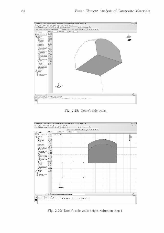
“K15072” — 2013/3/21 — 10:58�

�

�

�

�

�


Fig. 2.28: Dome’s side-walls.

Fig. 2.29: Dome’s side-walls height reduction step 1.

�

�

“K15072” — 2013/3/21 — 10:58�

�

�

�

�

�




�

�

“K15072” — 2013/3/21 — 10:58�

�

�

�

�

�



Fig. 2.33: Dome as shell structure.

�

�

“K15072” — 2013/3/21 — 10:58�

�

�

�

�

�


Fig. 2.34: Dome completed.

Fig. 2.35: Loaded Dome structure.

�

�

“K15072” — 2013/3/21 — 10:58�

�

�

�

�

�


Fig. 2.36: Meshed Dome structure.

Fig. 2.37: Contour plot of von Mises stress. Maximum values are 91, 020 MPa in thecolumns and 66, 922MPa in the shell.

�

�

“K15072” — 2013/3/21 — 10:58�

�

�

�

�

�


Suggested Problems

Problem 2.1 Solve Example 2.4 (p. 75) explicitly as it is done in Section 2.1, using onlytwo elements. Show all work.

Problem 2.2 From the solution of Problem 2.1, compute the axial displacement at (a)x = 500 mm, (b) x = 700 mm.

Problem 2.3 Using the same procedure in Example 2.1 (p. 46) calculate the element stiff-ness matrix and the equivalent force vector of a three-node element rod with quadratic in-terpolation functions. The interpolation functions are

Ne1 =

x− x2x1 − x2

x− x3x1 − x3

Ne2 =

x− x3x2 − x3

x− x1x2 − x1

Ne3 =

x− x1x3 − x1

x− x2x3 − x2

where x1, x2, and x3 are the coordinate positions of node 1, 2, and 3 respectively. Usex1 = 0, x2 = h/2, and x3 = h, where h is the element length. Show all work.

Problem 2.4 Program a FE code using the element formulation obtained in Example 2.1(p. 46) and the assembly procedure shown in Section 2.1.6. With this code, solve Exam-ple 2.4, p. 75. Show all work in a report.

Problem 2.5 Program a FE code using the element formulation obtained in Problem 2.3and the assembly procedure shown in Section 2.1.6. With this code, solve Example 2.4,p. 75. Show all work in a report.

�

�

“K15072” — 2013/3/21 — 10:58�

�

�

�

�

�

�

�

“K15072” — 2013/3/21 — 10:58�

�

�

�

�

�

Chapter 3

Elasticity and Strength ofLaminates

Most composite structures are built as assemblies of plates and shells. This isbecause the structure is more efficient when it carries membrane loads. Anotherimportant reason is that thick laminates are difficult to produce.

For example, consider a beam made of an homogeneous material with tensileand compressive strength σu subjected to bending moment M . Further, considera solid beam of square cross section (Figure 3.1), equal width and depth 2c, witharea A, inertia I, and section modulus S given by

A = 4c2

I =4

3c4

S =I

c=

4

3c3 (3.1)

When the stress on the surface of the beam reaches the failure stress σu, thebending moment per unit area is

mu =Mu

A=SσuA

=1

3cσu (3.2)

Now consider a square hollow tube (Figure 3.1) of dimensions 2c× 2c and wallthickness t, with 2c >> t, so that the following approximations are valid

A = 4(2c)t = 8ct

I = 2

[

t(2c)3

12+ c2(2ct)

]

=16

3tc3

S =I

c=

16

3tc2 (3.3)

Then

91

�

�

“K15072” — 2013/3/21 — 10:58�

�

�

�

�

�


Fig. 3.1: Solid section (a) and hollow square tube (b).

mu =Mu

A=SσuA

=163 tc

2σu

8ct=

2

3cσu (3.4)

The failure moment per unit area mu is twice as large for a hollow square tubewith thin walls than for a solid section.

Of course, the failure moment is limited by buckling of the thin walls (see Chap-ter 4). This is the reason buckling analysis is so important for composites. Mostcomposite structures are designed under buckling constraints because the thick-nesses are small and the material is very strong; so normally one does not en-counter material failure as in metallic structures (e.g., yield stress) but structuralfailure such as buckling.

Plates are a particular case of shells, having no initial curvature. Therefore,only shells will be mentioned in the sequel. Shells are modeled as two-dimensionalstructures because two dimensions (length and width) are much larger than thick-ness. The thickness coordinate is eliminated from the governing equations so thatthe 3D problem simplifies to 2D. In the process, the thickness becomes a parameterthat is known and supplied to the model.

Modeling of laminated composites differs from modeling conventional materialsin three aspects. First, the constitutive equations of each lamina are orthotropic(Section 1.12.3). Second, the constitutive equations of the element depend on thekinematic assumptions of the shell theory used and their implementation into the el-ement. Finally, material symmetry is as important as geometric and load symmetrywhen trying to use symmetry conditions in the models.

3.1 Kinematic of Shells

Shell elements are based on various shell theories, which in turn are based on kine-matic assumptions. That is, there are some underlying assumptions about the likelytype of deformation of the material. These assumptions are needed to reduce the3D governing equations to 2D. Such assumptions are more or less appropriate forvarious situations, as discussed next.

�

�

“K15072” — 2013/3/21 — 10:58�

�

�

�

�

�

Elasticity and Strength of Laminates 93

Fig. 3.2: Assumed deformation in FSDT.1

3.1.1 First-Order Shear Deformation Theory

The most popular composite shell theory is the first-order shear deformation theory(FSDT). It is based on the following assumptions:

i. A straight line drawn through the thickness of the shell in the undeformedconfiguration may rotate but it will remain straight when the shell deforms.The angles it forms (if any) with the normal to the undeformed midsurfaceare denoted by φx and φy when measured in the x − z and y − z planes,respectively (Figures 2.19 and 3.2).

ii. The change of the shell thickness is negligible as the shell deforms.

These assumptions are verified by experimental observation in most laminatedshells when the following are true:

– The aspect ratio r = a/t, defined as the ratio between the shortest surfacedimension a and the thickness t, is larger than 10.

– The stiffness of the laminas in shell coordinates (x, y, z) does not differ by morethan two orders of magnitude. This restriction effectively rules out sandwichshells, where the core is much softer than the faces.

1Reprinted from Introduction to Composite Materials Design, E. J. Barbero, Fig. 6.2, copyright(1999), with permission from Taylor & Francis.

�

�

“K15072” — 2013/3/21 — 10:58�

�

�

�

�

�


Based on the assumptions above, the displacement of a generic point B any-where in the shell can be written in terms of the displacement and rotations at themidsurface C as

u(x, y, z) = u0(x, y)− zφx(x, y)

v(x, y, z) = v0(x, y)− zφy(x, y) (3.5)

w(x, y, z) = w0(x, y)

The midsurface variables on the right-hand side of (3.5) are functions of onlytwo coordinates (x and y); thus the shell theory is 2D. On the left-hand side, thedisplacements are functions of three coordinates, and thus correspond to the 3Drepresentation of the material. At the 3D level, we use the 3D constitutive equations(1.68) and the 3D strain-displacement equations (1.5), which now can be written interms of 2D quantities as

εx(x, y, z) =∂u0∂x

− z∂φx∂x

= ε0x + zκx

εy(x, y, z) =∂v0∂y

− z∂φy∂y

= ε0y + zκy

γxy(x, y, z) =∂u0∂y

+∂v0∂x

− z

(

∂φx∂y

+∂φy∂x

)

= γ0xy + zκxy

γyz(x, y) = −φy + ∂w0

∂y

γxz(x, y) = −φx + ∂w0

∂xεz = 0 (3.6)

where

– The midsurface strains ε0x, ε0y , γ0xy, also called membrane strains, represent

stretching and in-plane shear of the midsurface.

– The change in curvature κx, κy, κxy, which are close but not exactly the sameas the geometric curvatures of the midsurface. They are exactly that for theKirchhoff theory discussed in Section 3.1.2.

– The intralaminar shear strains γxz, γyz, which are through-the-thickness sheardeformations. These are small but not negligible for laminated compositesbecause the intralaminar shear moduliG23, G13 are small when compared withthe in-plane modulus E1. Metals are relatively stiff in shear (G = E/2(1+ν)),and thus the intralaminar strains are negligible. In addition, the intralaminarshear strength values F4, F5, are relatively small when compared to the in-plane strength values F1t, F1c, thus making evaluation of intralaminar strains(and possibly stresses) a necessity. On the other hand, the shear strength

�

�

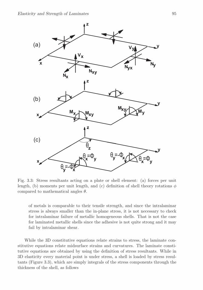
“K15072” — 2013/3/21 — 10:58�

�

�

�

�

�


(c)

Fig. 3.3: Stress resultants acting on a plate or shell element: (a) forces per unitlength, (b) moments per unit length, and (c) definition of shell theory rotations φcompared to mathematical angles θ.

of metals is comparable to their tensile strength, and since the intralaminarstress is always smaller than the in-plane stress, it is not necessary to checkfor intralaminar failure of metallic homogeneous shells. That is not the casefor laminated metallic shells since the adhesive is not quite strong and it mayfail by intralaminar shear.

While the 3D constitutive equations relate strains to stress, the laminate con-stitutive equations relate midsurface strains and curvatures. The laminate consti-tutive equations are obtained by using the definition of stress resultants. While in3D elasticity every material point is under stress, a shell is loaded by stress resul-tants (Figure 3.3), which are simply integrals of the stress components through thethickness of the shell, as follows

�

�

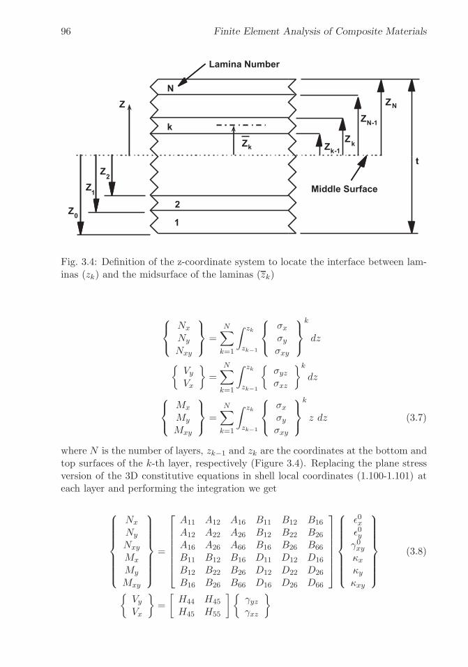
“K15072” — 2013/3/21 — 10:58�

�

�

�

�

�


Z

Z

ZZ

Z

Z

Z

t

1

2

k

N

Z

Lamina Number

Middle Surface1

2

0

k-1k

N-1

N

Zk

Fig. 3.4: Definition of the z-coordinate system to locate the interface between lam-inas (zk) and the midsurface of the laminas (zk)

⎧

⎨

⎩

Nx

Ny

Nxy

⎫

⎬

⎭

=N∑

k=1

∫ zk

zk−1

⎧

⎨

⎩

σxσyσxy

⎫

⎬

⎭

k

dz

{

VyVx

}

=N∑

k=1

∫ zk

zk−1

{

σyzσxz

}k

dz

⎧

⎨

⎩

Mx

My

Mxy

⎫

⎬

⎭

=

N∑

k=1

∫ zk

zk−1

⎧

⎨

⎩

σxσyσxy

⎫

⎬

⎭

k

z dz (3.7)

where N is the number of layers, zk−1 and zk are the coordinates at the bottom andtop surfaces of the k-th layer, respectively (Figure 3.4). Replacing the plane stressversion of the 3D constitutive equations in shell local coordinates (1.100-1.101) ateach layer and performing the integration we get

⎧

⎪

⎪

⎪

⎪

⎪

⎪

⎨

⎪

⎪

⎪

⎪

⎪

⎪

⎩

Nx

Ny

Nxy

Mx

My

Mxy

⎫

⎪

⎪

⎪

⎪

⎪

⎪

⎬

⎪

⎪

⎪

⎪

⎪

⎪

⎭

=

⎡

⎢

⎢

⎢

⎢

⎢

⎢

⎣

A11 A12 A16 B11 B12 B16

A12 A22 A26 B12 B22 B26

A16 A26 A66 B16 B26 B66

B11 B12 B16 D11 D12 D16

B12 B22 B26 D12 D22 D26

B16 B26 B66 D16 D26 D66

⎤

⎥

⎥

⎥

⎥

⎥

⎥

⎦

⎧

⎪

⎪

⎪

⎪

⎪

⎪

⎨

⎪

⎪

⎪

⎪

⎪

⎪

⎩

ε0xε0yγ0xyκxκyκxy

⎫

⎪

⎪

⎪

⎪

⎪

⎪

⎬

⎪

⎪

⎪

⎪

⎪

⎪

⎭

(3.8)

{

VyVx

}

=

[

H44 H45

H45 H55

]{

γyzγxz

}

�

�

“K15072” — 2013/3/21 — 10:58�

�

�

�

�

�


where

Aij =N∑

k=1

(

Qij

)

ktk; i, j = 1, 2, 6

Bij =

N∑

k=1

(

Qij

)

ktkzk; i, j = 1, 2, 6

Dij =

N∑

k=1

(

Qij

)

k

(

tkz2k +

t3k12

)

; i, j = 1, 2, 6

Hij =5

4

N∑

k=1

(

Q∗ij

)

k

[

tk − 4

t2

(

tkz2k +

t3k12

)]

; i, j = 4, 5 (3.9)

where(

Qij

)

kare the coefficients in laminate coordinates of the plane-stress stiffness

matrix for layer number k, tk is the thickness of layer k, and zk is the coordinate ofthe middle surface of the kth layer. For an in-depth discussion of the meaning ofvarious terms see [1]. In summary, the Aij coefficients represent in-plane stiffnessof the laminate, the Dij coefficients represent bending stiffness, the Bij representbending-extension coupling, and the Hij represent intralaminar shear stiffness. Allthese coefficients can be calculated by (3.9) and are implemented in widely availablesoftware packages such as CADEC [12].

When membrane and bending deformations are uncoupled (e.g., symmetric lam-inates), the governing equations of FSDT involve three variables for solving thebending problem (w0, φx, φy) and two to solve the membrane problem (u0, v0).Bending-extension coupling means that all five variables will have to be found si-multaneously, which is what FEA software codes do for every case, whether theproblem is coupled or not.

The equilibrium equations of plates can be derived by using the PVW (see(1.16)). Furthermore, the governing equations can be derived by substituting theconstitutive equations (3.8) into the equilibrium equations.

3.1.2 Kirchhoff Theory

Historically, Kirchhoff theory was preferred because the governing equations can bewritten in terms of only one variable, the transverse deflection of the shell w0. Inthe pre-information age, it was easier to obtain analytical solutions in terms of onlyone variable rather than in terms of the three variables needed in FSDT. This meansthat a wealth of closed form design equations and approximate solutions exist inengineering design manuals which are based on Kirchhoff theory [13]. Such simpledesign formulas can still be used for preliminary design of composite shells if weare careful and we understand their limitations. Metallic shells were and still arecommonly modeled with Kirchhoff theory. The FSDT governing equations can bereduced to Kirchhoff governing equations, and closed form solutions can be found,as shown in [14].

�

�

“K15072” — 2013/3/21 — 10:58�

�

�

�

�

�


In Kirchhoff theory the intralaminar shear strain is assumed to be zero. Fromthe last two equations in (3.6) we get

φx =∂w0

∂x

φy =∂w0

∂y(3.10)

and introducing them into the first three equations in (3.6) we get

εx(x, y, z) =∂u0∂x

− z∂2w0

∂x2= ε0x + zκx

εy(x, y, z) =∂v0∂y

− z∂2w0

∂y2= ε0y + zκy

γxy(x, y, z) =∂u0∂y

+∂v0∂x

− 2z∂2w0

∂x∂y= γ0xy + zκxy (3.11)

Notice that the variables φx, φy have been eliminated and Kirchhoff theory onlyuses three variables u0(x, y), v0(x, y), and w0(x, y). This makes analytical solutionseasier to find, but numerically Kirchhoff theory is more complex to implement.Since second derivatives of w0 are needed to write the strains, the weak form (2.30)will have second derivatives of w0. This will require that the interpolation functions(see Section 2.1.4) have C1 continuity. That is, the interpolation functions mustbe such that not only the displacements but also the slopes be continuous acrosselement boundaries. In other words, both the displacement w0 and the slopes∂w0/∂x, ∂w0/∂y will have to be identical at the boundary between elements whencalculated from either element sharing the boundary. This is difficult to implement.

Consider the case of beam bending. The ordinary differential equation (ODE)with an applied distributed load q(x) is

EId4w0

dx4= q(x) (3.12)

The weak form is obtained as in (2.3)

0 =

∫ xB

xA

v

[

−EI d4w0

dx4+ q(x)

]

dx (3.13)

Integrating by parts twice

0 =

∫ xB

xA

d2v

dx2EI

d2w0

dx2dx+ vEI

d3w0

dx3− dv

dxEI

d2w0

dx2−∫ xB

xA

vq(x)dx

0 = B(v,w0) + [vQx]xBxA

−[

dv

dxMx

]xB

xA

−∫ xB

xA

vM(x)dx

0 = B(v,w0) + L(v) (3.14)

�

�

“K15072” — 2013/3/21 — 10:58�

�

�

�

�

�


When the elements are assembled as in Section 2.1.6, it turns out that adjacentelements i and i+ 1 that share a node have identical deflection but opposite shearforce Qx and bending moment Mx at their common node, as follows

wi = wi+1

Qi = −Qi+1

M i = −M i+1 (3.15)

For the shear forces to cancel as in (2.24), it is only required to have vi = vi+1,which is satisfied by C0 continuity elements having wi = wi+1 at the commonnode. For the bending moments to cancel as in (2.24), it is required that dwi/dx =dwi+1/dx. This can only be done if the elements have C1 continuity. That is, theslopes dwi/dx = dwi+1/dx must be identical at the common node. Such elementsare difficult to work with ( [15, p. 276]).

In FSDT theory, only first derivatives are used in the strains (3.6). So, the weakform (2.30) has only first derivatives and, like (2.24), all the internal generalizedforces cancel at common nodes with only C0 element continuity.

3.1.3 Simply Supported Boundary Conditions

Composite plates with coupling effects may have bending, shear, and membranedeformations coupled even if loaded by pure bending, pure shear, or pure in-planeloads (see [1, Figure 6.7]). While the term simply supported always means to restrictthe transverse deflection w(x, y), it does not uniquely define the boundary conditionson the in-plane displacements un and us, normal and tangent to the boundary,respectively. In the context of analytical solutions, it is customary to restrict eitherun or us. Therefore, the following possibilities exist

– SS-1: w = us = φs = 0 ; Nn = Nn ; Mn = Mn

– SS-2: w = un = φs = 0 ; Nns = Nns ; Mn =Mn

In type SS-1, a normal force and a moment are specified. In SS-2, a shear forceand a moment are specified. The naming convention for the rotations is the same asthat used for moment resultants in Figure 3.3, where a subscript ()n indicates thedirection normal to the edge of the shell, and a subscript ()s indicates the directiontangent to the edge (see also [14, Figure 6.2.1]). Note that the rotation vector φsis perpendicular to the direction s, resulting in φs ≈ ∂w

∂s ; therefore, both SS-1 and

SS-2 set that rotation to zero. Finally, () represents a fixed known value, whichmay or may not be zero.

Geometrically linear analysis of a symmetric laminate subjected to bending onlywill not develop noticeable un, us, displacements. Therefore, SS-1 and SS-2 shouldgive virtually identical results. Differences may be important for other cases. Fur-thermore, the condition φs = 0 should not be neglected. For example, the calculatedcenter deflection was found to increase by 11.5% when the condition φs = 0 was notincluded in the solution of a sandwich plate [16] using 36 S4R elements.

�

�

“K15072” — 2013/3/21 — 10:58�

�

�

�

�

�


Fig. 3.5: (a) Micromechanics, (b) lamina level, and (c) laminate level approach.

3.2 Finite Element Analysis of Laminates

Deformation and stress analysis of laminated composites can be done at differentlevels (Figure 3.5). The level of detail necessary for description of the materialdepends on the level of post-processing desired.

When a great level of detail is necessary (Figure 3.5.a), the strain and stressare computed at the constituent level, i.e. fiber and matrix. In this case, it isnecessary to describe the microstructure, including the fiber shape and geometricaldistribution, and the material properties of the constituents. More details are givenin Chapter 6 where micromechanical modeling is used to generate properties for anycombination of fibers and matrix. Also, when the composite material is a wovenfabric, or the laminate is very thick, or when studying localized phenomena such asfree edges effects, the composite should be analyzed as solid, as shown in Chapter 5.However, it must be noted that most of the laminated structures can be analyzedusing the plates and shell simplifications explained in Section 3.1.

At the other end of the spectrum (Figure 3.5.c), the composite material canbe considered as a homogeneous equivalent material. In this case, its structuralbehavior can be analyzed by using orthotropic properties shown in Chapter 1. Ifthe whole laminate is analyzed as a homogeneous equivalent shell, using the macro-scale level approach (Figure 3.5.c), the stress distribution in the laminate cannotbe obtained. However, this very simple description of the laminate is sufficientwhen only displacements, buckling loads and modes, or vibration frequencies andmodes are required. In these cases, only the laminate stiffness (3.8) is needed (seeSection 3.2.9). In certain cases, even a simpler material description will suffice. Forexample, when the laminate is only unidirectional, or if the laminate is balancedand symmetric (see [1, Section 6.3]), the laminate can be modeled as a single laminaof orthotropic material (Section 3.2.10).

In most cases, stress and strains need to be calculated for every lamina in thelaminate. Then, the actual laminate stacking sequence (LSS) must be input to theprogram (Section 3.2.11). In this case, the elastic properties of each lamina, as wellas thickness and fiber orientation of every lamina, must be given. This method isusually called the mesoscale level approach (Figure 3.5.b).

A unidirectional lamina can be satisfactorily approximated as being transverselyisotropic. Then, it suffices to use E3 = E2, and G23 = E3/2(1 + ν23) in the equa-

�

�

“K15072” — 2013/3/21 — 10:58�

�

�

�

�

�


tions for an orthotropic material. The elastic properties of a unidirectional laminacan be computed using micromechanics (Chapter 6) or with experimental data ofunidirectional laminates. Material properties of some unidirectional composites areshown in Table 3.1.

In the analysis of most composite structures, it is usual to avoid the microme-chanics approach and to obtain experimentally the properties of the unidirectionallamina, or even the whole laminate. However, the experimental approach is notideal because a change of constituents or fiber volume fraction during the designprocess invalidates all the material data and requires a new experimental programfor the new material. It is better to calculate the elastic properties of the laminausing micromechanics formulas, using software such as [12] (see also Section 6.1).Unfortunately, micromechanics formulas are not accurate to predict strength, soexperimental work cannot be ruled out completely.

In summary, laminate properties can be specified in two ways:

– by the constitutive matrices A,B,D, and H, or

– by specifying the laminate stacking sequence (LSS) and properties for everylamina.

When the constitutive matrices A, B, D, H of the laminate are used to define thelaminate, the shell element cannot distinguish between different laminas. It can onlyrelate generalized forces and moments to generalized strains and curvatures. Onthe other hand, layered shell elements have the capability to compute the laminateproperties using the laminate stacking sequence (LSS) and the properties of thelaminas.

3.2.1 Element Types and Naming Convention

Shell elements allow one to model thin to moderately thick shells, down to a side-to-thickness ratio of 10. While some of them have 3 or 4 nodes, others have 8 nodes,thus using interpolation functions of higher degree. Shell elements are defined in3D space and have 5 or 6 degrees of freedom (DOF) at each node (translations inthe nodal x-, y-, and z-directions and rotations about the nodal x-, y-, and z-axis).The 6th DOF (rotation about the z axis) is included in the shell formulation toallow modeling of folded plates, but it would not be necessary if the shell surface issmooth.

The Abaqus documentation uses several terms that at first may seem confusingand/or overlapping. We have summarized them as follows:

Conventional shell elements require the geometry (mesh) to represent a 2Dflat/curved surface in 3D, as opposed to continuum shell elements. Conven-tional shell elements include thin shell elements, such as S8R5, and thick shellelements such as S8R.

Continuum shell elements require the geometry to model explicitly the thick-ness of the shell, as it would be done with 3D solid elements, but in contrast

�

�

“K15072” — 2013/3/21 — 10:58�

�

�

�

�

�


Table 3.1: Material properties of unidirectional carbon/epoxy composites.a

Property Unit AS4D/9310 T300/5208

E1 [GPa] 133.86 136.00E2 = E3 [GPa] 7.706 9.80G12 = G13 [GPa] 4.306 4.70

G23 [GPa] 2.76 4.261ν12 = ν13 0.301 0.280

ν23 0.396 0.150

Vf 0.55ρ [g/cm3] 1.52 1.54α1 [10−6/◦C] 0.32α2 [10−6/◦C] 25.89

F1t [MPa] 1830 1550F1c [MPa] 1096 1090

F2t = F3t [MPa] 57 59F2c = F3c [MPa] 228 207

F4 [MPa] 141 128F6 [MPa] 71 75

aF4 was calculated with α0 = 54◦ in [1, Eq. 4.109]

to the later, continuum shell elements enforce the FSDT constrains (Sec-tion 3.1.1) through particular element interpolation functions. Continuumshell elements include SC6R and SC8R.

Thin shell elements enforce the Kirchhoff constraint (Section 3.1.2), either the-oretically (e.g., STRI3), or numerically when the shell is thin (e.g., S8R5).Therefore, the transverse shear deformations are assumed to be zero or neg-ligible. They are not accurate for composites if the laminate is thick and/orthe transverse shear moduli G23 of one or more laminas are small, in whichcase the shear deformation may be underestimated. All thin shell elementsare conventional shell elements. Thin shell elements include STRI3, S4R5,STRI65, S8R5, S9R5, SAXA1N, and SAXA2N. They do not have a drillingrotation degree of freedom.

Thick shell elements only enforce the FSDT constraint (Section 3.1.1). There-fore, the transverse shear deformations are not zero. Thick shell elements canbe conventional (e.g., S3R, S4, S4R, S8R, SAX1, SAX2), or continuum, suchas SC6R and SC8R.

General purpose shell elements are appropriate to model both thick and thinshells. They include thick, conventional shell elements (e.g., S3, S3R, S3RS,S4, S4R, S4RS, S8R, S4RSW, SAX1, SAX2, SAX2T), as well as thick, con-tinuum shell elements such as SC6R and SC8R.

3D solid elements also called solid 3D continuum elements discretize the 3D

�

�

“K15072” — 2013/3/21 — 10:58�

�

�

�

�

�


body without using any assumptions of shell theory. Since they are not shellelements, the model may be computationally expensive. They can be usedfor detailed analysis in regions where a rapid variation of stress and strain isexpected. They require a 3D mesh, explicitly modeling the 3 dimensions ofthe shell, including the thickness. Shell-to-solid coupling constraints can beused to transition from shell to solid elements.

Another source of confusion arises around the use of the terms 2D and 3D.In shell theory, a shell is a 2D surface because only 2 curvilinear coordinates areneeded to locate any point on the reference surface of the shell. But in Abaqusdocumentation, a shell is said to be 3D because it occupies a portion of 3D space,as opposed to a 2D model that is always planar.

Furthermore, the Abaqus documentation uses the following naming conventionfor shell elements:

SnRsW Conventional Shell

S shell

n number of nodes

R reduced integration

s small membrane strains

W warping included

SCnRT Continuum Shell

S shell

C continuum

n number of nodes

R reduced integration

T thermo-mechanical coupling

STRInm Triangular Shell

S shell

TRI triangular

n number of nodes

m number of DOF

Type SAXAxN Axisymmetric Shell

S shell

AXA Axisymmetric

1N meridional linear interpolation, N Fourier modes

2N meridional quadratic interpolation, N Fourier modes

The terms introduced in this section are further explained in the following sec-tions.

�

�

“K15072” — 2013/3/21 — 10:58�

�

�

�

�

�


3.2.2 Thin (Kirchhoff) Shell Elements

When a shell is thin and the material has a high shear modulus, lines normal to themiddle surface remain normal during deformation. This is one of the assumptionsof Kirchhoff shell theory, also called the Kirchhoff constraint (see Section 3.1.2).

The Kirchhoff constraint states that a line normal to the reference surface inthe undeformed configuration remains normal to the deformed reference surface.This implies that the transverse shear deformations γxz, γyz are zero. Additional as-sumptions that are common to both Kirchhoff Theory and First Order DeformationTheory (FSDT, Section (3.2.4)) are that normals remain straight and inextensible(εzz = 0). Shell elements that enforce the Kirchhoff constraint are called thin shellelements, as opposed to thick shell elements that only enforce the FSDT constrains.All the thin shell elements are conventional shell elements in the sense that the ge-ometry is represented by a 2D flat/curved surface in 3D, as opposed to continuumshell elements that require the geometry to model explicitly the thickness of theshell, as it would be done with 3D solid elements.

Thin shell elements such as STRI3, S4R5, STRI65, S8R5, S9R5, SAXA1N,and SAXA2N are specifically formulated for modeling thin shells. They discretizethe reference surface of the shell, and the thickness is given as a section property.Element STRI3 enforces the Kirchhoff constraint analytically so it yields the thin-walled theory solution even for a thick shell. Elements S4R5, STRI65, S8R5, S9R5,SAXA1N, and SAXA2N impose the Kirchhoff constraint numerically. These ele-ments should not be used for applications in which transverse shear deformation isimportant, either because the shell is thick, or the shear modulus low, or both. SeeExample 3.4.a, p. 121.

All elements with name ending on 5 have 5 DOF per node, 3 displacements,and 2 in-plane rotations. They do not have drilling rotational DOF (see Section3.2.8). Five degrees of freedom elements, such as S4R5, STRI65, S8R5, S9R5, maybe more economical than other elements, but they are available only for modelingthin shells and they should not be used to model thick shells.

3.2.3 Thick Shell Elements

Composites should be modeled as thick shells even if they are geometrically thinbecause they have relatively low shear modulus, thus necessitating inclusion of theirshear deformation in the same way as thick shells do. Abaqus provides elements S3R,S3RS, S4, S4R, S4RS, S4RSW, S8R, SC6R, and SC8R to model laminated compos-ite shells. Continuum shell elements, such as SC6R and SC8R, can be used whenbetter resolution of the transverse shear deformation is needed. See Example 3.4.b,p. 121.

3.2.4 General-purpose (FSDT) Shell Elements

First-Order Shear Deformation Theory (FSDT, see Section 3.1.1) states that un-deformed normals to the reference surface in the undeformed configuration remain

�

�

“K15072” — 2013/3/21 — 10:58�

�

�

�

�

�


straight and inextensible but not necessarily normal to the deformed reference sur-face. This allows for non-zero transverse shear deformation.

General-purpose shell elements, such as S3, S3R, S3RS, S4, S4R, S4RS, S8R,S4RSW, SAX1, SAX2, and SAX2T, as well as SC6R and SC8R, include transverseshear deformation but they can be used for thin shells as well. Elements S3, S3R,S3RS, S4, S4R, S4RS, S4RSW, S8R, SAX1, SAX2, and SAX2T discretize the refer-ence surface of the shell, and the thickness is given as a section property. ElementsS3, S3R, S3RS, S4, S4R, S4RS, S4RSW, and S8R have 6 DOF per node, with DOF6 being a drilling rotation that allows the element to be used to model folded shells.Elements SC6R and SC8R are continuum elements (see Section 3.2.5), but theyqualify as general-purpose because they can be used for thin and thick shells.

3.2.5 Continuum Shell Elements

Continuum shell (CS) elements such as SC4R are basically 3D solid elements wherethe FSDT constraints are enforced by special interpolation functions [17]. Comparedto conventional shell elements, they have more nodes to depict the thickness in themodel.

Continuum shell elements have only displacement degrees of freedom, no rota-tions. Therefore, they can be stacked and they can be connected to solid elements.Continuum shell elements discretize the 3D geometry of the shell in the same wayas 3D solid elements do.

Continuum shell elements can be internally laminated to represent a laminateor sublaminate with just one element. Also, they can be stacked to provide a betterrepresentation of the shear deformation through the thickness. In this case, each ofthe stacked elements may represent a sublaminate. If only one internally laminatedelement is used to model the entire thickness of the laminate, the result is the sameas that of a FSDT element. But CS elements can be stacked, and there lies theiradvantage. By stacking several CS elements, the actual deformation of the normalcan be approximated to any precision. As the number of elements through thethickness approaches infinity, they yield the exact elasticity solution to the plateproblem. But they are better than 3D solid elements because CS elements have noaspect ratio problems; i.e., the thickness direction can be very thin compared to theother two dimensions. This is because CS elements incorporate the incompressibilityof the normals (εz = 0,(3.6)), just like FSDT elements.

Meshing is more difficult with continuum shell elements because the thicknessof the shell has to be meshed. Also, boundary conditions are more difficult to applybecause one cannot apply the classical shell boundary conditions, but rather one hasto simulate them by constraining the displacements at the top and bottom surfaceof the shell. For example, a simply supported boundary condition is rather difficultto apply if the continuum shell mesh does not have nodes located at the middlesurface of the shell. Clamped (encastre) and symmetry boundary conditions areeasy to apply. See Example 3.4.c, p. 126.

�

�

“K15072” — 2013/3/21 — 10:58�

�

�

�

�

�


3.2.6 Sandwich Shells

For a sandwich shell, the core is much softer that the faces, and the transverse sheardeformations are significant regardless of the total thickness of the shell. Conven-tional shell elements may not have the shear flexibility required. Use continuum shellelements instead. For the most refined model possible, stack three continuum shellelements through the thickness, one for each face and the core. See Example 3.7,p. 139.

3.2.7 Nodes and Curvature

Three and four node elements such as STRI3 and S4R5 are flat. For curved shells,it is better to use six, eight, or nine node elements such as STRI65, S8R5, andS9R5. Element S8R5 has a hidden internal ninth-node, which may end up outsidethe reference surface for doubly curved shells. If this happens, buckling loads maybe inaccurate and S9R5 would be better.

3.2.8 Drilling Rotation

Conventional shell elements are based on shell theory, which constrains the 3D con-tinuum deformations according to some kinematic assumptions, such as Kirchhoff,FSDT, or one of many others. In continuum theory, the deformation of a point in3D can be described in terms of the relative displacements of two points, thus re-quiring six degrees of freedom (three per point). Both Kirchhoff and FSDT theoriesformally reduce the requirement to three displacements and two in-plane rotationsat a single point. The two rotations, φx, φy, are rotations of the normal to thereference surface. These are called in-plane rotations because the rotation vectorslie on the surface of the shell. For a smoothly curved or flat shell, there is no needof tracking the rotation of the normal around itself, φz. This last rotation is calleddrilling rotation. However, if the shell has a fold, an in-plane rotation on one sideof the fold corresponds to a drilling rotation on the other side (Figure 3.6). Thus,to enforce compatibility of displacements, the drilling rotations become necessary.Since elements having 5 DOF do not have drilling rotation, they are suited to modelsmoothly curved shells but not folded shells.

Abaqus/Standard will automatically switch from 5 DOF elements to 6 DOFelements at any node when:

– A kinematic (displacement, velocity) boundary condition is applied to rota-tional degrees of freedom at the node,

– The node is used in a multi-point constraint that involves rotational degreesof freedom,

– The node is shared with a beam element or a shell element that uses the threeglobal rotation components at all nodes,

– The node is on a fold line in the shell, or– The node is loaded with moments

�

�

“K15072” — 2013/3/21 — 10:58�

�

�

�

�

�


A

�z

(1)�z

(1)

�x

(1)

�y

(1)

y(1)

x(1)

1

�z

(2)�x

(2)

�y

(2)

y(2)

x(2)

2

B

Fig. 3.6: Exploded view of a plate folded along AB. Drilling rotations φ(1)z and φ

(2)z

associated to elements 1 and 2, respectively.

3.2.9 A, B, D, H Input Data for Laminate FEA

As previously mentioned, macro-scale level (laminate level) analysis is adequate ifonly deflections, modal analysis, or buckling analysis are to be performed, with norequirement for detailed stress analysis. Then, it is not necessary to specify thelaminate stacking sequence (LSS), the thickness, and the elastic properties of eachlamina of the laminate. Only the elastic laminate properties (A,B,D,H matrices)defined in (3.9) are required. This is convenient because it allows one to inputthe aggregate composite material behavior with few parameters. The reduction ofthe complexity of the input data allows modeling of laminates with an unlimitednumber of laminas, using only four matrices.

When the A,B,D,H matrices are used to define the FE analysis, the computermodel knows the correct stiffness but it does not know the LSS. Therefore, thesoftware can compute the deformation response (including buckling and vibrations)and even the strain distribution through the thickness of the shell, but it cannotcompute the stress components because it does not know where the lamina materialproperties change from lamina to lamina.

The A,B,D,H input data can be found by using (3.9) or [12]. Then, these areinput into the FE software, as illustrated in Example 3.1.

In Abaqus, the A,B,D matrices can be input as Edit General Stiffness

Section (Figure 3.7), which is invoked as follows:

Module: Property

�

�

“K15072” — 2013/3/21 — 10:58�

�

�

�

�

�


Fig. 3.7: Input A, B, and D matrices.

Menu: Section, Edit, [Section-name]

The A,B,D, matrices are entered on the Stiffness tab (Figure 3.7). TheH matrix has to be converted into transverse shear stiffness values and enteredusing the Advanced tab (Figure 3.8). The transverse shear stiffness coefficientsH44,H45,H55, are defined in (3.9). Taking into account the way Abaqus handlescontracted notation, as shown in Table 1.1 (p. 5), compared to the standard (Voigt)definition used in this textbook, it turns out that the notation for transverse shearcoefficients in Figure 3.8 means that:

K11 = H55

K22 = H44

K12 = H45 (3.16)

Example 3.1 Consider a simply supported square plate ax = ay = 2000 mm, laminatedwith AS4D/9310 (Table 3.1) in a [0/90]n configuration. The total laminate thickness ist = 10 mm for all values of n. The plate is loaded in compression with an edge loadNx = 1 N/mm and (Ny = Nxy = Mx = My = Mxy = 0). Tabulate the center deflectionperpendicular to the plate surface when the number of layers is n = 1, 5, 10, 15, and 20.Calculate the A, B, D, H matrices and enter them into Abaqus. Use symmetry to model1/4 of the plate.

Solution to Example 3.1 The procedure to solve the [0/90] laminate (n = 1) is describedin detail next.

�

�

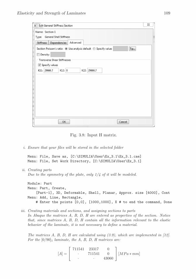
“K15072” — 2013/3/21 — 10:58�

�

�

�

�

�


Fig. 3.8: Input H matrix.

i. Ensure that your files will be stored in the selected folder

Menu: File, Save as, [C:\SIMULIA\User\Ex_3.1\Ex_3.1.cae]

Menu: File, Set Work Directory, [C:\SIMULIA\User\Ex_3.1]

ii. Creating partsDue to the symmetry of the plate, only 1/4 of it will be modeled.

Module: Part

Menu: Part, Create,

[Part-1], 3D, Deformable, Shell, Planar, Approx. size [4000], Cont

Menu: Add, Line, Rectangle,

# Enter the points [0,0], [1000,1000], X # to end the command, Done

iii. Creating materials and sections, and assigning sections to partsIn Abaqus the matrices A, B, D, H are entered as properties of the section. Noticethat, since matrices A, B, D, H contain all the information relevant to the elasticbehavior of the laminate, it is not necessary to define a material.

The matrices A, B, D, H are calculated using (3.9), which are implemented in [12].For the [0/90]1 laminate, the A, B, D, H matrices are:

[A] =

⎡

⎣

711541 23317 0· 711541 0· · 43060

⎤

⎦ [MPa ∗mm]

�

�

“K15072” — 2013/3/21 — 10:58�

�

�

�

�

�


[B] =

⎡

⎣

−1585193 0 0· 1585193 0· · 0

⎤

⎦

[

MPa ∗mm2]

[D] =

⎡

⎣

5929510 194306 0· 5929510 0· · 358833

⎤

⎦

[

MPa ∗mm3]

[H ] =

[

29442 0· 29442

]

[MPa ∗mm]

These are entered into Abaqus/CAE as follows:

Module: Property

Menu: Section, Create, [Section-1],

Shell, General Shell Stiffness, Cont

# In the pop-up window fill the stiffness matrix as follows

Tab: Stiffness,

# Upper part of matrix A in rows 1 to 3, columns 1 to 3

# matrix B in rows 1 to 3, columns 4 to 6

# Upper part of matrix D in rows 4 to 6, columns 4 to 6

# The Stiffness matrix should be

# 711541 23317 0 -1585193 0 0

# 711541 0 0 1585193 0

# 43060 0 0 0

# 5929510 194306 0

# 5929510 0

# 358833

Tab: Advanced,

# The values corresponding to the H matrix are entered here

Transverse Shear Stiffness, # checkmark: Specify values,

K11: [29442], K12: [0], K22: [29442], OK


iv. Creating the Assembly

Module: Assembly

Menu: Instance, Create, Independent, OK

v. Creating steps

Module: Step

Menu: Step, Create, Name [Step-1], Static/General, Cont, OK

vi. Adding BC and loads

�

�

“K15072” — 2013/3/21 — 10:58�

�

�

�

�

�


Module: Load

Menu: BC, Manager,

Create, Name [X-symm], Step: Initial,

Mechanical, Symm/Anti/Enca, Cont

# pick the left vertical line, Done, XSYMM, OK

Create, Name [Y-symm], Step: Initial,


# pick the upper horizontal line, Done, YSYMM, OK

Create, Name [Simple-Support],

Step: Initial, Mechanical, Disp/Rota, Cont

# pick right vertical and lower horizontal lines, Done,

# checkmark: U3, OK, # close BC Manager

Menu: Load, Create, Step: Step-1, Mechanical, Shell edge load, Cont

# pick the right vertical line, Done, Magnitude [1], OK

vii. Creating mesh

Module: Mesh

Menu: Seed, Instance, Approximate global size [50], Apply, OK

Menu: Mesh, Controls, Element Shape [Quad], Technique [Structured], OK

Menu: Mesh, Instance, # At the bottom of the WS select [Yes]

viii. Solving and visualizing the solution

Module: Job

Menu: Job, Manager

Create, Name [0-90_1], Cont, OK

# Job name should be changed for each laminate so the user can

# access results of different models without re-running

Data Check # To check the model for errors,

Submit # To run the model,

Results # To visualize the solution

Toolbar: Views, Apply Front View

Menu: Plot, Contours, On Deformed Shape,

Results, Field Output,

Output Variable [U], Component [U3], Apply, OK

# Note that maximum deflection should be -2.196e-01

# at the upper left corner of the plate

ix. Saving the model database

Menu: File, Save,

Menu: File, Save As [Ex_3.1(1).cae], OK

Menu: File, New Model Database, With Standard/Explicit Model

x. The “Save As” instruction allows the user to keep a copy of the model for the [0/90]1laminate, while the original model is modified to complete the analysis. Also noticethat the results of the model can be accessed using

Menu: File, Open, # Browse to C:\SIMULIA\User\Ex_3.1

File Filter, Output Database (*.odb*), # Select [0-90_1.odb], OK

�

�

“K15072” — 2013/3/21 — 10:58�

�

�

�

�

�


The solution for the remaining laminates with n > 1 is similar to the procedure de-scribed above. Modifying the number of layers used, without changing the thickness of thelaminate, affects only the bending-extension coupling matrix, B. For the additional stackingsequences, the matrix B is found by using [12], which yields

For [0/90]5:

[B] =

⎡

⎣

−317039 0 0· 317039 0· · 0

⎤

⎦

[

MPa ∗mm2]

For [0/90]10:

[B] =

⎡

⎣

−158519 0 0· 158519 0· · 0

⎤

⎦

[

MPa ∗mm2]

For [0/90]15:

[B] =

⎡

⎣

−105468 0 0· 105468 0· · 0

⎤

⎦

[

MPa ∗mm2]

For [0/90]20:

[B] =

⎡

⎣

−79260 0 0· 79260 0· · 0

⎤

⎦

[

MPa ∗mm2]

Next, modify the model previously saved as Ex 3.1.cae to use each of the bending-extension coupling matrices for n > 1.

i. Edit the section property, submit, and visualize

Menu: File, Open, # Browse to ...\Ex_3.1, [Ex_3.1.cae], OK

Module: Property

Menu: Section, Edit, Section-1

# In the pop-up window modify the cells of the new matrix B

# rows 1 to 3, columns 4 to 6. The new B sub-matrix is

# -317039 0 0

# 0 317039 0

# 0 0 0

OK

Module: Job

Menu: Job, Manager, Create, Name [0-90_5], Cont, OK


Submit # To run the model,






�

�

“K15072” — 2013/3/21 — 10:58�

�

�

�

�

�


The maximum deflection should be −2.109× 10−2 mm at the upper-left corner of theplate.

ii. Save the model database

Menu: File, Save,

Menu: File, Save As [Ex_3.1(5).cae], OK


The solution is tabulated in Table 3.2. Bending extension coupling produces a lateraldeflection, which diminishes for increasing number of layers n. Note how the bending-extension coupling coefficient −B11 decreases proportionally to the number of layers.

Table 3.2: Lateral deflection vs. number of layers in Example 3.1.n δ [mm] −B11 %

1 0.2196 1,585,193 1005 0.0211 317,039 1/510 0.0104 158,518 1/1015 0.0069 105,468 1/1520 0.0052 79,260 1/20

3.2.10 Equivalent Orthotropic Input for Laminate FEA

Some FEA codes do not have laminated elements and do not accept the A,B,D,and H matrices as explained in Section 3.2.9. However, if they have orthotropicelements, it is still possible to perform deformation, vibration, and buckling analysisfor laminated composites, as it is shown in this section.

Unidirectional Laminate FEA

To model a unidirectional laminate, standard shell elements can be used, even ifthey are not layered shell, and still obtain correct results of displacements, strains,and stress. The geometry of shells is a surface that represents the midsurface of thereal shell. The midsurface is located halfway through the thickness. The positivethickness coordinate points along a normal to the shell midsurface (local z-directionwhich coincides with the 3-direction). This is the normal definition of shells and itis used in shell elements, as shown in Example 3.2.

Example 3.2 Use Abaqus to model a simply supported rectangular plate with dimensionsax = 4, 000 mm, ay = 2, 000 mm, and plate thickness t = 10 mm. Apply a uniformtransverse load q0 = 0.12×10−3 MPa. The material is a unidirectional AS4D/9310 lamina(Table 3.1), with the fibers oriented in the x-direction. Determine the deflection of the centerpoint of the plate. Use (1.102–1.104) to calculate the orthotropic stiffness matrix and enterthe material as Type: Orthotropic. This example is continued in Example 3.8, p. 151.

Solution to Example 3.2 The thickness coordinate is eliminated from the governing equa-tions so that the 3D problem simplifies to 2D. In the process, the thickness becomes a param-eter, which is known and supplied to the modeling software. The model can be constructedand solved as follows:

�

�

“K15072” — 2013/3/21 — 10:58�

�

�

�

�

�


Menu: File, Save as [C:\SIMULIA\User\Ex_3.2\Ex_3.2.cae]

Menu: File, Set Work Directory [C:\SIMULIA\User\Ex_3.2]

i. Creating partsDue to the symmetry of the plate, only 1/4 of it will be modeled.

Module: Part

Menu: Part, Create,



# Enter the points [0,0], [2000,1000], X # ends the command, Done

ii. Creating materials and sections, and assigning sections to parts

Module: Property


Mechanical, Elasticity, Elastic, Type: Orthotropic,

# Enter the values of the components of the stiffness matrix, OK

Notice that the stiffness matrix in Abaqus is built in a different order than the oneshown in (1.68). In Abaqus

⎧

⎪

⎪

⎪

⎪

⎪

⎪

⎨

⎪

⎪

⎪

⎪

⎪

⎪

⎩

σ1σ2σ1σ6σ5σ4

⎫

⎪

⎪

⎪

⎪

⎪

⎪

⎬

⎪

⎪

⎪

⎪

⎪

⎪

⎭

=

⎡

⎢

⎢

⎢

⎢

⎢

⎢

⎣

C11 C12 C13 0 0 0· C22 C23 0 0 0· · C33 0 0 0· · · C66 0 0· · · · C55 0· · · · · C44

⎤

⎥

⎥

⎥

⎥

⎥

⎥

⎦

⎧

⎪

⎪

⎪

⎪

⎪

⎪

⎨

⎪

⎪

⎪

⎪

⎪

⎪

⎩

ε1ε2ε1γ6γ5γ4

⎫

⎪

⎪

⎪

⎪

⎪

⎪

⎬

⎪

⎪

⎪

⎪

⎪

⎪

⎭

and D1111 = C11, D1122 = C12, D2222 = C22, D1133 = C13, D2233 = C23, D3333 =C33, D1212 = C66, D1313 = C55, D2323 = C44. Using the mechanical properties ofAS4D/9310 (Table 3.1) to calculate the compliance matrix (1.104), and inverting it,the stiffness matrix is obtained

⎡

⎢

⎢

⎢

⎢

⎢

⎢

⎣

136222.40 3908.70 3908.70 0 0 0· 9251.35 3731.31 0 0 0· · 9251.35 0 0 0· · · 4306.00 0 0· · · · 4306.00 0· · · · · 2760.00

⎤

⎥

⎥

⎥

⎥

⎥

⎥

⎦

[MPa]


Shell, Homogeneous, Cont

Shell thickness [10], Material [Material-1], OK


Another option would be to enter the material properties as Engineering Constants

(9 values) or Lamina (5 values1) in the Edit Materials window of Abaqus/CAE.

1Considering that G12 = G13 for a transversely isotropic material.

�

�

“K15072” — 2013/3/21 — 10:58�

�

�

�

�

�


iii. Creating the assembly

Module: Assembly


iv. Creating analysis steps

Module: Step


v. Adding BC and loads

Module: Load

Menu: BC, Manager,

Create, Name [X-symm], Step: Initial,



Create, Name [Y-symm], Step: Initial,



Create, Name [Simple-supp], Step: Initial,

Mechanical, Disp/Rota, Cont

# pick the right vertical and the lower horizontal lines, Done,


Menu: Load, Create

Step: Step-1, Mechanical, Pressure, Cont

# pick the part, Done,

# Select side for the shell, Brown, Magnitude [0.12e-3], OK

vi. Creating the mesh

Module: Mesh




vii. Solving and visualizing the solution

Module: Job

Menu: Job, Manager

Create, Cont, OK


Submit # To run the model






The maximum deflection is 17.43mm at the center of the plate.

�

�

“K15072” — 2013/3/21 — 10:58�

�

�

�

�

�


Symmetric Laminate FEA

If a multidirectional laminate is balanced and symmetric, the apparent laminateorthotropic properties can be found as explained in Section 1.15. The apparentlaminate properties represent the stiffness of an equivalent (fictitious) orthotropicplate that behaves like the actual laminate under in-plane loads. These apparentproperties should not be used to predict bending response. When the only importantresponse is bending, e.g., a thick cantilever plate under bending, the formulationshown in [1, (6.36)] should be used to obtain the apparent laminate properties.However, in most of the structural design using composite shell, the laminate worksunder in-plane loads and the formulation in Section 1.15 should be used.

If the laminate is symmetric but not balanced, the axes of orthotropy are rotatedwith respect to the laminate coordinate system, but still the laminate is equivalent toan orthotropic material as per Section 1.15. For example, a unidirectional laminateoriented at an angle θ with respect to global axes should be modeled on a coordinatesystem oriented along the fiber direction (see Section 3.2.14).

Example 3.3 Use Abaqus to model a simply supported rectangular plate with dimensionsax = 2000 mm, ay = 2000 mm, for a laminate [±45/0]S. Apply a tensile edge loadNx = 200 N/mm. Determine the maximum horizontal displacement. Each layer is 1.0 mmthick with the following properties:

E1 = 37.88 GPa G12 = 3.405 GPa ν12 = 0.299E2 = 9.407 GPa G23 = 3.308 GPa ν23 = 0.422

Solution to Example 3.3 Since the laminate is balanced symmetric, compute the aver-aged laminate properties Ex, Ey and so on using Section 1.15 to yield

Ex = 20.104 GPa Gxy = 8.237 GPa νxy = 0.532Ey = 12.042 GPa Gyz = 3.373 GPa νyz = 0.203Ez = 10.165 GPa Gxz = 3.340 GPa νxz = 0.307

The model is implemented in Abaqus following the steps:

Menu: File, Save as, [C:\SIMULIA\User\Ex_3.3\Ex_3.3.cae]

Menu: File, Set Work Directory, [C:\SIMULIA\User\Ex_3.3]

i. Creating partsDue to the assumed symmetry of the plate, only 1/4 of it will be modeled.

Module: Part

Menu: Part, Create,



# Enter the points [0,0], [1000,1000], X # ends the command, Done


�

�

“K15072” — 2013/3/21 — 10:58�

�

�

�

�

�


Module: Property


Mechanical, Elasticity, Elastic, Type [Orthotropic],

# Enter the values of the components of the stiffness matrix, OK

Notice that the stiffness matrix in Abaqus is built in a different order than the oneshown in (1.68). In Abaqus

⎧

⎪

⎪

⎪

⎪

⎪

⎪

⎨

⎪

⎪

⎪

⎪

⎪

⎪

⎩

σ1σ2σ1σ6σ5σ4

⎫

⎪

⎪

⎪

⎪

⎪

⎪

⎬

⎪

⎪

⎪

⎪

⎪

⎪

⎭

=

⎡

⎢

⎢

⎢

⎢

⎢

⎢

⎣

C11 C12 C13 0 0 0· C22 C23 0 0 0· · C33 0 0 0· · · C66 0 0· · · · C55 0· · · · · C44

⎤

⎥

⎥

⎥

⎥

⎥

⎥

⎦

⎧

⎪

⎪

⎪

⎪

⎪

⎪

⎨

⎪

⎪

⎪

⎪

⎪

⎪

⎩

ε1ε2ε1γ6γ5γ4

⎫

⎪

⎪

⎪

⎪

⎪

⎪

⎬

⎪

⎪

⎪

⎪

⎪

⎪

⎭

and D1111 = C11, D1122 = C12, D2222 = C22, D1133 = C13, D2233 = C23, D3333 =C33, D1212 = C66, D1313 = C55, D2323 = C44. Using the mechanical properties givenabove to calculate the compliance matrix (1.104), and inverting it, the stiffness matrixis

⎡

⎢

⎢

⎢

⎢

⎢

⎢

⎣

26677.59 9531.84 5736.79 0 0 0· 15897.74 4216.73 0 0 0· · 11813.63 0 0 0· · · 8264.46 0 0· · · · 3378.38 0· · · · · 3344.48

⎤

⎥

⎥

⎥

⎥

⎥

⎥

⎦

[MPa]

which is entered into Abaqus/CAE as follows:



Shell thickness [6], Material [Material-1], OK


Alternatively, one could enter the material properties as Engineering Constants (9values) in the Edit Materials window of Abaqus/CAE.


Module: Assembly


iv. Creating analysis steps

Module: Step



�

�

“K15072” — 2013/3/21 — 10:58�

�

�

�

�

�


Module: Load

Menu: BC, Manager,

Create, Name [X-symm], Step: Initial, Mechanical,

Symm/Anti/Enca, Cont


Create, Name [Y-symm], Step: Initial, Mechanical,



Create, Name [Simple-supp], Step: Initial, Mechanical,

Disp/Rota, Cont

# pick the right vertical and the lower horizontal lines, Done,


Menu: Load, Create

Step: Step-1, Mechanical, Shell edge load, Cont

# pick the right vertical line, Done, Magnitude [-200], OK

vi. Creating the mesh

Module: Mesh




vii. Solving and visualizing the solution

Module: Job

Menu: Job, Manager

Create, Cont, OK


Submit # To run the model


# ‘Apply Front View’ from the ‘Views toolbar’,




The maximum displacement should be 1.667 at the right edge of the plate.

The resulting maximum horizontal displacement on a quarter-plate model is 1.667 mm.The planes x = 0 and y = 0 are not symmetry planes for a [±45/0]S but once the laminateis represented by equivalent orthotropic properties, as is done in this example, the lackof symmetry at the lamina level is lost and it does not have any effect on the mid-surfacedisplacements. Therefore, one-quarter of the plate represents well the entire plate as long asno stress analysis is performed. Furthermore, displacement and mid-surface strain analysiscan be done with the laminate replaced by an equivalent orthotropic material. However,even if the full plate were to be modeled, the stress values in the equivalent orthotropicmaterial are not the actual stress values of the laminate. While the material analyzed in thisexample is not homogeneous, but laminated, the material in Example 3.2 is a homogeneousunidirectional material. Therefore, the stress values are not correct in this example but theyare correct in Example 3.2, p. 113.

�

�

“K15072” — 2013/3/21 — 10:58�

�

�

�

�

�


Asymmetric Laminate FEA

If the laminate is not symmetric, bending-extension coupling must be considered.Strictly speaking, such material is not orthotropic and should not be modeled withan equivalent laminate material. Even then, if only orthotropic shell elements areavailable and the bending-extension coupling effects are not severe, the materialcould be approximated by an orthotropic material by neglecting the matrices Band D. The ratios defined in [1, (6.37–6.39)] can be used to assess the quality ofthe approximation obtained using apparent elastic properties. Care must be takenfor unbalanced laminates that the A and H matrix are formulated in a coordinatesystem coinciding with the axes of orthotropy of the laminate.

3.2.11 LSS for Multidirectional Laminate FEA

For computation of strain and stress at the mesoscale (lamina level), it is necessaryto know the description of the laminate and the properties of each lamina. Thedescription of the multidirectional laminate includes the LSS, which specifies theangle of each lamina with respect to the x-axis of the laminate, the thickness, andthe elastic material properties of each lamina. Then, the software computes thematrices A, B, D, and H internally. In this way, the software can compute thestress components in each layer. This approach is illustrated in the Example 3.4,p. 121. In Abaqus/CAE, the LSS can be specified in two ways, using CompositeSections or Composite Layups.

Composite Section

Composite Section is the basic tool that allows the user to define the LSS. It does notdiffer from the classical definition and assignment of all other types of sections suchas solid, shell, beam, truss, and so on. First, one defines one or more materials, whichin this case could be type isotropic, engineering constants, lamina, orthotropic, oranisotropic. In CAE, this is done as follows:

Module: Property

Menu: Material, Create, Mechanical, Elasticity, Elastic, Type: Lamina

Second, one defines a laminated section as follows.

Module: Property

Menu: Section, Create, Category: Solid, Composite, Cont

Material: [select], Thickness: [value], Orientation Angle: [value],

Integration Points: [value], Ply name: [value]

Note that category can be shell or solid depending on what type of elementyou intend to use. Continuum shell elements (e.g., SC8R), thin shell elements(e.g., S8R5), and general-purpose shell elements (e.g., S8R) need a shell, compositesection. Solid elements, such as C3D20, need a solid, composite section.

Solid elements can be laminated but the maximum order of variation of thedisplacements is quadratic. Therefore, the strain variation can be at most linear.

�

�

“K15072” — 2013/3/21 — 10:58�

�

�

�

�

�


This is often insufficient to model the variation of strain through the thickness ofa laminate. To alleviate this problem, solid elements can be stacked, even at oneelement per lamina. However, due to aspect ratio limitations a solid element withthe thickness of a lamina should not have the other two dimensions larger thanabout 10 times the thickness. This would lead to a very refined mesh that wouldresult in a computationally expensive solution.

For each section defined, the Edit Section window allows the user to definethe LSS by giving the following data for each lamina in the laminate: Material,Thickness, Orientation Angle, Integration Points, and Ply Name. Ply Name isoptional, but recommended because it helps understand the results. The materialis chosen from the materials previously defined. Thickness and orientation arerequired input data. For integration points, it is best to use the default, which is3 points using the Simpson rule. In this way, one point is on each surface and onein the middle of each lamina. This is optimal for results visualization provided oneremembers to modify the field output requests as follows:

Module: Step

Menu: Output, Field Output Requests, Edit, F-Output-1,

Output at shell, Specify: 1,2,3

where 1, 2, 3, ..., 3N, are the Simpson points through the thickness of the shell, whereN is the number of laminas in the laminate. Then, visualization is done by selecting


Menu: Results, Section Points, Selection method: Plies,

Plies: [select],

Ply result location: [Bottommost, Middle/Single, Topmost,

Top & Bottom]

If one selects Top & Bottom, the results on the faces of the laminate are shown.If a face is not in view, just rotate the model to see it.

Third, one must assign sections to regions in the classical way. If using conven-tional shell elements and general-purpose shell elements, the regions will be a flator curved surfaces, i.e., 2D cells. If using continuum shell elements, the regions willbe 3D cells.

If using conventional shell elements and general-purpose shell elements, the en-tire LSS is defined in a composite section and assigned to a region. Continuum shellelements may span the entire thickness of the shell, in which case the assignment issimilar, with one composite section assigned to each flat/curved surface. However,continuum shell elements can be stacked. This is accomplished by partitioning thethickness of the 3D cell to delimit the regions for each continuum shell element. Inthis case, a different composite section can be assigned to each region (cell). Eachcontinuum shell element will be laminated as mandated by its associated compositesection definition.

�

�

“K15072” — 2013/3/21 — 10:58�

�

�

�

�

�


Composite Layup

Composite Layup is an alternate way of defining the LSS. The concept of region isdifferent than the usual concept of region in classical CAE. A composite layup mustbe associated to a single element through the thickness of a region. If you refine themesh through the thickness of a region (cell) spanned by a composite layup, eachelement though the thickness will be laminated as specified by the composite layup,which would lead to erroneous results.

With composite layup, the user does not create a section nor assign a sectionto a region. Rather, the composite layup does the definition and assignment simul-taneously. If by mistake, both composite section and composite layup are used forthe same region, composite layup overwrites the former.

A composite layup window is invoked as follows:

Module: Property

Menu: Composite, Create

At this point one must decide what type of section to create: ConventionalShell, Continuum Shell, or Solid. Continuum shell elements (e.g., SC8R), thin shellelements (e.g., S8R5), and general-purpose shell elements (e.g., S8R) need a shell,composite section. Solid elements, such as C3D20, need a solid, composite section.

The Edit Composite Layup window (Figure 3.9) has four tabs: Plies, Offset,Shell Parameters, and Display. The LSS is specified in the Plies tab. The positionof the reference surface is given in the Offset tab. The thickness modulus is specifiedin the Shell Parameters tab.

The Plies tab has seven columns: Ply Name, Region, Material, Relative Thick-ness, CSYS, Rotation Angle, and Integration Points. Ply Name is optional, butrecommended because it helps understand the results. Region ties the ply to a re-gion. The material is chosen from the materials previously defined. The ply relativethickness are proportionality factors used to determine the thickness of the ply as afunction of the thickness of the element, which is given by the mesh. They do notneed to be actual thicknesses or add up to 1.0. CSYS is used to have additional flex-ibility in specifying the ply orientation with respect to the global coordinate systemof the model. Basically, CSYS allows the user to rotate the laminate coordinatesystem as a whole. Rotation Angle is the ply angle θk with respect to the laminatecoordinate system. For integration points, it is best to use the default, which is 3points using the Simpson rule. In this way, one point is on each surface and onein the middle of each lamina. This is optimal for results visualization provided oneremembers to modify the field output requests as explained in Section 3.2.11.

Example 3.4 Consider a simply supported square plate ax = ay = 2000 mm, t = 10 mmthick, laminated with AS4D/9310 (Table 3.1) in a [0/90/± 45]S symmetric laminate con-figuration. The plate is loaded with a tensile load Nx = 100 N/mm (Ny = Nxy = Mx =My = Mxy = 0). Compute the in-plane shear stress in lamina coordinate system σ6 usingfour modeling techniques:

a. with conventional shell elements,

�

�

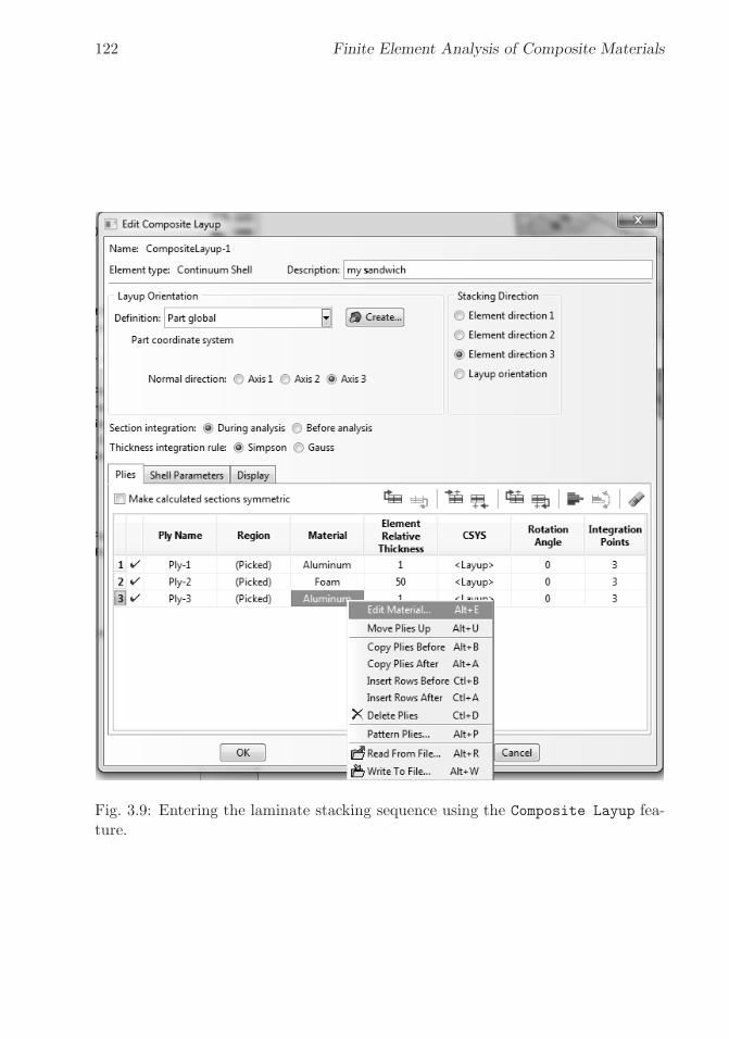
“K15072” — 2013/3/21 — 10:58�

�

�

�

�

�


Fig. 3.9: Entering the laminate stacking sequence using the Composite Layup fea-ture.

�

�

“K15072” — 2013/3/21 — 10:58�

�

�

�

�

�


b. with general-purpose shell elements,c. with continuum shell elements in a composite section with a single element through

the plate thickness, andd. with continuum shell elements in a composite layup with several elements through the

plate thickness.

This example is continued in Example 3.12, p. 167.

Solution to Example 3.4 Parts (a) and (b) involve conventional shell elements using amesh without thickness. Therefore, most of the model for parts (a) and (b) is independentof the type of element. Note the LSS is given starting at layer #1 at the bottom of thelaminate. The full plate is modeled without taking advantage of symmetry, and nodes areconstrained to illustrate how to constrain a model to prevent rigid body motion. The fol-lowing pseudo code illustrates the whole procedure. If in doubt, open Ex_3.4.cae availablein [5].

i. Make sure the .cae file is saved in the right place. You can also set the Work Directory

to the same folder where you saved the .cae file

Menu: File, Save as [c:\simulia\user\Ex_3.4\Ex_3.4.a.cae]

Menu: File, Set Work Directory [c:\simulia\user\Ex_3.4]

ii. Creating parts

Module: Part,

Menu: Part, Create,

Name [Part-1], 3D, Deformable, Shell, Planar, Approx size [2000], Cont

Menu: Add, Line, Rectangle, [-1000,-1000], [1000,1000], X, Done

iii. Creating materials and sections, and assigning sections to parts

Module: Property

Menu: Material, Create, Name [Material-1], Mech., Elast., Elastic,

Type [Engineering Constants],

# Note: you can cut and paste an entire row of values from Excel

[1.3386E+05 7.7060E+03 7.7060E+03 3.0100E-01 3.0100E-01

3.9600E-01 4.3060E+03 4.3060E+03 2.7600E+03], OK

Menu: Section, Create, Shell, Composite, Cont

# checkmark: Symmetric layers

Integration [Simpson]

# insert rows with right click until you have 4 rows

Material [Material-1] # for all

Thickness [1.25] #for all

Orientation [0,90,45,-45]

Integration points [3,3,3,3] # results at bot/mid/top of each ply

Ply Names [k1,k2,k3,k4], OK, # k1:bottom, k4:middle

# due to symmetry, CAE adds [-45,45,90,0] to the model,

Menu: Assign, Section, # pick part, Done, OK

iv. Creating assembly

Module: Assembly


�

�

“K15072” — 2013/3/21 — 10:58�

�

�

�

�

�


v. Creating analysis steps

Module: Step


Menu: Output, Field Output Requests, Edit, F-Output-1

Step: Step-1, Output variables:

# unselect everything, # select only what you need: S, E, U, RF

# request at 8x3=24 points (8 layers, 3 Simpson points per layer)

# Output at shell and layered section points:

Specify: [1,...24], OK # list all #’s from 1 to 24

vi. Adding loads

Module: Load

# since the part is a shell, an edge load is: Shell edge load

Menu: Load, Create, Name [Load-1], Step: Step-1, Mechanical,

Shell edge load, Cont

# pick the edges x=-1000 and x=1000, Done, Magnitude [-100], OK

In order to identify sets of nodes to constrain, when setting the BC, it is required tomesh the model now.

vii. Creating mesh

Module: Mesh

Menu: Seed, Instance, Approx global size [100], Apply, OK

Menu: Mesh, Controls, Element Shape [Quad], Technique [Structured],

OK

Menu: Mesh, Element Type, Std, Quad, DOF [5], OK # element S8R5


Menu: Tools, Set, Manager

Create, [center], Node, Cont, # center node, Done

Create, [y-hold], Node, Cont, # nodes at (-1000,0) and (1000,0),

Done

Create, [edges], Node, Cont, # nodes at the edges of the plate,

Done

# close Set Manager

viii. Adding BC

Module: Load

Menu: BC, Manager

Create, Name [edges], Step: Initial, Mechanical, Disp/Rota, Cont

Sets, # in the Region Selection pop-up window, [edges], Cont

# checkmark: U3, OK

Create, Name [center], Step: Initial, Mechanical, Disp/Rota, Cont

# in the Region Selection pop-up window, [center], Cont

# checkmark: U1, U2, and U3, OK

Create, Name [y-hold], Step: Initial, Mechanical, Disp/Rota, Cont

# in the Region Selection pop-up window, [y-hold], Cont

# checkmark: U2, and U3, OK

# close BC Manager

ix. Solving and visualizing the solution

�

�

“K15072” — 2013/3/21 — 10:58�

�

�

�

�

�


Module: Job

Menu: Job, Manager

Create, Cont, OK,

Submit # to run the model

Results # to visualize the solution

Menu: Viewport, Viewport Annotation Options, Tab: State Block,

Set font, Size [12], Apply to [# checkmark all], OK, OK

Menu: Plot, Undeformed Shape,

Menu: Plot, Allow Multiple Plot States,

Menu: Plot, Deformed Shape,

Menu: Plot, Material Orientations, On Deformed Shape

# by default shows the 0-deg layer on bottom

Menu: Result, Section Points, Plies, # select K1, Apply

# repeat for all the plies to visualize their orientation, OK

Menu: Plot, Contour, On Deformed Shape,

Field Output Toolbox, Primary, S, S12 # laminate stress_6

Menu: Result, Section Points, Plies, # select K1, Apply

# repeat for all the plies to visualize S12, OK

# select ply K1, Apply # sigma_6(K1) = 0.0

# select ply K2, Apply # sigma_6(K2) = 0.0

# select ply K3, Apply # sigma_6(K3) = -1.112

# select ply K4, Apply # sigma_6(K4) = 1.122, OK

(a) Solution using thin shell elementsIn the procedure given above, selection of a conventional shell element S8R5 is illustratedby:

Module: Mesh

Menu: Mesh, Element Type, Standard, Quadratic, DOF [5], OK

which results in element S8R5 being chosen. It is convenient to save the solution of thisproblem, and modify the model to solve part (b).

Menu: File, Save as [c:\simulia\user\Ex_3.4\Ex_3.4.a.cae], OK

Visualization of lamina stresses in lamina coordinate system results in

σ6 = 0, 0,−1.112, 1.112MPa

in the 0, 90, 45o,−45o plies, respectively. These results can be verified by comparison withthe classical lamination theory (CLT) results obtained with [12].

(b) Solution using general-purpose shell elementsTo change the analysis from thin shell to general-purpose shell, one only needs to changethe element type, by selecting DOF [6], as follows:

Menu: File, Save as [c:\simulia\user\Ex_3.4\Ex_3.4.b.cae], OK

Module: Mesh

Menu: Mesh, Element Type, Standard, Quadratic, DOF [6], OK # S8R

�

�

“K15072” — 2013/3/21 — 10:58�

�

�

�

�

�


This results in element S8R being chosen–a doubly-curved, general-purpose (thick/thin)shell with reduced integration. The job must be resubmitted for execution. Since this exampledoes not involve bending, the results are identical to those of part (a).

(c) Solution using continuum shell elements in a composite shellTo use continuum shell elements, the geometric model must be that of a solid, in this casewith dimensions 2, 000× 2, 000× 10 mm.

i. Saving the model, and setting the Work Directory

Menu: File, Save as [c:\simulia\user\Ex_3.4\Ex_3.4.c.cae]


ii. Creating parts

Module: Part

Menu: Part, Create,

Name [Part-1], 3D, Deformable, Solid, Extrusion, size [2000], Cont

Menu: Add, Line, Rectangle, [-1000,-1000], [1000,1000], X, Done,

Depth [10], OK

iii. Creating materials and sections, and assigning sections to parts

Module: Property




[1.3386E+05 7.7060E+03 7.7060E+03 3.0100E-01 3.0100E-01

3.9600E-01 4.3060E+03 4.3060E+03 2.7600E+03], OK

Menu: Section, Create, [Section-1], Shell, Composite, Cont


Material [Material-1] # for all, Thickness [1.25] # for all

Orientation [0,90,45,-45,-45,45,90,0],

Integration points [3] # for all

Ply Names [PLY-1,PLY-2,PLY-3,PLY-4,PLY-5,PLY-6,PLY-7,PLY-8], OK



Module: Assembly


v. Creating analysis steps

Module: Step



Step: Step-1, Output variables:

# unselect everything, # select only what you need: S, E, U, RF

# request at 8x3=24 points (8 layers, 3 Simpson points per layer)

# Output at shell and layered section points:

Specify: [1,...24], OK # 1,2,3,4,...

vi. Adding loads

�

�

“K15072” — 2013/3/21 — 10:58�

�

�

�

�

�


Module: Load

Menu: Load, Create

Name [Load-1], Step: Step-1, Mechanical, Surface traction, Cont

# an edge load of 100 N/mm on a surface 10 mm-thick equals 10 N/mm2

# Zoom into the upper-right corner of the plate

# pick the surface x=1000, Done,

Distribution [Uniform], Traction [General],

Vector, Edit, [0,0,0], [1,0,0], Magnitude [10], OK

# repeat the procedure to apply a surface traction of 10 N/mm2

# on the x=-1000 surface, # Name [Load-2] and direction [-1,0,0]

In order to identify the nodes to constrain, when setting the BC, it is required to meshthe model now.

vii. Creating mesh

Module: Mesh

Menu: Seed, Instance, Approx global size [100], OK

Menu: Mesh, Controls, # if required select the whole plate, Done,

Element Shape [Hex], Technique [Sweep], OK

Menu: Mesh, Element Type, # if required select whole plate, Done,

Family [Continuum Shell], # element SC8R has been selected, OK


# create sets of nodes to facilitate applying the BC to the model

Views Toolbar, Front View # to visualize better


Create, Name [edges], Type [Node], Cont

# select all the nodes along the edges of the plate, Done

Create, Name [center], Type [Node], Cont

# select the nodes at the center of the plate (x=0,y=0), Done

Create, Name [y-hold], Type [Node], Cont

# select the nodes at (x=-1000,y=0) and (x=1000,y=0), Done

# close the Set Manager pop-up window

viii. Applying BC

Module: Load

Menu: BC, Manager

Create, Name [edges], Step: Initial, Mechanical, Disp/Rota, Cont

Sets, # in the Region Selection pop-up window, [edges], Cont

# checkmark: U3, OK

Create, Name [center], Step: Initial, Mechanical, Disp/Rota, Cont

# in the Region Selection pop-up window, [center], Cont

# checkmark: U1, U2, and U3, OK

Create, Name [y-hold], Step: Initial, Mechanical, Disp/Rota, Cont

# in the Region Selection pop-up window, [y-hold], Cont

# checkmark: U2, and U3, OK

# close BC Manager


Module: Job

Menu: Job, Manager

�

�

“K15072” — 2013/3/21 — 10:58�

�

�

�

�

�


Create, Cont, OK,

Submit # to run the model

Results # to visualize the solution

Menu: Viewport, Viewport Annotation Options, Tab: State Block,

Set font, Size [12], Apply to [# checkmark all], OK, OK

Menu: Plot, Undeformed Shape,

Menu: Plot, Allow Multiple Plot States,

Menu: Plot, Deformed Shape,

Menu: Plot, Material Orientations, On Deformed Shape

Menu: Result, Section Points, Plies, # select PLY-1, Apply

# repeat for all the plies to visualize their orientation, OK

Menu: Plot, Contour, On Deformed Shape,

Field Output Toolbox, Primary, S, S12 # laminate stress_6

Menu: Result, Section Points, Plies, # select PLY-1, Apply

# repeat for all the plies to visualize S12 stress, OK

(d) Solution using continuum shell elements in a composite layupIn order to use a Composite Layup to model the laminate the solid part must be divided inregions, each one corresponding to a layer of the laminate. The creation of the part mustbe modified as

i. Creating parts

Module: Part

Menu: Part, Create,

Name [Part-1], 3D, Deformable, Solid, Extrusion, size [2000], Cont

Menu: Add, Line, Rectangle, [-1000,-1000], [1000,1000], X, Done,

Depth [10], OK

# zoom into the upper-right corner of the plate

# divide the thickness of the plate in 8 segments

Menu: Tools, Partition, Type [Edge], Method [Enter parameter]

# pick edge, Done, Normalized edge param [0.5], Create Partition

# repeat procedure until the edge is divided in 8 segments, Done

# in the Create Partition pop-up window select

Type [Cell], Method [Define cutting plane], Point & Normal,

# select one point defined previously (start at top of the plate),

# select edge used as normal direction (along positive z-axis),

Create Partition # create first region representing the top ply

# pick region to partition, Done,

Point & Normal, # repeat procedure,

# once 8 regions have been created, Done, # close pop-up window

The definition of the material properties must be modified as


Module: Property




[1.3386E+05 7.7060E+03 7.7060E+03 3.0100E-01 3.0100E-01

�

�

“K15072” — 2013/3/21 — 10:58�

�

�

�

�

�


3.9600E-01 4.3060E+03 4.3060E+03 2.7600E+03], OK


Initial ply count [8], Element Type [Continuum Shell], Cont

Thickness integration rule [Simpson]

# in column named Region double-click cell corresponding Ply-1,

# pick top region of laminate, Done, # repeat for other plies

# in column named Material double-click cell corresponding Ply-1,

Material [Material-1], OK

# repeat to assign Material-1 to the other plies

Element Relative Thickness [1] # for all plies

Rotation Angle [0, 90, 45, -45, -45, 45, 90, 0] # one per ply

Integration points [3] # for all plies, OK

The rest of the solution follows the same steps described in part (c).

3.2.12 FEA of Ply Drop-Off Laminates

Sometimes it is convenient to set the reference surface at the bottom (or top) of theshell. One such case is when the laminate has ply drop-offs, as shown in Figure 3.10.When the design calls for a reduction of laminate thickness, plies can be graduallyterminated from the thick to the thin part of the shell. As a rule of thumb, plydrop-off should be limited to a 1:16 to 1:20 ratio (Th : L ratio in Figure 3.10) unlessdetailed analysis and/or testing supports a steeper drop-off ratio. For this case, itis convenient to specify the geometry of the smooth surface, or tool surface.

Fig. 3.10: Ply drop-off of length (L) and thickness (Th) and FE model simplifica-tions.

Then, every time a ply or set of plies is dropped, the material and thickness forthose elements is changed. This is illustrated in the next examples. Not all softwarehas this capability and it may be necessary to assume that the midsurface is smooth

�

�

“K15072” — 2013/3/21 — 10:58�

�

�

�

�

�


while in reality only the tool surface is smooth. As long as the thickness is smallcompared to the other two dimensions of the structure, such assumption is unlikelyto have a dramatic effect in the results of a global analysis, such as deformation,buckling, and even membrane stress analysis. The exact description of the thicknessgeometry begins to play a role when detailed 3D stress analysis of the ply drop-offregion is required, but at that point, a 3D local model is more adequate.

Example 3.5 A composite strip 120mm long and 100mm wide has a ply drop-off betweenlaminate A: [90/0]S, and laminate B: [90/0], with ply thickness 0.75 mm. A ply drop-offratio 1:20 is used, meaning that the transition length is 20 times the dropped thickness.The strip is under tension N = 10 N/mm applied to the bottom edges on the strip. Thematerial is AS4D/9310 (Table 3.1). Use symmetry to model 1/2 of the tape. Visualize andreport the maximum deflection (in the Z-direction, normal to the plate). Also, tabulate themaximum values of σ11 at the top and bottom surface of each lamina (not the minimum,not the maximum absolute value).

Solution to Example 3.5 Three different sections are defined: one for laminate A, onefor laminate B, and one to model the ply drop-off between them (called laminate AB), whereonly the top 90◦ lamina has been dropped. The thickness of the drop-off is equivalent to twolaminas, 0.75 × 2 = 1.5 mm. With a ply drop-off ratio 1:20, the total length of ply drop-off is 1.5 × 20 = 30 mm. If the laminate A spans 0 < x < 60 mm, the transition goesfrom x = 60 mm to x = 90 mm, and laminate B from x = 90 mm to the loaded edge atx = 120mm.

The midsurface of each laminate (A, B, and AB) is offset at different z-distances withrespect to the flat bottom surface. Therefore, it is preferred to apply the load at the commonbottom surface. This however introduces a bending moment because the traction load isoffset with respect to the midsurface of the loading edge. This effect can be easily correctedby applying a bending moment equal to the product of the traction times one half the thicknessof the laminate at the loading edge, but it has not been done in this example to emphasizethe resulting deformation.

The bottom lamina is designated as #1. Additional laminas are stacked from bottom totop in the positive normal z-direction of the element coordinate system. With the surface ofthe plate resting on the x-y plane, the x-z plane is a plane of symmetry (YSYMM). Then,the thicker end of the strip (laminate A) on the left of the model can be properly supportedby imposing an Encastre-condition; this will guarantee symmetry conditions with respectto the y-z plane.

The material properties are defined in the Edit Material window (Figure 3.11), butthis is quite tedious. If the properties are listed in Excel, or in a Tab-separated file, onecan cut and paste directly into the Edit Material window. Otherwise, they can be accesseddirectly from the CADEC database using a Web service [18].

The laminate stacking sequence (LSS) is defined in the Edit Section window, whichis reached as follows:

Module: Property

Menu: Section, Create, Shell, Composite, Cont

In the Edit Section window (Figure 3.12), the first row corresponds to lamina #1,which is located at the bottom of the laminate. Subsequent rows are used to define LSS of alaminate with n laminas. The last row corresponds to the topmost lamina in the laminate.Note how we have assigned the names k1, k2, k3, k4, to the laminas, following the usualnotation where lamina #1 is at the bottom of the laminate.

�

�

“K15072” — 2013/3/21 — 10:58�

�

�

�

�

�


Fig. 3.11: The Edit Material window.

�

�

“K15072” — 2013/3/21 — 10:58�

�

�

�

�

�


Fig. 3.12: The Edit Section window is used to define the LSS.

�

�

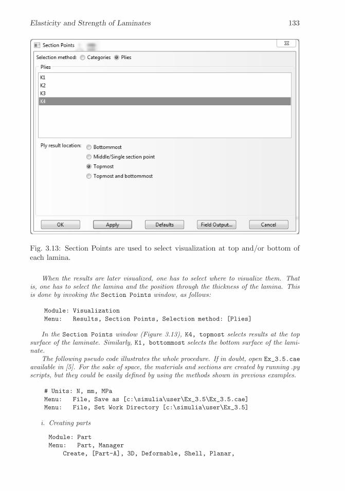
“K15072” — 2013/3/21 — 10:58�

�

�

�

�

�


Fig. 3.13: Section Points are used to select visualization at top and/or bottom ofeach lamina.

When the results are later visualized, one has to select where to visualize them. Thatis, one has to select the lamina and the position through the thickness of the lamina. Thisis done by invoking the Section Points window, as follows:


Menu: Results, Section Points, Selection method: [Plies]

In the Section Points window (Figure 3.13), K4, topmost selects results at the topsurface of the laminate. Similarly, K1, bottommost selects the bottom surface of the lami-nate.

The following pseudo code illustrates the whole procedure. If in doubt, open Ex_3.5.cae

available in [5]. For the sake of space, the materials and sections are created by running .pyscripts, but they could be easily defined by using the methods shown in previous examples.

# Units: N, mm, MPa

Menu: File, Save as [c:\simulia\user\Ex_3.5\Ex_3.5.cae]


i. Creating parts

Module: Part

Menu: Part, Manager

Create, [Part-A], 3D, Deformable, Shell, Planar,

�

�

“K15072” — 2013/3/21 — 10:58�

�

�

�

�

�


Approx size [500], Cont

Menu: Add, Line, Rectangle, [0,0], [60,50], X, Done

Create, [Part-AB], 3D, Deformable, Shell, Planar,



Create, [Part-B], 3D, Deformable, Shell, Planar,



# close the Part Manager

ii. Creating assembly

Module: Assembly

Menu: Instance, Create, [Part-A],

Independent, # uncheck Auto-offset, OK

Menu: Instance, Create, [Part-AB],


Menu: Instance, Create, [Part-B],


Menu: Instance, Merge/Cut, Intersecting Boundaries: Retain, Cont

# select all, Done, # creates Part-1

# on the .mdb tree, expand Assembly, expand Instances,

right-click Part-1, Make Independent

iii. Creating materials, section, and assigning sections to parts

Module: Property

# to display the whole Part-1, set the tabbed menus as follows:

Module: [Property], Model: [Model-1], Part: [Part-1]

# create materials by running .py scripts

Menu: File, Run Script, [AS4D--9310.py], OK

# create sections by running .py scripts

Menu: File, Run Script, [laminate-A.py], OK

Menu: File, Run Script, [laminate-AB.py], OK

Menu: File, Run Script, [laminate-B.py], OK

# recall that from bottom to top, section A is [90/0/0/90],

# section B is [90/0], and section AB is [90/0/0]

Menu: Section, Assignment Manager

Create, # pick the region/part Section-A, Done

Section: [Section-A], Shell Offset Definition: [Bottom Surface], OK

Create, # pick the region/part Section-AB, Done

Section: [Section-AB], Shell Offset Definition: [Bottom Surface], OK

Create, # pick the region/part Section-B, Done

Section: [Section-B], Shell Offset Definition: [Bottom Surface],

OK # close the Section Assignment Manager,

Done # close current command

iv. Defining analysis steps

Module: Step


Menu: Output, Field Output Request, Edit, F-Output-1

Output at shell, Specify [1,2,3,4,5,6,7,8,9,10,11,12], OK

�

�

“K15072” — 2013/3/21 — 10:58�

�

�

�

�

�



Module: Load

Menu: BC, Manager

Create, [BC-1], Step: Initial, Mechanical, Symm/Anti/Enca, Cont

# pick edge @ x=0, Done, Encastre, OK

Create, [BC-2], Step: Initial, Mechanical, Symm/Anti/Enca, Cont

# pick the 3 segments @ y=0, Done, YSYMM, OK, # close BC Manager

# since the part is a Shell, an edge load is: Shell edge load

# load applies on the offset defined during Assign

Menu: Load, Create

[Load-1], Step: Step-1, Mechanical, Shell edge load, Cont

# pick the edge at x=120, Done, Magnitude [-10], OK

vi. Creating mesh

Module: Mesh

Menu: Seed, Instance, Approx global size: [5], Apply, OK

Menu: Mesh, Controls, # select all the regions, Done

Element Shape [Quad], Technique [Structured]

Menu: Mesh, Element Type, # select all the regions, Done

Standard, Quadratic, DOF [6], OK # element selected S8R

Mesh, Instance, Yes

vii. Solving and visualizing the results

Module: Job

Menu: Job, Manager

Create, Cont, OK, Submit # when completed, Results


Menu: Viewport, Viewport Annotation Options,

Tab: State Block, Set Font, Size [10], Apply to [checkmark all],

OK, OK

Menu: File, Save Options, OK # to save options for future sessions

Menu: Plot, Undeformed Shape

Menu: Plot, Allow Multiple Plot States

Menu: Plot, Deformed Shape # you will see both shapes


Field Output Toolbar, [Primary], [U], [U3]

# read the maximum value from the legend on top left, U3=2.578 mm

Field Output Toolbar, [Primary], [S], [S11]

# next to select the top or bottom surface of each lamina

Menu: Result, Section Points

Selection method: [Plies], K1, Bottommost, Apply

# repeat for the other plies

Selection method: [Plies], K1, topmost, Apply

# repeat for the other plies

# a gray region means the ply is not modeled in that region

The maximum deflection is w = 2.578mm. The maximum values of stress are reportedin Table 3.3.

�

�

“K15072” — 2013/3/21 — 10:58�

�

�

�

�

�


Table 3.3: Stresses calculated in Example 3.5.Ply # z [mm] θ[◦] σ11[MPa]

1 (bot) 0.00 90 1.2331 (top) 0.75 90 0.62062 (bot) 0.75 0 73.172 (top) 1.50 0 6.5963 (bot) 1.50 0 6.5963 (top) 2.25 0 -19.154 (bot) 2.25 90 0.19074 (top) 3.00 90 0.4094

Fig. 3.14: Laminate with dropped laminas.

Example 3.6 Model the laminate shown in Figure 3.14. The laminate in section A is a[+45/ − 45/0/90/0]. The thickness of each lamina is 1.2 mm. A ply drop-off ratio 1:10is used. The strip is 120 mm long and 100 mm. It is loaded by tension Nx = 10 N/mmapplied to the bottom edges on the strip. Use symmetry to model 1/2 of the tape. Thematerial is AS4D/9310 (Table 3.1). Visualize and report the maximum value of transversedeflection U3. Also, visualize and tabulate the maximum value of σ11 at the top surface ofevery lamina (k1, k2, k3, k4, k5). Note the absence of results for the laminas dropped inthe region where those laminas have been dropped.

Solution to Example 3.6 In this example, we illustrate the use of partitions to separatethe three regions. With a drop-off ratio 1:10, the transition length is 2× 1.2× 10 = 24 mm,with drops at 12 mm on each side of the center line. With the center line at 60 mm fromthe left edge, the transitions are located at 48 mm and 72 mm. The bottom lamina isdesignated as lamina #1. Additional laminas are stacked from bottom to top in the positivenormal direction of the element coordinate system. The dropped laminas are #3 and #4.The following pseudo code illustrates the whole procedure. If in doubt, open Ex_3.6.cae

available in [5].

# Units: N, mm, MPa


Menu: File, Save As [Ex_3.6.cae]

i. Creating parts

Module: Part

Menu: Part, Create

[Part-1], 3D, Deformable, Shell, Planar, Approx size [300], Cont


# creating 3 partitions for the different regions

�

�

“K15072” — 2013/3/21 — 10:58�

�

�

�

�

�


Menu: Tool, Datum, Plane, Offset from principal plane

[YZ Plane], [48], Enter, [YZ Plane], [72], Enter, X

# close the Create Datum pop-up window

Menu: Tools, Partition, Face, Use datum plane,

# pick a datum plane, Create Partition

# pick face to partition (area not partitioned yet), Done

# pick datum plane, Create Partition, Done

# close the Create Partition pop-up window

ii. Creating materials, sections, and assigning sections to parts

Module: Property

Menu: Material, Create

Name [AS4D--9310], Mechanical, Elasticity, Elastic, Type [Lamina]

# you can cut and paste an entire row of values from Excel

[1.3386E5, 7.706E3, 0.301, 4.306E3, 4.306E3, 2.76E3], OK

# or use a .py file to create materials as in previous example

Menu: Section, Manager

Create, Name [Section-A], Shell, Composite, Cont


Material [AS4D--9310] # for all, Thickness [1.2] # for all

Orientation [45,-45,0,90,0], Integration points [3,3,3,3,3]

Ply names [k1,k2,k3,k4,k5], OK

Copy, [Section-AB], OK, Edit, # delete the center ply (k3), OK

Copy, [Section-B], OK, Edit, # delete the center ply (k4), OK

# close Section Manager

Menu: Section, Assignment Manager

Create, # pick the region on the left, Done

Section [Section-A], Shell Offset [Bottom surface], OK

Create, # pick the region in the middle, Done

Section [Section-AB], Shell Offset [Bottom surface], OK

Create, # pick the region on the right, Done

Section [Section-B], Shell Offset [Bottom surface], OK, Done

# close Section Assignment Manager

iii. Creating assembly

Module: Assembly



Module: Step

Menu: Step, Create

Name [Step-1], Procedure type: General, Static/General, Cont, OK

Menu: Output, Field Output Request, Edit, F-Output-1

Specify [1,2,3,4,5,6,7,8,9,10,11,12,13,14,15], OK


Module: Load

Menu: BC, Create

Name [BC-1], Step: Initial, Mechanical, Symm/Anti/Enca, Cont

�

�

“K15072” — 2013/3/21 — 10:58�

�

�

�

�

�


# pick edge @ x=0, Done, Encastre, OK

Menu: BC, Create

Name [BC-2], Step: Initial, Mechanical, Symm/Anti/Enca, Cont

# pick 3 segments @ y=0, Done, YSYMM, OK

# since the part is a Shell, an edge load is: Shell edge load

# load applied with an offset defined during Assign

Menu: Load, Create

Name [Load-1], Step: Step-1, Mechanical, Shell edge load, Cont

# pick edge @ x=120, Done, Magnitude [-10], OK

vi. Creating Mesh

Module: Mesh

Menu: Seed, Instance, Approx global size: [5], Apply, OK

Menu: Mesh, Controls, # select all regions, Done,

Element Shape [Quad], Technique [Structured], OK

Menu: Mesh, Element Type, # select all regions, Done

[Standard], [Quadratic], DOF [6], OK, # element used S8R



Module: Job

Menu: Job, Manager

Create, Cont, OK, Submit, # when completed, Results


Menu: Viewport, Viewport Annotation Options

Tab: State Block, Set Font, Size [10],

Apply to [checkmark all], OK, OK

Menu: File, Save Options, OK # to save options for future sessions

Menu: Plot, Undeformed shape


Menu: Plot, Deformed Shape # you will see both shapes

Menu: Plot, Material Orient., On Def. Shape # identify the 1-axis

Menu: Result, Section Points, [Plies], K1, Bottommost

# pick one ply at a time and comment on the results, OK

Field Output Toolbar, [Primary], [S], [S11]

Menu: Result, Section Points, [Plies], K1, Topmost

# pick one ply at a time and tabulate the results, OK

The maximum transverse deflection is 0.6075 mm. The maximum values of stress aregiven in Table 3.4.

Table 3.4: Maximum values of stress at the top surface of each ply for Example 3.6.Ply # z [mm] θ[◦] σ11[MPa]

1 1.2 45 10.12 2.4 −45 17.883 3.6 0 17.634 4.8 90 4.3035 6.0 0 9.632

�

�

“K15072” — 2013/3/21 — 10:58�

�

�

�

�

�


3.2.13 FEA of Sandwich Shells

Laminates should be modeled as sandwich shells when specifically designed forsandwich construction with thin faceplates and a thick, relatively weak, core (e.g.,honeycomb, foam, balsa wood). The faceplates are intended to carry all, or almostall, of the bending and in-plane normal load. Conversely, the core is assumed tocarry all of the transverse shear. Example 3.7 shows how to define and calculate asandwich cantilever beam.

The following assumptions are customarily made for a sandwich shell:

– The terms Hij in (3.9) depend only on the middle layer (core) and they canbe calculated as

Hij =(

Q∗ij

)

coretcore ; i, j = 4, 5 (3.17)

– The transverse shear moduli (G23 and G13) are set to zero for the top andbottom layers (non-core layers) so they do not add artificial stiffness to thesandwich shell.

– The transverse shear strains and stresses in the face plate (non-core) layersare neglected or assumed to be zero.

– The transverse shear strains and shear stresses in the core are assumed con-stant through the thickness.

Example 3.7 Consider a sandwich plate clamped around the boundary and loaded withuniform pressure on the top surface.2 The sandwich is made of two face plates and an innercore with properties, thicknesses, and pressure given in Table 3.5. Use symmetry conditionsto model one quarter of the plate. Use a surface mesh of 6 by 6 elements. Compute thecenter deflection using four different methods:

a. Conventional shell elements S4R.b. Continuum shell elements SC8R spanning the entire thickness, with the laminate

defined inside the element.c. Continuum shell elements SC8R stacked through the thickness, one for each face and

one or more for the core.d. Continuum shell elements SC8R for the core and conventional shell elements S4R for

the faces.

Solution to Example 3.7 Here we solve the problem in four ways. The results are tabu-lated in Table 3.6. The stacked continuum shell model (c) and stacked continuum shell plusskins (d) are more flexible than (a) and (b) models because in (c, d) the FSDT constraint(i.e., normals remain straight) is enforced separately in the core and two faces/skins. Thus,each lamina (core and each face) is able to rotate independently of the other laminas. Thismeans that each lamina achieves its own value of transverse shear deformation. Since thecore has lower transverse shear moduli (G13,G23), it can deform more. This additional

2This example is modified from [16, Test R0031/3] by making the edges clamped rather thansimply supported. The change is made because it is difficult to impose a simple support withcontinuum shell elements. Doing so requires to use constraint equations, which complicates theexample too much at this stage.

�

�

“K15072” — 2013/3/21 — 10:58�

�

�

�

�

�


Table 3.5: Data for Example 3.7.Quantity Units Face Core

E1 MPa 68947.57 0.068948E2 MPa 27579.03 0.068948ν12 0.3000 0.0000G12 MPa 12927.67 0.068948G13 MPa 12927.67 209.6006G23 MPa 12927.67 82.73708thickness mm 0.7112 19.0500half plate width mm 127.00pressure MPa 0.689476thickness modulus MPa 689475.7 689475.7

flexibility impacts the transverse deflection and more notably the transverse shear strainsand stresses. Increasing the number of elements through the thickness in the core does notchange the results because the core is homogeneous (not laminated). Therefore, its normaldeforms as a straight line regardless of how many elements are used to discretize its thick-ness. The conventional and single element continuum models yield similar results becausethe single, laminated SC8R element has the same kinematics as the conventional S4R (pro-vided the transverse compressibility of SC8R is constrained by selecting a high value for thethickness modulus).

Continuum shell elements in Abaqus need a thickness modulus E3 and they cannot readit from the given material properties, even if E3 is given in Engineering Properties,or it is implied for Isotropic (E3 = E) and Lamina (E3 = E2). So, the user mustremember to assign a thickness modulus in tab Shell Parameters of the Edit CompositeLayup window (Figure 3.15). Since a shell is incompressible in the thickness direction,we chose a thickness modulus ten times the highest modulus of the face material,3 i.e.,E3 = 10 × E1 = 689475.7 MPa. No thickness modulus is needed for conventional shellelements because they are intrinsically incompressible through the thickness.

(a) Solution with conventional shell elementsHere we show how to model the geometry of the sandwich plate as a 2D flat surface. Then,define the laminate inside the conventional shell element. The following pseudo code illus-trates the whole procedure. If in doubt, open Ex_3.7.a.cae available in [5].

# NAFEMS sandwich clamped metric conventional shell elements


Menu: File, Save As [Ex_3.7.a.cae]

i. Creating parts

Module: Part

Menu: Part, Create, 3D, Deformable, Shell, Planar, Cont


# name the part to make it easier to use Composite Modeler later

Menu: Tools, Set, Create, Name [plate], Cont, # select all, Done

3This is in agreement with r313 std sc8r composite.inp in [19, 4.9.3 R0031(3)].

�

�

“K15072” — 2013/3/21 — 10:58�

�

�

�

�

�


Fig. 3.15: Specify a thickness modulus for the shell section.

�

�

“K15072” — 2013/3/21 — 10:58�

�

�

�

�

�


ii. Defining materials, sections, and assigning sections to parts

Module: Property


Name [face], Mechanical, Elasticity, Elastic, Type [Lamina]

[68947.57, 27579.028, 0.3000, 12927.66938, 12927.66938,

12927.66938], OK


Name [core], Mechanical, Elasticity, Elastic, Type [Lamina]

[0.06894757, 0.06894757, 0.0000, 0.06894757, 209.6006128,

82.737084], OK

# use Composite Modeler instead of Create + Assign Sections

Menu: Composite, Create, Name [NAFEMS-sandwich],

Conventional Shell, Cont

# Name, region, Material, Thickness, CSYS, Angle, Integ Points

Ply-1, plate, face, 0.7112, <Layup>, 0, 3

Ply-2, plate, core, 19.050, <Layup>, 0, 3


OK

# to assign Region double click the cell corresp. to desired ply

Sets # to open Region Selection pop-up window, plate, Cont

# to assign Material double click the cell corresp. to desired ply

# in Select Material pop-up window, Material [face or core], OK


Module: Assembly



Module: Step

Menu: Step, Create

Procedure type: Linear perturbation, Static/General, Cont, OK


Module: Load

Menu: Load, Create

Name [Load-1], Step: Step-1, Mechanical, Pressure, Cont,

# pick the part, Done, Choose a side for the shell [Brown]

Magnitude [0.689476], OK

Menu: BC, Manager

Create, Step: Initial, Mechanical, Symm/Anti/Enca, Cont

# pick edges @ x=0 and y=0, Done, Encastre, OK


# pick edge @ x=127, Done, XSYMM, OK


# pick edge @ y=127, Done, YSYMM, OK

# close BC Manager

vi. Meshing the model

�

�

“K15072” — 2013/3/21 — 10:58�

�

�

�

�

�


Module: Mesh


Menu: Mesh, Controls, Element Shape [Quad], Tech [Structured], OK

Menu: Mesh, Element Type, # select all surfaces, Done

Element Library [Standard], Geometric Order [Linear], OK # S4R



Module: Job

Menu: Job, Manager




The displacement at the upper-right corner is −1.667mm

(b) Solution with continuum shell elementsHere we show how to model the geometry of the sandwich plate as a 3D body. Then, definethe laminate inside the continuum shell element. Note that in the composite modeler, therelative thicknesses do not need to add to 1.0. The actual ply thicknesses are calculated interms of the mesh thickness. To emphasize this, we have chosen to enter the thicknessesof the plies in inches (0.028”,075”,0.028”), even though the model is set up in SI units.The following pseudo code illustrates the whole procedure. If in doubt, open Ex_3.7.b.cae

available in [5].

# NAFEMS sandwich clamped metric laminated continuum shell elements


Menu: File, Save As [Ex_3.7.b.cae]

i. Creating parts

Module: Part

Menu: Part, Create, 3D, Deformable, Solid, Extrusion, Cont


Depth [20.4724], OK # core + two faces




Module: Property



[68947.57, 27579.028, 0.3, 12927.66938, 12927.66938,

12927.66938], OK



[0.06894757, 0.06894757, 0.0, 0.06894757, 209.6006128,

82.737084], OK

# use Composite Modeler instead of Create + Assign Section

Menu: Composite, Create, Name [sandwich], Type: Continuum Shell, Cont

�

�

“K15072” — 2013/3/21 — 10:58�

�

�

�

�

�


# Name, region, Material, Thickness, CSYS, Angle, Integ Points


Ply-2, plate, core, 0.75, <Layup>, 0, 3


# to assign Region double click the cell corresp. to desired ply

Sets # to open Region Selection pop-up window, plate, Cont

# to assign Material double click the cell corresp. to desired ply

# in Select Material pop-up window, Material [face or core], OK

Tab: Shell Parameters

Section Poisson’s ratio: Specify value [0.0]

# checkmark: Thickness modulus [689475.7], OK

# the last two instructions are very important!


Module: Assembly



Module: Step

Menu: Step, Create

Procedure type: Linear perturbation, Static/General, Cont, OK


Output variables: Edit variables [CF,CTSHR,LE,RF,S,SE,TSHR,U]

Output at shell: Specify [1,2,3,4,5,6,7,8,9], OK


Module: Load

Menu: Load, Create


# pick the top surface (z=20.4724), Done, Magnitude [0.689476], OK

Menu: BC, Manager


# pick surfaces @ x=0 and y=0, Cont, Encastre, OK


# pick surface @ x=127, Cont, XSYMM, OK


# pick surface @ y=127, Cont, YSYMM, OK

# close BC Manager


Module: Mesh


Menu: Mesh, Controls, Element Shape [Hex], Technique [Sweep], OK

Menu: Mesh, Element Type, # select all, Done

Family [Continuum Shell], OK # notice the element chosen is SC8R



�

�

“K15072” — 2013/3/21 — 10:58�

�

�

�

�

�


Fig. 3.16: Seeding an edge By number, using 50 elements through the length of theedge.

Module: Job

Menu: Job, Manager




The displacement at the upper-right corner is −1.667mm.

(c) Solution with stacked continuum shell elementsHere we show how to model the geometry of the sandwich plate as a 3D body, partitioned intoa core and two faces. Each region is then discretized with continuum shell (CS) elements.Discretizing with 3D solid elements would require a very fine mesh of the plate dimensions(3000× 600) to avoid locking. In fact, the element dimensions could not be smaller than 10times the thickness of the Aluminum face. Also in this example we show how to seed with asweep and how to re-seed an edge, using the local seeds window (Figure 3.16). Remember toassign a thickness modulus in tab Shell Parameters of the Edit Composite Layup window(Figure 3.15). The following pseudo code illustrates the whole procedure. If in doubt, openEx_3.7.c.cae available in [5]. Remeshing to accommodate 4 elements through the thicknessof the core does not alter the results.

# NAFEMS sandwich clamped metric stack 3 continuum shell elements


Menu: File, Save As [Ex_3.7.c.cae]

i. Creating parts

Module: Part

�

�

“K15072” — 2013/3/21 — 10:58�

�

�

�

�

�




Depth [20.4724], OK # core + two faces

# partition the faces from the core

Menu: Tool, Datum, Plane, Offset from principal plane

[XY], [0.7112], Enter, [XY], [19.7612], Enter,

X, # close Create Datum

Menu: Tools, Partition, Cell, Use datum plane

# the entire part is automatically selected

Select datum plane # back datum plane, Create Partition

# pick front cell to create the new partition, Done

Select datum plane, Create Partition, Done


Module: Property

Menu: Material, Manager

Create, Name [face], Mechanical, Elasticity, Elastic,

Type [Lamina]

[68947.57, 27579.028, 0.3, 12927.66938, 12927.66938,

12927.66938], OK

Create, Name [core], Mechanical, Elasticity, Elastic,

Type [Lamina]

[0.06894757, 0.06894757, 0.0, 0.06894757, 209.6006128,

82.737084], OK

# close Material Manager, # zoom in to pick the regions easily

# use Composite Modeler instead of Create + Assign Section


Name [front face], Initial ply count [1],

Element Type [Continuum Shell], Cont

# Name, region, Material, Rel. Thick., CSYS, Angle, Integ. Points

Ply-1, <picked>, face, 1, <Layup>, 0, 3

Tab: Shell Param., Section Poisson’s ratio: Specify value [0.0]

# checkmark: Thickness modulus: [689475.7], OK



Name [back face], Initial ply count [1],

Element Type [Continuum Shell], Cont


Ply-1, <picked>, face, 1, <Layup>, 0, 3





Name [core], Initial ply count [1], Type [Continuum Shell], Cont


Ply-1, <picked>, core, 1, <Layup>, 0, 3




�

�

“K15072” — 2013/3/21 — 10:58�

�

�

�

�

�


Module: Assembly



Module: Step

Menu: Step, Create

Procedure type: Linear perturbation, Static/Linear pert., Cont, OK

Menu: Output, Field Output Requests, Edit, F-Opuput-1


Output at shell: Specify [1,2,3], OK


Module: Load

Menu: Load, Create


# pick the top surface of the part (z=20.4724), Done


Menu: BC, Manager


# pick 3 surfaces @ x=0 and the 3 @ y=0, Done, Encastre, OK


# pick the three surfaces @ x=127, Done, XSYMM, OK


# pick the three surfaces @ y=127, Done, YSYMM, OK

# close the BC Manager pop-up window


Module: Mesh


Menu: Seed, Edges

# select the four vertical edges of the core part, Done

Method [By number], Number of elements [1], OK, X

Menu: Mesh, Controls, # select all regions, Done, Sweep, OK


Family [Continuum Shell], OK # SC8R



Module: Job

Menu: Job, Manager




The displacement at the upper-right corner is −1.892 mm. For a more refined meshin the core part of the sandwich, modify the procedure above as follows:

Module: Mesh

Menu: Seed, Edges

# select the four vertical edges of the core part, Done

�

�

“K15072” — 2013/3/21 — 10:58�

�

�

�

�

�


Method [By number], Number of elements [4], OK, X


(d) Solution with conventional and continuum shell elementsHere we show how to model the geometry of the core as a 3D body, then apply two skinsto represent the faces. The core is discretized with continuum shell elements and the faceswith conventional shell elements. One must be careful to offset the location of the referencesurface of the skins to coincide with the thickness of the core. Otherwise the results maybe more or less wrong depending on how thick is the skin. To offset correctly, one has toplace the reference at the top or bottom of the skin. This depends on the direction of thenormal to the shell surface. Skins inherit the normal of the underlying shell. So, one has tovisualize the normal to decide. If the normal is outward, then assigning the reference surfaceto the bottom of the skin will set the reference surface exactly where the surface nodes ofthe core are. The following pseudo code illustrates the whole procedure. If in doubt, openEx_3.7.d.cae available in [5].

# NAFEMS sandwich clamped metric using skins


Menu: File, Save As [Ex_3.7.d.cae]

i. Creating parts

Module: Part



Depth [19.05], OK # notice you created only the core part




Module: Property

Menu: Special, Skin, Create, # pick top face, Done

Menu: Special, Skin, Create, # pick back face, Done, X



[68947.57, 27579.028, 0.3, 12927.66938, 12927.66938,

12927.66938], OK



[0.06894757, 0.06894757, 0.0, 0.06894757, 209.6006128,

82.737084], OK

# Notice the type of element used for the core (Continuum Shell)


Name [core], Initial ply count [1], Type [Continuum Shell], Cont

# Name, Region, Mat., Relat. Thick., CSYS, Angle, Integ. Points

Ply-1, plate, core, 1, <Layup>, 0, 3

Tab: Shell Parameters,

Section Poisson’s ratio: Specify value [0.0]


# Notice type of element used for skins/faces (Conventional Shell)

�

�

“K15072” — 2013/3/21 — 10:58�

�

�

�

�

�



Name [back face], Initial ply count [1], Type [Conv. Shell], Cont

# Name, Region, Material, Thick., CSYS, Angle, Integ. Points

Ply-1, <picked>, face, 0.7112, <Layup>, 0, 3

# use actual thickness of the laminate

Tab: Offset,

Shell Reference Surface and Offsets [Bottom surface], OK

Menu: Composite, Create, Name [front face],

Initial ply count [1], Type [Conventional Shell], Cont

# Name, Region, Material, Thick., CSYS, Angle, Integ. Points

Ply-1, <picked>, face, 0.7112, <Layup>, 0, 3

# use the actual thickness of the laminate

Tab: Offset,

Shell Reference Surface and Offsets [Bottom surface], OK


Module: Assembly



Module: Step

Menu: Step, Create

Procedure type: Linear perturbation, Static/Linear pert., Cont, OK

Menu: Output, Field Output Requests, Edit, F-Opuput-1


Output at: Specify [1,2,3,4,5,6,7,8,9], OK # important step!


Module: Load

Menu: Load, Create


# pick the top surface of the part (z=19.05), Done


Menu: BC, Manager


# pick the surfaces @ x=0 and @ y=0, Done, Encastre, OK


# pick the surface @ x=127, Done, XSYMM, OK


# pick the surface @ y=127, Done, YSYMM, OK

# close BC Manager pop-up window


Module: Mesh


Menu: Mesh, Controls, Sweep, OK

Menu: Mesh, Element Type, # pick the core part, Done

Family [Continuum Shell], OK # element SC8R was applied

# pick the front and back faces (the skins), Done

�

�

“K15072” — 2013/3/21 — 10:58�

�

�

�

�

�


Table 3.6: Center Deflection for Example 3.7.Method Center deflection [mm]

Conventional 1.667Single continuum 1.667Stacked continuum 1.892Continuum + skins 1.892

Family [Shell], OK # element S4R was applied



Module: Job

Menu: Job, Manager




The displacement at the upper-right corner is −1.892mm.

3.2.14 Element Coordinate System

In the pre-processor, during the definition of the laminate, it is very important toknow the orientation of the laminate coordinate system. Material properties, therelative lamina orientation with respect to the laminate axis, and other parametersand properties are defined in the laminate coordinate system, unless specified oth-erwise. Also, it can be used to obtain the derived results (strains and stress) inthese directions. In FEA, the laminate coordinate system is associated to the ele-ment coordinate system, with a unique right-handed orthogonal system associatedto each element.

The element coordinate system orientation is associated with the element type.For bar or beam elements the orientation of the x-axis is generally along the linedefined by the end nodes of the element. For solid elements in two and threedimensions, the orientation is typically defined parallel to the global coordinatesystem. For shell elements, axes x and y are defined on the element surface, withthe z-axis always normal to the surface. The default orientation of x and y axesdepends on the commercial code and the element type.

There are various ways to define the default orientation of the element coordinatesystem in shell elements. In ANSYS ( Figure 3.17.(a)), the x-axis is aligned withthe edge defined by the first and second nodes of each element, the z-axis normalto the shell surface (with the outward direction determined by the right-hand rule),and the y-axis perpendicular to the x- and z-axis. In MSC-MARC, the x-axis isaligned with a line joining the middle points of two opposite edges (Figure 3.17.(b)).In Abaqus (Figure 3.17.(c)), the local x-direction is calculated projecting the globalX-direction onto the surface of the element, i.e.,

�

�

“K15072” — 2013/3/21 — 10:58�

�

�

�

�

�


( a )

node j

node knode l

node inode i

node knode l

xe

xe

ye

ze

ze ye

node j

( b )n^

i^

I^

k^

j^

node i

node j

node k

node l

I^

K^

J^

( c )

Z

X Y

Z

X Y

Fig. 3.17: Default orientations of element coordinate systems in shell elements: (a)ANSYS, (b) MSC-MARC, (c) Abaqus.

i = (I − i∗)/‖I − i∗‖k = n

j = k × i (3.18)

with i∗ = (I · n)n being the projection of the global x-direction, I, along the normalof the element, n. If the global X-direction, I, is within 0.1◦ of the normal to theelement, n, i.e., they are almost parallel, the local x-direction is calculated using theglobal z-direction, K, instead of I. The local coordinate system can be redefinedusing the procedures described in the Abaqus documentation [7, Section 2.2.5].

If no additional rotation is specified, the laminate coordinate system coincideswith the element coordinate system. Additional rotations are specified by ESYS inANSYS and CSYS in Abaqus, as shown in Examples 3.8 and 3.9 (pp. 151, 153).

In Examples 3.2-3.7, only rectangular plates with rectangular elements are ana-lyzed. All of them have the first and the second node aligned with the global X-axis.Therefore, the material axes have been chosen parallel to the global axis. But thisdoesn’t need to be the case. Most commercial codes have utilities to change theelement coordinate system. Example 3.8 illustrates how to define a local coordinatesystem. Example 3.9 illustrates how it can be done in a shell with curvature. Ex-ample 3.10 illustrates how different orientations can be used in different locationsof the structure.

Example 3.8 Use a local coordinate system to model the plate of Example 3.2 (p. 113) if

�

�

“K15072” — 2013/3/21 — 10:58�

�

�

�

�

�


the orthotropic material is rotated +30 degrees with respect to the x-direction. This examplecontinues with Example 3.13, p. 168.

Solution to Example 3.8 This example is a continuation of Example 3.2 (p. 113). How-ever, the material is no longer symmetric so we cannot reuse Ex._3.2.cae and we mustconstruct a new full model. In the procedure presented below the mechanical properties of thematerial are entered using the definition of a Lamina instead of using the [ABDH] matrix.

Menu: File, Set Work Directory, [C:\SIMULIA\User\Ex_3.8], OK

Menu: File, Save as, [Ex_3.8.cae], OK

i. Creating parts

Module: Part

Menu: Part, Create

3D, Deformable, Shell, Planar, Approximate size [4000], Cont

Menu: Add, Line, Rectangle

# Enter the points [-2000,-1000], [2000,1000], X, Done

ii. Defining materials

Module: Property

Menu: Material, Create, Mechanical, Elast., Elastic, Type: Lamina

[133860, 7706, 0.301, 4306, 4306, 2760], OK

iii. Creating a local axis oriented at 30 deg and assigning material orientation to regions

Menu: Tools, Datum

# enter: origin, point along new x-axis, point on xy-plane

# cos(30)=0.866, sin(30)=0.5

CSYS, 3 Points, Name [csys-1], Rectangular, Cont

[0,0,0], [0.866,0.5,0], [1,1,0], # close pop-up windows

Menu: Assign, Material Orientation, # pick the region, Done

Datum CSYS List, Names: csys-1, OK, # look at the figure, OK

iv. Creating sections and assigning sections to parts

Menu: Section, Create


Section integration: Before analysis, Thickness: Value [10], OK

Menu: Assign, Section, # pick part, Done, OK

v. Creating assembly

Module: Assembly


# the global and user-defined coordinate systems are displayed

vi. Defining analysis steps

Module: Step


vii. Adding BC and loads

�

�

“K15072” — 2013/3/21 — 10:58�

�

�

�

�

�


Module: Load

Menu: BC, Manager

Create, Name [SS1-xx], Step: Initial, Mech., Disp/Rota, Cont

# pick the lines @ x=-2000 and x=2000, Done, U2, U3, RU1, OK

Create, Name [SS1-yy], Step: Initial, Mech., Disp/Rota, Cont

# pick the lines @ y=-1000 and y=1000, Done, U1, U3, RU2, OK

# close BC Manager

Menu: Load, Create

Step [Step-1], Mech., Pressure, Cont, # pick the part, Done

# Choose a side for the shell: Brown, Magnitude [0.12e-3], OK

viii. Meshing the model

Module: Mesh


Menu: Mesh, Controls, Elem. Shape: Quad, Technique: Structured, OK

Menu: Mesh, Element Type, Geometric Order: Quadratic, DOF: 5, OK



Module: Job

Menu: Job, Manager




Field Output Toolbox, Primary, U, U3

The maximum deflection of the model is 8.704mm.

Example 3.9 Align the element coordinate system (laminate coordinate system) of a 3Dcurved shell with the projection of the global Y-axis onto the surface of the shell.

Solution to Example 3.9 The material used is AS4D/9310 in a [90/45/-45] laminateconfiguration. This example is solved in two steps. First, the laminate coordinate sys-tem will be aligned with the element coordinate system by selecting CSYS: <Layup> inComposite Layup, The orientation of the element coordinate system is explained in Section3.2.14. Second, an user-defined orientation will be created by a rotation of 90◦ around thez-axis of the element coordinate system, thus aligning the laminate coordinate system withthe projection of the global Y-axis on the surface of the shell.



i. Creating parts

Module: Part

Menu: Part, Create, 3D, Deformable, Point, Approx. size [500], Cont

[0,0,0] # creates a reference point denoted by RF

Menu: Tools, Datum, Point, Enter coordinates

[300,0,135], [0,0,235], [-300,0,135], [200,200,0],

[0,200,135], [-200,200,0], X, # close pop-up, Views: Iso View

Menu: Shape, Wire, Spline, # pick the two rightmost points, Done

�

�

“K15072” — 2013/3/21 — 10:58�

�

�

�

�

�


Fig. 3.18: Part geometry in Example 3.9.

Menu: Shape, Wire, Spline, # leftmost and topmost points, Done

Menu: Shape, Wire, Spline, # pick the lower three points, Done

Menu: Shape, Wire, Spline, # pick the upper three points, Done

Menu: Shape, Shell, Loft

Insert Before, # pick the leftmost straight line, Done

Insert After, # pick the rightmost straight line, Done

Tab: Transition, Method: Select path

Add, # pick lower curve, Done, Add, # pick upper curve, Done, OK

The part should look like the one displayed in Fig. 3.18.

ii. Defining materials, section, and assigning sections to parts

Module: Property

Menu: Material, Create, Mechanical, Elast., Elastic, Type: Lamina

[133860, 7706, 0.301, 4306, 4306, 2760], OK

Menu: Tools, Datum, # create a CSYS to be used later

CSYS, 3 Points, Name [user-csys], Rectangular, Cont

[0,0,0], [0,1,0], [-1,1,0], # close pop-up windows

Menu: Composite, Create, Element Type: Conventional Shell, Cont

Region # double click the cell corresponding to each ply

# pick the part, Done # the cell must read (Picked)

Material # double click the cell corresponding to each ply, OK

Thickness [1.05] # all plies, CSYS # <Layup> all plies

Rotation Angle [90,45,-45], Integ. Points [3] # all plies, OK


�

�

“K15072” — 2013/3/21 — 10:58�

�

�

�

�

�


Module: Assembly




Module: Step




v. Meshing the model

Module: Mesh


Menu: Mesh, Controls, Element Shape: Quad, Technique: Structure, OK


Since the goal of this example is to show the user how the element and laminatecoordinate system are oriented, it is not necessary to apply loads, BC, or to solve theproblem. However, doing a Data Check of the model allows the user to visualize theorientation of the element coordinate systems.

vi. Visualizing laminate coordinate systems

Module: Job

Menu: Job, Manager

Create, Cont, OK, Data Check # when completed, Results

# to visualize the coordinate system of the elements


Toolbar: Render Style, Render Model: Wireframe

Menu: Plot, Material Orientations, On Undeformed Shape

# select different plies and visualize their orientations

Menu: Results, Section Points, Selection method: Plies

By selecting <Layup> as the option for the CSYS of the Composite Layup,the user is choosing to define the laminate coordinate system aligned with theelement coordinate system. To use an user-defined orientation, the CSYS in theComposite Layup must be changed. In the pseudocode for Example 3.9, an user-defined orientation was defined and named user-csys. The pseudocode belowshows how to modify the problem to use an user-defined orientation.

# Defining materials, sections, and assigning sections to parts

Module: Property

Menu: Composite, Edit, CompositeLayup-1

Region # must read (Picked) for all the plies

Material # must read Material-1 for all the plies

Thickness [1.05] # for all plies

CSYS # double the cell corresponding to each ply

Base Orientation: CSYS, Select, Datum CSYS List, user-csys, OK, OK

# must read user-csys.3 for all the plies

Rotation Angle [90,45,-45], Integ.Points [3] # all plies, OK

�

�

“K15072” — 2013/3/21 — 10:58�

�

�

�

�

�


1

1

1

1

1

1

1

1

1

1

1

1

1

1

1

1

1

1

2

2

2

2

2

2

2

2

2

2

2

2

2

2

2

2

2

23

3

3

3

3

3

3

3

3

3

3

3

3

3

3

3

3

3

Fig. 3.19: Element coordinate system defined using Material Layup for the 90◦ layerof a [90/45/-45] laminate.

1

1

1

1

1

1

1

1

1

1

1

1

1

1

1

1

1

1

2

2

2

2

2

2

2

2

2

2

2

2

2

2

2

2

2

2

3

3

3

3

3

3

3

3

3

3

3

3

3

3

3

3

3

3

Fig. 3.20: Element coordinate system defined using user-defined CSYS for the 90◦

layer of a [90/45/-45] laminate.

�

�

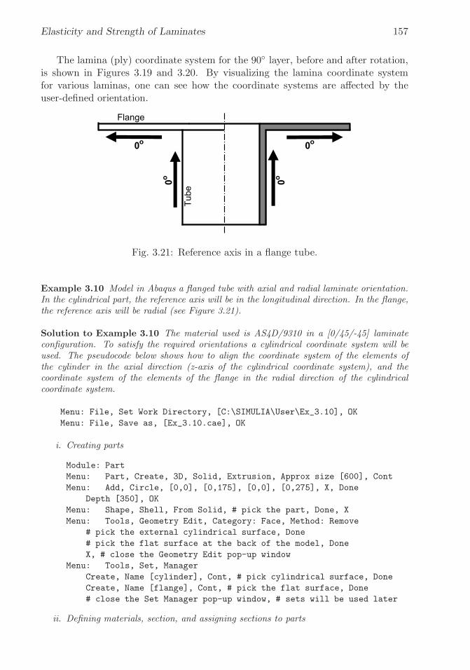
“K15072” — 2013/3/21 — 10:58�

�

�

�

�

�


The lamina (ply) coordinate system for the 90◦ layer, before and after rotation,is shown in Figures 3.19 and 3.20. By visualizing the lamina coordinate systemfor various laminas, one can see how the coordinate systems are affected by theuser-defined orientation.

Fig. 3.21: Reference axis in a flange tube.

Example 3.10 Model in Abaqus a flanged tube with axial and radial laminate orientation.In the cylindrical part, the reference axis will be in the longitudinal direction. In the flange,the reference axis will be radial (see Figure 3.21).

Solution to Example 3.10 The material used is AS4D/9310 in a [0/45/-45] laminateconfiguration. To satisfy the required orientations a cylindrical coordinate system will beused. The pseudocode below shows how to align the coordinate system of the elements ofthe cylinder in the axial direction (z-axis of the cylindrical coordinate system), and thecoordinate system of the elements of the flange in the radial direction of the cylindricalcoordinate system.



i. Creating parts

Module: Part

Menu: Part, Create, 3D, Solid, Extrusion, Approx size [600], Cont

Menu: Add, Circle, [0,0], [0,175], [0,0], [0,275], X, Done

Depth [350], OK

Menu: Shape, Shell, From Solid, # pick the part, Done, X

Menu: Tools, Geometry Edit, Category: Face, Method: Remove

# pick the external cylindrical surface, Done

# pick the flat surface at the back of the model, Done

X, # close the Geometry Edit pop-up window


Create, Name [cylinder], Cont, # pick cylindrical surface, Done

Create, Name [flange], Cont, # pick the flat surface, Done

# close the Set Manager pop-up window, # sets will be used later


�

�

“K15072” — 2013/3/21 — 10:58�

�

�

�

�

�


Module: Property

Menu: Material, Create, Mechanical, Elasticity, Elastic, Type: Lamina

[133860, 7706, 0.301, 4306, 4306, 2760], OK

Menu: Tools, Datum, CSYS, 3 Points, Name [cyl-csys], Cylindrical, Cont

[0,0,0], [1,0,0], [1,1,0], # close pop-up windows

Menu: Composite, Manager

Create, Name [cyl-zone], Element Type: Conventional Shell, Cont


Sets, cylinder, Cont, # the cell must read cylinder for all plies


# must read Material-1 for all plies, Thickness [1.05] # all plies

CSYS # double click the cell corresponding to each ply

Base Orientation: CSYS, Select, Datum CSYS List, cyl-csys, OK

Normal Direction: Axis 2, OK, # must read cyl-csys.2 for all plies

Rotation Angle [0,45,-45], Integration Points [3] # all plies, OK

Create, Name [flange-zone], Element Type: Conventional Shell, Cont


Sets, flange, Cont, # the cell must read flange for all plies


# must read Material-1 for all cells, Thickness [1.05] # all plies

CSYS # double click the cell corresponding to each ply

Base Orientation: CSYS, Select, Datum CSYS List, cyl-csys, OK

Normal Direction: Axis 3, OK, # must read cyl-csys.3 for all plies

Rotation Angle [0,45,-45], Integration Points [3] # all plies, OK

# close Composite Layup Manager


Module: Assembly




Module: Step




v. Meshing the model

Module: Mesh


Menu: Mesh, Controls, # pick all the surfaces, Done

Element Shape: Quad, Technique: Free, OK


The goal of this example is to show the user how to align the element’s orientationusing a cylindrical coordinate system. Therefore, it is not necessary to apply loads,BC, or to solve the problem. However, doing a Data Check of the model allows theuser to visualize the orientation of the element coordinate systems.

vi. Visualizing coordinate element systems

�

�

“K15072” — 2013/3/21 — 10:58�

�

�

�

�

�


Module: Job

Menu: Job, Manager

Create, Cont, OK, Data Check # when completed, Results


Toolbar: Render Style, Render Model: Shaded

# to easily visualize the coordinate system of all the elements

Menu: Plot, Material Orientations, On Undeformed Shape

Menu: Results, Section Points, Selection method: Plies

# select the different plies and visualize their orientations

3.2.15 Constraints

Constraints are used to restrict the motion of portions of a model in a variety ofways, as summarized below:

Tie Constraint tie two regions regardless of the meshes on the two regions beingidentical or not. See Example 6.3, p. 236.

Rigid Body Constraint couples the motion of regions in an assembly to the mo-tion of a reference point. Relative positions of regions that make up the rigidbody will remain unchanged during the analysis. Within rigid body con-straint, pin nodes makes all displacements equal to those of the referencepoint, and tie nodes makes all displacements and rotations equal to thoseof the reference point. Rigid body constraints are very useful to force pinnedboundary conditions as in Example 3.11.

Coupling Constraint couples the motion of a surface to the motion of a singlepoint. Although a mesh of 3D solids has only 3 DOF per node, the referencepoint will have 6 DOF. Therefore, it will be necessary to constrain the rota-tions of the RP if the intent is to have the coupled surface translate but notrotate as a rigid surface. See Example 7.5, p. 269.

Multi-point Constraint (MPC) couples the motion of selected slave nodes tothe motion of a single point.

Shell-to-solid Coupling Constraint couples the motion of a shell edge to themotion of an adjacent solid face. This is useful for detailed modeling of smallregions using solid elements while large portions of the model are idealizedwith shell elements.

Embedded Region Constraint embeds a (small) region of a model within a hostregion of a (larger) model. This is useful for local-global analysis, multi-scaleanalysis, and multi-physics analysis.

Example 3.11 Create a FE model for a pultruded composite column under axial compres-sion load P = 11, 452 N [20] and calculate the end axial displacement u(L/2), where x = 0is located at the half-length of the column. The column is simply supported (pinned) at bothends x = (−L/2, L2) but only one half needs to be discretized because the model is symmetricat half the length of the column. Its length is L = 1.816 m. The cross section of the column

�

�

“K15072” — 2013/3/21 — 10:58�

�

�

�

�

�


is that of a wide-flange I-beam (also called H-beam) with equal outside height and width,H = W = 304.8 mm. The thickness of both the flange and the web is tf = tw = 12.7 mm.The material properties are given by the A, B, D, and H matrices, with units [mm MPa],[mm2 MPa], [mm3 MPa], and [mm MPa], respectively.

For the flange:

[A] =

⎡

⎣

335,053 47,658 047,658 146,155 0

0 0 49,984

⎤

⎦ ; [B] =

⎡

⎣

-29,251 -1,154 0-1,154 -5,262 0

0 0 -2,274

⎤

⎦

[D] =

⎡

⎣

4,261,183 686,071 0686,071 2,023,742 0

0 0 677,544

⎤

⎦ ; [H ] =

[

34,216 00 31,190

]

For the web:

[A] =

⎡

⎣

338,016 44,127 044,127 143,646 0

0 0 49,997

⎤

⎦ ; [B] =

⎡

⎣

-6,088 -14,698 0-14,698 -6,088 0

0 0 0

⎤

⎦

[D] =

⎡

⎣

4,769,538 650,127 0650,127 2,155,470 0

0 0 739,467

⎤

⎦ ; [H ] =

[

34,654 00 31,623

]

Solution to Example 3.11 The geometry of the I-beam is defined by the midsurfaces ofthe web and the flanges. Notice that the geometry defined in the procedure below correspondsto an I section 292.1 mm in height and 304.8 in width. The column is symmetric aboutthe longitudinal direction (Z-axis). Therefore, only one half of the length of the column ismodeled. The load is applied as a concentrated load. This requires the use of a rigid bodyconstraint of the type tie nodes on the loaded end to guarantee that all the points at theloading edge follow the displacements and rotations of the point where the load is applied.



i. Creating parts

Module: Part

Menu: Part, Create

3D, Deformable, Shell, Extrusion, Approx size [500], Cont

Menu: Add, Line, Connected Lines, [-152.4,-146.05],

[152.4,-146.05], X

Menu: Add, Line, Connected Lines, [-152.4,146.05],

[152.4,146.05], X

Menu: Add, Line, Connected Lines, [0,-146.05],

[0,146.05], X, Done

Depth [908], OK


�

�

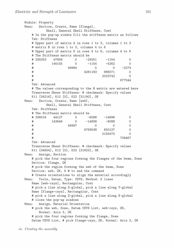
“K15072” — 2013/3/21 — 10:58�

�

�

�

�

�


Module: Property

Menu: Section, Create, Name [flange],


# In the pop-up window fill the stiffness matrix as follows

Tab: Stiffness

# Upper part of matrix A in rows 1 to 3, columns 1 to 3

# matrix B in rows 1 to 3, columns 4 to 6

# Upper part of matrix D in rows 4 to 6, columns 4 to 6


# 335053 47658 0 -29251 -1154 0

# 146155 0 -1154 -5262 0

# 49984 0 0 -2274

# 4261183 686071 0

# 2023742 0

# 677544

Tab: Advanced

# The values corresponding to the H matrix are entered here

Transverse Shear Stiffness: # checkmark: Specify values

K11 [34216], K12 [0], K22 [31190], OK

Menu: Section, Create, Name [web],


Tab: Stiffness


# 338016 44127 0 -6088 -14698 0

# 143646 0 -14698 -6088 0

# 49997 0 0 0

# 4769538 650127 0

# 2155470 0

# 739467

Tab: Advanced


K11 [34654], K12 [0], K22 [31623], OK


# pick the four regions forming the flanges of the beam, Done

Section: flange, OK

# pick the region forming the web of the beam, Done

Section: web, OK, X # to end the command

# Create orientations to align the material accordingly

Menu: Tools, Datum, Type: CSYS, Method: 2 lines

Name [web-csys], Rectangular, Cont

# pick a line along Z-global, pick a line along Y-global

Name [flange-csys], Rectangular, Cont

# pick a line along Z-global, pick a line along X-global

# close the pop-up windows

Menu: Assign, Material Orientation

# pick the web, Done, Datum CSYS List, web-csys, OK,

Normal: Axis 3, OK

# pick the four regions forming the flange, Done

Datum CSYS List, # pick flange-csys, OK, Normal: Axis 3, OK


�

�

“K15072” — 2013/3/21 — 10:58�

�

�

�

�

�


Module: Assembly



Module: Step

Menu: Step, Create, Cont, OK

v. Create constraints

Module: Interaction

# create a reference point (RP) at the loaded end of the I-beam

Menu: Tools, Reference Point, [0,0,0]

# define rigid body constraint of the loaded end

# Tie nodes makes all disp and rota equal to those of the RP

Menu: Constraint, Create, Rigid Body, Cont

Tie (nodes), Edit, # pick the 5 lines at the loaded end, Done

Reference Point: Edit, # pick the RP created, OK

vi. Adding loads and BC

Module: Load

Menu: Load, Create

Step: Step-1, Mechanical, Concentrated force, Cont

# select the RP, Done, CF3 [11452], OK

Menu: BC, Create

Step: Initial, Mechanical, Symm/Anti/Enca, Cont

# pick lines opposite to loaded end, Done, ZSYMM, OK

vii. Meshing the model

Module: Mesh

Menu: Seed, Edges

# pick the six longitudinal lines, Done

Method: By Number, Bias: None, Number of elements [10], Apply, OK

# pick edges of the flanges at both ends of the beam, Done


# pick the edges of the web at both ends of the beam, Done


Menu: Mesh, Controls, # select all, Done, Technique: Structured, OK


Geometric Order: Quadratic, DOF: 6, Family: Shell, OK # S8R in use


Create a set containing the central point of the end opposite to the loaded end. Thispoint will be used to apply an extra BC to prevent the movement on the symmetryplane.

Module: Mesh

Menu: Tools, Set, Create, Name [Cpoint], Type: Node, Cont

# pick the point at the center of unloaded end, Done

Module: Load

Menu: BC, Create

Step: Initial, Mechanical, Disp/Rota, Cont

Sets, Cpoint, Cont, # checkmark: U1,U2,UR3, OK

�

�

“K15072” — 2013/3/21 — 10:58�

�

�

�

�

�


viii. Solving and visualizing the results

Module: Job

Menu: Job, Manager

Create, Cont, OK, Submit, # when completed, Results



Menu: Plot, Deformed Shape

Toolbar: Field Output, Primary, U, U3

Notice that the displacement at the loaded end is 0.03584mm.

3.3 Failure Criteria

Failure criteria are curve fits of experimental data that attempt to predict failure un-der multiaxial stress based on experimental data obtained under uniaxial stress. Allfailure criteria described in this section predict the first occurrence of failure in oneof the laminas but are unable to track failure propagation until complete laminatefailure. Damage mechanics is used in Chapters 8 and 9 to track damage evolutionup to laminate failure. The truncated-maximum-strain criterion estimates laminatefailure without tracking damage evolution by making certain approximations andassumptions about the behavior of the laminate [1].

In this section, failure criteria are presented using the notion of failure index,which is used for several FEA packages, and it is defined as

IF =stress

strength(3.19)

Failure is predicted when IF ≥ 1. The strength ratio ( [1, Section 7.1.1]) is theinverse of the failure index

R =1

IF=strength

stress(3.20)

Failure is predicted when R ≤ 1.

3.3.1 2D Failure Criteria

Strength-based failure criteria are commonly used in FEA to predict failure eventsin composite structures. Numerous criteria exist for unidirectional (UD) laminassubjected to a state of plane stress (σ3 = 0). The most commonly used are describedin [1]. They are:

– Maximum stress criterion– Maximum strain criterion– Truncated maximum strain criterion, and– Interacting failure criterion

A few additional criteria are presented in this section.

�

�

“K15072” — 2013/3/21 — 10:58�

�

�

�

�

�


Hashin Failure Criterion

The Hashin failure criterion (HFC) proposes four separate modes of failure:

– Fiber tension– Fiber compression– Matrix tension– Matrix compression

that are predicted by four separate equations, as follows:4

I2Fft =

(

σ1F1t

)2

+ α

(

σ6F6

)2

if σ1 ≥ 0 (3.21)

I2Ffc =

(

σ1F1c

)2

if σ1 < 0 (3.22)

I2Fmt =

(

σ2F2t

)2

+

(

σ6F6

)2

if σ2 ≥ 0 (3.23)

I2Fmc =

(

σ22F4

)2

+

[

(

F2c

2F4

)2

− 1

]

σ2F2c

+

(

σ6F6

)2

if σ2 < 0 (3.24)

where α is a weight factor to give more or less emphasis to the influence of shearon fiber failure. With α = 0, Hashin FC and Maximum Stress FC would predictlongitudinal tensile failure of the unidirectional lamina at the same stress σ1. Note(3.22) predicts longitudinal compressive failure without influence of the shear stress,although it is well known that the state of shear has a strong influence on thelongitudinal compression failure [21].

Equations (3.21–3.24) define the square of failure indexes according to HFC.Abaqus documentation refers to the square of failure indexes for HFC, Tsai-Hill,Azzi-Tsai-Hill, and Tsai-Wu5, in contrast to the (not squared) failure indexes formaximum stress (MSTRS) and maximum strain (MSTRN) failure criteria.

The values of F1c and F2c are considered positive throughout this textbookand most of the literature, but in Abaqus they must be given with different signsin different areas of Abaqus. Specifically, when entering strength values in Edit

Material, Material Behavior: Elastic, Suboption: Fail Stress, F1c andF2c must be entered as negative values. However, when entering the same values todefine the threshold of damage initiation in Edit Material, Material Behavior:

Hashin Damage, they must be given as positive quantities.Although the threshold of damage initiation is calculated in Abaqus by the

Hashin failure criterion, the subsequent analysis of damage accumulation is doneby a decohesion methodology that is independent of the damage initiation criterion

4The Hashin failure equations on the right-hand side of (3.21–3.24) yield squares of failureindexes IF . Compare to the Maximum Stress Criterion (i.e., IFft = σ1/F1T ) and so on.

5The Tsai-Hill, Azzi-Tsai-Hill, and Tsai-Wu failure criteria are not recommended because theyoveremphasize the interaction between fiber (σ1) and transverse matrix (σ2) damage modes.

�

�

“K15072” — 2013/3/21 — 10:58�

�

�

�

�

�


used. Despite this, Abaqus documentation and Abaqus/CAE refer to the wholedamage methodology as Hashin Damage.

Puck Failure Criterion

The Puck failure criterion [22] distinguishes between fiber failure (FF) and matrixfailure (MF). In the case of plane stress, the MF criteria discriminates three differentmodes. Mode A is when transverse cracks appear in the lamina under transversetensile stress with or without in-plane shear stress. Mode B also denotes transversecracks, but in this case they appear under in-plane shear stress with small transversecompression stress. Mode C indicates the onset of oblique cracks (typically withan angle of 53◦ in carbon epoxy laminates) when the material is under significanttransverse compression.

The FF and the three MF modes yield separate failure indexes. The Puckcriterion assumes that FF only depends on longitudinal tension. Therefore, thefailure index for FF is defined as

IFF =

{

σ1/F1t if σ1 > 0−σ1/F1c if σ1 < 0

(3.25)

The MF failure indexes have different expressions depending on the mode thatbecomes active. With positive transverse stress, mode A is active. In this case, thefailure index for matrix dominated tensile failure (mode A) is

IMF,A =

√

(

σ6F6

)2

+

(

1− p6tF2t

F6

)2( σ2F2t

)2

+ p6tσ2F6

if σ2 ≥ 0 (3.26)

where p6t is a fitting parameter. Lacking experimental values, it is assumed thatp6t = 0.3 [22].

Under negative transverse stress, either mode B or mode C is active, dependingon the relationship between in-plane shear stress and transverse shear stress. Thelimit between mode B and C is defined by the relation F2A/F6A, where

F2A =F6

2p6c

[

√

1 + 2p6cF2c

F6− 1

]

(3.27)

F6A = F6

√

1 + 2p2c (3.28)

and p2c is defined as

p2c = p6cF2A

F6(3.29)

and p6c is another fitting parameter. Lacking experimental values, it is assumedthat p6c = 0.2 [22].

Finally, the failure index for matrix dominated shear (mode B) is

IMF,B =1

F6

[

√

σ26 + (p6cσ2)2 + p6cσ2

]

if

{

σ2 < 0∣

∣

∣

σ2σ6

∣

∣

∣ ≤ F2AF6A

(3.30)

�

�

“K15072” — 2013/3/21 — 10:58�

�

�

�

�

�


and for matrix dominated compression (mode C) is

IMF,C = −F2c

σ2

[

(

σ62(1 + p2c)F6

)2

+

(

σ2F2c

)2]

if

{

σ2 < 0∣

∣

∣

σ2σ6

∣

∣

∣ ≥ F2AF6A

(3.31)

3.3.2 3D Failure Criteria

Failure criteria presented here are 3D generalizations of the ones presented in [1,Section 7.1]. The 2D version of the criteria presented in this section can be recoveredby setting σ4 = σ5 = 0. The user of FEA packages should be careful because somepackages use only the in-plane stress components for the computation of the failureindex (e.g., Abaqus), even though all six stress components may be available fromthe analysis. In those cases the intralaminar and thickness components of stressshould be evaluated separately to see if they lead to failure.

In this section, the numerical subscript denotes the directions of 1) fiber, 2)in-plane transverse to the fibers, and 3) through the thickness of the lamina. Theletter subscript denotes t) tensile and c) compressive. Contracted notation is usedfor the shear components as described in Section 1.5.

Maximum Strain Criterion

The failure index is defined as

IF = max

⎧

⎪

⎪

⎪

⎪

⎪

⎪

⎨

⎪

⎪

⎪

⎪

⎪

⎪

⎩

ε1/ε1t if ε1 > 0 or −ε1/ε1c if ε1 < 0ε2/ε2t if ε2 > 0 or −ε2/ε2c if ε2 < 0ε3/ε3t if ε3 > 0 or −ε3/ε3c if ε3 < 0

abs(γ4)/γ4uabs(γ5)/γ5uabs(γ6)/γ6u

(3.32)

The quantities in the denominator are the ultimate strains of the unidirectionallamina. Note that compression ultimate strains in (3.32) are positive numbers.

Maximum Stress Criterion

The failure index is defined as

IF = max

⎧

⎪

⎪

⎪

⎪

⎪

⎪

⎨

⎪

⎪

⎪

⎪

⎪

⎪

⎩

σ1/F1t if σ1 > 0 or −σ1/F1c if σ1 < 0σ2/F2t if σ2 > 0 or −σ2/F2c if σ2 < 0σ3/F3t if σ3 > 0 or −σ3/F3c if σ3 < 0

abs(σ4)/F4

abs(σ5)/F5

abs(σ6)/F6

(3.33)

The letter F is used here to denote a strength value for a unidirectional laminaas in [23]. Note that compression strength in (3.33) are positive numbers.

�

�

“K15072” — 2013/3/21 — 10:58�

�

�

�

�

�


Tsai-Wu Criterion

Using the Tsai-Wu criterion the failure index is defined as

IF =1

R=

⎡

⎣− B

2A+

√

(

B

2A

)2

+1

A

⎤

⎦

−1

(3.34)

with

A =σ21

F1tF1c+

σ22F2tF2c

+σ23

F3tF3c+σ24F 24

+σ25F 25

+σ26F 26

+ c4σ2σ3√

F2tF2cF3tF3c+ c5

σ1σ3√F1tF1cF3tF3c

+ c6σ1σ2√

F1tF1cF2tF2c(3.35)

and

B =(

F−11t − F−1

1c

)

σ1 +(

F−12t − F−1

2c

)

σ2 +(

F−13t − F−1

3c

)

σ3 (3.36)

where ci, i = 4..6, are the Tsai-Wu coupling coefficients that by default are takento be −1. Note that compression strength in (3.35) and (3.36) are here positivenumbers.

The through-the-thickness strength values F3t and F3c are seldom available inthe open literature, so it is common practice to use the corresponding in-plane trans-verse values of strength. Also, the intralaminar strength F5 is commonly assumedto be equal to the in-plane shear strength. The intralaminar strength F4 can beestimated [1, (4.109)] in terms of transverse compression strength F2c and the angleof the fracture plane α0. The latter is consistently reported to be close to 53o.

Example 3.12 Compute the failure index IF and strength ratio R in each layer of Exam-ple 3.4 (p. 121) using the Maximum Stress Failure criterion and the Tsai-Wu criterion. Theelastic moduli and strength values for the lamina are given in Table 3.1, p. 102. Determinethe strength ratio of the laminate using both criteria.

Solution to Example 3.12 Hashin, Maximum Strain, and Maximum Stress failure cri-teria are adequate failure criteria in Abaqus, but Tsai-Hill and Tsai-Wu failure criteria arenot recommended because they overestimate the interaction between σ1 (S11) and σ2 (S22).Tsai-Wu is used in this example to be consistent with [8, Example 3.12].

Unlike the definition used in this textbook (3.34), Abaqus defines the Tsai-Wu failureindex as:

TSAIW = f1 ∗ S11 + f2 ∗ S22 + f11 ∗ S112 + f22 ∗ S222 + f66 ∗ S122 + 2f12 ∗ S11 ∗ S22which is a square of a failure index. Therefore, the values of TSAIW do not compare withthe failure indices for MSTRN (3.32) and MSTRS (3.33) unless a square root of TSAIWis taken. The same happens for the Tsai-Hill failure index TSAIH and for the four Hashinfailure indexes in Abaqus (compare the Abaqus documentation to (3.21–3.24)).

The strength values F1T, F1C, F2T, F2C, F6, f12, and Slim are supplied to theAbaqus/CAE using Edit Material, Material Behavior: Elastic, Suboption: Fail

Stress. Note that F1C and F2C must be given as negative numbers for TSAIW but as

�

�

“K15072” — 2013/3/21 — 10:58�

�

�

�

�

�


positive numbers for Hashin Damage (see Section 3.3.1). Also, f12 and the biaxial stressSlim default to zero if not given, which is good, because interaction f12 overestimates theinteraction between σ1 (S11) and σ2 (S22). However, in this example, we use f12 = −1 toreproduce the results of [8, Example 3.12].

To solve this example, open Ex_3.4.a.cae and Save As Ex_3.12.cae. Then, do thefollowing:

i. Set Work Directory


ii. Defining the damage parameters for the material

Module: Property


Edit, Suboptions, Fail Stress, # you can copy/paste from excel

[1830 -1096 57 -228 71 -1 0], OK, OK

# close Material Manager pop-up window

iii. Defining analysis step to create a field output for the failure index

Module: Step

Step: Step-1


# expand: Failure/Fracture, # checkmark: CFAILURE

# uncheck: everything else we don’t need, OK

iv. Solving and visualizing the results

Module: Jobs

Menu: Job, Manager

Submit, # when completed, Results



Menu: Result, Field Output, MSTRS, OK

Menu: Results, Section Points, Method: Plies

# pick a ply, Apply, # read the value, OK

Menu: Result, Field Output, TSAIW, OK

Menu: Results, Section Points, Method: Plies

# pick a ply, Apply, # read the value, OK

The results are tabulated in Table 3.7. You should compare the results to the classicallamination theory (CLT) solution using [12].

Example 3.13 [8, Example 3.14] Compute the Tsai-Wu failure index IF on each layerof Example 3.8 (p. 151) using a UMAT subroutine, available in [5, umatS8R5.for]. Theelastic moduli and strength values for the lamina are given in Table 3.1, p. 102.

Solution to Example 3.13 Environment variables must be set properly before executinga job with user programmable features (see Appendix C). To solve this example, first openEx_3.8.cae and save it as Ex_3.14.cae. Also, set the Work Directory to the local directoryso that all the files are easily accessed.

�

�

“K15072” — 2013/3/21 — 10:58�

�

�

�

�

�


Table 3.7: Index failure MSTRS (Maximum Stress Criterion), and TSAIW (Tsai-Wu) calculated in Example 3.12.

Ply # MSTRS TSAIW

IF R IF R

1 0.01442 69.34813 0.01447 69.108502 0.02430 41.15226 0.03107 32.185393 0.01566 63.85696 0.01873 53.390284 0.01566 63.85696 0.01873 53.39028


Menu: File, Open, [C:\SIMULIA\User\Ex_3.8\Ex_3.8.cae], OK

Menu: File, Save As, [C:\SIMULIA\User\Ex_3.14\Ex_3.14.cae], OK

Only a few things need to be modified in the .mdb. Remember that in Abaqus the stress/straincomponents for shell elements are ordered as follows: 11, 22, 12, 13, 23. Then, the sectionshear stiffness can be calculated using [12]. Alternatively, for a single ply shell of thicknesst, use

H44 = (5/6) t G23

H45 = 0

H55 = (5/6) t G13

or for a laminate use [1, (6.16)], or use Abaqus to calculate the values and read themfrom the .dat file as illustrated below. To calculate with Abaqus, start with the .cae ofExample 3.8 (p. 151) and modify it as follows:

i. Modifying the material definition to add failure parameters

Module: Property

# unidirectional material from Ex. 3.8 used to calculate H44, H45, H55


Name [unidirectional], Mechanical,

Elasticity, Elastic, Type: Lamina

[133860 7706 0.301 4306 4306 2760]

# or right-click on Data field, Read from File

Select, [uni_lam_prop.txt], OK, OK

# add Fail Stress values

Suboptions, Fail Stress

[1830 -1096 57 -228 71 -1], OK


Select, [uni_fail_stress.txt], OK, OK, OK,

OK # to close Edit Material


Tab: Basic, Material: unidirectional, OK

ii. Submitting the job and visualizing the results

Module: Job

Menu: Job, Manager

�

�

“K15072” — 2013/3/21 — 10:58�

�

�

�

�

�


Edit, Tab: General, # checkmark: Print model definition data, OK


Field Output Toolbar: Primary, U, U3, # U3max = 8.704 mm

Use a text editor to open the file Job-1.dat. The file must be stored in the Work

Directory (C:\SIMULIA\User\Ex_3.14). Read the values corresponding to the TransverseShear Stiffness for the Section. They should be:

Kts11 = K11 = H55 = 35883.0

Kts22 = K22 = H44 = 23000.0

Kts12 = K12 = H45 = 0.0

To run the user material subroutine, do the following:

i. Create a user material to be used with the UMAT subroutine and edit the correspond-ing section

Module: Property


Name [ud-user], General, User Material,

User material type: Mechanical

Mechanical constants, [133860 7706 0.301 0.396

4306 1830 1096 57 228 71 -1]


Select, [user_mat_props.txt], OK, OK

# see umats8r5.for for interpretation of Mechanical constants

General, Depvar,

Number of solution-dependent state variables [2], OK


Tab: Basic

Section integration: During analysis

Thickness: Shell thickness: Value [10]

Material: ud-user

Thickness integration rule: Simpson

Thickness integration points [3]

Tab: Advanced


K11: [35883], K12: [0], K22: [23000], OK

ii. Define output variables for the analysis step

Module: Step

Step: Step-1


Output variables: Edit variables: [S,E,U,RF,SDV], OK

iii. Submit the job and visualize the results.Before submitting the job make sure your system is properly setup to run a UMAT.Notice that if your system is not properly setup to run UMATs you will get an errorafter submitting the job for execution.

Module: Job

Menu: Job, Manager

�

�

“K15072” — 2013/3/21 — 10:58�

�

�

�

�

�


Edit, Tab: General,

User subroutine file: Select, [umatS8R5.for], OK, OK



Menu: Options, Contour, Contour Type: Quilt, OK

Menu: Plot, Contours on Deformed Shape

Field Output Toolbar: Primary, SDV1

Menu: Result, Section Points, Selection method: Plies

Ply result location: Bottommost, Apply

Ply result location: Topmost, Apply

OK # close the Section Points pop-up window

In case of an error, check that the configuration file C: \SIMULIA\Abaqus\Commands\

abq6102.bat is correct. Also, check that the following is included in the .inp file:

** Section: Section-1

*Shell Section, elset=_PickedSet2, material=uni-user, orientation=Ori-1

10., 3

*Transverse Shear

35883., 23000., 0.

and

*Material, name=uni-user

*Depvar

2,

*User Material, constants=11

133860., 7706., 0.301, 0.396, 4306., 1830., 1096., 57.

228., 71., -1.

From the visualization of SDV1 on a quilted contour, the bottom side reaches IF =1.767× 10−2 and the top side reaches IF = 9.444× 10−3.

3.4 Predefined Fields

The following example illustrates the analysis of thermal expansion and how tointroduce a Predefined Field in general.

Example 3.14 Display the deformed shape of a [0/90]T laminate illustrating thermal ex-pansion coupling (discussed in [1, Section 6.1.4, Figure 6.7]). Each lamina is 1.2 mmthick, made of AS4D/9310 (Table 3.1). The geometry of the plate is square with ax = ay =1000mm. The thermal loading is Δ T = −125◦ C. Use element S8R5 in Abaqus.

Solution to Example 3.14 A [0/90]T laminate under uniform thermal loading Δ T , withsquare geometry (ax = ay) on the x-y plane, is symmetric with respect to the x-z and y-zplanes, so only 1/4 of the plate needs to be modeled. Note that the fact that the LLS is notsymmetric does not affect the symmetry of the discretization, which is determined by threefactors: (a) symmetry of geometry, (b) symmetry of load, and (c) symmetry of material,the latter on the x-y plane only. The following pseudo code illustrates the procedure. Thesaddle shape of the deformed plate is shown in Figure 3.22. The CAE file is availablein [5, Ex 3 15.cae].

�

�

“K15072” — 2013/3/21 — 10:58�

�

�

�

�

�


i. Geometry

Module: Part

Menu: Part, Create, [Part-1], 3D, Deformable,

Shell, Planar, Approximate size [4000], Cont


# Enter the points [0,0], [1000,1000], X, Done

ii. Material and Section Properties

Module: Property


Name [Material-1], Mechanical, Elasticity, Elastic, Lamina,

[13386000 7706 0.301 4306 4306 2760]

Mechanical, Expansion, Type, Orthotropic,

[13.23672E-OO7 2.58908E-005 2.58908E-0051], OK

Menu: Section, Create, Name [Section-1], Shell, Composite, Cont

Material: Material-1 # for all

Thickness [1.2] # for all

Orientation [0,90]


# pick part, Done, OK

iii. Assembly and Step

Module: Assembly

Menu: Instance, Independent, OK

Module: Step


iv. Load and Boundary Conditions

Module: Load

Menu: BC, Create, Name [BC-1], Step: Initial,

Mechanical, Symmetry, Cont

# pick left vertical line, Done, XSIMM, OK

Menu: BC, Create, Name [BC-2], Step: Initial,

Mechanical, Symmetry, Cont

# pick lower horizontal line, Done, YSIMM, OK

Menu: BC, Create, Displacement/Mechanical, Cont,

# pick bottom left point, Done

# checkmark all (U1 to UR3), OK

Menu: Predefined Field, Create, Other, Temperature, Cont

# Select rectangle, Done, Magnitude [0], OK

Menu: Predefined Field, Manager

# Double click cell Predefined Field-2, Step-1 (Propagated)

Status, Modified, Magnitude [-150], OK

v. Mesh

Module: Mesh

Menu: Seed, Instance, Apply, OK

Menu: Mesh, Element type, Std, Quad, DOF [5], OK # S8R5


�

�

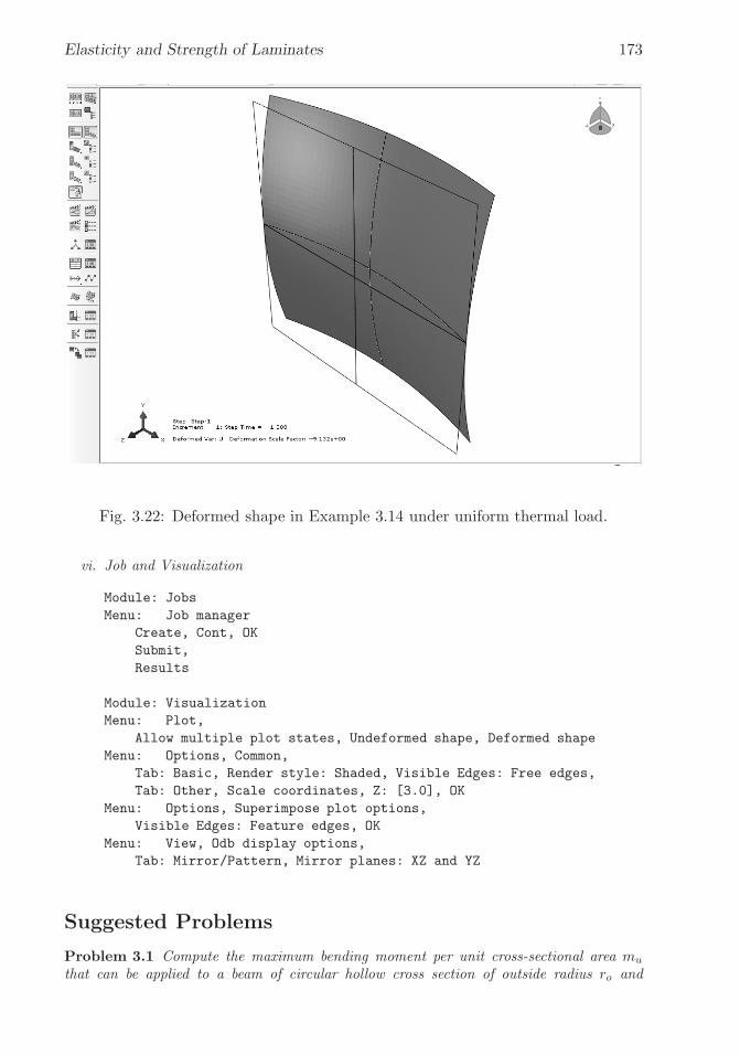
“K15072” — 2013/3/21 — 10:58�

�

�

�

�

�


Fig. 3.22: Deformed shape in Example 3.14 under uniform thermal load.

vi. Job and Visualization

Module: Jobs

Menu: Job manager

Create, Cont, OK

Submit,

Results


Menu: Plot,

Allow multiple plot states, Undeformed shape, Deformed shape

Menu: Options, Common,

Tab: Basic, Render style: Shaded, Visible Edges: Free edges,

Tab: Other, Scale coordinates, Z: [3.0], OK

Menu: Options, Superimpose plot options,

Visible Edges: Feature edges, OK

Menu: View, Odb display options,

Tab: Mirror/Pattern, Mirror planes: XZ and YZ

Suggested Problems

Problem 3.1 Compute the maximum bending moment per unit cross-sectional area mu

that can be applied to a beam of circular hollow cross section of outside radius ro and

�

�

“K15072” — 2013/3/21 — 10:58�

�

�

�

�

�


inner radius ri. The loading is pure bending, no shear. The material is homogeneous andfailure occurs when the maximum stress reaches the strength σu of the material. The hollowsection is filled with foam to prevent buckling. Derive an expression for the efficiency of thecross section as the ratio of mu of the hollow beam by mu of a solid rod of same outsideradius. Faced with the problem of using a strong and relatively expensive material, wouldyou recommend a small or large radius?

Problem 3.2 Compute the maximum outside radius for a cantilever beam of length L,loaded by a tip load P , otherwise similar to the beam in Problem 3.1 but subjected to pureshear loading. The shear strength is τu = σu/2. Consider only shear. Buckling of the thinwall is likely to limit further the practical thickness of the wall.

Problem 3.3 Compute the maximum deflection per unit volume δV that can be applied toa beam of circular hollow cross section of outside radius ro and inner radius ri. This isa cantilever beam of length L, loaded by a tip load P . The hollow section is made of anhomogeneous material with moduli E and G = E/2.5, filled with foam to prevent buckling.Derive an expression for the efficiency of the cross section as the ratio of δV between thehollow cross section and a solid rod of the same outside radius. Faced with the problem ofusing a relatively expensive and not quite stiff material, would you recommend a small orlarge radius?

Problem 3.4 Write a computer program to evaluate (3.9). The program data input is theLSS, the thickness of the laminas, and the material elastic properties. The output should bewritten in a file. Show all work in a report.

Problem 3.5 Using the program of Problem 3.4 compute the A,B,D, and H matrices forthe following laminates. The material is AS4D/9310 and all layers are 0.85 mm thick.Comment on the coupling of the constitutive equations for each case: (a) one layer [0], (b)one layer [30], (c) [0/90]2, (d) [0/90]s, (e) [0/90]8, (f) [±45]2 = [+45/ − 45/+ 45/ − 45],(g) [±45]s = [+45/− 45/− 45/+ 45], (h) [±45/0/90/± 30]. Show all work in a report.

Problem 3.6 Compute the value and location of the absolute maximum transverse shearstrain γ23 in Example 3.2, p. 113. At that location, plot the distribution of γ23 through thethickness of the plate. Is that distribution a reasonable answer?

Problem 3.7 Recompute Example 3.2, p. 113, with a doubly sinusoidal load

q(x, y) = q0 sin(πx/2a) sin(πx/2b)

where 2a, 2b are the plate dimensions in x and y, respectively. Compare the result with theexact solution at the center of the plate, that is

w0 = 16q0b4/[π4(D11s

4 + 2(D12 + 2D66)s2 +D22)]

where s = b/a ( [14, (5.2.8–5.2.10)]).

Problem 3.8 Calculate the first vibration frequency �11 of the plate with the analyticalsolution �2

mn = π4[D11m4s4+2(D12+2D66)m

2n2s2+D22n4]/(16ρhb4), where ρ, h are the

density and thickness of the plate, respectively ( [14, (5.7.8)]).

�

�

“K15072” — 2013/3/21 — 10:58�

�

�

�

�

�


Problem 3.9 Consider a rectangular plate with ax = 1000 mm and by = 100 mm. Eachlamina is 1.2 mm thick, made of AS4D/9310 (Table 3.1).

Propose three different LSS, each having one of the following couplings (shown in [1,Figure 6.7]); that is: (a) bending-extension coupling, (b) torsion-extension coupling, and(c) shear-extension coupling.

Next, consider reduced FEA models applying symmetry conditions; either (i) one-halfplate, 500×100mm, or (ii) one-quarter plate, 500×50mm. Use the smallest (1/4, 1/2, orfull plate) FEA model that is valid for each of the cases (a) through (c). Apply membraneloading Nx = 1000 N/mm (all other zero). Show all work in a report including pseudo codefor each case (a) through (c). Use element S8R5 in Abaqus. See Example 3.14, p. 171.

Problem 3.10 A failure envelope is a 3D surface for which If = 1. The intersection ofthis surface with each coordinate plane is a 2D curve. Using a program such as MATLAB,plot the failure envelope in the plane σ1 − σ2 for Maximum Stress, Tsai-Wu, and Puckfailure criteria in the same plot. Do a similar plot in the plane σ2 − σ6.

Problem 3.11 (a) Compute the failure index IF on each layer of Example 3.12 (p. 167)using the Maximum Stress Failure Criterion and the Hashin failure criterion. The laminastrength values are given in Table 3.1.

Problem 3.12 Using UMAT subroutine, compute the failure index IF on each layer ofExample 3.12 (p. 167) using the Puck failure criterion. The elastic moduli and strengthvalues for the lamina are given in Table 3.1, p. 102. Values for the Puck parameters aresuggested in Section 3.3.1, p. 165. Show all work in a report.

Problem 3.13 Write on a text file the nodal stress results at the top and bottom of eachlamina of Problem 3.11. Then, using an external program such as MATLAB, compute thesame failure indexes as in Problem 3.11 in terms of the nodal stress values at the center ofthe plate, and compare them to the results of Problem 3.11. Show all work in a report.

�

�

“K15072” — 2013/3/21 — 10:58�

�

�

�

�

�

�

�

“K15072” — 2013/3/21 — 10:58�

�

�

�

�

�

Chapter 4

Buckling

Most composite structures are thin walled. This is a natural consequence of thefollowing facts:

– Composites are stronger than conventional materials. Then, it is possible tocarry very high loads with a small area, and thus small thickness in mostcomponents.

– Composites are expensive when compared to conventional materials. There-fore, there is strong motivation to reduce the volume, and thus the thicknessas much as possible.

– The cost of polymer matrix composites increases with their stiffness. Thestiffness in the fiber direction can be estimated by using the fiber dominatedrule of mixtures, E1 = EfVf . For example, when glass fibers are combinedwith a polymer matrix, the resulting composite stiffness is lower than that ofaluminum. Using Aramid yields a stiffness comparable to aluminum. Carbonfibers yield composite stiffness lower than steel. Therefore, there is strongmotivation to increase the moment of inertia of beams and stiffeners withoutincreasing the cross-sectional area. The best option is to increase the momentof inertia by enlarging the cross section dimensions and reducing the thickness.

All the above factors often lead to design of composite structures with larger,thin walled cross sections, with modes of failure likely to be controlled by buckling.

4.1 Eigenvalue Buckling Analysis

Buckling is loss of stability due to geometric effects rather than material failure.But it can lead to material failure and collapse if the ensuing deformations arenot restrained. Most structures can operate in a linear elastic range. That is,they return to the undeformed configuration upon removal of the load. Permanentdeformations result if the elastic range is exceeded, as when matrix cracking occursin a composite.

177

�

�

“K15072” — 2013/3/21 — 10:58�

�

�

�

�

�


imperfect pathprimary path

w

�

�cr

secondary path

bifurcationP

w

Fig. 4.1: Equilibrium paths for the perfect column.

Consider a simply supported column of area A, length L, and moment of inertiaI, made of homogeneous material with modulus E and strength F along the lengthof the column. The column is loaded by a compressive load P acting on the centroidof the cross section [3]. If the column geometry, loading, and material have noimperfections, the axial deformation is

u = PL/EA (4.1)

with no lateral deformation w = 0. The deformation of the structure (u, v, w) beforebuckling occurs is called the primary path (Figure 4.1). The slightest imperfectionwill make the column buckle when

Pcr = π2(EI)/L2 (4.2)

The load capacity for long slender columns will be controlled by buckling, asopposed to the crushing strength of the material. What happens after the columnreaches its critical load depends largely on the support conditions. For the simplysupported column, the lateral deflection1

w = A sin(πx/L) (4.3)

will grow indefinitely (A → ∞) when the load just barely exceeds PCR. Such largelateral deflections will cause the material to fail and the column will collapse. Thebehavior of the structure after buckling has occurred is called post-buckling.

The simply supported column in Figure 4.1 experiences no deformations in theshape of the buckling mode (4.3) before buckling actually happens. In this case, it issaid that the structure has a trivial primary path. This is a consequence of havinga perfect structure with perfectly aligned loading. For these type of structures,

1With x measured from one end of the column.

�

�

“K15072” — 2013/3/21 — 10:58�

�

�

�

�

�

Buckling 179

Table 4.1: Lamina elastic properties for AS4/9310, Vf = 0.6.

Young’s Moduli Shear Moduli Poisson’s Ratio

E1 = 145880 MPa G12 = G13 = 4386 MPa ν12 = ν13 = 0.263E2 = E3 = 13312 MPa G23 = 4529 MPa ν23 = 0.470

buckling occurs at a bifurcation point. A bifurcation point is the intersection of theprimary path with the secondary path, i.e., the post-buckling path [24].

The bifurcation loads, one for every possible mode of buckling, are fairly easy toobtain using commercial software. The geometry of the structure is that of the per-fect undeformed configuration, loaded with the nominal loads, and the material iselastic. Such analysis requires a minimum of effort on the part of the analyst. Com-mercial programs refer to this analysis as an eigenvalue buckling analysis becausethe critical loads are the eigenvalues λi of the discretized system of equations

([K]− λ[Ks]){v} = 0 (4.4)

where K and Ks are the stiffness and stress stiffness matrix, respectively, and v isthe column of eigenvectors (buckling modes) [24].

Example 4.1 Consider a simple supported plate, with side dimensions ax = 1000 mm,ay = 500 mm, edge-wise loaded in compression with Nx = Ny = 1 N/mm. The plate ismade of [(0/90)3]S , AS4/9310 (Table 4.1) with fiber volume fraction 0.6 and total thicknesstT = 10.2 mm. Compute the critical load of the lowest four modes using eigenvalue analysis.Visualize the lower four modes.

Solution to Example 4.1 We model the whole plate to capture all buckling modes, notjust the symmetric ones. Element S8R5 is used because the we are modeling a thin plate.Since the laminate is symmetric and stress computation lamina by lamina is not required,the critical loads can be obtained using three different approaches. Note that for elementS8R5, you are not required to specify Transverse Shear Stiffness when the shell sectionis Homogeneous or Composite (see cases (a) and (c)), but they have to be entered for aGeneral Stiffness section (see case (b)).

(a) Using Equivalent Laminate ModuliIn this first approach, the equivalent laminate moduli are calculated and used along withan orthotropic shell element. In this case, laminate moduli represent the stiffness of anequivalent orthotropic plate that behaves like the actual laminate under in-plane loads (seeSection 3.2.10). Laminate moduli can be found as explained in Section 1.15. Introduce thelamina properties (Table 4.1) into (1.91), rotate each layer (1.53), add then according to(1.102) get the laminate moduli (1.105) listed in Table 4.2. Bending moduli [1, (6.36)] maygive better results for this example.

The following pseudo code illustrates the modeling, solution, and visualization procedureusing the GUI in Abaqus/CAE. The corresponding Ex_4.1.a.cae file is available on theWeb site [5]. The results are tabulated in Table 4.3.

# Ex.4.1.a using equivalent laminate moduli

Menu: File, Set Work Directory [C:\SIMULIA\user\Ex_4.1], OK

Menu: File, Save As [C:\SIMULIA\user\Ex_4.1\Ex_4.1.a.cae], OK

�

�

“K15072” — 2013/3/21 — 10:58�

�

�

�

�

�


Table 4.2: Equivalent laminate moduli for [(0/90)3]S .Young’s Moduli Shear Moduli Poisson’s Ratio

Ex = 79985 MPa Gxy = 4386 MPa νxy = 0.044Ey = 79985 MPa Gyz = 4458 MPa νyz = 0.415Ez = 16128 MPa Gxz = 4458 MPa νxz = 0.415

i. Creating the part

Module: Part

Menu: Part, Create

3D, Deformable, Shell, Planar, Approx size [2000], Cont

Menu: Add, Line, Rectangle, [-500,-250], [500,250]

X # to close command, Done


Module: Property


Name [Material-1], Mechanical, Elasticity, Elastic

Type: Engineering Constants

[79985, 79985, 16128, 0.044, 0.415, 0.415, 4386, 4458, 4458], OK


Name [Section-1], Shell, Homogeneous, Cont

Shell thickness: Value [10.2], Material: Material-1, OK


# pick the part, Done, OK


Module: Assembly


iv. Defining the analysis steps

Module: Step

Menu: Step, Create

Procedure type: Liner Perturbation, Buckle, Cont

Number of eigenvalues requested [10], Vectors/iteration [10], OK


Module: Load

Menu: Load, Create

Step: Step-1, Mechanical, Shell Edge Load, Cont

# pick: edges @ x=500 & y=250, Done, Magnitude [1.0], OK

Menu: BC, Manager

Create, Step: Initial, Mechanical, Disp/Rota, Cont

# pick: the 4 edges, Done, # checkmark: U3, OK


# pick: edge @ x=-500, Done, # checkmark: U1, OK


# pick: edge @ y=-250, Done, # checkmark: U2, OK, # close Manager

�

�

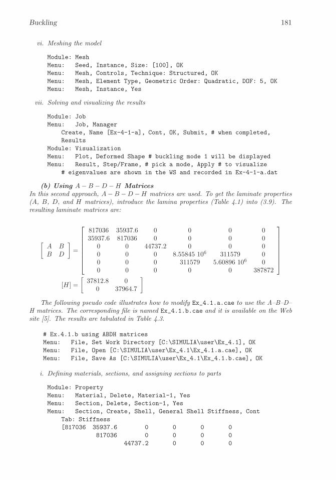
“K15072” — 2013/3/21 — 10:58�

�

�

�

�

�

Buckling 181


Module: Mesh

Menu: Seed, Instance, Size: [100], OK

Menu: Mesh, Controls, Technique: Structured, OK

Menu: Mesh, Element Type, Geometric Order: Quadratic, DOF: 5, OK



Module: Job

Menu: Job, Manager

Create, Name [Ex-4-1-a], Cont, OK, Submit, # when completed,

Results


Menu: Plot, Deformed Shape # buckling mode 1 will be displayed

Menu: Result, Step/Frame, # pick a mode, Apply # to visualize

# eigenvalues are shown in the WS and recorded in Ex-4-1-a.dat

(b) Using A−B −D −H MatricesIn this second approach, A−B −D −H matrices are used. To get the laminate properties(A, B, D, and H matrices), introduce the lamina properties (Table 4.1) into (3.9). Theresulting laminate matrices are:

[

A BB D

]

=

⎡

⎢

⎢

⎢

⎢

⎢

⎢

⎣

817036 35937.6 0 0 0 035937.6 817036 0 0 0 0

0 0 44737.2 0 0 00 0 0 8.55845 106 311579 00 0 0 311579 5.60896 106 00 0 0 0 0 387872

⎤

⎥

⎥

⎥

⎥

⎥

⎥

⎦

[H ] =

[

37812.8 00 37964.7

]

The following pseudo code illustrates how to modify Ex_4.1.a.cae to use the A–B–D–H matrices. The corresponding file is named Ex_4.1.b.cae and it is available on the Website [5]. The results are tabulated in Table 4.3.

# Ex.4.1.b using ABDH matrices


Menu: File, Open [C:\SIMULIA\user\Ex_4.1\Ex_4.1.a.cae], OK

Menu: File, Save As [C:\SIMULIA\user\Ex_4.1\Ex_4.1.b.cae], OK

i. Defining materials, sections, and assigning sections to parts

Module: Property

Menu: Material, Delete, Material-1, Yes

Menu: Section, Delete, Section-1, Yes

Menu: Section, Create, Shell, General Shell Stiffness, Cont

Tab: Stiffness

[817036 35937.6 0 0 0 0

817036 0 0 0 0

44737.2 0 0 0

�

�

“K15072” — 2013/3/21 — 10:58�

�

�

�

�

�


8.56e6 311579 0

5.61e6 0

387872]

Tab: Advanced

Transverse Shear Stiffnesses: # checkmark: Specify values

K11 [37812.8], K12 [0], K22 [37964.7], OK

ii. Defining analysis step

Module: Step

Menu: Step, Edit, Step-1

Maximum number of interactions [70], OK

# solve the problem using a smaller number for this quantity

# the following error message may be displayed

# TOO MANY ITERATIONS NEEDED TO SOLVE THE EIGENVALUE PROBLEM

iii. Solving and visualizing the results

Module: Job

Menu: Job, Manager

Create, Name [Ex-4-1-b], Cont, OK, Submit, # when completed,

Results

# visualize the results as it is indicated in part (a)

(c) Using the LSSIn this third approach, the laminate stacking sequence (LSS) and the lamina properties(Table 4.1) are entered. The following pseudo code illustrates how to change Ex_4.1.a.cae

to solve this part of the problem. The corresponding Ex_4.1.c.cae file is available on theWeb site [5]. The results are tabulated in Table 4.3.

# Ex_4.1.c using LSS


Menu: File, Open [C:\SIMULIA\user\Ex_4.1\Ex_4.1.a.cae], OK

Menu: File, Save As [C:\SIMULIA\user\Ex_4.1\Ex_4.1.c.cae], OK

i. Defining materials, sections, and assigning sections to parts

Module: Property

Menu: Material, Delete, Material-1, Yes

Menu: Section, Delete, Section-1, Yes


Name [Material-1], Mechanical, Elasticity, Elastic, Type: Lamina

[1.4588e5, 1.3312e4, 2.63e-1, 4.386e3, 4.386e3, 4.529e3], OK


Shell, Composite, Cont

# checkmark: Symmetric layers

# right-click: Insert Row After, # until there are six rows

Material: Material-1 # for all layers, Thickness [0.85]

Orientation Angle: [0,90,0,90,0,90], Integration Points [3]

Ply Name [k1, k2, k3, k4, k5, k6], OK


�

�

“K15072” — 2013/3/21 — 10:58�

�

�

�

�

�

Buckling 183

Table 4.3: Bifurcation loads [N/mm].Mode # (a) (b) (c )

1 253.27 210.1 210.042 320.05 319.87 319.753 573.36 643.18 642.814 998.64 831.65 831.11

Module: Step


Maximum number of interactions [70]

# solve the problem using a smaller number for this quantity

# the following error message may be displayed

# TOO MANY ITERATIONS NEEDED TO SOLVE THE EIGENVALUE PROBLEM

iii. Solving and visualizing the results

Module: Job

Menu: Job, Manager

Create, Name [Ex-4-1-c], Cont, OK, Submit,

# when Completed, Results

# visualize the results as it is indicated in part (a)

4.1.1 Imperfection Sensitivity

To illustrate the influence of imperfections in buckling, let us consider the solidlines in Figure 4.1. The lateral deflection is zero for any load below the bifurcationload PCR that is on the primary path of the perfect structure. The primary pathintersects the secondary path at the bifurcation point, for which the load is PCR.The post-critical behavior of the column is indifferent and slightly stable. Indifferentmeans that the column can deflect right or left. Stable post-critical path means thatthe column can take a slightly higher load once it has buckled. For a column, thisstiffening behavior is so small that one cannot rely upon it to carry any load beyondPCR. In fact, the column will deform laterally so much that the material will failand the system will collapse. Unlike columns, simply supported plates experiencesignificant stiffening on the secondary path.

4.1.2 Asymmetric Bifurcation

Consider the frame illustrated in Figure 4.2. An eigenvalue analysis using one finiteelement per bar [24, Sections 5.9 and 7.8] reveals the bifurcation load

PCR = 8.932(10−6)AE (4.5)

but gives no indication about the nature of the critical state: whether it is stableor not, whether the post-critical path is symmetric or not, and so on. We shall seelater on that the frame has an asymmetric, and thus unstable, post-critical path,as represented in Figure 4.2. That is, the post-critical path has a slope

�

�

“K15072” — 2013/3/21 — 10:58�

�

�

�

�

�


..

.

L

A

B�

P

L

X

Y

A

B

�

Fig. 4.2: Two bar frame.

P (1) = 18.73(10−9)AE (1/rad) (4.6)

in the force-rotation diagram in Figure 4.2, where θ is the rotation of the joint atthe load point.

In general, the problem with eigenvalue analysis is that it provides no indicationas to the nature of the post-critical path. If the post-critical path is stiffening andsymmetric as in Figure 4.1, the real structure may have a load capacity close to thebifurcation load. But if the post-critical path is unstable and/or asymmetric, as inFigure 4.2 or if there is mode interaction [20,25–29], the real structure may have aload capacity much smaller than the bifurcation load. In order to use the informa-tion provided by eigenvalue analysis, it is necessary to understand and quantify thepost-buckling behavior.

4.1.3 Post-critical Path

One way to investigate the post-buckling behavior is to perform a continuationanalysis of the imperfect structure, as presented in Section 4.2. This is perfectlypossible, but complicated and time consuming, as it will be seen later in this chap-ter. A more expedient solution can be obtained using software capable of predictingthe nature of the post-critical path, including symmetry, curvature, and mode in-teraction. If the secondary path is stable and symmetric, the bifurcation load canbe used as a good estimate of the load capacity of the structure. The curvature ofthe post-critical path gives a good indication of the post-buckling stiffening and itcan be used to a certain extent to predict post-buckling deformations.

The bifurcation load, slope, and curvature of the post-critical path emergingfrom the bifurcation (4.1) can be computed with BMI3 [26–28] available in [5]. Thepost-buckling behavior is represented by the following formula

�

�

“K15072” — 2013/3/21 — 10:58�

�

�

�

�

�

Buckling 185

Fig. 4.3: Node sets defined after meshing to be used for applying concentrated loadsat nodes.

Λ = Λ(cr) + Λ(1)s+1

2Λ(2)s2 + . . . (4.7)

where s is the perturbation parameter, which is chosen as one component of the dis-placement of one node, Λ(cr) is the bifurcation multiplier, Λ(1) is the slope, and Λ(2)

is the curvature of the post-critical path ( [25, (43)], see also [20,26–29]). When theslope is zero, the post-critical path is symmetric. Therefore, buckling is indifferent,and the real structure will buckle to either side. There is no way to predict whichway it is going to buckle, unless of course one knows the shape of the imperfectionson the real plate, which is seldom the case. A positive curvature denotes stiffeningduring post-buckling, and a negative one indicates that the stiffness decreases.

Example 4.2 Consider the simple supported plate of Example 4.1, p. 179. Compute thebifurcation multiplier Λ(cr), the critical load Ncr, the slope Λ(1), and the curvature Λ(2) ofthe post-critical path. Estimate the load when the maximum lateral deflection is equal to thethickness of the plate. As perturbation parameter, use the largest displacement componentof the buckling mode with lowest buckling load.

Solution to Example 4.2 The program BMI3 [5] is used in this case to compute thebifurcation multiplier Λ(cr), the slope Λ(1), and the curvature Λ(2) of the post-critical path.Refer to Appendix C for a description of the software interface and operation procedure.Since BMI3 requires the A-B-D-H matrices, we can use the .cae file generated during thesolution of Example 4.1(b) (available as Ex 4.1.b.cae in [5]), but a few changes are neededto satisfy the current limitations of BMI3, as follows.

i. Open the Ex_4.1.b.cae and save it as Ex_4.2.cae


Menu: File, Open [C:\SIMULIA\user\Ex_4.1\Ex_4.1.b.cae], OK

Menu: File, Save As [C:\SIMULIA\user\Ex_4.2\Ex_4.2.cae], OK

ii. Delete the mesh. Then reseed and remesh with a 2× 4 mesh of S8R5 elements.

Module: Mesh

Object: Assembly

Menu: Mesh, Delete Instance Mesh, Yes

Menu: Seed, Edges

�

�

“K15072” — 2013/3/21 — 10:58�

�

�

�

�

�


# pick: horizontal lines, Done

Method: By Number, Number of Elements [4], OK

# pick: vertical lines, Done

Method: By Number, Number of Elements [2], OK


iii. BMI3 only accepts concentrated loads. Therefore, the distributed edge loads must bereplaced by a set of concentrated loads. Since S8R5 are quadratic elements, a uniform(constant) distributed load on the edge is equivalent to three loads concentrated at thenodes. For a unit edge load (Nn = 1.0 N/mm), the element corner nodes get 1/6 eachand the mid-node gets 4/6. At a node where 2 elements contribute, the contributionsfrom both elements add up to 1/3. To do this change, first create node sets to laterapply the concentrated loads. Six sets are needed as illustrated in the Set Manager

window shown Figure in 4.3. A set is created as follows:

Module: Load


Create, Name [x-corner], Type: Node, Cont

# pick: the two corners of the plate on the edge at x=500, Done

iv. Using the same procedure, create the additional sets. The x-e-corner contains thenodes where pairs of elements join (at the edge at x = 500 mm). The x-e-mid

contains the mid–side nodes of elements on the edge at x = 500mm. The remainingsets, for the edge at y = 250mm, are created similarly.

v. Delete all the edge loads and replace them by concentrated loads, as follows:

Module: Load

Menu: Load, Manager

# delete the existing load

Create, Step: Step-1, Mechanical, Concentrated force, Cont

Sets, x-corner, Cont, CF1 [-41.67], OK


Sets, x-e-corner, Cont, CF1 [-83.33], OK


Sets, x-e-mid, Cont, CF1 [-166.67], OK

# Analogously add compressive loads on the edge y=250

# close the Load Manager

vi. Run the model to verify it produces the right results. Notice the eigenvalues are slightlydifferent than those obtained in Example 4.1; this is due to the coarseness of the meshused.

Module: Job

Menu: Job, Manager

Create, Name [Job-1], Cont, OK, Submit, # when Completed, Results

# visualize the mode shapes as it was indicated in Example 4.1

vii. Copy the filtering program inp2bmi3.exe (available in [5]) to the Work Directory.Execute this file by double-clicking on it. It will create the files ABQ.inp, BMI3.inp,and BMI3.dat, based on the file Job-1.inp. The file ABQ.inp is a filtered copy thatAbaqus can execute.

�

�

“K15072” — 2013/3/21 — 10:58�

�

�

�

�

�

Buckling 187

viii. Create a new Job to run ABQ.inp to verify everything went well with the filtering.Note that unlike previous examples where a Job was created to run a model, in thiscase a Job is created to run an input file. This is done as follows:

Module: Job

Menu: Job, Manager

Create, Name [ABQ], Source: Input file # not Model

Select, ABQ.inp, OK, Cont, OK

Submit, # when Completed, Results

ix. Copy the program bmi3.exe (available in [5]) to the Work Directory and execute itby double-clicking on it. Take note of the following results, either from the displayoutput of from the file BMI3.out:

By default, BMI3 chooses as perturbation parameter the largest displacement componentof the buckling mode with lowest buckling load, but that can be changed by editing the fileBMI3.dat. For this example, the default perturbation corresponds to the first buckling mode,the node in the middle of the plate, and the deflection direction U3 perpendicular to thesurface of the plate. The results, specially Λ(2), are sensitive to mesh refinement.

Since BMI3 solves the problem using reversed loads (see Appendix C), then (4.7) becomes

−N = Λ(cr) + Λ(1)s+ 12 Λ(2)s2

N = −Λ(cr) − Λ(1)s− 12 Λ(2)s2

and, in this case, the perturbation direction is s = −δ, so

N = −Λ(cr) − Λ(1)(−δ)− 12 Λ(2)(−δ)2

N = −Λ(cr) + Λ(1)δ − 12 Λ(2)δ2

Therefore, using the results from a more refined mesh, the secondary path is

N = −(−209.0) + (0) δ − (−0.1154) δ2 = 209.0 + 0.1154 δ2

Since the slope Λ(1) is zero, the post-critical path is symmetric. The post-buckling loadwhen the lateral deflection (w) is equal to the thickness (s = Th = 10.2 mm) is equal to221 N/mm, as shown in Figure 4.4.

4.2 Continuation Methods

The strain to failure of polymer matrix composites (PMC) is high. Compare 1.29%for AS4/3501 and 2.9% for S-glass/epoxy with only 0.2% for steel and 0.4% foraluminum. That means that buckling deformations can go into a post-bucklingregime while the material remains elastic. However, great care must be taken thatno matrix dominated degradation mode takes place, in which case the material willnot remain elastic (see Chapters 8 and 9). Eigenvalue buckling analysis is relativelysimple as long as the material remains elastic because classical theory of elasticstability can be used, as was done in Section 4.1. Material nonlinearity is onereason that motivates an incremental analysis. Another reason is to evaluate themagnitude of the buckling load for an imperfection sensitive structure.

In an incremental analysis, also called continuation analysis, the load is increasedgradually step by step. At each step, the deformation, and possibly the changing

�

�

“K15072” — 2013/3/21 — 10:58�

�

�

�

�

�


Fig. 4.4: Equilibrium paths for a perfect plate.

material properties, is evaluated. Incremental analysis must include some type ofimperfection, in the geometry, material, or alignment of loads. Lacking any imper-fection, incremental analysis will track the linear solution, revealing no bifurcationsor limit points.

Continuation methods are a form of geometrically nonlinear analysis. The sys-tem must have a nontrivial fundamental path, such as a flat plate with asymmetriclaminate stacking sequence (LSS) under edge loads.

If the system has a trivial fundamental path, such as a flat plate with symmetricLSS under edge load, the nontrivial fundamental path can be forced by introducingan imperfection. Several types of imperfections are possible, including material im-perfections (e.g., unsymmetrical LSS), geometric imperfections, or load eccentricityare used.

Since the real geometric imperfections are seldom known, the preferred artificialgeometric imperfection is in the form of the bifurcation mode having the lowestbifurcation load. This is true in most cases; however, in some cases, a second modethat is associated to imperfections that are more damaging to the structure shouldbe used [30]. Also, if the structure has an asymmetric post-buckling path, as thetwo-bar example in Figure 4.2, care must be taken not to force the structure alongthe stiffening path.

FEA codes allow the user to modify a mesh by superposing an imperfectionin the shape of any mode from a previous bifurcation analysis onto the perfectgeometry (see Example 4.3).

Example 4.3 Apply a geometric imperfection wp(x, y) = δ0 φ(x, y) to Example 4.1 (p. 179)and plot the load-multiplier vs. maximum lateral deflection for an imperfection magnitudeδ0 = Th/10 and δ0 = Th/100, where Th is the total laminate thickness, and φ(x, y) is the

�

�

“K15072” — 2013/3/21 — 10:58�

�

�

�

�

�

Buckling 189

buckling mode corresponding to the lowest bifurcation load found in Example 4.1, p. 179.

Solution to Example 4.3 The buckling modes were found in Example 4.1, p. 179. Herewe will be using model created as Ex_4.1.b.cae. First, open Ex_4.1.b.cae available in [5]and save it as Ex_4.3.cae. Then, write the Job-1.inp file from the Job Manager window.The solution procedure is summarized below:

i. Setting Work Directory

Menu: File, Set Work Directory, [C:\SIMULIA\user\Ex_4.3], OK

Menu: File, Open, [C:\SIMULIA\user\Ex_4.1\Ex_4.1.b.cae], OK

Menu: File, Save As, [C:\SIMULIA\user\Ex_4.3\Ex_4.3.cae], OK

Module: Job

Menu: Job, Manager

Create, Name [Job-1], Cont, OK, Write Input

# the input file Job-1.inp has been created in the Work Directory

ii. Compute and save the mode shapes (displacements) of the first few modes. For this,open Job-1.inp with Notepad++ (or your preferred text editor). Save the file asJob-pert.inp. Then, add the following lines to the *Buckle step before the text**BOUNDARY CONDITIONS

**Data lines to specify the reference load,

*NODE FILE, GLOBAL=YES, LAST MODE=4

U

**

and save the file. This will save the mode shapes of the first 4 modes to the .fil

results file. The .fil file is binary, so you cannot open it with Notepad; it is to beread by Abaqus only.

iii. In Abaqus CAE, create a new job and submit it as follows:

Module: Job

Menu: Job, Manager

Create, Name: [Job-pert], Source: Input file

Input file: Select, [Job-pert.inp], OK, Cont, OK

Submit

If the execution is completed without errors, the file Job-pert.fil should have beencreated in the Work Directory. Since the mode shapes are normalized, the maximumdisplacement in the results file is 1.0.

iv. Set up a Risk nonlinear analysis.Using the following procedure, the displacements from a previous analysis can be usedto update the geometry of the finite element model. In this example, the multiplierfactor for the first mode is chosen to be δ1 = 0.05. The contributions of modes 2 and3 are commented out in the .inp file (as denoted by lines starting with double star**). Therefore, an initial deflection equal to the first mode of buckling with a centraldeflection δ1 is forced on the structure. To do this, open Job-1.inp with Notepad++and save it as Job-risk.inp. Then, replace the following 3 lines

*Step, name=Step-1, perturbation

*Buckle

10, , 10, 70

�

�

“K15072” — 2013/3/21 — 10:58�

�

�

�

�

�


by the following:

**IMPERFECTION, FILE=Job-pert, STEP=n

** n : step number where the modes were calculated in the previous run

** if there was only a Initial Step followed by a Buckle Step, n=1

*IMPERFECTION, FILE=Job-pert, STEP=1

** Multiple data lines to specify the contributions of each mode

** m, delta_m

** m: mode number

** delta_m : scale factor for mode m

1,0.05

**2,0.02

**3,0.01

*STEP, NLGEOM

** next 2 lines (2nd one is empty) define increment/stopping criteria

*STATIC, RIKS

followed by the same multiple data lines to specify reference loading used in previouslyJob-pert.inp,

**Data lines to specify the reference load,

*NODE FILE, GLOBAL=YES, LAST MODE=4

U

**

Be sure to delete all the lines related to load case=2 and save the file. Otherwise,you will get an error message. The lines to be eliminated are similar to:

*Boundary, op=NEW, load case=2

_PickedSet5, 3, 3


_PickedSet6, 1, 1


_PickedSet7, 2, 2

v. In Abaqus CAE, create a new job and submit it as follows:

Module: Job

Menu: Job, Manager

Create, name: [Job-risk], Source: Input file

Input file: Select, [Job-risk.inp], OK, Cont, OK


# this finalizes the Risk analysis



Toolbar: Field Output: Primary, U, U3

Menu: Result, Step/Frame, Increment 25, Apply

Menu: Result, Step/Frame, Increment 30, Apply

Using a continuation method with this non-perfect geometry, the continuation equilib-rium paths shown in Figure 4.5 are obtained. It can be seen that eventually the continuationsolution approaches the secondary path of the perfect structure, shown by dashed lines inFigure 4.5. For smaller imperfections, the continuation solution follows more closely the

�

�

“K15072” — 2013/3/21 — 10:58�

�

�

�

�

�

Buckling 191

−5 0 5 10 150

50

100

150

200

s [mm]

N [N

/mm

]← δ

0= Th/100

← δ0= Th/10

Fig. 4.5: Equilibrium paths for a [(0/90)3 ]S plate, with δ0 = Th/10 and δ0 =Th/100.

primary path, then the secondary path. A structure with large imperfections deviates morefrom the behavior of the perfect structure, as shown by the solution corresponding to animperfection δ0 = Th/10.

Example 4.4 Find the buckling load multiplier and the first mode shape for the columnanalyzed in Example 3.11, p. 159.

Solution to Example 4.4 This example is solved simply modifying the file Ex_3.11.cae.The dead-load step must be redefined as a buckling step file. The pseudo code below describesthe necessary changes.

i. Open the Ex_3.11.cae and save it as Ex_4.4.cae


Menu: File, Open [C:\SIMULIA\user\Ex_3.11\Ex_3.11.cae], OK

Menu: File, Save As [C:\SIMULIA\user\Ex_4.4\Ex_4.4.cae], OK

ii. Create a buckling step to replace the dead-weight step used in Example 3.11

Module: Step

Menu: Step, Manager

# select: Step-1, Delete, Yes

Create, Procedure type: Linear perturbation, Buckle, Cont

Number of eigenvalues requested [1], OK, # close Step Manager

iii. Add a unitary load. The load created to be applied the Step-1 of Example 3.11 wasdeleted when the analysis step was deleted in the previous instruction.

Module: Load

Menu: Load, Create

�

�

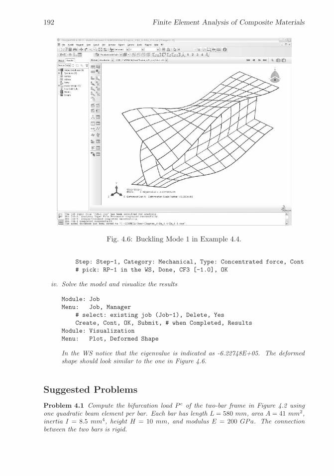
“K15072” — 2013/3/21 — 10:58�

�

�

�

�

�


Fig. 4.6: Buckling Mode 1 in Example 4.4.

Step: Step-1, Category: Mechanical, Type: Concentrated force, Cont

# pick: RP-1 in the WS, Done, CF3 [-1.0], OK

iv. Solve the model and visualize the results

Module: Job

Menu: Job, Manager

# select: existing job (Job-1), Delete, Yes

Create, Cont, OK, Submit, # when Completed, Results


Menu: Plot, Deformed Shape

In the WS notice that the eigenvalue is indicated as -6.22748E+05. The deformedshape should look similar to the one in Figure 4.6.

Suggested Problems

Problem 4.1 Compute the bifurcation load P c of the two-bar frame in Figure 4.2 usingone quadratic beam element per bar. Each bar has length L = 580 mm, area A = 41 mm2,inertia I = 8.5 mm4, height H = 10 mm, and modulus E = 200 GPa. The connectionbetween the two bars is rigid.

�

�

“K15072” — 2013/3/21 — 10:58�

�

�

�

�

�

Buckling 193

Problem 4.2 Perform a convergence study on the bifurcation load P c of the two-bar framein Problem 4.1 by increasing the number of elements per bar N until the bifurcation loadconverges within 2%. Plot P c vs. N .

Problem 4.3 Recalculate Example 4.2 when the LSS changes to [(0/90)6]T , thus becomingasymmetric. Do not introduce any imperfection but rather analyze the perfect system, whichin this case is asymmetric.

Problem 4.4 Recalculate Example 4.2 with [(0/90)6]T , and Nx = 1, Ny = Nxy = 0. Donot introduce any imperfection but rather analyze the perfect system, which in this case isasymmetric.

Problem 4.5 Using a FEA code, plot the continuation solution for δ0 = Th/100 as inFigure 4.5, for a cylindrical shell with distributed axial compression on the edges. Thecylinder has a length of L = 965 mm and a mid-surface radius of a = 242 mm. The LSSis [(0/90)6]S , with layer thickness t = 0.127 mm. The laminas are of E-glass/epoxy withE1 = 54 GPa, E2 = 18 GPa, G12 = 9 GPa, ν12 = 0.25, and ν23 = 0.38.

Problem 4.6 Compute the maximum stress failure index If of Problem 4.5 at P = Λ(cr).The strength values are F1t = 1034 MPa, F1c = 1034 MPa, F2t = 31 MPa, F2c = 138 MPa,and F6t = 41 MPa.

Problem 4.7 Plot the imperfection sensitivity of the cylindrical shell of Problem 4.5, forimperfections in the range (Th/200) < s < Th.

�

�

“K15072” — 2013/3/21 — 10:58�

�

�

�

�

�

�

�

“K15072” — 2013/3/21 — 10:58�

�

�

�

�

�

Chapter 5

Free Edge Stresses

In-plane loading Nx, Ny, Nxy of symmetric laminates induces only in-plane stressσx, σy, σxy in the interior of the laminate. Near the free edges, interlaminar stressesσz, σyz, σxz, are induced due to the imbalance of the in-plane stress components atthe free edge.

For illustration, consider a long laminated strip of length 2L, width 2b << 2L,and thickness 2H < 2b (Figure 5.1). The strip is loaded by an axial force Nx only.For a balanced, symmetric laminate the mid-plane strains and curvatures (see (3.6))are uniform over the entire cross section and given by

ε0x = α11Nx

ε0y = α12Nx

γ0xy = 0

kx = ky = kxy = 0 (5.1)

where α11, α12 are in-plane laminate compliances, which are obtained by inverting(3.8); see also [1, (6.21)]. From the constitutive equation [1, (6.24)] for lamina k,we get

σkx =(

Qk11α11 +Q

k12α12

)

Nx

σky =(

Qk12α11 +Q

k22α12

)

Nx

σkxy =(

Qk16α11 +Q

k26α12

)

Nx

σkz = σkxz = σkyz = 0 (5.2)

A piece of laminate taken out of the interior of the laminate will have balancedσy and σxy on opposite faces; the free body diagram (FBD) is in equilibrium withoutthe need for any additional forces. In this case we say the stress components areself-equilibrating. At the free edge in Figure 5.1, σy=σxy=σyz=0. If σy and σxy are

195

�

�

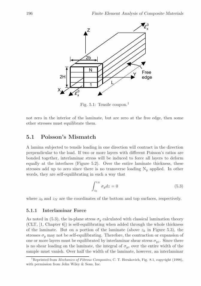
“K15072” — 2013/3/21 — 10:58�

�

�

�

�

�


Fig. 5.1: Tensile coupon.1

not zero in the interior of the laminate, but are zero at the free edge, then someother stresses must equilibrate them.

5.1 Poisson’s Mismatch

A lamina subjected to tensile loading in one direction will contract in the directionperpendicular to the load. If two or more layers with different Poisson’s ratios arebonded together, interlaminar stress will be induced to force all layers to deformequally at the interfaces (Figure 5.2). Over the entire laminate thickness, thesestresses add up to zero since there is no transverse loading Ny applied. In otherwords, they are self-equilibrating in such a way that

∫ zN

z0

σydz = 0 (5.3)

where z0 and zN are the coordinates of the bottom and top surfaces, respectively.

5.1.1 Interlaminar Force

As noted in (5.3), the in-plane stress σy calculated with classical lamination theory(CLT, [1, Chapter 6]) is self-equilibrating when added through the whole thicknessof the laminate. But on a portion of the laminate (above zk in Figure 5.3), thestresses σy may not be self-equilibrating. Therefore, the contraction or expansion ofone or more layers must be equilibrated by interlaminar shear stress σyz. Since thereis no shear loading on the laminate, the integral of σyz over the entire width of thesample must vanish. Over half the width of the laminate, however, an interlaminar

1Reprinted from Mechanics of Fibrous Composites, C. T. Herakovich, Fig. 8.1, copyright (1998),with permission from John Wiley & Sons, Inc.

�

�

“K15072” — 2013/3/21 — 10:58�

�

�

�

�

�

Free Edge Stresses 197

Fig. 5.2: Poisson’s effect.2

shear force exists if the stress σy above or below the surface is not self-equilibrating.The magnitude of these per unit length forces can be estimated by integrating theinterlaminar shear stress σyz over half the width of the laminate (0 < y < b). Byequilibrium

Fyz(zk) =

∫ b

0σyz(z=zk)

dy = −∫ zN

zk

σydz (5.4)

The interlaminar shear stress σyz is not available from classical lamination theorybut the transverse stress σy is. Therefore, the magnitude of the interlaminar shearforce can be computed anywhere through the thickness of a laminate in terms ofthe known transverse stress distribution σy.

The in-plane stress σy in a balanced, symmetric laminate under tensile load isconstant in each lamina. Therefore, when the interlaminar force is evaluated at aninterface (located at z=zk), the integration above reduces to

Fyz(zk) = −N∑

i=k

σiyti (5.5)

where ti are the thicknesses of the laminas.

The magnitude of the interlaminar shear force Fyz can be used to comparedifferent stacking sequences in an effort to minimize the free-edge interlaminar shearstress σyz. However, the force does not indicate how large the actual stress is.Therefore, it can be used to compare different LSS but not as a failure criterion.

5.1.2 Interlaminar Moment

The interlaminar shear stress σyz produces shear strain γyz, which must vanishat the center line of the sample because of symmetry. Therefore, σyz = 0 at the

2Reprinted from Mechanics of Fibrous Composites, C. T. Herakovich, Fig. 8.14, copyright(1998), with permission from John Wiley & Sons, Inc.

�

�

“K15072” — 2013/3/21 — 10:58�

�

�

�

�

�


Fig. 5.3: Free body diagram of sublaminate used for computation of Poisson-inducedforces Fyz and moments Mz.

center line. Also, at the free edge, σyz must vanish because σzy vanishes there. Butfor any position zk above which σy is not self-equilibrating, σyz must be non-zerosomewhere between the edge and the center line. A numerical solution of σyz isplotted in Figure 5.5 in terms of the distance y/b from the free edge. It revealsthat σyz grows rapidly near the free edge and then tapers out at the interior of thelaminate.

A not self-equilibrating distribution of stress yields both a force Fyz (5.5) and amoment. To compute the moment Mz, take moments of the stress σy with respectto point A in Figure 5.3. A non-vanishing moment produced by σy can only beequilibrated by a moment produced by transverse stress σz. Therefore, the momentMz is defined as

Mz(zk) =

∫ b

0σz(z=zk)

ydy =

∫ zN

zk

(z − zk)σydz (5.6)

where zk is the coordinate of the top surface of lamina k, and zN is the coordinate ofthe top surface of the laminate (see [1, Figure 6.6] for the definition of the coordinatesystem through the thickness of the laminate).

The existence of σz is corroborated by free-edge delamination during a tensiletest, at a much lower load than the failure load of the laminate. The magnitudeof the moment can be used to compare different stacking sequences in an effort tominimize the thickness stress σz. However, the moment does not indicate how largethe actual stress is, and thus it cannot be used as a failure criterion.

The in-plane stress σy in a balanced laminate under tensile load is constant in

�

�

“K15072” — 2013/3/21 — 10:58�

�

�

�

�

�


each lamina. Therefore, when the interlaminar moment is evaluated at an interface(located at z = zk), the integration above reduces to

Mz(zk) =

N∑

i=k

σiy(ziti +t2i2− zkti) (5.7)

Since σz is a byproduct of σyz, which vanishes at y = 0 due to symmetry, thenσz must vanish at the center line of the specimen (y = 0) but it is large near theedge. Since no vertical load is applied, the integral of σz must be zero. Therefore, itmust be tensile (positive) on some regions and compressive (negative) at others. Anumerical solution reveals that σz grows rapidly near the free edge, dips to negativevalues, and then tapers out at the interior of the laminate. A numerical solutionof σz is plotted in Figure 5.5 in terms of the distance y/b from the free edge.However, σz → ∞ as y → b. This is a singularity that is not handled well byFEA. Therefore the results, even for y < b, will be very dependent on the meshrefinement. Furthermore, since σz → ∞, the results cannot be used in a failurecriterion without further consideration.

Example 5.1 Compute Fyz and Mz at all interfaces of a balanced [02/902]s symmetriclaminate (Figure 5.1) loaded with Nx = 175 KN/m. Use unidirectional lamina carbon/epoxyproperties E1=139 GPa, E2=14.5 GPa, G12 = G13 = 5.86 GPa, G23 = 5.25 GPa, ν12 =ν13 = 0.21, ν23 = 0.38. The lamina thickness is tk = 0.127 mm.

Solution to Example 5.1 The in-plane stress distribution σy through the thickness canbe obtained by the procedure described in [1, Section 6.2], which is implemented in CADEC[12]. The stress values are shown in Table 5.1.

To calculate Fyz, compute the contribution of all layers above a given interface using(5.5). The in-plane stress σy in a balanced laminate under in-plane load is constant in eachlamina, so (5.5) applies. For other cases, (5.4) can be integrated exactly since σy is linearin z, or Fyz can be approximated by (5.5) using the average σy in each lamina.

Since the laminate is balanced and loaded with in-plane loads only, Mz can be computedusing (5.7). Otherwise, use (5.6) or approximate Mz by using the average σz in each laminainto (5.7).

The results are shown Table 5.1 and Figure 5.4.

Example 5.2 Plot the Poisson-induced stresses σz and σyz as a function of y for 0 <y < b (Figure 5.3) at the 90/0 interface above the middle surface of a [0/90]s laminatewith properties E1 = 139 GPa, E2 = 14.5 GPa, ν12 = ν13 = 0.21, ν23 = 0.38, G12 =G13 = 5.86 GPa, G23 = 5.25 GPa. Take 2b = 20 mm, length of the sample 2L = 80 mm,thickness of each lamina tk = 1.25 mm. Load the sample with a uniform strain εx = 0.01 byapplying a uniform displacement at x = L. Use orthotropic solid elements on each lamina.Refine the mesh towards the free edge. Use at least two quadratic elements through thethickness of each lamina and an element aspect ratio approximately one near the free edge.

Solution to Example 5.2 Note that it is not necessary to model the whole geometry.Symmetry can be used to model only the quadrant with x > 0, y > 0, z > 0 (i.e., one-eighthof the plate, Figure 5.3). Since any cross section y − z has the same behavior, only a shortsegment between x = 0 and x = L� needs to be modeled. Since free edge effects also occur at

�

�

“K15072” — 2013/3/21 — 10:58�

�

�

�

�

�


−1 −0.5 0 0.5 1−1

−0.8

−0.6

−0.4

−0.2

0

0.2

0.4

0.6

0.8

1 [02/90

2]s

Fyz

/Fyz max

; Mz/M

z max

z/H

Fyz

/Fyz max

Mz/M

z max

Fig. 5.4: Interlaminar force Fyz and moment Mz due to Poisson’s effect.

0 0.2 0.4 0.6 0.8 1−20

−15

−10

−5

0

5

10

15

20

y/b

σ [M

Pa]

σyz

σz

Fig. 5.5: Interlaminar stress σyz and σz at the 90/0 interface of a carbon/epoxy[0/90]S laminate (FEA).

�

�

“K15072” — 2013/3/21 — 10:58�

�

�

�

�

�


Table 5.1: Poisson’s interlaminar force Fyz.k Pos σy tk z Fyz Mz

[MPa] [mm] [mm] [kN/m] [N m/m]8 TOP 5.55 10−3 0.508 0.0008 BOT 5.55 10−3 0.127 0.381 -0.705 0.0457 TOP 5.55 10−3 0.381 -0.7057 BOT 5.55 10−3 0.127 0.254 -1.410 0.1796 TOP -5.55 10−3 0.254 -1.4106 BOT -5.55 10−3 0.127 0.127 -0.705 0.3135 TOP -5.55 10−3 0.127 -0.7055 BOT -5.55 10−3 0.127 0.000 0.000 0.3584 TOP -5.55 10−3 0.000 0.0004 BOT -5.55 10−3 0.127 -0.127 0.705 0.3133 TOP -5.55 10−3 -0.127 0.7053 BOT -5.55 10−3 0.127 -0.254 1.410 0.1792 TOP 5.55 10−3 -0.254 1.4102 BOT 5.55 10−3 0.127 -0.381 0.705 0.0451 TOP 5.55 10−3 -0.381 0.7051 BOT 5.55 10−3 0.127 -0.508 0.000 0.000

x = 0 and x = L�, take L� = 8h = 32tk, tk = 2.5 mm, and plot the results at x = L � /2 toavoid free edge effects at the two loaded ends of the model. The solution is shown in Figure5.5. See the pseudo code below and Figure 5.5.

i. Setting Work Directory

Menu: File, Set Work Directory, [C:\SIMULIA\user\Ex_5.2]

Menu: File, Save As, [C:\SIMULIA\user\Ex_5.2\Ex_5.2.cae]

ii. Creating the part

Module: Part

# Look at Fig. 5.3, layer thickness is tk=1.25 mm along Z-global

# b=10 mm, length along x is L=40 mm (shown as 1 in Fig. 5.3)

# Draw layers 3 and 4 above the middle surface

Menu: Part, Create

3D, Deformable, Solid, Extrusion, Approx size [100], Cont

Menu: Add, Line, Rectangle, [0,0], [40,10], X, Done, Depth [2.5], OK

# We need to cut the volume in 2 layers

Menu: Tools, Datum, Plane, Offset from ppal plane, XY Plane, [1.25]

X, # close the Create Datum pop-up window


# pick the plane parallel to the XY plane, Create partition, Done

# close the Create Partition pop-up window


Module: Assembly


iv. Defining materials, sections, and assigning sections to parts

�

�

“K15072” — 2013/3/21 — 10:58�

�

�

�

�

�


Module: Property


Mechanical, Elasticity, Elastic, Type: Engineering Constants

[1.39E5 1.45E4 1.45E4 0.21 0.21

0.38 5.86E3 5.86E3 5.2536E3], OK

Menu: Section, Create, Solid, Homogeneous, Cont, OK

Menu: Assign, Section, # pick: layer 3, Done, Section-1, OK

# pick: layer 4, Done, Section-1, OK, Done

# assign material orientation for 90-deg layer (near mid surface)

Menu: Assign, Material Orientation, # pick: layer 3, Done

Use Default Orientation, Definition: Coordinate system

Additional Rotation Direction: Axis 3

Additional Rotation: Angle [90], OK

# assign material orientation for 0-degree layer (top surface)

Menu: Assign, Material Orientation, #pick layer 4, Done,



Additional Rotation: None, OK

# to see the orientations do this:

# on the left menu tree,

# Models, Model-1, Parts, Part-1, Orientations

# you should have only 2 SYSTEM: <Global> entries, one per layer

v. Defining analysis steps

Module: Step

Menu: Step, Create

Procedure type: General, Static/General, Cont, OK


Module: Load

Menu: BC, Manager

Create, Name [DISP], Step: Step-1, Disp/Rota, Cont

# pick: surface x=40, Done, # checkmark: U1 [0.4], OK

# you may need to rotate the model to pick the surfaces

Create, Name [XSYMM], Step: Initial, Symm/Anti/Enca, Cont

# pick: surface x=0, Done, XSYMM, OK

Create, Name [YSYMM], Step: Initial, Symm/Anti/Enca, Cont

# pick: surface y=0, Done, YSYMM, OK

Create, Name [ZSYMM], Step: Initial, Symm/Anti/Enca, Cont

# pick surface z=0, Done, ZSYMM, OK



Module: Mesh

# Bias towards the edge y=10 is needed

Menu: Seed, Edges

# pick: 6 edges parallel to Y-global, Done

Method: By number, Bias: Single

Number of elements [10], Bias ratio [20], Apply, OK

Flip bias, # if required adjust bias direction, point toward y=10

�

�

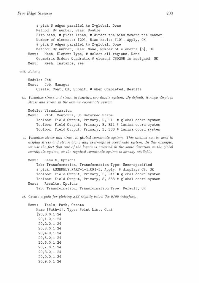
“K15072” — 2013/3/21 — 10:58�

�

�

�

�

�


# pick 6 edges parallel to X-global, Done

Method: By number, Bias: Double

Flip bias, # pick: lines, # direct the bias toward the center

Number of elements: [20], Bias ratio: [10], Apply, OK

# pick 8 edges parallel to Z-global, Done

Method: By number, Bias: None, Number of elements [6], OK


Geometric Order: Quadratic # element C3D20R is assigned, OK


viii. Solving

Module: Job

Menu: Job, Manager


ix. Visualize stress and strain in lamina coordinate system. By default, Abaqus displaysstress and strain in the lamina coordinate system.



Toolbox: Field Output, Primary, U, U1 # global coord system

Toolbox: Field Output, Primary, E, E11 # lamina coord system

Toolbox: Field Output, Primary, S, S33 # lamina coord system

x. Visualize stress and strain in global coordinate system. This method can be used todisplay stress and strain along any user-defined coordinate system. In this example,we use the fact that one of the layers is oriented in the same direction as the globalcoordinate system, so the required coordinate system is already available.

Menu: Result, Options

Tab: Transformation, Transformation Type: User-specified

# pick: ASSEMBLY_PART-1-1_ORI-2, Apply, # displays CS, OK

Toolbox: Field Output, Primary, E, E11 # global coord system

Toolbox: Field Output, Primary, S, S33 # global coord system

Menu: Results, Options

Tab: Transformation, Transformation Type: Default, OK

xi. Create a path for plotting S33 slightly below the 0/90 interface.

Menu: Tools, Path, Create

Name [Path-1], Type: Point List, Cont

[20,0.0,1.24

20,1.0,1.24

20,2.0,1.24

20,3.0,1.24

20,4.0,1.24

20,5.0,1.24

20,6.0,1.24

20,7.0,1.24

20,8.0,1.24

20,9.0,1.24

20,9.5,1.24

�

�

“K15072” — 2013/3/21 — 10:58�

�

�

�

�

�


20,9.8,1.24

20,9.9,1.24

20,10.,1.24]

# visualize the path created on the WS, OK

xii. Create an XY data set to visualize it and/or save it to a file later.

Menu: Tools, XY Data, Create

Source: Path, Cont, Path: Path-1, Model shape: Undeformed

X Values: True distance, Y Values: Field output: S, S33, OK

Save As [path1-S33], OK, Plot, # visualize on screen

# close XY Data pop-up window

xiii. Save the results on the path to a report file in the Work Directory.

Menu: Report, XY

# pick: path1-S33, Tab: Setup, File name [S33path1.rpt], OK

xiv. Repeat the visualization and report for a path slightly above the interface (definedbelow).

[20,0.0,1.26

20,1.0,1.26

20,2.0,1.26

20,3.0,1.26

20,4.0,1.26

20,5.0,1.26

20,6.0,1.26

20,7.0,1.26

20,8.0,1.26

20,9.0,1.26

20,9.5,1.26

20,9.8,1.26

20,9.9,1.26

20,10.,1.26]

Then, save the results in the file [S33path2.rpt]

The stress values along the paths defined above are plotted in Figure 5.6. Notice theresults of stress are virtually identical above and below the interface.

5.2 Coefficient of Mutual Influence

In classical lamination theory, it is assumed that the portion of the laminate beinganalyzed is far from the edges of the laminate. Stress resultants N and M are thenapplied to a portion of the laminate and these induce in-plane stress σx, σy, σxy oneach lamina. In the interior of the laminate, interlaminar stress σxz, σyz are inducedonly if shear forces are applied.

For uniaxial loading Nx, the transverse stresses generated in each lamina as aresult of Poisson’s effect must cancel out to yield a null laminate force Ny. Also, thein-plane shear stress on off-axis layers must cancel out with those of other layers to

�

�

“K15072” — 2013/3/21 — 10:58�

�

�

�

�

�


0 1 2 3 4 5 6 7 8 9−2

0

2

4

6

8

10

12

14

y−coord [mm]

σ 33, [

MP

a]

path1 (below interface)path2 (above interface)

Fig. 5.6: Stress σ33 below and above the 90/0 interface.

yield zero shear force Nxy for the laminate. The situation is more complex near theedges as the various components of in-plane stress do not cancel each other acrossthe lamina interfaces. For the time being, let us revisit the concept of laminateengineering properties. In material axes, the plane stress compliance equations are

⎧

⎨

⎩

ε1ε2γ6

⎫

⎬

⎭

=

⎡

⎣

S11 S12 0S12 S22 00 0 S66

⎤

⎦

⎧

⎨

⎩

σ1σ2σ6

⎫

⎬

⎭

(5.8)

It is also known that the compliance coefficients can be written in terms ofengineering properties as

[S] =

⎡

⎣

1/E1 −ν12/E1 0−ν12/E1 1/E2 0

0 0 1/G12

⎤

⎦ (5.9)

For an off-axis lamina (oriented arbitrarily with respect to the global axes), wehave

⎧

⎨

⎩

εxεyγxy

⎫

⎬

⎭

=

⎡

⎣

S11 S12 S16

S12 S22 S26

S16 S26 S66

⎤

⎦

⎧

⎨

⎩

σxσyσxy

⎫

⎬

⎭

(5.10)

Here it can be seen that uniaxial load (σy = σxy = 0) yields shear strain as aresult of the shear-extension coupling

�

�

“K15072” — 2013/3/21 — 10:58�

�

�

�

�

�


Fig. 5.7: Deformation caused by mutual influence.3

γxy = S16σx (5.11)

where

S16 = (2S11 − 2S12 − S66) sin θ cos3 θ (5.12)

− (2S22 − 2S12 − S66) sin3 θ cos θ

Now, the coefficients of[

S]

can be defined in term of the engineering propertiesfor the off-axis lamina as

S11 = 1/Ex ; S12 = −νxy/Ex = −νyx/Ey (5.13)

S22 = 1/Ey ; S66 = 1/Gxy

To complete the definition of[

S]

in (5.10), two new engineering propertiesdescribing shear-extension coupling, ηxy,x and ηxy,y, are defined as

S16 =ηxy,xEx

; S26 =ηxy,yEx

(5.14)

The engineering properties ηxy,x and ηxy,y are called coefficients of mutual in-fluence and they represent the shear caused by stretching. Their formal definitionis obtained by imposing an axial stress and measuring the resulting shear strain

ηij,i =γijεi

(5.15)

Alternatively, two other coefficients of mutual influence could be defined torepresent the stretching caused by shear

3Reprinted from Mechanics of Fibrous Composites, C. T. Herakovich, Fig. 8.14, copyright(1998), with permission from John Wiley & Sons, Inc.

�

�

“K15072” — 2013/3/21 — 10:58�

�

�

�

�

�


S16 =ηx,xyGxy

; S26 =ηy,xyGxy

(5.16)

These are defined by imposing a shear stress and measuring the axial strain

ηi,ij =εiγij

(5.17)

5.2.1 Interlaminar Stress due to Mutual Influence

Off-axis laminas induce in-plane shear stress when subject to axial loading becausethe natural shear deformations that would occur on an isolated lamina (Figure 5.7)are constrained by the other laminas. Through the whole thickness of the laminate,these stresses cancel out, but over unbalanced sublaminates (e.g., the top lamina inFigure 5.7), they amount to a net shear.

That shear can only be balanced by interlaminar stress σzx at the bottom of thesublaminate (Figure 5.8). Then, summation of forces along x leads to a net force

Fxz(zk) =

∫ b

0σzx(z=zk)

dy = −∫ zN

zk

σxydz (5.18)

Once again, the in-plane shear stress calculated with classical lamination theory(CLT) [1, Chapter 6] can be used to compute the interlaminar force per unit lengthFxz. For in-plane loading, CLT yields constant shear stress in each lamina. Whenthe interlaminar force is evaluated at an interface (located at z = zk), the integrationabove reduces to

Fxz(zk) = −N∑

i=k

σixyti (5.19)

The force Fxz, as well as the values of the coefficients of mutual influence, can beused to qualitatively select the LSS with the least interlaminar stress. Actual valuesof interlaminar stresses can be found by numerical analysis. However, σz → ∞ asy → b. This is a singularity that is not handled well by FEA. Therefore the results,even for y < b, are very dependent on mesh refinement. Furthermore, since σz → ∞,the results cannot be used in a failure criterion without further consideration. Anumerical approximation of σxz for a [±45]S laminate is plotted in Figure 5.10 interms of the distance y’ from the free edge.

Example 5.3 Compute Fxz at all interfaces of a [302/−302]s balanced symmetric laminate(Figure 5.1) loaded with Nx = 175 KN/m. The material properties are given in Example 5.1,p. 199. The lamina thickness is tk = 0.127 mm.

Solution to Example 5.3 In-plane shear stress σxy through the thickness of the laminatecan be obtained following the same procedure used to obtain σy in Example 5.1, p. 199.

For a symmetric balanced laminate under in-plane loads, use (5.19). For a generallaminate under general load, use (5.18) or approximate Fxz by (5.19) taking the average ofσxy in each lamina.

The results are obtained with a spreadsheet and shown in Table 5.2 and Figure 5.9.

�

�

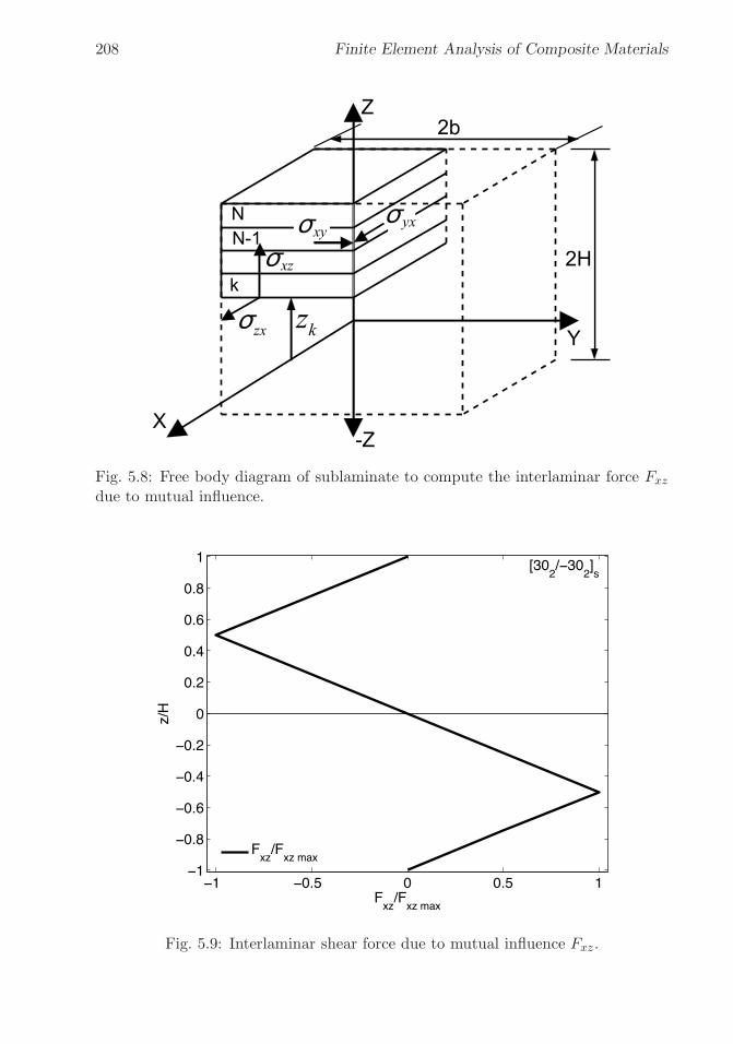
“K15072” — 2013/3/21 — 10:58�

�

�

�

�

�


Fig. 5.8: Free body diagram of sublaminate to compute the interlaminar force Fxz

due to mutual influence.

−1 −0.5 0 0.5 1−1

−0.8

−0.6

−0.4

−0.2

0

0.2

0.4

0.6

0.8

1 [302/−30

2]s

Fxz

/Fxz max

z/H

Fxz

/Fxz max

Fig. 5.9: Interlaminar shear force due to mutual influence Fxz.

�

�

“K15072” — 2013/3/21 — 10:58�

�

�

�

�

�


Table 5.2: Interlaminar force Fxz due to mutual influence.k Pos σxy tk z Fxz

[MPa] [mm] [mm] [kN/m]8 TOP 78.6 10−3 0.508 0.0008 BOT 78.6 10−3 0.127 0.381 -9.9827 TOP 78.6 10−3 0.381 -9.9827 BOT 78.6 10−3 0.127 0.254 -19.9646 TOP -78.6 10−3 0.254 -19.9646 BOT -78.6 10−3 0.127 0.127 -9.9825 TOP -78.6 10−3 0.127 -9.9825 BOT -78.6 10−3 0.127 0.000 0.0004 TOP -78.6 10−3 0.000 0.0004 BOT -78.6 10−3 0.127 -0.127 9.9823 TOP -78.6 10−3 -0.127 9.9823 BOT -78.6 10−3 0.127 -0.254 19.9642 TOP 78.6 10−3 -0.254 19.9642 BOT 78.6 10−3 0.127 -0.381 9.9821 TOP 78.6 10−3 -0.381 9.9821 BOT 78.6 10−3 0.127 -0.508 0.000

Example 5.4 Plot σxz at the interface above the middle surface of a [±45]S laminate usingthe material properties, geometry, and loading of Example 5.2, p. 199.

Solution to Example 5.4 Since the LSS is symmetric, it is possible to model half ofthe laminate (z > 0). However, it is not possible to use the symmetry conditions used inExample 5.2 (p. 199) because the material (say, a 30o lamina) is not symmetric with respectto the x − z and y − z planes (see Figure 5.8). Instead, the plane y − z at x = 0 is nota symmetry plane but rather a plane with εx = 0. Also, the edge effects at the ends of themodel at x = 0 and in x = L� are now important, so the results must be plotted at x = L�/2to avoid free edge effects at the loaded ends. The solution is shown in Figure 5.10.

i. Setting the Work Directory




Module: Part

Menu: Part, Create

3D, Deformable, Solid, Extrusion, Approx size [100], Cont

Menu: Add, Line, Rectangle, [0,0], [80,20], X, Done, Depth [2.5], OK

# We need to cut the volume in 2 layers

Menu: Tools, Datum, Plane,

Offset from principal plane, XY Plane, [1.25]

X, # close the pop-up window


# pick the plane parallel to the XY plane, Create partition, Done

# close pop-up window


�

�

“K15072” — 2013/3/21 — 10:58�

�

�

�

�

�


0 0.2 0.4 0.6 0.8 1−60

−50

−40

−30

−20

−10

0

10

20

30

40

y/b

σ [M

Pa]

σxz

Fig. 5.10: Interlaminar shear stress σxz at the interface above the middle-surface ofa carbon/epoxy [±45]S laminate (FEA).

Module: Assembly


iv. Defining materials, sections, and assigning sections to parts

Module: Property



[1.39E5 1.45E4 1.45E4 0.21 0.21

0.38 5.86E3 5.86E3 5.2536E3], OK

Menu: Section, Create, Solid, Homogeneous, Cont, OK

Menu: Assign, Section, # pick: layer 3, Done, Section-1, OK

# pick: layer 4, Done, Section-1, OK, Done

# assign material orientation -45 layer (near middle surface)

Menu: Assign, Material Orientation, # pick: layer 3, Done



Additional Rotation: Angle [-45], OK

# assign material orientation for +45-degree layer (top surface)

Menu: Assign, Material Orientation, #pick layer 4, Done,




# to see the orientations do this:

# on the left menu tree,

# Models, Model-1, Parts, Part-1, Orientations

�

�

“K15072” — 2013/3/21 — 10:58�

�

�

�

�

�


# you should have only 2 SYSTEM: <Global> entries, one per layer


Module: Step

Menu: Step, Create

Procedure type: General, Static/General, Cont, OK


Module: Load

Menu: BC, Manager

Create, Name [DISP], Step: Step-1, Disp/Rota, Cont

# pick: surface x=80, Done, # checkmark: U1 [0.8], OK

# you may need to rotate the model to pick the surfaces

Create, Name [XEND], Step: Initial, Rota/Disp, Cont

# pick: surface x=0, Done, # checkmark: U1, OK

Create, Name [ZSYMM], Step: Initial, Symm/Anti/Enca, Cont

# pick: surface z=0, Done, # checkmark: U3, OK



Module: Mesh

Menu: Seed, Edges

# pick: 6 edges parallel to Y-global, Done


# make sure the bias is directed toward the end of the lines

Number of elements [20], Bias ratio [10], Apply, OK

# pick 6 edges parallel to X-global, Done


Flip bias, # all the lines toward the center

Number of elements: [20], Bias ratio: [10], Apply, OK

# pick 8 edges parallel to Z-global, Done

Method: By number, Bias: None, Number of elements [6], Apply, OK


Geometric Order: Quadratic, # C3D20R is assigned, OK



Module: Job

Menu: Job, Manager




# create a path for plotting S13 slightly above the -45/+45 interface

Menu: Tools, Path, Create

Name [Path-1], Type: Point List, Cont

[40, 0.0, 1.26

40, 0.5, 1.26

40, 1.0, 1.26

40, 1.5, 1.26

�

�

“K15072” — 2013/3/21 — 10:58�

�

�

�

�

�


40, 2.0, 1.26

40, 2.5, 1.26

40, 3.0, 1.26

40, 3.5, 1.26

40, 4.0, 1.26

40, 4.5, 1.26

40, 5.0, 1.26

40, 6.0, 1.26

40, 7.0, 1.26

40, 8.0, 1.26

40, 9.0, 1.26

40, 10.0, 1.26

40, 11.0, 1.26

40, 12.0, 1.26

40, 13.0, 1.26

40, 14.0, 1.26

40, 15.0, 1.26

40, 15.5, 1.26

40, 16.0, 1.26

40, 16.5, 1.26

40, 17.0, 1.26

40, 17.5, 1.26

40, 18.0, 1.26

40, 18.5, 1.26

40, 19.0, 1.26

40, 19.5, 1.26

40, 20.0, 1.26]

# visualize the path created on the WS, OK

Menu: Tools, XY Data, Create

Source: Path, Cont, Path: Path-1, Model shape: Undeformed

X Values: True distance, Y Values: Field output: S, S13

Save As [S13plot], OK, Plot, # visualize result on screen

# close XY Data pop-up window

Menu: Report, XY

# pick: S13plot, Tab: Setup, File name [S13plot.rpt], OK

# the file S13plot.rpt must have been saved in the Work Directory

The stress values along the path are plotted in Figure 5.11.

Suggested Problems

Problem 5.1 Write a computer program to use tabulated data of σy and σxy (at the topand bottom of every lamina) to compute Fyz, Fxz, and Mz, for all locations through thethickness of a laminate with any number of layers. Using the program, plot Fyz, Fxz, andMz, through the thickness −4t < z < 4t of a [±45/0/90]s laminate with lamina thicknesst = 0.125 mm, loaded with Nx = 100 kN/m. Use carbon/epoxy properties E1=139 GPa,E2=14.5 GPa, G12 = G13 = 5.86 GPa, G23 = 5.25 GPa, ν12 = ν13 = 0.21, ν23 = 0.38.Submit a report including the source code of the program.

Problem 5.2 Repeat Problem 5.1 for Mx = 1 Nm/m. Submit a report including the sourcecode of the program.

�

�

“K15072” — 2013/3/21 — 10:58�

�

�

�

�

�


0 2 4 6 8 10 12 14 16 18

−20

0

20

40

60

80

y−coord [mm]

σ 13, [

MP

a]

σ13

Fig. 5.11: Stress σ13 below and above the −45/+45 interface.

Problem 5.3 Plot σz/σx0 and σyz/σx0 vs. y/b (0 < y/b < 1) at x = L/2, at the firstinterface above the mid-surface of a [0/90/90/0] laminate with lamina thickness t = 0.512mm, loaded with εx = 0.01. Compute the far-field uniform stress σx0 in terms of the appliedstrain. Use quadratic solid elements and a mesh biased toward the free edge (bias 0.1)to model 1/8 of a tensile specimen (see Example 5.2, p. 199), of width 2b = 25.4 mmand length 2L = 20 mm. Use carbon/epoxy properties E1 = 139 GPa, E2 = 14.5 GPa,G12 = G13 = 5.86 GPa, G23 = 5.25 GPa, ν12 = ν13 = 0.21, ν23 = 0.38. Attempt to keepthe aspect ratio of the elements near the free edge close to one. Submit the input commandfile to obtain the solution and the plot. In addition, submit the plot.

Problem 5.4 For the laminate and loading described in Problem 5.3, plot σz/σx0 andσyz/σx0 versus z/tk (0 < z/tk < 2) above the mid-surface, at a distance 0.1tk from thefree edge and x = L/2. Study the effect of mesh refinement by providing four curves withdifferent number of divisions along the z-direction. Attempt to keep the aspect ratio of theelements near the free edge close to one. Submit the input command file to obtain thesolution and the plot. In addition, submit the plot.

Problem 5.5 Plot σxz/σx0 as in Problem 5.3 for all the interfaces above the middle surfaceof a [±102]S laminate.

Problem 5.6 Plot σxz/σx0 as in Problem 5.4 for a [±102]S laminate.

Problem 5.7 Use solid elements and a biased mesh to model 1/8 of a tensile specimen(see Example 5.2, p. 199), of width 2b = 24 mm and length 2L = 20 mm. The laminateis [±45/0/90]s with lamina thickness t = 0.125 mm, loaded with Nx = 175 KN/m. Usecarbon/epoxy properties E1 = 139 GPa, E2 = 14.5 GPa, G12 = G13 = 5.86 GPa, G23 =5.25 GPa, ν12 = ν13 = 0.21, ν23 = 0.38. Plot the three interlaminar stress components,

�

�

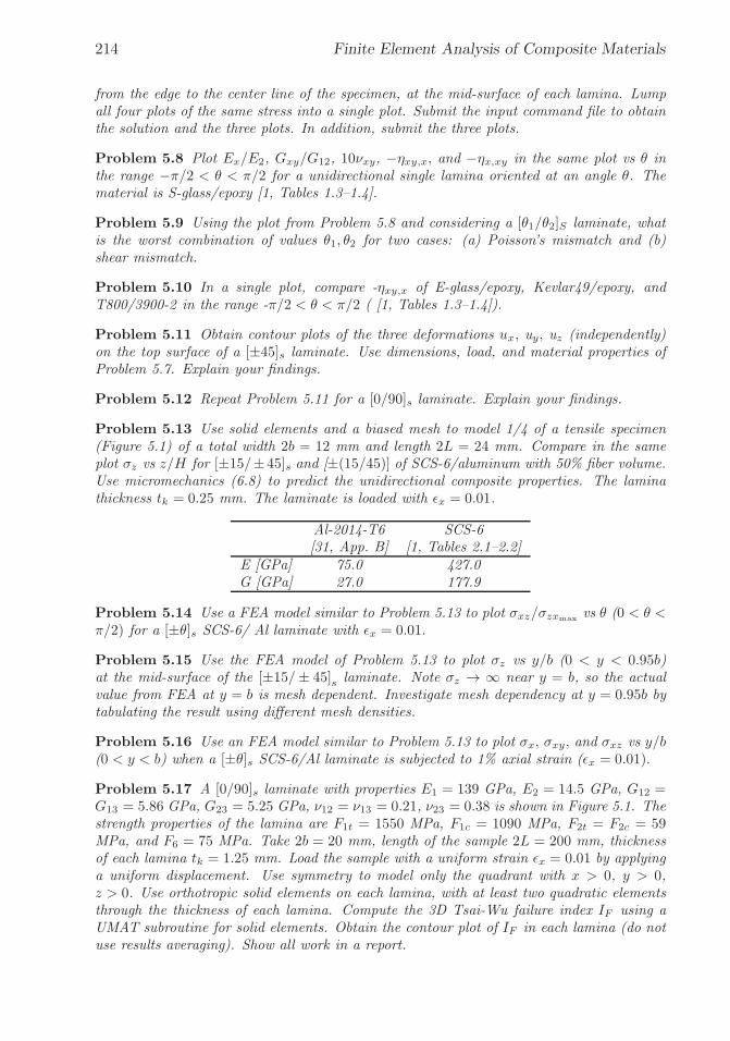
“K15072” — 2013/3/21 — 10:58�

�

�

�

�

�


from the edge to the center line of the specimen, at the mid-surface of each lamina. Lumpall four plots of the same stress into a single plot. Submit the input command file to obtainthe solution and the three plots. In addition, submit the three plots.

Problem 5.8 Plot Ex/E2, Gxy/G12, 10νxy, −ηxy,x, and −ηx,xy in the same plot vs θ inthe range −π/2 < θ < π/2 for a unidirectional single lamina oriented at an angle θ. Thematerial is S-glass/epoxy [1, Tables 1.3–1.4].

Problem 5.9 Using the plot from Problem 5.8 and considering a [θ1/θ2]S laminate, whatis the worst combination of values θ1, θ2 for two cases: (a) Poisson’s mismatch and (b)shear mismatch.

Problem 5.10 In a single plot, compare -ηxy,x of E-glass/epoxy, Kevlar49/epoxy, andT800/3900-2 in the range -π/2 < θ < π/2 ( [1, Tables 1.3–1.4]).

Problem 5.11 Obtain contour plots of the three deformations ux, uy, uz (independently)on the top surface of a [±45]s laminate. Use dimensions, load, and material properties ofProblem 5.7. Explain your findings.

Problem 5.12 Repeat Problem 5.11 for a [0/90]s laminate. Explain your findings.

Problem 5.13 Use solid elements and a biased mesh to model 1/4 of a tensile specimen(Figure 5.1) of a total width 2b = 12 mm and length 2L = 24 mm. Compare in the sameplot σz vs z/H for [±15/± 45]s and [±(15/45)] of SCS-6/aluminum with 50% fiber volume.Use micromechanics (6.8) to predict the unidirectional composite properties. The laminathickness tk = 0.25 mm. The laminate is loaded with εx = 0.01.

Al-2014-T6 SCS-6[31, App. B] [1, Tables 2.1–2.2]

E [GPa] 75.0 427.0G [GPa] 27.0 177.9

Problem 5.14 Use a FEA model similar to Problem 5.13 to plot σxz/σzxmax vs θ (0 < θ <π/2) for a [±θ]s SCS-6/ Al laminate with εx = 0.01.

Problem 5.15 Use the FEA model of Problem 5.13 to plot σz vs y/b (0 < y < 0.95b)at the mid-surface of the [±15/± 45]s laminate. Note σz → ∞ near y = b, so the actualvalue from FEA at y = b is mesh dependent. Investigate mesh dependency at y = 0.95b bytabulating the result using different mesh densities.

Problem 5.16 Use an FEA model similar to Problem 5.13 to plot σx, σxy, and σxz vs y/b(0 < y < b) when a [±θ]s SCS-6/Al laminate is subjected to 1% axial strain (εx = 0.01).

Problem 5.17 A [0/90]s laminate with properties E1 = 139 GPa, E2 = 14.5 GPa, G12 =G13 = 5.86 GPa, G23 = 5.25 GPa, ν12 = ν13 = 0.21, ν23 = 0.38 is shown in Figure 5.1. Thestrength properties of the lamina are F1t = 1550 MPa, F1c = 1090 MPa, F2t = F2c = 59MPa, and F6 = 75 MPa. Take 2b = 20 mm, length of the sample 2L = 200 mm, thicknessof each lamina tk = 1.25 mm. Load the sample with a uniform strain εx = 0.01 by applyinga uniform displacement. Use symmetry to model only the quadrant with x > 0, y > 0,z > 0. Use orthotropic solid elements on each lamina, with at least two quadratic elementsthrough the thickness of each lamina. Compute the 3D Tsai-Wu failure index IF using aUMAT subroutine for solid elements. Obtain the contour plot of IF in each lamina (do notuse results averaging). Show all work in a report.

�

�

“K15072” — 2013/3/21 — 10:58�

�

�

�

�

�

Chapter 6

Computational Micromechanics

In Chapter 1, the elastic properties of composite materials were assumed to beavailable in the form of elastic modulus E, shear modulus G, Poisson’s ratio ν, andso on. For heterogeneous materials such as composites, a large number of materialproperties are needed, and experimental determination of these many properties isa tedious and expensive process. Furthermore, the values of these properties changeas a function of the volume fraction of reinforcement and so on. An alternative, orat least a complement to experimentation, is to use homogenization techniques topredict the elastic properties of the composite in terms of the elastic properties of theconstituents (matrix and reinforcements). Since homogenization models are basedon more or less accurate modeling of the microstructure, these models are also calledmicromechanics models, and the techniques used to obtain approximate values ofthe composite’s properties are called micromechanics methods or techniques [1].Micromechanics models can be classified into empirical, semiempirical, analytical,and numerical. Accurate semiempirical models are described in [1].

This book deals only with strictly analytical or numerical models that do notrequire empirical adjusting factors, so that no experimentation is required. Sincemost of this book deals with 3D analysis, emphasis is placed on micromechanicsmodels that can estimate the whole set of elastic properties using a single model,rather than using a disjoint collection of models based on different assumptions toassemble the set of properties needed. Many analytical techniques of homogeniza-tion are based on the equivalent eigenstrain method [32, 33], which considers theproblem of a single ellipsoidal inclusion embedded in an infinite elastic medium.The Eshelby solution is used in [34] to develop a method that takes into account,approximately, the interactions among the inclusions. One of the more used homog-enization techniques is the self-consistent method [35], which considers a randomdistribution of inclusions in an infinite medium. The infinite medium is assumedto have properties equal to the unknown properties sought. Therefore, an iterativeprocedure is used to obtain the overall moduli. Homogenization of composites withperiodic microstructure has been accomplished by using various techniques includingan extension of the Eshelby inclusion problem [32,33], the Fourier series technique(see Section 6.1.3 and [36,37]), and variational principles. The periodic eigenstrainmethod was further developed to determine the overall relaxation moduli of linear

215

�

�

“K15072” — 2013/3/21 — 10:58�

�

�

�

�

�


viscoelastic composite materials (see Section 7.6 and [38,39]). A particular case, thecell method for periodic media, considers a unit cell with a square inclusion [40].

The analytical procedures mentioned so far yield approximate estimates of theexact solution of the micromechanics problem. These estimates must lie betweenlower and upper bounds for the solution. Several variational principles were devel-oped to evaluate bounds on the homogenized elastic properties of macroscopicallyisotropic heterogeneous materials [41]. Those bounds depend only on the volumefractions and the physical properties of the constituents.

In order to study the nonlinear material behavior of composites with periodic mi-crostructure, numerical methods, mainly the finite element method, are employed.Nonlinear finite element analysis of metal matrix composite has been studied bylooking at the behavior of the microstructure subjected to an assigned load his-tory [42]. Bounds on overall instantaneous elastoplastic properties of compositeshave been derived by using the finite element method [43].

6.1 Analytical Homogenization

As discussed in the introduction, estimates of the average properties of heteroge-neous media can be obtained by various analytical methods. Detailed derivationsof the equations fall outside the scope of this book.

Available analytical models vary greatly in complexity and accuracy. Simpleanalytical models yield formulas for the stiffness C and compliance S tensors of thecomposite [40, (2.9) and (2.12)], such as

C =∑

Vi CiAi ;

∑

ViAi = I

S =∑

Vi SiBi ;

∑

ViBi = I (6.1)

where Vi,Ci,Si are the volume fraction, stiffness, and compliance tensors (in con-

tracted notation)1 of the i-th phase in the composite, respectively, and I is the 6×6identity matrix. Furthermore, Ai,Bi are the strain and stress concentration ten-sors (in contracted notation) of the i-th phase [40]. For fiber reinforced composites,i = f,m represent the fiber and matrix phases, respectively.

6.1.1 Reuss Model

The Reuss model (also called rule of mixtures) assumes that the strain tensors2

in the fiber, matrix, and composite are the same ε = εf = εm; so, the strainconcentration tensors are all equal to the 6× 6 identity matrix Ai = I. The rule ofmixtures (ROM) formulas for E1 and ν12 are derived and computed in this way.

1Fourth-order tensors with minor symmetry are represented by a 6×6 matrix taking advantageof contracted notation.

2Tensors are indicated by boldface type, or by their components using index notation.

�

�

“K15072” — 2013/3/21 — 10:58�

�

�

�

�

�

Computational Micromechanics 217

2a2

2a3RVE

Fig. 6.1: Three possible RVE’s for a composite material with a periodic, squarefiber array.

6.1.2 Voigt Model

The Voigt model (also called inverse rule of mixtures) assumes that the stress tensorsin the fiber, matrix, and composite are the same σ = σf = σm; so, the stressconcentration tensors are all equal to the 6× 6 identity matrix Bi = I. The inverserule of mixtures (IROM) formulas for E2 and G12 are derived and computed in thisway. More realistic concentration tensors are given in [8, Appendix B].

6.1.3 Periodic Microstructure Model

If the composite has periodic microstructure, or if it can be approximated as havingsuch a microstructure (see Section 6.1.4), then Fourier series can be used to estimateall the components of the stiffness tensor of a composite. Explicit formulas for acomposite reinforced by isotropic, circular-cylindrical fibers, which are periodicallyarranged in a square array (Figure 6.1), were developed by [37] and they are pre-sented here. The fibers are aligned with the x1-axis, and they are equally spaced(2a2 = 2a3). If the fibers are randomly distributed in the cross section, the resultingcomposite has transversely isotropic properties, as explained in Section 6.1.4. Thecase of a composite reinforced with transversely isotropic fibers is presented in [39],and the resulting equations are implemented in [12].

Because the microstructure has square symmetry, the stiffness tensor has sixunique coefficients given by

C∗11 = λm + 2μm − Vf

D

[

S23

μ2m− 2S6S3

μ2mg− aS3μm c

+S26 − S2

7

μ2mg2

+aS6 + bS7μm gc

+a2 − b2

4 c2

]

C∗12 = λm +

VfDb

[

S32cμm

− S6 − S72cμm g

− a+ b

4 c2

]

C∗23 = λm +

VfD

[

aS72μm gc

− ba+ b2

4 c2

]

C∗22 = λm + 2μm − Vf

D

[

− aS32μm c

+aS6

2μm gc+a2 − b2

4 c2

]

�

�

“K15072” — 2013/3/21 — 10:58�

�

�

�

�

�


C∗44 = μm − Vf

[

−2S3μm

+ (μm − μf )−1 +

4S7μm(2− 2νm)

]−1

C∗66 = μm − Vf

[

− S3μm

+ (μm − μf )−1

]−1

(6.2)

where

D =aS2

3

2μ2mc− aS6S3

μ2mgc+a(S2

6 − S27)

2μ2mg2c

+ (6.3)

+S3(b

2 − a2)

2μm c2+S6(a

2 − b2) + S7(ab+ b2)

2μmgc2+

(a3 − 2b3 − 3 ab2)

8 c3

and

a = μf − μm − 2μf νm + 2μm νf

b = −μm νm + μf νf + 2μm νm νf − 2μ1 νm νf

c = (μm − μf )(μf − μm + μf νf − μm νm + 2μm νf − 2μf νm+

+ 2μm νm νf − 2μf νm νf )

g = (2− 2νm) (6.4)

The subscripts ()m, ()f refer to matrix and fiber, respectively. Assuming thefiber and matrix are both isotropic (Section 1.12.5), Lame constants of both mate-rials are obtained by using (1.75) in terms of the Young’s modulus E, the Poisson’sratio ν, and the shear modulus G = μ.

For a composite reinforced by long circular cylindrical fibers, periodically ar-ranged in a square array (Figure 6.1), aligned with x1-axis, with a2 = a3, theconstants S3, S6, S7 are given as follows [37]

S3 = 0.49247 − 0.47603Vf − 0.02748V 2f

S6 = 0.36844 − 0.14944Vf − 0.27152V 2f

S7 = 0.12346 − 0.32035Vf + 0.23517V 2f

(6.5)

The resulting tensorC∗ has square symmetry due to the microstructural periodicarrangement in the form of a square array. The tensor C∗ is therefore described bysix constants. However, most composites have random arrangement of the fibers (seeFigure 1.12), resulting in a transversely isotropic stiffness tensor. A generalizationfor transversely isotropic materials is presented in Section 6.1.4, next.

6.1.4 Transversely Isotropic Averaging

In order to obtain a transversely isotropic stiffness tensor (Section 1.12.4), equiva-lent in the average sense to the stiffness tensor with square symmetry, the followingaveraging procedure is used. A rotation θ of the tensor C∗ about the x1-axis pro-duces

�

�

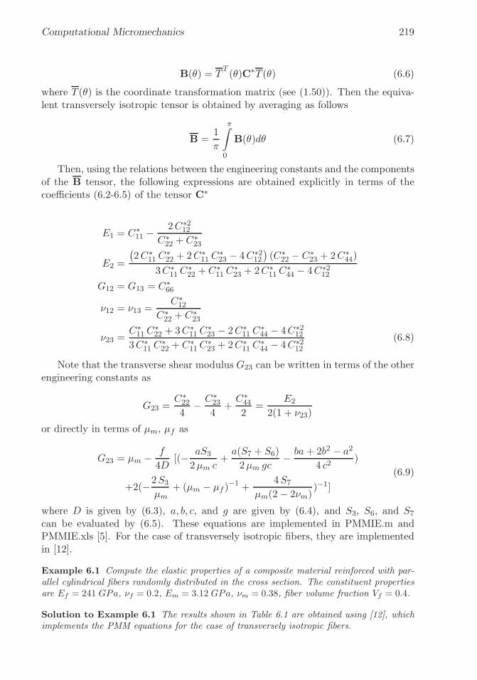
“K15072” — 2013/3/21 — 10:58�

�

�

�

�

�


B(θ) = TT(θ)C∗T (θ) (6.6)

where T (θ) is the coordinate transformation matrix (see (1.50)). Then the equiva-lent transversely isotropic tensor is obtained by averaging as follows

B =1

π

π∫

0

B(θ)dθ (6.7)

Then, using the relations between the engineering constants and the componentsof the B tensor, the following expressions are obtained explicitly in terms of thecoefficients (6.2-6.5) of the tensor C∗

E1 = C∗11 −

2C∗212

C∗22 + C∗

23

E2 =

(

2C∗11 C

∗22 + 2C∗

11 C∗23 − 4C∗2

12

)

(C∗22 − C∗

23 + 2C∗44)

3C∗11 C

∗22 + C∗

11 C∗23 + 2C∗

11 C∗44 − 4C∗2

12

G12 = G13 = C∗66

ν12 = ν13 =C∗12

C∗22 + C∗

23

ν23 =C∗11 C

∗22 + 3C∗

11 C∗23 − 2C∗

11 C∗44 − 4C∗2

12

3C∗11 C

∗22 + C∗

11C∗23 + 2C∗

11 C∗44 − 4C∗2

12

(6.8)

Note that the transverse shear modulus G23 can be written in terms of the otherengineering constants as

G23 =C∗22

4− C∗

23

4+C∗44

2=

E2

2(1 + ν23)

or directly in terms of μm, μf as

G23 = μm − f

4D[(− aS3

2μm c+a(S7 + S6)

2μm gc− ba+ 2b2 − a2

4 c2)

+2(−2S3μm

+ (μm − μf )−1 +

4S7μm(2− 2νm)

)−1]

(6.9)

where D is given by (6.3), a, b, c, and g are given by (6.4), and S3, S6, and S7can be evaluated by (6.5). These equations are implemented in PMMIE.m andPMMIE.xls [5]. For the case of transversely isotropic fibers, they are implementedin [12].

Example 6.1 Compute the elastic properties of a composite material reinforced with par-allel cylindrical fibers randomly distributed in the cross section. The constituent propertiesare Ef = 241 GPa, νf = 0.2, Em = 3.12 GPa, νm = 0.38, fiber volume fraction Vf = 0.4.

Solution to Example 6.1 The results shown in Table 6.1 are obtained using [12], whichimplements the PMM equations for the case of transversely isotropic fibers.

�

�

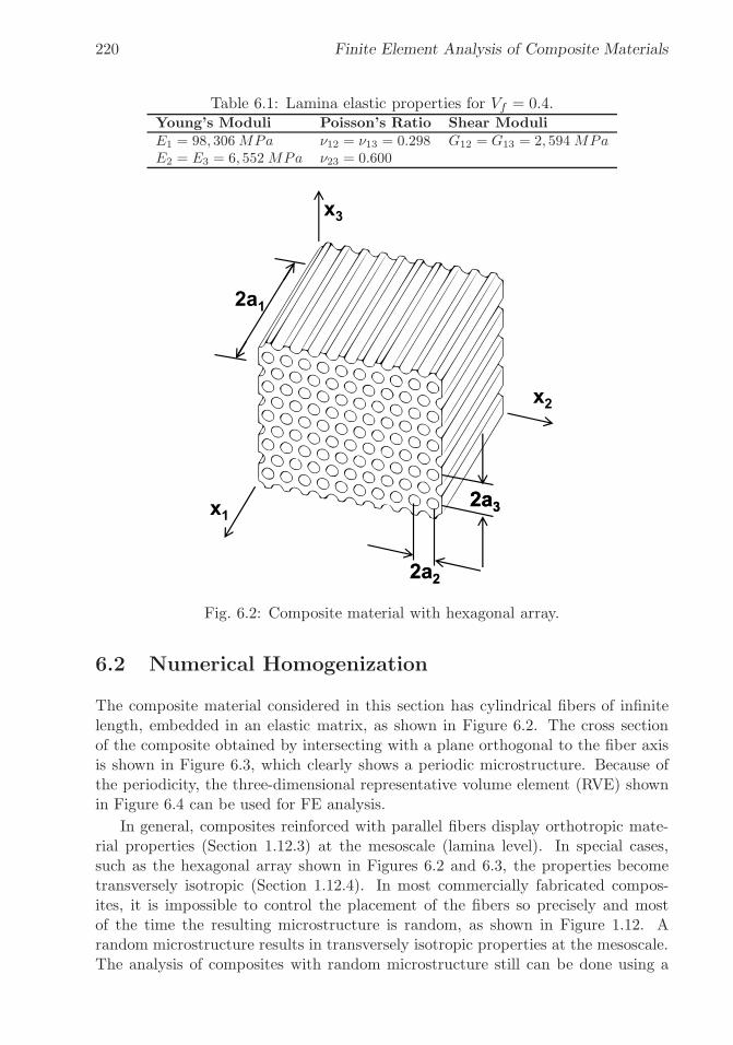
“K15072” — 2013/3/21 — 10:58�

�

�

�

�

�


Table 6.1: Lamina elastic properties for Vf = 0.4.Young’s Moduli Poisson’s Ratio Shear ModuliE1 = 98, 306MPa ν12 = ν13 = 0.298 G12 = G13 = 2, 594MPaE2 = E3 = 6, 552MPa ν23 = 0.600

Fig. 6.2: Composite material with hexagonal array.

6.2 Numerical Homogenization

The composite material considered in this section has cylindrical fibers of infinitelength, embedded in an elastic matrix, as shown in Figure 6.2. The cross sectionof the composite obtained by intersecting with a plane orthogonal to the fiber axisis shown in Figure 6.3, which clearly shows a periodic microstructure. Because ofthe periodicity, the three-dimensional representative volume element (RVE) shownin Figure 6.4 can be used for FE analysis.

In general, composites reinforced with parallel fibers display orthotropic mate-rial properties (Section 1.12.3) at the mesoscale (lamina level). In special cases,such as the hexagonal array shown in Figures 6.2 and 6.3, the properties becometransversely isotropic (Section 1.12.4). In most commercially fabricated compos-ites, it is impossible to control the placement of the fibers so precisely and mostof the time the resulting microstructure is random, as shown in Figure 1.12. Arandom microstructure results in transversely isotropic properties at the mesoscale.The analysis of composites with random microstructure still can be done using a

�

�

“K15072” — 2013/3/21 — 10:58�

�

�

�

�

�


Fig. 6.3: Cross section of the composite material.

Fig. 6.4: Representative volume element (RVE).

�

�

“K15072” — 2013/3/21 — 10:58�

�

�

�

�

�


fictitious periodic microstructure, such as that shown in Figure 6.1, then averag-ing the stiffness tensor C as in Section 6.1.4 to obtain the stiffness tensor of atransversely isotropic material. A simpler alternative is to assume that the randommicrostructure is well approximated by the hexagonal microstructure displayed inFigure 6.3. Analysis of such microstructure directly yields a transversely isotropicstiffness tensor, represented by (1.70), which is reproduced here for convenience

⎧

⎪

⎪

⎪

⎪

⎪

⎪

⎨

⎪

⎪

⎪

⎪

⎪

⎪

⎩

σ1σ2σ3σ4σ5σ6

⎫

⎪

⎪

⎪

⎪

⎪

⎪

⎬

⎪

⎪

⎪

⎪

⎪

⎪

⎭

=

⎡

⎢

⎢

⎢

⎢

⎢

⎢

⎣

C11 C12 C12 0 0 0C12 C22 C23 0 0 0C12 C23 C22 0 0 00 0 0 1

2(C22 − C23) 0 00 0 0 0 C66 00 0 0 0 0 C66

⎤

⎥

⎥

⎥

⎥

⎥

⎥

⎦

⎧

⎪

⎪

⎪

⎪

⎪

⎪

⎨

⎪

⎪

⎪

⎪

⎪

⎪

⎩

ε1ε2ε3γ4γ5γ6

⎫

⎪

⎪

⎪

⎪

⎪

⎪

⎬

⎪

⎪

⎪

⎪

⎪

⎪

⎭

(6.10)

where the 1-axis aligned with the fiber direction and an over-bar indicates the aver-age computed over the volume of the RVE. Once the components of the transverselyisotropic tensor C are known, the five elastic properties of the homogenized materialcan be computed by (6.11), i.e., the longitudinal and transversal Young’s moduliE1 and E2, the longitudinal and transversal Poisson’s ratios ν12 and ν23, and thelongitudinal shear modulus G12, as follows

E1 = C11 − 2C212/(C22 + C23)

ν12 = C12/(C22 + C23)E2 =

[

C11 (C22 + C23)− 2C212

]

(C22 − C23)/(

C11C22 − C212

)

ν23 =[

C11C23 − C212

]

/(

C11C22 − C212

)

G12 = C66

(6.11)

The shear modulus G23 in the transversal plane can be obtained by the classicalrelation (1.74) or directly as follows

G23 = C44 =1

2(C22 − C23) =

E2

2 (1 + ν23)(6.12)

In order to evaluate the overall elastic matrix C of the composite, the RVE issubjected to an average strain εβ [44]. The six components of strain ε0ij are appliedby enforcing the following boundary conditions on the displacement components

ui (a1, x2, x3)− ui (−a1, x2, x3) = 2a1ε0i1

−a2 ≤ x2 ≤ a2−a3 ≤ x3 ≤ a3

(6.13)

ui (x1, a2, x3)− ui (x1,−a2, x3) = 2a2ε0i2

−a1 ≤ x1 ≤ a1−a3 ≤ x3 ≤ a3

(6.14)

ui (x1, x2, a3)− ui (x1, x2,−a3) = 2a3ε0i3

−a1 ≤ x1 ≤ a1−a2 ≤ x2 ≤ a2

(6.15)

Note that tensor components of strain, defined in (1.5), are used in (6.13-6.15).Also, note that a superscript ()0 indicates an applied strain, while an over-line

�

�

“K15072” — 2013/3/21 — 10:58�

�

�

�

�

�


indicates a volume average. Furthermore, 2aj ε0ij is the displacement necessary to

enforce a strain ε0ij over a distance 2aj (Figure 6.4).

The strain ε0ij applied on the boundary by using (6.13-6.15) results in a complexstate of strain inside the RVE. However, the volume average of the strain in theRVE equals the applied strain, i.e.,

εij =1

V

∫

VεijdV = ε0ij (6.16)

For the homogeneous composite material, the relationship between average stressand strain is

σα = Cαβ εβ (6.17)

where the relationship between i, j = 1..3 and β = 1..6 is given by the definition ofcontracted notation in (1.9). Thus, the components of the tensor C are determinedsolving six elastic models of the RVE subjected to the boundary conditions (6.13-6.15), where only one component of the strain ε0β is different from zero for each ofthe six problems.

By choosing a unit value of applied strain, and once the problem defined by theboundary conditions (6.13-6.15) is solved, it is possible to compute the stress fieldσα, whose average gives the required components of the elastic matrix, one columnat a time, as

Cαβ = σα =1

V

∫

Vσα (x1, x2, x3) dV with ε0β = 1 (6.18)

where α, β = 1 . . . 6 (see Section 1.5). The integrals (6.18) are evaluated within eachfinite element using the Gauss-Legendre quadrature. Commercial programs, suchas Abaqus, have the capability to compute the average stress and volume, elementby element. Therefore, computation of the integral (6.18) is a trivial matter. Formore details see Example 6.2, p. 226.

The coefficients in C are found by setting a different problem for each columnin (6.10), as follows.

First Column of C

In order to determine the components Ci1, with i = 1, 2, 3, the following strain isapplied to stretch the RVE in the fiber direction (x1-direction)

εo1 = 1 εo2 = εo3 = γo4 = γo5 = γo6 = 0 (6.19)

Thus, the displacement boundary conditions (6.13-6.15) for the RVE in Figure6.4 become

�

�

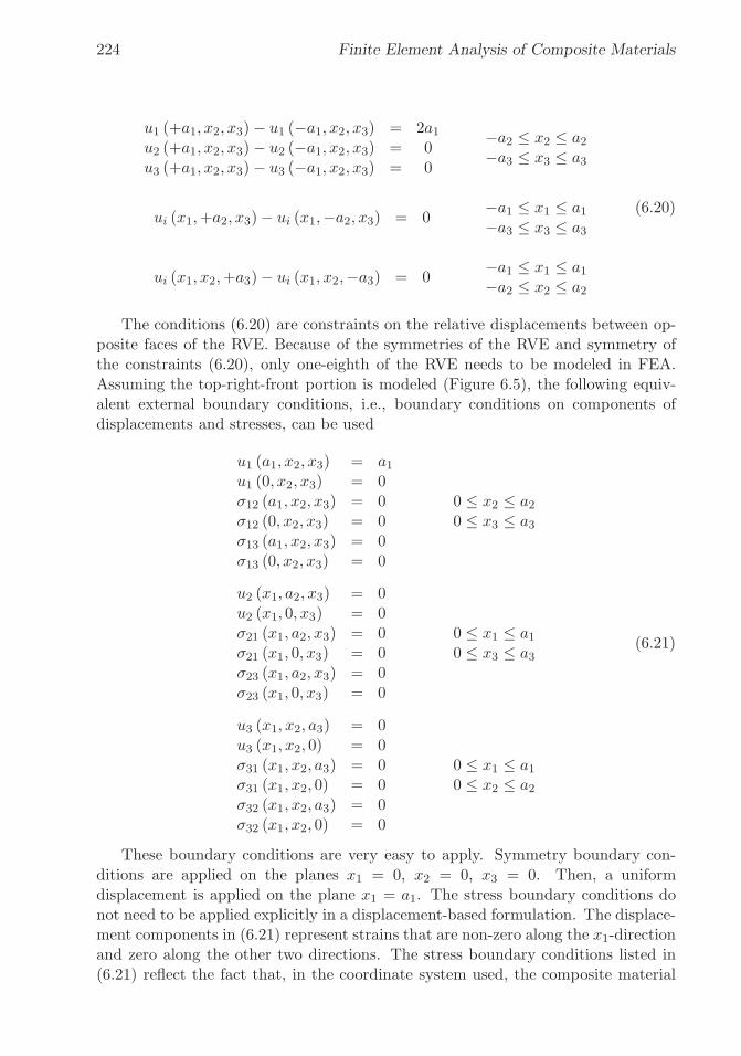
“K15072” — 2013/3/21 — 10:58�

�

�

�

�

�


u1 (+a1, x2, x3)− u1 (−a1, x2, x3) = 2a1u2 (+a1, x2, x3)− u2 (−a1, x2, x3) = 0u3 (+a1, x2, x3)− u3 (−a1, x2, x3) = 0

−a2 ≤ x2 ≤ a2−a3 ≤ x3 ≤ a3

ui (x1,+a2, x3)− ui (x1,−a2, x3) = 0−a1 ≤ x1 ≤ a1−a3 ≤ x3 ≤ a3

ui (x1, x2,+a3)− ui (x1, x2,−a3) = 0−a1 ≤ x1 ≤ a1−a2 ≤ x2 ≤ a2

(6.20)

The conditions (6.20) are constraints on the relative displacements between op-posite faces of the RVE. Because of the symmetries of the RVE and symmetry ofthe constraints (6.20), only one-eighth of the RVE needs to be modeled in FEA.Assuming the top-right-front portion is modeled (Figure 6.5), the following equiv-alent external boundary conditions, i.e., boundary conditions on components ofdisplacements and stresses, can be used

u1 (a1, x2, x3) = a1u1 (0, x2, x3) = 0σ12 (a1, x2, x3) = 0σ12 (0, x2, x3) = 0σ13 (a1, x2, x3) = 0σ13 (0, x2, x3) = 0

0 ≤ x2 ≤ a20 ≤ x3 ≤ a3

u2 (x1, a2, x3) = 0u2 (x1, 0, x3) = 0σ21 (x1, a2, x3) = 0σ21 (x1, 0, x3) = 0σ23 (x1, a2, x3) = 0σ23 (x1, 0, x3) = 0

0 ≤ x1 ≤ a10 ≤ x3 ≤ a3

u3 (x1, x2, a3) = 0u3 (x1, x2, 0) = 0σ31 (x1, x2, a3) = 0σ31 (x1, x2, 0) = 0σ32 (x1, x2, a3) = 0σ32 (x1, x2, 0) = 0

0 ≤ x1 ≤ a10 ≤ x2 ≤ a2

(6.21)

These boundary conditions are very easy to apply. Symmetry boundary con-ditions are applied on the planes x1 = 0, x2 = 0, x3 = 0. Then, a uniformdisplacement is applied on the plane x1 = a1. The stress boundary conditions donot need to be applied explicitly in a displacement-based formulation. The displace-ment components in (6.21) represent strains that are non-zero along the x1-directionand zero along the other two directions. The stress boundary conditions listed in(6.21) reflect the fact that, in the coordinate system used, the composite material

�

�

“K15072” — 2013/3/21 — 10:58�

�

�

�

�

�


Fig. 6.5: One-eighth model of the RVE. Note that the model is set up with the fiberalong the z-axis, which corresponds to the x1-direction in the equations.

is macroscopically orthotropic and that the constituent materials are orthotropictoo. Therefore, there is no coupling between extension and shear strains. This isevidenced by the zero coefficients above the diagonal in columns 4 to 6 in (6.10).

The coefficients in column one of (6.10) are found by using (6.18), as follows

Cα1 = σα =1

V

∫

Vσα (x1, x2, x3) dV (6.22)

Second Column of C

The components Cα2, with α = 1, 2, 3, are determined by setting

εo2 = 1 εo1 = εo3 = γo4 = γo5 = γo6 = 0 (6.23)

Thus, the following boundary conditions on displacements can be used

u1 (a1, x2, x3) = 0u1 (0, x2, x3) = 0u2 (x1, a2, x3) = a2u2 (x1, 0, x3) = 0u3 (x1, x2, a3) = 0u3 (x1, x2, 0) = 0

(6.24)

The trivial stress boundary conditions have not been listed because they areautomatically enforced by the displacement-based FEA formulation. Using (6.18),the stiffness terms in the second column of C are computed as

�

�

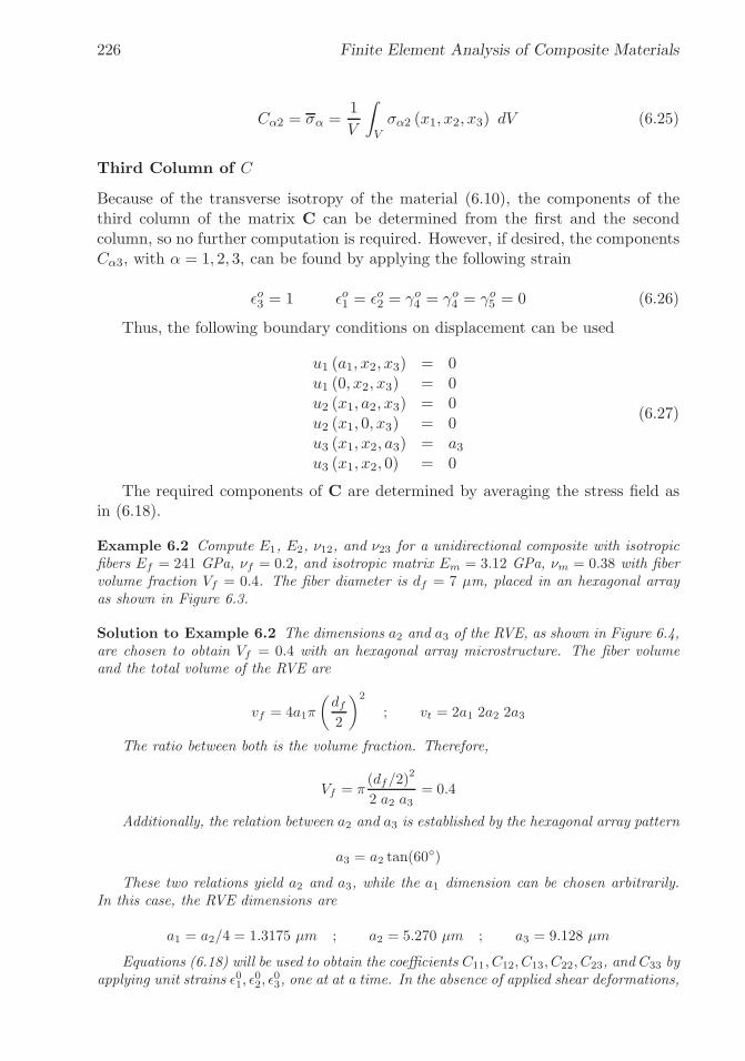
“K15072” — 2013/3/21 — 10:58�

�

�

�

�

�


Cα2 = σα =1

V

∫

Vσα2 (x1, x2, x3) dV (6.25)

Third Column of C

Because of the transverse isotropy of the material (6.10), the components of thethird column of the matrix C can be determined from the first and the secondcolumn, so no further computation is required. However, if desired, the componentsCα3, with α = 1, 2, 3, can be found by applying the following strain

εo3 = 1 εo1 = εo2 = γo4 = γo4 = γo5 = 0 (6.26)

Thus, the following boundary conditions on displacement can be used

u1 (a1, x2, x3) = 0u1 (0, x2, x3) = 0u2 (x1, a2, x3) = 0u2 (x1, 0, x3) = 0u3 (x1, x2, a3) = a3u3 (x1, x2, 0) = 0

(6.27)

The required components of C are determined by averaging the stress field asin (6.18).

Example 6.2 Compute E1, E2, ν12, and ν23 for a unidirectional composite with isotropicfibers Ef = 241 GPa, νf = 0.2, and isotropic matrix Em = 3.12 GPa, νm = 0.38 with fibervolume fraction Vf = 0.4. The fiber diameter is df = 7 μm, placed in an hexagonal arrayas shown in Figure 6.3.

Solution to Example 6.2 The dimensions a2 and a3 of the RVE, as shown in Figure 6.4,are chosen to obtain Vf = 0.4 with an hexagonal array microstructure. The fiber volumeand the total volume of the RVE are

vf = 4a1π

(

df2

)2

; vt = 2a1 2a2 2a3

The ratio between both is the volume fraction. Therefore,

Vf = π(df/2)

2

2 a2 a3= 0.4

Additionally, the relation between a2 and a3 is established by the hexagonal array pattern

a3 = a2 tan(60◦)

These two relations yield a2 and a3, while the a1 dimension can be chosen arbitrarily.In this case, the RVE dimensions are

a1 = a2/4 = 1.3175 μm ; a2 = 5.270 μm ; a3 = 9.128 μm

Equations (6.18) will be used to obtain the coefficients C11, C12, C13, C22, C23, and C33 byapplying unit strains ε01, ε

02, ε

03, one at at a time. In the absence of applied shear deformations,

�

�

“K15072” — 2013/3/21 — 10:58�

�

�

�

�

�


the average deformations are symmetric with respect to the three coordinate planes. TheRVE in Figure 6.5 is also geometrically symmetric with respect to the three coordinateplanes. Therefore, it is possible to model one-eighth of the RVE, as shown in Figure 6.5.The procedure used to model one-eighth of the RVE in Abaqus is given below.




ii. Creating parts

# Values used below, replace the variables accordingly.

# values in microns

# a_1 = 1.3175 # half RVE along x_1 (extrusion direction)

# a_2 = 5.270 # half RVE along x_2

# a_3 = 9.138 # half RVE along x_3

# r_f = 3.5 # fiber radius

Module: Part

Menu: Part, Create

3D, Deformable, Solid, Extrusion, Cont

Menu: Add, Line, Rectangle, [0,0], [a_2, a_3], X, Done

Depth [a_1], OK

Menu: Tools, Partition

Cell, Sketch planar partition, Sketch Origin: Specify

# pick: front face (z=a_1), Sketch origin X,Y,Z: [0,0,a_1]

Select and edge: vertical and on the right, # pick: right vertical

Menu: Add, Circle

[0,0], [0,r_f]

[a_2,a_3], [8.77,a_3], X, Done

Extrude/Sweep, # pick: lines forming lower quarter-circle, Done

Extrude Along Direction, # pick edge parallel to Z-global, OK

Create Partition

# pick: top cell (larger cell), Done

# pick: the lines forming the upper quarter-circle, Done

Extrude Along Direction, # pick edge parallel to Z-global, OK

Create Partition, Done, # close Create Partition pop-up window

iii. Defining materials, sections, and assigning sections to parts

Module: Property


Name [Fiber], Mechanical, Elasticity, Elastic, Type: Isotropic

[241000, 0.2], OK


Name [Matrix], Mechanical, Elasticity, Elastic, Type: Isotropic

[3120, 0.38], OK


Name [Fiber], Solid, Homogeneous, Cont, Material: Fiber, OK


Name [Matrix], Solid, Homogeneous, Cont, Material: Matrix, OK


# pick: the matrix, Done, Section: Matrix, OK

�

�

“K15072” — 2013/3/21 — 10:58�

�

�

�

�

�


# pick: both fibers, Done, Section: Fiber, OK, Done


Module: Assembly


v. Defining analysis steps. We need three steps, one for each column in Section 6.2. Tosolve this example, it will be necessary to include output variables S and IVOL on theOutput Requests.

Module: Step

Menu: Step, Manager

Create, Name [Column-1], Insert new step after: Initial

Procedure type: Linear perturbation, Static, Cont, OK

Create, Name [Column-2], Insert new step after: Column-1


Create, Name [Column-3], Insert new step after: Column-2


# close Step Manager pop-up window

Step: Column-1


Edit variables, [S,E,U,IVOL], OK

vi. Adding loads and BC.The boundary conditions are defined in three load steps, which are then used to obtainthe coefficients Cαβ in columns one, two, and three. A unit strain is applied alongeach direction, each time. Equations (6.18) are then used to obtain the stiffnesscoefficients. The procedure is shown below.

Module: Load

# each step has its own set of BC

# for step: Column-1

Menu: BC, Manager

Create, Name [xsymm-C1], Step: Column-1, Mechanical,


# pick: faces @x=0 and a_2, Done, XSYMM, OK

Create, Name [ysymm-C1], Step: Column-1, Mechanical,


# pick: faces @y=0 and a_3, Done, YSYMM, OK

Create, Name [zsymm-C1], Step: Column-1, Mechanical,


# pick: face @z=0, Done, ZSYMM, OK, # note only one face is picked

# imposed displacement(unit strain)

Create, Name [disp-C1], Step: Column-1, Mech., Disp/Rota, Cont

# pick: faces @z=a_1, Done, # Checkmark: U3 [a_1], OK




# pick: faces @z=0, and a_1, Done, ZSYMM, OK



# pick: faces @y=0 and a_3, Done, YSYMM, OK

�

�

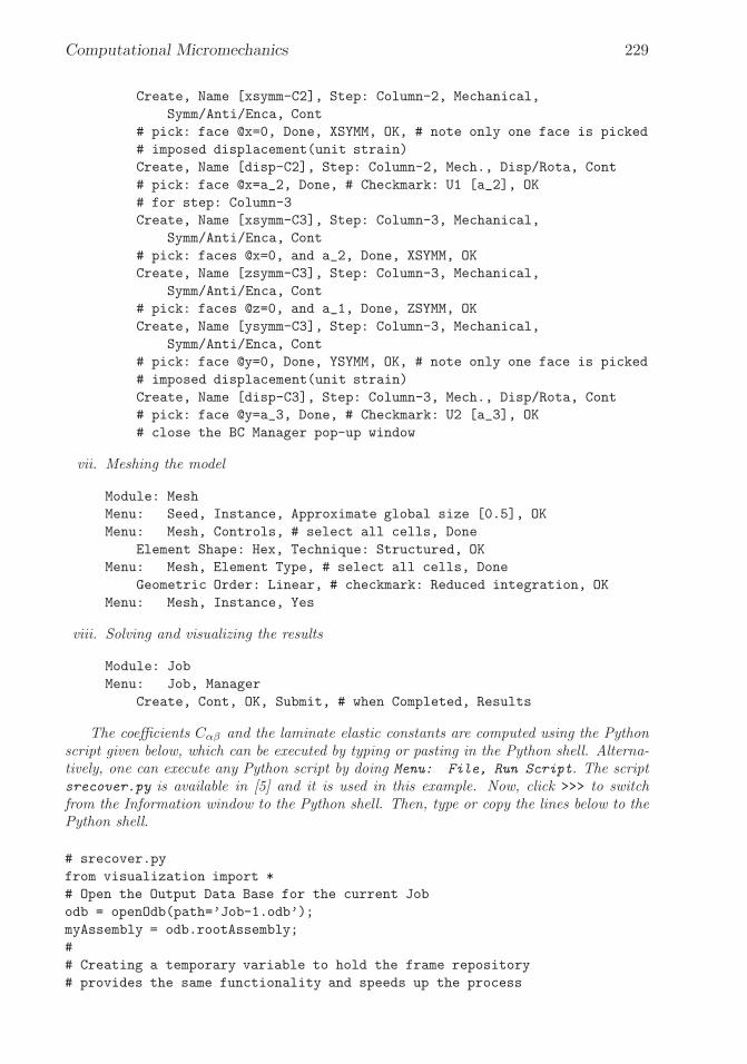
“K15072” — 2013/3/21 — 10:58�

�

�

�

�

�




# pick: face @x=0, Done, XSYMM, OK, # note only one face is picked



# pick: face @x=a_2, Done, # Checkmark: U1 [a_2], OK




# pick: faces @x=0, and a_2, Done, XSYMM, OK



# pick: faces @z=0, and a_1, Done, ZSYMM, OK



# pick: face @y=0, Done, YSYMM, OK, # note only one face is picked



# pick: face @y=a_3, Done, # Checkmark: U2 [a_3], OK

# close the BC Manager pop-up window


Module: Mesh

Menu: Seed, Instance, Approximate global size [0.5], OK

Menu: Mesh, Controls, # select all cells, Done

Element Shape: Hex, Technique: Structured, OK

Menu: Mesh, Element Type, # select all cells, Done

Geometric Order: Linear, # checkmark: Reduced integration, OK



Module: Job

Menu: Job, Manager


The coefficients Cαβ and the laminate elastic constants are computed using the Pythonscript given below, which can be executed by typing or pasting in the Python shell. Alterna-tively, one can execute any Python script by doing Menu: File, Run Script. The scriptsrecover.py is available in [5] and it is used in this example. Now, click >>> to switchfrom the Information window to the Python shell. Then, type or copy the lines below to thePython shell.

# srecover.py

from visualization import *

# Open the Output Data Base for the current Job

odb = openOdb(path=’Job-1.odb’);

myAssembly = odb.rootAssembly;

#

# Creating a temporary variable to hold the frame repository

# provides the same functionality and speeds up the process

�

�

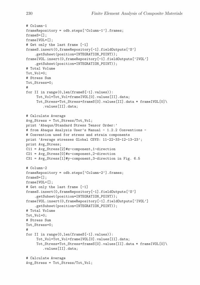
“K15072” — 2013/3/21 — 10:58�

�

�

�

�

�


# Column-1

frameRepository = odb.steps[’Column-1’].frames;

frameS=[];

frameIVOL=[];

# Get only the last frame [-1]

frameS.insert(0,frameRepository[-1].fieldOutputs[’S’]

.getSubset(position=INTEGRATION_POINT));

frameIVOL.insert(0,frameRepository[-1].fieldOutputs[’IVOL’]


# Total Volume

Tot_Vol=0;

# Stress Sum

Tot_Stress=0;

#

for II in range(0,len(frameS[-1].values)):

Tot_Vol=Tot_Vol+frameIVOL[0].values[II].data;

Tot_Stress=Tot_Stress+frameS[0].values[II].data * frameIVOL[0]\

.values[II].data;

# Calculate Average

Avg_Stress = Tot_Stress/Tot_Vol;

print ’Abaqus/Standard Stress Tensor Order:’

# from Abaqus Analysis User’s Manual - 1.2.2 Conventions -

# Convention used for stress and strain components

print ’Average stresses Global CSYS: 11-22-33-12-13-23’;

print Avg_Stress;

C11 = Avg_Stress[2]#z-component,1-direction

C21 = Avg_Stress[0]#x-component,2-direction

C31 = Avg_Stress[1]#y-component,3-direction in Fig. 6.5

# Column-2


frameS=[];

frameIVOL=[];






# Total Volume

Tot_Vol=0;

# Stress Sum

Tot_Stress=0;

#




.values[II].data;

# Calculate Average


�

�

“K15072” — 2013/3/21 — 10:58�

�

�

�

�

�



print ’Average stresses Global CSYS: 11-22-33-12-13-23’;

print Avg_Stress;




# Column-3


frameS=[];

frameIVOL=[];






# Total Volume

Tot_Vol=0;

# Stress Sum

Tot_Stress=0;

#




.values[II].data;

# Calculate Average



print ’Average stresses in Global CSYS: 11-22-33-12-13-23’;

print Avg_Stress;




#

EL=C11-2*C12*C21/(C22+C23) # Longitudinal E1 modulus

nuL=C12/(C22+C23) # 12 Poisson coefficient

ET=(C11*(C22+C23)-2*C12*C12)*(C22-C23)/(C11*C22-C12*C21) #E2

nuT=(C11*C23-C12*C21)/(C11*C22-C12*C21) # 23 Poisson coefficient

GT=(C22-C23)/2 # or GT=ET/2/(1+nuT) # 23 Shear stiffness

#

print "If Moduli are in TPa and dimensions in microns, results are in TPa"

print "E1=",EL

print "E2=",ET

print "PR12=",nuL

print "PR23=",nuT

# end srecover.py

The results are shown in Table 6.2. If you get any errors, check that the blanklines following each of the for loops are completely empty. These blank lines areneeded as terminators for the for loops in Python. Otherwise, try running the

�

�

“K15072” — 2013/3/21 — 10:58�

�

�

�

�

�


Table 6.2: Calculated elastic properties of the unidirectional lamina.Property PMM FEA

E1 [MPa] 98,306 98,197E2 [MPa] 6,552 7,472ν12 0.298 0.299ν23 0.6 0.540G12 2,594 (*)

(*) Not possible with the boundary conditions used in this example.

script as follows: Menu: File, Run Script: [srecover.py], OK.

The modeling procedure for Example 6.2 is quite involved. If one wishes toperform a parametric study, repeating this process on an interactive session usingthe CAE graphical user interface (GUI) would be very time consuming and proneto error. Instead, it is possible to capture the Python script generated by CAEduring an interactive session and use it to automate the process.

Fourth Column of C

For a transversally isotropic material, according to (6.10), only the term C44 isexpected to be different from zero and it can be determined as a function of the othercomponents, so no further computation is needed. Therefore, it can be determinedas

C44 =1

2(C22 − C23) (6.28)

If the material is orthotropic, a procedure similar to that used for column numbersix must be used.

Fifth Column of C

For a transversally isotropic material, according to (6.10), only the term C55 isdifferent from zero and it is equal to C66, which can be found from column numbersix. If the material is orthotropic, a procedure similar to that used for columnnumber six must be used.

Sixth Column of C

Because of the lack of symmetry of the loads, in this case it is not possible to useboundary conditions as was done for the first three columns. Thus, the boundaryconditions must be enforced by using coupling constraint equations (called CE inmost FEA commercial packages).

According to (6.10), only the term C66 is different from zero. The componentsCα6 are determined by setting

γ06 = ε012 + ε021 = 1.0 ε01 = ε02 = ε03 = γ04 = γ05 = 0 (6.29)

�

�

“K15072” — 2013/3/21 — 10:58�

�

�

�

�

�


Note that ε012 = 1/2 is applied between x1 = ±a1 and another one-half is appliedbetween x2 = ±a2. In this case, the CE applied between two periodic faces (exceptpoints in the edges and vertices) is given as a particular case of (6.13-6.15) as follows

u1 (a1, x2, x3)− u1 (−a1, x2, x3) = 0u2 (a1, x2, x3)− u2 (−a1, x2, x3) = a1u3 (a1, x2, x3)− u3 (−a1, x2, x3) = 0

−a2 < x2 < a2−a3 < x3 < a3

u1 (x1, a2, x3)− u1 (x1,−a2, x3) = a2u2 (x1, a2, x3)− u2 (x1,−a2, x3) = 0u3 (x1, a2, x3)− u3 (x1,−a2, x3) = 0

−a1 < x1 < a1−a3 < x3 < a3

u1 (x1, x2, a3)− u1 (x1, x2,−a3) = 0u2 (x1, x2, a3)− u2 (x1, x2,−a3) = 0u3 (x1, x2, a3)− u3 (x1, x2,−a3) = 0

−a1 < x1 < a1−a2 < x2 < a2

(6.30)

Note that (6.30) are applied between opposite points on the faces of the RVEbut not on edges and vertices. In FEA, CE are applied between degrees of freedom(DOF). Once a DOF has been used in a CE, it cannot be used in another CE. Forexample, the first of (6.30) for x2 = a2 becomes

u1(a1, a2, x3)− u1(−a1, a2, x3) = 0 (6.31)

The DOF associated to u1(a1, a2, x3) (for all −a3 < x3 < a3) are eliminatedbecause they are identical to u1(−a1, a2, x3), as required by (6.31) and enforced bya CE based on the same. Once the DOF are eliminated, they cannot be used inanother CE. For example, the fourth of (6.30) at x1 = a1 is

u1(a1, a2, x3)− u1(a1,−a2, x3) = 0 (6.32)

but this CE cannot be enforced because the DOF associated to u1(a1, a2, x3) havebeen eliminated by the CE associated to (6.31). As a corollary, constraint equa-tions on the edges and vertices of the RVE must be written separately from (6.30).Furthermore, only three equations, one for each component of displacement ui, canbe written between a pair of edges or pair of vertices. Simply put, there are onlythree displacements that can be used to enforce periodicity conditions.

For pairs of edges, the task at hand is to reduce the first six equations of (6.30)to three equations that can be applied between pairs of edges for the interval −a3 <x3 < a3. Note that the new equations will not be applied at x3 = ±a3 becausethose are vertices, which will be dealt with separately. Therefore, the last threeequations of (6.30) are inconsequential at this point.

The only way to reduce six equations to three, in terms of six unique DOF, isto add the equations for diagonally opposite edges. Figure 6.6 is a top view of theRVE looking from the positive x3-axis. Point A in Figure 6.6 represents the edgeformed by the planes x1 = a1 and x2 = a2. This location is constrained by the firstof (6.30) at that location, which is precisely (6.31). Point C in Figure 6.6 represents

�

�

“K15072” — 2013/3/21 — 10:58�

�

�

�

�

�


Fig. 6.6: Top view of the RVE showing that two displacements (vertical and hori-zontal) must be applied at edges to impose shear strain (shown as points A, B, C,and D in the figure).

the edge formed by the planes x1 = −a1 and x2 = −a2. This location is constrainedby the fourth of (6.30), which at that location reduces to

u1(−a1, a2, x3)− u1(−a1,−a2, x3) = a2 (6.33)

Adding (6.31) and (6.33) yields a single equation as follows

u1(a1, a2, x3)− u1(−a1,−a2, x3) = a2 (6.34)

Repeating the procedure for the components u2 and u3, and grouping the re-sulting equations with (6.34), results in

u1 (a1, a2, x3)− u1 (−a1,−a2, x3) = a2u2 (a1, a2, x3)− u2 (−a1,−a2, x3) = a1u3 (a1, a2, x3)− u3 (−a1,−a2, x3) = 0

−a3 < x3 < a3 (6.35)

Considering (6.30) between edges B and D in Figure 6.6 results in

u1 (a1,−a2, x3)− u1 (−a1, a2, x3) = −a2u2 (a1,−a2, x3)− u2 (−a1, a2, x3) = a1u3 (a1,−a2, x3)− u3 (−a1, a2, x3) = 0

−a3 < x3 < a3 (6.36)

The planes x1 = ±a1 and x3 = ±a3 define two pairs of edges restrained by thefollowing six CE

�

�

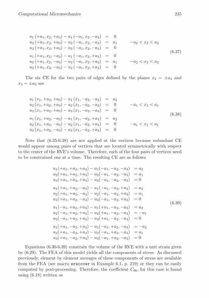
“K15072” — 2013/3/21 — 10:58�

�

�

�

�

�


u1 (+a1, x2,+a3)− u1 (−a1, x2,−a3) = 0u2 (+a1, x2,+a3)− u2 (−a1, x2,−a3) = a1u3 (+a1, x2,+a3)− u3 (−a1, x2,−a3) = 0

−a2 < x2 < a2

u1 (+a1, x2,−a3)− u1 (−a1, x2,+a3) = 0u2 (+a1, x2,−a3)− u2 (−a1, x2,+a3) = a1u3 (+a1, x2,−a3)− u3 (−a1, x2,+a3) = 0

−a2 < x2 < a2

(6.37)

The six CE for the two pairs of edges defined by the planes x2 = ±a2 andx3 = ±a3 are

u1 (x1,+a2,+a3)− u1 (x1,−a2,−a3) = a2u2 (x1,+a2,+a3)− u2 (x1,−a2,−a3) = 0u3 (x1,+a2,+a3)− u3 (x1,−a2,−a3) = 0

−a1 < x1 < a1

u1 (x1,+a2,−a3)− u1 (x1,−a2,+a3) = a2u2 (x1,+a2,−a3)− u2 (x1,−a2,+a3) = 0u3 (x1,+a2,−a3)− u3 (x1,−a2,+a3) = 0

−a1 < x1 < a1

(6.38)

Note that (6.35-6.38) are not applied at the vertices because redundant CEwould appear among pairs of vertices that are located symmetrically with respectto the center of the RVE’s volume. Therefore, each of the four pairs of vertices needto be constrained one at a time. The resulting CE are as follows

u1(+a1,+a2,+a3)− u1(−a1,−a2,−a3) = a2u2(+a1,+a2,+a3)− u2(−a1,−a2,−a3) = a1u3(+a1,+a2,+a3)− u3(−a1,−a2,−a3) = 0

u1(+a1,+a2,−a3)− u1(−a1,−a2,+a3) = a2u2(+a1,+a2,−a3)− u2(−a1,−a2,+a3) = a1u3(+a1,+a2,−a3)− u3(−a1,−a2,+a3) = 0

u1(−a1,+a2,+a3)− u1(+a1,−a2,−a3) = a2u2(−a1,+a2,+a3)− u2(+a1,−a2,−a3) = −a1u3(−a1,+a2,+a3)− u3(+a1,−a2,−a3) = 0

u1(+a1,−a2,+a3)− u1(−a1,+a2,−a3) = −a2u2(+a1,−a2,+a3)− u2(−a1,+a2,−a3) = a1u3(+a1,−a2,+a3)− u3(−a1,+a2,−a3) = 0

(6.39)

Equations (6.30-6.39) constrain the volume of the RVE with a unit strain givenby (6.29). The FEA of this model yields all the components of stress. As discussedpreviously, element by element averages of these components of stress are availablefrom the FEA (see macro srecover in Example 6.1, p. 219) or they can be easilycomputed by post-processing. Therefore, the coefficient C66, for this case is foundusing (6.18) written as

�

�

“K15072” — 2013/3/21 — 10:58�

�

�

�

�

�


C66 = σ6 =1

V

∫

Vσ6 (x1, x2, x3) dV with γ06 = 1 (6.40)

Finally, the elastic properties of the composite are determined using (6.11).

Example 6.3 Compute G12 for the composite in Example 6.2 (p. 226).

Solution to Example 6.3 First note that for the composite reinforced with an hexagonalarray of fibers, G12 = G13. Therefore, to compute G13 = C55 we can apply a deformationγ05 = 2ε013 = 1.0. Such state of average deformation is antisymmetric with respect to the(x1, x2) coordinate plane (X,Z plane in the Abaqus model shown in Figure 6.7) and sym-metric with respect to the (x1, x3) plane (Y, Z plane in the model). Therefore, we choose tomodel the full RVE. The deformed shape and contour plot of strain γ13 (E23 in the model)is shown in Figure 6.7. Such plot corresponds to an average deformation ε13 = 1.0 andaverage stress σ13 = 2, 579MPa, thus yielding G13 = 2, 579MPa according to

C55 = σ5 =1

V

∫

V

σ5 (x1, x2, x3) dV with γ05 = 1 (6.41)

The fiber diameter is df = 7 μm and the RVE dimensions are:

a1 = a2/4 = 1.3175 μm ; a2 = 5.270 μm ; a3 = 9.128 μm

The geometry (Module: Part), material and sections (Module: Property), assembly(Module: Assembly), step (Module: Step), and mesh (Module: Mesh) can be createdin the same fashion as it was done in Example 6.2, p. 226.

Model coordinates X,Y, Z (see Figure 6.7) are used in this section to describe the bound-ary conditions. The bottom of the RVE, at Y = −a3 in the model, is fixed. The top issubjected to a displacement U3 = 2×a3 to represent the applied shear strain ε13 = 1.0. Thesides of the RVE, at X = ±a2, are subject to symmetry BC, which emulate the periodicityconditions in this case because the deformation is symmetric with respect to the plane Y, Zin the model. The pseudo code below describes how to apply the boundary conditions.

Module: Load

Menu: BC, Manager

Create, Name [ysupp], Step: Step-1, Mechanical, Disp/Rota, Cont

# pick the face @ y=-a_3, Done, # Checkmark: U2 [0] and U3 [0], OK

Create, Name [ydisp], Step: Step-1, Mechanical, Disp/Rota, Cont

# pick the face @ y=a_3, Done, # Checkmark: U3 [18.276] # 2*a_3, OK

Create, Name [xsymm], Step: Step-1, Mechanical, Symm/Anti/Enca, Cont

# pick the faces @ x=-a_2 and x=a_2, Done, XSYMM, OK


Enforcing periodicity conditions on the faces at Z = ±a1 is more difficult. Theses facescannot be let free because normal strains will develop and the applied boundary conditionU3 = 2a3 would not lead to a unit average strain. Although the average deformation atthe mesoscale (composite) is pure shear γ13, the deformation at the microscale (fiber andmatrix) would include components E11, E22, and E33. Therefore, periodic conditions onthe faces at Z = ±a1 must be enforced. Since there is no applied strain E33, we can use tieconstraints.

Tie constraints are applied in the interaction module, as follows.

�

�

“K15072” — 2013/3/21 — 10:58�

�

�

�

�

�


Fig. 6.7: Deformed shape and contour plot of strain E23 for Example 6.3. Note thecoordinate system X,Y,Z.

�

�

“K15072” — 2013/3/21 — 10:58�

�

�

�

�

�


Table 6.3: In-plane shear modulus of the unidirectional lamina.Property PMM FEA

G12 [MPa] 2,594 2,579

Module: Interaction

Menu: Constraint, Create

Type: Tie, Cont

Choose the master type: Surface

# pick: front face (surfaces z=2*a_1), Done

Choose the slave type: Surface

# pick: back face (surfaces z=0), Done

Position Tolerance: Specify distance: [2.635] # 2*a_1

# Uncheckmark: Adjust slave surface initial position

# Uncheckmark: Tie rotational DOF if applicable

It is very important to specify the distance between the surfaces (position tolerance) sothat CAE can find the nodes on both surfaces.

You can extract the Python script corresponding to the pseudo code shown above bylooking at the .rec file. The complete script to solve this example is available in [5,Ex 6.3-TC.py]. The script can be executed inside Abaqus/CAE by doing Menu: File,

Run script: Ex 6.3-TC.py. It includes [5, srecover.py] to calculate the average strainsand average stresses, from which the result displayed in Table 6.3 is obtained.

6.3 Local-Global Analysis

In local-global analysis (Figure 6.8), an RVE is used to compute the stress for a givenstrain at each Gauss integration point in the global model . The global model is usedto compute the displacements and resulting strains, assuming that the material ishomogeneous. The local model takes the inhomogeneities into account by modelingthem with an RVE.

Equations (6.13-6.15) are used in Section 6.2 to enforce one component of strainat a time, with the objective of finding the equivalent elastic properties of thematerial. Equations (6.13-6.15) are still valid for a general state of strain appliedto the RVE but care must be taken with the specification of periodic boundaryconditions at the edges and vertices, as discussed in page 233. Equations (6.13-6.15) are nine constraint equations that can be imposed between all the pairs ofperiodic points on the faces of the RVE except on the edges and vertices.

On the faces x1 = ±a1, u1 is used to impose ε011, u2 is used to impose ε021 = γ6/2,and u3 is used to impose ε031 = γ5/2. To achieve this, (6.13) is expanded into itsthree components, using tensor notation for strains, as follows

u1(a1, x2, x3)− u1(−a1, x2, x3) = 2a1ε011

u2(a1, x2, x3)− u2(−a1, x2, x3) = 2a1ε021

u3(a1, x2, x3)− u3(−a1, x2, x3) = 2a1ε031 (6.42)

�

�

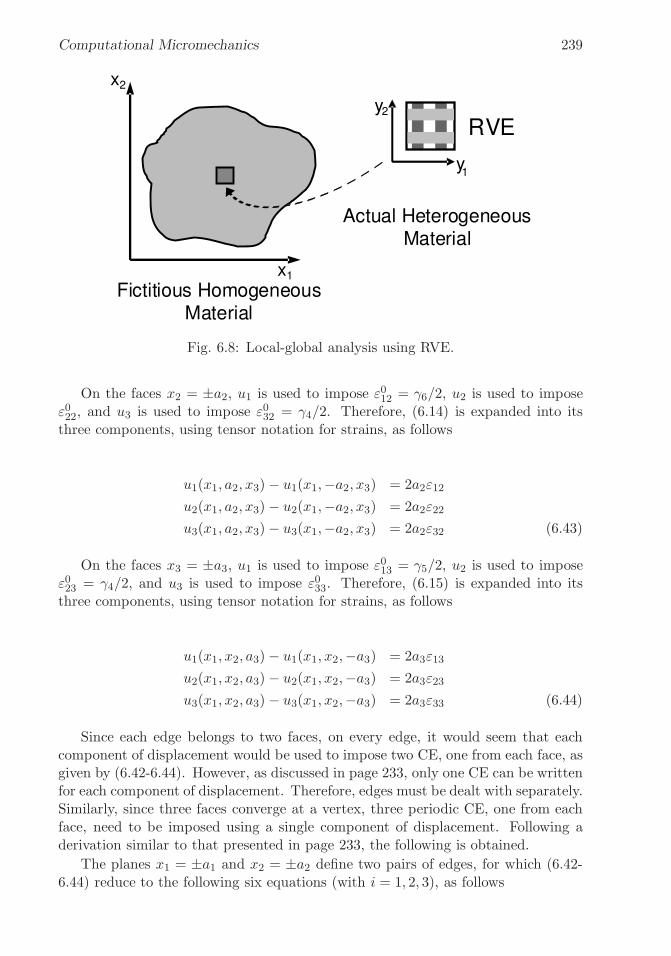
“K15072” — 2013/3/21 — 10:58�

�

�

�

�

�


Fig. 6.8: Local-global analysis using RVE.

On the faces x2 = ±a2, u1 is used to impose ε012 = γ6/2, u2 is used to imposeε022, and u3 is used to impose ε032 = γ4/2. Therefore, (6.14) is expanded into itsthree components, using tensor notation for strains, as follows

u1(x1, a2, x3)− u1(x1,−a2, x3) = 2a2ε12

u2(x1, a2, x3)− u2(x1,−a2, x3) = 2a2ε22

u3(x1, a2, x3)− u3(x1,−a2, x3) = 2a2ε32 (6.43)

On the faces x3 = ±a3, u1 is used to impose ε013 = γ5/2, u2 is used to imposeε023 = γ4/2, and u3 is used to impose ε033. Therefore, (6.15) is expanded into itsthree components, using tensor notation for strains, as follows

u1(x1, x2, a3)− u1(x1, x2,−a3) = 2a3ε13

u2(x1, x2, a3)− u2(x1, x2,−a3) = 2a3ε23

u3(x1, x2, a3)− u3(x1, x2,−a3) = 2a3ε33 (6.44)

Since each edge belongs to two faces, on every edge, it would seem that eachcomponent of displacement would be used to impose two CE, one from each face, asgiven by (6.42-6.44). However, as discussed in page 233, only one CE can be writtenfor each component of displacement. Therefore, edges must be dealt with separately.Similarly, since three faces converge at a vertex, three periodic CE, one from eachface, need to be imposed using a single component of displacement. Following aderivation similar to that presented in page 233, the following is obtained.

The planes x1 = ±a1 and x2 = ±a2 define two pairs of edges, for which (6.42-6.44) reduce to the following six equations (with i = 1, 2, 3), as follows

�

�

“K15072” — 2013/3/21 — 10:58�

�

�

�

�

�


ui(+a1,+a2, x3)− ui(−a1,−a2, x3)− 2a1εi1 − 2a2εi2 = 0

ui(+a1,−a2, x3)− ui(−a1,+a2, x3)− 2a1εi1 + 2a2εi2 = 0 (6.45)


ui(+a1, x2,+a3)− ui(−a1, x2,−a3)− 2a1εi1 − 2a3εi3 = 0

ui(+a1, x2,−a3)− ui(−a1, x2,+a3)− 2a1εi1 + 2a3εi3 = 0 (6.46)


ui(x1,+a2,+a3)− ui(x1,−a2,−a3)− 2a2εi2 − 2a3εi3 = 0

ui(x1,+a2,−a3)− ui(x1,−a2,+a3)− 2a2εi2 + 2a3εi3 = 0 (6.47)

Four pairs of corners need to be analyzed one at a time. For each pair, thecorners are located symmetrically with respect to the center of the RVE located atcoordinates (0, 0, 0). The resulting CE are as follows

ui(+a1,+a2,+a3)− ui(−a1,−a2,−a3)− 2a1εi2 − 2a2εi2 − 2a3εi3 = 0

ui(+a1,+a2,−a3)− ui(−a1,−a2,+a3)− 2a1εi2 − 2a2εi2 + 2a3εi3 = 0

ui(−a1,+a2,+a3)− ui(+a1,−a2,−a3) + 2a1εi2 − 2a2εi2 − 2a3εi3 = 0

ui(+a1,−a2,+a3)− ui(−a1,+a2,−a3)− 2a1εi2 + 2a2εi2 − 2a3εi3 = 0

(6.48)

Example 6.4 Apply ε02 = 0.2% and γ04 = 0.1% simultaneously to the composite in Exam-ple 6.2 (p. 226).Compute the average σ2 and σ12 in the RVE and the maximum stress σ2and σ12 anywhere in the RVE.

Solution to Example 6.4 Tie constraints cannot be used as a substitute for periodic con-ditions when the strain to be applied between two faces is not zero. Symmetry boundaryconditions cannot be used because the applied deformation ε02 = 0.002 and γ023 = 0.001 isnot symmetric with respect to the coordinate planes (x1, x2) and (x1, x3) (Z,X and Z, Y inthe model shown in Figure 6.9). Instead, the full RVE shown in Figure 6.4 must be usedalong with the CE explained in Eqs. (6.30-6.39). However, 2D model can be used becausethe geometry is prismatic, i.e., all cross sections normal to the x1-axis are identical anddeform identically. The periodic conditions on the faces at ±a1 with ε1 = γ12 = γ13 = 0 arerepresented on a 2D model by a plane strain condition, i.e., using plane strain elements.

The fiber diameter is df = 7 μm and the RVE dimensions are:

a1 = a2/4 = 1.3175 μm ; a2 = 5.270 μm ; a3 = 9.128 μm

The geometry (Module: Part), material and sections (Module: Property), assembly(Module: Assembly), step (Module: Step), and mesh (Module: Mesh) can be created

�

�

“K15072” — 2013/3/21 — 10:58�

�

�

�

�

�


Table 6.4: Average stress in the RVE and Maximum stress on the matrix for Ex-ample 6.4.Stress Component Model Labels Direction Average Maximum in Matrix

σ11 S33 Fiber 9.920 16.710σ22 S11 Transverse 21.534 28.710σ33 S22 Transverse 11.841 16.230σ23 S12 Transverse 2.425 5.640

in the same fashion as it was done in Example 6.2 but for a 2D model representing the RVEwith one full fiber and four quarter fibers as shown in Figure 6.4. No symmetry boundaryconditions can be used in this case. Instead, periodic boundary conditions (PBC) (6.13-6.15)must be enforced in Module: Load. These PBC are enforced by using constraint equations(CE). There are no loads per se, but rather the constant terms on the right-hand side (RHS)of (6.13-6.15), which are generated by the applied strains ε02, ε

03, ε

023, yield the loading for the

model.

To write the CEs, one needs to define a reference point, as well as master and slavenodes. Then, the master and slave nodes are connected by constraint equations representingexactly (6.13-6.15). As noted earlier, the equations for the vertices are dealt with separatelyfrom the equations for the faces. The task is automated in [5, PBC 2D.py].

The complete script to solve this example is available in [5, Ex 6.4-CE.py]. First, itgenerates the mesh and sets of nodes later to be used in the CE. The script can be executedinside Abaqus/CAE by doing Menu: File, Run script, [Ex 6.4-CE.py], OK. It calls[5, PBC 2D.py] to write the constraint equations and [5, srecover2D.py] to calculate theaverage stresses. The results are shown in Table 6.4.

6.4 Laminated RVE

A similar procedure to that used to obtain the RVE at the microscale can be usedto analyze laminates on the mesoscale. In this case the RVE represents a laminate.Therefore, the through-thickness direction should remain free to expand along thethickness. For example, with laminas parallel to the x-y plane, then σz = 0 and(6.15) is not enforced, so that the thickness coordinate is free to contract (see Figure6.10). In general, the RVE must include the whole thickness. For symmetricallaminates subjected to in-plane loads, the RVE can be defined with half the thicknessusing symmetry boundary conditions (see Example 6.5, p. 243).

The CE for a laminated RVE are simpler. Only (6.13) and (6.14) must beenforced. In an hexahedral RVE, such as shown in Figure 6.10, only four faces(x1 = ±a1 and x2 = ±a2) and the four edges defined by these faces need to beconsidered.

Therefore, in a laminated RVE the constraint equations (6.13) and (6.14) becomethe following. On the periodic pair of faces x1 = ±a1, the CE are derived from (6.13)as

�

�

“K15072” — 2013/3/21 — 10:58�

�

�

�

�

�


Fig. 6.9: Contour plot of ε22 (E11 in model coordinates X,Y,Z) for Example 6.4.

Fig. 6.10: Laminated RVE.

�

�

“K15072” — 2013/3/21 — 10:58�

�

�

�

�

�


u1(a1, x2, x3)− u1(−a1, x2, x3)− 2a1ε11 = 0u2(a1, x2, x3)− u2(−a1, x2, x3)− 2a1ε21 = 0u3(a1, x2, x3)− u3(−a1, x2, x3)− 2a1ε31 = 0

(6.49)

and on the pair of faces x2 = ±a2, the CE are derived from (6.14)

u1(x1, a2, x3)− u1(x1,−a2, x3)− 2a2ε12 = 0u2(x1, a2, x3)− u2(x1,−a2, x3)− 2a2ε22 = 0u3(x1, a2, x3)− u3(x1,−a2, x3)− 2a2ε32 = 0

(6.50)

The planes x1 = ±a1 and x2 = ±a2 define two pairs of periodic edges, for which(6.13-6.14) reduce to the following equations

u1(+a1,+a2, x3)− u1(−a1,−a2, x3)− 2a1ε11 − 2a2ε12 = 0u2(+a1,+a2, x3)− u2(−a1,−a2, x3)− 2a1ε21 − 2a2ε22 = 0

u3(+a1,+a2, x3)− u3(−a1,−a2, x3)− 2a3ε31 = 0(6.51)

and

u1(+a1,−a2, x3)− u1(−a1,+a2, x3)− 2a1ε11 + 2a2ε12 = 0u2(+a1,−a2, x3)− u2(−a1,+a2, x3)− 2a1ε21 + 2a2ε22 = 0

u3(+a1,−a2, x3)− u3(−a1,+a2, x3)− 2a3ε32 = 0(6.52)

For in-plane analysis, ε31 = ε32 = 0 and the third equation in (6.49)-(6.52) areautomatically satisfied.

Example 6.5 Compute Gxy for a [0/90/−45/45]S laminate with properties E1 = 139 GPa,E2 = 14.5 GPa, G12 = G13 = 5.86 GPa, G23 = 2.93 GPa, ν12 = ν13 = 0.21, ν23 = 0.38,and lamina thickness tk = 1.25mm.

Solution to Example 6.5 As a result of laminate symmetry, a representative volume ele-ment (RVE) of one half the laminate thickness and symmetry boundary conditions at z = 0can be used. The model of the RVE is discretized with 3D solid elements. The pseudo codebelow can be followed to build the model using the Abaqus CAE GUI.


Menu: File, Set Work Directory, [C:\Simulia\User\Ex_6.5], OK

Menu: File, Save As, [C:\Simulia\User\Ex_6.5\Ex_6.5.cae], OK

ii. Creating parts

Module: Part

Menu: Part, Create

3D, Deformable, Solid, Extrusion, Approx. size [10], Cont

Menu: Add, Line, Rectangle, [0,0], [1,1], X, Done, Depth [5], OK

Menu: Tools, Datum

Type: Plane, Method: Offset from principal plane

XY Plane, Offset [1.25]

�

�

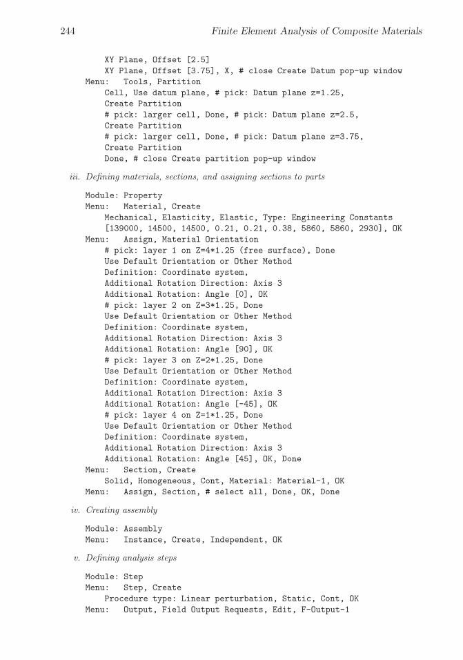
“K15072” — 2013/3/21 — 10:58�

�

�

�

�

�


XY Plane, Offset [2.5]

XY Plane, Offset [3.75], X, # close Create Datum pop-up window


Cell, Use datum plane, # pick: Datum plane z=1.25,

Create Partition

# pick: larger cell, Done, # pick: Datum plane z=2.5,

Create Partition

# pick: larger cell, Done, # pick: Datum plane z=3.75,

Create Partition

Done, # close Create partition pop-up window


Module: Property



[139000, 14500, 14500, 0.21, 0.21, 0.38, 5860, 5860, 2930], OK

Menu: Assign, Material Orientation

# pick: layer 1 on Z=4*1.25 (free surface), Done

Use Default Orientation or Other Method

Definition: Coordinate system,



# pick: layer 2 on Z=3*1.25, Done









Additional Rotation: Angle [-45], OK





Additional Rotation: Angle [45], OK, Done


Solid, Homogeneous, Cont, Material: Material-1, OK

Menu: Assign, Section, # select all, Done, OK, Done


Module: Assembly



Module: Step

Menu: Step, Create



�

�

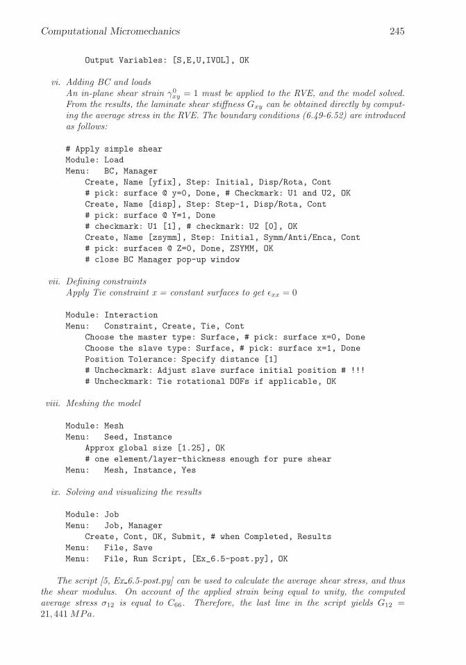
“K15072” — 2013/3/21 — 10:58�

�

�

�

�

�


Output Variables: [S,E,U,IVOL], OK

vi. Adding BC and loadsAn in-plane shear strain γ0xy = 1 must be applied to the RVE, and the model solved.From the results, the laminate shear stiffness Gxy can be obtained directly by comput-ing the average stress in the RVE. The boundary conditions (6.49-6.52) are introducedas follows:

# Apply simple shear

Module: Load

Menu: BC, Manager

Create, Name [yfix], Step: Initial, Disp/Rota, Cont

# pick: surface @ y=0, Done, # Checkmark: U1 and U2, OK

Create, Name [disp], Step: Step-1, Disp/Rota, Cont

# pick: surface @ Y=1, Done

# checkmark: U1 [1], # checkmark: U2 [0], OK

Create, Name [zsymm], Step: Initial, Symm/Anti/Enca, Cont

# pick: surfaces @ Z=0, Done, ZSYMM, OK


vii. Defining constraintsApply Tie constraint x = constant surfaces to get εxx = 0

Module: Interaction

Menu: Constraint, Create, Tie, Cont

Choose the master type: Surface, # pick: surface x=0, Done

Choose the slave type: Surface, # pick: surface x=1, Done

Position Tolerance: Specify distance [1]

# Uncheckmark: Adjust slave surface initial position # !!!

# Uncheckmark: Tie rotational DOFs if applicable, OK

viii. Meshing the model

Module: Mesh

Menu: Seed, Instance

Approx global size [1.25], OK

# one element/layer-thickness enough for pure shear


ix. Solving and visualizing the results

Module: Job

Menu: Job, Manager


Menu: File, Save

Menu: File, Run Script, [Ex_6.5-post.py], OK

The script [5, Ex 6.5-post.py] can be used to calculate the average shear stress, and thusthe shear modulus. On account of the applied strain being equal to unity, the computedaverage stress σ12 is equal to C66. Therefore, the last line in the script yields G12 =21, 441MPa.

�

�

“K15072” — 2013/3/21 — 10:58�

�

�

�

�

�


""" Post-processing Ex. 6.5 """

# make sure the Work Directory is OK

import os

os.chdir(r’C:\Simulia\User\Chapter_6\Ex_6.5’)

# Open the Output Database for the current Job




# Create temporary variable to hold frame repository speeds up the process

frameRepository = odb.steps[’Step-1’].frames;

frameS=[];

frameIVOL=[];

# Create a Coordinate System in the Laminate direction (Global)

coordSys = odb.rootAssembly.DatumCsysByThreePoints(name=’CSYSLAMINATE’,

coordSysType=CARTESIAN, origin=(0,0,0),

point1=(1.0, 0.0, 0), point2=(0.0, 1.0, 0.0) )

# Transform stresses from Lamina Coordinates

# to Laminate Coordinate System defined in CSYSLAMINATE

# stressTrans=odb.steps[’Step-1’].frames[-1].fieldOutputs[’S’]\

# .getTransformedField(datumCsys=coordSys)

stressTrans=frameRepository[-1].fieldOutputs[’S’]\

.getTransformedField(datumCsys=coordSys)

# Insert transformed stresses into frameS

frameS.insert(0,stressTrans.getSubset(position=INTEGRATION_POINT));

frameIVOL.insert(0,frameRepository[-1].fieldOutputs[’IVOL’]\


Tot_Vol=0; # Total Volume

Tot_Stress=0; # Stress Sum




.values[II].data;

#Calculate Average

Avg_Stress=Tot_Stress/Tot_Vol;


# From Abaqus Analysis User’s Manual - 1.2.2 Conventions

print ’ 11-22-33-12-13-23’;

print Avg_Stress;

print ’G12=’,Avg_Stress[3]

�

�

“K15072” — 2013/3/21 — 10:58�

�

�

�

�

�


Suggested Problems

Problem 6.1 Consider a unidirectional composite with isotropic fibers Ef = 241 GPa,νf = 0.2, and isotropic matrix Em = 3.12 GPa, νm = 0.38 with fiber volume fractionVf = 0.4. The fiber diameter is df = 7 μm, placed in a square array as shown in Figure 6.1.Choose an RVE including one full fiber in the center, with vertical faces spaced 2a2 andhorizontal faces spaced 2a3. Part a: compute the first 3 columns of the stiffness matrix in(6.10). Part b: compute C66.

Problem 6.2 Consider the same material and fiber distribution of Problem 6.1, but choosean RVE with faces rotated 45◦ with respect to the horizontal and vertical direction in Fig-ure 6.1. Therefore, the RVE size will be 2

√2a2 and horizontal faces 2

√2a3 and it will

include two fibers (one full and four quarters). Be careful to select a correct RVE that isperiodic.

Part a: compute the first 3 columns of the stiffness matrix in (6.10).Part b: compute C66.

Problem 6.3 Compute E1, E2, ν12, ν23, G12, and G23 using the stiffness matrices calculatedin Problem 6.1.

Problem 6.4 Compute E1, E2, ν12, ν23, G12, and G23 using the stiffness matrices calculatedin Problem 6.2.

Problem 6.5 Show that removing the tie constraints from Example 6.3 (p. 236) leads tononzero normal strains and to a wrong result for G13.

Problem 6.6 Compute G12 as in Example 6.3 (p. 236) but using symmetry boundary con-ditions to discretize only one quarter of the RVE.

Problem 6.7 Compute G23 by modifying the boundary conditions and tie constraints ofExample 6.3, p. 236.

Problem 6.8 Compute G23 by using Example 6.4 (p. 240) as a guide.

�

�

“K15072” — 2013/3/21 — 10:58�

�

�

�

�

�

�

�

“K15072” — 2013/3/21 — 10:58�

�

�

�

�

�

Chapter 7

Viscoelasticity

Our interest in viscoelasticity is motivated by observed creep behavior of polymermatrix composites (PMC), which is a manifestation of viscoelasticity. The timedependent response of materials can be classified as elastic, viscous, and viscoelastic.On application of a sudden load, which is then held constant, an elastic materialundergoes instantaneous deformation. In a one-dimensional state of stress, theelastic strain is ε = Dσ, where D = 1/E is the compliance or inverse of the modulusE. The deformation then remains constant. Upon unloading, the elastic strainreverses to its original value; thus all elastic deformation is recovered.

The viscous material flows at a constant rate ε = σ/η where η = τE0 is theNewton viscosity, E0 is the initial modulus, and τ is the time constant of thematerial. The accumulated strain ε =

∫

εdt cannot be recovered by unloading.

A viscoelastic material combines the behavior of the elastic and viscous materialin one, but the response is more complex than just adding the viscous strain to theelastic strain. Let H be the Heaviside function defined as

H(t− t0) = 0 when t < t0

H(t− t0) = 1 when t ≥ t0 (7.1)

Upon step loading σ = H(t − t0) σ0, with a constant load σ0, the viscoelasticmaterial experiences a sudden elastic deformation, just like the elastic material.After that, the deformation grows by a combination of recoverable and unrecoverableviscous flow.

A simple series addition of viscous flow and elastic strain (Maxwell model, Fig-ure 7.1(a), with η = τE0) yields totally unrecoverable viscous flow plus recoverableelastic deformation as

ε(t) =σ(t)

τE0+σ(t)

E0(7.2)

A simple parallel combination of elastic and viscous flow (Kelvin model, Fig-ure 7.1(b), with η = τE) yields totally recoverable deformation with no viscousflow as

249

�

�

“K15072” — 2013/3/21 — 10:58�

�

�

�

�

�


Fig. 7.1: Viscoelastic modes: (a) Maxwell, (b) Kelvin, (c) standard solid, (d)Maxwell-Kelvin.

σ(t) = τEε(t) + Eε(t) (7.3)

but the deformation does not recover instantaneously.Materials with unrecoverable viscous flow, such as (7.2), are called liquids even

though the flow may occur very slowly. Glass is a liquid material over the timespan of centuries; the thickness of window panes in medieval cathedrals is thickerat the bottom and thinner at the top, thus revealing the flow that took place overthe centuries under the load imposed by gravity. Materials with fully recoverableviscous deformations, such as (7.3), are called solids. We shall see that structuraldesign is much easier with solid materials than with liquid materials.

Please take heed of the common misconception introduced in early mechan-ics of materials courses that most structural materials are elastic. Only perfectlycrystalline materials are elastic. Most materials are viscoelastic if observed for suf-ficiently long periods of time, or at sufficiently high temperature. In other words,most real materials are viscoelastic.

For elastic materials, the compliance D is the inverse of the modulus E, both ofwhich are constants, and they are related by

DE = 1 (7.4)

For viscoelastic materials in the time domain, the compliance is called D(t) andit is related to the time varying relaxation E(t) in a similar but not so simple way,as it will be shown in Section 7.3. Note that the relaxation E(t) takes the placeof the modulus E. A brief derivation of the relationship between compliance andrelaxation is presented next, in order to facilitate the presentation of viscoelasticmodels in Section 7.1. When both the compliance D and the relaxation E arefunctions of time, (7.4) simply becomes

D(t)E(t) = 1 (7.5)

�

�

“K15072” — 2013/3/21 — 10:58�

�

�

�

�

�

Viscoelasticity 251

Both D(t) and E(t) are functions of time and thus it is not possible to operatealgebraically on (7.5) to get either function explicitly in terms of the other. To findone from the other, take the Laplace transform (see Section 7.3) to get

s2D(s)E(s) = 1 (7.6)

Since both D(s) and E(s) are algebraic functions of s, and the time t is notinvolved, it is possible to operate algebraically to get

E(s) =1

s2D(s)(7.7)

Finally, the relaxation in the time domain is the inverse Laplace of (7.7) or

E(t) = L−1[E(s)] (7.8)

Similarly, the compliance D(t) can be obtained from the relaxation E(t) as

D(t) = L−1

[

1

s2L[E(t)]

]

(7.9)

where L[ ] indicates the Laplace transform and L−1[ ] indicates the inverse Laplacetransform.

7.1 Viscoelastic Models

The viscoelastic material models presented in this section are convenient curve fitsof experimental data. In the time domain, the usual experiments are the creep andrelaxation tests. In the creep test, a constant stress σ0 is applied and the ensuingstrain is measured. The ratio of measured strain to applied stress is the complianceD(t) = ε(t)/σ0. In the relaxation test, a constant strain ε0 is applied and the stressneeded to maintain that strain is measured. The ratio of measured stress to appliedstrain is the relaxation E(t) = σ(t)/ε0.

7.1.1 Maxwell Model

To derive the compliance of the Maxwell model [45], a creep test is performed underconstant stress σ0 applied at the ends of the model shown in Figure 7.1(a). Therate of strain is given by (7.2). Integrating with respect to time we get

ε(t) =1

τE0

∫ t

0σ0dt+

σ0E0

(7.10)

where E0 is the elastic constant of the spring, τ is the time constant of the material,and η0 = τE0 in Figure 7.1(a). The spring and dashpot are subject to the sameload and to the same constant stress σ0, so evaluating the integral yields

ε(t) =σ0 t

τE0+σ0E0

(7.11)

�

�

“K15072” — 2013/3/21 — 10:58�

�

�

�

�

�


Table 7.1: Some common Laplace transforms.Function f(t)=L−1{f(s)} f(s)=L{f(t)}constant a a/slinear at a/s2

derivative df/dt sf(s)-f(0)

exponential exp(at) 1/(s − a)

convolution integral∫ t0 f(t− τ)g(τ)dτ L{f}L{g}

Then, the compliance is

D(t) =1

E0+

t

τE0(7.12)

To derive the relaxation of the Maxwell model, take the Laplace transform of(7.12) (using Table 7.1 or MATLAB) to get

D(s) =1

sE0+

1

s2τE0=sτ + 1

s2τE0(7.13)

At t = 0, the dashpot does not move, so E0 is also the initial elastic modulus ofthe material. Now, the relaxation in the Laplace domain is

E(s) =1

s2D(s)=

τE0

sτ + 1(7.14)

and the relaxation in the time domain is obtained by taking the inverse Laplacetransform (using Table 7.1 or MATLAB) to get

E(t) = E0 exp(−t/τ) (7.15)

Note that at t = τ , the relaxation decays to 36.8% of its initial value, and thusτ is called the time constant of the material.

7.1.2 Kelvin Model

For the Kelvin model, only the creep test is possible, since a relaxation test wouldrequire an infinitely large stress to stretch the dashpot in Figure 7.1(b) to a constantvalue in no time. For a creep test, a constant stress σ = σ0 is applied. Then, (7.3)is an ordinary differential equation (ODE) in ε(t), which is satisfied by ε(t) =(σ0/E) [1− exp(−t/τ)]. Therefore, the compliance D(t) = ε(t)/σ0 is

D(t) = 1/E0[1− exp(−t/τ)] (7.16)

Using (7.8), the relaxation function can be written with the aid of the Heavisidestep function H(t) and the Dirac delta function δ(t) as follows

E(t) = EH(t) + Eτδ(t) (7.17)

where δ(t− t0) = ∞ if t = t0 and zero for any other time. The following MATLABcode yields (7.17):

�

�

“K15072” — 2013/3/21 — 10:58�

�

�

�

�

�

Viscoelasticity 253

syms s complex; syms Dt Et t E tau real;

Dt=expand((1-exp(-t/tau))/E)

Ds=laplace(Dt)

Es=1/Ds/s^2

Et=ilaplace(Es)

7.1.3 Standard Linear Solid

To have an initial compliance 1/E0, a spring is added to the Kelvin model (Fig-ure 7.1.c). Then, the compliance is

D(t) = 1/E0 + 1/E2

[

1− exp

(−tτ2

)]

(7.18)

and

E(t) = E∞ + (E0 −E∞) exp

(−t (E0 + E2)

τ2E2

)

(7.19)

where E∞ = (E−10 + E−1

2 )−1 is the equilibrium modulus as time goes to infinity.

To obtain a better correlation, more spring-dashpot elements are added in series,as in

D(t) = D0 +n∑

j=1

Dj [1− exp (−t/τj)] (7.20)

where τj are the retardation times [17]. When n→ ∞,

D(t) =

∫ ∞

0Δ(τ) [1− exp (−t/τ) dτ ] (7.21)

where Δ(τ) is the compliance spectrum [17].

7.1.4 Maxwell-Kelvin Model

A crude approximation of a liquid material is the Maxwell-Kelvin model, also calledthe four-parameter model, described by Figure 7.1(d). Since the Maxwell and Kelvinelements are placed in series, the compliance is found by adding the compliances ofthe two individual modes, as

D (t) =1

E0+

t

τ1E0+

1

E2[1− exp (−t/τ2)] (7.22)

where E0 is the elastic modulus, τ1 takes the place of τ in (7.12), and E2, τ2 takethe place of E, τ in (7.16). The relaxation modulus is given by [45, page 28]

�

�

“K15072” — 2013/3/21 — 10:58�

�

�

�

�

�


E (t) =(

P 21 − 4P2

)−1/2[(

q1 − q2T1

)

exp (−t/T 1)−(

q1 − q2T2

)

exp (−t/T 2)

]

η1 = E0τ1 ; η2 = E0τ2

q1 = η1 ; q2 =η1 η2E2

T1 =1

2P2

[

P1 +√

P 21 − 4P2

]

; T2 =1

2P2

[

P1 −√

P 21 − 4P2

]

P1 =η1E0

+η1E2

+η2E2

; P2 =η1 η2E0E2

(7.23)

Another way to determine if a material is a liquid or a solid is to look at itslong-term deformation. If the deformation is unbounded, then it is a liquid. If thedeformation eventually stops, then it is a solid.

7.1.5 Power Law

Another model, which is popular to represent relatively short-term deformation ofpolymers, is the power law

E(t) = At−n (7.24)

The parameters A and n are adjusted with experimental data. The power lawis popular because it fits well the short-time behavior of polymers and becausefitting the data is very easy; just take logarithm on both sides of (7.24) so that theequation becomes that of a line, then fit the parameters using linear regression. Thecompliance is obtained by using (7.9) as

D(t) = D0 +Dc(t)

Dc(t) = [AΓ(1− n)Γ(1 + n)]−1tn (7.25)

where Γ is the Gamma function [46], D0 = 1/E0 is the elastic compliance, andthe subscript ()c indicates the creep component of the relaxation and compliancefunctions.

7.1.6 Prony Series

Although the short-term creep and relaxation of polymers can be described well bythe power law, as the time range becomes longer, a more refined model becomesnecessary. One such model is the Prony series, which consists of a number n ofdecaying exponentials

E(t) = E∞ +

n∑

i=1

Ei exp(−t/τi) (7.26)

�

�

“K15072” — 2013/3/21 — 10:58�

�

�

�

�

�

Viscoelasticity 255

where τi are the relaxation times, Ei are the relaxation moduli, and E∞ is theequilibrium modulus, if any exists. For example, a Maxwell material is a “liquid”and thus E∞ = 0. The larger the τi the slower the decay is. Note that at t = 0,E0 = E∞ +

∑

Ei. Equation (7.26) can be rewritten as

E(t) = E∞ +

n∑

1

miE0 exp(−t/τi) (7.27)

where mi = Ei/E0.The Prony series can be written in terms of the shear modulus and bulk modulus

(G, k, see Section 1.12.5) as follows

G(t) = G∞ +

n∑

1

giG0 exp(−t/τi)

k(t) = k∞ +

n∑

1

kik0 exp(−t/τi) (7.28)

where gi = Gi/G0 and ki = ki/k0, and G0, k0 are the initial values of shear modulusand bulk modulus, respectively. Noting that at t = 0, G∞ = G0(1 −∑n

1 gi), andk∞ = k0(1−

∑n1 ki), the Prony series can be rewritten as

G(t) = G0

(

1−n∑

1

gi

)

+

n∑

1

giG0 exp(−t/τi)

k(t) = k0

(

1−n∑

1

ki

)

+

n∑

1

kik0 exp(−t/τi)

(7.29)

Data are input to Abaqus/CAE in Edit Material by specifying separately theelastic properties (E0 and ν0) and the viscous properties (gi, ki, τi) for the i-thelement of the Prony series. Internally, Abaqus calculates G0 and k0 using thevalues entered for E0 and ν and equations (1.74) and (1.76). For most polymersand composites it is usual to assume that the Poisson’s ratio does not change withtime, which according to (1.74) and (1.76) is achieved by setting ki = gi. Also, if νis constant over time, mi = gi in (7.27).

Note that the Young modulus entered in Edit Material represents E0 if Modulitime scale (for viscoelasticity) is set to Instantaneous. Otherwise, if Modulitime scale (for viscoelasticity) is set to Long term, then the Young modulusrepresents E∞. Of course, one can be calculated from the other by using the rela-tionship E0 = E∞/(1−

∑

mi).For example, a Maxwell material (7.15) can be modeled by a one term Prony

series by setting gi = ki = 1. However, Abaqus cannot calculate a material withE∞ = 0, so the data must be such that

∑

gi < 1. Thus, to model a Maxwellmaterial one has to use g1 = k1 = 0.999.

�

�

“K15072” — 2013/3/21 — 10:58�

�

�

�

�

�


7.1.7 Standard Nonlinear Solid

While the Prony series can fit any material behavior if a large number of terms areused, other models are more efficient for fitting purposes, if harder to manipulatemathematically. For example the Standard Nonlinear Solid model

D(t) = D0 +D′1[1− exp(−t/τ)m] (7.30)

can approximate well the long-term compliance in the α-region of polymer creep [47].At room temperature, this is the region of interest to structural engineers since itspans the range of time from seconds to years. In contrast the β-region [47] isof interest to sound and vibration experts, among others, since it spans the sub-second range of times. In other words, for long-term modeling, all complianceoccurring in the β-region can be lumped in the term D0, with D

′1 representing all

the compliance that could ever be accumulated in the α-region. Equation (7.30) hasfour parameters. When the data span short times, it may be impossible to determineall four parameters because the material behavior cannot be distinguished from a3-parameter power law (7.31). This can be easily understood if (7.30) is expandedin a power series, truncated after the first term as follows [47]

D(t) = D0 +D′1(t/τ)

m[1− (t/τ)m + ...] ≈ D0 +D1tm ; D1 = D′

1/τ (7.31)

For short times, all higher order powers of t can be neglected. What remainsis a modified power law with only three parameters. Note that for short times,the parameter τ is combined with D′

1 to form D1. If the data cover a short time,the fitting algorithm will not be able to adjust both τ and D′

1 in (7.31); virtuallyany combination of τ and D′

1 will work. That means that short-term data must bemodeled by a smaller number of parameters, in this case three.

7.1.8 Nonlinear Power Law

All models described so far represent linear viscoelastic materials. In the context ofviscoelasticity, linear means that the parameters in the model are not a function ofstress (see Section (7.2.1)). That means that the deformation at any fixed time canbe made proportionally larger by increasing the stress. If any of the parameters area function of stress, the material is nonlinear viscoelastic. For example a nonlinearpower law takes the form

ε = AtBσD (7.32)

Take logarithm to both sides of (7.32) to get a linear equation in two variables

y = A+BX1 +DX2 ; A = log(A),X1 = log(t),X2 = log(σ) (7.33)

that can be fitted with a multiple linear regression algorithm in MATLAB.Although most materials are not linearly viscoelastic, they can be approximated

as linear viscoelastic if the range of stress at which the structure operates is narrow.

�

�

“K15072” — 2013/3/21 — 10:58�

�

�

�

�

�

Viscoelasticity 257

50 100 150 2001

1.5

2

2.5

3

t [s]

D [

GP

a-1

]

Experimental Data

Maxwell Model

Power Law

Std Nonlinear Solid

Fig. 7.2: Viscoelastic fit: Maxwell Model, Power Law, and Std Nonlinear Solid.

Example 7.1 Fit the creep data in Table 7.2 with (a) Maxwell (7.12), (b) Power Law(7.31), and (c) Std Nonlinear Solid (7.30).

Table 7.2: Creep data for Example 7.1.time [sec] 1 21 42 62 82 102 123 143 163 184 204D(t) [GPa−1] 1.49 1.99 2.21 2.35 2.56 2.66 2.75 2.85 2.92 2.96 3.01

Solution to Example 7.1 To fit the Maxwell model, fit a line to the secondary creep data;that is, ignore the curvy portion for short times to get E0 = 0.460 GPa, τ = 495 s.

To fit the Power Law, write (7.19) as

D(t)−D0 = D1tm

where D0 = 1.49 GPa−1 is the first datum in Table 7.2 (see also (7.31)). Take logarithmto both sides of above equation and adjust a line using linear regression to get D0 = 1.49GPa−1, D1 = 0.1117 (GPa sec)−1, and m = 0.5.

To fit the Standard Nonlinear Solid you need to use a nonlinear solver to minimize theerror between the predicted (expected) values ei and the experimental (observed) values oi.Such error is defined as the sum over all the available data points: χ2 =

∑

(ei − oi)2/o2i .

In this way, the following are obtained: D0 = 1.657 GPa−1, D′1 = 1.617 GPa−1, τ = 0.273

sec, and m = 0.0026.

The experimental data and the fit functions are shown in Figure 7.2.

�

�

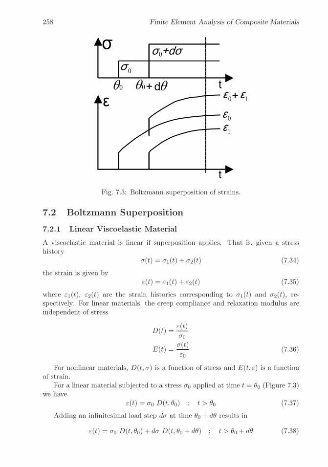
“K15072” — 2013/3/21 — 10:58�

�

�

�

�

�


Fig. 7.3: Boltzmann superposition of strains.

7.2 Boltzmann Superposition

7.2.1 Linear Viscoelastic Material

A viscoelastic material is linear if superposition applies. That is, given a stresshistory

σ(t) = σ1(t) + σ2(t) (7.34)

the strain is given byε(t) = ε1(t) + ε2(t) (7.35)

where ε1(t), ε2(t) are the strain histories corresponding to σ1(t) and σ2(t), re-spectively. For linear materials, the creep compliance and relaxation modulus areindependent of stress

D(t) =ε(t)

σ0

E(t) =σ(t)

ε0(7.36)

For nonlinear materials, D(t, σ) is a function of stress and E(t, ε) is a functionof strain.

For a linear material subjected to a stress σ0 applied at time t = θ0 (Figure 7.3)we have

ε(t) = σ0 D(t, θ0) ; t > θ0 (7.37)

Adding an infinitesimal load step dσ at time θ0 + dθ results in

ε(t) = σ0 D(t, θ0) + dσ D(t, θ0 + dθ) ; t > θ0 + dθ (7.38)

�

�

“K15072” — 2013/3/21 — 10:58�

�

�

�

�

�

Viscoelasticity 259

If stress changes continuously by dσ over intervals dθ, the summation (7.38) canbe replaced by an integral to yield the accumulated strain as

ε(t) = σ0 D(t, θ0) +

∫ t

θ0

D(t, θ)dσ = σ0 D(t, θ0) +

∫ t

θ0

D(t, θ)dσ

dθdθ (7.39)

where the discrete times θ0, θ0+dθ, etc., are represented by the continuous functionθ. Although aging effects are negligible over each infinitesimal dθ, they are signifi-cant over time. Therefore, the compliance D(t, θ) is a function of the current timet and all the time-history represented by θ in D(t, θ).

7.2.2 Unaging Viscoelastic Material

If the ε1(t, θ) curve has the same shape as the ε1(t, θ0) curve, only translated hori-zontally, any curve can be shifted to the origin (Figure 7.3)

D(t, θ) = D(t− θ) (7.40)

Equation (7.40) is the definition of unaging material. For a discussion of agingmaterials see [45, 48]. Equation (7.40) means that all the curves have the sameshape regardless of age θ, only shifted. Note θ in (7.40) is a continuous functionθ < t that denotes the time of application of each load (σ0, dσ, etc.).

The response ε(t, θ) at a fixed time t is a function of the response at all timesθ < t. Therefore, it is said that the response is hereditary. If the material is aging, tand θ are independent variables in D(t, θ). For unaging materials, only one variable,t−θ, is independent, so it does not matter how old the material is (t), it only mattersfor how long (t− θ) it has been loaded with dσ(θ).

The creep compliance is the response of the material to stress and always startswhen the stress is applied. If the change is gradual, from (7.39) we have

ε(t) =

∫ t

0D(t− θ) σ(θ) dθ (7.41)

The relaxation is

σ(t) =

∫ t

0E(t− θ) ε(θ) dθ (7.42)

The time dependent behavior of linear viscoelastic materials is hereditary, mean-ing that the behavior at time t depends on what happened to the material since thebeginning of loading at t = 0.

Example 7.2 Consider an unaging material represented by D(t − θ) = 1/E + (t − θ)/ηand loaded with (a) σ0H(θ) and (b) σ0H(θ − 1). Find ε(t) in both cases and comment onthe results.

�

�

“K15072” — 2013/3/21 — 10:58�

�

�

�

�

�


Solution to Example 7.2

(a) σ = σ0H(θ) ⇒ dσ/dt = σ0δ(0)

ε(t) =∫ t

0

[

1

E+

(t− θ)

η

]

σ0δ(0)dθ

ε(t) =

[

1

E+t

η

]

σ0 ; t > 0

(b) σ = σ0H(θ − 1) ⇒ dσ/dt = σ0δ(1)

ε(t) =∫ t

0

[

1

E+

(t− θ)

η

]

σ0δ(1)dθ

ε(t) =

[

1

E+

(t− 1)

η

]

σ0; t > 1

It can be seen that (b) is identical to (a), only shifted; meaning that there is no aging.

7.3 Correspondence Principle

The Laplace transform of a function f(t) in the time domain (t-domain) maps tothe Laplace domain (s-domain) as f(s). The Laplace transform is defined as

L[f(t)] = f(s) =

∫ ∞

0exp(−st)f(t)dt (7.43)

Most of the time, the Laplace transform can be obtained analytically, just usinga table of transforms, such as Table 7.1. Taking the Laplace transform of (7.41,7.42) yields

ε(s) = L[D(t)] L[σ(t)] = sD(s)σ(s) (7.44)

σ(s) = L[E(t)] L[ε(t)] = sE(s)ε(s) (7.45)

Multiplying (7.44) times (7.45) yields

s2 D(s)E(s) = 1 (7.46)

or

s D(s) = [s E(s)]−1 (7.47)

where it can be seen that sD(s) is the inverse of sE(s). This is analogous to (7.4)for elastic materials.

The correspondence principle states that all the equations of elasticity, availablefor elastic materials, are valid for linearly viscoelastic materials in the Laplace do-main. This principle is the basis, for example, of the determination of creep andrelaxation of polymer matrix composites in terms of fiber and matrix propertiesusing standard micromechanics methods, as shown in Section 7.6.

The inverse mapping from the Laplace domain to the time domain

f(t) = L−1(f(s)) (7.48)

�

�

“K15072” — 2013/3/21 — 10:58�

�

�

�

�

�

Viscoelasticity 261

is more difficult to compute. Decomposition in partial fractions [49] is a usefultechnique to break up f(s) into simpler component functions for which the inverseLaplace can be found analytically. Another useful technique is the convolutiontheorem defined in Table 7.1. Also, the limiting value theorems

f(0) = lims→∞[sF (s)]

f(∞) = lims→0

[sF (s)] (7.49)

can be used to evaluate the initial and final response of a material in the timedomain directly in the Laplace domain. Otherwise, the inverse Laplace can be foundnumerically using [50] or by the collocation method described in [8, Appendix D].

The Carson transform is defined as

f(s) = sf(s) (7.50)

In the Carson domain, the constitutive equations (7.41-7.42) become

ε(s) = D(s)σ(s)

σ(t) = E(s)ε(s) (7.51)

which are analogous, in the Carson domain, to the stress-strain equations of elasticmaterials in the time domain. Furthermore, the relationship between complianceand relaxation becomes

D(s) = 1/E(s) (7.52)

7.4 Frequency Domain

The Fourier transform maps the time domain into the frequency domain. It isdefined as

F [f(t)] = f(ω) =

∫ ∞

−∞exp(−iωt)f(t) dt (7.53)

and its inverse

f(t) =1√2π

∫ ∞

−∞exp(iωt)f(w)dω (7.54)

Applying the Fourier transform to (7.41-7.42) yields

ε(ω) = D(ω)σ(ω)

σ(ω) = E(ω)ε(ω) (7.55)

�

�

“K15072” — 2013/3/21 — 10:58�

�

�

�

�

�


and

D(ω) = − 1

ω2E(ω)(7.56)

where D(ω) = D′ + iD′′ and E(ω) = E′ + iE′′ are complex numbers. Here D′,D′′

are the storage and loss compliances, and E′, E′′ are the storage and loss moduli.

Using standard complex analysis we get

D′ =E′

E′2 + E′′2

D′′ =E′′

E′2 + E′′2 (7.57)

The frequency domain has a clear physical meaning. If a sinusoidal stressσ(ω, t) = σ0 exp(−iωt) is applied to a viscoelastic material, it responds with anout-of-phase sinusoidal strain ε(ω, t) = ε0 exp(−iωt + φ). Furthermore, the com-plex compliance is D(ω) = ε(ω, t)/σ(ω, t) and the complex relaxation is simply theinverse of the complex compliance, E(ω) = σ(ω, t)/ε(ω, t).

7.5 Spectrum Representation

The Prony series (7.26) provides a physical interpretation of polymer behavior as aseries of Maxwell models, each with its own decay time. In the limit, a real polymerhas an infinite number of such models [51], so that

E(t)− E∞ =

∫ ∞

−∞H(θ) exp(−t/θ)d ln θ =

∫ ∞

0

H(θ)

θexp(−t/θ)dθ (7.58)

where H(θ) is the relaxation spectrum [52]. In terms of compliance, we have

D(t)−D0 =t

η+

∫ ∞

−∞

L(θ)

θ[1− exp(−t/θ)]dθ (7.59)

where L(θ) is the retardation spectrum [52], D0 is the elastic compliance, η is theasymptotic viscosity of liquids, with η → ∞ for solids (see also [53]).

7.6 Micromechanics of Viscoelastic Composites

7.6.1 One-Dimensional Case

Recall the constitutive equations (7.51) in the Carson domain. By the correspon-dence principle, all equations of micromechanics for elastic materials are valid inthe Carson domain for linear viscoelastic materials. For example, the Reuss mi-cromechanical model assumes uniform identical strain in the matrix and fiber (seediscussion on page 216). Therefore, the stiffness of the composite C is a linear

�

�

“K15072” — 2013/3/21 — 10:58�

�

�

�

�

�

Viscoelasticity 263

combination of the stiffness of the constituents (fiber and matrix) weighed by theirrespective volume fractions Vm, Vf

C = VmCm + VfCf (7.60)

with Am = Af = I in (6.1). Taking into account the correspondence principle for aviscoelastic material (Section 7.3), it is possible to write the stiffness tensor in theCarson domain by analogy with (7.60) simply as

C(s) = VmCm + VfCf (7.61)

From it, the stiffness tensor in the Laplace domain is (see (7.47))

C(s) =1

sC(s) (7.62)

Finally, the stiffness tensor in the time domain is obtained by finding the inverseLaplace transform (7.48) as

C(t) = L−1[C(s)] (7.63)

Example 7.3 Derive the transverse compliance D2(t) in the time domain for a unidirec-tional composite with elastic fibers and a viscoelastic matrix represented by Dm = 1/Em +t/ηm. Plot Df , Dm(t), and D2(t) for 0 < t < 0.1, Ef = 10, Vf = 0.5, Em = 5, ηm = 0.05.Use the Reuss model and discuss the results.

Solution to Example 7.3 The elastic behavior of the fiber and viscoelastic behavior ofthe matrix are defined as follows:

Fiber (elastic): Ef = constant → Df =1

Ef

Matrix (Maxwell model (7.12) with Em = E0, ηm = τE0):1

Em=

1

Em+

t

ηmTake the Laplace transform,

Df (s) =1

sEfbecause

1

Efis constant.

Dm(s) =1

sEm+

1

s2ηmThen, the Carson transform is

Df (s) = s Df(s) =1

Ef

Dm(s) = s Dm(s) =1

Em+

t

sηmUsing the Reuss model (page 216) to compute the composite behavior

D2 = Vf Df + VmDm

D2 = Vf1

Ef+ Vm

(

1

Em+

1

sηm

)

Back to Laplace domain

D2(s) =VfsEf

+VmsEm

+Vms2ηm

Back to the time domain (inverse Laplace)

D2(t) = L−1(D2(s)) =VfEf

+Vm(Emt+ ηm)

Emηm

�

�

“K15072” — 2013/3/21 — 10:58�

�

�

�

�

�


To make a plot, take Ef = 10, Vf = 0.5, Em = 5, ηm = 0.05, which results in

Df = 0.1 = 1/10Dm(t) = 0.2 + 20tD2(t) = 0.15 + 10t

Since Vf = 0.5, the initial compliance is halfway between those of the fiber and the matrix.The elastic fiber has constant compliance. The creep rate of the composite 1/ηc is 1/2 ofthe creep rate of the matrix 1/ηm.

7.6.2 Three-Dimensional Case

The constitutive equation for an elastic, isotropic material (1.78) can be written interms of just two material parameters λ and μ = G as

σ = (λI(2) ⊗ I(2) + 2μI(4)) : ε (7.64)

where I(2) and I(4) are the second- and fourth-order identity tensors1 (see AppendixA). The constitutive equation of isotropic viscoelastic materials can be written interms of the viscoelastic Lame constants λ(s) and μ(s) as follows [53]

σ(t) =

∫ t

0λ(t− θ)I(2) ⊗ I(2) : ε(θ)dθ +

∫ t

02μ(t− θ)I(4) : ε(θ)dθ (7.65)

Using the convolution theorem (Table 7.1), the Laplace transform of (7.65) is

σ(s) = sλ(s)I(2) ⊗ I(2) : ε(s) + s 2μ(s)I(4) : ε(s) (7.66)

or in terms of the Carson transform

σ(s) = C(s) : ε(s) (7.67)

Assuming that the fiber is elastic, and the matrix is viscoelastic, the latterrepresented with a Maxwell model

Dm(t) = 1/Em + t/ηm (7.68)

the Carson transform is

Dm = 1/Em + 1/sηm =Em + sηmsηmEm

(7.69)

Using the correspondence principle yields

Em = 1/Dm =sηmEm

Em + sηm=

sEm

Em/ηm + s(7.70)

1Tensors are indicated by boldface type, or by their components using index notation.

�

�

“K15072” — 2013/3/21 — 10:58�

�

�

�

�

�

Viscoelasticity 265

Using (1.75) and assuming the Poisson’s ratio νm of the matrix to be constant,the Lame constant of the matrix in the Carson domain is

λm =Emνm

(1 + νm)(1− 2νm)(7.71)

and the shear modulus of the matrix is

μm =Em

2(1 + νm)(7.72)

Barbero and Luciano [39] used the the Fourier expansion method to get thecomponents of the relaxation tensor in the Carson domain for a composite withcylindrical fibers arranged in a square array with fiber volume fraction Vf . Theelastic, transversely isotropic fibers are represented by the transversely isotropicstiffness tensor C′ defined by (1.70,1.92) in terms of fiber properties in the axialand transverse (radial) directions EA, ET , GA, GT , and νT . Defining the matrix

properties in the Laplace ˜() and Carson domain () as λm = s˜λm(s) and μm =sμm(s), the components of the relaxation tensor of the composite in the Carsondomain L∗ become [39]

L∗11(s) =

λm + 2 μm − Vf( −a24 + a23

)

⎛

⎜

⎝−(

2 μm + 2 λm −C ′33 − C ′

23

)

(a24 − a23)

a1+

2 (a4 − a3)(

λm − C ′12

)2

a21

⎞

⎟

⎠

−1

L∗12(s) =

λm + Vf

⎛

⎝

(

λm −C ′12

)

(a4 − a3)

a1

⎞

⎠

⎛

⎜

⎝

(

2 μm + 2 λm − C ′33 −C ′

23

)

(a23 − a24)

a1+

2 (a4 − a3)(

λm − C ′12

)2

a21

⎞

⎟

⎠

−1

L∗22(s) =

λm + 2 μm − Vf

⎛

⎜

⎝

(

2 μm + 2 λm − C ′33 − C ′

23

)

a3

a1−(

λm − C ′12

)2

a21

⎞

⎟

⎠

⎛

⎜

⎝

(

2 μm + 2 λm − C ′33 −C ′

23

)

(a23 − a24)

a1+

2 (a4 − a3)(

λm − C ′12

)2

a21

⎞

⎟

⎠

−1

�

�

“K15072” — 2013/3/21 — 10:58�

�

�

�

�

�


L∗23(s) =

λm + Vf

⎛

⎜

⎝

(

2 μm + 2 λm − C ′33 −C ′

23

)

a4

a1−(

λm − C ′12

)2

a21

⎞

⎟

⎠

⎛

⎜

⎝

(

2 μm + 2 λm − C ′33 − C ′

23

)

(a23 − a24)

a1+

2 (a4 − a3)(

λm − C ′12

)2

a21

⎞

⎟

⎠

−1

L∗44(s) = μm − Vf

(

2

2 μm −C ′22 + C ′

23

−(

2S3 − 4S72− 2 νm

)

μ−1m

)−1

L∗66(s) = μm − Vf

(

(

μm − C ′66

) −1 − S3μm

)−1

(7.73)

where

a1 = 4 μ2m − 2 μm C′33 + 6 λm μm − 2C ′

11 μm − 2 μm C′23 + C ′

23C′11 + 4 λm C ′

12

− 2C ′ 212 − λm C ′

33 − 2C ′11λm + C ′

11 C′33 − λm C ′

23

a2 = 8 μ3m − 8 μ2mC′33 + 12 μ2m

λm − 4 μ2mC′11

− 2 μm C′ 223 + 4 μm λm C

′23 + 4 μm C

′11 C

′33

− 8 μm λm C′33 − 4 μm C

′ 212 + 2 μm C

′ 233 − 4 μm C

′11λm + 8 μm λm C

′12

+ 2 λm C ′11 C

′33 + 4C ′

12 C′23λm − 4C ′

12 C′33λm − 2 λm C ′

11 C′23

− 2C ′23 C

′ 212 +C ′ 2

23C′11 + 2C ′

33 C′ 212 − C ′

11 C′ 233 + λm C

′ 233 − λm C ′ 2

23

a3 =4 μ2m + 4 λm μm − 2C ′

11 μm − 2 μm C′33 − C ′

11λm − λm C ′

33 − C ′ 212

a2

+C ′11 C

′33 + 2 λm C ′

12

a2−S3 − S6

2− 2νmμm

a4 = −−2 μmC′23 + 2 λm μm − λm C ′

23 −C ′11λm − C ′ 2

12 + 2 λm C′12 + C ′

11 C′23

a2

+S7

μm (2− 2 νm)(7.74)

�

�

“K15072” — 2013/3/21 — 10:58�

�

�

�

�

�

Viscoelasticity 267

The coefficients S3, S6, S7 account for the geometry of the microstructure, in-cluding the geometry of the inclusions and their geometrical arrangement [36]. Forcylindrical fibers arranged in a square array [37] we have

S3 = 0.49247 − 0.47603Vf − 0.02748V 2f

S6 = 0.36844 − 0.14944Vf − 0.27152V 2f

S7 = 0.12346 − 0.32035Vf + 0.23517V 2f

(7.75)

Note that (7.73) yield six independent components of the relaxation tensor. Thisis because (7.73) represent a composite with microstructure arranged in a squarearray. If the microstructure is random (Figure 1.12), the composite is transverselyisotropic (Section 1.12.4) and only five components of the relaxation tensor areindependent. When the axis x1 is the axis of transverse isotropy for the composite,the averaging procedure (6.7) yields the relaxation tensor with transverse isotropyas

C11 = L∗11

C12 = L∗12

C22 =3

4L∗22 +

1

4L∗23 +

1

2L∗44

C23 =1

4L∗22 +

3

4L∗23 −

1

2L∗44

C66 = L∗66 (7.76)

where the remaining coefficients are found using (1.70) due to transverse isotropyof the material. For example, C44 = (C22 − C23)/2. This completes the derivationof the relaxation tensor Cij = sCij(s) in the Carson domain. Next, the inverseLaplace transform of each coefficient yields the coefficients of the stiffness tensor inthe time domain as

Cij(t) = L−1

[

1

sCij

]

(7.77)

A MATLAB code based on [50] is available in [5] to perform the inverse Laplacenumerically. Another algorithm is provided in [8, Appendix D].

Example 7.4 Consider a composite made with 60% by volume of transversally isotropicfibers with axial properties EA = 168.4 GPa, GA = 44.1 GPa, νA = 0.443, and transverseproperties ET = 24.8 GPa and νT = 0.005. The epoxy matrix is represented by a Maxwellmodel (7.12) with E0 = 4.08 GPa, τ = 39.17 min and νm = 0.311. Plot the relaxationE2(t) of the composite as a function of time for 0 < t < 100 minutes, compared to theelastic value of the transverse modulus E2.

Solution to Example 7.4 This example has been solved using MATLAB. The elastic andviscoelastic values of the transverse modulus E2 are shown in Figure 7.4. The calculationprocedure is explained next:

�

�

“K15072” — 2013/3/21 — 10:58�

�

�

�

�

�


0 20 40 60 80 1000

5

10

15

t [minutes]

E2(t

) [G

Pa]

Viscoelastic responseElastic

Fig. 7.4: Elastic and viscoelastic values of the transverse modulus E2.

– Program the equations of Section 7.6.2 and use them to calculate the elastic values ofthe composite’s elastic properties such as E2. These equations have been implementedin PMMViscoMatrix.m.

– Replace the elastic modulus of the matrix E0 by the Maxwell model for the matrix Eq.(7.15) in the Carson domain E0 (see PMMViscoMatrix.m), as follows:

i. The output from the portion of the code implementing (7.73-7.76) are equationsfor the relaxation moduli in terms of s in the Carson domain. Note that it isnecessary to declare the variable s as symbolic.

ii. Divide them by s to go back to the Laplace domain.

iii. Back transform to the time domain using the function invlapFEAcomp, whichis derived from [50].

iv. Finally, fit the numerical values of E2(t) with a viscoelastic model equation.Usually it is convenient to use the same model equation for the composite re-laxation as that used for the matrix relaxation; in this case the Maxwell model.This step is implemented in fitfunFEAcomp.m

The MATLAB codes PMMViscoMatrix.m, invlapFEAcomp.m, and fitfunFEAcomp.m

are available in [5]. The results are shown in Figure 7.4. The complete set of Maxwellparameters for the composite are calculated in Example 7.7, p. 272.

�

�

“K15072” — 2013/3/21 — 10:58�

�

�

�

�

�

Viscoelasticity 269

7.7 Macromechanics of Viscoelastic Composites

7.7.1 Balanced Symmetric Laminates

The in-plane viscoelastic behavior of a balanced symmetric laminate can be obtainedusing the procedure in Section 1.15 (Apparent Laminate Properties), but in theCarson domain. Start with the stiffness of the laminas (7.76) in lamina coordinates,in the Carson domain. Rotate each matrix to laminate coordinates. Then, averagethem using (1.102). Using (1.105), find the laminate engineering properties in theCarson domain and divide by s to go back to the Laplace domain. Finally, take theinverse Laplace transform to find the laminate stiffness in the time domain. Then,fit them with a model equation as it is done in Example 7.4, p. 267.

7.7.2 General Laminates

Thanks to the correspondence principle, the stress-resultant vs. strain-curvatureequations from classical lamination theory (CLT, see Chapter 3) are valid for linearlyviscoelastic laminated composites in the Carson domain. The A, B, D, H matricesof a laminate in the Carson domain can be computed by using the equations fromfirst-order shear deformation theory (FSDT, Section 3.1.1). This methodology wasused in [54].

7.8 FEA of Viscoelastic Composites

Most commercial codes have implemented viscoelasticity (creep) for isotropic ma-terials. This is a severe limitation for users interested in the analysis of viscoelasticbehavior of polymer matrix composites.

However, it is possible to take advantage of the user programmable featuresof commercial software in order to implement the formulations presented in thischapter. This is relatively easy because the approach used in this chapter is notstress dependent, but a linear viscoelastic approach, and its implementation is notcomplicated. A UMAT subroutine is used in Example 7.7 (p. 272) to implementthe viscoelastic formulation.

Example 7.5 Compute the creep response of a [0/908]s laminate. The thickness of eachlayer is tk = 1.25 mm. The laminate width is 2b = 20 mm and it has a length 2L = 80 mm.Load the sample with a uniform stress σx by using coupling constraints on the free end atx = L and a load P = 1000 N . Use solid elements on each layer and symmetry conditions tomodel 1/8 of the laminate. Both laminas are isotropic with the properties E0 = 11975MPa,ν23 = 0.1886, g1 = 0.999 (Maxwell), k1 = 0.999 (constant Poisson’s), and τ = 58.424min.

Solution to Example 7.5 Most of the model can be obtained by modifying the model ofExample 5.2 (p. 199) as illustrated in the following pseudo code:

i. Retrieve the cae file of Example 5.2




�

�

“K15072” — 2013/3/21 — 10:58�

�

�

�

�

�


ii. Modifying the part

Module: Part

# change thickness of 90-deg layer editing the section solid extrude

# on the .mdb tree, # expand: Parts(1), Part-1, Features

# right-click: Solid extrude, Edit, Depth [11.25], OK

# move the partition plane

# right-click: Datum plane-1, Edit, Offset [10], OK

iii. Modifying materials and section properties. The material defined as Material-1 inExample 5.2 must be removed because visco-analysis in Abaqus only accepts isotropicmaterials.

Module: Property


# select: Material-1, Delete, Yes

# create an isotropic visco-elastic material

Create, Name [iso-visco], Mechanical, Elasticity, Elastic

Type: Isotropic, [11975, 0.1866]

Moduli time scale: Instantaneous

# viscous part

Mechanical, Elasticity, Viscoelastic, Domain: Time, Time: Prony

g_1 [0.999], k_1 [0.999], tau_1 [58.242], OK

# close Material Manager pop-up window

Menu: Section, Edit, Section-1, Material: iso-visco, OK

iv. Modifying analysis step

Module: Step

Menu: Step, Manager

# select: Step-1, Delete, Yes, # this also deletes the BC applied

Create, Name [Step-1], Procedure type: General, Visco, Cont

Tab: Basic, Time period [150]

Tab: Incrementation, Type: Fixed, Max number of increments [200]

Increment size [1], OK, # close Step Manager pop-up window

v. Defining constraints and interactions

Module: Interaction

# make surface X=40 into a rigid surface to apply a force

Menu: Tools, Reference Point, [40,10,11.25], X # RP-1


Name [Constraint-1], Type: Coupling, Cont

# pick: RP-1 # constant control point

Surface, # pick the surfaces @ X=40, Done

Constrained degrees of freedom: U1 # uncheckmark: all but U1, OK

vi. Creating a set to request History Output

Module: Step, Model: Model-1, Step: Step-1 # Step-1 must be selected

Menu: Tools, Set, Create

Name [Set-1], Cont, # pick: RP-1, Done

Menu: Output, History Output Requests, Edit, H-Output-1

�

�

“K15072” — 2013/3/21 — 10:58�

�

�

�

�

�

Viscoelasticity 271

Table 7.3: Results Example 7.5.Time [min] U1 [mm] εx [%] σx [MPa]

0 0.0000 0.0000 0.00001 0.0299 0.0749 8.8889

150 0.1057 0.2643 8.8889

Domain: Set : Set-1, Output Variables: Select from list below

# expand: Stresses, #checkmark: S # make sure all terms are selected

# expand: Strains, #checkmark: E # make sure all terms are selected

# expand: Displacement/Velocity/Acceleration, # checkmark: U, OK

vii. Adding loads and BC

Module: Load

# restrain rotations UR2, UR3, of the reference point

Menu: BC, Create

Name [BC-RP-1], Step: Initial, Type: Disp/Rota, Cont

# pick: RP-1, Done, # checkmark: UR2, UR3, OK

# apply load at the reference point

Menu: Load, Create

Step: Step-1, Mechanical, Concentrated force, Cont

# pick: RP-1, Done, CF1 [1000.0], OK

viii. Remeshing the model

Module: Mesh



Module: Job

Menu: Job, Manager



# plot displacement vs. time

Menu: Result, History Output, U1, Plot, # close pop-up window


Toolbox: Field Output, Primary, U, U1

Menu: Result, Step/Frame, Index: 0, Apply



# analogously visualize the results of E11 and S11

The results are shown in Table 7.3. Note that the contour plots of stress and strain displayresults in the local coordinate systems that were assigned in Example 5.2, and thus the resultsshown in Table 7.3 are extracted from the outer lamina. This has been done on purpose toemphasize that contour plots display results in the local coordinate system defined by CSYSfor each lamina.

Example 7.6 Compute the relaxation response of the laminate in Example 7.5. Load thesample with a uniform strain εx = 0.1 by using coupling constraints on the free end at x = Land imposing a displacement U1 = 4 mm.

�

�

“K15072” — 2013/3/21 — 10:58�

�

�

�

�

�


Solution to Example 7.6 Most of the model can be obtained by modifying the model ofExample 7.5 as illustrated in the following pseudo code. Note how the initial displacementis applied over a short period of time (1 min) using automatic incrementation. Then, asecond step is set up to compute the relaxation over 150 min with fixed intervals to facilitatedata interpretation.

i. Retrieve the cae file of Example 7.5

Menu: Set Work Directory, [C:\SIMULIA\User\Ex_7.6], OK



ii. Modifying analysis step

Module: Step



Tab: Incrementation, Type: Automatic

Creep/swelling/viscoelastic strain error tolerance: [1E-6], OK

Menu: Step, Create

Name [Step-2], Procedure type: General, Visco, Cont


Tab: Incrementation, Type: Fixed, Max number of increments [200]

Increment Size [1], OK

iii. Modifying the applied loads and BC

Module: Load

# delete the load at RP-1

Menu: Load, Delete, Load-1, Yes

# specify a displacement at RP-1

Menu: BC, Create, Step: Step-1, Disp/Rota, Cont

# pick: RP-1, Done, # checkmark: U1 [4.0], OK

iv. Solving and visualizing the results

Module: Job

# create new Job. Do not overwrite the results of the creep case

Menu: Job, Manager



# plot displacement vs. time

Menu: Result, History Output, U1, Plot, # close pop-up window

# visualize the results at different times as in Example 7.5

The results are shown in Table 7.4.

Example 7.7 [8, Example 7.5] Compute the relaxation response of a [0/908]s laminate.The thickness of each layer is tk = 1.25 mm. The laminate width is 2b = 20 mm and itslength is 2L = 40 mm. Load the sample with a uniform strain εx = 0.1 by applying a uniformdisplacement at x = L. Use solid elements on each layer and symmetry conditions. Plotthe laminate stiffness Ex(t) for 0 > t > 150 minutes. Use the lamina material propertiesgiven in Table 7.5, which were computed with the procedure used in Example 7.4, p. 267.

�

�

“K15072” — 2013/3/21 — 10:58�

�

�

�

�

�

Viscoelasticity 273

Table 7.4: Results Example 7.6Total Time [min] Step Time [min] Step U1 [mm] εx σx [MPa]

0 0 Step-1 0.00 0.00 0.001 1 Step-1 4.00 0.10 1187.001 0 Step-2 4.00 0.10 1187.003 2 Step-2 4.00 0.10 1147.0011 10 Step-2 4.00 0.10 1001.00151 150 Step-2 4.00 0.10 91.48

Table 7.5: Lamina viscoelastic properties for Example 7.7.Young’s Moduli Shear Moduli Poisson’s Ratio(E1)0 = 102417 MPa (G12)0 = (G13)0 = 5553.8 MPa ν12 = ν13 = 0.4010τ1 = 16551 min τ12 = τ13 = 44.379 min(E2)0 = (E3)0 = 11975 MPa (G23)0 = 5037.3 MPa ν23 = 0.1886τ2 = τ3 = 58.424 min τ23 = 54.445 min

Solution to Example 7.7 The Maxwell parameters of the lamina are shown in Table 7.5.Using a UMAT subroutine in Abaqus, it is possible to implement the constitutive equationof an orthotropic material with the following time-dependent properties:

E1(t) = (E1)0 exp(−t/τ1) ; E2(t) = E3(t) = (E2)0 exp(−t/τ2) andG12(t) = G13(t) = (G12)0 exp(−t/τ12) ; G23(t) = (G23)0 exp(−t/τ23).This subroutine is available in [5, umat3dvisco.for]. The rest of the model can be con-

structed using a procedure similar to that used in Example 7.6, p. 271.

i. Retrieving cae file of Example 7.6 and setting Work Directory

Menu: Set Work Directory, [C:\SIMULIA\User\Ex_7.7], OK



ii. Creating a material to be used with the UMAT

Module: Property


Name [user], General, User Material, Type: Mechanical

[102417 11975 0.401 0.1886 5553.8 5037.3 16551 58.424 44.379

54.445]

# E1o, E2o, nu12o, nu23o, G12o, G23o, tau1, tau2, tau12, tau23

# entered as a column vector

General, Depvar,


iii. Modifying the analysis steps

Module: Step

Menu: Step, Manager

# pick: Step-1, Edit, Tab: Basic, Time period [0.001]

Tab: Incrementation, Type: Automatic, Error tolerance [1E-6], OK

# leave Step-2 as it is, # close Step Manager pop-up window

�

�

“K15072” — 2013/3/21 — 10:58�

�

�

�

�

�


Step: Step-1, # selected above WS


Output Variables: Edit variables [S,E,U,RF,SDV], OK


Output Variables: Edit variables [S11,E11,U1,RF1,SDV], OK

iv. Remeshing the model with quadratic elements to avoid specifying hourglass stiffness

Module: Mesh


Family: 3D Stress, Geometric Order: Quadratic

# checkmark: Reduced integration, OK


v. Solving and visualizing the results

Module: Job

# create a third Job

# but do not to overwrite the results of previous one

Menu: Job, Manager

Create, Cont, Tab: General,

User subroutine file [umat3dvisco.for], OK



# visualize the reaction force to calculate laminate stiffness

Toolbox: Field Output, Symbol, RF, RESULTANT

# to save data to Excel

# on the Left Tree

# expand: Output Databases, # expand: Job-4.odb (Job name used)

# expand: History Output, # right-click: Reaction Force

Save As, Name [XYData-RF1], OK

# expand: XYData, # right-click: XYData-RF1, Plot

# # right-click: XYData-RF1, Edit, # select: all data

# right-click: Copy, # paste in Excel

# close pop-up window

The results are shown in Figure 7.6.In Abaqus an analysis is often divided into steps s = 1...ns. Further, each step is often

divided into increments i = 1...ni. Abaqus maintains a record of the (total) time elapsed tsince the beginning of the analysis, including restart steps. In addition, Abaqus maintainsa record of the time elapsed since the beginning of the step, called step time ts.

With reference to Figure 7.5, the step time ts at the beginning of the current increment(within the current step) is passed to the user subroutines in the variable TIME(1). The(total) time t at the beginning of the current increment is TIME(2). The current timeincrement ΔT is DTIME.

In this way the current step time can be calculated as

ts = TIME(1)+ DTIME

and the current (total) time can be calculated as

t = TIME(2)+ DTIME

�

�

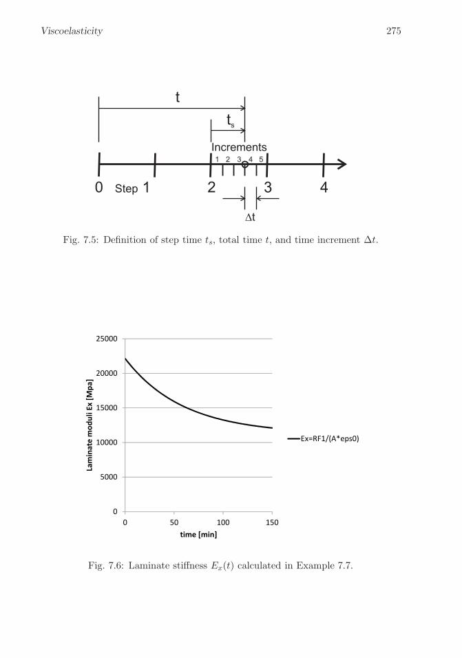
“K15072” — 2013/3/21 — 10:58�

�

�

�

�

�

Viscoelasticity 275

0 Step 1 2 3 4

�t

Increments

t

ts

1 2 3 4 5

Fig. 7.5: Definition of step time ts, total time t, and time increment Δt.

0

5000

10000

15000

20000

25000

0 50 100 150

La

min

ate

mo

du

li E

x [

Mp

a]

time [min]

Ex=RF1/(A*eps0)

Fig. 7.6: Laminate stiffness Ex(t) calculated in Example 7.7.

�

�

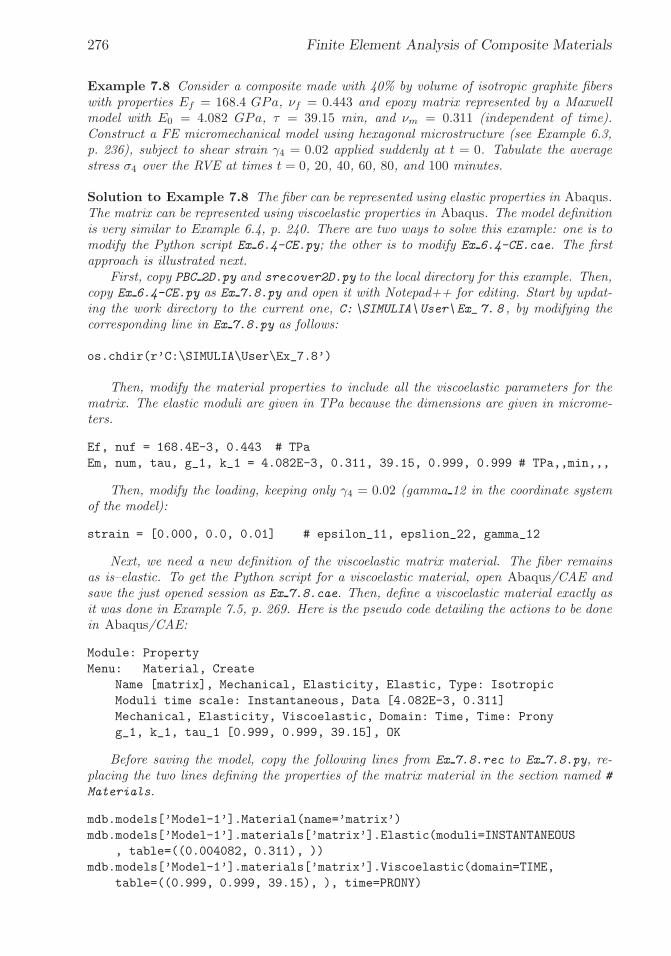
“K15072” — 2013/3/21 — 10:58�

�

�

�

�

�


Example 7.8 Consider a composite made with 40% by volume of isotropic graphite fiberswith properties Ef = 168.4 GPa, νf = 0.443 and epoxy matrix represented by a Maxwellmodel with E0 = 4.082 GPa, τ = 39.15 min, and νm = 0.311 (independent of time).Construct a FE micromechanical model using hexagonal microstructure (see Example 6.3,p. 236), subject to shear strain γ4 = 0.02 applied suddenly at t = 0. Tabulate the averagestress σ4 over the RVE at times t = 0, 20, 40, 60, 80, and 100 minutes.

Solution to Example 7.8 The fiber can be represented using elastic properties in Abaqus.The matrix can be represented using viscoelastic properties in Abaqus. The model definitionis very similar to Example 6.4, p. 240. There are two ways to solve this example: one is tomodify the Python script Ex 6.4-CE.py; the other is to modify Ex 6.4-CE.cae. The firstapproach is illustrated next.

First, copy PBC 2D.py and srecover2D.py to the local directory for this example. Then,copy Ex 6.4-CE.py as Ex 7.8.py and open it with Notepad++ for editing. Start by updat-ing the work directory to the current one, C: \SIMULIA\User\Ex_ 7. 8 , by modifying thecorresponding line in Ex 7.8.py as follows:

os.chdir(r’C:\SIMULIA\User\Ex_7.8’)

Then, modify the material properties to include all the viscoelastic parameters for thematrix. The elastic moduli are given in TPa because the dimensions are given in microme-ters.

Ef, nuf = 168.4E-3, 0.443 # TPa

Em, num, tau, g_1, k_1 = 4.082E-3, 0.311, 39.15, 0.999, 0.999 # TPa,,min,,,

Then, modify the loading, keeping only γ4 = 0.02 (gamma 12 in the coordinate systemof the model):

strain = [0.000, 0.0, 0.01] # epsilon_11, epslion_22, gamma_12

Next, we need a new definition of the viscoelastic matrix material. The fiber remainsas is–elastic. To get the Python script for a viscoelastic material, open Abaqus/CAE andsave the just opened session as Ex 7.8.cae. Then, define a viscoelastic material exactly asit was done in Example 7.5, p. 269. Here is the pseudo code detailing the actions to be donein Abaqus/CAE:

Module: Property


Name [matrix], Mechanical, Elasticity, Elastic, Type: Isotropic

Moduli time scale: Instantaneous, Data [4.082E-3, 0.311]

Mechanical, Elasticity, Viscoelastic, Domain: Time, Time: Prony

g_1, k_1, tau_1 [0.999, 0.999, 39.15], OK

Before saving the model, copy the following lines from Ex 7.8.rec to Ex 7.8.py, re-placing the two lines defining the properties of the matrix material in the section named #

Materials.

mdb.models[’Model-1’].Material(name=’matrix’)

mdb.models[’Model-1’].materials[’matrix’].Elastic(moduli=INSTANTANEOUS

, table=((0.004082, 0.311), ))

mdb.models[’Model-1’].materials[’matrix’].Viscoelastic(domain=TIME,

table=((0.999, 0.999, 39.15), ), time=PRONY)

�

�

“K15072” — 2013/3/21 — 10:58�

�

�

�

�

�

Viscoelasticity 277

and immediately replace numerical values by variable names (to parameterize the script),as follows:

mdb.models[’Model-1’].Material(name=’matrix’)

mdb.models[’Model-1’].materials[’matrix’].Elastic(moduli=INSTANTANEOUS

, table=((Em, num), ))

mdb.models[’Model-1’].materials[’matrix’].Viscoelastic(domain=TIME,

table=((g_1, k_1, tau), ), time=PRONY)

Now, save the model to reset the .rec file. Now, create a viscoelastic step-1 to apply thestrain, and a step-2 to track the ensuing relaxation, exactly as it was done in Example 7.6.Here is the pseudo code detailing the actions to be done in Abaqus/CAE:

Module: Step

Menu: Step, Create


Tab: Basic, Time period [0.001]

Tab: Incrementation, Type: Automatic, viscoelastic tolerance [1E-6], OK

Menu: Step, Create



Tab: Incrementation, Type: Fixed, Maximum number of increments: [200]

Increment Size [1], OK

Before saving the model, copy the following lines from Ex 7.8.rec to Ex 7.8.py, re-placing the line defining the Step-1 in the section named # Step.

mdb.models[’Model-1’].ViscoStep(cetol=1e-06, initialInc=0.001, maxInc=0.001,

minInc=1e-08, name=’Step-1’, previous=’Initial’, timePeriod=0.001)

mdb.models[’Model-1’].ViscoStep(cetol=0.0, initialInc=1.0, maxNumInc=200,

name=’Step-2’, previous=’Step-1’, timeIncrementationMethod=FIXED,

timePeriod=100.0)

Next, update the name of the file to add the BC to the model

execfile(’C:/SIMULIA/User/Ex_7.8/PBC_2D.py’)

Next, update the name of the file in

mdb.saveAs(pathName=’C:/SIMULIA/User/Ex_7.8/Ex_7.8.cae’)

Next, comment out the following lines

# Calculate Stresses and Strains

# execfile(’srecover2D.py’)

# visualize

# o3 = session.openOdb(name=’Job-1.odb’)

# session.viewports[’Viewport: 1’].setValues(displayedObject=o3)

At this point, your updated script should look like the one available in [5, Ex 7.8.py].Next, reset the Abaqus/CAE session to start a new model, and then run the script, asfollows:


Menu: File, Run Script [Ex_7.8.py], OK

�

�

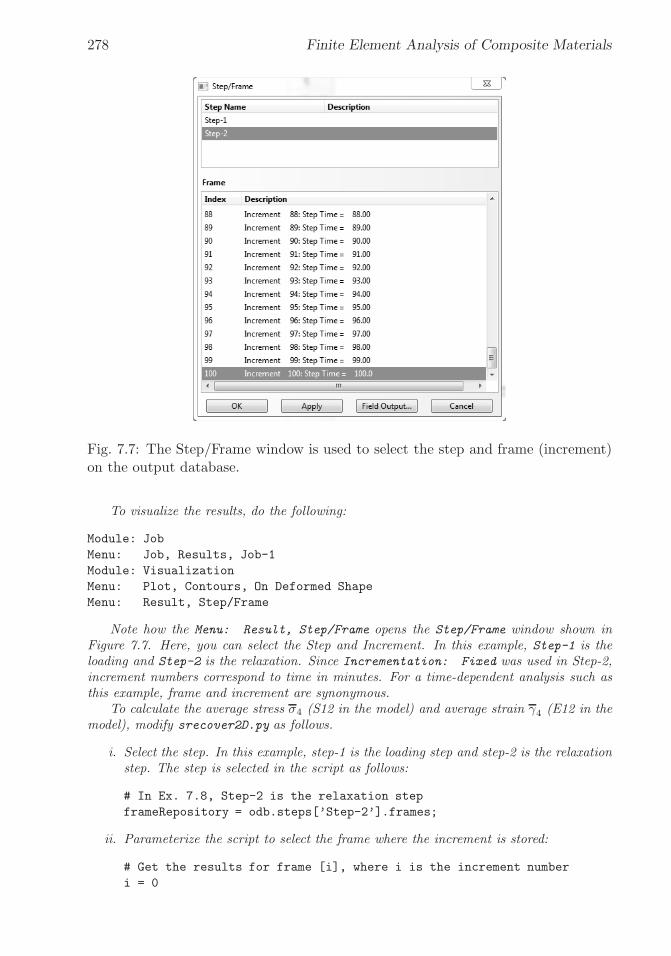
“K15072” — 2013/3/21 — 10:58�

�

�

�

�

�


Fig. 7.7: The Step/Frame window is used to select the step and frame (increment)on the output database.

To visualize the results, do the following:

Module: Job

Menu: Job, Results, Job-1



Menu: Result, Step/Frame

Note how the Menu: Result, Step/Frame opens the Step/Frame window shown inFigure 7.7. Here, you can select the Step and Increment. In this example, Step-1 is theloading and Step-2 is the relaxation. Since Incrementation: Fixed was used in Step-2,increment numbers correspond to time in minutes. For a time-dependent analysis such asthis example, frame and increment are synonymous.

To calculate the average stress σ4 (S12 in the model) and average strain γ4 (E12 in themodel), modify srecover2D.py as follows.

i. Select the step. In this example, step-1 is the loading step and step-2 is the relaxationstep. The step is selected in the script as follows:

# In Ex. 7.8, Step-2 is the relaxation step


ii. Parameterize the script to select the frame where the increment is stored:

# Get the results for frame [i], where i is the increment number

i = 0

�

�

“K15072” — 2013/3/21 — 10:58�

�

�

�

�

�

Viscoelasticity 279

frameS = frameRepository[i].fieldOutputs[’S’].values;

frameE = frameRepository[i].fieldOutputs[’E’].values;

frameIVOL = frameRepository[i].fieldOutputs[’IVOL’].values;

The rest of the script is unchanged. The complete script is given below (also available [5,srecover2D.py]).

# srecover2D.py modified for Ex. 7.8


# Open the output data base for the current Job



# Temporary variable to hold the frame repository speeds up the process

# In Ex. 7.8, Step-2 is the relaxation step


# Get the results for frame [i], where i is the increment number

i = 80

frameS = frameRepository[i].fieldOutputs[’S’].values;

frameE = frameRepository[i].fieldOutputs[’E’].values;

frameIVOL = frameRepository[i].fieldOutputs[’IVOL’].values;

Tot_Vol=0.; # Total Volume

Tot_Stress=0.; # Stress Sum

Tot_Strain = 0.; # Strain Sum

# Calculate Average

for II in range(0,len(frameS)):

Tot_Vol+=frameIVOL[II].data;

Tot_Stress+=frameS[II].data * frameIVOL[II].data;

Tot_Strain+=frameE[II].data * frameIVOL[II].data;


Avg_Strain = Tot_Strain/Tot_Vol;

# from Abaqus Analysis User’s Manual - 1.2.2 Conventions -

# Convention used for stress and strain components

print ’2D Abaqus/Standard Stress Tensor Order: 11-22-33-12’

print ’Average stresses Global CSYS: 11-22-33-12’;

print Avg_Stress;

print ’Average strain Global CSYS: 11-22-33-12’;

print Avg_Strain;

odb.close()

The average values at step-1, increment/frame i = 0, are strain γ4 = 2.0 × 10−2 andaverage stress σ4 = 6.26×10−5 TPa. In fact, the average strain is constant on a relaxationtest. By changing the value of Step (Step-1 or Step-2) and frame (i) in the script, all theresults can be obtained and tabulated as in Table 7.6.

Using an exponential regression it is possible to calculate the values of initial shearmodulus G0

23 = 3.13 GPa and relaxation time τ = 39.97 min that represent the relaxationof the composite in the 23-shear direction using a Maxwell model (see Figure 7.8).

�

�

“K15072” — 2013/3/21 — 10:58�

�

�

�

�

�


Table 7.6: Average stress σ4 over time.Frame: i 0 20 40 60 80 100Time [min] 0 20 40 60 80 100Average σ4 [MPa] 62.6 38.3 23.4 14.4 8.8 5.4

0 20 40 60 80 100 1200

0.5

1

1.5

2

2.5

3

3.5

t [min]

G23

[GP

a]FEM DataMaxwell Model

Fig. 7.8: Shear modulus G23 as a function of time.

Suggested Problems

Problem 7.1 Consider a composite made with 60% by volume of isotropic fibers with prop-erties Ef = 168.4 GPa and νf = 0.443, and epoxy matrix represented by a power law model(7.24) with D0 = 0.222 GPa−1, D1 = 0.0135 (GPa min)−1, m = 0.17, and νm = 0.311.Plot the relaxation C22(t) of the composite as a function of time for 0 < t < 100 minutes.Compare it to the elastic value of the stiffness C22 of the composite and the elastic stiffnessC22 of the matrix.

Problem 7.2 Consider a composite made with 60% by volume of transversely isotropicgraphite fibers with properties EA = 168.4 GPa, ET = 24.82 GPa, νA = 0.443, νT = 0.005,GA = 44.13 GPa, and epoxy matrix represented by a Maxwell model (7.15) with E0 = 4.082GPa, τ = 39.15 min, and νm = 0.311. Plot the relaxation tensor stiffness components C(t)of the composite as a function of time for 0 < t < 100 minutes, compared to the elasticstiffness C of the composite and the elastic stiffness Cm of the matrix.

Problem 7.3 Compute the parameters in the Maxwell model for unidirectional lamina (seeSection 1.14) of carbon/epoxy material used in Problem 7.2. Plot and compare the elasticand viscoelastic properties: E1(t), E2(t), and G12(t). Show all work in a report.

Problem 7.4 Use the user programmable features to implement the Maxwell model con-stitutive equations for a transversally orthotropic lamina material under plane stress con-ditions. Using the viscoelastic materials properties obtained in Problem 7.3, compute theresponse of a [±45/902]s laminate. The thickness of each layer is tk = 1.25 mm. Load

�

�

“K15072” — 2013/3/21 — 10:58�

�

�

�

�

�

Viscoelasticity 281

the sample with uniform edge load Nx = 1 N/mm. Plot the creep compliance Jx(t) of thelaminate as a function of time for 0 > t > 300 minutes.

Problem 7.5 Compute the parameters in the Maxwell model for all the nine engineeringproperties of a [0/90]S laminate. Each layer is 1.25 mm thick. The material is carbon T300and Epoxy 934(NR) with Vf = 0.62 and layer thickness 1.25 mm. Epoxy is represented by aMaxwell model (7.15) with E0 = 4.082 GPa, τ = 39.15 min, and νm = 0.311. Carbon T300is transversely isotropic with axial modulus EA = 202.8 GPa, transverse modulus ET = 25.3GPa, GA = 44.1 GPa, νA = 0.443, and νT = 0.005, where the subscripts A and T indicatethe axial and radial (transverse) directions of the fiber, respectively.

�

�

“K15072” — 2013/3/21 — 10:58�

�

�

�

�

�

�

�

“K15072” — 2013/3/21 — 10:58�

�

�

�

�

�

Chapter 8

Continuum Damage Mechanics

Many modes of damage can be observed in composite materials, including matrixcracks, fiber breakage, fiber-matrix de-bonding, and so on. Much work has beendone trying to quantify each of these damage modes, their evolution with respectto load, strain, time, number of cycles, etc., and their effect on stiffness, remaininglife, etc. Continuum Damage Mechanics (CDM) represents all these failure modesby the effect they have on the mesoscale behavior (lamina level) of the material.That is, CDM calculates the degraded moduli of the laminas and laminate in termsof continuum damage variables. Then, either strength or fracture mechanics failurecriteria are used to detect damage initiation. Finally, damage evolution is predictedin terms of empirical hardening equations set up in terms of additional parameters,such as the hardening exponent used for metal plasticity. For example, a form ofCDM is used in Chapter 10 to represent the degradation of the interface betweenlaminas.

Hardening equations require non-standard experimentation to adjust the addi-tional, empirical parameters. Since the parameters are adjusted to the model, someshortcomings of the model may be masked by the fitting of the parameters. Froma thermodynamics point of view, damage variables are the state variables of theformulation, and they are not measurable. This is in contrast to micromechanics ofdamage models (Chapter 9) and metal plasticity where the state variables, i.e., crackdensity and plastic strain, are measurable. From a practical point of view, CDMmajor shortcoming is the need for additional experimentation to determine parame-ters that are particular to each model. Furthermore, since the state variables are notmeasurable, the additional parameters need to be adjusted to the model throughthe loss of stiffness, which may not be sufficiently sensitive to damage [55].

One notable effect of damage is a reduction of stiffness, which can be used todefine damage [56]. One-dimensional models are used in Section 8.1 to introducethe concepts. The theoretical formulation for the general three-dimensional case isdeveloped in Sections 8.2-8.4.

283

�

�

“K15072” — 2013/3/21 — 10:58�

�

�

�

�

�


8.1 One-Dimensional Damage Mechanics

The development of a one-dimensional damage mechanics solution involves the def-inition of three major entities: 1) a suitable damage variable, 2) an appropriatedamage activation function, and 3) a convenient damage evolution, or kinetic equa-tion.

8.1.1 Damage Variable

Consider a composite rod of nominal area Ã, unloaded, and free of any damage(Figure 8.1.a). Upon application of a sufficiently large load P , damage appears(Figure 8.1.b). On a macroscopic level, damage can be detected by the loss ofstiffness of the material. In CDM, damage is represented by a state variable D,called damage variable, which represents the loss of stiffness [56]

D = 1− E/ ˜E (8.1)

where ˜E is the initial (virgin) Young’s modulus, and E is the modulus after dam-age.1 Earlier work [57] conceptualized damage as the reduction of area due toaccumulation of micro-cracks having the same effect as the actual damage

D = 1−A/ Ã (8.2)

where Ã, A are the initial and remaining cross-sectional areas, respectively. Thecomplement to damage is the integrity [58]

Ω = 1−D = A/ Ã (8.3)

which can be interpreted as the remaining cross-sectional area ratio, using the orig-inal area as basis. It is noted that, in principle, damage is a measurable parameter,which could be determined by measuring the damaged area, remaining area, ormore practically measuring the initial and remaining moduli. Therefore, in ther-modynamic terms, damage is a measurable state variable, in the same sense as thetemperature is a measurable state variable that quantifies in macroscopic terms therandom agitation of atoms, molecules, and other elementary particles. While it ispossible, but extremely difficult, to track the agitation of atoms and molecules, itis very easy to measure the temperature with a thermometer or other device. Thesame holds true for damage in composite materials.

The analysis of a structural component is done in terms of the nominal area Ã,which is the only one known to the designer. The remaining area A = (1−D) Ã is notknown a priori. The nominal stress is σ = P/ Ã. Neglecting stress concentrations atthe tips of the fictitious cracks representing damage in the damaged configuration(Figure 8.1.b), the value of effective stress2 acting on the remaining area A is σ =P/A > P/ Ã.

1See also (8.10).2Even taking into account stress concentrations, the volume average of the distribution of ef-

fective stress in the representative volume element (RVE, see Chapter 6) is still σ = P/A.

�

�

“K15072” — 2013/3/21 — 10:58�

�

�

�

�

�

Continuum Damage Mechanics 285

~~~~

~

Fig. 8.1: (a) Unstressed material configuration, (b) stressed material configurationwith distributed damage, (c) effective configuration.

Therefore, we can envision a configuration (Figure 8.1.c) free of damage, withnominal area ˜A, loaded by nominal stress σ, but internally subjected to effectivestress σ and degraded stiffness E. Thus, the effective configuration allows us toperform structural analysis using the nominal geometry but effectively taking intoaccount the increase of effective stress and the decrement of stiffness caused bydamage.

In the undamaged configuration (a), D = 0, σ = σ, ε = ε, and Hooke’s law is

σ = ˜E ε (8.4)

where ˜E is a constant. In the effective configuration (c)

σ = E ε (8.5)

where E is a function of D. The principle of strain equivalence assumes that thestrain is the same in the configurations (b) and (c), or ε = ε. Starting with thenominal stress σ = P/ ˜A, multiplying by A/A and using (8.3), the relationshipbetween effective stress σ and nominal stress σ (under strain equivalence) is

σ = σ [1−D] (8.6)

Using (8.6), (8.4), and ε = ε in (8.5), the apparent modulus is a function of thedamage D

E(D) = ˜E [1−D] (8.7)

The principle of energy equivalence [59] states that the elastic strain energy isidentical in the configurations (b) and (c). That is, σ : ε = σ : ε, which is satisfiedby

σ = σ [1−D]ε = ε [1−D]

(8.8)

�

�

“K15072” — 2013/3/21 — 10:58�

�

�

�

�

�


Substituting (8.8) in (8.5) yields

E(D) = ˜E [1−D]2 (8.9)

which redefines the damage variable as

D = 1−√

E/ ˜E (8.10)

Every state variable has a conjugate thermodynamic force driving its growth.In plasticity, the measurable state variable is the plastic strain tensor εp, whichis driven to grow by its conjugate thermodynamic force, the stress tensor σ. Thethermodynamic damage force Y is defined as conjugate to the state variable D.

A kinetic equation D(Y ) governs the growth of the state variable D as a functionof its conjugate thermodynamic force Y . In principle, any relevant variable can bechosen as independent variable Y to define the kinetic equation D(Y ), as long asit is independent of its conjugate state variable. When the damage D is a scalarand it is used to analyze one-dimensional problems, various authors have chosenindependent variables in the form of strain ε [60], effective stress σ [61, 62], excessenergy release rate G− 2γc [63], and so on. However, the choice is better based onthe appropriate form of the thermodynamic principle governing the problem, as itis shown in Section 8.3.

8.1.2 Damage Threshold and Activation Function

The elastic domain is defined by a threshold value for the thermodynamic forcebelow which no damage occurs. When the load state is in the elastic domain,damage does not grow. When the load state reaches the limit of the elastic domain,additional damage occurs. Furthermore, the elastic domain modifies its size orhardens. Typical one-dimensional responses of two materials are shown in Figure8.2. Initially the elastic domain is defined by the initial threshold values, σ ≤ σ0 andε ≤ ε0. While the load state is inside this domain, no damage occurs. When the loadstate is higher than the threshold, damage increases and the threshold changes. Theelastic domain may evolve as hardening or softening. A stress threshold increasesfor materials with hardening (see Figure 8.2a), and it decreases for materials withsoftening (see Figure 8.2b). On the other hand, a strain or effective stress thresholdalways increases for hardening and softening behavior, as shown in Figure 8.2.

The elastic domain can be defined by the damage activation function g as

g = g − γ ≤ 0 (8.11)

where g is a positive function (norm) that depends on the independent variable(in a one-dimensional case a scalar Y ) and γ is the updated damage threshold forisotropic hardening. According to the positive dissipation principle (see Section 8.3and (8.82),(8.97)), the updated damage threshold γ can be written as

γ = γ(δ) + γ0 (8.12)

�

�

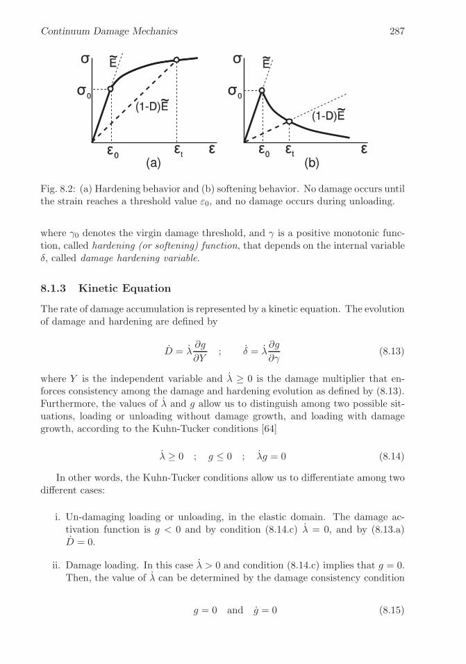
“K15072” — 2013/3/21 — 10:58�

�

�

�

�

�


Fig. 8.2: (a) Hardening behavior and (b) softening behavior. No damage occurs untilthe strain reaches a threshold value ε0, and no damage occurs during unloading.

where γ0 denotes the virgin damage threshold, and γ is a positive monotonic func-tion, called hardening (or softening) function, that depends on the internal variableδ, called damage hardening variable.

8.1.3 Kinetic Equation

The rate of damage accumulation is represented by a kinetic equation. The evolutionof damage and hardening are defined by

D = λ∂g

∂Y; δ = λ

∂g

∂γ(8.13)

where Y is the independent variable and λ ≥ 0 is the damage multiplier that en-forces consistency among the damage and hardening evolution as defined by (8.13).Furthermore, the values of λ and g allow us to distinguish among two possible sit-uations, loading or unloading without damage growth, and loading with damagegrowth, according to the Kuhn-Tucker conditions [64]

λ ≥ 0 ; g ≤ 0 ; λg = 0 (8.14)

In other words, the Kuhn-Tucker conditions allow us to differentiate among twodifferent cases:

i. Un-damaging loading or unloading, in the elastic domain. The damage ac-tivation function is g < 0 and by condition (8.14.c) λ = 0, and by (8.13.a)D = 0.

ii. Damage loading. In this case λ > 0 and condition (8.14.c) implies that g = 0.Then, the value of λ can be determined by the damage consistency condition

g = 0 and g = 0 (8.15)

�

�

“K15072” — 2013/3/21 — 10:58�

�

�

�

�

�


Example 8.1 Compute λ for a one-dimensional model under tensile load where the inde-pendent variable is the effective stress Y = σ, the activation function is defined by g = σ,and the hardening function is defined by

γ = (F0 − FR)δ + F0

where F0 and FR are the initial threshold and the strength of the strongest microscopicelement in the material, respectively.

Solution to Example 8.1 The damage activation function g is defined as

g = g − γ = σ − [(F0 − FR)δ + F0] ≤ 0

Therefore,∂g

∂σ= +1 ;

∂g

∂γ= −1

Using (8.13), the kinetic equations can be written as

D = λ∂g

∂σ= λ ; δ = λ

∂g

∂γ= −λ

When new damage appears, the consistency conditions (8.15) yield

g = 0 ⇒ γ = σ

and

g = 0 ⇒ g =∂g

∂σ˙σ +

∂g

∂γ˙γ = ˙σ − ˙γ = 0

where˙γ =

∂γ

∂δδ = (F0 − FR)(−λ) = (FR − F0)λ

Substituting into the second consistency condition (8.15) we obtain λ as

λ =1

FR − F0

˙σ

8.1.4 Statistical Interpretation of the Kinetic Equation

Let’s assume that individual damaging events are caused by the failure of micro-scopic elements inside the material (e.g., fiber breaks, matrix cracks, fiber-matrixde-bond, etc.). Furthermore, assume each of these material points has a failurestrength σ and that the collection of failure strengths for all these points, i.e., el-ements failing at a certain stress σ over the total number of elements available, isrepresented by a probability density f(σ) (Figure 8.3.b). The fraction of elementsbroken during an effective stress excursion from zero to σ provides a measure ofdamage

D(σ) =

∫ σ

0f(σ′)dσ′ = F (σ) (8.16)

where F (σ) is the cumulative probability (Figure 8.3.b) corresponding to the prob-ability density f(σ), and σ′ is a dummy integration variable. Then, the kineticequation in terms of effective stress σ is

D =dD

dσ˙σ = f(σ) ˙σ (8.17)

�

�

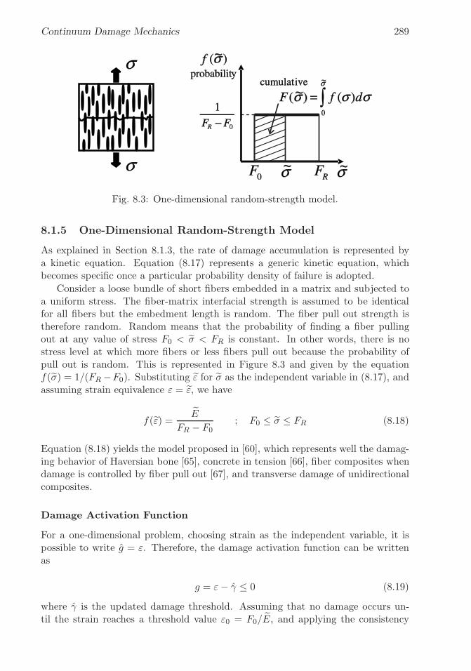
“K15072” — 2013/3/21 — 10:58�

�

�

�

�

�


~

~~

~ ~

Fig. 8.3: One-dimensional random-strength model.

8.1.5 One-Dimensional Random-Strength Model

As explained in Section 8.1.3, the rate of damage accumulation is represented bya kinetic equation. Equation (8.17) represents a generic kinetic equation, whichbecomes specific once a particular probability density of failure is adopted.

Consider a loose bundle of short fibers embedded in a matrix and subjected toa uniform stress. The fiber-matrix interfacial strength is assumed to be identicalfor all fibers but the embedment length is random. The fiber pull out strength istherefore random. Random means that the probability of finding a fiber pullingout at any value of stress F0 < σ < FR is constant. In other words, there is nostress level at which more fibers or less fibers pull out because the probability ofpull out is random. This is represented in Figure 8.3 and given by the equationf(σ) = 1/(FR −F0). Substituting ε for σ as the independent variable in (8.17), andassuming strain equivalence ε = ε, we have

f(ε) =˜E

FR − F0; F0 ≤ σ ≤ FR (8.18)

Equation (8.18) yields the model proposed in [60], which represents well the damag-ing behavior of Haversian bone [65], concrete in tension [66], fiber composites whendamage is controlled by fiber pull out [67], and transverse damage of unidirectionalcomposites.

Damage Activation Function

For a one-dimensional problem, choosing strain as the independent variable, it ispossible to write g = ε. Therefore, the damage activation function can be writtenas

g = ε− γ ≤ 0 (8.19)

where γ is the updated damage threshold. Assuming that no damage occurs un-til the strain reaches a threshold value ε0 = F0/ ˜E, and applying the consistency

�

�

“K15072” — 2013/3/21 — 10:58�

�

�

�

�

�


conditions (8.15) and using (8.19), the updated damage threshold γ is given by thehighest value of strain seen by the material, or

γ = max(ε0, ε) (8.20)

Kinetic Equation

The kinetic equation (8.17) for the case of random strength (8.18) in terms of strainsε = ε can be expressed as

D =dD

dεε =

{

˜E/(FR − F0)ε when ; ε > γ0 otherwise

(8.21)

In this case, the independent variable is ε, and using (8.19), the kinetic equation(8.13) reduces to

D = λ (8.22)

Using the Kuhn-Tucker conditions and (8.21), the consistency condition (8.15)reduces to

λ = ˜E/(FR − F0)ε (8.23)

when damage occurs and λ = 0 otherwise. In this particular case, the kineticequation is known explicitly (8.22-8.23). Therefore, it is not necessary to evaluatethe evolution of hardening (8.12) because hardening is computed explicitly by (8.20).Note that (8.23) is identical to the solution of Example 8.1 because the hardeningfunction was chosen deliberately to yield this result.

Secant Constitutive Equation

In this particular case, the damage variable is active when tensile load appears, andit can be obtained by integrating (8.21) as

Dt = ˜Eγ − ε0FR − F0

when ε > 0 (8.24)

Note that the damage state does not depend on the actual load state ε; itonly depends on the history of the load state γ. In this example, crack closure isassumed in compression, damage becomes passive, and Dc = 0. Mathematically,damage under unilateral contact conditions can be defined by the following equation

D = Dt〈ε〉|ε| +Dc

〈−ε〉|ε| (8.25)

where the McCauley operator 〈x〉 is defined as 〈x〉 := 12 (x+ |x|).

Substituting (8.24) into (8.5), and using strain equivalence, yields the followingconstitutive equation

σ = E(D) ε =

⎧

⎪

⎨

⎪

⎩

(

1− ˜Eγ − ε0FR − F0

)

˜E ε when ε > 0

˜E ε when ε < 0

(8.26)

�

�

“K15072” — 2013/3/21 — 10:58�

�

�

�

�

�


Tangent Constitutive Equation

In a finite element formulation, it is necessary to provide the constitutive equationin rate form, where the rates of stress σ and strain ε are expressed as functionsof pseudotime. In this particular case, the tangent constitutive equation can beobtained by differentiation of the secant constitutive equation as

σ = E(D)ε + E(D)ε (8.27)

The term E(D) is zero when new damage does not appear, i.e., when there iselastic loading or unloading. When damaging behavior occurs (8.20) yields γ = ε,and differentiating E(D) in (8.26) we obtain

E(D) = −˜E2

FR − F0ε (8.28)

Substituting (8.28) into (8.27) if damage occurs, or E(D) = 0 if no damageoccurs, the tangent constitutive equation can be written as

σ =

⎧

⎨

⎩

(

1− ˜E2γ − ε0FR − F0

)

˜E ε when ε > γ

E(D) ε when ε < γ(8.29)

Model Identification

The initial damage threshold ε0 represents the minimum strain to initiate damageand it is proportional to F0 as follows

F0 = ˜Eε0 (8.30)

Under load control, a tensile specimen breaks at ε = γ = εcr when dσ/dε = 0.Then, using (8.29.a), the only unknown parameter in the model can be computedas

FR = 2 ˜Eεcr (8.31)

The material parameters F0 and FR can be calculated from the experimentaldata using (8.30) and (8.31) with ˜E being the undamaged modulus of the material.The measurable values ε0 and εcr can be obtained easily from material testing atthe macroscopic level.

For the particular case ε0 = 0, using (8.24) and (8.31) at ε = εcr, the criticaldamage at failure under tensile load is

Dcr = 0.5 (8.32)

Therefore the critical effective stress is

σT cr = ˜Eεcr = 0.5FR (8.33)

�

�

“K15072” — 2013/3/21 — 10:58�

�

�

�

�

�


Fig. 8.4: One-dimensional random-strength model.3

and using (8.7) the critical applied stress is

σT cr = 0.25FR (8.34)

Therefore, in a material with initial threshold ε0 = 0, a tensile specimen underload control fails when D = 1/2 and applied stress FR/4.

A conservative estimate of transverse tensile strength of a fiber reinforced lam-ina can be obtained assuming that the fiber-matrix bond strength is negligible. Inthe limit, only the matrix between fibers carries the transverse load, with the fibersacting as holes. In this limit case, the matrix links can be assumed to have a ran-dom distribution of strength (8.18). Therefore, the random-strength model (8.29)applies, and the critical damage for transverse tensile loading of unidirectional fiber-reinforced lamina can be estimated by (8.32) as Dcr

2t = 0.5. At the present time,there is no model available to estimate the critical transverse-direction compressiondamage Dcr

2c.

Example 8.2 A beam of rectangular cross section, width b = 100 mm and height 2h =200 mm, is subjected to pure bending. The bending moment at failure is 25.1MN mm. Thebeam is made of carbon/epoxy composite with randomly oriented short fibers with undamaged

Young’s modulus ˜E = 46 GPa. Find the bending moment at failure in terms of FR in (8.21).Assume that the material does not damage in compression and it has a random distributionof strength in tension, with the strongest material element having unknown strength FR > 0and F0 = 0. Determine FR using the data given.

Solution to Example 8.2 This problem was solved in [67]. With reference to Figure 8.4,M is the applied bending moment, and yc, yt are the distances from the neutral axis to thestress resultants Nc, Nt on the tensile and compression portions of the beam.

Denoting by εt and εc the tension and compression strain on the outer surfaces of thebeam, y0 the distance from the mid-plane to the neutral surface, and assuming linear strain

3Reprinted from Mechanics of Materials, vol. 8, issue 2-3, D. Kracjcinovic, Damage Mechanics,Fig. 2.11, p. 134, copyright (1989), with permission from Elsevier.

�

�

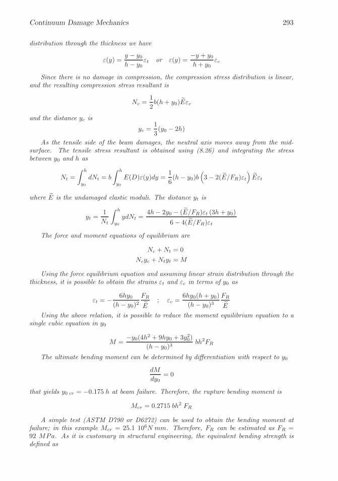
“K15072” — 2013/3/21 — 10:58�

�

�

�

�

�


distribution through the thickness we have

ε(y) =y − y0h− y0

εt or ε(y) =−y + y0h+ y0

εc

Since there is no damage in compression, the compression stress distribution is linear,and the resulting compression stress resultant is

Nc =1

2b(h+ y0) ˜Eεc

and the distance yc is

yc =1

3(y0 − 2h)

As the tensile side of the beam damages, the neutral axis moves away from the mid-surface. The tensile stress resultant is obtained using (8.26) and integrating the stressbetween y0 and h as

Nt =

∫ h

y0

dNt = b

∫ h

y0

E(D)ε(y)dy =1

6(h− y0)b

(

3− 2( ˜E/FR)εt

)

˜Eεt

where ˜E is the undamaged elastic moduli. The distance yt is

yt =1

Nt

∫ h

y0

ydNt =4h− 2y0 − ( ˜E/FR)εt (3h+ y0)

6− 4( ˜E/FR)εt

The force and moment equations of equilibrium are

Nc +Nt = 0

Ncyc +Ntyt =M

Using the force equilibrium equation and assuming linear strain distribution through thethickness, it is possible to obtain the strains εt and εc in terms of y0 as

εt = − 6hy0(h− y0)2

FR

˜E; εc =

6hy0(h+ y0)

(h− y0)3FR

˜E

Using the above relation, it is possible to reduce the moment equilibrium equation to asingle cubic equation in y0

M =−y0(4h2 + 9hy0 + 3y20)

(h− y0)3bh2FR

The ultimate bending moment can be determined by differentiation with respect to y0

dM

dy0= 0

that yields y0 cr = −0.175 h at beam failure. Therefore, the rupture bending moment is

Mcr = 0.2715 bh2 FR

A simple test (ASTM D790 or D6272) can be used to obtain the bending moment atfailure; in this example Mcr = 25.1 106N mm. Therefore, FR can be estimated as FR =92 MPa. As it is customary in structural engineering, the equivalent bending strength isdefined as

�

�

“K15072” — 2013/3/21 — 10:58�

�

�

�

�

�



σBcr =Mcr

S= 0.407 FR

where S is the section modulus (for a rectangular beam S = 23bh

2). Note that according to(8.34), the tensile strength of the same material assuming the same kinetic equation (8.26)would be σT cr = 0.25 FR. This gives a ratio of equivalent bending to tensile strength equal toσB cr/σT cr = 1.63, which is in good agreement with experimental data σB cr/σT cr = 1.6 [68]obtained for unreinforced concrete and also with the value σB cr/σT cr = 1.5 recommendedby the ACI Code [69].

8.1.6 Fiber-Direction, Tension Damage

If a lamina is subjected to tensile stress in the fiber direction, it is reasonableto assume that the matrix carries only a small portion of the applied load andno damage is expected in the matrix during loading. Then, the ultimate tensilestrength of the composite lamina can be accurately predicted by computing thestrength of a bundle of fibers.

Fiber strength is a function of the gauge length used during fiber strength tests.The length scale that determines how much of the fiber strength is actually used ina composite is the ineffective length δ. Starting at a fiber break point, the ineffectivelength is that length over which a fiber recovers a large percentage of its load (say,90%). Rosen [70] recognized this fact and proposed that the longitudinal ultimatestrength of fibers embedded in a ductile-matrix can be accurately predicted by thestrength of a dry bundle of fibers with length δ.

A dry bundle is defined as a number of parallel fibers of some given length anddiameter which, if unbroken, carry the same load. After a fiber within a dry bundlefails, the load is shared equally by the remaining unbroken fibers. A dry bundletypically refers to fibers which have not yet been combined with a matrix. Astensile load is slowly applied to a dry bundle of fibers, the weaker fibers (with largeflaw sizes) begin to fail and the stress on the remaining unbroken fibers increasesaccordingly. The Weibull expression [71]

F (σ) = 1− exp

(

− δ

L0

(

σ

σ0

)m)

(8.35)

is often used to describe the cumulative probability F (σ) that a fiber of length δ willfail at or below an effective stress σ. The values of σ0 and m, which represent the

�

�

“K15072” — 2013/3/21 — 10:58�

�

�

�

�

�


characteristic strength of the fiber, and the dispersion of fiber strength, respectively,can be determined from fiber strength experiments performed with a gauge lengthL0. Equation (8.35) can be simplified as

F (σ) = 1− exp (−δασm) (8.36)

where

α =1

L0σm0

=

[

Γ(1 + 1/m)

σav

]m 1

L0(8.37)

where Γ(x) is the Gamma function [46]; σav is the average strength for a gaugelength L0. Equation (8.36) provides the percentage of fibers in a bundle whichare broken as a function of the actual (or apparent) stress in the unbroken fibers.The percentage of fibers which are unbroken is 1 − F (σ). The apparent stress orbundle stress σ = σb is equal to the applied load divided by the total fiber cross-sectional area. It is also equal to the product of the stress in unbroken fibers andthe percentage of fibers which are unbroken

σ = σb = σ exp(−δασm) (8.38)

The value σmax, which maximizes (8.38), can be easily determined and is givenby

σmax = (δαm)−1/m (8.39)

The maximum (or critical) bundle strength σcr is determined by substituting(8.39) into (8.38)

σcr = (δαm)−1/m exp(−1/m) = (δαme)−1/m (8.40)

where e is the basis of the natural logarithms. The composite longitudinal tensilestrength is [1, (4.82)]

F1t =

[

Vf +Em

Ef(1− Vf )

]

σcr (8.41)

where Vf is the fiber volume fraction, and Ef and Em are the fiber and matrixelastic Young’s moduli, respectively.

Combining (8.36) and (8.39), we get

Dcr1t = 1− exp(−1/m) (8.42)

Therefore, the critical or maximum damage Dcr1t for longitudinal tensile load-

ing can be computed as the area fraction of broken fibers in the lamina prior tocatastrophic failure [61, 62], which turns out to be a function of the Weibull shapemodulus m only.

�

�

“K15072” — 2013/3/21 — 10:58�

�

�

�

�

�


Example 8.3 The data sheet of carbon fiber T300 from TorayTM Carbon Fibers, Inc. givesaverage tensile strength of the fiber σav = 3.53 GPa, and tensile modulus Ef = 230 GPa.Also, the same data sheet provides results of tensile tests of a uni-directional (UD) compositewith epoxy Em = 4.5 GPa and fiber volume fraction Vf = 0.6. The tensile strength reportedis F1t = 1860MPa. Using this experimental data, and assuming a Weibull shape parameterm = 8.9, identify the damage model under tensile load. Then, formulate the damage modeland implement it in Abaqus for a one-dimensional bar element. Finally, obtain the strainvs. stress response of the UD composite.

Solution to Example 8.3

MODEL IDENTIFICATION From (8.41) and using the experimental data available,it is possible to obtain σcr as

σcr =F1t

Vf + Em

Ef(1− Vf )

= 3060 MPa

Then, the product δα can be obtained using (8.40) as

δα =(σcr)

−m

me= 3.92 10−33

The properties Ef = 230 GPa, m = 8.9, and δα = 3.92× 10−33 are sufficient for theidentification of the model.

MODEL FORMULATION Following a procedure similar to that shown in Section 8.1.5to implement a damage model, the following items are needed

Damage Activation Function In this example, the effective stress is chosen as theindependent variable. Therefore, the damage activation function can be writtenas

g = σ − γ ≤ 0 (8.43)

where γ is the updated damage threshold. Assuming an initial threshold valueσ0 = 0, from the consistency conditions (8.15) and (8.19), γ is given by thehighest value of effective stress seen by the material

γ = max(0, σ) (8.44)

Secant Constitutive Equation In this example, the kinetic equation (8.1.3) isavailable in integral form and given explicitly by (8.36) as

D = 1− exp (−δαγm) when σ > 0; ε > 0 (8.45)

where the damage state does not depend on the actual load state σ; it onlydepends on the load history state γ.

Substituting (8.45) into (8.5) and (8.7), and using strain equivalence, yields theconstitutive equation

σ = E(D) ε = exp (−δαγm) ˜E ε when ε > 0 (8.46)

�

�

“K15072” — 2013/3/21 — 10:58�

�

�

�

�

�


Tangent Constitutive Equation The tangent constitutive equation can be obtainedby differentiating the secant constitutive equation as

σ = E(D)ε+ E(D)ε (8.47)

The factor E(D) is zero when no new damage appears, i.e., during elastic load-

ing or unloading. When damage occurs, (8.44) yields γ = ˜Eε, and differentiat-ing E(D) in (8.46) we obtain

E(D) = −δαmγm−1 exp (−δαγm) ˜E2ε (8.48)

The tangent constitutive equation is obtained by substituting (8.48) into (8.47)when damage occurs, or E(D) = 0 when no new damage appears. Therefore,the tangent constitutive equation can be written as

σ =

{

(1− δαmγm) exp (−δαγm) ˜E ε when ε > γ/ ˜E

E(D) ε when ε < γ/ ˜E(8.49)

NUMERICAL ALGORITHM The one-dimensional damage model is implemented inAbaqus using the UMAT subroutine umat1d83.for, available in [5]. The followingitems describe the procedure used to explicitly evaluate the damage constitutive equa-tion.4

i. Read the strain at time tεt

ii. Compute the effective stress (assuming strain equivalence)

σt = ˜Eεt

iii. Update the threshold value

γt = max(γt−1, σt)

iv. Compute the damage variable

Dt = 1− exp (−δα(γt)m)

v. Compute the nominal stress

σt = (1 −Dt) ˜E εt

vi. Compute the tangent stiffness

Edamt =

{

(1− δαm(γt)m) exp (−δα(γt)m) ˜E when γt > γt−1

(1 −Dt) ˜E when γt = γt−1

MODEL RESPONSE The pseudo code below and user subroutine umat1d83.for, avail-able in [5], are used to model a one-dimensional bar representative of a carbon fiberUD composite. The nominal stress-strain response is shown with a solid line in Fig-ure 8.6. The UD composite fails at εcr = 1.5%, in good agreement with the strain tofailure reported by Toray.

4See Section 8.4.1 for those cases for which it is not possible to integrate the constitutive equationexplicitly.

�

�

“K15072” — 2013/3/21 — 10:58�

�

�

�

�

�


i. Retrieve Ex 2.4.cae or use the instructions given in Example 2.6 (p. 79) torecreate the model




ii. Modify the geometry

Module: Part

# on the left tree, expand (+) the following items:

# expand: Model-1, # expand: Parts (1)

# expand: Part-1, # expand: Features, # expand: Wire-1

# right-click: Sketch, Edit

# use dimension tool to change the length to [10]

Menu: Add, Dimension

# pick: Line, # create the dimension below the line, [10]

X # to close the command, Done

Menu: Feature, Regenerate

Module: Assembly


iii. Delete the existing Material-1 and create a new Material-1 with the propertiesand parameters required by the user material. Modify the cross section.

Module: Property


# select: Material-1, Delete, Yes

Create, Name [Material-1], General, User Material

Mechanical Constants [203.0E3 8.9 3.92E-33]

# or right click Read from File, File: [props.txt]

General, Depvar, Number of state variables [2],

# SDV1: effective stress, see umat1d83.for

# SDV2: damage, see umat1d83.for

OK, # close Material Manager pop-up window

Menu: Section, Edit, Section-1, Cross-sectional area: [1.0], OK

iv. Delete the load and add a specified displacement

Module: Load

Menu: Load, Delete, Load-1, Yes

Menu: BC, Create

Name [BC-2], Step: Step-1, Disp/Rota, Cont

# pick: free-end node, Done, # checkmark: U1 [0.25], OK

v. Remesh with five elements

Module: Mesh

# to make the instance "independent", on the left tree

# expand: Assembly, # expand: Instances

# right-click: Part-1-1, Make Independent


Menu: Mesh, Element Type

Element Library: Standard, Geometric Order: Linear

Family: Trus # verify T2D2 is chosen, OK

�

�

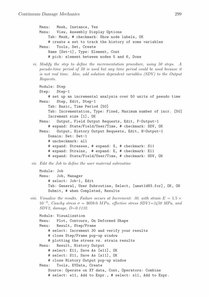
“K15072” — 2013/3/21 — 10:58�

�

�

�

�

�



Menu: View, Assembly Display Options

Tab: Mesh, # checkmark: Show node labels, OK

# create a set to track the history of some variables


Name [Set-1], Type: Element, Cont

# pick: element between nodes 5 and 6, Done

vi. Modify the step to define the incrementation procedure, using 50 steps. Apseudo-time period of 50 is used but any time period could be used because itis not real time. Also, add solution dependent variables (SDV) to the OutputRequests.

Module: Step

Step: Step-1

# set up an incremental analysis over 50 units of pseudo time


Tab: Basic, Time Period [50]

Tab: Incrementation, Type: Fixed, Maximum number of incr. [50]

Increment size [1], OK


# expand: State/Field/User/Time, # checkmark: SDV, OK


Domain: Set: Set-1

# uncheckmark: all

# expand: Stresses, # expand: S, # checkmark: S11

# expand: Strains, # expand: E, # checkmark: E11

# expand: State/Field/User/Time, # checkmark: SDV, OK

vii. Edit the Job to define the user material subroutine

Module: Job

Menu: Job, Manager

# select: Job-1, Edit

Tab: General, User Subroutine, Select, [umat1d83.for], OK, OK


viii. Visualize the results. Failure occurs at Increment: 30, with strain E = 1.5 ×10−2, Cauchy stress σ = 3059.0 MPa, effective stress SDV1=3450 MPa, andSDV2, damage, D=0.1132.



Menu: Result, Step/Frame

# select: Increment 30 and verify your results

# close Step/Frame pop-up window

# plotting the stress vs. strain results

Menu: Result, History Output

# select: E11, Save As [e11], OK

# select: S11, Save As [s11], OK

# close History Output pop-up window

Menu: Tools, XYData, Create

Source: Operate on XY data, Cont, Operators: Combine

# select: e11, Add to Expr., # select: s11, Add to Expr.

�

�

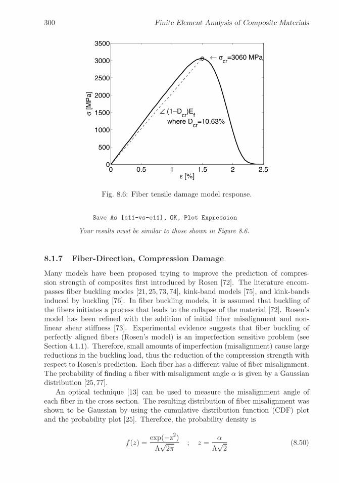
“K15072” — 2013/3/21 — 10:58�

�

�

�

�

�


0 0.5 1 1.5 2 2.50

500

1000

1500

2000

2500

3000

3500

ε [%]

σ [M

Pa]

← σcr

=3060 MPa

∠ (1−Dcr

)Ef

where Dcr

=10.63%

Fig. 8.6: Fiber tensile damage model response.

Save As [s11-vs-e11], OK, Plot Expression

Your results must be similar to those shown in Figure 8.6.

8.1.7 Fiber-Direction, Compression Damage

Many models have been proposed trying to improve the prediction of compres-sion strength of composites first introduced by Rosen [72]. The literature encom-passes fiber buckling modes [21, 25, 73, 74], kink-band models [75], and kink-bandsinduced by buckling [76]. In fiber buckling models, it is assumed that buckling ofthe fibers initiates a process that leads to the collapse of the material [72]. Rosen’smodel has been refined with the addition of initial fiber misalignment and non-linear shear stiffness [73]. Experimental evidence suggests that fiber buckling ofperfectly aligned fibers (Rosen’s model) is an imperfection sensitive problem (seeSection 4.1.1). Therefore, small amounts of imperfection (misalignment) cause largereductions in the buckling load, thus the reduction of the compression strength withrespect to Rosen’s prediction. Each fiber has a different value of fiber misalignment.The probability of finding a fiber with misalignment angle α is given by a Gaussiandistribution [25,77].

An optical technique [13] can be used to measure the misalignment angle ofeach fiber in the cross section. The resulting distribution of fiber misalignment wasshown to be Gaussian by using the cumulative distribution function (CDF) plotand the probability plot [25]. Therefore, the probability density is

f(z) =exp(−z2)

Λ√2π

; z =α

Λ√2

(8.50)

�

�

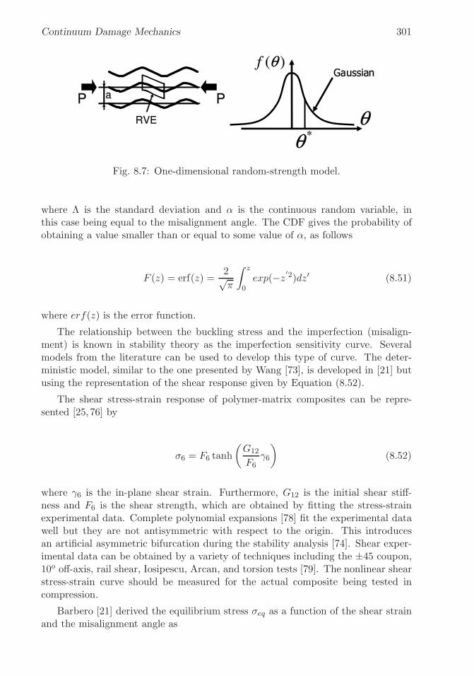
“K15072” — 2013/3/21 — 10:58�

�

�

�

�

�



where Λ is the standard deviation and α is the continuous random variable, inthis case being equal to the misalignment angle. The CDF gives the probability ofobtaining a value smaller than or equal to some value of α, as follows

F (z) = erf(z) =2√π

∫ z

0exp(−z′2)dz′ (8.51)

where erf(z) is the error function.

The relationship between the buckling stress and the imperfection (misalign-ment) is known in stability theory as the imperfection sensitivity curve. Severalmodels from the literature can be used to develop this type of curve. The deter-ministic model, similar to the one presented by Wang [73], is developed in [21] butusing the representation of the shear response given by Equation (8.52).

The shear stress-strain response of polymer-matrix composites can be repre-sented [25,76] by

σ6 = F6 tanh

(

G12

F6γ6

)

(8.52)

where γ6 is the in-plane shear strain. Furthermore, G12 is the initial shear stiff-ness and F6 is the shear strength, which are obtained by fitting the stress-strainexperimental data. Complete polynomial expansions [78] fit the experimental datawell but they are not antisymmetric with respect to the origin. This introducesan artificial asymmetric bifurcation during the stability analysis [74]. Shear exper-imental data can be obtained by a variety of techniques including the ±45 coupon,10o off-axis, rail shear, Iosipescu, Arcan, and torsion tests [79]. The nonlinear shearstress-strain curve should be measured for the actual composite being tested incompression.

Barbero [21] derived the equilibrium stress σeq as a function of the shear strainand the misalignment angle as

�

�

“K15072” — 2013/3/21 — 10:58�

�

�

�

�

�


σeq(α, γ6) =F6

2(γ6 + α)

(√2− 1)a+ (

√2 + 1)(b − 1)

1− a+ b

a = exp(√2g)− exp(2g)

b = exp(2g +√2g)

g =γ6G12

F6

(8.53)

with G12 and F6 as parameters. Note that if the shear behavior is assumed to belinear σ6 = G12γ6 [80], then (8.53) does not have a maximum with respect to γ6 andthus misaligned fibers embedded in a linear elastic matrix do not buckle. On thecontrary, by using the hyperbolic tangent representation of shear (8.52), a maximumwith respect to γ6 is shown in (8.53). The maxima of the curves σ(γ6) as a functionof the misalignment angle α is the imperfection sensitivity curve, which representsthe compression strength of a fiber (and surrounding matrix) as a function of itsmisalignment. For negative values of misalignment, it suffices to assume that thefunction is symmetric σ(−α) = σ(α).

The stress carried by a fiber reduces rapidly after reaching its maximum becausethe load carrying capacity of a buckled fiber is much lower than the applied load.Several models can be constructed depending on the assumed load that a fibercarries after buckling. A lower bound can be found assuming that buckled fiberscarry no more load because they have no post-buckling strength. According tothe imperfection sensitivity equation (8.53), fibers with large misalignment buckleunder low applied stress. If the post-buckling strength is assumed to be zero, theapplied stress is redistributed onto the remaining, unbuckled fibers, which thencarry a higher effective stress σ(α). At any time during loading of the specimen,the applied load σ (applied stress times initial fiber area) is equal to the effectivestress times the area of fibers that remain unbuckled

σ = σ(α)[1 −D(α)] (8.54)

where 0 ≤ D(α) ≤ 1 is the area of the buckled fibers per unit of initial fiber area.For any value of effective stress, all fibers having more than the corresponding valueof misalignment have buckled. The area of buckled fibers D(α) is proportional tothe area under the normal distribution located beyond the misalignment angle ±α.

Equation (8.54) has a maximum that corresponds to the maximum stress thatcan be applied to the composite. Therefore, the compression strength of the com-posite is found as

σc = max

[

σ(α)

∫ α

−αf(α′)dα′

]

(8.55)

where σ(α) is given by Equation (8.53) and f(α′) is given by (8.50). The maximumof (8.54), given by Equation (8.55), is a unique value for the compression strengthof the composite that incorporates both the imperfection sensitivity and the distri-bution of fiber misalignment. Note that the standard deviation Λ is a parameter

�

�

“K15072” — 2013/3/21 — 10:58�

�

�

�

�

�


that describes the actual, measured distribution of fiber misalignment, and it is notto be chosen arbitrarily as a representative value of fiber misalignment for all thefibers.

Since the distribution given in (8.50) cannot be integrated in closed form, (8.55)is evaluated numerically. However, it is advantageous to develop an explicit formulaso that the compression strength can be easily predicted. Following the explicit for-mulation in [21], the compression strength of the unidirectional composite, explicitlyin terms of the standard deviation of fiber misalignment Λ, the in-plane shear stiff-ness G12, and the shear strength F6 is

F1c

G12= (1 + 4.76Ba)

−0.69 (8.56)

where 4.76 and −0.69 are two constants chosen to fit the numerical solution to theexact problem [21], with the dimensionless group Ba given by

Ba =G12Λ

F6(8.57)

The misalignment angle of the fibers that buckle just prior to compression failureis given by [21, (23)]

αcr = a/ba = 1019.011G12C

22Λ

3 − 375.3162C32Λ

4 − 845.7457G212C2Λ

2

+g(

282.1113G12C2Λ2 − 148.1863G2

12Λ− 132.6943C22Λ

3)

b = 457.3229C32Λ

3 − 660.77G12C22Λ

2 − 22.43143G212C2Λ

+g(

161.6881C22Λ

2 − 138.3753G12C2Λ− 61.38939G212

)

g =√

C2Λ (8.0C2Λ− 9.424778G12)C2 = −G2

12/ (4F6)

(8.58)

Additionally, the shear strain at failure is

γcr = −αcr +

√

α2cr +

3

2

πF6αcr

G12(8.59)

In summary, when a fiber-reinforced lamina is compressed, the predominantdamage mode is fiber buckling. However, the buckling load of the fibers is lowerthan that of the perfect system because of fiber misalignment, so much that a smallamount of fiber misalignment could cause a large reduction in the buckling load. Foreach misalignment angle α, the composite area-fraction with buckled fibers D(α),corresponding to fibers with misalignment angle greater than α, can be taken as ameasure of damage. If the fibers are assumed to have no post-buckling strength,then the applied stress is redistributed onto the remaining unbuckled fibers, whichwill be carrying a higher effective stress. The applied stress, which is lower thanthe effective stress by the factor (1 − D), has a maximum, which corresponds tothe compressive strength of the composite. Therefore, it is possible to compute thecritical damage D1c for longitudinal compressive loading as

�

�

“K15072” — 2013/3/21 — 10:58�

�

�

�

�

�


Dcr1c = 1− Ω1c = 1− erf

(

αcr

Λ√2

)

(8.60)

where erf is the error function, Λ is the standard deviation of the actual Gaussiandistribution of fiber misalignment (obtained experimentally [77]), and αcr is thecritical misalignment angle at failure. The three-dimensional theoretical formulationis developed in the next three sections.

8.2 Multidimensional Damage and Effective Spaces

The first step in the formulation of a general multidimensional damage model isto define the damage variable as well as the effective stress and strain spaces, asshown in this section. The second step is to define the form of either the Helmholtzfree energy or the Gibbs energy and from them derive the thermodynamic forcesconjugate to the state variables representing damage and hardening, as shown inSection 8.3. The third step is to derive the kinetic laws governing the rate of damagehardening, which are functions of the damage and hardening potentials, as shownin Section 8.4.

Experimental knowledge of the degradation and subsequent material response isused to guide the selection on the variable used to represent damage. A second-orderdamage tensor D can be used to represent damage of orthotropic fiber-reinforcedcomposite materials, following Kachanov-Rabotnov’s approach [58, 81]. For com-posite materials reinforced with stiff and strong fibers, damage can be accuratelyrepresented by a second-order tensor5 with principal directions aligned with the ma-terial directions (1, 2, 3) [82–86]. This is due to the fact that the dominant modesof damage are microcracks, fiber breaks, and fiber-matrix debond, all of which canbe conceptualized as cracks either parallel or perpendicular to the fiber direction.6

Therefore, the damage tensor can be written as

D = Dij = Diδij no sum on i (8.61)

where Di are the eigenvalues of D, which represent the net stiffness reduction alongthe principal material directions ni, and δij is the Kronecker delta (δij = 1 if i = j, orzero otherwise). The integrity tensor is also diagonal, and using energy equivalence(8.8), we have

Ω = Ωij =√

1−Diδij no sum on i (8.62)

The integrity tensor is always symmetric and positive, because the net areareduction must be positive definite during damage evolution [87]. Both tensorsare diagonal when represented in the principal system. Introducing a symmetricfourth-order tensor, M, called the damage effect tensor, as

5Tensors are denoted by boldface type, or by their components with index notation.6Strictly speaking, damage is transversely isotropic since cracks can be aligned along any direc-

tion in the 2-3 plane.

�

�

“K15072” — 2013/3/21 — 10:58�

�

�

�

�

�


M =Mijkl =1

2(ΩikΩjl +ΩilΩjk) (8.63)

The transformation of stress and strain between the effective (σ) and damaged(σ) configurations is accomplished as follows

ε = M : ε

σ = M−1 : σ εe = M : εe (8.64)

εp = M : εp

where an over-bar indicates that the quantity is evaluated in the effective configura-tion and the superscripts e, p, denote quantities in the elastic and plastic domains,respectively.

By the energy equivalence hypothesis [59], it is possible to define the constitutiveequation in the effective configuration (Figure 8.1.c) as

σ = ˜C : εe ; εe = ˜C−1 : σ = ˜S : σ (8.65)

where the fourth-order tensors C and S denote the secant stiffness tensor and com-pliance tensor, respectively. The stress-strain equations in the damaged configura-tion (Figure 8.1.b) are obtained by substituting (8.65) into (8.64),

σ = M : σ = M : ˜C : εe,

σ = M : ˜C : M : εe,σ = C : εe

εe = M−1 : εe = M−1 : ˜S : σ ,

εe = M−1 : ˜S : M−1 : σ ,εe = S : σ

(8.66)

with

C = M : ˜C : M S = M−1 : ˜S : M−1 (8.67)

The explicit form of these tensors are presented in Appendix B. Given thatthe tensor M is symmetric, the secant stiffness and compliance tensors are alsosymmetric.

8.3 Thermodynamics Formulation

The damage processes considered in this chapter can be described by a series ofequilibrium states reached while the system traverses a nonequilibrium path due tothe irreversibility of damage and plasticity. In general, the current state of a system(e.g., stress, stiffness, compliance) depends on the current state (e.g., strain) as wellas on the history experienced by the system. This is the case for viscoelastic ma-terials discussed in Chapter 7. However, for damaging and elastoplastic materials,the current state can be described in terms of the current strain and the effectsof history on the material, which in this chapter are characterized by the damagetensor D and the plastic strain tensor εp.

�

�

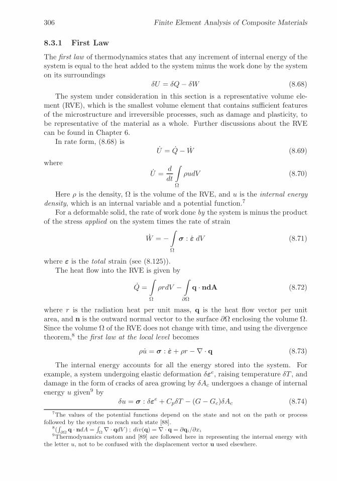
“K15072” — 2013/3/21 — 10:58�

�

�

�

�

�


8.3.1 First Law

The first law of thermodynamics states that any increment of internal energy of thesystem is equal to the heat added to the system minus the work done by the systemon its surroundings

δU = δQ− δW (8.68)

The system under consideration in this section is a representative volume ele-ment (RVE), which is the smallest volume element that contains sufficient featuresof the microstructure and irreversible processes, such as damage and plasticity, tobe representative of the material as a whole. Further discussions about the RVEcan be found in Chapter 6.

In rate form, (8.68) isU = Q− W (8.69)

where

U =d

dt

∫

Ω

ρudV (8.70)

Here ρ is the density, Ω is the volume of the RVE, and u is the internal energydensity, which is an internal variable and a potential function.7

For a deformable solid, the rate of work done by the system is minus the productof the stress applied on the system times the rate of strain

W = −∫

Ω

σ : ε dV (8.71)

where ε is the total strain (see (8.125)).The heat flow into the RVE is given by

Q =

∫

Ω

ρrdV −∫

∂Ω

q · ndA (8.72)

where r is the radiation heat per unit mass, q is the heat flow vector per unitarea, and n is the outward normal vector to the surface ∂Ω enclosing the volume Ω.Since the volume Ω of the RVE does not change with time, and using the divergencetheorem,8 the first law at the local level becomes

ρu = σ : ε+ ρr −∇ · q (8.73)

The internal energy accounts for all the energy stored into the system. Forexample, a system undergoing elastic deformation δεe, raising temperature δT , anddamage in the form of cracks of area growing by δAc undergoes a change of internalenergy u given9 by

δu = σ : δεe + CpδT − (G−Gc)δAc (8.74)

7The values of the potential functions depend on the state and not on the path or processfollowed by the system to reach such state [88].

8(∫

∂Ωq · ndA =

∫

Ω∇ · qdV ) ; div(q) = ∇ · q = ∂qi/∂xi

9Thermodynamics custom and [89] are followed here in representing the internal energy withthe letter u, not to be confused with the displacement vector u used elsewhere.

�

�

“K15072” — 2013/3/21 — 10:58�

�

�

�

�

�


where G is the strain energy release rate, Gc is the surface energy needed to createthe increment of the two surfaces of an advancing crack, and Cp = Cv is the specificheat capacity of the solid.

In general ε = ε(σ, u, sα) where sα are internal variables. Let’s assume for thetime being that the system is adiabatic, i.e., ρr − ∇ · q = 0. Further, if there areno dissipative effects or heat transfer, then u is a function of ε only, u = u(εe),where εe is the elastic strain. In such case, the internal energy density reduces tothe strain energy density, which in rate form is

ϕ(ε) = σ : εe (8.75)

and the complementary strain energy density is

ϕ∗(ε) = σ : εe − ϕ = σ : εe (8.76)

8.3.2 Second Law

The second law of thermodynamics formalizes the fact that heat flows from hot tocold. Mathematically, the heat flow q has opposite direction to the gradient10 oftemperature T , which is formally written as

q · ∇T ≤ 0 (8.77)

where the equal sign holds true only for adiabatic processes, i.e., when there is noheat exchange and thus no thermal irreversibility.

Let’s visualize a process of heat transfer from a hot reservoir to a cold reservoir,happening in such a way that no heat is lost to, and no work is exchanged with, theenvironment. Once heat has flowed to the cold reservoir, it is impossible to transferit back to the hot reservoir without adding external work. That is, the process ofheat transfer is irreversible even though, on account of the first law energy balance(8.73), no energy has been lost. For future use (8.77) can be written11 as

q · ∇T−1 ≥ 0 (8.78)

The second law justifies the introduction of a new internal variable, the entropydensity s = s(u, ε), which is also a potential function [90]. According to the secondlaw, the entropy density rate is s ≥ 0, where the equal sign holds true only foradiabatic processes.

Assume the specific entropy s = s(u, ε) is a potential function such that for areversible process [90]

ds =

(

δq

T

)

rev

(8.79)

with δQ =∫

Ω ρ δq dΩ, where δq = r − ρ−1∇ · q is the heat input per unit mass,and S =

∫

Ω s ρ dΩ is the entropy. We use δ, not d, to emphasize that δq is not thedifferential (perfect or total) of any (potential) function.

10The gradient of a scalar yields a vector, ∇T = ∂T/∂xi11∇T−1 = −T−2∇T

�

�

“K15072” — 2013/3/21 — 10:58�

�

�

�

�

�


As a preamble to the definition of conjugate variables (see (8.86, 8.92, 8.99)),note that using (8.79), the first law can be rewritten for a reversible process on anideal gas (pv = RT ), as the Gibbs equation for an ideal gas,

du = T ds− p dv (8.80)

where v is the specific volume (volume per unit mass). It can be seen in (8.80) thatv is conjugate to −p for calculating work input for an ideal gas and s is conjugateto T for calculating thermal energy input.

For a cyclic reversible process returning to its initial state characterized by state

variables (e.g., u, T, ε), by virtue of (8.79) we have∮

ds =∮

(

δqT

)

rev= 0. Since

s is a potential function but q is not, for an irreversible process we have∮

ds = 0

but∮

(

δqT

)

irrev< 0, as corroborated by experiments. The heat δq entering at

temperature Ti provides less entropy input δq/Ti than the entropy output δq/Toleaving the same cycle at temperature To < Ti (see also [91, Example 6-2]). Sinceentropy is a potential function, and therefore a state variable, it always satisfies∮

ds = 0. Therefore, a negative net entropy supply must be compensated by internalentropy production. The entropy of a system can be raised or lowered by adding orextracting heat (in the form of δq/T ) but it is always raised by internal irreversibleprocesses such as crack formation and so on (positive dissipation principle).

Adiabatic systems do not exchange heat with the surroundings (δq = 0), so theonly change in entropy is due to internal irreversibility s ≥ 0, where the equal signholds for reversible processes only. Note that any system and its surroundings canbe made adiabatic by choosing sufficiently large surroundings, e.g., the universe.For an arbitrary system, the total entropy rate is greater than (or equal to) the netentropy input due to heat

s ≥ r

T− 1

ρ∇ ·

(q

T

)

(8.81)

The left-hand side of (8.81) represents the total entropy rate of the system. Theright-hand side of (8.81) represents the external entropy supply rate. The differenceis the internal entropy production rate

γs = s− r

T+

1

ρ∇ ·

(q

T

)

≥ 0 (8.82)

Equation 8.82 is called the local Clausius-Duhem inequality. Noting that ∇ ·(

T−1q)

= T−1∇ · q+ q∇ T−1 results in

γs = s− 1

ρT(ρr −∇ · q) + 1

ρq · ∇ T−1 ≥ 0 (8.83)

where the first two terms represent the local entropy production due to local dissi-pative phenomena, and the last term represents the entropy production due to heatconduction12 [90]. Assuming it is possible to identify all local dissipative phenom-

12Even absent local dissipative phenomena, q · ∇T−1 ≥ 0 represents the well-known fact thatheat flows opposite to the temperature gradient ∇T .

�

�

“K15072” — 2013/3/21 — 10:58�

�

�

�

�

�


ena, their contributions can be written as products of conjugate variables pαsα ≥ 0,and (8.83) can be written as

ρT γs = pαsα + Tq · ∇T−1 ≥ 0 (8.84)

where α = 1 . . . n, spans the total number of dissipative phenomena considered.Note that the dissipation is a scalar given by the contracted product of a thermo-dynamic force pα times the increment of a measurable state variable sα. The statevariable, also called thermodynamic flux, describes univocally the effects of history(e.g., yield, damage) on the material. Note that γs is defined as an entropy, not asa dissipation heat, so that it is a potential function, while q is not.

For the particular case of damage due to penny-shaped cracks growing self-similarly [63], the state variable is the crack area Ac and the thermodynamic forceis the energy available to grow the cracks pc = G − Gc, which is equal to thedifference between the energy release rate (ERR) G and the critical ERR Gc = 2γc,the latter being equal to twice the surface energy because two surfaces must becreated every time a crack appears (see Chapter 10). In this case, the dissipation(heat) is ρT γ = pcAc.

From the first law (8.73), considering an adiabatic process (ρr−∇·q) and usingthe chain rule u = ∂u/∂ε : ε we have

[

σ − ρ∂u

∂ε

]

: ε = 0 (8.85)

Since ε = 0 would be a trivial solution, the stress tensor, conjugate to strain, isdefined as

σ = ρ∂u

∂ε(8.86)

The Clausius-Duhem inequality (8.83) for an isothermal (∇T = 0) system re-duces to

γs = s− 1

ρT(ρr −∇ · q) ≥ 0 (8.87)

and using the first law we get

ρT γs = ρT s− (ρu− σ : ε) ≥ 0 (8.88)

The Helmholtz free energy (HFE) density is defined as

ψ(T, ε, sα) = u− Ts (8.89)

which is also a potential function. The corresponding extensive function is theHelmholtz free energy13 A =

∫

Ω ρψdV . The rate of change of HFE density is

ψ = u− T s− T s (8.90)

13The nomenclature of [89] has been used.

�

�

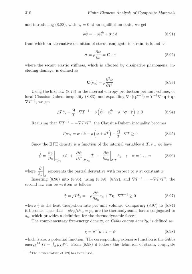
“K15072” — 2013/3/21 — 10:58�

�

�

�

�

�


and introducing (8.88), with γs = 0 at an equilibrium state, we get

ρψ = −ρsT + σ : ε (8.91)

from which an alternative definition of stress, conjugate to strain, is found as

σ = ρ∂ψ

∂ε= C : ε (8.92)

where the secant elastic stiffness, which is affected by dissipative phenomena, in-cluding damage, is defined as

C(sα) = ρ∂2ψ

∂ε2(8.93)

Using the first law (8.73) in the internal entropy production per unit volume, orlocal Clausius-Duhem inequality (8.83), and expanding ∇ · (qT−1) = T−1∇ ·q+q ·∇T−1, we get

ρT γs =q

T· ∇T−1 − ρ

(

ψ + sT − ρ−1σ : ε)

≥ 0 (8.94)

Realizing that ∇T−1 = −∇T/T 2, the Clausius-Duhem inequality becomes

Tργs = σ : ε− ρ(

ψ + sT)

− q

T· ∇T ≥ 0 (8.95)

Since the HFE density is a function of the internal variables ε, T, sα, we have

ψ =∂ψ

∂ε

∣

∣

∣

∣

T,sα

: ε +∂ψ

∂T

∣

∣

∣

∣

ε,sαT +

∂ψ

∂sα

∣

∣

∣

∣

ε,Tsα ; α = 1 . . . n (8.96)

where∂

∂y

∣

∣

∣

∣

x

represents the partial derivative with respect to y at constant x.

Inserting (8.96) into (8.95), using (8.89), (8.92), and ∇T−1 = −∇T/T 2, thesecond law can be written as follows

γ = ρT γs = −ρ ∂ψ∂sα

sα + Tq · ∇T−1 ≥ 0 (8.97)

where γ is the heat dissipation rate per unit volume. Comparing (8.97) to (8.84)it becomes clear that −ρ∂ψ/∂sα = pα are the thermodynamic forces conjugated tosα, which provides a definition for the thermodynamic forces.

The complementary free-energy density, or Gibbs energy density, is defined as

χ = ρ−1σ : ε− ψ (8.98)

which is also a potential function. The corresponding extensive function is the Gibbsenergy14 G =

∫

Ω ρχdV . From (8.98) it follows the definition of strain, conjugate

14The nomenclature of [89] has been used.

�

�

“K15072” — 2013/3/21 — 10:58�

�

�

�

�

�


to stress, and the definition of the thermodynamic forces, conjugate to the statevariables sα, as

ε = ρ∂χ

∂σ; pα = ρ

∂χ

∂sα= −ρ ∂ψ

∂sα(8.99)

where sα includes the damage variables and consequently pα includes the thermo-dynamic damage forces (see Example 8.4, p. 311).

The secant elastic compliance, which is affected by dissipative phenomena, in-cluding damage, is defined by

S(sα) = ρ∂2χ

∂σ2(8.100)

Example 8.4 The following Gibbs free energy is proposed to represent the onset and accu-mulation of transverse matrix cracks resulting from transverse tension and in-plane shearloads:

χ =1

2 ρ

[

σ21

˜E1

+σ22

(1−D2)2˜E2

+σ26

(1−D6)22G12

−(

ν21˜E2

+ν12˜E1

)

σ1σ21−D2

]

where ˜E1, ˜E2, ν12, ν21, and ˜G12 are the undamaged in-plane elastic orthotropic properties ofa unidirectional lamina where the subscript ()1 denotes the fiber direction and ()2 denotes thetransverse direction. The damage variables D2 and D6 represent the effect of matrix cracks.The proposed distinguishes between active (D2+) and passive damage (D2−), correspondingto the opening or closure of transverse matrix cracks, respectively. The determination ofthe active damage variable is based on the following equation:

D2 = D2+〈σ2〉|σ2| +D2−

〈−σ2〉|σ2|

where 〈x〉 is defined as 〈x〉 := 12 (x+ |x|).

For a lamina in a state of plane stress, subjected to in-plane stress only, without fiberdamage (D1 = 0), and using the energy equivalence principle (8.8), derive expressions for a)the secant stiffness tensor, b) the effective stress, and c) the thermodynamic forces associatedto the model. Use tensor components of strain (ε1, ε2, ε6).

Solution to Example 8.4 The constitutive model is defined as the derivative of the Gibbsfree energy with respect to the stress tensor

ε =ρ∂χ

∂σ= S : σ

whith ε6 = γ6/2 and the compliance tensor S defined as

S = ρ∂2χ

∂σ2

The compliance tensor for plane stress S in Voigt contracted notation is

S =

⎡

⎢

⎢

⎢

⎢

⎢

⎢

⎣

1

˜E1

− ν21˜E2 (1−D2)

0

− ν12˜E1 (1−D2)

1

˜E2 (1−D2)2

0

0 01

2 ˜G12 (1−D6)2

⎤

⎥

⎥

⎥

⎥

⎥

⎥

⎦

�

�

“K15072” — 2013/3/21 — 10:58�

�

�

�

�

�


The damage variables appear in S12, S21, S22, and S66. To perform tensor productsusing matrix multiplications, see (A.14) and (A.20). Using the energy equivalence principleand (8.67), the compliance matrix can be written as

S = M−1 : ˜S : M−1

where the undamaged compliance is

˜S =

⎡

⎢

⎢

⎢

⎢

⎢

⎢

⎣

1

˜E1

− ν21˜E2

0

− ν12˜E1

1

˜E2

0

0 01

2 ˜G12

⎤

⎥

⎥

⎥

⎥

⎥

⎥

⎦

and where the effective damage tensor M, written in contracted notation, multiplied by the3×3 version of the Reuter matrix (A.13) is

M =

⎡

⎣

1 0 00 (1−D2) 00 0 (1−D6)

⎤

⎦

The stiffness tensor C is obtained by

C = M : ˜C : M

where, for this particular example, the secant stiffness tensor is

C =

⎡

⎢

⎢

⎢

⎢

⎢

⎣

˜E1

1− ν21ν12

ν12 ˜E2 (1−D2)

1− ν21ν120

ν21 ˜E1 (1−D2)

1− ν21ν12

˜E2 (1−D2)2

1− ν21ν120

0 0 2 ˜G12

(

1− ˜D6

)2

⎤

⎥

⎥

⎥

⎥

⎥

⎦

The effective stress σ is related to the nominal stress σ by the effective damage tensorM using σ = M−1 : σ, which yields

σT =

{

σ1,σ2

1−D2,

σ61−D6

}

The thermodynamic forces are obtained by using Y = ρ∂χ/∂D, which for this particularexample yield

Y =

⎧

⎨

⎩

Y1Y2Y6

⎫

⎬

⎭

=

⎧

⎪

⎪

⎪

⎪

⎪

⎨

⎪

⎪

⎪

⎪

⎪

⎩

0σ2

2

(1−D2)3˜E2

− σ1σ2ν12

(1−D2)2˜E1

σ62

(1−D6)32 ˜G12

⎫

⎪

⎪

⎪

⎪

⎪

⎬

⎪

⎪

⎪

⎪

⎪

⎭

�

�

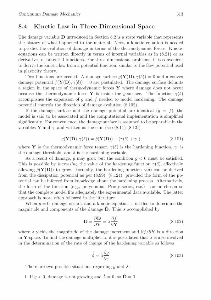
“K15072” — 2013/3/21 — 10:58�

�

�

�

�

�


8.4 Kinetic Law in Three-Dimensional Space

The damage variable D introduced in Section 8.2 is a state variable that representsthe history of what happened to the material. Next, a kinetic equation is neededto predict the evolution of damage in terms of the thermodynamic forces. Kineticequations can be written directly in terms of internal variables as in (8.21) or asderivatives of potential functions. For three-dimensional problems, it is convenientto derive the kinetic law from a potential function, similar to the flow potential usedin plasticity theory.

Two functions are needed. A damage surface g(Y(D), γ(δ)) = 0 and a convexdamage potential f(Y(D), γ(δ)) = 0 are postulated. The damage surface delimitsa region in the space of thermodynamic forces Y where damage does not occurbecause the thermodynamic force Y is inside the g-surface. The function γ(δ)accomplishes the expansion of g and f needed to model hardening. The damagepotential controls the direction of damage evolution (8.102).

If the damage surface and the damage potential are identical (g = f), themodel is said to be associated and the computational implementation is simplifiedsignificantly. For convenience, the damage surface is assumed to be separable in thevariables Y and γ, and written as the sum (see (8.11)-(8.12))

g(Y(D), γ(δ)) = g(Y(D)) − (γ(δ) + γ0) (8.101)

where Y is the thermodynamic force tensor, γ(δ) is the hardening function, γ0 isthe damage threshold, and δ is the hardening variable.

As a result of damage, g may grow but the condition g < 0 must be satisfied.This is possible by increasing the value of the hardening function γ(δ), effectivelyallowing g(Y(D)) to grow. Formally, the hardening function γ(δ) can be derivedfrom the dissipation potential as per (8.99), (8.124), provided the form of the po-tential can be inferred from knowledge about the hardening process. Alternatively,the form of the function (e.g., polynomial, Prony series, etc.) can be chosen sothat the complete model fits adequately the experimental data available. The latterapproach is more often followed in the literature.

When g = 0, damage occurs, and a kinetic equation is needed to determine themagnitude and components of the damage D. This is accomplished by

D =∂D

∂Y= λ

∂f

∂Y(8.102)

where λ yields the magnitude of the damage increment and ∂f/∂Y is a directionin Y-space. To find the damage multiplier λ, it is postulated that λ is also involvedin the determination of the rate of change of the hardening variable as follows

δ = λ∂g

∂γ(8.103)

There are two possible situations regarding g and λ:

i. If g < 0, damage is not growing and λ = 0, so D = 0.

�

�

“K15072” — 2013/3/21 — 10:58�

�

�

�

�

�


ii. If g = 0, damage occurs and λ > 0, so D > 0.

These are summarized by the Kuhn-Tucker conditions

λ ≥ 0 ; g ≤ 0 ; λg = 0 (8.104)

The value of λ can be determined by the consistency condition, which leads to

g =∂g

∂Y: Y +

∂g

∂γγ = 0 ; g = 0 (8.105)

On the other hand, the rates of thermodynamic forces and hardening functioncan be written as

Y =∂Y

∂ε: ε+

∂Y

∂D: D

γ =∂γ

∂δδ

(8.106)

or in function of λ, introducing (8.103) and (8.104) into (8.106) as follows

Y =∂Y

∂ε: ε+ λ

∂Y

∂D:∂f

∂Y

γ =∂γ

∂δλ∂g

∂γ

(8.107)

Introducing (8.107) into (8.105) we obtain the following equation

g =∂g

∂Y:

[

∂Y

∂ε: ε+ λ

∂Y

∂D:∂f

∂Y

]

+∂g

∂γ

∂γ

∂δλ∂g

∂γ= 0 (8.108)

Next, ∂f/∂γ = ∂g/∂γ = −1, (8.108) can be written as

g =∂g

∂Y:∂Y

∂ε: ε+

[

∂g

∂Y:∂Y

∂D:∂f

∂Y+∂γ

∂δ

]

λ = 0 (8.109)

Therefore, the damage multiplier λ can be obtained as

λ =

{

Ld : ε when g = 00 when g < 0

(8.110)

where

Ld = −∂g

∂Y:∂Y

∂ε∂g

∂Y:∂Y

∂D:∂f

∂Y+∂γ

∂δ

(8.111)

Equations (8.103), (8.104), and (8.110) yield the pair D, δ in rate form as

D = Ld :∂f

∂Y: ε ; δ = −λ (8.112)

�

�

“K15072” — 2013/3/21 — 10:58�

�

�

�

�

�


The tangent constitutive equation can be obtained by differentiation of the con-stitutive equation σ = C : ε, which yields

σ = C : ε+ C : ε (8.113)

where the last term represents the stiffness reduction. Next, the last term in (8.113)can be written as

C : ε =∂C

∂D: D : ε (8.114)

Introduce (8.112) and rearrange

C : ε =∂C

∂D: ε : Ld :

∂f

∂Y: ε (8.115)

Since (ε,D) are state variables, and thus independent variables,

∂ε

∂D= 0 (8.116)

Therefore,

C : ε =∂σ

∂D: Ld :

∂f

∂Y: ε (8.117)

Finally, reintroduce the above into (8.113) to get

σ = Ced : ε (8.118)

where the damaged tangent constitutive tensor, Ced, can be written as follows

Ced =

⎧

⎨

⎩

C if D ≤ 0

C+∂σ

∂D: Ld :

∂f

∂Yif D ≥ 0

(8.119)

The internal variables D, δ, and related variables, are found using numericalintegration, usually using a return-mapping algorithm as explained in Section 8.4.1.

As explained in Section 8.1.3 and 8.4, a number of internal material parametersare needed to define the damage surface, damage potential, and hardening func-tions. These parameters cannot be obtained directly from simple tests, but ratherthe model is identified by adjusting the internal parameters in such a way thatmodel predictions fit well some observed behavior that can be quantified experi-mentally. Model identification is very specific to the particular model formulation,material, availability of experiments, and feasibility of conducting relevant exper-iments. Therefore, model identification can be explained only on a case by casebasis, as it is done in Example 8.3, p. 296.

�

�

“K15072” — 2013/3/21 — 10:58�

�

�

�

�

�


8.4.1 Return-Mapping Algorithm

A return-mapping algorithm [82,84,85] is used to solve for the variables λ, δ, D, δ,and D, in numerically approximated form.

The internal variables are updated by a linearized procedure between two con-secutive iterations (k − 1 and k). The first-order linearization of (8.109) yields

(g)k − (g)k−1 =

(

∂g

∂Y:∂Y

∂D:∂f

∂Y+∂γ

∂δ

)

k−1

Δλk = 0 (8.120)

Successful iterations yield [g]k = 0 and

Δλk =−(g)k−1

(

∂g

∂Y:∂Y

∂D:∂f

∂Y+∂γ

∂δ

)

k−1

(8.121)

The complete algorithm used for a typical integration of constitutive equationsis shown next:

i. Retrieve the strain (ε)n−1 from the previous increment and the strain incre-ment (Δε)n for the current increment from the FEM code. The updatedstrain is calculated as

(ε)n = (ε)n−1 + (Δε)n

ii. Retrieve the state variables from the previous step and start the return-mapping algorithm by setting the predictor iteration k = 0

(D)n0 = (D)n−1 ; (δ)n0 = (δ)n−1

iii. Update the secant stiffness and Cauchy stress, which are used to calculate thethermodynamic forces and damage hardening at this point

(C)nk = (M)nk : ˜C : (M)nk(σ)nk = (C)nk : (ε)n

(Y)nk ; (γ)nk

iv. The damage threshold is evaluated at this point

(g)k = g ((Y)nk , (γ(δ))nk , γ0)

There are two possible cases:

(a) If (g)k ≤ 0, there is no damage, then Δλk = 0. Go to (viii).

(b) If (g)k > 0, there is damage evolution, then Δλk > 0. Go to (v).

�

�

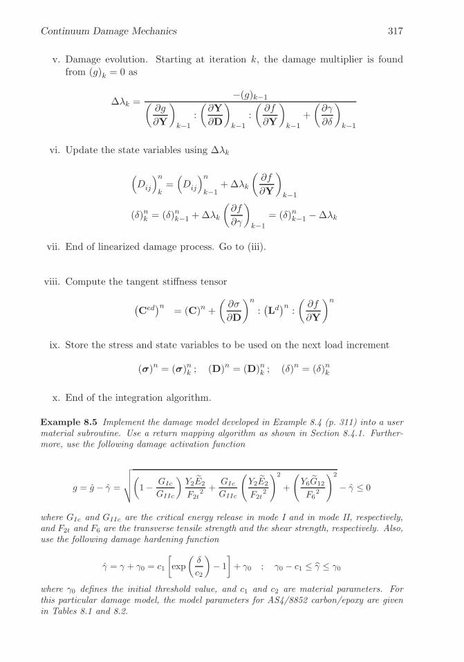
“K15072” — 2013/3/21 — 10:58�

�

�

�

�

�


v. Damage evolution. Starting at iteration k, the damage multiplier is foundfrom (g)k = 0 as

Δλk =−(g)k−1

(

∂g

∂Y

)

k−1

:

(

∂Y

∂D

)

k−1

:

(

∂f

∂Y

)

k−1

+

(

∂γ

∂δ

)

k−1

vi. Update the state variables using Δλk

(

Dij

)n

k=(

Dij

)n

k−1+Δλk

(

∂f

∂Y

)

k−1

(δ)nk = (δ)nk−1 +Δλk

(

∂f

∂γ

)

k−1

= (δ)nk−1 −Δλk

vii. End of linearized damage process. Go to (iii).

viii. Compute the tangent stiffness tensor

(

Ced)n

= (C)n +

(

∂σ

∂D

)n

:(

Ld)n

:

(

∂f

∂Y

)n

ix. Store the stress and state variables to be used on the next load increment

(σ)n = (σ)nk ; (D)n = (D)nk ; (δ)n = (δ)nk

x. End of the integration algorithm.

Example 8.5 Implement the damage model developed in Example 8.4 (p. 311) into a usermaterial subroutine. Use a return mapping algorithm as shown in Section 8.4.1. Further-more, use the following damage activation function

g = g − γ =

√

√

√

√

(

1− GIc

GIIc

)

Y2 ˜E2

F2t2 +

GIc

GIIc

(

Y2 ˜E2

F2t2

)2

+

(

Y6 ˜G12

F62

)2

− γ ≤ 0

where GIc and GIIc are the critical energy release in mode I and in mode II, respectively,and F2t and F6 are the transverse tensile strength and the shear strength, respectively. Also,use the following damage hardening function

γ = γ + γ0 = c1

[

exp

(

δ

c2

)

− 1

]

+ γ0 ; γ0 − c1 ≤ γ ≤ γ0

where γ0 defines the initial threshold value, and c1 and c2 are material parameters. Forthis particular damage model, the model parameters for AS4/8852 carbon/epoxy are givenin Tables 8.1 and 8.2.

�

�

“K15072” — 2013/3/21 — 10:58�

�

�

�

�

�


Table 8.1: Elastic and strength properties for AS4/8852 unidirectional lamina.

˜E1˜E2

˜G12 ν12 F2t F6

171.4 GPa 9.08 GPa 5.29 GPa 0.32 62.29 MPa 92.34 MPa

Table 8.2: Critical energy release, and hardening parameters for AS4/8852 unidi-rectional lamina.

GIc GIIc γ0 c1 c2170 J/m2 230 J/m2 1.0 0.5 -1.8

0 0.2 0.4 0.60

0.2

0.4

0.6

0.8

1

1.2

1.4

1.6

Y2

Y6

0 20 40 60 80−100

−80

−60

−40

−20

0

20

40

60

80

100

σ2 [MPa]

σ 6 [MP

a]

Fig. 8.8: Initial damage surface in thermodynamic and stress spaces.

�

�

“K15072” — 2013/3/21 — 10:58�

�

�

�

�

�


Solution to Example 8.5 This model represents damage caused by both transverse tensilestress and in-plane shear stress. Longitudinal tension/compression have no effect. There-fore, the model is defined in the thermodynamic force space Y2, Y6. The shape of the damagesurface for AS4/8852 lamina is shown in Figure 8.8.

To implement the return mapping algorithm shown in Section 8.4.1, expressions for∂f/∂Y, ∂g/∂Y, ∂f/∂γ, ∂g/∂γ,∂γ/∂δ, and ∂Y/∂D are needed.

Assuming f = g, the derivative of the potential function and the damage surface withrespect to (w.r.t) the thermodynamic forces is given by

∂g

∂Y=

∂f

∂Y=

⎧

⎪

⎪

⎪

⎨

⎪

⎪

⎪

⎩

01

g

((

1− GIc

GIIc

)

14F2t

√

2E2

Y2+ GIc

GIIc

E2

(F2t)2

)

1

gG12

⎫

⎪

⎪

⎪

⎬

⎪

⎪

⎪

⎭

and the derivative of the damage surface w.r.t. the damage hardening function is

∂g

∂γ=∂f

∂γ= −1

Also, the derivative of the hardening function γ w.r.t conjugate variable δ is needed

∂γ

∂δ=c1c2

exp

(

δ

c2

)

Next, the derivative of the thermodynamic forces w.r.t the internal damage variables iswritten as

∂Y

∂D=∂Y

∂D

∣

∣

∣

∣

σ=const

+∂Y

∂σ:∂σ

∂D

Furthermore, the derivative of the thermodynamic forces w.r.t strain is written as

∂Y

∂ε=∂Y

∂σ:∂σ

∂ε=∂Y

∂σ: C

The following are written in contracted notation as

∂Y

∂σ=

⎡

⎢

⎢

⎢

⎢

⎢

⎣

0 0 0−σ2ν12

(1−D2)2˜E1

2σ2

(1−D2)3˜E2

− σ1ν12

(1−D2)2˜E1

0

0 0σ6

(1−D6)3˜G12

⎤

⎥

⎥

⎥

⎥

⎥

⎦

and

∂σ

∂D=

⎡

⎢

⎢

⎢

⎢

⎢

⎢

⎣

0 −˜E2ν12

1− ν12ν21ε2 0

0 −˜E1ν21

1− ν12ν21ε1 − 2 (1−D2) ˜E2

1− ν12ν21ε2 0

0 0 −4(1−D6) ˜G12ε6

⎤

⎥

⎥

⎥

⎥

⎥

⎥

⎦

The equations are implemented in the subroutine umatps85.for, which is available in[5]. The material model subroutine can be used in conjunction with plain stress elementsand laminated shells elements. A pseudo code for transverse tensile load is shown below.

�

�

“K15072” — 2013/3/21 — 10:58�

�

�

�

�

�




Menu: File, Save As, [C:\SIMULIA\User\Ex_8.5\Ex_8.5.tra.cae], OK


Module: Part

Menu: Part, Create

2D Planar, Deformable, Shell, Cont



Module: Property


General, User Material

# read material properties from a file

# right-click in Data area, Read from file, [props.txt], OK, OK

General, Depvar



Solid, Homogeneous, Cont

# checkmark: Plane stress/strain thickness [1.0], OK

Menu: Assign, Section, # pick: part, Done, OK

iv. Creating the assembly

Module: Assembly



Module: Step

Menu: Step, Create

Name [transverse], Procedure type: General, Static/General, Cont

Tab: Basic, Time Period [50]

Tab: Incrementation, Type: Fixed

Maximum number of increments [50], Increment size [2.2], OK


Output Variables: Preselected Defaults, # add: [SDV], OK


Module: Load

Menu: BC, Manager

Create, Name [BC-1], Step: Initial, Symm/Anti/Enca, Cont

# pick: node @ origin, Done, ENCASTRE, OK

Create, Name [BC-2], Step: Initial, Symm/Anti/Enca, Cont

# pick: line @ Y=0, Done, YSYMM, OK

# transverse load imposed as displacement to create epsilon = 2%

Create, Name [traction], Step: transverse, Disp/Rota, Cont

# pick: line @ Y=10, Done, # checkmark: U2 [0.2], OK

# close Boundary Condition Manager pop-up window

�

�

“K15072” — 2013/3/21 — 10:58�

�

�

�

�

�


vii. Meshing the model. Use only one element because you will have uniform stress/strain.

Module: Mesh

Menu: Seed, Instance, Approximate global size [10], OK


Geometric Order: Quadratic # CPS8R avoid hourglass, OK


viii. Creating a set to track the stresses and strains in the element

Module: Mesh


Type: Element, Cont, # pick: the only element in the mesh, Done

Module: Step


Domain: Set: Set-1, # expand: Stresses, # checkmark: S

# expand: Strains, # checkmark: E, OK


Module: Job

Menu: Job, Manager

Create, Cont

Tab: General, User subroutine file [umatps85.for], OK, OK




# select: E22 at Element 1 Int Point 1, Save As [e22], OK

# select: S22 at Element 1 Int Point 1, Save As [s22], OK



Source: Operate on XY data, Cont, Operations: Combine



A shear load can be applied easily modifying the current cae model.

i. Saving current cae model and creating a new one

Menu: File, Save

Menu: File, Save As, [C:\SIMULIA\User\Ex_8.5\Ex_8.5.she.cae], OK


Module: Step

Menu: Step, Manager

# select: transverse, Rename, [shear], OK

Edit, Tab: Incrementation, Type: Fixed

Maximum number of increments [50], Increment size [3], OK

# close Step Manager pop-up window

iii. Adding BC and loads

�

�

“K15072” — 2013/3/21 — 10:58�

�

�

�

�

�


Module: Load

Menu: BC, Manager

# shear loading imposed as displacement U1 on step: shear

# select: traction, Rename, [shear], OK

Edit, # uncheckmark: U2, # checkmark: U1 [0.4], OK # gamma_6=4%


iv. Adding constraint to guarantee pure shear loading

Module: Interaction


Type: Tie, Cont

Surface, # pick: line @ x=0, Done

Surface, # pick: line @ x=10, Done

Discretization method: Surface to surface

Position Tolerance: Specify distance [10]

# uncheckmark: Adjust slave surface initial position, OK


Module: Job

Menu: Job, Manager




# select: E12 at Element 1 Int Point 1, Save As [e12], OK

# select: S12 at Element 1 Int Point 1, Save As [s12], OK



Source: Operate on XY data, Cont, Operations: Combine



The model response for the two cases is shown in Figure 8.9.

8.5 Damage and Plasticity

For polymer matrix composites reinforced by strong and stiff fibers, damage and itsconjugate thermodynamic force can be described by second-order tensors D and Y.Furthermore, the hardening processes that take place during plasticity and damageimply additional dissipation, so that

ρπ = Tρπs = σ : εp +R p+Y : D+ γδ (8.122)

where (R, p) is the thermodynamic force-flux pair associated to plastic hardening,and (γ, δ) is the thermodynamic force-flux pair associated to damage hardening,and ρπ is the dissipation heat due to irreversible phenomena.

For the particular case of (8.122), from (8.92) and (8.99), the following definitionsfor the thermodynamic forces are obtained

�

�

“K15072” — 2013/3/21 — 10:58�

�

�

�

�

�


0 0.2 0.4 0.6 0.8 1 1.2 1.4 1.6 1.8 20

20

40

60

80

100

120

140

ε2, ε

12 [%]

σ 2, σ6 [M

Pa]

inplane sheartransverse

Fig. 8.9: Response to in-plane shear stress and to transverse tensile stress.

σ = ρ∂ψ

∂ε= −ρ ∂ψ

∂εpε = ρ

∂χ

∂σY = −ρ ∂ψ

∂D= ρ

∂χ

∂D(8.123)

as well as definitions for the hardening equations

γ = ρ∂χ

∂δ= −ρ∂ψ

∂δ= ρ

∂π

∂δR = ρ

∂χ

∂p= −ρ∂ψ

∂p= ρ

∂π

∂p(8.124)

The additive decomposition [63]

ε = εe + εp (8.125)

can be rewritten taking into account that the elastic component of strain can becalculated from stress and compliance, so that

ε = S : σ + εp (8.126)

Therefore, the strain-stress law in incremental and rate form is

δε = S : δσ + δS : σ + δεp

ε = S : σ + S : σ + εp (8.127)

�

�

“K15072” — 2013/3/21 — 10:58�

�

�

�

�

�


showing that an increment of strain has three contributions, elastic, damage, andplastic. The elastic strain occurs as a direct result of an increment in stress, thedamage strain is caused by the increment in compliance as the material damages,and the plastic strain occurs at constant compliance. The elastic unloading stiffnessdoes not change due to plasticity but it reduces due to damage. Following thisargument, it is customary [92] to assume that the free energy and complementaryfree energy can be separated as follows

ψ(ε, εp, p,D, δ) = ψe(εe,D, δ) + ψp(εp, p)

χ(σ, εp, p,D, δ) = χe(σ,D, δ) + χp(εp, p) (8.128)

Suggested Problems

Problem 8.1 Using the formulation and properties of Example 8.2 (p. 292), obtain agraphical representation of the evolution strain vs. nominal stress (ε vs. σ) and the evolu-tion of strain vs. effective stress (ε vs. σ) for a point on the top surface of the beam andfor another point on the bottom surface of the beam. Comment on the graphs obtained.

Problem 8.2 Implement a UMAT for a one-dimensional CDM active in the x1-directiononly. Use 2D plane stress constitutive equations. Leave the x2-direction, Poisson’s, andshear terms as linear elastic with no damage. Verify the program by recomputing Exam-ple 8.2 and the plots obtained in Problem 8.1. Note that to obtain the same values, thePoisson’s ratio should be set to zero.

Problem 8.3 The Gibbs free energy is defined in expanded form and using Voigt contractednotation as

χ =1

2 ρ

[

σ21

(1−D1)2˜E1

+σ22

(1−D2)2˜E2

+σ26

(1−D1) (1−D2) ˜G12

−

−(

ν21˜E2

+ν12˜E1

)

σ1σ2(1−D1) (1−D2)

]

where ˜E1, ˜E2, ν12, ν21, and ˜G12 are the undamaged in-plane elastic orthotropic propertiesof a unidirectional lamina where the subindex ()1 denotes the fiber direction and ()2 denotesthe transverse direction. (a) Obtain the secant constitutive equations, C and S, using thegiven Gibbs free energy. (b) Obtain the thermodynamic forces Y1 and Y2 associated to D1

and D2. (c) If M is represented using Voigt contracted notation and multiplied by a Reutermatrix as

M =

⎡

⎣

(1−D1) 0 00 (1−D2) 00 0

√1−D1

√1−D2

⎤

⎦

check if this definition of M can be used as the damage effect tensor in a damage modelusing the principle of energy equivalence. Justify and comment on your conclusion.

Problem 8.4 The damage activation function, for the model shown in Problem 8.3, isdefined as

�

�

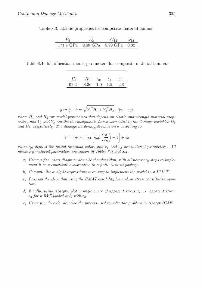
“K15072” — 2013/3/21 — 10:58�

�

�

�

�

�


Table 8.3: Elastic properties for composite material lamina.

˜E1˜E2

˜G12 ν12171.4 GPa 9.08 GPa 5.29 GPa 0.32

Table 8.4: Identification model parameters for composite material lamina.

H1 H2 γ0 c1 c20.024 8.36 1.0 1.5 -2.8

g := g − γ =

√

Y12H1 + Y2

2H2 − (γ + γ0)

where H1 and H2 are model parameters that depend on elastic and strength material prop-erties, and Y1 and Y2 are the thermodynamic forces associated to the damage variables D1

and D2, respectively. The damage hardening depends on δ according to

γ = γ + γ0 = c1

[

exp

(

δ

c2

)

− 1

]

+ γ0

where γ0 defines the initial threshold value, and c1 and c2 are material parameters. Allnecessary material parameters are shown in Tables 8.3 and 8.4.

a) Using a flow chart diagram, describe the algorithm, with all necessary steps to imple-ment it as a constitutive subroutine in a finite element package.

b) Compute the analytic expressions necessary to implement the model in a UMAT.

c) Program the algorithm using the UMAT capability for a plane stress constitutive equa-tion.

d) Finally, using Abaqus, plot a single curve of apparent stress σ2 vs. apparent strainε2 for a RVE loaded only with ε2.

e) Using pseudo code, describe the process used to solve the problem in Abaqus/CAE.

�

�

“K15072” — 2013/3/21 — 10:58�

�

�

�

�

�

�

�

“K15072” — 2013/3/21 — 10:58�

�

�

�

�

�

Chapter 9

Discrete Damage Mechanics

Prediction of damage initiation and propagation is tackled in Chapter 8 using con-tinuum damage mechanics (CDM). Alternatives to CDM include: micromechanicsof damage, crack opening displacement methods, computational micromechanics,and synergistic methods. While CDM (Chapter 8) homogenizes the damage andtreats it phenomenologically, the alternative methods attempt to represent the ac-tual geometry and characteristics of damage.

Prediction of transverse matrix cracking in laminated composites has been ex-tensively studied for the particular case of symmetric [0m/90n]S laminates undermembrane loads, for which matrix cracking is found in the 90◦ laminas (transverselaminas). Extensions to other laminate configurations, such as [0/ ± θ/0]S and[0/θ1/θ2]S , featuring cracks in the off-axis θ laminas, have been developed, but theyare still limited to symmetric laminates subjected to in-plane loading.

Micromechanics of Damage Models (MMD) find an approximate elasticity so-lution for a laminate with a discrete crack or cracks [93–114]. The solutions areapproximate because kinematic assumptions are made, such as a linear [115] or bi-linear [116] distribution of interlaminar shear stress through the thickness of eachlamina, as well as particular spatial distributions of in-plane displacement func-tions [113], stresses, and so on. The state variable is the crack density in thecracking lamina, defined as the number of cracks per unit distance perpendicularto the crack surface. Therefore, the state variable is measurable. One advantageof MMD is that the reduction of laminate moduli as a function of crack density iscalculated without resorting to additional parameters as in the case of CDM. Themain disadvantage of MMD is that most of the solutions available are limited tosymmetric laminates under membrane loads with only one or two laminas cracking.A generalization to the case of multiple cracking laminas is presented in this chapterby resorting to the concept of synergistic methods, explained below.

Crack Opening Displacement (COD) methods [117–124] are based on the theoryof elastic bodies with voids [125]. The distinct advantage of COD models is thatthe laminate stiffness can be calculated for any laminate configuration, even non-symmetric laminate stacking sequence (LSS), subject to any deformation, includingbending, featuring matrix cracking in any of its laminas [126].

Numerical solutions, such as FEA, provide 3D solutions without the kinematic

327

�

�

“K15072” — 2013/3/21 — 10:58�

�

�

�

�

�


2a02a0

L1

3

Fig. 9.1: Representative crack geometry.

simplifications of MMD and COD models [104, 120, 123, 127–130]. However, FEAsolutions require a new mesh and boundary conditions for each LSS, crack orienta-tion, and so on, making them too cumbersome for practical application. Anothernumerical approach is Monte Carlo simulation, where the probabilistic distributionof flaws in material is considered [131–133]. Unfortunately, Monte Carlo simulationsrequire additional parameters that have to be adjusted by fitting the results of themodel to experimental damage evolution data. Such data are scarce.

Synergistic Damage Mechanics (SDM) methods combine elements of differentmodeling strategies such as CDM and MMD [131, 132, 134–138], bringing the bestfeatures of each of the models involved. For example, in this chapter the laminatestiffness reduction is computed via MMDmethods and the generalization to multiplecracking laminas is made via CDM concepts, but unlike CDM models, no additionalparameters are needed.

9.1 Overview

In the following we describe how to use two material properties, the fracture tough-ness in modes I and II, GIc, GIIc, to predict the damaging behavior and transversetensile failure of a unidirectional fiber reinforced lamina embedded in a laminate.The constraining effect of adjacent laminas is taken into account, leading to ap-parent transverse tensile strength F2t being a function of ply thickness. The crackinitiation strain, crack density evolution as a function of stress (strain) up to cracksaturation, and stress redistribution to adjacent laminas are predicted accurately.

The physics of matrix cracking under transverse tension and in-plane shear isas follows. No matter how much care is taken during the production process, thereare always defects in the material. These defects may be voids, microcracks, fiber–matrix debonding, and so on, but all of them can be represented by a typical matrixcrack of representative size 2a0, as shown in Figure 9.1.

When subject to load, matrix cracks grow parallel to the fiber orientation, asshown in Figure 9.2, where it can be seen that cracks are aligned with the fiber

�

�

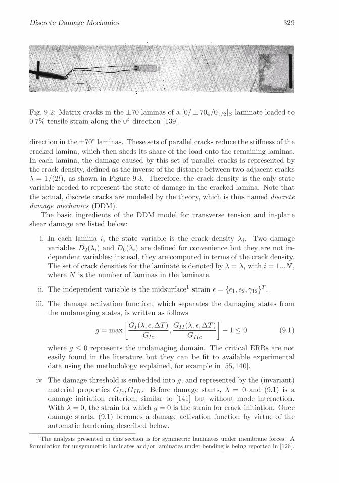
“K15072” — 2013/3/21 — 10:58�

�

�

�

�

�

Discrete Damage Mechanics 329

Fig. 9.2: Matrix cracks in the ±70 laminas of a [0/± 704/01/2]S laminate loaded to0.7% tensile strain along the 0◦ direction [139].

direction in the ±70◦ laminas. These sets of parallel cracks reduce the stiffness of thecracked lamina, which then sheds its share of the load onto the remaining laminas.In each lamina, the damage caused by this set of parallel cracks is represented bythe crack density, defined as the inverse of the distance between two adjacent cracksλ = 1/(2l), as shown in Figure 9.3. Therefore, the crack density is the only statevariable needed to represent the state of damage in the cracked lamina. Note thatthe actual, discrete cracks are modeled by the theory, which is thus named discretedamage mechanics (DDM).

The basic ingredients of the DDM model for transverse tension and in-planeshear damage are listed below:

i. In each lamina i, the state variable is the crack density λi. Two damagevariables D2(λi) and D6(λi) are defined for convenience but they are not in-dependent variables; instead, they are computed in terms of the crack density.The set of crack densities for the laminate is denoted by λ = λi with i = 1...N ,where N is the number of laminas in the laminate.

ii. The independent variable is the midsurface1 strain ε = {ε1, ε2, γ12}T .iii. The damage activation function, which separates the damaging states from

the undamaging states, is written as follows

g = max

[

GI(λ, ε,ΔT )

GIc,GII(λ, ε,ΔT )

GIIc

]

− 1 ≤ 0 (9.1)

where g ≤ 0 represents the undamaging domain. The critical ERRs are noteasily found in the literature but they can be fit to available experimentaldata using the methodology explained, for example in [55,140].

iv. The damage threshold is embedded into g, and represented by the (invariant)material properties GIc, GIIc. Before damage starts, λ = 0 and (9.1) is adamage initiation criterion, similar to [141] but without mode interaction.With λ = 0, the strain for which g = 0 is the strain for crack initiation. Oncedamage starts, (9.1) becomes a damage activation function by virtue of theautomatic hardening described below.

1The analysis presented in this section is for symmetric laminates under membrane forces. Aformulation for unsymmetric laminates and/or laminates under bending is being reported in [126].

�

�

“K15072” — 2013/3/21 — 10:58�

�

�

�

�

�


2 l

1x

y2

1

Side View

k Lamina

Homogenized Laminae

y

zRVE

RVE

Top View

2 l

symmetry plane

h/2

Fig. 9.3: Representative unit cell used in discrete damage mechanics.

�

�

“K15072” — 2013/3/21 — 10:58�

�

�

�

�

�


v. The hardening function is embedded into the damage activation functiong. For a given value of strain, the calculated values of energy release rateGI(λ), GII(λ) are monotonically decreasing functions of λ. Therefore, as soonas λ grows, GI(λ), GII (λ) decrease, making g < 0 and thus stopping furtherdamage until the driving thermodynamic force, i.e., the strain, is increased bythe application of additional load.

vi. No damage evolution function need to be postulated, with the advantagethat no new empirical parameters are needed. Simply the crack density λadjusts itself to a value that will set the laminate in equilibrium with theexternal loads for the current strain while satisfying g = 0. A return mappingalgorithm (Section 8.4.1) achieves this by iterating until g = 0 and updatingthe crack density with iterative increments calculated as Δλ = −g/ ∂g

∂λ .

vii. The crack density grows until the lamina is saturated with cracks (λ → ∞).At that point the lamina loses all of its transverse and shear stiffness (D2 ≈1,D6 ≈ 1), at which point all of the load is already transferred to the remaininglaminas in the laminate. The analysis of the cracked lamina is stopped whenthe crack density reaches λlim = 1/hk, where hk is the thickness of lamina k;i.e., when cracks are closely spaced at a distance equal to the lamina thickness.

Having described the ingredients of the model, it now remains to show how tocalculate the various quantities. The solution begins by calculating the degraded2

stiffness of the laminate Q = [A]/h for a given crack density λk in a cracked laminak, where [A] is the in-plane laminate stiffness matrix,3 and h is the thickness of thelaminate.

The following conventions are used in this section:

– (i) denotes any lamina in the laminate.– (k) denotes the cracking lamina.– (m) denotes any lamina other than the cracking one (m �= k).– A sub/superscript in parenthesis (i) denotes the lamina number; not a power

or order of differentiation.– xj with j = 1, 2, 3 denote the coordinates x1, x2, x3, or j = 1, 2, 6 for quantities

expressed in Voigt contracted notation.– u(xj), v(xj), w(xj) with j = 1, 2, 3 are the three components of the displace-

ment.– hat p denotes the thickness average of quantity p, where the thickness is

mentioned or it is obvious from context.– tilde p denotes the virgin value of quantity p.– over-line p denotes the volume average of quantity p.

2Also called “damaged”, “reduced”, or “homogenized”.3Not to be confused with the crack area A.

�

�

“K15072” — 2013/3/21 — 10:58�

�

�

�

�

�


9.2 Approximations

Most practical laminates are symmetric and the most efficient use of them is bydesigning the structure to be loaded predominantly with membrane loads [1, Chap-ter 12]. Therefore, the solution presented here is for a symmetric laminate undermembrane loads. In this case,

∂w(i)

∂x1=∂w(i)

∂x2= 0 (9.2)

where u(xj), v(xj), w(xj) with j = 1, 2, 3 are the displacements of a point in laminai as a function of the coordinates xj with j = 1, 2, 3. Furthermore, the thickness hiof the laminas are assumed to be small, so that the plane stress assumption holds

σ(i)3 = 0 (9.3)

Since all cracks are parallel to the fiber direction and practical designs avoidthick laminas, it can be expected that the cracks occupy the entire thickness of thelamina. Any crack smaller than the lamina thickness is unstable both through thelamina thickness and along the fiber direction [1, Section 7.2.1].

Since the objective is to calculate the laminate stiffness reduction due to cracks,it suffices to work with thickness averages of the variables. A thickness average isdenoted by

φ =1

h′

∫

h′φ dx3 ; h′ =

∫

dx3 (9.4)

where h′ can be the lamina or laminate thickness, denoted by hi, h, respectively.Specifically,

– u(i)(xj), v(i)(xj), w

(i)(xj) are the thickness-average displacements in lamina ias a function of the in-plane coordinates xj with j = 1, 2.

– ε(i)1 (xj), ε

(i)2 (xj), γ

(i)12 (xj) are the thickness-average strains in lamina i.

– σ(i)1 (xj), σ

(i)2 (xj), τ

(i)12 (xj) are the thickness-average stress in lamina i.

Out-of-plane (intralaminar) shear stress components appear due to the pertur-bation of the displacement field caused by the crack. These are approximated bylinear functions through the thickness of the lamina i, as follows

τ(i)13 (x3) = τ i−1,i

13 +(

τ i,i+113 − τ i−1,i

13

) x3 − xi−1,i3

hi

τ(i)23 (x3) = τ i−1,i

23 +(

τ i,i+123 − τ i−1,i

23

) x3 − xi−1,i3

hi(9.5)

where xi−13 is the thickness coordinate at the bottom of lamina i, i.e., at the in-

terface between lamina i − 1 and lamina i, and τ i−1,i13 is the shear stress at the

�

�

“K15072” — 2013/3/21 — 10:58�

�

�

�

�

�


interface between the i − 1 and the i lamina. This assumption, which is commonto several other analytical models, is called the shear lag assumption. The linearapproximation has been shown to yield accurate results [130].

The shear lag equations are obtained from the constitutive equations for out-of-plane shear strains and stresses using weighted averages [136, Appendix A],

{

u(i) − u(i−1)

v(i) − v(i−1)

}

= h(i−1)

6

[

S45 S55S44 S45

](i−1){

τ i−2,i−123

τ i−2,i−113

}

+

[

h(i−1)

3

[

S45 S55S44 S45

](i−1)

+h(i)

3

[

S45 S55S44 S45

](i)] {

τ i−1,i23

τ i−1,i13

}

+ h(i)

6

[

S45 S55S44 S45

](i){

τ i,i+123

τ i,i+113

}

(9.6)

Inverting (9.6), the intralaminar stresses are written in terms of displacementsat the interfaces, as follows

τ i,i+123 − τ i−1,i

23 =

n−1∑

j=1

[

[H]−12i−1,2j−1 − [H]−1

2i−3,2j−1

]{

u(j+1) − u(j)}

+[

[H]−12i−1,2j − [H]−1

2i−3,2j

]{

v(j+1) − v(j)}

τ i,i+113 − τ i−1,i

13 =n−1∑

j=1

[

[H]−12i,2j−1 − [H]−1

2i−2,2j−1

]{

u(j+1) − u(j)}

+[

[H]−12i,2j − [H]−1

2i−2,2j

]{

v(j+1) − v(j)}

(9.7)

in terms of the 2(N − 1) by 2(N − 1) coefficient matrix H.

9.3 Lamina Constitutive Equation

The stress-strain law for the cracking lamina k is that of an intact material, i.e.,

σ(k)i = ˜Q

(k)ij

(

ε(k)j − α

(k)j ΔT

)

(9.8)

where α(k) is the CTE of lamina k, σ(k)i =

{

σ(k)1 , σ

(k)2 , τ

(k)12

}T, and tilde denotes a

virgin property. The strain-displacement equations are

ε(k) =

⎧

⎪

⎨

⎪

⎩

ε(k)1 = u

(k),1

ε(k)2 = v

(k),2

γ(k)12 = u

(k),2 + v

(k),1

⎫

⎪

⎬

⎪

⎭

(9.9)

For the remaining laminas (m �= k), the constitutive equations can be obtained

using (9.8) and the stiffness matrix Q(m)ij , written in terms of their previously calcu-

lated damage values D(m)2 ,D

(m)6 , defined in (9.32), and rotated to the k coordinate

system using the usual transformation equations [1, Section 5.4]

�

�

“K15072” — 2013/3/21 — 10:58�

�

�

�

�

�


Q(m) = T−1

⎡

⎢

⎢

⎢

⎣

˜Q(m)11

(

1−D(m)2

)

˜Q(m)12 0

(

1−D(m)2

)

˜Q(m)12

(

1−D(m)2

)

˜Q(m)22 0

0 0(

1−D(m)6

)

˜Q(m)66

⎤

⎥

⎥

⎥

⎦

T−T

(9.10)

where T−1 = [T (−θ)] and T−T = [T (−θ)]T ; see [1, (5.35)].

9.4 Displacement Field

The objective now is to solve for the average displacements u(i)(xj), v(i)(xj); j = 1, 2,

in all laminas i for a given crack density set λ and applied strain ε. Taking intoaccount that the intralaminar shear stresses are assumed to vary linearly throughthe thickness of each lamina, the equilibrium equations (1.15) for each lamina canbe written as follows

σ(i)1,1 + τ

(i)12,2 +

(

τ i,i+113 − τ i−1,i

13

)

/hi = 0 (9.11)

τ(i)12,1 + σ

(i)2,2 +

(

τ i,i+123 − τ i−1,i

23

)

/hi = 0 (9.12)

Using the strain-displacement equations (9.9) and the constitutive equations(9.8) into the equilibrium equations (9.11)-(9.12) leads to a system of 2N partialdifferential equations (PDE) in u(i)(xj), v

(i)(xj). The PDE has particular solutionsof the form

u(i) = ai sinhλex2 + a x1 + b x2

v(i) = bi sinhλex2 + b x1 + a∗x2 (9.13)

where e is the eigenvalue number. The general solution can be written as

⎧

⎪

⎪

⎪

⎪

⎪

⎪

⎪

⎪

⎪

⎪

⎪

⎪

⎪

⎪

⎪

⎪

⎪

⎪

⎪

⎨

⎪

⎪

⎪

⎪

⎪

⎪

⎪

⎪

⎪

⎪

⎪

⎪

⎪

⎪

⎪

⎪

⎪

⎪

⎪

⎩

u(1)

u(2)

.

.

.

u(n)

v(1)

v(2)

.

.

.

v(n)

⎫

⎪

⎪

⎪

⎪

⎪

⎪

⎪

⎪

⎪

⎪

⎪

⎪

⎪

⎪

⎪

⎪

⎪

⎪

⎪

⎬

⎪

⎪

⎪

⎪

⎪

⎪

⎪

⎪

⎪

⎪

⎪

⎪

⎪

⎪

⎪

⎪

⎪

⎪

⎪

⎭

=

2N∑

e=1

Ae

⎧

⎪

⎪

⎪

⎪

⎪

⎪

⎪

⎪

⎪

⎪

⎪

⎪

⎪

⎪

⎪

⎪

⎪

⎪

⎪

⎨

⎪

⎪

⎪

⎪

⎪

⎪

⎪

⎪

⎪

⎪

⎪

⎪

⎪

⎪

⎪

⎪

⎪

⎪

⎪

⎩

a1a2...anb1b2...bn

⎫

⎪

⎪

⎪

⎪

⎪

⎪

⎪

⎪

⎪

⎪

⎪

⎪

⎪

⎪

⎪

⎪

⎪

⎪

⎪

⎬

⎪

⎪

⎪

⎪

⎪

⎪

⎪

⎪

⎪

⎪

⎪

⎪

⎪

⎪

⎪

⎪

⎪

⎪

⎪

⎭

e

sinh (ηex2) +

⎧

⎪

⎪

⎪

⎪

⎪

⎪

⎪

⎪

⎪

⎪

⎪

⎪

⎪

⎪

⎪

⎪

⎪

⎪

⎪

⎨

⎪

⎪

⎪

⎪

⎪

⎪

⎪

⎪

⎪

⎪

⎪

⎪

⎪

⎪

⎪

⎪

⎪

⎪

⎪

⎩

aa...abb...b

⎫

⎪

⎪

⎪

⎪

⎪

⎪

⎪

⎪

⎪

⎪

⎪

⎪

⎪

⎪

⎪

⎪

⎪

⎪

⎪

⎬

⎪

⎪

⎪

⎪

⎪

⎪

⎪

⎪

⎪

⎪

⎪

⎪

⎪

⎪

⎪

⎪

⎪

⎪

⎪

⎭

x1 +

⎧

⎪

⎪

⎪

⎪

⎪

⎪

⎪

⎪

⎪

⎪

⎪

⎪

⎪

⎪

⎪

⎪

⎪

⎪

⎪

⎨

⎪

⎪

⎪

⎪

⎪

⎪

⎪

⎪

⎪

⎪

⎪

⎪

⎪

⎪

⎪

⎪

⎪

⎪

⎪

⎩

bb...ba∗

a∗

.

.

.a∗

⎫

⎪

⎪

⎪

⎪

⎪

⎪

⎪

⎪

⎪

⎪

⎪

⎪

⎪

⎪

⎪

⎪

⎪

⎪

⎪

⎬

⎪

⎪

⎪

⎪

⎪

⎪

⎪

⎪

⎪

⎪

⎪

⎪

⎪

⎪

⎪

⎪

⎪

⎪

⎪

⎭

x2 (9.14)

�

�

“K15072” — 2013/3/21 — 10:58�

�

�

�

�

�


which substituted into the PDE leads to the eigenvalue problem[

α1 β1α2 β2

]{

ajbj

}

+ η2[

ζ26 ζ22ζ66 ζ26

]{

ajbj

}

=

{

00

}

(9.15)

where j = 1...2N ; η are the 2N eigenvalues and {aj , bj}T are the 2N eigenvectorsof (9.15).

It turns out that two of the eigenvalues are always zero (corresponding to thelinear terms in (9.14)), which can be taken to be the last two in the set, thusremaining only 2N − 2 independent solutions. Then, the general solution of thePDE system is built as the linear combination of the 2N − 2 independent solutionsas follows

{

u(i)

v(i)

}

=

2N−2∑

e=1

Ae

{

aibi

}

e

sinh (ηex2) +

{

ab

}

x1 +

{

ba∗

}

x2 (9.16)

where Ae are unknown coefficients in the linear combination. It can be seen thatthe general solution contains 2N + 1 unknown coefficients, including the scalarsa, b, a∗ and the sets Ae with e = 1...2N − 2. To determine these coefficients, oneneeds 2N + 1 boundary conditions on the boundary of the representative volumeelement (RVE) in Figure 9.3. Note that the RVE spans a unit length along thefiber direction x1, a distance 2l between successive cracks (along x2) and the wholethickness h of the symmetric laminate.

Two very important parameters are introduced through the boundary condi-tions, namely the crack density λ and the stress σ = {N}/h applied to the laminate,where {N} represents the three components of the in-plane force per unit length.4

The crack density enters through the dimension of the RVE, which has a width of2l = 1/λ. The applied stress (or strain) enters through the force equilibrium on theRVE. In summary, there are 2N + 1 boundary conditions that lead to a system of2N + 1 algebraic equations that can be solved for the 2N + 1 coefficients in (9.16).Therefore, the average displacements in all laminas are now known from (9.16) forgiven values of crack density λ and applied load σ = {N}/h.

9.4.1 Boundary Conditions for ΔT = 0

First consider the case of mechanical loads and no thermal loads. To find the valuesof Ae, a, a∗, b, the following boundary conditions are enforced: (a) stress-free atthe crack surfaces, (b) external loads, and (c) homogeneous displacements. Theboundary conditions are then assembled into an algebraic system as follows

[B]{

Ae, a, a*, b}T

= {F} (9.17)

where [B] is the coefficient matrix of dimensions 2N + 1 by 2N + 1;{

Ae, a, a*, b}T

represents the 2N + 1 unknown coefficients, and {F} is the RHS or force vector,also of dimension 2N + 1.

4Not to be confused with the number of laminas N .

�

�

“K15072” — 2013/3/21 — 10:58�

�

�

�

�

�


(a) Stress-free at the Crack Surfaces

The surfaces of the cracks are stress-free

1/2

∫−1/2

σ(k)2 (x1, l) dx1 = 0 (9.18)

1/2

∫−1/2

τ(k)12 (x1, l) dx1 = 0 (9.19)

(b) External Loads

In the direction parallel to the surface of the cracks (fiber direction x1) the load issupported by all the laminas

1

2l

N∑

i=1

hi

l∫

−l

σ(i)1 (1/2, x2)dx2 = hσ1 (9.20)

In the direction normal to the crack surface (x2 direction) only the uncracking(homogenized) laminas carry load

∑

m�=k

hm

1/2∫

1/2

σ(m)2 (x1, l) dx1 = hσ2 (9.21)

∑

m�=k

hm

1/2∫

1/2

τ(m)12 (x1, l)dx1 = hτ12 (9.22)

(c) Homogeneous Displacements

For a homogenized symmetric laminate, membrane loads produce a uniform dis-placement field through the thickness, i.e., all the uncracking laminas are subjectedto the same displacement

u(m) (x1, l) = u(r) (x1, l) ; ∀m �= k (9.23)

v(m) (x1, l) = v(r) (x1, l) ; ∀m �= k (9.24)

where r is an uncracked lamina taken as reference. In the computer implementation,lamina 1 is taken as reference unless lamina 1 is cracking, in which case lamina 2 istaken as reference.

9.4.2 Boundary Conditions for ΔT �= 0

Next, consider the case of thermal loads, which add a constant term to the boundaryconditions. Constant terms do not affect the matrix [B], but rather subtract from

�

�

“K15072” — 2013/3/21 — 10:58�

�

�

�

�

�


the forcing vector {F}, as follows

{F}ΔT �=0 =

⎧

⎪

⎪

⎪

⎪

⎪

⎪

⎪

⎪

⎪

⎪

⎪

⎪

⎪

⎪

⎪

⎪

⎪

⎪

⎪

⎪

⎪

⎪

⎪

⎪

⎪

⎨

⎪

⎪

⎪

⎪

⎪

⎪

⎪

⎪

⎪

⎪

⎪

⎪

⎪

⎪

⎪

⎪

⎪

⎪

⎪

⎪

⎪

⎪

⎪

⎪

⎪

⎩

ΔT∑

j=1,2,6Q

(k)1j α

(k)j

ΔT∑

j=1,2,6Q

(k)1j α

(k)j

ΔT∑

i �=(k)

∑

j=1,2,6Q

(i)1j α

(i)j

ΔT∑

i �=k

∑

j=1,2,6Q

(i)2j α

(i)j

ΔT∑

i �=k

∑

j=1,2,6Q

(i)6j α

(i)j

00. . .. . .00

⎫

⎪

⎪

⎪

⎪

⎪

⎪

⎪

⎪

⎪

⎪

⎪

⎪

⎪

⎪

⎪

⎪

⎪

⎪

⎪

⎪

⎪

⎪

⎪

⎪

⎪

⎬

⎪

⎪

⎪

⎪

⎪

⎪

⎪

⎪

⎪

⎪

⎪

⎪

⎪

⎪

⎪

⎪

⎪

⎪

⎪

⎪

⎪

⎪

⎪

⎪

⎪

⎭

(9.25)

In this way, the strain calculated for a unit thermal load (ΔT = 1) is thedegraded CTE of the laminate for the current crack density set λ.

9.5 Degraded Laminate Stiffness and CTE

In this section, we calculate the degraded stiffness of the laminate Q = A/h fora given crack density λk in a cracked lamina k, where A is the in-plane laminatestiffness matrix, and h is the thickness of the laminate. First, the thickness-averagedstrain field in all laminas can be obtained by using the kinematic equations (9.9),namely by differentiating (9.16). Then, the compliance of the laminate S in thecoordinate system of lamina k can be calculated one column at a time by solvingfor the strains (9.9) for three load cases, a, b, and c, all with ΔT = 0, as follows

aσ =

⎧

⎨

⎩

100

⎫

⎬

⎭

; bσ =

⎧

⎨

⎩

010

⎫

⎬

⎭

; cσ =

⎧

⎨

⎩

001

⎫

⎬

⎭

; Δ T = 0 (9.26)

Since the three applied stress states are unit values, for each case, a, b, c, thevolume average of the strain (9.9) represents one column in the laminate compliancematrix

S =

⎡

⎣

aεxbεx

cεxaεy

bεycεy

aγxybγxy

cγxy

⎤

⎦ (9.27)

where x, y are the coordinates of lamina k (Figure 9.3). Next, the laminate stiffnessin the coordinate system of lamina k is

Q = S−1 (9.28)

�

�

“K15072” — 2013/3/21 — 10:58�

�

�

�

�

�


To get the degraded CTE of the laminate, one sets σ = {0, 0, 0}T and ΔT = 1.The resulting strain is equal to the CTE of the laminate, i.e., {αx, αy, αxy}T ={εx, εy, γxy}T .

9.6 Degraded Lamina Stiffness

The stiffness of lamina m, with m �= k, in the coordinate system of lamina k (see

Figure 9.3) is given by (9.10) in terms of the previously calculated valuesD(m)2 ,D

(m)6 ,

given by (9.32). The stiffness of the cracking lamina Q(k) is yet unknown. Notethat all quantities are expressed in the coordinate system of lamina k.

The laminate stiffness is defined by the contribution of the cracking lamina kplus the contribution of the remaining N − 1 laminas, as follows

Q = Q(k)hkh

+

n∑

m=1

(1− δmk)Q(m)hm

h(9.29)

where the delta Dirac is defined as δmk = 1 ifm = k, otherwise 0. The left-hand side(LHS) of (9.29) is known from (9.28) and all values of Q(m) can be easily calculatedsince the m laminas are not cracking at the moment. Therefore, one can calculatethe degraded stiffness Q(k) of lamina k as follows

Q(k) =h

hk

[

Q−n∑

m=1

(1− δmk)Q(m)hm

h

]

(9.30)

where Q without a superscript is the stiffness of the laminate.

To facilitate later calculations, the stiffness Q(k) can be written using conceptsof continuum damage mechanics (Section 8.2) in terms of the stiffness of the un-

damaged lamina and damage variables D(k)2 ,D

(k)6 , as follows

Q(k) =

⎡

⎢

⎣

˜Q(k)11 (1−D2) ˜Q

(k)12 0

(1−D2) ˜Q(k)12 (1−D2) ˜Q

(k)22 0

0 0 (1−D6) ˜Q(k)66

⎤

⎥

⎦(9.31)

with D(k)j calculated for a given crack density λk and applied strain ε0, as follows

D(k)j (λk, ε

0) = 1−Q(k)jj /

˜Q(k)jj ; j = 2, 6; no sum on j (9.32)

where ˜Q(k) is the original value of the undamaged property andQ(k) is the degraded5

value computed in (9.30), both expressed in the coordinate system of lamina k.

5Homogenized.

�

�

“K15072” — 2013/3/21 — 10:58�

�

�

�

�

�


The coefficient of thermal expansion of the cracking lamina k is calculated in asimilar fashion, as follows

α(k) =1

hkS(k)

⎛

⎝h Q α−∑

m�=k

hmQ(m)α(m)

⎞

⎠ (9.33)

with S =[

Q(k)]−1

. The corresponding thermal damage is calculated as

Dα(k)j = 1− αj

(k)/α(k)j ; j = 2, 6 (9.34)

9.7 Fracture Energy

Under displacement control, the energy release rate (ERR) is defined as the partialderivative of the strain energy U with respect to the crack area A (see (10.1)).According to experimental observations on laminated, brittle matrix composites(e.g., using most toughened epoxy matrices), cracks develop suddenly over a finitelength, and thus are not infinitesimal. Then, Griffith’s energy principle is applied onits discrete (finite) form in order to describe the observed, discrete (finite) behaviorof crack growth, as follows

GI = −ΔUI

ΔA

GII = −ΔUII

ΔA(9.35)

where ΔUI ,ΔUII are the change in laminate strain energy during mode I and modeII finite crack growth, respectively; and ΔA is the newly created (finite) crackarea, which is one half of the new crack surface. Counting crack area as one-halfof crack surface is consistent with the classical fracture mechanics convention forwhich fracture toughness Gc is twice of Griffith’s surface energy γc.

To calculate the ERR, it is convenient to use the laminate stiffness Q in thec.s. of the cracked lamina, because in this way, the ERR can be decomposed intoopening and shear modes. Since the laminate stiffness is available from the analysisas a function of crack densityλ, the ERR can be calculated, for a fixed strain level(load), and using [110] and [142, Section 3.2.10], into (9.35), we arrive at

GI = − V

2ΔA(ε2 − α2ΔT )ΔQ2j (εj − αjΔT ) ; opening mode (9.36)

GII = − V

2ΔA(ε6 − α6ΔT )ΔQ6j (εj − αjΔT ) ; shear mode (9.37)

where V,ΔA are the volume of the RVE and the increment of crack area, respec-tively; ΔQij is the change in laminate stiffness corresponding to the change in crackarea experienced; and all quantities are laminate average quantities expressed inthe c.s of the cracked lamina in order to allow for ERR mode decomposition [110].

�

�

“K15072” — 2013/3/21 — 10:58�

�

�

�

�

�


In the current implementation of the model, which is used in Example 9.1(p. 341), ΔA = 1/hk is the area of one new crack appearing halfway between twoexisting cracks. In this case the crack density doubles and ΔQ = Q(2λ)−Q(λ) < 0.Alternative crack propagation strategies are considered in [126].

It can be seen that the proposed methodology provides the key ingredients forthe computation of the ERR; namely the degraded stiffness and degraded CTE ofthe laminate, both as a function of crack density.

The damage activation function (9.1) can now be calculated for any value of λand applied strain εx, εy, γxy. Note that the computation of the ERR componentsderives directly from the displacement solution (9.16) for a discrete crack (Figure9.3). When this formulation is used along with the finite element method (FEM),it does not display mesh dependency on the solution and does not require thearbitrary specification of a characteristic length [137], in contrast to formulationsbased on smeared crack approximations [55]. The effect of residual thermal stressesis incorporated into the formulation. The code is available as a user material forANSYS [137], a shell user element for ANSYS [138], and a user general section(UGENS) for Abaqus [140]; see Example 9.1, p. 341.

9.8 Solution Algorithm

The solution algorithm consists of (a) strain steps, (b) laminate-iterations, and(c) lamina-iterations. The state variables for the laminate are the array of crackdensities for all laminas i and the membrane strain ε. At each load (strain) step,the strain on the laminate is increased and the laminas are checked for damage.

9.8.1 Lamina Iterations

When matrix cracking is detected in lamina k, a return mapping algorithm (RMA)(Section 8.4.1) is invoked to iterate and adjust the crack density λk in lamina kin such a way that gk returns to zero while maintaining equilibrium between theexternal forces and the internal forces in the laminas. The iterative procedure worksas follows. At a given strain level ε for the laminate and given λk for lamina k,calculate the value of the damage activation function gk and the damage variables,which are both functions of λk. The RMA calculates the increment (decrement) ofcrack density as

Δλk = −gk/∂gk∂λ

(9.38)

until gk = 0 is satisfied within a given tolerance, for all k = 1...N , where N is thenumber of laminas in the laminate. The analysis starts with a negligible value ofcrack density present in all laminas (λ = 0.02 cracks/mm were used in the examples).

9.8.2 Laminate Iterations

To calculate the stiffness reduction of a cracked lamina (k -lamina), all of the otherlaminas (m-laminas) in the laminate are considered not damaging during the course

�

�

“K15072” — 2013/3/21 — 10:58�

�

�

�

�

�


Table 9.1: Properties for Example 9.1.Property Value

E1 [GPa] 44.7E2 [GPa] 12.7G12 [GPa] 5.8ν12 0.297ν23 0.41Ply thickness [mm] 0.144GIc [kJ/m

2] 0.254GIIc [kJ/m

2] -CTE1 [1E-6/C] 3.7CTE2 [1E-6/C] 30ΔT [C] 0

of lamina-iterations in lamina k, but with damaged properties calculated according

to the current values of their damage variables D(m)i . Given a trial value of λk,

the analytical solution provides gk,D(k)i for lamina k assuming all other laminas do

not damage while performing lamina iterations in lamina k. Since the solution forlamina k depends on the stiffness of the remaining laminas, a converged iterationfor lamina k does not guarantee convergence for the same lamina once the damagein the remaining laminas is updated. In other words, within a given strain step, thestiffness and damage of all the laminas are interrelated and they must all converge.This can be accomplished by laminate-iterations; that is, looping over all laminasrepeatedly until all laminas converge to g = 0 for all k. Unlike classical RMAset up for plasticity, where the hardening parameter is monotonically increasing(Section 8.4.1), the crack density λk must be allowed to decrease if in the courseof laminate iterations, other laminas sustain additional damage that makes thelaminate more compliant and thus requires a reduction of λk.

Example 9.1 Consider a [0/908/0/908/0] laminate made of Glass/Epoxy with prop-erties given in Table 9.1 subjected to a membrane strain εx �= 0, εy = γxy = 0. Plotcrack density in lamina k = 2 vs. strain 0 < εx < 2%.

Solution to Example 9.1 Since Abaqus does not have built in capability for cal-culating crack density, we have to use a plugin. In this case, we use a programmableUser General Section (UGENS, [143, Section 26.6.6]) that implements DiscreteDamage Mechanics. The DDM plugin is available in [5, ugens-std.obj] and thetheory behind it is explained in this chapter.

This example illustrates how to create a model using Abaqus/CAE; write an.inp file; modify the .inp file to add the data needed by the UGENS; run the Jobwith the plugin; and finally visualize the results. The procedure is illustrated usingpseudo code (review Example 2.3, p. 54, if needed) and screen shots of the GUI.

i. Starting Abaqus/CAE from a command window (command shell)Since we need a number of files to be readily available, we start Abaqus/CAE

�

�

“K15072” — 2013/3/21 — 10:58�

�

�

�

�

�


Fig. 9.4: Create the part.

in the folder (directory) of our choice. Right click on6 the folder c: \SIMULIA\User\Chapter_9\ Ex_ 9. 1 and choose Open command window here . Inthe command window, type: abaqus cae . This will open Abaqus/CAE withthe Work Directory set to the current folder.

ii. Creating the partSince the strain field inside the shell is uniform (in x and y), we use only oneS4R element to model a unit cell with dimensions a = 10× b = 10 mm, wherea, b are the dimensions of the model along the x, y, directions respectively. Thepseudo code for this example begins as follows:

Module: Part

Menu: Part, Create, Name; [Part-1], 3D, Deformable, Shell, Planar,

Approx. size: [20]

Add, Lines, Rectangle, [0,0], [10,10], X, Done

The first line in the pseudo code above is equivalent to Figure 9.4, and so on.

iii. Entering the section propertiesWith UGENS, the material properties and section parameters must be entered

6Do not place the pointer (cursor) in the folder, but on the yellow icon for the folder.

�

�

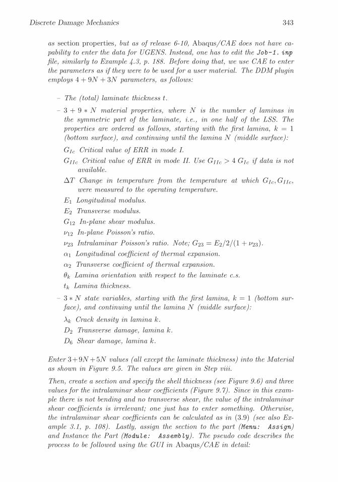
“K15072” — 2013/3/21 — 10:58�

�

�

�

�

�


as section properties, but as of release 6-10, Abaqus/CAE does not have ca-pability to enter the data for UGENS. Instead, one has to edit the Job-1. inpfile, similarly to Example 4.3, p. 188. Before doing that, we use CAE to enterthe parameters as if they were to be used for a user material. The DDM pluginemploys 4 + 9N + 3N parameters, as follows:

– The (total) laminate thickness t.

– 3 + 9 ∗ N material properties, where N is the number of laminas inthe symmetric part of the laminate, i.e., in one half of the LSS. Theproperties are ordered as follows, starting with the first lamina, k = 1(bottom surface), and continuing until the lamina N (middle surface):

GIc Critical value of ERR in mode I.

GIIc Critical value of ERR in mode II. Use GIIc > 4 GIc if data is notavailable.

ΔT Change in temperature from the temperature at which GIc, GIIc,were measured to the operating temperature.

E1 Longitudinal modulus.

E2 Transverse modulus.

G12 In-plane shear modulus.

ν12 In-plane Poisson’s ratio.

ν23 Intralaminar Poisson’s ratio. Note; G23 = E2/2/(1 + ν23).

α1 Longitudinal coefficient of thermal expansion.

α2 Transverse coefficient of thermal expansion.

θk Lamina orientation with respect to the laminate c.s.

tk Lamina thickness.

– 3 ∗ N state variables, starting with the first lamina, k = 1 (bottom sur-face), and continuing until the lamina N (middle surface):

λk Crack density in lamina k.

D2 Transverse damage, lamina k.

D6 Shear damage, lamina k.

Enter 3+9N+5N values (all except the laminate thickness) into the Materialas shown in Figure 9.5. The values are given in Step viii.

Then, create a section and specify the shell thickness (see Figure 9.6) and threevalues for the intralaminar shear coefficients (Figure 9.7). Since in this exam-ple there is not bending and no transverse shear, the value of the intralaminarshear coefficients is irrelevant; one just has to enter something. Otherwise,the intralaminar shear coefficients can be calculated as in (3.9) (see also Ex-ample 3.1, p. 108). Lastly, assign the section to the part (Menu: Assign)and Instance the Part (Module: Assembly). The pseudo code describes theprocess to be followed using the GUI in Abaqus/CAE in detail:

�

�

“K15072” — 2013/3/21 — 10:58�

�

�

�

�

�


Fig. 9.5: Create the material.

Module: Property

Menu: Material, Create, Name: [Material-1],

Material Behavior: User Material,

Mechanical Constants: # 3+9*N+5*N values

Section, Create, Name: [Section-1], Shell, Homogeneous, Cont

Tab: Basic, Shell thickness Value; [2.736],

Material: Material-1

Tab: Advanced: Transverse Shear Stiffness: [1,0,1]

Assign, Section, # select the part, Done, OK

Module: Assembly

Menu: Instance, Create, Name: [Part-1], Type: Independent, OK

iv. Creating a stepNext, a step is needed, among other things, to set the Field Output Requests

(See Figure 9.8). Since the analysis has material nonlinearity (damage), onehas to be careful with the solution strategy (see Figure 9.9). This is accom-

�

�

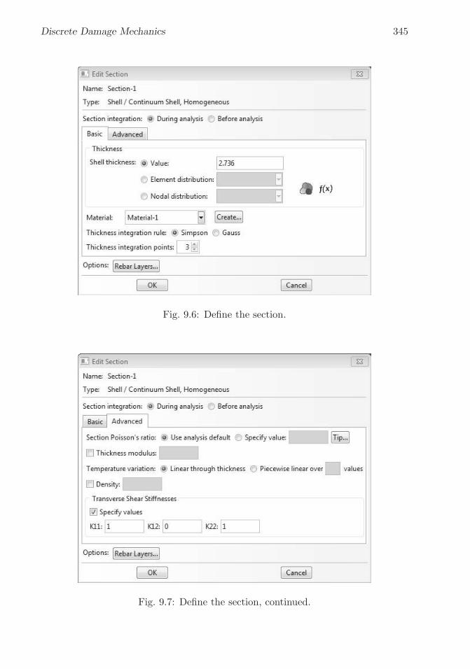
“K15072” — 2013/3/21 — 10:58�

�

�

�

�

�


Fig. 9.6: Define the section.

Fig. 9.7: Define the section, continued.

�

�

“K15072” — 2013/3/21 — 10:58�

�

�

�

�

�


Fig. 9.8: Field Output Request.

plished by following the pseudo code:

Module: Step

Menu: Step, Create, Name: [Step-1], After: Initial,

Type: General, Static, General, Cont

Tab: Basic, Time period: 1

Tab: Advanced, max. increments: [1000],

Incr.size: Initial: [0.01], Minimum; [1E-005], Maximum: [0.01]

v. Specifying boundary conditionsNext comes the boundary conditions, with symmetry along x = 0 and y = 0.The load is applied as a displacement, with a maximum value calculated as theproduct of the x-dimension of the model times the maximum strain expected,i.e., U1 = amax εx = 0.2 (see Figure 9.10). The details are given by thepseudo code:

�

�

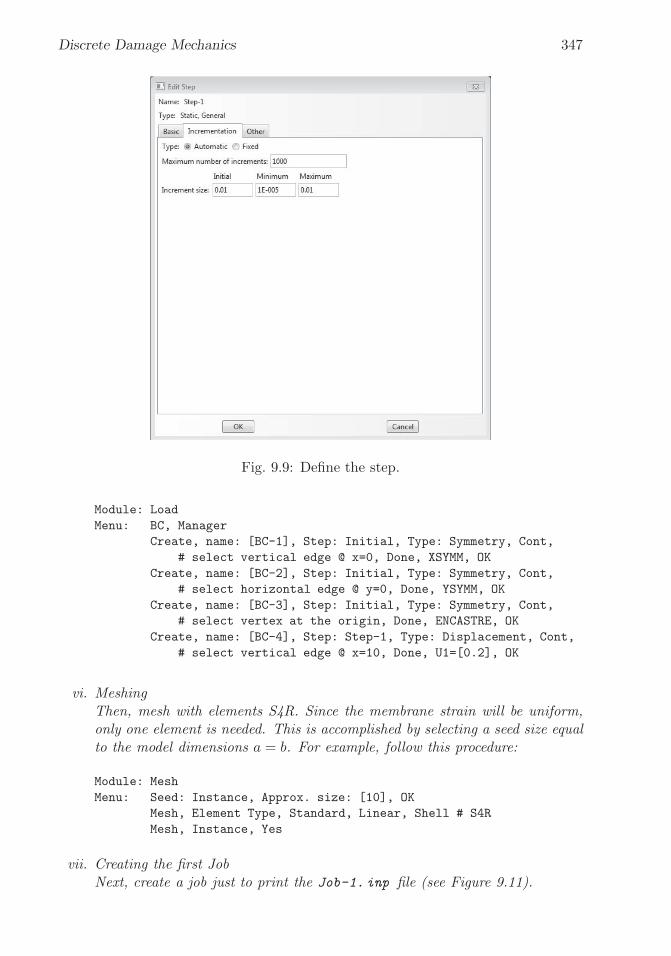
“K15072” — 2013/3/21 — 10:58�

�

�

�

�

�


Fig. 9.9: Define the step.

Module: Load

Menu: BC, Manager

Create, name: [BC-1], Step: Initial, Type: Symmetry, Cont,

# select vertical edge @ x=0, Done, XSYMM, OK


# select horizontal edge @ y=0, Done, YSYMM, OK


# select vertex at the origin, Done, ENCASTRE, OK

Create, name: [BC-4], Step: Step-1, Type: Displacement, Cont,

# select vertical edge @ x=10, Done, U1=[0.2], OK

vi. MeshingThen, mesh with elements S4R. Since the membrane strain will be uniform,only one element is needed. This is accomplished by selecting a seed size equalto the model dimensions a = b. For example, follow this procedure:

Module: Mesh

Menu: Seed: Instance, Approx. size: [10], OK

Mesh, Element Type, Standard, Linear, Shell # S4R

Mesh, Instance, Yes

vii. Creating the first JobNext, create a job just to print the Job-1.inp file (see Figure 9.11).

�

�

“K15072” — 2013/3/21 — 10:58�

�

�

�

�

�


Fig. 9.10: Boundary Conditions.

Module: Job

Menu: Job, Manager

Create, Name: [Job-1], Source: Model, Cont, OK

Data Check

Write Input

viii. Modifying the .inp fileNext copy Job-1.inp as Job-ddm.inp and modify it as follows. Both filesare available in [5].

Replace the following line:

*Shell Section, elset=_PickedSet2, material=Material-1

by the follwing single line (shown as two lines below due to space constraints,but it must be a single line in the .inp file) :

*Shell General Section,

elset=_PickedSet2, USER, PROPERTIES=30, VARIABLES=15

Take the material properties:

0.254, 1e+06, 0., 44700., 12700., 5800., 0.297, 0.41

3.7e-06, 3e-05, 0., 0.144, 44700., 12700., 5800., 0.297

0.41, 3.7e-06, 3e-05, 90., 1.152, 44700., 12700., 5800.

0.297, 0.41, 3.7e-06, 3e-05, 0., 0.072

�

�

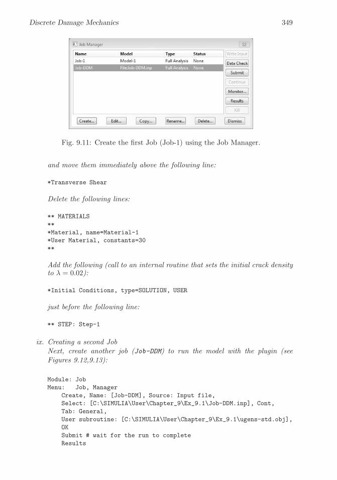
“K15072” — 2013/3/21 — 10:58�

�

�

�

�

�


Fig. 9.11: Create the first Job (Job-1) using the Job Manager.

and move them immediately above the following line:

*Transverse Shear

Delete the following lines:

** MATERIALS

**

*Material, name=Material-1

*User Material, constants=30

**

Add the following (call to an internal routine that sets the initial crack densityto λ = 0.02):

*Initial Conditions, type=SOLUTION, USER

just before the following line:

** STEP: Step-1

ix. Creating a second JobNext, create another job (Job-DDM) to run the model with the plugin (seeFigures 9.12,9.13):

Module: Job

Menu: Job, Manager

Create, Name: [Job-DDM], Source: Input file,

Select: [C:\SIMULIA\User\Chapter_9\Ex_9.1\Job-DDM.inp], Cont,

Tab: General,

User subroutine: [C:\SIMULIA\User\Chapter_9\Ex_9.1\ugens-std.obj],

OK

Submit # wait for the run to complete

Results

�

�

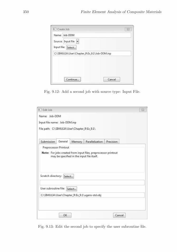
“K15072” — 2013/3/21 — 10:58�

�

�

�

�

�


Fig. 9.12: Add a second job with source type: Input File.

Fig. 9.13: Edit the second job to specify the user subroutine file.

�

�

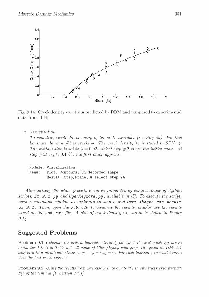
“K15072” — 2013/3/21 — 10:58�

�

�

�

�

�


0 0.2 0.4 0.6 0.8 1 1.2 1.4 1.6 1.8 20

0.2

0.4

0.6

0.8

1

1.2

1.4

Strain [%]

Cra

ck D

ensi

ty [1

/mm

]

Fig. 9.14: Crack density vs. strain predicted by DDM and compared to experimentaldata from [144].

x. VisualizationTo visualize, recall the meaning of the state variables (see Step iii). For thislaminate, lamina #2 is cracking. The crack density λ2 is stored in SDV=4.The initial value is set to λ = 0.02. Select step #0 to see the initial value. Atstep #24 (εx ≈ 0.48%) the first crack appears.


Menu: Plot, Contours, On deformed shape

Result, Step/Frame, # select step 24

Alternatively, the whole procedure can be automated by using a couple of Pythonscripts, Ex_ 9. 1. py and UgenKeyword.py , available in [5]. To execute the script,open a command window as explained in step i, and type: abaqus cae nogui=

ex_ 9. 1 . Then, open the Job.odb to visualize the results, and/or use the resultssaved on the Job.csv file. A plot of crack density vs. strain is shown in Figure9.14.

Suggested Problems

Problem 9.1 Calculate the critical laminate strain εcx for which the first crack appears inlaminates 1 to 3 in Table 9.2, all made of Glass/Epoxy with properties given in Table 9.1subjected to a membrane strain εx �= 0, εy = γxy = 0. For each laminate, in what laminadoes the first crack appear?

Problem 9.2 Using the results from Exercise 9.1, calculate the in situ transverse strengthF is2t of the laminas [1, Section 7.2.1].

�

�

“K15072” — 2013/3/21 — 10:58�

�

�

�

�

�


Table 9.2: Laminates for Exercise 9.1.

Laminate Number LSS

1 [0/908/0/908/0]2 [0/704/− 704/0/ − 704/704/0]3 [0/554/− 554/0/ − 554/554/0]4 [02/908/02]5 [15/− 15/908/− 15/15]6 [30/− 30/908/− 30/30]7 [40/− 40/908/− 40/40]

Problem 9.3 Calculate the critical laminate strain εcx for which the first crack appears inlaminates 4 to 7 in Table 9.2, all made of Glass/Epoxy with properties given in Table 9.1subjected to a membrane strain εx �= 0, εy = γxy = 0. For each laminate, in what laminadoes the first crack appear?

Problem 9.4 Using the results from Exercise 9.3, calculate the in situ transverse strengthF is2t of the laminas [1, Section 7.2.1].

�

�

“K15072” — 2013/3/21 — 10:58�

�

�

�

�

�

Chapter 10

Delaminations

Delamination is a frequent mode of failure affecting the structural performance ofcomposite laminates. The interface between layers offers a low-resistance path forcrack growth because the bonding between two adjacent layers depends only onmatrix properties. Delamination may originate from manufacturing imperfections,cracks produced by fatigue or low velocity impact, stress concentration near geomet-rical/material discontinuity such as joints and free edges, or due to high interlaminarstresses.

In laminates loaded in compression, the delaminated layers may buckle, andcracks propagate due to interaction between delamination growth and buckling.The presence of delaminations may reduce drastically the buckling load and thecompressive strength of the composite laminates [145] (Figure 10.1). Delamina-tions may also be driven by buckling in laminates under transverse loading [146].The analysis of delamination buckling requires the combination of geometricallynonlinear structural analysis with fracture mechanics.

According to its shape, delaminations are classified into through-the-width orstrip [146–153], circular [153–159], elliptic [160], rectangular [161] or arbitrary [162,163]. Depending on its location through the laminate thickness, delaminations areclassified into thin film, symmetric split [145, 148, 149], and general [150, 153, 156,157, 159]. In addition, analysis of combined buckling and growth for compositelaminates containing multiple delaminations under in-plane compressive loadinghas been carried out [164,165]. Experimental results on delamination buckling arepresented in [166,167].

Other delamination configurations that have been investigated in the literatureare the beam-type delamination specimens subjected to bending, axial, and shearloading [166–172] which form the basis for experimental methods used to measureinterlaminar fracture strength under pure mode I, mode II, and mixed mode con-ditions in composites, adhesive joints, and other laminated materials (Figure 10.2).

In plates with piezoelectric sensors or actuators, an imperfect bonding betweenthe piezoelectric lamina and the base plate may grow under mechanical and/orelectrical loading. As a consequence, the adaptive properties of the smart systemcan be significantly reduced since debonding results in significant changes to thestatic or dynamic response [173,174]. Finally, delamination growth may be caused

353

�

�

“K15072” — 2013/3/21 — 10:58�

�

�

�

�

�


axial shortening

preb

uckl

ing

path

Nc

axial load

*N

N

postbuckling path

N

N

N

delamination growth path

Fig. 10.1: Delamination buckling in a compressed laminate.

Fig. 10.2: Beam-type delamination specimens.

�

�

“K15072” — 2013/3/21 — 10:58�

�

�

�

�

�

Delaminations 355

by dynamic effects, such as vibration and impact. For instance, the dynamics effectsresulting from the inertia of the laminate on the growth process resulting from thebuckling of the delamination have been investigated for a circular delamination andtime-dependent loadings [175].

Delaminations can be analyzed by using cohesive damage models (Section 10.1)and fracture mechanics (Section 10.2). A cohesive damage model implements in-terfacial constitutive laws defined in terms of damage variables and a damageevolution law. Cohesive damage elements are usually inserted between solid ele-ments [176–179] or beam/shell elements [178].

In the fracture mechanics approach, the propagation of an existing delaminationis analyzed by comparing the amount of energy release rate (ERR) with the fracturetoughness of the interface. When mixed mode conditions are involved, the decom-position of the total ERR into mode I, mode II, and mode III components becomesnecessary due to the mixed-mode dependency of interface toughness [170, 180]. Anumber of fracture mechanics-based models have been proposed in the literatureto study delamination, including three-dimensional models [181–183] and simplifiedbeam-like models [145,147,172,184,185].

Fracture mechanics allows us to predict the growth of a preexisting crack or de-fect. In a homogeneous and isotropic body subjected to a generic loading condition,a crack tends to grow by kinking in a direction such that a pure mode I conditionat its tip is maintained. On the contrary, delaminations in laminated compositesare constrained to propagate in its own plane because the toughness of the interfaceis relatively low in comparison to that of the adjoining material. Since a delamina-tion crack propagates with its advancing tip in mixed mode condition, the analysisrequires a fracture criterion including all three mode components (Section 10.1.2).

The elastic strain energy per unit volume (density, in J/m3) is defined as U0 =1/2σijεij. The strain energy (in J) is defined as the volume integral U =

∫

V U0dV .The energy required to form, or to propagate, a crack is equal to the elastic energyreleased by the solid during crack formation. The energy released is the differencebetween the elastic strain energy available before and after the crack is formed, i.e.,−ΔU = Uafter − Ubefore. The rate of energy released per unit of crack area A isgiven, in J/m2, by

G = −ΔU

ΔA(10.1)

where A is one half the surface area created. The theory of crack growth may bedeveloped by using one of two approaches due to Griffith and Irwin, respectively.The Griffith energy approach uses the concept of Energy Release Rate G as the(computable) energy available for fracture on one hand, and the material propertyGc, which is the energy necessary for fracture, on the other hand. A crack growswhen

G ≥ Gc (10.2)

where for completeness note that Gc = 2γc, where γc is the critical fracture energyper unit surface crack area, and A is one half of the crack area formed, i.e., the area

�

�

“K15072” — 2013/3/21 — 10:58�

�

�

�

�

�


�

�s

Elastic zone(D = 0)

Stress transferzone (0 < D < 1)

Stress-freezone (D = 1)

Fig. 10.3: Cohesive zone method to simulate crack propagation.

of only one of the faces of the crack.The Irwin (local) approach is based on the concept of stress intensity factor,

which represents the energy stress field in the neighborhood of the crack tip. Thesetwo approaches are equivalent and, therefore, the energy criterion may be rewrittenin terms of stress intensity factors. Further, a number of path independent integralshave been proposed to calculate the ERR, such as the J -integral [186].

The elastic strain energy released ΔU during crack propagation, and thereforeused to create the new surface area, can be calculated as the work required to closethe crack, i.e.,

ΔU =Wclosure (10.3)

The crack closure method of computation provides the base for the Virtual CrackClosure Technique (VCCT) described in Section 10.2.

10.1 Cohesive Zone Method

The cohesive zone method (CZM) is based on the assumption that the stress transfercapacity between the two separating faces of a delamination is not lost completely atdamage initiation, but rather is a progressive event governed by progressive stiffnessreduction of the interface between the two separating faces (Fig. 10.3).

The interface between the two possible separating faces of the laminated materialis modeled with cohesive elements [187]. There are two types of CZM elements inAbaqus:

– CZM elements with finite thickness, which are based on a regular, contin-uum (σ − ε) constitutive behavior. This type of elements is used to modeldelamination behavior of adhesive bonds where the thickness of the interfaceis considerable.

– CZM elements with zero thickness, which are based on a traction–separation(σ − δ) constitutive behavior. This type of elements is used to model de-lamination behavior of adhesive bonds where the thickness of the interface isnegligible, as it is the case of laminated composites.

�

�

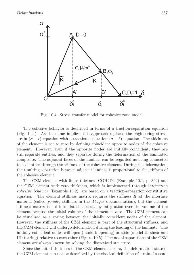
“K15072” — 2013/3/21 — 10:58�

�

�

�

�

�

Delaminations 357

Fig. 10.4: Stress transfer model for cohesive zone model.

The cohesive behavior is described in terms of a traction-separation equation(Fig. 10.4). As the name implies, this approach replaces the engineering stress-strain (σ − ε) equation with a traction-separation (σ − δ) equation. The thicknessof the element is set to zero by defining coincident opposite nodes of the cohesiveelement. However, even if the opposite nodes are initially coincident, they arestill separate entities, and they separate during the deformation of the laminatedcomposite. The adjacent faces of the laminas can be regarded as being connectedto each other through the stiffness of the cohesive element. During the deformation,the resulting separation between adjacent laminas is proportional to the stiffness ofthe cohesive element.

The CZM element with finite thickness COH2D4 (Example 10.1, p. 364) andthe CZM element with zero thickness, which is implemented through interactioncohesive behavior (Example 10.2), are based on a traction-separation constitutiveequation. The element stiffness matrix requires the stiffness ˜K of the interfacematerial (called penalty stiffness in the Abaqus documentation), but the elementstiffness matrix is not formulated as usual by integration over the volume of theelement because the initial volume of the element is zero. The CZM element canbe visualized as a spring between the initially coincident nodes of the element.However, the stiffness of the CZM element is part of the structural stiffness, andthe CZM element will undergo deformation during the loading of the laminate. Theinitially coincident nodes will open (mode I: opening) or slide (model II: shear andIII: tearing) relative to each other (Figure 10.5). The nodal separations of the CZMelement are always known by solving the discretized structure.

Since the initial thickness of the CZM element is zero, the deformation state ofthe CZM element can not be described by the classical definition of strain. Instead,

�

�

“K15072” — 2013/3/21 — 10:58�

�

�

�

�

�


(a) (b)

yx

(c)

yx

yx

yx

Fig. 10.5: Crack propagation modes: a) I-opening, b) II-shear, c) III: tearing.

the measure of the deformation becomes the separation δ between the faces con-nected through the CZM element, and this makes possible the use of the (σ − δ)traction-separation equation instead of the classical engineering (σ − ε) equation.1

10.1.1 Single Mode Cohesive Model

The CZM is formulated assuming the three crack propagation modes are uncoupled,even if multiple modes are active simultaneously, as described in Section 10.1.2. Inthis section we consider the case of a single mode deformation at an interface ofthe laminated material, either mode I, II, or III (Figure 10.5). The formulation issimilar for any of the three modes. The surface tractions at the interface are σi withi = I, II, III denoting the three modes of crack propagation. The correspondingseparations between the opposite faces of the CZM element are denoted as δi, eachrelated to the surface traction σi through the interface stiffness Ki, also calledpenalty stiffness. Therefore, material stiffness values are necessary for each of theloading modes, i.e., KI ,KII ,KIII . A discussion on how to choose numerical valuesfor Ki is provided in [188].

The behavior of the material at the interface is assumed to be linear-elastic upto the onset of damage (OA in Fig. 10.4) and damaging-elastic after that (OB inFig. 10.4). Consequently, the stress-separation is described by

σi = Ki δi (10.4)

and

Ki = (1−Di) ˜Ki (10.5)

where Di are the damage variables, and ˜Ki in [N/mm3] are the stiffness valuesof the undamaged material at the interface, relating the stresses σi to the relativeseparations δi between the opposite faces of the CZM element, with i = I, II, III.The stiffness values ˜Ki are additional material properties needed for the CZMmodel,which are different from the Young’s modulus E for normal deformation, or G forshear deformation.

1Abaqus documentation uses the word strain as synonymous to separation δ when describingthe deformation of the CZM element based on traction-separation equation.

�

�

“K15072” — 2013/3/21 — 10:58�

�

�

�

�

�

Delaminations 359

For each mode, there is a critical level of stress σ0i and separation δ0i when thedamage at the interface starts (point A in Fig. 10.4), called damage onset. Atdamage onset, the two laminas do not separate completely into a physical crackbut rather the interface material starts losing its stiffness. Here, σ0i representsthe strength of the interface with one value of strength for each crack propagationmode: σ0I , σ

0II , σ

0III . In CZM, these modes are called damage modes because the

CZM does not evaluate fracture mechanics. Instead, CZM replaces the fracturemechanics problem by a continuum damage mechanics problem (Chapter 8). Theinterface strengths are therefore additional material parameters required by theCZM element.

Therefore, the damage initiation criteria are

σi = σ0i (10.6)

and the separation at damage onset are calculated as

δ0i = σ0i /˜Ki (10.7)

After damage onset, the interface material starts losing its stiffness (OB inFig. 10.4), according to (10.5). Note that there are as many damage variablesas damage modes: DI ,DII ,DIII , which are state variables (8.61) to be determinedduring the analysis. Their physical interpretation is given by (10.5) as measuresof stiffness degradation (see also Section 8.2). The damage variables satisfy thefollowing conditions:

– D = 0 up to damage onset (OA in Fig. 10.4) while the interface material isundamaged, thus retaining its initial stiffness.

– 0 < D < 1 during degradation of the interface material (AC in Fig. 10.4),when the material is gradually losing its stiffness.

– D = 1 at fracture (point C in Fig. 10.4), when there is no remaining stiffnessfor the interface material, which means no stress transfer capacity is providedby the interface. This corresponds to the fracture of the cohesive connectionbetween the two faces of the CZM element.

With reference to Figure 10.4 we have:

Di =

{

0, δi ≤ δ0i1, δi = δci

(10.8)

In stress-strain space, the cohesive behavior depicted in Fig. 10.4 displays stresssoftening. That is, after damage onset the stresses σi in the damaged interface havelower values than the peak values σ0i .

The CZM element uses the classical assumption of elastic damage typical of con-tinuum damage mechanics (CDM, Chapter 8). Therefore, unloading from any pointsuch as B on the line AF in Fig. 10.4 will return to the origin without permanentdeformation upon unloading.

�

�

“K15072” — 2013/3/21 — 10:58�

�

�

�

�

�


Eventually, there will be total fracture of the cohesive bond (point C in Fig. 10.4)when the stiffness of the interface reduces to zero. Due to the fact that total lossof stiffness, and thus total loss of cohesive stress transfer, does not take place untilpoint C, the CZM is correlated with the Griffith crack propagation criterion (10.2)at point C. The correlation is made by considering that the area under the (σ − δ)curve in Fig. 10.4 is equal to the critical ERR Gic in Griffith’s principle (10.2). Inthis way, the separation at fracture δci can be calculated as

δci =2Gic

σ0i(10.9)

Since there is a critical ERR value for each damage mode, Gic, with i =I, II, III, there will be three separations at fracture–one per mode. The threeERR values are material properties required by the CZM, in addition to the threevalues of strength σ0i and the three values of interface stiffness ˜Ki. From the pointof view of the amount of experimental data needed to perform an analysis, this isa disadvantage of CZM because it requires nine experimental values. On the otherhand, discrete damage mechanics requires only the three values of ERR to predictboth the onset and the evolution of damage (Chapter 9).

Substituting (10.4) into (10.5) and rearranging, we get

Di = 1− σiδ0i

σ0i δi(10.10)

By similarity of triangles BB’F and AA’F, we have

σiσ0i

=δci − δiδci − δ0i

(10.11)

which substituted into (10.10) yields

Di =δci (δi − δ0i )

δi(δci − δ0i )(10.12)

In this way, the damage variables Di are calculated as a function of the relativeseparation between the faces of the laminate δi, which is provided by the FE solutionand the values δ0i , δ

ci calculated previously.

In summary, there are four distinct stages in the material behavior described byFig. 10.4:

– linear elastic undamaged material behavior (line OA), with the associatedconstitutive equation (10.4).

– damage initiation (point A), with the associated criterion (10.6).

– damage evolution (line AC), with the associated damage evolution equation(10.5), (10.12).

– fracture (crack formation), with the associated crack formation criterion (10.2).

�

�

“K15072” — 2013/3/21 — 10:58�

�

�

�

�

�

Delaminations 361

As previously stated, the formulation presented in this section works only forpure mode I, or II, or III. The general case of the mixed mode loading is presentedin the following section.

10.1.2 Mixed Mode Cohesive Model

When the interface of the laminated material is under mixed modes, all three trac-tion components σI , σII , σIII and all three separation components δI , δII , δIII areactive. In other words, mixed mode implies that two or more pairs (σi, δi) are non-vanishing, with i = I, II, III. However, to reduce the burden of experimentation,it is assumed that the penalty stiffness (10.7) is the same for all modes ˜K = ˜Ki.

Mixed mode ratios can be defined between pairs of mode components. Forexample, in terms of separations

βδII =δIIδI

; βδIII =δIIIδI

(10.13)

or in terms of ERR

βGII=

GII∑3

1Gi

; βGIII=

GIII∑3

1Gi

(10.14)

Regardless of the definition used, mixed mode ratios are just parameters char-acterizing the mixed mode state, which allow for a simplification of the analysis byassuming that decohesion progresses at constant mixed mode ratios. It is further as-sumed that the modes are uncoupled even though they occur simultaneously. Thatis, the stress-separation relationship for each uncoupled mode is again expressed by(10.4), separately for each mode.

Next, a mixed mode separation is defined by the L2 norm of the mode separa-tions, i.e.,

δm =

√

√

√

√

M∑

i=1

δ2i (10.15)

where M is the number of modes involved (i.e., 2 or 3 modes). Next, the singlemode damage initiation criterion in (10.6) is replaced, for example, by a quadraticstress criterion

M∑

i=1

(

σiσ0i

)2

= 1 (10.16)

Other mixed mode damage initiation criteria can be selected in Abaqus, such asthe quadratic displacement criterion, or a maximum-stress/maximum-displacementcriterion. Regardless of the damage initiation criterion selected, the goal is tocalculate the mixed mode separation δ0m at damage onset under mixed mode loading.

For the case of mode I and II only, M = 2 and the equivalent mixed modeseparation at damage onset δ0m is found as follows. First, rewrite the damage initi-ation criteria (10.16) in terms of separations using (10.7) and (10.4)-(10.5), taking

�

�

“K15072” — 2013/3/21 — 10:58�

�

�

�

�

�


into account that Di = 0 up to damage initiation. Therefore, mixed mode damageinitiation is predicted by

(

δIδ0I

)2

+

(

δIIδ0II

)2

= 1 (10.17)

Next, rewrite (10.15) using the first of (10.13) to get

δI =δm

√

1 + β2(10.18)

and using (10.13) again

δII = βδm

√

1 + β2(10.19)

Now, substitute (10.18) and (10.19) into (10.17), taking into account that since(10.17) represents damage initiation, one should write δ0m for δm. Therefore,

δ0m =

√

(δ0I )2(δ0II)

21 + β2

(δ0II)2 + β2(δ0I )

2(10.20)

The quantities δ0i in (10.20) represent the separations at damage onset duringsingle mode loading, calculated with (10.7), and β is the mixed mode ratio, whichis assumed to be constant during the damage process.

A mixed mode crack propagation criterion is now needed to replace the singlemode criterion (10.2). A possible choice is to use an ERR power criterion as follows

3∑

i=1

(

Gi

Gic

)αi

= 1 (10.21)

which attempts to predict fracture under mixed mode conditions, similarly to pointC in Fig. 10.4 for the single mode situation. To reduce the burden of experimenta-tion, it is customary to assume that the exponents are the same for all modes, i.e.,αi = α.

Each of the single mode component Gi can be calculated by one of two method-ologies. Some authors [176, 178] calculate each single mode component ERR byconsidering the area OABB’ in Fig. 10.4, thus including the recoverable energyOBB’ in the definition of Gi. This approach is indirectly related to linear elasticfracture mechanics (LEFM). Other authors [188] use a damage mechanics approachwhere each single mode component ERR is calculated by considering only the un-recoverable energy represented by the area OAB. Both approaches lead to the sameresults for a single-mode delamination since loss of adhesion occurs at δci whereboth approaches predict the same values for Gi (point B reaches point C). How-ever, different results are obtained for mixed-mode delamination because the crack

�

�

“K15072” — 2013/3/21 — 10:58�

�

�

�

�

�

Delaminations 363

propagates when an interaction criterion is satisfied, the latter involving the ratiosGi/Gic.

In principle, the approach based on LEFM should lead to conservative predic-tions of the load carrying capacity for mixed-mode delamination. On the otherhand, since the total energy dissipated during the delamination at each point is notreleased instantaneously as assumed in LEFM, the damage mechanics based defini-tion appears appropriate especially when the size of the nonlinear fracture processzone ahead of the delamination front is not negligible as it may occur in the caseof laminated composite materials where the damage zone may be comparable to orlarger than the single-ply thickness, which generally scales with the near-tip stressfield.

In the sequel, the damage mechanics approach is used. That is, for each singlemode separation δi, the single mode component ERR Gi is calculated as the areaOAB in Fig. 10.4, which represents dissipated energy, i.e.,

AOAB = AOAF −AOBF (10.22)

where AOAF is the single mode critical ERR Gic, and AOBF can be calculated basedon the geometry in Fig. 10.4 as

AOBF =1

2BB′ ×OF =

1

2Kiδ

0i

δci − δiδci − δ0i

δci (10.23)

where δci = OF , kiδ0i = σ0i , and σi/σ

0i is given by (10.11). Based on (10.22), (10.23),

the single mode component ERR at the moment of mixed mode fracture is calculatedas

Gi = Gic − 1

2Kiδ

0i δ

ci

δci − δiδci − δ0i

(10.24)

The assumed mode decomposition (10.24) is necessary so that each single modecomponent ERR Gi corresponding to mixed mode fracture can be expressed as afunction of the single mode separation δi, i.e., Gi = Gi(δi). All other quantities in(10.24) are known, as follows:

– Gic is the single mode critical ERR (material parameter).

– δ0i is the separation at damage onset under single mode loading (point A inFig. 10.4), given by (10.7)

– δci is the separation at fracture under single mode loading (point C in Fig. 10.4),given by (10.9).

The single mode ERR components of the mixed mode condition in (10.24) haveto satisfy the energy criterion (10.21) at the moment of fracture (crack propagation).For the case of two modes, and assuming αi = α = 2 in (10.21), the mixed modeseparation at fracture (point C) is calculated in [188, (15)] as

�

�

“K15072” — 2013/3/21 — 10:58�

�

�

�

�

�


δcm =

√1 + β

β2(δ0FI )2 + (δ0FII )2×

{

δ0I (δ0FII )

2 + βδ0II(δ0FI )2

+ δ0FI δ0FII

√

(δ0FII )2 − (δ0II)

2 + 2βδ0I δ0II − β2(δ0I )

2 + β2(δ0FI )2}

(10.25)

where δ0FI = δcI − δ0I , δ0FII = δcII − δ0II .

There are three energy crack extension criteria implemented in Abaqus:

– the power equation criterion in (10.21).

– the BK criterion, which is another closed form function of (Gi, Gic).

– a user input of the total mixed mode ERR at fracture Gc =∑3

1Gic.

Once the mixed mode separation at fracture (10.25) is calculated based on theselected criterion, and the mixed mode separation at damage onset is known basedon (10.20), the damage variable for mixed mode conditions can be expressed in asimilar manner as for the case of single mode condition (10.12) by satisfying therequirement in (10.8), i.e.,

Dm =δcm(δm − δ0m)

δm(δcm − δ0m)(10.26)

where the onset and fracture separations δ0m and δcm are calculated based on (10.20)and (10.25), respectively; and δm is the current level of separation under mixedmode conditions obtained using (10.15) in terms of the single modes separations δiprovided by the FE model. The stiffness degradation for the cohesive material isthen calculated according with (10.5). The stress softening evolution of the cohesivematerial under mixed mode conditions is similar to the one depicted in Fig. 10.4,by substituting δ0m, δ

cm for δ0, δc.

Besides the energy approach to mixed mode damage evolution as presented here,where the crack extension criterion is a function of ERR, and δcm is calculated basedon this energy criterion, Abaqus also has implemented a displacement approach todamage evolution. The displacement approach requires the user to directly providethe mixed mode separation at the moment of fracture δcm, which is then directlyused in (10.26).

Example 10.1 A laminated double cantilever beam (DCB) 100mm long and 20 mm wideis made up of two layers bonded by an adhesive layer of negligible thickness. Each layeris 1.5 mm thick. Apply a loading system to induce delamination and mode I crack growththrough the adhesive layer. Assuming linear elastic behavior, create a 2D model of the DCBusing CZM elements to represent the adhesive layer. Use the element-based cohesivebehavior implemented in Abaqus to represent the adhesive.

�

�

“K15072” — 2013/3/21 — 10:58�

�

�

�

�

�

Delaminations 365

Solution to Example 10.1 To facilitate the solution of this example, run the Pythonscript ws_composites_dcb.py in your Work Directory. The script can be fetched fromthe examples in the Abaqus documentation as follows

# open a Windows command prompt via the Windows Taskbar and Start Menu

Start, Run, Open [cmd], OK

# Navigate to the folder C:\SIMULIA\User\Ex_10.1

# you may need to create the directory using the command: mkdir Ex_10.1

# type the following command and press the Enter-key

abaqus fetch job=ws_composites_dcb.py

# this will copy the file ws_composites_dcb.py into the Work Directory

The script creates two models, of which only the 2D model named coh-els is used inthis example. The model contains the parts, assembly, materials, sections, sets, and surfacesneeded to apply boundary conditions, constraints, and to define the output requests fields.

During model set up, the cohesive elements representing the adhesive layer are definedwith a finite thickness. This is done only to facilitate manipulation and the definition ofconstraints. At the end of the setup process, the thickness of the cohesive elements is adjustedto zero, as explained in Section v, p. 367. That is, cohesive elements COH2D4 with zerothickness are used in this example.

Although the loading conditions applied in this example induce crack propagation inmode I only, Abaqus requires defining the parameters corresponding to all three propagationmodes.


i. Running the Python script

Menu: File, Run Script, [ws_composites_dcb.py], OK

# notice that the model has been named dcb.cae

Menu: Save As, [Ex_10.1.cae], OK

ii. Defining materials, sections, and assigning sections to parts.

The coh-els model is set up with units [m,Pa]. A material named ‘bulk’ contains theundamaged material properties of the laminas: E1 = 135.3× 109 Pa;E2 = E3 = 9×109 Pa; ν12 = ν13 = 0.24; ν23 = 0.46;G12 = G23 = 4.5× 109 Pa;G13 = 3.3× 109 Pa.

To enter the properties of the adhesive, a new material called ‘adhesive’ must bedefined using the pseudo code below. The adhesive stiffness values (10.4) are: KI =E/Knn = 570 × 1012 Pa, KII = E/Kss = 570 × 1012 Pa, and KIII = E/Ktt =570 × 1012 Pa, where Knn,Kss,Ktt are penalty parameters that are mentioned hereonly because that is how they are labeled in Abaqus/CAE. The adhesive strengthvalues (10.6) are: σ0

I = 5.7E7, σ0II = 5.7E7, σ0

III = 5.7E7. The adhesive parametersfor the Benzeggagh-Kenane (BK) crack extension criterion are: Power 2.284, andfracture energies GIc = 280 J/m2, GIIc = 280 J/m2, GIIIc = 280 J/m2 (see(10.2)).

Module: Property

Model: coh-els

Part: adhesive


Create, Name [cohesive], Mechanical, Elasticity, Elastic

�

�

“K15072” — 2013/3/21 — 10:58�

�

�

�

�

�


Type: Traction, E/Knn [5.7E14], G1/Ktt [5.7E14], G2/Kss [5.7E14]

# damage onset criterion

Mechanical, Damage for Traction Separation Laws, Quads Damage

Nominal Stress Normal-only Mode [5.7E7]

Nominal Stress First Direction [5.7E7]

Nominal Stress Second Direction [5.7E7]

# crack extension criterion and required parameters

# Benzeggagh-Kenane (BK) is used, see Abaqus documentation

Suboptions, Damage Evolution

Type: Energy, Mixed mode behavior: BK, # checkmark: Power [2.284]

Normal Mode Fracture Energy [280] # GIc

Shear Mode Fracture Energy First Direction [280] # GIIc

Shear Mode Fracture Energy Second Direction [280] # GIIIc

OK, OK, # close Material Manager pop-up window

Menu: Section, Manager

# a section named ’bulk’ defines the laminas

# create a section for the adhesive

Create, Name [cohesive], Category: Other, Type: Cohesive, Cont

Material: cohesive, Response: Traction Separation

# checkmark: Out-of-plane thickness [0.02], OK

# close Section Manager pop-up window


# pick the part, Done, Section: cohesive, OK

iii. Defining the analysis steps

Module: Step

Menu: Step, Create, Cont

# geometrical non-linearity for large displacements

Tab: Basic, Nlgeom: On

# parameters to setup the time increments for the solution

Tab: Incrementation, Maximum number of increments [1000]

Increment size: Initial [0.01], Minimum [1.0E-8], OK


Output Variables: # expand: State/Field/User/Time

# checkmark: STATUS, OK

# the STATUS variable is an on/off switch that indicates the CAE

# postprocessor when to stop drawing the cohesive elements

# a completely degraded (damaged) element will have STATUS 0 (off)

Menu: Output, History Output Requests, Create

Name [H-Output-2], Step: Step-1, Cont

Domain: Set : top

# expand: Displ/Veloc/Accel, # expand: U, # checkmark: U2

# expand: Forces/Reactions, # expand: RF, # checkmark: RF2, OK

# the values of U2 (imposed displacement) and RF2 (reaction force)

# at the specified set (node) will be stored for postprocessing

iv. Meshing the modelThe sweep technique is used because the length of the cohesive elements is orientation-dependent. For this case they need to be defined from the bottom to the top surfaceof the adhesive layer because their elongation will represent the separation of thelaminas.

�

�

“K15072” — 2013/3/21 — 10:58�

�

�

�

�

�

Delaminations 367

A viscosity parameter is used along with the COH2D4 element to speed up the con-vergence of the iterative solution. You may change its value to see how it affects thesolution.

Module: Mesh

Model: coh-els

Object: Part: beam

Menu: Mesh, Controls, Element Shape: Quad, Technique: Structured, OK


Family: Plane Strain, # checkmark: Incompatible modes

# Notice element CPE4I has been assigned, OK

Menu: Seed, Edges

# pick the top horizontal line, Done

Method: By number, Number of elements [400], OK

# pick the left vertical line, Done


Menu: Mesh, Part, Yes

Object: Part: adhesive

Menu: Mesh, Controls, Element Shape: Quad, Technique: Sweep

Redefine Sweep Path

# if the highlighted path coincides with the thickness direction

Accept Highlighted

# otherwise change accordingly to accomplish that, OK


Family: Cohesive, Viscosity: Specify [1.0E-5]

# notice element COH2D4 has been assigned, OK

Menu: Seed, Edges

# pick the top horizontal line, Done


# pick the left vertical line, Done



v. Creating model constraints.The use of a finite-thickness part to represent the adhesive layer facilitated the defini-tion of the cohesive elements properties. The constraints applied here guarantee thatthe top and bottom surfaces of the cohesive elements are coincident once the solutionprocess starts, effectively defining the initial length of the cohesive elements as zero.Although it is not visually shown, the procedure below adjusts the surfaces defined asslaves to follow those defined as masters.

Module: Interaction

Menu: Constraint, Create, Name [top], Type: Tie, Cont

Choose the master type: Surface, Surfaces, top, Cont

Choose the slave type: Surface, coh-top, Cont

Position Tolerance: Specify distance [0.002], OK

Menu: Constraint, Create, Name [bot], Type: Tie, Cont

Choose the master type: Surface, bot, Cont

Choose the slave type: Surface, coh-bot, Cont

Position Tolerance: Specify distance [0.002], OK

vi. Applying BC and loads

�

�

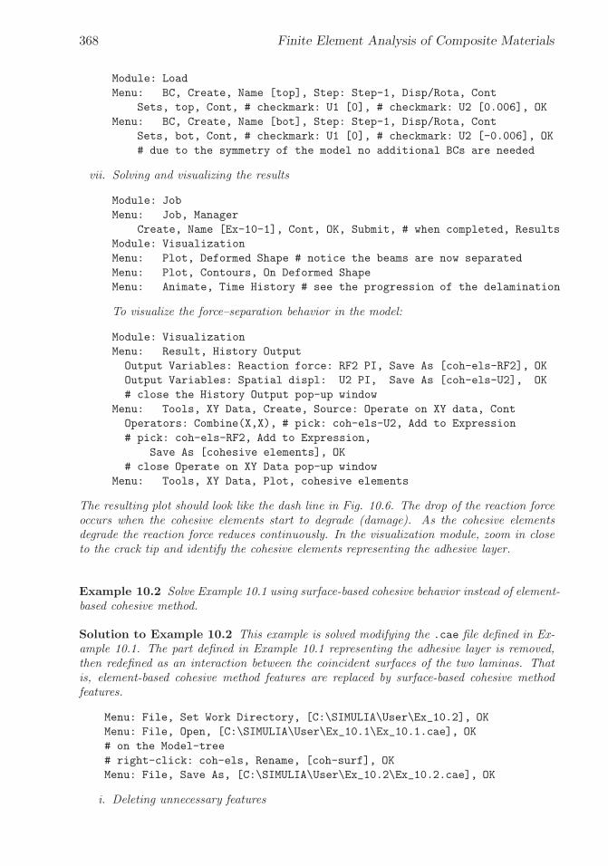
“K15072” — 2013/3/21 — 10:58�

�

�

�

�

�


Module: Load

Menu: BC, Create, Name [top], Step: Step-1, Disp/Rota, Cont

Sets, top, Cont, # checkmark: U1 [0], # checkmark: U2 [0.006], OK

Menu: BC, Create, Name [bot], Step: Step-1, Disp/Rota, Cont

Sets, bot, Cont, # checkmark: U1 [0], # checkmark: U2 [-0.006], OK

# due to the symmetry of the model no additional BCs are needed


Module: Job

Menu: Job, Manager

Create, Name [Ex-10-1], Cont, OK, Submit, # when completed, Results


Menu: Plot, Deformed Shape # notice the beams are now separated


Menu: Animate, Time History # see the progression of the delamination

To visualize the force–separation behavior in the model:



Output Variables: Reaction force: RF2 PI, Save As [coh-els-RF2], OK

Output Variables: Spatial displ: U2 PI, Save As [coh-els-U2], OK

# close the History Output pop-up window

Menu: Tools, XY Data, Create, Source: Operate on XY data, Cont

Operators: Combine(X,X), # pick: coh-els-U2, Add to Expression

# pick: coh-els-RF2, Add to Expression,

Save As [cohesive elements], OK

# close Operate on XY Data pop-up window

Menu: Tools, XY Data, Plot, cohesive elements

The resulting plot should look like the dash line in Fig. 10.6. The drop of the reaction forceoccurs when the cohesive elements start to degrade (damage). As the cohesive elementsdegrade the reaction force reduces continuously. In the visualization module, zoom in closeto the crack tip and identify the cohesive elements representing the adhesive layer.

Example 10.2 Solve Example 10.1 using surface-based cohesive behavior instead of element-based cohesive method.

Solution to Example 10.2 This example is solved modifying the .cae file defined in Ex-ample 10.1. The part defined in Example 10.1 representing the adhesive layer is removed,then redefined as an interaction between the coincident surfaces of the two laminas. Thatis, element-based cohesive method features are replaced by surface-based cohesive methodfeatures.



# on the Model-tree

# right-click: coh-els, Rename, [coh-surf], OK


i. Deleting unnecessary features

�

�

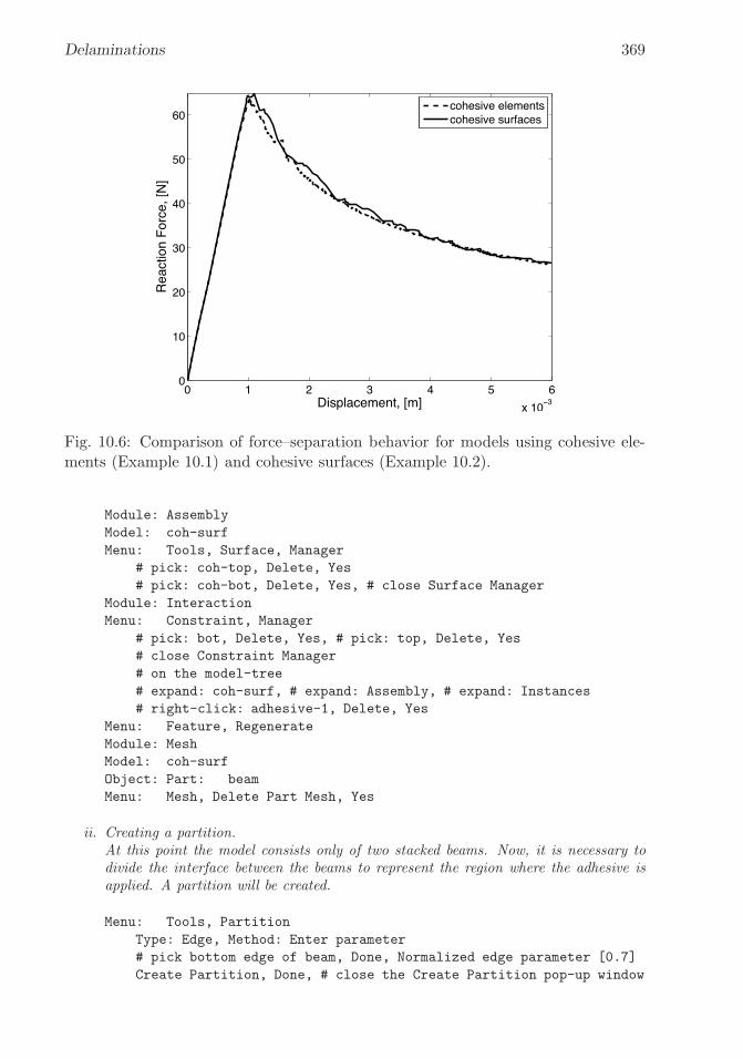
“K15072” — 2013/3/21 — 10:58�

�

�

�

�

�

Delaminations 369

0 1 2 3 4 5 6

x 10−3

0

10

20

30

40

50

60

Displacement, [m]

Rea

ctio

n F

orce

, [N

]

cohesive elementscohesive surfaces

Fig. 10.6: Comparison of force–separation behavior for models using cohesive ele-ments (Example 10.1) and cohesive surfaces (Example 10.2).

Module: Assembly

Model: coh-surf

Menu: Tools, Surface, Manager

# pick: coh-top, Delete, Yes

# pick: coh-bot, Delete, Yes, # close Surface Manager

Module: Interaction

Menu: Constraint, Manager

# pick: bot, Delete, Yes, # pick: top, Delete, Yes

# close Constraint Manager

# on the model-tree

# expand: coh-surf, # expand: Assembly, # expand: Instances

# right-click: adhesive-1, Delete, Yes


Module: Mesh

Model: coh-surf

Object: Part: beam

Menu: Mesh, Delete Part Mesh, Yes

ii. Creating a partition.At this point the model consists only of two stacked beams. Now, it is necessary todivide the interface between the beams to represent the region where the adhesive isapplied. A partition will be created.


Type: Edge, Method: Enter parameter

# pick bottom edge of beam, Done, Normalized edge parameter [0.7]

Create Partition, Done, # close the Create Partition pop-up window

�

�

“K15072” — 2013/3/21 — 10:58�

�

�

�

�

�


iii. Meshing the part


iv. Creating sets and surfaces.The surface called top in Example 10.1 will be redefined to be the whole interfacebetween the beams. Since the two beams are stacked, selecting only one of the coin-cident surfaces is cumbersome. To facilitate selecting the desired surface, a usefulvisualization tool is introduced –Display Group Toolbar.

Module: Assembly

# locate the Toolbar named Display Group, If it is not available

# enable it using Menu: View, Toolbars, Display Group

# click the first icon of Display Group Toolbar (Replace Selected)

# pick the top beam, Done, # only the picked part will be visible

Menu: Tools, Surface, Edit, top

# pick the two lines forming the bottom edge of the beam, Done


Name [bond], Type: Geometry, Cont

# pick the longest line at the bottom of the beam, Done

# click on third icon of Display Group Toolbar (Replace All)

# the full assembly will be visualized

The set named bond will represent the adhesive layer in the same way the part namedadhesive-1 did in Example 10.1.

v. Defining interactions to represent the adhesive layer.First the properties and characteristics of the contact are defined. Then the interact-ing surfaces are selected.

Module: Interaction

Menu: Interaction, Property, Create

Name [coh], Type: Contact, Cont

Mechanical, Tangential Behavior, Friction formulation: Frictionless

Mechanical, Normal Behavior, Pressure-Overclosure: Hard Contact

Constraint enforcement method: Default

Mechanical, Cohesive Behavior

Eligible Slave Nodes: Specify the bounding node set in surf-to-surf

Traction-separation Behavior: Specify stiffness coeffs, Uncoupled

Knn [5.7e14], Kss [5.7e14], Ktt [5.7e14] # KI, KII, and KIII

Mechanical, Geometric Properties,

Out-of-plane surface thickness [0.02]

Mechanical, Damage, Criterion: Quadratic traction

Normal Only [5.7e7], Shear-1 Only [5.7e7], Shear-2 [5.7e7]

# these define the onset of damage in the adhesive layer

# checkmark: Specify damage evolution

Type: Energy,

# checkmark: Specify mixed mode behavior: Benzeggagh-Kenane

# checkmark: Specify power-law/BK exponent [2.284]

Normal Fracture Energy [280], # Critical crack propagation GIc

1st Shear Fracture Energy [280] # GIIc

2nd Shear Fracture Energy [280] # GIIIc

# checkmark: Specify damage stabilization, Viscosity coeff. [1e-5]

�

�

“K15072” — 2013/3/21 — 10:58�

�

�

�

�

�

Delaminations 371

# it plays the same role as the one used for cohesive elements

OK # the properties of the adhesive layer have been defined

Menu: Interaction, Create

Name [coh], Step: Initial, Type: Surface-to-surface (Standard), Cont

Surfaces, # pick: bot, Cont # this is the master surface

Surfaces, # pick: top, Cont # this is the slave surface

Discretization method: Node to surface

Tab: Bonding

# checkmark: Limit bonding to slave nodes in subset: bond

# This represents the adhesive layer bonding the beams, OK

vi. Solving and visualizing the results

Module: Job

Menu: Job, Manager



Menu: Plot, Deformed Shape # notice the beams have been separated


Menu: Animate, Time History # progression of the delamination

To visualize the force–separation behavior in the model:



Output Variables: Reaction force: RF2 PI,

Save As [coh-surf-RF2], OK

Output Variables: Spatial displ: U2 PI,

Save As [coh-surf-U2], OK



Operators: Combine(X,X), # pick: coh-surf-U2, Add to Expression

# pick: coh-surf-RF2, Add to Expression,

Save As [cohesive surfaces], OK


Menu: Tools, XY Data, Plot, cohesive surfaces

The resulting plot should look like the solid line in Fig. 10.6. The drop-off of the reactionforce occurs when the separation between the surfaces reaches a critical value, δ0i , whichcorrespond to a critical stress value, σ0

i . Unlike Example 10.1, where cohesive elementsare used, in this example the progressive damage of the interphase is calculated by Abaquswithout the use of particular elements. In the visualization module, zoom-in close to thecrack-tip and notice that no elements are depicted to represent the adhesive layer.

10.2 Virtual Crack Closure Technique

The virtual crack closure technique (VCCT) can be used to analyze delaminationsin laminated materials using a fracture mechanics approach. The method imple-ments Linear Elastic Fracture Mechanics (LEFM). Only brittle crack propagationis modeled. The energy dissipated by the formation of plastic zones at the crack-tipis not considered.

�

�

“K15072” — 2013/3/21 — 10:58�

�

�

�

�

�


w16

1

6

2

5

Load

3

4

F25

F25

d

Crackpropagation

Load

Fig. 10.7: VCCT

The condition for crack propagation is based on Griffith’s principle (10.2). Forthe case of single mode deformation under mode I conditions, the crack grows when

GI

GIc≥ 1 (10.27)

where GI is the ERR for mode I crack formation and GIc a material propertyrepresenting the critical ERR for mode I crack formation.

The definition of ERR is given by (10.1). In VCCT, the Irwin principle (10.3)is used to calculate the change in strain energy ΔU , which is considered to be equalto the work required for crack closure Wclosure.

By substituting (10.3) and (10.1) into (10.27), the condition for crack propaga-tion under mode I loading becomes

Wclosure/ΔA

GIc≥ 1 (10.28)

Abaqus [189] calculates Wclosure from the FE nodal displacements and forcesas illustrated in Fig. 10.7. Initially the crack surfaces are rigidly bonded. Thenodal forces at the coincident nodes 2− 5 are calculated from the FE solution. Thehypothesis of self-similar crack propagation is used, which says that during crackpropagation, the crack configuration between nodes 2− 3− 4− 5 will be similar tothe crack configuration between nodes 1−2−5−6. This implies that the separationbetween nodes 2−5 after crack propagation will be equal to the separation betweennodes 1 − 6 before crack propagation: v2,5 = v1,6. If the nodes 2 − 5 open (crackpropagation), the elastic work required to close the crack is

Wclosure =1

2F2,5 v2,5 =

1

2F2,5 v1,6 (10.29)

By substituting (10.29) in (10.28), the condition for crack propagation becomes

F2,5 v1,62ΔA

1

GIc≥ 1 (10.30)

�

�

“K15072” — 2013/3/21 — 10:58�

�

�

�

�

�

Delaminations 373

0 1 2 3 4 5 6

x 10−3

0

10

20

30

40

50

60

Displacement, [m]

Rea

ctio

n F

orce

, [N

]

cohesive elementscohesive surfacesVCCT

Fig. 10.8: Comparison of force–separation behavior using Virtual Crack ClosureTechnique (VCCT), cohesive elements, and cohesive surfaces.

The area ΔA of the newly formed crack is ΔA = d× b, where d is the length ofthe finite element undergoing crack propagation, and b is the width of the crack.

The VCCT method works similarly for the modes II or III, by considering thecorresponding components of the separation and nodal forces. A refined formulationcalled Jacobian derivative method is available in [190].

The crack propagation criterion (10.30) applies for single mode loading only,as it is derived from the single mode criterion in (10.2). For mixed mode loading,the single mode crack propagation criterion (10.2) has to be replaced with a mixedmode criterion. For example, one could use the power equation (10.21), where thecritical ERRs Gic, with i = I, II, III, are material properties and the ERRs Gi arecalculated similarly to (10.30) by using VCCT. Alternatively, one could use the BKequation [191] or the Reeder equation [180,192].

Example 10.3 Solve Example 10.1 (p. 364) using the virtual crack closure technique.

Solution to Example 10.3 This example is solved modifying the cae file defined in Ex-ample 10.2, p. 368. Initially, the contact definition must be changed deleting the propertiesassociated with the surface-based cohesive formulation and redefining the contact charac-teristics. Then, the Output Requests must be modified to include the calculation of StrainEnergy Release Rate, G, in the model. And finally, the Keyword Editor will be used to addthe VCCT features before submitting the model to the solver.



# on the Model-tree

�

�

“K15072” — 2013/3/21 — 10:58�

�

�

�

�

�


# right-click: coh-surf, Rename, [vcct], OK


i. Deleting unnecessary features

Module: Interaction

Menu: Interaction, Property, Edit, coh

# pick: Cohesive Behavior, Delete

# pick: Damage, Delete, OK

ii. Redefining the contact definition

Menu: Interaction, Edit, coh

Sliding formulation: Small sliding

Tab: Clearance

Initial clearance: Uniform value across slave surface,

[1.0e-7], OK

The use of an initial clearance will facilitate the solution of the model by preventinginitial overclosures product of the meshing algorithm. See Abaqus documentation fordetails.

iii. Modifying Outfield Requests

Module: Step

Step: Step-1


Output Variables: # expand: Failure/Fracture

# checkmark: ENRRT, # checkmark: BDSTAT, OK

# ENRRT and BDSTAT allow tracking damage evolution

iv. Adding Keywords related to VCCT

Menu: Model, Edit Keywords, vcct

# click on the line that starts with the text: *Contact Pair

Add After, # Type in the following text:

[*Initial Conditions, type=CONTACT

top, bot, bond]

# click on the line that starts with the text: *Static

Add After, # Type in the following text:

[*Debond, slave=top, master=bot

*Fracture criterion, type=VCCT, mixed mode behavior=BK,

tolerance=0.1

280.0,280.0,280.0,2.284]

OK


Module: Job

Menu: Job, Manager



Menu: Plot, Deformed Shape # notice the beams have been separated


Menu: Animate, Time History # see progression of the delamination

�

�

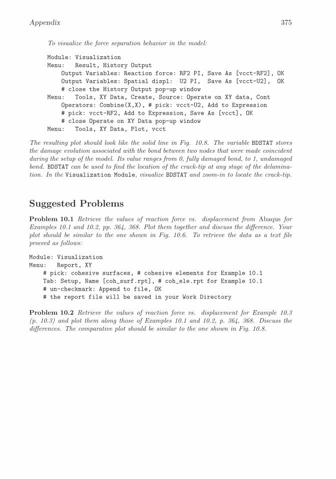
“K15072” — 2013/3/21 — 10:58�

�

�

�

�

�

Appendix 375

To visualize the force separation behavior in the model:



Output Variables: Reaction force: RF2 PI, Save As [vcct-RF2], OK

Output Variables: Spatial displ: U2 PI, Save As [vcct-U2], OK



Operators: Combine(X,X), # pick: vcct-U2, Add to Expression

# pick: vcct-RF2, Add to Expression, Save As [vcct], OK


Menu: Tools, XY Data, Plot, vcct

The resulting plot should look like the solid line in Fig. 10.8. The variable BDSTAT storesthe damage evolution associated with the bond between two nodes that were made coincidentduring the setup of the model. Its value ranges from 0, fully damaged bond, to 1, undamagedbond. BDSTAT can be used to find the location of the crack-tip at any stage of the delamina-tion. In the Visualization Module, visualize BDSTAT and zoom-in to locate the crack-tip.

Suggested Problems

Problem 10.1 Retrieve the values of reaction force vs. displacement from Abaqus forExamples 10.1 and 10.2, pp. 364, 368. Plot them together and discuss the difference. Yourplot should be similar to the one shown in Fig. 10.6. To retrieve the data as a text fileproceed as follows:


Menu: Report, XY

# pick: cohesive surfaces, # cohesive elements for Example 10.1

Tab: Setup, Name [coh_surf.rpt], # coh_ele.rpt for Example 10.1

# un-checkmark: Append to file, OK

# the report file will be saved in your Work Directory

Problem 10.2 Retrieve the values of reaction force vs. displacement for Example 10.3(p. 10.3) and plot them along those of Examples 10.1 and 10.2, p. 364, 368. Discuss thedifferences. The comparative plot should be similar to the one shown in Fig. 10.8.

�

�

“K15072” — 2013/3/21 — 10:58�

�

�

�

�

�

�

�

“K15072” — 2013/3/21 — 10:58�

�

�

�

�

�

Appendix A

Tensor Algebra

Tensor operations are needed for the derivation of some of the equations in thistextbook. Since most of these operations are not easily found in textbooks, theyare presented here for reference [193].

A.1 Principal Directions of Stress and Strain

Since stress and strain tensors are symmetric and of second order, they have threereal principal values and three orthogonal principal directions. The principal valuesλq and directions nqi of the stress tensor σij satisfy the following

[σij − λqδij ]nqi = 0 (A.1)

nqinqj = 1 (A.2)

where δij is the Kronecker delta (δij = 1 if i = j, zero otherwise). Each of theprincipal directions is described by its direction cosines with respect to the originalcoordinate system.

The principal directions are arranged by rows into a matrix [A]. Then, thediagonal matrix [A∗] of the principal values is

[A∗] = [a][A][a]T (A.3)

It can be shown that [a]−1 = [a]T , where [a] is the transformation matrix givenby (1.21).

A.2 Tensor Symmetry

Minor symmetry provides justification for using contracted notation (Section 1.5).Minor symmetry refers to identical values of tensor components when adjacentsubscripts are swapped. For example, minor symmetry of the stiffness tensor Cmeans

Aijkl = Ajilk = Aαβ (A.4)

377

�

�

“K15072” — 2013/3/21 — 10:58�

�

�

�

�

�


Major symmetry refers to identical values when adjacent pairs of subscripts areswapped, or when contracted subscripts are swapped. For example,

Aijkl = Aklij

Aαβ = Aβα (A.5)

A.3 Matrix Representation of a Tensor

A tensor Aijkl with a minor symmetry has only 36 independent constants. Thereforeit can be represented in contracted notation by a 6 × 6 matrix. Let [a] be thecontracted form of the tensor A. Each element of [a] corresponds to an element inthe tensor A according to the following transformation

aαβ = Aijkl (A.6)

with

α = i when i = j

α = 9− (i+ j) when i �= j (A.7)

The same transformations apply between β and k and l, or in matrix represen-tation, as

[a] =

⎡

⎢

⎢

⎢

⎢

⎢

⎢

⎣

A1111 A1122 A1133 A1123 A1113 A1112

A2211 A2222 A2233 A2223 A2213 A2212

A3311 A3322 A3333 A3323 A3313 A3312

A2311 A2322 A2333 A2323 A2313 A2312

A1311 A1322 A1333 A1323 A1313 A1312

A1211 A1222 A1233 A1223 A1213 A1212

⎤

⎥

⎥

⎥

⎥

⎥

⎥

⎦

(A.8)

It is convenient to perform tensor operations using contracted form, especiallyif the result can be represented also in contracted form. This saves memory andtime since it is faster to operate on 36 elements than on 81 elements. Examples ofthese operations are the inner product of two fourth-order tensors and the inverseof a fourth-order tensor. However, tensor operations in index notation do not trans-late directly into matrix operations in contracted form. For example, the doublecontraction of two fourth-order tensors is

C = A : B

Cijkl = AijmnBmnkl (A.9)

Let [a], [b], and [c] be the 6 × 6 matrix representations of the above tensors.Then, it can be shown that

[a] [b] �= [c] or

aαβbβγ �= cαγ (matrix multiplication) (A.10)

The rest of this appendix presents formulas for adequate representation of tensoroperations in their contracted form.

�

�

“K15072” — 2013/3/21 — 10:58�

�

�

�

�

�

Appendix 379

A.4 Double Contraction

In (A.9), an element like C1211 can be expanded as

C1211 = A1211B1111 +A1222B2211 +A1233B3311

+2A1212B1211 + 2A1213B1311 + 2A1223B2311 (A.11)

In order to achieve the same result by matrix multiplication, multiply the lastthree columns of the matrix [a] by 2, and then perform the multiplication

[c] =

⎡

⎢

⎢

⎢

⎢

⎢

⎢

⎣

A1111 A1122 A1133 2A1123 2A1113 2A1112

A2211 A2222 A2233 2A2223 2A2213 2A2212

A3311 A3322 A3333 2A3323 2A3313 2A3312

A2311 A2322 A2333 2A2323 2A2313 2A2312

A1311 A1322 A1333 2A1323 2A1313 2A1312

A1211 A1222 A1233 2A1223 2A1213 2A1212

⎤

⎥

⎥

⎥

⎥

⎥

⎥

⎦

⎡

⎢

⎢

⎢

⎢

⎢

⎢

⎣

B1111 B1122 B1133 B1123 B1113 B1112

B2211 B2222 B2233 B2223 B2213 B2212

B3311 B3322 B3333 B3323 B3313 B3312

B2311 B2322 B2333 B2323 B2313 B2312

B1311 B1322 B1333 B1323 B1313 B1312

B1211 B1222 B1233 B1223 B1213 B1212

⎤

⎥

⎥

⎥

⎥

⎥

⎥

⎦

(A.12)

This transformation can be produced by using the Reuter matrix [R]

[R] =

⎡

⎢

⎢

⎢

⎢

⎢

⎢

⎣

1 0 0 0 0 00 1 0 0 0 00 0 1 0 0 00 0 0 2 0 00 0 0 0 2 00 0 0 0 0 2

⎤

⎥

⎥

⎥

⎥

⎥

⎥

⎦

(A.13)

Substituting in (A.12) we have

[c] = [a] [R] [b] (A.14)

A.5 Tensor Inversion

First, it is convenient to define the fourth-order identity tensor Iijkl as a tensor thatmultiplied innerly by another fourth-order tensor yields this same tensor, or

IijmnAmnkl = Aijkl (A.15)

If Aijkl has a minor symmetry, the following tensor achieves (A.15)

�

�

“K15072” — 2013/3/21 — 10:58�

�

�

�

�

�


Iijkl =1

2(δikδjl + δilδjk) (A.16)

where δij is the Kronecker delta, defined as

δij = 1 if i = jδij = 0 if i �= j

(A.17)

In Voigt contracted notation, the fourth-order identity tensor is denoted as [i],which is equal to the inverse of the Reuter matrix

[i] =

⎡

⎢

⎢

⎢

⎢

⎢

⎢

⎣

1 0 0 0 0 00 1 0 0 0 00 0 1 0 0 00 0 0 1/2 0 00 0 0 0 1/2 00 0 0 0 0 1/2

⎤

⎥

⎥

⎥

⎥

⎥

⎥

⎦

= [R]−1 (A.18)

Now, the inverse of a tensor is a tensor that multiplied by the original tensoryields the identity tensor, as follows:

AijmnA−1mnkl = Iijkl (A.19)

Let us introduce the following notation:

[a]−1 = inverse of the contracted form of Aijkl

[

a−1]

= contracted form of the inverse of Aijkl

If Aijkl has a minor symmetry, the components of a−1αβ are:

i. Multiply the last three columns of [a] by 2 by using the matrix [R].

ii. Invert the obtained matrix.

iii. Multiply the matrix by [i].

In orther words, the matrix[

a−1]

is computed as

[

a−1]

= [[a] [R]]−1 [i] = [i] [a]−1 [i] (A.20)

A.6 Tensor Differentiation

A.6.1 Derivative of a Tensor with Respect to Itself

Any symmetric second-order tensor Φij satisfies the following:

dΦij = dΦji (A.21)

�

�

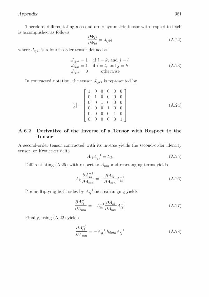
“K15072” — 2013/3/21 — 10:58�

�

�

�

�

�

Appendix 381

Therefore, differentiating a second-order symmetric tensor with respect to itselfis accomplished as follows

∂Φij

∂Φkl= Jijkl (A.22)

where Jijkl is a fourth-order tensor defined as

Jijkl = 1 if i = k, and j = lJijkl = 1 if i = l, and j = kJijkl = 0 otherwise

(A.23)

In contracted notation, the tensor Jijkl is represented by

[j] =

⎡

⎢

⎢

⎢

⎢

⎢

⎢

⎣

1 0 0 0 0 00 1 0 0 0 00 0 1 0 0 00 0 0 1 0 00 0 0 0 1 00 0 0 0 0 1

⎤

⎥

⎥

⎥

⎥

⎥

⎥

⎦

(A.24)

A.6.2 Derivative of the Inverse of a Tensor with Respect to theTensor

A second-order tensor contracted with its inverse yields the second-order identitytensor, or Kronecker delta

AijA−1jk = δik (A.25)

Differentiating (A.25) with respect to Amn and rearranging terms yields

Aij

∂A−1jk

∂Amn= − ∂Aij

∂AmnA−1

jk (A.26)

Pre-multiplying both sides by A−1li and rearranging yields

∂A−1ij

∂Amn= −A−1

ik

∂Akl

∂AmnA−1

lj (A.27)

Finally, using (A.22) yields

∂A−1ij

∂Amn= −A−1

ik JklmnA−1lj (A.28)

�

�

“K15072” — 2013/3/21 — 10:58�

�

�

�

�

�

�

�

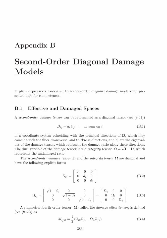
“K15072” — 2013/3/21 — 10:58�

�

�

�

�

�

Appendix B

Second-Order Diagonal DamageModels

Explicit expressions associated to second-order diagonal damage models are pre-sented here for completeness.

B.1 Effective and Damaged Spaces

A second-order damage tensor can be represented as a diagonal tensor (see (8.61))

Dij = di δij ; no sum on i (B.1)

in a coordinate system coinciding with the principal directions of D, which maycoincide with the fiber, transverse, and thickness directions, and di are the eigenval-ues of the damage tensor, which represent the damage ratio along these directions.The dual variable of the damage tensor is the integrity tensor, Ω =

√I−D, which

represents the undamaged ratio.

The second-order damage tensor D and the integrity tensor Ω are diagonal andhave the following explicit forms

Dij =

⎡

⎣

d1 0 00 d2 00 0 d3

⎤

⎦ (B.2)

Ωij =

⎡

⎣

√1− d1 0 00

√1− d2 0

0 0√1− d3

⎤

⎦ =

⎡

⎣

Ω1 0 00 Ω2 00 0 Ω3

⎤

⎦ (B.3)

A symmetric fourth-order tensor, M, called the damage effect tensor, is defined(see (8.63)) as

Mijkl =1

2(ΩikΩjl +ΩilΩjk) (B.4)

383

�

�

“K15072” — 2013/3/21 — 10:58�

�

�

�

�

�


The damage effect tensor in contracted form multiplied by the Reuter matrixtakes the form of a 6× 6 array as follows

M = Mαβ =

⎡

⎢

⎢

⎢

⎢

⎢

⎢

⎣

Ω21 0 0 0 0 00 Ω2

2 0 0 0 00 0 Ω2

3 0 0 00 0 0 Ω2Ω3 0 00 0 0 0 Ω1Ω3 00 0 0 0 0 Ω1Ω2

⎤

⎥

⎥

⎥

⎥

⎥

⎥

⎦

(B.5)

The damaged stiffness tensor C multiplied by the Reuter matrix can be writtenin explicit contracted notation for an orthotropic material by a 6 × 6 array as afunction of the undamaged stiffness tensor C as follows

Cαβ =

⎡

⎢

⎢

⎢

⎢

⎢

⎢

⎣

C11Ω41 C12Ω

21Ω

22 C13Ω

21Ω

23 0 0 0

C12Ω21Ω

22 C22Ω

42 C23Ω

22Ω

23 0 0 0

C13Ω21Ω

23 C23Ω

22Ω

23 C33Ω

43 0 0 0

0 0 0 2C44Ω22Ω

23 0 0

0 0 0 0 2C55Ω21Ω

23 0

0 0 0 0 0 2C66Ω21Ω

22

⎤

⎥

⎥

⎥

⎥

⎥

⎥

⎦

(B.6)where C44 = G23, C55 = G13, and C66 = G12. The Voigt contracted notation forfourth-order elasticity tensors is used here: Cαβ replaces Cijkl where α, β take thevalues 1, 2, 3, 4, 5, 6, corresponding to the index pairs 11, 22, 33, 23, 13 and 12,respectively.

The relations between the effective and actual stress components assume thefollowing expressions

σ1 = σ1 Ω−21 ; σ4 = σ4Ω

−12 Ω−1

3 ;

σ2 = σ2 Ω−22 ; σ5 = σ5Ω

−11 Ω−1

3 ;

σ3 = σ3 Ω−23 ; σ6 = σ6Ω

−11 Ω−1

2 ;

(B.7)

and the strain components

ε1 = ε1 Ω21; ε4 = ε4 Ω2Ω3;

ε2 = ε2 Ω22; ε5 = ε5 Ω1Ω3;

ε3 = ε3 Ω23; ε6 = ε6 Ω1Ω2;

(B.8)

where the over-line indicates an effective property.

B.2 Thermodynamic Force Y

By satisfying the Clausius-Duhem inequality, thus assuring non-negative dissipation,the following thermodynamic forces (see (8.128)) are defined

Yij = − ∂ψ

∂Dij= −1

2

(

εkl−εpkl) ∂Cklpq

∂Dij

(

εpq−εppq)

= −1

2εekl∂Cklpq

∂Dijεepq (B.9)

�

�

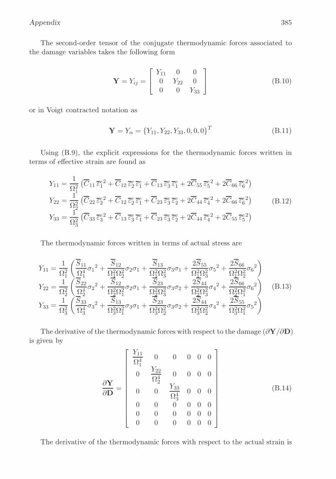
“K15072” — 2013/3/21 — 10:58�

�

�

�

�

�

Appendix 385

The second-order tensor of the conjugate thermodynamic forces associated tothe damage variables takes the following form

Y = Yij =

⎡

⎣

Y11 0 00 Y22 00 0 Y33

⎤

⎦ (B.10)

or in Voigt contracted notation as

Y = Yα = {Y11, Y22, Y33, 0, 0, 0}T (B.11)

Using (B.9), the explicit expressions for the thermodynamic forces written interms of effective strain are found as

Y11 =1

Ω21

(

C11 εe12 + C12 ε

e2 ε

e1 + C13 ε

e3 ε

e1 + 2C55 ε

e52 + 2C66 ε

e62)

Y22 =1

Ω22

(

C22 εe22 + C12 ε

e2 ε

e1 + C23 ε

e3 ε

e2 + 2C44 ε

e42 + 2C66 ε

e62)

Y33 =1

Ω23

(

C33 εe32 + C13 ε

e3 ε

e1 + C23 ε

e3 ε

e2 + 2C44 ε

e42 + 2C55 ε

e52)

(B.12)

The thermodynamic forces written in terms of actual stress are

Y11 =1

Ω21

(

S11

Ω41

σ12 +

S12

Ω21Ω

22

σ2σ1 +S13

Ω21Ω

23

σ3σ1 +2S55

Ω21Ω

23

σ52 +

2S66

Ω21Ω

22

σ62

)

Y22 =1

Ω22

(

S22

Ω42

σ22 +

S12

Ω22Ω

21

σ2σ1 +S23

Ω22Ω

23

σ3σ2 +2S44

Ω22Ω

23

σ42 +

2S66

Ω22Ω

21

σ62

)

Y33 =1

Ω23

(

S33

Ω43

σ32 +

S13

Ω23Ω

21

σ3σ1 +S23

Ω23Ω

22

σ3σ2 +2S44

Ω23Ω

22

σ42 +

2S55

Ω23Ω

21

σ52

)

(B.13)

The derivative of the thermodynamic forces with respect to the damage (∂Y/∂D)is given by

∂Y

∂D=

⎡

⎢

⎢

⎢

⎢

⎢

⎢

⎢

⎢

⎢

⎢

⎢

⎢

⎣

Y11Ω41

0 0 0 0 0

0Y22Ω42

0 0 0 0

0 0Y33Ω43

0 0 0

0 0 0 0 0 00 0 0 0 0 00 0 0 0 0 0

⎤

⎥

⎥

⎥

⎥

⎥

⎥

⎥

⎥

⎥

⎥

⎥

⎥

⎦

(B.14)

The derivative of the thermodynamic forces with respect to the actual strain is

�

�

“K15072” — 2013/3/21 — 10:58�

�

�

�

�

�


given by

∂Y

∂εe=

⎡

⎢

⎢

⎢

⎢

⎢

⎢

⎢

⎢

⎢

⎢

⎢

⎢

⎢

⎢

⎣

−P11

Ω21

−C12 εe1Ω2

1−C13 εe1

Ω21

0 −2C55 εe5Ω2

1−2

C66 εe6Ω2

1

−C12 εe2Ω2

2−P22

Ω22

−C23 εe2Ω2

2−2

C44 εe4Ω2

20 −2

C66 εe6Ω2

2

−C13 εe3Ω2

3−C23 εe3

Ω23

−P33

Ω23

−2C44 εe4Ω2

3−2

C55 εe5Ω2

30

0 0 0 0 0 0

0 0 0 0 0 0

0 0 0 0 0 0

⎤

⎥

⎥

⎥

⎥

⎥

⎥

⎥

⎥

⎥

⎥

⎥

⎥

⎥

⎥

⎦

(B.15)

whereP11 = 2C11 ε

e1 + C12 ε

e2 + C13 ε

e3

P22 = C12 εe1 + 2C22 ε

e2 + C23 ε

e3

P33 = C13 εe1 + C23 ε

e2 + 2C33 ε

e3

(B.16)

The derivative of the thermodynamic forces with respect to the actual unrecov-erable strain is given by

∂Y

∂εp= −∂Y

∂εe(B.17)

The derivative of the actual stress with respect to damage is given by

∂σ

∂D=

⎡

⎢

⎢

⎢

⎢

⎢

⎢

⎢

⎢

⎢

⎢

⎢

⎢

⎢

⎣

P ′11 0 0 0 0 0

0 P ′22 0 0 0 0

0 0 P ′33 0 0 0

0 −12Ω3C44 εe4

Ω2−1

2Ω2C44 εe4

Ω30 0 0

−12Ω3C55 εe5

Ω10 −1

2Ω1C55 εe5

Ω30 0 0

−12Ω2C66 εe6

Ω1−1

2Ω1C66 εe6

Ω20 0 0 0

⎤

⎥

⎥

⎥

⎥

⎥

⎥

⎥

⎥

⎥

⎥

⎥

⎥

⎥

⎦

(B.18)

whereP ′11 = −C11 ε

e1 − C12 ε

e2 − C13 ε

e3

P ′22 = −C12 ε

e1 − C22 ε

e2 − C23 ε

e3

P ′33 = −C13 ε

e1 − C23 ε

e2 − C33 ε

e3

(B.19)

B.3 Damage Surface

An anisotropic damage criterion expressed in tensorial form, introducing two fourth-order tensors, B and J, defines a multiaxial limit surface in the thermodynamic forcespace, Y, that bounds the damage domain. The damage evolution is defined bya damage potential associate to the damage surface and by an isotropic hardeningfunction. The proposed damage surface gd is given by

gd =(

Y Nij JijhkY

Nhk

)1/2+(

Y SijBijhkY

Shk

)1/2 − (γ(δ) + γ0) (B.20)

�

�

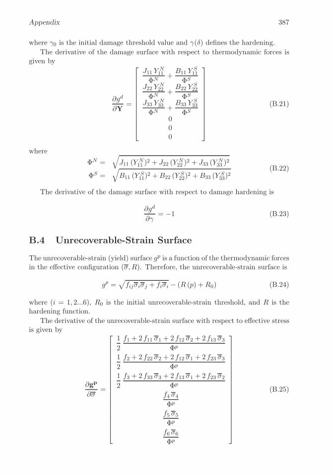
“K15072” — 2013/3/21 — 10:58�

�

�

�

�

�

Appendix 387

where γ0 is the initial damage threshold value and γ(δ) defines the hardening.

The derivative of the damage surface with respect to thermodynamic forces isgiven by

∂gd

∂Y=

⎡

⎢

⎢

⎢

⎢

⎢

⎢

⎢

⎢

⎢

⎢

⎢

⎣

J11 YN11

ΦN+B11 Y

S11

ΦS

J22 YN22

ΦN+B22 Y

S22

ΦS

J33 YN33

ΦN+B33 Y

S33

ΦS

000

⎤

⎥

⎥

⎥

⎥

⎥

⎥

⎥

⎥

⎥

⎥

⎥

⎦

(B.21)

where

ΦN =√

J11 (Y N11 )

2 + J22 (Y N22 )

2 + J33 (Y N33 )

2

ΦS =√

B11 (Y S11)

2 +B22 (Y S22)

2 +B33 (Y S33)

2(B.22)

The derivative of the damage surface with respect to damage hardening is

∂gd

∂γ= −1 (B.23)

B.4 Unrecoverable-Strain Surface

The unrecoverable-strain (yield) surface gp is a function of the thermodynamic forcesin the effective configuration (σ,R). Therefore, the unrecoverable-strain surface is

gp =√

fijσiσj + fiσi − (R (p) +R0) (B.24)

where (i = 1, 2...6), R0 is the initial unrecoverable-strain threshold, and R is thehardening function.

The derivative of the unrecoverable-strain surface with respect to effective stressis given by

∂gp

∂σ=

⎡

⎢

⎢

⎢

⎢

⎢

⎢

⎢

⎢

⎢

⎢

⎢

⎢

⎢

⎢

⎢

⎢

⎢

⎢

⎢

⎣

1

2

f1 + 2 f11 σ1 + 2 f12 σ2 + 2 f13 σ3Φp

1

2

f2 + 2 f22 σ2 + 2 f12 σ1 + 2 f23 σ3Φp

1

2

f3 + 2 f33 σ3 + 2 f13 σ1 + 2 f23 σ2Φp

f4 σ4Φp

f5 σ5Φp

f6 σ6Φp

⎤

⎥

⎥

⎥

⎥

⎥

⎥

⎥

⎥

⎥

⎥

⎥

⎥

⎥

⎥

⎥

⎥

⎥

⎥

⎥

⎦

(B.25)

�

�

“K15072” — 2013/3/21 — 10:58�

�

�

�

�

�


whereΦp = (f1 σ1 + f2 σ2 + f3 σ3+

+f11 σ12 + f22 σ2

2 + f33 σ32+

+2 f12 σ1 σ2 + 2 f13 σ1 σ3 + 2 f23 σ2 σ3+

+f6 σ62 + f5 σ5

2 + f4 σ42)1/2

(B.26)

The derivative of the yield surface with respect to unrecoverable-strain hardeningis

∂gp

∂R= −1 (B.27)

�

�

“K15072” — 2013/3/21 — 10:58�

�

�

�

�

�

Appendix C

Software Used

Only four software applications are used throughout this textbook. Abaqus is byfar the most used. BMI3 is used only in Chapter 4. MATLAB is used for sym-bolic as well as numerical computations. Finally, Intel Fortran must be availableto compile and link Abaqus with user programmed material subroutines, but itsusage is transparent to the user because it is called by a batch file requiring nouser intervention. Of course, some knowledge of Fortran is required to programnew user material subroutines, but programming is made easier by several examplesubroutines, which are provided and used in the examples.

The aim of this section is to present an introduction to the software used inthis textbook, namely Abaqus and BMI3, as well as how to use Intel Fortran tocompile and link user subroutines with Abaqus. It is assumed that the reader canuse MATLAB without help besides that provided by the self-explanatory MATLABcode included with the examples, either printed in this textbook or downloadablefrom the Web site [5].

Operation of the software is illustrated for a Windows 7 platform but operationin a Linux environment is similar. For the sake of space, this section is very brief.The vendors of these applications have a wealth of information, training sessions,user groups, and so on, that the reader can use to get familiar with the softwareinterface. One such source of information is the Web site for this textbook at http://barbero.cadec-online.com/feacm-abaqus [5]. Another source of informationis the textbook’s forum [194].

C.1 Abaqus

Abaqus is a commercial finite element analysis (FEA) application. It has a friendlygraphical user interface (GUI) called CAE and an extensive documentation system.Once started, the user should have no difficulty navigating menus and so on.

All the mouse clicks in the GUI generate CAE script, which are saved in severalfiles, but the script is very difficult to understand without significant time investmentin learning CAE scripting [195].

The examples in this textbook were produced using Abaqus version 6.10. They

389

�

�

“K15072” — 2013/3/21 — 10:58�

�

�

�

�

�


Fig. C.1: Edit the shortcut to change the default Work directory.

work identically in Windows 7 and Linux platforms. On Windows 7, Abaqus isaccessible from the START menu, through Start, All Programs, Abaqus 6.10,

Abaqus CAE.In this textbook, it is assumed that the user has created a folder c:\Simulia\

User, where the model files will reside.If the GUI is started using the shortcut Start, All Programs, Abaqus 6.10,

the temporary files reside in the default Work directory, which was set duringinstallation of the Abaqus software, typically c:\temp. The default work directorycan be changed by editing the Start in: field in the shortcut, as shown in FigureC.1. Otherwise, the Work Directory for the current session can be changed fromwithin Abaqus/CAE by doing the following:

Menu: File, Set Work Directory

The default directory is used by Abaqus as a default location to store temporaryfiles, including:

.dat The data file contains a printout of requested results.

.fil The result file contains results such as mode shapes and so on (see Example 4.3,p. 188). This file is unformatted.

�

�

“K15072” — 2013/3/21 — 10:58�

�

�

�

�

�

Appendix 391

.inp The input file contains the input to the Abaqus processor.

.jnl The journal file contains changes to the .mdb since the last Save.

.log The log file contains a brief log of the last execution of the Abaqus processor.

.odb The output database file contains all the results from an execution of theAbaqus processor.

.rec The recovery file contains a record of the operations performed by the user onthe GUI since the last Save.

.rpy The replay file contains a replay of the whole procedure that you used in theGUI to generate the model.

In this textbook, we prefer to store and overwrite temporary files in the defaultWork directory to maintain clean user folders, but sometimes we will purposelystore temporary files in a user folder. For example, if we want to read some outputfrom the .dat file, we will store it in a user folder.

This section attempts to describe the installation and “systems” aspects ofAbaqus software. On the other hand, a description of the Abaqus/CAE GUI isintegrated within the examples in the textbook, starting with Chapter 3. There-fore, it is highly recommended that the user installs Abaqus, then proceeds to studyChapter 3 and personally “do” all the examples in Chapter 3. By the end of Chap-ter 3, you should be quite skilled in Abaqus/CAE, at least as far is concerned withcomposites modeling. Even higher proficiency will be achieved by studying andpracticing the examples in the entire textbook. It has been my experience thatstudents successfully teach themselves Abaqus/CAE by working the examples inthis textbook, along with the help system and the documentation included withAbaqus. Another source of help is the video recordings illustrating the execution ofthe examples by using the Abaqus/CAE GUI [5].

C.1.1 Abaqus Programmable Features

To prepare Abaqus for running UMAT subroutines and other Abaqus programmablefeatures, the following software must be installed in this order:

i. Microsoft Visual Studio c© (VS) 2008.

ii. Intel Fortran c© 11.1.

First, install Microsoft Visual Studio 2008 (VS2008) and update it to servicepack 1 (SP1) with the update available on the Web.

Next, install Intel Fortran 11.1. Fortran must be installed after VS so that VS isready to integrate Fortran into it. During installation, install the X64 Compiler andTools, which are not installed by default, by check marking the box X64 Compilersand Tools as shown in Figure C.2.

�

�

“K15072” — 2013/3/21 — 10:58�

�

�

�

�

�


Fig. C.2: Visual Studio 2008. Setup page.

Next, locate the batch file:c:\SIMULIA\Abaqus\Commands\abq6102.bat

Make a backup copy. Then, modify it as follows (also available in [5]).

rem Windows 64 version of .bat file to execute Abaqus

rem with User Programmable Features and Intel MKL Math libraries

SET PATH=C:\Program Files (x86)\Microsoft Visual Studio 9.0\VC\Bin;%PATH%;

SET PATH=C:\Program Files (x86)\Intel\Compiler\11.1\048\bin\Intel64;%PATH%;

SET PATH=C:\Program Files (x86)\Common Files\Microsoft Shared\VSA\9.0\VsaEnv;

%PATH%;

SET LIB=C:\Program Files (x86)\Microsoft Visual Studio 9.0\VC\Lib;%LIB%

SET LIB=C:\Program Files (x86)\Intel\Compiler\11.1\048\mkl\em64t\lib;%LIB%

call "C:\Program Files (x86)\Intel\Compiler\11.1\048\bin\intel64

\ifortvars_intel64"

rem keep next lines exactly as in your original installation

@echo off

call "C:\SIMULIA\Abaqus\6.10-1\exec\abq6101.exe" %*

Note that file names and locations may be slightly different in your installation,especially if you are using a 32-Bit system. If you modify the abq6102.bat, you

�

�

“K15072” — 2013/3/21 — 10:58�

�

�

�

�

�

Appendix 393

must use the exact location of the files in your system. Failing to do so will causeAbaqus to prompt an error message while trying to compile/link UMAT subroutines.

Next, locate the environment file:C:\SIMULIA\Abaqus\6.10-2\site\abaqus_v6.env

Make a backup copy. Then, modify the compile fortran directive to include threeadditional switches. The first two, /DABQ WIN86 64 and /Qmkl:sequential, allowuse of the Intel math library MKL. The third, free, allows Abaqus to understand freeformatted fortran code in the user subroutines even though Abaqus requires .forextension for any user supplied Fortran code. For a Windows 64 bit system, theresulting section of the environment file should look something like this:

compile_fortran=[’ifort’,’/c’,’/DABQ_WIN86_64’,’/Qmkl:sequential’,’/free’,

’/recursive’,’/Qauto-scalar’,’/QxW’,’/nologo’,’/Od’,’/include:%I’]

Using Visual Studio 2008, you should debug your Fortran code before linking itto Abaqus. A simple program such as umat tester.f90, which is available in [5],can be used to test your user material subroutine before linking it to Abaqus. Youcan modify the umat tester.f90 to suit your needs.

Fortran code can be written in free format as long as the file name given toAbaqus has an extension .for or it is compiled into object code .obj using theabaqus make utility. By default, VS2008 interprets files having extension .for ascontaining 72 column, fixed format, Fortran 77 code. Since F77 is very limited,free format, Fortran 90 is preferred. VS2008 is be able to work with a .for fileeven if it contains free formatted code, provided you add the compiler directive!DEC$ FREEFORM as the first line to the code. Otherwise, the VS2008 default be-havior can be changed inside VS2008. In addition to that, the “free” switch shouldbe added to the compile fortran directive in the environment file so that Abaquscan deal with free formatted code.

UMAT, VUMAT, UGENS, and UEL examples in Abaqus documentation are written inF77. A free converter, written in F90, is available in [196].

An Errata for the textbook is maintained in [5]. Known installation issues willbe reported there.

C.2 BMI3

Native BMI3 code accepts an input file in Abaqus.inp format, as long as the in-put file is filtered by the program inp2bmi3.exe. Therefore, one can create themodel in Abaqus/CAE, write the .inp file from the Job Manager, filter it withinp2bmi3.exe, and execute it with bmi3.exe. The executables are available in [5].The input/output file sequence is described in Table C.1. The sequence of executionis:

– Create a model in Abaqus/CAE and write the Job-1.inp file

�

�

“K15072” — 2013/3/21 — 10:58�

�

�

�

�

�


Table C.1: Input/Output files to execute BMI3.Program Read Write Comments

inp2bmi3.exe Job-1.inp BMI3.inp filtered modelBMI3.dat material propertiesABQ.inp filtered Abaqus

BMI3.exe BMI3.inp BMI3.out resultsBMI3.dat MODES.out mode shapes

– Execute inp2bmi3.exe to get the filtered files. If needed, modify the mode,node, component in the BMI3.dat file

– Execute bmi3.exe. Record the results from the display or from BMI3.out

Not all of the Abaqus.inp commands are understood by the filter inp2bmi3.exe.Most of the limitations could be removed by modifying the filter, for which thesource code inp2bmi3.f90 is available in [5]. The current limitations are:

– The mesh must refer to S8R or S8R5 elements (see Example 4.2, p. 185).

– All loads must be concentrated loads.

– The material properties must be given using Shell General Stiffness.

– Only one material can be used for the entire model.

– Constrained boundary conditions cannot be used.

– Materials Orientation (*orientation) cannot be used.

Abaqus/CAE writes an .inp file every time a job is submitted, or Write Input

is executed from the Job Manager window. Then, run inp2bmi3.exe to generateBMI3.inp, ABQ.inp, and BMI3.dat. If ABQ.inp is executed using Abaqus in com-mand mode (see Example 2.1, p. 46), or imported into Abaqus/CAE and executed,it will give the bifurcation loads Λ(cr) and the mode shapes.

The material properties and perturbation parameters are provided via BMI3.dat,which is automatically created by the filter. The last line in BMI3.dat containsmodenum, nodenum, component. These are the mode, node, and component usedas perturbation parameter δ. If all three values are zeros (the default), BMI3 picksthe lowest mode and the node-component combination that yields the largest modeamplitude. The results of BMI3 are printed in BMI3.out and the mode shapes savedin the MODES.out file.

Note that the results (bifurcation loads, slopes, and curvatures) appear withnegative sign. This is usual in stability analysis. Another peculiarity of the BMI3software is that transverse deflections w (perpendicular to the plate) have oppositesign to Abaqus results. Since transverse deflections w are often used as perturbationparameters, the change in sign must be taken into account during interpretation ofresults (see Example 4.2, p. 185).

�

�

“K15072” — 2013/3/21 — 10:58�

�

�

�

�

�

References

[1] E. J. Barbero. Introduction to Composite Materials Design–Second Edition. http://barbero.cadec-online.com/icmd. CRC Press, Boca Raton, FL, 2010.

[2] D. Frederick and T.-S. Chang. Continuum Mechanics. Scientific Publishers, Cam-bridge, MA, 1972.

[3] F. P. Beer, E. R. Johnston Jr., and J. T. DeWolf. Mechanics of Materials, 3rd Edition.McGraw-Hill, Boston, MA, 2001.

[4] J. N. Reddy. Energy and Variational Methods in Applied Mechanics. Wiley, 1984.

[5] E. J. Barbero. Web resource: http://barbero.cadec-online.com/feacm-abaqus.

[6] S. S. Sonti, E. J. Barbero, and T. Winegardner. Mechanical properties of pultrudedE-glass–vinyl ester composites. In 50th Annual Conference, Composites Institute,Society of the Plastics Industry (February) pp. 10-C/1-7., 1995.

[7] Simulia. Abaqus documentation. The default location for the HTML documentationis http://HOME:2080/v6.10/where HOME is the url of the server where the documen-tation is stored during installation. The default location for the PDF documentationis C:\SIMULIA\Documentation\docs\v6.10\pdf_books\index.pdf.

[8] E. J. Barbero. Finite Element Analysis of Composite Materials–First Edition. CRCPress, Boca Raton, FL, 2007.

[9] ANSYS Inc. Ansys mechanical apdl structural analysis guide, release 140.0, http://www1.ansys.com/customer/content/documentation/140/ans_str.pdf, 2011.

[10] Simulia. Abaqus keywords reference manual. The default location is http://HOME:

2080/v6.10/books/key/default.htm where HOME is the url of the server where thedocumentation is stored during installation.

[11] SolidWorks. http://www.solidworks.com/sw/engineering-education-software.htm.

[12] E. J. Barbero. Computer aided design environment for composites. http://www.cadec-online.com, 2011.

[13] R. J. Roark and W. C. Young. Roark’s Formulas for Stress and Strain, 6th Edition.McGraw-Hill, New York, NY, 1989.

[14] J. N. Reddy. Mechanics of Laminated Composite Plates and Shells, 2nd Edition. CRCPress, Boca Raton, FL, 2003.

[15] E. Hinton and D. R. J. Owen. An Introduction to Finite Element Computations.Pineridge Press, Swansea, UK, 1979.

395

�

�

“K15072” — 2013/3/21 — 10:58�

�

�

�

�

�


[16] NAFEMS. Test R0031/3. Technical report, National Agency for Finite ElementMethods and Standards (UK), 1995.

[17] E. J. Barbero. 3-d finite element for laminated composites with 2-d kinematic con-straints. Computers and Structures, 45(2):263–271, 1992.

[18] E. J. Barbero. Cadec application program interface. http://www.cadec-online.

com/Help/API.aspx.

[19] Simulia. Abaqus benchmarks manual. The default location is http://HOME:2080/

v6.10/books/bmk/default.htm where HOME is the url of the server where the doc-umentation is stored during installation.

[20] E. J. Barbero and J. Trovillion. Prediction and measurement of post-critical behaviorof fiber-reinforced composite columns. Composites Science and Technology, 58:1335–1341, 1998.

[21] E. J. Barbero. Prediction of compression strength of unidirectional polymer matrixcomposites. Journal of Composite Materials, 32(5)(5):483–502, 1998.

[22] A. Puck and H. Schurmann. Failure analysis of frp laminates by means of physicallybased phenomenological models. Composites Science and Technology, 62:1633–1662,2002.

[23] MIL17.org. The composite materials handbook, web resource, http://www.mil17.org.

[24] L. A. Godoy. Theory of Stability-Analysis and Sensitivity. Taylor and Francis,Philadelphia, PA, 2000.

[25] E. J. Barbero, L. A. Godoy, and I. G. Raftoyiannis. Finite elements for three-modeinteraction in buckling analysis. International Journal for Numerical Methods inEngineering, 39(3):469–488, 1996.

[26] L. A. Godoy, E. J. Barbero, and I. G. Raftoyiannis. Finite elements for post-bucklinganalysis. i - the w-formulation. Computers and Structures, 56(6):1009–1017, 1995.

[27] E. J. Barbero, I. G. Raftoyiannis, and L. A. Godoy. Finite elements for post-bucklinganalysis. ii - application to composite plate assemblies. Computers and Structures,56(6):1019–1028, 1995.

[28] I. G. Raftoyiannis, L. A. Godoy, and E. J. Barbero. Buckling mode interaction incomposite plate assemblies. Applied Mechanics Reviews, 48(11/2):52–60, 1995.

[29] E. J. Barbero. Prediction of buckling-mode interaction in composite columns. Me-chanics of Composite Materials and Structures, 7(3):269–284, 2000.

[30] S. Yamada and J. G. A. Croll. Buckling behavior pressure loaded cylindrical panels.ASCE Journal of Engineering Mechanics, 115(2):327–344, 1989.

[31] C. T. Herakovich. Mechanics of Fibrous Composites. Wiley, New York, 1998.

[32] J. D. Eshelby. The determination of the elastic field of an ellipsoidal inclusion andrelated problems. Proceedings of the Royal Society, A241:376–396, 1957.

[33] J. D. Eshelby. The elastic field outside an ellipsoidal inclusion. Acta Metall.,A252:561–569, 1959.

[34] T. Mori and K. Tanaka. The elastic field outside an ellipsoidal inclusion. Acta Metall.,21:571–574, 1973.

�

�

“K15072” — 2013/3/21 — 10:58�

�

�

�

�

�

References 397

[35] R. Hill. A self-consistent mechanics of composite materials. J. Mech. Phys. Solids,13:213–222, 1965.

[36] S. Nemat-Nasser and M. Hori. Micromechanics: Overall Properties of HeterogeneousMaterials. North-Holland, Amsterdam, 1993.

[37] R. Luciano and E. J. Barbero. Formulas for the stiffness of composites with periodicmicrostructure. I. J. Solids and Structures, 31(21):2933–2944, 1995.

[38] R. Luciano and E. J. Barbero. Analytical expressions for the relaxation moduli oflinear viscoelastic composites with periodic microstructure. ASME J. Applied Me-chanics, 62(3):786–793, 1995.

[39] E. J. Barbero and R. Luciano. Micromechanical formulas for the relaxation tensorof linear viscoelastic composites with transversely isotropic fibers. I. J. Solids andStructures, 32(13):1859–1872, 1995.

[40] J. Aboudi. Mechanics of Composite Materials : A Unified Micromechanical Approach.Vol. 29 of Studies in Applied Mechanics. Elsevier, New York, NY, 1991.

[41] Z. Hashin and S. Shtrikman. A variational approach to the elastic behavior of multi-phase materials. J. Mechanics and Physics of Solids, 11:127–140, 1963.

[42] V. Tvergaard. Model studies of fibre breakage and debonding in a metal reinforcedby short fibres. J. Mechanics and Physics of Solids, 41(8):1309–1326, 1993.

[43] J. L. Teply and G. J. Dvorak. Bound on overall instantaneous properties of elastic-plastic composites. J. Mechanics and Physics of Solids, 36(1):29–58, 1988.

[44] R. Luciano and E. Sacco. Variational methods for the homogenization of periodicmedia. European J. Mech. A/Solids, 17:599–617, 1998.

[45] G. J. Creus. Viscoelasticity: Basic Theory and Applications to Concrete Structures.Springer-Verlag, Berlin, 1986.

[46] Eric W. Weisstein. Gamma function. MathWorld–A Wolfram Web Resource. http://mathworld.wolfram.com/GammaFunction.html.

[47] G. D. Dean, B. E. Read, and P. E. Tomlins. A model for long-term creep and the effectsof physical ageing in poly (butylene terephthalate). Plastics and Rubber Processingand Applications, 13(1):37–46, 1990.

[48] B. F. Oliveira and G. J. Creus. An analytical-numerical framework for the study ofageing in fibre reinforced polymer composites. Composites B, 65(3-4):443–457, 2004.

[49] K. Ogatha. Discrete-Time Control System. Prentice Hall, Englewood Cliffs, NJ, 1987.

[50] K. J. Hollenbeck. Invlap.m: A matlab function for numerical inversion of Laplacetransforms by the de Hoog algorithm (1998), http://www.mathworks.com/.

[51] R. S. Lakes. Viscoelastic Solids. Boca Raton, FL, 1998.

[52] J. D. Ferry. Viscoelastic Properties of Polymers. 3rd. Edition. Wiley, New York, 1980.

[53] R. M. Christensen. Theory of Viscoelasticity. New York, 1972.

[54] P. Qiao, E. J. Barbero, and J. F. Davalos. On the linear viscoelasticity of thin-walledlaminated composite beams. Journal of Composite Materials, 34(1):39–68, 2000.

[55] E. J. Barbero, F. A. Cosso, R. Roman, and T. L. Weadon. Determination of mate-rial parameters for Abaqus progressive damage analysis of E-Glass Epoxy laminates.Composites Part B:Engineering, 46(3):211–220, 2012.

�

�

“K15072” — 2013/3/21 — 10:58�

�

�

�

�

�


[56] J. Lemaitre and A. Plumtree. Application of damage concepts to predict creep-fatiguefailures. In American Society of Mechanical Engineers, 78-PVP-26, pages 10–26, 1978.

[57] I. N. Rabotnov. Rabotnov: Selected Works - Problems of the Mechanics of a De-formable Solid Body. Moscow Izdatel Nauka, 1991.

[58] L. M. Kachanov. On the creep fracture time. Izv. Akad. Nauk USSR, 8:26–31, 1958.

[59] N. R. Hansen and H. L. Schreyer. A thermodynamically consistent framework fortheories of elastoplasticity coupled with damage. International Journal of Solids andStructures, 31(3):359–389, 1994.

[60] J. Janson and J. Hult. Fracture mechanics and damage mechanics - a combinedapproach. J. Mec. Theor. Appl. 1, pages S18–28, 1977.

[61] E. J. Barbero and K. W. Kelly. Predicting high temperature ultimate strength of con-tinuous fiber metal matrix composites. Journal of Composite Materials, 27(12):1214–1235, 1993.

[62] K. W. Kelly and E. Barbero. Effect of fiber damage on the longitudinal creep of acfmmc. International Journal of Solids and Structures, 30(24):3417–3429, 1993.

[63] J. R. Rice. Continuum Mechanics and Thermodynamics of Plasticity in Relation toMicroscale Deformation Mechanisms, chapter 2, pages 23–79. Constitutive Equationsin Plasticity. MIT Press, Cambridge, MA, 1975.

[64] J. C. Simo and T. J. R. Hughes. Computational Inelasticity. Springer, Berlin, 1998.

[65] D. Krajcinovic, J. Trafimow, and D. Sumarac. Simple constitutive model for a corticalbone. Journal of Biomechanics, 20(8):779–784, 1987.

[66] D. Krajcinovic and D. Fanella. Micromechanical damage model for concrete. Engi-neering Fracture Mechanics, 25(5-6):585–596, 1985.

[67] D. Krajcinovic. Damage mechanics. Mechanics of Materials, 8(2-3):117–197, 1989.

[68] A. M. Neville. Properties of Concrete, 2nd Edition. Wiley, New York, NY, 1973.

[69] ACI, American Concrete Institute.

[70] B. W. Rosen. The tensile failure of fibrous composites. AIAA Journal, 2(11):1985–1911, 1964.

[71] W. Weibull. A statistical distribution function of wide applicability. Journal of AppliedMechanics, 18:293–296, 1951.

[72] B. W. Rosen. Fiber Composite Materials, chapter 3. American Society for Metals,Metals Park, OH, 1965.

[73] A. S. D. Wang. A non-linear microbuckling model predicting the compressive strengthof unidirectional composites. In ASME Winter Annual Meeting, volume WA/Aero-1,1978.

[74] J. S. Tomblin, E. J. Barbero, and L. A. Godoy. Imperfection sensitivity of fibermicro-buckling in elastic-nonlinear polymer-matrix composites. International Journalof Solids and Structures, 34(13):1667–1679, 1997.

[75] D. C. Lagoudas and A. M. Saleh. Compressive failure due to kinking of fibrouscomposites. Journal of Composite Materials, 27(1):83–106, 1993.

[76] P. Steif. A model for kinking in fiber composites. i. fiber breakage via micro-buckling.International Journal of Solids and Structures, 26 (5-6):549–61, 1990.

�

�

“K15072” — 2013/3/21 — 10:58�

�

�

�

�

�

References 399

[77] S. W. Yurgartis and S. S. Sternstein. Experiments to Reveal the Role of Matrix Prop-erties and Composite Microstructure in Longitudinal Compression Strength, volume1185 of ASTM Special Technical Publication, pages 193–204. ASTM, Philadelphia,PA, 1994.

[78] C. Sun and A. W. Jun. Effect of matrix nonlinear behavior on the compressive strengthof fiber composites. In AMD, volume 162, pages 91–101, New York, NY, 1993. ASME,American Society of Mechanical Engineers, Applied Mechanics Division.

[79] D. Adams and E. Lewis. Current status of composite material shear test methods.SAMPE Journal, 31(1):32–41, 1995.

[80] A. Maewal. Postbuckling behavior of a periodically laminated medium in compression.International Journal of Solids and Structures, 17(3):335–344, 1981.

[81] L. M. Kachanov. Rupture time under creep conditions problems of continuum me-chanics. SIAM, pages 202–218, 1958.

[82] E. J. Barbero and P. Lonetti. Damage model for composites defined in terms ofavailable data. Mechanics of Composite Materials and Structures, 8(4):299–315, 2001.

[83] E. J. Barbero and P. Lonetti. An inelastic damage model for fiber reinforced laminates.Journal of Composite Materials, 36(8):941–962, 2002.

[84] P. Lonetti, R. Zinno, F. Greco, and E. J. Barbero. Interlaminar damage model forpolymer matrix composites. Journal of Composite Materials, 37(16):1485–1504, 2003.

[85] P. Lonetti, E. J. Barbero, R. Zinno, and F. Greco. Erratum: Interlaminar damagemodel for polymer matrix composites. Journal of Composite Materials, 38(9):799–800,2004.

[86] E. J. Barbero, F. Greco, and P. Lonetti. Continuum damage-healing mechanics withapplication to self-healing composites. International Journal of Damage Mechanics,14(1):51–81, 2005.

[87] S. Murakami. Mechanical modeling of material damage. Journal of Applied Mechan-ics, 55:281–286, 1988.

[88] J. M. Smith and H. C. Van Ness. Introduction to Chemical Engineering Thermody-namics, 3rd Edition. McGraw-Hill, New York, NY, 1975.

[89] E. R. Cohen, T. Cvita, J. G. Frey, B. Holmstrm, K. Kuchitsu, R. Marquardt, I. Mills,F. Pavese, M. Quack, J. Stohner, H. L. Strauss, M. Takami, and A. J. Thor. Quanti-ties, Units and Symbols in Physical Chemistry : The IUPAC Green Book, 3rd Edition,http:// old. iupac.org/publications/books/author/cohen.html . RSC Pub-lishing, 2007.

[90] L. E. Malvern. Introduction to the Mechanics of a Continuous Medium. Prentice Hall,Upper Saddle River, NJ, 1969.

[91] Y. A. Cengel and M. A. Boles. Thermodynamics: An Engineering Approach, 3rdEdition. McGraw-Hill, New York, NY, 1998.

[92] J. Lubliner. Plasticity Theory. Collier Macmillan, New York, NY, 1990.

[93] J. A. Nairn. The strain energy release rate of composite microcracking: a variationalapproach. Journal of Composite Materials, 23(11):1106–29, 11 1989.

�

�

“K15072” — 2013/3/21 — 10:58�

�

�

�

�

�


[94] J. A. Nairn, S. Hu, S. Liu, and J. S. Bark. The initiation, propagation, and effectof matrix microcracks in cross-ply and related laminates. In Proc. of the 1st NASAAdvanced Comp. Tech. Conf., pages 497–512, Oct. 29 - Nov. 1, 1990.

[95] S. Liu and J. A. Nairn. The formation and propagation of matrix microcracks in cross-ply laminates during static loading. Journal of Reinforced Plastics and Composites,11(2):158–78, Feb. 1992.

[96] J. A. Nairn. Microcracking, microcrack-induced delamination, and longitudinal split-ting of advanced composite structures. Technical Report NASA Contractor Report4472, 1992.

[97] J. A. Nairn and S. Hu. Damage Mechanics of Composite Materials, volume 9 ofComposite Materials Series, chapter Matrix Microcracking, pages 187–244. Elsevier,1994.

[98] J. A. Nairn. Applications of finite fracture mechanics for predicting fracture eventsin composites. In 5th Int’l Conf. on Deform. and Fract. of Comp., 18-19 March 1999.

[99] J. A. Nairn. Polymer Matrix Composites, volume 2 of Comprehensive CompositeMaterials, chapter Matrix Microcracking in Composites, pages 403–432. ElsevierScience, 2000.

[100] J. A. Nairn. Fracture mechanics of composites with residual stresses, imperfect in-terfaces, and traction-loaded cracks. In Workshop ‘Recent Advances in ContinuumDamage Mechanics for Composites’, volume 61, pages 2159–67, UK, 20-22 Sept. 2000.Elsevier.

[101] J. A. Nairn and D. A. Mendels. On the use of planar shear-lag methods for stress-transfer analysis of multilayered composites. Mechanics of Materials, 33(6):335–362,2001.

[102] J. A. Nairn. Finite Fracture Mechanics of Matrix Microcracking in Composites, pages207–212. Application of Fracture Mechanics to Polymers, Adhesives and Composites.Elsevier, 2004.

[103] Y. M. Han, H. T. Hahn, and R. B. Croman. A simplified analysis of transverse plycracking in cross-ply laminates. Composites Science and Technology, 31(3):165–177,1988.

[104] C. T. Herakovich, J. Aboudi, S. W. Lee, and E. A. Strauss. Damage in compositelaminates: Effects of transverse cracks. Mechanics of Materials, 7(2):91–107, 11 1988.

[105] J. Aboudi, S. W. Lee, and C. T. Herakovich. Three-dimensional analysis of laminateswith cross cracks. Journal of Applied Mechanics, Transactions ASME, 55(2):389–397,1988.

[106] F. W. Crossman, W. J. Warren, A. S. D. Wang, and G. E. Law. Initiation and growthof transverse cracks and edge delamination in composite laminates. ii - experimentalcorrelation. Journal of Composite Materials Suplement, 14(1):88–108, 1980.

[107] D. L. Flaggs and M. H. Kural. Experimental determination of the in situ trans-verse lamina strength in graphite/epoxy laminates. Journal of Composite Materials,16:103–16, 03 1982.

[108] S. H. Lim and S. Li. Energy release rates for transverse cracking and delamina-tions induced by transverse cracks in laminated composites. Composites Part A,36(11):1467–1476, 2005.

�

�

“K15072” — 2013/3/21 — 10:58�

�

�

�

�

�

References 401

[109] S. Li and F. Hafeez. Variation-based cracked laminate analysis revisited and funda-mentally extended. International Journal of Solids and Structures, 46(20):3505–3515,2009.

[110] J. L Rebiere and D. Gamby. A decomposition of the strain energy release rate associ-ated with the initiation of transverse cracking, longitudinal cracking and delaminationin cross-ply laminates. Composite Structures, 84(2):186–197, 2008.

[111] S. C. Tan and R. J. Nuismer. A theory for progressive matrix cracking in compositelaminates. Journal of Composite Materials, 23:1029–1047, 1989.

[112] R. J. Nuismer and S. C. Tan. Constitutive relations of a cracked composite lamina.Journal of Composite Materials, 22:306–321, 1988.

[113] T. Yokozeki and T. Aoki. Stress analysis of symmetric laminates with obliquely-crossed matrix cracks. Advanced Composite Materials, 13(2):121–40, 2004.

[114] T. Yokozeki and T. Aoki. Overall thermoelastic properties of symmetric laminatescontaining obliquely crossed matrix cracks. Composites Science and Technology,65(11-12):1647–54, 2005.

[115] Z. Hashin. Analysis of cracked laminates: a variational approach. Mechanics ofMaterials, 4:121:136, 1985.

[116] J. Zhang, J. Fan, and C. Soutis. Analysis of multiple matrix cracking in [±θ/90n]scomposite laminates, part I, inplane stiffness properties. Composites, 23(5):291–304,1992.

[117] P. Gudmundson and S. Ostlund. First order analysis of stiffness reduction due tomatrix cracking. Journal of Composite Materials, 26(7):1009–30, 1992.

[118] P. Gudmundson and S. Ostlund. Prediction of thermoelastic properties of compositelaminates with matrix cracks. Composites Science and Technology, 44(2):95–105,1992.

[119] P. Gudmundson and W. Zang. An analytic model for thermoelastic properties ofcomposite laminates containing transverse matrix cracks. International Journal ofSolids and Structures, 30(23):3211–31, 1993.

[120] E. Adolfsson and P. Gudmundson. Thermoelastic properties in combined bending andextension of thin composite laminates with transverse matrix cracks. InternationalJournal of Solids and Structures, 34(16):2035–60, 06 1997.

[121] E. Adolfsson and P. Gudmundson. Matrix crack initiation and progression in com-posite laminates subjected to bending and extension. International Journal of Solidsand Structures, 36(21):3131–3169, 1999.

[122] W. Zang and P. Gudmundson. Damage evolution and thermoelastic properties ofcomposite laminates. International Journal of Damage Mechanics, 2(3):290–308, 071993.

[123] E. Adolfsson and P. Gudmundson. Matrix crack induced stiffness reductions in[(0m/90n/+p/-q)s]m composite laminates. Composites Engineering, 5(1):107–23,1995.

[124] P. Lundmark and J. Varna. Modeling thermo-mechanical properties of damagedlaminates. In 3rd International Conference on Fracture and Damage Mechanics, FDM2003, volume 251-252 of Advances in Fracture and Damage Mechanics, pages 381–7,Switzerland, 2-4 Sept. 2003. Trans Tech Publications.

�

�

“K15072” — 2013/3/21 — 10:58�

�

�

�

�

�


[125] M. Kachanov. Elastic solids with many cracks and related problems, volume 30 ofAdvances in Applied Mechanics, chapter X, pages 260–445. Academic Press, Inc.,1993.

[126] A. Adumitroiaie and E. J. Barbero. Intralaminar damage model for laminates sub-jected to membrane and flexural deformations. Mechanics of Advanced Materials andStructures, 2013.

[127] T. Yokozeki, T. Aoki, and T. Ishikawa. Transverse crack propagation in the specimenwidth direction of cfrp laminates under static tensile loadings. Journal of CompositeMaterials, 36(17):2085–99, 2002.

[128] T. Yokozeki, T. Aoki, and T. Ishikawa. Consecutive matrix cracking in contiguousplies of composite laminates. International Journal of Solids and Structures, 42(9-10):2785–802, 05 2005.

[129] T. Yokozeki, T. Aoki, T. Ogasawara, and T. Ishikawa. Effects of layup angle andply thickness on matrix crack interaction in contiguous plies of composite laminates.Composites Part A (Applied Science and Manufacturing), 36(9):1229–35, 2005.

[130] E. J. Barbero, F. A. Cosso, and F. A. Campo. Benchmark solution for degrada-tion of elastic properties due to transverse matrix cracking in laminated composites.Composite Structures, 98(4):242–252, 2013.

[131] S. Li, S. R. Reid, and P. D. Soden. A continuum damage model for transverse matrixcracking in laminated fibre-reinforced composites. Philosophical Transactions of theRoyal Society London, Series A (Mathematical, Physical and Engineering Sciences),356(1746):2379–412, 10/15 1998.

[132] Janis Varna, Roberts Joffe, and Ramesh Talreja. A synergistic damage-mechanicsanalysis of transverse cracking [±θ/904]s laminates. Composites Science and Tech-nology, 61(5):657–665, 2001.

[133] A. S. D. Wang, P. C. Chou, and S. C. Lei. A stochastic model for the growth ofmatrix cracks in composite laminates. Journal of Composite Materials, 18(3):239–54,05 1984.

[134] S. Li, S. R. Reid, and P. D. Soden. Modelling the damage due to transverse matrixcracking in fiber-reinforced laminates. In Proc. 2nd Int. Conf. on Nonlinear Mechanics(ICNP-2), pages 320–323. Peking University Press, 1993.

[135] D.H. Cortes and E.J. Barbero. Stiffness reduction and fracture evolution of obliquematrix cracks in composite laminates. Annals of Solid and Structural Mechanics,1(1):29–40, 2010.

[136] E. J. Barbero and D. H. Cortes. A mechanistic model for transverse damage initia-tion, evolution, and stiffness reduction in laminated composites. Composites Part B,41:124–132, 2010.

[137] E. J. Barbero, G. Sgambitterra, A. Adumitroaie, and X. Martinez. A discrete consti-tutive model for transverse and shear damage of symmetric laminates with arbitrarystacking sequence. Composite Structures, 93:1021–1030, 2011.

[138] G. Sgambitterra, A. Adumitroaie, E.J. Barbero, and A. Tessler. A robust three-nodeshell element for laminated composites with matrix damage. Composites Part B:Engineering, 42(1):41–50, 2011.

�

�

“K15072” — 2013/3/21 — 10:58�

�

�

�

�

�

References 403

[139] A. M. Abad Blazquez, M. Herraez Matesanz, Carlos Navarro Ugena, and E. J. Bar-bero. Acoustic emission characterization of intralaminar damage in composite lami-nates. In Asociacion Espanola de Materiales Compuestos MATCOMP 2013, Algeci-ras, Spain, July 2–5, 2013.

[140] E. J. Barbero and F. A. Cosso. Determination of material parameters for discretedamage mechanics analysis of composite laminates. Composites Part B:Engineering,2013.

[141] H. T. Hahn. A mixed-mode fracture criterion for composite materials. CompositesTechnology Review, 5:26–29, 1983.

[142] Allan F. Bower. Mechanics of Solids. CRC, 2010. Free at http://solidmechanics.org/.

[143] Simulia. Abaqus analysis user’s manual, version 6.10.

[144] J. Varna, R. Joffe, N. V. Akshantala, and R. Talreja. Damage in composite laminateswith off-axis plies. Composites Science and Technology, 59(14):2139–2147, 1999.

[145] H. Chai, C. D. Babcock, and W. G. Knauss. One dimensional modeling of failurein laminated plates by delamination buckling. International Journal of Solids andStructures, 17(11):1069–1083, 1981.

[146] M.-K. Yeh and L.-B. Fang. Contact analysis and experiment of delaminated cantilevercomposite beam. Composites: Part B, 30(4):407–414, 1999.

[147] W. L. Yin, S. N. Sallam, and G. J. Simitses. Ultimate axial load capacity of adelaminated beam-plate. AIAA Journal, 24(1):123–128, 1986.

[148] D. Bruno. Delamination buckling in composite laminates with interlaminar defects.Theoretical and Applied Fracture Mechanics, 9(2):145–159, 1988.

[149] D. Bruno and A. Grimaldi. Delamination failure of layered composite plates loadedin compression. International Journal of Solids and Structures, 26(3):313–330, 1990.

[150] G. A. Kardomateas. The initial post-buckling and growth behaviour of internal de-laminations in composite plates. Journal of Applied Mechanics, 60(4):903–910, 1993.

[151] G. A. Kardomateas and A. A. Pelegri. The stability of delamination growth in com-pressively loaded composite plates. International Journal of Fracture, 65(3):261–276,1994.

[152] I. Sheinman, G. A. Kardomateas, and A. A. Pelegri. Delamination growth during pre-and post-buckling phases of delaminated composite laminates. International Journalof Solids and Structures, 35(1-2):19–31, 1998.

[153] D. Bruno and F. Greco. An asymptotic analysis of delamination buckling and growthin layered plates. International Journal of Solids and Structures, 37(43):6239–6276,2000.

[154] H.-J. Kim. Postbuckling analysis of composite laminates with a delamination. Com-puter and Structures, 62(6):975–983, 1997.

[155] W. G. Bottega and A. Maewal. Delamination buckling and growth in laminates–closure. Journal of Applied Mechanics, 50(14):184–189, 1983.

[156] B. Cochelin and M. Potier-Ferry. A numerical model for buckling and growth ofdelaminations in composite laminates. Computer Methods in Applied Mechanics,89(1-3):361–380, 1991.

�

�

“K15072” — 2013/3/21 — 10:58�

�

�

�

�

�


[157] P.-L. Larsson. On delamination buckling and growth in circular and annular or-thotropic plates. International Journal of Solids and Structures, 27(1):15–28, 1991.

[158] W.-L. Yin. Axisymmetric buckling and growth of a circular delamination in a com-pressed laminate. International Journal of Solids and Structures, 21(5):503–514, 1985.

[159] K.-F. Nilsson, L. E. Asp, J. E. Alpman, and L. Nystedt. Delamination buckling andgrowth for delaminations at different depths in a slender composite panel. Interna-tional Journal of Solids and Structures, 38(17):3039–3071, 2001.

[160] H. Chai and C. D. Babcock. Two-dimensional modeling of compressive failure indelaminated laminates. Journal of Composite Materials, 19(1):67–98, 1985.

[161] J. D. Withcomb and K. N. Shivakumar. Strain-energy release rate analysis of plateswith postbuckled delaminations. Journal of Composite Materials, 23(7):714–734,1989.

[162] W. J. Bottega. A growth law for propagation of arbitrary shaped delaminations inlayered plates. International Journal of Solids and Structures, 19(11):1009–1017.

[163] B. Storakers and B. Andersson. Nonlinear plate theory applied to delamination incomposites. Journal of the Mechanics and Physics of Solids, 36(6):689–718, 1988.

[164] P.-L. Larsson. On multiple delamination buckling and growth in composite plates.International Journal of Solids and Structures, 27(13):1623–1637, 1991.

[165] M. A. Kouchakzadeh and H. Sekine. Compressive buckling analysis of rectangu-lar composite laminates containing multiple delaminations. Composite Structures,50(3):249–255, 2000.

[166] J. M. Comiez, A. M. Waas, and K. W. Shahwan. Delamination buckling: Experimentand analysis. International Journal of Solids and Structures, 32(6/7):767–782, 1995.

[167] G. A. Kardomateas. Postbuckling characteristics in delaminated kevlar/epoxy lam-inates: An experimental study. Journal of Composites Technology and Research,12(2):85–90, 1990.

[168] O. Allix and A. Corigliano. Modeling and simulation of crack propagation in mixed-modes interlaminar fracture specimens. International Journal of Fracture, 77(2):111–140, 1996.

[169] D. Bruno and F. Greco. Delamination in composite plates: Influence of shear de-formability on interfacial debonding. Cement and Concrete Composites, 23(1):33–45,2001.

[170] J. W. Hutchinson and Z. Suo. Mixed mode cracking in layered materials. Advancesin Applied Mechanics, 29:63–191, 1992.

[171] N. Point and E. Sacco. Delamination of beams: An application to the dcb specimen.International Journal of Fracture, 79(3):225–247, 1996.

[172] J. G. Williams. On the calculation of energy release rate for cracked laminates.International Journal of Fracture, 36(2):101–119, 1988.

[173] A. Tylikowsky. Effects of piezoactuator delamination on the transfer functions ofvibration control systems. International Journal of Solids and Structures, 38(10-13):2189–2202, 2001.

[174] C. E. Seeley and A. Chattopadhyay. Modeling of adaptive composites includingdebonding. International Journal Solids and Structures, 36(12):1823–1843, 1999.

�

�

“K15072” — 2013/3/21 — 10:58�

�

�

�

�

�

References 405

[175] W. J. Bottega and A. Maewal. Dynamics of delamination buckling. InternationalJournal of Non-Linear Mechanics, 18(6):449–463, 1983.

[176] G. Alfano and M. A. Crisfield. Finite element interface models for the delaminationanalysis of laminated composites: Mechanical and computational issues. InternationalJournal for Numerical Methods in Engineering, 50(7):1701–1736, 2001.

[177] P. P. Camanho, C. G. Davila, and M. F. Moura. Numerical simulation of mixed-modeprogressive delamination in composite materials. Journal of Composite Materials,37(16):1415–1438, 2003.

[178] Z. Zou, S. R. Reid, and S. Li. A continuum damage model for delaminations inlaminated composites. Journal of the Mechanics and Physics of Solids, 51(2):333–356, 2003.

[179] X-P Xu and A. Needleman. Numerical simulations of fast crack growth in brittlesolids. Journal of the Mechanics and Physics of Solids, 42:1397–1434, 1994.

[180] J. R. Reeder. A bilinear failure criterion for mixed-mode delamination in compositematerials. ASTM STP 1206, pages 303–322, 1993.

[181] H. Chai. Three-dimensional fracture analysis of thin-film debonding. InternationalJournal of Fracture, 46(4):237–256, 1990.

[182] J. D. Withcomb. Three dimensional analysis of a post-buckled embedded delamina-tion. Journal of Composite Materials, 23(9):862–889, 1989.

[183] D. Bruno, F. Greco, and P. Lonetti. A 3d delamination modelling technique based onplate and interface theories for laminated structures. European Journal of MechanicsA/Solids, 24:127–149, 2005.

[184] J. G. Williams. The fracture mechanics of delamination tests. Journal of StrainAnalysis, 24(4):207–214, 1989.

[185] W.-L. Yin and J. T. S. Wang. The energy-release rate in the growth of a one-dimensional delamination. Journal of Applied Mechanics, 51(4):939–941, 1984.

[186] J. R. Rice. A path independent integral and the approximate analysis of strainconcentrations by notches and cracks. Journal of Applied Mechanics, 35:379–386,1968.

[187] Simulia. Abaqus analysis user’s manual, version 6.10. chapter 29.5: Cohesive elements.

[188] C. G. Davila, P. P. Camanho, and M. F. De Moura. Mixed-mode decohesion elementsfor analyses of progressive delamination. In 42nd AIAA/ASME/ASCE/AHS/ASCStructures, Structural Dynamics, and Materials Conference, April 16 - 19, 2001,volume 3, pages 2277– 88, Seattle, WA, 2001. AIAA.

[189] Simulia. Abaqus analysis user’s manual, version 6.10. chapter 11.4.3: Crack propaga-tion analysis.

[190] E.J. Barbero and J.N. Reddy. Jacobian derivative method for three-dimensional frac-ture mechanics. Communications in Applied Numerical Methods, 6(7):507–518, 1990.

[191] M. Benzeggagh and M. Kenane. Measurement of mixed-mode delamination fracturetoughness of unidirectional glass/epoxy composites with mixed-mode bending appa-ratus. Composite Science and Technology, 56:439, 1996.

�

�

“K15072” — 2013/3/21 — 10:58�

�

�

�

�

�


[192] J. Reeder, S. Kyongchan, P. B. Chunchu, and D. R.. Ambur. Postbuckling andgrowth of delaminations in composite plates subjected to axial compression. In43rd AIAA/ASME/ASCE/AHS/ASC Structures, Structural Dynamics, and Mate-rials Conference, Denver, Colorado, vol. 1746, p. 10, 2002.

[193] A. Caceres. Local Damage Analysis of Fiber Reinforced Polymer Matrix Composites,Ph.D. dissertation. PhD thesis, West Virginia University, Morgantown, WV, 1998.

[194] E. J. Barbero. Composite materials forum. http://forum.cadec-online.com/

viewforum.php?f=4.

[195] G. Puri. Python Scripts for Abaqus. abaquspython.org, Atlanta, GA, 2011.

[196] M. Metcalf. A tool to convert f77 source code to f90. ftp://ftp.numerical.rl.ac.uk/pub/MandR/convert.f90.




Using AbaqusTM

Ba

rbe

roFinite Elem

ent Analysis of Composite

Materials Using Abaqus

TM

ISBN: 978-1-4665-1661-8

9 781466 516618

9 0 0 0 0

K15072

MATERIALS SCIENCE/MECHANICAL ENGINEERING

“In my opinion, the book is very well written; it is easy to follow and includes topics that students, engineers, and researchers from different fields can find very interesting and useful. The examples are very well detailed and provide valuable guidance on how to implement and understand theoretical solutions when translated into finite element models of composite materials and structures. Overall, this is a great book if the reader is looking for a comprehensive treatment of composite materials covering detailed theoretical background followed by implementation of the concepts into practical problems using a powerful modeling tool such as Abaqus.” — EDUARDO M. SOSA , West Virginia University

“The book is essential for any academic in the area of solid mechanics. I use this book with my students, as the subject and the materials are very clear. Model files for the finite element examples in the book help students progress and make my guidance more productive. It has both theory and applications using the finite element method. This book is also essential for composite engineers as a quick reference of topics that can be of use in their field.” — GASSER ABDELAL , Queen’s University Belfast

“This book by Professor Barbero does an excellent job introducing the fundamentals of mechanics of composite materials and the finite element method in a concise way. Some of the most common problems that the practicing engineer has to face when designing with composites using finite element analysis are covered in detail. … a valuable asset for any reader dealing with modeling of composite structures using the finite element method.” — JOAQUIN GUTIERREZ , Blade Dynamics LLLP



Using AbaqusTM

K15072_Cover_mech.indd All Pages 3/19/13 10:09 AM

Finite Element Analysis of Composite Materials Using Abaqus

Documents

Transcript of Finite Element Analysis of Composite Materials Using Abaqus