Copyright c© 2005 Tech Science Press CMC, vol.2, no.1, pp.23-38, 2005

A four-node hybrid assumed-strain finite element for laminated composite plates

A. Cazzani1, E. Garusi2, A. Tralli3 and S.N. Atluri4

Abstract: Fibre-reinforced plates and shells are find-ing an increasing interest in engineering applications.Consequently, efficient and robust computational toolsare required for the analysis of such structural models.As a matter of fact, a large amount of laminate finite el-ements have been developed and incorporated in mostcommercial codes for structural analysis.In this paper a new laminate hybrid assumed-strain plateelement is derived within the framework of the First-order Shear Deformation Theory (i.e. assuming that par-ticles of the plate originally lying along a straight linewhich is normal to the undeformed middle surface re-main aligned along a straight line during the deformationprocess) and assuming perfect bonding between laminae.The in-plane components of the (infinitesimal) strain ten-sor are interpolated and by making use of the constitu-tive law, the corresponding in-plane stress distribution isdeduced for each layer. Out-of-plane shear stresses arethen computed by integrating the equilibrium equationsin each lamina, account taken of their continuity require-ments. Out-of-plane shear strains are finally obtained viathe inverse constitutive law.The resulting global strain field depends on a fixed num-ber of parameters, regardless of the total number of lay-ers; 12 degrees of freedom are for instance assumed forthe developed rectangular element.The proposed model does not suffer locking phenomenaeven in the thin plate limit and provides an accurate de-scription of inter-laminar stresses. Results are comparedwith both analytical and other finite element solutions.

keyword: Laminated composite plates, hybrid finiteelements, assumed strain methods, shear-locking.

1 DIMS, University of Trento, Trento, ITALY; corresponding author.2 Italferr, Milano, ITALY.3 DI, University of Ferrara, Ferrara, ITALY.4 UCI, Irvine, CA, USA.

1 Introduction

Finite elements for the analysis of laminated compositeplates have been derived by using different laminate the-ories proposed in the literature [see Reddy (2004), andreferences quoted therein]. Such theories are usually re-ferred to as:

• Equivalent Single Layer (ESL) theories, such as:

– the Classical Lamination Theory (CLT) basedon the Kirchhoff model;

– the First-order Shear Deformation Theory(FSDT);

– Higher-order Shear Deformation Theories(HSDTs);

• Layer-wise Lamination Theory (LLT);

• Three dimensional elasticity.

In the context of ESL theories, the simplest one is theCLT which neglects the shear contribution in the lami-nate thickness. However, flat structures made of fiber-reinforced composite materials are characterized by non-negligible shear deformations in the thickness direction,since the longitudinal elastic modulus of the lamina canmuch higher than the shear and the transversal moduli;hence the use of a shear deformation laminate theory isrecommended.

The extension of the Reissner (1945) and Mindlin (1951)model to the case of laminated anisotropic plates, i.e.FSDT [Yang, Norris, and Stavsky (1966); Whitney andPagano (1970)], accounts for shear deformation along thethickness in the simplest way. It gives satisfactory resultsfor a wide class of structural problems, even for mod-erately thick laminates, requiring only C0-continuity forthe displacement field. However in the classical FSDT:

• the transverse shearing strains (stresses) are as-sumed to be constant along the plate thickness so

24 Copyright c© 2005 Tech Science Press CMC, vol.2, no.1, pp.23-38, 2005

that stress boundary conditions on the top and thebottom of the plate are violated;

• shear correction factors must be introduced. Thedetermination of shear correction factors is not atrivial task, since they depend both on the lamina-tion sequence and on the state of deformation [see,e.g. Whitney (1973); Vlachoutsis (1992); Savoia,Laudiero, and Tralli (1994)] and can be quite dif-ferent from the value 5/6 which is typical of homo-geneous plates.

Some methods have been proposed for improving FSDTresults. For instance post-processing can be applied inorder to improve the transverse shear stresses [viz. Noorand Burton (1990); Rolfes and Rohwer (1997)], and thetransverse normal stress [Rolfes, Rohwer, and Baller-staedt (1998); Yu, Hodges, and Volovoi (2003)] in finiteelement analysis.

Recently, refined FSDT models have been proposed: ad-ditive shear warping functions [Pai (1995)] or the as-sumption that shear strains vary in the thickness in cylin-drical bending with the same law as the shear stress ob-tained by integrating the equilibrium equations [Qi andKnight (1996); Auricchio and Sacco (2003)] have beensuccessfully employed.

More refined laminate theories are available, of course,and they can be broadly divided into the three groups out-lined above.

On one hand, several ESL higher-order theories (and re-lated finite elements models) have been proposed: withinthese theories, for instance, the transverse displace-ment has been either expanded in power series in termsof thickness coordinates up to a given order [Chepiga(1976); Lo, Christensen, and Wu (1977); Reddy (1984);Pandya and Kant (1988); Yoda and Atluri (1992); Yongand Cho (1995); Gaudenzi, Mannini, and Carbonaro(1998)] or has been modelled by Legendre polynomials[Poniatovskii (1962); Cicala (1962)].

On the other hand, LLT [Reddy (1987); Di Sciuva(1987); Robbins and Reddy (1993); Bisegna and Sacco(1997)] assumes a displacement representation formulain every layer.

Finally, analytical solutions based on three dimensionalelasticity (and corresponding finite element models) havebeen developed, for instance, by Pagano (1970); Paganoand Hatfield (1972); Liou and Sun (1987).

All these higher-order theories lead to more accurate re-sults, especially for very thick laminates. However thecomputational cost will be significantly increased [Rob-bins and Reddy (1993)], due to the increase of variablesassociated to either the description of the transversal dis-placement or the number of layers.

“To date, FSDT is still considered the best compromisebetween the capability for prediction and computationalcost for a wide class of applications” [Cen, Long, andYao (2002)].

With reference to finite element models, although it isusual to present FSDT within the framework of displace-ments approaches, nonetheless, in the literature, hybridand mixed formulations have been proposed as well,mainly for developing innovative finite element mod-els: see Atluri (1983); Punch and Atluri (1984a); Atluri(2004). Assumed-stress four-node single-layer — i.e.homogeneous — plate elements have been developedsince many years [Spilker and Munir (1980); Punch andAtluri (1984b)].

Four-node hybrid stress laminated elements includingtransverse shear effects have been developed by Mau,Tong, and Pian (1972), where the stress field is definedseparately for each layer and by Spilker, Orringer, andWitmer (1976), which, on the contrary, define the stressfield for the laminate as a whole with inter-layer tractioncontinuity and upper/lower laminate free surface con-ditions enforced exactly. The four-node hybrid stressmulti-layer plate elements quoted above have the poten-tial disadvantage of possessing two spurious zero energymodes. To overcome this problem, Spilker (1982) devel-oped an 8-node multi-layer laminated plate element forboth thin and thick plates which has the correct rank anddoes not lock in the thin plate limit.

In all the above quoted papers, however, both the trans-verse (i.e. out-of-plane) and the in-plane stress com-ponents within the element are independently assumed.The interpolation functions, in order to enforce the inter-laminar continuity conditions, appear to be very compli-cated.

Finally it should be emphasized that new finite elementsbased on FSDT are still being proposed by many re-searchers [see e.g. the recent papers by Singh, Raju, andRao (1998); Sadek (1998); Auricchio and Sacco (1999);Cen, Long, and Yao (2002)].

Hybrid assumed-strain laminated element 25

In this paper, a new four-node hybrid assumed-strain fi-nite element for composite laminate plates is developed,which retains the basic assumptions of the FSDT: i.e.that particles of the plate originally lying along a straightline, which is normal to the undeformed middle surface,are assumed to remain aligned along a straight line dur-ing the deformation process, together with perfect bond-ing between laminae. The in-plane components of thestrain tensor are interpolated and assumed to vary lin-early along the thickness. By making use of the con-stitutive law, the corresponding in-plane stress distribu-tion is deduced for each layer whereas out-of-plane shearstresses are then computed by integrating the equilibriumequations in each lamina, account taken of their continu-ity requirements. Out-of-plane shear strains are finallyobtained via the inverse constitutive law.

In this way the basic hypothesis of FSDT allows keep-ing a reasonably small number of strain parameters(which is, however, independent of the number of lam-inae), while preserving a sufficiently accurate descrip-tion of inter-laminar stress distribution. Moreover itturns out that there is no need of a priori defining anyshear-correction factor. In analogy with a recently de-veloped non-symmetric hybrid stress assumed homoge-neous plate element [Garusi, Cazzani, and Tralli (2004)]the shear strain energy turns out to be exactly zero in thethin plate limit, and this prevents the occurrence of lock-ing phenomena.

The organization of the paper is as follows: in section 2the FSDT equations are presented in a way which is suit-able for developing the formulation of the model. In Sec-tion 3 the four-node element is derived from a three-fieldhybrid-mixed variational principle, and in Section 4 thestiffness matrix is obtained. Finally, in Section 5, the per-formance of the new element is assessed with referenceto meaningful benchmark problems, chosen in order toshow its effectiveness and accuracy.

2 Laminated plates and FSDT

With the term laminate plate we refer to a thin (or mod-erately thick) flat body, constituted by K layers with dif-ferent mechanical characteristics, stacked one above theother and occupying the domain:

Ω =(x1,x2,x3) ∈ R3 | x3 ∈ [−h/2,+h/2],

(x1,x2) ∈ Ω ⊂ R2 (1)

Figure 1 : Coordinate system and layer numbering usedfor a typical laminated plate.

Figure 2 : A symmetric laminate: lamination scheme[γ/β/α/α/β/γ]= [γ/β/α]S.

where the plane Ω (i.e. x3 = 0) coincides with the middlesurface of the undeformed plate, and the transverse di-mension, whose thickness is h, is small compared to theother two dimensions, see Figure 1.

The layers are assumed to lie parallel to the middle sur-face Ω; the typical k-th layer lies between the thicknesscoordinates hk−1 and hk and is supposed to be orthotropicwith material axes oriented at an angle θk with referenceto the laminate coordinate x1.

The whole lateral surface of the body, ∂Ω, is the union ofthe upper and lower faces Ω+ and Ω− and of the lateralsurface ΩL.

2.1 Symmetric laminate

Before discussing in detail the laminate kinematics andstatics, it is useful to introduce the terminology associ-ated with the particular lamination scheme considered.The lamination scheme of a laminate will be denoted by[α/β/γ/δ/ε/ . . .], where α is the orientation of the firstlayer with reference to x1, β that of the second layer, andso on (see Figure 2).

A laminate is said to be symmetric if the layer stack-ing sequence, the material properties and the geometryof the layers are symmetric with reference to the mid-

26 Copyright c© 2005 Tech Science Press CMC, vol.2, no.1, pp.23-38, 2005

plane, Ω, of the laminate. Only the sequence relevantto laminae having a positive x3 coordinate need to beprescribed since, by virtue of the above mentioned sym-metry, the same sequence appears when moving on thenegative side of the axis. From now on, only laminatedplates satisfying a symmetric lamination scheme will beconsidered.

2.2 Load conditions

To avoid, for the sake of simplicity, stretching effects,loading on the plate upper and lower surfaces (bases)Ω± is assumed to consist only of distribution of exter-nal surface loads f±3 , acting along the x3-direction. Forthe same reason, the in-plane components of the bodyforces (b1, b2) are assumed to be zero within each lam-ina; whereas the out-of-plane (or transverse) component,b3, is assumed to be constant in each layer. An analo-gous hypothesis is adopted for the traction distributionsapplied to the lateral surface ΩL.

As a consequence, by taking into account only the non-zero surface and body forces, the following load condi-tion is assumed:

f3 = f ±3 on Ω± (2)

bk3 = b k

3 on Ω (3)

f k1 = x3 f k

1 , f k2 = x3 f k

2 on ΩL. (4)

where the symbol ˜denotes a field defined on the middlesurface, Ω, being, therefore, a function of coordinates x1,x2 only.

2.3 Strain and stress fields

Let us assume the typical assumption of the Reissner-Mindlin and FSDT theories: particles of the plate origi-nally lying along a straight line, which is normal to theundeformed middle surface, remain on a straight line dur-ing deformation, but this line is no more necessarily per-pendicular to the deformed middle surface. Hence, theeffects of shear deformations can be taken into account.

Thus, the in-plane strain components can be written as:

ε11 = x3ε11(x1,x2) (5)

ε22 = x3ε22(x1,x2) (6)

ε21 = ε12 = x3ε12(x1,x2). (7)

According to Eq. (5)–(7) the in-plane components of thestrain tensor vary linearly along the thickness, as in theclassical plate theory.

As a consequence, by making use of the Constitutive Law(CL) enforced at the local level for the k-th lamina, itturns out that the in-plane stress components (σk

11, σk22,

σk12 = σk

21) vary linearly along the transverse direction ofthe lamina, just like in the classical plate theories; how-ever, in general, these components are discontinuous atthe interface between two laminae having different ori-entation and/or material properties.

Since the single lamina is assumed to be thin, the stresscomponent σk

33, which is perpendicular to the middle sur-face of the laminate, is assumed to vanish, as it is custom-ary in the theory of homogeneous thin plates.

Moreover, for the sake of simplicity (even though an ex-tension to the monoclinic case is straightforward) it isassumed that each lamina is orthotropic, so that its in-plane elastic behaviour is completely defined by four co-efficients only; let Ck

11, Ck12, Ck

22, Ck66 be the independent

components of the elastic tensor — written in the usual,compact notation dating back to Voigt — for the k-thlamina.

Then CL applied to Eqs. (5)–(7) yields:

σk11 = x3σk

11(x1,x2) = x3[Ck11ε11 +Ck

12ε22] (8)

σk22 = x3σk

22(x1,x2) = x3[Ck12ε11 +Ck

22ε22] (9)

σk12 = x3σk

12(x1,x2) = x3[2Ck66ε12] (10)

Looking at Eqs. (8)–(10), it should be remarked thatthe in-plane strain components do not depend on the k-th layer so that only a small number of parameters needto be introduced to completely describe the stress fieldwithin the plate.

Stress components are labelled in such a way that theformer index denotes their direction, and the latter thenormal to the face they are relevant to, and, as a short-hand notation, a comma denotes partial derivative withrespect to the corresponding coordinate.

Thus, the Linear Momentum Balance (LMB) equationsfor the k-th layer read, account taken of Eq. (3):

σk11,1 +σk

12,2 +σk13,3 = 0 (11)

σk21,1 +σk

22,2 +σk23,3 = 0 (12)

σk31,1 +σk

32,2 +bk3 = 0. (13)

By taking now into account the equilibrium equations(i.e. the LMB) in the x1 and x2 directions, the out-of-plane components of the stress field in the k-th layer,

Hybrid assumed-strain laminated element 27

σk31 = σk

13, σk32 = σk

23 can be derived explicitly. It is use-ful to note that, while the Angular Momentum Balance(AMB) equation for the in-plane stress components, i.e.σk

12 = σk21, turns out to be satisfied as a consequence of

the symmetry of the strain tensor, the AMB conditionsfor the out-of-plane stress components are a priori en-forced, as it is customary in the classical theory of linearelasticity.

Eqs. (11)–(12) can be rewritten as:

σk13,3 = −x3(σk

11,1 + σk12,2) (14)

σk23,3 = −x3(σk

21,1 + σk22,2). (15)

Then the out-of-plane shear components can be obtainedas follows:

σk13 = σ0,k

13 −x3∫

−h/2

x3(σk11,1 + σk

12,2)dx3 (16)

σk23 = σ0,k

23 −x3∫

−h/2

x3(σk21,1 + σk

22,2)dx3, (17)

where σ0,k13 , σ0,k

23 are integration constants.

Traction Boundary Conditions (TBCs) require that bothσ13 and σ23 must vanish on the plate bases Ω±; they aresimply satisfied by setting σ1

13(h0) = 0, σ123(h0) = 0 and

σK13(hK) = 0, σK

23(hK) = 0, where indices 1 and K referobviously to the bottom and top layers respectively, asshown in Figure 1.

Therefore it results, for the first layer:

σ113 = −1

2(x2

3 −h20)(σ1

11,1 + σ112,2) (18)

σ123 = −1

2(x2

3 −h20)(σ1

21,1 + σ122,2), (19)

and for the k-th layer:

σk13 = σ0,k

13 − 12(x2

3 −h2k−1)(σk

11,1 + σk12,2) (20)

σk23 = σ0,k

23 − 12(x2

3 −h2k−1)(σk

21,1 + σk22,2), (21)

where the explicit form of the integration constants σ0,k13

and σ0,k23 is:

σ0,k13 =

k−1

∑=1

−12(h2

−h2−1)(σ

11,1 + σ12,2) (22)

σ0,k23 =

k−1

∑=1

−12(h2

−h2−1)(σ

21,1 + σ22,2). (23)

Once the transverse shear stresses are known, by mak-ing use of the inverse CL the corresponding out-of-planeshear strain components can be evaluated: if, accordingto the usual notation, Ck

44 and Ck55 are the relevant com-

ponents of the elastic tensor for the k-th lamina, then:

εk13 =

σk13

2Ck55

(24)

εk23 =

σk23

2Ck44

(25)

2.4 Displacement field

The in-plane component (u1, u2) of the displacementfield are assumed, analogously to the classical Reissner-Mindlin model, to vary linearly along the transverse di-rection of the laminated plate, while the normal compo-nent, u3, is assumed to be constant along the x3-axis:

u1(x1,x2,x3) = −x3ϕ1(x1,x2) (26)

u2(x1,x2,x3) = −x3ϕ2(x1,x2) (27)

u3(x1,x2,x3) = u3(x1,x2). (28)

Here ϕ1 and ϕ2 are the rotations (see Figure 3) of thetransverse line elements, which initially lie perpendicularto the middle surface, about the x1- and x2-axes.

x1

x2

x3

ϕ1

ϕ2

φ1

φ2

Figure 3 : Rotations of the transverse line element ofthe plate ϕ1 and ϕ2 used in the present formulation andcorresponding Cartesian components, φ1 and φ2, of theinfinitesimal rotation vector.

3 Variational formulation

In this Section a brief deduction of assumed-strain hybridfinite elements is presented. A 3-D continuum is consid-ered, occupying a volume Ω, bounded by a smooth sur-face ∂Ω = ∂Ωu ∪ ∂Ωs, with ∂Ωu ∩ ∂Ωs = /0; ∂Ωu is theportion of the boundary where the displacement field isprescribed, whereas ∂Ωs is the complementary part of theboundary, where TBCs must be fulfilled.

28 Copyright c© 2005 Tech Science Press CMC, vol.2, no.1, pp.23-38, 2005

Let us assume the following three-field variational princi-ple (often credited to Hu-Washizu, see Washizu (1982)):

ΠHW (σi j,εi j,ui) =12

∫Ω

(Ci jmnεi jεmn −biui)dV

−∫Ω

σi j[εi j − 12(ui, j +u j,i)]dV

−∫

∂Ωs

fiuidS−∫

∂Ωu

σi jn j(ui −ui)dS. (29)

In Eq. (29) Ci jmn,σi j , εi j , ui denote, respectively, theCartesian components of the fourth-order elasticity ten-sor, of the second-order stress and strain tensors and ofthe displacement vector; bi and fi denote the componentsof body and surface forces respectively, while ui are theprescribed displacement components.

It can be easily shown that the stationarity conditions offunctional (29), when AMB is a priori satisfied, providethe following field equations:

• LMB: σi j, j +bi = 0 in Ω;

• CC: εi j = uSi, j in Ω;

• CL: σi j = Ci jmnεmn in Ω ;

• TBC: σi jn j = fi on ∂Ωs;

• DBC: ui = ui on ∂Ωu,

where CC stands for Compatibility Condition, and DBCfor Displacement Boundary Condition; whereas uS

i, j =12 (ui, j + u j,i) is the symmetric part of the displacementgradient.

If CL is a priori enforced, then it is possible, by apply-ing also the divergence theorem, to eliminate the stresscomponents from Eq. (29), obtaining this modified Hu-Washizu functional, depending only on strain and dis-placement fields:

ΠHW,mod(εi j,ui) = −12

∫ΩCi jmnεi jεmndV

−∫

Ω(Ci jmnεmn, j +bi)uidV

+∫

∂Ωs

(Ci jmnεmnn j − fi)uidS

+∫

∂Ωu

Ci jmnεmnn juidS. (30)

If, instead of a continuous homogeneous solid, a lami-nated body is considered, which satisfies the previouslyintroduced hypotheses about geometry, Eq. (1), loads,Eqs. (2)–(4), strain distribution, Eqs. (5)–(7) and (24)–(25), the variational principle (30) must be modified ac-cordingly:

ΠHW,mod(εi j,ui) =K

∑k=1

[−1

2

∫ΩCk

i jmn

∫ hk

hk−1

εki jε

kmndx3dA

−∫

Ω(Ck

i jmn

∫ hk

hk−1

εkmn, juidx3 + b3u3)dA

+∫

ΩLCk

i jmn

∫ hk

hk−1

εkmnn juidx3dl

], (31)

where, for the sake of simplicity, a laminated plate withonly prescribed DBCs on its boundary ΩL has been con-sidered, so that the external load contribution, b3, is de-fined as follows:

b3 =K

∑k=1

b k3(hk −hk−1)+ f +

3 + f −3 . (32)

Functional (31) can be easily modified to cope with thecase when also TBCs are given on a portion of the plateboundary ΩL.

For a hybrid type laminate element, the discretized ver-sion of functional (31) is:

ΠH,eHW,mod(εi j,ui, ui) =

K

∑k=1

[−1

2

∫Ωe

Cki jmn

∫ hk

hk−1

εki jε

kmndx3dA

−∫

Ωe(Ck

i jmn

∫ hk

hk−1

εkmn, juidx3 + b3u3)dA

+∫

ΩLeCk

i jmn

∫ hk

hk−1

εkmnn juidx3dl

], (33)

where ui is a displacement field defined only on theboundary ΩLe of the e-th element, whose domain is Ωe.

4 The finite element model

The starting point to derive a Hybrid Assumed-StrainLaminate (or briefly, HASL) model [see, for instance,Cazzani and Atluri (1993)] for the Reissner-Mindlinplate consists in enforcing the stationarity conditions ofthe previously introduced mixed-hybrid functional (33).Let us subdivide the plate mid-surface, Ω, into M sub-domains, Ωe, such that Ω ∼= ∪eΩe.

Hybrid assumed-strain laminated element 29

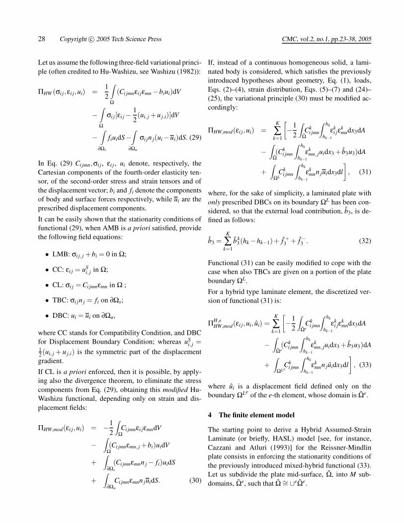
Figure 4 : The rectangular Hybrid Assumed-Strain Lam-inated element (HASL).

A simple quadrilateral 12 degrees-of-freedom (dofs)laminated plate with constant thickness can be developedas follows (see Figure 4).

Let us assume a local reference system (x1, x2, x3), wherethe x1- and x2-axes are aligned with the 1–2 and 1–4 sidesrespectively, and the x3-axis is determined by the right-hand rule. A plane natural reference system (ξ1, ξ2),with −1 ≤ ξ i ≤ 1 (i=1, 2) is then introduced [see, forinstance Zienkiewicz and Taylor (1991); Hughes (1987);Bathe (1996)] and is related to the local one by the fol-lowing relationships (as in standard isoparametric ele-ments):

xi(ξ i) =4

∑=1

N(ξ i)xi (34)

where xi , (with = 1, . . .,4), are the nodal coordinates of

the element, while N(ξi) are the shape functions givenby:

N(ξi) =14(1+ξ1ξ

1)(1+ξ2ξ2) ( = 1, . . .,4). (35)

The nodal coordinates in the natural reference systemare, of course, given by (ξ1,ξ2) = (±1,±1).

4.1 The strain field

With reference to the natural reference system ξ1,ξ2 (seeFigure 4), let us assume the following in-plane compo-nents of the strain tensor ε∗i j:

ε∗k11 = ε∗11 = x3ε∗11 = x3(α0 +α1ξ1 +α2ξ2) (36)

ε∗k22 = ε∗22 = x3ε∗22 = x3(β0 +β1ξ1 +β2ξ2) (37)

ε∗k12 = ε∗12 = x3ε∗12 = x3(γ0 + γ1ξ2

1 + γ2ξ22). (38)

A strain vector β is then introduced, as a short-hand no-tation, to collect component-wise the above introducedstrain parameters:

β = α0,α1,α2,β0,β1,β2,γ0,γ1,γ2T . (39)

The in-plane stress components, corresponding to the in-plane strain components (36)–(38), are given, for thegeneric k-th layer, by Eqs. (8)–(10). By substituting(36)–(38) into (8)–(10), one obtains the following stresscomponents, expressed in the natural reference system:

σk11 = x3[Ck

11(α0 +α1ξ1 +α2ξ2) (40)

+Ck12(β0 +β1ξ1 +β2ξ2)]

σk22 = x3[Ck

21(α0 +α1ξ1 +α2ξ2) (41)

+Ck22(β0 +β1ξ1 +β2ξ2)]

σk12 = x3[2Ck

66(γ0 + γ1ξ21 + γ2ξ2

2)]. (42)

The out-of-plane components σk13, σk

23 (referred againto the natural reference system) can be determined bymaking use of the LMB equations, as shown in Sec-tion 2.3; for the assumed strain interpolations (36)–(38),Eqs. (14)–(15) provide:

σk13 = −1

2(x2

3 −h2k−1)[(C

k11α1 +Ck

12β1)+Ck66(4γ2ξ2)]

+σ0,k13 (43)

σk23 = −1

2(x2

3 −h2k−1)[(C

k12α2 +Ck

22β2)+Ck66(4γ1ξ1)]

+σ0,k23 , (44)

where the integration constants σ0,k13 , σ0,k

23 are defined ex-actly as in Eqs. (22)–(23).

Similarly, the out-of-plane strain components ε∗k13, ε∗k

23 arecomputed by Eqs. (24)–(25).

It should be remarked that if a linear interpolation is as-sumed for the in-plane shear strain components, ε∗12 =ε∗21 — instead of the adopted incomplete quadratic one,Eq. (38) — the out-of-plane shear stress components, σk

13and σk

23 turn out to be constant along both the ξ1 and theξ2 direction, providing a too stiff element [see Garusi,Cazzani, and Tralli (2004)].

Finally, the Cartesian strain components of the k-th lam-ina, ε∗k

i j defined in the natural reference system need to beexpressed in the local (or physical) reference system; thecorresponding Cartesian components, εk

i j are defined bythe following transformation rule:

εkmn = Jimε∗k

i j J jn, (45)

30 Copyright c© 2005 Tech Science Press CMC, vol.2, no.1, pp.23-38, 2005

where Jim denotes the elements of the Jacobian matrixof the isoparametric transformation (34); see for instanceCazzani and Atluri (1993).

Even though the formulation can be extended to coverthe case of distorted element, only simple cases — likethe rectangular one — where the Jacobian of the elementis constant (and therefore coincides with its value at thecentroid) will be discussed here.

4.2 The displacement field

In the following, the displacement field can be conve-niently expressed in terms of the transverse displace-ments u

3 ( = 1, . . .,4) and of the rotations ϕ i (with

i = 1,2) of transverse line elements, evaluated at the fournodes of the plate.

The components of the assumed displacement field arethen functions of these nodal dofs and are expressed interms of the shape functions (34) as follows:

u1 = −x3

4

∑=1

N(ξ i)ϕ1 (46)

u2 = −x3

4

∑=1

N(ξ i)ϕ2 (47)

u3 =4

∑=1

N(ξ i)u 3. (48)

As a short-hand notation, the following generalized nodaldisplacement vector is introduced:

q =

u13 , ϕ1

1 , ϕ12 , u2

3 , ϕ21 , ϕ2

2 , u33 , ϕ3

1 , ϕ32 , u4

3 , ϕ41 , ϕ4

2

T.

(49)

It should be remarked that in the HASL element, the dis-placement field components ui (i = 1,2,3), occurring inEq. (33) are defined by the same shape functions (46)–(48), but need to be defined only on the element edgesξ1 = ±1 and ξ2 = ±1.

4.3 The finite element stiffness matrix

The stiffness matrix K of the HASL element is derivedby substituting the interpolation fields defined in the pre-vious Sections 4.1 and 4.2 into the modified Hu-Washizufunctional (33).

The two independently discretized fields of displace-ments ui, ui and strains, εi j written in the physical ref-erence system xi (i = 1,2,3) of the finite element read as

follows:

ui(xi) = Nu(xi)q (50)

εi j(xi) = Nε(xi)β, (51)

where Nu(xi) denotes the matrix of the shape functionsfor the displacement field (46)–(48); Nε(xi) denotes thematrix of the shape functions for the strain field (36)–(38), whereas the corresponding vectors q, β are definedin Eqs. (49) and (39).

Substitution of Eqs. (50) and (51) into (33) yields the fol-lowing discretized variational principle:

ΠH,eHW,mod = −1

2βTHββ β+βTGq−FTq, (52)

where:

βTHββ β = ∑k

[∫Ωe

Cki jmn

∫ hk

hk−1

εki jε

kmndx3dA

]; (53)

βTGq = ∑k

[−

∫Ωe

Cki jmn

∫ hk

hk−1

εkmn, juidx3dA

+∫

ΩLeCk

i jmn

∫ hk

hk−1

εkmnn juidx3dl

]; (54)

FTq =∫

Ωeb3u3dA. (55)

All the above integrals, defined in the physical configura-tion, are evaluated, with the usual techniques employedin isoparametric formulation, on the reference (i.e. natu-ral) configuration.

It should be outlined that the first term on the right-handside of Eq. (52) represents (to within the sign) the ele-ment strain energy, Ue, as it clearly appears in Eq. (53).In the present context, by virtue of the symmetric lam-ination scheme and of the load conditions (2)–(4), itcan be shown that the strain energy can be written asUe = Ue

b +Ues i.e. it splits into two contributions, the for-

mer, Ueb , due to bending stresses, the latter, Ue

s , to trans-verse (or out-of-plane) shear stresses.

The strain energy due to these transverse shear stresses— see Eqs. (24)–(25) and (45) — is given by:

Ues = ∑

k

∫Ωe

∫ hk

hk−1

2[Ck

55(εk13)

2 +Ck44(εk

23)2]

dx3dA, (56)

and, with a procedure similar to that adopted in Garusi,Cazzani, and Tralli (2004) it follows that when h → 0,

Hybrid assumed-strain laminated element 31

then Ues → 0 like h5. Since it can be proven, with the

same method, that the bending strain energy Ueb is a cu-

bic function of the laminate thickness h, when thicknessbecomes smaller and smaller, the shear strain energy Ue

sis negligible if compared to the bending strain energy, i.e.the ratio Ue

s /Ueb goes to zero with the correct order in the

thin plate limit.

By invoking now the stationarity conditions of ΠH,eHW,mod

with reference to β and q, the following system of simul-taneous linear algebraic equations is obtained:

[ −Hββ GGT O

]βq

=

0F

. (57)

By making use of static condensation techniques on β,the following discrete equilibrium equations are obtainedfrom Eq. (57):

Kq = F, (58)

where the stiffness matrix K appearing in Eq. (58) can beevaluated as follows:

K = GT H−1ββ G. (59)

In this way, when the strain parameters are eliminatedat the element level, at the assembly stage the elementhas exactly the same number and type of dofs as a stan-dard displacement-based one. For this reason, the so-lution procedure is that of a standard stiffness formula-tion, and it is allowed mixing an element of this type withdisplacement-formulated ones.

For the HASL element under consideration — dual hy-brid, according to Brezzi and Fortin (1991) — matrixHββ has to be positive-definite in order to satisfy the el-lipticity condition, and this is verified for the assumedstrain shape functions, as it can be checked. Thereforeit is possible to evaluate β element by element, once thenodal displacement values q are known, by the followingequation:

β = H−1ββ Gq. (60)

The discrete inf-sup condition for dual-hybrid methodscan be verified by performing a singular value decom-position of matrix K, see Xue and Atluri (1985); Garusiand Tralli (2002). With the assumed strain distributiononly the three zero eigenvalues corresponding to the threerigid body motions are found.

5 Numerical examples

Several numerical examples are discussed for both thickand thin laminated plates to evaluate the performances ofthe presented element.

The obtained results are compared with those available inthe technical literature and with the solutions provided bythe commercial finite element code ANSYS version 5.3:brick elements with assigned material properties havebeen used to model each layer.

In particular, results provided by the following elementshave been reported: the partial-mixed models EML4 byAuricchio and Sacco (1999); the Partial-Hybrid StressLaminated plate (denoted here by PHSL) by Yong andCho (1995); the isoparametric displacement-based ele-ments QUAD4 and QUAD9 by Zienkiewicz and Tay-lor (1991); the CTMQ20 Timoshenko-Mindlin quadri-lateral finite element with 20 dofs by Cen, Long, andYao (2002); the Discrete Shear Triangular (DST) plate-bending element by Lardeur and Batoz (1989); theREC56-Z0 (with 56 dofs) and REC72-Z0 (with 72 dofs)elements by Sadek (1998). Finally, where it has beenpossible, analytical series solutions given for the 3-Dcase by Pagano (1970) and for the 2-D case (i.e. corre-sponding to FSDT) by Reddy (2004) have been reported,along with the Higher order laminated plate solutions byLo, Christensen, and Wu (1977).

The following material constants have been used for allthe considered examples:

E1/E2 = 25; G12 = G13 = 0.5E2; G23 = 0.2E2;

ν12 = ν13 = 0.25,

corresponding to a high-modulus orthotropic graphite-epoxy composite material.

5.1 1-D analysis of laminated plate

As a preliminary series of test, some cylindrical bendingproblems are considered: a laminated cantilever plate isconstrained in such a way that its behavior is equivalentto that of a cantilever beam.

5.1.1 Cantilever laminated plate under tip line-load

The first considered problem is a four-layer [0/90/90/0]laminated cantilever plate subjected to a shear load ap-plied to the free end (see Figure 5).

32 Copyright c© 2005 Tech Science Press CMC, vol.2, no.1, pp.23-38, 2005

Figure 5 : Four-layer laminated cantilever plate undershear load at the free end. (a) One element discretization;(b) Four elements discretization.

Each layer has equal thickness h/4; a one-element dis-cretization and a four-elements discretization have beenconsidered (see Figure 5a and 5b). Results have beencompared with those provided by the 2-D analyticalFSDT solution.

Table 1 shows the deflection at the free end of the lam-inate element for different thickness values. Results areexpressed in normalized form, by dividing the numericalresults by the theoretical one, provided in Reddy (2004)[Table 4.3.1, page 193]. It should be noticed that for allthickness values the results are in excellent agreementwith those of the analytical solution and no locking phe-nomena are encountered.

Table 1 : Normalized deflection, u3, at the free end of alaminated [0/90/90/0] cantilever plate under tip line-load

a/h el. 1000 100 10 1HASL 1 1.002 1.002 1.001 0.992HASL 4 1.002 1.002 1.001 0.993FSDT — 1.000 1.000 1.000 1.000

Figure 6 presents the distribution of the shear stressσ13(x3) for the problem under consideration (with a/h =1), produced by the ANSYS code when a finite elementanalysis with eight-noded brick elements is performed.

Figure 7 shows instead the profile of the shear stressσ13(x3) for the one-element discretization (again in thecase a/h = 1), which is compared with the one provided

Figure 6 : Distribution of shear stress σ13 for the[0/90/90/0] laminated plate (with a/h = 1) subjected totip line-load, analyzed with brick elements: the finite el-ement mesh is also shown.

Figure 7 : Distribution of shear stress σ13 along thethickness for the [0/90/90/0] laminated plate (a/h = 1)under tip line-load: comparison between HASL andbrick model results.

by the finite element analysis already performed withbrick elements.

It should be noticed that in any standard laminate the-ory (viz. CLT or FSDT), as in the present HASL model,the shear stress distribution does not vary along the x1-axis, whereas the 3-D solution (and, consequently, thefinite element result produced by solid brick elements)takes into account the boundary-layer effects [see Savoia,Laudiero, and Tralli (1993)] and therefore exhibits a dif-ferent behavior close to the boundary (i.e for x1 = 0.5)and in a generic section like that, here considered, de-fined by x1 = 6.5.

As it is expected, the element shows a good ability tocompute in a satisfactory way the through-the-thicknessand inter-laminar shear stress, by satisfying exactly both

Hybrid assumed-strain laminated element 33

inter-laminar and top and bottom equilibrium conditions.

5.1.2 Cantilever laminated plate under uniformly dis-tributed load

The second 1-D test is a four-layer [0/90/90/0] laminatedcantilever plate subjected to a uniform load acting on thetop surface Ω+ (see Figure 8). As in the previous prob-lem each layer has equal thickness (h/4).

Again, two different discretizations have been consid-ered, one consisting of four elements, the other of eightelements; results, in terms of normalized tip deflection,have been compared with those provided by the FSDTanalysis, which provides a reference solution given byReddy (2004) [Table 4.3.1, page 193].

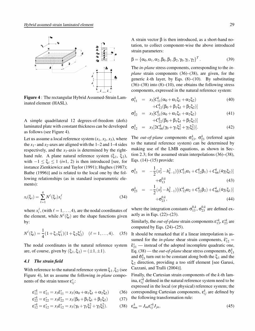
These results in terms of normalized tip deflection at themiddle surface of the HASL element are given in Table 2.The results are compared with the FSDT solution forseveral values of the depth-to-thickness ratio. Figure 9presents the distribution of the shear stress σ13(x3) for theproblem under consideration (with a/h = 1), produced

Figure 8 : Four-layer laminated cantilever plate underuniformly distributed load. (a) Four elements discretiza-tion; (b) Eight elements discretization.

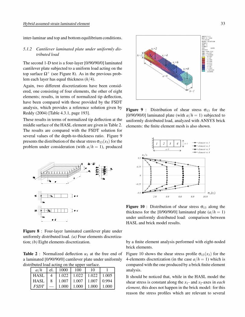
Table 2 : Normalized deflection u3 at the free end ofa laminated [0/90/90/0] cantilever plate under uniformlydistributed load acting on the upper surface.

a/h el. 1000 100 10 1HASL 4 1.022 1.022 1.022 1.005HASL 8 1.007 1.007 1.007 0.994FSDT — 1.000 1.000 1.000 1.000

Figure 9 : Distribution of shear stress σ13 for the[0/90/90/0] laminated plate (with a/h = 1) subjected touniformly distributed load, analyzed with ANSYS brickelements: the finite element mesh is also shown.

Figure 10 : Distribution of shear stress σ13 along thethickness for the [0/90/90/0] laminated plate (a/h = 1)under uniformly distributed load: comparison betweenHASL and brick model results.

by a finite element analysis performed with eight-nodedbrick elements.

Figure 10 shows the shear stress profile σ13(x3) for the4-elements discretization (in the case a/h = 1) which iscompared with the one produced by a brick finite elementanalysis.

It should be noticed that, while in the HASL model theshear stress is constant along the x1- and x2-axes in eachelement, this does not happen in the brick model: for thisreason the stress profiles which are relevant to several

34 Copyright c© 2005 Tech Science Press CMC, vol.2, no.1, pp.23-38, 2005

values of the x1 coordinate are shown. Obviously, also inthis case boundary layer effects are taken into account inthe 3-D solution only, as shown in Savoia, Laudiero, andTralli (1993).

5.2 Composite laminate plates

In order to establish the performance of the proposed el-ement in a truly 2-D environment, a simply-supportedsquare laminated plate has been considered. The plateside length is denoted by a, whereas its thickness is h.The following boundary conditions have been adopted(corresponding to hard boundaries):

@ x1 = 0 and x1 = a : u2 = u3 = 0, ϕ1 = 0

@ x2 = 0 and x2 = a : u1 = u3 = 0, ϕ2 = 0.

The symmetric three-layer (i.e. [0/90/0]) and four-layer(i.e. [0/90/90/0]) cross-ply laminates have been sepa-rately considered, as shown in Figure 11.

Figure 11 : Simply-supported square laminated plate un-der distributed loads: the pattern of mesh refinement ispartially shown. In (a) the [0/90/0] three-layer laminateis shown, in (b) the [0/90/90/0] four-layer one.

The plate has been loaded either by a uniformly dis-tributed load (UDL), q0, or by a doubly-sinusoidal load(SSL), q = q0 sin(πx1/a) sin(πx2/a), acting on the uppersurface, Ω+.

Due to geometric and loading symmetry only a quarter ofthe plate was studied, and different meshes were adopted.

5.2.1 Symmetric [0/90/0] cross-ply laminated plate

In this case, shown in Figure 11a, the following normal-ization of the deflection of the plate center has been usedwhen presenting the results [see Table 7.2.1, page 385in Reddy (2004)]:

u3 =100E2h3

q0a4 u3. (61)

UDL: Uniformly distributed load

Table 3 presents the normalized transversal displacementat the plate center for the considered load case. For com-parison purposes, the FSDT analytical solution and theresults obtained by the hybrid 4-node (EML4) and theisoparametric displacement-based 4-node (QUAD4) and9-node (QUAD9) elements are reported as well.

Table 3 : Normalized deflection, u3, measured at the cen-ter of a simply-supported square laminated [0/90/0] plateunder UDL.

a/h mesh 100 10HASL 3×3 0.6756 1.0445

6×6 0.6711 1.029312×12 0.6700 1.0262

EML4 3×3 — 1.02356×6 — 1.0223

12×12 — 1.0220QUAD4 3×3 — 1.0331

6×6 — 1.024312×12 — 1.0225

QUAD9 6×6 — 1.022212×12 — 1.0219

FSDT — 0.6697 1.0219

SSL: Double sinusoidally distributed load

Table 4 reports the normalized transversal deflection atthe plate center for the present load case. Analogously asbefore, the analytical solution and some results availablein the literature are presented for comparison purposes.

5.2.2 Symmetric [0/90/90/0] cross-ply laminated plate

The considered case is shown in Figure 11b; as beforethe two load conditions are considered separately.

UDL: Uniformly distributed load

The same normalized displacement given by Eq. (61) isused here in the presentation of results. Table 5 providesthe normalized deflection at the plate center for the con-sidered load case.

Hybrid assumed-strain laminated element 35

Table 4 : Normalized deflection, u3, measured at the cen-ter of a simply-supported square laminated [0/90/0] plateunder SSL.

a/h mesh 100 20 10HASL 6×6 0.4343 0.4932 0.6726EML4 3×3 — — 0.6696

6×6 — — 0.669412×12 — — 0.6693

QUAD4 3×3 — — 0.67086×6 — — 0.6696

12×12 — — 0.6694QUAD9 6×6 — — 0.6694

12×12 — — 0.6693FSDT — 0.4337 0.4921 0.6693

Table 5 : Normalized deflection, u3, measured at the cen-ter of a simply-supported square laminated [0/90/90/0]plate under UDL.

a/h mesh 100 20 10HASL 3×3 0.6884 0.7751 1.0364

6×6 0.6844 0.7689 1.0253ANSYS 3×3 0.6894 0.7693 1.0249

6×6 0.6844 0.7694 1.0250FSDT — 0.6833 0.7694 1.0250

For comparison purposes, the FSDT analytical solutionand the results obtained by ANSYS with the shell 99 el-ement are reported as well.

In Figure 12 the distribution of out-of plane shear stressesσ13(x3) and σ23(x3) at point x1 = a/12, x2 = a/12 areplotted for several values of the side-to-thickness ratioa/h.

SSL: Double sinusoidally distributed load

In this case, the following normalization of displacementis used in the presentation of results, instead of Eq. (61):

u3 =π4Qh3

12q0a4 u3, (62)

where

Q = 4G12 +E1 +E2(1+2ν23)

1−ν12ν21. (63)

Table 6 presents the normalized deflection of the platecenter for the present load case. Along with some numer-

Figure 12 : Distribution of shear stresses σ13 and σ23

at point (a/12, a/12) for the laminate [0/90/90/0] underUDL for different a/h ratios.

Table 6 : Deflection, u3, normalized according toEq. (62) measured at the center of a simply-supportedsquare laminated [0/90/90/0] plate under SSL.

a/h mesh 100 50 10HASL 6×6 1.007 1.024 1.548EML4 5×5 — — 1.727PHSL 4×4 1.0060 1.0306 1.7154

CTMQ20 4×4 1.007 1.031 1.7358×8 1.008 1.031 1.729

16×16 1.008 1.031 1.728DST 10×10 — 1.067 1.727

REC56-Z0 2×2 0.956 0.993 1.445REC72-Z0 2×2 0.962 1.006 1.663

FSDT — 1.006 — 1.537Higher order — 1.0034 1.0275 1.6712

3-D — 1.008 1.031 1.733

ical results available in the literature, the following ana-lytical solutions are reported for comparison purposes:FSDT; Higher order plate theory by Lo, Christensen,and Wu (1977); 3-D elastic theory, provided by Pagano(1970).

Finally, in Figure 13 the distribution of transversal

36 Copyright c© 2005 Tech Science Press CMC, vol.2, no.1, pp.23-38, 2005

shear stresses σ13(x3) and σ23(x3) at point x1 = a/12,x2 = a/12 are plotted for several values of the side-to-thickness ratio a/h.

Figure 13 : Distribution of shear stresses σ13 and σ23

at point (a/12, a/12) for the laminate [0/90/90/0] underSSL for different a/h ratios.

It should be noticed, by making reference to the transver-sal deflection, that the results provided by the HASLelement are in good agreement with those of the 3-Dsolution for all the side-to-thickness ratio. Like in allother cases no shear-locking phenomena occurs in thethin plate limit.

Acknowledgement: The financial support of bothMIUR, the Italian Ministry of Education, University andResearch (under Grant Cofin 2003: Interfacial DamageFailure in Structural Systems: Applications to Civil En-gineering and Emerging Research Fields) and the Uni-versity of Trento is gratefully acknowledged.

The research project has been partially developed duringa research stay of E. Garusi at UCLA with a researchgrant provided by Prof. S.N. Atluri.

References

Atluri, S. N. (1983): Recent studies of hybrid and mixedfinite element methods in mechanics. In Atluri, S. N.; et.

al. (Eds): Hybrid and Mixed Finite Element Methods, J.Wiley & Sons, pp. 51–72.

Atluri, S. N.; Han, Z. D.; Rajendran, A. M. (2004):A new implementation of the meshless finite volumemethod, through the MLPG “mixed” approach. CMES:Computer Modeling in Engineering & Sciences, vol. 6,pp. 491–514.

Auricchio, F.; Sacco, E. (1999): A mixed-enhancedfinite-element for the analysis of laminated compositeplates. International Journal for Numerical Methods inEngineering, vol. 69, pp. 1481–1504.

Auricchio, F.; Sacco, E. (2003): Refined first-ordershear deformation theory models for composite lami-nates. Journal of Applied Mechanics ASME, vol. 70,pp. 381–390.

Bathe, K. J. (1996): Finite element procedures. Pren-tice Hall, Englewood Cliffs, NJ, 2nd edition.

Bisegna, P.; Sacco, E. (1997): A layer-wise laminatetheory rationally deduced from the three-dimensionalelasticity. Journal of Applied Mechanics ASME, vol. 64,pp. 538–545.

Brezzi, F.; Fortin, M. (1991): Mixed and hybrid finiteelement methods. Springer, New York, 1st edition.

Cazzani, A.; Atluri, S. N. (1993): Four-noded mixedfinite elements, using unsymmetric stresses, for linearanalysis of membranes. Computational Mechanics, vol.11, pp. 229–251.

Cen, S.; Long, Y.; Yao, Z. (2002): A new hybrid-enhanced displacement-based element for the analysis oflaminated composite plates. Computers & Structures,vol. 80, pp. 819–833.

Chepiga, V. E. (1976): Refined theory of multilayeredshells. Soviet Applied Mechanics, vol. 12, pp. 1127–1130. English translation from Prikladnaia mekhanika,vol. 12, pp. 45–49.

Cicala, P. (1962): Consistent approximations in shelltheory. Journal of the Engineering Mechanics DivisionASCE, vol. 88, pp. 45–74.

Di Sciuva, M. (1987): An improved shear deformationtheory for moderately thick multi-layered anisotropicshells and plates. Journal of Applied Mechanics, vol.54, pp. 589–596.

Hybrid assumed-strain laminated element 37

Garusi, E.; Cazzani, A.; Tralli, A. (2004): An unsym-metric stress formulation for Reissner-Mindlin plates: asimple and locking-free hybrid rectangular element. In-ternational Journal of Computational Engineering Sci-ence. In print.

Garusi, E.; Tralli, A. (2002): A hybrid stress-assumedtransition element for solid-to-beam and plate-to-beamconnections. Computers & Structures, vol. 80, pp. 105–115.

Gaudenzi, P.; Mannini, A.; Carbonaro, R. (1998):Multi-layer higher order finite elements for the analysisof free-edge stresses in composite laminates. Interna-tional Journal for Numerical Methods in Engineering,vol. 41, pp. 851–873.

Hughes, T. J. R. (1987): The finite element method —Linear static and dynamic finite element analysis. Pren-tice Hall, Englewood Cliffs, NJ, 1st edition.

Lardeur, P.; Batoz, J. L. (1989): Composite plateanalysis using a new discrete shear triangular finite el-ement. International Journal for Numerical Methods inEngineering, vol. 27, pp. 343–359.

Liou, W.; Sun, C. T. (1987): A three-dimensional hy-brid stress isoparametric element for the analysis of lam-inated composite plates. Computers & Structures, vol.25, pp. 241–249.

Lo, K. H.; Christensen, R. M.; Wu, E. M. (1977): Ahigher-order theory of plate deformation: Part 2, lami-nated plates. Journal of Applied Mechanics ASME, vol.44, pp. 669–676.

Mau, S. T.; Tong, P.; Pian, T. H. H. (1972): Finiteelement solutions for laminated plates. Journal of Com-posite Materials, vol. 6, pp. 304–311.

Mindlin, R. D. (1951): Influence of rotatory inertiaand shear on flexural motions of isotropic elastic plates.Journal of Applied Mechanics ASME, vol. 18, pp. 31–38.

Noor, A. K.; Burton, W. S. (1990): Assessmentof computational models for multilayered anisotropicplates. Composite Structures, vol. 14, pp. 233–265.

Pagano, N. J. (1970): Exact solutions for rectangularbidirectional composites and sandwich plates. Journalof Composite Materials, vol. 4, pp. 20–34.

Pagano, N. J.; Hatfield, S. J. (1972): Elastic behaviorof multilayered bidirectional composites. AIAA Journal,vol. 10, pp. 931–933.

Pai, P. F. (1995): A new look at shear correction factorsand warping functions of anisotropic laminates. Inter-national Journal of Solids and Structures, vol. 32, pp.2295–2313.

Pandya, B. N.; Kant, T. (1988): Flexure analysis oflaminated composites using refined higher-order C0 platebending elements. Computer Methods in Applied Me-chanics and Engineering, vol. 66, pp. 173–198.

Poniatovskii, V. V. (1962): Theory for plates of mediumthickness. PMM, vol. 26, pp. 478–486. English transla-tion from Prikladnaia Matematika i Mekhanika, vol. 26,pp. 335–341.

Punch, E. F.; Atluri, S. N. (1984a): Applications ofisoparametric three-dimensional hybrid-stress finite ele-ments with least-order stress fields. Computers & Struc-tures, vol. 19, pp. 409–430.

Punch, E. F.; Atluri, S. N. (1984b): Least-order, stable,invariant isoparametric hybrid finite elements for linearcontinua and finitely deformed plates. In Proceedingsof the 25th AIAA/ASME/ASCE Structures, Structural Dy-namics and Materials Conference, Palm Springs, CA, pp.190–202.

Qi, Y.; Knight, N. F. (1996): A refined first-ordershear-deformation theory and its justification by plane-strain bending problem of laminated plates. Interna-tional Journal of Solids and Structures, vol. 33, pp. 49–64.

Reddy, J. N. (1984): A simple higher-order theory forlaminated composite plates. Journal of Applied Mechan-ics ASME, vol. 51, pp. 745–752.

Reddy, J. N. (1987): A generalization of two-dimensional theories of laminated composite plates.Communications in Applied Numerical Methods, vol. 3,pp. 173–180.

Reddy, J. N. (2004): Mechanics of laminated compos-ite plates and shells — Theory and analysis. CRC Press,Boca Raton, FL, 2nd edition.

38 Copyright c© 2005 Tech Science Press CMC, vol.2, no.1, pp.23-38, 2005

Reissner, E. (1945): The effect of transverse shear de-formation on the bending of elastic plates. Journal ofApplied Mechanics ASME, vol. 12, pp. 69–77.

Robbins, D. H.; Reddy, J. N. (1993): Modeling ofthick composites using a layerwise laminate theory. In-ternational Journal for Numerical Methods in Engineer-ing, vol. 36, pp. 655–677.

Rolfes, R.; Rohwer, K. (1997): Improved transverseshear stresses in composite finite elements based on firstorder shear deformation theory. International Journalfor Numerical Methods in Engineering, vol. 40, pp. 51–60.

Rolfes, R.; Rohwer, K.; Ballerstaedt, M. (1998): Ef-ficient linear transverse normal stress analysis of layeredcomposite plates. Computers & Structures, vol. 68, pp.643–652.

Sadek, E. A. (1998): Some serendipity finite elementsfor the analysis of laminated plates. Computers & Struc-tures, vol. 69, pp. 37–51.

Savoia, M.; Laudiero, F.; Tralli, A. (1993): A refinedtheory for laminated beams: Part I - a new high-orderapproach. Meccanica, vol. 28, pp. 39–51.

Savoia, M.; Laudiero, F.; Tralli, A. (1994): A two-dimensional theory for the analysis of laminated plates.Computational Mechanics, vol. 14, pp. 38–51.

Singh, G.; Raju, K. K.; Rao, G. V. (1998): A newlock-free, material finite element for flexure of moder-ately thick rectangular composite plates. Computers &Structures, vol. 69, pp. 609–623.

Spilker, R. L. (1982): Hybrid-stress eight-node elementfor thin and thick multilayered laminated plates. Inter-national Journal for Numerical Methods in Engineering,vol. 18, pp. 801–828.

Spilker, R. L.; Munir, N. I. (1980): A hybrid-stressquadratic serendipity displacement Mindlin plate bend-ing element. Computers & Structures, vol. 12, pp. 11–21.

Spilker, R. L.; Orringer, O.; Witmer, E. A. (1976):Use of the hybrid-stress finite-element model for thestatic and dynamic analysis of composite plates and shell.Technical Report ASRL TR 181–2, MIT, 1976.

Vlachoutsis, S. (1992): Shear correction factors forplates and shells. International Journal for NumericalMethods in Engineering, vol. 33, pp. 1537–1552.

Washizu, K. (1982): Variational methods in elasticityand plasticity. Pergamon Press, Oxford, 3rd edition.

Whitney, J. M. (1973): Shear correction factors for or-thotropic laminates under static load. Journal of AppliedMechanics ASME, vol. 40, pp. 302–304.

Whitney, J. M.; Pagano, N. J. (1970): Shear defor-mation in heterogeneous anisotropic plates. Journal ofApplied Mechanics ASME, vol. 37, pp. 1031–1036.

Xue, W.-M.; Atluri, S. N. (1985): Existence andstability, and discrete B and rank conditions, for gen-eral mixed-hybrid finite elements in elasticity. In Spilker,R. L.(Ed): Hybrid and Mixed Finite Element Methods,AMD, volume 73, pp. 91–112.

Yang, P. C.; Norris, C. H.; Stavsky, Y. (1966): Elasticwave propagation in heterogeneous plates. InternationalJournal of Solids and Structures, vol. 2, pp. 665–684.

Yoda, T.; Atluri, S. N. (1992): Post-buckling analysisof stiffened laminated composite panels, using a higher-order shear deformation theory. Computational Mechan-ics, vol. 9, pp. 390–404.

Yong, Y.-K.; Cho, Y. (1995): Higher-order, partial hy-brid stress, finite element formulation for laminated plateand shell analysis. Computers & Structures, vol. 57, pp.817–827.

Yu, W.; Hodges, D. H.; Volovoi, V. V. (2003): Asymp-totically accurate 3-D recovery from Reissner-like com-posite plate finite elements. Computers & Structures,vol. 81, pp. 439–454.

Zienkiewicz, O. C.; Taylor, R. L. (1991): The finiteelement method. McGraw-Hill, New York, 4th edition.