
6 Composite Materials from Natural Resources: Recent Trends and Future Potentials
Upload
independentCategory
view
0download
0

StructuralCompositeMaterials
F.C. Campbell
ASM International®
Materials Park, Ohio 44073-0002www.asminternational.org

Copyright © 2010by
ASM International®
All rights reserved
No part of this book may be reproduced, stored in a retrieval system, or transmitted, in any form or by any means, electronic, mechanical, photocopying, recording, or otherwise, without the writ-ten permission of the copyright owner.
First printing, November 2010
Great care is taken in the compilation and production of this book, but it should be made clear that NO WARRANTIES, EXPRESS OR IMPLIED, INCLUDING, WITHOUT LIMITATION, WAR-RANTIES OF MERCHANTABILITY OR FITNESS FOR A PARTICULAR PURPOSE, ARE GIVEN IN CONNECTION WITH THIS PUBLICATION. Although this information is believed to be accurate by ASM, ASM cannot guarantee that favorable results will be obtained from the use of this publication alone. This publication is intended for use by persons having technical skill, at their sole discretion and risk. Since the conditions of product or material use are outside of ASM’s control, ASM assumes no liability or obligation in connection with any use of this information. No claim of any kind, whether as to products or information in this publication, and whether or not based on negligence, shall be greater in amount than the purchase price of this product or publica-tion in respect of which damages are claimed. THE REMEDY HEREBY PROVIDED SHALL BE THE EXCLUSIVE AND SOLE REMEDY OF BUYER, AND IN NO EVENT SHALL EITHER PARTY BE LIABLE FOR SPECIAL, INDIRECT OR CONSEQUENTIAL DAMAGES WHETHER OR NOT CAUSED BY OR RESULTING FROM THE NEGLIGENCE OF SUCH PARTY. As with any material, evaluation of the material under end-use conditions prior to speci-fication is essential. Therefore, specific testing under actual conditions is recommended.
Nothing contained in this book shall be construed as a grant of any right of manufacture, sale, use, or reproduction, in connection with any method, process, apparatus, product, composition, or system, whether or not covered by letters patent, copyright, or trademark, and nothing contained in this book shall be construed as a defense against any alleged infringement of letters patent, copyright, or trademark, or as a defense against liability for such infringement.
Comments, criticisms, and suggestions are invited, and should be forwarded to ASM International.
Prepared under the direction of the ASM International Technical Book Committee (2009–2010), Michael J. Pfeifer, Chair.
ASM International staff who worked on this project include Scott Henry, Senior Manager, Content Development & Publishing; Steven R. Lampman, Content Developer; Eileen De Guire, Senior Content Developer; Ed Kubel, Technical Editor; Ann Britton, Editorial Assistant; Bonnie Sanders, Manager of Production; Madrid Tramble, Senior Production Coordinator; Diane Whitelaw, Pro-duction Coordinator; and Patricia Conti, Production Coordinator.
Library of Congress Control Number: 2010937090 ISBN-13: 978-1-61503-037-8
ISBN-10: 0-61503-037-9SAN: 204-7586
ASM International®
Materials Park, OH 44073-0002www.asminternational.org
Printed in the United States of America

This book is dedicated to my youngest granddaughter, Matilda, who is so little yet is so brave and strong.

“This page left intentionally blank.”

Contents
Preface xiAbout the Author xv
Chapter 1 Introduction to Composite Materials 11.1 Isotropic, Anisotropic, and Orthotropic Materials 41.2 Laminates 71.3 Fundamental Property Relationships 81.4 Composites versus Metallics 101.5 Advantages and Disadvantages of Composite Materials 141.6 Applications 18
Chapter 2 Fibers and Reinforcements 312.1 Fiber Terminology 312.2 Strength of Fibers 322.3 Glass Fibers 332.4 Aramid Fibers 392.5 Ultra-High Molecular Weight Polyethylene Fibers 412.6 Carbon and Graphite Fibers 422.7 Woven Fabrics 492.8 Reinforced Mats 522.9 Chopped Fibers 522.10 Prepreg Manufacturing 52
Chapter 3 Matrix Resin Systems 633.1 Thermosets 643.2 Polyester Resins 653.3 Epoxy Resins 673.4 Bismaleimide Resins 703.5 Cyanate Ester Resins 713.6 Polyimide Resins 723.7 Phenolic Resins 743.8 Toughened Thermosets 753.9 Thermoplastics 81
3.9.1 Thermoplastic Composite Matrices 823.9.2 Thermoplastic Composite Product Forms 87
3.10 Quality Control Methods 903.10.1 Chemical Testing 913.10.2 Rheological Testing 923.10.3 Thermal Analysis 943.10.4 Glass Transition Temperature 97
3.11 Summary 99

vi / Contents
Chapter 4 Fabrication Tooling 1014.1 General Considerations 1014.2 Thermal Management 1044.3 Tool Fabrication 111
Chapter 5 Thermoset Composite Fabrication Processes 1195.0 Lay-up Processes 1195.1 Wet Lay-Up 1195.2 Prepreg Lay-Up 122
5.2.1 Manual Lay-Up 1235.2.2 Flat Ply Collation and Vacuum Forming 1245.2.3 Roll or Tape Wrapping 1255.2.4 Automated Methods 1255.2.5 Vacuum Bagging 1315.2.6 Curing 133
5.3 Low-Temperature Curing/Vacuum Bag Systems 1375.4 Filament Winding 1415.5 Liquid Molding 146
5.5.1 Preform Technology 1485.5.2 Resin Injection 1625.5.3 Priform Process 1645.5.4 RTM Curing 1665.5.5 RTM Tooling 1675.5.6 RTM Defects 1705.5.7 Vacuum-Assisted Resin Transfer Molding 172
5.6 Resin Film Infusion 1745.7 Pultrusion 175
Chapter 6 Thermoplastic Composite Fabrication Processes 1836.1 Thermoplastic Consolidation 1836.2 Thermoforming 1866.3 Thermoplastic Joining 192
Chapter 7 Processing Science of Polymer Matrix Composites 2017.1 Kinetics 2027.2 Viscosity 2067.3 Heat Transfer 2077.4 Resin Flow 209
7.4.1 Hydrostatic Resin Pressure Studies 2147.4.2 Resin Flow Modeling 217
7.5 Voids and Porosity 2197.5.1 Condensation-Curing Systems 226
7.6 Residual Curing Stresses 2267.7 Cure Monitoring Techniques 232
Chapter 8 Adhesive Bonding 2358.1 Theory of Adhesion 2358.2 Surface Preparation 235
8.2.1 Composite Surface Preparation 2378.2.2 Aluminum Surface Preparation 2398.2.3 Titanium Surface Preparation 2428.2.4 Aluminum and Titanium Primers 243
8.3 Epoxy Adhesives 2448.3.1 Two-Part Room-Temperature Curing Epoxy Liquid and Paste
Adhesives 2458.3.2 Epoxy Film Adhesives 247

Contents / vii
8.4 Bonding Procedures 2488.4.1 Prekitting of Adherends 2498.4.2 Prefit Evaluation 2498.4.3 Adhesive Application 2508.4.4 Bondline Thickness Control 2518.4.5 Bonding 252
Chapter 9 Sandwich and Integral Cocured Structure 2559.1 Sandwich Structure 2559.2 Honeycomb Core Sandwich Structure 255
9.2.1 Honeycomb Processing 2649.2.2 Cocured Honeycomb Assemblies 267
9.3 Foam Cores 2719.3.1 Syntactic Core 272
9.4 Integrally Cocured Unitized Structure 273
Chapter 10 Discontinuous-Fiber Composites 28510.1 Fiber Length and Orientation 28510.2 Discontinuous-Fiber Composite Mechanics 28710.3 Fabrication Methods 28910.4 Spray-Up 28910.5 Compression Molding 290
10.5.1 Thermoset Compression Molding 29010.5.2 Thermoplastic Compression Molding 295
10.6 Structural Reaction Injection Molding 296 10.7 Injection Molding 297
10.7.1 Thermoplastic Injection Molding 29810.7.2 Thermoset Injection Molding 304
Chapter 11 Machining and Assembly 30711.1 Trimming and Machining Operations 30711.2 General Assembly Considerations 30911.3 Hole Preparation 311
11.3.1 Manual Drilling 31111.3.2 Power Feed Drilling 31411.3.3 Automated Drilling 31511.3.4 Drill Bit Geometries 31611.3.5 Reaming 31711.3.6 Countersinking 317
11.4 Fastener Selection and Installation 31811.4.1 Special Considerations for Composite Joints 32011.4.2 Solid Rivets 32211.4.3 Pin and Collar Fasteners 32311.4.4 Bolts and Nuts 32311.4.5 Blind Fasteners 32611.4.6 Interference-Fit Fasteners 328
11.5 Sealing and Painting 329
Chapter 12 Nondestructive Inspection 33312.1 Visual Inspection 33312.2 Ultrasonic Inspection 33512.3 Portable Equipment 34112.4 Radiographic Inspection 34212.5 Thermographic Inspection 345

viii / Contents
Chapter 13 Mechanical Property Test Methods 35113.1 Specimen Preparation 35113.2 Flexure Testing 35213.3 Tension Testing 35313.4 Compression Testing 35413.5 Shear Testing 35613.6 Open-Hole Tension and Compression 35713.7 Bolt Bearing Strength 35813.8 Flatwise Tension Test 36113.9 Compression Strength After Impact 36113.10 Fracture Toughness Testing 36213.11 Adhesive Shear Testing 36413.12 Adhesive Peel Testing 36413.13 Honeycomb Flatwise Tension 36713.14 Environmental Conditioning 36713.15 Data Analysis 369
Chapter 14 Composite Mechanical Properties 37314.1 Glass Fiber Composites 37414.2 Aramid Fiber Composites 37614.3 Carbon Fiber Composites 37914.4 Fatigue 38314.5 Delaminations and Impact Resistance 38814.6 Effects of Defects 393
14.6.1 Voids and Porosity 39314.6.2 Fiber Distortion 39714.6.3 Fastener Hole Defects 398
Chapter 15 Environmental Degradation 40115.1 Moisture Absorption 40115.2 Fluids 41115.3 Ultraviolet Radiation and Erosion 41115.4 Lightning Strikes 41215.5 Thermo-Oxidative Stability 41515.6 Heat Damage 41615.7 Flammability 417
Chapter 16 Structural Analysis 42116.1 Lamina or Ply Fundamentals 42116.2 Stress-Strain Relationships for a Single Ply Loaded Parallel to the
Material Axes (θ = 0° or 90°) 42516.3 Stress-Strain Relationships for a Single Ply Loaded Off-Axis to the
Material Axes (θ ≠ 0° or 90°) 42716.4 Laminates and Laminate Notations 42916.5 Laminate Analysis—Classical Lamination Theory 43016.6 Interlaminar Free-Edge Stresses 43916.7 Failure Theories 44016.8 Concluding Remarks 446
Chapter 17 Structural Joints—Bolted and Bonded 44917.1 Mechanically Fastened Joints 44917.2 Mechanically Fastened Joint Analysis 45017.3 Single-Hole Bolted Composite Joints 45517.4 Multirow Bolted Composite Joints 45917.5 Adhesive Bonding 463

Contents / ix
17.6 Bonded Joint Design 46417.7 Adhesive Shear Stress-Strain 46617.8 Bonded Joint Design Considerations 47517.9 Stepped-Lap Adhesively Bonded Joints 47917.10 Bonded-Bolted Joints 481
Chapter 18 Design and Certification Considerations 48918.1 Material Selection 48918.2 Fiber Selection 49018.3 Product Form Selection 491
18.3.1 Discontinuous-Fiber Product Forms 49218.3.2 Continuous-Fiber Product Forms 493
18.4 Matrix Selection 49418.5 Fabrication Process Selection 496
18.5.1 Discontinuous-Fiber Processes 49618.5.2 Continuous-Fiber Processes 497
18.6 Trade Studies 49818.7 Building Block Approach 49918.8 Design Allowables 50118.9 Design Guidelines 50318.10 Damage Tolerance Considerations 50818.11 Environmental Sensitivity Considerations 512
Chapter 19 Repair 51719.1 Fill Repairs 51719.2 Injection Repairs 51719.3 Bolted Repairs 52019.4 Bonded Repairs 52319.5 Metallic Details and Metal-Bonded Assemblies 533
Chapter 20 Metal Matrix Composites 53720.1 Aluminum Matrix Composites 54020.2 Discontinuous Composite Processing Methods 54220.3 Stir Casting 54220.4 Slurry Casting—Compocasting 54420.5 Liquid Metal Infiltration 545
20.5.1 Squeeze Casting 54520.5.2 Pressure Infiltration Casting 54520.5.3 Pressureless Infiltration 546
20.6 Spray Deposition 54620.7 Powder Metallurgy Methods 54820.8 Secondary Processing of Discontinuous MMCs 54920.9 Continuous-Fiber Aluminum MMCs 55020.10 Continuous-Fiber Reinforced Titanium Matrix Composites 55420.11 Continuous-Fiber TMC Processing Methods 55720.12 TMC Consolidation Procedures 56020.13 Secondary Fabrication of TMCs 56220.14 Particle-Reinforced TMCs 56620.15 Fiber Metal Laminates 567
Chapter 21 Ceramic Matrix Composites 57321.1 Reinforcements 57521.2 Matrix Materials 57821.3 Interfacial Coatings 58021.4 Fiber Architectures 580

x / Contents
21.5 Fabrication Methods 58121.6 Powder Processing 58121.7 Slurry Infiltration and Consolidation 58321.8 Polymer Infiltration and Pyrolysis (PIP) 584
21.8.1 Space Shuttle C-C Process 58521.8.2 Conventional PIP Processes 58721.8.3 Sol-Gel Infiltration 588
21.9 Chemical Vapor Infiltration (CVI) 58921.10 Directed Metal Oxidation (DMO) 59221.11 Liquid Silicon Infiltration (LSI) 594
Appendix A Metric Conversion Factors 597Index 599

Preface
Composite materials are pervasive throughout our world and include both natural and man-made composites. For example, in nature, wood is a composite consisting of wood fibers (cellulose) bound together by a matrix of lignin. Composite materials have been used by mankind for thousands of years; many of the sun-dried mud brick buildings of the earliest known civilization in Mesopotamia at Sumer were reinforced with straw as early as 4900 b.c. However, with the advent of high-strength man-made fibers and the tremendous advances in polymer chemistry during the twentieth century, in many in-stances composite materials now can be made that offer advantages comparable to those of competing materials. The advantages of these advanced composites are many, includ-ing lighter weight, the ability to tailor composites for optimum strength and stiffness, improved fatigue life, corrosion resistance, and, with good design practice, reduced assembly costs due to fewer detail parts and fasteners. The specific strength (strength/density) and specific modulus (modulus/density) of high-strength fiber-reinforced com-posites, especially those with carbon fibers, are higher than those of comparable metal alloys. This translates into greater weight savings, resulting in improved performance, greater payloads, longer ranges (for vehicles), and fuel savings.
This book is intended primarily for technical personnel who want to learn more about modern composite materials. It would be useful to designers, structural engineers, ma-terials and process engineers, manufacturing engineers, and production personnel in-volved with composites.
The book deals with all aspects of advanced composite materials: what they are, where they are used, how they are made, their properties, how they are designed and analyzed, and how they perform in service. It covers continuous- and discontinuous- fiber composites fabricated from polymer, metal, and ceramic matrices, with an empha-sis on continuous-fiber polymer matrix composites. The book covers composite materi-als at the introductory to intermediate level. Throughout the book, practical aspects are emphasized more than theory. Because I spent 38 years in the industry, the information covers the current state-of-the-art in composite materials.
The book starts with an overview of composite materials (Chapter 1) and how highly anisotropic composites differ from isotropic materials, such as metals. Some of the important advantages and disadvantages of composites are discussed. Chapter 1 wraps up with some of the applications for advanced composites. Chapter 2 examines the reinforcements and their product forms, with an emphasis on glass, aramid, and carbon fibers. Chapter 3 covers the main thermosetting and thermoplastic resin sys-tems. Thermoset resin systems include polyesters, vinyl esters, epoxies, bisma-leimides, cynate esters, polyimides, and phenolics. Thermoplastic composite matrices include polyetheretherketone, polyetherketoneketone, polyetherimide, and polypro-pylene. The principles of thermoset resin toughening are also presented, along with an introduction to the physiochemical tests that are used to characterize resins and cured laminates.

xii / Preface
Chapters 4 through 11 describe the progression of composite fabrication steps. Chap-ter 4 covers the basics of cure tools. This is followed by a discussion of thermoset com-posite fabrication processes (Chapter 5). Important thermoset lay-up methods include wet lay-up, prepreg lay-up, automated tape laying, fiber placement, filament winding, and pultrusion. Vacuum bagging in preparation for cure is also discussed, along with the cure processes for both addition and condensation curing thermosets. Thermoset liquid molding covers preforming technology (weaving, knitting, stitching, and braiding) fol-lowed by the major liquid molding processes, namely, resin transfer molding, resin film infusion, and vacuum-assisted resin transfer molding.
In Chapter 6, thermoplastic composite consolidation is covered, along with the differ-ent methods of thermoforming thermoplastics. Finally, the joining processes that are unique to thermoplastic composites are discussed. After these processing fundamentals are fully described, Chapter 7 deals with some of the detailed processing issues unique to thermoset and thermoplastic composites. The concept of cure modeling is introduced along with the importance of both lay-up and cure variables, hydrostatic resin pressure, chemical composition, resin and prepreg, debulking, and caul plates. Residual cure stresses and exothermic reactions are also covered, followed by a brief description of in-process cure monitoring.
Adhesive bonding, sandwich, and integrally cocured structures are introduced in Chapters 8 and 9. The basics of adhesive bonding are covered, along with its advantages and disadvantages. The importance of joint design, surface preparation, and bonding procedures is discussed, along with honeycomb bonded assemblies, foam bonded as-semblies, and integrally cocured assemblies. Large, one-piece composite airframe struc-tures have demonstrated the potential for impressive reductions in part counts and as-sembly costs.
The properties and fabrication technology for discontinuous-fiber polymer matrix composites are addressed in Chapter 10, with an emphasis on spray-up, compression molding, structural reaction injection molding, and injection molding.
Assembly (Chapter 11) can represent a significant portion of the total manufacturing cost, as much as 50 percent of the total delivered cost. In this chapter, the emphasis is on mechanical joining, including the hole preparation procedures and fasteners used for structural assembly. Sealing and painting are also briefly discussed.
Chapters 12 through 15 cover the test methods and properties for composite materials. Important nondestructive test methods (Chapter 12) include visual, ultrasonics, radio-graphic, and thermographic inspection methods. Mechanical property test methods (Chapter 13) include tests for both composite materials and adhesive systems. In Chap-ter 14, the strength and stiffness for both discontinuous and continuous reinforced com-posites are compared. Chapter 15 covers the important topic of environmental degrada-tion, including moisture absorption, fluids exposure, ultraviolet radiation and erosion, lightning strikes, thermo-oxidative behavior, heat damage, and flammability.
Chapters 16 through 19 cover the analysis, design, and repair of composites. Struc-tural analysis (Chapter 16) starts with analysis at the lamina, or ply, level and then uses classical lamination theory to illustrate the analysis methods for more complex lami-nates. The concept of interlaminar free edge stresses is introduced. Four failure theo-ries are discussed: the maximum stress criterion, the maximum strain criterion, the Azzi-Tsai-Hill maximum work theory, and the Tsai-Wu failure criterion. The impor-tant topic of analysis of composite joints, both bolted and bonded, is covered in Chap-ter 17. Chapter 18 deals with composite design and certification considerations, includ-ing materials and process selection, design trade studies, the building block approach to certification, design allowables, and design guidelines. Considerations for handling damage tolerance and environmental issues are also discussed. Repair of composites (Chapter 19) includes fill repairs, injection repairs, bolted repairs, and bonded repairs.
Metal matrix composites (Chapter 20) offer a number of advantages compared to their base metals, such as higher specific strengths and moduli, higher elevated-temperature resistance, lower coefficients of thermal expansion, and, in some cases, better wear re-

Preface / xiii
sistance. On the downside, they are more expensive than their base metals and have lower toughness. Because of their high costs, commercial applications for metal matrix composites are limited. As with metal matrix composites, there are few commercial ap-plications for ceramic matrix composites (Chapter 21), also because of their high costs, as well as concerns for reliability. Carbon-carbon composites have been used in aero-space applications for thermal protection systems. However, metal and ceramic matrix composites remain an important material class, because they are considered enablers for future hypersonic flight vehicles.
The reader is cautioned that the data presented in this book are not design allow-ables. The reader should consult approved design manuals for statistically derived design allowables.
I would like to acknowledge the help and guidance of Ann Britton, Eileen De Guire, Steve Lampman, and Madrid Tramble, ASM International, and the staff at ASM for their valuable contributions. I would also like to thank my wife, Betty, for her continuing support.
F.C. CampbellSt. Louis, Missouri
July 2010

“This page left intentionally blank.”

About the Author
F.C. Campbell’s 38-year career at The Boeing Company (retired 2007) was closely divided equally between engineering and manufacturing. He worked in the engineering laboratories, manufacturing research and development, as well as engineering on four production aircraft programs, and in production operations. At the time of his retire-ment, he was a Senior Technical Fellow in the field of structural materials and manufac-turing technology. He is knowledgeable about a large number of materials, fabrication, and assembly processes for airframe structural materials. Previously, he was director of manufacturing process improvement (1995–2000), and from 1987–1995, he was direc-tor of manufacturing research engineering. Earlier in his career, he worked in materials and process development with responsibility for composite related research and devel-opment programs. He has also worked on the F-15, F/A-18, AV-8B, and C-17 aircraft programs, conducted manufacturing research on composite and metallic materials, and worked as a laboratory engineer doing process development on both metal matrix and organic matrix composite materials.

“This page left intentionally blank.”

Chapter 1
Introduction to Composite Materials
Structural Composite Materials Copyright © 2010, ASM International®
F.C. Campbell All rights reserved.www.asminternational.org
Chapter 1
Introduction to Composite Materials
A CoMpoSIte MAterIAl can be defined as a combination of two or more materials that results in better properties than those of the indi-vidual components used alone. In contrast to metallic alloys, each material retains its separate chemical, physical, and mechanical properties. the two constituents are a reinforcement and a matrix. the main advantages of composite ma-terials are their high strength and stiffness, com-bined with low density, when compared with bulk materials, allowing for a weight reduction in the finished part.
the reinforcing phase provides the strength and stiffness. In most cases, the reinforcement is harder, stronger, and stiffer than the matrix. the reinforcement is usually a fiber or a particulate. particulate composites have dimensions that are approximately equal in all directions. they may be spherical, platelets, or any other regular or ir-regular geometry. particulate composites tend to be much weaker and less stiff than continuous-fiber composites, but they are usually much less expensive. particulate reinforced composites usu-ally contain less reinforcement (up to 40 to 50 volume percent) due to processing difficulties and brittleness.
A fiber has a length that is much greater than its diameter. the length-to-diameter (l/d ) ratio is known as the aspect ratio and can vary greatly. Continuous fibers have long aspect ratios, while discontinuous fibers have short aspect ratios. Continuous-fiber composites normally have a preferred orientation, while discontinuous fibers generally have a random orientation. examples of continuous reinforcements include unidirec-tional, woven cloth, and helical winding (Fig. 1.1a), while examples of discontinuous rein-forcements are chopped fibers and random mat (Fig. 1.1b). Continuous-fiber composites are often made into laminates by stacking single
sheets of continuous fibers in different orienta-tions to obtain the desired strength and stiffness properties with fiber volumes as high as 60 to 70 percent. Fibers produce high-strength com-posites because of their small diameter; they con-tain far fewer defects (normally surface defects) compared to the material produced in bulk. As a general rule, the smaller the diameter of the fiber, the higher its strength, but often the cost increases as the diameter becomes smaller. In addition, smaller-diameter high-strength fibers have greater flexibility and are more amenable to fabrication processes such as weaving or forming over radii. typical fibers include glass, aramid, and carbon, which may be continuous or discontinuous.
the continuous phase is the matrix, which is a polymer, metal, or ceramic. polymers have low strength and stiffness, metals have intermediate strength and stiffness but high ductility, and ce-ramics have high strength and stiffness but are brittle. the matrix (continuous phase) performs several critical functions, including maintaining the fibers in the proper orientation and spacing and protecting them from abrasion and the envi-ronment. In polymer and metal matrix compos-ites that form a strong bond between the fiber and the matrix, the matrix transmits loads from the matrix to the fibers through shear loading at the interface. In ceramic matrix composites, the objective is often to increase the toughness rather than the strength and stiffness; therefore, a low interfacial strength bond is desirable.
the type and quantity of the reinforcement determine the final properties. Figure 1.2 shows that the highest strength and modulus are ob-tained with continuous-fiber composites. there is a practical limit of about 70 volume percent rein-forcement that can be added to form a composite. At higher percentages, there is too little matrix to support the fibers effectively. the theoretical

2 / Structural Composite Materials
strength of discontinuous-fiber composites can approach that of continuous-fiber composites if their aspect ratios are great enough and they are aligned, but it is difficult in practice to main-tain good alignment with discontinuous fibers. Discontinuous-fiber composites are normally somewhat random in alignment, which dramati-cally reduces their strength and modulus. How-ever, discontinuous-fiber composites are gen-erally much less costly than continuous-fiber composites. therefore, continuous-fiber com-posites are used where higher strength and stiff-ness are required (but at a higher cost), and discontinuous-fiber composites are used where cost is the main driver and strength and stiffness are less important.
Both the reinforcement type and the matrix af-fect processing. the major processing routes for polymer matrix composites are shown in Fig. 1.3. two types of polymer matrices are shown: ther-mosets and thermoplastics. A thermoset starts as
a low-viscosity resin that reacts and cures during processing, forming an intractable solid. A ther-moplastic is a high-viscosity resin that is pro-cessed by heating it above its melting tempera-ture. Because a thermoset resin sets up and cures during processing, it cannot be reprocessed by reheating. By comparison, a thermoplastic can be reheated above its melting temperature for ad-ditional processing. there are processes for both classes of resins that are more amenable to dis-continuous fibers and others that are more ame-nable to continuous fibers. In general, because metal and ceramic matrix composites require very high temperatures and sometimes high pres-sures for processing, they are normally much more expensive than polymer matrix composites. However, they have much better thermal stabil-ity, a requirement in applications where the com-posite is exposed to high temperatures.
this book will deal with both continuous and discontinuous polymer, metal, and ceramic matrix
Fig. 1.1 Typical reinforcement types

Chapter 1: Introduction to Composite Materials / 3
Fig. 1.2 Influence of reinforcement type and quantity on composite performance
Fig. 1.3 Major polymer matrix composite fabrication processes

4 / Structural Composite Materials
composites, with an emphasis on continuous- fiber, high-performance polymer composites.
1.1 Isotropic, anisotropic, and Orthotropic Materials
Materials can be classified as either isotropic or anisotropic. Isotropic materials have the same material properties in all directions, and normal loads create only normal strains. By compari-son, anisotropic materials have different mate-rial properties in all directions at a point in the body. there are no material planes of symmetry, and normal loads create both normal strains and shear strains. A material is isotropic if the prop-erties are independent of direction within the material.
For example, consider the element of an iso-tropic material shown in Fig. 1.4. If the material is loaded along its 0°, 45°, and 90° directions, the modulus of elasticity (E) is the same in each direction (E0° = E45° = E90°). However, if the
material is anisotropic (for example, the compos-ite ply shown in Fig. 1.5), it has properties that vary with direction within the material. In this example, the moduli are different in each direc-tion (E0° ≠ E45° ≠ E90°). While the modulus of elasticity is used in the example, the same depen-dence on direction can occur for other material properties, such as ultimate strength, poisson’s ratio, and thermal expansion coefficient.
Bulk materials, such as metals and polymers, are normally treated as isotropic materials, while composites are treated as anisotropic. However, even bulk materials such as metals can become anisotropic––for example, if they are highly cold worked to produce grain alignment in a certain direction.
Consider the unidirectional fiber-reinforced composite ply (also known as a lamina) shown in Fig. 1.6. the coordinate system used to de-scribe the ply is labeled the 1-2-3 axes. In this case, the 1-axis is defined to be parallel to the fibers (0°), the 2-axis is defined to lie within the plane of the plate and is perpendicular to the fi-bers (90°), and the 3-axis is defined to be normal
Fig. 1.4 Element of isotropic material under stress

Chapter 1: Introduction to Composite Materials / 5
Fig. 1.5 Element of composite ply material under stress
Fig. 1.6 Ply angle definition

6 / Structural Composite Materials
to the plane of the plate. the 1-2-3 coordinate system is referred to as the principal material coordinate system. If the plate is loaded parallel to the fibers (one- or zero-degree direction), the modulus of elasticity E11 approaches that of the fibers. If the plate is loaded perpendicular to the fibers in the two- or 90-degree direction, the modulus E22 is much lower, approaching that of the relatively less stiff matrix. Since E11 >> E22 and the modulus varies with direction within the material, the material is anisotropic.
Composites are a subclass of anisotropic mate-rials that are classified as orthotropic. ortho-tropic materials have properties that are different in three mutually perpendicular directions. they have three mutually perpendicular axes of sym-metry, and a load applied parallel to these axes produces only normal strains. However, loads that are not applied parallel to these axes produce both normal and shear strains. therefore, ortho-tropic mechanical properties are a function of orientation.
Consider the unidirectional composite shown in the upper portion of Fig. 1.7, where the unidi-rectional fibers are oriented at an angle of 45 de-grees with respect to the x-axis. In the small, isolated square element from the gage region, be-cause the element is initially square (in this ex-ample), the fibers are parallel to diagonal AD of the element. In contrast, fibers are perpendicular to diagonal BC. this implies that the element is stiffer along diagonal AD than along diagonal BC. When a tensile stress is applied, the square element deforms. Because the stiffness is higher along diagonal AD than along diagonal BC, the length of diagonal AD is not increased as much as that of diagonal BC. therefore, the initially square element deforms into the shape of a par-allelogram. Because the element has been dis-torted into a parallelogram, a shear strain gxy is induced as a result of coupling between the axial strains exx and eyy.
If the fibers are aligned parallel to the direc-tion of applied stress, as in the lower portion of
Fig. 1.7 Shear coupling in a 45° ply. Source: Ref 1

Chapter 1: Introduction to Composite Materials / 7
Fig. 1.7, the coupling between exx and eyy does not occur. In this case, the application of a ten-sile stress produces elongation in the x-direction and contraction in the y-direction, and the dis-torted element remains rectangular. therefore, the coupling effects exhibited by composites occur only if stress and strain are referenced to a non–principal material coordinate system. thus, when the fibers are aligned parallel (0°) or perpendic-ular (90°) to the direction of applied stress, the lamina is known as a specially orthotropic lam-ina (θ = 0° or 90°). A lamina that is not aligned parallel or perpendicular to the direction of ap-plied stress is called a general orthotropic lam-ina (θ ≠ 0° or 90°).
1.2 Laminates
When there is a single ply or a lay-up in which all of the layers or plies are stacked in the same orientation, the lay-up is called a lamina. When the plies are stacked at various angles, the lay-up is called a laminate. Continuous-fiber compos-
ites are normally laminated materials (Fig. 1.8) in which the individual layers, plies, or laminae are oriented in directions that will enhance the strength in the primary load direction. Unidirec-tional (0°) laminae are extremely strong and stiff in the 0° direction. However, they are very weak in the 90° direction because the load must be car-ried by the much weaker polymeric matrix. While a high-strength fiber can have a tensile strength of 500 ksi (3500 Mpa) or more, a typical polymeric matrix normally has a tensile strength of only 5 to 10 ksi (35 to 70 Mpa) (Fig. 1.9). the longitudinal tension and compression loads are carried by the fibers, while the matrix distributes the loads between the fibers in tension and stabi-lizes the fibers and prevents them from buckling in compression. the matrix is also the primary load carrier for interlaminar shear (i.e., shear be-tween the layers) and transverse (90°) tension. the relative roles of the fiber and the matrix in detemining mechanical properties are summa-rized in table 1.1.
Because the fiber orientation directly impacts mechanical properties, it seems logical to orient
Fig. 1.8 Lamina and laminate lay-ups

8 / Structural Composite Materials
as many of the layers as possible in the main load-carrying direction. While this approach may work for some structures, it is usually nec-essary to balance the load-carrying capability in a number of different directions, such as the 0°, +45°, -45°, and 90° directions. Figure 1.10 shows a photomicrograph of a cross-plied con-tinuous carbon fiber/epoxy laminate. A balanced laminate having equal numbers of plies in the 0°, +45°, –45°, and 90° degrees directions is called a quasi-isotropic laminate, because it car-ries equal loads in all four directions.
1.3 Fundamental property relationships
When a unidirectional continuous-fiber lam-ina or laminate (Fig. 1.11) is loaded in a di-rection parallel to its fibers (0° or 11-direction), the longitudinal modulus E11 can be estimated from its constituent properties by using what is known as the rule of mixtures:
E11 = EfVf + EmVm (eq 1.1)
where Ef is the fiber modulus, Vf is the fiber vol-ume percentage, Em is the matrix modulus, and Vm is the matrix volume percentage.
the longitudinal tensile strength s11 also can be estimated by the rule of mixtures:
s11 = sVf + smVm (eq 1.2)
where sf and sm are the ultimate fiber and ma-trix strengths, respectively. Because the proper-ties of the fiber dominate for all practical vol-ume percentages, the values of the matrix can often be ignored; therefore:
E11 ≈ EfVf (eq 1.3)
s11 ≈ sVf (eq 1.4)
Fig. 1.9 Comparison of tensile properties of fiber, matrix, and composite
table 1.1 effect of fiber and matrix on mechanical properties
Dominating composite constituent
Mechanical property Fiber Matrix
Unidirectional0º tension √ …0º compression √ √Shear … √90º tension … √
Laminatetension √ …Compression √ √In-plane shear √ √Interlaminar shear … √

Chapter 1: Introduction to Composite Materials / 9
Fig. 1.10 Cross section of a cross-plied carbon/epoxy laminate
Fig. 1.11 Unidirectional continuous-fiber lamina or laminate

10 / Structural Composite Materials
Figure 1.12 shows the dominant role of the fi-bers in determining strength and stiffness. When loads are parallel to the fibers (0°), the ply is much stronger and stiffer than when loads are transverse (90°) to the fiber direction. there is a dramatic decrease in strength and stiffness re-sulting from only a few degrees of misalignment off of 0°.
When the lamina shown in Fig. 1.11 is loaded in the transverse (90° or 22-direction), the fibers and the matrix function in series, with both car-rying the same load. the transverse modulus of elasticity E22 is given as:
1/E22 = Vf /Ef + Vm/Em (eq 1.5)
Figure 1.13 shows the variation of modulus as a function of fiber volume percentage. When the fiber percentage is zero, the modulus is essen-tially the modulus of the polymer, which in-creases up to 100 percent (where it is the modu-lus of the fiber). At all other fiber volumes, the E22 or 90° modulus is lower than the E11 or zero degrees modulus, because it is dependent on the much weaker matrix.
other rule of mixture expressions for lamina properties include those for the poisson’s ratio n12 and for the shear modulus G12:
n12 = nfVf + nmVm (eq 1.6)
1/G12 = Vf /Gf + Vm/Gm (eq 1.7)
these expressions are somewhat less useful than the previous ones, because the values for poisson’s ratio (nf) and the shear modulus (Gf) of the fibers are usually not readily available.
physical properties, such as density (r), can also be expressed using rule of mixture relations:
r12 = rfVf + rmVm (eq 1.8)
While these micromechanics equations are useful for a first estimation of lamina properties when no data are available, they generally do not yield sufficiently accurate values for design pur-poses. For design purposes, basic lamina and laminate properties should be determined using actual mechanical property testing.
1.4 Composites versus Metallics
As previously discussed, the physical character-istics of composites and metals are significantly different. table 1.2 compares some properties of composites and metals. Because composites are highly anisotropic, their in-plane strength and
Fig. 1.12 Influence of ply angle on strength and modulus

Chapter 1: Introduction to Composite Materials / 11
stiffness are usually high and directionally vari-able, depending on the orientation of the rein-forcing fibers. properties that do not benefit from this reinforcement (at least for polymer matrix composites) are comparatively low in strength and stiffness—for example, the through-the-thickness tensile strength where the relatively weak matrix is loaded rather than the high-strength fibers. Figure 1.14 shows the low through-the-thickness strength of a typical com-posite laminate compared with aluminum.
Metals typically have reasonable ductility, con-tinuing to elongate or compress considerably when they reach a certain load (through yielding) without picking up more load and without fail-ure. two important benefits of this ductile yield-ing are that (1) it provides for local load relief by distributing excess load to an adjacent material or structure; therefore, ductile metals have a great capacity to provide relief from stress concentra-tions when statically loaded; and (2) it provides great energy-absorbing capability (indicated by the area under a stress-strain curve). As a result, when impacted, a metal structure typically de-forms but does not actually fracture. In contrast, composites are relatively brittle. Figure 1.15 shows a comparison of typical tensile stress-strain curves for two materials. the brittleness of the composite is reflected in its poor ability to toler-ate stress concentrations, as shown in Fig. 1.16. the characteristically brittle composite material has poor ability to resist impact damage without extensive internal matrix fracturing.
the response of damaged composites to cyclic loading is also significantly different from that of metals. the ability of composites to withstand cyclic loading is far superior to that of metals, in contrast to the poor composite static strength when it has damage or defects. Figure 1.17
table 1.2 Composites versus metals comparisonCondition Comparative behavior relative to metals
load-strain relationship More linear strain to failureNotch sensitivity Static Fatigue
Greater sensitivityless sensitivity
transverse properties WeakerMechanical property
variabilityHigher
Fatigue strength HigherSensitivity to hydrothermal
environmentGreater
Sensitivity to corrosion Much lessDamage growth mechanism In-plane delamination instead of
through thickness cracks
Source: ref 2
Fig. 1.13 Variation of composite modulus of a unidirectional 0° lamina as a function of fiber volume fraction

12 / Structural Composite Materials
Fig. 1.14 Comparison of through-the-thickness tensile strength of a composite laminate with aluminum alloy sheet. Source: Ref 3
Fig. 1.15 Comparison of typical stress-strain curves for a composite laminate and aluminum alloy sheet. Source: Ref 3

Chapter 1: Introduction to Composite Materials / 13
Fig. 1.16 Compared with aluminum alloy sheet, a composite laminate has poor tolerance of stress concentration because of its brittle nature. Source: Ref 3
Fig. 1.17 Comparative notched fatigue strength of composite laminate and aluminum alloy sheet. Source: Ref 3

14 / Structural Composite Materials
shows a comparison of the normalized notched specimen fatigue response of a common 7075-t6 aluminum aircraft metal and a carbon/epoxy laminate. the fatigue strength of the composite is much higher relative to its static or residual strength. the static or residual strength require-ment for structures is typically much higher than the fatigue requirement. therefore, because the fatigue threshold of composites is a high percent-age of their static or damaged residual strength, they are usually not fatigue critical. In metal structures, fatigue is typically a critical design consideration.
1.5 advantages and Disadvantages of Composite Materials
the advantages of composites are many, in-cluding lighter weight, the ability to tailor the lay-up for optimum strength and stiffness, improved fatigue life, corrosion resistance, and, with good design practice, reduced assembly costs due to fewer detail parts and fasteners.
the specific strength (strength/density) and specific modulus (modulus/density) of high-strength fibers (especially carbon) are higher than those of other comparable aerospace metal-lic alloys (Fig. 1.18). this translates into greater weight savings resulting in improved perfor-mance, greater payloads, longer range, and fuel savings. Figure 1.19 compares the overall struc-tural efficiency of carbon/epoxy, ti-6Al-4V, and 7075-t6 aluminum.
the chief engineer of aircraft structures for the U.S. Navy once told the author that he liked composites because “they don’t rot [corrode] and they don’t get tired [fatigue].” Corrosion of aluminum alloys is a major cost and a con-stant maintenance problem for both commer-cial and military aircraft. the corrosion resis-tance of composites can result in major savings in supportability costs. Carbon fiber composites cause galvanic corrosion of aluminum if the fi-bers are placed in direct contact with the metal surface, but bonding a glass fabric electrical insulation layer on all interfaces that contact aluminum eliminates this problem. the fatigue
Fig. 1.18 Comparison of specific strength and modulus of high-strength composites and some aerospace alloys

Chapter 1: Introduction to Composite Materials / 15
Fig. 1.19 Relative structural efficiency of aerospace materials
resistance of composites compared to high-strength metals is shown in Fig. 1.20. As long as reasonable strain levels are used during de-sign, fatigue of carbon fiber composites should not be a problem.
Assembly costs can account for as much as 50 percent of the cost of an airframe. Compos-ites offer the opportunity to significantly reduce the amount of assembly labor and the number of required fasteners. Detail parts can be combined into a single cured assembly either during initial cure or by secondary adhesive bonding.
Disadvantages of composites include high raw material costs and usually high fabrication and assembly costs; adverse effects of both tempera-ture and moisture; poor strength in the out-of-plane direction where the matrix carries the pri-mary load (they should not be used where load paths are complex, such as with lugs and fittings); susceptibility to impact damage and delamina-tions or ply separations; and greater difficulty in repairing them compared to metallic structures.
the major cost driver in fabrication for a com-posite part using conventional hand lay-up is the cost of laying up or collating the plies. this cost is generally 40 to 60 percent of the fabrication cost, depending on part complexity (Fig. 1.21). Assem-
bly cost is another major cost driver, accounting for about 50 percent of the total part cost. As pre-viously stated, one of the potential advantages of composites is the ability to cure or bond a number of detail parts together to reduce assembly costs and the number of required fasteners.
temperature has an effect on composite me-chanical properties. typically, matrix-dominated mechanical properties decrease with increas-ing temperature. Fiber-dominated properties are somewhat affected by cold temperatures, but the effects are not as severe as those of elevated temperature on the matrix-dominated properties. Design parameters for carbon/epoxy are cold-dry tension and hot-wet compression (Fig. 1.22). An important design factor in the selection of a matrix resin for elevated-temperature applica-tions is the cured glass transition temperature. the cured glass transition temperature (Tg) of a polymeric material is the temperature at which it changes from a rigid, glassy solid into a softer, semiflexible material. At this point, the polymer structure is still intact but the crosslinks are no longer locked in position. therefore, the Tg de-termines the upper use temperature for a com-posite or an adhesive and is the temperature above which the material will exhibit significantly

16 / Structural Composite Materials
reduced mechanical properties. Since most ther-moset polymers will absorb moisture that se-verely depresses the Tg, the actual use tempera-ture should be about 50 ºF (30 ºC) lower than the wet or saturated Tg.
Upper Use temperature = Wet tg – 50 °F (eq 1.9)
In general, thermoset resins absorb more mois-ture than comparable thermoplastic resins.
the cured glass transition temperature (Tg) can be determined by several methods that are outlined in Chapter 3, “Matrix resin Systems.”
the amount of absorbed moisture (Fig. 1.23) depends on the matrix material and the relative humidity. elevated temperatures increase the
rate of moisture absorption. Absorbed mois-ture reduces the matrix-dominated mechani-cal properties and causes the matrix to swell, which relieves locked-in thermal strains from elevated-temperature curing. these strains can be large, and large panels fixed at their edges can buckle due to strains caused by swelling. During freeze-thaw cycles, absorbed moisture expands during freezing, which can crack the matrix, and it can turn into steam during thermal spikes. When the internal steam pressure ex-ceeds the flatwise tensile (through-the-thickness) strength of the composite, the laminate will delaminate.
Composites are susceptible to delaminations (ply separations) during fabrication, during assembly,
Fig. 1.20 Fatigue properties of aerospace materials

Chapter 1: Introduction to Composite Materials / 17
and in service. During fabrication, foreign mate-rials such as prepreg backing paper can be inad-vertently left in the lay-up. During assembly, improper part handling or incorrectly installed fasteners can cause delaminations. In service, low-velocity impact damage from dropped tools or forklifts running into aircraft can cause dam-age. the damage may appear as only a small indentation on the surface but it can propagate
through the laminates, forming a complex net-work of delaminations and matrix cracks, as shown in Fig. 1.24. Depending on the size of the delamination, it can reduce the static and fatigue strength and the compression buckling strength. If it is large enough, it can grow under fatigue loading.
typically, damage tolerance is a resin-domi-nated property. the selection of a toughened
Fig. 1.21 Cost drivers for composite hand lay-up. NDI, nondestructive inspection

18 / Structural Composite Materials
resin can significantly improve the resistance to impact damage. In addition, S-2 glass and aramid fibers are extremely tough and damage tolerant. During the design phase, it is impor-tant to recognize the potential for delamina-tions and use sufficiently conservative design strains so that a damaged structure can be repaired.
1.6 applications
Applications include aerospace, transpor-tation, construction, marine goods, sporting goods, and more recently infrastructure, with construction and transportation being the largest. In general, high-performance but more costly continuous-carbon-fiber composites are used
Fig. 1.22 Effects of temperature and moisture on strength of carbon/epoxy. R.T., room temperature

Chapter 1: Introduction to Composite Materials / 19
where high strength and stiffness along with light weight are required, and much lower-cost fiberglass composites are used in less demand-ing applications where weight is not as critical.
In military aircraft, low weight is “king” for performance and payload reasons, and compos-ites often approach 20 to 40 percent of the air-frame weight (Fig. 1.25). For decades, helicop-ters have incorporated glass fiber–reinforced rotor blades for improved fatigue resistance, and in recent years helicopter airframes have been built largely of carbon-fiber composites. Mili-tary aircraft applications, the first to use high- performance continuous-carbon-fiber composites,
drove the development of much of the technology now being used by other industries. Both small and large commercial aircraft rely on composites to decrease weight and increase fuel performance, the most striking example being the 50 percent composite airframe for the new Boeing 787 (Fig. 1.26). All future Airbus and Boeing aircraft will use large amounts of high-performance composites. Composites are also used exten-sively in both weight-critical reusable and ex-pendable launch vehicles and satellite structures (Fig. 1.27). Weight savings due to the use of composite materials in aerospace applications generally range from 15 to 25 percent.
Fig. 1.23 Absorption of moisture for polymer matrix composites. RH, relative humidity

20 / Structural Composite Materials
the major automakers (Fig. 1.28) are in-creasingly turning to composites to help them meet performance and weight requirements, thus improving fuel efficiency. Cost is a major driver for commercial transportation, and com-posites offer lower weight and lower mainte-nance costs. typical materials are fiberglass/polyurethane made by liquid or compression molding and fiberglass/ polyester made by compression molding. recreational vehicles have long used glass fibers, mostly for their du-rability and weight savings over metal. the product form is typically fiberglass sheet mold-ing compound made by compression molding.
For high-performance Formula 1 racing cars, where cost is not an impediment, most of the chassis, including the monocoque, suspension, wings, and engine cover, is made from carbon fiber composites.
Corrosion is a major headache and expense for the marine industry. Composites help minimize these problems, primarily because they do not corrode like metals or rot like wood. Hulls of boats ranging from small fishing boats to large racing yachts (Fig. 1.29) are routinely made of glass fibers and polyester or vinyl ester resins. Masts are frequently fabricated from carbon fiber composites. Fiberglass filament-wound SCUBA
Fig. 1.24 Delaminations and matrix cracking in polymer matrix composite due to impact damage

Chapter 1: Introduction to Composite Materials / 21
tanks are another example of composites im-proving the marine industry. lighter tanks can hold more air yet require less maintenance than their metallic counterparts. Jet skis and boat trail-ers often contain glass composites to help mini-mize weight and reduce corrosion. More re-cently, the topside structures of many naval ships have been fabricated from composites.
Using composites to improve the infrastruc-ture (Fig. 1.30) of our roads and bridges is a rela-tively new, exciting application. Many of the world’s roads and bridges are badly corroded and in need of continual maintenance or replacement.
In the United States alone, it is estimated that more than 250,000 structures, such as bridges and parking garages, need repair, retrofit, or re-placement. Composites offer much longer life with less maintenance due to their corrosion re-sistance. typical processes/materials include wet lay-up repairs and corrosion-resistant fiberglass pultruded products.
In construction (Fig. 1.31), pultruded fiber-glass rebar is used to strengthen concrete, and glass fibers are used in some shingling materials. With the number of mature tall trees dwindling, the use of composites for electrical towers and
Fig. 1.25 Typical fighter aircraft applications. Source: The Boeing Company

22 / Structural Composite Materials
Fig. 1.26 Boeing 787 Dreamliner commercial airplane. Source: The Boeing Company
Fig. 1.27 Launch and spacecraft structures

Chapter 1: Introduction to Composite Materials / 23
light poles is greatly increasing. typically, these are pultruded or filament-wound glass.
Wind power is the world’s fastest-growing en-ergy source. the blades for large wind turbines (Fig. 1.32) are normally made of composites to
improve electrical energy generation efficiency. these blades can be as long as 120 ft (37 m) and weigh up to 11,500 lb (5200 kg). In 2007, nearly 50,000 blades for 17,000 turbines were deliv-ered, representing roughly 400 million pounds
Fig. 1.28 Transportation applications

24 / Structural Composite Materials
(approximately 180 million kg) of composites. the predominant material is continuous glass fibers manufactured by either lay-up or resin infusion.
tennis racquets (Fig. 1.33) have been made of glass for years, and many golf club shafts are made of carbon. processes include compression molding for tennis racquets and tape wrapping or
Fig. 1.29 Marine applications

Chapter 1: Introduction to Composite Materials / 25
Fig. 1.30 Infrastructure applications
filament winding for golf shafts. lighter, stron-ger skis and surfboards also are possible using composites. Another example of a composite ap-plication that takes a beating yet keeps on per-
forming is a snowboard, which typically involves the use of a sandwich construction (composite skins with a honeycomb core) for maximum spe-cific stiffness.

26 / Structural Composite Materials
Although metal and ceramic matrix com-posites are normally very expensive, they have found uses in specialized applications such as those shown in Fig. 1.34. Frequently, they
are used where high temperatures are involved. However, the much higher temperatures and pressures required for the fabrication of metal and ceramic matrix composites lead
Fig. 1.31 Construction applications
With the number of mature tall trees dwindling, the use of composites for electrical towers and light poles is greatly increasing.

Chapter 1: Introduction to Composite Materials / 27
Fig. 1.32 Composite clean energy generation
to very high costs, which severely limits their application.
Composites are not always the best solution. An example is the avionics rack for an ad-vanced fighter aircraft shown in Fig. 1.35. this part was machined from a single block of alu-minum in about 8.5 hours and assembled into the final component in five hours. Such a part made of composites would probably not be cost competitive.
Advanced composites are a diversified and growing industry due to their distinct advantages over competing metallics, including lighter weight, higher performance, and corrosion resis-
tance. they are used in aerospace, automotive, marine, sporting goods, and, more recently, infra-structure applications. The major disadvantage of composites is their high cost. However, the proper selection of materials (fiber and matrix), product forms, and processes can have a major impact on the cost of the finished part.
reFerenCeS
1. M.e. tuttle, Structural Analysis of Poly-meric Composite Materials, Marcel Dekker, Inc., 2004

28 / Structural Composite Materials
Fig. 1.33 Sporting goods applications
Fig. 1.34 Metal and ceramic matrix composite applications

Chapter 1: Introduction to Composite Materials / 29
2. M.C.Y. Niu, Composite Airframe Struc-tures, 2nd ed., Hong Kong Conmilit press limited, 2000
3. r.e. Horton and J.e. McCarty, Damage tolerance of Composites, Engineered Ma-terials Handbook, Vol 1, Composites, ASM International, 1987
Fig. 1.35 Composites are not always the best choice. This avionics rack machined from an aluminum alloy block would not be cost-competitive if made of composites. Source: The Boeing Company
SeLeCteD reFerenCeS
• High-Performance Composites Sourcebook 2009, Gardner publications Inc
• S.K. Mazumdar, Composites Manufacturing: Materials, Product, and Process Engineer-ing, CrC press, 2002

“This page left intentionally blank.”

Structural Composite Materials Copyright © 2010, ASM International®
F.C. Campbell All rights reserved.www.asminternational.org
Chapter 2
Fibers and reinforcements
ReInFoRCeMentS for composite materials can be particles, whiskers, or fibers. Particles have no preferred orientation and provide minimal im-provements in mechanical properties. they are frequently used as fillers to reduce the cost of the material. Whiskers are single crystals that are ex-tremely strong but are difficult to disperse uni-formly in the matrix. they are small in both length and diameter compared to fibers. Fibers have a very long axis compared to particles and whis-kers. they are usually circular or nearly circular and are significantly stronger in the long direction because they are normally made by either draw-ing or pulling during the manufacturing process. Drawing orients the molecules so that tension loads on the fibers pull more against the molecu-lar chains themselves than against a mere entan-glement of chains. Due to the strength and stiff-ness advantages of fibers, they are the predominant reinforcement for advanced composites. Fibers may be continuous or discontinuous, depending on the application and manufacturing process.
this chapter covers the fibers used for organic matrix composites, with an emphasis on contin-uous fibers. Fibers used for metal- and ceramic-matrix composites are discussed in Chapters 20 and 21, “Metal Matrix Composites” and “Ceramic Matrix Composites,” respectively.
2.1 Fiber terminology
Before examining the various types of fibers used as composite reinforcements, the major ter-minology used for fiber technology will be re-viewed. Fibers are produced and sold in many forms.• Fiber—A general term for a material that has
a long axis that is many times greater than its
diameter. the term aspect ratio, which refers to fiber length divided by diameter (l/d), is frequently used to describe short fiber lengths. Aspect ratios are normally greater than 100 for fibers.
• Filament—the smallest unit of a fibrous material. For spun fibers, this is the unit formed by a single hole in the spinning pro-cess. the term filament is synonymous with fiber.
• End—A term used primarily for glass fibers that refers to a group of filaments in long par-allel lengths.
• Strand—Another term associated with glass fibers that refers to a bundle or group of un-twisted filaments. Continuous strand rovings provide good overall processing characteris-tics through fast wet-out (penetration of resin into the strand), even tension, and abrasion resistance during processing. they can be cut cleanly, and they disperse evenly throughout the resin matrix during molding.
• Tow—Similar to a strand of glass fiber, tow is used for carbon and graphite fibers to de-scribe the number of untwisted filaments pro-duced at one time. tow size is usually ex-pressed as Xk; for example, a 12k tow contains 12,000 filaments.
• Roving—A number of strands or tows col-lected into a parallel bundle without twisting. Rovings can be chopped into short fiber segments for sheet molding compound, bulk molding compound or injection molding.
• Yarn—A number of strands or tows collected into a parallel bundle with twisting. twisting improves the handleability and makes pro-cesses such as weaving easier, but the twist also reduces the strength properties.
• Band—the thickness or width of several rovings, yarns, or tows as it is applied to a

32 / Structural Composite Materials
mandrel or tool; a common term used in fila-ment winding.
• Tape—A composite product form in which a large number of parallel filaments (such as tows) are held together with an organic matrix material (such as epoxy) commonly referred to as prepreg (preimpregnated with resin). the length of the tape in the direction of the fibers is much greater than the width, and the width is much greater than the thickness. typ-ical tape product forms are several hundred feet long, 6 to 60 in. (15 cm to 1.5 m) wide, and 0.005 to 0.010 in. (125 to 255 mm) thick.
• Woven Cloth—Another composite product form made by weaving yarns or tows in vari-ous patterns to provide reinforcement in two directions, usually zero and 90 degrees. typi-cal two-dimensional woven cloth is several hundred feet long, 24 to 60 in. (60 cm to 1.5 m) wide, and 0.010 to 0.015 in. (255 to 380) mm thick. Woven cloth is normally supplied either without resin (dry) or as prepreg with resin.
Additional fiber and textile terminology will be introduced as different fiber types, processes, and product forms are discussed.
the physical and mechanical properties of some commercially important fibers are given in table 2.1, and a graph of specific strengths ver-sus specific moduli is given in Fig. 2.1. Several types of fibers are used for polymeric compos-ites, with glass, aramid (for example, Kevlar), and carbon being the most common. Boron fiber was the original high-performance fiber before
carbon was developed. It is a large-diameter fiber made by pulling a fine tungsten wire through a long, slender reactor, where it is coated with boron using chemical vapor deposition. It is very expensive because it is made one fiber at a time rather than thousands of fibers at a time. Due to its large diameter and high modulus, it has out-standing compression properties. on the negative side, it does not conform well to complicated shapes and is very difficult to machine. other high-temperature ceramic fibers, such as silicon carbide (nicalon), aluminum oxide, and alu-mina boria silica (nextel), are frequently used in ceramic-based composites but rarely in polymer-based composites. the stress-strain curves in Fig. 2.2 show that high-strength fibers are usu-ally linearly elastic up to the point of failure. Figure 2.3 shows some relative fiber costs versus performance data. Carbon and graphite fibers are the most expensive, followed by aramid, S-2 glass, and e-glass. Because e-glass is a very af-fordable high-performance fiber, it is the most widely used and dominates in commercial com-posite applications.
2.2 Strength of Fibers
Fibers generally exhibit much higher strengths than the bulk form of the same material. the probability of a flaw per unit length present in a sample is an inverse function of the volume of the material. Since fibers have a very low volume
table 2.1 properties of some commercially important high-strength fibers
Type of fiberTensile strength,
ksiTensile modulus,
msiElongation at
failure, %Density, g/cm2
Coefficient of thermal expansion,
10−6 °CFiber diameter,
µm
Glasse-glass 500 10.0 4.7 2.58 4.9–6.0 5–20S-2 glass 650 12.6 5.6 2.48 2.9 5–10Quartz 490 10.0 5.0 2.15 0.5 9
OrganicKevlar 29 525 12.0 4.0 1.44 –2.0 12Kevlar 49 550 19.0 2.8 1.44 –2.0 12Kevlar 149 500 27.0 2.0 1.47 –2.0 12Spectra 1000 450 25.0 0.7 0.97 … 27
PAN-based carbonStandard modulus 500–700 32–35 1.5–2.2 1.80 –0.4 6–8Intermediate modulus 600–900 40–43 1.3–2.0 1.80 –0.6 5–6High modulus 600–80 50–65 0.7–1.0 1.90 –0.75 5–8
Pitch-based carbonLow modulus 200–450 25–35 0.9 1.9 … 11High modulus 275–400 55–90 0.5 2.0 –0.9 11Ultra-high modulus 350 100–140 0.3 2.2 –1.6 10
note: Representative only. For specific properties, contact the fiber manufactures. PAn, polyacrylonitrile

Chapter 2: Fibers and reinforcements / 33
per unit length, they are much stronger on aver-age than the bulk material, which has a high vol-ume per unit length. on the other hand, because a bulk material has a much higher content of weakening flaws, it exhibits much lower vari-ability in strength. thus, the smaller the fiber diameter and the shorter its length, the higher the average and maximum strength but the greater the variability. the effect of fiber diameter on the strength of glass fibers is shown in Fig. 2.4. therefore, fibers have higher strength than their bulk counterparts, but they have greater scatter in their strength. the variability in the strength of fibers is a function of the flaws they contain and, in particular, the flaws they contain on the surface. Flaws can be minimized by careful manufactur-ing processes and the application of coatings to protect them from mechanical and environmental damage. Precursors used in fiber manufacturing processes must be of high purity and free of inclusions.
Many fiber manufacturing processes involve drawing or spinning operations that impose very high degrees of orientation parallel to the fiber axis, thus producing a more favorable orientation in the crystalline or atomic structure. In addition,
some processes involve very high cooling rates that produce ultrafine-grained structures, which are not achievable in most bulk materials.
2.3 Glass Fibers
Due to their low cost, high tensile strength, high impact resistance, and good chemical resis-tance, glass fibers are used extensively in com-mercial composite applications. However, their properties do not match those of carbon fibers in high-performance composite applications. Com-pared to carbon fibers, they have a relatively low modulus and inferior fatigue properties. Although there are many types of glass fibers, the three most commonly used in composites are e-glass, S-2 glass, and quartz. e-glass is the most com-mon and least expensive, providing a good com-bination of tensile strength 500 ksi (3.5 GPa) and modulus 10.0 msi (70 GPa). S-glass, which has a tensile strength of 650 ksi (4.5 GPa) and a modulus of 12.6 msi (87 GPa), is more expen-sive, but is 40 percent stronger than e-glass and retains a greater percentage of its strength at elevated temperatures. Quartz fiber is a rather
Fig. 2.1 Specific strength and modulus of some commercially important fibers. Source: Ref 1

34 / Structural Composite Materials
expensive ultrapure silica glass that is a low- dielectric fiber and is used primarily in demand-ing electrical applications.
High-strength glass fibers were first developed in the 1930s and today represent a worldwide structural composite reinforcements market of roughly four to five million tons (3630 to 4540 kg) per year. Glass is an amorphous material that consists of a silica (Sio2) backbone with various oxide components to give specific compositions and properties. Glass fibers are made from silica sand, limestone, boric acid, and minor amounts of other ingredients such as clay, coal, and fluor-spar. Silica, which melts at 3128 °F (1720 °C), is also the basic element in quartz, a naturally oc-curring rock. However, quartz is crystalline with a rigid, highly ordered atomic structure and is
99 percent or more silica. If silica is heated above its melting temperature and slowly cooled, it crys-tallizes and becomes quartz. on the other hand, glass is produced by altering the temperature and cool-down rates. If pure silica is heated above 3128 °F (1720 °C) and then quickly cooled, crys-tallization can be prevented and the process yields a glass with an amorphous, or randomly ordered, atomic structure. Although the process is refined and improved continuously, today’s glass fiber manufacturers combine this high-heat/quick-cool strategy with other steps in a process that is basi-cally the same as that developed in the 1930s.
High-strength glass fibers are made by blend-ing raw materials, melting them in a three-stage furnace, extruding the molten glass through bushings in the bottom of the forehearth, cooling
Fig. 2.2 Comparison of stress-strain curves of high-strength fibers. Source: Ref 1

Chapter 2: Fibers and reinforcements / 35
Fig. 2.3 Relative fiber cost and performance of some high-strength fibers. Source: Ref 1
Fig. 2.4 Effect of fiber diameter on strength of glass fibers. Source: Ref 2

36 / Structural Composite Materials
the filaments with water, and applying a chemical size. the filaments are gathered and wound into a package. the production process can be broken down into five basic steps: batching, melting, fi-berization, coating, and drying/packaging.
Batching. Although a viable commercial glass fiber can be made of silica alone, other ingredi-ents are added to reduce the working temperature and impart other properties that are useful in spe-cific applications. For example, originally tar-geted for electrical applications, e-glass with a composition including silica, alumina (Al2o3), calcium oxide (Cao), and magnesium oxide (Mgo) was developed as a more alkali-resistant alternative to the original soda-lime glass. Later, boron oxide (B2o3) was added to increase the difference between the temperatures at which the e-glass melted and then formed a crystalline structure to prevent clogging of the nozzles used in fiberization. S-glass fibers, developed for higher strength, are based on a silica-alumina-magnesium oxide formulation but contain higher percentages of silica for applications in which tensile strength is the most important property. the maximum use temperature of glass fibers ranges from 930 ºF (500 °C) for e-glass up to 1920 ºF (1050 °C) for quartz.
Batching consists of weighing the raw materi-als in exact quantities and thoroughly mixing them. Batching is automated using computer-ized weighing units and enclosed material trans-port systems. each ingredient is transported by pneumatic conveyors to its designated multistory storage bin (silo), which is capable of holding 70 to 260 ft³ (2 to 7.5 m3) of material. Directly beneath each bin is an automated weighing and feeding system that transfers the precise amount of each ingredient to a pneumatic blender in the batch-house basement.
Melting. From the batch house, another pneumatic conveyor sends the mixture to a high-temperature, approximately equals 2550 ºF (1400 °C), natural gas–fired furnace for melting. the furnace is typically divided into three sec-tions with channels that aid glass flow. the first section receives the batch, where melting occurs and uniformity is increased, including the re-moval of bubbles. the molten glass then flows into the refiner, where its temperature is reduced to 2500 ºF (1370 °C). the final section is the forehearth, beneath which is located a series of four to seven bushings that are used to extrude the molten glass into fibers. Large furnaces have several channels, each with its own forehearth. Control of oxygen flow rates is crucial because
furnaces that use the latest technology burn nearly pure oxygen instead of air; pure oxygen helps the natural gas fuel to burn cleaner and hotter, melt-ing glass more efficiently. It also lowers operating costs by using less energy and reduces nitrogen oxide (nox) emissions by 75 percent and carbon dioxide (Co2) emissions by 40 percent.
two processes used to make high-strength glass fibers are the marble process and the direct melt process. In the marble process, the glass ingredients are shaped into marbles, sorted by quality, and then remelted into fiber strands. Al-ternatively, molten glass is introduced directly to form fiber strands. In the marble process, molten glass is sheared and rolled into marbles roughly 0.6 inches in diameter, which are cooled, pack-aged, and transported to a fiber-manufacturing facility where they are remelted for fiberization. the marbles allow visual inspection of the glass for impurities, resulting in a more consistent product. the direct melt process transfers mol-ten glass in the furnace directly to fiber-forming equipment. Because direct melting eliminates the intermediate steps and the cost of forming mar-bles, it has become the more widely used method.
Fiberization. Glass fiber formation, or fiber-ization, involves a combination of extrusion and attenuation. After being heated to approximately 2200 ºF (1200 °C), the molten glass flows or is extruded from the forehearth through an electri-cally heated platinum-rhodium alloy bushing or spinneret containing a large number (200 to 8000) holes in its base to form filaments, which are immediately quenched with water or an air spray to yield an amorphous structure (Fig. 2.5). Bushing plates are heated electrically, and the temperature is precisely controlled to maintain a constant glass viscosity. Attenuation is the process of mechanically drawing the extruded streams of molten glass into fibrous elements called filaments. A high-speed winder catches the molten streams and, because it revolves at a circumferential speed of approximately two miles per minute (much faster than the molten glass exiting the bushings), tension is applied, draw-ing them into thin filaments.
nozzle diameter determines filament diame-ter, and the number of nozzles equals the number of ends. Fiber diameter (typically around 5 to 20 mm) is controlled by hole size, draw speed, temperature, melt viscosity, and cooling rate. In typical glass fiber terminology, a number of indi-vidual strands (or ends) are usually incorporated into a roving to provide a convenient form for subsequent processing. Rovings are preferred

Chapter 2: Fibers and reinforcements / 37
for most reinforcements because they have higher mechanical properties than twisted yarns. Rov-ings are wound onto individual spools (Fig. 2.6) containing 20 to 50 lb (9 to 23 kg) of fiber. If the material is to be used for weaving, it is usually twisted into a yarn to provide integrity during the weaving operations. the strands are speci-fied by their yield (yd/lb) or denier (the weight in grams of 9000 m of fiber). Another textile term frequently encountered is tex, which is the weight in grams of 1000 m of fiber.
Coating. Because glass fibers are mono-lithic, linearly elastic brittle materials, their high strength depends on the absence of flaws and de-fects. Flaws are nanometer-size submicroscopic inclusions and cracks. tensile strength depends on the internal stresses at the surface, which are different than in the interior due to the very high cooling rates on solidification. Although this sur-face layer is only about one nanometer thick, it is on the order of the flaw size that controls the strength of glass fibers. Virgin glass filaments are very susceptible to degradation from exposure to both air and mechanical abrasion. the tensile strength of as-drawn fibers can be reduced by more than 20 percent after contact with air dur-ing drawing under normal ambient conditions due to absorption of atmospheric moisture into
microscopic flaws, which reduces the fracture energy. therefore, a sizing is applied immedi-ately after manufacturing to prevent scratches from forming on the surface during spooling and from mechanical damage from weaving, braid-ing, and other textile processes. Sizings are ex-tremely thin coatings that account for only about one to two percent by weight. the sizing (usu-ally a starch and a lubricant) can be removed by either solvents or heat scouring after all mechan-ical operations are completed.
After the sizing is removed, it is replaced with a surface finish that greatly improves the fiber-to-matrix bond. For example, organosilane cou-pling agents have one end group that is compat-ible with the silane structure of the glass and another end group that is compatible with the organic matrix. the silane molecule on hydra-tion in water can be represented by the following simplified formula:
R ... Si(oH)3
the silane bonds with the oxide film at the sur-face of the inorganic fiber glass, while the organic functional group R is incorporated into the or-ganic matrix during its cure. Coupling agents are critical to the performance of the glass-reinforced
Fig. 2.5 Manufacturing processes for fiberglass fibers

38 / Structural Composite Materials
composites. Improvements of over 100 percent have been demonstrated in composite tensile, flexural, and compression strength. the cou-pling agent also helps to protect the glass fiber from attack by water. Some sizings also function as coupling agents, and therefore remain on the fiber throughout the manufacturing process. the organic functional group R must be a group that is chemically compatible with the matrix resin. For example, for an epoxy resin, an epoxy silane may be used. Many different types of sizings/finishes are available, and it is important that the one selected is compatible with both the fiber and the matrix. A partial list of some of the cou-pling agents for various resins include vinyl si-lane (methacrylate silane) used for polyester resins; Volan (methacrylate chromic chloride) used for polyester and epoxy resins; amino si-lane used for epoxy, phenolic, and melamine
resins; and epoxy silane used for epoxy and phe-nolic resins.
Antistatic agents and lubricants can also be used to improve handling and processing char-acteristics such as hardness and softness. If the glass fiber will be chopped into short lengths for fiber spraying, hardness is a desirable property because it improves the ability to be chopped. on the other hand, if the fiber will be used in a lay-up operation where drapablility and form-ing are important, then softness is a desirable property.
Drying/packaging. Drawn, sized filaments are collected together into a bundle, forming a glass strand consisting of 51 to 1624 filaments. the strand is wound on a drum into a forming package. Forming packages, still wet from water cooling and sizing, are dried in an oven, after which they are ready to be palletized and shipped
Fig. 2.6 Typical glass fiber product forms

Chapter 2: Fibers and reinforcements / 39
or further processed into chopped fiber, roving, or yarn. Roving is a collection of strands with little or no twist. For example, an assembled rov-ing might be made from 10 to 15 strands wound together into a multi-end roving package. Yarn is made from one or more strands, which are twisted to protect the integrity of the yarn during subse-quent processing operations such as weaving.
While glass has a high tensile strength compa-rable to that of some high-strength carbon fibers, its modulus and fatigue properties are inferior to those of carbon. In addition, glass fibers are sus-ceptible to static fatigue in which their strength decreases with time under a static tensile load. While glass fibers do not absorb water into their bulk, water molecules can attach to their surface, forming a very thin, softened layer. this adsorbed layer can have an important effect on fiber strength because water and other surface active substances lead to surface microcracks. Humid environments reduce the strength of glass fibers under sustained loading, as the moisture adsorbed onto the surface of the flaw reduces the surface energy, thus pro-moting slow crack growth to a critical size.
2.4 aramid Fibers
Aramid fibers are organic fibers with stiffness and strength intermediate between those of glass and carbon. Dupont’s Kevlar fiber is the most prevalent. these aromatic polyamides are part of the nylon family. Aramid fibers are based on the amide linkage formed by the reaction between carboxolic acid and the amine group. When the linkage occurs between straight-chained satu-
rated molecules, aliphatic amides known com-mercially as nylon are formed. When the link-age occurs between unsaturated benzene rings, aromatic amides called aramids are formed (Fig. 2.7). the aromatic ring structure contrib-utes high thermal stability, while the para con-figuration leads to stiff, rigid molecules that con-tribute high strength and high modulus.
Kevlar is made by reacting para-phenylene diamine with terephthaloyl chloride in an or-ganic solvent to form polyparaphenylene tere-phthalamide (aramid). this is a condensation reaction that is followed by extrusion, stretch-ing, and drawing. the polymer is washed and then dissolved in sulfuric acid. At this point, the polymer is a partially oriented liquid crystal. the polymer solution is then extruded through small holes (spinnerets). the fibers are oriented in so-lution and during spinning and are further ori-ented as they pass through the spinneret. the fibers are then washed, dried, and wound up.
the structure of aramid fibers (Fig. 2.8) con-sists of highly crystalline, aligned polymer chains separated into distinct zones or fibrils. the aro-matic rings provide thermal stability and result in a crystalline, rigid, rod-like structure held to-gether by strong covalent bonds. However, the bonds between the chains are relatively weak hydrogen bonds, which result in defibrillation failures in tension and kink band formation in compression (Fig. 2.9). the compression strain-to-failure is only about 25 percent of the tensile value. As a result of this compression behavior, the use of aramid fibers in applications that are subject to high-strain compressive or flex-ural loads is limited. However, the compressive
Fig. 2.7 Chemical structure of para-aramid. Source: Ref 3

40 / Structural Composite Materials
buckling characteristics have led to the develop-ment of crashworthy structures that rely on the fail-safe behavior of aramid composites under sustained high compressive loading.
Due to their extreme toughness, aramid fibers are often used for ballistic protection. A major advantage of aramid fibers is their ability to ab-sorb large amounts of energy during fracturing, which results from their high strain-to-failure values, their ability to undergo plastic deforma-tion in compression, and their ability to defibril-
late during tensile fracture. the Kevlar fibrillar structure and compressive behavior contribute to composites that are less notch sensitive and that fail in a ductile, nonbrittle, or noncatastrophic manner, as opposed to glass and carbon.
Unlike glass and carbon, or graphite, fibers, aramid fibers are not surface treated because no acceptable surface treatment for aramid fibers has been developed to date. Sizings are used when the fiber will be woven, made into rope, or used in ballistic applications. Aramid fibers are
Fig. 2.8 Conventional polymer and liquid crystal–like aramid polymers. Source: Ref 3
Fig. 2.9 Aramid fiber failure modes. Source: Ref 3

Chapter 2: Fibers and reinforcements / 41
lightweight and have a combination of good ten-sile strength and modulus, excellent toughness, and outstanding ballistic and impact resistance. However, due to the lack of adhesion to the matrix, they exhibit relatively poor transverse tension, longitudinal compression, and interlam-inar shear strengths. Like carbon and graphite, aramid fibers exhibit a negative coefficient of thermal expansion.
the three most prevalent aramid fibers are Kevlar 29 (low modulus, high toughness), Kev-lar 49 (intermediate modulus), and Kevlar 149 (high modulus). the property differences in the different grades of Kevlar are due to changes in process conditions that promote additional crys-tallinity in the intermediate- and high-modulus fibers. the tensile modulus of Kevlar fibers is a function of molecular orientation. Kevlar 29 has a modulus of 12 msi (83 GPa) that is slightly higher than that of e-glass 10 msi (70 GPa). Heat treatment under tension increases crystal-line orientation, and the resulting fiber (Kevlar 49) has a modulus of 19 msi (130 GPa). Kevlar 149 has an even higher modulus approximately 27 msi (185 GPa); and is available on special order. normal bundle size ranges from 134 to 10,000 filaments per bundle.
Like carbon fibers, aramid fibers are available in tows or yarns of various weights that can be converted to woven cloth or chopped fiber mat. However, because the fibers are extremely tough, they are more difficult to cut, which causes some handling problems. Because aramid yarns and rovings are relatively flexible and nonbrittle, they can be processed in most conventional textile operations, such as twisting, weaving, knitting, carding, and felting. Yarns and rovings are used in filament winding, prepreg tape, and pultrusion processes. Applications include missile cases, pressure vessels, sporting goods, cables, and ten-sion members. Aramid paper used in honeycomb sandwich constructions is made of nomex ara-mid fiber. nomex is chemically related to Kev-lar, but its strength and modulus are considerably lower, more like those of conventional textile fibers.
the aromatic chemical structure of aramid fi-bers imparts a high degree of thermal stability. they decompose in air at 800 °F (425 °C) and are inherently flame resistant, with a limiting oxygen index of 0.29. they can be used at a temperature range of -330 to +390 °F (-200 to +200 °C), but they are not generally used for extended pe-riods at temperatures above 300 °F (150 °C) because of oxidation. Aramid fibers are resistant
to most solvents except strong acids and bases, and they have a strong tendency to absorb mois-ture. At 60 percent relative humidity, Kevlar 49 absorbs about four percent moisture and Kevlar 149 absorbs around 1.5 percent moisture due to its higher crystallinity. the effect of moisture on tensile strength at ambient temperatures is not significant. Aramid fibers are prone to signifi-cant short-term creep even at modest tempera-tures, but long-term creep is negligible. Aramid fibers are also prone to stress rupture under pro-longed static loading, but they are much less sen-sitive to this mode of failure than glass fibers. Aramid fibers are degraded in strength by pro-longed exposure to ultraviolet radiation, and while this can be a serious concern with cables that have exposed fibers, it is not a significant problem for aramid composites because the fi-bers are protected by the resin matrix.
2.5 Ultra-high Molecular Weight polyethylene Fibers
Gel-spun polyethylene fibers are ultra-strong, high-modulus fibers based on the standard poly-ethylene molecule. Gel-spun polyethylene fibers are produced from polyethylene having a very high molecular weight (UHMWPe). this mate-rial is chemically identical to normal high-density polyethylene, but the molecular weight is higher than that of the commonly used polyethylene grades. the chemical nature of polyethylene re-mains in the gel-spun fiber, which can be both an advantage and a limitation; abrasion and flex life are very high, but the melting point is some-times too low for use in many applications.
UHMWPe fibers are commercially produced under the trade names Dyneema in the nether-lands and Japan and Spectra in the United States. In the gel-spinning process, the molecules are dissolved in a solvent and spun through a spin-neret. In solution, the molecules become disen-tangled and remain in that state after the solution is spun and cooled to produce filaments. Be-cause of its low degree of entanglement, the gel-spun material can be drawn to a very high extent (super-drawn). As the fiber is superdrawn, a very high level of macromolecular orientation is attained (Fig. 2.10), resulting in a fiber with a very high strength and modulus. Gel-spun fibers are characterized by a high degree of chain ex-tension, parallel orientation greater than 95 per-cent, and a high level of crystallinity (up to 85 percent).

42 / Structural Composite Materials
owing to their low density and good mechani-cal properties, their performance on a weight basis is extremely high. At a density of 0.97 g/cm3, they are even lighter than aramid fibers; they are so light that they will float on water. they have high impact resistance and attractive electri-cal properties (in this case, low dielectric constant and low loss tangent), and they have exceptional chemical resistance and low moisture absorption characteristics.
Due to the relatively low melting point of polyethylene, UHMW-polyethylene fibers are limited to a maximum use temperature of 200 ºF (95 °C). For example, Spectra melts at a temper-ature of around 300 °F (150 °C). on a specific basis, polyethylene fibers have tensile properties exceeding those of most other fibers, including aramid. Like aramid fibers, polyethylene fibers exhibit low compression strength and fail under compression through kink band formation. Also, they do not form a strong bond to the matrix, which results in poor transverse tension and compression strengths.
Because they are thermoplastic, polyethylene fibers are subject to creep under continuous load-ing, even at modest temperatures, which limits their use in applications involving high, pro-longed static loading. Creep occurs in part be-
cause the fibers cannot be drawn to their full extent in commercial production. However, slid-ing of the polymer chains encouraged by the weak interchain bonding also makes a signifi-cant contribution.
2.6 Carbon and Graphite Fibers
Carbon and graphite fibers are the most preva-lent fiber forms used in high-performance com-posite structures. they can be produced with a wide range of properties. they generally exhibit superior tensile and compressive strength, have high moduli, have excellent fatigue properties, and do not corrode. Although the terms are often used interchangeably, graphite fibers are sub-jected to heat treatments above 3000 ºF (1650 °C), have three-dimensional ordering of their atoms, have carbon contents greater than 99 percent, and have elastic moduli (E) greater than 50 msi (345 GPa). Carbon fibers have lower carbon contents (93 to 95 percent) and are heat treated at lower temperatures.
the graphite structure consists of carbon atoms arranged in a lamellar structure of hexagonal layers (Fig. 2.11). the high strengths and mod-uli of carbon and graphite fibers are a result of the strong covalent bonds (≈525 kJ/mol) along the basal planes (in this case, the ABABAB stack-ing sequence). Carbon fibers actually consist of graphite and nongraphitic carbonaceous material. the graphitic phase is in the form of crystallites with discrete dimensions that can be oriented dif-ferently from each other, with high-stiffness car-bon fibers containing a large portion of graphite aligned in the fiber direction. As the graphitiza-tion heat treatment temperature increases, the planes become oriented more parallel to the fiber axis. Carbon and graphite fibers are extremely anisotropic. Because the covalently bonded basal planes are held together by rather weak van der Waals forces (≈10 kJ/mol), the transverse strength and modulus of the fiber are much less than the longitudinal values. For example, the longitudinal modulus can be as high as 145 msi (1000 GPa), while the transverse modulus may only be ap-proximately 5 msi (35 GPa).
Carbon and graphite fibers can be made from rayon, polyacrylonitrile (PAn), and petroleum-based pitch precursors. Although PAn fibers are more expensive than rayon fibers, PAn is used extensively for structural carbon fibers because the carbon yield is almost double that of rayon fibers. the pitch process produces fibers that
Fig. 2.10 Macromolecular orientation of ultra-high molecu-lar weight (UHMWPE) and normal polyethylene
(PE). Source: Ref 4

Chapter 2: Fibers and reinforcements / 43
have lower strength than those produced from PAn, but it can produce high-modulus fibers 50 to 145 msi (345 to 1000 GPa). the general-ized manufacturing processes for PAn and pitch-based carbon fibers are shown in Fig. 2.12.
rayon-Based Carbon Fibers. Rayon-based fibers originate from wood pulp in which the cellulose is extracted and the tows are produced by wet spinning. the fibers are then heat treated at 400 to 800 °F (205 to 410 °C) to start the con-version process to carbon. Unlike PAn- and pitch-based fibers, rayon-based fibers do not re-quire a stretching and heat-setting process prior to carbonization; they can be carbonized without melting. During carbonization and graphitiza-tion, there is a gradual ordering of the structure. However, the alignment is rather poor compared to that of PAn- and pitch-based fibers. to im-prove the strength and modulus of rayon-based fibers, it is necessary to hot stretch the graphi-tized fibers up to 50 percent at 5000 to 5500 °F (2760 to 3040 °C), which increases the orienta-tion of the basal planes; they rotate toward the fiber axis, and the porosity within the fibers is reduced. the disadvantages of rayon-based car-bon fibers are (1) the decreasing availability of a suitable rayon precursor; (2) a low yield, only 15 to 30 percent; and (3) problems with hot stretching the fiber at the end of the cycle. However, rayon-based carbon fibers work well in carbon-carbon and carbon-phenolic compos-ites, where fibers produced with low moduli minimize microcracking of the matrix during fabrication.
paN-Based Carbon Fibers. Polyacrylonitrile-based fibers exhibit a high degree of orientation in the raw precursor form and have much higher yields of approximately 50 percent than rayon-based fibers. the production process of PAn-based carbon fibers can be divided into five steps:
1. Spinning and stretching the PAn copolymer to form a fiber
2. Stabilization and oxidation in air at 390 to 570 ºF (200 to 300 °C) under tension
3. Carbonization in an inert atmosphere at 1800 to 2900 ºF (980 to 1595 °C)
4. Graphitization in an inert atmosphere at 3600 to 5500 ºF (1980 to 3040 °C)
5. Surface treatment and sizing
Polyacrylonitrile is formed by the polymer-ization of the acrylonitrile monomer, an olefin derived from the substitution of the nitrile group for a hydrogen. Because PAn decomposes be-fore melting, it is necessary to make a solution using a solvent such as dimethyl formamide to be able to spin the material into a fiber. the spin-ning operation can be done either dry, where the solvent evaporates in a spinning chamber, or wet, where the fiber is placed in a coagulating bath solution. In dry spinning, the rate of solvent re-moval is greater than the rate of diffusion within the fiber, and the surface of the filament hardens faster than the interior, resulting in its collapse and the formation of a dogbone cross section. In wet spinning, the fiber dries uniformly and the cross section is circular. of the two processes,
Fig. 2.11 Structure of graphite crystal

44 / Structural Composite Materials
only wet-spun PAn is currently used for carbon-fiber precursors. the spun fiber is composed of a fibrillar, or ribbon-like, network, which ac-quires a preferred orientation parallel to the fiber axis, provided that the fiber is stretched either while it is still in the coagulating bath or subse-quently in boiling water. Stretching results in an elongation of 500 to 1300 percent, and is an es-sential step in obtaining high-strength fiber.
Heat setting or oxidation crosslinks the PAn and stabilizes the structure so that it will not melt during the carbonization process. the heat-setting process converts the thermoplastic PAn into a nonplastic cyclic or ladder compound capable of withstanding the high temperatures used during carbonization. the PAn fibers are heated to 390 to 570 ºF (200 to 300 °C) in air for one to two hours while the fibers are under tension. Suffi-cient tension, causing elongation of 300 to 500 percent, is used to unfold the tightly folded chain molecules. the oxidizing environment causes the unfolded chains to crosslink with oxygen molecules, replacing hydrogen molecules on ad-jacent chains. Hydrogen combines with excess
oxygen and is evolved as water vapor. oxidation causes the formation of C=C bonds and the incor-poration of hydroxyl (-oH) and carbonyl (-Co) groups in the structure, which promotes cross-linking and thermal stability. the product at this stage is often referred to as oxy-PAN.
Carbonization is conducted in a nitrogen at-mosphere at 1800 to 2900 ºF (980 to 1595 °C) and converts the PAn to carbon. During carbon-ization, the fibers shrink in diameter and lose approximately 50 percent of their weight. As the PAn is slowly heated to the carbonization temperature, approximately equals 40 °F/min (22 °C/min), considerable amounts of volatile by-products are released, including water, car-bon dioxide, carbon monoxide, ammonia (nH3), hydrogen cyanide (HCn), methane (CH4), and other hydrocarbons. the carbon yield is 50 to 55 percent. the circular morphology of the fiber is maintained, and the final diameter varies from 5 to 8 mm, which is approximately half that of the precursor PAn fiber. the removal of nitrogen occurs gradually over a range of tem-peratures: nitrogen evolution starts at 1110 °F
Fig. 2.12 Polyacrylonitrile (PAN) and pitch-based carbon fiber manufacturing processes

Chapter 2: Fibers and reinforcements / 45
(600 °C), reaching a maximum at 1650 °F (900 °C), approximately six percent remains at 1830 °F (1000 °C), and only 0.3 percent remains at 2380 °F (1305 °C). Carbonization results in a carbon network of hexagonal ribbons, known as turbostatic graphite, that tends to align parallel to the fiber axis (Fig. 2.13). the crystal structure is very small, which contributes to its high strength.
If a true graphite fiber is desired, the fiber is graphitized at temperatures between 3600 and 5500 °F (1980 and 3040 °C), which produces a more crystalline structure and a higher elastic modulus. the final carbon content is greater than 99 percent. this treatment completes the con-version of the remaining carbonaceous material to graphite. the graphite tends to align the basal planes in the direction of the fiber. However, during the process, the crystallite size can in-crease. the increase in graphite content results in increased stiffness, while the increase in crys-tallite size lowers the strength.
Carbon-fiber costs reflect the cost of heat treatment (Fig. 2.14). Higher-modulus fibers re-
quire higher heat-treating temperatures to pro-duce the greater amounts of aligned graphite. Graphitization improves the degree of alignment of one ribbon to the next along the fiber axis. As the final graphitization temperature increases, the elastic modulus increases, while the strength reaches a maximum and then decreases in the manner shown in Fig. 2.15.
When carbon fibers were first introduced in the 1960s, it was soon realized that the as-manufactured carbon fiber did not bond well to epoxy resins. the importance of the effect of a proper surface treatment on fiber-to-matrix ad-hesion is shown in Fig. 2.16. Untreated carbon fibers exhibit almost no adhesion to the epoxy matrix. While poor adhesion does not affect 0° tensile strength, it does adversely affect matrix-dependent properties such as 90° tensile strength, 0° compressive strength, and interlaminar and in-plane shear strength. therefore, in the next to last production step, the carbon fibers are subjected to an electrolytic oxidation that re-moves weak surface layers, etches the fibers,
Fig. 2.13 Carbon fiber structure. Source: Ref 5

46 / Structural Composite Materials
Fig. 2.14 Carbon fiber cost increases with the heat treatment used to obtain a higher modulus. Source: Ref 1
Fig. 2.15 Effect of heat treatment on the strength and modulus of PAN-based carbon fiber. PAN, polyacrylonitrile. Source: Ref 6

Chapter 2: Fibers and reinforcements / 47
and generates reactive, or polar, groups. the sur-face treatment attaches carboxyl, carbonyl, and hydroxyl groups to the fiber surface, which can bond to the polymeric matrix.
the fiber emerges from the heat-treating fur-nace and passes around a positively charged roller (anode) and into an aqueous electrolytic cell. Various electrolytes, such as sodium hydroxide (naoH), are used to conduct current and to cre-ate surface groups. the fiber is washed and dried before it enters the size-application bath. the surface generated by this treatment greatly im-proves adhesion to thermosets and to some ther-moplastic resins.
the last step is the application of a protective material called sizing to the carbon fiber. If the fiber will be woven, sizes (usually uncatalyzed epoxy) are applied to the fiber to protect the fiber surface from mechanical abrasion. Size, sizing, and finish are all names for coatings applied to carbon fibers to make them easier to handle. the size protects the small filaments from damage by holding them together and reducing friction. only a small amount of sizing is used, typically 0.5 to 1.5 percent. It should be noted that sizes for carbon fibers are not coupling agents, as are silane compounds used with glass fibers.
pitch-Based Carbon Fibers. Pitch-based car-bon and graphite fibers are made by heating coal
tar pitch for up to 40 hours at 800 °F (425 °C), forming a highly viscous liquid having a high de-gree of molecular order known as a mesophase. the mesophase is spun through a small orifice that aligns the molecules along the fiber axis. Pitch-based fibers are then processed following the same basic steps used in PAn-based fiber manufacturing, namely, carbonization, graphiti-zation, and surface treatment.
Pitch is a by-product of the distillation of coal, crude oil, and asphalt. Its carbon yield can ex-ceed 60 percent, which is appreciably higher than the yield of PAn approximately 50 percent. the composition of pitch includes four generic fractions in variable proportions: (1) saturates, which are aliphatic compounds having a low molecular weight similar to that of wax; (2) nap-thene aromatics, which are low molecular weight compounds having a saturated ring; (3) polar ar-omatics, which are medium molecular weight compounds with some heterocyclic molecules; and (4) asphaltenes, which have a high molecu-lar weight and a high degree of aromaticity. the higher the ratio of asphaltene, the higher the soft-ening point, thermal stability, and carbon yield.
Pitch-based fibers can be divided into two groups: isotropic pitch fibers, which have low mechanical properties but are relatively low in cost, and mesophase pitch fibers, which have
Fig. 2.16 Effect of surface treatments on fiber-to-matrix bonds: (a) good bond; (b) poor bond. Source: Ref 7

48 / Structural Composite Materials
very high moduli but are more expensive. Low-cost carbon fibers are produced from an isotro-pic pitch with a low softening point. the precur-sor is melt spun, thermoset at a relatively low temperature, and carbonized. the resulting fi-bers generally have low strength and a low mod-ulus. Carbon fibers from mesophase pitch have medium strength and a high modulus. the pro-cessing of mesophase pitch fibers is similar to that of PAn fibers, except that the stretching step during heat treatment is not necessary. the pro-cessing steps can be summarized as follows:
1. Polymerization of the isotropic pitch to pro-duce mesophase pitch
2. Spinning the mesophase pitch to obtain a green fiber
3. thermosetting the green fiber 4. Carbonization and graphitization to obtain a
high-modulus carbon or graphite fiber
the pitch is heated to approximately 750 °F (400 °C) and is transformed from an isotropic to a mesophase, or liquid crystal, structure consist-ing of large polyaromatic molecules with ori-ented layers in parallel stacking. the mesophase pitch is melt spun in a mono- or multifilament spinneret heated to 570 to 850 °F (300 to 455 °C) and pressurized with inert gas. It is drawn at a speed greater than 400 ft/min (122 m/min) with a draw ratio of approximately 1000 to l to a di-ameter of 10 to 15 mm (0.4 to 0.6 mil). the draw ratio is an important factor in the control of the orientation of the fiber structure; the higher the draw ratio, the greater the orientation and unifor-mity. At this stage the fiber is thermoplastic, and a thermosetting operation is needed to avoid re-laxation of the structure and to prevent the fila-ments from fusing together. this thermosetting operation is carried out in an oxygen atmosphere or in an oxidizing liquid at approximately 570 °F (300 °C), causing oxidation crosslinking and sta-bilization of the filament. temperature control during this thermosetting step is critical, because a temperature that is too high will relax the mate-rial and eliminate its oriented structure. the ther-moset fibers are then carbonized at temperatures of up to 1830 °F (1000 °C). this is done slowly to prevent rapid gas evolution and the formation of bubbles and other flaws. Carbonization is fol-lowed by high-temperature graphitization at 5000 to 5500 °F (2760 to 3040 °C).
Pitch-based graphite fibers have a higher modulus and lower strength than PAn-based carbon fibers. In addition, pitch-based fibers tend to have more flaws such as pits, scratches,
striations, and flutes. these flaws are detrimen-tal to tensile properties but do not necessarily af-fect the modulus and thermal conductivity. As with PAn-based fibers, as the heat treatment temperature during carbonization/graphitization is increased, the fiber strength increases to a maximum and then decreases, while the modulus continues to increase. the higher temperatures used in the graphitization process for graphite fi-bers result in more orientation of the graphite cystallites parallel to the fiber axis. the better the alignment of the crystallites, the higher the mod-ulus of the fiber. However, high crystallinity also causes the fiber to be weak in shear, which re-sults in lower compressive strength. therefore, high-crystalline graphite fibers do not exhibit balanced tensile and compressive mechanical properties. Pitch-based, high-modulus graphite fibers having a modulus between 50 and 145 msi (345 and 1000 GPa) are often used in space struc-tures requiring high rigidity.
In addition to their high modulus and low thermal expansion, pitch-based graphite fibers have high values of thermal conductivity—for example, 900 to 1000 W/mK compared to only 10 to 20 W/mK for PAn-based carbon fibers. the large crystallites in graphite fibers are struc-turally close to the perfect graphite crystal and well aligned along the fiber axis, offering few scattering sites for phonons. this means that these fibers have high thermal conductivity along the fiber axis. Fibers with the highest degree of orientation, such as the pitch-based fibers, have the highest thermal conductivity. their conduc-tivity along the axis is higher than that of even the best metal conductor. Polyacrylonitrile-based fibers have much lower thermal conductivity be-cause of their more pronounced isotropic struc-ture. these high thermal conductivities are used to remove and dissipate heat in space-based struc-tures. High-modulus graphite fibers can also be manufactured using the PAn process. However, the highest modulus attainable is around 85 msi (585 GPa).
the strength of carbon and graphite fibers de-pends on the type of precursor used, the process-ing conditions during manufacturing such as fiber tension and temperatures, and the presence of flaws and defects. Flaws in the carbon fiber microstructure include internal pits and inclu-sions, external gouges, scratches, and stuck fila-ment residues, as well as undesirable character-istics such as striations and flutes. these flaws can have a considerable impact on fiber tensile strength but have little, if any, effect on modulus,

Chapter 2: Fibers and reinforcements / 49
conductivity, and thermal expansion. Both car-bon and graphite fibers usually have a slightly negative coefficient of thermal expansion, which becomes more negative as the modulus of elas-ticity increases. one consequence of using high and ultrahigh-modulus carbon fibers is the in-creased possibility of matrix microcracking dur-ing processing or environmental exposure due to the larger mismatch in the coefficients of thermal expansion between the fibers and the matrix.
Carbon fibers are available from a number of domestic and foreign producers having a wide range of strength and moduli. Polyacrylonitrile-based carbon fibers having strengths ranging from 500 to 1000 ksi (3.5 to 7 GPa) and moduli ranging from 30 to 45 msi (205 to 310 GPa) with elongations of up to two percent are commer-cially available. Standard-modulus PAn fibers have good properties with lower cost, while higher-modulus PAn fibers are higher in cost because high processing temperatures are re-quired. Heating the fibers to 1800 °F (980 °C) yields PAn fibers containing 94 percent carbon and six percent nitrogen, while heating to 2300 °F (1260 °C) removes the nitrogen and raises the carbon content to around 99.7 percent. Higher processing temperatures increase the tensile modulus by refining the crystalline structure and the three-dimensional nature of the structure. Carbon fiber diameters usually range from 0.3 to 0.4 mil (7.6 to 10 mm).
Carbon fibers are provided in untwisted bun-dles of fibers called tows. tow sizes can range from as little as 1000 fibers/tow up to more than 200,000 fibers/tow. A typical designation of “12k tow” indicates that the tow contains 12,000 fibers. normally, as the tow size decreases, the strength and cost increase. Due to its cost, the small 1k tow size is normally not used unless the property advantages outweigh the cost disad-vantages. For aerospace structures, normal tow sizes are 3k, 6k, and 12k, with 3k and 6k being the most prevalent for woven cloth and 12k for unidirectional tape. It should be noted that there are very large tow sizes greater than 200k, which are primarily used in commercial applications and are normally broken down after manufactur-ing into smaller tow sizes such as 48k for subse-quent handing and processing. the cost of car-bon fibers depends on the manufacturing process, the type of precursor used, the final mechanical properties, and the tow size. Costs can vary from less than $10 per pound for large-tow commer-cial fibers to several hundred or even several thousand dollars per pound for small-tow, ultra-
high-modulus, pitch-based fibers. the maximum use temperature of carbon and graphite fibers in an oxidizing atmosphere is 930 ºF (500 °C).
the ideal engineering material would have high strength, high stiffness, high toughness, and low weight. Carbon fibers combined with poly-mer matrices meet these criteria more closely than any other material. Carbon fibers are elastic to failure at normal temperatures, creep resistant and not susceptible to failure; are chemically inert except in strong oxidizing environments or in contact with certain molten metals; and have excellent damping characteristics. Some disad-vantages of carbon fibers are brittleness and low impact resistance, low strains-to-failure, lower compressive strengths than tensile strengths, and higher in cost than glass fibers.
2.7 Woven Fabrics
two dimensional woven products (Fig. 2.17) are usually offered as a 0º, 90º construction. However, bias weaves (45º, 45º) can be made by twisting the basic 0º, 90º construction. Weaves are made on a loom by interlacing two orthogo-nal (mutually perpendicular) sets of yarns (warp and fill). the warp direction is parallel to the length of the roll, while the fill, weft, or woof direction is perpendicular to the length of the roll. textile looms (Fig. 2.18) produce woven cloth by separation of the warp yarns and inser-tion of the fill yarns. Most weaves contain simi-lar numbers of fibers and use the same material in both the warp and fill directions. However, hybrid weaves (Fig. 2.19), such as carbon and glass, and weaves dominated by warp yarns can also be produced. these hybrid weaves can be used to obtain specific properties, such as mixing carbon with aramid to take advantage of the toughness of aramid, or to reduce costs, such as mixing glass with carbon fibers. Woven broad-goods may be purchased either as a dry preform or preimpregnated with a B-staged resin. In most applications, multiple layers of two-dimensional weaves are laminated together. As with tape lam-inates, layers are oriented to tailor the strength and stiffness.
Weaves may be classified by the pattern of in-terlacing, as shown in Fig. 2.20. Probably the two most prevalent weaves used in high-performance composites are the plain and satin weaves, which are compared in Fig. 2.21. the simplest pattern is the plain weave, in which every warp and fill yarn goes alternatively over and then under

50 / Structural Composite Materials
successive warp and fill yarns, respectively. Plain weaves have more interlaces per unit area than any other type of weave, and therefore the tightest basic fabric design, and are the most re-sistant to in-plane shear movement. therefore, plain weaves resist distortion during handling but may be difficult to form on complex con-tours. they are also more difficult to wet-out during impregnation. Another disadvantage of the plain weave is the frequent exchanges of po-sition from top to bottom made by each yarn. this waviness, or yarn crimp, reduces the strength and stiffness of the composite.
the basket weave is a variation of the plain weave in which two (or more) warp and two (or more) fill yarns are woven together. An arrange-ment of two warps crossing two fills is desig-nated as a 2 × 2 basket, but the arrangement of fibers need not be symmetrical; it is possible to have 8 × 2, 5 × 4, and other variations. the basket weave has less crimp than the plain weave and is therefore somewhat stronger.
Satin weaves are characterized by a minimum of interlacing and, therefore, have less resistance to in-plane shear movement and have the best drapablility. Plain weaves are often used for less curved parts, while harness satin weaves are used for more highly contoured parts. In the four-harness satin weave, the warp yarns skip over three fill yarns and then under one fill yarn.
In the five-harness satin weave, the warp yarns skip over four fill yarns and then under one fill yarn. In the eight-harness satin weave, the warp yarns skip over seven fill yarns and then under one fill yarn. Due to less fiber crimp, satin weave fabrics are stronger than plain weave fabrics. they also provide smooth part surface finishes at a minimum per ply thickness. the eight-harness satin weave has the best drapablility of this group. However, five-harness weaves normally use a 6k carbon tow, which is less expensive than the 3k carbon tow used for eight-harness satin weaves. the trend in industry has been to move toward greater use of the less expensive five-harness satin weaves.
twill weaves are occasionally used because they have better drapablility than the plain weaves and are known for their extremely good wet-out during impregnation. In this weave, one or more warps alternately weave over and under two or more fills in a regular repeating manner, produc-ing the visual effect of a straight or broken “rib” to the fabric.
the leno and mock leno weaves are rarely used for structural composites. the leno weave is also a form of the plain weave in which the adjacent warp fibers are twisted around consec-utive fill fibers to form a spiral pair, effectively locking each fill in place. this construction pro-duces an extremely open fabric with a low fiber
Fig. 2.17 Two-dimensional dry woven carbon cloth

Chapter 2: Fibers and reinforcements / 51
content. the leno weave is frequently used to tie the edges of dry fabric together so that it will not unravel during handling. the mock leno (also a version of the plain weave) has occasional warp fibers at regular intervals but several fibers apart, which deviate from the alternate under-over in-terlacing and instead, interlace every two or more
fibers. this happens with similar frequency in the fill direction, and the overall result is a fabric having increased thickness, a rougher surface, and more porosity.
Woven fabrics often contain tracer yarns. For example, yellow aramid tracers are often woven on two-inch (50 mm) spacings in carbon cloth
Fig. 2.18 Weaving glass cloth on a textile loom

52 / Structural Composite Materials
along the warp direction to help fabricators identify warp and fill direction during composite part lay-up.
the selection of a weave involves manufactur-ing considerations as well as final mechanical properties. the weave type affects dimensional stability and the conformability (or drape) of the fabric over complex surfaces. For example, satin weaves exhibit good conformability. Unfortu-nately, good conformability and resistance to shear are mutually exclusive. thus, while woven fabrics are frequently the material of choice for complex geometries, the designer must be aware that specified material directions may be impos-sible to maintain on compound contours and other complex shapes; that is, initially orthogonal yarns may not remain orthogonal in the finished product. Commonly used weave styles for high-performance composites are shown in table 2.2.
2.8 reinforced Mats
Reinforced mats (Fig. 2.6) are made of either chopped strands or continuous strands layed down in a swirl pattern. Mats are generally held together by resinous binders. they are used for medium-strength parts having uniform cross sec-tions. Both chopped and continuous-strand rein-forcing mats are available in weights varying from 0.75 to 4.5 oz/ft2 (240 to 1430 g/m2) and in various widths. Surfacing mats, or veils, are thin, lightweight materials used in conjunction with reinforcing mats and fabrics to provide good surface finish. they are effective in block-ing out the fiber pattern of the underlying mat or fabric. Combination mats, consisting of one ply of woven roving chemically bonded to chopped strand mat, are available from several processors
of glass reinforcements. these products form a drapable reinforcement that combines the bidi-rectional fiber orientation of woven roving with the multidirectional fiber orientation of chopped strand mat. this saves time in hand lay-up since two layers can be placed in the mold in a single operation. other combinations are available for surface finish improvement as well as for multi-layer reinforcement.
2.9 Chopped Fibers
Chopped fibers (Fig. 2.6) produce higher strength in compression and in injection-molded parts. Chopped fibers are usually available in lengths ranging from 0.125 to 2 in. (3.2 to 50 mm), although shorter milled fibers and longer fibers are available. they are blended with resins and other additives to prepare molding com-pounds for compression or injection moldings, encapsulation, and other processes. Chopped-glass reinforcement is available with many sur-face treatments to ensure optimum compatibility with most thermosetting and thermoplastic resin systems. the shorter chopped reinforcements are best suited for blending with thermoplastic resin systems for injection molding. Longer chopped reinforcements are blended with thermosetting resins for compression and transfer molding. Milled fibers combine reinforcing properties with processing ease in encapsulation or injection molding. Milled fibers are 0.03125 to 0.125 in. (0.8 to 3.2 mm) lengths of fibrous glass. they are used to reinforce thermoplastic parts where strength requirements are low to moderate and for reinforcing fillers in adhesives.
2.10 prepreg Manufacturing
Prepreg is an important product form in which either unidirectional fibers or woven cloth is im-pregnated with a controlled amount of resin. the resin is staged or advanced (B-staged) to the point where the resin in the prepreg is a tacky semisolid, which allows the layers to be layed up to form a laminate that can be cured. A resin goes through several stages in the manufacturing process. Resins are normally made by batch man-ufacturing, in which the ingredients are placed in mixers (Fig. 2.22) and slowly heated to the A-stage condition, or initial mixed state, where the resin has a very low viscosity, which allows
Fig. 2.19 Examples of hybrid weaves

Chapter 2: Fibers and reinforcements / 53
flow and impregnation of the fibers. Because the resins and curing agents used in composite ma-trices can be quite reactive, careful temperature control during mixing is critical to prevent an exothermic reaction, which could result in an
explosion or a fire. Some components may re-quire premixing before being added to the main mix. After mixing, the resin is usually placed in plastic bags and frozen until it is needed for pre-pregging or until it must be shipped for processes
Fig. 2.20 Common two-dimensional weave styles. Source: Ref 8

54 / Structural Composite Materials
such as wet filament winding, liquid molding, or pultrusion.
Prepreg is the most prevalent product form used in advanced composite manufacturing. It usually consists of a single layer of fibers em-bedded in a B-staged resin (Fig. 2.23). During prepregging, the resin advances to a B-stage condition in which it is a semisolid at room temperature, and remelts and flows during the cure cycle. the B-staged resin normally contains some tack, or stickiness, to allow it to adhere to itself and tooling details during the lay-up oper-ation. Because the resin is in a state of continual advancement (i.e., reaction), the degree of ad-vancement and the resultant tack and flow be-
havior will change unless it is kept refrigerated when not in use.
Variables that define a prepreg are fiber type, fiber form (such as unidirectional or woven), resin type, fiber areal weight (FAW), prepreg resin content, and cured per ply thickness. Fiber areal weight is simply the weight of the fibers in a given area and is usually specified in g/m2. Pre-preg resin content specifies the percentage of resin by weight in the prepreg; this is not neces-sarily the resin content of the cured part. Some resins are prepregged with excess resin (e.g., 42 percent), which will be bled off (removed) during cure to yield a final cured resin content of 28 to 30 percent by weight. other resins, called net-resin-content prepregs, will be prepregged to almost the same resin content as the final cured part; therefore, no bleeding of excess resin is required for this product form. Cured per ply thickness is specified as the thickness of each ply in inches. It should be noted that the final cured per ply thickness is strongly dependent on part configuration (especially part thickness) and the user’s processing conditions.
Prepreg is usually supplied as narrow unidi-rectional tape, roving (or towpreg), wide unidi-rectional tape, and woven cloth called broad-goods (Fig. 2.24). Prepreg rovings or tows are bundles of fibers that are used primarily for fila-ment winding or fiber placement. As the name
Fig. 2.21 Plain and satin weave cloths are most often used in high-performance composites. Source: Ref 1
table 2.2 Common weave styles used in high-performance composites
WeaveType of
fiber
Construction yarns/in.
warp × fill
Fiber areal
weight, g/m2
Approximate cured per ply thickness(a),
in.
Style 120 e-glass 60 × 58 107 0.005Style 7791 e-glass 57 × 54 303 0.010Style 120 Kevlar 49 34 × 34 61 0.004Style 285 Kevlar 49 17 × 17 17 0.0108-harness satin 3K carbon 24 × 23 370 0.0145-harness satin 6K carbon 11 × 11 370 0.0145-harness satin 1K carbon 24 × 24 125 0.005Plain 3K carbon 11 × 11 193 0.007
(a) Actual cured per ply thickness depends on resin system, resin content, and processing conditions.

Chapter 2: Fibers and reinforcements / 55
implies, a single bundle of fibers is impregnated with the resin during prepregging. the cross section of both product forms is a flat rectangle with a width between 0.100 and 0.250 in (2.5 to 6.4 mm). the material is supplied in long lengths, up to 20,000 ft (6100 m), on a single spool. Uni-directional tape prepreg is a combination of mul-
tiple tows aligned in parallel that are impregnated with resin. typical FAWs range from as low as 30 to as high as 300 g/m2, with typical values being 95, 145, and 190 g/m2, which correspond to cured per ply thicknesses of 0.0035, 0.005, and 0.0075 in. (0.09, 0.13, and 0.19 mm), respec-tively. Widths range from 6 to 60 in. (15 cm to
Fig. 2.22 Resin-mixing schematics. Sources: Photo, Cytec Engineered Materials; figure, Ref 9

56 / Structural Composite Materials
Fig. 2.23 Unidirectional and woven cloth prepreg. Source: Ref 10
Fig. 2.24 Unidirectional prepreg tape, towpreg, and broadgoods (unidirectional tape and woven cloth). Source: The Boeing Company

Chapter 2: Fibers and reinforcements / 57
1.5 m). Automated tape-laying machines usually use 6 or 12 in. (15 or 30 cm) wide material, while the wider 48 to 60 in. (1219 to 1524 mm) broadgoods are machine cut into ply shapes and used for hand lay-up. Fabric prepregs consist of a woven fabric impregnated with a resin. Be-cause fabric prepregs are primarily used for hand lay-up, the material is usually supplied as wide rolls (up to 60 in. (1.5 m) wide) to minimize the number of splices required in a part. Fabric pre-pregs usually have higher FAWs than unidirec-tional tape and thicker cured per ply thickness such as 0.014 in./ply. Prepregs normally produce the highest laminate strengths when they are layed up and autoclave cured. Some typical cured carbon/epoxy properties for unidirectional tape materials are shown in table 2.3, and woven cloth laminate properties are given in table 2.4.
Prepregging can be accomplished by hot melt impregnation, resin filming, and solvent im-pregnation. In the original hot melt process (Fig. 2.25), fibers are fed from a creel, colli-mated, impregnated with the melted resin, and immediately cooled prior to spooling on the roll. the newer resin filming process consists of two operations. the resin is first filmed to a con-trolled thickness on backing paper, as shown in Fig. 2.26. the spooled film can then be either taken directly to the prepregging operation or frozen for future use. the majority of prepreg is
currently made by the filming technique, be-cause it allows better control of resin content and FAW. typical filming weights are in the range of 0.06 to 0.25 oz/ft2 (20 to 80 g/m2) with speeds of up to 40 ft/min (12 m/min). When the resin film is ready for impregnation, it is con-ducted on a separate machine (Fig. 2.27) in which the fiber web is protected on both sur-faces with a backing paper. Impregnation is achieved by the application of heat and nip-roll pressure as the fibers, resin film, and upper and lower backing papers are pulled through the line. After the material passes through the second set of nip rollers, it is immediately chilled to raise the resin’s viscosity and produce the semisolid prepreg. At the exit, the upper paper sheet is re-moved and discarded, the edges are trimmed straight with slitter blades, and the finished pre-preg is rolled up on the spool. this process runs at the rate of about 8 to 20 ft/min (2.5 to 6 m/min) in widths of up to 60 in. (1.5 m).
A third method, solvent impregnation (Fig. 2.28), is used almost exclusively for towpreg, woven fabrics, and high-temperature resins (e.g., polyimides) that are not amenable to hot melt prepregging and must be dissolved in solvents. A disadvantage of this process is that residual solvent may remain in the prepreg and cause a volatile evolution problem during cure. there-fore, the recent trend has been to use hot melt or resin film methods for both unidirectional and fabric prepregs. the solution process is operated with a treater line. the fabric web is drawn off a reel into a dip tank containing the resin solu-tion (acetone is a common solvent for epoxies) and pulled through a controlled set of nip rollers to set the resin content. typical speeds are 10 to 15 ft/min (3 to 4.5 m/min) for 60 in. (1.5 m) wide material. the web moves to a hot-air oven that serves to both evaporate the bulk of the sol-vent and advance the resin for tack control. At the end of the oven, the material is spooled up with a layer of plastic film applied to one side to
table 2.4 typical properties of woven carbon/epoxy cloth laminates
Style weave A193-P plainA280-5H
5-harness satinA370-5H
5-harness satinA280-5H
8-harness satin1360-5H
5-harness satin
Fiber type AS-4 AS-4 AS-4 AS-4 IM-6tow size 3K 3K 6K 3K 12KAreal weight, g/m2 193 280 370 370 360tensile strength, ksi 100 100 100 100 146tensile modulus, msi 10.0 10.5 10.5 10.0 14.0Interlaminar shear, ksi 9.5 10.0 10.0 10.0 10.2Cured per ply thickness, mils
6.9 10.0 13.2 13.2 12.8
Source: Ref 11
table 2.3 typical properties of 0° tape carbon/epoxy laminates
Fiber typeAS-4 AS-4 IM-6 AS-4
Resin typeProperty 3502 3501-6 3501-6 8552
0º tensile strength, ksi 275 310 350 3300º tensile modulus, msi 20.3 20.5 23.0 20.40º compression strength, ksi 240 240 240 221Interlaminar shear, ksi 18.5 17.5 18.0 18.6Compression after impact, ksi 22 22 22 33
Source: Ref 11

58 / Structural Composite Materials
provide a separator. Some products require com-paction at this stage to close the weave. others may be distorted during the passage through the treater line and require reworking in a tenter, which pulls and straightens the fabric to restore alignment.
reFereNCeS
1. R. Bohlmann, M. Renieri, G. Renieri, and R. Miller, training course notes given to thales in the netherlands entitled “Ad-vanced Materials and Design for Integrated topside Structures,” 15–19 April 2002
2. A.G. Metcalf and K.G. Schmitz, ASTM Proc., Vol 64, 1075, 8, 1974
3. K.K. Chang, Aramid Fibers, ASM Hand-book, Vol 21, Composites, ASM Interna-tional, 2001
4. J.L.J. Van Dingenen, Gel-Spun High- Performance Polyethylene Fibres, High-Performance Fibres, CRC Press, 2000
5. S.C. Bennett and D.J. Johnson, Structural Heterogeneity in Carbon Fibers, Proceed-ings of the 5th Carbon and Graphite Con-ference, Vol 1, Society for Chemical Indus-tries, 1978, p 377–386
6. W. Watt, Proc. R. Soc., Vol A319 (no. 5), 1970
7. L.t. Drzal, Interfaces and Interphases, ASM Handbook, Vol 21, Composites, ASM Inter-national, 2001
8. SP Systems “Guide to Composites”
Fig. 2.25 Hot melt resin impregnation process. Source: Ref 9

Chapter 2: Fibers and reinforcements / 59
9. C. Smith and M. Gray, ICI Fiberite Impreg-nated Materials and Processes—An over-view, unpublished white paper
10. Hexcel Product Literature, “Prepreg tech-nology,” 1997
11. Hexcel Product Literature, “Graphite Fibers and Prepregs,” 1988
SeleCteD reFereNCeS
• S. Backer, textiles: Structures and Processes, The Encyclopedia of Materials Science and Engineering, Pergamon Press, 1986
• K.K. Chawla, Fibrous Materials, Cambridge University Press, 1998
• Fabrics and Preforms, ASM Handbook, Vol 21, Composites, ASM International, 2001, p 59–68
• t.G. Gutowski, Cost, Automation, and De-sign, Advanced Composites Manufacturing, John Wiley & Sons, Inc., 1987
• P. Morgan, Carbon Fibers and Their Com-posites, taylor & Francis, 2005
• Pitch Fibers take the Heat (out), High Perform. Compos., September/December 2001
• t.L. Price, G. Dalley, P.C. McCullough, and L. Choquette, “Handbook: Manufacturing Advanced Composite Components for Air-frames,” Report Dot/FAA/AR-96/75, office of Aviation Research, April 1997
Fig. 2.26 Resin filming process. Source: Ref 9

60 / Structural Composite Materials
Fig. 2.27 Process for producing hot melt tape from resin film. Source: Ref 9
Fig. 2.28 Solution impregnation line for producing prepreg

Chapter 2: Fibers and reinforcements / 61
• S. Rebouillat, Aramids, High-Performance Fibres, CRC Press, 2000
• D.A. Schultz, Advances in UHM Carbon Fi-bers, SAMPE J., March/April 1987
• A.B. Strong, Fundamentals of Composite Manufacturing: Materials, Methods, and Ap-plications, SMe, 1989
• A.B. Strong, Practical Aspects of Carbon Fiber Surface treatment and Sizing
• J.-S. tsai, Carbonizing Furnace effects on Carbon Fiber Properties, SAMPE J., May/June 1994
• P.J. Walsh, Carbon Fibers, ASM Handbook, Vol 21, Composites, ASM International, 2001

“This page left intentionally blank.”

Structural Composite Materials Copyright © 2010, ASM International®
F.C. Campbell All rights reserved.www.asminternational.org
Chapter 3
Matrix resin Systems
BINDING THE FIBERS together in an or-derly array and protecting them from the envi-ronment is the role of the matrix. The matrix transfers loads to the fibers and is critical in com-pression loading in preventing premature failure due to fiber microbuckling. The matrix also pro-vides the composite with toughness, damage tol-erance, and impact and abrasion resistance. The properties of the matrix also determine the maxi-mum usage temperature, resistance to moisture and fluids, and thermal and oxidative stability.
Polymeric matrices for advanced composites are classified as either thermosets or thermoplas-tics. Thermosets are low molecular weight, low viscosity monomers (≈2000 centipoise) that are converted during curing into three-dimensional crosslinked structures that are infusible and insoluble. Crosslinking (Fig. 3.1) results from chemical reactions that are driven by heat gener-ated either by the chemical reactions themselves
for example, exothermic heat of reaction, or by externally supplied heat. As curing progresses, the reactions accelerate and the available volume within the molecular arrangement decreases, re-sulting in less mobility of the molecules and an increase in viscosity. After the resin gels and forms a rubbery solid, it cannot be remelted. Further heating causes additional crosslinking until the resin is fully cured. This progression through cure is shown in Fig. 3.2. Since cure is a thermally driven event requiring chemical reac-tions, thermosets are characterized as having rather long processing times. In contrast, ther-moplastics are not chemically crosslinked with heat and therefore do not require long cure cy-cles. They are high molecular weight polymers that can be melted, consolidated, and then cooled. Since thermoplastics do not crosslink, they may be subsequently reheated for forming or joining operations; however, due to their inherently high
Fig. 3.1 Comparison of thermoset and thermoplastic polymer structures

64 / Structural Composite Materials
viscosity and high melting points, high tempera-tures and pressures are normally required for processing.
3.1 thermosets
Thermoset composite matrices include polyes-ters, vinyl esters, epoxies, bismaleimides, cyanate esters, polyimides, and phenolics (Table 3.1). Ep-oxies currently are the dominant resins used for low and moderate temperatures (up to 275 °F or 135 °C). Bismaleimides are used primarily in the temperature range of 275–350 °F (135–175 °C). For very-high-temperature applications (up to 550–600 °F or 290–315 °C), polyimides are typically the material of choice. Polyesters and vinyl esters, which can be used at approximately the same temperatures as epoxies, are used ex-tensively for commercial applications but rarely for high-performance composite matrices be-cause of their lower mechanical properties and somewhat poorer environmental resistance. Cy-anate esters are a relatively new class of resins that were designed to compete with both epoxies and bismaleimides. These newer resins offer some advantages in lower moisture absorption
and have attractive electrical properties but at a significantly higher price. Phenolics are high-temperature systems that offer outstanding smoke and fire resistance and are frequently used for aircraft interior components. Due to their high
Fig. 3.2 Stages of cure for thermoset resin. (a) Polymer and curing agent prior to reaction. (b) Curing initiated with size of molecules increasing. (c) Gelation with full network formed. (d) Full cured and crosslinked. Source: Ref 1
table 3.1 relative characteristics of thermoset resin matrices
Polyesters Used extensively in commercial applications. Relatively inexpensive, with processing flexibility. Used for continuous and discontinuous composites.
Vinyl Esters Similar to polyesters, but are tougher and have better moisture resistance.
Epoxies High-performance matrix systems for primary continuous-fiber composites. Can be used at temperatures up to 250–275 °F. Give better high-temperature performance than polyesters and vinyl esters.
Bismaleimides High-temperature resin matrices for use in the temperature range of 275–350 °F with epoxy-like processing. Requires elevated-temperature postcure.
Cyanate Esters High-temperature resin matrices for use in the temperature range of 275–350 °F with epoxy-like processing. Requires elevated-temperature postcure.
Polymides Very-high-temperature resin systems for use at 550–600 °F. Very difficult to process.
Phenolics High-temperature resin systems with good smoke and fire resistance. Used extensively for aircraft interiors. Can be difficult to process.

Chapter 3: Matrix resin Systems / 65
char yield, they can also be used as ablators and as precursors for carbon-carbon (C-C) compo-nents. Polyesters, epoxies, bismaleimides, and cyanate esters are all classified as addition- curing polymers, while polyimides and pheno-lics are condensation-curing systems. The most distinct difference between the two types of re-actions is that condensation reactions give off water or alcohol, while addition-curing reac-tions do not give off a by-product. This differ-ence is illustrated in Fig. 3.3, which compares a reaction for an addition-curing epoxy with one for a condensation-curing phenolic. The evolu-tion of water and/or alcohols during curing pres-ents a volatile management problem. If these by-products are not removed prior to the resin gelling or setting up, voids and porosity in the
cured matrix will occur. Thus, condensation-curing systems are much more difficult to pro-cess than addition-curing systems.
3.2 polyester resins
Polyesters are used extensively in commercial applications but are limited for use in high- performance composites. Although lower in cost than epoxies, polyesters generally have lower temperature capability, lower mechanical prop-erties and inferior weathering resistance, and they exhibit more shrinkage during cure. Polyes-ters cure by addition reactions in which unsatu-rated carbon-carbon double bonds (C=C) are the locations where crosslinking occurs. A typical
Fig. 3.3 Comparison of addition and condensation reactions
Condensation Reaction to Form Crosslink

66 / Structural Composite Materials
polyester consists of at least three ingredients: a polyester; a crosslinking agent such as styrene; and an initiator, usually a peroxide such as methyl ethyl ketone peroxide or benzoyl peroxide. Sty-rene acts as the crosslinking agent and also lowers the viscosity to improve processability. Styrene is not the only curing agent (crosslinker); others include vinyl toluene, chlorostyrene (which im-parts flame retardance), methyl methacrylate (im-proved weatherability), and diallyl phtalate, which has low viscosity and is often used for prepregs. The properties of the resultant polyester are strongly dependent on the crosslinking or curing agent used. One of the main advantages of poly-esters is that they can be formulated to cure at either room or elevated temperature, allowing great versatility in their processing.
The basic chemical structure of a typical poly-ester (Fig. 3.4) contains ester groups and unsatu-rated or double bond reactive groups (C=C). Polyesters are usually viscous liquids consisting of a solution of polyester in a monomer, usually styrene. Styrene in amounts up to 50 percent re-duces the viscosity of the solution, thereby im-
proving processability, and reacts with the poly-ester chain to form a rigid crosslinked structure. Since polyesters have a limited pot life and will set or gel at room temperature over a long period of time, small quantities of inhibitors, such as hydroquinone, can be added to slow the reaction rate and extend the out-time. A solution of poly-ester and styrene alone polymerizes too slowly for practical purposes; therefore, small amounts of accelerators or catalysts are always added to speed up the reaction. Catalysts are added to the resin just prior to use to initiate the polymeriza-tion reaction. The catalyst does not actually take part in the chemical reaction but simply activates the process. Accelerators, such as cobalt napthe-nate, diethyl aniline, and dimethyl aniline, can also be added to speed up the reaction. A wide variety of monomers and curing agents are avail-able that yield a broad range of physical and me-chanical properties. For example, the bulky ben-zene ring improves rigidity and thermal stability.
Vinyl esters are very similar to polyesters but only have reactive groups at the ends of the molecular chain (Fig. 3.4). Since this results in
Fig. 3.4 Typical polyester and vinyl ester structures. Source: Ref 2

Chapter 3: Matrix resin Systems / 67
lower crosslink densities, vinyl esters are nor-mally tougher than the more highly crosslinked polyesters. In addition, since the ester group is susceptible to hydrolysis by water and since vinyl esters have fewer ester groups than polyesters, they are more resistant to degradation from water and moisture.
3.3 epoxy resins
Epoxies are the most common matrix material for high-performance composites and adhesives. They have an excellent combination of strength, adhesion, low shrinkage, and processing versa-tility. Commercial epoxy matrices and adhesives can be as simple as one epoxy and one curing agent; however, most contain a major epoxy, one to three minor epoxies, and one or two curing agents. The minor epoxies are added to provide viscosity control, impart higher elevated temper-ature properties, provide lower moisture absorp-tion or to improve toughness. Two main major epoxies are used in the aerospace industry. The first is diglycidyl ether of Bisphenol A (DGEBA), which is used extensively in filament winding, pultrusion, and some adhesives. The second is tetraglycidyl methylene dianiline (TGMDA), also known as tetraglycidyl-4,40-diaminodiphe-nylmethane (TGGDM), which is the major epoxy used for a large number of the commercial com-posite matrix systems.
The epoxy group, or oxirane ring, is the site of crosslinking:
The cure of epoxy resins is based on the oxi-rane ring opening and crosslinking with the cur-ing agent. The epoxide group has unfavorable bond angles, which makes it chemically reactive with a variety of substances that can easily open the ring to form a highly crosslinked structure.
The crosslinking may occur through the epoxy groups or the resulting hydroxy groups. The three-member epoxy group is usually present as either a glycidyl ether or a glycidyl amine or as part of an aliphatic ring. Glycidyl ethers and amines are normally used for composites, while cycloali-phatics are used extensively in electrical appli-cations or as a minor epoxy in composite matrix systems. With amine curing agents, each hydro-gen is reactive and can open one epoxide ring to form a covalent bond (Fig. 3.5). When the amine nitrogen contains two hydrogens, each reacts with a different epoxide ring. The reaction between epoxide and amine produces a carbon-nitrogen (C-N) bond. It should be emphasized that the properties of a cured epoxy are strongly depen-dent on the specific curing agent used. Like poly-esters, they may be formulated to cure at either room or elevated temperatures.
The most widely used epoxy type is DGEBA (Fig. 3.6). Since it is a difunctional epoxy (such as two epoxy end groups that can react) that can be either a liquid or a solid; and is available as a liquid at several viscosities, it is frequently used for filament winding and pultrusion. If the repeat unit (n) is between 0.1 and 0.2, it is a liquid with a viscosity in the range of 6000 to 16,000 cps.
Fig. 3.5 Amine crosslinking reaction with epoxies
Fig. 3.6 Diglycidyl ether of Bisphenol A (DGEBA)

68 / Structural Composite Materials
The effect of the repeat unit on viscosity is shown in Table 3.2. As n approaches two, it be-comes a solid. For n values greater than two, it is not useful as a matrix material because the crosslink density becomes too low.
Glycidyl amines contain higher functionality (such as three or four reactive epoxy end groups) because the resins are based on aromatic amines. The most important glycidyl amine is TGMDA or TGGDM. This resin, shown in Fig. 3.7, is the base resin used in the majority of composite epoxy matrix systems. Its high functionality (four) pro-vides highly crosslinked structures that exhibit high strength, rigidity, and elevated temperature resistance. In some adhesive systems, where toughness (such as peel strength) is an important property, suppliers will mix difunctional DGEBA with tetrafunctional TGMDA to help provide more flexibility in the cured adhesive. If a lower crosslink density is desired, there are also tri-functional epoxies available, such as the triglyc-idyl derivative of p-aminophenol (TGAP), shown in Fig. 3.8.
Minor epoxies are frequently added to improve processability (viscosity), elevated-temperature performance, or other properties of the cured resin system. Typical minor epoxies include amine-based phenols, novolacs, cycloaliphatics, and others.
The composition of a typical epoxy matrix system is:
Component Total percent (wt)
Tetraglycidyl methylenedianiline (TGMDA) 56.4Alicyclic diepoxy carboxylate 9.0Epoxy cresol novolac 8.54,4’ Diaminodiphenyl sulfone (DDS) 25.0Boron trifluoride amine complex (BF3) 1.1
In this case, TGMDA is the major epoxy, while the alicyclic diepoxy carboxylate and epoxy cre-sol novolac are the two minor epoxies. The cur-ing agent is DDS, and BF3 is a catalyst.
Diluents are sometimes added to epoxy resin systems to reduce viscosity, improve shelf and pot life, lower the exotherm, and reduce shrinkage. They are normally used in small amounts (three to five percent) because higher concentrations de-grade the mechanical and thermal properties of the cured system. Typical diluents include butyl glycidyl ether, cresyl glycidyl ether, phenyl glyc-idyl ether, and aliphatic alcohol glycidyl ethers.
There are a wide variety of curing agents that can be used with epoxies; the most common ones for adhesives and composite matrices in-clude (1) aliphatic amines, (2) aromatic amines, (3) miscellaneous and catalytic curing agents, and (4) anhydrides. A number of these different types of curing agents are shown in Fig. 3.9.
Aliphatic amines are very reactive, producing enough exothermic heat given off by the reac-tion to cure at room or slightly elevated tempera-ture. In fact, if they are mixed in large mass, the exotherm can be large enough to cause a fire. However, since these are room-temperature curing systems, their elevated-temperature prop-erties are lower than those of the elevated- temperature cured aromatic amine systems. Ali-phatic amine systems form the basis for many room-temperature curing adhesive systems. Their elevated-temperature performance can some-times be improved by initially curing at room
table 3.2 effect repeat unit on weight per epoxide (Wpe) and viscosity for DGeBa resinsRepeat unit n Weight per epoxide(a) Viscosity or melting point
0 170–178 4–6000 cps0.07 180–190 7–10000 ops0.14 190–200 10–16000 cps2.3 450–550 65–80 °C4.8 850–1000 95–105 °C9.4 1500–2500 115–130 °C11.5 1800–4000 140–155 °C30 4000–6000 115–165 °C
(a) Epoxy prepolymers are characterized by the epoxide content or weight per epoxide (WPE), which is the weight of resin containing one mole of epoxide groups.
Fig. 3.7 Tetraglycidyl methylene dianiline (TGMDA)

Chapter 3: Matrix resin Systems / 69
temperature followed by a second cure cycle at elevated temperature to increase crosslink density.
Aromatic amines require elevated temperatures, usually 250 to 350 °F (120 to 175 °C), to obtain full cure. These systems are widely used for curing matrix resins, filament winding resins, and high temperature adhesives. Aromatic amines produce structures with greater strength, lower shrinkage,
and better temperature capability but less tough-ness than aliphatic amines. Aromatic amine curing agents are usually solids at room temperature that must be melted, although some low melting point eutectic liquids are available. Diaminodiphenyl sulfone (DDS) is by far the most common curing agent used in epoxy composite matrices and in a high percentage of the high-temperature adhesive systems. It should be noted that methylene diani-line, the curing agent used in the high-temperature polyimide PMR-15, and occasionally used with epoxies, is a suspected carcinogen that can either be inhaled or absorbed through the skin.
Catalytic curing agents, such as BF3, promote epoxy-to-epoxy or epoxy-to-hydroxyl reactions. They do not serve as crosslinking agents; how-ever, they produce very tightly crosslinked struc-tures and are characterized by long shelf lives. Fig. 3.8 Triglycidyl derivative of p-aminophenol (TGAP)
Fig. 3.9 Curing agents for epoxy resins

70 / Structural Composite Materials
A typical catalytic curing agent is boron trifluo-ride mono ethyl amine (BF3-MEA), which is a Lewis acid. It is normally used along with an-other curing agent (for example, DDS) in small amounts (1 to 5 phr) to reduce the flow and im-prove the processability of the composite ma-trix. It is a latent curing agent with a long pot life that requires a temperature of 200 °F (95 °C) or higher to initiate cure. However, once cure is ini-tiated, it proceeds at a very rapid rate. Dicyandi-amide (dicy) is also a very important latent cur-ing agent used in both prepregs and adhesives. It is a solid powder that must be thoroughly mixed into the resin to provide uniform cures.
Anhydride curing agents require high temper-atures and long duration cures to achieve full cure. They are characterized by their long pot lives and low exotherms. They yield good high-temperature properties, chemical resistance, and electrical properties. They can be blended with epoxies to reduce viscosity. Anhydride curing agents generally require the addition of a cata-lyst to proceed at a rapid rate. One anhydride group reacts with one epoxy group during cure. However, anhydride curing agents are suscepti-ble to moisture pickup, which can inhibit the cure reaction. Nadic methyl anhydride is the most frequently used anhydride curing agent.
The curing of an epoxy resin system consists of low molecular weight resins and curing agents reacting under heat at room or elevated tempera-ture to yield high crosslinked structures. The im-portant points to remember are:
• Commercial matrix resins and adhesives are usually a blend of two or more epoxies com-bined with one or two curing agents. The prin-cipal epoxy in the majority of epoxy matrix systems and high-temperature adhesives is TGMDA. Frequently two, or sometimes three, minor epoxies are added to control viscosity or influence the final cured properties, such as modulus or toughness. The major curing agent used in matrix resins and many adhesives is DDS. Catalytic curing agents can be added to reduce flow and accelerate the cure. Epoxy resins for both composite matrices and adhe-sives are truly engineered systems to yield the best combination of processability and final properties.
• Higher cure temperatures and long cure times give the highest glass transition tempera-tures, Tg. When these are combined with high functionality (for example, four reactive end groups), the highest possible crosslink densi-
ties are achieved, which yield strong, stiff, but somewhat brittle structures. The resin is frequently toughened by a number of differ-ent means, but this often results in lower usage temperatures. The use of flexibilizing units (either the epoxy or the curing agent) gives higher elongation and impact strength at the expense of Tg, tensile and compression strength, and modulus. However, recent ad-vances in epoxy chemistry and formulation have allowed much tougher resin systems with acceptable elevated-temperature performance.
• Epoxy matrices and adhesives––in fact, al-most all thermoset resins––will absorb mois-ture from the atmosphere that degrades their elevated-temperature matrix-dependent prop-erties (Fig. 3.10). However, the moisture problem is well understood and can be ac-counted for in the structural design process. The effect of moisture absorption on com-posite properties is covered in more detail in Chapter 15, “Environmental Degradation.”
3.4 Bismaleimide resins
Bismaleimides (BMIs) were developed to bridge the temperature gap between epoxies and polyimides with dry Tg in the range of 430 to 600 °F (220 to 315 °C) and use temperatures of 300 to 450 °F (150 to 230 °C). They process very similarly to epoxies by curing through addition reactions at 350 to 375 °F (175 to 190 °C). To ob-tain their high-temperature properties, they are given freestanding post cures at 450 to 475 °F (230 to 245 °C) to complete the polymerization reactions. Bismaleimide composites can be pro-cessed by autoclave curing, filament winding, and resin transfer molding. The tack and drape of most BMIs are quite good due to the liquid com-ponent of the reactants. Since BMIs process at the same temperature (such as 350 °F or 175 °C) and pressures (in this case 100 psig) as epoxies, con-ventional nylon bagging films, bleeder and breather materials, and other expendables can be used. In contrast, the higher-temperature tradi-tional polyimide materials usually require higher temperature cures (600 to 700 °F or 315 to 370 °C) and higher pressures (in this case 200 psig or higher), resulting in more expensive and diffi-cult tooling and bagging materials.
Bismaleimide chemistry is quite varied, with many potential paths to producing matrix mate-rials. Both BMIs and polyimides contain the imide group shown in Fig. 3.11. Bismaleimide

Chapter 3: Matrix resin Systems / 71
monomers are synthesized by reacting a pri-mary diamine with maleic anhydride. The most prevalent BMI base monomer for matrices and adhesives is 4,49-bismaleimidedodiphenylmeth-ane. Commercial BMIs are usually one of five forms: (1) BMIs or mixtures of different BMIs, (2) blends of BMIs and BMI-diamines, (3) BMI and olefinic monomers and/or oligomeric blends, (4) BMI and epoxy blends, or (5) BMI and 0,09- dicyanobisphenol A mixtures. Although early BMI materials were characterized as being hard to process (low tack and short out-times) and possessing low toughness (brittle), the BMI ma-terials being produced today have much better tack and long out-times. In addition, some BMIs (such as Cytec 5250-4) are almost as tough as some toughened epoxies. Bismaleimides can also readily be processed by using liquid molding processes such as resin transfer molding (RTM).
One potential usage problem with BMIs, and with any polymer containing the imide end group, is a phenomenon known as imide corrosion. This is a form of hydrolysis that results in degradation of the polymer itself. It was originally observed in the aerospace industry with carbon fiber/BMI composites galvanically coupled to aluminum in a sump environment (in this case, a stagnant mix-ture of salt water and jet fuel). If the aluminum corrodes, the composite, because it is electrically coupled to the aluminum through the carbon fi-bers, becomes the cathode. Water reduction in the presence of oxygen occurs at the cathode, leading to the formation of hydroxyl ions that at-tack the imide-carbonyl linkage of the BMI. The mechanism is shown schematically in Fig. 3.12. No corrosion occurs with nonconductive fibers such as glass or aramid, nor does corrosion occur if the metal is galvanically similar to carbon, such as titanium or stainless steel. Studies have shown that increases in temperature and bare exposed carbon edges accelerate the deteriora-tion. Electrically isolating the carbon from the aluminum will prevent the problem, which can be accomplished by curing a layer of fiberglass on the composite faying surface and then sealing the edges with a polysulfide sealant.
3.5 Cyanate ester resins
Cyanate esters are often used in applications requiring low dielectric loss properties, such as
Fig. 3.10 Effect of moisture absorption on hot-wet matrix mechanical properties
Fig. 3.11 Bismaleimide chemical structure

72 / Structural Composite Materials
antennas and radomes. They are potential substi-tutes for both epoxies and BMIs with dry Tgs ranging from 375 to 550 °F (190 to 290 °C). However, due to a rather limited market and an inherently expensive monomer, they are expen-sive materials. The prepreg is also susceptible to moisture pickup that can produce carbon dioxide during cure. Their adhesion, or bondability, is inferior to that of epoxies. The cured laminates exhibit lower moisture absorption than epoxies or BMIs and are inherently flame resistant.
Cyanate esters are bisphenol derivatives con-taining a ring-forming cyanate functional group. This family of thermosetting monomers and their prepolymers are esters of bisphenols and cyanic acid that cyclotrimerize to substituted tri-azine rings upon heating (Fig. 3.13). During cure, three-dimensional networks of oxygen-linked triazine rings and bisphenol units cross-link by addition reactions. The high aromatic content of the triazine and benzene rings pro-vides a high Tg. The single-atom oxygen linkages function somewhat like ball joints to dissipate localized stresses. Moderate crosslink densities contribute to toughness. In addition, both rubber and thermoplastic toughening mechanisms have successfully been used with cynate esters to fur-ther enhance toughness.
The attractive electrical properties, low dielec-tric constant, and dissipation factor are a result of the balanced dipoles and the absence of strong hydrogen bonding. This lack of polarity, along with the symmetry of the triazine rings, makes cyanate esters more resistant to water absorption than most epoxies and BMIs. The low moisture absorption (in the range of 0.6 to 2.5 percent) creates less outgassing, a critical factor in the di-mensional stability required for space structures.
3.6 polyimide resins
Polyimides are high-temperature matrix mate-rials intended for usage temperatures as high as 500 to 600 °F (260 to 315 °C). Polyimides can be thermoplastics or thermosets. They are normally condensation-curing systems. The con-densation systems give off water or water and alcohol, which causes a severe volatile manage-ment problem during cure. If the volatiles are not removed prior to resin gellation, they be-come entrapped as voids and porosity that lower the matrix-dependent mechanical properties. In addition, polyimides are usually formulated with high-temperature solvents, such as dimethyl-formamide (DMF), dimethylactamide (DMAC), N-methylpyrrolidone (NMP), or dimethylsufox-ide (DMSO), which must also be removed either prior to or during the cure cycle.
Polyimides are much more difficult to process than epoxies or BMIs. They require high pro-cessing temperatures (such as 600 to 700 °F or 315 to 370 °C), long cure cycles, and higher pressures (such as 200 psig). Volatiles and voids are always potential problems when processing polyimides. Even the so-called addition-curing systems can exhibit volatile problems as the low molecular weight monomers are usually dis-solved in solvents during manufacturing.
The best known of the addition-curing poly-imide materials is PMR-15. It’s a polymeric monomer reactants with a molecular weight of 15,000. In PMR-15, three types of monomers (Fig. 3.14) are mixed together along with a sol-vent, usually methyl or ethyl alcohol. However, one of the monomers, 4,49 methylene dianaline (MDA), is a suspected carcinogen that can be absorbed through the skin or inhaled if used as a
Fig. 3.12 Galvanic corrosion mechanism for imide linkage. Source: Ref 3

Chapter 3: Matrix resin Systems / 73
Fig. 3.13 Cure of cyanate resins
Fig. 3.14 Components of PMR-15

74 / Structural Composite Materials
spray. Several non-MDA polyimides have been formulated and sold; however, their elevated-temperature performance is not as good as that of the original formulation. Even though PMR-15 is classified as an addition-curing reaction, it un-dergoes condensation reactions early in the cure cycle during the imidization stage that creates a volatile management problem, and the impreg-nation solvent must be removed before the resin gels; otherwise, the solvent will result in voids and porosity. PMR-15 has a usage temperature of 550 to 600 °F (290 to 315 °C) for 1000 to 10,000 hours, depending on the specific use tem-perature. The main disadvantages of PMR-15 are the potential for voids, poor tack and drape, inadequate resin flow for fabricating thick and complicated structures, a tendency toward mi-crocracking, and the health and safety concerns regarding MDA.
Considerable effort has been expended over the last 25 years on the development of high-temperature polymers that have good thermal-oxidative behavior in the 500 to 600 °F (260 to 315 °C) range yet are easy to process. Much of this effort has either been led or funded by the National Aeronautics and Space Administra-tion (NASA), most recently to support the High Speed Civil Transport program conducted dur-ing the mid-1990s. The goal was to develop a resin system capable of withstanding a tempera-ture of 350 °F (175 °C) for 60,000 hours. After screening of the available materials, the most promising resin developed was PETI-5, a phenyl-ethynyl terminated imide. A matrix resin, an ad-hesive, a RTM grade, and a resin film infusion grade of PETI-5 were developed during the pro-gram. As with other high-temperature resin sys-tems that use high- boiling-point solvents for manufacturing––NMP in this case––management of volatiles during cure is a major consideration.
However, successful demonstration parts were fabricated using all of these product forms.
3.7 phenolic resins
Phenolics are normally very brittle and ex-hibit large shrinkage during cure. Their primary use is for aircraft interior structures because of their low flammability and low smoke produc-tion. They are also used for high-temperature heat shields, due to their excellent ablative re-sistance, and as the starting material for C-C composites because of their high char yield dur-ing graphitization.
Phenolics are made by a condensation reac-tion with phenol and formaldehyde that gives off water as a by-product. A typical phenolic reac-tion is shown in Fig. 3.15. Phenolics are usually classified as either resoles or novolacs. If the phenol-formaldehyde reaction is carried out with an excess of formaldehyde and a base cata-lyst, the result is a low molecular weight liquid resole. If the reaction is carried out with an ex-cess of phenol and an acid catalyst, the result is a solid novolac. Resoles are normally used for phenolic prepregs.
Phenolics are one route to the production of high-temperature-resistant C-C composites. The phenolic is charred, or pyrolized, to produce a carbon matrix. Since the charring process pro-duces a porous structure due to the vaporization of the organics in the phenolic, the process has to be repeated several times. Before each subse-quent pyrolization, the porous structure is im-pregnated with either pitch, phenolic resin, or directly with carbon by chemical vapor deposi-tion. This is a slow process that must be done with great care to prevent delaminations and se-vere matrix cracking. Quite frequently, three-
Fig. 3.15 Typical phenolic condensation reaction

Chapter 3: Matrix resin Systems / 75
dimensional reinforcements will be used to resist ply delaminations. Carbon-carbon composites can also be made directly using chemical vapor deposition. A carbon preform is impregnated with a methane gas. Since there is a tendency for the deposited carbon to seal off internal voids and porosity, intermittent machining operations are required to remove the surface layer to allow the carbon deposit access to the internal struc-ture. Carbon-carbon composites are dealt with in more detail in Chapter 21, “Ceramic Matrix Composites.”
3.8 toughened thermosets
The toughness limitation of the thermoset ma-trix is a direct result of the rigid, highly cross-linked, glassy polymer structures that form during cure. These rigid structures have both advan-tages and disadvantages. The main advantages are high-temperature capability and the ability of the rigid matrix to stabilize the reinforcing fi-bers during compression loading. The greatest disadvantage is their susceptibility to delamina-tions when impacted. Of particular concern are low-velocity impacts causing internal delamina-tions that cannot be detected during visual walk-around inspections.
Since the early 1980s, a large amount of effort has been expended to develop resin systems that are tougher and less susceptible to impact dam-age. Two candidates emerged in the mid-1980s:
(1) damage-tolerant thermoplastic composites and (2) toughened thermoset composites. Al-though these systems are radically different in chemical structure, their resultant properties are somewhat similar. Both have improved resis-tance to low-velocity impact damage, resulting in greater load-carrying capability after being im-pacted. Also, compared to the stiff thermoset sys-tems, both have a somewhat lower resin modulus and therefore exhibit lower compression strengths. Although it is certainly not true in every case, the tougher systems generally have less heat resis-tance than the rigid glassy thermosets.
Due to the inhomogeneous nature of these systems, where the properties vary in many di-rections, toughness is more complicated for composites than for homogeneous metallic ma-terials. In composite structures, in-plane loading is controlled primarily by the reinforcing fibers, while out-of-plane loading is dominated by the properties of the resin matrix. Therefore, com-posite structures are intentionally designed so that the load paths are stiff and are primarily in-plane. However, out-of-plane loading can occur. Out-of-plane loads develop during in-plane com-pressive buckling but, more important, out-of-plane loads are induced by a variety of design features. Five of the more common design details that can cause out-of-plane loading are shown in Fig. 3.16. Even under normal in-plane loading conditions, interlaminar shear and normal stresses develop at these locations. These indirect loads can act either alone or in combination with direct
Fig. 3.16 Design details that cause out-of-plane loads

76 / Structural Composite Materials
out-of-plane loads, such as fuel or air pressures. If the out-of-plane loads become large enough, interply delaminations can form and propagate. Fortunately, current design criteria are conser-vative enough that even if a small delamination is present, either from a manufacturing defect or from service abuse, it will normally not propagate.
Crosslinks are the chemical ties between two or more polymer chains that give the cured polymer its strength, rigidity, and thermal resistance. As shown conceptually in Fig. 3.17, the higher the crosslink density (in this case, the number of cross-links per unit volume) and the shorter the polymer chain lengths between the crosslinks, the more constrained the chain motion, and thus the stiffer and more thermally resistant the molecular struc-ture. Further stiffening can be imparted by the use of stiffener backbones in the main chains. How-ever, this rigidity results in brittleness, low strain-to-failure, and poor impact and postimpact prop-erties. Highly crosslinked rigid structures usually exhibit good thermal stability due to their ability to restrict the relative motion of the polymer chains by the chemical bonds holding them to-gether. Since the crosslink bonds are primary co-valent bonds, they retain a large portion of their strength as the temperature is increased. When the crosslink density is high and the bond lengths are short, acceptable properties are maintained up to near the glass transition temperature of the resin. Above the glass transition temperature, the rigid solid polymer converts to a softer rubber-like material as the main backbone chains themselves soften. Therefore, highly crosslinked polymers possess moderate to high strength and stiffness and excellent temperature resistance. However, being rigid and glassy structures, they are some-what brittle and susceptible to impact damage.
The molecular structure of a thermosetting polymer determines how it processes and its re-
sultant properties. Examples of properties that are a function of molecular structure include glass transition temperature, moisture absorp-tion, strength, modulus, elongation, and tough-ness. By altering the molecular structure, it is possible to alter these performance properties. The molecular structure is controlled by its back-bone structure (in this case the main polymer chains) and its network structure (in this case the number and types of crosslinks). The chemical structure of the main monomer defines the back-bone structure and to some extent the network structure. The network structure is also influenced by the type of curing agent, or hardener, used in the curing reaction. Resin formulators have ex-pended a significant amount of effort to develop new molecular structures that result in polymers with improved toughness.
The improved postimpact compression strength of the toughened systems is a direct result of the amount of damage inflicted during the impact event. As shown in Fig. 3.18, the toughened systems (Hexcel’s IM-7/8551-7 in this exam-ple) experience much less internal damage when impacted. Therefore, when the specimens are subsequently loaded to failure, the toughened systems have a larger cross-sectional area of un-damaged material to help support the compres-sion load.
To impart greater toughness to the cross-linked thermoset polymers, a number of differ-ent approaches have evolved. Some are used by themselves, while others are often combined to further enhance toughness. Four toughening ap-proaches will be discussed: (1) network altera-tion, (2) rubber elastomer second phase tough-ening, (3) thermoplastic elastomer toughening, and (4) interlayering.
Network alteration. Since the brittleness of thermosetting polymers is a direct consequence of their high crosslink densities, one method of
Fig. 3.17 Effect of crosslink density on rigidity

Chapter 3: Matrix resin Systems / 77
toughening a thermoset polymer is to lower the crosslink density. This approach, when taken to the extreme case in which there are no more crosslinks, results in a thermoplastic polymer. Since amorphous thermoplastic polymers are in-herently tough, the more the crosslink density is reduced, the tougher the resulting polymer. How-ever, the decrease in crosslink density is also ac-companied by a decrease in desirable properties such as the glass transition temperature and the resin modulus.
There are three well-known methods for re-ducing the crosslink density of thermoset poly-mers (Fig. 3.19). The first is to alter the main monomer backbone chain by increasing the mo-lecular weight between crosslinks with long-chain monomers. The resulting decrease in glass transition temperature can be somewhat offset by constructing a long-chain monomer with rigid bulky side groups, such as benzene rings. The decreased mobility of the polymer chains will somewhat compensate for the loss in glass tran-sition temperature due to the lower crosslink density.
A second method is to lower the monomer functionality. Most highly crosslinked thermo-setting polymers have a functionality of four, which means that there are four reactive end groups that can react and crosslink during cure. If a portion of the polymer mix contains a mono-
mer with a functionality of two, there are fewer available sites for crosslinking during cure and the toughness will therefore be improved due to the lower crosslink density. However, the heat resistance is again affected, as evidenced by the lower glass transition temperatures of difunc-tional monomers.
A third method is to incorporate flexible sub-groups into the main chain backbone of either the resin or the curing agent. Although these subgroups are depicted as “springs” in Fig. 3.19, in actuality more flexible aliphatic segments are used in preference to the more rigid and bulky aromatic groups that contain the large benzene ring. As with the other approaches described above, there is a trade-off in glass transition tem-perature. This can be minimized by using some stiff segments along with the flexible ones.
rubber elastomer Second phase toughen-ing. When a crack begins in a brittle glassy solid, it requires very little energy to propagate. In fiber-reinforced composites, the fibers will prevent in-plane crack growth. However, if the crack is interlaminar or between the plies, the fibers are of no help in preventing crack propa-gation. One way of reducing crack propagation is to use second-phase elastomers. Discrete rub-ber particles help to blunt crack growth by pro-moting greater plastic flow at the crack tip, as shown in Fig. 3.20.
Fig. 3.18 Damage comparison during low-velocity impact

78 / Structural Composite Materials
The size of the elastomeric domains is a critical factor in determining the microdeformation pro-cesses that control toughening. Rubber particles, usually round, having domain diameters of 100 to 1000 Å, initiate shear yielding, while larger domains (10,000 to 20,000 Å) are generally be-lieved to lead to crazing. Very small domains are
used to enhance the shear deformation processes. However, if the crosslink density permits the use of larger domain sizes, bimodal distributions (such as a mixture of large and small domains) of the elastomer will result in both crazing and shear. Since these mechanisms complement each other, the toughening effect can be nearly doubled.
Fig. 3.19 Network alteration toughening mechanisms

Chapter 3: Matrix resin Systems / 79
A finely dispersed phase of elastomer-rich do-mains can be obtained by using either (1) pre-formed rubber particles or (2) a rubber elastomer system that is initially soluble in the liquid resin but then phase separates (i.e., precipitates) dur-ing cure. Preformed particles are advantageous because they can be used as additives or fillers. Also, their domain size is easier to control than when a phase separation process is used. Unfor-tunately, commercially available preformed rub-ber particles are suitable only for toughening some of the lower-temperature thermosets. When elastomer domains are to be precipitated during cure, it is necessary to use a rubber with suitable solubility. The rubber must be initially soluble in the resin and then phase separate into the desired small domains during the cure process. An elas-tomer that is too soluble will remain in solution too far into cure, and significant quantities will be trapped in solution when the resin gels. The trapped elastomer will then act as a plasticizer and subsequently will lower the glass transition temperature and the hot-wet properties. On the other hand, if the elastomer is not soluble enough, a stable solution with the resin will not be pos-sible and a fine dispersion of particles will not be obtained. If just the right amount of compat-ibility exists, then the elastomer will initially remain in solution, and once the resin begins to cure, small particles will precipitate uniformly
into the resin matrix. Early and complete phase separation is necessary to maintain good hot-wet matrix performance.
In epoxy-based composites and adhesives, reac-tive liquid polymers, such as carboxyl terminated butadiene-acrylonitrile (CTBN) rubber, are often used to provide the desired solution and compati-bility characteristics. Functional carboxyl groups, such as CTBN rubbers, are usually blended and prereacted with one of the epoxy monomers to provide the desired solubility. In addition, the car-boxyl groups react with some of the epoxy groups to form light crosslinks that increase the cohesive strength of the elastomeric domains. Good bond-ing between the elastomer domains and the con-tinuous resin phase is important. If the bond is poor, the elastomer can debond from the resin dur-ing cooling and form voids.
The elastomer itself must have good rubbery characteristics. Specifically, the elastomer-rich domain must have a Tg lower than about –100 °F (–75 °C) so that when a crack travels rapidly through the material, the domains still act as elastomers. If the Tg is too high (in this case, too close to room temperature), then at high defor-mation rates it will behave in a glassy manner and the desired toughening effect will not be achieved. Another requirement is that the elasto-mer must be thermally and thermally-oxidatively stable. If unstable rubbers are used, they are likely
Fig. 3.20 Elastomeric toughening

80 / Structural Composite Materials
to crosslink or degrade when oxidized, which would embrittle the elastomeric domains.
Elastomeric second phase toughening is not always effective. If the resin is too highly cross-linked, then the resin will lack the ability to de-form locally. In the absence of some localized deformation, the addition of an elastomeric sec-ond phase is largely ineffective. As the crosslink density is lowered, the benefits of second-phase elastomeric toughening rapidly increase. In epoxy resins, it has been shown that the relatively small gains in toughness, obtained by modification of the monomer stiffness or length, or by altering the network structure, can be greatly amplified by the use of second-phase toughening.
thermoplastic elastomeric toughening. A number of important commercially available toughened thermoset composite systems are based on thermoplastic toughening, which can exhibit four distinct morphologies in the cured composite: (1) homogeneous (single phase), (2) particulate (thermoplastic particles in a con-tinuous thermoset matrix), (3) cocontinuous (both the thermoplastic and thermoset are continuous), and (4) phase inverted (the thermoplastic is con-tinuous and the thermoset is discontinuous). It has been shown that the cocontinuous morphology results in the greatest toughness improvements. Polyetherimide, polyethersulfone, and polysul-fone have all been evaluated.
In a cocontinuous structure, the thermoplastic increases the toughness, while the crosslinked thermoset helps to retain a high glass transition temperature and hot-wet performance. A ther-moplastic with a high Tg helps to maintain the final Tg, since the Tg is at least the average of those of the separate components. The selection of the optimum thermoplastic component depends on its compatibility, heat resistance, and thermal sta-bility. Chemical compatibility is required so that the thermoplastic will remain in solution (i.e., not phase separate) until the thermoset network has
gelled. In addition, the viscosity of the ungelled resin must be controlled so that it remains low enough to allow fiber wetting and ply bonding during cure. Finally, the thermoplastic must have good heat resistance and be thermally stable to maintain the hot-wet performance.
As an example, functionalized polyaromatic thermoplastic toughening agents can be pro-duced that allow the thermoplastic to bond cova-lently to the thermosetting resin during cure. The use of an amino functionalized polyethersulfone (Fig. 3.21) at even low content (10 phr) is useful in improving the toughness of an epoxy resin.
Interlayering. A “mechanical” or “engineered” approach to toughness can be achieved by incor-porating a thin layer of a tough, ductile resin be-tween the individual prepreg plies. As shown in Fig. 3.22, this layer is usually thin (0.001 in. (0.025 mm) or less) and must remain fairly dis-crete during the composite curing operation. The rationale behind this approach is that the stiff, brittle matrix will support the carbon fibers in compression and thus help to maintain the hot-wet performance, while the tough interlayers provide the desired increase in resistance to low-velocity impact. Since the tough interlayer has a high strain-to-failure, it helps to reduce the inter-laminar shear and normal forces that can induce delaminations.
The original development work was conducted using tough film adhesives that were simply placed between the prepreg plies during lay-up. More recently, discrete thermoplastic toughen-ing particles have been added to the surfaces during the prepregging operation. The particles are larger than the fibers and therefore remain on the interlayers during prepregging and cure. The interlayering approach can be used with either brittle or toughened resin systems. Although a toughened resin system used in combination with interlayers will provide better impact resistance, the hot-wet compression strength will decrease
Fig. 3.21 Amino functionalized polyethersulfone. Source: Ref 4

Chapter 3: Matrix resin Systems / 81
somewhat compared to that of a stiff, brittle ma-trix used by itself.
3.9 thermoplastics
During the 1980s and early 1990s, govern-ment agencies, aerospace contractors, and mate-rial suppliers invested hundreds of millions of dollars in developing thermoplastic composites to replace thermosets. Despite all of this invest-ment and effort, continuous fiber thermoplastic composites account for only a handful of pro-duction applications for commercial and mili-tary aircraft. In this section, we will examine the potential advantages of thermoplastics and dis-cuss why they failed to replace thermoset com-posites in the aerospace industry.
Before considering the potential advantages of thermoplastic composite materials, it is necessary to understand the difference between a thermoset and a thermoplastic. As shown in Fig. 3.1, a ther-moset crosslinks during cure to form a rigid, in-tractable solid. Prior to cure, the resin is a rela-tively low molecular weight semisolid that melts and flows during the initial part of the cure pro-cess. As the molecular weight builds during cure, the viscosity increases until the resin gels and then strong covalent bond crosslinks form during cure. Due to the high crosslink densities obtained for high-performance thermoset systems, they are inherently brittle unless steps are taken to en-hance their toughness. Thermoplastics, by con-trast, are high molecular weight resins that are fully reacted prior to processing. They melt and flow during processing but do not form crosslink-
ing reactions. Their main chains are held together by relatively weak secondary bonds. However, since they are high molecular weight resins, the viscosities of thermoplastics during processing are orders of magnitude higher than those of ther-mosets (for example, 104–107 poise for thermo-plastics vs. 10 poise for thermosets). Since ther-moplastics do not crosslink during processing, they can be reprocessed. For example, they can be thermoformed into structural shapes by simply reheating to the processing temperature. On the other hand, thermosets, due to their highly cross-linked structures, cannot be reprocessed and will thermally degrade and eventually char if heated to high enough temperatures. However, there is a limit to the number of times a thermoplastic can be reprocessed. Since the processing temperatures are close to the polymer degradation temperatures, multiple reprocessing will eventually degrade the resin, and in some cases it may crosslink.
The structural difference between thermosets and thermoplastics yields some insight into the potential advantages of thermoplastics. Since thermoplastics are not crosslinked, they are in-herently much tougher than thermosets. There-fore, they are much more damage tolerant and resistant to low-velocity impact damage than the untoughened thermoset resins used in the early to mid-1980s. However, as a result of improved toughening approaches for thermoset resins, pri-marily with thermoplastic additions to the resin, the thermosets available today exhibit toughness somewhat comparable to that of thermoplastic systems.
Since thermoplastics are fully reacted high molecular weight resins that do not undergo
Fig. 3.22 Interface toughening

82 / Structural Composite Materials
chemical reactions during cure, the processing for these materials is theoretically simpler and faster. Thermoplastics can be consolidated and thermoformed in minutes (or even seconds), while thermosets require long cures (hours) to build molecular weight and crosslink through chemical reactions. However, since thermoplas-tics are fully reacted, they contain no tack and the prepreg is stiff and boardy. In addition, com-peting thermoset epoxies are usually processed at 250 to 350 °F (120 to 175 °C), while high-performance thermoplastics require temperatures in the range of 500 to 800 °F (260 to 425 °C). This greatly complicates the processing opera-tions, requiring high-temperature autoclaves or presses and bagging materials that can withstand the higher processing temperatures. Another ad-vantage of thermoplastic composites involves health and safety. Since these materials are fully reacted, there is no danger to the worker from low molecular weight unreacted resin compo-nents. In addition, thermoplastic composite pre-pregs do not require refrigeration, as thermoset prepregs do. They have essentially an infinite shelf life but may require drying to remove sur-face moisture prior to processing.
Another potential advantage of thermoplas-tics is their low moisture absorption. Cured ther-moset composite parts absorb moisture from the atmosphere, which lowers their elevated tem-perature (hot-wet) performance. Since many ther-moplastics absorb very little moisture, the design does not have to take such a severe structural “knockdown” for lower hot-wet properties. In contrast, thermosets are highly crosslinked and are resistant to most fluids and solvents encoun-tered in service. Some amorphous thermoplas-tics are very susceptible to solvents and may even dissolve in methylene chloride, a common base for many paint strippers, while others, pri-marily semicrystalline thermoplastics, are quite resistant to solvents and other fluids.
Since thermoplastics can be reprocessed by simply heating them above their melting tem-perature, they offer advantages in forming and joining applications. For example, large, flat sheets of thermoplastic composite can be auto-clave or press consolidated, cut into smaller blanks, and then thermoformed into structural shapes. Unfortunately, this has proven to be much more difficult in practice than originally anticipated. Press forming processes are limited to relatively simple geometric shapes because of the inextensible nature of the continuous fiber
reinforcement. If a defect (such as an unbond) is discovered, the part can often be reprocessed to heal the defect, but in practice such repairs are rarely practical without undesirable fiber distor-tion and the associated structural property deg-radation. The melt fusible nature of thermoplas-tics also offers a number of attractive joining options such as melt fusion, resistance welding, ultrasonic welding, and induction welding, in addition to conventional adhesive bonding and mechanical fastening.
3.9.1 Thermoplastic Composite Matrices
During the 1980s, dozens of thermoplastic matrices and product forms were available to industry. The number commercially available today is much more modest. The five most im-portant materials are shown in Fig. 3.23. Poly-etheretherketone (PEEK), polyetherketoneketone (PEKK), polyphenylene sulfide (PPS), and poly-propylene (PP) are semicrystalline thermoplas-tics, while polyetherimide (PEI) is an amorphous thermoplastic. PEEK, PEKK, PPS, and PEI are normally used for continuous fiber-reinforced thermoplastic composites, while PP is a lower-temperature resin that is used extensively in the automotive industry as a discontinuous glass fiber stampable sheet product form called glass mat reinforced thermoplastic. High-performance thermoplastics, such as PEEK, PEKK, PPS, and PEI, have high Tgs with good mechanical prop-erties, much higher than those of conventional thermoplastics, but are also more costly. High-performance thermoplastics are usually aro-matic, containing the benzene ring (actually, the phenylene ring), which increases the Tg and provides thermal stability. Also, when n (i.e., the number of units in the molecular chain) is large, there is a high degree of orientation in the liquid state that helps promote crystallinity during freezing. Highly aromatic thermoplastics exhibit good flame retardance because of their tendency to char and form a protective surface layer.
The differences between an amorphous and a semicrystalline thermoplastic are shown in Fig. 3.24. An amorphous thermoplastic contains a massive random array of entangled molecular chains. The chains themselves are held together by strong covalent bonds, while the bonds be-tween the chains are much weaker secondary bonds. When the material is heated to its pro-cessing temperature, it is these weak secondary

Chapter 3: Matrix resin Systems / 83
Fig. 3.23 Chemical structure of several thermoplastic resins

84 / Structural Composite Materials
bonds that break down and allow the chains to move and slide past one another. Amorphous thermoplastics exhibit good elongation, tough-ness, and impact resistance. As the chains get longer the molecular weight increases, resulting in higher viscosities, higher melting points, and greater chain entanglement, all leading to higher strength.
Semicrystalline thermoplastics contain areas of tightly folded chains (crystallites) that are connected together with amorphous regions. As shown in Fig. 3.25, amorphous thermoplastics exhibit a gradual softening on heating, while semicrystalline thermoplastics exhibit a sharp melting point when the crystalline regions start dissolving. As the polymer approaches its melt-ing point, the crystalline lattice breaks down and the molecules are free to rotate and translate, while noncrystalline amorphous thermoplastics exhibit a more gradual transition from a solid to a liquid. In general, the melting point Tm in-creases with increasing chain length, greater at-tractive forces between the chains, greater chain stiffness, and increasing crystallinity. The glass transition temperature Tg increases with lower free volume, greater attractive forces between the molecules, decreasing chain mobility, in-creasing chain stiffness, increasing chain length, and, for thermosets, increasing crosslink den-
sity. Crystallinity provides the following attri-butes to a thermoplastic resin:• Crystalline regions are held together by amor-
phous regions. The maximum crystallinity ob-tainable is about 98 percent, whereas metallic structures are usually 100 percent crystalline and exhibit much more ordered structures.
• Crystallinity increases density. The density in-crease helps to explain the improved solvent re-sistance of semicrystalline thermoplastics since it becomes more difficult for the solvent mole-cules to penetrate the tightly packed crystallites.
• Crystallinity increases strength, stiffness, creep resistance, and temperature resistance but usually decreases toughness. The tightly packed crystalline structure behaves some-what like crosslinking in thermosets by de-creasing and restricting chain mobility.
• Crystalline polymers are either opaque or translucent, while transparent polymers are always amorphous.
• Crystallinity can be increased by mechanical stretching.
• Crystallinity is an exothermic process in which heat is given off to obtain the lowest free en-ergy state.
In general, thermoplastics used for composite matrices contain 20 to 35 percent crystallinity. It
Fig. 3.24 Comparison of amorphous and semicrystalline thermoplastic structures

Chapter 3: Matrix resin Systems / 85
should also be noted that all thermoset resins are amorphous but are crosslinked to provide strength, stiffness, and temperature stability. As a general class of polymers, thermoplastics are much more widely used than thermosets, accounting for about 80 percent of all polymers produced.
Crystallites form from the melt as spherulites during cooling by a nucleation and growth pro-cess, as shown in Fig. 3.26. Spherulites are fami-lies of crystallites radiating from a single nucle-ation point. If carbon fibers are present, they will
frequently nucleate on the surface of the fibers and grow outward until they impinge on another spherulite. The degree of crystallinity is depen-dent on the cooling rate. As shown in Fig. 3.27, it is possible to quench a semicrystalline ther-moplastic from the melt at very high cooling rates and form a primarily amorphous structure. Slow cooling rates are required to provide the time necessary for the nucleation and growth process. The optimum cooling rate for PEEK is in the range of 0.2 to 20 °F/min (0.1 to 11 °C/min),
Fig. 3.25 Matrix stiffness versus temperature
Fig. 3.26 Nucleation and growth of spherulites in PEEK

86 / Structural Composite Materials
which will yield a crystalline content of 25 to 35 percent. If the material is quenched to produce an amorphous structure, the proper amount of crystallinity can be established by a short (1 min) annealing cycle at 430 to 520 °F (220 to 270 °C). The rate of crystallization is also dependent on the specific annealing temperature. As shown in Fig. 3.28, the peak rate lies at about the midpoint between the glass transition temperature (Tg) and the melt temperature (Tm). The specific volume- versus-temperature curve of Fig. 3.29 illustrates the reduction in free volume that occurs during crystallization and helps to explain the superior solvent resistance of semicrystalline thermo-plastics. Since there is no step change in density for amorphous thermoplastics, they have less tendency to warp or distort during rapid cooling, as residual stresses are typically lower.
It should be pointed out that many condensa-tion polyimides are also thermoplastics. Some, like Avimid K-III, are often classified as pseudo-thermoplastics because they can undergo light crosslinking during processing. These materials can be supplied in either low or high molecular weight forms. When supplied as a low molecular weight prepreg, they process in a manner similar to that of thermoset prepregs; that is, long pro-cessing cycles are required to achieve the mo-
lecular weight buildup. Low molecular weight thermoplastic polyimide prepregs are normally produced using conventional thermoset prepreg-ging equipment. Thus, both unidirectional and woven data product forms are readily available. However, due to the chemical inertness of some of the resin components, they must be dissolved in high boiling point solvents (such as NMP) to facilitate prepregging. Although some of the sol-vent is removed in a subsequent drying operation, an appreciable amount remains (as much as 12 to 18 percent in Avimid K-III). This residual solvent can cause problems with volatile evolution re-sulting in voids during elevated temperature pro-cessing. In addition, the condensation reactions give off water and ethanol, further contributing to the void problem. Extensive use of breather and vacuum porting arrangements can facilitate vola-tile removal. Although these materials do pos-sess tack and drapability, their handling proper-ties are inferior to those of production grades of carbon/epoxy prepreg. High-temperature heat guns and respirators are required when forming the prepreg to complex contours. The high mo-lecular weight forms are somewhat easier to process; however, voids can also be formed in some of these materials through additional high-temperature reactions evolving carbon dioxide.
Fig. 3.27 Crystallization versus cooling rate for carbon/PEEK laminate. Source: Ref 5

Chapter 3: Matrix resin Systems / 87
The low molecular weight thermoplastic poly-imide prepregs are processed in a manner simi-lar to that of thermoset composite parts but at much higher pressures and temperatures. The prepregs can be layed up, bagged, and autoclave processed. The processing cycles are necessar-ily long, and high temperatures such as 650 to 700 °F or (345 to 370 °C) are required to build up the required final molecular weight and allow time for volatile removal. The processing is com-plicated by water, alcohol, and solvent evolution. These volatile by-products can cause voids in the final laminate; therefore, they are very difficult to process. After consolidation, they can be re-heated and formed in a press; however, the vis-cosity remains high, and high pressures must be used to form even simple structural shapes. K-polymers, such as Avamid K-III), based on the polyamideimide family, are actually prepoly-mers with tack that first polymerize to a powdery solid, which allows removal of volatiles before finally melting and fusing. In addition, since many of them have a tendency to lightly cross-link (approximately 10 to 15 percent), their form-ability is much less than that of the true melt-fusible thermoplastics. As such, they are not true thermoplastics. Even this small amount of cross-linking makes them much more difficult to re-process and thermally form. The crosslinking does, however, impart added solvent resistance.
The remainder of this section will deal with true melt-fusible thermoplastics.
3.9.2 Thermoplastic Composite Product Forms
Thermoplastic composite materials can be supplied in a number of different product forms, several of which are shown in Fig. 3.30. Unidi-rectional tape, tow, and woven cloth prepregs are boardy and contain no tack. If the resin is amor-phous (such as PEI), it can be dissolved in sol-vents and prepregged similarly to thermoset pre-pregs. A distinct disadvantage of this process is that the solvent must be removed prior to laminate consolidation. Even trace amounts of solvent have been shown to reduce the Tg and properties of the composite due to the plasticizing effect of the sol-vent. One investigation reported that Tg decreased from 400 to 250 °F (205 to 120 °C) as the residual solvent increased from zero to 3.7 percent.
Hot melt impregnation of thermoplastics, a requirement for the semicrystalline materials that will not dissolve in solvents, is much more dif-ficult than the equivalent process for thermosets. Much higher temperatures are required to melt the high molecular weight resins, and even at their melt temperature their viscosities are or-ders of magnitude higher than those of thermoset resins. This makes uniform fiber impregnation
Fig. 3.28 Crystallization rate dependency on annealing temperature. Source: Ref 5

88 / Structural Composite Materials
very difficult, and those who have mastered the process consider it a closely guarded trade se-cret. References to flowing the resin through a series of porous heated spreader plates com-bined with nip rollers to push the resin into the fiber tows followed by an extrusion die are re-ported in the literature. The extrusion die pro-duces shear thinning (in this case, reduces vis-cosity by several orders of magnitude) by forcing the resin through a heated die that creates large shear stresses. Hot melt prepregging with viscous polymers requires high pressures, slow speeds, and thin fiber beds. A well-impregnated hot melt tape usually contains resin-rich surface layers.
An alternative method developed for impreg-nating carbon tows is called powder coating. Here a fluidized bed is used to introduce powder onto the carbon fiber surface, which is then fused to the fibers in an oven. The powder is charged and fluidized, while the tow is spread and
grounded in order to pick up the charged powder. Other processes, such as electrostatic dry powder and slurry coatings, have also been developed.
Comingled fiber prepreg is another method of making a drapable product form. Fine fibers of the thermoplastic resin are extruded and then comingled with the carbon fiber tows. Both the powder-coated and the comingled tows are then normally woven into a tackless but very drap-able product form. It should be pointed out that the fiber distribution for powder-coated and com-ingled product forms will not be as uniform as the fiber distribution achievable by prepreg-ging; therefore, it is difficult to achieve consis-tent fiber volume contents during consolidation. In addition, there is considerable bulk in these product forms. This bulk, combined with the ex-tensive drapability, can also result in wrinkling and buckling of fibers during material place-ment and consolidation.
Fig. 3.29 Cooling behavior of amorphous and semicrystalline thermoplastics

Chapter 3: Matrix resin Systems / 89
Thermoplastic consolidation occurs by a pro-cess called autohesion, as depicted in Fig. 3.31. When two interfaces come together, they must achieve intimate contact before the polymer chains can diffuse across the interface and ob-tain full consolidation. Due to the low flow and tow height nonuniformity of thermoplastic pre-pregs, the surfaces must be physically deformed under heat and pressure to provide the intimate contact required for chain migration at the ply
interfaces. To obtain intimate contact and auto-hesion, the material must be heated above the Tg if it is amorphous, and above the Tm if it is semi-crystalline. In general, higher pressures and higher temperatures lead to shorter consolida-tion times.
Autohesion is a diffusion-controlled process in which the polymer chains move across the in-terface and entangle with neighboring chains. As the contact time increases, the extent of polymer
Fig. 3.30 Forms of thermoplastic composite prepreg

90 / Structural Composite Materials
entanglement increases and results in the forma-tion of a strong bond at the ply interfaces. Con-solidation times are usually longer for amor-phous thermoplastics since they do not melt and generally maintain higher viscosities at the pro-cessing temperature; however, shorter times can be used if higher pressures are employed. The time required for autohesion is directly propor-tional to the polymer viscosity; therefore, a cer-tain amount of bulk consolidation must occur at the interfaces prior to the initiation of autohe-sion. Consolidation is also aided by resin flow due to the applied pressure that aids in ply con-tact and eventually leads to 100 percent autohe-sion. The process is essentially complete when the fiber bed is compressed to the point at which it reacts with the applied processing pressure.
Thermoplastic composites offer some definite advantages compared to thermoset composites; however, in spite of large investments over the last 25 years, very few continuous-fiber thermo-plastic composites have made it into production applications. Compared to thermoset compos-ites, thermoplastic composites offer the poten-tial for short processing times, but their inherent characteristics have prevented them from re-placing thermoset composites in the aerospace industry:• High processing temperatures (500 to 800 °F
or 260 to 425 °C) increase the cost of the pre-preg and complicate the use of conventional processing equipment.
• The lack of tack and boardiness of the pre-preg results in expensive manual handling operations.
• Thermoforming of continuous-fiber rein-forced thermoplastics has proven to be much more difficult than anticipated due to the
tendency of the fibers to wrinkle and buckle if not maintained under tension during the forming operation.
• The early claims of superior toughness and damage tolerance have largely been negated by the development of much tougher thermo-set resins.
• Solvent and fluid resistance properties re-main major barriers to the use of amorphous thermoplastic composites.
In the author’s opinion, two criteria must be met to take advantage of continuous-fiber ther-moplastic composites: (1) there must be a de-mand for a large quantity of parts and (2) the process must be automated to remove almost all manual operations. Unfortunately, neither of these criteria has been met in the aerospace in-dustry, where lot sizes are small and production rates cannot justify the investment in highly so-phisticated automated equipment. However, it is interesting and insightful that glass mat thermo-plastics (GMTs) have made significant inroads in the automotive industry, where the demand for parts is large and the process has been almost totally automated.
3.10 Quality Control Methods
Composites are unlike metals in that their final properties are dependent upon chemical re-actions. Since the fabricator cures the part, meth-ods must be used to control fabrication, and physical, chemical, and thermal testing must be performed on the starting materials rather than on just the finished product. The quality of a com-posite part can be assured by either postfabrica-tion testing of “tagalong” or “process control”
Fig. 3.31 Autohesion at thermoplastic interfaces

Chapter 3: Matrix resin Systems / 91
test specimens fabricated with the production hardware, using the same materials, or by being certain that the proper raw materials were used and processed correctly. In the early phases of integrating a new material into production, both approaches are usually used. The supplier will run a battery of physical, chemical, and mechan-ical property tests before shipping the material. When the fabricator receives the material, these tests are often repeated. During part fabrication, the same material that is used in the part will also be used to fabricate tagalong (or process control) specimens. After fabrication, the part is normally subjected to nondestructive testing and the process control specimens are destructively tested. As more confidence is gained in the ma-terial and processing, it is normal practice to reduce this rather expensive battery of testing. Frequently, the material supplier is given the re-sponsibility for all testing of the raw material and supplies certification sheets to the user. As the fabricator gains more experience and confi-dence, it is normal practice to scale back on the number of in-process control specimens fabri-cated with the production part.
Physiochemical testing is a series of chemical, rheological, and thermal tests used to character-ize both uncured resins and cured composites. These tests are useful in evaluating new resins, developing processing parameters, and ensuring the quality of incoming materials. The major factors that must be considered to ensure the uniformity of a resin include the types and pu-rity of the ingredients, the concentration of the individual ingredients, and the homogeneity and advancement of the resin mix.
3.10.1 Chemical Testing
Chromatographic methods can be used to en-sure that the correct ingredients are present in the resin in the prescribed ratios. These methods ac-complish separation of the resin by the interaction of soluble resin components with a flowing liquid or mobile phase and a solid stationary phase. Fre-quently, they are used in conjunction with spectro-graphic methods to identify and quantify the spe-cific components in the resin. High-performance liquid chromatography (HPLC) uses a mobile liquid phase and a solid stationary phase. A resin sample is dissolved in a suitable organic solvent, injected into the chromatograph, and then swept through a column packed with fine solid parti-cles. A detection device senses the presence of each molecular fraction. The detector monitors
the concentrations of the separated components, and its signal response, recorded as a function of the time after injection, provides a “finger-print” of the resin’s chemical composition. If the components are known and sufficiently well resolved, and if standards are available, then quantitative information can be obtained for the sample. A chromatograph of the epoxy resin system 3501-6 is shown in Fig. 3.32. Peak loca-tions are associated with the chemical structure of the individual components, and the areas under the peaks are proportional to the amounts of each component. A subset of HPLC is gel permeation chromatography (GPC), in which the components are separated based on molec-ular size. In GPC, the components are sepa-rated by their permeation through a porous packing gel.
Infrared (IR) spectroscopy is based on mo-lecular vibrations in which a continuous beam of electromagnetic radiation is passed through or reflected off the surface of the sample. Individ-ual molecular bonds and bond groupings vibrate at characteristic frequencies and selectively ab-sorb IR radiation at matching frequencies. The amount of radiation absorbed or passed through unchanged depends on the chemical composition of the sample, and the resultant curve is known as an infrared spectrum, as shown in Fig. 3.33 for 3501-6 epoxy resin. Another use of IR spec-troscopy is for identifying the specific ingredi-ents by comparing the sample with a computer-ized spectrum search. Computerized libraries of spectra for common materials exist for direct comparison and identification of the resin in-gredients. Infrared spectroscopy is sensitive to changes in the dipole moments of vibrating groups of molecules, which yields useful infor-mation about the identity of resin components. It also provides a “fingerprint” of the resin com-position and may be used with gases, liquids, or solids. Fourier transform infrared spectroscopy (FTIR) is a computer-assisted method in which Fourier transformation of the IR spectra is used to enhance the signal-to-noise ratio and provide improved spectra for interpretation. For metal-lic catalysts such a BF3, atomic absorption is a useful test.
The equivalent weight or weight percent ep-oxide is a measure of the number of active sites available for crosslinking. Knowing the equiva-lent weight allows one to calculate the amount of curing agent required to fully cure the resin. Equivalent weight is usually determined by titra-tion that utilizes a known concentration of one

92 / Structural Composite Materials
substance to react with and detect the amount of reaction species in the unknown sample.
3.10.2 Rheological Testing
Rheology is the study of deformation and flow. It is frequently used to determine the flow (viscosity changes) of uncured resins. The vis-cosity of an uncured resin is usually determined by a parallel plate rheometer in which a small sample is placed between two oscillating parallel plates and then heated. During curing, the resin is converted from an uncrosslinked liquid or semisolid into a rigid crosslinked solid. As shown in the viscosity curves in Fig. 3.34, as heat is ap-plied, the semisolid resin melts and flows. At this point in the cure process there are two compet-ing forces: (1) as the temperature increases, the resin melts, the mobility of the molecules in-creases, and the viscosity falls; and (2) as the temperature increases, the molecules start to react and grow in size, leading to an increase in viscosity. On further heating, the crosslinking reactions cause the viscosity to rise rapidly, and eventually the resin gels and transforms from a liquid to a rubbery state. Gellation is the point in
Fig. 3.32 HPLC Curve for 3501-6 epoxy resin. DDS, diaminodiphenyl sulfone; TGMDA, tetraglycidyl methylene dianiline. Source: Ref 6
Fig. 3.33 IR identification of DDS curing agent. Source: Ref 7

Chapter 3: Matrix resin Systems / 93
the cure process at which the reacting molecules have become so large that no further flow can take place. At gellation, the resin is normally about 58 to 62 percent crosslinked. The gel point is the point at which the viscous liquid becomes an elastic gel and the beginning of an infinite crosslinked network. Flow behavior affects the way in which the resin can be processed, and gel-lation marks the end of flow. Gellation is often arbitrarily taken as the point where the resin reaches a viscosity equal to 1000 poise. The resin is then held at the cure temperature, usually 250 to 350 °F or 120 to 175 °C, until the crosslinking reactions are completed and the resin is fully cured. Further heating above 480 °F (250 °C) re-sults in resin degradation for a typical epoxy resin.
Rheology is a valuable tool in characterizing new resins and developing cure cycles. For ex-ample, note in Fig. 3.34 that if the same resin
was heated at different heat-up rates, the sample heated at the fastest rate (7.2 °F/min or 4 °C/min) obtained the lowest viscosity and gelled in the shortest time, while the sample heated at the slowest rate (1.8 °F/min or 1 °C/min) had the highest minimum viscosity and took the longest time to gel. Since the sample with the slowest heat-up rate took a lot longer to gel, it remained at a low viscosity for a significantly longer time. To quantify viscosity behavior, a flow number was calculated for each viscosity curve where the flow number is defined as the reciprocal of viscosity (h) when integrated as a function of time between the starting time (t0) and the time to gellation (tgel):
Flow Number =ηdt
t
t
0
gel
∫
(Eq 3.1)
Fig. 3.34 Viscosity curves at three different heating rates

94 / Structural Composite Materials
The larger amount of flow for the slowly heated sample would allow more time for resin flow and bleeding than the sample with the faster heat-up rate.
The chemical composition of the resin can also significantly affect viscosity. Viscosity curves for three different epoxy matrix resins are shown in Fig. 3.35. All three resins contain TGMDA as the main epoxy and DDS as the curing agent. The resin that also contains the BF3 catalyst re-acts more quickly than the unmodified resin, re-sulting in higher minimum viscosity and less total flow. When tougheners are added to a resin, there is normally a significant increase in vis-cosity. However, since almost all of these newer systems are net resin content prepregs, less resin flow is needed, as there is no bleeding of excess resin during the cure.
3.10.3 Thermal Analysis
Thermal analysis is the general term given to a group of analytical techniques that measure the properties of a material as it is heated or cooled. Techniques such as differential scanning calorimetry, thermal mechanical analysis, and thermogravimetric analysis are used to deter-mine the degree of cure, the rates of cure, heats of reactions, melting points of thermoplastics, and thermal stability.
Differential scanning calorimetry (DSC) is the most widely used method for obtaining the degree of cure and reaction rate. It is based on the measurement of the differential voltage, con-verted into heat flow in a calorimeter, necessary to obtain thermal equilibrium between the resin sample and an inert reference. A small sample of
Fig. 3.35 Viscosity comparison of toughened and untoughened epoxies

Chapter 3: Matrix resin Systems / 95
resin is placed in a sealed packet and then in-serted into the calorimeter heating chamber along with a known standard of material. The temperature is increased and the amount of heat given off (exothermic) or taken in (endothermic) is compared to a known standard. Heating modes used to run DSC can be either isothermal or a dynamic. In the isothermal mode, it measures the thermal changes as a function of time at a con-stant temperature. In the dynamic mode, it mea-sures the thermal changes as a function of tem-perature at predetermined heating rate. A typical dynamic DSC scan is shown in Fig. 3.36. The two resins shown in this scan are the same unmodified (TGMDA + DDS) and BF3-added (TGMDA + DDS + BF3) samples shown in the viscosity curves of Fig. 3.35. The initial exotherm
peak on the resin with the catalyst is due to the BF3 addition, which is only added at 1.1 percent. Similar to the indication on the viscosity curves, the catalyst addition causes the resin to react faster and reach its peak exotherm (414 °F or 215 °C) at a lower temperature.
Critical points on the curve are:• Ti, the initiation or onset temperature of
the reaction indicating the beginning of polymerization
• Texo, the major exotherm peak temperature• Tf, the final temperature, indicating the end of
heat generation and the completion of cure
As the resin cures, the Tg rises until it becomes fixed. The extent of cure at any given time can be defined as the degree of cure a. Since cure of
Fig. 3.36 DSC scans for epoxy matrix resins

96 / Structural Composite Materials
thermoset resins is an exothermic process, a can be related to the heat released during the cure reaction:
α =∆∆
H
Ht
R
(Eq 3.2)
where: DHt = heat of reaction at time t DHR = total heat of reactionFor a 100 percent cure, the degree of cure
a = 1. The degree of cure progression during a typical cure cycle is depicted in Fig. 3.37. Dur-ing the initial portion of the cycle when the resin melts and reaches its minimum viscosity, the rate of degree of cure is low but then rises as the resin gels and starts to crosslink. It eventually slows down with longer and longer times, pro-ducing only slight increases in the degree of cure. Composite matrix systems usually attain a degree of cure of 90 to 95 percent. Higher de-grees of cure take excessively long times and may cause the resin to become too brittle.
As previously stated, DSC can be conducted isothermally or dynamically. Two methods are commonly used for isothermal DSC measure-ments. In the first method, the resin sample is placed in a previously heated calorimeter, or in an unheated calorimeter, and the temperature is raised as quickly as possible to the cure temper-ature. In the second method, the resin sample is cured for various times until no additional curing can be detected and the sample is then
scanned at a heating rate of 2 to 20 °C/min to measure the residual heat of reaction (DHres). The degree of cure can be calculated from:
α =∆ ∆
∆H H
HR res
R
− (Eq 3.3)
DSC can also be used with thermoplastic res-ins to measure the melting point and determine whether a semicrystalline thermoplastic is in an amorphous or a semicrystalline state. The differ-ences between an amorphous and a semicrystal-line C/PEEK laminate are shown in the DSC scans in Fig. 3.38.
Thermogravimetric analysis (TGA) measures the weight gain or loss of a material as a function of temperature as it is heated isothermally or dynamically. The TGA unit is a sensitive micro-balance within a precision-controlled furnace. As the material is heated, various changes in weight are recorded as a function of either temperature (isothermal) or time (dynamic). Thermogravimet-ric analysis is used to measure the amount of moisture which will evolve at 212 °F (100 °C), the total volatiles in the sample, and the temperature and rate of thermal decomposition. It’s often used in conjunction with mass spectroscopy so that as the gases evolve from the sample, they can be col-lected and analyzed for their composition. One of the most important uses of TGA is in determining the thermal degradation profile of a composite as it is heated to higher and higher temperatures.
Fig. 3.37 Degree of cure progression

Chapter 3: Matrix resin Systems / 97
3.10.4 Glass Transition Temperature
As explained in Chapter 1 “Introduction to Composite Materials”, the cured glass transition temperature (Tg) of a polymeric material is the temperature at which it changes from a rigid glassy solid into a softer, semiflexible material. At this point, the polymer structure is still intact but the crosslinks are no longer locked in posi-tion. The Tg determines the upper use temperature for a composite or an adhesive, above which the material will exhibit significantly reduced me-
chanical properties. Since most thermoset poly-mers will absorb moisture that severely depresses the Tg, the actual service temperature should be about 50 °F (30 °C) lower than the wet or satu-rated Tg. The cured glass transition temperature can be determined by several methods, such as TMA, DSC, and DMA, all of which give differ-ent results because each measures a different property of the resin. Idealized schematic outputs from these three methods are shown in Fig. 3.39.
Thermal mechanical analysis (TMA) mea-sures the thermal expansion of a sample as it is
Fig. 3.38 DSC Scans for C/PEEK. Source: Ref 8

98 / Structural Composite Materials
heated. The slope of the thermal expansion-versus-temperature curve changes at the Tg due to changes in the coefficient of thermal expan-sion as it passes through the Tg. Materials below their Tg expand linearly at a lower rate than
above their Tg, where the material is more mo-bile; the molecules are moving more rapidly, and as a result, the material’s expansion rate in-creases dramatically. Cured thermosets usually exhibit two linear regions. The first is associated
Differential Scanning Calorimetry
Stor
age
Mod
ulus
An
d Lo
ss T
ange
nt (ta
n δ)
T em pera ture
Tg (tan δ Peak)Tg (S to rage Modu lus )
Hea
t Flo
w
T g
Tem pera ture
Dynamic Mechanical Analysis (DMA)
Ther
mal
Exp
ansi
on
T em pera ture
T g
Thermal Mechanical Analysis (TMA)
Differential Scanning Calorimetry
Stor
age
Mod
ulus
T em pera ture
Tg T g (S to rage Modu lus )
Hea
t Flo
w
T g
Tem pera ture
Dynamic Mechanical Analysis (DMA)
Ther
mal
Exp
ansi
on
T em pera ture
T g
Thermal Mechanical Analysis (TMA)
Fig. 3.39 Schematics Tg curves

Chapter 3: Matrix resin Systems / 99
with the glassy state and is followed by a change at the Tg to a second linear region of higher slope associated with the rubbery state.
The Tg can also be measured by DSC since the glass transition is an exothermic reaction. Although DSC is an accepted method of deter-mining Tg, it is sometimes difficult to accurately determine the Tg from the curve, especially for high crosslinked resin systems. An advantage of DSC is that a small sample size (25 mg) can be used to determine the Tg.
Dynamic mechanical analysis (DMA) mea-sures the ability of a material to store and dissi-pate mechanical energy upon deformation. There-fore, DMA is a mechanical measure of the Tg in which a cured sample is loaded under a sinusoi-dal stress and the displacement is measured. The Tg is the point where the storage modulus (G9 or E9) or stiffness drops by several orders of mag-nitude. The loss modulus (G0 or E 0) is usually associated with the viscosity or toughness of the material. The specimen may be loaded in either torsion or flexure. In a typical DMA test, a small bar of cured composite is either twisted (torsion) or flexed (tension) while it is being heated. Two properties are normally reported: (1) the tor-sional (G9) or bending (E9) storage modulus and (2) the loss tangent (tan d). As the material nears its Tg, it loses stiffness and G9 (or E9) drops rap-idly with increasing temperature, as shown in Fig. 3.39. The loss tangent is a measure of the energy stored in the polymer’s structure as a re-sult of its viscoelastic behavior. This stored en-ergy rises to a sharp peak and then drops rapidly. The peak in the tan d curve is often reported as the glass transition temperature, but this gives artificially high values. A more realistic Tg is the intercept of the two tangent lines on the storage modulus curve because this represents the point at which the composite starts exhibiting a sig-nificant loss in mechanical stiffness. The com-plex modulus (G*), the storage modulus (G9), the loss modulus (G0), and the loss tangent (tan d) are mathematically related by the follow-ing equations:
G* = G9 + G0
Tan d = G0/G9 (Eq 3.4)
3.11 Summary
In general, the specific resin chemistries and their formulation practices are closely held trade
secrets of the material suppliers. However, these suppliers will work with their customers to se-lect the right material system for the required application and will help to develop the compos-ite characterization methods and processing cy-cles. It is important to seek their help early and often when implementing any new material sys-tem. Since uncured resin systems can contain materials that are potentially hazardous to the health and safety of the workers, it is again im-portant to coordinate with the material supplier and closely examine the Material Safety Data Sheet (MSDS) for any new material.
reFereNCeS
1. R.B. Prime, Chapter 5, Thermal Character-ization of Polymeric Materials, E.A. Turi, Ed., Academic Press, 1981
2. SP Systems, “Guide to Composites” 3. M.I. Rommel, A.S. Postyn, and T.A. Dyer,
Accelerating Factors in Galvanically In-duced Polyimide Degradation, SAMPE J., Vol 30 (No. 2), Mar/Apr 1994, p 10–15
4. G. Di Pasquale, O. Motta, A. Recca, J.T. Carter, P.T. McGrail, and D. Acierno, New High-Performance Thermoplastic Tough-ened Epoxy Thermosets, Polymer, Vol 38 (No. 17), 1997, p 4345–4348
5. B.T. Astrom, Manufacturing of Polymer Composites, Chapman & Hall, 1997
6. T.A. Sewell, Quality Assurance of Graphite/Epoxy by High-Performance Liquid Chro-matography, Composite Materials: Quality Assurance and Processing, ASTM STP 797, 1983, p 3–14
7. J.F. Carpenter, Assessment of Composite Starting Materials: Physiochemical Quality Control of Prepregs, AIAA/ASME Sympo-sium on Aircraft Composites: The Emerging Methodology for Structural Assurance, San Diego, CA, 24–25 March 1977
8. F.N. Cogswell, Thermoplastic Aromatic Poly-mer Composites, Butterworth-Heinemann Ltd., 1992
SeleCteD reFereNCeS
• G.R. Almen, R.M. Byrens, P.D. MacKenzie, R.K. Maskell, P.T. McGrail, and M.S. Sefton, 977––A Family of New Toughened Epoxy Matrices, 34th International SAMPE Sympo-sium; Reno, NV; 8–11 May 1989, p 259–270

100 / Structural Composite Materials
• A. Bottcher and L.A. Pilato, Phenolic Resins for FRP Systems, SAMPE J., Vol 33 (No. 3), May/June 1997, p 35–40
• V.M.A. Calado and S.G. Advani, Thermoset Resin Cure Kinetics and Rheology, Process-ing of Composites, Hanser, 2001, p 32–107
• J.F. Carpenter, Physiochemical Testing of Al-tered Composition 3501-6 Epoxy Resin, 24th National SAMPE Symposium, San Francisco, CA, 8–9 May 1979
• J.F. Carpenter, “Processing Science for AS/ 3501-6 Carbon/Epoxy Composites,” Techni-cal Report N00019-81-C-0184, Naval Air Systems Command, 1983
• J.M. Criss, C.P. Arendt, J.W. Connell, J.G. Smith, and P.M. Hergenrother, Resin Trans-fer Molding and Resin Infusion Fabrication of High-Temperature Composites, SAMPE J., Vol 36 (No. 3), May/June 2000, p 31–41
• H.H. Gibbs, Processing Studies on K-Poly-mer Composite Materials, 30th National SAMPE Symposium, 1985, p 1585–1601
• H.J. Harrington, Phenolics, Engineered Materials Handbook, Vol. 2: Engineering Plastics, ASM International Inc., 1988, p 242–245
• P.M. Hergenrother, Development of Com-posites, Adhesives and Sealants for High-Speed Commercial Airplanes, SAMPE J., Vol 36 (No. 1), Jan/Feb 2000, p 30–41
• M.L. Huang and J.G. Williams, Mechanisms of Solidification of Epoxy-Amine Resins During Cure, Macromolecules, Vol 27, 1994, p 7423–7428
• B.Z. Jang, Fibers and Matrix Resins, Advanced Polymer Composites: Principles and Applications, ASM International Inc., 1994, p 24
• D.C. Leach, F.N. Cogswell, and E. Nield, High Temperature Performance of Thermoplastic Aromatic Polymer Composites, 31st National SAMPE Symposium, 1986, p 434–448
• D. Lesser and B. Banister, Amorphous Ther-moplastic Matrix Composites for New Appli-
cations, 21st SAMPE Technical Conference, 25–28 Sept 1989, p 507–513
• V.P. McConnell, Tough Promises from Cyanate Esters, Adv. Compos., May/June 1992, p 28–37
• J.D. Muzzy and J.S. Colton, The Processing Science of Thermoplastic Composites, Ad-vanced Composites Manufacturing, John Wiley & Sons, Inc., 1997
• J. Muzzy, L. Norpoth, and B. Varughese, Characterization of Thermoplastic Compos-ites for Processing, SAMPE J., Vol 25 (No. 1), Jan/Feb 1989, p 23–29
• J.W. Park and S.C. Kim, Phase Separation and Morphology Development During Cure of Toughened Thermosets, Processing of Composites, Hanser, 2000, p 108–136
• R.H. Prater, Thermosetting Polyimides: A Review, SAMPE J., Vol 30 (No. 5), Sept/Oct 1994, p 29–38
• S. Robitaile, Cyanate Ester Resins, ASM Handbook, Vol. 2, Composites, ASM Interna-tional Inc., 2001, p 126–131
• S.L. Rosen, Fundamental Principles of Poly-meric Materials, John Wiley & Sons, 1971
• D.A. Scola, Polyimide Resins, ASM Hand-book, Vol 21, Composites, ASM Interna-tional, Inc., 2001, p. 107
• W. Smith, Chapter 3, Resin Systems, Pro-cessing and Fabrication Technology, Vol. 3, Delaware Composites Design Encyclopedia, Technomic Publishing Company, Inc., 1990, p 15–86
• H. Stenzenberger, Bismaleimide Resins, ASM Handbook, Vol 21, Composites, ASM International Inc., 2001, p. 97
• A.B. Strong, Fundamentals of Composite Manufacturing: Materials, Methods, and Ap-plications, Society of Manufacturing Engi-neers, 1989
• A.B. Strong, High Performance and Engi-neering Thermoplastic Composites, Tech-nomic Publishing Co., Inc., 1993
• Vantico, Inc. Data Sheets for MY-720 and MY-721

Structural Composite Materials Copyright © 2010, ASM International®
F.C. Campbell All rights reserved.www.asminternational.org
Chapter 4
Fabrication tooling
ToolIng For CoMpoSITe FAbrICA-TIon is a major up-front nonrecurring cost. It is not unusual for a large bond tool to cost as much as $500,000 to $1,000,000. Unfortunately, if the tooling is not designed and fabricated correctly, it can become a recurring headache, requiring continual maintenance and modifications and, in the worst-case scenario, replacement. This chap-ter will cover some of the basics of bond tools for composites, primarily for autoclave curing. As other composite manufacturing processes are introduced in later chapters, additional tooling information specific to those processes will be presented.
Tooling for composite structures is a complex discipline in its own right, based largely on years of experience. It should be pointed out that there is no single correct way to tool a part. There are usually several different approaches that will work, with the final decision based largely on knowledge of what has and has not worked in the past. The purpose of the bond tool is to trans-fer the autoclave heat and pressure during cure to yield a dimensionally accurate part, and there are a number of alternatives that will usually work. Although this chapter provides an intro-duction to tooling, the interested reader is re-ferred to ref 1 for much more comprehensive coverage. A shorter review of some of the key principles of ref 1 can be found in ref 2 to 4.
4.1 General Considerations
There are many requirements a tool designer must consider when selecting a tooling material and a fabrication process for a given application; however, the number of parts to be made on the tool and the part configuration are often the overriding factors in the selection process. For
instance, it would not make good economic sense to build an inexpensive prototype tool that would only last for several parts when the ap-plication calls for a long production run. part configuration or complexity will also drive the tooling decision process. For example, while welded steel tools are often used for large wing skins, it would not be cost effective to use steel for a highly contoured fuselage section due to the high fabrication cost and complexity.
one of the first tooling choices that must be made is which side of the part should be tooled—the inside or outside surface, as shown in Fig. 4.1. Tooling a skin to the outside or outer moldline (oMl) surface provides the opportunity to pro-duce a part with an extremely smooth outside surface finish. However, if the part is going to be assembled to substructure, with mechanical fas-teners for example, tooling to the inside or inner moldline (IMl) surface will provide a better fit, with fewer gaps and less shimming required. An example is the wing skin shown in Fig. 4.1, which was tooled to the IMl surface to ensure the best possible fit to the substructure during assembly. A caul plate is used on the bag side during cure to provide an acceptable oMl aero-dynamic surface finish. The part shown in Fig. 4.1 contains severe thickness transitions on the IMl surface. If the part were constant in thickness or contained little thickness variation, then it might have been more sensible to tool it to the oMl surface. ease of part fabrication is another tool-ing concern. Depending on part geometry, it may be easier to lay up the plies on a particular surface. In general, it is normally easier to col-late plies on a male tool rather than down inside a female tool cavity.
Selection of the material used to make the tool is another important consideration. Several key properties of various tooling materials are

102 / Structural Composite Materials
Fig. 4.1 Male and female tooling. Source: The Boeing Company

Chapter 4: Fabrication tooling / 103
presented in Table 4.1. normally, reinforced polymers can be used for low to intermediate temperatures, metals for low to high tempera-tures, and monolithic graphite or ceramics for very high temperatures. Tools for autoclave cur-ing traditionally have been made of either steel or aluminum. electroformed nickel became pop-ular in the early 1980s, followed by the introduc-tion of carbon/epoxy and carbon/bismaleimide composite tools in the mid-1980s. Finally, in the early 1990s, a series of low-expansion iron-nickel alloys was introduced under the trade names Invar and nilo.
Steel is a fairly inexpensive material with ex-ceptional durability. It is readily castable and weldable and has been known to withstand more than 1500 autoclave cure cycles and still be ca-pable of making good parts. However, steel is heavy, has a higher coefficient of thermal expan-sion (CTe) than the carbon/epoxy parts usually built on the tool, and for large, massive tooling it can have slow heat-up rates in an autoclave. When a steel tool fails in service, it is usually due to a cracked weldment.
Aluminum, by contrast, is much lighter and has a much higher coefficient of thermal con-ductivity and and a much higher CTe. It is also much easier to machine than steel, but it is more difficult to produce pressure tight castings and weldments. The two biggest drawbacks of alu-minum are that (1) it is a soft material and thus rather susceptible to scratches, nicks, and dents; and (2) it has a very high CTe. Aluminum tools are frequently hard anodized to improve dura-bility. However, hard anodize coatings tend to spall and flake off as the aluminum temper ages during multiple thermal cycles. Due to its light weight and ease of machinability, aluminum is often used for what are called form block tools.
As shown in Fig. 4.2, a number of aluminum form block tools can be placed on a large, flat aluminum project plate. This plate is then cov-ered with a single vacuum bag for cure, a consid-erable cost savings compared to bagging each in-dividual part. Another application for aluminum tools is matched-die tooling, where all surfaces are tooled, as shown for the spar in Fig. 4.3. An advantage of aluminum for matched-die tools is that the aluminum will shrink away from the part during cool-down, making part removal much easier.
electroformed nickel has the advantage that it can be made into complex contours and does not require a thick faceplate. When backed with an open tubular-type substructure, this kind of tool has excellent heat-up rates in an autoclave. However, to make an electroformed nickel tool, a mandrel must be fabricated to the exact con-tour of the final tool. The mandrel is then placed in a bath for the electroplating operation.
Carbon/epoxy or glass/epoxy tools (Fig. 4.1) also require a master or mandrel for lay-up during tool fabrication. A distinct advantage of carbon/epoxy tools is that their CTe can be tai-lored to match that of the carbon/epoxy parts they build. In addition, composite tools are relatively light and exhibit good heat-up rates during auto-clave curing, and a single master can be used to fabricate duplicate tools. on the downside, there has been a lot of negative experience with com-posite tools that are subject to 350 ºF (175 ºC) autoclave cure cycles: The matrix has a tendency to crack, and with repeated thermal cycles it can develop leaks. Another consideration when specifying composite tools is that the surface is somewhat soft and easily scratched. If plies are cut directly on the tool, it is necessary to place a metal shim between the ply and the tool to
table 4.1 properties of typical tooling materials
MaterialMax service
temp., °FCoefficient of thermal
expansion × 10–6/°F Density, lb/in.3Thermal conductivity,
Btu/h ⋅ ft ⋅ °F
Steel 1500 6.3–7.3 0.29 30Aluminum 500 12.5–13.5 0.10 104–116electroformed nickel 550 7.4–7.5 0.32 42–45Invar/nilo 1500 0.8–2.9 0.29 6–9Carbon/epoxy 350 °F 350 2.0–5.0 0.058 2–3.5Carbon/epoxy rT/350 °F 350 2.0–5.0 0.058 2–3.5glass/epoxy 350 °F 350 8.0–11.0 0.067 1.8–2.5glass/epoxy rT/350 °F 350 8.0–11.0 0.067 1.8–2.5Monolithic graphite 800 1.0–2.0 0.060 13–18Mass cast ceramic 1650 0.40–0.45 0.093 0.5Silicone 550 45–200 0.046 0.1Isobutyl rubber 350 ≈ 90 0.040 0.1Fluoroelastomer 450 ≈ 80–90 0.065 0.1
note: For reference only. Check with material supplier for exact values.

104 / Structural Composite Materials
prevent scouring of the tool surface. In general, this is a bad practice since it increases the chance of the shim being left in the lay-up through cure, producing a possible repair or scrap condition. An additional consideration is that composite tools will absorb moisture if not in continual use. It may be necessary to dry tools slowly in an oven after prolonged storage to allow the mois-ture to diffuse out. A moisture-saturated tool placed directly in an autoclave and heated to 350 °F (175 ºC) could very easily develop blis-ters and internal delaminations due to the ab-sorbed moisture.
Invar and the nilo series of alloys were intro-duced in the early 1990s as the answer for com-posite tooling. being low-expansion alloys, they very closely match the CTe of the carbon/epoxy parts. Their biggest disadvantages are high cost and slow heat-up rates. The material itself is very expensive, and it is even more difficult to work with than steel. It can be cast, machined, and welded. It is used for premium tooling ap-plications such as wing skins.
4.2 thermal Management
Since many common tooling materials, such as aluminum and steel, expand at greater rates than the carbon/epoxy part being cured on them, it is necessary to correct their size or compen-sate for the differences in thermal expansion. As
the tool heats up during cure, it grows or ex-pands more than the composite laminate. During cool-down, the tool contracts more than the cured laminate. If not handled correctly, both of these conditions can cause problems ranging from incorrect part size to cracked and damaged laminates. Thermal expansion is normally han-dled by shrinking the tool at room temperature using the calculation method shown in Fig. 4.4. For example, an aluminum tool producing a part 120.0 in. (3.05 m) in length might actually be made as 119.7 in. (3.04 m) long, assuming that it will be cured at 350 °F (175 ºC).
Another correction required for tooling for parts with geometric complexity is spring-back. When sheet metal is formed at room tempera-ture, it normally springs back, or opens up some-what, after forming. To correct for spring-back, sheet metal parts are overformed. The opposite phenomenon occurs in composite parts: They tend to spring in, or close up, during the cure process. Therefore, it is necessary to compen-sate for angled parts, as shown in Fig. 4.5. The degree of compensation required is somewhat dependent on the actual lay-up orientation and thickness of the laminate. A great deal of prog-ress has been made in calculating the degree of spring-in using finite element analysis, but it still usually requires some experimental data for the particular material system, cure conditions, orientation, and thickness to establish tool de-sign guidelines.
Fig. 4.2 Typical form block tooling

Chapter 4: Fabrication tooling / 105
Cool-down from cure can also cause problems because now the tool shrinks or contracts at a faster rate than the part. Several potential prob-lem areas are illustrated in Fig. 4.6. For a tooling material with a large CTe such as aluminum, the tool can actually bind the part, causing ply cracking or delaminations. For skins and other parts, Teflon shear pins are often used to prevent damage. It is possible to hard pin a tooling detail at one or possibly two locations on the bond tool, but the detail must be allowed to contract freely and separate from the bond tool upon cooling. Another example is the draft that is needed in a tool pocket to allow the part to be pushed out from the pocket during cool-down, avoiding the possibility of ply cracking.
Unless the tool is a form block tool that can be placed on a project plate, it generally requires a substructure to support the faceplate. Two exam-ples are shown in Fig. 4.7. The design of the sub-structure is important because it can affect the gas flow to the tool during autoclave curing. In gen-eral, the more “open” the substructure, the better the gas flow and the faster the heat-up rate. In one study (ref 5), three different tool designs were compared for their heat-up rates during autoclave processing. The designs, shown in Fig. 4.8, con-sisted of a steel faceplate with a welded eggcrate substructure, a numerical controlled (nC) ma-chined aluminum form block tool placed on an aluminum project plate, and an electroformed nickel tool with an open tubular substructure.
Fig. 4.3 Example of a matched-die aluminum tool. Source: The Boeing Company

106 / Structural Composite Materials
Fig. 4.4 Thermal expansion correction for tooling
Fig. 4.5 Spring-in correction

Chapter 4: Fabrication tooling / 107
Fig. 4.6 Potential thermal contraction issues

108 / Structural Composite Materials
The steel and aluminum tools were used to produce the same part configuration, a wing panel, while the electroformed nickel tool was used to produce a highly contoured fuselage sidewall panel containing cocured hat stiffeners on the inside surface. The faceplate on the steel tool was 0.45 to 0.55 in. (11.4 to 14.0 mm) thick.
The welded steel eggcrate support contained circular cutouts to improve autoclave gas flow. This tool was identified as Tool “A.” The nC machined aluminum project plate tool was iden-tified as Tool “b.” Although it is used to make the same aircraft part as Tool “A,” the design concept is entirely different. Tool “b” consists of a thick
Fig. 4.7 Eggcrate structures for bond tools. Photo Source: The Boeing Company

Chapter 4: Fabrication tooling / 109
aluminum slab 2.2 to 2.3 in. (56 to 58 mm) that was nC machined to the moldline contour on one surface and flat on the other surface. During autoclave curing, it was placed on a standard 1.0 in. (25.4 mm) thick aluminum project plate. normally, a number of these types of tools are placed on each project plate. The electroformed nickel bond tool, identified as Tool “C,” con-
sisted of a relatively thin 0.25 to 0.38 in. (6.4 to 9.7 mm) electroformed nickel shell supported by an open support structure. rubber mandrels and pressure intensifiers were used at locations requiring cocured hat stiffeners.
The nesting positions (autoclave locations) for the three batches were predetermined sim-ply by rotating the tool position for each batch.
Fig. 4.8 Tools used for autoclave heat-up tests. NC, numerical control. Source: Ref 5

110 / Structural Composite Materials
The same production autoclave was used for all three batches. After the tools were vacuum bagged and leak checked, they were nested in the autoclave using the positions shown in Fig. 4.9 to 4.11. Additional thermocouples were then placed above the tool surfaces to measure the autoclave free air temperature. The autoclave was pressurized to between 85 and 100 psig for each run. The tools were then heated through a
typical cure cycle profile to 350 °F (175 ºC) while thermocouple data were recorded during heat-up and cool-down.
The autoclave characterization tests revealed three significant findings:
1. The aluminum project plate tool (Tool “b”) exhibited a slower heat-up rate than either the steel tool (Tool “A”) or the electro-
Fig. 4.9 First autoclave heat-up rate test. NC, numerical control. Source: Ref 5
Fig. 4.10 Second autoclave heat-up rate test. NC, numerical control. Source: Ref 5

Chapter 4: Fabrication tooling / 111
formed nickel tool (Tool “C”). This slower heat-up rate was a function of the large ther-mal mass of the thick aluminum tool. How-ever, the heat-up rate for the aluminum tool improved when it was located at the front of the autoclave (Fig. 4.11), where higher gas velocity increased the heat transfer rate from the autoclave free air to the tool.
2. The electroformed nickel tool (Tool “C”) exhibited the fastest thermal response; how-ever, the rubber mandrels used to support the cocured hats created localized cold spots on the tool due to their heat sink effect and insulative qualities.
3. The heat-up rate for the steel tool (Tool “A”) was about the same, irrespective of nesting in the front, middle, or back of the auto-clave. A possible explanation is that the thick eggcrate support structure acted as a flow blocker and minimized the effects of auto-clave gas velocity differences.
4.3 tool Fabrication
The fabrication sequence for a typical large steel bond tool is shown in Fig. 4.12. prior to the start of fabrication, the steel faceplate sections are formed, rolled, or machined to contour. The eggcrate substructure is made from steel plates that are welded together. The faceplate sections are then welded to sections of the eggcrate, and
the final contour of the faceplate is nC ma-chined. Finally, if the tool is very large, like the one shown in Fig. 4.12, the sections are welded together. All welds are ground smooth, the face-plate is finished to give a smooth surface, and the tool is vacuum leak checked. normally, this type of tool will have integral vacuum manifolds incorporated around the periphery of the tool with multiple lines for vacuum and static read-ings. At a minimum, two manifolds are required: one for the dynamic vacuum and one for the static gauge. As a rule of thumb, vacuum ports should be located no farther than 6 to 10 ft (1.8 to 3.0 m) apart. To make production easier, most vacuum and static ports are equipped with quick-disconnect fittings. Thermocouples are nor-mally welded to the back side of the tool. Han-dling provisions, such as casters with wheels and tow bars, are provided for movement. The fabri-cation approach for Invar-type tools is very simi-lar to that for steel tools except that more cast shapes are used that are then welded to final contour. If the contour is simple, it may be pos-sible to roll a metal faceplate to contour and attach it directly to the substructure. For tools with thin faceplates, it is common practice to use threaded connectors so that adjustments can be made to the faceplate contour.
electroformed nickel and composite tools re-quire that a master model be made prior to tool fabrication; that is, it takes a tool to make a tool. Master models must have the correct shape and
Fig. 4.11 Third autoclave heat-up rate test. NC, numerical control. Source: Ref 5

112 / Structural Composite Materials
a smooth surface finish, be able to withstand the processing temperature for tool curing, be leak free, have a sealed surface, and be mold released prior to use. There are many methods for mak-ing master models. However, with the advent of more powerful computer-aided design/manufac-turing computer packages, masters are generally nC machined directly from materials such as mass cast epoxies, foams, plasters, wood, and laminated polyurethane tooling boards, as shown in Fig. 4.13. once the master model is complete, a plastic-faced plaster (pFp) is usually made off of the master. plastic-faced plasters can be made of pure plaster, have epoxy faces backed by plas-ter, or have fabric-reinforced faces backed by plaster. Higher-temperature intermediate or fa-cility tools can also be fabricated off of the mas-ter or the pFp, depending on the processing tem-
perature required for the final tool. The number of steps involved in fabricating a composite tool can be numerous, as shown in Table 4.2, de-pending on which surface is the work surface and what material system is used. note that some accuracy is lost each time the tool surface is rep-licated, primarily due to material shrinkage dur-ing cure.
The use of a pFp to fabricate an electroformed nickel tool is shown in Fig. 4.14. The pFp or plaster splash is used to make a laminated tool, usually glass/polyester 0.4 to 0.5 in. (10.2 to 12.7 mm) thick, that is then coated with a thin layer of silver so that it will be conductive when placed in the electroforming bath. It is important that the electroforming mandrel remain stable during the plating process. If the tool is large, the plating mandrel is frequently supported with
Fig. 4.12 Manufacturing sequence for large NC machined steel bond tool. NC, numerical control. Source: The Boeing Company

Chapter 4: Fabrication tooling / 113
a substructure to ensure stability. The surface of the plating mandrel must be as smooth as that of the desired tool, since the plating procedure will reproduce the mandrel’s smoothness. The elec-troforming procedure usually takes several weeks
to build up the required faceplate thickness, usu-ally around 0.2 to 0.4 in. (5.1 to 10.2 mm). The plating bath temperature is approximately 120 °F (50 ºC). After removal, the faceplate is attached to the substructure before the plating mandrel is
Fig. 4.13 Numerical control (NC) machined master models. Source: The Boeing Company
table 4.2 Options for making composite tools
AccuracyNumber of steps Master pattern Master mold Intermediate or production tool
Most accurate 1 step
rT/HT prepreg mold
2 steps
pFp 200 °F prepregmold
3 steps
pFp rT/HTintermediatemold
250 °F or 350°F prepregmold
3 steps
Splash pFp 200 °F prepreg mold
least accurate 4 steps
Splash pFp rT/HTintermediate mold
250 °F or 350 °F prepreg mold
pFp, plastic-faced plaster; rT/HT, room temperature/high temperature. Source: ref 5.

114 / Structural Composite Materials
removed. electroforming is capable of making quite large tools, essentially limited by the size of the plating bath. Tools with more than 200 ft2
(18.6 m2) of surface area have been fabricated.
Sharp corners and recesses are difficult to plate uniformly; the plating tends to build up exces-sively in these areas. Fittings, tooling pin loca-tors, vacuum connectors, and threaded pins for
Fig. 4.14 Process flow for electroformed nickel tools. Source: Photo, the Boeing Company; figure, Ref 7

Chapter 4: Fabrication tooling / 115
attaching the substructure can be embedded dur-ing the plating operation to provide vacuum- and pressure-tight connections. In general, nickel has better damage tolerance than aluminum or com-posite tools and is more scratch resistant. electro-formed nickel tools can be repaired by soldering or brazing; however, this is generally more diffi-cult than the weld repair of a steel or Invar tool. The lead in some repair solders can react with the nickel, causing joint cracking and leaks. If a su-perior surface hardness is required, the tool sur-face can be chrome plated. After plating, the tool is polished to give a smooth laminating surface.
For the fabrication of a composite tool, a pFp is used to lay up and cure a carbon or glass laminate. For aerospace tools, epoxies are normally used, while polyesters and vinyl esters dominate com-mercial applications. The predominant reinforce-ments are twill, plain, or satin weave carbon or glass fabrics. balanced, symmetric quasi-isotropic lay-ups are normally used where the plies are cut into large rectangles and then butt spliced during lay-up. Finer fabrics can be used on the surface to improve the surface finish, while heavier fab-rics are used internally to reduce lay-up time. For vacuum bag–cured tools, gel coats may also be useful in improving the surface finish, while pre-preg films or adhesive layers are often used for autoclave-cured tools. periodic vacuum debulk-ing to consolidate the lay-up generally improves tool quality. Several different material systems have been used for fabricating composite tools: (1) wet lay-up in which a liquid resin is used to impregnate dry cloth layer by layer, which is cured at room or elevated temperature; (2) high-temperature/high-temperature (HT/HT) prepregs in which the tool is again layed up layer by layer and then cured at elevated temperatures such as 350 °F (175 ºC) followed by elevated-temperature postcure such as 350 °F (175 ºC); and, more recently, (3) low-temperature/high-temperature (lT/HT) prepreg that is layed up and cured at low temperatures such as 150 °F (65 ºC), followed by a high-temperature such as 350 °F (175 ºC) post-cure. If the cures are conducted at an elevated temperature, curing can be accomplished in ei-ther an oven or an autoclave, although autoclave curing produces higher-quality tools.
The highest-quality tools are made using ei-ther HT/HT or lT/HT prepregs that are auto-clave cured to give maximum compaction and low void contents. Voids need to be avoided in tool facesheets because they can serve as initia-tion points for microcracks that will eventually propagate through the thickness, resulting in
potential leak paths. The biggest advantage of lT/HT systems is that they can initially be cured on low-temperature-capability pFps and then re-moved from the pFp for the elevated-temperature postcure. by contrast, HT/HT prepregs require an intermediate or facility tool with greater tem-perature tolerance than a pFp. To prevent distor-tion during the postcure, the eggcrate support structure is usually attached to the faceplate prior to postcure. (Details of a typical eggcrate support structure are shown in Fig. 4.7.) The eggcrate support structure can be made from honeycomb laminates or carbon/epoxy tooling board or con-structed from carbon/epoxy prefabricated tubes. Alternatives to eggcrate support systems include stiffeners molded to the back side of the tool and tubular support systems. To help protect the edges of the faceplate from handling damage, they should either be even, slightly recessed, or have rolled edges. A typical faceplate is usually about 0.25 in. (6.4 mm) thick, which, in the au-thor’s opinion, causes one of the major problems during service: leakage. The author thinks that thicker faceplates would have less tendency to develop leaks. Another potential leakage prob-lem is due to the creation of holes in the face-plate for vacuum connections and manifolds. Although molded-in pass-throughs are better than ones that are potted in after cure, an even better approach is to never put a hole in a composite faceplate and instead use through-the-vacuum-bag fittings for evacuation and static readings. Thicker faceplates with no penetrations are more tolerant of both handling damage and thermal cycling. When a leak does develop in a compos-ite tool, it can be extremely difficult to locate and repair. The leak may start at an edge or a surface, propagate in a winding path down through the laminate layers, and exit several feet away from where it started.
If high processing temperatures are required, for example 500 to 700 °F (260 to 370 ºC) for high-temperature polyimides or thermoplastic composites, either steel or Invar 42 tooling can be used. Monolithic graphite and mass cast ce-ramics are options as well. blocks of monolithic graphite can be bonded together and then nC ma-chined to final contour, while mass cast ceramics are mixed, poured, and cured. both of these ma-terials have excellent temperature capability and low CTes. Monolithic graphite is lightweight, easy to machine (but messy), has a high thermal conductivity, and can be used at temperatures up to 800 °F (425 ºC) in air. Ceramics are also relatively lightweight; however, their thermal

116 / Structural Composite Materials
conductivities are lower, and they must be thor-oughly surface sealed prior to use. Ceramic tools are also more difficult to fabricate than mono-lithic graphite due to their slow cure rates and their tendency to crack during cure. reinforcing bars or grids are often embedded in the casting to strengthen it. The biggest drawbacks to both monolithic graphite and cast ceramics are that they are very brittle materials and are suscepti-ble to breakage and handling damage.
elastomeric tooling materials, such as silicone rubber, butyl rubber, and fluoroelastomers, are frequently used for caul pads and pressure inten-sifiers. They are used to either intensify pressure or redistribute pressure during the cure cycle. They are frequently used in areas where it is dif-ficult to vacuum bag and there is a danger of the bag bridging, such as radii in corners. elasto-mers can be used in one of two ways (Fig. 4.15): (1) the fixed-volume method, in which the elas-tomer is totally contained within a hard tool and expands during heating to apply pressure to the part; or (2) the variable-volume method, in which the elastomer is allowed to vent or release excess pressure against the autoclave pressure (usually 85 to 100 psi).
The problem with the fixed-volume method is that it requires quite precise calculations of the volume of rubber required; otherwise, it can re-sult in either too much or too little pressure. Methods for calculating the required amount of rubber can be found in ref. 7.
The fabrication sequence for a typical caul pad is shown in Fig. 4.16. In this sequence, the
Fig. 4.15 Fixed-volume and variable-volume elastomeric tooling methods. Source: Ref 7
Fig. 4.16 Method for making a conforming caul sheet or pad

Chapter 4: Fabrication tooling / 117
caul pad is made from a calendered elastomeric sheet stock that is placed over a “dummy” part and cured on the bond tool. A dummy part is simply a first article part made on a tool without an intensifier. After cure, any surface wrinkles are filled and splined smooth. The dummy part is then used to make the caul pad. If a dummy part is unavailable, the part thickness can be built up with layers of special tooling waxes. elastomeric tooling materials generally come as either calendered sheet stock or liquids that can be cast to shape in molds and room temperature vulcanized or cured. A composite tool with an elastomeric caul plate is shown in Fig. 4.17. In this application, the elastomeric caul plate cov-ers both the stiffeners and the skin.
The life of elastomeric tooling details is lim-ited, usually to fewer than 30 autoclave cycles. resins tend to attack some elastomers and the continual heat cycling causes shrinkage and embrittles them, leading to cracking and tear-ing. layers of carbon cloth are often embed-ded in elastomeric intensifiers to provide local stiffening and improve durability. elastomers also have low thermal conductivities and can act as heat sinks if large masses are used in a local area.
For flat or mildly contoured parts, it is com-mon practice to use a caul sheet or caul plate on the nontooled surface (in this case, the bag side) to provide improved surface finishes. Caul plates can be made from metal, reinforced glass or car-
bon, or elastomers. It is important that the caul plate be flexible enough so that local surface bridging does not occur. The caul plate may be perforated to allow air evacuation and, in some cases, resin bleeding.
reFerenCeS
1. J.J. Morena, Advanced Composite Mold Making, Van nostrand reinhold Company, 1984
2. J.J. Morena, Mold engineering and Materi-als—part I, SAMPE J., Vol 31, (no. 2), March/April 1995, p 35–40
3. J.J. Morena, Advanced Composite Mold Fabrication: engineering, Materials, and processes—part II, SAMPE J., Vol 31 (no. 3), May/June 1995, p 83–87
4. J.J. Morena, Advanced Composite Mold Fabrication: engineering, Materials, and processes—part III, SAMPE J., Vol 31 (no. 6), november/December 1995, p 24–28
5. J.M. griffith, F.C. Campbell, and A.r. Mallow, effect of Tool Design on Auto-clave Heat-Up rates, SME Composites in Manufacturing, Vol 7, December 1987
6. J.J. Morena, Advanced Composite Mold Making, Van nostrand reinhold Company, 1988
7. Engineered Materials Handbook, Vol 1, Composites, ASM International, 1987
Fig. 4.17 Elastomeric caul plate or pad. IML, inside moldline; OML, outside moldline. Source: The Boeing Company

118 / Structural Composite Materials
SeleCted reFerenCeS
• ASM Handbook, Vol 21, Composites, ASM International, 2001
• “The nilo nickel-Iron Alloys for Com-posite Tooling,” Inco Alloys International, 1994
• S. black, epoxy-based pastes provide An-other Choice for Fabricating large parts, High-Perform. Comp., January/February 2001, p 20–24
• M.C.Y. niu, Composite Airframe Structures: Practical Design Information and Data, Conmilit press, Hong Kong, 1992

Structural Composite Materials Copyright © 2010, ASM International®
F.C. Campbell All rights reserved.www.asminternational.org
Chapter 5
thermoset Composite Fabrication processes
The MAjor TherMoSeT composite fabri-cation processes for continuous-fiber composites, including lay-up, vacuum bagging, and curing are covered in this chapter. Three lay-up pro-cesses are discussed: wet lay-up, prepreg lay-up, and low-temperature/vacuum bag curing pre-preg. Wet lay-up is used extensively in commer-cial industries to fabricate fiberglass/polyester parts. Prepreg lay-up and autoclave curing is the predominant fabrication method used in the aerospace industry to make carbon/epoxy parts. The third lay-up process, low-temperature/vac-uum bag curing prepreg, was originally devel-oped for making carbon/epoxy tools. however, due to material and process improvements, it is now viewed as an alternative to autoclave curing when the part count is small and the cost of au-toclavable tools is too high.
Filament winding and pultrusion are two other processes with deep roots in commercial part fabrication. While filament winding can be con-ducted using liquid resins and prepreg, by far the majority of parts are fabricated using the liquid resin method. Pultrusion is a high-rate commer-cial process used primarily to make long fiber-glass/polyester parts of constant cross section.
Liquid molding includes resin transfer mold-ing, vacuum-assisted resin transfer molding, and resin film infusion. These processes use a dry preform that is then injected with a liquid resin to form the part. Preforms can be manufactured by textile processes such as weaving, knitting, stitch-ing, and braiding. Although structural reaction injection molding is used to make continuous-fiber parts, this process is more frequently used to make discontinuous-fiber parts and is there-fore covered in Chapter 10, “Discontinuous-Fiber Composites.”
5.0 Lay-up processes
Lay-up processes are ideally suited for the manufacture of low-volume, medium-sized to large parts. however, manual lay-up processes are labor intensive, and part quality is strongly dependent on worker skill. Three lay-up pro-cesses will be covered: (1) wet lay-up, (2) pre-preg lay-up, and (3) low-temperature curing/vacuum bag prepreg lay-up.
5.1 Wet Lay-Up
Wet lay-up is capable of making very large parts with minimal tooling costs, such as custom-built yacht hulls. In the wet lay-up process, shown schematically in Fig. 5.1, a dry reinforcement, usually a woven glass cloth, is placed manually on the mold. A low-viscosity liquid resin is then applied to the reinforcement by pouring, brush-ing, or spraying. Squeegees or rollers are used to densify the lay-up, thoroughly wetting the rein-forcement with the resin and removing excess resin and entrapped air. The laminate is built up layer by layer until the required thickness is ob-tained. e-glass is the most prevalent material, but S-2 glass, carbon, or aramid can be used where the improved properties justify the higher costs. heavy glass woven rovings (500 g/m2) can be used to build up the thickness quickly and reduce labor costs, yielding a part with approximately 40 percent glass content. Although heavy woven rovings reduce lay-up times, these heavy weaves are more difficult to impregnate than the lighter-weight glass cloths. Where the high strength of woven roving or glass cloth is not required, glass mats can be used to reduce costs. Glass mats can

120 / Structural Composite Materials
be either continuous strand mats, in which con-tinuous strands of glass are swirled onto a mov-ing carrier and then tacked with a binder, or chopped strand mats, in which chopped fibers approximately 1 to 2 in. (25.4 to 50.8 mm) are sprayed onto a moving carrier and again heat tacked with a liquid, spray, or powder binder. Frequently, to reduce weight and save labor costs, core materials such as honeycomb, balsa, or foams are added to produce a sandwich construc-tion, which, in the case of a boat hull, can also help provide flotation. In general, foam cores should be sealed prior to lay-up to reduce exces-sive resin absorption. Since impregnation is done by hand, voids, resin-rich, and resin-starved areas can be a problem. Improvement in the impreg-nation consistency can be obtained by preim-pregnating the reinforcement before it is placed on the tool. This can be accomplished by placing a layer of biaxially oriented polyethylene teraph-thalate (boPeT: a clear sheet of polyester made from stretched polyethylene teraphthalate) on a flat bench, covering the boPeT with the dry rein-
forcement, applying a predetermined amount of resin, covering with another layer of boPeT, and then thoroughly rolling the resin into the rein-forcement. (BoPeT is known by several trade names, the most common being Mylar by Du-Pont.) The boPeT sheets can then be used to sup-port the preimpregnated ply as it is moved to the lay-up. Some manufacturers improve the quality and productivity by building their own impreg-nation machines. one simple example is shown in Fig. 5.2, in which a dry reinforcement is being impregnated through rollers with a liquid resin.
To provide a smooth surface finish on the tool side, a gel coat is often applied to the mold- released tool prior to the start of lay-up. Gel coats, which are specially formulated resins that provide a resin-rich surface on the cured lami-nate, can be applied by either brushing or spray-ing. The normal thickness for a gel coat should be 0.020 to 0.040 in. (0.5 to 1.0 mm). If it is too thick, resin crazing and cracking can develop-ment in service. Usually lay-up can begin after the gel coat cures to a tacky condition. Gel coats
Fig. 5.1 Typical wet lay-up operation

Chapter 5: thermoset Composite Fabrication processes / 121
can be formulated for improved flexibility, blis-ter resistance, stain resistance, weatherability, and toughness. Tough, resilient gel coats can provide impact and abrasion resistance to the laminate surface. Gel coats can also be pigmented to pro-vide the cured part with a variety of colors. Some manufacturers also use a fine mat or woven cloth (veil) as the first ply to further enhance surface finish. Veils, which are used primarily for surface plies, consist of thin weaves with very fine fibers to enhance the surface finish.
If the part is cured at room or low tempera-tures, extremely inexpensive tooling can be fab-ricated from wood, plaster, sheet metal, or glass laminates. These tooling approaches make this process attractive for large parts where the size of the part and the expense of autoclave curing would not be practical. The process is also good for making prototype parts where the design may change prior to production. Typically, wet lay-up molding is done on an open single-sided tool. The tool configuration can be designed to control the internal shape and surface finish (male tool) or the outside shape and surface fin-ish (female tool). Cured parts will have one fin-ished surface (i.e., the tool surface) that is es-sentially as smooth as the tool itself, while the untooled surface will be somewhat rougher.
Wet layed-up parts are usually cured at room temperature without a vacuum bag. Although a vacuum bag increases costs, it provides better con-solidation and more uniform laminates. A vacuum bag cure also produces laminates with higher re-
inforcement contents, more uniform thicknesses, and better surface finishes. Vacuum bags can also be used for intermediate debulks during the lay-up process. If the part is cured at a slightly elevated temperature, for example less than 200 °F (95 °C), heat lamps are often used or a simple forced air convection oven can be built around the part. The ovens are frequently constructed of ply-wood with foam insulation and heated with hot-air blowers. If this process is used, it is a good idea to conduct a trial heat cycle on the tool prior to part fabrication to identify any hot or cold areas. Thermocouples can be attached to the tool to monitor the cure cycle.
Polyesters and vinyl esters are the predomi-nant resins used for wet layed-up glass fiber re-inforced parts. In fact, polyesters are the most commonly used thermoset resins for all com-mercial composite parts. These resins provide a balance of good mechanical, chemical, and elec-trical properties, dimensional stability, ease of handling, and low cost. They can be formulated for low- or high-temperature usage, for room or high-temperature cure, and for flexible or rigid products. Additives can be incorporated to pro-vide flame retardance, superior surface finishes, pigmentation, low shrinkage, weather resistance, and other properties. Vinyl esters, although some-what most costly than regular polyesters, offer some advantages in toughness and weathering resistance (i.e., lower moisture absorption). Vinyl esters can also be formulated for higher-temperature resistance.
Polyester resins are usually supplied in liquid form as a mixture of resin and a liquid monomer, usually styrene. The amount of monomer is the major determinant of resin viscosity. The addi-tion of a catalyst and its subsequent activation (usually by heat) cause the crosslinking reaction. Completion of the reaction is dependent on both the formulation and the cure cycle for the se-lected formulation. In room-temperature curing systems, an accelerator can be used to promote a catalytic reaction. Inhibitors can also be added to provide slower cures and a longer working life (i.e., pot life), an important consideration when laying up large parts. Since polyester resins are more susceptible to exotherm than epoxies, the cure temperature must be properly controlled.
Polyester resins can be formulated to provide special processing characteristics:
• hot strength allows hot parts to be removed from the tool or die without losing their di-mensional stability or shape.
Fig. 5.2 Example of a simple impregnation process

122 / Structural Composite Materials
• Low exothermic heat is used for thick lami-nates to minimize the heat given off during cure, an important consideration for parts with extremely thick sections.
• extended pot life is necessary for large, com-plex parts where resin flow is needed for some time during the lay-up and cure process.
• Air drying provides a tack-free cure at room temperature, which again is useful when fab-ricating very large parts such as boat hulls and pool liners.
• Thixotropy, a property of the resin that causes it to resist flowing or sagging on a vertical surface, is important when laying up boat hulls or pool liners.
• Additives for special end use requirements can be added to the resin formulation to pro-vide the finished part with special properties dictated by end use requirements. These in-clude the following additives:
1. Pigments are available that can provide almost any color and shade for the fin-ished part. Pigments can also be added to gel coats.
2. Fillers are usually inorganic or inert mate-rials that can improve the surface appear-ance, processability and some mechanical properties, and reduce costs.
3. Flame retardants are often used when in-terior parts are being manufactured and toxic fumes from a fire are a concern.
4. Ultraviolet absorbers can be added to the resin to improve resistance to extended sunlight exposure.
5. Mold release agents can either be applied directly to the mold or blended with the resin to facilitate part removal.
6. Low-shrink and low-profile additives, usu-ally thermoplastic types, give the cured part minimum surface waviness and low shrinkage.
epoxies exhibit better temperature resistance than polyesters. They have good to excellent mechanical strength-to-weight ratios and better dimensional stability than polyesters. epoxies are ideal for applications requiring elevated tem-peratures. however, they are not as economical as polyesters, but their extended range of proper-ties can make them cost effective in certain ap-plications. Flame retardants, pigments, and other additives can also be added to epoxies. They can be formulated for room-temperature cure, but more commonly heat is used to cure epoxies if high mechanical properties are required.
If higher mechanical properties are required, the following methods may be used to reduce voids and porosity and ensure consistent glass contents:• Vacuum Bag: A flexible film (e.g., nylon) is
placed over the completed lay-up or spray-up, its joints are sealed, and a vacuum is drawn. Bleeders and breathers can be used to remove excess resin and promote the evacuation of air. The vacuum bag pressure helps minimize voids in the laminate and forces excess resin and air from the lay-up. The addition of pres-sure also yields higher reinforcement concen-trations and provides better adhesion between the layers.
• Pressure Bag: A tailored rubber sheet is placed against the finished lay-up, and air pressure is applied between the rubber sheet and a pressure plate. Steam may be applied to heat the resin to accelerate cure. Pressure eliminates voids and drives excess resin and air out of the laminate, increasing the density and improving the surface finish.
• Autoclave: either a vacuum bag or a pres-sure bag process can be further improved by using an autoclave, which provides addi-tional heat and pressure capabilities, produc-ing greater laminate densification. This pro-cess is usually employed in the production of high-performance laminates using epoxy resin systems in aircraft and aerospace appli-cations. however, either a pressure bag or an autoclave usually increases the costs substan-tially and negates many of the cost advan-tages of the wet lay-up process.
The main advantages of the wet lay-up pro-cess are that it is a simple method offering low-cost tooling and simple processing, and it is capable of producing a wide range of part sizes. There is a minimum investment in equipment; however, skilled operators are needed to produce consistent part quality, and the processes are somewhat messy and labor intensive. There are also growing environmental and health concerns about using polyesters that contain styrene in open molding processes.
5.2 prepreg Lay-Up
Automated ply cutting, manual ply collation or lay-up, and autoclave curing is the most widely used process for high-performance com-posites in the aerospace industry. While manual

Chapter 5: thermoset Composite Fabrication processes / 123
ply collation is expensive, this process is capa-ble of making complex and high-quality parts. Since cost has become a major driver, a number of other processes such as automated tape lay-ing, filament winding, and fiber placement are used for certain classes of parts. In addition, other low-cost processes, such as liquid molding and pultrusion, are either in limited production or are emerging as production-ready processes. The fabrication of sandwich and cocured struc-tures creates the ability to make large structures that incorporate many smaller parts into a single assembly, which can eliminate a significant por-tion of the final assembly costs.
Cutting and manual ply collation are the major cost drivers in composite part fabrication; nor-mally, they account for 40 to 60 percent of the cost, depending on part size and complexity. Ply collation can be accomplished by hand, automated tape laying, or fiber placement. hand lay-up is generally the most labor-intensive method, but it may be the most economical if the number of parts to be built is limited, the part size is small, or the part configuration is too complex to automate.
5.2.1 Manual Lay-Up
Manual hand collation is conducted using ei-ther prepreg tape (24 in. (0.6 m) maximum width) or broadgoods (60 in. (1.5 m) maximum width). Prior to actual lay-up, the plies are usu-ally precut and kitted into ply packs for the part. The cutting operations are normally automated unless the number of parts to be built does not justify the cost of programming an automated ply cutter. however, if hand cutting is selected, templates to facilitate the cutting operation may have to be fabricated. In addition, if the lay-up has any contour of the plies, the contour will also have to be factored into the templates.
Automated ply cutting of broadgoods, usually 48 to 60 in. (1.2 to 1.5 m) wide, is the most prev-alent method used today. Both reciprocating knives and ultrasonically driven ply-cutting methods are currently used in the composites in-dustry. The reciprocating knife concept origi-nated in the garment industry. In this process, a carbide blade reciprocates up and down, similar to a saber saw, while the lateral movement is controlled by a computer-controlled driven head. The bed supporting the prepreg consists of nylon bristles that allow the blade to penetrate the pre-preg during the cutting operation. With a recip-rocating knife cutter, normally one to five plies can be cut during a single pass.
The ultrasonic ply cutter operates in a similar manner; however, the mechanism is a chopping rather than a cutting action. Instead of a bristle bed that allows the cutter to penetrate, a hard plastic bed is used with the ultrasonic method. A typical ultrasonic ply cutter, shown in Fig. 5.3, can cut at speeds approaching 2400 fpm (approx-imately 730 m/min) while holding accuracies of ± 0.003 in. (0.08 mm). one of the primary advan-tages of all automated methods is that they can be programmed off-line, and nesting routines are used to maximize material utilization. In addi-tion, many of these systems have automated ply labeling systems in which the ply identification label is placed directly on the prepreg release paper. A typical ply label will contain both the part number and the ply identification number. This makes sorting and kitting operations much simpler after the cutting operations are com-pleted. Modern automated ply cutting equipment is fast and produces high-quality cuts.
Prior to ply collation, the tool should have ei-ther been coated with a liquid mold release agent or covered with a release film. If the surface will be painted or adhesively bonded after cure, some lay-ups also require a peel ply on the tool sur-face. Peel plies are normally nylon, polyester, or fiberglass fabrics. Some are coated with release agents and some are not. It is important to thor-oughly characterize any peel ply material that is bonded to a composite surface, particularly if that surface will be structurally adhesively bonded in a subsequent operation.
The plies are placed on the tool in the location and orientation specified by the engineering drawing or shop work order. Prior to placing a ply on the lay-up, the operator should make sure that all of the release paper has been removed and that there are no foreign objects on the surface. Large boPeT (clear polyester film) templates are often used to define ply location and orientation. however, these are quite bulky and difficult to use and are rapidly being displaced by laser pro-jection units. These units, shown schematically in Fig. 5.4, use low-intensity laser beams to proj-ect the ply periphery on the lay-up. They are pro-grammed off-line using computer-aided design (CAD) data for each ply and, with advanced software, are capable of projecting ply locations on both flat and highly contoured lay-ups. The accuracy is generally in the ± 0.015 to 0.040 in. (0.4 to 1.0 mm) range, depending on the projec-tion distance required for the part. Ply location accuracy requirements are normally specified on the engineering drawing or applicable process

124 / Structural Composite Materials
specification. For unidirectional material, gaps between plies are normally restricted to 0.030 in. (0.8 mm), and overlaps and butt splices are not permitted. For woven cloth, butt splices are usually permitted but require an overlap of 0.5 to 1.0 in. (12.7 to 25.4 mm). The engineering draw-ing should also control the number of ply drop-offs at any one location in the lay-up.
The lay-up should be vacuum debulked every three to five plies or more often if the shape is complex. Vacuum debulking consists of cover-ing the lay-up with a layer of porous release material, applying several layers of breather ma-terial, applying a temporary vacuum bag, and pulling a vacuum for a few minutes. This helps to compact the laminate and remove entrapped air from between the plies. For some complex parts, hot debulking, or prebleeding, in an oven under a vacuum or autoclave pressure at tem-peratures of approximately 150 to 200 °F (65 to 95 °C) can be useful for reducing the bulk factor. Prebleeding is similar to hot debulking except that prebleeding intentionally removes some of the resin with the addition of bleeder cloth, while in hot debulking no resin is intentionally removed.
5.2.2 Flat Ply Collation and Vacuum Forming
To lower the cost of ply-by-ply hand collation, in which plies are placed directly on the contour of the tool, a method called flat ply collation was developed in the early 1980s. This method, shown schematically in Fig. 5.5, consists of manually collating the laminate in the flat condi-tion and then using a vacuum bag to form it to the contour of the tool. If the laminate is thick, this process may have to be done in several steps to prevent wrinkling and buckling of the ply packs. heat (<150 °F (65 °C)) can be used to soften the resin to aid in forming if the contour is severe.
This process has also been used successfully to make substructure parts, such as C-channels. Normally woven cloth is used and the parts are flat ply collated, placed on a form block tool, cov-ered with a release film, and then vacuum formed to shape using a silicone rubber vacuum bag. Note that it is important to keep tension in the fi-bers during the forming process. If compression occurs, the fibers will wrinkle and buckle. To maintain uniform tension during the forming
Fig. 5.3 Large ultrasonic ply cutter. Source: The Boeing Company

Chapter 5: thermoset Composite Fabrication processes / 125
operation, a double diaphragm forming tech-nique can be used, in which the plies are sand-wiched between two thin, flexible diaphragms pulled together with a vacuum. The application of low heat to soften the resin and aid in form-ing is quite prevalent. After cure, these long parts can be trimmed into shorter lengths, thus saving the cost of laying up each part on its in-dividual tool.
5.2.3 Roll or Tape Wrapping
Small-diameter, hollow cylindrical parts, such as golf club shafts and fishing rods, are made by a process called roll wrapping. rectangular or triangular prepreg plies, called flags, are cut and then roll wrapped at various angles on mold-released steel mandrels. Specialized roll-ing tables are used to provide some degree of auto mation, which also improves the quality of the lay-up. The lay-up is then wrapped with shrink tape and hung in an oven for cure. Dur-ing cure, the tape shrinks and provides some compaction to the plies. The mandrels are nor-mally tapered to facilitate part removal after
cure. Since the shrink tape produces a rather rough surface finish, the parts are cylindrically ground after cure.
5.2.4 Automated Methods
A number of automated ply collation meth-ods, primarily automated tape laying and fiber placement, have been developed to reduce the costs of composite part fabrication. Automated tape laying is advantageous for flat or mildly contoured skins, such as large, thick wing skins. Fiber placement is a hybrid process that pos-sesses some of the characteristics of automated tape laying and filament winding. It was devel-oped to allow the automated fabrication of large parts that could not be fabricated by either tape laying or filament winding alone.
automated tape laying (atL) is a process that is very amenable to large, flat parts such as wing skins. Tape layers usually lay down 3, 6, or 12 in. (7.6, 15.2, or 30.5 cm) wide unidirectional tape, depending on whether the application is for flat structure or mildly contoured structure. Automated tape layers are normally gantry-style
Fig. 5.4 Principle of laser ply projection. Source: Ref 1

126 / Structural Composite Materials
Fig. 5.5 Flat ply collation
Fig. 5.6 Typical gantry-style tape-laying machine. Source: Ref 2

Chapter 5: thermoset Composite Fabrication processes / 127
machines (Fig. 5.6) that can contain up to 10 axes of movement. Normally, five axes of movement are associated with the gantry itself and the other five axes with the delivery head movement. A typical tape layer consists of a large floor-mounted gantry with parallel rails; a cross-feed bar that moves on precision ground ways; and a ram bar that raises and lowers the delivery head, which is attached to the lower end of the ram bar. Commercial tape layers can be configured to lay either flat or mildly contoured parts. Flat tape-laying machines (FTLMs) are either fixed-bed machines or open-bay gantries, while con-tour tape-laying machines (CTLMs) are nor-mally open-bay gantries. The tool is rolled into the working envelope of the gantry and secured to the floor, and the delivery head is initialized onto the working surface.
The delivery heads (Fig. 5.7) for both FTLM and CTLM are basically the same configuration and will normally accept 3, 6, or 12 in. (7.6, 15.2, or 30.5 cm) wide unidirectional tape. To facilitate the tape-laying process, the unidirec-tional tape purchased for ATL applications is closely controlled for width and tack. The FTLMs use either 6 or 12 in. (15.2 or 30.5 cm) wide tape to maximize material deposition rates for flat parts, while most CTLMs are restricted to 3 or 6 in. (7.6 or 15.2 cm) wide tape to minimize tracking errors (gaps and overlaps) when laying contoured parts. The CTLM process currently applies to mild contours that rise and fall at an-gles up to about 20 percent. More highly con-toured parts are normally made by processes such as hand lay-up, filament winding, or fiber placement, depending on the geometry and com-plexity of the part. Material for ATL comes in large-diameter spools, some containing almost 3000 lineal ft (900 m) of material. The tape con-tains a backing paper that must be removed dur-ing the tape-laying operation.
The spool of material is loaded onto the deliv-ery head supply reel (reels as large as 25 in. (0.64 m) in diameter are used) and threaded through the upper tape guide chute and past the cutters. The material then passes through the lower tape guides, under the compaction shoe, and onto a backing paper take-up reel. The back-ing paper is separated from the prepreg and wound onto a take-up roller. The compaction shoe makes contact with the tool surface, and the material is laid onto the tool with compaction pressure. To ensure uniform compaction pres-sure, the compaction shoe is segmented so that it follows the contour of the lay-up. The segmented
compaction shoe is a series of plates that are air pressurized and conform to lay-up surface devi-ations, maintaining a uniform compaction pres-sure. The machine lays the tape according to a previously generated numerical control (NC) program and cuts the material at the correct length and angle. When a length (course) is com-pleted, it lays out tail, lifts off the tool, retracts to the course start position, and begins laying the next course.
Modern tape-laying heads have optical sen-sors that will detect flaws during the tape-laying process and send a signal to the operator. In addition, machine suppliers now offer a laser boundary trace in which the boundary of a ply can be traced by the operator to verify the cor-rect position. Modern tape-laying heads also contain a hot-air heating system that will preheat the tape (80 to 110 °F (25 to 45° C)) to improve the tack and tape-to-tape adhesion. Computer-controlled valves maintain the temperature in proportion to the machine speed; that is, if the head stops, the system diverts the hot-air flow to prevent overheating the material.
Software to drive modern tape layers has im-proved dramatically in the last 10 years. All modern machines are programmed off-line with systems that automatically compute the “natural path” for tape laying over a contoured surface. As each ply is generated, the software updates the surface geometry, eliminating the need for the designer to redefine the surface for each new ply. The software can also display detailed infor-mation about the fiber orientation of each course and the predicted gaps between adjacent courses. once the part has been programmed, the soft-ware will generate NC programs that optimize the maximum quantity of composite tape laid per hour.
Part size and design are key drivers for com-posite tape layer efficiency. As a general rule, larger parts and simpler lay-ups are more effi-cient. This is illustrated in Fig. 5.8 for a FTLM. If the design is highly sculptured (many ply drop-offs) or the part size is small, the machine will spend a significant amount of time deceler-ating, cutting, and then accelerating back to full speed.
Fiber placement, shown conceptually in Fig. 5.9, is a hybrid between filament winding and tape laying. A fiber placement, or tow place-ment, machine allows individual tows of prepreg to be placed by the head. The tension on the in-dividual tows normally ranges from zero up to about 2 lb (0.9 kg). Therefore, true zero degree

128 / Structural Composite Materials
(longitudinal) plies pose no problems. In addition, a typical fiber placement machine (Fig. 5.10) contains 12, 24, or 32 individual tows that may be cut separately and then added back in during the placement process. Since the tow width nor-
mally ranges from 0.125 to 0.182 in. (3.2 to 4.6 mm), bands as wide as 1.50 to 5.824 in. (38.1 to 148.0 mm) can be applied, depending on whether a 12- or 32-tow head is used. The adjustable tension employed during this process
Fig. 5.7 Composite tape layer delivery head. Source: The Boeing Company

Chapter 5: thermoset Composite Fabrication processes / 129
also allows the machine to lay tows into concave contours, limited only by the diameter of the roller mechanism. This allows complicated ply shapes similar to those that can be obtained by hand lay-up. In addition, the head contains a compliant compaction roller that applies pres-sure in the range of 10 to 400 lb (4.5 to 180 kg) during the process, effectively debulking the laminate during lay-up. Advanced fiber place-ment heads also contain heating and cooling ca-pability. Cooling is used to decrease the towpreg tack during the cutting, clamping, and restarting processes, while heating can be used to increase the tack and compaction during lay-down. For the current generation of fiber placement heads, a minimum convex radius of approximately 0.124 in. (3.1 mm) and a minimum concave ra-dius of 2 in. (5.1 cm) are obtainable. one limita-tion of the fiber placement process is that there is a minimum course (or ply) length, normally about 4 in. (10.2 cm). This is a result of the cut-and-add process. A ply that is cut or added must then pass under the compliant roller, resulting in
Fig. 5.8 Tape-laying efficiency versus part size. Source: Ref 3
Fig. 5.9 Fiber placement process

130 / Structural Composite Materials
a minimum length that is dependent on the roller diameter.
Fiber placed parts are usually autoclave cured on carbon/epoxy, steel, or low-expansion Invar™ tools to provide dimensionally accurate parts. Typical applications for fiber placement are en-gine cowls, inlet ducts, fuselage sections, pres-sure tanks, nozzle cones, tapered casings, fan blades, and C-channel spars. The aft section of a V-22 fuselage, in which the skin is fiber placed over cocured stiffeners, is shown in Fig. 5.11.
extensive testing has shown that the mechani-cal properties of fiber-placed parts can be essen-tially equivalent to those of hand layed-up parts. As with hand layed-up parts, gaps and overlaps are typically controlled to 0.030 in. (0.8 mm) or less. one difference between fiber-placed and hand layed-up plies is the stair-step ply termina-tions obtained with fiber placement, since each tow is cut perpendicular to the fiber direction. Again, this stair-step ply termination has been
shown to be equivalent in properties to the smooth transition obtained with manual lay-up. In fact, some parts have been designed so that either fiber placement or manual hand lay-up may be used for fabrication. Since the tows are added in and taken out as needed, there is very little wasted material; scrap rates of only two to five percent are common in fiber placement. In addition, since the head can “steer” the fiber tows, there is the potential for the design of highly efficient load-bearing structure.
The software required to program and con-trol a fiber placement machine is even more complex than that required for an automated tape layer or a modern filament winder. The software translates CAD part and tooling data into five-axis commands, developing the paths and tool rotations for applying the composite tows to the part’s curved and geometric features while keeping the compaction roller normal to the surface. A simulator module confirms the
Fig. 5.10 Fiber placement machine. Source: Ref 4

Chapter 5: thermoset Composite Fabrication processes / 131
part program with three-dimensional anima-tion, while integrated collision avoidance post-processing of the NC program automatically detects interferences.
Modern fiber placement machines are ex-tremely complex and can be very large installa-tions. Most machines contain seven axes of motion (cross-feed, carriage traverse, arm tilt, mandrel rotation, and wrist yaw, pitch, and roll). The larger machines are capable of handling parts up to 20 ft (6 m) in diameter and 70 ft (20 m) long, with mandrel weights up to 80,000 lb (36.3 metric tons). They typically contain refrigerated creels for the towpreg spools, towpreg delivery systems, redirect mechanisms to minimize twist, and tow sensors to sense the presence or absence of a tow during placement.
Although complex part geometries and lay-ups can be fabricated using fiber placement, the biggest disadvantages are that the current ma-chines are very expensive and complex and the lay-down rates are slow compared to most con-ventional filament winding operations.
5.2.5 Vacuum Bagging
After ply collation, the laminate is sealed in a vacuum bag for curing. A typical bagging sche-matic is shown in Fig. 5.12. To prevent resin from escaping from the edges of the laminate, dams are placed around the periphery of the lay-up. Typically, cork, silicone rubber, or metal dams are used. The dams should be butted up against the edge of the lay-up to prevent resin pools from forming between the laminate and the dams. The dams are held in place with either double-sided tape or Teflon pins.
If the surface will be bonded or painted, a peel ply may be applied directly to the laminate sur-face. Then a layer of porous release material, usually a layer of porous glass cloth coated with Teflon, is placed over the lay-up. This layer al-lows resin and air to pass through the layer with-out the bleeder material bonding to the laminate surface. The bleeder material can be a synthetic material (e.g., polyester mat) or dry fiberglass cloth, such as style 120 or 7781 glass. The amount
Fig. 5.11 V-22 aft fuselage. Source: The Boeing Company

132 / Structural Composite Materials
of bleeder material depends on the laminate thickness and the desired amount of resin to be removed. For the newer net resin content pre-pregs, bleeder cloth is not required since it is not necessary to remove any excess resin.
After the bleeder is placed on the lay-up, an inner bag made of boPeT (polyester, e.g., Mylar), polyvinyl fluoride (e.g., Tedlar), or polytetrafluo-roethylene (e.g., Teflon) is placed over the lay-up.
The purpose of the inner bag is to let air escape while containing the resin within the bleeder pack. The inner bag is sealed to the edge dams with double-sided tape and then perforated with a few small holes to allow air to escape into the breather system. The breather material is similar to the bleeder material; either a synthetic mat ma-terial or dry glass cloth can be used. If dry glass cloth is used, the last layer next to the vacuum
Fig. 5.12 Typical vacuum-bagging schematic

Chapter 5: thermoset Composite Fabrication processes / 133
bag should no coarser than style 7781 glass. heavy glass fabrics, such as style 1000, have been known to cause vacuum bag ruptures dur-ing cure. As a result of autoclave pressure, the nylon bagging material can be pushed down into the coarse weave of the fabric and rupture. The purpose of the breather is to allow air and vola-tiles to evacuate out of the lay-up during cure. Therefore, it is important to place the breather over the entire lay-up and extend it past the vac-uum ports.
The vacuum bag, which provides the mem-brane pressure to the laminate during autoclave cure, is normally a 0.1 to 0.2 in. (3 to 5 mm) thick layer of nylon-6 or nylon-66. It is sealed to the periphery of the tool with a butyl rubber or chro-mate rubber sealing compound. Nylon vacuum bags can be used at temperatures up to 375 °F (190 °C). If the cure temperature is higher than 375 °F (190 °C), a polyimide material (such as DuPont’s Kapton film) can be used up to approx-imately 650 °F (345 °C), along with a silicone bag sealant. Still higher temperatures usually re-quire the use of a metallic bag (e.g., aluminum foil) and a mechanical sealing system. It should be noted that polyimide bagging films are stiffer and harder to work with than nylon. Some man-ufacturers have invested in reusable silicone rub-ber vacuum bags to reduce costs and lessen the chance of a leak or bag rupture during cure. These bags normally require some type of me-chanical seal to the tool. Also, if the part is large, reusable rubber vacuum bags become heavy and difficult to handle, so they may require an over-head handling system to facilitate their installa-tion and removal. There are suppliers who sell both of the materials to make silicone rubber vacuum bags or provide a complete bag and sealing system ready for use.
Caul plates, or pressure plates, can be used to provide a smoother part surface on the bag side. Caul plates are frequently made of mold release coated aluminum, steel, fiberglass, or glass-reinforced silicone rubber. They range in thickness from 0.060 in. (1.5 mm) up to about 0.125 in. (3.2 mm). The design of a caul plate and its location in the lay-up are important con-siderations in achieving the desired surface fin-ish. The caul plate may be placed above or within the bleeder pack, but close to the lami-nate surface to provide a smooth surface. how-ever, it will then require a series of small holes (e.g., 0.060 to 0.090 in. (1.5 to 2.3 mm) diame-ter) to allow resin to pass through the caul plate into the top portion of the bleeder pack. It should
be noted that a caul plate containing holes is not placed next to the laminate surface, because the holes will mark off on the laminate surface. In general, the farther the caul plate is from the laminate surface, the less effective it is in pro-ducing a smooth surface due to the cushioning effect of increasing amounts of bleeder material.
The current trend in the composites industry is to use net or near-net resin systems (32 to 35 percent resin by weight), which require little or no bleeding, in contrast to the more tradi-tional 40 to 42 percent resin systems. Since the labor and cost of the bleeder material are elimi-nated, the bagging system is simplified. how-ever, when using this type of system, it is even more important to seal the inner bag system properly to prevent resin loss during cure or resin-starved laminates may result. The edges are a particularly critical area, where excessive gaps or leaks in the dams can result in excessive resin loss and thinner than desired edges. In ad-dition to eliminating the need for a bleeder pack, net resin content prepregs produce laminates with a more uniform thickness and resin content. The problem with the traditional 40 to 42 percent resin content prepregs is that as the laminate gets thicker (i.e., the number of plies increases), the ability to bleed resin through the thickness de-creases. As more bleeder is added, the plies clos-est to the surface become overbled, while those in the middle and on the tool side of the laminate are underbled.
5.2.6 Curing
Autoclave curing is the most widely used method of producing high-quality laminates in the aerospace industry. An autoclave works on the principle of differential gas pressure, as il-lustrated in Fig. 5.13. The vacuum bag is evacu-ated to remove the air, and the autoclave sup-plies gas pressure to the part. Autoclaves are extremely versatile pieces of equipment. Since the gas pressure is applied isostatically to the part, almost any shape can be cured in an auto-clave. The only limitations are the size of the autoclave and the large initial capital investment required to purchase and install it. A typical au-toclave system, shown in Fig. 5.14, consists of a pressure vessel, a control system, an electrical system, a gas generation system, and a vacuum system. Autoclaves lend considerable versatility to the manufacturing process. They can accom-modate a single large composite part, such as a large wing skin, or numerous smaller parts loaded

134 / Structural Composite Materials
onto racks and cured as a batch. While autoclave processing is not the most significant cost driver of the total part cost, it does represent a culmina-tion of all of the previously performed manufac-
turing operations, because final part quality (per ply thickness, degree of crosslinking, and void and porosity content) is often determined during this operation.
Fig. 5.13 Principle of autoclave curing
Fig. 5.14 Typical production autoclave

Chapter 5: thermoset Composite Fabrication processes / 135
Autoclaves are normally pressurized with inert gas, usually nitrogen or carbon dioxide. Air can be used, but it increases the danger of a fire within the autoclave during the heated cure cycle. The gas is circulated by a large fan at the rear of the vessel and passes down the walls next to a shroud containing the heater banks, usually electrical heaters. The heated gas strikes the front door and then flows back down the center of the vessel to heat the part. There is consider-able turbulence in the gas flow near the door, which produces higher velocities that stabilize as the gas flows toward the rear. The practical effect of this flow field is that higher heating rates are encountered for parts placed close to the door; however, the flow fields are dependent on the actual design of the autoclave and its gas flow characteristics. Another problem that can be encountered is blockage, in which large parts can block the flow of gas to smaller parts lo-cated behind them. Manufacturers typically use large racks to ensure uniform heat flow and maximize the number of parts that can be loaded for cure.
Composite parts can also be cured in presses or ovens. The main advantage of a heated platen press is that much higher pressures such as 500 to 1000 psi (3400 to 6900 kPa) can be used to consolidate the plies and minimize void forma-tion and growth. Presses are often used with polyimides that give off water, alcohols, or high boiling point solvents, such as N-methylpyrrol-idone. on the other hand, presses usually require mat ched metal tools for each part configuration and are limited by platen size to the number of parts that can be processed at one time. ovens, usually heated by convective forced air, can also be used to cure composite flow (bleed) and allow volatiles to escape. however, since pressure is provided only by a vacuum bag ≤14.7 psia (101 kPa), the void contents of the cured parts are normally much higher (for example, five to ten percent) than those of autoclave-cured parts (less than one percent).
addition Curing thermoset Composites. A typical cure cycle for a 350 °F (175 °C) curing thermoset epoxy part is shown schematically in Fig. 5.15. It contains two ramps and two iso-thermal holds. The first ramp and isothermal hold, usually in the range of 240 to 280 °F (115 to 135 °C), is used to allow the resin to flow (bleed) and volatiles to escape. The imposed vis-cosity curve on the figure shows that the semi-solid resin matrix melts on heating and experi-ences a dramatic drop in viscosity. The second
ramp and hold is the polymerization portion of the cure cycle. During this portion, the resin viscosity initially drops slightly due to the ap-plication of additional heat, and then rises dra-matically, as the kinetics of the resin start the crosslinking process. The resin gels into a solid and the crosslinking process continues during the second isothermal hold, usually at 340 to 370 °F (170 to 185 °C) for epoxy resin systems. The resin is held at this cure temperature for nor-mally four to six hours, allowing time for the crosslinking process to be completed. It should be noted that as the industry has moved towards net resin content systems, the use of the first iso-thermal hold which allows time for resin bleed-ing, has been eliminated by many manufactur-ers, resulting in a straight ramp-up to the cure temperature.
even though high pressures such as 100 psi (690 kPa) are commonly used during autoclave processing to provide ply compaction and sup-press void formation, porosity and voids can be problems, even with addition-curing thermosets. A detailed discussion of the causes of voids and porosity is presented in Chapter 7, “Processing Science of Polymer Matrix Composites.”
Condensation Curing Systems. The chemi-cal composition of a thermoset resin system can dramatically affect volatile evolution, resin flow, and reaction kinetics. Addition-curing polymers, in which no reaction by-products are given off during crosslinking, are, in general, much easier to process than condensation systems. Because of the reaction by-products and solvents that evolve during processing, condensation systems, such as phenolics and polyimides, are extremely difficult to process without voids and porosity.
Condensation curing systems, such as poly-imides and phenolics, give off water and alcohols as part of their chemical crosslinking reactions. In addition, to allow prepregging, the polymer re-actants are often dissolved in high-temperature boiling point solvents, such as dimethylformamide, dimethylactamide, N-methylpyrrolidone, or di-methylsufoxide. even the addition-curing poly-imide PMr-15 uses methanol as a solvent for prepregging. The eventual evolution of these vola-tiles during cure creates a major volatiles manage-ment problem, which can result in high void and porosity percentages in the cured part. Unless a heated platen press or a hydroclave with extremely high pressures for example, 1000 psi (6900 kPa) is used to keep the volatiles in solution until gelation, they must be removed during cure heat-up when resin viscosity is low. In addition, since

136 / Structural Composite Materials
these materials boil or condensate at different temperatures during heat-up, it is important to know the point(s) during the cycle when the dif-ferent species will evolve.
There are three strategies for volatile manage-ment: (1) use a press or a hydroclave with an applied hydrostatic resin pressure greater than the volatile vapor pressure to keep the volatiles in solution until the resin gels; (2) remove the volatiles by laying up only a few plies at a time and hot debulking under vacuum bag pressure at a temperature higher than the volatile boiling point; or (3) use slow heat-up rates and vacuum pressure during cure, with intermediate holds, to remove the volatiles before resin gelation. It should be noted that more than one of these strategies can be used at the same time. The ad-vantage of a heated platen press or hydroclave is that high pressures can be used to suppress
volatile evolution. however, the tooling must be designed to withstand the higher pressures, and special damming systems must be incorporated to prevent excessive resin squeeze-out. The sec-ond method, intermediate hot debulks under vacuum pressure, is effective but very costly and labor intensive, since the ply collation operation has to be interrupted every several plies and the part must be bagged and moved to an oven, hot debulked, and then cooled before further colla-tion. The last method, as shown in Fig. 5.16 for a typical autoclave cure cycle for PMr-15, in-corporates multiple holds under vacuum during heat-up to evacuate the volatiles during various points in the cure cycle. Frequently, only a par-tial vacuum is used during the early stages of cure, with a full vacuum applied later in the cycle. After all of the volatiles have been evacuated, full autoclave pressure is applied. Although the
Fig. 5.15 Typical autoclave cure cycle. RT, room temperature

Chapter 5: thermoset Composite Fabrication processes / 137
final cure of PMr-15 is an addition reaction, it undergoes condensation reactions early in the cure cycle during the imidization stage, which creates a volatile management problem. The dif-ficult part to this approach is determining the optimum times and temperatures for the hold periods and the heat-up rates to use. Physio-chemical test methods can be used in helping to design these cure cycles. To obtain full cross-linking, polyimides often require extended post-cure cycles. Note that even the postcure cycle incorporates multiple hold periods during heat-
up to help minimize residual stress buildup and reduce the likelihood of matrix microcracking.
5.3 Low-temperature Curing/Vacuum Bag Systems
Low-temperature curing/vacuum bag (LTVB) prepregs were originally developed for build-ing composite tooling. however, over the last 15 years, they have evolved to the point where they are useful for making composite structural
Fig. 5.16 Typical PMR-15 cure cycle

138 / Structural Composite Materials
parts. They are normally supplied as carbon fabric prepregged with a low-temperature curing epoxy resin; however, other reinforcements and even unidirectional material forms are available. These materials have several advantages over wet lay-up: (1) because they are prepregs, the resin content is much more tightly controlled; (2) there is no chance for mixing errors that can occur with liquid resins; (3) much higher fiber volumes are obtain-able (in this case, 55 to 60 percent versus 30 to 50 percent for a typical wet lay-up); (4) these ma-terials are net resin content prepregs that do not require bleeding of excess resin during cure; and (5) they are available in both unidirectional tape and woven cloth product forms. Their disadvan-tage is that they cost as much as conventional 250 to 350 °F (120 to 175 °C) curing prepregs; how-ever, much of the additional material cost is offset by the labor involved in wet lay-up to mix the resin, impregnate the dry plies, and then roll out air and excess resin. As for wet lay-up, the main driver for using LTVB materials is the ability to make large parts with minimal tooling investment. These prepregs have been successfully used in a number of low-rate-prototype aerospace programs.
Since these materials are formulated to ini-tially cure at temperatures in the range of 100 to 200 °F (35 to 95 °C), they contain very reactive curing agents, and their working life is normally short compared to that of conventional prepregs. In general, the lower the cure temperature, the shorter the out-time. For example, there are ma-terials that initially cure at temperatures as low as 100 °F (35 °C) for 14 hours under vacuum bag pressure, but the total out-time for the mate-rial is only two to three days. on the other hand, if tooling can be designed to tolerate tempera-tures of 150 °F (65 °C) for 12 hours, the out-time increases to five to seven days at room tempera-ture. A typical cure and postcure cycle is shown in Fig. 5.17. The manufacturing approach is to initially cure the part at low temperatures such as 175 to 200 °F (80 to 95 °C) for four to six hours under a vacuum bag on an inexpensive tool. Low-cost tooling can be made from ply-wood, plaster, syntactic core, tooling dough, or other materials. heat for cure can be provided by placing the part in an oven or by building a low-cost foam oven with hot air blowers around the part. The initial low-temperature cure produces a
Fig. 5.17 Notional cure cycle for low-temperature curing/vacuum bag prepreg parts

Chapter 5: thermoset Composite Fabrication processes / 139
part that is approximately 40 to 50 percent cured. After the initial cure, the part is removed from the tool and postcured at 350 °F (175 °C) to optimize its mechanical properties and elevated-temperature resistance. Lower-temperature post-cures can be used if the service temperature is lower. During the initial cure, the part develops enough green strength to prevent it from sagging or warping during postcure. As the part heats up to the postcure temperature, the glass transi-tion temperature Tg steps ahead of the postcure temperature to prevent part distortion. Since the initial cure is done at low temperatures less than 212 °F (100 °C) water and volatile vapor pres-sure should not be a problem, as they can be for the 250 to 350 °F (120 to 175 °C) curing systems.
When LTVB materials were first developed for use on aerospace prototype vehicles, excessive porosity was a problem. Depending on the mate-rial (for example, fabric style) and lay-up orien-tation, porosity levels as high as three to five per-cent were occasionally experienced. This is not surprising, since the only consolidation pressure during cure is vacuum pressure less than 15 psia (103 kPa). Since the initial cure is done at low temperatures less than 212 °F (100 °C), water and volatile vapor pressure should not be a prob-lem, as they can be for the 250 to 350 °F (120 to 175 °C) curing systems. It should be noted that a conventional 350 °F (175 °C) curing prepreg cured under only vacuum pressure will contain five percent or more porosity due to the combi-nation of entrapped air and volatiles such as water coming off during cure. however, air entrapped
during lay-up can be a major problem for the low-temperature curing materials. Attempts were made to reduce porosity by reducing the viscos-ity of these resins. While this approach was par-tially successful, porosity remained a problem since the viscosity was constantly changing as the material aged during lay-up. To reduce or eliminate the porosity problem, manufacturers developed three methods to allow the air to es-cape during the initial portion of cure. The first method is a partially impregnated prepreg that was originally developed for 350 °F (175 °C) curing prepregs to help eliminate porosity. In partially impregnated prepregs, the resin is placed on the surfaces of the prepreg and contains some “dry fiber” in the middle to provide a path for the air to escape. on further heating during the initial cure, the resin flows in behind the evacu-ating air to fully impregnate the plies. A photo-micrograph of a carbon/epoxy tape laminate made using this technique (Fig. 5.18) shows es-sentially no significant porosity. The second method is to coat only one surface of the prepreg with resin, which allows entrapped air to evacu-ate from the uncoated surface, and the resin again subsequently flows through the fiber bed to impregnate the plies. The third method con-sists of leaving narrow, unimpregnated bands 0.50 to 1.50 in. (12.7 to 38.1 mm) wide to allow the air to evacuate. These methods have been successful in reducing the porosity contents to less than one percent, essentially equivalent to those of autoclave-processed parts.
The success of making good parts with these materials is providing an escape route for air
Fig. 5.18 Low-temperature vacuum bag (LTVB) cured laminate. Source: Ref 5

140 / Structural Composite Materials
during the initial evacuation and cure; therefore, several precautions need to be taken during lay-up and bagging. During lay-up it is important to work as much air out of the lay-up as possible. When laying plies, one should tack them in the middle first and work outward toward the edges. extreme care should be taken to make sure that there is no “bridging” or gaps between the plies, especially at the inside radii of stiffeners. The number of vacuum debulks should be minimized during lay-up, as these can often seal off the edges, making it harder to remove entrapped air. If debulks are required, edge breathers should be placed around the part and the vacuum bag should not pinch off at the edges. A recom-mended bagging schematic for debulking and cure is shown in Fig. 5.19, illustrating the im-portance of edge breathing and avoiding vacuum bag pinching during evacuation. Since the only source of pressure for consolidation of the plies is a vacuum, it is important to have a vacuum bag with no leaks and to pull as good a vacuum as possible during cure. The minimum accept-able vacuum is in the range of 25 in. (635 mm)
of mercury or higher. Some manufacturers rec-ommend that once the final bag is applied, the part should remain under vacuum for four to eight hours to allow all air to be evacuated. Dur-ing cure, it is important not to exceed the manu-facturer’s recommended heat-up rates. These resins contain extremely reactive curing agents, and an exothermic reaction may occur if they are heated too rapidly.
It should be noted that these materials can also be processed in an autoclave. Since the initial cure temperature is low, many of the low-cost tooling approaches can still be used; however, the tool must be capable of withstanding autoclave pressures of 50 to 100 psi (345 to 690 kPa). While an autoclave may not always be available, it does provide positive pressure and allows more complex configurations to be made than a vac-uum bag alone.
As shown in Fig. 5.20, the tooling cost for a large production program is minimal when it is amortized over a large number of parts; how-ever, if only a few to several parts will be fabri-cated, tooling can be a substantial cost of the
Fig. 5.19 Low-temperature vacuum bag (LTVB) bagging schematic. Source: Ref 5

Chapter 5: thermoset Composite Fabrication processes / 141
total program—up to 40 percent if conventional autoclavable tooling is produced. These tool-ing approaches can be used for wet lay-up methods and low-temperature curing/vacuum bag prepregs.
Low-cost molds can be fabricated by a num-ber of approaches, several of which are shown in Fig. 5.21. A number of facesheet materials can be used with a plywood substructure, including thin aluminum, drapable plywood, or wet layed-up or sprayed-up fiberglass if a master model is avail-able. Many parts can be fabricated directly off of a master model constructed from plaster, NC ma-chined polyurethane, or syntactic foams. Simple aluminum headers can be used if a full computer-aided design (CAD) model of the part is not available. For very large parts, the mold can be built in sections (Fig. 5.22) and then bonded to-gether, splined smooth, and surface sealed.
5.4 Filament Winding
Filament winding is a high-rate process in which a continuous fiber band is placed on a ro-tating mandrel. Lay-down rates as high as 100 to 400 lb/h (45 to 180 kg/h) are not uncommon. Filament winding is also a highly repeatable process that can fabricate large and thick-walled structure. It is a mature process, having been in continuous use since the mid-1940s. It can be used to fabricate almost any body of revolution, such as cylinders, shafts, spheres, and cones. Filament winding can also fabricate a wide range of part sizes; parts smaller than 1 in. (25.4 mm)
in diameter (for example, golf club shafts) and as large as 20 ft (6 m) in diameter have been wound. The major restriction on geometry is that concave contours cannot be wound, because the fibers are under tension and will bridge across the contour. Typical applications for filament winding are cylinders, pressure vessels, rocket motor cases, and engine cowlings. end fittings are often wound into the structure, producing strong and efficient joints.
A typical filament winding process is shown in Fig. 5.23. Dry tows are drawn through a bath containing liquid resin, collimated into a band, and then wound on a rotating mandrel. To de-liver the fiber tows from the spool to the part, the band must pass through a series of guides, redi-rects, and spreader bars. During the entire deliv-ery process, tension on the tows is minimized to preferably 1 lb (0.5 kg) or less. Low tension helps to reduce abrasion to the fibers, minimizes the possibility of tow breakage, and helps to spread the band as it passes over the spreader bar. Many modern filament winding machines are equipped with automatic tensioning devices to help con-trol the amount of tension during the winding process.
Filament winding equipment costs can be low, moderate, or high, depending on part size, the type of winder, and the sophistication of the con-trol system (mechanical or NC control). For high-rate applications, some winders have been designed with multiple pay-out systems and mul-tiple mandrels so that several parts can be fabri-cated simultaneously. Filament-wound parts are usually cured in ovens rather than autoclaves, with
Fig. 5.20 Tooling cost comparison: production versus prototype program

142 / Structural Composite Materials
the compaction pressure provided by mandrel expansion and fiber tension on the lay-up. Cir-cular windings, separated from the part by caul plates or separator sheets, can also be used to provide compaction during cure. Forced-air con-vection ovens are the most common curing equip-ment. others, such as microwave ovens, are faster but result in higher equipment costs.
Mandrel costs can be moderate to high, de-pending on part size and complexity. The man-drel must be able to be removed from the part. This is often accomplished by shrinkage of the mandrel during cool-down; incorporation of a
slight draft or taper; and wash-out, plaster break-out, inflatable, or, for complex parts, segmented mandrels, which can be removed from the inside of the part in sections. While the inner surface (mandrel side) of the part is usually smooth, the outer surface can be quite rough. If this presents a problem, it is possible to wind sacrificial lay-ers on the outer surface and then grind, or ma-chine, the outer surface smooth after cure.
Fiber orientation can be a problem for some filament-wound designs; the minimum fiber angle that can usually be wound is 10 to 15 degrees due to slippage of the fiber bands at the mandrel ends.
Fig. 5.21 Low-cost skin tools

Chapter 5: thermoset Composite Fabrication processes / 143
however, schemes such as inserting temporary pins in the mandrel ends during winding can sometimes be used to overcome this limitation.
helical, polar, and hoop are the three domi-nant winding patterns used in filament winding (Fig. 5.24). helical winding is a very versatile process that can produce almost any combina-tion of length and diameter. In helical winding the mandrel rotates, while the fiber carriage tra-verses back and forth at the speed necessary to
generate the desired helical angle (θ). As the band is wound, the circuits are not adjacent and additional circuits must be applied before the surface begins to be covered with the first layer. This winding pattern produces band crossovers at periodic locations along the part, which can be controlled somewhat by the newer NC-controlled winding machines. Due to this crossover wind-ing pattern, a layer is made up of a two-ply bal-anced laminate. If the end dome openings are
Fig. 5.22 Fabrication of large prototype lay-up tools. NC, numerical control

144 / Structural Composite Materials
the same size, a geodesic wind pattern may be used. This pattern produces the shortest band path possible and results in uniform tension in the filaments throughout their length. An addi-tional advantage of the geodesic pattern is that it produces a no-slip condition; that is, there is no tendency for the bands to slip or shift on the mandrel surface.
Polar winding is somewhat simpler than heli-cal winding in that (1) a constant winding speed can be used; (2) it is not necessary to reverse the carriage during winding; and (3) the bandwidths are laid adjacent to each other as the part is wound. Polar winding is an excellent method for fabricating spherical shapes. In this process, the bands pass tangentially to the opening at one end of the part, reverse direction, and then pass tangentially to the opening at the opposite end of the part. The lay-down is planar, with the band-widths adjacent to each other since the winding arm generates a great circle during each pass. Simple polar winders have only two axes of mo-
tion, the mandrel and the winding arm. Polar winding machines are generally much simpler than helical winding machines, but they are also somewhat limited in their capabilities. For ex-ample, the length-to-diameter ratio must be less than 2.0. Polar winding machines are frequently used to wind spherical shapes by utilizing a con-tinuous step-out pattern. A variation of the polar winder is the tumble winder, in which the man-drel is mounted at an inclined axis and tumbles in a polar path, while the roving strands remain stationary. While tumble winders are very effi-cient for spherical shapes, they are usually lim-ited to diameters of 20 in. (0.5 m) or less.
hoop winding, also known as circumferential or circ winding, is the simplest winding process. This winding action is similar to that of a lathe, where the mandrel speed is much greater than the carriage travel. each full rotation of the man-drel advances the carriage one full bandwidth so that the bands are wound adjacent to each other. During part fabrication, hoop winding is often
Fig. 5.23 Filament winding process. Source: Ref 27

Chapter 5: thermoset Composite Fabrication processes / 145
combined with longitudinal (helical or polar) winding to provide adequate part strength and stiffness. The hoop windings are applied to the cylindrical portion of the part, while the longitu-dinal windings are applied to both the cylindrical and domed portions. It should again be pointed out that the minimum wind angle for longitudi-nal winding is generally about 10 to 15 degrees to preclude slippage of the bands at the ends of the mandrel.
There are three main variants of the filament winding process: (1) wet winding, in which the dry reinforcement is impregnated with a liquid resin just prior to winding; (2) wet-rolled prepreg winding, in which the dry reinforcement is im-pregnated with the liquid resin and then rewound prior to filament winding; and (3) towpreg wind-ing, in which a commercially impregnated tow is purchased from a material supplier. The ma-jority of filament winding fabricators formulate their own resin systems for both wet winding
and wet-rolled prepreg. If a prepreg product form is specified, then they will normally pur-chase the preimpregnated tow from one of the major prepreg suppliers. Viscosity and pot life are two of the main factors in selecting a resin for wet winding. Low viscosity, generally around 2000 centipoise, is desirable to help wet the fi-bers, spread the band, and lower the friction over the guides during the winding process. Pot life is primarily a function of the time it takes to wind the part; larger and thicker parts require a longer pot life than smaller and thinner parts. A number of premixed wet winding resin systems are also available from material suppliers. While preimpregnated tow (towpreg) is more expen-sive than wet winding resin systems, it has sev-eral important advantages: (1) a qualified fiber and resin system can often be prepregged onto a tow; (2) it allows the best control of resin con-tent; (3) it allows the highest winding speeds because there is no wet resin that will be thrown off during winding; and (4) the tack can be ad-justed to allow less slippage when winding shallow angles.
Wet winding is accomplished by pulling the dry tows either through a resin bath or directly over a roller that contains a metered volume of resin controlled by a doctor blade. The resin content of wet-wound parts is difficult to con-trol, being affected by resin reactivity, resin vis-cosity, winding tension, pressure at the mandrel interface, and mandrel diameter. For example, a resin with too low viscosity will impregnate the strands thoroughly but will tend to squeeze out during the pressure of the winding operation, re-sulting in an excessively high fiber content. At the other extreme, a resin with too high viscosity will not sufficiently impregnate the strands, and there will be a tendency for the cured part to contain excessive porosity. Due to the generally low viscosity of wet winding resins, it is not un-common to have parts with higher fiber volume percentages (70 percent and sometimes higher) than are normally found in composite parts fab-ricated with higher-viscosity prepreg resins (ap-proximately 60 volume percent).
To circumvent some of the problems of con-trolling a direct wet winding process, wet-rolled prepreg is sometimes manufactured by wet im-pregnating the strands in the normal manner and then respooling them prior to winding. There are two main advantages to this process: (1) the fab-ricator can conduct off-line quality assurance testing on the wet-wound prepreg prior to use; and (2) the fabricator can control the viscosity
Fig. 5.24 Filament winding patterns. Source: Ref 7

146 / Structural Composite Materials
and tack somewhat by room temperature staging. Staging at room or slightly elevated temperature is commonly called B-staging. The objective is to advance the resin to increase the viscosity and tack. on the negative side, wet-wound prepreg has to be packaged and refrigerated for storage unless it is immediately used for winding.
Commercially supplied prepregs offer the best control of resin content, uniformity, and band-width control but are also the most expensive of the product forms, usually 1.5 to 2 times the cost of wet winding materials. While prepreg tows are the predominant prepreg form used in filament winding, some aerospace manufacturers specify slit prepreg tape to ensure extremely tight con-trol of the bandwidth, and the resultant gaps, during the fiber placement or filament winding of flight-critical hardware. Prepreg tows for fila-ment winding generally (1) have the longest pot lives; (2) allow higher winding speeds because there is less chance of “resin throw” during the winding process; and (3) allow winding angles closer to longitudinal (zero degrees) because they contain higher tack than most wet winding sys-tems and do not tend to slip as much at the ends.
The choice of a mandrel material and design is to a great extent a function of the design and size of the part to be built. Many materials have been used for filament winding mandrels. Dissolvable mandrels are often used for parts with only small openings. This type of mandrel includes water-soluble sand, water-soluble or breakout plaster, low-temperature eutectic salts, and occasionally low-melting-point metals. After cure, the dis-posable mandrel is dissolved out with hot water, melted, or broken into small pieces for removal. An alternative to these approaches is to use an inflatable mandrel that can be either left inside the part as a liner or extracted through an open-ing. reusable mandrels can either be segmented or nonsegmented. Segmented mandrels are re-quired when the geometry of the part does not allow it to be removed by simply sliding it off the mandrel after cure. Segmented mandrels are generally more expensive to fabricate and use than nonsegmented mandrels. Nonsegmented mandrels usually have a slight draft or taper to ease part removal after cure.
After the winding operation is complete, wet-wound parts are often B-staged prior to final cure to remove excess resin by heating the part to a slightly elevated temperature but below the resin gel temperature. Frequently, the part is heated with heat lamps and the excess resin is removed as the part rotates. The majority of filament-
wound parts are cured in an oven (electric, gas-fired, or microwave) without a vacuum bag or any other supplemental method of applying pres-sure. As the part heats up to the cure tempera-ture, the mandrel expands but is constrained by the fibers in the wound part. This creates pres-sure that helps to compact the laminate and re-duce the amount of voids and porosity. Since the majority of filament-wound parts are cured in ovens rather than autoclaves, filament winding is capable of making very large structures, lim-ited only by the size of the winder and the curing oven available.
Autoclave curing may also be used to further reduce the amount of porosity; however, the com-paction pressure applied by an autoclave can also induce fiber buckling and even wrinkles in the part. The use of thin caul plates that are al-lowed to slip over the surface may help to allevi-ate some wrinkling on cylindrical surfaces, but these plates are prone to leaving mark-off on the part surface where they terminate. Caul plates with circumferential windings over their outside surface have also been used in oven-cured parts to improve compaction and provide a smoother surface finish. occasionally, the part will be wrapped with shrink tape to provide compaction pressure, a common method employed in manu-facturing carbon fiber golf club shafts.
5.5 Liquid Molding
Liquid molding comprises a number of com-posite fabrication processes that are capable of fabricating extremely complex and dimension-ally accurate parts. one of the main advantages of liquid molding is part-count reduction, in which a number of parts that would normally be made individually and either fastened or bonded together are integrated into a single molded part. Another advantage is the ability to incorporate molded-in features, such as the incorporation of a sandwich core section in the interior of a liquid-molded part. resin transfer molding (rTM), the most widely used of the liquid molding pro-cesses, is a matched mold process that is well suited to fabricating three-dimensional struc-tures requiring tight dimensional tolerances on several surfaces. excellent surface finishes are possible, mirroring the surface finish of the tool. The major limitation of the rTM process is the relatively high initial investment in the matched-die tooling. Sufficient part quantities, usually in the 100 to 5000 range, are necessary to justify

Chapter 5: thermoset Composite Fabrication processes / 147
the high nonrecurring cost of the tooling. A sum-mary of the advantages and disadvantages of the rTM process is presented in Table 5.1.
The rTM process consists of fabricating a dry fiber preform that is placed in a closed mold, impregnating with a resin, and then cured in the mold. The basic rTM process, shown in Fig. 5.25, consists of the following steps:
1. Fabricate a dry composite perform. 2. Place the preform in a closed mold. 3. Inject the preform with a low-viscosity liq-
uid resin under pressure. 4. Cure the part at elevated temperature in the
closed mold under pressure. 5. Demold and clean up the cured part.
over the past several years many variations of liquid molding processes have been devel-oped, including resin film infusion and vacuum-assisted resin transfer molding. The objective of all of these processes is to fabricate near-net molded composite parts at low cost. In this sec-tion, we will examine the basic rTM process and some of the major variants that have evolved over the past several years. A comparison of
table 5.1 resin transfer molding (rtM) process advantages and disadvantagesAdvantages Disadvantages
• Best tolerance control—tooling controls dimensions
• Class A surface finish possible• Surfaces may be gel coated for
better surface finish• Cycle times can be very short• Molded-in inserts, fittings, ribs,
bosses, and reinforcements possible
• Low pressure operation (usually less than 100 psig)
• Prototype tooling costs relatively low
• Volatile emissions (e.g., styrene) controlled by close mold process
• Lower labor intensity and skill levels
• Considerable design flexibility: reinforcements, lay-up sequence, core materials, and mixed materials
• Mechanical properties comparable to autoclave part (void content <1%)
• Part size range and complexity make rTM appealling
• Smooth finish on both surfaces• Near net molded parts
• Mold and tool design critical to part quality
• Tooling costs can be high for large production runs
• Mold filling permeability based on limited permeability data base
• Mold filling software still in development stages
• Preform and reinforcement alignment in mold is critical
• Production quantities typically range from 100 to 5000 parts
• requires matched, leakproof molds
…
…
……
Source: ref 8
Fig. 5.25 Conceptual process flow for resin transfer molding (RTM). Source: Ref 9

148 / Structural Composite Materials
the three major types of liquid molding pro-cesses is presented in Table 5.2. however, many variations of these processes are in development and use.
5.5.1 Preform Technology
The most important types of preforms for liq-uid molding processes are (1) woven, (2) knit-ted, (3) stitched, (4) braided, and (5) nonwoven mats. In many cases, conventional textile ma-chinery has been modified to handle the high-modulus fibers needed in structural applications and to reduce costs through automation. In ad-dition, to meet the growing demand for three-dimensional reinforced preforms, manufacturers have developed specialized machinery. A large variety of advanced textile architectures is pos-sible, several which are shown in Fig. 5.26.
Fibers. Textile machines have been adapted to handle most of the fibers commonly used in structural composites, including glass, quartz, aramid, and carbon. The main limitation is that most textile processes subject yarns to bending
table 5.2 Comparison of major liquid molding processesProcess terminology Process attributes
resin transfer molding (rTM)
• resin injected into matched mold under pressure
• Vacuum assistance may or may not be used
• excellent surface finishes on both surfaces• Can obtain high fiber volumes (59–60 v/o)• Tooling costs can be high
Vacuum assisted rTM (VArTM)
• Single sided tool normally used• Vacuum pulls liquid resin into perform
(no applied pressure)• resin distribution media used to facilitate
perform infiltration• requires low viscosity resins• excellent surface finish on tool side• Tooling less expensive than rTM• Lower fiber volumes normally obtained
(50–55 v/o)resin film infusion process (rFI)
• resin film placed in bottom of tool and autoclave heat and pressure used to melt and force resin into preform
• Normally requires matched die tools for complex parts
• Variations include individual resin layers placed between preform layers
• Capable of producing high quality parts, depending on the tooling
Source: ref 8
Fig. 5.26 Advanced textile material forms. 2-D, two-dimensional; 3-D, three-dimensional. Source: Ref 10

Chapter 5: thermoset Composite Fabrication processes / 149
and abrasion. Although machines have been mod-ified to minimize fiber damage, in many pro-cesses exceptionally brittle or stiff fibers will suf-fer significant strength degradation. In general, the higher the modulus of the fiber, the harder it is to process and the more prone it is to damage. Strength reductions can vary, depending on the property being measured and the textile process used to fabricate the preform. Polymeric sizings are usually applied to fibers to improve their han-dling characteristics and minimize strength deg-radation during processing. The sizing may be removed after processing or left on the fibers for the lamination process. If the sizing remains on the fibers, it is important that it be compatible with the matrix resin. A surface treatment is nor-mally used to improve the adhesion between the fibers and the matrix.
In traditional textile processes, yarns are usu-ally twisted to improve handling, structural in-tegrity, and their ability to hold shape. however, twist reduces the axial strength and stiffness of the fibers, which is paramount in structural applications. Therefore, yarns with minimal or nominally zero twist (strands and tows) are pre-ferred. Different processes and weaves require different strand or tow sizes. In general, the smaller the tow size, the more expensive the ma-terial will be on a per unit weight basis, particu-larly for carbon fiber.
Woven fabrics are available as two-dimen-sional (2-D) reinforcements (x- and y-directions) or three-dimensional (3-D) reinforcements (x-, y-, and z-directions). When high in-plane stiffness and strength are required, 2-D woven reinforce-ments are used. The various types of 2D weaves are described in Chapter 2, “Fibers and rein-forcements;” however, it should be noted that 2-D woven products can be supplied as either a prepreg or a dry cloth for hand lay-up, preform-ing, or repair applications. Two-dimensional weaves have the following advantages: (1) they can be accurately cut using automated ply cut-ters; (2) complicated lay-ups with ply drop-offs are possible; (3) a wide variety of fibers, tow sizes, and weaves are commercially available; and (4) 2-D weaves are more amenable to thin-ner structures than 3-D weaves.
Three-dimensional reinforced fabrics are nor-mally used to (1) improve the handleability of the perform; (2) improve the delamination resis-tance of the composite structure; or (3) carry a significant portion of the load in the composite structure, such as a composite fitting that would be subject to complex load paths and major out-
of-plane loading. If improved handleability is the objective, usually z-direction fiber volumes as low as one to two percent will suffice. Major improvements in the delamination resistance of composite structures can be obtained with as little as three to five percent z-direction fiber; however, as the amount of z-direction fiber is in-creased, the delamination resistance and dura-bility increase. If the application calls for major out-of-plane loading, as much as 33 percent z-direction fiber reinforcement may be required. The fibers will then be arranged with roughly equal load-bearing capacity along all three axes of a Cartesian coordinate system.
three-Dimensional Woven Fabrics. histor-ically, composite designs have been restricted to structure that experiences primarily in-plane loading, such as fuselage or wing skins. one of the key reasons for the lack of composite struc-tures in complex substructure, such as bulkheads or fittings, is the inability of 2-D composites to handle complex out-of-plane loads effectively. The planar load-carrying capability of compos-ites is primarily a fiber-dominated property re-quiring well-defined load paths. Unfortunately, the planar loads must ultimately be transferred through a 3D joint into adjacent structure (e.g., a skin attached to a bulkhead). These 3-D joints are subject to high shear, out-of-plane tension, and out-of-plane bending loads, all of which are matrix property–dominated properties in a tradi-tional composite design. Since loading the ma-trix with large primary loads is a totally unac-ceptable design practice, metallic fittings are used to attach composite structure to metallic bulk-heads with mechanical fasteners. With the intro-duction of high-performance 3-D textiles, both woven and braided, this barrier to composite de-signs has the potential to be eliminated. other design benefits include stiffening concepts for monolithic composite aircraft skins in which the stiffeners are woven integral with the skin struc-ture. This eliminates the need for mechanical or bonded stiffener attachment, reducing the part count and cost for the assembly.
Three-dimensional woven fabrics are usually produced on rather complex multiwarp looms such as the one shown in Fig. 5.27. In a conven-tional 2-D loom, harnesses alternately lift and lower the warp yarns to form the interlacing pat-tern. In a multiwarp loom, separate harnesses lift different groups of warp yarns to different heights, so that some are formed into layers while others weave the layers together to form the net shape preform. A 3-D weave contains

150 / Structural Composite Materials
multiple planes of nominally straight warp and fill yarns that are connected together by warp weavers to form an integral structure. The most common classes are shown in Fig. 5.28. Within each class, there are several parameters that can be varied. Angle interlock weaves can be catego-rized by the number of layers that the warp weav-ers penetrate. A through-the-thickness interlock fabric, in which the warp weavers pass though the entire thickness, is shown in Fig. 5.28a. Figures 5.28b and c show layer-to-layer inter-lock patterns, where a given weaver connects only two planes of fill yarns but the weavers col-lectively bind the entire thickness. Various inter-mediate combinations can be fabricated with the weavers penetrating a specified number of layers.
In orthogonal interlock weaves, the warp weav-ers pass through the thickness orthogonal to both in-plane directions, as shown in Fig. 5.28d. Interlock weaves are sometimes manufactured without straight warp yarns (stuffers) to produce a composite reinforced predominantly in one direction. They may also be fabricated with fill rather than warp yarns used for interlock. A major limitation of 3-D weaves is the difficulty of introducing bias direction yarns to achieve in-plane isotropy. one solution is to stitch addi-tional 2-D fabric plies oriented at ± 45 degrees onto the woven preform. Three-dimensional weaving is capable of producing a wide variety of architectures, several of which are shown in Fig. 5.29.
Fig. 5.27 Three-dimensional weaving equipment

Chapter 5: thermoset Composite Fabrication processes / 151
While 3-D woven preforms have the potential to fabricate complex net-shaped preforms, the setup time is extensive and the weaving process is slow. In addition, small tow sizes, which gen-erally increase the cost, must be used to achieve high fiber volume percentages and eliminate large resin pockets that are susceptible to matrix microcracking during cure or later when the part is placed in service.
Multiaxial Warp Knits. Traditional knitted fabrics, such as the weft and warp knits, are highly flexible and conformable fabrics, but the extreme crimp of the fibers results in low structural prop-erties. however, knitting can be used effectively to produce multiaxial warp knits (MWKs), also called stitch bonding, which combines the me-chanical property advantages of unidirectional tape with the handling and low-cost fabrication advantages of fabrics. Multiaxial warp knitting (Fig. 5.30) consists of unidirectional tows of strong, stiff fibers woven together with fine yarns of glass or polyester thread. The glass or polyes-ter thread, which normally amounts to only two percent of the total weight, serves mainly to hold the unidirectional tows together during subse-quent handling. An advantage of this process is that the x- and y-tows remain straight and do not suffer as much strength degradation as woven
materials, in which the tows are crimped during the weaving process.
The MWK process is used to tie tows of uni-directional fibers together in layers with 0, ± θ, and 90 degree orientations (where θ is the off-axis orientation). During knitting, the polyester threads are passed around the primary yarns, and around one another, in interpenetrating loops. Selecting the tow percentage in each of the orientations can be used to tailor the me-chanical properties of the resulting stack. The MWK stacks form building blocks two to nine layers thick that can be laminated to form the desired thickness of the structure (Fig. 5.31). Multiple layers of MWK are often stitched to-gether in a secondary operation to form stacks of any desired thickness, which can be stacked, folded, and stitched into net shapes. The stitching operation also greatly improves the durability and damage tolerance of the cured composite. Multiaxial warp knitting has the advantages of being fairly low cost, having uniform thick-nesses, capable of being ordered in prefabri-cated blanket-like preforms, and being very amenable to gentle or no contour parts, such as large skins. The MWK material is supplied by the Saertex Company in Germany. The Saertex material can typically be supplied as either
Fig. 5.28 Three-dimensional weave architectures. Source: Ref 9

152 / Structural Composite Materials
seven- or nine-layer-thick material with typi-cal orientations of 0°, ± 45°, and 90°. This ma-terial is made on a Libra warp knitting machine (Fig. 5.32) that uses a 72 denier polyester thread to hold the stack-ups together.
Stitching has been used for more than 20 years to provide through-the-thickness reinforcement in composite structures, primarily to improve damage tolerance. The major manufacturing ad-vance in recent years has been the introduction of liquid molding processes that allow stitching of dry preforms rather than prepreg material. This
increases speed, allows stitching through thicker material, and greatly reduces damage to the in-plane fibers. In addition to enhancing damage tolerance, stitching aids fabrication. Many tex-tile processes generate preforms that cannot serve as the complete structure. Thus, stitching provides a mechanical connection between the preform elements before the resin is introduced, allowing the completed preform to be handled without shifting or damage. In addition, stitch-ing compacts (debulks) the fiber preform closer to the final desired thickness. Therefore, less
Fig. 5.29 Three-dimensional (3D) woven preforms

Chapter 5: thermoset Composite Fabrication processes / 153
mechanical compaction needs to be applied to the preform in the tool.
Two forms of stitching are normally employed for structural applications: the modified lock stitch and the chain stitch (Fig. 5.33). The chain stitch uses only one stitching thread, while the lock stitch requires a separate bobbin and needle thread. In the modified lock stitch, the thread tension is adjusted so that the knot forms on the outer surface of the laminate rather than inter-nally, helping to minimize distortion of the lami-nate. Important stitching parameters include the pitch between penetrations, the spacing between parallel rows of stitching, the stitching material, and the weight of the stitching yarn. robotic 3D stitching machines are available that can per-form one-sided stitching using either a lock stitch or a tuft. In tufting, a loop is inserted from one side and folds over on the back side to se-cure the reinforcement.
Various stitching materials have been success-fully used, including carbon, glass, and aramid, with Kevlar 29 (aramid) being the most popular. Yarn weights for Kevlar of between 800 and 2000 denier have been used. Stitching that con-tributes around three to five percent of the total areal weight of the completed fabric has usually been found to impart satisfactory damage toler-ance (such as compression strength after impact). however, one disadvantage of aramid is that it
absorbs moisture and can sometimes exhibit leaks through the skin at the stitch locations.
Braiding is a commercial textile process dating from the early 1800s. In braiding, a mandrel is fed through the center of the machine at a uniform rate, and fiber yarns from moving carriers on the machine braid over the mandrel at a controlled rate. The carriers work in pairs to accomplish an over/under braiding sequence, as shown schemati-cally in Fig. 5.34. Two or more systems of yarns are intertwined in the bias direction to form an in-tegrated structure. Important parameters in braid-ing include yarn tension, mandrel feed rate, braider rotational speed, number of carriers, yarn width, perimeter being braided, and reversing ring size.
Braided preforms are known for their high level of conformity, torsional stability, and dam-age resistance. either dry yarns or prepregged tows can be braided. Typical fibers include glass, aramid, and carbon. Braiding normally produces parts with lower fiber volume fractions than fila-ment winding, but it is much more amenable to intricate shapes. The rotational speed of the yarn carriers relative to the traversing speed of the mandrel controls the orientation of the yarns. The mandrel can vary in cross section, with the braided fabric conforming to the mandrel shape. Typical braiding machines contain anywhere from 3 to 144 carriers. An actual braider in opera-tion and a schematic of a large 144-carrier braider
Fig. 5.30 Multiaxial warp knit architecture. Source: Ref 9

154 / Structural Composite Materials
are shown in Fig. 5.35. State-of-the-art braiding equipment provides full control over all of the braiding parameters, including translational and rotational control of the mandrel, vision systems for in-process inspection, laser projection systems to check braid accuracy, and, in some instances, integrated circumferential filament winding.
Yarn width and the number of carriers deter-mine the approximate braid angle for a given part perimeter in accordance with the relationship:
sinθ =WN
P2
(eq 5.1)
where:θ = braid angleW = yarn width
N = number of carriersP = part perimeter
If the number of carriers and the braiding speed are controlled, the orientation of the braid angle and the diameter of the braid can be controlled. The total thickness of a braided part can be con-trolled by overbraiding, in which multiple passes of the mandrel are made through the braiding machine laying down a series of nearly identical layers similar to a lamination. Possible fiber ori-entations are ± θ or 0/± θ degrees with no 90-degree layers unless the braider is fitted with filament winding capability.
A number of braided preforms are shown in Fig. 5.36. Due to the material conformity inher-ent in a braided product form, braided socks can
Fig. 5.31 Libra™ warp knitting machine and typical product form produced. Source: Ref 11

Chapter 5: thermoset Composite Fabrication processes / 155
be removed from the braiding mandrel and formed over a mandrel of a different shape for curing. In other situations, the braided part is cured directly on the mandrel. Both permanent and water-soluble or breakout mandrels can be used. Fixed, straight axial yarns (0°) can also be introduced at the center of orbit of the braider yarn carriers. The braider yarns lock the axial yarns into the fabric, forming a triaxial braid, that is, a braid reinforced in three in-plane direc-
tions. Cutting the cylindrical sheet from the mandrel and stretching it out flat can form a flat braided sheet.
Three-dimensional braiding can produce thick net section preforms in which the yarns are so intertwined that there may be no distinct layers. Three-dimensional braided socks can also be shaped into a preform suitable for use in joints and stiffeners. Due to the nature of braiding, a bias or 45° fiber orientation is inherent in
Fig. 5.32 Libra™ warp knitting machine

156 / Structural Composite Materials
the braided preform and theoretically allows the preform to carry high shear loads without the necessity of 45 degrees hand layed-up overwrap plies. A 3-D braiding machine can be set up to produce a near-net shape to the cross section of the final part. examples of the complex fiber ar-chitectures that can be produced by 3-D braiding are shown in Fig. 5.37. The disadvantages of 3-D braiding are similar to those of 3-D weaving, namely, complicated setups and slow through-put. Again, resin microcracking can be a problem with maximum fiber volumes of 45 to 50 per-cent obtainable.
random Mat. Many preforms for com-mercial applications that do not require high mechanical properties can be made from ran-dom mat using either discontinuous chopped fiber or swirled fiber mat. This is a very eco-nomical approach that allows complex shapes with compound contours. Since the fiber vol-ume is about 40 percent maximum, mats are
also easy to infuse by a variety of liquid mold-ing processes.
preform advantages and Disadvantages. Textile preforms will continue to play an inte-gral role in the composites industry due to their ability to improve damage resistance and their potential to reduce composite part costs.
1. Textile preforms have a handling advantage compared to unidirectional products forms. They are manufactured as dry fiber preforms that are held together without any polymer or matrix material. A textile preform can be shipped, stored, draped (within limits that depend on the kind of fabric), and pressed into shaped molds. The finished product can be cured in a mold by liquid molding.
2. Separate preforms can be easily joined by cocuring if joints of moderate strength suf-fice or by stitching if joints must be stron-ger. Textile product forms allow designers
Fig. 5.33 Modified lock and chain stitches for stitching preforms. Source: Ref 9

Chapter 5: thermoset Composite Fabrication processes / 157
to step beyond conventional laminate con-cepts. For example, with conventional tape lay-up, a laminate skin is stiffened to prevent buckling by nonintegral ribs, which must be attached in a separate process, such as co-curing, bonding, or mechanical fastening. Textile preforms and liquid molding pro-cesses allow the manufacture of net shape integral parts. The skin and stiffeners can be manufactured as one piece. Net shape man-ufacturing of integral structures provides considerable potential cost savings over pre-preg lay-up because forming complex shapes through hand lay-up is difficult and integral structures eliminate joining steps. Integral structures are also superior in performance because, given a correct design, failure by delamination of the attached parts should be eliminated as a failure mechanism.
3. Preforming eliminates the high-cost matched metal molding die in the resin transfer mold-ing (rTM) process from everything but loading, curing, and unloading. It is com-mon practice to use lower-cost preforming tools to lay up and heat set the preform to shape.
With the exception of improved damage toler-ance and possibly lower cost, most preform prod-ucts exhibit lower mechanical properties than
unidirectional products. The lower properties are a combination of several factors:
1. Any time high-strength fibers are handled or bent, particularly carbon fibers, their properties are degraded. In many of the tex-tile processes described above, there is con-siderable mechanical abrasion and bending of the tows or yarns.
2. In weaving and braiding, the interlocking nature of the fiber architecture creates crimp or bending in the fibers that is not present in a laminate made from unidirectional mate-rial. There is also considerable pinching of the tows or yarns at the crossover points in the weave. Knitted or stitched unidirectional preforms generally behave more like unidi-rectional material.
3. When a flat woven preform is formed to a tool with a complex compound contour, the fiber orientation will change and the origi-nal orthogonal construction will become distorted. In braided products, changes in the mandrel diameter will generally result in changes in the braid angle. For 3-D woven products, during compaction the z-direction reinforcement can become com-pressed and lose its straightness.
4. In general, the more complex the preform becomes (such as 3-D woven preforms), the
Fig. 5.34 Principle of braiding. Source: Ref 12

158 / Structural Composite Materials
more difficult it becomes to achieve as high a fiber volume in the cured composite as with unidirectional materials. For example, unidirectional laminates usually contain about 60 volume percent fiber, while many 3-D product forms are in the 50 to 55 volume percent range. This can also lead to large resin pockets that are prone to microcrack-ing on cool-down from cure.
Some of the advantages and disadvantages of the different textile processes used to make pre-forms are summarized in Table 5.3.
preform Lay-Up. Since the stiffness and strength of polymeric composites are dominated by the reinforcing fibers, maintaining accurate positioning of the fibers during all steps in the manufacturing process is paramount. Poor han-dling and processing after preforming can destroy
Fig. 5.35 144-carrier horizontal braiding machine. Sources: top: Ref 11; bottom: Ref 12

Chapter 5: thermoset Composite Fabrication processes / 159
fiber uniformity. Uncontrolled material handling, draping the material over curved tools, debulk-ing, and tool closure can spread or distort the fi-bers. Manufacturing prove-out parts should be examined to establish that the minimum fiber volume fractions have been obtained, with par-ticular attention paid to geometric details such as joints. Maintaining the desired fiber content is most challenging when fabrics are draped. The draping characteristics of a fabric over a
singly curved surface are a direct function of the shear flexibility of the weave. Satin weaves have fewer crossover points than plain weaves, as well as lower shear rigidity, and are therefore more easily draped. Draping over a complex com-pound contour also depends on the in-plane ex-tensibility and compressibility of the fabric. This is difficult for fabrics containing high-volume fractions of more or less straight in-plane fibers, as required for most structural applications. For
Fig. 5.36 Braided preform examples. 2-D, two-dimensional

160 / Structural Composite Materials
these products, only mild double curvature can be accommodated by draping without a signifi-cant loss of fiber regularity. however, compound contours can be achieved through net shape pro-cesses, such as braiding onto a mandrel, thus avoiding the problems of draping.
There are several reasons that preforming is conducted prior to the injection process. First, preforming does not tie up the expensive matched die tool; the tool can be used to cure parts while the preforming operations are done ahead of time and off-line. Second, a well-constructed preform (Fig. 5.38) will be rather stiff and rigid as op-posed to laying up loose fabric directly into the mold. Therefore, preforming improves the fiber alignment of the resultant part and reduces part-to-part variability.
Planar fabric preforms can be stitched to-gether or held together with a tackifier. A tacki-fier is usually an uncatalyzed thermoset resin that is applied as a thin veil, a solvent spray, or a powder. Veils can be placed between adjacent plies of fabric, followed by fusing the ply stacks with heat and pressure to form the preform. Tackifiers can be thinned with a solvent and then sprayed on the fabric plies. A third method is to apply powder to the surface, followed by heating to melt the powder and allowing it to impregnate the fabric. Tackified fabric can be thought of as a low-resin-content prepreg (usu-ally in the range of four to six percent) that can be made into ply kits using conventional auto-mated broadgoods cutting equipment. It is im-
portant to keep the tackifier content as low as possible because it reduces the permeability of the preform and makes resin filling more diffi-cult. It is also important that the tackifier and the resin to be injected are chemically compatible, preferably with the same base resin system. once the tackifier has been applied to the fabric layers, they are formed to the desired shape on a low-cost preforming tool and then heat-set by heating to approximately 200 °F (95 °C) for 30 to 60 seconds.
Fig. 5.37 Examples of net shaped three-dimensional braided structures. Source: Ref 13
table 5.3 relative advantages and disadvan-tages of various textile processesTextile process Advantages Disadvantages
2-D woven fabric
• Good in-plane properties• Good drapeablility• highly automated
preform fabrication process
• Integrally woven shapes possible
• Suited for large area coverage
• extensive data base
• Limited tailorability for off-axis properties
• Low out-of-plane properties
3-D woven fabric
• Moderate in-plane and out-of-plane properties
• Automated preform fabrication processes
• Limited woven shapes possible
• Limited tailorability for off-axis properties
• Poor drapeablility
• Process is slow and expensive
2-D braided preform
• Good balance of off-axis properties
• Automated preform fabrication process
• Well suited for complex curved parts
• Good drapeablility
• Size limitation due to machine availability
• Low out-of-plane properties
3-D braided preform
• Good balance of in-plane and out-of-plane properties
• Well suited for complex shapes
• Process is slow and expensive
• Size limitation due to machine availability
Multiaxial warp knit
• Good tailorability for balanced in-plane properties
• highly automated preform fabrication process
• Multilayer high throughput material suited for large area coverage
• Low out-of-plane properties unless stitched
• Low design flexibility
• Poor drapeability
Stitching • Good in-plane properties• highly automated
process provides excellent damage tolerance and out-of-plane strength
• excellent assembly aid
• Small reduction in in-plane properties
• Poor accessibility to complex curved shapes
2-D, two-dimensional; 3-D, three-dimensional.

Chapter 5: thermoset Composite Fabrication processes / 161
The compaction behavior of a preform de-pends on the preform method used, the type of reinforcement, the tackifier used, the compac-tion pressure, and the compaction tempera-ture. The effects of compaction pressure and temperature are notionally shown in Fig. 5.39. A tackifier can act as a lubricant and increase
compaction, but this will also decrease the preform permeability and make injection more difficult. For any preform construction, it is important that the preform be dried prior to resin injection to remove all moisture that may have condensed on the surface from the atmosphere.
Fig. 5.38 Example of a preform and a liquid molded part

162 / Structural Composite Materials
5.5.2 Resin Injection
resin injection follows Darcy’s law of flow through a porous medium, which predicts that the flow rate per unit area (Q/A) is proportional to the preform permeability (k) and the pres-sure gradient (DP/L) and inversely proportional to the viscosity (h) of the resin and the flow length (L):
Q
A
k P
L=
∆η
(eq 5.2)
Therefore, for a short injection time (high Q/A), one would want a preform with high permea-bility (k), high pressure (DP), low resin viscos-ity (h), and short flow length (L). This equation can provide useful guidelines for rTM: (1) use resins with low viscosity, (2) use higher pres-sures for faster injections, and (3) use multiple injection ports and vents for faster injections.
The ideal resin for rTM will have (1) low vis-cosity to allow flow through the mold and com-plete impregnation of the fiber preform, (2) a
sufficient pot life where the viscosity is low enough to allow complete injection at reason-able pressures, (3) low volatile content to mini-mize the occurrence of voids and porosity, and (4) a reasonable cure time and temperature to produce a fully cured part. A more complete list of the variables that can affect the rTM process is given in Table 5.4.
resin viscosity is a major consideration when selecting a resin system for rTM. Low-viscosity resins are desirable, with an ideal range of 100 to 300 centipoise (cps) and about 500 cps as the upper limit. Although resins with higher vis-cosity have been successfully injected, high in-jection pressures or temperatures are required, which results in the use of more massive tools to prevent tool deflection. Normally, the resin is mixed and catalyzed before it is injected into the mold; alternatively, if the resin is a solid at room temperature with a latent curing agent, it must be melted by heating. Vacuum degassing in the injection pot (Fig. 5.40) is a good practice to re-move entrained air from mixing and low boiling
Fig. 5.39 Influence of compaction pressure and temperature on preform fiber volume. Source: Ref 14

Chapter 5: thermoset Composite Fabrication processes / 163
point volatiles. Both epoxies and bismaleimides are amenable to rTM, and preformulated resins are available from a large number of suppliers. As with prepreg resins, it is important to under-stand the resin viscosity and cure kinetics of any resin used for rTM.
Although resin injection pressures can range from vacuum only up to an applied pressure of 400 to 500 psi (2800 to 3400 kPa), applied pres-sures are normally 100 psi (690 kPa) or lower. Although high pressures are often needed to fully impregnate the preform, the higher the in-jection pressure, the greater the chance of pre-form migration; that is, the pressure front can cause the dry preform to migrate and move out of its desired location. resin transfer molding dies are normally designed either so that they are stiff enough to oppose the injection pressures or they are placed in a platen press under pressure to oppose the injection pressure. As a rule of thumb, the higher the injection pressure, the higher the tooling cost. heating the resin or tool prior to or during injection can reduce the vis-cosity, but it will also reduce the working or pot life of the resin. It is normal practice to vacuum degas the resin prior to injection to remove as many volatiles as possible, thereby reducing the chance of voids and porosity in the cured part. A vacuum is also frequently used during the injec-tion process to remove entrapped air from the preform and mold. The vacuum pressure also helps to pull resin into the mold and preform, helps to remove moisture and volatiles, and aids in reducing voids and porosity. It has been re-ported that the use of a vacuum is a significant variable in improving product quality by reduc-ing the occurrence of voids and porosity.
The time it takes for the resin to fill the mold is a function of the resin viscosity, the permea-bility of the fiber preform, the injection pressure, the number and location of the injection ports, and the size of the part. The injection strategy usually consists of one of three main types shown in Fig. 5.41: (1) point injection, (2) edge injection, or (3) peripheral injection. Point injec-tion is usually done by injecting at the center of the part and allowing the resin to flow radially into the reinforcement as air is vented along the part’s periphery. edge injection consists of in-jecting the resin at one end of the part and allow-ing it to flow unidirectionally down the length as air is vented at the opposite end. Finally, in pe-ripheral injection, the resin is injected into a channel around the part, and the flow is radially inward as air is vented at the center of the part. Peripheral injection is usually the fastest of the three methods, although it is not uncommon to use more than one of them on the same part. Additionally, the locations of the injection and venting ports are important considerations in achieving complete filling without entrapped air
table 5.4 resin transfer molding (rtM) processing variables and their effectsRTM process parameter Potential effects on processing or structure
resin viscosity • 100–1000 cps typical flow processing range
• Processing at 10–100 cps at high temperatures also typical
• higher viscosity—preform fails to wet out• Lower viscosity—rapid infusion may leave
dry areas and voids
resin pot life • Too short—resin fails to fill preform• Too long—process cycle lengthened
unnecessarily
resin injection pressure
• helps drive resin into mold and preform• Too fast or too high—may move prefom
within mold• Too high—may damage mold or tooling• Too high—may ‘blow’ out seals and cause
leakage• Too low—cycle times very long• Too low—resin may gel during fill period
resin injection vacuum level
• 10–28 in. hg is typical processing range• helps pull resin into mold and preform• Aids in reducing void content• Assists in holding mold halves together• Aids in removing moisture and volatiles
Multiple injection ports
• Commonly used to assure complete wet-out
• Sometimes used sequentially to fill very long parts
Internal rubber/ elastomeric tooling
• rubber inserts used to provide very high compaction
• high fiber volumes (>65%) achievable• Very low void contents typical• Tooling must be robust to withstand high
pressures
Closed mold pressurization
• Pressure increased to 100–200 psig after resin wet out
• Desreases microvoids by collapse of bubble cavities
Fiber sizing or coupling agents
• Sizing chemistry must be compatible with resin selection
• Sizing level reduces resin flow (lower permeability)
Fiber volume • resin flow permeability inversely proportional to volume
• high fiber volumes (>60%) require more work to wet out
• Commercial market- usually 25–55% by volume
• Aerospace market- usually 50–70% by volume
Mold-in inserts and fitting
• Very possible with rTM process• resin flow around fittings can leave dry
areas and voids
Source: ref 8

164 / Structural Composite Materials
pockets or unimpregnated dry spots. Although there are several ways to reduce the time needed to fill the mold, such as using lower-viscosity resins or higher injection pressures, the most ef-fective method is to design an injection and port-ing system that minimizes the distance the resin has to flow. however, in designing an injection and porting system, the most important consid-eration is to have a system that will minimize any entrapped air pockets, as these will result in dry, unimpregnated areas in the cured part. In peripheral injection, a phenomenon known as race tracking can occur in which the resin runs around the peripheral injection channel and then migrates inward but traps air pockets, resulting in dry spots. This can usually be avoided by the judicious selection of the location and number of the porting vents.
Vacuum assistance during injection will usu-ally help to reduce the void content significantly. however, it is important that the mold be vac-uum tight (sealed) if vacuum assistance will be used. If the mold leaks, air will be sucked into it, causing a potentially higher void content. In ad-
dition to entrapped air in the preform and mold, entrained air, moisture, and volatiles within the resin itself can be sources of voids and porosity. The normal practice is to thoroughly vacuum degas the mixed resin at room or slightly ele-vated temperature to remove these gases prior to resin injection. During the injection process, when the mold is almost full, resin will start flowing out through the porting system. If there is evidence of bubbles in the exiting resin, the resin should be allowed to continue to bleed out until the bubbles disappear. To further reduce the possibility of voids and porosity, once the injec-tion is complete, the ports can be sealed while the pumping system is allowed to build up hy-drostatic resin pressure within the mold.
5.5.3 Priform Process
even though some preforms used for rTM have 3-D reinforcement to provide greater tough-ness and damage tolerance, the use of toughened epoxies, rather than brittle unmodified epoxies, would naturally be desirable for rTM parts.
Fig. 5.40 Schematic of a typical resin transfer molding (RTM) process

Chapter 5: thermoset Composite Fabrication processes / 165
Fig. 5.41 Resin injection strategies

166 / Structural Composite Materials
however, as shown in Fig. 5.42, the viscosity of toughened resin systems is too high to obtain complete preform filling during normal injec-tion pressures. In this comparison, 977-2 is a thermoplastic-modified toughened epoxy matrix system that is used as a prepreg resin system. The resin designated as 977-20 is exactly the same resin system except that the thermoplastic toughener has been removed. It falls within the range of viscosities necessary to obtain well-impregnated rTM parts.
To circumvent this viscosity problem with toughened resin, Cytec engineered Materials re-moved the thermoplastic toughener from 977-2 and spun it into fibers that were then woven into the carbon cloth preform, a product form and process they supply under the name Priform™. Thus, the much lower-viscosity, untoughened resin is injected into the preform, and when the part is heated for cure, the thermoplastic fibers melt and mix with the resin to form a fully tough-ened matrix. The time required for dissolution of the thermoplastic fibers, as a function of temper-ature, is shown in Fig. 5.43. During the heat-up to the 350 °F (175 °C) cure temperature, a hold is incorporated at 250 to 285 °F (120 to 140 °C) to give the thermoplastic fibers adequate time to dissolve and mix with the resin. obviously, the advantage of this process is that one can obtain an rTM part with a tough, damage-tolerant ma-trix. The disadvantage is the extra cost of having to spin thermoplastic fibers and then integrally weave them into the preform. A preform and a
finished aircraft spoiler hinge made using the Priform process are shown in Fig. 5.44. Since this is a hinge that could experience out-of-plane loadings, the preform was also stitched together to provide z-direction reinforcement.
5.5.4 RTM Curing
Curing can be accomplished using several methods:
1. Matched die molds are used with integral heaters—electric, hot water, or hot oil.
2. Matched die molds are placed in an oven. 3. Matched die molds are placed between a
heated platen press that provides the heat and reaction pressure on the mold.
4. For liquid molding processes that use vac-uum injection only, such as vacuum-assisted resin transfer molding (VArTM), a single-sided tool with only a vacuum bag is used for pressure application. In this case, heat can be provided by integral heaters, ovens, or even heat lamps if a low-temperature cur-ing resin is used.
In comparison to autoclave curing, where the operator can control the variables time, tempera-ture, and pressure, in rTM the pressure variable is often predetermined by the pressure applied to the resin during the injection process; in VArTM it is limited to the pressure that can be developed by a vacuum less than or equal to 14.7 psia (101 kPa). In some match mold applications, the vent ports
Fig. 5.42 Viscosity comparison: toughened and untoughened epoxy. Source: Cytec Engineered Materials

Chapter 5: thermoset Composite Fabrication processes / 167
can be sealed off and pressure can continue to be applied by the pump. To improve productivity, rTM parts are frequently cured in their molds, demolded, and then given freestanding postcures in ovens. Several examples of completed rTM composite parts are shown in Fig. 5.45.
5.5.5 RTM Tooling
Tooling is probably the single most important variable in the rTM process. A properly designed and built mold will normally yield a good part, while a poorly designed or fabricated mold will almost certainly produce a deficient part. There are several characteristics that must be consid-ered when designing a tool for rTM:
1. The tool must be stiff enough to not deflect when the preform is initially loaded into the tool, and it must be able to react or oppose the resin injection pressures during mold-ing. If the mold will be used freestanding or not in a platen press, it may be neces-sary to incorporate external stiffening struc-ture to prevent the mold from deflecting during the injection process.
2. It is extremely important that the tool be ca-pable of being vacuum sealed to prevent air from being sucked into it when vacuum as-sistance is used during injection. Although several different approaches are used, they
Fig. 5.43 Dissolution time for thermoplastic (TP) fiber. Source: Cytec Engineered Materials
Fig. 5.44 Spoiler fitting made from Priform. Source: Cytec Engineered Materials

168 / Structural Composite Materials
usually involve some type of rubber o-ring that fits within a groove placed around the periphery of the tool (Fig. 5.46). If possible, it is best to keep the seal on a single plane since it is more difficult to effectively seal a tool along a curved surface.
3. The mold clamping system must be suffi-cient to hold the mold together during pre-form compression and resin injection. Large threaded bolts are frequently used, although hydraulic systems have been used for high-volume applications. Note that injection pres-sures can exert tremendous separation forces on a tool. For example, an injection pressure of 60 psi (415 kPa) on a mold with an area of 20 ft2 (2 m2) will exert a force of 80 tons (73 metric tons) on the mold.
4. The mold must either be integrally heated or placed in an oven or press for curing.
5. The mold must have an injection and port-ing system that will allow complete preform impregnation and mold filling during injec-tion. The location and number of injection and venting ports is not a science; they are frequently determined by experience and trial and error.
Conventional rTM tooling consists of matched molds, usually machined from tool steel. If the part is complex, even small dies can contain nu-merous pieces that must all fit together precisely (Fig. 5.47). Steel dies yield long lives for large
production runs and are resistant to handling damage. The dies are usually blended and buffed to a fine surface finish that will provide good surface finishes on the rTM part. Many matched metal molds are built with sufficient rigidity that they do not need to be placed in a platen press during injection and cure to oppose the resin in-jection pressures. Since these molds necessarily become extremely heavy, attachment fittings are built into the mold to provide hoisting capability for cranes. They are held together with a system of heavy bolts and are often designed with inter-nal ports for heating with hot water or oil. hot water heaters are effective up to about 280 °F (135 °C). Above that temperature, hot oil must be used. electric heaters can also be placed within the mold, but they are generally less reli-able than hot oil because of the problems of re-placing burned-out heaters. resin transfer molds can also be placed in convectively heated ovens, but for large tools the heat-up rates will be ex-tremely slow.
Steel matched metal molds have two disad-vantages: (1) they are expensive and (2) the heat-up and cool-down rates are slow. Matched metal molds have been fabricated from Invar 42 to match the coefficient of thermal expan-sion of carbon composites. They have also been fabricated from aluminum because it is easier to machine (less costly) and has a high coeffi-cient of thermal expansion that can be useful in some applications; however, it is much more
Fig. 5.45 Examples of resin transfer molding (RTM) carbon composite parts. Source: GKN Aerospace Services

Chapter 5: thermoset Composite Fabrication processes / 169
Fig. 5.47 Matched-metal resin transfer molding (RTM) die complexity
Fig. 5.46 Typical resin transfer molding (RTM) die

170 / Structural Composite Materials
prone to wear and damage than steel or Invar. For prototype and short production runs, matched molds can be made of high-temperature resins that are frequently reinforced with glass or carbon fibers. If the injection pressures are not too high, prototype dies can be numerical con-trol (NC) machined directly from mass cast blocks laminated on a master model or lami-nated first, then finished by NC machining of the surface.
A distinct advantage of processes that use only vacuum pressure during injection and cure, such as VArTM, is that the tooling is much sim-pler. The lower pressures used in VArTM allow much lighter and thus less expensive tooling. In fact, most of these processes use single-sided hard tooling on one side and a vacuum bag on the other side. For VArTM processes, a porous distribution medium is almost always used on top of the fiber preform to aid in resin filling during injection.
5.5.6 RTM Defects
If the radii in a part are designed too tight, some bridging of the preform in the radius may occur, often resulting in a resin-rich area on the outside of the radius, as illustrated in Fig. 5.48. Since the resin is not reinforced with fiber, it will often craze or break off. If the bridging condition at the radius is extremely severe, ply compaction may be inadequate and delaminated plies may result. As a general rule, the radius should be at
least three times larger than the part thickness. There are also other potential problems with radii that are too small: (1) they can restrict resin impregnation; (2) they make it more difficult to fit the preform in the tool; (3) fiber damage can occur when the mold is closed; and (4) if the mold is made of a soft material, such as a com-posite laminate, the tool itself can be damaged.
During injection, the resin is very fluid and will follow the path of least resistance. If there are gaps between the preform and the tool, or lo-cations in the preform where the permeability is higher than average, the resin can “race” ahead of the flow front and isolate areas in the preform where air pressure cannot escape; dry or unim-pregnated spots will result. This “race tracking” phenomenon is shown schematically in Fig. 5.49. It is important that the preform fits tightly around the periphery of the mold. If it does not then extra sealing material may need to be placed between the preform edges and the mold (Fig. 5.50). Proper design of the inlet and venting systems is also important in preventing race tracking. The problem is more prevalent with peripheral injec-tion systems than with point or edge injection designs. A somewhat similar phenomenon can also occur in sandwich construction in which the resin flows faster along one surface than the other, resulting in nonuniform skin thicknesses. The core is actually pushed toward the thinner skin by the advancing flow front. To circumvent some of the infusion problems with foam cores, core manufacturers can supply core with scoured
Fig. 5.48 Resin-rich area formed between preform and tool

Chapter 5: thermoset Composite Fabrication processes / 171
intersecting lines on the surface to provide infu-sion paths, and even holes through the foam that allow the resin to flow through the core and equal-ize the pressure on both sides. This approach is frequently used with VArTM to reduce infusion time and improve part quality.
If the injection pressure is too high, the ad-vancing flow front can actually displace portions of the perform, resulting in fiber wash. This is a more prevalent problem in parts with lower fiber volume percents. With higher fiber volume load-ings, there are usually higher compaction pres-
sures from the tool that react with the forces causing fiber wash. however, higher compac-tion pressures also lower the permeability of the preform and make injection more difficult.
Voids in rTM parts are usually not as much of a problem as in conventional autoclave-cured parts. however, voids can occur if vacuum as-sistance is used to remove air from the mold during the injection process. This is usually the result of a leak in the mold sealing system that allows the vacuum to pull additional air into the mold. Several steps can be taken to reduce
Fig. 5.49 Resin race tracking during injection

172 / Structural Composite Materials
voids: (1) make sure that the mold is vacuum tight, particularly if vacuum will be used during the injection process; (2) vacuum degas the resin in the pot to remove volatiles and entrained air just prior to injection; (3) let the resin exiting the vent tubes flow until all air bubbles disappear; and (4) continue to apply pressure after the mold is sealed off to ensure that there is adequate hy-drostatic pressure on the resin during the cure cycle.
All liquid molding processes, including rTM, can benefit from mathematical modeling of both the preforming process and the injection pro-cess. Using the product geometry, there are fi-nite element models that can be used to predict both fiber movement and distortions during the preforming process, as well as the flow of resin into the tool and preform during injection. The proper use of these advanced models can signifi-cantly reduce the time and cost needed to de-velop a new part configuration. The proper ap-plication of these models can also be a significant aid in developing injection and venting strate-gies for new tool configurations.
5.5.7 Vacuum-Assisted Resin Transfer Molding
Since VArTM processes use only vacuum pressure for both injection and cure, the single biggest advantage of VArTM is that the tooling is much less expensive and simpler to design than that for conventional rTM processes. In ad-dition, since an autoclave is not required for cur-ing, the potential exists to make very large struc-tures using VArTM processes, such as the large boat hull shown in Fig. 5.51. Also, much lower pressures are used in VArTM processes; thus, lightweight foam cores can easily be incorpo-rated into the lay-ups. VArTM-type processes have been used for many years to build fiber-glass boat hulls, but they have only recently at-tracted the attention of the aerospace industry.
A typical VArTM process, shown in Fig. 5.52, consists of single-sided tooling with a vacuum bag. VArTM processes normally use some type of porous medium on top of the preform to facili-tate resin flow across and then saturation through the preform. This porous distribution medium
Fig. 5.50 Edge seals to prevent race tracking during injection

Chapter 5: thermoset Composite Fabrication processes / 173
should be a highly permeable material that al-lows resin to flow through the material with ease. When a porous distribution medium is used, the resin typically flows through the distribution me-dium and then migrates down into the preform. Typical distribution media include nylon screens and knitted polypropylene. Since resin infiltra-tion is in the through-the-thickness direction, race tracking and resin leakage around the pre-form are largely eliminated.
Since the VArTM processes use only vacuum pressure for both injection and cure, autoclaves are not required and parts with very large sizes can be made. ovens and integrally heated tools are normally used, and because the pressures are low, in this case, less than or equal to 14.7 psia (101.4 kPa), low-cost, lightweight tools can be used. Some manufacturers use double vacuum bags to minimize variations in compaction pres-sure and to guard against potential vacuum leaks in the primary vacuum bag. A layer of breather between the two bags increases the ability to re-move any air from leak locations. reusable vac-uum bags can also be used to reduce the cost of
bagging complex shapes. one of the keys to suc-cessful VArTM processes is maintaining a very good vacuum (greater than 27 in. (686 mm) of mercury) during the entire process.
The resins used for VArTM processing should have an even lower viscosity than those used for traditional rTM. resin viscosities less than 100 cps are desirable to give the flow needed to impregnate the preform at only vacuum pres-sure. Vacuum degassing prior to infusion is often used to help remove entrained air from the mix-ing operation. Some resin systems may be in-fused at room temperature, while others require heating. It is desirable to keep the resin source and the vacuum trap away from the heated tool. This makes it easier to control the temperature of the resin at the source and minimizes the chance of an exotherm at the trap. For large part sizes, multiple injection and venting ports are utilized. As a rule of thumb, resin feed lines and vacuum sources should be placed about 18 in. (45 cm) apart. It is more difficult to obtain high fiber volume contents in thick preforms. Since perfect fiber bundle nesting does not occur, there
Fig. 5.51 Vacuum-assisted resin transfer molding (VARTM) of a large boat hull

174 / Structural Composite Materials
is an increase in free volume with every addi-tional layer, which results in lower fiber volume contents in thick parts.
Since the pressure is much lower than that normally used in the conventional rTM or auto-clave processes, it is more difficult to obtain as high a fiber volume percent as with the higher-pressure processes; however, this process disad-vantage is being overcome with near-net pre-forms. In addition, the VArTM processes cannot hold as tight dimensional tolerances as conven-tional rTM, and the bag-side surface finish will not be as good as that of a hard-tooled surface. Thickness control is generally a function of the preform lay-up, the number of plies, the fiber volume percent, and the quality of the vacuum applied during the process.
5.6 resin Film Infusion
resin film infusion (rFI) is a process originally developed by NASA and the Long Beach divi-sion of McDonnell-Douglas (now Boeing). There were two drivers for the development of this process: (1) the desire to have three-dimensional (3-D) reinforcement for a damage-tolerant com-mercial wing design and (2) the desire to use a qualified prepreg resin system for the matrix resin. The problem with using prepreg resin sys-tems for conventional rTM is that the minimum
viscosities (greater than 500 cps) are too high for successful injection and filling of the stitched preform during injection. The process developed by NASA and Boeing, shown schematically in Fig. 5.53, consists of placing a controlled layer of matrix resin (hexcel’s 3501-6), which is a solid at room temperature, in the bottom of the mold. A stitched preform is then loaded into the mold on top of the resin layer. During autoclave cure the resin melts, and vacuum and autoclave pressure are used to draw the liquid resin up through the tool to impregnate the preform. once the infiltration cycle is complete, the tempera-ture is raised to the cure temperature and the part is cured using autoclave heat and pressure. The key to the rFI process is understanding the com-paction and permeability of the preform and the viscosity and kinetics of the resin system. For example, infusing a large preform may require a resin with a viscosity of less than 250 cps at 250 °F (120 °C) for one to two hours. In addi-tion, preform design and placement within the tool, as well as tool design and dimensional con-trol, are critical for this process. A special cure cycle was developed to achieve the correct time-temperature-viscosity profile to ensure complete preform saturation.
Boeing-Long Beach, under the NASA Com-posite Wing Program, successfully designed, built, assembled, and tested a 42 ft (13 m) long by 8 ft (2.4 m) wide composite wing using the rFI
Fig. 5.52 Typical vacuum-assisted resin transfer molding (VARTM) process setup

Chapter 5: thermoset Composite Fabrication processes / 175
process. For this program, they used the matrix resin 3501-6 with stitched preforms supplied by the Saertex Company of Germany. A completed stitched, infused, and cured wing cover is shown in Fig. 5.54. The Saertex material was supplied as either seven- or nine-layer-thick material with typical orientations of 0°, ± 45°, and 90°.
A schematic of the stitching processes used is shown in Fig. 5.55. The skin, stringers, and in-tercostals were individually stitched and then the skin, stringers, and intercostal clips were stitched together. The Saertex stack-ups were stitched together using 1600 denier aramid fiber (in this case, DuPont’s Kevlar 29) thread. A typi-cal stitching operation is shown in Fig. 5.56. A modified lock stitch was used to stitch the stack-ups on a 0.20 in. (5.1 mm) wide spacing with a pitch of eight stitches per inch. The large wing covers normally contained five to eleven stacks of the Saertex material with built-up areas as thick as 17 stacks at 0.94 in. (24 mm).
To extend the time at low viscosity, a reduced-catalyst version of 3501-6 was used that main-tained a low viscosity (100 to 300 cps) for up to two hours to allow time for the resin to flow up the tool and impregnate the preform. It was im-portant to allow sufficient time during the initial heat-up to 250 °F (120 °C) and to hold at that temperature for the resin to melt and thoroughly infuse the preform. Additionally, the resin was vacuum degassed to reduce voids and surface porosity.
A variant of the rFI process involves using thin layers of resin film between the dry preform
layers (Fig. 5.57) instead of putting a large mass of resin in the bottom of the tool. The advantage of this process, sometimes referred to as SP resin Infusion Technology (SPrINT), is that the resin does not have to flow very far to im-pregnate each layer, and vacuum bag pressure is often sufficient for full impregnation. how-ever, for thicker laminates, lay-up bulk can be a problem.
5.7 pultrusion
Pultrusion is a mature process that has been used in commercial applications since the 1950s. In the pultrusion process, continuous fibrous reinforcement is impregnated with a matrix and is then continuously consolidated into a solid composite. While there are several different vari-ations of the pultrusion process, the basic process for thermoset composites is shown in Fig. 5.58. The reinforcement, usually glass rovings, is pulled from packages on a creel stand and gradually brought together and pulled into an open resin bath where the reinforcement is impregnated with liquid resin. After emerging from the resin bath, the reinforcement is first directed through a preform die that aligns the rovings to the part shape and then guides them into a heated con-stant cross-section die where the part cures as it progresses through the die. Curing takes place from the outside of the part toward the interior. Although the die initially heats the resin, the exotherm resulting from the curing polyester
Fig. 5.53 Schematic of the resin film infusion (RFI) process. Source: Ref 15

176 / Structural Composite Materials
resin can also provide a significant amount of the heat required for cure. The temperature peak caused by the exotherm should occur within the confines of the die and allow the composite to shrink away from the die at the exit. The com-posite part emerges from the die as a fully cured part, which cools as it is being pulled by the puller mechanism. Finally, the part is cut to the required length by a cutoff saw.
While pultrusion has the advantage of being an extremely cost-effective process for making long, constant cross-section composite parts, it is defi-nitely a high-volume process, as the setup time for a production run can be rather costly. In addi-tion, there are limitations in that the part must be of constant cross section, and the flexibility in defining reinforcement orientation is somewhat
limited. Pultrusion is capable of making a wide variety of structural shapes, as shown in Fig. 5.59, including hollow sections when a mandrel is used. While glass fiber/polyester materials domi-nate the market, a considerable amount of work has been done to develop the process for the aero-space industry with higher-performance carbon/epoxy materials. Floor beams in commercial air-craft are a potential application.
The major advantages of the pultrusion process are (1) low production cost due to the continuous nature of the process; (2) low raw material costs and minimal scrap; (3) uncomplicated machin-ery; and (4) a high degree of automation. how-ever, there are several disadvantages: (1) the pro-cess is limited to constant cross-section shapes; (2) setup times and initial process start-up are
Fig. 5.54 Integral wing cover panel fabricated by the resin film infusion (RFI) process. Source: Ref 16

Chapter 5: thermoset Composite Fabrication processes / 177
labor intensive; (3) parts may have higher void contents than allowed for some structural ap-plications; (4) the majority of the reinforcement is oriented in the longitudinal direction; (5) the resin used must have low viscosity and long pot life; and (6) in the case of polyesters, styrene emissions can create worker health concerns. The critical processing variables are die design, resin formulation, material guidance before and after impregnation, and temperature control in the die.
Due to the nature of the pultrusion process, continuous reinforcement must be used, either in the form of rovings or rolls of fabric; however, discontinuous mats and veils can be incorpo-rated. To facilitate setup, creel stands are often placed on wheels so that the majority of the setup can be done off-line, reducing the down-time for the pultruder. A consideration for the preimpregnation guide mechanism is that the re-inforcement is usually fragile and, in the case of glass and carbon, abrasive. Dry rovings are often guided by ceramic eyelets to reduce wear on
both the fibers and the guidance mechanism. Fabrics, mats, and veils can be guided with plas-tic or steel sheets with machined slots or holes. Chopped strand mat is often used at an areal weight of 1.5 oz/yd2 (51 g/m2) in rolls of up to 300 ft (90 m) with a minimum width of 4 in. (10 cm). Several sets of guidance mechanisms may be required to gradually shape the rein-forcements prior to impregnation. In a process called pull-winding, moving winding units are used to overwrap the primarily unidirectional reinforcement, thereby providing additional tor-sional stiffness.
Several different methods can be used for the impregnation process. The first, and most com-mon, is to guide the reinforcements down into an open resin bath. Impregnation results from capillary action and by sets of rods in the bath that the reinforcements pass over and under. This method produces good impregnation and is simple; however, in the case of polyester resins, styrene emissions can be a problem. To reduce
Fig. 5.55 Process flow for stitching a resin film infusion (RFI) wing cover. Source: Ref 11

178 / Structural Composite Materials
this problem, another approach uses an enclosed bath in which the reinforcement travels horizon-tally and enters and exits the bath through slots cut in the ends of the bath. The main advantage of this method is that the reinforcement is not bent and the styrene emissions are somewhat re-duced. Vented hoods are frequently placed over the resin bath to help remove the styrene fumes from the immediate work area. A third method, called injection or reaction injection pultrusion (Fig. 5.60), injects the resin under pressure after the reinforcement has entered the die. While this method virtually eliminates the styrene emissions problem, the temperature of the die at the injec-tion point must be closely controlled to prevent premature resin gelation. It should also be noted that this method significantly complicates die de-sign. The dies are usually longer, more complex, and more expensive than conventional dies. A fourth method, although rarely used to date, is to use preimpregnated reinforcements. Although more costly than the inline impregnation meth-ods, preimpregnation allows better control of the resin content and fiber areal weight.
For the open bath impregnation process, the resin must have low viscosity (approximately
Fig. 5.56 Stitching of the intercostal substructure to the wing cover. Source: Ref 16
10 poise) and long pot life so that it will readily impregnate the fibers and not gel in the bath. resin impregnation baths are usually 3 to 6 ft (0.9 to 1.8 m) long. The resin can be heated to reduce the viscosity, but this will generally shorten the pot life considerably. For the injection pul-trusion process, more reactive resins with shorter pot lives can be used. The resin should crosslink throughout the part thickness before it exits the die. The faster it crosslinks—while keeping the exotherm under control so that thermally in-duced residual stresses are minimized and resin cracking is prevented—the faster and more pro-ductive the process. however, for epoxy resins that do not react as quickly as polyesters and vinyl esters, a freestanding postcure in an oven after pultrusion may be required to complete the cure reaction. After the reinforcements have been impregnated, they pass through another set of guidance devices to further shape the rein-forcements prior to entering the die cavity. These guidance devices aid in gradually shaping the reinforcements prior to curing.
The pultrusion die itself is usually machined from tool steel and typically has a length of 24 to 60 in. (0.6 to 1.5 m). With the exception of a

Chapter 5: thermoset Composite Fabrication processes / 179
gradual taper at the entrance end of the die, the die cross section is usually constant, with ex-tremely smooth surfaces that have been chrome plated for durability and reduced friction. Al-most all dies are segmented so that they may be taken apart for inspection and cleaning. Pultru-sion dies generally have multiple heating zones that allow the temperature to be varied along the length of the die. For high exothermic resin sys-tems such as polyesters, they may even have cooling zones near the exit to help maintain tem-perature control.
After the part is cured in the die, it is gripped and pulled over a rather long distance to allow it to cool sufficiently before being cut to length. A number of different puller mechanisms are used in industry. The simplest method is to use a se-ries of rubber wheels that grip the part in pairs and pull it. Although this method is simple and cheap, it is limited to small cross sections where the pulling forces are low. Conventional belt pullers may also be used; frequently, these are caterpillar belt pullers where successive rubber pads are mounted on the belt. The most common
Fig. 5.57 Resin film infusion (RFI) with resin film
Fig. 5.58 Pultrusion process. Source: Ref 7

180 / Structural Composite Materials
pulling method involves hydraulic clamp pullers with rubber pads. The pulling motion may be in-termittent or continuous. It should be noted that the rubber pads must be tailored to fit the part geometry; otherwise, excessive lateral pressure may be exerted on the part. A typical puller mechanism may have a pulling capacity of 5 to 10 tons (4.5 to 9.0 metric tons), although larger machines may have a capacity of several hun-dred tons. A water-cooled abrasive cutoff saw is used to cut the pultruded part to the required
length. The saw is mounted to the pultrusion unit and travels with the puller mechanism. De-pending on the material to be cut, the cutting may be done dry or with flood coolant. Diamond-impregnated or carbide circular saw blades are normally used to produce a clean cut.
Glass/polyester is the predominant material used for pultruded parts. other matrices used in-clude vinyl esters, acrylics, phenolics, and epox-ies. A processing advantage of polyesters and vinyl esters is the high shrinkage (seven to nine
Fig. 5.59 Pultruded parts
Fig. 5.60 Injection pultrusion die process. Source: Ref 17

Chapter 5: thermoset Composite Fabrication processes / 181
percent) they undergo during cure. This helps the part to shrink away from the die, reducing the friction and pulling forces required. By con-trast, epoxies exhibit much less shrinkage dur-ing cure (one to four percent), and the friction and pulling forces are substantially higher. In general, epoxies do not produce as good a sur-face finish, and the process must be run at higher temperatures and slower speeds. Typical pro-cessing speeds for polyesters are 24 to 48 in./min (0.6 to 1.2 m/min); however, under certain circumstances, speeds may approach 200 in./min (5 m/min). As the pulling speed increases, the pulling force increases. Too fast a pulling speed may move the peak exotherm temperature outside of the die and result in defects such as scaly and cracked surfaces, porosity and internal cracks, warpage, and discoloration. Although a longer die may ensure that the peak exotherm temperature remains inside the die, the trade-off is that greater pulling forces will be required. In fact, the pulling force required during pultrusion is often used as an indicator of the health of the process. If the pulling force starts to increase above the normal force required, it might be an indication that the process is going out of control.
Continuous glass rovings are the most preva-lent reinforcement, although it is standard prac-tice to interleave chopped or continuous strand mats to improve transverse properties and sur-facing mats, veils, and nonwovens to improve the surface finish. For applications that require higher transverse strength or torsional stiffness, fabrics and braids that are stitched together can be used.
reFerenCeS
1. Virtek Laseredge product literature 2. M.N. Grimshaw, Automated Tape Laying,
ASM Handbook, Vol 21, Composites, ASM International, 2001, p 480–485
3. M.N. Grimshaw, C.G. Grant, and j.M.L. Diaz, Advanced Technology Tape Laying for Affordable Manufacturing of Large Com-posite Structures, 46th International SAMPE Symposium, May 2001, p 2484–2494
4. D.o. evans, Fiber Placement, ASM Hand-book, Vol 21, Composites, ASM Interna-tional, 2001, p 477–479
5. L. repecka and j. Boyd, “Vacuum-Bag-only-Curable Prepregs That Produce Void-Free Parts,” SAMPE 2002, 12–16 May 2002
6. S.C. Mantel and D. Cohen, Filament Wind-ing, Processing of Composites, hanser, 2000
7. M.K. Grover, Fundamentals of Modern Manufacturing: Materials, Processes, and Systems, Prentice hall Inc., 1996
8. S.W. Beckwith and C.r. hyland, resin Transfer Molding: A Decade of Technology Advances, SAMPE J., Vol 34 (No. 6), No-vember/December 1998, p 7–19
9. j.B. Ardolino and T.M. Fegelman, Fiber Placement Implementation for the F/A-18 e/F Aircraft, 39th International SAMPE Symposium, April 1994, p 1602–1616
17. B.T. Astrom, Manufacturing of Polymer Composites, Chapman & hall, 1997
8. S.W. Beckwith and C.r. hyland, resin Transfer Molding: A Decade of Technology Advances, SAMPE J., Vol 34 (No. 6), No-vember/December 1998, p 7–19
9. B.N. Cox and G. Flanagan, “handbook of Analytical Methods for Textile Com-posites,” NASA Contractor report 4750, March 1997
10. A. Dobrowolski and N. White, “re-Useable Customized Vacuum Bags,” 33rd Interna-tional SAMPE Technical Conf., November 2001
11. M.B. Dow and h.B. Dexter, “Development of Stitched, Braided and Woven Composite Structures in the ACT Program and at Lang-ley research Center (1985 to 1997), Sum-mary and Bibliography,” NASA/TP-97-206234, November 1997
12. F.K. Ko, Braiding, Engineered Materials Handbook, Vol 1, Composites, ASM Inter-national, 1987, p 519–528
13. T.G. Gutowski, Cost, Automation, and De-sign, Advanced Composites Manufacturing, john Wiley & Sons, Inc., 1997
14. C.C. Poe, h.B. Dexter, and L.S. raju, “A review of the NASA Textile Composites research,” AIAA, 1997
15. B.r. Gebart and L.A. Strombeck, Prin-ciples of Liquid Composite Molding, Processing of Composites, hanser, 2000, p 359–386
16. r. Palmer, “Techno-economic require-ments for Composite Aircraft Components,” Fiber-Tex 1992 Conference, NASA Confer-ence Publication 3211, 1992
17. M. Karal, “AST Composite Wing Pro-gram—executive Summary,” NASA/Cr-2001-210650, March 2001
18. B.T. Astrom, Manufacturing of Polymer Composites, Chapman & hall, 1997

182 / Structural Composite Materials
SeLeCteD reFerenCeS
• j.B. Ardolino and T.M. Fegelman, Fiber Placement Implementation for the F/A-18 e/F Aircraft, 39th International SAMPE Sym-posium, April 1994, p 1602–1616
• M. Braley and M. Dingeldein, Advancements in Braided Materials Technology, 46th Inter-national SAMPE Symposium, May 2001, p 2445–2454
• L. Dickinson, M. Salama, and D. Stobbe, De-sign Approach for 3D Woven Composites: Cost vs. Performance, 46th International SAMPE Symposium, May 2001, p 765–777
• G. Dillon, P. Mallon, and M. Monaghan, The Autoclave Processing of Composites, Ad-vanced Composites Manufacturing, john Wiley & Sons, Inc., 1997, p 205–258
• “FrP—An Introduction to Fiberglas-rein-forced Plastics/Composites,” owens/Corning Fiberglas Corporation, 1976
• j.S. hayward and B. harris, effect of Process Variables on the Quality of rTM Mouldings, SAMPE J., Vol 26 (No. 3), May/june 1990, p 35–46
• S. hinrichs, r. Palmer, and A. Ghumman, Mechanical Property evaluation of Stitched/rFI Composites, 5th NASA/DoD Advanced Composites Technical Conf., NASA CP-3294, Vol 1, 1995, p 697–716
• K. jackson, Low Temperature Curing Materi-als: The Next Generation, 43rd International SAMPE Symposium, May/june 1998, p 1–8
• j.L. Kittleson and S.C. hackett, Tackifier/resin Compatibility Is essential for Aero-space Grade resin Transfer Molding, 39th International SAMPE Symposium, April 1994, p 83–96
• F.K. Ko and G.W. Du, Processing of Textile Preforms, Advanced Composites Manufac-turing, john Wiley & Sons, Inc., 1997
• A.C. Loos, j. Sayre, r. McGrane, and B. Grimsley, VArTM Process Model Devel-opment, 46th International SAMPE Sympo-sium, May 2001, p 1049–1060
• W.C. Mace, Curing Polyimide Composites, Engineered Materials Handbook, Vol 1, Composites, ASM International, 1987
• P.K. Mallick, Fiber Reinforced Composites: Materials, Manufacturing and Design, Mar-cel Dekker, Inc., 1993
• r. Palmer, Manufacture of Multi-Axial Stitched Bonded Non-Crimp Fabrics, 46th
International SAMPE Symposium, May 2001, p 779–788
• S.T. Peters, W.D. humphrey, and r.F. Foral, Filament Winding Composite Structure Fab-rication, 2nd ed., SAMPe, 1995
• T.L. Price, G. Dalley, P.C. McCullough, and L. Choquette, “handbook: Manufacturing Advanced Composite Components for Air-frames,” report DoT/FAA/Ar-96/75, office of Aviation research, April 1997
• C. ridgard, Low Temperature Moulding (LTM) Tooling Prepreg with high Tempera-ture Performance Characteristics, Reinf. Plast., March 1990, p 28–33
• C. ridgard, Affordable Production of Com-posite Parts Using Low Temperature Curing Prepregs, 42nd International SAMPE Sympo-sium, May 1997, p 147–161
• C. ridgard, Advances in Low Temperature Curing Prepregs for Aerospace Structures, 45th International SAMPE Symposium, May 2000, p 1353–1367
• C. ridgard, “Composite Tooling—Design and Manufacture: Getting It right,” The Ad-vanced Composites Group
• L.r. Sanders, “Braiding—A Mechanical Means of Composite Fabrication,” 8th Na-tional SAMPE Conference, october 1976
• S.B. Shim, K. Ahn, j.C. Seferis, and A.j. Berg, Cracks and Microcracks in Stitched Structural Composites Manufactured with resin Film Infusion Process, J. Adv. Mater., july 1995, p 48–62
• P. Simacek, j. Lawrence, and S. Advani, Nu-merical Mold Filling Simulations of Liquid Composite Molding Processes—Applications and Current Issues, 2002 European SAMPE, p 137–148
• A.B. Strong, Fundamentals of Composite Manufacturing: Materials, Methods, and Ap-plications, Society of Manufacturing engi-neers, 1985
• A.B. Strong, Manufacturing, International Encyclopedia of Composites, Stuart Lee, ed., VCh Publishers, Inc., 1990, p 102–126
• j. Wittig, robotic Three-Dimensional Stitch-ing Technology, 46th International SAMPE Symposium, May 2001, p 2433–2444
• G.F. Xu, L. repecka, and j. Boyd, Cycom X5215—An epoxy Prepreg That Cures Void Free out of Autoclave at Low Temperature, 43rd International SAMPE Symposium, May/june 1998, p 5–15

Structural Composite Materials Copyright © 2010, ASM International®
F.C. Campbell All rights reserved.www.asminternational.org
Chapter 6
thermoplastic Composite Fabrication processes
therMoplAStIC CoMpoSIte FAbrI-CAtIon proCeSSeS are discussed in this chapter. the three main areas covered are con-solidation, thermoforming, and joining. the basics of thermoplastic composite materials were discussed in Chapter 3, “Matrix resin Systems.”
6.1 thermoplastic Consolidation
Consolidation of melt-fusible thermoplastics consists of heating, consolidation, and cooling, as depicted schematically in Fig. 6.1. As with ther-moset composites, the main processing variables are time (t), temperature (T), and pressure (P).
Fig. 6.1 Typical thermoplastic composite process cycle. Source: Ref 1

184 / Structural Composite Materials
heating can be accomplished with infrared heat-ers, convection ovens, heated platen presses, or autoclaves. Since time for chemical reactions is not requisite, the time required to reach consoli-dation temperature is a function of the heating method and the mass of the tooling. the consoli-dation temperature depends on the specific ther-moplastic resin, but it should be well above the glass transition temperature Tg for amorphous resins or above the melt temperature Tm for semi-crystalline materials.
As a general rule, the processing temperature for an amorphous thermoplastic composite should be 400 °F (205 °C) above its Tg, and for a semi-crystalline material it should be 200 °F (95 °C) or less above its Tm. however, heating most ther-moplastics above 800 °F (425 °C) will result in degradation. the time at the consolidation tem-perature is primarily a function of the product form used. For example, well-consolidated hot melt–impregnated tape can be successfully con-solidated in very short times (minutes if not sec-onds), while woven powder coated or comingled prepregs require longer times for the resin to flow and impregnate the fibers. occasionally, a process called film stacking is used, in which al-ternating layers of thermoplastic film and dry woven cloth are layed up and consolidated. the time for successful consolidation for film stacked lay-ups becomes even longer, since the high-viscosity resin has even longer distances to flow. A typical processing cycle to achieve fiber wet-out and full consolidation for a film stacked laminate might be one hour at 150 psi (1035 kpa) applied pressure. like the heat-up rate, the cool-down rate from consolidation is a function of the processing method used and the tooling mass. the only caveat concerning cooling is that semi-crystalline thermoplastics should not be cooled so quickly or quenched so that they fail to form the desired semicrystalline structure that pro-vides optimal elevated-temperature performance and solvent resistance. During cooling, the pres-sure should be maintained until the temperature falls well below the Tg. this restricts the nucle-ation of voids, suppresses the elastic recovery of the fiber bed, and helps to maintain the desired dimensions. Finally, pressure during the process provides the driving force to put the layers in intimate contact, pushes them together, and fur-ther helps to impregnate the fiber bed. It should be noted that the properties of solvent-impregnated prepreg, powder-coated, comingled, and film-stacked laminates are not as good as those made from hot melt–impregnated prepreg due to the
superior fiber-to-matrix bond formed during the hot melt impregnation process.
Several methods are employed to consolidate thermoplastic composites. Flat sheet stock can be preconsolidated for subsequent forming in a platen press. two press processes are shown in Fig. 6.2. In the platen press method, precollated ply packs are preheated in an oven and then rap-idly shuttled into the pressure application zone for consolidation. If the material requires time for resin flow for full consolidation or crystallin-ity control, then the press may require heating. If a well-consolidated prepreg is used, then rapid cooling in a cold platen press may suffice. It should be pointed out that this process still re-quires collation of the ply packs or layers, usu-ally a hand lay-up operation. Since the material contains no tack, soldering irons, heated to 800 to 1200 °F (425 to 650 °C), are frequently used to tack the edges to prevent the material from slipping. handheld ultrasonic guns have also been used for ply tacking. A continuous consolidation process is the double belt press that contains both pressurized heating and cooling zones. this process is widely used in making glass mat ther-moplastic prepreg for the automotive industry, with polypropylene as the resin and glass fiber as the reinforcement.
If the part configuration is complex, an auto-clave is certainly an option for part consolida-tion; however, there are several disadvantages to this technique. First, it may prove difficult to find an autoclave that is capable of attaining the 650 to 750 °F (345 to 400 °C) temperatures and 100 to 200 psi (690 to 1380 kpa) pressures required for some advanced thermoplastics. Second, at these temperatures, the tooling will be expensive and may be massive, dictating slow heat-up and cool-down rates. third, since high processing temperatures are required, it is very important that the coefficient of thermal expansion of the tool match that of the part. For carbon fiber thermo-plastics, monolithic graphite, cast ceramic, steel, and Invar 42 are normally used. Fourth, the bag-ging materials must be capable of withstanding the high temperatures and pressures. In a typical bagging operation (Fig. 6.3), the materials re-quired include high-temperature polyimide bag-ging material, glass bleeder cloth, and silicone bag sealant. the polyimide bagging materials (for example, Kapton or Upilex) are more brittle and harder to work with than the nylon materials used for 250 to 350 °F (120 to 175 °C) curing ther-mosets. In addition, the high-temperature silicone rubber sealants have minimal tack and tend not to

Chapter 6: thermoplastic Composite Fabrication processes / 185
seal very effectively at room temperature. Clamp bars are often placed around the periphery to help get the seal to tack at room temperature. As the temperature is increased, the sealant develops tack under pressure and the seal becomes much more effective. A typical autoclave consolidation cycle for carbon/polyetheretherketone (peeK) prepreg would be 680 to 750 °F (360 to 400 °C) at 50 to 100 psi (345 to 690 kpa) pressure for 5 to 30 minutes; however, the actual cycle time to heat and cool large tools is normally in the range of 5 to 15 hours. In spite of all of these disadvan-tages, autoclaves have a place in thermoplastic composite part fabrication for parts that are too complex to make by other methods.
Autoconsolidation, or in situ placement of melt-fusible thermoplastics, is a series of pro-cesses that includes hot tape laying, filament winding, and fiber placement. In the autocon-solidation process, only the area that is being im-mediately consolidated is heated above the melt temperature; the remainder of the part is held well below that temperature. two processes are shown in Fig. 6.4—a hot tape laying process that relies on conduction heating and cooling from hot shoes, and a fiber placement process that uses a focused laser beam at the nip point for heating. other forms of heating include hot gas torches, quartz lamps, and infrared (Ir) heaters. the mere fact that autoconsolidation is possible illustrates
Fig. 6.2 Fabrication methods for sheet stock

186 / Structural Composite Materials
that the contact times for many thermoplastic polymers at normal processing temperatures can be quite short. provided that full contact pressure is made at the ply interfaces, autoconsolidation can occur in less than half a second.
A potential problem with autoconsolidation is lack of consolidation due to insufficient diffu-sion time. If a well-impregnated prepreg is used, then only the ply interfaces need be consoli-dated. however, if there are intraply voids, then the process time is so short as to be insufficient to heal and consolidate these voids, and a post-consolidation cycle will be required to achieve full consolidation. previous studies have shown that the interlaminar shear strength of a compos-ite is reduced about seven percent for each one percent of voids up to a maximum of four per-cent. A reasonable goal is 0.5 percent or less po-rosity. It has been reported that hot tape laying operations usually result in 80 to 90 percent consolidation, indicating the necessity of sec-ondary processing to obtain full consolidation. however, productivity gains for processes such as hot tape laying of 200 to 300 percent have
been cited compared to traditional hand lay-up methods.
6.2 thermoforming
one of the main advantages of thermoplastic composites is their ability to be rapidly processed into structural shapes by thermoforming. the term thermoforming encompasses a broad range of manufacturing methods. however, thermo-forming is essentially a process that uses heat and pressure to form a flat sheet or ply stack into a structural shape. A typical thermoforming setup is shown in Fig. 6.5. the first step in ther-moforming is to collate the ply pack. the col-lated ply pack could then be preconsolidated into a flat laminate or the thermoforming opera-tion could be conducted using the unconsoli-dated ply pack. there is some disagreement as to whether it is better to use preconsolidated blanks or loose, unconsolidated ply packs for thermoforming. preconsolidated blanks offer the advantage of being well consolidated, with
Fig. 6.3 Typical vacuum bag configuration

Chapter 6: thermoplastic Composite Fabrication processes / 187
no voids or porosity, but they do not slip as well as loose, unconsolidated ply packs during the forming operation. the laminate or unconsoli-dated ply pack would then be heated for form-
ing, such as in the Ir oven shown in Fig. 6.5. After reaching the forming temperature, it would be rapidly transferred to the thermoforming press and formed. the part must be held under pressure
Fig. 6.4 Principle of autoconsolidation

188 / Structural Composite Materials
until it cools below its Tg to avoid inducing re-sidual stresses and part warpage.
the primary preheating methods used for press thermoforming are Ir heater banks, convection ovens, and heated platen presses. In Ir heating the heating time is typically short, in this case, one to two minutes, but temperature gradients can form within thick ply packs. Since the surface heats considerably faster than the center, there is a dan-ger of overheating unless the temperature is care-fully controlled. In addition, it is difficult to obtain uniform heating of complex contours. neverthe-less, Ir heating is a good choice for thin precon-solidated blanks of moderate contour. by contrast, convection heating takes longer, in this case, 5 to 10 minutes but is generally more uniform through the thickness and is the preferred method for unconsolidated blanks and blanks containing high contour. Impingement heating is a variation of convection heating that uses a multitude of high-velocity jets of heated gas that impinge on the sur-faces, greatly enhancing the heat flow and reduc-ing the time required to heat the part.
In any thermoforming operation, the transfer time from the heating station to the press is criti-
cal. the part must be transferred or shuttled to the press and formed before it cools below its Tg for amorphous resins or below its Tm for semi-crystalline resins. this usually dictates a transfer time of 15 seconds or less. For optimum results, presses with fast closing speeds, for example, 200 to 500 in./min (5.1 to 12.7 m/min), that are capable of producing pressures of 200 to 500 psi (1380 to 3445 kpa) are preferred.
Although matched metal dies can be used for thermoforming, they are expensive and unfor-giving; that is, if the dies are not precisely made and aligned, there will be high- and low-pressure points that will result in defective parts. the dies can be made with internal heating and/or cool-ing capability. Facing one of the die halves with a heat-resistant rubber, typically a silicone rub-ber, can help equalize the pressure. Similarly, one of the die halves can be made entirely from rubber, either as a flat block or one that is cast to the shape of the part (Fig. 6.6). Although the flat block is simpler and cheaper to fabricate, the shaped block provides more uniform pressure distribution and better part definition. Silicone rubber of 60 to 70 Shore A hardness is commonly
Fig. 6.5 Typical thermoforming setup. Source: Ref 2

Chapter 6: thermoplastic Composite Fabrication processes / 189
used. A press used for thermoforming and sev-eral formed parts are shown in Fig. 6.7. Another method of applying pressure during the forming process is hydroforming, in which an elasto-meric bladder is forced down around the part and the lower die half using fluid pressure. typi-cal thermoforming pressures are 100 to 500 psi (690 to 3445 kpa); however, some hydroforming presses are capable of pressures as high as 10,000 psi (68,945 kpa).
While these approaches seem fairly straightfor-ward, they are actually quite complicated because of the inextensibility of the continuous fiber re-
inforcement. there are four primary resin flow phenomena that must be dealt with when con-solidating and forming thermoplastic composite parts (Fig. 6.8): (1) resin percolation, (2) trans-verse squeeze flow, (3) interply slip, and (4) in-traply slip. resin percolation and transverse squeeze flow normally occur during consolida-tion but are also factors during forming. resin percolation is the flow of the viscous polymer through or along the fiber bed that allows the plies to bond together, while transverse squeeze flow eliminates slight variations in prepreg thick-ness by allowing the prepreg layers to spread
Fig. 6.6 Rubber block forming

190 / Structural Composite Materials
laterally due to applied pressure. the polymer matrix tends to flow parallel to the fiber axis, while flow through the fiber bed is much more difficult. When flow occurs in a direction off-axis to the fiber orientation, the fibers tend to move with the resin. Interply slip, or slip be-tween the plies at the resin-rich ply interfaces, and intraply slip, or slip within the plies them-selves by a combination of transverse and axial shear, are normally encountered in thermoform-ing. If these slip mechanisms did not occur dur-ing forming, the reinforcing fibers would either break or buckle or fail to form the part. Another
way of looking at these flow mechanisms is shown in Fig. 6.9. to form a double-contoured part requires all four mechanisms, while a single-curvature part requires only three. Consolida-tion of flat or mildly contoured skins requires only resin percolation and transverse squeeze flow. Some examples of these mechanisms are shown in Fig. 6.10 and 6.11. In Fig. 6.10, trans-verse flow of a single-curvature part often re-sults in ply thickening and ply thinning, particu-larly at or near radii. In Fig. 6.11, interply slip prevents buckling or wrinkling of the plies at the radius.
Fig. 6.7 Thermoforming press and composite parts

Chapter 6: thermoplastic Composite Fabrication processes / 191
Carbon fibers in a viscous, or near-liquid, ther-moplastic resin are still extremely strong in ten-sion but will buckle and wrinkle readily when placed in compression. therefore, either the part shape or the die has to be designed to keep the fibers in tension throughout the forming process, but at the same time allow them to move through slip. If neither the part shape nor the die design is amenable to preventing compression buckling of the fibers, a special holding/clamping fixture can be used during the forming operation. these fix-tures (Fig. 6.12) can be as simple as peripheral clamping fixtures for the blank that allow the material to slip as necessary during forming, or they can be sophisticated mechanisms involving springs located at strategic positions to provide variable tension. properly designed, the springs allow the part to rotate out-of-plane, yielding im-proved force to fiber directional alignment and allowing greater variations in draw depth. the type of holding fixture, and the location of its springs, are usually determined by previous ex-perience and by considerable trial and error. Slower forming speeds also help to reduce wrin-
kling and buckling. It has been shown that fiber buckling and waviness reduce part strength by up to 50 percent and that tensioning pressures of 40 to 100 psi (275 to 690 kpa) are often sufficient to suppress fiber buckling.
Diaphragm forming is a unique process that is capable of making a wider range of part configu-rations, and more severe contours, than can be made by press forming. A typical diaphragm forming cycle for a peeK thermoplastic part is shown in Fig. 6.13. Diaphragm forming can be done in either a press or an autoclave. In this process, unconsolidated ply packs, to more read-ily promote ply slippage, rather than preconsoli-dated blanks, are placed between two flexible diaphragms. A vacuum is drawn between the dia-phragms to remove air and provide tension on the lay-up. the part is then placed in a press and heated above the melt temperature. Gas pressure is used to form the pack down over the tool sur-face. During forming, the plies slide within the diaphragms, creating tensile stresses that reduce the tendency toward wrinkling. the gas pressure both forms and consolidates the part to the tool
Fig. 6.8 Resin flow patterns during thermoplastic composite processing. Source: Ref 3

192 / Structural Composite Materials
contour. pressures usually range from 50 to 150 psi (345 to 1035 kpa) with cycle times of 20 to 100 minutes; however, for more massive tools, cycle times of four to six hours are not unusual. Slow pressurization rates are recommended to avoid out-of-plane buckling. Diaphragm mate-rials include Supral superplastic aluminum and high-temperature polyimide films (Upilex-r and Upilex-S). Supral aluminum sheet is more ex-pensive than the polyimide films but is less sus-ceptible to rupturing during the forming cycle. therefore, polyimide films work well for thin parts with moderate draws, while Supral sheet is preferred for thicker parts with complex geom-etries. typical diaphragm-forming temperatures are 750 °F (400 °C) for Supral and 570 to 750 °F (300 to 400 °C) for the polyimide films. one disadvantage of this process is that the materials that can be formed must comply with the form-ing temperatures of the available diaphragm ma-terials. In addition, the diaphragm materials are expensive (especially Supral) and can be used only once.
Fig. 6.9 Deformation processes during consolidation and forming. Source: Ref 3
Many other processes have been evaluated for fabricating thermoplastic composite struc-tural shapes, including continuous consolida-tion, roll forming, and pultrusion. A continuous consolidation process is shown in Fig. 6.14 and a roll forming process is shown in Fig. 6.15. the trick with both of these processes is to maintain uniform pressure on all portions of the part throughout heat-up, forming, and cool-down. If uniform pressure is not maintained on the molten portions of the part being formed, de-consolidation will occur due to relaxation of the fiber bed. thermoplastic composites have also been successfully pultruded, but due to the high melt temperatures and viscosities, the process is much more difficult and expensive than that for thermosets.
6.3 thermoplastic Joining
Another unique advantage of thermoplastic composites is the many joining options available.

Chapter 6: thermoplastic Composite Fabrication processes / 193
While thermosets are restricted to cocuring, ad-hesive bonding, and mechanical fastening, ther-moplastic composites can be joined by melt fusion, dual resin bonding, resistance welding, ultrasonic welding, or induction welding, as well
as by conventional adhesive bonding and me-chanical fastening.
adhesive Bonding. In general, structural bonds using thermoset such as epoxy adhesives produce lower bond strengths with thermoplastic
Fig. 6.10 Transverse flow affects ply thickness. Source: Ref 4

194 / Structural Composite Materials
composites than with thermoset composites. this is believed to be due primarily to the differ-ences in surface chemistry between thermosets and thermoplastics. thermoplastics contain rather inert, nonpolar surfaces that impede the ability of the adhesive to wet the surface. A number of different surface preparations have been evalu-ated, including sodium hydroxide etching, grit blasting, acid etching, plasma treatments, silane coupling agents, corona discharge, and Kevlar (aramid) peel plies. While a number of these sur-face preparations, or combinations of them, give acceptable bond strengths, the long-term service durability of thermoplastic adhesively bonded joints has not yet been established.
Mechanical Fastening. thermoplastic com-posites can be mechanically fastened in the same manner as thermoset composites. Initially, there was concern that thermoplastics would creep ex-cessively, resulting in a loss of fastener preload and thus lower joint strengths. extensive testing has shown that this was an unfounded fear and that mechanically fastened thermoplastic com-posite joints behave very similarly to thermoset composite joints.
Melt Fusion. Since thermoplastics can be processed multiple times by heating above their Tg for amorphous resins or above their Tm for semicrystalline resins with minimal degrada-tion, melt fusion essentially produces joints as strong as those of the parent resin. An extra layer of neat (unreinforced) resin film can be placed in the bondline to fill gaps and to ensure that there is adequate resin to facilitate a good bond. however, if the joint is produced in a local area,
Fig. 6.11 Importance of interply slip during forming
Fig. 6.12 Typical tensioning methods

Chapter 6: thermoplastic Composite Fabrication processes / 195
adequate pressure must be provided over the heat-affected zone to prevent the elasticity of the fiber bed from producing delaminations at the ply interfaces.
Dual resin Bonding. In this method, a lower melting temperature thermoplastic film is placed at the interfaces of the joint to be bonded. As shown in Fig. 6.16, in a process called amorphous bonding or the Thermabond process, a layer of amorphous polyetherimide (peI) is used to bond two peeK composite laminates together. to provide the best bond strengths, a layer of peI is fused to both peeK laminate surfaces prior to bonding to enhance resin mixing. In addition, an extra layer of film may be used at the interfaces for gap-filling purposes. Since the processing temperature for peI is below the melt tempera-ture of the peeK laminates, the danger of ply
delamination within the peeK substrates is avoided. like the melt fusion process, dual resin bonding is normally used to join large sections together, such as bonding stringers to skins.
resistance Welding. In resistance welding, a metallic heating element is embedded in a thermoplastic film and placed in the bondline (Fig. 6.17). this process is used to weld the ribs to the skin for the Airbus A380 wing leading edge. For all fusion welding operations with ther-moplastic composites, it is necessary to maintain adequate pressure at all locations that are heated above the melt temperature. If pressure is not maintained at all locations that exceed the melt temperature, deconsolidation due to fiber bed relaxation will likely occur. the pressure should be maintained until the part is cooled below its Tg. typical processing times for resistance
Fig. 6.13 Diaphragm forming method for carbon/PEEK parts

196 / Structural Composite Materials
welding are 30 seconds to 5 minutes at 100 to 200 psi (690 to 1380 kpa) pressure.
Ultrasonic Welding. Ultrasonic welding is used extensively in commercial processes to join lower-temperature unreinforced thermoplastics and can also be used for advanced thermoplastic composites. An ultrasonic horn, also known as a sonotrode, is used to produce ultrasonic energy at the composite interfaces to convert electrical
Fig. 6.14 Continuous compression molding
energy into mechanical energy. the sonotrode is placed in contact with one of the pieces to be joined. the second piece is held stationary while the vibrating piece creates frictional heating at the interface. Ultrasonic frequencies of 20 to 40 khz are normally used. the process works best if one of the surfaces has small asperities (protrusions) that act as energy directors or in-tensifiers. the asperities have a high energy per

Chapter 6: thermoplastic Composite Fabrication processes / 197
unit volume and melt before the surrounding material. the quality of the bond is increased with increasing time, pressure, and amplitude of the signal. Again, it is common practice to incor-porate a thin layer of neat resin film to provide gap filling. typical weld parameters are less than 10 seconds at 70 to 200 psi (480 to 1380 kpa) pressure. this process is somewhat similar to spot welding of metals.
Induction Welding. Induction welding tech-niques have been developed in which a metallic susceptor may or may not be placed in the bon-dline. however, it is generally accepted that the use of a metallic susceptor produces superior joint strengths. A typical induction setup uses an
induction coil to generate an electromagnetic field that results in heating due to eddy currents in the conductive susceptor and/or hysteresis losses in the susceptor. Susceptor materials that have been evaluated include iron, nickel, carbon fibers, and copper meshes. typical welding pa-rameters are 5 to 30 minutes at 50 to 200 psi (345 to 1380 kpa) pressure.
A comparison of single-lap shear strengths produced in thermoplastic composites, using the various techniques described above, is given in Fig. 6.18. note that adhesive bonding yields lower joint strengths than fusion bonding tech-niques and is very dependent on the surface prep-aration method used. Autoclave coconsolidated
Fig. 6.15 Roll forming of thermoplastic composites

198 / Structural Composite Materials
(melt fusion) joint strengths approach virgin au-toclave molded strengths. typically, resistance and induction welding strengths exhibit similar properties, both of which are superior to those of ultrasonic welding.
reFerenCeS
1. J. Muzzy, l. norpoth, and b. Varughese, Characterization of thermoplastic Com-posites for processing, SAMPE J., Vol 25 (no. 1), Jan/Feb 1989, p 23–29
2. D.A. McCarville and h.A. Schaefer, pro-cessing and Joining of thermoplastic Com-
posites, ASM Handbook, Vol 21, Compos-ites, ASM International, 2001, p 633–645
3. F.n. Cogswell, Thermoplastic Aromatic Poly-mer Composites, butterworth-heinemann ltd., 1992
4. D.C. leach, F.n. Cogswell, and e. nield, high temperature performance of thermo-plastic Aromatic polymer Composites, 31st National SAMPE Symposium, 1986, p 434–448
SeleCteD reFerenCeS
• F.n. Cogswell and D.C. leach, processing Science of Continuous Fibre reinforced
Fig. 6.16 Amorphous or dual-resin bonding. PEEK, polyetheretherketone; PEI, polyetherimide

Chapter 6: thermoplastic Composite Fabrication processes / 199
thermoplastic Composites, SAMPE J., May/June 1988, p 11–14
• r.C. harper, thermoforming of thermoplas-tic Matrix Composites—part I, SAMPE J., Vol 28 (no. 2), Mar/Apr 1992, p 9–17
• r.C. harper, thermoforming of thermoplas-tic Matrix Composites—part II, SAMPE J., Vol 28 (no. 3), May/June 1992, p 9–17
• A.C. loos and M.-C. li, Consolidation Dur-ing thermoplastic Composite processing,
Fig. 6.17 Thermoplastic welding methods. Source: Ref 2
Processing of Composites, hanser/Gardner publications, Inc., 2000
• J.D. Muzzy and J.S. Colton, the processing Science of thermoplastic Composites, Ad-vanced Composites Manufacturing, John Wiley & Sons, Inc., 1997
• r.K. okine, Analysis of Forming parts from Advanced thermoplastic Sheet Materials, SAMPE J., Vol 25 (no. 3), May/June 1989, p 9–19

200 / Structural Composite Materials
• W. Soll and t.G. Gutowski, Forming ther-moplastic Composite parts, SAMPE J., May/June 1988, p 15–19
Fig. 6.18 Lap shear strength comparison of different joining methods. Source: Ref 2
• A.b. Strong, High Performance and Engi-neering Thermoplastic Composites, tech-nomic publishing Co., Inc., 1993

Structural Composite Materials Copyright © 2010, ASM International®
F.C. Campbell All rights reserved.www.asminternational.org
Chapter 7
processing Science of polymer Matrix Composites
proCeSSeS For new CoMpoSIte MA-terIAlS, during the 1960s and 1970s, were based solely on previous experience and a great deal of empirical testing. In the 1980s, to reduce the amount of testing required and to add some scientific basis to composite processing, the concept of processing science evolved and ma-tured. while an appreciable amount of testing and process development is still required, com-posite processing science allows one to design and execute more informed process development. In addition, a more in-depth understanding greatly aids in troubleshooting when a process is out of control. processing science consists of mathe-matical modeling of the cure process, methods of monitoring the curing reactions during pro-cessing, and experiments to validate the models and theories of the processes that occur during composite curing.
A number of mathematical models of the cur-ing process have been developed that can quite accurately predict resin kinetics, resin viscosity, resin flow, heat transfer, void formation, and residual stresses. like in-process cure monitor-ing, these models can be invaluable tools for
characterizing new materials and for cure cycle development. they can also be used for model-ing the heat-up and cool-down rates for candi-date tool designs. Models have been developed for processes such as thermoset curing, thermo-plastic consolidation, filament winding, pultru-sion, and liquid molding. In addition, for many years, models have been successfully developed for injection and compression molding.
A simplified cure model for an addition-curing thermoset composite is shown in Fig. 7.1. the kinetic submodel predicts the amount of conver-sion, or degree of cure, of the resin during pro-cessing. the viscosity submodel predicts the viscosity of the resin as it initially melts, flows, and then gels during cure. the heat transfer sub-model predicts the transfer of heat that occurs during cure. the output of the heat transfer sub-model drives both the kinetic and viscosity mod-els. the most complicated submodel is the flow submodel, which predicts the resin flow through the fiber bed in both the horizontal and vertical directions during cure. the void submodel pre-dicts how processing conditions can lead to voids and porosity in the final cured part. Finally, the
Fig. 7.1 Thermoset cure model framework

202 / Structural Composite Materials
residual stress submodel predicts the buildup of residual stresses that occur during cure and cool-down. Although Fig. 7.1 does not indicate it, these models are highly interdependent. For ex-ample, the resin flow submodel depends on the viscosity as predicted from the viscosity sub-model, which in turn is dependent on the resin kinetics (kinetics submodel), which in turn is dependent on heat (heat transfer submodel). when using any model, it is important to under-stand (1) the mathematics of the equations that make up the model, (2) all assumptions that were made in the model formulation, (3) the boundary conditions for the model, and (4) the solution method used for the model.
7.1 Kinetics
Commercial resin systems are complex, con-sisting of several different epoxies and one or more curing agents. In addition, because the re-actions do not occur isothermally but occur under dynamic heating conditions, both the kinetic and viscosity submodels are normally developed em-pirically. In the case of kinetics, differential scan-ning calorimetry is used to characterize the resin in both the isothermal and dynamic heating modes. typical isothermal and dynamic scans for an epoxy resin are shown in Fig. 7.2.
the total heat of reaction to complete a curing reaction is equal to the area under the rate of
heat generation-time curve obtained in a dy-namic heating mode:
HdQ
dtdt
t
Rd
f
=
∫
0
(eq 7.1)
where:Hr = heat of reaction(dQ/dt)d = rate of heat generation in a dynamic testtf = time required to complete the reaction
the amount of heat released in time t at a con-stant curing temperature is determined from iso-thermal experiments. the area under the rate of heat generation-time cure is expressed as:
HdQ
dtdt
t
=
∫
i0
(eq 7.2)
where:H = amount of heat released in time t(dQ/dt)i = rate of heat generation in an isother-mal test conducted at temperature t
the degree of cure a at any time t can then be expressed as:
α =H
Hr (eq 7.3)
As shown in Fig. 7.3, the rate of reaction (da/dt) proceeds more rapidly at higher temperatures,
Fig. 7.2 Differential scanning calorimetry curves

Chapter 7: processing Science of polymer Matrix Composites / 203
and sufficiently high temperatures are required to obtain a high degree of cure (a). At the high-est temperature Tc, both the rate of reaction and the degree of cure are obtained within reason-able times. However, for the lower temperatures Ta and Tb, the conversion rate is much slower and a high degree of cure will either not be ob-tained at all or not be obtained within a reason-able cure time.
It is generally recognized that resin flow prior to gellation is a critical variable in processing carbon/epoxy laminates. too much flow can re-sult in resin-starved laminates, which will often contain excessive porosity, while too little flow can produce resin-rich laminates, which can ex-ceed thickness tolerances and cause assembly fit-up problems. Formulators of epoxy resin sys-tems often use catalysts to control or alter the flow behavior of their base resin systems. Since a catalyst increases the reaction rate, it is normal for a catalyzed resin to exhibit less total flow during processing than an uncatalyzed system. However, the addition of a catalyst will also affect the resin system kinetics. the effect of cat-alyst additions can be seen in the dynamic dif-ferential scanning calorimetry (DSC) curves for three different epoxy resins shown in Fig. 7.4. the chemical compositions of all three are the same except for the amount of boron trifluoride (BF3) catalyst. the resin with no catalyst exhib-its only a single large exothermic peak charac-teristic of epoxy resins lacking a BF3 catalyst,
such as Hexcel’s 3502 and Cytec’s 5208. this resin also has a much higher total heat of reac-tion. Again, this is a function of the absence of the catalyst; since the catalyst reacts rapidly at low temperatures, total heat of reaction is re-duced. the epoxy with a 1.1% BF3 catalyst ex-hibits two distinct exotherm peaks, typical of Hexcel’s 3501-6 resin. the first, or minor peak, is a direct result of the BF3 catalyst. on the other hand, for the resin with twice the normal catalyst content (2.2% BF3), the first exother-mic peak (usually the minor) is larger than the second peak.
the proposed sequenced of the reactions for an epoxy resin cured with a primary amine is shown in Fig. 7.5. In general, the reaction rate constant K3 is much smaller than K1 and K2, and the reactivities of primary amine and secondary amine are similar for many systems. Since hy-droxy groups and other proton donor species in the system act as catalytic sites in the cure reac-tion, an overall kinetic equation may be written in the terms of epoxide conversion as:
d
dtB
αα α α= + − −( )( )( )K K1 2 1 (eq 7.4)
where K1 and K2 are rate constants and B is the initial ratio of diamine equivalents to epoxide equivalents.
In some epoxy systems, especially ones cata-lyzed by lewis acids, such as Hexcel’s 3501-6, which contains a BF3 catalyst, an overlapping
Fig. 7.3 Temperature effects on curing

204 / Structural Composite Materials
Fig. 7.4 Dynamic DSC scan comparison. Source: Ref 1
Fig. 7.5 Possible reactions for an epoxy cured with a primary amine. Source: Ref 2

Chapter 7: processing Science of polymer Matrix Composites / 205
multiple-peak exotherm is observed. the kinetic equations can then be modified as:
d
dtB
αα α α α ≤= + − −( )( )( ) .K K for1 2 1 0 3
(eq 7.5)
d
dt
αα α >= −K for3 1 0 3( ) . (eq 7.6)
where K1, K2, K3, and B are determined by seg-mental curve fitting.
when a thermoset polymer cures, the chemi-cal reactions give off heat and the reaction is exothermic. the concern when curing a com-posite laminate in an autoclave is that the heat-up rate can be too fast, resulting in a significant rise in temperature in a thick laminate, as shown in Fig. 7.6. this could result in degradation of the laminate by overheating or cause uneven curing through the thickness. In a worst-case scenario, the exotherm could be so great that the laminate and bagging materials would catch fire or at least char.
this condition rarely occurs in production for epoxy resins because (1) thick laminates usually drive thick tools that exhibit very slow heat-up rates and (2) thick laminate parts are often made in matched metal tools. In order to get the lay-up
to fit within these tools, the plies, or ply packs, either have to be hot debulked if the material is a net resin content prepreg or prebled to remove resin and compact the lay-up if the material is an excess resin content prepreg. these two factors, namely, large and heavy matched metal dies with slow heat-up rates and compacted net resin con-tent plies that have been advanced during the hot debulking or prebleeding operation, are the main reasons why runaway exothermic reactions are not widely observed in industry. If a part is expe-riencing an excessive temperature rise due to an exothermic reaction, then it may be necessary to use net resin content prepregs, slow the heat-up rate, and even put in intermediate holds that allow the autoclave and the part to stabilize at the same temperature. If exotherm still remains a problem, it may be necessary to use a resin with a less re-active curing agent. embedding thermocouples within a test laminate and monitoring their tem-peratures during cure can measure the potential for an exotherm in thick laminates.
In thermoplastic composites, bonding of the layers occurs by the process of autohesion, as ex-plained in Chapter 6, “thermoplastic Composite Fabrication processes.” During autohesion, seg-ments of long polymer chains migrate across the
Fig. 7.6 Conceptual exotherm during composite curing

206 / Structural Composite Materials
ply interfaces to obtain good ply-to-ply bonding. the movement of polymers in the fibers is mod-eled by reptation theory for molecular movement, with the degree of autohesion Dau defined as:
DS
Sau =∞
(eq 7.7)
where S = bond strength at time t and S∞ = ulti-mate bond strength at t∞. the degree of autohesion is generally assumed to follow the relationships:
D taau = χ 1 4/ (eq 7.8)
and
χ χ= −0 exp( / )E RT (eq 7.9)
where:c = Arrhenius-type temperature-dependent constantc0 = constantE = activation energyR = universal gas constantT = temperature in degrees Kelvin
It has been found that autohesion occurs very rapidly and is not a concern in relatively slow processes such as autoclave or press consolida-tion. It only comes into play for the very short processing cycles in autoconsolidation processes, such as hot tape laying or hot filament winding.
while thermoplastics do not undergo a cure during processing, control of crystallinity during processing is important for the semicrystalline thermoplastics. Differential scanning calorime-try can be used to determine the crystallinity in a fashion analogous to that of the degree of cure:
cH
Hcmax = T
Ultr (eq 7.10)
where:cmax = maximum theoretical crystallinityHt = heat of reaction at temperature THUlt = theoretical ultimate heat of reactioncr = relative crystallinity in polymer in weight percent
Additional information on thermoplastic crys-tallinity is given in Chapter 3, “Matrix resin Systems.”
7.2 Viscosity
the viscosity of a fluid is a measure of its re-sistance to flow under shear stress. As shown in
Fig. 7.7, when a solid B-staged resin is initially heated, it melts and flows. As it starts to polym-erize, the viscosity increases as the reaction pro-gresses. Finally, crosslinking occurs and the resin becomes a solid gel. the resin viscosity prior to gellation affects the resin flow in the laminate and the resultant final resin content and thickness of the cured part. like kinetics, vis-cosity is determined empirically for the particu-lar resin system under consideration.
Chemical composition affects the viscosity. the dramatic effect of the BF3 catalyst is again evident in the viscosity curves shown in Fig. 7.8. In addition to viscosity-versus-time curves, flow number:
Flow Numberget
= ∫ dt
t
t
η0
(eq 7.11)
is calculated from each curve. Flow is the recip-rocal of viscosity (h) when integrated as a func-tion of time between the starting time (t0) and the time to gellation (tgel).
the resin with a high catalyst content (2.2% BF3) exhibits a flow number approximately one-half that of the resin with a catalyst content of 1.1% BF3 and an order of magnitude less flow than that of the resin with no catalyst. the mini-mum viscosity for the resin with no catalyst is much lower than that of the resin with 2.2% BF3 catalyst. the gel temperature also shows the ef-fect of varying the catalyst content. the resin with a high catalyst content (2.2% BF3) gells at a lower temperature than the resin with 1.1% BF3, while the resin with no catalyst gells at a much higher temperature. the temperature at the minimum viscosity is also significantly higher. these results can be explained by the fact that the BF3 catalyst greatly accelerates the reaction at relatively low temperatures, resulting in higher reaction rates, lower total flow, higher minimum viscosities, and lower gellation temperatures. when the catalyst is absent, higher temperatures are necessary to initiate the chemical reactions, thereby providing more time for total flow and higher gellation temperatures.
the influence of kinetics on resin viscosity is normally described in models such as:
η η α= +
∞ exp
E
TRk
(eq 7.12)
where:h = viscosityh∞ = constantE = activation energy for viscous flow

Chapter 7: processing Science of polymer Matrix Composites / 207
k = temperature-independent constantr = gas constantT = temperature in degrees Kelvin
7.3 heat transfer
Autoclaves are normally pressurized with inert gas, usually nitrogen or carbon dioxide. Air can be used, but it increases the danger of a fire within the autoclave during the heated cure cycle. A schematic of the gas flow in a typical auto-clave is shown in Fig. 7.9. the gas is circulated by a large fan at the rear of the vessel and passes down the walls next to a shroud containing the heater banks, usually electrical heaters, but steam heating is sometimes used. the heated gas strikes
the front door and then flows back down the cen-ter of the vessel to heat the part. there is consid-erable turbulence in the gas flow near the door, which produces higher velocities that stabilize as the gas flows toward the rear. the practical effect of this flow field is that higher heating rates are often encountered for parts placed close to the door; however, the flow fields are dependent on the design of the autoclave and its gas flow char-acteristics. Another problem that may be encoun-tered is blockage, in which large parts can block the flow of gas to smaller parts located behind them. Manufacturers typically use large racks to ensure even heat flow and to maximize the num-ber of parts that can be loaded for cure.
At least three non-tool-related variables are known to affect convective heat transfer in an
Fig. 7.7 Typical viscosity curve for an epoxy resin

208 / Structural Composite Materials
autoclave: (1) increasing the gas pressure, (2) in-creasing the gas velocity, and (3) increasing the gas flow turbulence all improve convective heat transfer. In one study, a standard production size
autoclave was used that was 40 ft (12.2 m) in length and 12 ft (3.7 m) in diameter, with a heat-ing capability to 650 °F (345 °C) and a maximum pressure of 150 psi (1035 kpa). the autoclave
Fig. 7.8 Effect of catalyst content on viscosity. Source: Ref 1
Fig. 7.9 Gas flow velocity turbulence near autoclave door

Chapter 7: processing Science of polymer Matrix Composites / 209
was pressurized with nitrogen gas circulated by a 600 rpm fan producing a gas flow of 60,000 cfm. the results showed that:
1. the highest velocities occurred near the front and along the centerline of the autoclave. As a result, a low- or zero-velocity region oc-curred at some outer radial positions. Anal-ysis showed that recirculation occurs in this region. the high-velocity region is caused by the supply flow striking the autoclave door at the edges and moving toward the center to form a rearward-flowing high-velocity plume. As the gas moves rearward, the plume dissipates and the flow becomes slower and more uniform. this velocity drop over the tools in the middle of the autoclave causes their convection coefficient to be lower than for parts located near the door.
2. the velocity was noticeably higher at the top of the autoclave than at the sides.
3. the average axial velocity was between 10 and 16 fps (3 and 5 mps); however, veloci-ties as high as 44 fps (13.4 mps) occurred near the door.
4. the axial variation in velocity started to de-crease approximately 13 ft (4 m) from the door (entrance) and became more and more uniform downstream.
5. the turbulence intensity was very high at the door region, typically 13 to 15 percent, dampening out at the same time that the ra-dial velocity distribution became more uni-form and kept decreasing toward the rear of the autoclave.
tool design can also dramatically affect part heat-up rates. recommendations for the de-sign of an individual tool are fairly obvious and well understood in industry: thin tools heat faster than thick tools; materials with high thermal conductivity heat faster than those with lower thermal conductivity; and tools with well-designed gas flow paths heat faster than those with restricted flow paths for example, tools with open egg-crate support structures heat faster than those without open support structures). Match die tooling, often used for complex parts and large unitized structures, presents its own special set of problems. tool dimensions and fit become critical. If the tool is not dimensionally correct, it will not be possible to obtain quality parts. Mismatches and incorrect dimensions will result in high- and low-pressure areas during cure, resulting in excessive thin-out, voids, and porosity.
while convective heat transfer is certainly im-portant, heat transfer is usually modeled as con-duction of heat through the thickness of the lay-up:
∂ ρ∂
∂∂
∂∂
∂∂
∂∂
∂∂
∂∂
( )C T
tv
x y
z
=
+
+
+
xK
T
x yK
P
y
zK
P
z
ddH
dt
(eq 7.13)
where r and Cv are the density and specific heat of the composite; Kx, Ky, and Kz are the thermal conductivities in the x-, y-, and z-directions; and T is the temperature. the rate of heat generation by chemical reaction dH/dt is defined as:
dH
dt
d
dtH=
αr (eq 7.14)
where Hr is the total heat of reaction and a is the degree of cure as predicted by the kinetic sub-model. In addition to supporting kinetic and vis-cosity submodels, heat transfer submodels are useful during the initial design phases for tool-ing. they can be used to predict and compare heat-up rates for candidate tool designs.
7.4 resin Flow
Under the influence of heat and pressure ap-plied during the cure cycle, the prepreg resin flows in both the vertical and horizontal direc-tions (Fig. 7.10). As the top plies lose resin into the bleeder, they move closer together and be-come compacted. this makes it harder for the plies in the middle and those at the bottom close to the tool to bleed and compact. note that as resin bleeding occurs and the fiber volume per-centage increases in the top plies, the through-the-thickness permeability decreases (Fig. 7.11), making it harder for the plies underneath to effectively bleed. this can often result in lami-nates containing a resin content and thickness gradient through the thickness, as shown for the resin content results in Fig. 7.12. Here three dif-ferent laminate thicknesses (10, 25, and 60 plies) were cured at three different pressures of 25, 50, and 100 psi (175, 345, and 690 kpa). the nominal prepreg resin content before curing was 42 percent by weight. only the thinnest laminate (10 plies) had a fairly uniform resin content through-the-thickness. Both the 25- and 60-ply thick laminates exhibited higher resin contents

210 / Structural Composite Materials
at the middle and tool side, indicating that most of the vertical bleeding occurred on the top surface.
However, the current trend in the composites industry is toward net or near-net resin systems (32 to 35 percent resin by weight) that require little or no bleeding, in contrast to the more tra-ditional 40 to 42 percent resin systems. this sim-plifies the bagging system since the labor and the cost of the bleeder material are eliminated. However, when using this type of material, it is
even more important to seal the inner bag system properly to prevent resin loss during cure; other-wise, resin-starved laminates may result. the edges are a particularly critical area since exces-sive gaps or leaks in the dams can result in ex-cessive resin loss and thinner than desired edges. In addition to eliminating the need for a bleeder pack, net resin content prepregs produce lami-nates with more uniform thickness and resin content. the problem with the traditional 40 to
Fig. 7.10 Horizontal and vertical resin flow
Fig. 7.11 Effect of fiber volume on permeability. Source: Ref 3

Chapter 7: processing Science of polymer Matrix Composites / 211
42 percent resin content prepregs is that as the laminate gets thicker in this case, as the number of plies increases), the ability to bleed resin through the thickness decreases. As more and more bleeder is added, the plies closest to the surface become overbled, while those in the middle and on the tool side of the laminate are underbled.
to develop a better understanding of the inter-actions of the resin flow process, a mechanical analogy is presented in Fig. 7.13. In this anal-ogy, a laminate undergoing cure is simulated as a piston-spring-valve setup. the spring repre-sents the fiber bed and is assumed to have a load-carrying capability. Just like a spring, the fiber bed will support larger and larger loads as it undergoes compression. the liquid contained in the piston represents the ungelled liquid resin. Finally, the valve is the means by which the liq-uid resin can leave the system; that is, it could be representative of bleeder, a poorly dammed part, or any other system leak.
each step in this simplified model is described:
Step 1 Initially, there is no load on the system. the liquid hydrostatic pressure and the load carried by the fiber bed are zero.
Step 2 A 100 lb (45 kg) load is applied to the system, but no liquid has escaped (closed valve). the liquid carries the entire load, and the load on the fiber bed is zero. note that the downward force (in this case 100 lb) is equal to the upward force (again 100 lb). this upward force is the sum of the load carried by the liquid (100 lb) and the spring-like fiber bed (0 lb).
Step 3 the valve is now opened, allowing resin to escape (e.g., resin bleeding). How-ever, at this point the resin still carries the entire 100 lb load.
Step 4 liquid continues to escape, but at a decreasing rate since a portion of the load is now being carried by the spring
Fig. 7.12 Through-the-thickness resin content measurements

212 / Structural Composite Materials
at 25 lb (11.3 kg). this is analogous to bleeding in a laminate occurring rapidly until the fiber bed starts supporting a por-tion of the applied autoclave pressure.
Steps liquid continues to escape, but at an 5 and ever-decreasing rate, as a greater portion6 of the load is being carried by the spring.
In an actual laminate, the rate of bleed-ing would be retarded both by the in-creasing fiber bed load-carrying capabil-ity and by the reduced permeability of the fiber bed as it is compacted.
Step 7 no further bleeding occurs because the pressure on the resin has now dropped to
zero, and the entire load (100 lb) is being carried by the spring. If this condition occurs during actual autoclave process-ing before the resin gels (solidifies), it would be quite easy for dissolved vola-tiles to vaporize out of solution and form voids.
Although this analogy greatly simplifies the composite flow process, it illustrates several key points. In the early stages of the cure cycle, the hydrostatic resin pressure should be equal to the applied autoclave pressure. As resin flow occurs, resin pressure drops. If a laminate is severely
Fig. 7.13 Resin flow analogy. Source: Ref 4

Chapter 7: processing Science of polymer Matrix Composites / 213
overbled, the resin pressure could drop to a low enough level to allow void formation; therefore, the hydrostatic resin pressure is directly depen-dent on the amount of resin bleeding that occurs. As the amount of bleeding increases, the fiber volume increases, resulting in an increase in the load-carrying capability of the fiber bed (Fig. 7.14). It should be noted that resin flow and bleeding can be intentional or unintentional. In-tentional bleeding is, of course, caused by the bleeder cloth used to remove excess resin from the prepreg during cure. examples of uninten-tional bleeding are excessive gaps between the dams and the laminate, tears in the inner bag that allow resin to flow into the breather mate-rial, and mismatched tooling details that allow escape paths for the liquid resin. therefore, the hydrostatic resin pressure is directly dependent on the amount of resin bleeding that occurs. As resin bleeding increases, fiber volume increases, resulting in an increase in the load-carrying ca-pability of the fiber bed and a decrease in the hydrostatic resin pressure.
once a laminate is collated, it must be bagged for autoclave curing. the bagging operation
includes several variables that can affect part quality, a number of which are illustrated in Fig. 7.15. If too much bleeder is used, overbleed-ing can occur, which could result in a large drop in the hydrostatic resin pressure, a condition conducive to porosity and void formation. If the resin has low viscosity in this case, high flow, the danger of overbleeding is even greater. even if the correct amount of bleeder is used, an im-properly sealed inner bagging system can allow resin to escape into the breather system. For ex-ample, if the caul plate severs the inner bag or the dams are not properly sealed, the resin will es-cape and the hydrostatic resin pressure could fall below the volatile vapor pressure, leading to voids and porosity. Another variable that occa-sionally causes a problem is that if the caul plate is misallocated or slips and bridges over the top of a dam, the result can be a localized low-pressure area along the edge of the laminate that will ex-perience voids or possibly even large delamina-tions. Finally, if the outer vacuum bag (usually nylon film) bridges and ruptures during the auto-clave cycle, a partial or total loss of the compac-tion force can result. If the resin has not already
Fig. 7.14 Effect of fiber volume on bulk compressive stress. Source: Ref 3

214 / Structural Composite Materials
reached the point of gellation in the cure cycle, massive amounts of voids and porosity can form.
7.4.1 Hydrostatic Resin Pressure Studies
the experimental setup in Fig. 7.16 was used to study the flow behavior of real laminates. to measure the hydrostatic resin pressure, a transducer was recessed into the tool surface and filled with an uncatalyzed liquid resin. to ensure that the laminate did not deflect under pressure and contact the transducer, a stiff wire screen was placed over the transducer recess. two different laminate thicknesses were evaluated; 10 plies and 40 plies thick. In both cases, Hex-cel’s 3501-6 carbon/epoxy prepreg was used, and the laminates were cross-plied containing
0-, 90-, and ±45-degree plies. A standard cure cycle was used for both tests.
the resin pressure results for a thin (10 plies) and a thick (40 plies) laminate are shown in Fig. 7.17. note that the resin pressure for the thicker laminate essentially follows the applied autoclave pressure. However, since the resin pres-sure was measured at the tool surface, it was not known if there was a through-the-thickness pressure gradient in the thicker laminate. the higher resin pressure exhibited for the 40 ply laminate could be due to the inability to bleed thicker laminates. this has been qualitatively observed with materiallographic sections taken from 0.5 in. (12.7 mm) thick laminates in which the surface plies appear to be overbled (i.e., thin per ply thicknesses) and the center and tool side
Fig. 7.15 Potential bagging problems

Chapter 7: processing Science of polymer Matrix Composites / 215
Fig. 7.16 Hydrostatic resin pressure setup. Source: Ref 4
Fig. 7.17 Laminate thickness comparison. Source: Ref 4

216 / Structural Composite Materials
plies appear to be underbled in this case, thick per ply thicknesses).
to investigate the potential pressure gradients that can exist within a laminate during curing, miniature pressure transducers capable of mea-suring the hydrostatic resin pressure were embed-ded at multiple locations within laminates to study the effects of vertical and horizontal pressure gra-dients. Because the previous thick laminate test (40 plies) showed almost no pressure drop at the tool surface, a 60-ply laminate was collated with miniature pressure transducers embedded at mul-tiple locations within the laminate and the bleeder. three tool-mounted transducers were also used to monitor the resin pressure at several locations along the surface of the tool. the pressure curves from this vertical flow test (Fig. 7.18) confirmed that a significant pressure gradient can exist within a laminate. Again, the resin pressure at the tool surface was essentially equal to the applied autoclave pressure. these results also illustrate the vertical compaction process. Initially, the resin pressure within the entire laminate is near the ap-plied autoclave pressure. As resin bleeding oc-curs, the hydrostatic resin pressure at the top of the laminate drops (transducer 3). At this point, resin begins to bleed from the middle of the lami-nate toward the top and the pressure drops here also (transducer 2), but it remains above the pres-sure at the top. the opposite process occurs in the bleeder. As resin fills the bleeder, the pressure in the bleeder rises. resin contents and photomicro-graphs were taken to confirm the resin pressure
results. one resin content specimen was split into three pieces, one each from the top, middle, and bottom 20 plies. the resin content at the top was 24.6 percent, at the middle it was 31.0 percent, and at the bottom it was 33.0 percent, confirming the resin pressure results. the photomicrographs showed the same results; the top plies were com-pacted considerably more than those at the lami-nate bottom near the tool surface.
Just as the thick laminate experienced a pres-sure gradient, it was suspected that a horizontal pressure gradient also existed. previously, all measurements had been conducted at the center of the laminate. two laminates were processed to investigate horizontal pressure gradients. the first had cork dams located as close as possible to the laminate edges, while the second had a large 0.5 in. (13 mm) gap between the laminate edges and the dams. Both laminates (Fig. 7.19) contained nonporous release film against the top surface to prevent vertical flow. the pressure curves for both laminates (Fig. 7.20) show the existence of a horizontal pressure gradient and demonstrate that the magnitude of the gradient depends on the amount of horizontal flow; that is, the larger gap distance between the laminate edges and the dams resulted in more horizontal flow. the pressure curves also illustrate the hori-zontal flow process. Initially, the resin pressure approaches the applied autoclave pressure and then decreases as bleeding occurs. the opposite occurs in the bleeder. Initially, the applied vac-uum is measured, and the pressure increases as
Fig. 7.18 Vertical flow laminate. Source: Ref 4

Chapter 7: processing Science of polymer Matrix Composites / 217
resin begins to fill the bleeder. note that the hori-zontal pressure gradient is very small for a ma-jority of the laminate but becomes large near the edges. resin content results confirmed the resin pressure results, showing that a large resin con-tent gradient (Fig. 7.19) existed at the edge of the laminate. Figure 7.19 also shows that resin bled further into the bleeder when a large gap was used between the laminate edges and the dams.
7.4.2 Resin Flow Modeling
the resin flow in the laminate is usually mod-eled in terms of Darcy’s law for flow in a porous medium, which requires the determination of the permeability k of the fiber bed and the vis-cosity h of the flowing resin:
qk dP
dx= −
η (eq 7.15)
where:q = volumetric flow rate per unit area in the x-directionk = permeabilityh = viscositydP/dx = pressure gradient, which is negative for flow in the x-direction
the permeability is determined by the Kozeny-Carman equation for horizontal flow or flow along the fiber direction:
kkxf f
f
= −−r V
V
2 3
24
1( )
(eq 7.16)
Fig. 7.19 Horizontal flow bagging arrangement showing resultant resin contents. Source: Ref 4

218 / Structural Composite Materials
Fig. 7.20 Horizontal flow laminates. Source: Ref 4

Chapter 7: processing Science of polymer Matrix Composites / 219
where:rf = fiber radiusk = Kozeny constant based on the geometric form of the fibrous bed (kx is the Kozeny constant for horizontal flow)Vf = fiber volume fraction
For vertical flow or flow transverse to the fibers, eq 7.16 was modified to account for the decrease of vertical flow as the resin content increases:
kkzf
a f
a f
= −−( )+( )
r V V
V V
2
3
4
1
19
9
9
/
/
(eq 7.17)
where V9a is the available fiber volume fraction when vertical flow stops and kz is the Kozeny constant for vertical flow.
Using these inputs, the equation governing flow is:
∂∂ η
∂∂
∂∂
∂∂
∂∂
∂∂
∂∂
P
t m xk
P
x yk
P
y zk
P
z=
+
+
1
vx y z
(eq 7.18)
where:kx, ky, kz = specific permeabilities in the x-, y-,
and z-directionsP = hydrostatic resin pressuret = timemv = coefficient of volume change
7.5 Voids and porosity
Voids and porosity have been two of the major problems in composite part fabrication. As shown in Fig. 7.21, voids and porosity can occur at either the ply interfaces (interlaminar) or within the individual plies (intralaminar). the terms voids and porosity are generally inter-changeably in industry; however, void usually implies one large pore, whereas porosity implies a series of small pores. there are two main reasons for voids and porosity in composite laminates: (1) entrapped air during lay-up and (2) insuffi-cient resin hydrostatic pressure to keep any re-sidual moisture or volatiles dissolved in the liquid resin until gellation occurs.
High pressures such as 100 psi (690 kpa) are commonly used during autoclave processing to provide ply compaction and suppress void for-mation. Autoclave gas pressure is transferred to the laminate due to the pressure differential be-tween the autoclave environment and the vacuum
bag interior. translation of the autoclave pres-sure to the resin depends on several factors, in-cluding the fiber content, laminate configuration, and the amount of bleeder used. even though a relatively high autoclave pressure such as 100 psi (690 kpa) may be used during the cure cycle, the hydrostatic resin pressure or the actual pressure on the resin can be significantly less.
During collation or ply lay-up, air can become entrapped between the prepreg plies. the amount of air entrapped depends on many variables: the prepreg tack, the resin viscosity at room tem-perature, the degree of impregnation of the pre-preg and its surface smoothness, the number of intermediate debulk cycles used during colla-tion, and geometrical factors such as ply drop-offs, radii, and so forth. An obvious place where entrapped air pockets form is at the terminations of internal ply drop-offs. In addition, air can be entrained in the resin itself during the mixing and prepregging operations.
It is been found through hard experience that prepreg physical quality can greatly influence final laminate quality (Fig. 7.22). the original carbon/epoxy prepregs supplied to the aerospace industry in the 1970s were made by the original hot melt impregnation process (Section 2.10). they had a rather rough surface due to the pre-dominance of fibers on the prepreg surface— sometimes referred to as a corduroy texture—and in general, they made porosity-free parts. Al-though it was not known at the time, the some-what rough texture provided evacuation paths
Fig. 7.21 Interply and intraply voids and porosity

220 / Structural Composite Materials
for air to escape during the initial portions of the cure cycle. later, when resin filming became the predominant method of prepreg manufacture, the prepreg surfaces were nice and smooth but pro-duced many porous parts. After several years, it was determined that the slick, smooth surfaces mated, sealed off, and did not allow air evacua-tion; air became trapped in the laminate, result-ing in porosity. to circumvent this problem while maintaining the quality advantages of the resin filming process, the manufacturers deliber-ately began only partially impregnating the pre-preg. It should be noted that partially impreg-nated prepregs have the same resin content and fiber areal weight as fully impregnated material. the only difference is the placement of the resin with respect to the fibers. Since the fibers in the center of the layer are fairly dry, they provide the evacuation paths for air. After the air is evacu-ated and the resin melts, it flows into the dry fiber areas and impregnates them.
prepreg tack can also influence final laminate quality. prepreg tack is a measure of the sticki-ness, or self-adhesive nature, of the prepreg plies. often prepregs with a high tack level have resulted in laminates with severe voids and porosity. this could be due to the potential difficulty of remov-ing entrapped air pockets during collation with tacky prepreg. Moisture can be a factor; prepregs with a high moisture content have been found to be inherently tackier than those with a low mois-ture content. previous work has indicated a pos-sible correlation between prepreg tack and resin viscosity; that is, prepregs that are extremely tacky also have high initial resin viscosities.
the resin mixing and prepregging operations can also influence the processability of the final prepreg. During normal mixing operations, air can easily be mixed into the resin. this entrained
air can later serve as nucleation sites for voids and porosity. However, some mixing vessels are equipped with seals that allow vacuum degas-sing during the mixing operation, a practice that has been found to be effective in removing en-trained air and may be beneficial in producing superior-quality laminates.
Void formation and growth in addition-curing composite laminates can also occur as a result of entrapped volatiles, primarily water absorbed by the prepreg but also residual solvents from the resin mixing or prepregging process. Higher temperatures result in higher volatile pressures. Void growth will potentially occur if the void pressure or the volatile vapor pressure exceeds the actual pressure on the resin in this case the hydrostatic resin pressure, while the resin is a liquid (Fig. 7.23). the prevailing relationship is:
If Pvoid > Phydrostatic → then Void Formation
and Growth
when the liquid resin viscosity dramatically increases or gellation occurs, the voids are locked into the resin matrix. note that the applied pres-sure on the laminate is not necessarily a factor. As we have shown, the hydrostatic resin pres-sure can be low even though the applied auto-clave pressure is high, leading to void formation and growth.
Composite prepregs, like most organic mate-rials, absorb moisture from the atmosphere. the amount of moisture absorbed is dependent on the relative humidity of the surrounding envi-ronment, while the rate of moisture absorption is dependent on the ambient temperature. while the carbon fibers themselves absorb minimal mois-ture, epoxy resins readily absorb moisture. thus, the final prepreg moisture content is a function
Fig. 7.22 Effects of prepreg physical quality

Chapter 7: processing Science of polymer Matrix Composites / 221
of the relative humidity, ambient temperature, and prepreg resin content.
Since moisture is typically the most predomi-nant volatile present in hot melt addition curing prepregs, the amount of absorbed moisture in the prepreg determines the resultant vapor pres-sure of volatiles generated during the cure cycle. An examination of Fig. 7.23 explains why com-posite fabricators control the lay-up room envi-ronment; that is, higher moisture contents result in higher vapor pressures, increasing the propen-sity for void formation and growth. even though relatively small amounts of moisture are involved as much as one percent, they can generate large gas volumes and pressures when heated. It should also be pointed out that other types of volatiles, such as solvents used in a solvent impregnation process or volatiles resulting from condensation-curing reactions, can greatly complicate this prob-lem, leading to much higher vapor pressures and a much greater propensity for void formation. Because of the load-carrying capability of the fiber bed in a composite lay-up, the hydrostatic resin pressure needed to suppress void forma-tion and growth can be only a fraction of the ap-plied autoclave pressure. the hydrostatic resin pressure is critical, because it is this pressure that helps to keep volatiles dissolved in solution.
If the resin pressure drops below the volatile vapor pressure, then volatiles will come out of solution and form voids.
referring to the cure cycle shown in Fig. 7.24, the second ramp portion of this cycle is critical from a void nucleation and growth standpoint. During this ramp portion the resin is still a liq-uid, the temperature is high, the resin pressure can be near its minimum, and the volatile vapor pressure is high and rising with the temperature. these are the ideal conditions for void forma-tion and growth.
Several more laminates were fabricated to further assess resin pressure using the same test setup shown in Fig. 7.16. these results showed that:
1. A high-flow resin system experiences a larger pressure drop than a low-flow system.
A comparison of the resin pressures for 3501-6 and 3502 (Fig. 7.25) shows that the higher-flow 3502 resin system experiences a larger pressure drop than the lower-flow 3501-6 system. the 3501-6 system is a lower-flow system because it contains a boron trifluoride (BF3) catalyst that significantly alters the cure behavior, resulting in a lower-flow system that gels at a lower tem-perature. Since high-flow resin systems are more
Fig. 7.23 Potential for void formation. Source: Ref 5

222 / Structural Composite Materials
prone to bleeding, additional care must be taken when they are tooled or bagged. High-flow lam-inates should be tightly bagged and sealed to eliminate leak paths. Since high-flow resin sys-
tems also typically have high gel temperatures, additional care must be taken to ensure that the potential void pressure does not exceed the hy-drostatic resin pressure prior to resin gellation.
Fig. 7.24 Typical carbon/epoxy cure cycle
Fig. 7.25 Resin flow comparison. Source: Ref 4

Chapter 7: processing Science of polymer Matrix Composites / 223
2. overbleeding a laminate causes a large drop in resin pressure.
A comparison of normal bleeding with overbleeding is shown in Fig. 7.26. overbleeding was accomplished by using three times the nor-mal amount of glass bleeder and by removing the inner bag to create a free-bleeding condition. while this would normally not be done in com-posite part fabrication, overbleeding can and does occur because of leaky damming systems or leaky matched die molds. the analysis of these cured laminates included nondestructive testing (nDt), thickness measurements, resin content determinations, and materiallographic cross sec-tions. the resin contents and thickness measure-ments showed the dramatic effect of overbleed-ing. the resin contents and thickness values of the overbled laminate were significantly lower than those of standard bled laminate. Since the resin pressure actually dropped to below zero psi due to the vacuum pulled underneath the bag, little resistance to void growth existed. As ex-pected, the ultrasonic nDt results and material-lographic cross sections revealed gross voids and porosity in the overbled laminate.
3. Internal bag pressure can be used to main-tain hydrostatic resin pressure and reduce resin flow.
Internally pressurized bag (IpB) curing was originally developed during the ref 6 program. In this process, two separate pressure sources are used: (1) a normal external applied autoclave pressure that provides the ply compaction and (2) a somewhat smaller internal bag pressure that applies hydrostatic pressure directly to the liquid resin to keep volatiles in solution and thereby prevent void nucleation and growth. An auto-clave setup for IpB curing is shown in Fig. 7.27. In the cycle used for this experiment (Fig. 7.28), an external applied autoclave pressure of 100 psi (690 kpa) was used along with an internal bag pressure of 70 psi (480 kpa). this results in a compaction or membrane pressure of 30 psi (205 kpa) (applied autoclave pressure – internal bag pressure = 100 psi – 70 psi) on the plies and a hydrostatic pressure of 70 psi (480 kpa) mini-mum on the resin. there is nothing magical about these pressure selections. If desired, the compac-tion pressure could be raised again to 100 psi (690 kpa) by simply increasing the applied auto-clave pressure to 170 psi (1170 kpa). the only restriction is that the applied autoclave pressure must be greater than the internal bag pressure to prevent blowing the bag off of the tool. of course, the internal bag pressure needs to be high enough to keep the volatiles in solution to prevent void nucleation and growth. to test a worst-case con-dition, the IpB laminate was bagged in the same
Fig. 7.26 Overbleeding causes pressure loss. Source: Ref 4

224 / Structural Composite Materials
manner as the previous overbled laminate in which the resin pressure had dropped to zero. even though this bagging procedure resulted in a severely overbled and porous laminate in the previous test, the addition of internal bag pres-sure prevented both overbleeding and porosity.
the absence of overbleeding was a result of the lower membrane pressure (30 psi (205 kpa) for the IpB cure versus 100 psi (690 kpa) for the normal cure).
Internally pressurized bag curing is not nor-mally used because it is not needed if one forms
Fig. 7.27 Principle of internal bag pressurization
Fig. 7.28 IPB maintains resin pressure. Source: Ref 4

Chapter 7: processing Science of polymer Matrix Composites / 225
a proper hydraulic cell with the inner bag. one application in which it proved useful was for the sine wave spars shown in Fig. 7.29. In this in-stance, the aluminum matched metal tools be-came worn from repeated use and allowed ex-cessive amounts of resin to escape from the tool during cure, resulting in gross porosity, espe-
Fig. 7.29 Complex sine wave spar
cially in the relatively thin webs. three actions were taken to resolve the porosity problem— (1) the cure was switched to an IpB-type cure to reduce the resin loss and keep hydrostatic pres-sure on the resin; (2) the solvent-impregnated woven cloth was switched to a hot melt–impreg-nated cloth to remove any problem with residual

226 / Structural Composite Materials
solvent; and (3) a layer of film adhesive was added to both surfaces of the web to provide more resin and help seal the surfaces.
Changes in chemical composition can also affect processability. A real-world example of the effect of chemical composition on flow was experienced during the early development work for the cocured rib shown in Fig. 7.30. Due to its geometrical complexity, this rib was manufac-tured in match die tooling. the resin system was a new toughened epoxy that had high viscosity in this case, very little resin flow). the result was that the resin did not flow enough to adequately fill the tool. this yielded unacceptable parts in which the surfaces contained numerous “dry” areas that were resin starved, and the net molded edges were rough and poorly impregnated. Ul-trasonic inspection revealed numerous areas of porosity and voids. the solution selected was to have the material supplier reformulate the resin so that it had lower viscosity. of course, if the viscosity is too low, this can also create prob-lems with excessive resin leaking out of the tool. Since matched die tools normally consist of a number of tooling details that must be fitted to-gether during lay-up, they contain multiple leak paths that can allow a very-low-viscosity resin to escape during the cure cycle. thus, complex part processing requires not only resin systems amenable to matched die tooling but also well-designed tooling.
7.5.1 Condensation-Curing Systems
Condensation-curing systems, such as poly-imides and phenolics, give off water and alcohols
as part of their chemical crosslinking reactions. In addition, the reactants are often dissolved in high-temperature boiling point solvents, such as dimethylformamide, dimethylactamide, N-methylpyrrolidone (nMp) or dimethylsufoxide, to allow prepregging. even the addition-curing polyimide pMr-15 uses methanol as a solvent for prepregging. the eventual evolution of these volatiles during cure creates a major volatiles management problem that can result in high void and porosity percentages in the cured part. Unless a heated platen press with extremely high pressures for example, 1000 psi (6900 kpa) is used to keep the volatiles in solution until gel-lation, they must be removed either before the cure cycle or during cure heat-up. In addition, since these materials boil or condense at differ-ent temperatures during heat-up, it is important to know the point(s) during the cycle when the different species will evolve. An example of the complex volatile evolution for the thermoplas-tic polyimide K-IIIB is shown in Fig. 7.31. Here one has to deal not only with water but also with large amounts of ethanol and nMp volatile evolution. In addition, the volatiles are continually evolving over a major portion of the cure cycle.
7.6 residual Curing Stresses
residual stresses develop during the elevated temperature cure of composite parts. they can result in either physical warpage or distortion of the part (particularly thin parts) or in matrix microcracking either immediately after cure or during service. Distortion and warpage cause problems during assembly and are more trouble-some for composite parts than metallic ones. while the distortion in thin sheet metal parts can often be pulled out during assembly, composite parts run the danger of cracking, and even de-lamination, if they are stressed too much during assembly. Microcracking is known to result in degradation of the mechanical properties of the laminate, including the moduli, poisson’s ratio, and the coefficient of thermal expansion (Cte). Microcracking (Fig. 7.32) can also induce sec-ondary forms of damage, such as delamination, fiber breakage, and the creation of pathways for the ingression of moisture and other fluids. Such damage modes have been known to result in pre-mature laminate failure.
the major cause of residual stresses in com-posite parts is the thermal mismatch between the Fig. 7.30 Complex cocured rib

Chapter 7: processing Science of polymer Matrix Composites / 227
fibers and the resin matrix. recall that the re-sidual stress on a simple constrained bar is:
σ α ∆= E T (eq 7.19)
where:s = residual stressa = coefficient of thermal expansion (Cte)E = modulus of elasticityDT = temperature change
A rather simplified analogy for a composite part is that the Cte difference between the fibers (approximately zero for carbon fiber) and the resin is large (approximately 20 to 35 × 10-6/°F for thermoset resins). the modulus difference between the fibers (30 to 140 msi) and the resin (0.5 msi) is also large. the temperature differ-ence (DT) is the difference from the time when
Fig. 7.31 Volatile evolution of K-IIIB prepreg. Source: Ref 5
Fig. 7.32 Matrix microcracking

228 / Structural Composite Materials
the resin becomes a solid gel during cure and the use temperature. the so-called stress-free temperature is somewhere between the gel tem-perature and the final cure temperature as the crosslinking structure develops strength and ri-gidity. the use temperature for epoxy compos-ites usually ranges anywhere from -67 to 250 °F (-55 to 120 °C).
there are several observations that we can make from this simplified analogy. High-modulus carbon, graphite, and aramid fibers have nega-tive Ctes. normally, the higher the fiber modu-lus, the more negative the Cte becomes, which leads to increases in residual stresses and helps to explain why more matrix microcracking is observed with high-modulus graphite fibers than with high-strength carbon fibers. Carbon/epoxy resin systems are usually cured at either 250 or 350 °F (120 or 175 °C). Since DT will be smaller for the systems cured at 250 °F (120 °C) (Fig. 7.33), they should experience less micro-cracking than the systems cured at 350 °F (175 °C). Very-high-temperature polyimides, and many thermoplastics, that are cured or processed at temperatures in the range of 600 to 700 °F (315 to 370 °C) develop very high residual stresses and are susceptible to microcracking. Most ther-moplastics are tough enough to resist micro-cracking; however, the locked-in residual stresses are still high. Since the DT differential becomes
larger when the use temperature is lowered — for example, when the temperature is -40 to -67 °F (-40 to -55 °C) for a cruising airliner at 30,000 to 40,000 ft (9.1 to 12.2 km) — more micro-cracking is normally observed after cold expo-sures than after elevated-temperature exposures. the analogy presented above greatly oversim-plifies the residual stress problem in composite structures. In fact, analysis of residual stresses in composites is probably one of the most complex problems analysts have tried to address, and there is quite a bit of conflicting data in the lit-erature on the various causes of residual stresses and the effects of material, lay-up, tooling, and processing variables on residual stresses.
Composites by their very nature are anisotro-pic materials, and residual stresses result due to differences in ply orientations. For example, as shown in Fig. 7.34, a zero-degree ply expands very little during cure because it has a very low Cte, while a 90-degree ply expands significantly because it is dominated by the thermal expansion of the matrix. Similar types of residual stress are created at all ply interfaces having a different ori-entation (for example, at +45- and -45-degree ply interfaces). If the laminate is not balanced and symmetric, macrowarpage will certainly occur during cool-down. A balanced laminate is one in which, for every +θ-ply in the lay-up, there is an equiv alent -θ-ply in the lay-up. An example of
Fig. 7.33 Residual curing stresses increase with increases in cure temperature (°F)

Chapter 7: processing Science of polymer Matrix Composites / 229
a balanced laminate is 0°, +45°, -45°, 90°, -45°, +45°, 0°, while an unbalanced laminate would be 0°, +45°, -45°, 90°, -45°, +45°, 90°. A sym-metric laminate is one that is balanced at its cen-terline and forms a mirror image on both sides of the centerline. For example, a balanced and symmetric laminate would be 0°, +45°, -45°, -45°, +45°, 0°, while a nonsymmetric laminate would be 0°, +45°, -45°, +45°, -45°, 0°. to complicate the situation even further, small de-viations in ply alignment, even a couple of de-grees, can produce warpage in thin laminates. while the warpage may not show up in thicker laminates, it still exists as residual stress but is constrained by the thickness of the laminate.
In the simplified analogy presented at the be-ginning of this section, the concept of DT and stress-free temperature was introduced. there is considerable controversy in the literature over whether the gel temperature or the cure tem-perature should be taken as the stress-free tem-perature. Actually, a lot depends on the cure cycle employed. For example, it is possible to heat many carbon/epoxy systems to their cure temperatures using fairly aggressive heat-up rates and have the resin not gel until the 350 °F (175 °C) cure temperature is reached. on the other hand, one can use a slow heat-up rate such as 1 to 2 °F/min (0.6 to 1.2 °C) and gel the resin at temperatures as much as 15 to 30 °C (25 to 50 °F) below the final 350 °F (175 °C) cure temperature.
A resin fraction gradient through the thick-ness of the laminate has been shown to influence the distortion of both flat and complex shaped symmetric parts. Since it is common practice to bleed laminates from the bag side, in a thick laminate the side of the laminate closest to the bag will generally have a lower resin content than the side closest to the tool. the bleeder materials cause the bag side of the laminate to be resin poor, while the center and tool side may have too high a resin content. Fiber volume percentages of 52 and 59 percent have been observed for the bag and tool side, respectively, while the middle had a fiber volume of 57 percent. this produces an asymmetric laminate condition with more shrinkage in the areas with more resin because of the high Cte of the resin and the chemical shrinkage of the resin due to crosslinking. the high resin Cte, together with the chemical shrinkage that occurs during cure, causes the bottom of the laminate to shrink more than the top portion because of the higher resin fraction in the bottom portion, resulting in distortion in a convex-up curvature shape.
In general, the more complex the shape, the more complex the residual stress state be-comes. the spring-in that occurs during curing in a simple 90° angled part is shown in Fig. 7.35. this is somewhat analogous to the spring-back phenomena observed in sheet metal forma-tion, although the causes are totally different. Volumetric shrinkage usually occurs in epoxies
Fig. 7.34 Differential ply expansion during cure. Source: Ref 7

230 / Structural Composite Materials
(approximately minus one to four percent) as they cure. while the fiber reinforcement tends to limit this effect in the in-plane direction, shrink-age through the thickness is largely unrestrained. this has little effect on flat symmetric lami-nates, but it contributes to the spring-in of curved parts. this effect can be illustrated by consider-ing a laminate with a bend that is compressed through its thickness. If the bend angle is con-strained during this compression, the inside ply will be stretched while the outside ply is com-pressed. when the constraint is removed after cure, spring-in results. A further complicating factor is that it is quite common for male corners to thin out at the radius due to pressure intensifi-cation, while female corners are often too thick due to lack of pressure (Fig. 7.36). taking a ply of 0°, 90° woven cloth and draping it over any shape makes it obvious to even the casual ob-server that the fibers move and adjust to accom-modate the shape; the more complex the shape, the more the fibers must move to accommodate it. tool dimensions must be sized to account for these dimensional changes that occur in both the tool and the part during cure. As was dis-cussed in Chapter 4, “Fabrication tooling,” it is common practice to accommodate spring-in by adjusting the tooling angle outwards by one to three degrees.
Differences in thermal expansion between the tool material and the composite part must also be considered. For example, an aluminum tool that has a very high Cte will require more com-pensation than a composite tool that has almost the same Cte as the composite part. In addition,
there is the potential for part-tool interaction or mold stretching (Fig. 7.37) due to Cte differ-ences between the tooling and the composite part. It should be noted that while some re-searchers have found that part-tool interactions are dependent on the type of tooling material, others have failed to find any significant effects. According to part-tool interaction theory, large differences in the Cte of metal tools (such as, aluminum with a Cte of 23.6 me/°C) and carbon/epoxy composite parts with a Cte of approxi-mately zero for a zero-degree ply results in shear stresses in the part surface as the tool heats up. Based on friction between the part and the tool surface, the tool pulls the fibers on the tool sur-face layer of the composite as it expands. A state
Fig. 7.35 Composite part spring-in
Fig. 7.36 Low- and high-pressure areas during cure

Chapter 7: processing Science of polymer Matrix Composites / 231
of residual tensile strain develops in the tool sur-face plies as the surrounding resin cures at ele-vated temperature. Upon removal of the auto-clave pressure and separation of the part from the tool after cool-down, part curvature results as the tensile strains cause the plies that were adjacent to the tool surface to contract. How-ever, test results have shown that the surface roughness of the tool does not have a strong ef-fect on distortion, while the tooling material does, as shown in Fig. 7.38 for thin and thick laminates cured on aluminum, steel, and glass tooling plates. note that the thicker laminates displayed less distortion than the thin laminates. However, this does not necessarily mean that the residual stress state was lower for the thick lami-nates. the fact that they were thicker would help to minimize the visible distortion. In fact, some experimental data suggest that thicker laminates, while not displaying as much distortion, have a greater tendency to microcrack during thermal cycling.
one study that was conducted on the effects of processing temperature and lay-up on t300/976 carbon/epoxy laminates found that spring-in was lower when lower cure temperatures were
used and when the degree of cure a was lower. the study proposed a cure cycle in which the part is first cured at a low temperature to develop an a of 0.5 to 0.7 followed by a final elevated-temperature cure. For such a cure cycle, the spring-in was less than when the laminates were cured at a constant elevated temperature. the study also found that the spring-in was some-what less with a slow cooling rate, although oth-ers have found no such effect. other researchers also found that higher cure temperatures caused the formation of microcracks that were more tortuous and wider than those in laminates cured at lower temperatures. they concluded that larger thermal stresses were generated in laminates cured at higher temperatures and that fracture processes relieved these stresses in the laminates when cycled to cryogenic temperatures (liquid nitrogen), resulting in delaminations, wider mi-crocracks, and higher microcrack densities. A concurrent study found that adding rubber tough-ening agents to the resin increased the cryogenic microcracking resistance.
while residual stresses in composites are ex-tremely complicated, and while there are consid-erable conflicting data on the effects of different
Fig. 7.37 Mold stretching during cure. Source: Ref 8

232 / Structural Composite Materials
variables, the following guidelines are offered for minimizing their effects:
• Use only balanced and symmetric laminates. Minimize ply lay-up misorientation or distor-tion whenever possible.
• Design tools with compensation factors to ac-count for thermal growth and angular spring-in. the use of low-Cte tools will probably help to minimize residual stresses when cur-ing carbon fiber composites.
• the use of lower-modulus fibers and tougher resin systems helps to minimize residual stresses and microcracking.
• Slow heat-up rates during cure with interme-diate holds and lower curing temperatures are likely to help minimize residual stresses by balancing the rate of chemical resin shrink-age with the rate of thermal expansion. there is also some evidence that slow cool-down rates help to minimize residual stresses.
7.7 Cure Monitoring techniques
over the past 35 years, considerable research has been done on in-process curing monitoring. the most thoroughly researched method is di-electrics, in which either a sensor is placed on the laminate or sensors are placed on both sur-faces of the laminate. As the resin melts and flows during the initial part of the cure cycle, the molecules fluctuate within the alternating dielec-tric field and give an indication of the viscosity of the resin. the readings taken by the dielec-trometer can then be used to indicate when the resin viscosity starts to rise and full autoclave pressure should be applied. there is also a body of evidence showing that the end of cure can also be detected, so one would know when the cure is complete and when to start cool-down; however, as curing proceeds, molecular activity decreases drastically and the dielectric response becomes weaker. other methods that have been
Fig. 7.38 Effects of tool material, orientation, and thickness on laminate distortion. Source: Ref 8

Chapter 7: processing Science of polymer Matrix Composites / 233
researched include acoustic emission, ultrason-ics, acousto-ultrasonics, fluorescence techniques, and mechanical impedance analysis. In spite of all of this research, thermocouples, usually at-tached to the bottom of the tool, remain the in-dustry standard.
In-process cure monitoring is a good tool for resin characterization and cure cycle develop-ment, but it has rarely been used in production for two reasons: (1) the incorporation of sensors during lay-up adds to both the collation and bag-ging costs; and (2) when multiple parts are cured in an autoclave, they may experience different heat-up rates and it becomes difficult to know which part should be the controlling one for pressure application. As stated previously, for addition-curing thermosets, it is usually better to apply the pressure at the start of the cure cycle, thus removing any decision making from the autoclave operator. However, if condensation-curing systems are being used where one needs to delay full pressure application until all the vol-atiles are removed from the resin, then the use of in-process cure monitoring may be warranted, at least during the early stages of part production.
aCKnowledgMent
Dr. C.e. Browning, while at the U.S. Air Force Materials laboratory, initiated the concept of processing science of polymer matrix compos-ites. During the 1980s and 1990s, he funded and championed a number of processing science programs that has greatly expanded our under-standing of composite materials.
reFerenCeS
1. F.C. Campbell, A.r. Mallow, and J.F. Car-penter, Chemical Composition and process-ing of Carbon/epoxy Composites, American Society of Composites, Second Technical Conference, Sept 1987, p 77–96
2. l.J. lee, liquid Composite Molding, Processing of Composites, Hanser, 1999, p 393–456
3. t. Gutowski et al., Consolidation experi-ments for laminate Composites, J. Com-pos. Mater., Vol 21, July 1987, p 650–669
4. F.C. Campbell, A.r. Mallow, and C.e. Browning, porosity in Carbon Fiber Com-posites: An overview of Causes, J. Adv. Mater., Vol 26 (no. 4), July 1995, p 18–33
5. J.l. Kardos, Void Growth and Dissolution, Processing of Composites, Hanser, 1999, p 182–206
6. r.A Brand, G.G. Brown, and e.l. Mc-Kague, “processing Science of epoxy resin Composites,” Air Force Contract no. F33615-80-C-5021, Final report for Aug 1980 to Dec 1983
7. S.w. tsai, Composites Design—1986, Think Composites, 1986, p 15-1–15-21
8. D.A. Darrow and l.V. Smith, evaluating the Spring-In phenomena of polymer Matrix Composites, 33rd International SAMPE Technical Conference, nov 2001, p 326–337
SeleCted reFerenCeS
• C.e. Browning, F.C. Campbell, and A.r. Mallow, effect of precompaction on Carbon/epoxy laminate Quality, AIChE Conference on Emerging Materials, Aug 1987
• M.t. Cann and D.o. Adams, effect of part-tool Interaction on Cure Distortion of Flat Composite laminates, 46th International SAMPE Symposium, May 2001, p 2264–2277
• A.K. Dharia, B.S. Hays, and J.C. Seferis, evaluation of Microcracking in Aerospace Composites exposed to thermal Cycling: effect of Composite lay-up, laminate thick-ness and thermal ramp rate, 33rd Interna-tional SAMPE Technical Conference, nov 2001, p 120–128
• J.M. Griffith, F.C. Campbell, and A.r. Mal-low, effect of tool Design on Autoclave Heat-Up rates, Society of Manufacturing engineers, Composites in Manufacturing 7 Conference and Exposition, 1987
• J.l. Kardos, the processing Science of reac-tive polymer Composites, Advanced Com-posites Manufacturing, John wiley and Sons, Inc., 1997, p 68–77
• r. Karkkainen, M. Madhukar, J. russell, and K. nelson, empirical Modeling of In-Cure Volume Changes of 3501-6 epoxy, 45th In-ternational SAMPE Symposium, May 2000, p 123–135
• r. Kim, B. rice, A. Crasto, and J. russell, Influence of process Cycle on residual Stress Development in BMI Composites, 45th International SAMPE Symposium, May 2000, p 148–155
• M. nobelen, B.S. Hayes, and J.C. Seferis, low-temperature Microcracking of Com-posites: effects of toughness Modifier

234 / Structural Composite Materials
Concentration, 33rd International SAMPE Technical Conference, nov 2001, p 1619–1628
• H. Sarrazin, B. Kim, S.H. Ahn, and G.e. Springer, effects of processing temperature and layup on Springback, J. Compos. Mater., Vol 29 (no. 10), 1995, p 1278–1294
• A.M. Sastry, Impregnation and Consolida-tion phenomena, Comprehensive Composite Materials, Vol 2, Polymer Matrix Compos-ites, elsevier Science ltd., 2000
• B. thorfinnson and t.F. Bierrinann, produc-tion of Void Free Composite parts without
Debulking, 31st International SAMPE Sym-posium and Exposition, Apr 1986
• B. thorfinnson and t.F. Bierrinann, Mea-surement and Control of prepreg Impregna-tion for elimination of porosity in Composite parts, Society of Manufacturing Engineers, Fabricating Composites ’88, Sept 1988
• J.F. timmerman, B.S. Hayes, and J.C. Seferis, Cryogenic Cycling of polymeric Composite Materials: effects of Cure Condi-tions on Microcracking, 33rd International SAMPE Technical Conference, nov 2001, p 1597–1606

Structural Composite Materials Copyright © 2010, ASM International®
F.C. Campbell All rights reserved.www.asminternational.org
Chapter 8
adhesive Bonding
AdheSIve bondIng is a method of join-ing structures together that eliminates some, or all, of the cost and weight of mechanical fasten-ers. In adhesive bonding, a polymeric adhesive is used to join two separate pieces—the adher-ends or substrates. Cured composites or metals are adhesively bonded to other cured compos-ites, honeycomb core, foam core, or metallic pieces. A number of possible adhesive bonding joint configurations are shown in Fig. 8.1. The ability to make large bonded structures can elim-inate a significant amount of the assembly costs. In addition to fabricating large bonded compo-nents, adhesive bonding is frequently used for repairing damaged structural parts.
Adhesives used for structural bonding are cured at either room or elevated temperatures and must possess adequate strength to transfer the loads through the joint. There are many types of structural adhesives; however, epoxies, bis-maleimides, cyanate esters, and polyimides are the most prevalent for composite bonding.
In this chapter, the basics of adhesive bonding will be covered. The uses of adhesives in sand-wich and integrally cocured structure are covered in Chapter 9, “Sandwich and Integrally Cocured Structure.” In addition, some of the design and analysis considerations for adhesively bonded joints are discussed in Chapter 17, “Structural Joints—bolted and bonded.” Adhesive bonding can also be used to join thermoplastic compos-ites. The specifics of adhesive bonding and other joining methods for thermoplastic composites are covered in Chapter 6, “Thermoplastic Com-posite Fabrication Processes.”
8.1 theory of adhesion
Although there are a number of theories on the nature of adhesion during adhesive bonding,
there is general agreement about what leads to a good adhesive bond. Surface roughness plays a key role. The rougher the surface, the more sur-face area is available for the liquid adhesive to penetrate and lock onto. however, for this pen-etration to be effective, the adhesive must wet the surface, a function of adherend cleanliness, adhesive viscosity, and surface tension. The im-portance of surface cleanliness cannot be over-emphasized; it is one of the cornerstones of suc-cessful adhesive bonding.
In metals, coupling effects, as a result of chemical etching/anodizing, or other treatments, can also play a role in adhesion by providing chemical end groups that attach to the metal ad-herend surface and provide other end groups that are chemically compatible with the adhesive.
Therefore, for the best possible adhesive joint, the following conditions must exist: the surface must be clean, the surface should have maxi-mum area through mechanical roughness, the adhesive must flow and thoroughly wet the sur-face, and the surface chemistry must be such that there are attractive forces on the adherend surface to bond to the adhesive.
8.2 Surface preparation
Surface preparation of a material prior to bonding is the basis of the adhesive bond. extensive field service experience with struc-tural adhesive bonds has repeatedly demon-strated that adhesive durability and longevity depend on the stability and bondability of the adherend surface. The effects of several differ-ent surface preparations on aluminum adher-ends are shown in Fig. 8.2. Phosphoric acid anodize and chromic acid anodize are both considered acceptable surface preparations for

236 / Structural Composite Materials
aluminum; plain grit blasting and solvent de-greasing are not, as they quickly degrade under heat and moisture.
high-performance structural ad hesive bond-ing requires that great care be exercised through-
out the bonding process to ensure the quality of the bonded product. Chemical composition control of the adhesive, strict control of surface preparation materials and process parameters, and control of the adhesive lay-up, part fit-up,
Fig. 8.1 Examples of adhesively bonded joint configurations. Source: Ref 1

Chapter 8: adhesive Bonding / 237
tooling, and the curing process are all required to produce durable structural assemblies.
8.2.1 Composite Surface Preparation
Moisture absorption of the laminate is the first consideration in preparing a composite part for secondary adhesive bonding. Absorbed laminate moisture can diffuse to the surface of the lami-nate during elevated-temperature cure cycles, re-sulting in weak bonds or porosity or voids in the adhesive bondline. In extreme cases, where fast heat-up rates are used, actual delaminations can occur within the composite laminate plies. If honeycomb is used in the structure, moisture can turn to steam, resulting in node bond failures or blown core. The dramatic reduction in the hot-wet strength of adhesively bonded joints caused by as little as 0.25 percent absorbed moisture in composite adherends before bonding is shown in Fig. 8.3. Less than 20 percent of the room-temperature strength was retained.
Relatively thin composite laminates (0.125 in. (3mm) or less in thickness) can be effectively
dried in an air circulating oven at 250 °F (120 °C) for four hours minimum. drying cycles for thicker laminates should be developed empiri-cally using the actual adherend thicknesses. After drying, the surface should be prepared for bonding and then the actual bonding operation conducted as soon as possible. Prebond thermal cycles, such as those using encapsulated film adhesive to check for part fit-up prior to bonding, can also serve as effective drying cycles for thin sections. In addi-tion, storage of dried details in a temperature- and humidity-controlled lay-up room can extend the time between drying and curing.
numerous surface preparation techniques are currently used prior to the adhesive bonding of composites. The success of any technique de-pends on establishing comprehensive material, process, and quality control specifications and adhering to them strictly. one method that has gained wide acceptance is the use of a peel ply. In this technique, a closely woven nylon or poly-ester cloth is used as the outer layer of the com-posite during lay-up; this ply is torn or peeled away just before bonding or painting. The theory
Fig. 8.2 Effect of aluminum surface treatments on bond durability. Source: Ref 2

238 / Structural Composite Materials
is that the tearing or peeling process fractures the resin matrix coating and exposes a clean, vir-gin, roughened surface for the bond ing process. The surface roughness attained can, to some ex-tent, be determined by the weave characteristics of the peel ply. Some manufacturers state that this is sufficient, while others maintain that an additional hand sanding or light grit blasting is required to adequately prepare the surface. The abrasion increases the surface area of the sur-faces to be bonded and may remove residual con-tamination, as well as removing fractured resin left behind from the peel ply. however, the abrad-ing opera tion should be conducted with care to avoid exposing or rupturing the reinforcing fi-bers near the surface.
The use of peel plies on composite surfaces that will be structurally bonded certainly deserves careful consideration. Factors that need to be considered include the chemical makeup of the peel ply such as, nylon vs. polyester, as well as its compatibility with the composite matrix resin; the surface treatment used on the peel ply because sili-cone coatings that make the peel ply easier to re-move can also leave residues that inhibit structural
bonding; and the final surface preparation for ex-ample, hand sanding vs. light grit blasting. over-all, peel plies are very effective in preventing gross surface contamination that could occur between laminate fabrication and secondary bonding.
A typical cleaning sequence would be to re-move the peel ply and then lightly abrade the surface with a dry grit blast at approximately 20 psi (138 kPa). After grit blasting, any remain-ing residue on the surface can be removed by dry vacuuming or wiping with a clean dry cheese-cloth. Although hand sanding with 120 to 240 grit silicon carbide paper can be substituted for grit blasting, it is not as effective as grit blasting in reaching all of the surface impressions left by the weave of the peel ply. In addition, the poten-tial for removing too much resin and exposing the carbon fibers is higher for hand sanding than it is for grit blasting.
If it is not possible to use a peel ply on a sur-face requiring adhesive bonding, the surface can be precleaned (prior to surface abrasion) with a solvent such as methyl ethyl ketone to remove any gross organic contaminants. In cases where a peel ply is not used, some type of light abrasion
Fig. 8.3 The effect of prebond moisture on bond strength. Source: Ref 3

Chapter 8: adhesive Bonding / 239
followed by a dry wipe (or vacuuming) is re-quired to break the glazed finish on the matrix resin surface. The use of solvents to remove resi-due after hand sanding or grit blasting is dis-couraged due to the possibility of recontaminat-ing the surface.
All composite surface treatments should have the following principles in common: (1) the sur-face should be clean prior to abrasion to avoid smearing contamination into the surface; (2) the glaze on the matrix surface should be roughened without damaging the reinforc ing fibers or form-ing subsurface cracks in the resin matrix; (3) all residue should be removed from the abraded sur-face using a dry process in this case, no solvent; and (4) the prepared surface should be bonded as soon as possible after preparation.
8.2.2 Aluminum Surface Preparation
Although seemingly adequate bond strength can be obtained with simple surface treatments such as, surface abrasion or sanding of aluminum adherends, long-term durable bonds in actual service environments can suffer significantly if the metal adherend has not been processed using the proper chemical surface preparation. The for-mation of a suitable oxide layer on aluminum adherends is critical for long-term durability. There have been many instances of adhesively bonded aluminum structures failing when placed in service due to improper surface preparation. A successful adhesive bond requires a system-atic approach (Fig. 8.4) that includes a suitable oxide on the aluminum surface, a corrosion-resistant primer, and a compatible adhesive layer. The oxide layer must be strong enough to resist stresses, either residual or applied, at the interface between the oxide and the adhesive. In addition,
the oxide layer must resist hydration of diffused moisture to protect the aluminum adherends from corrosion. Surface preparation treatments first remove any grease or oil and then remove the existing oxide layer so that it can be replaced with an optimized oxide.
Surface preparation techniques for aluminum adherends consist of either etching or anodizing in acid solutions. These techniques result in mi-crorough adherend morphologies, which have been shown to produce the best bond durability. The three most prevalent commercial processes used for aluminum alloys are chromic/sulfuric acid etch (Forest Products Laboratory, FPL), phosphoric acid anodize (PAA), and chromic acid anodize (CAA).
Forest Products Laboratory etching is a chro-mic/sulfuric acid etch and is one of the earliest of the modern methods developed for aluminum surface preparation. The FPL oxide morphology (Fig. 8.5) consists of shallow pores and whisker-like protrusions of amorphous Al2o3 on top of a thin barrier layer. The microroughness provides a means of mechanical interlocking between the adhesive and the oxide surface that is critical for bond durability.
The PAA process was developed by the boeing Company in the late 1960s and early 1970s to im-prove the durability of bonded structures. bonds formed with PAA-treated adherends exhibit dura-bility during exposure to humid environments that is superior to the durability of bonds formed using the FPL process. In addition, PAA bonds are less sensitive than FPL bonds to process variables, such as rinse water chemistry and time before rinsing. The PAA oxide (Fig. 8.6) has an even greater degree of microroughness than the FPL etch. The oxide consists of a well-developed net-work of pores on top of a barrier layer. Whiskers
Fig. 8.4 Aluminum adhesive bonded system

240 / Structural Composite Materials
Fig. 8.5 Surface morphology of chromic/sulfuric acid etch (FPL). Source: Ref 4
Fig. 8.6 Surface morphology of phosphoric acid anodize (PAA). Source: Ref 4

Chapter 8: adhesive Bonding / 241
protrude from the pores away from the alloy adherend. The total oxide thickness is approxi-mately 400 nm. This degree of microroughness can provide more mechanical interlocking than FPL-treated adherends for improved bond strength and durability, but the improvement occurs only if the primer has low enough viscosity to pene-trate the oxide. Chemically, the PAA film is amorphous Al2o3, with a layer of phosphate in-corporated onto the surface.
Although the CAA process is not as popular as the FPL and PAA processes in the United States, it has been extensively developed and is widely used in europe. In contrast to the PAA process, which is conducted at a constant volt-age, the CAA process uses a variable voltage that is gradually increased during processing. The CAA oxide is a dense structure of tall col-umns (Fig. 8.7). The outer surface can be quite smooth, with fine pores running through most of the oxide layer at the junction of the column
walls. The total oxide thickness is 1 to 2 μm, which is much greater than that of the other treatments. The barrier layer at the bottom of the columns is also relatively thick because of the high anodization voltages used. The CAA oxide is also Al2o3, the upper portion being amorphous with indications that the lower portion is crystal-line. Although it might seem that the denser oxide would have less interlocking potential than the PAA oxide, it has been shown that primers can readily penetrate the pores. Pretreatments prior to conducting the CAA process or varying pro-cessing conditions are also used to modify the final surface morphology. one advantage of the CAA process is that the oxide is more robust and not as susceptible to damage.
nearly all long-term durability failures of alu-minum adhesively bonded joints have been ini-tiated by moisture. The wedge-crack propaga-tion test (ASTM d 3672), illustrated in Fig. 8.8, is often used to evaluate surface preparation
Fig. 8.7 Surface morphology of chromic acid anodize (CAA). Source: Ref 4

242 / Structural Composite Materials
techniques for long-term durability. A crack is initiated in one end of the test specimen, and its propagation in a wet environment is recorded as a function of time. Failure analysis is then per-formed to provide insight into the mechanism of crack propagation. because water is present at the crack tip while it is under stress, the wedge test is more severe than the lap shear test, in which moisture must diffuse into the bondline from the edges of the specimen. When the test specimens are subjected to moisture, the oxide surface adsorbs water from the adhesive and sub-sequently hydrates. This hydration of the mono-layer is believed to be responsible for the bond failure, that is, the disruption of the adhesive-to-oxide bond.
because crack propagation occurs as a result of hydration, bond durability can be improved by decreasing the rate of water diffusion through the adhesive or along the bondline and/or by increas-ing the hydration resistance of the oxide. These improvement concepts are shown in Fig. 8.8. The poorest bond durability is the one with the FPL etch with a moisture-wicking adhesive (FM123). When the FPL etch is used with a more moisture-resistant adhesive (FM300), much better bond
durability results. The best bond durability is the one with the PAA process used with a corrosion-inhibiting primer (bR127) and the FM300 adhe-sive. bonds made with the PAA process exhibit better durability than those with the FPL etch because of the better hydration resistance of the PAA process and the more developed micror-oughness and interlocking capability of the oxide and adhesive. The CAA oxides, which are some-what equivalent to the PAA oxides, protect the aluminum surface as a result of their greater thickness.
While it is permissible to bond composite ad-herends to aluminum honeycomb core, compos-ite adherends should never be bonded to solid aluminum adherends. The coefficients of ther-mal expansion are so different that if the bond does not fail on cool-down from the cure tem-perature, it will contain high residual stresses that invariably will cause it to fail when the joint is exposed to low temperatures in service.
8.2.3 Titanium Surface Preparation
Several methods are also used with titanium. Any method developed for titanium surface prep-
Fig. 8.8 Wedge-crack propagation test results. Source: Ref 1

Chapter 8: adhesive Bonding / 243
aration should undergo a thorough test program prior to production implementation and must be monitored closely during production usage. A typical process used in the aerospace industry involves:• Solvent wiping to remove all grease and oils• Liquid honing at 40 to 50 psi (276 to 345 kPa)
pressure• Alkaline cleaning in an air-agitated solution
maintained at 200 to 212 °F (90 to 100 °C) for 20 to 30 minutes
• Thorough rinsing in tap water for three to four minutes
• etching for 15 to 20 minutes in a nitric/hydrofluoric acid solution maintained at a temperature below 100 °F (40 °C)
• Thorough rinsing in tap water for three to four minutes followed by rinsing in deion-ized water for two to four minutes
• Inspecting for a water break–free surface• oven drying at 100 to 170 °F (40 to 80 °C)
for 30 minutes minimum • Adhesive bonding or applying primer within
eight hours of cleaning
The combination of liquid honing, alkaline cleaning, and acid etching results in a complex chemically activated surface topography, increas-ing the surface area that the adhesive can pene-trate and adhere to. The adhesive bond strength
is a result of both mechanical interlocking and chemical bonding. other methods, such as dry chromic acid anodizing, are also used.
because metallic cleaning is such a critical step, dedicated processing lines are normally constructed and chemical controls, as well as pe-riodic lap shear cleaning control specimens, are employed to ensure in-process control. Auto-mated overhead conveyances are used to trans-port the parts from tank to tank in computer-controlled cycles to ensure the proper processing time in each tank.
8.2.4 Aluminum and Titanium Primers
due to the rapid formation of surface oxides on both titanium and aluminum, the surfaces should be bonded within eight hours of cleaning or primed with a thin protective coat 0.0001 to 0.0005 in. (2.5 to 13 μm) of epoxy primer. Primer thickness is important. In practice, thinner coat-ings within this range give better long-term dura-bility than thicker coatings. Color chips are often used in production to determine primer thickness. For parts that will function in a severe service en-vironment, priming is always recommended, be-cause today’s primers contain corrosion-inhibiting compounds (strontium chromates) that enhance long-term durability (Fig. 8.9). The two critical variables in corrosion of metal bonds are the
Fig. 8.9 Effect of primers on bond durability. Source: Ref 5

244 / Structural Composite Materials
metal surface preparation treatment and the chemistry of the primer. Some primers contain phenolics, which have been found to produce outstanding bond durability. once the primer has been cured, for instance, at 250 ºF (120 ºC), the parts may be stored in an environmentally controlled clean room for long periods of time, for example, up to 50 days or longer would not be unusual.
All cleaned and primed parts should be care-fully protected during handling or storage to prevent surface contamination. normally, clean white cotton gloves are used during handling, and wax-free kraft paper may be used for wrap-ping and longer storage. gloves, which are used to handle cleaned and/or primed adherends, should be tested to ensure that they do not con-tain silicones or hydrocarbons, which can con-taminate the bondline, or sulfur, which can in-hibit the cure of the adhesive.
Materials containing silicone should be avoided during all stages of adhesive bonding. Silicone contamination can result in weak kissing bonds that have no strength. In addition, once a part is contaminated with silicone, it is very difficult, if not impossible, to remove it. Wiping with sol-vent just smears it around the surface. Potential sources of silicone include peel plies (it makes them easier to remove), mold release agents, ad-hesives on pressure-sensitive tapes, coatings on rubber gloves, and silicone rubber sheet stock used as pressure pads during bonding. All materi-als that can potentially enter a bond room area should be chemically checked for the presence of silicones.
8.3 epoxy adhesives
The selection of an adhesive is often deter-mined by the maximum service temperature. For example, a high-temperature structure fabricated from carbon/bismaleimide will normally warrant the use of a compatible bismaleimide adhesive. Film adhesives for epoxy, bismaleimide, cyanate ester, and polyimide structures are available.
epoxy-based adhesives are by far the most commonly used materials for bonding or repair of aircraft structures. epoxy adhesives create high-strength bonds and provide long-term du-rability in a wide range of temperatures and en-vironments. The ease with which formulations can be modified allows the epoxy adhesive fab-ricator to employ various materials to control specific performance properties, such as density,
toughness, flow, mix ratio, pot life/shelf life, shop handling characteristics, cure time/temperature, and service temperature.
Advantages of epoxy adhesives include excel-lent adhesion, high strength, low or no volatiles during cure, low shrinkage, and good chemical resistance. disadvantages include relatively high cost, brittleness unless modified, moisture ab-sorption that adversely affects properties, and relatively long cure times. A wide range of one- and two-part epoxy systems are available. Some sys tems cure at room temperature, while others require elevated temperatures.
epoxy resins used as adhesives are generally supplied as liquids or low-melting-temperature solids. The rate of the reaction can be adjusted by adding accelerators to the formulation or by in-creasing the cure temperature. To improve struc-tural properties, particularly at elevated tempera-tures, it is common to use cure temperatures close to (or preferably above) the maximum use temperature. epoxy resin systems are usually modified by a wide range of additives that control particular properties, including accelera tors, vis-cosity modifiers and other flow control additives, fillers and pigments, flexibilizers, and toughen-ing agents. epoxy-based adhesives are available in two basic cure chemistries: room-temperature and elevated-temperature cure.
The properties of two toughened and two un-toughened epoxy film adhesives are shown in Table 8.1. Toughened epoxy adhesive one is cured at 250 °F (120 °C) and has a recommended maximum usage temperature of 180 °F (80 °C). It has a combination of a high single lap shear strength of 6000 psi (41.4 MPa) and peel strength of 70 pli when tested at room temperature. Tough-ened epoxy adhesive two has a higher usage temperature of 300 °F (150 °C) that results in a somewhat lower single lap shear strength of 5080 psi (35 MPa) and peel strength of 29 pli. The lower strength and lower peel resistance are the results of a trade-off that is made to obtain a higher usage temperature. The two untough-ened epoxy adhesives have even lower lap shear strengths of 4200 and 4100 psi (29 and 28.3 MPa) and, since they are not toughened, dramatically lower peel strengths of 3 and 8 pli. Toughening of epoxy adhesives is often accomplished by the addition of liquid rubber compounds (for exam-ple, approximately 15 percent of carboxyl termi-nated butadiene rubber) that precipitate during cure, as was discussed in Chapter 3, “Matrix Resin Systems.” The rubber toughener increases the strength and peel resistance but also lowers

Chapter 8: adhesive Bonding / 245
the maximum usage temperature, as illustrated by the lower glass transition temperatures for the two toughened epoxy adhesives shown in Table 8.1. The results of thick adherend testing of a number of epoxy film adhesives are given in Fig. 8.10. In this series of tests, three different environmental conditions were evaluated: room temperature dry (RTd), elevated temperature dry (eTd) at 180 °F (80 °C), and elevated tem-perature wet (eTW) at 180 °F (80 °C) after con-ditioning at 145 °F (65 °C) and 85 percent relative humidity for 1000 hours (approximately 42 days). both the strength and the modulus decrease at el-evated temperatures, especially when they have been exposed to moisture.
bismaleimide and polyimide adhesives have even higher service temperatures but are generally not as strong or tough as the lower-temperature epoxy adhesives. however, there are some for-mulations of both bismaleimide and cyanate ester adhesives that are toughened with thermo-plastic additions with only a moderate reduction in upper usage temperature.
The data shown in Table 8.1 are for short-term elevated-temperature exposures. Untough-ened adhesive two still has a single lap shear strength of 2900 psi (20 MPa) at 420 °F (220 °C). however, these data are for an extremely short exposure at elevated temperature, and no mois-ture conditioning was performed. Since mois-ture lowers the glass transition temperature Tg of adhesives in the same manner as it does for the resin matrices, it is extremely important to test adhesives under the same environmental condi-
tions that the actual structure will experience in service. In fact, the reported dry glass transition temperature of untoughened adhesive 2 of 352 °F (180 °C) is lower than the recommended maxi-mum usage temperature of 420 °F (220 °C). Un-less the time at temperature is extremely short, it is never sound practice to use an adhesive or ma-trix resin system at a temperature that is higher than its Tg.
8.3.1 Two-Part Room-Temperature Curing Epoxy Liquid and Paste Adhesives
epoxy-based adhesives are most commonly used when a room-temperature cure is desired. They are available as clear liquids or as filled pastes, with a consistency ranging from low-viscosity liquids to heavy-duty putties. Typical cure times at room temperature are five to seven days; however, in most cases, 70 to 75 percent of the ultimate cure can be achieved within 24 h and, if needed, the pressure can usually be re-leased at that point. Under normal bondline thick-ness conditions at 0.005 to 0.010 in. (0.1 to 0.3 mm), cure can be accelerated with heat with-out fear of exotherm. A typical elevated temper-ature cure is one hour at 180 °F (80 °C).
A comparison between two room-temperature-curing epoxy adhesives is shown in Table 8.2. one of these is a low-viscosity resin and the other is a filled thixotropic paste. both of these are the same resin and curing agent, the only dif-ference being that the paste contains a filler to increase the viscosity. The properties of both are
table 8.1 properties of several epoxy film adhesives
Adhesive typeToughened
epoxy 1Toughened
epoxy 2Untoughened
epoxy 1Untoughened
epoxy 2
Cure temperature (°F) 250 350 350 350glass transition temperature (°F) 203 296 345 352Maximum usage temperature (°F) 180 300 350 420RT single lap shear (psi) 6000 5080 4200 4100Metal-to-metal peel (pli)(a) 70 29 3 8Single lap shear @ service temperature (°F) 4340
@180 °F2900
@300 °F3100
@350 °F1850
@420 °F
(a) Metal-to-metal peel can be measured by the rolling ball method. Results are reported as pounds per linear inch (pli).

246 / Structural Composite Materials
Fig. 8.10 Thick adherend properties of several epoxy adhesives. RTD, room temperature dry; ETD, elevated temperature dry; ETW, elevated temperature wet. Source: Ref 6

Chapter 8: adhesive Bonding / 247
similar at all test temperatures. even though these adhesives were cured at room temperature, they have fairly respectable strengths up to around 300 to 350 °F (150 to 180 °C), at least in the dry condition. Since these adhesives cure at room temperature, they generally contain some type of aliphatic curing agent that generates exo-thermic heat to cure the resin.
Two-part systems require mixing Part A (the resin and filler portion) with Part b (the curing agent portion) in a predetermined stoichiometric ratio. Two-part epoxy adhesives usually require mixing in precise proportions to avoid a signifi-cant loss of cured properties and environmental stability. The amount of material to be mixed should be limited to that needed to accomplish the task. In general, the larger the mass, the shorter the pot, or working, life of the material. Pot life is defined as the period between the time of mixing the resin and curing agent and the time at which the viscosity has increased to the point where the adhesive can no longer be successfully applied as an adhesive. Attempting to use an ad-hesive beyond the time of its pot life may result in such a high viscosity that the adhesive does not flow enough to wet the surface properly, re-sulting in bonds of lower than desired strength.
Two-part resin systems are frequently used to repair damaged aircraft assemblies. Low-viscosity versions can be used to impregnate dry carbon cloth for repair patches or injected into cracked bondlines or delaminations. Thicker pastes are used to bond repairs where more flow control is required. For example, if the material has too low a viscosity and is cured under high pressure, the potential for bondline starvation exists due to excessive flow and squeeze-out. viscosity con-trol of two-part adhesives is usually done with metallic and/or nonmetallic fillers. Fumed silica is frequently added to provide slump and flow control.
Many adhesives are of the same resin and cur-ing chemistry family. however, different ver-
sions are manufactured (nonfilled, metallic or nonmetallic filled, thixotroped, low density, and toughened) for specific performance require-ments. For example, a nonmetallic-filled adhe-sive may be preferred over a metallic-filled ad-hesive if there is concern about possible galvanic corrosion in the joint. In thin structures where bending or flexing is a concern, a toughened ad-hesive is usually warranted. In addition to bond-ing and repair applications, two-part epoxy paste adhesives are used for liquid shim applications during mechanical assembly operations. The ability to tailor flow, cure time, and compressive strength has made these materials ideal for use in areas of poor fit-up.
8.3.2 Epoxy Film Adhesives
Structural adhesives for aerospace applica tions are generally supplied as thin films supported on a release paper and stored under refrigerated con-ditions, such as, 0 °F (20 °C). Film adhesives are preferred to liquids and pastes because of their uniformity and reduced void content. In addition, since film adhesives contain latent curing agents that require elevated temperatures to cure, the ad-hesives are stable at room temperature for as long as 20 to 30 days. Film adhesives are available using high-temperature aromatic amine or cata-lytic curing agents, with a wide range of flexibil-izing and toughening agents. Rubber-toughened epoxy film adhe sives are widely used in the air-craft industry. The upper temperature limit of 250 to 350 °F (120 to 180 °C) is usually dictated by the degree of toughening required and by the overall choice of resins and curing agents. In general, toughening an adhesive results in a lower usable service temperature. A comparison of the single lap shear strength of a toughened and an untoughened epoxy film adhesive at dif-ferent temperatures is shown in Fig. 8.11. It is usually desirable to use the toughest adhesive that will meet the operating temperature require-ments, because high-strain adhesives are much more forgiving than unmodified systems. While the two may have similar lap shear strengths, the toughened systems offer a great advantage in joints that may experience some peel.
Film mate rials are frequently supported by fi-bers (scrim cloth) that serve to improve handling of the films prior to cure, control adhesive flow during bonding, assist in bondline thickness con-trol, and provide galvanic insulation. Fibers can be incorporated as short fiber mats with random orientation or as a woven cloth. Commonly used
table 8.2 Comparison of low-viscosity and paste epoxy adhesivesProperty Low-viscosity adhesive Filled paste adhesive
Single lap shear strength (psi)-55 °F 3300 3300
77 °F 3500 4200180 °F 3200 2900300 °F 1800 1600350 °F 1250 1200400 °F … 600
note: epoxy adhesives; 2024-T3 Al adherends.

248 / Structural Composite Materials
fibers are polyesters, polyamides (nylon), and glass. Adhesives containing woven cloth may have slightly degraded environmental proper-ties because of wicking of water by the fiber. Random-mat scrim cloth is not as efficient for controlling film thickness as woven cloth, be-cause the unrestricted fibers move during bond-ing. Spun-bonded nonwoven scrims do not move and are therefore widely used.
The effects of adhesive film weight on the properties of a typical toughened epoxy film ad-hesive system are shown in Table 8.3. note that the single lap shear strengths of these materials are quite a bit higher than those of the two-part liquid adhesives shown in Table 8.2. The reason for showing the different film weights relates to honeycomb bonded assemblies. While the metal-to-metal lap shear properties are similar for the different film weights, notice that for honeycomb-bonded assemblies, both the climbing drum peel and flatwise tension strengths are higher for the higher-film-weight materials. Climbing drum
peel is a test in which an aluminum facesheet is peeled off a honeycomb core and is measured in torque (in.-lb), usually in 3 in. (7.5 cm) widths. In flatwise tension testing, the facesheet is pulled off a core section in pure tension. The higher-film-weight materials produce more filleting of the honeycomb core and thus higher strengths.
8.4 Bonding procedures
Some general guidelines for adhesive bonding are summarized in Table 8.4. The basic steps in the adhesive bonding process are:
• Collection of all the parts in the bonded as-sembly, which are then stored as a kit
• verification of the fit to bondline toler ances• Cleaning the parts to promote good adhesion• Application of the adhesive• Mating of the parts and adhesive to form the
assembly
Fig. 8.11 Temperature resistance of two epoxy film adhesives

Chapter 8: adhesive Bonding / 249
• Application of force concurrent with ap-plication of heat to the adhesive to pro mote cure, if required
• Inspection of the bonded assembly
8.4.1 Prekitting of Adherends
Many adhe sives have a limited working life at room temperature, and adherends, especially metals, can become contaminated by exposure to the environment. Thus, it is normal practice to kit the adherends so that application of the adhe-sive and buildup of the bonded assemblies can proceed without interrup tion. The kitting se-quence is determined by the product and the production rate. Prefitting of the details is also useful in determining locations of potential mis-match such as high and low spots. A prefit check fixture is often used for complex assemblies con-taining multiple parts. This fixture simulates the bond by locating the various parts in their exact relationship to one another as they will appear in
the actual bonded assembly. Prefitting is usually conducted prior to cleaning so that the details can be reworked if necessary.
8.4.2 Prefit Evaluation
For complex assemblies, a prefit evaluation (verifilm) is frequently conducted, as depicted in Fig. 8.12. The bondline thickness is simulated by placing a vinyl plastic film, or the actual ad-hesive encased in plastic film, in the bondlines. The assembly is then subjected to the heat and pressure normally used for curing. The parts are disassembled, and the vinyl film or cured adhe-sive is then evaluated visually or dimensionally to see what corrections are required. These cor-rections can include sanding the parts to provide more clearance, reforming metal parts to close
table 8.3 effect of adhesive film weight on properties
Adhesive film weight
Property 0.10 psf 0.08 psf 0.05 psf 0.03 psf
Single lap shear strength (psi)-67 °F 4300 4500 4300 400075 °F 5400 5900 4900 4300180 °F 5200 5300 5100 4800250 °F 3800 3700 3800 3600
Honeycomb climbing drum peel (in.-lb/3 in.)(a)-67 °F 36 34 15 1575 °F 50 45 20 17250 °F 50 45 20 16
Flatwise tension strength (psi)(b)-67 °F 1200 1100 950 61075 °F 1200 1100 900 600180 °F 1000 950 750 500250 °F 700 690 500 450
note: Modified epoxy adhesive; 2024-T3 Al adherends; aluminum honeycomb core. (a) Climbing drum peel test peels skin off the honeycomb core. (b) Flatwise tension test pulls honeycomb core off skin in tension.
table 8.4 General considerations for adhesive bonding
• When received, the adhesive should be tested for compliance with the material specification. This may include both physical and chemical tests.
• The adhesive should be stored at the recommended temperature.• Cold adhesive should always be warmed to room temperature in
a sealed container.• Liquid mixes should be degassed, if possible, to remove
entrained air.• Adhesives which evolve volatiles during cure should be avoided.• The humidity in the lay-up area should be below 40% relative
humidity for most formulations. Lay-up room humidity can be absorbed by the adhesive and is released later during heat cure as steam, yielding porous bondlines and possibly interfering with the cure chemistry.
• Surface preparation is absolutely critical and should be conducted carefully.
• The recommended pressure and the proper alignment fixtures should be used. The bonding pressure should be great enough to ensure that the adherends are in intimate contact with each other during cure.
• The use of a vacuum as the method of applying pressure should be avoided whenever possible, since an active vacuum on the adhesive during cure can lead to porosity or voids in the cured bondline.
• heat curing systems are almost always preferred, because they yield bonds that have a better combination of strength, and resistance to heat and humidity.
• When curing for a second time, such as during repairs, the temperature should be at least 50 °F below the earlier cure temperature. If this is not possible, then a proper and accurate bond form must be used to maintain all parts in proper alignment and under pressure during the second cure cycle.
• Traveler coupons should always be made for testing. These are test coupons that duplicate the adherends to be bonded in material and joint design. The coupon surfaces are prepared by the same method and at the same time as the basic bond. Coupons are also bonded together at the same time with the same adhesive lot used in the basic joint and subjected to the same curing process simultaneously with the basic bond. Ideally, traveler coupons are cut from the basic part, on which extensions have been provided.
• The exposed edges of the bond joint should be protected with an appropriate sealer, such as an elastomeric sealant or paint.
Source: Ref 7

250 / Structural Composite Materials
the gaps, or applying addition al adhesive (within permissible limits) to particular locations in the bondline. verification of bondline thickness may not be required for all applications, but the tech-nique can be used to validate the fit of the mat-ing parts prior to the start of production or to determine why large voids are produced in re-petitive parts. once the fit of mating parts has been evaluated, any necessary corrections can be made. For cases in which the component parts can be dimensionally correct ed, it is much more efficient to make the correction than to risk hav-ing to scrap the bonded assembly or, worse, hav-ing it fail in service. Prior to bonding, all sub-strates made of polymeric materials should be dried to prevent moisture that could either inter-fere with the curing reaction or cause voids when absorbed moisture boils off during elevated-temperature curing.
8.4.3 Adhesive Application
In general, the adhesive should be stored ac-cording to the manufacturer’s recommended pro-cedure. Film adhesives normally require storage at 0 °F (–20 °C) or lower. Two-part adhesives are frequently stored at room temperature or refrig-erated at around 40 °F (5 °C). The manufactur-
er’s recommended storage conditions should al-ways be followed. When an adhesive is removed from cold storage, it is important to allow it to come to room temperature before opening it; otherwise, moisture condensation may form on the adhesive and perhaps inhibit proper curing or create voids when the moisture boils during elevated-temperature curing. The dramatic loss in fatigue life under slow-cycle testing of bonded aluminum joints, as a function of different levels of moisture in the adhesive film prior to bonding, is shown in Fig. 8.13. Like prepreg, film adhesives should be handled and applied in a temperature- and humidity-controlled clean room.
The most commonly used adhesives are sup-plied as liquids, pastes, or prefabricated films. The liquid and paste systems may be supplied as one-part or two-part systems. The two-part systems must be mixed before use and thus require scales and a mixer. The amount of material to be mixed should be limited to the amount needed to accom-plish the task; the larger the mass, the shorter the pot or working life of the mixed adhesive. To pre-vent potential exotherm conditions, excess mixed material should be removed from the container and spread out in a thin film. This will prevent the risk of mass-related heat buildup and the possibil-ity of a fire or the release of toxic fumes.
Fig. 8.12 Prefit of details using verifilm

Chapter 8: adhesive Bonding / 251
one factor that must be considered in adhesive application is the time interval between adhesive preparation and final assembly of the adherend. This factor, which is referred to as pot, open, out-time, or working life, must be matched to the pro-duction rate. obviously, materials that are ready to bond quickly are needed for high-rate applica-tions, such as those found in the automotive and appliance industries. Many two-part systems that cure by chemical reaction at room temperature have a limited working life before they become too viscous to apply. Application of liquid adhe-sives can be accomplished using brushes, rollers, manu al sprays, or robotically controlled sprays. Application of paste adhesives can be accom-plished by brush, by spreading with a grooved tool, or by extrusion from cartridg es or sealed containers using compressed air.
Film adhesives are high quality but costly and thus are used mainly in aircraft applications. They consist of an epoxy, bismaleimide, cyanate ester, or polyimide resin film and a fabric car-rier. The fabric guarantees a minimum bondline thickness, because it prevents adherends from
contacting each other directly. These adhesives are manually cut to size, usually with knives, and placed in the bondlines. When applying film adhesives, it is important to prevent or elim-inate entrapped air pockets between the adher-end and the adhesive film by pricking bubbles or “porcupine” rolling over the adhesive prior to application.
8.4.4 Bondline Thickness Control
Control ling the thickness of the adhesive bon-dline is an important factor in bond strength. This con trol can be obtained by matching the quantity of available adhesive to the size of the gap between the mating surfaces under actual bonding conditions (heat and pressure). For liq-uid and paste adhesives, it is common practice to embed nylon or polyester fibers in the adhesive to prevent adhesive-starved bondlines. Applied loads during bonding tend to reduce bondline thickness. A slight overfill is usually desirable to ensure that the gap is totally filled. Conversely, if all of the adhesive is squeezed out of a local
Fig. 8.13 Effects of prebond moisture on fatigue strength. Source: Ref 8

252 / Structural Composite Materials
Fig. 8.14 Staging and embossing of adhesive film
area due to a high spot in one of the adherends, a disbond can result.
For highly loaded bondlines and large struc-tures, film adhesives are used that contain a cal-endared film with a thin fabric layer. The fabric maintains the bondline thickness by preventing contact between the adherends. In addition, the carrier acts as a corrosion barrier between car-bon skins and the aluminum honeycomb core. In the most common case, bondline thickness can vary from 0.002 to 0.010 in. (0.05 to 0.3 mm). extra adhesive can be used to handle up 0.02 in. (0.5 mm) gaps. Larger gaps must be accommo-dated by reworking the parts or by producing hard shims to bring the parts within tolerance.
When bonding substrates that contain a large amount of bond area, entrapped air can result in adhesive voids. one method that has been found to be effective in reducing air entrapment is to stage and emboss the adhesive, as shown in
Fig. 8.14. This can be done by placing the film adhesive on a flat plate, then covering it with a layer of polytetrafluoroethylene (PTFe) film. A section of honeycomb core is then placed on top of the PTFe film and a vacuum bag is placed over the assembly. The adhesive is then staged at a low temperature in an oven under vacuum bag pressure. This leaves an imprint of the honey-comb cell structure on the adhesive that allows the removal of air before the adhesive melts and flows to fill in the embossed pattern. This pro-cess of staging and embossing the adhesive is also used for bonding repair patches.
8.4.5 Bonding
Theoretically, only contact pressure is required so that the adhesive will flow and wet the sur-face during cure. In reality, somewhat higher pressures are usually required to (1) squeeze out
Chapter 8: adhesive Bonding / 253
excess adhesive to provide the desired bondline thickness and/or (2) provide sufficient force to ensure that all of the interfaces obtain intimate contact during cure.
The position of the adherends must be main-tained during cure. Slippage of one of the adher-ends before the adhesive gels will result in the need for costly reworking or even the scrapping of the entire assembly. When a paste or liquid adhesive is used, it is usually helpful to have a load applied to the joint to deform the adhe-sive to fill the bondline. C-clamps, spring-loaded clamps, shot bags, and jack screws are frequently used for simple configurations. but if elevated-temperature curing is required, care must be taken to ensure that these pressure devices do not become heat sinks.
Liquid and paste adhesives that are cured at room temperature will normally develop enough strength after 24 hours that the pressure can be removed. For those adhesives that require mod-erate cure temperatures at 180 ºF (80 ºC), heat lamps or ovens are frequently used. When heat lamps are used, caution is necessary to ensure that the part does not get locally overheated. If the contour is complex, it may be necessary to bag the part and employ the isostatic pressure of an autoclave. Instead of using the positive pressure of a vented bag in an autoclave, a vac-uum bag less than 15 psia in an oven is com-monly used. The disadvantage of this process is that the vacuum tends to cause many adhesives to release volatiles and form porous and weak bondlines.
When elevated-temperatures ranging 250 to 350 ºF (120 to 180 ºC) curing film adhesives are used, autoclave pressures of 15 to 50 psi (103 to 345 kPa) are normally used to force the adher-ends together. The majority of these adhesive systems cure in one to two hours at elevated temperature. Autoclave bonded parts are made on bond tools very similar to the ones used for cure tooling. The bagging procedures for auto-clave bonding are also very similar to those used for composite curing except that bleeder is not required since there is no attempt to remove any excess resin during cure. both straight heat-up and ramped (intermediate hold) cure cycles are used. A typical autoclave cure cycle for a 350 ºF (180 ºC) curing epoxy film adhesive is:
• Pull a 20 to 29 in. hg vacuum on the assem-bly and check for leaks. If the assembly con-tains honeycomb core, do not pull more than an 8 to 10 in. hg vacuum.
• Apply autoclave pressure, usually in the range of 15 to 50 psi (103 to 345 kPa). vent the bag to atmosphere when the pressure reaches 15 psi (103 kPa).
• heat to 350 ºF (180 ºC) at a rate of 1 to 5 ºF/min (0.5 to 3 ºC/min). (An optional intermedi-ate hold at 240 ºF (120 ºC) for 30 minutes is sometimes used to allow the liquid resin to flow and thoroughly wet the adherend surfaces.)
• Cure at 350 ± 10 ºF (180 ± 5 ºC) for one to two hours under 15 to 50 psi (103 to 345 kPa).
• Cool to 150 ºF (65 ºC) before releasing auto-clave pressure.
during cure, the adhesive flows and forms a fillet or spew at the edge of the bond. It is impor-tant not to remove this fillet during cleanup after bonding. Testing has shown that the presence of the fillet significantly improves both the static and fatigue joint strengths.
one of the main disadvantages of adhesive bonding is that there is no reliable method of nondestructively inspecting a bonded assembly to determine the actual strength of the bond-lines. nondestructive testing will determine only whether an interface such as at unbond is pres-ent. Therefore, it is common practice to make and destructively test process control or traveler specimens. These tests should be made at the same time and from the same materials as the actual assembly; that is, the actual adhesives are used, the adherends are cleaned and primed along with the assembly adherends, and they are cured at the same time under the same bag. however, as discussed in Chapter 17, “Structural Joints—bolted and bonded,” the process control speci-mens will not represent the actual joints since the overlaps are much smaller and the adhesive fails rather than forcing the failure into the adherends, which is the goal of a well-designed joint. never-theless, process control specimens, such as sin-gle lap shear specimens, are useful in checking that the surface preparation was conducted cor-rectly and that the adhesive was properly cured.
reFerenCeS
1. Adhesive bonding, ASM Specialty Hand-book: Aluminum and Aluminum Alloys, ASM International, 1993
2. e.M. Petrie, Surfaces and Surface Prepara-tion, Handbook of Adhesives and Sealants, Mcgraw-hill, 2000
3. b.M. Parker, The effect of Composite Prebond Moisture on Adhesive-bonded

254 / Structural Composite Materials
CFRP-CFRP Joints, Composites, vol 14, July 1983, p 226–232
4. J.d. venables, d.K. Mcnamara, J.M. Chen, T.S. Sun, and R.L. hopping, “oxide Mor-phologies on Aluminum Prepared for Adhe-sive bonding,” Appl. Surf. Sci., vol 3, no. 1, 1979, p. 88–98.
5. e.M. Petrie, Primers and Adhesion Promot-ers, Handbook of Adhesives and Sealants, Mcgraw-hill, 2000
6. J. Tomblin, W. Seneviratne, P. escobar, and Y.Yoon-Khian, “Shear Stress-Strain data for Structural Adhesives,” U.S. department of Transportation, Federal Aviation Admin-istration, doT/FAA/AR-02/97, Final Re-port, nov 2002
7. F.C. Campbell, Secondary Adhesive bond-ing of Polymer-Matrix Composites, ASM Handbook, vol 21, Composites, ASM Inter-national, 2001
8. e.W. Thrall, Prospects for bonding Primary Aircraft Structures in the 80’s, 25th Na-tional SAMPE Symposium, vol 25, 6–8 May 1980, p 716–727
SeleCted reFerenCeS
• d.M. gleich, M.J. Tooren, and A. beukers, Structural Adhesive bonded Joint Review,
45th International SAMPE Symposium, 21–25 May 2000, p 818–832
• L.J. hart-Smith, d. brown, and S. Wong, Surface Preparations for ensuring That the glue Will Stick in bonded Composite Struc-tures, 10th DOD/NASA/FAA Conference on Fibrous Composites in Structural Design, 1–4 nov 1993, hilton head Island, SC
• L.J. hart-Smith, g. Redmond, and M.J. davis, The Curse of the nylon Peel Ply, 41st SAMPE International Symposium and Exhi-bition, 25–28 Mar 1996, Anaheim, CA
• R.b. heslehurst and L.J. hart-Smith, The Science and Art of Structural Adhesive bond-ing, SAMPE J., vol 38 (no. 2), Mar/Apr 2002, p 60–71
• R.J. hinrichs, vacuum and Thermal Cycle Modifications to Improve Adhesive bond-ing Quality Consistency, 34th International SAMPE Symposium, 8-11 May 1989, p 2520–2529
• R.b. Krieger, A Chronology of 45 Years of Corrosion in Airframe Structural bonds, 42nd International SAMPE Symposium, 4–8 May 1997, p 1236–1242
• “Redux bonding Technology,” hexcel Com-posites, dec 2001
• W.M. Scardino, Adhesive Specifications, En-gineered Materials Handbook, vol 1, Com-posites, ASM International, 1987, p 689–701

Structural Composite Materials Copyright © 2010, ASM International®
F.C. Campbell All rights reserved.www.asminternational.org
Chapter 9
Sandwich and Integral Cocured Structure
SAndwICh And IntegrAl cocured struc-tures provide an opportunity to reduce the weight and assembly costs of structures that would oth-erwise use mechanical fasteners. the term sand-wich structure normally means a structure that is adhesively bonded with skins on the outside and some type of lightweight core material on the in-side. Sandwich structure can be fabricated by first curing the separate composite details and then adhesively bonding them to form a com-pleted assembly. Alternatively, in cocuring, the skins are cured at the same time that they are bonded to the interior sandwich. A third option is a cocured, unitized structure in which all of the details are cured together at the same time with-out an interior sandwich to produce a one-piece structure. In this option, tooling blocks are used in the interior to define and support the structure. After cure, the tooling blocks are removed.
In this chapter, some of the main methods of fabricating sandwich construction and integral cocured structure will be examined and the ad-vantages and disadvantages of each of these methods will be discussed.
9.1 Sandwich Structure
Sandwich con struction is used extensively in both the aerospace and commercial industries, because it is an extremely lightweight type of construction that exhibits high stiffness and high strength-to-weight ratios. the basic concept of a sandwich panel is that the facings carry the bending loads (tension and compression), while the interior sandwich or core carries the shear loads, much like the I-beam comparison shown in Fig. 9.1. As shown in Fig. 9.2, sandwich con-
struction, especially honeycomb core construc-tion, is extremely structurally efficient, particu-larly in stiffness-critical applications. doubling the thickness of the core increases the stiffness over seven times with only a three percent weight gain, while quadrupling the core thickness in-creases stiffness over 37 times with only a six percent weight gain. It is little wonder that struc-tural designers like to use sandwich construction whenever possible. Sandwich panels are typi-cally used for their structural, electrical, insula-tion, and/or energy absorption characteristics.
Commonly used facesheet materials are alu-minum, glass, carbon, and aramid. A typical sand-wich structure has relatively thin facing sheets of 0.010 to 0.125 in. (0.25 to 3 mm) with core densities in the range of 1 to 30 pcf (pounds per cubic foot) (16 to 480 kg/m3). Core materials in-clude metallic and nonmetallic honeycomb core, balsa wood, open and closed cell foams, and syntactics. A cost-performance comparison for core materials is given in Fig. 9.3. honeycomb cores are more expensive than foam cores but offer superior performance. this explains why many commercial applications use foam cores, which are also easier to work with, while aero-space applications use the higher-performance but more expensive honeycombs. A relative strength-stiffness comparison of different core materials is shown in Fig. 9.4.
9.2 honeycomb Core Sandwich Structure
the details of a typical honeycomb core panel are shown in Fig. 9.5. typical facesheets include aluminum, glass, aramid, and carbon. Structural

256 / Structural Composite Materials
film adhesives are normally used to bond the facesheets to the core. It is important that the ad-hesive provide a good fillet at the core-to-skin interface. typical honeycomb core terminology is given in Fig. 9.6. the honeycomb itself can be manufactured from aluminum, glass fabric, ara-
mid paper, aramid fabric, or carbon fabric. hon-eycomb manufactured for use with organic matrix composites is bonded together with an adhesive, called the node bond adhesive. the “L” direc-tion is the core ribbon direction and is stronger than the width (node bond) or “W” direction.
Fig. 9.1 Why sandwich structures are so efficient. Source: Ref 1
Fig. 9.2 Efficiency of the sandwich structure. Source: Ref 1

Chapter 9: Sandwich and Integral Cocured Structure / 257
the thickness is denoted by “t,” and the cell size is the dimension across the cell, as shown in Fig. 9.6.
Although a variety of cell configurations are available, the three most prevalent (Fig. 9.7) are hexagonal core, flexible core, and overexpanded core. hexagonal core is by far the most com-monly used core configuration. It is available in aluminum and all nonmetallic materials. hex-agonal core is structurally very efficient and can even be made stronger by adding longitudinal reinforcement (reinforced hexagonal core) in the “L” direction along the nodes in the ribbon di-rection. the main disadvantage of the hexagonal configuration is its limited formability; alumi-num hexagonal core is typically roll-formed to shape, while nonmetallic hexagonal core must be heat-formed. Flexible core was developed to provide much better formability. this configu-ration provides for exceptional formability on compound contours without cell wall buckling.
It can be formed around tight radii in both the “L” and “W” directions. however, it must be held in place after forming or it will spring back to the flat condition on the release of pressure. Overex-panded core has better formability than hexago-nal core, although not as good as that of flexible core. this configuration is hexagonal core that has been overexpanded in the “W” direction, pro-viding a rectangular configuration that facilitates forming in the “L” direction. the length in the “W” direction is about twice that in the “L” direc-tion. this configuration, compared to regular hexagonal core, increases the “W” shear proper-ties but decreases the “L” shear properties.
honeycomb core is normally made by either the expansion or the corrugation process shown in Fig. 9.8. the expansion process is most preva-lent for lower-density ≤10 pcf (≤160 kg/m3) honeycomb core used for bonded assemblies. the foil is cleaned, corrosion-protected if it is aluminum, printed with layers of adhesive, cut
Fig. 9.3 Cost versus performance for core materials. Source: Ref 2

258 / Structural Composite Materials
to length, stacked, and then placed in a press under heat and pressure to cure the node bond adhesive. After curing, the block, or honeycomb before expansion (called a hOBe) is sliced to the correct thickness and expanded by clamping and then pulling on the edges. expanded alumi-num honeycomb retains its shape at this point due to yielding of the aluminum foil during the expansion process. nonmetallic cores, such as glass or aramid, must be held in the expanded position and dipped in a liquid resin, which then must be cured before the expansion force can be released. Although epoxy and polyester resin systems are possible, phenolic and to some ex-tent polyimide for higher-temperature applica-tions are by far the most prevalent. Several dip and cure sequences can be required to produce
the desired density. Since phenolics and poly-imides are high-temperature condensation curing resins, it is important that they are thoroughly cured to drive off all volatiles. If the volatiles are not totally removed during core manufacturing, they can evolve during sandwich curing, creat-ing enough pressure to potentially split the node bonds. therefore, after the initial cure, it is com-mon practice to postcure the phenolic or poly-imide core at higher temperatures to ensure that the reactions are complete. Corrugation is a more expensive process reserved for materials that cannot be made by expansion or for higher-density cores such as ≥10 pcf (≥160 kg/m3) cores. For example, high-temperature metallic core such as titanium is made by corrugation and then welded together at the nodes to make the completed core sections.
the comparative properties of some com-mercial honeycomb cores are given in table 9.1 and typical mechanical properties are shown in table 9.2. For each material, the first property value listed is for a large-cell honeycomb core with relatively thin cell walls. the second prop-erty value listed is for a small-cell honeycomb core with relatively thick cell walls. For example, a large-cell honeycomb core made of thin 5052 aluminum foil has a honeycomb core density of 1.0 pcf. A small-cell honeycomb core made of relatively thick aluminum foil has a honeycomb core density of 12.0 pcf. the strength retentions of a number of honeycomb cores at elevated temperature are shown in Fig. 9.9. Aluminum honeycomb has the best combination of strength and stiffness. the higher-performance aerospace grades are 5052-h39 and 5056-h39, and the commercial grade is 3003 aluminum. Although 2024 aluminum core is available, it is rarely used because it has poor corrosion resistance. Cell sizes range from 1/16 to
3/8 in. (1.5 to 9.5 mm) but 1/8 and 3/16 in. (3 and 4.8 mm) are the ones most frequently used for aerospace applications. glass fabric honeycomb can be made from either a normal bidirectional glass cloth or a bias weave (± 45 degrees) cloth. It is usually impregnated with phenolic resin, but for high-temperature applications a polyimide resin is used. the ad-vantage of the bias weave is that it enhances the shear modulus and improves the damage toler-ance of the core. nomex core is made by im-pregnating aramid paper with either a phenolic or polyimide resin. however, because the resin cannot fully impregnate the paper, excessive moisture absorption can result. therefore, du-Pont has developed an improved aramid paper
Fig. 9.4 Strength and stiffness of various core materials. Source: Ref 1

Chapter 9: Sandwich and Integral Cocured Structure / 259
Fig. 9.5 Honeycomb panel construction. Source: Ref 3
Fig. 9.6 Honeycomb core terminology. Source: Ref 1

260 / Structural Composite Materials
Fig. 9.7 Types of honeycomb core cell configurations. Source: Ref 4
Fig. 9.8 Fabrication methods for the honeycomb core. Source: Ref 4

Chapter 9: Sandwich and Integral Cocured Structure / 261
core, designated n636, that has better moisture resistance. Kevlar honeycomb is made by im-pregnating Kevlar 49 fabric. Finally, bias weave carbon fabric core is a high-performance but expensive material that was developed for spe-cial applications requiring high specific stiffness
and thermal stability when bonded with carbon-reinforced facesheets.
honeycomb core offers superior performance compared to other sandwich cores. A comparison of strength and stiffness for several core types was shown in Fig. 9.4. Aluminum core has the
table 9.1 Characteristics of typical honeycomb core materials
Name and type of core Strength/stiffnessMaximum
temperature, °FTypical
product forms Density, pcf
5052-h39 and 5056-h39 Al core high/high 350 hexagonal flex-core
1–12 2–8
3003 Al commercial grade hexagonal core
high/high 350 hexagonal 1.8–7
glass fabric reinforced phenolic high/high 350 hexagonal flex-core OX
2–12 2.5–5.5
3–7
Bias weave glass fabric reinforced phenolic
high/very high 350 hexagonal OX
2–8 4.3
Bias weave glass fabric reinforced polyimide
high/high 500 hexagonal 3–8
Aramid paper reinforced phenolic (nomex)
high/moderate 350 hexagonal flex-core OX
1.5–92.5–5.5 1.8–4
Aramid paper reinforced polyimide (nomex)
high/moderate 500 hexagonal OX
1.5–9 1.8–4
high performance aramid Paper reinforced phenolic (n636)
high/high 350 hexagonal flex-core
2–9 4.5
Aramid fabric reinforced epoxy high/moderate 350 hexagonal 2.5
Bias weave carbon fabric reinforced phenolic
high/high 350 hexagonal 4
Source: ref 5
table 9.2 typical rt mechanical properties of honeycomb core materials
Honeycomb core density, pcf
CompressionParallel to core ribbon,
L shearPerpendicular to core ribbon,
W shear
Core Strength, psi Modulus, ksi Strength, psi Modulus, ksi Strength, psi Modulus, ksi
5052 1.0 55 10 45 12 30 7 Aluminum 12.0 2900 900 1940 210 1430 75
5056 1.0 60 15 55 15 35 7 Aluminum 8.1 1900 435 945 143 560 51
2024 2.8 320 40 200 42 120 19 Aluminum 9.5 2500 480 1150 170 650 64
3003 1.3 70 16 55 14 40 7 Aluminum 4.8 630 148 335 63 215 31
0°, 90° fiberglass 2.2 180 13 120 6 60 3 Phenolic 12.0 2520 260 985 48 625 28
± 45° fiberglass 2.0 170 17 115 15 60 5 Phenolic 8.0 1750 129 580 49 340 24
± 45° fiberglass 3.2 310 27 195 19 95 8 Polyimide 8.0 1210 126 700 55 420 22
nomex 1.5 100 6 75 3 40 2 Phenolic 9.0 2100 90 515 18 300 11
± 45° graphite 5.0 950 85 590 94 350 40 Phenolic 10.0 3060 170 1060 215 760 90
note: For each material, the first property value listed is for a large-cell honeycomb core with relatively thin cell walls. the second property value listed is for a small-cell honeycomb core with relatively thick cell walls. Source: ref 4

262 / Structural Composite Materials
Fig. 9.9 Strength retention at temperature. Source: Ref 4
best combination of strength and stiffness, fol-lowed by the nonmetallic honeycombs and then polyvinyl chloride (PVC) foam. Unfortunately honeycomb core is expensive and can be difficult to fabricate into complex assemblies, and the in-service experience, particular with aluminum honeycomb, has not always been good. It can also be difficult to make major repairs to honey-comb assemblies, especially if the assembly has been in service and water is present.
Aluminum honeycomb assemblies have expe-rienced serious in-service durability problems, the most severe being moisture migrating into the assemblies and causing corrosion of the alu-minum core cells. An example of severe alumi-num honeycomb corrosion is shown in Fig. 9.10. honeycomb suppliers have responded by pro-ducing corrosion-inhibiting coatings that have improved durability. the newest corrosion pro-tection system, called phosphoric acid anodize (PAA) core, is shown in Fig. 9.11. the core foil is
first cleaned and phosphoric acid anodized. It is then coated with a corrosion-inhibiting primer before being printed with node bond adhesive. the improved corrosion protection is the result of the very thick primer bonded to the porous PAA oxide layer. however, PAA core costs about 20 percent more than standard conversion-coated aluminum core. Phosphoric acid anodize core has demonstrated an approximate threefold increase in corrosion protection compared to typical (non-PAA) corrosion-resistant aluminum honeycomb. however, even the most rigorous corrosion protection methods will not stop core corrosion but only delay its onset.
If liquid water is present in the honeycomb cells, freeze-thaw cycles encountered during a typical aircraft flight can cause node bond failures. At high altitudes, the standing water in the core freezes, expands, and stresses the cell walls. After landing, the water thaws and the cell walls relax. After a number of these freeze-thaw

Chapter 9: Sandwich and Integral Cocured Structure / 263
Fig. 9.10 Corroded aluminum honeycomb core
Fig. 9.11 Construction of the phosphoric acid anodize (PAA) honeycomb core. Source: Ref 3

264 / Structural Composite Materials
cycles, the node bonds fail and the damage prop-agates. this freeze-thaw cyclic damage is not confined to aluminum honeycomb but can also occur in nonmetallic cores. water in the honey-comb can also cause disbonds and delaminate the facesheets, particularly if the temperatures exceeds the boiling point of water 212 ºF (100 ºC), as can happen during operation or repair.
liquid water normally enters the core through exposed edges, such as panel edges, closeouts, door and window sills, attachment fittings, or almost any location where the skin and core bond terminates. the majority of the damage is typi-cally found at the edges of panels. Adhesive bond degradation will lower the skin-to-core bond strength, the fillet bond strength, and the node bond strength. node bond degradation can re-duce the core shear strength so that the assembly fails prematurely by core failure. In addition, water will enter the assembly through any punc-ture in the facesheets. Since some honeycomb assemblies contain extremely thin skins, water has been known to pass through the skins and then condense on the cell walls. Interconnected microcracks in thin-skin honeycomb panels can also allow water ingression. Although absorbed moisture affects the properties of any composite assembly, it is the presence of liquid water in the cells that does the majority of the damage. Many field reports blame water ingression on “poor” sealing techniques. good sealing practices are important, but in most cases it is just a matter of time until water finds its way into the core of most honeycomb designs and initiates the dam-age process.
9.2.1 Honeycomb Processing
the construction of a typical aircraft control surface is shown in Fig. 9.12. Film adhesive is used to bond the skins to the core and the skins to the closure members (front spar, ribs, and ar-rowhead). Foaming adhesive is used to bond the core to the closure members. honeycomb pro-cessing before adhesive bonding in cludes pe-rimeter trimming, mechanical or heat forming, core splicing, core potting, contour machining, and cleaning.
trimming. the four primary tools used to cut honeycomb to dimensions are a serrated knife, a razor blade knife, a band saw, and a die. the ser-rated and razor edge knives and the die cutter are used on light-density cores, while heavy-density cores and complex shaped cores are usually cut with a band saw.
Forming. Metallic hexagonal honeycomb can be roll- or brake-formed into curved parts. the brake-forming method crushes the cell walls and densifies the inner radius. Overexpanded honey-comb can be formed to a cylindrical shape on assembly. Flexible core can usually be shaped to compound curvatures on assembly but must be restrained in place. nonmetallic honeycomb can be heat-formed to obtain curved parts. Usually the core is placed in an oven at high temperature for a short period of time, for example, 550 ºF (290 ºC) for one to two minutes. the heat soft-ens the resin and allows the cell walls to deform more easily. Upon removal from the oven, the core is quickly placed on a shaped tool and held in place until it cools.
Fig. 9.12 Typical honeycomb control surface
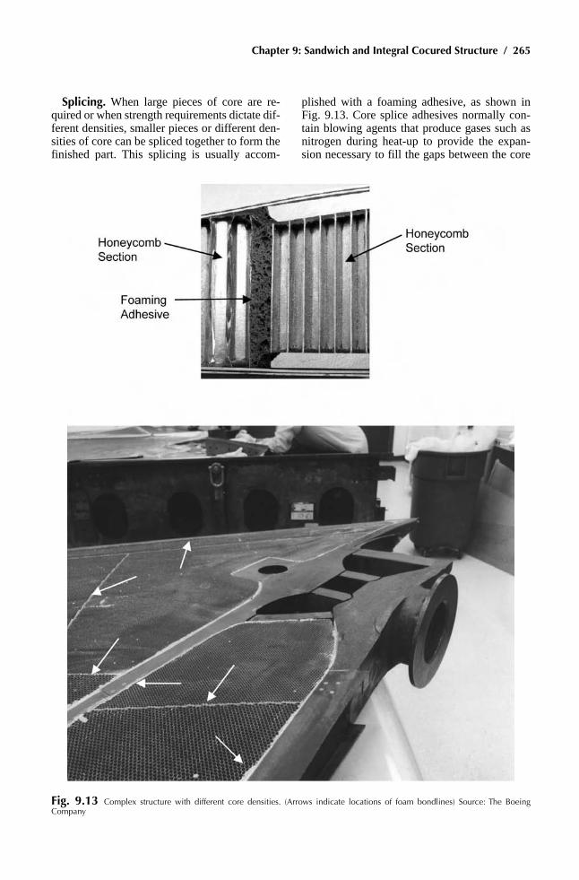
Chapter 9: Sandwich and Integral Cocured Structure / 265
Splicing. when large pieces of core are re-quired or when strength requirements dictate dif-ferent densities, smaller pieces or different den-sities of core can be spliced together to form the finished part. this splicing is usually accom-
plished with a foaming adhesive, as shown in Fig. 9.13. Core splice adhesives normally con-tain blowing agents that produce gases such as nitrogen during heat-up to provide the expan-sion necessary to fill the gaps between the core
Fig. 9.13 Complex structure with different core densities. (Arrows indicate locations of foam bondlines) Source: The Boeing Company
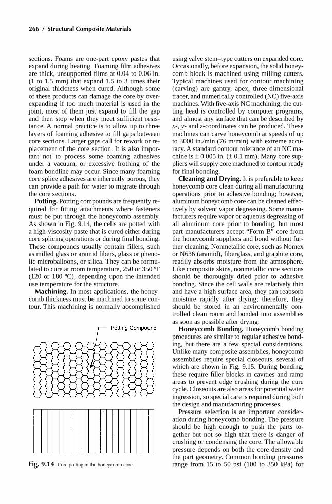
266 / Structural Composite Materials
sections. Foams are one-part epoxy pastes that expand during heating. Foaming film adhesives are thick, unsupported films at 0.04 to 0.06 in. (1 to 1.5 mm) that expand 1.5 to 3 times their original thickness when cured. Although some of these products can damage the core by over-expanding if too much material is used in the joint, most of them just expand to fill the gap and then stop when they meet sufficient resis-tance. A normal practice is to allow up to three layers of foaming adhesive to fill gaps between core sections. larger gaps call for rework or re-placement of the core section. It is also impor-tant not to process some foaming adhesives under a vacuum, or excessive frothing of the foam bondline may occur. Since many foaming core splice adhesives are inherently porous, they can provide a path for water to migrate through the core sections.
potting. Potting compounds are frequently re-quired for fitting attachments where fasteners must be put through the honeycomb assembly. As shown in Fig. 9.14, the cells are potted with a high-viscosity paste that is cured either during core splicing operations or during final bonding. these compounds usually contain fillers, such as milled glass or aramid fibers, glass or pheno-lic microballoons, or silica. they can be formu-lated to cure at room temperature, 250 or 350 ºF (120 or 180 ºC), depending upon the intended use temperature for the structure.
Machining. In most appli cations, the honey-comb thickness must be machined to some con-tour. this machining is normally accomplished
using valve stem–type cutters on expanded core. Oc casionally, before expansion, the solid honey-comb block is machined using milling cutters. typical machines used for contour machining (carving) are gan try, apex, three-dimensional tracer, and numeri cally controlled (nC) five-axis machines. with five-axis nC machining, the cut-ting head is controlled by computer programs, and almost any surface that can be described by x-, y- and z-coordinates can be produced. these machines can carve honey comb at speeds of up to 3000 in./min (76 m/min) with extreme accu-racy. A standard contour tolerance of an nC ma-chine is ± 0.005 in. (± 0.1 mm). Many core sup-pliers will supply core machined to contour ready for final bonding.
Cleaning and Drying. It is preferable to keep honeycomb core clean during all manufacturing operations prior to adhesive bonding; however, aluminum honeycomb core can be cleaned effec-tively by solvent vapor degreasing. Some manu-facturers require vapor or aqueous degreasing of all aluminum core prior to bonding, but most part manufacturers accept “Form B” core from the honeycomb suppliers and bond without fur-ther cleaning. nonmetallic core, such as nomex or n636 (aramid), fiberglass, and graphite core, readily absorbs moisture from the atmosphere. like composite skins, nonmetallic core sections should be thoroughly dried prior to adhesive bonding. Since the cell walls are relatively thin and have a high surface area, they can reabsorb moisture rapidly after drying; therefore, they should be stored in an environmentally con-trolled clean room and bonded into assemblies as soon as possible after drying.
honeycomb Bonding. honeycomb bonding procedures are similar to regular adhesive bond-ing, but there are a few special considerations. Unlike many composite assemblies, honeycomb assemblies require special closeouts, several of which are shown in Fig. 9.15. during bonding, these require filler blocks in cavities and ramp areas to prevent edge crushing during the cure cycle. Closeouts are also areas for potential water ingression, so special care is required during both the design and manufacturing processes.
Pressure selection is an important consider-ation during honeycomb bonding. the pressure should be high enough to push the parts to-gether but not so high that there is danger of crushing or condensing the core. the allowable pressure depends on both the core density and the part geometry. Common bonding pressures range from 15 to 50 psi (100 to 350 kPa) for Fig. 9.14 Core potting in the honeycomb core

Chapter 9: Sandwich and Integral Cocured Structure / 267
honeycomb assemblies. the positive pressure of an autoclave, with a vented bag, usually gives quality superior to that of a bond produced in an oven under vacuum bag pressure. the amount of pressure and the adhesive selected are impor-tant in forming fillets at the core-to-skin bond-lines. the degree of filleting largely determines the strength of the assembly. therefore, adhe-sive film weights of at least 0.08 psf (4 Pa) or higher are recommended to provide sufficient filleting.
Pressures applied on the sides of the core can easily condense the cells. Since honeycomb is stronger in the longitudinal (L) direction than in the width (W ) direction, the core is more prone to crushing in the “w” direction. even when the initial vacuum is pulled, vacuum pressure alone has been known to cause core migration and cell crushing. Some manufacturers limit the vacuum level to 8 to 10 in. (27 to 34 kPa) of hg to help prevent differential pressures within the cells. Autoclave processing of honeycomb as-semblies is also more sensitive to bag leaks than regular adhesive bonding. If pressure enters the
bag through a leak, it can literally blow the honey-comb apart due to the large differential pressure.
In some applications where weight savings is extremely critical, fabricators will reticulate the adhesive prior to bonding, as shown in Fig. 9.16. In this process, an unsupported film adhesive is placed over the core and a hot-air blast melts the adhesive film so that it coagulates on the cell walls. this allows a lighter film adhesive to be used and eliminates the film weight between the cells. this process is frequently used for lightly loaded panels for space applications. It is also used for engine nacelle assemblies that are de-signed for the air (noise) to flow through the cells to reduce the noise level.
9.2.2 Cocured Honeycomb Assemblies
honeycomb assemblies can also be made by cocuring the composite plies onto the core. In this process, the composite skin plies are con-solidated and cured at the same time that they are bonded to the core. Although a film adhesive is normally used at the skin-to-core interface,
Fig. 9.15 Examples of honeycomb structure closeouts

268 / Structural Composite Materials
self-adhesive prepreg systems are available that do not require a film adhesive. to prevent core crushing and migration, this process is normally performed at approximately 40 to 50 psi (275 to 345 kPa), as opposed to the normal 100 psi (690 kPa) used for regular laminate processing. this can not only produce skins that are more porous than those processed under higher pres-sures, but also create pillowing or dimpling in the skins (Fig. 9.17), because the skin is sup-
ported only at the cell walls. Although the sche-matic is somewhat exaggerated in showing the amount of pillowing usually experienced, pil-lowing does create a serious knockdown in me-chanical properties, as much as 30 percent in some cases. the amount of pillowing can be re-duced, if not eliminated, by using a smaller cell size such as 1/8 vs. 3/16 in. (3 vs. 4.8 mm).
Although core migration and crushing can be problems when bonding precured composite
Fig. 9.16 Reticulation of adhesive film
Fig. 9.17 Pillowing effect in composite cocured honeycomb panels

Chapter 9: Sandwich and Integral Cocured Structure / 269
skins, they are even bigger problems with co-cured skins (Fig. 9.18). A considerable amount of work has been done to solve this problem. Potential solutions include: (1) reducing the ramp angle (20 degrees or less is recommended);
(2) increasing the core density; (3) using grip, or hold-down, strips to restrain the plies; (4) pot-ting the cells in the ramp area to increase the core rigidity; (5) encapsulating the core with a layer of adhesive prior to cocuring; (6) bonding
Fig. 9.18 Edge crush in cocured honeycomb panels. F, force vector. Source: Ref 23

270 / Structural Composite Materials
fiberglass plies into the center of the core (sep-tums) to increase core rigidity; (7) adjusting the temperature and pressure during heat-up; and (8) even using “high-friction” prepregs that min-imize ply movement during curing. As the num-ber of these solutions indicates, core migration and crushing are major problems, particularly in cocured assemblies.
there are three basic approaches to producing honeycomb cocured structure. In the first method, both skins are cocured at the same time that they are bonded to the core. Since this process is lim-ited to about 50 psi (345 kPa) autoclave pressure to prevent core crushing, the skins will contain more porosity than skins cured at full autoclave pressure. this process has the shortest cycle time but is the riskiest. the second method consists of
precuring one of the skins at full autoclave pres-sure and then bonding it to the core at the same time that the other skin is cocured. this method takes longer but at least one of the skins should have minimal porosity. In the third method, one skin is precured in an autoclave and then adhe-sively bonded to the core. then, in a separate operation, the other skin is cocured and bonded to the core. the main advantage of this third method is that the core is stabilized during the initial bond cycle in which the first precured skin is bonded to the core. this method has been used when core edge migration and crushing are problems. Although this method takes the lon-gest time, it is the least risky approach.
A potential pitfall that can result in unbonds is shown in the data of Fig. 9.19. Although both of
Fig. 9.19 Flatwise tension strength versus test temperature

Chapter 9: Sandwich and Integral Cocured Structure / 271
the adhesives shown are cured at 350 °F (180 °C), the toughened adhesive FM300 has a very low flatwise tension strength at this temperature. If, on completion of the adhesive bond cycle, the pressure is completely vented to facilitate faster autoclave cooling, residual stresses or gas pres-sure within the cells can push the skins off the core. By comparison, the flatwise tension strength of the untoughened adhesive FM400 is high enough that it will not cause the same problem. In the case of adhesives like FM300, it is wise to keep some pressure on the assembly until it cools down to below 200 °F (90 °C).
Adhesively bonded joints and assemblies are normally nondestructively inspected after all bonding operations are completed. radiographic and ultrasonic inspection methods are typically used to look for defects in both the bondlines and the honeycomb core portions of the assemblies. In addition, it is common practice to leak-check honeycomb bonded assemblies by immersing the assembly for a short time in a tank of hot water at least 180 °F (80 °C). the hot water heats the residual air inside the honeycomb core, and any leaks can be detected by air bubbles es-caping from the assembly.
9.3 Foam Cores
A second type of core material frequently used in adhesively bonded structure is foam core. Although the properties of foam cores are not as good as those of honeycomb core, foam cores are used extensively in such commercial applications as boat building and light aircraft construction. the terms polymer foam and cel-lular polymer refer to a class of materials that are two-phase gas-solid systems in which the polymer is continuous and the gaseous cells are dispersed throughout the solid. Polymeric foams can be produced by several methods, including extrusion, compression molding, injection mold-ing, reaction injection molding, and other solid-state methods. Foam cores are made by using a blowing or foaming agent that expands during manufacture to give a porous cellular structure. the cells may be open and interconnected or closed and discrete. Usually, the higher the den-sity, the greater the percentage of closed cells. Almost all foams used for structural applications are classified as closed-cell, meaning that almost all of their cells are discrete. Open-cell foams, while good for sound absorption, are weaker than the higher-density closed-cell foams and also ab-
sorb more water. however, water absorption can be problematic in both open- and closed-cell foams. Both uncrosslinked thermoplastic and crosslinked thermoset polymers can be foamed. the thermoplastic foams exhibit better form-ability, while the thermoset foams exhibit better mechanical properties and higher temperature resistance. Almost any polymer can be made into a foam material by adding an appropriate blow-ing or foaming agent.
the blowing agents used to manufacture foams are usually classified as either physical or chemical. Physical blowing agents are usually gases, mixed into the resin, that expand as the temperature is increased, while chemical blow-ing agents are normally powders that decom-pose on heating to give off gases, usually nitro-gen or carbon dioxide. Although there are foams that can be purchased as two-part liquids that ex-pand after mixing for foam-in-place applications, the majority of structural foams are purchased as preexpanded blocks that can be bonded together to form larger sections. Sections may be bonded together using either paste or adhesive film. Sec-tions can also be heat-formed to contour using procedures similar to those used for nonmetallic honeycomb core. Although the uncrosslinked thermoplastic foams are easier to thermoform, many of the thermoset foams are only lightly crosslinked and exhibit some formability. Core densities normally range from about 2 to 40 pcf (32 to 640 kg/m3). the most widely used struc-tural foams are summarized in table 9.3. It is important to thoroughly understand the chemi-cal, physical, and mechanical properties of any foam considered for a structural application, par-ticularly with respect to solvent and moisture resistance and long-term durability. depending on their chemistry, foam core materials can be used in the temperature range 150 to 400 °F (70 to 200 °C).
Polystyrene cores are lightweight, low cost, and easy to sand, but are rarely used in structural applications because of their low mechanical properties. they cannot be used with polyester resins, because the styrene in the resin will dis-solve the core; therefore, epoxies are normally employed.
Polyurethane foams are available as either thermoplastics or thermosets, with varying de-grees of closed cells. there are polyurethane foams that are available as finished blocks and formulations that can be mixed and foamed in place. Polyurethane foams exhibit only moder-ate mechanical properties and the resin-to-core

272 / Structural Composite Materials
interface bond tends to deteriorate with age, which can lead to skin delaminations. Polyure-thane foams can be readily cut and machined to contours, although hot wires should be avoided for cutting since harmful fumes can be released.
Polyvinyl chloride (PVC) foams are among the most widely used core materials for sandwich structures. these foams can be either uncross-linked (thermoplastic) or crosslinked (thermoset). the uncrosslinked versions are tougher, more damage resistant, and easier to thermoform, while the crosslinked materials have higher mechani-cal properties, are more resistant to solvents, and have better temperature resistance. how-ever, crosslinked foams are more brittle and more difficult to thermoform than uncrosslinked ma-terials. On the other hand, because they are not highly crosslinked, like normal thermoset adhe-sives and matrix systems, they can be thermo-formed to contours. the crosslinked systems can also be toughened, a process in which some of the mechanical properties of the normal cross-linked systems are traded for some of the tough-ness of the uncrosslinked materials. the PVC foams are often given a heat stabilization treat-ment to improve their dimensional stability and reduce the amount of off-gassing during elevated temperature cures. Styrene acrylonitrile foams are also available that have mechanical proper-ties similar to those of crosslinked PVC but have the toughness and elongation of the uncross-linked PVCs. Patterns of grooves can be scribed in the surfaces of foams to act as infusion aids for resin transfer molding.
Polymethylmethacrylimides are lightly cross-linked closed-cell foams that have excellent me-chanical properties and good solvent and heat
resistance. they can be thermoformed to con-tours and are capable of withstanding autoclave curing with prepregs. these foams are expensive and are usually reserved for high-performance aerospace applications.
9.3.1 Syntactic Core
Syntactic core consists of a matrix such as epoxy that is filled with hollow spheres such as glass or ceramic microballoons, as shown in Fig. 9.20. Syntactics can be supplied as pastes for filling honeycomb core or as B-staged form-able sheets for core applications. Syntactic cores generally have much higher density than honey-comb, with densities ranging from 30 to 80 pcf (480 to 1300 kg/m3). the higher the percentage of the microballoon filler, the lighter and weaker the core becomes. Syntactic core sandwiches are used primarily for thin secondary composite structures that would be impractical or too costly to machine honeycomb to thin gages. when cured against precured composite details, syn-tactics do not require an adhesive. however, if the syntactic core is already cured and requires adhesive bonding, it should be scuff-sanded and then cured with a layer of adhesive.
glass microballoons are the most prevalent filler used in syntactic core, ranging in diameter from 0.04 to 13.78 mil (1 to 350 mm) but typically from 2 to 4 mil (50 to 100 mm). glass microbal-loons have specific gravities 18 times lower than those of fillers like calcium carbonate (CaCO3). Ceramic microballoons have properties similar to those of glass but better elevated-temperature properties, while polymeric microballoons such as phenolic are lower in density than either glass
table 9.3 Characteristics of some foam sandwich materials
Name and type of core Density, pcfMaximum
temperature, °F Characteristics
Polystyrene (styrofoam)
1.6–3.5 165 low-density, low-cost, closed-cell foam capable of being thermoformed. Used for wet or low-temperature lay-ups. Susceptible to attack by solvents.
Polyurethane foam 3–29 250–350 low- to high-density closed cell foam capable of thermoforming at 425–450 °F. Both thermoplastic and thermoset foams are available. Used for cocured and secondarily bonded sandwich panels with both flat and complex curved geometries.
Polyvinyl chloride foam (Klegecell and divinycell)
1.8–26 150–275 low- to high-density foam. low-density foam can contain some open cells. high-density foam is closed cell. Can be either thermoplastic (better formability) or thermoset (better properties and heat resistance). Used for secondarily bonded or cocured sandwich panels with both flat and complex curved geometries.
Polymethacrylimide foam (rohacell)
2–18.7 250–400 expensive high-performance closed-cell foam that can be thermoformed. high-temperature grades (wF) can be autoclaved at 350 °F/100 psi. Used for secondarily bonded or cocured high-performance aerospace structures.

Chapter 9: Sandwich and Integral Cocured Structure / 273
or ceramic but have lower mechanical properties. the properties of the microballoons can be im-proved by increasing the wall thickness at the expense of higher densities. In most commercial applications, the microballoons have a size dis-tribution to improve the packing density. Pack-ing densities as high as 60 to 80 percent have been achieved.
9.4 Integrally Cocured Unitized Structure
Cocuring is a process in which uncured com-posite plies are cured and bonded simultane-
ously during the same cure cycle either to core materials or to other composite parts. Integrally cocured or unitized structure is another manu-facturing approach that can greatly reduce the part count and final assembly costs for compos-ite structures. An example of a cocured control surface is shown in Fig. 9.21. In this structure, the ribs were cocured to the lower skin. the upper skin was cured at the same time, but a re-lease film was used so that it could be removed after cure to allow the installation of a metallic hinge fitting.
In cocuring, pressure is provided both by the autoclave and by the expansion of aluminum substructure blocks, as shown in Fig. 9.22.
Fig. 9.20 Syntactic core construction

274 / Structural Composite Materials
the autoclave applies pressure to the skins and rib caps, while expansion of the aluminum sub-structure blocks applies pressure to the rib webs. If required, the expansion of the aluminum sub-structure blocks can be supplemented by the presence of silicone rubber intensifiers.
the advantages of this type of structure are obvious: fewer detail parts, fewer fasteners, and fewer problems with part fit-up on final assem-bly. the main disadvantages are the cost and ac-curacy of the tooling required and the complexity of the lay-up, which requires a highly skilled
Fig. 9.21 Cocured unitized control surface. Source: The Boeing Company
Fig. 9.22 Pressure application for unitized cocured structure

Chapter 9: Sandwich and Integral Cocured Structure / 275
workforce. to help control tool accuracy, the substructure tooling is usually machined as a single block (Fig. 9.23) and then sectioned into the individual tooling details.
the process flow for this type of structure is shown in Fig. 9.24. the skins, which are unidi-rectional prepreg, are laid up on separate facility tools and hot debulked. hot debulking is used to
Fig. 9.23 Machining substructure spar mandrels and filler blocks. Photo source: The Boeing Company

276 / Structural Composite Materials
consolidate the lay-up to near-net thickness to aid in tool location. At the same time, the rib plies, made from woven prepreg, are laid up on their individual form blocks and hot debulked. Film adhesive sheet is used between the rib flanges and the lower skin for improved joint strength. It is cut and staged. In addition, twisted film to fill the intersection between the ribs and the lower skin (Fig. 9.25) is cut, twisted, and staged. As shown in the figure, it is important to overstuff the joint at the stiffener-to-skin bond intersection to prevent ply distortion during cure. After all of the components are prepared, the lay-up is assembled (Fig. 9.26) and then au-toclave-cured. For larger assemblies where the weight of the tooling becomes an issue, it is pos-sible to use hollow tooling details, as shown in Fig. 9.27.
One potential problem with this type of struc-ture is spring in. As shown in Fig. 9.28, both the spar cap and the web will spring in during cool-down after cure. the web spring in can largely be eliminated by placing a couple of plies on the
backside to support the web. however, the spar cap spring in cannot be counteracted by increas-ing the angle on the tooling block, because that would cause an indentation in the concurrently cured upper skin. It is therefore necessary to shim this joint during final assembly.
Also frequently cocured are skins with co-cured hats, such as the one shown during lay-up in Fig. 9.29. Although matched die tooling can be used to make this type of structure, the more common practice is to use localized tooling only at the hat stiffener locations. A typical bagging arrangement, shown in Fig. 9.30, contains an elastomeric mandrel to support the hat during cure, an elastomeric pressure intensifier to en-sure that the radii obtain sufficient pressure, and some thin plastic shims to minimize mark-off on the skin from the pressure intensifier. the man-drels are solid elastomer or are an elastomer re-inforced with carbon or glass cloth. It is important to keep some autoclave pressure on the assembly during cool-down after curing. If the pressure is dumped immediately after cure, the pressure of
Fig. 9.24 Key processing steps for cocured design

Chapter 9: Sandwich and Integral Cocured Structure / 277
the elastomeric inset can push the hat section off the skin and create cracks like those shown in Fig. 9.31. If the stiffeners require exact location, it may be necessary to use female cavity tooling similar to that shown in Fig. 9.32.
A key design detail for cocured stiffeners is the stiffener terminations. Since the bond hold-ing the stiffener to the skin is essentially a resin or an adhesive bond, any peel loads induced at
the stiffener ends could cause the bondline to “unzip” and fail. the most prevalent method for preventing this involves installing mechanical fasteners near the stiffener terminations. the hat can also be made thicker at the ends and scarfed to further help reduce the tendency for bondline peeling. Other methods include stitching and pinning in the transverse “Z” direction. however, stitching of pregreg lay-ups is expensive and can
Fig. 9.25 Adhesive nugget application

278 / Structural Composite Materials
damage the fibers. Z-pinning, shown in Fig. 9.33, is a technology in which small-diameter pre-cured carbon pins are driven through the prepreg lay-up before cure with an ultrasonic gun.
Cobonding is a hybrid process combining co-curing and adhesive bonding. As shown in the joint in Fig. 9.34, a series of precured stiffeners are adhesive-bonded to a skin at the same time that the skin is cured. the surfaces of the pre-cured composite parts must, of course, be pre-pared for adhesive bonding, just as in any other adhesive bonding process. the advantage of this process is that, in certain situations, the amount of tooling required for the curing operation can be reduced.
Cocured unitized structure is a trade-off. the advantages include fewer parts, fewer fasteners,
and better fit-up at assembly. these advantages must be weighed against the additional tooling costs and span time required to produce the tool-ing, the lay-up costs, the personnel requirements for large complex assemblies, and ma terial out-time issues if the lay-up requires a long time.
reFerenCeS
1. “hexweb honeycomb Sandwich design technology,” hexcel Composites, 2000
2. J. Kindinger, lightweight Structural Cores, ASM Handbook, Vol 21, Composites, ASM International, 2001
3. F.C. Campbell, Secondary Adhesive Bond-ing of Polymer-Matrix Composites, ASM
Fig. 9.26 Cocured unitized control surface tooling approach. Photo source: The Boeing Company

Chapter 9: Sandwich and Integral Cocured Structure / 279
Handbook, Vol 21, Composites, ASM Inter-national, 2001
4. t. Bitzer, Honeycomb Technology—Materi-als, Design, Manufacturing: Applications and Testing, Chapman & hall, 1997
5. S. Black, Improved Core Materials lighten helicopter Airframes, High-Perform. Com-pos., May 2002, p 56–60
6. S. Zeng, J.C. Seferis, K.J. Ahn, and C.l. Pederson, Model test Panel for Processing and Characterization Studies of honey-
comb Composite Structures, J. Adv. Mater., January 1994, p 9–21
SeleCteD reFerenCeS
• t.h. Brayden and d.C. darrow, effect of Cure Cycle Parameters on 350 ºF Cocured epoxy honeycomb Panels, 34th Interna-tional SAMPE Symposium, 8–11 May 1989, p 861–874
Fig. 9.27 Hollow mandrels to reduce tool mass. Source: The Boeing Company
Fig. 9.28 Spring in for cocured joints
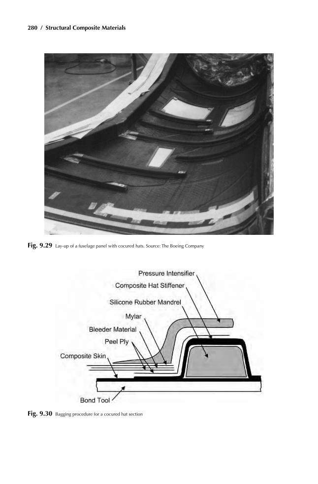
280 / Structural Composite Materials
Fig. 9.29 Lay-up of a fuselage panel with cocured hats. Source: The Boeing Company
Fig. 9.30 Bagging procedure for a cocured hat section

Chapter 9: Sandwich and Integral Cocured Structure / 281
Fig. 9.31 Cracks at a stiffener leg
Fig. 9.32 Cavity tool for precise location of substructure. Al, aluminum
• J. Corden, honeycomb Structures, ASM En-gineered Materials Handbook, Vol 1, Com-posites, ASM International, 1987
• d. danver, Advancements in the Manufac-ture of honeycomb Cores, 42nd Interna-tional SAMPE Symposium, 4–8 May 1997, p 1531–1542
• l. gintert, M. Singleton, and w. Powell, “Corrosion Control for Aluminum honey-comb Sandwich Structures,” 33rd Interna-tional SAMPE Technical Conference, 5–8 nov 2001
• B. harmon, J. Boyd, and B. thai, “Advanced Products designed to Simplify Co-Cure

282 / Structural Composite Materials
Fig. 9.33 Principle of Z pin reinforcement
Over honeycomb Core,” 33rd International SAMPE Technical Conference, 5–8 nov 2001
• I.l. herbeck, M. Kleinberg, and C. Schop-pinger, “Foam Cores in rtM Structures:
Manufacturing Aid or high-Performance Sandwich?” 23rd International Europe Conference of SAMPE, 9–11 Apr 2002, p 515–525

Chapter 9: Sandwich and Integral Cocured Structure / 283
Fig. 9.34 Principle of cobonding. Photo source: The Boeing Company
• “hexweb honeycomb Selector guide,” hex-cel Composites, 1999
• h.M. hsiao, S.M. lee, r.A. Buyny, and C.J. Martin, “development of Core Crush resis-tant Prepreg for Composite Sandwich Struc-tures,” 33rd International SAMPE Technical Conference, 5–8 nov 2001
• h.Y. loken, d.A. nollen, M.w. wardle, and g.e. Zahr, “water Ingression resistant thin Faced honeycomb Cored Composite Sys-tems with Facesheets reinforced with Kevlar
Aramid Fiber and Kevlar with Carbon Fi-bers,” e.I. duPont de nemours & Company
• g.F. Moors, A.A. Arseneau, l.w. Ashford, and M.K. holly, “AV-8B Composite horizontal Stabilator development,” 5th Conference on Fibrous Composites in Structural Design, 27–29 Jan 1981
• t.C. radtke, A. Charon, and r. Vodicka, “hot/wet environmental degradation of honey-comb Sandwich Structure representative of F/A-18: Flatwise tension Strength,” report

284 / Structural Composite Materials
dStO-tr-0908, Australian defence Science & technology Organization (dStO)
• d.J. renn, t. tulleau, J.C. Seferis, r.n. Cur-ran, and K.J. Ahn, Composite honeycomb Core Crush in relation to Internal Pressure Measurement, J. Adv. Mater., October 1995, p 31–40
• J.e. Shafizadeh and J.C. Seferis, the Cost of water Ingression on honeycomb repair and Utilization, 45th International SAMPE Sym-posium 21–25 May 2000, p 3–15
• t.P. Stankunas, d.M. Mazenko, and g.A. Jensen, Cocure Investigation of a honey-comb reinforced Spacecraft Structure, 21st International SAMPE Technical Conference, 25–28 Sept 1989, p 176–188
• J.C. watson and d.l. Ostrodka, “AV-8B For-ward Fuselage development,” 5th Confer-
ence on Fibrous Composites in Structural Design, 27–29 Jan 1981
• e. weiser, F. Baillif, B.w. grimsley, and J.M. Marchello, high temperature Structural Foam, 43rd International SAMPE Sympo-sium, 31 May–4 June 1998, p 730–740
• S. whitehead, M. Mcdonald, and r.A. Bartholomeusz, “loading, degradation and repair of F-111 Bonded honeycomb Sandwich Panels—A Preliminary Study,” report dStO-tr-1041, Australian de-fence Science & technology Organization (dStO)
• S. Zeng, J.C. Seferis, K.J. Ahn, and C.l. Ped-erson, Model test Panel for Processing and Characterization Studies of honeycomb Composite Structures, J. Adv. Mater., January 1994, p 9–21

Structural Composite Materials Copyright © 2010, ASM International®
F.C. Campbell All rights reserved.www.asminternational.org
Chapter 10
Discontinuous-Fiber Composites
DISContInuouS-FIber CoMpoSIteS are used where the higher strength and stiffness of continuous-fiber composites are not required, as they are much less expensive to manufacture. Manufacturing methods such as spray-up, com-pression and transfer molding, reaction injection molding, and injection molding are much cheaper than the processes used for continuous-fiber com-posites. Some of these methods are high-volume processes capable of producing millions of parts per year, while others are limited to much smaller quantities.
the two main factors that determine the strength and stiffness of composites are fiber length and orientation. In theory, a discontinuous-fiber composite with a sufficient fiber length that is perfectly oriented will approach the strength and stiffness of a continuous-fiber composite. In reality, it is extremely difficult to control the ori-entation in discontinuous-fiber composites. Dur-ing processing, resin flow fronts push the fibers around, causing misorientation. In addition, some processes, such as injection molding, mechani-cally fracture the fibers, resulting in fiber lengths that are shorter than the starting lengths. thus, discontinuous or short-fiber composites cannot obtain the strength and stiffness properties of continuous-fiber composites. However, they can be used to improve significantly both the strength and the stiffness of unreinforced polymers, as shown for the epoxy and nylon matrices in table 10.1.
10.1 Fiber Length and Orientation
For a single fiber embedded in a matrix, as shown in Fig. 10.1, the stress applied to the ma-trix is transferred to the fiber by shear across the
interface. the matrix and the fiber will experi-ence different tensile strains because their mod-uli are different. In the region near the fiber ends, the strain in the fiber will be less than that in the matrix. As a result of this strain difference, shear stresses are induced around the fibers in the direction of the fiber axis, and the fiber is stressed in tension. the analytical stress distri-bution along a fiber aligned parallel to the load-ing direction of the matrix is shown in Fig. 10.2. the tensile stress is zero at the fiber ends and is maximum at the center of the fiber. by compari-son, the shear stress around the fiber is maxi-mum at the fiber ends and, for a sufficiently long fiber, falls to zero at the center. It is the variation of shear stress that causes the buildup of tensile stress in the fiber. to achieve a high degree of reinforcing efficiency, a strong interfacial bond is required. to achieve full stress in the fiber, the fiber length must be at least equal to what is known as the critical fiber length lc. the critical fiber length is the minimum fiber length for a given diameter that will allow tensile failure of the fiber rather than shear failure of the interface
table 10.1 Glass-filled epoxy and nylon strength and stiffness
PropertyUnfilled epoxy
Glass-filled epoxy, 35%
Unfilled nylon
Glass-filled nylon, 35%
Glass-filled nylon, 60%
Density, g/cc 1.25 1.90 1.15 1.62 1.95tensile strength, ksi
10.0 43.5 11.9 29.0 42.0
tensile modulus, msi
0.50 3.63 0.42 2.10 3.16
Specific tensile strength, σ/ρ
0.055 0.16 0.082 0.16 0.149
Specific tensile modulus, E/ρ
2.8 8.26 2.52 8.26 11.18

286 / Structural Composite Materials
or matrix. For a fiber with a tensile strength of σtu and a diameter of df, and a fiber-to-matrix interface bond with a shear strength of τi, the critical fiber length lc can be calculated from:
l dctu
if=
στ2
σtu
2τi
(eq 10.1)
As the interfacial bond strength τi increases, the critical fiber length lc decreases.
the effects of fiber length on failing stress are shown in Fig. 10.3. For lf < lc, failure will occur either at the fiber-to-matrix interfacial bond or in
the matrix before the fiber reaches its ultimate strength. For lf > lc, the maximum fiber strength will be obtained over much of its length and the fiber will fail before the matrix. However, over a distance lc/2 from each end, the fiber will not obtain its ultimate strength. For effective fiber reinforcement in which the fibers reach their full strength potential, the fiber length lf needs to be significantly greater than the critical fiber length lc. While discontinuous-fiber com-posites are not as strong as continuous-fiber com-posites, when lf > 5 lc, more than 90 percent of strengthening can be achieved with discontinu-ous fibers, as shown in Fig. 10.4, if the align-ment is perfect.
the fiber length and orientation obtained in a discontinuous-fiber composite are dependent on both the material selected and the manufacturing process used to produce the part. For most pro-cesses the fiber orientation is random, and it can be hard to predict and control. For example, liq-uid flow fronts during processing can carry short fibers with them, resulting in either desirable or undesirable orientations. the changes in fiber orientation as a result of shear and elongation flow are shown schematically in Fig. 10.5. Mis-orientation lowers the strength and stiffness, as shown for the short-fiber reinforced epoxies in Fig. 10.6. In addition, where two flow fronts come together and solidify, they can produce planes of weakness called knit lines. Further-more, processes that contain significant shear forces, such as injection molding, normally frac-ture the fibers and thus produce fibers shorter than their starting lengths.
Fig. 10.1 Effect of deformation on strain around a short fiber. Source: Ref 1
Fig. 10.2 Tensile and shear stresses for short fiber. Source: Ref 1

Chapter 10: Discontinuous-Fiber Composites / 287
10.2 Discontinuous-Fiber Composite Mechanics
the elastic properties of a unidirectional (zero degrees) discontinuous-fiber lamina or ply (Fig. 10.7a) can be calculated by using the Halpin-tsai equations:
Longitudinal modulus El d v
vE11
1 2
1=
+ ( )−f f L f
L fm
ηη
(eq 10.2)
Transverse modulus Ev
vE22
1 2
1=
+−
ηη
T f
T fm (eq 10.3)
Shear modulus G Gv
vG12 21
1
1= =
+−
ηη
G f
G fm
(eq 10.4)
Poisson’s ratio υ υ υ
υ υ
12
2122
1112
= +
=
f f m mv v
E
E
(eq 10.5)
Fig. 10.3 Effect of critical fiber length on stress of discontinuous fiber
Fig. 10.4 Effect of fiber length on tensile strength. Source: Ref 1

288 / Structural Composite Materials
where:
ηLf m
f m f f
= ( ) −
( ) + ( )E E
E E l d
1
2
(eq 10.6)
ηTf m
f m
=( ) −
( ) +E E
E E
1
2
(eq 10.7)
ηGf m
f m
=( ) −
( ) +G G
G G
1
1
(eq 10.8)
If the fiber orientation is random (Fig. 10.7b), then the following equations can be used to esti-mate the elastic properties:
E E Erandom = +3
8
5
811 22 (eq 10.9)
Fig. 10.5 Change in fiber orientation during flow. Source: Ref 2
Fig. 10.6 Strength and modulus as functions of load alignment. Source: Ref 3, 4, 5

Chapter 10: Discontinuous-Fiber Composites / 289
G E Erandom = +1
8
1
411 22 (eq 10.10)
υrandomrandom
random
= −E
G21
(eq 10.11)
10.3 Fabrication Methods
there are a number of important composite fabrication processes that are used more widely in the commercial marketplace than for high-performance aerospace products. In this chapter, four of the most important of these processes will be covered: spray-up, compression molding, re-action injection molding, and injection molding. Some of these processes are capable of produc-ing over a million parts per year, while others are more amenable to low production rates. Some are restricted to thermoset resins, while others can accommodate both thermoset and thermo-plastic resins. Although many different types of reinforcement can be used, e-glass fibers are the most predominant because of their relatively low cost, the availability of a large number of product forms, and their overall good combination of physical and mechanical properties.
10.4 Spray-Up
Spray-up is a low- to medium-volume, open-mold method similar to hand lay-up in its suit-ability for simple medium to large part sizes. However, greater shape complexity is possible with spray-up than with hand lay-up. Continuous-
strand glass roving is fed through a combination chopper and spray gun. the gun (Fig. 10.8) si-multaneously deposits chopped roving 1 to 3 in. (2.5 to 7.5 cm) long and catalyzed resin onto the tool. the laminate is then densified with rollers or squeegees in order to remove air and work the resin thoroughly into the reinforcing strands.
Fig. 10.7 Discontinuous unidirectional and random orienta-tions
Fig. 10.8 Chopped fiber spray-up gun

290 / Structural Composite Materials
Additional layers of chopped roving and resin are added as required for thickness. Cure is usually performed at room temperature but can be accel-erated by the moderate application of heat. As with hand lay-up, superior surface finishes can be achieved by spraying a gel coat onto the tool surface prior to spray-up. Woven roving or cloth is occasionally added to the laminate to provide higher strengths in certain locations, and core ma-terials are easily incorporated. General-purpose, room-temperature-curing or low-temperature-curing polyesters are used with single-sided tools. If the part complexity or size requires it, the tool can be assembled in sections and then disassem-bled when the part is removed. As with the wet lay-up process, the major advantages are low-cost tooling, simple processing, portable equip-ment that permits on-site fabrication, and virtu-ally unlimited part sizes. An additional advantage of spray-up is that it is very amenable to automa-tion, thereby reducing labor costs and the expo-sure of workers to potentially hazardous fumes. Sprayed-up glass parts are limited to a maximum of about 30 to 35 weight percent or 15 to 20 vol-ume percent reinforcement. typical properties are a tensile strength of around 10 ksi (70 Mpa), a tensile modulus of 1 msi (7 Gpa), and an elon-gation of 1.8 percent.
10.5 Compression Molding
At the other end of the manufacturing spec-trum, compression molding is a high-volume,
high-pressure process suitable for molding com-plex, high-strength, glass fiber-reinforced parts using either thermoset or thermoplastic resins. Compression molding is the single largest pri-mary manufacturing process used for automotive composite applications today. the three main groups of materials that are compression molded are sheet molding compounds for thermosets, glass-fiber-mat-reinforced thermoplastics, and long-fiber-reinforced thermoplastics. Compres-sion molding (Fig. 10.9) is a matched-die pro-cess that can produce fairly large parts with ex-cellent overall surface finishes, good dimensional control, and a high degree of complexity. “High volume” means that at least 1000 parts per year, but more typically approximately 100,000 parts per year, would be needed to justify the invest-ment in equipment and tooling. the process is capable of producing parts with surface areas ranging from 1 to 40 ft2 (0.09 to 3.7 m2), al-though less than 10 ft2 (0.9 m2) is more typical. Wall sections can be as thin as 0.05 in. (1.3 mm). Molded-in inserts for attachments are common.
10.5.1 Thermoset Compression Molding
thermoset compression molding begins with a compression molding compound consisting of chopped strands of glass fiber in combination with a resin, in either sheet form (sheet molding compound) or bulk form (bulk molding com-pound). A “charge” of these compounds is placed in a matched metal mold and cured under heat and pressure. During cure the material flows to
Fig. 10.9 Compression molding of thermosets

Chapter 10: Discontinuous-Fiber Composites / 291
fill the mold. For more complex parts, preforms of glass fiber can be fabricated ahead of time and then placed in the tool for cure.
Compression Molding Compounds usually consist of phenolics, but alkyds and epoxies are also available. A typical compound might con-tain 40 percent glass fibers 0.040 in. (1 mm) in length or shorter. prior to molding, the com-pound is palletized into cylinders 0.5 to 2.5 in. (1.5 to 6.5 cm) in diameter by 0.25 to 1 in. (0.5 to 2.5 cm) long. A typical compression molding cycle for phenolics would be 340 to 375 °F (170 to190 °C) and 700 to 3000 psi (5 to 20 Mpa) for one to ten minutes. the parts are frequently postcured when elevated-temperature resistance is required.
Sheet Molding Compound (SMC). A typi-cal process schematic for making thermoset sheet molding compound (SMC) is shown in Fig. 10.10. Continuous-strand glass fiber roving is chopped to the desired length of 1 to 2 in. (2.5 to 5 cm) and deposited onto a coat of filled polyester resin paste traveling on a polyethylene film web. After fiber deposition is complete, a second web also carrying resin paste joins the first web, forming a continuous sandwich of glass and resin. this is compacted and rolled under controlled tension onto standard package-sized
rolls. typical SMC is 0.25 in. (0.5 cm) thick and comes in rolls 40 to 80 in. (1 to 2 m) wide. the SMC roll is then aged at 85 to 90 °F (approxi-mately 30 °C) for one to seven days in order to thicken it.
A typical composition consists of 25 percent polyester resin, 25 percent glass fiber, and up to 50 percent filler; however, molding compounds with glass contents as high as 65 percent are also available. Although polyesters dominate the mar-ket, vinyl esters, phenolics, ureas, melamines, and epoxies are also commonly used as compression molding compounds. Chopped strand mats are used when higher properties are required, and oc-casionally longitudinal glass strands are added. the resin can be a standard polyester, a low-shrink formulation, or a low-profile formulation. Standard polyesters are used when the highest mechanical properties are required, but they also shrink the most during molding (0.3 percent). Low-shrinkage formulations shrink less (0.05 to 0.3 percent), while low-profile resins exhibit al-most no shrinkage (less than 0.05 percent), result-ing in better surface finishes and less tendency for cracking. Fillers, such as calcium carbonate, aluminum trihydrates, or kaolins (clays), reduce cost and shrinkage. Mold release agents, such as zinc or calcium sterates, can be added to the
Fig. 10.10 Sheet molding compound machine. Source: Ref 6

292 / Structural Composite Materials
formulation to provide self-releasing properties after molding. thickeners (magnesium oxide (Mgo), calcium oxide (Cao), magnesium hy-droxide (Mg(oH)2), or calcium hydroxide (Ca(oH)2)) are added to increase viscosity and improve the flow characteristics during molding.
As shown in Fig. 10.11, SMCs can be classi-fied as either SMC-r (random), SMC-Cr (con-tinuous/random), or XMC (continuous/random). random SMC contains 1 to 2 in. (2.5 to 5 cm) long glass fibers oriented in a random order. the influence of fiber content on several mechanical properties of SMC-r containing e-glass fibers
in a polyester resin is shown in Fig. 10.12. Continuous/random SMC consists of an oriented array of unidirectional strands covered with a mixture of random fibers. Continuous/random XMC contains continuous strands arranged in an X-pattern where the angle between the inter-laced strands is between five and seven degrees. Sheets of XMC are manufactured by a filament winding process in which continuous strand rov-ings are pulled through a tank of resin paste and wound under tension around a large rotating cy-lindrical drum. Chopped fibers, usually 1 in. (2.5 cm) long, are deposited on the continuous
Fig. 10.11 Types of sheet molding compound. Sheet molding compound (random) SMC-R; sheet molding compound (continuous/random) SMC-CR; sheet molding compound (continuous/random with continuous in X-pattern) XMC
Fig. 10.12 Effect of fiber content on strength of sheet molding compound (SMC). Source: Ref 7

Chapter 10: Discontinuous-Fiber Composites / 293
fiber layer during winding. After the desired thick-ness is obtained, the built-up material is cut off the drum to form a sheet. Due to the unidirec-tional strands, SMC-Cr and XMC are stronger but also harder to mold. random SMC is used more frequently due to its lower cost, better flow, and moldability. A comparison of these different forms of sheet molding compounds is given in table 10.2.
Layers of SMC are stacked into “charges” for compression molding. the charge size is typi-cally 40 to 70 percent smaller than the projected mold surface. the weight of the charge is made a bit larger than the weight of the part to be molded in order to ensure mold filling and in-clude some additional material for edge trim-ming. Different thicknesses of charge can be placed in different portions of the mold to ac-count for thickness or geometry changes in the part. Close control of charge weight and size al-lows the production of molded parts with very little excess material on the edge that has to be trimmed after cure. Charge placement is critical to minimizing knit lines where two flow fronts merge and create a location of lower strength. the charges are heated in a continuous oven with infrared (Ir) or forced-air impingement heaters. they are then placed in heated matched-die molds and press-cured.
Bulk molding compound (BMC) is a mix-ture of shorter 0.125 to 1.25 in. (0.3 to 3 cm) glass fibers and resin containing filler, catalyst, pigment, and other additives. the fiber rein-forcement level is usually 10 to 20 percent. bulk molding compounds are usually made in an ex-truder. this premixed material, with the consis-tency of modeling clay, can be provided in bulk form or can be extruded into rope 1 to 2 in. (2.5 to 5 cm) in diameter or log-like forms for easier handling. As with SMC, the weighed charge of bMC is placed into a heated matched-metal die,
the die is closed, and pressure is applied. the completed cured part is removed from the die after an interval of several seconds to a few min-utes, depending on part size and thickness. bulk molding compound is commercially available in various combinations of resin, additives, and glass reinforcements. these provide for a variety of end use requirements in high-volume applica-tions where good finishes, good dimensional stability, part complexity, and good overall me-chanical properties are important. the longer fiber lengths obtainable with SMC provide higher mechanical properties compared to parts made with bMC, especially those having relatively thin cross sections. More bMC is used for ther-moset injection molding than for the traditional compression molding process.
preforming. A third approach to the prepara-tion of a ready-to-mold form of preblended glass fiber reinforcement and resin is the preform. this is a mat of chopped glass fiber strands with a binder that allows the preform to hold its shape. the preform is made to the approximate shape of the product to be molded. there are two common methods of producing preforms, the directed-fiber method and the plenum-chamber method. In the directed-fiber method (Fig. 10.13), continuous-strand glass fiber roving is cut into 1 to 2 in. (2.5 to 5 cm) lengths and blown with a binder onto a rotating metal screen that approxi-mates the shape of the final part. Suction is used to hold the fibers in place. After the binder is heat-set in an oven, the preform is ready for the die. the plenum-chamber method is similar but involves the distribution of chopped fibers and binder into an air chamber, where they are sucked onto a rotating preform screen. preform meth-ods are used for applications requiring medium-sized to large parts having relatively constant cross sections and high concentrations of glass reinforcement. In preform molding, the major
table 10.2 Mechanical properties of selected sheet molding compounds (SMCs)Properties SMC-R25 SMC-R50 SMC-R65 SMC-C20R30 XMC-31
Specific gravity 1.83 1.87 1.82 1.81 1.97tensile strength, ksi 12.0 23.8 32.9 41.9 (L), 12.2 (t) 81.4 (L), 10.2 (t)tensile modulus, msi 1.91 2.29 2.15 3.05 (L), 1.74 (t) 5.22 (L), 1.74 (t)poisson’s ratio 0.25 0.31 0.26 0.30 (L), 0.18 (t) 0.31 (L), 0.12 (t)Strain to failure, % 1.34 1.73 1.63 1.7 (L), 1.6 (t) 1.7 (L), 1.5 (t)Compressive strength, ksi 26.5 32.6 34.6 44.4 (L), 24.1 (t) 63.9 (L), 22.3 (t)Compressive modulus, msi 1.70 2.31 2.60 2.90 (L), 1.74 (t) 5.37 (L), 2.03 (t)Flexural strength, ksi 31.9 32.6 58.5 92.8 (L), 23.2 (t) 141 (L), 20.3 (t)In-plane shear strength, ksi 11.5 8.99 18.6 12.2 13.2In-plane shear modulus, msi 0.65 0.86 0.78 0.60 0.65Interlaminar shear strength, ksi 4.35 4.63 6.53 5.95 7.98
Glass fibers in polyester resin. (L): property values measured in the longitudinal direction (parallel to the continuous fibers); (t): property values measured in the trans-verse direction (perpendicular to the continuous fibers). Source: ref 8

294 / Structural Composite Materials
portion of the resin is added just before molding or after the preform is placed within the mold. Most applications use either SMC or bMC, but for flat sheets and simple shapes, glass mats can be placed directly into the mold, resin poured over the mat, and the mold closed under pres-sure to consolidate the resin and glass. For com-plex parts, preforms are normally made before they are placed in the tool.
During compression molding, the matched-die mold is mounted in a hydraulic or modified me-chanical molding press such as the one shown in Fig. 10.14. the two halves of the die are closed, and heat and pressure are applied at 225 to 320 °F (105 to 160 °C), 150 to 2000 psi (1 to 14 Mpa). parts with higher glass contents or more complex geometries require higher pressures. Depending on the thickness, size, and shape of the part, cure cycles range from less than one minute to about five minutes. press closing occurs in two steps: a fast initial step followed by a slower step to allow the material time to flow. Higher molding tem-peratures and faster curing times require faster closing speeds to prevent premature gellation. If a condensation curing resin, such as a phenolic, is being molded, it is common practice to open
the mold momentarily to let the volatiles escape during the curing process. After cure, the mold is opened and the finished part is removed. If hol-low parts are required, low-melting eutectic met-als can be inserted into the mold and then melted out after molding.
the matched-metal dies usually are made from hardened and chrome-plated steel. they can be single or multiple-cavity molds, usually cored for steam or hot-oil heating. electrical and hot-water heating systems can also be used. Side cores, provisions for inserts, and other features are often employed. the dies are also equipped with part ejectors that may employ either me-chanical pins or air pressure. Mold materials in-clude cast or forged steel, cast iron, and cast alu-minum. Compression molding is an ideal process when the volume is high enough to justify the investment in precision matched-metal dies, and with the advent of high-speed machining of alu-minum dies, the process is becoming more eco-nomical for lower-volume production runs. It is capable of producing extremely uniform parts with superior surface finishes. Inserts and attach-ments can be molded in, and final trimming and machining operations are minimal.
Fig. 10.13 Directed fiber spray-up process for preforms. Source: Ref 9

Chapter 10: Discontinuous-Fiber Composites / 295
transfer molding (Fig. 10.15) is similar to compression molding, except that the charge of molding compound is heated to 300 to 350 °F (150 to 180 °C) in a separate chamber, then transferred by a ram under heat and pressure into a closed die, where the shape of the part is deter-mined and cure takes place, usually in 45 to 90 seconds. the process is used for small, intri-cate parts requiring tight dimensional tolerances. Although good resin flow is required, the process is not sensitive to precise charge weight. typical reinforcement levels are 10 to 35 percent.
10.5.2 Thermoplastic Compression Molding
Glass mat thermoplastic (GMt) consists of glass-reinforced thermoplastic, usually polypro-pylene, that flows to fill the mold during the compression molding cycle. A typical GMt fab-rication line is shown in Fig. 10.16. Several rein-forcements are available, including continuous fiber mat, chopped fiber mat, and unidirectional fiber mat, normally at a glass content of 40 vol-ume percent. this process has gained a foothold
in the automotive market because of the automa-tion used and the short processing cycles (some as short as 30 seconds, although longer times are sometimes required to obtain the proper amount of crystallinity). Glass mat thermoplastic mate-rial is made using the double-belt process de-scribed in Chapter 6, “thermoplastic Composite Fabrication processes.” the material is then re-heated in continuous moving furnaces using Ir heater banks to 600 °F (320 °C) in two to three minutes. It is then inserted into a high-speed hy-draulic press with the mold heated to 275 °F (135 °C) and consolidated under 1000 to 4000 psi (7 to 28 Mpa) pressure. A two-stage pressuriza-tion cycle is frequently used; the pressure is ap-plied quickly, 200 to 500 in./min (5 to 12 m/min), in the first stage and more slowly in the second stage, 1 to 10 in./min (2 to 25 cm/min), to allow the material time to flow and fill the mold. Such high pressures are needed to move the reinforce-ment structure throughout the cavity and ensure a high degree of air expulsion and composite consolidation. Sometimes, holding fixtures are required during cooling to minimize distortion
Fig. 10.14 Compression molding machine

296 / Structural Composite Materials
or warping. Most applications contain some re-processed production waste products, ranging from a few percent up to 50 percent recyclate.
Long Discontinuous thermoplastic. the long-fiber thermoplastic (LFt) process uses
Fig. 10.15 Principle of transfer molding
glass reinforcements in a polypropylene matrix. the fibers are normally 0.5, 1.0, or 2.0 in. (12, 25, or 50 mm) long. the LFt process is even more highly automated than the GMt process. the polypropylene is fed into an extruder that heats and melts the material and then adds the glass fiber near the end. this feedstock is then trans-ferred directly to the compression molding press without the need to reheat it, as required in the GMt process, thus further reducing costs. In com-parison to the GMt and SMC processes, the in-dividual discontinuous production process steps are eliminated. As in the GMt process, recycled material is frequently included in the LFt pro-cess to reduce costs.
the advantages of the LFt process are:
1. the process is more cost effective than GMt, not only due to the elimination of single process steps, but also because less manpower is needed for production.
2. In comparison with GMt, cycle times are reduced by 15 percent as a result of better flowability of the plasticized material.
3. the impregnation process for LFt is superior to that for GMt in not being suscep tible to surface defects caused by poor impregnation.
Comparative properties of GMt, LFt, and SMC molded test pieces are given in table 10.3.
10.6 Structural reaction Injection Molding
reaction injection molding (rIM), shown in Fig. 10.17, is a process for rapid fabrication of unreinforced thermoset parts. A highly reactive
Fig. 10.16 Automated fabrication of glass mat thermoplastic (GMT) parts

Chapter 10: Discontinuous-Fiber Composites / 297
two-component resin system is injected into a closed mold, where the resin quickly reacts and cures. reaction injection molding resins must have low viscosities (500 to 2,000 cps) and fast cure cycles. polyurethanes are the most preva-lent, but nylons, polyureas, acrylics, polyesters, and epoxies have also been used. the two com-ponents (isocyanate and polyol in the case of polyurethanes) are kept separate and are con-stantly recirculated under high pressure. they are mixed in a dynamic mix head under high pressures of 1500 to 3000 psi (10 to 20 Mpa) and high speeds of 4000 to 8000 in./s (100 to 200 m/s). the crosslinking reaction is initiated by mixing rather than by heat and gel and can occur in as little time as two to ten seconds. the actual injection pressure is quite low, and the die is heated to about 120 to 150 °F (50 to 70 °C) to accelerate cure and then remove the exothermic heat of reaction during the latter part of cure. Since rIM resin systems have very low viscosi-ties, they can be injected at low pressures less than 100 psi (700 kpa). these low pressures
allow the use of inexpensive molds and low-force clamping systems. typical tooling materials are steel, cast aluminum, electroformed nickel, and composites. Cycle times as short as two minutes for large automotive bumpers have been reported. Since isocyanate vapors are harmful, rIM work cells must be provided with exhaust ventilation.
reinforced reaction injection molding (rrIM), as shown in Fig. 10.18, is similar to rIM except that short glass fibers are added to one of the resin components. the fibers must be extremely short at least 0.03 in. (0.8 mm) or the resin viscosity will be too great. Short fibers, milled fibers, and flakes are commonly used. Again, polyurethanes are the predominant resin system in rrIM. the addition of the fibers improves the modulus, im-pact resistance, and dimensional tolerance and lowers the coefficient of thermal expansion.
Structural reaction injection molding (SrIM) is similar to the previous two processes except that a continuous glass preform is placed in the die prior to injection (Fig. 10.19). this process, too, is used almost exclusively with polyure-thanes. because of the highly reactive resins and short cycle times, SrIM cannot produce as large a part size as resin transfer molding see Chapter 5, “thermoset Composite Fabrication processes”. Also, SrIM parts have lower fiber volumes and generally more porosity than rtM parts.
10.7 Injection Molding
Injection molding, which is capable of pro-ducing more than a million parts per year, is the highest-volume method of any of the processes for fabricating parts of glass-fiber-reinforced
table 10.3 Comparative properties of LFt, GMt, and SMCProperty LFT GMT SMC
Glass fiber content, wt% 40 40 30recyclate content, wt% 30 … 5tensile strength, ksi 8.7 9.4 8.7tensile modulus, msi 1.0 0.9 1.4Flexural strength, ksi 16 16 23Flexural modulus, msi 0.8 0.6 1.3Impact strength, kJ/m2 60 75 70Density, g/cm3 1.21 1.21 1.80
LFt—long fiber thermoplastic; GMt—glass mat thermoplastic; SMC—sheet molding compound. Source: ref 7
Fig. 10.17 Reaction injection molding (RIM) (no reinforcement)

298 / Structural Composite Materials
materials. Injection molding can be used to fab-ricate either unreinforced or reinforced parts. Like compression molding, injection molding requires expensive matched-metal dies because of the high processing temperatures and pres-sures. However, because many complex parts can be molded at high production rates, the cost per part can often be quite low. Although other reinforcements are occasionally used, glass fi-bers are most common. Since the fibers are short ranging 0.03 to 0.125 in. (0.8 to 3 mm), the vol-ume percentage of fiber is low (typically 30 to 40 percent), and the fiber orientation is random or aligned by flow into the mold, the mechanical properties of injection-molded parts are again much lower than those of continuous-fiber rein-forced parts. However, very complex parts with all surfaces closely controlled can be achieved
with injection molding. either single- or multi-cavity dies are used to produce very large vol-umes of complex parts at very high production rates, from a wide range of thermoplastic resins and with a variety of resultant properties.
10.7.1 Thermoplastic Injection Molding
Injection-molded glass-fiber-reinforced ther-moplastics are used extensively in the automotive and appliance industries. Design flexibility, the ability of glass-fiber-reinforced thermoplastics to form intricate shapes, very high production rates, and low cost per piece account for the extensive application thermoplastic injection molding.
In injection molding, the molding compound, in pellet form, compound concentrate, or dry
Fig. 10.18 Reinforced reaction injection molding (RRIM) (short-fiber reinforcement)
Fig. 10.19 Structural reaction injection molding (SRIM) (long-fiber reinforcement)

Chapter 10: Discontinuous-Fiber Composites / 299
blend, is heated in the injection chamber of the molding machine. A typical injection molding cycle is illustrated in Fig. 10.20. As the material progresses down the screw, it is melted by a combination of heat from the barrel and the shearing action of the screw. the material accu-mulates in the barrel and is then injected under high pressure as a hot fluid into a relatively cold closed die. After the desired shot size is accumu-lated, the screw stops rotating and moves for-ward at a controlled rate, acting as a ram or plunger and forcing the plastic melt in front of the screw into the mold. the molten material flows through the nozzle into a water-cooled die where it flows through a sprue, a runner system, and finally the gate into the mold cavity. When the mold is completely filled, the screw remains stationary to keep the thermoplastic in the mold under pressure. During this hold or dwell time, additional melt is injected into the mold to com-pensate for the shrinkage due to cooling. After the gate freezes, the mold becomes isolated from the injection unit. the melt that accumulates at the end of the screw pushes the screw backward; that is, the screw is rotating and moving backward at the same time. the rate at which the plastic melt accumulates in front of the screw for the next shot is controlled by the backpressure, which is the hydraulic pressure exerted on the screw. When a sufficient melt has accumulated in front of the screw, the screw stops rotating while the part in
the mold cools and solidifies. After a short cool-ing cycle, usually 20 to 120 seconds, the part has solidified sufficiently to enable it to be removed from the mold without distortion. the cycle time for the process is usually controlled by the cool-ing rate, which in turn is usually dependent on the die design, part thickness, and reinforcement content. After cooling, knockout pins eject the part from the mold. the sprue, runners, and gates are separated from the part and are usually recy-cled by grinding them into powder and mixing them with fresh material.
Virtually all thermoplastics are injection-moldable, including nylon, acetal, vinyl, poly-carbonate, polyethylene, polystyrene, polypro-pylene, polysulfone, modified polyphenylene oxide, fluorocarbons, polyetherimide, acryloni-trile-butadiene-styrene, and styrene-acrylonitrile. For injection molding, chopped strands of glass fiber can be blended with thermoplastic resin molding powders or pellets. Carbon fibers can be used when higher properties are required. these fibers also provide enhanced electrical and thermal conductivity. Carbon fibers are fre-quently used as electrically conductive fillers in parts requiring electromagnetic interference shielding, antistatic, electrostatic discharge, and other electrical properties.
A lower-cost thermoplastic resin can often be strengthened by the addition of glass fiber re-inforcement to the point where it will offer the
Fig. 10.20 Injection molding machine sequence. Source: Ref 10

300 / Structural Composite Materials
superior performance characteristics of a more costly unreinforced resin. the addition of glass fibers also provides sufficient strength and dimen-sional stability to enable many reinforced thermo-plastics to compete effectively with stamped sheet metal and die castings. thermoplastic molding compounds usually include pigments, fillers, mold release agents, and lubricants, and may occasion-ally contain other additives for special purposes. their corrosion resistance and molded-in color also provide design advantages. the list of ther-moplastics reinforced with glass fibers for injec-tion molding is long and includes resins offering an extremely broad range of mechanical, chemi-cal, electrical, and thermal properties. Some poly-mers require both injection speed and injection pressure to vary during the molding cycle. A heat-sensitive polymer, for example, can be degraded if the fill rate is too rapid; forcing the polymer through the small restrictions of the sprue, run-ner, and gate systems at high speed will increase the internal shear and raise the temperature to the point where polymer degradation occurs. programming different injection speeds and pres-sures during the injection process may be re-quired to prevent resin degradation.
Injection molding compounds are usually supplied in a form that can be fed directly into the injection molding machine. they are usually made by mixing short chopped fibers with a pow-dered or pelletized resin in an extruder. In extru-sion processing, fiber breakage is a major prob-lem. to minimize breakage, deep flighted screws or twin screws are used and the fibers are fed into the barrel after the resin has melted. prepelletized blends are available in controlled ratios of glass fiber reinforcement to resin and with specified ad-ditives such as pigments, flame retardants, stabi-lizers, and lubricants. these pellets are available in nearly all of the common injection-molding thermoplastics. Concentrates are similar to the glass fiber/resin prepelletized blends but have very high percentages of glass to resin, up to 80 percent by weight compared to the 10 to 40 percent customary in pellets. the concentrated pellets are blended with nonreinforced thermo-plastic pellets to achieve the desired glass-to-resin ratio in the molded part. With these formulations, the injection molder can select a glass-reinforced compound to satisfy end-use needs with respect to mechanical properties, chemical properties, impact strength, surface finish, and color.
It is important that the material be thoroughly dried prior to injection molding. Drying can be accomplished off-line as a batch drying process
or on-line in a hopper dryer on the machine. Some polymers absorb moisture primarily on the surface (nonhydroscopic), while others ab-sorb moisture into the pellets or granules (hygro-scopic). Drying of nonhydroscopic materials, such as polypropylene and polyethylene, can be accomplished by simply heating to evaporate the moisture from the surface. Hydroscopic materi-als, such as nylon and polycarbonate, must be dried using dehumidified hot air to remove the moisture and generally require longer drying cycles. It is common practice to use up to 20 per-cent regrind for injection-molded parts; how-ever, since the properties of the part will often decrease with increasing regrind content, it is important to test prior to incorporating regrind. the reinforcing effects of glass and carbon fi-bers decrease with repeated processing because repeated exposure to heat causes breakdown of the fibers and thermal degradation of the resin.
the advantages of glass-reinforced injection-molded parts over unreinforced parts include higher tensile strength and modulus, greater im-pact resistance, reduced shrinkage, improved di-mensional stability, and higher temperature ca-pability. Whereas normal polymers shrink about five percent, fiber-reinforced parts usually shrink one percent or less. A disadvantage of fiber rein-forcement is lower ductility. In general, slightly higher injection pressures and barrel tempera-tures are required for reinforced parts due to their higher viscosities. the mixing and shearing ac-tion of the injection molder reduces the fiber length; therefore, the gates and runners should be as large as possible. Injection pressures are usu-ally 10 to 15,000 psi (70 kpa to 100 Mpa). Mini-mal back pressure at 25 to 50 psi (170 to 350 kpa) and low screw speeds (30 to 60 rpm) should be utilized to avoid excessive fiber breakage. Cavi-ties should be filled as rapidly as possible to min-imize the degree of fiber orientation and enhance knit-weld-line integrity, especially for thin-walled parts. Higher barrel temperatures at 30 to 60 °F (15 to 30 °C) (than those for unfilled resin) are also used when injection molding reinforced parts; the higher temperature minimizes fiber breakage by melting the polymer rather than al-lowing it to be melted by the heat generated by the shearing action of the screw. After the cavity is filled, a longer hold time is needed to help maintain the dimensional tolerances. one prob-lem with reinforced parts is that the fiber orien-tation is largely controlled by the flow forces and the part geometry and can result in parts with variable strengths in different sections of

Chapter 10: Discontinuous-Fiber Composites / 301
the part. Also, knit lines form where the flow fronts meet and result in areas of lower strength. this problem is accentuated for parts containing longer fibers and higher fiber contents.
the main parts of an injection molding ma-chine (Fig. 10.21) are the clamping unit and the injection unit (also called a plasticizing unit). the clamping unit, which holds the die, contains fixed and moving plates, tie bars, and the mech-anisms for opening, closing, and clamping the die. the injection unit melts the thermoplastic and injects it into the mold, and a drive unit pro-vides power for both the injection and clamping units. Screw machines dominate the injection molding industry, but plunger machines are also available. reciprocating plunger machines are inferior to screw machines, because all of the heat has to be supplied by conduction from the barrel heaters and mixing is not as thorough; the conse-quences are low plasticizing (melting) rates and thermally nonuniform melts. Screw machines generate heat within the material and provide mixing, thus producing much more uniform melts. Generally, a screw consists of three sec-tions: (1) a feed section, (2) a compression sec-tion, and (3) a metering section. the feed section transports pellets from the hopper to the heated section of the barrel. In the feed section, the screw flights are along the same dimension. In the compression section, the polymer is melted by the combined heat generated by the barrel heaters and the shearing action of the screw. In this section, the volume of the screw flights de-creases to compensate for changes in the mate-rial density. Finally, in the metering section, the flight dimensions are constant as the final melt-ing and mixing of the polymer occur. Screw de-signs vary with the material being molded. three
screw designs are shown in Fig. 10.22. A design for highly crystalline polymers is shown in Fig. 10.22(a). Since these materials have very sharp melting points, a very short compression section is used. the compression section is longer for semicrystalline thermoplastics (Fig. 10.22b) be-cause they require more time to melt. For an amorphous thermoplastic (Fig. 10.22c) that does not have a true melting point, the screw is de-signed with a gradually increasing compression over its length. the barrel heaters are divided into zones to provide better control of the heat-ing process.
Injection molding machines are rated in terms of tons of mold clamping capacity and ounces of shot size and can range from laboratory units of 2 tons, 0.25 oz (1800 kg, 7 g) to large industrial units of 3500 tons, 1500 oz (3200 metric tons, 40 kg). A typical laboratory-size injection mold-ing machine is shown in Fig. 10.23. the clamping mechanism must have sufficient locking force to resist the tendency of the molten polymer, in motion and under pressure, to force the mold halves apart. Since reinforced thermoplastics have higher viscosities than unreinforced resins, they are injected at higher pressures; therefore, the clamping mechanism must be even stronger. Mold clamping pressure is usually provided by either a toggle lock or a hydraulic cylinder or a combination of the two. Modern injection mold-ing machines are equipped with automatic feed-back control systems that monitor the process parameters to produce consistently high-quality parts. Important processing parameters that need to be controlled include individual control of the injection and holding pressures, ram position and velocity, back pressure, and screw speed. barrel and nozzle temperature control is important for
Fig. 10.21 Injection molding machine schematic. Source: Ref 10

302 / Structural Composite Materials
Fig. 10.22 Injection molding screw designs. Source: Ref 11
Fig. 10.23 Injection molding machine

Chapter 10: Discontinuous-Fiber Composites / 303
achieving low thermal stresses in the molded part. Lower molding temperatures will promote rapid cooling and higher production rates but produce lower-quality parts. rapid cooling af-fects internal stresses, the degree of fiber orien-tation, postmold shrinkage, and warpage.
Matched-metal dies for thermoplastic produc-tion runs are normally made of high-strength tool steels that are often plated for additional abrasion resistance. typical coatings include nickel phos-phorus impregnated with polymers, hard chrome, electroless nickel, titanium nitride, and diamond black (boron carbide thin film with tungsten
disulfide). In the two-plate cold-runner config-uration (Fig. 10.24a), the material is injected through the sprue bushing, the runner system, and the gates into the die cavities. After cooling, the parts are removed along with the sprue, run-ner system, and gates. the sprue, runner sys-tem, and gates are then removed manually for recycling. In the three-plate cold-runner system shown in the bottom portion of Fig. 10.24(b), the middle plate separates the sprue, runner sys-tem, and gates from the parts during the ejection cycle. there are also more expensive three-plate hot-runner systems that keep the sprue, runner
Fig. 10.24 Injection molding runner designs. Source: Ref 10

304 / Structural Composite Materials
system, and gates in a molten state throughout the process for more economical recycling since there is no labor or material waste associated with recycling the sprue, runner, and gate sys-tem. Injection molding dies normally contain vents to let the air in the die escape as the hot polymer flows into the die cavity. Vents are usu-ally placed in the areas that fill last, near knit lines, and even in the runner system. Sprues and runners should have gentle bends. runners should be as short as possible to avoid pressure drops. the gates control the fill rate, the amount of ma-terial flowing into the cavity, and the rate of ma-terial solidification. the gating system should be designed to avoid or minimize weak weld or knit lines. If more than one gate is needed to fill the mold, weld lines will result; these should be located in lower-stressed locations in the part. Since part cooling is often the longest part of the injection molding cycle, dies should be de-signed with efficient cooling channels. In gen-eral, (1) since cooling rate is dependent on thick-ness, cooling fluid should be located close to the cavity surface; (2) cooling lines should be lo-cated exactly where they are needed to cool the part uniformly; (3) turbulent flow of the cooling medium should take place in a manner that pro-vides maximum heat transfer (sharp turns and high speeds promote turbulent flow); and (4) the cooling system should be designed so that cool-ing is uniform in each mold half.
one of the main challenges in injection mold-ing is producing parts with correct dimensional accuracy and minimal warpage. Warpage occurs when the internal stresses in the part exceed the inherent part stiffness and cause a permanent de-formation. Cooling gradients, which lead to dif-ferential shrinkage, are the primary cause of part warpage. Shrinkage is dependent on the mate-rial, the part design, the mold design, and the processing parameters. because of their lower inherent shrinkages, amorphous resins are fre-quently selected over semicrystalline resins when tight tolerances are required. In general, the ad-dition of fibrous fillers increases part warpage because of the anisotropic nature of their flow patterns as the fibers align with the flow. When differential cooling occurs, part designs with nonuniform wall thicknesses tend to warp more than those with uniform wall thicknesses. Stiff-eners or gussets are often incorporated during design to reduce or minimize warpage. Gate lo-cation and cooling passages are important con-siderations during die design. Ideally, the mold should be filled uniformly during the injection
process and then cool uniformly until it is ready for ejection. If the gates and the cooling system are not properly designed, regions in the part cavity will fill prematurely and start to solidify before the remainder of the mold is filled. Like-wise, an improperly designed cooling system will result in thermal gradients during the cool-ing process. During processing, cavity fill time is important. If the time is too short, high shear rates can cause substantial melt shearing and high residual stresses, which lead in turn to part warpage. If the time is too long, a large melt temperature drop occurs as cavity filling is com-pleted, resulting in thermal gradients leading to part warpage.
Gas-assist molding is used to mold hollow injection-molded parts by the controlled injec-tion of an inert gas (n2) into the hot polymer melt. the gas forms a continuous channel through the hotter, less viscous, thicker sections of the melt. Gas injection pressures of 400 to 800 psi (2.8 to 5.5 Mpa) are commonly used. Injection compression molding is another variant in which the melted polymer is injected into a partially opened mold. the mold closes, compresses the melt, and distributes it throughout the cavity. the injection compression molding process helps to prevent fiber breakage and improve the prop-erties of the molded part. thin wall injection molding is a process capable of making parts with 0.020 to 0.080 in. (0.5 to 2 mm) walls and a flow length-to-thickness (l/t) ratio of greater than 75. Since thinner walls cool rapidly, equip-ment capable of extremely high fill pressures of 15 to 35 ksi (100 to 240 Mpa) is required along with very short fill times (less than 0.75 seconds) to produce the part. this process usually requires thicker dies to resist deflections with specially designed runner and vent systems. In structural foam molding, chemical blowing agents are used to produce parts with solid skins and foamed cores. this process allows the fabrication of large parts with high strength-to-weight ratios and good dimensional control. tooling costs can be lower because aluminum dies are acceptable for some part configurations.
10.7.2 Thermoset Injection Molding
thermoset molding compounds can be injection-molded when the injection screw or plunger and chamber of the molding machine are maintained at low temperatures and the mold itself is heated at 250 to 400 °F (120 to 200 °C). this causes the thermoset material to cure after

Chapter 10: Discontinuous-Fiber Composites / 305
several minutes in the mold under heat and pres-sure. precise control of temperature and cycle time must be maintained to prevent the resin from gelling in the barrel. the process requires low-viscosity resins that maintain their low vis-cosity for a period of time but cure quickly after gelation. particulate fillers, chopped glass fibers, and short milled fibers less than 0.80 in. (2 cm) can be used for reinforcement; however, chopped and milled glass fibers increase the viscosity of the resin more than particulate fillers and are therefore harder to mold. For thermoset injec-tion molding, the screw is usually shorter and has a lower compression ratio. the barrel is set at low temperatures ranging 160 to 212 °F (70 to 100 °C), and cure is conducted with heated molds with injection pressures of 7.5 to 15 ksi (50 to 100 Mpa). Adequate venting of volatiles is criti-cal, especially for condensation curing pheno-lics; venting passages are therefore built into the mold at parting lines, ejector pins, and core pins. the maximum weight of parts made using this process is about 10 lb. bulk molding com-pounds (bMCs) are also frequently used for thermoset-injection-molded parts. polyesters, vinyl esters, and epoxies are used with glass fi-bers 0.25 to 1 in. (6 to 25 mm) in length. When bMC is used, larger machines are frequently em-ployed to produce larger moldings at lower pres-sures such as 750 to 1500 psi (5 to 10 Mpa) than for conventional thermoset injection molding. typical cures occur in two to five minutes.
reFerenCeS
1. F.L. Mathews and r.D. rawlings, Compos-ite Materials: Engineering and Science, Woodhead publishing Ltd., 1994
2. D. Hull, An Introduction to Composite Ma-terials, Cambridge university press, 1981
3. L. Kacir, M. narkis, and o. Ishai, oriented Short Glass-Fiber Composites, I, prepara-tion and Statistical Analysis of Aligned Fiber Mats, Polym. Eng. Sci., Vol 15, Soci-ety of plastics engineers, 1975, p 525–532
4. L. Kacir, M. narkis, and o. Ishai, oriented Short Glass-Fiber Composites, III, Struc-ture and Mechanical properties of Molded Sheets; Polym. Eng. Sci., Vol 17, Society of plastics engineers, 1977, p 234–241
5. L. Kacir, M. narkis, and o. Ishai, oriented Short Glass-Fiber Composites, IV, Depen-dence of Mechanical properties on the Distribution of Fiber orientations; Polym. Eng. Sci., Vol 18, Society of plastics engi-neers, 1978, p 45–52
6. Molding Compounds, ASM Handbook, Vol 21, Composites, ASM International, 2001, p 141–149
7. C.W. peterson, G. ehnert, K. Liebold, K. Horsting, and r. Kuhfusz, Compression Molding, ASM Handbook, Vol 21, Compos-ites, ASM International, 2001, p 515–535
8. D.A. reigner and b.A. Sanders, Proceed-ings of National Technical Conference, So-ciety of plastics engineers, 1979
9. b.Z. Zang, Advanced Polymer Composites: Principles and Applications, ASM Interna-tional, 1994
10. M.p. Groover, Fundamentals of Modern Manufacturing—Materials, Processes, and Systems, prentice-Hall, Inc., 1996
11. V. John, Introduction to Engineering Materials, Industrial press Inc., 1992, p 342–343
SeLeCteD reFerenCeS
• b.t. Astrom, Manufacturing of Polymer Composites, Chapman & Hall, 1997
• “Injection Molding processing Guide,” Lnp engineering plastics Inc., 1998
• b.Z. Jang, Advanced Polymer Composites: Principles and Applications, ASM Interna-tional, 1994
• p.K. Mallick, Fiber-Reinforced Compos-ites: Materials, Manufacturing, and Design, 2nd ed., Marcel Dekker, 1993
• r.D. pistole, Compression Molding and Stamping, ASM Engineered Materials Hand-book, Vol 2, Engineering Plastics, ASM In-ternational, 1988
• S.L. rosen, Fundamental Principles of Polymeric Materials, John Wiley & Sons, 1982
• A.b. Strong, High Performance and Engi-neering Thermoplastics, technomic publish-ing, 1993
• “user’s Guide for Short Carbon Fiber Com-posites,” Zoltek Companies Inc., 2000

“This page left intentionally blank.”

Structural Composite Materials Copyright © 2010, ASM International®
F.C. Campbell All rights reserved.www.asminternational.org
Chapter 11
Machining and assembly
CoMpoSIteS Allow for the manufacture of large integral structures, thereby reducing the number of parts and mechanical fasteners required to assemble them. Many structures can be either cocured or bonded together to in-tegrate a significant number of detail parts into a single assembly. In spite of these technical advances, assembly still accounts for a signifi-cant portion of the total manufacturing cost, representing as much as 50 percent of the total cost of a delivered part. Assembly operations are labor-intensive and involve many steps. For example, a composite wing requires, first, a framing operation in which all of the spars and ribs must be properly located and connected with shear ties. each skin must then be located on the substructure, and shimmed; holes must be drilled and fasteners installed. During and after skin installation, various sealing opera-tions must be performed. last, the leading edges, wing tips, and control surfaces of the wing torque box must be assembled. A typical fighter aircraft can have 200,000 to 300,000 mechani-cal fasteners, whereas a commercial airliner or transport aircraft can have 1,500,000 to 3,000,000, depending on the aircraft size. A hole must be drilled for each fastener, and then the fas-tener must be installed. this brief description is a gross oversimplification of the complex-ity involved in assembling a large structural component.
In this chapter, the basic machining and assembly operations are explained, with an emphasis on hole preparation and the types of mechanical fasteners used in composite structures. Some of the design and analysis as-pects for mechanical fasteners are covered in Chapter 17, “Structural Joints—Bolted and Bonded.”
11.1 trimming and Machining Operations
Composites are more prone to damage during trimming and machining than conventional met-als, as they contain strong and very abrasive fi-bers held together by a relatively weak, brittle matrix. During machining, they are prone to de-laminations, cracking, fiber pull-out, fiber fuzz-ing (aramid fibers), matrix chipping, and heat damage. It is therefore important to minimize forces and heat generation during machining. During metallic machining, the chips help to re-move much of the heat generated during the cut-ting operation. Because of the much lower ther-mal conductivity of the fibers (especially glass and aramid), heat buildup can occur rapidly and degrade the matrix, resulting in matrix cracking and even delaminations. when machining com-posites, high speeds, low feed rates, and small depths of cuts are used to minimize damage.
Although conventional machining methods such as milling are not normally used on com-posite parts (since they cut through the continu-ous fibers and reduce the strength), most such parts require peripheral edge trimming after cure. edge trimming is done either manually with high-speed cutoff saws or automatically with numerically controlled (NC) abrasive water jet machines. lasers have often been proposed for trimming of cured composites, but the sur-faces become charred by the intense heat and are unacceptable for most structural applications.
Carbon fibers are very abrasive and quickly wear out conventional steel cutting blades; there-fore, trimming operations should be conducted using either diamond-coated circular saw blades, carbide router bits, or diamond-coated router bits. A typical manual edge-trimming operation,

308 / Structural Composite Materials
shown in Fig. 11.1, is conducted with a high-speed air motor at 20,000 rpm using either a carbide router bit or, less commonly, a diamond-impregnated cutoff wheel. Fiberglass laminate trim templates are often clamped to the part to ensure that the true trim path is followed and provide edge support to help prevent delamina-tions. typical feed rates are 10 to 14 in./min (25 to 35 cm/min). Hand trimming requires that the operator wear a respirator, have eye and ear protection, and wear heavy-duty gloves. Many facilities have installed ventilated trim booths to help control the noise and fine dust generated by this operation. As trimming is a hand operation, the quality of the cut is strongly dependent on the skill of the operator. too fast a feed rate can cause excessive heat, which in turn can cause matrix overheating and ply delaminations.
Abrasive water jet trimming has emerged as the preferred method for trimming cured com-posites; however, the process uses large, expen-sive NC machine tools (Fig. 11.2). the advan-tages of abrasive water jet cutting are that consistent delamination-free edges are produced and that tooling requirements are simpler be-cause the cutting path is NC. Abrasive water jet
cutting is primarily an erosion process rather than a true cutting process, so very little force is exerted on the part during trimming; therefore, only simple holding fixtures are required to sup-port the part. In addition, no heat is generated during cutting, so there is no risk of matrix deg-radation. water pumped at low volumes of 1 to 2 gal/min (4 to 8 l/min) enters the top of the head and is then mixed with garnet grit that is expelled through a 0.040 in. (1 mm) diameter sapphire nozzle at 40 to 45 ksi (280 to 340 Mpa). In general, higher grit size numbers (smaller grain diameters) produce better surface finishes, with a typical grit size being #80. once the abra-sive slurry has penetrated the composite lami-nate, there is a catcher filled with steel balls that spin to dissipate the flow. other than the expense of these tools, the main disadvantage is the noise generated during the process. It is not unusual for the noise of trimming operations to exceed 100 dB; therefore, ear protection is required, and many units are isolated within their own sound-proof rooms. If edge sanding is required, die grinders at speeds of 4000 to 20,000 rpm can be used along with 80-grit aluminum oxide paper for roughing and 240- to 320-grit silicon carbide paper for finishing.
Fig. 11.1 Hand trimming. Source: Ref 1

Chapter 11: Machining and assembly / 309
11.2 General assembly Considerations
Framing operations, in which the substructure is located and fastened in its proper location, have made significant progress in the last 40 years. In the 1960s and 1970s, substructures were manu-
ally located (with a few positions located using hard tooling), usually supplemented with large pieces of clear plastic film that’s typically biaxi-ally oriented polyethylene terephthalate (bopet, such as Dupont’s Mylar) scribed with hole pattern locations. the design, tooling, and fabrication
Fig. 11.2 Abrasive water jet trimming machine tool. Source: The Boeing Company

310 / Structural Composite Materials
databases were not necessarily coordinated, so high variability and poorly fitting parts were common. During the 1980s and 1990s, there was less use of bopet and greater reliance on hard tooling to position parts, which increased the nonrecurring investment required at the start of a new program. with the advent of solid mod-eling and electronic master models in the 1990s, a process called determinant assembly emerged. In this process, coordinated undersized fastener holes are drilled in the parts during fabrication. these holes are then used to position the parts during assembly, eliminating the need for hard tooling locators. Another recent development is the use of laser projection units for establishing part and hole location. A typical application for a laser projection system is shown in Fig. 11.3.
It is important to check all joints for gaps be-fore starting to drill holes and install fasteners. Gaps can unnecessarily preload metallic mem-bers when fasteners are installed, and such pre-loading can initiate premature fatigue cracking and even stress corrosion cracking of aluminum. However, gaps in composite structures can cause even more serious problems than in metallic struc-tures. Since composites do not yield and are more brittle and less forgiving than metals, excessive
gaps can result in delaminations during fastener installation. the force exerted by the fastener can bend the composite, which may then develop matrix cracks and/or delaminations around the holes. Cracks and delaminations usually occur on multiple layers through-the-thickness and can adversely affect joint strength. Gaps can also trap metal chips and contribute to backside hole splintering. If the skin is composite and the sub-structure is metal, and if an appreciable gap is present during fastener installation, the compos-ite skin will often crack and delaminate. If both the skin and substructure are composite, cracks can develop in either the skin or the substruc-ture, or both. Substructure cracking often occurs at the radius between the top of the stiffener and the web.
to prevent unnecessary preloading of metallic structure, and the possibility of cracking and de-laminations in composite structure, it is impor-tant to measure all gaps and then shim any that are greater than 0.005 in. (0.1 mm). liquid shim, which is a filled thixotropic epoxy paste adhe-sive, can be used to shim gaps between 0.005 and 0.030 in. (0.1 and 0.8 mm). If the gap ex-ceeds 0.030 in. (0.8 mm), then a solid shim is normally used. engineering approval is often
Fig. 11.3 Laser projection location. Source: Laser Projection Technologies, Inc.

Chapter 11: Machining and assembly / 311
required for a gap this large. Solid shims can be made from solid metal, laminated metal that can be peeled to the correct thickness, or composite. when selecting a solid shim material, it is im-portant to make sure that there is no potential for galvanic corrosion within the joint.
liquid shimming can be accomplished by first drilling a series of undersized holes in the two mating surfaces so that temporary fasteners can be installed to provide a light clamp-up during the shimming process. the liquid shim is usually bonded to one of the two mating surfaces. the surface to be bonded should be clean and dry to provide adequate adhesion. Composite surfaces are scuff-sanded. the other surface is covered with release tape or film. After the liquid shim is mixed, it is buttered onto one surface; the other surface is located and then clamped with mold-released temporary fasteners. the excess or squeeze-out is removed prior to gellation, which usually occurs within one hour of mixing. After the shim material has cured, typically for about 16 hours, the part is disassembled and any voids or holes in the shim are repaired. After the repair has cured, the parts can be assembled.
11.3 hole preparation
the differences between fighter aircraft and commercial passenger aircraft create different problems in each. Fighter aircraft designs are highly tailored to performance and loads, and therefore have many thickness variations in the skins and substructure to reduce the weight. As a result, such aircraft incorporate a wide variety of fastener types, grip lengths, and diameters but a limited number of actual fasteners. Because of the smaller size of a fighter airframe, more areas are difficult to access during assembly. By con-trast, larger commercial aircraft have much more fastener commonality with regard to type, grip length, and diameter but also, because of their size, many more fasteners. Skins and substruc-ture tend to be more uniform in thickness. lim-ited access is not as much of a problem, but the large size of the parts makes them difficult to handle. there are many types of drill motors and units that can be used to drill structures, but they can be broadly classified as hand, power feed, and automated drilling units.
11.3.1 Manual Drilling
Manual, or freehand, drilling using handheld drill motors, like the one shown in Fig. 11.4, has
the least chance of making a close-tolerance hole that measures +0.003/-0.000 in. (+0.08 mm/ -0.00 mm). All that really can be controlled is the drill speed (rpm). It is up to the operator to make sure that the drill: (1) is properly located; (2) is perpendicular to the surface; and (3) is fed with enough pressure to generate the hole but not enough to damage it. Although freehand drilling is obviously not the best method, it is frequently used because it requires no investment in tooling such as drill templates, and in many applications in which access is limited, it may be the only vi-able method. A typical tight-access situation is shown in Fig. 11.5, where a mechanic is install-ing the collars on Hi-lok two-part self-locking fasteners. For tight-access areas, right-angle drill motors are available. If freehand drilling is used, the operators should use a drill bushing or a tri-pod support to ensure normality, and they should be provided with detailed written instructions for hole generation and inspection.
Manual hole drilling during assembly is often done by drilling undersized holes (pilot holes), installing temporary fasteners to hold the parts to-gether, and then bringing the holes up to full size. pilot holes are usually drilled with small-diameter drill bits measuring 0.09 to 0.125 in. (2 to 3 mm). Hole diameters for aerospace structures nomi-nally range from 0.164 to 0.375 in. (4 to 10 mm) in diameter, with the predominant hole sizes being 0.188 and 0.250 in. (4.8 and 6.4 mm). During drilling, it is important to use a sharp drill bit, which will not wander as easily as a dull one; drilling is faster; and lower forces are re-quired, minimizing the possibility of injury or part damage. when drilling multimaterial stack-ups, it is important to make sure that they are securely clamped together.
Fig. 11.4 Typical freehand drill motor. Source: Cooper Power Tools

312 / Structural Composite Materials
the speeds used in manual drilling depend on both the materials and their thickness. Drilling holes in composites is more difficult than drill-ing them in metals because of the tendency of composites to heat damage and their weakness in the through-the-thickness direction. Compos-ites are very susceptible to surface splintering (Fig. 11.6), particularly if unidirectional material is present on the surface. Splintering can occur at either side of the hole. As shown in Fig. 11.7, when the drill enters the top surface, it creates peeling forces on the matrix as it grabs the top plies. when it exits the hole, it induces punching forces that create peel forces on the bottom sur-face plies. top-surface splintering is usually a sign that the feed rate is too fast, whereas exit-surface splintering indicates that the feed force is too high. It is common practice to cure a layer of
fabric on both surfaces of composite parts. this practice largely eliminates the hole-splintering problem; woven cloth is much less susceptible to splintering than unidirectional material. A backup material such as aluminum or compos-ite, clamped to the backside, will frequently help to prevent backside hole splintering. Coolant is normally not used for carbon/epoxy laminates that are 0.250 in. (6 mm) thick or thinner. when drilling composites dry, operators should be pro-vided with vacuum capability to collect the dust and should always wear both eye protection and a respirator.
Since epoxy matrix composites will start to degrade if heated above 400 °F (200 °C), it is important that heat generation be minimized dur-ing drilling. typical drilling parameters are 2000 to 3000 rpm at feed rates of 0.002 to 0.004 in.
Fig. 11.5 Limited-access fastener installation. Source: The Boeing Company

Chapter 11: Machining and assembly / 313
per revolution (ipr) (0.05 to 0.1 mm/rev), al-though this will vary, depending on the drill ge-ometry and the type of equipment used. thermo-couples and heat-sensitive paints are often used during drilling parameter development tests to
monitor the heat generated. Drilling parameters for composite-to-metal stack-ups are often con-trolled more by the metal than by the composite. For example, when drilling carbon/epoxy (C/e) to aluminum, a speed of 2000 to 3000 rpm
Fig. 11.6 Composite hole splintering
Fig. 11.7 Drilling forces on composite laminate. Source: Ref 2

314 / Structural Composite Materials
with a feed rate of 0.001 to 0.002 ipr (0.03 to 0.05 mm/rev) might be used, whereas a stack-up of C/e to titanium would require a slower speed of 300 to 400 rpm and a higher feed rate of 0.004 to 0.005 ipr (0.1 to 0.13 mm/rev). titanium alloy (ti-6Al-4V) is also very sensitive to heat buildup (hence the lower speed) and tends to work-harden rapidly if light cuts are used (hence the higher feed rate).
to help to reduce the variability in manual hole drilling, some manufacturers produce de-tailed written instructions covering specific hole-drilling operations and provide kits that have
all of the correct tools needed for a specific operation.
11.3.2 Power Feed Drilling
power feed drilling is preferable to hand drill-ing. In this process, the drill unit is locked into a template that establishes hole location and main-tains drill normality. In addition, the unit is pro-grammed to drill at a given speed and feed once the drilling operation starts. Some units, such as the one shown in Fig. 11.8, can be programmed for different peck cycles. peck drilling (Fig. 11.9)
Fig. 11.8 Power feed peck drill. Source: Cooper Power Tools
Fig. 11.9 Peck drilling. Source: Ref 3

Chapter 11: Machining and assembly / 315
is a process in which the drill bit is periodically withdrawn to clear the chips from the flutes. It is used almost exclusively when drilling composite-to-titanium stack-ups, because the hard titanium chips have a tendency toward back counterbor-ing (Fig. 11.10). the process also greatly re-duces the rapid heat buildup that can occur when drilling titanium.
All of these controls lead to much better and more consistent hole quality, particularly in the drilling of composite-to-metal stack-ups. A typi-cal peck drilling cycle for a 0.188 in. (5 mm) diameter hole through a C/e-to-titanium stack-up comprises a speed of 550 rpm, a feed rate of 0.002 to 0.004 ipr (0.05 to 1 mm/rev), and a peck rate of 30 to 60 pecks per in. (1 to 2 pecks per mm) of thickness.
when drilling into composite-to-metal stack-ups, a phenomenon called back counterboring can occur. As shown in Fig. 11.10, as the metal chips of aluminum or titanium travel up the flutes, they tend to erode the softer liquid shim and compos-ite matrix material, causing eroded and oversize holes. Back counterboring can be minimized by: (1) eliminating all gaps; (2) using a drill geom-etry that produces small chips; (3) changing speeds and feeds; (4) providing better clamp-up; (5) reaming the hole to the final diameter after drilling; or (6) employing peck drilling.
11.3.3 Automated Drilling
For high-volume hole generation, automated drilling equipment can be designed and built for specific applications. Being large, sophisticated machine tools, these units are expensive, so the
number of holes drilled and the number of units produced need to be large enough to justify the equipment investment. one of these large units is shown in Fig. 11.11. these machines are ex-tremely rigid and allow for accurate hole loca-tion and normality. they are NC, so there is no need for drill templates. they have vision sys-tems that can scan the substructure and software that will then adjust the hole location to match the actual location of the substructure even if it is not exactly where the design says it should be. All drilling parameters are automatically con-trolled, and it is possible to change speeds and feeds when drilling through different materials. Because of the thick stack-ups that must be drilled in a wing, a water-soluble flood or mist coolant is usually used during the hole-drilling opera-tions. All drilling data are automatically recorded and stored for quality control purposes. the drill holders contain bar codes that the drilling pro-gram uses to make sure that the correct drills are used for the correct holes. these machines can also install temporary fasteners to clamp the skins to the substructure during drilling, and they fre-quently use integral drill-countersink cutters that drill the hole and then continue to countersink it during the same operation.
the current trend in the aerospace industry is to replace these large installations with smaller, more flexible units. An off-the-shelf commercial robot, with some modifications and a special drilling end effector, is used to drill holes in the control surface shown in Fig. 11.12. Another ap-proach is to integrate drilling units into the as-sembly fixture, using what are called numeri-cally controlled drill jigs. An example of such a
Fig. 11.10 Back counterboring

316 / Structural Composite Materials
relatively low-cost unit is shown in Fig. 11.13 for a fighter aircraft outer wing.
11.3.4 Drill Bit Geometries
Many variations of twist drills (Fig. 11.14) are used in drilling metallic structures. Since specific drill bit geometries can influence both
the quality and the quantity of holes drilled, many geometries are proprietary to the various aerospace manufacturers. Although standard twist drills are used for drilling metallic struc-tures, some unique drill geometries have been developed for composites, several of which are shown in Fig. 11.15. the design of the drill and the drilling procedures are highly depen-
Fig. 11.11 Automated composite wing drilling system. Source: PaR Systems, Inc.

Chapter 11: Machining and assembly / 317
dent on the materials being drilled. For example, carbon and aramid fibers exhibit different ma-chining behavior and therefore require different drill geometries and procedures. In addition, composite-to-metal stack-ups require different cutters and procedures. the flat two-flute and four-flute dagger drills were developed specifi-cally for drilling stack-ups of C/e. the two-flute variety is normally run at 2000 to 3000 rpm and the four-flute variety at 18,000 to 20,000 rpm. when drilling through composite-to-metal stack-ups, the drill geometry is controlled more by the metal and special twist drill geometries are often used. Due to their low compressive strengths, aramid fibers have a tendency to re-cede back into the matrix rather than being cleanly cut, resulting in fuzzing and fraying during drilling. therefore, the aramid drill con-tains a “C”-type cutting edge that grabs the fi-bers on the outside of the hole and keeps them in tension during the cutting process. typical drilling parameters for aramid fiber composites are 5000 rpm and a feed rate of 0.001 ipr (0.03 mm/rev).
Standard high-speed steel (HSS) drills work well in glass and aramid composites, but the ex-tremely abrasive nature of carbon fibers requires that carbide drills be used to obtain an adequate drill life. For example, a HSS drill may be ca-pable of drilling only one or two acceptable holes in C/e, but a carbide drill of the same geometry can easily generate 50 or more ac-ceptable holes. For drilling C/e in rigid auto-mated drilling equipment, polycrystalline dia-
mond (pCD) drills have exhibited outstanding productivity improvements. A pCD drill has a carbide body with a vein of diamond grains sin-tered into the cutting edge. Although pCD drills are very expensive, the number of holes obtained per drill and the fewer changes required make them cost-effective. However, pCD drills cannot be used with freehand or nonrigid setups; the point will immediately chip and break if any vi-bration or chatter is present during drilling.
11.3.5 Reaming
Although it is desirable to drill the hole to its final size in one pass, it is often necessary to ream the hole to its final diameter. Reaming is done with carbide reamers at about one-half of the drilling speed at 500 to 1000 rpm. In some composite-to-metal structures, fasteners are installed clearance-fit in the composite and interference-fit in the metallic structure to im-prove the metallic fatigue life. In this situa-tion, the final hole diameter is drilled in the composite-to-metal stack-up, the composite skin is taken down, and the holes in the composite skin are reamed to provide a clearance fit for the fastener. when the stack-up is reassembled, the fasteners are installed clearance-fit in the com-posite and interference-fit in the metal.
11.3.6 Countersinking
Countersinking should be used only when protruding-head fasteners will not satisfy design requirements. In general, countersinking reduces static joint strength and fatigue life. During countersinking for flush-head fasteners, it is im-portant not to countersink too deeply and create a knife-edge condition in the countersunk member. A knife edge creates a significant stress riser and also allows the fastener to tilt and rise up on the countersink surface, resulting in low joint yield strength and reduced fatigue life. As a general rule, countersinking should never bring the head of the fastener any closer than 0.025 in. (0.6 mm) to the far side of the sheet or through more than 80 percent of the sheet thickness, as illustrated in Fig. 11.16. piloted countersinks are helpful in centering the countersink tool in the hole, and microstop cages can be used to control the depth.
Countersinking is performed for composite structures in much the same way as for metals, except that the area where the countersink transi-tions into the hole must have a radius equal to the fastener’s head-to-shank radius. Because of the
Fig. 11.12 Robotic drilling of composite control surface. Source: The Boeing Company

318 / Structural Composite Materials
low interlaminar shear strength of composites, failure to satisfy this condition can result in cracks and delaminations under the force of fastener in-stallation. Countersinking cutters for composites are normally made of solid carbide, steel with carbide inserts, or steel with pCD inserts.
11.4 Fastener Selection and Installation
Many types of fasteners are used in aero-space structural assembly, the most prevalent being solid rivets, pins with collars, bolts with nuts, and blind fasteners. examples are shown
Fig. 11.13 Composite outer wing numerically controlled drill jig (NCDJ) drilling system. Source: The Boeing Company

Chapter 11: Machining and assembly / 319
Fig. 11.14 Twist drill geometry
Fig. 11.15 Composite drill configurations
Fig. 11.16 Countersinking

320 / Structural Composite Materials
in Fig. 11.17. there are also many other types of fasteners, including quick-release multiple-piece fasteners, latches, straight pins, headed pins, lock pins, cotter pins, threaded inserts, re-taining rings, and washers.
Because so many fasteners of so many differ-ent types are used in aircraft construction, aero-space companies have developed fastener usage policies that specify, for each program, how fas-teners are to be selected and used. typically, such a policy includes usage limitations, selection criteria, hole size callout information, strength al-lowables, material compatibility and protection, and lists of approved fasteners. Minimum edge distances and fastener spacing requirements may also be specified in the fastener usage policy if they are not already specified in the individual engineering drawings. For a hole of diameter d, typical edge distances are 2d to 3d with typical fastener spacings of 4d to 6d.
Mechanical fastener material selection for composites is important in preventing corrosion problems. Aluminum- and cadmium-coated steel fasteners will galvanically corrode in contact with carbon fibers. titanium alloy (ti-6Al-4V) is usually the best fastener material for carbon fiber composites because of its high strength- to-weight ratio and corrosion resistance. when higher strength is required, cold-worked A286 iron-nickel or the iron-nickel based alloy Inconel 718 can be used. If extremely high strengths are required for very highly loaded joints, the nickel-cobalt-chromium multiphase alloys Mp35N and Mp159 are available. Glass and aramid fibers, being nonconductive, do not cause galvanic cor-rosion of metallic fasteners.
It is important to measure the grip length of a fastener before installing it in a structure. Com-mercial gauges are available that can be placed through the hole to measure the correct grip length. In determining the fastener grip length for threaded fasteners, it is important that the fas-tener be long enough that the threads are never loaded in bearing or shear; that is, no threads should be inside the hole. In addition, at least one thread and no more than three threads should be showing when the nut is installed and tight-ened to the proper torque. Fasteners exposed to the outer moldline of the aircraft are normally installed “wet” by dipping the end of the fas-tener in polysulfide sealant prior to installation. this practice helps to prevent the intrusion of moisture that can cause corrosion of metallic substructure.
11.4.1 Special Considerations for Composite Joints
when a hole is placed in a composite laminate, it creates a stress concentration and the overall load-bearing capacity of the laminate is severely reduced. even a properly designed mechanically fastened joint exhibits only 20 to 50 percent of the basic laminate tensile strength. like hole drilling, fastener installation in composites is more difficult and damage-prone than in metal-lic structures. Some of the potential problems with fastener installation are shown in Fig. 11.18. As previously discussed, unshimmed gaps can cause cracking of either the composite skin or the composite substructure (or both) as the fas-tener is being installed. In fuel tanks, channel seal grooves are often used to help prevent fuel leakage. Fasteners with o-ring seals can also be used to further prevent leakage; however, it has been found through experience that fasteners with o-ring seals can result in interlaminar crack-ing. Although good clamp-up of the fastener is certainly desirable, overtorquing fasteners can also result in cracking. If the countersink radius is too small and does not match that of the fas-tener head-to-shank radius, the fastener can apply a concentrated point load and cause matrix crack-ing. likewise, fastener misalignment, in which the hole and the countersink are not properly aligned, can result in point loading and cracking.
In any mechanically fastened joint, high clamp-up forces are beneficial to both static and fatigue strength. High clamp-up produces friction in the joint, delays fastener cocking, and reduces joint movement or ratcheting during fatigue loading. Most holes eventually fail in bearing as a result of fastener cocking and locally high bearing stresses. to allow the maximum clamp-up in composites without locally crushing the surface, special fas-teners have been designed that have large foot-prints (large heads and nuts that bear against the composite) to help spread the fastener clamp-up loads over as large an area as possible. washers are also frequently used under the nut or collar to help spread the clamp-up loads. In general, the larger the bearing area, the greater the clamp-up that can be applied to the composite and the higher the resulting joint strength. In addition, tension-head rather than shear-head fasteners are normally used in composites because they are not as susceptible to bolt bending during fatigue and their larger heads help to prevent fastener pull-through during installation in thin structures.

Chapter 11: Machining and assembly / 321
Fig. 11.17 Typical aerospace fastener types

322 / Structural Composite Materials
11.4.2 Solid Rivets
traditionally, riveting has been the most prev-alent method of building aerospace structures. As composite and titanium structures replace alumi-num structures on newer aircraft, the number of riveted structures will decrease in the future, since rivets are not normally used in titanium or composite structures. However, rivets are, and will remain, an important fastening method for aerospace structures. During rivet installation, several physical changes take place: (1) the rivet expands to fill the hole (thus guaranteeing a tight fit); (2) the hardness of the rivet increases through work hardening; and (3) the manufactured head is formed through plastic deformation.
Rivets are rarely used in composites for two reasons: (1) aluminum rivets galvanically cor-rode in contact with carbon fibers; and (2) the vibration and expansion of the rivet during the driving process can cause delamination. If riv-ets are used, the type of rivet selected is usually bimetallic, consisting of a ti-6Al-4V pin with a softer titanium-niobium tail that is installed by squeezing rather than by vibration driving. In addition, the head that is upset must be against metal rather than composite. there are also hollow-end solid rivets designed to allow flaring of the ends without damaging expan-sion when used in double-countersunk holes in composites.
Fig. 11.18 Fastener installation defects

Chapter 11: Machining and assembly / 323
11.4.3 Pin and Collar Fasteners
pin and collar fasteners are the most commonly used fasteners for permanent installations where there is no requirement to remove the fastener later. the pin, similar to a bolt, is used with a self-locking or swaged-on collar that cannot be re-moved with typical tools without destroying the collar or pin. pin and collar fasteners are high-strength fasteners made from either ti-6Al-4V, A286 iron-nickel, or Inconel 718. typical head designs include the protruding tension head, pro-truding shear head, 100-degree full countersink, and 100-degree reduced countersink.
A typical pin and collar fastener is the Hi-lok fastener shown in Fig. 11.19. A Hi-lok fastener consists of a threaded pin and a collar. the threaded pin is essentially a modified bolt, whereas the collar is basically a nut with a breakaway groove that controls the amount of torque and preload on the pin. Hi-lok fasteners are available in both flush and protruding heads, and as shear and tension-shear fasteners. Although Hi-lok fasten-ers can be installed either clearance-fit or inter-ference-fit, they are normally installed clearance-fit in composite structures. the fastener pin is usually made from ti-6Al-4V with an A286 nut. titanium nuts are occasionally used, but these must be coated with an antigalling lubricant; oth-erwise, the threads tend to gall and long-term clamp-up is adversely affected. A hex key is in-serted into the fastener stem to oppose the torque applied to the nut. the nut is tightened down until a predetermined torque level is achieved and the top portion of the nut fractures. washers can be used under the head to help spread the bearing load on the surface.
the lockbolt is another common pin and col-lar fastener that can be installed by either pull-ing or swaging the collar from the backside. A typical pull-type lockbolt installation sequence is shown in Fig. 11.20. lockbolts differ from Hi-loks in that a Hi-lok has true threads onto which the nut is threaded, whereas a lockbolt has a series of annular grooves into which the collar is swaged. once swaged in place, lock-bolts cannot “back off” (loosen) and they have superior vibration resistance. lockbolts are avail-able with flush or protruding heads, as shear- or tension-pull types, and as shear-stump types. A lockbolt is normally lighter and costs less to install than a bolt-nut combinations of the same diameter. two precautions must be fol-lowed when installing lockbolts in composite structures: (1) pull-type lockbolts exert quite a
bit of force on composites through the pulling action necessary to swage the collar onto the pin. If the composite is thin, fastener pull-through is possible, and if there are any unshimmed gaps, cracking and delaminations can occur when the fastener pin fractures. (2) If backside lockbolts (called stump lockbolts) are installed in com-posites, they should be installed by automated equipment so that the swaging operation can be carefully controlled.
A third type of pin and collar fastener is the eddie-Bolt shown in Fig. 11.21. As shown in the installation sequence, the collar initially threads onto the pin but then is swaged into flutes on the pin. this swaging provides a positive lock and confers on eddie-Bolts the advantage of retain-ing clamp-up loads better than Hi-loks, which rely on torque only. However, the fasteners and installation tools are expensive, the socket tools are subject to wear, and the installation proce-dure is difficult. eddie-Bolts are often specified in inlet duct areas, where it would otherwise be possible for a fastener pin to come loose, fly into the engine blades, and damage the engine.
11.4.4 Bolts and Nuts
Bolts, along with nuts and washers, are used to join highly loaded structural members that may have to be removed to provide service access. they are also used for permanent attachments. Structural bolts are used in fatigue-, shear-, and tension-critical joints. Nuts, which are tightened with wrenches, may be used when there is access to both sides; nut plates and gang channels are used when there is access to only one side. the shank of each structural bolt must be long enough to ensure that there are no threads bearing in the joint. extra washers may be used to adjust the grip length. However, the use of lock washers is often prohibited because they can damage the protective finish on the structure being joined. A washer should be used under both the bolt head of protruding bolts and the nut to help distribute the load and prevent crushing damage to the compos-ite surface.
there are many head styles, including the pro-truding tension flange head, protruding shear head, 100-degree full countersink, and 100-degree reduced countersink. For structural bolts, the threads are rolled and the heads are forged for additional strength. Since both of these opera-tions induce residual compressive stresses in the fastener, they also improve the fastener’s resis-tance to stress corrosion cracking. Bolts smaller

324 / Structural Composite Materials
Fig. 11.19 Installation of the Hi-Lok fastener. Source: Ref 4

Chapter 11: Machining and assembly / 325
than 0.190 in. (5 mm) in diameter are considered nonstructural; they are used to attach brackets and other miscellaneous hardware. the threads on nonstructural bolts can be either machined or
rolled. Some nuts are self-locking and others are not; cotter pins and safety wire are used to se-cure those that are not. Self-aligning nuts (up to eight degrees) are also available for situations in
Fig. 11.20 Installation of the pull-type Lockbolt. Source: Ref 4
Fig. 11.21 Eddie-bolt positive lock fastener. Source: Refs 4, 5

326 / Structural Composite Materials
which the structural members are not parallel. there are also nuts designed specifically for tension- or shear-loading applications.
when installing structural bolts, a high preload or high torque helps to prevent fatigue and vibra-tion. However, since a high preload places the bolt under tensile stress, too high a preload can increase the susceptibility of certain fastener ma-terials to stress corrosion cracking. therefore, bolt preload is usually restricted to about 50 to 60 percent of the bolt’s yield strength. It is also important that all of the fasteners in the joint are preloaded to approximately the same torque so that the fasteners share the load equally. If the fas-teners are subjected to varying torque, those that are preloaded to higher values will carry a sub-stantially higher portion of the load than those with lower torque. low bolt preloads can result in joint rotation, misalignment, loosening, and the formation of gaps between mating parts. low bolt preloads also reduce the fatigue life of the fasten-ers. For highly loaded bolted joints, torque values are often specified on the engineering drawing.
High-strength bolts or screws, together with nut plates or gang channels, are used for skins that may need to be removed. A typical nut plate and gang channel are shown in Fig. 11.22. three holes are required for each nut plate: two small holes for rivets to attach the nut plate to the struc-
ture, and the main fastener hole, which is threaded to accept the screw. A wide variety of nut plate configurations are available for different installa-tions, including self-aligning nut plates. Because gang channels do not require two rivet holes per fastener, they are frequently used when there are long rows of fasteners to be installed. they are attached at periodic points along the channel, thus saving installation labor. Bolts with nut plates or gang channels do not perform as well as blind fasteners, either in static or fatigue loading, be-cause of increased joint deflection and less stiff-ness of the fastening system (Fig. 11.23).
11.4.5 Blind Fasteners
Blind fasteners are used in areas where there is limited (or no) access to the backside of the structure. However, the solid pin and collar fasteners previously discussed are usually pre-ferred, because they are stronger, provide better clamp-up, and have better fatigue resistance. two types of blind fastener are the threaded-core bolt type and the pull type shown in Fig. 11.24. the threaded-core bolt (Fig. 11.25) relies on an internal screw mechanism to deform the head and pull it up tight against the structure, whereas the pull-type blind fastener uses a pure pulling ac-tion to form the backside head. Higher clamp-up
Fig. 11.22 Nut plate and gang channel. Source: Ref 4

Chapter 11: Machining and assembly / 327
Fig. 11.23 Blind fasteners better in fatigue than screws and nut plates. Source: Ref 4
Fig. 11.24 Blind fasteners. Source: Ref 4
forces larger footprints, and therefore longer fa-tigue life is obtainable with the threaded-core bolt. However, the pull types are installed more quickly, are lighter, and are less expensive. the use of blind fasteners in composite materials is
not recommended unless the upset portion of the fastener bears against metal. However, there are some special blind fasteners with large foot-prints that can be placed directly against com-posite surfaces.

328 / Structural Composite Materials
11.4.6 Interference-Fit Fasteners
Interference-fit fasteners are also frequently used in metallic structures to improve fatigue life. when the interference-fit fastener is in-stalled in metal, it plastically deforms a small zone around the hole, setting up a compressive stress field, which is beneficial when fatigue loading is primarily in tension. the amount of interference can vary, depending on structural requirements, but it is usually in the range of 0.003 to 0.004 in. (0.08 to 0.1 mm). In some highly loaded holes, both cold working and interference-fit fasteners are used. Although both
have been shown to improve the fatigue resis-tance of metallic structures, each increases as-sembly costs and should be specified only when it is really needed.
In composite-to-metal assemblies, it is possi-ble to have interference-fit in the metallic struc-ture and clearance-fit in the composite. this is normally accomplished by drilling the hole through the stack-up. the composite skin is re-moved and opened to a larger diameter with a reamer; the composite skin is then reassembled to the metallic structure, and the fastener is in-stalled clearance-fit through the composite skin
Fig. 11.25 Installation of blind fasteners. Source: Ref 4

Chapter 11: Machining and assembly / 329
but interference-fit in the metallic substructure. even then, it is important to be careful when in-stalling the interference-fit fastener; excessive vibration from a rivet gun can produce delami-nations around the composite hole even though it is a clearance-fit.
Since composites do not plastically deform, the fatigue life of a composite structure is not improved by interference-fit fasteners. However, they do help to “lock up” the structure and pre-vent any movement at the joint (called ratchet-ing) during fatigue loading. Installing standard interference-fit fasteners in composites, with as little as 0.0007 in. (0.02 mm) of interference, can lead to cracking and interlaminar delaminations. to eliminate this problem, special sleeve-type interference-fit fasteners (Fig. 11.26) have been designed with sleeves that spread the load evenly during installation, thus preventing delamina-tions. with these fasteners, interferences as high
as 0.006 in. (0.15 mm) have been obtained with-out damaging the composite. Both pin-and-collar (lockbolt) fasteners and threaded-core blind bolt fasteners (Fig. 11.27) are available with sleeves. there are several advantages to using interference-fit fasteners in composite structures: lower joint deflection, reduction of fastener cocking (and therefore of high localized bearing stresses), locking up of structure (which prevents ratcheting during fatigue), and reduction of assembly costs when interference fits are required in metallic structures (because no disassembly and ream op-eration is required for the composite).
11.5 Sealing and painting
Many structures require sealing to protect against corrosion, keep water out of the struc-ture, or keep fuel in the structure. the typical
Fig. 11.26 Interference fit fasteners in composites. Source: Ref 4

330 / Structural Composite Materials
Fig. 11.27 Installation of sleeve-type interference fit fasteners. Source: Ref 4

Chapter 11: Machining and assembly / 331
aircraft wing fuel tank configuration shown in Fig. 11.28 illustrates the various sealing and corrosion-protection methods. For joints be-tween carbon/epoxy (C/e) and aluminum parts, it is common practice to cocure or bond a thin layer of glass cloth to the surface of the C/e part to act as an electrical isolation barrier to prevent galvanic corrosion of the aluminum.
A good sealant must have good adhesion properties, high elongation, and high resistance to both temperature and chemicals. Sealing is usually accomplished with polysulfide sealants, which are available in a variety of product forms with a range of viscosities and cure times. poly-sulfide sealants are usable in the temperature range of -65 to 250 °F (-50 to 120 °C), and they can withstand temperatures of up to 350 °F (180 °C) for short periods of time. they contain leachable corrosion-resistant compounds that help keep the aluminum substructure from cor-roding. If higher temperatures are required, it is possible to use silicone sealants that can with-stand temperatures as high as 500 °F (260 °C). Moldline fasteners are usually installed “wet” by applying sealant to the fastener before installa-tion. the nuts are often overcoated after installa-
tion. During assembly, the faying surfaces are sealed and then fillet seals are placed around the periphery. the fay surface seal cannot be con-sidered the primary seal because it is extremely thin and may be broken by structural deflec-tions; the fillet seal is the primary seal. All po-tential leak paths must be fillet-sealed. Fillet beads must be dressed with a filleting tool to work out air bubbles and voids and provide the finished fillet shape. Adequate fillet size is im-portant in preventing leakage. Selecting the right sealant working life is important: If too short a working life is selected, the sealant may set be-fore the job is completed; if the working life is too long, the cure may take so long that the pro-duction schedule is affected.
A fuel tank often has a channel groove that is packed with a fluorosilicone sealant containing about 10 percent of small microspheres gradu-ated from 0.002 to 0.030 in. (0.05 to 0.8 mm) in diameter for more effective gap filling. these mi-crospheres assist in keeping the compound in the groove and in sealing gaps up to 0.010 in. (0.3 mm) wide. the sealant swells upon contact with fuel, thus helping to seal the structure further. Normally, the channel is prepacked with sealant
Fig. 11.28 Typical wing fuel tank sealing

332 / Structural Composite Materials
and then injected under pressure up to 4000 psi (28 Mpa) after assembly. Injection points, usually spaced 4 to 6 in. (10 to 15 cm) apart, can be at fastener holes or through specially designed fas-teners that contain internal injection ports.
Making paint adhere to composite structures is not as difficult as it is with metallic structures. the surface should be clean of all dirt and grease. If the part contains a peel ply, it should be re-moved. the surface can be prepared either by scuff sanding with 150- to 180-grit sandpaper or by lightly grit blasting. For aerospace applica-tions, the standard finishing system is an epoxy primer followed by a polyurethane topcoat. epoxy primers are addition-curing polyamides that con-tain the following: (1) strontium chromate, which is an exceptional corrosion inhibitor for alumi-num; (2) titanium dioxide, which enhances du-rability and chemical resistance; and (3) fillers such as silica, which control viscosity and reduce cost. the part should be primed within 36 hours after sanding. the primer is applied to a dry film thickness of 0.0008 to 0.0014 in. (0.02 to 0.04 mm) and then cured for a minimum of six hours. polyurethane topcoats are aliphatic ester-based polyurethanes that exhibit good weathering resistance, chemical resistance, durability, and flexibility. they are applied to a dry film thickness of about 0.002 in. (0.05 mm) with an initial cure within two to eight hours and a full cure within six to 14 days. More environmentally friendly paint systems are being developed that are free of or low in solvents; these are called low–volatile organic compound coatings. toxic heavy metals such as chromium are being replaced with self-priming topcoats consisting of nonchromated high-solids polyurethane; these replace both the epoxy primer and the traditional polyurethane topcoat.
reFerenCeS
1. t.l. price, G. Dalley, p.C. McCullough, and l. Choquette, “Handbook: Manufacturing Advanced Composite Components for Air-frames,” Report Dot/FAA/AR-96/75, of-fice of Aviation Research, Apr 1997
2. B.t. Astrom, Manufacturing of Polymer Composites, Chapman & Hall, 1997
3. M.J. paleen and J.J. Kilwin, Hole Drilling in polymer-Matrix Composites, ASM Hand-book, Vol 21, Composites, ASM Interna-tional, 2001
4. R.t. parker, Mechanical Fastener Selection, ASM Handbook, Vol 21, Composites, ASM International, 2001
5. K.B. Armstrong and R.t. Barrett, Care and Repair of Advanced Composites, SAe In-ternational, 1998
SeleCted reFerenCeS
• Aerospace Manufacturing Technology Con-ference, 10–14 Sept 2001
• e.l. Bohanan, F/A-18 Composite wing Automated Drilling System, 30th National SAMPE Symposium, 19–21 Mar 1985, p 579–585
• J.A. Bolt and J.p. Chanani, Solid tool Ma-chining and Drilling, Engineered Materials Handbook, Vol I, Composites, ASM Interna-tional, 1987
• G.C. Born, “Single-pass Drilling of Compos-ite/Metallic Stacks,” 2001 Aerospace Con-gress, SAE Aerospace Manufacturing Tech-nology Conference, 10–14 Sept 2001
• C.A. Fraccihia and R.e. Bohlmann, the ef-fects of Assembly Induced Delaminations at Fastener Holes on the Mechanical Behavior of Advanced Composite Materials, 39th In-ternational SAMPE Symposium, 11–14 Apr 1994, p 2665–2678
• J. Jones and M. Buhr, “F/A-18 e/F outer wing lean production System,” 2001 Aero-space Congress, SAE Aerospace Manufac-turing Technology Conference, 10–14 Sept 2001
• J.D. McGahey, A.J. Schaut, e. Chalupa, p. thompson, and G. williams, “An Investiga-tion into the Use of Small, Flexible, Machine tools to Support the lean Manufacturing en-vironment,” 2001 Aerospace Congress, SAE Aerospace Manufacturing Technology Con-ference, 10–14 Sept 2001
• M.C.Y. Niu, Composite Airframe Structures: Practical Design Information and Data, Conmilit press, 1992
• M. Ramulu, M. Hashish, S. Kunaporn, and p. posinasetti, “Abrasive waterjet Machin-ing of Aerospace Materials,” 33rd Interna-tional SAMPE Technical Conference, 5–8 Nov 2001
• A.B. Strong, Fundamentals of Composites Manufacturing: Materials, Methods, and Ap-plications, SMe, 1989

Structural Composite Materials Copyright © 2010, ASM International®
F.C. Campbell All rights reserved.www.asminternational.org
Chapter 12
Nondestructive Inspection
FlAwS CAn oCCur, unfortunately, at al-most any stage of the composite manufacturing process or during service. A summary of some potential flaws and damage is shown in Fig. 12.1. During ply collation, foreign objects are the most serious issue. These include the backing paper or plastic liner on the prepreg, lay-up materials such as release films and tapes, and tools such as knife blades. Since these can cause serious de-laminations during curing, they normally result in either the need for a repair or scrapping of the part if the foreign object is large enough or lo-cated in a highly stressed area. The cure process can also result in defects, the most serious being porosity and voids. If an adhesive bonding op-eration is involved, adhesive unbonds are some of the most serious flaws, followed closely by a large number of potential honeycomb core de-fects. Delaminations are the most serious type of defect encountered during machining and as-sembly, resulting from improper trimming op-erations, part handling, or hole drilling or from installing fasteners with unshimmed gaps. Dur-ing service, delaminations are again the most prevalent type of damage. runway debris hit-ting control surfaces, hailstones from storms, tools dropped by maintenance mechanics, and collisions with ground handling equipment such as forklifts can all cause varying degrees of damage. It is important to be able to reliably find these types of flaws and damage and repair them if warranted.
nondestructive inspection (nDI) methods are normally used to inspect completed parts and bonded assemblies to make sure that any flaws are not large enough or located in critical areas that could cause the part to fail in service. once a part is placed in service, nDI methods are used to locate and evaluate the extent of damage.
Based on the severity of the damage, a repair may or may not be required.
nondestructive inspection is an engineering discipline in its own right. All large aerospace companies and many part manufacturers have nDI groups that work full time at developing new and improved methods of inspecting parts. The literature on nDI is extensive; therefore, in this chapter only the basics, and how nDI can be used to detect flaws in composite parts, will be covered. nondestructive inspection methods range from simple visual inspections to very so-phisticated automated systems with extensive data-handling capabilities. It should be noted that composites are generally more difficult to inspect than metals due to their nonhomoge-neous nature; that is, they are laminated struc-tures containing multiple ply orientations with numerous ply drop-offs. In addition, it is impor-tant that technicians conducting nDI be trained and certified in the method they are using.
12.1 Visual Inspection
Visual inspection is a very valuable yet limited method for inspecting composite parts. Since only surface or edge defects are visible, visual in-spection reveals nothing about the internal integ-rity of the part. nevertheless, all parts should be periodically inspected for surface cracks, blisters, porosity, depressions or waviness, edge delami-nations, or paint discoloration. Proper lighting and low-power magnifiers (five to ten times) can help with visual inspection. Borescopes and mir-rors are often used if the area to be inspected is hidden from direct view. Edge delaminations and tight surface cracks can be enhanced by taking a clean cotton cloth, dampening it with a solvent such as acetone, wiping the suspected area, and

334 / Structural Composite Materials
then watching the solvent evaporate. If a crack or delamination is present, some residual sol-vent will continue to bleed out, revealing the flaw’s location and size. However, normal dye penetrants should never be used, because they
can contaminate the internal surfaces of the de-lamination, making subsequent repair more dif-ficult or impossible.
Although tap testing is normally classified as a sonic test method, actually a low-frequency
Fig. 12.1 Potential for damage in composite parts

Chapter 12: Nondestructive Inspection / 335
vibration method, it will be discussed here since it is frequently used during visual inspection. In tap testing, a heavy coin, washer, or small ham-mer is used to lightly tap the surface. If a good region is tapped, the reflected sound will contain more high-frequency vibrations and produce a ringing sound, while if a bad region such as, an unbond is tapped, the reflected sound will con-tain fewer high-frequency vibrations and the sound will be much duller. Tap testing can do a credible job of finding unbonds or delaminations in honeycomb assemblies containing relatively thin skins less than 0.040 in. (1.0 mm) or thinner. For composite laminates, the tap test may be capable of detecting delaminations in the first few surface plies but it cannot detect deeper de-fects. About the smallest defect that can be de-tected is ½ in. (12.7 mm) in diameter at a depth up to about ¼ in. (6.4 mm). Electronic tap testing equipment is available that will provide a more accurate test. Although tap testing can be used as a preliminary screening method, it is strongly recommended that instrumented ultrasonic equip-ment be used to make the final determination of defect size. For example, an impact delamination may result in only a small indication on the sur-face at the point of impact; however, the delami-nation often radiates from the impact point, re-sulting in an extensive network of internal matrix cracks and delaminations.
12.2 Ultrasonic Inspection
ultrasonic inspection is the most valuable technique for inspection of composite parts. The two most prevalent fabrication defects in solid laminates are porosity and foreign objects. Po-rosity is detectable because it contains solid-air interfaces that transmit very little and reflect large amounts of sound. Inclusions, or foreign objects, are detectable if the acoustic impedance of the foreign object is sufficiently different than that of the composite material.
ultrasonics operates on the principle of trans-mitted and reflected sound waves. An ultrasonic wave traveling through a composite laminate that encounters a defect such as porosity will reflect some of the energy at the interface while the re-mainder of the energy passes through the poros-ity. The more severe the porosity, the greater the amount of reflected energy and the less energy that is transmitted through the defect. ultrasonic waves are produced when an electrical signal generator sends a burst of electrical energy to a
piezoelectric crystal in the transducer, causing the crystal to vibrate and convert the electrical pulses into mechanical vibrations (sound waves). The piezoelectric crystal will also convert the re-turning sound waves back into electrical energy when the sound is received from the part. A single crystal can be pulsed to send and receive sound waves or two crystals can be used, with one send-ing and the other receiving the pulse. Flaws are detectable because they alter the amount of sound returned to the receiver.
ultrasonic inspection is defined as inspection conducted in the frequency range of 1 to 30 MHz, although most composite structure is usually tested at 1 to 5 MHz. Higher frequencies (short wavelengths) are more sensitive to small defects, while lower frequencies (long wavelengths) can penetrate to greater depths. As the ultrasonic beam passes through the composite, it is atten-uated or lost due to scattering, absorption, and beam spreading. This loss or attenuation is usu-ally expressed in decibels (dB). Thicker lami-nates will attenuate more sound than thinner laminates.
Through transmission ultrasonics is one of the two most common methods used to inspect fabricated composite laminates and assemblies. In the through transmission method, shown in Fig. 12.2, a transmitting transducer generates a longitudinal ultrasonic wave that travels through the laminate and is received by a receiving trans-ducer placed on the opposite side of the part. If the part contains a defect, such as porosity or a delamination, some (or all) of the sound will be either absorbed or scattered, so that some (or all) of the sound is not received by the receiving transducer. Through transmission is excellent at detecting porosity, unbonds, delaminations, and some types of inclusions. However, this method cannot detect all types of foreign objects, and it cannot determine the depth of the defects. Mylar film and nylon tapes are particularly difficult to detect with through transmission. Through trans-mission is usually conducted in a water tank or by using a water squirter method.
Since through transmission is not capable of detecting all types of foreign objects or the depth of defects, pulse echo ultrasonic inspection is fre-quently used in conjunction with through trans-mission ultrasonics to inspect parts. In the pulse echo method (Fig. 12.3), the sound is transmit-ted and received by the same transducer. Thus, it is an excellent method when there is access to only one side of the part. The amplitude of the echo received from the back surface is reduced

336 / Structural Composite Materials
by the presence of defects in the structure. At-tenuation of the ultrasound is affected by inter-nal defects, and the time delay of the pulse is related to the depth of the defect. Pulse echo ul-trasonics detects almost all types of foreign ob-jects, but it cannot determine porosity levels as thoroughly as through transmission. If appropri-ate reference standards are available, pulse echo can be used to measure laminate thickness and the depth of defects. Pulse echo is more sensitive to transducer alignment than through transmis-sion. For pulse echo inspection, the transducer needs to be within about two degrees of normal to the surface, while through transmission can tolerate misalignments up to about ten degrees.
Since there is a large impedance mismatch be-tween air and a solid interface, ultrasound does not propagate well through air; therefore, a cou-plant is used to transmit the sound more effec-tively from the transducer to the part. For hand inspection, glycerin compounds are frequently used, while all automated systems use water. As shown in Fig. 12.4, automated systems can ei-ther be squirter systems or submerged reflector plate systems. Squirter systems, the most fre-quently used in production, are usually large gan-try systems (Fig. 12.5) that are computer con-trolled to track the contour of the part and keep the transducers normal to the surface. They also index at the end of each scan pass. The ultrasonic
Fig. 12.2 Through transmission ultrasonics
Fig. 12.3 Pulse echo ultrasonics

Chapter 12: Nondestructive Inspection / 337
Fig. 12.4 Automated ultrasonic scanning units

338 / Structural Composite Materials
Fig. 12.5 Modern ultrasonic scanning squirter unit. Source: The Boeing Company

Chapter 12: Nondestructive Inspection / 339
energy is converted to digital data and stored in a file. Imaging software allows C-scan displays in either shades of gray or color. Modern units are capable of scan speeds of up to 40 in./s (1.0 m/s), and some units can record through transmission and pulse echo data simultaneously, eliminating the need to scan the part twice. There are also special units for cylindrical parts that contain turntables that rotate the part during the scan-ning operation.
The output from these automated units is dis-played as a C-scan, which is a planar map of the part, where light (white) areas indicate less sound attenuation and are of higher quality than dark (gray to black) areas that indicate more sound attenuation and are of lower quality. Through transmission C-scans of both a good part and one with rejectable porosity are shown in Fig. 12.6. lead reference standards are placed on the part so that the actual part location can be correlated
Fig. 12.6 Ultrasonic C-scans of composite laminates

340 / Structural Composite Materials
with the C-scan printout. As depicted in Fig. 12.7, the darker the area, the more severe the sound at-tenuation and the poorer the quality of the part. It should be noted that while through transmission is good at detecting porosity, it cannot tell the difference between scattered porosity (Fig. 12.8) and planar voids if the defect densities are simi-lar. In addition, other defects, such as ply wrin-kling, can often appear to be porosity.
C-scan units can be programmed to print out the changes in sound levels as varying shades of gray or can be set in a go-no go mode where
only rejectable areas are printed. Part manufac-turers usually establish a baseline attenuation in dB for each part. when the attenuation level ex-ceeds the baseline by a predetermined dB, that area of the part is rejected. For example, if the baseline for a good laminate of a given thickness is 25 dB and the rejection threshold is 18 dB, then any indication over 43 dB (25 + 18 dB) would be rejected. Baselines and thresholds are determined by conducting effects-of-defects test programs in which known good laminates are compared with laminates of varying porosity
Fig. 12.7 Relationship between attenuation and display

Chapter 12: Nondestructive Inspection / 341
levels. Both photomicrographs and mechanical property testing are used to establish the thresh-old levels. Part zoning can also be used to reduce cost. Areas that are highly stressed would be zoned to lower threshold values than noncritical lower-stressed areas.
Carbon/epoxy laminates are usually scanned at around 5 MHz, while honeycomb assemblies re-quire lower frequencies (1 or 2.25 MHz) to pen-etrate thicker structures. Foam-filled structures require even lower frequencies, with 250 kHz, 500 kHz, or 1 MHz being typical. Since the abil-ity to detect defects is reduced at lower frequen-cies, parts are generally scanned with the highest frequency that can penetrate the part. neverthe-less, air-coupled ultrasonics are occasionally used for materials with low acoustic impedance (i.e., lower-density materials) such as honeycomb as-semblies. Air coupling has been used to inspect honeycomb materials up to 8 in. (20 cm) thick. The transducers are placed close to the part sur-face within 1 in. (2.5 cm), and frequencies of 50 kHz to 5 MHz are employed.
12.3 portable equipment
Both pulse echo and through transmission equipment are available for field inspections. A typical setup, shown in Fig. 12.9, consists of a transducer connected to a console. Again, 1 to 5 MHz frequencies are normally used. Glycerin pastes are frequently used as couplants rather than water. Pulse echo is the most frequently used method, because it requires only one trans-ducer and it can conduct inspections where ac-cess to the backside is not available. note that the display is normally in the A-scan format, in which the height of the amplitude signal is an indication of the severity of the defect, and its location between the front and back surfaces is an indication of its depth.
There are also a fairly large number of bond testers that generally operate below 1 MHz, some as low as the audio or near-audio range (12 to 20 kHz). At the low end of the frequency range, a couplant is generally not required. A summary of some of these units is given in Table 12.1.
Fig. 12.8 Ultrasonic indications

342 / Structural Composite Materials
Advanced portable units, such as the Mobile Automated ultrasonic Scanning (MAuS) sys-tem shown in Fig. 12.10, can conduct multi-ple types of inspection, including ultrasonics (through transmission, pulse echo, shear wave), bond tests (resonance, pitch/catch, mechanical impedance) and eddy current (single and dual frequency).
12.4 radiographic Inspection
radiographic inspection is normally used to look for microcracks in solid composite lami-nates and is used extensively to detect defects in honeycomb assemblies. radiographic inspec-tion is not normally used to inspect composite laminates unless they contain radii that are sus-
Fig. 12.9 Portable pulse echo unit

Chapter 12: Nondestructive Inspection / 343
pected to contain cracks. Typical honeycomb defects detected include crushed core, core mi-gration, blown core, dimpled core, node bond failures, and the presence of water in the cells.
As depicted in Fig. 12.11, the part is exposed to x-ray radiation that penetrates the part and produces an image on the film located under the part. Images produced on the film are a result of differential absorption of the x-rays due to changes in material makeup or construction. Since composites are nearly transparent to x-rays, low-energy x-rays are used with lower frequen-cies and longer wavelengths than high-energy x-rays. The sensitivity (radiographic contrast) to feature changes is improved by using x-rays with lower energy, usually less than 50 kV. Higher-energy x-rays are required to penetrate
thicker or higher-density materials. An internal void or gap will decrease the amount of solid material through which the radiation passes, in-creasing the intensity of radiation reaching the film and creating a darker area on the film. By contrast, a metallic inclusion or metallic honey-comb core will increase the amount of solid ma-terial that the radiation passes through and de-crease the intensity of radiation reaching the film, creating a lighter area on the film.
Variations in density, thickness, and part con-struction all cause variations in the radiographic image. Changes in density can be caused by changes in part thickness, cracks, porosity, crushed core, or liquid water in honeycomb cells. The film used is a high-contrast film with a small grain size. The source-to-film distance should be as great as possible for the best resolution. As with ultrasonic inspection, reference standards are nor-mally used. reference standards can be fabri-cated, such as those shown in Fig. 12.12, but some of the best ones are pieces of scrapped as-semblies that are cut up for dissection since they contain the same materials and thicknesses as the part being inspected. Flaw orientation is crit-ical for detection reliability. The major dimen-sion of the flaw should be parallel to the beam direction for maximum sensitivity. Some depth resolution can be obtained by tilting either the x-ray source or the part.
Several forms of radiography are normally employed to inspect composite assemblies. Static x-ray units, like the one depicted in Fig. 12.11, do not move. The part is manually indexed under the x-ray source, and multiple shots are taken to provide complete part coverage. Static x-ray units can be stationary or portable for on-aircraft inspection. Both methods require proper shield-ing of personnel. In a method called in-motion x-ray, there are two robots (a source robot and a media robot) that are mounted on a gantry. The system is computer controlled to synchro-nize the movement of the two robots along the part as it is being x-rayed. Being computer con-trolled, the system can be programmed to vary the x-ray parameters along the length of the structure.
A summary of some of the defects detected by x-ray in honeycomb bonded assemblies is shown in Fig. 12.13. Blown core is usually caused by a vacuum bag leak during bonding. Small leaks can result in small areas of blown core, while large leaks, for example, total loss of the vacuum bag, can result in massive areas of blown core to the extent that the part will be unrepairable and
table 12.1 Summary of bond testing techniques
resonance method
Transducer is driven at the resonance frequency (25–500 kHz), causing electrical impedance changes to detect unbonds or delaminations. Test requires a couplant and a variety of different transducer designs. Capable of detecting unbonds 0.050 in. or larger. Maximum thickness of 0.5 in. Delaminations in the bottom one or two plies are difficult to detect due to small change in material impedance detected by probe.
Pitch/catch sweep method
Dual-element transducer method in which one element transmits sound and the other element receives sound. Sound waves are transmitted across the part in a plate wave mode. unbonds and deeper defects are detected as the sound loss. Transducer is swept in a circular manner to detect flaws. Sweep frequencies of 20–40 or 30–50 kHz are normally used. no couplant is required.
Pitch/catch impulse method
Dual-element transducer method in which one element transmits sound and the other element receives sound. low-frequency probes of 5–25 kHz used. Sound waves are transmitted in bursts into the part. unbonds are detected by differences in wave amplitude and/or phase changes. no couplant is required.
Eddy current sonic tester
Transducer contains an eddy current driver coll surrounding the sonic receiver. Pulsed eddy currents cause unbonds to resonate at the frequency detected by the sonic receiver. operates at around 14 kHz and requires no couplant. Capable of detecting near and far side unbonds. Frequently used on aluminum honeycomb assemblies. Also known as a harmonic bond tester. Capable of detecting crushed and fractured core.
Mechanical impedance method
Dual-element transducer in which the transmitter element generates audible sound waves and the receiver detects the effect of bond variations due to local stiffness changes in the part. The transmitter is swept through 2.5 to 10 kHz during setup to establish the test frequency. This method is capable of detecting unbonds, crushed core, and defects in composite laminates. no couplant is required. Changes in surface contour will influence the response.

344 / Structural Composite Materials
will have to be scrapped. Condensed core, or lat-eral compression of the cell walls, is usually a result of the core slipping or migrating before the adhesive gels during the bond cycle. It is more prevalent at edges of parts or at core ramp
areas. node bond failures, in which the foil rib-bons are separated at their connecting points or nodes, are usually defects that occur during the core manufacturing process, but they can also result from gas pressure differentials in the cells
Fig. 12.10 Mobile automated scanning system. Source: The Boeing Company

Chapter 12: Nondestructive Inspection / 345
during bonding. Crushed core is usually associ-ated with a dent in the skin or excessive pressure on thick sections of low-density core. Core dim-pling, or waviness in the cell walls, is similar to crushed core but does not usually warrant repair. Both crushed core and dimpled core often re-quire x-rays to be taken at a shallow angle for detection.
water in the core (Fig. 12.14) is a serious problem with honeycomb assemblies. It can lead to corrosion of aluminum core, node bond failures and skin-to-core unbonds due to freeze-thaw cycles, and skin unbonds if the structure is heated above the boiling point of water. For water to be detectable in honeycomb core, ten percent or more of the cell must be filled with liquid water. For thicker composite or aluminum skins, a larger volume of water is required for detection. Since water appears as dark gray areas in discrete cells or groups of cells, this can pose a problem if the part is in service, because water in cells appears very similar to resin in cells, and it is difficult to distinguish between the two without the original radiograph that was taken when the part was manufactured.
Foaming adhesive bondlines can form voids (Fig. 12.15) during bonding that can be difficult to detect. If the foaming adhesive void is less
than one-half of the height of the foam bond, de-tection is questionable. If a void is suspected at a closure member, then pulse echo or a bond test method may be warranted.
Skin-to-core unbonds in sandwich structures (Fig. 12.16) are usually more detectable with ul-trasonic methods than with radiography. These adhesive unbonds can be a result of mismatches between detail parts (skins, core, closure mem-bers), lack of locally applied pressure due to bridging, entrapped volatiles (air, water, residual solvents), or contaminated skins or core. Al-though adhesive unbonds are detectable, there are no nDI methods currently available that will determine the strength of an adhesive bond. For example, a high-strength bond with a 5000 psi (34.5 MPa) shear strength will appear the same as a low-strength bond with a 500 psi (3.4 MPa) shear strength. Therefore, mechanical property process control specimens are fabricated along with the production unit using the same surface preparation procedures and adhesives.
12.5 thermographic Inspection
Although not as widely used as ultrasonics or x-ray, thermographic inspection is a relatively
Fig. 12.11 Radiographic inspection. Source: Ref 1

346 / Structural Composite Materials
fast, noncontact, single-sided process that has a wide coverage area. It can be used to detect de-laminations, impact damage, water ingression into honeycomb, inclusions, and density varia-tions. In thermography (Fig. 12.17), it is first necessary to heat the surface uniformly. This is normally accomplished by flash lamps that pulse for a few milliseconds to provide heat to the surface. High-wattage tungsten halide lamps are frequently used that raise the surface tem-perature by 12 to 30 °F (7 to 18 °C). As heat is conducted into the part, the surface temperature falls. Since defects cause differences in heat conduction, the surface temperature cools at a different rate above a defect than in a defect-free area. The surface of the part is monitored with an infrared camera that collects the radia-tion from the surface. Imaging software is then used to examine the radiation received pixel by pixel and provide a map of the surface showing the defects. The output is often a colored map
depicting temperature variations as contrasting colors. Airlines often use thermographic inspec-tion to check honeycomb bonded assemblies for the presence of liquid water. This inspection is done immediately after the aircraft lands and be-fore the ice trapped in the cone melts and heats up to am bient temperature. An example of a hon-eycomb assembly with water ingression is shown in Fig. 12.18.
reFereNCeS
1. T.l. Price, G. Dalley, P.C. McCullough, and l. Choquette, “Handbook: Manufacturing Advanced Composite Components for Air-frames,” report DoT/FAA/Ar-96/75, of-fice of Aviation research, Apr 1997
2. nondestructive Testing, ASM Handbook, Vol 21, Composites, ASM International, 2001, p 699–725
Fig. 12.12 Typical nondestructive inspection (NDI) reference standards

Chapter 12: Nondestructive Inspection / 347
Fig. 12.13 Common core defects detected by radiography

348 / Structural Composite Materials
Fig. 12.14 Water in the core detected by radiography
Fig. 12.15 Voids in foaming adhesive
SeleCted reFereNCeS
• K.B. Armstrong and r.T. Barrett, Care and Repair of Advanced Composites, Society of Automotive Engineers, Inc., 1998
• ASM Handbook, Vol 17, Nondestructive Evaluation and Quality Control, ASM Inter-national, 1989
• r. Bohlmann, M. renieri, G. renieri, and Miller, “Advanced Materials and Design for Integrated Topside Structures,” training course given to Thales in the netherlands, 12–19 Apr 2002
• D.J. Hagemaier, Adhesive-Bonded Joints, ASM Handbook, Vol 17, Nondestructive Evaluation and Quality Control, ASM Inter-national, 1989, p 612–640

Chapter 12: Nondestructive Inspection / 349
Fig. 12.16 Typical skin-to-core unbonds
Fig. 12.17 Infrared thermography. IR, infrared. Source: Ref 2

350 / Structural Composite Materials
Fig. 12.18 Infrared detection of water in a honeycomb assembly
• J. Krautkramer and H. Krautkramer, Ultra-sonic Testing of Materials, 4th ed., Springer-Verlag, 1990
• X.P.V. Maldague, Nondestructive Evaluation of Materials by Infrared Thermography, Springer-Verlag, 1993
• Nondestructive Testing Handbook, 2nd ed., American Society of nondestructive Testing, 1991
• “Supportability,” MIl-HDBK-17-1F, Volume 3, Materials Usage, Design, and Analysis, u.S. De-partment of Defense, 12 Dec 2001, p 8-1–8-60

Structural Composite Materials Copyright © 2010, ASM International®
F.C. Campbell All rights reserved.www.asminternational.org
Chapter 13
Mechanical property test Methods
When hIgh-Strength composites were first developed in the 1960s, the same test meth-ods for homogeneous and isotropic metals were initially used; however, since composite materi-als are nonhomogeneous (layered) and anis-tropic (orthotropic), it was necessary to develop specialized test methods. In addition, since early composite development was limited to aero-space companies, each company developed its own procedures. eventually, standards for test-ing composites were developed. the two most widely recognized test standards are those of the American Society for testing Materials (AStM) and Suppliers of Advanced Composites Manufac-turers Association (SACMA). Although SACMA is no longer in existence, many of its standards are still used and are being incorporated as AStM standards. these standards had to ac-count for: (1) the materials’ orthotropy, which required more properties to be determined than for isotropic materials; (2) their laminated con-struction; (3) the fact that unidirectional com-posites are extremely strong and stiff in one principal direction and weak and flexible in the other; and (4) the sensitivity they exhibit to tem-perature and moisture.
testing is used for many purposes, such as characterization of new materials and processes, development of design allowables, qualification of materials for specific applications, and quality control of production processes. Prior to con-ducting a large, expensive test program, a pre-liminary smaller, less expensive test program is usually warranted. A typical procedure would be to characterize the basic lamina properties first. then, using classical lamination theory, the lam-ina properties are used to predict laminate prop-erties and behavior. Limited laminate tests are then performed to verify these theoretical predic-tions. More specialized tests, such as bolt bearing
and impact tests, can then be performed. typical composite test procedures include tension, com-pression, shear, flexure, open hole tension, open hole compression, bolt bearing, impact and com-pression after impact, and sometimes fracture toughness. Adhesive bonding test procedures in-clude measurement of adhesive shear strength, measurement of peel strength, and tests to assess the quality of bonding to sandwich cores.
In this chapter, only a brief introduction to test methods for composites and adhesives will be given. reference 1 gives much more informa-tion on composite test methods, and ref 2 gives a fairly comprehensive list of adhesive test speci-fications. MIL-hnBK-17-1F (ref 3) offers an exhaustive source on all aspects of composite testing. the relevant AStM and SACMA stan-dards explain these methods in great detail.
13.1 Specimen preparation
Specimen preparation is critical for composite test specimens. great care is needed at all stages of the preparation process for meaningful results to be obtained. Laminate fabrication procedures should reflect the actual procedures used for production parts. After fabrication, the laminates should be inspected ultrasonically to ensure that they are of high quality. Diamond-coated cutoff wheels with flood coolant are recommended for all trimming operations. Compression specimens usually require flat and parallel ends, which are best achieved using a setup on a surface grinder. All holes must be drilled with carbide drills using the parameters given in Chapter 11, “Machin-ing and Assembly.” the adhesive used for apply-ing end tabs must be of sufficient strength to transfer the loads from the grips through shear to the test specimen without failing.

352 / Structural Composite Materials
Mechanical properties are usually reported in terms of the volume fraction of fibers or fiber volume percent. however, it is much easier to determine weights using laboratory analysis techniques. For example, a cured sample is first weighed and the matrix is then dissolved in acid. the remaining fibers are dried and weighed. Using these values, the weight percents of the fibers and matrix can be calculated. Using the densities of the fibers (rf) and the matrix (rm), the volume fraction of the fibers (Vf) can be calculated:
VW
W Wfm f
m f m f
=ρ
ρ + ρ
(eq 13.1)
where Wf is the weight of the fibers and Wm is the weight of the matrix, and it is assumed that the void content of the composite is negligible. A comparison of the volume fraction of fibers and the weight fraction of fibers is shown in Fig. 13.1. the densities of carbon, aramid, and glass fibers are all different; therefore, conver-sions will all be different. In other words, a given weight fraction of fiber will yield a different vol-ume fraction of fiber for carbon, aramid, and glass. Cured resin content is usually expressed as weight percent, the value for a 60 fiber vol-ume percent carbon/epoxy composite means a
resin content of around 30 percent by weight and a 70 percent fiber content by weight.
13.2 Flexure testing
Although the data cannot be used for design purposes, flexure testing is one of the simplest and most straightforward methods for initial screening of new materials for comparison pur-poses. the flexure test, shown in Fig. 13.2, is essentially a beam in bending, with the bottom surface in tension and the top surface in compres-sion. the maximum shear stress occurs at the center of the cross section. Since the stress varies through the cross section, failure can occur in ten-sion, compression, shear, or some combination of these conditions. Although the three-point test requires less material, the four-point test has the advantage that uniform tensile or compressive stresses are produced over the area between the loading points, not just under the center loading point, as in the three-point bending test.
Flexure testing is covered in AStM D 790 (three-point loading) and AStM D 6272 (four-point loading). the specimen length is depen-dent on the thickness. A span-to-thickness ratio of 16 to 1 is recommended if the ratio of tensile strength to shear strength is less than eight to one. the span-to-thickness must be increased if
Fig. 13.1 Comparison of fiber volume fraction to fiber weight fraction

Chapter 13: Mechanical property test Methods / 353
tensile strength to shear strength is greater than eight to one. Although essentially any orienta-tion can be tested, the normal practice is to test either a zero-degree or 90-degree lamina. A de-flectometer can be used to determine the mid-span deflection and allows the calculation of a modulus value. Again, this test method is very useful for quality control testing, process verifi-cation testing, specification purposes, and com-parative testing of different materials. however, the results of flexure testing are not normally used for design purposes.
13.3 tension testing
Axial tension testing of unidirectional (zero-degree) composites is a challenge; it is difficult
to transmit load from the testing machine to the composite because the composite interlaminar shear strength is much lower than the uniaxial tensile strength. Longitudinal tensile tests are extremely sensitive to fiber alignment; even a deviation of several degrees will result in artifi-cially low values. If a standard metallic dogbone test configuration is used, shear failure in the gripping region is a common problem. there-fore, straight-sided specimens (Fig. 13.3) are used along with fiberglass/epoxy tabs bonded to both ends. the tabs distribute the gripping forces and protect the composite from surface damage. Since the forces are transferred by shear, a large bond area and a strong adhesive are used to pre-vent the tabs from shearing off under load. A successful test must cause failure within the gage region. Failure at the tab edge (or gripped
Fig. 13.2 Three- and four-point flexure tests

354 / Structural Composite Materials
edge) or within the tab is unacceptable. For longitudinal (zero-degree) specimen tests, thin specimens are preferred to minimize the shear stresses in the adhesive. Since unidirectional composites are rather weak in the transverse or 90-degree direction, transverse testing is much easier, and tabs are not usually required for 90-degree specimens. however, thicker speci-mens are recommended since thin specimens can be easily damaged during handling.
tensile testing procedures are covered by AStM D 3039 and SACMA SrM-13. the most common geometry is a 9 in. (23 cm) long by 1.0 in. (2.5 cm) wide specimen. Different orientations can be tested, such as unidirec-tional, off-axis, cross-ply, and quasi-isotropic. Mechanical or hydraulic wedge-type grips are used. either an extensometer or bonded strain gages are used to monitor strain. If Poisson’s ratio is desired, then biaxial strain gages are needed.
13.4 Compression testing
Compression testing is even more difficult than tension testing. Several problems arise in compression testing: Longitudinal compression strength is very sensitive to fiber alignment; end crushing of the composite can occur before true compression strength is attained; and the test setup must be designed to prevent global buckling. generally, compression failure occurs through buckling, ranging from classical col-umn buckling of the entire specimen cross section to local microbuckling of fibers, which often leads to failure through the process of kink band formation. therefore, the greater resis-tance to buckling the test fixture provides to the
specimen, the higher the value of compressive strength that is obtained. While many test meth-ods have been developed, the most prevalent are the Modified AStM D 695, AStM D 3410, and AStM D 6641.
Modified aStM D 695. the Modified AStM D 695 test method (Fig. 13.4), also cov-ered by SACMA SrM-1, uses two test coupons, one for strength and one for modulus. the method has the advantage that only a small specimen is required but two specimens must be used if both strength and modulus are to be measured. thick-ness can range from 0.040 to 0.12 in. (1.0 to 3.0 mm). Since this method introduces the loads by end loading, the ends must be ground flat and parallel. Loading tabs are required for the strength coupon but not for the modulus coupon. this test can be used for unidirectional (zero- and 90-degree) laminae and laminates. the Modified AStM D 695 compression test fixture is required, but it is a rather small and light-weight fixture. this test is sensitive to the amount the screws in the fixture are tightened; if they are tightened too much, the fixture will pick up some of the load due to friction. torque val-ues just above finger tight are recommended. Back-to-back strain gages are used for the mod-ulus coupon but no gages are required for the strength coupon. Since two separate coupons are required, a full stress-strain curve cannot be measured.
aStM D 3410. the Illinois Institute of technology research Institute (IItrI) method (Fig. 13.5) is specified in AStM D 3410. the specimen is 6 in. (15 cm) long by 1.5 in. (3.8 cm) wide with a thickness ranging from 0.12 (3.0 mm) to 0.25 in. (6.4 mm). Any orientation can be tested. Uniaxial back-to-back strain gages are used to monitor potential bending. Biaxial gages
Fig. 13.3 Straight-sided tension test

Chapter 13: Mechanical property test Methods / 355
may be used to measure Poisson’s ratio. the IItrI method is very sensitive to thickness vari-ations across the width. Since this method intro-duces the load through shear at the grips, end tabs are not strictly required. however, end tabs are usually used for two reasons: (1) the grips are knurled and tend to bite into the specimen surface; and (2) since the test is sensitive to thickness variations, end tabs are ground flat and parallel across the thickness. If a thin laminate or a laminate with a relatively low modulus is going to be tested, an analytical buckling check is required using the procedure given in AStM D 3410.
aStM D 6641. the most recent test proce-dure is the combined loading compression (CLC)
test (Fig. 13.6), which is covered in AStM D 6641. It is called a combined loading test since part of the load is introduced in shear and part through end loading. Since part of the load is introduced at the ends, the ends must be ground flat and parallel. the specimen is 5.5 in. (14.0 cm) long by 0.50 in. (1.3 cm) wide, with a gage length of 0.50 in. (1.3 cm). this test is used for all laminate configurations other than unidirec-tional zero degrees. A special CLC test fixture is required, but it has the advantage that it is some-what simpler and lighter than the IItrI fixture. Back-to-back strain gages are recommended to monitor potential bending during the test. If Poisson’s ratio is required, then biaxial strain gages are used.
Fig. 13.4 Modified ASTM D 695 compression test

356 / Structural Composite Materials
13.5 Shear testing
there are a number of different methods for determining the shear properties of composites, including the ± 45-degree tensile coupon, the rail shear test, the Iosipescu shear test, and the interlaminar or short beam shear test. the ideal test for shear is torsion of a thin-walled tube, which provides a pure shear stress state, yet this method is not often used. the specimens are relatively expensive, fragile, and difficult to hold and align correctly, and the technique requires a torsion testing machine of sufficient capacity.
± 45-degree tensile test (Fig. 13.7) is cov-ered by AStM D 3518 and SACMA SrM-7. the test is essentially a tensile test of a laminate that has a ± 45-degree lay-up. this test is very similar to standard tensile testing except that bi-
axial strain gages are used to obtain the neces-sary data to calculate the shear strength, modu-lus, and strain-to-failure. this test method yields only the in-plane lamina shear properties. Other methods must be used to obtain data for lami-nates. Since this test is essentially a ± 45-degree tension test, the ± 45-degree tensile strength and modulus can also be measured.
rail Shear test. the rail shear test (Fig. 13.8) is covered in AStM D 4255. Both two-rail and three-rail shear methods are used. the specimen for the two-rail shear test is 6 by 3 in. (15 by 7.5 cm), while the one for the three-rail test is 6 by 5.375 in. (15 by 13.7 cm). rosette strain gages are required if shear modulus and shear strains are desired. While this test method has
Fig. 13.5 IITRI compression test
2 .1 in .
2 .5 in .
5 .50 in .
2 .1 in .
2 .5 in .
2 .1 in .
2 .5 in .
0 .5 in .gage
Specim en
A lignm ent rods andlinear bearings
C lam ping screws Recess fo r
extensom ete r
W idth w(0 .50 in . nom ina l)
Th ickness t
Back - to -backs tra ingages
CL5.50 in .
Specim en ends m ust be para lle l to each o ther w ith in 0 .001 in . and perpend icu la r to the long itud ina laxis w ith in 0 .001 in .
Fig. 13.6 Combined loading compression (CLC) test

Chapter 13: Mechanical property test Methods / 357
been used for many years, it requires a large amount of material, the metal rails must be bonded to the specimen, holes for fixture at-tachment must be drilled in test specimens, and stress concentrations may develop at bolt holes during the test.
Iosipescu Shear test. the Iosipescu shear test (Fig. 13.9), covered by AStM D 5379, is a more recent test procedure that can be used to obtain both lamina and laminate in-plane shear properties. the specimen is 3 in. (7.5 cm) long by 0.75 in. (1.9 cm) wide, with a 90-degree notch that is 20 to 22 percent deep and has a root radius of 0.050 in. (0.1 cm). tabs are recommended to eliminate bearing failures. An Iosipescu fixture is required, and essentially any orientation can be tested. A biaxial or a rosette strain gage is required for modulus and shear strain. An ad-vantage of this test is that it can be used to mea-sure shear properties in any orientation. thus, the Iosipescu method can be used to provide in-terlaminar shear properties by machining the specimen so that the interlaminar plane is paral-lel to the plane of the gage area.
Interlaminar shear test (Fig. 13.10), also commonly referred to as short beam shear, is covered in AStM D 2344 and SACMA SrM-8. the geometry depends on the thickness, with a span-to-thickness ratio of four to one recom-mended. the width is a minimum of 0.25 in. (0.6 cm). Although any fiber orientation except a 90-degree lamina can be used, the normal practice is to use a zero-degree lamina. no special instrumentation is required; the load-versus-machine crosshead travel is typically re-corded. As with the flexure test specimens, fail-
ure can occur by tension, compression shear, or mixed mode. Only shear failures yield legiti-mate results. Shear strength determined by this method cannot be used for design data; however, this test method is relatively inexpensive and is very useful for quality control testing, process verification testing, specification purposes, and comparative type testing of different materials.
13.6 Open-hole tension and Compression
the open-hole tension test is very similar to the standard tensile test method; however, end tabs are not generally required. A 0.25 in. (0.6 cm) hole diameter in a 1.50 in. (3.8 cm) wide speci-men (Fig. 13.11) is normally used. this test is generally performed on lay-ups representative of actual structure. gross failure stress and strain are generally reported for comparison with speci-mens without holes. the open-hole tension test is specified in AStM D 5766 and SACMA SrM-5. the most common geometry is a specimen 12 in. (30.5 cm) long by 1.5 in. (3.8 cm) wide, with a 0.25 in. (0.6 cm) diameter hole located at the cen-ter. It is used to test quasi-isotropic or other lay-ups representative of actual structure. A uniaxial strain gage is required if failure strain is desired. Since this specimen should fail at the hole, end tabs are not typically used.
Open-hole compression testing is covered in AStM D 6484 and SACMA SrM-3. the speci-men is very similar to the open-hole tension specimen; it is normally 12 in. (30.5 cm) long by
Fig. 13.7 ± 45° Tensile shear test

358 / Structural Composite Materials
1.5 in. (3.8 cm) wide, with a 0.25 in. (0.6 cm) diameter hole. As in the open-hole tension test, quasi-isotropic or other lay-ups representative of actual structure are tested. Back-to-back uniax-ial strain gages are normally used.
13.7 Bolt Bearing Strength
the two most common tests are double shear (pin bearing) and single shear. Many different specimen configurations are used. Often they
Fig. 13.8 Two-rail shear test

Chapter 13: Mechanical property test Methods / 359
Fig. 13.9 Iosipescu shear test

360 / Structural Composite Materials
Fig. 13.10 Interlaminar shear test
are representative of actual joint configurations. A typical specimen is 6 in. (15 cm) long by a width six times that of the bolt diameter. A 0.25 in. (0.6 cm) diameter hole is the most common size. Quasi-isotropic or other lay-ups representative of actual structure are tested. the load-versus-head deflection is typically recorded.
Double Shear. the dimensions shown in Fig. 13.12 are for reference only. Other widths, edge distances, and hole diameters can be used to represent actual joint geometries. the thick-ness should be representative of actual joints. normally, the fastener torque is only finger tight. Loading results in pure bearing stress in the hole and double shear on the fastener.
Fig. 13.11 Typical notched tension/compression test

Chapter 13: Mechanical property test Methods / 361
Single Shear. the configuration of the single shear specimen (Fig. 13.13) is very similar to that of the double shear specimen. Single shear specimens usually have a countersunk hole. their dimensions are usually the same as those of the double shear specimen. Although eccen-tricities cause bending moments and the fas-tener tends to rotate and dig into the compos-ite, this configuration is representative of many actual joint geometries. As a result of these ec-centricities, this test does not give the true bear-ing strength.
13.8 Flatwise tension test
Flatwise tension testing of composite lami-nates is covered in AStM D 7291. either a 1 or 2 in. (2.5 or 5 cm) diameter disk is adhesively bonded to metal loading blocks, as shown in
Fig. 13.14. Although any laminate orientation can be used, a quasi-isotropic orientation is the most common. no instrumentation is used, and only the flatwise tension strength is reported. Photographs of the failed surfaces are recom-mended to document the failure mode.
13.9 Compression Strength after Impact
After impacting in accordance with AStM D 7136, the compression strength after impact can be determined using AStM D 7137. the speci-men (Fig. 13.15) is 6 in. (15 cm) long by 4 in. (10 cm) wide, with a quasi-isotropic or lay-up representative of the actual structure. A “picture frame” impact test fixture is used for the impact, and then the specimen is loaded to failure in compression. Ultrasonic inspection is normally
Fig. 13.12 Double shear bolt bearing test

362 / Structural Composite Materials
used to determine the extent of damage after impact but before compression testing. Four uni-axial strain gages are used during the compres-sion test. Different energy levels can be tested; 1500 in.-lb/in. is often used. the compression strength and modulus for impacted specimens are compared with those for control (no impact damage) specimens.
13.10 Fracture toughness testing
Fracture toughness testing originated with metals, where it is widely used to determine the life of metallic structures. the application of fracture mechanics to composite materials is much less widely used. the three modes of failure are Mode I (opening mode), Mode II (shear mode), and Mode III (tearing mode), as shown in Fig. 13.16. Fracture toughness tests (Fig. 13.17) for composites include the double cantilever beam per AStM D 5528, end notched flexure, cracked lap shear, and edge delamina-tion tests. the most prevalent test is the double
Fig. 13.13 Single shear bearing test
Fig. 13.14 Laminate flatwise tension test

Chapter 13: Mechanical property test Methods / 363
Fig. 13.15 Compression after impact test

364 / Structural Composite Materials
Fig. 13.16 Modes of crack opening displacement
cantilever beam test, which measures the Mode I or opening mode of failure. this test is often used to compare the matrix toughness of different resin systems. reference 1 describes the various fracture toughness tests used for composites.
13.11 adhesive Shear testing
the three most prevalent shear tests for adhe-sives (Fig. 13.18) are the single lap shear test, the double lap shear test, and thick adherend testing. When testing adhesives, it is important to examine the failure mode. Failure of the adhesive itself (cohesive failure) is the desired failure mode. If the adhesive pulls off of the adherend (adhesive failure), it is not a valid test and is usu-ally indicative of improper surface preparation. Surface preparation methods for aluminum, tita-nium, and composite adherends are covered in Chapter 8, “Adhesive Bonding.”
Single lap shear test (AStM D 1002) is the simplest but least efficient test due to the pres-ence of eccentric loading, as shown in Fig. 13.19.
Due to the eccentric load path, the adherends try to bend with increasing load, inducing peel loads at the ends of the bondlines. While metal adher-ends (aluminum more so than titanium) will bend to try to compensate, composite adherends, being brittle, will often fail in interlaminar peel. In addition, the bondline is not long enough, typically the overlap is 0.5 in. (1.3 cm), to be representative of actual bonded joints. In spite of these shortcomings, the single lap shear test is used extensively for process control testing of adhesively bonded structures. It is useful for verifying surface preparation and the cure of the ad hesive. Although either zero-degree laminae or oriented laminates can be tested, it is more common to test the adhesive shear strength using either aluminum or titanium adherends. no in-strumentation is used, and only the lap shear strength is reported.
the double lap shear test (Fig. 13.20), per AStM D 3528, is the recommended configu-ration for adhesive screening tests and for the determination of typical shear stress values. Since the load path is essentially straight, it does not suffer from the eccentric problem, as does the single lap shear configuration. this test is frequently used with composites, as well as with metal adherends. It can be used to determine the shear stress of both secondarily bonded and co-cured composite joints. Again, no instrumenta-tion is used and only the lap shear strength is reported.
the thick adherend test (Fig. 13.21), speci-fied in AStM D 5656, is used to determine the design properties of an adhesive system. Al-though it is a single lap shear configuration, the adherends are so thick that bending does not occur. two Kgr-1 extensometers are used to accurately monitor very small deflections ap-proximately 0.000001 in. (0.025 4 mm). the true shear stress, shear modulus, and shear strain can be measured in this test, as shown in the exam-ple shear stress-strain curve in Fig. 13.22. the significance and use of these properties are cov-ered in Chapter 17, “Structural Joints—Bolted and Bonded.”
13.12 adhesive peel testing
Although it is never desired to intentionally load an adhesive bondline in peel, it is important to understand the peel strength of any adhesive

Chapter 13: Mechanical property test Methods / 365
Fig. 13.17 Typical composite materials fracture toughness tests
Fig. 13.18 Adhesive shear tests

366 / Structural Composite Materials
Fig. 13.19 Single lap shear test

Chapter 13: Mechanical property test Methods / 367
used. the two most widely used peel tests are the roller bell peel test and the climbing drum peel test. Since both of these tests involve peeling an adherend off of another adherend or from the honeycomb core, a flexible adherend is required; therefore, aluminum is used rather than compos-ite. the floating roller bell peel test (AStM D 3167), shown in Fig. 13.23, is used for testing metal-to-metal adhesive bonds, while the climb-ing drum peel test (Fig. 13.24) tests the peel strength of the adhesive on the honeycomb core. the climbing drum peel test (AStM D 1781) checks both the filleting and peel strength char-acteristics of a film adhesive. During testing, one of the aluminum adherends is progressively peeled off of the honeycomb core. Both strength and failure mode are important. In a proper failure mode, most of the adhesive will be pres-ent on the peeled adherend but there will still be a significant amount of adhesive adhering to the cells of the honeycomb core, indicating good filleting.
13.13 honeycomb Flatwise tension
Flatwise tension testing (Fig. 13.25), speci-fied in AStM C297, checks filleting and the flatwise tension strength of film adhesives. the specimen can be round or square, and both metal and composite facesheets can be used. A sandwich panel is fabricated and then tested in tension, pulling the adhesively bonded skins off of the core. Both strength and failure mode are important. Failure should occur either within the adhesive or within the core (core tearing). If failure occurs within the adhesive, there should be a significant amount of adhesive resi-due adhering to the honeycomb cell walls. the strength measured in this test is strongly de-pendent on the density of the honeycomb core. higher values will be found for higher-density cores that have smaller cell sizes and thicker cell walls.
13.14 environmental Conditioning
Since composite materials are sensitive to the ravages of the environment, it is common prac-tice to environmentally condition specimens prior to testing. tests on composites are usually conducted at the lowest usage temperature, for example, –67 °F (–53 °C), room temperature, and the highest usage temperature, for example, 250 °F (120 °C) for epoxies. In addition, matrix-dependent test specimens, such as compres-sion, 90-degree tension, and shear specimens, are moisture conditioned prior to testing. elevated temperatures combined with moisture result in the largest degradations. typically, moisture con-ditioning is conducted using elevated tempera-tures in a humidity cabinet to drive the moisture into the laminate. the use of elevated tempera-tures is a valid approach provided that the mode of diffusion remains unchanged and no matrix damage is introduced. MIL-hDBK-17 recom-mends conditioning at a level of up to 170 °F (75 °C) for 350 °F (175 °C) curing composites and 150 °F (65 °C) for 250 °F (120 °C) curing composites. Although boiling water is some-times used to accelerate moisture uptake, there is the danger that it will cause matrix cracking and the test results will then be suspect. how-ever, water boil testing is often used as a screen-ing test because it is fast and cheap.
A higher initial humidity level can be used to force moisture more rapidly into the sample
Fig. 13.20 Typical double lap shear test

368 / Structural Composite Materials
center before equilibrium is achieved at the tar-get humidity level. MIL-hDBK-17 states that this practice is acceptable provided that the hu-midity level does not exceed 95 percent relative humidity (rh). A typical procedure is shown in Fig. 13.26. here an exposure of 160 °F (70 °C) and 95 percent rh was used to accelerate the initial moisture intake. the humidity was then reduced to 70 percent rh to obtain the desired moisture content within 90 days. note that the specimen exposed to a constant 70 percent rh
and 160 °F (70 °C) did not absorb the desired moisture content even after 180 days. testing should be conducted immediately after humidity testing, and soaks at elevated temperature must be minimized to prevent the specimens from de-sorbing moisture.
typically, most thermosets and semicrystal-line thermoplastics are resistant to most com-mon solvents and hydraulic fluids, but some amorphous thermoplastics are very sensitive to solvents, especially paint strippers that con-
Fig. 13.21 Thick adherend test method. Source: Ref 4

Chapter 13: Mechanical property test Methods / 369
13.15 Data analysis
Design allowables for composite materials usu-ally assume a normal distribution, although other types of statistical distributions are available and are used. three types of design allowables are considered: A-basis, B-basis, and S-basis. A-basis and B-basis allowables are calculated using the following formulas:
sA = s– - KAs (eq 13.2)
sB = s– - KBs (eq 13.3)
where:sA = A-basis design allowablesB = B-basis design allowables = mean or average strengths = standard deviation
KA = one-sided tolerance factor corresponding to a proportion at least 0.99 of a normal distribu-tion with a confidence coefficient of 0.95
Fig. 13.22 Thick adherend adhesive shear stress-strain curve
Fig. 13.23 Metal-to-metal floating roller bell peel test
tain methylene chloride. testing should be conducted after exposure to the various flu-ids that the composite can be exposed to in service.

370 / Structural Composite Materials
KB = one-sided tolerance factor corresponding to a proportion at least 0.90 of a normal distribu-tion with a confidence coefficient of 0.95
therefore, if we test 100 specimens, 99 of them will have a value that is greater than the A-basis allowable. Likewise, if we test 100 spec-imens, 90 of them will be higher than the B-basis allowable. Our confidence level that this will hap-pen is 95 percent. therefore, A-basis allowables are more conservative than B-basis allowables. however, the more common practice in industry
Fig. 13.24 Honeycomb sandwich climbing drum peel test
is to use B-basis allowables. A list of KB factors is given in table 13.1. Sometimes S-basis allow-ables are quoted; however, S-basis allowables are just swags and have absolutely no statistical basis.
A- and B-basis allowables are very dependent on the number of specimens tested. For example, if the sample size is 10 specimens with an aver-age value of 125 ksi and a standard deviation of 15 ksi, the B-basis allowable will be 90 ksi. If the sample size is increased to 30 specimens and the

Chapter 13: Mechanical property test Methods / 371
Fig. 13.25 Honeycomb sandwich flatwise tension test
table 13.1 B-basis factors for normal distributionn KB n KB
1 … 21 1.905 2 20.581 22 1.886 3 6.155 23 1.869 4 4.162 24 1.853 5 3.407 25 1.838 6 3.006 26 1.824 7 2.755 27 1.811 8 2.582 28 1.799 9 2.454 29 1.78810 2.355 30 1.77711 2.275 35 1.73212 2.210 40 1.69713 2.155 45 1.66914 2.109 50 1.64615 2.068 55 1.62616 2.033 60 1.69017 2.002 70 1.58118 1.974 80 1.55919 1.949 90 1.54220 1.926 100 1.527
same average and standard deviation are ob-tained, the B-basis allowable increases to 98 ksi. A standard procedure for design allowables gen-eration is to require five separate batches of ma-terials with six specimens tested from each batch to give a total sample size of 30.
Distributions other than a normal distribution are also used. One of the most popular alterna-tive distributions is the two-parameter Weibull distribution.
reFerenCeS
1. D.F. Adams, L.A. Carlsson, and r.B. Pipes. Experimental Characterization of Advanced Composite Materials, 3rd ed., CrC Press, 2003

372 / Structural Composite Materials
2. W.M. Scardino, Adhesive Specifications, ASM Engineered Materials Handbook, Vol 1, Com-posites, ASM International, 1987, p 689–701
3. MIL-hnBK-17-1F, Polymer Matrix Com-posites, Vol I, Guidelines for Characteriza-
Fig. 13.26 Accelerated moisture absorption procedure
tion of Structural Materials, U.S. Depart-ment of Defense, 2001
4. r.B. Krieger, Analyzing Joint Stresses Using an extensometer, Adhes. Age, Vol 28 (no. 11), Oct 1985, p 26–28

Structural Composite Materials Copyright © 2010, ASM International®
F.C. Campbell All rights reserved.www.asminternational.org
Chapter 14
Composite Mechanical properties
The MeChAnICAl properTIeS of a composite material depend on many factors, in-cluding whether or not the fibers are continuous or discontinuous; the strength and stiffness of the fibers themselves; whether or not the fibers are in an orderly arrangement or are randomly oriented; the amount or volume percentage of the fiber reinforcement; the strength and stiff-ness of the matrix; whether the loading is static or fluctuating; and the specific operating tem-perature and environment.
Some comparative mechanical properties for unidirectional composites made from e-glass/epoxy, aramid/epoxy, high-strength carbon/epoxy, and intermediate modulus carbon/epoxy are sum-marized in Table 14.1. With regard to this table, there are two words of caution: (1) the properties shown are for unidirectional composites, which are useful for comparing material systems but not for determining overall structural perfor-mance since purely unidirectional composites are almost never used in real applications; they must be cross-plied to accept loads in several di-rections; and (2) mechanical properties are very dependent on the specific fiber and resin system and also on the fabrication method used. The reader is cautioned to view all composites data
available from vendors and the literature with great skepticism. Design allowables should al-ways be based on the actual material systems to be used, and all specimens should be fabricated using the same conditions that will be used for the actual parts. In addition, obtaining reliable test data from composite materials is generally trickier than for isotropic metals, and a lot of conflicting data are reported. even in this chap-ter, the careful reader will note discrepancies in the results reported, a result of obtaining data from multiple sources. Test methods for deter-mining the mechanical properties of composite materials are discussed in Chapter 13, “Mechan-ical property Test Methods.”
The largest publicly accessible database for composite materials is the MIl-hnBK-17 se-ries (ref 1 to 5). Volume 2 contains databases on polymer matrix systems, and Volumes 4 and 5 contain information on metal and ceramic ma-trix composites, respectively. however, even here the reader is cautioned. The data sets in these volumes, although rigorously controlled, are from many different sources fabricated under widely differing conditions. The bottom line is that there is no substitute for one’s own fabrication and testing.
table 14.1 typical properties of unidirectional composite materials
Property E glass/epoxy Aramid/epoxyHigh-strength carbon/epoxy
Intermediate-modulus carbon/epoxy
Specific gravity 2.1 1.38 1.58 1.640° tensile strength, ksi 170 190 290 3480° tensile modulus, msi 7.60 12.0 18.9 24.790° tensile strength, ksi 5.08 5.08 11.6 11.690° tensile modulus, msi 1.16 1.16 1.31 1.310° compression strength, ksi 131 36.3 189 2320° compression modulus, msi 6.09 10.9 16.7 21.8In-plane shear strength, ksi 8.70 6.53 13.4 13.8In-plane shear modulus, msi 0.580 0.304 0.638 0.638Interlaminar shear strength, ksi 10.9 8.70 13.4 13.1poisson’s ratio 0.28 0.34 0.25 0.27

374 / Structural Composite Materials
In this chapter the static, fatigue, and damage tolerance properties of glass, aramid, and carbon fiber systems will be examined. In addition, the effects of some important types of defects will be discussed. The details of environmental deg-radation on properties are further discussed in Chapter 15, “environmental Degradation.”
14.1 Glass Fiber Composites
Due to their low material costs compared to aramid and carbon fibers, glass fiber composites are the most widely used composite material. They are available in the widest variety of product forms, ranging from short chopped fibers that are randomly oriented within the matrix to unidirec-tional continuous fiber composites. The biggest advantage of glass fiber composites, especially those with e-glass, is fairly good tensile strength at a low material cost. The biggest disadvantage of glass is its relatively low modulus compared with aramid and especially carbon. In addition, glass fiber composites have somewhat higher densities than aramid and carbon fiber compos-ites. Another problem with glass fiber compos-ites is that they are more sensitive to fatigue load-ing than aramid or carbon fiber composites.
one of the largest markets for glass-reinforced composites is injection molding. While both thermosets and thermoplastic materials can be injection molded, by far the greatest number are molded using thermoplastics. Since the fibers are short and randomly oriented, the amount of strength and stiffness improvement is only nomi-nal, as shown for the properties of e-glass/nylon in Table 14.2. however, the improvement is sub-stantial compared to the unreinforced polymer.
longer glass fibers, usually 1 to 2 in. (2.5 to 5 cm), are used extensively in sheet molding compounds (SMCs), which are compression molded in matched metal dies into structural parts. Although the reinforcements can be either
random or continuous, random reinforcements are more prevalent. normally, polyester resins are used that contain fillers such as calcium car-bonate. Some typical properties of several SMCs are shown in Table 14.3. The SMC-r material contains randomly oriented short glass fibers and has somewhat isotropic properties in the two planes of the molded sheet. The designations SMC-r25 and SMC-r50 indicate that the fibers are random and the glass contents are 25 and 50 percent, respectively. The SMC-C20/r-30 material contains 20 percent continuous fibers and 30 percent random fibers, giving a total glass content of 50 percent. naturally, the strength is higher in the direction of the continuous fibers. The last material shown, XMC, contains con-tinuous fibers in a ± 7.5-degree X-pattern with a high glass fiber content of 75 percent. The mate-rials with random fibers, SMC-r, are the most widely used because they flow better in the mold and are thus capable of making more complex part shapes than the materials containing con-tinuous glass fibers.
reaction injection molding (rIM) is another process conducted in a matched die mold. here, rapidly polymerizing polymers, frequently poly-urethanes, are injected into a mold where cure times are less than one minute. Glass fibers can be added to these polymers for additional strength and stiffness, as shown in Table 14.4. When milled or chopped glass fibers are added to the
table 14.2 typical properties of injected molded e-glass/nylonProperty Unreinforced 30% glass fibers
Specific gravity 1.14 1.39Tensile strength, ksi 12.0 24.9Tensile modulus, msi 0.42 1.31elongation, % 60 4Flexural strength, ksi 17.3 36.0Flexural modulus, msi 0.40 1.31notched izod impact, j/m 53 107heat deflection temperature, °F 194 486
table 14.3 typical sheet molding compound (SMC) propertiesMaterial Specific gravity Glass, wt% Tensile strength, ksi Elongation, % Flexural modulus, msi
SMC-r25 1.83 25 12.0 1.34 1.70SMC-r50 1.87 50 23.8 1.73 2.30SMC-C20/r30 1.81 50 … … … longitudinal … … 41.9 1.73 3.73 Transverse … … 12.2 1.58 0.86XMC-3 ± 7.5°X-pattern 1.97 75 … … … longitudinal … … 81.4 1.66 4.95 Transverse … … 10.1 1.54 0.99
Source: ref 6

Chapter 14: Composite Mechanical properties / 375
process, it is referred to as reinforced reaction injection molding (rrIM). In milled glass fiber, with lengths of 1/32 to
1/8 in. (0.8 to 3.2 mm), re-inforced parts tend to develop directional prop-erties due to the fiber orientation that occurs during the injection process; chopped glass fi-bers can be added to the formulation to reduce the directionality. The properties of rrIM parts tend to be somewhat lower than those produced with compression-molded SMCs. Strength and stiffness more comparable to those of SMC parts can be produced by placing preforms containing continuous glass fibers in the mold before injec-tion. The material is then referred to as struc-tural reaction injection molding (SrIM).
Manual wet lay-up and spray-up of glass fiber composites are used to make low- to medium-volume applications. The mechanical properties of a number of these types of materials impreg-nated with polyester resin are shown in Table 14.5. Spray-up, in which chopped glass fibers are mixed with resin and then sprayed onto the mold, pro-duces more or less randomly oriented fibers 1 to 2 in. (2.5 to 5 cm) long. Since the fiber content is only moderate (30 to 35 percent), the proper-
ties are normally fairly low. Chopped strand mat (CSM) is also a randomly oriented product form in which glass fibers are either chopped and sprayed to produce a mat or are swirled into a mat product. Depending on the fiber content, the properties are again only low to moderate. higher strength and stiffness can be obtained by combining CSM with continuous fiber woven roving, as shown in Table 14.6. In this table, CSM properties are compared with those of roving woven combi, which is a combination of CSM and woven cloth; a biaxial 0°/90° woven cloth; and a unidirectional woven cloth that has a high percentage of reinforcement in the zero-degree direction. Both the strength and stiffness are improved as the amount of continuous rein-forcement is increased.
higher-strength glass fiber parts are also fab-ricated by processes such as filament winding and pultrusion. The properties of filament-wound and pultruded parts are compared in Table 14.7. In filament winding, rovings of continuous glass fibers are impregnated with a liquid resin, wound around a mandrel, and then cured; in pultrusion, the reinforcement is impregnated with a resin,
table 14.4 typical reinforced reaction injection molding (rrIM) propertiesMaterial Specific gravity Glass, wt% Tensile strength, ksi Elongation, % Flexural modulus, msi
rrIM-milled 1.08 15 … … … glass/polyurethane longitudinal … … 2.80 110 0.078 transverse … … 2.80 140 0.048
rrIM-chopped 1.15 20 … … … glass/polyurethane longitudinal … … 3.50 25 0.194 transverse … … 3.65 35 0.180
rrIM-chopped 1.18 20 … … … glass/polyurea longitudinal … … 4.83 31 0.244 transverse … … 4.43 31 0.250
SrIM glass/polyurethane 1.5 37 24.9 4.2 1.80
Source: ref 6
table 14.5 typical properties of glass chopped strand mat (CSM) composites
Property Spray roving Chopped strand mat Chopped strand mat Chopped strand matChopped strand mat/
woven roving
Glass content, wt% 30–35 25–30 30–35 35–40 45–50Glass content, vol% 16–20 14–16 16–20 20–24 28–32Density, g/cm3 1.45 1.40 1.45 1.50 1.68Tensile strength, ksi 10 10 13 16 26Tensile elongation, % 1.0 1.8 1.8 1.8 2.0Tensile modulus, msi 1.0 0.9 1.1 1.3 1.8Flexural strength, ksi 20 20 22.5 25 35Flexural modulus, msi 0.9 0.8 0.95 1.2 1.5Compressive strength, ksi 16 14.5 17.4 20 22Compressive modulus, msi 1.1 0.95 1.2 1.4 1.8
Source: ref 7

376 / Structural Composite Materials
normally a polyester, and then pulled through a die, where it is simultaneously formed into a shape and cured. Although most of the reinforce-ment is normally aligned axially along the length of the part, glass mat and woven cloth can be incorporated to improve the off-axis properties.
Glass fibers are also available as both unidi-rectional and fabric prepreg that can be vacuum bag or autoclave molded. Again, e-glass, being fairly low in cost, is the most prevalent product form. For demanding aerospace applications, the higher-cost S-2 glass can be used. As shown in Table 14.8, S-2 glass provides both higher strengths and stiffnesses, but at a higher cost.
In addition to having a lower modulus and thus less stiffness than carbon fiber composites, glass fiber composites have fatigue properties that are not as good as those of carbon or aramid fiber composites (Fig.14.1). In general, stiffer fibers such as carbon, and to some extent aramid, strain the matrix less during fatigue cycling and are thus more fatigue resistant. In addition, glass fiber
composites are subject to static fatigue or stress rupture. Static fatigue is the time-dependent frac-ture of a material under a constant load, as op-posed to the cyclic load employed in a conven-tional fatigue test. This phenomenon is illustrated in Fig. 14.2. When glass fiber–reinforced com-posites are exposed to moist or other aggressive environments, they are also prone to degradation caused by weakening of the fiber-to-matrix inter-facial bond. This generally occurs by chemical attack at the fiber surface. The degree of weaken-ing depends on the matrix, the fiber coating, and the type of fiber. Weakening of the interface will result in significant loss in matrix-dominated me-chanical properties such as transverse tension, shear, and compression strength. Thus, environ-mental degradation is a significant concern for structural applications in which the ability to carry high loads is required and particularly in applications under long-sustained loading.
14.2 aramid Fiber Composites
Aramid composites, introduced in the 1970s, originally had tensile properties somewhat simi-lar to those of the carbon fiber composites pro-duced at that time. however, the properties of carbon fibers have improved dramatically over the past 35 years to the point where aramid is not as competitive with carbon as it once was. Ara-mid fiber composites offer good tensile proper-ties at a lower density than glass fiber composites but at a higher cost. however, their compressive properties are extremely poor, which limits them to tension-dominated designs. The unidirectional composites shown in Fig. 14.3 exhibit the poor compressive strength of aramid composites. In addition, due to the relatively poor fiber-to-matrix bond strength, the matrix-dominated properties, such as in-plane and interlaminar shear and trans-
table 14.6 typical properties of glass chopped strand mat (CSM)/woven composites
Property
Chopped strand
mat
Woven roving combi
Biaxial 0/90
Biaxial unidirectional
Fiber content, wt%
35 50 58 60
Fiber content, vol%
20 32 41 42
Density, g/cm3 1.50 1.60 1.70 1.75Tensile strength,
ksi18.1 29.7 50.7 87.0
Tensile elongation, %
1.9 1.9 2.5 2.4
Tensile modulus, msi
1.1 2.3 2.9 4.1
Compressive strength, ksi
21.7 36.2 40.6 78.3
Compressive modulus, msi
1.1 2.4 3.0 4.2
Source: ref 7
table 14.7 typical properties of filament-wound and pultruded glass fiber composites
Processing method
Property
MaterialTensile strength,
ksiTensile modulus,
msiFlexural
strength, ksiCompression strength, ksi
Filament winding 30–80 wt% glass roving-epoxy resin, variable angle
40–80 3.0–6.0 40–80 45–70
pultrusion rod and bar 60–80 wt% glass roving only 60–100 4.5–6.0 50–80 40–60pultrusion profile 40–55 wt% glass roving/
continuous strand mat12–30 1.0–2.5 15–35 15–30
pultrusion profile 50–65 wt% glass roving/continuous strand mat/fabric
30–45 3.9–4.5 20–50 14–55
Source: ref 8

Chapter 14: Composite Mechanical properties / 377
verse tension, are somewhat lower than those of glass and carbon fiber composites. even if a sur-face treatment is used to increase the fiber-to-matrix bond strength, the fibers themselves will then tend to fail through defibrillation, and no increase in properties is observed.
Although unidirectional aramid composites respond elastically when loaded in tension, they exhibit nonlinear ductile behavior under com-pression. At a compression strain of only 0.3 to 0.5 percent, a yield is observed (Fig. 14.4). This corresponds to the formation of structural de-fects known as kink bands, which are related to compressive buckling of the aramid fiber mole-cules. As a result of this compression behavior, the use of aramid composites in applications that are subject to high-strain compressive or flex-ural loads is limited. however, the compressive
table 14.8 Unidirectional e- and S-glass/epoxy propertiesProperty E-glass/epoxy S-glass/epoxy
Density, lb/in.3 0.072 0.0720° tensile strength, ksi 170 2350° tensile modulus, msi 7.60 8.6090° tensile strength, ksi 5.80 5.8090° tensile modulus, msi 1.74 2.320° compression strength, ksi 90 100In-plane shear strength, ksi 10.1 11.6In-plane shear modulus, msi 0.798 1.10Interlaminar shear strength, ksi 10.2 11.6poisson’s ratio 0.28 0.28
104 105 106 1070
20
40
60
80
100
120
140
160
180
200
Num ber of C yc les to Fa ilu re (N)
Max
imum
Stre
ss (k
si)
C a rbon/Epoxy
Kevlar/Epoxy
S -G lass /Epoxy
E -G lass /Epoxy
RT , R = 0 .1
104 105 106 1070
20
40
60
80
100
120
140
160
180
200
Num ber of C yc les to Fa ilu re (N)
Max
imum
Stre
ss (k
si)
C a rbon/Epoxy
S -G lass /Epoxy
E -G lass /Epoxy
RT , R = 0 .1
Fig. 14.1 Fatigue behavior of unidirectional composites
49/Epoxy
50556065707580858095
100
Kevlar
S-G lass /Epoxy
0.1 1 10 102 103 104 10 550556065707580858095
100
Ulti
mat
e te
nsile
stre
ngth
, %
T im e to Fa ilu re , h
Un id irec tiona l Com pos ites
Fig. 14.2 Stress rupture properties of Kevlar 49 and S-glass epoxies. Source: Ref 9
Fig. 14.3 Relative compression strengths of unidirectional composites
Fig. 14.4 Typical tension and compression behavior of ara-mid composite. Source: Ref 9

378 / Structural Composite Materials
buckling characteristics have led to the develop-ment of crashworthy structures that rely on the fail-safe behavior of aramid composites under sustained high compressive loads.
Although not as good as carbon fiber compos-ites (Fig. 14.1), aramid composites perform very well in fatigue. For aramids, tension-tension fa-tigue generally is not of significant concern in applications where an adequate static safety fac-tor has been used. Aramid composites have been found to be superior to glass fiber composites in both tensile-tensile and flexural fatigue loading. For the same number of cycles to failure, Kevlar 49/epoxy composites can operate at a signifi-cantly larger percentage of their static strength than glass fiber composites.
Fiber-dominated laminates of aramid com-posites exhibit very little creep. In general, creep strain increases with increasing temperature, in-creasing stress, and decreasing fiber modulus. however, under long-term loading, aramid com-posites, like glass fiber composites, are subject to stress rupture, that is, failure of the fiber under sustained loading with little or no accompanying creep. The stress rupture performance of Kev-lar 49 compared to that of S-glass is shown in Fig. 14.2. Although aramids perform better than glass fiber composites, the phenomenon of stress rupture must be considered in any design where long-term loading is anticipated.
Aramid fibers are noted for their toughness and damage tolerance. The same microstructural characteristics that lead to the weakness of ara-mid fibers in buckling also make them very tough. During failure, the widespread bending, buckling, and other internal damage to the fibers absorb a great deal of energy. The fibrillar struc-ture and compressive behavior of aramid fibers contribute to composites that are less notch sen-sitive and that fail in a ductile, nonbrittle, or non-catastrophic manner, as opposed to carbon fiber composites. In addition, the strength of aramid fibers is not very strain rate sensitive; an increase in strain rate of more than four orders of magni-tude decreases the tensile strength by only about 15 percent. The good energy-absorbing proper-ties of aramid fibers make them useful for bal-listics, tires, ropes, cables, asbestos replacement, and protective apparel.
Because aramid yarns and rovings are rela-tively flexible and nonbrittle, they can be pro-cessed in most conventional textile operations, such as twisting, weaving, knitting, carding, and felting. Yarns and rovings are used in filament-winding, prepreg tape, and pultrusion processes.
Applications include missile cases, pressure vessels, sporting goods, cables, and tension mem-bers. Although continuous-filament forms domi-nate composite applications, discontinuous- or short-fiber forms are also used, because the in-herent toughness and fibrillar nature of aramid allow the creation of fiber forms not readily available with other fibers.
As a result of their high tensile strengths and superior damage tolerance, aramid composites are often used for lightweight pressure vessels, usually fabricated by filament winding. A com-parison of Kevlar 49/epoxy and S-glass/epoxy pressure vessels is presented in Table 14.9. The density is lower and the strength and modulus of the Kevlar pressure vessel are higher than those of the S-glass vessel. In pressure vessels, the relative performance is often measured by the parameter PV/W, that is, the burst pressure P times the volume V divided by the vessel weight W. The PV/W index is higher for the Kevlar vessel. In addition, the fatigue perfor-mance is superior for the Kevlar vessel, an impor-tant parameter if the vessel will be subjected to multiple pressurization/depressurization cycles.
Being an organic fiber, aramid absorbs mois-ture. Aramid composites exhibit a linear de-crease in both tensile strength and modulus when tested at elevated temperatures in air. The effects of temperature and moisture on a Kevlar 49/epoxy woven cloth are shown in Fig. 14.5. Ara-mid fiber has an equilibrium moisture content that is determined by the relative humidity (rh). At 60 percent rh, the equilibrium moisture of Kevlar 49 fiber is about four percent. The gain of moisture is completely reversible and, once re-moved, produces no permanent property changes. At cryogenic temperatures, the modulus increases slightly and the strength is not degraded.
Ultraviolet radiation also can degrade bare aramid fibers. however, in composite form, they are protected by the matrix, which is normally painted before being placed in service. In aramid
table 14.9 Mechanical properties of filament-wound Kevlar 49/epoxyProperty Kevlar 49/epoxy S-glass/epoxy
Density, lb/in-3 0.044 0.069Fiber volume, % 65 65Tensile strength, ksi 223 197Tensile modulus, msi 13.2 8.8PV/W, 106 4.1 3.0relative fatigue performance
at 90% of ultimate strength10 1
Source: ref 9

Chapter 14: Composite Mechanical properties / 379
composite laminates, in-service strength loss has not been observed. Because aramid is an or-ganic fiber that is susceptible to oxidation, ara-mid composites are generally not used for long times at temperatures above 300 °F (150 °C). In the transverse direction, aramid fibers are like most other materials in that they expand with in-creasing temperature. however, in the longitudi-nal direction, the fibers contract somewhat as temperature increases. The negative thermal ex-pansion coefficient of aramid fibers can be used to advantage in designing composites with a tai-lored or zero thermal expansion coefficient.
The poor off-axis and compressive properties of aramid fibers must be considered in any de-sign. however, because of their high strength in axial tension and their toughness, aramid fiber
composites are often used in applications such as pressure vessels, where the loading is almost totally in longitudinal tension. Although com-posites with carbon fibers have now supplanted aramid composites as having the highest spe-cific strengths, aramids still offer combinations of properties not available with any other fiber. For example, aramids offer high specific strength, toughness, and creep resistance combined with moderate cost. however, the applications of ara-mid composites continue to be limited by their poor compressive and off-axis properties and, in some applications, by their tendency to absorb water. nonetheless, aramids will continue to be a fiber of choice when outstanding impact resis-tance is critical.
14.3 Carbon Fiber Composites
The mechanical properties of a typical second-generation toughened epoxy (Cycom 977-3) with an intermediate modulus carbon fiber (IM-7) are summarized in Table 14.10. This material system cures at 350 °F (175 °C) and has an ac-ceptable usage up to 300 °F (150 °C), although it is often restricted in usage to 250 °F (120 °C). It is generally accepted that the critical environ-mental conditions for carbon fiber composites are cold-dry tension and hot-wet compression. The cold-dry condition normally produces less of a problem than the hot-wet condition. note that the cold-dry condition of –75 °F (–60 °C) produces only a moderate reduction in 0° tensile strength, while the 0° wet compression strength progres-sively decreases with increasing temperatures up to 300 °F (150 °C) (Fig. 14.6). part of this
7065605550454035302520151050
50 100 150 200 250 300
D ry Tens ile S trength
W et Tens ile S trength
D ry Com press ion S trength
W et Com press ion S trength
Kevlar 49 S tyle 120 C lo th in 350 °F Curing Epoxy
Test Tem pera ture , °F
Stre
ss (k
si)
Fig. 14.5 Effect of temperature and moisture on Kevlar/epoxy strength
table 14.10 properties of intermediate modulus carbon/toughened epoxy
Property –75 °F RT
220 °F 250 °F 270 °F 300 °F
-Dry -Wet Dry Wet Dry Wet Dry Wet
0° tensile strength, ksi 353 364 … … … … … … … …0° tensile modulus, msi 22.9 23.5 … … … … … … … …90° tensile strength, ksi … 9.3 … … … … … … … …90° tensile modulus, msi … 1.21 … … … … … … … …0° compression strength, ksi … 244 … 221(a) 195(a) … 180(a) 160(a)0° compression modulus, msi … 22.3 21.4 21.2(a) 20.4 21.2(a) 20.2 22.6(a) 21.5 21.7(a)0° flexural strength, ksi … 256 246 173(a) 221 162(a) 218 140(a) 206 125(a)0° flexural modulus, msi … 21.7 22.4 20.1(a) 20.8 21.2(a) 21.0 19.6(a) 21.0 18.9(a)90° flexural strength, ksi … 19.0 … … … … … … … …90° flexural modulus, msi … 1.19 … … … … … … … …In-plane shear modulus, msi … 0.72 … 0.61(c) … 0.58(c) … 0.50(c) … 0.34(c)Interlaminar shear strength, ksi … 18.5 13.6 12.9(a) 13.3 11.4(a) 12.4 10.1(a) 11.4 9.0(a)open-hole comp. strength, ksi … 46.7 … 37.0(b) … 35.0(b) … … … …Compression after impact, ksi … 28.0 … … … … … … … …
Fiber dominated properties normalized to 0.60 fiber volume. (a) Wet = 1 week immersion in 160 °F water. (b) Wet = 2 week immersion in 160 °F water. (c) Wet = 150 °F/85% rh to equilibrium, approximately 1.1% weight gain. Source: ref 10

380 / Structural Composite Materials
reduction in compression strength is due to a simple temperature increase and part is due to the absorbed moisture. The plot of interlaminar shear strength versus temperature for both dry and wet specimens in Fig. 14.7 illustrates the reduction due to both temperature and moisture. other matrix-dependent properties affected by temper-ature and humidity include 90-degree tension and compression, the shear properties (in-plane and interlaminar), the flexural properties, and open-hole compression strength. While one might logically think that zero-degree compression and zero-degree flexural properties are fiber-dependent properties, the compression strength depends on the matrix to stabilize the fiber against microbuckling.
For a longitudinal (zero-degree) specimen loaded in axial compression, microbuckling of the fibers can occur either by what is known as the extensional mode or by the shear mode, as illustrated in Fig. 14.8. In the extensional mode, adjacent fibers buckle in opposite directions. This mode derives its name from the fact that the major deformation of the matrix is an extension of the matrix material in a direction perpendicu-lar to the fibers. In the shear mode, the fibers buckle in the same wavelength and in phase with one another so that the matrix material between
the adjacent fibers deforms primarily by a shear. The shear mode occurs in composites with a higher volume fraction of fibers and is therefore the predominant failure mode in high-strength carbon fiber composites. The main reason ara-mid fiber composites have such low compres-sion strengths is that the fibers themselves form kink bands (see Fig. 2.9) at rather low stresses. Tests have shown that the modulus of elasticity of the matrix is also important, with stiffer ma-trices providing better support to the fibers and thus higher compression strengths.
To date, most high-performance carbon/epoxy structures have been fabricated using prepreg that is autoclave cured at either 250° or 350 °F (120° or 175 °C). In the early 1990s, work began on the development of lower-temperature curing prepregs at less than 200 °F (95 °C) that could be cured under only vacuum bag pressure. The driver for this development was the need to be able to produce small numbers of parts without large expenditures for expensive autoclave-hardened tooling. Initially, the same prepregs that were being used to produce carbon/epoxy tools were used, but later developments resulted in nonautoclave low-temperature/vacuum bag (lTVB) materials that have the same properties as autoclave-cured prepregs, at least for reason-
Fig. 14.6 Hot-wet compression strength of an intermediate-modulus carbon-toughened epoxy

Chapter 14: Composite Mechanical properties / 381
ably sized parts. The properties of one of these materials, Cycom 5215, are compared with those of a standard autoclave-cured carbon/epoxy in Table 14.11. The standard carbon/epoxy mate-rial was cured at 350 °F (175 °C) for two hours under 85 psi (586 kpa) autoclave pressure. The low-temperature/vacuum bag 5215 material was
initially cured for 14 hours at 150 °F (65 °C) under vacuum bag pressure and then removed from the tool and given a freestanding postcure at 350 °F (175 °C) for two hours. The properties of both materials in unidirectional and woven cloth form are essentially equivalent. however, two points need to be made concerning these ma-terials. First, since there is no autoclave pressure to suppress void formation and since the removal of entrapped air is critical, it may be more diffi-cult to produce consistent void-free parts, espe-cially for larger and thicker parts where the air evacuation paths are longer. The second point is that currently these materials have compression strengths after impact (CAI) somewhat equiva-lent to those of the first-generation brittle epox-ies. however, this toughness limitation is only temporary; a toughened version of this material (Cycom 5320) has recently been introduced.
high-modulus pitch-based carbon/epoxy is used in spacecraft applications where extremely light-weight, stiff, and dimensionally stable structures are required. however, as shown in Table 14.12, all of the properties except the longitudinal modulus are lower for high-modulus material compared to the standard high-strength material. high-modulus materials are also considerably
Fig. 14.7 Effect of temperature and moisture on interlaminar shear strength
Fig. 14.8 Compression buckling modes for unidirectional composites

382 / Structural Composite Materials
more expensive than the standard modulus materi-als. In addition, more expensive cynate ester resins are often specified because they absorb less mois-ture and are thus more dimensionally stable and less prone to outgassing in the near-vacuum atmo-sphere of space. Therefore, high-modulus carbon and graphite fiber composites are somewhat re-stricted for usage in specialized applications.
Although much work has been done on ther-moplastic composites, very few applications have resulted for the reasons discussed in Chapter 6, “Thermoplastic Composite Fabrication pro-cesses.” one of the main attractions of ther-moplastics is their improved damage tolerance compared to brittle epoxies. The majority of the development work has been conducted using polyetheretherketone (peeK). More recently, the emphasis has shifted to polyetherketoneke-tone (peKK) for two reasons: (1) the basic peKK polymer is inherently less expensive to produce than the peeK polymer, and (2) peKK com-posites can be processed at lower temperatures at 645 °F (340 °C) than peeK composites at 735 °F (390 °C). The properties of the two ma-terials are compared in Table 14.13 and appear to be fairly equivalent when both high-strength
and intermediate-modulus carbon fibers are used, although the CAI strength of the peKK compos-ites, at least for this data set, appears to be a little lower than that of the peeK composites. The ten-sile and flexural properties for several other ther-moplastic composites are shown in Table 14.14. polyetherimide is an amorphous thermoplastic with good high-temperature resistance up to 250 °F (120 °C). polyphenylene sulfide is a semi-crystalline thermoplastic with a lower usage temperature at less than 200 °F (95 °C) than peeK and peKK at 250 °F (120 °C). Finally, polypropylene is a semicrystalline thermoplastic that is limited to low usage temperatures at less than 150 °F (65 °C).
epoxy matrix composites are generally lim-ited to service temperatures of around 250 °F (120 °C). For higher usage temperatures, bisma-leimides, cyanate esters, and polyimides are
table 14.11 Comparative properties of Cycom 5215 carbon/epoxy
Property
Unidirectional tape 6k 5 harness satin woven cloth
G30-500 carbon/ 1st generation epoxy
G30-500 carbon/ 5215 epoxy
G30-500 carbon/ 1st generation epoxy
G30-500 carbon/ 5215 epoxy
rT dry 0° tensile strength, ksi 200 297 75.0 95.0rT dry 0° compression strength, ksi 205 210 67.5 105250 °F dry 0° compression strength, ksi 145 175 45.0 76.9rT dry interlaminar shear strength, ksi 15.0 15.5 8.5 8.0250 °F dry interlaminar shear strength, ksi 9.0 10.0 6.5 7.1250 °F wet(a) interlaminar shear strength, ksi 7.5 8.7 2.5 4.4Compression after impact, ksi 17.5 16.0 25.0 23.7Dry glass transition temperature Tg, °F 350 378 350 366Wet(b) glass transition temperature Tg, °F 250 331 250 328
(a) Wet = 24 h water boil. (b) Wet = 48 h water boil. Source: ref 10
table 14.12 Comparative properties of high-strength and high-modulus composites
PropertyAS-4/3501-6
carbon/epoxyGY-70/934
carbon/epoxy
Specific gravity 1.58 1.59Fiber volume, % 63 570° tensile strength, ksi 331 85.30° tensile modulus, msi 20.6 42.60° tension strain, % 0.015 0.00290° tensile strength, ksi 8.27 4.2690° tensile modulus, msi 1.48 0.9390° tensile strain, % 0.006 0.0050° compression strength, ksi 209 71.2In-plane shear strength, ksi 10.3 8.58In-plane shear modulus, msi 1.04 0.71poisson’s ratio μ
120.27 0.23
table 14.13 Comparative properties of unidi-rectional carbon/peeK and carbon/peKK
PropertyAS-4/PEEK
AS-4/PEKK
IM-7/PEEK
IM-7/PEKK
0° tensile strength, ksi
341 340 421 400
0° tensile modulus, msi
20.0 19.7 24.9 24.4
0° compression strength, ksi
197 234 190 177
0° compression modulus, msi
18.0 17.8 22.0 21.8
In-plane shear strength, ksi
27.0 21.2 26.0 18.9
In-plane shear modulus, msi
0.826 0.812 0.797 0.711
Interlaminar shear strength, ksi
15.2 14.2 … …
open-hole tens. strength, ksi
61.8 56.4 69.0 74.6
open-hole comp. strength, ksi
47.0 48.6 47.0 45.7
Compression after impact, ksi
51.1 36.4 53.1 44.5
Fiber dominated properties normalized to 0.60 fiber volume. Source: ref 11

Chapter 14: Composite Mechanical properties / 383
available. Bismaleimide and cyanate ester com-posites are useful at temperatures up to around 350 to 400 °F (175 to 205 °C) For higher tem-peratures, up to 500 to 600 °F (260 to 315 °C), polyimides must be used. While cyanate esters and bismaleimides process in a similar manner to epoxies, polyimides are generally condensa-tion curing systems that require high processing temperatures and pressures. Since the condensa-tion reaction gives off either water or alcohols, polyimides are very prone to developing voids and porosity. In addition, they are brittle systems that are subject to microcracking. The relative temperature performance of a number of these material systems is shown in the plot of interlami-nar shear strength versus temperature in Fig. 14.9.
14.4 Fatigue
Fatigue failures occur due to the application of fluctuating stresses that are much lower than the stress required to cause failure during a sin-
gle application of stress. Three basic factors are necessary to cause fatigue: (1) a maximum stress of sufficiently high value, usually a tensile stress, (2) a large enough variation or fluctuation in the applied stress, and (3) a sufficiently large num-ber of cycles of the applied stress. There are many types of fluctuating stresses. Several of the more common types encountered are shown in Fig. 14.10. A completely reversed stress cycle is commonly used in testing where the maximum and minimum stresses are equal. Another com-mon stress cycle is the repeated stress cycle, in which a mean stress (sm) is applied on top of the maximum and minimum stresses. Figure 14.10 shows the condition in which both stresses are tensile in nature, but one could also test with both stresses in compression. In addition, the maxi-mum and minimum stresses do not necessarily have to be equal. The last type shown is the ran-dom or spectrum (irregular) stress cycle, in which the part is subjected to random loads during ser-vice, often referred to as spectrum loading.
A fluctuating stress is made up of two compo-nents, a mean or steady stress sm and an alter-nating or variable stress sa. The stress range sr is the difference between the maximum and mini-mum stress in a cycle:
σ σ σr = −max min (eq 14.1)
The alternating stress is one-half of the stress range:
σσ σ σ
ar= =
−2 2
max min (eq 14.2)
table 14.14 Comparative properties of unidirectional thermoplastic compositesProperty AS-4/PEI AS-4/PPS E-Glass/PP
Fiber volume fraction, % 59 59 600° tensile strength, ksi 278 297 1080° tensile modulus, msi 18.8 18.5 4.190° tensile strength, ksi 11.0 7.2 …90° tensile modulus, msi 1.3 1.3 …0° flexural strength, ksi 269 243 850° flexural modulus, msi 17.8 16.3 3.8
peI, polyetherimide; pp, polypropylene; ppS, polyphenylene sulfide. Source: ref 12
Fig. 14.9 Elevated-temperature interlaminar shear strength. BMI, bismaleimide

384 / Structural Composite Materials
Fig. 14.10 Typical fatigue loading cycles

Chapter 14: Composite Mechanical properties / 385
The mean stress is the algebraic average of the maximum and minimum stress in the cycle:
σσ σ
m =+max min
2
(eq 14.3)
Two ratios frequently used in presenting fa-tigue data are:
Stress ratio: R =σσ
min
max
(eq 14.4)
Amplitude ratio: AR
R= =
−+
σσ
a
m
1
1
(eq 14.5)
Fatigue data inherently have more scatter than static test results, and since composites display more scatter than metals in static test-
ing, it stands to reason that fatigue data for com-posites will have considerable scatter in the re-sults. Therefore, to obtain meaningful data, a number of specimens should be tested at each stress level.
Compared to metals, carbon fiber composites exhibit superior fatigue performance. A com-parison of the fatigue performance of a carbon/epoxy laminate with that of several aerospace-grade metals is shown in Fig. 14.11. In compari-son with metals, advanced composites exhibit superior fatigue performance due to their high fatigue limit and resistance to corrosion. Com-pared to metals, in which fatigue life is a major design parameter, for a well-designed carbon fiber composite structure, static load capability rather than fatigue life is normally the critical design parameter. This is probably a result of two
Fig. 14.11 Fatigue properties of aerospace materials. Source: Ref 13

386 / Structural Composite Materials
factors: (1) carbon fiber composites have inher-ently superior fatigue properties; and (2) since high-performance composites are still a rather new class of material, the structures designed to date have used rather conservative design strains. In the future, as designers try to squeeze more and more performance out of composite materials, fatigue can be expected to become a bigger problem. Currently, the main concerns for carbon fiber designs are impact damage, de-laminations, stability under compression load-ing, the low bearing strength of joints, and envi-ronmental degradation.
The fatigue failure mechanisms in metals and composites are vastly different. Fatigue failure in metals normally results from a single crack that slowly propagates through the section until it be-comes so long that the remaining section can no longer support the load and failure occurs. Fa-tigue of composites is considerably different. In-stead of one discrete crack, many different kinds of damage occur at different locations and even-tually link up to cause failure. There are five major damage mechanisms: matrix cracking, fiber frac-
ture, crack coupling, delamination initiation, and delamination growth and fracture.
The damage state versus percent of life in a quasi-isotropic subjected to tension-compression fatigue loading during the three phases of dam-age progression is illustrated in Fig. 14.12.
phase I: Matrix Cracking. During the first phase, matrix cracks develop due to tension loads in the off-axis plies, initially in the 90-degree plies and then in the 45-degree plies. More and more matrix cracks develop until they reach a steady state or saturation level that is a function of ply thickness and material properties. The dam-age during this phase is relatively small and oc-curs during the first 10 to 25 percent of life. Al-though the strength loss is negligible and the stiffness loss is less than 10 percent, matrix cracks are the precursors for future damage events. In addition, if the matrix cracks are open to the sur-face (and they almost always are), they can pro-vide paths for moisture ingression, which can accelerate the failure process.
phase II: Fiber Fracture, Crack Coupling, and Delamination Initiation. As the matrix
Fig. 14.12 Progressive fatigue damage. Source: Ref 14

Chapter 14: Composite Mechanical properties / 387
cracks grow in the off-axis plies, they eventually intersect the main load-bearing zero-degree plies. The zero-degree plies blunt the crack growth, but this results in stress concentrations that initiate fiber fracture in the adjacent plies and induce longitudinal cracks running parallel to the zero-degree fibers and perpendicular to the matrix cracks. This combination of longitudinal and ma-trix cracking is called crack coupling. During the latter stages of phase II, as a result of exten-sive crack coupling, large interlaminar stresses develop at the intersection of the matrix cracks and the longitudinal cracks, leading to the initia-tion of delaminations. phase II damage occurs at a slower rate than phase I damage and accounts for the next 70 to 80 percent of life.
phase III: Delamination Growth and Frac-ture. The final phase is dominated by delamina-tion growth and the eventual failure of the zero-degree plies. The delaminations initiated during phase II start growing between the ply inter-faces, eventually isolating the zero-degree plies. When the delaminations become large enough, the laminate section is essentially divided into a number of sublaminates, resulting in a large re-duction in stiffness. The presence of compres-sion loads during phase III is especially detri-mental, since the compression loads cause the
sublaminates to start buckling. eventually, the strength and stiffness become so reduced that gross section failure occurs.
As the percentage of zero-degree plies in a laminate increases, the fatigue life increases be-cause a larger percentage of the load is carried by the axially aligned fibers, as shown in the S-N curves in Fig. 14.13 for T-300/934 carbon/epoxy laminates under tension-compression loading. The lower fatigue lives for the laminates with more off-axis plies are an effect of higher loads in the matrix resulting in the acceleration of damage associated with off-axis matrix crack-ing, crack coupling, and delamination formation and growth. Compared with metals, the curves of the composite have a relatively high fatigue threshold, and the slope is relatively low due to the insensitivity of carbon fibers to fatigue. For practical laminates, the slope of the S-N curve tends to increase, becoming less negative, as the percentage of off-axis plies increases.
The effect of loading variations can be deter-mined by constructing S-N curves for different stress ratios (R), such as tension-tension, com-pression-compression, and tension-compression loading. Tension-compression loading is the most severe, followed by compression-compression and tension-tension loading. In tension-compression
Fig. 14.13 S/N fatigue curves for carbon/epoxy laminates. Source: Ref 15

388 / Structural Composite Materials
loading, the tension cycles initiate matrix crack-ing leading to small delaminations and the for-mation of sublaminates, which are then subject to buckling during the compression cycles.
A primary concern in the fatigue of com-posites is delamination. however, S-N data representing in-plane axial loading provide little information in characterizing interlaminar fail-ure. Thus, it is necessary to develop S-N rela-tionships between interlaminar stresses and in-terlaminar failure. experience has shown that three- or four-point short beam shear testing can be used to correlate cyclic interlaminar shear stress with delamination. The axial tension-tension and short beam shear S-N curves for uni-directional carbon/epoxy laminates are shown in Fig. 14.14.
When cyclic tests are conducted at ambient temperatures, experience has shown that, within reasonable limits, results are relatively insensi-tive to the cyclic rate. For example, test results from panels tested at 5 hz have correlated well with results from panels tested at 25 cycles per minute (0.5 hz). The latter simulates a loading
rate that might be applied to spectrum cycling of a large full-scale test component. The 5 hz rate is considered a maximum rate for composite small coupon cyclic load testing.
14.5 Delaminations and Impact resistance
Delaminations can occur during manufactur-ing operations or later when the part is placed in service. Manufacturing-induced delaminations can occur during part fabrication or assembly. examples of fabrication delaminations are those caused by foreign objects left in the lay-up (such as release paper) or by insufficient pressure dur-ing cure due to vacuum bag rupture or poorly fitting tool details. During assembly, improper hole drilling can cause surface splintering of the plies; even more serious are delaminations caused by unshimmed gaps during fastener in-stallation. The clamping force that is applied as the fastener is torqued can cause matrix crack-ing and delaminations at gap locations. When
N
2 3 4 5 6 7 80.4
0.5
0.6
0.7
0.8
0.9
Log N
Interlam inar shear
Axial tension
Unid irectional carbon/epoxyRT dryR = 0.1
Max
imum
str
ess
Sta
tic s
tren
gth
Fig. 14.14 S/N fatigue curves for axial tension and interlaminar shear. Source: Ref 16

Chapter 14: Composite Mechanical properties / 389
the part is placed in service, delaminations can occur from runway debris, hail storms, bird impacts, or dropped tools or other unintended maintenance impacts.
When a delamination occurs, the main con-cern is in compression loading. Since a delami-nation splits the single laminate into two or more sublaminates, the section at the delamination is more susceptible to buckling during compres-sion loading. Another key issue is whether or not the delamination will grow and get bigger under fatigue loading, compression loading again being the prime concern.
low-velocity impacts are an important con-cern because they not only create delaminations, but also result in a network of matrix cracking and some crushing of fibers, depending on the energy level of the impact. The delaminations normally occur at the ply interfaces, as shown in the impact-damaged carbon/epoxy laminate in Fig. 14.15. extensive diagonal shear cracks occur in the ma-trix between the transverse-oriented fibers, that is, the fibers oriented normal to the plane. extensive delamination has also taken place in the matrix be-tween the plies. In most instances of low-velocity impact, the damage is confined to the matrix and little fiber damage occurs. Therefore, the in-plane tension strength of the laminate may not be seri-ously degraded. however, even with impact levels that leave little indication of damage on the sur-face, the matrix damage may be significant; there-fore, the ability of the matrix to stabilize the fibers in compression may be seriously degraded. For
this reason, tolerance to impact damage is often the critical design consideration, and compression is the critical loading mode.
Take another look at Fig. 14.15. note that there is very little evidence of damage on the surface impacted. This damage could be difficult to de-tect visually. It spreads out like a pine tree at the point of impact, with most of the damage being internal and with higher energy impacts produc-ing broken fibers on the exit side. Thus, one of the main concerns is that the structure could sus-tain a low-velocity impact that no one is aware of, which could then grow under either static or fatigue loading, eventually leading to failure. This concern has led to the concept of barely visible impact damage. This is a somewhat arbi-trary term since the ability to detect an impact is dependent on lighting conditions, the type of surface finish on the part, the observer’s distance from the impact, and differing capabilities of the human eye. nevertheless, a lot of work has been conducted to correlate impacts with differ-ing energy levels and with the visual ability to detect them.
A comparison of the compressive static and fatigue degradation for delaminations and impact damage of carbon/epoxy laminates is shown in Figs. 14.16 and 14.17, respectively. The degra-dation due to a single-layer delamination is less than that of an impact, since the damage is con-fined to a single layer. In addition, since delami-nations usually occur during manufacturing, they are more likely to be detected during routine
Fig. 14.15 Impact damage in carbon/epoxy laminate

390 / Structural Composite Materials
Fig. 14.16 Static strength loss due to impact damage
Fig. 14.17 Relative severity of defects on compression fatigue strength

Chapter 14: Composite Mechanical properties / 391
nondestructive testing. Although impacts can also occur during manufacturing, they are more likely to occur in service, where, unless they are visi-ble on an inspectable surface, they can remain undetected for a long time or even for the life of the structure. The concern with impact damage is apparent in Fig. 14.16, where a laminate can lose 60 to 65 percent of its undamaged static compression strength during an impact event that is essentially invisible. The loss of cyclic load-carrying capability is also greatest when an impact occurs. Thus, while fatigue and corrosion are the Achilles heels of metals, delaminations and impact resistance are the weak points of car-bon fiber composites.
The type of fiber, the matrix, and the material product form can all affect the impact perfor-mance of composite laminates. The impact resis-tance of glass, in particular S-glass, and of aramid composites is quite good (Fig. 14.18). S-glass/epoxy composites are about seven times more impact resistant than high-strength carbon/epoxy and about 35 times more resistant than high-modulus carbon/epoxy. Glass/epoxy and Kevlar/epoxy composites are even more impact resis-tant than 4330 steel and 7075-T6 aluminum, a
common aircraft grade of aluminum. Both glass/epoxy and aramid fiber composites are used when high resistance to impact damage is required, such as in gas pressure vessels subject to rough handling. The ballistic performance of S-glass and aramid fiber composites is similar, as mea-sured by the V50 parameter. The V50 parameter is the velocity at which there is a 50 percent probability that a projectile will penetrate the target. This type of evaluation shows that both S-glass and aramid fiber composites provide a similar level of protection, and both are superior to e-glass and aluminum.
The early epoxy systems used from the 1970s through the mid-1980s, now referred to as first-generation epoxies, were highly crosslinked systems that were fairly brittle. A comparison of the compression strength after impact (CAI) of these systems and of some of the newer tough-ened epoxies and thermoplastics is shown in Fig. 14.19. Several points are noteworthy here. First, even for the first-generation epoxies, the impact resistance of woven cloth is somewhat better than that of tape material. Second, the newer thermoplastic-toughened epoxies have much higher CAI values, some of which approach those of
Fig. 14.18 Impact properties of various engineering materials. Source: Ref 17

392 / Structural Composite Materials
thermoplastics. Third, the CAI performance of the 200 °F (95 °C) system is higher than that of the 250 °F (120 °C) system. In other words, greater toughness can be obtained for systems with lower operating temperatures. Fourth, the impact performance is somewhat improved with the newer intermediate-modulus carbon fibers, although other design factors will determine whether a high-strength or intermediate-modulus fiber is selected.
A third method of improving damage tolerance is product form selection. Through-the-thickness
reinforcement has been shown to improve the delamination resistance and impact performance of composites. Various methods have been de-veloped including stitching, three-dimensional weaving, and three-dimensional braiding, usually in conjunction with liquid molding techniques, as described in Chapter 5, “Thermoset Composite Fabrication processes.” An example of the im-provement due to through-the-thickness stitching is shown in Fig. 14.20. however, through-the-thickness reinforcement usually results in a re-duction of the in-plane properties.
Fig. 14.19 Relative CAI strengths of carbon-reinforced composite systems

Chapter 14: Composite Mechanical properties / 393
14.6 effects of Defects
Besides delaminations and impact-induced damage, other types of defects can degrade the performance of composite parts. Again, the major effect is on the compression properties. Three types of manufacturing-related defects are dis-cussed in this section: voids and porosity, fiber distortion, and fastener hole defects.
14.6.1 Voids and Porosity
Voids and porosity are one of the most detri-mental manufacturing defects that can occur during manufacturing. While porosity control is discussed in some detail in Chapter 7, “process-ing Science of polymer Matrix Composites,” the two main reasons for porosity in continuous fiber polymer matrix composites that are autoclave processed are (1) air that becomes trapped be-tween the plies during lay-up and cannot be suc-cessfully evacuated later during the initial part
of the cure cycle and (2) dissolved water or other entrapped volatiles that come out of solution as the cure temperature increases and are then locked in place when the matrix solidifies or gels. porosity can form either at the ply interfaces (in-terply porosity) or within the individual plies (in-traply porosity), as shown in Fig. 14.21. It can form in isolated areas or it can be pervasive throughout the part. Although the terms voids and porosity are generally used interchangeably, porosity is usually smaller and more extensive, while voids are usually larger and fairly discrete.
porosity adversely affects almost all of the matrix-dependent mechanical properties. The curves in Figs. 14.22 and 14.23 illustrate the re-duction in interlaminar shear and compression strength due to porosity. note that as little as two percent porosity causes a significant reduc-tion in properties. A properly processed auto-clave-cured laminate should contain one percent or less porosity. Fiber-dominated longitudinal tensile strength is minimally affected, but the
0 20 40 60 80 100
14.5
29.0
43.5
58.0
72.5
87.0
0
102
Impact energy, J
Com
pres
sion
str
engt
h, k
si
AS- 4/3501-6 carbon/epoxy 48-ply thick quasi- isotropic laminate w ith stitch pitch and spacing of around 0.12 in.
Stitched
Unstitched
Fig. 14.20 Use of stitching to improve damage tolerance. Source: Ref 18

394 / Structural Composite Materials
matrix-dependent properties, such as flexural strength, interlaminar shear strength, and com-pression strength, degrade with increasing per-centages of porosity.
To study the interaction of matrix-dependent properties, a combined compression-interlaminar shear strength test was performed using the test setup shown in Fig. 14.24. In this test, both com-pression and shear loading can be individually controlled but can also be applied at the same time. The results of this test method are shown in Fig. 14.25 for a series of carbon/epoxy lami-nates with negligible porosity and those contain-ing two percent porosity. As shown, porosity ad-versely affects both static and fatigue strength.
one of the problems in studying the effects of porosity is accurately determining the poros-ity level and its extent. one method is to use acid digestion to dissolve the matrix and then use the constituent weights and densities to cal-culate the porosity. however, this method de-
pends on an assumed fiber and resin density. Due to inaccuracies in these assumptions, even negative porosity levels are sometimes reported! In addition, while this method gives a gross po-rosity level, it tells nothing about how the poros-ity is distributed. Another method involves a materiallographic examination, such as the pho-tomicrographs shown in Fig. 14.21. The prob-lem with this method is that only a small area is examined. A third method is the use of ultrasonic inspection. Ultrasonic inspection is discussed in more detail in Chapter 12, “nondestructive In-spection,” but the method used to quantify po-rosity is the ultrasonic attenuation method; that is, the more porous the laminate, the more sound is attenuated (lost because of absorption and scattering) due to the presence of porosity. If one knows what the sound attenuation is for a porosity-free laminate, then it is assumed that attenuation above that level is due to porosity, and the greater the attenuation, the greater the
Fig. 14.21 Various forms of voids and porosity

Chapter 14: Composite Mechanical properties / 395
amount of porosity. For example, if a porosity-free laminate attenuates sound to a level of 20 dB and a similar laminate with porosity attenuates at 36 dB, it can be assumed that the extra attenu-ation (D16 dB) is due to porosity and that a simi-
lar laminate that attenuates at 56 dB is worse than the one at 36 dB. To confirm that these as-sumptions are correct, extensive cross sections are taken from areas with different attenuation levels and examined for porosity. In what is
Fig. 14.22 Effect of porosity on interlaminar shear strength of carbon/epoxy. Source: Ref 19
Fig. 14.23 Strength loss due to porosity

396 / Structural Composite Materials
Fig. 14.24 Combined compression shear test method. ITTRI, Illinois Institute of Technology Research Institute
In te rlam inar Shear S tress F isu (ks i)
70
60
50
40
30
20
10
0
Com
pres
sive
Stre
ss F
cu(k
si)
9 ,000
8,000
7,000
6,000
5,000
4,000
3,000
2,000
1,000
0
Elas
tic M
embr
ane
Stra
in ε
c(µ
in./i
n.)
0 2 4 6 8 10 12 14
Neglig ib le Poros ity (0 .5% Vo ids)Severe Poros ity (~2% Vo ids)
Poros ity Reduction Factor,Com press ion / Shear is 10 :1
F2cu
F 1cu
S ta tic
RP =F 2
cu
F 1cu
= 39 ks i50 ks i
= 0 .78
Fatigue(12,000 SFH )
AS-4 /3501-6 Carbon/Epoxy
In terlam inar Shear S tress F isu (ks i)
70
60
50
40
30
20
10
0
Com
pres
sive
Stre
ss F
cu(k
si)
9 ,000
8,000
7,000
6,000
5,000
4,000
3,000
2,000
1,000
9,000
8,000
7,000
6,000
5,000
4,000
3,000
2,000
1,000
0
Elas
tic M
embr
ane
Stra
in ε
c(µ
in./i
n.)
0 2 4 6 8 10 12 14
Neglig ib le Poros ity (0 .5% Vo ids)Severe Poros ity (~2% Vo ids)Neg lig ib le Poros ity (0 .5% Vo ids)Severe Poros ity (~2% Vo ids)
Poros ity Reduction Factor,Com press ion / Shear is 10 :1
F 2cu
F 1cu
S ta tic
RP =F 2
cu
F 1cu
= 39 ks i50 ks i
= 0 .78RP =F2
cu
F 1cu
= 39 ks i50 ks i
= 0 .78
Fatigue(12,000 SFH )
AS-4 /3501-6 Carbon/Epoxy
Fig. 14.25 Effects of porosity on combined compression-interlaminar shear properties

Chapter 14: Composite Mechanical properties / 397
called an effect of defects test program, matrix-dependent mechanical properties are measured on both porosity-free laminates and those con-taining various degrees of porosity. once this work is completed, it provides a way of deter-mining the severity of porosity in production parts. A curve showing the reduction in inter-laminar shear strength of carbon/epoxy with in-creasing DdB levels is shown in Fig. 14.26. In this example, if a 0.15-inch thick laminate had an attenuation of 40 dB over the baseline for this thickness of laminate, the interlaminar shear strength would be reduced to about 80 percent of that of a nonporous laminate.
14.6.2 Fiber Distortion
While fibers used in high-performance com-posites are strong and stiff in tension, they also have very small diameters that make them rather weak in compression when they are not sup-ported by a fully cured matrix. Thus, during cur-ing, when the matrix is a fairly low-viscosity fluid, the fibers can be subjected to movement and rearrangement due to the hydraulic pres-sures caused by the flowing resin. In addition,
mismatches in tooling details can result in fiber wrinkling and distortion, also known as fiber marcelling. A number of examples of fiber dis-tortion caused by tool mark-off are shown in Fig. 14.27. Mark-off that is caused by a vacuum bag wrinkle will usually have some resin buildup on the surface. These resin lumps can make the mark-off appear deeper than it really is. Therefore, the resin buildups can be removed by lightly sanding to obtain a true mark-off depth.
While wrinkled fibers will reduce almost all of the mechanical properties to some extent, it is the compression strength that is most adversely affected, as shown for the carbon/epoxy lami-nate in Fig. 14.28. Since the wrinkled carbon fi-bers are already prebuckled, it should not be surprising that the compression strength is ad-versely affected. note that in the example shown in Fig. 14.28, the compression strength was re-duced by almost 80 percent for a 40 percent in-dentation. It is obvious that when this type of defect is detected, it needs to be fully character-ized and corrective action immediately taken. Unfortunately, ply wrinkling can be difficult to detect. During ultrasonic inspection, since the
Fig. 14.26 Ultrasonic attenuation for porosity characterization

398 / Structural Composite Materials
Fig. 14.27 Examples of tool mark-off causing ply distortion
wrinkled plies scatter sound in a manner similar to that of porosity, wrinkled plies will often be mistaken for porosity.
14.6.3 Fastener Hole Defects
Fastener hole preparation and fastener instal-lation in composites are more error prone than for metals. As discussed in more detail in Chap-ter 11, “Machining and Assembly,” composites are subject to delaminations on both the entrance and exit sides of holes; they can be damaged by excessive heat generated during machining or drilling; and fasteners that are not installed in properly prepared holes can further induce de-laminations. While interference fit fasteners are often used in metallic structures to improve fa-tigue life, normal interference fit fasteners in-stalled in composite structures have often resulted in matrix crushing and delaminations. The ef-fects of a number of these defects on the tension and compression strength of carbon/epoxy are shown in Table 14.15. Two of the most severe defects are improper fastener seating depth and tilted countersinks. These are detrimental be-cause they tend to cause delaminations in the plies adjacent to the holes when placed under load. Severe porosity around the hole is espe-
cially detrimental in elevated-temperature com-pression loading.
reFerenCeS
1. MIl-hnBK-17-1F, Polymer Matrix Com-posites, Vol 1, Guidelines for Characteriza-tion of Structural Materials, U.S. Depart-ment of Defense, 2001
2. MIl-hnBK-17-2F, Polymer Matrix Com-posites, Vol 2, Polymer Matrix Composites Materials Properties, U.S. Department of Defense, 2001
3. MIl-hnBK-17-3F, Polymer Matrix Com-posites, Vol 3, Materials Usage, Design, and Analysis, U.S. Department of Defense, 2001
4. MIl-hnBK-17-4A, Composites Materials Handbook, Vol 4, Metal Matrix Compos-ites, U.S. Department of Defense, 2002
5. MIl-hnBK-17-5, Composites Materials Handbook, Vol 5, Ceramic Matrix Compos-ites, U.S. Department of Defense, 2002
6. J.C. reindl, Commercial and Automotive Applications, Engineered Materials Hand-book, Vol 1, Composites, ASM Interna-tional, 1987

Chapter 14: Composite Mechanical properties / 399
Fig. 14.28 Effect of tool mark-off on compression strength of carbon/epoxy
7. F.r. Andresen, open-Molding: hand lay-Up and Spray-Up, ASM Handbook, Vol 21, Composites,ASM International, 2001
8. J.e. Sumerak and J.D. Martin, pultrusion, ASM Handbook, Vol 21, Composites, ASM International, 2001
9. M.W. Wardle, Aramid Fiber reinforced plastics––properties, Comprehensive Com-posite Materials, Vol 2, Polymer Matrix Composites, elsevier Science ltd., 2000
10. “Cycom 977-3 Toughened epoxy resin,” Cytec engineered Materials data sheet, 1995
11. J-M. Bai and D. leach, high performance Thermoplastic polymers and Composites,
presented at a SAMPE conference, long Beach, CA, 1–5 May, 2005
12. TenCate Advanced Composites Data Sheet, “CeTeX Thermo-lite Thermoplastic Com-posites for Automated Fiber placement & rapid lamination processes,” 2008
13. r. Bohlmann, M. renieri, G. renieri, and r. Miller, Training course notes given to Thales in The netherlands entitled “Ad-vanced Materials and Design for Integrated Topside Structures,” 14–19 April 2002
14. r.l. reifsnider, Composite Materials Se-ries: Fatigue of Composite Materials, Vol 4, elsevier Science publishing Company, 1991

400 / Structural Composite Materials
15. A. rotem and h.G. nelson, residual Strength of Composite laminates Subjected to Tensile-Compressive Fatigue loading, J. Compos. Technol. Res., Vol 12 (no. 2), 1990, p 76–84
16. J.r. Schaff, Fatigue and life prediction, ASM Handbook, Vol 21, Composites, ASM International, 2001
17. S.K. Mazumdar, Composites Manufactur-ing: Materials, Product, and Process Engi-neering, CrC press, 2002
18. C.C. poe, h.B. Dexter, and I.S. raju, re-view of nASA Textile Composites research, J. Aircr., Vol 36 (no. 5), 1999, p 876–884
19. M.J. Yokota, In-process Controlled Curing of resin Matrix Composites, SAMPE J., Vol 11, 1978
SeleCteD reFerenCeS
• A. Baker, S. Dutton, and D. Kelly, Composite Materials for Aircraft Structures, 2nd ed., American Institute of Aeronautics and Astro-nautics, Inc., 2004
• l.l. Clements, organic Fibers, Handbook of Composites, Chapman & hall, 1982
• “Cycom 5215 Modified epoxy resin,” Cytec engineered Materials data sheet
• r.e. horton and J.e. McCarty, Damage Tol-erance of Composites, Engineered Materials Handbook, Vol 1, Composites, ASM Interna-tional, 1987
• J.r. Schaff and A. Dobyns, “Fatigue Analysis of helicopter Tail rotor Spar,” AIAA report 98-1738, American Institute of Aeronautics and Astronautics––ASM Symposium, long Beach, CA, 1998
• G.D. Sims and W.r. Broughton, Glass Fiber reinforced plastics––properties, Compre-hensive Composite Materials, Vol 2, Polymer Matrix Composites, elsevier Science ltd., 2000
table 14.15 Strength degradation due to fastener hole defects
RTD Tension
Compression
RT(a) 250° F(a)
Out-of-round holes50/40/10 laminate (b) … …30/60/10 laminate -4.8 … …
Broken fibers exit side of holeSevere -7.3 -8.4 -9.2Moderate -1.4 -3.2 -4.2
Porosity around holeSevere (b) -10.3 -30.8Severe with freeze/thaw … -11.6 …Moderate … -7.1 -13.3Moderate with freeze/thaw … -8.4 …
Improper fastener seating depth80% thickness -16.4 … …100% thickness -34.3 … …
Tilted countersinksAway from bearing surface (b) … -16.7Toward bearing surface -21.4 … -16.7
Interference fit tolerances, in.50/40/10 @ 0.003 (b) … +9.1(c) @ 0.008 (b) … +9.1(c)30/60/10 @ 0.003 (b) … (b, c) @ 0.008 (b) … (b, c)
Fastener removal and reinstallation100 cycles (b) … -8.3
notes: elipses indicates no test. (a) Moisture content = 0.86%. (b) less than 2% change. (c) Tensile loading.

Structural Composite Materials Copyright © 2010, ASM International®
F.C. Campbell All rights reserved.www.asminternational.org
Chapter 15
environmental Degradation
ExpoSurE oF CoMpoSItES to various environmental conditions may or may not cause degradation, depending on the specific material system and the specific environment. When en-vironmental degradation does occur, it is usually, but not always, the matrix that is affected. In this chapter, a number of potential environments that can cause varying degrees of loss of performance will be covered. Since water is pervasive, mois-ture absorption in polymeric matrix composites is a primary concern. other potential degrada-tion conditions covered include fluids, ultravio-let radiation, erosion, lightning strikes, thermo-oxidative stability of high-temperature polymeric composites, heat damage, and flammability.
15.1 Moisture absorption
When a composite absorbs moisture, the prop-erties of the matrix are affected in several ways (Fig. 15.1):
1. Since moisture attacks the matrix, it is the elevated-temperature matrix-dependent prop-erties (the hot-wet condition) that are most affected. Since real laminates that are used in structures normally have 40 to 50 percent off-axis plies, almost all laminates are af-fected to some degree.
2. If liquid water is trapped in microcracks or delaminations, since water expands when it freezes, it can form larger macrocracks or delaminations when the composite is sub-jected to freeze-thaw cycles.
3. Absorbed moisture can cause the composite to swell, producing strains in the through-the-thickness direction, which can lead to warpage.
4. In adhesives, especially untoughened adhe-sives, the plasticizing effect of moisture can
actually be beneficial in that the adhesive becomes more ductile and forgiving.
5. Absorbed moisture can be a detriment when conducting elevated-temperature repairs. the moisture can inhibit proper cure of the repair patch or adhesive or, if present in sufficient quantities during elevated-temperature cures, can result in steam pressure delamination. therefore, parts to be repaired by bonding at elevated temperature should always be thor-oughly dried before being heated.
6. thermal spiking, or rapidly heating to elevated temperatures, can cause matrix cracking and greater amounts of moisture absorption.
7. Finally, if liquid water is present in either a honeycomb assembly or within a laminate, heating it to high temperatures can turn the trapped water into steam, resulting in steam pressure delamination.
When a polymer matrix absorbs moisture from the atmosphere, it reduces the glass transi-tion temperature Tg in the manner shown for the carbon/epoxy and carbon/bismaleimide com-posites in Fig. 15.2. As moisture is absorbed, the temperature at which the matrix changes from a glassy solid to a softer, more viscous state de-creases. thus, the elevated-temperature strength properties decrease with increasing moisture. Since the glass transition temperature is re-duced, the maximum usage temperature of the composite must be reduced.
Epoxy resins are the most widely used matrix systems, and they have multiple sites for hydrogen bonding for water molecules, such as hydroxyl groups, phenol groups, amine groups, and sulfone groups. Water molecules become attached to the main molecular chains and also form secondary crosslinking in the manner shown in Fig. 15.3. the crosslinking mechanism shown contributes

402 / Structural Composite Materials
to matrix swelling that occurs during moisture absorption. However, provided that there is no damage such as microcracking or delamina-tions, this process is reversible. When the mois-ture content of the composite is decreased, the glass transition temperature increases and the original strength properties return.
the effects of absorbed moisture on the ten-sile and compressive strengths of carbon/epoxy are shown in Fig. 15.4. While moisture does not appreciably affect the fiber-dominated longitu-dinal tensile strength, it severely impairs the hot-wet compression strength. the most severe deg-radation is at the highest temperature of 350 °F (175 °C); however, epoxies are usually limited to lower usage temperature ranging 225 to 250 °F (105 to 120 °C), where the degradation is more modest but still large enough to be of concern. All matrix-dependent properties are affected. Exam-ples of transverse tensile strength and interlami-nar shear strength are shown in Fig. 15.5. Again,
the degradation is more modest at the lower tem-peratures. In these plots, the term wet indicates that the material is fully saturated. this condition corresponds to a state of equilibrium with the en-vironment at which the relative humidity (rH) is nearly 100 percent. the equilibrium moisture content at full saturation for typical epoxy com-posite systems ranges from about 1.0 to 2.5 per-cent weight gain. However, as we shall see, full saturation usually does not occur in service.
When a material is subjected to a moist envi-ronment, depending on the environment and the material, it may absorb or lose moisture. the percent moisture content or percent weight gain M is calculated by:
M =−Weight of Moist Material Weight of Dry Material
Weight of Dry Material×100
M =−Weight of Moist Material Weight of Dry Material
Weight of Dry Material×100
M =−Weight of Moist Material Weight of Dry Material
Weight of Dry Material×100 (Eq 15.1)
Fig. 15.1 Potential moisture effects

Chapter 15: environmental Degradation / 403
Fig. 15.2 Effect of moisture on glass transition temperature
Fig. 15.3 Water attachment to molecular structure. Source: Ref 1

404 / Structural Composite Materials
Moisture can be absorbed through humid air or by immersion in liquid water. In either case, the actual absorption is controlled by diffusion. Moisture diffusion can occur in either a Fickian or non-Fickian manner. Fortunately, the diffusion
behavior of most composite matrix systems is Fickian. In this type of diffusion, the moisture up-take reaches an asymptotic value as it approaches saturation or equilibrium Meq (Fig. 15.6). If the weight gain of a sample exposed to constant
Fig. 15.4 Effects of moisture on tension and compression strength of carbon/epoxy. Source: Ref 2

Chapter 15: environmental Degradation / 405
humidity and temperature is plotted against the square root of time, there will be a linear region up to about 60 percent of the maximum moisture uptake followed by a gradual approach to a con-stant or asymptotic saturation level. Since com-posite structures are generally thin, with large surface areas and small amounts of edge, Fick’s first law of diffusion states that the flux of mois-ture in the through-the-thickness direction x will be dependent only on the moisture concentration through the sample in that direction.
Moisture Flux = −∂∂
Dc
xx
(Eq 15.2)
where Dx is the diffusivity or diffusion constant and c is the concentration of moisture.
Fick’s second law defines the differential equation for the diffusion process if the diffusiv-ity Dx is independent of x:
∂∂
=∂∂
c
tD
c
xx
2
2
(Eq 15.3)
the diffusion constant Dx is independent of time and is assumed to be constant through the sample thickness; however, it varies exponen-tially with temperature according to the Arrhe-nius equation:
D D E RTx d= −( )0 exp (Eq 15.4)
where D0 is a preexponential constant, Ed is the activation energy, R is the universal gas constant, and T is the absolute temperature. An 18 °F (10 °C) increase in temperature typically dou-bles the diffusion rate.
Solutions to this time-dependent problem (Eq 15.3) are readily available, and considerable work has been performed in the area of moisture absorption. the most interesting feature of the solutions to Eq 15.3 relates to the magnitude of the coefficient Dx, which is a measure of the speed of moisture diffusion. In typical epoxy matrix systems, Dx is on the order of 645 × 10–8 mm2/s (1 × 10⁻⁸ in.2/s) to 645 × 10–10 mm2/s (1 × 10⁻¹⁰ in.2/s). thus, the diffusion coefficient is sufficiently small that full saturation of a resin matrix composite may require months or even years, even when subjected to 100 percent rH. Equation 15.3 is usually solved using a com-puter program, such as the one found in ref 3.
the maximum moisture content of many composite materials is related to the rH by:
Maximum Moisture Uptake = ( )k RHn (15.5)
where k is a constant, usually around 0.017 to 0.019, and n is between 1.4 and 1.8 for many composite materials. For a typical carbon/epoxy material with a 60 percent volume fraction, the maximum moisture uptake for exposure at 100 percent rH is around two percent.
Moisture absorption is a function of rH (Fig. 15.7). As the rH increases, the amount of absorbed moisture increases. the effect of in-creasing temperature on moisture absorption is illustrated in Fig. 15.8. Increasing the tempera-ture increases the rate of moisture absorption since the diffusion constant increases with increasing
Fig. 15.5 Effects of moisture on matrix-dominated proper-ties of carbon/epoxy. Source: Ref 2

406 / Structural Composite Materials
temperature. However, while increasing the temperature accelerates the rate of moisture ab-sorption, it does not increase the final or equilib-rium moisture content (Meq). In other words, the Meq of the samples exposed at the two lower tem-peratures 73 °F and 110 °F (20 °C and 45 °C),
if exposed long enough, would be the same as that of the sample exposed at 170 °F (75° C) at about 1.7 percent.
When a sample is exposed to moisture, since moisture is a diffusion-driven process, the sur-face plies saturate first, while the center of the
Fig. 15.6 Typical moisture absorption behavior
Fig. 15.7 Moisture absorption as a function of humidity. Source: Ref 4

Chapter 15: environmental Degradation / 407
sample is still dry. the effects of sample thickness on moisture absorption are shown in Fig. 15.9. these data illustrate that as sample thickness in-creases, it takes longer to reach an equilibrium moisture content through the entire thickness. As shown, for a sample thickness of only 0.080 in. (2.0 mm), full saturation will not have occurred after two years of exposure, and for thicker lami-nates at 0.24 in. (6.1 mm), even after 50 years the specimen will not have reached equilibrium. therefore, most thick structures will contain moisture gradients through their thickness.
to complicate the situation even further, real structures are exposed to environments in which both the temperature and humidity fluctuate. the samples in Fig. 15.10 were moisturized at 140 °F (60 °C) and 68 percent rH, and then they were demoisturized by lowering the humidity level at 140 °F (60 °C) to eight percent rH. If no struc-tural damage is associated with the moisturization cycle, then the original dry properties will to a
large extent be reestablished. However, compos-ites exposed to multiple absorption-desorption cycles will often display more rapid moisturiza-tion than the original material.
the results of long-term outdoor environ-mental exposure in Malaysia are shown in Fig. 15.11. three different types of specimens were tested. Specimens classed as “exposed” were fully exposed to solar radiation during the day, “protected” specimens were fully protected from direct incident radiation by a stainless steel plate, and “shaded” specimens were placed be-neath a piece of aluminum honeycomb that re-stricted direct exposure to radiation to only a few hours at midday. the protected coupons had the highest moisture content, as they were not subject to direct sunlight, which dries out the composite. Also, note that decreases in weight occurred due to loss of epoxy material from the exposed surface layer caused by ultraviolet degradation. thus, even though carbon/epoxy can absorb upward of
Fig. 15.8 Moisture absorption as a function of temperature

408 / Structural Composite Materials
Fig. 15.9 Moisture absorption profiles as a function of thickness. Source: Ref 1
Fig. 15.10 Moisture absorption and desorption for carbon/epoxy

Chapter 15: environmental Degradation / 409
two percent under constant-exposure humidity cabinet conditions, a real-world environment usually produces moisture absorption levels of around 1.0 percent. the absorption and desorp-tion of moisture will occur on a continual basis for the life of a component in service as it is ex-posed to a changing environment.
Moisture absorption causes the matrix to swell and exert through-the-thickness strain. the coef-ficient of moisture expansion defines the way a volume changes during moisture absorption.
the volume change in a composite due to swelling can be approximated by the empirical relation:
∆ ∆V
Vc
M
Md
0 0
0 01= +
.
(Eq 15.6)
where V0 and M0 represent initial volume and mass and c and d are swelling constants. For a typical epoxy resin (3501-6), the swelling con-stants are c = –0.61 and d = 0.87.
the type of reinforcement can substantially change the moisture absorption behavior. Carbon fibers are generally unaffected by most moisture conditions, and the interface between the fiber and resin is usually relatively stable. While glass fibers themselves are largely unaffected by mois-ture, surface effects can be substantial. Adhe-sion of the resin to the glass fiber is critical and is affected by the sizes, finishes, and binders applied. Moisture can migrate along the fiber-
to-matrix interface, affecting the adhesion. the surface of the fiber can also be attacked. Aramid fibers are unusual in that they can absorb a higher weight percentage of moisture than the matrix.
one of the potential advantages of thermo-plastic composite materials is that they inher-ently absorb less moisture than thermosets. the moisture absorption characteristics of several thermosets and thermoplastic composites are shown in Fig. 15.12. the lowest moisture levels are attained with the semicrystalline thermoplas-tic polyetheretherketone. the amorphous ther-moplastic, high temperature amorphous (HtA), absorbs more moisture but is still better than the two thermosets. Note that while the final moisture contents of the two thermosets are similar, the bismaleimide material absorbs moisture faster than the epoxy.
the moisture absorption discussed so far has been well-behaved Fickian diffusion. How-ever, non-Fickian behavior can occasionally occur, which can cause unusual-looking mois-ture absorption-desorption curves. An example is shown in Fig. 15.13. Here an anhydride curing agent was used to cure an epoxy. When the epoxy was exposed to a humid environment at 105 °F (40 °C), excess anhydride curing agent com-bined with the water to produce an acid that re-sulted in progressive degradation of the matrix. on drying, severe weight loss resulted.
Another potential moisture problem can occur if thermal spiking is experienced. thermal spik-ing is the effect of exposing a composite to rapid
Fig. 15.11 Environmental exposure of carbon/epoxy in Malaysia. Source: Ref 5

410 / Structural Composite Materials
increases in temperature. Microcracks can form during rapid thermal cycles, which result in higher equilibrium moisture contents and can even result in delaminations if the temperature increases are sufficient. As shown in Fig. 15.14, the surfaces are the most vulnerable. A steam pressure de-lamination curve for a carbon/BMI material is shown in Fig. 15.15. When the internal pressure due to the formation of steam exceeds the flat-wise or through-the-thickness tensile strength, panel delamination can occur. thermal spikes
on dry composite laminates are normally not detrimental.
Low temperatures can also have an impact on composite properties. Water trapped in cracks or delaminations can freeze when exposed to cold temperatures. Since water expands 8.3 percent in volume on freezing and has a bulk modulus three to four times greater than that of the epoxy matrix, it will create pressure within the cracks or delami-nations, making them grow in size and allowing even greater amounts of moisture absorption.
Fig. 15.12 Moisture absorption for thermosets and thermoplastics. C/BMI, carbon/bismaleimide; C/E, carbon/epoxy
Fig. 15.13 Example of non-Fickian diffusion. Source: Ref 1

Chapter 15: environmental Degradation / 411
15.2 Fluids
the resistance of thermoset and semicrystalline matrices to most aircraft fluids is good. How-ever, amorphous thermoplastics are susceptible to a number of solvents. For example, methylene chloride, which is used in many paint strippers, will dissolve most amorphous thermoplastics. the maximum moisture contents of two thermo-set composites in several aircraft fluids are shown in table 15.1, and the maximum moisture con-tents of several polyester and vinyl ester E-glass composites are given in table 15.2. Note the se-vere effects of antifreeze and gasoline on the sheet molding compounds. the important point to remember is that any composite should be tested for fluid resistance using the fluids that it will, or by accident can, encounter in service. Interlaminar shear testing at room and elevated temperatures is often used as a test method in fluids screening.
15.3 Ultraviolet radiation and erosion
Since all polymers absorb moisture to varying degrees, protective coatings such as paints provide little protection against moisture absorption. How-ever, paint systems are useful in protecting com-posite structures from ultraviolet (uV) radiation. ultraviolet radiation is the band of light from 300 to about 4000 Å. It can cause degradation through molecular weight change and crosslinking in the resin system. However, this damage is generally limited to darkening of the resin at the surface layer. Aramid fiber, in particular, is subject to uV degradation. In general, polyester resins are more resistant to uV radiation than epoxies. Standard marine paint, pigmented gel coatings, and poly-urethanes have been used to prevent uV damage and weathering erosion of marine composites. paint systems, and more robust and thicker poly-urethane coatings, are useful in minimizing dam-age due to rain erosion, snow, and ice impact.
Fig. 15.14 Effects of thermal spiking on moisture absorption of carbon/epoxy. Source: Ref 6

412 / Structural Composite Materials
15.4 Lightning Strikes
Aircraft extremities, such as the nose, tail cone, wing tips, and engine nacelles, are the most vulnerable areas for lightning attachment. Surfaces aft of the attachment points may be susceptible to swept strokes in which the light-ning attaches to the structure as it sweeps over the surface. the lightning strike zones for a commercial airliner are shown in Fig. 15.16. Zone 1 areas are subject to direct lightning at-tachment, while Zone 2 is subject to swept at-tachment as a result of the direct strike. Attach-ments in Zone 3 areas are referred to as indirect
Fig. 15.15 Steam pressure delamination curve for carbon/bismaleimide
effects in which voltage and/or currents induced by lightning in electrical wiring can upset or damage electrical and electronic systems. Zone 1 and 2 attachments can produce physical damage to the aircraft structure and electrical systems by burning and vaporizing aircraft surfaces. these lightning attachment mechanisms for a wing are shown in Fig. 15.17. Note that the currents are quite high, as much as 200 kA for a direct at-tachment. traditional aluminum airframes con-duct electrical currents readily and are able to dissipate the energy experienced during a light-ning strike. However, composites either do not conduct electrical energy at all or, in the case of carbon fiber composites, conduct electricity but not nearly as well as aluminum does.
When carbon fiber thermoset composites ex-perience a lightning strike, the temperature rises instantaneously and the resin matrix begins to break down, typically as a result of burning or pyrolysis. If the gases that the burning resins give off are trapped in the laminate, an explosive release may occur, with attendant damage to the structure (Fig. 15.18). the damage may be great enough to result in a puncture. the principal risk is structural damage, although this is normally
table 15.1 Maximum absorption in carbon/epoxy immersed in aircraft fluids
Fluid
Maximum absorption, %
AS/3501-5 carbon/epoxy
T-300/5208 carbon/epoxy
Distilled water 1.90 1.50Saturated salt water 1.40 1.12No. 2 diesel fuel 0.55 0.45Jet A fuel 0.52 0.40Aviation oil 0.65 0.60
Source: ref 3

Chapter 15: environmental Degradation / 413
table 15.2 Maximum absorption in sheet molding compounds exposed to different environments
Substance Temperature, °F
Maximum absorption, %
Polyester SMC-R25 Vinyl ester SMC-R50 Polyester SMC-R50
50% rH humid air 73 0.17 0.13 0.10200 0.10 0.10 0.22
100% rH humid air 73 1.00 0.63 1.35200 0.30 0.40 0.56
Distilled water 73 3.60 – –122 3.50 – –
Salt water 73 0.85 0.50 1.25200 2.90 0.75 1.20
No. 2 diesel fuel 73 0.29 0.19 0.45200 2.80 0.45 1.00
Lubricating oil 73 0.25 0.20 0.30200 0.60 0.10 0.25
Antifreeze 73 0.45 0.30 0.65200 4.25 3.50 2.25
Gasoline 73 3.50 0.25 0.60200 4.50 5.00 4.25
Source: ref 3
Fig. 15.16 Lightning strike zones on commercial airliners. Source: Ref 7

414 / Structural Composite Materials
Fig. 15.17 Lightning strike on wing. Source: Ref 7
Fig. 15.18 Lightning strike damage of carbon/epoxy laminate
local to the puncture, especially if the punctured skin is comprised of cloth plies. unidirectional tape ply laminates may allow damage to propa-gate further, at least on the surface ply.
A conductive coating can be applied to the exte-rior surfaces of composites to prevent electric field penetration and puncturing and to conduct light-ning currents. protective materials include arc or flame-sprayed metals, woven wire fabrics, ex-panded metal foils, aluminized fiberglass, nickel-plated aramid fiber, and metal-loaded paints. All of these coatings are applied to the exterior sur-
face of a composite skin, and there should be only one layer of protective material. When ap-plying lightning protection materials to carbon fiber composites, one has to make sure that the carbon fibers will not cause galvanic corrosion to the metal protection material.
Some weight penalty is always associated with lightning protection materials. the inter-woven wires in carbon/epoxy have the least im-pact, while the weights of other materials are dependant on thicknesses and adhesion meth-ods. Wire fabric alone weighs about 2 lb/100 sq ft

Chapter 15: environmental Degradation / 415
(0.1 kg/m2) and, when cocured, the total weight is about 3 lb/100 sq ft (0.15 kg/m2). Secondary bonding with additional adhesive can increase the weight to 5 lb/100 sq ft (0.25 kg/m2). A sum-mary of typical weight penalties that may be ex-pected is given in table 15.3.
15.5 thermo-Oxidative Stability
one of the advantages of polyimides like pMr-15 is that they are capable of operating at about twice the temperature of epoxy-based composites, in the range of 500 to 600 °F (260 to
315 °C). However, with extended aging at these tem peratures, their thermo-oxidative stability (toS) becomes an issue. thermal-oxidative aging can result in embrittlement, changes in the glass transition temperature, and microcracking ulti-mately leading to reductions in stiffness, strength, and fracture toughness, as shown for compres-sion strength in Fig. 15.19. Matrix degradation is usually measured in terms of weight loss. A primary measure of the toS of pMr-15 and other high-temperature composite materials is the percentage weight loss as a function of aging time and temperature (Fig. 15.20).
Both the fiber and the resin matrix can be af-fected. the early polyacrylonitrile-based carbon fibers contained significant alkali content and exhibited poor toS. the sodium and potassium on the fiber surfaces catalyzed air oxidation of the fibers at elevated temperatures. More re-cently produced carbon fibers have much lower sodium contents and greatly improved toS.
the dominant degradation mechanism for the carbon/polyimides is oxidation of the matrix at the laminate edges. photomicrographic exami-nation reveals that the degradation occurs as a
table 15.3 Weights of lightning protection systemsCoating material Weight, lb/100 ft2
Interwoven wire (aluminum) 0.024Expanded aluminum foil 1.6–6 (2.9 typical)Woven wire mesh 2.5–5Wire fabric 3–5thermal spray (aluminum) 5.75–8Aluminum foil (solid) 8.5Conductive paint (silver) 8
Fig. 15.19 Compression strength versus aging time for PMR-15. Source: Ref 8

416 / Structural Composite Materials
thin surface layer that develops near the speci-men edges and grows inward with thermal aging. the surface layer develops matrix microcrack-ing and voids and has a chemical composition that is somewhat different from that of the inner bulk matrix. the major mechanism associated with the weight loss is believed to be the release of a reaction volatile component (cyclopentadi-ene), followed by oxidation resulting in the for-mation of the surface layer. As a result of the composition differences between the surface layer and the bulk matrix, surface tensile stresses develop that result in matrix cracking. Machined edges are the most susceptible to attack; in par-ticular, those that have the fibers perpendicular to the cut edges allow the cracks to grow inward in the composite and expose more resin and fiber surfaces to degradation. For cut surfaces with the fibers parallel to the cut surfaces, the fibers act as a protective barrier for the matrix resin.
Embrittlement of the surface layer induced by thermal oxidation leads to density increase and weight loss; both processes contribute to shrink-age of the oxidized layer, which generates tensile
stresses and possibly spontaneous cracks. the crack faces provide additional diffusion surfaces and accelerate the material degradation and growth of the oxidation layer. Severe surface oxidation degradation results in the formation of fiber-matrix disbonds coalescing into transverse surface cracks (Fig. 15.21). these cracks not only reduce strength but also create enhanced pathways for oxygen to penetrate deeper into the composite. Microcracking can also accelerate moisture absorption and desorption, and can make the laminate subject to steam pressure de-lamination if thermal spiking occurs.
15.6 heat Damage
the material system AS-4/3501-6 carbon/epoxy is normally used in the temperature range of 225 to 250 °F (105 to 120 °C). However, it can be exposed to higher temperatures in service, for example, due to hot gas blasts from engine ex-hausts. the effects of elevated temperatures on the unidirectional and cross-plied interlaminar shear
Fig. 15.20 Weight loss versus aging time for PMR-15 at 600 °F. Source: Ref 8

Chapter 15: environmental Degradation / 417
strengths are shown in Fig. 15.22. this particular material is fairly stable for up to one hour at 500 °F (260 °C) and then starts to degrade rapidly in the 500 to 600 °F (260 to 315 °C) range, with longer times causing greater strength loss. the effects of exposure to 550 °F (285 °C) on tensile and com-pression strengths are shown in Fig. 15.23.
15.7 Flammability
Composite structures contain two components, the fibers and the resin, which behave differently in a fire, depending on their respective thermal stabilities. All the fibers used for composites ex-cept ultrahigh molecular weight polyethylene are relatively nonflammable; however, at high tem-peratures they soften, char, or melt, and their me-chanical strength is reduced. Composite lami-nates tend to burn in layers. When heated, the resin in the first layer degrades, and any combus-tible products formed are ignited. the heat pene-trates the adjacent fiber layer and then penetrates further, reaching the underlying resin, causing it to degrade; any products formed will then move to the burning zone through the fibrous char. A laminate will burn in distinct stages as the heat penetrates subsequent layers and degradation products move to the burning zone through the fibrous layers. In general, the thickness of a struc-ture can affect the surface flammability character-istics, depending on the external heat flux. At lower heat fluxes, thicker laminates burn more slowly, but at higher heat fluxes, thick and thin laminates burn at about the same rate.
Fig. 15.21 Matrix microcracking and oxidation. Source: Ref 9
Studies indicate that ranking of fire resistance of thermoset resins is:
phenolic > polyimide > Bismaleimide > Epoxy
> Vinyl Esters > polyesters
Cured phenolic resins do not ignite easily be-cause of their high thermal stability and high charring tendency on decomposition. the inher-ent fire-retardant behavior of the phenolics is due to the char-forming tendency of their cross-linked chemical structure. Since they contain a large proportion of aromatic structures, phenolic resins carbonize in a fire and self-extinguish once the source of fire is removed. Indeed, as a result of their charring characteristics, phenolic composites are used for ablative exhaust nozzles for rockets and as a starting material in the pro-duction of carbon-carbon composites. they ba-sically encapsulate themselves in char and there-fore do not produce much smoke. the principal volatile decomposition products are methane, acetone, carbon monoxide, propanol, and pro-pane. polyimides are also characterized by high char formation on pyrolysis, low flammability, and low smoke production.
Epoxy and unsaturated polyesters, on the other hand, carbonize less than phenolics and con-tinue to burn in a fire, and structures based on these aromatic compounds produce more smoke. Crosslinked epoxy resins are combustible, and their burning is self-supporting. Because of their structure, polyesters flame readily, sometimes vigorously after ignition. unsaturated polyes-ters, crosslinked with styrene, burn with heavy

418 / Structural Composite Materials
Fig. 15.22 RT interlaminar shear strength after exposure to elevated temperature
sooting. the burning behavior of vinyl esters falls between that of polyester and epoxy resins.
For a flame-retarding thermoset matrix, reac-tive additive agents are generally used. If flame-retardant chemicals, which are compatible with
both fibers and resin matrix, are selected, the effect can be synergistic. Char-forming agents seem to be the best choice, and there are com-mercially available resins that improve the flame-retardance properties. the flame resistance of

Chapter 15: environmental Degradation / 419
Fig. 15.23 RT tension and compression strength after exposure to 550 °F

420 / Structural Composite Materials
epoxy and other thermoset polymers, such as polyesters, can be improved by using flame retar-dants such as aluminum oxide trihydrate, haloge-nated compounds in combination with antimony oxide, and phosphorus and phosphorus-halogen compounds.
thermoplastics soften when heated. In a fire, such materials can soften enough to flow under their own weight and drip or run. the extent of dripping depends on such factors as the ther-mal environment, the polymer structure, the mo-lecular weight, and the presence of additives and fillers. Dripping can increase or decrease the fire hazard, depending on the fire situation. With small ignition sources, removal of heat and flame by the dripping away of burning polymer can protect the rest of the material from the spreading flame. In other situations, the flaming molten polymer might flow and ignite other materials.
reFerenCeS
1. A.r. Bunsell and J. renard, Fundamentals of Fibre Reinforced Composite Materials, Institute of physics publishing, 2005
2. Macromechanics Analysis of Laminate properties, ASM Handbook, Vol 21, Com-posites, ASM International, 2001
3. G.S. Springer, Environmental Effects on Composite Materials, Vol I, technomic press, 1981
4. C.H. Shen and G.S. Springer, Moisture Ab-sorption and Desorption of Composite Ma-terials, J. Compos. Mater., Vol 10 (No. 2), 1976
5. r. Vodicka, B. Nelson, J. van den Berg, and r. Chester, “Long-term Environmental Du-rability of F/A-18 Composite Material,” DSto-tr-0826, Defense Science and technology organisation, 1999
6. G. Clark, D.S. Saunders, t.J. van Blaricum, and M. richmond, Moisture Absorption in
Graphite/Epoxy Laminates, Compos. Sci. Technol., Vol 39 (No. 355), 1990
7. M.C.Y. Niu, Composite Airframe Struc-tures, 2nd ed., Hong Kong Conmilit press Limited, 2000
8. K.J. Bowles, “thermal and Mechanical Durability of Graphite-Fiber-reinforced pMr-15 Composites,” technical Memo-randum 113116/rev 1, National Aeronau-tics and Space Administration, July 1998
9. K.J. Bowles, L. McCorkle, and L. Ingrahm, “Comparison of Graphite Fabric reinforced pMr-15 and Avimid N Composites After Long term Isothermal Aging at Various temperatures”, NASA/tM-1998-107529, National Aeronautics and Space Adminis-tration, Feb 1998
SeLeCteD reFerenCeS
• A. Baker, S. Dutton, and D. Kelly, Composite Materials for Aircraft Structures, 2nd ed., American Institute of Aeronautics and Astro-nautics, 2004
• B.K. Kandola and A.r. Horrocks, Compos-ites, Fire Retardant Materials, CrC press, 2000
• D.r. ruffner, Hygrothermal Behavior, ASM Handbook, Vol 21, Composites, ASM Inter-national, 2001
• G.A. Schoeppner, G.p. tandon, and E.r. rip-berger, Anistropic oxidation and Weight Loss in pMr-15 Composites, Composites Part A, Applied Science and Manufacturing, Vol 38, 2007, p 890–904
• G.p. tandon, K.V. pochiraju, and G.A. Scho-eppner, Modeling of oxidative Development in pMr-15 resin, Polym. Degradation Stab., Vol 91, 2006, p 1861–1869
• A.F. Whitaker, M.M. Finckenor, H.W. Dur-sch, r.C. tennyson, and p.r. Young, Envi-ronmental Effects on Composites, Handbook of Composites, Chapman & Hall, 1982

Structural Composite Materials Copyright © 2010, ASM International®
F.C. Campbell All rights reserved.www.asminternational.org
Chapter 16
Structural analysis
StruCturAl AnAlySIS deals with stresses, strains, and deformations in engineer-ing structures subjected to mechanical and ther-mal loads. the analysis of composite structures is more complicated than that of conventional metallic structures. While metallic structures can usually be treated as isotropic materials in which the properties do not depend on orientation, com-posite materials are not homogeneous and are anistropic in nature. In this chapter, we will give a brief introduction to lamina and laminate anal-ysis. lamina or ply analysis will be addressed first, initially for a unidirectional ply and then for plies oriented an angle to the loading axis. Once the properties of the plies are determined, classical lamination theory can then be used to determine the response of a laminate to external loads and moments. the calculations for ply and laminate analysis are tedious, time-consuming, and prone to human error. Computer programs are therefore generally used to conduct calcula-tions, so only a cursory introduction is given here. Much more extensive treatment of com-posite structural analysis can be found in the ref-erences listed at the end of this chapter. Since composite laminates are normally thin compared to their length and width and are loaded in plane stress conditions, the emphasis will be on in-plane loading.
16.1 Lamina or ply Fundamentals
Consider the single ply shown in Fig. 16.1. two right-hand coordinate systems are shown. the 1-2-3 system is known as the principal ma-terial axes system, with the 1-direction parallel or longitudinal to the fiber direction (zero-degree) and the two-direction perpendicular or transverse to the fiber direction (90-degree). the second
system, represented by x-y-z, is the structural loading direction or the direction in which loads are applied to the ply. the angle θ between the x-axis and the 1-axis is called the fiber orientation angle. By convention, the sign of the angle de-pends on the right-hand coordinate system that is specified. If the 1- and z-axes point vertically up-ward from the ply plane, then θ is positive when measured in a counterclockwise direction from the positive x-axis. However, if the z-axis is ori-ented downward from the ply plane, then θ is measured clockwise from the positive x-axis. For a zero-degree ply, the principal material axis 1 is parallel to the loading axis x, while for a 90-degree ply, the principal material axis 1 is at a 90-degree angle to the structural axis. Composite plies and laminates possess three mutually orthogonal planes of symmetry and are known as orthotropic. under plane-stress conditions, the stresses in the material axes are denoted as s11, s22, and t12, with the associated strains denoted as ε11, ε22, and g12.
Such ply properties as tensile modulus, shear modulus, and Poisson’s ratio are denoted by two subscripts, as illustrated in Fig. 16.2. the first subscript represents the direction of the outward normal to the plane in which the stress compo-nent acts, while the second subscript represents the direction of the stress component. For ex-ample, the shear stress component txy operates in the y-direction and the x denotes the outward normal to the xy plane. Composite laminates constructed of unidirectional plies are almost al-ways loaded in plane stress conditions, that is, in the 1-2 plane. loading in the 3- or z-direction can be catastrophic, as there are no fibers paral-lel to this direction to carry the load, only the relatively weak matrix.
Since the mechanical behavior of an isotropic material is independent of the direction of shear stresses, the sign convention for shear stresses

422 / Structural Composite Materials
and strains does not matter for an isotropic ma-terial. this is not the case for an orthotropic composite material. As shown in Fig. 16.3, for a positive shear stress, the maximum tensile stress
is parallel to the fiber direction and is supported by the strong fibers. However, if the shear stress is negative, the maximum tensile stress is per-pendicular to the fiber direction and the much
Fig. 16.1 Material and structural coordinate systems
x,y,z- Loading or structural axes (x parallel to applied load in x-direction)1,2,3- Material axes (1- parallel to ply fiber orientation)

Chapter 16: Structural analysis / 423
weaker matrix must support the load. thus, a posi-tive shear stress leads to a higher load-carrying capability than a negative shear stress.
Since real laminates are composed of many plies oriented at different angles, it is important to be able to calculate the stress-strain relationships of the off-axis ply. Once the elastic constants of both the on-axis and off-axis plies are obtained, they may be used to predict the overall laminate response using classical lamination theory. As shown in Fig. 16.1, angle θ is measured from the x-axis to the 1-axis. the stresses in the structural axes (sxx, syy, and txy) can be obtained from those in the material axes (s11, s22, and t12) by:
σσ
τ
xx
yy
xy
=−
−
−
m
n
mn
n
m
mn
mn
mn
m n
2
2
2
2
2 2
2
2
σστ
11
22
12
(Eq 16.1)
where m = cos θ and n = sin θ.It is also possible to transform the stress from
the structural axes (sxx, syy, and txy) to the mate-rial axes (s11, s22, and t12). this can be accom-plished as follows:
σστ
σ11
22
12
2
2
2
2
2 2
2
2
=−
−
−
m
n
mn
n
m
mn
mn
mn
m n
xxx
yy
xy
σ
τ
(Eq 16.2)
the strains in the material axes (ε11, ε22, and g12) can be obtained from those in the structural axes (εxx, εyy, and gxy) as follows:
εεγ
ε11
22
12
2
2
2
2
2 22 2
=−
−
−
m
n
mn
n
m
mn
mn
mn
m n
xxx
yy
xy
ε
γ
(Eq 16.3)
In like manner, the strains from the structural axes (εxx, εyy, and gxy) can be transformed to the material axes (ε11, ε22, and g12) as follows:
εεγ
11
22
12
2
2
2
2
2 22 2
2
2
=−
−
−
m
n
mn
n
m
mn
mn
mn
m n
εε
γ
xx
yy
xy
(Eq 16.4)
For a thin isotropic material in plane stress loading (Fig. 16.4a), the stress-strain relation-ships within the elastic range are:
εσ
νσ
ε νσ σ
γτ
xxxx yy
yyxx yy
xyxy
= −
= − +
=
E E
E E
G
(Eq 16.5)
where E, G, and n are the modulus of elasticity, the shear modulus, and Poisson’s ratio, respectively.
Fig. 16.2 Stress-strain notation

424 / Structural Composite Materials
the stress-strain relationships for a thin ortho-tropic laminate in plane stress (Fig. 16.4b) within the elastic region are similar:
εσ
νσ
τ
ε νσ σ
τ
γ
xxxx
xxyx
yy
yyx xy
yy xyxx
xx
yy
yyy xy
xy
= − −
= − + −
= −
E Em
E Em
mm mGx xx y yy
xy
xy
σ στ
− +
(Eq 16.6)
the additional elastic constants, mx and my, are called the coefficients of mutual influence. they result from the extension-shear coupling that oc-curs when a ply is loaded in tension, as discussed in Chapter 1, “Introduction to Composite Mate-rials.” the coefficients mx and my are given by:
mE E G
E E E G
x = ( ) + −
− ( ) + + −
sin
cos
21 1
2
1 2 1 1
12
11 22 12
2
11
12
11 22
θν
θν
112
12
11 22 12
2
11
21 1
2
1 2
= ( ) + −
− ( ) +
mE E G
E
y sin
sin
θν
θν112
11 22 12
1 1
E E G+ −
mE E G
E E E G
x = ( ) + −
− ( ) + + −
sin
cos
21 1
2
1 2 1 1
12
11 22 12
2
11
12
11 22
θν
θν
112
12
11 22 12
2
11
21 1
2
1 2
= ( ) + −
− ( ) +
mE E G
E
y sin
sin
θν
θν112
11 22 12
1 1
E E G+ −
Fig. 16.3 Shear stress state on 45° lamina

Chapter 16: Structural analysis / 425
mE E G
E E E G
x = ( ) + −
− ( ) + + −
sin
cos
21 1
2
1 2 1 1
12
11 22 12
2
11
12
11 22
θν
θν
112
12
11 22 12
2
11
21 1
2
1 2
= ( ) + −
− ( ) +
mE E G
E
y sin
sin
θν
θν112
11 22 12
1 1
E E G+ −
mE E G
E E E G
x = ( ) + −
− ( ) + + −
sin
cos
21 1
2
1 2 1 1
12
11 22 12
2
11
12
11 22
θν
θν
112
12
11 22 12
2
11
21 1
2
1 2
= ( ) + −
− ( ) +
mE E G
E
y sin
sin
θν
θν112
11 22 12
1 1
E E G+ −
(Eq 16.7)
For a ply in which the fibers have either a zero-degree or 90-degree orientation, no extension-shear coupling exists and mx and my are both equal to zero. When this is the case and the prin-cipal material axes 1 and 2 coincide with the loading axes x and y, the ply is known as a spe-cially orthotropic ply and the stress-strain rela-tionships simplify as follows:
ε εσ
νσ
xxxx yy= = −1111
2122E E
(Eq 16.8)
ε ε νσ σ
yyxx yy= = − +22 1211 22E E
(Eq 16.9)
γ γ γ γτ
xy yxxy= = = =12 2112G
(Eq 16.10)
the coefficients of mutual influence mx and my are functions of the fiber orientation angle θ and exhibit maximum values at an intermediate angle between θ = 0° and 90°, as shown in Fig. 16.5.
16.2 Stress-Strain relationships for a Single ply Loaded parallel to the Material axes (θ = 0° or 90°)
In the structural analysis of composite materi-als, it is convenient to express the elastic constants in terms of the reduced stiffness coefficients and to represent the stress-strain relationships in ma-trix form. As previously mentioned, a specially
Fig. 16.4 Plane stress conditions
Fig. 16.5 Coefficients of mutual influence as a function of ply angle

426 / Structural Composite Materials
orthotropic ply is one in which the ply is oriented at either a zero-degree or 90-degree direction. the stress-strain relationship for a specially or-thotropic material under in-plane stress loading with the load applied parallel with the material axes (θ = 0° or 90°) is as follows:
ε σ
εε
γ
{ } = [ ]{ }
= =( )
S
S
S S
S
S
S
xx
yy
xy
11
21 12
12
22
60 0
0
0
66
σσ
τ
xx
yy
xy
(Eq 16.11)
where:
S E
S S E E
S E
S G
11 11
12 21 12 11 21 22
22 22
66 12
1
1
1
== = − = −
==
ν ν
where E11 and E22 are the moduli of elasticity in the 1- and 2-directions, respectively, n12 is the major Poisson’s ratio specifying the contrac-tion in the 2-direction for a tension load in the 1-direction, n21 is the minor Poisson’s ratio for a contraction in the 1-direction for a tension load in the 2-direction, and G12 is the in-plane shear modulus. By symmetry:
ν ν12
11
21
22E E=
(Eq 16.12)
therefore, there are only four independent ma-terial constants required for analysis (E11, E22, n12, and G12).
example 16.1: Determine the strains induced in a unidirectional carbon/epoxy composite spe-cially orthotropic ply subjected to in-plane stresses where the magnitude of each stress component is:
sxx = s11 = 30,000 psi
syy = s22 = 5,000 psi
txy = t12 = 2,000 psi
use the following material properties:
E1 = 18.2×10⁶ psi
E2 = 1.82×10⁶ psi
n12 = 0.30
G12 = 1.0×10⁶ psi
n21 = (n12/E11) E22 = (0.30/18.2 × 106) 1.82 × 106 = 0.03
Solution: Each term within the reduced com-pliance matrix can be calculated using Eq 16.11:
εε
γ
ννxx
yy
xy
= −−
1
0
1
0
0
0
1
1
12 1
21 2
2
12
E
E
E
E
G
σσ
τ
xx
yy
xy
Substituting in the values gives:
εε
γ
xx
yy
xy
= −
−−
−
−5 49 10
1 65 10
0
1 65 10
5 49
8
8
8.
.
.
.
×
×
×
××
×
10
0
0
0
1 00 10
33 000
5 000
2 000
7
6
−
−
.
,
,
,
×εε
γ
xx
yy
xy
= −
−−
−
−5 49 10
1 65 10
0
1 65 10
5 49
8
8
8.
.
.
.
×
×
×
××
×
10
0
0
0
1 00 10
33 000
5 000
2 000
7
6
−
−
.
,
,
,
Completing the matrix multiplication gives:
εxx = ( ) ( ) + −( ) ( ) =− −5 49 10 33 000 1 65 10 5000 1570 108 8 6. , .× × × in./in.
εεyy = −( ) ( ) + ( ) ( ) =− −1 65 10 33 000 10 5000 2260 108 7 6. ,× × ×5.49 in./in..
in./in.γ xy = ( ) ( ) =−1 00 10 2000 2000 106 6. × ×
εxx = ( ) ( ) + −( ) ( ) =− −5 49 10 33 000 1 65 10 5000 1570 108 8 6. , .× × × in./in.
εεyy = −( ) ( ) + ( ) ( ) =− −1 65 10 33 000 10 5000 2260 108 7 6. ,× × ×5.49 in./in..
in./in.γ xy = ( ) ( ) =−1 00 10 2000 2000 106 6. × ×
εxx = ( ) ( ) + −( ) ( ) =− −5 49 10 33 000 1 65 10 5000 1570 108 8 6. , .× × × in./in.
εεyy = −( ) ( ) + ( ) ( ) =− −1 65 10 33 000 10 5000 2260 108 7 6. ,× × ×5.49 in./in..
in./in.γ xy = ( ) ( ) =−1 00 10 2000 2000 106 6. × ×
εxx = ( ) ( ) + −( ) ( ) =− −5 49 10 33 000 1 65 10 5000 1570 108 8 6. , .× × × in./in.
εεyy = −( ) ( ) + ( ) ( ) =− −1 65 10 33 000 10 5000 2260 108 7 6. ,× × ×5.49 in./in..
in./in.γ xy = ( ) ( ) =−1 00 10 2000 2000 106 6. × ×
εxx = ( ) ( ) + −( ) ( ) =− −5 49 10 33 000 1 65 10 5000 1570 108 8 6. , .× × × in./in.
εεyy = −( ) ( ) + ( ) ( ) =− −1 65 10 33 000 10 5000 2260 108 7 6. ,× × ×5.49 in./in..
in./in.γ xy = ( ) ( ) =−1 00 10 2000 2000 106 6. × ×
If a specially orthotropic ply is loaded parallel to the material’s natural axes, the resulting stresses can be related to the accompanying strains by the reduced stiffness [Q] matrix:
σ ε
σσ
τ
{ } = [ ]{ }
=
Q
Q
Q
Q
Q
Q
xx
yy
xy
11
12
12
22
660 0
0
0
εε
γ
xx
yy
xy
(Eq 16.13)
where the reduced stiffness coefficients Qij are given by:
Q E
Q E
Q E
Q G
11 1 12 21
12 21 1 12 21
22 2 12 21
66 12
1
1
1
= −( )= −( )= −( )
=
ν ν
ν ν ν
ν ν
Equations 16.11 through 16.13 are applica-ble not only to a single ply but also to a unidi-rectional laminate in which the fiber direction

Chapter 16: Structural analysis / 427
(zero-degree or 90–degree) is the same in all of the plies.
16.3 Stress-Strain relationships for a Single ply Loaded Off-axis to the Material axes (θ ≠ 0° or 90°)
the elastic constants for an angle ply or off-axis ply can be calculated by using the following equations:
E E Gv
E
E
xx = + −
+
cos sin cos
sin
4
11 12
12
11
2 2
4
1 2θ θ θ
θ 222
1
−
E E Gv
E
E
xx = + −
+
cos sin cos
sin
4
11 12
12
11
2 2
4
1 2θ θ θ
θ 222
1
−
(Eq 16.14)
E E Gv
Eyy = + −
+
sin sin cos
cos
4
11 12
12
11
2 2
4
1 2θ θ θ
θ EE22
1
−
E E Gv
Eyy = + −
+
sin sin cos
cos
4
11 12
12
11
2 2
4
1 2θ θ θ
θ EE22
1
−
(Eq 16.15)
GE E
vE G E
G
xy =+ + −
+ +
2 2 2 4 111 22
12
11 12
2 2
11
4 4
1
sin cos
sin cos
θ θ
θ θ22
1
−
GE E
vE G E
G
xy =+ + −
+ +
2 2 2 4 111 22
12
11 12
2 2
11
4 4
1
sin cos
sin cos
θ θ
θ θ22
1
−
(Eq 16.16)
v Ev
E
E E G
xy xx=+( )
− + −
124 4
11
11 22 12
1 1 1
sin cosθ θ
ssin cos2 2θ θ
v Ev
E
E E G
xy xx=+( )
− + −
124 4
11
11 22 12
1 1 1
sin cosθ θ
ssin cos2 2θ θ
(Eq 16.17)
ν νyx xyyy
xx
=E
E (Eq 16.18)
the variations of elastic constants with fiber ori-entation are shown in Fig. 16.6. At θ = 0°, Exx = E11 and at θ = 90°, Exx = E22. the shear modulus Gxy reaches a maximum value at θ = 45°, and nxy and nyx are the same as θ = 45°.
the stress-strain relationships for a general orthotropic ply (θ ≠ 0° or 90°) are given below, where [S̄] represents the compliance matrix:
εε
γ
σσ
τ
εε
xx
yy
xy
xx
yy
xy
xx
yy
=
S
γγ
σ
xy
x
=
S
S
S
S
S
S
S
S
S
11
12
16
12
22
26
16
26
66
xx
yy
xy
σ
τ
εε
γ
σσ
τ
εε
xx
yy
xy
xx
yy
xy
xx
yy
=
S
γγ
σ
xy
x
=
S
S
S
S
S
S
S
S
S
11
12
16
12
22
26
16
26
66
xx
yy
xy
σ
τ
(Eq 16.19)
where:
S S S S
S
S S
11 114
12 662 2
224
12 12
2= + +( )+
=
cos sin cos
sin
s
θ θ θ
θ
iin cos
sin cos
4 4
11 22 662 2
16 11 122 2
θ θ
θ θ
+( )+ + −( )
= −
S S S
S S S −−( )− − −( )
=
S
S S S
S S
663
22 12 663
22 11
2 2
sin cos
sin cos
si
θ θ
θ θ
nn sin cos sin
sin
412 66
2 222
4
26 11 12 663
2
2 2
θ θ θ θ
θ
+ +( ) +
= − −( )S S S
S S S S ccos
sin cos
θ
θ θ − − −( )= + − −
2 2
2 2 2 4
22 12 663
66 11 22 12
S S S
S S S S SS
S
662 2
664 4
( )+ +( )
sin cos
sin cos
θ θ
θ θ
Fig. 16-6 Variation of elastic constants with fiber orientation

428 / Structural Composite MaterialsS S S S
S
S S
11 114
12 662 2
224
12 12
2= + +( )+
=
cos sin cos
sin
s
θ θ θ
θ
iin cos
sin cos
4 4
11 22 662 2
16 11 122 2
θ θ
θ θ
+( )+ + −( )
= −
S S S
S S S −−( )− − −( )
=
S
S S S
S S
663
22 12 663
22 11
2 2
sin cos
sin cos
si
θ θ
θ θ
nn sin cos sin
sin
412 66
2 222
4
26 11 12 663
2
2 2
θ θ θ θ
θ
+ +( ) +
= − −( )S S S
S S S S ccos
sin cos
θ
θ θ − − −( )= + − −
2 2
2 2 2 4
22 12 663
66 11 22 12
S S S
S S S S SS
S
662 2
664 4
( )+ +( )
sin cos
sin cos
θ θ
θ θ
S S S S
S
S S
11 114
12 662 2
224
12 12
2= + +( )+
=
cos sin cos
sin
s
θ θ θ
θ
iin cos
sin cos
4 4
11 22 662 2
16 11 122 2
θ θ
θ θ
+( )+ + −( )
= −
S S S
S S S −−( )− − −( )
=
S
S S S
S S
663
22 12 663
22 11
2 2
sin cos
sin cos
si
θ θ
θ θ
nn sin cos sin
sin
412 66
2 222
4
26 11 12 663
2
2 2
θ θ θ θ
θ
+ +( ) +
= − −( )S S S
S S S S ccos
sin cos
θ
θ θ − − −( )= + − −
2 2
2 2 2 4
22 12 663
66 11 22 12
S S S
S S S S SS
S
662 2
664 4
( )+ +( )
sin cos
sin cos
θ θ
θ θ
Inverting Eq 16.19 allows the stiffness matrix [Q
–] to be written:
σσ
τ
εε
γ
σσ
xx
yy
xy
xx
yy
xy
xx
yy
=
Q
ττ
ε
xy
x
=
Q
Q
Q
Q
Q
Q
Q
Q
Q
11
12
16
12
22
26
16
26
66
xx
yy
xy
ε
γ
σσ
τ
εε
γ
σσ
xx
yy
xy
xx
yy
xy
xx
yy
=
Q
ττ
ε
xy
x
=
Q
Q
Q
Q
Q
Q
Q
Q
Q
11
12
16
12
22
26
16
26
66
xx
yy
xy
ε
γ
(Eq 16.20)
where:
Q Q Q Q
Q
Q Q
11 114
12 662 2
224
12 12
2 2= + +( )+
=
cos sin cos
sin
θ θ θ
θ
ssin cos
sin cos
4 4
11 22 662 2
16 11 12
4
θ θ
θ θ
+( )+ + −( )
= −
Q Q Q
Q Q Q −−( )+ − +( )
=
2
2
663
12 22 663
22 11
Q
Q Q Q
Q Q
sin cos
sin cos
si
θ θ
θ θ
nn sin cos
cos
412 66
2 2
224
26 11 12 6
2 2
2
θ θ θ
θ
+ +( )+
= + −
Q Q
Q
Q Q Q Q
663
12 22 663
66 11 22
2
2
( )+ − +( )
= + −
sin cos
sin cos
θ θ
θ θ Q Q Q
Q Q Q QQ Q
Q
12 662 2
664 4
2−( )+ +( )
sin cos
sin cos
θ θ
θ θ
Q Q Q Q
Q
Q Q
11 114
12 662 2
224
12 12
2 2= + +( )+
=
cos sin cos
sin
θ θ θ
θ
ssin cos
sin cos
4 4
11 22 662 2
16 11 12
4
θ θ
θ θ
+( )+ + −( )
= −
Q Q Q
Q Q Q −−( )+ − +( )
=
2
2
663
12 22 663
22 11
Q
Q Q Q
Q Q
sin cos
sin cos
si
θ θ
θ θ
nn sin cos
cos
412 66
2 2
224
26 11 12 6
2 2
2
θ θ θ
θ
+ +( )+
= + −
Q Q
Q
Q Q Q Q
663
12 22 663
66 11 22
2
2
( )+ − +( )
= + −
sin cos
sin cos
θ θ
θ θ Q Q Q
Q Q Q QQ Q
Q
12 662 2
664 4
2−( )+ +( )
sin cos
sin cos
θ θ
θ θ
trigonometric identities can be used to write the elements of the [Q
–] matrix as:
Q U U U
Q Q U U
Q U U
11 1 2 3
12 21 4 3
16 2 3
2 4
4
1 2 2
= + +
= = −
= +
cos cos
cos
sin si
θ θ
θ
θ nn
cos cos
sin sin
co
4
2 4
1 2 2 422 1 2 3
26 2 3
66 5 3
θ
θ θ
θ θ
Q U U U
Q U U
Q U U
= − +
= −
= − ss4θ (Eq 16.21)
where U1 through U5 are equal to:
U Q Q Q Q
U Q Q
U Q Q Q
1 11 22 12 66
2 11 22
3 11 22 12
1 8 3 3 2 4
1 2
1 8 2
= + + +( )= −( )
= + + − 44
1 8 6 4
1 2
66
4 11 22 12 66
5 1 4
Q
U Q Q Q Q
U U U
( )= + + −( )
= −( )
Similar expressions for the elements of the [S̄] matrix are:
S V V V
S S V V
S V V
11 1 2 3
12 21 4 3
16 2 3
2 4
4
2 2
= + +
= = −
= +
cos cos
cos
sin sin
θ θ
θ
θ 44
2 4
2 2 4
4
22 1 2 3
26 2 3
66 5 3
θ
θ θ
θ θ
S V V V
S V V
S V V
= − +
= −
= −
cos cos
sin sin
cos44θ (Eq 16.22)
where:
V S S S S
V S S
V S S S S
1 11 22 12 66
2 11 22
3 11 22 12
1 8 3 3 2
1 2
1 8 2
= + + +( )= −( )
= + − − 666
4 11 22 12 66
5 1 4
1 8 6
2
( )= + − −( )
= −( )V S S S S
V V V
these trigonometric identities are useful if manual calculations are required.
example 16.2: Determine the elements of the stiffness matrix for an angle-ply of carbon/epoxy. Consider fiber orientations of both +45° and -45°. use the following ply values:
E11 = 18.2 × 10⁶ psi
E22 = 1.82×10⁶ psi

Chapter 16: Structural analysis / 429
G12 = 1.00×10⁶ psi
u12 = 0.30
u21 = 0.03 since u21 = u12(E22/E11)
Solution: the first step is to calculate the val-ues Q11, Q22, Q12, Q21, and Q66.
QE
QE
1111
12 21
66
2222
1
18 2 10
1 0 30 0 0318 37 10=
−=
− ( ) ( ) =
=
ν ν.
. ..
×× psi
11
1 82 10
1 0 30 0 031 84 10
12 21
66
12 2112 22
−=
− ( ) ( ) =
= =
ν ν
ν
.
. ..
×× psi
Q QE
11
0 30 1 82 10
1 0 30 0 03
0 551 10
12 21
6
6
66 12
−=
( )− ( ) ( )
=
=
ν ν. .
. .
.
×
× psi
Q G == 1 00 106. × psi
QE
QE
1111
12 21
66
2222
1
18 2 10
1 0 30 0 0318 37 10=
−=
− ( ) ( ) =
=
ν ν.
. ..
×× psi
11
1 82 10
1 0 30 0 031 84 10
12 21
66
12 2112 22
−=
− ( ) ( ) =
= =
ν ν
ν
.
. ..
×× psi
Q QE
11
0 30 1 82 10
1 0 30 0 03
0 551 10
12 21
6
6
66 12
−= ( )
− ( ) ( )=
=
ν ν. .
. .
.
×
× psi
Q G == 1 00 106. × psi
next, calculate the angle-invariant stiffness properties U1, U2, U3, U4, and U5.
U Q Q Q Q1 11 22 12 66
6 6
1 8 3 3 2 4
1 8 3 18 37 10 3 1 84 10
= + + +( )= ( ) ( ) + ( ) ( ) +. .× × 22 0 551 10 4 1 00 10 8 22 106 6 6( ) ( ) + ( ) ( )
=. . .× × × psi
U Q Q Q Q1 11 22 12 66
6 6
1 8 3 3 2 4
1 8 3 18 37 10 3 1 84 10
= + + +( )= ( ) ( ) + ( ) ( ) +. .× × 22 0 551 10 4 1 00 10 8 22 106 6 6( ) ( ) + ( ) ( )
=. . .× × × psiU Q Q Q Q1 11 22 12 66
6 6
1 8 3 3 2 4
1 8 3 18 37 10 3 1 84 10
= + + +( )= ( ) ( ) + ( ) ( ) +. .× × 22 0 551 10 4 1 00 10 8 22 106 6 6( ) ( ) + ( ) ( )
=. . .× × × psi
U Q Q
U
2 11 22
26 6 6
1 2
1 2 18 37 10 1 84 10 8 27 10
= −( )= − =. . .× × × psi
U Q Q Q Q
U
3 11 22 12 66
36 6
1 8 2 4
1 8 18 37 10 1 84 10 2 0 55
= + − −( )= = + −( )
/
/ . . .× × 11 10
4 1 0 10 1 89 10
6
6 6
×
× ×
( )
−( ) ( ) psi. .
U Q Q Q Q
U
3 11 22 12 66
36 6
1 8 2 4
1 8 18 37 10 1 84 10 2 0 55
= + − −( )= = + −( )
/
/ . . .× × 11 10
4 1 0 10 1 89 10
6
6 6
×
× ×
( )
−( ) ( ) psi. .
U Q Q Q Q
U
4 11 22 12 66
46 6
1 8 6 4
1 8 18 37 10 1 84 10 6 0 551 1
= + + −( )= + + ( ). . .× × × 00
4 1 0 10 2 44 10
6
6 6
( )
−( )( ) = psi. .× ×
U Q Q Q Q
U
4 11 22 12 66
46 6
1 8 6 4
1 8 18 37 10 1 84 10 6 0 551 1
= + + −( )= + + ( ). . .× × × 00
4 1 0 10 2 44 10
6
6 6
( )
−( )( ) = psi. .× ×
U U U
U
5 1 4
56 6 6
1 2
1 2 8 22 10 2 44 10 2 89 10
= −( )= − =. . .× × × psi
Finally, calculate the elements of the stiffness matrix Q
–11, Q
–12, Q
–22, Q
–16, Q
–26, and Q
–66, for the
ply orientation of θ = +45°.
Q U U U
Q
11 1 2 3
116 6
2 4
8 22 10 8 27 10 90
1 89 1
= + +
= + ( )+
cos cos
. . cos
.
θ θ
× ×
×
00 180 6 33 106 6cos .( ) = × psi
Q Q U U
Q
12 21 4 3
126 6
6
4
2 44 10 1 89 10 180
4 33 10
= = −
= − ( )=
cos
. . cos
.
θ
× ×
×
pssi
Q U U U
Q
22 1 2 3
226 6
2 4
8 22 10 8 27 10 90
1 89 1
= − +
= − ( )+
cos cos
. . cos
.
θ θ
× ×
×
00 180 6 33 106 6cos .( ) = × psi
Q U U
Q
16 2 3
166 6
1 2 2 4
1 2 8 27 10 90 1 89 10 1
= +
= ( ) ( ) +
sin sin
. sin . sin
θ θ
× × 880
4 14 106
( )= . × psi
Q U U
Q
26 2 3
266 6
1 2 2 4
1 2 8 27 10 90 1 89 10 1
= −
= ( )( ) −
sin sin
. sin . sin
θ θ
× × 880
4 14 106
( )= . × psi
Q U U
Q
66 5 3
666 6
6
4
2 89 10 1 89 10 180
4 78 10
= −
= − ( )=
cos
. . cos
.
θ
× ×
×
psi
In a similar manner, the values for the stiff-ness matrix for a ply with an orientation of θ = –45° are:
Q
Q
Q
Q
116
126
226
166
6 33 10
4 33 10
6 38 10
4 14 10
=
=
=
= −
.
.
.
.
×
×
×
×
psi
psi
psi
ppsi
psi
psi
Q
Q
266
666
4 14 10
4 78 10
= −
=
.
.
×
×
note that the values for the +45° and -45° plies are the same except that the signs are nega-tive for Q
–16 and Q
–26 for the -45° orientation.
16.4 Laminates and Laminate Notations
laminae or plies are stacked together at vari-ous angles and cured together to form laminates.

430 / Structural Composite Materials
there are a number of standard laminate types and notations that are important:
Unidirectional Laminates. In a unidirec-tional laminate, all of the plies are oriented in the zero-degree or 90-degree direction. An ex-ample is the four-ply thick zero-degree laminate [0°, 0°, 0°, 0°]. note that this is the same as a single ply or lamina, only thicker, as a result of multiple layers.
angle-ply Laminates. In an angle-ply lami-nate, all of the plies follow a sequence of +θ/–θ. An example is a [30°/–30°]4 laminate with a stacking sequence of [30°, –30°, 30°, –30°, 30°, –30°, 30°, –30°]. the subscript 4 indicates that the pattern is repeated four times.
Cross-ply Laminates. In a cross-ply lami-nate, the plies are stacked in alternating layers of zero-degree and 90-degree. An example is [0°, 90°]2, where the subscript 2 indicates that the pattern repeats twice [0°, 90°, 0°, 90°].
Symmetric Laminates. In a symmetric lami-nate, the ply fiber orientation is symmetrical about the centerline of the laminate. For each ply above the centerline, there is an identical ply of the same material and thickness at an equal distance below the centerline. An example of a symmetric laminate is [0°, 45°, –45°, 90°]s, where the subscript s indicates the laminate is symmetric and only the first half of the stacking sequence is shown. the full form is [0°, 45°, –45°, 90°, 90°, –45°, 45°, 0°].
Balanced Laminates. In a balanced lami-nate, for every ply of + θ orientation, there is an identical ply of the same material and thickness of –θ orientation. An example of a balanced laminate is [0°, 30°, –30°, 30°, –30°, 0°]. this laminate is balanced but is not symmetric. However, it could be made symmetric by reor-dering the stacking order to [0°, 30°, –30°, –30°, 30°, 0°].
Quasi-Isotropic Laminates. A quasi-isotropic laminate is made up of three or more plies of identical materials and thicknesses with equal angles between each ply and the next. If the total number of plies is n, the angle between plies is p/n. Quasi-isotropic laminates usually exhibit isotropic elastic behavior in the xy plane. An example of a balanced and symmetric quasi-isotropic laminate is [0°, 90°, 45°, –45°, –45°, 45°, 90°, 0°]. this laminate has two 0° plies, two 90° plies, two 45° plies, and two –45° plies.
hybrid Laminates. Hybrid laminates consist of a mixture of different materials, such as carbon and glass. A possible designation of a
carbon-glass hybrid laminate would be [0°c, ±45°g, 9–
0–°c]s where c stands for carbon and g stands for
glass. the bar over the 90° ply indicates that the centerline of symmetry passes midway through the 90° ply. In the expanded form, this laminate would be represented as [0°c, 45°g, -45°g, 90°c, -45°g, 45°g, 0°c ].
Some other laminate notations are as follows:
the designation -+45° indicates that the –45° ply comes before the +45° ply.
the designation 0°3 in the balanced and sym-metric laminate [0°3, ±45°, 90°]s indicates that there are three 0° plies lumped together; i.e., [0°, 0°, 0°, 45°, –45°, 90°, 90°, –45°, 45°, 0°, 0°, 0° ].
the designation [±45°]2s indicates that the ±45° grouping repeats twice on either side of the center of symmetry, that is, [45°, –45°, 45°, –45°, –45°, 45°, –45°, 45°].
the designation [50, 40, 10] is a shorthand notation used in the aerospace industry and indicates that the laminate contains 50% 0°, 40% ± 45°, and 10% 90° plies but tells noth-ing about their specific orientations.
16.5 Laminate analysis––Classical Lamination theory
lamination theory is used to calculate the stresses, strains, and curvature in each ply of a thin laminate under loading, as well as the over-all elastic constants of the laminate. the main assumptions in classical plate lamination theory are these:
1. the thickness of the plate is much smaller than the in-plane direction.
2. the strains in the deformed plate are small compared to unity.
3. normals to the undeformed plate surface remain normal to the deformed plate surface.
4. Vertical deflection does not vary through the thickness.
5. Stress normal to the plate is negligible.
A coordinate system is established such that the midplane of the laminate contains the x- and y-axes with the z-axis normal to the midplane. As shown in Fig. 16.7, a laminate with a total thickness of t is constructed from N plies. the individual thicknesses of each ply are t1, t2, t3, and so on.

Chapter 16: Structural analysis / 431
the sequence of steps in a typical calculation is as follows:
1. Calculate the stiffness matrices for the lami-nate from the ply stiffness matrices [Qij] and [Q
–ij].
2. Calculate the midplane strains and curva-tures for the laminate as a result of a given set of forces and moments.
3. Calculate the in-plane strains εxx, εyy, and gxy for each ply.
4. Calculate the in-plane stresses sxx, syy, and txy in each ply.
5. Calculate the explicit elastic constants Exx, Eyy, nxy, nyx, and Gxy of the laminate.
6. Estimate the laminate strength by using a suitable failure criterion.
On the basis of the assumptions listed above, it can be shown that the in-plane displacements consist of a midsurface displacement, desig-nated by the superscript 0, plus a linear displace-ment through the thickness, as indicated by:
ε ε
ε ε
γ ε
xx xx xx
yy yy yy
zz zz zz
= +
= +
= +
zk
zk
zk
(Eq 16.23)
where:ε°xx, ε°yy = midplane normal strains in the laminate
ε°zz = midplane shear strain in the laminatekxx, kyy = bending curvatures in the laminatekzz = twisting curvature in the laminatez = distance from the midplane in the thickness direction
the in-plane, bending, and twisting loads ex-perienced by a laminate are shown in Fig. 16.8. It can be shown that the applied force and mo-ment resultants are related to the midplane strains and curvatures by:
N A A A B k B k
B k
N A
xx xx yy xy xx yy
xy
yy xx
= + + + +
+
=
11 12 16 11 12
16
12
ε ε γ
ε
+ + + +
+
= +
A A B k B k
B k
N A A
22 26 12 22
26
16 26
ε γ
ε ε
yy xy xx yy
xy
xy xx yy ++ + +
+
= + + +
A B k B k
B k
M B B B
66 16 26
66
11 12 16
γ
ε ε γ
xy xx yy
xy
xx xx yy xy
DD k D k
D k
M B B B D k D
11 12
16
12 22 26 12 2
xx yy
xy
yy xx yy xy xx
+
+
= + + + +ε ε γ
22
26
16 26 66 16 26
66
k
D k
M B B B D k D k
D k
yy
xy
xy xx yy xy xx yy
+
= + + + +
+
ε ε γ
xxy
(Eq 16.24)
Fig. 16.7 Laminate stacking sequence notation

432 / Structural Composite Materials
where:Nxx, Nyy = normal force resultants in the x- and y-directions per unit widthNxy = shear force resultant per unit widthMxx, Myy = bending moment resultants in the yz and xz planes per unit widthMxy = twisting moment resultant per unit width
In matrix form:
N
N
N
A B
kxx
yy
xy
xx
yy
xy
xx
= [ ]
+ [ ]
ε
ε
γ
kk
k
yy
xy
(Eq 16.25)
and
M
M
M
B D
kxx
yy
xy
xx
yy
xy
xx
= [ ]
+ [ ]
ε
ε
γ
kk
k
yy
xy
(Eq 16.26)
the extensional stiffness matrix [A] in lb/in. for the laminate is:
A
A
A
A
A
A
A
A
A
A
[ ] =
11
12
16
12
22
26
16
26
66
(Eq 16.27)
the coupling stiffness matrix [B] in lb for the laminate is:
B
B
B
B
B
B
B
B
B
B
[ ] =
11
12
16
12
22
26
16
26
66
(Eq 16.28)
the bending stiffness matrix [D] in lb-in. for the laminate is:
D
D
D
D
D
D
D
D
D
D
[ ] =
11
12
16
12
22
26
16
26
66
(Eq 16.29)
the elements of the stiffness matrices [A], [B], and [D] are calculated from:
A Q h hj j j
j
N
mn mn= ( ) −( )−=
∑ 1
1
(Eq 16.30)
B Q h hj j j
j
N
mn mn= ( ) −( )−=
∑1
22
12
1
(Eq 16.31)
D Q h hj j j
j
N
mn mn= ( ) −( )−=
∑1
33
13
1
(Eq 16.32)
where, referring to Fig. 16.7:
N = total number of plies in the laminate[Q
–mn]j = element of the [Q
–] matrix of the jth ply
hj-1 = distance from midplane to the top of the jth plyhj = distance from the midplane to the bottom of the jth ply
where h is taken to be positive below the mid-plane and negative above the midplane.
the important characteristics of the [A], [B], and [D] matrices are as follows:
• the elements of the [A], [B], and [D] matri-ces that cause coupling effects are shown in Fig. 16.9. the terms A16 and A26 bring in tension-shear coupling, while the terms B16 and B26 represent tension-twisting cou-pling. the terms D16 and D26 represent flexure-twisting coupling when a moment is applied.
• the [A] matrix represents extensional stiff-ness. the terms A11, A12, A22, and A66 are never negative. For a balanced laminate, A16 = A26 = 0, and no normal stress-shear cou-pling exists. the [A] matrix is not affected by stacking sequence.
Fig. 16.8 In-plane, bending, and twisting loads applied to a laminate

Chapter 16: Structural analysis / 433
• the [B] matrix represents coupling stiffness. In a symmetric laminate, the [B] matrix = 0 and no extension-bending occurs. In lami-nates where the [B] matrix is nonzero, a normal force such as Nxx or a bending mo-ment such as Mxx will produce extensional and shear deformations as well as bending-twisting curvatures. In other words, if the [B] matrix is nonzero, these laminates will warp under a load or a moment. For a laminate that is both balanced and symmetric, [B] = A16 = A26 = 0.
• the [D] matrix represents bending stiffness. the terms D11, D12, D22, and D66 are always positive. the [D] matrix is most affected by stacking sequence. the terms D16 and D26 are zero for all plies with a 0° or 90° orientation. the terms D16 and D26 will also be zero if, for each ply oriented at +θ and at a given distance above the midplane, there is an identical ply oriented at –θ at the same dis-tance below the midplane. However, such a laminate will not be symmetric and [B] ≠ 0. the terms D16 and D26 will not be zero for any midplane symmetric laminate except for a unidirectional laminate (zero-degree or 90-degree) or a cross-ply laminate (zero-degree, 90-degree). However, D16 and D26 become small when a large number of plies
are stacked at ±θ. Generally, D16 and D26 be-come insignificant for thicknesses of more than 16 plies.
• laminates that are not balanced and symmet-ric tend to bend, twist, and/or warp under ap-plied loads and moments. In fact, due to ther-mal contraction, they tend to warp and twist on cooling down from elevated-temperature cure cycles. they should be avoided if at all possible; balanced and symmetric laminates should always be used.
example 16.3: Determine the [A], [B], and [D] matrices for (a) a [+45°, –45°] angle ply laminate and (b) a [+45°, –45°]s symmetric laminate.
Solution: part (a). From Example 16.2, we have already calculated the [Q
–]45° and [Q
–]45°
matrices.
Q =
45
6
6 33
4 33
4 14
4 33
6 33
4 14
4 14
4 14
4 78
10
.
.
.
.
.
.
.
.
.
ppsi
Q =− −
−−
−45
6 33
4 33
4 14
4 33
6 33
4 14
4 14
4 14
4 78
.
.
.
.
.
.
.
.
.
106 psi
Fig. 16.9 Characteristics of the ABD matrices

434 / Structural Composite Materials
For part (a), shown in Fig. 16.10, h0 = –0.005 in., h1 = 0, and h2 = +0.005 in.
the first term of the [A] matrix, A11, can be calculated using Eq 16.30:
A Q h hj j j
j
N
mn mn= ( ) −( )−=
∑ 1
1
where:
Q Q
Q Q
mn mn
mn mn
( ) = ( )( ) = ( )−
1 45
2 45
A Q h h Q h h
A
11 11 45 1 0 11 45 2 1
11 6 33 0 0 005
= ( ) −( ) + ( ) −( )= [ ] ( ) − −( )
−
. . + [ ] ( ) − ( ) =
6 33 0 005 0
6 33 104
. .
. × lb/in.
the remainder of the [A] matrix is calculated in a similar manner.
A[ ] =
6 33
4 33
0
4 33
6 33
0
0
0
4 78
104
.
.
.
.
.
lb/in.
the first term of the [B] matrix, B11, can be calculated using Eq 16.31:
B Q h h
B Q h h Q
j j j
j
N
mn mn
mn mn mn
= ( ) −( )
= ( ) −( ) + ( )
−=
−
∑1
2
1
2
21
2
1
45 12
02
445 22
12
11 11 45 12
02
11 45 22
121
2
h h
B Q h h Q h h
−( )
= ( ) −( ) + ( ) −(− ))
= [ ] ( ) − −( )
{
+ [ ] ( ) − ( )
B112 2
2 2
1
26 33 0 0 005
6 33 0 005 0
. .
. .} = 0 lb
the remainder of the [B] matrix is calculated in a similar manner.
B[ ] =− −
−−
0
0
1 04
0
0
1 04
1 04
1 04
0
102
. .
.
. lb
the first term of the [D] matrix, D11, can be calculated using Eq 16.32.
D Q h h
D Q h h Q
j j j
j
N
mn mn
mn mn mn
= ( ) −( )
= ( ) −( ) + ( )
−=
−
∑1
3
1
3
31
3
1
45 13
03
445 23
13
11 11 45 13
03
11 45 23
131
3
h h
D Q h h Q h h
−( )
= ( ) −( ) + ( ) −(− ))
= [ ] ( ) − −( )
{
+ [ ] ( ) − ( )
D113 3
3 3
1
36 33 0 0 005
6 33 0 005 0
. .
. .} = 0 510. lb-in.
the remainder of the [D] matrix is calculated in a similar manner.
D[ ] =
0 510
0 378
0
0 378
0 510
0
0
0
0 416
.
.
.
.
.
lb-in.
Solution: part (b). to solve part (b), see Fig. 16.11, where:h0 = –0.010 in.h1 = –0.005 in.h2 = 0 in.h3 = 0.005 in.h4 = 0.010 in.
then the first term of the [A] matrix, A11, can be calculated using Eq 16.30:
A Q h hj j j
j
N
mn mn= ( ) −( )−=
∑ 1
1
Fig. 16.10 Example 16-3a ply diagram
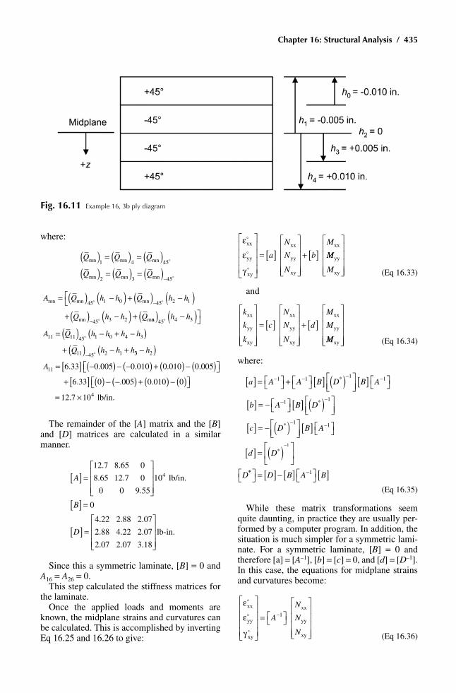
Chapter 16: Structural analysis / 435
where:
Q Q Q
Q Q Q
mn mn mn
mn mn mn
( ) = ( ) = ( )( ) = ( ) = ( )−
1 4 45
2 3 45
A Q h h Q h h
Q h h Q
mn mn mn
mn m
= ( ) −( ) + ( ) −( )
+( ) −( ) +
−
−
45 1 0 45 2 1
45 3 2
nn( ) −( )= ( ) − + −( )
+ ( ) − +−
45 4 3
11 11 45 1 0 4 3
11 45 2 1
h h
A Q h h h h
Q h h h33 2
11 6 33 0 005 0 010 0 010 0 005
−( )= [ ] −( ) − −( ) + ( ) − ( )
h
A . . . . .
lb/in.
+ [ ] ( ) − −( ) + ( ) − ( ) =
6 33 0 005 0 010 0
12 7 104
. . .
. ×
the remainder of the [A] matrix and the [B] and [D] matrices are calculated in a similar manner.
A
B
D
[ ] =
[ ] =
[ ] =
12 7
8 65
0
8 65
12 7
0
0
0
9 55
10
0
4
4
.
.
.
.
.
lb/in.
..
.
.
.
.
.
.
.
.
22
2 88
2 07
2 88
4 22
2 07
2 07
2 07
3 18
lb-in.
Since this a symmetric laminate, [B] = 0 and A16 = A26 = 0.
this step calculated the stiffness matrices for the laminate.
Once the applied loads and moments are known, the midplane strains and curvatures can be calculated. this is accomplished by inverting Eq 16.25 and 16.26 to give:
ε
ε
γ
xx
yy
xy
xx
yy
xy
xx
= [ ]
+ [ ]a
N
N
N
b
M
MM
M
yy
xy
(Eq 16.33)
and
k
k
k
c
N
N
N
d
M
Mxx
yy
xy
xx
yy
xy
xx
yy
= [ ]
+ [ ]
MMxy
(Eq 16.34)
where:
a A A B D B A
b A B
[ ] = + [ ] ( )
[ ]
[ ] = − [
− − − −
−
1 1 1 1
1
*
]] ( )
[ ] = − ( )
[ ]
[ ] = ( )
−
− −
∗−
D
c D B A
d D
D
*
*
1
1 1
1
** = [ ] − [ ] [ ]−D B A B1
(Eq 16.35)
While these matrix transformations seem quite daunting, in practice they are usually per-formed by a computer program. In addition, the situation is much simpler for a symmetric lami-nate. For a symmetric laminate, [B] = 0 and therefore [a] = [A–1], [b] = [c] = 0, and [d] = [D–1]. In this case, the equations for midplane strains and curvatures become:
ε
ε
γ
xx
yy
xy
xx
yy
xy
=
−A
N
N
N
1
(Eq 16.36)
Fig. 16.11 Example 16, 3b ply diagram

436 / Structural Composite Materials
and
k
k
k
D
M
M
M
xx
yy
xy
xx
yy
xy
=
−1
(Eq 16.37)
Equations 16.36 and 16.37 show that for sym-metric laminates, in-plane forces produce in-plane strains with no curvatures, and bending and twisting moments produce curvatures with no in-plane strains.
the values of the midplane strains and curva-tures can be used to calculate the strains in the individual plies. As a result of the linear relation-ship of strain in the thickness direction, we have:
ε
ε
γ
ε
ε
γ
xx
yy
xy
xx
yy
xy
xx
yy
xy
=
+
z
k
k
k
j
(Eq 16.38)
where zj is the distance from the laminate mid-plane to the midplane of the jth ply. the stresses in the jth ply can be calculated by using its stiff-ness matrix.
σσ
τ
εε
γ
xx
yy
xy
mn
xx
yy
xy
mn
=
=
j
j
j
Q
Q
+
j j j
z Q
k
k
k
ε
ε
γ
xx
yy
xy
mn
xx
yy
xy
σσ
τ
εε
γ
xx
yy
xy
mn
xx
yy
xy
mn
=
=
j
j
j
Q
Q
+
j j j
z Q
k
k
k
ε
ε
γ
xx
yy
xy
mn
xx
yy
xy
(Eq 16.39)
For a balanced symmetric laminate, where [B] = 0 and A16 = A26 = 0, the extensional stiff-ness matrix [A] simplifies to:
A
A
A
A
A
A
[ ] =
11
12
12
22
660 0
0
0
(Eq 16.40)
the inverse of the [A] matrix is:
AA A A
A
A
A
A
A A A
A
− =−
−−
−( )
1
11 22 122
22
12
12
11
11 22 122
66
1
0 0
0
0
(Eq 16.41)
therefore, Eq 16.36 gives:
ε
ε
γ
xx
yy
xy
=−
−−
1
0 0
0
011 22 12
2
22
12
12
11
11
A A A
A
A
A
A
A AA A
A
N
N
N22 122
66
−( )
xx
yy
xy
ε
ε
γ
xx
yy
xy
=−
−−
1
0 0
0
011 22 12
2
22
12
12
11
11
A A A
A
A
A
A
A AA A
A
N
N
N22 122
66
−( )
xx
yy
xy
(Eq 16.42)
For the case of a uniaxial tensile load applied in the x-direction with Nxx = hsxx and Nyy = Nxy = 0, we have:
ε σ
ε σ
γ
xx xx
yy xx
xy
=−
=−
=
A
A A Ah
A
A A Ah
22
11 22 122
12
11 22 122
0
which gives:
EA A A
hAxxxx
xx
= =−σ
ε11 22 12
2
22
(Eq 16.43)
νε
εxyyy
xx
= =
A
A12
22
(Eq 16.44)
In turn, applying Nxx and Nxy separately, it can be determined that:
EA A A
hAxy =−11 22 12
2
11
(Eq 16.45)
νyx =A
A12
11 (Eq 16.46)
GA
hxy = 66 (Eq 16.47)
the bending behavior of a balanced symmet-ric laminate beam where [B] = 0 can be analyzed as follows. First, the [D] matrix:
D
D
D
D
D
D
D
D
D
D
[ ] =
11
12
16
12
22
26
16
26
66
is inverted to give:
DD
D
D
D
D
D
D
D
D
D
− =
1
0
11
12
16
12
21
26
16
26
66
1
(Eq 16.48)

Chapter 16: Structural analysis / 437
where the elements of the [D–1] matrix are:
D D D D D D D D D D D D D D D
D
0 11 22 66 262
12 12 66 16 26 16 12 26 22 16= −( ) − −( ) + −( )111 11 22 66 26
2
12 12 12 66 16 26
16 16 12 2
= −( )= − −( )=
D D D D
D D D D D D
D D D D 66 22 16
22 22 11 66 162
26 26 11 26 12 16
6
−( )= −( )= − −( )
D D
D D D D D
D D D D D D
D
66 66 11 22 122 = −( )D D D D
D D D D D D D D D D D D D D D
D
0 11 22 66 262
12 12 66 16 26 16 12 26 22 16= −( ) − −( ) + −( )111 11 22 66 26
2
12 12 12 66 16 26
16 16 12 2
= −( )= − −( )=
D D D D
D D D D D D
D D D D 66 22 16
22 22 11 66 162
26 26 11 26 12 16
6
−( )= −( )= − −( )
D D
D D D D D
D D D D D D
D
66 66 11 22 122 = −( )D D D D (Eq 16.49)
If a bending moment is applied in the yz-plane to produce Mxx, and Myy and Mxy are both zero, the specimen curvatures can be obtained from Eq 16.37:
kD
DM
kD
DM
kD
DM
xx xx
yy xx
xy xx
=
=
=
11
12
16
(Eq 16.50)
Even though no twisting moment is applied, the laminate would tend to twist, owing to the presence of kxy, unless D°16 = D16 (D12D26 – D22D16) = 0. this is possible only if a balanced symmetric laminate contains plies in the 0° and 90° directions.
example 16.4: For the [0°, 45°, –45°, 90°]s symmetric laminate, calculate the ply stresses at the midplane of each ply generated by an ap-plied load of Nxx = 100 lb/in. the material prop-erties for the carbon/epoxy material are:
E11 = 25.0×10⁶ psi
E22 = 1.70×10⁶ psi
u12 = 0.30
u 21 = 0.020 since u 21 = u 12(E22/E11)
Solution: the first step is to calculate the val-ues Q11, Q22, Q12, Q21, and Q66 using Eq 16.13:
Q11 = 25.15×10⁶ psi
Q22 = 1.71×10⁶ psi
Q12 = Q21 = 5.13×10⁶ psi
Q66 = 6.50×10⁶ psi
the Q–
matrices are then determined for the 0°, 45°, –45°, and 90° plies in the same manner as illustrated in Example 16.3.
For the 0° plies:
Q =
0
5
251 5
5 13
0
5 13
17 1
0
0
0
6 50
10
.
.
.
.
.
psi
For the +45° plies:
Q =
45
6
7 62
6 32
5 86
6 32
7 62
5 86
5 86
5 86
6 45
10
.
.
.
.
.
.
.
.
.
psi
For the –45° plies:
Q =− −
−−
−45
7 62
6 32
5 86
6 32
7 62
5 86
5 86
5 86
6 45
.
.
.
.
.
.
.
.
.106 psi
For the 90° plies:
Q =
90
5
17 1
5 13
0
5 13
251 5
0
0
0
6 50
10
.
.
.
.
.
psi
the [A], [B], and [D] matrices can now be determined in a manner similar to that of Ex-ample 16.3. Since this is a symmetric laminate, [B] = 0. the [A] matrix for this laminate is:
A
A
A
A
A
A
[ ] =
=11
12
12
22
660 0
0
0
4 38
1 42
0
1 42
4 38
0
0
0
1 48
.
.
.
.
.
105 in./lb
the effective laminate constants can now be determined from Eq 16.43 through 16.47:
EA A A
hAxx =−
=( )( ) − ( )11 22 12
2
22
6 6 6 24 38 10 4 38 10 1 42 10
0 0416
. . .
.
× × ×
(( ) ( ) =
=−
=
4 38 109 42 10
9 42 10
66
11 22 122
11
6
..
.
××
×
psi
psiEA A A
hA
G
xy
xyy
xy
yx
= =
= =
= =
A
hA
A
A
A
66 6
12
22
12
11
3 55 10
0 325
0 325
.
.
.
× psi
ν
ν
EA A A
hAxx =−
=( )( ) − ( )11 22 12
2
22
6 6 6 24 38 10 4 38 10 1 42 10
0 0416
. . .
.
× × ×
(( ) ( ) =
=−
=
4 38 109 42 10
9 42 10
66
11 22 122
11
6
..
.
××
×
psi
psiEA A A
hA
G
xy
xyy
xy
yx
= =
= =
= =
A
hA
A
A
A
66 6
12
22
12
11
3 55 10
0 325
0 325
.
.
.
× psi
ν
ν
EA A A
hAxx =−
=( )( ) − ( )11 22 12
2
22
6 6 6 24 38 10 4 38 10 1 42 10
0 0416
. . .
.
× × ×
(( ) ( ) =
=−
=
4 38 109 42 10
9 42 10
66
11 22 122
11
6
..
.
××
×
psi
psiEA A A
hA
G
xy
xyy
xy
yx
= =
= =
= =
A
hA
A
A
A
66 6
12
22
12
11
3 55 10
0 325
0 325
.
.
.
× psi
ν
ν

438 / Structural Composite Materials
EA A A
hAxx =−
=( )( ) − ( )11 22 12
2
22
6 6 6 24 38 10 4 38 10 1 42 10
0 0416
. . .
.
× × ×
(( ) ( ) =
=−
=
4 38 109 42 10
9 42 10
66
11 22 122
11
6
..
.
××
×
psi
psiEA A A
hA
G
xy
xyy
xy
yx
= =
= =
= =
A
hA
A
A
A
66 6
12
22
12
11
3 55 10
0 325
0 325
.
.
.
× psi
ν
ν
Since this is a quasi-isotropic laminate, Exx and Eyy are the same.
the inverse of the [A] matrix can be found by using Eq 16.41:
AA A A
A
A
A
A
A A A
A
− =−
−−
−( )
1
11 22 122
22
12
12
11
11 22 122
66
1
0 0
0
0
the first term is calculated as follows:
AA A A
A− =−
( )
=( )( ) − ( )
111
11 22 122 22
5 5 5 2
1
1
4 38 10 4 38 10 1 42 104
. . .× × ×..
.
38 10
2 55 10
5
6
×
×
( )
= − in./lb
the remainder of the [A–1] matrix is:
A− − = −−
1 6
2 55
0 829
0
0 829
2 55
0
0
0
6 76
10
.
.
.
.
.
in./lb
using Eq 16.36 and 16.37, the [ε°] and [k] matrices can now be calculated. First, the [ε°] matrix is calculated as follows:
ε
ε
γ
xx
yy
xy
xx
yy
xy
=
=−A
N
N
N
1
2 5
. 55
0 829
0
0 829
2 55
0
0
0
6 76
10 6−−
−.
.
.
.
in./lb
100
0
0
lb/in.
ε
ε
γ
xx
yy
xy
xx
yy
xy
=
=−A
N
N
N
1
2 5
. 55
0 829
0
0 829
2 55
0
0
0
6 76
10 6−−
−.
.
.
.
in./lb
100
0
0
lb/in.
which yields:
ε°xx = 2,550 × 10-6 in./in.
ε°yy = –829×10-6 in./in.
g°xy = 0
Since this is a balanced and symmetric lami-nate, the [A] and [B] matrices are uncoupled, [B] = 0, and there are no applied moments, it can be inferred that the curvature matrix [k] is zero, and the strains in each ply in the laminate co-ordinate system are identical to the midplane strains. In pure uniaxial tension of a symmetric and balanced laminate, the strains will be con-stant through the thickness but the stresses may vary, as shown in Fig. 16.12. the 0° plies carry the most stress and the 90° plies carry the least. For flexural loading, the strains vary linearly through the thickness and the stresses vary with the loading condition and their stress-carrying capability.
now, using Eq 16.39, sxx, syy, and txy are cal-culated at the midplane of the 0°, +45°, –45° and 90° plies.
For the 0° plies:
σσ
τ
εε
γ
xx
yy
xy
mn
xx
yy
xy
=
=
0
0
0
2
Q
551 5
5 13
0
5 13
17 1
0
0
0
6 50
105
.
.
.
.
.
−
psi
2550
829.0
0
= −
−10
6370
11 0
0
6 in./in. psi.
σσ
τ
εε
γ
xx
yy
xy
mn
xx
yy
xy
=
=
0
0
0
2
Q
551 5
5 13
0
5 13
17 1
0
0
0
6 50
105
.
.
.
.
.
−
psi
2550
829.0
0
= −
−10
6370
11 0
0
6 in./in. psi.
σσ
τ
εε
γ
xx
yy
xy
mn
xx
yy
xy
=
=
0
0
0
2
Q
551 5
5 13
0
5 13
17 1
0
0
0
6 50
105
.
.
.
.
.
−
psi
2550
829.0
0
= −
−10
6370
11 0
0
6 in./in. psi.
For the +45° plies:
σσ
τ
εε
γ
xx
yy
xy
mn
xx
yy
xy
=
+
+
45
45
Q
++
=
45
6
7 62
6 32
5 86
6 32
7 62
5 86
5 86
5 86
6 45
10
.
.
.
.
.
.
.
.
.
psi
22550
829.0
0
in./in. p−
=
−10
1420
980 0
1010
6 . ssi
σσ
τ
εε
γ
xx
yy
xy
mn
xx
yy
xy
=
+
+
45
45
Q
++
=
45
6
7 62
6 32
5 86
6 32
7 62
5 86
5 86
5 86
6 45
10
.
.
.
.
.
.
.
.
.
psi
22550
829.0
0
in./in. p−
=
−10
1420
980 0
1010
6 . ssi
σσ
τ
εε
γ
xx
yy
xy
mn
xx
yy
xy
=
+
+
45
45
Q
++
=
45
6
7 62
6 32
5 86
6 32
7 62
5 86
5 86
5 86
6 45
10
.
.
.
.
.
.
.
.
.
psi
22550
829.0
0
in./in. p−
=
−10
1420
980 0
1010
6 . ssi

Chapter 16: Structural analysis / 439
For the –45° plies:
σσ
τ
εε
γ
xx
yy
xy
mn
=
−
−
45
45
Qxx
yy
xy −−
=−
45
1420
980 0
1010
. psi
For the 90° plies:
σσ
τ
εε
γ
xx
yy
xy
mn
xx
yy
xy
=
90
90
90
Q
= −
394 0
1954
0
.
psi
Although the strains are the same through the thickness, the stresses in the plies are a function of the ply orientation, with the 0° plies carrying the highest stresses. If desired, these stresses can be converted to the 1-2 coordinate system by using the stress transformation equation (Eq 16.2).
16.6 Interlaminar Free-edge Stresses
Provided that the laminate is sufficiently wide, lamination theory estimates laminate behavior fairly accurately in the interior of the laminate. However, within about one laminate thickness
Fig. 16.12 Variation of ply stresses and strains through the laminate thickness

440 / Structural Composite Materials
of free edges, lamination theory breaks down and fails to predict the large interlaminar stresses that can develop. At the free edges, delamination under in-plane loading can occur. large inter-laminar stresses can develop, leading to delami-nation of plies or matrix cracking at the edges.
Edge effects arise as a result of the require-ment for strain compatibility between the plies in the laminate. Interlaminar shear and through-the-thickness peel stresses develop near the free edges of the laminate. the principal reason for the development of these interlaminar stresses is the mismatch of Poisson’s ratios nxy and the co-efficients of mutual influence mx and my between adjacent plies. the result is the production of normal stresses sxy in each ply and interlaminar shear stress tyz at the ply interfaces. Consider a laminate consisting of alternating 0° and 90° plies under tensile loading parallel to the zero-degree plies. the difference in Poisson’s ratios leads to different transverse contractions, as shown in Fig. 16.13. However, since the plies are bonded together, they have the same transverse strain. this leads to interlaminar shear stresses between the plies, forcing the zero-degree ply to expand in the transverse direction and the 90-degree ply to contract. the shear force is confined to the edge because once the required tension syy is es-tablished in the zero-degree ply, compatibility will be ensured across the middle of the lami-nate. At the free edge, the tension stress must drop to zero if there is no applied edge stress. Since the shear stress shown in Fig. 16.13 is offset from the axis of the resultant the stress syy, a turning moment is produced. to balance this moment, peel stresses szz develop in the lami-nate with the distribution indicated in the figure. these peel stresses can cause delaminations at the edge. Interlaminar shear stresses also occur in angle-ply laminates as the plies distort differ-ently under applied loads.
the magnitude of free-edge stresses is a func-tion of laminate lay-up, stacking sequence, prop-erties of the constituent materials, and stress state. As an example of laminate lay-up, a cross-plied [0°, 90°]s laminate experiences less severe interlaminar stress components than a [± 30°, 90°]s laminate. thus, the [± 30°, 90°]s laminate is more prone to free-edge delamination. the stack-ing sequence can determine whether an interlam-inar normal stress will be tensile or compressive at the free edges and determine the magnitude of the interlaminar stress components. under the same uniaxial tensile loading condition, [± 45°, 0°, 90°]s and [90°, 45°, 0°, –45°]s laminates pro-
duce large tensile and compressive szz stresses at the midsurface, respectively. therefore, the latter laminate is not as prone to delamination under tensile loading as the former laminate. In-terspersing the ± 45° plies to produce an alter-nating positive and negative stress state has been found to reduce szz and thus also the tendency to delaminate.
Any free edge, including a hole, can introduce interlaminar stresses. the consequences of these stresses need to be evaluated for structural ap-plications, particularly when fatigue loading is present. It becomes extremely complex to de-velop quantitative analytical solutions for free-edge stresses in all but the simplest geometric shapes. the magnitude and effects of free-edge stresses are usually evaluated by finite difference or finite element methods. In most cases, the possibility of delaminations as a result of free-edge stresses is determined through testing rather than by computation.
16.7 Failure theories
Failure prediction for metallic structures is normally performed by comparing stresses or strains caused by applied loads with the allow-able strength or strain capacity of the material. For isotropic materials that exhibit yielding, ei-ther the tresca maximum shear stress theory or the von Mises distortional energy theory is com-monly used. However, composites are not iso-tropic and they do not yield. Failure modes in composites are generally noncatastrophic and may involve localized damage via such mecha-nisms as fiber breakage, matrix cracking, debond-ing, and fiber pull-out. these can progress si-multaneously and interactively, making failure prediction for composites complex.
there are five independent strength constants that are important for a single ply:
• Slt or εlt––longitudinal tensile strength or strain
• Stt or εtt––transverse tensile strength or strain• Slc or εlc––longitudinal compressive strength
or strain • Stc or εtc––transverse compressive strength
or strain• Ss or gs––in-plane shear strength or strain
Maximum Stress Criterion. According to this theory, failure occurs when any stress in the principal material directions is equal to or greater

Chapter 16: Structural analysis / 441
Fig. 16.13 Interlaminar shear and peel stresses in a 0°, 90° laminate. Source: Ref 1

442 / Structural Composite Materials
than the corresponding allowable strength. to avoid failure, one must have:
–Slc < s11 < Slt
–Stc < s22 < Stt
–Ss < t12 < Ss (Eq 16.51)
For the case of simple tension where sxx is present and syy = sxy = 0, depending on the angle θ, three failure modes are considered:
1. Failure parallel to the fiber direction domi-nated by fiber fracture:
σθxx
Lt=S
cos2
(Eq 16.52)
2. Failure transverse to the fiber direction dominated by matrix failure or fiber-matrix interface failure:
σθxx
Tt=S
sin2 (Eq 16.53)
3. Failure by shear of the matrix or fiber-matrix interface, or both:
σθ θxx
s=S
sin cos
(Eq 16.54)
the disadvantage of this theory is that it does not account for the interaction of stresses and the occurrence of mixed-mode failures.
Maximum Strain theory. the maximum strain theory is very similar to the maximum stress theory except that strains are used instead of stresses. According to this theory, failure will occur if any strain in the principal material axes is equal to or greater than the corresponding al-lowable strain. to avoid failure, one must have:
- εlc < ε11 < εlt
- εtc < ε22 < εtt
- gs < g12 < gs (Eq 16.55)
For an orthotropic ply subjected to a simple tension stress sxx, it can be shown that in the principal material directions the following hold:
εσ
νσ
θ ν θ σ
εσ
ν
1111
1121
22
22 11
212
2
2222
2212
1= − = −( )= −
E E E
E
cos sin xx
σσθ ν θ σ
γτ
θ θ σ
11
11 22
221
2
1212
12 12
1
1
E E
G G
= −( )= = ( )
sin cos
sin cos
xx
xxx
(Eq 16.56)
Failure occurs when:
ε11 > εlt
ε22 > εlt or
g12 > gs
On the assumption that the material is linearly elastic up to the failure strain, failure of the ply occurs if the applied stress sxx exceeds the smallest of these values:
E S
E
112
122 2
122
222
21
εθ ν θ θ ν θ
εθ ν
Lt Lt
Tt
cos sin cos sin
sin c
−=
−
−
or
oos sin cos
sin cos sin cos
2 221
2
12
θ θ ν θγ
θ θ θ θ
=−
=
S
G S
Tt
s s
or
(Eq 16.57)
the maximum stress theory and the maxi-mum strain theory give similar results. Again, there is no interaction between strengths in dif-ferent directions.
azzi-tsai-hill Maximum Work theory. the maximum work theory states that for plane stress, failure initiates when the following in-equality is violated:
σ σ σ σ τ112
211 22
2222
2122
21
S S S SLt Lt Tt s
− + + < (Eq 16.58)
where s11 and s22 are both tensile stresses. When the state of stress is compression rather than ten-sion, the compressive stresses s11 and s22 are used in Eq 16.58. In uniaxial tension, failure is predicted if:
σθ θ θ θ θ θ
xx
Lt Lt Tt s
≥
− − −
1
4
2
2 2
2
4
2
2 2
2
cos sin cos sin sin cos
S S S S
− 1
2
(Eq 16.59)
A failure envelope for the Azai-tsai-Hill failure criterion for plane stress conditions is shown in Fig. 16.14. the failure envelope is a graphic representation of the safe and unsafe conditions for loading. It can be separated into quadrants.
In the first quadrant, where s11 and s22 > 0:
σ σ σ σ τ11
2
211 22
2222
2122
21
S S S SLt Lt Tt s
− + = −

Chapter 16: Structural analysis / 443
In the second quadrant, where s11 < 0 and s22 > 0:
σ σ σ σ τ11
2
211 22
2222
2122
21
S S S SLc Lc Tt s
+ + = −
In the third quadrant, where s11 and s22 < 0:
σ σ σ σ τ11
2
211 22
2222
2122
21
S S S SLc Lc Tc s
− + = −
In the fourth quadrant, where s11 > 0 and s22 < 0:
σ σ σ σ τ11
2
211 22
2222
2122
21
S S S SLt Lt Tc s
+ + = −
the advantage of the Azai-tsai-Hill criterion is that the interaction between strengths and fail-ure modes is taken into account. As shown in the comparison with the maximum stress and maxi-mum strain theories (Fig. 16.15), the Azai-tsai-Hill criterion gives a better fit to the experimen-tal data.
tsai-Wu Failure Criterion. In the tsai-Wu criterion, a composite ply subject to plane stress conditions will fail when the following condi-tion is satisfied:
F F F F F F F11 11 2 22 6 12 11 112
22 222
66 122
12 11 222 1σ σ τ σ σ τ σ σ+ + + + + + =
F F F F F F F11 11 2 22 6 12 11 112
22 222
66 122
12 11 222 1σ σ τ σ σ τ σ σ+ + + + + + = (Eq 16.60)
where the strength coefficients are defined as:
FS S
FS S
F
FS S
FS S
FS
1
2
6
11
22
66 2
1 1
1 1
0
1
1
1
= −
= −
=
=
=
=
Lt Lc
Tt Tc
Lt Lc
Tt Tc
s
Although the strength coefficients F1, F2, F11, F22, and F66 can be calculated using the tensile, compressive, and shear strength properties in the principal material directions, F12 must be deter-mined by a biaxial tensile test. under a biaxial stress state with t12 = 0 and s11 and s22 = s at failure, Eq 16.60 reduces to:
F F F F F1 2 11 22 1222 1+( ) + + +( ) =σ σ (Eq 16.61)
Fig. 16.14 Failure envelope for the Azai-Tasi-Hill failure criterion

444 / Structural Composite Materials
which can be rearranged to give:
FS S S S S S S S12 2
1
21
1 1 1 1 1 1= − − + −
− +
σ
σLt Lc Tt Tc Lt Lc Tt Tc
σσ2
FS S S S S S S S12 2
1
21
1 1 1 1 1 1= − − + −
− +
σ
σLt Lc Tt Tc Lt Lc Tt Tc
σσ2
since a biaxial tensile test is difficult to conduct, an approximate value for F12 is given by:
− ( ) ≤ ≤1
2011 22
1 212F F F
the tsai-Wu criterion is generally believed to give the best fit to experimental test data. repre-sentative failure envelopes for the maximum strain, Azai-tsai-Hill, and tsai-Wu failure crite-ria are shown in Fig. 16.16. It should also be noted that these are not the only failure criteria; a number of others are available.
Once a failure criterion is selected, the proce-dure to predict laminate failure is as follows:
1. Calculate the stresses or strains in each ply using lamination theory.
2. transform the individual stresses or strains in the loading direction into stresses or strains in the principal material directions.
3. using one of the failure criteria, determine whether a ply has failed. After a ply fails, the stresses and strains in the remainder of the laminate increase and the laminate stiff-ness is reduced.
4. Since the failed ply may not carry its share of the load in all directions, several methods can be used to account for the failed ply and subsequent laminate behavior:
Total discount method. In this method, zero strength and stiffness are assigned to the failed ply in all directions.
Fig. 16.15 Comparison of maximum stress, maximum strain, and the Azai-Tsai-Hill failure criterion. Source: Ref 2 and 3

Chapter 16: Structural analysis / 445
Limited discount method. If the ply failure occurs in the matrix, then zero strength and stiff-ness are assigned to the failed ply for the trans-verse and shear modes. If the ply fails by fiber rupture, then the total discount method is used.
Residual property method. In this method, residual strength and stiffness are assigned to the failed ply.
When a laminate is loaded to failure, not all plies fail at the same time. the progressive
Fig. 16.16 Failure envelopes for maximum strain, Azai-Tsai-Hill, and Tsai-Wu criteria. Source: Ref 4
ply failures in a [0°/45°/90°/–45°]s laminate are shown in Fig. 16.17. Plies will fail successively in increasing order of strength in the loading di-rection. Because the transverse strength of uni-directional plies is lower than the longitudinal strength, the transverse plies will fail first. Fail-ure of the 90-degree plies is generally followed by failure of other off-angle plies such as ± 45°, and finally of the much stronger zero-degree pl the occurrence of first ply failure, although a

446 / Structural Composite Materials
relatively conservative design criterion, is often used in the aerospace industry to indicate lami-nate failure.
16.8 Concluding remarks
this chapter gives only a brief introduction to composite structural analysis. Actual analysis of composite structures requires a much deeper un-derstanding of the available analysis methods. Again, the reader is referred to more detailed texts for a more rigorous treatment. lamination theory can also be expanded to account for ther-mal stresses that result from curing at elevated temperatures and the effects of moisture absorp-tion. Any respectable computerized laminate code is capable of handling these extensions.
reFereNCeS
1. A. Baker, S. Dutton, and D. Kelly, Compos-ite Materials for Aircraft Structures, 2nd ed.,
American Institute of Aeronautics and As-tronautics, 2004
2. V.D. Azai and S.W. tsai, Exp. Mech., Vol 5 (no. 283), 1965
3. r.M. Jones, Mechanics of Composite Ma-terials, 2nd ed., Hemisphere Publications, 1998
4. S.W. tsai and H.t. Hahn, Inelastic Behav-ior of Composite Materials, American Soci-ety of Mechanical Engineers, 1975
SeLeCted reFereNCeS
• B.D. Agarwal and l.J. Broutman, Analysis and Performance of Fiber Composites, John Wiley and Sons, Inc., 1980
• V.K.S. Choo, Fundamentals of Composite Materials, Knowen Academic Press, 1990
• r.M. Christensen, Mechanics of Composite Materials, Dover Publications, 2005
• I.M. Daniel and O. Ishai, Engineering Me-chanics of Composite Materials, 2nd ed., Ox-ford university Press, 2005
Fig. 16.17 Progressive ply failure for a [0°/45°/90°/-45°]s laminate

Chapter 16: Structural analysis / 447
• D. Gay, S.W. Hoa, and S.W. tsai, Composite Materials Design and Applications, CrC Press, 2003
• Z. Hahin, B.W. rosen, E.A. Humphreys, C. newton, and S. Chaterjee, Fiber Compos-ite Analysis and Design: Composite Materi-als and Laminates, Vol I, u.S. Department of transportation, Federal Aviation Administra-tion, DOt/FAA/Ar-95/29, I, Final report, Oct 1997
• l.P. Kollar and G.S. Springer, Mechanics of Composite Structures, Cambridge university Press, 2002
• M. Piggott, Load Bearing Fibre Composites, 2nd ed., Kluwer Academic Publishers, 2002
• G.H. Stabb, Laminar Composites, Butterworth-Heinemann, 1999
• S.W. tsai and H.t. Hahn, Introduction to Composite Materials, technomic Publishing, 1980
• M.E. tuttle, Structural Analysis of Polymeric Composite Materials, Marcel Dekker, Inc., 2004
• V.V. Vasiliev and E.V. Morozov, Mechanics and Analysis of Composite Materials, Else-vier Science ltd., 2001
• J.r. Vinson and r.l. Sierakowski, The Be-havior of Structures Composed of Composite Materials, 2nd ed., Kluwer Academic Pub-lishers, 2004

“This page left intentionally blank.”

Structural Composite Materials Copyright © 2010, ASM International®
F.C. Campbell All rights reserved.www.asminternational.org
Chapter 17
Structural Joints—Bolted and Bonded
AnAlytICAl ConSIderAtIonS, as dis-cussed in the previous chapter, includes much discussion of unnotched laminates. However, for practical purposes, the joints in a composite structure should be designed first and then the space between them filled in with appropriate laminate orientations. optimization of the basic structure first can often compromise the design of the joints, resulting in lower overall structural efficiency and possibly producing a structure that is more difficult to repair.
two primary methods of joining are used for polymer matrix composites: mechanical fasten-ing and adhesive bonding. Since fastener holes cut through the fibers and destroy the load path, much more efficient load transfer can be ob-tained with adhesively bonded joints. A well-designed adhesively bonded joint will actually be stronger than the base laminate. on the other hand, even a well-designed mechanically fas-tened joint will be only about 40 to 50 percent as strong as the base laminate. In spite of this ad-vantage, adhesively bonded joints are not always practical. Bonded joints are preferred if thin com-posite sections are to be joined where bearing stresses in bolted joints would be unacceptably high or when the weight penalty for mechanical fasteners is too high. In general, thin structures with well-defined load paths are good candidates for adhesive bonding, whereas thicker structures with complex load paths are good candidates for mechanical fastening.
the low efficiency of mechanically fastened joints in composites is a direct consequence of their inherent brittleness. When a metallic struc-ture is highly loaded, the metal will yield lo-cally in the vicinity of the bolt hole to reduce the elastic stress concentration. However, since composites are relatively brittle, they do not yield and the stress concentration remains high.
the stress concentration is reduced somewhat due to localized delaminations around the fas-tener hole, but the reduction is small compared to the gross yielding that occurs in metallic alloys. In addition, nearly quasi-isotropic lami-nates with 0°, ± 45°, 90° orientations are re-quired to develop sufficient joint strengths, which lowers the basic laminate strength from a more highly orthotropic (0° dominated) lami-nate orientation.
this chapter discusses mechanically fastened joints and adhesively bonded joints. like the Chapter 16, “Structural Analysis,” this chapter is primarily an overview of analytic considerations for joints. Much more extensive treatments can be found in some of the references listed at the end of this chapter. the details of hole prepara-tion and fastener installation are found in Chap-ter 11, “Machining and Assembly,” and adhesive bonding procedures are covered in Chapter 8, “Adhesive Bonding.”
17.1 Mechanically Fastened Joints
Compared to adhesive bonding, mechanically fastened joints have both advantages and disad-vantages. the advantages of mechanical fasten-ing include the following:• Mechanical fastening is a much more straight-
forward and less risky joining process. Whereas adhesive bonding requires stringent surface preparations and the quality of the bond is de-pendent on the cure of polymerizable materi-als, mechanical fastening does not require much surface preparation and is much less af-fected by environmental exposure.
• Compared to adhesive bonding, mechanical fastening provides better through-the-thickness

450 / Structural Composite Materials
reinforcement and is not as sensitive to peel stresses or residual-stress effects.
• Unlike adhesively bonded joints, mechani-cally fastened joints do not normally require nondestructive testing.
• Many mechanically fastened joints allow dis-assembly or panel removal. depending on the specific fastener selected, some are de-signed for permanent installation and others allow easy removal.
• Mechanically fastened joints are much more amenable to field repairs because cleanliness, perishable materials, and elevated-temperature cures are not concerns.
the disadvantages of mechanical fastening in-clude the following:• Much lower joint efficiencies are obtained with
mechanically fastened joints. Composites are notch sensitive, and even the best mechanically fastened joints can only attain about 40 to 50 percent of the base laminate strength.
• Composites have low bearing strengths com-pared to metals and can experience hole elon-gation due to in-service fatigue, which de-grades joint strength.
• Improper hole preparation procedures and poor shimming practices can induce delaminations during assembly. Unshimmed gaps are a major
problem and can result in delaminations in both composite skins and substructure.
• Composite-to-metal joints are subject to fret-ting and corrosion of the metal in service. Fa-tigue cracking of metal components can also be a problem.
17.2 Mechanically Fastened Joint analysis
A simple single-fastener single-lap shear joint is shown in Fig. 17.1. the key dimensions are these:
d—fastener diametert—thickness of the joint elementsw—width of the platee—edge distanceP—loaddt—bearing area loaded in compression2et—total shear-out area loaded in shear(w-d)/t—net section loaded in tensionwt—gross section loaded in tension
the average stresses in the joint are as follows:
Average bearing stress σb = P/dt (eq 17.1)
Average shear-out stress σso = P/ 2et (eq 17.2)
G rossSectionwt
ShearO utSection2et
w
e
dP P
BearingSectiondt
NetSection(w-d)t
G rossSectionwt
ShearO utSection2et
w
e
dP P
BearingSectiondt
NetSection(w-d)t
Fig. 17.1 Single-shear joint. Source: Ref 1

Chapter 17: Structural Joints—Bolted and Bonded / 451
Average net section stress σn = P/(w-d)t (eq 17.3)
Average gross section stress σg = P/wt (eq 17.4)
In traditional joint analysis, it is necessary to calculate the failing stress for each of these con-ditions. Failure will occur at the condition with the lowest joint strength. However, since bolted joints are always weaker than the base laminate, gross section failures will not occur unless the joint area has been thickened considerably. In addition, the selection of a nearly quasi-isotropic laminate is necessary in order for the bolt loads
to be carried effectively and shear-out failures to be thereby eliminated. therefore, the emphasis of the following discussion will be on bearing and net tension failures.
the various failure modes for composite joints are shown in Fig. 17.2. Potential causes include:
1. Bearing: Bearing failures are characterized by localized damage, such as delaminations and matrix crazing around the hole. local-ized compression loading caused by the
Fig. 17.2 Mechanically fastened composite joint failure modes

452 / Structural Composite Materials
fastener leads to buckling and kinking of the fibers followed by crushing of the matrix.
2. Shear-out: Shear-out failures result from in-sufficient edge distance or from having too many plies oriented in the load direction, for example 0°.
3. Tension: tension failures are caused by insuf-ficient width or by having too few plies ori-ented in the load direction, for example 0°.
4. Cleavage-tension: Cleavage-tension failures occur due to insufficient edge distance and width or an insufficient number of cross-plies, for example ± 45º and 90º.
5. Fastenerpull-through: Fastener pull-through can occur when the countersink is too deep or when a shear head fastener is used.
6. Fastenerfailure: the fastener itself can fail if it is too small for the laminate thickness, if there are unshimmed gaps or excessive shimmed gaps in the joint, or if there is in-sufficient fastener clamp-up.
If a high-strength, highly orthotropic lami-nate has a large portion of 0° plies, the joint strength will be low because of the likelihood of fastener shear-out. Using an insufficient number of 0° plies in a laminate will result in tension failure at a lower than desired load. therefore, a more balanced laminate is required, that is, a laminate that is close to quasi-isotropic consist-ing of 0°, ± 45°, 90° ply orientations. the 0° fi-bers carry the bearing and tension loads, and the ± 45° and 90° fibers carry the load around the
hole to prevent shear-out or cleavage-type fail-ures. the addition of 0° plies improves bearing strength up to about 60 percent. However, above about 60 percent, failure occurs by splitting be-cause the transverse tensile strength becomes in-sufficient to prevent shear-out failures. the opti-mum bearing strength for a 0°, ± 45° laminate occurs with fiber orientations of about 50 per-cent, 0°; and 50 percent ± 45° plies. Because in-terplay stresses are reduced as the laminate be-comes more homogeneous, bearing strength can further be improved by thoroughly dispersing the 0° and ± 45° plies throughout the lay-up. Some designers consider bearing failures to be the only acceptable failure mode because they are not catastrophic, whereas through-the-thickness tension failures are abrupt and catastrophic. How-ever, designing in accordance with this criterion will result in less than optimum joint strengths. tension failure modes are associated with far higher bolted composite joint strengths; it is all but impossible to design a multirow bolted joint that will fail by bearing.
the failure mode is also dependent on the ra-tios of the edge distance to the diameter of the fastener (e/d) and the width of the joint to the diameter of the fastener hole (w/d), as illustrated for a quasi-isotropic laminate in Fig. 17.3. For large values of e/d and w/d, the joint fails in bear-ing with the failing load being independent of e/d or w/d. If the edge distance e is reduced, then a shear-out failure occurs with the joint strength approaching zero at e/d = 0.5. If the width w is
Fig. 17.3 Effects of edge distance and width on mechanically fastened failure modes. Source: Ref 2

Chapter 17: Structural Joints—Bolted and Bonded / 453
reduced, then a net tension failure will occur with the joint strength approaching zero at w/d = 1.
the preferred fiber orientation design enve-lope for mechanically fastened joints is shown in Fig. 17.4. Shear-out does not occur within the recommended design envelope of laminate pat-terns shown here. However, outside the recom-mended design envelope, shear-out with through-the-thickness cracks parallel to the 0° plies is likely to result in premature failures. Shear-out cannot be corrected by adding more edge dis-tance e to a highly orthotropic laminate. even an increase in thickness, without changing to a more quasi-isotropic laminate pattern, is not
very effective. therefore, the joint can never be loaded to the levels predicted by lamination theory for unnotched laminates. the strength of composite structures with both loaded and un-loaded holes depends only slightly on the fiber pattern for nearly quasi-isotropic laminates; the stress concentration factor increases almost as rapidly as the unnotched strength for slightly orthotropic patterns. therefore, throughout the range of fiber patterns surrounding the quasi-isotropic lay-up, the bearing strengths and gross-section strengths are almost constant.
Since we are dealing with holes, which are notches, stress concentration factors K must be
Fig. 17.4 Recommended design envelope for mechanically fastened composites. Source: after Ref 3

454 / Structural Composite Materials
used. they account for the increase in stress σmax over the nominally applied stress σnom. In other words:
σmax = Kσnom (eq 17.5)
the stress concentration factor varies with the severity of the notch; sharper notches produce higher stress concentration factors and thus in-crease the applied nominal stresses. For an iso-tropic metal with a round hole, the stress con-centration factor is usually taken as 3.0 within the elastic region.
In a composite laminate, the degree of stress concentration effect depends on the laminate pattern. Analysis has shown that the theoretical elastic stress concentration Kte at the edge of a hole at 90° to an applied tension stress is given by the following equation:
KE
E
E
Gtexx
yyxy
xx
xy
= +
−
+
1 2 ν
(eq 17.6)
According to this equation, Kte varies from 7.5 for a 100 percent 0° laminate down to
about 1.8 for a 100 percent ± 45° laminate. Since the laminate tensile strength falls with an increase in the percentage of ± 45° plies, the optimum ply configuration is again on the order of 50 percent ± 45° plies. the peak stress level does not necessarily occur at 90° to the applied load; in the case of an all ± 45° lami-nate, the peak stress occurs at 45° to the load-ing direction.
When a mechanically fastened composite joint is loaded, microcracks and delaminations around the hole cause internal load redistribu-tions that are not accounted for in elastic design. thus, there is substantial nonlinear behavior as-sociated with the normal fastener sizes used in composite structures. While these softened zones (Fig. 17.5) are not the same as yielding zones in metallic structures, they produce somewhat sim-ilar effects. For example, any increase in the softened zone around fasteners in composites causes an increase in the static tensile strength, and the gentle fatiguing of bolted composite struc-tures can increase the static tensile strength to-ward the unnotched net section strength. the corresponding increase in compressive strength will not be as large, because (1) it is dominated
Fig. 17.5 Stress concentration reduction in composite laminates. Source: Ref 3

Chapter 17: Structural Joints—Bolted and Bonded / 455
more by bearing stresses than by net section stresses and (2) the localized damage area desta-bilizes axially compressed fibers. As shown in Fig. 17.6, at the elastic level the peak tension stress alongside the loaded bolt hole in an isotro-pic panel is of the same order of magnitude as the average bearing stress (P/dt). Keeping the bear-ing stress low is a key to structurally efficient bolted composite joints, particularly multirow joints. Since the peak hoop tension stress is of the same order of magnitude as the average bearing stress, the bolts should be placed close together to minimize the peak hoop tension stresses.
Because of the nonlinear material behavior of composites around both loaded and unloaded holes, empirically established correlation fac-tors are required. Using this method, it is neces-sary to assume that the amount of stress concen-tration relief is proportional to the intensity of the original elastic stress concentration. With a correlation factor determined from single-hole test specimens as a starting point, the strength of highly loaded multirow bolted composite joints can be effectively predicted. Corrections both for the nonlinear behavior around a fastener and for orthotropy can be combined into a single cor-relation coefficient C (as discussed below), pro-vided that the mode and location of failure do not change. Separate analyses are needed for bearing failures and for tension through-the-hole failure modes. Compression strengths tend to be higher
and not as sensitive to stress concentrations, be-cause some of the load can be transmitted through the fastener rather than around it.
two other semiempirical criteria are cur-rently used for analyzing the tensile stress state around a hole in a plate of finite width: the aver-age stress and point stress criteria. Under the average stress criterion, failure is considered to occur when the average value of the tensile stress over some characteristic length a0 from the hole reaches the unnotched ultimate tensile strength of the laminate. Under the point stress criterion, failure is considered to occur when the local value of the stress at some characteristic dis-tance d0 from the hole reaches the unnotched ultimate tensile strength. the values a0 and d0, which are considered to be material properties, are determined from plots of strength reduction versus hole size to give the best fit to the experi-mental results. the two criteria are related through the relationship a0 = 4d0. However, in the following discussion, we will use the corre-lation coefficient C.
17.3 Single-hole Bolted Composite Joints
the relationships between the strengths of bolted joints in ductile metals, composites, and brittle materials are shown in Fig. 17.7. For
Fig. 17.6 Bearing and hoop stresses at the bolt hole. Source: Ref 3

456 / Structural Composite Materials
metals under high stresses, localized yielding reduces the effective stress concentration factor from 3.0 to around 1; therefore, failure is simply dependent on the net cross-section area. How-ever, for a purely brittle material, since no yield-ing occurs, the effective stress concentration factor remains high. For composites, as a result of the localized damage adjacent to the hole, there is some stress concentration relief, but not as much as for gross localized yielding in met-als. the maximum attainable joint efficiencies are 65 percent for metal, 40 percent for compos-ite, and 21 percent for a perfectly brittle mate-rial. For both metal and composite, a change in failure mode from net tension to bearing is pre-
dicted to occur at a d/w of approximately 0.3. Also, the strength increase shown in Fig. 17.7 for roughly 0.25 in. (6.5 mm) diameter bolts in carbon/epoxy composites decreases asymptoti-cally as the fastener diameter increases, and, for very large bolt holes or cutouts, the linearly elas-tic predictions would be expected to apply.
As can be derived from eq 17.3, the maxi-mum tensile stress σmax at the edges of a loaded hole in a joint under a load P is given by the fol-lowing equation:
σmax = ( ) =−( )K
K P
t w dtc average net section stress tc
(eq 17.7)
Ductile meta l
Tens ion fa ilu res
Com pos ite
B rittle m ateria l
Bear
ing
failu
res
Join
t stru
ctur
al e
ffici
ency
[(P
/(Ftu
wt)]
0
0 .1
0 .2
0 .3
0 .4
0 .5
0 .6
0 .7
0 0.2 0.4 0 .6 0 .8 1 .0
Ratio o f bo lt d iam eter to s trip w id th (d/w)
Fig. 17.7 Joint efficiency versus d /w for ductile metals, composites, and brittle materials. Source: Ref 3

Chapter 17: Structural Joints—Bolted and Bonded / 457
where Ktc is the effective stress concentration factor based on the net section. note that Ktc is lower than the theoretical stress concentration factor Kte owing to the localized damage mecha-nisms adjacent to the hole, which produce a soft-ening effect (Fig. 17.5). the relationship be-tween Ktc and Kte is determined experimentally from strength tests on joints. A summary of some of the important stress concentration factors for various geometries is given in table 17.1. An ap-proximate linear relationship exists and can be expressed as follows:
Ktc= 1 + C(Kte+ 1) (eq 17.8)
where C is the correlation coefficient for the par-ticular laminate pattern, joint geometry, and envi-ronmental conditions. For a perfectly plastic ma-terial, the value of C is 0, and for a purely brittle material, the value of C is 1.0. the value of C is close to 0.25 for 0.25 in. (6.5 mm) bolts in quasi-isotropic carbon/epoxy laminates. the value ofC will increase for more orthotropic laminates. For 0.25 in. (6.5 mm) diameter fasteners in lami-nates within the shaded area in Fig. 17.4:
C ≈ % 0 Plies°100
(eq 17.9)
this linear relationship between C and the per-centage of 0° plies is shown in Fig. 17.8.
the use of a single value for C is applicable only when the failure mode does not change. For small d/w (or large w/d) ratios, the laminates will fail at a lower load in bearing under the bolt rather than by tension through the hole. there-fore, a lower-bound cutoff is needed to cover this failure mode. this is shown on the left of the middle curve in Fig. 17.7. Bearing failures also occur for ductile metal alloys, as shown to the left of the top curve in Fig. 17.7. However, this approach becomes invalid for most of the fiber patterns outside the shaded area shown in Fig. 17.4 because of a predominance of shear-out failures.
When allowance is made for the nonlinear be-havior of the composite around the bolt holes, the optimal w/d ratio is approximately three to one for 0.25 in. (6.5 mm) diameter bolts, being slightly higher for smaller bolts and lower for larger ones. this optimal ratio applies to single-row joints in which all of the load is transferred through a single row of fasteners; different val-ues are required for multi-row composite joints. Also, whereas the maximum strength for ductile metals occurs at the intersection of the bearing and tension strengths, the maximum efficiency for single-row bolted composite joints is devel-oped by tensile failures of the net section, at a bearing stress that is typically only about three-fourths of the bearing stress the composite mate-rial could withstand at wider bolt spacings.
the bearing strength of composite laminates is strongly influenced by the amount of through-the-thickness clamp-up, as shown in Fig. 17.9. there is a nearly two to one difference between the pin-loaded case, in which there is no clamp-up at all, and the finger-tight case, in which the bolt head and nut prevent any initially damaged composite material from unloading itself by de-flecting sideways. Because all of the material is confined with the finger-tight condition, the joint can carry higher loads. this improvement in strength is customarily accounted for in de-sign. However, the even greater strengths that can be achieved by torquing the bolts down tightly should not be relied on for design pur-poses, because it would be very difficult to de-tect a single undertorqued fastener that would substantially reduce the static strength of the joint. In contrast, the loss of clamp-up in metal joints would merely reduce the fatigue life, with no associated reduction in static strength. In any case, the improvement in bearing strength of com-posites because of additional bolt torque is often not realized, because tension through-the-hole
table 17.1 theoretical stress concentration factors Kte for composites
Stress concentration factor for an unloaded hole of diameter d in a finite strip of width w
kd
wte = + −
2 13
Stress concentration factor for an infinite plate with a row of unloaded holes at a pitchp
kd
wte = + −
1 2 11 5.
Stress concentration factor for a loaded hole in a finite-width strip with the center of the hole a distance e from the edge of the laminate
kw
d
d
w
d
w
w
d
d
w
w
ee w
te = + + −
≈ +
= −
≤
0 5 1
1 1
. ,
:
/
Θ
Θ
Θ
where
for
== ≥0 1for e w/
Stress concentration for a row of loaded holes in an infinite panel at a pitch of p
kp
d
d
p
p
d
p
ee p
e p
te = + −
≈
= −
≤
=
0 5 1
1 1
0
. ,
:
Θ
Θ
Θ
where
for
for ≥≥1

458 / Structural Composite Materials
Fig. 17.8 Stress concentration relief at bolt holes in composite laminates. Source: Ref 3
Fig. 17.9 Effect of bolt torque on bearing strength. Source: Ref 3

Chapter 17: Structural Joints—Bolted and Bonded / 459
strength may govern the design, particularly for large fasteners.
Because bearing strength depends to a large degree on the strength of the matrix and elevated temperatures decrease matrix strength and stiff-ness, the effects of elevated temperature on the bearing strength of two 350 °F (180 °C) cured carbon/epoxy material systems are shown in Fig. 17.10. At the recommended maximum usage temperature of around 250 °F (120 °C), the bear-ing strengths are still fairly respectable.
the use of countersunk fasteners, particularly in single shear joints, causes problems because of the eccentric load path, which makes fasten-ers rotate (Fig. 17.11). Fastener cocking during loading can result in point loading and lead to progressive damage during fatigue cycling. therefore, double shear joints are preferable when possible. Some propose that in the analy-sis of countersunk fasteners, the head should be totally discounted. Such an approach means re-stricting the depth of the countersink. the coun-
tersink depth has to be closely controlled to prevent a knife edge in thin structure; the recom-mended countersink depth is no more than 50 to 70 percent of the thickness of the countersunk member.
17.4 Multirow Bolted Composite Joints
Single-row fastened joints in composite struc-tures are not weight-competitive with well- designed aluminum structures; multi-row fas-tener patterns must be used. the nomenclature for a multi-row joint is shown in Fig. 17.12. the use of softening strips such as fiberglass plies adjacent to the holes or local pad-ups at the holes allows for higher operating strains and thus higher structural efficiency. However, such a structure may be irreparable in areas adjacent to the holes as a direct consequence of the higher operating strains. As shown in Fig. 17.13, in a
Fig. 17.10 Effect of temperature on bearing strength. Source: Ref 4

460 / Structural Composite Materials
Fig. 17.11 Fastener cocking in single lap shear. Source: Ref 5

Chapter 17: Structural Joints—Bolted and Bonded / 461
metallic joint, the elements yield under load to even out load transfer among the fasteners. Since composites are brittle and do not yield, the load transfer is not uniform. therefore, for the high structural efficiency of bolted composite joints to be attained, each fastener must accept its correct share of the load. normally, computer programs are required to predict the correct pat-tern of load sharing among the fasteners. Because composites fail at a very low strain level, proper load sharing is incompatible with loose-fit holes. therefore, close tolerance +0.003/ -0.000 in. (+0.08 mm/-0.000) is normally specified. If the joint has been properly designed to reduce bearing loads, the joint will fail in net tension under tension loading. For multirow joints, two loads must be considered: (1) the bearing load that is opposed or reacted by the fastener and (2) the bypass load that passes by the fastener and is opposed or reacted by other parts of the joint. this interaction for tensile loads is shown in Fig. 17.14. the situation for compression loading is somewhat more complex, as shown in Fig. 17.15.
When the bearing load is high enough, there is a bearing stress cutoff for sufficiently wide fas-tener spacings, but for closer spacings, the fail-ure will be in the net section whether the load is all taken out on that fastener (pure bearing) or all picked up by other fasteners in the joint (pure bypass). As shown in Fig. 17.14, there is a linear interaction between bearing and bypass loads
whenever the joint fails in tension through the hole; that is:
σnetKtc + σbrg Ktb ≤ Ftu and σbrg ≤ Fbrg (eq 17.10)
where Ktb is the bearing stress concentration fac-tor and Fbrg is the ultimate bearing strength.
Joint efficiency charts like the one shown in Fig. 17.16 can be constructed to cover all the in-termediate cases for single-row joints between a pure bypass load along the upper envelope and a pure bearing load on the lowest curve. the only way to improve the joint efficiency of an opti-mized single-row joint is to move the fasteners in the most critical row farther apart and simul-taneously decrease the bearing stress on the same row of fasteners. the last row of a multi-row joint in each member, where there is no bypass load left and a reduced total load, can be designed using the geometry for an optimized single-row joint.
Analyses of multi-row bolted composite joints have shown that if the basic structure is to be reparable, the optimal splices must contain uni-formly thick skins with tapered splice plates, as shown in Fig. 17.17. the diameters of the fas-teners vary throughout the joint. the innermost bolts, adjacent to where the skins butt together, are largest, at about a w/d ratio of three to one. the splice plate is thickest at this location. the next two rows of fasteners are sized at a w/d ratio of four to one, because some bypass load is
Fig. 17.12 Multifastener joint. Source: Ref 1

462 / Structural Composite Materials
Fig. 17.13 Metal versus composite joint load transfer comparison. Source: Ref 2
present in all members. the critical fastener row is the outermost one, near the tip of the splice plate. the smallest, most flexible fasteners are used there (w/d= 5), and the tip thickness of the splice plate is limited to prevent those bolts from picking up too much load. It has been found that the bearing stress in the skin on that critical row
of fasteners can be kept below 25 percent of the ultimate bearing strength. the resulting high structural efficiency, at a gross-section strain of 5000 m in./in. (50 mm/cm), is much higher than can be obtained with either optimized single-row bolted composite joints or nonoptimized multi-row bolted composite joints.

Chapter 17: Structural Joints—Bolted and Bonded / 463
Considerable simplification of the design process for mechanically fastened composite structures is afforded by the use of diagrams like those shown in Fig. 17.18. these charts can safely cover all of the relatively lightly loaded fasteners, such as skin-to-spar and skin-to-rib joints on wings, leaving only the few major load transfer splices requiring more de-tailed analysis. Some general design guidelines for mechanically fastened joints are given in table 17.2.
17.5 adhesive Bonding
Adhesive bonding offers much more efficient load transfer than mechanically fastened joints. However, the technical and quality-control re-quirements for adhesive bonding are much more stringent. the advantages of adhesive bonding include the following:• Bonding provides a more uniform stress dis-
tribution than mechanical fasteners by elimi-nating the individual stress concentration peaks caused by mechanical fasteners. As shown in Fig. 17.19, the stress distribution across the joint is much more uniform for the adhe-sively bonded joint than for the mechanical joint, leading to better fatigue life than for the mechanically fastened joint. Bonded joints
also provide superior vibration and damping capability.
• Because no mechanical fasteners are used, bonded joints are usually lighter than me-chanically fastened joints and are less expen-sive in some applications.
• Bonded joints enable the design of smooth external surfaces and integrally sealed joints with minimum sensitivity to fatigue crack propagation. dissimilar materials can be as-sembled with adhesive bonding without gal-vanic corrosion of metallic adherends because the joints are electrically insulating.
• Bonded joints provide a stiffening effect in comparison to mechanically fastened joints. Whereas mechanical fasteners provide local point stiffening, bonded joints provide stiffen-ing over the entire bonded area. the signifi-cance of this effect is shown in Fig. 17.19, where bonded joints may increase the buckling strength of the structure by 30 to 100 percent.
the disadvantages of adhesive bonding in-clude the following:• Bonded joints should be considered perma-
nent joints. disassembly is not easy and often results in damage to the adherends and sur-rounding structure.
• Adhesive bonding is much more sensitive to surface preparation than mechanical fasten-ing. Proper surface preparation is absolutely
Fig. 17.14 Tension bearing-bypass load interaction. Source: Ref 6

464 / Structural Composite Materials
essential for a strong, durable bond. For field repair applications, proper surface prepara-tion can be extremely difficult. For original manufacturing, adhesive bonding requires clean rooms with temperature and humidity control.
• Although bonded joints can be nondestruc-tively tested for the presence of voids and un-bonds, at this time there is no reliable nonde-structive method for determining the strength of a bonded joint. therefore, traveler or process-control test specimens must be fabri-cated and destructively tested using the same surface preparation, adhesive, and bond cycle as the actual structure.
• Adhesive materials are perishable. they must be stored according to the manufacturer’s recommended procedures (which often in-clude refrigeration). once mixed or removed
from the freezer, they must be assembled and cured within a specified time.
• Adhesives are susceptible to environmental degradation. Most will absorb moisture and exhibit reduced strength and durability at el-evated temperature. Some are degraded by such chemicals as paint strippers and other solvents.
17.6 Bonded Joint Design
In a structural adhesive joint, the load in one component is transferred through the ad hesive layer to another component. the load transfer efficiency depends on the joint design, the adhe-sive character istics, and the adhesive/substrate interface. to transfer loads through the adhesive effectively, the substrates (or adherends) are
Fig. 17.15 Outer envelope of bearing-bypass load interactions. Source: Ref 6

Chapter 17: Structural Joints—Bolted and Bonded / 465
Fig. 17.16 Influence of bolted joint design on structural efficiency. Source: Ref 3
Fig. 17.17 Example of optimized multirow bolted composite joint. Source: Ref 3

466 / Structural Composite Materials
overlapped so that the adhesive is loaded in shear. typical joint designs are shown in Fig. 17.20. there is a limit to the thickness of the adherends that can be loaded by a single bondline. As the applied loads increase, the thickness of the ad-herends increases; eventually, one must move from the single-lap to the double-lap joint and finally to the double-cocured scarf or stepped-lap joint. the effect of joint design with increas-ing loads is shown in Fig. 17.21. the increase in joint complexity is necessary to ensure that the bond strength is higher than the strength of the increasing adherend thickness.
the load path for a single-lap shear joint is highly eccentric, producing large secondary bending moments and thereby resulting in se-vere peel stresses. therefore, this type of joint should be used only for very lightly loaded structures or skins that are supported by such underlying structures as internal frames or stiff-eners. normally, single-lap joints should not be considered for joints thicker than about 0.07 in. (1.8 mm) for quasi-isotropic composite lami-nates. Although the double-lap joint has no pri-mary bending moment because the resultant load is collinear, peel stresses arise as a result of the moment produced by the unbalanced shear stresses at the ends of the outer adherend. the resulting peel stresses are much smaller than those in single-lap joints; however, they do limit the thickness of the material that can be joined. As shown in Fig. 17.21, tapering the ends of the joint significantly increases the load capa-bility of the double-lap joint. Because the scarf and stepped-lap joints develop negligible peel stresses, they can be used to join thicker com-posite laminates. However, the scarf joint requires
a shallow taper angle to transfer the load effec-tively and its use can therefore result in a very long joint in a thick composite laminate. there-fore, it is rarely used as a primary joining tech-nique, although it is frequently used for repair-ing thin skins in honeycomb structures. Although the stepped-lap joint configuration is difficult to fabricate, it does contain discrete steps that can be used for ply location during fabrication. Be-cause of these difficulties associated with scarf and stepped-lap joints, mechanical fastening is probably a more viable option for laminates thicker than about 0.125 in. (3 mm).
the analysis and design of adhesively bonded joints are conducted using an elastic-plastic ad-hesive model. detailed analyses of single-lap, double-lap, scarf and stepped-lap bonded joints can be found in ref 9 to 11, respectively. In ad-dition, the A4e series of computer programs is available for joints of various geometries. the design and analysis of stepped-lap joints are somewhat more complex and are based on non-linear continuum mechanics.
17.7 adhesive Shear Stress-Strain
Adhesive bond strength is usually measured by the simple single-lap shear test shown in Fig. 17.22. the lap shear strength is reported as the failing stress in the adhesive, which is calcu-lated by dividing the failing load by the bond area. Because the stress distribution in the adhe-sive is not uniform over the bond area (it peaks at the edges of the joint), the reported shear stress is lower than the true ultimate strength of the ad-hesive. While this test specimen is relatively
Fig. 17.18 Bearing-bypass interaction diagrams

Chapter 17: Structural Joints—Bolted and Bonded / 467
table 17.2 Guidelines for mechanically fastened jointsGuidelines Remarks
1. design the joint first and fill in the gaps afterward; optimizing the basic structure first compromises the joint design and results in low overall structural efficiency.
2. the best bolted joint design can barely exceed half of the strength of unnotched laminates.
3. laminate percentages for efficient load transfer: 0° = 30–50%; 45°/135° = 40–60% 90° = minimum of 10%
>50% 0° results in in-plane shear failure and no load redistribution.
4. Maximize ply dispersion throughout the laminate. Keep the laminate as symmetric and balanced as possible.
Ply concentrations of the same angle do not allow load shearing between plies.
5. Composite joints should be designed to fail in either bearing or tension.
Shear-out failures result in low joint strengths.
6. Minimum fastener edge distance (e/d) should be 2.6d. e/d less than 2.6 can result in a shear failure (eliminates load redistribution).
7. Minimum fastener pitch (W/d) should be 4.
8. Many bolted composite joints contain too few bolts, spaced too far apart, and the diameters are too small to permit maximizing the strength of the laminate.
Use d/t ~ 1d = bolt diameter t = laminate thickness
9. rated shear strength of selected fastener should be conservative. Allows redistribution of loading without concern that fastener will fall in shear.
10. Peak hoop tension stress around bolt holes is roughly equal to the average bearing stress.
11. Bolt-bearing strength is sensitive to through-the-thickness clamp-up of laminates.
Higher clamp-up results in higher bearing strength.
12. Bolt bending is much more significant for composites than for metals, because composite members are thicker (for a given load).
d/t ~ 1 generally provides sufficient bolt bending strength.
13. Countersink depth should not exceed two-thirds of the total sheet thickness.
leaves one-third of total sheet thickness to carry most of the bearing load.
14. the preferred fastener material for use with carbon composites is titanium.
Best coefficient of thermal expansion match and minimum corrosion problem.
15. do not use interference fit-type fasteners that require driving the fasteners into the hole.
May cause hold damage, which will degrade bearing strength.
16. Use a CreS washer on all bolt/nut systems. Minimize corrosion.
17. do not buck rivets in composite structure. Shank expansion will damage holes.
18. Squeeze rivets can be used if a washer is provided on the tail side. Washer will spread out the bearing stress from installation.
19. do not overtorque flush countersunk fasteners May cause bearing failure under the head of the fastener.
20. Avoid the use of 3/16 in. diameter fasteners for through-the-thickness tension loading.
Small-diameter fasteners can be easily overtorqued and fail during installation. Use 1/4 in. minimum.
21. Consider fastener fatigue effects of end fasteners in a multirow joint since they have the highest load.
22. there are no fastener threads in bearing. threads could initiate a delamination and reduce fatigue life.
23. Use only titanium or A286, PH13-8Mo, or PH17-4 stainless steel fasteners with carbon/epoxy.
to prevent corrosion of fasteners. titanium is preferred; steel is acceptable only in a low-corrosion environment.
24. do not use aluminum, cadmium-plated steel, or aluminum-coated fasteners with graphite/epoxy.
these materials are very susceptible to corrosion.
25. Steel fasteners in contact with carbon should be permanent and installed with sealant.
to prevent corrosion of fasteners.
26. Use a layer of fiberglass or Kevlar (0.005 in. minimum) on faying surfaces of graphite/epoxy panels adjacent to aluminum.
to prevent corrosion.
27. Use tension head fasteners for all applications. Shear head fasteners may be used in special applications with stress approval only.
Potentially high bearing stress under fasteners head; may cause laminate bearing failure.
28. For blind attachments to composite substructure, use big-foot-type titanium blind fasteners or equivalent recommended.
to prevent damage to composite substructure.
29. Use close tolerance fit. Improved load distribution in a multifastener joint.

468 / Structural Composite Materials
easy to fabricate and test, it does not give a true measure of the shear strength because of adherend bending and induced peel loads. In addition, there is no method of measuring the shear strain and thus calculating the adhesive shear modulus that is required for structural analysis. even in a balanced double-lap shear joint, the load transfer is not uni-form along the bondline but peaks at the ends of the overlap in the manner shown in Fig. 17.23. this nonuniform load transfer results from the
compatibility of deformations associated with the variation of direct stress within the adherends from one end of the bonded joint to the other.
the design of adhesively bonded structures is based on stress-strain curves generated by the thick adherend test, as previously discussed in Section 13.11. to measure the adhesive shear stress-strain properties, an instrumented thick-adherend test can be conducted where the adher-ends are so thick that the bending forces are neg-
Fig. 17.19 Load distribution comparison for mechanically fastened and bonded joints. Source: Ref 7
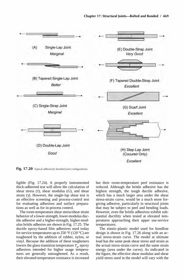
Chapter 17: Structural Joints—Bolted and Bonded / 469
ligible (Fig. 17.24). A properly instrumented thick-adherend test will allow the calculation of shear stress (t), shear modulus (G), and shear strain (g). However, the single-lap shear test is an effective screening and process-control test for evaluating adhesives and surface prepara-tions as well as for in-process control.
the room-temperature shear stress/shear strain behavior of a lower-strength, lower-modulus duc-tile adhesive and a higher-strength, higher-mod-ulus brittle adhesive are shown in Fig. 17.25. the ductile epoxy-based film adhesives used today for service temperatures up to 250 °F (120 °C) are toughened by the addition of rubber, nylon, or vinyl. Because the addition of these tougheners lowers the glass transition temperature Tg, epoxy adhesives intended for higher usage tempera-tures are generally untoughened. As a result, their elevated-temperature resistance is increased
Fig. 17.20 Typical adhesively bonded joint configurations
but their room-temperature peel resistance is reduced. Although the brittle adhesive has the highest strength, the tough ductile adhesive, which has a much larger area under the shear stress-strain curve, would be a much more for-giving adhesive, particularly in structural joints that may be subject to peel and bending loads. However, even the brittle adhesives exhibit sub-stantial ductility when tested at elevated tem-peratures approaching their upper use-service temperatures.
the elastic-plastic model used for bondline design is shown in Fig. 17.26 along with an ac-tual stress-strain curve. the model at ultimate load has the same peak shear stress and strain as the actual stress-strain curve and the same strain energy (area under the curve). As indicated in the figure, the effective shear modulus and shear yield stress used in the model will vary with the

470 / Structural Composite Materials
strain level. two analyses are normally required: (1) an elastic analysis using the actual adhesive shear modulus to make sure that the adhesive will not deform plastically at limit load and (2) an elastic-plastic analysis to predict the actual joint strength. the elastic-plastic analysis is inappro-priate for the lower-load-level case, because the initial shear modulus is too low and the elastic
strain energy is too high. It is important to un-derstand that the simple elastic-plastic model is a mathematical approximation. on unloading, while there is some hysteresis, there is almost complete recovery of the strain; however, it is far from a straight-line load reduction.
the adhesive shear stress-strain curves for a ductile adhesive vary with the operating envi-
Fig. 17.21 Effect of adherend thickness on failure modes of adhesively bonded joints. Ref 8
Fig. 17.22 Typical single-lap shear test specimen

Chapter 17: Structural Joints—Bolted and Bonded / 471
ronment, as illustrated in Fig. 17.27 for a typical example. While the individual properties, such as peak shear strength and strain-to-failure, vary greatly with temperature, the areas under all three curves are quite similar. the ultimate strength of a long-overlap bonded joint between uniform ad-herends is shown by analysis to be defined by the strain energy of the adhesive layer in shear, not by any individual properties, such as peak shear
stress. the strain energy is proportional to the area under each of these curves. Consequently, the strength of a realistically configured bonded joint is not very sensitive to its operating environ-ment, provided that its temperature is kept below the adhesive’s glass transition temperature.
there are several important points that should be considered when testing or characterizing adhesive materials: (1) All test conditions must
Fig. 17.23 Shear of adhesive in balanced joints. Source: Ref 12
Fig. 17.24 Thick adherend test method. Source: Ref 13Fig. 17.25 Typical stress-strain behavior for brittle and duc-
tile adhesives. Source: Ref 8

472 / Structural Composite Materials
Fig. 17.26 Elastic-plastic model. Source: Ref 12
Fig. 17.27 Effect of temperature on adhesive shear stress-strain. RT, room temperature; Source: Ref 12

Chapter 17: Structural Joints—Bolted and Bonded / 473
be carefully controlled, including the surface preparation, the adhesive, and the bonding cycle. (2) tests should be run on the actual joint(s) that will be used in production. (3) A thorough evalu-ation of the in-service conditions must be made, including temperature, moisture, and any solvents or fluids to which the adhesive will be exposed during its service life. the failure modes for all test specimens should be examined. Some accept-able and unacceptable failure modes are shown in Fig. 17.28. For example, if the specimen exhibits
an adhesive failure at the adherend-to-adhesive interface, rather than a cohesive failure within the adhesive, this may be an indication of a sur-face preparation problem that will result in de-creased joint durability. the desired failure mode is a 100 percent cohesive failure of the ad-hesive bondline (Fig. 17.29).
Bonding to composites rather than metals in-troduces significant differences in criteria for adhesive selection for two reasons: (1) compos-ites have lower interlaminar shear stiffness than
Fig. 17.28 Typical failure modes of bonded joints
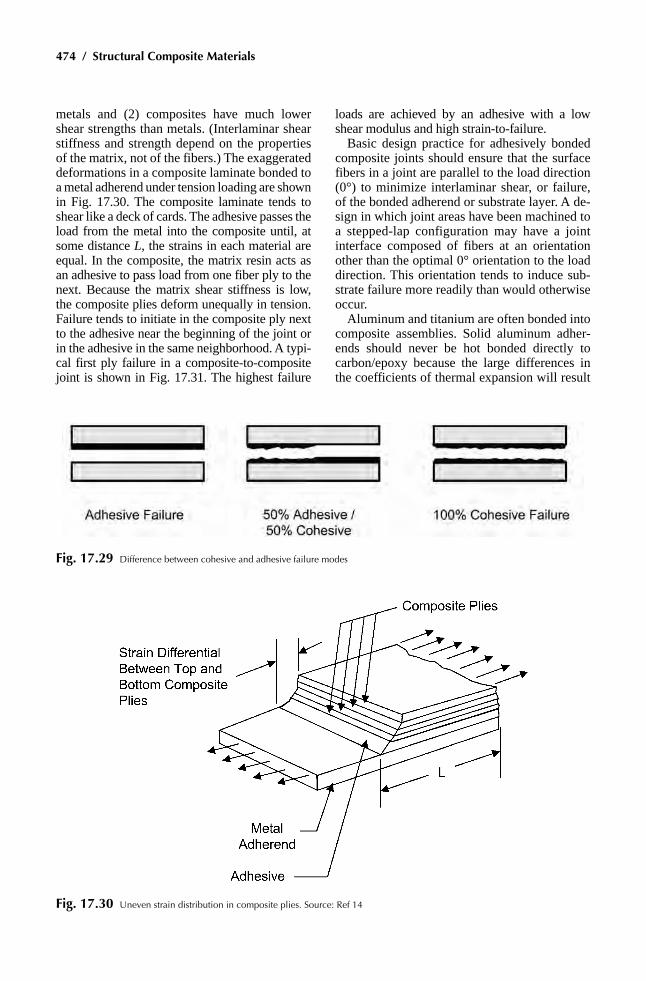
474 / Structural Composite Materials
metals and (2) composites have much lower shear strengths than metals. (Interlaminar shear stiffness and strength depend on the properties of the matrix, not of the fibers.) the exaggerated deformations in a composite laminate bonded to a metal adherend under tension loading are shown in Fig. 17.30. the composite laminate tends to shear like a deck of cards. the adhesive passes the load from the metal into the composite until, at some distance L, the strains in each material are equal. In the composite, the matrix resin acts as an adhesive to pass load from one fiber ply to the next. Because the matrix shear stiffness is low, the composite plies deform unequally in tension. Failure tends to initiate in the composite ply next to the adhesive near the beginning of the joint or in the adhesive in the same neighborhood. A typi-cal first ply failure in a composite-to-composite joint is shown in Fig. 17.31. the highest failure
Fig. 17.29 Difference between cohesive and adhesive failure modes
loads are achieved by an adhesive with a low shear modulus and high strain-to-failure.
Basic design practice for adhesively bonded composite joints should ensure that the surface fibers in a joint are parallel to the load direction (0°) to minimize interlaminar shear, or failure, of the bonded adherend or substrate layer. A de-sign in which joint areas have been machined to a stepped-lap configuration may have a joint interface composed of fibers at an orientation other than the optimal 0° orientation to the load direction. this orientation tends to induce sub-strate failure more readily than would otherwise occur.
Aluminum and titanium are often bonded into composite assemblies. Solid aluminum adher-ends should never be hot bonded directly to carbon/epoxy because the large differences in the coefficients of thermal expansion will result
Fig. 17.30 Uneven strain distribution in composite plies. Source: Ref 14

Chapter 17: Structural Joints—Bolted and Bonded / 475
in significant residual stresses, and because car-bon fiber in contact with aluminum will form a galvanic cell that will corrode the aluminum. total destruction of a bond between carbon/epoxy and aluminum has been observed. A test article was fabricated in which aluminum hinges were cocured to a carbon/epoxy control surface. even though a high strain toughened epoxy film adhe-sive was used, the bondline totally split apart (100 percent cohesive failure) on cooling down from the 350 °F (180 °C) cure cycle due to the residual stresses that developed as a result of the large differences in coefficients of thermal ex-pansion between the two. even if the bond had survived cool-down to room temperature, it would have had little chance of survival if the operating environment subjected it to cold temperatures, for example, –55 °F (–50 °C), in which the re-sidual stresses would have been even greater.
17.8 Bonded Joint Design Considerations
the first rule of adhesively bonded joint de-sign is that in no case should the strength of the joint be less than that of the surrounding struc-ture; otherwise, the bonded joint will have little damage tolerance and can act as a weak link. the strong ductile adhesives typically used by the aerospace industry produce a bond that is in-evitably stronger than the adherends for prop-erly designed joints between thin members. For thicker structures, the bond can always be made stronger than the structure by using enough steps in a stepped-lap joint. Because adhesively bonded joints can be strong in shear but are inevitably weak in peel, the second rule of adhesively bonded joint design is to make sure that the ad-hesive is loaded in shear while minimizing any
Fig. 17.31 First ply failure in a composite-to-composite joint

476 / Structural Composite Materials
direct or induced peel stresses. tension, cleav-age, and peel loading (Fig. 17.32) should all be avoided when using adhesives. In practice, ten-sion loading is acceptable for nonstructural bonds as long as there is appreciable surface area, but certainly not in the butt joint shown.
It is important that bonded joint strengths ex-ceed the strengths of the adherends by at least 50 percent to allow for minor manufacturing flaws or imperfections. the loss of bond strength that is sometimes associated with bondline flaws or damage to the bond is shown in Fig. 17.33. even with such degradation, the bond will be stronger than the adherends. If the adherend
thickness is greater than that for which the bond and member strengths are equal, there is abso-lutely no tolerance with respect to flaws, poros-ity, or damage. the slightest imperfection would lead to catastrophic unzipping of the entire bond area if sufficient load were applied.
there are two factors that affect the long-term durability of adhesively bonded joints: (1) surface preparation and (2) adhesive creep. the impor-tance of proper surface preparation is covered in Chapter 8, “Adhesive Bonding.” Creep is re-stricted by selecting a long enough overlap to pro-duce a low-stress trough, as shown in Fig. 17.34. If a short overlap is used, the minimum adhesive
Fig. 17.32 Load paths to avoid in bonded structure. Source: Ref 14
Fig. 17.33 Relative strength of adhesive and adherends as affected by bond flaws. Source: Ref 6

Chapter 17: Structural Joints—Bolted and Bonded / 477
shear stress and strain are nearly as high as the peak values at the ends. Because adhesive creep can accumulate under both static and cyclic loads, there is no mechanism for the adhesive to recover to its original state when the load is re-moved. A joint with short overlap is susceptible to creep failure, but the adhesive shear stress and strain can be made as low as desired by using a sufficiently long overlap. Although there is creep in the adhesive at the ends of the long overlap, between points F and G, where the stress at point J is high, there is none in the middle, between points D and E, if the stress at point A is low enough. Consequently, the creep that does occur cannot accumulate, because the stiff ad-herends push the adhesive back to its original position whenever the joint is unloaded. this re-covery in part of the adhesive prevents gross
creep and is a key to a durable bonded structure. Without it, there can be no successfully bonded structure.
For structural aluminum alloys, an overlap of approximately 30 times the central adherend thickness is used in a double-lap joint. In addition, because the modulus of nearly quasi-isotropic carbon/epoxy laminates is of the same order of magnitude as for aluminum alloys, a similar overlap-to-thickness ratio would also be satis-factory for such laminates. the static strength of bonded joints between uniform adherends is quite insensitive to the precise length of a suffi-ciently long overlap, as shown in Fig. 17.35. Any longer overlap beyond point C would be superfluous. For all overlaps longer than the abrupt drop in the adhesive shear strain shown in the upper diagram, the maximum strain in the
Fig. 17.34 Nonuniform stresses and strains in bonded joints. Source: Ref 6

478 / Structural Composite Materials
adhesive is limited by the adherend strength to a value below that which would be needed to make the adhesive fail. no such protection is afforded for short overlaps or thick adherends. If the adherends are too thick, the limit on the peak shear strain shown in Fig. 17.35 disap-pears. therefore, a more complex stepped-lap joint is appropriate for adherends thicker than about 0.125 in. (3 mm). the limiting strength of the joint is usually set by the lowest service tem-perature, whereas the design overlap is set by the highest service temperature, at which the ad-hesive is the softest.
Another consideration in the design of bonded joints is the need to restrict the maximum shear strain developed in the adhesive at the ends of the bonded overlap. once the knee in the stress-strain curve has been exceeded, progressively more damage occurs in the adhesive as a result of the tensile stress associated with the shear de-formations. It is therefore necessary to ensure
Fig. 17.35 Influence of overlap on adhesive shear strains. Source: Ref 6
that the design limit load does not strain the ad-hesive beyond the knee in the stress-strain curve. Because the shear strength of the bonded joint is proportional to the square root of the adhesive strain energy in shear, a design ultimate load 50 percent higher than the limit load would be associated with an ultimate shear strain almost twice that at the knee, as shown in Fig. 17.36. the remainder of the stress-strain curve for ductile adhesives is reserved for damage toler-ance and the redistribution of loads around local damage. For brittle adhesives, the limits on joint strength would be established by equating the design ultimate load to the end of the stress-strain curve, which would not contain any dis-tinct knee.
After the overlap length is determined, the elimination of peel stress needs to be addressed. Peel stresses occur for single-lap joints due the eccentricity in the load path, as previously shown in Fig. 17.22. Although not immediately

Chapter 17: Structural Joints—Bolted and Bonded / 479
apparent, peel stresses also occur in seemingly balanced double-lap joints, as shown for the thick composite adherends in Fig. 17.37. the elimination of peel stresses is accomplished by slightly modifying the joint geometry, as shown in Fig. 17.38, in which the tips of the adherends are made thin and flexible so that only negligible peel stresses can develop. local thickening of the adhesive at the tips is beneficial. However, such local thickening of the adhesive layer must be used cautiously with high-flow elevated-temperature-curing adhesives to prevent the cre-ation of voids by capillary action. the use of additional adhesive or scrim fillers can help to prevent any such problems. the exact propor-tions in tapering the adherend or thickening the adhesive layer are not critical. If the overlap is long enough, it is impossible to overdo the peel stress relief. In addition, the natural fillet, or spew, that occurs when the adhesive flows during cure
should never be removed. testing has shown that it improves both the static and fatigue prop-erties of the joint.
17.9 Stepped-Lap adhesively Bonded Joints
Composite laminates that are too thick (and hence too strong) to be joined by simple uni-form lap shear-bonded joints can be successfully bonded together using stepped-lap joints of the type shown in Fig. 17.39. Scarf joints are not attractive because the scarf slope needs to be very shallow (no more than about 0.02), so very long joints would be required for thick lami-nates. each step of the stepped-lap bonded joint is governed by the same differential equation that governs double-lap joints. Consequently, there
Fig. 17.36 Modeling of adhesives for design of shear loads. Source: Ref 12

480 / Structural Composite Materials
is a highly nonuniform shear stress distribution in the adhesive, with the load transfer concentrated at the ends of each step, as shown in Fig. 17.40.
the design and analysis of stepped-lap bonded joints are conducted using computer programs based on an elastic-plastic shear model. Some rules of thumb for initial design are as follows. the end steps must be neither too thick nor too long; 0.030 in. (0.8 mm) thick titanium with a step length of 0.375 in. (10 mm) is typical to prevent fatigue failures. Most of the other steps are usually 0.50 to 0.75 in. (13 to 19 mm) long, with step thicknesses no greater than 0.02 in.
(0.5 mm) and preferably much less on either side of the joint, with one longer step near the middle of the overlap to provide creep resis-tance. once the proportions have been adjusted properly, the most powerful variable with which to increase the joint strength is the number of steps; merely increasing the bond area for the same number of steps is not effective. the strength continues to increase as the number of steps is increased to one per ply, and the number should always be sufficient to ensure that the bond strength exceeds the adherend strengths by at least 50 percent.
Fig. 17.37 Peel stress failure of thick composite joints. Source: after Ref 12

Chapter 17: Structural Joints—Bolted and Bonded / 481
While cocured stepped-lap joints can be used to produce weight-efficient joints in thick com-posites, they are difficult to manufacture and in-spect. A cocured stepped-lap joint is used on the F/A-18 fighter aircraft at the wing root fitting, as shown in Fig. 17.41. A distinct advantage of this joint is that it allows the entire wing to be re-moved and replaced if necessary, as per con-tractual requirements. Manufacturing consists of laying up the bottom half of the plies using tem-plates to locate the plies correctly for mating with the bottom half of the splice plate. the tita-nium splice plate is covered with a layer of film adhesive that is staged at elevated temperature in an oven; staging increases the adhesive viscosity and makes the step locations on the splice plate more easily visible. the staged splice plate is then placed on the bottom half of the lay-up, and the top halves of the plies are laid up to the steps. However, during cure, because the resin be-comes liquid, hydraulic pressure tends to push the plies off the steps, creating gaps. these gaps
produce wrinkling of the continuous plies that bridge over the steps, as shown schematically in Fig. 17.42. While these wrinkles only moder-ately degrade the tension properties, large gaps (wrinkles) can seriously degrade the compres-sion properties because the load-bearing fibers are already prebuckled. Also, inspection and de-tection of gaps must be done using special radio-graphic inspection techniques, and interpreta-tion of the radiographs is difficult. Although this joint has performed flawlessly in service, in practice it probably makes more sense to use mechanically fastened joints for thick composite structures.
17.10 Bonded-Bolted Joints
Analysis has shown that in a joint that is both bonded and mechanically fastened, the mechan-ical fasteners carry only about one percent of the load. In other words, the adhesive carries almost
Fig. 17.38 Tapering edges to reduce peel stresses. Source: after Ref 12

482 / Structural Composite Materials
all of the load until it fails, and then the fasteners pick up the load. therefore, unless a redundant joint is needed, the fasteners just add cost and weight. on the other hand, fasteners are often used to prevent peel stresses in certain instances,
Fig. 17.39 Typical cocured stepped-lap joint. Source: Ref 6
Fig. 17.40 Shear stress and strain distribution in a stepped-lap joint. Source: Ref 6
such as at the ends of cocured stiffeners, as shown in Fig. 17.43. Here, three different peel prevention concepts are used: (1) antipeel fas-teners are used at the end of the hat to prevent delaminations from propagating down the length

Chapter 17: Structural Joints—Bolted and Bonded / 483
Fig. 17.41 Wing root splice fabrication. Source: The Boeing Company

484 / Structural Composite Materials
Fig. 17.42 Gaps on a splice plate
Fig. 17.43 Bonded-bolted joint to prevent peel failures

Chapter 17: Structural Joints—Bolted and Bonded / 485
table 17.3 Guidelines for adhesively bonded jointsGuidelines Remarks
1. never design for an adhesive bond to be the weak link in a structure. the bonds should always be stronger than the members being joined.
Bonded joints must always be designed to be stronger than the adjacent structure; otherwise, the bond can act as a weak-link fuse and unzip catastrophically from a local defect.
2. Use secondary adhesive bonding extensively for thin, lightly loaded composite structures, restricting the use of mechanical fastening mainly to thicker, more heavily loaded structures.
thick bonded joints can fail prematurely in peel. Bonding works best for thin structures.
3. Proper joint design should be used, avoiding tension, peel, or cleavage loading whenever possible. If peel forces cannot be avoided, a lower modulus (nonbrittle) adhesive having a high peel strength should be used.
Adhesives work best in shear and are poor in peel. Composites are even weaker in interlaminar tension.
4. ensure that the bonded joint configuration is 100% inspectable. …
5. Proper surface preparation is critical. Beware of cleaning solvents and peel plies. Mechanical abrasion is more reliable.
Surface gloss must be removed. Some peel plies use silicone.
6. Bonded joint strength is usually less in a cold environment, where adhesive is brittle.
…
7. Balanced adherend stiffnesses improve joint strength. …
8. Minimize joint eccentricities. eccentricities cause bending and peel stresses in adhesive.
9. Use adherends with similar coefficients of thermal expansion. …
10. Use ductile adhesives rather than brittle ones. ductile adhesives are far more forgiving than brittle adhesives.
11. Use film adhesives rather than pastes. Film adhesives have higher strength and controlled bondline thickness.
12. Adhesives are well characterized by a thick-adherend test coupon, generating a complete nonlinear stress-strain curve in shear.
…
13. Be aware of the need to dry laminates before doing bonded repairs.
desorbing moisture during cure can blow out adhesive.
14. Care is needed to taper the ends of bonded overlaps—down to 0.020 in. thick with a 1-in-10 slope—to minimize induced peel stresses that would cause premature failures.
…
15. design of simple, uniformly thick (for nearly quasi-isotropic carbon/epoxy) bonded splices is very simple—about 30t overlap in double shear, 80t overlap for single-lap joints, and a 1-in-30 slope for scarf joints.
…
16. For highly loaded bonded joints, cocured, multiple-step, double-sided lap joints are preferred.
…
17. thick bonded structures need complex stepped-lap joints to develop adequate efficiency.
…
18. design of stepped-lap joints for thick structure needs a nonlinear analysis program.
…
19. thick bonded structures are very difficult to repair; so, except for one-shot and throwaway structures, original designs should be bolted together to permit bolted repairs.
…
20. the fillet or spew at the end of the exposed joint should not be removed.
Fillet improves static and fatigue properties.
21. Selection tests for structural adhesives should include durability testing for heat, humidity (and/or fluids), and stress simultaneously.
Prevents unexpected long-term durability problems.
Composite-to-metal splice joints22. Bonded step joints preferred to scarf joints. More consistent results.
23. Where possible, 0° plies (primary load direction) should be placed adjacent at the bondline; 45° plies are also acceptable; 90° plies should never be placed adjacent to the bondline unless it is also the primary load direction.
to maximize lap shear.
24. For a stepped joint, the metal thickness at the end step should be 0.020 in. minimum.
to prevent metal failure
(continued)

486 / Structural Composite Materials
table 17.3 (continued)Guidelines Remarks
25. If possible, have ± 45° plies end on the first and last steps of bonded step joints.
…
26 If possible, do not end more than two 0° plies (not more than 0.014 maximum thickness) on any one step surface.
…
27. tension and peel stresses should be avoided in adhesive bonded joints.
Good design practice.
Composite-to-metal continuous joints28. Bonding composites to titanium (preferred) and steel
(acceptable).Material compatibility and best match of expansion coefficients.
29. thermal expansion of dissimilar materials must be considered. due to the large thermal expansion difference between carbon composite and aluminum, adhesively bonded joints between these two materials have been known to fail during cool-down from elevated-temperature cures as a result of the thermal stresses induced by their differential expansion coefficients.
to minimize interlaminar shear stress due to the large difference in the coefficient of thermal expansion between carbon composites and aluminum.
of the bondline, (2) the end of the hat is scarfed to allow a more gradual transition of the loads, and (3) the skin itself is thickened under the hat end to make the joint stiffer.
Some general design guidelines for adhe-sively bonded joints are given in table 17.3.
aCknowLeDGMent
dr. John Hart-Smith, while working for the douglas Aircraft Company, a part of Mcdonnell-douglas Corporation and now Boeing, is the ac-knowledged world leader in developing analysis methods for both mechanically fastened and ad-hesively bonded joints. He developed almost all of the concepts covered in this chapter.
reFerenCeS
1. d.W. oplinger, Mechanical Fastening and Adhesive Bonding, HandbookofCompos-ites, Chapman & Hall, 1982
2. A. Baker, S. dutton, and d. Kelly, Compos-ite Materials for Aircraft Structures, 2nd ed., American Institute of Aeronautics and Astronautics, Inc., 2004
3. l.J. Hart-Smith, “Bolted Joint Analysis for Fibrous Composite Structures—Current empirical Methods and Future Scientific Prospects,” AStM StP 1455, JoiningandRepairofCompositeStructures, American Society for testing and Materials, 2004
4. J.A. Baile, M.F. duggan, n.C. Bradshaw, and t.G. McKenzie, “design data for Car-
bon Cloth epoxy Bolted Joints at tempera-tures up to 450K,” AStM StP 749, JoiningofCompositeMaterials, American Society for testing and Materials, 1981
5. r.t. Parker, Mechanical Fastener Selection, ASMHandbook,Vol 21, Composites, ASM International, 2001, p 651–658
6. l.J. Hart-Smith, Bolted and Bonded Joints, ASMHandbook,Vol 21, Composites, ASM International, 2001
7. “redux Bonding technology,” Hexcel Composites, december 2001
8. r.B. Heslehurst and l.J. Hart-Smith, the Science and Art of Structural Adhesive Bonding, SAMPEJ., Vol 38 (no. 2), Mar/Apr 2002, p 60–71
9. l.J. Hart-Smith, “Adhesive-Bonded Single-lap Joints,” nASA Contract report nASA Cr 112236, 1973
10. l.J. Hart-Smith, “Adhesive-Bonded double-lap Joints,” nASA Contract report nASA Cr 112235, 1973
11. l.J. Hart-Smith, “Adhesive-Bonded Scarf and Stepped-lap Joints,” nASA Contract report nASA Cr 112237, 1973
12. l.J. Hart-Smith, the design of Adhesively Bonded Joints, AdhesionScienceandEngi-neering,Vol 1,TheMechanicsofAdhesion, elsevier Science, 2002
13. r.B. Krieger, Analyzing Joint Stresses Using an extensometer,Adhes.Age,Vol 28 (no. 11), oct 1985, p 26–28
14. F.C. Campbell, Secondary Adhesive Bond-ing of Polymer-Matrix Composites, ASMHandbook, Vol 21, Composites, ASMHandbook 21, ASM International, 2001

Chapter 17: Structural Joints—Bolted and Bonded / 487
SeLeCteD reFerenCeS
• l.J. Hart-Smith, “design Methodology for Bonded-Bolted Composite Joints,” AFWAl-tr-81-3154, 1982
• l.J. Hart-Smith, design and Analysis of Bolted and riveted Joints in Fibrous Com-posite Structures, RecentAdvancesinStruc-
turalJointsandRepairsforCompositeMate-rials, Kluwer Academic Publishers, 2003
• l.J. Hart-Smith, Adhesively Bonded Joints for Fibrous Composite Structures, RecentAdvances in Structural Joints and RepairsforCompositeMaterials, Kluwer Academic Publishers, 2003

“This page left intentionally blank.”

Structural Composite Materials Copyright © 2010, ASM International®
F.C. Campbell All rights reserved.www.asminternational.org
Chapter 18
Design and Certification Considerations
the Author worked on his first air-craft program in the mid-1970s when there were no computers or workstations. designers made drawings on large plastic sheets with ink pens. the strength engineer specified the laminate ori-entations and number of plies needed to meet strength and stiffness requirements; the designer took overall responsibility for the design, con-sulting with the proper engineering group when there was a technical question.
today’s design environment is totally different. designs are now created by concurrent engineer-ing or integrated product definition (IPd) teams that consist of engineering, tooling, manufactur-ing, quality, and supportability personnel. even the customers participate in preliminary, critical, and final design reviews. design tools have also greatly improved. Computerized laminate analy-sis codes and finite element modeling tools are available for detailed composite designs. Modern design is done on workstations with advanced computer-aided design (CAd)/computer-aided manufacturing (CAM) packages.
Integrated product definition teams have more freedom with composite construction than they do when using traditional metals, because with composites they are free to select different rein-forcements, combine them with a choice of dif-ferent matrices, and then fabricate them using a variety of processes. the design team is free to determine the amount and distribution of the constituents. A composite laminate can be built to any thickness, and the fibers may be oriented to achieve the desired strength and stiffness. Al-though this design freedom increases the num-ber of choices, it also makes the process more complex.
this chapter will cover, to a very limited ex-tent, the activities of the IPd team during the design process. topics covered include material selection, manufacturing process selection, ini-tial trade studies to select the material and de-sign concept, the building block approach to testing and certification used in the aerospace industry, design allowables, and some guide-lines for detailed design. In addition, a number of considerations important in composites design are covered, including damage tolerance and en-vironmental sensitivity. Although these activi-ties are discussed serially in this chapter, they are actually conducted in an iterative manner, especially in the early stages of the design pro-cess. once the design is finalized, it is expensive to have to go back and change it. It has been postulated that as much as 90 to 95 percent of the final product cost is determined by the deci-sions made during the first five percent of the design process. therefore, it is important to do the upfront work carefully before the detailed design starts.
18.1 Material Selection
In the materials selection process, a broad choice can be made between the use of compos-ite construction, metals, unreinforced polymers, and natural materials. As a general guideline, if a part can easily be fabricated from a traditional material like aluminum, steel, wood, or plastic, this choice may represent the lowest-cost solu-tion. however, composite construction has many advantages, including reduced weight, higher stiffness, and better corrosion resistance.

490 / Structural Composite Materials
18.2 Fiber Selection
Since the fibers provide the strength and stiff-ness, it is appropriate to consider fiber selection first. Glass fibers are the most widely used rein-forcement because of their good balance of me-chanical properties and low cost. e-glass is the most common glass fiber and is used extensively in commercial composite products. e-glass is a low-cost, high-density, low-modulus fiber that has good corrosion resistance and good handling characteristics. S-2 glass was developed in re-sponse to the need for a higher-strength fiber for filament-wound pressure vessels and solid rocket motor casings. Although more expensive than e-glass, it has a density, performance and cost between those of e-glass and carbon. Quartz fiber is used in many electrical applications because of its low dielectric constant; however, it is very expensive.
Aramid fiber (such as kevlar) is an organic fiber that has a low density and is extremely tough, exhibiting excellent damage tolerance. It has a high tensile strength but performs poorly in compression. It is also sensitive to ultraviolet light and should be used for long-term service only at temperatures less than 300 °F (150 °C). Another organic fiber is made from ultra-high molecular weight polyethylene (uhMwPe), such as Spectra. It has a low density with excellent radar transparency and a low dielectric constant. Because of its low density, it exhibits very high specific strength and modulus at room tempera-ture. however, being polyethylene, it cannot with-stand temperatures higher than 200 °F (90 °C). Like aramid and S-2 glass, uhMwPe has ex-cellent impact resistance; however, like aramid, it often exhibits poor adhesion to its matrix.
Carbon fiber offers the best combination of properties but is also more expensive than either glass or aramid. Carbon fiber has a low density and a low coefficient of thermal expansion (Cte), and it is conductive. It is structurally very effi-cient and exhibits excellent fatigue resistance. It is also brittle (strain-to-failure less than two per-cent) and exhibits low impact resistance. Being conductive, it causes galvanic corrosion if placed in direct contact with more anodic metals (such as aluminum). Carbon and graphite fibers are available in a wide range of strength and stiffness, with strengths of 300 to1000 ksi (2000 to 7000 MPa) and moduli of 30 to 145 msi (4 to 21 GPa). with this wide range of properties, carbon fiber is frequently classified as either (1) high strength, (2) intermediate modulus, or (3) high modulus.
Both carbon and graphite fibers are produced as untwisted bundles called tows. Common tow sizes are 1k, 3k, 6k, 12k, and 24k, where k = 1000 fibers. Immediately after fabrication, car-bon and graphite fibers are normally surface-treated to improve their adhesion to the poly-meric matrix.
Several other fibers are occasionally used for polymeric composites. Boron fiber was the orig-inal high-performance fiber before carbon was developed. It is a large-diameter fiber that is made by pulling a fine tungsten wire through a long, slender reactor in which boron is applied by chemical vapor deposition. Since it is made one fiber at a time rather than thousands of fi-bers at a time, it is very expensive. owing to its large diameter and high modulus, it exhibits out-standing compression properties. on the nega-tive side, it does not conform well to compli-cated shapes and is very difficult to machine. other high-temperature ceramic fibers, such as silicon carbide (Nicalon), aluminum oxide, and alumina boria silica (Nextel), are frequently used in ceramic-based composites but rarely in polymeric composites.
the following factors should be considered when choosing among glass, aramid, and carbon fibers:
• Tensile strength. If tensile strength is the pri-mary design parameter, e-glass may be the best selection because of its low cost.
• Tensile modulus. when designing for tensile modulus, carbon has a distinct advantage over both glass and aramid.
• Compression strength. If compression strength is the primary requirement, carbon has a dis-tinct advantage over glass and aramid. Be-cause of its poor compression strength, aramid should be avoided.
• Compression modulus. Carbon fiber is the best choice, e-glass the worst.
• Density. Aramid fibers have the lowest density, followed by carbon and then S-2 and e-glass.
• Coefficient of thermal expansion. Aramid and carbon fibers have a Cte that is slightly neg-ative, whereas the Ctes of S-2 and e-glass are positive.
• Impact strength. Aramid and S-2 fibers have excellent impact resistance, but carbon is brit-tle and should be avoided. however, it should be noted that matrix selection also has a sig-nificant influence on impact strength.
• Environmental resistance. Matrix selection has the biggest impact on composite environ-

Chapter 18: Design and Certification Considerations / 491
mental resistance. however, (1) aramid fibers are degraded by ultraviolet light, and the long-term service temperature should be kept below 300 °F (150 °C); (2) carbon fibers are subject to oxidation at temperatures ex-ceeding 700 °F (370 °C), although long-term 1000 hours of thermal oxidation stability tests in polyimides have shown strength decreases in the 500 to 600°F (260 to 315 °C) range; and (3) glass sizings tend to be hydrophilic and absorb moisture.
• Cost. e-glass is the least expensive fiber and carbon is the most expensive. In carbon, the smaller the tow size, the more expensive the fiber. Larger tow sizes help reduce labor costs because more material is deposited with each ply. however, large tow sizes in woven cloth can increase the chances of voids and
matrix microcracking caused by larger resin pockets.
18.3 product Form Selection
A multitude of material product forms are used in composite structures, some of which are illus-trated in Fig. 18.1. the fibers can be continuous or discontinuous. they can be oriented or disori-ented (random). they can be furnished as dry fi-bers or preimpregnated with resin (prepreg).
Not all fiber or matrix combinations are avail-able in a particular material form, since the mar-ket drives availability. In general, the more op-erations required by the supplier, the higher the cost. For example, prepreg cloth is more expen-sive than dry woven cloth. while complex dry
Fig. 18.1 Product forms used in composites

492 / Structural Composite Materials
preforms may be expensive, using them can lower fabrication costs overall by reducing or eliminating hand lay-up costs. If structural effi-ciency and weight are important design param-eters, continuous-reinforced product forms are normally used because discontinuous fibers yield lower mechanical properties. Some common trade-offs when selecting composite materials are given in table 18.1, and a comparison of be-tween dry fiber/neat resin and prepreg is pre-sented in table 18.2.
18.3.1 Discontinuous-Fiber Product Forms
Chopped fiber is made by mechanically chop-ping rovings, yarns, or tows into short lengths, typically 1/4 to 2 in. (6 to 50 mm) long. It is im-portant that the chopped fibers be no shorter than this to ensure maximum reinforcement efficiency. Milled fibers, typically 1/32 to 1/4 in. (0.8 to 6 mm) long, have low aspect ratios (length/diameter) that provide minimal strength and therefore should not be considered for struc-tural applications. the strength of the composite is greatly improved with increased fiber length, although stiffness is much less affected. Chopped glass fibers are often embedded in thermoplastic or thermoset resins in the form of pellets for in-jection molding.
Chopped fibers or entangled continuous strands are combined with a binder to form mat or veil materials. A veil is a thin mat that is used to im-prove the surface finish of a molded composite.
this material form is used extensively for auto-motive, industrial, recreational, and marine ap-plications, where high-quality Class A exterior surface finishes are required. these are very in-expensive product forms in which e-glass is the fiber most commonly used. other fibers may be available in mat form, but they are generally ex-pensive due to the specialty nature of the prod-uct. At the time of this writing, carbon mats are uncommon because of low demand. Some car-bon veils for electromagnetic interference pro-tection are available (though expensive). his-torically, the aerospace industry has not been interested in this product form because of its low structural inefficiency and the weight penalty as-sociated with its discontinuous reinforcement. the automotive industry has not been interested in it either; although the industry uses mats ex-tensively, it has not been willing to pay the cost penalty for carbon-fiber material.
Sheet molding compound (SMC) consists of flat sheets of chopped, randomly oriented fibers, typically 1 to 2 in. (25 to 50 mm) in length, with a B-staged resin matrix, usually consisting of e-glass fiber in either a polyester or vinyl ester resin. the material is available either as rolls or as precut sheets. Bulk molding compounds (BMCs) are also short, randomly oriented pre-impregnated materials; however, the fibers are normally only 1/8 to 11/4 in. (3 to 6 mm) long, and the reinforcement percentage is lower. As a re-sult, the mechanical properties of BMC compos-ites are lower than those of SMC composites.
table 18.1 Common trade-offs when selecting composite materialsDesign decision Common trade-offs Typically lowest cost Typically highest performance
Fiber type Cost, strength, stiffness, density (weight), impact strength, electrical conductivity, environmental stability, corrosion, thermal expansion
e-glass Carbon
tow size (if carbon is selected)
Cost, fiber volume, improved fiber wet-out, structural efficiency (minimize ply thickness), surface finish
12k tow 3k tow
Fiber modulus (if carbon is selected)
Cost stiffness, weight, brittleness Lowest-modulus carbon
highest-modulus carbon
Fiber form (continuous vs. discontinuous)
Cost, strength, stiffness, weight, fiber volume, design complexity
random/discontinuous oriented and continuous
Matrix Cost, service temperature, compressive strength, interlaminar shear, environmental performance (fluid resistance, uV stability, moisture absorption), damage tolerance, shelf life, processability, thermal expansion
Vinyl ester and polyester
high-temperature— polyimide(a)
Low-moderate temperature— epoxy
toughness—toughened epoxy
Composite material forms Cost (material and labor), process compatibility, fiber volume control, material handling, fiber wet-out, material scrap
Base form—neat resin/rovings
Prepreg(b)
(a) depends on how “highest performance” is defined—high temperature, toughness, and superior mechanical properties. (b) Material form is not driven by performance, but is typically defined by the manufacturing process.

Chapter 18: Design and Certification Considerations / 493
Bulk molding compounds are available in dough-like bulk form or are extruded into logs for eas-ier handling. Vinyl esters, polyesters, and phe-nolics are the most common matrices used for BMCs. Sometimes, for convenience of termi-nology, chopped prepreg, used for compression molding, is referred to as BMC.
18.3.2 Continuous-Fiber Product Forms
rovings, tows, and yarns are collections of continuous fiber. this is the basic material form; it can be chopped, woven, stitched, or pre-pregged into other product forms. It is the least expensive product form, and it is available for all fiber types. rovings and tows are supplied with no twist; yarns have a slight twist, which im-proves their handleability at the expense of fiber strength. Some processes, such as wet filament winding and pultrusion, use rovings as their pri-mary product forms.
Continuous-thermoset prepreg materials are available in many fiber and matrix combina-tions. A prepreg is a fiber form that has a prede-termined amount of uncured resin impregnated in the fiber by the material supplier. Prepreg rov-ings and tapes are usually used in automated processes (for example, filament winding and automated tape laying); unidirectional tape and prepreg fabrics are used for hand lay-up. unidi-rectional prepreg tapes offer improved structural properties compared to woven prepregs because there is no fiber crimp and because designs can be tailored more easily. however, the increased drapability of woven prepregs makes them at-tractive for complex substructure parts. with the exception of predominantly unidirectional de-signs, unidirectional tapes require placement of more individual plies during lay-up. For exam-ple, with cloth, for every 0° ply in the lay-up, a 90° reinforcement is also included. with unidi-rectional tape, a 0° ply and a separate 90° ply must be placed on the tool.
Prepregs are supplied with either a net resin (prepreg resin content ≈ final part resin content) or excess resin (prepreg resin content > final part resin content). the excess resin approach relies on the matrix flowing through the plies, remov-ing entrapped air, while the extra resin is re-moved by impregnating bleeder plies on top of the lay-up. the amount of bleeder used in the lay-up dictates the final fiber and resin content; however, as the laminate gets thicker, it becomes more difficult to remove the excess resin. Accu-rate calculations of the number and areal weight of bleeder plies for a specific prepreg are re-quired to ensure the correct final physical proper-ties. Since the net resin approach contains the final resin content weight in the prepreg, no resin re-moval is necessary and the fiber and resin volumes can therefore be easily controlled. thermoset pre-preg properties include volatile content, resin con-tent, resin flow, gel time, tack, drape, shelf life, and out-time. Careful testing, evaluation, and control of these characteristics are necessary to ensure that the prepreg materials’ handling char-acteristics are optimal and final part structural performance is obtained.
woven fabric is the most common continuous dry material form. A woven fabric consists of interlaced warp and fill yarns. the warp is in the 0° direction as the fabric comes off the roll, and the fill (or weft) is the 90° fiber. typically, woven fabrics are more drapable than stitched materi-als; however, the specific weave pattern will af-fect their drapability. the weave pattern will also affect the handleability and structural prop-erties of the woven fabric. Many weave patterns are available. All weaves have advantages and disadvantages, and consideration of the part con-figuration is necessary during fabric selection. Most fibers are available in woven fabric form. however, it can be very difficult to weave some high-modulus fibers due to their inherent brit-tleness. Advantages of woven fabric include drap-ability, ability to achieve high fiber volumes, structural efficiency, and market availability. A disadvantage of woven fabric is the crimp that is introduced in the fibers during weaving, which adversely affects the strength properties. Fin-ishes or sizings are typically put on the fibers to aid in the weaving process and minimize fiber damage. It is important to ensure that the finish is compatible with the matrix selection when specifying a fabric.
A stitched fabric consists of unidirectional fi-bers oriented in specified directions and then stitched together. A common stitched design
table 18.2 relative comparison of dry fiber/neat resin and prepreg
Dry fiber/neat resin Prepreg
Cost Lower higherShelf life Better worseStorage Better worseMaterial handling• drapability Better worse• tack worse Betterresin control worse BetterFiber volume control worse BetterPart quality worse Better

494 / Structural Composite Materials
includes 0°, +45°, 90°, and -45° plies in one multidirectional fabric. Advantages include the following: (1) off-axis orientations can be in-corporated as the fabric is removed from the roll. off-axis cutting is not needed for a multidirec-tional stitched fabric and can reduce scrap rates (up to 25 percent) compared to conventional woven materials. (2) Labor costs are also reduced when multi-ply stitched materials are used be-cause fewer plies need to be cut or handled during fabrication of a part. (3) Ply orientation remains intact during handling because of the z-axis stitch threads. disadvantages include the following: (1) only specific stitched ply set designs are available without customization. typically, tailor-ing to the requirements of a customer will neces-sitate a special order. (2) Not as many companies stitch as weave. (3) drapability is reduced (which, however, can be an advantage for parts with large, simple curvature). Careful selection of the stitch-ing thread is necessary to ensure compatibility with the matrix and process temperatures.
Hybrids are material forms that make use of two or more fiber types. Common hybrids include glass/carbon, glass/aramid, and aramid/carbon fibers. hybrids are used to take advantage of properties or features of each reinforcement type. In a sense, a hybrid is a trade-off reinforce-ment that allows increased design flexibility. hy-brids can be interply (two alternating layers), in-traply (both in one layer), or hybridized only in selected areas. hybridization with carbon in se-lected areas is usually performed to increase the local strength or stiffness of a part, whereas hybridization with glass in carbon laminates is performed to make the laminate locally softer. Carbon/aramid hybrids have low thermal stresses compared to other hybrids (because the two ma-terials have similar Ctes), increased modulus and compressive strength compared to an all-aramid design, and increased toughness com-pared to an all-carbon design. Carbon/e-glass hybrids have increased properties compared to an all-e-glass design but lower cost than an all-carbon design. the Cte of each fiber type in a hybrid needs careful evaluation to ensure that no high internal stresses are introduced to the lami-nate during cure, especially at higher cure tem-peratures. the use of hybrids normally increases the amount of material that must be stocked and can increase the lay-up costs.
A preform is a preshaped fibrous reinforce-ment that has been formed on a mandrel or in a tool before it is placed into a mold. the shape of the preform closely resembles the final part
configuration; a simple multi-ply stitched fabric is not a preform unless it is shaped to approxi-mately its final configuration. the preform is the most expensive dry, continuous, oriented fiber form; however, using preforms can reduce fabri-cation labor. A preform can be made using rov-ings, chopped, woven, stitched, or unidirectional material forms. these reinforcements are formed and held in place by stitching, braiding, or three-dimensional weaving, or with organic binders or tackifiers. Advantages include reduced labor costs, minimal material scrap, reduced fiber fray-ing of woven or stitched materials, improved dam-age tolerance for three-dimensional stitched or woven preforms, and the fact that desired fiber orientations are locked in place. disadvantages include high preform costs, fiber wettability concerns for thick, complex shapes, possible in-compatibility between the tackifier or binder and the matrix, and limited flexibility if design changes are required. A common defect is that the preform is out of tolerance and therefore hard to place in the tool, and it may have to be trimmed. the use of preforms is not appropriate for all applications. All issues must be carefully considered before a preform is baselined. If the component is not a very complex configuration, the money saved in labor reduction may not off-set the cost of the preform. each application should be evaluated individually to determine whether the preform approach offers cost and quality advantages.
8.4 Matrix Selection
the matrix holds the fibers in their proper po-sition, protects the fibers from abrasion, transfers loads between fibers, and provides the matrix-dependent mechanical properties. A properly chosen matrix also provides resistance to heat, chemicals, and moisture; has a high strain-to-failure; cures at as low a temperature as possible and yet has a long pot or out-time life; and is nontoxic. Matrices for polymeric composites can be either thermosets or thermoplastics. the most prevalent thermoset resins used for composite matrices are polyesters, vinyl esters, epoxies, bis-maleimides, cynate esters, polyimides, and phe-nolics. A comparison of the major thermoset resin systems is given in table 18.3.
the first consideration in selecting a resin sys-tem is the service temperature required for the part. the glass transition temperature Tg is a good indicator of the temperature capability of

Chapter 18: Design and Certification Considerations / 495
the matrix. the Tg of a polymeric material is the temperature at which it changes from a rigid, glassy solid to a softer, semiflexible material. At this point, the polymer structure is still intact but the crosslinks are no longer locked in position. A resin should never be used above its Tg unless the service life is very short (for example, a mis-sile body). A good rule of thumb is to select a resin in which the Tg is 50 °F (28 °C) higher than the maximum service temperature. Since most polymeric resins absorb moisture, thereby low-ering the Tg, it is not unusual to require that the Tg be as much as 100 °F (56 °C) higher than the service temperature. therefore:
Maximum usage temperature = wet Tg - 50 °F
(eq 18.1)
different resins absorb moisture at different rates, and the saturation levels can be different as well; therefore, each specific resin candidate must be evaluated for environmental performance. In general, thermoplastics absorb less moisture than thermosets. however, some thermoplastics, in particular amorphous thermoplastics, have poor solvent resistance. Most thermoset resins are fairly resistant to solvents and chemicals.
In general, the higher the temperature perfor-mance required, the more brittle and less damage-tolerant the matrix. toughened thermoset resins are available, but they are more expensive and their Tgs are typically lower. high-temperature resins are also more costly and more difficult to process. temperature performance is difficult to quantify because it is dependent on time at tem-perature, but it is important to have a thorough understanding of the environment in which the matrix is expected to perform.
higher-Tg resins also require higher cure tem-peratures and longer times. epoxies generally
have cure times of two to six hours at elevated temperatures. A postcure may not be required for some epoxies, polyesters, and vinyl esters; therefore, elimination of postcure requirements should be evaluated as a possible way to de-crease processing costs if the service tempera-ture is low enough. higher-Tg resins (such as bismaleimides and polyimides) require longer cure cycles and postcures. Postcuring further de-velops higher-temperature mechanical proper-ties and improves the Tg of the matrix for some epoxies, bismaleimides, and polyimides. Very short cure times are desired for some processes (such as compression molding and pultrusion). Cure temperatures can range from 250 to 350 °F (120 to 180 °C) for epoxies. Bismaleimide cure temperatures typically range from 350 to 475 °F (177 to 246 °C), including postcure. Polyimide cure and postcure temperatures range from 600 to 700 °F (315 to 370 °C).
Polyesters, vinyl esters, epoxies, cynate es-ters, and bismaleimides are all addition-curing systems, whereas phenolics and polyimides cure by condensation reactions that evolve water or alcohols. Since the evolution of volatiles in-creases the propensity for voids and porosity, condensation-curing materials are more difficult to process. however, phenolics are often pro-cessed by compression molding processes, in which high pressures can be applied to suppress void formation. In addition, phenolic matrix composites are often used for interior furnish-ings for commercial aircraft because they tend to char instead of burn. Since these are only lightly loaded structures, the void content is not very important. Since polyimide matrix compos-ites are more difficult to process than addition-curing systems, their usage should be restricted to high-temperature applications where they are really required.
table 18.3 Comparison of thermoset matrix systemsAttribute Polyester Vinyl ester Epoxy Phenolic Bismaleimide Cynate ester
Applicationstypical applications Marine, general Marine, general Aerospace,
generalFire, smoke, and
toxicity apps.Aerospace,
electricalAerospace
PerformanceStructural Fair Good Good Good, brittle Good GoodCorrosion and chemical
resistancePoor excellent Good excellent Good excellent
Moisture absorption Poor excellent Fair to good excellent Fair to good excellentGlass transition
temperature (Tg)(°F)(a)160 160–325 with
post cure200–350 with
post cure160–250+ with
post cure300–425 with
post cure350–450 with
post cureFire, smoke, and toxicity … requires
additivesreqs. adds. excellent Good Good
(a) Actual Tg varies with each system and cure method. Source: ref 1

496 / Structural Composite Materials
Although fiber selection usually dominates the mechanical properties of the composite, matrix selection can also influence performance. Some resins wet out and adhere to fibers better than others, forming a chemical and/or mechanical bond that affects the fiber-to-matrix load transfer capability. the matrix can also microcrack dur-ing cure or in service. resin-rich pockets and brittle resin systems are susceptible to micro-cracking, especially when the processing tem-peratures are high and the use temperatures are low, for example −65 °F (−36 °C), since this con-dition creates a very large difference in thermal expansion between the fibers and the matrix. Again, toughened resins help prevent micro-cracking but often at the expense of elevated-temperature performance.
18.5 Fabrication process Selection
once the fiber, product form, and matrix are selected, the fabrication process selection is nar-rowed to those used to make discontinuous-fiber composites and those used to make the higher-strength and -stiffness continuous-fiber compos-ites. often the material product form will be a major determining factor in the process selected, as shown in the examples in table 18.4.
18.5.1 Discontinuous-Fiber Processes
Injection molding is a high-volume process used to make small to medium-sized parts. the reinforcement is usually chopped glass fibers with either a thermoplastic or thermoset resin; the majority of applications use thermoplastics because these process faster and have greater toughness. In the injection molding process, pel-
lets containing embedded fibers or chopped fibers and resin are fed into a hopper. they are heated to their melting temperature and then injected under high pressure into a matched metal die. After the thermoplastic part cools or the thermoset part cures, they are ejected and the next cycle is started. Since expensive matched die molds are required, the number of parts to be produced must be large enough that the tooling cost can be recovered. Labor costs are minimal, as most in-jection molding facilities are highly automated and have only a minimal number of operators.
Spray-up is a more cost-effective process than wet lay-up, but the mechanical properties are greatly reduced by the use of randomly oriented chopped fibers. Continuous glass roving is fed into a special gun that chops the fibers into short lengths and simultaneously mixes them with ei-ther a polyester or a vinyl ester resin that is then sprayed onto the tool. Manual compaction with rollers is used to compact the lay-up. Vacuum bag cures can be used to improve part quality, but this is not common practice. Since the fibers are short and the orientation is random, this process is not used to make structural load-bearing parts.
Compression molding is another matched-die process that uses either discontinuous, randomly oriented SMC or BMC. A charge of predeter-mined weight is placed between the two dies, and then heat and pressure are applied. the molding compound flows to fill the die and then cures in one to five minutes, depending on the type of polyester or vinyl ester used. thermo-plastic composites, usually consisting of glass fiber and polypropylene for the automotive in-dustry, are compression molded using highly automated production lines.
reaction injection molding (rIM) is a process for rapidly making unreinforced thermoset parts.
table 18.4 typical material product forms versus processProcess
Material form Pultrusion RTM Compression molding Filament winding Hand lay-up Auto tape laying
DiscontinuousSheet molding compound … … l … … …Bulk molding compound … … l … … …
Random continuousSwirl mat/neat resin l l l l l …
Oriented continuousunidirectional tape … … l … l lwoven prepreg … … l … l …woven fabric/neat resin l l … l l …Stitched material/neat resin … l … … … …Prepreg roving … … … l … …roving/neat resin l … … l l …Preform/neat resin … l … … … …

Chapter 18: Design and Certification Considerations / 497
A two-component highly reactive resin system is injected into a closed mold, where the resin quickly reacts and cures. Polyurethanes are the most prevalent, but nylons, polyureas, acrylics, polyesters, and epoxies have also been used. the rIM resin systems have very low viscosities and can be injected at low pressures less than 100 psi (700 kPa) so that inexpensive molds and low-force clamping systems can be used. typical tooling materials include steel, cast aluminum, electroformed nickel, and composites. Cycle times as short as two minutes for large automo-tive bumpers are typical. reinforced reaction injection molding (rrIM) is similar to rIM ex-cept that short glass fibers are added to one of the resin components. the fibers must be ex-tremely short, for example 0.03 in. (0.8 mm), or the resin viscosity will be too great. Short fi-bers, milled fibers, and flakes are commonly used. Again, polyurethanes are the predominant resin system. the addition of the fibers im-proves modulus, impact resistance, and dimen-sional tolerance and lowers the Cte. Structural reaction injection molding (SrIM) is similar to the previous two processes except that a con-tinuous glass preform is placed in the die prior to injection. Again, this process is used almost exclusively with polyurethanes. owing to the highly reactive resins and short cycle times, SrIM cannot produce as large a part size as resin transfer molding (rtM). Also, SrIM parts have lower fiber volumes and are more porous than rtM parts.
18.5.2 Continuous-Fiber Processes
wet lay-up in open molds is the least expen-sive process for a relatively small number of units. this is a common process for large production marine manufacturing, where thick, heavy, woven fiberglass mat and randomly oriented chopped fiber mat are hand or spray impregnated with polyester resin and cured at room temperature. After the ply is placed on the lay-up, hand roll-ers are used to remove excess resin and air and compact the plies. After lay-up, cure can be done at room or elevated temperature. Cure is frequently performed without a vacuum bag, but vacuum pressure helps to improve laminate quality. Since cure is usually performed at room or low temperatures, very inexpensive tooling (such as wood or fiberglass) can be used to min-imize the cost. Although the process is condu-cive to large and inexpensive production, it does not generally optimize fiber properties and often
fails to minimize weight, and the level of preci-sion is very operator-dependent.
Prepreg materials often offer the best mechan-ical properties. Prepreg provides a consistent product with a uniform distribution of reinforce-ment and resin, with high fiber volume frac-tions possible. Since laminated structures typi-cally require much hand labor and autoclave processing, the manufacturing costs are rela-tively high. Prepreg lay-up is a process in which individual layers of prepreg are laid up on a tool, in the required directions and to the correct thickness. A vacuum bag is then placed over the lay-up, and the air is evacuated to draw out air between the plies. the bagged part is placed in an oven or an autoclave and cured under speci-fied time, temperature, and pressure conditions. If oven curing is used, atmospheric pressure at 14.7 psi or less (100 kPa or less) is the maxi-mum that can be obtained. An autoclave offers the advantage that much higher pressures, for example 100 psi (700 kPa), can be used with the result that better compaction, higher fiber vol-ume percentages, fewer voids, and less porosity are achieved. Presses can also be used for this process, but they have several disadvantages: (1) the size of the part is limited by the press platen size, (2) the platens may produce high- and low-pressure spots if the platens are not flat and parallel, and (3) complex shapes are difficult to produce. the combination of automated ply cutting, manual ply collation or lay-up, and au-toclave curing is the most widely used process for high-performance composites in the aero-space industry. Although manual ply collation is expensive, this process is capable of making high-quality, complex parts.
to reduce the costs of expensive autoclave hardened tooling, low-temperature/vacuum bag prepregs were developed. these materials are capable of producing autoclave quality parts by initially curing the part at low temperatures on less expensive tooling under vacuum bag pres-sure. the part is then removed from the tool and given a freestanding postcure in an oven to in-crease its temperature resistance. however, even with these materials, the potential for voids and porosity exists, especially for larger parts, from which it may be more difficult to remove the en-trapped air during the evacuation portion of the cure cycle.
the term liquid molding covers a fairly exten-sive set of processes. In resin transfer molding, a dry preform or lay-up is placed in a matched metal die and a low-viscosity resin is injected

498 / Structural Composite Materials
under pressure to fill the die. Since this is a matched-die process, it is capable of holding very tight dimensional tolerances. the die can contain internal heaters or be placed in a heated platen press for cure. other variations of this process include vacuum-assisted resin transfer molding (VArtM), in which a single-sided tool is used along with a vacuum bag. Instead of in-jecting the resin under pressure, a vacuum pulls the resin through a flow medium that helps to impregnate the preform. the biggest disadvan-tage of rtM is the typical expense of large, complicated matched-die tools. Since VArtM uses single-sided tools and the pressures are lower, it is inherently less expensive than rtM.
Filament winding is a process that has been used for many years to build highly efficient structures that are, or are nearly, bodies of revo-lution. wet winding, in which dry fiber rovings are pulled through a resin bath prior to winding on the mandrel, is the most prevalent process, but prepregged roving or tows can also be fila-ment wound. wet filament winding is the pri-mary manufacturing method for cylindrical or spherical pressure vessels, because continuous fibers can be easily placed in the hoop direction. Low-cost constant-cross-section components can be made using a filament winder with two degrees of freedom: the rotation of the mandrel and the translation of the payout eye. Additional payout eyes can increase the speed of the pro-cess. Increasing the number of degrees of free-dom increases the complexity both of the pro-cess and of the parts that can be created. hoop (circumferential) winding involves laying fibers at nearly 90° with respect to the longitudinal axis of the mandrel. this process results in a cyl-inder with high hoop strength. however, helical (off-axis) or polar (axial, near-longitudinal) wind-ings provide reinforcement along the length of the structure. As these fibers are wound, they have a tendency to slip. one exception is a geodesic path, which is a straight line on the flat-tened equivalent surface. As the part is formed, its thickness increases, thus changing the geom-etry of the process. Curing is usually conducted in an oven with or without a vacuum bag.
Pultrusion is a specialized composite fabri-cation process that is capable of making long, constant-thickness parts. dry e-glass rovings are normally pulled through a wet resin bath and then preformed to a desired shape before enter-ing a heated die. Mats and veils are frequently incorporated into the part. Cure occurs inside the die, and the cured part is pulled to the desired
length and cut off. Quick-curing polyesters and vinyl esters are the predominant resin systems. design limitations include the need for a large proportion of reinforcement in the longitudinal (axial) direction.
18.6 trade Studies
trade studies are conducted early in the design process to determine the best material, process, and structural configuration for a given part. the first task of the integrated product definition (IPd) team is to determine the requirements or important attributes of the part, such as stiffness, weight, fatigue resistance, nonrecurring and re-curring costs, and damage tolerance/repairabil-ity. once the attributes are determined, they are assigned relative weighting factors based on their importance. the team then identifies candi-date structural configurations along with their respective materials and processes. once the candidate configurations have been identified, the team assigns relative scores to each of the important part attributes. the scores are then tabulated to identify the winning concept.
the results of a notional trade study for an air-craft control surface are shown in Fig. 18.2. In this study, four candidate designs were consid-ered. the first design, an aluminum built-up structure, consists of machined aluminum skins and substructure that is assembled with mechani-cal fasteners. this structure scored low in stiff-ness, weight, and fatigue resistance but high in cost and damage tolerance/repairability. the sec-ond design is a titanium structure fabricated using superplastic forming/diffusion bonding. Its stiff-ness is better than that of the aluminum structure, but it is heavier and the nonrecurring tooling cost is high. however, it has outstanding damage tol-erance. the third design, which is the first com-posite structure, cocured carbon/epoxy, scored high marks where one would expect: in stiffness, weight, and fatigue resistance. however, the non-recurring tooling costs are high, and the damage tolerance and repairability of the structure are lower than for the metallic structures. even though the fourth design, the carbon/epoxy hon-eycomb, also scored low in damage tolerance and repairability, this structure was the one selected, primarily because of its outstanding stiffness, weight, and fatigue resistance. Although a de-tailed structural analysis is not required at this point, rough order sizing is needed to obtain com-parative weights, properties, and costs.

Chapter 18: Design and Certification Considerations / 499
Although a quantified trade study like the one in Fig. 18.2 is not entirely objective, it is hoped that the widely differing knowledge, experience, and beliefs of the members of the IPd team will result in an overall objective choice.
18.7 Building Block approach
the building block approach to testing and certification is used extensively in the aerospace industry. It starts with large numbers of simple
coupon tests and, at each succeeding level, builds on the level below with fewer but more complicated tests. the pyramid in Fig. 18.3 il-lustrates the building block concept. At the low-est levels, the basic materials properties are determined using large quantities of small test specimens from multiple batches (usually five or six) of material. At each succeeding level, pro-gressively more complicated specimens and struc-tures are built and tested, and the failure modes and loads are predicted by analysis based on the lower-level data. when more data are obtained,
Fig. 18.2 Trade study example. SPF/DB, super plastic forming/diffusion bonding

500 / Structural Composite Materials
the structural analysis models are refined as needed to agree with the test results. As the test structures become more complex, the number of replicate specimens of the same type and envi-ronment and the number of environments are reduced. the culmination of the building block pyramid is often a single confirming test of a full-scale component or a full-scale structural assembly.
Large full-scale tests are not normally per-formed in the worst-case design environment; it would be extremely difficult, for example, to ex-pose to the environment a large structure like an entire airframe and then conduct the test at an elevated temperature. data from the lower levels of the building block test program are used to
establish environmental compensation values that are applied to the loads of higher-level room-temperature tests. Similarly, lower-level fatigue tests are used to determine truncation approaches for fatigue spectra and compensation for fatigue scatter at the full-scale level.
the building block approach consists of the following steps:
• order materials to a specification that in-cludes controls on the chemical and physi-cal properties of the fibers, resins, and pre-pregs. Normally, five or six separate batches are required using fibers from different lots and resins from different batches of raw ingredients.
Fig. 18.3 Aircraft industry building block approach. Source: Ref 2

Chapter 18: Design and Certification Considerations / 501
• Perform coupon testing at the lamina and laminate levels on each batch of prepreg. Cal-culate preliminary design allowables using statistical analysis. Perform lamina testing to establish allowables that can be used along with classical lamination theory to predict laminate properties. Perform laminate testing to confirm those predictions. the laminate orientations tested should be the major ones to be used in the final structure.
• Based on analysis of the structure, select crit-ical areas and design features for subsequent verification tests. For each critical design fea-ture, determine the load–environment combi-nation that is expected to produce a given failure mode with the lowest margin. Special attention should be given to matrix-sensitive failure modes, such as compression, shear, bondlines, and potential “hot spots” caused by out-of-plane loads.
• design and test a series of test specimens, each of which simulates a single selected fail-ure mode and a load–environment condition. Compare the test results to previous analytical predictions and adjust analysis models or de-sign properties as necessary.
• Conduct increasingly complicated tests that evaluate more complex loading situations with the possibility of failure from several different potential failure modes. Compare the test re-sults to previous analytical predictions and adjust analysis models as necessary.
• Conduct, as required, full-scale component or assembly static and fatigue testing for final validation of internal loads and structural in-tegrity. Compare the results to the analysis. In the aircraft industry, this means conducting a full-scale static test and a full-scale fatigue test of two separate airframes.
the building block approach is more than just a test program. during all levels of increasing complexity, manufacturing has the opportunity to develop and refine tooling and processing ap-proaches that will later be used during produc-tion. Since this is an expensive and lengthy pro-cess, small-scale testing should be conducted on candidate materials prior to full-scale qualifica-tion. Although this is a very expensive approach involving thousands of tests, it has been used successfully to design and build sophisticated systems such as aircraft systems, where safety is paramount. Such an extensive test program should not be required for many applications in
which unexpected product failure would not re-sult in injury or death.
18.8 Design allowables
design allowables are statistically determined material property values derived from test data generated during the building block approach. they are the limits of stress, strain, or stiffness that are allowed for a specific material, configu-ration, application, and environmental condition. design allowables must account for all materials property variability that can reasonably be ex-pected in the manufacture and assembly of a composite component. they must also account for manufacturing process variations and accept-able anomalies as well as for limitations of structural analysis. the selection of appropriate design allowables for structures composed of composite materials is essential for the safe and efficient use of these materials.
Values for design allowables are chosen to en-sure that failure will not occur. Statistics are ap-plied to select an acceptable likelihood of failure. typical statistical values are termed A-basis and B-basis. Methods for calculating A- and B-basis allowables are given in Section 13.15. For A-basis, 99 percent of the test results should ex-ceed the allowable value with 95 percent assur-ance. For B-basis, 90 percent of the test results should exceed the allowable value 95 percent of the time. A-basis allowables are more conserva-tive and are used on single-load-path structures, in which failure of the part will result in failure of the structure. B-basis values are typically higher than A-basis values and are used where multiple load paths exist and failure of one part will not ordinarily result in failure of the entire structure. Allowables must also account for the environmental spectrum to which the structure will be exposed during its service life. For this purpose, mechanical testing is performed with coupons conditioned at room temperature, at the minimum and maximum temperatures of the ex-pected exposure range, and at critical tempera-tures after environmental exposure.
Given specific angle orientations as constraints and the assumption of a uniaxial load, laminate data can be represented by carpet plots, which are maps of a laminate property versus the percent-age of one of the lamina orientations. typical car-pet plots for the strength and modulus of carbon/epoxy tape are shown in Fig. 18.4. the carpet

502 / Structural Composite Materials
Fig. 18.4 Typical carpet plots for carbon/epoxy tape

Chapter 18: Design and Certification Considerations / 503
plot is for a given design temperature and for a certain design strength criterion, such as B-basis for the ultimate properties.
the strength that a structure must possess is based on the ultimate combination of loads that will be applied under the most severe environ-mental conditions for the structure. however, to ensure that the structure will not fail at this ulti-mate load condition, a safety factor is applied. A typical safety factor for aircraft structures is 1.5. therefore, if the design limit load (dLL) is the maximum load anticipated for a structure, then the design ultimate load (duL) at which no fail-ure or unacceptable deformations would occur would be:
duL = 1.5 × dLL (eq 18.2)
this means that a structure designed to with-stand a load of 10,000 lb (4500 kg) will actually be designed to withstand 15,000 lb (6800 kg) (10,000 × 1.5 = 15,000).
For non-aerospace engineering applications where a weight penalty is not an issue, safety factors as high as 6 to 10 may be applied. the safety factor is often mandated by industry regu-lations. A safety factor is intended to account for engineering miscalculations, material and pro-cess flaws, or assembly defects.
A margin of safety is another method for de-signing extra strength into a structure. For com-posite structures, once the safety factor has been applied to the design load and a laminate has been designed to withstand the loading condi-tion, any additional load-carrying capability of the laminate is considered a margin of safety. the ability of a laminate to meet and exceed the required design strength or other criteria is iden-tified by its having a positive margin of safety.
18.9 Design Guidelines
Since the choice of materials, processes, and structural configurations is so extensive, offer-ing detailed design guidelines for composites is an overwhelming and problematic task. how-ever, during the last 40 years of use of high-performance composites in the aerospace indus-try, many lists of design guidelines and lessons learned have been compiled. the ones listed in MIL-hNBk-17 (ref 3) are reproduced in table 18.5. this list, though certainly not com-prehensive, was compiled by a team of composite
experts representing both government agencies and industry.
Perhaps the most important guideline for the detailed design of composites is to use bal-anced and symmetric laminates to prevent warp-age and distortion on cool-down from elevated-temperature cures (table 18.6). Laminates cured at room temperature using typical wet lay-up or VArtM do not exhibit the same degree of dis-tortion since they are subjected to much smaller thermal stresses. the residual stresses that result from using unbalanced and/or asymmetric lami-nates make subsequent assembly operations very difficult, as the laminate will have to be forced back into shape during assembly. Since compos-ites have low out-of-plane properties, the result will be high stresses that can cause matrix crack-ing and/or delaminations.
As discussed in Chapter 17, “Structural Joints––Bolted and Bonded,” the joints are the critical areas. they should be designed first and then the space between them should be filled in with appropriate laminates. Since most composite structures have some type of mechanically at-tached joints, the use of quasi-isotropic or near-quasi-isotropic laminates is required for the structure to carry the fastener bearing loads. while a quasi-isotropic has equal properties in the 0°, ±45°, and 90° directions, a near-quasi-isotropic laminate may have a few more plies in the main load-carrying direction (e.g., the 0° direction) to provide additional strength and stiffness while maintaining adequate bearing strength.
Along with the joints and basic skin laminate thicknesses and orientations, skin-stiffening ap-proaches need to be considered. Several stiffen-ing methods commonly used with composite structures are shown in Fig. 18.5. Blade stiffen-ers are simple to fabricate and easy to attach to frames and ribs, but since they do not have a top flange, they are structurally inefficient in bend-ing and provide only marginal torsional stability. J-sections are more difficult to fabricate than blades and have improved bending efficiency but are still somewhat unstable in torsion. I-beams are more difficult to fabricate than either blades or J-sections but are very structurally efficient in both bending and torsion. however, tying them into frames and ribs is somewhat more compli-cated. hat sections are also structurally efficient, providing bending and torsional stiffness, but are very difficult to tie in to frames and ribs. In addition, if drain paths are not provided, they can trap water. Finally, honeycomb sandwich

504 / Structural Composite Materials
table 18.5 Guidelines for composite designGuidelines Remarks
1. Concurrent engineering or Integrated Product design is the preferred design approach. A new product or system is developed jointly and concurrently by a team composed of designers, stress analysts, materials and processes, manufacturing, quality control, and support engineers, (reliability, maintainability, survivability), as well as cost estimators.
to improve the quality and performance and reduce the development and production costs of complex systems.
2. In general, design large cocured assemblies. Large assemblies must include consideration for handling and repair.
Lower cost due to reduced part count and assembly time. If the assembly requires overly complex tooling, the potential cost savings can be negated.
3. Structural designs and the associated tooling should be able to accommodate design changes associated with the inevitable increases in design loads.
to avoid scab-on reinforcements and similar last minute disruptions.
4. Not all parts are suited to composite construction. Material selection should be based on a thorough analysis that includes consideration of performance, cost, schedule, and risk.
the type of material greatly influences performance characteristics as well as producibility factors.
5. uniwoven and bi-directional woven fabric should be used only when justified by trade studies (reduced fabrication costs). If justified, woven fabric may be used for 45° or 0°/90° plies.
Fabric has reduced strength and stiffness properties and the prepreg material costs more than tape. Fabric may be necessary for complex shapes and some applications may require the use of fabric for its drapeability.
6. whenever possible, mating surfaces should be tool surfaces to help maintain dimensional control. If this is not possible, either liquid shims or, if the gap is large, a combination of precured and liquid shims should be used.
to avoid excessive out-of-plane loads that can be imposed if adjoining surfaces are forced into place. Large gaps may require testing.
7. Part thickness tolerance varies directly with part thickness; thick parts require larger tolerance.
thickness tolerance is a function of the number of plies and the associated per ply thickness variation.
8. Carbon fibers must be isolated from aluminum or steel by using an adhesive layer and/or a thin glass fiber ply at faying surfaces.
Galvanic interaction between carbon and aluminum or steel will cause corrosion of the metal.
9. the inspectability of structures, both during production and in-service, must be considered in the design. Large defects or damage sizes must be assumed to exist when designing composite structures if reliable inspection procedures are not available.
there is a much better chance that problems will be found if a structure is easily inspected.
10. In Finite element Analysis (FeA) a fine mesh must be used in regions of high stress gradients, such as around cut-outs and at ply and stiffener drop-offs.
Improper definition or management of the stresses around discontinuities can cause premature failures.
11. eliminate or reduce stress risers whenever possible. Composite (fiber-dominated) laminates are generally linear to failure. the material will not yield locally and redistribute stresses. thus, stress risers reduce the static strength of the laminate.
12. Avoid or minimize conditions which cause peel stresses such as excessive abrupt laminate terminations or cocured structures with significantly different flexural stiffnesses (i.e., eI1 >> eI2).
Peel stresses are out-of-plane to the laminate and hence, in its weakest direction.
13. Buckling or wrinkling is permissible in thin composite laminates provided all other potential failure modes are properly accounted for. In general, avoid instability in thick laminates.
Significant weight savings are possible with postbuckled design.
14. Locating 90° and ±45° plies toward the exterior surfaces improves the buckling allowables in many cases. Locate 45° plies toward the exterior surface of the laminate where local buckling is critical.
Increases the load carrying capability of the structure.
15. when adding plies, maintain balance and symmetry. Add between continuous plies in the same direction. exterior surface plies should be continuous.
Minimizes warping and interlaminar shear. develops strength of plies. Continuous surface plies minimize damage to edge of ply and help to prevent delamination.
16. Never terminate plies in fastener patterns. reduces profiling requirements on substructure. Prevents delamination caused by hold drilling. Improves bearing strength.
17. Stacking order of plies should be balanced and symmetrical about the laminate midplane. Any unavoidable unsymmetric or unbalanced plies should be placed near the laminate midplane.
Prevents warpage after cure. reduces residual stresses. eliminates “coupling” stresses.
18. use fiber dominated laminate wherever possible. the [0°/±45°/90°] orientation is recommended for major load carrying structures. A minimum of 10% of the fibers should be oriented in each direction.
Fibers carry the load; the resin is relatively weak. this will minimize matrix and stiffness degradation.
19. when there are multiple load conditions, do not optimize the laminate for only the most severe load case.
optimizing for a single load case can produce excessive resin or matrix stresses for the other load cases.
20. If the structure is mechanically fastened, an excess of 40% of the fibers oriented in any one direction is inadvisable.
Bearing strength of laminate is adversely affected.
(continued)

Chapter 18: Design and Certification Considerations / 505
acts much like an I-beam, with the upper and lower skins carrying the bending loads and the core reacting to the shear loads. Although thin-skinned honeycomb assemblies are very struc-turally efficient, they have poor damage toler-ance to impacts and can trap moisture in the cells, degrading both the skin bondlines and the
core properties. each of these methods except honeycomb assemblies requires one or more filler nuggets formed at the radii. For small radii, a twisted rope of a toughened adhesive film can be used. It is important that the adhesive be toughened to prevent microcracking of the nug-get. For larger radii, composite plies should be laid up and placed in the void areas.
Any of several fabrication and assembly meth-ods can be selected; four of them are shown in Fig. 18.6. In mechanical fastening, all of the composite parts are cured on their individual tools and then assembled with mechanical fas-teners. this method is normally used for such highly loaded structures as wings, in which the loads are too high for bonded structure. the dis-advantages of this method are the weight and cost of the mechanical fasteners. In addition, any mismatches in the parts or assembly will have to be properly shimmed. In secondary bonding, the
table 18.5 (continued)Guidelines Remarks
21. whenever possible maintain a dispersed stacking sequence and avoid grouping similar plies. If plies must be grouped, avoid grouping more than 4 plies of the same orientation together.
Increases strength and minimizes the tendency to delaminate. Creates a more homogeneous laminate. Minimizes interlaminar stresses. Minimizes matrix microcracking during and after service.
22. If possible, avoid grouping 90° plies. Separate 90° plies by a 0° or ±45° plies where 0° is direction of critical load.
Minimizes interlaminar shear and normal stresses. Minimizes multiple transverse fracture. Minimizes grouping of matrix critical plies.
23. two conflicting requirements are involved in the pairing or separating of ±θ° plies (such as ±45°) in a laminate. Laminate architecture should minimize interlaminar shear between plies and reduce bending/twisting coupling.
Separating ±θ° plies reduces interlaminar shear stresses between plies. Grouping ±θ° plies together in the laminate reduces bending/twisting coupling.
24. Locate at least one pair of ±45° plies at each laminate surface. A single ply of fabric will suffice.
Minimizes splintering when drilling. Protects basic load carrying plies.
25. Avoid abrupt ply terminations. try not to exceed dropping more than 2 plies per increment. the plies that are dropped should not be adjacent to each other in the laminate.
Ply drops create stress concentrations and load path eccentricities. thickness transitions can cause wrinkling of fibers and possible delaminations under load. dropping non-adjacent plies minimizes the joggle of other plies.
26. Ply drop-offs should not exceed 0.010 in. thick per drop with a minimum spacing of 0.20 in. in the major load direction. If possible, ply drop-offs should be symmetric about the laminate midplane with the shortest length ply nearest the exterior faces of the laminate. Shop tolerance for drop-offs should be 0.04 in.
Minimizes load introduction into the ply drop-off creating interlaminar shear stresses. Promotes a smooth contour. Minimizes stress concentration.
27. Skin ply drop-offs should not occur across the width of spars, rib, or frame flange.
Provides a better load path and fit-up between parts.
28. In areas of load introduction there should be equal numbers of +45° and -45° plies on each side of the mid-plane.
Balanced and symmetric pairs of ±45° plies are strongest for in-plane shear loads which are common at load introduction points.
29. A continuous ply should not be butt-spliced transverse to the load direction.
Introduces a weak spot in the load path.
30. A continuous ply may be butt-spliced parallel to the load direction if coincident splices are separated by at least four plies of any orientation.
eliminates the possibility of a weak spot where plies are butted together.
31. the butt joint of plies of the same orientation separated by less than four plies of any direction must be staggered by at least 0.6 in.
Minimizes the weak spot where plies are butted together.
32. overlaps of plies are not permitted. Gaps shall not exceed 0.08 in. Plies will bridge a gap, but must joggle over an overlap.
Source: ref 3
table 18.6 the importance of using balanced and symmetric laminatesType Example orientations Comments
Symmetrical, balanced
(+45, -45, 0, 0, -45, +45) Flat, constant midplane stress
Nonsymmetrical, balanced
(90, +45, 0, 90,-45, 0) Induces curvature
Symmetrical, Nonbalanced
(-45, 0, 0, -45) Induces twist
Nonsymmetrical, nonbalanced
(90, -45, 0, 90, -45, 0) Induces twist and curvature
Source: ref 1

506 / Structural Composite Materials
detailed parts are again precured on their indi-vidual tools, but instead of using mechanical fasteners, the parts are assembled by adhesive bonding. to reduce the number of cure cycles required, cobonding and cocuring can be con-sidered. In cobonding, the stiffeners are pre-cured on their individual tools and then adhe-sively bonded to the skin at the same time that the skin is cured. In cocuring, all of the details are layed up on individual tooling details and then assembled; everything is cured and bonded together in one cure cycle. Cobonding is often used for large parts for which the mass of the
tooling required for cocuring would be exces-sive. Both cobonding and cocuring can reduce the number of bond cycles required, but in each the tooling must be precise and a highly skilled workforce is required.
the design of substructure-to-skin joints needs to be performed carefully to prevent peel forces from causing separations or delaminations at the bondlines. As shown in Fig. 18.7, stiffener de-lamination can occur if the stiffener is not sup-ported to prevent it. even moderately low side loads on the stiffener web can cause failure at the stiffener-to-skin joint. Stiffener terminations are
Fig. 18.5 Common composite stiffening approaches

Chapter 18: Design and Certification Considerations / 507
another location where peel stresses can cause de-laminations. In the hat stiffener design shown in Fig. 18.8, antipeel fasteners are used at the stiff-ener run-outs, the loads are gradually transitioned by tapering or scarfing the ends of the stiffener, and the skin itself is locally stiffened to minimize peel stresses. the radii used in stiffeners or other members need to be considered with regard to the ability to manufacture different radii, as shown for the male and female radii in Fig. 18.9.
As pointed out earlier, sandwich structures, in particular honeycomb assemblies, are very struc-turally efficient. however, they should be used with great caution. thin-skinned honeycomb as-semblies have poor resistance to impact damage and are sometimes troubled by moisture ingres-sion. these concerns are emphasized in the MIL-hNBk-17 guidelines listed in table 18.7.
In thin-skinned assemblies, even minor im-pacts can penetrate the skin and cause internal
core damage that, if not immediately repaired, provides a path for water ingression. Since thin-skinned assemblies do not have sufficient skin thickness to carry fastener-bearing loads, repair of honeycomb assemblies usually requires some type of bonded repair. thin-skinned aircraft honeycomb assemblies will often have the words “No Step” painted on the exterior skin as a warn-ing to maintenance personnel that their weight could crush the underlying core. however, the author has seen a number of aircraft returned from the field that had visible footprints right on top of the “No Step” warning.
water ingression in honeycomb assemblies is always a danger and can occur through multiple paths, including cracked-edge potting, cracked paint, failed/cracked sealant, through fasteners, porosity in the skins of cloth or thin unidirec-tional skins, porous adhesive in lap joints, wick-ing through aramid fibers, and wicking along
Fig. 18.6 Fabrication and assembly options

508 / Structural Composite Materials
foaming adhesive and along metallic doublers. once inside the sandwich, the water causes fail-ures through various mechanisms. water ab-sorbed in the polymer matrix or adhesive lowers its glass transition temperature and significantly degrades its mechanical properties. water also degrades the honeycomb cell walls, increasing the ease of water migration. eventually, when a honeycomb cell contains sufficient water, the expansion during freezing can be strong enough to cause the skin to delaminate from the core. If aluminum honeycomb is used, stagnant water within the cells will cause corrosion and the eventual destruction of the core.
during repairs, water must be removed for epoxy repairs to cure and bond properly, even at room temperature. drying of water adds time to repairs. If water is not detected and sufficiently dried, the subsequent elevated-temperature cure generates steam that often causes delaminations, both in sandwich structures and in solid lami-nates. If enough water enters the assembly, it can also affect the weight and balance properties of the assembly. during the overhaul of 250 Boe-ing 757 spoilers conducted by united Airlines,
the average weight of water per spoiler was de-termined to be 3.5 lb (1.6 kg).
18.10 Damage tolerance Considerations
damage tolerance is the ability of a structure to sustain a certain level of damage, or to have a preexisting defect of a certain size, and still be able to perform successfully for the duration of its life. the structure must have adequate resid-ual strength and stiffness to continue in service safely until the damage can be detected during a scheduled maintenance inspection or, if the damage is never detected, for the remainder of the structural life. therefore, safety is the pri-mary goal of damage tolerance. Both static load and durability-related damage tolerance must be determined experimentally because there are few, if any, accurate analytical methods. the normal design approach to ensuring that these requirements can be met is to keep normal oper-ating stresses and strains in the structure low enough that if damage does occur, the structure
Fig. 18.7 Preventing stiffener delamination

Chapter 18: Design and Certification Considerations / 509
Fig. 18.8 Bonded-bolted joint to prevent peel failures
Male Tooling
Female Tooling
Issue Potential Solution
F ilam ent w illfractu re if rad ius istoo sm all
B ridg ingof fiber
R es inrich area
• U se R = 0.08 + th ickness (o r g rea ter)
Fem ale too l
(0 .08 + th ickness) m in
• U se R = 0.06 (M in) o r g rea ter ins ide*
* N ote : 0 .06 isa process ingm in im um . Ala rger rad iusis p re ferab le .
M aletoo l
0 .06R(M in .)
-
Fig. 18.9 Fabrication limits on radii

510 / Structural Composite Materials
will still have sufficient residual strength to re-sist failure.
there are basically two types of damage: (1) defects that occur during the manufacturing process and (2) damage that the part suffers when placed in service. while large defects that occur during the manufacturing process should be detected during normal nondestructive test-ing, some “escapes” beyond acceptable limits may not be detected. Consequently, their occur-rence must be assumed during the design pro-cess and subsequent static and fatigue testing performed to verify structural integrity.
In-service damage can originate from a vari-ety of sources, including runway debris that hits control surfaces, hailstones from storms, tools dropped by maintenance mechanics, and colli-sions with ground handling equipment (e.g., forklifts). the major damage tolerance concern for composites is delamination caused by low-
velocity impact damage (LVId). when an impact contains sufficient energy, it can cause internal delaminations and extensive matrix cracking that, depending on the energy level and lami-nate construction, may or may not be visible on the surface of the composite part. Since damage areas can be sizable without being clearly visi-ble, the part must be designed to perform its function when it contains nonvisible damage. Low-velocity impact damage tests are usually performed with 0.5 in. (12 mm) diameter impac-tors, which tend to limit fiber breakage and max-imize delamination damage. A full range of lam-inate thickness and stacking sequences should be tested at various impact energies to establish the true relationships among panel attributes, impact energy, dent depth, and visibility.
Most criteria define undesirable damage as that which is clearly visible to a trained observer at a set distance, for example 5 ft (1.5 m). A criterion
table 18.7 Guidelines for design of sandwich structuresGuidelines Remarks
1. Facesheets should be designed to minimize people induced damage during handling or maintenance of component.
thin skin honeycomb structure is very susceptible to damage by harsh handling.
2. when possible avoid laminate buildup on the core side of the laminate.
Minimizes machining of the core.
3. Core edge chamfers should not exceed 20° (from the horizontal plane). Larger angles may require core stabilization. Flex core is more sensitive than rigid core.
Prevents core collapse during cure cycle.
4. use only non-metallic or corrosion resistant metal honeycomb core in composite sandwich assemblies.
Prevents core corrosion.
5. Choice of honeycomb core density should satisfy strength requirements for resisting the curing temperature and pressure during bonding or cocuring involving the core. 3.1 pcf is a minimum for non-walking surfaces.
Prevents crushing of the core.
6. For sandwich structure used as a walking surface, a core density of 6.1 pcf is recommended.
3.1 pcf core density will result in heel damage to the walking surface.
7. do not use honeycomb core cell size greater than 3/16 inch for cocuring sandwich assemblies (1/8 in. cell size preferred).
Prevents dimpling of face sheets.
8. when core is required to be filled around bolt holes, etc., this should be done using an approved filler to a minimum of 2d from the bolt center.
Prevents core crushing and possible laminate damage when bolt is installed.
9. two extra layers of adhesive should be applied to the inner moldline at the core run out (edge chamfer). this should be applied a minimum of 0.6 in. from the intersection of the inner skin and edge band up the ramp and a minimum of 0.2 in. from that point into the edge band.
Curing pressures tend to cause the inner skin to “bridge” in this area creating a void in the adhesive (skin to core bond).
10. the use of honeycomb sandwich construction must be carefully evaluated in terms of its intended use, environment, inspectability, repairability, and customer acceptance.
thin skin honeycomb is susceptible to impact damage, water intrusion due to freeze/thaw cycles, and is difficult to repair.
Source: ref 3

Chapter 18: Design and Certification Considerations / 511
incorporating this definition allows composite surfaces to be visually inspected during routine walk-around inspections. Although visibility is somewhat subjective, based on the viewing con-ditions and surface finish, often a dent-depth cri-terion can be established and matched to a visi-bility requirement. An upper limit on impact energy is usually established based on an analy-sis of threats found in the operating environment (Fig. 18.10). In the aircraft industry, once a level of nondetectable damage is established, fatigue testing verifies that it will not endanger the nor-mal operation of the aircraft structure for two lifetimes. After the fatigue tests are completed, the structure is statically loaded to failure.
other properties of composites affect their damage tolerance characteristics. one factor is ply orientation. Impacted laminates with stiff ply orientations––that is, a higher percentage of plies oriented parallel to the loading direction––typically fail at lower strains than those with softer orientations (Fig. 18.11). however, struc-tural weight is more significantly related to stress capability than to strain. thus, a laminate with a higher modulus may be able to operate to a higher stress even though its strain capability may be less. each specific case must be carefully
Fig. 18.10 Impact energy cutoff diagram. Source: Ref 4
examined. the potential advantage of using a soft laminate, especially in damage-prone areas or in areas where there are stress concentra-tions, should be considered. For example, a soft laminate might be used effectively for an outer skin, whereas the interior stiffeners, which are exposed to less damage, might advantageously use a stiffer and hence a more weight-efficient but less damage-tolerant lay-up.
Single-layer delaminations are also important; however, unless they are very large (more than 2 in. (5 cm) in diameter), they are only a con-cern for thin laminates. the effects of such man-ufacturing defects as porosity and flawed fas-tener holes that are slightly in excess of the maximum allowable are usually less severe. they are generally accounted for by the use of design allowable properties that have been obtained by testing specimens with stress concentrations, such as open- and filled-hole tension and com-pression tests. these specimens normally have a 0.25 in. (6 mm) diameter hole located at the cen-ter of the specimen, which is left open (no fas-tener) or filled (fastener installed). Since open holes are more critical than filled holes in com-pression loading, open-hole specimens are typi-cally used for compression tests. For tension

512 / Structural Composite Materials
loading, filled holes may be more critical, espe-cially for laminates with ply orientations with a majority of plies oriented in the loading direc-tion. therefore, the design allowables generated with these tests can be used to account for a nominal design stress concentration caused by an installed or missing fastener, at least to a 0.25 in. (6 mm) diameter.
18.11 environmental Sensitivity Considerations
As discussed in Chapter 15, “environmental degradation,” when a polymer matrix compos-ite is exposed to the environment, the matrix ab-sorbs moisture, resulting in a reduction in the glass transition temperature: As moisture is ab-sorbed, the temperature at which the matrix changes from a rigid glassy state to a softer vis-
cous state decreases. thus, the matrix-dependent strength properties decrease with increasing mois-ture content when tested at elevated tempera-tures in what is commonly called the hot-wet condition.
when a polymer matrix composite is exposed to a moist environment for a sufficiently long time, the moisture concentration will eventu-ally reach equilibrium and become uniform or achieve saturation. A typical saturation moisture content for severe humidity exposure of epoxy matrix composites is around 1.1 to 1.3 percent weight gain. the approach for design purposes often assumes a worst-case condition. Material allowables can be developed for specimens that are fully saturated and then tested at the maxi-mum use temperature. the reduction of the al-lowable design strain due to moisture is illustrated in Fig. 18.12. this is a conservative approach, since typical service environments do not generate
Fig. 18.11 Effect of laminate orientation on residual compression strain after impact. Source: Ref 5

Chapter 18: Design and Certification Considerations / 513
full saturation for most real structures. once the diffusivity of a composite material is known, the moisture content and through-the-thickness dis-tribution can be accurately predicted by mois-ture diffusion programs.
with metals, corrosion protection is a major design consideration. Polymer matrix compos-ites, by contrast, do not corrode and are immune to varying degrees to most chemical substances. however, if carbon fiber composites are placed in contact with active metals, the metals them-selves can corrode. Carbon fiber is cathodic (noble), and aluminum and steel are anodic (least noble), as shown in the galvanic series in seawater in table 18.8. thus, carbon fibers in contact with aluminum or steel promote gal-vanic action that results in corrosion of the metal. Corrosion barriers, made of such materi-als as fiberglass and sealants, are placed at inter-faces between composites and metals to prevent metal corrosion (Fig. 18.13).
Although thermoset polymers are fairly resis-tant to most chemical compounds, chemical paint strippers are very powerful and can attack the matrix; strippers containing methylene chlo-ride can actually dissolve some amorphous ther-
Fig. 18.12 Hot-wet allowable design envelope
table 18.8 Galvanic series in seawater
Cathodic (protected) PlatinumGoldGraphitetitaniumSilverStainless steels (passive)Nickel-based alloys (passive)Cu-35% Zn brassNickel-based alloys (active)Manganese bronzeCu-40% ZntinLead316 stainless steel (active)50% Pb-50% Sn solder410 stainless steel (active)Cast ironLow-carbon steel2024 aluminum2017 aluminumCadmiumAlclad6053 aluminum1100 aluminum3003 aluminum5052 aluminumGalvanized steelZinc
Anodic (corrodes) Magnesium alloysMagnesium

514 / Structural Composite Materials
moplastics. thus, chemical paint stripping is forbidden on composite structures. Mechanical media blasting is often used on composite struc-tures to remove paint.
other environmental effects include the effect of long-term exposure to radiation. ultraviolet rays from the sun can degrade epoxy resins. however, a good paint system will effectively protect the composite. Another factor is erosion or pitting caused by high-speed impact of rain or dust particles. this is likely to occur on the un-protected leading edges of aircraft. Special sur-face finishes such as thick rain erosion coatings and paints are available to prevent surface wear. Lightning is also a danger to composites; a di-rect strike can cause considerable damage to a laminate. to prevent it, conductive surfaces are applied to lightning strike susceptible surfaces. In cases in which the substructure is also a com-posite, the inside end of attachment bolts may need to be connected electrically with each other and grounded by a conducting wire. one impor-tant consideration when selecting a lightning strike system is the potential for galvanic corro-sion between carbon fibers and the conductive lightning strike material, often aluminum or copper.
resins are the environmental weak link in a polymer matrix composite. Small impacts, heat, and ultraviolet rays can erode away the resin on the surface of a laminate and leave the fiber rein-forcement unsupported. Maintaining a proper surface finish, controlling service temperature,
and keeping trimmed edges and fastener holes sealed all help to mitigate the adverse effects of environmental degradation.
reFerenCeS
1. J. Bottle, F. Burzesi, and L. Fiorini, design Guidelines, ASM Handbook, Vol 21, Com-posites, ASM International, 2001
2. r.e. Fields, overview of testing and Certi-fication, ASM Handbook, Vol 21, Compos-ites, ASM International, 2001
3. MIL-hNBk-17-3F, Polymer Matrix Com-posites, Vol 3, Materials Usage, Design, and Analysis, u.S. department of defense, 2001
4. “General Specification for Aircraft Struc-tures,” MIL-A-872221, u.S. Air Force, Feb 1985
5. r.e. horton and J.e. McCarty, damage tolerance of Composites, Engineered Ma-terials Handbook, Vol 1, Composites, ASM International, 1987
SeleCteD reFerenCeS
• C. Boshers, design Allowables, ASM Hand-book, Vol 21, Composites, ASM Interna-tional, 2001
• e. Chesmar, Product reliability, In-Service experience, and Lessons Learned, ASM
Fig. 18.13 Electrical isolation of carbon/epoxy and aluminum

Chapter 18: Design and Certification Considerations / 515
Handbook, Vol 21, Composites, ASM Inter-national, 2001
• w.F. Cole and M.S. Forte, Maintainability Is-sues, ASM Handbook, Vol 21, Composites, ASM International, 2001
• L.J. hart-Smith and r.B. heslehurst, de-signing for repairability, ASM Handbook, Vol 21, Composites, ASM International, 2001
• M.C.Y. Niu, Composite Airframe Structures, 2nd ed., hong kong Conmilit Press Limited, 2000.
• A.J. Vizzini, design, tooling, and Manufac-turing Interaction, ASM Handbook, Vol 21, Composites, ASM International, 2001
• M.r. woodward and r. Stover, damage tol-erance, ASM Handbook, Vol 21, Composites, ASM International, 2001

“This page left intentionally blank.”

Structural Composite Materials Copyright © 2010, ASM International®
F.C. Campbell All rights reserved.www.asminternational.org
Chapter 19
repair
RepAIRS CAn be CAtegoRIzed as fill, injection, bolted, or bonded, as shown in Fig. 19.1. Simple fill repairs are conducted with paste ad-hesives to repair such nonstructural damage as minor scratches, gouges, nicks, and dings. Injec-tion repairs use low-viscosity adhesives that are injected into composite delaminations or ad-hesive unbonds. bolted repairs are usually done on thick, highly loaded composite laminates, whereas bonded repairs are often required for thin-skin honeycomb assemblies.
All repairs of composite or bonded aircraft as-semblies should be conducted according to the specific instructions outlined in the structural re-pair manual or technical order for the aircraft. each such manual is prepared by the aircraft manufacturer and approved by the appropriate governing agency, such as the Federal Aviation Agency for commercial aircraft or the Air Force/navy/Army agency for military aircraft. If the damage exceeds the limits specified in the man-ual, it is imperative that a qualified stress engi-neer approve the repair procedure. All personnel conducting structural repairs should be trained and certified in the repair procedure. the in-structions in the repair manual must be followed to the letter. A repair that is done incorrectly can often result in a second, more extensive and complicated repair.
Information on the design of bolted repairs is given in Ref 2, while Ref 3 covers bonded repair designs. detailed procedures for many compos-ite repairs can be found in Ref 4.
19.1 Fill repairs
Fill repairs are nonstructural and therefore should be confined to minor damage. two-part high-viscosity thixotropic epoxy adhesives are
normally used for these types of repairs. the surface to be repaired should be dry and free of any contamination that would prevent the filler from adhering. prior to filling, the surface should be lightly sanded with 180- to 240-grit silicon carbide paper. once the adhesive is mixed and applied to the surface, most epoxy adhesives will cure sufficiently within 24 hours at room tem-perature so that they can be sanded flush with the surface. It normally takes five to seven days at room temperature for them to develop their full strength. Heat lamps are often used to ac-celerate the cure by heating the adhesive to 180 ºF (80 ºC) for one hour. there are also special fill-ers, called aerodynamic smoothing compounds, which are rubber-toughened epoxy resins with high resistance to crazing and cracking in ser-vice. It is advisable not to heat these types of repairs to over 200 ºF (95 ºC), as moisture in the laminate could cause a steam pressure delamina-tion problem that would require a much more extensive repair.
19.2 Injection repairs
Injection repairs are somewhat controversial and can produce mixed results. If the repair is for an adhesive unbond or a delamination dur-ing cure, the internal surfaces of the unbond or delamination will normally contain a glossy oxidized surface to which the injected adhesive may not adhere. on the other hand, if the de-lamination occurred because of an impact that broke the layers apart, the surfaces will be ame-nable to bonding with the injected adhesives. However, delaminations caused by impacts are often in multiple layers and connected with tight microcracks that are difficult or impossible to fill.

518 / Structural Composite Materials
Low-viscosity two-part epoxy adhesives are injected under low or moderate pressure, as shown in the two examples in Fig. 19.2. If the delamina-tion does not extend to an edge, small-diameter, flat-bottom holes 0.050 in. (1.3 mm) in diam-eter are drilled to a depth usually determined by pulse echo ultrasonics. two or more holes are generally required, one for injection and one for
venting. to help the resin flow into a tight de-lamination, it is helpful to preheat the delami-nated area to 120 to 140 ºF (50 to 60 ºC). pre-heating reduces the resin’s viscosity and helps it flow into the delamination. For tight delamina-tions, pressures as high as 40 psi (280 kpa) can be used if necessary. (If the delamination is suc-cessfully filled at lower pressure, adhesive will
Fig. 19.1 Typical composite repairs. Source: Ref 1

Chapter 19: repair / 519
flow out of the vent hole.) If honeycomb core will be exposed to the pressure, it should be lim-ited to 20 psi (140 kpa) to prevent the core from blowing. Flow can be verified by injecting air into one hole and monitoring air flow out of the other hole. A useful way to monitor this flow is to seal a piece of rubber hose over the vent hole and immerse the other end in a cup of water; air flow is indicated by the presence of bubbles. edge delaminations are somewhat easier to fill and do not normally require vent holes. In addi-tion, after filling an edge delamination, C-clamps can be applied to provide pressure to spread the adhesive and push the plies back together.
the multiple-layer nature of a delamination around a fastener hole caused by torquing a fas-tener down over an unshimmed gap is shown in Fig. 19.3. A photomicrograph of a section through
the hole (Fig. 19.4) reveals a complex network of delaminations and matrix cracks on multiple lay-ers through the laminate; some of the delamina-tions do not even extend to the edge of the hole. An injection scheme for this type of delamination (Fig. 19.5) involves a series of small injection and venting holes. to provide pressure during cure, a temporary mold-released fastener with oversize washers can be placed in the hole and tightened. Ultrasonic pulse echo can be used to map the boundaries and depths of the delaminations.
Although injection repairs may not restore the original strength, they do help to stabilize the sub-laminates that occur during delamination, which is particularly important when compression load-ing is present. As shown in the compression test results for specimens that had delaminations around fastener holes in Fig. 19.6, the specimens
Fig. 19.2 Filling delaminations with low-viscosity resins

520 / Structural Composite Materials
that were repaired by injection had higher com-pression strengths than the unrepaired specimens.
If a skin-to-core adhesive unbond needs to be injected, the honeycomb assembly should be inverted so that the unbond is on the bottom sur-face. Using this orientation will prevent the low-viscosity resin from running down the cell walls.
19.3 Bolted repairs
bolted repairs are usually preferred over bonded repairs because they are simpler and less prone to errors. A guide to help decide when to use bolted or bonded repairs is given in table 19.1. the advantages of bolted repairs are obvious; however, the initial design of the structure must be able to accommodate the fastener bearing loads. In other words, the original design strains of the structure must be low enough that a bolted repair can be designed to carry ultimate design loads with a positive margin of safety.
bolted repair patches (Fig. 19.7) can be ap-plied to the external surface, the internal surface, or both. the load transfer efficiency with single-
shear fasteners, as shown for the single external and internal patches, is limited because the fas-teners tend to rotate under load, causing edge bearing failure in the composite skin. the dou-ble external/internal patch shown has much bet-ter load transfer capability because the fasteners are loaded in double shear.
A typical bolted repair (Fig. 19.8) consists of an external titanium patch, a center plug in the damaged area, and a two-piece internal patch. the internal patch is split into two pieces so that it can be inserted inside the skin. normal compos-ite drilling and fastener installation procedures are used. both protruding patches (Fig. 19.9) and flush patches (Fig. 19.10) can be designed, al-though protruding patches are easier to install.
the procedure for installing a one-sided patch is as follows. the area to be repaired is routed to form a circle or oval with no sharp edges or other stress concentrations. Undersize pilot holes are predrilled in the patch. to locate the patch, the skin is marked with intersecting lines establishing the 0º and 90º directions. the patch is then placed on the skin, and two opposing end hole locations are marked. the patch is removed,
Fig. 19.3 Multiple levels of delamination around the fastener hole. Source: Ref 1

Chapter 19: repair / 521
Fig. 19.4 Photomicrograph of delaminations and matrix cracks. Source: Ref 1
and two pilot holes are drilled in the skin. the patch is then repositioned on the skin and held in place by temporary fasteners. A number of other pilot holes are then transferred from the patch to the skin. Additional temporary fasteners are in-stalled as the pilot holes are drilled to provide clamp-up between the patch and skin. After all pilot holes are drilled and clamped in place, they can be enlarged to their final diameter by first drilling and then reaming, usually with a toler-ance of +0.003/–0.000 in. (+0.08/–0.00 mm). Again, temporary fasteners are used to provide clamp-up between the patch and fastener. After all of the holes have been drilled and reamed to their final sizes, the patch is removed and de-burred. A layer of woven glass cloth is impreg-nated with sealant to provide both sealing and corrosion protection. the full-size holes in the patch are countersunk, and the patch is installed with either one-sided blind fasteners (if there is access to only one side) or pin and collar fasten-ers (if there is access to two sides). All fasteners should be installed wet with sealant, and the edges of the patch should be fillet-sealed. Al-though one-sided patches are easier to install,
they provide only single shear and asymmetry in the load path.
two-sided patches provide double shear and more balanced load paths but are more difficult to install, particularly if only single-sided access is possible. pilot holes, at least one through each piece, should be mate-drilled through the out-side and inside patch pieces before starting in-stallation. the interior patch pieces are often split so that they can be slipped through the hole in the skin. Again, the outer patch is used to es-tablish pilot holes in the skin. the interior and exterior patches are located and held in place with temporary fasteners inserted through the pilot holes located at either end. Using the exist-ing pilot holes in the exterior patch and skin, pilot holes are drilled through the interior patch sections. temporary fasteners are installed in the pilot holes as they are drilled. After all pilot holes have been drilled, they are brought up to full size by first drilling and then reaming to final size. the patch sections are then removed, countersunk on the exterior surface, deburred, fay-surface-sealed, and reinstalled with tem-porary fasteners. Full-size fasteners are then

522 / Structural Composite Materials
Fig. 19.5 Injection scheme for delaminated fastener hole. Source: Ref 1
Fig. 19.6 Compression tests on repaired and unrepaired delaminated fastener holes

Chapter 19: repair / 523
installed. If access to only one side is possible, then either blind fasteners can be used or nut plates can be installed on the interior patch sec-tions for removable screws. pin and collar fasten-ers can be used if access to both sides is available.
19.4 Bonded repairs
bonded repairs are the most difficult and error-prone repairs. there are many variations of this type of repair, and only a few examples will be given. three typical bonded repairs (Fig. 19.11) are the bonded patch, the scarf repair, and the stepped-lap repair. the bonded patch repair can be accomplished using prepreg, wet lay-up, or thin titanium sheets bonded together with layers of adhesive. For structures requiring higher load-bearing capability, the scarf or stepped-lap re-pair is normally required; however, both of these methods require precise machining operations for effective load transfer. bonded scarf repairs also require significant areas of material to be re-moved (Fig. 19.12) to prevent high peeling forces on the adhesive.
A typical hot-bonded field repair procedure consists of the following steps:
1. the damaged area is mapped out with pulse echo ultrasonics to determine whether the repair falls within the limits of the structural repair manual. (If it does not, then a strength engineer should be consulted for an alterna-tive course of action.)
2. the damaged plies are carefully removed using high-speed routers with depth control. If the stepped-lap configuration is required, this will probably end up being a tedious job of hand cutting the steps ply by ply.
3. If the repair is to be cured at a temperature of 200 ºF (90 ºC) or higher, the repair area is dried at 200 ºF for a minimum of four hours.
4. the repair area is bagged with a heat blan-ket (as shown in Fig. 19.13), subjected to full vacuum (22 in. (559 mm) of Hg vacuum minimum), slowly heated to the cure tem-perature, for example, 250 or 350 ºF (120 or 180 ºC), and held under vacuum at that tem-perature for the required period of time, for example, two to four hours. Vacuum pres-sure is maintained on the cured patch until it cools down to 150 ºF (65 ºC).
5. the cured patch is unbagged and the area cleaned up. the quality of the repair is in-spected with pulse echo ultrasonics. the repaired area is refinished to match the rest of the structure.
For field repairs, there are commercial units (Fig. 19.14) that provide electrical power, ther-mocouple readouts, and vacuum sources and can be programmed to provide uniform heat-up, hold, and cool-down temperatures.
bonded repair patches are usually made of prepreg, wet lay-ups, precured composites, or thin titanium sheets adhesively bonded together. Since field repairs are conducted with only vacuum bag pressure (≤14.7 psia or less), the quality of the repair is not as high as that of the original laminate, which was cured in an au-toclave at 100 psi (700 kpa). prepreg patches produce higher-quality patches than wet lay-up patches. However, prepreg must be stored in a 0 ºF (-18 ºC) freezer and has a shelf life of one year or less. Some resins used for wet lay-up patches can be stored at room temperature for six to 12 months. An additional concern with wet lay-up patches is that it may be difficult or impossible to match the strength and stiffness of the original structure if the structure is thin and made from unidirectional tape, since the wet lay-up material will be woven cloth. both pre-preg and wet lay-up patches have the advantage that they can be easily formed to the contour re-quired for the repair.
precured patches and patches constructed by adhesively bonding multiple layers of 0.019 to 0.020 in. (0.48 to 0.5 mm) thick titanium sheets together can produce repairs with few or no voids. the bagging operations are also simpli-fied since no bleeder is required. often a series of small holes is drilled in precured patches to allow air removal at the adhesive bondline. the biggest disadvantage of these patches is that
table 19.1 Considerations when selecting the structural repair method
Recommended
Condition Bolting Bonding
Lightly loaded, thin (~<.10 in.) X XHighly loaded, thick (~>.10 in.) X …peeling stresses high X …High reliability required X …Repairing honeycomb structure … XAdherend surfaces dry X X Wet X … Clean X X Contaminated X …Sealing required X Xdisassembly required X …Restore “no-hole” strength … X
Source: Ref 1

524 / Structural Composite Materials
Fig. 19.7 Basic bolted repair joints
they have very limited formability to contour. they are normally used if a number of units re-quire the same repair and the patches can be pre-pared ahead of time. If titanium patch material is used, it must be precleaned, primed, and stored in moistureproof bags.
All damaged material should be removed and the hole or bottom of the repair should be round or oval, with no sharp edges. Machining of a scarf or stepped-lap repair is an operation that requires a great deal of care and skill. templates and depth-control fixtures should be used with
high-speed sanders or routers. In stepped-lap re-pairs, it is important not to damage the plies under the step during the machining operation.
It is important that the area to be repaired is thoroughly dry, particularly if the repair area is going to be heated to above 200 ºF (90 ºC). Absorbed moisture in skins or liquid water in honeycomb can turn to steam and cause delami-nations and blistering, and water in core can blow skins or cause additional core damage by blowing core cells. to help prevent moisture dam-age, the entire repair area should be thoroughly

Chapter 19: repair / 525
Fig. 19.8 Bolted repair concept. Source: Ref 1
dried by slowly heating, for example, 1 ºF/min (0.6 oC/min) to 200 ºF (90 ºC) and holding for a period of time (typically four hours for thin skins). thick skins may take a considerably lon-ger time, and it may be necessary to use mois-ture absorption/desorption computer programs to determine the appropriate drying time. the drying operation can often be combined with a trial run of the repair process by substituting dry glass cloth for the prepreg plies and bagging in the same manner as for the actual patch cure. this trial run will also reveal potential hot or cold spots in the repair area that can be corrected before committing to the actual repair cure cycle. extra insulation or multiple heat blankets with zone control may be required to obtain uni-form temperatures.
the type of resin and adhesive selected for the repair is also important. For example, if the origi-nal structure was bonded using a 250 ºF (120 ºC) curing adhesive, then it would certainly not be appropriate to use a 350 ºF (180 ºC) curing adhe-sive for a repair. In general, the lower the cure
temperature for the composite patch plies and adhesive, the better the chances for a successful repair that does not result in additional damage to the structure. If the repair is done by the origi-nal equipment manufacturer (oeM) or at a depot with an autoclave, then the repair can be per-formed using the same materials used for the original part manufacture, since the part can be bagged and the repair cured at the same temper-ature and pressure used during the original fab-rication. For example, if 350 ºF (180 °C) curing systems were originally used, then the autoclave pressure will hold everything together during a repair performed at 350 ºF (180 °C). on the other hand, if only a local vacuum bag is used and the part is heated to 350 ºF (180 °C), the part might delaminate or unbond as the adhesive bondlines can become extremely weak at the 350 ºF (180 °C) curing temperature. In addition, any moisture in either the laminate or the honey-comb will reach much higher vapor pressures at 350 ºF (180 °C) than at lower temperatures, such as 250 °F (120 °C) or less.

526 / Structural Composite Materials
Fig. 19.9 Bolted protruding patch repair. Source: Ref 1
the author once observed the aftermath of a disastrous repair of a large, expensive compos-ite skinned honeycomb assembly. the assembly contained precured carbon/epoxy skins adhe-sively bonded to full-depth honeycomb core. the adhesive used cured at 350° F (180 °C) but was limited in use to 250 °F (120 °C). A repair was required as a result of a small puncture in one of the skins. the repair seemed straightforward and consisted of adhesive bonding a small tita-nium patch over the puncture. Rather than placing the assembly back on its tool and vacuum bag-ging the entire assembly, the repair team placed a small local vacuum bag over the repair area and put the entire assembly in an oven for the 350 °F (180 °C) repair cure. the original adhesive bond-lines became so weak at 350 °F (180 °C), with no pressure to hold them together, that residual
stresses in the assembly allowed the bondlines to fail. both skins popped off of the core, and as a result the assembly was scrapped.
For field repairs, where only vacuum pressure is normally available, it is important to use repair materials that cure at temperatures significantly lower (50 to 100 ºF (10 to 40 ºC)) than the original cure temperatures. Again, it is important to make sure that the entire assembly is dry if it is placed in an autoclave, or that at least the repair area is dry if a vacuum bag is used for a field repair. In general, complicated repairs involving precision machining and complex lay-ups, such as bonded scarf and stepped-lap repairs, should be con-ducted at either the oeM or a depot where more extensive tooling and autoclaves are available.
epoxy film adhesives and prepregs are avail-able that cure at 250 to 350 ºF (120 to 180 ºC)

Chapter 19: repair / 527
for one to four hours. Wet-lay resins and adhe-sives will generally cure at room temperature in five to seven days; alternatively, they can be heat-cured at 160 to 180 ºF (70 to 80 ºC) in one to two hours. Although these materials require five to seven days to obtain full strength, they generally cure sufficiently at room temperature in 24 hours so that the pressure can be removed and cleanup such as hand sanding or refinishing can be performed.
Although materials that cure at lower temper-atures are beneficial in repairs, the benefit is not unlimited: the lower the cure temperature, the lower the glass transition temperature (Tg) and
the ultimate service temperature. If a wet lay-up or precured composite patch is cured with a liq-uid or paste adhesive, then a lightweight layer of glass cloth should be embedded in the bondline to provide bondline thickness control and corro-sion protection if a carbon patch is cured against aluminum honeycomb core.
pressure for repair cures can be provided by an autoclave, mechanically, for example, with C-clamps, or with a vacuum bag. An autoclave is preferable because it can provide full pres-sure, for example, 100 psi (700 kpa), and the pressure application is isostatic; however, it does require drying of the entire assembly, usually in
Fig. 19.10 Bolted flush patch repair. Source: Ref 1

528 / Structural Composite Materials
an oven, and either envelope bagging the assem-bly or placing it on the original tool and vacuum bagging it. Mechanical pressure can be very ef-fective if the repair area is small and located in an area accessible to clamps. two concerns with
clamps, though, are that (1) it is possible to apply too much pressure and locally crush the part and that (2) clamps can act as heat sinks and make it difficult to obtain uniform heating. If clamps are used, pads should be used to spread
Fig. 19.11 Composite laminate bonded repair approaches

Chapter 19: repair / 529
the localized clamp loading across the surface. Vacuum bags are frequently used for field re-pairs because, with them, the repair can often be performed without having to remove the part from the aircraft. there are several disadvan-
Fig. 19.12 Taper angle required for effective load transfer for bonded repair. Source: Ref 1
Fig. 19.13 Typical bagging sequence for field repair
tages to vacuum bags: (1) the maximum pres-sure obtainable is 8 to 15 psi, (55 to 100 kpa); (2) the pressure is applied only at the repair area, and adjacent areas are left without pressure if they get hot during heating; and (3) curing under

530 / Structural Composite Materials
Fig. 19.14 Setup for bonded field repairs
Fig. 19.15 Double-bag method for debulking prepreg and wet lay-up patches

Chapter 19: repair / 531
Fig. 19.16 Double-bag staging cycle
vacuum tends to draw volatiles out of the matrix and adhesive during heating and thereby cause voids, porosity, and frothy bondlines.
to improve the quality of vacuum bag cures, the patch (prepreg or wet lay-up) can be staged prior to cure using the double-bag technique shown in Fig. 19.15. A typical double-bag stag-ing cycle is shown in Fig. 19.16. In this proce-dure, two vacuum bags are used. the inner vac-uum is applied by a conventional nylon vacuum bag and the outer vacuum is applied to a hard-back chamber. Since the vacuum levels are nearly equal, the outer vacuum applied in the hardback keeps the nylon inner vacuum from consolidat-ing the plies––but at the same time, the inner-bag vacuum atmosphere allows the evacuation of any air and volatiles from the lay-up. the patch is then heated to the staging temperature to remove any volatiles that evolve at higher tem-peratures. the staging temperature depends on the resin system used, but it should be (1) high enough to allow volatiles to escape from be-tween the plies (since there is no pressure push-ing them together), yet (2) low enough that the resin does not gel. For example, the staging temperature for a 350 ºF (180 ºC) curing adhe-sive might be 240 to 260 ºF (115 to 130 ºC) for
30 minutes. After the staging cycle is completed, the outer vacuum on the hardback is released and the inner vacuum bag is thereby allowed to consolidate the plies. the patch is then cooled to below 150 ºF (70 ºC) before the pressure is re-leased. After staging, the patch can be formed to the required contour by reheating with a hot air gun to soften the resin. the patch is then cured in the normal manner using a vacuum bag. this procedure greatly helps to reduce porosity and voids in cured patches. In addition, staging and embossing the film adhesive, as discussed in Chapter 8, “Adhesive bonding,” is useful in help-ing to remove entrapped air.
Heat for curing may be supplied by an auto-clave, an oven, heat blankets, or heat lamps, depending on where and how the repair is per-formed. Autoclaves and ovens provide the best temperature control. As previously discussed, if a heat blanket is used, it is advisable to conduct a trial run to make sure that there is sufficient power and to identify any hot or cold spots. Heat blankets are available in a large range of sizes and coil designs that allow multiple blankets to be used if necessary to obtain uniform heating. Heat lamps are often used for simple repairs such as fill repairs or for preheating localized

532 / Structural Composite Materials
areas for injection repairs. In all cases, an ample number of thermocouples should be strategi-cally placed so that the hottest and coldest areas are monitored. the cure temperature should be governed by the hottest thermocouple, and the
cure time should be governed by the lagging or coldest thermocouple.
After the patch has been allowed to cure below 150 ºF (70 ºC) under pressure, it can be un-bagged, cleaned up, inspected, sealed, and refin-
Fig. 19.17 Difficulty of removing moisture from honeycomb assemblies. Source: Ref 5

Chapter 19: repair / 533
ished. Cleanup consists of removing all resin flash and sanding the patch area smooth. Flash-breaker release tape may be placed around the patch area before cure to minimize cleanup, but it should not be located so close to the top patch ply that it prevents filleting between the patch and the skin. during lay-up the adhesive film can be allowed to extend beyond the composite patch plies to ensure a good fillet. All bonded repair patches should be inspected after curing, using ultrasonic pulse echo to determine patch quality. If necessary, the patch can be sealed by painting it with a low-viscosity resin and then sanded when cured. the original finish system (primer and top coat) can then be applied.
Repairs of bonded honeycomb assemblies are similar to laminate repairs except that the honey-comb itself is often damaged and has to be re-placed. drying honeycomb assemblies is prob-lematic. the drying cycle recommended for thin laminates at 200 ºF (90 ºC) for four hours may not be sufficient for honeycomb assemblies if there is water in the core. In fact, removing water from honeycomb assemblies is very difficult, as shown in Fig. 19.17. even with both heat and vacuum, it took 30 days to remove the moisture from this particular assembly. two points are important: (1) honeycomb assemblies should not be heated above 200 °F (90 ºC) during dry-ing cycles because of the danger of steam pres-sure delamination, and (2) while vacuum will help remove liquid water from honeycomb as-semblies, it will not help remove absorbed mois-ture from monolithic laminates since moisture removal from them depends on diffusion. the use of x-ray inspection can be helpful in look-ing for water, but it is difficult to detect small amounts. Moisture is one of the main reasons that many bonded repairs are unsuccessful.
A simple repair on a small area (Fig. 19.18) can often be accomplished by removing the damaged section of core and replacing it with a mixture of paste adhesive and milled glass fi-bers. After the filler cures, the surface should be scuff-sanded and a repair patch then bonded. If the damaged section is larger, it is necessary to remove the damaged core and replace it with an undamaged piece of the same density. typical single- and double-sided repairs are shown in Fig. 19.19. Core can often be removed by slicing the cell walls with a sharpened putty knife and pulling pieces out with needle-nose pliers. the remainder can then be ground down to the film adhesive on the undamaged skin. Replacement core is usually bonded into the main core body
with either a foaming or a paste adhesive. Foam-ing adhesives are normally used at the oeM and depot level, where ovens are available, because foaming adhesives froth excessively under vac-uum; paste adhesives are usually used for field repairs. the core ribbon direction for the re-placement section should match that of the re-mainder of the structure.
19.5 Metallic Details and Metal-Bonded assemblies
If metallic details or metallic assemblies are being repaired by adhesive bonding, then all of the details must be chemically cleaned and primed using procedures like those outlined in Chapter 8, “Adhesive bonding.” However, there are procedures and materials that can be used for chemical cleaning for field repairs. While not generally as reliable as the production tank pro-cedures, they are far superior to simple hand sanding or abrading.
A carbon/epoxy repair patch must never be hot-bonded to an aluminum assembly. the coef-ficients of thermal expansion are so different that the bonded patch will contain extremely high re-sidual stresses, so high that it may even fail on cool-down from the cure temperature. For repair-ing aluminum assemblies, boron/epoxy prepreg has been used with good success.
Fig. 19.18 Composite honeycomb minor repair. Source: Ref 1

534 / Structural Composite Materials
reFerenCeS
1. R. bohlmann, M. Renieri, g. Renieri, and Miller, “Advanced Materials and design for Integrated topside Structures,” training course given to thales in the netherlands, 15–19 Apr 2002
2. R.e. bohlmann, g.d. Renieri, and M. Libes-kind, bolted Field Repair of Carbon/epoxy Wing Skin Laminates, Joining of Composite Materials, K.t. Kedward, ed., Stp 749, Amer-ican Society for Materials, 1981, p 97–116
3. C.n. duong and C.H. Wang, Composite Re-pair––Theory and Design, elsevier, 2007
Fig. 19.19 Composite honeycomb bonded repairs
4. R.F. Wegman and t.R. tullos, Handbook of Adhesive Bonded Repair, noyes publica-tions, 1992
5. C. Li, R. Ueno, and V. Lefebvre, “Investiga-tion of an Accelerated Moisture Removal Approach of a Composite Aircraft Control Surface,” Society for the Advancement of Material and process engineering, 2006
SeleCteD reFerenCeS
• S.H. Ahn and g.S. Springer, “Repair of Composite Laminates,” dot/FAA/AR-00/46,

Chapter 19: repair / 535
U.S. department of transportation/Federal Aviation Administration, 2000
• K.b. Armstrong and R.t. barrett, Care and Repair of Advanced Composites, Society of Automotive engineers, Inc., 1998
• baker, F. Rose, and R. Jones, Advances in the Bonded Repair of Metallic Aircraft Structure, Vols 1 and 2, elsevier Science Ltd., 2002
• “Composite Repair,” Hexcel Composites, April 1998
• A.L. Seidl, Repair Aspects of Composite and Adhesively bonded Aircraft Structures, Handbook of Composites, Chapman & Hall, 1998
• J.S. tomblin, L. Salah, J.M. Welch, and M.d. borgman, “bonded Repair of Aircraft Composite Sandwich Structures,” dot/FAA/AR-03/74, U.S. department of trans-portation/Federal Aviation Administration, 2004

“This page left intentionally blank.”

Structural Composite Materials Copyright © 2010, ASM International®
F.C. Campbell All rights reserved.www.asminternational.org
Chapter 20
Metal Matrix Composites
MetAl MAtrIx CoMpoSIteS (MMCs) offer a number of advantages compared to their base metals, such as higher specific strengths and moduli, higher elevated-temperature resistance, lower coefficients of thermal expansion, and, in some cases, better wear resistance. However, due to their high cost, commercial applications for MMCs are few. there are some limited uses for discontinuously reinforced MMCs but al-most no current applications for continuously reinforced MMCs.
In an MMC, the matrix phase is a monolithic alloy, usually a low-density nonferrous alloy, and the reinforcement consists of high-performance carbon, metallic, or ceramic additions. Metal ma-trix composites can be subdivided according to the type of reinforcement shown in Fig. 20.1. the reinforcement can be particulates (particles that are approximately equiaxed), high-strength single-crystal whiskers, short fibers that are usu-ally random but can contain some degree of align-ment, or long aligned multifilament or monofila-ment fibers.
Discontinuous reinforcements consist mainly of silicon carbide (SiC) in whisker (w) form; par-ticulate (p) types of SiC, alumina (Al2o3), and titanium diboride (tiB2); and short or chopped fibers (c) of Al2o3 or graphite. particulate rein-forced composites (Fig. 20.2), primarily SiC or Al2o3 ceramic particles in an aluminum ma-trix, are known as discontinuously reinforced aluminum (DrA). they exhibit high stiffness, low density, high hardness, and adequate tough-ness at volume percentages less than 25 percent, and are relatively low in cost. Normal volume percentages are 15 to 25 percent, with SiCp par-ticle diameters of 0.19 to 1.2 mil (3 to 30 mm). Discontinuously reinforced aluminum is usually manufactured by melt incorporation during cast-ing or by powder blending and consolidation.
the microstructure of a typical SiCp DrA is shown in Fig. 20.3.
Metal matrix composites can also be reinforced with single-crystal SiCw whiskers (Fig. 20.4) made by vapor deposition processes or from rice hulls. they have better mechanical properties than particulate-reinforced MMCs, but whiskers are more expensive than particles, they are more difficult to distribute uniformly in the matrix, and they raise health hazard concerns.
Short fibers are also used to reinforce MMCs; for example, Saffil short alumina fibers are used in aluminum matrices. Short fiber reinforced MMCs can also be produced by melt infiltration, squeeze casting, or powder blending/consolidation. typi-cal fiber lengths are a few micrometers to several hundred micrometers but are broken up during processing so that their aspect ratios (length/ diameter) range from three to about 100.
Continuous-fiber reinforcements include graph-ite, SiC, boron, aluminum oxide (Al2o3), and re-fractory metal wires. Continuous reinforcements usually consist of small multifilaments or much larger monofilaments. Small multifilaments, typ-ically less than 0.79 mil (20 mm) in diameter, usually consist of tows or bundles with thousands of fibers and are derived from textile materials, while monofilaments are much larger, ranging from 3.9 to 5.5 mil (100 to 140 mm) in diameter, and are made one filament at a time by chemical vapor deposition on a small substrate, normally tungsten wire or carbon fiber.
large, stiff boron and silicon carbide mono-filament fibers (Fig. 20.5) have been evaluated for high-value aerospace applications. early work was conducted in the 1970s with boron or Borsic (a silicon carbide-coated boron fiber) reinforced aluminum for aircraft/spacecraft applications. later work in the 1990s concentrated on SiC monofilaments in titanium (Fig. 20.6) for the

538 / Structural Composite Materials
National Aerospace plane. potential applications are extremely high-temperature airframes and engine components. Multifilament fibers, such as carbon and the ceramic fibers Nextel (alu-mina based) and Nicalon (silicon carbide), have also been used in aluminum and magnesium ma-trices; however, the smaller and more numerous multifilament tows are difficult to impregnate using solid state processing techniques, such as diffusion bonding, because of their small size and the tightness of their tow construction. In addition, carbon fiber reacts readily with alumi-
num and magnesium during processing and can cause these matrices to corrode galvanically dur-ing service.
the primary MMC fabrication processes are often classified as either liquid phase or solid state. liquid phase processing is generally con-siderably less expensive than solid state pro-cessing. Characteristics of liquid phase pro-cessed discontinuous MMCs include low-cost reinforcements such as silicon carbide particles, low-temperature melting matrices such as alu-minum and magnesium, and near-net-shaped
Fig. 20.1 Metal matrix composite reinforcements. Source: Ref 1

Chapter 20: Metal Matrix Composites / 539
Fig. 20.2 Silicon carbide particulate
Fig. 20.3 Microstructure of 20 volume percent silicon car-bide particulate discontinuously reinforced alumi-
num. Source: Ref 2,3
Fig. 20.4 Silicon carbide whiskers
Fig. 20.5 Silicon carbide monofilament
Fig. 20.6 Silicon carbide monofilament/titanium matrix composite
parts. liquid phase processing results in intimate interfacial contact and strong reinforcement-to-matrix bonds, but can also result in the formation of brittle interfacial layers due to interactions with the high-temperature liquid matrix. liquid

540 / Structural Composite Materials
phase processes include various casting pro-cesses, liquid metal infiltration, and spray depo-sition. However, since continuous aligned fiber reinforcement is normally not used in liquid state processes, the strengths and stiffness are lower.
Solid state processes, in which no liquid phase is present, are usually associated with some type of diffusion bonding to produce final consolida-tion, whether the matrix is in a thin sheet or powder form. Although the processing tempera-tures are lower for solid state diffusion bonding, they are often high enough to cause significant reinforcement degradation. In addition, the pres-sures are almost always higher for the solid state processes. the choice of a fabrication process for any MMC is dictated by many factors, the most important being preservation of reinforce-ment strength; preservation of reinforcement spacing and orientation; promotion of wetting and bonding between the matrix and reinforce-ment; and minimization of reinforcement dam-age, due primarily to chemical reactions be-tween the matrix and reinforcement.
20.1 aluminum Matrix Composites
Most of the commercial work on MMCs has focused on aluminum as the matrix metal. Alumi-num’s combination of light weight, environmen-tal resistance, and useful mechanical properties is attractive. the melting point is high enough to meet many applications, yet low enough to allow reasonable processing temperatures. In addition, aluminum can accommodate a variety of rein-forcing agents. Although much of the early work on aluminum MMCs concentrated on continuous fibers, most of the present work is focused on dis-continuously reinforced (particulate) aluminum MMCs because of their greater ease of manufac-ture, lower production costs, and relatively isotro-
pic properties. the most common reinforcement materials in discontinuously reinforced alumi-num composites are SiC and Al2o3, although sili-con nitride (Si3N4), tiB2, graphite, and others have also been used in some specialized applica-tions. For example, graphite/aluminum MMCs have been developed for tribological applications due to their excellent antifriction properties, wear resistance, and antiseizure characteristics. typical fiber volumes of discontinuous DrAs are usually limited to 15 to 25 percent because higher vol-umes result in low ductility and fracture tough-ness. the properties of common reinforcements for DrA composites are given in table 20.1.
the influence of hard particle reinforcement (such as SiC) on the relevant mechanical and physical properties of DrAs can be summarized as follows:• Both the ultimate tensile strength and yield
strength increase with an increase in rein-forcement fraction.
• the fracture toughness, ductility, percent elon-gation, and strain-to-failure decrease with an increase in reinforcement volume fraction.
• the modulus of elasticity increases with an increase in reinforcement volume fraction.
• the thermal and electrical conductivities and the coefficient of thermal expansion de-crease with increasing reinforcement volume fraction.
A number of physical and mechanical prop-erties of SiCp DrA composites, as a function of reinforcement volume percent, are shown in Fig. 20.7. Note that the strength and stiffness in-crease with increasing volume percent, while the elongation and fracture toughness decrease. the thermal and electrical conductivity and the coef-ficient of thermal expansion all decrease with increasing percentages of reinforcement. Due to their reinforcement, DrA composites also retain a greater percentage of their strength and stiff-
table 20.1 Common reinforcements for discontinuous aluminum compositesReinforcement
Property SiCp Al2O3p TiB2p Al2O3c(a) SiCw(b)
Density, g/cm3 3.21 3.97 4.5 3.3 3.19Diameter, um . . . . . . . . . 3–4 0.1–1.0 Coefficient of thermal
expansion, 10-6 · K-14.3–5.6 7.2–8.6 8.1 9 4.8
tensile strength, ksi 14.5–116(c) 10–145(c) 101.5–145(c) >290 435–2030 Young’s modulus, msi 29–70 55 75–83 43.5 58–101.5 elongation, % . . . . . . . . . 0.67 1.23
(a) Saffil (96%Al2o3–4%Sio2) (b) >98% SiC (c) transverse rupture strength of bulk material. Source: ref 2

Chapter 20: Metal Matrix Composites / 541
ness at elevated temperatures compared to their base metals (Fig. 20.8).
Because more aluminum MMCs are produced than all other MMCs combined, the Aluminum Association developed a standard designation sys-
tem for aluminum MMCs that has since been ad-opted by the American National Standards Insti-tute. ANSI 35.5-1992 uses the following format:
matrix/reinforcement/volume percent form
Fig. 20.7 Properties of silicon carbide particulate (SiCp) discontinuously reinforced aluminum composites. CTE, coefficient of thermal expansion; International Annealed Copper Standard (IACS). Source: Ref 2
Fig. 20.8 Elevated-temperature properties of silicon carbide (SiC) particulate discontinuously reinforced aluminum (Al) composites. Source: Ref 4

542 / Structural Composite Materials
For example, 2124/SiC/25w describes alloy 2124 reinforced with 25 volume percent of sili-con carbide whiskers; 7075/Al2o3/10p is the alloy 7075 reinforced with 10 volume percent of alu-mina particles; 6061/SiC/47f is the alloy 6061 reinforced with 47 volume percent of continu-ous SiC fibers; and A356/C/05c is the casting alloy A356 reinforced with 5 volume percent of chopped graphite fibers.
20.2 Discontinuous Composite processing Methods
A relative comparison of composite perfor-mance with materials and process technologies for a number of MMCs is shown in Fig. 20.9. Continuous fiber MMCs offer the highest per-formance but also the highest cost, while discon-tinuous MMCs, in particular those made by cast-ing processes, have lower properties but also much lower costs. processing methods for dis-continuous MMC composites include various casting processes, liquid metal infiltration, spray deposition, and powder metallurgy. A wide range
of conventional as well as specialized aluminum casting processes has been explored for DrAs. Casting is currently the least expensive method of producing MMCs and lends itself to the pro-duction of large ingots, which can be further worked by extrusion, hot rolling, or forging. In any casting process, reinforcement wetting and distribution are important processing parame-ters. In addition, any mechanical process, such as blending or stirring, which severely abrades short fibers, will tend to break them up and re-duce their aspect ratios.
20.3 Stir Casting
In casting of metal matrix composites, the re-inforcement is incorporated into the molten metal matrix as loose particles or whiskers. Because most metal reinforced systems exhibit poor wet-ting, the mechanical force produced by stirring is required to combine the phases. In stir casting, shown schematically in Fig. 20.10, the particu-late/whisker/short-fiber reinforcement is me-chanically mixed into a molten metal bath. A
Fig. 20.9 Performance/cost trade-offs for metal matrix composites. DRA, discontinuously reinforced aluminum; SiC, silicon car-bide. Source: Ref 4

Chapter 20: Metal Matrix Composites / 543
heated crucible is used to maintain the molten matrix at the desired temperature, while a motor drives a mixing impeller that is submerged in the molten matrix. the reinforcement is slowly poured into the molten matrix at a controlled rate to ensure a smooth, continuous feed. As the impeller rotates, it generates a vortex that draws the reinforcement particles into the melt from the surface. the impeller is designed to create high shear to strip adsorbed gases from the rein-forcement surfaces. Shearing also helps to cover the reinforcement with molten matrix, promoting reinforcement wetting. proper mixing tech-niques and impeller design are required to pro-duce adequate melt circulation and a homoge-neous reinforcement distribution. the use of an inert atmosphere or a vacuum is essential to avoid the entrapment of gases. A vacuum pre-vents the uptake of gases, eliminates the gas boundary layer at the melt surface, and eases the conditions for particle entry into the melt. Diffi-culties can include segregation/settling of the secondary phases in the matrix, particle agglom-
eration, particle fracture during stirring, and ex-cessive interfacial reactions.
Good particle wetting is important. Adding par-ticles, especially fibers, to the melt increases the viscosity. In general, ceramic particles are not wetted by the metallic matrix. Wetting can be en-hanced by coating the reinforcement with a wet-table metal that serves three purposes: (1) protects the reinforcement during handling, (2) improves wetting, and (3) reduces particle agglomeration. For example, the addition of magnesium to mol-ten aluminum has been used to improve the wet-tability of alumina, and silicon carbide particles have been coated with graphite to improve their wettability in A356 aluminum. effective wet-ting also becomes more difficult as the particle size decreases due to increases in surface en-ergy, greater difficulty in dispersing due to in-creased surface area, and a greater tendency to agglomerate.
Microstructural inhomogeneities can occur due to particle agglomeration and sedimenta-tion in the melt. redistribution, as a result of the
Fig. 20.10 Stir casting. Source: Ref 5

544 / Structural Composite Materials
reinforcements being pushed by an advancing solidification front, can also cause segregation. After mixing, reinforcement segregation can occur due to both gravity effects and solidifica-tion effects. the reinforcement, when it encoun-ters a moving liquid/solid interface, may either be engulfed in the metal or it may be pushed by the interface into areas that solidify last, such as in-terdendritic regions. Because stir casting usually involves prolonged liquid-reinforcement con-tact, substantial interfacial reactions can result that degrade the composite properties and also increase the viscosity of the melt, making cast-ing more difficult. In SiCp/Al, the formation of Al4C3 and silicon can be extensive. the rate of reaction can be reduced—and even become zero—if the melt is silicon rich, either by prior alloying or as a result of the reaction. therefore, stir casting of SiCp/Al is well suited for high-silicon-content aluminum casting alloys but not for most wrought alloys.
Unreinforced liquid metals generally have viscosities in the range of 0.1 to 1.0 poise. Add-ing particles to a liquid metal increases the apparent viscosity because the particles interact with the liquid metal and with each other, result-ing in more resistance to shear. typical values are in the range of 10 to 20 poise for alu minum reinforced with 15 volume percent SiCp. Be-cause viscosity is a function of reinforcement percentage, shape, and size, an increase in vol-ume fraction or a decrease in size will increase the viscosity of the slurry, often limiting the re-inforcement level to about 30 volume percent.
porosity in cast parts usually results from gas entrapment during mixing, hydrogen evolution, and/or shrinkage during solidification. preheat-ing the reinforcement before mixing can help remove moisture and trapped air between the particles. During casting, porosity can be re-duced by (1) casting in a vacuum, (2) bubbling inert gas through the melt, (3) casting under pressure, and (4) deformation processing after casting to close the porosity. It has been ob-served that porosity in cast composites increases almost linearly with particle content.
Matrix alloys include aluminum-silicon casting compositions specially designed for MMC pro-cessing. reinforcements include 0.39 to 0.79 mil (10 to 20 mm) SiC or Al2o3 particles with vol-ume fractions ranging from 10 to 20 percent. the automotive industry is the main proponent of cast DrAs. Current or potential appli cations include brake rotors and drums, brake calipers, brake pad backing plates, and cylinder liners.
20.4 Slurry Casting—Compocasting
When a liquid metal is vigorously stirred dur-ing solidification, it forms a slurry of fine spheri-cal solids floating in the liquid. Stirring at high speeds creates a high shear rate that tends to re-duce the viscosity of the slurry, even at solid fractions as high as 50 to 60 percent volume. the process of casting a slurry, in which the liq-uid metal is held between the liquidus and soli-dus temperatures, is called rheocasting. the slurry can also be mixed with particulates, whis-kers, or short fibers before casting. this modi-fied form of rheocasting to produce near-net-shaped MMC parts is called compocasting. the particulate reinforcement becomes trapped in the slurry, helping to minimize segregation. Contin-ued stirring then reduces the viscosity, resulting in a mutual interaction between the matrix melt and the reinforcement, which enhances wetting and bonding between the two.
Because their densities differ from that of the melt, reinforcements have a tendency to either float to the top or segregate near the bottom of the melt; the advantages of this process are the increase in apparent viscosity of the slurry and the prevention of settling by the buoyant action of the liquid metal. Continuous stirring of the slurry helps create intimate contact between the reinforcement and the matrix. Good bonding is achieved by reducing the slurry viscosity, as well as by increasing the mixing time. the slurry viscosity can be reduced by increasing the shear rate and by increasing the slurry temperature. Compocasting can be performed at temperatures lower than those conventionally employed in foundry practice during pouring, resulting in re-duced thermo-chemical degradation of the rein-forcement surface. the slurry can be transferred directly to a shaped mold prior to complete so-lidification, or it can be allowed to solidify in a billet or rod shape so that it can be reheated into a slurry for further processing by techniques such as die casting.
the melt reinforced slurry can be cast by gravity, die, centrifugal, or squeeze casting. A careful choice of casting technique, as well as the mold configuration, is important in obtain-ing a uniform distribution of reinforcements in compocast MMCs. particles and discontinuous fibers of SiC, Al2o3, tiC, Si3N4, graphite, mica, glass, slag, magnesium oxide and boron carbide have been incorporated into vigorously agitated, partially solidified aluminum alloy slurries by compocasting.

Chapter 20: Metal Matrix Composites / 545
20.5 Liquid Metal Infiltration
liquid metal infiltration techniques normally consist of infiltrating a discontinuous-fiber pre-form with a liquid metal. A Saffil Al2o3 preform is shown in Fig. 20.11. Binders are frequently required to maintain preform integrity for han-dling. Binders (5 to 10 weight percent) can ei-ther be fugitive ones that are burned off during casting or high-temperature silica or Al2o3 com-pounds that require firing before casting.
20.5.1 Squeeze Casting
Squeeze casting is a metal-forming process in which solidification is accomplished under high pressure (Fig. 20.12) to help eliminate shrinkage porosity and reduce porosity by keeping gases dissolved in solution. Squeeze cast parts are usu-ally fine-grained, with excellent surface finishes and almost no porosity. to produce MMCs, po-rous preforms of reinforcement material are infil-trated by molten metal under pressure. reinforce-ment forms can be continuous fibers, discontinuous fibers, or particulates with aluminum or magne-sium alloys. the volume fraction of reinforce-ment in the MMC can vary from 10 to 70 volume percent, depending on the particular application for the material.
pressure is applied to the solidifying system by a hydraulically actuated ram. this process is sim-ilar to conventional die casting, except that the ram continues to apply pressure during solidifi-cation and the pressures are higher (usually in the range of 1.5 to 15 ksi) and applied slowly. High pressure helps to increase processing speed, pro-ducing finer matrix microstructures, and produc-ing sounder castings by minimizing solidifica-
tion shrinkage. to help minimize solidification shrinkage, the pressure is maintained until so-lidification is complete. If cold dies and rein-forcements are used along with high pressures, chemical reactions between the liquid metal and reinforcement can be minimized due to the shorter processing cycles.
Squeeze casting is one of the most economical processes for fabricating MMCs and allows rela-tively large parts to be made. Squeeze casting is attractive because it minimizes material and energy usage, produces net shape components, and offers the capability for selective reinforcement. Both discontinuous and continuous aluminum-copper, aluminum-silicon, and aluminum-magnesium casting alloys reinforced with up to 45 volume per-cent SiC have been produced.
20.5.2 Pressure Infiltration Casting
pressure infiltration casting (pIC) is similar to squeeze infiltration except that gas, rather than mechanical pressure, is used to promote con-solidation. In pIC, an evacuated particulate or fiber preform with molten metal is subjected to
Fig. 20.11 Saffil alumina fiber preform Fig. 20.12 Squeeze casting. Source: Ref 6

546 / Structural Composite Materials
isostatically applied gas pressure, usually an inert gas such as argon, in the range of 150 to 1500 psi. the most common composite fabricated using the pIC process is discontinuously reinforced aluminum (DrA). Although there are several variations on the pIC process, all involve the in-filtration of molten aluminum into a freestand-ing evacuated preform by an externally applied isostatic inert gas. Both the mold and the pre-form are evacuated, generally by placing the en-tire mold assembly in a vacuum/pressure vessel and evacuating both the mold and the vacuum/pressure chamber. After the mold is preheated and the aluminum melt has reached the desired superheat temperature, inert gas pressure in the range of 150 to 1500 psi is applied. As liquid alu-minum infiltrates the preform, the pressure act-ing on the mold quickly approaches the isostatic state; therefore, the mold supports the pressure difference for only a very short period of time, so that large, expensive, and cumbersome molds are not needed. to minimize porosity, the mold is cooled directionally, and pressure is maintained until the entire casting is solidified.
Discontinuously reinforced aluminum fabri-cated using a preform provides a uniform rein-forcement distribution with no segregation of the reinforcement during solidification. In pIC, the preform acts as a nucleation site for solidifi-cation and inhibits grain growth during solidi-fication and cool-down, resulting in a very fine cast microstructure. In addition, because the pre-form is evacuated and the mold is directionally cooled, properly designed and processed com-ponents can be produced without porosity. pre-forms have been fabricated and pressure infiltra-tion cast in a range of reinforcement levels varying from 30 percent to greater than 70 percent. Cur-rent technology does not allow for lower rein-forcement volume fractions, because the pre-form must have sufficient reinforcement content to produce a stable geometry. pressure infiltra-tion casting is used to make DrA electronic packages for integrated circuits and multichip modules. the benefits of DrA for this applica-tion include a controlled coefficient of thermal expansion that closely matches that of the inte-grated circuits and high thermal conductivity, which aids in the removal of the heat generated by the electronics.
20.5.3 Pressureless Infiltration
A pressureless metal infiltration process, called the Primex process, allows an aluminum alloy to
infiltrate a reinforcement preform without the application of pressure or vacuum. the reinforce-ment level can be controlled by the starting den-sity of the preform being infiltrated. As long as interconnected porosity and appropriate infiltra-tion conditions exist, the liquid aluminum will spontaneously infiltrate the preform. Key process characteristics include an aluminum alloy, the presence of magnesium, and a nitrogen atmo-sphere. During heating to the infiltration tem-perature of 1380 °F (750 °C), magnesium reacts with the nitrogen atmosphere to form magne-sium nitride (Mg3N2). Magnesium nitride is the infiltration enhancer that allows the aluminum alloy to infiltrate the reinforcing phase without the need of applied pressure or vacuum. During infiltration, Mg3N2 is reduced by the aluminum to form a small amount of aluminum nitride (AlN). the AlN forms small precipitates and a thin film on the surface of the reinforcing phase. reinforcement loading can be as high as 75 vol-ume percent, given the right combination of par-ticle shape and size. the most widely used cast composite produced by liquid metal infiltration is an Al-10Si-1Mg alloy reinforced with 30 vol-ume percent SiCp. the only restriction in the se-lection of an aluminum alloy is the presence of magnesium to allow the formation of the Mg3N2. For SiCp- containing systems, silicon must also be present in sufficient quantity to suppress the formation of Al4C3.
20.6 Spray Deposition
Spray atomization and deposition is a process in which a stream of molten metal is atomized into fine droplets of 11.8 mil (300 mm) or less using a high-velocity inert gas, usually argon or nitrogen, which is then deposited on a mold or substrate. When the particles impact the substrate, they flatten and weld together to form a high-density preform that can be subsequently forged to form a fully dense product. the production of MMCs by spray deposition can be accomplished by introducing particulates into the metal spray, leading to codeposition with the atomized metal onto the substrate. the process is a rapid solidi-fication process because the metal experiences a rapid transition through the liquidus to the soli-dus, followed by slower cooling from the solidus to room temperature. Inherent in spray processes are composites with minimal reinforcement deg-radation, little segregation, and fine-grained ma-trices. the critical process parameters are the

Chapter 20: Metal Matrix Composites / 547
initial temperature, size distribution, and velocity of the metal droplets; the velocity, temperature, and feed rate of the reinforcement; and the tem-perature of the substrate. In general, spray depo-sition methods are characterized by significant porosity levels. Careful control of the atomizing and particulate feeding conditions are required to ensure that a uniform distribution of particulates is produced within a typically 90 to 98 percent dense aluminum matrix.
Spray deposition was developed commercially by osprey, ltd., as a method of building up bulk material by atomizing a molten stream of metal with jets of cold gas. It has been adapted to par-ticulate MMC production by injection of ce-ramic powder into the spray. the four stages in the osprey method, shown in Fig. 20.13, are (1) melting and dispensing, (2) gas atomization, (3) deposition, and (4) collector manipulation. Induction heating is used to produce the melt
that flows into a gas atomizer. Melting and dis-pensing is carried out in a vacuum chamber. the atomized stream of metal is collected on a sub-strate placed in the line of flight. overspray is separated by a cyclone and collected. Among the notable microstructural features of osprey MMC material are strong interfacial bonds, few or no interfacial reaction layers, and very low oxide contents. A major attraction of the process is its high rate of metal deposition.
the advantages of spray deposition processes include fine grain sizes and minimal reinforce-ment degradation. Disadvantages include high porosity levels and the resulting need to process these materials further to achieve full consolida-tion. In general, spray processes are more ex-pensive than casting due to the longer process-ing times, the high costs of the gases used, and the large amount of waste powder that results from spraying.
Fig. 20.13 Osprey spray process. Source: Ref 1

548 / Structural Composite Materials
A number of aluminum alloys containing SiC particulates have been produced by spray depo-sition. these include aluminum-silicon casting alloys and wrought alloys of the 2xxx, 6xxx, 7xxx, and the aluminum-lithium alloys of the 8xxx series. Significant increases in specific moduli can be obtained with SiC-reinforced 8090 alloy. products that have been produced by spray deposition include solid and hollow extru-sions, forgings, sheet, and remelted pressure die castings.
20.7 powder Metallurgy Methods
When higher-strength discontinuous MMCs are required, powder metallurgy (pM) processes are often used because segregation, brittle reac-tion products, and high residual stresses from solidification shrinkage can be minimized. In addition, with the advent of rapid solidification and mechanical alloying technology, the matrix alloy can be produced as a prealloyed powder
rather than starting with elemental blends. pow-der metallurgy processing can be used to make aluminum MMCs with both SiC particulates and whiskers, although Al2o3 particles and Si3N4 whiskers have also been employed. processing, as shown in Fig. 20.14, involves (1) blending the gas-atomized matrix alloy and reinforcement in powder form; (2) compacting (cold pressing) the homogeneous blend to roughly 75 to 80 percent density; (3) degassing the preform (which has an open interconnected pore structure) to remove volatile contaminants (lubricants and mixing and blending additives), water vapor, and gases; and (4) consolidation by vacuum hot pressing or hot isostatic pressing. then the consolidated billets are normally extruded, rolled, or forged.
the matrix and reinforcement powders are blended to produce a homogeneous distribution. prealloyed atomized matrix alloy powder is mixed with the particulate or whisker reinforce-ment and thoroughly blended. Since the metal powder is usually 1.0 to 1.2 mil (25 to 30 mm) and the ceramic particulates are often much
Fig. 20.14 Powder metallurgy processing. PM Al, powder metallurgy aluminum; SiCp, silicon carbide particulate

Chapter 20: Metal Matrix Composites / 549
smaller 0.04 to 0.20 mil (1 to 5 mm), the large size difference creates agglomeration of the par-ticulates in the blend. Ultrasonic agitation can be used to break up the agglomerations. Dry blending is normally conducted in an inert envi-ronment. the blending stage is followed by cold pressing to produce what is called a green body, which is about 75 to 80 percent dense and can be easily handled.
the next step is hot pressing, either uniaxial or isostatic, to produce a fully dense billet. the hot pressing temperature can be either below or above that of the matrix alloy solidus. the pow-der blend is loaded into a metal can and evacu-ated at 750 to 930 °F (400 to 500 °C) to remove all air and volatiles. evacuation times are long; times as long as 10 to 30 hours are not unusual. outgassing removes adsorbed water from the reinforcement and matrix powder, chemically combined water, and other volatile species. After outgassing, the can is sealed. If a vacuum hot press is used, the canning and sealing processes are not necessary and the powder can be loaded directly into the press. Hot pressing or hot iso-static pressing (HIp) is normally conducted at as high a temperature as possible so that the matrix will be in its softest condition. Although liquid-phase sintering is normally not used due to grain boundary segregation and reinforcement degra-dation, a small amount of liquid phase allows the use of lower pressures. Another method is to consolidate the blend in a can to about 95 per-cent density by hot pressing, and then removing the can, and HIp to produce full density. Con-solidation occurs by creep of the matrix material into the interstices between the reinforcement particles. When all the interconnected porosity is closed at about 90 percent density, diffusion closes the remaining porosity at triple points and grain boundaries. powder metallurgy-processed billets are then normally extruded, forged, and/or hot rolled to produce useful shapes.
the pM technique generally produces proper-ties superior to those obtained by casting and liquid metal infiltration (squeeze casting) tech-niques. Because no melting or casting is involved, the pM process offers several advantages. Con-ventional wrought alloys such as 2xxx, 6xxx, and 7xxx can be processed. A lower temperature can be used compared to that required for casting. this results in less interaction between the matrix and the reinforcement, minimizing undesirable interfacial reactions, which leads to improved mechanical properties. the distribution of par-ticulate or whiskers is usually better when the
pM method rather than casting is used. It is popu-lar because it is reliable compared with alternative methods, but it also has some disadvantages. the blending step is a time-consuming, expensive, and potentially dangerous operation. In addition, it is difficult to achieve an even distribution of particulate throughout the product, and the use of powders requires a high level of cleanliness; otherwise, inclusions will be incorporated into the product, with a deleterious effect on fracture toughness and fatigue life.
20.8 Secondary processing of Discontinuous MMCs
After full consolidation, many discontinuous reinforced MMCs are subjected to additional de-formation processes to improve their mechanical properties and produce part shapes. Secondary deformation processing of discontinuously rein-forced MMCs helps to break up reinforcement agglomerates, reduce or eliminate porosity, and improve the reinforcement-to-matrix bond.
extrusion can generate fiber alignment paral-lel to the extrusion axis, but often at the expense of progressive fiber fragmentation. Due to the presence of 15 to 25 percent hard, nondeform-able particulates or whiskers, fracture during ex-trusion can occur with conventional extrusion dies. therefore, streamlined dies that gradually neck down are used to help minimize fracture. the degree of fiber fracture decreases with in-creasing temperature and decreasing local strain rate. particulate segregation, in which particu-late clusters occur next to regions containing little or no reinforcement, can also be a problem. For whisker-reinforced composites, whisker ro-tation and alignment with the metal flow direc-tion can occur. In addition, the aspect ratio of whiskers is generally reduced due to the shear-ing action. to prevent extrusion-related defects, it is important that the material remain in com-pression during the extrusion process. Another microstructural feature of extruded MMCs is the formation of ceramic-enriched bands parallel to the extrusion axis. the mechanism of band for-mation is still unclear, but it appears to involve the concentration of shear strain in regions where ceramic particles or fibers accumulate. However, extrusion of consolidated MMCs, such as cast-ings, can reduce the level of clustering and inho-mogeneities in the material.
Hot rolling is used after extrusion to produce sheet and plate products. Because the compressive

550 / Structural Composite Materials
stresses are lower in rolling than in extrusion, edge cracking can occur during rolling. to mini-mize edge cracking, discontinuous composites are rolled at temperatures around 0.5Tm, where Tm is the absolute melting temperature, using relatively slow speeds. Isothermal rolling using light reductions and large-diameter rolls can also reduce cracking. Isothermal rolling is often con-ducted as a pack rolling operation in which the MMC is encapsulated by a stronger metal. Dur-ing rolling, the outside of the pack cools while the interior containing the MMC remains at a fairly constant hot temperature. When the roll-ing temperature is low, light reductions and in-termediate anneals may be required. As with extrusion, rolling further breaks up the particu-late agglomerates. In heavily rolled sheet that has undergone about a 90 percent reduction in thickness, the particulate clusters are completely broken up and the matrix has flowed between the individual particles.
processes such as rolling and forging, which involve the application of high strains, quickly can cause damage such as cavitation, particle fracture, and macroscopic cracking, particularly at low temperatures. In addition, very high tem-peratures increase the chance of matrix liqua-tion, resulting in hot tearing or hot shortness. In contrast, HIp generates uniform stresses and there-fore is unlikely to give rise to either microstruc-tural or macroscopic defects. It is an attractive method for removing residual porosity. However, it can be very difficult to remove residual porosity in regions of very high ceramic content, such as within particle clusters, and the absence of any macroscopic shear stresses means that such clus-ters are not readily dispersed during HIp.
Machining discontinuous MMCs can be ac-complished using circular saws and router bits. For straight cuts, diamond grit-impregnated saws with flood coolant produce good edges. For con-tour cuts, solid carbide router bits with a diamond-shaped chisel cut geometry or diamond-coated router bits can be used with good results. Due to the hard reinforcement particles, speeds and feeds for all machining operations must be ad-justed. In general, the speed is reduced to mini-mize tool wear, while the feed is increased to obtain productivity before the tools wear. the higher the reinforcement content, the greater the tool wear, with wear generally being a bigger problem than excessive heat generation. poly-crystalline diamond cutting tools exhibit longer lives than either solid or diamond-coated car-bide tools but are also more expensive. they
also require a rigid setup to prevent edge chip-ping. other methods, such as abrasive water jet cutting and wire electrical discharge machining, can also be used to produce acceptable cuts.
20.9 Continuous-Fiber aluminum MMCs
As previously shown in Fig. 20.9, aluminum metal matrix composites (MMCs) reinforced with continuous fibers provide the highest strength and stiffness. Some mechanical properties of sev-eral aluminum matrix continuous-fiber MMCs are given in table 20.2. In these data, only unidi-rectional properties are shown, which is a little misleading since cross-plied constructions are normally required for real-life applications. of the reinforcements shown, boron and silicon carbide (SCS-2) are monofilaments and graphite and Nextel 610 are multifilaments. the smaller and more numerous multifilament tows are dif-ficult to impregnate using solid state processing techniques, such as diffusion bonding, because of their small size and the tightness of their tow construction. one of the main advantages of both continuous-fiber aluminum and titanium matrix composites is their ability to be used at higher temperatures than their base metals (Fig. 20.15). However, because of their high cost, most applications have been limited, even in the aerospace industry.
Boron/aluminum (B/Al) was one of the first systems evaluated. Applications include the tu-bular truss members in the mid-fuselage structure of the Space Shuttle orbiter and cold plates in electronic microchip carrier boards. Boron was developed in the early 1960s and was initially
table 20.2 properties of continuous-fiber aluminum matrix composites
Property B/6061 AlSCS-2/
6061 Al(a)P100 Gr/ 6061 Al
Nextel 610/Al(b)
Fiber content, vol%
48 47 43.5 60
longitudinal modulus, msi
31 29.6 43.6 35
transverse modulus, msi
. . . 17.1 7.0 23.2
longitudinal strength, ksi
220 212 79 232
transverse strength, ksi
. . . 12.5 2 17.4
(a) SCS-2 is a silicon carbide fiber. (b) Nextel 610 is an alumina fiber. Source: ref 2

Chapter 20: Metal Matrix Composites / 551
used successfully in an epoxy matrix on the F-14 and F-15 aircraft. Boron is made as a single monofilament using chemical vapor deposition, as shown schematically in Fig. 20.16. A 12.7 mm tungsten wire is drawn through a long glass reactor where boron trichloride (BCl3) gas is chemically reduced to deposit boron on the tung-sten core. Since this process produces a single 4 mil (101.6 mm) monofilament per reactor, many reactors (Fig. 20.17) are needed to produce production quantities. the process is inherently more expensive than those used for multifila-ment fiber forms, such as carbon fibers, in which as many as 12,000 fibers are made with a single pass through a reactor. Due to the high cost of continuous-fiber aluminum matrix composites and their limited temperature capabilities, the emphasis has shifted to continuous-fiber tita-nium matrix composites that have potential pay-offs in hypersonic airframes and jet engine com-ponents. However, since many of the processing procedures originally developed for aluminum MMCs have been transitioned to titanium, a brief review of these methods will be given.
early work with boron monofilament/alumi-num matrix composites in the 1970s used pri-marily diffusion bonding. Several methods, shown in Fig. 20.18, were developed for producing single-layer B/Al sheets called monotapes that were provided by material suppliers. the origi-
nal single-ply monotapes were generally made by winding the boron fiber on a drum, applying aluminum foil over the wound fibers, and then securing the fibers with an organic binder. the material supplier then diffusion bonded each monotape layer in a vacuum hot press. these diffusion-bonded monotapes were supplied to the user, who layed up multilayer laminates and diffusion bonded them together. A typical diffu-sion bonding cycle for B/Al is 950 to 1000 °F (510 to 535 °C) at 1000 to 3000 psi (7 to 21 Mpa) for 60 minutes, and a typical microstructure is shown in Fig. 20.19. However, it was soon rec-ognized that the boron fiber could react with alu-minum during processing, forming brittle inter-metallic compounds at the fiber interface, which degraded the fiber strength properties. Strong interfacial bonding led to reduced longitudinal tensile strengths but higher transverse strengths, while weaker interfacial bonding resulted in higher longitudinal but lower transverse strengths.
other methods of making monotape included placing a layer of aluminum foil on a mandrel, followed by filament winding the boron fiber over the foil in a collimated manner. An organic fugitive binder, such as an acrylic adhesive, was used to maintain the fiber spacing and alignment once the preform was cut from the mandrel. In this method, often called the green tape method (Fig. 20.20), the fibers were normally wound
Fig. 20.15 Strength retention at elevated temperature for continuous fiber silicon carbide/aluminum (SiC/Al) and silicon carbide/titanium (SiC/Ti). MMC, metal matrix composite. Source: Ref 7

552 / Structural Composite Materials
onto a foil-covered rotating drum and over-sprayed with resin, followed by cutting the layer from the drum to provide a flat sheet of mono-tape. Since this product form contains a fugitive organic binder, it must be removed by outgas-sing before diffusion bonding. A typical process would be to place the vacuum pack between the platens of a hot press, apply a small load to hold the fibers in place, heat under vacuum to an in-termediate level, and hold at that temperature until the binder is outgassed.
plasma spraying was another method devel-oped for B/Al monotapes. In this process, a mandrel was again covered with a thin layer of aluminum and fibers were wound onto the drum. the fibers were then plasma sprayed with the aluminum matrix material to produce a some-what porous monotape. the spraying operation was carried out in a controlled atmosphere to minimize matrix oxidation. the advantages of this process were that no organic binders were required that could potentially lead to contami-nation problems, and no diffusion bond cycle was required to produce the monotape, which lessened the potential for fiber degradation.
With the advent of boron fiber coated with a thin layer of SiC (Borsic) to minimize fiber degradation during processing, a variant of the plasma-sprayed material was offered in which the thin aluminum foil next to the drum surface was replaced with a thin layer of 713 aluminum alloy braze foil. Although the processing tem-peratures required for braze bonding were some-what higher than those for diffusion bonding, the pressures were far less. A typical consolidation cycle was 1080 °F (580 °C) for 15 minutes at less than 300 psi (2 Mpa). A disadvantage of both plasma-sprayed product forms was that the monotape was extremely stiff and had a tendency to curl due to the residual stresses introduced during plasma spraying, and therefore required vacuum annealing prior to forming structural shapes.
In the 1980s, continuous SiC monofilaments largely replaced boron because they have similar properties and are not degraded by hot alumi-num during processing. the SCS-2 SiC mono-filament, which was tailored specifically for alu-minum matrices, has a 0.04 mil (1 mm) thick carbon-rich coating that increases in silicon
Fig. 20.16 Boron monofilament manufacture. BCl3, boron trichloride

Chapter 20: Metal Matrix Composites / 553
content toward its outer surface. Hot molding was a low-pressure, hot pressing process de-signed to fabricate SiC/Al parts at significantly lower cost than was possible with solid state dif-fusion bonding. Because the SCS-2 fibers can withstand molten aluminum for long periods, the molding temperature could be raised into the liquid-plus-solid region of the alloy to ensure alu-minum flow and consolidation at low pressure, thereby eliminating the need for high-pressure die molding equipment. A plasma-sprayed alu-minum preform was laid into the mold, heated to near molten aluminum temperature, and pres-sure consolidated in an autoclave by a metallic vacuum bag. SiC/Al MMCs exhibit increased strength and stiffness compared to unreinforced aluminum, with no weight penalty. In contrast to the base metal, the composite retains its tensile strength at temperatures up to around 500 °F (260 °C).
Graphite/aluminum (Gr/Al) MMCs were de-veloped primarily for space applications where
high-modulus carbon or graphite multifilaments could be used to produce structures with high stiffness, low weight, and little or no thermal ex-pansion over large temperature swings. Unidi-rectional high-modulus graphite p100 Gr/6061 aluminum tubes exhibit an elastic modulus in the fiber direction significantly greater than that of steel, with a density approximately one-third that of steel. In addition, carbon and graphite fi-bers quickly became less expensive than either boron or SiC monofilaments. However, Gr/Al composites are difficult to process: (1) the car-bon fiber reacts with the aluminum matrix dur-ing processing, forming Al4C3, which acts as a crack nucleation site leading to premature fiber failure; (2) molten aluminum does not effec-tively wet the fiber; and (3) the carbon fiber oxi-dizes during processing. In addition, Gr/Al parts can be subject to severe galvanic corrosion if they are used in a moist environment. two pro-cesses have been used for making Gr/Al MMCs: liquid metal infiltration of the matrix on spread
Fig. 20.17 Boron monofilament reactor banks. Source: Specialty Materials Inc.

554 / Structural Composite Materials
tows and hot press bonding of spread tows sand-wiched between thin sheets of aluminum.
Alumina (Al2o3)/aluminum MMCs have been fabricated by a number of methods, but liquid or semisolid state processing techniques are commonly used. the 3M Company produces a material by infiltrating Nextel 610 Al2o3 fibers with an aluminum matrix at a fiber volume frac-tion of 60 percent. A fiber-reinforced aluminum MMC is used in pushrods for high-performance racing engines. Hollow pushrods of several di-ameters are produced; the fibers are axially aligned along the pushrod length. Hardened steel end caps are then bonded to the ends of the MMC tubes.
20.10 Continuous-Fiber reinforced titanium Matrix Composites
Continuous monofilament titanium matrix com-posites (tMCs) offer the potential for strong, stiff, lightweight materials at usage temperatures as high as about 1500 °F (815 °C) (Fig. 20.15). the principal applications for this class of mate-rials are for hot structures, such as hypersonic airframe structures, and for replacing superal-loys in some portions of jet engines. However, the use of tMCs has been restricted by the high cost of the materials, fabrication, and assembly procedures.
Fig. 20.18 Metal matrix composite monotape product forms

Chapter 20: Metal Matrix Composites / 555
Specialty Materials’ SCS-6 SiC fiber is the fiber most often used in continuous reinforced tMCs. SCS-6 is made in a manner very similar to that of boron fiber. A small-diameter carbon
100 µm
Fig. 20.19 Monofilament boron/aluminum composite. Source: Ref 4
Fig. 20.20 Green tape method for MMC fabrication
substrate of 1.3 mil (33 mm) in diameter is resis-tively heated as it passes through a long glass reactor, and SiC is chemically vapor deposited. A gradated carbon-rich SiC protective coating is then applied to help slow the interaction between the fiber and the titanium matrix, both during processing and later during elevated-temperature service. If the metal matrix and the fiber surface interact extensively during processing or elevated-temperature usage, the fiber surfaces can develop brittle intermetallic compounds, and even surface notches, which drastically lower the fiber tensile strength. A photomicrograph of a consolidated SCS-6 tMC laminate is shown in Fig. 20.21. In the insert, the protective carbon coating on the fiber is visible along with a small reaction layer. typical properties of 5.6 mil (142 mm) diameter SCS-6 fiber include a tensile strength of 550 ksi (4 Gpa), a modulus of 58 msi (400 Gpa), and a density of 0.11 lb/in.3 (3 g/cm3). Some typi-cal properties of a SCS-6/ti-6Al-4V composite with unidirectional fiber orientation are listed in table 20.3.
two other small-diameter SiC fibers, SCS-9 and Sigma, have also been evaluated as rein-forcements for tMCs. the SCS-9 fiber, also made by Specialty Materials, is basically the

556 / Structural Composite Materials
same as SCS-6 except for its smaller diameter of 3.2 mil (8 mm). It is also deposited on a 1.3 mil (33 mm) carbon core. By comparison, the core comprises about 16 percent of the SCS-9 cross
Fig. 20.21 Silicon carbide monofilament/titanium matrix composite
section but only about 5 percent of the SCS-6 cross section, so the SCS-9 has lower mechani-cal properties (a tensile strength of 500 ksi (3.5 Gpa) and a modulus of 47 msi (324 Gpa) but, being smaller in diameter, has better form-ability and lower density (0.09 lb/in.3). Sigma is a 4 mil (100 mm) diameter fiber currently pro-duced by the Defence evaluation and research Agency in the United Kingdom. Unlike the SCS fibers, Sigma is deposited on a tungsten core rather than on carbon. Sigma has a tensile strength of 500 ksi, a modulus of 60 msi (414 Gpa), and a density of 0.1 lb/in.3 (2.8 g/cm3). Sigma SM1240, which contains a 0.04 mil
table 20.3 properties of unidirectional silicon carbide/titanium metal matrix compositeProperty SCS-6/Ti-6Al-4V
Fiber content, vol% 37 longitudinal modulus, 106 psi 32 transverse modulus, 106 psi 24 longitudinal strength, ksi 210 transverse strength, ksi 60
Source: ref 2

Chapter 20: Metal Matrix Composites / 557
Fig. 20.22 Silicon carbide monofilaments
(1 mm) coating of tiB2 over a 0.04 mil (1 mm) inner coating of carbon, was developed for tita-nium aluminide matrices, while SM1140+, which contains a thicker 0.2 mil (4.5 mm) coating of only carbon, was developed originally for beta titanium alloys. Cross sections of an SCS-6 fiber and a Sigma fiber are compared in Fig. 20.22.
ti-6Al-4V, the most prevalent titanium alloy used in the aerospace industry, was one of the first alloys to be evaluated as a matrix for tMC composites. However, ti-6Al-4V, being a lean alpha-beta alloy, has at least two serious short-comings: (1) it has only moderate strength at elevated temperature and (2) it is not very ame-nable to cold rolling into thin foil for foil-fiber-foil lay-ups or for cold forming into structural shapes. to overcome the forming problem, a considerable amount of work was conducted with the beta alloy ti-15V-3Cr-3Sn-3Al (ti-15-3-3-3). testing showed that the ti-15-3-3-3 alloy performs well in all respects but one; its oxidation resistance at temperatures approach-ing 1300 to 1500 °F (705 to 815 °C) is poor. the need for a matrix alloy with the good forming characteristics of ti-15-3-3-3 but with improved oxidation resistance led titanium Metals Corpo-ration (timet) to initiate a program to develop an alloy with improved oxidation resistance. the ti-15Mo-2.8Nb-3Al-0.2Si alloy was selected as the most promising. this alloy, subsequently designated Beta 21S, was found to be far supe-rior not only to ti-15-3-3-3 but also to alloys such as Commercially pure and ti-6Al-4V from the standpoint of oxidation resistance. It should
be noted that the addition of alloying elements such as vanadium, molybdenum, and aluminum has been found to reduce the tendency of the ti-tanium matrix to degrade the fiber. titanium alu-minide matrices offer the potential of even higher temperature usage. However, the aluminides are both difficult to process and very expensive, so their use may be prohibitive from a cost stand-point except where they are required to meet the most stringent high-temperature requirements.
20.11 Continuous-Fiber tMC processing Methods
processing techniques for continuous-fiber tMCs include foil-fiber-foil processing, tape casting, plasma spraying, pM, and electron beam deposition of the titanium matrix directly onto the fibers. of these, the foil-fiber-foil method is probably the most widely studied.
the most prevalent method used to fabricate continuous SiC fiber titanium matrix composites is the foil-fiber-foil method shown in Fig. 20.23. the fabric is a uniweave system in which the relatively large-diameter SiC monofilaments are straight and parallel and held together by a cross-weave of molybdenum, titanium, or titanium-niobium wire or ribbon. the titanium foil is nor-mally cold rolled down to a thickness of 4.5 mil (0.11 mm). the foil surfaces must be cleaned prior to lay-up to remove all volatile contami-nants. the thin foils should also be uniform in thickness to avoid uneven matrix flow during

558 / Structural Composite Materials
diffusion bonding. A fine grain size in the foil will enhance diffusion bonding by facilitating creep and possibly superplastic deformation. Because extremely thin foils with good surface finishes are required, the final rolling condition is cold rolling. For tMC, this dictates the use of beta titanium alloys that can be cold rolled to thin gauges. the plies are cut, layed up on a con-solidation tool and then consolidated by either
vacuum hot pressing or HIp. A disadvantage the foil-fiber-foil process is the rather poor fiber dis-tribution with some fibers touching, which has a detrimental effect on mechanical properties, es-pecially fatigue crack nucleation.
the green tape method, previously discussed for continuous-fiber aluminum matrix compos-ites (Fig. 20.20), has also been used for continu-ous-fiber tMCs. the same uniweave fabric used
Fig. 20.23 Foil-fiber-foil fabrication process. HIP, hot isostatic pressing; Sic, silicon carbide

Chapter 20: Metal Matrix Composites / 559
in the foil-fiber-foil process can be used in a pro-cess called tape casting. Here a slurry of titanium powder held together by a fugitive organic binder is cast into thin sheets of titanium matrix. these sheets are then combined with uniweave mats to produce the laminate stack-up. As with the green tape method, the fugitive organic binder must be removed prior to final consolidation.
plasma spraying has also been evaluated for SiC/ti composites. In vacuum plasma spray-ing, metallic powders of 0.79 to 3.93 mil (20 to 100 mm) are fed continuously into a plasma, where they are melted and propelled at high ve-locity onto a single layer of fibers, which have been wound onto a drum. one potential disad-vantage of plasma spraying is that titanium, being an extremely reactive metal, can pick up oxygen from the atmosphere, potentially leading to em-brittlement problems. this method has been evaluated primarily for titanium aluminide ma-trix composites due to the extreme difficulty of rolling these materials into thin foil.
Another method for fabricating tMCs is to apply the matrix directly to the SiC fibers using physical vapor deposition (pVD). A single pVD matrix-coated SiC fiber is shown in Fig. 20.24. An evaporation process involves passing the fiber through a region with a high vapor pressure of the metal to be deposited, where condensation
takes place to produce a coating. the vapor is produced by directing a high-power of an ap-proximately10 kW electron beam onto the end of a solid bar feedstock. typical deposition rates are approximately 0.2 to 0.4 mil/min (5 to 10 mm/min). Alloy composition can be tailored, because differences in evaporation rates between differ-ent solutes are compensated for by changes in composition of the molten pool formed on the end of the bar until a steady state is reached wherein the alloy content of the deposit is the same as that of the feedstock. electron beam evaporation from a single source is possible if the vapor pressures of the elements in the alloy are relatively close to each other; otherwise, multiple-source evaporation can be used if low-vapor-pressure elements, such as niobium or zir-conium, are present in the alloy.
Composite fabrication is completed by assem-bling the coated fibers into a bundle and consoli-dating by vacuum hot pressing or HIp. Very uni-form fiber distributions can be produced in this way, with fiber contents of up to about 80 per-cent, as shown in the Fig. 20.25 photomicro-graph. the fiber volume fraction can be accu-rately controlled by the thickness of the deposited coatings, and the fiber distribution is always very homogeneous. the main advantages of this pro-cess are that (1) the fiber distribution and volume
Fig. 20.24 Physical vapor deposition coated silicon carbide monofilament. Source: Ref 8

560 / Structural Composite Materials
percentage are readily controllable, (2) the time required for diffusion bonding is shorter, and (3) the coated fiber is relatively flexible and can be wound into complex part shapes.
20.12 tMC Consolidation procedures
the two primary consolidation procedures for continuous-fiber tMCs are vacuum hot press-ing (VHp) and HIp. Diffusion bonding is attrac-tive for titanium because the metal dissolves its own oxide at temperatures above about 1300 °F (705 °C) and exhibits extensive plastic flow at diffusion bonding temperatures. typical fiber contents for continuous-fiber tMC laminates range from 30 to 40 volume percent.
In the VHp technique, the lay-up is sealed in a stainless steel envelope and placed in a vacuum hot press. After evacuation, a small positive pres-sure is applied by the press platens. this pres-sure acts to hold the filaments in place during the initial 800 to 1000 °F (425 to 535 °C) soak used to decompose any volatile organics and re-move them under the action of a dynamic vacuum. the temperature is then gradually increased to a level where the titanium flows around the fibers under full pressure and the foil interfaces are dif-fusion bonded together. A typical VHp cycle is
1650 to 1750 °F (900 to 955 °C) at 6 to 10 ksi pressure for 60 to 90 minutes.
Hot isostatic pressing has largely replaced VHp as the consolidation technique of choice. the primary advantages of HIp consolidation are that (1) the gas pressure is applied isostati-cally, alleviating the concern about uneven platen pressure, and (2) the HIp process is much more amenable to making complex structural shapes. typically, the part to receive HIp is canned (or a steel bag is welded to a tool), evacuated, and then placed in the HIp chamber. A typical HIp facility is shown in Fig. 20.26. For tMC, typical HIp parameters are 1600 to 1700 °F (870 to 925 °C) at 15 ksi gas pressure for two to four hours. Since HIp processing is a fairly expen-sive batch processing procedure, it is normal practice to load a number of parts into the HIp chamber for a single run. the vertical HIp units can have large thermal gradients from top to bottom. the temperature is slowly ramped up and held until all points on the tool are at a uni-form temperature. the gas pressure is then in-creased after the tool has reached this uniform temperature. the pressure then deforms the steel bag and plastically consolidates the laminate when everything is soft. the hold time must be sufficient to ensure complete diffusion bonding and consolidation.
Fig. 20.25 Physical vapor deposition coated silicon carbide/titanium composite. Source: Ref 8

Chapter 20: Metal Matrix Composites / 561
Diffusion bonding consists of creep flow of the matrix between the fibers to make metal-to-metal contact and then diffusion across the inter-faces to complete the consolidation process. In the foil-fiber-foil method, obtaining complete flow in the interstices between the fiber mid-planes and the foil segments on either side is dif-ficult (Fig. 20.27). Fine-grained foil materials and high temperatures where the matrix is either very soft or superplastic can help. However, high processing temperatures can create fiber-to-matrix reactions that cause degradation of the fiber strength. thermal expansion mismatches between the fiber and matrix can also cause high residual stresses, resulting in matrix cracking during cool-down.
the selection of diffusion bonding parameters can have an effect on the occurrence of structural defects such as fiber breakage, matrix cracking, and interfacial reactions. For example, reducing the levels of fiber breakage and matrix cracking would dictate high processing temperatures and low pressures, while minimizing interfacial reac-tions would dictate exactly the opposite: low pro-cessing temperatures and high pressures. High consolidation temperatures promote creep and diffusion processes that contribute to void clo-sure but at the same time can result in excessive interfacial reactions and grain growth in the ma-trix. low consolidation temperatures lead to long processing times and require higher pressures, which can result in fiber cracking.
Fig. 20.26 Loading a large hot isostatic pressing furnace

562 / Structural Composite Materials
20.13 Secondary Fabrication of tMCs
Successful joining of tMC components by diffusion bonding can be accomplished at pres-sures and temperatures lower than those for normal HIp runs. to process preconsolidated
C-channels into spars, as shown in Fig. 20.28, they can be joined together in a back-to-back fashion. For secondary diffusion bonding in a HIp chamber, the parts are assembled and en-capsulated in a leak-free steel envelope or bag. Because the bag is subjected to the same high
Fig. 20.27 Diffusion bonding progression. Source: Ref 9

Chapter 20: Metal Matrix Composites / 563
pressure and temperature as the parts, the ability of the bag to withstand the HIp forces is critical for success. If the bag develops a leak, the iso-static pressure is lost and so is the bonding pres-sure. to minimize the risk associated with the ex-treme pressures and temperatures required for initial consolidation, lower temperatures and pres-sures can be used for secondary diffusion bond-ing. lower temperatures and pressures reduce the risk of bag failures during the secondary HIp bonding cycle. However, since tMC is inherently stiffer than conventional sheet metal components, it generally requires higher pressures to achieve secondary diffusion bonding. A machined filler is placed in the corner to fill the void created by the C-channels. By not pinning the tMC components together and allowing them to slide a little in rela-tion to one another, complete bonding is achieved. Incomplete bonding or damage can occur if move-ment is not permitted. Successful bonding can be achieved with HIp pressures as low as 5 ksi at 1600 °F (870 °C) for two hours.
Superplastic forming and diffusion bonding (SpF/DB) can be used to take advantage of elevated-temperature characteristics inherent in certain titanium alloys. Structural shapes, which combine superplastic forming and bonding of the parent metal, can be fabricated from thin tita-nium alloy sheets to achieve high levels of struc-tural efficiency. Components fabricated from tMC do not lend themselves to superplastic forming. However, since they retain the diffusion bonding capability of the matrix alloy, tMC components can be readily bonded with super-plastically formed sheet metal substructures. A
tMC-reinforced SpF/DB structural panel re-tains the structural efficiency of tMC while pos-sessing the fabrication simplicity of a superplas-tically formed part. two potential methods of fabricating tMC stiffened SpF/DB panels are shown in Fig. 20.29. the core pack, which forms the substructure, can be fabricated from a higher-temperature titanium alloy, such as ti-6Al-2Sn-4Zr-2Mo, rather than ti-6Al-4V, which is nor-mally used in SpF/DB parts. ti-6Al-2Sn-4Zr-2Mo has good superplastic forming characteristics at a moderate processing temperature of 1650 °F (900 °C). the final shape and size of the sub-structure are determined by the resistance seam welding pattern of the core pack prior to the SpF/DB cycle, which is inflated during the SpF/DB cycle with argon gas to form the substructure.
Conventional nondestructive testing tech-niques, including both through transmission and pulse echo ultrasonics, can be used for the detec-tion of manufacturing defects. Conventional ul-trasonic and x-ray techniques have the ability to find many tMC processing defects, including lack of consolidation, delaminations, fiber swim-ming, and fiber breakage. Ultrasonics can find defects as small as 3/64 in. (1.2 mm) in diameter, with through transmission giving the best resolu-tion. Normal radiographic x-ray inspection can also be used to examine tMC components.
titanium matrix composite is extremely diffi-cult to machine. the material is highly abrasive, and tool costs can be high. Improper cutting not only damages tools but can damage the part as well. Abrasive waterjet cutting, illustrated in Fig. 20.30, has been found to work well on
Fig. 20.28 Secondary diffusion bonding of titanium matrix composite (TMC) spars. HIP, hot isostatic pressing

564 / Structural Composite Materials
Fig. 20.29 Methods for making superplastic forming and diffusion bonding (SPF/DB) titanium matrix composite (TMC) reinforced parts
tMC. typical machining parameters are 45,000 psi water pressure, dynamically mixed with #80 garnet grit, at a feed rate of 0.5 to 1.2 in. per minute. the waterjet cutter has multi-axis capa-bility and can make uninterrupted straight and curved cuts. A diamond cut-off wheel also pro-duces excellent cuts. However, this method is limited to straight cuts and is rather slow. the diamond cut-off wheel is mounted on a horizon-tal mill, and cutting is done with a flood coolant using controlled speeds and feeds. Because this method is basically a grinding operation, cutting rates are typically slow; however, the quality of the cut edge is excellent.
Wire electrical discharge machining (eDM) is also a flexible method of cutting tMC. It is a noncontact cutting method that removes mate-rial through melting or vaporization by high-frequency electric sparks. Brass wire that is 0.010 in. (0.25 mm) in diameter can be used at a feed rate of 0.020 to 0.050 ipm. the eDM unit is self-contained, with its own coolant and power system. electrical discharge machining has the advantage of being able to make small-diameter cuts, such as small scallops and tight radii. like waterjet cutting, the eDM method is program-
Fig. 20.30 Abrasive waterjet cutting of titanium matrix com-posite. Source: The Boeing Company

Chapter 20: Metal Matrix Composites / 565
mable and can make uninterrupted straight or curved cuts.
Several methods can be used to generate holes in tMC. For thin components, such as three plies, with only a few holes; the cobalt grades of high-speed steel , for example M42, twist drills can be used with power feed equipment; how-ever, tool wear is so rapid that several drills may be required to drill a single hole. punching has also been used successfully on thin tMC lami-nates. Using conventional dies, punching is fast and clean, with no coolant required. punching results in appreciable fiber damage and metal smearing, but most of the disturbed metal can be removed and the hole cleaned up by reaming. However, some holes may require several passes, and several reamers, to sufficiently clean up the hole. In some instances, the diameter of the reamer
is actually reduced, due to wear of the reamer cutting edges, rather than increasing the diame-ter of the hole. punching is not used extensively because of the large number of fastener holes required in the internal portion of structures. In addition, load-bearing sections are normally too thick for punching.
Neither conventional twist drills nor punching will consistently produce high-quality holes in tMC, especially in thicker material. the use of diamond core drills has greatly improved hole drilling quality in thick tMC components. High-quality holes can be produced consistently with diamond core drills. the core drills are tu-bular, with a diamond matrix buildup on one end. this construction is similar to that of some grind-ing wheels. A typical core drill and coolant chuck is shown in Fig. 20.31. the important parameters
Fig. 20.31 Diamond-impregnated core drill and coolant chuck. TMC, titanium matrix composite

566 / Structural Composite Materials
for successful diamond core drilling are drill de-sign, coolant delivery system, drill plate design, type of power feed drilling equipment used, and the speeds and feeds used during drilling. Dur-ing drilling, the core drill abrasively grinds a cy-lindrical core plug from the material. Some fab-ricators even mix an abrasive grit with the water coolant to improve the material removal rate. Multiple drill setups on a tMC structure are shown in Fig. 20.32. the drill plate can hold sev-eral drill motors, which allows the operator to operate more than one at a time. the drill plates must be stiff enough to produce a rigid setup. A properly drilled hole can hold quite good toler-ances, depending on the thickness of the tMC: ± 0.0021 in. (0.05 mm) in 4 plies, ± 0.0030 in. (0.08 mm) in 15 plies, and ± 0.0055 in. (0.1 mm) in 32 plies.
Another method for joining thin tMC compo-nents into structures is resistance spot welding. Conventional 50 kW resistance welding equip-ment (Fig. 20.33), with water-cooled copper electrodes, has been successfully used to spot weld thin tMC. Fabricators often use conven-tional titanium, such as ti-6Al-4V, to set the ini-tial welding parameters. As with any spot weld-ing operation, it is important to thoroughly clean the surfaces before welding. Initial welding pa-
rameters should be verified by metallography and lap shear testing.
20.14 particle-reinforced tMCs
particle reinforced-tMCs are processed by pM methods. Although a variety of materials have been studied, the most common combination is ti-6Al-4V reinforced with 10 to 20 weight percent tiC. these composites offer increased hardness and wear resistance compared to con-ventional titanium alloys. the properties of un-reinforced and reinforced ti-6Al-4V are com-pared in table 20.4.
As opposed to adding reinforcements as dis-tinct and separate constituents, there are some systems in which the reinforcement can be formed within the metallic matrix during solidi-fication, referred to as in situ composites. Direc-tional solidification of certain eutectic systems can produce fibers or rod-like structures, as shown for the niobium-niobium carbide system in Fig. 20.34. While these structures can be pro-duced, the growth rates are slow, approximately 0.4 to 2.0 in./h (1 to 5 cm/h), due to the need to maintain a stable growth front, which requires a large temperature gradient. In addition, all of the
Fig. 20.32 Diamond core drilling of a titanium matrix composite component. Source: The Boeing Company

Chapter 20: Metal Matrix Composites / 567
reinforcement is aligned in the growth or solidification direction. there are also limita-tions on the nature and volume fraction of the reinforcement.
Another in situ method, the exothermic disper-sion process, utilizes exothermic reactions be-tween two reactants to produce a third com-pound. Generally, a master alloy is produced that contains a high volume fraction of a ceramic re-inforcing phase. the master alloy is then mixed
Fig. 20.33 Spot welding titanium matrix composite hat stiffeners. Source: The Boeing Company
table 20.4 Mechanical properties of discontinuous titanium carbide particle/ titanium matrix composites
Property Ti-6Al-4V
10 wt% TiC/
Ti-6Al-4V
20 wt% TiC/
Ti-6Al-4V
Density, lb/in.3 0.160 0.16 0.16 tensile strength, ksi at: rt 130 145 153 1000 °F 65 80 90 Modulus, msi at: rt 16.5 19.3 21 1000 °F 13 15.3 16 Fatigue limit, 106 cycles,
ksi75 40 . . .
Fracture toughness, ksi · in.1/2
50 40 29
Hardness (HrC) 34 40 44
HrC, ; rt, room temperature. Source: ref 2
and remelted with a base alloy to produce the de-sired amount of particle reinforcement. For ex-ample, if a mixture of aluminum, titanium, and boron is heated sufficiently, an exothermic reac-tion takes place between the aluminum and tita-nium, which produces a mixture of tiB2 ceramic particles distributed in a titanium aluminide ma-trix. Strength levels of greater than 100 ksi (690 Mpa) were measured at room temperature and at 1470 °F (800 °C) for a gamma titanium aluminide (ti-45 at % Al) alloy reinforced with tiB2 ce-ramic particulates. Compared to the conven-tional metal matrix composites (MMCs), in situ MMCs offer several possible advantages: (1) the in situ formed reinforcements are thermodynam-ically stable, leading to less degradation at ele-vated temperature; (2) the reinforcement-to-matrix interfaces are clean, resulting in a strong interfacial bonding; and (3) the in situ formed reinforcements are finer in size and their distri-bution in the matrix is more uniform.
20.15 Fiber Metal Laminates
Fiber metal laminates are laminated materials consisting of thin layers of metal sheet and uni-directional fiber layers embedded in an adhesive

568 / Structural Composite Materials
system. GlAre (Glass laminate Aluminum reinforced) is a type of aluminum fiber metal laminate in which unidirectional S-2 glass fibers are embedded in FM-34 epoxy structural film adhesive. A typical construction is shown in Fig. 20.35. the S-2 glass is bonded to the alumi-num sheets with the film adhesive. the alumi-num metal layers are chemically cleaned (chro-
mic acid anodized or phosphoric acid anodized) and primed with Br-127 corrosion-inhibiting primer. the adhesion between the FM-34 adhe-sive and the treated metal surface, and between FM-34 and S-2 glass fibers, is so high that these bondlines often remain intact until cohesive ad-hesive failure occurs.
GlAre is normally available in six different standard grades, as outlined in table 20.5. they are all based on unidirectional S-2 glass fibers embedded with FM-34 adhesive, resulting in a 0.005 in. (0.13 mm) thick prepreg with a nomi-nal fiber volume fraction of 59 percent. the pre-preg is layed up in different orientations between the aluminum alloy sheets. From 1990 to 1995, GlAre laminates were produced only as flat sheets. It was believed that the aircraft manufac-turer would use these sheets to manufacture fu-selage panels by applying the curvature, thick-ness steps, and joints using conventional methods developed for metal structures (forming, bond-ing, riveting, etc.). Several studies showed the benefits in performance and weight of these GlAre shells, but they also indicated the high cost of these parts in comparison with conven-tional aluminum structures.
to reduce manufacturing costs, a self-forming technique (SFt) was developed (Fig. 20.36) in which autoclave pressure is used to form the laminate over external and internal doublers, Fig. 20.34 Rod-reinforced niobium carbide/niobium eutec-
tic. Source: Ref 7
Fig. 20.35 Typical GLARE ply construction. Al, aluminum
table 20.5 Commercial GLare gradesGlare grade Sub grade Material sheet thickness, in., alloy Prepreg orientation in each layer Principal benefits
Glare 1 . . . 0.020–0.016, 7475-t761 0/0 Fatigue, strength, yield strengthGlare 2 Glare 2A 0.0008–0.020, 2024-t3 0/0 Fatigue, strength
Glare 2B 0.0008–0.020, 2024-t3 90/90 Fatigue, strengthGlare 3 . . . 0.0008–0.020, 2024-t3 0/90 Fatigue, impactGlare 4 Glare 4A 0.0008–0.020, 2024-t3 0/90/0 Fatigue, strength in 0° direction
Glare 4B 0.0008–0.020, 2024-t3 90/0/90 Fatigue, strength in 90° direction Glare 5 . . . 0.0008–0.020, 2024-t3 0/90/90/0 ImpactGlare 6 Glare 6A 0.0008–0.020, 2024-t3 +45/-45 Shear, off-axis properties
Glare 6B 0.0008–0.020, 2024-t3 -45/+45 Shear, off-axis properties
Source: ref 10

Chapter 20: Metal Matrix Composites / 569
because the stiffness of the package of thin alu-minum layers and still uncured adhesive and fiber layers is low. Additional adhesive, of the same type as that used to impregnate the glass fibers in the prepreg, is also added at certain lo-cations to adhere interrupted metal sheets to each other, to adhere thin aluminum internal or
external doublers to the aluminum layers of the laminate, and to fill gaps in the laminate that would otherwise remain unfilled. Splices used during the SFt, shown in Fig. 20.37, are not critical during static or fatigue loading. In other words, the splice is not the weakest link in the panel strength.
Fig. 20.36 GLARE self-forming technique. Source: Ref 10
Fig. 20.37 GLARE splice concepts. Source: Ref 10

570 / Structural Composite Materials
the primary advantages of GlAre are better fatigue crack propagation resistance than alumi-num, superior damage tolerance compared to aluminum, higher bearing strengths than carbon/epoxy, 10 percent lighter weight than alumi-num, and lower cost than carbon/fiber compos-ite but higher cost than aluminum. In addition to GlAre, the introduction of titanium foils in carbon/epoxy laminates (tiGr) has been evalu-ated, primarily for improved bearing strengths.
reFerenCeS
1. t.W. Clyne and p.J. Withers, An Introduc-tion to Metal Matrix Composites, Cam-bridge University press, 1993
2. Metal-Matrix Composites, Metals Hand-book Desk Edition, 2nd ed., ASM Interna-tional, 1998
3. C.A. Smith, Discontinuous reinforcements for Metal-Matrix Composites, ASM Hand-book, Vol 21, Composites, ASM Interna-tional, 2001
4. processing of Metal-Matrix Composites, ASM Handbook, Vol 21, Composites, ASM International, 2001, p 579–588
5. D.r. Herling, G.J. Grant, and W. Hunt, low-Cost Aluminum Metal Matrix Com-posites, Adv. Mater.Process., 2001, p 37–40
6. V.J. Michaud, liquid State processing, Fundamentals of Metal-Matrix Composites, Butterworth-Heinemann, 1993, p 3–22
7. J.V. Foltz and C.M. Blackmon, Metal- Matrix Composites, ASM Handbook, Vol 2, Properties and Selection: Nonferrous Al-loys and Special-Purpose Materials, ASM International, 1990
8. C.M. Ward-Close and p.G. partridge, A Fibre Coating process for Advanced Metal Matrix Composites, J. Mater. Sci., Vol 25, 1990, p 4315–4323
9. A.K. Ghosh, Solid State processing, Fun-damentals of Metal-Matrix Com posites, Butterworth-Heinemann, 1993, p 2-32–2-41
10. A. Vlot and J.W. Gunnick, Fibre Metal Laminates: An Introduction, Kluwer Aca-demic publishers, 2001
SeLeCteD reFerenCeS
• G.B. Bilow and F.C. Campbell, “low pres-sure Fabrication of Borsic/Aluminum Com-
posites,” 6th Symposium of Composite Mate-rials in Engineering Design, May 1972
• J.U. ejiofor and r.G. reddy, Developments in the processing and properties of particulate Al-Si Composites, J. Met., Vol 49 (No. 11), 1997, p 31–37
• M.r. Ghomashchi and A. Vikhrov, Squeeze Casting: An overview, J. Mater. Process. Technol., Vol 101, 2000, p 1–9
• Z.x. Guo and B. Derby, Solid-State Fabrica-tion and Interfaces of Fibre reinforced Metal Matrix Composites, Prog. Mater. Sci., Vol 39, 1995, p 411–495
• J. Hashim, l. looney, and M.S.J. Hashmi, Metal Matrix Composites: production by the Stir Casting Method, J. Mater. Process. Tech-nol., Vol 92–93, 1999, p 1–7
• J. Hashim, l. looney, and M.S.J. Hashmi, the Wettability of SiC particles by Molten Aluminum Alloy, J. Mater. Process. Technol., Vol 119, 2001, p 324–328
• J.W. Kaczmar, K. pietrzak, and W. Wlosin-ski, the production and Application of Metal Matrix Composites, J. Mater. Process. Tech-nol., Vol 106, 2000, p 58–67
• V.K. lindroos and M.J. talvitie, recent Advances in Metal Matrix Composites, J. Mater. Process. Technol., Vol 53, 1995, p 273–284
• J.A. Mcelman, Continuous Silicon Carbide Fiber MMCs, Engineered Materials Hand-book, Vol 1, Composites, ASM International, 1987
• M.A. Mittnick, Continuous SiC Fiber reinforced Materials, 21st International SAMPE Technical Conference, Sept 1989, p 647–658
• S.V. Nair, J.K. tien, and r.C. Bates, SiC-reinforced Aluminum Metal Matrix Com-posites, Int. Met. Rev., Vol 30 (No. 275), 1985
• r.A. Shatwell, Fibre-Matrix Interfaces in ti-tanium Matrix Composites Made with Sigma Monofilament, Mater. Sci. Eng., Vol A259, 1999, p 162–170
• t.S. Srivatsan, t.S. Sudarshan, and e.J. lavernia, processing of Discontinuously-reinforced Metal Matrix Composites by rapid Solidification, Prog. Mater. Sci., Vol 39, 1995, p 317–409
• D.M. Stefanescu and r. ruxanda, Funda-mentals of Solidification, ASM Handbook, Vol 9, Metallography and Microstructures, ASM International, 2004

Chapter 20: Metal Matrix Composites / 571
• S. Sullivan, “Machining, trimming and Drilling Metal Matrix Composites for Struc-tural Applications,” ASM International Mate-rials Week 92, Chicago, 2–5 Nov 1992
• Vassel, Continuous Fibre reinforced tita-nium and Aluminum Composites: A Com-parison, Mater. Sci. Eng., Vol A263, 1999, p 305–313
• C.M. Ward-Close and p.G. partridge, A Fibre Coating process for Advanced Metal Matrix Composites, J. Mater. Sci., Vol 25, 1990, p 4315–4323
• C.M. Ward-Close et al., Advances in the Fabrication of titanium Matrix Compos-ite, Mater. Sci. Eng. Vol A263, 1999, p 314–318

“This page left intentionally blank.”

Structural Composite Materials Copyright © 2010, ASM International®
F.C. Campbell All rights reserved.www.asminternational.org
Chapter 21
Ceramic Matrix Composites
MonolIthIC CerAMIC MAterIAlS have many desirable properties, such as high mod-uli, high compression strengths, high temperature capability, high hardness and wear resistance, low thermal conductivity, and chemical inertness. As shown in Fig. 21.1, the high-temperature capa-bility of ceramics makes them very attractive materials for extremely high-temperature envi-ronments. however, due to their very low fracture toughness, ceramics are limited in structural ap-plications. While metals deform plastically due to the high mobility of dislocations, that is slip, ce-ramics do not exhibit plastic deformation at room
temperature and are prone to catastrophic failure under mechanical or thermal loading. they have very low tolerance to crack-like defects, which can occur either during fabrication or in service. even a very small crack can quickly grow to criti-cal size, leading to sudden failure.
While reinforcements such as fibers, whis-kers, or particles are used to strengthen polymer and metal matrix composites, reinforcements in ceramic matrix composites are used primarily to increase toughness. Some differences be-tween polymer matrix and ceramic matrix com-posites are illustrated in Fig. 21.2. the toughness
Fig. 21.1 �Relative�material�temperature�limits.�Carbon-carbon�(C-C),�carbon�fiber�reinforced�plastic�(CFRP),�ceramic�matrix�com-posite�(CMC),�carbon-silicon�carbide�(C-SiC),�glass-ceramic�matrix�composite�(GCMC),�metal�matrix�composite�(MMC),�
silicon-aluminum-oxygen-nitrogen�(SIALON)

574 / Structural Composite Materials
increases afforded by ceramic matrix composites are due to energy-dissipating mechanisms such as fiber-to-matrix debonding, crack deflection, fiber bridging, and fiber pull-out. A notional stress-strain curve for a monolithic ceramic and a ce-ramic matrix composite is shown in Fig. 21.3. Since the area under the stress-strain curve is often considered an indication of toughness, the large increase in toughness for the ceramic matrix composite is evident. the mechanisms of debond-ing and fiber pull-out are shown in Fig. 21.4. For these mechanisms to be effective, there must be a relatively weak bond at the fiber-to-matrix in-terface. If there is a strong bond, the crack will propagate straight through the fibers, resulting in little or no energy absorption. therefore, proper control of the interface is critical. Coatings are often applied to protect the fibers during process-ing and to provide a weak fiber-to-matrix bond.
Carbon-carbon (C-C) composites are the old-est and most mature of the ceramic matrix com-posites. they were developed in the 1950s by the aerospace industry for use as rocket motor casings, heat shields, leading edges, and thermal protection. It should be noted that C-C compos-ites are often treated as a separate material class from other ceramic matrix composites, but their usage and fabrication procedures are similar and overlap other ceramic matrix composites. A rel-ative comparison of C-C with other ceramic ma-trix composites is given in table 21.1. For high-
temperature applications, C-C composites offer exceptional thermal stability at greater than 4000 °F (2205 °C) in nonoxidizing atmospheres, along with low densities of 0.054 to 0.072 lb/in.3
(1.49 to 1.99 g/cm3). their low thermal expan-sion and range of thermal conductivities provide high thermal shock resistance. In vacuum and inert gas atmospheres, carbon is an extremely stable material, capable of use to temperatures exceeding 4000 °F (2205 °C). however, in oxi-dizing atmospheres, it starts oxidizing at temper-atures as low as 950 °F (510 °C). therefore, C-C composites for elevated-temperature applica-tions must be protected with oxidation-resistant coating systems, such as silicon carbide that is overcoated with glass. the silicon carbide coat-ing provides the basic protection, while the glass overcoat melts and flows into coating cracks at elevated temperature. oxidation inhibitors, such as boron, are often added to the matrix to pro-vide additional protection.
Ceramic matrix materials include carbon, glass, glass-ceramics, oxides such as alumina (Al2o3) and nonoxides such as silicon carbide (SiC). the majority of ceramic materials are crystalline with predominantly ionic bonding, along with some covalent bonding. these bonds, in particular the strongly directional covalent bond, provide high resistance to dislocation motion and go a long way toward explaining the brittle nature of ceramics. Since ceramics and C-C composites require
Fig. 21.2 Comparison�of�polymer�and�metal�with�ceramic�matrix�composites

Chapter 21: Ceramic Matrix Composites / 575
extremely high processing temperatures com-pared to polymer or even metal matrix compos-ites, ceramic matrix composites are difficult and expensive to fabricate.
reinforcements for ceramic matrix compos-ites are usually carbon, oxide, or nonoxide ce-ramic fibers, whiskers, or particulates. Carbon fiber is used in C-C composites; while oxide fi-bers such as alumina, or nonoxide fibers such as silicon carbide, are used in glass, glass-ceramic, and crystalline ceramic matrices. Most high-performance oxide and nonoxide continuous fi-bers are expensive, further increasing the high cost of ceramic matrix composites. the cost and great difficulty of consistently fabricating high-quality ceramic matrix composites have greatly limited their applications to date.
21.1 reinforcements
Fibers used in ceramic matrix composites, classified according to their diameters and aspect
ratios, fall into three general categories: whis-kers, monofilaments, and textile multifilament fibers. reinforcements in the form of particu-lates and platelets are also used. A summary of a number of oxide and nonoxide continuous ce-ramic fibers is given in table 21.2.
Whiskers are nearly perfect single crystals with strengths approaching the theoretical strength of the material. they are usually 0.04 mil (1 mm) in diameter or less and up to 7.9 mil (200 mm) long. Because they are reinforcements, it is their size and aspect ratio (length/diameter) that determine their strengthening effect. Silicon carbide, silicon ni-tride (Si3n4), and alumina are the most commonly used whiskers for ceramic matrix composites.
Monofilament silicon carbide fibers are pro-duced by chemical vapor deposition of silicon carbide on a 1.3 mil (33.0 mm) diameter amor-phous carbon substrate, resulting in a large 5.5 mil (139.7 mm) diameter fiber. A carbon substrate is preferred to a tungsten substrate because, above 1500 °F (815 °C), silicon carbide reacts with tungsten, resulting in fiber strength degradation.
Fig. 21.3 Stress-strain�for�monolithic�and�ceramic�matrix�composites

576 / Structural Composite Materials
During manufacture, a 0.04 mil (1 mm) thick layer of pyrolytic graphite is deposited on a re-sistance-heated carbon substrate to provide a smooth surface and control its electrical conduc-tivity. the coated substrate is then chemically
vapor deposited using a mixture of silane and hydrogen gases. When the substrate exits the re-actor, a thin layer of carbon and silicon carbide is applied to provide improved handleability, act as a diffusion barrier for reducing the reaction
Fig. 21.4 Crack�dissipation�mechanisms

Chapter 21: Ceramic Matrix Composites / 577
between the fiber and the matrix, and heal sur-face flaws for improved fiber strength. Since these monofilaments are large, they can tolerate some surface reaction with the matrix without significant loss of strength. their use in complex structures is inhibited due to their large diameter and high stiffness, which limits their ability to be formed over tight radii.
Ceramic textile multifilament fibers, in tow sizes ranging from 500 to 1000 fibers, are available that combine high-temperature properties with small diameters of 0.4 to 0.8 mil (10.2 to 20.3 mm),
allowing them to be used for a wide range of manufacturing options, such as filament wind-ing, weaving, and braiding. A useful measure of the ability of a fiber to be formed into complex part shapes is the critical bend radius rcr, which is the smallest radius that the fibers can be bent before they fracture. the critical bend radius can be calculated by multiplying the fiber failure strain by the fiber radius. high strength, low modulus, and small diameters all contribute to fibers that can be processed using conventional textile technology. For example, while silicon carbide monofilaments have a critical bend ra-dius of only 275.6 mil (7 mm), many ceramic textile multifilament fibers are less than 1 mm (39.4 mil).
Both oxide and nonoxide fibers are used for ceramic matrix composites. oxide-based fibers, such as alumina, exhibit good resistance to oxidizing atmospheres; however, due to grain growth, their strength retention and creep resis-tance at high temperatures are poor. oxide fibers can have creep rates of up to two orders of magnitude greater than those of nonoxide fibers. nonoxide fibers, such as carbon and silicon car-bide, have lower densities, much better high-temperature strength, and creep retention than oxide fibers, but they have oxidation problems at high temperatures.
Ceramic oxide fibers are composed of oxide compounds, such as alumina (Al2o3) and mull-ite (3Al2o3-2Sio2). Unless specifically identi-fied as single-crystal fibers, oxide fibers are polycrystalline. 3M’s nextel family of fibers is by far the most prevalent. nextel is produced by a sol-gel process in which a sol-gel solution is
table 21.1 Carbon-carbon and ceramic composite comparisonCarbon-carbon Continuous CMCs Discontinuous CMCs
exceptionally high-temperature mechanical properties
excellent high-temperature mechanical properties
excellent high-temperature mechanical properties
high specific strength and stiffness
low to moderate toughness
high specific strength and stiffness
low to moderate toughness
lower specific strength and stiffness
Dimensional stability
low thermal expansion
Dimensional stability
low thermal expansion
Fracture toughness good but lower than that of continuous CMCs
high thermal shock resistance
Graceful failure modes
Good thermal shock resistance
Graceful failure modes
thermal shock resistance lower than that of continuous CMCs
tailorable properties
MachinabilityPoor oxidation
resistance
oxidation resistance Machining more
difficultProcessing more
complicated and expensive
Amenable to lower-cost, conventional processes
Machining expensive
table 21.2 properties of selected continuous ceramic fibers
Fiber Composition
Tensile strength,
ksi
Tensile modulus,
msiDensity, g/cm3
Diameter, mils
Critical bend radii, mm
SCS-6 SiC on C monofilament 620 62 3.00 5.5 7.0
nextel 312 62Al2o3-14B2o3-15Sio2 250 22 2.7 0.4 0.48nextel 440 70Al2o3-2B2o3-28Sio2 300 27 3.05 0.4–0.5 …nextel 480 70Al2o3-2B2o3-28Sio2 330 32 3.05 0.4–0.5 …nextel 550 73Al2o3-27Sio2 290 28 3.03 0.4–0.5 0.48nextel 610 99 α-Al2o3 425 54 3.88 0.6 …nextel 720 85Al2o3-15Sio2 300 38 3.4 0.4–0.5 …Almax 99 α-Al2o3 260 30 3.60 0.4 …Altex 85 Al2o3-15Sio2 290 28 3.20 0.6 0.53
nicalon nl200 57Si-31C-12o 435 32 2.55 0.6 0.36hi-nicalon 62Si-32C-0.5o 400 39 2.74 0.6 …hi-nicalon-S 68.9Si-30.9C-0.2o 375 61 3.10 0.5 …tyranno loX M 55.4Si-32.4C-10.2o-2ti 480 27 2.48 0.4 0.27tyranno ZM 55.3Si-33.9C-9.8o-1Zr 480 28 2.48 0.4 …Sylramic 66.6Si-28.5C-2.3B-2.1ti-0.8o-0.4n 465 55 3.00 0.4 …tonen Si3n44 58Si-37n-4o 360 36 2.50 0.4 0.80

578 / Structural Composite Materials
dry spun into fibers, dried, and then fired at 1800 to 2550 °F (980 to 1400 °C). nextel 312, 440, and 550 were designed primarily as thermal in-sulation fibers. Both nextel 312 and 440 are alu-minosilicate fibers containing 14 percent boria (B2o3) and two percent boria, respectively, which means that both of these fibers contain both crys-talline and glassy phases. Although boria helps to retain short-time high-temperature strength, the glassy phase also limits its creep strength at high temperatures. Since nextel 550 does not contain boria, it does not contain a glassy phase and exhibits better high-temperature creep resis-tance but lower short-time high-temperature strength. For composite applications, nextel 610 and 720 do not contain a glassy phase and have more refined α-Al2o3 structures, which allows them to retain a greater percentage of their strength at elevated temperatures. nextel 610 has the highest room-temperature strength due to its fine-grained single-phase composition of α-Al2o3, while nextel 720 has better creep re-sistance due to the addition of Sio2 that forms α-Al2o3/3Ao2o3-2Sio2, which reduces grain boundary sliding. As a class, oxide fibers are poor thermal and electrical conductors, have higher coefficients of thermal expansion (Cte), and are denser than nonoxide fibers. Due to the presence of glass phases between the grain boundaries, and as a result of grain growth, oxide fibers rap-idly lose strength in the 2200 to 2400 °F (1205 to 1315 °C) range.
Ceramic nonoxide fibers are dominated by sili-con carbide–based compositions. All of the fibers in this category contain some oxygen, which limits their upper usage temperatures. nippon’s nicalon series of SiC fibers are the most preva-lent. nicalon fibers are produced by a polymer pyrolysis process that results in a structure of ul-trafine ß-SiC particles approximately 1 to 2 nm dispersed in a matrix of amorphous silicon oxide and free carbon. Fiber manufacture consists of synthesizing a spinnable polymer, spinning the polymer into a precursor fiber, curing the fiber to crosslink it so that it will not melt during py-rolysis, and then pyrolyzing the cured precursor fiber into a ceramic fiber. nicalon’s high oxygen content (12 percent) causes instability above 2200 °F (1205 °C) by producing gaseous carbon monoxide. therefore, a low oxygen content (0.5 percent) variety, called hi-nicalon, was de-veloped that has improved thermal stability and creep resistance. the oxygen content is reduced by radiation curing using an electron beam in a helium atmosphere. their latest fiber, hi-
nicalon-S, has an even lower oxygen content (0.2 percent) and a larger grain size (21 to 200 nm) for enhanced creep resistance.
Another SiC-type fiber with titanium carbide (tiC) in its structure is tyranno, produced by Ube Industries. It contains two weight percent titanium to help inhibit grain growth at elevated temperatures. In the tyranno ZM fiber, zirco-nium is used instead of titanium to enhance creep strength and improve the resistance to salt corro-sion. A new silicon carbide fiber, Sylramic-iBn, contains excess boron in the fiber, which diffuses to the surface, where it reacts with nitrogen to form an in situ boron nitride coating on the fiber surface. the removal of boron from the fiber bulk allows the fiber to retain its high tensile strength while significantly improving its creep resistance and electrical conductivity.
Although the creep strengths of the stoichio-metric fibers, such as hi-nicalon-S, tyranno SA, and Sylramic, are better than those of the earlier nonstoichiometric silicon carbide fibers, their moduli are 50 percent higher and their strain-to-failures are one-third lower, which reduces their ability to toughen ceramic matrices. however, of the commercial fibers currently available, the ad-vanced nicalon and tyranno fibers are the best in terms of as-produced strength, diameter, and cost of ceramic matrix composites for service tem-peratures up to approximately 2000 °F (1095 °C).
the oxide-based fibers are typically more strength limited at high temperatures than the nonoxide fibers; however, oxide fibers have a dis-tinct advantage in having greater compositional stability in high-temperature oxidizing environ-ments. While fiber creep can be a problem with both oxide and nonoxide fibers, it is generally a bigger problem with oxide fibers. Fiber grain size is a compromise; small grains contribute to higher strength, while large grains contribute to better creep resistance.
21.2 Matrix Materials
the selection of a ceramic matrix material is usually governed by thermal stability and pro-cessing considerations. the melting point is a good first indication of high-temperature stabil-ity. however, the higher the melting point, the more difficult the matrix is to process. Mechani-cal and chemical compatibility of the matrix with the reinforcement determines whether or not a useful composite can be fabricated. For some whisker-reinforced ceramics, even moderate re-

Chapter 21: Ceramic Matrix Composites / 579
actions with the matrix during processing can consume the entire reinforcement. likewise, large differences in thermal expansion between the fibers and matrix can result in large residual stresses and matrix cracking. Several important matrix materials are listed in table 21.3.
Carbon is an exceptionally stable material in the absence of oxygen, capable of surviving temperatures greater than 4000 °F (2205 °C) in vacuum and inert atmospheres. In addition, car-bon is lightweight, with a density of approximately 0.072 lb/in.3 (1.99 g/cm3). however monolithic graphite is brittle, low in strength, and cannot be easily formed into large, complex shapes. to overcome these limitations, C-C composites were developed, in which high-strength carbon fibers are incorporated into a carbon matrix. For high-temperature applications, C-C composites offer exceptional thermal stability greater than 4000 °F (2205 °C) in nonoxidizing atmospheres along with low densities of 0.054 to 0.072 lb/in.3 (1.49 to 1.99 g/cm3). Carbon-carbon composites are used in rocket nozzles, nose cones for reentry ve-hicles, leading edges, cowlings, heat shields, air-craft brakes, brakes for racing vehicles, and high-temperature furnace setters and insulation. these applications utilize the following nominal prop-erties of C-C composites (which depend on fiber type, fiber architecture, and matrix density): Ultimate tensile strength greater than 40 ksi
(275 MPa) Modulus of elasticity greater than 10 msi
(69 GPa) thermal conductivity 0.9 to 19 Btu-in./
(s-ft2-°F) thermal expansion 1.1 ppm/K Density less than 0.072 lb/in.3 (1.99 g/cm3)
the low thermal expansion and range of ther-mal conductivities give C-C composites high ther-mal shock resistance. As previously mentioned, the one major shortcoming of C-C composites is their oxidation susceptibility. At temperatures
above 950 °F (510 °C), both the matrix and the fiber are vulnerable to oxidation if they are not protected from oxygen exposure. the two pri-mary oxidation protection methods are external coatings and internal oxidation inhibitors. Sur-face coatings, such as silicon carbide, provide an external barrier to oxygen penetration. the addi-tion of internal oxidation inhibitors acts either as an internal barrier to oxygen ingress or as an ox-ygen sink (forming a protective barrier). In high-temperature oxidizing environments, the time-temperature cyclic capabilities of these oxidation barriers are the primary limit to the temperature capabilities of current C-C composites.
Because they can be consolidated at lower tem-peratures and pressures than polycrystalline ce-ramic materials, glass-ceramics are potentially at-tractive matrix materials. Since all glass-ceramics contain some residual glass after ceraming, the upper use temperature is controlled by the soft-ening point of the residual glass; however, silica-based glass-ceramics can be used for moderate temperature applications. the most common glass-ceramic systems are lAS, MAS, MlAS, CAS, and BMAS, where l = lithium oxide (li2o), A = alumina (Al2o3), S = silica (Sio2), M = mag-nesium oxide (Mgo), C = calcium oxide (Cao), and B = barium oxide (Bao). Glass-ceramics have the advantage, that being glasses, they can be melted to relatively low viscosities during hot pressing to impregnate the fiber bundle, and the processing temperatures are lower than for tradi-tional crystalline ceramics, thereby reducing fiber degradation. After hot pressing, they are converted to a glass-ceramic by a heat treatment, in this case ceraming. the amount of crystalline phase can be as high as 95 to 98 percent. however, the presence of the residual glassy phase limits their elevated temperature creep resistance.
nonoxide matrices include carbon, silicon car-bide, and silicon nitride (Si3n4). Carbon is ex-tremely refractory and has a low density; however, for elevated-temperature applications, it must be
table 21.3 Select ceramic matrix materials
MatrixModulus of rupture,
ksiModulus of
elasticity, msiFracture toughness,
ksi-in.1/2 Density, g/cm3Thermal expansion,
20–6/°C Melting point, °F
Pyrex glass 8 7 0.07 2.23 3.24 2285lAS glass-ceramic 20 17 2.20 2.61 5.76 …Al2o3 70 50 3.21 3.97 8.64 3720Mullite 27 21 2.00 3.30 5.76 3360SiC 56–70 48–67 4.50 3.21 4.32 3600Si3ni4 72–120 45 5.10 3.19 3.06 3400Zr2o3 36–94 30 2.50–7.70 5.56–5.75 7.92–13.5 5000
note: Values depend on exact composition and processing.

580 / Structural Composite Materials
protected from oxidation. Silicon carbide has a high melting point and excellent mechanical properties at elevated temperatures. It is a little less refractory than carbon and has a slightly higher density, with oxidation resulting in the formation of silica; however, it can be used up to 2700 °F (1480 °C) in air. Silicon nitride matrices have properties similar to those of silicon car-bide, except that they are less thermally stable and exhibit lower conductivities.
oxide matrices include alumina (Al2o3), mullite (3Al2o3-2Sio2), cordierite (2Mgo-2Al2o3-5Sio2), and zirconia (Zro2). oxide ma-trices are relatively low in cost, rapidly sinter at moderate temperatures, and exhibit high- temperature oxidation resistance. limitations include poor thermal expansion matches with many fibers, intermediate strength, and low high-temperature properties. Alumina is the most prevalent oxide matrix and contains the best balance of properties. Mullite has lower thermal expansion than alumina, processes well with sol-gel methods and exhibits good toughness. Cordi-erite has very low thermal expansion and is often used in conjunction with other oxides, such as mullite for matrices. Ziconia, which has excel-lent toughness when partially stabilized, loses much of its toughness at elevated temperatures.
In selecting a fiber-matrix combination for a ceramic matrix composite, several factors need to be considered. First, the constituents need to be compatible from the standpoint of Cte. If the Cte of the matrix is greater than the radial Cte of the fiber, the matrix, on cooling from the pro-cessing temperature, will clamp the fibers, re-sulting in a strong fiber-to-matrix bond and ex-hibiting brittle failures in service. on the other hand, if the Cte of the matrix is less than the radial Cte of the fibers, the fibers may debond from the matrix on cooling. Chemical compati-bility of the constituents is also an important fac-tor. Due to the high processing temperatures for ceramic matrix composites, reactions between the fiber and matrix resulting in reduced fiber strengths are a constant concern. For example, silicon carbide fibers react with silica-based glass-ceramics, so the fibers must be coated with a protective interfacial coating.
For temperatures exceeding 1800 °F (980 °F), candidate matrices are carbon, silicon carbide, silicon nitride, and alumina. Although these compositions are possible, the performance re-quirement that the matrix material have a Cte very close to that of the commercially available carbon-, silicon carbide– and alumina-based fi-
bers effectively eliminates silicon nitride and alumina as matrix choices for the silicon carbide fibers and silicon carbide and silicon nitride as matrix choices for the alumina-based fibers. the lack of high thermal conductivity and the avail-ability of oxide-based fibers that are creep resis-tant for long times above 1800 °F (980 °F) are two factors currently limiting the commercial vi-ability of oxide/oxide ceramic matrix composites.
21.3 Interfacial Coatings
Interfacial, or interphase, coatings are often re-quired to (1) protect the fibers from degradation during high-temperature processing, (2) aid in slowing oxidation during service, and (3) provide the weak fiber-to-matrix bond required for tough-ness. the coatings (Fig. 21.5), ranging in thick-ness from 0.004 to 0.04 mil (0.1 to 1.0 mm), are applied directly to the fibers prior to processing, usually by chemical vapor deposition. Chemical vapor deposition produces coatings of relatively uniform thickness, composition, and structure, even with preforms of complex fiber architec-ture. Carbon and boron nitride (Bn) are typical coatings, used either alone or in combination with each other. Frequently, in addition to the interfacial coatings, an overcoating is also ap-plied, such as a thin layer approximately 0.02 mil (0.5 mm) of silicon carbide that becomes part of the matrix during processing. the silicon car-bide overcoating helps to protect the interfacial coating from reaction with the matrix during processing. Since carbon and Bn interfacial coat-ings will degrade in an ambient environment due to moisture absorption, the overcoating is usu-ally applied immediately after the interfacial coat-ing. During service, the overcoating also acts to protect the fibers and interfacial coatings from aggressive environments such as oxygen and water vapor. the interfacial coating and over-coating are sometimes repeated as multilayer coatings to provide environmental protection lay-ers in the presence of in-service-generated matrix cracks.
21.4 Fiber architectures
Fiber architecture is similar to that used for polymer matrix composites. either unidirec-tional or woven cloth can be prepregged, or tex-tile techniques such as weaving or braiding can

Chapter 21: Ceramic Matrix Composites / 581
be used to form a near-net preform. to form uni-directional prepreg, tows are precoated with the interfacial protection system and filament wound on a drum, which can be prepregged with the ceramic matrix precursor material or held to-gether with a fugitive binder. the sheets are then cut from the drum and layed up in the desired orientation. For fabric constructions, the tows are usually woven prior to applying the interfa-cial coatings to minimize damage to the coat-ings. these prepregging approaches are illus-trated in Fig. 21.6. near-net-shaped preforms can also be constructed using textile technolo-gies such as weaving, stitching, and braiding. Again, to avoid coating damage, the interfacial coating system is normally applied after the tex-tile-forming operations are complete.
21.5 Fabrication Methods
Fabrication of ceramic matrix composites can be performed using solid, liquid, or gas phase processing to infiltrate the matrix onto the rein-
forcement. In any process, the objectives are to achieve minimum porosity, obtain uniform dis-persion of reinforcement, and control the fiber-to-matrix bonding. Although many fabrication methods have been explored, the most prevalent fabrication approaches for ceramic matrix com-posites include:• Powder processing for discontinuous matrix
composites• Slurry infiltration and consolidation for glass
and glass-ceramic composites• Polymer infiltration and pyrolysis• Chemical vapor infiltration• Directed metal oxidation• liquid silicon infiltration
21.6 powder processing
In a manner similar to that used for monolithic ceramic materials, powder processing can be used to fabricate discontinuously reinforced ceramic matrix composites. While this process works well
Fig. 21.5 Interfacial�coating

582 / Structural Composite Materials
for very small reinforcements such as whiskers and particulates, longer discontinuous fibers are broken into shorter fibers during the mixing and consolidation processes. the basic processing steps are:• Powder mixing (matrix and reinforcement)• Green body fabrication• Machining if required• Binder removal• Consolidation and densification• Inspection
the process flow for the powder method is shown in Fig. 21.7. A uniform, fine dispersion of the reinforcement and matrix powder helps minimize voids in the consolidated composite. When the constituents are not effectively packed, densification becomes more difficult, requiring higher pressures and longer times. optimum packing occurs when the particle size distribu-tion contains about 30 percent by volume of small particles and 70 percent by volume of large par-ticles. Constituent mixing is often accomplished by ball milling.
Short fibers or whiskers are often mixed with a ceramic powder slurry, dried, and hot pressed. Short fibers and whiskers often undergo some orienting during hot pressing. Whisker agglom-eration in the green body is a major problem. Mechanical stirring and adjustment of the ph level of the suspension (whiskers and matrix powder in water) can help. Addition of whiskers to a slurry can result in unacceptable increases in viscosity. Also, whiskers with a large aspect ratio
greater than 50 tend to form bundles and clumps. obtaining well-separated and deagglomerated whiskers is important for a uniform composite. organic dispersants and techniques such as agi-tation mixing assisted by ultrasonics can be used along with deflocculation by proper ph control.
organic binders are usually mixed with the re-inforcement and matrix so that near-net-shaped parts can be produced by cold forming processes such as uniaxial pressing, cold isostatic pressing, tape casting, extrusion, and injection molding. After cold consolidation, the green body can be handled and even machined without damage. All organic binders must be burned out either before or during the consolidation process.
While sintering without pressure is often used to fabricate monolithic ceramics, the presence of reinforcements significantly hinders the sinter-ing process. Although SiC whisker-reinforced alumina with whisker contents less than 10 per-cent by volume can be pressureless sintered to greater than 95 percent theoretical densities, higher volume fractions will result in unaccept-able porosity levels. to improve consolidation and provide acceptable levels of porosity, very fine ceramic particle sizes are used as well as pressure applied by hot pressing or hot isostatic pressing (hIP). Both hot pressing and hIP have limitations. hot pressing is restricted by press size and tonnage and is not practical for complex shapes, while hIP can be expensive and difficult if the part must be “canned” with a metal bag for parts containing porosity open to the surface. hot pressing is used to make cutting tools, such as
Fig. 21.6 Ceramic�prepreg�fabrication.�Chemical�vapor�deposition�(CVD)

Chapter 21: Ceramic Matrix Composites / 583
those shown in Fig. 21.8, that are used to ma-chine metals that are difficult to machine, such as nickel based superalloys. the SiCw/Al2o3 composites can be hot pressed at 2700 to 3450 °F (1480 to 1900 °C) at pressures of 3 to 6 ksi (20 to 40 MPa).
21.7 Slurry Infiltration and Consolidation
Slurry infiltration and consolidation is the process most often used to make glass and glass- ceramic composites, mainly because the process-ing temperatures used for glass and glass-ceramics are lower than those used for crystalline ceram-ics. the melting point of crystalline ceramics is so high that even fibers with interfacial coatings can either be dissolved or severely degraded. An-other problem is the large temperature difference between the extremely high processing tempera-tures and room temperature, which can result in shrinkage and matrix cracking. In addition, crys-talline ceramics heated past their melting points have such high viscosities that the infiltration of preforms is very difficult, if not impossible.
Glass-ceramics start as amorphous glasses that can be formed into a shape and transformed
into crystalline ceramics by a high-temperature heat treatment (devitrification). During heat treatment, small crystallites approximately 1 nm, nucleate and grow until they impinge on adja-cent crystallites. on further heating, very fine, less than 0.04 mil (1 mm), angular crystallites form. the resulting glass-ceramic is a micro-crystalline material in a glassy matrix with a crystalline content as high as 95 to 98 percent.
It should be noted that not all glass composi-tions are capable of forming glass-ceramics. Most commercial glass-ceramics are made from li2o-Al2o3-Sio2 (lAS) compositions. lAS glass with small amounts of titanium dioxide (tio2) added as a nucleating agent will crystallize into b-spodumene (li2o-Al2o3-4Sio2) or b-quartz (Sio2), depending on the initial glass composi-tion. When the lAS glass is heated to 1400 °F (760 °C) for 1.5 hours, titanium dioxide precipi-tates nucleate in the glass matrix. When the tem-perature is raised to 1750 °F (955 °C), crystalli-zation initiates at the tio2 nuclei.
In slurry infiltration, fiber tows or a preform are impregnated in a tank containing the liquid slurry matrix, as shown in Fig. 21.9. the slurry consists of the matrix powder, an organic binder, and a liquid carrier such as water or alcohol. the slurry composition is very important. Variables
Fig. 21.7 Fabrication�sequence�for�powder�processing.�Hot�isostatic�processing�(HIP)

584 / Structural Composite Materials
such as the powder content, particle size distri-bution, and type and amount of binder, as well as the carrier medium, have a significant impact on part quality. For example, using a matrix powder that is smaller than the fiber diameter will facili-tate thorough impregnation, thereby reducing porosity. Wetting agents can also be used to help infiltration into the fiber tows or preform.
After infiltration, the liquid carrier is allowed to evaporate. the resulting prepreg can then be layed up on a tool for consolidation. Prior to consolidation, the organic binder must be burned out. Consolidation is normally accomplished in a hot press; however, hIP is an option if com-plex shapes are required. Consolidation param-eters (time, temperature, and pressure) also af-fect part quality. While high temperatures, long times, and high pressures may help to reduce po-rosity, fiber damage can result from either high pressures (mechanical damage) or high temper-atures and long times (interfacial reactions).
the slurry infiltration process generally yields a composite with a fairly uniform fiber distribu-tion and low porosity. the main disadvantage is that it is restricted to relatively low melting or low softening point matrix materials.
21.8 polymer Infiltration and pyrolysis (pIp)
the PIP process is very similar to the processes used to make polymer matrix composites. either a fiber-reinforced prepreg is made with a matrix
Fig. 21.8 �SiCw/Al2O3� composite� cutting� tools.� Source:�Greenleaf�Corporation
Fig. 21.9 Slurry�infiltration�and�consolidation

Chapter 21: Ceramic Matrix Composites / 585
material that can be converted to a ceramic upon heat treatment (pyrolysis) or a dry preform is in-filtrated multiple times with a liquid organic pre-cursor that can be converted by pyrolysis to a ceramic. In the case of prepreg, after the initial conversion to a ceramic, subsequent infiltrations are performed with a liquid precursor material. Instead of a conventional thermoset resin such as epoxy, an organometallic polymer is used. the PIP process, shown schematically in Fig. 21.10, consists of:
• Infiltration of the preform with the polymer• Consolidation of the impregnated preform• Cure of the polymer matrix to prevent melt-
ing during subsequent processing• Pyrolysis of the cured polymer to convert it to
a ceramic matrix• repetition of the infiltration and pyrolysis
process N times to produce the desired density
this section covers three types of PIP pro-cesses: the Space Shuttle C-C process, the con-ventional PIP process, and the sol-gel infiltra-tion and pyrolysis process.
21.8.1 Space Shuttle C-C Process
the fabrication process for the C-C Space Shuttle nose cap and wing leading edge compo-nents (Fig. 21.11) is a multistep process typical of the infiltration and pyrolysis technology used to produce C-C composites. As shown in Fig. 21.12, initial material lay-up is similar to that used for thermoset composite parts. Plain weave carbon fabric, impregnated with phenolic resin, is layed up on a fiberglass/epoxy tool. laminate thick-ness varies from 19 plies in the external skin and web areas up to 38 plies at the attachment loca-tions. the part is vacuum bagged and autoclave cured at 300 °F (150 °C) for eight hours. the cured part is rough trimmed, x-rayed, and ultra-sonically inspected. the part is then postcured by placing it in a graphite restraining fixture, loading it into a furnace, and heating it to 500 °F (260 °C) very slowly to avoid distortion and de-lamination. the postcure cycle alone can take up to seven days.
the next step is initial pyrolysis. the part is loaded into a graphite restraining fixture and placed in a steel retort, which is packed with cal-cined coke. the part is slowly heated to 1500 °F
Fig. 21.10 Polymer�impregnation�and�pyrolysis�process

586 / Structural Composite Materials
(815 °C) and held for 70 hours to facilitate con-version of the phenolic resin to a carbon state. During pyrolysis, the resin forms a network of interconnected porosity that allows volatiles to escape. this stage is extremely critical. Ade-quate volatile escape paths must be provided, and sufficient times must be provided to allow the volatiles to escape. If the volatiles become trapped and build up internal pressure, massive delaminations can occur in the relatively weak
matrix. After this initial pyrolysis cycle, the car-bon is designated reinforced carbon-carbon-0 (rCC-0), a state in which the material is ex-tremely light and porous, with a flexural strength of only 3000 to 3500 psi.
Densification is accomplished in three infil-tration and pyrolysis cycles. In a typical cycle, the part is loaded into a vacuum chamber and impregnated with furfural alcohol. It is then au-toclave cured at 300 °F (150 °C) for two hours
Fig. 21.11 Space�shuttle�carbon-carbon�applications.
Fig. 21.12 Fabrication�sequence�for�space�shuttle�carbon-carbon�parts.�Carbon-carbon�(C-C)

Chapter 21: Ceramic Matrix Composites / 587
and postcured at 400 °F (205 °C) for 32 hours. Another pyrolysis cycle is then conducted at 1500 °F (815 °C) for 70 hours. After three infil-tration/pyrolysis cycles, the material is desig-nated rCC-3, with a flexural strength of around 18,000 psi (125 GPa).
to allow usage at temperatures above 3600 °F (1980 °C) in an oxidizing atmosphere, it is nec-essary to apply an oxidation-resistant coating system. the coating system consists of two steps: (1) applying a silicon carbide diffusion coating to the C-C part and (2) applying a glassy sealer to the silicon carbide diffusion coating. the coat-ing process (Fig. 21.13) starts with blending of the constituent powders, consisting of 60 percent silicon carbide, 30 percent silicon, and 10 percent alumina. In a pack cementation process, the mix is packed around the part in a graphite retort. the retort is loaded into a vacuum furnace, where it undergoes a 16-hour cycle that includes drying at 600 °F (315 °C) and then a coating reaction up to 3000 °F (1650 °C) in an argon atmosphere. During processing, the outer layers of the C-C are converted to silicon carbide. the silicon carbide–coated C-C part is removed from the re-tort, cleaned, and inspected. During cool-down from 3000 °F (1650 °C), the silicon carbide coating contracts slightly more than the C-C sub-strate, resulting in surface crazing (coating fis-
sures). this crazing, together with the inherent material porosity, provides paths for oxygen to reach the C-C substrate.
to obtain increased life, it is necessary to add a surface sealer. the surface sealing process in-volves impregnating the part with tetraethylortho-silicate (teoS). the part is covered with a mesh and placed in a vacuum bag, and the bag is filled with liquid teoS. A five-cycle teoS impregna-tion process is then performed on the bagged part. After the fifth impregnation cycle, the part is re-moved from the bag and oven cured at 600 °F (315 °C) to liberate hydrocarbons. this process leaves Sio2 in all of the microcracks and fissures, greatly enhancing the oxidation protection.
21.8.2 Conventional PIP Processes
For ceramic matrices other than carbon, silicon-based organometallic polymers are the most common precursors, including silicon-carbon, silicon-carbon-oxygen, silicon-nitrogen, silicon-oxygen-nitrogen, and silicon-nitrogen-carbon-oxygen precursors. Aluminum-oxygen and Bn have also been studied. the polymeric precursor should produce a high char yield to obtain the desired density in as few polymer infiltration and pyrolysis cycles as possible. Polymers contain-ing highly branched and crosslinked structures,
C -CPart
Pack Partin
Retort
D iffus ion CoatS iC
Surface Sea lan tApp lica tion and
Cure
CoatedC -CPart
TEO SIm pregnation
3 to 5T im es
C -CPart
Pack Partin
Retort
D iffus ion CoatS iC
Surface Sea lan tApp lica tion and
Cure
CoatedC -CPart
TEO SIm pregnation
3 to 5T im es
Fig. 21.13 �Coating�sequence�for�space�shuttle�carbon-carbon�parts.�Carbon-carbon�(C-C),�silicon�carbide�(SiC),�tetraethylortho-silicate�(TEOS)

588 / Structural Composite Materials
and those with high percentages of ring struc-tures, are good candidates. those that contain long chains tend to break up into low-weight volatiles and are poor choices. Polymer branch-ing and crosslinking increases the ceramic yield by inhibiting chain scission and the formation of volatile silicon oligomers during pyrolysis. Ini-tial pyrolysis produces an amorphous ceramic matrix, while high-temperature treatments lead to crystallization and shrinkage as the amorphous matrix develops small domains of crystalline structures. Fillers, such as silica or ceramic whis-kers, can improve matrix properties by reducing and disrupting the matrix cracks that form dur-ing shrinkage. typical filler loadings are 15 to 25 volume percent of the matrix.
If prepreg is going to be used, the first step is to impregnate the reinforcement with the pre-cursor matrix material. Another option is to use a dry preform and to infiltrate the precursor resin directly into the preform before pyrolysis. resin transfer molding, vacuum impregnation, fiber placement, and filament winding have all been used to impregnate and form preceramic preforms. the composite part is initially auto-clave cured at 300 to 500 °F (150 to 260 °C) and 50 to 100 psi. the part is then put through the first pyrolysis cycle to convert the precursor matrix to ceramic. Pyrolysis in either argon or nitrogen atmospheres of at least 1300 °F (705 °C) is required, with typical processing tempera-tures in the range of 1700 to 2200 °F (925 to 1205 °C).
During pyrolysis, large amounts of organic volatiles, such as h2 and carbon monoxide, are released. therefore, pyrolysis cycles must be done slowly to allow the volatiles to escape without causing part delamination. As a result of pore formation and growth, pyrolysis gases can produce both micro- and macrocracking. In addition, there is an extremely large reduction in volume during the matrix conversion from poly-mers to ceramics. Cycles as long as one to two days are not uncommon.
Subsequent infiltrations are conducted with a low-viscosity prepolymer. Infiltration is best done by vacuum impregnation in a vacuum bag. After the first pyrolysis cycle, the matrix is amorphous and highly porous, with multiple matrix cracks and a void content of 21 to 30 percent. the infil-tration and pyrolysis process is repeated, often between five and ten times to reduce the porosity, fill the cracks, and obtain the desired density. After the last pyrolization cycle, the part can be heat treated at higher temperatures to convert the
amorphous matrix to a crystalline phase, relieve residual stresses, and provide final consolidation.
the biggest advantage of the PIP process is the use of the familiar methods employed in or-ganic matrix composite fabrication. however, the multiple infiltration and pyrolysis cycles re-quired to obtain high-density parts are expensive and the lead times are long. In addition, it is al-most impossible to fill all of the fine matrix cracks, which degrades mechanical properties.
21.8.3 Sol-Gel Infiltration
Sol-gel infiltration is a lower-temperature infil-tration and pyrolysis process that can be used for oxide-based ceramic matrix composites. Densifi-cation still requires pressure and high tempera-tures, but the densification temperatures are usu-ally less than those required in the slurry infiltrated matrices. Sol-gel techniques require minimal ex-posures to temperatures above 1800 °F (980 °C), which helps to reduce thermal damage to the fibers. Infiltration can be performed at tempera-tures below 600 °F (315 °C), using either vacuum infiltration or autoclave molding. In addition, sin-tering aids, such as boria, are not required due to the lower processing temperatures.
In sol-gel infiltration, a chemical precursor is hydrolyzed, polymerized into a gel, and then dried and fired to produce a glass or ceramic composition. the precursors range from mix-tures of water, alcohols, and metal oxides to commercially available stabilized colloids con-taining discrete ceramic particles. hydrolysis reactions form an organometallic solution, or sol, composed of polymer-like chains contain-ing metallic ions and oxygen. Amorphous oxide particles form from the solution, producing a rigid gel. the gel is then dried and fired to pro-vide sintering and densification of the final ce-ramic part.
As an example, in the sol-gel process for alu-mina, an organometallic precursor is hydrolyzed, converted to colloidal solution that is peptized with hydrochloric acid, and then fired at increas-ing temperatures to produce first g-alumina and eventually α-alumina as follows:
Al(oC4h9)3 + h2o → Al(oC4h9)2 + C4h9oh
(hydrolysis)
2Al(oC4h9)2(oh) + h2o hCl C4h9o–Aloh–o–
Aloh–oC4h9 + 2C4h9oh (Peptization)
2Alo(oh) → g-Al2o3 + h2o → α-Al2o3 (Firing)

Chapter 21: Ceramic Matrix Composites / 589
the ideal sol should have as high a ceramic content greater than 30 weight percent if possi-ble, a low viscosity (15 to 20 cps), and a small particle size less than 30 nm if possible. A neu-tral ph helps minimize fiber degradation. the sol should be capable of being processed at room temperature for several hours and should be stable enough to allow shipping and storage.
Again, fillers can be used to help reduce shrink-age and subsequent matrix cracking. Ceramic filler powders can: (1) reduce shrinkage and ma-trix cracking as the matrix loses water and alco-hols, (2) provide sites for the nucleation of grains, and (3) maximize matrix densification during the infiltration. typically, alumina particles are added to alumina sols. however, loading the liquid pre-cursor with powder increases the viscosity con-siderably and hinders the reimpregnation step.
Impregnation of fiber tows can be accomplished by several methods: (1) the tows can be passed through a bath containing the sol and then hydro-lyzed in humid air; (2) the tows can be passed through a bath containing a partially hydrolyzed sol and then wet wound; or (3) the tows can be dry wound and then pressure infiltrated with the sol. For woven two- and three-dimensional fiber ar-chitectures, it is normal practice to weave the fab-ric first and then infiltrate the woven preform with the sol. For two-dimensional woven fabrics that will require lay-up, polymeric binders are often used to provide tack and drape but require burn-off prior to densification.
A typical fabrication sequence is to weave a preform and then impregnate it with the sol. Impregnation can be conducted by immersing the preform in the sol and pulling a vacuum to facilitate impregnation. An autoclave can also be used to provide positive pressure, resulting in better impregnation. the sol is then gelled by heating. temperatures in the range of 200 to 400 °F (95 to 205 °C) will remove water and alcohols, while higher temperatures of 550 to 750 °F (285 to 400 °C) can be used to drive off any organics.
the infiltration and gelling cycle is repeated until the desired density is obtained. Processing under vacuum pressure usually yields a compos-ite with about 20 percent porosity. lower poros-ity levels can be achieved by using 50 to 100 psi (345 to 690 kPa) autoclave pressure. After the desired density is achieved through multiple in-filtration cycles, the part is fired at high tempera-tures to obtain the final ceramic microstructure.
While lower processing temperatures can be used in the sol-gel process, the disadvantages
are high shrinkage, which results in matrix crack-ing; low yield, which requires multiple infiltra-tions; and high precursor costs. high shrinkage of the gelled sols results from the large volume of water and alcohols that must be removed, often resulting in significant levels of porosity and ex-tensive matrix micro- and macrocracking. ex-cess water is typically used to ensure complete hydrolysis, but large amounts of water also re-duce the yield of the dried matrix obtained per infiltration cycle. In some cases, the polymeric precursor chemicals are very expensive, and most metal-organic compounds are very sensi-tive to moisture, heat, and light.
21.9 Chemical Vapor Infiltration (CVI)
Chemical vapor deposition (CVD) is a well-established industrial process for applying thin coatings to materials. When it is used to infil-trate and form a ceramic matrix, it is called chemical vapor infiltration (CVI). In CVI, a solid is deposited within the open volume of a porous structure by the reaction or decomposi-tion of gases or vapors. A porous preform of fi-bers is prepared and placed in a high-temperature furnace, as shown in Fig. 21.14. reactant gases or vapors are pumped into the chamber and flow around and diffuse into the preform. the gases decompose or react to deposit a solid onto and around the fibers. As the reaction progresses, the apparent fiber diameter increases and even-tually fills the available porosity, as depicted in Fig. 21.15. Since this is essentially a deposition process, there is very little mechanical stress on the fibers. the primary processes involved are mass and heat transfer, with the objective of maximizing the rate of matrix deposition while minimizing density gradients.
one of the problems with CVI is that the reac-tions occur preferentially at or near the first sur-faces contacted by the reactant gases, resulting in sealing off the interior pores in the preform. to minimize this effect, it is necessary to run the process at low temperatures and reduced pres-sures and use dilute reactant concentrations, all of which translate into long processing times.
the most important uses of CVI are to pro-duce carbon and silicon carbide matrix compos-ites. A carbon matrix can be formed by the de-composition of methane for example, Ch4 + nitrogen + hydrogen, on a hot fibrous preform. For a silicon carbide matrix, methyltrichlorosi-lane (Ch3SiCl3) is used, along with hydrogen at

590 / Structural Composite Materials
1800 °F (980 °C), according to the following reaction:
Ch3SiCl3 (g) → SiC(s) + 3hCl(g)
to obtain the desired microstructure and delay the closing of porosity at the preform surface, it is important to control parameters such as the
temperature, pressure, flow rate of the gases, and preform temperature. It should be noted that the microstructure produced by CVI is normally not as fine as that produced by hot pressing. In addition, carbon fiber and silicon carbide are in-compatible from a coefficient of thermal expan-sion standpoint, and the silicon carbide matrix will develop microcracks, allowing oxygen pen-
Fig. 21.14 Chemical�vapor�infiltration�fabrication�sequence.�Chemical�vapor�infiltration�(CVI)
Fig. 21.15 Chemical�vapor�infiltration�growth.�Source:�Ref�1

Chapter 21: Ceramic Matrix Composites / 591
etration into the structure during service. there-fore, silicon carbide fibers are often used with silicon carbide matrices.
the equipment used for CVI includes gas han-dling and distribution equipment, a reactor or fur-nace to heat the substrates, a pressure control sys-tem, and scrubbers or traps to remove hazardous materials from the effluent gases. the details of a reactor are shown in Fig. 21.16, and a schematic of the equipment layout is given in Fig. 21.17. reac-tants may be gases, liquids, or solids at room tem-perature. Direct evaporation of liquids and solids can be accomplished; however, liquids are usually swept through the reactor as vapors by bubbling carrier gases such as hydrogen, argon, nitrogen, or helium through the reactant liquid. the reactors are normally heated by either resistance or induction. Graphite fixtures are used to support the preforms during the initial stages of infiltration. Vacuum pumps are used to control the process pressure.
there are a number of variations on the CVI process, the most important being the isother-mal, forced gradient, and pulse flow processes.
the objectives of the forced gradient and pulse flow processes are to utilize temperature (or temperature and pressure) gradients or, by puls-ing the reactant gases, to reduce the long cycle times inherent in the isothermal process.
the isothermal process is by far the most com-mon process and the only one widely used com-mercially. the gases flow outside the preform by convection and inside the preform by diffusion. to delay sealing off the interior of the preform by sur-face crusting, deposition is performed at relatively low temperatures and reduced pressures. the rela-tively low temperatures result in lower reaction rates, with the reduced pressures favoring diffu-sion. Since pore sealing on the surface occurs (sometimes called crusting or canning), it is nec-essary to periodically remove the part and machine the surface to allow further densification. An ad-vantage of the isothermal process is that a furnace can be loaded with a number of parts with differ-ent configurations for processing at the same time.
In forced gradient CVI, a graphite tool that holds the preform is placed in contact with a
Fig. 21.16 Chemical�vapor�infiltration�reactor

592 / Structural Composite Materials
water-cooled metallic gas distributor. the pre-form is heated on one side and the reactant gases are injected through the cooler side, where al-most no deposition occurs under pressure. the reactant gases pass unreacted through the pre-form because of the lower temperature. When the gases reach the hot zone, they decompose and deposit on the fibers to form the matrix. As the matrix material is deposited in the hot portion of the preform, the preform density and thermal conductivity increase and the hot zone moves progressively from the hot side toward the cooler side. this process reduces the number of ma-chining cycles required to obtain a dense part.
In the pressure pulse CVI process, the chamber is evacuated, and reactant gases are then injected for a very short time followed by another evacu-ation. this cycle is repeated until the part is fully dense. the pulsing action speeds the deposition process by continually removing spent gases and supplying fresh reactant gases, but it still does not eliminate all of the machining operations.
the CVI method offers several advantages. First, it is conducted at relatively low tempera-tures, so damage to the fibers is minimal. Since most interfacial coatings are applied using CVD, matrix infiltration can be conducted immedi-ately after the interfacial coatings are applied. It can also be used to fabricate fairly large and complex near-net shapes. the mechanical and thermal properties are good because high-purity matrices with controlled microstructures can be
obtained. In addition, a large number of ceramic matrices can be formed using CVI; a few of these are listed in table 21.4. the major disadvantage of the CVI process is that it is not possible to obtain a fully dense part since the amount of residual porosity (Fig. 21.18) is around 15 to 20 percent, which adversely affects the mechan-ical and thermal properties, particularly after matrix cracking occurs in an oxidizing atmo-sphere at elevated temperatures. the other big disadvantage is that long processing times, often greater than 100 hours, and multiple machining cycles result in high costs.
21.10 Directed Metal Oxidation (DMO)
Directed metal oxidation (DMo), or reactive melt infiltration, uses liquid aluminum that is al-lowed to react with air (oxygen) to form alumina (Al2o3) or with nitrogen to form aluminum ni-tride (Aln). A fiber preform, which has been precoated with a Bn interfacial coating and a silicon carbide protective overcoating, is brought in contact with molten aluminum alloy held in a suitable container, along with air or nitrogen, for the growth of an alumina or aluminum nitride matrix according to the following reactions:
2Al (l) + 3o2 (g) → Al2o3 (s)
Al (l) + n2 (g) → Aln (s)
Fig. 21.17 Chemical�vapor�infiltration�(CVI)�equipment

Chapter 21: Ceramic Matrix Composites / 593
When the liquid aluminum is heated to 1650 to 2200 °F (900 to 1205 °C) in air, the alumina matrix grows by a complex process involving the dissolution of oxygen and the precipitation of alumina. Wicking of the molten aluminum along interconnected microscopic channels in the reaction product sustains the reaction, pro-moting outward growth from the original metal surface. to form near-net-shaped parts, the pre-form surface is coated on all surfaces except the surface in contact with the molten metal. the coating is a gas-permeable barrier layer that is applied by either spraying or dipping. Since the barrier layer is not wetted by the molten alumi-num, an impervious barrier is formed when the growth front comes in contact with the barrier. the process flow for fabricating a part by DMo is shown in Fig. 21.19.
Important process parameters include alloy composition, growth temperature, oxygen par-tial pressure, and the presence of fillers, which can be used to control grain size and act as nu-cleation sites for the reaction. Magnesium, added as a minor alloying element, forms a thin layer of magnesia at the molten interface that prevents the formation of a dense protective scale of alumina that would otherwise stop the in-depth diffusion of oxygen. the matrix slowly builds up approximately 1 in. (25.4 mm) per day within the fiber preform and fills in the space between the fibers. Since the reaction product is not continuous and contains microscopic chan-nels, the liquid metal wicks to the surface and reacts with the gaseous atmosphere.
For discontinuous composites, preforming can be conducted using conventional ceramic pro-cesses such as slip casting, pressing, and injec-tion molding. For continuous-fiber composites,
table 21.4 CVI reactions for ceramic matricesCeramic matrix Reactant gases Reactant temperature, °F
C Ch4-h2 1800–2200tiC tiC4-Ch4-h2 1650–1800SiC Ch3-SiCl3-h2 1800–2550B4C BoI3-Ch4-h2 2200–2550
tin tiCl4-n2-h2 1660–1800Si3n4 SiCl-nh3-h2 1800–2550Bn BCl3-nh3-h2 1800–2550Ain AiCl3-nh3-h2 1475–2200
Ai2o3 AlCl3-Co2-h2 1650–2010Sio2 Sih-Co2-h2 400–1110tio2 tiCl3-h2o 1470–1830Zio2 ZrCl4-Co2-h2 1650–2200
tiB2 tiCl4-BCl3-h2 1470–1830WB WCl6-BBi3-h2 2550–2900
Fig. 21.18 CVI�residual�porosity
fabric lay-up, weaving, braiding, or filament winding can all be used. Since thin layers of both carbon and Bn oxidize rapidly during ma-trix growth of alumina-based composites, a du-plex coating of Bn/silicon carbide is used to protect the fiber and provide the necessary weak interface. the overcoating of silicon carbide at 0.1 to 0.2 mil (3 to 4 mm) protects the thin inner Bn layer of 0.01 to 0.02 mil (0.2 to 0.5 mm) from attack by the molten aluminum during processing.
this process is relatively low in cost, with near-net-shape capabilities, and complex shaped parts can be fabricated. only small dimensional changes occur during processing since the ma-trix fills the pores within the preform without disturbing the reinforcement. A disadvantage is the presence of residual aluminum phase, approx-imately 5 to 10 percent, in the matrix that must be removed if the part is to be used above the melting point of aluminum 1220 °F (660 °C). the residual metal can be leached away by an acid treatment that leaves behind open porosity with a residual metal content of approximately one percent. Matrix cracking also occurs due to the thermal expansion mismatch between the alumina matrix and the protective silicon car-bide overcoating. this cracking and the resid-ual porosity from the removed aluminum phase reduce the strength and thermal conductivity. this process is conducted commercially as the proprietary Dimox process, which stands for directed metal oxidation.

594 / Structural Composite Materials
21.11 Liquid Silicon Infiltration (LSI)
liquid silicon, or one of its lower melting point alloys, is used to infiltrate a fibrous pre-form to form a silicon carbide matrix. the fibers must contain an interfacial coating, along with a SiC overcoating, to protect them from the liquid silicon. Before infiltration, a fine-grained silicon carbide particulate is slurry cast into the fiber preform. After removal of the slurry carrier liq-uid, melt infiltration is usually done at 2550 °F (1400 °C), or higher, and is usually complete within a few hours, as illustrated in Fig. 21.20. the liquid silicon bonds the silicon carbide par-ticulates together and forms a matrix that is somewhat stronger and denser than that obtained by CVI. Since the resulting matrix can contain up to 50 percent unreacted silicon, the long-term use temperature is limited to about 2200 °F (1205 °C). the amount of unreacted silicon can be reduced by infiltrating the preform with car-bon slurries prior to the silicon infiltration pro-cess. however, some unreacted or free silicon will always be present in the matrix.
In another variant of the liquid metal infiltra-tion process, liquid silicon is reacted with un-protected carbon fibers to form a silicon carbide matrix. After the initial step of using prepreg to form a highly porous carbon matrix part, liquid silicon is infiltrated into the structure, where it reacts with the carbon to form silicon carbide along with unreacted silicon and carbon. Since the carbon fibers are intended to react with the liquid silicon, no coatings are used on the fibers. however, the poor oxidation resistance of the carbon fibers means that the entire part will re-quire an oxidation-resistant coating.
the liquid metal infiltration processes have several advantages: (1) they produce a fairly dense silicon carbide–based matrix with a mini-mum of porosity; (2) the processing time is shorter than for most ceramic matrix composite fabrication processes; and (3) the dense and closed porosity on the surface can often elimi-nate the need for a final oxidation-resistant coat-ing. the major disadvantage is the high temper-atures greater than 2550 °F (1400 °C) required for liquid silicon infiltration that expose the fibers
Fig. 21.19 Directed�metal�oxidation�process.�Aluminum�(Al),�chemical�vapor�deposition�(CVD)

Chapter 21: Ceramic Matrix Composites / 595
to possible degradation due to the high tempera-tures and corrosive nature of liquid silicon. In addition, the temperatures can be even higher due to the possibility of an exothermic reaction between silicon and carbon.
reFerenCeS
1. W.J. lackey and t.l. Starr, Fabrication of Fiber-reinforced Ceramic Composites by Chemical Vapor Infiltration: Processing, Structure and Properties, Fiber Reinforced Ceramic Composites: Materials, Processing and Technology, noyes Publications, 1990, p 397–450
SeLeCteD reFerenCeS
• M.F. Amateau, Ceramic Composites, Hand-book of Composites, Chapman & hall, 1998, p 307–332
• P.F. Becher, t.n. tiegs, and P. Angelini, Whisker reinforced Ceramic Composites, Fiber Reinforced Ceramic Composites: Ma-
terials, Processing and Technology, noyes Publications, 1990, p 311–327
• J.D. Buckley, Carbon-Carbon Composites, Handbook of Composites, Chapman & hall, 1998, p 333–351
• K.K. Chawla, Processing of Ceramic Matrix Composites, Ceramic Matrix Composites, Chapman & hall, 1993, p 126–161
• Composites, Ceramics Information Analysis Center, 1995, p 1–31
• G.h. Cullum, Ceramic Matrix Composite Fabrication and Processing: Sol-Gel Infil-tration, Handbook on Continuous Fiber-Reinforced Ceramic Matrix Composites, Ce-ramics Information Analysis Center, 1995, p 185–204
• J.A. DiCarlo and n.P. Bansal, “Fabrication routes for Continuous Fiber-reinforced Ce-ramic Composites (CFCC),” nASA/tM-1998-208819, national Aeronautics and Space Administration, 1998
• J.A. DiCarlo and S. Dutta, Continuous Ce-ramic Fibers for Ceramic Matrix Composites, Handbook on Continuous Fiber-Reinforced Ceramic Matrix Composites, Ceramics Infor-mation Analysis Center, 1995, p 137–183
Fig. 21.20 Liquid�silicon�infiltration�process.�Chemical�vapor�infiltration�(CVI),�silicon�(Si),�silicon�carbide�(SiC),�ceramic�matrix�composite�(CMC)

596 / Structural Composite Materials
• A.S. Fareed, Ceramic Matrix Composite Fabrication and Processing: Directed Metal oxidation, Handbook on Continuous Fiber-Reinforced Ceramic Matrix Composites, Ce-ramics Information Analysis Center, 1995, p 301–324
• J.e. French, Ceramic Matrix Composite Fab-rication and Processing: Polymer Pyrolysis, Handbook on Continuous Fiber-Reinforced Ceramic Matrix Composites, Ceramics Infor-mation Analysis Center, 1995, p 269–299
• W.J. lackey and t.l. Starr, Fabrication of Fiber-reinforced Ceramic Composites by Chemical Vapor Infiltration: Processing, Structure and Properties, Fiber Reinforced Ceramic Composites: Materials, Processing and Technology, noyes Publications, 1990, p 397–450
• F.F. lange et al, Powder Processing of Ce-ramic Matrix Composites, Material Science and Engineering, A144, 1991, p 143–152
• D. lewis III, Continuous Fiber-reinforced Ceramic Matrix Composites: A historical overview, Handbook on Continuous Fiber-Reinforced Ceramic Matrix Composites, Ce-ramics Information Analysis Center, 1995
• r.A. lowden, D.P. Stinton, and t.M. Bes-mann, Ceramic Matrix Composite Fabrication and Processing: Chemical Vapor Infiltration, Handbook on Continuous Fiber-Reinforced Ceramic Matrix Composites, Ceramics Infor-mation Analysis Center, 1995, p 205–268
• K.l. luthra and G.S. Corman, “Melt Infil-trated (MI) SiC/SiC Composites for Gas tur-
bine Applications,” Ge research and Devel-opment Center, technical Information Series, 2001
• t. Mah et al, Ceramic Fiber reinforced Metal-organic Precursor Matrix Composites, Fiber Reinforced Ceramic Composites: Ma-terials, Processing and Technology, noyes Publications, 1990, p 278–310
• A. Marzullo, Boron, high Silica, Quartz and Ceramic Fibers, Handbook of Composites, Chapman & hall, 1998, p 156–168
• r.r. naslain, Ceramic Matrix Composites: Matrices and Processing, Encyclopedia of Materials: Science and Technology, elsevier Science ltd., 2000
• r. naslain, Design, Preparation and Proper-ties of Non-Oxide CMCs for Application in Engines and Nuclear Reactors: An Over-view, Compos. Sci. Technol., Vol 64, 2004, p 155–170
• “3M nextel Ceramic textiles technical notebook,” 3M Ceramic textiles and Com-posites, 2003
• State of the Art in Ceramic Fiber Perfor-mance, Ceramic Fibers and Coatings: Ad-vanced Materials for the Twenty-First Cen-tury, national Academy of Sciences, 1998, p 21–36
• r. Zolandz and r.l. lehmann, Crystalline Matrix Materials for Use in Continuous Fila-ment Fiber Composites, Handbook on Con-tinuous Fiber-Reinforced Ceramic Matrix Composites, Ceramics Information Analysis Center, 1995, p 111–136

Structural Composite Materials Copyright © 2010, ASM International®
F.C. Campbell All rights reserved.www.asminternational.org
Appendix A
Metric Conversions
Conversion factorsTo convert from to multiply by
Areain.2 mm2 6.451 600E+02 in.2 cm2 6.451 600E+00in.2 m2 6.451 600E-04ft2 m2 9.290 304E-02
Forcelbf N 4.448 222E+00kip (1000 lbf) N 4.448 222E+03
Fracture toughnessksi (in.)1/2 MPa (m)1/2 1.098 800 E+00
Lengthmil μm 2.540 000E+01in. mm 2.540 000E+01in. cm 2.540 000E+00ft m 3.048 000E-01yd m 9.144 000E-01
Massoz kg 2.834 952E-02lb kg 4.535 924E-01
Mass per unit area (areal weight)oz/in.2 kg/m2 4.395 000E+01oz/ft.2 kg/m2 3.051 517E-01oz/yd2 kg/m2 3.390 575E-02lb/ft2 kg/m2 4.882 428E+00
Mass per unit volume (density)lb/in.3 g/cm3 2.767 990E+01lb/in.3 kg/m3 2.767 990E+04lb/ft3 g/cm3 1.601 846E-02lb/ft3 kg/m3 1.601 846E+01
To convert from to multiply by
Pressure (fluid)lbf/in.2 (psi) Pa 6.894 757E+03in. of Hg (60 °F) Pa 3.376 850E+03atm (Standard) Pa 1.013 250E+05
Stress (force per unit area)lbf/in.2 (psi) MPa 6.894 757E-03ksi (1,000 psi) MPa 6.894 757E+00msi (1,000,000 psi) MPa 6.894 757E+03
Temperature°F °C 5/9 (°F-32)K °C K-273.15
Thermal conductivityBtu/ft · h · °F W/m · K 1.730 735E+00
Thermal expansionin./in. · °F m/m · K 1.800 000E+00in./in. · °C m/m · K 1.000 000E+00
Velocityin./s m/s 2.540 000E-02ft/s m/s 3.048 000E-01ft/min m/s 5.080 000E-03ft/h m/s 8.466 667E-05
Viscositypoise Pa · s 1.000 000E-01
Volumein.3 m3 1.638 706E-05ft3 m3 2.831 685E-02

“This page left intentionally blank.”

Structural Composite Materials Copyright © 2010, ASM International®
F.C. Campbell All rights reserved.www.asminternational.org
Index
4,4’ methylene dianaline (MDA), 72, 74
AA286 iron-nickel, 320, 323, 467adhesive bonding, 193–194
adhesion, theory of, 235advantages of, 463, 468(F)aluminum primers, 243–244(F)design guidelines, 506disadvantages of, 463–464epoxy adhesives, 244–249(F,T)overview, 235, 236(F)surface preparation
aluminum, 239–242(F)composite, 237–239(F)overview, 235–237(F)
titanium surface preparation, 242–243adhesive bonding procedures
adherends, prekitting of, 249adhesive application, 250–251(F)bonding, 252–253bondline thickness control, 251–252(F)prefit evaluation, 249–250(F)steps in, 248–249(T)
adhesive peel testingclimbing drum peel test (ASTM D 1781), 367, 370(F)floating roller bell peel test (ASTM D 3167), 367, 369(F)overview, 364, 367
adhesive shear testingdouble lap shear test (ASTM D 3528), 364, 367(F)single lap shear test (ASTM D 1002), 364, 366(F)thick adherend test (ASTM D 5656), 364, 368(F), 369(F)
aerodynamic smoothing compounds, 517aerospace
Airbus A380, 195applications, 19, 21(F), 22(F), 27, 29(F)automated drilling, 315–316(F)Boeing 757 (weight of water per spoiler), 508composite materials, advantages of, 14–15(F)continuous-fiber aluminum MMCs, 551corrosion, 331(F), 332, 385(F)epoxy resins, 67F-14, 551F-15, 551
F/A-18 fighter aircraft, 481, 483(F), 484(F)fasteners, 307 (see also fasteners)fluids, 411, 412(T)imide corrosion, 71, 72(F)lightning strikes, 412–415(F,T)materials, fatigue properties of, 16(F)materials, structural efficiency of, 14–15(F)S-2 glass, 376, 377(T)space shuttle C-C process, 585–587(F)trade study, aircraft control surface, 498–499(F)
aluminumA356, 542, 543adhesive bonding primers, 243–244(F)adhesive bonding surface preparation, 239–242(F)adhesive shear stress-strain, 474–475aluminum nitride (AlN), 546autoclave curing, 103bonded joint design considerations, 477–478caul plates, 133composite laminate, through-the-thickness tensile
strength versus, 11, 12–13(F)continuous-fiber aluminum MMCs, 550–554(F,T),
555(F)corrosion, 262discontinuously reinforced aluminum (DRA), 537,
540–541, 546drilling, 313form block tools, 103, 105(F)honeycomb core, 262imide corrosion, 71, 72(F)integrally cocured unitized structure, 273–278(F),
279–283(F)matrix composites, 540–542(F,T)sealing, 3317075-T6, 14, 15(F), 391(F)spray deposition, 548stir casting, 543–544thermal management, 105, 107(F), 108–111(F)
aluminum nitride (AlN), 546, 592American Society for Testing Materials (ASTM), 351amorphous bonding, 195amorphous polyetherimide (PEI), 195amorphous thermoplastic HTA, 409anhydride curing agents, 70, 409, 410(F)anisotropic materials, 4–7(F)

600 / Index
applicationsaerospace, 19, 21(F), 22(F), 27, 29(F)automakers, 20, 23(F)construction, 21, 23, 26(F)infrastructure, 21, 25(F)marine industry, 20–21, 24(F)metal and ceramic matrix composites, 26–27, 28(F)overview, 18–19sporting goods, 24–25wind power, 23–24, 27(F)
aramid, 39, 153aramid composites
impact performance of, 391impact resistance, 391(F)mechanical properties, 376–379(F,T)standard high-speed steel (HSS) drills, 317sustained high compressive loading, 40ultraviolet radiation, prolonged exposure to, 41
aramid fibers, 18, 39–41(F)aspect ratio, 1assembly
considerations, 309–311(F)determinant assembly, 310fastener selection and installation (see fasteners)hole preparation (see hole preparation)overview, 307painting, 332sealing, 329, 331–332(F)
ASTM, 351ASTM 2344 (interlaminar shear test), 357ASTM C297 (flatwise tension test), 367, 371(F)ASTM D 1002 (single lap shear test), 364, 366(F)ASTM D 1781 (climbing drum peel test), 367, 370(F)ASTM D 3039, 354ASTM D 3167 (floating roller bell peel test), 367, 369(F)ASTM D 3410, 354–355, 356(F)ASTM D 3518, 356ASTM D 3528 (double lap shear test), 364, 367(F)ASTM D 3672 (wedge-crack propagation test),
241–242(F)ASTM D 5379, 357ASTM D 5528, 362ASTM D 5656 (thick adherend test), 364, 368(F), 369(F)ASTM D 5766, 357ASTM D 6272 (four-point loading), 352, 356ASTM D 6484, 357ASTM D 6641, 355, 356(F)ASTM D 7136, 361ASTM D 7137, 361ASTM D 7291, 361ASTM D 790 (three-point loading), 352mechanical property test methods, 351modified ASTM D 695, 354, 355(F)
attenuationdefinition of, 36ultrasonic inspection, 335, 336, 339, 340(F), 394–395,
397(F)autoclave curing, 133–135(F)autoclave process, 122autoconsolidation, 185–186, 187(F), 206
autohesion, 89–90(F), 205–206automakers, applications for, 20, 23(F)automated tape laying (ATL), 125–127(F), 128(F), 129(F)average stress criteria, 455Avimid K-III, 86, 87Azzi-Tsai-Hill maximum work theory, 442–443(F), 444(F)
Bback counterboring, 315(F)ballistic protection, 40band, definition of, 31–32barely visible impact damage, 389biaxial strain gage, 357biaxially oriented polyethylene teraphthalate (boPET), 120,
132bismaleimide resins (BMIs), 70–71(F), 72(F)Boeing
757 spoilers, average weight per spoiler, 508787, 19, 22(F)PAA process, 239–241(F)resin film infusion (RFI), 174–175(F)
bolt shearing strengthdouble shear, 360, 361(F)overview, 358, 360single shear, 361, 362(F)
bond testers, 341, 343(T)boron
aerospace applications, 537, 551aluminum assemblies, 533batching, 36boron trifluoride mono ethyl amine (BF3-MEA), 68, 70,
203, 221ceramic matrix composites, 574continuous-fiber aluminum MMCs, 550–552(F), 553(F),
554(F), 555(F)continuous-fiber reinforcements, 537epoxy resins, 68, 70fiber, 32, 490, 551, 552fiber selection, 490interfacial coatings, 580monofilament boron/aluminum composite, 555(F)overview, 32particle-reinforced TMCs, 567slurry casting—compocasting, 544Sylramic-iBN, 578thermoplastic injection molding, 303
boron nitride (BN), 580Borsic, 537, 552braiding, 153–156, 157(F), 158(F), 159(F), 160(F)broadgoods, 54, 123B-staging, 146building-block approach, 499–501(F)bulk molding compounds (BMCs), 293, 305, 492–493
Ccanning, 549, 591carbon fibers
overview, 42–43(F), 44(F)

Index / 601
PAN-based, 43–47(F)pitch-based, 47–49rayon-based, 43
carbon-carbon (C-C) composites, 573(F), 574–575, 577(T)carbon/epoxy (C/E), 313, 329carbon-nitrogen (C-N) bond, 67carboxyl terminated butadiene-acrylonitrile (CTBN)
rubber, 79caul pad, 116–117(F)caul plates, 117(F), 133, 142, 146cellular polymer, 271ceramic matrix composites
carbon-carbon (C-C) composites, 573(F), 574–575, 577(T)
chemical vapor infiltration (CVI), 589–592(F), 593(F,T)directed metal oxidation (DMO), 592–594(F)fabrication methods, 581fiber architectures, 580–581, 582(F)glass-ceramic systems, 579interfacial coatings, 580, 581(F)liquid silicon infiltration (LSI), 594–595(F)matrix materials, 578–580(T)overview, 373–375(F), 376(F), 377(T)polymer infiltration and pyrolysis (PIP), 584–589(F)powder processing, 581–583(F), 584(F)reinforcements, 575–578(T)slurry infiltration and consolidation, 583–584(F)
certification considerations. See also design considerationsbuilding-block approach, 499–501(F)
chemical vapor infiltration (CVI), 589–592(F), 593(F,T)chopped fibers, 52chopped strand mat (CSM), 375, 376(T)chromic acid anodize (CAA), 239, 241(F), 242cobonding, 278, 283(F), 506cocured hats, 276, 280(F)cocuring, 156–157, 193, 255, 267–269(F), 506, 510(T). See
also integrally cocured unitized structurecoefficient of thermal expansion (CTE), 103, 226, 227–228,
229, 230, 580coefficients of mutual influence, 424combined loading compression (CLC) test, 355, 356(F)combined loading test. See combined loading compression
(CLC) testcompocasting, 544composite materials
advantages of, 14–15(F), 16(F)anisotropic materials, 4–7(F)applications, 18–27(T), 28(F), 29(F)composites versus metallics, 10–14(F,T)defined, 1delamination, 16–18, 20(F)disadvantages of, 15–18(F), 20(F), 27fabrication processes, 2, 3(F)impact damage, resistance to, 11, 15, 17–18, 20(F)isotropic materials, 4–6(F)laminates, 7–8(F,T), 9(F)orthotropic materials, 6–7(F)overview, 1–4(F)property relationships, 8–10(F), 11(F)reinforcement, 1–4(F)
composite mechanical propertiesaramid fiber composites, 376–379(F,T)barely visible impact damage, 389carbon fiber composites, 379–383(F,T)defects, effects of
effect of defects test program, 397fastener hole defects, 398, 400(T)fiber distortion, 397–398(F), 399(F)fiber marcelling, 397overview, 393tool mark-off, 397, 398(F), 399(F)voids and porosity, 393–397(F)
delaminations, 388–392(F), 393(F)fatigue
overview, 383–386(F)phase 1: matrix cracking, 386(F)phase 2: fiber fracture, crack coupling, and delamina-
tion, 386–387(F)phase 3: delamination growth and fracture, 386(F),
387–388(F)glass fiber composites, 374–376(T), 377(T)impact resistance, 389–392(F), 393(F)overview, 373–374(T)
compression moldingdiscontinuous-fiber processes, 496overview, 290(F)thermoplastic
glass mat thermoplastics (GMTs), 295–296(F)long-fiber thermoplastic (LFT) process, 296, 297(T)
thermosetbulk molding compound (BMC), 293compounds, 291overview, 290–291preforming, 293–294(F), 295(F)sheet molding compound (SMC), 291–293(F,T)transfer molding, 295, 296(F)
compression strength after impact (CAI), 381, 391–392(F)compression testing
ASTM D 3410, 354–355, 356(F)ASTM D 6641, 355, 356(F)modified ASTM D 695, 354, 355(F)overview, 354
computer-aided design (CAD), 123, 131, 489computer-aided manufacturing (CAM), 489construction applications, 21, 23, 26(F)contour tape-laying machines (CTLMs), 127corduroy texture, 219corrosion
advanced composites, 27aluminum honeycomb assemblies, 262, 508bismaleimide resins (BMIs), 71bolted repairs, 521, 527bolts, 323bondline thickness control, 252composite materials, 14composite materials, trade-offs when selecting, 492(T)composites versus metals comparison, 11(T)composite-to-metal joints, 450E-glass, 490fatigue, 385(F)

602 / Index
corrosion (continued)galvanic, 247 (see also galvanic corrosion)imide, 71, 72(F)impact damage, 391infrastructure, 21inhibiting primer, 242, 243–244(F), 568marine industry, 20, 21mechanical fastener material, 320, 326mechanically fastened joints, 467(T)phosphoric acid anodize (PAA) core, 262, 263(F)radiographic inspection, 345resistant primer, 239(F)salt, 578sandwich structures, 513sealing, 329, 331(F)thermoplastic molding compounds, 300thermoset matrix systems, comparison of, 495(T)
coupling agents, 37–38, 47, 163(T), 197crack coupling, 386–387critical fiber length lc, 285–286crosslinking
description of, 63(F)epoxy resins, 67polyester resins, 65–66(F)toughened thermosets, 76, 77
crusting, 591C-scan displays, 339–340(F)CTBN rubbers, 79curing
addition, 135, 136(F)autoclave, 133–135(F)condensation curing systems, 135–137(F)low-temperature curing/vacuum bag (LTVB) systems,
137–141(F), 142(F), 143(F)cyanate ester resins, 71–72, 73(F)Cycom 5215, 381, 382(T)Cycom 5320, 381Cycom 977-3, 379(T)
Ddamage tolerance considerations, 510–512(F)debulking
bagging schematic, 140(F)double-bag method, 530(F)hot, 124, 136, 205, 275–276vacuum, 115, 124
debulks, definition of, 152decibels (dB), 335defects, effects of
defects test program, effect of, 397fastener hole defects, 398, 400(T)fiber distortion, 397–398(F), 399(F)overview, 393voids and porosity, 393–397(F)
Defence Evaluation and Research Agency (UK), 556delaminations
bearing failures, 451, 454bond testing, 343(T)bonded repairs, 524bonded-bolted joints, 482, 484
composite mechanical properties, 388–392(F), 393(F)composite surface preparation, 237countersinking, 317design guidelines, 503, 505(T)edge, 333–334, 365(F), 519fabrication tooling, 104fastener hole defects, 398fatigue, 386foam cores, 272gaps, 310–311, 323growth and fracture, 387, 388impact resistance and, 388–392(F), 393(F)initiation, 387injection repairs, 517–520(F), 521(F), 522(F)interference-fit fasteners, 329interlaminar free-edge stresses, 440interlayering, 80low-velocity impact damage (LIVID), 510machining, 307, 308mechanical fastening, 450melt fusion, 195moisture absorption, 401, 410nondestructive inspection (NDI), 333overview, 16–17, 20(F)phenolic resins, 74–75pin and collar fasteners, 323residual curing stresses, 231resin flow, 213single-layer, 511Space Shuttle nose cap, 586stiffener, 506–507, 508(F)tap testing, 335thermal management, 105thermographic inspection, 346TMC processing defects, 563toughened thermosets, 75, 76ultrasonic inspection, 335visual inspection, 333–335
denier, 37design considerations
allowables, 501–503(F)building-block approach, 499–501(F)damage tolerance considerations, 508, 510–512(F)design limit load (DLL), 503design ultimate load (DUL), 503environmental sensitivity considerations, 512–514(F,T)fabric process selection
continuous-fiber processes, 497–498discontinuous-fiber processes, 496–497overview, 496(T)
fiber selection, 490–491guidelines, 503–508(F,T), 509(F), 510(T)material selection, 489matrix selection, 494–496(T)overview, 489product form selection
continuous-fiber product forms, 493–494discontinuous-fiber product forms, 492–493overview, 491–492(F,T), 493(T)
trade studies, 498–499(F)design limit load (DLL), 503

Index / 603
design ultimate load (DUL), 503determinant assembly, 310diaminodiphenyl sulfone (DDS), 68, 69, 70, 92(F), 94differential scanning calorimetry (DSC), 94–95(F)differential scanning calorimetry (DSC) curves, 203diffusion
autoconsolidation, 186autohesion, 89chemical vapor infiltration (CVI), 591dry spinning, 43environmental sensitivity considerations, 513Fickian (see Fickian)moisture, 404powder metallurgy (PM) methods, 549reinforcements, 576–577space shuttle C-C process, 587(F)TMC consolidation procedures, 561trade study, aircraft control surface, 498, 499(F)
diffusion bonding, 561–562(F)continuous-fiber aluminum MMCs, 551, 552, 554(F),
555(F)continuous-fiber TMC processing methods, 557–558,
560solid state processes, 540superplastic forming and diffusion bonding (SPF/DB),
563, 564(F)TMC consolidation procedures, 560–562(F)TMCs, secondary fabrication of, 562–563(F)trade study, aircraft control surface, 498, 499(F)
diglycidyl ether of Bisphenol A (DGEBA), 67–68(F,T)dimethylactamide (DMAC), 72dimethylformamide (DMF), 72dimethylsufoxide (DMSO), 72Dimox™ process, 593directed metal oxidation (DMO), 592–594(F)discontinuous-fiber composites
compression molding (see compression molding)fabrication methods, 289fiber length, 285–286(F), 287(F)fiber orientation, 286, 288(F)injection molding (see injection molding)mechanics of, 287–289(F)overview, 279–283(F), 285(T)reaction injection molding (RIM), 296–297(F), 298(F)reinforced reaction injection molding (RRIM),
297, 298(F)spray-up, 289–290(F)structural reaction injection molding (SRIM),
297, 298(F)discontinuously reinforced aluminum (DRA), 537,
540–541drawing (manufacturing process), 31dual resin bonding, 193, 195, 198(F)dummy part, 117dynamic mechanical analysis (DMA), 99
EEddie-Bolt, 323, 325(F)edge delamination, 333–334, 365(F), 519effect of defects test program, 397
eggcrate support, 108, 111, 115E-glass, 32, 33
batching, 36corrosion resistance, 490fiber selection, 490
electrical discharge machining (EDM), 564–565elevated temperature dry (ETD), 245elevated temperature wet (ETW), 245end, definition of, 31environmental degradation
diffusion, 404–405erosion, 411Fickian diffusion, 404flammability, 417–418, 420fluids, 411, 412(T), 413(T)heat damage, 416–417, 418(F), 419(F)indirect effects, 412, 413(F)lightning strikes, 412–415(F,T)moisture absorption, 401–410(F), 411(F), 412(F)overview, 401thermal spiking, 409–410, 411(F)thermo-oxidative stability (TOS), 415–416(F), 417(F)ultraviolet (UV) radiation, 411
environmental sensitivity considerations, 512–514(F,T)epoxy adhesives
epoxy film adhesives, 247–248(T), 249(T)overview, 244–245(T), 246(F)two-part room-temperature curing epoxy liquid and paste
adhesives, 245, 247(T)epoxy resins, 67–70(F,T), 71(F)extensional mode, 380
Ffabrication tooling
general considerations, 101–104(F), 105(F)overview, 101thermal management, 104–111(F)tool fabrication, 111–117(F,T)tooling materials, properties of, 103(T)
fastenersblind fasteners, 326–327(F), 328(F)bolts, 323, 325, 326, 326(F), 327(F)composite joints, 320, 322(F)gang channels, 326(F)hole defects, 398, 400(T)interference-fit fasteners, 328–329(F), 330(F)material selection, 320nut plates, 326(F), 327(F), 523nuts, 323, 325–326overview, 319–321(F)pin and collar fasteners, 323, 324(F), 325(F)screws, 326, 327(F)solid rivets, 322washers, 323
fatiguecrack coupling, 387overview, 383–386(F)phase 1: matrix cracking, 386(F)phase 2: fiber fracture, crack coupling, and delamination,
386–387(F)

604 / Index
fatigue (continued)phase 3: delamination growth an fracture, 386(F),
387–388(F)spectrum loading, 383, 385
fiber, definition of, 31fiber areal weight (FAW), 54fiber marcelling, 397fiber metal laminates, 567–570(F,T)fiber orientation angle, 421fiber placement machine, 127–130(F)fiber wash, 171fibers
aramid, 39–41(F)carbon, 42–49(F)chopped, 52glass, 33–34, 36–39(F)graphite, 42–49(F)milled, 52overview, 31prepreg manufacturing, 52–58(F,T), 59(F), 60(T)reinforced mats, 52relative costs and performance, 35(F)strength of, 32–33, 35(F)terminology, 31–32(F,T), 34(F), 35(F)ultra-high molecular weight polyethylene (UHMWPE),
41–42(F)woven, 49–52(F), 53(F), 54(F,T)
Fickian, 404–405, 406(F)Fickian diffusion, 404filament, definition of, 31filament winding
autoclave curing, 146B-staging, 146glass fiber composites, 375–376(T)helical winding, 143–144hoop winding (circumferential or circ winding), 144–145mandrel material and design, 146overview, 141–143, 144(F), 145(F)polar winding, 144resin systems, 145towpreg winding, 146wet winding, 145wet-rolled prepreg winding, 145–146
film stacking, 184finish, definition of, 47first generation epoxies, 391flags, 125flammability, 417–418, 420flat ply collation, 124–125, 126(F)flat tape-laying machines (FTLMs), 127flaws
bond flows, 476(F)definition of, 37NDI methods, 333, 334(F)pitch-based fibers, 48–49strength of fibers, 33ultrasonic inspection, 335
foil-fiber-foil method, 557–558(F)Forest Products Laboratory, FPL, 239–241(F), 242forging, 542, 548, 550
form block tools, 103Fourier transform infrared spectroscopy (FTIR), 91
Ggalvanic corrosion
adhesive bonding, 247, 463carbon fiber composites, as a cause of, 14, 490Gr/Al MMCs, 553imide linkage, mechanism for, 72(F)lightning protection, 414, 514mechanical fastener material, 320sealing to prevent, 331shim material, 311
galvanized steel, 513(T)gang channels, 326(F)gel coat, 120–121gel permeation chromatography (GPC), 91gellation, 92–93general orthotropic lamina (θ ≠ 0° or 90°), 7glass fibers
batching, 36coating, 37–38coupling agents, 38drying/packaging, 38–39fiberization, 36–37(F), 38(F)melting, 36overview, 33–34, 36product forms, 38(F)
Glass Laminate Aluminum Reinforced (GLARE), 568–570(F,T)
glass mat reinforced thermoplastic, 82glass mat thermoplastics (GMTs), 90, 295–296(F)glass-ceramic matrix composite (GCMC), 573(F)glass-ceramic systems, 579glass-ceramics, 574–575, 579(T), 583glycidyl amine, 67(F), 68(F)glycidyl ether, 67graphite fibers
overview, 42–43(F), 44(F)PAN-based, 43–47(F)pitch-based, 47–49rayon-based, 43
green body, 549green fiber, 48green tape method, 551–552, 555(F), 558–559
Hheated platen press, 135High Speed Civil Transport program, 74High Temperature Amorphous (HTA), 409high-performance liquid chromatography (HPLC), 91high-speed steel (HSS) drills, 317high-temperature/ high-temperature (HT/HT) prepregs, 115Hi-Lok fasteners, 323, 324(F)Hi-Nicalon, 578HOBE, 258hole preparation
automated drilling, 315–316(F), 317(F), 318(F)

Index / 605
back counterboring, 315(F)countersinking, 317–318, 319(F)drill bit geometries, 316–317, 319(F)high-speed steel (HSS) drills, 317manual (freehand) drilling, 311–314(F)numerically controlled drill jigs, 315–316(F)overview, 311peck drill, 314–315(F)polycrystalline diamond (PCD) drills, 317power feed drilling, 314–315(F)reaming, 317
honeycomb core sandwich structurecell configurations, 257, 260(F)comparative properties of, 258, 261(T)corrosion protection system, 262, 263(F)details of, 259(F)durability problems, 262–264(F)fabrication methods, 257–258, 260(F)facesheets, 255HOBE, 258honeycomb processing (see honeycomb processing)materials, 256node bond adhesive, 256strength retention at temperature, 258, 261–262(F)terminology, 259(F)
honeycomb processingcleaning, 266cocured honeycomb assemblies, 267–271(F)core migration, 268–270(F)crushing, 268–270(F)drying/packaging, 266forming, 264honeycomb bonding, 266–267(F), 268(F)machining, 266overview, 264(F)potting, 266(F)splicing, 265–266(F)trimming, 264
hot isostatic pressing (HIP), 549, 559–560(F), 562–563(F), 582, 584
hot pressingcontinuous-fiber aluminum MMCs, 553continuous-fiber TMC processing methods, 558, 559matrix materials, 579powder metallurgy (PM) methods, 549powder processing, 582–583, 584(F)TMC consolidation procedures, 560vacuum hot pressing (VHP), 558, 559
hot rolling, 542, 549–550hot-wet condition, 512–513(F)hybrids, 494hygroscopic, 300
IIllinois Institute of Technology Research Institute (IITRI),
354, 356(F)imide corrosion, 71, 72(F)impact damage
barely visible impact damage, 389
carbon fiber designs, 386composites resistance to, 11, 13(F), 14, 15delaminations, 389–391(F)low-velocity, 17, 20(F), 75, 81, 389low-velocity impact damage (LVID), 510(T)thermographic inspection, 345thermoplastics, 81thin-skinned honeycomb assemblies, 507tolerance to, 17–18toughened thermosets, 75, 76
in situ composites, 566–567in situ MMCs, 567Inconel 718, 320, 323indirect effects, 412, 413(F)infrared (IR), 185infrared (IR) spectroscopy, 91infrared spectrum, 91, 92(F)infrastructure applications, 21, 25(F)injection molding
discontinuous-fiber processes, 496machine, 301–303(F)overview, 297–298runner designs, 302(F)schematic, 301(F)sequence, 299(F)thermoplastic, 298–304(T)thermoset, 304–305
injection pultrusion, 178in-motion x-ray, 343, 347(F)inner moldline (IML) surface, 101, 102(F)integrally cocured unitized structure, 273–278(F),
279–283(F)integrated product definition (IPD) team, 489, 498interlaminar free-edge stresses, 439–440, 441(F)internally pressurized bag (IPB) curing, 223–225(F)interply slip, 190, 191(F), 192(F), 194(F)intraply slip, 190, 191(F), 192(F)Invar 42, 115, 168, 184Invar alloys, 103(T), 104, 170, 184Invar/Nilo, 103(T)Invar-type tools, 111, 115, 130isothermal rolling, 550isotropic materials, 4–6(F)
Jjoints, mechanically fastened
advantages of, 449–450analysis, 450–455(F)average stress criteria, 455disadvantages of, 450failure modes, 451–453(F)point stress criteria, 455
KKapton, 133, 184Kevlar
adhesive bonding, 194epoxy strength, 379(F)

606 / Index
Kevlar (continued)honeycomb, 261Kevlar/epoxy composites, 391manufacturing process, 39properties of, 32(T), 40, 41, 490yarn weights, 153
Kevlar 29, 41, 153, 175, 178(F)Kevlar 49
comparison: Kevlar 49 and S-2 glass epoxy, 378(T)effect of temperature and moisture on Kevlar/ epoxy
strength, 379(T)Kevlar honeycomb, 261properties of, 32(T), 41, 378weave styles in high-performance products, 54(T)
Kevlar 149, 32(T), 41K-IIIB, 223–225(F), 227(F)kink bands, 377knit lines, 285–286
Llamina, 4, 5(F), 7(F)laminate notations, 430. See also laminateslaminates, 7–8(F,T), 9(F), 429–430
angle-ply laminates, 430balanced laminates, 430cross-ply laminates, 430defined, 7hybrid laminates, 430lay-ups, 7(F)other laminate notations, 430quasi-isotropic laminate, 8, 430symmetric laminates, 430unidirectional laminates, 430
laser projection, 123–124, 125(F), 154, 310(F)length-to-diameter (l/d) ratio, 1lightning strikes, 412–415(F,T), 514liquid metal infiltration
overview, 545(F)pressure infiltration casting (PIC), 545–546pressureless infiltration, 546squeeze casting, 545(F)
liquid moldingcontinuous-fiber processes, 497–498overview, 146–148(F,T)preform technology
advantages, 156–157, 160(T)braiding, 153–156, 157(F), 158(T), 159(F), 160(F)disadvantages, 157, 158, 160(T)fibers, 148–149multiaxial warp knits (MWKs), 151–152, 153(F),
154(F), 155(F)overview, 148(F)preform lay-up, 158–161(F), 162(F)random mat, 156stitching, 152–153, 156(F)three-dimensional woven fabrics, 149–151(F), 152(F)woven fabrics, 149
Priform process, 164–166(F), 167(F)resin injection, 162–164(F,T), 165(F)
RTM curing, 166–167, 168(F)RTM defects, 170–172(F)RTM tooling, 167–170(F)vacuum-assisted resin transfer molding (VARTM),
172–174(F)liquid shim, 247, 310–311, 315(F), 504(T)liquid shimming, 311liquid silicon infiltration (LSI), 594–595(F)Lockbolt, 323, 325(F)long-fiber thermoplastic (LFT) process, 296,
296(F), 297(T)low velocity impact damage (LVID), 17, 75, 81, 510low-temperature curing/vacuum bag (LTVB) systems, 137–
141(F), 142(F), 143(F), 380–381low-temperature/high-temperature (LT/HT) prepreg, 115low-viscosity resins
aircraft assemblies, damaged, 247bonded repairs, 533comparison: low-viscosity and paste epoxy adhesives,
245–246, 247(T)injection repairs, 517, 518–519(F)PIP processes, 588resin transfer molding, 497–498RTM process, 147, 162thermoset, 2thermoset injection molding, 305voids and porosity, 226wet lay-up, 119
low–volatile organic compound coatings, 332
Mmachining. See also assembly
machining, 307, 309(F)trimming, 307–308(F), 309(F)
Malaysia, environmental exposure in, 407, 409(F)marbles, 36marine industry applications, 20–21, 24(F)Material Safety Data Sheet (MSDS), 99matrix resin systems
bismaleimide resins (BMIs), 70–71(F), 72(F)cyanate ester resins, 71–72, 73(F)epoxy resins, 67–70(F,T), 71(F)overview, 63–64(F)phenolic resins, 74–75(F)polyester resins, 65–67(F)polyimide resins, 72–74(F)quality control methods
chemical testing, 91–92(F)glass transition temperature, 97–99(F)overview, 90–91rheological testing, 92–94(F)thermal analysis, 94–96(T), 97(F)
summary, 99thermoplastics, 81–90(F)thermosets, 64–65(F,T)thermosets, toughened, 75–81(F)vinyl esters, 66–67
mechanical fastening, 194, 505–506melt fusion, 194–195

Index / 607
mesophase, 47metal and ceramic matrix composites applications, 26–27,
28(F)metal matrix composites (MMCs)
aluminum matrix composites, 540–542(F,T)aluminum nitride (AlN), 546compocasting, 544continuous-fiber aluminum MMCs, 550–554(F,T),
555(F)continuous-fiber reinforced (TMCs), 554–557(F,T)continuous-fiber TMC processing methods, 557–560(F)discontinuous composite processing methods, 542(F)discontinuous MMCs, secondary processing of, 549–550discontinuously reinforced aluminum (DRA), 537, 546fiber metal laminates, 567–570(F,T)hot isostatic pressing (HIP), 549liquid metal infiltration, 545–546(F)Osprey method, 547(F)overview, 337–340(F)particle-reinforced TMCs, 566–567(T), 568(F)powder metallurgy (PM) methods, 548–549(F)rheocasting, 544in situ MMCs, 567slurry casting, 544spray deposition, 546–548(F)stir casting, 542–544(F)TMC consolidation procedures, 560–562(F)TMCs, secondary fabrication of, 562–566(F), 567(F)
metallics, composites versus, 10–14(F,T)microcracking, 226, 227(F)milled fibers, 52Mobile Automated Ultrasonic Scanning (MAUS) system,
342, 344(F)monolithic graphite, 103(T), 115, 116, 184, 579monotapes, 551multiaxial warp knits (MWKs), 151–152, 153(F), 154(F),
155(F)Mylar, 120, 132
NNASA Composite Wing Program, 174–175, 176(F),
177(F), 178(F)National Aeronautics and Space Administration (NASA),
74, 174–175(F)net-resin-content prepregs, 54Nextel, 577–578Nicalon fibers, 578nickel
A286 iron-nickel, 320, 323electroformed, 103(T), 111electroformed tools, 105, 108, 109(F), 497galvanic series in seawater, 513(T)iron-nickel alloys, 103 (see also Invar alloys; Nilo alloys)MP159 (nickel-cobalt-chromium multiphase alloy), 320MP35N (nickel-cobalt-chromium multiphase alloy),
115, 320nickel-plated aramid fiber, 414, 467(T)
nickel tools, 112, 114(F)Nilo alloys, 103(T), 104
N-methylpyrrolidone (NMP), 72node bond adhesive, 256nondestructive inspection (NDI)
bond testing, summary of, 343(T)common core defects detected by radiography, 347(F)damage in composite parts, potential for, 334(F)in-motion x-ray, 343, 347(F)Mobile Automated Ultrasonic Scanning (MAUS) system,
342, 344(F)overview, 333, 334(F)portable equipment, 341–342(F), 343(T), 344(F)pulse echo inspection, 336radiographic inspection, 342–345(F), 346(F), 347(F),
348(F), 349(F)tap testing, 334–335thermographic inspection, 345–346, 349(F), 350(F)ultrasonic inspection, 335–341(F)visual inspection, 333–334
nondestructive testing (NDT), 223non-Fickian, 404, 409, 410(F)nonhydroscopic, 300novolacs, 74numerical control (NC) machined, 105, 170numerically controlled drill jigs, 315–316(F)nylon, 39, 122, 123, 133, 238, 285(T), 335
Oopen, definition of, 251original equipment manufacturer (OEM), 525orthotropic, 421orthotropic materials, 6–7(F)Osprey method, 547(F)out time, 66, 71, 138, 251, 493, 494outer moldline (OML) surface, 101, 102(F)oxy-PAN, 44
PPAN-based carbon fibers, 43–47(F)peck drill, 314–315(F)peel ply, 123, 131, 237–239, 332PETI-5, 74phenolic resins, 74–75(F)phosphoric acid anodize (PAA), 239–241(F)phosphoric acid anodize (PAA) core, 262, 263(F)physical vapor deposition (PVD), 559pillowing, 268(F)pitch, definition of, 47pitch-based carbon fibers, 47–49plasma spraying, 559plastic-faced plaster (PFP), 112, 113(F), 115plasticizing unit, 301PMR-15, 73–74(F), 136–137(F), 415(F), 416(F)point stress criteria, 455polyacrylonitrile (PAN), 42polycrystalline diamond (PCD) drills, 317polyester resins, 65–67(F)polyetheretherketone (PEEK), 82, 83(F), 85–86, 185,
195, 382(T)

608 / Index
polyetherimide (PEI), 82, 83(F)polyetherketoneketone (PEKK), 82, 83(F), 382(T)polyimide resins, 72–74(F)polymer foam, 271polymer infiltration and pyrolysis (PIP)
conventional processes, 587–588overview, 584–585(F)sol-gel infiltration, 588–589space shuttle C-C process, 585–587(F)
polymer matrix compositescure monitoring techniques, 232–233heat transfer, 207–209(F)kinetics, 202–206(F)overview, 201–202(F)residual curing stresses, 226–232(F)resin flow
hydrostatic resin pressure studies, 214–217(F), 218(F)overview, 209–214(F)resin flow modeling, 217–219
thermoset cure model framework, 201(F)viscosity, 206–207(F), 208(F)voids and porosity
condensation-curing systems, 226, 227(F)overview, 219–226(F)
polymeric monomer reactants, 72polymethylmethacrylimides, 272polyphenylene sulfide (PPS), 82, 83(F)polypropylene (PP), 82, 83(F)polytetrafluoroethylene (PTFE) film, 252polyvinyl chloride (PVC) foam, 262, 272porosity (use of term), 219, 393. See also voids and
porositypot, definition of, 251pot life, 247powder coating, 88powder metallurgy (PM) methods, 7, 548–549(F)prepreg lay-up
automated methodsautomated tape laying (ATL), 125–127(F),
128(F), 129(F)fiber placement, 127–131(F)overview, 125
curingaddition curing, 135, 136(F)autoclave, 133–135(F)condensation curing systems, 135–137(F)
flat ply collation and vacuum forming, 124–125, 126(F)manual lay-up, 123–124(F), 125(F)overview, 122–123roll wrapping, 125tape wrapping, 125vacuum bagging, 131–133(F)
prepreg manufacturingadvanced composite manufacturing, 54, 56(F)fiber areal weight (FAW), 54hot melt impregnation, 57, 58(F)net-resin-content prepregs, 54overview, 52prepreg rovings or tows, 54–56(F)resin filming process, 57, 59(F)
resins, 52–54, 55(F)solvent impregnation, 57–58, 60(F)
pressure bag process, 122pressure infiltration casting (PIC), 545–546Priform process, 164–166(F), 167(F)principal material axes system, 421principal material coordinate system, 6process control test specimens, 90–91pulling (manufacturing process), 31pull-winding process, 177pulse echo inspection, 336pultrusion, 175–181(F), 375–376(T), 498pultrusion die, 178–179(F)pyrolysis, 585–587, 588
Qquartz fibers, 32(T), 33–34, 36quasi-isotropic laminate, 8
Rrace tracking, 164ratcheting, 329rayon-based carbon fibers, 43reaction injection molding (RIM), 296–297(F), 298(F),
374, 496–497reaction injection pultrusion, 178reinforced carbon-carbon-0 (RCC-0), 586reinforced mats, 52reinforced reaction injection molding (RRIM), 297, 298(F),
374–375(T), 497reinforcements, 575–578(T). See also fibersrelative humidity (RH), 368, 378repairs
aerodynamic smoothing compounds, 517bolted, 520–521, 523(T), 524(F), 525(F), 526(F), 527(F)bonded, 523–533(F), 534(F)fill, 517injection, 517–520(F), 521(F), 522(F)metal-bonded assemblies, 533metallic details, 533method selection, 523(T)overview, 517, 518(F)
resin film infusion (RFI), 174–175, 176(F), 177(F), 178(F), 179(F)
resin injection, 162–164(F,T)resin transfer molding (RTM)
bismaleimides (BMIs), 71continuous-fiber processes, 498curing, 166–167, 168(F)defects, 170–172(F)process, 146–148(F,T)resin injection, 162–164(F,T), 165(F)tooling, 167–170(F)voids, 171–172
resins. See also matrix resin systemsepoxy, 67–70(F,T), 71(F)prepreg manufacturing, 52–54, 55(F)resin filming process, 57, 59(F)

Index / 609
resistance spot welding, 566resoles, 74rheocasting, 544rheological testing, 92–94(F)rivets, 322roll wrapping, 125room temperature dry (RTD), 245rosette strain gage, 357roving, definition of, 31rovings, 37, 39RTM curing, 166–167, 168(F)RTM defects, 170–172(F)RTM tooling, 167–170(F)rubber elastomer system, 79rubbers, 79–80rule of mixtures, 8
SS-2 glass
advantages of, 18, 33aerospace applications, 376, 377(T)batching, 36costs, 32fiber metal laminates, 568fiber selection, 490Glass Laminate Aluminum Reinforced (GLARE),
568(F)impact resistance, 391(F)overview, 33wet lay-up, 119
sandwich cocured structurefoam cores, 271–273(F,T)honeycomb core (see honeycomb core sandwich
structure)overview, 255structure, 255, 256(F), 257(F), 258(F)syntactic core, 272–273(F)
sandwich structureguidelines for design of, 510(T)honeycomb core, 255–264(F,T)impact damage, 507, 510(T)moisture ingression, 507, 510(T)overview, 255PVC foams, 272radiographic inspection, 345repairs, 508
self-forming technique (SFT), 568–570(F)shear testing
± 45-degree tensile test, 356, 357(F)interlaminar shear test, 357, 360(F)Iosipescu shear test, 357, 359(F)overview, 356rail shear test, 356–357, 358(F)short beam shear, 357, 360(F)
sheet molding compounds (SMCs), 291–293(F,T), 374(T), 492
shims, 310–311short beam shear, 357, 360(F)shot size, 299
Sigma, 556–557(F)size, 47sizing, 37, 38, 47slurry casting—compocasting, 544sol-gel infiltration, 588–589sol-gel process, 577–578sonotrode, 196SP Resin Infusion Technology (SPRINT), 175space shuttle C-C process, 585–587(F)specially orthotropic lamina (θ = 0° or 90°), 7specially orthotropic ply, 424spectrum loading, 383, 385sporting goods applications, 24–25spray deposition, 546–548(F)spray-up, 289–290(F), 496spring in, 276, 279(F)squeeze casting, 545(F)stainless steel, 71, 407, 467(T), 513(T), 560stair-step ply terminations, 130steel
adhesively bonded joints, guidelines for, 486(T)autoclave curing, 103caul plates, 133composite design, guidelines for, 504(T)continuous-fiber aluminum MMCs, 554countersinking cutters, 318dies, 168discontinuous-fiber processes, 497fabrication tooling, 101, 103(T)fasteners, 320fiber placement, 1304330 steel, 391(F)galvanic series in seawater, 513(T)galvanized, 513(T)laminate distortion, effects of tool material, orientation,
and thickness on, 170, 231, 232(F)matched metal dies, thermoplastic production runs, 303matched metal molds, 168mechanically fastened joints, guidelines for, 467(T)preforming, 294pultrusion die, 178–179(F)RTM tooling, 168standard high-speed steel (HSS) drills, 317structural reaction injection molding (SRIM), 297thermal management, 104, 108–111(F)TMC, generating holes in, 565tool fabrication, 111, 112(F), 115
stir casting, 542–544(F)stitch bonding, 151stitching, 152–153, 156(F)strand, definition of, 31stress-strain curves, 11, 12(F), 32, 34(F), 468–469, 470–
471, 472(F)structural analysis
coefficients of mutual influence, 424failure theories
Azzi-Tsai-Hill maximum work theory, 442–443(F), 444(F)
maximum strain theory, 442maximum stress criterion, 440, 442

610 / Index
structural analysis (continued)overview, 440Tsai-Wu failure criterion, 443–444, 445(F)
fiber orientation angle, 421interlaminar free-edge stresses, 439–440, 441(F)lamina fundamentals, 421–425(F)laminate analysis—classical lamination theory
example 16.3, 433–437(F)example 16.4, 437–439(F)overview, 430–433(F)
laminate failure, predictinglimited discount method, 445overview, 444–446residual property method, 445total discount method, 444
laminates and laminate notations, 429–430overview, 421ply fundamentals, 421–425(F)principal material axes system, 421specially orthotropic ply, 424stress-strain relationships for a single ply loaded off-axis
to the material axes (θ = 0° or 90°), 427–429(F)stress-strain relationships for a single ply loaded parallel
to the material axes (θ = 0° or 90°), 425–427structural joints—bolted and bonded
adhesive bonding, 463–464, 468(F)adhesive shear stress-strain, 466, 468–475(F)bonded joint design, 464, 466, 469(F), 470(F)bonded joint design considerations, 475–479(F),
480(F), 481(T)bonded-bolted joints, 481–482, 484–486(F,T)failure modes, 451–453(F)mechanically fastened joint analysis, 450–455(F)mechanically fastened joints, 449–450, 467(T)multirow bolted composite joints, 459, 461–463(T),
464–465(F), 466(F), 467(F)overview, 449single-hole bolted composite joints, 455–459(F,T),
460(F)stepped-lap adhesively bonded joints, 479–481, 482(F),
483(F), 484(F)structural reaction injection molding (SRIM), 297,
298(F), 497stump Lockbolts, 323superplastic forming and diffusion bonding (SPF/DB), 563Suppliers of Advanced Composites Manufacturers Associa-
tion (SACMA), 351SACMA SRM-3, 357SACMA SRM-5, 357SACMA SRM-7, 356SACMA SRM-8, 357SACMA SRM-13, 354
Supral sheet, 192Sylramic, 578
Ttackifier, 160–161tagalong test specimens, 91tap testing, 334–335
tape, definition of, 32tape casting, 559tape wrapping, 125Tedlar, 132Teflon, 132test methods, mechanical property, 355
adhesive peel testing, 364, 367, 369(F), 370(F)adhesive shear testing, 364, 365–366(F), 367(F), 368(F),
369(F)bolt shearing strength, 358, 360–361(F), 362(F)compression strength after impact, 361–362, 363(F)compression testing, 354–355(F), 356(F)data analysis, 369–371(T)double cantilever beam test, 362, 364, 365(F)environmental conditioning, 367–369, 372(F)flatwise tension test, 361, 362(F)flexure testing, 352–353(F)fracture toughness testing, 362, 364(F), 365(F)honeycomb flatwise tension, 367, 371(F)open-hole compression testing, 357–358open-hole tension test, 357, 360(F)overview, 351shear testing, 356–357(F), 358(F), 359(F), 360(F)specimen preparation, 351–352(F)tension testing, 353–354(F)
tetraethylorthosilicate (TEOS), 587tetraglycidyl methylene dianiline (TGMDA), 67, 68(F), 70,
92(F), 94, 95tetraglycidyl-4,40-diaminodiphenylmethane (TGGDM), 67,
68(F)tex, 37Thermabond process, 195thermal analysis, 94–96(F), 97(F)thermal mechanical analysis (TMA), 97–99(F)thermal spiking, 409–410, 411(F), 416thermoforming
continuous consolidation process, 192, 196(F)diaphragm forming, 191, 195(F)dies for, 188heating methods, 188interply slip, 190, 191(F), 192(F), 194(F)intraply slip, 190, 191(F), 192(F)press, 189, 190(F)resin percolation, 189, 191(F), 192(F)roll forming process, 192, 197(F)rubber block forming, 188–189(F)setup, 186–188(F)springs, 191, 194(F)transverse squeeze flow, 189–190, 191(F),
192(F), 193(F)thermogravimetric analysis (TGA), 96thermo-oxidative stability (TOS), 415–416(F), 417(F)thermoplastic composite fabrication processes
thermoforming (see thermoforming)thermoplastic consolidation, 183–186(F), 187(F)thermoplastic joining (see thermoplastic joining)
thermoplastic consolidation, 183–186(F), 187(F)thermoplastic joining
adhesive bonding, 193–194dual resin bonding, 195, 198(F)

Index / 611
induction welding, 197–198, 200(F)mechanical fastening, 194melt fusion, 194–195overview, 192–193resistance welding, 195–196, 199(F)ultrasonic welding, 196–197
thermoplasticsoverview, 81–82thermoplastic composite matrices, 82–87(F), 88(F)thermoplastic composite product forms, 87–90(F)
thermoset composite fabrication processesfilament winding, 141–146(F)lay-up processes
overview, 119prepreg lay-up (see prepreg lay-up)wet lay-up, 119–122(F)
liquid molding (see liquid molding)low-temperature curing/vacuum bag (LTVB) systems,
137–141(F), 142(F), 143(F)overview, 119pultrusion, 175–181(F)resin film infusion (RFI), 174–175, 176(F), 177(F),
178(F), 179(F)thermosets, 64–65(F,T)thermosets, toughened
interlayering, 80–81(F)network alteration, 76–77, 78(F)overview, 75–76(F), 77(F)rubber elastomer second phase toughening, 77–80(F)thermoplastic elastomeric toughening, 80(F)
thixotropy, 120–121titanium
adhesive bonding primers, 243–244(F)adhesive bonding surface preparation, 242–243drilling, 313Ti-6Al-4V, 14, 15(F), 313, 320, 557, 566, 567(T)Ti-6Al-4V pin, 322, 323Ti-15Mo-2.8Nb-3Al-0.2Si, 557Ti-15V-3Cr-3Sn-3Al (Ti-15- 3-3-3), 557
titanium matrix composites (TMCs)consolidation procedures, 560–562(F)continuous-fiber reinforced (TMCs), 554–557(F,T)continuous-fiber TMC processing methods, 557–560(T)particle-reinforced, 566–567(T), 568(F)secondary fabrication of, 562–566(F), 567(F)in situ composites, 566–567
tool mark-off, 397, 398(F), 399(F)tow placement machine, 127–130(F)tows, 31, 49tracer yarns, 51–52trade studies, 498–499(F)transfer molding, 295, 296(F)triglycidyl derivative of p-aminophenol (TGAP), 68, 69(F)trimming
abrasive water jet trimming, 308, 309(F)edge trimming, 307manual edge-trimming, 307–308(F)
Tsai-Wu failure criterion, 443–444, 445(F)turbostatic graphite, 45Tyranno, 577(T), 578
Uultra-high molecular weight polyethylene (UHMWPE),
41–42(F), 490ultrasonic horn, 196ultraviolet (UV) radiation, 411Upilex, 184Upilex-R, 192Upilex-S, 192
VV50 parameter, 391vacuum bag process, 122vacuum bagging, 131–133(F), 528vacuum bags, 121, 133, 173, 529, 531(F)vacuum debulk, 115, 124, 140. See also debulkingvacuum forming, 124–125, 126(F)vacuum hot pressing (VHP), 559–560(F)vacuum pressure
bonded repairs, 523, 526condensation curing systems, 136continuous-fiber processes, 497honeycomb bonding, 267LTVB systems, 139pressure infiltration casting (PIC), 546resin injection, 163sol-gel infiltration, 589VARTM, 170, 172, 173
vacuum-assisted resin transfer molding (VARTM), 166, 170, 172–174(F), 498
veil, 490verifilm, 249viscosity
addition curing thermoset composites, 135, 136(F)anhydride curing agents, 70autohesion, 90comparison: low-viscosity and paste epoxy adhesives,
247(T)comparison: toughened and untoughened epoxy, 166(F)condensation curing systems, 135cure monitoring techniques, 232DGEBA resins, 67–68(T)epoxy resins, 67, 68(T)high-viscosity thixotropic epoxy adhesives, 517injection repairs, 518–519(F)low-temperature curing/vacuum bag (LTVB) systems, 139LTVB systems, 139matrix resin systems, 63polyester resins, 66polymer matrix composites, 206–207(F), 208(F)powder processing, 582prepreg manufacturing, 57resin, 162–163(T)resin viscosity, determinant of, 121RFI process, 174rheological testing, 92–94(F)shear thinning, 88slurry casting—compocasting, 544sol-gel infiltration, 589

612 / Index
viscosity (continued)stir casting, 543, 544thermal analysis, 95–96thermoplastic composite matrices, 87thermoplastic elastomeric toughening, 80thermoplastics, 81thermoset injection molding, 305VARTM, 173wet winding, 145–146whiskers, 582
voids (use of term), 219, 393. See also voids and porosityvoids and porosity
carbon fiber composites, 383composite mechanical properties, 393–397(F)condensation curing systems, 135continuous-fiber processes, 497filament winding, 146heat transfer, 209matrix selection, 495polyimide resins, 72, 74polymer matrix composites, 219–226(F)resin flow, 213, 214resin injection, 162, 163, 164thermosets, 65void submodel, 201wet lay-up, 122
Wwarp, 49washers, 320, 323weaves
basket, 50leno/mock leno, 50–51overview, 49plain, 49–50satin, 50styles, 54(T)twill, 50
weldinginduction welding, 197–198, 200(F)resistance welding, 195–196, 199(F)ultrasonic welding, 196–197
wet lay-up, 496, 497bonded repairs, 523composite tool fabrication, 115continuous-fiber processes, 496fabrication process selection, 496glass fiber composites, 375laminates, 503low-temperature curing/vacuum bag (LTVB) systems,
138, 141thermoset composite fabrication processes,
119–122(F)vacuum bag cures, 531
wet lay-up patches, 523, 527, 530(F)whiskers. See also reinforcements
ceramic matrix composites, 575, 577(T)discontinuous MMCs, secondary processing of, 549MMCs, 537PAA process, 239, 240(F), 241PIP processes, 588powder metallurgy (PM) methods, 548(F), 549powder processing, 582reinforcements, 31silicon carbide, 539(F), 542slurry casting—compocasting, 544stir casting, 543(F)
wind power applications, 23–24, 27(F)winding. See filament windingworking life, 251woven cloth, definition of, 32woven fabrics, 49–52(F), 53(F), 54(F,T), 149
three-dimensional, 149–151(F), 152(F)
Yyarn, 31, 39
Copyright © 2022 FDOKUMEN