THESIS WEAK GALERKIN FINITE ELEMENT METHODS FOR ...

THESIS

WEAK GALERKIN FINITE ELEMENT METHODS FOR THE DARCY EQUATION

Submitted by

Zhuoran Wang

Department of Mathematics

In partial fulfillment of the requirements

For the Degree of Master of Science

Colorado State University

Fort Collins, Colorado

Spring 2018

Master’s Committee:

Advisor: Jiangguo (James) LiuCo-Advisor: Simon Tavener

Tammy Donahue

Copyright by Zhuoran Wang 2017

All Rights Reserved

ABSTRACT

WEAK GALERKIN FINITE ELEMENT METHODS FOR THE DARCY EQUATION

The Darcy equation models pressure-driven flow in porous media. Because of the impor-

tance of ground water flow in oil recovery and waste mitigation, several types of numerical

methods have been developed for solving the Darcy equation, such as continuous Galerkin

finite element methods (CGFEMs) and mixed finite element methods (MFEMs).

This thesis describes the lowest-order weak Galerkin (WG) finite element method to solve

the Darcy equation and compares it to those well-known methods. In this method, we

approximate the pressure by constants inside elements and on edges. Pressure values in

interiors and on edges might be different. The discrete weak gradients specified in the local

Raviart-Thomas spaces are used to approximate the classical gradients.

The WG finite element method has nice features, e.g., locally mass conservation, contin-

uous normal fluxes and easy implementation. Numerical experiments on quadrilateral and

hybrid meshes are presented to demonstrate its good approximation and expected conver-

gence rates. We discuss the extension of WG finite element methods to three-dimensional

domains.

ii

TABLE OF CONTENTS

ABSTRACT . . . . . . . . . . . . . . . . . . . . . . . . . . . . . . . . . . . . . . . . ii

Chapter 1: Introduction . . . . . . . . . . . . . . . . . . . . . . . . . . . . . . . . . . 1

1.1 Background . . . . . . . . . . . . . . . . . . . . . . . . . . . . . . . . . . . . 1

1.2 Outline . . . . . . . . . . . . . . . . . . . . . . . . . . . . . . . . . . . . . . . 2

Chapter 2: Existing Finite Element Methods for the Darcy Equation . . . . . . . . . 3

2.1 Continuous Galerkin Finite Element Methods . . . . . . . . . . . . . . . . . 3

2.1.1 CGFEMs on Triangular Meshes . . . . . . . . . . . . . . . . . . . . . 5

2.1.2 CGFEMs on Rectangular Meshes . . . . . . . . . . . . . . . . . . . . 9

2.1.3 Features of CGFEMs . . . . . . . . . . . . . . . . . . . . . . . . . . . 10

2.2 Mixed Finite Element Methods . . . . . . . . . . . . . . . . . . . . . . . . . 11

2.2.1 Mixed Formulation . . . . . . . . . . . . . . . . . . . . . . . . . . . . 11

2.2.2 Raviart-Thomas Elements (RT0, P0) on Triangles . . . . . . . . . . . 12

2.2.3 Raviart-Thomas Element (RT[0], Q0) on Rectangles . . . . . . . . . . 16

2.2.4 Features of MFEMs . . . . . . . . . . . . . . . . . . . . . . . . . . . . 16

Chapter 3: WGFEMs for Darcy on Two-Dimensional Meshes . . . . . . . . . . . . . 18

3.1 Lowest Order WG Finite Elements on Triangles and Quadrilaterals . . . . . 20

3.1.1 Triangular Elements . . . . . . . . . . . . . . . . . . . . . . . . . . . 20

3.1.2 Quadrilateral Elements . . . . . . . . . . . . . . . . . . . . . . . . . . 23

3.2 WGFEMs for Darcy . . . . . . . . . . . . . . . . . . . . . . . . . . . . . . . 26

3.3 Properties and Convergence . . . . . . . . . . . . . . . . . . . . . . . . . . . 27

3.3.1 Local Mass Conservation . . . . . . . . . . . . . . . . . . . . . . . . . 27

3.3.2 Normal Flux Continuity . . . . . . . . . . . . . . . . . . . . . . . . . 28

3.3.3 Convergence . . . . . . . . . . . . . . . . . . . . . . . . . . . . . . . . 29

3.4 Lowest Order WG Scheme for the Darcy Equation . . . . . . . . . . . . . . . 30

iii

3.5 Numerical Results on Quadrilateral Meshes . . . . . . . . . . . . . . . . . . . 38

3.6 Lowest Order WGFEMs on Hybrid Meshes . . . . . . . . . . . . . . . . . . . 41

Chapter 4: WGFEMs on Hexahedral Meshes . . . . . . . . . . . . . . . . . . . . . . 43

4.1 WG (Q0, Q0;RT[0]) Elements on Hexahedra . . . . . . . . . . . . . . . . . . . 43

4.2 Lowest Order WG Scheme for Darcy on Hexahedra . . . . . . . . . . . . . . 44

Chapter 5: WGFEMs for Elasticity . . . . . . . . . . . . . . . . . . . . . . . . . . . 48

Chapter 6: Conclusion . . . . . . . . . . . . . . . . . . . . . . . . . . . . . . . . . . . 53

6.1 Other Combinations for WG Elements . . . . . . . . . . . . . . . . . . . . . 53

6.1.1 WG(Q1, P1;RT[0]) Elements on Quadrilaterals . . . . . . . . . . . . . 53

6.1.2 WG(Q0, Q0;RT[1]) Elements on Quadrilaterals . . . . . . . . . . . . . 56

6.2 Conclusion . . . . . . . . . . . . . . . . . . . . . . . . . . . . . . . . . . . . . 58

Bibliography . . . . . . . . . . . . . . . . . . . . . . . . . . . . . . . . . . . . . . . . 60

iv

CHAPTER 1

INTRODUCTION

1.1 Background

In 1856, the French engineer Henry Darcy formulated the Darcy’s law for flow in a porous

medium based on his experiments of water flowing through beds of sand. In Figure (1.1), Q

Figure 1.1: Darcy’s law

(m3/s) is the total discharge, A (m2) is the cross-sectional area to flow, (pb − pa) (pascals)

is the total pressure drop, ∇l (m) is the length over the pressure drop. Darcy’s law was

introduced by Darcy [14] and then refined by Morris Muskat. It becomes

Q = −κA(pb − pa)

µ∇l, (1.1)

where κ (m2) is the permeability of the medium, µ (Pa·s) is the viscosity of fliud, the negative

sign comes from the reason that the fluid flows from higher pressure to lower pressure.

Darcy’s law has become an important tool in analysis of the ground water flow and is

widely used in the areas of hydrodynamics, oil recovery, chemical engineering and many

other engineering fields. The Darcy equation coupled with the elasticity equation has been

used to describe flow in a poroelastic medium.

1

1.2 Outline

This thesis concentrates on a typical boundary value problem defined by the Darcy

equation on a domain Ω. The Darcy equation is formulated as

∇ · (−K∇p) ≡ ∇ · u = f, x ∈ Ω,

p = pD, x ∈ ΓD, u · n = uN , x ∈ ΓN ,

(1.2)

where Ω ⊂ Rn(n = 2, 3) is a bounded domain. In the context of the flow of a fluid through

a porous medium, p is the pressure, K is a permeability tensor, u = −K∇p is the Darcy

velocity which is the flow per unit cross sectional area of the porous medium, f is the source

term, pD, uN are respectively Dirichlet and Neumann boundary data.

Several methods have been developed for solving the Darcy equation, such as continuous

Galerkin finite element methods (CGFEMs) and mixed finite element methods (MFEMs)

[7, 10, 14, 32]. For both these two methods, we ultimately need to solve a large-scale

linear system. Although CGFEMs have fewer unknowns, they are also known to lack local

mass conservation and flux continuity. MFEMs solve the unknown pressure and the velocity

simultaneously, but they need to satisfy the inf-sup condition and result in an indefinite linear

system. Here, we use the weak Galerkin finite element methods (WGFEMs) introduced in

[28] to solve the Darcy equation.

This thesis is organized as follows. In Chapter 2, we present the existing finite element

methods, CGFEMs and MFEMs, for solving the Darcy equation. In Chapter 3, WGFEMs

are presented in detail, such as the construction of weak Galerkin finite element schemes

on quadrilateral and triangular meshes and numerical experiments. Chapter 4 discusses the

WG method for three-dimensional flows. Chapter 5 describes the future work for WGFEMs

and Chapter 6 concludes this thesis.

2

CHAPTER 2

EXISTING FINITE ELEMENT METHODS FOR THE DARCY EQUATION

There are several finite element methods for solving the Darcy equation, including CGFEMs,

discontinuous Galerkin finite element methods (DGFEMs), WGFEMs and MFEMs. In

this chapter, we focus on describing two well-known finite element methods, CGFEMs and

MFEMs [8, 12].

2.1 Continuous Galerkin Finite Element Methods

The Darcy equation on a bounded polygonal domain Ω ∈ Rn(n = 2, 3) is formulated as

∇ · (−K∇p) ≡ ∇ · u = f, x ∈ Ω,

p = pD, x ∈ ΓD, u · n = uN , x ∈ ΓN .

(2.1)

Here, for simplicity, we take a homogeneous Dirichlet boundary condition on the entire

boundary of a two-dimensional domain.

We define the spaces for scalar-valued function

H1(Ω) = p ∈ L2(Ω),∇p ∈ L2(Ω), (2.2)

H10 (Ω) = p ∈ H1(Ω) : p|∂Ω = 0. (2.3)

The Ritz-Galerkin form of the Darcy equation (1.2) is

∫

Ω

∇ · (−K∇p)q =

∫

Ω

fq, ∀q ∈ H10 (Ω), (2.4)

where q is a test function in the space, and q = 0 on the Dirichlet boundaries ΓD. Through

integration by parts, the left hand side becomes

3

∫

Ω

∇ · (−K∇p)q = −

∫

∂Ω

q(K∇p) · n+

∫

Ω

K∇p · ∇q. (2.5)

We define the space V = H10 (Ω). So the variational form of the Darcy equation (1.2) by

CGFEMs is∫

Ω

K∇p · ∇q =

∫

Ω

fq, ∀q ∈ V. (2.6)

Let Eh be a collection of elements E, and Ω = ∪E∈EhE. The boundary term of the right

hand side of (2.5) vanishes because the test function q = 0 on the Dirichlet boundaries

and there is no Neumann boundary condition. We define the finite dimensional subspace

Vh = SpanΦ1,Φ2, · · ·Φn, and Vh ⊂ V. The primal pressure is ph =∑n

j=1 cjΦj, and the

finite element scheme for the Darcy equation on Vh is

∫

Ω

K∇ph · ∇q =

∫

Ω

fq, ∀q ∈ Vh, (2.7)

∫

Ω

K∇(n

∑

j=1

cjΦj) · ∇Φi =

∫

Ω

fΦi, 1 ≤ i ≤ n, (2.8)

So for the Darcy equation with Dirichlet and Neumann boundary conditions, we have

the following scheme:

Ah(ph, q) = F(q), (2.9)

where ph is the numerical pressure, q is the test function in the finite element space, and

q = 0 on ΓD, and Ah(ph, q) is the bilinear form

Ah(ph, q) :=∑

E∈Eh

∫

E

K∇ph · ∇q, ∀q ∈ Vh, (2.10)

and F(q) is the linear form

F(q) :=∑

E∈Eh

∫

E

f q −∑

γ∈ΓNh

∫

γ

uNq, ∀q ∈ Vh. (2.11)

4

2.1.1 CGFEMs on Triangular Meshes

For the basis functions φi in each element, we use P-type polynomials. For example, we

use P1-type polynomial, which is the polynomial with the form of xiyj and (i+ j) ≤ 1. For

CGFEMs with P1-type polynomial, we denote it as CGP1. Let Th be a triangular mesh.

On each triangular element T , the basis functions φ1, φ2, φ3 are defined on the element using

locations of three vertices, and

φ1 =|T1|

|T |=

∣

∣

∣

∣

∣

∣

∣

∣

∣

∣

1 x y

1 x2 y2

1 x3 y3

∣

∣

∣

∣

∣

∣

∣

∣

∣

∣

∣

∣

∣

∣

∣

∣

∣

∣

∣

∣

1 x1 y1

1 x2 y2

1 x3 y3

∣

∣

∣

∣

∣

∣

∣

∣

∣

∣

, φ2 =|T2|

|T |=

∣

∣

∣

∣

∣

∣

∣

∣

∣

∣

1 x1 y2

1 x y

1 x3 y3

∣

∣

∣

∣

∣

∣

∣

∣

∣

∣

∣

∣

∣

∣

∣

∣

∣

∣

∣

∣

1 x1 y1

1 x2 y2

1 x3 y3

∣

∣

∣

∣

∣

∣

∣

∣

∣

∣

, φ3 =|T3|

|T |=

∣

∣

∣

∣

∣

∣

∣

∣

∣

∣

1 x1 y1

1 x2 y2

1 x y

∣

∣

∣

∣

∣

∣

∣

∣

∣

∣

∣

∣

∣

∣

∣

∣

∣

∣

∣

∣

1 x1 y1

1 x2 y2

1 x3 y3

∣

∣

∣

∣

∣

∣

∣

∣

∣

∣

,

(2.12)

where |T | is the scalar value of each element’s area, |Ti| is a function of x and y and it is

Figure 2.1: Triangle geometric information used for CGFEMs

the area of the small triangle, shown in Figure (2.1), and φi(Pj) = δij, Pj(j = 1, 2, 3) are

vertices of the element.

5

In implementation, the global basis functions Φi(i = 1, 2, · · · , n) will be the “gluing-

together” of the local basis functions φi. For solving the weak form of the Darcy equation on

a whole triangular mesh, the left hand side of the finite element scheme is a product of the

global stiffness matrix and the array of the coefficients. So we calculate the element stiffness

matrices on all local elements and then assemble them into the global stiffness matrix.

The element stiffness matrix on each element is

∫

T∇φ1 · ∇φ1

∫

T∇φ1 · ∇φ2

∫

T∇φ1 · ∇φ3

∫

T∇φ2 · ∇φ1

∫

T∇φ2 · ∇φ2

∫

T∇φ2 · ∇φ3

∫

T∇φ3 · ∇φ1

∫

T∇φ3 · ∇φ2

∫

T∇φ3 · ∇φ3

. (2.13)

It is easy to derive

∇φ1 =1

2|T |(y2 − y3, x3 − x2), (2.14)

∇φ2 =1

2|T |(y3 − y1, x1 − x3), (2.15)

∇φ3 =1

2|T |(y1 − y2, x2 − x1). (2.16)

According to Equation (2.10), the global stiffness matrix is

∫

Ω∇Φ1 · ∇Φ1

∫

Ω∇Φ1 · ∇Φ2 · · ·

∫

Ω∇Φ1 · ∇Φn

∫

Ω∇Φ2 · ∇Φ1

∫

Ω∇Φ2 · ∇Φ2 · · ·

∫

Ω∇Φ2 · ∇Φn

...

∫

Ω∇Φn · ∇Φ1

∫

Ω∇Φn · ∇Φ2 · · ·

∫

Ω∇Φn · ∇Φn

, (2.17)

which is a symmetric non-singular matrix. Then assemble the element stiffness matrices to

6

get the global stiffness matrix (2.17),

A(∇Φi,∇Φj) =∑

T∈Th

AK(φi, φj), (2.18)

where AK(φi, φj) =∫

T∇φi · ∇φj. That is, we compute the global stiffness matrix A by

computing the element stiffness matrix first and then sum up contributions from all other

related triangles.

Global basis functions are defined in the nodal orientation. On a node of the triangular

mesh, it has a support which is the union of triangles around it. If Φi,Φj don’t interact in a

support, (∇Φi,∇Φj) = 0. So the global stiffness matrix is a sparse symmetric non-singular

matrix. The left hand side of the weak form on the domain is a linear system

∫

Ω∇Φ1 · ∇Φ1

∫

Ω∇Φ1 · ∇Φ2 · · ·

∫

Ω∇Φ1 · ∇Φn

∫

Ω∇Φ2 · ∇Φ1

∫

Ω∇Φ2 · ∇Φ2 · · ·

∫

Ω∇Φ2 · ∇Φn

...

∫

Ω∇Φn · ∇Φ1

∫

Ω∇Φn · ∇Φ2 · · ·

∫

Ω∇Φn · ∇Φn

c1

c2

...

cn

. (2.19)

The right hand side is an array of integrations of source term f and the basis functions

of the finite dimensional space. It is the same way of assembling the right hand side of

Equation (2.8),∫

Ω

fΦi =∑

T∈Th

∫

T

fφj, (2.20)

where∑

T∈Th

∫

Tfφj is calculated by adding up contributions to Φi from local triangles.

When we calculate the right hand side, we use the Gaussian quadrature, which is the

sum of multiplications of function values on quadrature points and weights, to approximate

definite integrals. For example, on a one dimensional integral,∫ 1

−1f(x), the length of this

7

interval is 2, applying Gaussian quadrature, it becomes

∫ 1

−1

f(x) = 2n

∑

i=1

f(xi)wi,

xi(i = 1, . . . , n) are Gaussian quadrature points, wi are weights of the points. On an arbitrary

line interval [a, b], x ∈ [a, b], we change the variable x to be t ∈ [−1, 1], x = a+b2

+ b−a2t, so

the integral becomes∫ b

a

g(x)dx =

∫ 1

−1

f(t)b− a

2dt.

As for a two dimensional integral,∫

TfdT , on a triangular element T , by the Gaussian

quadrature, we derive

∫

T

fdT ≈ |T |

N∑

k=1

wkf(αkP1 + βkP2 + γkP3), (2.21)

where α, β, γ are barycentric coordinates of the quadrature points on triangles, P1, P2, P3 are

three vertices of T,

α =|T1|

|T |, β =

|T2|

|T |, γ =

|T3|

|T |, (2.22)

they are the same as local basis functions φ1, φ2, φ3. (αkP1+βkP2+γkP3) = P is a quadrature

point in the element, wk(k = 1, · · · , N) are weights of the quadrature points, N is the number

of the Gaussian quadrature points on the element.

Figure 2.2: Triangle geometric information for barycentric coodinates

8

2.1.2 CGFEMs on Rectangular Meshes

Figure 2.3: Rectangle geometric information for basis functions

Solving the Darcy equation by CGFEMs on rectangles is similar to solving the Darcy

equation by CGFEMs on triangles. On each rectangle, there are four basis functions

φ1, φ2, φ3, φ4, which are defined on the element E using the locations of four vertices. For

example, on an arbitrary rectangular element E = [x1, x2]× [y1, y2], we use the Q1-type poly-

nomial, which means that the polynomial is with the form xiyj(i, j ≤ 1), and φi(Pj) = δij,

φ1 =(x2−x)(y2−y)

(x2−x1)(y2−y1), φ2 =

(x−x1)(y2−y)(x2−x1)(y2−y1)

,

φ3 =(x−x1)(y−y1)

(x2−x1)(y2−y1), φ4 =

(x2−x)(y−y1)(x2−x1)(y2−y1)

,

(2.23)

where (x, y) is a point inside the element. The components of gradients of these basis

functions are no longer constants. We then use these basis functions on each element to

construct the element stiffness matrix,

[ < ∇φi,∇φj >E ]1≤i,j≤4

= ( y2−y1x2−x1

)16

2 −2 −1 1

−2 2 1 −1

−1 1 2 −2

1 −1 −2 2

+ (x2−x1

y2−y1)16

2 1 −1 −2

1 2 −2 −1

−1 −2 2 1

−2 −1 1 2

,

(2.24)

9

Summing up all contributions from the related rectangular elements, we derive the global

stiffness matrix and use the Gaussian quadrature to solve the linear system (2.19).

2.1.3 Features of CGFEMs

CGFEMs have fewer unknowns compared with MFEMs andWGFEMs. But the CGFEMs

lack “local mass conservation” and “continuity of bulk normal fluxes”, which are two impor-

tant physical properties of fluids such as water and oil [9, 27].

For example, we use CGP1 to show that CGFEMs don’t satisfy those two properties.

For simplicity, let

K =

1 0

0 1

,

so

f = ∇ · (−∇p).

ph is the numerical pressure and uh = −∇ph is the numerical velocity. Because ∇ph is a

constant vector on each element, the Darcy velocity uh is a constant vector on each element

and ∇ · uh = 0. On the local element T , by Gauss Divergence Theorem,

∫

T∂

uh · n =

∫

T

∇ · uh = 0. (2.25)

But∫

Tf is not necessarily to be 0. Therefore, CGFEMs don’t satisfy “local mass conserva-

tion”.

CGFEMs also lack “continuity of bulk normal fluxes”. Let γ be the interior edge shared

by two adjacent elements. The values of bulk normal fluxes crossing γ of these two elements

are different. In other words,

∫

γ

uh|E1· n1 +

∫

γ

uh|E2· n2 = 0. (2.26)

10

2.2 Mixed Finite Element Methods

2.2.1 Mixed Formulation

MFEMs solve for the pressure and the Darcy velocity simultaneously. The Darcy equation

is

∇ · (−K∇p) = f, in Ω,

p = pD, on ΓD,

(−K∇p) · n = uN , on ΓN .

(2.27)

We introduce u = −(K∇p), so the second order PDE system can be rewritten as the first

order PDE system

K−1u+∇p = 0, in Ω,

∇ · u = f, in Ω,

(2.28)

then multiply by test functions for each PDE.

In order to understand MFEMs well, we introduce spaces

H(div; Ω) = v ∈ L2(Ω)2 : ∇ · v ∈ L2(Ω), (2.29)

H0,N(div; Ω) = v ∈ H(div; Ω) : v · n = 0 on ΓN, (2.30)

HuN ,N(div; Ω) = v ∈ H(div; Ω) : v · n = uN on ΓN. (2.31)

The mixed variational form for (2.28) is: Seek u ∈ HuN ,N(div,Ω) and p ∈ L2(Ω) such

that

∫

Ω

(K−1u) · v −

∫

Ω

p(∇ · v) = −

∫

ΓD

pDv · n−

∫

ΓN

p(v · n), ∀v ∈ H0,N(div; Ω),

−∫

Ω(∇ · u)q = −

∫

Ωfq, ∀q ∈ L2(Ω),

(2.32)

because ∀v ∈ H0,N(div; Ω), so v · n = 0 on ΓN , see Equation (2.30). The mixed variational

11

form becomes

∫

Ω

(K−1u) · v −

∫

Ω

p(∇ · v) = −

∫

ΓD

pDv · n, ∀v ∈ H0,N(div; Ω),

−∫

Ω(∇ · u)q = −

∫

Ωfq, ∀q ∈ L2(Ω).

(2.33)

We introduce finite dimensional spaces

Uh ⊂ H(div; Ω); UNh ⊂ HuN ,N(div; Ω); U0

h ⊂ H0,N(div; Ω);

Wh = q ∈ L2(Ω), q|T = constant, ∀T ⊂ Eh;

Uh = UN + Uh, UN is Neumann boundary conditions; U0

h = U0h + Uh.

(2.34)

MFEMs use pairs of finite element spaces, such as (RT0, P0) on triangles and (RT[0], Q0)

on rectangles.

Mixed finite element scheme is formulated as: seek uh ∈ Uh, ph ∈ Wh such that

∑

E∈Eh

∫

E

(K−1uh) · v −∑

E∈Eh

∫

E

ph(∇ · v) = −∑

γ∈ΓDh

∫

γ

pDv · n, ∀v ∈ U0h ,

−∑

E∈Eh

∫

E

(∇ · uh)q = −∑

E∈Eh

∫

E

fq, ∀q ∈ Wh.

(2.35)

MFEMs need to satisfy the inf-sup condition [21]. On a pair of mixed finite elements

(Uh,Wh), the inf-sup condition is

infw∈Wh,w =0supv∈V h,v =0

(∇ · v, w)

∥v∥H(div)∥w∥L2

> 0. (2.36)

2.2.2 Raviart-Thomas Elements (RT0, P0) on Triangles

In MFEMs, we introduce pairs of finite element spaces for solving the velocity and pres-

sure simultaneously. We will use basis functions in the Raviart-Thomas (RT ) spaces to

approximate the numerical velocity. Here, we discuss some basis functions in finite element

12

spaces [22, 3, 6, 13, 15, 21, 30, 31].

RTK(T ) = PdK(T ) + xPK(T ), d = 2, (2.37)

where PK is a P-type polynomial, x is a vector, T is a triangle. We use RT0(T ) as an

example.

Natural basis When K = 0, d = 2,

RT0(T ) = Span

1

0

0

1

x

y

. (2.38)

Normalized basis

RT0(T ) = Span

1

0

0

1

X

Y

, (2.39)

where X = x− xc, Y = y − yc, (xc, yc) is the barycenter of T .

Edge-based basis

RT0(T ) = Span φ1, φ2, φ3 , (2.40)

and

φ1 =|e1|

2|T |(P − P1), φ2 =

|e2|

2|T |(P − P2), φ3 =

|e3|

2|T |(P − P3), (2.41)

where |ei| is the length of the corresponding edge, |T | is the area of the element, Pi = (xi, yi)

is the vertex of the triangle, P = (x, y) is a moving point in the triangle, shown in Figure

(2.4). There are two properties of edge-based basis functions in the RT space,

• φi · nj = δij,

• ∇ · φi =|ei||T |.

13

Figure 2.4: Edge-based basis for MFEMs

At the discrete level of triangular elements, we have

RT0(T ): Local Raviart-Thomas space on each element T ,

RT0(Th): Global Raviart-Thomas space on the mesh Th.

And RT0(Th) is defined as

RT0(Th) =

v : v|E ∈ RT0(T ), ∀T ∈ Th;

v · n is continous across any interior of the mesh;

v · n = 0 on any boundary edge.

We will use the global Raviart-Thomas space to approximate the velocity.

Implementation We show how to solve the Darcy equation on triangular meshes by

MFEMs. In a pair of space, Φi(i = 1, 2, . . .m) are the basis functions of RT0, Ψi(i =

1, 2, . . . n) are the basis functions defined on elements. So uh =∑m

i=1 ciΦi, ph =∑n

i=1 biΨi.

Then on each element T , we have

∫

T

(ciK−1Φi) · Φj −

∫

T

biΨi(∇ · Φj) = −

∫

γ

pDΦj · n,∫

T

ci(∇ · Φi)Ψj = −

∫

T

fΨj.(2.42)

14

In order to get the global matrix of the whole mesh, we calculate the local matrices and

then assemble local ones into the global matrix.

On each element T , local edge-based basis functions, φ1, φ2, φ3, are defined in (2.41), and

ψi = 1 on the very element. Then

∫

T

K−1φiφj =1

48|T |

σ1|e1| 0 0

0 σ2|e2| 0

0 0 σ3|e3|

BT (A⊗K−1)B

σ1|e1| 0 0

0 σ2|e2| 0

0 0 σ3|e3|

,

(2.43)

and∫

T

(∇ · φi)ψj = σi|ei|. (2.44)

The local matrices for calculating the above equations are

A =

2 1 1

1 2 1

1 1 2

, B =

P1 − P1 P1 − P2 P1 − P3

P2 − P1 P2 − P2 P2 − P3

P3 − P1 P3 − P2 P3 − P3

, (2.45)

where P1, P2, P3 are three vertices of a triangle, |T | is the area of an element, σi is the sign

function ensures the continuity of (v ·n) on edges, |ei| is the length of each edge. Matrix CT

is 3× 3, BT is a 6× 6 matrix, (A⊗K−1) is 6× 6.

The finite element scheme on the whole mesh Th is formulated as

∑

T∈Th

∫

T

(ciK−1φi) · φj −

∑

T∈Th

∫

T

biψi(∇ · φj) = −∑

γ∈ΓDh

∫

γ

pDφj · n,

−∑

T∈Th

∫

T

ci(∇ · φi)ψj = −∑

T∈Th

∫

T

fψj,

(2.46)

where φi and ψi are local basis functions on each element. Use the former local matrices to

assemble the global matrix.

15

2.2.3 Raviart-Thomas Element (RT[0], Q0) on Rectangles

RT[K](E) = PK+1,K × PK,K+1, d = 2, (2.47)

it is the cartesian product of PK+1,K and PK,K+1, and PK+1,K =∑K+1

i=0

∑K

j=0 aijxiyj. For

example, on a rectangle element E, when K = 0, d = 2, the natural basis is

RT[0](E) = Span

1

0

0

1

x

0

0

y

. (2.48)

At the discrete level, we have

RT[0](E): Local Raviart-Thomas space on each element E,

RT[0](Eh): Global Raviart-Thomas space on the mesh Eh.

And RT[0](Eh) is defined as

RT[0](Eh) =

v : v|E ∈ RT[0](E), ∀E ∈ Eh;

v · n is continous across any interior of the mesh;

v · n = 0 on any boundary edge.

Implementations of MFEMs on rectangles are similar to MFEMs on triangles.

2.2.4 Features of MFEMs

Solutions have the properties “local mass conservation” and “bulk normal flux continu-

ity”. We prove them on a rectangular mesh. The proof in a triangular mesh is identical.

“Local mass conservation” comes from the mixed variational form (2.33). Because q ∈

L2(Ω), q = 1 on the element of the whole domain and q = 0 on the other edges and elements,

16

so we simplify the original mixed variational form as

−

∫

E

(∇ · u) = −

∫

E

f. (2.49)

Then by Gauss Divergence Theorem, we derive

−

∫

E∂

u · n = −

∫

E

f. (2.50)

This is “local mass conservation”.

As for “bulk normal flux continuity” on the rectangular element E, because u ∈ RT[0],

the space ensures the “bulk normal flux continuity”.

The disadvantage of MFEMs is that it results in indefinite discrete linear systems.

17

CHAPTER 3

WGFEMS FOR DARCY ON TWO-DIMENSIONAL MESHES

In this chapter, we introduce a family of relatively new finite element methods, called

weak Galerkin finite element methods (WGFEMs) [20, 26, 25, 28]. WGFEMs use discrete

weak functions to approximate the pressure and discrete weak gradients to approximate

classical gradients.

To understand WGFEMs, we need to introduce some spaces. At the continuous level,

we have spaces

• L2(Ω): scalar functions;

• H1(Ω): scalar functions;

• L2(Ω)2: vector functions;

• H(div,Ω): vector functions, e.g., Darcy velocity.

Weak functions are defined as distributions [16]. The space of weak functions on an

element E is defined as

W (E) := v = v, v∂, v ∈ L2(E), v∂ ∈ L2(E∂), (3.1)

where v is the value of v in the interior of E, v∂ is the value of v on the boundary of E.

For a weak function v, its weak gradient ∇wv is a functional defined through integration

by parts,

(∇wv,w) =

∫

E∂

v∂(w · n)−

∫

E

v(∇ ·w), ∀w ∈ H(div, E). (3.2)

Suppose l,m are two non-negative integers. A discrete weak function space on the element

E is

W (E, l,m) = v = v, v∂, v ∈ P l(E), v∂ ∈ Pm(E∂), (3.3)

18

where v is a polynomial with degree ≤ l defined in E, v∂ is a polynomial with degree ≤ m

defined on E∂.

Let Eh be a collection of elements. Two spaces of discrete weak functions on the mesh

Eh are

Sh(l,m) = v = v, v∂ : v|E ∈ W (E, l,m), ∀E ∈ Eh, (3.4)

S0h(l,m) = v = v, v∂ ∈ Sh(l,m) : v∂|E∂∩ΓD = 0, ∀E ∈ Eh, (3.5)

where ΓD represents Dirichlet boundaries.

For a discrete weak function, its discrete weak gradient ∇w,dv is a functional defined on

P n(E)2 via integration by parts,

∫

E

(∇w,dv) ·w =

∫

E∂

v∂(w · n)−

∫

E

v(∇ ·w), ∀w ∈ P n(E)2, (3.6)

where n is a non-negative integer.

In CGFEMs, the shape functions are continuous polynomials. But in WGFEMs, we

use discrete weak functions as shape functions. Generally, the discrete weak function v ∈

P l(E), v∂ ∈ Pm(E∂), and the discrete weak gradient ∇w,dv ∈ P n(E)2. We will consider

triangular, rectangular and quadrilateral elements E.

For example, if E is a triangular element, the spaces of WGFEMs could be chosen as

(P0, P0;RT0), and RT0 ⊂ P 1(E)2, where

P 1(E)2 =

a0 + a1x+ a2y

b0 + b1x+ b2y

. (3.7)

With this choice, l = 0,m = 0, n = 1. Additionally, we can also choose (P1, P1;RT1), and

19

RT1 ⊂ P 2(E)2, where

RT1 =

1

0

,

x

0

,

y

0

,

0

1

,

0

x

,

0

y

,

x2

xy

,

xy

y2

, (3.8)

P 2(E)2 =

a0 + a1x+ a2x2 + a3y + a4y

2 + a5xy

b0 + b1x+ b2x2 + b3y + b4y

2 + b5xy

. (3.9)

In this case, l = 1,m = 1, n = 2.

If E is a rectangular element, WG(Q0, Q0;RT[0]) could be selected. RT[0] is defined in

Chapter 2. So in this case, l = 0,m = 0, n = 1. In the following sections, we will further

discuss weak Galerkin finite elements on quadrilaterals.

In MFEMs, we used the global Raviart-Thomas space to approximate the numerical

velocity, see Section 2.2.2. In WGFEMs, we will use the broken Raviart-Thomas space,

ΠT∈ThRT0(T ), to approximate discrete weak gradients on triangles. The global Raviart-

Thomas space is the subspace of the broken Raviart-Thomas space. So our solutions are in

a bigger space. We will prove bulk normal flux continuity by WGFEMs.

3.1 Lowest Order WG Finite Elements on Triangles and Quadrilaterals

In this section, we will discuss WGFEMs on triangles and quadrilaterals. Rectangles are

regarded as a special case of quadrilaterals [2, 4, 5, 11].

3.1.1 Triangular Elements

RT0 on Triangles

On each triangular element with vertices (xi, yi), i = 1, 2, 3, the local Raviart-Thomas

space RT0 = Span(w1,w2,w3), with w1 =

1

0

, w2

0

1

, w3 =

X

Y

. The Gram

20

matrix of the basis functions is

GM =

(w1,w1) (w1,w2) (w1,w3)

(w2,w1) (w2,w2) (w2,w3)

(w3,w1) (w3,w2) (w3,w3)

=

|T | 0 0

0 |T | 0

0 0 S

, (3.10)

where |T | is the area of an triangle element, and

S =|T |

36((x1 − x2)

2 + (x2 − x3)2 + (x3 − x1)

2 + (y1 − y2)2 + (y2 − y3)

2 + (y3 − y1)2).

WG(P0, P0;RT0) Elements on Triangles

WG(P0, P0;RT0) means that all discrete weak functions are degree 0 polynomials and

discrete weak gradients are defined in RT0 space. We use discrete weak functions to approx-

imate the pressure in interiors and on the boundaries of the element T .

Figure 3.1: Weak functions on a triangle

On each triangular element, there are four weak functions: φ0, φ1, φ2, φ3, as shown in

Figure (3.1):

• φ0 = 1 in the interior, φ0 = 0 on the three edges;

21

• φi = 1 (i = 1, 2, 3) on the very edge, φi = 0 on the other edges and in the interior.

The discrete weak gradient ∇w,dφ is specified in the Raviart-Thomas space. By definition

of the discrete weak gradient, we have

∫

T

(∇w,dφ) ·w =

∫

T ∂

φ∂(w · n)−

∫

T

φ(∇ ·w), ∀w ∈ RT0(T ). (3.11)

Let ∇w,dφ =∑3

i=1 ciwi, where wi are defined above.

On each local element, we have

3∑

i=1

ci

∫

T

wi ·wj =

∫

T∂

φ∂(wj · n)−

∫

T

φ(∇ ·wj). (3.12)

Since φ0 = 1, φ∂

0 = 0 and φ∂i = 1, φ

i = 0 (i = 1, 2, 3), we can simplify Equation (3.12).

For example, on an element T , ∇w,dφ0 =∑3

i=1 ciwi. And it is easy to see that ∇ ·w1 =

0,∇ ·w2 = 0,∇ ·w3 = 2. Since φ0 = 1, φ∂

0 = 0,

∫

T ∂

φ∂0(w · n) = 0.

Then (3.12) for φ0 becomes

3∑

i=1

ci

∫

T

wi ·wj = −

∫

T

φ0(∇ ·wj), (3.13)

Using (3.10), we solve for the coefficients and

∇w,dφ0 = 0w1 + 0w2 +−2|T |

Sw3. (3.14)

As for the coefficients of ∇w,dφ1, since φe11 = 1 on the first edge, φ∂

1 = 0 on the other

edges, φ1 = 0, so

−

∫

T

φ1(∇ ·wj) = 0.

22

Then (3.12) for φ1 becomes

3∑

i=1

ci

∫

T

wi ·wj =

∫

e1

φe11 (wj · n1) =

∫

e1

(wj · n1). (3.15)

Using (3.10), we solve for the coefficients and

∇w,dφ1 =(y3 − y2)

|T |w1 +

(x2 − x3)

|T |w2 +

2|T |

3Sw3. (3.16)

In the end, we have

∇w,dφ0 = 0w1 + 0w2 + −2|T |S

w3,

∇w,dφ1 =(y3−y2)

|T |w1 + (x2−x3)

|T |w2 + 2|T |

3Sw3,

∇w,dφ2 =(y1−y3)

|T |w1 + (x3−x1)

|T |w2 + 2|T |

3Sw3,

∇w,dφ3 =(y2−y1)

|T |w1 + (x1−x2)

|T |w2 + 2|T |

3Sw3.

(3.17)

It is used to calculate the global stiffness matrix of the WG finite element scheme on a

triangular mesh.

3.1.2 Quadrilateral Elements

RT[0] on Quadrilaterals

On each quadrilateral element, the local Raviart-Thomas space

RT[0] = Span(w1,w2,w3,w4), (3.18)

23

with w1 =

1

0

, w2

0

1

, w3 =

X

0

, w4 =

0

Y

. The Gram matrix of basis

functions is

GM =

(w1,w1) (w1,w2) (w1,w3) (w1,w4)

(w2,w1) (w2,w2) (w2,w3) (w2,w4)

(w3,w1) (w3,w2) (w3,w3) (w3,w4)

(w4,w1) (w4,w2) (w4,w3) (w4,w4)

=

|E| 0∫

EX 0

0 |E| 0∫

EY

∫

EX 0

∫

EX2 0

0∫

EY 0

∫

EY 2

.

(3.19)

where |E| is the area of the quadrilateral element. When E is a rectangle as a special case,

the Gram matrix becomes a diagonal matrix with∫

EX and

∫

EY = 0.

WG(Q0, Q0;RT[0]) Elements on Quadrilaterals

WG(Q0, Q0;RT[0]) means that all of discrete weak functions are degree 0 polynomials and

discrete weak gradients are in RT[0] space. Discrete weak functions are defined in interiors

and on the boundaries of an element E. On each quadrilateral element, there are five weak

Figure 3.2: Weak functions on a quadrilateral

functions: φ0, φ1, φ2, φ3, φ4, as shown in Figure (3.2):

• φ0 = 1 in the interior, φ0 = 0 on the four edges;

24

• φi = 1 (i = 1, 2, 3, 4) on the very edge, φi = 0 on the other edges and in the interior.

The discrete weak gradient ∇w,dφ is specified in the Raviart-Thomas space, so ∇w,dφ =∑4

i=1 ciwi. Through integration by parts [28], we have a small linear system,

∫

E

(∇w,dφ) ·w =

∫

E∂

φ∂(w · n)−

∫

E

φ(∇ ·w), ∀w ∈ RT[0](E). (3.20)

On each local element, we have

4∑

i=1

ci

∫

E

wi ·wj =

∫

E∂

φ∂(wj · n)−

∫

E

φ(∇ ·wj), (3.21)

the left hand side is a multiplication of coefficients and the Gram matrix. Since we define

φ0 = 1, φ∂

0 = 0, φ∂i = 1, φ

i = 0, (i = 1, 2, 3, 4), we can simplify the right hand side when we

do calculations. The computations are similar to what we have discussed for coefficients on

triangles.

When E is a rectangle as a special case, we derive the following equations

∇w,dφ0 = 0w1 + 0w2 + −12(x2−x1)2

w3 + −12(y2−y1)2

w4,

∇w,dφ1 = 0w1 + −1y2−y1

w2 + 0w3 + 6(y2−y1)2

w4,

∇w,dφ2 =1

x2−x1

w1 + 0w2 + 6(x2−x1)2

w3 + 0w4,

∇w,dφ3 = 0w1 + 1y2−y1

w2 + 0w3 + 6(y2−y1)2

w4,

∇w,dφ4 =−1

x2−x1

w1 + 0w2 + 6(x2−x1)2

w3 + 0w4.

(3.22)

It is used to calculate the global stiffness matrix of the WG finite element scheme on a

rectangular mesh.

25

3.2 WGFEMs for Darcy

For the Darcy equation, our unknown is the pressure p. We define pressure p ∈ H1(Ω).

After we calculate the pressure, we calculate the Darcy velocity u.

Using WGFEMs for solving the Darcy equation, we define weak functions in weak finite

element spaces, construct discrete weak gradients in the local Raviart-Thomas spaces.

The weak form of the Darcy equation derived via integration by parts is: seek p ∈

H1D,pD

(Ω), such that

∫

Ω

K∇p · ∇q =

∫

Ω

f q −

∫

ΓN

uNq, q ∈ H1D,0(Ω), (3.23)

where H1D,pD

(Ω) = q ∈ H1(Ω) : q|ΓD = pD, H1D,0(Ω) = q ∈ H1(Ω) : q|ΓD = 0.

Then the WG finite element scheme of the Darcy equation is, seek ph = ph, p∂h ∈ Sh

such that p∂h|ΓDh

= Q∂h(pD) (L2−projection of Dirichlet boundary data into the space of

piecewise constants on ΓDh ) and

Ah(ph, q) = F(q), ∀q = q, q∂ ∈ S0h, (3.24)

where

Ah(ph, q) :=∑

E∈Eh

∫

E

K∇w,dph · ∇w,dq, (3.25)

and

F(q) :=∑

E∈Eh

∫

E

f q −∑

γ∈ΓNh

∫

γ

uNq∂ . (3.26)

We can solve for the numerical pressure ph. The discrete weak gradient ∇w,dph is

calculated in each element. And ∇w,dph is in the local RT space. So for the velocity

uh = −K∇w,dph, we take the L2-projection Qh to project it into the local RT space. Fi-

nally, on an edge e of an element E, the flux∫

euh · n is calculated.

26

3.3 Properties and Convergence

WGFEMs satisfy two important physical properties, which we will prove using WGFEMs

on some arbitrary discretizations. We state a proposition about the convergence rates in

pressure, velocity and flux.

3.3.1 Local Mass Conservation

Theorem: On each element of the mesh, with n being the outward normal vector on

the boundary, uh being the numerical velocity,

∫

E∂

uh · n =

∫

E

f. (3.27)

Proof.

Take a test function q so that q|E = 1 but q|E∂ = 0. Use the definition of discrete weak

gradient and Gauss Divergence Theorem, we have the following equations

∫

E

f =

∫

E

(K∇w,dph) · ∇w,dq =

∫

E

Qh(K∇w,dph) · ∇w,dq

= −

∫

E

uh · ∇w,dq = −

∫

E∂

q∂(uh · n) +

∫

E

q(∇ · uh)

=∫

E∇ · uh =

∫

E∂ uh · n.

The first equal sign comes from∫

Efq =

∫

Ef because q = 1. Qh is the projection ensures

(K∇w,dph) in the finite element space. The third equal sign comes from the definition of uh,

the fourth and fifth are the use of integration by parts and values of q. In the end, we use

Gauss Divergence theorem and finish the proof.

27

3.3.2 Normal Flux Continuity

Theorem: An interior edge γ shared by two neighboring elements E1, E2, with n1,n2

as outward normal vectors:

∫

γ

uh|E1· n1 +

∫

γ

uh|E2· n2 = 0. (3.28)

Proof.

We take a test function q = q, q∂, q∂ = 1 only on the very edge γ, q∂ = 0 on other edges

and in interiors, q = 0 in interiors. Applying the projection Qh, and the definition of the

discrete weak gradient, we have

0 =

∫

E1

(K∇w,dph) · ∇w,dq +

∫

E2

(K∇w,dph) · ∇w,dq

=

∫

E1

Qh(K∇w,dph) · ∇w,dq +

∫

E2

Qh(K∇w,dph) · ∇w,dq

=

∫

E1

(−u(1)h ) · ∇w,dq +

∫

E2

(−u(2)h ) · ∇w,dq

= −

∫

γ

u(1)h · n1q

∂ +

∫

E

1

u(1)h q −

∫

γ

u(2)h · n2q

∂ +

∫

E

2

u(2)h q

= −

∫

γ

u(1)h · n1 −

∫

γ

u(2)h · n2.

The first equal sign comes from the WGFEMs scheme (3.24). Because we define q∂ = 1 on

γ, q = 0 in interiors, so q∂ = 0 on the Neumann boundaries, so the value of right hand

side of the WG scheme is 0. Since the discrete weak gradients have contributions from the

two adjacent elements, then∫

E1

(K∇w,dph) · ∇w,dq +∫

E2

(K∇w,dph) · ∇w,dq = 0. The second

equal sign is the use of projection to ensure (K∇w,dph) is still in RT[0]. The third one is the

definition of uh, the next two equal signs are the use of integration by parts and how to

define values of q.

In MFEMs, uh is in the global Raviart-Thomas space, which is the finite dimensional

subspace of H(div). In WGFEMs, we enforce the discrete weak gradients to be in the RT

28

space and calculate uh. Actually, we can prove that the numerical Darcy velocity calculated

by WGFEMs is in a subspace of H(div).

In Equation (3.28), n1 = −n2 on the interior edge γ. Let nE be the outward normal

vector with respect to E1. We rewrite the equation to be

∫

γ

(uh|E1− uh|E2

) · nE =

∫

γ

uh · nE = 0. (3.29)

Since components of uh and nE are constants on γ, we have uh · nE = 0 on γ, which means

that the normal component of uh is continuous across the edge γ. For the whole mesh Eh,

we can also see that uh · nE = 0 on all interior edges. So the normal component of uh is

continuous across all interior edges of the mesh. From the Lemma 3.66 of [19], if uh ·nE is

continuous for all interior edges of the mesh, uh is in a subspace of H(div). So the numerical

Darcy velocity is in the subspace of H(div).

3.3.3 Convergence

Proposition (Convergence in pressure, velocity, and flux) [24]. p is the exact solution

of the Darcy problem and u = −K∇p. The exact solution has regularity p ∈ H1+s(Ω) and

u ∈ Hs(Ω)2 for some s ∈ (0, 1]. When the quadrilaterals are asymptotically parallelograms,

there hold

∥p− ph∥ ≤ Ch, ∥u− uh∥ ≤ Chs, ∥(u− uh) · n∥ ≤ Chs, (3.30)

where C > 0 is a constant that is independent of the mesh size h.

We will see the convergence rates of several examples in a later section.

To measure the errors in pressure, Darcy velocity and flux for WGFEMs, we use L2

norms, which is defined as ||f ||L2(Ω) = (∫

Ω|f |2)

1

2 ,

∥p− ph∥2 =

∑

E∈Eh

∥p− ph∥2L2(E), (3.31)

29

∥u− uh∥2 =

∑

E∈Eh

∥u− uh∥2L2(E)2 , (3.32)

∥(u− uh) · n∥2 =

∑

E∈Eh

∑

γ⊂E∂

|E|

|γ|∥u · n− uh · n∥

2L2(γ). (3.33)

3.4 Lowest Order WG Scheme for the Darcy Equation

In this section, we will use WG(Q0, Q0;RT[0]) to solve the Darcy equation [17, 23]. The

WG scheme of the lowest order is the same as the general scheme we discussed in Section

3.2. The space for discrete weak functions is Q0, the space for discrete weak gradients

is RT[0]. Solving by WG(P0, P0;RT0) has the same idea as solving by WG(Q0, Q0;RT[0]).

The differences are in basis functions of the Raviart-Thomas spaces and weak functions of

WGFEMs.

On the space of weak functions, Sh, we have weak functions defined in interiors and on

edges. In the finite element space RT[0], discrete weak gradients are linear combinations of

basis functions of RT[0], so we construct 5×5 local stiffness matrices and then assemble them

to get the global stiffness matrix.

WG(Q0, Q0;RT[0]) Scheme for the Darcy Equation

Seek ph = ph, p∂h ∈ Sh such that p∂h|ΓD

h= Q∂

h(pD) (L2−projection of Dirichlet boundary

data into the space of piecewise constants on ΓDh ) and

Ah(ph, q) = F(q), ∀q = q, q∂ ∈ S0h, (3.34)

where

Ah(ph, q) :=∑

E∈Eh

∫

E

K∇w,dph · ∇w,dq, (3.35)

30

and

F(q) :=∑

E∈Eh

∫

E

f q −∑

γ∈ΓNh

∫

γ

uNq∂ . (3.36)

The left hand side of the scheme is a multiplication of coefficients and the global stiffness

matrix. Based on how we define φi, we can simplify the terms of right hand side to be

∑

E∈Eh

∫

E

f q =∑

E∈Eh

∫

E

f,

∑

γ∈ΓNh

∫

γ

uNq∂ =

∑

γ∈ΓNh

∫

γ

uN .

Bilinear mapping When we perform calculations, such as calculating integrals on quadri-

laterals, we use the bilinear mapping to map the unit square [0, 1]2 onto a quadrilateral.

Figure 3.3: Mapping from the unit square to a quadrilateral.

The relation between coordinates on the unit square and on the quadrilateral is

x = a1 + a2x+ a3y + a4xy,

y = b1 + b2x+ b3y + b4xy,

(3.37)

where

a1 = x1

b1 = y1

a2 = x2 − x1

b2 = y2 − y1

a3 = x4 − x1

b3 = y4 − y1

a4 = (x1 + x3)− (x2 + x4)

b4 = (y1 + y3)− (y2 + y4)(3.38)

31

and (xi, yi)(i = 1, 2, 3, 4) are four vertices of the quadrilateral element and (x, y) ∈ [0, 1]2.

The Jacobian matrix used for calculating the mapping is

J =

∂x∂x

∂x∂y

∂y

∂x

∂y

∂y

=

a2 + a4y a3 + a4x

b2 + b4y b3 + b4x

, (3.39)

the Jacobian determinant is

J = det(J) = (a2b3 − a3b2) + (a2b4 − a4b2)x+ (a4b3 − a3b4)y

=

∣

∣

∣

∣

∣

∣

∣

a2 a3

b2 b3

∣

∣

∣

∣

∣

∣

∣

+

∣

∣

∣

∣

∣

∣

∣

a2 a4

b2 b4

∣

∣

∣

∣

∣

∣

∣

x+

∣

∣

∣

∣

∣

∣

∣

a4 a3

b4 b3

∣

∣

∣

∣

∣

∣

∣

y.

(3.40)

The above results indicate that the Jacobian determinant is a linear polynomial of x, y. We

will use this change of variables to calculate definite integrals on quadrilateral elements.

For example, if we calculate∫

EfdE by the K-point Gaussian quadrature on a quadrilat-

eral element E, then∫

E

fdE ≈

K∑

k=1

wkf(x, y)J, E ∈ Eh, (3.41)

where wk is the weight, J is the determinant of Jacobian matrix.

Numerical pressure On a quadrilateral mesh Eh,

Sh(l,m) = SpanΦ1,Φ2, · · · ,Φn,Φn+1, · · · ,Φm,

where Φ1,Φ2, · · · ,Φn, are defined in the interiors of all elements, n is the number of elements

of the mesh, Φn+1, · · · ,Φm are defined on the edges of the mesh. Let φ0, φ1, φ2, φ3, φ4 be the

basis functions on each quadrilateral element E.

32

The element stiffness matrix on each element is

∫

EK∇w,dφ0 · ∇w,dφ0

∫


∫


∫


∫


∫


∫


∫


∫


∫


∫


∫


∫


∫


∫


∫


∫


∫


∫


∫


∫


∫


∫


∫


∫


.

(3.42)

We find that (∇w,dφ0,∇w,dφ0)E is the interaction of the element itself, (∇w,dφ0,∇w,dφi)E(i =

1, 2, 3, 4) are interactions of the element and its edges, (∇w,dφi,∇w,dφj)E(i, j = 1, 2, 3, 4) are

interactions of four edges.

From Equation (3.21), we define

∇w,dφi = c1w1 + c2w2 + c3w3 + c4w4 =

c1 + c3X

c2 + c4Y

, (3.43)

∇w,dφj = d1w1 + d2w2 + d3w3 + d4w4 =

d1 + d3X

d2 + d4Y

, i, j = 0, 1, 2, 3, 4 (3.44)

and c1, · · · , c4, d1, · · · , d4 have been calculated from Equation (3.21).

So for the components of the element stiffness matrix, we have

K∇w,dφi · ∇w,dφj =

K11 K12

K21 K22

c1 + c3X

c2 + c4Y

·

d1 + d3X

d2 + d4Y

=

K11(c1 + c3X) +K12(c2 + c4Y )

K21(c1 + c3X) +K22(c2 + c4Y )

·

d1 + d3X

d2 + d4Y

,

(3.45)

33

and

(K∇w,dφi,∇w,dφj)E = [c1, · · · , c4]

∫

EK11

∫

EK21

∫

EK11X

∫

EK21Y

∫

EK12

∫

EK22

∫

EK12X

∫

EK22Y

∫

EK11X

∫

EK21X

∫

EK11X

2∫

EK21XY

∫

EK12Y

∫

EK22Y

∫

EK12XY

∫

EK22Y

2

d1...

d4

.

(3.46)

We derive element-level small matrices which are interactions of the discrete weak gradi-

ents. In implementation, we use these small matrices to assemble the sparse global stiffness

matrix,

(K∇w,dΦ1,∇w,dΦ1)Ω · · · (K∇w,dΦ1,∇Φn)Ω (K∇w,dΦ1,∇Φn+1)Ω · · · (K∇w,dΦ1,∇Φm)Ω

(K∇w,dΦ2,∇w,dΦ1)Ω · · · (K∇w,dΦ2,∇Φn)Ω (K∇w,dΦ2,∇Φn+1)Ω · · · (K∇w,dΦ2,∇Φm)Ω

...

(K∇w,dΦm,∇w,dΦ1)Ω · · · (K∇w,dΦm,∇Φn)Ω (K∇w,dΦm,∇Φn+1)Ω · · · (K∇w,dΦm,∇Φm)Ω

,

(3.47)

where (K∇w,dΦi,∇w,dΦj)Ω(i, j = 1, 2, · · · , n) are interactions of elements themselves,

(K∇w,dΦi,∇w,dΦj)Ω (i = 1, · · · , n, j = n+1, · · · ,m) are interactions of elements and edges,

(K∇w,dΦi,∇w,dΦj)Ω(i, j = n + 1, · · · ,m) are interactions of all edges. So we extract these

interactions from all local matrices (3.42) and assign them into the global stiffness matrix.

We denote the global stiffness matrix as a blocked matrix,

Aee Aeg

Age Agg

, (3.48)

where components in the block Aee are interactions among elements. Since each element only

interacts with itself, Aee is diagonal. Aeg reflects interactions of elements and their edges,

Age is the transpose of Aeg, and Agg reflects interactions of all edges. The global stiffness

34

matrix is a spare SPD matrix. The WG finite element scheme of the Darcy with homogenous

Dirichlet boundary conditions on the entire boundary is

Aee Aeg

Age Agg

a1...

an

an+1

...

am

=

∫

EfdE

...∫

EfdE

0

...

0

(3.49)

where a1, · · · , an are numerical pressure in interiors and an+1, · · · , am are numerical pressure

on edges, the right hand side is calculated in (3.41).

Darcy velocity In the space RT[0], the velocity of quadrilateral elements is a linear com-

bination of basis functions of RT[0], and the velocity uh = c1w1 + c2w2 + c3w3 + c4w4.

On each element, numerical pressure ph = a0φ0 + a1φ1 + a2φ2 + a3φ3 + a4φ4, ∇p can be

approximated by five discrete weak gradients ∇w,dφ0,∇w,dφ1, ∇w,dφ2,∇w,dφ3,∇w,dφ4,

∇w,dph =4

∑

i=0

ai∇w,dφi. (3.50)

And ∇w,dφi =∑4

j=1 bijwj, so

∇w,dph =4

∑

i=0

ai

4∑

j=1

bijwi =4

∑

i=0

4∑

j=1

aibijwj, (3.51)

where ai are results of Equation (3.49), bij are results of Equation (3.21).

The numerical velocity uh = −K∇w,dph. So

uh = −K∇w,dph = −4

∑

i=0

4∑

j=1

aibijKwj. (3.52)

35

When K is a diagonal matrix, Kwj is in the space RT[0]. The projection can be omitted.

When K is a non-diagonal matrix, then Kwj is not in the space RT[0]. Thus, we need to

project it back to the space.

For example, K =

K11 K12

K21 K22

, test function in RT[0] is u =

a+ cx

b+ dy

. So

Ku =

K11 K12

K21 K22

a+ cx

b+ dy

=

K11a+K12b+K11cx+K12dy

K12a+K22b+K12cx+K22dy

. (3.53)

The first component of this vector is no longer a linear function of the first variable, and the

second component of this vector is no longer a linear function of the second variable, so Ku

is clearly not in RT[0] space. Here, we use L2-projection.

Projection Use local L2-projection to project u ∈ L2(Ω)2 into RT[0](E), that is, let

Qh(u) ∈ RT[0](E). On a quadrilateral element E,

Qh(u) = c1w1 + c2w2 + c3w3 + c4w4, (3.54)

where wi(i = 1, 2, 3, 4) are basis functions of RT[0](E).

Definition∫

E

Qh(u) ·wi =

∫

E

u ·wi.

Substituting Qh(u) by Equation (3.54), we have the following linear system to solve for the

coefficients,

(w1,w1) (w1,w2) (w1,w3) (w1,w4)

(w2,w1) (w2,w2) (w2,w3) (w2,w4)

(w3,w1) (w3,w2) (w3,w3) (w3,w4)

(w4,w1) (w4,w2) (w4,w3) (w4,w4)

c1

c2

c3

c4

=

(u,w1)

(u,w2)

(u,w3)

(u,w4)

.

36

We define the projection as Qh(Kwj) =∑4

k=1 djkwk. For any j, (Qh(Kwj),wk)E =

(Kwj,wk)E. So the numerical velocity becomes

uh = Qh(−K∇w,dph) = −4

∑

i=0

4∑

j=1

aibijQh(Kwj). (3.55)

and we have the following linear system to solve for the coefficients djk,

(w1,w1) (w1,w2) (w1,w3) (w1,w4)

(w2,w1) (w2,w2) (w2,w3) (w2,w4)

(w3,w1) (w3,w2) (w3,w3) (w3,w4)

(w4,w1) (w4,w2) (w4,w3) (w4,w4)

dj1

dj2

dj3

dj4

=

(Kwj,w1)

(Kwj,w2)

(Kwj,w3)

(Kwj,w4)

, (3.56)

where the Gram matrix of RT[0] is calculated in the previous section.

So for the elementwise velocity

uh = −4

∑

i=0

4∑

j=1

aibij

4∑

k=1

djkwk =4

∑

k=1

−(4

∑

j=1

4∑

i=0

aibijdjk)wk. (3.57)

Bulk normal flux After we’ve calculated the velocity, we use it to approximate the nu-

merical flux∫

e

uh · n = uh · n|e|, (3.58)

where uh is the numerical velocity at the edge’s midpoint, n is the outward unit vector, |e|

is the edge length. The velocity on the quadrilateral is

uh = c1w1 + c2w2 + c3w3 + c4w4 =

c1 + c3X

c2 + c4Y

. (3.59)

And

n|e| =

yi+1 − yi

−(xi+1 − xi)

, (3.60)

37

uh · n|e| =

c1 + c3(x− xc)

c2 + c4(y − yc)

·

yi+1 − yi

−(xi+1 − xi)

, (3.61)

where (xc, yc) is the center of the quadrilateral element.

3.5 Numerical Results on Quadrilateral Meshes

In this section, we will show numerical experiments by WG finite element methods on

quadrilateral meshes.

Quadrilateral meshes Here, we consider five types of quadrilateral meshes,

Type I Type II Type III Type IV Type V

Figure 3.4: Five types of meshes.

• Type I meshes are logically rectangular meshes which are derived from perturbed

rectangular meshes.

• Type II meshes are asymptotically parallelogram trapezoidal meshes [4]. In this family

of quadrilateral meshes, let θ1 be the angle between the outward normal vectors of

opposite two sides and θ2 be the angle between the other sides. We define σk = max

(|π − θ1|, |π − θ2|) and hk to be the diameter of convex quadrilateral element E. For

all elements in the mesh, if σk

hkis uniformly bounded (σk

hk≤ C), [4] then this family of

quadrilateral meshes is called asymptotically parallelogram quadrilateral. Any polygon

can be meshed into an asymptotically parallelogram trapezoidal mesh.

• Type III are quadrilateral meshes obtained from triangular meshes. We create a new

38

node at the center of each triangle, a new node at the midpoint of each original edge,

and connect the new centroid with new midpoints on each triangle.

• Type IV meshes are hybrid meshes consisting of quadrilateral elements and triangular

elements.

• Type V meshes are trapezoid meshes.

In this thesis, we mainly discuss Type I, II, III, IV meshes.

Smooth solution The exact pressure is p = sin2(πx) sin(πy), f = 2π2 cos(πx) sin(πy), in

the domain Ω = (0, 1)2. We test it on the logically rectangular meshes, which are adopted

from [30]. Specifically, the quadrilateral mesh points are

x = x+ 0.06 sin(2πx) sin(2πy),

y = y − 0.05 sin(2πx) sin(2πy),

where (x, y) are the corresponding rectangular mesh points. We also test it on a quadrilateral

mesh which is refined from a triangular mesh.

0 0.2 0.4 0.6 0.8 1

0

0.1

0.2

0.3

0.4

0.5

0.6

0.7

0.8

0.9

1

WG Numerical pressure and velocity

0.1

0.2

0.3

0.4

0.5

0.6

0.7

0.8

0.9

0 0.2 0.4 0.6 0.8 1

0

0.1

0.2

0.3

0.4

0.5

0.6

0.7

0.8

0.9

1WG Numerical pressure and velocity

0.1

0.2

0.3

0.4

0.5

0.6

0.7

0.8

0.9

Type I Type III

Figure 3.5: Smooth solution: Numerical pressure and velocity from the WGFEMs on a logicallyrectangular mesh (left) and a quadrilateral mesh (right). Both have mesh size h = 1/16.

39

Table 3.1: Smooth solution example: Numerical results of WG(Q0, Q0;RT[0]) method on quadri-lateral meshes

1/h ∥p− ph∥ ∥u− uh∥ ∥(u− uh) · n∥ min(ph) max(ph)Type I meshes

8 7.9787e-02 2.9333e-01 3.9052e-01 4.9321e-03 9.1103e-0116 3.9992e-02 1.4134e-01 1.9217e-01 7.9909e-04 9.7451e-0132 2.0008e-02 6.9866e-02 9.5649e-02 1.2073e-04 9.9313e-0164 1.0006e-02 3.4827e-02 4.7769e-02 1.6882e-05 9.9822e-01

Conv.rate 0.998 1.024 1.01 N/A N/A

Type IV meshes8 7.8950e-02 7.1381e-01 9.2420e-01 -5.4381e-03 8.6684e-0116 3.6052e-02 3.5510e-01 4.6914e-01 9.1560e-04 9.5896e-0132 1.7429e-02 1.6021e-01 2.1262e-01 1.4879e-04 9.9110e-0164 8.6739e-03 7.3582e-02 9.8494e-02 2.0641e-05 9.9823e-01

Conv.rate 1.062 1.092 1.076 N/A N/A

The exact solution for pressure is p = sin2(πx) sin(πy), it is easy to see that the maximum

is 1 and the minimum is 0. From the table, with the better refinement of the quadrilateral

mesh, the min(NumerPresEm) is getting closer to 0 and the max(NumerPresEm) is getting

closer to 1. There is no singularities in the domain, so the convergence rates of pressure,

velocity and flux are around 1.

Lower regularity solution In the domain Ω = (0, 1)2, K = I2, the analytic equation for

pressure is

p(x, y) = x(1− x)y(1− y)(√

x2 + y2)−(2−a),

and the source term

f =− (x2 + y2)(−2+0.5a)(2x4 − 2x3 + (−a2 + 6− 2a)x2y + (a2 − 8 + 4a)x2y2

+ (a2 − 4)xy + (−a2 + 6− 2a)xy2 + 2y4 − 2y3),

with homogeneous Dirichlet boundary conditions on the entire boundary. The pressure

allows a corner singularity at the origin, so the function is with a lower regularity. For the

test example, we take the regularity parameter a = 13.

40

0 0.2 0.4 0.6 0.8 10

0.1

0.2

0.3

0.4

0.5

0.6

0.7

0.8

0.9

1WG Numerical pressure and velocity

0.02

0.04

0.06

0.08

0.1

0.12

0.14

0.16

0.18

0.2

Figure 3.6: Lower regularity solution: Numerical pressure and velocity from the lowest-order weakGalerkin method on a asymptotically parallelogram mesh with mesh size h = 1/32.

Table 3.2: Low regularity example: Numerical results of WG(Q0, Q0;RT[0]) method on asymp-totically parallelogram quadrilateral meshes

1/h ∥p− ph∥ ∥u− uh∥ ∥(u− uh) · n∥ min(ph) max(ph)8 2.67E-02 5.0765E-01 1.6957E+00 2.5994E-03 2.6493E-0116 1.2341E-02 3.9273E-01 1.3020E+00 6.7727E-04 2.3842E-0132 5.9880E-03 3.0796E-01 1.0164E+00 1.7388E-04 2.1801E-0164 2.9648E-03 2.4305E-01 8.0019E-01 4.2116E-05 2.1582E-01128 1.4782E-03 1.9239E-01 6.3256E-01 1.0354E-05 2.1564E-01

Conv.rate 1.043 0.349 0.355 N/A N/A

Table (3.2) shows that the pressure error is with first order convergence. As for the

convergence rates of velocity and flux error, we take the ratio of the former error and the

later error, denote it as c, then calculate log2(c) which is the convergence rate. And the

convergence rates of velocity and flux are around 13. This result verifies the proposition (3.30),

which stated that if the domain or the function is with a lower regularity, the convergence

rates of velocity and flux are around that regularity parameter.

3.6 Lowest Order WGFEMs on Hybrid Meshes

In previous sections, we showed how to use WGFEMs to solve the Darcy equation on

quadrilateral meshes. Here, we will see that WGFEMs can also be used for solving the Darcy

equation on hybrid meshes, which consist of quadrilaterals and triangles [1].

We test a simple example. The exact solution for the pressure is p = sin(πx) sin(πy). On

41

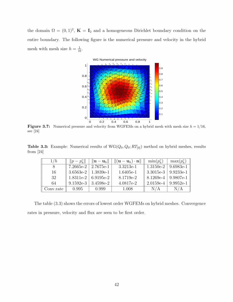
the domain Ω = (0, 1)2, K = I2 and a homogeneous Dirichlet boundary condition on the

entire boundary. The following figure is the numerical pressure and velocity in the hybrid

mesh with mesh size h = 116.

0 0.2 0.4 0.6 0.8 10

0.2

0.4

0.6

0.8

1

WG Numerical pressure and velocity

0.1

0.2

0.3

0.4

0.5

0.6

0.7

0.8

0.9

Figure 3.7: Numerical pressure and velocity from WGFEMs on a hybrid mesh with mesh size h = 1/16,see [24]

Table 3.3: Example: Numerical results of WG(Q0, Q0;RT[0]) method on hybrid meshes, resultsfrom [24]

1/h ∥p− ph∥ ∥u− uh∥ ∥(u− uh) · n∥ min(ph) max(ph)8 7.2665e-2 2.7675e-1 3.3213e-1 1.3150e-2 9.6983e-116 3.6563e-2 1.3839e-1 1.6405e-1 3.3015e-3 9.9233e-132 1.8311e-2 6.9195e-2 8.1719e-2 8.1269e-4 9.9807e-164 9.1592e-3 3.4598e-2 4.0817e-2 2.0159e-4 9.9952e-1

Conv.rate 0.995 0.999 1.008 N/A N/A

The table (3.3) shows the errors of lowest order WGFEMs on hybrid meshes. Convergence

rates in pressure, velocity and flux are seen to be first order.

42

CHAPTER 4

WGFEMS ON HEXAHEDRAL MESHES

In previous chapters, we showed how to use WGFEMs to solve the Darcy equation on

quadrilateral and hybrid meshes. In this chapter, we discuss the lowest order WGFEMs for

the Darcy equation on hexahedral meshes and present some numerical results. Readers are

referred to [18] for further details of the construction of meshes.

4.1 WG (Q0, Q0;RT[0]) Elements on Hexahedra

On a hexahedron E, the local Raviart-Thomas space is defined as

RT[0](E) = Span(w1,w2,w3,w4,w5,w6), (4.1)

where (xc, yc, zc) is the center of the hexahedron, and X = x− xc, Y = y − yc, Z = z − zc,

w1 =

1

0

0

,w2 =

0

1

0

,w3 =

0

0

1

,w4 =

X

0

0

,w5 =

0

Y

0

,w6 =

0

0

Z

.

The Gram matrix of the above basis is a 6× 6 symmetric positive-definite (SPD) matrix.

Definitions of weak functions, weak gradients, discrete weak functions and discrete weak

gradients are similar to those defined in Chapter 3. On the hexahedron E, seven discrete

weak functions are defined in the interior and on the six faces of the element respectively,

• φ0 = 1 in the interior E, φ0 = 0 on the boundary E∂ ;

• φi = 1(i = 1, 2, · · · , 6) on the very face, φi = 0 on all other five faces and in the interior.

43

The discrete weak gradient ∇w,dφ is again specified in RT[0](E) via integration by parts,

∫

E

(∇w,dφ) ·w =

∫

E∂

φ∂(w · n)−

∫

E

φ(∇ ·w), ∀w ∈ RT[0](E). (4.2)

The discrete weak gradients of the seven basis functions for the pressure are specified in the

local RT[0] space as

∇w,dφi = ci1w1 + ci2w2 + ci3w3 + ci4w4 + ci5w5 + ci6w6, i = 0, 1, 2, 3, · · · , 6.

As in Section 3.1.1, 3.1.2, we use Equation (4.2) and definitions of φi to solve for the coeffi-

cients.

Specifically, when E is a brick, we have

∇w,dφ0 = 0w1 + 0w2 + 0w3 + −12(x1−x0)2

w4 + −12(y1−y0)2

w5 + −12(z1−z0)2

w6,

∇w,dφ1 = −1x1−x0

w1 + 0w2 + 0w3 + 6(x1−x0)2

w4 + 0w5 + 0w6,

∇w,dφ2 = 1x1−x0

w1 + 0w2 + 0w3 + 6(x1−x0)2

w4 + 0w5 + 0w6,

∇w,dφ3 = 0w1 + −1y1−y0

w2 + 0w3 + 0w4 + 6(y1−y0)2

w5 + 0w6,

∇w,dφ4 = 0w1 + 1y1−y0

w2 + 0w3 + 0w4 + 6(y1−y0)2

w5 + 0w6,

∇w,dφ5 = 0w1 + 0w2 + −1z1−z0

w3 + 0w4 + 0w5 + 6(z1−z0)2

w6,

∇w,dφ6 = 0w1 + 0w2 + 1z1−z0

w3 + 0w4 + 0w5 + 6(z1−z0)2

w6.

4.2 Lowest Order WG Scheme for Darcy on Hexahedra

In this section, we show how to use WG(Q0, Q0;RT[0]), the lowest order WG finite el-

ements, to construct a finite element scheme on a hexahedral mesh and solve the Darcy

equation (1.2).

Let Eh be a hexahedral mesh for a three-dimensional polyhedral domain Ω, Sh and S0h be

spaces of discrete weak functions over this mesh, defined in a similar way to Equation (3.4),

(3.5).

44

WG(Q0, Q0;RT[0]) for the Darcy equation on a hexahedral mesh: Seek ph = ph, p∂h ∈

Sh, where ph is a set of numerical pressure values in all elements’ interiors, p∂h is a set of

numerical pressure values on all faces, such that p∂h|ΓDh= Q∂

h(pD) (the L2-projection of the

Dirichlet boundary data into the space of all piecewise constant functions on ΓDh and

Ah(ph, q) = F(q), ∀q = q, q∂ ∈ S0h, (4.3)

where

Ah(ph, q) :=∑

E∈Eh

∫

E

K∇w,dph · ∇w,dq, (4.4)

and

F(q) :=∑

E∈Eh

∫

E

fq −∑

γ∈ΓNh

∫

γ

uNq∂ . (4.5)

This large size sparse SPD linear system will be solved to obtain the numerical pressure.

For the numerical velocity, it is obtained by postprocessing. In particular, on each ele-

ment, uh = Qh(−K∇w,dph), where Qh is an L2-projection of (−K∇w,dph) into the subspace

RT[0](E). When K is an elementwise constant scalar matrix, K∇w,dph is still in the space

RT[0](E), this projection can be omitted.

This WG finite element scheme still satisfies the two important physical properties and

the convergence proposition. The proofs are similar to those in Section 3.4. See [18] for

details.

Now we use the following norms

∥p− ph∥2 :=

∑

E∈Eh

∥p− ph∥2L2(E), ∥u− uh∥

2 :=∑

E∈Eh

∥u− uh∥2L2(E)3 , (4.6)

∥(u− uh) · n∥2 :=

∑

E∈Eh

∑

γ⊂E∂

|E|

|γ|∥u · n− uh · n∥

2L2(γ), (4.7)

where h is the mesh size, |E| is the volume of the hexahedron in the mesh, |γ| is the area of

any face of the hexahedral element E.

45

This WG finite element scheme has been tested on hexahedral meshes [18]. Two types

of meshes could be used for testing. A type I mesh is obtained from h2-perturbations of

uniform brick meshes [18], [31]. A type II mesh is the refinement of a tetrahedral mesh by

connecting the centroid of each original tetrahedron, the centroid of each original triangular

face and the midpoint of each original edge. These meshes are asymptotically parallelopiped

[31].

Type I hexahedral meshes, Ref. [18] Type II hexahedral meshes, Ref. [18]

Figure 4.1: Two types of hexahedral meshes [18]. Type I: A logically brick mesh [30]; Type II: Refinementof a tetrahedral mesh into the hexahedral mesh.

Example 1. The exact pressure solution is p(x, y, z) = cos(πx) cos(πy) cos(πz), the

source term is f = 3π2 cos(πx) cos(πy) cos(πz), on the domain Ω = (0, 1)3 (the unit cube)

with the exact solution values on Dirichlet boundaries ΓD = ∂Ω, K = I3. Figure (4.2) shows

the numerical pressures for Type I and II hexahedral meshes. Tables (4.1) and (4.2) are the

numerical results from the WG (Q0, Q0;RT[0]) finite element methods. From the tables, we

observe that convergence rates in pressure, velocity, and flux close to the first order.

Table 4.1: Example 1: Convergence rates of errors in pressure, velocity, and flux on the Type I mesh [18]

1/h ∥p− ph∥ ∥u− uh∥ ∥(u− uh) · n∥8 7.0011E-2 3.2844E-1 7.1386E-216 3.5623E-2 1.6527E-1 3.5469E-232 1.7905E-2 8.2288E-2 1.7623E-264 8.9652E-3 4.1069E-2 8.7969E-3

Conv.rate 0.988 0.999 1.006

46

Hexahedral meshes Type I, h = 1/8 Hexahedral meshes Type II , h = 1/8

Figure 4.2: Example 1: Numerical pressure profiles on Type I and II hexahedral meshes [18]

Table 4.2: Example 1: Convergence rates of errors in pressure, velocity, and flux on the Type II mesh [18]

1/h ∥p− ph∥ ∥u− uh∥ ∥(u− uh) · n∥4 3.0310E-5 1.2359E-3 2.2008E-48 1.4466E-5 5.7003E-4 1.2107E-416 7.1904E-6 2.8141E-4 6.2760E-532 3.6280E-6 1.4303E-4 3.2173E-564 1.8858E-6 7.7412E-5 1.7172E-5

Conv.rate 1.001 0.998 0.920

47

CHAPTER 5

WGFEMS FOR ELASTICITY

From previous chapters, we see that weak Galerkin finite element methods can be used

for solving the Darcy equation on two-dimensional and three-dimensional domains, and

they satisfy two important physical properties. We can establish concepts of discrete weak

divergence and discrete weak curl also. So WGFEMs can be developed for solving the Stokes

equation and the elasticity equation.

In this chapter, we establish weak Galerkin finite element methods for solving the linear

elasticity equation,

−∇ · σ(u) = f , in Ω,

u = u, on Γ,(5.1)

where u is the displacement vector, f is the exterior force, u is boundary value, ε(u) is the

strain tensor,

ε(u) =1

2(∇u+∇(u)T ),

σ(u) is the stress tensor,

σ(u) = 2µε(u) + λ(∇ · u)I,

λ and µ are Lame constants, which are material based quantities.

When there is only Dirichlet boundary conditions, we have

− (µ∆u+ (µ+ λ)∇(∇ · u)) = f , in Ω, (5.2)

which is subject to certain boundary conditions.

Before talking about the WG finite element methods, we recall how to calculate the

gradient of vectors and divergence of matrices.

48

For example, u = (u1, u2), then

∇u =

∂xu1 ∂yu1

∂xu2 ∂yu2

;

matrix A =

a11 a12

a21 a22

, then the divergence of the matrix A is

∇ · A =

∂xa11 + ∂ya12

∂xa21 + ∂ya22

.

Weak divergence. [29] The weak divergence of v ∈ W (E), denoted as ∇w · v, is a linear

functional in the Soblev space H1(E), so its action on any test function φ ∈ H1(E) is

∫

E

(∇w · v)φ = −

∫

E

v · (∇φ) +

∫

E∂

v∂ · (φ n), (5.3)

where W (E) is the space of weak functions in an element E and defined as

W (E) = v = v,v∂ : v ∈ L2(E)2,v∂ ∈ L2(E∂)2, (5.4)

and

H1(E) = v : v ∈ L2(E),∇v ∈ L2(E), (5.5)

v is the value of v defined in E, v∂ is the value of v defined on the boundary E∂ , n is the

unit outward normal vector on E∂ .

49

Discrete weak divergence. [29] The discrete weak divergence is denoted as ∇w,d · v ∈

P r(E), satisfying

∫

E

(∇w,d · v)φ = −

∫

E

v · (∇φ) +

∫

E∂

v∂ · (φ n), ∀φ ∈ P r(E), (5.6)

where φ is a scalar-valued degree r polynomial, ∇φ is taken in the classical sense, P r(E) is

a set of polynomials on E with degree no larger than r.

Weak gradient. The weak gradient of v ∈ W (E), denoted as ∇wv, is a linear functional

in the Soblev space H1(E)2×2, so its action on W ∈ H1(E)2×2 is [29]

∫

E

(∇wv) : W = −

∫

E

v · (∇ ·W ) +

∫

E∂

v∂ · (Wn), ∀W ∈ H1(E)2×2, (5.7)

where W is a 2× 2 matrix with entries in H1(E), n is the outward normal vector on E∂ .

Discrete weak gradient. Th discrete weak gradient ∇w,dv is a matrix valued polynomial,

such that,

∫

E

(∇w,dv) : W = −

∫

E

v · (∇ ·W ) +

∫

E∂

v∂ · (Wn), ∀W ∈ P r(E)2×2, (5.8)

where W is a matrix-valued degree r polynomial.

Weak form. Seek u ∈ H1(Ω)2,

∫

Ω

2µ(εw(u) : εw(v)) +

∫

Ω

λ(∇w · u)(∇w · v) =

∫

Ω

fv, ∀v ∈ H10 (Ω)

2, (5.9)

εw(u) is the weak strain tensor, ∇w · u is the weak divergence. Use the weak gradient and

the weak divergence, the weak strain tensor is defined as

50

εw(v) =1

2

(

∇wv + (∇wv)T)

, (5.10)

and the weak stress tensor is defined as

σw(v) = 2µεw(v) + λ(∇w · v)I. (5.11)

As for Equation (5.2), the weak form of it is

µ(∇wu,∇wv) + (µ+ λ)(∇w · u,∇w · v) = (f ,v). (5.12)

Let E be a quadrilateral element. We consider the lowest order WG (Q20, Q

20;RT

2[0], Q0).

The first Q20 means that two-dimensional vector-valued polynomials are used to approximate

the displacement in the interior; the second Q20 means that two-dimensional vector-valued

polynomials are used to approximate the displacement on the boundaries;

RT 2[0] = Span

1 0

0 0

,

0 1

0 0

,

0 0

1 0

,

0 0

0 1

,

X 0

0 0

,

0 Y

0 0

,

0 0

X 0

,

0 0

0 Y

;

(5.13)

the last Q0 means that the divergence of these vector-valued polynomials are constants.

In Equation (5.6), φ is taken as constant 1, so ∇φ = (0, 0), then the equation becomes

∫

E

(∇w · v)φ =

∫

E∂

v∂ · (φ n). (5.14)

In Equation (5.8), W is taken from the following matrices:

1 0

0 0

,

0 1

0 0

,

0 0

1 0

,

0 0

0 1

, (5.15)

51

so ∇ ·W is the zero vector. Then the equation becomes

∫

E

(∇w,dv) : W =

∫

E∂

v∂ · (Wn). (5.16)

The discrete weak function space on each element E is

W (E, l,m) = v = (v,v∂),v ∈ P l(E)2,v∂ ∈ Pm(E∂)2. (5.17)

Two spaces of discrete weak functions over the mesh Eh are

Sh = v = v,v∂ : v|E ∈ W (E, l,m), ∀E ∈ Eh, (5.18)

S0h = v = v,v∂ ∈ Sh,v

∂ = 0 on Γ. (5.19)

WG FE scheme. For a numerical solution of the elasticity equation, find uh = uh,u

∂h ∈

Sh, where uh is the value in E, u∂

h is the value on E∂ , and u∂h|Γh

= Q∂h(uD), such that

A(uh,v) = F(v), ∀v ∈ S0h, (5.20)

where

A(uh,v) =∑

E∈Eh

2µ(εw,d(uh), εw,d(v))E +∑

E∈Eh

λ(∇w,d · uh,∇w,d · v)E, (5.21)

F(v) =∑

E∈Eh

(f ,v)E. (5.22)

52

CHAPTER 6

CONCLUSION

6.1 Other Combinations for WG Elements

In previous chapters, we have investigated the lowest order weak Galerkin finite element

methods for the Darcy equation. Due to the flexibility in constructing weak Galerkin finite

elements, we explore other possible combinations for weak Galerkin finite elements.

6.1.1 WG(Q1, P1;RT[0]) Elements on Quadrilaterals

In this combination, WG basis functions are Q1 polynomials in element interiors and P1

polynomials on edges, their discrete weak gradients are in RT[0].

On each quadrilateral element, there are twelve WG basis functions, four for interior:

φ01, φ02, φ03, φ04; two for each edge: φi1, φi2(i = 1, 2, 3, 4), as shown in Figure 6.1:

• φ0j = 1, X, Y,XY (j = 1, 2, 3, 4) for the interior;

• φkl = 1, r(k = 1, 2, 3, 4; l = 1, 2) on each edge.

Figure 6.1: Twelve weak Galerkin basis functions on a quadrilateral

We calculate the discrete weak gradients of these basis functions, and then use these

discrete weak gradients to approximate the classical gradient. We use this WG method to

solve the pressure in the Darcy equation.

53

In the process of solving the Darcy equation, we use the discrete weak gradients to

calculate element stiffness matrices, which are assembled into a global stiffness matrix. For

this method, we observed that the global stiffness matrix is singular. We examine further

the structures of element stiffness matrices and the global stiffness matrix.

For simplicity, we consider a 2× 2 uniform rectangular mesh over the unit square [0, 1]2.

On each rectangular element E, we have∫

EX = 0,

∫

EY = 0,

∫

EXY = 0, where X, Y are

the normalized coordinates.

For a rectangular element, the Gram matrix of RT[0] is a diagonal matrix

GM =

|E| 0 0 0

0 |E| 0 0

0 0∫

EX2 0

0 0 0∫

EY 2

. (6.1)

Comparing WG(Q1, P1;RT[0]) with WG(Q0, Q0;RT[0]), the difference is that we have

three more WG basis functions X, Y,XY defined in the interior and one more basis function

r on each edge in WG(Q1, P1;RT[0]).

For these three new WG basis functions for the element interior (X, Y,XY ), we check

the right hand sides of the following definition equation:

∫

E

(∇w,dφ) ·w =

∫

E∂

φ∂(w · n)−

∫

E

φ(∇ ·w), ∀w ∈ RT[0](E). (6.2)

Clearly, the right hand sides are respectively

0

0

−∫

EX

−∫

EX

,

0

0

−∫

EY

−∫

EY

,

0

0

−∫

EXY

−∫

EXY

. (6.3)

54

When E is a rectangular element,∫

EX = 0,

∫

EY = 0,

∫

EXY = 0. Then the right hand

sides become

0

0

0

0

,

0

0

0

0

,

0

0

0

0

. (6.4)

So ∇w,dφ0i = 0w1 + 0w2 + 0w3 + 0w4, i = 2, 3, 4. For these three new WG basis functions

(X, Y,XY ), they are not constants. But their discrete weak gradients are zero vectors. Re-

call the first property in the paper [28, pg.107]:

If ∇w,dv = 0 on the element , then one must have v ≡ constant on the element.

In other words, v = v∂ =constant.

We can see that WG(Q1, P1;RT[0]) does not satisfy this property.

On each element of the mesh, we compute its element stiffness matrix as follows,

(K∇w,dφi,∇w,dφj)

. (6.5)

For a simple case K = I2, we have found that the interaction among the discrete weak

gradients of the WG basis functions for the element interior has the following structure

∗ 0 0 0

0 0 0 0

0 0 0 0

0 0 0 0

, (6.6)

where ∗ is a non-zero entry.

Then we use the element stiffness matrices to construct the global stiffness matrix. On

a 2 × 2 rectangular mesh, the global stiffness matrix is 40 × 40. The 16 × 16 block in the

55

top-left corner of the matrix represents the interaction among the WG basis functions for

element interiors. We have a block diagonal structure here. Each block on the diagonal is a

4× 4 matrix with the structure shown in Equation (6.6). Since the discrete weak gradients

in different element interiors do not interact with each other, the other parts of this 16× 16

block are zeros. From previous discussion, the discrete weak gradient of any of these new

WG basis functions is zero, then the interaction between this discrete weak gradient and

the discrete weak gradient of any egde basis function is also zero. So in this global stiffness

matrix, there is at least one row that that is entirely zero. Enforcing Dirichlet boundary

conditions will not affect this row, since it corresponds to an interior basis function. Thus

the determinant of the global stiffness matrix is zero, and it is a singular matrix.

6.1.2 WG(Q0, Q0;RT[1]) Elements on Quadrilaterals

We have seen the application of the lowest order Raviart-Thomas space in construction

of WG finite elements, so we want to explore use of higher order RT spaces, e.g., RT[1].

Definition. Consider a rectangular element, for a non-negative integer k, the Raviart-

Thomas space RT[k] is defined as

RT[k] = (Qk)2 + xQk, (6.7)

where Qk is the space of Q-type polynomials with degrees no larger than k, x is a two-

dimensional vector. It could also be written as

RT[k] = Pk+1,k × Pk,k+1, (6.8)

where

Pk+1,k =k+1∑

i=0

k∑

j=0

aijxiyj, Pk,k+1 =

k∑

i=0

k+1∑

j=0

aijxiyj.

Clearly, dim RT[k] = 2(k + 1)(k + 2).

56

For example, when k = 1, dim RT[k] = 12, the Raviart-Thomas space is

RT[1] = Span w1,w2,w3,w4,w5,w6,w7,w8,w9,w10,w11,w12 , (6.9)

where

w1 =

1

0

, w2 =

0

1

, w3 =

X

0

, w4 =

0

Y

,

w5 =

0

X

,w6 =

Y

0

,w7 =

X2

0

,w8 =

XY

0

,

w9 =

X2Y

0

,w10 =

0

Y 2

,w11 =

0

XY

,w12 =

0

XY 2

,

and (xc, yc) is the center of the quadrilateral element E, X = x− xc, Y = y − yc.

WG(Q0, Q0;RT[1]) means that all WG basis functions are degree 0 polynomials and their

discrete weak gradients are in RT[1]. Comparing WG(Q0, Q0;RT[1]) with WG(Q0, Q0;RT[0]),

we note that the first four basis functions of RT[1] are the same as the basis functions of

RT[0]. So for a WG basis function φ, the top four components of the right hand sides in

Equation (6.2) are the same, when RT[0] or RT[1] is used.

Then we use the element stiffness matrices to construct the global stiffness matrix and

solve the Darcy equation using WG(Q0, Q0;RT[1]) in a similar fashion to Section 3.4.

Here, we perform a numerical test on a popular example. The exact pressure is p =

sin(πx) sin(πy) in the domain Ω = (0, 1)2. We test it on rectangular meshes. The following

figures show numerical pressure and velocity obtained from using WG(Q0, Q0;RT[1]).

We can see from Figure 6.2 that as the mesh is refined, the maximum of the numerical

pressure is still about 0.16, but the maximum of the exact pressure should be 1. So this WG

method is not suitable for solving the Darcy equation. It is possible that this combination

violates the first property in [28, pg.107]. This needs further theoretical investigation.

57

0 0.2 0.4 0.6 0.8 1

0

0.1

0.2

0.3

0.4

0.5

0.6

0.7

0.8

0.9

1

Numerical pressure and velocity

0.02

0.04

0.06

0.08

0.1

0.12

0.14

0.16

0 0.2 0.4 0.6 0.8 1

0

0.1

0.2

0.3

0.4

0.5

0.6

0.7

0.8

0.9

1

Numerical pressure and velocity

0.02

0.04

0.06

0.08

0.1

0.12

0.14

0.16

Figure 6.2: Numerical pressure and velocity obtained from using WG(Q0, Q0;RT[1]) on rectan-gular meshes, with mesh size h = 1/8 and h = 1/16, respectively.

6.2 Conclusion

In this thesis, we have described development and implementation of the lowest order

WGFEMs for solving the Darcy equation. We have compared this new approach to two well

known methods, CGFEMs and MFEMs. The WG method is based on the novel ideas of

using discrete weak functions to approximate the pressure and discrete weak gradients to

approximate classical gradients. We have considered triangular and quadrilateral meshes.

Rectangular meshes are treated as a special case of quadrilateral meshes. We have presented

numerical results on quadrilateral meshes and hybrid meshes, which are combinations of

quadrilateral and triangular elements. And expected convergence rates are obtained with

mesh refinements. We have also discussed the extension of WGFEMs to three-dimensional

domains. Except for the lowest order WGFEMs, we discussed two other possible WGFEMs.

In comparison to CGFEMs and MFEMs, WGFEMs have nice features, including

• Local mass conservation,

• Bulk normal flux continuity,

• SPD linear systems.

58

Numerical experiments suggest that WGFEMs form a new family of efficient and robust

solvers for the Darcy equation.

Similar to the discrete weak gradients, discrete weak divergence and discrete weak curl

can also be established. In our future work, we will develop WGFEMs to solve the elasticity

equation and poroelasticity problems.

59

BIBLIOGRAPHY

[1] H.-T. Ahn and G. Carey. An enhanced polygonal finite-volume method for unstructured

hybrid meshes. Int. J. Numer. Meth. Fluids, 54:29–46, 2007.

[2] J. Alberty, C. Carstensen, and S. Funken. Remarks around 50 lines of Matlab: short

finite element implementation. Numer. Algor., 20:117–137, 1999.

[3] T. Arbogast and M. R. Correa. Two families of H(div) mixed finite elements on quadri-

laterals of minimal dimension. SIAM J. Numer. Anal., 54:3332–3356, 2016.

[4] D. Arnold, D. Boffi, and R. Falk. Approximation by quadrilateral finite elements. Math.

Comput., 71:909–922, 2002.

[5] D. Arnold, D. Boffi, and R. Falk. Quadrilateral H(div) finite elements. SIAM J. Numer.

Anal., 42:2429–2451, 2005.

[6] C. Bahriawati and C. Carstensen. Three Matlab implementations of the lower-order

Raviart-Thomas MFEM with a posteriori error control. Comput. Meth. Appl. Math.,

5:333–361, 2005.

[7] P. Bastian and B. Riviere. Superconvergence and h(div) projection for discontinuous

galerkin methods. Int. J. Numer. Meth. Fluids, 42:1043–1057, 2003.

[8] F. Brezzi and M. Fortin. Mixed and hybrid finite element methods. Springer-Verlag,

1991.

[9] L. Bush and V. Ginting. On the application of the continuous Galerkin finite element

method for conservation problems. SIAM J. Sci. Comput., 35:A2953–A2975, 2013.

[10] L. Chen. iFEM: An integrated finite element methods package in Matlab. Technical

Report, University of California at Irvine, 2009.

60

[11] S.-H. Chou and S. He. On the regularity and uniformness conditions on quadrilateral

grids. Comput. Meth. Appl. Mech. Engrg., 191:5149–5158, 2002.

[12] B. Cockburn, J. Gopalakrishnan, and H. Wang. Locally conservative fluxes for the

continuous Galerkin method. SIAM J. Numer. Anal., 45:1742–1770, 2007.

[13] L. Durlofsky. Accuracy of mixed and control volume finite element approximations to

Darcy velocity and related quantities. Water Resour. Res., 30:965–973, 1994.

[14] R. E. Ewing. The mathematics of reservoir simulation. SIAM, 1983.

[15] R. E. Ewing, M. M. Liu, and J. Wang. Superconvergence of mixed finite element

approximations over quadrilaterals. SIAM J. Numer. Anal., 36:772–787, 1999.

[16] G.B.Folland. Real analysis: Modern techniques and their applications. 1999.

[17] V. Ginting, G. Lin, and J. Liu. On application of the weak Galerkin finite element

method to a two-phase model for subsurface flow. J. Sci. Comput., 66:225–239, 2016.

[18] G. Harper, J. Liu, and B. Zheng. The THex algorithm and a simple Darcy solver on

hexahedral meshes. Proc. Comput. Sci., pages Preprint, Colorado Sate University, 2017.

[19] V. John. Finite element methods for incompressible flow problems. Springer, 2016.

[20] G. Lin, J. Liu, L. Mu, and X. Ye. Weak galerkin finite element methdos for darcy flow:

Anistropy and heterogeneity. J. Comput. Phys., 276:422–437, 2014.

[21] G. Lin, J. Liu, and F. Sadre-Marandi. A comparative study on the weak Galerkin,

discontinuous Galerkin, and mixed finite element methods. J. Comput. Appl. Math.,

273:346–362, 2015.

[22] J. Liu, L. Mu, and X. Ye. A comparative study of locally conservative numerical methods

for darcy’s flows. Proc. Comput. Sci., 4:974–983, 2011.

61

[23] J. Liu, F. Sadre-Marandi, and Z. Wang. DarcyLite: A Matlab toolbox for Darcy flow

computation. Procedia Computer Science, 80:1301–1312, 2016.

[24] J. Liu, S. Tavener, and Z. Wang. The lowest-order weak galerkin finite element method

for the darcy equation on quadrilateral and hybrid meshes. Submitted.

[25] L. Mu, J. Wang, and X. Ye. Weak galerkin finite element methdos on polytopal meshes.

Int. J. Numer. Anal. Model., 12:31–53, 2015.

[26] L. Mu, J. Wang, and X. Ye. A weak Galerkin finite element method with polynomial

reduction. J. Comput. Appl. Math., 285:45–58, 2015.

[27] S. Sun and J. Liu. A locally conservative finite element method based on piecewise con-

stant enrichment of the continuous Galerkin method. SIAM J. Sci. Comput., 31:2528–

2548, 2009.

[28] J. Wang and X. Ye. A weak Galerkin finite element method for second order elliptic

problems. J. Comput. Appl. Math., 241:103–115, 2013.

[29] J. Wang and X. Ye. A weak galerkin mixed finite element method for second order

elliptic problems. Math. Comput., 2014.

[30] M. Wheeler, G. Xue, and I. Yotov. A multipoint flux mixed finite element method on

distorted quadrilaterals and hexahedra. Numer. Math., 2012.

[31] M. Wheeler and I. Yotov. A multipoint flux mixed finite element method. SIAM J.

Numer. Anal., 44:2082–2106, 2006.

[32] T. Wihler and B. Riviere. Discontinuous Galerkin methods for second-order elliptic pde

with low-regularity solutions. J. Sci. Comput., 46:151–165, 2011.

62

THESIS WEAK GALERKIN FINITE ELEMENT METHODS FOR ...

Documents

Transcript of THESIS WEAK GALERKIN FINITE ELEMENT METHODS FOR ...