Computation of variably saturated subsurface flow by adaptive mixed hybrid finite element methods

Advances in Water Resources 27 (2004) 565–581

www.elsevier.com/locate/advwatres

Computation of variably saturated subsurface flow by adaptivemixed hybrid finite element methods

M. Bause *, P. Knabner

Institut f€ur Angewandte Mathematik, Universit€at Erlangen-N€urnberg, Martensstraße 3, 91058 Erlangen, Germany

Received 24 December 2002; received in revised form 28 October 2003; accepted 19 March 2004

Abstract

We present adaptive mixed hybrid finite element discretizations of the Richards equation, a nonlinear parabolic partial differ-

ential equation modeling the flow of water into a variably saturated porous medium. The approach simultaneously constructs

approximations of the flux and the pressure head in Raviart–Thomas spaces. The resulting nonlinear systems of equations are solved

by a Newton method. For the linear problems of the Newton iteration a multigrid algorithm is used. We consider two different kinds

of error indicators for space adaptive grid refinement: superconvergence and residual based indicators. They can be calculated easily

by means of the available finite element approximations. This seems attractive for computations since no additional (sub-)problems

have to be solved. Computational experiments conducted for realistic water table recharge problems illustrate the effectiveness and

robustness of the approach.

� 2004 Elsevier Ltd. All rights reserved.

Keywords: Saturated–unsaturated flow; Nonlinear elliptic–parabolic problem; Mixed finite element method; Raviart–Thomas spaces; A posteriori

error indicator

1. Introduction

Accurate, reliable and efficient simulations of mois-

ture fluxes through porous media are desirable in

hydrological and environmental studies, as well as incivil and environmental engineering. The ability to

model time dependent flows in composite soil forma-

tions that may be intermittently saturated and drained is

particularly important from the point of view of physi-

cal realism. This paper focuses on an appropriate and

controlled treatment of saturated–unsaturated subsur-

face flows, ensuring accuracy and efficiency in a robust

space adaptive grid refinement algorithm.Numerous papers have been written on numerical

schemes for the Richards equation which is typically

used to describe variably saturated flow in porous

media. The most successful approximation schemes

have been based on conservative methods; cf. [18,33]. In

this work we present an adaptive mixed finite element

*Corresponding author. Tel.: +49-9131-8528455; fax: +49-9131-

8527670.

E-mail address: [email protected] (M. Bause).

0309-1708/$ - see front matter � 2004 Elsevier Ltd. All rights reserved.

doi:10.1016/j.advwatres.2004.03.005

discretization scheme of the Richards equation. Mixed

finite element methods have become popular in recent

years for modeling flow in porous media due to their

inherent conservation properties and the fact that the

models provide flux approximations as part of the for-mulation. These fluxes are often of greater importance

than the pressure head itself. We will consider a hybrid

variant of the mixed finite element method with lowest

order Raviart–Thomas spaces by applying the Lagrange

multiplier technique (cf., e.g., [16]) to the nonlinear and

possibly degenerate Richards equation. The Lagrange

multipliers then become the unknowns of a global

nonlinear system of equations which we solve by adamped version of Newton’s method combined with a

W-cycle multigrid algorithm for the linear problems of

the Newton iteration. For linear elliptic problems it is

well known that the Lagrange multiplier approach

provides certain implementational advantages over the

standard mixed formulation of the problem, for in-

stance, for building the multigrid algorithm (cf. [21]) and

an adaptive grid refinement algorithm by superconver-gence based a posteriori error estimation (cf. [43]). As we

shall see, these advantages can be carried over to the

Richards equation. However, since this one is nonlinear,

mail to: [email protected]

566 M. Bause, P. Knabner / Advances in Water Resources 27 (2004) 565–581

the discrete equation of continuity does not allow an

explicit representation of the piecewise constant pressure

approximation in terms of the Lagrange multipliers and,

thereby, an elimination of the pressure variable. This

complicates the application of the multiplier technique.It has rather to be embedded into the Newton iteration

by computing after each Newton correction of the

Lagrange multipliers the pressure values in terms of el-

ementwise nonlinear problems which we again solve by

Newton’s method. In the subsequent Newton step the

Jacobian matrix is then calculated in terms of these

recomputed pressure values. The flux approximation is

determined locally by some postprocessing procedure.The convergence of the scheme will be demonstrated by

numerical experiments. For analyses of the mixed ap-

proach to the Richards equation we refer to [3,36,44].

Our principal objective, which is certainly a long

range one, is to develop robust efficient and mathe-

matically rigorous adaptive (finite element) approxima-

tion schemes for the Richards equation of variably

saturated subsurface flow by, firstly, establishing exis-tence and regularity, then, based on these results,

proving efficient and reliable sharp a posteriori error

estimates for a space–time adaptive algorithm and,

finally, providing convergence proofs for the (non-)lin-

ear solver. However, our current approach still relies,

in the general nonlinear and degenerate case, on heu-

ristic arguments which are either physically reason-

able or confirmed by our computations. For saturatedflow all arguments are rigorous and based on proofs.

In scientific computing, techniques which were devel-

oped and emerged to work well for simple (linear)

problems are naturally applied to more general and

sophisticated ones. This is also done here by considering

variably saturated flow as a perturbation of saturated

flow.

In this work we present an adaptive variant of themixed finite element approach to the Richards equation

by applying a posteriori error estimators established for

linear elliptic problems (cf. [43]) to our degenerate

nonlinear one. This leads to error indicators in contrast

to sharp error estimators verified by a rigorous mathe-

matical analysis. The resulting error indicators are ra-

ther easy and fast to evaluate by means of the already

computed finite element approximations and yield con-vincing numerical results. First, a superconvergence

based error indicator for the pressure head is proposed

which is due to some specific superconvergence

approximation property of the mixed hybrid finite ele-

ment method (cf. [16]). Then, this concept is carried over

to the flux variable. By a simple post processing of its

tangential components on interelement edges (cf. [11])

an additional higher order approximation of the flux isobtained which directly gives rise to an error indicator.

Finally, a residual based error indicator for the total

error of pressure head and flux is presented which relies

on a Helmholtz decomposition of the flux ansatz space;

cf. [17,43]. In calculations our adaptive grid refinement

algorithm nicely resolves steep saturation fronts with

high accuracy, that occur as water infiltrates dry soil,

and leads to smaller discretization errors than an uni-form triangulation; cf. Section 8.

Alternative adaptive approaches to subsurface flow

and related problems are described, e.g., in [22,23,28,40].

In [40], a least-squares mixed finite element method is

introduced for the Richards equation with refinement

strategies based on local least-squares functionals. In

[23], a Zienkiewicz and Zhu type error indicator [45] is

designed for multiphase problems. In [28], a movingmesh technique is proposed. In [22], mixed and Galerkin

methods are combined and iterative techniques of do-

main decomposition type are used.

The plan for the paper is as follows. First, we intro-

duce the Richards equation of variably saturated sub-

surface flow, recall regularity results and give basic

notations. In Section 3 its mixed hybrid finite element

approximation is briefly presented; cf. also [19]. Section4 is devoted to the solution process of the resulting

nonlinear algebraic system of equations. The elimina-

tion of internal degrees of freedom and the (non-)linear

solver are described. In Section 5, the theoretical con-

vergence rates of the linear elliptic case (cf. [16]) are

verified for two one-dimensional nonlinear degenerate

problems. In Section 6 we present two-dimensional

numerical tests with steep fronts. Section 7 is devoted tothe adaptive techniques. The error indicators for the

mixed hybrid finite element approximation of the

Richards equation are given and our adaptive mesh

refinement algorithm is described. In Section 8 numeri-

cal tests are presented. One of the water table recharge

problems is recomputed by the proposed adaptive

method. Additionally, it is shown for one test case that

the adaptive grid refinement in fact leads to smaller er-rors than the uniform triangulation. We end with con-

clusions.

2. Formulation of the problem

We consider saturated–unsaturated flow in soil

modeled by the Richards equation

otHðwÞ � r � ðKðwÞrðwþ zÞÞ ¼ f ð1Þ

for the pressure head w : X ! R in a polyhedral domain

X Rd , d ¼ 2 or 3, with boundary C. The pore spacesmay contain both water and air. The ‘‘saturated zone’’ isthe portion of the medium that is water saturated, while

the ‘‘unsaturated zone’’ contains both water and air.

These zones may vary with space and time. In (1), HðwÞdenotes the volumetric water content and KðwÞ ¼KskrwðHðwÞÞ denotes the permeability where Ks ¼ kaqg=l is the permeability in the saturated zone and krw is the

M. Bause, P. Knabner / Advances in Water Resources 27 (2004) 565–581 567

relative permeability of water to air in the unsaturated

regime. The constant ka is the absolute permeability, q isthe water density, g is the gravitational accelerationconstant and l is the water viscosity. The function fdescribes sources and sinks. The hydraulic head wþ zrepresents the height of the water column above some

reference elevation (z ¼ 0). The elevation head z atany point is simply the height of that point (against

the gravitational direction), and the pressure head

indicates the vertical distance between the point and the

water table. Functional forms for HðwÞ and KðwÞ, bothof which are bounded, have been derived in the litera-

ture. In our computations we use models based on[26,34,35]. The relations given in [26,34] lead to un-

bounded K 0ðwÞ in the neighborhood of the saturatedlimit for some types of soil. This is avoided by a suitable

modification of KðwÞ close to the saturated regime; cf.Section 6.

The formulation of Richards equation given above

assumes that the medium itself is incompressible and

thus that the porosity / does not change with time orhydraulic head. The formulation is valid for the two

regimes of our interest. Where the medium is fully water

saturated, HðwÞ ¼ / and krwðHðwÞÞ ¼ 1. Where themedium is partially water saturated, H0ðwÞ > 0 and0 < krw < 1. Thus, (1) is elliptic in the saturated zoneand parabolic in the unsaturated zone. Moreover, both

regimes can exist within a single flow domain. In this

paper we do not consider dry regions where the mediumis (nearly) air saturated and KðwÞ, as well as K 0ðwÞ andH0ðwÞ, may be very small. In this case, Eq. (1) effectivelyreduces to the system (cf. (4) and (5) below)

r � q ¼ f ; q ¼ 0;for the flux q, leaving w completely undetermined. Dryregions are beyond the scope of our applications.However, in such case one may regularize (1) by

replacing KðwÞ with eK ðwÞ ¼ Kmin þ ð1� Kmin=KsÞKðwÞand Kmin � Ks which implies that 0 < Kmin6 eK ðwÞ6Ksuniformly in X; cf. [40]. Of course, one needs to be verycareful with the choice of Kmin to make sure that thecomputational results are still meaningful. A numerical

sensitivity study may be helpful for an appropriate

choice of the parameter Kmin.Let CD be the portion of the boundary oX of X where

Dirichlet conditions are specified, and let CN be the

portion where Neumann conditions are specified. We

assume that oX ¼ CD [ CN. We consider solving Rich-ards equation (1) over J X, where J ¼ ð0; T Þ andT > 0 is some final time. Boundary and initial condi-tions are given as

w ¼ gD on CD;

� KðwÞrðwþ zÞ � m ¼ gN on CN; ð2Þ

w ¼ w0 for t ¼ 0: ð3Þ

Here, m denotes the outer unit normal to oX. Only inorder to simplify the notation, we tacitly assume from

now on that gN ¼ 0 and f ¼ 0.Then, Eq. (1) can be rewritten as the following

equivalent system of equations:

otHðwÞ þ r � q ¼ 0; ð4Þ

qþ KðwÞrðwþ zÞ ¼ 0: ð5ÞEq. (4) describes the conservation of mass. Eq. (5)

which links the flux q to the hydraulic head is the Darcylaw; cf., e.g., [8]. Alt and Luckhaus [2] state the fol-

lowing existence and regularity result for the system (4)

and (5):

HðwÞ 2 L1ðJ ; L1ðXÞÞ; q 2 L2ðJ ; L2ðXÞÞ;otHðwÞ 2 L2ðJ ;W �1

2 ðXÞÞ:ð6Þ

Here, LqðXÞ and W kp ðXÞ are the standard Lebesgue and

Sobolev spaces; cf., e.g., [1]. By W �k2 ðXÞ, for k a positive

integer, we denote the dual space of W k2 ðXÞ. For

p 2 ½1;1� and a Banach space X we denote by LpðJ ;X Þthe space of strongly measurable functions u : J 7!Xsuch that ð

RJ kuðtÞk

pX dtÞ

1=p<1 if 16 p <1 and

ess supJ kuðtÞkX <1 if p ¼ 1. We do not distinguishthrough the notation between scalar and vector valued

functions, or function spaces, or norms. The precise

meaning is always clear from the context. By h�; �i wewill denote the L2ðXÞ inner product, and k � k is its norm.According to (6), otHðwÞ 2 L2ðJ ;W �1

2 ðXÞÞ can gen-erally be assumed only. Hence, a variational formula-

tion of (4) relying on (6) would require test functions for

(4) to be taken in W 12 ðXÞ. In order to relax this

requirement, an alternate time integrated variational

formulation based on the Kirchhoff transformation, a

term which requires computing integrals of the perme-ability, may be used for the approximation of the system

(4), (5). For details of this technique and an error

analysis for the finite element approximation of the time

integrated problem we refer to [3,36,44]. Our discreti-

zation and computations are based on the untrans-

formed formulation (4), (5). This saves compute time

since there is no need for integrated values of the

transformation. The test problems in Sections 6 and 8will show that our approach leads to robust and stable

approximations of the Richards equation also in

degenerate cases.

The regularity result (6) does not ensure that HðwÞexists pointwise everywhere in time. However, we know

that since HðwÞ physically represents water saturation,HðwÞ is defined pointwise at every time. Thus we mayassume that

HðwÞ 2 L1ðJ ; L1ðXÞÞsuch that, below, test functions for the time discrete

version of Eq. (4) may be chosen in L2ðXÞ instead ofW 12 ðXÞ. We further assume that


q 2 L1ðJ ;HðX; divÞÞ;

where HðX; divÞ ¼ fq 2 L2ðXÞjr � q 2 L2ðXÞg. We alsoneed the subspace H0;NðX; divÞ ¼ fq 2 HðX; divÞjhq�m; wioX ¼ 0 8 w 2 H 1

0;DðXÞg where H 10;DðXÞ ¼ fw 2 W 1

2

ðXÞjwjCD ¼ 0g. Here, h�; �ioX denotes the duality betweenH�1=2ðoXÞ and H 1=2ðoXÞ; cf. [16] for details. For short,we set W ¼ L2ðXÞ and V ¼ H0;NðX; divÞ.Now we discretize the Eqs. (4) and (5) in time by an

implicit Euler scheme. This gives rise to the following

mixed variational problem:

For given wn�1 2 W find ðwn; qnÞ 2 W V such that

there holds

hHðwnÞ;wi þ snhr � qn;wi ¼ hHðwn�1Þ;wi;hKðwnÞ�1qn; vi � hwn;r � vi þ hrz; vi ¼ �hgnD; v � miCD

ð7Þ

for all w 2 W , v 2 V and nP 1.

Here, sn ¼ tn � tn�1 is the time step size and gnD ¼gDðtn; �Þ. The starting value is w0 ¼ w0. Since we do notconsider the case of a fully dry porous medium with

vanishing K in this paper, the term KðwnÞ�1 in (7) is welldefined. In practical computations one may bound Kfrom below by aKs with some sufficiently small factor a.The variational problem (7) represents the dual mixedformulation (cf. [16]) of the (time) discrete form of (4),

(5). We are now in a position to formulate a fully dis-

crete approximation scheme for (1)–(3).

3. Mixed finite element discretization

Let Ph ¼ fKg be a finite element decomposition ofmesh size h of the polyhedral domain X into closedsubsets K, triangles in two dimensions and tetrahedronsin three dimensions. The decompositions are assumed to

be face to face. The set of faces is denoted by Eh ¼ EIh[EDh [ ENh where E

Ih refers to the interior faces and E

Dh and

ENh to those located on CD and CN, respectively. We usethe notation ‘‘face’’ in the two- and three-dimensionalcase. If d ¼ 2, then the faces are the sides of the trian-gles. We form discrete subspaces of Wh and Vh of L2ðXÞand H0;NðX; divÞ using the lowest order mixed finiteelement spaces of Raviart–Thomas; cf., e.g., [16].

Restricting our approach to the lowest order Raviart–

Thomas spaces does not seem to be strongly limiting

since the solution most likely lacks enough regularity

needed for getting a global improvement by using higherorder finite elements. Nevertheless, for the future we

plan to test higher order mixed finite elements, e.g., RT1or BDM2 elements; cf. [16]. We expect a local improve-

ment by such elements, for instance, inside the saturated

or unsaturated zones, respectively, since the solution

may admit higher regularity there.

In what follows let

Wh ¼ fwh 2 W jwhjK 2 P0ðKÞ 8Kg;Vh ¼ fvh 2 V jvhjK 2 RT0ðKÞ 8Kg

denote the lowest order Raviart–Thomas spaces (cf.,

e.g., [16]) where RT0ðKÞ ¼ P0ðKÞd þ xP0ðKÞ with PiðKÞdenoting the set of all polynomials on K of degree less orequal than i and x ¼ ðx1; . . . ; xdÞ, x 2 K. A fully discretemixed approximation ðwn

h; qnhÞ of (1)–(3) is now obtained

by solving (7) in Wh Vh. In what follows, we tacitlyassume that ðwnh; qnhÞ exists uniquely.From the linear elliptic case, which corresponds to

the saturated regime, it is known that the discrete ver-

sion of (7) leads to a linear system of equations with an

indefinite matrix; cf. [16, p. 178]. This is definitely a

considerable source of trouble for solving the linear

system. To overcome this difficulty, we use the technique

of interelement Lagrange multipliers (cf., e.g., [16])

which can also be interpreted as a hybridization of the

mixed formulation (7). In the elliptic case this approachleads to a linear system of equations with a positive

definite matrix. Hence, standard linear solvers can be

used for solving the system. The degenerate nonlinear

case is more complex. However, the technique of inter-

element multipliers can also be applied to this case. For

an analysis of the technique in more general cases than

the linear one we refer to [19] as well as [4,14,15].

The condition v 2 HðX; divÞ implies the continuity ofthe normal component of the fluxes over interior faces;

cf. [7]. The basic idea of interelement Lagrange multi-

pliers consists in first weakening and then reformulating

the continuity constraint for the normal component of

the fluxes over interelement boundaries. By weaken-

ing the continuity constraint we enlarge the approxi-

mation space Vh. This enables us to eliminate internaldegrees of freedom which is better known as staticcondensation. The enlarged approximation space for the

flux variable is defined bybVh ¼ fvh 2 L2ðXÞjvhjK 2 RT0ðKÞ 8Kg:The condition vh 2 bVh does not necessarily imply the

continuity of the normal component of the fluxes over

interior faces. For the Lagrange multipliers we introduce

the function space

Mh;g ¼ lh 2 L2ðEhÞjlhjE 2 P0ðEÞ 8E 2 Eh;

�lhjE ¼ jEj

�1ZEgD dr 8E 2 EDh

�and Mh ¼ Mh;0. If vh 2 bVh, then (cf. [16, p. 179])P

K2Phhvh � m; lhioK ¼ 0 for all lh 2 Mh if and only if

vh 2 Vh. This implies the following mixed hybrid finiteelement approximation of (1)–(3):

For given wn�1h 2 Wh find ðwnh; qnh; k

nhÞ 2 Wh bVh Mh;g

such that there holds


hHðwnhÞ;whi þ snhrh � qnh;whi ¼ hHðwn�1h Þ;whi;

hKðwnhÞ�1qnh; vhi � hw

nh;rh � vhi þ hrz; vhi

¼ �XK2Ph

hknh; vh � mioK ; ð8Þ

XK2Ph

hqnh � m;lhioK ¼ 0

for all wh 2 Wh, vh 2 bVh, lh 2 Mh and nP 1.

In (8), the operator ‘‘rh’’ denotes the gradient oper-

ator understood in the piecewise sense with respect to

the decomposition Ph, rather than in the distributional

sense with respect to X. In particular, qnh 2 Vh is ensured.For nonhomogeneous Neumann boundary conditions

gN 6¼ 0, we getP

K2Phhqnh � m; lhioK ¼ hgN; lhiCN for all

lh 2 Mh instead of the last of the identities (8).

4. Elimination of internal degrees of freedom and solution

algorithm

The mixed hybrid finite element approximation (8)

looks even more complex than the original formulation(7). But now we can eliminate the internal degrees of

freedom of the system (8). In the following we shall

eliminate the flux variable qnh and the pressure functionwnh. Then the interelement Lagrange multipliers knh be-come the unknowns of a global nonlinear system of

equations which we solve by a Newton method and a

multigrid algorithm. Finally, the flux qnh and the pressurewnh can be recovered locally, that is, elementwise, fromthe Lagrange multipliers by some post processing pro-

cedure. We describe the elimination of the internal de-

grees of freedom for the two-dimensional case d ¼ 2only. The techniques can be applied analogously for

d ¼ 3. However, the computations become more com-plex.

To eliminate the flux variable qnh and the pressurefunction wn

h, we first rewrite (8) as an algebraic system ofequations. In terms of basis functions, the solution

ðwnh; qnh; knhÞ 2 Wh Vh Mh;g of the system (8) admits the

representation

wnh ¼XK2Ph

wnKvK ; qnh ¼X

E2EIh[EDh

qnEwE

and, similarly, knh ¼P

E2Eh knEvE where vK and vE denotethe characteristic functions of the element K and the faceE. They are defined on X and Eh, respectively, and equalto one on K and E, respectively, and zero elsewhere. ByfwEg we denote the set of basis functions of Vh. We recallthat the normal components vh � m of the fluxes on thefaces are the degrees of freedom of functions vh 2 Vh; cf.[16]. We further introduce

BK;EE0 ¼ZKwK;E � wK;E0 dx;

bK ¼XE0oK

B�1KEE0 ; zK;E ¼ZKrz � wK;E dx;

where wK;E is the restriction of wE to K. Since the rowsum of the matrix B�1KEE0 does not depend on the row,which follows from the next but one formula, the term

bK is written without the additional index E. With theabbreviation

B ¼XE

jEj4 jEj20B@ �

XeE :eE 6¼E jeEj2

1CA;

one computes for the two-dimensional case that

B�1K;EE0 ¼ 16jKj dEE0XeE :eE 6¼E jeEj2ðjeEj2

0B@ � jEj2Þ

þ edEE0 XeE ðd

EeE0@ þ d

E0eE þ 0:5ÞjeEj4 þ jEj2jE0j21A

�XeE ;bE :eE 6¼bE jeEj2jbEj2

1CAB�1; zK;E ¼1

3ðzE � zOÞ;

bK ¼ 48jKjXE

jEj2 !�1

1

� 6B�1 �

YE

jEj2!;

where edEE0 ¼ 1� dEE0 , zE is the midpoint of the triangleside E and zO is the vertex opposite to E, that is, zO 62 E.Clearly, B�1K;EE0 is the element EE

0 of the inverse matrix

and not the reciprocal of BK;EE0 . Further, jKj is the areaof the triangle K and jEj the length of the side E. Thesummation over eE has to be understood as for alleE oK, and bE : bE 6¼ eE as for all bE oK with bE 6¼ eE,eE oK, etc.Choosing the basis functions of Wh, bVh and Mh as test

functions in (8), then the hybrid mixed finite elementapproximation (8) of (1)–(3) can be rewritten as the

algebraic system

HðwnKÞ þ

snjKj

XEoK

qnK;E ¼ Hðwn�1K Þ;XE0oK

BKEE0qnK;E0 ¼ KðwnKÞðw

nK � knE � zK;EÞ

ð9Þ

for all K 2 Ph and E oK. Further, we haveXK:EoK

qnK;E ¼ 0 ð10Þ

for all E 2 Eh n EDh . We simplify (9) and (10) in twosteps. Firstly, the second identity in (9) implies

qnK;E ¼ KðwnKÞXE0oK

B�1KEE0 ðwnK � knE0 � zK;E0 Þ: ð11Þ


We substitute (11) into the first equation of (9) and (10).

From the representation of zK;E given above we obtainPEoK zK;E ¼ 0. Therefore, no gravitational term arises

in the resulting discrete continuity equation that thus

can be rewritten asXEoK

knE ¼ F ðwnKÞ ð12Þ

for all K 2 Ph where F ðwnKÞ is defined by

F ðwnKÞ ¼ 3wnK þ jKj

HðwnKÞ �Hðwn�1K ÞsnbKKðwnKÞ

: ð13Þ

Hence we have obtained a system of equations which

consists of one equation per element and per face for the

unknowns wnK and knE. Eq. (12) implicitly defines the

pressure head wnK . Assuming that the inverse functionF �1 exists, (12) implies that wnK ¼ F �1ð

PE0oK knE0 Þ. The

existence of F �1 is not obvious and may impose

restrictions on the temporal and spatial step sizes of thediscretization. For an analysis of the invertability of Fwe refer to [7,38]. Secondly, substituting this represen-

tation of wnK in terms of the Lagrange multipliers intothe flux conservation equation resulting from the first

simplification step yields

XK:EoK

K F �1XE0oK

knE0

! ! XE00 oK

B�1KEE00

� F �1XE0oK

knE0

! � knE00 � zK;E00

!¼ 0 ð14Þ

for all E 2 Eh n EDh . Thus we get the system

GEðeknÞ ¼ 0 ð15Þ

for all E 2 Eh n EDh where GE is defined by the left-handside of (14). Here ekn ¼ ðkn; knDÞT with kn ¼ ðknEÞE2EhnEDhand knD ¼ ðk

nEÞE2EDh is the vector of the Lagrange multi-

pliers. Since we require knh 2 Mh;g, we have knE ¼jEj�1

RE g

nDdr for E 2 EDh .

In every time step, the global nonlinear system (15)

has to be solved for the Lagrange multipliers

fknEgE2EhnEDh . For this a damped version of Newton’smethod, Armijo’s rule (cf. [29]), is used. In the Newton

steps the resulting linear system is solved by a multigrid

method. Based on an equivalence of nonconforming and

mixed finite element methods, the multigrid method is

built from intergrid transfer operators derived for thelowest-order Crouzeix–Raviart element; cf. [10,21].

Namely, for linear elliptic problems

�r � ðAruÞ ¼ f in X; u ¼ 0 on oX; ð16Þ

where AðxÞ is a symmetric, uniformly positive definite,bounded tensor and f 2 L2ðXÞ it has been shown (cf.,e.g., [4,20]) that the mixed finite element method is

equivalent to an augmented nonconforming Galerkin

method. The modified nonconforming method yields a

positive definite problem. However, various bubble

functions have been used to prove the equivalence be-

tween the two methods. In the particular case of the

lowest-order Raviart–Thomas element it has beenestablished in [21] that the linear system which arises

from the mixed finite element discretization of (16) and

is algebraically condensed to a positive definite system

for the Lagrange multipliers is identical to the system

arising from the standard nonconforming finite element

method if a minor modification of the usual mixed

method with the projection of the coefficients A�1

(component-by-component) and of the nonconformingmethod with the projection of the right-hand side f intothe space Wh of piecewise constant functions is intro-duced. Hence, the equivalence between the mixed and

nonconforming methods holds without adding any

bubble functions. This induces us to apply the intergrid

transfer operators constructed for the lowest-order

Crouzeix–Raviart element (cf. [10] for details) to our

algebraically condensed system of the hydrid mixed fi-nite element approximation. No bubble functions are

used in the implementation of the multigrid algorithm

designed for the linear problems of the Newton itera-

tion. We use the W-cycle multigrid method. For prob-

lem (16) its convergence and approximation property is

shown in [21]. While we have not found any proof for

the convergence of the V-cycle multigrid method, theresults of our numerical experiments favorably indicatealso its convergence. The difference between standard

multigrid convergence results for nonconforming finite

elements by, e.g., Braess and Verf€urth (cf. [10]) and forthe modified usual mixed finite element method is the

projection of A�1 and f into the space Wh. For the W-

cycle multigrid method the standard techniques can be

carried over by a careful handling of the modified

coefficients whereas they can not be applied to V-cyclemultigrid methods; cf. [21]. Finally, the results of [13]

indicate the multigrid convergence even for nonsmooth

solutions as they arise for the Richards equation; cf.

Section 2.

In our multigrid method the coarse grid matrices

are defined by a customary approximation of the

Galerkin product. Its non-vanishing entries which

link degrees of freedom on edges of different elementsare added to the diagonal element of the respective

row. The linear problem on the base level of the grid

hierarchy is solved by LU decomposition. On the fine

grid levels we use standard pre- and postsmoothers

like Gauss–Seidel or ILU (cf. [29]). In our performed

computations of subsurface flow the Gauss–Seidel

smoother has shown to be, usually, the more robust

alternative.To apply Newton’s method to the system (15), we

need the Jacobian AðknÞ ¼ ðoGÞ=ðoknÞ which we com-pute analytically. We assume that


oFownK

¼ 3þ jKjðsnbKKðwnKÞ2Þ�1 Kðwn

KÞ �H0ðwnKÞ

�� K 0ðwn

KÞðHðwnKÞ �Hðwn�1

K ÞÞ�

ð17Þ

remains strictly positive. By choosing the time step size

sn sufficiently small we can ensure that the term

�K 0ðwnKÞðHðw

nKÞ �Hðwn�1

K ÞÞ in (17), which might

potentially be negative, is sufficiently small and, thus,that oF

ownKremains positive. Now, recalling (12), we com-

pute that

ownKoknE

¼ o

ownK

F ðwnKÞ� ��1

ð18Þ

where the term on the right-hand side is evaluated in

wnK ¼ F �1ðP

E0oK knE0 Þ. Together, (18) and (12) yield forthe components AEE0 of the Jacobian matrix AðknÞ theidentity

AEE0 ¼X

K:ðEoK^E0oKÞ

KðwnKÞ

0@� B�1K;EE0 þ bK

þ K

0ðwnKÞKðwn

KÞ

�XE00 oK

B�1K;EE00 ðwnK � knE00 � zK;E00 Þ

!jKjsnbK

�H0ðwnKÞKðwn

KÞþ 3þ K

0ðwnKÞ

KðwnKÞXE00 oK

ðwnK � knE00 Þ

!�11A;

where the first summation has to be understood as for

all K 2 Ph with E oK and E0 oK.In the ith Newton step where the iterate kn;ðiÞ is

computed we thus solve the linear system AðiÞcðiÞ ¼ rðiÞwhere AðiÞ is defined by AðiÞ ¼ Aðkn;ði�1ÞÞ, cðiÞ is the un-known correction and rðiÞ ¼ Gðekn;ði�1ÞÞ denotes the

residual of the nonlinear system of equations (15). Tocompute rðiÞ, that is, to evaluate (15) for ekn;ði�1Þ, wefirst have to determine the pressure wn;ði�1ÞK ¼F �1ð

PE0oK kn;ði�1ÞE0 Þ for all K 2 Ph by solving element-

wise the local problems (12). Again, this is done by

Newton’s method applied to (12). Finally, the normal

components qn;ði�1ÞK;E of the fluxes are calculated element-

wise by (11).

5. Numerical convergence tests

In this section we shall analyze numerically the con-

vergence rates of the proposed mixed hybrid finite ele-

ment approximation of problem (1)–(3). For simplicity,this is done for the one-dimensional case X R only. By

an obvious appropriate interpretation of the boundary

integrals, that is, by evaluating the integrands in the

boundary points of the domain or element, respectively,

the scheme can easily be rewritten for one space

dimension. Since we are primarily interested in simu-

lating two- and three-dimensional subsurface flows, this

is not explicitly done here. The numerical results will

figure out (cf. also [38]) that the expected theoretical

convergence rates of the linear elliptic case (cf. [16]) can

even be recovered for our nonlinear degenerate problem.In the first computational experiment (cf. [27]) we

consider a relatively simple formulation of the Richards

equation which however is nonlinear and elliptic–para-

bolic degenerate. We use the parametrization HðwÞ ¼2ððp=2Þ2 � ðarctanðwÞÞ2Þ and KðwÞ ¼ 2=ð1þ w2Þ for

w < 0 as well as HðwÞ ¼ p2=2 and KðwÞ ¼ 2 for w P 0.

Further, we suppose that z � 0. Thus, there is no grav-itational force. Then Eq. (1) admits a travelling wavesolution uðsÞ, with s ¼ x� t, that is given by uðsÞ ¼�s=2 for s6 0 and uðsÞ ¼ � tanðes�1

esþ1Þ for s > 0. In ournumerical calculations we use the data J X ¼ ð0; 2Þ ð0; 10Þ, wð0; xÞ ¼ uðxÞ in X as well as gDðt; 0Þ ¼ uð�tÞand gDðt; 10Þ ¼ uð10� tÞ for t > 0. At the initial timet ¼ 0 the interface between the saturated and unsatu-rated region coincides with the left boundary and the

domain X is unsaturated. At the final time T ¼ 2 thesubdomain ð0; 2Þ is saturated. We choose discretizationparameters s 2 ½0:001; 0:1� and h 2 ½0:001; 1:0� and

compute the L2-error between the exact and the

numerical solution (8) at T ¼ 2. Precisely, for the dis-cretization parameters and within their respective

intervals we use the three values 10i, 2 10i and 5 10ifor every order of magnitude i, with i ¼ �3;�2;�1; 0.The resulting errors kw� whkL2ðXÞ and kq� qhkL2ðXÞ,respectively, at T ¼ 2 are visualized in Fig. 1. The x-axisgives the spatial step sizes h (a,c) and the temporal stepsizes s (b,d), respectively. The convergence order of thediscretization error is indicated by the slope of the

respective triangle. We clearly observe first order con-

vergence in space and time for the pressure variable wand also a first order convergence rate for the temporal

discretization of the flux variable q. This is in completeagreement with theoretical results proven for linear

elliptic problems; cf., e.g., [16]. Further we observe sec-

ond order convergence for the spatial discretization of

the flux q although a first order rate is only predicted forthe lowest order Raviart–Thomas element by error

analyses; cf., e.g., [16]. However, the second order con-

vergence is due to the fact that we are in one space

dimension. Here, RT0 equals P1ðKÞ whereas in d > 1dimensions RT0 is a strict subspace of P1ðKÞd . Further, ifd ¼ 1, the lowest order Raviart–Thomas and Brezzi–Douglas–Marini (BDM) element (cf. [16]) coincide and

the lowest order BDM element is known to yield in fact

second order convergence of the flux variable. Hence,

the flux approximation is also consistent with theoretical

results for linear elliptic problems. By an interpolation

of the interelement Lagrange multipliers in the lowestorder Crouzeix–Raviart space (cf. Section 7), a second

order accurate approximation of the primal variable w isobtained; cf. [16]. This superconvergence result is also

0.0001

0.001

0.01

0.1

1

0.001 0.01 0.1 10.0001

0.001

0.01

0.1

0.001 0.01 0.10.0001

0.001

0.01

0.1

0.001 0.01 0.1 10.0001

0.001

0.01

0.1

0.001 0.01 0.1

(a) (b) (c) (d)

τ = 0.1

h = 0.1

h = 0.001τ = 0.001

τ = 0.1

τ = 0.001

h {0.001,...,0.1}

1

12 1

Fig. 1. Pressure (a, b) error kw� whkL2ðXÞ and flux (c, d) error kq� qhkL2ðXÞ over spatial (a, c) and temporal (b, d) step size for travelling wave solutionat time T ¼ 2.

0

0.2

0.4

0.6

0.8

Coo

rdin

ate

x

1

-2 -1.5 -1 -0.5 00

0.2

0.4

0.6

0.8

1

-0.00015 -0.0001 -5e-05 0

(b)(a)t = 100

t = 2000

t = 100

t = 2000

Fig. 2. Calculated profiles of pressure (a) and flux (b) at time T ¼ 0,100 and 2000 for the second of the infiltration problems.


confirmed by our calculations. We omitted the plots

since they are similar to those in Fig. 1. Moreover, since

the flux and piecewise constant pressure approximation

are computed in terms of the Lagrange multipiers in a

postprocessing procedure and since their convergence

rates are in complete agreement with linear elliptic the-

ory, it seems to be obvious that the convergence of theLagrange multipiers also has to be of optimal order.

Our second example is more complex. We simulate

the infiltration of a vertical soil column. Gravitation is

included by putting z ¼ x. We let J X ¼ ð0; 2000Þ ð0; 1Þ, w0ðxÞ ¼ �1� x as well as gDðt; 0Þ ¼ �1 for t > 0and gDðt; 1Þ ¼ �2þ 0:022t for 0 < t6 100 and

gDðt; 1Þ ¼ 0:2 for t > 100. Here, length is measured inmeter and time in seconds. For the parametrization ofHðwÞ and KðwÞ we use the model of van Genuchten andMualem; cf. [26,34]. To dispel any question of parameter

choice, we explicitly give the functional forms for HðwÞand KðwÞ and the parameters which we used in ourcomputations. This shall allow one to compare directly

own results with those of our computations. Precisely,

for w < 0 they read as

HðwÞ ¼ Hr þ ðHs �HrÞh; h ¼ ð1þ ð�awÞnÞ�m

krwðHðwÞÞ ¼ffiffiffih

pð1� ð1� h1=mÞmÞ2;

KðwÞ ¼ KskrwðHðwÞÞ; m ¼ 1� 1=n:

Here, h denotes the relative saturation, Hr is the residual

water content and Hs is the saturated water content. We

consider soil characterized by the parameters Hr ¼0:084,Hs ¼ 0:362, a ¼ 1:0, n ¼ 2:0 and Ks ¼ 1:25 10�5[m/s]. An analytical solution is not available anymore.

0.0001

0.001

0.01

0.1

0.0001 0.001 0.01 0.1

0.0001

0.001

0.01

0.1

0.1 1

τ = 5.0

τ = 0.1

h = 0.1

h = 0.00005

(a) (b)

11

Fig. 3. Pressure (a, b) error kw� whkL2ðXÞ and flux (c, d) error kq� qhkL2ðXÞ osolution at time T ¼ 2000.

Therefore, we first determine a reference solution on a

fine grid with s ¼ 2:0 10�3 and h ¼ 1:0 10�4 that isvisualized in Fig. 2 for t ¼ 0, 100 and 2000. Then wecompute the difference of the solutions calculated on a

sequence of coarser meshes to the reference one. Simi-

larly to the previous example, this is done for the dis-

cretization parameters 10i, 2 10i, 5 10i, i ¼0;�1; . . ., in the intervals s 2 ½0:1; 5� and h 2 ½2 10�5;0:1�. The resulting errors at time T ¼ 2000 are shown inFig. 3.

Within the range of convergence, that is, for suffi-

ciently small values of h and s, respectively, we nicelyobserve the same convergence rates as in the first

example. In Fig. 3c and d we omitted the range of very

small step sizes, since for these values the accuracy of the

reference solution is not high enough. Hence, we con-clude that the convergence rates established in the lit-

erature for linear elliptic problems may even be obtained

for nonlinear degenerate problems.

1e-09

1e-08

1e-07

1e-06

1e-05

0.0001 0.001 0.01 0.1

1e-09

1e-08

1e-07

1e-06

1e-05

0.1 1

τ = 5.0

τ = 0.1

h = 0.1

h = 0.0001

(c) (d)

2 1

ver spatial (a, c) and temporal (b, d) step size for numerical reference


6. Two-dimensional test problems

For our two-dimensional numerical tests of the pro-

posed mixed hybrid finite element approximation we use

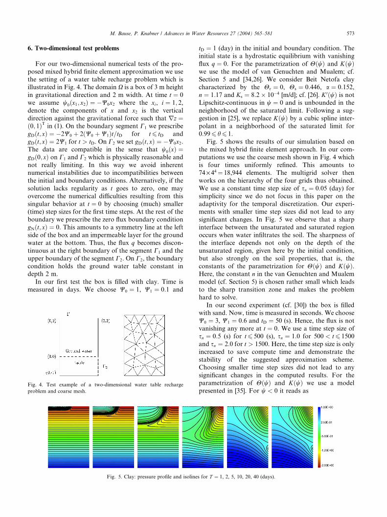
the setting of a water table recharge problem which isillustrated in Fig. 4. The domain X is a box of 3 m heightin gravitational direction and 2 m width. At time t ¼ 0we assume w0ðx1; x2Þ ¼ �W0x2 where the xi, i ¼ 1; 2,denote the components of x and x2 is the verticaldirection against the gravitational force such that rz ¼ð0; 1ÞT in (1). On the boundary segment C1 we prescribegDðt; xÞ ¼ �2W0 þ 2ðW0 þW1Þt=tD for t6 tD and

gDðt; xÞ ¼ 2W1 for t > tD. On C2 we set gDðt; xÞ ¼ �W0x2.The data are compatible in the sense that w0ðxÞ ¼gDð0; xÞ on C1 and C2 which is physically reasonable andnot really limiting. In this way we avoid inherent

numerical instabilities due to incompatibilities between

the initial and boundary conditions. Alternatively, if the

solution lacks regularity as t goes to zero, one mayovercome the numerical difficulties resulting from this

singular behavior at t ¼ 0 by choosing (much) smaller(time) step sizes for the first time steps. At the rest of the

boundary we prescribe the zero flux boundary condition

gNðt; xÞ ¼ 0. This amounts to a symmetry line at the leftside of the box and an impermeable layer for the ground

water at the bottom. Thus, the flux q becomes discon-tinuous at the right boundary of the segment C1 and theupper boundary of the segment C2. On C2, the boundarycondition holds the ground water table constant indepth 2 m.

In our first test the box is filled with clay. Time is

measured in days. We choose W0 ¼ 1, W1 ¼ 0:1 and

Fig. 4. Test example of a two-dimensional water table recharge

problem and coarse mesh.

Fig. 5. Clay: pressure profile and isoline

tD ¼ 1 (day) in the initial and boundary condition. Theinitial state is a hydrostatic equilibrium with vanishing

flux q ¼ 0. For the parametrization of HðwÞ and KðwÞwe use the model of van Genuchten and Mualem; cf.

Section 5 and [34,26]. We consider Beit Netofa claycharacterized by the Hr ¼ 0, Hs ¼ 0:446, a ¼ 0:152,n ¼ 1:17 and Ks ¼ 8:2 10�4 [m/d]; cf. [26]. K 0ðwÞ is notLipschitz-continuous in w ¼ 0 and is unbounded in theneighborhood of the saturated limit. Following a sug-

gestion in [25], we replace KðwÞ by a cubic spline inter-polant in a neighborhood of the saturated limit for

0:996 h6 1.Fig. 5 shows the results of our simulation based on

the mixed hybrid finite element approach. In our com-

putations we use the coarse mesh shown in Fig. 4 which

is four times uniformly refined. This amounts to

74 · 44¼ 18,944 elements. The multigrid solver then

works on the hierarchy of the four grids thus obtained.

We use a constant time step size of sn ¼ 0:05 (day) forsimplicity since we do not focus in this paper on the

adaptivity for the temporal discretization. Our experi-ments with smaller time step sizes did not lead to any

significant changes. In Fig. 5 we observe that a sharp

interface between the unsaturated and saturated region

occurs when water infiltrates the soil. The sharpness of

the interface depends not only on the depth of the

unsaturated region, given here by the initial condition,

but also strongly on the soil properties, that is, the

constants of the parametrization for HðwÞ and KðwÞ.Here, the constant n in the van Genuchten and Mualemmodel (cf. Section 5) is chosen rather small which leads

to the sharp transition zone and makes the problem

hard to solve.

In our second experiment (cf. [30]) the box is filled

with sand. Now, time is measured in seconds. We choose

W0 ¼ 3, W1 ¼ 0:6 and tD ¼ 50 (s). Hence, the flux is notvanishing any more at t ¼ 0. We use a time step size ofsn ¼ 0:5 (s) for t6 500 (s), sn ¼ 1:0 for 500 < t6 1500and sn ¼ 2:0 for t > 1500. Here, the time step size is onlyincreased to save compute time and demonstrate the

stability of the suggested approximation scheme.

Choosing smaller time step sizes did not lead to any

significant changes in the computed results. For the

parametrization of HðwÞ and KðwÞ we use a modelpresented in [35]. For w < 0 it reads as

s for T ¼ 1, 2, 5, 10, 20, 40 (days).

Fig. 6. Sand: pressure profile and isolines for T ¼ 50, 100, 200, 500, 1500, 4000 (seconds).


HðwÞ ¼ Hr þ ðHs �HrÞð1þ ð�awÞnÞ�1;KðwÞ ¼ Ksð1þ ð�bwÞmÞ�1:

We choose Hr ¼ 0:075, Hs ¼ 0:3, a ¼ 2:71, n ¼ 3:96,b ¼ 2:0, m ¼ 4:74 and Ks ¼ 10�4 [m/s].Fig. 6 shows the results of our simulation. Again, we

obtain a stable approximation of problem (1)–(3). Thus,

the mixed hybrid finite element methodology leads to apowerful approach to handle the nonlinear degenerate

problems of unsaturated–saturated flow.

7. Derivation of error indicators and adaptive mesh

refinement algorithm

In particular our first test problem in Section 6 has

shown that steep saturation fronts occur as water infil-

trates dry soil. In order to resolve these fronts with a

reasonable number of degrees of freedom and high

accuracy, a local mesh refinement of the triangulations is

inevitable for variably saturated subsurface flow prob-

lems. In this section shall present an error controlmechanism for the mixed hybrid finite element approx-

imation of problem (1)–(3). Our approach leads to error

indicators in contrast to sharp error estimators verified

by a rigorous mathematical analysis such that somewhat

heuristic arguments may be allowed in the following.

However, all performed calculations have led to con-

vincing results and the error indicators are rather easy

and fast to evaluate.The strategies for error control and mesh refinement

used in the finite element context are mostly based on a

posteriori error estimates in global norms which involve

local residuals of the computed solution. The resulting

mesh refinement process then aims at equilibrating these

local error indicators. For mixed finite element discret-

izations of linear elliptic problems Wohlmuth and

Hoppe [42,43] have recently derived and analyzed fourdifferent kinds of a posteriori error estimators: a residual

based estimator, a hierarchical one, error estimators

relying on the solution of local subproblems and on

superconvergence results. By similar techniques Car-

stensen [17] has also established a residual based esti-

mator. The estimators generalize the standard concepts

for a posteriori error estimators of the standard primal

formulation to the mixed setting. For an excellent

comparison of different kinds of error estimators in theconforming setting we refer to the work of Verf€urth [41].The investigation of the mixed approach is more com-

plicated and requires some additional tools. Our ap-

proach relies on the residual and the superconvergence

based a posteriori estimator of Wohlmuth and Hoppe

which we apply to our nonlinear degenerate problem

(1)–(3). They can be easily calculated by means of the

available finite element approximations. In contrast tothe hierarchical estimator, no additional subproblems

have to be solved which seems attractive for numerical

calculations. Controlling the accuracy in space by a

posteriori error estimators constructed for stationary

problems is a standard technique for dealing with par-

abolic ones; cf. [9,31,32]. Moreover, our performed

computations of subsurface flow and infiltration prob-

lems have borne out that the spatial discretization errorusually dominates the temporal one. Our computed re-

sults have shown not to be strikingly sensitive to changes

in the time step sizes; cf. Section 6. In the special case of

the superconvergence based error estimator, the funda-

mental error estimates on which the estimator relies can

be reproven for the spatial discretization of a quite

general class of parabolic problems; cf. [7]. Together,

this may be considered as a motivation or, even, justi-fication of our heuristic approach.

Another possibility to control the error is to discretize

simultaneously in space and time employing a discon-

tinuous Galerkin method and to apply coupled space–

time estimators; cf. [24]. Such a posteriori estimators

exist and have been rigorously analyzed for standard

discretizations but not for mixed finite element methods

of Raviart–Thomas type and degenerate problems.Moreover, since an additional dual problem has to be

solved, the efficient implementation of these estimators

is of fundamental importance and a demanding task.

For the future we are planning to incorporate global

residual based error control mechanisms relying on such

concepts. However, currently we follow the first more

heuristic approach which leads to simple error indica-

tors. The resulting numerical approximations are stableand robust as our examples in Section 8 confirm.


First, we give now an error indicator for the primal

variable w based on a superconvergence result. For thiswe recall that the multiplier technique that we have

applied in Section 3 has two significant advantages. The

first one is related to the specific structure of theresulting system of equations and the impact on the

efficiency of the solution process as shown in Section 3

and 4. The second advantage is some sort of a super-

convergence result concerning the approximation of w inthe L2 norm which we use to derive the error indicator.

In the standard conforming case, error estimators ob-

tained by some postprocessing of the approximation are

well known; cf. [37].To explain the fundamental superconvergence result

we consider, for simplicity, the linear elliptic problem

(16). We introduce the space of lowest order Crouzeix–

Raviart finite elements,

CRh ¼ flh 2 L2ðXÞjlh 2 P1ðKÞ 8K 2 Ph;

lhjKðmEÞ ¼ lhjK 0 ðmEÞ 8E ¼ K \ K 0; E 2 EIhg

where mE is the midpoint of an edge E 2 EIh. For a givensufficiently regular function g, let CRh;g be definedthrough CRh;g ¼ flh 2 CRhjlhðmEÞ ¼ gðmEÞ 8E 2 EDh g,where mE is the midpoint of an edge E 2 EDh . From nowon let ðuh; ph; vhÞ always denote the mixed hybrid finiteelement approximation of (16) obtained by applying the

discretization techniques described in Section 3 and 4 for

the Richards equation to the linear elliptic problem (16);

cf. [16]. Let uh be the interpolate in CRh;0 of the Lagrangemultipliers vh defined by means ofZEðuh � vhÞdr ¼ 0 ð19Þ

for all E 2 Eh. Then there holds (cf. [16])

ku� uhk6 chðkukW 22ðXÞ þ kf kW 1

2ðXÞÞ ð20Þ

as well as (k � k2HðX;divÞ ¼ k � k2 þ kr � ð�Þk2)

kp � phkHðX;divÞ6 chðkukW 22ðXÞ þ kf kW 1

2ðXÞÞ: ð21Þ

Further, we have (cf. [16])

ku� uhk6 ch2ðkukW 22ðXÞ þ kf kW 1

2ðXÞÞ: ð22Þ

The generic constant c does not depend on h. This showsthat uh provides a higher order approximation of theprimal variable u than the piecewise constant approxi-mation uh.The convergence rate estimates (20) and (22) now

motivate us to make the following (so-called) saturation

assumption:

There exists some constant 06 b < 1 such that

ku� uhk6 bku� uhk: ð23Þ

By means of the triangle inequality it is easy to see that

(23) gives rise to upper and a lower bounds for the

discretization error of the primal variable u in the L2

norm,

b1kuh � uhk6 ku� uhk6 b2kuh � uhk ð24Þ

with b1 ¼ ð1þ bÞ�1 and b2 ¼ ð1� bÞ�1. Then the errorestimator gS;u is given as follows:

g2S;u ¼XK2Ph

g2S;u;K ; gS;u;K ¼ kuh � uhkL2ðKÞ:

Clearly, condition (23) is used to ensure that the error

ku� uhk can be bounded below and above in terms ofkuh � uhk implying the reliability and sufficiency of theestimator gS;u. An equivalence between kuh � uhk and aweighted sum of the squared jumps of uh across theedges E 2 Eh can be established; cf. [43]. This is ofimportance if the original mixed system instead of itshybrid form is solved such that uh is not availablewithout solving additional local problems.

We return to the approximation of the subsurface

flow problems (1)–(3). Eq. (1) degenerates to an elliptic

equation in the fully saturated regime and remains

parabolic in the unsaturated one. Therefore, considering

the degenerate case as a perturbation of the saturated

one and proceeding in almost exactly the same way asbefore, we make the following saturation assumption:

For n ¼ 1; . . . ;N there exists some constant cn with

06 cn < 1 such that

kwðtnÞ � wnhk6 cnkwðtnÞ � wnhk: ð25Þ

Here wðtnÞ denotes the solution of (1)–(3) at time tn andwnh 2 CRh;g is the nonconforming extension of ekn definedanalogously to (19) by

REðwh � knhÞdr ¼ 0 for all E 2 Eh.

The fundamental convergence results (20) and (22)

that justify the assumption (23) and (25), respectively,may be violated for a combination of Dirichlet and

Neumann boundary conditions or, in particular, our

nonlinear degenerate problem where the solution lacks

enough regularity. Nevertheless, we may realistically

expect that they hold at least in some sense locally such

that the saturation assumption (25) remains reasonable.

This might be sufficient for our local error estimation

and grid refinement strategies and lead to a goodworking error indicator. We shall see. Further, we note

that the estimates (20) and (22) can be reproven for the

semidiscretization in space of a quite general class of

parabolic problems with sufficiently regular solution; cf.

[7]. If the fully discretized problem is considered, of

course, an additional term of the order OðkÞ arises in theerror estimates where k denotes the time step size. If k isof the order Oðh2Þ, then the superconvergence result (22)even holds for the fully discretized mixed finite element

approximation of such parabolic problems. Of course,

such severe restriction of the time step sizes would not be

efficient for computations, and it is also not necessary as

our performed calculations confirm; cf. Section 8. This

may be due to the minor importance of the temporal


discretization error already mentioned above. Our error

indicator (cf. (26)) is solely based on the saturation

assumption (25). No further restriction is used. Finally,

we note that the saturation assumption is formulated in

terms of the pressure head w and not the hydraulic headwþ z since w represents the primal variable of our for-mulation and we aim to control its approximation error

by an indicator. Alternatively, we could formulate a

saturation assumption for the hydraulic head wþ z byadding projections of z onto the spaces CRh and Wh to wn

h

and wnh, respectively. This is not done here.

Using the triangle inequality, assumption (25) directly

gives rise to the following upper and a lower bounds forthe L2-discretization error of w,

cn;1kwnh � wnhk6 kwðtnÞ � wnhk6 cn;2kw

nh � wn

hk

with cn;1 ¼ ð1þ cnÞ�1 and cn;2 ¼ ð1� cnÞ�1. Then the

superconvergence based error indicator gS;w for the

pressure head is given as (k � k ¼ k � kL2ðKÞ)

g2S;wn ¼XK2Ph

g2S;wn;K ; gS;wn;K ¼ kwnh � wn

hk: ð26Þ

Employing the trapezoidal quadrature rule, the local

error indicator gS;wn;K can be rewritten as

g2S;wn;K ¼1

3jKj

XEoK

ðeknE � wnKÞ2: ð27Þ

The terms on the right-hand side of this identity are

available without any additional computations. The

vector ekn ¼ ðeknEÞE2Eh is the vector of the unknowns ofthe global nonlinear system of equations which is solved

in each time step. The piecewise constant approxima-

tions wnK are computed locally in the Newton iterationswhen the residual of the nonlinear system of equations is

evaluated; cf. Section 4. Hence, gS;wn is rather easy andfast to compute. We recall that the basic estimates (20),

(22) hold in two and three dimensions such that (26)

may be applied in both cases.

So far, we have provided a superconvergence based

error indicator for the primal variable w of our flow

problems (1)–(3). For the mixed formulation (7) it isnatural to ask whether the error in the flux variable qcan be estimated and controlled similarly. Then, by

superposition we get an error indicator for the total

error. This seems possible by using a result of Brandts

[11]. To explain it, we restrict ourselves to the two-

dimensional case X R2. An extension to three space

dimensions seems possible but has not been completely

investigated and tested yet. For simplicity, let us firstconsider the linear elliptic problem (16) again. We fur-

ther suppose that the triangulation Ph is uniform which

means that two adjacent triangles of Ph form a paral-

lelogram; cf. [11]. Of course, this will be violated in an

adaptive grid refinement process. We will return to this

later. We introduce the operator Jh : Vh 7!CRh which is

locally given by its value at the midpoint mE of the tri-angulation

JhphðmEÞ ¼ 0:5 � ðphjK þ phjK 0 ÞðmEÞ;

with E ¼ K \ K 0, if E 2 EIh is an interior edge. SinceVh Hðdiv;XÞ is satisfied, the normal components toedges of functions vh 2 Vh are continuous across thoseedges of triangles. Hence, the operator Jh is actually onlypostprocessing the tangential components here. If we are

dealing with a boundary edge, that is, one which has

only a triangle K on one side of that edge, then there

exists, due to our assumption, at least one K 0 2 Ph such

that K [ K 0 is a parallelogram. The straight line throughthe midpoint mE of the boundary edge and the center mCof the parallelogram intersects the boundary of K [ K 0in another point mP . We will assume that Jhph is alreadydefined at mC and mP of at least one of the parallelo-grams K [ K 0 associable to K. Then we choose such aparallelogram and define the value of Jhph in mE bylinear extrapolation

JhphðmEÞ ¼ 2JhphðmCÞ � JhphðmP Þ: ð28ÞLet now u 2 W 3

2 ðXÞ, p ¼ �Aru denote the solution ofthe equations (16). Then, for a uniform and regular

triangulation there holds (cf. [11])

kp � Jhphk6 ch3=2kpkW 22ðXÞ ð29Þ

for the Dirichlet problem as well as

kp � Jhphk6 ch2kpkW 22ðXÞ ð30Þ

for the homogeneous Neumann problem where ph is themixed (hybrid) finite element approximation of p.Recalling (21), we see that Jhph provides a higher orderapproximation of p than ph.We now proceed in exactly the same way as for the

pressure. Motivated by the a priori estimates (21), (29)

and (30), we make the following saturation assumption:

There exists some constant 06 b < 1 such that

kp � Jhphk6 bkp � phk: ð31ÞAgain, (31) gives rise to upper and lower bounds for the

L2-discretization error of p,

b1kJhph � phk6 kp � phk6 b2kJhph � phkwith b1 ¼ ð1þ bÞ�1 and b2 ¼ ð1� bÞ�1. The error esti-mator gS;p is then given as

g2S;p ¼XK2Ph

g2S;p;K ; gS;p;K ¼ kJhph � phkL2ðKÞ:

It is easy to see that gS;u as well as gS;p is an asymptot-ically exact error estimator, that is, the quotient of the

error estimator and the error itself converges to 1 when htends to zero.

We return to problems (1)–(3). In an adaptive grid

refinement process the above-made uniformity assump-

tion about the triangulation which is fundamental for


the convergence rate estimates (29) and (30) is usually

violated. The rationale for using nevertheless the fol-

lowing approach based on (29) and (30) comes in the

numerical results; cf. Section 8. First, the extrapolation

(28) for boundary edges has to be redefined. The straightline through the midpoint mE of the boundary edge Eand the midpoint mE of another edge E of the triangle Kintersects the element K 0 adjacent to E in some point p eEon eE 6¼ E that is not necessarily the midpoint of eE. Theoperator eJh is then defined analogously to Jh, now withlinear extrapolation from mE and peE . Motivated by (21),(29) and (30), we make the saturation assumption:

For n ¼ 1; . . . ;N there exists some constant cn with

06 cn < 1 such that

kqðtnÞ � eJhqnhk6 cnkqðtnÞ � qnhk: ð32ÞHere qðtnÞ denotes the solution of (2)–(5) at time tn. Oursuperconvergence based error indicator for the flux q isthen given by (k � k ¼ k � kL2ðKÞ)

g2S;qn ¼XK2Ph

g2S;qn;K ; gS;qn;K ¼ kqnh � eJhqnhk: ð33Þ

Again, (32) ensures the existence of lower and upper

bounds for kqðtnÞ � qnhk in terms of kqnh � eJhqnhk.Employing the trapezoidal quadrature rule, the term

gS;qn;K can be rewritten as

g2S;qn;K ¼1

3

XK2Ph

jKjXEoK

ðqnE � eJhqnhðmEÞÞ2:In the parabolic case a superconvergence result for

the flux q, similarly to (29) and (30), can be proven forthe semidiscretization in space with respect to the norm

of L2ðJ ; L2ðXÞÞ; cf. [7]. This would require a time-inte-grated saturation assumption and lead to an error esti-

mator for the totalized error ðPn

i¼0 aikqðtiÞ � qihk2Þ1=2

with some weights ai depending, in particular, on thetime step sizes si. Nevertheless, we use the non-inte-grated version (32) of the saturation assumption, pri-marily, since we aim to apply the a posteriori error

estimator of the stationary case also to parabolic and

degenerate problems and, secondly, since computations

have shown that (33) leads to more robust results than

its corresponding totalized counterpart.

Finally, we give a residual based indicator for the

total error kwðtnÞ � wnhk þ kqðtnÞ � qnhkHðX;divÞ. For sim-

plicity, we first consider the linear elliptic problem (16)again. We further suppose that A is a piecewise constantdiagonal matrix. The basic idea behind the construction

of the residual based error estimator is to use the

Helmholtz decomposition of the flux space HðX; divÞ,HðX; divÞ ¼ H 0ðdiv;XÞ H 1ðdiv;XÞ;where H 0ðdiv;XÞ ¼ fq 2 HðX; divÞjr � q ¼ 0g and

H 1ðdiv;XÞ ¼ fq 2 HðX; divÞjhA�1q;q0i ¼ 0 8q0 2H 0ðdiv;XÞg; cf. [17,43]. According to this splitting, the fluxerror can uniquely be written as pe ¼ p0e þ p1e where

p0e 2 H 0ðdiv;XÞ and p1e 2 H 1ðdiv;XÞ. The mixed varia-tional problem satisfied by the error ðue; peÞ ¼ðu� uh; p � phÞ can then be decomposed into two inde-pendent subproblems which are treated separately. The

first subproblem is associated with the solenoidal sub-space and gives rise to the problem (cf. [43])

hA�1p0e ; vi ¼ rðvÞ for all v 2 H 0ðdiv;XÞ; ð34Þ

where the residual r is given by rðvÞ ¼ �hA�1ph; viþhr � v; uhi. From (34) it follows (cf. [43]) thatP

EoK wEaEhEk½A�1ph � f�k2

L2ðEÞ yields sharp upper and

lower bounds for the solenoidal part p0e of the flux error.Here, hE denotes the length of the edge E and f is theunit tangential vector on oK obtained by rotating theouter normal m on oK by p=2 counterclockwise. Let aK0and aK1 , 0 < aK0 6 aK1 , be the local bounds of the coeffi-cient matrix A defined by means of aK0 jnj

26 nTAn6

aK1 jnj2, n 2 R2, for almost all x 2 K. Then, the weighting

factors aE are defined by aE :¼ 14ðaK10 þ aK20 þ aK11 þ aK21 Þ

and wE ¼ 12if E ¼ oK1 \ oK2 is an interior edge, and by

aE :¼ 12ðaK0 þ aK1 Þ and wE ¼ 1 if E oK \ oX. The jump

½�� on the interior edge E ¼ oK1 \ oK2 is defined by½A�1ph� f� ¼A�1ph � fjK1 � A�1ph � fjK2 , and on the bound-ary edge E oK \ oX as ½A�1ph � f� ¼ A�1ph � fjK .To obtain a sharp estimate for pe, in a second step the

term p1e is considered. Recalling r � pe ¼ r � p1e , themixed approximation of (16) also yields

hr � p1e ;wi ¼ hf � P0f ;wi for all w 2 L2ðXÞ; ð35Þ

where P0f denotes the L2-projection of f onto Wh. Eq.(35) readily provides a lower and upper L2-bound forr � p1e and, moreover, using a norm equivalence on

H 1ðdiv;XÞ, also for p1e in terms of f � P0f ; cf. [43] fordetails. The error ue in the primal variable is thenbounded above and below by making use of the pre-

ceding estimates and standard duality techniques. Pre-

cisely, the residual based error estimator proven in [43]

for a piecewise constant diagonal matrix A reads as

g2R;u;p ¼XK2Ph

g2R;u;p;K ;

g2R;u;p;K ¼ kf � P0f k2

L2ðKÞ þ h2KkA�1phk2

L2ðKÞ

þXEoK

wEaEhEk½A�1ph � f�k2L2ðEÞ;

where hK the diameter of K. Again, an error estimator isobtained which can be easily calculated by means of the

available finite element approximations of the primal

variable and the flux. No additional subproblems haveto be solved. In the special case of the Poisson equation

with homogeneous Dirichlet boundary conditions the

sum gS;u þ gS;p of the superconvergence based estimatorfor the primal variable and the flux is locally equivalent

with the residual based error estimator; cf. [43]. Hence,

we may expect similar meshes for the either indicators.


For our subsurface flow problems (1)–(3) the corre-

sponding indicator reads as (k � k ¼ k � kL2ðKÞ)

g2R;wn;qn ¼XK2Ph

g2R;wn;qn;K ;

g2R;wn;qn;K ¼ kz� P0zk2 þ h2KkKðw

nÞ�1qnhk2

þXEoK

wEaEhEk½KðwnhÞ�1qnh � f�k

2

L2ðEÞ

with wE and aE being defined analogously to the ellipticcase. The formulation of the error indicator again relieson our approach to apply systematically the error esti-

mator of the linear elliptic regime also to parabolic and

degenerate problems.

Finally, it remains to describe our adaptive mesh

refinement algorithm; cf. also [6]. As input this algo-

rithm receives a hierarchy P ¼ fPjhjg

mj¼0 of simplicial

triangulations of X on which the linear problem of the

Newton iteration is solved (cf. Section 4) and where theleaf elements (those without sons) have been tagged with

a refinement rule or a coarsening tag. Here, we use the

well known refinement process due to Bank et al. [5].

The refinement rule is such that a triangle K 2 Pjhj ,

06 j6m, either remains unrefined, or is subdivided intofour congruent subtriangles, or is bisected into two

subtriangles. Following the refinement in [5], each tri-

angle K 2 Pjh is geometrically similar either to an ele-

ment of P0h0or to a bisected triangle of P0

h0. If all sons of

an element are tagged for coarsening, they are deleted

from the data structure. Of course only leaf elements can

be removed, since coarsening should be an inverse

operation to refinement. A high-level version of the

global refinement algorithm reads as:

RefineMultiGrid(P;m) ¼ {

for l ¼ m;m� 1; . . . ; 1MakeConsistent(Pl

hl)

RestrictTags(Plhl,Pl�1

hl�1)

for l ¼ 0; 1; . . . ;mMakeConsistent(Pl

hl)

DetermineCopies(Plhl)

RefineGrid(Plhl) }

The overall structure of the algorithm RefineMultiGrid

resembles a multigrid V-cycle. The first for-loop pro-ceeds from the top level m to level 1. No manipulation ofthe data structure is done in this first loop, only the

refinement tags are manipulated. The function Make-

Consistent computes a consistent grid for level lþ 1 bytagging elements of level l with the refinement rule.Function RestrictTags computes the influence of level-l-tags on level-(l� 1)-tags. In the second loop the datastructure is actually modified proceeding from coarse to

fine levels. When the second loop is entered, the grid on

level l has already been modified and level lþ 1 isconstructed from tags stored on level l. Again Make-

Consistent is called to compute consistent tags. Then

DetermineCopies computes the algebraic classes which

in turn determine the copy elements required on level

lþ 1. The function RefineGrid actually modifies thedata structure. Appropriate objects are created/deletedon level lþ 1. After completion the function Refine-Multigrid has constructed a new multigrid hierarchy. Its

top level is either m� 1, m or mþ 1. Intergrid transferoperators for systems with element- and edgewise de-

grees of freedom are defined and analyzed in [12]. In

[12], the prolongation of the edge values is independent

of the element values. Therefore, we instead use the

prolongation given in [10] for the lowest-order Crou-zeix–Raviart element; cf. Section 4. Restriction is the

adjoint mapping. The intergrid transfer operator for the

elementwise degrees of freedom is defined by averaging;

cf. [12].

For local tagging of the elements K of a gridPh of the

hierarchy P, the elementwise contributions gK of therespective error indicator gS;wn , gS;qn or gR;wn;qn , respec-tively, are computed. An element K 2 Ph is tagged forcoarsening if g2K jKj

�1< r � e, where e is a prescribed

accuracy and r is a tolerance that is typically chosen in½ 110; 16�. The factor r inhibits the coarsening of the ele-

ments and, thereby, prevents spurious oscillations in the

grid generation process. The element K is tagged for

refinement if g2K jKj�1

> e. If r � e6 g2K jKj�1

6 e, K re-

mains unmodified.

The adaptive mesh refinement algorithm is appliedonly once before a time step is performed except for the

initial time where an iteration between setting of the

initial value and grid adaptation is done. This seems to

be a practicable and an efficient approach. The result is

in fact a good working error indicator as the simulations

in Section 8 confirm. Computations have shown that

iterating in each time step strongly increases the com-

pute time, but does not lead to any significant changes inthe adaptively generated grids. Further, it should not be

forgotten, that our adaptive techniques lead to error

indicators in contrast to mathematically rigorous esti-

mators. Of course, the error indicators may also be

applied in an iterative way which means that every time

step is recomputed on a modified grid until the (local)

error indicators satisfy the prescribed tolerances.

8. Adaptive simulations

For the numerical test of our error indicators and

mesh refinement algorithm we recompute the first of thewater table recharge problems of Section 6. At the initial

time, the coarse grid (level zero) of the multigrid algo-

rithm is generated by subdiving all triangles of the mesh

shown in Fig. 4 into four congruent subtriangles. In

either experiments (cf. Fig. 7), the iteration at t ¼ 0between setting of the initial value and grid adaptation

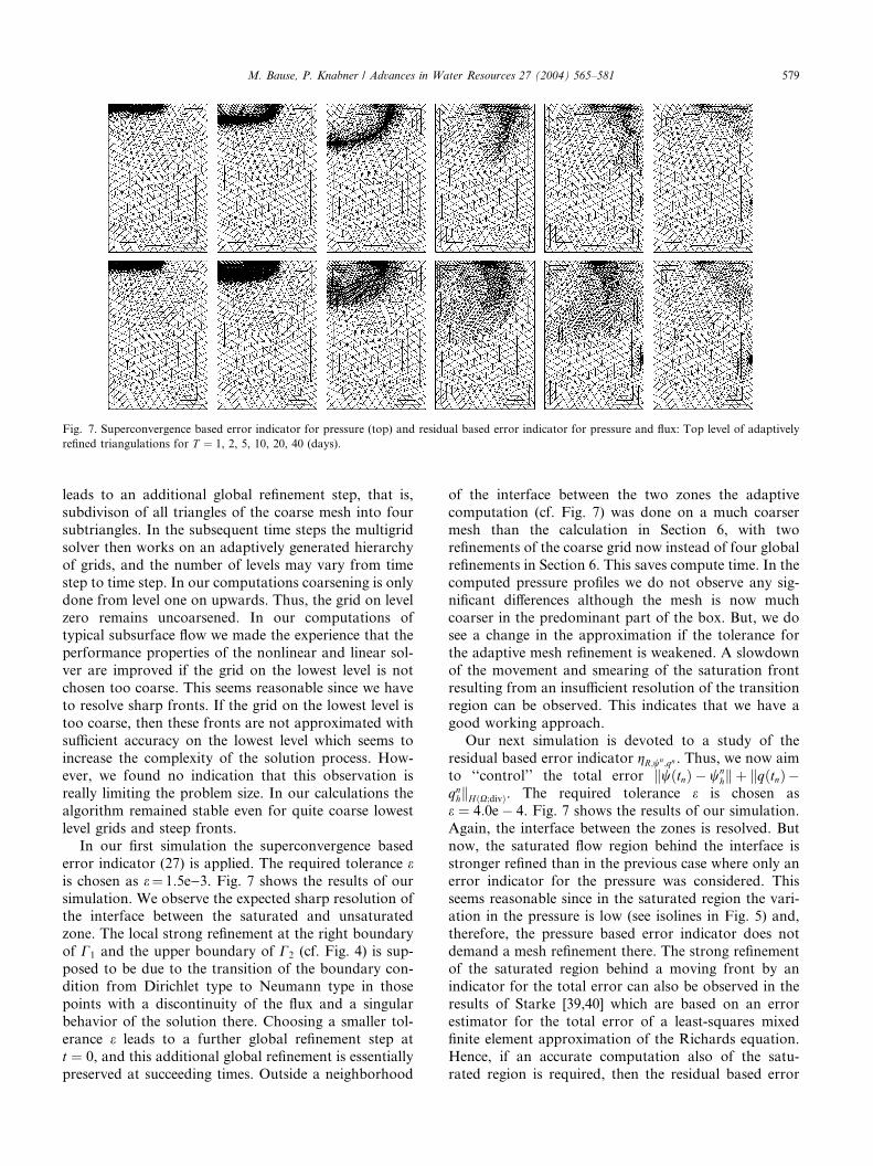
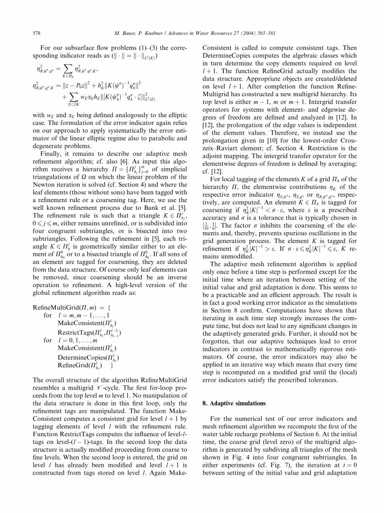
Fig. 7. Superconvergence based error indicator for pressure (top) and residual based error indicator for pressure and flux: Top level of adaptively

refined triangulations for T ¼ 1, 2, 5, 10, 20, 40 (days).


leads to an additional global refinement step, that is,

subdivison of all triangles of the coarse mesh into four

subtriangles. In the subsequent time steps the multigrid

solver then works on an adaptively generated hierarchy

of grids, and the number of levels may vary from time

step to time step. In our computations coarsening is only

done from level one on upwards. Thus, the grid on level

zero remains uncoarsened. In our computations oftypical subsurface flow we made the experience that the

performance properties of the nonlinear and linear sol-

ver are improved if the grid on the lowest level is not

chosen too coarse. This seems reasonable since we have

to resolve sharp fronts. If the grid on the lowest level is

too coarse, then these fronts are not approximated with

sufficient accuracy on the lowest level which seems to

increase the complexity of the solution process. How-ever, we found no indication that this observation is

really limiting the problem size. In our calculations the

algorithm remained stable even for quite coarse lowest

level grids and steep fronts.

In our first simulation the superconvergence based

error indicator (27) is applied. The required tolerance eis chosen as e¼ 1.5e)3. Fig. 7 shows the results of oursimulation. We observe the expected sharp resolution ofthe interface between the saturated and unsaturated

zone. The local strong refinement at the right boundary

of C1 and the upper boundary of C2 (cf. Fig. 4) is sup-posed to be due to the transition of the boundary con-

dition from Dirichlet type to Neumann type in those

points with a discontinuity of the flux and a singular

behavior of the solution there. Choosing a smaller tol-

erance e leads to a further global refinement step att ¼ 0, and this additional global refinement is essentiallypreserved at succeeding times. Outside a neighborhood

of the interface between the two zones the adaptive

computation (cf. Fig. 7) was done on a much coarser

mesh than the calculation in Section 6, with two

refinements of the coarse grid now instead of four global

refinements in Section 6. This saves compute time. In the

computed pressure profiles we do not observe any sig-

nificant differences although the mesh is now much

coarser in the predominant part of the box. But, we dosee a change in the approximation if the tolerance for

the adaptive mesh refinement is weakened. A slowdown

of the movement and smearing of the saturation front

resulting from an insufficient resolution of the transition

region can be observed. This indicates that we have a

good working approach.

Our next simulation is devoted to a study of the

residual based error indicator gR;wn;qn . Thus, we now aimto ‘‘control’’ the total error kwðtnÞ � wn

hk þ kqðtnÞ�qnhkHðX;divÞ. The required tolerance e is chosen as

e ¼ 4:0e� 4. Fig. 7 shows the results of our simulation.Again, the interface between the zones is resolved. But

now, the saturated flow region behind the interface is

stronger refined than in the previous case where only an

error indicator for the pressure was considered. This

seems reasonable since in the saturated region the vari-ation in the pressure is low (see isolines in Fig. 5) and,

therefore, the pressure based error indicator does not

demand a mesh refinement there. The strong refinement

of the saturated region behind a moving front by an

indicator for the total error can also be observed in the

results of Starke [39,40] which are based on an error

estimator for the total error of a least-squares mixed

finite element approximation of the Richards equation.Hence, if an accurate computation also of the satu-

rated region is required, then the residual based error


indicator seems to be superior to the superconvergence

based indicator for the pressure. Otherwise, for appli-

cations in which only the position of the saturation front

is of importance, the superconvergence based error

indicator seems to be sufficient and more efficient.Similarly to the previous case, we observe a local strong

refinement at the right boundary of C1 and the upperboundary of C2 due to the change of the type of theboundary conditions there.

If the adaptive grid generation is based on the sum of

the superconvergence based error indicators gS;wn andgS;qn for pressure head w and flux q, we obtain grids quitesimilar to those of the previous case (cf. Fig. 7) in whichthe flow region behind the interface is again stronger

refined than in the first case. However, since gS;qn istypically much smaller than gS;wn , one has to weight thetwo terms by considering c1gS;wn þ c2gS;qn with somefixed constants c1 and c2. The equivalence of the gridsdoes not seem to be surprising due to the above-men-

tioned known local equivalence of the error estimators

for the Poisson equation.Finally, we shall show that the proposed adaptive

algorithm is in fact superior to a computation on a

uniform mesh. This is done by comparing the resulting

discretization errors. For simplicity, we consider a one-

dimensional problem. We recompute the second of the

examples of Section 5. It is done for the temporal step

size s ¼ 0:1 only. For spatial discretization parametersh 2 ½2 10�4; 0:1� we calculate the L2-error of the pres-sure by comparing the approximate solutions obtained

on these meshes to the reference solution calculated on a

very fine grid; cf. Section 5. This is done for the time

t ¼ 100 and 2000. The adaptive computations are per-formed with tolerance r ¼ 1=6 and for accuracy

parameters e 2 ½10�7; 10�2�. Precisely, within the res-

pective interval of h and e we choose the values 10i,2 10i and 5 10i for every order of magnitudei ¼ �1;�2; . . .. In the adaptive simulations we use thesuperconvergence based error indicator gS;w for the

pressure. The approximation errors over the number of

elements are visualized in Fig. 8. Similar plots are ob-

tained for the residual based indicator.

We nicely observe that the adaptive calculations lead

to smaller discretization errors over the whole range

0.001

0.01

0.1

10 100 10000.0001

0.001

0.01

0.1

10 100 1000

t = 100 t = 2000

Fig. 8. Error kw� whkL2ðXÞ over number of elements for uniform(––) and adaptive (}) mesh.

and, thus, have an advantage over the uniform com-

putations. At t ¼ 100 this difference is more significantthan at t ¼ 2000 which is due to the fact that the pres-sure profile is much steeper at t ¼ 100. It is resolvedmore accurately by the adaptive distribution of the finiteelements. In the left plot the curves approach a constant

number for h! 0 which is due to the dominating tem-

poral discretization error in this range.

9. Conclusions

We think that these numerical results show theeffectiveness of the adaptive mixed hybrid finite element

approach for the nonlinear degenerate problems arising

in variably saturated subsurface flow. In particular, the

results of our computational tests demonstrate two

favorable properties: (i) the use of the proposed heuristic

based error indicators which are easy and fast to eval-

uate without solving additional (sub-)problems leads to

a good working adaptive mesh refinement algorithm,and (ii) the Newton and multigrid method are robust

schemes to solve the resulting nonlinear system of

equations. The mixed hybrid finite element methodology

thus leads to a powerful approach to handle the non-

linear degenerate problems in saturated–unsaturated

subsurface flow.

Acknowledgements

The authors thank the referees for their suggestions

for improving the presentation of the paper.

References

[1] Adams RA. Sobolev spaces. New York: Academic Press; 1975.

[2] Alt HW, Luckhaus S. Quasilinear elliptic–parabolic differential

equations. Math Z 1983;183:311–41.

[3] Arbogast T, Wheeler MF, Zhang NY. A nonlinear mixed finite

element method for a degenerate parabolic equation arising

in flow in porous media. SIAM J Numer Anal 1996;33:1669–

87.

[4] Arnold DN, Brezzi F. Mixed and nonconforming finite element

methods: implementation, postprocessing and error estimates.

RAIRO Model Math Anal Numer 1985;19(1):7–32.

[5] Bank R, Sherman A, Weisser A. Refinement algorithm and data

structure for regular local mesh refinement. In: Stepleman R et al.,

editors. Scientific computing, vol. 44. Amsterdam: North-Hol-

land; 1993.

[6] Bastian P, Birken K, Johannsen K, Lang S, Neuß N, Rentz-

Reichert H, Wieners C. UG––a flexible software toolbox for

solving partial differential equations. Comput Visual Sci 1997;1:

27–40.

[7] Bause M, Knabner P. Superconvergence of mixed hybrid finite

element methods and adaptive approximation of variably satu-

rated subsurface flow, to appear.

[8] Bear J. Dynamics of fluids in porous media. New York: Elsevier;

1972.


[9] Berzins M, Capon PJ, Jimack PK. On spatial adaptivity and

interpolation when using the method of lines. Appl Numer Math

1998;26:117–33.

[10] Braess D, Verf€urth R. Multigrid methods for nonconforming

finite element methods. SIAM J Numer Anal 1990;27:979–86.

[11] Brandts J. Superconvergence and a posteriori error estimation for

triangular mixed finite elements. Numer Math 1994;68:311–24.

[12] Brenner SC. Multigrid algorithm for the lowest-order Raviart–

Thomas mixed triangular finite element method. SIAM J Numer

Anal 1992;29:647–78.

[13] Brenner SC. Convergence of nonconforming multigrid methods

without full elliptic regularity. Math Comput 1999;68:25–53.

[14] Brezzi F, Douglas J, Duran R, Fortin M. Mixed finite elements

for second order elliptic problems. Numer Math 1987;51:237–50.

[15] Brezzi F, Douglas J, Fortin M, Marini LD. Efficient rectangular

mixed finite elements in two and three space variables. Math

Model Numer Anal 1987;21:581–604.

[16] Brezzi F, Fortin M. Mixed and hybrid finite element methods.

New York: Springer; 1991.

[17] Carstensen C. A posteriori error estimate for the mixed finite

element method. Math Comput 1997;66(218):465–76.

[18] Celia MA, Bouloutas ET, Zarba RL. A general mass-conservative

numerical solution for the unsaturated flow equation. Water

Resour Res 1990;26:1483–96.

[19] Chavent G, Roberts JE. A unified physical presentation of mixed,

mixed-hybrid finite element method and standard finite difference

approximations for determination of velocities in water flow

problems. Adv Water Resour 1991;14(6):329–48.

[20] Chen Z. Analysis of mixed methods using conforming and

nonconforming finite element methods. M2AN 1993;27:9–34.

[21] Chen Z. Equivalence between and multigrid algorithms for

nonconforming and mixed methods for second-order elliptic

problems. J Numer Math 1996;4:1–33.

[22] Chen Z, Ewing RE. Degenerate two-phase incompressible flow

IV: local refinement and domain decomposition. J Sci Comput

2003;18(3):329–60.

[23] Ehlers W, Ammann M, Diebels S. h-Adaptive FE methods

applied to single- and multiphase problems. Int J Numer Meth

Eng 2002;5(11):1579–603.

[24] Eriksson K, Johnson C. Adaptive finite element methods for

parabolic problems IV: nonlinear problems. SIAM J Numer Anal

1995;32:1729–49.

[25] Fuhrmann J. Zur verwendung von mehrgitterverfahren bei der

numerischen behandlung elliptischer partieller differentialgleich-

ungen mit variablen koeffizienten. PhD thesis, University Chem-

nitz, 1993.

[26] van Genuchten MT. A closed-form equation for predicting the

hydraulic conductivity of unsaturated soils. Soil Sci Soc Am

1980;44:892–8.

[27] Hornung U, Messing W. A predictor corrector alternating

direction implicit method for two-dimensional unsteady satu-

rated–unsaturated flow in porous media. J Hydrol 1980;47:317–23.

[28] Huang WZ, Zheng L, Zhan XY. Adaptive moving mesh methods

for simulating one-dimensional groundwater problems with

sharp moving fronts. Int J Numer Meth Eng 2002;54(11):1579–

603.

[29] Kelley CT. Iterative methods for linear and nonlinear equations.

Philadelphia: SIAM; 1995.

[30] Knabner P. Finite element solution of saturated–unsaturated flow

through porous media. In: Deufelhard P, Engquist B, editors.

Large scale computing. Stuttgart: Birkhauser; 1987. p. 83–93.

[31] Lang J. Adaptive multilevel solution of nonlinear parabolic PDE

systems. Berlin: Springer; 2001.

[32] Moore PK. A posteriori error estimation with finite element semi-

and fully discrete methods for nonlinear parabolic equations in

one space dimension. SIAM J Numer Anal 1994;31:149–69.

[33] Mos�e R, Siegel P, Ackerer P. Application of the mixed bybrid

finite element approximation in a groundwater flow model: luxury

or necessity. Water Resour Res 1994;30(11):3001–12.

[34] Mualem Y. A new model for predicting hydraulic conductivity of

unsaturated porous media. Water Resour Res 1976;12:513–22.

[35] Haverkamp R, Vauclin M, Touma J, Wierenga PJ, Vachaud G. A

comparison of numerical simulation models for one-dimensional

infiltration. Soil Sci Soc Am J 1977;41:285–94.

[36] Radu F, Pop IS, Knabner P. Order of convergence estimates in

time and space for an implicit Euler/mixed finite element

discretization of Richards equation by equivalence of mixed and

conformed approaches. SIAM J Numer Anal, in press.

[37] Rodriguez R. Some remarks on Zienkiewicz–Zhu estimator.

Numer Meth Partial Different Eqns 1994;10:625–36.

[38] Schneid E. Hybrid mixed finite element discretization of the

Richards equation (in German). PhD thesis, University Erlangen-

N€urnberg, 2000.

[39] Starke G. Gauss–Newton multilevel methods for least-squares

finite element computations of variably saturated subsurface flow.

Computing 1999;64:323–38.

[40] Starke G. Least-squares mixed finite element solution of variably

saturated subsurface flow problems. SIAM J Sci Comput

2000;21:1869–85.

[41] Verf€urth R. A review of a posteriori error estimation and adaptive

mesh-refinement techniques. Chichester: Wiley–Teubner; 1996.

[42] Wohlmuth BI, Hoppe RHW. Adaptive multilevel techniques for

mixed finite element discretizations of elliptic boundary value

problems. SIAM J Numer Anal 1997;34(4):1658–81.

[43] Wohlmuth BI, Hoppe RHW. A comparison of a posteriori error

estimators for mixed finite element discretizations by Raviart–

Thomas elements. Math Comput 1999;68(228):1347–78.

[44] Woodward CS, Dawson CN. Analysis of expanded mixed finite

element methods for a nonlinear parabolic equation modeling

flow into a variably saturated porous media. SIAM J Numer Anal

2000;37:701–24.

[45] Zienkiewicz OC, Zhu JZ. A simple error estimator and adaptive

procedure for practical engineering analysis. Int J Numer Meth

Eng 1987;28:28–39.

Computation of variably saturated subsurface flow by adaptive mixed hybrid finite element methods

Documents

Transcript of Computation of variably saturated subsurface flow by adaptive mixed hybrid finite element methods