Prediction of error in finite element results
10
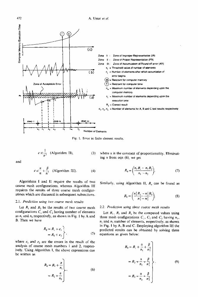
PREDICTION OF ERROR IN FINITE ELEMENT RESULTS A. Umar,t H. Abbas,f A. Qadeerf and D. K. Sehgals tuniversity Polytechnic, Aligarh Muslim University, Aligarh 202 002, India fDepartment of Civil Engineering, Aligarh Muslim University, Aligarh 202 002, India §Department of Applied Mechanics, Indian Institute of Technology, New Delhi 110 016, India (Received 13 January 1995) Abstract-The precision in the results of analysis using the finite element (FE) technique requires that a structure to be analyzed shall be discretized using a finer mesh. The number of elements into which the structure shall be discretized so as to obtain the FE results within an acceptable tolerance is usually decided by experience or a guess. Moreover, the error in the results of FE analysis is an unknown, therefore, it is difficult to say whether the results are within an acceptable tolerance. It is due to these reasons that an extrapolation technique is presented in the present paper to predict the results more precisely by carrying out the analysis for two mesh configurations which have a different number of elements in each case, but possess a similar discretization pattern. This is done by taking into consideration the variation of parameters within the body of the structure. The error in the results of analysis of plane strain and plate bending problems has been found to be inversely proportional to the number of elements. Two other algorithms for the modeling of error have also been tested. Several numerical examples under the two categories of problems considered in the study are presented to demonstrate the utility of the proposed extrapolation technique. Copyright 0 1996 Elsevier Science Ltd. 1. INTRODUCTION The precision in the results of analysis using the finite element method (FEM) requires that the structure to be analyzed shall be discretized using a finer mesh in addition to the correct representation of the structure [ 1,2]. However, finer mesh discretization requires a large computer memory as well as execution time. The variation of FE results with the increase in the number of elements is shown in Fig. 1. The whole range of number of elements has been divided into three zones. When the number of elements is small (n < n,) then the FE results are not reliable; this has been named as the zone of improper representation (IR). The increase in the number of elements beyond ni leads to the gradual convergence of test results as shown in Fig. l(a), provided the discretization is done by taking into consideration the expected variation of parameters within the body of the structure. Otherwise the convergence is achieved only when very large number of elements are taken, as shown in Fig. l(b). This zone has been known as the zone of proper representation (PR) which is the zone II. The increase in the number of elements beyond n, (Fig. 1) leads to the accumulation of round off error consequently FE results become deviated from the correct results instead of getting converged. It is obvious that the increase in the number of elements gives rise to the increase in the requirement of computer memory and execution time, shown in Fig. I(c). If the minimum number of the elements n required for the acceptable error suits the machine as well as the user (i.e. n < nr and n <n,) then the FE results will be reliable. However, when the number of elements n required for the acceptable error does not suit the machine or the user (i.e. n > nT or n > n,) then the FE results become unreliable. Moreover, the minimum number of elements required for the acceptable error is an unknown. Therefore, it is always advisable to carry out the analysis for two or three mesh configurations having different number of elements in each case, but having similar discretiza- tion pattern. This takes into consideration the vari- ation of parameters within the structure, with better results being predicted, or the error in the analysis may be checked using the algorithm presented in the paper. To demonstrate the versatility of the approach, some numerical examples have been presented. 2. EXTRAPOLATION TECHNIQUE Let R, be the correct results and R be the result of a coarse mesh analysis obtained by using n number of elements. If e is the error in the result, then R,= R fe. (1) Three different algorithms tested in the present study for modeling of the error e are; e cc: (Algorithm I),
-
Upload
unversitycentralpunjablahore -
Category
Documents
-
view
1 -
download
0
Transcript of Prediction of error in finite element results
htiizh Com~ulers & Srrucrures Vol. 60. No. 3. pp. 471480. 1996
> Pergamon 0045-7949~95Mo41 l-4 Copyright 0 1996 El&ier Science Ltd
Pnnted in Great Britain. All riehts reserved
w . I
OiMS-7949/96 ;I 5.00 + 0.00
PREDICTION OF ERROR IN FINITE ELEMENT RESULTS
A. Umar,t H. Abbas,f A. Qadeerf and D. K. Sehgals
tuniversity Polytechnic, Aligarh Muslim University, Aligarh 202 002, India fDepartment of Civil Engineering, Aligarh Muslim University, Aligarh 202 002, India
§Department of Applied Mechanics, Indian Institute of Technology, New Delhi 110 016, India
(Received 13 January 1995)
Abstract-The precision in the results of analysis using the finite element (FE) technique requires that a structure to be analyzed shall be discretized using a finer mesh. The number of elements into which the structure shall be discretized so as to obtain the FE results within an acceptable tolerance is usually decided by experience or a guess. Moreover, the error in the results of FE analysis is an unknown, therefore, it is difficult to say whether the results are within an acceptable tolerance. It is due to these reasons that an extrapolation technique is presented in the present paper to predict the results more precisely by carrying out the analysis for two mesh configurations which have a different number of elements in each case, but possess a similar discretization pattern. This is done by taking into consideration the variation of parameters within the body of the structure. The error in the results of analysis of plane strain and plate bending problems has been found to be inversely proportional to the number of elements. Two other algorithms for the modeling of error have also been tested. Several numerical examples under the two categories of problems considered in the study are presented to demonstrate the utility of the proposed extrapolation technique. Copyright 0 1996 Elsevier Science Ltd.
1. INTRODUCTION
The precision in the results of analysis using the finite element method (FEM) requires that the structure to be analyzed shall be discretized using a finer mesh in addition to the correct representation of the structure [ 1,2]. However, finer mesh discretization requires a large computer memory as well as execution time. The variation of FE results with the increase in the number of elements is shown in Fig. 1. The whole range of number of elements has been divided into three zones. When the number of elements is small (n < n,) then the FE results are not reliable; this has been named as the zone of improper representation (IR). The increase in the number of elements beyond ni leads to the gradual convergence of test results as shown in Fig. l(a), provided the discretization is done by taking into consideration the expected variation of parameters within the body of the structure. Otherwise the convergence is achieved only when very large number of elements are taken, as shown in Fig. l(b). This zone has been known as the zone of proper representation (PR) which is the zone II. The increase in the number of elements beyond n, (Fig. 1) leads to the accumulation of round off error consequently FE results become deviated from the correct results instead of getting converged. It is obvious that the increase in the number of elements gives rise to the increase in the requirement of computer memory and execution time, shown in Fig. I(c).
If the minimum number of the elements n required for the acceptable error suits the machine as well
as the user (i.e. n < nr and n <n,) then the FE results will be reliable. However, when the number of elements n required for the acceptable error does not suit the machine or the user (i.e. n > nT or n > n,) then the FE results become unreliable. Moreover, the minimum number of elements required for the acceptable error is an unknown. Therefore, it is always advisable to carry out the analysis for two or three mesh configurations having different number of elements in each case, but having similar discretiza- tion pattern. This takes into consideration the vari- ation of parameters within the structure, with better results being predicted, or the error in the analysis may be checked using the algorithm presented in the paper. To demonstrate the versatility of the approach, some numerical examples have been presented.
2. EXTRAPOLATION TECHNIQUE
Let R, be the correct results and R be the result of a coarse mesh analysis obtained by using n number of elements. If e is the error in the result, then
R,= R fe. (1)
Three different algorithms tested in the present study for modeling of the error e are;
e cc: (Algorithm I),
471
A. Umar et al.
Zone of Acceptable Error
( cl
e cc; (Algorithm II),
and
, zollc-I,,
I- -
c “1
Number of Elements
Fig. 1. Error in finite element results.
e cc: + $ (Algorithm III). (4)
Algorithms I and II require the results of two coarse mesh configurations, whereas Algorithm III requires the results of three coarse mesh configur- ations which are discussed in subsequent subsections.
2.1. Prediction using two coarse mesh results
Let R, and R, be the results of two coarse mesh configurations C, and C, having number of elements as n, and n, respectively, as shown in Fig. 1 by A and B. Then we have
R, = R, + e,
= R,+e, 1
’ (5)
where e, and e2 are the errors in the result of the analysis of coarse mesh numbers 1 and 2, respect- ively. Using Algorithm I, the above expressions can be written as
R,=R,+E 4
=R,f;
Zone I : Zone of Improper Representation (IR)
Zone II : Zone of Proper Representation (PR)
Zone 111 : Zone of Accumulation of Round off error (AR)
n, = Threshold value of number of elements
n, = Number of elements after which accumlation of
error begms M = Restraint for computer memory 8 T = Restramt lor computer bme
n, = Maximum number of elements depending upon the
computer memory
nI = Maximum number of elements depending upon the
execution time
R, = Correct result
n,. n2, n3 = Number of elements for A, B and C test results respectwely
(f-5)
where c[ is the constant of proportionality. Eliminat- ing c( from eqn (6) we get
R,=(nJ-:R2). (7)
Similarly, using Algorithm II, R, can be found as
2.2. Prediction using three coarse mesh results
Let R,, R, and R, be the computed values using three mesh configurations C, , C, and C, having n,, n2 and n3 number of elements, respectively, as shown in Fig. 1 by A, B and C. Employing algorithm III the predicted results can be obtained by solving three equations as given below:
=R,+;+$
=R,+;+$
(9)
Error prediction in finite element results 413
D:2MP’.l p:lMPo
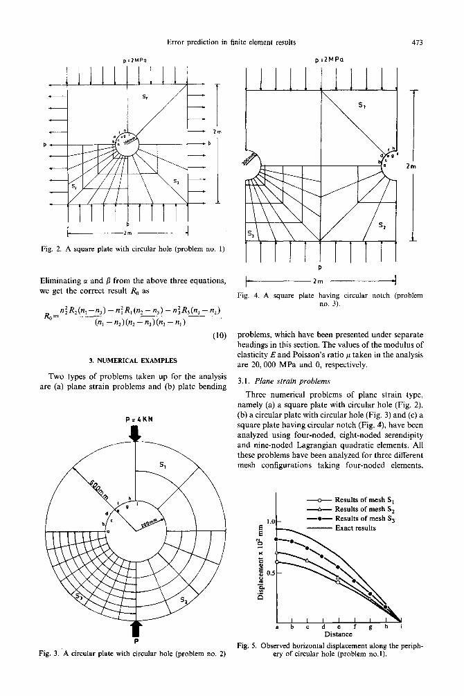
Fig. 2. A square plate with circular hole (problem no. 1)
Eliminating a and /3 from the above three equations, we get the correct result R, as
%= n:R,(n,--n,)-nn:R,(n,-nn,)-n:R,(n, -n2)
(n,-n,)(n,-n,)(n,-n,) .
(10)
3. NUMERICAL EXAMPLES
Two types of problems taken up for the analysis are (a) plane strain problems and (b) plate bending
P.4KN
Fig. 3. ‘A circular plate with circular hole (problem no. 2)
I 2m
I
+---,‘------A Fig. 4. A square plate having circular notch (problem
no. 3).
problems, which have been presented under separate headings in this section. The values of the modulus of elasticity E and Poisson’s ratio p taken in the analysis are 20,000 MPa and 0, respectively.
3.1. Plane strain problems
Three numerical problems of plane strain type, namely (a) a square plate with circular hole (Fig. 2), (b) a circular plate with circular hole (Fig. 3) and (c) a square plate having circular notch (Fig. 4), have been analyzed using four-noded, eight-noded serendipity and nine-noded Lagrangian quadratic elements. All these problems have been analyzed for three different mesh configurations taking four-noded elements.
v Results of mesh S,
I Results of mesh S,
-o- Results of mesh S,
a b c d e f g h i Distance
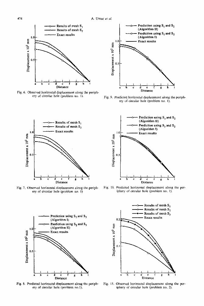
Fig. 5. Observed horizontal displacement along the periph- ery of circular hole (problem no.1).
474 A. Umar et al.
I v Results of mesh S, _ Results of mesh S,
- Exact results
a b c d e f g h i Distance
Fig. 6. Observed horizontal displacement along the periph- ery of circular bole (problem no. 1).
I v Results of mesh S, d Results of mesh S,
Distance - abcdefahi
Fig. 7. Observed horizontal displacement along the periph- ery of circular hole (problem no. I)
+ Prediction using S, and S, (Algorithm I)
---(>--- Prediction using S, and S,
1.0 (Algorithm II)
a b c d e f g h i Distance
Fig. 8. Predicted horizontal displacement along the periph- ery of circular hole (problem no.1).
_ Prediction using S, and S, (Algorithm II)
v Prediction using St and S, (Algorithm I)
I.0 - - Exact results
I I I I I I 1 a b c d e f n h i
Distance w
Fig. 9. Predicted horizontal dispiacement along the periph- ery of circular hole (problem no. I).
d Prediction using S, and S, (Algorithm II)
V Prediction using S, and S, (Algorithm I)
Distance ” abcdefehi
Fig. 10. Predicted horizontal displacement along the per- iphery of circular hole (problem no. 1).
--o- Results of mesh S, Results of mesh S,
abcdefghi Distance
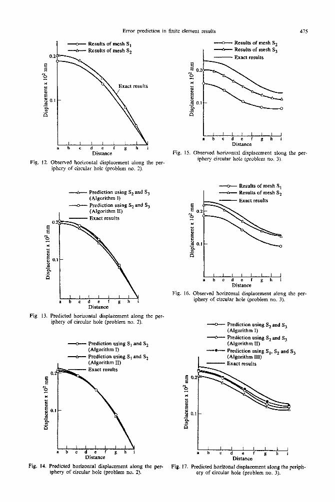
Fig. I I. Observed horizontal displacement along the per- iphery of circular hole (problem no. 2).
Error prediction in finite element results
Fig.
Y Results of mesh St Results of mesh S,
a b c d e f g h i Distance
12. Observed horizontal djspla~mcnt along the per- iphery of circular hole (problem no. 2).
0 Prediction using S2 and Ss (Algorithm I)
- Prediction using S2 and S, , (Algorithm R)
a bcdefzhi Distance _
Fig. 13. Predicted horizontal displacement along the per- iphery of circular hole (problem no. 2).
e Prediction using S, and S2 (Algorithm I)
- Prediction using St and S2 (Algorithm II)
w a B h i Distance
II I I II I Cl abedefghi
Distance _ Fig. 14. Predicted horizontal displacement along the per-
iphery of circular hole (problem no. 2). Fig. 17. Predicted horizonal displacement along the periph-
ery of circular hole (problem no. 3).
--o-- Results of mesh S2
I --d+- Results of mesh S,
Distance
Fig. 15. Observed horizontal displacement along the per- iphery circular hole (problem no. 3).
--o- Results of mesh St
I -+-- Results of mesh S2
- Exact results
%-he+++ a I
Distance
Fig. 16. Observed horizontal displacement along the per- iphery of circular hole (‘problem no. 3).
e Prediction using S2 and S3 (Algorithm I)
e Prediction using S2 and S, (Algorithm II)
-*-- Prediction using St, S, and S, (Algorithm III)
- Exact results
476 A. Umar er al.
(Algorithm I)
* Prediction using S, and S, (Algorithm II)
I - Exact results
Distance
Fig. 18. Predicted horizontal displacement along the periphery of circular hole (problem no. 3).
While using quadratic elements, only two mesh configurations are analyzed. Taking advantage of the symmetry, only one quadrant of the plate has been analyzed.
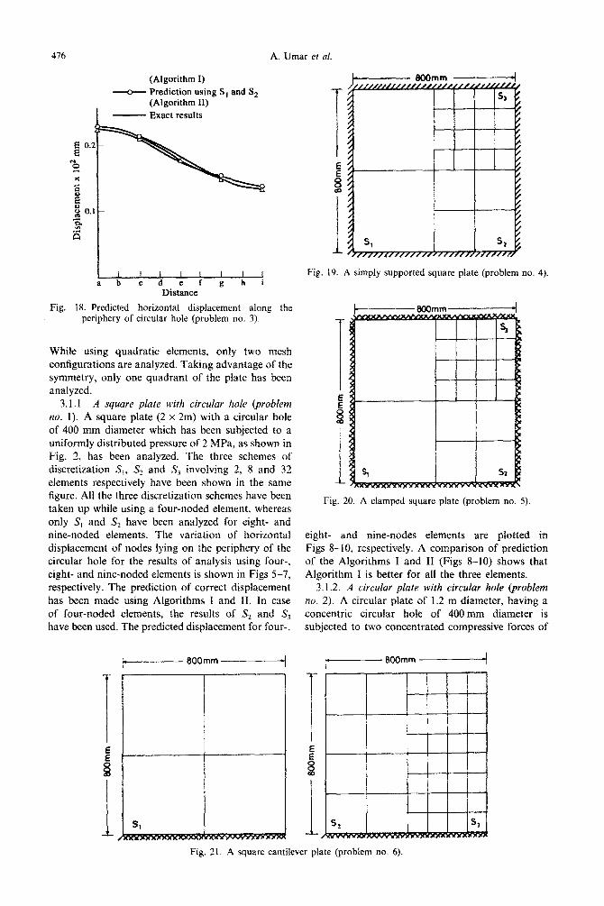
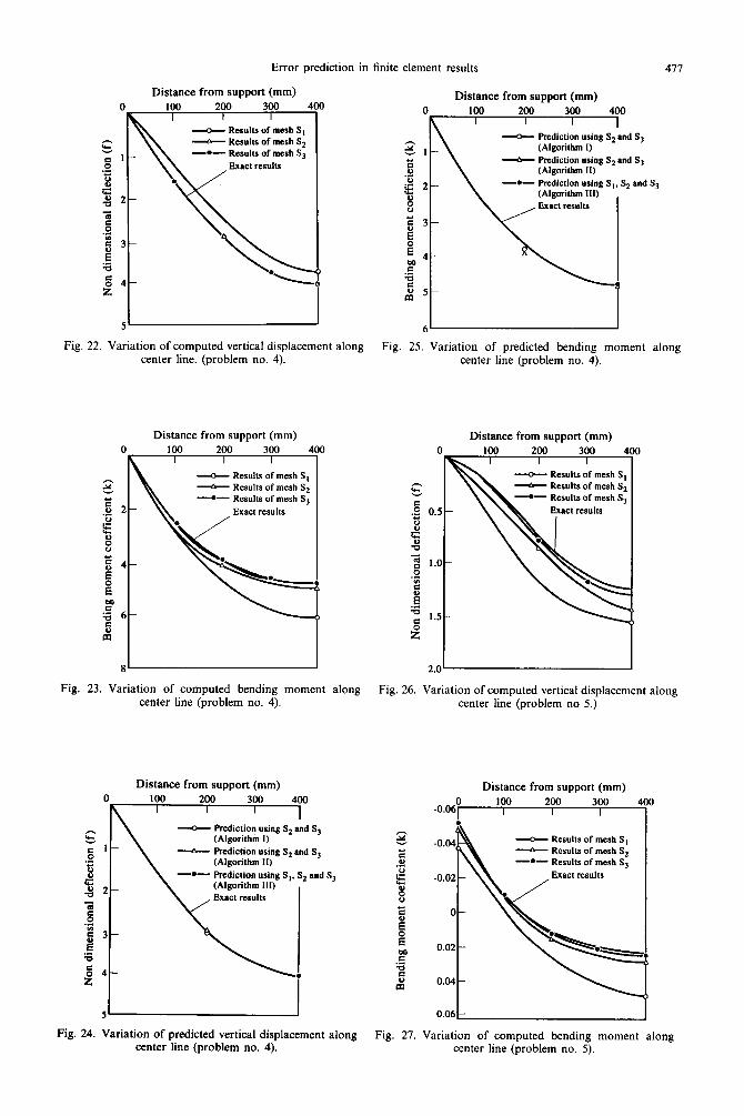
3.1 .I A square plate with circular hole (problem no. 1). A square plate (2 x 2m) with a circular hole of 400 mm diameter which has been subjected to a uniformly distributed pressure of 2 MPa, as shown in Fig. 2, has been analyzed. The three schemes of discretization S,, S, and S, involving 2, 8 and 32 elements respectively have been shown in the same figure. All the three discretization schemes have been taken up while using a four-noded element, whereas only S, and S, have been analyzed for eight- and nine-noded elements. The variation of horizontal displacement of nodes lying on the periphery of the circular hole for the results of analysis using four-, eight- and nine-noded elements is shown in Figs 5-7, respectively. The prediction of correct displacement has been made using Algorithms I and II. In case of four-noded elements, the results of S, and S, have been used. The predicted displacement for four-,
b------- 800mm ---j
800mm
S,
Fig. 19. A simply supported square plate (problem no. 4).
Fig. 20. A clamped square plate (problem no. 5).
eight- and nine-nodes elements are plotted in Figs 8-10, respectively. A comparison of prediction of the Algorithms I and II (Figs S-IO) shows that Algorithm I is better for all the three elements.
3. I .2. A circdar plate with circular hole (problem no. 2). A circular plate of 1.2 m diameter, having a concentric circular hole of ~Omm diameter is subjected to two concentrated compressive forces of
I= 800mm ~-4
Fig. 21. A square cantilever plate (problem no. 6).
Error prediction in finite element results 471
Distance from support (mm)
0 100 200 300
-o- Results of mesh St
- Results of mesh S,
-a- Results of mesh S,
Fig. 22. Variation of computed vertical displacement center line. (problem no. 4).
Distance from support (mm) 100 200 300 d
I I I - Results of mesh St
- Results of mesh S2
-.- Results of mesh Sj
Exact results
along
Fig. 23. Variation of computed bending moment along center line (problem no. 4).
Distance from support (mm)
0 Prediction using S, and SJ (Algorithm I)
b- Rediction using .S2 and S, (Algorithm II)
-*- Prediction using St. S, and Sj (Algorithm 111)
.
5
Fig. 24. Variation of predicted vertical displacement along center line (problem no. 4).
Distance from support (mm) 0 100 200 300 400
_ Prediction using S2 and S, (Algorithm I)
- Prediction using S, and S, (Algorithm II)
-.- F’rediction using St, S2 and S, (Algorithm III)
Fig. 25. Variation of predicted bending moment along center line (problem no. 4).
Distance from support (mm)
Fig. 26. Variation of computed vertical displacement along center line (problem no 5.)
Distance from support (mm)
0 Results of mesh S,
-b Results of mesh Sz
-*- Results of mesh S,
Fig. 27. Variation of computed bending moment along center line (problem no. 5).
478 A. Umar et al
Distance from suppon (mm) 0 loo 200 300 400
I I I I
I\ - Prediction using 5, and Sj
0.2 (Algorithm I) - Prediction using 5, and S,
(Algorithm II) Prediction using St. S2 and S, (Algorithm III) Exact results
I
l.6-
Fig. 28. Variation of predicted vertical displacement along center line (problem no. 5).
4 kN each acting diametrically opposite, as shown in Fig. 3, has also been analyzed. The three schemes of discretization S,, S, and Sj involving four, 16 and 64 elements, respectively, have been shown in the same figure. All three discretization schemes have been used for the four-noded element, whereas only S, and S, have been considered for the eight-noded element. The horizontal displacement of the nodes lying on the periphery of the circular hole for the results of analysis using four- and eight-noded elements has been plotted in Figs 11 and 12, respectively. The prediction of correct displacement has been made using Algorithms I and II. The results of mesh S, and S, have been used for the four-noded element. The prediction of displacement for the four- and eight- noded elements is presented in Figs 13 and 14, respectively. In the case of the four-noded element, the predicted results using Algorithm I are found to be very close to the exact result and the prediction of both the algorithms is good in the case of the eight-noded elements.
3.1.3. A square plate having circular notch (problem
no. 3). A square plate (2 x 2m) with two symmetrical semi-circular notches of 200 mm radius which has been subjected to a uniform pressure of 2 MPa, as shown in Fig. 4, has also been analyzed. The schemes of discretization considered in the study, namely S,, S2 and S, involving two, eight and 32 elements, respectively, have also been shown in Fig. 4. The discretization schemes S, and S, have been taken with four-noded elements, whereas only the S, and S, discretization schemes have been used with the nine-noded Lagrangian element. The variation of horizontal displacement of the nodes lying on the periphery of the circular notch for the results of analysis using four- and nine-noded elements is shown in Figs 15 and 16, respectively. The prediction of better results has been done by using Algorithms I, II and III for the four-noded element. Algorithms I and II have been employed for the nine-noded elements. The predicted displacement for four- and
nine-noded elements are plotted in Figs. 17 and 18, respectively. It is seen from Fig. 17 that the prediction using Algorithm III is better than the rest. Yet the prediction using Algorithm I is also producing good results. In the case of the nine-noded element, the results of the algorithm are very close to the exact.
3.2. Plate bending problems
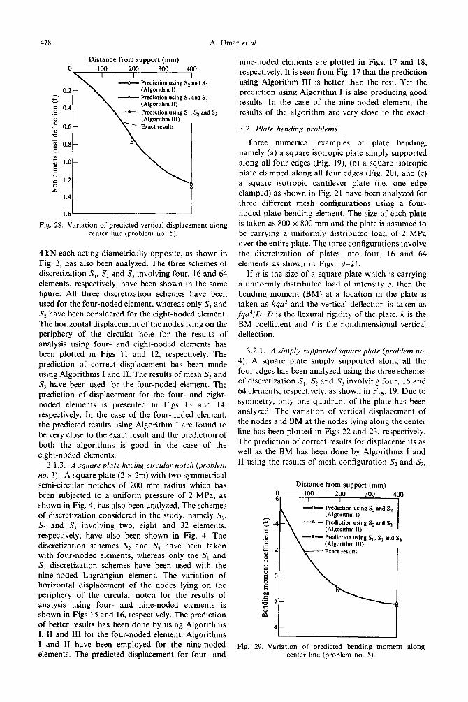
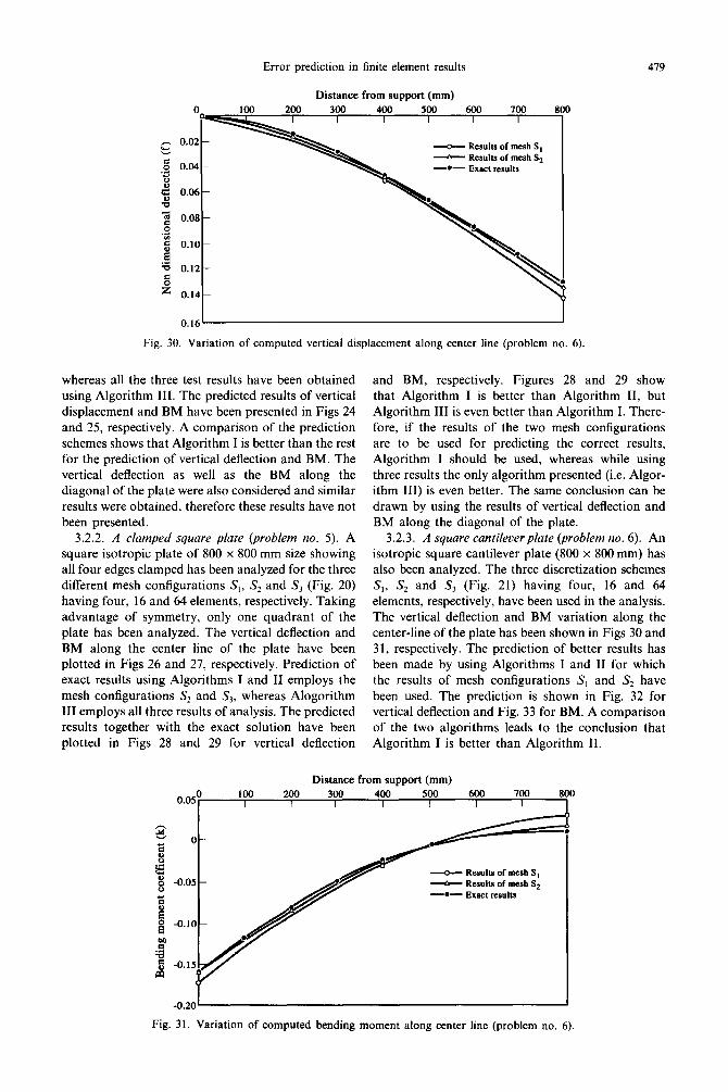
Three numerical examples of plate bending, namely (a) a square isotropic plate simply supported along all four edges (Fig. 19), (b) a square isotropic plate clamped along all four edges (Fig. 20) and (c) a square isotropic cantilever plate (i.e. one edge clamped) as shown in Fig. 21 have been analyzed for three different mesh configurations using a four- noded plate bending element. The size of each plate is taken as 800 x 800 mm and the plate is assumed to be carrying a uniformly distributed load of 2 MPa over the entire plate. The three configurations involve the discretization of plates into four, 16 and 64 elements as shown in Figs 19-21.
If a is the size of a square plate which is carrying a uniformly distributed load of intensity q, then the bending moment (BM) at a location in the plate is taken as kqa* and the vertical deflection is taken as fqa4/D. D is the flexural rigidity of the plate, k is the BM coefficient and f is the nondimensional vertical deflection.
3.2.1. A simply supported square plate (problem no.
4). A square plate simply supported along all the four edges has been analyzed using the three schemes of discretization S,, S, and S, involving four, 16 and 64 elements, respectively, as shown in Fig. 19. Due to symmetry, only one quadrant of the plate has been analyzed. The variation of vertical displacement of the nodes and BM at the nodes lying along the center line has been plotted in Figs 22 and 23, respectively. The prediction of correct results for displacements as well as the BM has been done by Algorithms I and II using the results of mesh configuration S2 and S3,
Distance from support (mm) 100 200 300 400 I I I
- Prediction using S, and Sj (Algorithm I)
- Prediction using S, and Sj (Algorithm II)
-*- Prediction using S,. S, and Sj (Algorithm 111)
4-
Fig. 29. Variation of predicted bending moment along center line (problem no. 5).
Error prediction in finite element results
Distance from support (mm)
479
Fig. 30. Variation of computed vertical displacement along center line (problem no. 6).
whereas all the three test results have been obtained using Algorithm III. The predicted results of vertical displacement and BM have been presented in Figs 24 and 25, respectively. A comparison of the prediction schemes shows that Algorithm I is better than the rest for the prediction of vertical deflection and BM. The vertical deflection as well as the BM along the diagonal of the plate were also considered and similar results were obtained, therefore these results have not been presented.
and BM, respectively. Figures 28 and 29 show that Algorithm I is better than Algorithm II, but Algorithm III is even better than Algorithm I. There- fore, if the results of the two mesh configurations are to be used for predicting the correct results, Algorithm I should be used, whereas while using three results the only algorithm presented (i.e. Algor- ithm III) is even better. The same conclusion can be drawn by using the results of vertical deflection and BM along the diagonal of the plate.
3.2.2. A clamped square plate (problem no. 5). A square isotropic plate of 800 x 800 mm size showing all four edges clamped has been analyzed for the three different mesh configurations S,, S, and S, (Fig. 20) having four, 16 and 64 elements, respectively. Taking advantage of symmetry, only one quadrant of the plate has been analyzed. The vertical deflection and BM along the center line of the plate have been plotted in Figs 26 and 27, respectively. Prediction of exact results using Algorithms I and II employs the mesh configurations S, and S,, whereas Alogorithm III employs all three results of analysis. The predicted results together with the exact solution have been
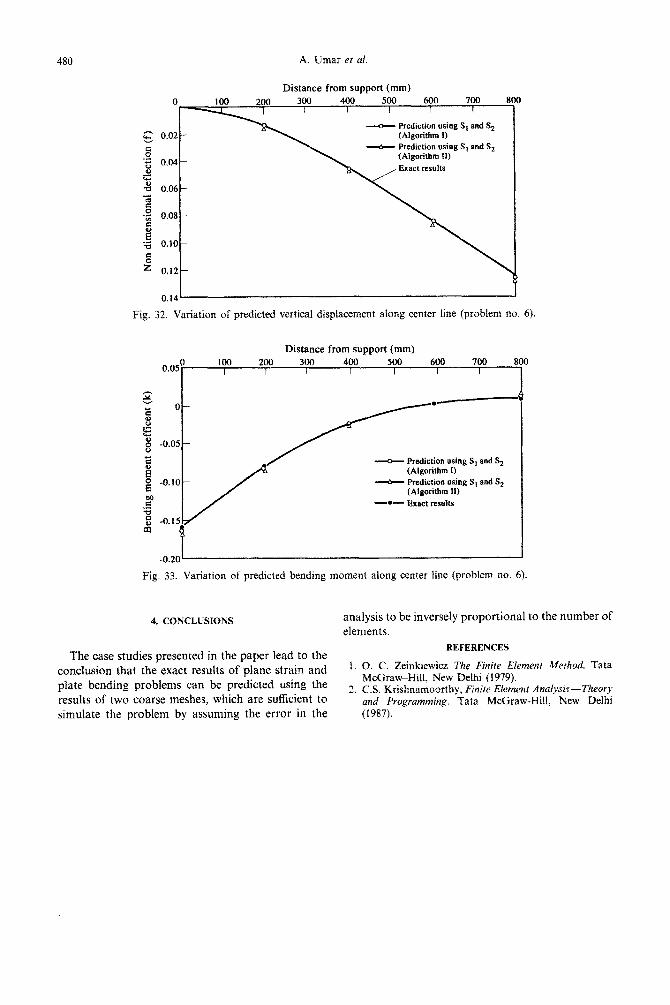
3.2.3. A square cantilever plate (problem no. 6). An isotropic square cantilever plate (800 x 800 mm) has also been analyzed. The three discretization schemes S,, S, and S3 (Fig. 21) having four, 16 and 64 elements, respectively, have been used in the analysis. The vertical deflection and BM variation along the center-line of the plate has been shown in Figs 30 and 31, respectively. The prediction of better results has been made by using Algorithms I and II for which the results of mesh configurations S, and S, have been used. The prediction is shown in Fig. 32 for vertical deflection and Fig. 33 for BM. A comparison of the two algorithms leads to the conclusion that
plotted in Figs 28 and 29 for vertical deflection Algorithm I is better than Algorithm II.
Distance from support (mm) 0.05; too 200 300 400 500 600 700 8
I I I I I I I
Fig. 31. Variation of computed bending moment along center line (problem no. 6).
480 A. Umar et al.
Distance from support (mm) 0 100 200 300 400 500 600 700 8
- Prediction using St and S, 0.02 - (Algorithm I)
- Prediction using St and S, 0.04 - (Algorithm II)
0.06 -
0.08 -
0.10 -
0.12-
Fig. 32. Variation of predicted vertical dispia~ment along center iine (problem no. 6).
Distance from support (mm)
(Algorithm I) --b Prediction using S1 and S2
(Al@xithm 11)
-*- Exact nsults
Fig. 33. Variation of predicted bending moment along center line (problem no. 6).
4. CONCLUSIONS analysis to be inversely proportional to the number of elements.
The case studies presented in the paper lead to the conclusion that the exact results of plane strain and plate bending problems can be predicted using the results of two coarse meshes, which are sufficient to
REFERENCES
I. 0. C. Zeinkiewicz The Finite Element Method. Tata M~raw-Hill, New Delhi (1979).
2. C.S. ~rishnamoorthy, Finite Element Ana~~~sis-T~eo~y and Programming. Tata McGraw-Hill, New Delhi
simulate the problem by assuming the error in the (1987)