A posteriori error controlof finite element approximationsfor Coulomb’s frictional contact

Patrice COOREVITS 1, Patrick HILD 2 and Mohammed HJIAJ 3

1 Laboratoire de Mecanique et CAO,Universite de Picardie - Jules Verne, IUT,

48 rue d’Ostende, 02100 SAINT-QUENTIN, France.

2 Laboratoire de Mathematiques,Universite de Savoie / CNRS EP 2067,73376 LE BOURGET DU LAC, France.

3 Laboratoire de Mecanique de Lille,Universite des sciences et techniques de Lille / CNRS URA 1441

Bvd Paul Langevin, 59655 VILLENEUVE D’ASCQ, France.

This paper is concerned with the frictional unilateral contact problem governed byCoulomb’s law. We define an a posteriori error estimator based on the concept of errorin the constitutive relation to quantify the accuracy of a finite element approximation of theproblem. We propose and study different mixed finite element approaches and discuss theirproperties in order to compute the estimator. The information given by the error estimatesis then coupled with a mesh adaptivity technique which provides the user with the desiredquality and minimizes the computation costs. The numerical implementation of the errorestimator as well as optimized computations are performed.

Keywords : Coulomb’s friction law, a posteriori error estimates, finite elements, error in theconstitutive relation, optimized computations.

2000 Mathematics Subject Classification. 65N30, 74M10

1. Introduction and problem set-up

The finite element method is currently used in the numerical realization of fric-tional contact problems occurring in many engineering applications (see [13]). Animportant task consists of evaluating numerically the quality of the finite elementcomputations by using a posteriori error estimators. In elasticity, several differentapproaches leading to various error estimators have been developed, in particular theerror estimators introduced in [2] based on the residual of the equilibrium equations,the estimators linked to the smoothing of finite element stresses (see [22]) and theestimators based on the errors in the constitutive relation (see [14, 17]). A review of

1

A posteriori error for Coulomb frictional contact 2

different a posteriori error estimators can be found in [21].For frictionless unilateral contact problems, the residual based method was con-

sidered and studied in [3] (see also the references quoted therein) using a penalizedapproach and the study of error in the constitutive relation was performed in [5].

In the present paper, we are interested in the more general and currently usedCoulomb’s frictional contact model and we choose the estimators in the constitutiverelation to quantify the accuracy of the finite element approximations. As far as weknow, there is no literature concerning a posteriori error estimators for Coulomb’sfrictional unilateral contact model. The latter is recalled hereafter.

Let be given an elastic body occupying a bounded domain Ω in R2 whose generic

point is denoted x = (x1, x2). The boundary Γ of Ω is Lipschitz and divided asfollows: Γ = ΓD ∪ ΓN ∪ ΓC where ΓD, ΓN and ΓC are three open disjoint parts. Wesuppose that the displacement field is given on ΓD (to simplify, we assume afterwardsthat the body is clamped on ΓD). On the boundary part ΓN , a density of forcesdenoted F ∈ (L2(ΓN))2 is applied. The third part is the segment ΓC , in frictionalcontact with a rigid foundation (see Figure 1). The body Ω is submitted to a givendensity of volume forces f ∈ (L2(Ω))2. Let the notation n = (n1, n2) represent theunit outward normal vector on Γ and define the unit tangent vector t = (−n2, n1).Let us denote by µ > 0 the friction coefficient on ΓC .

The problem consists of finding the displacement field u : Ω −→ R2 and the stress

tensor field σ : Ω −→ S2 satisfying (1.1)-(1.10)

σ(u) = C ε(u) in Ω, (1.1)

div σ(u) + f = 0 in Ω, (1.2)

σ(u)n = F on ΓN , (1.3)

u = 0 on ΓD. (1.4)

where S2 stands for the space of second order symmetric tensors on R2, ε(u) =

12(∇u+∇T u) denotes the linearized strain tensor field, C is a fourth order symmetric

and elliptic tensor of linear elasticity and div represents the divergence operator oftensor valued functions.

In order to introduce the equations on ΓC , let us adopt the following notation:u = unn + utt and σ(u)n = σn(u)n + σt(u)t. The equations modelling unilateralcontact with Coulomb friction are as follows on ΓC :

un ≤ 0, (1.5)

σn(u)≤ 0, (1.6)

σn(u)un = 0, (1.7)

|σt(u)| ≤µ|σn(u)|, (1.8)

|σt(u)|<µ|σn(u)| =⇒ ut = 0, (1.9)

|σt(u)|=µ|σn(u)| =⇒ ∃λ ≥ 0 such that ut = −λσt(u). (1.10)

A posteriori error for Coulomb frictional contact 3

The variational formulation of problem (1.1)-(1.10) has been obtained by Duvaut andLions in [8]. It consists of finding u such that

u ∈ Kad, a(u,v − u) + j(u,v) − j(u,u) ≥ L(v − u), ∀v ∈ Kad, (1.11)

where

a(u,v) =

∫

Ω

(Cε(u)) : ε(v) dΩ, j(u,v) =

∫

ΓC

µ|σn(u)||vt| dΓ,

L(v) =

∫

Ω

f .v dΩ +

∫

ΓN

F .v dΓ,

are defined for any u and v in

V =

v ∈ (H1(Ω))2; v = 0 on ΓD

.

The notation H1(Ω) represents the standard Sobolev space, · and : stand for the innerproduct in R

2 and S2 respectively. In (1.11), Kad denotes the closed convex cone ofadmissible displacement fields satisfying the non-penetration condition

Kad =

v ∈ V ; vn ≤ 0 on ΓC

.

The first existence result for problem (1.11) has been obtained in [20] when Ω isan infinitely long strip and if the friction coefficient of compact support in ΓC issufficiently small. The extension of these results to domains with smooth boundariescan be found in [12]. A recent improvement in [9] states existence when the friction

coefficient µ is lower than√

3−4ν2−2ν

, ν denoting Poisson’s ratio in Ω (0 < ν < 12).

When the loads f and F are not equal to zero, there is to our knowledge neitheruniqueness result nor non-uniqueness example for problem (1.11). Let us mentionthat there exists several laws “mollifying” Coulomb’s frictional contact model (see,e.g. [13, 19] and the references quoted therein) and that such regularizations lead tomore existence and uniqueness properties.

Ω

ΓC

ΓDΓN

rigid foundation

f

F

n

t

Figure 1: Setting of the problem

A posteriori error for Coulomb frictional contact 4

Our paper is outlined as follows. In section 2, we first recall the convenient set-ting which consists of separating the kinematic conditions, the equilibrium equationsand the constitutive relations in order to define the error estimator and to study itsproperties. In section 3, we propose two mixed finite element methods for Coulomb’sfrictional unilateral contact problem. We prove the existence of solutions and westudy the discrete frictional contact properties satisfied by such solutions. Section4 is concerned with the practical construction of such an estimator. In section 5,several numerical studies in which we compute and couple the estimator with a meshadaptivity procedure are performed.

2. The error estimator for Coulomb’s frictional contact problem

The aim of this section is to introduce the concept of error in the constitutiverelation for the frictional unilateral contact problem. Before defining the estimator,let us begin with some useful setting and notation.

2.1. The appropriate setting for error in the constitutive relation

To define the error in the constitutive relation, the contact part ΓC is consideredlike in [15, 5] as an interface on which two unknowns w (displacement field) and r

(density of surfacic forces due to the frictional contact with the rigid foundation) areto be found. If n = (n1, n2) and t = (−n2, n1) stand for the unit outward normaland tangent on Γ, we adopt afterwards the notation z = znn + ztt for any vector z.

The unilateral contact problem with Coulomb’s friction law (1.1)-(1.10) is refor-mulated by using these quantities and it consists of finding the displacement field u

on Ω, the stress tensor field σ on Ω and w, r on ΓC satisfying the following equations(2.1)–(2.9).

• The displacement fields u and w verify the kinematic conditions:

u = 0 on ΓD and w = u on ΓC . (2.1)

• The fields σ and r satisfy the equilibrium equation:

−∫

Ω

σ : ε(v) dΩ +

∫

Ω

f .v dΩ +

∫

ΓN

F .v dΓ +

∫

ΓC

r.v dΓ = 0, ∀v ∈ V . (2.2)

• The fields σ and u are linked by the constitutive law of linear elasticity:

σ = Cε(u). (2.3)

• The displacement field w = wnn + wtt and the density of forces r = rnn + rtt

A posteriori error for Coulomb frictional contact 5

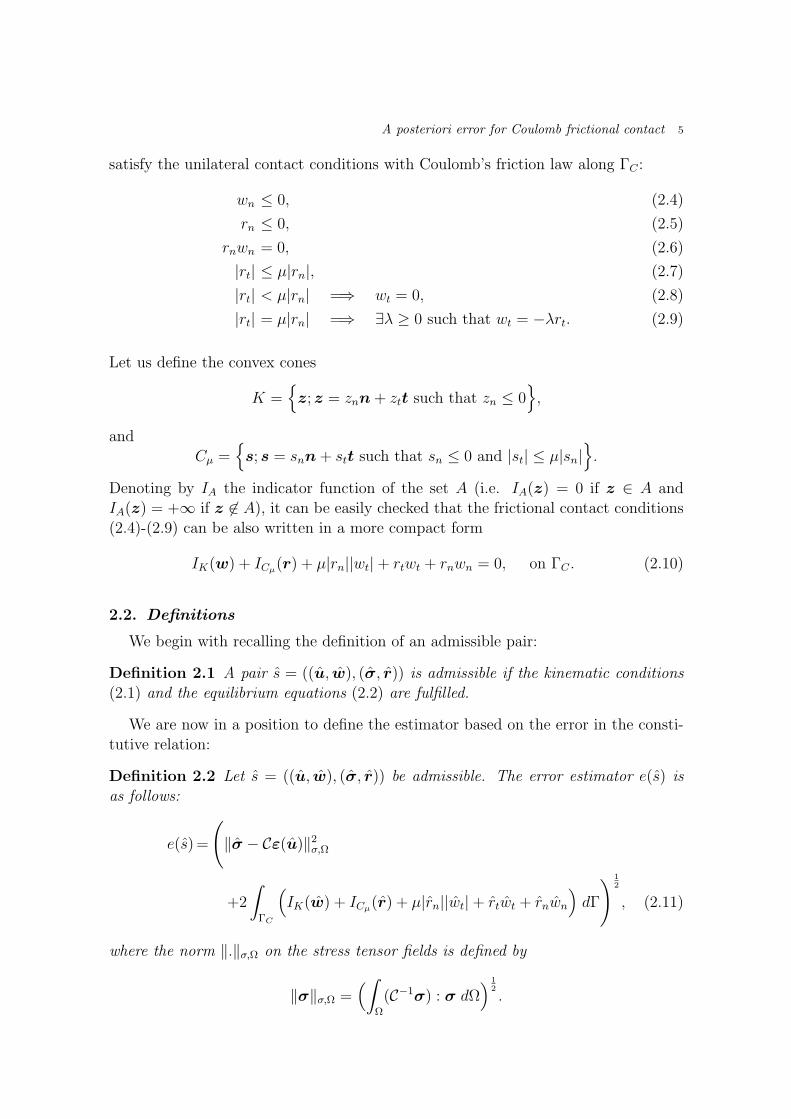
satisfy the unilateral contact conditions with Coulomb’s friction law along ΓC :

wn ≤ 0, (2.4)

rn ≤ 0, (2.5)

rnwn = 0, (2.6)

|rt| ≤ µ|rn|, (2.7)

|rt| < µ|rn| =⇒ wt = 0, (2.8)

|rt| = µ|rn| =⇒ ∃λ ≥ 0 such that wt = −λrt. (2.9)

Let us define the convex cones

K =

z; z = znn + ztt such that zn ≤ 0

,

andCµ =

s; s = snn + stt such that sn ≤ 0 and |st| ≤ µ|sn|

.

Denoting by IA the indicator function of the set A (i.e. IA(z) = 0 if z ∈ A andIA(z) = +∞ if z 6∈ A), it can be easily checked that the frictional contact conditions(2.4)-(2.9) can be also written in a more compact form

IK(w) + ICµ(r) + µ|rn||wt| + rtwt + rnwn = 0, on ΓC . (2.10)

2.2. Definitions

We begin with recalling the definition of an admissible pair:

Definition 2.1 A pair s = ((u, w), (σ, r)) is admissible if the kinematic conditions(2.1) and the equilibrium equations (2.2) are fulfilled.

We are now in a position to define the estimator based on the error in the consti-tutive relation:

Definition 2.2 Let s = ((u, w), (σ, r)) be admissible. The error estimator e(s) isas follows:

e(s) =

(

‖σ − Cε(u)‖2σ,Ω

+2

∫

ΓC

(

IK(w) + ICµ(r) + µ|rn||wt| + rtwt + rnwn

)

dΓ

)1

2

, (2.11)

where the norm ‖.‖σ,Ω on the stress tensor fields is defined by

‖σ‖σ,Ω =(

∫

Ω

(C−1σ) : σ dΩ)

1

2

.

A posteriori error for Coulomb frictional contact 6

Let us notice that the function in the integral term of (2.11) is always nonnegativeat x ∈ ΓC : it is equal to +∞ if w(x) 6∈ K or r(x) 6∈ Cµ; otherwise it is nonnegativeowing to (µ|rn||wt|+rtwt)(x) ≥ 0 and (rnwn)(x) ≥ 0. To avoid more notation, we willskip over the regularity aspects of the functions defined on ΓC which are beyond thescope of this paper and we write afterwards integral terms instead of duality pairings.The first natural property arising directly from the definition of e(s) becomes:

Property 2.3 Let s be admissible. Then e(s) = 0 if and only if s = ((u, w), (σ, r))is solution to the reference problem (2.1)-(2.9).

Let us define some quantities useful for the forthcoming study:

Definition 2.4 Let s be admissible. The relative error ǫ(s) is as follows:

ǫ(s) =e(s)

‖σ + Cε(u)‖σ,Ω

. (2.12)

Given a part E of Ω, the local error contribution ǫE(s) is defined as

ǫE(s) = (2.13)(

‖σ − Cε(u)‖2σ,E + 2

∫

ΓC∩E

(

IK(w) + ICµ(r) + µ|rn||wt| + rtwt + rnwn

)

dΓ

)1

2

‖σ + Cε(u)‖σ,Ω

where ‖σ‖σ,E =(

∫

E

(C−1σ) : σ dΩ)

1

2

.

For the sake of simplicity of notations, we will write ǫ and ǫE instead of ǫ(s) andǫE(s) in the following studies. It is straightforward that

⋃

Ei∩Ej=∅, i6=j

Ei = Ω =⇒ ǫ2 =∑

i

ǫ2Ei.

2.3. Link between the estimator and the other errors

This part is concerned with the relation between the error in the constitutivelaw and the other errors. We suppose that a solution to the exact problem (2.1)-(2.9) exists which is satisfied when µ is small enough (see [9]). The next propositiongeneralizes former results (see [5]) obtained in the frictionless case (corresponding toµ = 0).

Proposition 2.5 Let (u,w,σ, r) be solution to Coulomb’s frictional contact problem(2.1)-(2.9). Let s = ((u, w), (σ, r)) be admissible. Then

‖σ − σ‖2σ,Ω + ‖u − u‖2

u,Ω + 2µ

∫

ΓC

(rn − rn)(|wt| − |wt|) dΓ ≤ e2(s), (2.14)

A posteriori error for Coulomb frictional contact 7

where the norm ‖.‖u,Ω on the displacement fields is defined by

‖u‖u,Ω =(

∫

Ω

(Cε(u)) : ε(u) dΩ)

1

2

=(

a(u,u))

1

2 .

Consequently

‖σ − σ‖2σ,Ω + 2µ

∫

ΓC

(rn − rn)(|wt| − |wt|) dΓ ≤ e2(s), (2.15)

and

‖u − u‖2u,Ω + 2µ

∫

ΓC

(rn − rn)(|wt| − |wt|) dΓ ≤ e2(s). (2.16)

Proof. We begin with noticing that the property obviously holds when w 6∈ K orr 6∈ Cµ on a set of positive measure. In such a case the error estimator is equal toinfinity. Next, we then suppose that w ∈ K and r ∈ Cµ almost everywhere. Oneimmediately gets

‖σ − Cε(u)‖2σ,Ω = ‖σ − σ + Cε(u − u)‖2

σ,Ω

= ‖σ − σ‖2σ,Ω + ‖u − u‖2

u,Ω + 2

∫

Ω

(σ − σ) : ε(u − u) dΩ.

The stress fields σ and σ satisfy the equilibrium equation (2.2) and the displace-ment fields u and u verify the kinematic conditions (2.1). Hence

‖σ − Cε(u)‖2σ,Ω = ‖σ − σ‖2

σ,Ω + ‖u − u‖2u,Ω + 2

∫

ΓC

(r − r).(w − w) dΓ. (2.17)

Developing the integral term yields

∫

ΓC

(r − r).(w − w) dΓ =

∫

ΓC

rnwn dΓ +

∫

ΓC

rtwt dΓ +

∫

ΓC

rnwn dΓ +

∫

ΓC

rtwt dΓ

−∫

ΓC

rnwn dΓ−∫

ΓC

rtwt dΓ −∫

ΓC

rnwn dΓ −∫

ΓC

rtwt dΓ. (2.18)

Putting together (2.17) and (2.18) in the definition (2.11) of the estimator leads to

e2(s) = ‖σ − σ‖2σ,Ω + ‖u − u‖2

u,Ω

+2

∫

ΓC

rnwn dΓ + 2

∫

ΓC

rtwt dΓ + 2

∫

ΓC

rnwn dΓ + 2

∫

ΓC

rtwt dΓ

−2

∫

ΓC

rnwn dΓ − 2

∫

ΓC

rtwt dΓ + 2

∫

ΓC

µ|rn||wt| dΓ.

A posteriori error for Coulomb frictional contact 8

Noting that rnwn ≥ 0, rnwn ≥ 0 and rnwn = 0 on ΓC , we get

e2(s)≥‖σ − σ‖2σ,Ω + ‖u − u‖2

u,Ω

+2

∫

ΓC

rtwt dΓ + 2

∫

ΓC

rtwt dΓ − 2

∫

ΓC

rtwt dΓ + 2

∫

ΓC

µ|rn||wt| dΓ.

According to (2.7)-(2.9), the equality

−rtwt = µ|rn||wt|

holds on ΓC . Moreover r ∈ Cµ and r ∈ Cµ lead to the bounds

rtwt ≥ −µ|rn||wt| and rtwt ≥ −µ|rn||wt|.

Consequently

e2(s) ≥ ‖σ − σ‖2σ,Ω + ‖u − u‖2

u,Ω + 2µ

∫

ΓC

(|rn| − |rn|)(|wt| − |wt|) dΓ.

The bound (2.14) is obtained thanks to rn ≤ 0 and rn ≤ 0. Both bounds (2.15) and(2.16) are an obvious consequence.

It is easy to check that no information on the sign of the integral term in (2.14)is available. This is not at all surprising because the evaluation of such a termcorresponds also to the study of the uniqueness for the (quasi-)variational inequality(1.11) with classical arguments (i.e. by choosing and subtracting two solutions) whichdoes not lead to a successful conclusion. Nevertheless, the following remark showsthat the integral term can be bounded at least in a particular case.

Remark 2.6 If the exact solution and the admissible solution satisfy wt ≥ 0 andwt ≥ 0 on ΓC (or wt ≤ 0 and wt ≤ 0 on ΓC), and if the measure of ΓD is positive,then inequality (2.14) becomes more relevant since the integral term in (2.14) can beestimated as follows:

∣

∣

∣

∫

ΓC

(rn − rn)(|wt| − |wt|) dΓ∣

∣

∣=∣

∣

∣

∫

ΓC

(rn − rn)(wt − wt) dΓ∣

∣

∣

≤‖rn − rn‖H−

1

2 (ΓC)‖wt − wt‖

H1

2 (ΓC)

≤C‖σ − σ‖(L2(Ω))4‖u − u‖(H1(Ω))2

≤C ′‖σ − σ‖σ,Ω‖u − u‖u,Ω

≤C ′′(

‖σ − σ‖2σ,Ω + ‖u − u‖2

u,Ω

)

,

where H1

2 (ΓC) stands for a fractionally Sobolev space (see [1]) and H− 1

2 (ΓC) is itsdual space. The bounds of ‖rn − rn‖

H−1

2 (ΓC)and ‖wt − wt‖

H1

2 (ΓC)are obtained using

Green’s formula and the trace theorem respectively. Moreover the norms ‖.‖(H1(Ω))2

and ‖.‖u,Ω are equivalent since meas(ΓD) > 0. In such a case, the integral term can

A posteriori error for Coulomb frictional contact 9

be removed from (2.14), (2.15) and (2.16) and we come to the conclusion that thereexists a positive constant C such that for small friction coefficients, ‖σ − σ‖σ,Ω and‖u − u‖u,Ω can be bounded by (1/

√1 − µC)e(s). Concerning the general case, we

think that one could reasonably expect that if the exact and admissible solutions aresmooth enough and if the friction coefficient is small then the integral term multipliedby 2µ is small in comparison with ‖u − u‖2

u,Ω and ‖σ − σ‖2σ,Ω.

Remark 2.7 If instead of Coulomb’s law (2.10), one considers a Tresca’s type fric-tion law:

IK(w) + IC(r) + k|wt| + rtwt + rnwn = 0, on ΓC , (2.19)

where k ≥ 0 and where

C =

s; s = snn + stt such that sn ≤ 0 and |st| ≤ k

,

then the problem (2.1)-(2.3), (2.19) admits an unique solution (uk,wk,σk, rk) andthe bound

‖σk − σ‖2σ,Ω + ‖uk − u‖2

u,Ω ≤ e2(s), (2.20)

holds for any admissible s = ((u, w), (σ, r)).Estimate (2.20) is obtained following the same points as in the proof of estimate

(2.14). In particular, if k = 0 in (2.19) or equivalently µ = 0 in (2.10), we recoverthe frictionless unilateral contact model.

3. The discrete Coulomb’s frictional contact problem

In this section, we propose and study the properties of two mixed discrete finiteelement formulations for Coulomb’s frictional contact in order to implement the errorestimator. Let us mention that a detailed study of several (different) mixed finiteelement methods for frictionless and frictional contact problems can be found in [10],[11].

3.1. The mixed finite element formulations

The body Ω is discretized by using a family of triangulations (Th)h made of finiteelements of degree one. For technical purposes, we assume (in Section 3.1 only) thatΓD∩ΓC = ∅ which is generally not restrictive in engineering applications and that thebilinear form a(., .) is V −elliptic. Let us denote by h > 0 the discretization parameterrepresenting the greatest diameter of a triangle in Th. The space approximating V

becomes:

Vh =

vh; vh ∈ (C (Ω))2, vh|T ∈ (P1(T ))2 ∀T ∈ Th, vh = 0 on ΓD

,

where C (Ω) stands for the space of continuous functions on Ω and P1(T ) representsthe space of polynomial functions of degree one on T . On the boundary of Ω, we still

A posteriori error for Coulomb frictional contact 10

keep the notation vh = vhnn + vhtt for every vh ∈ Vh and we denote by (Th)h thefamily of monodimensional meshes on ΓC inherited by (Th)h.

We next introduce two convex sets of Lagrange multipliers denoted M ′h(g) and

M ′′h (g). The convex M ′

h(g) is defined by M ′h(g) = M ′

hn ×M ′ht(g) where

M ′hn =

ν; ν ∈ C (ΓC), ν|S ∈ P1(S), ∀S ∈ Th, ν ≤ 0 on ΓC

,

and for g ∈ −M ′hn, we define M ′

ht(g) as follows:

M ′ht(g) =

ν; ν ∈ C (ΓC), ν|S ∈ P1(S), ∀S ∈ Th, |ν| ≤ g on ΓC

.

We denote by p the number of nodes of the triangulation on ΓC and by ψi, 1 ≤ i ≤ pthe monodimensional basis functions on ΓC (the function ψi is continuous on ΓC ,linear on each segment of Th, equal to 1 at node i and to 0 at the other nodes). Thesecond convex M ′′

h (g) is given by M ′′h (g) = M ′′

hn ×M ′′ht(g) with

M ′′hn =

ν; ν ∈ C (ΓC), ν|S ∈ P1(S), ∀S ∈ Th,

∫

ΓC

νψi dΓ ≤ 0, ∀1 ≤ i ≤ p

.

If g ∈ −M ′′hn, M ′′

ht(g) is given by:

M ′′ht(g) =

ν; ν ∈ C (ΓC), ν|S ∈ P1(S), ∀S ∈ Th,∣

∣

∣

∫

ΓC

νψi dΓ∣

∣

∣≤∫

ΓC

gψi dΓ,

∀1 ≤ i ≤ p

.

Next, the notation Mh(g) = Mhn ×Mht(g) denotes either M ′h(g) = M ′

hn ×M ′ht(g) or

M ′′h (g) = M ′′

hn ×M ′′ht(g).

We then introduce a intermediary problem with a given slip limit −µghn whereghn ∈Mhn. This problem denoted P (ghn) consists of finding uh ∈ Vh and (λhn, λht) ∈Mhn ×Mht(−µghn) = Mh(−µghn) such that:

(P (ghn))

a(uh,vh) −∫

ΓC

λhnvhn dΓ −∫

ΓC

λhtvht dΓ = L(vh), ∀vh ∈ Vh,∫

ΓC

(νhn − λhn)uhn dΓ +

∫

ΓC

(νht − λht)uht dΓ≥ 0,

∀(νhn, νht) ∈ Mh(−µghn).(3.1)

Problem P (ghn) is equivalent of finding a saddle-point (uh, λhn, λht) = (uh,λh) ∈Vh × Mh(−µghn) verifying

L (uh,νh) ≤ L (uh,λh) ≤ L (vh,λh), ∀vh ∈ Vh, ∀νh ∈ Mh(−µghn),

where

L (vh,νh) =1

2a(vh,vh) −

∫

ΓC

νhnvhn dΓ −∫

ΓC

νhtvht dΓ − L(vh).

A posteriori error for Coulomb frictional contact 11

By using classical arguments on saddle-point problems as Haslinger, Hlavacek andNecas (1996, p.338), we deduce that there exists such a saddle-point. The strict con-vexity of a(., .) implies that the first argument uh is unique. Besides, the assumptionΓD ∩ ΓC = ∅ allows us to write

∫

ΓC

νhnvhn dΓ −∫

ΓC

νhtvht dΓ = 0, ∀vh ∈ Vh, =⇒ νhn = 0, νht = 0.

Consequently, the second argument λh is unique and P (ghn) admits a unique solution.It becomes then possible to define a map Φh as follows

Φh :Mhn −→Mhn

ghn 7−→ λhn,

where (uh, λhn, λht) is the solution of P (ghn). The introduction of this map allowsthe definition of a discrete solution of Coulomb’s frictional contact problem.

Definition 3.1 Let Mh(g) = M ′h(g) or Mh(g) = M ′′

h (g). A solution of Coulomb’sdiscrete frictional contact problem is the solution of P (λhn) where λhn ∈ Mhn is afixed point of Φh.

Proposition 3.2 Let Mh(g) = M ′h(g) or Mh(g) = M ′′

h (g). Then for any µ, thereexists a solution to Coulomb’s discrete frictional contact problem.

Proof. To establish existence, we use Brouwer’s fixed point theorem.Step 1. We prove that the mapping Φh is continuous. Set

Vh =

vh ∈ Vh; vht = 0 on ΓC

, Wh =

ν; ν ∈ C (ΓC), ν|S ∈ P1(S), ∀S ∈ Th

.

Since ΓD ∩ ΓC = ∅, it is easy to check that the definition of ‖.‖− 1

2,h given by

‖ν‖− 1

2,h = sup

vh∈Vh

∫

ΓC

νvhn dΓ

‖vh‖1

,

is a norm on Wh. The notation ‖.‖1 represents the (H1(Ω))2-norm.Let (uh, λhn, λht) and (uh, λhn, λht) be the solutions of (P (ghn)) and (P (ghn)) re-

spectively. On the one hand, we get

a(uh,vh) −∫

ΓC

λhnvhn dΓ =L(vh), ∀vh ∈ Vh,

and

a(uh,vh) −∫

ΓC

λhnvhn dΓ =L(vh), ∀vh ∈ Vh.

A posteriori error for Coulomb frictional contact 12

Subtracting the previous equalities and using the continuity of the bilinear form a(., .)gives

∫

ΓC

(λhn − λhn)vhn dΓ = a(uh − uh,vh) ≤M‖uh − uh‖1‖vh‖1 ∀vh ∈ Vh.

Hence, we get a first estimate

‖λhn − λhn‖− 1

2,h ≤M‖uh − uh‖1. (3.2)

On the other hand, we have from (3.1)

a(uh,vh) −∫

ΓC

λhnvhn dΓ −∫

ΓC

λhtvht dΓ = L(vh), ∀vh ∈ Vh, (3.3)

and

a(uh,vh) −∫

ΓC

λhnvhn dΓ −∫

ΓC

λhtvht dΓ = L(vh) ∀vh ∈ Vh. (3.4)

Choosing vh = uh − uh in (3.3) and vh = uh − uh in (3.4) implies by addition:

a(uh − uh,uh − uh) =

∫

ΓC

(λhn − λhn)(uhn − uhn) dΓ +

∫

ΓC

(λht − λht)(uht − uht) dΓ.

(3.5)

Let us notice that the inequality in (3.1) is obviously equivalent to the two followingconditions:

∫

ΓC

(νhn − λhn)uhn dΓ≥ 0, ∀νhn ∈Mhn, (3.6)

∫

ΓC

(νht − λht)uht dΓ≥ 0, ∀νht ∈Mht(−µghn). (3.7)

According to the definitions of M ′hn and M ′′

hn, we can choose νhn = 0 and νhn = 2λhn

in (3.6) which gives

∫

ΓC

λhnuhn dΓ = 0 and

∫

ΓC

νhnuhn dΓ ≥ 0, ∀νhn ∈Mhn,

from which we deduce that∫

ΓC

(λhn − λhn)(uhn − uhn) dΓ ≤ 0.

Denoting by α the ellipticity constant of the bilinear form a(., .), (3.5) becomes

α‖uh − uh‖21 ≤

∫

ΓC

(λht − λht)(uht − uht) dΓ. (3.8)

A posteriori error for Coulomb frictional contact 13

To evaluate the latter integral term, let us first introduce the p-by-p mass matrixM = (mij)1≤i,j≤p on ΓC as

mij =

∫

ΓC

ψiψj dΓ, 1 ≤ i, j ≤ p, (3.9)

and let UT , UT , GN , GN , denote the vectors of components the nodal values of uht,uht, ghn and ghn respectively.

• We begin with considering the mixed method where Mh(g) = M ′h(g). From

(3.7), we get∫

ΓC

λhtuht dΓ≤∫

ΓC

νhtuht dΓ, ∀νht ∈Mht(−µghn),

or equivalently

∫

ΓC

λhtuht dΓ≤p∑

i=1

Mi(MUT )i, ∀M ∈ Rp such that |Mi| ≤ −µ(GN)i, 1 ≤ i ≤ p.

It is easy to construct a vector M minimizing the sum and yielding the followingbound:

∫

ΓC

λhtuht dΓ≤µ

p∑

i=1

(GN)i|(MUT )i|.

A similar expression can be obtained when integrating the term λhtuht. The tworemaining terms of the integral in (3.8) are roughly bounded as follows:

−∫

ΓC

λhtuht dΓ ≤ −µp∑

i=1

(GN)i|(MUT )i| ; −∫

ΓC

λhtuht dΓ ≤ −µp∑

i=1

(GN)i|(MUT )i|

Finally, (3.8) becomes

α‖uh − uh‖21 ≤µ

p∑

i=1

(GN −GN)i

(

|(MUT )i| − |(MUT )i|)

≤µ

(

p∑

i=1

(GN −GN)2i

)1

2

(

p∑

i=1

(M(UT − UT ))2i

)1

2

=µ‖GN −GN‖Rp ‖UT − UT‖Rp,M, (3.10)

where∣

∣|x|− |y|∣

∣ ≤ |x− y| and Holder inequality have been used. The notations ‖.‖Rp

and ‖.‖Rp,M whose definitions are straightforward represent norms on Rp (the mass

matrix M is nonsingular). As a consequence, there exists constants C1(h) and C2(h)depending on h (or equivalently on p) such that

‖GN −GN‖Rp ≤ C1(h)‖ghn − ghn‖− 1

2,h (3.11)

A posteriori error for Coulomb frictional contact 14

and

‖UT − UT‖Rp,M ≤ C2(h)‖uht − uht‖L2(ΓC) ≤ C3(h)‖uh − uh‖1, (3.12)

where the trace theorem has been used. Combining (3.10), (3.11), (3.12) and (3.2)implies that there exists a constant C(h) such that

‖λhn − λhn‖− 1

2,h ≤ µC(h)‖ghn − ghn‖− 1

2,h. (3.13)

Hence Φh is continuous.

• In the case where Mh(g) = M ′′h (g), the proof is analogous: first (3.7) implies

∫

ΓC

λhtuht dΓ≤p∑

i=1

(MM)i(UT )i, ∀M ∈ Rp s.t. |(MM)i| ≤ −µ(MGN)i, 1 ≤ i ≤ p.

Therefore

∫

ΓC

λhtuht dΓ≤µ

p∑

i=1

(MGN)i|(UT )i|.

Expression (3.8) leads then to

α‖uh − uh‖21 ≤µ

p∑

i=1

(M(GN −GN))i

(

|(UT )i| − |(UT )i|)

≤µ

(

p∑

i=1

(M(GN −GN))2i

)1

2

(

p∑

i=1

(UT − UT )2i

)1

2

=µ‖GN −GN‖Rp,M ‖UT − UT‖Rp ,

and the continuity of Φh is proved following the same arguments as in the first case.Step 2. Let (uh, λhn, λht) be the solution of (P (ghn)). Taking vh = uh in (3.1) gives

a(uh,uh) −∫

ΓC

λhnuhn dΓ −∫

ΓC

λhtuht dΓ = L(uh). (3.14)

According to∫

ΓC

λhnuhn dΓ = 0 and

∫

ΓC

λhtuht dΓ ≤ 0,

we deduce from (3.14), the V −ellipticity of a(., .) and the continuity of L(.):

α‖uh‖21 ≤ a(uh,uh) ≤ L(uh) ≤ C‖uh‖1,

where the constant C depends on the loads f and F . So, we get

‖uh‖1 ≤C

α.

A posteriori error for Coulomb frictional contact 15

In other respects

a(uh,vh) −∫

ΓC

λhnvhn dΓ = L(vh), ∀vh ∈ Vh,

leads to∫

ΓC

λhnvhn dΓ ≤M‖uh‖1‖vh‖1 + C‖vh‖1, ∀vh ∈ Vh.

That implies

‖λhn‖− 1

2,h ≤M‖uh‖1 + C ≤

(M

α+ 1)

C.

Finally‖Φh(ghn)‖− 1

2,h ≤ C ′, ∀ghn ∈Mhn,

where C ′ depends only on the applied loads f ,F and on the continuity and ellip-ticity constant of a(., .). This together with the continuity of Φh proves that thereexists at least a solution of Coulomb’s discrete frictional contact problem accordingto Brouwer’s fixed point theorem.

Remark 3.3 From (3.13) when Mh(g) = M ′h(g) or from the equivalent bound which

is obtained when Mh(g) = M ′′h (g), we get a (quite weak) uniqueness result when

µ C(h) ≤ 1. That means that uniqueness holds when µ is small enough where thedenomination “small” depends on the discretization parameter. A more detailed studywould show that we are not able to prove that C(h) remains bounded as h tends towards0. Using another mixed finite element formulation (with a single multiplier instead oftwo which is not adapted to our a posteriori error estimator) leads to similar existenceand uniqueness results (see [10],[11]).

3.2. The matrix formulation of the frictional contact conditions

Let us consider a solution (uh, λhn, λht) ∈ Vh ×Mhn ×Mht(−µλhn) of Coulomb’sdiscrete frictional contact problem. We are interested in the matrix translation of thefrictional contact conditions:

∫

ΓC

(νhn − λhn)uhn dΓ≥ 0, ∀νhn ∈Mhn, (3.15)

∫

ΓC

(νht − λht)uht dΓ≥ 0, ∀νht ∈Mht(−µλhn). (3.16)

As previously, ΓC contains p nodes of the triangulation and ψi, 1 ≤ i ≤ p denotethe scalar monodimensional basis functions on ΓC . The p-by-p mass matrix M =(mij)1≤i,j≤p on ΓC is given by (3.9).

Let UN and UT denote the vectors of components the nodal values of uhn and uht

respectively and let LN and LT denote the vectors of components the nodal valuesof λhn and λht respectively. We begin with considering the mixed method whereMh(g) = M ′

h(g).

A posteriori error for Coulomb frictional contact 16

Proposition 3.4 Let Mh(g) = M ′h(g). The vectors UN , UT , LN , LT associated with

a solution of Coulomb’s discrete frictional contact problem satisfy for any 1 ≤ i ≤ p :

(LN)i ≤ 0, (3.17)

(MUN)i ≤ 0, (3.18)

(LN)i(MUN)i = 0, (3.19)

|(LT )i| ≤−µ(LN)i, (3.20)

|(LT )i|<−µ(LN)i =⇒ (MUT )i = 0, (3.21)

(LT )i(MUT )i ≤ 0. (3.22)

Proof. From λhn ∈ M ′hn, we immediately get (3.17). Condition (3.15) is equivalent

to∫

ΓC

νhnuhn dΓ ≥ 0, ∀νhn ∈M ′hn and

∫

ΓC

λhnuhn dΓ = 0. (3.23)

Choosing in the inequality of (3.23), νhn = −ψi, 1 ≤ i ≤ p, and writing uhn =∑p

j=1(UN)j ψj gives (3.18). Putting λhn =∑p

i=1(LN)i ψi and uhn =∑p

j=1(UN)j ψj

in the equality of (3.23) yields

p∑

i=1

(LN)i(MUN)i = 0.

The latter estimate together with (3.17) and (3.18) implies (3.19).

Inequality (3.20) follows directly from λht ∈ M ′ht(−µλhn). For any 1 ≤ i ≤ p,

choose νht in (3.16) as follows: νht = µλhn at node i and νht = λht at the p− 1 othernodes. We obtain

∫

ΓC

(νht − λht)uht dΓ = (µLN − LT )i

∫

ΓC

ψiuht dΓ

= (µLN − LT )i(MUT )i ≥ 0. (3.24)

Similarly, take νht = −µλhn at node i and νht = λht at the p− 1 other nodes. We get∫

ΓC

(νht − λht)uht dΓ = (−µLN − LT )i(MUT )i ≥ 0. (3.25)

Putting together estimates (3.24) and (3.25) implies (3.21).It remains to prove (3.22). Define νht in (3.16) as follows: νht = 1

2λht at node i

and νht = λht at the p− 1 other nodes. Therefore∫

ΓC

(νht − λht)uht dΓ =−1

2(LT )i

∫

ΓC

ψiuht dΓ

=−1

2(LT )i(MUT )i ≥ 0.

Hence inequality (3.22).

Proceeding in a similar way when Mh(g) = M ′′h (g), we obtain the following propo-

sition.

A posteriori error for Coulomb frictional contact 17

Proposition 3.5 Let Mh(g) = M ′′h (g). The vectors UN , UT , LN , LT associated with

a solution of Coulomb’s discrete frictional contact problem satisfy for any 1 ≤ i ≤ p :

(MLN)i ≤ 0,

(UN)i ≤ 0,

(MLN)i(UN)i = 0,

|(MLT )i| ≤−µ(MLN)i,

|(MLT )i|<−µ(MLN)i =⇒ (UT )i = 0,

(MLT )i(UT )i ≤ 0.

Remark 3.6 We show in the next section that the choice of the method using M ′h(g)

is quite appropriate and easier than M ′′h (g) to compute the estimator. But most of

the finite element codes solving contact problems (with or without friction) make useof nodal displacements UN , UT and of nodal forces FN , FT as dual unknowns (and notpressures like LN , LT ) on the contact part ΓC. This means that the frictional contactconditions are generally: (FN)i ≤ 0, (UN)i ≤ 0, (FN)i(UN)i = 0, |(FT )i| ≤ −µ(FN)i,and so on. This is precisely the choice of M ′′

h (g) when supposing that pressures andforces are linked by FN = MLN and FT = MLT . As a consequence, we must also beable to propose a practical computation of the estimator for this widespread case.

4. Construction of admissible fields

The purpose of this section is to describe the building of admissible fields u, w, σ, rsatisfying the kinematic conditions (2.1) and the equilibrium equations (2.2) to com-pute the error estimator (2.11). Moreover, in order to obtain a finite value of theerror estimator, the displacement fields w on the contact part ΓC must satisfy thenon-penetration conditions and the densities of forces r should belong to Coulomb’sfriction cone Cµ on ΓC .

To perform such a construction, we will obviously make use of the finite ele-ment solution of Coulomb’s frictional contact problem (uh, λhn, λht) ∈ Vh ×Mhn ×Mht(−µλhn) = Vh × Mh(−µλhn) which satisfies:

a(uh,vh) −∫

ΓC

λhnvhn dΓ −∫

ΓC

λhtvht dΓ =L(vh), ∀vh ∈ Vh,∫

ΓC

(νhn − λhn)uhn dΓ +

∫

ΓC

(νht − λht)uht dΓ ≥ 0,

∀(νhn, νht) ∈ Mh(−µλhn),

where Mh(−µλhn) = Mhn × Mht(−µλhn) denotes either M ′h(−µλhn) = M ′

hn ×M ′

ht(−µλhn) or M ′′h (−µλhn) = M ′′

hn ×M ′′ht(−µλhn).

We begin with building the displacements fields u and w satisfying the kinematicconditions (2.1) and the non-penetration conditions.

4.1. Construction of the displacement fields

A posteriori error for Coulomb frictional contact 18

For both finite element approaches (i.e. Mh(g) = M ′h(g) or Mh(g) = M ′′

h (g)) thefinite element displacement field uh verifies the embedding conditions in (2.1).

When Mh(g) = M ′h(g), the finite element displacement field may not fulfill the

non-penetration conditions according to Proposition 3.4. At the nodes xj whichare not located on ΓC , we set u(xj) = uh(xj). At the nodes xi lying on ΓC , weset ut(xj) = uht(xj) and un(xj) = min(uhn(xj), 0). Using these nodal values, thedisplacement field u is then built in Vh (and w = u on ΓC).

When Mh(g) = M ′′h (g), the finite element displacement field satisfies also the

non-penetration conditions according to Proposition 3.5. In that case, we simplytake u = uh in Ω (and w = u on ΓC).

4.2. Construction of the stress fields

Let us describe the building of the stress fields σ and r verifying the equilibriumequations and r ∈ Cµ on ΓC .

4.2.1. Building of r ∈ Cµ on ΓC

When Mh(g) = M ′h(g), the building is straightforward. According to Proposition

3.4, we can choose directly r = λh (i.e. rn = λhn and rt = λht).

When Mh(g) = M ′′h (g), the situation is more complicated. However, from Propo-

sition 3.5, we are not assured that the multipliers λh = (λhn, λht) belong always to Cµ

on ΓC (i.e. satisfy λhn ≤ 0 and |λht| ≤ −µλhn) as in the previous case. Nevertheless,there is in the construction a freedom on the choice of the tangential components rt.Indeed, they can be modified edge by edge by adding a density with null resultantand moment. More precisely, when the computed multipliers satisfy |λht| > −µλhn

at the node i, it is possible to compute a new density λht on the edge [i, j] (j is oneof the neighboring nodes) as follows:

λht = λht − d, at node i, (4.1)

λht = λht + d, at node j.

If d ∈ R is chosen such that |λht| ≤ −µλhn at nodes i and j, then the modificationis satisfying. In such a case, the modified tangential pressure λht is piecewise linearon each mesh and possibly discontinuous on ΓC . We finally choose rn = λhn andrt = λht.

4.2.2. Building of σ verifying the equilibrium equations

Next, having at our disposal r, the stress fields σ satisfying (2.2) are to be con-structed. It is straightforward that the stress field obtained from the finite elementdisplacement field uh with the constitutive relation: σh = C ε(uh) does not satisfy theequilibrium equation (2.2). If we want to compute the error estimator, a stress field σ

that strictly satisfies the equilibrium equations must be obtained. The constructionof σ is performed in two steps which can be summarized as follows:

A posteriori error for Coulomb frictional contact 19

• the first step consists of building densities of forces F on each edge of the meshsatisfying equilibrium with the body forces f :

∫

E

f .v dΩ +

∫

∂E

ηEF .v dΓ = 0, for all v such that ε(v) = 0,

where ηE is a function defined on the boundary of the triangular element E, constanton each edge of E, equal to 1 or equal to −1 and satisfying ηE + ηE′ = 0 on thecommon edge to adjacent elements E and E ′. Note that the construction of F isalways possible and it is generally not unique. In the numerical experiments, thenon-uniqueness of F is handled in minimizing (locally, on each patch of elementsconnected to a node) the difference (least squares) with the finite element solution.The choice of such a technique leads very often to satisfactory effectivity indexes(between 1 and 1.5, see 5.2.2 hereafter). The details of these techniques can be foundin [18].

• the second step is devoted to the construction of σ locally on each element E bysolving:

div σ + f = 0 in E,

σn = ηEF on ∂E,

where n stands for the unit outward normal on ∂E.There are two techniques to compute locally the stress admissible field from the

densities:− analytical construction; it is easy to check that there does not exist an σ linear onE due to the stress symmetry requirement. The chosen technique for determining σ

on each triangle E is then to divide E into three subtriangles and to search σ whichis linear on each subtriangle. The details of this construction can be found in [18].− numerical construction by using higher-degree polynomials (see [4]).

5. Numerical studies

5.1. Mesh adaption

The aim of adaptive procedures is to offer the user a level of accuracy denotedǫ0 with a minimal computational cost. We use the h-version which is the mostwidespread procedure of adaptivity currently in use: the size and the topology of theelements are modified but the same kind of basis functions for the different meshesare retained. A mesh T ∗ is said to be optimal with respect to a measure of the errorǫ∗ if [16]:

ǫ∗ = ǫ0N∗minimal (N∗: number of elements of T ∗)

(5.1)

To solve problem (5.1), the following procedure is applied:

1. an initial analysis is performed on a relatively uniform and coarse mesh T ,

A posteriori error for Coulomb frictional contact 20

2. the corresponding global error ǫ in (2.12) and the local contributions ǫE in (2.13)are computed,

3. the characteristics of the optimal mesh T ∗ are determined in order to minimizethe computational costs in respect of the global error,

4. a second finite element analysis is performed on the mesh T ∗.

The optimal mesh T ∗ is determined by the computation of a size modificationcoefficient rE on each element E of the mesh T :

rE =h∗EhE

,

where hE denotes the size of E and h∗E represents the size that must be imposed to theelements of T ∗ in the region of E in order to ensure optimality. The computation ofthe coefficients rE uses the rate of convergence of the error which depends on the usedelement but also on the regularity of the solution [6]. So, to compute the coefficientsrE, we use a technique detailed in [7] that automatically takes into account the steepgradient regions. The mesh T ∗ is generated by an automatic mesher able to respectaccurately a map of sizes. Practically, the previous procedure allows to divide in twoor three the error ǫ. If the user wishes more accuracy, then the procedure is repeatedas far as a precision close to ǫ0 is reached (see [6]).

5.2. Examples

We consider two-dimensional plane strain problems where no body forces are ap-plied. As a constitutive relation in Ω, we choose Hooke’s law of homogeneous isotropicelastic materials:

σij =Eν

(1 − 2ν)(1 + ν)δijεkk(u) +

E

1 + νεij(u),

where E and ν denote Young’s modulus and Poisson’s ratio respectively and thenotation δij stands for Kronecker’s symbol. The implementation is achieved usingCASTEM 2000 developed at the CEA and an HP-C3000 computer has been used.

Three examples are studied with various friction coefficients. The computationshave been carried out by using the mixed finite element method with Mh(g) = M ′′

h (g)(see Remark 3.6 for comments).

5.2.1. First example

We consider the problem depicted in Figure 2. The dimensions of the rectangularbody are 40mm ×160mm and computations are performed on the left half of thestructure due to symmetry. The material characteristics are E = 13 Gpa, ν = 0.2and µ = 0.5 is the friction coefficient. The load on the left side is 10 N.mm−2 andthe upper side is clamped.

A posteriori error for Coulomb frictional contact 21

The initial mesh comprises 1088 three-node elements and 627 nodes for an accuracyǫ of 9.74% (Fig. 3). We show the deformed body in which separation occurs in Figure4 and the contributions to the error ǫE in Figure 5. The contact pressures are reportedon Figure 6. We show the normal pressure −λhn, the friction cone (between −|λhn|and |λhn|), the tangential pressure −λht and the modified tangential pressure −λht

Due to the separation on the left part of ΓC and the choice of the finite elementmethod Mh(g) = M ′′

h (g), we see that the normal pressure does not always satisfy theconvenient sign property. Moreover, at the last mesh on the right part, the tangentialpressure is outside the friction cone. By using the modification of the densities (4.1),we are able to compute a modified tangential pressure inside the cone which allowsthe computing of the statically admissible field. Concerning the normal pressure, thedifficulty can not solved by the densities modification. The proposed mixed finiteelement method Mh(g) = M ′

h(g) will allow us to solve this difficulty.The prescribed accuracy ǫ0 is 5%. The optimized mesh is obtained in one step and

comprises 1148 three-node elements, 647 nodes for an accuracy ǫ of 4.28% (Fig. 7).

Ω

Γ

ΓD

C

NΓ

Figure 2: Setting of the problem

Figure 3: Initial mesh: 1088 three-node elements, 627 nodes, ǫ=9.74%

Figure 4: Deformed configuration

A posteriori error for Coulomb frictional contact 22

2.10E-02

1.75E-02

3.54E-03

3.92E-05

1.40E-02

7.03E-03

1.05E-02

Figure 5: Local contributions ǫE

.00 10.00 20.00 30.00 40.00 50.00 60.00 70.00 80.00

−1.50

−1.00

−.50

.00

.50

1.00

1.50

2.00

2.50

Modified tang. pressure

Tangential pressure

Friction cone

Friction cone

Normal pressure

Figure 6: Contact pressures

Figure 7: Optimized mesh: 1148 three-node elements, 647 nodes, ǫ=4.28%

5.2.2. Second example

Next, we consider the structure depicted in Figure 8. The dimensions of therectangle are 40mm ×80mm, and symmetry conditions are adopted. We choose

A posteriori error for Coulomb frictional contact 23

E = 13Gpa, ν = 0.2 and a friction coefficient of 0.3. The load on the upper side is 5N.mm−2 and no embedding conditions are applied. In such a case, the bilinear forma(., .) is no longer V −elliptic but satisfies some semi-coercivity property (see [11],Theorem 6.3).

The initial mesh is made of 544 three-node elements and 323 nodes correspondingto an accuracy ǫ of 1.46% (Fig. 9). The deformed configuration and the map oflocal contributions ǫE are shown in Figures 10 and 11 respectively. On Figure 12, thenormal contact pressure, the friction cone and the tangential pressure are reported.We can notice than on the left node, the tangential pressure is outside the cone.By using the modification of the densities (4.1), we compute a modified tangentialpressure which gives a new pressure inside the cone. Notice that in this example, wehave stick on the contact zone whereas the body was slipping in the previous example(see also Proposition 3.5 for some corroboration).

The prescribed accuracy ǫ0 is 0.5%. The optimized mesh (obtained in one step)comprising 1178 three-node elements and 666 nodes for an accuracy ǫ of 0.57% isrepresented on Figure 13.

Ω

CΓ

ΓN

Figure 8: Setting of the problem

Figure 9: Initial mesh: 544 three-node elements, 323 nodes, ǫ=1.46%

A posteriori error for Coulomb frictional contact 24

Figure 10: Deformed configuration

9.79E-03

6.53E-03

4.91E-03

2.58E-05

1.65E-03

3.28E-03

8.16E-03

Figure 11: Local contributions ǫE

.00 5.00 10.00 15.00 20.00 25.00 30.00 35.00 40.00

−4.00

−2.00

.00

2.00

4.00

6.00

8.00

10.00

12.00

Modified tang. pressure

Tangential pressure

Friction cone

Friction cone

Normal pressure

Figure 12: Contact pressures

A posteriori error for Coulomb frictional contact 25

Figure 13: Optimized mesh: 1178 three-node elements, 666 nodes, ǫ=0.57%

Next, we consider again the initial mesh in Figure 9 and we compute the effectivityindexes as a function of the friction coefficient µ. Since no analytical solution isavailable, we use a reference solution denoted uref corresponding to a very refinedmesh. The exact error denoted ǫex and the effectivity index γ can be defined asfollows:

ǫex =‖uref − uh‖u,Ω

‖uref + uh‖u,Ω

, γ =e

‖uref − uh‖u,Ω

,

where e is the error estimator defined in (2.11). The results are reported in Table1. Note that the frictionless case is not interesting because it corresponds to a purecompression case and the error is negligible. The effectivity indexes close to 1 showthe accuracy of the error estimator.

µ ǫ(in%) ǫex(in%) effectivity γ

0.2 1 , 26 0 , 93 1 , 36

0.4 1 , 50 1 , 02 1 , 48

0.6 1 , 50 1 , 02 1 , 48

0.8 1 , 50 1 , 02 1 , 48

Table 1: effectivity indexes

5.2.3. Third example: numerical extension to two bodies in frictional contact

We consider the problem of two elastic bodies initially in contact (Fig. 14). The up-per body is submitted to an uniform load of 10 N.mm−2. We have adopted symmetryconditions on the lower side of Ω2 in order to avoid a greater number of singularitiesand the lower body is fixed on the left node of its lower side. The two materials areidentical (E = 200GPa, ν = 0.25), the dimensions are 100mm ×100mm and 200mm×200mm and the friction coefficient µ is 0.3.

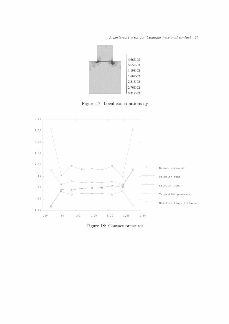
The initial mesh with 640 three-node elements, 370 nodes and an accuracy ǫ of8.51% is shown on Figure 15. We show the deformed bodies (Fig. 16) and thecontributions to the error ǫE (Fig. 17). The contact pressures are drawn on Figure18. As in the previous example the computed tangential pressure is outside the frictioncone (on both extreme meshes) and as previously, it can be successfully modified tocompute the estimator.

A posteriori error for Coulomb frictional contact 26

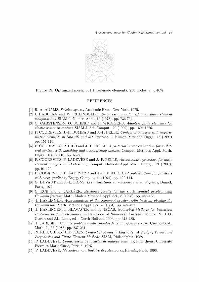
An accuracy ǫ0 of 5% is prescribed. The optimized mesh, obtained in one step,made of 381 three-node elements and 230 nodes for an accuracy ǫ of 5.46% is shownin Figure 19.

Γ

ΓN

C

Ω

Ω1

2

Figure 14: Setting of the problem

Figure 15: Initial mesh: 640 three-node elements, 370 nodes, ǫ=8.51%

Figure 16: Deformed configuration

A posteriori error for Coulomb frictional contact 27

3.31E-02

5.55E-03

1.10E-02

1.66E-02

2.21E-02

2.76E-02

4.66E-05

Figure 17: Local contributions ǫE

.40 .60 .80 1.00 1.20 1.40 1.60

−1.00

−.50

.00

.50

1.00

1.50

2.00

2.50

3.00

Modified tang. pressure

Tangential pressure

Friction cone

Friction cone

Normal pressure

Figure 18: Contact pressures

A posteriori error for Coulomb frictional contact 28

Figure 19: Optimized mesh: 381 three-node elements, 230 nodes, ǫ=5.46%

REFERENCES

[1] R. A. ADAMS, Sobolev spaces, Academic Press, New-York, 1975.[2] I. BABUSKA and W. RHEINBOLDT, Error estimates for adaptive finite element

computations, SIAM J. Numer. Anal., 15 (1978), pp. 736-754.[3] C. CARSTENSEN, O. SCHERF and P. WRIGGERS, Adaptive finite elements for

elastic bodies in contact, SIAM J. Sci. Comput., 20 (1999), pp. 1605-1626.[4] P. COOREVITS, J.–P. DUMEAU and J.–P. PELLE, Control of analyses with isopara-

metric elements in both 2D and 3D, Internat. J. Numer. Methods Engrg., 46 (1999)pp. 157-176.

[5] P. COOREVITS, P. HILD and J.–P. PELLE, A posteriori error estimation for unilat-eral contact with matching and nonmatching meshes, Comput. Methods Appl. Mech.Engrg., 186 (2000), pp. 65-83.

[6] P. COOREVITS, P. LADEVEZE and J.–P. PELLE, An automatic procedure for finiteelement analysis in 2D elasticity, Comput. Methods Appl. Mech. Engrg., 121 (1995),pp. 91-120.

[7] P. COOREVITS, P. LADEVEZE and J.–P. PELLE, Mesh optimization for problemswith steep gradients, Engrg. Comput., 11 (1994), pp. 129-144.

[8] G. DUVAUT and J.–L. LIONS, Les inequations en mecanique et en physique, Dunod,Paris, 1972.

[9] C. ECK and J. JARUSEK, Existence results for the static contact problem withCoulomb friction, Math. Models Methods Appl. Sci., 8 (1998), pp. 445-468.

[10] J. HASLINGER, Approximation of the Signorini problem with friction, obeying theCoulomb law, Math. Methods Appl. Sci., 5 (1983), pp. 422-437.

[11] J. HASLINGER, I. HLAVACEK and J. NECAS, Numerical Methods for UnilateralProblems in Solid Mechanics, in Handbook of Numerical Analysis, Volume IV,, P.G.Ciarlet and J.L. Lions, eds., North Holland, 1996, pp. 313-485.

[12] J. JARUSEK, Contact problems with bounded friction. Coercive case, Czechoslovak.Math. J., 33 (1983) pp. 237-261.

[13] N. KIKUCHI and J. T. ODEN, Contact Problems in Elasticity : A Study of VariationalInequalities and Finite Element Methods, SIAM, Philadelphia, 1988.

[14] P. LADEVEZE, Comparaison de modeles de milieux continus, PhD thesis, UniversitePierre et Marie Curie, Paris 6, 1975.

[15] P. LADEVEZE, Mecanique non lineaire des structures, Hermes, Paris, 1996.

A posteriori error for Coulomb frictional contact 29

[16] P. LADEVEZE, G. COFFIGNAL and J.–P. PELLE, Accuracy of elastoplastic anddynamic analysis, in Accuracy estimates and adaptative refinements in finite elementcomputations, Babuska, Gago, Oliveira, Zienkiewicz, eds., J. Wiley; 1986, pp. 181-203.

[17] P. LADEVEZE and D. LEGUILLON Error Estimate Procedure in the Finite ElementMethod and Applications, SIAM J. Numer. Anal., 20 (1983) pp. 485–509.

[18] P. LADEVEZE, J.–P. PELLE and P. ROUGEOT, Error estimates and mesh optimiza-tion for FE computation, Engrg. Comput., 8 (1991) pp. 69-80.

[19] C. Y. LEE and J. T. ODEN, A posteriori error estimation of h − p finite elementapproximations of frictional contact problems, Comput. Methods Appl. Mech. Engrg.,113 (1994), pp. 11-45.

[20] J. NECAS, J. JARUSEK and J. HASLINGER, On the solution of the variationalinequality to the Signorini problem with small friction, Boll. Unione Mat. Ital. 17-B(5)(1980), pp. 796-811.

[21] R. VERFURTH, A review of a posteriori error estimation techniques for elasticityproblems, Comput. Methods Appl. Mech. Engrg., 176 (1999), pp. 419-440.

[22] O. C. ZIENKIEWICZ and J. Z. ZHU, A simple error estimator and adaptive procedurefor practical engineering analysis, Internat. J. Numer. Methods Engrg., 24 (1987), pp.337-357.