A posteriori error estimation by means of the exactly equilibrated fields

A posteriori error estimationby means of the exactly equilibrated fields

I. Anufriev2 , V. Korneev1,2 and∗ † V. Kostylev3

November 17, 2007

Dedicated to L.A. Rozin

1 St. Petersburg State University, Russia,2 St. Petersburg State Polytechnical University, Russia

2 All-Russian Scientific-Research Institute of Hydroengineering, Russia

[email protected] , [email protected] , Vol [email protected]

Abstract

In this paper, we advocate the ”classical” approach to the a posteriori error estima-tion, which for the theory elasticity problems stems from the Lagrange and Castiglianovariational principles. In it, the energy of the error of an approximate solution, satisfyinggeometrical restrictions, is estimated by the energy of the difference of the stress tensorcorresponding to the approximate solution and any stress tensor, satisfying the equationsof equilibrium. Notwithstanding a popular point of view that the construction of equi-librated stress fields requires considerable computational effort, we show that it can bepractically always done for a number of arithmetic operations, which is asymptotically op-timal. Numerical experiments show that a posteriori error estimators, based on the use ofexactly equilibrated stress fields, provide very good coefficients of effectiveness, which inmany cases can be convergent to the unity. At the same time they have linear complexityand are robust.

1 Introduction

Publications on a posteriori error estimates for approximate, e.g., numerical solutions of par-tial differential equations are numerous. The earliest a posteriori error estimates were apparentlyknown in mechanics from the time when the Lagrange and Castigliano principles, which, fromthe mathematical point of view, provide the primal and dual formulations in theory elasticity,

∗ Research is supported by the grant from the Russian Fund of Basic Research N 05-01-00779-a.†The second author has partially been supported by Johann Radon Institute for Computational and Applied

Mathematics (RICAM) of the Austrian Academy of Sciences (AAS), Linz, Austria.

1

obtained a mature form. Such estimates are deduced from the fact that approximate solutionsobtained on the basis of these principles approach the exact solution in the energy sense from theopposite directions, and, namely, from above and from below, respectively. Let u be the vectorof exact displacements of a linearly elastic body, σ = σ(u) is the corresponding stress tensor,|| · ||U and || · ||σ are the potential energy norms expressed in displacements and stresses. If u is anarbitrary displacement vector of finite energy, satisfying geometric boundary conditions, and τis an arbitrary stress tensor of finite energy, satisfying the equilibrium equations (including theboundary conditions in stresses), then the classical a posteriori estimate is

||u− u||U ≤ ||σ(u)− τ ||σ , (1.1)

and may be found, e.g., in the Mikhlin’s book [33]. In spite of its simple form and enormousamount of publications on a posteriori estimates, the authors were unable to find references whereit had been directly used in practical FE applications.

During several last decades, a few groups of a posteriori error estimation techniques havebeen developed and, first of all, so called residual-based techniques found in Babuska I andReinbolt [5, 6], Verfurth [51] Stewart and Hudges [48] and more recent publications. Amongthem there are distinguished the explicit residual method, see Bernardi and Girault [9] andCarstensen [11] and the related paper by Clement [12] on special interpolation, and the implicitand equilibrated residual methods, for which we refer to Babuska I and Reinbolt [5], Kelly[18], Ladevese and Leguillon [31], and Ainsworth, Demkowicz and Kim [1]. Many papers arededicated to obtaining of indicators of the error, which do not necessarily bound it, but areapproximately proportional to the error, and, therefore, can be used for the mesh refinement inadaptive computations. A pioneering paper of Zienkiewicz and Zhu [55], see also Ainsworth andOden [2], commenced the group of such techniques widely used in applications and employingsuperconvergence properties of finite element solutions. Many contributions have been relatedto a posteriori error estimation for specific problems of mathematical physics. The developmentof a posteriori estimation techniques in recent decades, as well as the bibliography, are reflectedin the books of Aubin [3], Verfurth [52], Ainsworth and Oden [2] Babuska and Strouboulis [7]and Neittaanmaki and Repin [35].

The main idea of some of the mentioned approaches to the error estimation is to use fieldsof stresses, which can be obtained from the FE solution and at the same time are most close tothe exact equilibrated fields (i.e., representing the exact solution of the problem). An exampleis the equilibrated residual method, which now gains more attention as a method which allow toobtain reliable bounds, often without solving some global systems of algebraic equations, see, e.g.,Ainsworth, Demkowicz and Kim [1], Luce and Wohlmuth [32], Vejchodsky [50] and Braess andSchoberl [10]. However, it is also true that the purpose of most authors is to outflank constructionof exactly equilibrated fields at all1. One way of obtaining equilibrated fields2, which approximateequilibrated fields of the exact solution of the primal problem, is approximate solution of thedual problem, which in the theory of elasticity is expressed by the Castigliano principle of virtualequilibrated states. As a rule a motivation for avoiding the use of equilibrated fields is that

1In general discussions we use the theory elasticity problem for a model without special remarks.2In the paper the both terms equilibrated and exactly equilibrated field imply that a field satisfies equilibrium

equations exactly in classical or generalized sense.

2

the solution of the dual problem or other ways of finding such fields are computationally tooexpensive.

The purpose of this paper is to illustrate that in many cases the estimate (1.1) can be directlyused as an efficient and cheap error estimator. This is for the reason that indeed equilibratedfields are not difficult to find in a variety of ways. As one of the options, as we will see not themost efficient in many cases, the numerical solution of the dual problem can be considered. Foradvocating this option, the following fact is important: numerical solutions of the discretizationsof the primal and dual problems, having the same (in the order) accuracy in the energy norm,can be found for the same (in the order) computational cost. More over, under some conditions,the discretization of the dual problem may be obtained in such a way that its matrix will coincidewith the FE matrix for the primal problem up to the boundary conditions. Therefore, practicallythe same solver can be used for solution of the both discrete problems.

From the above discussion, one concludes that the option of solving the dual problem forevaluating the equilibrated fields deserves examination. Suppose that discretizations of the sameorder of accuracy are used for the primal and dual problems. In general, one can expect that theefficiency coefficient will converge to the unity at h→ 0, if the error estimator is super-convergent.In the practice, such convergence was observed for a number of alternative a posteriori errorestimators, considered in this paper and papers of other authors, see, e.g., Luce and Wohlmuth[32]. In our numerical experiments with the use of classical error estimate of the type (1.1) andof the equilibrated fields, obtained by solution of the dual problem with the same accuracy, theobserved effectiveness coefficient remained close to 1.25. Further improvement of the efficiencycoefficient is possible, e.g., if we solve the dual problem on a denser, then for the primal problem,mesh, which results in a greater cost of an error estimator, than the cost of the solution to bevalidated.

At least not less promising approach can be referred as direct evaluation of the equilibratedfields. It is based on the fact that the equilibrium equations (in stresses) are under-determined.For instance, in the theory of elasticity, the symmetric stress tensor σ = σkl3

k,l=1 with sixstresses for the entries satisfies three equilibrium equations. Therefore, in order to satisfy theequilibrium equations it is sufficient to perform two steps:

1) to specify three stresses, say shear stresses

σkl , k 6= l, (1.2)

by arbitrary sufficiently smooth functions and2) to find the rest stresses from the equilibrium equations by evaluating 1-d integrals.

The presence of the boundary conditions for stresses often does not make this procedure sig-nificantly more difficult. When this procedure is used in the a posteriori estimator, e.g., forthe FE solution, the stresses (1.2) are found from the FE solution with the accurate use of itssuperconvergence properties.

The approach of direct evaluation of the equilibrated fields allows us not only to design cheapalgorithms for evaluating a posteriori error estimators, often producing convergent the efficiencycoefficients, but to come to a new type of general a posteriori estimates. For simplicity, let usconsider the Dirichlet problem for the Poisson equation in the rectangle Ω = (a1, b1)× (a2, b2)

−∆u = f(x) , x = (x1, x2) ∈ Ω , u∣∣∂Ω

= 0 , (1.3)

3

and any function v from H1(Ω) = w ∈ H1(Ω) : u∣∣∂Ω

= 0, which is considered as an ”approxi-mation” for u. Then for any ε > 0 the error estimate can be written in the form

‖∇(v − u)‖20,Ω ≤

≤ (1 + ε)‖∇v − y‖20,Ω + (1 + 1

ε)‖

∑k=1,2

∫ xk

ak(x3−k)αk(f −∇ · y)(ηk, x3−k) dηk‖2

0,Ω ,(1.4)

y = (y1, y2)> is any sufficiently smooth vector-function, functions αk = αk(x) satisfy α1 +α2 ≡ 1,

and by convention ∇ · y = div y. If f ∈ L2(Ω) and αk ∈ C(Ω), it is natural to considery ∈ H(Ω, div) = z : ∇ · z ∈ L2(Ω). If v = ufem is the FE solution, then y may be obtainedby the averaging of the derivatives ∂ufem/∂xk at the nodes and interpolation. In our numericalexperiments, algorithms of that type almost always produced good and convergent effectivenesscoefficients. In the algorithms presented in the paper we implement a variety of techniques ofdirect evaluation of the exactly equilibrated fields for their use in the a posteriori estimators.

Clearly, estimate (1.4) fetches additional opportunities in comparison with the known esti-mates of a close appearance, in which the second term in the right part is, e.g., ‖f −∇ · y‖−1,Ω.Numerical evaluation of this negative norm is not at all easy, whereas its replacement in (1.4)can be often computed for a number of arithmetic operations proportional to the number ofunknowns. In particular, this is true for the FE discretizations by means of the orthogonal grids.Another example is Galerkin methods with the coordinate functions specified by analytical ex-pressions in the whole domain. In the paper we discuss also the procedures, which can providethe optimal computational cost in more general situations.

The equilibrium equations in the theories of thin shells and shells of moderate thickness, see,e.g., Gol’denweizer [17] Novozhilov [37, 36] and Reissner [44], are written in terms of internalforces, i.g., shear forces and bending and twisting moments. These equations are more com-plicated, than the equilibrium equations in the theory of elasticity. However, a quite similarapproach can be implemented for obtaining the exactly equilibrated functions of internal forces.This approach originates from the papers devoted to numerical methods for solving the bendingthin plate and shell problems on the basis of the Castigliano principle and the method of splittingof the thin plate and shell partial differential equations, studied by Rozin [45, 46], Korneev/Rozin[29, 30], Korneev [19, 20, 21, 25, 27].

Considerable part of the algorithms contained in the paper were tested numerically. Wepresent the graphs and tables of numbers illustrating the dependence of effectiveness indices andarithmetical work on numbers of unknowns. Obviously, all tested algorithms are optimal in thecomputational work. Additionally to this, the practical computational costs of the a posteriorierror estimators and of the optimal multigrid solvers for the primal problem were compared. Asa rule the latter exceeded the former in two times at the least.

The paper is arranged as follows. In Section 2, we consider a posteriori estimators for thePoisson equation in the unite square and arbitrary Lipshits continuous domain with differentboundary conditions. The special case of the differential operator with the discontinuous co-efficient in the main term is treated in Subsection 2.3. It is shown that the algorithms of aposteriori estimators are easily adjusted to this case. The results of numerical tests for this case,presented in Subsection 5.2, show that discontinuity practically does not affect the efficiency ofthe a posteriori error estimator. Section 3 deals with the a posteriori error estimators for the

4

plane elasticity problem. All a posteriori error estimators of Sections 2 and 3 are based on thedirect evaluation of the balanced fluxes and equilibrated stress tensors, i.e., without solving anysystems of algebraic equations. In Section 4.1, we consider an alternative approach based onsolution of the dual problem equivalent to the Castigliano principle of virtual complementarywork. We show that it is possible to chose a basis in the space of the self-equilibrated tensors ofstresses in such a way that the system of algebraic equations will possess practically the sameproperties as the FE system for the primal problem. Throughout the paper alongside with thegeneral algorithms, we present the algorithms, which we tested numerically. Results of numericalexperiments are discussed in Section 5.

Throughout the paper, we use the notations listed below.Pp and Qp are the spaces of polynomials of the total order p and of the order p in each

variable, e1 = (1, 0), e2 = (0, 1), d is the dimension.L2(Ω) is the space [L2(Ω)]d with the norm ‖ · ‖ = ‖ · ‖0,Ω and the same notation is used for

the norm in L2(Ω),| · |k,Ω, ‖ · ‖k,Ω stand for the semi-norm and the norm in the Sobolev space Hk(Ω), i.e.,

| v |2k,Ω =∑|q|=k

∫Ω

(Dqxv)

2dx , ‖ v ‖2k,Ω = ‖v‖2

0,Ω +k∑

l=1

|v|2l,Ω ,

where

Dqxv := ∂|q|v/∂xq1

1 ∂xq2

2 , ..∂xqd

d , q = (q1, q2, .., qd), qk ≥ 0, |q| = q1 + q2 + ..+ qd ,

H1(Ω) := v ∈ H1(Ω) : v|∂Ω = 0 is the subspace of functions from H1(Ω) vanishing on theboundary ∂Ω.

We use also the abbreviations: a.o. – arithmetic operations, FE - finite element. In thevectors of the space variables x = (x1, x2) or x = (x1, x2, x3), sometimes we interchange thepositions of variables and write x = (xk, x3−k) and x = (xk, xk+1, xk+2), assuming in the lattercase that indices k + l are taking values modulo 3.

2 Poisson equation

2.1 An outline of the approach

In this section, we illustrate basics of the approach of the direct evaluation of equilibratedfields on a simple model problem. Let us consider a boundary value problem for the Poissonequation in the unite square Ω = (0, 1)× (0, 1) with the mixed boundary conditions

−∆u = f(x) , x = (x1, x2) ∈ Ω , ∂Ω = ΓD ∪ ΓN ,

u|ΓD= 0 , ∂u/∂ν|ΓN

= 0 .(2.1)

whereΓD = x| x1 ∈ (0, 1] , x2 = 1 ∪ (x1, x2)| x1 = 1 , x2 ∈ (0, 1] ,

ΓN = x| x1 ∈ [0, 1) , x2 = 0 ∪ (x1, x2)| x1 = 0 , x2 ∈ [0, 1) ,(2.2)

5

and ν is the distance from the boundary along the outward normal. The generalized formulationof this boundary value problem reads

a(u, v) = (f, v)Ω , ∀ v ∈ V(Ω) , (2.3)

where V(Ω) = v ∈ H1(Ω) : v|ΓD= 0

a(v, w) =

∫Ω

∇v · ∇w dx , (v, w)Ω =

∫Ω

v w dx .

Let V(Ω) be the finite element space of the piece wise bilinear functions on the uniform squaregrid of size h = 1/n, n > 1, with the nodes x(i) = h(i1, i2), ik = 0, 1, .., n, and V0(Ω) be thesubspace of functions from V(Ω), vanishing on ΓD. By ufem is denoted the finite element solutionbelonging to V0(Ω) and satisfying the identity

a(ufem, v) = (f, v)Ω , ∀ v ∈ V0(Ω) . (2.4)

In order to be able to efficiently implement the a posteriori estimate (1.1), it is necessary withthe use of the obtained FE solution ufem to construct the vector valued function t = (t1, t2)

>,which obeys the two conditions:

α) it satisfies the balance differential equation

−∇ · t = f , (2.5)

and the boundary conditionsν · t|ΓN

= 0 , (2.6)

where ν is a unite vector normal to ∂Ω, andβ) is as much close as possible to the gradient ∇u of the exact solution.

We shall use notations Qf , Q0 for the sets of functions satisfying (2.5),(2.6) with the given fand f = 0, respectively, from which Q0 is clearly a liner space. The balance law (2.5) modelsequilibrium equations in the case of the theory elasticity boundary value problems. Elementsof Qf will be termed balanced or equilibrated, whereas elements of Q0 – self-balanced or self-equilibrated. The sets Qf , Q0 can be defined constructively by means of the splitting technique,which was introduced by Korneev and Rozin [45, 29, 27] at developing numerical methods forsolving problems of the theory of elastic thin plates and shells in solid mechanics on the basis ofthe Castigliano principle. For the problem under consideration constructive definition of the setQf of the ”equilibrated” vectors is quite simple. If q is an arbitrary sufficiently smooth function,then the vector t = (t1, t2)

> with the components

t1(x) =

∫ x1

0

q(ξ1, x2) dξ1 , t2(x) = −∫ x2

0

(f(x1, ξ2) + q(x1, ξ2)) dξ2 (2.7)

satisfies equation (2.5) and boundary conditions (2.6). Clearly, Qf = Q0 + tf , where tf anyelement of Qf , and Q0 is defined by (2.7) with f ≡ 0. For all q ∈ L2(Ω) one comes to the spaceQ0 with the norm ||t||σ = ||t||, where ‖ · ‖ stands for the [L2(Ω)]2 norm.

6

The estimate (1.1) takes the form

‖∇(u− ufem)‖ ≤ ‖∇ufem − t‖ , ∀ t ∈ Qf . (2.8)

Obviously, a better approximation of ∂u/∂x1 by t1 (e.g., with the use of values of the gradientof the finite element solution at superconvergence points) will result in a better a posterioriestimate. In turn, from (2.7) it is seen that the function q has the sense of the second derivative∂2u/∂x2

1.Taking for αk, sufficiently smooth functions satisfying α1 + α2 = 1, one can use more ”sym-

metric” formulas instead of (2.7):t1(x) = −

∫ x1

0(α1f − q) (ξ1, x2) dξ1 ,

t2(x) = −∫ x2

0(α2f + q) (x1, ξ2) dξ2 .

(2.9)

They can provide more accurate a posteriori estimates, especially with a good choice of functionsαk, , but require more a.o.

If the approach, presented above, is used for a posteriori estimation, then different boundaryconditions should be given attention. Suppose, u is an approximate twice differentiable solutionof (2.1),(2.2), e.g., obtained by the Galerkin method or any other function from V(Ω). Forinstance, we can set q = ∂2u/∂x2

1 and come to the expressions

t1 =∫ x1

0∂2u/∂x2

1(ξ1, x2)d ξ1 ,

t2 = −∫ x2

0(f + ∂2u/∂x2

1)(x1, ξ2)d ξ2 .(2.10)

Similarly, we can proceed from setting q = ∂2u/∂x22 and obtain the a posteriori estimates

‖∇(u− u)‖2 ≤∫

Ω

[ ∂u∂xk

−∫ xk

0∂2u∂x2

k(ξk, x3−k)d ξk]

2 +

+ [ ∂u∂x3−k

+∫ x3−k

0(f + ∂2u

∂x2k)(xk, ξ3−k)d ξ3−k]

2d x , k = 1, 2 .

(2.11)

Taking into account boundary conditions at ΓN and triangular inequality, one comes from (2.11)to

‖∇(u− u)‖ ≤∑k=1,2

‖∂uxk

∣∣xk=0

‖(0,1) + ‖∫ x2

0

(f + ∆u)(x1, ξ2) d ξ2‖ (2.12)

Another vector t, which belongs to Qf simultaneously with t from (2.10), is

t1 =∫ x1

0(α1∂

2u/∂x21 − α2(f + ∂2u/∂x2

2)) (ξ1, x2)d ξ1 ,

t2 =∫ x2

0(α2∂

2u/∂x22 − α1(f + ∂2u/∂x2

1)) (x1, ξ2)d ξ2 .(2.13)

The corresponding a posteriori error estimates are

‖∇(u− u)‖ ≤∑

k=1,2

∫Ω

[∂u∂xk

−∫ xk

0

(αk

∂2u∂x2

k− α3−k(f + ∂2u

∂x23−k

))

(ξk, x3−k)d ξk

]2

d x

1/2

≤

≤∑

k=1,2

[‖∂u

xk

∣∣xk=0

‖(0,1) + ‖∫ xk

0α3−k(f + ∆u)(ξk, x3−k) d ξk‖

](2.14)

7

which for αk ≡ 0.5 is invariant with respect to xk, k = 1, 2, . It easy to see, that adding andsubtracting α3−k∂

2u/∂x2k inside round brackets, taking into account boundary conditions at ΓN

and triangular inequality, we obtain the same estimate (2.12).In the case of the Dirichlet boundary value problem

a(u, v) = (f, v)Ω , u, ∀ v ∈ V(Ω) = H1(Ω) , (2.15)

the estimates (2.12),(2.14) take especially simple forms. Instead of the latter we have

‖∇(u− u)‖ ≤∑k=1,2

‖∫ xk

0

α3−k(f + ∆u)(ξk, x3−k) d ξk‖ . (2.16)

Let for simplicity α2 ≡ 0. Since in the case under consideration no boundary conditions areimposed on the equilibrated fluxes, we can set

t1 = ∂u/∂x1 ,

t2 = ∂u/∂x2(x1, 0)−∫ x2

0(f + ∂2u/∂x2

1)(x1, ξ2)d ξ2 ,(2.17)

and, therefore,

∂u∂x1

− t1 = 0 ,

∂u∂x2

− t2 = ∂u∂x2

− ∂u∂x2

(x1, 0) +∫ x2

0(f + ∂2u

∂x21)(x1, ξ2)d ξ2 =

∫ x2

0(f −∆u)(x1, ξ2) d ξ2 ,

completing the proof. In the case of an arbitrary sufficiently smooth domain, the proof is similar.

Lemma 2.1. Let Ω be Lipshits continuous domain, f ∈ L2(Ω), u - solution of (2.15), and u beany function in H2(Ω) satisfying boundary condition u

∣∣∂Ω

= 0. Then the error u− u satisfies aposteriori estimate (2.16).

2.2 Examples of algorithms for finite element solutionsof Poisson equation

Solutions obtained by FE methods compatible in C, which are primarily used in practicefor second order elliptic equations, do not have second derivatives. Basically, three ways tooutflank this obstacle can be distinguished. All of them start from the procedure of constructingsome smooth approximation of the second, or first derivatives of FE solution, or the FE solutionitself. In what follows, this procedure is termed smoothing procedure. After smoothing procedurehas been applied, we proceed in one of the ways described in Subsection 2.1. The distinctionsbetween three types of a posteriori error estimation algorithms for our model problem can beillustrated on example of ”nonsymmetric” algorithms, in which 1-d integration of f is involvedin the definition of only one of the fluxes. Since this flux is uniquely defined by the balanceequation and the boundary condition on ΓN , it is sufficient to point out the way of evaluationof one flux, which is calculated first. Briefly, three types of such a posteriori error estimationalgorithms are the following:

8

a) Calculate second derivative of the FE solution along one of the axes approximately withthe use of finite differences at some set of discrete points (e.g., FE nodes). Define q (e.g., asa function of the FE space V(Ω)) by interpolation of the calculated approximate values of thesecond derivative. Define the corresponding flux by 1-d integration of q (like in the first expression(2.7)) and by adding the boundary value of the flux, given by the boundary conditions on ΓN .

b) Calculate the first derivative of the FE solution in one of the directions xk at the nodalpoints, e.g. by averaging. Define the tentative flux in the chosen direction as the FE function,which belongs to V(Ω) and takes at the nodes calculated values. Define the flux by adjustmentof the tentative flux to the boundary condition on ΓN .

c) Construct twice differentiable approximation of the FE solution. Define the tentativeflux in one of the axes as the first derivative of the smoothed FE solution. Define the flux byadjustment of the tentative flux to the boundary condition on ΓN .

Indeed each of a),b) and c) allows to define two equilibrated fluxes t(k), k = 1, 2, corre-sponding to the direction xk, the flux along which is defined first. The flux for the a posterioriestimator can be defined as t = α1t

(1) + α2t(2).

Apart from ”symmetric” versions, other variations of the outlined algorithms are numerous.For instance, in the smoothing procedures of a) and b) some other finite dimensional functionalspaces W(Ω) can be used instead of the basic FE space V(Ω). Since it is not necessary for q tobe continuous, we can cover Ω by some nonoverlapping subdomains Ωj and in each define q bythe list squares method with the use of polynomials of some specific order pj. In the vicinityof singularities in the exact solution of the problem, special representations for q, equilibratedfluxes or the smoothed FE solution can be implemented. In the latter case it is more appropriateto use the term preprocessed FE solution. It is also worth adding that in different subdomainsone can use algorithms of different types, i.e., a), b) or c), for obtaining equilibrated fluxes.

In this subsection, we present a few simple examples of the outlined algorithms for the Poissonequation in the unit square and arbitrary sufficiently smooth domain with different boundaryconditions. For the problems in the unit square, the FE space V(Ω) is the space of continuouspiece wise bilinear functions on the square mesh of size h = 1/n. For the nodes of this mesh weuse notation x(i) = hi, i = (i1, i2). We start from the algorithm of the type c) for the problem(2.1)(2.2).

Algorithm 2.1.Step 1. For each node x(i) ∈ ∂Ω calculate the value of the mesh function vh = (v

(i)2,1)

ni1,i2=0,

which is the finite-difference approximation of the second derivative ∂2u/∂x12(x(i)). For

internal nodes of horizontal mesh lines x2 ≡ hi2, i2 = 0, 1, .., n, use

v(i)2,1 =

ufem(h(i1 + 1), hi2)− 2ufem(hi1, hi2) + ufem(h(i1 − 1), hi2)

h2, i1 = 1, 2.., n− 1 .

For the nodes (0, i2) on the axis x1 ≡ 0 set

v(i)2,1 = ∂2u0/∂x1

2(0, hi2) ,

where u0 is the 3-rd order interpolation polynomial of x1 over the values ufem(x(i)) for i1 =0, 1, 2, and ∂ufem/∂x1(0, hi2). For the nodes (n, i2) calculate

v(i)2,1 = ∂2u1/∂x1

2(1, hi2) ,

9

where u1 is the 3-rd order Lagrange interpolation polynomial of x1 over the values ufem(x(i))for i1 = n− 3, n− 2, n− 1, n.Step 2. Define I2,1(x) ⊂ V(Ω) as the piece wise bilinear interpolation of vh.Step 3. Define t by evaluating the integrals

t1(x) =∫ x1

0I2,1(ξ1, x2) dξ1 ,

t2(x) = −∫ x2

0(f(x1, ξ2) + I2,1(x1, ξ2)) dξ2 .

(2.18)

Step 4. Evaluate the estimator η := ‖∇ufem − t‖2.

Remark 2.1. Formulas (2.18) correspond to (2.7),(2.10). Since I2,2 ∼ ∂2u/∂x12 can be cal-

culated in a similar way, a more ”symmetric” formulas, corresponding to (2.9),(2.13), can beused:

t1 =∫ x1

0[α1I2,1 − α2(f + I2,2)](ξ1, x2) dξ1 =

∫ x1

0[I2,1 − α2(f + I2,1 + I2,2)](ξ1, x2) dξ1 ,

t2 =∫ x2

0[α2I2,2 − α1(f + I2,1)](x1, ξ2) dξ2 =

∫ x2

0[I2,2 − α1(f + I2,1 + I2,2)](x1, ξ2) dξ2 .

(2.19)

In Step 1, we used finite-difference approximations of the second derivative ∂2u/∂x21, which

provide the same order h2 of approximation for a sufficiently smooth u. In Step 3, the wayof the evaluation of integrals of Iv and f may be different. In particular, in many cases theanalytical integration can be performed. In general, procedures, used in Steps 3, depend onthe way of evaluating the norm ‖∇ufem − t‖2 in Step 4. For instance, for each finite elementτi := h(i1 − 1, i1) × h(i2 − 1, i2), we can use quadratures exact for polynomials of some orderpi ≥ 1. Then it is necessary to evaluate tk only at the quadrature nodes, and for doing thisother quadratures can be used. The type of the quadratures, used element wise for evaluatingt2 and the norm ‖∇ufem − t‖2 may depend on the local smoothness of f , if the integral of f isnot evaluated exactly. Bounds for quadrature errors will enter the resulting error bound for theFE solution with the right part depending only on ufem and f . However, we will not elaborateon these subjects in the present paper aimed to illustrate main features of the approach.

In the case ΓN = ∅, i.e. when only the Dirichlet boundary conditions are imposed in (2.1),then the estimate (2.8) is true for any vector valued function t satisfying the balance equa-tion (2.5) and not subjected any boundary conditions.. But when boundary conditions aredifferent from the ones considered above in (2.1) and ΓN 6= ∅ then some remedy should be donein order t to fulfill the boundary conditions (2.6). For instance, let

ΓD = (x1, x2)| x1 ∈ [0, 1] , x2 = 1 , ΓN = ΓN,1 ∪ ΓN,2 ∪ ΓN,3 ,

whereΓN,1 = (x1, x2)| x2 ∈ [0, 1] , x1 = 0 ,ΓN,2 = (x1, x2)| x1 ∈ [0, 1] , x2 = 0 ,ΓN,3 = (x1, x2)| x2 ∈ [0, 1] , x1 = 1 ,

and the boundary conditions are

u|ΓD= 0 , ∂u/∂ν|ΓN

= g , (2.20)

10

where g ∈ C(ΓN) and

g =

g1(x2), on ΓN,1 ,g2(x1), on ΓN,2 ,g3(x2), on ΓN,3 .

(2.21)

The estimate (2.8) is true, if the vector valued function t satisfies the equation (2.5) and theboundary condition (2.6). The steps 1 and 2 may be the same as in the algorithm adduced above,but they produce only a tentative flux, which should be adjusted to the boundary condition (2.6).Let

t1(x) =

∫ x1

0

(I2,1 + r)(ξ1, x2) dξ1 + g1(x2) ,

t2(x) = −∫ x2

0

(f + I2,1 + r)(x1, ξ2) dξ2 + g2(x1) ,(2.22)

where r(x) is chosen with the purpose to fulfill the boundary condition (2.6) on ΓN,3. It issufficient to take r depending only on x2

r(x1, x2) = g3(x2)− g1(x2)−∫ 1

0

I2,1(ξ1, x2) dξ1 . (2.23)

Hence

t1(x) =

∫ x1

0

I2,1(ξ1, x2) dξ1 − x1

∫ 1

0

I2,1(ξ1, x2) dξ1 + (1− x1)g1(x2) + x1g3(x2) ,

t2(x) = −∫ x2

0

(f + I2,1)(x1, ξ2) dξ2 +

∫ x2

0

∫ 1

0

I2,1(ξ1, ξ2)) dξ1dξ2+

+

∫ x2

0

(g1 − g3)(ξ2) dξ2 + g2(x1) .

(2.24)

In the case of the homogeneous Neumann boundary condition on ΓN , the expressions (2.24) takea simpler form

t1 =

∫ x1

0

I2,1(ξ1, x2) dξ1 − x1

∫ 1

0

I2,1(ξ1, x2) dξ1 ,

t2 = −∫ x2

0

(f + I2,1)(x1, ξ2) dξ2 +

∫ x2

0

∫ 1

0

I2,1(ξ1, ξ2)) dξ1dξ2 .

(2.25)

The described approach is easily realized in a much more general situation. Suppose, Ω isthe domain occupied by the arbitrary triangulation Sh with the triangles τr, r = 1, 2, ..,R, V(Ω)is the space of the continuous piece wise linear functions and V(Ω) = v ∈ V(Ω) : v

∣∣∂Ω=0

. Wewill turn to the algorithm of the type b) for the problem with the Dirichlet boundary condition.Namely, we consider the problem

a(u, v) = (f, v)Ω , u, ∀ v ∈ V(Ω) = H1(Ω) , (2.26)

and its FE solution ufem satisfying

a(ufem, v) = (f, v)Ω , ufem,∀ v ∈ V(Ω) . (2.27)

11

Let us assume for simplicity that each line xk ≡ const crosses Ω not more than in two points,Γk,− is the part of the boundary containing the points of such pairs, having lesser coordinate xk,

xk = ak(x3−k) is the equation of Γk,−, x3−k = a3−k, b3−k are the coordinates of the ends of Γk,−.We also use the notation Bi = r : τr ∈ Ω, x(i) ∈ τ r for the set of the numbers of finite elements,having x(i) for a vertex, and notation V(Γk,−) for the space of the traces of functions from V(Ω)on Γk,−. Among simplest is the algorithm, which is not invariant with respect to xk, k = 1, 2,and is based on the averaging and the procedure reflected in Remark 2.1.

Algorithm 2.2.Step 1. For each node calculate the average

u(i)fem,1 =

∑r∈Bi

∂u(r)fem

∂x1

(x(i)) ,

where u(r)fem = ufem

∣∣∣τr

is the restriction of the FE solution to τr.

Step 2. Define the interpolation I(ufem,1) ∈ V(Ω) satisfying

I(ufem,1)(x(i)) = u

(i)fem,1 , ∀ x(i) ∈ Ω .

Step 3. For each node x(i) ∈ Γ2,− calculate the average

u(i)fem,2 =

∑r∈Bi

∂u(r)fem

∂x2

(x(i)) ,

and for x ∈ Γ2,− define the piece wise linear continuous interpolation IΓk,−(ufem,2) satisfying

I(ufem,2)(x(i)) = u

(i)fem,2 , ∀ x(i) ∈ Γ2,− .

Step 4. For components of an equilibrated vector t = (t1, t2)> set

t1 = I(ufem,1) , t2∣∣Γ2,−

= t2(x1, φ2(x1)) := IΓk,−(ufem,2)∣∣Γ2,−

,

and evaluate

t2(x) = t2(x1, φ2(x1))−∫ x2

a2

(f +∂t1∂x1

)(x1, ξ2) dξ2 .

Step 5. Evaluate the bound ‖∇ufem − t‖2.The algorithm, based on averaging, can be made invariant with respect to xk, k = 1, 2,.Algorithm 2.3.Step 1. For each node and k = 1, 2 calculate the averages

u(i)fem,k =

∑r∈Bi

∂u(r)fem

∂xk

(x(i)) .

Step 2. Define the interpolations I(ufem,k) ∈ V(Ω) satisfying

I(ufem,k)(x(i)) = u

(i)fem,k , ∀ x(i) ∈ Ω .

12

Clearly, the vector t = (t1, t2)>, tk = I(ufem,k), approximates the equilibrated vector.

Step 3. For k = 1, 2 calculate

qfem,k = −∂I(ufem,k)/∂xk , δf = f − qfem,1 − qfem,2 .

Step 4. For α1(x) + α2(x) ≡ 1 and θk(x3−k) = I(ufem,k)(ak(x3−k), x3−k), k = 1, 2, calcu-late

tk(x) = θk(x3−k)−∫ xk

ak(qfem,k + αkδf)(ξk, x3−k) dξk =

= (1− αk)I(ufem,k)−∫ xk

akαk(f + qfem,3−k)(ξk, x3−k) dξk .

Step 5. Evaluate the bound ‖∇ufem − t‖2.Functions θk(x3−k) specify boundary conditions for t. They can be defined differently from

Step 4, and for their evaluation by means of the FE solution special more accurate procedurescan be used. The simplest choice for α is α ≡ 1/2, however a number of more sophisticatedprocedures for the evaluation of this function can be considered. For instance, in some regionsα can be chosen on the basis of the local analysis. Obviously, the procedures of Algorithm 2.2are a part of Algorithm 2.3. The whole process of the a posteriori estimation can be arrangedin the following way. One uses Algorithm 2.2. If the a posteriori estimate is unsatisfactory thenadditional calculations are performed according Algorithm 2.3 with some choice of αk. Furtherperfection of the a posteriori estimator is possible in a variety of ways. For instance, it is notnecessary to use the same FE mesh for the evaluation of t. In order to simplify the computationsand make the estimate more accurate, a subsidiary mesh can be used for finding t, which, e.g.,is orthogonal inside the domain and provide some hp FE interpolation for fluxes, determined bythe FE solution ufem.

Remark 2.2. Evaluation of a posteriori error bounds according Algorithm 2.1-Algorithm 2.3involves only three operations

-- numerical differentiation with the use of finite differences,

-- interpolation, and

-- evaluating of 1-d integrals.For this reason, these algorithms are obviously optimal in the arithmetic operations count, ifthe mesh is orthogonal. In the case of an arbitrary quasiuniform triangulation, the evaluation ofintegrals may be often arranged by layers of elements. From layer to layer the number of points, atwhich we need to evaluate an equilibrated flux may in general double. Therefore, the computationalcost of the third among listed operations is estimated as O(nkn

23−k), where nk is the maximal

number of nodes in one layer and n3−k is the number of layers. In this paper, we concentrateon basic facts of a posteriori estimation, but several recipes can be immediately suggested forthe reduction of the computational work, even in the case of nonuniform unstructured meshes.For instance, we can cover the computational domain by the nonuniform orthogonal mesh withthe hanging nodes, matching in density the FE grid. Then we calculate one or both fluxes atthe nodes of this mesh by means of averaging and interpolation. After that with the use of theintroduced orthogonal mesh, we obtain corrections, which are necessary in order to make fluxesequilibrated.

13

Remark 2.3. There are known a posteriori estimates for the Dirichlet problem (2.26)

‖∇ufem −∇u‖20,Ω ≤ (1 + ε)‖∇ufem − y‖2

0,Ω + (1 + 1ε)‖∇ · y − f‖2

−1,Ω ,

‖∇ufem −∇u‖20,Ω ≤ (1 + ε)‖∇ufem − y‖2

0,Ω + cΩ(1 + 1ε)‖∇ · y − f‖2

0,Ω , ∀ ε > 0 ,(2.28)

where y is an arbitrary vector and cΩ is the constant from the Friedrich’s inequality, see Re-pin/Frolov [41] and Neittaanmakki/Repin [35]. One of our estimates can be written in the form

‖∇ufem −∇u‖20,Ω ≤ ‖∇ufem − t‖2

0,Ω ≤

≤ (1 + ε)‖∇ufem − y‖20,Ω + (1 + 1

ε)‖

∑k=1,2

∫ xk

ak(x3−k)αk(f −∇ · y)(ηk, x3−k) dηk‖2

0,Ω .(2.29)

In particular, in Algorithm 2.3 we used y = (I(ufem,1), I(ufem,2))>. The right part f enters the

last a posteriori estimate in a more adequate way, than in the second estimate (2.28). At thesame time, it is easily computable, whereas the negative norm, entering the right part of the firstbound (2.28), makes the bound difficult for the use in practice.

2.3 Heat conduction problem with discontinuous coefficient

The extension of the advocated approach and in particular of the algorithms of the previoussection to the elliptic equations with discontinuous coefficients is straightforward. Let us consideras an example the boundary value problem

− ∇ · (ρ(x)∇u) = f(x) , x ∈ Ω = (0, 1)× (0, 1) ,

u∣∣ΓD

= g , ∂u∂ν

∣∣ΓN

= 0 ,(2.30)

with ΓD,ΓN defined as in (2.2), ρ(x) > 0 and

ρ(x) =

ρ1 = const for x ∈ Ω1 := x ∈ Ω : 0 < x1 < 0.5 ,ρ2 = const for x ∈ Ω2 := Ω \ Ω1 .

For simplicity it is assumed that the boundary conditions are consistent and there exits suchu0 ∈ H2(Ω) that u0

∣∣ΓD

= g. We define the approximate solution ufem of this problem as a

function belonging to the set L(Ω) = V0(Ω) + u0 and satisfying the identity

aρ(ufem, v) = (f, v)Ω , ∀ v ∈ V0(Ω) , (2.31)

where

aρ(v, w) =

∫Ω

ρ∇v · ∇w dx1dx2

and V0(Ω) is the FE space defined in Subsection 2.1. If to introduce the norms

‖v‖ρ = (aρ(v, v))1/2 , ‖t‖ρ−1 = (

∫Ω

ρ−1t · t dx)1/2 (2.32)

14

and imply by Qf the set of the equilibrated vectors satisfying (2.5),(2.6), then the a posteriorierror estimate (2.8) takes the form

‖∇(u− ufem)‖ρ ≤ ‖ρ∇ufem − t‖ρ−1 . (2.33)

Algorithms 2.1-2.3 are easily adapted to the problem under consideration. For instance, the firstone is written as follows.

Algorithm 2.4.Step 1. For each node x(i) ∈ ∂Ω calculate the value of the mesh function vh = (v2,1(i))

ni1,i2=0,

which is the finite-difference approximation of ∂(ρ∂u/∂x1)∂x1(x(i)). For internal nodes of

horizontal mesh lines x2 ≡ hi2, i2 = 0, 1, .., n, use

v1,1(i) = ρ((i1 − 0.5)h, i2)[ufem(hi)− ufem(h(i1 − 1), hi2)] ,

v2,1(i) = 1h2 [v1,1(i1 + 1, i2)− v1,1(i)] , i1 = 1, 2.., n− 1 .

For the nodes (0, i2) on the axis x1 ≡ 0 set

v2,1(i) = ρ1∂2u0/∂x1

2(0, hi2) ,

where u0 is the 3-rd order interpolation polynomial of x1 over the values ufem(x(i)) for i1 =0, 1, 2, and ∂ufem/∂x1(0, hi2). For the nodes (n, i2) calculate

v2,1(i) = ρ2∂2u1/∂x1

2(1, hi2) ,

where u1 is the 3-rd order Lagrange interpolation polynomial of x1 over the values ufem(x(i))for i1 = n− 3, n− 2, n− 1, n.Step 2. Define I2,1(x) ⊂ V(Ω) as the piece wise bilinear interpolation of vh.Step 3. Define t by evaluating the integrals

t1(x) =∫ x1

0I2,1(ξ1, x2) dξ1 ,

t2(x) = −∫ x2

0(f(x1, ξ2) + I2,1(x1, ξ2)) dξ2 .

(2.34)

Step 4. Evaluate ‖ρ∇ufem − t‖2ρ−1 .

3 Linear elasticity problems

3.1 A posteriori estimation for plane problems

Let E be the Young’s modulus, ν – the Poisson’s ratio, I – the unit tensor and tr(κ) = κ : I –the trace of a tensor κ. The linearly elastic plain strain problem in some domain Ω is formulatedin terms of the displacement vector u(x) = (u1(x), u2(x))

> and symmetric strain and stresstensors

σ =

(σ11 σ12

σ21 σ22

), ε =

(ε11 ε12

ε21 ε22

),

15

related by the system of equationsdiv σ + f = 0 , (3.1)

ε(u) = (εkl(u))k,l=1,2 , εkl =1

2(∂uk/∂xl + ∂ul/∂xk) , (3.2)

σ(ε) =E

1 + ν

[ν

1− 2νtr(ε) I + ε

], (3.3)

supplied by boundary conditions. The mixed homogeneous boundary conditions may have theform

u|ΓD= 0 , σn = τ n|ΓN

= 0 , (3.4)

where σn(x) and τ n(x) are stresses normal and tangential to the boundary at a point x ∈ ΓN .We turn to the case of the first boundary value problem when ΓN = ∅ and for the boundary

conditions we haveu|∂Ω = 0 . (3.5)

We assume that for positive constants cE, .., cν

cE ≤ E(x) ≤ cE , cν ≤ ν(x) ≤ cν < 0.5 ,

and introduce the space V = [H1(Ω)]2. The generalized solution u of the problem (3.1)–(3.3),(3.5)formulated in respect to displacements satisfies∫

Ω

σ(u) : ε(v) dx =

∫Ω

f · v dx , ∀v ∈ V . (3.6)

For simplicity it is assumed that the domain of the FE assemblage coincides with Ω. For ap-proximate solution of (3.6), we use the subspace V = [V(Ω)]2 = [V(Ω)]2 ∩ V, where V(Ω) is thespace of FE scalar functions. The FE solution is found from the identity∫

Ω

σ(ufem) : ε(v) dx =

∫Ω

f · v dx , ∀v ∈ V(Ω) . (3.7)

The Hook’s law (3.3) can be written in the inversed form

ε(σ) =1 + ν

E[σ + ν tr(σ) I] , (3.8)

and the both relations define the norms for arbitrary tensors σ and ε

||ε||ε =

(∫Ω

σ(ε) : ε dx

)1/2

, ||σ||σ =

(∫Ω

σ : ε(σ) dx

)1/2

. (3.9)

If σ and ε satisfy (3.8), then clearly ‖ε‖ε = ‖σ‖σ, and, if additionally σ = σ(u) and ε = ε(u)are related by equations (3.2),(3.3), then the energy norm for displacements is defined accordingto the expression

||u||U =

(∫Ω

σ(u) : ε(u) dx

)1/2

(3.10)

16

The set Qf of equilibrated stress tensors is specified as Qf = τ +Q0, where τ is any tensorsatisfying the equilibrium equations

div τ + f = 0 (3.11)

and Q0 is the linear space of self-equilibrated functions, i.e., satisfying equilibrium equationswith f ≡ 0. The latter space can be considered as a Hilbert space with the scalar product

[σ,σ′]σ =

∫Ω

σ : ε(σ′) dx

and the norm || · ||σ. For the exact and the FE solutions u = (u1, u2)>, ufem = (ufem,1, ufem,2)

>,respectively, of the plain strain problem (3.6), we have the a posteriori estimate

||u− ufem|| U ≤ ||σ(ufem)− τ || σ , ∀ τ ∈ Qf . (3.12)

For obtaining a good tensor τ , we use the same approach as before. The system of theequilibrium equations is underdetermined and specify the set Qf of equilibrated vectors up tothe linear space Q0 of the self-equilibrated functions, i.e., satisfying equilibrium equations withf ≡ 0. This fact allows a simple way of a constructive definition of the whole set Qf , theessence of which is the following: we specify one of the components τkl by a sufficiently smootharbitrary function and find other components from the equilibrium equations. Note, where nospecial assumptions on f ∈ L2(Ω) are made, we always assume that f ∈ L2(Ω). In algorithmsof a posteriori estimators, it is sufficient to point out the way of definition of sufficiently smoothtensors τ ∈ Qf .

Algorithm A.1. We specify an arbitrary function ψ12 ∈ L1

∞(Ω), arbitrary functions ψkk,Γk,−(x3−k) ∈L1∞ [a3−k, b3−k], and set τ12 = ψ12.

2. Find q1 = ∂ψ12/∂x2 and

τ11 = ψ11,Γ1,−(x2)−∫ x1

a1(x2)

(f1 + q1)(ξ1, x2) dξ1 . (3.13)

3. Find q2 = ∂ψ12/∂x1 and

τ22 = ψ22,Γ2,−(x1)−∫ x2

a2(x1)

(f2 + q2)(x1, ξ2) dξ2 . (3.14)

As well one can also start from specifying· two functions ψkk,Γk,−(x3−k) ∈ L∞ [a3−k, b3−k],

· function ψ12,Γk,−(x3−k) ∈ L∞ [a3−k, b3−k], and· function q(x).

Then the tangential stress is defined by the integral

τ12 = ψ12,Γk,−(x3−k)−∫ xk

ak(xx3−k)

q(ξk, x3−k) dξk

for one of k = 1, 2, and other stresses are defined according to the above algorithm.

17

If steps 1-3 are used for obtaining an a posteriori estimate, functions ψ12 and ψkk,Γk,− arecalculated by means of the obtained FE solution. This should be done in the most accurateway (e.g., with the use of superconvergence properties of the FE solution), since the closenessof these functions to the true stresses σ12(u) on Ω and to σkk(u) on the part of the boundaryΓk,− is crucial for the accuracy of the a posteriori estimate. In particular, ψ12 can be specified asan element of the FE space V(Ω) with the nodal values obtained by the procedure of averagingsimilar to the used in Steps 2,3 of Algorithm 2.2. In the case of a rectangular domain andorthogonal mesh, this procedure is especially simple

ψ12(x(i)) = σfem,12(i1h− 0, i2h− 0) + σfem,12(i1h+ 0, i2h− 0)+

+ σfem,12(i1h− 0, i2h+ 0) + σfem,12(i1h+ 0, i2h+ 0) .(3.15)

Here σfem,12 = σ12(ufem) is the stress defined by the FE solution and it is assumed that σfem,12(i1h±0, i2h± 0) = 0, if the corresponding element τj, j = (j1 ± 1, j2 ± 1) does not belong to Ω.

In the case of a more general domain, ΓN ⊂ (Γ1,−∩Γ2,−) and the nonhomegeneous boundarycondition on ΓN , i.e.,

σn

∣∣ΓN

= t , (3.16)

functions ψkl,Γk,−(x3−k), x3−k ∈ (a3−k, b3−k), on the subset corresponding to ΓN should satisfy(3.16). Vector t can be replaced by some more convenient for the use in (3.13),(3.14), butsufficiently accurate approximation t. The estimate of the error t − t of approximation in anappropriate norm will enter the right part of the a posteriori estimate.

The approach under consideration may be realized in a number of ways. For the first stepone can specify τkk = ψkk and then find τ12, τ3−k,3−k from the equilibrium equations. However,such a path is not invariant with respect to xk, k = 1, 2. Besides, in the process of obtaining suchequilibrated symmetric stress tensor, this function is differentiated twice in xk and integratedtwice along x3−k. The latter requires more smoothness from ψkk at least in xk. In general anadditional differentiation will certainly result in cruder a posteriori error estimates, if it is notcompensated by the integration along the same direction, and this was observed in our numericalexperiments. However, more complicated algorithms, but having the same asymptotical compu-tational complexity, may be designed, which are invariant with respect to xk, k = 1, 2, and atthe same time provide continuous equilibrated stress tensors. An example of such algorithms forthe problem (3.1)–(3.3),(3.5) in Ω = (0, 1)× (0, 1) is Algorithm B.

Algorithm B.1. Using the finite element solution, define a continuous piece wise bilinear function

I(κ h12) ∈ V , which ”approximates” the second mixed derivative

I(κ h12) ∼

∂σ12

∂x1∂x2

=E

2(1 + ν)(∂3u1

∂x1∂x22

+∂3u2

∂x21∂x2

)

of the stress σ12 = σ12(u). Here, κ h12 = κ12(i) is the mesh function and, e.g., I(κ h

12)(x(i)) =

κ12(i). Inverted commas stand for the reason that indeed ∂σ12(ufem)/∂x1∂x2 may not be definedeven on finite elements, and, therefore, some special ways of evaluation of κ h

12 should be imple-mented. They should allow us to expect approximation in some sense of σ12(u) by τ12(ufem),evaluated in a posteriori estimator by means of κ h

12. For instance, below τ12 is defined by the

18

backward double integration of I(κ h

12

)in such a way that under some conditions one can expect

the same accuracy from τ12 as from σ12(ufem). If the square bilinear or higher order elements areused, one can evaluate ∂σ12(ufem)(x(i))/∂x1∂x2 for each element at its nodes, than for each nodeof FE assemblage calculate κ12(i) as the average of ∂σ12(ufem)(x(i))/∂x1∂x2 for each element.

2. Evaluate

τ12 =∫ x2

0

∫ x1

0I

(κ h

12

)dx1 dx2 + c0 +

∫ x1

0c1(x1) dx1 +

∫ x2

0c2(x2) dx2 ,

τ11 =∫ x1

0

[f1 −

∫ x1

0I

(κ h

12

)dx1

]dx1 + c3(x2)− c2(x2)x1 ,

τ22 =∫ x2

0

[f2 −

∫ x2

0I

(κ h

12

)dx2

]dx2 + c4(x1)− c1(x1)x2 ,

(3.17)

where

c0 ' σ12

∣∣x1=0, x2=0

, c1(x1) ' ∂σ12/∂x1

∣∣x2=0

, c2(x2) ' ∂σ12/∂x2

∣∣x1=0

,

c3(x2) ' σ11

∣∣x1=0

, c4(x1) ' σ22

∣∣x2=0

,(3.18)

and σkl may be understood as exact or FE values of the stresses.There are many other ways of finding the appropriate stresses τkl by means of the FE

solution, which can be used as starting ones for evaluation of the equilibrated stress tensor τ . Inparticular, smoother interpolations may be more efficient.

In order to illustrate the essential difference from the approaches used by other authors,we formulate below basic a posteriori estimates in a form, in which the error in the smoothedFE stresses and the residual are separated.

Lemma 3.1. Let v be arbitrary vector in V = [H1(Ω)]2, σ(v) be the stress tensor satisfying(3.2), (3.3) for u = v and y = ykl2

k,l=1 be an arbitrary symmetric tensor with the componentsin H1(Ω). Then for u− v either of the estimates

||u− ufem|| U ≤ ||σ(ufem)− τ || σ ,

||u− ufem|| U ≤ ||σ(ufem)− y|| σ + ||δτ || σ ,

||u− ufem|| U ≤ ||σ(ufem)− y|| σ+

+∑

k=1,2 ‖(1−ν2

E)1/2

∫ xk

ak(x3−k)(fk − ∂yk,k

∂xk− ∂y1,2

∂x3−k)(ηk, x3−k) dηk‖0 ,

(3.19)

holds, where τ is the stress tensor with the components

τ12 = y12 , τkk = ykk(ak(x3−k)) +

∫ xk

ak(x3−k)

(fk −∂y1,2

∂x3−k

)(ηk, x3−k) dηk

and

δτ =

(δτ11 00 δτ22

), δτkk =

∫ xk

ak(x3−k)

(fk −∂yk,k

∂xk

− ∂y1,2

∂x3−k

)(ηk, x3−k) dηk .

19

For the stress tensor τ one can also take one of the two tensors with the components, defined fork = 1 or k = 2 by formulas

τkk = ykk , τ12 = y12(ak(x3−k)) +

∫ xk

ak(x3−k)

(fk −∂yk,k

∂x3−k

)(ηk, x3−k) dηk ,

τ3−k,3−k = y3−k,3−k(a3−k(xk)) +

∫ x3−k

a3−k(xk)

(f3−k,3−k −∂yk,3−k

∂xk

)(xk, η3−k) dη3−k .

Proof. Since all tensors τ , appearing in Lemma, satisfy the equilibrium equations, the firstestimate (3.19) clearly holds. Tensor τ = y + δτ also satisfies the equilibrium equations. Forthis reason, the proof of the rest estimates requires only the inversion of the stress-strain relationsand application of the Couchy and triangular inequalities.

Assumptions of Lemma on the smoothness of tensor y can be easily sharpened and madematching the equilibrium equations in a weak sense (remind that in general tensor y itself doesnot satisfy them).

Remark 3.1. Clearly, among three estimates (3.19), the most exact is the first one.

3.2 Linear elasticity and more general problemsof solid mechanics in 3-d

In the case of 3-d elasticity problem, the stress tensor

σ =

σ11 σ12 σ13

σ21 σ22 σ23

σ31 σ32 σ33

,

satisfying the equilibrium equations

∂σk1

∂x1

+∂σk2

∂x2

+∂σk3

∂x3

= fk , k = 1, 2, 3 . (3.20)

can be obtained in a similar to the described above ways. For, instance we specify the shearstresses σ12, σ13, σ23 by some sufficiently smooth functions, approximating the stresses, specifiedby the FE solution. Then the rest stresses are found from the equilibrium equations and theirboundary values, specified either by the boundary conditions in stresses or by the approximatevalues, found by means of the FE solution. We will not describe these obvious algorithms andrestrict ourselves to the formulation of a statement similar to Lemma 3.1.

For definiteness of the norms ||·|| U , ||·|| σ, ||·|| ε one can assume Hooke’s law for the homogeneouslinearly elastic body

σkk =E

(1 + ν)(1− 2ν)[(1− ν)εkk + ν(εk+1,k+1 + εk+2,k+2)] , σkl =

E

1 + νεkl , k 6= l .

However, according to the above discussion, the first two estimates (3.21), given below, hold in amuch more general situation under assumption of the proper definition of the norms || · || U , || · || σ.

20

Lemma 3.2. Let v be arbitrary vector in V = [H1(Ω)]3, σ(v) be the stress tensor satisfying(3.20), (3.2) for u = v and y = ykl3

k,l=1 be an arbitrary tensor with the components in H1(Ω).Then for u− v either of the estimates

||u− ufem|| U ≤ ||σ(ufem)− τ || σ ,

||u− ufem|| U ≤ ||σ(ufem)− y|| σ + ||δτ || σ, ,

||u− ufem|| U ≤ ||σ(ufem)− y|| σ+

+∑3

k=1 ‖1√E

∫ xk

ak(fk − ∂yk,k

∂xk− ∂yk,k+1

∂xk+1− ∂yk,k+2

∂xk+2)(ηk, xk+1, xk+2) dηk‖0 ,

(3.21)

holds, where ak = ak(xk+1, xk+2), τ is the stress tensor with the components

τkl = ykl , k 6= l ,

τkk = ykk(ak, xk+1, xk+2) +

∫ xk

ak

(fk −∂yk,k+1

∂xk+1

− ∂yk,k+2

∂xk+2

)(ηk, xk+1, xk+2) dηk

and

δτ =

δτ11 0 00 δτ22 00 0 δτ33

, δτkk =

∫ xk

ak

(fk−∂yk,k

∂xk

− ∂yk,k+1

∂xk+1

− ∂yk,k+2

∂xk+2

)(ηk, xk+1, xk+2) dηk .

Proof. The proof is similar to the proof of Lemma 3.1.

There are several other sequences of constructing symmetric equilibrated stress tensors.We can start from setting τkl = ykl with arbitrary functions ykl ∈ H1(Ω) for three componentsτkl. Besides (1,2),(1,3),(2,3), there are other admissible combinations of k, l: (11),(22),(12);(22),(33),(23);(11),(33),(31);(12),(13),(22); (31),(32),(22). The rest stresses τmp are found fromthe equilibrium equations by 1-d integration. Boundary values, entering these integrals, arespecified by arbitrary sufficiently smooth functions

τmp

∣∣Γp,−

= τmp(ap(xp+1, xp+2), xp+1, xp+2) ∈ H1/2(Γp,−) .

Let us underline that the equilibrium conditions do not depend on the type of the Hooke’slaw, e.g., for orthotropic, transversally isotropic or other types of elastic bodies. As well they arenot changed for a wide range of physically and geometrically nonlinear solid bodies. Therefore,the ways of obtaining of equilibrated and self-equilibrated stress tensors, introduced in this paper,are applicable to a wide range of problems in solid mechanics. All mentioned factors influenceonly techniques of evaluation of the (smoothed, if necessary) stress tensor, corresponding to theapproximate solution, being subjected to a posteriori error estimation, and the specific energynorms, in which error estimation is produced.

Let us turn to a general case of nonlinear problems of solid mechanics, for which the ap-proximate solutions obtained by means of the Lagrange principle of virtual work and Castigliano

21

principle of complementary work provide an upper and a lower bounds for the true potentialenergy of the body. As it is well known, in this case the a posteriori estimate can be written inthe form

L(v)− L(u) ≤ L(v)− C(τ ) , (3.22)

and under some conditions

β‖u− v‖V ≤ L(v)− C(τ ) , 0 < β = const , (3.23)

whereL(v) is the functional of the complete potential energy of the body on displacements v,

satisfying all geometric conditions,u is the exact solution of the problem minimizing the functional L,C(τ ) is the functional of the complementary work on the stress tensor τ , satisfying the

equilibrium conditions, and‖ · ‖V is a norm satisfying the inequality

β‖u− v‖V ≤ L(v)− L(u) . (3.24)

The estimate (3.22) expresses basic properties of the Lagrange and Castigliano principlessee, e.g., de Vebeke [15], Arthurs [4] Mosolov/Myasnikov [34], Washizu [54], Berdichevskii [8],where references on the earlier publications can be found. The estimate (3.23) follows from (3.22)under the condition that (3.24) is fulfilled. In a mathematical setting the basic facts for validityof the bounds (3.22),(3.23) may be found, e.g., in Ekeland/Temam [14] and Duvaut/Lions[13],Glowinski [16]. They are found in the duality theory of the variational calculus and the theoryof monotone/coercive operators. The latter allows to formulate conditions on the smoothness ofdata and the type of nonlinearity under which (3.24) holds.

The primal problem to be solved may be formulated in the following way: find u ∈ U suchthat

L(u) = infv∈U

L(v) , U ∈ V , (3.25)

where L is a proper convex, lower simicontinuous functional, V is a reflexive Banah space withthe norm ‖ · ‖V and U is a closed convex subset of V. The variable τ and the functional C(τ ) ofthe complementary work are the dual variable and the dual functional with respect to the primalvariational problem (3.25). At that τ belongs to the set Qf = Q0 + τ f of tensors satisfyingequilibrium equations, e.g., (3.20), with Q0 being the space of the self-equilibrated tensors. Theproblem of finding the stresses by means of the Castigliano principle is the dual problem: findσ ∈ Q = Q0 + τ u, such that

C(σ) = supτ∈Q

C(τ ) , U ∈ V . (3.26)

Assume that (−C(τ 0)) is also a proper convex, lower simicontinuous functional, which is coerciveon reflexive Banah space Q0, then

C(τ ) ≤ C(σ) = L(u) ≤ L(v) , ∀v ∈ V , ∀ τ ∈ Q0 ,

22

see,e.g., Ekeland/Temam [14].Many authors consider the use of the a posteriori estimates (3.22),(3.23) computationally

very costly for the two reasons. One is that it is allegedly impossible to find the equilibratedtensor τ close to the exact stress tensor σ in a direct and sufficiently cheap way. Another reasonis based on the conviction that numerical solution of the dual problem for finding τ is much moredifficult that the numerical solution of the primal problem. Such reasons are soundly pronouncedin some contemporary publications. However, in the preceding sections we have demonstratedthat at least in some cases the first reason in a delusion. In what follows we consider someadditional ways (including practical algorithms optimal in the arithmetic operations count) forfinding equilibrated stress tensors close to the solution. Apart from that we will show that inmany cases it is with no doubt feasible to develop numerical techniques for solving dual problems,which are comparable with the most efficient numerical techniques for solving primal problemsin respect of the computational cost.

3.3 Examples of algorithms for numerical testing

Below we illustrate the described approach by the two algorithms for obtaining a posterioriestimates in the case of the linear plain strain elasticity problem problem (3.1)–(3.3),(3.5) in thesquare Ω = (0, 1)× (0, 1). We use notations e1 = (1, 0), e2 = (0, 1), whereas σfem stands for thestress tensor, determined by the FE solution.

Algorithm 3.1.Step 1. For each point y(i) = (hi1 + h/2, hi2 + h/2), ik = 0, 1, . . . , n− 1, calculate

σfem,12(y(i)) =

E

2(1 + ν)

(∂ufem,1

∂x2

(y(i)) +∂ufem,2

∂x1

(y(i))

),

using the finite element solution ufem.Step 2. Calculate approximate values φ(i) of ∂σfem,12/∂x2 at the middle points y(i) =

(hi1 + h/2, hi2), of the horizontal mesh intervals:

φ(i) =σfem,12(y

(i))− σfem,12(y(i−e2))

h, i1 = 0, 1, .., n− 1, i2 = 1, 2, .., n− 1 .

Step 3. Evaluate approximate values φ(i) of ∂σfem,12/∂x2 at the internal nodes x(i):

φ(i) =1

2

(φ(i−e1) + φ(i)

), ik = 1, 2, .., n− 1 .

Step 4. Calculate values φ(0,i2), φ(n,i2) for i2 = 1, 2, .., n−1 by means of linear extrapolationfrom the interior of Ω over the two nearest values φ(i) on the mesh line x ≡ i2h. In the sameway calculate the values φ(i1,0) and φ(i1,n) for i1 = 1, 2, .., n− 1.Step 5. Determine values of φ(i) for i1, i2 = 0, n corresponding the vertices, for instance,

as the mean value of the two linear extrapolations along the two edges.Step 6. Determine the piece wise bilinear continuous interpolation I(φh) ∈ V(Ω) of the

mesh function φh = (φ(i))ni1,i2=0.

23

Step 7. Evaluate components of the stress tensor τ satisfying the equilibrium equa-tion (3.11).

Step 7.1. For xk ∈ (0, 1), define as piece linear continuous functions c12(x1) ' σfem,12(x1, 0),c11(x2) ' σfem,11(0, x2) , and c22(x1) ' σfem,22(x1, 0) . For instance, c12 is uniquely deter-mined by its nodal values

c12(i1h) = σfem,12(i1h, 0) , for i1 = 0, n ,

c12(i1h) = σfem,12(i1 − 0, 0) + σfem,12(i1 + 0, 0) , for i1 = 1, 2, .., n− 1 ,

and similar procedures are used for ckk.Step 7.2. Determine components

τ12 = c12(x1) +

∫ x2

0

I(φh) dx2 , τ21 = τ12 , (3.27)

τ11 = c11(x2)−∫ x1

0

(f1 + I(φh)) dx1 , (3.28)

τ22 = c22(x1)−∫ x2

0

(f2 +

∂τ21∂x1

)dx2 (3.29)

of the equilibrated stress tensor t.Step 8. Calculate ||σ(ufem)− τ || σ for the a posteriori estimate.Let us denote the stress tensor obtained by Algorithm 3.1 by t(1). If to change variables

x1, x2 for x2, x1, with the use of the same algorithm we come to another equilibrated stress tensort(2). Clearly, the tensor t = α1t

(1) + α2t(2) also belongs to Qf and

||u− ufem|| U ≤ ||σ(ufem)− (α1t(1) + α2t

(2))|| σ , ∀ α1 + α2 ≡ 1 . (3.30)

Another invariant to variables x1, x2 procedure for finding a tensor τ , satisfying the equilibriumequations (3.11), follows Algorithm B and is presented in the algorithm 3.2.

Algorithm 3.2.Step 1. Calculate the derivatives of the finite element solution ufem = (ufem,1, ufem,2) at

the centers of the mesh cells y(i) = (h(i1 + 0.5), h(i2 + 0.5)), ik = 0, 1, . . . , n− 1,

u(i1+1/2,i2+1/2)fem,1,2 =

∂ufem,1

∂x2

(xi1,i2) , u(i1+1/2,i2+1/2)fem,2,1 =

∂ufem,2

∂x1

(xi1,i2) (3.31)

for i1, i2 = 0, 1, . . . , n− 1.Step 2. Define values

u(i1+1/2,i2)1,22 =

u(i1+1/2,i2+1/2)fem,1,2 −u

(i1+1/2,i2−1/2)fem,1,2

h,

u(i1,i2+1/2)2,11 =

u(i1+1/2,i2+1/2)fem,2,1 −u

(i1−1/2,i2+1/2)fem,2,1

h

(3.32)

for i1, i2 = 0, 1, . . . , n− 1.

24

Step 3. Define values

u(i1,i2)1,221 =

u(i1+1/2,i2)1,22 − u

(i1−1/2,i2)1,22

h, u

(i1,i2)2,112 =

u(i1,i2+1/2)2,11 − u

(i1,i2−1/2)2,11

h(3.33)

for i1, i2 = 1, 2, . . . , n− 1.Step 4. At the mesh nodes (hi1, 0) of the boundary for i1 = 1, 2, . . . , n−1 , calculate u

(i1,0)1,221

with the use of the linear extrapolation by the two nearest values u(i1,1)1,221 and u

(i1,2)1,221 . Calculate

u(i1,n)1,221 , u

(0,i2)1,221 , u

(n,i2)1,221 , u

(i1,0)2,112 , u

(i1,n)2,112 , u

(0,i2)2,112 , u

(n,i2)2,112

similarly. For the corner point (0, 0), determine u(0,0)1,221, e.g., as the arithmetic mean of the

two values obtained by linear extrapolations along two axes x1, x2 with the use of the twonearest values. Determine

u(0,n)1,221, u

(n,0)1,221, u

(n,n)1,221, u

(0,0)2,112, u

(0,n)2,112, u

(n,0)2,112, u

(n,n)2,112

similarly.Step 5. Calculate

σ(i)12,21 =

E

2(1 + ν)

(u

(i)1,221 + u

(i)2,112

).

Step 6. Evaluate components of the stress tensor τ satisfying the equilibrium equa-tion (3.11).

Step 6.1. Determine

τ12 =

∫ x2

0

∫ x1

0

I(σ12,21) dx1dx2 + c0 +

∫ x1

0

c1(x1) dx1 +

∫ x2

0

c2(x2) dx2 ,

τ21 = τ12, where I(σ12,21) is the bilinear interpolation for σ(i)12,21 on the finite element mesh

and

c0 ' σfem,12(0, 0) , c1(x1) '∂σfem,12

∂x1

(x1, 0) , c2(x2) '∂σfem,12

∂x2

(0, x2) .

Step 6.2. For c3(x2) ' σfem,11(0, x2), determine

τ11 =

∫ x1

0

(f1 −

∫ x1

0

I(σ12,21) dx1

)dx1 + c3(x2)− x1c2(x2) . (3.34)

Step 6.3. Define

τ22 =

∫ x2

0

(f2 −

∫ x2

0

I(σ12,21) dx2

)dx2 + c4(x1)− x2c1(x1),

where c4(x1) ' σfem,22(x1, 0).Step 7. Calculate the a posteriori estimator ||σ(ufem)− τ || σ.

25

We do not give formulas for evaluation of functions ck, implying, however, averaging andinterpolation procedures similar to those used in algorithms for Poisson equation. They providethe accuracy O(h2) for stresses, if understood as direct approximations of stresses correspondingto smooth displacements. Let us emphasize that less accurate approximation of the boundarystresses, than inside of the domain, can damage the accuracy of the a posteriori estimator. Thechoice of ck can be optimized on purpose to minimize the posteriori estimator. The system ofalgebraic equations for finding such ck has by the order of h smaller dimension. This allows toarrange computations in such a way that the optimization will not compromise the optimalityof the a posteriori estimator in the computational cost.3

4 Equilibrated fluxes/stresses

obtained by means of Castigliano principle

To some authors, dual formulations of the boundary value problems, expressing in me-chanics of solid bodies the Castigliano principle, seem difficult for numerical solution. By thisreason dual formulations are often discarded from consideration as a tool in the process of the aposteriori estimation. However, we will illustrate that numerical solution of dual problems maybe as simple as of primal problems.

4.1 Poisson equation

Solution of the problem (2.15) minimizes the functional

J(v) =1

2a(v, v)− (f, v)Ω , ∀ v ∈ V = H1(Ω) .

If to define Qf as the set of functions satisfying the equilibrium equations in the generalizedsense

Qf = t ∈ L2(Ω) :

∫Ω

(t · ∇v − fv) = 0, ∀ v ∈ V , (4.1)

then the dual formulation of the problem is: find such z ∈ Qf that

J∗(z) = mint∈Qf

J∗(t) , J∗(t) =1

2

∫Ω

t · t dx . (4.2)

The solution of the dual problem can be represented in the form z = z0 +tf , where tf any vectorfrom Qf and the vector z0 ∈ Q0 satisfies the equation∫

Ω

(z0 − tf )t0 dx = 0 , ∀ t0 ∈ Q0 . (4.3)

For deriving a discrete approximation of the dual problem, we use the same as before squaremesh of size h = 1/n, n > 1, and define a subset Qh

f ⊂ Qf , which is represented as

Qhf = tf +Qh

0 ,3See, V.S. Kostylev. A posteriori estimates optimal in the computational cost . Master thesis. Chair of Applied

Mathematics. St. Petersburg State Polytechnical University, St. Petersburg, Russia, 2006 (In Russian).

26

where Qh0 is a finite dimensional subspace of Q0 and tf is any fixed vector from Qf . The

approximate solution zh ∈ Qhf satisfies the equation∫Ω

(zh0 − tf )t

h0 dx = 0 , ∀ th

0 ∈ Qh0 . (4.4)

In previous sections, we considered a number of ways of evaluation of the vector tf . For thepurpose of discretization of the dual problem the simplest one can be used, e.g., as in (2.7) at q ≡0. At the same time it is worth emphasizing that a good choice of tf can considerably improve the

a posteriori estimate, see also Remark 4.1. Suppose, Qh0 = span [φ(i)(x) = (φ

(i)1 (x), φ

(i)2 (x))>]i∈Ih ,

where Ih is the appropriate set of indices i, then (4.4) is reduced to solving the system

Cw = f , (4.5)

with the matrix C and the vector f defined as

C = ci,ji,j∈Ih , w = w(i)i∈Ih , f = f (i)i∈Ih ,

ci,j =∫

Ωφ(i) · φ(j) d x , f (i) =

∫Ω

φ(i) · tf d x .

(4.6)

Remark 4.1. Instead of the vector tf , one can use its approximation thf . Then the bound for the

error of approximation ‖tf −thf‖ = O(hγ)N(f) with some γ and some norm N(f) of the function

f will appear in the right part of the a posteriori estimate. The approximation thf may be chosen

on purpose, e.g., to simplify integration (since thf can be obtained by approximation of f).

The self-equilibrated vectors φ(i), ik = 1, 2, .., n, should be chosen in a way which leadto the system (4.5) with good computational properties. This can be anticipated, if they havelocalized supports. Each φ(i) introduced below has for the support the set κi = ωi ∩ Ω , whereωi = x : h(ik − 1) < xk < h(ik + 1), k = 1, 2. Before doing this, we remind the notationτi = x : h(ik − 1) < xk < hik for the square nests of the mesh. First we define subsidiary localfunctions q(i) which at the definition of self-equilibrated vectors play the same role as q in (2.7).Namely, we set

q(i)(x) =

1 , x ∈ τi ∪ τi1+1,i2+1 ,

−1 , x ∈ τi1+1,i2 ∪ τi1,i2+1 ,0 , Ω \ ωi .

(4.7)

For the master linearly independent vectors, denoted as µ(i) = (µ(i)1 , µ

(i)2 )>, and the vector tf , we

take

µ(i)1 (x) =

x1∫0

q(i)(η, x2) dη , µ(i)2 (x) = −

x2∫0

q(i)(x1, η) dη ,

tf (x) = (0, tf,2)> , tf,2(x) =

x2∫0

f(x1, η) dη .(4.8)

Clearly, the supports of these vectors are the sets ωi, and instead of (4.8) one can use

µ(i)1 (x) =

x1∫(i1−1)h

q(i)(η, x2) dη , µ(i)2 (x) = −

x2∫(i2−1)h

q(i)(x1, η) dη . (4.9)

27

The vectors φ(i) are defined as restrictions to κ(i) = ω(i) ∩ Ω of the vectors µ(i), determined in(4.9), whereas Ih = i : 0 ≤ ik ≤ n.

Now we compare the system (4.5), generated with the use of the coordinate vectors φ(i),and the FE systems for the Poisson equation. Namely we consider two FE systems

KDuD,fem = fD,fem , KNuN,fem = fN,fem , (4.10)

generated by the spaces V(Ω) and V(Ω) for the Poisson equation in the unite square with thehomogeneous Dirichlet and Neumann boundary conditions on its boundary, respectively. Remindthat V(Ω) is the space of the continuous piece wise bilinear functions and V(Ω) is its subspace offunctions vanishing on ∂Ω. Let p(i)(x) be the standard piece wise bilinear continuous function,satisfying conditions p(i)(x(j)) = δi,j with δi,j being the Kronecker’s delta, and p(i)(x) be itsrestriction to Ω. It is easy to conclude that

q(i) =∂2p(i)

∂x1∂x2

, φ(i) = (∂p(i)

∂x2

,−∂p(i)

∂x1

)> , (4.11)

whence it immediately follows that C = KN.The system (4.10) with the matrix KD defines the FE solution of the primal problem. In

order to obtain the equilibrated vector valid for the a posteriori estimation of the FE solution,one has to solve the second system (4.10) with the matrix C = KN. Clearly, the both can besolved very efficiently by many fast solvers, developed for FE methods.

Remark 4.2. It is easy to note that the introduced localized fluxes satisfy the equality∑i∈Ih

φ(i) = 0 , ∀ x ∈ Ω , (4.12)

which is in agreement with to the fact that the matrix C = KN has the eigenvector y0 = 1 =y(i)

0 = 1i∈Ih with the unity for all entries. This eigenvector corresponds to zero eigenvalue.According to (4.12), the right part in (4.5) satisfies the solvability condition, and if w is thesolution, then w + c1 is also solution, where c is an arbitrary number.

Suppose K is the FE matrix induced by (2.4), i.e., it is the FE matrix for the problem(2.1),(2.2) with the mixed boundary condition. In this case, the matrix C coincides with the FEmatrix for the problem

−∆u = f(x) , x ∈ Ω , ∂Ω = ΓD ∪ ΓN ,

u|ΓN= 0 , ∂u/∂ν|ΓD

= 0 ,(4.13)

with ΓD,ΓN defined as in (2.2).

Remark 4.3. The analogy between matrices C for the discretized dual problem and FE matricesK for the primal problem is retained for discretizations on rectangular grids by higher orderrectangular finite elements. The situation is more complicated for triangulations by triangularelements compatible in C, because the second mixed derivative do not exist. However, if any

28

elements of the class C1 are used, then the analogy is retained. If the differential operator hasthe form Lu =

∑2k,l=1 ∂(akl∂u/∂xk)/∂xl. Coefficients in the dual formulation will be entries of

the matrix A−1, where A = akl2k,l=1 enters the primal formulation. In this case, the matrix

C again will be the FE matrix, induced by the same coordinate functions as in the FE methodfor the primal formulation. However, C is generated for the elliptic problem with the coefficientsdefined by the matrix A−1.

Below we obtain another characterization of the of the space Qh0 and the set of vectors

φ(i)i∈Ih , used for generating system (4.5) with the matrix C = KN. This characterization willilluminate what kind of approximation is used for the dual problem. Yet another characterizationby means of the integral equation with respect to the unknown function q will be considered inthe next subsection.

We return again to the Dirichlet boundary value problem (2.26) in the unite square. Let

g(i) =

1 for x ∈ τi ∩ Ω ,0 for x ∈ Ω \ τi ,

(4.14)

and

µi3−k

k0 (x3−k) =

1 for x3−k ∈ h(i3−k − 1, i3−k) , i3−k = 1, 2, .., n ,0 for x3−k /∈ h(i3−k − 1, i3−k) .

(4.15)

The set g(i)ni1,i2=1 is the basis in the space Lh

2(Ω), which is a discrete approximation for L2(Ω)and contains piece wise constant functions on the uniform square mesh of size h. At the definitionof self-equilibrated vectors, the functions

g =n∑

i1,i2=1

a(i)g(i)(x)

play the same role as q in (2.7). In turn, functions µi3−k

k0 (x3−k)ni3−k=1 will serve as the basis

for the approximation of the value of the boundary flux at xk ≡ 0. In accordance with suchunderstanding, we define the finite dimensional space of the self-equilibrated fluxes as Qh

0 =span [t(i)]i∈Ih

?where Ih

? = i = (ik, i3−k), ik = 0, 1, .., n, i3−k = 1, 2, .., n and

t(i)1 (x) =

∫ x1

0

g(i)(ξ1, x2) dξ1 , t(i)2 (x) = −

∫ x2

0

g(i)(x1, ξ2) dξ2 (4.16)

t(0,i3−k)k (x) = µ

i3−k

k0 (x3−k) , t(0,i3−k)3−k (x) ≡ 0 . (4.17)

It is easy to see that functions q(i), 1 ≤ ik ≤ n, are linear combinations of g(i) for the samei. Therefore, for these i fluxes φ(i) are linear combinations of fluxes t(i). Fluxes φ(0,i3−k) areobtained by means of q(i), ik = 0, 1 ≤ i3−k ≤ n and boundary fluxes µ

i3−k

k0 (xk). Therefore, wehave proved the following lemma.

Lemma 4.1. The space Qh0(Ω) = span [t(i)]i∈Ih

?, spanned over fluxes (4.16),(4.17), and the space

Qh0(Ω) = span [φ(i)(x)]i∈Ih, spanned over localized fluxes (4.9), coincide.

29

Remark 4.4. Solution of the system generated with the use of the coordinate functions t(i)i∈Ih?

may be unstable. The reason is not that this system has a bad condition number, which indeed isO(h−2). The system is equivalent to the discretized integral equation of the first kind – see nextsubsection – and at h→ 0 the smallest nozero eigenvalue of its matrix tends to zero.

Suppose that we have to solve the problem (2.1),(2.2) for Poisson equation with the Neu-mann boundary condition on ΓN 6= ∅. The approximate solution of the dual problem is repre-sented as

zh = zh0 + tf,N , zh

0 =

n−1,n∑i1,i2=1

w(i)φ(i) ,

where vector tf,N ∈ Qf should satisfy the balance equation and the Neumann boundary con-ditions whereas zh

0 belongs to the space of vectors satisfying homogeneous balance equationand homogeneous Neumann boundary conditions. In the case under consideration, the vectortf,N ∈ Qf can be defined as in the preceding case of the Dirichlet boundary condition, see (4.8).Coefficients, w(i) for i ∈ I0 := i : 1 ≤ i1 ≤ n− 1, 1 ≤ i2 ≤ n are found from the system

Cw = f , (4.18)

with the matrix C and the vectors f defined as

C = ci,ji,j∈I0 , w = w(i)i∈I0 , f = f (i)i∈I0 ,

ci,j =∫

Ωφ(i) · φ(j) d x , f (i) =

∫Ω

φ(i) · tf d x ,

tf (x) = (0, tf,2)> , tf,2(x) =

x2∫0

f(x1, η) dη .

(4.19)

In the particular case of the nonhomogeneous Neumann boundary condition (2.20),(2.21)the definition of tf = (tf,1, tf,2) should be changed. In particular, one can define tf,1 as anarbitrary sufficiently smooth function satisfying boundary conditions on ΓN,k, k = 1, 3, and set

tf,2(x) = g2(x1) +

x2∫0

(f − ∂tf,1

∂x1

)(x1, η) dη .

Remark 4.5. Suppose that we have to solve the problem (2.1) for the Poisson equation in anarbitrary domain ∂Ω with the Neumann boundary condition, i.e., ΓN = ∂Ω and

∂u/∂ν∣∣∂Ω

= g , (4.20)

which for the dual formulation is essential. The solution zf,g of the dual problem can be repre-sented in the form z = z0,0 + tf,g. Here tf,g is any vector from the set Qf,g, satisfying the balanceequation and the boundary condition, and z0,0 is from the space Q0,0 and satisfies the identity∫

Ω

(z0,0 − tf,g)t0,0 dx = 0 , ∀ t0,0 ∈ Q0,0 . (4.21)

30

Since the main difficulty in defining tf,g is satisfying the boundary condition, for simplicity weassume f ≡ 0. One of the options is to use discrete approximation of t0,g. Let Qh

0 be the space

defined as in the case of the Dirichlet boundary condition: Qh0 = span [φ(i)]i∈Ih

Ωwith Ih

Ω = i :

mes [ω(i)∩Ω 6= 0]. Note that among the set φ(i)i∈IhΩ

not all elements are linearly independent,

in what follows by IhΩ ⊂ Ih

Ω is understood such a subset that φ(i)i∈Ih

Ω

is the basis in Qh0 . Let

also Qh∂Ω,0 = span [φ(i)]i∈Ih

∂Ω, and

χ(i)(x) = φ(i)1 e1 · ν(x) + φ

(i)2 e2 · ν(x), ∀ x ∈ ∂Ω , ∀ i ∈ Ih

∂Ω ,

be the trace on ∂Ω of the normal to the boundary component of the flux φ(i). We approximate gby

gh =∑i∈Ih

∂Ω

biχ(i) ,

which by its definition is equilibrated. The approximation thν may be found in different ways, e.g.,by the collocation or the least square methods.

Now we define the vector

t0,gh =∑i∈Ih

∂Ω

biφ(i) ,

belonging to the subspace Qh0 and satisfying approximately the equivalent to (4.20) boundary

condition for the flux through the boundary. We can consider the Laplace equation with g in theboundary condition (4.20) replaced by gh, denoting its exact solution by ugh. It can be solvedalso approximately on the basis of the Castigliano principle with the solution z0,gh = zh

0,0 − t0,gh

satisfying ∫Ω

(zh0,0 − t0,gh)th

0,0 dx = 0 , zh0,0,∀ th

0,0 ∈ Qh0,0 . (4.22)

If ufem is the FE solution of the Laplace equation with the boundary condition (4.20), then

‖∇(ugh − ufem)‖ ≤ ‖∇ufem − z0,gh‖ . (4.23)

At the same time‖∇(u− ugh)‖2 ≤ ‖u− ugh‖0,∂Ω ‖g − gh‖0,∂Ω

and, therefore, by the trace theorem and Friedrichs inequality

‖∇(u− ugh)‖2 ≤ ctrace(1 + cF)‖∇(u− ugh)‖ ‖g − gh‖0,∂Ω .

Combining the last bound with (4.23), one gets the a posteriory estimate

‖∇(u− ufem)‖ ≤ ‖∇ufem − z0,gh‖+ ctrace(1 + cF)‖g − gh‖0,∂Ω . (4.24)

In this a posteriory estimate, instead of z0,gh one can use t0,gh as well.

31

Estimate (4.24) allows to consider a direct way of its implementation without attractingthe dual formulation. First of all it can be rewritten in the form

‖∇(u− ufem)‖0,Ω ≤ ‖∇ufem − zh0‖0,Ω + ctrace(1 + cF)‖g − gh(zh

0)‖0,∂Ω , ∀ zh0 ∈ Qh

0 , (4.25)

in which gh(z0) is the normal component of the flux z0 on ∂Ω. At the choice of the basis φ(i)i∈Ih

Ω

in Qh0 , the conditions of the minimimum of the functional F (zh

0) = ‖∇ufem − zh0‖2

0,Ω, ∀ zh0 ∈ Qh

0 ,result in the system of algebraic equations with the matrix having the 9-point stencil, similar tothe FE matrix for the primal problem. One can also obtain an admissible vector zh

0 ∈ Qh0 in a

way of minimization of the sum∑

y(j)(∇ufem − zh0)

2∣∣y(j) over a set of properly chosen points y(j),

or in another way of approximation of FE flux ∇ufem by the vector from Qh0 .

4.2 Some remarks and generalizations

Several obvious, but having important consequences, remarks can be made.α) Since the Dirichlet boundary condition is natural for the dual formulation, we can

use orthogonal grid for obtaining equilibrated fluxes in the case of arbitrary sufficiently smoothdomain Ω.

β) For solving the dual problem it is not necessary to use the same mesh, which was usedfor FE discretization. More over, since equilibrated fluxes from Q0, see (4.1), are not supposedto satisfy compatibility conditions, we can easily add any equilibrated coordinate vectors to thebasis φ(i)

i∈Ih

Ω

and enrich the space Qh0 . For instance, additional coordinate vectors can be

defined with the use of local finer mesh, arbitrarily oriented with respect to the mesh used forthe definition of the basis φ(i)

i∈Ih

Ω

We can add also coordinate vectors with specific properties

admitting a better approximation of concentration of fluxes or their singularities.Arbitrary domain. Since the Dirichlet boundary condition is natural for the dual for-

mulation, we can use orthogonal grid for obtaining equilibrated fluxes in the case of arbitrarysufficiently smooth domain Ω.

Suppose, we would like to obtain the equilibrated fluxes for the Dirichlet boundary valueproblem (2.26). Formally, the formulation of the dual problem is not changed, and again we haveto solve integral identity (4.3) with the use of Q0 defined for a given Ω as in (4.1). Namely, forfinding the equilibrated fluxes which approximate the exact ones, we can cover the domain by theuniform square mesh of size h. Let Ih

Ω = i : mes [ω(i) ∩ Ω 6= 0] and Qh0 = spani∈Ih

Ω[φ(i)], where

each φ(i) is defined as the restriction of µ(i) to Ω. It is necessary to underline that since mes κ(i)

can be small for some i ∈ IhΩ, the condition of matrix C of the system (4.5) for the problem

under consideration can be bad. However, due to the discussed at the end of the precedingsubsection analogy with the FE systems, several simple remedies for improving the conditioncan be used. They can be borrowed from those designed for solving primal problems with thenatural boundary conditions by FE methods on the regular grids. We refer in this relation toKorneev [26] and Oganesian/Ruhovets [38].

In the case of the Neumann boundary condition on the whole boundary ∂Ω, as in (4.20), ageneral and relatively cheap way of obtaining a posteriory estimate of the error is to use (4.25)with zh

0 defined at the end of Remark 4.5. The alternative way, which requires solution of the

32

dual problem (4.22) seems more difficult, for the reason that normal components of t0,gh andzh

0,0 on ∂Ω must be equal to gh and 0. However, it is easy to come to conclusion that it isequivalent to solution by FE method of the Dirichlet problem with the explicitly given firstboundary condition.

Lemma 4.2. Let for simplicity ∂Ω be a continuously differentiable domain, g ∈ L∞(∂Ω) and∫∂Ω

gd s = 0 , ϕ =

∫ s

s0

g ds .

where d s is the element of the length of the curve ∂Ω. Let also u and w be the functions satisfying,respectively,

−∆u = 0 , x ∈ Ω , ∂ν∣∣∂Ω

= g ,

∫∂Ω

g ds = 0 , (4.26)

−∆w = 0 , x ∈ Ω , w|∂Ω = ϕ , ϕ =

∫ s

s0

g ds . (4.27)

Then∂u

∂x1

=∂w

∂x2

,∂u

∂x2

= − ∂w

∂x1

.

Proof. Indeed, if v is the arbitrary sufficiently smooth function, then t = (∂v/∂x2,−∂v/∂x1)>

satisfies the balance equation, e.g., for the problem (4.26). Besides, by the definitions of t andϕ, the boundary condition t ·ν

∣∣∂Ω

= g is equivalent to ∂v/∂s = g or v = c+ϕ with any constant

c. Let Q0 = t = (∂v/∂x2,−∂v/∂x1)> : ∀ v ∈ H1(Ω) and Q0,g = t ∈ Q0 : t · ν

∣∣∂Ω

= g. For

so defined Q0, we have Q0 = ∫

Ωt · ∇ψ dx, ∀ ψ ∈ H1(Ω), and, therefore, one can find the flux

zg for the problem (4.26) from the dual formulation

F (zg) = mintg∈Q0,g

F (tg) , F (tg) :=

∫Ω

tg · tg dx .

But by the definition of fluxes tg ∈ Q0,g and function ϕ, one has

mintg∈Q0,g

F (tg) = minv∈H1(Ω), v|∂Ω=ϕ

∫Ω

∇v · ∇v dx ,

completing the proof.

From Lemma 4.2, it follows that for obtaining an a posteriory estimate we can pro-ceed in the following way. If wfem ∈ H1(Ω) is the FE solution of (4.27), we calculate zh

0 =(∂wfem/∂x2,−∂wfem/∂x1)

> and substitute it in (4.25). Note, that solutions of (4.27) by Galerkin’smethod and by other methods can be used with the same purpose. If the approximate solutionwfem is obtained by means of a discretization with noncompatible elements, one can smooth itand then use the smoothed FE solution instead of wfem.

Densening of the mesh. For solving the dual problem, it is convenient to use the samemesh, which was used for FE discretization (e.g., for evaluation of the norms entering a posteriorierror estimate), but not necessary. For instance, since equilibrated fluxes from Q0, see (4.1), are

33

not supposed to satisfy compatibility conditions, we can easily add any equilibrated coordinatevectors to the set of such vectors, spanning the space Qh

0 , see, e.g., (4.16),(4.17), and enrich thisspace up to some space Qh

0,? ⊃ Qh0 . For instance, additional coordinate vectors can be defined

with the use of local finer mesh. We can add also coordinate vectors with specific propertiesadmitting a better approximation of singularities in fluxes. A good source of functions, whichcan serve for generating the localized equilibrated functions are coordinate functions used inmeshless methods, see Oden/Duarte/Zienkiewcz [40] and Strouboulis/Babuska/Copps [47] andreach collection of references there. It seems also that coordinate functions of meshless methodshave special advantages when used as generating functions p(i) in (4.11) for the coordinate vectorsof self-balanced fluxes spanning the spaces Qh

0 and Qh0,? for solving dual problems.

We consider only a simple example of densening the mesh. Suppose that in a strictlyinternal subdomain D ⊂ Ω it is necessary to use more accurate approximation. Since the case ofan arbitrary sufficiently smooth domain was discussed above, we restrict considerations to thecase when Ω is the unit square. We can proceed in the following way. Let Dh is the least ”meshdomain” covering D, i.e.,

Dh= ∪i∈Ih

Dτh

i , IhD = i : τh

i ∩ D 6= ∅ ,

τhi is the nest of the mesh of size h. Each square nest τh

i , i ∈ ID, is subdivided in four squares,defining the mesh of size ~ = h/2 on Dh. Retaining old indices i = (i1, i2) for old nodes, we addindices i = (i1 ± 1/2, i2 ± 1/2) for new nodes. We use the notation τ~

i for all smaller and biggernests, assuming that i is the index of the right upper vertex of τ~

i , and introduce sets

I~D = i : τ~

i ∩ Dh 6= ∅ , IhΩ = i : τh

i ∩ Ω 6= ∅ ,

Ih

Ω\Dh = i : τhi ∩ Ω 6= ∅ , Ih,~ = Ih

Ω\Dh ∪ I~D .

It is convenient to use the common notation τi for τhi , i ∈ Ih

Ω\Dh and for τ~i , i ∈ I~

D. Now we

can directly use (4.14),(4.15) and (4.16),(4.17) for defining the coordinate vectors of equilibratedfluxes, spanning the space of equilibrated fluxes, which we denote Qh,~

0 . The dimension of Qh,~0

is card[Ih,~] + 2n.The above consideration shows that in essence the densening is simple. However, the basis

vectors (4.16),(4.17) are not localized and, therefore, the matrix of the corresponding systemwill have considerable fill in. Apart from that, solving this system may be unstable for thereason pointed out in Remark 4.4. The instability can be removed by the transformation ofthe introduced coordinate self-equilibrated fluxes to the localized ones. Instead of one type, twotypes of the localized self-equilibrated fluxes are used. If to use the notation φ

(i)h = φ(i) for

the fluxes, introduced in (4.7),(4.8),(4.9) on the mesh of size h, the second type fluxes φ(j)h/2 are

similarly defined on the mesh of size h/2.Interpretation as solution of integral equation. We turn to the Dirichlet prob-

lem (2.26) in an arbitrary sufficiently smooth domain and consider the equivalent system of three

34

equations∂2u(1)

∂x21

= α1f − q , u(1)∣∣∂Ω

= 0 ,

∂2u(2)

∂x22

= α2f + q , u(2)∣∣∂Ω

= 0 ,

u(1) = u(2) , ∀x ∈ Ω .

(4.28)

In the mechanical sense, this system describes the two systems of strings stretched along axesxk with each string of one direction fastened to the strings of other direction at the cross points.Function q is the internal force, acting between the two systems of strings. For simplicity weassume again that each line xk ≡ const crosses Ω not more than in two points, Γk,− and Γk,+ arethe parts of the boundary containing the points of such pairs, having lesser and larger coordinatesxk, respectively. We write the equations defining the curves Γk,− and Γk,+ as xk = ak(x3−k),

and xk = bk(x3−k) for a3−k < x3−k < b3−k, . Let Gk(xk, x3−k, yk) be the Grin’s functions for theordinary differential operators in (4.28), so that

u(k)(x) =

∫ bk(x3−k)

ak(x3−k)

Gk(xk, x3−k, yk)(αkf − q)(yk, x3−k) d yk .

Satisfying the equality u(1) = u(2), one comes to the integral equation∑k=1,2

∫ bk(x3−k)

ak(x3−k)Gk(xk, x3−k, yk)q(yk, x3−k) d yk =

=∑

k=1,2

∫ bk(x3−k)

ak(x3−k)Gk(xk, x3−k, yk)αkf(yk, x3−k) d yk .

(4.29)

In Rozin [45], Korneev/Rozin [29, 30], the class of integral equations of a more general but similarto (4.29) type was termed integral equations of the method of splitting.

For discretization of the integral equation (4.29), one can use the space Gh(Ω) of the piecewise constant functions with the basis g(i)i∈Ih

Ωdefined as in (4.14), where Ih

Ω = i : τhi ∩Ω 6= ∅.

As we will show below, in this way we come to the system equivalent to (4.5) up to the choice ofthe basis functions and αk. However, from (4.29) it becomes clear that this system is not goodfor the numerical solution. Since (4.29) is an integral equation of the 1-st kind, this basis willlead to the unstable system of algebraic equations, the matrix of which has considerable fill in.The use of another set of coordinate fluxes q(i), which produce local self-equilibrated fluxes,results (as in Subsection 4.1) in the system, which computational properties are the same asof the FE system for the Poisson equation with the Neumann boundary condition. In order tomake more clear the interrelation between solving procedures of the integral equation and thedual problem (4.2), we note that the generalized formulation of (4.29) is: find q ∈ L2(Ω) suchthat for any q ∈ L2(Ω) we have∫

Ωq(x)

∑k=1,2

∫ bk(x3−k)

ak(x3−k)Gk(xk, x3−k, yk)q(yk, x3−k) d yk d x =

=∫

Ωq(x)

∑k=1,2

∫ bk(x3−k)

ak(x3−k)Gk(xk, x3−k, yk)αkf(yk, x3−k) d yk d x .

(4.30)

35

Taking into account the equalities∫ bk(x3−k)

ak(x3−k)

Gk(xk, x3−k, yk)q(yk, x3−k) d yk = 0 for xk = ak(x3−k), bk(x3−k) ,

and integrating by parts, we obtain∫ bk(x3−k)

ak(x3−k)q(x)

∫ bk(x3−k)

ak(x3−k)Gk(xk, x3−k, yk)q(yk, x3−k) d yk d xk = −

∫ bk(x3−k)

ak(x3−k)ψ(x3−k)+

+∫ xk

ak(x3−k)q(ηk, x3−k) dηk ∂

∂xk

∫ bk(x3−k)

ak(x3−k)Gk(xk, x3−k, yk)q(yk, x3−k) d yk d xk ,

where ψ(x3−k) is an arbitrary sufficiently smooth function. By the definition of the Green’sfunction Gk, we have the equality

∂

∂xk

∫ bk(x3−k)

ak(x3−k)

Gk(xk, x3−k, yk)p(yk, x3−k) d yk = −t0,k(x3−k)−∫ xk

ak(x3−k)

p(ηk, x3−k) dηk ,

in which −t0,k(x3−k) = t0,k(p(x), ak(x3−k), x3−k) is the boundary value for the derivative in theleft part and, therefore, is uniquely defined by the function p. Suppose that for discretizing theproblem we use the basis g(i)i∈Ih

Ωand

t(i) (x) = (t

(i),1, t

(i),2)

> , t(i),k = ∂

∂xk

∫ bk(x3−k)

ak(x3−k)Gk(xk, x3−k, yk)q

(i)(yk, x3−k) d yk ,

tf (x) = (t(i)f,1, t

(i)f,2)

> , tf,k = ∂∂xk

∫ bk(x3−k)

ak(x3−k)Gk(xk, x3−k, yk)αkf(yk, x3−k) d yk ,

(4.31)

Qh = span [t

(i) ]i∈Ih

Ω. Then the discrete form of (4.30) can be reformulated: find zh = zh

+ tf ,

where tf was defined above and the vector zh ∈ Qh

satisfies the equation∫Ω

(z − tf )t(i) d x = 0 , ∀ i ∈ Ih

Ω . (4.32)

Let us underline that the coordinate functions g(i) of the internal forces are not self-equilibrated,but the fluxes t

(i) are due to their definition by means of the green’s functions.

Remark 4.6. Note that it is not necessary to use Green’s functions Gk for evaluating vectorst(i) , tf . If the points x,ik = x,ik (x3−k), x

fk = xf,k

k (x3−k) are such that∫ bk(x3−k)

ak(x3−k)

(xk − x,ik )q(i)(x) d xk = 0 ,

∫ bk(x3−k)

ak(x3−k)

(xk − xfk)αkf(x) d xk = 0 ,

thent(i),k(x) = t

(i),k,−(x3−k) + (−1)(3−k)

∫ xk

ak(x3−k)q(i)(yk, x3−k) d yk ,

tf,k(x) = tf,k,−(x3−k) +∫ xk

ak(x3−k)αkf(yk, x3−k) d yk ,

(4.33)

where

t(i),k,−(x3−k) =

bk − x,ik

bk − ak

∫ bk(x3−k)

ak(x3−k)

q(i)(x) d xk , tf,k,−(x3−k) =bk − x,ik

bk − ak

∫ bk(x3−k)

ak(x3−k)

αkf(xk) d xk .

36

The formulation (4.32) differs from (4.4) not only by the choice of the basis, but also in thespaces of coordinate functions. Indeed, we have Qh

⊂ Qh0 and instead of (4.8) the relationships

(4.33) are used. That means that vectors t(i),k, tf,k satisfy additional conditions in comparison

with t(i)0,k, tf,k entering (4.4). If one defines

v(i)k (x) :=

∫ xk

ak(x3−k)

t(i),k(yk, x3−k) d yk , wk(x) :=

∫ xk

ak(x3−k)

tf,k(yk, x3−k) d yk ,

thenv

(i)k , wk

∣∣∂Ω

= 0 .

according to (4.31),(4.33) and definitions of Green’s functions.

Remark 4.7. In this paper, we do not discuss convergence of the described Riesz-Galerkin meth-ods for the minimization of the functionals of the complementary work or corresponding integralequations of the splitting method. The analysis of the convergence does not meet difficulties. Forthe techniques which can be applied and results we refer to Korneev/Rozin [29, 30] and Korneev[19, 20, 21, 25, 27]. In these works, simpler for the realization, but more complicated for theanalysis discretizations were studied. For instance, in Korneev [20, 21] 1-d integrals in (4.29)were approximated by the trapezium quadratures on a rectangular grid and then the collocationmethod was applied for obtaining the system of algebraic equations. Namely, it was required that(4.29) holds for the quadrature nodes. Let us also note, that integral equations obtained by themethod of splitting for the bending problem of thin plates and cylindrical shells were studied byKorneev/Rozin [29, 30] and Korneev [22] – [25]. Construction of localized equilibrated functionsof internal forces for thin shells and shells of moderate thickness was completed in Korneev [27]under rather general assumptions on the configuration of the middle surface. Also in [27] theanalysis of the convergence may be found for numerical methods, based on the use of these equili-brated functions for the minimization of the functional of the complementary work for shells witharbitrary sufficiently smooth middle surfaces.

Remark 4.8. For the boundary value problems of mechanics of solid bodies two level of splittingare distinguished: i) splitting of the equilibrium equations and ii) splitting of partial differentialequations of a boundary value problem in respect to displacements. The latter means that we areable to split the equilibrium, stress-strain, strain-displacements relations and boundary conditions.When this is possible, one can obtain integral equations of the method of splitting, which wereintroduced in mechanics of solid bodies by Rozin [45, 46]. From his and other works, mentionedin Remark 4.7, it follows that in rather general case ii) can be accomplished, if the Poisson ratioν is zero. However, for an efficient use of the a posteriori error estimation algorithms of thespecific class under consideration one needs only to split equilibrium equations, which is alwayspossible. The latter is true for the possibility of obtaining discrete dual formulations based on theCastigliano principle, which are comparable in the computational cost of their solution with FEmethods for primal formulations in respect to displacements.

Remark 4.9. Let ufem be the function from the FE space interpolating the exact solution u. Werewrite (2.8) in the form

‖∇u−∇ufem‖ ≤ ‖∇(ufem − ufem)‖+ ‖∇ufem − z‖ , ∀ z ∈ Qf , (4.34)

37

and assume that the FE space is the space of the continuous piece wise bilinear functions. Weassume also that z is obtained by the approximate solution of the dual problem. Note that allfunctions in the right part are from the finite dimensional spaces. For convenience, let us callby the gauge order the order of convergence of the norm in the left, given by the a priori esti-mate. Due to the superconvergence property, the first term in the right can be estimated withan additional with respect to the gauge order, see, e.g., Oganesian/Ruhovets [38], Korneev [28]and Whalbin [53], Babuska/Strouboulis [7]. At the approximation of q by the piece wise constantfunctions it is easy to prove the estimate of the second norm with the gauge order. Therefore, theaccuracy of the a posteriori error estimate is the same in the order as of the a priori estimate.

Comparison of discrete primal and dual formulations. The equality CI = K takesplace in a much more general case. To illustrate this we turn to the Dirichlet problem (2.26) inan arbitrary sufficiently smooth domain and its FE discretization (2.27). We can assume that thefinite elements of the FE assemblage are arbitrary which can provide that V(Ω) ∈ C(Ω)∩ H1(Ω).In other words, the finite elements are allowed to be be curvilinear and associated with thetriangular or rectangular reference element with any compatible in C(Ω)∩H1(Ω) shape functions.The Hermite finite elements are not excluded, but we number the FE Galerkin basis functions ofthe space V(Ω) consecutively with the use of the number l = 1, 2, ..,L without making differencebetween basis functions, corresponding to the values of FE functions or their derivatives at thenodes. Therefore, L is the total number of the FE Galerkin basis functions, for which we usenow the notation p[l](x). The number of the internal basis functions is denoted by LI so that

and V(Ω) = span[p[l]]LIl=1. The finite element solution satisfies the identity (2.27). The basis self-

equilibrated vectors φ[l]0 = (φ

[l]0,1, φ

[l]0,2)

> in the space Q0 = span[φ[l]0 ]Ll=1 can be defined by means

of the FE basis functions according to

φ[l]0,k = (−1)1−k ∂p[l]

∂x3−k

, k = 1, 2 , l = 1, 2, ..,LI . (4.35)

It is clear that vectors φ[l]0 satisfy the equilibrium equation

∂φ[l]0,1

∂x1

+∂φ

[l]0,2

∂x2

=∂2p[l]

∂x1∂x2

− ∂2p[l]

∂x2∂x1

= 0 (4.36)

in classical sense only when the finite elements are compatible in C1. In general, for elementscompatible in C, second derivatives in (4.36) are Dirack’s deltas on the borders of finite elements,and therefore (4.36) involves equalities for the Dirack’s deltas corresponding to ∂2p[l]/∂xk∂x3−k

for k = 1, 2. However, in the weak sense, see (4.1), the equilibrium equations are satisfied. Nowwe see that KI = CI , where

K = kl,ml,m∈LI, C = cl,ml,m∈LI

, ,

kl,m =∫

Ω∇p[l] · ∇p[m] dx , cl,m =

∫Ω

φ[l]0 · φ

[m]0 d x .

(4.37)

Clearly, in the case of more general equations of second order, e.g., when the coefficients aredifferent and variable, the matrices KI and CI are not equal. For instance, if we turn to the

38

equation ∇ · ρ∇u = f where ρ is a diagonal 2× 2 matrix ρ = diag[ρ1, ρ2], then KI is the sameas CI for the similar equation with ρ = diag[ρ−1

2 , ρ−11 ]. Indeed, the basis in Qf is the same, and

the coefficients of the stiffness and deflection matrices are the integrals

kl,m =

∫Ω

∇p[l] · ρ∇p[m] dx , cl,m =

∫Ω

φ[l]0 · ρ−1φ

[m]0 d x .

From the above considerations, one can conclude that at least for regular elliptic problemscomputational properties of the discretizations of primal and dual problems are in essential thesame and solutions of these diecretizations can be obtained by fast solvers of the same types.

Remark 4.10. For 3d Dirichlet problem (2.15) we have for the flux t = (t1, t2, t3)> the balance

equation∂t1∂x1

+∂t2∂x2

+∂t3∂x3

+ f = 0 . (4.38)

Therefore, in order to obtain an equilibrated flux, two of the components can be specified byarbitrary functions and only third found from (4.38). Again, sufficiently smooth local functionscan be used for generating self-balanced fluxes. Suppose for simplicity that φ(x) has local supportδ and ∂3φ/∂x1∂x2∂x3 is bounded in the vicinity of δ. Then for sufficiently smooth functionsαk, k = 1, 2, 3, α1 + α2 + α3 = 0, components of a self-balanced flux are defined by

tk = αk∂2tk

∂xk+1∂xk+2

, k = 1, 2, 3 . (4.39)

Suppose, V(Ω), Ω = (0, 1)3, is the space of the continuous piece wise trilinear functions onthe FE cubic mesh of size h and φ(i)(x) satisfies φ(i)(x(j)) = δi,j, where i = (i1, i2, i3), j =(j1, j2, j3), x

(i) = hi, x(j) = hj and h = 1/n. Then substituting φ(x) = φ(i)(x) in (4.39), one

obtains local self-balanced fluxes t(i) = (t(i)1 , t

(i)2 , t

(i)3 )>.

4.3 Linear elasticity problems

State of plain stress. In this section we will use the matrix-vector form of the stressstrain relations for the state of plain stress

σ = Dε , D =E

(1 + ν)(1− 2ν)

1− ν ν 0ν 1− ν 00 0 (1− 2ν)/2

,

whereσ = (σ11, σ22, σ12)

>, ε = (ε11, ε22, γ12)> , γ12 = 2ε12 ,

and we turn to the problem (3.6). The solution of the dual problem is the stress vector z = z0+tf ,where tf any vector from Qf and the vector z0 ∈ Q0 satisfies the equation∫

Ω

(z0 − tf )D−1t0 dx = 0 , ∀ t0 ∈ Q0 . (4.40)

39

In order to discretize this integral identity, one can proceed along the lines of Algorithms A orB. Suppose for simplicity that the domain is covered by the square mesh of size h, Ωh is somemesh domain containing Ω and defined below, and

V(Ωh) = v : v ∈ C(Ωh), v

∣∣τi∈ Qp, p ≥ 1 ,

where Qp is the space of polynomials of the the order p in each variable. For defining a discretesubspace Qh

0(Ω) ⊂ Q0(Ω), at first we define the space of stresses σ12 as the restriction V(Ω) ofthe space V(Ωh) to Ω. The stresses σkk are evaluated according (3.13),(3.14) with fk ≡ 0 andfunctions ψkk,Γk,− from appropriate finite dimensional spaces of traces. The coefficients before thebasis functions of these spaces are clearly additional unknowns in the discrete dual formulation.It is possible to avoid special description of functions ψkk,Γk,− by choosing a proper basis inQh

0(Ω). At the same time, it is possible to define the basis functions in such a way that theirsupports will be localized on the squares, containing 9 mesh sells. Since the generalization toany p ≥ 1 is obvious, we will describe one of the bases for the case p = 1.

Let p(i)(x), p(i)(x(j)) = δi,j be the usual nodal coordinate function in the space of continuouspiece wise bilinear functions, and

φ(i)(x) = p(i)(x)− p(i1−1,i2)(x)− p(i1,i2−1)(x) + p(i1−1,i2−1)(x) , (4.41)

so that supp [φ(i)(x)] = ω(i), and ω(i) = x : (ik − 1)h < xk < (ik + 1)h. First, we define themaster basis vector µ(i) by the equalities

µ(i)12 = φ(i)(x) , µ

(i)kk = −

∫ xk

(ik−1)h

∂φ(i)

∂x3−k

(ηk, x3−k) dηk ,

Elements of the basis φh,i0 Ih , Ih ⊆ Ih = i : κ(i) := ω(i)∩Ω 6= ∅, in Qh

0(Ω) are the restrictions

of µ(i) to Ω. Note that for Ωh one can take the domain with the closure Ωh

= ∪Ihω(i). Discreteformulation of (4.40) is the following one: find such vector z = zh

0 + tf with zh0 ∈ Qh

0(Ω) that∫Ω

(zh0 − tf )D

−1φh,i0 dx = 0 , ∀ φh,i

0 ∈ Qh0 . (4.42)

3-d elasticity. As it is seen from Section 3, the construction of the space of the self-equilibrated stresses for 3-d is similar to 2-d case. The same is true about the construction ofthe basis functions in the space Qh

0 , which have local supports. In the matrix-vector form thestress strain relations are

σ = Dε ,

D = E(1+ν)(1−2ν)

1− ν ν ν 0 0 0

1− ν ν 0 0 01− ν 0 0 0

(1− 2ν)/2 0 0SYM (1− 2ν)/2 0

(1− 2ν)/2

,(4.43)

40

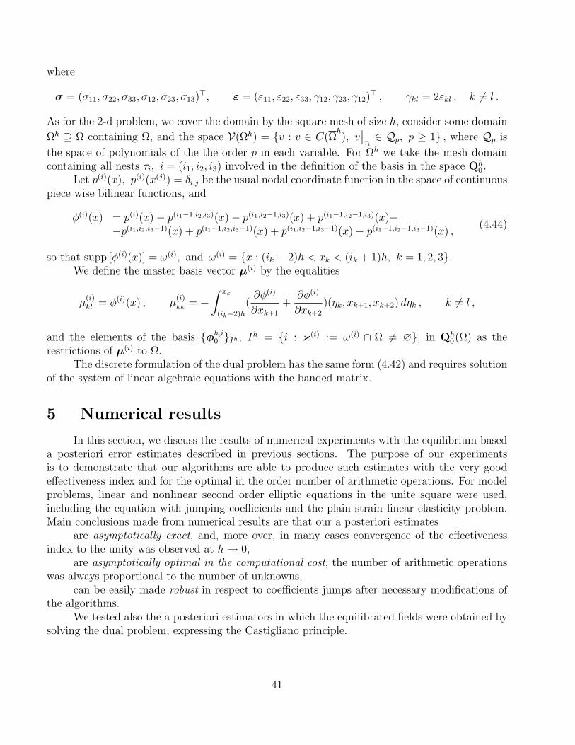
where

σ = (σ11, σ22, σ33, σ12, σ23, σ13)>, ε = (ε11, ε22, ε33, γ12, γ23, γ12)

> , γkl = 2εkl , k 6= l .

As for the 2-d problem, we cover the domain by the square mesh of size h, consider some domain

Ωh ⊇ Ω containing Ω, and the space V(Ωh) = v : v ∈ C(Ωh), v

∣∣τi∈ Qp, p ≥ 1 , where Qp is

the space of polynomials of the the order p in each variable. For Ωh we take the mesh domaincontaining all nests τi, i = (i1, i2, i3) involved in the definition of the basis in the space Qh

0 .Let p(i)(x), p(i)(x(j)) = δi,j be the usual nodal coordinate function in the space of continuous

piece wise bilinear functions, and

φ(i)(x) = p(i)(x)− p(i1−1,i2,i3)(x)− p(i1,i2−1,i3)(x) + p(i1−1,i2−1,i3)(x)−−p(i1,i2,i3−1)(x) + p(i1−1,i2,i3−1)(x) + p(i1,i2−1,i3−1)(x)− p(i1−1,i2−1,i3−1)(x) ,

(4.44)

so that supp [φ(i)(x)] = ω(i), and ω(i) = x : (ik − 2)h < xk < (ik + 1)h, k = 1, 2, 3.We define the master basis vector µ(i) by the equalities

µ(i)kl = φ(i)(x) , µ

(i)kk = −

∫ xk

(ik−2)h

(∂φ(i)

∂xk+1

+∂φ(i)

∂xk+2

)(ηk, xk+1, xk+2) dηk , k 6= l ,

and the elements of the basis φh,i0 Ih , Ih = i : κ(i) := ω(i) ∩ Ω 6= ∅, in Qh

0(Ω) as therestrictions of µ(i) to Ω.

The discrete formulation of the dual problem has the same form (4.42) and requires solutionof the system of linear algebraic equations with the banded matrix.

5 Numerical results

In this section, we discuss the results of numerical experiments with the equilibrium baseda posteriori error estimates described in previous sections. The purpose of our experimentsis to demonstrate that our algorithms are able to produce such estimates with the very goodeffectiveness index and for the optimal in the order number of arithmetic operations. For modelproblems, linear and nonlinear second order elliptic equations in the unite square were used,including the equation with jumping coefficients and the plain strain linear elasticity problem.Main conclusions made from numerical results are that our a posteriori estimates

are asymptotically exact, and, more over, in many cases convergence of the effectivenessindex to the unity was observed at h→ 0,

are asymptotically optimal in the computational cost, the number of arithmetic operationswas always proportional to the number of unknowns,

can be easily made robust in respect to coefficients jumps after necessary modifications ofthe algorithms.

We tested also the a posteriori estimators in which the equilibrated fields were obtained bysolving the dual problem, expressing the Castigliano principle.

41

5.1 The Poisson equation

5.1.1 Direct evaluation algorithms

Consider the model problem

−∆u =5π2

2cos

3π

2x1 cos

π

2x2 , (x1, x2) ∈ Ω = (0, 1)× (0, 1) ,

u|ΓD= 0 , u|ΓN

= 0 ,ΓD = (x1, x2)| x1 ∈ [0, 1] , x2 = 1 ∪ (x1, x2)| x1 = 1 , x2 ∈ [0, 1] ,ΓN = (x1, x2)| x1 ∈ [0, 1] , x2 = 0 ∪ (x1, x2)| x1 = 0 , x2 ∈ [0, 1] .

(5.1)

with the exact solution

u(x1, x2) = cos3π

2x1 cos

π

2x2 . (5.2)

The FE space of the piece wise bilinear functions for this problem V0(Ω) was defined inSection 2. For the FE solution ufem on the mesh of size h, we used Algorithm 2.1 in orderto calculate the vector-valued function t(x) = (t1(x), t2(x))

>, which satisfies the balance equa-tion (2.5) and the boundary conditions (2.6). Then we calculated the energy norm of the errore = ‖∇(u− ufem)‖ and the a posteriori estimator η = ‖∇ufem − t‖, i.e., the left and right sidescorrespondingly in (2.8).

Figure 1 shows the dependence of the energy norm of the FE error and of the a posterioriestimator on the number of unknowns N . It demonstrates the same asymptotic behavior ofthe both values. The number of unknowns in this experiment exceeded 4 · 106, but these linespractically coincide for N greater than 104. The a posteriori estimator η stays greater than theenergy norm of the error e (see Table 1). This validates that the equilibrium based a posterioriestimate guarantees the upper asymptotically exact estimate.

N e η Ieff16 8.40422 · 10−1 2.87729 · 10−1 3.4236264 4.08785 · 10−1 8.38575 · 10−1 2.05138256 2.02318 · 10−1 2.67228 · 10−1 1.320831024 1.00877 · 10−1 1.09368 · 10−1 1.084174096 5.04023 · 10−2 5.14654 · 10−2 1.0210916384 2.51966 · 10−2 2.53287 · 10−2 1.0052565536 1.25977 · 10−2 1.26141 · 10−2 1.00131262144 6.29880 · 10−3 6.30085 · 10−3 1.000331048576 3.14939 · 10−3 3.14965 · 10−3 1.000084194304 1.57469 · 10−3 1.57473 · 10−3 1.00002

Table 1.

Figure 2 shows the dependence of (Ieff − 1 on N), where

Ieff =η

e(5.3)

42

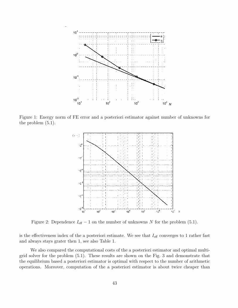
Figure 1: Energy norm of FE error and a posteriori estimator against number of unknowns forthe problem (5.1).

Figure 2: Dependence Ieff − 1 on the number of unknowns N for the problem (5.1).

is the effectiveness index of the a posteriori estimate. We see that Ieff converges to 1 rather fastand always stays grater then 1, see also Table 1.

We also compared the computational costs of the a posteriori estimator and optimal multi-grid solver for the problem (5.1). These results are shown on the Fig. 3 and demonstrate thatthe equilibrium based a posteriori estimator is optimal with respect to the number of arithmeticoperations. Moreover, computation of the a posteriori estimator is about twice cheaper than

43

solving the finite element system (this results were obtained on AMD Athlon 64 3200+ 2.01GHzwith 2 Gb of RAM).

Figure 3: Computational costs (in ms) of multigrid solver and η against the number of unknownsfor the problem (5.1).

5.1.2 Algorithms based on the Castigliano principle

In the unite square, we considered the Dirichlet problem having for the exact solution

u = sin(2πx1) sin(πx2) + (x1 + 1)(2x2 + 1) .

The corresponding right part is f = 5π2 sin(2πx1) sin(πx2) and nonhomogeneous Dirichlet bound-ary condition is u

∣∣∂Ω

= (x1 + 1)(2x2 + 1).The FE solution ufem was obtained by means of the space of the continuous piece wise bi-

linear functions. For obtaining the approximate solution zh of the discretized dual problem (4.4),we used the subspace Qh

0 with the local flux basis vectors φ(i), described in Subsection 4.1. Twochoices for the vector tf and respectively for the set Qh

f were implemented: one according tosecond line of (4.8) and another according to the formulas

tf (x) = (tf,1, tf,2)> , tf,k(x) =

1

2

xk∫0

f(ηk, x3−k) dηk .

For these two choices of fluxes, satisfying the balance equation, we introduce notations tf =

t(1)f , t

(2)f . These fluxes result in the two a posteriori estimators

ηc,j = ‖∇ufem − zh,j‖ , zh,j = zh,j0 + t

(j)f , j = 1, 2 ,

44

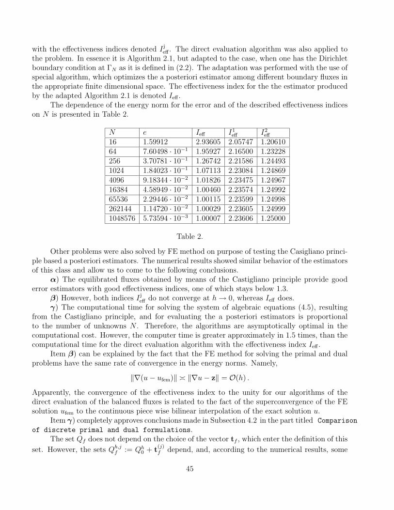
with the effectiveness indices denoted I jeff . The direct evaluation algorithm was also applied to

the problem. In essence it is Algorithm 2.1, but adapted to the case, when one has the Dirichletboundary condition at ΓN as it is defined in (2.2). The adaptation was performed with the use ofspecial algorithm, which optimizes the a posteriori estimator among different boundary fluxes inthe appropriate finite dimensional space. The effectiveness index for the the estimator producedby the adapted Algorithm 2.1 is denoted Ieff .

The dependence of the energy norm for the error and of the described effectiveness indiceson N is presented in Table 2.

N e Ieff I1eff I2

eff

16 1.59912 2.93605 2.05747 1.2061064 7.60498 · 10−1 1.95927 2.16500 1.23228256 3.70781 · 10−1 1.26742 2.21586 1.244931024 1.84023 · 10−1 1.07113 2.23084 1.248694096 9.18344 · 10−2 1.01826 2.23475 1.2496716384 4.58949 · 10−2 1.00460 2.23574 1.2499265536 2.29446 · 10−2 1.00115 2.23599 1.24998262144 1.14720 · 10−2 1.00029 2.23605 1.249991048576 5.73594 · 10−3 1.00007 2.23606 1.25000

Table 2.

Other problems were also solved by FE method on purpose of testing the Casigliano princi-ple based a posteriori estimators. The numerical results showed similar behavior of the estimatorsof this class and allow us to come to the following conclusions.

α) The equilibrated fluxes obtained by means of the Castigliano principle provide gooderror estimators with good effectiveness indices, one of which stays below 1.3.

β) However, both indices I jeff do not converge at h→ 0, whereas Ieff does.

γ) The computational time for solving the system of algebraic equations (4.5), resultingfrom the Castigliano principle, and for evaluating the a posteriori estimators is proportionalto the number of unknowns N . Therefore, the algorithms are asymptotically optimal in thecomputational cost. However, the computer time is greater approximately in 1.5 times, than thecomputational time for the direct evaluation algorithm with the effectiveness index Ieff .

Item β) can be explained by the fact that the FE method for solving the primal and dualproblems have the same rate of convergence in the energy norms. Namely,

‖∇(u− ufem)‖ ‖∇u− z‖ = O(h) .

Apparently, the convergence of the effectiveness index to the unity for our algorithms of thedirect evaluation of the balanced fluxes is related to the fact of the superconvergence of the FEsolution ufem to the continuous piece wise bilinear interpolation of the exact solution u.

Item γ) completely approves conclusions made in Subsection 4.2 in the part titled Comparison

of discrete primal and dual formulations.The set Qf does not depend on the choice of the vector tf , which enter the definition of this

set. However, the sets Qh,jf := Qh

0 + t(j)f depend, and, according to the numerical results, some

45

allow to approximate true fluxes better. Besides, the error estimator ηc,2 is more symmetric withrespect to the axes xk, than ηc,1. Probably, these factors caused the difference of the effectivenessindexes, reflected in α).

5.2 Second order elliptic equation with discontinuous coefficient

We tested also our a posteriori estimator as applied to the problem:

−∇ · (ρ(x)∇u) = f(x), x ∈ Ω = (0, 1)× (0, 1) , (5.4)

with the same boundary conditions as in (5.1) and the piece-wise constant coefficient, which hasa jump across the common boundary γ for the two parts of Ω:

Ω1 = x| x1 ∈ (0, 0.5), x2 ∈ (0, 1) , (5.5)

Ω2 = x| x1 ∈ (0.5, 1), x2 ∈ (0, 1) . (5.6)

For the function ρ, we used

ρ(x) =

ρ1 = 10−2, x ∈ Ω1 ,ρ2 = 102, x ∈ Ω2 .

(5.7)

The right-hand side f as well as the mixed boundary conditions corresponded to the exactsolution

u = (cos(2πx)− 1) cos

(3π

2y

) x2 + 1, x < 0.5

−(x− 1)2 ρ1

ρ2+ 0.25ρ1

ρ2+ 1.25, x > 0.5

(5.8)

For obtaining FE solution, we used the space V0(Ω) of the continuous piece-wise bilinear func-tions, satisfying the Dirichlet boundary condition on ΓD.

N e η Ieff64 9.14308 1.02954 · 101 1.12604256 4.44483 4.77467 1.074211024 2.20395 2.25318 1.022344096 1.09958 1.10628 1.0060916384 5.49486 · 10−1 5.50364 · 10−1 1.0016065536 2.74705 · 10−1 2.74818 · 10−1 1.00041262144 1.37348 · 10−1 1.37362 · 10−1 1.000101048576 6.86734 · 10−2 6.86751 · 10−2 1.00003

Table 3.

The vector t(x) = (t(x)1, t(x)2)>, satisfying the balance equation (2.5) and the Neumann

boundary conditions (5.1) on ΓN , was calculated according to Algorithm 2.4 in Subsection 2.3.In turn, this vector allowed to evaluate the a posteriori estimator ηρ = ‖ρ∇ufem − t‖ρ−1 , whichenters the estimate (2.33). Figure 4 shows the dependence of the energy norm, of the error

46

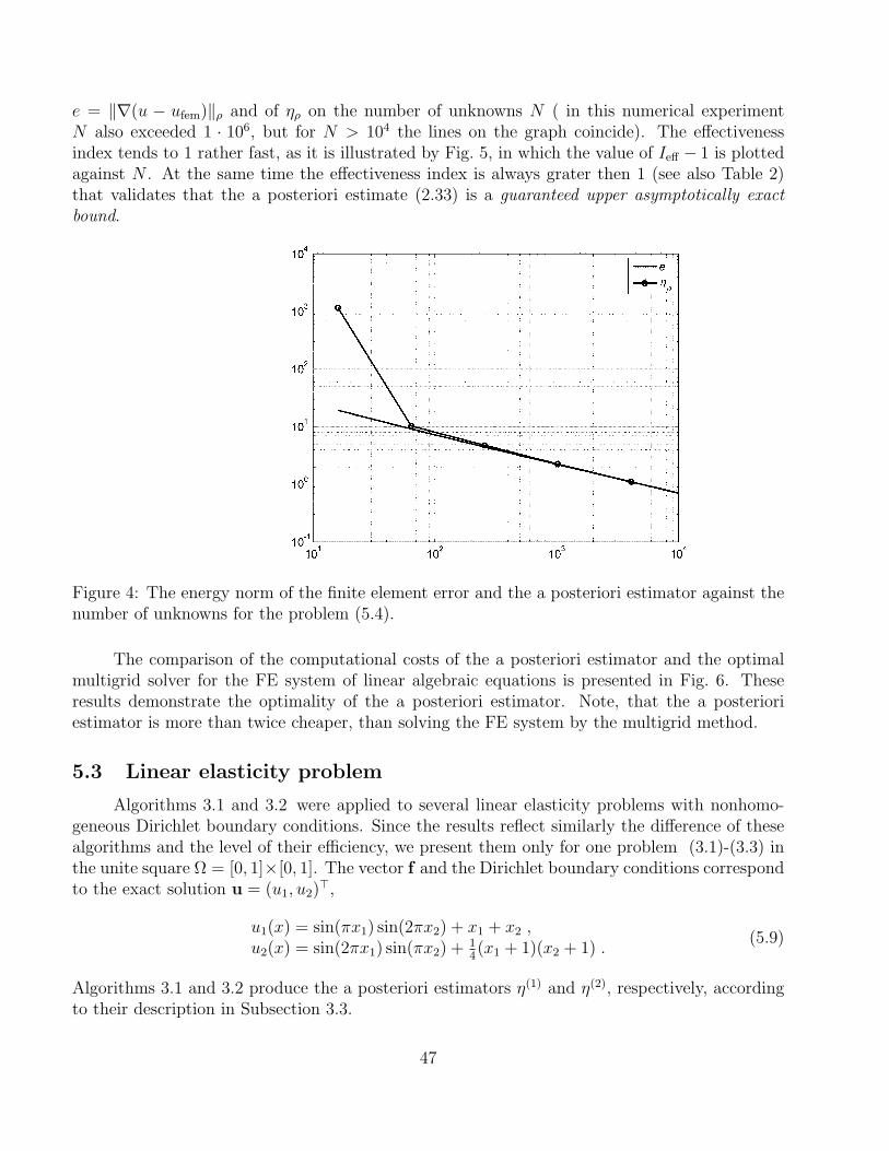
e = ‖∇(u − ufem)‖ρ and of ηρ on the number of unknowns N ( in this numerical experimentN also exceeded 1 · 106, but for N > 104 the lines on the graph coincide). The effectivenessindex tends to 1 rather fast, as it is illustrated by Fig. 5, in which the value of Ieff − 1 is plottedagainst N . At the same time the effectiveness index is always grater then 1 (see also Table 2)that validates that the a posteriori estimate (2.33) is a guaranteed upper asymptotically exactbound.

Figure 4: The energy norm of the finite element error and the a posteriori estimator against thenumber of unknowns for the problem (5.4).

The comparison of the computational costs of the a posteriori estimator and the optimalmultigrid solver for the FE system of linear algebraic equations is presented in Fig. 6. Theseresults demonstrate the optimality of the a posteriori estimator. Note, that the a posterioriestimator is more than twice cheaper, than solving the FE system by the multigrid method.

5.3 Linear elasticity problem

Algorithms 3.1 and 3.2 were applied to several linear elasticity problems with nonhomo-geneous Dirichlet boundary conditions. Since the results reflect similarly the difference of thesealgorithms and the level of their efficiency, we present them only for one problem (3.1)-(3.3) inthe unite square Ω = [0, 1]×[0, 1]. The vector f and the Dirichlet boundary conditions correspondto the exact solution u = (u1, u2)

>,

u1(x) = sin(πx1) sin(2πx2) + x1 + x2 ,u2(x) = sin(2πx1) sin(πx2) + 1

4(x1 + 1)(x2 + 1) .

(5.9)

Algorithms 3.1 and 3.2 produce the a posteriori estimators η(1) and η(2), respectively, accordingto their description in Subsection 3.3.

47

Figure 5: Dependence of Ieff − 1 on the number of unknowns N for the problem (5.4).

Figure 6: The computational costs of the a posteriori estimator and the multigrid solver againstthe number of unknowns for the problem (5.4).

Figures 7 and 8 demonstrate the behavior of η(1). The results obtained for η(2) are presentedin Figures 9-11, see also Table 3 for numbers. The numerical results show, that the a posterioriestimator η(2) outperforms η(1). The effectiveness index I

(2)eff of η(2) tends to 1 staying grater then

1, whereas the effectiveness index I(1)eff of η(1) does not converge and stays slightly greater than

2. Both a posteriori estimators are optimal in the computational cost. Figures 8 and 11 present

48

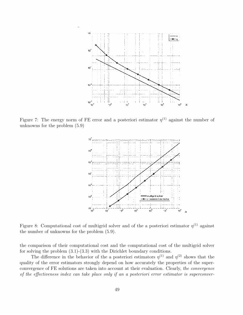
Figure 7: The energy norm of FE error and a posteriori estimator η(1) against the number ofunknowns for the problem (5.9)

Figure 8: Computational cost of multigrid solver and of the a posteriori estimator η(1) againstthe number of unknowns for the problem (5.9).

the comparison of their computational cost and the computational cost of the multigrid solverfor solving the problem (3.1)-(3.3) with the Dirichlet boundary conditions.

The difference in the behavior of the a posteriori estimators η(1) and η(2) shows that thequality of the error estimators strongly depend on how accurately the properties of the super-convergence of FE solutions are taken into account at their evaluation. Clearly, the convergenceof the effectiveness index can take place only if an a posteriori error estimator is superconver-

49

Figure 9: Energy norm of FE error and the a posteriori estimator η(2) against the number ofunknowns for the problem (5.9).

Figure 10: Dependence of Ieff − 1 for the aposteriori estimator η(2) on the number of unknownsN for the problem (5.9).

gent. Algorithm 3.1 is simpler, but it is not invariant in respect to axes xk and the accuracy ofapproximation of the boundary values for stresses provides only an approximation of the orderof h.

50

Figure 11: Computational costs of the multigrid solver and the a posteriori estimator η(2) againstthe number of unknowns for the problem (5.9).

N e η(1) I(1)eff η(2) I

(2)eff

16 3.29126 · 10−1 2.11430 6.42399 2.45022 7.4446264 1.63481 · 10−1 5.54014 · 10−1 3.38885 3.54162 · 10−1 2.16638256 8.17444 · 10−2 1.94481 · 10−1 2.37914 1.46349 · 10−1 1.790331024 4.08766 · 10−2 8.62833 · 10−2 2.11083 5.45946 · 10−2 1.335604096 2.04389 · 10−2 4.18226 · 10−2 2.04622 2.56000 · 10−2 1.1038716384 1.02196 · 10−2 2.07433 · 10−2 2.02976 1.05054 · 10−2 1.0279765536 5.10979 · 10−3 1.03501 · 10−2 2.02554 5.14644 · 10−3 1.00717262144 2.55490 · 10−3 5.17229 · 10−3 2.02446 2.55953 · 10−3 1, 001811048576 1.27745 · 10−3 2.58580 · 10−3 2.02419 1.27804 · 10−3 1.00046

Table 4.

References

[1] Ainsworth M, Demkowicz L and Kim C-W. Analysis of the equilibrated residual method fora posterioti estimation on meshes with hanging nodes. Submitted for publication.

[2] Ainsworth M and Oden JT. A posteriori estimation in finite element analysis. John Wiley& Sons, Inc., New York, 2000: xx+240p.

[3] Aubin J-P. Approximation of elliptic boundary-value problems. Wiley Interscience, a divisionof John Wiley & Sons, Inc., New York-London-Sydney-Toronto, 1972.

[4] Arthurs AM. Complementary variational principles. Calderon Press, Oxford, 1980.

51

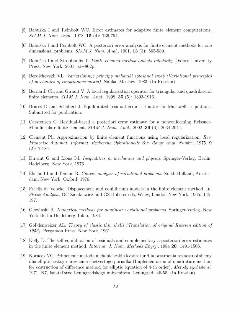
[5] Babuska I and Reinbolt WC. Error estimates for adaptive finite element computations.SIAM J. Num. Anal., 1978, 15 (4): 736-754.

[6] Babuska I and Reinbolt WC. A posteriori error analysis for finite element methods for onedimensional problems. SIAM J. Num. Anal., 1981, 13 (3): 565-589.

[7] Babuska I and Strouboulis T. Finite element method and its reliability. Oxford UniversityPress, New York, 2001: xi+802p.

[8] Berdichevskii VL. Variatsionnye principy mahaniki sploshnoi sredy (Variational principlesof mechanics of conytinuous media). Nauka, Moskow, 1983. (In Russian)

[9] Bernardi Ch. and Girault V. A local regularization operator for triangular and quadrilateralfinite elements. SIAM J. Num. Anal., 1998, 35 (5): 1893-1916.

[10] Braess D and Schoberl J. Equilibrated residual error estimator for Maxswell’s equations.Submitted for publication.

[11] Carstensen C. Residual-based a posteriori error estimate for a nonconforming Reissner-Mindlin plate finite element. SIAM J. Num. Anal., 2002, 39 (6): 2034-2044.

[12] Clement Ph. Approximation by finite element functions using local regularization. Rev.Francaise Automat. Informat. Recherche Operationelle Ser. Rouge Anal. Numer., 1975, 9(2): 72-84.

[13] Duvaut G and Lions I-I. Inequalities in mechanics and physics. Springer-Verlag, Berlin,Hedelberg, New York, 1976.

[14] Ekeland I and Temam R. Convex analysis of variational problems. North-Holland, Amster-dam, New York, Oxford, 1976.

[15] Fraeijs de Vebeke. Displacement and equilibrium models in the finite element method. In:Stress Analysis, OC Zienkiewicz and GS Holister eds, Wiley, London-New York, 1965: 145-197.

[16] Glowinski R. Numerical methods for nonlinear variational problems. Springer-Verlag, NewYork-Berlin-Heidelberg-Tokio, 1984.

[17] Gol’denweizer AL. Theory of elastic thin shells (Translation of original Russian edition of1953). Pergamon Press, New York, 1961.

[18] Kelly D. The self equilibration of residuals and complementary a posteriori error estimatesin the finite element method. Internat. J. Num. Methods Engrg., 1984 20: 1491-1506.

[19] Korneev VG. Primenenie metoda mehanicheskih kvadratur dlia postroenia raznostnoi shemydlia ellipticheskogo uravnenia chetvertogo poriadka (Implementation of quadrature methodfor costruction of difference method for elliptic equation of 4-th order). Metody vychislenii,1971, N7, Isdatel’stvo Leningradskogo universiteta, Leningrad: 46-55. (In Russian)

52

[20] Korneev VG. O sviazi raznostnyh shem dlia ellipticheskih uravnenii vtorogo poriadka so she-mami kvadratur dlia integral’nyh uravnenii metoda raschlenenia (On interrelation betweendifference schemes for elliptic equations of second order and quadrature method for integralequations of splitting method).Vestnik Leningradskogo universiteta. 1973, (1): 18-27. (InRussian)

[21] Korneev VG. Raznostnaya shema poriadka tochnosti h3/2 v norme ‖ · ‖h,W 12

dlia elliptich-eskogo uravnenia vtorogo poriadka v proizvol’noi oblasti (Difference scheme of accuracyh3/2 in the norm ‖ · ‖h,W 1

2for elliptic equation of second order in arbitrary domain). Vestnik

Leningradskogo universiteta. 1973, (7): 25-33. (In Russian)

[22] Korneev VG. Svedenie zadachi rascheta arochnoi plotiny k zadache na minimum rabotyuprugih sil nepreryvnoi sterzhnevoi sistemy (Reduction of the arch dam analysis problemto minimization of work of elastic forces for continuous rod system ). Trudy Gidroproekta,pod redaktsiei D.M. Yurinova. 1973, N 22, Moskva: 4-12. (In Russian)

[23] Korneev VG. Diskretizatsia raboty uprugih sil nepreryvnoi sterzhnevoi sistemy (Discretiza-tion of functional of elastic forces work for continuous rod system). Trudy Gidroproekta, podredaktsiei D.M. Yurinova. 1973, N 22, Moskva: 12-32. (In Russian)

[24] Korneev VG. O ratsional’nom vybore koordinatnyh funktsii pri minimizatsii diskretnogofunktsionala raboty uprugih sil (On rational choice of the coordinate functions at mini-mization of the discrete functional of the work of elastic forces). Trudy Gidroproekta, podredaktsiei D.M. Yurinova. 1973, N 22, Moskva: 86-102. (In Russian)

[25] Korneev VG. Issledovanie shodimosti priblizhennyh reshenii (Analysis of convergence ofapproximate solutions). Trudy Gidroproekta, pod redaktsiei D.M. Yurinova, 1973, N 22,Moskva: 141-182. (In Russian)

[26] Korneev VG. Shemy metoda konechnyh elementov poriadkov tochnosti (The finite elelmentmethods of high oreders of accuracy). Izdatel’stvo Leningradskogo universiteta, Leningrad,1977. (In Russian)

[27] Korneev VG. On numerical solution of the shell theory problems in stresses on skew-angularmeshes. Comput. Maths and Math. Physics, 1981, 21 (2): 441-450.

[28] Korneev VG. Superconvergence of the finite element solutions in the mesh norms. Comput.Maths and Math. Physics, 1982, 22 (5): 1133-1148.

[29] Korneev VG and Rozin LA. Algorithmy rascheta obolochek po sterzhnevoi sheme i ihmatematicheskoe issledovanie (Algorithms for numerical solution of shell problems and theirmathematical analysis). In: Materialy 6-oi vsesoyuznoi konferetsii po teorii obolochek i plas-tin (Proc. of 6-th all-union conference on shell and plate theory) , Baku, 1966, Nauka:555-560. (In Russian)

[30] Korneev VG and Rozin LA. Chislennaia relizatsia metoda raschlenenia na primere zadachiizgiba plastinki (Numerical realization of the splitting method for the plate bending prob-lem). Izvestia akademii nauk SSSR, Mehanika tverdogo tela. 1967 (2). (In Russian)

53

[31] Ladevese P and Leguillon D. Error estimate procedure in the finite element method andapplications. SIAM J. Num. Anal., 1983, 20: 485-509.

[32] Luce R and Wohlmuth B. A local a posteriori error estimator based on equilibrated fluxes.SIAM J. Num. Anal., 2004, 42: 1394-1414.

[33] Mikhlin SG. Variational methods in mathematical physics. Pergamon, Oxford, 1964.

[34] Mosolov PP and Myasnikov VP. Mechanics of rigid plastic bodies. Nauka, Moskow, 1981.(In Russian)

[35] Neittaanmaki P and Repin SI. Reliable methods for computer simulation Error control anda posteriori estimates. Elsevier, New York, 2004, 305p.

[36] Novozhilov VV. Teoria tonkih obolochek (Theory of thin shells). Gosudarstvennoe soyuznoeizdatel’stvo sudostroitel’noi promyshlennosti, Leningrad, 1962, 431p. (In Russian)

[37] Novozhilov VV. Theory of thin shells. Noordoff, Dordrecht, 1959.

[38] Oganesian LA and Ruhovets LA. Variatsionno-raznostnye metody reshenia ellipticheskihuravnenii (Variational-difference methods for solution of elliptic equations). Izdatel’stvoArmianskoi akademii nauk, Erevan, 1979, 234p.

[39] Oden JT, Demkowicz L, Rachowicz W and Westermann TA. Towards a universal h-p adap-tive finite element strategy. Part 2, A posteriori error estimation. Comput. Methods Appl.Mech. Engrg., 1989, 77: 113-180.

[40] Oden T, Duarte C. and Zienkiewcz O. A new cloud based finite element method. Comput.Methods Appl. Mech. Engrg., 1998, 153: 117-126.

[41] Repin S and Frolov M. Ob a posteriornyh otsenkah tochnosti priblizhennyh reshenii kraevyxzadach dlia ellipticheskih uravnenii. (On a posteriori estimates of approximate solutions ofboundary value problems for elliptic equations). Zhurnal vychislit. matem. i matem. phiziki,2002, 42 (12): 1774-1787.

[42] Repin S, Neittaanmakki P and Frolov M. On computational properties of a posteriori es-imates based upom the method of duality error majorants. In: Numerical Mathematicsand Advanced Applications (ENUMATH-2003). Berlin-Heidelberg, Springer-Verlag, 2004:346-357.

[43] Repin SI and Xanthis LS. A posteriori error estimation for elasto-plasric problems based onduality theory. Comput. Meth. Appl. Mech. Engrg., 1996, 138: 317-339.

[44] Reissner E. On the derivation of the theory of thin elastic shells. J. Math. Phis, 1963, 42(4).

[45] Rozin LA. Metod raschlenenia v teorii obolochek (The splitting method in the shell theory).Prikladnaia matematika i mehanika, 1961, 25 (5). (in Russian)

54

[46] Rozin LA. Nekotorye voprosy raschlenenia i diskretizatsii uravnenii teorii obolochek (Somequestions of splitting and discretization of equations of the shell theory). Issledovaniapo teorii uprugosti i plastichnosti. 1965 (4), Izdatel’stvo Leningradskogo universiteta,Leningrad.

[47] Strouboulis T, Babuska I and Copps K. The design and analysis of the generalized finiteelement method. Comput. Methods Appl. Mech. Engrg., 2000, 181: 43-69.

[48] Stewart JR Hudges TJR. A tutorial in elementary finite element error analysis. A systematicpresentation of a priori and a posteriori error estimates. Comput. Meth. Appll. Mech. Eng.,1998, 158 (1-2): 1-22.

[49] Temam R. Problemes Mathematique en Plasticite. Bordas, Paris, 1983.

[50] Vejchodsky T. Local a posteriori error estimator based on the hypercircle method. In: Proc.of the European Congress on Computational Method in Applied Mechanics and Engrg. (EC-COMUAS 2004). Yavaskyla, Finland.

[51] Verfurth RA. A posteriori error estimates for nonlinear problems. Finite element discretiza-tions of elliptic equations. Math. of Comput., 1994, 62 (206): 445-465.

[52] Verfurth RA. A review of a posteriori error estimation and adaptive mesh refinement tech-niques. John Wiley & Sons, BG Teubner, 1996: vi+127.

[53] Walbin LB. Superconvergence in Galerkin finite elelemnt methods. Lecture notes in Mathe-matics. 1995, Springer, Berlin.

[54] Washizu K. Variational principles in elasticity and plasticity, 3-rd edition. Pergamon Press,New York, 1982

[55] Zienkiewicz OC and Zhu JZ. The superconvergence path recovery (SPR) and adaptive finiteelement refinement. Comput. Meth. Appll. Mech. Eng., 1992 29 (1): 78-88.

55

A posteriori error estimation by means of the exactly equilibrated fields

Documents

Transcript of A posteriori error estimation by means of the exactly equilibrated fields