25th International Scientific ConferenceOctober 6–8

TRANSPORT MEANS2021

ProceedingsPart II

ISSN 1822-296 X (print) ISSN 2351-7034 (online)

KAUNAS UNIVERSITY OF TECHNOLOGY

KLAIP DA UNIVERSITY IFToMM NATIONAL COMMITTEE OF LITHUANIA

LITHUANIAN SOCIETY OF AUTOMOTIVE ENGINEERS THE DIVISION OF TECHNICAL SCIENCES OF LITHUANIAN ACADEMY OF SCIENCES

VILNIUS GEDIMINAS TECHNICAL UNIVERSITY

TRANSPORT MEANS 2021 Sustainability: Research and Solutions

PROCEEDINGS OF THE 25th INTERNATIONAL SCIENTIFIC CONFERENCE

PART II

October 06-08 , 2021 Online Conference - Kaunas, Lithuania

CONFERENCE IS ORGANIZED BY Kaunas University of Technology, In cooperation with Klaipeda University, IFToMM National Committee of Lithuania, Lithuanian Society of Automotive Engineers, The Division of Technical Sciences of Lithuanian Academy of Sciences, Vilnius Gediminas Technical University

The proceedings of the 25th International Scientific Conference Transport Means 2021 contain selected papers of 9 topics: Aviation, Automotive, Defence Technologies, Fuels and Combustion, Intelligent Transport Systems, Railway, Traffic, Transport Infrastructure and Logistics, Waterborne Transport.

All published papers are peer reviewed.

The style and language of authors were not corrected. Only minor editorial corrections may have been carried out by the publisher.

All rights preserved. No part of these publications may be reproduced, stored in a retrieval system, or transmitted in any form or by any means, electronic, mechanical, photocopying, recording or otherwise, without the permission of the publisher.

Kaunas University of Technology, 2021

SCIENTIFIC EDITORIAL COMMITTEE

Chairman – Prof. V. Ostaševi ius, Member of Lithuanian and Swedish Royal Engineering Academies of Sciences, Chairman of IFToMM National Committee of Lithuania

MEMBERS

Prof. H. Adeli, The Ohio State University (USA) Dr. A. Alop, Estonian Maritime Academy of Tallinn University of Technology (Estonia) Dr. S. Ba kaitis, US Transportation Department (USA) Prof. Ž. Bazaras, Department of Transport Engineering, KTU (Lithuania) Prof. M. Bogdevi ius, Faculty of Transport Engineering, VGTU (Lithuania) Dr. D. Bazaras, Faculty of Transport Engineering, VGTU (Lithuania) Prof. R. Burdzik, Silesian University of Technology (Poland) Prof. P.M.S.T. de Castro, Porto University (Portugal) Prof. R. Cipollone, L’Aquila University (Italy) Prof. Z. Dvorak, University of Žilina (Slovakia) Prof. A. Fedaravi ius, Department of Transport Engineering, KTU (Lithuania) Prof. J. Furch, University of Defence (Czech Republic) Dr. S. Himmeto lu, Hacettepe University (Turkey) Dr. hab. I. Jacyna-Go da, Warsaw University of Technology (Poland) Dr. J. Jankowski, Polish Ships Register (Poland) Prof. I. Kabashkin, Transport and Telecommunications Institute (Latvia) Prof. A. Keršys, Department of Transport Engineering, KTU (Lithuania) Prof. Y. Krykavskyy, Lviv Polytechnic National University (Ukraine) Dr. B. Leitner, University of Žilina (Slovakia) Dr. J. Ludvigsen, Transport Economy Institute (Norway) Prof. V. Lukoševi ius, Department of Transport Engineering, KTU (Lithuania) Prof. J. Majer ák, University of Žilina (Slovakia) Dr. R. Makaras, Department of Transport Engineering, KTU (Lithuania) Dr. R. Markšaityt , Vytautas Magnus University (Lithuania) Prof. A. Mohany, Ontario Tech University (Canada) Prof. V. Paulauskas, Department of Marine Engineering, KU (Lithuania) Prof. O. Prentkovskis, Faculty of Transport Engineering, VGTU (Lithuania) Prof. V. Priednieks, Latvian Maritime Academy (Latvia) Dr. L. Raslavi ius, Department of Transport Engineering, KTU (Lithuania) Dr. J. Ryczy ski, Tadeusz Kosciuszko Military Academy of Land Forces (Poland) Dr. D. Rohacs, Budapest University of Technology and Economics (Hungary) Prof. M. Sitarz, WSB University, (Poland) Prof. D. Szpica, Bialystok University of Technology (Poland) Dr. C. Steenberg, FORCE Technology (Denmark) Dr. A. Šakalys, Faculty of Transport Engineering, VGTU (Lithuania) Dr. Ch. Tatkeu, French National Institute for Transport and Safety Research (France) Prof. M. Wasiak, Warsaw University of Technology (Poland) Prof. Z. Vintr, University of Defence (Czech Republic)

ORGANIZING COMMITTEE

Chairman – Prof. Ž. Bazaras, Department of Transport Engineering, KTU (Lithuania) Vice-Chairman – Prof. V. Paulauskas, Department of Marine engineering, KU (Lithuania) Vice-Chairman – Prof. A. Fedaravi ius, Department of Transport Engineering, KTU (Lithuania) Secretary – Dr. R. Keršys, Department of Transport Engineering, KTU (Lithuania)

MEMBERS

Dr. R. Junevi ius, Vice-Dean for Reserach of the Faculty of Transport Engineering, VGTU Dr. A. Vilkauskas, Dean of the Faculty of Mechanical Engineering and Design, KTU Dr. R. Makaras, Head of Department of Transport Engineering, KTU Dr. B. Pla ien , Department of Marine engineering, KU Dr. A. Keršys, Department of Transport Engineering, KTU Dr. S. Japertas, Department of Transport Engineering, KTU Dr. S. Kilikevi ius, Department of Transport Engineering, KTU Dr. V. Lukoševi ius, Department of Transport Engineering, KTU R. Džiaugien , Department of Transport Engineering, KTU M. Lendraitis, Department of Transport Engineering, KTU R. Litvaitis, Department of Transport Engineering, KTU S. Kvietkait , Department of Transport Engineering, KTU Dr. R. Skvireckas, Department of Transport Engineering, KTU Dr. D. Juodvalkis, Department of Transport Engineering, KTU Dr. A. Pakalnis, Department of Transport Engineering, KTU Dr. V. Dzerkelis, Department of Transport Engineering, KTU

Conference Organizing Committee address: Kaunas University of Technology, Student 56 LT – 51424, Kaunas, Lithuania https://transportmeans.ktu.edu

PREFACE

25th international scientific conference TRANSPORT MEANS 2021 due to the COVID-19 pandemic in the

world, for the second time was organized as a virtual event on 06-08 October, 2021. It continues long tradition and reflects the most relevant scientific and practical problems of transport engineering.

The conference aims to provide a platform for discussion, interactions and exchange between researchers,

scientists and engineers. The reports cover a vide variety of topics related to the most pressing issues of today’s transport systems

development. The main areas covered in plenary session and in the sections are: design development, maintenance and

exploitation of transport means, implementation of advanced transport technologies, development of defense transport, environmental and social impact, advanced and intelligent transport systems, transport demand management, traffic control, specifics of transport infrastructure, safety and pollution problems, integrated and sustainable transport, modeling and simulation of transport systems and elements.

In the invitations to the conference, sent five months before the conference starts, the instructions how to prepare reports and how to model the manuscripts are provided as well as the deadlines for the reports are indicated.

Those who wish to participate in the conference should send the texts of the reports that meet relevant requirements under indicated deadlines. Each report must include: a short description of the idea or technique being presented, a brief introduction orienting to the importance an uniqueness of the submission, a thorough description of research course and comments on the results.

The submissions are matched to the expertise according to the interests and are forwarded to the selected reviewers.

Scientific Editorial Committee revises, groups the properly prepared reports according to the theme and design the conference programme.

The Proceedings are compendium of selected reports presented at the Conference.

Member of Lithuanian and Swedish Royal Engineering Academies of Sciences

Prof. V. Ostaševi ius

549

Proceedings of 25th International Scientific Conference. Transport Means 2021. Before and after COVID-19 car brands: Longitudinal Study of Car Brands Value Sources in Slovak Republic J. Majerova1, M. Nadanyiova2, L. Gajanova3 1University of Zilina, Faculty of Operation and Economics of Transport and Communications, Department of Economics, Univerzitna 1, 010 26, Zilina, Slovak Republic, E-mail: jana.majerova@fpedas.uniza.sk 2University of Zilina, Faculty of Operation and Economics of Transport and Communications, Department of Economics, Univerzitna 1, 010 26, Zilina, Slovak Republic, E-mail: margareta.nadanyiova@fpedas.uniza.sk 3University of Zilina, Faculty of Operation and Economics of Transport and Communications, Department of Economics, Univerzitna 1, 010 26, Zilina, Slovak Republic, E-mail: lubica.gajanova@fpedas.uniza.sk Abstract Pandemic crisis COVID-19 has significantly changed consumer behaviour. Implications of this phenomenon are present in a wide managerial context. First, consumers are more willing to save. Thus, the perspectives of the automotive market are not very optimistic in the near future. More than ever before, car brands managers should be aware of behavioural specifics of their consumers. It is because not only valuable brand existence is enough. Managers should exactly know brand value sources and based on this knowledge adapt so far applied concepts of brand value building and management. So, the aim of this paper is to identify the shift in car brand value sources in three main time periods – before pandemic crisis, during pandemic crisis, after pandemic crisis. When applying this concept, years 2019-2021 are analysed. However, in socio-economic aspect it can not be stated clearly that year 2021 could be considered as etalon of post-pandemic period due to the fact that the pandemic is still present worldwide. On the other hand, the consumers are fully accommodated on new reality and they have passed the shock connected with lock-down practice in many countries. Primary data used in the presented study were obtained by our own survey carried out on the sample of 2000 respondents (citizens of the Slovak Republic older than 18 years) in years 2019-2021. The given data were statistically evaluated by the factor analysis supported by implementation of KMO Test, Barlett's test of sphericity and calculation of Cronbach's Alpha for relevant car brands value sources. The rankings of top ten car brands according to Slovak perceptions have been detected as well as the brand value sources in analysed years. Based on these findings, the platform for erudite managerial decision-making has been created to facilitate the economic survival of (post)pandemic era which is supposed to be challenging for car brands due to the already clearly stated willingness to savings. KEY WORDS: brand, brand value, car brand, automotive market, pandemic COVID-19 1. Introduction

Generally, the need to revise traditional branding patterns in (post)pandemic times has been stated [1]. However, due to the relatively short time in which the society is facing to the COVID-19, the reformulation of postulates relevant to specific categories of brands and branding activities, has not been provided so far. One of the reason of this fact is the absence of relevant data, which would be adequate platform for such an activity. In scope of contemporary research trends in social sciences, longitudinal study seems to be optimal research method [2]. Only via critical comparison of pre-data and post-data, the shift in market reality could be identified. Despite the fact that our own longitudinal study focused on the research of brand loyalty sources in various brand categories was not intended to analyze pandemic impact on branding originally, current situation creates new dimension for the usage of obtained data [3, 4]. The reason is that more than ever before, brand managers should be aware of behavioral specifics of their consumers. This is applicable especially in those brand categories where the discrepancy between price and subjectively perceived value has been harmed by the pandemic crisis. The reason is that not only valuable brand existence is accurate. Managers should exactly know brand value sources and based on this knowledge adapt so far applied concepts of brand value building and management. Mainly in those sectors, where the needs saturation is not of vital nature and the willingness to savings is evident. 2. Literature Review

Car brands do not form a specific category of brand research, which would be reasoned by the specifics of the brand and the market where this brand operates. However, recently there is more and more interest paid to the issue of environmental aspects of brand value and management in the scope of brand value sources identification. Thus, the prospective of car brand research is flourishing due to the significant carbon footprint of this product category [5-7]. Another significant trend in contemporary branding research indicates the possibilities of brand value establishment in times of crisis [8, 9]. The majority of studies, which are focused on the pandemic COVID-19 impact on contemporary brand value building and management patterns state the simple existence of the significant pandemic impact on

550 branding in the scope of its specific aspects. These aspects are mainly connected with distribution and promotion. Shehzadi et al. (2021) discusses the digitalization of traditionally personally provided services on the evidence of university brands [10]. Similarly, Badenhop and Frasquet (2021) highlights the pandemic implications of online grocery shopping at multichannel supermarkets [11]. In scope of marketing communication, two main directions of research can be observed. First, content marketing is discussed. Jimenez-Barreto et al. (2021) point out the importance of exact argumentation in favor of hygienic securement of hotels. Second, the digitalization of marketing communication is stated [12]. Arango-Pastrana et al. (2021) discuss the importance of so called e-WOM strategy in scope of brand communication policy [13].

The brand equity in transport and automotive industry has been always analyzed only marginally [14]. Moreover, the aim of the research was not the identification of individual relevant brand value sources, but the identification of the impact of selected marketing activities on the predefined brand value sources. Murtiasih et al. (2012) were the first who evaluated the influence of WOM towards brand equity on automotive customer in Indonesia. They found out that the WOM influenced brand awareness, association, loyalty, and perceived quality significantly in the positive direction. Subsequently brand awareness, association, loyalty, and perceived quality influenced brand equity significantly and positively [15]. Similarly, Lobschat et al. (2013) indicated a valid description of social currency and found a positive effect of social currency on the brand equity measures: perceived quality, brand loyalty, and brand trust [16]. Recently, Adetunji et al. (2018) revealed that, the selected automotive brands have notable presence on Facebook, YouTube, Instagram and Twitter. Furthermore, it was found that, social media advertising, social media promotions and social media word-of-mouth have positive relationships with the CBBE of automotive brands [17]. Another analyzed attribute with impact on brand equity and its sources was service quality. Hanaysha (2016) found out that service quality has a significant positive effect on brand equity. Furthermore, services quality had a significant positive effect on all dimensions of brand equity: brand awareness, brand loyalty, brand image and brand leadership [18].

Currently, the issue of brand value and brand equity experiences its renaissance as it has been detected that the impact of pandemic COVID-19 on consumer preferences and market reality has been significant. However, the competitive potential of valuable brand and its systematic building and management has been realized mainly in those sectors, which have been significantly harmed by pandemic crisis. Sarker et al. (2021) have focused on airline service where they have found out that direct experience and brand consistency are highly important aspects for strengthening brand equity components of services. Subsequently, maximizing perceived value, followed by creating favorable brand meaning are the nucleus of branding services [19]. Bose et al. (2021) have focused on brand equity in tourism. Results of theirs exploratory factor analysis have showed a four-dimensional structure of customer-based place brand equity consisting of brand salience, brand meaning, perceived quality, and brand attachment [20]. Han et al. (2021) have analyzed the gastronomic sector focusing on the operation of global brands. Their findings have indicated that both cognitive process and the social process of brand equity have an effect on cultural values. In particular, social process elements such as brand prestige and brand identification can reduce the risk of consumer uncertainty [21]. 3. Methods and Data

In accordance with the literature review provided above, the main aim of the article is to identify the shift in car brand value sources in three main time periods – before pandemic crisis, during pandemic crisis and after pandemic crisis. To achieve this aim, own research was realized where the relevant primary data were collected. The research was provided sequentially in first quarter of: 1) year 2019 (before COVID-19); 2) year 2020 (during COVID-19) and 3) year 2021 (after COVID-19). In this research, 2000 respondents older than 18 years were asked about their subjectively perceived car brands value sources in each one of the time series of provided surveys. The questionnaire has been composed by: (1) descriptive socio-demographic part and (2) identification car brand value sources part. The research of car brands value sources subjectively perceived by Slovak consumers, has been provided on the basis of four basic brand value sources: 1) imageries, 2) attitudes, 3) attributes and 4) benefits. Respondents have stated the intensity of their agreement (on the 5 points Likert scale where 1 is strong influence and 5 is weak influence) with importance of brand value source and its component in their car brand value perception. Identified car brands value sources and their components are summarized in the Table 1.

The data obtained via own research about the subjectively perceived car brand value sources before COVID-19 pandemic crisis, during COVID-19 pandemic crisis and after COVID-19 pandemic crisis have been statistically evaluated via factor analysis. This statistical method, explains the variance of measured variables [22]. The initial conditions of factor analysis include high correlations of a large number of variables and low partial correlations [23]. Whether the correlation and partial correlation matrices satisfy the assumptions is therefore tested by various coefficients and indices, usually Kaiser-Meyer-Olkin measure (KMO) and Bartlett's test of sphericity. Based on these statistic tests, it has been created relevant basis for the reordering of car brand value sources and their components before COVID-19 pandemic crisis, during COVID-19 pandemic crisis and after COVID-19 pandemic. Therefore, managerial implications for optimal branding in turbulent post-pandemic times can be formulated and patterns, which have been created so far can be modified to take the reorganization of personal values ranking of consumers into account.

551 Table 1

Brand value sources and components (own processing)

Brand value sources Components of brand value sources imageries prestige modernity certainty pleasure expectations attitudes I aim to buy branded products I am interested in branded products on a regular basis branded products attract my attention because I consider them better branded products attract my attention because I consider them more prestigious attributes image quality popularity modernity creativity of ad benefits it makes me happier it increases my social status it makes it easier for me to get friends it attracts the attention of others it suits my lifestyle

4. Results and Discussion

Simple comparison of car brands ranking in years 2019-2021 in Slovak Republic indicates the shift in

subjectively perceived brand value sources. While in years 2019 vs. 2020 the order remained almost equal, in 2021 the situation radically changed. In first two compared years, only first and second place have been replaced (Volkswagen vs. Škoda in favor of Škoda in 2020). In the third analyzed year, only the first (Škoda) and the last place (Suzuki) of the ranking remained the same in comparison with previous year. For more details, see Table 2.

Based on the simple comparative analysis of the TOP 10 car brands ranking in years 2019-2021, significant changes in car brand value sources could be expected. The initial conditions of factor analysis were met. In all cases, the KMO test confirmed that the relationships between the two variables are real, close and not only mediated by the influence of the third variable in research issues. Bartlett test has proved that there is not only self-correlation between the variables and that there are dependencies between the variables with equal variances for normal distributions. Below shown Tables 3-5 show identified ranking of subjectively perceived car brand value sources in years 2019-2021.

Table 2 Top 10 car brands ranking in 2019-2021 in Slovak Republic (own processing)

Ranking Car brands 2019 2020 2021

1 Volkswagen Škoda Škoda 2 Škoda Volkswagen Kia 3 Toyota Toyota Volkswagen 4 Kia Kia Toyota 5 Hyundai Hyundai Hyundai 6 Peugeot Peugeot Renault 7 Opel Opel Dacia 8 Renault Renault Opel 9 Dacia Dacia Peugeot 10 Suzuki Suzuki Suzuki

Table 3

The car brand value sources in 2019 in Slovak Republic (own processing)

Factors F1 F2 F3 F4 Benefits Imageries Attitudes Attributes

N of Items 5 5 4 5 Cronbach's Alpha 0.873 0.854 0.840 0.868

% of Variance 46.947 12.626 7.054 5.034

552 Table 4

The car brand value sources in 2020 in Slovak Republic (own processing)

Factors F1 F2 F3 F4 Imageries Benefits Attitudes Attributes

N of Items 5 5 4 5 Cronbach's Alpha 0.813 0.842 0.849 0.813

% of Variance 49.303 13.660 7.264 6.325

Table 5 The car brand value sources in 2021 in Slovak Republic (own processing)

Factors F1 F2 F3 F4 Imageries Benefits Attitudes Attributes

N of Items 5 5 4 5 Cronbach's Alpha 0.854 0.837 0.841 0.869

% of Variance 50.002 10.949 7.665 6.001

Based on the outcomes of the factor analysis, it has been proven that the order of car brand value sources has changed (from 1) benefits; 2) imageries; 3) attitudes and 4) attributes in 2019 to 1) imageries; 2) benefits; 3) attitudes and 4) attributes in 2020 and 2021). However, this change was not as radical as it would be expected in the light and shadow of provided simple comparative analysis of TOP10 car brands. Thus, the individual components of brand value sources should be analyzed as prospective reason of detected restructuring of TOP10 ranking in years 2020 vs. 2021. As it is shown in Table 6, the ranking of individual components of brand value sources doesn´t remain in 2020 vs. 2021.

Table 6

The car brand value sources and their components (own processing)

Brand value sources

Components of brand value sources Ranking 2019

Ranking 2020

Ranking 2021

imageries prestige 7 2 4 modernity 8 3 5 certainty 6 1 1 pleasure 10 5 2 expectations 9 4 3 attitudes I aim to buy branded products 14 14 14 I am interested in branded products on a regular basis 13 12 13 branded products attract me - I consider them better 12 13 12 branded products attract me - I consider them more prestigious 11 11 11 attributes image 15 15 15 quality 17 18 18 popularity 16 16 16 modernity 18 17 17 creativity of ad 19 19 19 benefits it makes me happier 4 9 9 it increases my social status 1 10 10 it makes it easier for me to get friends 5 6 8 it attracts the attention of others 3 7 6 it suits my lifestyle 2 8 7

Table 7

The most relevant components of car brand value sources (own processing)

Ranking 2019

Ranking 2020

Ranking 2021

1 it increases my social status certainty certainty 2 it suits my lifestyle prestige pleasure 3 it attracts the attention of others modernity expectations 4 it makes me happier expectations prestige 5 it makes it easier for me to get friends pleasure modernity

553 While in 2020, the order was: 1) certainty; 2) prestige; 3) modernity; 4) expectations and 5) pleasure, in 2021,

the order was following: 1) certainty; 2) pleasure; 3) expectations; 4) prestige and 5) modernity. This finding explains the significant changes in order of TOP 10 brands while the order of brand value sources remained the same. For more details, see Table 7. 5. Conclusions

The aim of this paper was to identify the shift in car brand value sources in three main time periods – before the pandemic crisis, during the pandemic crisis, after the pandemic crisis. When applying this concept, years 2019-2021 were analyzed. Primary data used in the presented study were obtained by our own survey carried out on the sample of 2000 respondents - citizens of the Slovak Republic older than 18 years, in the years 2019-2021. The given data were statistically evaluated by the factor analysis supported by the implementation of KMO Test, Barlett's test of sphericity and calculation of Cronbach's Alpha for relevant car brands value sources. The rankings of top ten car brands according to Slovak perceptions have been detected as well as the brand value sources in analyzed years. It has been found out that while in years 2019 vs. 2020 the order remained almost equal, in 2021 the situation radically changed. In the first two compared years, only first and second place has been replaced (Volkswagen vs. Škoda in favor of Škoda in 2020). In the third analyzed year, the only the first (Škoda) and the last place (Suzuki) of the ranking remained the same in comparison with the previous year. The results of factor analysis have verified the original expectation that the pandemic is willing to cause significant changes in car brand value perception by Slovak consumers. The sources have been ordered as 1) benefits, imageries, attitudes, attributes in 2019 (before COVID-19 pandemic crisis); 2) imageries, benefits, attitudes, attributes in 2020 (during COVID-19 pandemic crisis) and 3) imageries, benefits, attitudes, attributes in 2021 (after COVID-19 pandemic crisis). However, the situation detected via a simple comparison of the TOP10 car brand ranking has indicated serious differences between consumer's perceptions in 2020 a 2021. The reasoning of this phenomenon lies in the subsequently identified difference in the order of individual components of analyzed brand value sources. Based on these findings, the platform for erudite managerial decision-making has been created to facilitate the economic survival of (post)pandemic era, which is supposed to be challenging for car brands due to the already clearly stated willingness to savings. Acknowledgement

This contribution is a partial output of scientific project VEGA 1/0032/21: Marketing engineering as a

progressive platform for optimizing managerial decision-making processes in the context of the current challenges of marketing management. References 1. Damle, S.; Aghav, S. 2021. Trademarks, Brand Engagement and Pandemic 2020: A Need of New Approach,

International Journal of Modern Agriculture 10(2): 1450-1457. 2. Kirca, A.H.; Randhawa, P.; Talay, M.B.; Akdeniz, M.B. 2020. The interactive effects of product and brand

portfolio strategies on brand performance: Longitudinal evidence from the US automotive industry, International Journal of Research in Marketing 37(2): 421-439.

3. Kovacs, L. 2019. Insights from Brand Associations: Alcohol Brands and Automotive Brands in the Mind of the Consumer, Market-Trziste 31(1): 97-121.

4. Drexler, D.; Fiala, J.; Havlickova, A.; Potuckova, A.; Soucek, M. 2018. The Effect of Organic Food Labels on Consumer Attention, Journal of Food Products Marketing 24(4): 441-455.

5. Rahman, M.; Rodriguez-Serrano, M.A.; Faroque, A.R. 2021. Corporate environmentalism and brand value: A natural resource-based perspective, Journal of Marketing Theory and Practice 4: 463-479.

6. Rizomyliotis, I.; Poulis, A.; Konstantoulaki, K.; Giovanis, A. 2021. Sustaining brand loyalty: The moderating role of green consumption values, Business Strategy and the Environment, 1-15.

7. Li, J. 2021. An Empirical Study of Green Marketing on Perceived Value based on Brand Image in Smart Health Care Industry, Revista De Cercetare Si Interventie Sociala 72: 149-161.

8. Lim, H.S.; Brown-Devlin, N. 2021. The Value of Brand Fans during a Crisis: Exploring the Roles of Response Strategy, Source, and Brand Identification, International Journal of Business Communication, 2329488421999699.

9. Baghi, I.; Gabrielli, V. 2021. The role of betrayal in the response to value and performance brand crisis, Marketing Letters 32: 203-217.

10. Shehzadi, S.; Nisar, Q.A.; Hussain, M.S.; Basheer, M.F.; Hameed, W.U.; Chaudhry, N.I. 2021. The role of digital learning toward students’ satisfaction and university brand image at educational institutes of Pakistan: A post-effect of COVID-19, Asian Education and Development Studies 10(2): 276-294.

11. Badenhop, A.; Frasquet, M. 2021. Online Grocery Shopping at Multichannel Supermarkets: The Impact of Retailer Brand Equity, Journal of Food Products Marketing, 89-104.

12. Jimenez-Barreto, J.; Loureiro, S.; Braun, E.; Sthapit, E.; Zenker, S. 2021. Use numbers not words! Communicating hotels’ cleaning programs for COVID-19 from the brand perspective, International Journal of Hospitality Management 94: 102872.

554 13. Arango-Pastrana, A.C.; Osorio-Andrade, F.C.; Arango-Espinal, E. 2021. eWOM in times of COVID-19: An

empirical analysis of Colombian brands on Facebook, Estudios Gerenciales 37(158): 28-36. 14. Krizanova, A. 2008. The Current Possition and Perspecives of the Integrated Transport Systems in Slovak

Republic, Eksploatacja I Niezawodnosc-Maintenance and Reliability 4: 25-27. 15. Murtiasih, S.; Siringoringo, H. 2013. How Word of Mouth Influence Brand Equity for Automotive Products in

Indonesia. V A. I. Iacob (Ed.), World Congress on Administrative and Political Sciences (Ro . 81: 40-44). Elsevier Science Bv.

16. Lobschat, L.; Zinnbauer, M.A.; Pallas, F.; Joachimsthaler, E. 2013. Why Social Currency Becomes a Key Driver of a Firm’s Brand Equity—Insights from the Automotive Industry, Long Range Planning 46(1–2): 125-148.

17. Adetunji, R.R.; Rashid, S.M.; Ishak, M.S. 2018. Social Media Marketing Communication and Consumer-Based Brand Equity: An Account of Automotive Brands in Malaysia, Jurnal Komunikasi-Malaysian Journal of Communication 34(1): 1-19.

18. Hanaysha, J. 2016. Testing the Effect of Service Quality on Brand Equity of Automotive Industry: Empirical Insights from Malaysia, Global Business Review 17(5): 1060-1072.

19. Sarker, M.; Mohd-Any, A.A.; Kamarulzaman, Y. 2021. Validating a consumer-based service brand equity (CBSBE) model in the airline industry, Journal of Retailing and Consumer Services 59: 102354.

20. Bose, S.; Pradhan, S.; Bashir, M.; Roy, S.K. 2021. Customer-Based Place Brand Equity and Tourism: A Regional Identity Perspective, Journal of Travel Research, 0047287521999465.

21. Han, S.H.; Chen, C.-H.S.; Lee, T.J. 2021. The interaction between individual cultural values and the cognitive and social processes of global restaurant brand equity, International Journal of Hospitality Management 94: 102847.

22. Palus, H.; Mattova, H.; Krizanova, A.; Parobek, J. 2014. A Survey of Awareness of Forest Certification Schemes Labels on Wood and Paper Products, Acta Facultatis Xylologiae Zvolen 56(1): 129-138.

23. Valaskova, M.; Krizanova, A. 2008. The Passenger Satisfaction Survey in the Regional Integrated Public Transport System, Promet-Traffic & Transportation 20(6): 401-404.

555

Proceedings of 25th International Scientific Conference. Transport Means 2021. Modelling the Overall, Mass and Aerodynamic Characteristics of the First and Second Stages of the System for Launching Micro- and Nanosatellites into Low Earth Orbits N. Kuleshov1,2, S. Kravchenko1,2, V. Shestakov1,2, I. Bloomberg1, D. Titov1, N. Panova1,2 1Riga Technical University, 1 Kalku, street, Riga, LV-1658, Latvia, E-mail: nikolajs.kulesovs@rtu.lv 2Cryogenic and vacuum systems, Andreja iela 7/9, Ventspils, LV-3601, Latvia, E-mail: kuleshov0552@gmail.com Abstract The Riga Technical University (RTU) is developing a system for launching pico- and nanosatellites into low Earth orbits (LEO). The system as a platform includes the transport aircraft A319 and a three-stage launching system with the code name LatLaunch. One of the supersonic fighters was selected as the LatLaunch aerodynamic prototype based on its technical characteristics (flight altitude record, flight speed record, and information availability on some aircraft aerodynamic characteristics). The article presents the results of modelling the aerodynamic characteristics of the first and the second stages of the LatLaunch system, represented by modelling using 3D modelling of SolidWorks software and Scilab at subsonic, transonic, supersonic and low hypersonic flight speed modes of LatLaunch flight. KEY WORDS: platform aircraft, a satellite launch system, aerodynamic characteristics, mathematical modelling 1. Introduction

Currently, space technology is actively developing a direction that ensures the prompt and efficient launch of pico- and nano-satellites (hereinafter referred to as PNS) into LEO. The use of PNS in LEO has, in addition to significant cost savings, a number of commercial advantages:

– the lifetime of PNS in LEO can be up to three months, which is much less than 25 years, regulated by international agreements on space debris;

– LEO allows for a high data transfer rate due to a decrease in the distance between the PNS and the ground station;

– and fly below the Earth's radiation belt, which is a great advantage, since they can use conventional commercial electronic components that are not certified for high radiation exposure;

– flight of the International Space Station (ISS) constellation in an orbit with an altitude of less than 330 km (the orbit of the ISS is maintained within 335-400 km) guarantees the prevention of collisions of satellites with the ISS and with another spacecraft (SC);

– limited-service life of PNS in the orbit and low launch cost allow solving local (special, short-term, seasonal) tasks.

Developments in this direction are carried out by the leading space powers - the USA, EU countries, Russia, China. There are already studies at various levels in these areas. So, the Zero2Infinity Company (Spain) is studying the use of balloons for these purposes. Company Bloostar offers to combine balloons and traditional stepped rockets in one launch [1]. The disadvantage is that these platforms cannot rise above 35-40 km. For example, in Russia, at the present time, for launching the PNS, they use a medium-tonnage carrier with a passing launch or a carrier rocket ( R) of the "Dnepr" type, designed for group launch of these types of vehicles. In the USA, the "Delta" rocket in various modifications is used to launch the PNS. The main disadvantage of these methods is waiting for a suitable launch date and a planned launch orbit for the launch vehicle [2]. The most effective way, at the present time, is proposed by the American agency DARPA - to use jet aircraft for these purposes [3]. A two-stage launch vehicle is installed on the aircraft, the launch of which is possible when the aircraft makes a pitchup maneuver, during which it launches a rocket or drops a rocket by parachute. Then the engines of the first stage bring the second stage with the satellite capsule beyond the atmosphere. The significant disadvantages of this method include the use of a braking parachute and powerful hypersonic aircraft engines. Therefore, the task of creating a launch vehicle for PNS remains relevant.

In 1989-1990 OHB-System AG (Germany) and MKB "Raduga" (USSR) presented independent development projects of the aerospace complex using supersonic aircraft: the Diana project based on the Concorde passenger aircraft and the Burlak project based on the Tu- 160. In 1993, a joint project "Diana-Burlak" was presented on the basis of a modified Tu-160SK carrier aircraft [4]. The total take-off weight of the aircraft-launch vehicle is 275 tons, the weight of the rocket launch vehicle is 28.5 tons, the mass of the payload launched into a circular orbit with an altitude of 200 km: into a polar orbit - 775 kg, into an equatorial orbit - 1100 kg. With such a "carrying capacity", the Diana-Burlak complex turns out to be in the sphere of effective use of light conversion missiles, with which it is difficult to compete in terms of the unit cost of launching the payload.

The MiG-Cosmos aerospace complex based on the MiG-31 fighter-interceptor is designed to launch a satellite with a payload weight of up to 150 kg into low Earth orbits. The MiG-31 aircraft has unique characteristics that ensure

556 its high efficiency as a carrier aircraft. The complex includes aircraft carrier Fig.1, designated MiG-31I, a three-stage carrier rocket suspended between the engine nacelles, and an air command and measurement complex based on the Il-76MD aircraft. The take-off weight of the MiG-31I aircraft with the launch vehicle is 50 tons (the take-off weight of the carrier aircraft is 40 tons; the launch weight of the carrier rocket is 10 tons). The flight range to the launch point is 600 km, the launch point altitude is from 15 to 18 km, and the speed at the launch point is 2120-2230 km / h.

Fig. 1 MiG-31I with the three-stage Ishim carrier rocket [4]

In the USA, some aircraft were studied as a possible first stage of such a launch system (F-106, F-4, F-14, F-15), the RASCAL project (Responsive Access, Small Cargo, Affordable Launch) [5]. The most suitable for use as a carrier aircraft is the F-15 aircraft of various modifications with a launch weight of up to 32 tons. RASCAL is an initiative of the US Department of Defence. The general start-up concept includes three stages, see Fig. 2. The first phase will consist of a reusable aircraft similar to the Air Force's large-scale fighter. The first stage will also use pre-compressor-cooled turbojets with fuel injection (MIPCC - Mass Injection Pre-Compressor Cooling), which will raise the stage by about two hundred thousand feet before launching the second and third rocket stages. The first stage will be similar to a large fighter of the F-22 class, but with a turbojet engine will be found in the more affordable F100 class. As a result of the development of RASCAL, the concept of the MPV (MIPCC-powered Vehicle) launch system begins to develop.

Fig. 2 Launch component Breakdown according RASCAL [5]

In this article, the authors consider their version of the LatLaunch project using an air platform based on a modern transport aircraft. The purpose of the article is to present the results of modelling the space available for placing LatLaunch under the fuselage of A319 and the developed mathematical model for obtaining the aerodynamic characteristics of subsonic, transonic, and supersonic flight modes of LatLaunch, including flights at high altitudes, as well as the results of calculating some of its parameters at subsonic flight modes. 2. Determination of the Main Parameters of LatLaunch

As a result of the analysis of various types of aircraft (AC), a transport aircraft of the A319 type was chosen as a

platform aircraft [6]. In accordance with the LatLaunch concept, its first and second stages should have the ability to fly at subsonic, transonic, supersonic, and the second stage at hypersonic speeds. Therefore, as a prototype, aircraft were considered primarily with the ability to operate in all these speed ranges. In particular, such aircraft include reconnaissance aircraft with records of speeds and altitudes [7, 8], as well as interceptor fighters [9, 10] with the same

557 capabilities. As a result, one of the supersonic fighter-interceptors was selected as an aerodynamic prototype of LatLaunch, based on its technical characteristics such as a record of flight altitude, record of flight speed, etc. The availability of information on some of the aerodynamic characteristics of this aircraft was also taken into account. When modelling the aerodynamic characteristics of the aircraft, the fact that with a change in the flight speed of the aircraft its aerodynamic characteristics can change was also taken into account. This is especially true at aircraft flight speeds in the range of speeds close to and exceeding the speed of sound. Therefore, when modelling LatLaunch, the specific aerodynamic and weight characteristics of the prototype, capable of flying at record heights with record speeds, were used, and also some design features were taken into account, which ensures its flights at high speeds and altitudes. The external views of the launching system under consideration are shown in Fig. 3.

To simulate the available space for placing LatLaunch on a platform aircraft, a 3D model of the A319 was created using SolidWorks [11, 12], taking into account the change in its configuration during the operation of its various systems, with various modes of A319 operation. The space available for the LatLaunch under the A319 fuselage was modelled, taking into account the location of the external payload suspension points on this aircraft. Taking into account the limitations imposed by the kinematics of various structural elements of the A319, the main geometrical dimensions of LatLaunch are:

– The permissible span, taking into account the gaps between the parts of the 1st stage of LatLaunch and the aircraft-platform A319, is 8.5 m;

– First LatLaunch stage length: 12.9 m; – First LatLaunch stage wing area: 26.6 m2; – LatLaunch total weight: no more than 10 tons (a limitation imposed by the A319 design); – Wing loading, maximum: 3678 N / m2 (significantly lower than the maximum wing loading of the prototype

- 6327 N / m2).

a b

Fig. 3 General views of the considered LatLaunch system: a a combination of a platform aircraft and available space for accommodating LatLaunch; b available space for LatLaunch placement

Less by about 40%, due to the limitations imposed by the platform aircraft, the maximum wing loading allows

the geometric dimensions of LatLaunch to be reduced to the required values that are acceptable for use in the design of LatLaunch due to the occurrence of any additional geometric constraints. 3. Development of a Mathematical Model of the Aerodynamic Characteristics of the First and Second Stages of

LatLaunch

A numerical simulation of the aerodynamic characteristics of the launch system LatLaunch on LEO was carried out using the Scilab software [13], and the comparison of the simulation results with the results of the classical calculation of aerodynamic characteristics. The diagram of changes in the aerodynamic characteristics of the considered prototype aircraft is shown in Fig. 4. For this purpose, calculations and modelling of aerodynamic characteristics in all speed ranges were carried out, both using the methods of classical aerodynamics (including for verification of numerical modelling performed using Scilab), and using mathematical models of the aerodynamic characteristics of aircraft, in form of nonlinear equations which were obtained as a result of the application of regression analysis [14], and statistical methods [15]. In aerodynamics, the characteristics of an aircraft are conventionally considered for several flight modes: subsonic, transonic, supersonic, hypersonic, etc. When an aircraft is flying in different modes, its aerodynamic characteristics change significantly. The first such change occurs when the aircraft speed approaches the speed of sound, the so-called sound barrier. Prior to the appearance of the effect of air compressibility on aerodynamic characteristics, the flight mode of an aircraft is called subsonic, at speeds close to the speed of sound - transonic, and then - supersonic and hypersonic modes. Flights at ultra-high altitudes and space velocities also have a great influence on the aerodynamics of an aircraft, since there are significant changes in the properties of the environment and the nature of the impact of aircraft on this environment.

558

Fig. 4 Changes in the aerodynamic characteristics of the aircraft in terms of flight speed, expressed in the Mach number M (change in the derivative of the lift coefficient with respect to the angle of attack, depending on the flight speed) [9]

The graph in Fig. 4 allows us to divide the flight modes of the prototype aircraft by speed, expressed in Mach M. For the subsonic mode, where there is no influence of air compressibility, the velocity is M <0.5, for the transonic mode the velocity is in the range 0.5 M <1.5, and for the supersonic mode the velocity is M 1.5 (taking into account that for the boundaries of the indicated intervals are available drag polars of the aircraft prototype).

3.1. Parameters of the Mathematical Model for Subsonic Flight

The results of calculating the aerodynamic characteristics based on the developed mathematical models and their comparison with experimental data for various ranges of flight speeds are presented in graphs below after representing the models. The following dependence describing the dependence of the aircraft drag coefficient Cx(M, Cy( )) on the aircraft lift coefficient Cy( ) and the aircraft flight speed, which was expressed by the Mach number M, was adopted as a mathematical model:

, br Mr r r r rCx M Cy a M Cy c M (1)

where ra M , rb M , rc M are the coefficients characterizing the flight mode of the aircraft; M aircraft speed, expressed in Mach number, M; – the angle of attack, deg.; r – mode parameter (sub – subsonic, t – transonic, sup – supersonic).

Moreover, the coefficients ra M , rb M and rc M are power polynomials of the aircraft flight speed expressed in the Mach number M, the degree of which depends on the flight mode r:

0

nari

r ii

a M ka M ,

0

nbri

r ii

b M kb M ,

0

ncri

r ii

c M kc M ,

where kai are the coefficients of the polynomial of the parameter ar(M), 0, , ri na, rna, r ; kbi are the coefficients of the polynomial of the parameter br (M), 0, , ri nb, rnb, r ; kci are the coefficients of the polynomial of the parameter cr (M),

0, , ri nc, rnc, r ; nar, nbr, and ncr are the degrees of the polynomials of the parameters ar(M), br(M), and cr(M), respectively, depending on the r mode.

After processing the data on the aerodynamics of the prototype aircraft using the regression analysis programs of the Scilad software, the parameters of the mathematical model were obtained at the subsonic flight speed of the aircraft, that is, at M < 0.50: asub(M) = 0.169; bsub(M) = 2.034; csub(M) = 0.025, and the correlation coefficient corrsub = 0.998 was calculated. That is, the dependence of the drag coefficient Cxsub(Cysub( )) on the lift coefficient Cysub( ) at a subsonic flight speed of the aircraft is described by the equation:

, bsub Msub sub sub sub subCx M Cy a M Cy c M . (2)

The values of the model coefficients are constants for flight speeds M < 0.50, which means that the coefficient

559 Cxr(Cyr( )) of the aircraft does not depend on the flight speed for a given flight mode. In Fig. 5 shows the values of the MCx( i) set depending on the corresponding MCy( i) set values for the velocities M < 0.50 and the trajectory of the function Cxsub(Cysub( )), which simulates their dependence at subsonic aircraft flight mode.

Fig. 5 Comparison plots of calculated and experimental data of the prototype aircraft drag polar ( < 0.50).

In the graph in Fig. 5, let us denote by MCy0i and MCx0i - the values of the elements of the array of coefficients Cy( ) and Cx(Cy( )), respectively, in the subsonic flight mode, through Cy - the lift coefficient and through fC 0(Cy) – the coefficient of drag calculated according to the obtained formula (it is Cxsub(Cysub( )) function). On the graph “x” is points of the array, the red line is the curve of the functional dependence fC 0(Cy). 3.2. Parameters of the Mathematical Model in the Transonic Flight Mode

As a model describing the dependence of the coefficient Cx( ) of the aircraft drag vs the aircraft lift coefficient

Cy( ) and the flight speed of the aircraft, expressed in the Mach number M, for the transonic flight mode, we also use the function , br M

r r r r rCx M Cy a M Cy c M . After processing the data for the transonic flight mode of the prototype aircraft, that is, at 0.50 M < 1.5, the

coefficients of the functional dependence were obtained - a mathematical model of the dependence of the coefficients of aerodynamic characteristics of the aircraft and their correlation coefficients are:

20.785 1.411 0.787ta M M M , 0.999tcorra ;

22.655 1.426 0.780tb M M M , 0.956tcorrb ;

20.039 0.120 0.046tc M M M , 0.963tcorrc .

That is, the dependence of the drag coefficient Cxt(M,Cyt( )) on the lift coefficient Cyt( ) and the flight speed, expressed in Mach number M, for the transonic flight regime has the following form: , bt M

t t t t tCx M Cy a M Cy c M . (3)

The values of the model coefficients have a quadratic dependence on the flight speed, expressed in Mach numbers M, for a given mode. In Fig. 6 shows the aircraft drag polars for various values of the Mach number M.

Let us denote by 0i, ..., 3i - arrays of lift coefficients at different flight speeds (from 0.0 M to 3.0 M, in accordance with the array index), and through 0i, ..., 3i arrays drag coefficients, respectively. Through fCx0(Cy) the values of the function Cx(M,Cy( )) at M < 0.50, through fCx1(Cy) the values of the function Cx(1,Cy( )) and through fCx2(Cy) and fCx3(Cy), graphs functions modelling the values of Cx(2,Cy( )) and Cx(3,Cy( )), respectively. 3.3. Parameters of the Mathematical Model at Supersonic Flight Speed

The same functional dependence is used as a model describing the dependence of the coefficient Cx( ) of the

aircraft drag vs the coefficient of Cy( ) of the aircraft lift for supersonic and low hypersonic flight speeds, which were

expressed in the Mach number M, that is, , br Mr r r r rCx M Cy a M Cy c M .

After processing the data for the supersonic flight mode of the prototype aircraft, that is, for M 1.5, the

560 coefficients of the functional dependence Cxsup(M,Cysup( )) on Cysup( ) and their correlation coefficients were obtained:

3 20.225 0.270 0.103 0.014supa M M M M , 0.994supcorra ;

3 2( ) 2.919 0.425 0.020 0.013supb M M M M , 0.982supcorrb ;

3 3 2 3 40.049 2.063 10 2.944 10 4.902 10supc M M M M , 0.996supcorrc .

That is, the dependence of the drag coefficient Cxsup( ) on the lift coefficient Cysup( ) and the flight speed, expressed in Mach number M, for the supersonic flight regime has the following form: , bsup M

sup sup sup t supCx M Cy a M Cy c M . (4)

The values of the model coefficients have a cubic dependence on the flight speed, expressed in Mach numbers M, for a given mode. In Fig. 6 shows the aircraft drag polars for speeds M = 2 and M = 3, that is, for M 1.5.

Fig. 6 LatLaunch drag polars depending on flight modes, expressed in Mach numbers M (red line – < 0.50; green – = 1; blue – = 2 and burgundy – = 3)

4. Calculation of Some Flight Parameters

4.1. Calculation of the LatLaunch Landing Speed in an Emergency

One of the scenarios for the production of launching satellites into orbit is the assumption of the need for an

emergency landing of the platform aircraft immediately after take-off from the base airfield. In such a case, the platform aircraft may not be able to make an emergency landing with a payload (LatLaunch) under the fuselage. In this case, the platform aircraft drops the payload and LatLaunch should be able to land autonomously with full launch weight. With the weight and overall dimensions of LatLaunch given above and the calculated aerodynamic characteristics, the landing speed of the first stage of LatLaunch carrying the full payload will be 280 km / h, and when the second stage of LatLaunch is dropped from its first stage, the landing speed of the first stage will be 220 km / h. Even in the first case, the speed of 280 km / h does not exceed the landing speed of the prototype aircraft (270-290 km / h), which indicates the acceptability of such a solution in the event of an emergency. 4.2. Estimation of LatLaunch Flight Parameters after its Resetting from a Platform Aircraft

The program of actions at the stage of the LatLaunch reset before the transition to level flight consists of several

stages: 1. Resetting LatLaunch and its exit to the steady-state planning mode. 2. Steady LatLaunch planning prior to starting its own engines. 3. Transition of LatLaunch to level flight. The second stage is decisive. It is proposed to carry out planning in the mode of maximum aerodynamic quality

of the aircraft. This ensures minimum height loss. Gliding occurs with a minimum angle of inclination of the trajectory while maintaining a constant indicated speed. Gliding takes place at the most favourable speed, which depends on the

561 flight altitude. It is 239.4 m/s for an altitude of 11000 meters (the calculated drop altitude of LatLaunch) and 224.4 m/sec for the altitude of 9950 meters, which LatLaunch will reach 35 seconds after resetting from the platform aircraft. This time is necessary for starting and entering the mode of LatLaunch's own engines. At the same time, LatLaunch loses 1000 meters of altitude and 12 m / s of horizontal speed, gaining a vertical speed of descent of 30 m/s. These calculations show that the aerodynamic design of the prototype aircraft is capable of gliding at such heights and speeds, and, accordingly, LatLaunch has sufficient time to start its engines by performing controlled gliding. 5. Conclusions

3D modelling of the available space for the LatLaunch launch system, using the A319 as a platform aircraft,

showed the A319's suitability for this purpose, both in terms of the available space for the LatLaunch, and in terms of its weight parameters. It gives the possibility of using specific characteristics of the prototype aircraft, to LatLaunch designing, if geometric similarity Latlaunch and prototype aircraft be made.

LatLaunch's mathematical models of aerodynamic characteristics are quite accurate. The correlation coefficients of the values of the regression equations describing the aerodynamic characteristics of the first stage of LatLunch and the real values of the aerodynamic characteristics of the prototype aircraft are within 0.956–0.999 for all flight modes.

Calculations carried out using these models show that the aerodynamic characteristics of LatLaunch allow it to land in an emergency with a full load and allow it to be resetting from the platform aircraft with a transition to a planning mode with an acceptable loss of altitude and speed until its own engines are started to continue the launch mission to deliver satellites on LEO. Acknowledgment

The authors are grateful for the support of the Latvian Council of Science, within the framework of which Project No. Lzp-2018/2-0344 “Design and modelling of Aerospace System for Launching pico- and nano- Satellites to Low Earth Orbit” the discussed research was performed. References 1. Bloostar - space satellites on balloons [online cit.: 2021-04-15]. Available from: http://www.novate.ru/blogs/

241014/28281. 2. Ovchinnikov, M.Yu. Small world of this world, Computers (15) [online cit.: 2021-04-15]. Available from:

https://www.litmir.me/bd/?b=14761. 3. Airborne Launch Assist Space Access (ALASA) [online cit.: 2021-04-15]. Available from: https://www.fie.undef.

edu.ar/ceptm/?p=278. 4. Balashov, V.V.; Buzulukov, V.M.; Davidson, B.Kh.; Smirnov, A.V. Vozmozhnosti ispolzovaniya sverhzvukovih

samoletov-nositeley dlya zapuska malih, mini- i mikrosputnikov. [online cit.: 2021-04-06]. Available from: https://readings.gmik.ru/lecture/2003-vozmozhnosti-ispolzovaniya-sverhzvukovih-samoletov-nositeley-dlya-zapuska-malih-mini--i-mikrosputnikov (in Russian).

5. Young, D.; Olds, J. Responsive Access Small Cargo Affordable Launch (RASCAL) Independent Performance Evaluation. [online cit.: 2021-04-06]. Available from: https://arc.aiaa.org/doi/abs/10.2514/6.2005-3241

6. AIRBUS A319. AIRCRAFT CHARACTERISTICS AIRPORT AND MAINTENANCE PLANNING. 2005. AIRBUS S.A.S., 367 p.

7. SR 71SR-71 Flight Manual. Section I: Description and Operation. [online cit.: 2021-04-14]. Available from: https://www.sr-71.org/blackbird/manual/1/.

8. Creating the Blackbird. [online cit.: 2021-04-15]. Available from: https://www.lockheedmartin.com/en-us/news/features/history/blackbird.html

9. Zuenko, Ju.A.; Korostelev, S.E. 1994. Military aircraft of Russia. Handbook, Moscow: ELAKOS. 192 p. (in Russian).

10. Kulikov, A.A. 1978. Practical aircraft aerodynamics MiG-25RB. / Ed. Silin A. N., Moscow: Military publishing house of the USSR Ministry of Defense, 320 p. (tutorial, in Russian)

11. Reyes, A. 2015. Beginner’s Guide to SolidWorks 2015 – Level I. SDC publication, 634 p. 12. Reyes, A. 2015. Beginner’s Guide to SolidWorks 2015 – Level II. SDC publication, 552 p. 13. Scilab Reference Manual [online cit.: 2021-04-15]. Available from: http://www.eeng.dcu.ie/~ee317/Matlab_

Clones/manual.pdf. 14. Serber, G.A.F.; Wild, C.J. 2003. Nonlinear Regression, Wiley, 800 p. 15. Lvovskiy, E.N. 1988. Statistical methods for constructing empirical formulas, Moscow: Higher School, 240 p. (in

Russian)

562

Proceedings of 25th International Scientific Conference. Transport Means 2021. Design of a Track Chassis of the Locust 1203 Skid-steer Loader M. Blatnický1, J. Dižo2, O. Kravchenko3 1University of Žilina, Univerzitná 8215/1, 010 26 Žilina, Slovak Republic, E-mail: miroslav.blatnicky@fstroj.uniza.sk 2University of Žilina, Univerzitná 8215/1, 010 26 Žilina, Slovak Republic, E-mail: jan.dizo@fstroj.uniza.sk 3Zhytomyr Polytechnic State University, 103, Chudnivska str., Zhytomyr, 10005, Ukraine, E-mail: avtoap@ukr.net Abstract Mankind has always used animals to move cargo or people, and later wheels and vehicles associated with them. Examples are cars or chariots. However, a lack of infrastructure and the needs of transportation of goods in worse conditions have forced to develop systems, which would make the traction better in the heavy terrain conditions. This is the origin of a chassis with a track. Today, these track systems are developed and produced by several larger as well as smaller companies. They become still more and more popular for machines, which move in heavy- terrain conditions, e. g. in agriculture, construction and many others. The main advantage is, that the machines equipped with the track chassis have better traction ability in comparison with wheels together with lower contact pressure. From this, there are more soil-friendly. In this article, the authors explain the use of the track chassis and its working the principle. Moreover, they compare results for wheel and track loaders. Last, but not least, they describe a model of the track chassis, which is designed based on requirements defined by the Locust 1203 producer, i.e. by the Way Industries, Inc. company. KEY WORDS: engineering design; skid-steer loader, chassis, track 1. Introduction

The history of tracked chassis is at beginning of the 18th century, when the British politician and inventor Richard Lovell Edgeworth aimed at the idea of “a trolley, which would carry the own track”. However, this idea has never been realized and it has been just as a concept. Subsequently, other investors proceeded in the design of similar ideas and several designs and patents in the 19th century were created. Later, in the middle of 19th century, James Boydell invented the wheel “dreadnought”, which did not look like a tracked system, however, it worked on a very similar principle. Further, John Fowler modified this wheel, who covered several wheels together with a tension wheel, which supported a track. In the seventies, the Russian Fyiodor Blinov developed a wagon running on rails. At the same time, the American Henry T. Stith developed several prototypes of endless belts, which he called a traction wheel. At the same time, Frank Beamond received in England the patent for “a caterpillar belt” as well as for a chassis system similar to recent track chasses.

The track systems have overcome the long way, from unsuccessful experiments, through various modifications and improvements to these days. Recently, several larger as well as smaller companies pay attention to this issue. Machines equipped with a tracked chassis are more and more popular manly for an application for heavy off-road conditions, e.g. agriculture, buildings and others, when the traction ability is better in comparison with standard wheels and they are friendlier to soil [1].

Fig. 1 A Locust 1203 skid-steer loader Fig. 2 Basic components of a track chassis: 1 – a frame, 2 – a sprocket, 3 – a guiding and tension pulley, 4 – rollers, 5 – a track

Loaders are mobile machines, which the primary task is to manipulate with materials, their loading and

unloading to a transport mean, or their transport to sort directions [2]. This is ensured by lifting arms, on which, an attachment is mounted. It is usually a shovel with a shape of an open container. Despite of a shovel, other types of

563 attachments can be also used, e.g. an angle broom, a backhoe, a damping hopper, a concrete mixer, a fork and others [3]. The Locust skid-steer loader is shown in Fig. 1 and the basic components of the designed chassis are depicted in Fig. 2. They are described in more details in Section 2.

Skid-steer loaders are four-wheeled or double-tracks working machines. Wheels are located on both sides and they are allowed to rotate independently. This arrangement together with the sort height of a cabin does them very well handled machines. Thank independent control of left and right sides of a loader, the turning radius can be very small, even zero, as wheels can rotate in the opposite direction on both sides. It is one of the biggest advantages of these machines. The cabin design allows to enter and leave it is from the front side, because the lifting arms are on both sides of the loader. The rear part includes a door to an engine. The cab itself is possible to release to reach aggregates in case of maintenance or fixing. The loader is powered by a diesel engine. They have a power range from 35 kW to 79 kW. Some types of power-trains also include lower gear ratio for movement to longer distances. Driving torque is transmitted to wheel by a hydrostatic power-train [4].

An operator steers and controls a loader by two levers. One of them is determined for the chassis controlling and the other one controls the lifting arms with an attachment [5]. If the lever of the chassis is moved frontward, all wheels will rotate at the same speed. If this lever is moved also to the left or right side, wheels the given side will rotate slower and the opposite wheels faster. In the case, that the lever is back and will be moved sideward, wheels on the opposite side will rotate slower. If the lever is in the central position and subsequent motion to sideward, wheels in the given side will move backward and the opposite wheels frontward. This is the way, how skid-steer loader change movement direction. The other lever is determined to control lifting arms by moving it frontward and backward, sideward motions control the tilting of a shovel.

Skid-steer loaders have the widest range of attachments among loaders. Thank this, they are very versatile. Quick clamping devices ensure to change attachments in a very short time. As was mentioned above, they also have low height and possible zero turning radius, large a number of possible versatile attachments for loading or transport materials [5]. 2. Materials and Methods

For a selection of a proper material for a design, it is important to take into account several factors, which directly influences lifetime of individual parts of a chassis, e.g. wear. It is also necessary take into account a technology and costs. The basic condition, which has to be met in term of the material choice, is the transmitting the dynamic forces from a cabin and an attachment due to the driving on an unevenness terrain and parts mounted on it, mainly in the case an unsprung chassis. Then, there are more types of wear, e.g. fatigue or abrasive wear, which is generated during operation of a loader in dust environment. Hard particles deteriorate individual parts of a machine. This wear can be eliminated by a proper choice of the used material, which are characterized by high hardness, sufficient toughness, and additional properties reached by a surface treatment [6].

Other types of wear relate with particular parts, e.g. in a case of rubber belts, in addition to resistance of abrasive wear, it is also resistance to cutting, when the belt is exposed to sharp particles or rocks and stones. Figure 2 shows a track chassis of the Caterpillar producer, in which, main components can be seen. A frame is a basic part of the chassis and all other parts are mounted on it. It is usually welded structure of drawn and rolled profiles. It should not be deformed under the loads, therefore, the sufficient stiffness must be ensured. There are used steels suitable for welding, e.g. S355J0 steel [6].

A turas is the other part. It is a toothed wheel connected to a gearbox, which transmit torque from the gearbox to the track by means of a gear with a shaped contact. Older track chasses have used a monoblock turas. During repairing process, the old one has to be cut and the new one welded to a shaft. More often, it was replaced by a welded adapter, which allowed to mount a segmented turas. It saved the time for repairing. Currently, the turas is manufactured from one part, which is screwed to the gearbox. The turas has odd number of teeth to ensure a change in a contact with the track during every revolution. This approach allows evenly wear of teeth. Similar to other components, it has to be made of abrasion resistant steel, namely of 50Mn, 40Mn, 40SiMnTi, 35MnB, 35Mn steels with the high ultimate strength of 600 MPa and with good resistance against fatigue [7-9].

Guiding and tension pulleys guide and tension the track by means of a tension device, which at the same time absorbs mainly hard particles, e.g. hard rocks and minerals, which are between the track and other parts of a chassis. It means, that in the case of a particle presence, the tension mechanism will compensate forces acting to individual parts of the chassis. Thus, it reduces a risk of a track rapture, or mechanical damage of some surface. Due to abrasive wear, they have to be made of the abrasion resistant steel similarly to the turas, e.g. 40Mn, 40MnB or 50Mn steel [7, 8, 10].

Travelling pulleys serve for the track guidance and prevent to take off the track by means of shaped teeth in the tracks as well as shaped parts in travelling and guiding pulleys. There are three basic types of guidance, i.e. internal, external and their combination. In case of the internal guidance, the pulley has one indent, which is placed in the middle of metal liners similarly to the turas. It prevents to take off the track. The external guidance has two indents, which are located on sides of liners. The combined guidance guides the track in both the internal and the external sides. Travelling pulleys are made of the abrasive resistance steel as other components of the chassis. Particular examples of used materials are similar to other components, i.e. 40Mn2, 50Mn and 40SiMnTi steels [7, 8].

The track is a component of a chassis, which is in the direct contact with a terrain, or with a roadway and it ensures traction and flotation. They are made of rubber of steel. Rubber tracks consists of longitudinal fibres and a

564 metal cord body, which are vulcanized to one whole. Longitudinal fibres transmit longitudinal forces, thus, they are stressed by tension. They can be either steel or textile and they are coiled similar to steel ropes for improved strength. The metal cord bodies have teeth for the track guidance in the guidance pulleys and gaps are between individual segments for the turas gear. They are usually forged and tempered to improve the toughness together to retain as high strength as possible. Subsequently, these components are vulcanized into one whole, the track. The most often, it is a mixture of natural caucho and synthetic rubber. The natural caucho ensures the tensile and flexibility and the synthetic rubber improves the wear resistance and the resistance to cutting. Rubber tracks are divided to convent ones, then tracks without metal cord bodies and versatile.

The first two are usable only on chasses, which are intended to be used for rubber tracks, however, versatile can be used also on chasses, which are intended to be used for steel tracks. The difference between them consists in the cord body shape. Steel tracks are made of abrasive resistant, which are hardened and tempered for the wear resistance improving. Components, which are in the direct contact with the terrain, i.e. steel plates, are made of steels alloyed with manganese or boron, e.g. Xar300, HARDOX 450, 23MnB. The plate shape is milled to the long profile, which is cut to the required track width. Then, holes for screws and soil removal are drilled. Subsequently, plates are screwed or riveted to a chain. When the track surface has to be protected, rubberized plates are mounted to original plates. 3. Results

The authors’ effort is to design such a track chassis, which will be different from the current solutions. The reason is to protect the solved technical solution by a patent. Firstly, design solutions of individual components are presented. The chassis frame is made of sheet metals with the thickness of t = 8 mm. It is bended to the “U” shape and subsequently, stiffeners are welded to it to improve the stiffness (Fig. 3). In the internal side of the frame, semi-sphere elements are welded around holes for the guiding pulleys and they transmit forces from pulleys to the frame. On the bottom part of the frame, two sheet metals of triangular shape are welded to mount the guiding pulleys. Next to them, smaller sheet metals are placed to mount the tension mechanism. On sides, circular bushes for sliding bearings and holes for screws for travelling pulleys are welded.

Fig. 3 Various views of the chassis frame design The design of the travelling pulleys (Fig. 4 left) have come from the Caterpillar 289C pulleys. They are mounted

to the frame similar to the other parts by two screws with dimensions of M20x50 STN EN 24017. At the same, they support the chassis frame by means of shaped elements, thus the load is not transmitted only by the screws. The guiding pulleys (Fig. 4 right) are adopted from the original Locust 1203 chassis and they are supported by the element welded to the frame in the shape of an annulus. It lightens the screws loading.

Fig. 4 Design of the travelling pulley (left) and the guiding pulley (right) The tension arm is the welded part, which is made of sheet metals with the thickness of t = 8 mm (Fig. 5 left).

They are mounted rotary against to the frame by means of a bolt, which is embedded in sliding bearings and on the other side, they are also mounted rotary together with the tension mechanism. It includes two stiffeners to avoid deformations during forces transmission. In the upper pater, a hole is placed for a hydromotor, around which, twelve holes for screws with dimensions M12x30 STN EN 24017, by which, a hydromotor is mounted to the arm. On one side of the chassis, two same assemblies with suspension systems are located (Fig. 5 left), on the front part and one on the rear part. It is ensured by means of fourteen screws M16x35 STN EN 24017. On this plate, a profile with the width of b = 125 mm and the wall thickness t = 6 mm. Inside it, a square profile with dimensions of 80x80 mm

565 is located. It is rotated against the other by the angle of 45° and vulcanized rubber is placed between them (Fig. 6 right). It works also as a suspension system.

Fig. 5 Design of the plate with the suspension system (left) and the tension arm (right)

On the internal profile, a circular plate is welded to seal up the space with rubber and two arms, which are mounted rotary in the chassis frame. In the opposite side, the other circular plate is screwed to the forehead of the internal profile, which also seals up the space with rubber. The suspension system is torsional, and in the case that the loader moves on a rough terrain raising forces are transmitted to the frame through pulleys and to arms welded to the internal profile. It causes rotation against the external profile and this force is absorbed by rubber by means of its deformation. When the force ceases to act, the rubber will come back to the original shape.

The turas is made of abrasion resistant steel. It has fifteen teeth (Fig. 6 left) and it is screwed to the hydromotor by twelve screws with dimensions of M12x30 STN EN 24017.

Fig. 6 Design of the sprocket (left) and the rubber suspension elements (right) The overall model of the chassis comes mainly from a TrackOne chassis. This chassis has been provided by the

Way Industries Company as a final acquirer of the new chassis design solution. However, only basic dimensions, such as width of the chassis and the track width and shapes of the guiding pulleys, the sprocket and the hydromotor have been adopted.

Fig. 7 Design of the chassis, a right part: an internal view (left), an external view (right) Fig. 7 shows a right part of the chassis. A left side is the same but mirrored. There are used four travelling

pulleys and three guiding pulleys, at which, two are placed on fringes and one supports the track in the upper part not to overhang to a square profile. This profile protrudes from the plate, which is screwed to the loader frame. The chassis is suspended between the loader frame and the chassis frame. The suspension system is torsional by means of rubber elements, which are placed between square profiles rotated relative to each other. Thanks to removing of the wheels gearboxes, the suspension system can be covered inside the loader frame.

Figure 8 shows the final model of the skid-steer loader with the applied track chassis. The future research will be aimed at calculations of the track length and calculation of the contact pressure to the ground. Moreover, there will be calculated maximal angles for the loader passing downhill with the load, uphill without the load, maximal angles for overturning and skidding of the loader on the slope and calculation of the stability coefficient in the static horizontal position. For the real using of the loader, strength calculations of individual load bearing elements under maximal loads

566 will be necessary [11-13]. It will be calculated for the maximal load, when only front wheel transmit the load. In the case of satisfactory results of dimensions, the entire drawing documentation will have to be created. Further, technological process and details about welding and assembling, lifespan of the loader, a maintenance plan, a manual for assembling will also have to be defined.

Fig. 8 Design of the skid-steer loader Locust 1203 with the modified chassis 4. Conclusions

The theoretical part of the article includes general information about loaders. Moreover, the definition of these machines as well as using possibilities are described. Further, information about skid-steer loaders is described in more detail including their specific properties and differences regarding other types of loaders, their design and parameters. Authors focused on materials, which individual parts of track chassis are made of and based on which, properties and functions depend. The practical part of the article includes the model of the track chassis, which is designed based on the requirements of the Way Industries Company. There are also explained construction parts of individual elements of the chassis, such as the frame, travelling pulleys, guiding pulleys, the sprocket, the tension mechanism and the suspension system.

Acknowledgement

This work was supported by the Cultural and Educational Grant Agency of the Ministry of Education of the Slovak Republic in the project No. KEGA 023ŽU-4/2020: Development of advanced virtual models for studying and investigation of transport means operation characteristics. References 1. Kašpárek, J.; Škopán, M. 2017. Experimental verification of the regaled vibration on the subsoil,

Vibroengineering Procedia 13: 15-19. 2. Dveges, R.; Durovsky, F.; Fedak, V. 2019. Skid steering of robotic vehicle for autonomous applications,

Proceedings of 20th International Conference on Electrical Drives and Power Electronics, Novy Smokovec, Slovakia, 335-341.

3. Láskavý, J. 2013. A connectional design of a track chassis of a Locust 1003C (In Slovak). Bratislava. 4. Nice, K. 2010. How Caterpillar Skid Steer Loaders & Multi Terrain Loaders Work. [Online]. 5. Blatnický, M.; Dižo, J. 2020. FEM analysis of a variant solution of a quick clamping device of attachments for a

skid-steer loader, Proceedings of the 24th International Scientific Conference on Transport Means 2020, 69-74. 6. Zdravecká, E.; Ondá , M. 2021. Characterization of abrasive wear processes (In Slovak), Engineering [Online]. 7. Bajla, J.; Bron ek, J.; Antala, J.; Sekerešová, D. 2014. Engineering tables (In Slovak). Slovak Office of

Standards, Metrology and Testing of the Slovak Republic, 488 pages. ISBN 978-80-8130-039-4. 8. McCaslin, 2019. Early Development of Continuous Tracks. [Online]. 9. Pastir ák, R.; Š ury, J., Moravec, J. 2017. The effects of pressure during the crystallization on properties of the

AlSi12 alloy, Archives of Foundry Engineering 17(3): 103-106. 10. Moravec, J. 2017. Increase of the operating life of active parts of cold-moulding tools, Technicki Vjesnik

24: 143-146. 11. Droppa, P.; Kalna, P.; Filípek, S. 2015. Application diagnostics methods for modernization vehicle IFV-2,

Proceedings of the 5th International Conference on Military Technologies, ICMT 2015, Brno, Czech Republic. 12. Fomin, O.; Gerlici, J.; Lovksa, A.; Kravchenko, K.; Potapenko, P.; Fomina, A.; Hauser, V. 2019. Durability

determination of the bearing structure of an open freight wagon body made of round pipes during its transportation on the railway ferry, Communications – Scientific Letters of the University of Zilina 21(1): 28-34.

13. Jakubovi ová, L.; Sapietová, A.; Moravec, J. 2018. Static analysis of transmission tower beam structure, MATEC Web of Conferences 244.

567

Proceedings of 25th International Scientific Conference. Transport Means 2021. Tactile Modifications at the Platforms with Rail – Bus Transfer Hubs J. Koš álová University of Pardubice, Faculty of Transport Engineering, Studentská 95, CZ-53210 Pardubice, E-mail: jana.kostalova1@student.upce.cz Abstract The paper deals with tactile walking surface indicators (TWSI) within integrated public transport hubs, namely a built in platform with two edges connecting railway and bus. Platforms, especially those that are less than 7 meters wide must be designed to ensure safe passage. With the growing population ageing demographic curve, it is vital to provide a free passage along the TWSIs during the design stages, their implementation, and maintenance of the building. The most significant factor preventing safe passage is the unobstructed width in the thoroughfares (e.g. framework constructions of roofing systems, information and orientation systems, station furniture, and other equipment). The movement and orientation of people with limited mobility in such cramped conditions are restricted. Such conditions can cause life-threatening situations for visually impaired people. That is why this paper focuses on features of such obstacles, which designers (planners), investors, and property managers must take into consideration. The article publishes partial measurements of unobstructed width needed by visually impaired people at platforms of integrated transport. KEY WORDS: accessibility, obstacles, manoeuvring zone, unobstructed width, blind passengers’ safety 1. Introduction

The ageing population in Europe is a demographic trend that will shape mobility patterns in the future. According to the EU Green Paper (27/01/2021), public transport (PT) providers will have to modify their services to the growing number of passengers with disabilities or reduced mobility. They will have to invest in barrier-free intelligent transport infrastructure and vehicles [1]. The consequences of the COVID-19 pandemic crisis will decrease public funding and increase pressure on sustainable public transport. Gradual modernisation of the transport system, bringing hubs closer to places with higher usage demand, can prevent a potential loop in the PT. A new hub is frequently designed to an already built-in environment that takes advantage of current buildings or amenities. The joined edge-edge (E-E) platforms started to be created used in the Czech Republic, especially after 2008. The E-E platform presents a hub within a platform with integrated transport. The author of this article only focuses on a built-in platform with two edges connecting the rail and bus. The platforms do not have height differences between the walking surfaces. One edge of the platform is for railway transport and the opposite for the public non-railway transport (buses or trolleybuses). This double access creates more demanding conditions in terms of safety for all the passengers, especially those with limited mobility and orientation.

Universal Design (UD) says that the distance in a transfer hub should be very short (without height differences) to accommodate flexibility in use. A transfer hub has to be safe in terms of independent movement of people (spatial arrangement, surfaces, orientation and information system). Simplicity, swift transfer, and easy access to public toilets are the significant features required. The priorities are smooth and safe transport and passenger safety in the transfer hub.

Barrier-free passenger accessibility in the built-in environment depends on specific temporary and permanent restrictions or health disabilities. When we compare the definitions from the Czech and European legislation, it can be concluded that the general definition of Universal Design (UD) is the most precise. UD, when very simplified, emphasises “meeting the requirement of human diversity and equality” [2]. In other words, it aims at accessibility without barriers for everybody. What creates a barrier for people with severe mobility disabilities might not create a barrier for other passengers and vice versa. Therefore, finding the shortest possible, safe, and barrier-free access for all disabled people is essential during the designing process. Based on critical thinking, it is crucial to ask the following questions:

What is safe and unique access for a user? How can the access be maintained during the building life span? What are the financial requirements?

The suggested width of the integrated platform is frequently a problem. It has to be adjusted to various restrictions in terms of shape (such as the type of transport, permanent objects, width of roads and engineering networks). In case the platforms are created in a densely built-up area, the dimensions of the platforms or walking surface areas are often beyond the edge of the safe design as the safety and functions requirements of the designed tactile indicators for visually impaired people are not met. It is essential to understand that transport solutions positively and negatively influence the development of urban agglomerations and thus directly impact the environment.

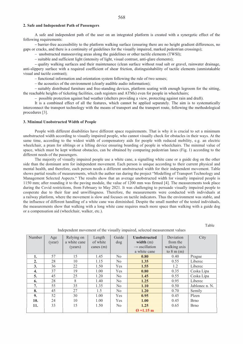
568 2. Safe and Independent Path of Passengers

A safe and independent path of the user on an integrated platform is created with a synergetic effect of the following requirements:

barrier-free accessibility to the platform walking surface (ensuring there are no height gradient differences, no gaps or cracks, and there is a continuity of guidelines for the visually impaired, marked pedestrian crossings);

unobstructed manoeuvring areas along the guidelines or other tactile elements (TWSI); suitable and sufficient light (intensity of light, visual contrast, anti-glare elements); quality walking surfaces and their maintenance (clean surface without road salt or gravel, rainwater drainage,

anti-slippery surface with a required coefficient of shear friction, distinguishability of tactile elements (unmistakable visual and tactile contrast);

functional information and orientation system following the rule of two senses; the acoustics of the environment (clearly audible audio information); suitably distributed furniture and free-standing devices, platform seating with enough legroom for the sitting,

the reachable heights of ticketing facilities, cash registers and ATMs) even for people in wheelchairs; possible protection against bad weather (shelters providing a view, protecting against rain and draft).

It is a combined effect of all the features, which cannot be applied separately. The aim is to systematically interconnect the transport technology with the means of transport and the transport route, following the methodological procedures [3]. 3. Minimal Unobstructed Width of People

People with different disabilities have different space requirements. That is why it is crucial to set a minimum unobstructed width according to visually impaired people, who cannot visually check for obstacles in their ways. At the same time, according to the widest width of compensatory aids for people with reduced mobility, e.g. an electric wheelchair, a pram for siblings or a lifting device ensuring boarding of people in wheelchairs. The minimal value of space, which must be kept without obstacles, can be obtained by comparing pedestrian lanes (Fig. 1) according to the different needs of the passengers.

The majority of visually impaired people use a white cane, a signalling white cane or a guide dog on the other side than the dominant arm for independent movement. Each person is unique according to their current physical and mental health, and therefore, each person needs a different unobstructed width for their independent movement. Table shows partial results of measurements, which the author ran during the project “Modelling of Transport Technology and Management Selected Aspects.“ The results show that an average unobstructed width for visually impaired people is 1150 mm; after rounding it to the paving module, the value of 1200 mm was firmed [4]. The measurements took place during the Covid restrictions, from February to May 2021. It was challenging to persuade visually impaired people to cooperate due to their fear and unwillingness. Therefore, the measurements were conducted with individuals at a railway platform, where the movement is slow and focuses on tactile indicators. Thus the environment was stable, and the influence of different handling of a white cane was diminished. Despite the small number of the tested individuals, the measurements show that walking with a long white cane requires much more space than walking with a guide dog or a compensation aid (wheelchair, walker, etc.).

Table Independent movement of the visually impaired, selected measurement values

Number Age (year)

Relying on a white cane

(years)

Length of white

canes (m)

Guide dog

Unobstructed width (m) oscillation

a white cane

Deviation from the

walking axis to 8 m (m)

City

1. 57 15 1.45 No 0.80 0.40 Prague 2. 28 10 1.15 No 1.35 0.55 Liberec 3. 36 22 1.50 Yes 1.55 1.2 Liberec 4. 37 19 1.00 Yes 0.80 0.35 Ceska Lipa 5. 45 25 1.20 No 1.45 0.55 Ceska Lipa 6. 28 8 1.40 No 1.25 0.95 Liberec 7. 55 35 1.35 No 1.10 0.50 Jablonec n. N. 8. 45 27 1.5 No 1.20 0.70 Semily 9. 52 30 1.00 Yes 0.95 0.45 Plzen 10. 24 10 1.00 Yes 1.00 0.45 Brno 11. 33 15 1.50 No 1.25 0.65 Brno

Ø =1.15 m

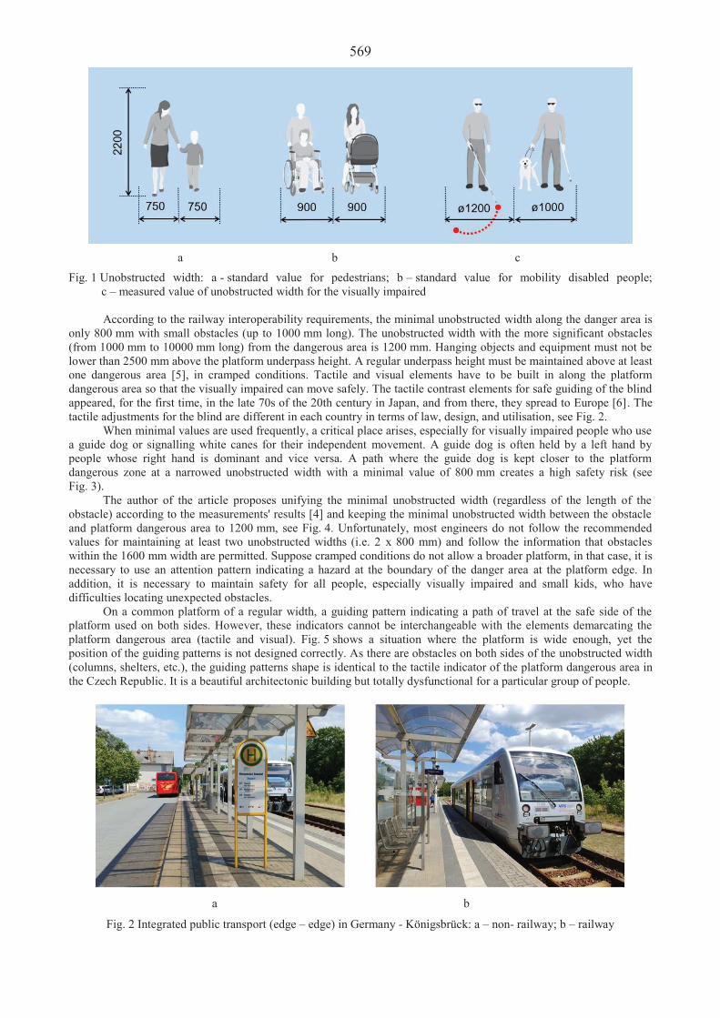
569

a b c

Fig. 1 Unobstructed width: a - standard value for pedestrians; b – standard value for mobility disabled people; c – measured value of unobstructed width for the visually impaired

According to the railway interoperability requirements, the minimal unobstructed width along the danger area is

only 800 mm with small obstacles (up to 1000 mm long). The unobstructed width with the more significant obstacles (from 1000 mm to 10000 mm long) from the dangerous area is 1200 mm. Hanging objects and equipment must not be lower than 2500 mm above the platform underpass height. A regular underpass height must be maintained above at least one dangerous area [5], in cramped conditions. Tactile and visual elements have to be built in along the platform dangerous area so that the visually impaired can move safely. The tactile contrast elements for safe guiding of the blind appeared, for the first time, in the late 70s of the 20th century in Japan, and from there, they spread to Europe [6]. The tactile adjustments for the blind are different in each country in terms of law, design, and utilisation, see Fig. 2.

When minimal values are used frequently, a critical place arises, especially for visually impaired people who use a guide dog or signalling white canes for their independent movement. A guide dog is often held by a left hand by people whose right hand is dominant and vice versa. A path where the guide dog is kept closer to the platform dangerous zone at a narrowed unobstructed width with a minimal value of 800 mm creates a high safety risk (see Fig. 3).

The author of the article proposes unifying the minimal unobstructed width (regardless of the length of the obstacle) according to the measurements' results [4] and keeping the minimal unobstructed width between the obstacle and platform dangerous area to 1200 mm, see Fig. 4. Unfortunately, most engineers do not follow the recommended values for maintaining at least two unobstructed widths (i.e. 2 x 800 mm) and follow the information that obstacles within the 1600 mm width are permitted. Suppose cramped conditions do not allow a broader platform, in that case, it is necessary to use an attention pattern indicating a hazard at the boundary of the danger area at the platform edge. In addition, it is necessary to maintain safety for all people, especially visually impaired and small kids, who have difficulties locating unexpected obstacles.

On a common platform of a regular width, a guiding pattern indicating a path of travel at the safe side of the platform used on both sides. However, these indicators cannot be interchangeable with the elements demarcating the platform dangerous area (tactile and visual). Fig. 5 shows a situation where the platform is wide enough, yet the position of the guiding patterns is not designed correctly. As there are obstacles on both sides of the unobstructed width (columns, shelters, etc.), the guiding patterns shape is identical to the tactile indicator of the platform dangerous area in the Czech Republic. It is a beautiful architectonic building but totally dysfunctional for a particular group of people.

a b

Fig. 2 Integrated public transport (edge – edge) in Germany - Königsbrück: a – non- railway; b – railway

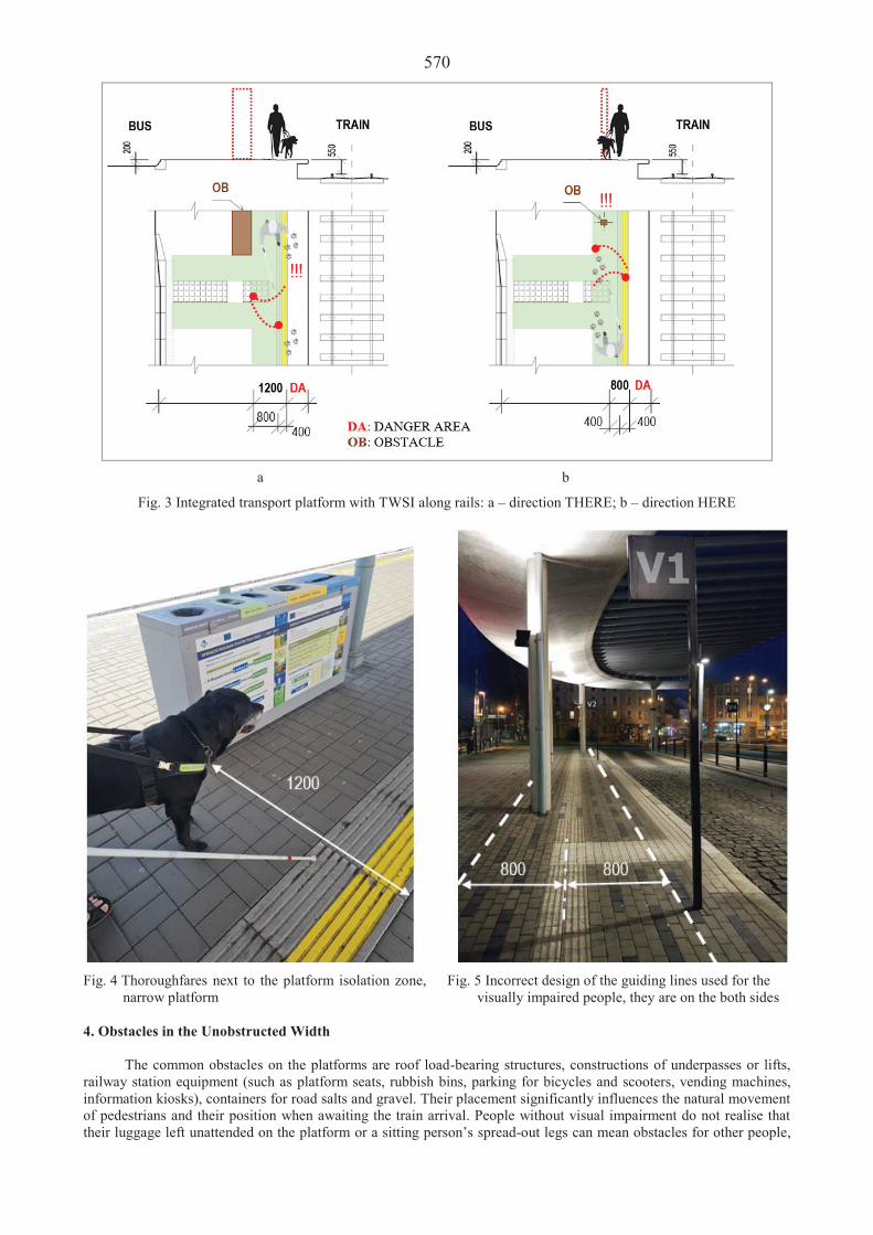
570

a b

Fig. 3 Integrated transport platform with TWSI along rails: a – direction THERE; b – direction HERE

Fig. 4 Thoroughfares next to the platform isolation zone, narrow platform

Fig. 5 Incorrect design of the guiding lines used for the visually impaired people, they are on the both sides

4. Obstacles in the Unobstructed Width

The common obstacles on the platforms are roof load-bearing structures, constructions of underpasses or lifts, railway station equipment (such as platform seats, rubbish bins, parking for bicycles and scooters, vending machines, information kiosks), containers for road salts and gravel. Their placement significantly influences the natural movement of pedestrians and their position when awaiting the train arrival. People without visual impairment do not realise that their luggage left unattended on the platform or a sitting person’s spread-out legs can mean obstacles for other people,

571 see Fig. 6. Currently, people pay more attention to their phones than to caring behaviour towards the people around them. When designing, it is crucial to work with details, especially in connection with the information and orientation systems at the platforms of integrated transport. Most of the buildings maintain unobstructed width during the official approval, but after replacing or adding equipment or adding platform cleaning elements, the situation significantly worsens, see Fig. 6, 7.

a b

Fig. 6 Benches and leg room for sitting passengers: a – current position; b – outstretched legs

a b

Fig. 7 Added obstacle: a – in the direction from the stairs to the tactile indicator; b – in the direction along the tactile indicator towards to the guideline

Fig. 7 shows a construction which was added additionally and is an obstacle in longitudinal and transverse

direction of walking. The wall along the stairs is the guiding line and the signalling belt connects, for the visually impaired, access with the guiding line at the boarding edge. 5. Conclusions

An essential element of interoperability is the ensure safe, barrier-free access with sufficient unobstructed width. The accessibility requirements must be considered during the designing building, maintenance, modernisation and operational process of the subsystem [7]. The integrated transport platform width is conditioned not only by its position but also by its actual equipment, plus the width, shape and distribution of its furniture. Areas where it is possible to widen the unobstructed width using the guiding patterns on both sides, which are not along the platform dangerous area, are considered safer. Universal solutions allow further modifications, change in equipment, faster escape and access in emergencies. Fuzzy sets enable us to establish the degree of usability of tactile elements and unobstructed widths on both sides of the platform by users [8]. It is a mathematical evaluation of usability in a particular space and a financial evaluation of a meaningful proposal.

The author of the article has confirmed that it is necessary to widen the minimal unobstructed width without obstacles from 800 mm to 1200 mm from the edge of the platform dangerous zone. According Aspe SW software [9] increasing the width of the platform by 400 mm increases the overall budget by 0.1% to 0.25% of the total price. The

572 percentage increase will depend on the specific platform construction system used (prefabricated part) and its current price.

If engineers, investors, owners or landlords of the facility do not understand why it is crucial to maintain the unobstructed width without obstacles, it is impossible to ensure safe and independent movement of the passengers on the platform. Therefore, feedback and checks during the designing and building of the platform is a must. Adequate awareness positively impacts the maintenance of the unobstructed with during the life-span of the facility. Acknowledgements

The work was created in connection with the scientific research project of the University of Pardubice “Modelling of Transport Technology and Management Selected Aspects” no. SGS_2021_018. The author is grateful for their support. References 1. GRENN PAPER ON AGEING Fostering solidarity and responsibility between generations COM/2021/50 [online

cit.: 2021-05-06]. Available from: https://eur-lex.europa.eu/legal-content/EN/ALL/?uri=CELEX:52021DC0050 2. The EIDD Stockholm Declaration. EIDD Design for All Europe. [online cit.: 2021-05-06]. Available from:

http://dfaeurope.eu/what-is-dfa-documents/the -eidd-stockholm-declaration-2004/. 3. Matuška, J. 2017. Railway system accessibility evaluation for wheelchair users: case study in the Czech Republic,

Transport 32: 32-43. DOI:10.3846/16484142.2014.941396. 4. Modelling of Transport Technology and Management Selected Aspects. Student Grant Competition. Number SGS

2021_018. 5. Commission Regulation (EU) No 1300/2014 on the technical specifications for interoperability relating to

accessibility of the Union’s rail systém for person with disabilities and persons with reduced mobility. 2014. Official Journal of the European Union, L 356. Available from: https://eur-lex.europa.eu/legal-content/EN/TXT/?uri= CELEX%3A32014R1300&qid=1624921217383.

6. Aoki, H.; Mitani, S. 2012. Tactile walking surface indicators. Making streets safer for visually impaired pedestrians, ISO Focus. Special Report TC 173.

7. Directive (EU) 2016/797 of the European Parliament and of the Council of 11 May 2016 on the interoperability of the rail system within the European Union. 2016. Official Journal of the European Union, L 138. Available from: https://eur-lex.europa.eu/legal-content/EN/TXT/PDF/?uri=CELEX:32016L0797&from=CS.

8. Koš álová, J.; Matuška, J. 2018. Determining the Extent of Usability of Tactile Walking Surface Indicators. In Proceedings of the Fourth International Conference on Traffic and Transport Engineering, 824-830 s. ISBN 978-86-916153-4-5.

9. Aspe SW. 2021. Prague: Sagasta s.r.o. [online cit.: 2021-05-24].

573

Proceedings of 25th International Scientific Conference. Transport Means 2021. Infrastructural and Organizational Problems of Suburban Trams in ód after 1989 A. Soczówka1, M. Paj k2 1Railway Research Institute, ul. Ch opickiego 50, 04-275 Warszawa, Poland, E-mail: asoczowka@ikolej.pl 2Lodz Metropolitan Rail, al. Pi sudskiego 12, 90-051 ód , Poland, E-mail: marcin.pajak@lka.lodzkie.pl Abstract The article presents the history and role of ód suburban tram lines in the transport system of ód agglomeration. Particular attention is drawn to the most characteristic features and technical solutions used in this network. Basing on the literature, the routes of lines, stages of development and regress was presented on a map. The major research is focused on the social and economic transformation period of the ód agglomeration after 1989. The aim of the article is to find out which infrastructural and organizational factors contributed to the regress of ód suburban tram lines after 1989 and what are the possibilities to reconstruct and reactivate transport of suspended or closed lines. The ód suburban tram network is one of five narrow gauge networks (1000 mm) in Poland. Suburban lines offer services for medium-sized and small towns as well as villages of the ód agglomeration. The adopted model of transport organization after 1989 resulted in a gradual regress which finally led to a complete closure of operation of all suburban lines. Initially the closures occurred due to problems with transport financing by some communes (the buses exploitation was cheaper) and conflicts with road infrastructure being extended. Traffic has been suspended due to the high degree of the infrastructure wear and tear only in recent years. Despite the difficulties with tariff integration (separate tickets), the model of entrusting the infrastructure and transport maintenance of separated from the city tram operators was important for the sustainability of the system. After the systems integration (2012) emerged problem the financing of the ongoing maintenance of the run-down infrastructure and repairs. All started currently activities aimed at reactivating transport are co-financed from the EU Cohesion Fund, as their costs are beyond the financial possibilities of some communes. The SWOT analysis showed that only a part of the lines can be rebuilt and the transport restored. Due to the length of the route and the fact that it crosses rural areas, the biggest problem is the reconstruction of the line from Zgierz to Ozorków. KEY WORDS: suburban trams, infrastructure, organization, network 1. Introduction

The social and economic transformation in Poland started in 1989. For the ód agglomeration, where the textile industry was the dominant branch of industry, the transformation marked the beginning of a crisis, both economic and demographic. Most of the textile industry factories were unable to function in the market economy conditions and went bankrupt in the 1990s. The lack of jobs for young people became the reason for economic migration or daily commuting to Warsaw. ód also faced the problem of to be suburbanisation to the towns around it and an intensive demographic ageing. As a result, within 30 years the number of inhabitants of ód decreased from 900 thousand to 700 thousand. The situation of ód and other towns of the ód agglomeration began to improve after Poland's accession to the EU, when access to investment funds (e.g. for transport and urban space revitalisation) was granted, and the favourable transport location at the junction of the A1 and A2 motorways made investors notice the investment potential of ód and new industrial zones were established.

Suburban tram lines in the ód agglomeration were built in the early 20th century. Like the ód tram network, the suburban lines had a gauge of 1000 mm. The construction of most sections was carried out at the beginning of the 20th century, the maximum development took place in the 1970s and 1980s, and from the 1990s began a gradual regression, which led to the suspension or closure of traffic on all suburban lines. Hence the major research is focused on the social and economic transformation period of the ód agglomeration after 1989. The aim of the article is to find out which infrastructural and organizational factors contributed to the regress of ód suburban tram lines after 1989 and examine the possibilities to reconstruct and reactivate transport of suspended or closed lines.

The research was conducted mainly by the desk research method, based on the literature and available data. The source materials included publications on the history of public transport in ód , archival timetables and information obtained directly from the public transport authority and transport operators in ód . The field research comprised an inventory of the remains of decommissioned tram lines and lines with suspended traffic in terms of their possible revitalisation. The SWOT analysis was used in the analysis of possibilities and purposefulness revitalisation of suburban tram lines.

Tram transport was almost completely liquidated after the Second World War in Western European countries. Currently, this mode of transport is undergoing its renaissance. Last year new tram systems are being built and expanded [1-5]. Meanwhile in Poland on the one hand, with the support of EU funds, new tram networks are opened (Olsztyn -

574 2015), other tram networks are intensively modernised and extended [6-8], but at the same time, spectacular tram line closures were continued.

In addition it is worth nothing that there is an important terminological difference regarding the naming of the tram system. In Western European countries the term 'light rail' is used for modern tram systems, while in the countries of Central and Eastern Europe it is only 'fast tram', as opposed to a conventional tram. In reality it is the same mode of public transport, but the name itself is important for their perception - the train is more important and better rated than the tram. 2. Outline of the History of Suburban Trams in ód

The history of suburban trams in ód has been described in detail by [9-12], among others. Therefore, only the most important dates and facts will be mentioned in the article. The network of suburban tram lines historically covered 6 routes:

Line 41 on the route ód and Pabianice. The line was built in 1901, extended in 1905 and 1924 to the railway station in Pabianice, the Wiejska loop at the border of Pabianice was built in 1969. The line ran from the Niepodleg o ci Square in ód with a maximum frequency of every 11 minutes (since 1970s). In Pabianice, an additional Line 41bis ran on the section Du y Skr t loop – Wiejska loop. In the 1990s, Line 41bis was suspended, and the frequency of Line 41 was reduced. Between 2004 and 2008, line 11 ran as the ód Regional Tram on the route from Pabianice to Zgierz via

ód . Line 11 later was replaced by Line P from the Chocianowice-Ikea loop in ód , and later again by Line 41. After the changes of the tram routes in ód in 2017 the line ran only every 24 minutes. Currently, the route to Pabianice is being repaired since 2020 and the line operation is planned to be restored after the maintenance.

Line 42 (Line 80 in the years 1940-1945) on the route ód - Rzgów – Tuszyn. The line was built in 1916 as a steam traction line, in 1927 it was electrified and the loop in Tuszyn at Wschodnia Street in Tuszyn was built in 1967. The line ran initially from Rynek G ówny Square, then from Reymont Square and finally from Niepodleg o ci Square. In the 1970s additional services were launched during peak hours on the route from ód to Rzgów as Line 42bis. From 1978 the route was shortened to Rzgów. The section to Tuszyn was closed due to the construction of a two-lane road from Piotrków Trybunalski to ód (formerly national road no. 1, now no. 91). The section between Rzgów and the Skrajna loop in ód was terminated in 1993. The excuse for the closure of the ód tram section was the reconstruction of Pabianicka Street in ód . The line was closed despite the fact that four years earlier the section from Pabianicka Street to the Popio y loop on this route had been renovated.

Line 43 on the route ód - Konstantynów ódzki – Lutomiersk. The line was built in 1910 to Konstantynów ódzki, it was extended in 1929 to Kazimierz and in 1931 to Lutomiersk, the track triangle in Konstantynów ódzki was

built in 1954, and the Lutomiersk loop - in 1957. The line ran from the Pó nocna terminus, with additional services to Konstantynów ódzki as 43bis. In 2012, Line 43 was extended to the Stoki loop limiting the frequency to one service per hour, and Line 43bis was replaced by extended services of Line 9. After the changes of the tram routes in ód in 2017 lines 43A from Konstantynów ódzki and 43B from Lutomiersk were shortened to the Pó nocna terminus. In 2019, the line was suspended. The general renovation of the route from ód to Konstantynów ódzki is planned with the support of EU funds, at the same time analyses are underway regarding the possibility to renovate and restore traffic on the Konstantynów ódzki - Lutomiersk section.

Line 44 on the route ód - Aleksandrów ódzki. The line was built in 1910 although the loop at Ko ciuszko Square in Aleksandrów ódzki was built in 1981. The line initially ran from Zgierska Street, then from Ba ucki Square, Wolno ci Square and finally from Pó nocna terminus. The line was closed in 1991 as the first closed suburban line on the

ód tram network. The infrastructure was kept passable till 1995 in case a decision was taken to resume service. Line 45 on the route ód - Zgierz; the line was built in 1901, and the Kili skiego Square loop in Zgierz was

built in 1944. The line ran from the Pó nocna terminus with a maximum frequency of every 10 minutes. From 2004 to 2008 it operated as Line 11 from Pabianice, from 2008 to 2017 as Line 16 from the ód Chojny loop, and from 2017 again as Line 45 from the Stoki loop with limited frequency. Since 2018 the line has been suspended, currently a renovation of the route from the city border (Helenówek loop) to Zgierz is being carried out and the operation of the line is planned to be restored after its general renovation.

Line 46 (until 1956 Line 40) on the route ód - Zgierz - Ozorków; the line was built in 1922 as a steam traction line and electrified in 1926 to Wyszy skiego street in Ozorków, the final section to the Cegielniana loop was built in 1986. Like the line to Aleksandrów ódzki, Line 46 initially ran from Zgierska street, then from Ba ucki Square, from Wolno ci Square and finally from Pó nocna terminus. Interestingly - the line ran every 20 minutes for many years, but in the 1990s the frequency was increased to every 16 minutes. After the changes of the tram routes in ód in 2017 the frequency was reduced to every 24 minutes. Traffic on the line was suspended in 2018. No final decision has yet been taken on the general renovation and get the service back on the route.

Initially the suburban tram lines were built as single-track lines with passing loops, in later years some of the sections with the highest traffic volumes were converted to double-track. The frequency on the individual lines was determined in fact by the length of the single-track sections and the location of the passing loop. Therefore, they were different on the individual lines. Traffic on the single-track sections was secured by means of traffic lights. In the course of time the signalling system became inoperative on some of the routes, and traffic was managed using fixed passing loops specified in the timetable. the stages of network development and regress are shown in Figure 1. Historical changes in the frequency of services on the suburban tram lines are shown in Table 1.

575

Fig. 1 Development and regress of suburban tram lines in ód

Table 1 Frequencies of suburban tram lines services in ód

Year / Line 41 41bis 42 42bis 43 43bis 44 45 40 / 46 1948 24’ - 24’ - 40’ - 25` 20` 20` 1972 11’ 11’ 24’ 24’ 30’ 30’ 15’ 11’ 20’ 1999 20’ - - - 30’ 15’-30’ - 10’ 16’ 2017 24’ - - - ~60’ 24’ - 24` 24’

3. Organisation of Suburban Tram Services in ód after 1989

Initially, the organisation and operation of suburban tramway lines, as well as public transport in ód , was managed by a single enterprise - the state-owned Miejskie Przedsi biorstwo Komunikacyjne (Municipal Transport Company in ód - MPK ód ). In 1993-1994, the company were municipalided and the organisational structure was changed, creating an own company for the city of ód with the same name and two new companies which were entrusted with the organisation of suburban tram lines in ód : Mi dzygminna Komunikacja Tramwajowa (Inter-communal Tram Transport - MKT) and Tramwaje Podmiejskie (Suburban Trams - TP). These companies were owned by the City of ód

576 and the suburban communes. The task of the newly established operators was the day-to-day maintenance of the infrastructure and operation of traffic on suburban lines.

Mi dzygminna Komunikacja Tramwajowa took over the Helenówek tram depot in the northern part of ód and Lines 41, 41bis, 45 and 46, while Tramwaje Podmiejskie took over the Brus tram depot in the western part of ód and Lines 43 and 43bis. The new companies created for services on suburban lines used articulated Konstal 102NaW and Konstal 803N trams taken over from MPK ód (from the 1970s, modernised in the 1990s) and second-hand GT6 and GT8 series trams purchased in later years from Austrian and German tram networks. A total of 40 second-hand vehicles were imported in the 1990s and the beginning of the 20th century, with the first second-hand vehicles being imported still by MPK ód in the early 1990s. The type of rolling stock became a feature distinguishing the suburban lines from the urban lines operated by Konstal 805N and 805Na carriages.

The first major organisational changes occurred in 2004 with the implementation of the ód Regional Tram project and the launch of Line 11 from Zgierz to Pabianice via ód operated by MPK ód , which replaced Line 41 and Line 45. In effect the routes to Pabianice and to Zgierz was taken over by MPK ód . Line 46 was extended from the city centre of ód to the Chocianowice loop in south part of ód . Additionally was launched Line 46A between Helenówek and Chocianowice in ód , which compensated the operator for the lost operational performance as a result of the changes of the routes.

Another significant change occurred in 2012, when the operation of all suburban lines was entrusted to MPK ód , transferring both rolling stock and employees from suburban tram companies to the city operator. The MKT and TP ód tram companies were put into liquidation, but the depots did not changes their function - the Helenówek depot will serve as a workshop, whereas the Brus depot as a public transport museum.

The third significant change was the reform of the transport system in 2017 in ód (was changed tram routes and frequency modules), when in an attempt to adapt the frequency modules of the suburban lines to the urban system, the travel time was significantly extended. This was a consequence of the timetable adjustment to the passing loops layout, which was not adapted for this frequency module, i.e. every 24 minutes. This resulted in a significant increase of travel times, regardless of the deteriorating state of the infrastructure.

The organizational model of entrusting infrastructure maintenance and operations to separate operators from MPK ód had both advantages and disadvantages. Despite the difficult financial situation, the separate operators were able to

maintain the infrastructure and carry out transport operations on it in good condition. A disadvantage was the onerous tariff disintegration. Outside the city limits of ód , separate tickets were valid on suburban tram lines, which resulted in situations when at the administrative borders of the cities there was a queue of passengers in suburban trams waiting to buy a ticket valid outside ód . The problem was solved by transferring the service on suburban lines to MPK ód in 2012 by implementing an integrated tariff.

The problem not solved in the 1990s, when the state-owned company MPK ód was municipalided and was created new operators, started to be more and more noticeable. The newly adopted model of organisation and financing suburban tram transport in ód agglomeration secured the funds to provide current services on suburban lines, it did not secure the funds to renovate the decapitalised infrastructure. Funds received by the operator were sufficient only to cover the current costs of line maintenance and services. Suburban municipalities were not able to cover the costs of such large renovation tram infrastructure on their own. At the same time, due to the agreements signed between the communes, it was not possible to finance infrastructure renovation or tram transport service from the voivodeship budget, despite the intercommunal nature of the line. This is explanation how began the slow degradation of the infrastructure in the 1990s.

The operators presented a quite different approach to the technical condition of the suburban lines infrastructure. For MKT ód and TP ód , the priority was, above all, the operation of the line, as the operation of these operators was directly dependent on the possibility of carrying out public transport on these lines. MPK ód approached the issue of the technical condition of the lines differently, as for this operator they were only additional lines. The new operator paid more attention to the technical condition of the infrastructure, primarily to the condition of the track and catenary network (the problem of wear of the contact wire), expecting necessary repairs from the municipalities. In some cases emergency repairs were carried out. Unfortunately, these repairs proved to be insufficient for the continuation of services. 4. Prospects for Suburban Trams in ód

In order to obtain an answer to the research question concerning the prospects of suburban tramway lines in the ód agglomeration, the authors of the article conducted a SWOT analysis on the advisability of reconstructing those

lines (table 2). The results of the analysis were confronted with the results of field research of the closed sections of the suburban part of tram network and with the activities of the local governments of the ód agglomeration aimed at raising funds for the reconstruction.

The SWOT analysis has shown that the restoration and reinstatement of suburban line traffic is definitely justified. Strengths and opportunities outweigh weaknesses and threats. In the case of sections of the network decommissioned in the early 1990s, it is no longer possible to physically rebuild them. The strip of land that remained after the tramway was decommissioned has been incorporated by extensive road infrastructure. Thus, it is no longer possible to restore trams to Rzgów (Line 42) and Aleksandrów ódzki (Line 44).

The situation is different for the remaining suburban lines. All suburban municipalities affected by the suspension of trams in recent years have declared their willingness to rebuild these lines. However, none of the suburban municipalities were in a position to finance such a major reconstruction on their own. So far, steps have been taken to

577 restore trams on routes to Pabianice (Line 41) and Zgierz (Line 45). Two projects co-financed by the European Regional Development Fund within the Regional Operational Programme of the ódzkie Voivodeship are in progress:

the project entitled “ ód Metropolitan Tram: Pabianice - Ksawerów stage” worth PLN 175.2 million (~EUR 38.5 million), co-funded with PLN 99.7 million (~EUR 21.9 million), submitted by Pabianice and the rural municipality of Ksawerów,

the project “Improvement of quality, functioning and development of the transport system offer in the Zgierz municipality” worth PLN 24.1 million (~EUR 5.3 million), co-funded with PLN 18.0 million (~EUR 3.95 million).

In the case of the line to Konstantynów ódzki (Line 43bis), the city authorities take active measures to obtain funds for the reconstruction of the tram line. The Lutomiersk rural municipality is also interested in the reconstruction of their line (Line 43). The most problematic issue is the reconstruction of Line 46 to Ozorków, which runs over a distance of many kilometres through the rural municipality of Zgierz and the rural municipality of Ozorków. For these communes there is a problem to find funds for their own contribution to co-funded EU funds projects and to cover non-eligible costs of the co-funded EU funds projects. It is a really barrier to participation in co-funded EU funds projects. Therefore, there is a risk that from among the suburban tram lines in ód agglomeration, it will be possible to restore traffic and services only on a part of the routes, and the remaining routes will remain just history.

Table 2

SWOT analysis on the reconstruction of suburban tram lines in ód

STRENGTHS WEAKNESSES - low-emission mode of transport - higher transport speed than road transport - high durability of infrastructure compared to road transport - high transport capacity in comparison to road transport - high spatial accessibility tram’s network in the city center of ód

- high cost of rebuilding infrastructure - need to ensure adequate frequency standards - historical route alignment deviating from area development directions - limited capacity of single-track sections

OPPORTUNITIES THREATS - a highly reliable means of transport - independence from traffic congestion - low maintenance costs of infrastructure with a long service life - possibility to reconstruct the infrastructure and rolling stock purchase from European Union aid funds - increase in land and real estate values in the neighbourhood of the tramway line

- failure to provide funding for reconstruction closed routes - failure to ensure adequate frequency standard - technical impossibility of reconstructing some tram rutes

5. Conclusions

Contemporary theories of regional development or business location emphasise the importance of quality of life and quality of public services for attracting investors in leading industries. One such service relevant to quality of life is the quality of public transport. The mode of transport is also important in quality, as rail transport (railway, metro, tram) adds value to public transport.

The transport systems based on buses could likewise hamper progress and deprive regions of innovative mobility solutions they often so need [13]. Light rail, called fast tram in the east part of Europe, often provides the most appropriate transport solution for the well-established European city structure and, increasingly, for extended regional services [14].

Urban transportation has become a very important issue in public policy. Municipalities are responsible for the development of environmentally friendly, energy-sustainable, fast, attractive, competitive, well urban-integrated and welfare-maximizing city transport systems which are, however, constrained by limited financial resources [15]. Investments in transport infrastructure are key to shaping functional and spatial structure of the agglomeration.

The travel behaviours in the case study of Pozna in Poland showed that public transport usage are more common in neighbourhoods with better access to the relevant infrastructure, while residents of neighbourhoods with limited accessibility to sustainable transport infrastructure tend to buy fewer public transport season tickets, to own more cars, and to use them more frequently [16]. Bus based systems lack that “mythical” allure that can help mobilize various actors to support the investment process [13]. The importance of tram quality in Pozna was demonstrated on the example of residential property prices by J. Gadzi ski et al. [19]. They proved how much the prices of properties located next to a fast tram line differ in the northern part of the city from the prices of properties next to a classic tram line.

Mao Y. et al. [17] shows a causal relationship between passenger tram traffic and land development, ticket prices, service level and the efficiency of transfers. Four feedback loop diagrams included: causal link between passenger flow and land use (loop 1), passenger flow - causal link with charges (loop 2), passenger flow - service level causality (loop 3), and passenger flow - causality of transfer efficiency (loop 4). After the model adaptation to local conditions, it can be concluded that the key factor in the decline of the popularity of the suburban tram was the increased travel time, resulting not only from the poor state of the technical infrastructure, but also from the matching of the frequency module to the passing loops layout on single-track sections with much shorter running time.

The case of ód suburban trams is not the only one of intercity tram regress in Poland. A similar situation took place in the Silesian Metropolis in Poland, where as many as five tram lines were suspended and closed down due to

578 technical and economic reasons [18]. The Silesian Metropolis is also a similar problem region, which is undergoing a socio-economic transformation involving the replacement of heavy industry (coal mining, metallurgy) with the service sector and high-tech industry. Similarly to the ód agglomeration, as a consequence of the post-1989 transformation, a strong urban depopulation process has occurred. The tram transport crisis proved to be one of the characteristics of a problematic region undergoing post-industrial transformation.

When searching for new solutions, it is sometimes worth learning from the experience of other countries. An interesting technical solution is the suburban tram line in Alicante, Spain, classified as a tram-train system. The tram line was created and extended on the basis of the former narrow gauge railway (1000 mm). In the city of Alicante it is partly a metro, partly a high-speed tram, partly a classic tram, while outside the city it is a light urban rail, reaching speeds of up to 90-100 km/h. The suburban section is a single-track line with passing loops. On the non-electrified part of the route (from Benidom to Dénia) the line is operated by light diesel vehicles. The tram-train vehicle runs partly on railway tracks with a railway signaling system and other railway equipment [20].

The reconstruction of a tram line in ód agglomeration should not just be a replacement old routes investment, with all the flaws and imperfections of previous solutions. A modern tram should contain all the best features of a train and a tram at the same time. In the city, the tram should ensure the greatest possible spatial accessibility, and from the technical point of view - the greatest possible separation from road traffic and high priority at junctions with other types of traffic, while outside the city it should achieve the highest possible transport speed. Only in this way, a high competitive position in relation to other modes of transport will be achieved. References 1. Martín, L.; Calvo, F.; Hermoso, A.; de Oña, J. 2014. Analysis of light rail systems in Spain according to their type

of funding. Procedia, Social and Behavioral Sciences 162: 419-428. 2. Groneck, Ch.; Schwandl, R. 2014. Tram Atlas Frankreich, Berlin: Robert Schwandl Verlag. 3. Schwandl, R. 2015. Metro & Tram Atlas Spanien, Berlin: Robert Schwandl Verlag. 4. Boquet, Y. 2016. The renaissance of tramways and urban redevelopment in France, Miscellanea Geographica –

Regional Studies on Development 1(1): 5-18. 5. Petkov, D. 2020. Tramway Renaissance in Western Europe, Wiesbaden: Springer VS. 6. Beister, M.; Górny, J.; Po om, M. 2015. Rozwój infrastruktury tramwajowej w Polsce w okresie cz onkostwa w

Unii Europejskiej, TTS Technika Transportu Szynowego 7-8: 20-36. 7. Ko o , A.; Taczanowski, J. 2016. Fundusze europejskie jako czynnik rozwoju miejskiego transportu szynowego w

Polsce, Prace Komisji Geografii Komunikacji PTG 19: 9-20. 8. Orze , A.; Paj k, A.; Graf, M. 2017. Perspektywy rozwoju komunikacji tramwajowej w miastach polskich w

perspektywie finansowej 2014–2020, TTS Technika Transportu Szynowego 7-8: 24-31. 9. Dobrodziej, M. 1986. ódzka komunikacja publiczna, Acta Universitas Lodzenis, Folia Oeconomica 58: 33-53. 10. Raczy ski, J. (ed.) 2001. ódzka podmiejska komunikacja tramwajowa 1901-2001, ód : Emi-Press. 11. Wojtowicz, J.; ródlak, W. 2007. Historia linii tramwajowej do Zgierza i Ozorkowa. Zgierskie Zeszyty Regionalne,

t. II. 12. Stiasny, M.; Danyluk Z. 2017. Rybnik: Atlas linii tramwajowych, Eurosprinter. 13. De Bruijn, H.; Veeneman, W. 2009. Decision-making for light rail, Transportation Research Part A 43: 349-359. 14. Hamiduddin, I. 2015. Connecting European Regions using Innovative Transport Investing in light rail and tram

systems: Technological and organizational dimensions, London: University College. 15. Seidenglanz, D.; Kvizda, M.; Nigrin, T.; Tomeš, Z.; Dujka, J. 2016. Czechoslovak light rail – Legacy of socialist

urbanism or opportunity for the future? Journal of Transport Geography 54: 414-429. 16. Radzimski, A.; Gadzi ski, J. 2019. Travel behaviour in a post-socialist city, European Spatial Research and Policy

26(1): 43-60. 17. Mao, Y.; Ninghui, Y.; Zhibin, L.; Lingling, M.; Yajing, Ch. 2019. Modeling Influencing Factors for Passenger

Flow Growth of Modern Trams Using System Dynamics Method, Journal of Advanced Transformation, https://doi.org/10.1155/2019/8475937

18. Soczówka, A. 2012. Zarys historii komunikacji tramwajowej na obszarze konurbacji katowickiej, Acta Geographica Silesiana 12: 57-70.

19. Gadzi ski, J.; Radzimski, A. 2016. The first rapid tram line in Poland: how has it affected travel behaviours, housing choices and satisfaction, and apartment prices? Journal of Transport Geography 54: 451-463.

20. Novales, M.G.; Cerezo, J.A.; Ortega R. 2013. Light Rail in Alicante, Spain: Improving the Use of Existing Railway Lines, Transportation Research Record Journal of the Transportation Research Board 2353 (2353): 69-81.

579

Proceedings of 25th International Scientific Conference. Transport Means 2021.

External Control of the Divergence Process Taking into Account the Form of the Safety Domain I. Burmaka1, A. Borodulin2, D. Fedorov3, O. Petrychenko4

1National University «Odessa Maritime Academy», Didrikhson str. 8, 65029, Odessa, Ukraine, E-mail: burmaka1964@gmail.com 2National University «Odessa Maritime Academy», Didrikhson str. 8, 65029, Odessa, Ukraine, E-mail: nav.dep.nuoma@gmail.com 3National University «Odessa Maritime Academy», Didrikhson str. 8, 65029, Odessa, Ukraine, E-mail: nav.dep@mail.ru 4National University «Odessa Maritime Academy», Didrikhson str. 8, 65029, Odessa, Ukraine, E-mail: oapetrychenko@gmail.com

Abstract

The article considers the application of unacceptable values of courses of dangerously approaching ships at their external control to choose divergence maneuver in case of use of safety domain which shape differs from the circle. It is shown that the maximum permissible approach distance depends on the size of the domain and the angle of approaching ships. The article includes the computer implementation of this method and a numerical example. KEY WORDS: navigational safety, ship collision avoidance, external control of divergence process, elliptical shape safety domain 1. Introduction

One of the most actual problems of ship navigation safety is to increase safety of ships divergence at their dangerous approach in the congested waters. Therefore, congested navigation areas with especially heavy traffic are equipped with ship control stations which should be equipped with modern means of warning of vessel collision which causes urgency and prospects of researches on this subject.

Vessel interaction formalization models at divergence and methods of divergence manoeuvre selection are proposed in articles [1-10]. The first attempts to formalize the process of divergence are undertaken in articles [1] and [2], moreover, in article [1] method of non-linear integral invariance is offered for description of divergence process, and article [2] is devoted to application of methods of optimal discrete processes theory for solution of this task.

The problem of ship collision prevention and development of method of flexible strategies of their divergence, which allows forming optimal strategy of ship divergence with several dangerous targets taking into account essential factors, are investigated in detail in work [3]. Application of differential game theory for formalization of vessel interaction at divergence is described in articles [4, 5].

Article [6] gives results on effectiveness of paired divergence manoeuvres, and article [7] considers control of three ships for safe divergence.

The monograph [8] considers the problem of vessels divergence at sea by the method of shifting a vessel to a line parallel to the course. In [9] formalization of COLREG-72 and analytical description of ships interaction in case of collision threat is proposed.

In [10] management of ship divergence process by means of VTS is suggested, which uses principle of external management of divergence process. The main method for determining the divergence manoeuvre of two vessels under external control of the divergence process is the use of the domains limit of invalid data of Qk vessel courses. In work [10] formation of area Qk at use of a safety domain of the circular form which radius is equal to the maximum – permissible distance of convergence is considered.

However, in recent years, safety domains have been proposed for use in divergence, the shape of which is different from a circle. Therefore it is necessary for such domains to consider the procedure of forming the domains limit of invalid data of vessels' courses. In this article we will consider procedure of formation of domains limit of invalid data of vessels' courses for safety domain with elliptical shape, which centre is displaced in relation to the centre of a vessel towards the bow.

1.2. Purpose

The purpose of this article is to develop a method of formation of the domains limit of invalid data of ship courses and its application to the selection of divergence manoeuvre when using elliptical shaped safety domain.

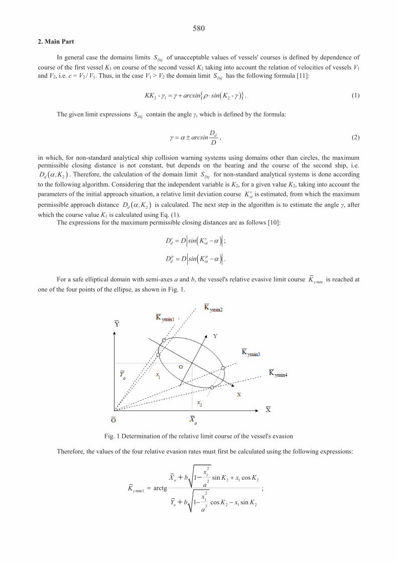
580 2. Main Part

In general case the domains limits DijS of unacceptable values of vessels' courses is defined by dependence of course of the first vessel K1 on course of the second vessel K2 taking into account the relation of velocities of vessels V1 and V2, i.e. c = V2 / V1. Thus, in the case V1 > V2 the domain limit DijS has the following formula [11]:

2 1 2KK - arcsin sin K - . (1)

The given limit expressions DijS contain the angle , which is defined by the formula:

dDarcsin

D, (2)

in which, for non-standard analytical ship collision warning systems using domains other than circles, the maximum permissible closing distance is not constant, but depends on the bearing and the course of the second ship, i.e.

2dD ,K . Therefore, the calculation of the domain limit DijS for non-standard analytical systems is done according to the following algorithm. Considering that the independent variable is K2, for a given value K2, taking into account the parameters of the initial approach situation, a relative limit deviation course s

otK is estimated, from which the maximum permissible approach distance 2dD ,K is calculated. The next step in the algorithm is to estimate the angle , after which the course value K1 is calculated using Eq. (1).

The expressions for the maximum permissible closing distances are as follows [10]: s s

d otD D sin K ;

p pd otD D sin K .

For a safe elliptical domain with semi-axes a and b, the vessel's relative evasive limit course y minK is reached at

one of the four points of the ellipse, as shown in Fig. 1.

Fig. 1 Determination of the relative limit course of the vessel's evasion Therefore, the values of the four relative evasion rates must first be calculated using the following expressions:

min1yK =

21

2 1 22

21

2 1 22

1 sin cosarctg

1 cos sin

o

o

xX b K x K

a

xY b K x K

a

;

581

min 2yK =

21

2 1 22

21

2 1 22

1 sin cosarctg

1 cos sin

o

o

xX b K x K

a

xY b K x K

a

;

min3yK =

22

2 1 22

22

2 1 22

1 sin cosarctg

1 cos sin

o

o

xX b K x K

a

xY b K x K

a

;

min 4yK =

22

2 1 22

22

2 1 22

1 sin cosarctg

1 cos sin

o

o

xX b K x K

a

xY b K x K

a

,

where 2 22 2 2 22

1 2 2 22 2 2 2 2 2

a c b ra cb a cbxa c r a c ra c r

;

)(

)(2(222

2222

222

2

222

2

2 )rca

rbca

rca

cba

rca

cbax ,

2

2 2sin coso o

acb Y K X K

and 2 2cos sino or Y K X K .

After calculating the values of min1yK , min 2yK , min3yK and min 4yK

the required values of the relative limit

courses of the ship's deviation to the right sotK and left p

otK are found from the expressions:

sotK = max { min1yK , min 2yK , min3yK , min 4yK },

minpotK { min1yK , min 2yK , min3yK , min 4yK }.

Let us choose as an example a situation of dangerous approach, the parameters of which are characterized by the

following values: 150 °, 3D miles, 1 122K °, 1 22V knots, 2 351K °, 2 18V knots. Fig. 2 shows the domain DijS plotted for an elliptical domain with its major axis equal to 1 mile and its minor axis equal to 2/3 of a mile.

As it follows from the above figure, the point corresponding to the initial courses of the vessels is in the domain DijS , which indicates dangerous approach and necessity of choosing divergence manoeuvre. For this purpose, at the upper domain limit DijS corresponding to the relative deviation to the right, a point is selected with courses 1 132K ° and

2 3K ° (Fig. 2), which is the divergence manoeuvre. It should be noted that in this divergence manoeuvre, indicated by concentric circles on the domain limit DijS ,

the closest approach distance 0,24mL is miles and equals the maximum permissible deviation distance to the right

dsD . Fig. 3 shows that this manoeuvre is corresponded to a relative course line which is tangential to the elliptical domain.

582

Fig. 2 Selection of divergence manoeuvre by relative evasion to the right

Fig. 3 Divergence manoeuvre by relative evasion to the right 3. Conclusions

The method of formation of the limit of the domain invalid data of ship courses and its application for selection of divergence manoeuvre when using elliptical shape safety domain is considered.

Analytical expressions for calculation of relative limit courses of ship evasion and maximum-permissible distances of approach at its relative evasion to the right and to the left are received.

583 The example of the construction of domains limit of invalid data of vessels' courses for the given situation of

dangerous approach and definition with its help of manoeuvre of divergence in case of application of safety domain of elliptical form results.

References

1. Pavlov, V.V.; Senshin, N.I. 1985. Some questions of choice of maneuver in the situations of divergence of vessels,

Kibernetika i vychislitelnaya tekhnika 68: 43-45. 2. Kulikov, A.M.; Poddubnyy, V.V. 1984. Optimum management by divergence of vessels, Sudostroenie 12: 22-24. 3. Tsymbal, N.N.; Burmaka, I.A.; Tyupikov, E.E. 2007. Flexible strategies of divergence of vessels. Odessa: KP

OGT, 424 p. 4. Kudryashov, V.E. 1978. Synthesis of algorithms of safe management by a ship at divergence with a few objects,

Sudostroenie 5: 35-40. 5. Lisowski, J. 2005. Dynamic games methods in navigator decision support system for safety navigation, Advances

in Safety and Reliability 2: 285-1292. 6. Pyatakov, E.N.; Zaichko, S.I. 2008. Estimation of efficiency of pair strategies of going away vessels,

Sudovozhdenie 15: 166-171. 7. Burmaka, I.A.; Bulgakov, .Y. 2014. Maneuver of divergence of three vessels by the change of courses,

Avtomatizatsiya sudovykh tekhnichtskikh sredstv 20: 18-23. 8. Vagushchenko, L.L. 2013. Divergence with vessels by displacement on the parallel line of way. Odessa: Feniks,

180 p. 9. Pyatakov, E.N.; Buzhbeckij, R.Y.; Burmaka, I.A.; Bulgakov, .Y. 2015. Cooperation of vessels at divergence

for warning of collision. Kherson: Grin D.S, 312 p. 10. Burmaka, I.; Pyatakov, E., Bulgakov, . 2016. Management by vessels in the situation of dangerous

rapprochement. LAP LAMBERT Academic Publishing, Saarbryukken (Germany), 585 p. 11. Bulgakov, .Y. 2014. Use of dangerous region of courses of two vessels for the choice of possible manoeuvre of

divergence, Vodnyy Transport 2(20):12-17.

584

Proceedings of 25th International Scientific Conference. Transport Means 2021.

Utilization of Modern Methods for Documentation of Traffic Accidents in Road Transport P. Kudela1, M. Fandáková2, M. Pal ák3, J. Kordek4

1University Science Park, University of Žilina, Univerzitná 8215/1, 010 26, Žilina, Slovakia, E-mail: pavol.kudela@uvp.uniza.sk 2University Science Park, University of Žilina, Univerzitná 8215/1, 010 26, Žilina, Slovakia, E-mail: miriam.fandakova@uvp.uniza.sk 3University Science Park, University of Žilina, Univerzitná 8215/1, 010 26, Žilina, Slovakia, E-mail: michal.palcak@uvp.uniza.sk 4University Science Park, University of Žilina, Univerzitná 8215/1, 010 26, Žilina, Slovakia, E-mail: juraj.kordek@uvp.uniza.sk Abstract Investigation of traffic accidents is a daily routine for the police and experts. When analyzing accidents or collisions between motor vehicles and pedestrians or cyclists, an important aspect is the capture of the place of the accident and its most accurate documentation. New methods in the field of digitization are currently being used for this purpose. The article therefore provides insight into the utilization of modern methods in the documentation of traffic accidents via current digital technologies. The main goal of the article is to compare three basic methods of digitization of traffic accidents, to describe their positives and negatives that can be used in their documentation. In conclusion of the article is the evaluation of individual methods of digitization in the documentation of accidents in road transport. These methods are compared with regard to the level of detail and parameterization for their subsequent analysis in the investigation of traffic accidents, which can be the basis for an expert testimony creation. KEY WORDS: scanning, photogrammetry, UAV, analyze, traffic accident 1. Introduction

The main problem in the analysis of traffic accidents (TA) in Slovak Republic is to find out exactly how the

accident occurred and to prove the course of the accident. In today's era of constant technological advancement, it is expected that new methods of digitization in documenting accidents will be used mainly for the most accurate documentation of criminalistic traces. Subsequently, investigators and experts in the field of traffic accidents have accurate information and can use it to evaluate data, establish certain hypotheses, select or create a mathematical model of the accident, perform numerical simulations, interpret and evaluate the reality of information obtained and finally write a comprehensive accident report. This paper describes selected methods of digitization and their benefits and negatives of use in documenting TA [4].

2. Technologies for Documenting Traffic Accidents

In the case of TA [4] documentation, the first and probably the most important part of the investigation is the

collection and analysis of available data, the documentation of criminalistic traces, with an emphasis on capturing and documenting the crime scene as accurately as possible. When documenting these tracks, the police officer focuses on the trasological and biological tracks upon arrival. Therefore, upon arrival at the scene, the police officer must evaluate the situation and set up a clear method of documentation. The available methods are as follows: rectangular, triangular and rectifying. The most used method is the rectangular method, where the imaginary main axis is selected and the subsequent ones are perpendicular to it at distances of individual tracks. In terms of the measuring method, a wheel, spirit level, leveling rod or measuring band is used for place of accident. In general, however, only a wheel is usually used to document the TA and clear the road as quickly as possible. Often the police encounter problems that the wheel does not have the counter switched on, communication is right or. counterclockwise and it is difficult to focus on it, there is an obstacle during the measurement or there is dirt on the road. These circumstances result in an error in documenting the TA. In addition to this information, the police has to obtain information on who arrived at the TA site and in what order. Another aspect is the creation of TA image documentation. Above all, the standard automatic mode is used, which is predefined for simple and fast documentation. However, if set incorrectly, it creates poor exposure, which complicates trace identification when analyzed on a PC. Also, when preparing the documentation, there is not an adequate ability to recognize whether the photo is of sufficient quality and with the correct sharpness. It often happens that an expert or other investigator is not immediately present at the scene of the accident and has no influence on the documented data and accepts them as fact. Such a report may only contain information such as a description of events or certain measurements and photographs, but they may not be sufficient. Exactly in this phase it is possible to take advantage of new possibilities

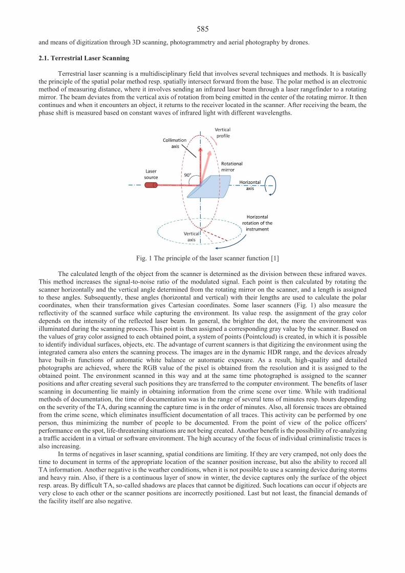
585 and means of digitization through 3D scanning, photogrammetry and aerial photography by drones.

2.1. Terrestrial Laser Scanning

Terrestrial laser scanning is a multidisciplinary field that involves several techniques and methods. It is basically the principle of the spatial polar method resp. spatially intersect forward from the base. The polar method is an electronic method of measuring distance, where it involves sending an infrared laser beam through a laser rangefinder to a rotating mirror. The beam deviates from the vertical axis of rotation from being emitted in the center of the rotating mirror. It then continues and when it encounters an object, it returns to the receiver located in the scanner. After receiving the beam, the phase shift is measured based on constant waves of infrared light with different wavelengths.

Fig. 1 The principle of the laser scanner function [1]

The calculated length of the object from the scanner is determined as the division between these infrared waves. This method increases the signal-to-noise ratio of the modulated signal. Each point is then calculated by rotating the scanner horizontally and the vertical angle determined from the rotating mirror on the scanner, and a length is assigned to these angles. Subsequently, these angles (horizontal and vertical) with their lengths are used to calculate the polar coordinates, when their transformation gives Cartesian coordinates. Some laser scanners (Fig. 1) also measure the reflectivity of the scanned surface while capturing the environment. Its value resp. the assignment of the gray color depends on the intensity of the reflected laser beam. In general, the brighter the dot, the more the environment was illuminated during the scanning process. This point is then assigned a corresponding gray value by the scanner. Based on the values of gray color assigned to each obtained point, a system of points (Pointcloud) is created, in which it is possible to identify individual surfaces, objects, etc. The advantage of current scanners is that digitizing the environment using the integrated camera also enters the scanning process. The images are in the dynamic HDR range, and the devices already have built-in functions of automatic white balance or automatic exposure. As a result, high-quality and detailed photographs are achieved, where the RGB value of the pixel is obtained from the resolution and it is assigned to the obtained point. The environment scanned in this way and at the same time photographed is assigned to the scanner positions and after creating several such positions they are transferred to the computer environment. The benefits of laser scanning in documenting lie mainly in obtaining information from the crime scene over time. While with traditional methods of documentation, the time of documentation was in the range of several tens of minutes resp. hours depending on the severity of the TA, during scanning the capture time is in the order of minutes. Also, all forensic traces are obtained from the crime scene, which eliminates insufficient documentation of all traces. This activity can be performed by one person, thus minimizing the number of people to be documented. From the point of view of the police officers' performance on the spot, life-threatening situations are not being created. Another benefit is the possibility of re-analyzing a traffic accident in a virtual or software environment. The high accuracy of the focus of individual criminalistic traces is also increasing.

In terms of negatives in laser scanning, spatial conditions are limiting. If they are very cramped, not only does the time to document in terms of the appropriate location of the scanner position increase, but also the ability to record all TA information. Another negative is the weather conditions, when it is not possible to use a scanning device during storms and heavy rain. Also, if there is a continuous layer of snow in winter, the device captures only the surface of the object resp. areas. By difficult TA, so-called shadows are places that cannot be digitized. Such locations can occur if objects are very close to each other or the scanner positions are incorrectly positioned. Last but not least, the financial demands of the facility itself are also negative.

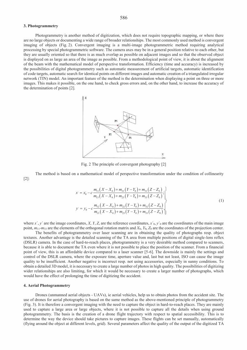
586 3. Photogrammetry

Photogrammetry is another method of digitization, which does not require topographic mapping, or where there

are no large objects or documenting a wide range of broader relationships. The most commonly used method is convergent imaging of objects (Fig. 2). Convergent imaging is a multi-image photogrammetric method requiring analytical processing by special photogrammetric software. The camera axes may be in a general position relative to each other, but they are usually oriented so that there is as much overlap as possible on adjacent images and so that the observed object is displayed on as large an area of the image as possible. From a methodological point of view, it is about the alignment of the beam with the mathematical model of perspective transformation. Efficiency (time and accuracy) is increased by the possibilities of digital photogrammetry such as automatic measurement of artificial targets, automatic identification of code targets, automatic search for identical points on different images and automatic creation of a triangulated irregular network (TIN) model. An important feature of the method is the determination when displaying a point on three or more images. This makes it possible, on the one hand, to check gross errors and, on the other hand, to increase the accuracy of the determination of points [2].

Fig. 2 The principle of convergent photography [2]

The method is based on a mathematical model of perspective transformation under the condition of collinearity [2]:

11 0 21 0 31 00

13 0 23 0 33 0

12 0 22 0 32 00

13 0 23 0 33 0

;

,

, ,

, ,

m X X m Y Y m Z Zx x c

m X X m Y Y m Z Z

m X X m Y Y m Z Zy y c

m X X m Y Y m Z Z

(1)

where x´, y´ are the image coordinates, X, Y, Z, are the reference coordinates, x´0, y´0 are the coordinates of the main image point, m11-m33 are the elements of the orthogonal rotation matrix and X0, Y0, Z0 are the coordinates of the projection center.

The benefits of photogrammetry over laser scanning are in obtaining the quality of photographs resp. object textures. Another advantage is the detailed scanning of the TA area from multiple positions of digital single-lens reflex (DSLR) camera. In the case of hard-to-reach places, photogrammetry is a very desirable method compared to scanners, because it is able to document the TA even where it is not possible to place the position of the scanner. From a financial point of view, this is an affordable device compared to a laser scanner [5-6]. The downside is mainly the settings and control of the DSLR camera, where the exposure time, aperture value and, last but not least, ISO can cause the image quality to be insufficient. Another negative is incorrect resp. not using accessories, especially in sunny conditions. To obtain a detailed 3D model, it is necessary to create a large number of photos in high quality. The possibilities of digitizing wider relationships are also limiting, for which it would be necessary to create a larger number of photographs, which would have the effect of prolonging the time of digitizing the accident.

4. Aerial Photogrammetry

Drones (unmanned aerial objects - UAVs), ie aerial vehicles, help us to obtain photos from the accident site. The

use of drones for aerial photography is based on the same method as the above-mentioned principle of photogrammetry (Fig. 3). It is therefore a convergent imaging with the need to capture the object in hard-to-reach places. They are mainly used to capture a large area or large objects, where it is not possible to capture all the details when using ground photogrammetry. The basis is the creation of a drone flight trajectory with respect to spatial accessibility. This is to determine the way the device should take pictures to capture images. These flights can be set manually, automatically (flying around the object at different levels, grid). Several parameters affect the quality of the output of the digitized TA

587 [10]. The basic parameters include the flight path, which is recommended in at least two flights perpendicular to each other. This ensures sufficient overlap between the images obtained from the UAV [7]. In the case of lateral overlap, the spacing between the individual flight paths is determined so as to minimize the loss of object information generated during frontal capture. Important parameters for digitizing TA include flight altitude resp. the distance of the UAV from the object of interest [8]. The height itself affects ground sampling distance (GSD), ie the quality of detail in the resulting photo. Therefore, if the low value of GSD is maintained, we will achieve a very high quality and detailed view of the TA site.

Fig. 3 The principle of aerial photogrammetry with UAV [8]

The benefits of aerial photogrammetry [9] in documenting DN lies in the speed of documenting the site, but also in the possibility of control by one person. What takes several days in traditional ground mapping can be handled by an unmanned device operated by a one trained operator in a few tens of minutes of flight, with the same accuracy and with significantly wider possibilities of using the collected data. In the case of a hard-to-reach place, it is not necessary for the police officer to map this place within the TA to document forensic traces.

However, the use of this method also has its negatives, such as low target resolution of GSD and scaling of the TA area. TA places, which are in densely overgrown forests, as well as very cramped conditions are also problematic. Another negative in aerial photography is that there are zones where it is not allowed to fly due to the fact that they belong to the secure areas of the state. A person with the appropriate permits must be trained to operate a UAV. Partial restriction occurs not only in the case of weather conditions, but also in the length of the UAV flight itself. 5. Conclusions

When documenting forensic footprints and creating a virtual 3D area of TA, ground and aerial photogrammetry in

combination with terrestrial laser scanning proved to be one of the best available tools a police officer or investigator can have. Some complicated TA such as large extensive resp. chain accidents can prove to be very problematic in the traditional method of eye-level photography in demonstrating the overall nature of the event and the conditions surrounding it. In such cases, aerial photogrammetry can be very effective in providing a better perspective (orthophotomaps), while providing additional information to refine and more easily understand how TA occurred compared to direct evidence. Taking into account the shortcomings of existing methods in terms of accuracy of reconstruction and increased overload, photogrammetry is one of the recommended techniques in transport for accident reconstruction [11]. In conclusion, we can state that technologies such as laser scanning, ground and aerial photogrammetry are essential and valuable technologies in documenting forensic footprints at the TA site under various traffic conditions. Aerial photogrammetry provides a dimension of visual reference as part of TA documentation. Acknowledgment

This publication was realized with support of Operational Program Integrated Infrastructure 2014 - 2020 of the project: Innovative Solutions for Propulsion, Power and Safety Components of Transport Vehicles, code ITMS 313011V334, co-financed by the European Regional Development Fund. References 1. Medic, T.; Holst, Ch.; Kuhlmann, H. 2017. Towards System Calibration of Panoramic Laser Scanners from a Single

Station, [online cit.: 2021-06-08]. Available from: https://www.researchgate.net/publication/316990821_Towards _System_Calibration_of_Panoramic_Laser_Scanners_from_a_Single_Station

2. Fraštia, M. 2008. Kalibrácia a testovanie digitálnych kamier pre aplikácie blízkej fotogrametrie: Edícia vedeckých prác. Zošit . 52. Bratislava: Slovenská technická univerzita v Bratislave, Vydavate stvo STU. ISBN 978-80-227-2812-6.

3. Feng-Hui, Wang; Lang, Wei & Shun, Tian; Ling-Yi, Li; Yong-Tao, Liu 2019. Road traffic accident scene detection and mapping system based on aerial photography, International Journal of Crashworthiness, [online cit.: 2021-06-08]. Available from: https://www.tandfonline.com/doi/full/10.1080/13588265.2020.1764719?scroll=top& needAccess=true

4. Balista, M. 2017. The study of traffic accidents-methods and their [online cit.: 2021-06-08]. Available from: https://www.researchgate.net/publication/320196358_The_study_of_traffic_accidents-

588 methods_and_their_reliability

5. Osman, M.R.; Tahar, K.N. 2016. 3D accident reconstruction using low-cost imaging technique, Adv Eng Softw 100: 231-237.

6. Luhmann, T.; Robson, S.; Kyle, S.; Harley, I. 2006 Close range photogrammetry: Principles, techniques and applications. Whittles Publishing, Dunbeath, UK.

7. Martínez-Carricondo, P.; Carvajal-Ramírez, F.; Yero-Paneque, L.; Agüera-Vega, F. 2020 Combination of Nadiral and Oblique UAV Photogrammetry and HBIM for the Virtual Reconstruction of Cultural Heritage, Case Study of Cortijo del Fraile in Níjar, Almería (Spain), Build. Res. Inf. 48: 140-159.

8. Almeshal, A.M.; Alenezi, M.R.; Alshatti, A.K. 2020 Accuracy Assessment of Small Unmanned Aerial Vehicle for Traffic Accident Photogrammetry in the Extreme Operating Conditions of Kuwait [online cit.: 2021-06-08]. Available from: https://www.mdpi.com/2078-2489/11/9/442

9. Pádua, L.; Sousa, J.; Vanko, J.; Hruška, J.; Adao, T.; Peres, E.; Sousa, A.; Sousa, J.; 2020 Digital Reconstitution of Road Traffic Accidents: A Flexible Methodology Relying on UAV Surveying and Complementary Strategies to Support Multiple Scenarios [online cit.: 2021-06-08]. Available from: https://www.mdpi.com/1660-4601/17/6/1868

10. Liu, X.; Zhao, L.; Peng, Z.-R.; Gao, T.; Geng, J. 2017. Use of Unmanned Aerial Vehicle and Imaging System for Accident Scene Reconstruction; Transportation Research Board: Washington, DC, USA, p. 14.

11. Rucoba, R.; Duran, A.; Carr, L.; Erdeljac, D.A. 2008 Three-Dimensional Crush Measurement Methodology Using Two-Dimensional Photographs (No. 2008-01-0163); SAE Technical Paper: Warrendale, PA, USA. [online cit.: 2021-06-08]. Available from: https://www.mdpi.com/2078-2489/11/9/442/pdf

589

Proceedings of 25th International Scientific Conference. Transport Means 2021. Research of Freight Cars Malfunctions in Operation O. Koshel1, S. Sapronova2, V. Tkachenko3, M. Buromenska4, M. Radkevich1

1Railway carriage and Railway carriage property, State University of Infrastructure and Technologies, 04071 Kyiv, Ukraine, E-mail: koshela1520mm@gmail.com 2Railway carriage and Railway carriage property, State University of Infrastructure and Technologies, 04071 Kyiv, Ukraine, E-mail: doc.sapronova@gmail.com 3Traction rolling stock of the railway, State University of Infrastructure and Technologies, 04071 Kyiv, Ukraine, E-mail: v.p.tkachenko.detut@gmail.com 4Research Department, State University of Infrastructure and Technologies, 04071 Kyiv, Ukraine, E-mail: English.anti.school@gmail.com Abstract The article presents a study of malfunctions of freight cars in operation on the railways of Ukraine. The main groups of malfunctions of freight cars are revealed. The analysis of freight cars malfunctions according to group codes and accord-ing to maintenance data is carried out. The largest number of faults occurs in the load-bearing structures (frame and body of the car), wheelsets. This situation indicates the need to develop modernization projects for load-bearing structures that have already exhausted their intended service life, because the current repair documentation does not provide for the elimination of such defects. The conducted researches will promote the prevention of premature failure of elements of freight cars in operation. KEY WORDS: malfunctions, rejections, exploitation, freight car, dump truck, hopper 1. Introduction

Dump trucks (DT) and hoppers (H) are mostly used in track economy and given their specifics have seasonal use. As of 01.05.2021, the assigned fleet of hoppers is 1454 units, the average age of cars is 44 years, with a standard service life of 25 years and an average wear of 98.00%. Dump trucks have 942 units, the average age of which is 35 years, with a standard service life of 22 years and an average wear of 100.00%. The analysis of the given data testifies to physical and moral wear of freight cars park which in turn negatively influences faultlessness of work of its knots and can lead to the emergence of delays in transportation process and maintenance of infrastructure in a proper condition. 2. More Information

The study of exploitation failures of hoppers for grain transportation was carried out in [5, 6], the results of which identified the main groups of failures of cars. The publication [7] describes methodological approaches to determining the failures and service life of the freight car according to the criterion of safety, considers the classification of failures, malfunctions and damage to freight cars. In [8] the analysis of failures that cause uncoupling in the current repair of passenger cars is made. The results which have allowed us to define problem knots of the passenger car which need improvement are received [9-11].

Analysis of research shows a small number of them on this issue. The purpose of the article is to study the malfunctions of the fleet of freight cars of JSC "Ukrzaliznytsia" in oper-

ation, for which it is necessary to solve the following tasks: – detection of the main groups of freight cars malfunctions; – analysis of freight cars malfunctions according to group codes according to maintenance data. Malfunction is the state of the object, in which it is unable to perform at least one of the specified functions [3]. Malfunctions of freight cars are divided into the following groups: 1 malfunction of the wheel pair; 2 malfunction of the cart; 3 malfunction of autocoupling equipment;

4 malfunction of self-braking equipment; 5 malfunction of the car body; 6 malfunction of the car frame; 8 mal-function of the car body, which leads to the exclusion of the car from the inventory; 9 service codes not related to the technical condition of the car [2].

Freight cars malfunctions according to [4] in most cases are eliminated by maintenance - M, M-1 and M-2. M is a set of operations to maintain the efficiency or serviceability of the car in the formed or transit trains, as well as an empty car during the preparation for transportation without detaching it from the train or group of cars. M-1 and M-2 are mainte-nance of the car with its detachment from the train or group of cars, transferring it to the non-working fleet. Repairs are performed to ensure or restore the performance of the car with the replacement or restoration of individual components. During M-1 there is performed maintenance and repair of an empty car, with its detachment from the warehouse or group of cars, to conduct a set of operations to prepare the car for transportation. During M-2 there is performed maintenance

590and repair of the car with detachment from transit and arriving before the disbandment of trains or formed train depots, to restore the capacity of the loaded or empty car.

The sample of malfunctions of the fleet of freight cars owned by «Ukrzaliznytsia» was formed in accordance with the information certificate [1] for the period from 02.03.2021 to 30.04.2021 (60 days) and the results of technical diag-nostics of the main scientific organization of «Ukrzaliznytsia» for the period from 2018 to 2020 year. The generated fault data according to the information are given in Table 1.

Table 1Freight cars malfunctions according to maintenance data during the last 60 days

Group code Code and name of malfunction Total number, items

1 – wheel pair

102 – a thin crest; 106 – slider on the rolling surface; 107 – notch of the wheel rim; 109 – sharp roll of the crest; 111 – a thin rim;

157 – bearing heating in the axle box housing; 160 – overdue term of average repair of wheel pair

12

2 – carriage

218 – crack (fracture) of the vibration damper wedge; 219 – increase (decrease) of the friction wedge relative to the bearing surface of the

spring beam; 227 – weakening of rivets of a lath of a frictional damper of fluctuations

7

3 – autocoupling equipment

302 – sagging of the autocoupling; 304 – crack of the autocoupling body; 348 – failure of the absorbing apparatus; 363 – break of the lever

of the coupling drive8

4 – self-braking equipment

403 – malfunction of the air distributor; 443 – fracture of levers and rods of brake lever transmission; 444 – wear of the triangle bushings;

445 – shoe welding5

5 – body503 – breakage of a rack weld; 549 – malfunction of the load-distrib-

uting mechanism of specialized cars; 575 – early overhaul according to the technical condition

196

6 – frame 616 – breakage/ crack of intermediate racks 38 – malfunction

leading to exclusion - 0

9 – service codes - 0

According to the results of the analysis of freight cars malfunctions, the distribution by groups according to the maintenance data was performed (Fig. 1). Fault group codes correspond to those in Table 1.

Fig. 1 Distribution of freight cars malfunctions by group codes according to maintenance data

Out of 2396 freight cars for the last 60 days, 231 cars were uncoupled in unscheduled repairs (M-1, M-2), which is 9,6% of the total fleet.

The analysis of freight cars malfunctions according to the results of technical diagnostics for the period from 2018to 2020 is given in Table 2. The total number of freight cars that were diagnosed in this period was 1581 units. During the technical diagnosis, only the load-bearing structures of the wagons were subject to inspection. Therefore, only mal-functions of groups 5, 6 and 8 were taken into account.

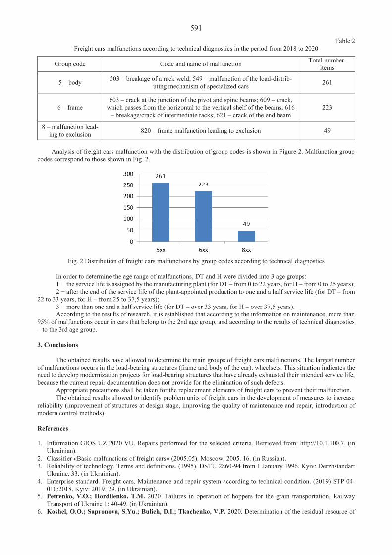
591Table 2

Freight cars malfunctions according to technical diagnostics in the period from 2018 to 2020

Group code Code and name of malfunction Total number, items

5 – body 503 – breakage of a rack weld; 549 – malfunction of the load-distrib-uting mechanism of specialized cars 261

6 – frame603 – crack at the junction of the pivot and spine beams; 609 – crack,

which passes from the horizontal to the vertical shelf of the beams; 616 – breakage/crack of intermediate racks; 621 – crack of the end beam

223

8 – malfunction lead-ing to exclusion 820 – frame malfunction leading to exclusion 49

Analysis of freight cars malfunction with the distribution of group codes is shown in Figure 2. Malfunction group codes correspond to those shown in Fig. 2.

Fig. 2 Distribution of freight cars malfunctions by group codes according to technical diagnostics

In order to determine the age range of malfunctions, D and H were divided into 3 age groups:1 the service life is assigned by the manufacturing plant (for D – from 0 to 22 years, for H – from 0 to 25 years);2 after the end of the service life of the plant-appointed production to one and a half service life (for D – from

22 to 33 years, for – from 25 to 37,5 years);3 more than one and a half service life (for D – over 33 years, for H – over 37,5 years).According to the results of research, it is established that according to the information on maintenance, more than

95% of malfunctions occur in cars that belong to the 2nd age group, and according to the results of technical diagnostics – to the 3rd age group.

3. Conclusions

The obtained results have allowed to determine the main groups of freight cars malfunctions. The largest number of malfunctions occurs in the load-bearing structures (frame and body of the car), wheelsets. This situation indicates the need to develop modernization projects for load-bearing structures that have already exhausted their intended service life, because the current repair documentation does not provide for the elimination of such defects.

Appropriate precautions shall be taken for the replacement elements of freight cars to prevent their malfunction.The obtained results allowed to identify problem units of freight cars in the development of measures to increase

reliability (improvement of structures at design stage, improving the quality of maintenance and repair, introduction of modern control methods).

References

1. Information GIOS UZ 2020 VU. Repairs performed for the selected criteria. Retrieved from: http://10.1.100.7. (in Ukrainian).

2. Classifier «Basic malfunctions of freight cars» (2005.05). Moscow, 2005. 16. (in Russian).3. Reliability of technology. Terms and definitions. (1995). DSTU 2860-94 from 1 January 1996. Kyiv: Derzhstandart

Ukraine. 33. (in Ukrainian).4. Enterprise standard. Freight cars. Maintenance and repair system according to technical condition. (2019) STP 04-

010:2018. Kyiv: 2019. 29. (in Ukrainian).5. Petrenko, V.O.; Hordiienko, T.M. 2020. Failures in operation of hoppers for the grain transportation, Railway

Transport of Ukraine 1: 40-49. (in Ukrainian).6. Koshel, O.O.; Sapronova, S.Yu.; Bulich, D.I.; Tkachenko, V.P. 2020. Determination of the residual resource of

592 carrying metal frames of cars of hopper dosers and dumpcars (dumpers) based on the results of technical diagnostics and typical tests, Collection of scientific works of the SUIT, Series “Transport Systems and Technologies” 35: 14-23. (in Ukrainian).

7. Bolotin, M.M.; Vorotnikov, V.G. 2012. Failures and lifetime of a freight car, World of Transport 2: 152-161. (in Russian).

8. Muradian, L.A.; Shaposhnyk, V.Yu.; Pitsenko, I.V.; Podosenov, D.O. 2019. Research of malfunctions of passen-ger cars, The Modern Movement of Science: Abstracts of the IX International Scientific and Practical Internet Con-ference, 2-3 december 2019 – Dnipro. Part II: 548-553. (in Ukrainian).

9. Koshel, O.; Sapronova, S.; Bulich, D.; Tkachenko, V. 2020. Determination of the Load-Bearing Metal Structures Residual Operation Time of the Ukraine Railway, Proceedings of 24th International Scientific Conference Transport Means 2020: Sustainability: Research and Solutions Part I: 228-232.

10. Dependability in railway technics. General concepts. Terms and definitions. (2016). GOST 32192-2013 from 1 July 2014. Moscow: Standartinform. 35. (in Russian).

11. Operation, maintenance and repair of railway rolling stock. Terms and definitions. (2019). GOST 32884-2014 from 1 May 2015. Moscow: Standartinform. 15. (in Russian).

593

Proceedings of 25th International Scientific Conference. Transport Means 2021. Increasing Resilience of Critical Infrastructure Subjects Providing Transport Services M. Luskova1, B. Leitner2

1University of Žilina, Univerzitna 8215/1, 010 26 Žilina, Slovakia, E-mail: Maria.Luskova@uniza.sk 2University of Žilina, Univerzitna 8215/1, 010 26 Žilina, Slovakia, E-mail: Bohus.leitner@uniza.sk Abstract Transport infrastructure and services provided in transport are an integral part of the daily life of the population. The paper addresses the issue of increasing the resilience of critical entities providing essential services in line with the proposal for a Directive of the European Parliament and of the Council COM (2020) 829 on the resilience of critical entities which is due to enter into force in 2022. The paper presents the responsibilities of Member States and critical entities in terms of increasing their resilience to current and supposed future risks, a framework for assessing the resilience of critical entities, identification of critical entities in the transport sector and proposal of possible adaptive measures to increase the resilience of road and rail transport to the adverse effects of climate change. KEY WORDS: resilience, critical infrastructure, transport, extreme weather 1. Introduction

Today, the term critical infrastructure is relatively new but the systems and services necessary for people's lives have existed for centuries. Critical infrastructure has played an important role in the distant past. Its protection has been dealt with by ancient civilizations. There are known histories of strategies aimed at protecting one's own critical infrastructure from danger or destroying enemy infrastructure, especially during war.

In recent decades, the risk of critical infrastructure disruption has been steadily increasing for reasons [1]: Decreasing state control due to the liberalization and privatization of infrastructures. The growing use of information and telecommunications technologies (ICT) to support, monitor and control

the functionality of critical infrastructure. Urbanization, which emphasizes the use of old infrastructures for as long as possible. Growing interconnections, chaining and dependencies of infrastructure services. Enemies of society who increasingly understand that a successful attack can cause disaster.

ICT combined with easy access to the Internet have added a new dimension to critical infrastructure protection. The physical infrastructure has suddenly become vulnerable not only to conventional methods of destruction but also the state-of-the-art technical networks that run it, have become a potential target for terrorists, criminals, disloyal employees and other criminal elements. A number of technological and societal changes have meant that infrastructures, which in the past were autonomous vertically integrated systems with very little interconnection with other infrastructures, are now tightly interconnected and have a large number of dependencies. While this has had many positive impacts on society, it has also increased the complexity and vulnerability of infrastructures and the associated risk to society.

In addition to the above, a very serious and immediate problem today is climate change and its negative consequences. The current approach to climate change is based on the synergy of mitigation and adaptation measures. While mitigation is a set of activities aimed at long-term and sustainable reducing of greenhouse gas emissions, adaptation aims to mitigate the adverse effects of climate change, reduce vulnerability and increase the adaptive capacity of natural and man-made systems to current or expected negative effects of climate change [2].

The European Union has been addressing the issue of critical infrastructure (CI) for a long time. The process of critical infrastructure protection has been going on since 2004, within the framework of which several documents were prepared, in which prevention, preparedness and responses to threats threatening CI were addressed, focusing mainly on the threat of terrorism. Important outcomes of this process include Council Directive 2008/114/ EC of 8 December 2008 on the identification and designation of European critical infrastructure and the assessment of the need to improve their protection. The directive was evaluated in 2019 and an important result was the finding that due to the number of changes in the operational environment of CI entities, protective measures are insufficient and it is necessary to focus on the resilience of critical entities.

2. Proposal for a Directive of the European Parliament and of the Council on the Resilience of Critical Entities,

COM (2020) 829

As significant changes have taken place in the operational environment of CI entities in recent years and the risk of disruption to basic services has been steadily increasing, it has become necessary to fundamentally change the current approach to CI protection introduced in 2008 and move from infrastructure protection to increasing the resilience of

594 critical entities.

A revised approach to CI resilience, which better reflects the current and expected future risk environment, the increasingly interdependence of different sectors, as well as the increasingly interdependent relationships between physical and digital infrastructures, is also a priority for the EC and the EU Security Union Strategy. Based on the above mentioned facts, on 16 December 2020, the EC published the Proposal for a Directive of the European Parliament and of the Council COM (2020) 829 on the resilience of critical entities. That Directive lays down the obligations of Member States and operators of CI elements.

The main obligations of the Member States under the Directive include [3]: the adoption of a strategy to strengthen the resilience of critical entities within three years of the entry into

force of this Directive. The strategy needs to define strategic objectives and priorities aimed at achieving and maintaining a high level of resilience of critical entities, identify critical entities and measures to support these entities. Critical entities must cover the minimum sectors listed in Table 1;

an assessment of the relevant risks that may affect the provision of basic services within three years of the entry into force of the Directive and thereafter as necessary, but at least every 4 years;

creation of a list of identified critical entities, information on their obligations; support of critical entities e.g. in the form of advisory material, in connection with the organization of exercises

to test their resilience and provide training to employees of critical entities. The main obligations of critical entities under the Directive include [3]: assessment of all relevant risks that may disrupt the operations of critical entities within six months of receipt

of the notification of classification as critical entities; adoption of appropriate and proportionate technical and organizational measures to ensure its resilience; implementation of a resilience plan describing the relevant technical and organizational measures; reporting incidents that significantly disrupt or may significantly disrupt their operations.

Table 1

Critical Entities Sectors under Directive COM (2020) 829 on Critical Entity Resilience

Sector Subsectors 1. Energy Electricity, district heating and cooling, oil, gas, hydrogen. 2.Transport Air, rail, water, road. 3. Banking 4. Financial market infrastructures 5. Health 6. Drinking water 7. Waste water 8. Digital infrastructure 9. Public administration 10. Space

3. Framework for Assessing the Resilience of Critical Entities

The issue of resilience is a very current and extensive topic which is addressed in various scientific disciplines, e.g. in psychology, medicine, economics, environmental sciences, safety and other disciplines. There are a number of definitions of resilience with application potential in infrastructure systems in the literature. Many commonalities can be found within these definitions. They are all based on the condition of resisting change, and also many cite adaptation, absorption, and recovery as factors influencing the level of resilience [4].

The starting point for the proposal of technical and organizational measures that contribute to increasing the resilience of critical entities in the transport sector can be the approach to the assessment of resilience of critical entities developed in the CIERA methodology [5].

According to this methodology, the resilience of a critical entity is defined as its internal preparedness for adverse events, or the ability of the entity to ensure and maintain its functions even during the negative effects of external and internal factors. A similar understanding of resilience is presented by Allenby and Fink (2005) who define resiliency as a capability of a specific system to maintain its structure and functions during exposition to internal and external changes [6].

The assessment of the resilience of critical entities (Fig. 1) is made on the basis of data related to [5]: basic structural and performance parameters of the evaluated critical subject (topological and technological

structure); applied safety and security measures (crisis preparedness, redundancy, detection capability, response

capability, physical resilience, material, financial and human resources, recovery processes); resilience-enhancing processes (risk management, innovation processes, education and development

processes); the specific adverse events against which resilience is assessed (natural, human hazards, technical hazards).

595

Fig. 1 Framework for assessing the resilience of critical entities

According to the CIERA methodology [5], the resilience of a critical entity integrates two basic areas of resilience, namely technical and organizational resilience. Technical resilience is formed by elements that are part of the applied security measures, organizational resilience is formed by elements of processes that strengthen resilience. The overall level of resilience of a critical entity is determined on the basis of a set of relevant indicators defined within individual areas of technical and organizational resilience. In case of insufficient level of resilience of the subject according to predetermined criteria, it is necessary to identify and analyse weaknesses and security deficits and take appropriate technical and organizational measures to increase the resilience of the subject, based on decomposition of evaluation results.

4. Identification of Critical Entities in the Transport Sector

The aim of the proposal for a Directive of the European Parliament and of the Council on the resilience of critical entities COM (2020) 829 is to ensure a more coherent approach to the resilience of critical entities in several sectors across the European Union. One of the obligations of the Member States is to identify the critical entities for the sectors and subsectors given in Table 1.

The following criteria need to be applied when identifying critical entities: the entity provides one or more basic services; the provision of this service depends on the infrastructure located in a Member State; the incident would have a serious disruptive effect on the provision of the service or other basic services in

the sectors given in Table 1 which depend on the service. Within the Transport sector, four sub-sectors are identified: air, rail, waterborne and road transport. The overview

of critical entities in road and rail transport subsectors is given in Table2.

Table 2 Overview of critical entities in road and rail transport subsectors [3]

Sector Subsector Critical entities

Transport Road Road authorities responsible for road traffic control. Operators of intelligent transport systems.

Rail Infrastructure managers. Railway undertakings.

In road transport: A road authority is any public authority responsible for planning, controlling or managing roads which fall

within its territorial jurisdiction [6]. Intelligent Transport Systems "or" ITS "are systems in which information and communication technologies are

CRITICAL ENTITY

RESILIENCE ASSESSMENT

Security measures

Processes

Adverse event

Structural and performance parameters

596 applied in the field of road transport, including infrastructure, vehicles and users, and in the field of traffic management and mobility management, as well as for interfaces with other modes of transport [7].

In railway transport: "infrastructure manager" means a body or undertaking that is responsible in particular for establishing,

managing and maintaining railway infrastructure, including traffic management, control and signalling. The function of infrastructure manager on a network or part of a network may be entrusted to different authorities or undertakings [8];

“railway undertaking” means any public or private undertaking licensed under the Directive (8), the principal activity of which is to provide services for the transport of goods and / or passengers by rail, with traction; this includes undertakings which only provide traction [8];

“service facility operator” means any public or private entity responsible for the management of one or more service facilities or for the provision of one or more of the services listed in Annex II, points 2 to 4 of Directive 2012/34 / EU to a railway undertaking [9]. 5. Resilience of Critical Entities in the Transport Sector to the Adverse Effects of Climate Change

Extreme weather events in road and rail transport occur immediately and often with significant negative consequences, as they lead to increased transport time for the transport of goods, longer travel time and an increased likelihood of accidents and damage to transport infrastructure. High and low temperatures, intense storms with the consequent occurrence of floods and snow calamities which increase in frequency and intensity due to climate change, cause serious complications for all modes of transport [10].

For the conditions of the Slovak Republic, the negative consequences of climate change relate mainly to road transport infrastructure (less rail transport), especially in connection with intense storm showers and the subsequent emergence of flood situations, whether at local or regional level. Risk elements are mainly drainage and sewerage systems and parts of roads in the immediate vicinity of watercourses. Extremes of weather not only lead to damage to transport infrastructure, but also cause significant damage in connection with the economic consequences of loss of functionality and performance. The consequences of climate change and examples of adaptation measures in road and rail transport are given in Table 3.

Table 3

Consequences of climate change and examples of adaptation measures in road and rail transport

Transport Consequences of climate change Possible adaptation measures

Road Outages of roads. Damage to road infrastructure. Increase in the number of traffic accidents. Increased requirements for winter maintenance. Blocking in traffic routes due to slope landslides.

Modification of an asphalt mixture resilient to increasing extreme weather events. Improving surface and subsurface drainage systems. Optimization of projects and maintenance strategies with an impact on quality. Ensuring the stability of notch slopes, elimination of landslide activity and potential traffic hazards.

Rail Increased requirements for winter maintenance, damage to tracks and switches. Blocking in railway track due to landslides.

Carry out targeted engineering and geological surveys in landslide-prone areas. Preventive felling of trees and removal of vegetation and grass around the entire perimeter of the track to reduce the risks associated with extreme weather events. Building protective barriers in geologically and weather-hazardous areas.

6. Conclusions

Transport infrastructure and services provided in transport affect the way of life of every inhabitant. The continuous development of the transport sector is also a necessary condition for the successful development of each country, as its consequences affect other sectors. Emergency events, in the Slovak Republic it is especially extreme weather conditions, have demonstrated the need to increase the resilience of the transport system. Therefore, in line with the proposal for a directive COM (2020) 829, the most important role of the transport sector is to increase the resilience of transport entities and thus contribute to the creation of a reliable transport infrastructure that will connect the individual regions of the country. At the same time, preconditions will be created so that employees, facilities and equipment, information systems that are critical for the functioning of the society, do not cease to fulfil their function in any risk and threat scenarios.

597 Acknowledgement

This work has been supported by VEGA grant 1/0371/19 Societal vulnerability assessment due to failure of important systems and services in electricity sector and by VEGA grant No. 1/0159/19 Assessment of the resilience level of the key elements in the land transport infrastructure. References 1. Setola, R.; et al. 2016. Managing the Complexity of Critical Infrastructures. A Modelling and Simulation Approach.

Springer Open. ISSN 2198-4190. 2. VUD. 2018. Methodological guide to assessing the impacts of climate change on large projects in the transport sector.

[online cit.: 2021-05-06]. Available from: https://www.opii.gov.sk/download/f/zmena_ klimy/metodicka_prirucka_ posudzovania_dopadov_zmeny_klimy.pdf

3. EC. 2020. Proposal for a Directive of the European Parliament and of the Council COM (2020) 829 on the resilience of critical entities. [online cit.: 2021-04-30]. Available from: https://eur-lex.europa.eu/legal-content/EN/TXT/HTML/ ?uri=CELEX:52020PC0829&from=EN

4. Biringer, B.; Vugrin, E.; Warren, D. 2013. Critical Infrastructure System Security and Resiliency. ISBN 9781466557505. Published April 16, 2013 by CRC Press, 229 p.

5. Rehak, D.; et al. 2018. Critical Infrastructure Elements Resilience Assessment. [online cit.: 2021-05-06]. Available from: https://www.researchgate.net/profile/David-Rehak/publication/324210621_Metodika_hodnoceni_resilience_ prvku_kriticke_infrastruktury/links/5b1fd0d3458515270fc56389/Metodika-hodnoceni-resilience-prvku-kriticke-infrastruktury.pdf

6. Allenby, B.; Fink, J. 2005. Toward Inherently Secure and Resilient Societies. [online cit.: 2021-05-10]. Available from: https://www.researchgate.net/publication/7660506_Toward_Inherently_Secure_and_Resilient_Societies

7. EC. 2014. COMMISSION DELEGATED REGULATION (EU) 2015/962 of 18 December 2014 supplementing Directive 2010/40/EU of the European Parliament and of the Council with regard to the provision of EU-wide real-time traffic information services. [online cit.: 2021-05-11]. Available from: https://eur-lex.europa.eu/legal-content/EN/TXT/PDF/?uri=CELEX:32015R0962&from=SK

8. EC. 2010. Directive 2010/40/EU of the European Parliament and of the Council of 7 July 2010 on the framework for the deployment of Intelligent Transport Systems in the field of road transport and for interfaces with other modes of transport. [online cit.: 2021-05-11]. Available from: https://eur-lex.europa.eu/legal-content/EN/ALL/?uri= CELEX%3A32010L0040

9. EC. 2012. DIRECTIVE 2012/34/EU OF THE EUROPEAN PARLIAMENT AND OF THE COUNCIL of 21 November 2012establishing a single European railway area. [online cit.: 2021-05-11]. Available from: https://eur-lex.europa.eu/legal-content/EN/TXT/PDF/?uri=CELEX:32012L0034&from=SK

10. Durech, P.; Sventekova, E.; Ballay, M. 2017. Process of Organizations Renewal Damaged Way Interaction of Extraordinary Events in Consideration of Increase in Security Population, Transport Means Proceedings of the international conference, 968-972, ISSN: 1822-296X.

598

Proceedings of 25th International Scientific Conference. Transport Means 2021. Watering of Cargo for Reducing Dust Emissions from Coal Wagon M. Biliaiev1, V. Kozachyna2, V. Biliaieva3, O. Berlov4, P. Mashykhina5, S. Tyshchenko6 1Dnipro National University of Railway Transport named after Academician V. Lazaryan, Lazaryan st. 2, 49010, Dnipro, Ukraine, E-mail: diit.hydro.eco@gmail.com 2Dnipro National University of Railway Transport named after Academician V. Lazaryan, Lazaryan st. 2, 49010, Dnipro, Ukraine, E-mail: v.kozachyna@gmail.com 3Oles Honchar Dnipro National University, Haharin ave. 72, 49010, Dnipro, Ukraine, E-mail: vika_lulu@mail.ru 4Prydniprovska State Academy of Civil Engineering and Architecture, Chernyshevsky st. 24a, 49600, Dnipro, Ukraine, E-mail: berlov.oleksandr@pgasa.dp.ua 5Dnipro National University of Railway Transport named after Academician V. Lazaryan, Lazaryan st. 2, 49010, Dnipro, Ukraine, E-mail: gidro_eko@ukr.net 6Dnipro State Agrarian and Economic University, Serhii Efremov st. 25, 49600, Dnipro, Ukraine, E-mail: voloskrs@i.ua Abstract Open topped coal wagons are widely used in different countries. The coal surface exposed to air emits intensively fugitive dust. Water application is used for reducing fugitive dust emissions from open topped coal trains. The objective of this research was to develop numerical model to study efficacy of water application on the surface of coal. To simulate air flow over coal wagon Euler equations were used. These equations were written in Helmholtz variables “vorticity–flow function”. Finite difference schemes of splitting were used for numerical integration of Euler equations. To simulate coal dust dispersion from coal wagon mass transfer equation was used. This equation took into account air flow speed, turbulent diffusion, dust emission rate from cargo surface. To solve mass transfer equation change-triangle implicit difference scheme of splitting was used. To simulate water evaporation from cargo and dust emission rate dependence from moisture, empirical models were used. On the basis of developed numerical model computer code was developed using FORTRAN. Results of numerical experiments are presented. KEY WORDS: coal wagon, watering of cargo, atmosphere pollution, numerical simulation 1. Introduction

Coal dust emissions from trains have been the subject of many studies in the world [1-6]. Emissions of particulate matter in the form of coal dust impact ambient air quality in transport corridor. Coal dust may contain traces of heavy metals. This coal dust is toxic for human being and people who live near the transport corridor and can be affected. Coal transportations by trains may have cumulative impact on people. That is why much attention is put to the development of different methods to reduce coal dust pollution. To reduce coal dust emissions different methods are used: load profiling of coal surface, veneering, application of special covers on the wagon, etc [1, 2]. One of the simplest approaches to reduce coal dust emissions is watering of cargo in the wagon. But during transportation water is evaporated from the cargo and coal dust emissions increase. That is why it is important to know time period when "protection" function of this method is vanished. Mathematical simulation is a powerful method to solve this problem 2. Mathematical Model

Coal dust is emmited from the surface of cargo in coal wagon. To simulate coal dust dispersion in atmosphere convective-diffusion equation was used [10, 12]:

1

i i i

Nv w CC uC div gradC Q t x x y yt x y i

(1)

where C is coal dust concentration; ,x y are coefiicients of turbulent diffusion; Q is coal dust emission rate from the

cargo surfaceIt is considered that, , ,i iQ f x y M ; M is moisture content; ,i ix y are Cortesian coordinates;

i ix x y y is Dirac delta-function; w is gravitation fallout; t is time. Surface of cargo is modelled using point sources and Delta function. Parameters ,x y are computed using empirical formulae [11]. Initial and boundary conditions for governing

equations are discussed in [10]. There are different formulas to calculate coal dust emissions from the coal surface. As a rule, these are empiric

599 formulas. In this work to calculate coal dust emission rate the following empiric formula was used [6]: 4,2 ( ),tQ V V (2) where tV is threshold speed; V is wind local velocity over the coal surface.

Watering of coal surface in the coal wagon changes coal moisture. Addition moisture enlarges the threshold wind velocity tV and that results in decreasing of emission rate. If moisture is large the emission rate is small. For practice, it is important to find out the relationship between emission rate and moisture or the relationship between moisture and threshold wind velocity. As a rule, empiric models are used to describe such relationship for different substances. For instance, relationship between moisture and threshold speed tV of sandy loam can be described as following [7]: 1,584,97 0,268tV W . (3)

During coal wagon movement moisture content decreases as the result of water evaporation. The more coal train speed the bigger is the evaporation process. To describe this process the following empiric relation was used [8]: 5,83 4,1w HQ V P M , (4) where wQ is water evaporation rate (g/(m2h)), V is local wind velocity near the surface of coal; HP is water vapor saturation pressure; is water molecular mass.

If we supplied water volume watW on the coal surface coalS , then the depth of water penetration can be calculated as following:

watwat

coal coal

WhS P

,

where coalP is porosity.

Change of coal moisture as a result of watering can be defined as:

100%n

n

coal

MWM

,

where coalM is coal mass in watering zone; 0

n nwaterM M m is mass of water in coal at current time step;

n nwaterM W ; is water density; 0m is initial water mass in this zone before watering.

Moisture content in coal will be changed during time as a result of evaporation and it can be calculated as following:

1 0 100%n

n

coal

M dmW

M,

where dm0 is evaporated mass of water during time period dt; n

waterM is mass of water in coal at previous time step. To apply the empiric models (Eq. (2), Eq. (4)) it is necessary to compute local wind velocity at the surface of the

cargo. This surface has a complex geometrical form and wind local velocity is different at different points of cargo surface. To simulate wind flow over the coal wagon with cargo Euler’s equations were used. These equations were written using Helmholtz variables [9]:

0u vt x y ; (5)

2 2

2 2x y, (6)

v x u y is vorticity; is flow function; ,u y v x are velocity components. Initial and boundary conditions for Eq. (5), Eq. (6) are discussed in [9]. For numerical integration of governing equations rectangular grid was used. To "create" geometrical form of

600 cargo in the coal wagon markers ("porosity technique") were used.

To solve numerically Eq. (5) two steps finite difference scheme of splitting was used [9]:

– at the first step of splitting finite difference equation was as follows ( 12

k ):

, , 0;k ni j i j k k

x yL Lt

(7)

– at the second step of splitting finite difference equation was as follows ( 12

k ):

1

, , 1 1 0.n ki j i j n n

x yL Lt

(8)

In Eq. (9), Eq. (10) the following relations were used:

,u u ux x x

,v v vy y y

, ,2 2

u u u uu u

, ,2 2

v v v vv v

1 1

1, , , 1, 1,n n

i j i j i j i j nx

u uu Lx x

1 1

1, 1, , , 1,n n

i j i j i j i j nx

u uu Lx x

1 1

, 1 , , , 1 1,n n

i j i j i j i j nyL

y y

1 1

, 1 , 1 , , 1.n n

i j i j i j i j nyL

y y

Parameter " " was calculated from Eq. (9), Eq. (10) using explicit formulas of "running calculation" [9]. To solve Eq. (6) the following finite difference scheme was used [12]:

1, , , , 1, , , 1, , , , 1,2 2

2 2i j k i j k i j k i j k i j k i j kijx y

. (9)

Wind velocity compionents were calculated as follows:

, 1 , 1, ,, ,, .i j i j i j i j

i j i ju vy x

To solve numerically Eq. (1) it was split preliminarily as follows:

0C uC Ct x y

(10)

601

x y

C C Ct x x y y

(11)

( ) ( )i i iC Q x x y yt

(12)

We use here designation w . At the next step the following approximations were made [9]:

,uC u C u Cx x x

,vC v C v Cy y y

, ,2 2

u u u uu u

, ,2 2

v v v vv v

1 1

1, , , 1, 1n n

i j i j i j i j nx

u C u Cu C L Cx x

,

1 1

1, 1, , , 1,n n

i j i j i j i j nx

u C u Cu C L Cx x

1 1

, 1 , , , 1 1,n n

i j i j i j i j ny

C CC L Cy y

1 1

, 1 , 1 , , 1.n n

i j i j i j i j ny

C CC L Cy y

Finite difference scheme of splitting to solve Eq. (13) was as follows :

– at the first step of splitting finite difference equation was as follows ( 12

k ):

, , 0k ni j i j k k

x y

C CL C L C

t; (13)

– at the second step of splitting finite difference equation was as follows ( 12

k ):

1

, , 1 1 0n ki j i j n n

x y

C CL C L C

t. (14)

From Eq (13), Eq (14) parameter "C" was computed using explicit formulas of "running calculation" [9, 12]. To solve numerically Eq. (11) two steps difference scheme of splitting was used [12]: – at the first step of splitting finite difference equation was as follows:

1 1 1 1 12 2 2 2 2

, , , 1, , , 12 2 ,

n n n n nni j i j i j i j i j i jC C C C C C

t x y

– at the second step of splitting finite difference equation was as follows:

6021

1 1 1 1 12, , 1, , , 1 ,

2 2 .nn n n n n

i j i j i j i j i j i jC C C C C Ct x y

From these dependencies, parameter "C" was computed using explicit formulas of "running calculation".Euler’s method was used for numerical integration of equation (13):

1 ( ) ( )n nij ij i i iC C t Q x x y yii ((Q (i (t .

Computer code was developed on the basis of created numerical model. FORTRAN language was used for coding.

3. Results

Fig. 1-3 show coal dust concentration near the wagon for different time steps. The initial water content in coal was 4%. It was supposed that 1 liter of water was supplied on 1 m2 of coal surface. Wind velocity was 18m/s, gravitational fallout was 0.001 m/sec. Computational domain was 33 m×21 m.

Every number in Fig. 1 – Fig. 3 shows concentration in percent from concentration C = 120 mg/m3, which corresponds to the maximum coal dust concentration in computational region for the case without watering. This approach allows to analyze quickly concentration field change near the coal wagon for every specific time step.

Fig. 1 Coal dust concentration near the wagon, t = 200 sec:1 – dust concentration in the range 1.2 mg/m3–3.6 mg/m3

Fig. 2 Coal dust concentration near the wagon, t = 2889 sec: 1 – dust concentration in the range 1.2 mg/m3–8.4 mg/m3

Fig. 3 Coal dust concentration near the wagon, t = 4699sec:1 – dust concentration in the range 1.2mg/m3–10.8mg/m3

From these Figures one can see that water evaporation from coal surface results in increasing of dust concentration near the coal wagon. During 75 min (from time t = 200 sec till time t = 4699 sec) maximum concentration increased in 3 times. It means that mitigating "capacity" of coal watering in wagon decreased quickly.

Worthy of note that computational time was 10sec.

603 4. Conclusions

In short, a new numerical model was developed to compute ambient air pollution from coal trains. The model allows taking into account the effect of coal watering on the intensity of ambient air pollution. The developed numerical model takes into account the most important physical factors which affect the coal dust

pollution during coal transportation. To predict wind flow over the coal wagon Euler equations were used. This approach allows predicting wind flow

pattern over the coal wagon in 10 sec. A developed numerical model can be used to assess the efficiency of coal watering in the wagon to reduce

ambient air pollution. References 1. Ferreira, A.D.; Viegas, D.X.; Sousa, A.C.M. 2003. Full-scale measurements for evaluation of coal dust release

from train wagons with two different shelter covers, Journal of Wind Engineering and Industrial Aerodynamics 91(10): 1271-1283.

2. Ferreira, A.D.; Vaz, P.A. 2004. Wind tunnel study of coal dust release from train wagons, Journal of Wind Engineering and Industrial Aerodynamics 92(7-8): 565-577.

3. Final Report Environmental Evaluation of Fugitive Coal Dust Emissions from Coal Trains. Goonyella, Blackwater and Moura Coal Rail Systems. Queensland Rail Limited, Queensland Government Environmental Protection Agency, Queensland [online cit.: 2008-04-08]. Available from: https://majorprojects.planningportal.nsw.gov.au/ prweb/PRRestService/mp/01/getContent?AttachRef=MP09_0024%2120190814T054754.584%20GMT

4. Final Report on the Independent Review of Rail Coal Dust Emissions Management Practices in the NSW Coal Chain. NSW Chief Scientist & Engineer, Sydney [online cit.: 2016-08-01]. Available from: https://www.chiefscientist.nsw.gov.au/__data/assets/pdf_file/0008/89864/160805-FINAL-Coal-Dust-Report.pdf.

5. Literature Review of Coal Train Dust Management Practices. NSW Environment Protection Authority [online cit.: 2014-12-01]. Available from: https://www.epa.nsw.gov.au/~/media/EPA/Corporate%20Site/resources/epa/coaltrain-litreview.ashx.

6. Biliaiev, M.M.; Kozachyna, V.A.; Oladipo, M.O. 2019. Numerical analysis of atmosphere pollution from coal train, East European Scientific Journal 3(43): 10-15.

7. Chen, W.; Dong, Z. 1996. Wind Tunnel Test on the Influence of moisture on the Erodibility of loessial loam soil by wind, Journal of Arid Environments 34: 391-402.

8. , . . 1959. , . M : , 231 . (in Russian)

9. , . .; , . .; , . .; , . . 1997. . : . , 368 . (in Russian)

10. , . . 2000. . : , 443 . (in Russian)

11. Biliaiev, M.; Kozhachyna, V.; Biliaieva, V.; Oladipo, M.O.; Chernyatyeva, K. 2019. Modeling of the Atmosphere Pollution from Coal Trains, MATEC Web of Conferences, Vol. 294: 2nd International Scientific and Practical Conference Energy-Optimal Technologies, Logistic and Safety on Transport, Lviv: 1-7.

12. , . . 1983. . : , 616 . (in Russian).

604

Proceedings of 25th International Scientific Conference. Transport Means 2021. Comparative Analysis of Options for Strengthening the Railway Subgrade with Vertical Elements O. Tiutkin1, R. Keršys2, L. Neduzha3 1Dnipro National University of Railway Transport named after Academician V. Lazaryan, Lazaryan St. 2, 49010, Dnipro, Ukraine, E-mail: alexeytutkin@gmail.com 2Kaunas University of Technology, Studentu st. 56, 51424, Kaunas, Lithuania, E-mail: robertas.kersys@ktu.lt 3Dnipro National University of Railway Transport named after Academician V. Lazaryan, Lazaryan St. 2, 49010, Dnipro, Ukraine, E-mail: nlorhen@i.ua Abstract In paper the task set to investigate and determine the impact of the parameters for strengthening with vertical elements (piles) on the stress and displacement of the track superstructure. The scientific hypothesis is the possibility of selecting such parameters of these elements that minimally affect the stress state of the track superstructure. For this finite-element models of two options for strengthening have been developed. Using a professional complex at different values of deformation characteristics values of displacements and stresses were obtained. The analysis of the stress-strain state for both options reveals that the more effective option of strengthening the subgrade. It has a more positive effect on the deformation state of the subgrade, reduces the vertical displacement of the track superstructure, reduces its stress state, the value of which allows us to testify to the normal operation of the subgrade. KEY WORDS: subgrade, base, track superstructure, deformation parameters,numerical analysis, stress-strain state 1. Introduction

The main issue in the normal operation of transport facilities that use soil as a building material (in particular, railways, roads, and airfields) is establishing a security system for the overall transport structure. This issue is analyzed in many countries with advanced transportation systems [1-3]. This system consists of elements, each of which contributes to the overall security. The main elements of the railway safety system are the track superstructure (TS), subgrade (S), rolling stock (RS) and its base, at this TS in turn also consists of several elements (rails, fastenings, sleepers, etc.). Thus, the safety system of the overall transport structure consists of numerous subsystems that require comprehensive analysis, the results of which will help to improve the safety of railway traffic.

It should be noted that namely the comprehensive analysis is the most representative, since only the consideration of the general "RS – TS – S" system can provide with the results that are adequate to the real interaction between the RS and the supporting structure consisting of the TS, the S and the soil base of the S. However, such significant analysis requires large computational complexes and its full implementation is complex [4-6]. Therefore, a "piece by piece" analysis seems more realistic, each of which should be implemented as fully and adequately as possible to the specific transport situation.

The "piece by piece" analysis envisages the research of stress-strain state (SSS) for each of the parts in the "RS – TS – S". First, the operation of the RS, which is characterized by significant dynamic loads, is analyzed, then the obtained data are transmitted in the form of impacts on a part in the "TS – S" system [7-10]. In this case, there is no separation of the parts in the system with the loss of one of them, since the characteristics of the RS are determined taking into account the features of the TS, for example, geometrical irregularities and rails unevenness, their geometric position in the plane (circular and transition curves), TS parameters, spatial impact of the wheel on the rail, rail defects, etc [11-14].

An important part of the research that provides the opportunity to correct theoretical foundations is physical simulation [15-17]. Simulation and mathematical modeling as a research tool requires data, obtained from nature or a physical experiment. The use of these data allows us to obtain more comprehensive behavioral parameters of both RS and "TS – S" systems but requires complex mechanical installations such as testing benches [18-20]. It should also be emphasized that the experimental data are incomplete as they require a theoretical justification. Therefore, the most effective in the study is the combination of theoretical and experimental research methods.

Taking into account the particularities in the research of RS, it is necessary to examine the characteristic tasks while analyzing the "TS – S" system. The main task for the normal operation of this system is to ensure the normative deformation characteristics of the S, which stabilize the impact from the RS, counteract the emergence of deformations and defects and work together with the TS as an elastic system. But in the real cases, there are disagreements with the providing of performance standards, which leads to an increase in the number of TS repairs, the emergence of the S deformations and the overall decrease in traffic safety.

605 2. Methodology

Strengthening the S using various technologies has a positive effect on its SSS. Such technologies include the placing layers of low-deformable material, reinforcement based on the geosynthetic elements, strengthening with vertical or inclined elements, made on the basis of drilling-mixing technology or jet-grouting technology. As a result, a decrease in deformations is observed, which is explained by an increase in the total stiffness of the "TS – S" system, obtained by immersing different types of elements (piles, geotextiles, layers of different deformation capacity, and so on) into the soil of the S.

This research examines the change in stresses and displacements of the "TS – S" system when strengthening the railway subgrade with vertical elements – piles (Fig. 1, a).

a

b c

Fig. 1 a – one of the characteristic schemes of strengthening the S with vertical elements; b – the design diagram of the strengthened S, general view; c – fragment of TS with vertical elements (piles)

However, such strengthening, significantly affects the stresses and displacements of the TS, for example, by

immersion of vertical elements (piles made on the basis of different technologies). In most cases, increasing the value of the modulus of elasticity in the system under consideration, after strengthening the S with piles, leads to an abrupt increase in the stiffness of the TS, which is problematic for its normal operation and safety of movement.

In this connection, the task is set to investigate and determine the impact of the parameters for strengthening the S with vertical elements (piles) on the stress and displacement of the track superstructure. The scientific hypothesis which forms the basis of this task is the possibility of selecting such parameters of these elements that maximize the deformation ability of the S and minimally affect the stress state of the TS. In this research two options for strengthening the S with vertical elements were considered: 1) near the rail (Option 1); 2) near the ballast section (Option 2). The total number of circuit nodes is 28 203 pieces (approximately 85 thousand degrees of freedom, so the task is considered large-scale), the number of finite element (FE) is 31 572 pieces, in the scheme they are accepted compatible, that is, all the nodes of neighboring elements agree, which positively affects the accuracy of the results.

Fig. 1, b presents a model of the "TS – S" system developed in the SCAD professional complex, which solves the task with the help of FEM. Fig. 1 c shows a fragment of TS with vertical elements (piles) – for understanding vertical elements are placed in the S. Model measurements are the following: length (base) – 40.6 m, width – 1.64 m, height – 11.1 m (the S height of which is 6 m). The deformation characteristics are selected in accordance with the deformation properties in the "TS – S" system. Fig. 2, a and Fig. 2, b shows a map of the deformation characteristics for FE models.

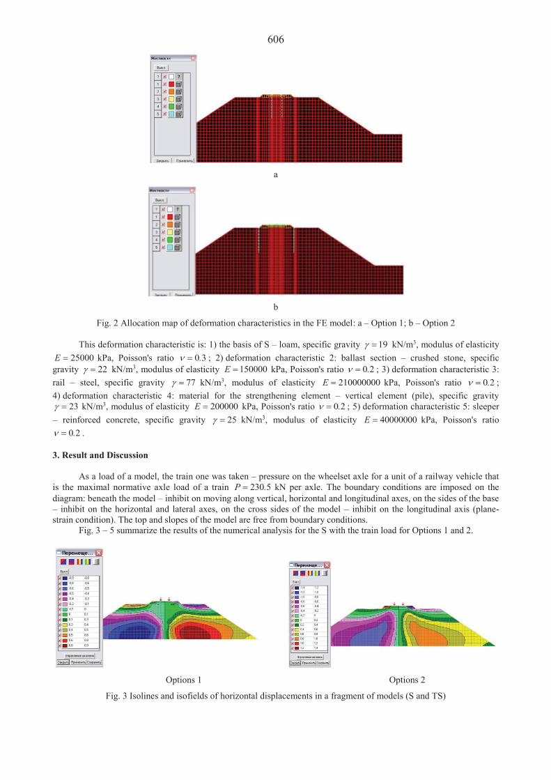
606

a

b

Fig. 2 Allocation map of deformation characteristics in the FE model: a – Option 1; b – Option 2

This deformation characteristic is: 1) the basis of S – loam, specific gravity 19 kN/m3, modulus of elasticity 25000E kPa, Poisson's ratio 0 3. ; 2) deformation characteristic 2: ballast section – crushed stone, specific

gravity 22 kN/m3, modulus of elasticity 150000E kPa, Poisson's ratio 0 2. ; 3) deformation characteristic 3: rail – steel, specific gravity 77 kN/m3, modulus of elasticity 210000000E kPa, Poisson's ratio 0 2. ; 4) deformation characteristic 4: material for the strengthening element – vertical element (pile), specific gravity

23 kN/m3, modulus of elasticity 200000E kPa, Poisson's ratio 0 2. ; 5) deformation characteristic 5: sleeper – reinforced concrete, specific gravity 25 kN/m3, modulus of elasticity 40000000E kPa, Poisson's ratio

0 2. . 3. Result and Discussion

As a load of a model, the train one was taken – pressure on the wheelset axle for a unit of a railway vehicle that is the maximal normative axle load of a train 230 5P . kN per axle. The boundary conditions are imposed on the diagram: beneath the model – inhibit on moving along vertical, horizontal and longitudinal axes, on the sides of the base – inhibit on the horizontal and lateral axes, on the cross sides of the model – inhibit on the longitudinal axis (plane-strain condition). The top and slopes of the model are free from boundary conditions.

Fig. 3 – 5 summarize the results of the numerical analysis for the S with the train load for Options 1 and 2.

Options 1 Options 2

Fig. 3 Isolines and isofields of horizontal displacements in a fragment of models (S and TS)

607

Options 1 Options 2

Fig. 4 Isolines and isofields of vertical displacements in a fragment of models (S and TS)

Options 1 Options 2

Fig. 5 Isolines and isofields of normal vertical stresses in a fragment of models (S)

The purpose of this research is to determine the effectiveness of the options. From the analysis of Fig. 4 it can be stated that the horizontal displacements in Option 1 are 1.56 times less than in Option 2 (Option 1 is 0.9 mm, Option 2 is 1.4 mm) (Fig. 3).

The placement of vertical elements near the ballast section (Option 2) qualitatively changes the pattern of displacement as opposed to the position near the rail (Option 1), more evenly distributing the horizontal stresses along the sod line of the S and its depth. If we consider the non-maximum displacement values, that in Option 2 they are observed in the angels of the ballast section, the mean values in both options of strengthening are almost the same.

Vertical displacements (Fig. 4) are quantitatively and qualitatively different: vertical displacements in Option 1 are 1.73 times less than in Option 2 (Option 1 – 6.2… 6.3 mm, Option 2 – 10.7… 10.9 mm). This is due to the fact that the vertical elements near the rail (Option 1) are actively involved in the redistribution of vertical displacements since their stiffness allows not only to reduce vertical displacements but also changes their shape. This is evidenced by the distortion of the isolines and isofields in the zone of development of the largest vertical displacements under the action of the train load, specific to the distribution of this factor in the case of piles, immersed in a more deformed soil of the base or S. In the case of vertical elements near the ballast section (Option 2), the distribution of displacements is specific to the distribution under the shallow foundation, and the piles themselves have almost no effect on the decrease in displacements since they are outside the active area of displacements accumulation.

The distribution of vertical stresses for two options is also is fundamentally different both qualitatively and quantitatively (Fig. 5). The values of maximum vertical stresses for Option 1 are -43 kPa, as opposed to Option 2 -420 kPa (almost 9.7 times). It should be noted that the maximum stresses in both options, which are in the range -93 ... -420 kPa, are also in the body of the vertical elements, and the minimum values (-28 ... -43 kPa) are both in the pile area (Option 1), and ballast under the sleeper (Option 2), which demonstrates the significant effectiveness in the application of this type of strengthening. However, the vertical stresses in the body of the S are as follows: for Option 1 – -12 ... -22 kPa, for Option 2 – -640 kPa, that is, Option 1 more actively reduces the vertical stresses in the body of the S below the assembled rails and sleepers. 4. Conclusions

Both options for strengthening the S with vertical elements near the rail (Option 1) and near the ballast section (Option 2) can be implemented technologically by immersing the vertical elements (piles) from the railway platforms with partial motion cessation (operation in "windows").

SSS analysis of both options reveals that a more effective option for strengthening the S is Option 1. It has a more positive effect on the deformed state of the S, reduces the vertical displacement of TS, reduces its stress state, the value of which allows us to testify to the normal operation of S. That is, the use of vertical elements (piles) located near

608 the rail, more effectively affects the operation in the "TS – S" system.

The obtained results are the basis for making scientifically grounded decisions, in particular, the selection of geometric parameters of vertical elements for strengthening. Determining the effective geometric position for the elements of strengthening that is proven in this research is a strategic decision that can be increased by several tactical ones that will enhance the security of the overall transport structure. References 1. Lovska, A.; Fomin, O.; Píšt k, V.; Ku era, P. 2020. Dynamic load modelling within combined transport trains

during transportation on a railway ferry, Applied Sciences 10(16), 5710. Available from: doi: 10.3390/app10165710 2. Goolak, S.; Gubarevych, O.; Yermolenko, E.; Slobodyanyuk, M.; Gorobchenko, O. 2020. Mathematical

modeling of an induction motor for vehicles, Eastern-European Journal of Enterprise Technologies 2(2-104): 25-34. Available from: https://doi.org/10.15587/1729-4061.2020.199559

3. Loganathan, M.K.; Gandhi, O.P. 2017. Reliability enhancement of manufacturing systems through functions, Proceedings of the Institution of Mechanical Engineers Part B Journal of Engineering Manufacture 231(10): 1850-1868. Available from: https://doi.org/10.1177/0954405415612324

4. Tiutkin, O.; Neduzha, L.; Kalivoda, J. 2021. Finite-element Analysis of Strengthening the Subgrade on the Basis of Boring and Mixing Technology, Transport Problems 16(2): 1-10.

5. Hubar, O.; Markul, R.; Tiutkin, O.; Andrieiev, V.; Arbuzov, M.; Kovalchuk, O. 2020. Study of the interaction of the railway track and the rolling stock under conditions of accelerated movement, IOP Conference Series: Materials Science and Engineering, 985(1), 012007.

6. Ignatenko, D.; Tiutkin, O.L.; Petrenko, V.D.; Alkhdour, A.M. 2019. Application of centrifugal modeling for the study of landscape structure stability, International Journal of Civil Engineering and Technology (IJCIET) 10(01): 2179-2187.

7. Shendkar, M.R.; Kontoni, D.-P.N.; Mandal, S.; Maiti, P.R.; Gautam, D. 2021. Effect of lintel beam on seismic response of reinforced concrete buildings with semi-interlocked and unreinforced brick masonry infills, Infrastructures 6(1): 1-18. Available from: https://doi.org/10.3390/infrastructures6010006

8. Sambito, M.; Severino, A.; Freni, G.; Neduzha L. 2021. A Systematic Review of the Hydrological, Environmental and Durability Performance of Permeable Pavement Systems. Sustainability 2021, 13, 4509. Available from: https://doi.org/10.3390/su13084509

9. Lunys, O.; Neduzha, L.; Tatarinova, V. 2019. Stability research of the main-line locomotive movement, Transport Means – Proceedings of the International Conference, pt. III: 1341-1345.

10. Ižvolt, L.; Dobeš, P.; Hodas, S. 2019. Experimental monitoring and numerical modeling of the thermal regime of selected track substructures, Transport Problems 14(4): 89-100.

11. Wodecki, J.; Góralczyk, M.; Krot, P.; Zi tek, B.; Szrek, J.; Worsa-Kozak, M.; Zimroz, R.; liwi ski, P.; Czajkowski, A. 2020. Process Monitoring in Heavy Duty Drilling Rigs-Data Acquisition System and Cycle Identification Algorithms, Energies 13(24), 6748. Available from: https://doi.org/10.3390/en13246748

12. Krol, O.; Sokolov, V. 2019. Parametric Modeling of Gear Cutting Tools, Advances in Manufacturing II. Lecture Notes in Mechanical Engineering 4: 3-11. Available from: https://doi.org/10.1007/978-3-030-16943-5_1

13. Chybowski, L.; Nozdrzykowski, K.; Grz dziel, Z.; Jakubowski, A.; Przetakiewicz, W. 2020. Method to Increase the Accuracy of Large Crankshaft Geometry Measurements Using Counterweights to Minimize Elastic Deformations, Applied Sciences 10(14): 4722. Available from: doi:10.3390/app10144722

14. Posmitiukha, O.; Hlavatskyi, K.; Kravets, S.; Suponyev, V.; Koval, A. 2020. Analytical method of determining the movement resistance of a tip for forming rectangular technological hole in the lower structure tracks, IOP Conference Series: Materials Science and Engineering 985(1): 012033. Available from: doi:10.1088/1757-899X/985/1/012033

15. Poljak, I.; Orovi , J.; Mrzljak, V.; Berne i , D. 2020. Energy and exergy evaluation of a two-stage axial vapour compressor on the LNG carrier, Entropy 22(1): 115. Available from: doi: 10.3390/e22010115

16. Kicki, J.; Sobczyk, E.J.; Kaminski, P. 2015. Vertical and Decline Shaft Sinking: Good Practices in Technique and Technology, International Mining Forum 2015: 1-208. Available from: https://doi.org/10.1201/b18506

17. Wahrhaftig, A.D.M.; Magalhães, K.M.M.; Brasil, R.M.L.R.F. 2020. Updating the bearing capacity, stresses, and strain for retrofitting reinforced concrete towers of the cellular and internet system, Mechanics Based Design of Structures and Machines, 1-17. Available from: https://doi.org/10.1080/15397734.2020.1846559

18. Kurhan, D.M. 2015. Features of perception of loading elements of the railway track at high speeds of the movement, Science and Transport Progress 2(56): 136-145. Available from: doi 10.15802/stp2015/42172

19. Kampczyk, A.; Dybe , K. 2021. Integrating surveying railway special grid pins with terrestrial laser scanning targets for monitoring rail transport infrastructure, Measurement: Journal of the International Measurement Confederation 170: 108729.

20. Miros aw, T.; Kwa niewski, A.; Ci kowski, P.; Maciejewski, J. 2019. The model of soil compaction process and concept of smart compactor, Applied Condition Monitoring 15: 250-259.

609

Proceedings of 25th International Scientific Conference. Transport Means 2021. Influence of Fatigue on Pilot’s Physical Activity During 24-hour Experiments L. Hanáková1,2, V. Socha1,2, K. Snížková1, T. Gavura1, P. Olexa1, R. Matyáš1 1Czech Technical University in Prague, Faculty of Transportation Sciences, Horská 3, 128 03, Prague, Czech Republic, E-mail: hanakle1@fd.cvut.cz, sochavla@fd.cvut.cz, snizkkla@fd.cvut.cz, gavurtim@fd.cvut.cz, olexapet@fd.cvut.cz, matyarom@fd.cvut.cz 2Czech Technical University in Prague, Faculty of Biomedical Engineering, Nám. Sítná 3105, 272 01, Kladno, Czech Republic Abstract Due to the characteristics of their profession, pilots are often exposed to fatigue. Irregular shifts, night flights, prolonged wakefulness, crossing multiple time zones and associated circadian rhythm disruptions are just some of the factors contributing to pilot fatigue. As a result of fatigue, cognitive and motor functions are affected, which could lead to reduced performance. If an emergency situation occurs when the pilot is fatigued, it may limit its correct and successful resolution, as evidenced by the accidents to which fatigue was a contributing factor. For these reasons, attention is paid to fatigue in aviation. Many of the negative effects that fatigue has on aircraft crew performance are now known, but the overall impact of fatigue is often underestimated. This is due to a low knowledge of the complexity of the effects of fatigue, as data are collected in the form of individual testimonies of crew members, and therefore the application of this subjective data to the entire population is inaccurate and can lead to errors. One of the characteristics that are affected by fatigue is motor skills. The pilot's movement in the cockpit is severely limited. Most of the physical activity is performed by the upper limbs and head, more precisely the eyes. Compared to the upper limbs, the load on the lower limbs during standard flight is much lower, as the pilot operates not only the control element for deflecting the control surfaces with the upper limbs, but also other on-board instruments. When moving in the cockpit, emphasis is placed on accuracy and fluency. When piloting an aircraft, it is important that the yoke is deflected with maximum precision to achieve the required maneuver. Furthermore, the movement must be well coordinated so that the control surfaces do not cross. Due to fatigue, T-scanning can also be impaired, which can lead to a loss of awareness of the aircraft's position in space, degradation of piloting accuracy and subsequent excessive and rough control inputs, which can cause further problems. For the purpose of monitoring the effect of fatigue on the pilot's physical activity, a 24-hour experiment by the means of simulated flights with a variable level of fatigue was designed. Physical activity was monitored by wireless motion capture sensors. The assessment was based on the average acceleration in the three five-minute sections, at the beginning, middle, and end of each simulated flight. The results show that in the morning hours, corresponding to the window of circadian low, there was a significant change in the locomotor activity of the pilots, especially in the data obtained from the sensor located on the right biceps. The paper presents a concept for monitoring the effect of fatigue on physical activity and can serve to expand the knowledge base for further research in this area. KEY WORDS: acceleration; aviation; circadian rhythm; fatigue, motion capture, pilot, physical activity, upper limb 1. Introduction

Fatigue is caused by long-term stress as well as weaker and normal stimulation or insufficient or monotonous stimulation. Fatigue can be divided into physical and mental fatigue according to the predominant nature of the load and the manifestation of fatigue. Both of these types are interconnected. Common symptoms of fatigue include fast breathing, sweating, increased heart rate, impaired neuromuscular coordination, decreased sensitivity to perception, slower decision times, muscle pain, head pain, eye pain, decreased performance and a general feeling of tiredness [1].

To avoid endangering flight safety due to fatigue of the aircraft crew, the number of hours that the crew may be on duty is limited by the part-ORO regulation. This regulation defines two basic services. The period of duty (DP) means the period which begins when the operator requires the crew member to report or commence an obligation and ends when the crew member no longer has any obligations. This period also includes flight activities [2]. Flight duty period (FDP) means the period beginning with the crew member's announcement for a service that includes one or more sectors and ending with the engines being switched off after the last sector in which the crew member is working as an operator [2]. Daily limits are specified on the basis of FDP. The maximum FDP depends on the number of sectors and the time when the FDP starts. Shift planning is a very important component that affects a crew member's ability to plan sufficient rest and maintain the required attention. The operator should distribute the shifts so that the crew load is in balance with the operational requirements [2]. However, it often happens that operators plan aircraft crews within the legal limits, which can lead to higher risks.

In the field of aviation, research is underway into the effect of fatigue on the mental state, level of crew concentration and on the accuracy of piloting [3, 4]. However, loss of concentration and inaccurate piloting can be caused by excessive and inaccurate movements of the pilot in the cockpit. It is therefore obvious to examine the overall movement

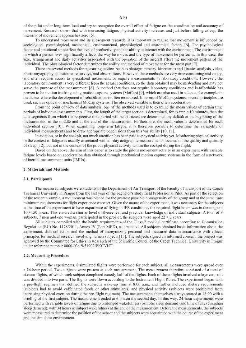
610

of the pilot under long-term load and try to recognize the overall effect of fatigue on the coordination and accuracy of movement. Research shows that with increasing fatigue, physical activity increases and just before falling asleep, the intensity of movement approaches zero [5].

To understand movement and its subsequent research, it is important to realize that movement is influenced by sociological, psychological, mechanical, environmental, physiological and anatomical factors [6]. The psychological factor and emotional state affect the level of productivity and the ability to interact with the environment. The environment in which a person lives significantly affects the way he moves and the type of movement he performs. In this case, the size, arrangement and daily activities associated with the operation of the aircraft affect the movement pattern of the individual. The physiological factor determines the ability and method of movement for the most part [7].

There are several methods for measuring motion, such as photogrammetry, kinematics and kinetics analysis, video, electromyography, questionnaire surveys, and observations. However, these methods are very time consuming and costly, and often require access to specialized instruments or require measurements in laboratory conditions. However, the laboratory environment is very different from the actual conditions, so the data obtained may be misleading and may not serve the purpose of the measurement [8]. A method that does not require laboratory conditions and is affordable has proven to be motion tracking using motion capture systems (MoCap) [9], which are also used in science, for example in medicine, where the development of rehabilitation is often monitored. In terms of MoCap systems, several principles are used, such as optical or mechanical MoCap systems. The observed variable is then often acceleration.

From the point of view of data analysis, one of the methods used is to examine the mean values of certain time periods of individual measurements. First, the length of the target section is determined, for example 10 minutes, then the data segments from which the respective time period will be extracted are determined, by default at the beginning of the measurement, in the middle and at the end of the measurement. Furthermore, the mean value is determined for each individual section [10]. When examining long-term fatigue, it is therefore possible to determine the variability of individual measurements and to draw appropriate conclusions from this variability [10, 11].

In aviation, or in the cockpit, not much attention has been paid to physical activity yet. Monitoring physical activity in the context of fatigue is usually associated with all-day actigraphic measurements focused on the quality and quantity of sleep [12], but not in the context of the pilot's physical activity within the cockpit during the flight.

Based on the above, the aim of this paper is to study the pilot's movement activity in an experiment with variable fatigue levels based on acceleration data obtained through mechanical motion capture systems in the form of a network of inertial measurement units (IMUs). 2. Materials and Methods 2.1. Participants

The measured subjects were students of the Department of Air Transport of the Faculty of Transport of the Czech Technical University in Prague from the last year of the bachelor's study field Professional Pilot. As part of the selection of the research sample, a requirement was placed for the greatest possible homogeneity of the group and at the same time minimum requirements for flight experience were set. Given the nature of the experiment, it was necessary for the subjects at the time of the experiment to have experience of flying in IFR conditions, the required flight hours was in the range of 100-150 hours. This ensured a similar level of theoretical and practical knowledge of individual subjects. A total of 8 subjects, 7 men and one woman, participated in the project, the subjects were aged 22 ± 3 years.

All subjects complied with the health requirements of the Class 2 medical certificate according to Commission Regulation (EU) No. 1178/2011, Annex IV (Part-MED), as amended. All subjects obtained basic information about the experiment, data collection and the method of anonymizing personal and measured data in accordance with ethical principles for medical research involving human subjects [13]. The subjects signed an informed consent, the project was approved by the Committee for Ethics in Research of the Scientific Council of the Czech Technical University in Prague under reference number 0000-03/19/51902/EK VUT. 2.2. Measuring Procedure

Within the experiments, 8 simulated flights were performed for each subject, all measurements were spread over a 24-hour period. Two subjects were present at each measurement. The measurement therefore consisted of a total of sixteen flights, of which each subject completed exactly half of the flights. Each of these flights involved a layover, so it was divided into two parts. The flights were flown according to the Instrument Flight Rules. The experiment began with a pre-flight regimen that defined the subject's wake-up time at 8:00 a.m., and further included dietary requirements (subjects had to avoid caffeinated foods or other stimulants) and physical activity (subjects were prohibited from increasing physical exertion during the pre-flight regimen). The measurements themselves always started at 18:00 with a briefing of the first subject. The measurement ended at 6 pm on the second day. In this way, 24-hour experiments were performed with variable levels of fatigue due to prolonged wakefulness (osmotic sleep demand) and time of day (circadian sleep demand), with 34 hours of subject wakefulness at the end of the measurement. Before the measurements, the subjects were meassured to determine the position of the sensor and the subjects were acquainted with the course of the experiment and the simulator environment.

611The measurement itself began with a briefing at 18:00, when the first subject began to set up on-board instruments

and get acquainted with the track and maps. Jeppesen maps have been used, which are currently used by most large and small carriers in commercial air transport. The flights took place on the simulator of a twin-engine Beechcraft propeller aircraft, which can faithfully evoke the feeling of a real cockpit. In order for the flight to be conducted without a visual reference, IMC meteorological conditions suitable for the ILS CAT I approach were set. During the flight, the subject was forced to communicate with the air traffic controller, simulate changing from one frequency to another, and change flight levels to bring the simulated flight as close as possible to real flight. After completing the first full landing, the pilot was again moved to the threshold of the runway and continued in the second part of the flight. The data collection was completed when the landing gear wheels first touched the runway of the destination airport. So this one flight consisted of two parts and lasted about an hour. Then the subject was disconnected from the sensors and exchanged with his colleague. In the meantime, further testing of the subject took place between the individual measurements. The measurement protocol is described in more detail in [14]. A similar setup of the experiment was used in previous studies of the research team [3, 4, 15].

2.3. Data Acquisition and Processing

Data were collected via a MoCap system consisting of a Basic Inertia Gateway central unit (Inertia Technology B.V., Enschede, NL) and five ProMove-mini wireless IMUs (Inertia Technology B.V., Enschede, NL). The ProMove-mini is equipped with a set of 3-D digital sensors that allow you to monitor the following data: acceleration, turning radius, magnetic field strength and barometric pressure. Data is transmitted via 2.4GHz radio to the central unit, which can be connected to a computer via USB. The data is further stored in the internal memory of the sensors, so that in case of poor wireless transmission they can be recovered [16]. The sampling frequency of the sensors was 200 Hz. The range of accelerometers that are part of IMUs is ± 8 g.

The IMUs themselves are ergonomically shaped so that their placement and wearing is comfortable and without affecting the stability when placed on a flat surface. The encoders are related to a reference system with three axes (X, Y, Z). It is always necessary to reset the position of all sensors before the measurement itself. Each IMU is equipped with 2GB of internal memory, in which the recorded data can be stored. It is also used to store user settings of sensors. For attachment, the sensor is equipped with two handles, which can be used to pass, for example, a Velcro strap [16].

The measuring system is supplemented by the Ineria Studio software environment (Inertia Technology B.V., Enschede, NL). Inertia Studio not only records and graphically displays the measured data, but also serves to adapt the sensors to the user's needs, to calibrate the sensors, set sensitivity ranges or display the battery status and signal quality received by the central unit. Data collection is performed using an algorithm that uses data from inertial sensors to calculate the orientation of the movement [16].

The subject always wore 5 ProMove-mini units, see Fig. 1. They were placed on the right biceps (unit 315), the left biceps (unit 316), the right forearm (unit 318) and the left forearm (unit 319) and around the waist in the navel area (unit 317). The exact position was determined on the basis of anthropometric points defined in the standard CSN EN ISO 7250 - 1. These are points that are located in precisely defined places, they are easily palpable, because in these places the bone base is covered only by skin and not muscle or fat. The distance between the shoulder and the elbow was used for the sensors on the biceps. The position of these sensors was then defined as the distance from the acromion point to the center of the sensor. The distance from the elbow to the wrist was used for the sensors on the forearms. As with the biceps sensors, the exact position was determined as the distance from the elbow to the center of the sensor. The position of the last sensor is then described by the sitting height, expressed as the distance from the vertex point to the center of the sensor mount, because the sensor has been placed on the front of the body. Both full anthropometric distances and the distances derived from them were used to determine the position of the sensors. Overall, the following dimensions were measured for each subject: sitting height, sitting eye height, sitting elbow height, sitting shoulder height, elbow to wrist distance, and shoulder to elbow distance.

Fig. 1 Placement of the inertial measurement units (IMUs) on the pilot before the experiment (left) and on the fatigued wooden man (right)

Acceleration data were first filtered using the Savitzky-Golay filter [17]. From the adjusted acceleration values in

612

the individual axes, the 3D acceleration a was subsequently calculated as: 2 2 2

x y za a a a (1) where ax is the acceleration in the direction of the x-axis, ay is the acceleration in the direction of the y-axis and az is the acceleration in the direction of the z-axis [18]. As part of the signal evaluation, the data were first precisely divided into individual flights according to the recorded start and end times of each flight. Because each measurement contained a layover, each measurement was divided into two flights. Subsequently, the first and last minutes of each flight were trimmed, as these were phases with more intense physical activity, which could introduce an error into the results. From this modified data, three 5-minute sections were selected for each flight - always at the beginning (S), middle (M) and end (E) of the flight (1 – 1st flight, 2 – 2nd flight), see Fig. 2. The initial assumption was that in the initial and final sections, the subject will be more vigilant, with regard to the preparation for performing take-off and landing. In contrast, a greater manifestation of fatigue was expected for the middle section, given the monotony of this flight phase. The average value (mean) and standard deviation (SD) of the 3D acceleration [19] were calculated for each of these sections, see Fig. 2.

Fig. 2 Measuring schedule and selection of specific 5min sections 2.4. Statistical Analysis

To determine the effect of fatigue on the overall movement of the pilot during the entire measurement, the first, middle and last 5 minutes of each flight were selected. In these time periods, the mean value and standard deviation were calculated from the 3D acceleration data. In this way, 12 monitored parameters were created. The values of parameters (i.e. averages and standard deviations of individual 5-minute sections) were then statically compared between individual measurements (Meas1– Meas8). With regard to the size of the test group, the data were subsequently evaluated using non-parametric methods. Taking into account the fact that the data are repeatedly scanned from the same group of subjects, i.e. they are paired data and 8 groups of data are compared (measurements Meas1– Meas8), Friedman's test at the significance level of 5 % was used for statistical testing with subsequent post-hoc analysis using the Dunn-Sidak approach. The distribution of individual parameters was graphically represented by boxplots. Statistical analysis was performed in MATLAB R2017a software (The MathWorks, Inc., Natick, MA, US). 3. Results

The results described below are addressing the description of the statistically significant differences between the particular pairs of the measurements and that for every individually observed parameter for the particular sensors. The results are also graphically depicted in the boxplot form in Fig. 3.

Between the Meas1 and the Meas4 there was a significant (p = 0.0148 a CI = (-11.398; -0.602)) increase of the parameter meanS1 on the sensor 316. The significant increase (p = 0.025 a CI = (-11.145; -0.352)) of the parameter meanS1 was recorded also on the sensor 317. On this sensor there was also measured a significant parameter meanM1 (p = 0.00859 a CI = (-11.648; -0.852)) growth. With the post-hoc analysis it was later determined that for the comparison of the Meas1 with the Meas5, there were changes of several parameters on the 316 sensor. A prominent growth of parameter meanM was discovered (p = 0.00489 a CI = (-11.898; -1.102)). Significant growth was present at the meanE1 parameter (p = 0.0027 a CI = (-12.148; -1.352)). Parameters meanM1 (p = 0.01295 a CI = (-13.233; -0.767)) and meanE1 (p = 0.0423 a CI = (-12.566; -0.100)) have risen also notably.

In the comparison of the Meas1 and Meas7 a markable growth of parameter meanM1 (p = 0.041 a CI = (-10.898; -0.102)) and considerable growth of parameter SDM1 on sensor 315. On sensor 317 the SDM1 parameter rose prominently (p = 0.041 a CI = (-10.989; -0.102)). Furthermore, a significant rose of SDS1 (p = 0.041 a CI = (-10.898; -0.102)) was recorded and a prominent growth of parameter SDS2 on sensor 318 (p = 0.025 a CI = (-11.148; -0.352)).

Between the Meas1 and the Meas8 there was a notable change of several parameters. A rose of the parameter meanS1 on the sensor 315 (p = 0.025 CI = (-11.148; -0.352)) was observed. Further, there was a notable (p = 0.0049 a CI = (-11.898; -1.102)) rose of the parameter SDM1 on sensor 315. On the same sensor there was observed a noteworthy

613

growth of parameter SDE1 (p = 0.0086 CI = (-11.648; -0.852)). A prominent growth was also on the sensor 315 for the parameter SDS2 (p = 0.042 a CI = (-12.566; -0.100)). On the sensor 316 there was a noticeable rose of meanM1 parameter (p = 0.0049 a CI = (-11.898; -1.102)) and a significant growth of SDM1 parameter (p = 0.041 a CI = (-10.898; -0.102)).

An obvious decrease of the parameter SDE1 (p = 0.00859 a CI = (0.852; 11.648)) between the Meas2 and Meas3 can be observed only on sensor 317. It was observed that when comparing the Meas2 and Meas4, there was a significant growth of the parameter SDS1 (p = 0.041 a CI = (-10.898; -0.102)) on the sensor 315. On the sensor 317, for the same comparison, there was notable growth of the parameter meanM1 (p = 0.0148 a CI = (-11.398; -0.602)) and a noteworthy growth of the parameter meanE1 (p = 0.025 a CI = (-11.148; -0.352)).

We can also observe several parameter changes between the measurements 2 and 5. On the sensor 316, remarkably grew the parameter meanM1 (p = 0.0411 a CI = (-10.898; -0.102)) and we can observe also an obvious growth of the parameter meanE1 (p = 0.00859 a CI = (-11.648; -0.852)) on the same sensor.

When focusing on the measurement 2 and 6, it is obvious that there was a visible decrease of the parameter SDE1 (p = 0.0249 a CI = (0.352; 11.148)). Comparing the measurement 2 and 7, there was discovered a remarkable increase (p = 0.041 a CI = (-10.898; -0.102)) of the parameter SDS1 on the sensor 315. A notable increase of the parameter SDS1 was also observed on the sensor 316 (p = 0.0041 a CI = (-10.898; -0.102)). Between the measurement 2 and 8, there was spotted only one observable change of parameter. On the sensor 316 notably rose the parameter meanM1 (p = 0.041 a CI = (-10.898; -0.102)).

For the comparison of the Meas3 and Meas4, only growth of the parameter meanM1 on the sensor 317 seems significant (p = 0.041 a CI = (-10.898; -0.102)). Similarly as when comparing the measurement 3 and 8, there was also only one significant change and it was the evident decrease of parameter meanM2 on the sensor 318 (p = 0.00489 a CI = (1.102; 11.898)). With the next couple comparison, in which there was only one more significant change are the measurements 5 and 7. Between these two parameters there was an evident growth (p = 0.0249 a CI = (-11.148; -0.352)) of parameter SDS1 on the sensor 318.

The post-hoc analysis has shown that between the measurement Meas5 and Meas8, there was a notable growth of parameter SDE2 on the sensor 315 (p = 0.042 a CI = (-12.566; -5.333)). Further it was observed that on the sensor 316, there was a significant growth of the parameter SDS2 (p = 0.042 a CI = (-12.566; -6.333)). Only one notable growth (p = 0.025 a CI = (-11.148; -0.352)) between the measurement 6 and 8 was recorded and it was on the sensor 315 for the parameter SDE1.

4. Discussion

For the analysis of the physical activity, there were 12 parameters selected that were examined within all measurements. These parameters were captured by the 3D acceleration method of the Motion Capture system with the integral measurements units. The results have shown that the most statistically significant changes were occuring between first (Meas1–Meas2) and last measurements (Meas7–Meas8) and between first (Meas1–Meas2) and middle measurements (Meas4–Meas5). These changes were mostly captured by the IMUs fastened on the biceps and it was always the rise of the parameters. In the case of the unit fastened on the left forearm, there were no statistically significant changes observed, however when focusing on the trend of the parameters course in the particular measurements, it was possible to observe a similar trend as for the other sensors.

When looking into the boxplots (see Fig. 3), it is possible to observe a certain trend that the parameters had during the measurements. Except for the small deviations, it is possible to state that the parameters rose, around the fourth or fifth measurements there was a stagnation and the parameters began to drop. Towards the last (Meas7–Meas8) the parameters were rising again. The parameters maximums were observed either at the middle (Meas4–Meas5) or during the last measurements (Meas7–Meas8). The opposite – the minimums were reached on the beginning of the measurements and after reaching the first rising in the middle parts. It is however necessary to underline that the overall trend was increscent.

Their increments are depicting a greater movability of the IMUs, and hence the greater amplitude (the averages of the five minutes laps) and variability of the movements (the standard deviation of the five minute laps) of the given segments where the IMUs were fastened at. It is therefore possible to state that for the objects there were periods of the greater movement with the more resting periods. When looking into the average time, it is possible to determine that the most significant measurements were performed around 4-5 a.m., when the subjects were approximately 20 hours without sleep. This time falls into the circadian outcrop, that is usually between the 2–6 a.m. [20]. The other two significant measurements, the seventh and the eight would then be according to the afternoon hours at around 17-18PM. In this time, the subjects were sleepless for around 34 hours and the osmotic need of sleep was already taking effect.

The study of the fatigue effect on the human movements are showing that the fatigue is influencing the movement variability and it is leading to the decrease or increase of the variability, depending on the measured quantities [21]. The studies [10, 11, 21], also show that with greater fatigue, the movement frequency is decreasing. The results of this study described in this paper show that with the greater fatigue not only the movement variability but also the movement frequency is increasing. It is however necessary to underline that the aforementioned studies were dealing only with physical fatigue and the experiments conducted within these studies were in comparison to this experiment only short-termed. The different results are therefore most probably given by the distinct experiment set up, but the results are still within the context of the similarly set up experiments described in the previous publications [3, 4, 15].

614

Fig. 3 Graphical representation of distribution of parameters with significant differences in specific units. IMU 3XX represents specific inertial measurement unit, SD represents standard deviation, mean represents average value, S stands for the first 5 minutes of flight, M stands for the middle 5 minutes of flight, E stands for the last 5 minutes of flight, number represents 1st or 2nd flight.

5. Conclusions

The aim of this paper was to evaluate the effect of fatigue on the physical activity of pilots during an experiment with variable levels of fatigue using the Motion Capture system. An analysis of the current state of human motion monitoring, the use of Motion Capture systems and the use of these systems in fatigue monitoring was performed. During this process, shortcomings were discovered in the study of the effect of fatigue on human mobility. Based on these shortcomings, an experiment was performed, which consisted of four twenty-four-hour measurements involving eight subjects. Individual measurements represented simulated flights, during which the movement of subjects was recorded. Based on the analysis, sensors for motion sensing, their location and method of evaluating the measured data were selected.

The results show the effect of fatigue on the physical activity of pilots during the set experiment. The results show that the variability of movement increased with increasing fatigue, as did the mobility of the subjects themselves. Furthermore, the influence of the circadian rhythm on the physical activity of the measured subjects was evident, so that in the period of the circadian attenuation window there was an increase in the average acceleration and its standard

615

deviation. The main limitation of this research is a small group of subjects. Such a small group was measured due to the high

personnel and time-consuming measurement. On the other hand, the study was built as a trial, as a similar experiment had not been performed before.

The paper could therefore serve to better understand the complexity of the effects of fatigue on the human body. Furthermore, it could open the topic of the influence of pilot mobility in the cockpit on its overall performance. From the point of view of the research team, the work will serve as a basis for follow-up research and at the same time the work expands the knowledge base in the given issue. However, in terms of further research, it would be appropriate to expand the group of tested subjects. Furthermore, it would be possible to integrate flights that are more difficult into piloting techniques, which would make it possible to study the effect of fatigue on the coordination and smoothness of the movements performed. Acknowledgement

This work has been supported by the project SGS19/124/OHK2/2T/16 “Study of Fatigue Influence on Pilots’ Performance”. References 1. Rosekind, M.R.; Gander, P.H.; Gregory, K.B.; Smith, R.M.; Miller, D.L.; Oyung, R.; Webbon, L.L.; Johnson,

J.M. 1996. Managing fatigue in operational settings. 1: Physiological considerations and countermeasures, Behavioral Medicine 21(4): 157-165.

2. European Union Aviation Safety Agency. 2019. Easy access rules for air operations [online cit.: 2020-08-22]. Available from: https://www.easa.europa.eu/document-library/easy-access-rules/easy-access-rules-air-operations

3. Socha, V.; Hanáková, L.; Stoji , S.; Kušmírek, S.; Socha, L.; Antoško, M. 2018. A fatigue influence on pilot’s reaction ability during 24 hours flight simulation: A case series study, New Trends in Civil Aviation, Prague: 45-19.

4. Hanáková, L.; Socha, V.; Socha, L.; Lališ, A.; Kraus, J.; Malich, T. 2019. The influence of fatigue on psychophysiological indicators during 24 hours testing of pilots, SAMI 2019 IEEE 17th World Symposium on Applied Machine Intelligence and Informatics - PROCEEDINGS. Prague: Czechoslovakia Section IEEE, 181-186.

5. Vural, E.; Cetin, M.; Ercil, A.; Littlewort, G.; Bartlett, M.; Movellan, J. 2007. Drowsy driver detection through facial movement analysis. In: International Workshop on Human-Computer Interaction. Berlin. Springer. pp. 6-18.

6. Godfrey, A.C.; Conway, R.; Meagher, D.; ÓLaighin, G. 2008. Direct measurement of human movement by accelerometry, Medical engineering & physics 30(10): 1364-86.

7. Trew, M.; Everett, T. 2005. Human movement: an introductory text. London: Churchill Livingstone, 267 p. 8. Mathie, M.; Coster, A.C.F.; Lovell, N.H.; Celler, B.G. 2004. Accelerometry: providing an integrated, practical

method for long-term, ambulatory monitoring of human movement, Physiological measurement 25(2): R1-20. 9. Guerra-Filho, G. 2005. Optical Motion Capture: Theory and Implementation, RITA 12(2): 61-90. 10. Strohrmann. C.; Harms, H.; Kappeler-Setz, C.; Troster. G. 2012. Monitoring kinematic changes with fatigue in

running using body-worn sensors, IEEE transactions on information technology in biomedicine 16(5):983-90. 11. Adlerton, A.K.; Moritz, U.; Moe Nilssen, R. 2003. Forceplate and accelerometer measures for evaluating the effect

of muscle fatigue on postural control during one legged stance, Physiotherapy Research International 8(4):187-199. 12. Kandera, B.; Škultéty, F.; Mesárošová, K. 2019. Consequences of flight crew fatigue on the safety of civil aviation,

Transportation research procedia 43: 278-289. 13. World Medical Association and others. 2013. World Medical Association Declaration of Helsinki: ethical principles

for medical research involving human subjects, Jama 310(20): 2191-2194. 14. Hanáková, L.; Socha, V.; Bo il, J.; Herman, L.; Štrobl, J.; Pilmannová, T. 2020. Subjective evaluation of fatigue

in pilots during 24-hour testing, 2020 New Trends in Civil Aviation, Prague: 111-116. 15. Socha, V.; Hanáková, L.; Freigang, M.; Kraus, J.; Stoji , S.; Socha, L.; Hanák, P. 2019. Impact of pilots' tiredness

on the outcome of psychological testing, Transport Problems 14(2): 55-67. 16. ProMove mini Wireless Inertial Sensing Platform [online cit.: 2020-05-20]. Available from: http://inertia-

technology.com/wp-content/uploads/2019/09/ProMoveMiniBscGwUserManual3.8.5.pdf 17. Karaim, M.; Noureldin, A.; Karamat, T.B. 2019. Low-Cost IMU Data Denoising Using Savitzky-Golay Filters,

2019 International Conference on Communications, Signal Processing, and their Applications (ICCSPA), Sharjah: 1-5.

18. Strohrmann, C.; Harms, H.; Kappeler-Setz, C.; Troster, G. 2012. Monitoring kinematic changes with fatigue in running using body-worn sensors, IEEE transactions on information technology in biomedicine 16(5): 983-990.

19. Baek, J.; Lee, G.; Park, W.; Yun, B.J. 2004. Accelerometer signal processing for user activity detection, International Conference on Knowledge-Based and Intelligent Information and Engineering Systems, Wellington: 610-617.

20. Transportation Research Board and National Research Council. 2011. The Effects of Commuting on Pilot Fatigue, Washington, DC: The National Academies Press, 222 p.

21. Cortes, N.; Onate, J.; Morrison, S. 2014. Differential effects of fatigue on movement variability, Gait & posture 39(3): 888-893.

616

Proceedings of 25th International Scientific Conference. Transport Means 2021. Adoption of Digital Technologies at Regional Airports in the Slovak Republic A. Novák Sedlá ková1, T. Remencová2 1University of Žilina, Univerzitná 8215/1, 010 08 Žilina, Slovakia, E-mail: alena.sedlackova@fpedas.uniza.sk 2University of Žilina, Univerzitná 8215/1, 010 08 Žilina, Slovakia, E-mail: tatiana.remencova@stud.uniza.sk Abstract Nowadays the implementation of digital technologies has become a new trend at airports, but especially for Slovak airports. Airports are constantly adapting new technologies, various concepts and processes to ensure more efficient, safer, and faster operation focusing on overall passenger satisfaction. In the world is using of these new technologies at big airports quite often, but at the regional airports not so much. The criterion of the decision if implemented or not implemented these technologies depend on the strategy of the airport and on the economic and social environment of the states or region, where is the airport situated. At the Slovak airports isn’t these technologies adopted and the management of the airport argues with economic inefficiency. The implementation of new digital technologies represents an investment challenge, but on the other side it brings several benefits as for example reduction of operating costs or even in connection with the Covid-19 pandemic, these technologies can prevent the spread of the virus from staff to passengers. Airports are opened to technological innovation, but digitization is different for regional airports. They are still in the process of adapting to a new trend. Most of them are undeveloped, and they do not have enough funds for digital transformation, therefore they often remain with the traditional airport concept. The performance and reliability of each deployed system need to be tested, and this takes time and finance. The main goal of our research is to find out how much the regional airport can save on costs if it decides to invest in digital technology within the passenger and baggage section. The results of the analysis show that digital transformation is possible in the case of regional airports. The implementation of 1-unit check-in kiosk can significantly affect the operational costs of the airport and the return of investments is more than certain. KEY WORDS: Smart Airport, Digital Technologies, Airport Digital Transformation, Check-in kiosk, Cost Reduction 1. Introduction

Digital technologies have been present everywhere all around us for several years. During this period, we enjoy them, and we consider them as a necessary standard. We are surrounded by smartphones and tablets, which are full of the newest applications and programs to make our lives easier. The trend of digital technologies has also become popular at airports. It is the growing volumes of passengers, flights and increasing competitiveness caused, that the airports are focused on new digital technologies. Passenger's experience and satisfaction have become a priority for the airports, which implement self-service registration systems, biometrics technology, various intelligent systems, applications and even artificial intelligence. Thanks to these new technologies they are able to serve several thousand passengers and transport tones of baggage in a very short time. New technologies also speed up all other processes at the airports and the passengers can enjoy travelling without long waiting in a line and other complications. In general, we can claim that the airports implemented the new technologies successfully. Many of them have already managed the process of digital transformation, the others are still preparing for it. In the case of regional airports, the issue of digital transformation is still opened. These airports use mostly the traditional respectively simple model of operation, because they do not have enough funds for any digital changes. Nevertheless, the regional airports have become more attractive for passengers because they provide a quieter and more pleasant environment, less crowded spaces and of course, shorter duration of all processes. The passengers are more satisfied too and the atmosphere of the smaller airport in comparison with the larger airport is quite different. These could also be the reasons for the digital transformation of a regional airport. In this paper we focus on selected regional airports in the Slovak Republic. These are the ones use the traditional model of operation, without using some special digital technologies. Despite their situation, they generate a loss for several years. Therefore, we propose their modernization by implementing check-in kiosks. We examine the impact of this "new technology" on the total operating costs of an airport which are rising every year, and it is necessary to optimize them. The successful implementation of this technology could have a positive effect on the costs of regional airports and help them take a step towards a better future. The potential savings could be used later for other development projects. Most airports in the world have confirmed that the implementation of digital technologies has had a positive effect on their financial situation. However, airports in the Slovak Republic refer precisely to the financial aspect and this article demonstrates that airports should consider the savings that this technology can bring them. 2. Literature Review

Digital transformation of the airport is a complex process. The presented paper follows up the previous study

617 done by Remencová and Novák Sedlá ková (2021), which described digital transformation of regional airports in Slovak republic. This paper is focused on real data, which were provided by Embross company (USA), which delivers automation solutions to the world’s airports [1]. The study Halpern et. al. (2019) applies a concept of maturity models to the digital transformation of an airport, where it is focused on passenger's experience. The authors describe the key factors, which is needed to take into account in the digital transformation of the airport on the basis of their proposed model [2]. The study Saputra (2020) examines the impact of airport digital culture on airport staff. They conducted the research at 15 Indonesian airports, which provide the top-quality of services with using of digital technologies [3]. The paper Stark (2020) deals with digital transformation of the regional airport at Springfield. Author explains the reasons of digital transformation of this airport. He is interested in four important areas, namely improving the passenger's experience, optimized planning, intelligent management of facilities and equipment and air traffic control [4]. The study Knoch et. al. (2020) proposes the platform, which is able to collect the information about passenger frequency flows in selected areas at the airport. On the basis of this platform, the authors performed the analysis of requirements and developed a prototype of system that effectively connects data flows and generates alerts that warn airport staff in the case of declining passenger satisfaction [5]. The passenger satisfaction is really important factor. In order to passengers’ flow through the airport was faster and smooth, the processes need to be carried out quickly and efficiently. The study Sabatova et. al. (2016) deals with the current state of using of self-service registration services in the world and also predict the expected development of these services in the future. The authors present a new design of a self-service kiosk and a graphical user interface (GUI) based on an analysis of the functions and features available on the market and taking into account all currently known IATA requirements and criteria [6]. Badánik et al. (2018) dealt with airport strategies according to the size of the airport and its infrastructure. The solution is in particular to increase revenues and returns from the airport's own operations [7]. The study by Novák Sedlá ková et al. (2019) monitored, through ex-ante financial analysis, liquidity indicators and the self-financing capacity of Slovak airports. In conclusion, it considers most Slovak airports in the long run as loss-making entities, with the exception of the partially privatized Košice Airport and Slia Airport with mixed operations, which, however, was mainly financed by the Ministry of Defence and is currently closed to commercial air transport [8]. The paper Zhao et. al. (2015) deals with the situation of self-service check-in at airports. The authors examine the choice of passenger and thus the traditional method of check-in, the method of self-service and the waiting time in a line in a different time. On the basis of results, they try to determine the correct number of self-service kiosks that should be at the airport [9]. The paper Chen and Ku (2013) examines the using of self-service check-in kiosks by passengers at Taiwan Airport. The results showed that if we want to achieve the desired effect, there is needed to have a clear and simply process of providing of service for passengers, especially for those who need to help with using a check-in kiosk. Also, the enjoyment and visually pleasing design of check-in machines are an important factor in choosing of the method of check-in service [10]. The study Wittmer (2011) deals with acceptance of self-service registration (e-check-in) by passengers. They are particularly interested in registration on the web, registration on a mobile phone, use of a check-in kiosk and personalized registration methods. The authors found out that e-check-in plays a very important role because it shortens waiting times and the passengers are more satisfied. However, the new procedures are not credible, and therefore it is necessary to use operational registration procedures. Self-service technology is attractive more for business travellers than tourists. Web check-in was used by passengers mainly between the ages of 31 and 40 [11]. The paper Chen et. al. (2015) is focused on customer satisfaction at the airport in connection with providing of services. The authors propose the evaluation model for the impact of service innovation, customer satisfaction and increasing customer value at the airport. The results showed that value of customer was significantly affected by customer satisfaction and service innovation [12]. The study Bogicevic et. al. (2017) examines the impact of digital technologies on airports passengers and their satisfaction. The authors test the theoretical model, which examines the relationship among various types of airport technologies in terms of passenger's confidence, pleasure and satisfaction. The results showed the positive relationship among airport self-service technologies, passenger's pleasure and satisfaction in the area of trust [13]. The passenger flow and modern friendly networks are for regional airports very important [14, 15]. The study Khalil et. al. (2021) assesses the factors as comfort and satisfaction in the operating areas of Dubai Airport in order to identify the strengths and weaknesses of providing services. They conducted a survey which included 35 attributes of comfort. The result showed that the Dubai airport provides high quality of services, which are standard for comfort of passengers [16]. The study Rajapaksha and Jayasuriya (2020) is focused on smart airport applications which are used within the passenger terminal. The authors remind that digital transformation and its implementation is an investment-intensive process. The airport staff should be adequately trained to develop a positive approach to this transformation [17]. Digital technologies are expensive and currently the situation of airports connected with Covid-19 pandemic is more complicated. The airports have financial problems, and it is necessary to save more finance. The paper Kazda and Serrano (2020) assesses the situation of airports after the Covid-19 pandemic. The authors predict that the costs of the airports and airlines will increase due to cleaning and disinfection. They expect that the airports will be reassessed their budgets with a view to reducing staff costs [18]. 3. Methodology

The digital technologies As a part of modernization of regional airports in SR we suggest implementing 1 unit of check-in kiosk for these airports: M.R.Štefánik Airport in Bratislava, Košice International Airport, Pieš any Airport and Žilina-Dolný Hri ov Airport. Therefore, we contacted several foreign companies because of price offer this product.

618 Unfortunately, we only received one from Embross company, which is situated in Ontario, USA. They recommended for this research Embross V2 CUSS check-in kiosk with this configuration: Boarding Pass Printer, Bard Code Reader, Bag tag Printer, Card Reader (MSR) for frequent Flyer cards, Full Page Passport Reader with RFID reader, Perpetual CUSS license, Installation and Shipping. The price for this check-in kiosk is USD 13,738, but it is necessary to pay an extra fee for software every year USD 240 per one unit. For a better calculation we recalculated the data from USD to € according current conversion rate 1 USD= €0,82. Total price for check-in kiosk including software fee is €11,410.61. We used the FinStat database too, where we searched the profit and loss statements for individual airports. We were concentrated on the values of costs (total operating costs, labour costs and training costs) and number of employees for the period 2014-2018, which we listed in Table 1. Subsequently, we calculated the costs per employee in gross per year, where we had to add the value 35.2%, which represents the employer’s contributions. This value is set out in the Act no. 461/2003 Coll. on social insurance and in the Act no. 580/2004 Coll. on health insurance in SR. Based on these data, we calculated the labour costs savings and total costs savings of selected airports in the SR, which we listed in Table 2.

Table 1

Total operating costs, Labour costs, Training costs, number of employees Source: Annual Reports of the Airports (2014-2018)

Reviewed period

Total operating costs in € (a)

Labour costs in € (b)

Training costs per 1 employee

in € (c)

Number of employee (d)

Bratislava

2018 33,355,000 8,615,875 127.05 608 2017 32,453,000 7,579,339 122.43 617 2016 33,159,000 7,054,206 178.32 612 2015 32,021,000 6,318,102 98.10 561 2014 31,913,000 5,926,544 95.69 538

Košice

2018 10,068,424 2,257,691 495.91 147 2017 9,045,861 2,016,179 736.63 139 2016 7,202,546 1,866,447 424.78 134 2015 7,081,841 1,786,642 252.72 128 2014 7,155,604 1,733,237 229.97 129

Pieš any

2018 1,229,560 322,888 276.62 26 2017 980,746 278,385 214.93 27 2016 1,132,655 268,276 419.16 30 2015 1,172,618 279,748 215.80 30 2014 1,031,871 274,701 174.47 32

Žilina

2018 860,476 203,340 789.90 19 2017 856,287 206,071 308.42 19 2016 844,631 209,864 606.11 19 2015 1,067,890 226,725 374.37 19 2014 955,681 228,045 231.83 18

We calculated according to the following formulas:

35 2bE , %d

, (1)

where E labour costs per employee per year in €; b labour costs in €; d number of employees; 35,2% = employer’s contributions. F=E+c, (2) where F total costs in a gross per employee in €; E labour costs in gross per employee in €; c training costs per employee in €. G=F-11,410.61, (3)

where G financial labour cost savings in €; F total costs in a gross per employee in €; 11,410.61 total costs of 1 check-in kiosk including all fees in €.

619

100GHF

, (4)

where H - labour cost savings in %.

100GIa

, (5)

where I total costs savings in %; a total operating costs in €.

Table 2 Labour costs in gross per employee, total costs per employee in a gross, financial labour cost savings,

labour cost savings in % and total costs savings in %. Source: Authors

Reviewed Period

Labour costs in gross per

employee in €(E)

Total costs in gross per employee in in

€ (F)

Financial labour costs

savings in € (G)

Labour cost savings in %

(H)

Total cost savings in

% (I)

Bratislava

2018 19,158.99 19,286.04 7,875.43 40,83% 0,02% 2017 16,608.21 16,730.64 5,320.03 31,80% 0,02% 2016 15,583.81 15,762.13 4,351.52 27,61% 0,01% 2015 15,226.51 15,324.61 3,914.00 25,54% 0,01% 2014 14,893.47 14,989.16 3,578.55 23,87% 0,01%

Košice

2018 20,764.62 21,260.53 9,849.92 46,33% 0,10% 2017 19,610.61 20,347.24 8,936.63 43,92% 0,10% 2016 18,831.62 19,256.40 7,845.77 40,74% 0,11% 2015 18,871.41 19,124.13 7,713.52 40,33% 0,11% 2014 18,165.40 18,395,37 6,984.76 37,97% 0,10%

Pieš any

2018 16,790.18 17,066.80 5,656.19 33,14% 0,46% 2017 13,939.88 14,154.81 2,744.20 19,39% 0,28% 2016 12,090.30 12,509.46 1,098.85 8,78% 0,10% 2015 12,607.31 12,823.11 1,412.50 11,02% 0,12% 2014 11,606.12 11,780.59 369.98 3,14% 0,04%

Žilina

2018 14,469.25 15,259.14 3,848.54 25,22% 0,45% 2017 14,663.58 14,972.00 3,561.39 23,79% 0,43% 2016 14,933.48 15,539.59 4,128.98 26,57% 0,49% 2015 16,133.27 16,507.64 5,097.03 30,88% 0,48% 2014 17,128.70 17,360,53 5,949.92 34,27% 0,62%

Fig. 1 Percentage labour cost savings at selected regional airports in SR

620 4. Discussion

Based on the performed analysis we can claim that the implementation of check-in kiosks at the selected regional airports in SR has an impact on cost management. The percentage saving in labour costs reached different values during the reviewed period, when the highest value 46.33% was reached at the airport Košice in 2018. The lowest value 3.14% was reached at the airport Pieš any in 2014. In general, the percentage saving of labour costs is increasing during the period for almost all airports. The exception is the airport Žilina-Dolný Hri ov, where surprisingly the labour cost savings is slightly declining during the period (Fig. 1). This result is significantly influenced by the situation of the airport, because nowadays this airport does not operate any scheduled flights for several years and the issue of its ownership was solved too. In this case we claim that the investing to check-in kiosk would be unnecessary because the airport has an existential problem. In the case of Pieš any Airport we can see a significant change during the period, when in 2014 the savings in labour costs reached the value of € 369.98 and in 2018 already € 5,656.19, which represents more than a 1000% increase. Given these results, the implementation of a check-in kiosk could be successful at this airport, as well as at the airports in Bratislava and Košice, where they could also consider the implementation of several units of check-in kiosks. The fact is that all airports in SR does not have such machines, therefore they have to employ more staff due to working holidays or incapacity for work. The problem is that personal costs are still rising every year and it is becoming more difficult for airports management to find areas where is possible to save some funds. If we evaluate the savings in terms of the impact on the total operating costs of airports, the percentage savings are generally very low. It is less than 1%. We could consider the low values to be negligible in this respect, but any reduction in costs is very important for regional airports. Investing in this technology would bring several benefits not only to the airports but also to passengers. It is the passenger's satisfaction, that should be the most important value for the airport. Today's young generation loves modern digital technologies, therefore self-service check-in has been standard at foreign airports for several years. People have adapted to this trend and they like the advantages of it because it provides them the convenience of self-check-in, experience, shorter waiting times in a line and a shorter check-in process. On the other side the airports can reduce their operating costs, employ less staff and also improve their providing of services thanks to this technology. However, it is clear that digital technologies will never replace direct face-to-face communication. This fact can be seen in the context of older people, who may have a problem with the using of the digital technologies. These types of people usually choose check-in process at the counter with an employee because of the feeling of greater certainty and better information. In spite of this fact, this is not a problem for the operator, because he can employ a person, who will be in the vicinity of this machine and will be able to guide the passenger in the correct way at the moment. The only thing, that we are not able to completely eliminate is the failure of this machine, which will be common because of daily use. However, the operator can deal with this situation by employing the person in the context of multitasking, who will be trained for failures of such equipment. 5. Conclusions

This article dealt with modernization of selected regional airports in SR. The main goal was to find out how much can save on costs regional airport if it implements one unit of check-in kiosk into the operation. Although it is not the newest technology, it can be the first step of modernization for them. Nowadays, digital technologies are really expensive, and the costs connected with their implementation are rising. In spite of this fact the airports are interested in digital transformation. However, the digital transformation of regional airports is different because of their negative economic situation and the lack of funding. Based on the results, we can claim that investing in this technology is successful and brings positive results in terms of reducing daily operating costs and can also speed up the flow of passengers at the airport. The return on investment is more than certain for several years. Therefore, the airports would make an assessment of their economic situation and state, in which they are. Based on their findings, they would develop a plan of digital transformation, in which they should certainly take into account the financial situation of the airport, its business context, objectives, readiness for change and the structure of the digital changes, which they plan to apply. It is also important to identify a group of employees who will be actively working on the process of digital transformation. The opinion and satisfaction of the passenger is a very important factor that must be taken into account too. Therefore, we recommend conducting a survey among passengers, because it is necessary to know their opinion on digital changes.

Acknowledgement

This paper was supported by national grant scheme VEGA 1/0695/21 Air transport and COVID-19: Research of the crises impacts with a focus on the possibilities to revitalize the industry. References 1. Remencová, T.; Novák Sedlá ková, A. 2021. Modernization of Digital Technologies at Regional Airports and its

Potential Impact on the Cost Reduction, In: International scientific conference on sustainable, modern and safe Transport. Transcom 2021, Horný Smokovec, Slovak republic, in press.

2. Halpern, N.; Budd, T.; Suau-Sanchez, P.; Brathen, S. 2019. Towards Airport 4.0: Airport Digital Maturity and

621 Transformation. Conference: 23rd Air Transport Research Society World ConferenceAt: Amsterdam, Netherlands. [online cit.: 2021-05-07]. Available from: https://www.researchgate.net/publication/335015282_Towards_Airport _40_Airport_Digital_Maturity_and_Transformation.

3. Saputra, N.; M. Saputra, A. 1999. 2020. On-Becoming Digital Organisation: Digital Competence, Digital Leadership and Digital Culture in Indonesia Airports. Conference: GCBSS 2020 - 11th Global Conference on Business and Social Science. Bangkok. [online cit.: 2021-05-07]. Available from: http://gcbss.org/ CIMSSR2020THAILAND/PDF/CIMSSR-00245.pdf

4. Stark, J. 2020. Digital Transformation of Springfield Regional Airport, In book: Digital Transformation of Industry, 85-89.

5. Knoch, S. Staudt, P.; Puzzolante, B.; Maggi, A .2020. A Smart Digital Platform for Airport Services Improving Passenger Satisfaction, 2020 IEEE 22nd Conference on Business Informatics. June 2020. Antwerp, Belgium. [online cit.: 2021-05-07]. Available from: https://ieeexplore.ieee.org/abstract/document/9140289

6. Sabatová, J. 2016. Modern Trends in Airport Self Check-in Kiosks, Magazine of Aviation Development 4(20):10. 7. Badánik, B.; Kazda, A.; Tomová, A.; Laplace, I.; Lenoir, N. 2013. Future airports development strategies,

Communications- Scientific Letters of the University of Zilina 15(2): 19-24. 8. Novák Sedlá ková, A.; Švecová, D.; Tomová, A. 2019. Slovak Airports As Profit/Loss Making Entities:

Consequences For Transport Policies, Journal of Tourism and Services 10: 153-163. 9. Zhao, G.; Zheng, X.; Zhang, J. 2015. Simulation of Optimal Allocation of Self- Service Check-in Kiosks at the

Airport, Fifth International Conference on Transportation Engineering. September 2015. Dalian, China. [online cit.: 2021-05-07]. Available from: https://trid.trb.org/view/1369469

10. Ku, E.; Chen, Ch. 2013. Fitting facilities to self-service technology usage: Evidence from kiosks in Taiwan airport, Journal of Air Transport Management (32): 87-94.

11. Wittmer, A. 2011. Acceptance of self-service check-in at Zurich airport, Research in Transportation Business & Management (1): 136-143.

12. Chen, J.; Batchuluun, A.; Batnasan, J. 2015. Services innovation impact to customer satisfaction and customer value enhancement in airport, In: Technology in Society (43): 219-230.

13. Bogicevic, V.; Bujisic, M.; Bilgihan, A., Yang, W.; Cobanoglu, C. 2017. The impact of traveler-focused airport technology on traveler satisfaction, Technological Forecasting and Social Change 123(C): 351-361.

14. Matas, M.; Novak, A. 2008. Models of processes as components of air passenger flow model, Komunikacie 10(2): 50-54.

15. Novák, A. 2006. Modern telecommunication networks in the aeronautical telecommunication network (atn), Aviation 10(4): 14-17. doi:10.1080/16487788.2006.9635942

16. El Naggar, M.K.; Tawfik, H.F.; Soliman, D. 2021. Passenger Comfort Attributes at Dubai Airport, International Academic Journal of Faculty of Tourism and Hotel Management, Helwan University 8(1): 31-40.

17. Rajapaksha, A.; Jayasuriya, N. 2020. Smart Airport: A Review on Future of the Airport Operation, In: Global Journal of Management and Business Research 20(3): 2249-4588.

18. Serrano, F.; Kazda, A. 2020. The future of airports post COVID-19, In: Journal of Air Transport Management 89: 101900.

622

Proceedings of 25th International Scientific Conference. Transport Means 2021. Selected Elements of Railway Security in the Czech Republic Š. Kavan1, J. Dušek2 1Faculty of Health and Social Science, University of South Bohemia in eské Bud jovice, J. Boreckého 1167/27, 370 11

eské Bud jovice, Czech Republic, E-mail: stepan.kavan@email.cz 2College of European and Regional Studies, Žižkova t . 4,370 01 eské Bud jovice, Czech Republic, E-mail: dusek@vsers.cz Abstract The paper focuses on selected specific elements of railway security in the conditions of the Czech Republic. Security in railway transport is one of the basic preconditions for the satisfaction of passengers and employees. In the Czech Republic, the railways form the backbone of the transport system and play a key role in the country's transport services. The railway network is subject to ever-increasing demands in terms of speed, capacity, passenger comfort and also safety. The aim of the paper is to characterize the process of ensuring the protection of persons and property of the national carrier eské dráhy a.s. in connection with the services provided by the supplier security agency and also in connection with the growing volume of services. Methods of literary research, content analysis of documents, synthesis, comparison and research in the form of a structured interview are mainly used to fulfill the goal. The results of the paper are presented in the system of individual safety characteristics of the carrier eské dráhy a.s. and contracted security agencies. Rail transport is one of the safest modes of transport. However, the policy of strict safety requirements must be applied very consistently to all entities involved in rail transport. KEY WORDS: Czech Railways, Security, Train, Security Policy, Risk Management 1. Introduction

Transport security is one of the prerequisites for the satisfaction of passengers and railway employees. Railway transport in the Czech Republic is used by a wide range of the population. Therefore, bodies and institutions are established to oversee its safe operation. The work focuses in more detail on the joint-stock company eské dráhy ( D), which is a national carrier and at the same time the largest carrier on the railway network in the Czech Republic. The aim of the paper is to characterize the process of ensuring the protection of persons and property of the national carrier D in connection with the services provided by the supplier security agency and also in connection with the growing volume of services.

In the Czech Republic, the railways form the backbone of the transport system and play a key role in the country's transport services. The total length of the lines is 9,560 km, making it one of the densest railway networks in Europe per capita. Of this, 20% is multi-track and 34% electrified. In the context of the European Union's transport policy, a dense rail network is an advantage. As part of its European Union policy, it calls for the current density of the rail network to be maintained [7, 22]. Passenger transport has the potential for a further increase in transport, not only in suburban transport. The main rail network consists of four national transit corridors connected to a pan-European corridor network. In addition, three European rail freight corridors out of a total of nine in Europe run through the Czech Republic.

In recent years, there has been a gradual increase in both the number of passengers and the average transport distance. The main reasons for this development are, among others, the growing quality of the vehicle fleet, the gradual improvement of the services of carriers and the economic reasons on the part of passengers. Rail transport is very often used as the backbone network in suburban transport. As most passenger rail transport is operated at a loss (as well as, for example, regional bus transport), in the case of long-distance transport the state and in the case of regional transport the region lends to the carriers to cover this provable loss [10, 18]. However, in an international comparison, payments in the Czech Republic per train-kilometer are lower than in most neighboring countries [6, 19].

The railway network, which is managed by the state organization Railway Administration in the Czech Republic, is subject to ever-increasing requirements in terms of speed, capacity, comfort for passengers and also safety. These requirements are continuously fulfilled by the Railway Administration through a number of investment projects, such as large-scale construction (eg construction of lines III and IV of the transit railway corridor, modernization of important railway junctions and line sections), especially reconstruction of smaller stations, bridges, tunnels, supply and switching stations, reconstruction of platforms or construction of new underpasses. The preparation of constructions themselves is a very complex process, which usually takes several years. There are constructions where the implementation can be started within one year, and on the other hand there are also cases (fortunately there are not many of them) where the preparation takes up to 15 years [8, 21].

2. Methodology

The work deals with safety in railway transport, which is one of the prerequisites for the satisfaction of

623 passengers and employees. It focuses specifically on the main organization that provides rail transport in the Czech Republic - the joint-stock company eské dráhy and the safety agency, which cooperates contractually in ensuring safety in railway transport. Methods of literary research, content analysis of documents, synthesis, comparison and research in the form of a structured interview are mainly used to meet the goal. Literary research together with content analysis serves to classify and gather relevant information sources.

Furthermore, the current status of documentation and security measures taken by both the national carrier D and the security agency Securitas was ascertained. The final synthesis characterizes the cooperation of these two entities in ensuring safety on the railways in the conditions of the Czech Republic. The paper reflects the necessary security standards and characterizes the responsibility and uniform procedure in securing tasks to protect people and property. The protection of persons and property is addressed as a set of organizational, regime and technical measures with the aim of creating the necessary conditions to ensure the safety of employees, customers, business partners and to protect property on the railway.

The method for determining the state of security is a controlled interview with employees of the security agency providing security for D in the South Bohemian and Plze regions, who were asked 12 specific questions concerning their work in ensuring security. These are security guards of physical security in eské Bud jovice and Tábor and members of patrols of passenger trains of eské Bud jovice and Plze .

3. Results and Discussion

The joint-stock company eské dráhy was established on 1 January 2003 on the basis of Act 77/2002 Coll. as one of the successor subjects of the original state organization Czech Railways [16]. At present, in addition to D, there are several new carriers operating on the railways, not only in commercial transport, but since GVD 2019/2020 also in mandatory transport, ie on connections paid by the Ministry of Transport or individual regions. The most important new carriers include Arriva, Leo Express, RegioJet, Die Länderbahn (DLB), GW Train and AŽD Praha.

3.1. Security Policy of Czech Railways

Czech Railways considers it necessary to address the protection of the company, its customers, employees and

assets with a comprehensive security system, which is built on the basis of the requirements of legal standards and D's internal security standards. The basic standard is the document D Security Policy, which is further expanded and specified by the D Security Rules and the resulting individual security measures. By declaring their security policy,

D expresses its will and responsibility to set and maintain basic security standards for the protection of the company against security risks throughout the company, all areas of its operations and related activities [11, 12, 20]. The security policy is fully supported by the company's management and is binding for all D employees [9].

The management of D, together with its employees, undertakes [2]: • Based on the performed risk analyzes, evaluate the identified risks and implement recommended safety

measures to eliminate or minimize these risks. • Take steps to ensure a high level of security for customers, employees and company assets. • Maintain a consistently high readiness of the company to effectively address security threats, emergencies or

crisis situations, and continuously improve security and crisis planning and management. • Delegate responsibility for safety to all employees of the company within the scope of their job classification

and maintain a high level of their professional readiness by providing an appropriate method of safety training. • Require compliance with all legal standards and internal safety standards of D. • Maintain the principle that security measures must be designed so that, while maintaining their purpose and

effectiveness, they represent the least possible restrictions for the company's customers and have the least possible negative impact on the company's operations.

3.2. Czech Railways Security Management

At D, safety management is top-level provided by the company's top management; executive management is

transferred to all levels of management by a valid organizational structure. Management documents are elaborated into internal regulations and directives. The general safety goal of D is to provide safe, reliable and ecological services in railway transport. The setting of security goals at D is based not only on the analysis of extraordinary events, but also on the analysis of their previous and expected development. The established risk management system also plays an important role. The division of responsibilities and competencies of D bodies within the organization of the risk management system is defined by the Safety Policy, the Quality Policy and occupational health and safety. The organizational structure of the risk management system consists of three levels: supervisory - performed by the Supervisory Board, managing - performed by the Board of Directors and executive - performed by risk owners and analysts [4].

Among other things, the following safety objectives are set for D [3]: • ensure safe passenger transport; • continue cooperation with the Police, or expand the activities of security agencies under the direction of D

in the area of escorting hobby trains; • prepare and implement special organizational measures for the carriage of specific groups of passengers;

624 • ensure the protection of persons and property in connection with the operated railway transport; • ensure the protection of information assets; • ensure the security of information systems and technologies; • ensure personnel security and protection of personal data; • ensure environmental protection; • ensure fire safety; • ensure safety and health at work. Czech Railways Safety Department The area of crisis management and security at D is provided by the Security Department. Its basic mission is to

ensure comprehensive management and coordination of activities within D in the area of protection of classified information, fire protection, crisis planning, protection of property and persons, and in the area of cyber and information security.

The scope of the department is [5]: • create and update the D Security Policy and set strategic goals in the area of D security, comprehensively

ensure tasks in the area of security of persons, property and information in cooperation with the departments of DG D and OS D, develop methodological guidelines for security;

• coordinate, manage, deploy and control the activities of security agencies operating in D facilities and trains;

• in co-operation with the relevant bodies of the Parliament of the Czech Republic, the Municipal Police and the Customs Administration, to create preconditions for the systemic provision of safety and order on the railway, protection of property, employees and customers of D;

• conduct regular analysis of security incidents and take corrective action to prevent their recurrence; • cooperate with foreign partners in the field of security; • ensure obligations and tasks in the field of fire protection, cyber and information security of data, protection

of information and personal data and protection of classified information in D in accordance with applicable laws; • comprehensively ensure and fulfill tasks related to the readiness of D for resolving non-military and

military crisis situations in accordance with applicable laws and regulations and ensure control of their security at the D OS;

• be the main contact entity for the National Security Office and the National Office for Cyber and Information Security on behalf of D.

3.3. Ensuring the Protection of Persons and Property at Czech Railways by the Security Agency

Protecting your assets and the health of your customers and employees is an important aspect of any large

company [23]. Czech Railways places great emphasis on ensuring safety, which is why in the past they have introduced a uniform security policy throughout the country.

In addition to its own issued directives and measures and close cooperation with the Police of the Czech Republic, the protection of persons and property at D is ensured nationwide through hired security agencies [15]. These agencies have been selected through tenders and cover two areas. The first area is cash collection. This involves the collection of sales and cash from railway stations selected on the basis of the amount of sales and safety analyzes prepared. The actual cash collection takes place according to the processed schedules. Due to the fact that these activities take place in the regime of "confidential information", D does not provide more information. The second area is the protection of persons and property, which has been provided on the entire D network by the security agency SECURITAS R.

Security Agency SECURITAS CR On D trains, not only employees of train crews supervise safety, but also hired employees of the security

agency. Another part of security staff moves in depots, remote parts of stations where cars are parked and at parking stations. Their task is, in particular, to act preventively and, by their presence, to discourage the commission of offenses or criminal offenses [1, 17].

By the end of 2011, about 60 security agencies worked for D. The services of various security agencies were hired by the executive units and organizational units of D themselves at their discretion. In addition to different prices for provided services, different quality of services in individual regions was also recorded. Therefore, D decided to use one security agency throughout the Czech Republic. Since January 2012, this service has been provided centrally by the security agency SECURITAS R. It is a multinational company based in Sweden which, due to its size and long tradition, has a leading position in the commercial security market in [14].

SECURITAS R security staff provides D with four forms of security, namely physical security of D's buildings and property, escorts of passenger trains, monitoring of the premises, which are connected to the Emergency Services Center and the anti-graffiti team. As part of physical security on a guarded building to the extent specified in the "Service Directive", security personnel shall prevent, in particular, theft, loss, misuse, damage and destruction of property, unauthorized entry of persons or unauthorized entry of vehicles into the guarded building or area. In the security of property, security staff cooperates with D employees and with the Police of the Czech Republic, or with the city police [12].

Passenger train patrols are two-member patrols that accompany pre-selected passenger trains, especially night

625 and other high-risk connections, such as boating trains, or trains transporting passengers to various cultural events and festivals. More patrols in trains also mean less risk of attacking both train crews and other passengers.

The anti-graffiti team is a service primarily focused on the prevention of graffiti, however, it also aims to combat vandalism in its broadest sense. This team specializes in monitoring, detection, registration, analysis, prevention and elimination of damage caused by vandalism on D's movable and immovable property, especially on passenger cars. In cooperation with D employees, it monitors and evaluates the activities of sprayers, manages the central database of graffiti and vandalism, and cooperates with the Police of the Czech Republic in the field of combating spraying and vandalism.

Furthermore, the security agency SECURITAS R provides for D with a monitoring system for continuous remote protection of buildings by connecting D security systems (especially electronic security systems and emergency systems) to the Emergency Services Center. As a result, D's assets, especially the premises of personal cash registers, D Centers and administrative buildings, are constantly guarded by operators. They respond immediately to all types of alarm signals and take action according to pre-agreed instructions in the emergency plans. If necessary, the operators will immediately send an intervention unit to the building. In dealing with emergencies, they cooperate with the Police of the Czech Republic and with the components of the integrated rescue system.

3.4. Results of Own Investigation

Structured interviews with employees of the security agency who provide activities for D revealed that their

work is very specific, strenuous and often risky due to the movement in the track and in the operated traffic route. Security staff often guard cars and trains individually at remote depots and train stations, even at night. In order to improve the quality of services and increase their personal safety, it would be appropriate to introduce security, at least for two people, especially at night. The causes of theft on the railways can be seen mainly in the fact that they are mostly recidivists who commit this crime repeatedly. Among the perpetrators are often people addicted to drugs who need funds to buy addictive substances. Another reason for theft is the deteriorating social situation among socially disadvantaged groups and unemployment.

In January 2013, the railway police were abolished. Police officers, who were trained to move on the railway and were in charge of combating crime on trains and between switches and tracks, were mostly transferred to the district department. This has increased the ability of ordinary police officers to move in railway traffic conditions. At the same time, however, a very important activity for railway workers was terminated, namely the escort of passenger trains by police officers. At present, the police forces of the Czech Republic only accompany trains that carry risky groups of sports fans. In the border areas of international train connections, members of the Alien Police can be met on the train. To ensure the safety of train crews and passengers, D gradually began to introduce escorts for VOD patrols on passenger trains. The justification for this step stems from the fact that the exclusion of passengers from transport, which is often associated with the interventions of the safety agency on trains, is still rising. On the contrary, the number of interventions by the Police of the Czech Republic is declining. This is due to the fact that some security incidents can only be resolved with the help of patrols of passenger trains and the Police of the Czech Republic does not have to be called. Unfortunately, not all cases can be handled by Security Agency staff themselves, as their powers of intervention cannot be compared to those of police officers.

The current security model of D meets the requirements of systematic and conceptual security management. D considers it necessary to address the protection of the company and its rail transport through an interconnected

safety system. D's security policy is binding for all employees and members of D's bodies. The protection of persons and property at D is currently ensured through the security agency SECURITAS R.

Following the gradual increase in the services provided by this security agency for D, the total amount of damages and the number of security incidents have a declining trend. In the case of ensuring security in the form of physical security, it can be stated that the provision of these activities through the supplier agency is functional. Cash withdrawals are also provided by the supplier security agency without serious security incidents. If they do occur, it is mainly a failure to meet the times at individual railway stations. It was also found that there are more and more attacks on staff on trains, and train crews do not feel safe, especially on night connections, and have been calling for greater protection for a long time. Prevention on trains is currently provided by patrols of passenger trains. 4. Conclusions

Rail transport is one of the safest modes of transport. However, the policy of strict safety requirements must be applied very consistently to all entities involved in rail transport. At a time when the liberalization of access of individual carriers to the European railway network is beginning to be fulfilled, it is necessary to pay maximum attention to the issue of railway safety. National railways, which have hitherto had a privileged position in the operation of railways and rail transport, must take into account competition in rail transport. However, this situation must not lead to a reduction in the level of safety on the railways.

The vision for the future is to create a common online information platform. The considered variant is a shared information system, to which designated persons from individual cooperating parties would have access. The carrier is already able to reliably identify critical points and successfully prevent incidents, and if an incident still occurs, it can be effectively eliminated. On trains and lines with the highest number of safety incidents, the carrier, in cooperation with

626 the safety forces, shall take adequate safety measures. Acknowledgement

The authors have no competing interests to declare. This study was supported by the Faculty of Health and Social Studies, University of South Bohemia in eské Bud jovice. References 1. ESKÉ DRÁHY. Bezpe nost pod palcem. 2020. [online cit.: 2020-06-11]. Available from:

http://www.ceskedrahy.cz/tiskove-centrum/aktualni-tema/-10954/>. 2. ESKÉ DRÁHY. Bezpe nostní politika. 2020. [online cit.: 2020-06-11]. Available from:

https://izamportal.cd.cz/Aplikace/izamportal/pdata.nsf. 3. ESKÉ DRÁHY. 2010. Bezpe nostní ád eských drah, a.s. Praha: 2010. 4. ESKÉ DRÁHY. Manuál systému zajiš ování bezpe nosti. 2019. [online cit.: 2020-06-11]. Available from:

https://zamportal.cd.cz/Aplikace/normis/normisdks.nsf/xpSearch.xsp >. 5. ESKÉ DRÁHY. Organiza ní ád generálního editelství. 2019. [online cit.: 2020-06-11]. Available from:

https://izamportal.cd.cz/Aplikace/izamportal/pdata.nsf >. 6. DELOITTE TEAM. eská konkurenceschopná doprava pro 21. století. 2014: Deloitte eská republika. ISBN 978-

80-260-8163-0. 7. Dušek, J. 2013. European Grouping of Territorial Cooperation as a Way of Cross-Border Regional Cooperation

Within the European Union, In Conference Proceedings „16th International Colloquium on Regional Sciences“, Brno: Masaryk University - Faculty of Economics and Administration, 329-336. DOI: 10.5817/CZ.MUNI.P210-6257-2013-40. WOS:000358519700041.

8. Hofhanzl, P.; P ibylová, S.; Stoklasa, J. 2018 Významné investi ní akce - Správa železni ní dopravní cesty. Praha: Roadmedia, 2018.

9. Kavan, S. 2018. Specifics of Rail Transport Safety in Condition of the Czech Republic, In Transport Means 2018 Proceedings of the 22nd International Scientific Conference Part II: 665-668. ISSN 1822-296

10. Kro ová, Š.; Kavan, Š. 2019. Cooperation in the Czech Republic border area on water management sustainability, In Land Use Policy 86: 351-356. Elsevier, 2019. ISSN: 0264-8377. https://doi.org/10.1016/j.landusepol. 2019.05.019

11. Malerova, L.; Pokorny, J. 2017. Transport of Dangerous Substance in Territory, In: Proceedings of the 21th International Scientific Conference Transport Means 2017, 607-610. ISSN 1822-296 X.

12. Monitorovací služby. Komplexní bezpe nostní služby pro Vás – Securitas. 2020. [online cit.: 2020-06-11]. Available from: https:// <www.securitas.cz/bezpecnostni-služby/monitoring-pco-cns/>.

13. Oulehlová, A.; Kavan, Š. 2017. Preparation for Providing Crisis Communikation During Blackout Occurence In Vision 2020: Sustainable Economic Development, Innovation Management and Global Growth, Proceedings of the 30th International Business Information Management Association Conference, IBIMA, 1416-1425. ISBN 978-0-9860419-9-0.

14. SECURITAS R: Pomáháme vytvá et váš sv t bezpe n jším – Securitas 2020. [online cit.: 2020-06-11]. Available from: https:// <www.securitas.cz/o-se7curitas/>.

15. Šimonová, J. 2018. Stála poriadková jednotka - dôležitý prvok garancie bezpe nosti, In Polícia ako garant bezpe nosti. Bratislava: Akadémia Policajného zboru v Bratislave, 2018. ISBN 978-80-8054-751-6. s. 387-391.

16. Act No. 77/2002 Coll.,o akciové spole nosti eské dráhy, státní organizaci Správa železnic a o zm n zákona . 266/1994 Sb., o dráhách, ve zn ní pozd jších p edpis , a zákona . 77/1997 Sb., o státním podniku, ve zn ní pozd jších p edpis In Sbírka zákon , 2020, amount 34 of 5.2.2020.

17. Malerova, L.; Adamec, V.; Pokorny, J. 2016. Expert Preparedness of Crisis Staff - Traffic Accident with Leak of Dangerous Substance, In: Proceedings of the 20th International Scientific Conference Transport Means 2016, 794-797. ISSN 1822-296X.

18. Coppola, P.; Silvestri, F. 2021. Gender Inequality in Safety and Security Perceptions in Railway Stations, SUSTAINABILITY, 13/7. DOI 10.3390/su13074007.

19. Hatzivasilis, G; Fysarakis, K; Ioannidis, S; Hatzakis, I; Vardakis, G; Papadakis, N; Spanoudakis, G. 2021. SPD-Safe: Secure Administration of Railway Intelligent Transportation Systems, ELECTRONICS, 10/1. DOI 10.3390/electronics10010092.

20. Coppola, P.; Silvestri, F. 2020. Assessing travelers' safety and security perception in railway stations, CASE STUDIES ON TRANSPORT POLICY, 8/4. DOI 10.1016/j.cstp.2020.05.006.

21. Lu, C.F.; Cai, C.X. 2020. Overview on safety management and maintenance of high-speed railway in China, TRANSPORTATION GEOTECHNICS, 25. DOI 10.1016/j.trgeo.2020.100397.

22. Ivanova, L.; Parvanov, P. 2020. Influence of the institutional framework on the opportunities for development of the railway transport in Bulgaria in the context of the european railway systém, REVISTA INCLUSIONES, 7. WOS:000583804300046.

23. Edla, D.R.; Tripathi, D.; Kuppili, V.; Dharavath, R. 2020. Multilevel Automated Security System for Prevention of Accidents at Unmanned Railway Level Crossings, WIRELESS PERSONAL COMMUNICATIONS, 111/3. DOI 10.1007/s11277-019-06952-4.

627

Proceedings of 25th International Scientific Conference. Transport Means 2021. Numerical Study of Gas Flows in the Diffuser Blades of a Marine Engine Turbocharger V. Aftaniuk1, O. Kiris2, A. Aftaniuk3 1National University “Odessa Maritime Academy”, Didrikhson 8, 65029, Odessa, Ukraine, E-mail: valera2187@ukr.net 2National University “Odessa Maritime Academy”, Didrikhson 13, building 3, 65029, Odessa, Ukraine, E-mail: alexkiris48@gmail.com 3National University “Odessa Maritime Academy”, Didrikhson 8, 65029, Odessa, Ukraine, E-mail: andrey18092000@gmail.com

Abstract The article presents the results of a numerical study of the flow around the blades of diffuser a centrifugal turbocharger of marine engines. At the first stage of the research, the analysis of the operating modes of the turbocharger of a marine engine, depending on the load on the engine, was carried out. This allowed us to identify areas of unstable of the diffuser of turbocharger operation. To increase the zone of stable operation of the turbocharger, it was proposed to change the design of the blades. The blades should be made with bulges that allow reducing the likelihood of flow separation and the occurrence of a zone of unstable operation of the turbocharger. For comparison of gas flow around solid-state models of standard and "convex" blades have been developed. The flow was simulated for three flow regimes around the blades. In the study, the angle of the gas flow around the blades changed: 0 , +5 , +10 . The simulation results made it possible to analyze the distribution of velocities when flowing around the blades. Based on the analysis of the flow of gas, the presence of a zone of increased velocity was determined when the angle of attack changed to + 5 , which could cause surge flows. The visualization of gas flows on the blades of the diffuser shows a much smaller area of increased velocity when the angle of attack is changed to +5 for a "convex" blade. The blade operation in this mode may not require anti-surge flows measures. When the angle of attack is changed to +10 , it is necessary to carry out anti-surge measures for both types of blades. KEY WORDS: marine pressurization systems, solid models of turbocharger blades, diffuser of turbocharger, numerical modeling of gas flows 1. Introduction

An important problem in the operation of turbochargers of marine engines is the occurrence of the phenomenon of the surge, which is associated with changes in air supply, and as a consequence of reducing the angle of attack when flowing around the impeller blades and diffuser [1]. This phenomenon applies to both the impeller of the turbocharger and the diffuser.

The phenomenon of the surge in the compressor is accompanied by a sharp increase in noise, pressure pulsation and supply of forced air, there is vibration. Operation of the turbocharger in the surge zone is not allowed.

The nature of the flow around the blades of the diffuser of the centrifugal compressor, with reduced and increased feeds at constant shaft speed is shown in Fig. 1 [1].

a b c

Fig. 1 Flow around the diffuser blades at constant speed and different feed [1]: a standard mode (i = 0); b reduced feed ( 0); c increased feed ( 0).

628 Analysis of the flow of the diffuser blades shows that in the standard mode, the angle of entry 3 coincides with

the angle of attack , the angle of attack is zero (Fig. 1, a). Therefore, the loss of kinetic energy in the working channel of the diffuser is minimal.

With reduced feed and constant speed of the compressor shaft, the absolute velocity c3 of the inlet (and its projection on the radial direction c3r) becomes less than in the standard mode, and the angle of attack becomes positive. On the inner (curved) surface of the blade can be a process of disruption of flow and vortex formation (Fig. 1, b). At large angles of attack, the resulting vortex fills the diffuser channel and disrupts the turbocharger.

Increasing the feed leads to an increase in the angle of entry of the absolute speed (Fig. 1, c), the angle of attack becomes negative. In this mode of operation, the flow disruption observed on the outer (curved) surface of the diffuser blade increases the losses and reduces the efficiency of the turbocharger.

From the considered figures it is seen that the formation of the flow disruption is safer on the inside of the diffuser blade than on the back. Therefore, in the diffuser of the turbocharger surge occurs at large positive angles of attack.

Improving the efficiency of turbo-machines (by reducing the area where the flow separation is observed) by increasing the angle of attack of the gas flow is possible by using a more rational design of the diffuser blade [2].

The study of air flows during the flow around the diffuser blade is performed using computer simulations, which allows to provide a variety of designs of the diffuser blade and modes of operation.

The study aimed to change the design of the blade so as to ensure a continuous flow of the blade on the inner and outer surface. To achieve this goal, it was decided to use biconvex profiles of the diffuser blades (by analogy with [2]).

When conducting computer simulations, it is first necessary to develop three-dimensional models of blades (Fig. 2). The geometrical parameters correspond to the existing designs used in marine turbochargers (Fig. 3). Further, the design of the blades can be studied using numerical simulation of gas flows [3].

Fig. 2 Model of turbocharger diffuser blades

a b

Fig. 3 Diffuser blades: a – standard blade; b biconvex blade

2. Research of Diffuser Blades

For numerical calculations, three-dimensional geometric models of blades were imported into the Flow Simulation subroutine [3]. In this module, the geometry of the flow region was prepared to solve an external problem.

629 In the computer model of flows as limit conditions were accepted: initial velocity v, (m/s) of gas at the inlet.

Thus on walls of blades conditions of sliding of a gas stream, are considered inelastic. Carrying out numerical calculations included the following stages: – loading of geometric model of blades; – construction of a grid model of the calculation area; setting initial and boundary conditions; – setting the parameters of the solution; - start the calculation and get the results of calculations; – visualization and analysis of numerical calculation results. In the numerical experiment, three values of the angle of attack (three cases) were investigated: the first at i = 0 ;

the second when i = +5 ; third i = + 10 . The speed for all cases was the same. At the first stage of aerodynamic research, calculations of the movement of air flow through the blades with an

angle of attack i = 0 were performed. From the obtained pictures of the gas flow it was determined that the flow washes the blades evenly with a slow

decrease in speed. Zones of high speeds are not observed from above or below. This pattern of gas flow (for the angle of attack i = 0) is typical for both standard and "convex" blade. The simulation allowed to determine that for the angle of attack i = 0, the increased "curvature" of the blade does not significantly affect the nature of the flow, areas of unstable operation are not observed.

At the second stage of aerodynamic researches modeling of the movement of a gas stream through blades with an angle of attack i = +5 is carried out (Fig. 4, and Fig. 5).

Gas flow analysis (Fig. 4), shows that the change of the angle of attack significantly affects the flow pattern, in the middle of the inner side of the standard blade there is a zone of reduced velocities and increased pressures in which the flow can break away, which can contribute to the phenomenon of surge.

Fig. 4 Flow model for standard blades at i = +5

Analysis of the gas flow for the "biconvex" blade (Fig. 5) at i = +5 shows that the zone of increased velocities where the separation of the flow and turbulence of the flow is significantly reduced (approximately 3 times), ie the probability of surge also decreases. Flow simulation (Fig. 5) confirms that the convex shape of the blade has a positive effect on the flow by reducing the gas supply to the turbocharger diffuser, and prevents surges.

Fig. 5 Flow model for a "biconvex" blade at i = +5

630 To determine the pattern of the flow with increasing angle of attack i = +10 conducted a third series of

numerical experiments. Consideration of currents showed that when the angle of attack increases to i = + 10 , the zone of unstable current increases significantly, approximately 1,5 times, compared with the angle of attack i = +5 . That is, the area that contributes to the surge increases.

When operating the turbocharger in this mode, it is advisable to carry out anti-surge measures (such as releasing air from the receiver or installing a valve on the pipeline that connects the supply and exit of gases from the turbocharger).

Analysis of the model for the gas flow (angle of attack i = +10 ) for the "biconvex" blade also shows an increase in the zone of unstable flow 1,2 times (which may contribute to the surge). In this mode, when using a "convex" blade, it is rational to carry out anti-surge measures, and bring the mode of operation of the turbocharger to the level of the angle of attack i = +5 . 3. Conclusions

Solid-body models of blades (standard and "biconvex") have been developed to study gas flows during the operation of a centrifugal turbocharger diffuser.

Numerical simulation of gas flows on the blades showed the presence of a zone of unstable operation of the diffuser when changing the angle of attack to i = +5 (which can cause surges).

Visualization of gas flows on the blades shows a much smaller zone of unstable operation when the angle of attack changes to i = +5 for a "biconvex" blade (Fig. 4, and Fig. 5). Operation of the "convex" blade in this mode may not require anti-surge measures.

When changing the angle of attack to i = +10, it is necessary to carry out anti-surge measures for both standard and "convex" blades.

The results of the study allow us to consider a more detailed study of models of "biconvex" diffuser blade (with varying degrees of "convexity").

Developed models of centrifugal turbocharger diffuser blades can be used in research to compare the efficiency of turbochargers.

References 1. Voznitsky, I.; Punda, A. 2010. Ships engines internal combustion. Moscow, 382 p. Available from:

https://www.morkniga.ru 2. Kiris, O.; Garagula, B.; Aftaniuk, V. 2020. Research of the flow around the steam turbines blades of biconvex

profile, 24th International Scientific Conference on Transport Means 2020, 311-315. ISSN 1822-296X. 3. Discover the power of SOLIDWORKS with a free trial. Available from: https://plm-group.ru/solidworks-trial

631

Proceedings of 25th International Scientific Conference. Transport Means 2021. Acquisition of Practical Knowledge During Trainings in Poland by Railway Traffic Specialists M. Kornaszewski1, R. Pniewski2, M. Chrzan3 1Kazimierz Pulaski University of Technology and Humanities in Radom, Faculty of Transport, Electrical Engineering and Informatics, Malczewskiego 29, 26-600 Radom, Poland, E-mail: m.kornaszewski@uthrad.pl 2Kazimierz Pulaski University of Technology and Humanities in Radom, Faculty of Transport, Electrical Engineering and Informatics, Malczewskiego 29, 26-600 Radom, Poland, E-mail: r.pniewski@uthrad.pl 3Kazimierz Pulaski University of Technology and Humanities in Radom, Faculty of Transport, Electrical Engineering and Informatics, Malczewskiego 29, 26-600 Radom, Poland, E-mail: m.chrzan@uthrad.pl Abstract Practical trainings uses the methods of direct activity of the participants and the identification of typical threats with the use of realistic simulations. In many branches of industry, simulators are treated as solutions faithfully reproducing the real working environment. Their users are often not even able to figure out whether they work in real or simulated conditions. Realistic simulations with the use of devices are used during practical training of railway transport workers, in particular railway traffic specialists. For railway professionals, appropriate scenarios are prepared for various real-life emergency circumstances and the handling of the disruptions that occur. For the needs of the PKP PLK S.A. company, professional equipment was developed and appropriate practical training is provided. An example is a simulator called “Mazovian Railways” which is a reflection of the electric multiple unit type 22WEe – EN76 “Elf”. Also universities in Poland, including Kazimierz Pulaski University of Technology and Humanities in Radom – Faculty of Transport, Electrical Engineering and Informatics, have numerous laboratory workstations and simulators of railway signalling devices used to conduct appropriate practical training. The article presents, among others, technical characteristics of selected simulation stations corresponding to the latest solutions of computer railway signalling devices used in railway transport in Poland. KEY WORDS: railway transport; railway signalling devices; practical training; laboratory workstation; simulator; railway traffic specialist 1. Introduction

Simulators of real devices have now become so realistic that they are already used even in training aircraft pilots. The article presents the technical aspects and application of modern technologies in the training of engine-driver’s and railway traffic operator. They allow to practice the employees’ behavior during performing routine railway traffic steering as well as safe behavior in critical and emergency situations.

The article provides complementary content which is presented in the publication titled “Training of specialists in the field of railway signalling using modern railway devices simulators” at the 24th International Scientific Conference Transport Means 2020 [13].

Fig. 1 Simulator of railway signalling devices designed by PKP PLK company representing the existing Local Railway Signalling Control Centre in Minsk Mazowiecki [7] Previous trainings were limited to learning theory and tests based on available textbooks. It was necessary to

gain further experience in the daily practice of running actual train traffic under the guidance of an experienced employee. Practicing emergency circumstances scenarios and handling of disturbances were difficult because they could not be safely conducted under realistic railway transport operating conditions. Nowadays, trainings of railway industry specialists consist of theoretical lectures and extensive practical classes, which are based on methods related to

632

direct participant activity and typical dangers recognition with use of realistic simulations [1, 9, 10, 16].

Fig. 2 Training workstation for testing station railway signalling devices launched by PKP PLK company in 2015 [7]

Fig. 1 and Fig. 2 show typical stands and simulators of railway signalling devices used by PKP PLK. Several monitors show the situations on the tracks and the railway signalling devices operation. During the training specialists can practice 40 situations which they may encounter, such as power failure, splitting the whole train, train running on the wrong track, etc. These simulators provide the ability to generate different situations. It is also possible to create individual scenarios [3, 7].

Fig. 3, a and Fig. 3, b show another simulator named “Mazovian Railways” launched in 2014 and located at the Rolling Stock Repair and Exploitation Section in Warsaw. This simulator is a real representation of an electric multiple unit type 22WEe - EN76 “Elf” [8].

a b

Fig. 3 The views of instructor's console (a) and engine-driver’s console (b) of railroad vehicle type 22WEe-76 in “Mazovian Railways” simulator [8]

2. Characteristics of Signalling Devices Used on Polish Railway for Practical Training of Railway Traffic Specialists

2.1. The Railway Signalling Devices in Poland Made in Different Technologies

With the development of the railroad industry, railway signalling devices has improved its technical solutions in

line with the growing needs, requirements and expectations. Over the ensuing years, these device systems have undergone a gradual evolution from mechanical, to electromechanical, relay to hybrid and computerized devices [4, 18].

Fig. 4 A percentage distribution of the currently used signalling devices made in different technologies on the example of railway station devices in 2019 [18]

633

The latest generation of railway signalling devices are computer systems, which combine modernity, reliability and ensure a very high level of traffic safety (Fig. 4). It is assumed that computer technologies set the standard and directions of railway signalling technology progress [2, 19].

At the end of the 1980s, the first Signalling Control Centre using the Visual Display Unit system was installed in the UK (London). This system significantly simplifies the management of train traffic, both in terms of complexity and the geographical extent of the control areas [7].

The Faculty of Transport, Electrical Engineering and Informatics of Technology and Humanities University in Radom has a specialist laboratory base equipped with simulators of railway signalling devices intended for training students and specialists in train traffic management. Selected stations and simulators located in this laboratory are characterized below.

Selected stations and simulators located in this laboratory are characterized below [5]. 2.2. Characteristics of a Simulation Station for Testing Automatic Level Crossing Signaling System of SPA-5

Type Another important simulator of the railway signalling devices is included in the model of the level crossing

signalling SPA-5 type (Fig. 5a). The laboratory stand of the level crossing signalling SPA-5 type includes [5]: rack of control equipment; rack of power supply equipment; simulation desk of SPA-5 signalling enabling the verification of all functional possibilities of the level crossing

signalling with its activation and releasing by a simulated train; stand of remote control device ERP-700 type; diagnostic device EZG-1701 type; one roads signalling light EHZ-77 type; one warning target for engine-driver on level crossing EHZ-5000 type.

The simulation desk used in the model of the level crossing signalling SPA-5 system (Fig. 5, b) allows to verify all his functional possibilities. Using the SPA-5 level crossing signalling simulator, it is possible to carry out train driving tests in both directions. When simulating the train running through a railway level crossing, one must remember about the proper sequence of occupying the zones of individual railway sensors and about the proper order of closing and opening the railway barrier drives located on the right and the left side of the road [5, 12].

a b

Fig. 5 Laboratory model of the computerized automatic level crossing signalling SPA-5 type [own elaboration]: a General view of the laboratory workstation; b The control panel for simulation of the level crossing events There is also the possibility of remote control of the SPA-5 level crossing signalling from the remote control device

ERP-7 type. Railway level crossings (in the number of 1 to 8) are interrogated sequentially by the remote control unit at regular intervals, with an accuracy to one control channel. It is also possible to remotely monitor the system via a telephone line and modem.

The remote control device ERP-7 type is operated by a colour LCD touch screen. The basic screen which appears after device start is shown in Figure 6. The railway traffic operator can choose one of four tabs located on the right side of the screen: Current status, History, Commands and Options [5].

For each railway level crossing there are assigned two buttons corresponding to the two control channels of the automatic level crossing signalling. Decisions in both control channels (A and B) are worked out independently and there may be situations in which there will be differences between channels in reporting events and faults [6, 12].

634

Fig. 6 General view of the remote control device ERP-7 type [own elaboration] 2.3. Characteristics of a Simulation Station for Testing Automatic Level Crossing Signalling System of RASP-4Ft

Type Another workstation for conducting important simulations in the field of railway signalling is the automatic level

crossing signalling system of RASP-4Ft type (Fig. 7a). The level crossing signalling devices of RASP-4Ft type perform the following functions [5]: they switch on the signalling lights on roads; they close the entry turnpikes (the right half of the road) after minimum 8 seconds from switching on the

signalling lights on roads (the closing time of the turnpikes has to be max. 16 seconds); they turn on and off white or orange lights on the level crossing warning targets for the engine-drivers at the

appropriate time; they open the turnpikes no longer than 6 seconds after the rail vehicle has left the level crossing; they switch off the warning lights on traffic signal lights after lifting the turnpikes by the road barriers drives; they enable switching off track sensors for any railway track (via the remote control device); they enable remote switch off the level crossing signalling (via the remote control device); they enable service of the level crossing from the place (from the local desktop, from the service panel); they causing continuous operation of signalling in the event of the next train arriving in the level crossing zone.

a b

Fig. 7 View of the stand for testing of the RASP-4Ft system: a Block diagram of the level crossing signalling operation [5]; b General view of the simulating workstation [own elaboration]

Block diagram of the RASP-4Ft level crossing signalling operation is shown in Fig. 7, b. To operate entire

laboratory workstation of the RASP-4Ft system (Fig. 8a), there is used the operator panel (Fig. 8, b). On the panel

635

computer monitor there is presented configuration of the RASP-4ft devices.

a b

Fig. 8 View of the control panel of the RASP-4Ft level crossing system [own elaboration]: a The front wall of the operator panel for local operation of the RASP-4Ft level crossing signalling; b View of the real simulator control panel for local operation of the level crossing RASP-4Ft type

The simulator control panel allows simulation of train driving in both directions with an optionally selected number of axes (wheel sensors Ci in Fig. 8, b). In addition, it allows to check the reaction of the level crossing signalling system to defects. This stand also has a connections set of the automatic level crossing signalling with the station railway signalling devices. It enables making the indications on railway station of the exit and entry signalling lights according to the state of the automatic level crossing signalling devices [11, 14].

2.4. Characteristics of a Simulation Train’s Axle Counter System SOL-21 Type

From the safety point of view in regards to the moving railway vehicles, the railway tracks occupancy control device are particularly important. The train’s axle counter system SOL-21 type is intended for the occupancy control of railway tracks and railway crossover. The laboratory workstation of the SOL-21 system includes the EZF-3 test rack (Fig. 9, a) and wheel sensors (Fig. 9, c) connected to each other by transmission cables. The counting unit is the central element of the SOL-21 system and it has a particular importance. Therefore, it is doubled by an additional counting unit, what acts as a hot reserve [15].

a b c

Fig. 9 View of the simulation workstation for the SOL-21 railway tracks occupancy control system testing [own elaboration]: a Laboratory workstation with control equipment and a touch screen monitor of the SOL-21 railway tracks occupancy control system; b Event recorder of EZE-12 type; (c) Wheel sensors of ELS-93 type with track-side electronics assemblies

The model of the axle counter SOL-21 system in the laboratory version is composed of the following components:section of the UIC60 rail with a length of 1,5 m;two EFM-2 wheel sensor heads with fixing;two EDS-2 assemblies of electronics track-side;stand of the tester EZF-3 (as a counting unit and a power supply for the axle counter) with the EZE-12 computer

event recorder (Fig. 9, b).The EZF-3 tester acts as the central system unit and it allows for a simulation of all functional possibilities. The

636

EZE-12 event recorder enables issuing the resetting commands in reference to comparators and for switching on-line and stand-by units. 2.5. Characteristics of a Simulation Track Occupancy Control Counter System SKZR-2 Type

The track occupancy control counter system SKZR-2 type (manufactured by KOMBUD) replaces track circuits.

The input circuits cooperate with rail sensors which generate signals for each passing train axle – the axle counters. The SKZR-2 system includes: PLC controllers (PLCA and PLCB), relay interface, operator panel or operating workstation, rail sensors with rating cards [5, 17].

Fig. 10 Learning of manage the track occupancy control counter system SKZR-2 type [own elaboration] Laboratory model of the track occupancy control counter system type SKZR-2 (Fig. 10) contains the following

components [5]: one real wheel sensor type RSR-180; PLC RX3i type [6,12]; card of relay’s interface comparator; wheel sensor simulator (on the stand); operator’s station – a panel computer.

To operation of the SKZR-2 railway system stand there is used the operator panel. The panel computer monitor presents an example configuration of SKZR-2 devices which is used to testing of the system and check his responses to selected faults. 3. Conclusions

Railway industry employees participating in specialized training are under the constant supervision of an

experienced instructors. They can freely change scenarios: from standard undisturbed traffic situations to the most complex cases involving train damage, railway signalling devices failures or adverse weather conditions. The instructors can record and reconstruct waveforms of performed simulations. They can also conduct a detailed analysis of practical knowledge acquired by trainees.

Only regular confrontation of railway signalling specialists and practical operate of real objects can ensure a high level of safe device functioning and predictability of typical human behavior.

Typical railway signalling devices used by simulation participants are exact replicas of real devices. In practice they are often the same device. The applied railway signalling devices and railway infrastructure elements react in the same way as in real situations. They will cause the trainee to experience the same behavioral sequences of a given control system with visual and audible working conditions.

Simulations that replicate the way of railway traffic managing are the primary method in which all dangers that disrupt train operations can be analyzed and rehearsed in a safe manner that does not affect the operation of the actual railway infrastructure.

The simulators presented in this article are located in the Railway Signalling Systems Laboratory at the Kazimierz Pulaski University of Technology and Humanities in Radom. They are used during practical studies of students in the field of railway signalling, during trainings of traffic control specialists working in the Polish railroad, as well as for scientific research on railway traffic management issues.

References 1. Astengo, G.; Castagnola, A.; Cosulich, G.; Saccani, P. 1998. A new approach to model signaling systems on

railway networks, Computers in Railways VI, Advances in Transport 2: 1077-1084. 2. Ciszewski, T.; Nowakowski, W. 2016. Interoperability of IT systems in the international railways, Proceedings of

16th International Scientific Conference Globalization and Its Socio-Economic Consequences; Rajecke Teplice, Slovak Republic 1: 312-320.

637

3. Ciszewski, T.; Nowakowski, W.; Wojciechowski, J. 2015. Symulator pulpitu maszynisty, Logistyka (4): 2819-2824 (in Polish).

4. D'Amore, P.; Tedesco, A. 2015. Technologies for the Implementation of a Security System on Rail Transportation Infrastructures. Railway Infrastructure Security, Topics in Safety Risk Reliability and Quality 27: 123-141.

5. Dyduch, J.; Kornaszewski, M.; Pniewski, R. 2016. Rozwój infrastruktury badawczej UTH Radom o nowe urz dzenia automatyki kolejowej. AUTOBUSY Technika, Eksploatacja, Systemy Transportowe 6(196): 849-852 (in Polish).

6. Georgieva, M.; Nenov. I. 2005. Implementation of microcontrollers in railway automatic traffic control systems, Proceedings of 28th International Spring Seminar on Electronics Technology, International Spring Seminar on Electronics Technology ISSE, Vienna, Austria, 60-63.

7. Symulator urz dze sterowania ruchem kolejowym PKP PLK S.A. [online cit.: 2021-01-22]. Available from: http://symulatory.net.pl/art%2C8%2Csymulator-urzadzen-sterowania-ruchem-kolejowym-pkp-plk-sa

8. Symulator Koleje Mazowieckie – KM Sp. z .o.o. [online cit.: 2021-02-04]. Available from: http://symulatory.net. pl/art,5,symulator-koleje-mazowieckie-km-sp-z-oo

9. Symulacje wysokiej klasy dok adno ci [online cit.: 2021-02-05]. Available from: https://translinkmaster.com/ index.php/2019/07/16/symulacje-wysokiej-klasy-dokladnosci/

10. Kara, T.; Savas, M.C. 2016. Design and Simulation of a Decentralized Railway Traffic Control System, Engineering Technology & Applied Science Research 6(2): 945-951.

11. Kim, I.; Ferreira, L.; Tey, L.S.; et al. 2013. Integration of driving simulator and traffic simulation to analyse behaviour at railway crossings, Proceedings of The Institution of Mechanical Engineers, Journal of Rail and Rapid Transit, London 227(5): 427-438.

12. Kornaszewski, M. 2018. Microprocessor technology and programmable logic controllers in new generation railway traffic control and management systems, Archives of Transport System Telematics 11(2): 18-23.

13. Kornaszewski, M.; Pniewski R. 2020. Training of Specialists in the Field of Railway Signalling using Modern Railway Devices Simulators, Proceedings of the 24th International Scientific Conference Transport Means 2020, Sustainability: Research and Solutions, Kaunas, Lithuania 1: 410-415.

14. Kornaszewski, M.; Pniewski, R. 2019. The Impact of New Telematics Solutions on the Safety of Railway Traffic on the Example of Modern Simulators Railway Traffic Control Devices, Development of Transport by Telematics, Communications in Computer and Information Science 1049: 32-43.

15. Kornaszewski, M.; Chrzan, M.; Olczykowski, Z. 2017. Implementation of new solutions of intelligent transport systems in railway transport in Poland, Smart Solutions in Today's Transport, Communications in Computer and Information Science 715: 282-292.

16. Krivka, J.; Elis, L.; Vlasek, J.; Zahour, J.; Stetka, P.; Kosturik, K. 2013. Hardware for rail traffic simulator, Proceedings of Conference: 21st Telecommunications Forum (TELFOR); Belgrade, Serbia, 590-593.

17. Mikulski, J.; Bogacki, D.; Sobanski, M. 1997. Computer models of simulation of the railway traffic control system operation as a didactic aid. Advances in Intelligent Systems, Frontiers in Artificial Intelligence and Applications 41: 262-266.

18. PKP Polskie Linie Kolejowe S.A. 2020. Zarz dca narodowej sieci linii kolejowych: Raport roczny za 2019 rok, Warszawa, 82s. (in Polish).

19. Popa, A.M. 2016. The Impact of Information Technology on the Management of Train Traffic, New Approaches in Social and Humanistic Sciences: 429-432.

638

Proceedings of 25th International Scientific Conference. Transport Means 2021. Road with Fan for Reducing Exposure to Traffic Emissions M. Biliaiev1, . Rusakova2, V. Biliaiev 3, V. Kozachyna4, M. Oladipo5 1Dnipro National University of Railway Transport named after academician V. Lazaryan, Lazaryan 2, 49010, Dnipro, Ukraine, E-mail: biliaiev.m@gmail.com

2Oles Honchar Dnipro National University Haharin av. 72, 49010, Dnipro, Ukraine, E-mail: rusakovati1977@gmail.com

3Oles Honchar Dnipro National University Haharin av. 72, 49010, Dnipro, Ukraine, E-mail: biliaiev.m@gmail.com 4Dnipro National University of Railway Transport named after academician V. Lazaryan, Lazaryan 2, 49010, Dnipro, Ukraine, E-mail: v.kozachyna@gmail.com

5Dnipro National University of Railway Transport named after academician V. Lazaryan, Lazaryan 2, 49010, Dnipro, Ukraine, E-mail: biliaiev.m@gmail.com Abstract In this paper, a numerical model is proposed for calculating pollution zones near the road, where axial exhaust fans are locally installed at the height of protective barriers, which ensure the intake of emissions from vehicles. The basis of the mathematical model is the equation of convective-diffusion transfer of impurities, which takes into account the intensity of emissions from cars, the unevenness of the air flow, atmospheric diffusion. The calculation of the wind flow velocity field in the presence of cars, an axial fan and a protective screen on the road is carried out on the model of a vortex-free flow of an ideal fluid. For the numerical integration of the mass transfer equation, implicit difference splitting schemes are used. For the numerical solution of the aerodynamic equation, a conditional approximation difference scheme is used. A computer code has been developed that implements the constructed numerical model. The results of computational experiments to assess the effectiveness of axial fans to reduce the level of gas pollution near highways are presented. Scenarios considered: axial fan and protective barrier; additional screen on the barrier; axial fan and two protective barriers KEY WORDS: noise barrier, axial fan near road, numerical simulation, air pollution 1. Introduction

Currently, there is a steady upward trend in the number of vehicles. The development of transport, construction and maintenance of transport infrastructure increases the burden on the environment and people due to air pollution. Air pollutants, such as carbon monoxide, nitrogen oxides, hydrocarbons or lead, accumulate near sources of pollution, along the road, on the street, in tunnels, at intersections. During the construction and reconstruction of the city districts, technological solutions are needed to reduce the level of harmful substances during the idle operation of the car engine at the stop. Emissions from cars on highways significantly affect the quality of the air.

There are two important tasks within this problem. The first task is to predict the level of air pollution near the highway. The second problem is to minimize the level of air pollution near the highway.

To minimize the level of pollution at the working areas near highways, a number of tools are used, for example [1-5]: the use of vegetation; installation of protective barriers [8-9]; the use of suction devices near the track; the use of special solutions for dust suppression on the highway; the use of a special coating that "neutralizes" the impurity; the use of axial fans located at a certain height from the highway.

For the practical use of a specific means to protect air from pollution near highways, a scientific justification of its effectiveness is needed at the stage of creating a project. Conducting physical experiments to solve this important task requires considerable time to set up and conduct the experiment. Therefore, it is important to have specialized mathematical models that allow to assess quickly the effectiveness of a particular method of protection at the stage of development of a project to protect air from pollution near the highway. This paper considers the construction of a numerical model for the analysis of axial fans efficiency while reducing the level of air pollution near the highway. 2. Statement of the Problem and Its Solution 2.1. Mathematical Model

A city-wide highway with continuous three-lane traffic is considered, the width of one lane is 3.75 m, on one side of the road there are protective screens (barriers) with an axial fan installed at the location of the traffic light, because there is the highest level of CO during idle operation of vehicles (Fig. 1). The task is to calculate the zone of air pollution during the emission of pollutants from vehicles, as well as to assess the impact of the axial fan on reducing the concentration of harmful substances behind the screen. Exhaust of polluted air that got into the selection system can be carried out through ventilation pipes by supplying polluted air to the cleaning system [9].

639

Fig. 1 The scheme of axial fan usage together with a protective barrier: 1 – the car; 2 – protective barrier; 3 – axial fan; A, B, C, D – boundaries of the calculated domain

The following equations are used to estimate the level of air pollution near the highway, where the protective

barrier with an axial fan is located (Fig. 1) [2, 7]:

1

N

x i i ii

C uC vC C C Q x x y yt x y x x y y

; (1)

2 2

2 2 0P Px y

; (2)

Pux ;

Pvy . (3)

where C – the concentration of impurities in the air, [kg/m3]; , – turbulent diffusion coefficients, [m2/s]; u , v – components of the air flow velocity vector, [m/s]; iQ – impurity emission intensity [kg/(s·m3)];

i ix x y y – delta Dirac function; ,i ix y – coordinates of pollutant sources, [m]; P – speed potential; t – time, [s].

The following boundary conditions are set for solving the system of equations Eq. (1) – Eq. (3) – (Fig. 1):

1. entranceC C or 0C ; A

P Ux

– at the boundary of the inlet of stream A, where U – the known flow

speed;

2. 0B

Cx

; constP – at the boundary B "exit" of the flow;

3. ,

0C D

Cy

; ,

0C D

Py

– at the impenetrable boundaries C, D;

4. On all solid walls, taking into account the screen, the body of the car is a condition of impermeability for both concentration and speed potential, depending on the direction of the normal to the surface.

For the moment of time 0t , the initial condition is written as follows 0 0tC . The Eq. (1) is used to calculate the impurity concentration field near the highway. Eq. (2) is used together with

relations (3) to calculate the air velocity field near the highway, where the protective barrier with the axial fan is located.

2.2. Numerical Model

Consider the methodology for constructing a numerical model based on the equations Eq. (1) – Eq. (2). Numerical integration of modeling equations is carried out on a rectangular difference grid ,, ,i jy i x j y ,

,i j Z . For numerical integration of the equation Eq. (1) two different schemes are used. Splitting the equation Eq. (1) at the differential level is carried out as follows:

0C uC Ct x y

; (4)

640

x yC C Ct x x y y ; (5)

i i iC Q x x y yt

. (6)

Further, the following transformations and approximations of derivatives are performed [2, 7]:

uC u C u Cx x x

; vC v C v Cy y y

; (7)

2u u

u ; 2

u uu ;

2v v

v ; 2

v vv . (8)

1 11, , , 1, 1

n ni j i j i j i j n

x

u C u Cu C L Cx x

; 1 1

1, 1, , , 1n n

i j i j i j i j nx

u C u Cu C L Cx x

(9)

1 1, 1 , , , 1 1

n ni j i j i j i j n

y

C CC L Cy y ;

1 1, 1 , 1 , , 1

n ni j i j i j i j n

y

C CC L Cy y ; (10)

1 1 1 11, 1, 1 1

2 2

n n n ni j ij ij i j n n

x x x xx xx

C C C CC M C M Cx x x x

; (11)

1 1 1 1, 1 , 1 1 1

2 2

n n n ni j ij ij i j n n

y y y yy yy

C C C CC M C M Cy y y x

. (12)

For Eq. (4) the following splitting scheme is used:

– first step, , , 0k ni j i j k k

x y

C CL C L C

t;

– the second step,

3 13 34 2

, , 4 4 0n n

n ni j i jx y

C CL C L C

t.

For numerical integration of Eq. (5) two-step splitting scheme is used:

3 11 3 1 34 2

, , 2 4 2 40.5n n

n n n ni j i jxx xx yy yy

C CL C L C M C M C

t; (13)

31 3 34

, , 1 14 40.5nn

n ni j i j n nxx xx yy yy

C CL C L C M C M C

t; (14)

Numerical integration of Eq. (6) is carried out by the method of Euler [2, 6]:

1 / /n nij ij i i iC C t Q x x y y x y/ /i i it Q x x y y x y/ /i i ii iii yQit x xii ; (15)

For numerical integration of the equation an explicit finite-difference scheme of numerical integration is used. Laplace Eq. (2) reduces to an equation of the evolutionary type:

2 2

2 2

P P Px y , (16)

where is the dummy time, when , the solution of equation (16) goes to the solution of Laplace Eq. (2). Tosolve this equation it is necessary to specify the initial condition, the potential field at 0 . For example, you can take

0 0P to the entire calculation area.Based on the method of numerical integration [2, 6], the calculated dependence for solving Eq. (16) has the

form:

641

1, 1, , 1 , 112 2

2 2n n n n n ni j ij i j i j ij i jn n

ij ij

P P P P P PP P t t

x y, (17)

With the help of this explicit dependence, the velocity potential field in all internal cells of the computational

domain is determined. The calculation of the velocity potential ends when the condition: 1m mij ijP P , where – a

small number ( 0.001); m – iteration number. The value of the velocity potential is determined in the centers of the difference cells, the value of the

components of the velocity vector is calculated on the sides of the difference cells:

1ij i , jij

P Pu

x; 1ij i, j

ij

P Pv

y. (18)

2.3. Results of Computational Experiments

Based on this numerical model, the code "SCREEN-2A" was created in the FORTRAN programming language,

which was used to solve the problem of assessing the level of pollution near the road in the presence of emission source (vehicles), with the location of screens and axial fan.

Various scenarios for the location of vehicles, screens and axial fan were considered. The calculations were performed with the following data: air flow speed 1.7 m/s and 6 m/s, the average intensity of carbon monoxide emissions from vehicles – 0,02 g/(s m), the geometric dimensions of the area – 12 m along the axis Ox and 10 m along the axis of , which is directed vertically upward. The coordinates of the CO emission source are the coordinates of the exhaust pipe of the car. It is assumed that this is a point source of emission, so in the mathematical model it is given by the delta Dirac function ij, and in the numerical model – the position of the difference cell in which the emission source is located, namely /numerical sourceQ = Q t x y , where

sourceQ t , is the actual CO emission from the car [g/(s m)], x y – the area of the difference cell. The highway is modeled as a set of point sources. Since the two-dimensional model is used, the wind direction is chosen perpendicular to the highway (along the axis Ox). The model problem is solved taking into account the action of the screen as a barrier, cars with dimensions were considered as vehicles: width – 1,7 m, height – 1,6 m, but the calculation program allows to take into account any size of vehicles; turbulent diffusion coefficient 2 m2/s; height of the protective barrier 5 m; air suction speed at the fan inlet 12 m/s.

The effectiveness of reducing air pollution near the highway was studied in the following scenarios: – barrier + axial fan (scenario 1, Fig. 1); – barrier + axial fan + additional screen on the barrier (scenario 2, Fig. 2); – barrier + axial fan + barrier on the other side of the highway (scenario 3, Fig. 3). Based on the calculations, the following results were obtained. Figure 4 shows the distribution of the CO

concentration field for two values of wind speed 1.7 m/s (Fig. 4a) and 6 m/s (Fig. 4b). In these figures, each number shows the concentration as a percentage of its maximum value in the calculation area. It can be seen that the efficiency of the fan decreases with increasing wind speed due to the fact that at higher wind speeds there is a "wear" of the plume of pollution from the fan. The level of CO concentration behind the barrier is higher at a wind speed of 6 m/s than at 1.7 m/s by 3-5 %.

Fig. 2 Calculation scheme, scenario 2: 1 – car; 2 – noise barrier; 3 – axial fan; 4 – additional screen on the barrier; A, B, C, D – boundaries of the calculated domain

642

Fig. 3 Calculation scheme, scenario 3: 1 – car; 2 – noise barrier; 3 – axial fan; 4 – barrier on the left side of the highway; A, B, C, D – boundaries of the calculated domain

a b Fig. 4 Field of CO concentration, scenario 1: 1 – car, 2 – barrier, 3 – axial fan ( COC as a percentage of maxOC ), where

a wind speed of 1.7 m/s, maxOC = 7.6869 mg/m3; b wind speed of 6 m/s, maxOC = 5.2694 mg/m3 In Fig. 5, a shows the distribution of the CO concentration field at a wind speed of 6 m s in the presence of an

additional screen on the barrier (scenario 2, Fig. 2). In Fig. 5, b shows the distribution of the CO concentration field at a wind speed of 6 m/s in the presence of a barrier on the other side of the highway (scenario 3, Fig. 3). The presence of an additional screen on the barrier (Fig. 5, a) allows to change the geometry of the flow and direct it to a greater height, thereby, due to diffusion to reduce the level of pollutant concentration behind the barrier. The usage of barrier on the other side of the road as an additional obstacle to the wind flow reduces the "wear" of the plume of pollution from the fan, thereby facilitating its localization near the fan and more efficient CO selection.

a b

Fig. 5 Field of CO concentration, scenario 2 and scenario 3: 1 – car, 2 – barrier, 3 – axial fan ( COC as a percentage of

maxOC ), where a wind speed 6 m/s, maxOC = 5.1068 mg/m3 for barrier with screen b wind speed of 6 m/s,

maxOC = 9.6927 mg/m3 two barriers

643 Fig. 6, a shows the change of CO concentration behind the barrier at a height of 1.7 m with time at a wind speed

of 1.7 m/s and 6 m/s for scenario 1. It can be seen that the axial fan for large values of wind speed 6 m/s works less efficiently, so additional technological means are needed to reduce the level of pollution and at such wind speeds. It has been proposed to use an additional screen on the barrier (scenario 2), it reduces the wind speed near the fan, redirects the flow in height, which reduces the concentration value behind the barrier by 50%. At the next stage of the study, calculations were made taking into account the establishment of the second barrier on the opposite side of the road (scenario 3), which leads to a decrease in concentration by 80% behind the first barrier, but the maximum level of concentration on the road is much higher than in previous cases, which is harmful to drivers and passengers who are in the cabin during traffic lights on city roads.

a b

Fig. 6 Change in CO concentration along the barrier at a height of 1.7 m over time: a scenario 1, wind speed 1.7 m/s and 6 m/s; b scenarios 1, 2, 3 for a wind speed of 6 m/s

It can be seen from Fig. 6, b that in scenario 3 the most effective reduction of the impurity concentration behind

the barrier takes place. The calculation time of one scenario is 5 s. 3. Conclusions

A numerical model has been developed to determine the effectiveness of reducing air pollution using protective barriers on which an axial fan is installed.

The model is based on the mass transfer equation and the equation for the velocity potential. A feature of the model is the possibility to take into account the complex geometric shape of the barrier. The results of computational experiments conducted on the basis of a split numerical model show that with

increasing wind speed, the efficiency of the fan decreases. It is possible to increase the efficiency of this tool by using an additional screen on the protective barrier and an

additional barrier on the opposite side of the road. Refereces 1. Zhong, J.; Cai, X.; Bloss, W. 2015. Modelling the dispersion and transport of reactive pollutants in a deep urban

street canyon, Environmental Pollution 200: 42-52. 2. Biliaiev, M.; et al. 2020. Application of local exhaust systems to reduce pollution concentration near the road,

Transport Problems 15(4) Part 1: 137-148. DOI: 10.21307/tp-2020-055. 3. Sang, J.J. 2015. A CFD Study of Roadside Barrier Impact on the Dispersion of Road Air Pollution, Asian Journal

of Atmospheric Environment 9-1: 22-30. Available at: http://dx.doi.org/10.5572/ajae.2015.9.1.022. 4. Deborah M.S. Madalozzo; Alexandre L. Braun and Armando M. Awruch. 2012. A numerical model for

pollutant dispersion simulation in canyons, Mecanica Computacional XXXI: 211-235. 5. Cheng-Hsin Chang; Jin-Shian Lin; Chii-Ming Cheng; Yung-Shan Hong. 2013. Numerical simulations and wind

tunnel studies of pollutant dispersion in the urban street canyons with different height arrangements, Journal of Marine Science and technology 21(2): 119-126.

6. Samarsky, A.A.; Mikhailov, A.P. Mathematical Modeling. Moscow: Fizmatlit 2001, 320 p. 7. Zgurovsky, M.Z.; Skopetsky, V.V.; Khrushch, V.K.; Biliaiv, M.M. 1997. Numerical modeling of the spread of

pollution in the environment. Kiev: Naukova dumka, 368. 8. Wonsik, C.; Shishan, Hu; Meilu, He; Kozawa, K. Spatial Heterogeneity of Roadway Pollutant in Los Angeles.

URL: http://www.aqmd.gov/docs/default-source/technologyresearch/TechnologyForums/near-road-mitigationmeasures /near-road_mitigation-agenda-presentations.pdf

9. Officially reported emission data. EMEP Centre on Emission Inventories and Projections. Available at: https://www. ceip.at/webdab-emission-database/reported-emissiondata

644

Proceedings of 25th International Scientific Conference. Transport Means 2021. Assessment of the Railway Track Deformability Behaviour as the Parameter of Operational Availability Function I. Bondarenko1, A. Keršys2, L. Neduzha3 1«Futurum Ukraine» Non-governmental Organization, Molodogvardeyskay str., 24, 49022, Dnipro, Ukraine, E-mail: dr.iryna.bondarenko@gmail.com 2Kaunas University of Technology, Studentu st. 56, 51424, Kaunas, Lithuania, E-mail: arturas.kersys@ktu.lt 3Dnipro National University of Railway Transport named after Academician V. Lazaryan, Lazaryan St. 2, 49010, Dnipro, Ukraine, E-mail: nlorhen@i.ua Abstract In paper discusses the problem of the maintenance conditions of the railway track to ensure operational availability in terms of ensuring reliability and maintainability program. The research aims to assess the amount of work spent in railway track deformability under vehicle influence when various railway track stiffness and at different speeds of the vehicle. The research aims to assess the amount of work spent in railway track deformability under vehicle influence when various railway track stiffness and at different speeds of the vehicle. Authors considered the influence of the vehicle speed movement on the vertical dynamic load from vehicle to the rail, the vertical dynamic rail deflection, and vertical dynamic stiffness of the railway track. It allowed estimating the amount of deformability work performed by the rail at vertical load. KEY WORDS: operational availability, track deformability, dynamic load, dynamic rail deflection, stiffness of the railway track 1. Introduction

During operation, under the influence of rolling stock and the environment, changes occur both in the technical condition of the elements and in the structure of the railway track. Consequently, there are such limiting technical states of both elements and track structures, which are criteria of unserviceability for their normal operation (that is, unserviceability for the second limiting state, which is also called unserviceability for deformability). Without these criteria, the task of ensuring that the life cycle costs of track elements and structures are minimized while maximizing RAMS (reliability, availability, maintenance and safety, IEC 62278: 2002, EN 50126-1-2017, IEC 60300-3-3: 2017) of the operational availability of systems is impossible.

Track deformability under a dynamic load is the main characteristic of its operational availability since it determines the turnaround time and costs for current maintenance, the service life of the elements of the superstructure and the track structure as a whole, the possibility of increasing the load density, train speeds, axial loads of rolling stock and the economic efficiency of work of transport systems.

Determination of the track deformability indicators during the experiments made it possible to obtain qualitative new characteristics of its main properties. In combination with the regime data of the track measuring devices on the change in state, it will ensure the prediction of the functional and safe state of the track structure, as well as rationally distribute the costs of maintaining and strengthening the track.

Investigation of the processes of track deformability under the influence of rolling stock occurs simultaneously in several directions. Thus, specialists in the study of the properties of materials are studying the possibilities of adapting the operation of elements under the influence of various climatic and operating conditions [1-5]. To extend the service life of elements, the influence of the design feature is studied under certain conditions of contact of elements arising during operation [6-10], on the basis of statistical measurements and data obtained in experiments, the assessment, control, and verification of correlation dependences takes place [11-14]. On the basis of the experimental studies obtained, models [15-22] are developed to study and predict the operation of structures in various conditions, which are subsequently used as tools for studying deformability.

Evaluation of the operational availability of the railway track is carried out in three directions: evaluation of its geometry, evaluation of the elasticity of the rail base, and evaluation of the elasticity of the sleeper base. It is the elastic (stiff) characteristics that form changes in the track state at the second limit state, i.e. at the track deformability. This issue is fundamental and its study will take into account, plan, forecast, and manage the stiffness of the railway track to perform its functions in specific operating conditions, with specific restraint systems, and for specific requirements of economic efficiency.

Forecasting changes in the track states from one condition to another with different financial investments in track maintenance and construction systems will allow managing the functionally safe operation of transport systems. This area of research is relevant and requires detailed study.

The results of these studies can be included in the Security Management System (SMS), in which companies

645must constantly identify threats in all aspects of their activities, including threats arising from cooperation with other entities (for instance, cooperation with the infrastructure operator), work with subcontractors (for instance, infrastructure services or vehicle maintenance, traction services, and staff outsourcing) and manage the risks associated with such threats.

2. Research Methodology

The track operational availability function characterizes the share of time to perform its function, to pass the rolling stock at a set speed, of the total service life. Consequently, the more time the track is not repaired, the more timeit takes to perform its function. Since for the track, the factors regarding the need for repairs are normalized, we will assume that the repair of the track structure according to the track category is a basic indicator, and the deformability work of the track structure, which the track performs under the influence of the rolling stock, that is, the product of the dynamic load acting from the rolling stock, on the dynamic rail deflection under this load. The values of the quantities are determined according to [23].

The calculations were carried out for a track on reinforced concrete sleepers, which belongs to the second category of track [24]. According to the normative documents [24], conditions have been established for all types of railway track repairs. So, changes in the railway track design lead to changes in the stiffness of the railway.

The modulus of elasticity of the under-rail base characterizes the stiffness of the railway track depending on the geometric and physical-mechanical characteristics of the railway track structure elements.

Thus, a quantitative criterion of action on the track is proposed - the mechanical work of the vertical force on the cross-section of the track. This indicator can be considered a more open form of missed tonnage and used to assess the gradual wear of the track and the timing of repairs, but taking into account the characteristics of rolling stock and track condition. So, it gives the opportunity to consider track the influence of two factors simultaneously such as the measure of load and the rail deflection, depending on the stiffness of the railway track. Since both factors have valid values for certain conditions of railway track structure, so it is known the valid value of track mechanical work for the particular state of the railway track.

3. Results of Investigation

Deformation work of a track is a process of dynamic track deformability occurring under the influence of rolling stock. The life cycle of deformation work of a track is a set of interrelated, consistently carried out processes of track deformability that take place from initial conditions, when railway tracks laying, to decommissioning them.

Further solution of the issue is associated with the establishment of the dependence of the deformability processes and the amount of energy required to perform the deformation work of the track structure. The relationship between the amount of deformation work and technical conditions related to different degrees of reliability will make it possible to predict the behaviour of the track structure under certain conditions during the service life of the track elements and structure.

According to the proposed method, the work of vertical forces when passing along the track of different units of rolling stock depending on the speed of movement was calculated. The results of the calculation for the section having a standard design of the upper structure of the track (rails P65, reinforced concrete sleepers, gravel ballast continuous welded rail track) and is in good condition (deviation from the norms within I… IV degree, the track modulus of elasticity of the under-rail base 50 MPa) are shown in Table 1 and Fig 1.

Fig. 1 shows the change in the amount of work of the vertical force depending on the speed of movement of the indicated units of the rolling stock with the stiffness of the railway track of 50 MPa and I degree of track subsidence.

Fig. 1 The amount of work of the vertical force per unit of rolling stock

646 Analysis of the calculation results (Fig. 1) shows that with an increase in travel speed by 20 km/h, the work of

vertical forces increases on average for a passenger car by 8%, a freight car - 15%, locomotive VL80 – 12%, and a locomotive CHS7 – 10%. Analysis of Table 1 shows that there is a similar trend in which an increase in the rigidity of the track helps to reduce the amount of work spent on the process of deformability of the track under the influence of the rolling stock.

Table 1

The amount of work of the vertical force per unit of rolling stock depending on track states, kNm

The track modulus of elasticity of the

under-rail base, MPa

The degree of track subsidence

I II III IV

Freight car, speed 60 km / h 10 27.21 27.53 28.319 29.166 20 14.965 15.637 15.94 16.698 30 10.763 11.414 11.675 12.4 40 8.894 9.107 9.34 10.044 50 7.349 7.542 8.206 8.44 60 6.603 6.789 6.988 7.679 70 5.816 5.989 6.648 6.858

Locomotive VL80, speed 60 km / h 10 49.389 52.586 54.983 58.462 20 30.736 32.789 34.926 37.167 30 23.838 25.81 27.869 30.036 40 19.274 21.167 23.154 25.253 50 17.501 18.318 20.263 22.326 60 15.614 16.389 18.309 20.352 70 13.651 15.469 17.397 18.238

Passenger car, speed 120 km / h 10 10.976 11.736 12.532 13.681 20 6.487 7.454 8.163 8.917 30 4.961 5.585 6.249 6.961 40 4.182 4.793 5.448 6.153 50 3.64 4.242 4.89 5.593 60 3.386 3.99 4.258 4.944 70 3.105 3.707 3.965 4.652

Locomotive CHS7, speed 120 km / h 10 46.73 50.596 54.642 58.908 20 30.534 33.153 36.937 40.969 30 23.878 26.352 30.059 32.869 40 19.414 22.848 25.39 28.099 50 17.704 20.043 22.524 25.181 60 15.849 18.144 20.589 23.218 70 13.897 16.115 18.493 22.378

Investigation of the calculation results (Table 1) shows that with an increase in the track modulus of elasticity of

the under-rail base, the work of vertical forces reduces on average: – when 10 MPa to 20 MPa for a passenger car by 44%, a freight car - 37%, locomotive VL80 – 37%, and a

locomotive CHS7 – 33%; – when 20 MPa to 30 MPa for a passenger car by 27%, a freight car - 21%, locomotive VL80 – 24%, and a

locomotive CHS7 – 20; – when 30 MPa to 40 MPa for a passenger car by 19%, a freight car - 17%, locomotive VL80 – 14%, and a

locomotive CHS7 – 16%; – when 40 MPa to 50 MPa for a passenger car by 16%, a freight car - 12%, locomotive VL80 – 11%, and a

locomotive CHS7 – 11%; – when 50 MPa to 60 MPa for a passenger car by 11%, a freight car - 10%, locomotive VL80 – 9%, and a

locomotive CHS7 – 9%; – when 60 MPa to 70 MPa for a passenger car by 10%, a freight car - 9%, locomotive VL80 – 7%, and a

647 locomotive CHS7 – 9%.

Moreover, there remains a stable dependence of the increase in the amount of work of the vertical force performed providing by increasing the degree of track subsidence under the influence of the rolling stock. For the same speed of movement of the rolling stock, the increase in the degree of track subsidence for vehicles on average is:

– from I to II: a passenger car by 1.03%, a freight car – 1.08%, locomotive VL80 – 1.15%, and a locomotive CHS7 – 1.13 %;

– from II to III: a passenger car by 1.05%, a freight car – 1.09%, locomotive VL80 – 1.1%, and a locomotive CHS7 – 1.2%;

– from III to IV: a passenger car by 1.,05%, a freight car – 1.08%, locomotive VL80 – 1.13%, and a locomotive CHS7 – 1.12%.

From the above data (Table 1), for different units of rolling stock we have slightly different dependences of the vertical force on the modulus of elasticity of the under-rail base and the presence of track subsidence. A more objective assessment can be obtained by considering the flow of trains passing through the calculated cross-section of the track, Table 2. According to the data on the researching railroad, the average freight train consists of 2 locomotives and 36 cars, and the passenger train – of 1 locomotive and 18 cars, the number of freight trains per day – 45, passenger – 35.

Table 2

The amount of work of the vertical force from the daily passage of trains, Nm

The track modulus of elasticity of the

under-rail base, MPa

The degree of track subsidence

I II III IV

10 57075.64 58495.88 60632.88 63191.31 20 32165.04 34139.33 35401.63 37447.42 30 23542.64 25254.45 26410.65 28327.09 40 19457.09 20477.64 21535.55 23403.91 50 16393.31 17240.63 18986.43 20087.07 60 14790.02 15621.93 16371.53 18199.01 70 13093.06 13993.83 15480.7 16465.37

Table 3

The ratio between the amount of work of the vertical force, %

The track modulus of elasticity of the

under-rail base, MPa

The degree of track subsidence

I II III IV

10 348 357 370 385 20 196 208 216 228 30 144 154 161 173 40 119 125 131 143 50 100 105 116 123 60 90 95 100 111 70 80 85 94 100

If it is taken for 100% (16393.31 in Table 2) the amount of work of the vertical force under the condition when

the track modulus of elasticity of 50 MPa and the presence of track subsidence to the I degree of track subsidence, it can estimate the impact of changes both the track elastic modulus and the degree of track subsidence on the amount of work of the vertical force. The results of this comparison are presented in Table 3. 3. Conclusions

The effect of vertical forces on the track linearly depends on the degree of track subsidence, increasing the amount of subsidence by one degree increases the effect of vertical forces on the track by about 5… 12%;

When reducing the modulus of elasticity of the under-rail base to 30 MPa, the effect of vertical forces on the track increases by 1.44… 1.73 times, then there is a sharper deterioration of the process – with a modulus of elasticity of 20 MPa, the effect on the track increases by about 1.96…2.28 times, and at 10 MPa – 3.48… 3.85 times.

The values of the energy change, as a change in the work performed by the elements of the track structure under the influence of the rolling stock, make it possible to predict the state of the track. That is, to evaluate and predict the behavior of the structure of the railway track and its objects with a certain probability, taking into account the influence of the stiffness of the track and the speed of the rolling stock.

648 References 1. Bohatkiewicz, J.; Jukowski, M.; Ha ucha, M.; D bi ski, M. 2020. Influence of the Acoustic Cover of the

Modular Expansion Joint on the Acoustic Climate in the Bridge Structure Surroundings, Materials 13(12): 2842. Available from: https://doi.org/10.3390/ma131228424

2. Viederyte, R.; Paulauskiene, T.; Anne, O.; Abele, L. 2019. Industrial symbiosis efficiency parameters in context of Regional sustainable development, IOP Conference Series: Earth and Environmental Science 390: 012050. Available from: doi:10.1088/1755-1315/390/1/012050

3. Zelenko, Yu.; Zelenko, D.; Neduzha, L. 2020. Contemporary principles for solving the problem in noise reduction from railway rolling stock, IOP Conference Series: Materials Science and Engineering 2020, 985(1): 012015. Available from: doi:10.1088/1757-899X/985/1/012015

4. Sambito, M.; Severino, A.; Freni, G.; Neduzha L. 2021. A Systematic Review of the Hydrological, Environmental and Durability Performance of Permeable Pavement Systems, Sustainability 2021, 1: 4509. Available from: https://doi.org/10.3390/su13084509

5. Bibik, S.; Strelko, O.; Nesterenko, H.; Muzykin, M.; Kuzmenko, A. 2020. Formulation of the mathematical model for the planning system in the carriage of dangerous goods by rail, IOP Conference Series: Materials Science and Engineering 985(1): 012024. Available from: doi:10.1088/1757-899X/985/1/012024

6. Plášek, O.; Hruzíková, M.; Svoboda, R.; Vendel, J. 2015. Influence of under sleeper pads on track quality, Akustika 23(1): 28-33.

7. Kampczyk, A.; Dybe , K. 2021. Integrating surveying railway special grid pins with terrestrial laser scanning targets for monitoring rail transport infrastructure, Measurement: Journal of the International Measurement Confederation 170: 108729.

8. Wodecki, J.; Góralczyk, M.; Krot, P.; Zi tek, B.; Szrek, J.; Worsa-Kozak, M.; Zimroz, R.; liwi ski, P.; Czajkowski, A. 2020. Process Monitoring in Heavy Duty Drilling Rigs-Data Acquisition System and Cycle Identification Algorithms, Energies 13(24): 6748. Available from: https://doi.org/10.3390/en13246748

9. Chybowski, L.; Nozdrzykowski, K.; Grz dziel, Z., Jakubowski, A.; Przetakiewicz, W. 2020. Method to Increase the Accuracy of Large Crankshaft Geometry Measurements Using Counterweights to Minimize Elastic Deformations, Applied Sciences 10(14): 4722. Available from: https://doi.org/10.3390/app10144722

10. Blanco, B.; Gil-Negrete, N.; Kari, L.; Alonso, A. 2021. On the correction of rail accelerations predicted by numerical track models based on Timoshenko beam theory, Vehicle System Dynamics.

11. Kljaic, Z.; Cipek, M.; Mlinaric, T.J.; Pavkovic, D.; Zorc, D. 2019. Utilization of Track Condition Information from Remote Wireless Sensor Network in Railways-A Mountainous Rail Track Case Study, 27th Telecommunications Forum, TELFOR 2019, 8971066.

12. Srivastava, J.P.; Sarkar, P.K.; Kiran, M.R.; Ranjan, V. 2019. A numerical study on effects of friction-induced thermal load for rail under varied wheel slip conditions, Simulation 95(4). Available from: https://doi.org/10.1177/0037549718782629

13. Miros aw, T.; Kwa niewski, A.; Ci kowski, P.; Maciejewski, J. 2019. The model of soil compaction process and concept of smart compactor, Applied Condition Monitoring, 15: 250-259.

14. Erhova, N.; Bondarenko, I.; Shibko, O.; Velmagina, N. 2018. Development of the procedure for verifying the feasibility of designing an active suspension system for transport carriages, Eastern-European Journal of Enterprise Technologies 3(7-93): 53-63. Available from: doi: 10.15587/1729-4061.2018.131534

15. Bondarenko, I. 2016. Modeling for establishment of evaluation conditions of functional safety of the railway track, Eastern-European Journal of Enterprise Technologies 1/7(79): 4-10.

16. Bondarenko, I. 2016. Development of algorithm for calculating dynamic processes of railroad track deformability work. Eastern-European Journal of Enterprise Technologies 6/7(84): 28-36.

17. Wahrhaftig, A.D.M.; Magalhães, K.M.M.; Brasil, R.M.L.R.F. 2020. Updating the bearing capacity, stresses, and strain for retrofitting reinforced concrete towers of the cellular and internet system, Mechanics Based Design of Structures and Machines: 1-17. Available from: https://doi.org/10.1080/15397734.2020.1846559

18. Šestaková, J.; Iåvolt, L.; Me ár, M. 2019. Degradation-Prediction Models of the Railway Track Quality, Civil and Environmental Engineering 15(2): 115-124.

19. Babyak, M.; Keršys, R.; Neduzha, L. 2020. Improving the dependability evaluation technique of a transport vehicle, Transport Means – Proceedings of the International Conference II: 646-651.

20. Vilar, M.M.S.; Sartorato, M.; Santana, H.B.; Leite, M.R. 2018. Finite elements numerical solution to deep beams based on layerwise displacement field, Journal of the Brazilian Society of Mechanical Sciences and Engineering 40: 477. Available from: https://doi.org/10.1007/s40430-018-1391-2

21. Lewandrowski, T.; Muzolf, P.; Idczak, W. 2017. The approximate modelling of a “rail vehicle-railway track- substructure” system, Bulletin of the Military University of Technology 66(2): 107-121.

22. Ricci, S.; upták, V.; Chovancová, M. 2017. Baseline Model to Increase Railway Infrastructure Capacity on a Single-Track Section: a Case Study, LOGI – Scientific Journal on Transport and Logistics 8(2): 69-80.

23. Rules for calculating the railway track for strength and stability. 2004. Ukrzaliznytsia, 960- , 170 p. 24. Regulations on carrying out planned maintenances on the railways of Ukraine. 2014. Ukrzalizn., 470- , 45 p.

649

Proceedings of 25th International Scientific Conference. Transport Means 2021. Development of Aeroservoelastic Analysis Method for High Flexibility Aircraft M. Dagilis1, S. Kilikevi ius2 1Kaunas University of Technology, Student 56, 51424, Kaunas, Lithuania, E-mail: m.dagilis@ktu.edu 2Kaunas University of Technology, Student 56, 51424, Kaunas, Lithuania, E-mail: sigitas.kilikevicius@ktu.edu Abstract Aeroservoelasticity modelling is increasingly important in modern aviation. This paper describes a computational aeroservoelastic model, design to model the flight of high flexibility aircraft. The aeroservoelastic model is created by combining the vortex lattice method, a lumped mass structural model and a traditional kinematic model. A flight control algorithm is developed to control the modelled aircraft. Two flight scenarios are calculated and analysed to showcase the capabilities of the developed model. KEY WORDS: aeroservoelasticity; vortex lattice method; computational aerodynamics 1. Introduction

There is a trend of increasing use of composite materials in aircraft construction [1]. Composite materials usually

have excellent strength-mass ratios, but their stiffness-mass ratios are more similar to traditional structural materials. This results in structures that have low mass, but high flexibility, which causes a decrease in flutter speed and controllability of the aircraft [2]. To partially alleviate these adverse effects, active flutter damping [3, 4] and flight control algorithms [5] can be used. To develop such algorithms good aeroservoelastic flight models are required, taking into account the aerodynamic forces, the structural deformations and the control systems of the aircraft. Such models require both high fidelity and a fast computational speed (to make optimisation possible), making computationally expensive CFD based methods and less precise traditional analytical methods less suitable. In this work a computational aeroservoelastic flight model which runs faster than a CFD based model and is more precise than analytical methods will be designed.

2. Physical Aeroservoelastic Model

2.1. General Description

The developed model uses the vortex lattice method for aerodynamic calculations, a structural model based on

angular springs and dampeners and motion equations derived from a classical kinematic model. These methods were chosen because they provide sufficient precision for the intended purpose and are computationally inexpensive.

The modelled aircraft is divided into a low number of rigid elements (For the aircraft used to test the model, 8 elements were used), to make the model less computationally expensive. The relations between the elements form a tree graph, with one root element and multiple branches. The connections between the elements are rigid in linear motion and damped-elastic in rotational motion. Each element is divided into panels for aerodynamic calculations.

2.2. Kinematic Model

A traditional kinematic method is used to calculate the motion of the elements. The linear and angular

accelerations of each element are determined by solving the force equations. The acceleration is then integrated to calculate the velocity, and the velocity is integrated to calculate the new position of the elements [6].

Because there are imprecisions in the discrete computational implementation of this model, the positional integration errors accumulate over time. To avoid this, a positional correction is performed during calculations. The correction is performed on the linear position of the elements based on their rotational position. The global location of each element is recalculated based on the rotation of the element and the rotation and global location of its parent element. 2.3. Structural Model

The elements of the aircraft are considered to be perfectly rigid. They are connected with angular damped springs, described by a stiffness matrix and a damping matrix. The connections between elements are perfectly rigid in translation. This model is useful for calculating bending and torsion deformations, but neglects tension and shear deformations. Since bending and torsion are dominant in aircraft, this drawback is considered acceptable.

The stiffness moment acting on each element is calculated by equation [7]:

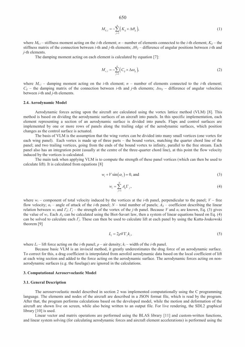
650

,1

,n

k i ij ijj

M K (1)

where Mk,i – stiffness moment acting on the i-th element; n – number of elements connected to the i-th element; Kij – the stiffness matrix of the connection between i-th and j-th elements; ij – difference of angular positions between i-th and j-th elements.

The damping moment acting on each element is calculated by equation [7]:

,1

,n

c i ij ijj

M C (2)

where Mc,i – damping moment acting on the i-th element; n – number of elements connected to the i-th element; Cij – the damping matrix of the connection between i-th and j-th elements; ij – difference of angular velocities between i-th and j-th elements.

2.4. Aerodynamic Model

Aerodynamic forces acting upon the aircraft are calculated using the vortex lattice method (VLM) [8]. This method is based on dividing the aerodynamic surfaces of an aircraft into panels. In this specific implementation, each element representing a section of an aerodynamic surface is divided into panels. Flaps and control surfaces are implemented by one or more rows of panels along the trailing edge of the aerodynamic surfaces, which position changes as the control surface is actuated.

The basis of VLM is the assumption that the wing vortex can be divided into many small vortices (one vortex for each wing panel). Each vortex is made up of three parts – the bound vortex, matching the quarter chord line of the panel; and two trailing vortices, going from the ends of the bound vortex to infinity, parallel to the free stream. Each panel also has an integration point (usually at the centre of the three-quarter chord line), at this point the flow velocity induced by the vortices is calculated.

The main task when applying VLM is to compute the strength of these panel vortices (which can then be used to calculate lift). It is calculated from equations [8]

sin 0, andi iw V (3)

1

,N

i ij jj

w A (4)

where wi – component of total velocity induced by the vortices at the i-th panel, perpendicular to the panel; V – free flow velocity; i – angle of attack of the i-th panel; N – total number of panels; Aij – coefficient describing the linear relation between wi and j; j – the strength of the vortex of the j-th panel. Because V and i are known, Eq. (3) gives the value of wi. Each Aij can be calculated using the Biot-Savart law, then a system of linear equations based on Eq. (4) can be solved to calculate each j. These can then be used to calculate lift at each panel by using the Kutta-Joukowski theorem [9]

2 ,i i iL V k (5) where Li – lift force acting on the i-th panel; – air density; ki – width of the i-th panel.

Because basic VLM is an inviscid method, it greatly underestimates the drag force of an aerodynamic surface. To correct for this, a drag coefficient is interpolated from aerofoil aerodynamic data based on the local coefficient of lift at each wing section and added to the force acting on the aerodynamic surface. The aerodynamic forces acting on non-aerodynamic surfaces (e.g. the fuselage) are ignored in the calculations.

3. Computational Aeroservoelastic Model 3.1. General Description

The aeroservoelastic model described in section 2 was implemented computationally using the C programming

language. The elements and nodes of the aircraft are described in a JSON format file, which is read by the program. After that, the program performs calculations based on the developed model, while the motion and deformation of the aircraft are shown live on screen, while also being written to an output file. For live rendering, the SDL2 graphical library [10] is used.

Linear vector and matrix operations are performed using the BLAS library [11] and custom-written functions, and linear system solving (for calculating aerodynamic forces and aircraft element accelerations) is performed using the

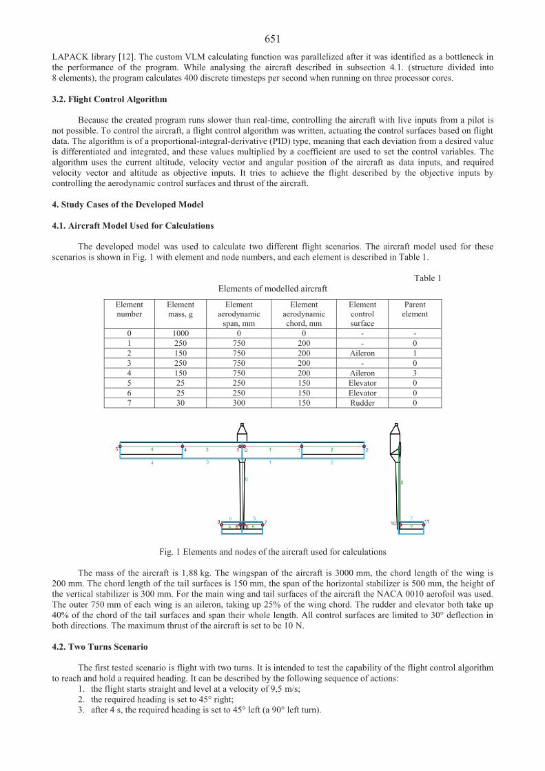
651 LAPACK library [12]. The custom VLM calculating function was parallelized after it was identified as a bottleneck in the performance of the program. While analysing the aircraft described in subsection 4.1. (structure divided into 8 elements), the program calculates 400 discrete timesteps per second when running on three processor cores.

3.2. Flight Control Algorithm

Because the created program runs slower than real-time, controlling the aircraft with live inputs from a pilot is not possible. To control the aircraft, a flight control algorithm was written, actuating the control surfaces based on flight data. The algorithm is of a proportional-integral-derivative (PID) type, meaning that each deviation from a desired value is differentiated and integrated, and these values multiplied by a coefficient are used to set the control variables. The algorithm uses the current altitude, velocity vector and angular position of the aircraft as data inputs, and required velocity vector and altitude as objective inputs. It tries to achieve the flight described by the objective inputs by controlling the aerodynamic control surfaces and thrust of the aircraft.

4. Study Cases of the Developed Model 4.1. Aircraft Model Used for Calculations

The developed model was used to calculate two different flight scenarios. The aircraft model used for these scenarios is shown in Fig. 1 with element and node numbers, and each element is described in Table 1.

Table 1

Elements of modelled aircraft

Element number

Element mass, g

Element aerodynamic

span, mm

Element aerodynamic chord, mm

Element control surface

Parent element

0 1000 0 0 - - 1 250 750 200 - 0 2 150 750 200 Aileron 1 3 250 750 200 - 0 4 150 750 200 Aileron 3 5 25 250 150 Elevator 0 6 25 250 150 Elevator 0 7 30 300 150 Rudder 0

Fig. 1 Elements and nodes of the aircraft used for calculations

The mass of the aircraft is 1,88 kg. The wingspan of the aircraft is 3000 mm, the chord length of the wing is 200 mm. The chord length of the tail surfaces is 150 mm, the span of the horizontal stabilizer is 500 mm, the height of the vertical stabilizer is 300 mm. For the main wing and tail surfaces of the aircraft the NACA 0010 aerofoil was used. The outer 750 mm of each wing is an aileron, taking up 25% of the wing chord. The rudder and elevator both take up 40% of the chord of the tail surfaces and span their whole length. All control surfaces are limited to 30° deflection in both directions. The maximum thrust of the aircraft is set to be 10 N. 4.2. Two Turns Scenario

The first tested scenario is flight with two turns. It is intended to test the capability of the flight control algorithm to reach and hold a required heading. It can be described by the following sequence of actions:

1. the flight starts straight and level at a velocity of 9,5 m/s; 2. the required heading is set to 45° right; 3. after 4 s, the required heading is set to 45° left (a 90° left turn).

652 During the flight, a constant required flight speed of 9,6 m/s and altitude was set. The results of the calculations

are presented in Fig. 2 and Fig. 3. In Fig. 2 the trajectory of the aircraft viewed from above is shown. The aircraft starts a right turn immediately when the scenario starts, and at 2 s the turn is mostly finished. At 4 s, when the right turn is fully finished, the aircraft starts a left turn. At 8 s, the left turn is finished, and the aircraft continues to fly straight.

Fig. 2 Trajectory of the aircraft during the two turns flight scenario

Fig. 3 Aileron deflection angle and aircraft bank angle over time during the two turns flight scenario

In Fig. 3 it can be seen that the aircraft starts the flight with ailerons fully deflected to perform the first turn. The

aircraft goes into a bank of 50,64° (the algorithm is limited to 50° banks, but can overshoot because of rolling inertia) and returns to level flight as it approaches the required heading. At 4 s as the second turn starts, the ailerons are deflected fully in the opposite direction. The aircraft enters a bank of 52,52° and holds it until 6,5 s, returning to level flight as it approaches the new heading. There is an oscillation as the aircraft exits the manoeuvre, caused by rolling inertia and wing flexing, but it is damped by the control algorithm. After the manoeuvre the aircraft stays in a 5° right bank, attempting to correct its course (in Fig. 2 it is shown that the aircraft is heading slightly more left than the required 45° heading). 4.3. Pitch Up Scenario

The second flight scenario was a pitch up manoeuvre. It is intended to test the bending of the wings under aerodynamic loading. It can be described by the following sequence of actions:

1. the flight starts straight and level at a velocity of 10 m/s; 2. after two seconds elevator is set to a fixed 20° angle; 3. while pitching up, the rudder and ailerons are used to hold the heading straight and the wings level. In Fig. 4 and Fig. 5 the results of this calculation are presented. Fig. 4 shows a side-view trajectory of the

aircraft. There is an initial dip in altitude because the aircraft starts at zero angle-of-attack. By 1 s, it is corrected. The aircraft then continues to fly straight until 2 s, when it starts pitching up. The radius of the trajectory arc is decreasing as the velocity of the aircraft decreases. By 5 s the aircraft is past the vertical and partially inverted.

Fig. 4 Trajectory of the aircraft during the pitch up flight scenario

653

Fig. 5 Elevator deflection angle and aircraft wing bending angle over time during the pitch up flight scenario Fig. 5 shows the elevator deflection angle and aircraft wing bending angle changing over time. Over the first two

seconds of the flight, the wings and elevator are in a damped oscillation as the aircraft returns to level flight from the initial dip. At 2 s, the elevator is set to a constant 20° angle, the deflection of the wings start increasing until it reaches 4,57° at about 3 s, then starts decreasing as the velocity of the aircraft and the aerodynamic loads start decreasing. Because the wings are kept level and the aerodynamic loads are symmetrical, both wings are bent at the same angle, until the plane becomes inverted. After that, the flight algorithm tries to roll the plane back up using ailerons, which causes asymmetrical loading and bending of the wings.

5. Conclusions

A physical aeroservoelastic model for analysing the flight characteristics of high flexibility aircraft was

developed by combining the vortex lattice method, a lumped mass structural model and a traditional kinematic model. The physical model was implemented computationally using the C programming language. The program

calculates 400 discrete timesteps per second when running on three processor cores. A flight control algorithm was created to control the aircraft during the calculations. The algorithm is of the

proportional-integral-differential type. Two test scenarios were successfully calculated using the developed program. It was shown that the flight

algorithm can reach and hold a required heading and that the structure of the aircraft deforms under aerodynamic loading as expected. Acknowledgement

This project has received funding from European Social Fund (project No 09.3.3-LMT-K-712-24-0020) under grant agreement with the Research Council of Lithuania (LMTLT). References 1. Slayton, R.; Spinardi, G. 2015. Radical innovation in scaling up: Boeing’s Dreamliner and the challenge of socio-

technical transitions, Technovation 47: 47-58. 2. Swaim, R.L.; Yen, W.Y. 1978. Effects of dynamic aeroelasticity on handling qualities and pilot rating, 4th

Atmospheric Flight Mechanics Conference, Palo Alto 266-271. 3. Brillante, C.; Mannarino, A. 2016. Improvement of aeroelastic vehicles performance through recurrent neural

network controllers, Nonlinear Dynamics 84(3):1479-1495. 4. Zhang, K.; Marzocca, P.; Behal, A. 2015. Adaptive aeroelastic control of nonlinear airfoil with multiple flaps

under unsteady flow, Journal of Vibration and Control 23(10):1593-1606. 5. Livet, T.; Kubica, F.; Magni, J.F. 1995. Robust Flight Control Design With Respect to Delays and Control

Efficiencies, Control Engineering Practice 3(10):1373-1384. 6. Beggs, J.S. 1983. Kinematics, New York: Hemisphere Publishing Corporation. 7. Fedaravi ius, A.; Jurkauskien , E.; Miku ionien , J.; Rudgalvien , N. 2009. Teorin mechanika: teorijos

pagrindai ir uždaviniai. Kaunas: Technologija (in Lithuanian). 8. Cummings, R.M.; Hason, W.H.; Morton, S.A.; McDaniel, D.R. 2015. Applied Computational Aerodynamics: A

Modern Engineering Approach (Cambridge Aerospace Series), Cambridge: Cambridge University Press. 9. Anderson, J. 2017. Fundamentals of Aerodynamics (6th edition), New York: McGraw-Hill Education, 275 p. 10. Simple DirectMedia Layer [online cit: 2021-07-20]. Available from: https://www.libsdl.org/ 11. BLAS (Basic Linear Algebra Subprograms) [online cit: 2021-07-16]. Available from: https://www.netlib.org/blas/ 12. LAPACK—Linear Algebra PACKage [online cit: 2021-07-16]. Available from: https://www.netlib.org/lapack/

654

Proceedings of 25th International Scientific Conference. Transport Means 2021. Oil Spectrometric Analysis as a Monitoring Tool in the Wear of an Aircraft Piston Engine A. Bielec1, J. Nowakowski2 1University of Bielsko-Biala, Willowa 2, 43-309, Bielsko-Biala, Poland, E-mail: ab054535@student.ath.edu.pl 2University of Bielsko-Biala, Willowa 2, 43-309, Bielsko-Biala, Poland, E-mail: jnowakowski@ath.bielsko.pl Abstract Spectrometric analysis of engine oil was introduced around 1960 as an engine condition assessment tool. It is perceived as an effective tool for monitoring the condition of the engine in aircraft used for military purposes, it was introduced as a standard in the operation of some General Aviation turbine engines, while in piston engines it has so far performed a supporting role based on the manufacturer's recommendation. During the test, ten small aircraft (with a maximum take-off weight not exceeding 2730 kg) were assessed. Based on the obtained data, a Cessna T207A aircraft for skydiving with a Continental TSIO-520-M piston engine was selected for a detailed study. This type of use is characterized by high seasonal intensity. The plane makes from several to a dozen daily departures at an altitude of 800 to a maximum of 4000 meters above sea level. In the off-season, the aircraft performs occasional flights on the basis of ferrying to / from a maintenance organization or a berth. KEY WORDS: aircraft engine; engine oil; spectrometric oil analysis, piston engine, aircraft, Part-ML, exceptions, time between overhaul 1. Introduction

The maintenance of civil aircraft consists of mandatory activities resulting from certification processes or Airworthiness Directives issued by aviation authorities, as well as non-mandatory activities that are recommended by manufacturers of aviation equipment in the Maintenance Manuals or additional documents such as service bulletins, service lists, etc. In accordance with the current Part-ML regulations, the user of a small aircraft not used in certified air transport may deviate from other than mandatory maintenance activities, including the piston engine overhaul period. On August 29, 2019, the President of the Civil Aviation Authority issued Guidelines No. 9 [1], which describe the methodology for derogating from the main inspections of a piston engine, thus introducing the spectrometric analysis of used engine oil as one of the main tools for assessing the condition of the engine. 2. Test Results and Their Analysis

During the study 10 aircraft were assessed, Table below lists the types of aircraft tested.

Table Types of aircraft tested

Aircraft Engine model Aircraft operations Cessna TU206G Continental TSIO-520-M skydiving Cessna T207A Continental TSIO-520-M skydiving Koliber 160 Lycoming O-320-D2A private, non-commercial operation Cessna 172S Lycoming IO-320-L2A private, non-commercial operation Beech Baron Continental IO-550 private, non-commercial operation Socata Rallye 180TS Lycoming O-360 private, Approved Training Organization/

Declared Training Organization PS28 Cruiser Rotax 912 private, non-commercial operation Cessna 182P Continental O-470-R private, non-commercial operation Cessna 182P Continental O-470-R private, non-commercial operation Cessna F150M Continental O-200-A private, non-commercial operation

Usually, a sample is taken when the engine oil is changed - every 50 hours of flight or four months, whichever

comes first. This interval may be reduced to 25 hours of flight time when the engine break-in, i.e. new or after major repair, or has been exposed to: volcanic ash, particulate matter, sand, dust debris, extreme weather conditions or salt salt in coastal environment.

Sampling procedure [2]: 1. Run the engine until the oil temperature stabilizes, then shut down the engine.

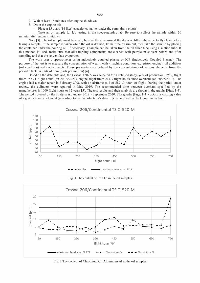
6552. Wait at least 15 minutes after engine shutdown. 3. Drain the engine oil:

– Place a 15 quart (14 liter) capacity container under the sump drain plug(s).– Take an oil sample for lab testing in the spectrographic lab. Be sure to collect the sample within 30

minutes after engine shutdown. Note [3]: The oil sample must be clean; be sure the area around the drain or filler tube is perfectly clean before

taking a sample. If the sample is taken while the oil is drained, let half the oil run out, then take the sample by placing the container under the pouring oil. If necessary, a sample can be taken from the oil filler tube using a suction tube. If this method is used, make sure that all sampling components are cleaned with petroleum solvent before and after sampling and that the solvent has evaporated.

The work uses a spectrometer using inductively coupled plasma or ICP (Inductively Coupled Plasma). The purpose of the test is to measure the concentration of wear metals (machine condition, e.g. piston engine), oil additives (oil condition) and contaminants. These parameters are defined by the concentrations of various elements from the periodic table in units of ppm (parts per million) [4].

Based on the data obtained, the Cessna T207A was selected for a detailed study, year of production: 1980, flight time: 7853.1 flight hours (on 20/05/2021), engine flight time: 214.3 flight hours since overhaul (on 20/05/2021). The engine had a major repair in February 2008 with an airframe raid of 5871.9 hours of flight. During the period under review, the cylinders were repaired in May 2019. The recommended time between overhaul specified by the manufacturer is 1600 flight hours or 12 years [5]. The test results and their analysis are shown in the graphs [Figs. 1-4].The period covered by the analysis is January 2018 - September 2020. The graphs [Figs. 1-4] contain a warning value of a given chemical element (according to the manufacturer's data [3]) marked with a black continuous line.

Fig. 1 The content of Iron Fe in the oil samples

Fig. 2 The content of Chromium Cr, Aluminum Al in the oil samples

656

Fig. 3 The content of Copper Cu, Silicone Si in the oil samples

Fig. 4 The content of metallic elements in the oil samples

The cylinder was repaired after 150 flight hours. Before the cylinder repair, one can see an increased concentration of iron, zinc, nickel and an increased amount of ferromagnetic elements in the oil samples (PQ index -diagram in Fig. 4). These indicators and the defect that appeared in the aircraft logbook entry, i.e. "excessive fuel

657 consumption, significant loss of engine power" prompted the user to check the condition of the engine and in May 2019 all cylinders were repaired. Further intensive use in the period May - September 2020 led to the appearance of unusual engine vibrations and the appearance of small elements on the oil filter. After a thorough inspection, the engine was found damaged and the need for a complete overhaul. The results of the tests carried out on the occasion of disassembly of the engine indicate increased values of iron concentration, persistently high values of chromium and silicon concentrations, exceeding the concentration of aluminum and at the same time an increased concentration of ferromagnetic elements. Iron, aluminum, and chrome can often be seen together in engine oil samples as they form the metallurgy of liners, pistons, and rings. This is usually seen in conjunction with elevated levels of silicon, as dirt ingress through the air intake system can cause abnormal wear. In engines, cylinder liners and crankshaft are the main wear parts, as are timing gears, shafts and valves. In gearboxes and drive train components, iron is the major component of gears, shafts and rolling bearings. The rings are usually made of or coated with chrome. In rare cases, the inserts may be chrome-plated and the rings are then made of cast iron. The source of aluminum in the oil can be excessive wear of the connecting rod, accessory housing, oil pump body, cylinder head, pistons, piston pin plugs, oil pan baffle, turbocharger inlet housing or plain bearings [4].

As a result of the repair, damage to the piston was found due to the dislodged counterweight of the crankshaft. The obtained concentration values of individual elements coincide with the results of the engine condition control during its main repair. In the case of the tested engine, its failure was sudden and previous analyzes of the used engine oil did not indicate a problem. The analyzes showed normal concentration of aluminum, and the iron remained at a constant high level, but not exceeding the warning level. This engine was put into service as is, with a deviation from the manufacturer's recommended maintenance interval, and its use exceeded the manufacturer's recommended maintenance interval by 167 flight hours / 7 months. The other tested engines did not show any faults, as well as the results of the concentrations of individual chemical elements did not exceed the warning level. 3. Conclusions

The ukasiewicz Institute of Aviation published in April 2021 a work entitled "Analysis of aviation events caused by failures of airframe and engine installations in 2008 - 2020" [6]. This study in the field of defects related to General Aviation piston engines contains information about the increase in more than two times the number of piston engine failures in the years between 2016 and 2020, where in 2016 the Guidelines of the President of the Civil Aviation Authority No. 9 were published [1]. One of the possible reasons for the obtained results is the introduction of the aforementioned guidelines and some kind of freedom in the operation of aircraft piston engines. The study also contains information about the need to carry out more thorough maintenance of piston power units in order to counteract a further increase in aviation incidents [6].

The application of a deviation from the manufacturer's recommendations, although permissible in the scope of the Aviation Law, requires taking over responsibility for its implementation. It can be concluded that only having appropriate knowledge and experience in the use and analysis of engine parameters - including indicators of the content of individual chemical elements in used engine oil allows for deviations from the recommendations of aviation equipment manufacturers.

The use of spectrometric analysis programs for engine oil is recommended by almost all engine manufacturers - the results of these analyzes, however, do not constitute a clear indication of negative processes that occur in a given engine. They are only an indication that the degradation of a given element may begin and the engine should be inspected e.g. by a borescope inspection or by major repair.

Summing up, the spectrometric analysis of used engine oil as an independent tool is not a correct tool for analyzing the wear trends of a piston engine, however, when combined with other tools, such as the analysis of engine operating parameters, control of engine oil consumption, fuel consumption control, boroscopic inspection, etc., it is an effective tool analysis of piston engine wear trends.

The use of all the above-mentioned tools comprehensively allows you to examine the condition of the engine during its operation and react to any emerging deviations from trends that may indicate possible engine malfunctions. References 1. Prezes ULC 2019. Wytyczne Nr 9 z dnia 29 sierpnia 2019r. w sprawie okresów mi dzy-remontowych silników

t okowych (in Polish). 2. Oil Servicing, Metallic Solids Identification After Oil Servicing, and Associated Corrective Action [online cit.:

2021-05-20]. Available from: https://www.lycoming.com/content/service-bulletin-no-480-f. 3. General aspects of Spectrometric Oil Analysis, [online cit.: 2021-05-20]. Available from: https://www.lycoming.

com/content/service-letter-no-l171. 4. Evans, J. 2010. Where does all that metal come from? Wearcheck AFRICA Technical Bulletin Issue 47. 5. Time between Overhaul Periods, [online cit.: 2021-05-20] Available from: http://www.continental.aero/

uploadedFiles/Content/xImages/TBO%20Page%20SIL98-9C.pdf . 6. G owacki, P. 2021. Analiza zdarze lotniczych powodowanych niesprawno ciami instalacji p atowcowych i

silnikowych w latach 2008 – 2020: Instytut Lotnictwa ukasiewicz 2021 (in Polish).

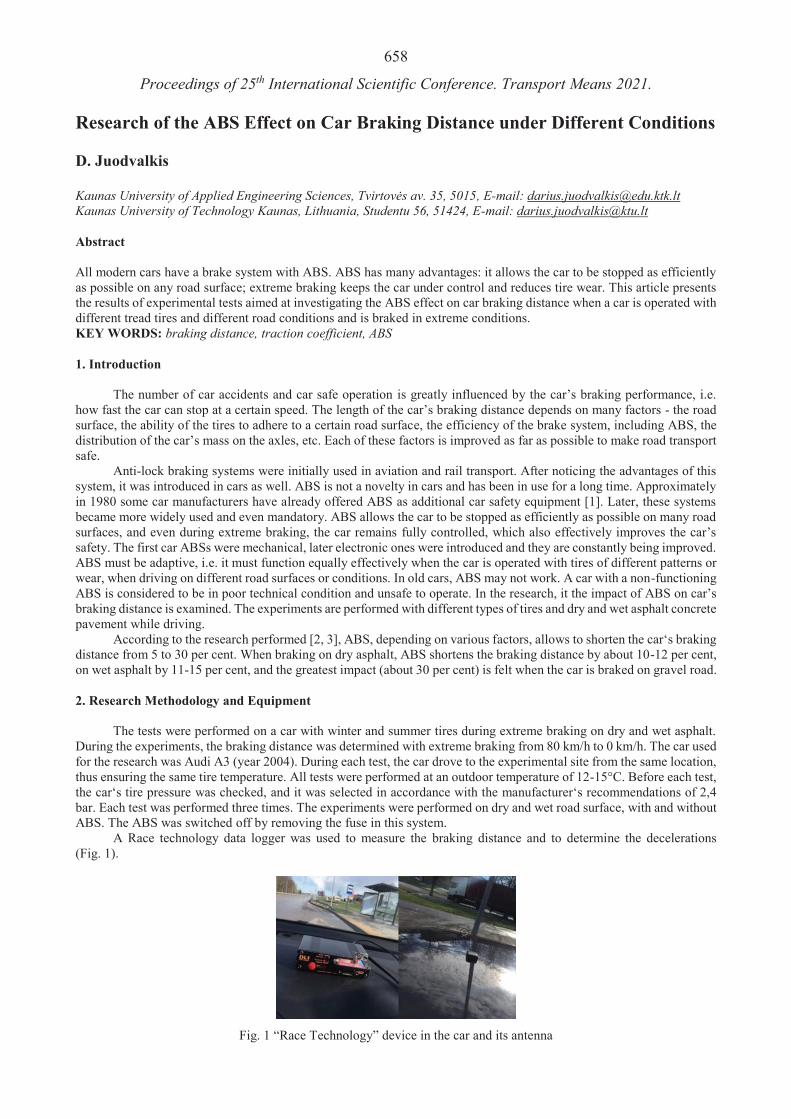
658

Proceedings of 25th International Scientific Conference. Transport Means 2021. Research of the ABS Effect on Car Braking Distance under Different Conditions D. Juodvalkis Kaunas University of Applied Engineering Sciences, Tvirtov s av. 35, 5015, E-mail: darius.juodvalkis@edu.ktk.lt Kaunas University of Technology Kaunas, Lithuania, Studentu 56, 51424, E-mail: darius.juodvalkis@ktu.lt Abstract All modern cars have a brake system with ABS. ABS has many advantages: it allows the car to be stopped as efficiently as possible on any road surface; extreme braking keeps the car under control and reduces tire wear. This article presents the results of experimental tests aimed at investigating the ABS effect on car braking distance when a car is operated with different tread tires and different road conditions and is braked in extreme conditions. KEY WORDS: braking distance, traction coefficient, ABS 1. Introduction

The number of car accidents and car safe operation is greatly influenced by the car’s braking performance, i.e. how fast the car can stop at a certain speed. The length of the car’s braking distance depends on many factors - the road surface, the ability of the tires to adhere to a certain road surface, the efficiency of the brake system, including ABS, the distribution of the car’s mass on the axles, etc. Each of these factors is improved as far as possible to make road transport safe.

Anti-lock braking systems were initially used in aviation and rail transport. After noticing the advantages of this system, it was introduced in cars as well. ABS is not a novelty in cars and has been in use for a long time. Approximately in 1980 some car manufacturers have already offered ABS as additional car safety equipment [1]. Later, these systems became more widely used and even mandatory. ABS allows the car to be stopped as efficiently as possible on many road surfaces, and even during extreme braking, the car remains fully controlled, which also effectively improves the car’s safety. The first car ABSs were mechanical, later electronic ones were introduced and they are constantly being improved. ABS must be adaptive, i.e. it must function equally effectively when the car is operated with tires of different patterns or wear, when driving on different road surfaces or conditions. In old cars, ABS may not work. A car with a non-functioning ABS is considered to be in poor technical condition and unsafe to operate. In the research, it the impact of ABS on car’s braking distance is examined. The experiments are performed with different types of tires and dry and wet asphalt concrete pavement while driving.

According to the research performed [2, 3], ABS, depending on various factors, allows to shorten the car‘s braking distance from 5 to 30 per cent. When braking on dry asphalt, ABS shortens the braking distance by about 10-12 per cent, on wet asphalt by 11-15 per cent, and the greatest impact (about 30 per cent) is felt when the car is braked on gravel road.

2. Research Methodology and Equipment

The tests were performed on a car with winter and summer tires during extreme braking on dry and wet asphalt. During the experiments, the braking distance was determined with extreme braking from 80 km/h to 0 km/h. The car used for the research was Audi A3 (year 2004). During each test, the car drove to the experimental site from the same location, thus ensuring the same tire temperature. All tests were performed at an outdoor temperature of 12-15°C. Before each test, the car‘s tire pressure was checked, and it was selected in accordance with the manufacturer‘s recommendations of 2,4 bar. Each test was performed three times. The experiments were performed on dry and wet road surface, with and without ABS. The ABS was switched off by removing the fuse in this system.

A Race technology data logger was used to measure the braking distance and to determine the decelerations (Fig. 1).

Fig. 1 “Race Technology” device in the car and its antenna

659This equipment is suitable for use in a variety of vehicles, from cars to bicycles. DL can be used in a variety of

industries. This data logger has advanced technology, built-in 5Hz GPS receiver, digital 3-axis accelerometers, Compact Flash memory, eight 12bit analogue inputs, dual RPM inputs, 4 wheel or shaft speed inputs, has OBDII adapter. The Race technology device can store data from a variety of sources, including its own high-precision GPS and acceleration sensors.

Used Goodyear winter tread pattern and Guigiaro summer tread pattern tires were used in the tests (Fig. 2).

Fig. 2 Tires used in the research

Tire wear is about 50%, i.e. tread pattern depth is about 4-5 mm. Both sets of tires were made in 2017. The dimensions of the tires are the same as for the AUDI A3 - 205/55R16.

After the experiments, the deceleration of the car and the braking distance of the car were determined using the data measured by the device Race Technology (Fig. 3).

a b

Fig. 3. Examples of the results: a deceleration; b braking distance

Knowing the deceleration or braking distance of the car, the traction coefficient of the tire to the road surface can be calculated [4]:

20

2 braking

vg S

; (1)

where – traction coeficient; v – initial speed (m/s); g – acceleration of gravity (m/s2); brakingS – braking distance (m).The traction coefficient of a tire to the road surface also depends on the slip of the tire in relation to the road. The

anti-lock braking system controls wheel slip and supports it by about 10 -20 per cent [5]. When braking without ABS, the wheels are locked and the wheel slip in relation to the road is 100 per cent.

3. Research Results

After performing experiments on braking the car on different surfaces and with different tires, the lengths of the braking distance during different experiments were determined. In total eight different tests were performed:

Test No.1. Summer tires, dry road surface and braking without ABS;Test No.2. Summer tires, dry road surface and braking with ABS;Test No.3. Summer tires, wet road surface and braking without ABS;Test No.4. Summer tires, wet road surface and braking with ABS;Test No.5. Winter tires, dry road surface and braking without ABS;Test No.6. Winter tires, dry road surface and braking with ABS;Test No.7. Winter tires, wet road surface and braking without ABS;

660Test No.8. Winter tires, wet road surface and braking with ABS;For more accurate results, each experiment was performed three times, i.e. in total 24 measurements were

performed and mathematical average of the results was calculated.The results of tests with summer tires are presented in Fig. 4.

Fig. 4 Tests with summer tires under different conditions

The results of tests with winter tires are presented in Fig. 5.

Fig. 5 Tests with winter tires under different conditions

Analysing the results of the experiments performed, which are presented in Fig. 4, it can be observed that, as might be expected, the shortest braking distance was obtained when braking on a dry road surface, a car with summer-type tires and with anti-lock braking system in operation that prevented the wheels from locking. In this case, the resulting braking distance from the initial speed of 80 km/h was about 29 m. Under the same conditions, but with the ABS switched off, the braking distance was already longer and it was about 33 m. With summer tires, the worst result was obtained when braking on wet road surface and with ABS switched off - about 40 m. If the braking distance with ABS and without ABSis compared, then it can be noticed that on dry and wet road surfaces and when ABS is switched off, braking distance is longer about 11 per cent. Comparing the lengths of the braking distance in the case of dry and wet road surface, it can benoticed that with and without ABS, in the case of wet road surface, braking distance is about 20% longer.

Analysing the results of experiments with winter type tires, which are presented in Fig. 5, it can be observed that, as with summer tires, the shortest braking distance was obtained when braking on a dry road surface and the car’s anti-lock braking system was in operation, which prevented the wheels from locking. In this case, the resulting braking distance from the initial speed of 80 km/h was about 32 m. Under the same conditions, but with the ABS switched off, the resulting braking distance is longer and it is 35 m. With winter tires, the worst result was obtained when braking on wet road surface and with ABS switched off - about 44 m. If the braking distance with ABS and without ABS is compared, then it can be noticed that on dry and wet road surfaces and when ABS is switched off, braking distance is longer about 9.5 per cent. Comparing the lengths of the braking distance in the case of dry and wet road surface, it can be noticed that with and without ABS, in the case of wet road surface, braking distance is about 22% longer.

Comparing the results of experiments with summer and winter tires (Fig. 4 and Fig. 5), it is noticed that in

661 practically in all cases the results of braking experiments with winter type tires are about 10% worse. Thus, it can be concluded that at an ambient temperature of about 12-15°C, it is safer to use summer-type tires because they provide a shorter braking distance, i.e. these tires grip the road better. It is likely that this difference would be even greater with increasing ambient temperature.

In Table the calculated traction coefficient between the tire and the road surface are presented.

Table Traction coefficient

Type of tyres

Traction coefficient ( ) Dry asphalt with

ABS Dry asphalt

without ABS Wet asphalt with

ABS Wet asphalt

without ABS Summer 0.86 0.76 0.68 0.62 Winter 0.78 0.71 0.61 0.57

Analysing the results presented in Table 1, it is seen that the best traction coefficient is obtained with summer tires

on dry asphalt and with ABS - 0.86, and the worst when the tires are winter type, the road surface is wet and without ABS - 0.57. It can be said that when driving a car with winter type tires, with wet road surface and without ABS, the braking distance will be about 1.5 times longer than with summer tires on dry road surface and with ABS.

4. Conclusions

ABS shortens the braking distance of the car in all cases of the performed experiments; the resulting braking distance with ABS is about 10% shorter than without ABS.

In the case of wet road surfaces, about 10% of all tested types of tires have poorer grip on the road surface, whether braking with or without ABS.

At an ambient temperature of about 12-15 C, it is safer to operate cars with summer-type tires, as summer tires with both dry and wet road surfaces provide about 10% better grip on the road surface than winter tires.

The performed experiments have shown that when driving a car with winter tires, on wet road surface and without ABS, the braking distance will be about 1.5 times longer than with summer tires on dry road surface and with ABS. References

1. ABS brakes helped airlines make more money before they helped you stop. [online cit.: 2021-06-22]. Available from:

https://www.digitaltrends.com/cars/the-history-of-abs-brakes-from-airplanes-to-cars 2. NHTSA Light Vehicle ABS Research Program. Final report. [online cit.: 2021-06-20]. Available from:

https://www.nhtsa.gov/sites/nhtsa.gov/files/nhtsaabst4finalrpt.pdf 3. A Comparative Study of Different Control Methods for Anti-Lock Braking System (ABS). [online cit.: 2021-06-25].

Available from: https://svusrc.journals.ekb.eg/article_177078_b03f2bd1bfe747e5dc409ee5e8a4ebd9.pdf 4. Sabri, M.; Fauza, A. 2018. Analysis of vehicle braking behaviour and distance stopping, IOP Conference Series:

Materials Science and Engineering 309: 012020. 10.1088/1757-899X/309/1/012020. 5. Kudarauskas, N. 2007. Analysis of emergency braking of a vehicle, Transport 22(3): 154-159. https://doi.org/

10.3846/16484142.2007.9638118

662

Proceedings of 25th International Scientific Conference. Transport Means 2021. Evaluation of Suburban Bus Transport Performance in a Selected Region of the Slovak Republic During the Covid-19 P. Kral1, K. Janoskova2 1University of Žilina, Faculty of Operation and Economics of Transport and Communications, Univerzitna 8215/1, 010 26 Žilina, Slovakia, E-mail: pavol.kral@fpedas.uniza.sk 2University of Žilina, Faculty of Operation and Economics of Transport and Communications, Univerzitna 8215/1, 010 26 Žilina, Slovakia, E-mail: katarina.janoskova@fpedas.uniza.sk Abstract The Covid-19 pandemic has affected socio-economic situation around the world. However, its impact on regions and sectors of the economy is different. Public passenger transport is one of the most affected segments in connection with the measures taken to prevent the spread of the Covid-19 virus. The number of transported people due to the pandemic has dropped significantly. The main purpose of this paper is to point out the decline in public transport performance (suburban bus transport) in the Prešov Region in Slovakia in 2020, using selected statistical apparatus to formulate appropriate conclusions and outline the concept of gradual renewal of transport services and restoration of public confidence in transport services. The article also addresses the issue of advance payment for public interest services providing transport services for the inhabitants of the region. Only through systematic and rational measures, it will be possible to revitalize public transport and ensure its competitiveness in relation to individual transport. KEY WORDS: Covid-19 pandemic, suburban bus transport, public transport performance, advanced payment 1. Introduction

Pandemics have appeared several time in history and have always brought significant threats but also new

challenges. In order to protect public health and not collapse the health system, the governments of the countries have been forced to take strict measures to restrict the movement of the population including very strict lockdown measures and prohibition of some out of home activities. This situation has, of course, been reflected in a decline in mobility, a decline in the performance of public and individual transport, as well as in other sectors of the economy. The transport sector is still facing a significant economic crisis, especially with regard to public transport. On the other hand, some positive effects are also known. United Nations Economic Commission for Europe reported interesting data outcome regarding transportation of several countries. Lockdown period have witnessed a downfall in road fatality in countries such as Norway ( 54%), France ( 56%), London ( 36%) compared to the month of 2019, Budapest confirmed 50% decline in traffic congestion, in Berlin was reduced road traffic by 40%, cyclists increased by 50% in New Work city during March 2020 etc. Many researchers and organizations consistently investigate impacts of COVID-19 pandemic on the transport sector and corresponding actions. It is obvious that it will not be possible to ensure sustainability of public transport without fundamental changes.

2. Literature Review

The need to address the issue of public transport during a pandemic is evidenced by a number of scientific publications. Scientifically suitable approaches that may lead to correct policy decisions on transportation sector in terms of COVID-19 pandemic are deficient. Researchers of transport segment of different countries should stress on the concept of monetary compensation for each transport industries facing a massive loss throughout the pandemic [1].

Based on a survey by the World Conference on Transport over half of the experts surveyed (54.6%) reported that in the town (city) where they were living, the number of passengers boarding public transport vehicles was restricted, and 22.2% of the experts observed online bookings for use of public transport during the pandemic, 27.8% of experts observed that monetary compensation had been given to transport and logistics firms suffering from economic losses as a measure to address the impacts of the pandemic.

According to the Guidelines on the progressive restoration of transport services and connectivity – COVID-19 [2] an entirely risk-free environment for travel is not feasible, as is the case for any other activity, but risks should be minimised as much as possible throughout the duration of the outbreak.

The 50 to 60% drop in km travelled is a major threat to the current operation of public transport in Switzerland, with its short headways, clear priority for signal control, fixed timetables and all-day and all-region service. This level of service and reliability is the basis for the large proportion of Swiss residents who own season tickets [3]. An empirical research conducted in Germany projected the dynamic impact of COVID-19 on the transportation volume

663 and bulk-goods capacity in food material trade [4].

Private car usage in cities also fell initially as more people have been urged to work from home, and home working may become the new normal for a much larger proportion of workers in the future. However, fear of infection also seems likely to have led to more private car usage for commuting in the short to medium term during the recovery thus compounding the financial problems for public transport operators [5]

The pandemic also significantly affected all areas of the shared economy including the sharing of means of transport and property owners of accommodation capacities in tourism sector, education, and psychosomatic well-being [6, 7].

The shutdown measures put an end to the activities of many entrepreneurs, who had to lay off their employees. Thus, the Covid-19 pandemic is a major reason behind the rising unemployment. The Government of the Slovak Republic seeks to eliminate the effects of anti-pandemic measures by introducing interventions to help the businesses survive and provide at least partial compensation to employers so that they are able to retain their employees [8].

3. Results of Research

The main purpose of the scientific research is the knowledge of the impact of the COVID-19 pandemic on public transport and its performance in the Prešov self-governing region (PSR) which is one of the eight regions of the Slovak Republic. The most of the input data was obtained from the document “Report on the calculation of the advance contribution for services in the public interest in suburban bus transport for the year 2020” that was prepared directly by the Department of Transport of PSR [9]. Due to its size, PSR must provide transport services over a larger area. For this reason, carriers operating in PSR must to realize higher driving performance compared to the other regions of the Slovak Republic that subsequently have more space for increasing the cost per unit of output. Values of planned driving performance for 2020 in all regions are presented in Table 1.

Table 1 Planned driving performance for 2020

Self-governing region Planned driving performance [km]

Percentage difference compared to PSR [%]

Bratislava 15 330 107 -46 Banská Bystrica N/A N/A Košice 25 664 861 -11 Nitra 22 676 039 -22 Prešov 29 021 000 100 Tren ín 22 237 587 -23 Trnava 20 172 896 -30 Žilina 22 400 000 -16

The achieved revenues from bus transport in 2020 recorded a large decrease. Compared to 2019, the decline was

almost at the level of a third in all regions of the Slovak Republic (Table 2).

Table 2 Revenues of public bus transport in 2019 and 2020

Self-governing region 2019 2020 Difference [%] Banská Bystrica 12 661 824 8 503 182 -4 158 642 -32.84 Nitra 10 291 870 7 024 952 -3 266 918 -31.74 Bratislava 9 298 052 5 884 545 -3 413 507 -36.71 Žilina 13 415 096 8 941 579 -4 473 517 -33.35 Košice 13 147 504 8 969 411 -4 178 093 -31.78 Trnava 8 460 708 5 289 000 -3 171 708 -37.49 Tren ín 11 439 167 7 879 624 -3 559 543 -31.12 Prešov 12 808 717 8 993 962 -3 814 755 -29.78

Performance in public transfer has been recording a long-term declining trend in Slovak Republic. Compared to

the reference year 2002, this represents an overall decrease in the number of transported passengers by more than 64% in PSR. Figure 1 shows the year-on-year percentage decrease in passenger in the years 2003 – 2020. The pandemic COVID-19 caused an extreme decrease in performance to the level of 35.7%.

664

Fig. 1 Year-on-year percentage decrease in passengers (2003 – 2020)

Four contracted transport companies provide transport services in the territory of the Prešov region. They realized a total driving performance of more than 27 million km in 2020 (Table 3). It should be emphasized that during the pandemic transportation organizations are a part of pandemic planning and response system.

Table 3Quarterly driving performance of public carriers in 2020

Public transport enterprise I. Q II. Q III. Q IV.QPercentage of

the output[%]

SAD Prešov 2 393 188 1 966 982 2 355 170 2 533 253 9 248 593 34.2SAD Humenné 2 330 431 2 080 602 2 418 097 2 484 108 9 313 238 34.5SAD Poprad 1 744 306 1 491 931 1 778 196 1 832 330 6 846 763 25.4BUS Karpaty 407 979 364 664 401 694 422 560 1 596 897 5.9Driving performance to ensure public transport services in the region of Prešov 27 005 491 100

The actual driving performance in relation to the planned performance was lower by almost 7%. Changes that are more dramatic occurred in the case of a decrease in sales as well as the number of transported passengers. In the suburban bus transport segment, revenues decreased by almost 30% in 2020 compared to 2019 (from 12,808,717 to 8,993,962 passengers). The amount of revenues from suburban bus transport is one of the input data of the calculation formula and thus determines the amount of the additional payment of economically justified costs.

The number of transported persons decreased significantly due to the pandemic. The year-on-year decrease in passengers in relation to 2019 was up to 35.7%. The decrease in the number of transported passenger was caused by several actions, e.g.:

distance education of primary and secondary school pupils and students;restrictions on the functioning of kindergartens;closures of companies provided services and retail stores;restrictions on the church services;other measures aimed at eliminating the movement of persons in an effort to slow down, resp. stop the spread

of coronavirus. During 2020, the Department of Transport of the PSR Office implemented several measured aimed at preventing

the movement of the population:1. From the 23rd of March 2020 – In accordance with the decision of the crisis staff, the PSR changed the

format of transport services because passengers in an emergency stopped using some suburban transport lines. The bus lines operated in the non-working days (Saturday, Sunday) mode with the addition of special connections for workers. The so-called a special holiday mode for workers and for ensuring the basic needs of population has been set up.

2. From the 1st of April 2020 – Bus connections in suburban transport were strengthened, an extraordinary timetable came into force, and the so-called special regime in suburban bus transport throughout eastern Slovakia was applied. It was an agreement of representatives of the Prešov and Košice self-governing regions in cooperation with the organization Integrated Transport System (ITS) East. Municipalities took this step after a significant drop in transported passengers. This special transport mode was based on the existing holiday regime, which was extended to special connections.

3. From the 10th of April to the 13th of April 2020 (Easter holiday) – Suburban bus transport was completely

665 interrupted due to a ban on services, masses, religious events, closure of retail establishments and service companies on the basis of movement restrictions announced by the Government of the Slovak Republic.

4. From the 1st of May 2020 – Additional stores and companies began to open which caused an increased pressure on suburban bus transport. PSR added more connections again.

5. From the 1st of June 2020 – full-time teaching at primary schools was restarted; therefore, the bus connections were strengthened in the morning and in the afternoon (enabling the transport of pupils to and from schools). It was not a classic school regime, because the teaching of older pupils (the second level of primary school, and secondary school) continued at a distance.

6. From the 22nd of June 2020 to 30th of June 2020 – the standard school regime was restarted because the both primary and secondary school pupils returned to schools.

7. From the 1st of July 2020 – The timetables for the summer school holiday were in force. 8. From the October 2020 – Connections serving as a transport to and from dormitories were suspended. 9. From the 21st of December 2020 – The timetable for the school holiday was in force.

4. Conclusions

Public transport recorded rapid declines in output during the COVID-19 pandemic. These were mainly caused by measures taken by state authorities to restrict the mobility of the population. Based on scientific studies based on the movement of people, it was fond that more than half of the world´s population reduced travel by more than 50% in April 2020. Public carriers did not have a direct opportunity to influence this situation. At the time of the full lockdown, their activities were limited to the transport of persons working in the so-called strategic infrastructure. Passenger behaviour has changed. Concerns about possible contagion in public transport have led to a loss of confidence in public transport. According to a BCG survey, depending on the region, between 40% and 60% of respondents intend to reduce their dependence on public transport in the future and use a bicycle, walk or use their own vehicle instead. Public companies are still struggling with this phenomenon and are looking for suitable tools to increase their confidence. All safety and hygiene measures taken in accordance with government and public health authority regulations help to make public transport safe. New challenges await not only public transport, but also other sectors.

Acknowledgement

This publication was created thanks to support under the Operational Program Integrated Infrastructure for the project: Identification and possibilities of implementation of new technological measures in transport to achieve safe mobility during a pandemic caused by COVID-19 (ITMS code: 313011AUX5), co-financed by the European Regional Development Fund.

References 1. Zhang, J. 2020. Transport policymaking that accounts for the COVID-19 and future public health threats: a PASS

approach Transport Pol. 99: 405-418, 10.1016/j.tranpol.2020.09.009 2. Guidelines on the progressive restoration of transport services and connectivity – COVID-19 (2020/C 169/02),

Official Journal of the European Union. 3. Axhaused, Kay W. 2020. COVID-19 and the Dilemma of Transport Policymaking, Disp – The Planning Review

56(4): 82-87. 4. Loske, D. 2020.The impact of COVID-19 on transport volume and freight capacity dynamics: an empirical analysis

in German food retail logistics, Transp. Res. Interdiscip. Perspect. 6 (2020): 100165 5. Vickerman, R. 2021. Will Covid-19 put the public back in public transport? A UK perspective. Transport policy

103: 95-102. 6. Fialova, V.; Vasenska, I. 2020. Implications of the COVID-19 crisis for the sharing economy in tourism: The case

of Airbnb in the Czech Republic, Ekonomicko-manazerske spektrum 14(2): 78-89. 7. Dam, P.; et al. 2020. COVID_19: Impact on transport and mental health, Journal of Transport & Health

19: 100969. 8. Svabova, L.; Metzker, Z.; Tomasz, P. 2020. Development of unemployment in Slovakia in the context of the

COVID-19 pandemic, Ekonomicko-manazerske spektrum 14(2): 114-123. 9. Prešovský samosprávny kraj: (2021): Správa o vyú tovaní zálohového príspevku za služby vo verejnom záujme

v prímestskej autobusovej doprave za rok 2020.

666

Proceedings of 25th International Scientific Conference. Transport Means 2021. Algorithm for Train Overtaking at Railway Stations within Railway Line Simulation Models with Parameter Fine-tuning T. Vy ítal1, M. Bažant2 1University of Pardubice, Studentská 95, 532 10, Pardubice, Czech Republic, E-mail: tomas.vycital@student.upce.cz 2University of Pardubice, Studentská 95, 532 10, Pardubice, Czech Republic, E-mail: michael.bazant@upce.cz Abstract In a simulation model of a railway system it is also important, besides other crucial algorithms, to also have correct behaviour of train overtaking in stochastic conditions where train categories also play an important role. This problem is not being addressed satisfactorily nowadays in any simulation tool that is focused on railway traffic. In train overtaking at railway stations within simulation models of railway lines [2] an algorithm for more natural train overtaking has been described. The goal of this paper is to improve upon its performance by changing its single parameter configuration for a more flexible multi parameter configuration while still keeping it simple and intuitive. These new parameters allow to overtake stopped trains more aggressively and also to tweak how aggressive/conservative the algorithm is based on the kind of considered trains (e.g. all other things being equal a passenger train can be more likely to overtake a freight train than the other way around). In this paper is included a case study covering over 50 km of railway lines trough Pardubice that helps to assess this approach. KEY WORDS: simulation of railway traffic; decision-making support; train overtaking 1. Introduction

In simulation models of railway system operation, decision support corresponding to reality is very important, especially for simulation models operating at the microscopic level. Several simulation tools for microscopic simulation are available on the market, and some aspects of decision making are usually not addressed at a satisfactory level.

One of the problematic issues in this area is the question of train handling by priority in stations, in the sense that it often makes sense to give priority to a faster train over a slower one in a station (rather than clearing trains in FIFO mode - the first to arrive is also the first to leave). Problematic cases are also those where it is appropriate to wait for the departure of a slower train for the arrival of a faster train that has not yet arrived at the station. This approach then leads to avoiding problems on the line where the slower train would block the faster train, either in terms of the speed of the train itself or by stopping at stations etc. In this article the term "overtaking" will be used for this problem.

Overtaking is not very intuitive or easy to configure. It is often difficult or impossible to achieve overtaking that closely resembles real-world situations without having to program custom algorithms for decision making. The result is usually a behaviour of the simulation model that cannot be considered ideal from this point of view. Rather, it is often a behaviour that users are not satisfied with and seek a solution other than the one that is included by default in the simulation tool.

The work described in this paper seeks to translate the mindset of dispatchers into a formal algorithm, implement it in code, and use it to resolve conflicts within simulation models. The main goal is to replicate the real-world process of human dispatchers into models while the simulation is running.

Other important requirements are ease of use, intuitive configuration and easy extensibility of the algorithm. To demonstrate and validate the merits of this approach, an application was developed and deployed on top of the OpenTrack simulation tool using its API. For verification, a simulation model of the operation of the main railway line (corridor line) passing through Pardubice was created (the created model has over 50 km of lines). The results were then compared with the results obtained in the OpenTrack simulation tool in standard settings and also with the much simpler algorithm described in train overtaking at railway stations within simulation models of railway lines [2].

2. State of the Art

Generally speaking, the problem addressed in this paper is close to the problem of changing the train timetable

(TTR – Trains Timetable Rescheduling) that is a well-researched topic with many interesting ideas that are constantly being refined. However, to the best of our knowledge, this particular case has not yet been properly explored. The work we have found mostly focuses on finding the best rescheduling results, creating the ideal timetable, optimizing algorithm performance on computers, etc. These are of course very important aspects of rail operations, but not necessarily desirable in, for example, a simulation that tries to faithfully replicate the infrastructure and traffic managed by human dispatchers, and the goal of the presented algorithms is to get as close as possible to real decision making within simulation tools. As the TRR problem is complex it takes nontrivial time to solve but in simulation models with tens or hundreds of replications and online animation output it is needed to produce results immediately even if sub-optimal.

667 The paper [3] proposed an integrated framework of plan change to reduce the delay time of trains during line

closures. First of all, a TTR model with different disturbances was mathematically evaluated to find the schedule layout with the smallest total weighted delay for which the planning deviations were reduced. For this purpose, linear programming with mixed integer programming was introduced to solve the TTR problem in railway networks. Although an efficient and fast heuristic algorithm was used to find the optimal solutions in a reasonable time, the computation time is in the order of minutes and some trains could be cancelled when there were large disruptions. The computation time and clearance of all trains is very important for microscopic simulation calculations.

Under related topics, different methods were explored that could be applied in an appropriate way. For example, the algebra of linear max-plus models is described in [4]. However, the solution assumes many simplified conditions, e. g. the stations have sufficient capacity for all trains under consideration, a periodic timetable, fixed journey times, etc. Given these assumptions, this is not a universal solution, at least not without further work. In the paper [5] good results were achieved using a particle swarm-based algorithm. In particular, the authors focused on maximizing schedule stability by rescheduling trains. They achieved good results with this method, although they did not try to mimic human dispatchers, but tried to achieve even better results than those usually achieved by humans. 3. Simulation Model

Model of the mainline through Pardubice has been built in OpenTrack in order to test the algorithm with real world infrastructure and traffic. The model is centred around the town Pardubice in the Czech Republic with over 50 km of mainline plus a short branch line through Rosice joining with the mainline in Pardubice. Thanks to the branch line trains are leaving and entering the mainline at different locations and also occasionally crossing the mainline tracks to get from the southern tracks of Pardubice main station to Rosice, which is to the north. The model contains 2 h of traffic based on data obtained from SŽ (local railway infrastructure manager, formerly SŽDC) whereas the timetable is organized as theoretical concept that is investigated within the simulation model. The delays were configured according to SŽDC SM124 guideline [1] (up to 2 h on entry).

The same configuration was used with default OpenTrack without any external decision-making support, with the original algorithm from [2] and with the extended algorithm described in this paper. Each variant was simulated with 25 different delay scenarios (the same scenario was always used with all methods). Begin to end delay differences per train category were measured and compared. The general behaviour (e.g. whether waiting trains block the mainline or use the sidings) was also observed, though it wasn’t quantified.

Dispatching in all simulation experiments was set to default (FIFO) with 0 m look ahead distance for all train categories and in all runs. Compared with other possible values, these didn’t cause deadlocked runs. As for the configuration of the forementioned algorithms, the threshold of the original algorithm was 4 min, the same as in [2]. The extended algorithm was configured with the same threshold of 4 min, 1 min penalty for stopping trains, bonuses for passenger trains and penalties for freight trains (see The parameters section in this paper for details).

For the evaluation trains have been grouped into 3 categories: express passenger (passes through stops without stopping, stops only in stations and even then not necessarily all of them), commuter passenger (stops in most stations and stops) and freight. This grouping should allow simple evaluation of the effects of category-based bonuses and penalties. The actual categories used in the model correspond to real world categories used by railway companies. However this grouping is not very useful in this case as many of these categories behave very similar to one another in the model (they stop at the same stations, drive at about the same speed etc.) or may not even have enough trains to draw any meaningful conclusions. The difference between them can be as insignificant as a train belonging to company A vs a train belonging to a company B. 3.1. The Algorithm

The algorithm presented in this paper is based directly on the algorithm presented in Train overtaking at railway

stations within simulation models of railway lines [2]. Its general way of operation is the same, only the parameters and final decision process has been extended.

The basic concept behind the algorithm is to identify overtaking opportunities, i.e. places where one train can overtake another. For each such place the input traffic is monitored and when a change is detected (a new train entered the area, delay of an existing train changes etc.) the decision logic of the algorithm is executed for each pair of trains approaching given overtaking opportunity. For each pair of trains the next overtaking opportunity or a place where they split to various directions is found and each train’s ETA at found place is calculated. The ETA is based on the planned arrival of the train according to its timetable and adjusted by its current delay. Afterwards a penalty (according to the user chosen parameters) is added if the train stops there and additionally a penalty or a bonus is added based on the train’s category (again defined by a user chosen parameter). This shifts the ETA to be more optimistic (leading to higher

668 probability of overtaking) or pessimistic (higher probability of being overtaken). These parameters are further discussed in Parameters. With the ETA for each train of the pair, a comparison is made to determine whether the train that is currently running first should stop at the overtaking opportunity and wait for the second train to overtake. Since the ETA assumes empty railroad (it doesn’t take into account slower trains ahead etc.), these values can be compared to answer the question whether the train currently running second could arrive first if the other train wasn’t in its way. To prevent too common overtaking a threshold is used. The difference between the two trains has to exceed the threshold in favor of the train running second for the overtaking to be planned.

3.2. The Parameters

The threshold from the original

algorithm has been retained as the basis for decision making and all the new parameters have been added as bonuses or penalties that tweak this threshold for each individual train and its situation (Fig. 1). A bonus is expressed as the number of seconds that will be subtracted from given train’s expected arrival to given overtaking opportunity, giving the train a more optimistic ETA than it would get otherwise. Penalties then work the same way but add time instead (i.e. bonus = -penalty), giving a more pessimistic ETA.

The first and simplest extension allows to penalize a train that stops at an overtaking opportunity. The idea behind this is that since the train will stop anyway, we may as well use this as an opportunity to overtake the train. Of course, if both considered trains would stop there, they would both get the penalty and its effect would be zero.

The second and more elaborate extension adds a penalty or a bonus to trains based on their categories (Table 1 and 2). For example, express trains may get a bonus of 60 s and commuter trains may get a penalty of 60 s. This will lead to more optimistic ETAs for express trains and more pessimistic ones for commuter trains. Since express trains stop at fewer stations than commuter trains, it is quite a safe assumption that even if an express train doesn’t catch up with a commuter train prior to one overtaking opportunity, it’s quite likely that the express train will catch up with the commuter train eventually. Under this assumption it makes sense to plan overtaking more aggressively when an overtaking of a commuter train by an express train is considered and more conservatively when an overtaking of an express train by a commuter train is considered. Of course, this can be configured based on completely different reasoning, the example above is just what has been used in the case study in this paper.

Fig. 1 Flowchart of the extended part of the algorithm

669 Table 1

Per category configuration of the designed algorithm

Train category as used in evaluation (SŽ assigned category as used in the

model) Bonus/Penalty

express passenger (EC, EN, IC, RJ, SC, rj) 120 s bonus

express passenger (Ex) 80 s bonus express passenger (R) 60 s bonus

commuter passenger (Sp) 30 s bonus commuter passenger (Os) 0 s bonus

freight (Nex) 30 s penalty freight (Rn) 60 s penalty

freight (Lv, Mn, Pn, Sv, Vn) 80 s penalty

Table 2 Remaining configuration of the designed algorithm

Configuration option Configuration value

Base overtaking threshold at least 240 s difference in ETAs of considered trains

Trains stopping at given station even if not overtaken by any other train 60 s penalty

4. Results and Discussion

The results collected using default OpenTrack and the original algorithm are comparable to the results from [2] which is to be expected as the configuration of both is the same (all were rerun for this paper to make sure there are no side effects caused by a new version of OpenTrack etc. the actual data from the original paper is not being compared here).

Fig. 2 Average delays gained by all trains in the model Fig. 3 Average delays gained by freight trains in the model

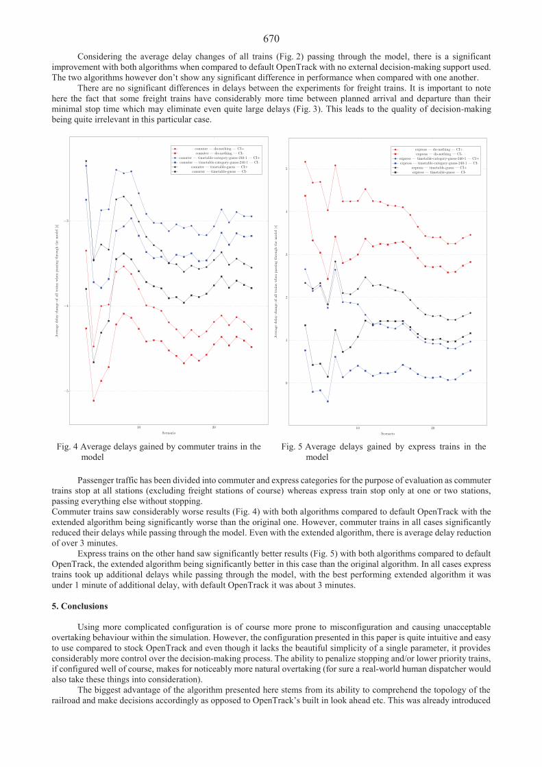
670 Considering the average delay changes of all trains (Fig. 2) passing through the model, there is a significant

improvement with both algorithms when compared to default OpenTrack with no external decision-making support used. The two algorithms however don’t show any significant difference in performance when compared with one another.

There are no significant differences in delays between the experiments for freight trains. It is important to note here the fact that some freight trains have considerably more time between planned arrival and departure than their minimal stop time which may eliminate even quite large delays (Fig. 3). This leads to the quality of decision-making being quite irrelevant in this particular case.

Fig. 4 Average delays gained by commuter trains in the model

Fig. 5 Average delays gained by express trains in the model

Passenger traffic has been divided into commuter and express categories for the purpose of evaluation as commuter

trains stop at all stations (excluding freight stations of course) whereas express train stop only at one or two stations, passing everything else without stopping. Commuter trains saw considerably worse results (Fig. 4) with both algorithms compared to default OpenTrack with the extended algorithm being significantly worse than the original one. However, commuter trains in all cases significantly reduced their delays while passing through the model. Even with the extended algorithm, there is average delay reduction of over 3 minutes.

Express trains on the other hand saw significantly better results (Fig. 5) with both algorithms compared to default OpenTrack, the extended algorithm being significantly better in this case than the original algorithm. In all cases express trains took up additional delays while passing through the model, with the best performing extended algorithm it was under 1 minute of additional delay, with default OpenTrack it was about 3 minutes. 5. Conclusions

Using more complicated configuration is of course more prone to misconfiguration and causing unacceptable

overtaking behaviour within the simulation. However, the configuration presented in this paper is quite intuitive and easy to use compared to stock OpenTrack and even though it lacks the beautiful simplicity of a single parameter, it provides considerably more control over the decision-making process. The ability to penalize stopping and/or lower priority trains, if configured well of course, makes for noticeably more natural overtaking (for sure a real-world human dispatcher would also take these things into consideration).

The biggest advantage of the algorithm presented here stems from its ability to comprehend the topology of the railroad and make decisions accordingly as opposed to OpenTrack’s built in look ahead etc. This was already introduced

671 in [2] and can be achieved without the extensions presented in this paper.

The advantage of the extended algorithm presented here over the original one is primarily in allowing the delays to be reorganized between train categories rather than reduced overall. This can be seen in the included case study where express trains got significant reduction in delays at the expense of commuter trains, though commuter trains still managed to leave the model with less delay than they entered with. This stems from the fact that when express trains are to overtake commuter trains, category-based bonuses and penalties allow for reduction of express trains trailing commuter trains and at the same time commuter trains overtaking express trains just to be overtaking the other way around at the next overtaking opportunity, having the express train trail the commuter train or even both. This isn’t really achievable without the extensions presented in this paper as simply changing the threshold on its own improves one issue by worsening the other and vice versa.

The algorithm could also be further extended, for example it could be very useful to take into consideration the length and speed limits of tracks used for overtaking as this can add significantly to the delay of given train or maybe even per station tweaks of the general parameters.

Acknowledgement

This work was supported by Internal Grant Agency of University of Pardubice in the frame of Student Grant Competition 2021, project SGS_2021_019.

References 1. SŽDC SM124: Zjiš ování kapacity dráhy. SŽDC SM124: Zjiš ování kapacity dráhy. SŽDC, 2019, Prague. Table 3,

page 33. 2. Vy ítal, T.; Bažant, M. 2020. Train overtaking at railway stations within simulation models of railway lines. In

Affenzeller, M., Bruzzone, A. G., Longo, F., and Petrillo, A., editors, Proceedings of the 32nd European Modeling & Simulation Symposium (EMSS 2020), 28-34.

3. Shakibayifar, M.; Sheikholeslami, A.; Corman, F.; Hassannayebi, E. 2020. An integrated rescheduling model for minimizing train delays in the case of line blockage, Oper Res [Internet] 20(1):59-87.

4. Van Den Boom, T.J.J.; Weiss, N.; Leune, W.; Goverde, R.M.P.; De Schutter, B. 2011. A permutation-based algorithm to optimally reschedule trains in a railway traffic network. In: IFAC Proceedings Volumes (IFAC-PapersOnline) [Internet], 9537-9542.

5. Meng, X.; Jia, L.; Qin, Y. 2010. Train timetable optimizing and rescheduling based on improved particle swarm algorithm, 71 p.

672

Proceedings of 25th International Scientific Conference. Transport Means 2021. Optimization of the Intersection with Regard to Safety in Mikulov R. Dvoracek, R. Pavelek, L. Janak, G. Tylova, K. Vichova Tomas Bata University in Zlín, Faculty of Logistics and Crisis Management, Studentské nám stí 1532, 686 01 Uherské Hradišt , Czech Repubic, E-mail: kvichova@utb.cz Abstract The optimization of the intersections leads to a reduction in the length of the traffic jams and accidents and mainly increased safety for all road users. Therefore, each city's goal should be to select critical intersections and address their optimization to increase security in the city. This paper deals with simulation software PTV Vissim to optimize the intersection in Mikulov, Czech Republic. The aim was to optimize the selected intersection to increase its safety and reduce column formation. The optimization was based on the simulation's visual data from the software. KEY WORDS: intersection, simulation, model, traffic, PTV Vissim 1. Introduction

Land transport infrastructure provides services essential to a modern society´s functioning [1]. Dvorak states that transport together with other sectors is the essential part of critical infrastructure protection [2]. As a part of transport infrastructure belongs intersections, roads, and routes [3].

It is necessary to ensure the renewal of transport infrastructure to ensure higher capacity and safety. The development of cities or regions can have different forms [4]. In current conditions, traffic intensity and transport composition undergo significant changes [5]. With the increase of vehicles on roads, traffic congestion has become a more serious topic for scientists and researchers [6].

This work deals with the issue of intersection optimization based on visual data from the simulation. The intersection will be optimized mainly concerning safety, as the intersection selected for optimization was, according to some media, marked as one of the most dangerous in the South Moravian Region. The work is divided into several parts, which give a comprehensive view of road safety at the intersection and show how the optimization will affect traffic at the intersection.

The work is based on data from the centre of traffic research, which shows the number of traffic incidents on a given section of road, while these data are processed into clear graphs and tables. The simulation is based on data from the national traffic census in the Czech Republic from 2016. 2. Theoretical Background 2.1. National Road Safety Strategy for the Period 2011-2020

The National Road Safety Strategy for the period 2011-2020 is a different material of the Ministry of Transport, which sets out the objectives, basic principles, and proposals for specific measures aimed at significantly reducing road accidents in the Czech Republic. The main goal was to reduce the number of people killed in road traffic to the level of the European average by 2020 and at the same time to reduce the number of seriously injured people by 40% compared to 2009 [7]. It turned out that the measures implemented so far were not sufficiently effective in reducing the most serious, fatal consequences of accidents, as the set reduction in the serious consequences of accidents was not achieved. Therefore, the current National Road Safety Strategy was comprehensively revised. A proposal for the necessary measures and procedures was prepared, which was the subject of a new updated material: Revision and update of the National Road Safety Strategy 2011 - 2020 valid from 2017. The updated version included the following parts: Accident analysis, Strategic Objectives of EU Countries, Action Program, Financial Complexity, Indirect Indicators and Information on Implementation, respectively evaluation of the implementation of the NSBSP Action Program 2011-2020 [7]. 2.2. The Conception of Road Safety in the South Moravian Region

The Government has accepted the National Road Safety Strategy, which is in line with the government-approved "State Transport Policy" and in the Besip area specifies the individual tasks with a proposal for responsibility for their implementation. The primary goal of the road safety concept in the South Moravian Region is to define appropriate individual measures of the Strategy in the conditions of the region, which could positively affect both the region and other entities active in the Besip, especially in their fields of activity in the South Moravian Region. The goals and measures set for the region in this concept will be fulfilled on an ongoing and long-term basis. An annual update of this

673 Besip concept in the South Moravian Region is not expected, only in the case of necessary and substantial changes in the region's focus on road safety [8]. 2.3. The Nationwide Traffic Census

The nationwide traffic census is used to determine the intensity of traffic on the highway and road network of the

Czech Republic and provides information for road network development, construction and repair plan, maintenance planning, construction documentation processing, protection against excessive traffic noise, etc. It is performed regularly in 5-year cycles – in 2000, 2005, 2010; last was in 2016 and next in 2020 [9].

Fig. 1 shows the traffic in Mikulov. It is a figure from the National Census of Traffic from 2016. Regarding the selected intersection on the left in the figure, we can see that the highest traffic intensity is marked by a red line (15001 – 25000 vehicles / 24 hours). It is a road I / 52 from Brno to Mikulov. The right road is marked by yellow colour (3001 – 5000 vehicles / 24 hours), which indicates a lower density than red. It is a road II/414.

Fig. 1 Results of the traffic census [10]

2.4. Accident Statistics

These are statistical data on accidents in the Czech Republic. Accident statistics can be traced in the

geographical information system of the Ministry of Transport of the Czech Republic, which is called the Unified Transport Vector Map (JDVM) – it is used to visualize accidents on a map. This geographical system contains statistical data on accidents from the Center for Transport Research (falls under the Ministry of Transport of the Czech Republic), the Directorate of Roads and Motorways, and from the Directorate of the Traffic Police Service of the Czech Republic, which falls under the Police Presidium of the Czech Republic. Thanks to JDVM, it is easy to trace how many accidents happened in a given municipality, or it is possible to trace a specific accident in a municipality - when it happened, what its cause was, etc. [11].

Table 1

Traffic accidents in Mikulov 2020 [7]

January 5 February 10 March 3 April 2 May 6 June 8 July 6 August 6 September 5 October 2 November 2 Total 55

674 The Table 1 shows how many traffic accidents occurred in the city of Mikulov in 2020 and what kind of traffic

accident it was. It was found that 55 accidents had occurred in the town of Mikulov in 2020. At the selected intersection it was six accidents, and five of them were a collision with a moving non-rail vehicle [7].

The following Table 2 shows what type of accidents happened in Mikulov in 2020, how many accidents it was, and their consequences.

Table 2 Types of traffic accidents in Mikulov in 2020 (for 11 months) [7]

Type of accident Number of accidents Dead people Severely

injured persons Slightly injured

persons Collision with a moving non – rail vehicle 16 0 1 14 Collision with forest animals 12 0 0 0 Collision with a parked vehicle 11 0 0 3 Collision with a fixed obstacle 10 0 1 3 Crash 3 0 0 3 Another kind of accident 2 0 0 1 Collision with a pedestrian 1 0 0 1 Total 55 0 2 25

There were six collisions at this intersection in 2020. Five of them was the collision with a moving non-rail

vehicle and, in one case, collision with a fixed obstacle. 3. Methodology

Before we define microscopic simulation tools, the concept of traffic simulation and its types will be explained. Traffic simulation is one of the essential disciplines of traffic engineering. It is a mathematical model of a transport system (these are motorways, intersections, roundabouts, and more), created using a computer program and helped plan, design, and manage transport systems. Visual demonstrations of the current state and possible traffic development scenarios development can be the output of a traffic simulation.

There are three basic approaches to modelling the transport network. They are macroscopic, microscopic, and mesoscopic approaches. The choice of approach is usually a compromise between the size of the transport network area and the level of detail.

Macroscopic simulations are used for large territorial units that have an extensive network of roads, on which the intensity of the traffic flow is modelled [12-14].

Microscopic simulations focus their attention on each vehicle and its behavior (driver behavior), properties, and interactions with other vehicles in the traffic flow and transport infrastructure. The main representatives of microscopic simulation tools include VISSIM, PARAMICS or AIMSUN. Among the others, we can at least mention CORSIM, MITSIM, DRACULA, FRESIM, HUTSIM, MICROSIM, SIGSIM, or TRAFFICWARE.

PTV VISSIM is a microscopic simulation tool developed by the German company PTV AG in cooperation with the Technical University of Karlsruhe. It is software for microscopic simulation of individual and public transport. It can accurately simulate both city traffic, including cyclists and pedestrians, and highway sections, including large grade-separated intersections.

PTV Vissim is used to analyse networks of all sizes, from individual intersections to large metropolitan areas. In these transport networks, it could model all functional categories of roads from highways to purpose-built drives. Vissim's scope of application also includes public transport and routes for cyclists and pedestrians. In addition, the ability to define an unlimited number of vehicle types allows the user a full range of multimodal operations. Vehicle types include cars, trucks, buses, rail vehicles (trams, trains, high-speed), cyclists, wheelchairs, pedestrians, airplanes, etc.

PTV Vissim is frequently used to assess transport infrastructure designs, traffic management design, analysis, and simulation of telematics benefits in traffic management, public transport simulation, etc.

The car-following model is the most common type of microscopic model. This model describes the movement and behavior of the vehicle in the traffic flow depending on the previous vehicle. Such models have been developed since the 1950s. The basic principle of the vehicle sequence model is to determine the dependence of the vehicle acceleration on the ambient conditions; in the simpler case, it means on the condition of the vehicle in front of the following vehicle. In general, the acceleration of a vehicle in this model can be expressed as follows:

a a (v, v, x),

where a is the acceleration of the vehicle, v is the speed of the vehicle, v is the relative speed compared to the succeeding vehicle, and x is the distance from the succeeding vehicle [12, 15].

675 4. Results

The following part presents the results of simulations in the PVT Vissim. First, a simulation of the current state

is presented, where there is a high accident rate on ground roads. Therefore, we proposed a variant of optimization with a roundabout. Both variants are presented in the form of figures from the PVT Vissim; the figures are also used to compare both variants.

Fig. 2 Current state of the intersection

Fig. 3 Optimized of the intersection

Firstly, we would like to present the current state of the intersection. From the transit point of view, Mikulov is a

historical place, also an essential element for our country, as it is a border crossing to the Republic of Austria. According to statistics, there is a high rate of traffic incidents at the selected Brn nská / 28 íjna intersection. Last year (2020), there were six accidents at an intersection chosen, of which 5 were a traffic incident with a non-rail vehicle. According to the simulation of the current state, it can be seen that for some drivers, a traffic situation that can lead to a traffic incident can be a complicated solution. The current state of the intersection is quite confusing and complex. The advantages of driving from a side road can be complicated by not estimating the time needed to be included in the main road, especially for novice and inexperienced drivers.

The simulation also shows that congestion could form on side roads during rush hours, which can lead to dangerous maneuvers from some drivers when entering the main road. In Fig. 2 we can see a simulation of the current state.

Secondly, we prepared the optimized variant (Fig. 3). As already indicated in the theoretical part, most traffic incidents occur when leaving an industrial area, where drivers must give priority to driving to connect to the road on October 28. After the team brainstorming, a proposal was made to solve the traffic problem by adding a roundabout. This variant was chosen primarily concerning safety, but the flow of traffic was not neglected either. During rush hours, even in this variant, more minor traffic jams may form, but there should be no severe traffic incidents concerning the

676 roundabout geometry. The roundabout was also chosen because at two intersections on the same road in the vicinity; this variant proved successful. Below the text, we can see figures of the optimization with a roundabout.

5. Conclusions

The aim of the paper was to present a selected traffic intersection in the town of Mikulov. First, a literature

search and presentation of software for simulations in transport were performed. Secondly, a case study was presented to the city of Mikulov with a selected traffic intersection. The paper's central part was to give the current state of the intersection using PTV Vissim software. Based on this, optimization was performed. A roundabout was designed to increase safety at a selected traffic intersection. Acknowledgement

This research was supported by the Internal Grant Agency of Tomas Bata University in Zlín – IGA/FLK /2021/001. References 1. Patrman, D.; Splichalova, A.; Rehak, D.; Onderkova, V. 2019. Factors Influencing the Performance of Critical

Land Transport Infrastructure Elements, Proceedings of 13th International Scientific Conference on Sustainable, Modern and Safe Transport (TRANSCOM 2019), Transportation Research Procedia 40: 1518-1524.

2. Dvorak, Z.; Sventekova, E.; Rehak, D.; Cekerevac, Z. 2017. Assessment of Critical Infrastructure Elements in Transport, Proceeding of 10th International Scientific Conference Transbaltica 2017: Transportation Science and Technology. Procedia Engineering 187: 548-555.

3. Dvorak, Z.; Leitner, B.; Novak, L. 2012. National Transport Information System in Slovakia as a Tool for Security Enhancing of Critical Accident Locations, Proceedings of 16th International Conference Transport Means, Kaunas, 145-148.

4. Lacinak, M.; Ristvej, J. 2017. Smart City, Safety and Security, Proceedings of TRANSCOM 2017: International scientific conference on sustainable, modern and safe transport, Proceedia Engineering 192: 522-527.

5. Volkova, E.; Stepanenko, A. 2019. Traffic intensity on highway R-255 Siberia in Irkutsk region, IOP Conference Series: Materials Science and Engineering 667: 1-6.

6. Kaur, D.; Sharma, S. 2020. A new two-lane lattice model by considering predictive effect in traffic flow, Physica A, 539: 1-9.

7. National security strategy [online cit.: 2021-01-07]. Available from: https://www.czrso.cz/nsbsp/post/aktualni-strategie

8. Road safety [online cit.:2021-01-08]. Available from: https://www.kr-jihomoravsky.cz/Default.aspx?ID=256636 &TypeID=2

9. Nationwide traffic census [online cit.: 2021-01-07]. Available from: https://scitani.vars.cz/ 10. South-Moravian Region [online cit.: 2021-01-07]. Available from: http://scitani2016.rsd.cz/content/doc/64-

09.jpg?v=2016b 11. Statistical representation of accidents in the geographic information system [online cit.: 2021-01-07]. Available

from: http://www.srvo.cz/wp-content/uploads/2017/12/JDVM-2009.pdf 12. Editor and simulator of road traffic using cellular automata [online cit.: 2021-01-07]. Available from:

https://www.vutbr.cz/www_base/zav_prace_soubor_verejne.php?file_id=118708 13. Methodology for creation and evaluation of macroscopic transport models [online cit.: 2021-01-07]. Available from:

https://www.cdv.cz/file/metodika-pro-tvorbu-a-hodnoceni-makroskopickych-dopravnich-modelu/ 14. Modelling of traffic on roads (Part 1) [online cit.: 2021-01-07]. Available from: http://projekt150.ha-el.cz/node/94. 15. Modelling of traffic on roads (Part 3) [online cit.: 2021-01-07]. Available from: http://projekt150.ha-vel.cz/node/96.

677

Proceedings of 25th International Scientific Conference. Transport Means 2021.

Product and its Life Cycle Cost Analysis J. Furch1, V. Kone ný2

1University of Defence, Kounicova 65, 66210 Brno, Czech Republic, E-mail: jan.furch@unob.cz 2University of Defence, Kounicova 65, 66210 Brno, Czech Republic, E-mail: vlastimil.konecny@unob.cz Abstract The article characterizes the product and the relevant imposed requirements including the life cycle management process. It presents the basic principles of life cycle cost analysis (LCC) and also provides guidance on how to perform a life cycle cost analysis. It describes and explains the importance of life cycle cost analysis as an important part of quality management processes, especially in the design and development phases. It includes knowledge and information on two basic calculation approaches to life cycle costing. Furthermore, a ten-step procedure for a detailed analysis of product life cycle costs is presented. KEY WORDS: life cycle cost analysis, process of life management, stage of product life cycle 1. Introduction

At present, almost every user evaluates, selects and assesses products not only in terms of real utility value but also in terms of both the acquisition cost of the product, and mainly the cost of ownership. Various economic analyses are used to clearly illustrate and quantify the required expenditures. In recent years, the product life cycle cost analysis has been used. When deciding to buy a product, a number of factors is considered; they are related not only to costs but also to reliability. It must not be forgotten that the basic aim should be to achieve customer satisfaction. The product is required to ensure proper reliability and life cycle costs to be as low as possible (optimal - not necessarily the lowest cost). At the same time, the product must perform its function safely without undue impact on the environment and the operation. The purchase of a product is determined not only by the initial costs (acquisition), as is sometimes perceived but also by the expected ownership costs, which are operating costs and maintenance costs for the entire life of the product. Last but not least, the costs of the settlement (disposal) must not be neglected.

Life cycle cost analysis is the process of economic analysis to assess the total cost of acquisition, ownership and settlement (disposal) of a product. It can be used throughout the product life cycle, or in some parts, or in a combination of different life cycle stages. The basic goal of life cycle cost analysis is to provide input data for decisions made at any stage, or at all stages of the life cycle.

During various stages of the product acquisition, there are some variations that affect the cost uncertainty and associated risks. The need for formal use of the product life cycle cost analysis usually depends on the customer's requirements or the requirements stipulated in the contract. However, the life cycle cost analysis provides useful input data for any process in which a design decision is made. Therefore, it should be as integral as possible to the design process so that the product features and costs can be optimized 1.

The process of optimizing the product life cycle costs must start from the very beginning, i.e. from the concept and specifying the requirements, through design and development to the production. All decisions made on the design and manufacture of the product may affect other requirements, such as its performance, safety, reliability, maintainability and providing maintenance, etc.

The general product requirements are: product readiness; minimal life cycle costs while ensuring product readiness and customer needs; safe operation without undue impact on the environment; easy maintainability over the lifetime.

More general types of decisions that use a life-cycle cost analysis process as an input include, for example: evaluation and comparison of alternative design approaches and optional settlement technologies (disposal); assessment of economic feasibility of products; identifying items that contribute to costs and cost-effective improvements; evaluation and comparison of alternative strategies for the use, operation, testing, inspection, and maintenance

of the product; evaluating and comparing different approaches to replacing, restoring/extending life or disposing of aging

equipment; distribution (allocation) of available funds to individual competitive priorities in product

development/improvement; assessment of product assurance criteria through verification tests and cost-benefit optimization; long-term financial planning.

678Life cycle cost analysis can be used to provide input data to the analysis of integrated logistics. Fig. 1 presents the incurred costs that may arise within the product life cycle. It can be seen from the above that

the costs of LCC are most affected in the first stages of the life cycle. According to Fig. 1, this can be up to 50%, which is not realistic in practice. On the contrary, during production and operation by the user, it can be only 5%. The figure also shows that around 72% are operating, maintenance and disposal costs, depending on the type of product.

Fig. 1 Costs incurred and committed during the life cycle acquisition process 2

The process of life management (PLM), which can be defined as the process of product life management from the conception, through production, operation and maintenance, to disposal, must not be neglected in the implementation of the above product life cycle analysis. It can also be seen as an information strategy of the company integrating people, data, processes, management system and technology. This approach integrates systems, procedures and tools to address the implementation of both the new and the innovative product 3. The description of said PLM information is graphically shown in Fig. 2.

Fig. 2 Graphic illustration of the process of life management (PLM) 3

It is possible to look at the product life cycle management from different perspectives, in terms of sales volume (i.e. marketing perspective), in terms of product life, or in terms of transformation processes. If we look at PLM in terms of the most common and well-known marketing perspective and in terms of product life, its individual stages can be described using the following steps (Fig. 3).

Fig. 3 Marketing view of the stages of the product life cycle

Analysis of lack Product and prototyping conceptptt Product development ent Preparation of

production

Production Sales and distribution oon Product maintenance and repair

cee Disposal and recycling of the product

679 It is, therefore, necessary to look at the product as a whole, from the idea of its implementation to its disposal.

Customers did not realize this view in the past. This important information came to light only when customers had to start paying a recycling fee, or a fee that reflects the ability of designers to come up with a product that will be easy or, conversely, difficult to recycle.

The life cycle (time interval) very often varies depending on the type of product. For example, with food or medication, it is a short interval. Conversely, with technical equipment as household appliances, vehicles or buildings, the life cycle is long. In practice, this means that for each product the determination of the life cycle length is different and the accuracy of the determination will significantly affect the accuracy of the calculation or at least the estimate of life cycle costs.

Life cycle cost analysis provides important input data to the decision-making process in the design, development, use and settlement stages. Product suppliers are able to optimize their designs by evaluating various alternatives and conducting appropriate cost-benefit optimization studies. It can be used and effectively applied for:

evaluation of costs that are associated with a specific activity (evaluation of different concepts of approaches in the maintenance system);

solving various problems related to a specific part of the product; solving problems that relate to the selected stage or stages of the product life cycle.

LCC is a tool of economic analysis that includes all types of costs related to a product or process throughout its life and its methodology 4.

2. Importance and Application of Life Cycle Cost Analysis

Life cycle cost analysis is most effectively used in the initial design stage to optimize the basic design approach. It can also be updated and used during subsequent life-cycle stages to identify the areas of significant cost uncertainty and risk. The need for official use of the process of the product life cycle cost analysis usually depends on the customer's requirements or the requirements stated in the contract. However, life cycle cost analysis provides useful input data for any process in which a design decision is made. It should therefore be as integral as possible to the design process so that the product features and the costs can be optimized.

The view of life cycle costs on the part of prospective users of the product is often significantly dominant. This is because the estimated life cycle cost can in many cases be the primary criterion for the interested party. Based on this information, the user then chooses the final decision to purchase the offered product. The user can also decide, depending on the amount of life cycle costs, to replace, renew or discard the products used so far. The estimated life cycle cost is therefore frequently used information. After purchasing a certain product, the user can no longer significantly influence the amount of life cycle costs, which is presented in figure 1. In operation, only operating costs can be monitored, and on the basis of such data, the maintenance or disposal system can be optimized.

In the product design and development stage, similar analyses can also be used to: optimize the design of the product so that the future expenses of the users are completely minimal during

warranty performance; provide follow-up advice and guidance that can be used by designers, constructors and technologists to design

new products in connection with cost-effective improvements; evaluate the economy of operational reliability of all technical systems, as it is known that the more susceptible

to damage and failure these systems are, the greater effort the user has to expend on maintenance and troubleshooting 5.

3. Variants of Life Cycle Cost Analysis

There are two basic variants of analyses with information and data on life-cycle costs, and they differ in the purpose of the further use 5:

a) variant 1 – the purpose is to find opportunities to minimize the total costs for users of a certain technical system; b) variant 2 – the purpose is to optimize expenditures in individual phases of the life cycle of a certain technical

system. ad a) For variant 1, three basic groups of life cycle costs are defined 5: purchase costs – CP (acquisition) costs for building the system; ownership costs – CO ownership costs (operating costs, maintenance costs throughout the life of the system); disposal costs – CD settlement or disposal costs.

LCC = CP + CO + CD. (1)

Acquisition costs are generally visible and can be easily evaluated before deciding to purchase a product. It includes the purchase price, delivery and installation.

However, ownership costs, which very often represent the main component of LCC costs (Figs. 1 and 4), in many cases exceed the acquisition costs and are not easily apparent. These costs are not easy to predict and may include installation costs 5. The ongoing ownership costs include fuel and energy consumption costs, costs of spare parts for preventive maintenance and maintenance after a failure, labour costs for maintenance staff, other costs for repairs and

680maintenance of the equipment and the facilities, training costs, selected parts of other administrative costs, etc.

Settlement (disposal) costs may in some cases form a significant part of LCC total costs. High expenses for large construction projects, such as nuclear power plants, can be considered as an example. The settlement or disposal costs of the system are, in fact, the final expenses that the user must incur after the life of the product.

ad b) For variant 2 it is recommended to monitor five cost groups 5:costs of concept period – CC,costs of design and development period – CDD, purchase costs;costs of manufacture and installation period – CMI,costs of operating state and maintenance period – COM – ownership costs;costs of disposal period – CD – liquidation costs.

LCC = CC + CDD + CMI + COM + CD. (2)

Costs of the concept period - this is the determination of requirements, especially for the costs of market research, project management, analysis of the concept and project design, etc.

Costs of the design and development period - represent the costs of the design documentation, making prototypes, software development, demonstration and validation, verification and review of the design, etc.

Costs of the manufacture and installation period - include one-off costs and costs that are repeated for each product or service provided. One-off costs include industrial engineering and analysis of operational activities, equipment design, production tools and test equipment, special support and test equipment, initial spare parts and repair kits, initial training, documentation and type approval tests. Recurring costs include production and engineering management, equipment maintenance, quality management and control, assembly, installation and final inspection, packaging, storage, shipping and transportation, ongoing training and practice.

The costs of the operation, maintenance and settlement period are listed in the variant 1 as ownership costs and settlement costs.

4. Purpose of Life Cycle Cost Analysis

LCC analysis can only be performed by manufacturers (suppliers), only by users, or both (both the manufacturer and the user). Product life cycle cost analysis can be performed based on the following basic conditions:

a) products with long-term potential for use that is over 12 months. For products with a shorter lifespan, similar analyses are irrelevant;

b) products for which the expected life cycle costs will be significantly higher than the purchase price of a particular product. For products where the life cycle cost is the same as the purchase price, similar analyses are irrelevant.

The above-mentioned conditions will apply to the vast majority of machinery, equipment and facilities, where life cycle cost analyses will play a very important role.

It is generally recommended that the life cycle cost analysis be started as soon as possible at the beginning of the product life cycle which means already during the design period. Illustrations of the degree of life cycle stages to the amount of product life cycle costs are shown in Fig. 4.

50

Optimal period

Cost commitment

Saving potential

Concept Development Production Ownership

Program phases

Perc

enta

ge o

f LC

C

100

Fig. 4 Scheme of the degree of influence of life cycle stages on the amount of product life cycle costs 6

It is clear from figure 4 that not users but manufacturers have the greatest potential to influence the future costs of

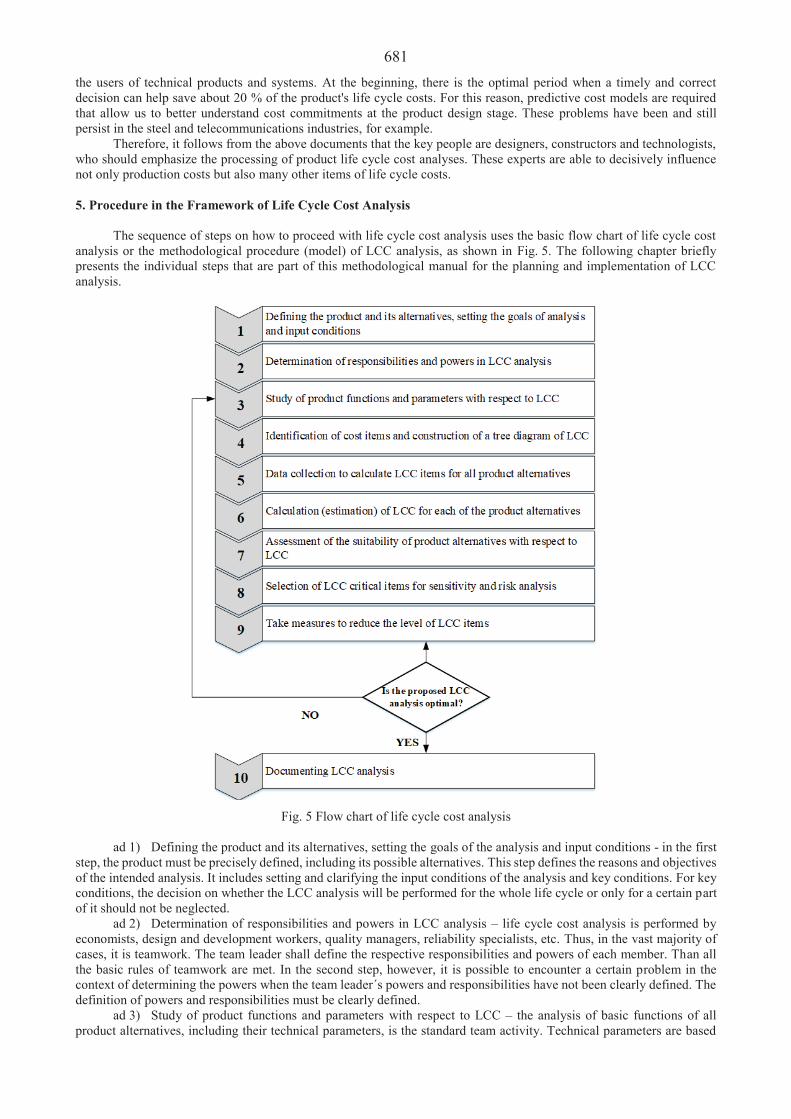
681 the users of technical products and systems. At the beginning, there is the optimal period when a timely and correct decision can help save about 20 % of the product's life cycle costs. For this reason, predictive cost models are required that allow us to better understand cost commitments at the product design stage. These problems have been and still persist in the steel and telecommunications industries, for example.

Therefore, it follows from the above documents that the key people are designers, constructors and technologists, who should emphasize the processing of product life cycle cost analyses. These experts are able to decisively influence not only production costs but also many other items of life cycle costs.

5. Procedure in the Framework of Life Cycle Cost Analysis

The sequence of steps on how to proceed with life cycle cost analysis uses the basic flow chart of life cycle cost

analysis or the methodological procedure (model) of LCC analysis, as shown in Fig. 5. The following chapter briefly presents the individual steps that are part of this methodological manual for the planning and implementation of LCC analysis.

Fig. 5 Flow chart of life cycle cost analysis

ad 1) Defining the product and its alternatives, setting the goals of the analysis and input conditions - in the first step, the product must be precisely defined, including its possible alternatives. This step defines the reasons and objectives of the intended analysis. It includes setting and clarifying the input conditions of the analysis and key conditions. For key conditions, the decision on whether the LCC analysis will be performed for the whole life cycle or only for a certain part of it should not be neglected.

ad 2) Determination of responsibilities and powers in LCC analysis – life cycle cost analysis is performed by economists, design and development workers, quality managers, reliability specialists, etc. Thus, in the vast majority of cases, it is teamwork. The team leader shall define the respective responsibilities and powers of each member. Than all the basic rules of teamwork are met. In the second step, however, it is possible to encounter a certain problem in the context of determining the powers when the team leader´s powers and responsibilities have not been clearly defined. The definition of powers and responsibilities must be clearly defined.

ad 3) Study of product functions and parameters with respect to LCC – the analysis of basic functions of all product alternatives, including their technical parameters, is the standard team activity. Technical parameters are based

682 on customer requirements and legislation. Finding out the functions and parameters is a necessary input for the next step.

ad 4) Identification of cost items and construction of a tree diagram of LCC – this is an important and characteristic step of all cost analysis of the product life cycle. The tree diagram is a classic tool that consists of arranged individual cost items. These cost items are determined by the team using all their experience and skills.

ad 5) Data collection to calculate LCC items for all product alternatives – in this stage, information and data are collected. It is very often dependent on mutual communication between product manufacturers and their users. It is also important that the team has the certainty that there will be all the data at their disposal which are essential to calculate or at least make a qualified estimate of the life cycle costs. It is very important for this area to define responsibilities, as well as to follow the rules and procedures for the collection of information, documents and data. These are essential for this stage, as they will serve as background material for the individual items of life-cycle costs.

ad 6) Calculation (estimation) of LCC for each of the product alternatives - within the given step and point 4, it is necessary to determine the amount of expected costs for each cost item, both in individual years of the life cycle and in total. Furthermore, in order to determine the total amount of cost items, the requirement to use financial mathematics tools (discounting) is necessary, in order to take into account the time factor and the effect of inflation. If there are complications when it is not possible to calculate cost items, it is necessary to make at least their expert estimate, which can be inferred, for example, from a comparison with other similar data based on experience from previous periods or previous years.

ad 7) Assessment of the suitability of product alternatives with respect to LCC - calculation or estimation of life cycle costs should be performed for all considered product alternatives. The team will then have sufficient evidence to assess the economic advantage of the product alternatives offered. Regarding the impact of individual alternatives on the environment or occupational safety, these calculations or life cycle cost estimates should also be included. This is mainly for legislative reasons as well as for customer requests.

ad 8) Selection of LCC critical items for sensitivity and risk analysis - Pareto analysis can be used; it is an important tool in managerial decision-making. Then it is necessary to identify those essential items of life cycle costs that contribute decisively to the total amount of life cycle costs. For these items, the team can use, for example, brainstorming (an intuitive method for generating ideas and solution proposals) or the DFMA (Design for Manufacturing and Assembly) method. This method focuses on changes in product design and technology to reduce production and assembly requirements in terms of time consumption, cost, poor quality, and minimization of other undesirable phenomena. Also the IRM (Innovation Road Map) method can be used, which is a systematic methodology that focuses on the innovation of technical products and that performs a sensitivity analysis to changes in factors. This method can significantly affect the amount of costs. Furthermore, risk analysis can be used, which is especially relevant to considering the fact that the obtained information and data may be burdened with a certain uncertainty.

ad 9) Taking measures to reduce the level of LCC items - this step is based on real data and information. One of the basic objectives of the measures is the analysis of life cycle costs, which will lead to an overall reduction in costs. Here, the team should agree on the design of sufficiently effective and efficient measures, even if their subsequent enforcement and implementation are no longer within their competence. However, these procedures can also be designed by the so-called design review team. Whatever proposed measures are processed by any team, they should also be actively supported by the top management of the product manufacturer, as they can lead to both a reduction in the cost of product implementation at the manufacturer and an increase in real value for users. Subsequently, it is recommended to make a final decision on whether the processed LCC analysis is acceptable, or whether to accept the proposed measures, to carry out a new life cycle cost analysis. This is to demonstrate the effectiveness of these measures.

ad 10) Documenting the LCC analysis - this task requires the results to be analyzed, recorded and presented in the final report of the LCC analysis of the product. This final report should become a standard part of the managed records, as demanded by the requirements for quality management systems 5. 6. Conclusions

The article describes possible procedures that can be used in the analysis of product life cycle costs. This life cycle cost analysis should already be used in the design of LCC, which brings significant savings, as shown in figures 1 and 4. It is also recommended to use LCC analysis in product acquisition, especially when the aim is to acquire a large amount of a given product. It should be noted that, as shown by LCC analyses of the product, the expenses of subsequent ownership costs can be up to 72%, as shown in Fig. 4. At the end of the article, the design of the flow chart of life cycle cost analysis is presented, which is shown in Fig. 5. Subsequently, the individual points of the flow chart of LCC analysis are described, which can serve as the basis for processing LCC analysis of the product.

The higher initial costs may lead to the improvement of reliability and maintainability, and thus they may improve the product availability and subsequently cut the operation cost and maintenance cost. Concerns about the sphere of product reliability must be an integral part of the process of LCC design and assessment. All these concerns must be scanned during the preparation of the product specification. They must be continuously assessed in the course of the whole stage of the product reliability design to optimize the product reliability design and life cycle cost 7.

Finally, it should be emphasized that life cycle costs must be assessed in conjunction with the required product reliability in order to meet customer needs at an affordable price, which should be the goal of all manufacturers.

683 Acknowledgement

Presented work has been prepared with the support of the Ministry of Defence of the Czech Republic, Partial

Project for Institutional Development and Specific Research, Department of Combat and Special Vehicles, University of Defence in Brno.

References 1. Furch, J. 2016. A model for predicting motor vehicle life cycle cost and its verification, Transactions of FAMENA

1(40): 15-26. 2. Farr, J. 2012. Life cycle cost considerations for complex systems. Systems engineering-practice and theory. 3. Görner, T.; Šimon, M.; Edl, M. 2011. Ergonomics and product life cycle, Journal of Safety Research and

Applications (JOSRA) [online]. Prague: VÚBP, 4(3) [cit. 2021-02-23]. Available at: http://www.bozpinfo.cz/ josra/josra-03-2011/ergonomie-produkt.html

4. Hunkeler, D.; Lichtenvort, K.; Rebitzer, G. 2008. Environmental life cycle costing. CRC press. 5. SN EN 60300-3-3. 2017. Dependability management: Part 3-3: Application guide - Life cycle costing. Prague: NI. 6. Pesonen, L.T.T. 2001. Implementation of design to profit in a complex and dynamic business context. Finland, Oulu:

University of Oulu. 7. Balík, R.; Barták, J.; or ák, Š. and Furch, J. 2005. A Relation between Dependability Specific Aspects and

Vehicles LCC in Operation and Maintenance, In: Proceedings of 9-th International Conference Transport Means. Kaunas: Kaunas University of Technology, Lithuania.

684

Proceedings of 25th International Scientific Conference. Transport Means 2021. Studying of Dynamic Parameters Impulse Impact of the Vehicle Taking into Account the Track Stiffness Variations I. Bondarenko1, R. Keršys2, L. Neduzha3 1«Futurum Ukraine» Non-governmental Organization, Molodogvardeyskay str., 24, 49022, Dnipro, Ukraine, E-mail: dr.iryna.bondarenko@gmail.com 2Kaunas University of Technology, Studentu st. 56, 51424, Kaunas, Lithuania, E-mail: robertas.kersys@ktu.lt 3Dnipro National University of Railway Transport named after Academician V. Lazaryan, Lazaryan St. 2, 49010, Dnipro, Ukraine, E-mail: nlorhen@i.ua Abstract Authors analysed the ways of descriptions of the dynamic parameters impulse impact of the rail vehicle and surveyed the features of the system “vehicle-track” modelling. Dynamic parameters of impulse impact of the rail vehicle and them influence of describing ways of the dynamic parameters of the vehicle impulse on the dynamic track deformability were examined. Finally, basic conclusions and recommendations are given. KEY WORDS: dynamic parameters impulse impact, track deformability, dynamic load, dynamic rail deflection, system “vehicle-track” modelling 1. Introduction

Usually, when calculating the parameters of the stress-strain state of the railway track design the influence of rolling stock, quasi-dynamic methods are used, in which the dynamic load acting on the railway track design from the wheels when the system “vehicle-track” interact is described by a sinusoidal function. Physically, this means that over time, the dynamic load at each point changes its value from 0 to the maximum value and returns to 0. But the time, during which the transfer of loads from wheels to the railway track, is not taken into account. This is due to the fact that the existing methods for determining the stress-strain state of the railway track design while the influence of rolling stock apply the principles that were developed to determine the strength of the track which do not take into account the time component.

To determine the strength of any object, an important factor is to determine the maximum values of dynamic deflections or stresses that are the criteria for operability. That is, it did not matter what conditions contribute to the appearance of maximum values of deflections or stress, the main thing is that these values are not higher than acceptable [1-2].

The lack of a time component does not allow describing the dynamic process when system “vehicle-track” modeliing in full. The use of quasi-dynamic methods changes the essence of dynamic processes. The reason for it that the application of quasi-dynamic loads causes track deformability, at which the dynamic rail deflection shifts simultaneously along with the motion of the train. Whereas there is a discrepancy in the time of occurrence of the maximum value of the dynamic deflection of the rail and the action of the maximum value of the dynamic load of the wheels for a certain section of the railway.

In addition, typical modeling approaches do not classify impacts. For example, dynamic parameters impulse impact of rail impact to wheels is not classified depending on track design, track plan and profile [3-5]. The same approach is used to carry out the railway track simulation, so the effects from the rolling stock are presented, in fact, as quasi-dynamic, for which the field of influence from the static load is built, which moves along the track [6-17]. The finite element method takes into account the geometry of the railway track design, but the propagation time of the action of the dynamic load along the track structure, the speed of the rolling stock, and the degree of deformability of the track structure elements are not taken into account.

In the quasi-dynamic studies, the calculations are performed for different values of frequency of quasi dynamic excitation [18-19], defined as the ratio of speed to the magnitudes of distances between the wheels of one cart and adjacent carts, or distance between the track's supporting elements. In the physical essence, the excitation frequency that is used in quasi-dynamic calculations, inversely proportional to the geometric lengths of the position of the wheels in the train, and characterizes the recurrence of load occurrence in the examined track section. And for static calculations, load characterizes the amount of the dynamic load that acts in the examined track section at a certain point in time. The excitation frequency magnitude, in this case, is dependent on the length of the contact area of the rail with the wheel and the duration of dynamic load acting on the track section. And though all acknowledge that the speed of motion affects the frequency of excitation, it is not used in quasi-dynamic calculations. When moving the dynamic load, the distance between the force application place and the examined section changes. Thus, not only the part of the load magnitude of dynamic load that acts in the examined section changes but the vector of load. The frequency of excitation, inversely proportional to the period of action of the load by physical essence is characterized by an impulse of dynamic load,

685which acts on the track and allows applying the basic equation of dynamics over time.

After studying the work of objects of structures of railway superstructures and objects of formation substructure, it is come to the understanding that, in order to ensure the requirements of reliability, availability, maintainability, and safety (RAMS – which determines the main development direction of technical objects) during the operation of any structures, it is necessary to study the features of the deformability (associated with the dynamic characteristics of the object's stiffness) of operation of elements track structures under the influence of rolling stock.

Of course, the study of such issues requires the use of both theoretical and experimental innovations, since the existing standard approaches and methods for conducting experiments are based on the provisions for determining the strength and stability of objects that do not take into account the time component.

Furthermore, in the established estimating methods of the operation state of the railway track, track deformability characteristics are either not taken into account, or are introduced as an additional criterion based on experimental experience. The main difficulty in studying deformability is that it is necessary to take into account changes in the stress-strain state of objects in time.

Thus, in order to examine the dynamic processes of deformability of the track, it was suggested to take into account the differences between static and dynamic characteristics of loads such as:

1. Dynamic load has a time of action and intensity of action, is applied in time along the railway track.2. Dynamic irregularities of the railway track are calculated depending on the physical, mechanical and

geometric parameters of the track structure elements and the characteristics of the dynamic load.3. It is not considered the final stresses (meaning as a result of the full action of the force) that are used as

strength criteria, but track deformability that change in time under the influence of dynamic load. The last has certain dynamic parameters of impulse impact.

The changes proposed will also provide for the possibility under the assigned operating conditions to define, by the criteria of reliability, design of the track, or measures related to its strengthening with the provision of certain resource of its work.

2. Research Methodology

A mechanical impulse, acting on an object, transfers a certain amount of energy to it, which is absorbed and transmitted inside the element by force waves creating force fields. The latter cause the material particles to move, causing various physical processes to occur inside the element with a change in time:

– material local density (change in the distance between particles under the influence of force waves);– material local temperature (due to friction during the displacement of particles or inelastic collision of force

waves);– material compressibility (due to a change in the local density of the material and due to this change in the

movement of particles under the force waves action);– element volume (as a combination of the physical processes described above).These physical processes cause: changes in the particle’s local concentration, changes in the local volume inside

the element, changes in the local velocity of particles and, according to the second law of motion, can be written as:

0/ / / / ,F t R t dP dt d m dt d pV dt d nm V dt (1)

where F t – is the impulse external force acting on the object; R(t) – is the momentum of the force field acting inside the object; m – is the mass of the object, absorbing the influence of an external impulse, by means of a force field pulse, which is formed on the basis of a superposition of force waves; P – impulse; - is the density of the material through which the wave propagates; n – concentration, the number of molecules per unit volume; 0m – is the mass of one molecule; p – is the material density of the object; V – is the object's volume, absorbing the influence of an external impulse, by means of a force field pulse, which is formed on the basis of a superposition of force waves; – is the velocity of particles exposed to the force field that are dependent on the transverse tC and longitudinal CC wave propagation speeds in a particular medium;

0 ,fF t F sin t (2)

where 0F - is the maximum value that the force gains in the intersection; f - frequency of transferring load pulse (frequency of excitation of intersections of the rails) and with the aggregate action area. A range of parameters of this oscillation along the length of the track depends on the motion speed and position of the wheelset in a track; t – is the time; f t - varies from 0 to , and during this time, depending on the speed, the wheel goes through the entire cycle of impact on the track: the pressure appears, gradually increases to the maximum, and goes out.

The velocity of longitudinal waves in that kind of medium is given

686

1,

1 1 2E

CC ,2 1t

EC (3)

where E - the Young modulus or the modulus of elasticity; - Poisson's ratio; tC , CC are the transverse and longitudinal wave propagation speeds in a particular medium.

According to the first law of thermodynamics, for any volume it is true:

,K t U t A t Q t (4)

where K t - is the change in the kinetic energy of the body; U t – change in the internal energy of the body;

A t – change in work performed by external forces; Q t – is the change in thermal energy.

3. Results of Investigation

Modern requirements for technical systems are deformability requirements (characterize the conditions of functionally safe operation), and not strength and stability (characterize the conditions of operational serviceability). Deformability characterizes the change in the stiffness characteristics of an object over time.

Since the main provisions that the propagation of a force action inside an object occurs through the propagation of elastic waves are undeniable, the main provisions of the theory of elastic waves were adopted to determine the propagation of force fields inside an object during modeling [20-21].

In physics, a state of matter is one of the distinct forms in which matter can exist. Four states of matter are observable in everyday life: solid, liquid, gas, and plasma. The theory of elastic waves describes the basic principles of the appearance and propagation of elastic waves in various states of matter. So, it is known that only longitudinal waves propagate in liquid and gaseous states. In a wave of this type, particles move in the direction of wave propagation. In the solid-state of matter, both longitudinal and transverse waves can propagate. In physics, a transverse wave is a wave whose oscillations are perpendicular to the direction of the wave.

The main advantage of the proposed modeling method is the use of the ability of elastic waves to propagate the energy of force actions (pulses) in space and time.

The materials properties determine the propagation velocity inside the elements of transverse tC and/or longitudinal CC waves (Eq. (3)). The magnitude and the direction of the mechanical action determine the direction and value of the movements of the particles inside the element. Fig. 1, a shows the direction of the movement of both all kind of wave propagation with respect to the direction of the acting force and of particles under the longitudinal waves action. Fig. 1 b shows the directional movement of particles under the transverse waves action. Fig. 1 displays the directions of particle movement for one of the cross-sections of the spatial distribution of spherical transverse and longitudinal waves.

As shown in Fig. 1, a and b, longitudinal waves move particles along the lines of wave propagation, and transverse waves are perpendicular to the directions of wave propagation. The application of the theory of propagation of elastic waves allowed to describe the mechanism of influence of rolling stock on the track by pulses that excite the areas of contact of rails with wheels located on the trajectory of the wheel pair, taking into account the time of occurrence and action of loads depending on train speed further propagated by force waves.

To apply this method, a mathematical model of the railway track structure was developed, taking into accountthe spatial propagation of elastic waves during the interaction of track and rolling stock. This model combines three blocks: the mechanism of influence of rolling stock on the track, the propagation of the force wave in the structural elements of the track, and the transition of the force wave from one element to another.

The propagation velocities of longitudinal and transverse waves in each element in the directions of propagation are determined by the physical characteristics of the materials of the railway track construction elements.

a bFig. 1 Directional movement of particles under: a – the longitudinal waves action, b – the transverse waves action

687 The coordinates of the trajectory of the wheels of the rolling stock are determined on the geometric model of the

track structure. These coordinates are crucial for the construction of local coordinate systems, which will consider the propagation of pulses applied along the rail at a certain point in time as an excitation factor. The geometric location of the local coordinates of the contact area is due to the direction of force acting at a certain point from the rolling stock on the rail. The value of the forces acting on the track is determined by existing methods. The duration of the force depends on the speed of the rolling stock.

But for the proposed model, the geometric parameters describing the physical process of force wave propagation in the structural elements of the track are basic.

a b

c d

i f

Fig. 2 Impulse characteristics: a – impulse force, b – time of action, c – length of contact area (L), d – measure of impulse (p), i – force per unit of time ( ), f – force per unit of action length (J)

Therefore, when modeling the deformability processes that occur in the structural elements of the railway track

in time, the following principles are used: 1. A 3D model of all elements of the track structure is used. This is important because the propagation of elastic

688 waves in time is considered. This means that the geometry of the elements determines, firstly, the time of passage of the load acting in each element, which is carried by the incident waves, and secondly, the time and propagation of reflected waves, as well as refracted ones.

2. The use of elastic waves makes it possible to use Newton's second law (Eq. (1)) and the first law of thermodynamics (Eq. (4)) in time.

3. Dynamic load has a time of action and intensity of action, is applied in time along the railway track (Eq. (2)). 4. Dynamic irregularities of the railway track are calculated depending on the physical, mechanical and

geometric parameters of the track structure elements and the characteristics of the dynamic load [21]. The law of dynamic load change is of decisive importance since the dynamic parameters of the impulse action of

each load wave characterize the law of deformability change at each point of the railway track design. Moreover, the ratio of the dynamic parameters of the impulse action and the geometric, physical, and mechanical

characteristics of the track design elements determine the places of energy concentration inside the t 2 294P rack structure elements. Thus, for a correct description of the processes of deformability of the railway track, a correct description of the law of change in the dynamic load is necessary.

The impulse characteristics are shown in Fig. 2 under the action of the forces 1 224P kN, and 3 450P kN. Fig. 2, a demonstrates an increase in impulse action with an increase in both the magnitude of the impact force

and with an increase in vehicle speed. Fig. 2, b shows a curvilinear decrease in contact time with an increase in vehicle speed. Dependences 2, a and b also determine the qualitative change in deformability processes for each type of wave. The results shown in Fig. 2, demonstrate that with an increase in the speed of movement, such characteristics of

the impulse as the magnitude of the force, the time of action, the magnitude of the force per unit length and time increase, while the time of action and the total value decrease. An increase in the value of the strength of the impulse leads to an increase in all its characteristics.

Fig. 2, and f characterize the change in the intensity of the track deformability. 4. Conclusions

The use of the main provisions of the theory of elastic wave propagation makes it possible to use Newton's second law and the first law of thermodynamics in time. This made it possible to create analytical dependencies to study the change in the track deformability depending on the dynamic parameters of the impulse action.

The paper demonstrates that for a correct description of the processes of deformability of the railway track, a correct description of the law of change in the dynamic load is necessary. References 1. Wahrhaftig, A.D.M.; Magalhães, K.M.M.; Brasil, R.M.L.R.F. 2020. Updating the bearing capacity, stresses, and

strain for retrofitting reinforced concrete towers of the cellular and internet system, Mechanics Based Design of Structures and Machines: 1-17. Available from: https://doi.org/10.1080/15397734.2020.1846559

2. Šprljan, P.; Cipek, M.; Klai , M.; Staroveški, T.; Kolar, D.; Pavkovi , D. 2020. Automation systems design and laboratory prototyping aimed at mature petroleum drilling rig retrofitting, Tehnicki Vjesnik 27(1): 229-236.

3. Posmitiukha, O.; Hlavatskyi, K.; Kravets, S.; Suponyev, V.; Koval, A. 2020. Analytical method of determining the movement resistance of a tip for forming rectangular technological hole in the lower structure tracks, IOP Conference Series: Materials Science and Engineering, 2020, 985(1), 012033. Available from: doi:10.1088/1757-899X/985/1/012033

4. Mahapatra, G.; Das, S.; Maurya, A.K. 2021. Joint distribution modelling of vehicle dynamic parameters using copula, Transportation Letters. Available from: doi 10.1080/19427867.2021.1897936

5. Kampczyk, A.; Dybe , K. 2021. Integrating surveying railway special grid pins with terrestrial laser scanning targets for monitoring rail transport infrastructure, Measurement: Journal of the International Measurement Confederation 170: 108729.

6. Erhova, N.; Bondarenko, I.; Shibko, O.; Velmagina, N. 2018. Development of the procedure for verifying the feasibility of designing an active suspension system for transport carriages, Eastern-European Journal of Enterprise Technologies 3(7-93): 53-63. Available from: doi: 10.15587/1729-4061.2018.131534

7. Tiutkin, O.; Neduzha, L.; Kalivoda, J. 2021. Finite-element Analysis of Strengthening the Subgrade on the Basis of Boring and Mixing Technology, Transport Problems 16(2): 1-10.

8. Klimenko, I.; Kalivoda, J.; Neduzha, L. 2018. Parameter Optimization of the Locomotive Running Gear, Transport Means – Proceedings of the International Conference, pt. III: 1095-1098.

9. Zelenko, Yu.; Zelenko, D.; Neduzha, L. 2020. Contemporary principles for solving the problem in noise reduction from railway rolling stock, IOP Conference Series: Materials Science and Engineering 985(1): 012015. Available from: doi:10.1088/1757-899X/985/1/012015

10. Milojevic, S.; Peši , R.; Luki , J.; Taranovi , D.; Skrucany, T.; Stojanovi , B. 2019. Vehicles optimization regarding to requirements of recycling example: Bus dashboard, IOP Conference Series: Materials Science and Engineering 659 (1): 012051. Available from: doi:10.1088/1757-899X/659/1/012051

11. Bibik, S.; Strelko, O.; Nesterenko, H.; Muzykin, M.; Kuzmenko, A. 2020. Formulation of the mathematical

689 model for the planning system in the carriage of dangerous goods by rail, IOP Conference Series: Materials Science and Engineering 985(1): 012024. Available from: doi:10.1088/1757-899X/985/1/012024

12. Pillai, N.; Shih, J.Y.; Roberts, C. 2021. Evaluation of Numerical Simulation Approaches for Simulating Train-Track Interactions and Predicting Rail Damage in Railway Switches and Crossings (S&Cs), Infrastructures 2021, 6, 63. Available from: https://doi.org/10.3390/infrastructures6050063

13. Fomin, O.; Gerlici, J.; Lovska, A.; Lack, T.; Bykovets, N.; Shatkovska, H.; Kravchenko, K. 2020. Determination of the strength of a flat wagon by elastic viscous interaction with tank containers, IOP Conference Series: Materials Science and Engineering 776: 012015. Available from: doi:10.1088/1757-899X/776/1/012015

14. Szafra ski, M.; Galewski, T.; apigrowski, R. 2018. Stress analysis of the bridge hangers in terms of the fatigue verification, Proceedings of the 11th International Conference on Shell Structures: Theory and Applications, SSTA 2017, 4: 473-476. Available from: doi 10.1201/9781315166605-109

15. Dovhaniuk, S.; Shaposhnyk, V.; Shykunov, O.; Shatunov, A.; Visloguzov, V. 2020. The results of brake tests of the DPKr-3 diesel train, IOP Conference Series: Materials Science and Engineering 985(1): 012020.

16. Noga, M.; Mareczek, M. 2020. Vibrations problems in the range extender developed for an electric light commercial vehicle, AIP Conference Proceedings 2239: 020034.

17. Czaja, P.; Kami ski, P. 2018. Preliminary work on the new lining construction for the shafts passing through salt rock massif, International Multidisciplinary Scientific GeoConference Surveying Geology and Mining Ecology Management, SGEM, 18(1.3): 669-676.

18. Loganathan, M.K.; Gandhi, O.P. 2017. Reliability enhancement of manufacturing systems through functions, Proceedings of the Institution of Mechanical Engineers Part B Journal of Engineering Manufacture 231(10): 1850-1868.

19. Ricci, S.; upták, V.; Chovancová, M. 2017. Baseline Model to Increase Railway Infrastructure Capacity on a Single-Track Section: a Case Study, LOGI – Scientific Journal on Transport and Logistics 8(2): 69-80. Available from: https://doi.org/10.1515/logi-2017-0018

20. Bondarenko, I. 2016. Modeling for establishment of evaluation conditions of functional safety of the railway track, Eastern-European Journal of Enterprise Technologies 1/7(79): 4-10. Available from: doi: 10.15587/1729-4061.2016.59874

21. Bondarenko, I. 2016. Development of algorithm for calculating dynamic processes of railroad track deformability work, Eastern-European Journal of Enterprise Technologies 6/7(84): 28-36. Available from: doi: 10.15587/1729-4061.2016.85464

690

Proceedings of 25th International Scientific Conference. Transport Means 2021. Fuzzy Logic Inference in the Diagnosis and Maintenance of Railway Traffic Control Systems R. Pniewski1, M. Chrzan2, M. Kornaszewski3 1University of Technology and Humanities, Malczewskiego 29, 26-600, Radom, Poland, E-mail: r.pniewski@uthrad.pl 2University of Technology and Humanities, Malczewskiego 29, 26-600, Radom, Poland, E-mail: m.chrzan@uthrad.pl 3University of Technology and Humanities, Malczewskiego 29, 26-600, Radom, Poland, E-mail: m.kornaszewski@uthrad.pl Abstract One of the main tasks guaranteeing the required safety level of railway traffic control systems is to ensure an appropriate operation strategy. In 2015-2018, a Computer-aided system for analyzing the reliability and safety of railway automation systems (SADEK) was developed at UTH. Inference rules to determine the predicted state of devices have been implemented in the R package. This system will create a great knowledge base about the entire operation process of railway automation devices. The experience gathered during the use of the developed system allowed us to draw the following conclusions: Due to safety requirements, active control (testing) is not possible - assessment of the condition of the object on the basis of observation of its reaction to the given extortions. Only passive inspection is allowed - assessment of the condition of the object without external forces. For this reason, the information obtained from the operated facilities should be classified as incomplete and uncertain. In such situations, an excellent tool is to use fuzzy logic inference. Fuzzy-Logic is an extension of classical Boolean logic. It introduces between absolute truth and absolute falsehood - most often represented by 1 and 0, intermediate values. This allows for the determination of the "truth" of the phenomenon under study (e.g., almost false, half true, almost true), and allows the use of more human understanding, where there is often no value in specific numbers, and there is an approximate subjective assessment of reality and assigning the size of the researched phenomena to an abstract range. The article presents the developed rules of inference about the operational state of railway traffic control devices, implementation methods and the connection of the developed solution with the SADEK system. KEY WORDS: railway traffic control; fuzzy logic, exploitation 1. Introduction

The Operational Data Analysis System in Railway Automation (SADEK) is a system in which the main element is an internet database storing information on the operation of railway traffic control devices and systems [6]. Obtaining reliable results regarding the reliability of these elements of the railway infrastructure requires having the largest possible data set. Based on the analysis of the E11 instruction on the operation of railway traffic control systems and the data collected in electronic dependency systems, a general structure of the operational data collection and analysis system was developed [9]. The general structure of the system for collecting and processing operational data of railway traffic control systems is presented in Fig. 1.

Import from Exel

Base of exploitation events Access via the Internet Diagnostic interfaces

Statistical database R Packet Expert System Remote access to data

Fig. 1 Functional structure of the SADEK system

The operation support system provides for the installation of two separate databases, due to the data transfer

speed requirements, they were installed in the research version on separate servers. The event database contains the information specified in the E11 instruction. The statistical database contains basic information from the database of events concerning the times of correct operation of devices, the results of statistical analysis (performed in the R package) and the results of inference about the condition of devices (expert system). Information into the event database can be entered using 3 interfaces:

– import of an XLS file containing information according to the E1758 book; – remote access interface (using VPN); – automatic saving of information to the database via diagnostic interfaces (developed as part of the project). The structure of links between the individual program modules is shown in Fig. 2

691

Fig. 2 The structure of the information system The Sadek system modules presented in Fig. 2 perform the following functions: Mail server: the main task of the module is to automatically receive and save mail attachments (XLS files). This

solution allows for "filling" the database of events by using information sent to the PLK Automation Office. File analyser: The program reads xls files saved on the disk and adds to the database "BASE 1" subsequent

records in the format analogous to the Excel file. An additional field contains information about the time of writing to the database. After saving the record to the database, the XLS file is deleted from the disk. The database contains the following fields (compliant with E-1758): Key field; Duration of the fault; Date of occurrence; end date; Operation section; Railway Lines Department; Line number (according to ld-12); Type of facility; Name of the traffic station, facility, route; LCS Coverage (LCS Name); Device type; Mileage (facility location); The nature of the damage; Costs (in case of theft, devastation); Damaged component; Damaged Item Type (in Subassembly); Damage symptoms (description field according to the entry in E-1758); Detailed description of the fault (description field in accordance with E-1758); Error code from the diagnostic panel; Damage / disturbance caused by the passage of a rail vehicle (vehicle type); Time of train delays (according to SEPE).

Remote access module: It enables remote access to the database (adding new records). The software can be organized in 2 ways: VPN use and onsite program; PHP script and website access

Data analysis: The program analysis subsequent entries in the database (DATABASE) and modifies the records based on them in the database (SYSTEM DATABASE). The modification consists in changing the values of the fields containing times damage and correct operation and the time of the last modification of the record. Compare information about times: writing in the database "DATABASE" and modification of the record in the database allows verification of the consistency of transmitted data. Extra tag field in original database allows you to determine whether a given record in this database has already been "handled" by system. Records that have been analysed can be removed from the database, it is possible also their archiving on external media (ARCH. module). In case of When a new device appears in the records, a new record is added to the "SYSTEM DATABASE”.

AUTOMATIC LOGS: Software enabling automatic modification of fields in the database for assigned devices. An additional computer was used to cooperate with the database, which connects to the interface modules for automatic collecting data on the state of the supervised railway traffic control system. 2. Operational Data Analysis

Each data analysis is a response to a given research problem. It can be clearly formulated as well as more

generally, e.g. in the form of a hypothesis to be explained. There is no procedure on how to accurately conduct an analysis given problem. It all depends on the analyst's knowledge, experience and intuition [2, 3, 8, 10]. How also on the availability of data, their correctness, time for work, etc.

Data analysis stages: – Analysis is asking questions and looking for answers to them. Therefore, when starting work on conducting

the analysis, it is necessary to define the research questions on which it will try answer during data analysis. – Identifying the components of a given research problem. At this stage, we break down the assigned research

problem into prime factors. – Preparation of datamarts. A datamart is a table that contains all the necessary variables to perform an analysis

in a particular area. Datamart is usually created by combining data from different sources. The better we can with define all the necessary questions for analysis in advance, the less time will be needed to complete the tables with missing data. Datamart variables are data that has a dimension or measure character. At the stage of building a datamart, the following are usually performed: categorization, grouping (aggregation), normalization or standardization, formatting, shortening (coding) of data.

– Data validation. After all data is combined, and before starting the proper analysis, it is always worth taking a moment to check the correctness of the data. What should include check: whether the data contain records for the entire audited period, all the calculations are correct, there are no missing values (so-called missing values), there are no wrong data, whether there were any events that could have an impact during the period under review on the analysed data.

692 2.1. SADEK System Limitations

Only a small part of the databases collected is used in the system of automatic analysis of operational data. Due to safety requirements, active control (testing) is not possible - assessment of the condition of the object on the basis of observation of its reaction to the given extortions [5]. Only passive inspection is allowed - assessment of the condition of the object without external forces. For this reason, the information obtained from the operated facilities should be classified as incomplete and uncertain.

2.2. Fuzzy Inference

The task of expert systems is to implement the knowledge possessed by the expert in a computer program, i.e. to algorithmise it. The most important advantages of these systems include [4, 7]:

– the possibility of algorithmising the knowledge possessed by an expert and sometimes the knowledge of many experts needed to solve a problem;

– independence from specialised knowledge (available to a small group of people); – it can be used by many users located in any place of the globe; – proposing a solution with an indication of the premises on the basis of which it was selected. A knowledge base is a set of rules on the basis of which decisions are made. It reflects the knowledge and

experience of an expert. The basic element of the knowledge base is the rule. It has the form: IF condition THEN action. This rule allows you to take action when the condition is met, for example: IF it's raining THEN put on the raincoat It is possible to combine multiple conditions with each other by means of AND logic operations, e.g.: IF it's dark AND you go to the forest THEN take a flashlight or OR e.g. IF if you are hungry OR your sugar level has dropped THEN eat something In order to solve a given problem, the inference module uses the rules collected in the knowledge base. It pursues

the following goals: – finds all possible answers to a given problem; – finds data that supports each of the possible answers; – ranks the obtained answers according to their probability. The rules of inference in expert systems presented above are based on developed mathematical models of

exploitation processes. The mathematical model of a technical object is a set of cause-effect relationships described by appropriate quantities (physical, chemical, economic). There can be many mathematical models to describe the research object, i.e. the operating processes that take place. Therefore, there is a problem of choosing the mathematical model that best describes the object exploitation processes. Taking into account the time, the share of random phenomena (probability), and the possibility of superposition, we obtain commonly known models: dynamic and static, random and deterministic, nonlinear and linear, and models dependent on the number of quantities characterizing them. These groups are subject to further division. For example, in the group of random models, the following can be distinguished:

– random models in which the inputs and outputs are described by random quantities; – random models whose only outputs are random quantities, the inputs are determined and discrete. In stochastic models, usually a determined continuous quantity is equated with time, but it can be any other

quantity. These models may be stationary models ergodic or non-ergodic. Stochastic models describe stochastic processes. The random function X (t) is the function of the argument t such that it is the value at any argument value is a random variable. The argument of the function is usually time. This may be another physical quantity, for example the number of cycles (number of switch travels, number of SSP trips). The most important property of the stochastic process (function random) is the dependence on the beginning of the adopted time interval. We distinguish between stochastic processes - stationary and non-stationary. For stationary random processes all multivariate probability distributions depend only on the mutual distance of moments t1, t2, ...tn..A random process is stationary if its statistical properties do not change when the time axis is shifted.

Fuzzy-Logic is an extension of classical Boolean logic [1]. It introduces between absolute truth and absolute falsehood - most often represented by 1 and 0, intermediate values. This allows for the determination of the "truth" of the phenomenon under study (e.g. almost false, half true, almost true), and allows the use of a more human understanding, where there is often no value in specific numbers, but an approximate subjective assessment of reality and assigning the size of the studied phenomenon to an abstract interval. An example would be the age of people. When trying to define the boundary between old and young people, there is a problem with qualifying the age of each person to the concepts of young, middle-aged and old. This qualification is based on subjective feelings. When we use classical logic, i.e. rigid, unchanging boundaries - where we could define young people aged 0-30, middle-aged 30-40, and over 40 as old, by conducting a survey asking which of these groups to include 38 -year-old, part from of those polled could ascribe it to old people. Likewise, when asked about the 27-year-old, some respondents said she could be middle-aged. Such a subjective assessment blurs the rigid boundaries of classical logic. The above example is shown in Figure 3. Fuzzy logic has been formulated by prof. Lotfi Zadeh. In 1965, he created the fuzzy sets theory, which he used to describe phenomena and concepts that were not defined by the classical, ancient set theory and logic.

693

Fig. 3 The comparison of classical and fuzzy logic

Fuzzy logic is used wherever the answer to a question is defined as subjective, when an exact value cannot be given. This is similar to a human decision-making process - for example, the question “what temperature It is in the room?" subjective feelings, acquired experience and knowledge will influence. Also, the answer to the above question will not be an exact value, but will belong to specific, abstract ranges, with limits determined subjectively by each of the questioners (e.g. warm, very cold, quite hot, etc.) The fuzzy set theory enables the description of complex nonlinear phenomena or poorly defined concepts that are difficult to define using the classical mathematical apparatus (bivalent logic). Each of the linguistic terms (much, little, fast, slow), with imprecisely defined differences between them, is a not sharp (fuzzy) concept. The basic unit of knowledge representation in fuzzy reasoning is the linguistic variable. For example, age is a linguistic variable. Its values are expressed in words, not numbers, for example: young, not young, very young, quite young, old, not very old, etc. Linguistic quantities can be assigned specific numerical variables for which appropriate describing functions can be assigned. The basis of the activities is the so-called the principle of expansion, enabling the transfer of properties and laws of Boolean algebra to multivalued functions. The basic concepts of the fuzzy set theory are: set “A” and the relation of belonging to it harvesting. In fuzzy sets there is no sharp border between the elements that belong to a given set and those that belong to other sets. The inference process using fuzzy logic consists of successive actions:

Fusification: This is an operation that converts the input numeric values that are associated with the data of the linguistic variables into values from the domain of fuzzy sets. For this purpose, the values of the membership function are determined for successive linguistic variables and for a given real value. The most common method of blurring is the singleton method.

Fuzzy reasoning: In the inference section, the resulting membership function of the expert system's output is calculated from the input degrees of membership. This process takes place through:

Aggregations - an operation which, based on the degree of fulfillment of the premises of individual rules, and with the use of logical operators AND, OR and NOT, calculates the degree of fulfillment of each rule.

Fuzzy inference operations, which on the basis of the degree of fulfillment of individual rules, using an appropriate inference model, calculates fuzzy sets constituting the conclusions of these rules. The basis of fuzzy inference is the "modus ponens" rule. It is generalized in relation to the classical one, adapted to the theory of fuzzy sets. This rule allows us to infer the truth of its successor on the basis of the truth of the predecessor of implication. However, unlike from the classical rule "modus ponens" it contains the notion of the degree of truthfulness of both the predecessor and the successor of implication as a certain predicate. Implication is a two-argument fuzzy relation that enables the selection of an appropriate function that will perform the implication depending on the needs of the system.

Cumulations - it is an operation of applying an appropriate s-norm to fuzzy sets obtained in the inference phase and creating a single fuzzy set.

Defusification: It is a transformation operation by appropriately adjusting the resultant fuzzy set method to the real value value which is the output value of the model.

The Mamdani method inference is rule-based and uses linguistic operators as well as minimum and maximum operations. The input quantities x0, y0 can be treated as fuzzy linguistic variables. The result of each rule is described with an appropriate linguistic label, while the result of the entire model is calculated by applying the superposition of the results of each rule by: determining the weight of each rule, using the fuzzy set Fi determined (introduced) by the i-th rule, the max operation is performed aggregation of the remaining sets. The weight of each rule is determined by the formula: w1 = min [mA1(x0), mB1(y0)] (1) where mA1 (x0) and mB1 (y0) are the values of the function of belonging to the numbers x0, y0 to the fuzzy sets A1, B1.

This type of inference is most commonly used in regulation systems, where rules give linguistic expressions of control strategies based on expert knowledge of the system and common sense.

Larsen's method of inference is similar to the previous one. The rule weights are calculated identically as the minimum of w1 = min [mA1 (x0), mB1 (y0)], but the decision is the fuzzy set C1 'with membership function being the product of mC1' (z) = w1 * mC1 (z). The conclusion from both rules is a fuzzy set C with membership function mC = max [w1 * mC1, w2 * mC2].

694 Inference using the Takagi-Sugeno method introduces functional-type successors in place of fuzzy successors.

The advantage of this modeling is the ability to use linear dynamical systems analysis in the system and does not require the application of the sharpening process to calculate the output result.

The Motorola FUDGE program was used to synthesize the fuzzy inference model.

Fig. 4 Editing the rules and evaluator window in Fudge The software enables the selection of linguistic variables for individual inputs (Fig. 4), development of the rule

base and checking the functioning (evaluator window). On the basis of the developed base of rules and the values of linguistic variables, the program generates a source file in C (ANSI standard). The code generated by the program was implemented in the developed module for cooperation with the database. 3. Conclusions

The use of fuzzy-logic inference allows for a more precise analysis of the operational states of rail traffic control systems. Thanks to such a solution and analysis of a large amount of data, the possibility of predicting device states was obtained. Earlier prediction of operating conditions allows replacement of system components before critical damages occur, which may affect the safety of operated systems.

The method used allows for a precise description of the experts' knowledge. Acknowledgement

The authors would like to thank all members of the research team of the University of Technology and Humanities in Radom, implementing the SADEK project. They also thank the companies cooperating with the University as part of the project: Scheidt & Bachmann Polska Spó ka z o.o., Rail-Mil Computers Sp. z o.o. Sp. k., Voestalpine Signaling Poland Sp. z o.o. , Zak ady automatyki KOMBUD S. A. References 1. Czoga a, E.; Pedrycz, W. 1985. Elementy i metody teorii zbiorów rozmytych. PWN, Warszawa (in Polish) 2. Mulawka, J. 1996. Systemy ekspertowe. WNT, Warszawa (in Polish). 3. Kauschke, S.; Schweizer, I.; Fiebrig, M.; Jassen, F. 2014. Learning to Predict Component failures in trains,

Processing of Learning, Knowledge Adaptation Workshop, 71-82. 4. Mitchell, T. 1997. Machine Learning, MIT Press. 5. Pniewski, R.; Kornaszewski, M.; Chrzan, M. 2016. Safety of electronic ATC systems in the aspect of technical

and operational, Proceedings of the 16th International Scientific Conference Globalization and Its Socio-Economic Consequences, Rajecke Teplice, Slovakia, Part IV: 1729-1735.

6. Kornaszewski, M.; Pniewski, R. 2018. Impact of new informatics solutions using in railway transport on its safety, Proceedings of the International Conference Transport Means Part II: 996-1001.

7. Abacoumkin, C.; Ballis, A. 2004. Development of an expert system for the evaluation of conventional and innovative technologies in the intermodal transport area, European Journal of Operational Research, Piraeus, Greece, 152: 410-419.

8. Ciszewski, T.; Nowakowski, W. 2018. Economic analysis of the life cycle cost structure for railway traffic control systems, Ekonomicko-Manazerske Spektrum 12(1): 30-43.

9. Mikulski, J. 2002. Malfunctions of railway traffic control systems – failure rate analysis, In 3rd International Conference on Computer Simulation in Risk Analysis and Hazard Mitigation, Book Series: Management Information Systems 5: 141-147.

10. Pniewski, R. 2018. Computer aided synthesis of reversible logic in traffic control systems, Archives of Transport System Telematics 11(3): 43-48.

695

Proceedings of 25th International Scientific Conference. Transport Means 2021. Ways to Improve the Cooling System of the Main Engines of Ship A. Danylyan1, N. Tiron-Vorobiova2, I. Maslov3, V. Chymshyr4 1Danube Institute of National University “Odessa Maritime Academy”, Fanahoriyska Str., 9, 68607 Izmail, Odessa region, Ukraine, E-mail: enginmarin@ukr.net 2Danube Institute of National University “Odessa Maritime Academy”, Fanahoriyska Str., 9, 68607 Izmail, Odessa region, Ukraine, E-mail: natasha.vorobyova051982@gmail.com 3Danube Institute of National University “Odessa Maritime Academy”, Fanahoriyska Str., 9, 68607 Izmail, Odessa region, Ukraine, E-mail: igormslv@ukr.net 4Danube Institute of National University “Odessa Maritime Academy”, Fanahoriyska Str., 9, 68607 Izmail, Odessa region, Ukraine, E-mail: chimshir@gmail.com Abstract On the basis of the studied scientific works of domestic and foreign scientists in the field of improving the cooling system of high-speed, four-stroke low-power engines, tests were carried out on a two-stroke crosshead engine B&W 6S90MC-C, with a total power Ne=29340 kW. In order to reduce the thermal load on the engine parts of the internal cooling circuit - the cylinder-piston group studies were carried out using multigraphene of various concentrations in a 30% aqueous solution of ethylene glycol. The studies were carried out with a change in the speed of the coolant flow in the full speed mode of the vessel with a nominal load on the main engine. The results obtained make it possible to recommend this cooler for use in marine two-stroke crosshead engines. KEY WORDS: two-stroke crosshead engines, multigraphene, ethylene glycol. 1. Introduction

Improving the cooling system on sea vessels is one of the most basic issues in the technical operation of marine engines. This question is dictated by the rapid development of diesel engine construction and its perfection, as well as the constantly changing parameters of the thermal load on marine engines upward.

Various types of newly built ships in the world maritime fleet must meet the spirit of the times, their technical operation, which has changed over the past 10-15 years in pursuit of traffic intensity. The principle is quite simple you need to transport as much cargo as possible in a short time while ensuring the safety of navigation. Due to this, the load on the engines increases, and the old cooling systems of the internal circuit do not ensure the safe operation of the main engine. It would seem that the recently adopted cooling system, which in practice is called a two-circuit: - a high-temperature cooling circuit of the engine block; - low-temperature cooling circuit, practically cools all systems serving the engine, including its high-temperature circuit, does not provide modern requirements for the reliable and safe operation of the engine [1].

Low-power engines, such as diesel generators, began to use antifreeze to cool the internal circuit, which ensures their reliable operation at high-temperature loads on the cylinder-piston group and the crank mechanism. This approach is currently unacceptable for main engines due to the complexity of the design of the engine itself and the financial cost of an expensive coolant.

Nowadays, the series includes three-circuit engines, the third circuit is called the super-temperature circuit, which provides cooling of the combustion chamber in the area of the upper part of the cylinder liner of the main engine. It is too early to talk about the widespread use of such cooling; it is necessary to conduct a number of studies on operating ships with engines of this design.

Long-term experiments associated with reducing the thermal load on the ship's main engine by many scientists and engineers have led them to a new scientific path associated with the use of nanotechnology. Recent tests carried out on modern main engines of ship-owning companies: Maersk, Mediterranean Shipping Company MSC, with the use of a water cooler with nano additives, have determined the rather effective use of such a mixture in cooling low-speed marine engines of increased power [2]. 2. Object of the Research

In this work, scientific materials were taken as a basis on modern methods of cooling the internal circuit of low-power high-speed four-stroke diesel engines, the power of which does not exceed 100 kilowatts, the engine speed is 1500 rpm. Comparisons were made with this group of types of diesel, where water cooling of the internal circuit and cooling using antifreeze were investigated. A suspension with a mass concentration of multigraphene particles was investigated on these engines. Good results were achieved by cooling the internal circuit of the engine with multigraphene particles [3]. This led to the decision to conduct research on low-speed crosshead engines of high power 20-50 thousand kilowatts

696 with a rotation frequency of 80 to 150 rpm.

Fig. 1 Cross-section of crosshead engines of the B&W range

Research carried out on high-power crosshead engines was carried out for the first time with the introduction of nanoparticles into the cooling system of the engine's internal circuit, which required researchers to understand new processes performed in large volumes of cooled engine fluid. 3. Methodology

The research methodology of this work was divided into two parts: -theoretical and empirical research; - full-scale studies directly on crosshead engines.

Selection and analysis of the literature, critical analysis, clarification of terminology, systematization of information, comparative analysis of the cooling media of the internal circuit of the engine were performed. Selection and justification of methods for collecting primary information and their processing. We used qualitative and quantitative information processing on the processes of cooling the main ship engine by various cooling media.

Field studies made it possible to compare the conditions of robots with coolants containing multigraphene additives. The research work was carried out at a rated engine load of 90% and for a short time at 100% load. During the period of load tests of the engine, its indirect and direct indicators were determined. An analysis was made of the operation of two media: - base fluid; - suspensions water ethylene glycol with multigraphene at the above-indicated engine operating

697 loads with different speeds of coolants, the quality of heat removal from the surface of the cylinder bushings of the internal cooling circuit of the crosshead engine was recorded. 4. Results and Discussion

This work used the materials of scientific research on the cooling of low-power high-speed four-stroke marine engines, describes the tests of a VEB GBC 225 SIL-900S marine diesel generator with a capacity of 38 kilowatts with fresh water and antifreeze coolants. Such an analysis is necessary to determine counter-correct decisions on the possible use of alternative cooling of marine diesel engines.

The results of the experiment confirmed that when working with the passport parameters of the engine (tcool = 70°C and tm = 70-80°C) and when using freshwater as a coolant with an increase in the load from 25% to the nominal, an increase in the effective efficiency occurs (from 24 to 37%). Losses to cooling water when the load changes from 25 to 75% decrease from 32 to 23%, but at a load of 100% they increase to 28%, which, apparently, is associated with the onset of surface boiling of subcooled water in the upper part of the casing space and cylinder covers accompanied by an increase in the intensity of heat transfer. The relative heat losses with the exhaust gases are approximately constant (about 20%) over the entire range of the investigated loads. When using antifreeze at 90º with an increase in the load from 25% to the nominal mode, the effective efficiency increases (from 25.3% to 38.3%). The relative heat losses with exhaust gases are also approximately constant (about 23%), but higher than when cooled with water at 70°C. Both absolute and relative heat losses in antifreeze are significantly reduced in the entire investigated range of loads [4].

Fig. 2 Thermal conductivity coefficient of nanofluid depending on the temperature at a different mass concentration of multigraphene: fm = 0,2% ( ); fm = 0,4% ( ); fm = 0,6% ( ); fm = 0,75% ( ); basic cool

Pure antifreeze could be used in high-power marine crosshead engines, as shown in a study with two coolants

(fresh water and antifreeze). Today the market price for high-quality antifreeze is quite high. Such a cooler can be used in the future in marine diesel generators and low-power high-speed engines. Antifreeze has a high coefficient of heat removal from the cooling surface of the cylinder block while increasing the efficiency of the engine while reducing the specific fuel consumption. With all its positive indicators, its cost does not allow it to be used in its pure form on two-stroke crosshead engines with a large volume of coolant.

Sailing in different latitudes, the vessel is constantly changing external conditions for the entire propulsion ship complex and, first of all, for the main engine. It is not uncommon to load and force the engine to an emergency run - 110% of the maximum trimming power, which leads to a sharp increase in the thermal load on the engine, and in this regard, we need to ensure effective cooling of its internal circuit.

Two coolants were studied for cooling the internal circuit of the engine: - base fluid - fresh water treated with chemicals and a suspension of 30% water ethylene glycol solution with multigraphene; tests were carried out on a B&W 6S90MC-C engine (Fig. 1). Engine technical data: - Ne- total cylinder power 29340 kW; - D - piston diameter 900 mm.; - S - piston stroke 3 meters 168 cm; - n - maximum engine speed 76 rpm; - Pe - average effective pressure per cycle 19 bar; - V - the volume of the cooled liquid in the internal circuit is more than 40 tons [5].

Research carried out in three stages with multigraphene additives with the addition of additives from 0.2 mg per liter of coolant to 0.75 mg (Fig. 2). The obtained results of the study were correlated with the previously obtained test data with the base cooler.

The resulting heat removal increased from 18% to 60%, which was monitored by remote sensors installed on the coolers of the internal circuit of the engine on the incoming and outgoing coolant. The temperature rises at the cooler

nf, Wt/mK

698 increased to 14 degrees Celsius. At the same time, an alternative control of the internal circuit temperature was carried out on each cylinder of the engine with simultaneous control of the engine exhaust gases. The temperature of the exhaust gases has significantly decreased at full speed of the vessel - the rated load is 90%. The thermometers installed on each cylinder showed a decrease in the temperature of the exhaust gases from 340 degrees, aiming to 320 degrees.

Guided by the previously obtained results from scientific articles, it is safe to say that our results fully confirm the correctness of the scientific conclusions made by our colleagues.

The explanation of such results reveals the features of the use of multigraphene in a mixture with an aqueous solution of ethylene glycol. The peculiarity is that the particles of multigraphene in the solution of the cooling liquid, in contact with the engine parts in the outer space, actively carry out heat removal, carrying away additional heat in the core of the cooling stream.

Checking the speed of the coolant flow was carried out in the range: 0.8 m/s, 1.0 m/s, 1.4 m/s, these speed modes correspond to this brand of the main engine. A feature of the speed modes, as shown by the test results, the maximum heat was observed at the third speed of fluid movement (1.4 m/s) at a concentration of multigraphene in the mixture of 0.75 milligrams. The control was carried out according to the old method, water entering and leaving the cooler of the main engine, and by heating the cooling water in the engine block for each cylinder. The exhaust gases were monitored by thermometers installed on each cylinder and remote thermometers. An increase in heat removal inside the engine block made it possible to further reduce the heating of the bushing mirror at a full stroke in relation to the first test by another 10%.

This study made it possible to reveal a contradiction about a speed mode of 1.4 m/s with a base cooler and a suspension with multigraphene. At high speed, heat removal deteriorates with the base coolant, and vice versa increases with the multigraphene additive. This can be explained by the high ability of heat removal by the nanoparticle; with an increase in velocity, the liquid from the laminar flow regime goes into a turbulent regime, while creating increased friction inside the engine block due to an increase in the kinetic energy of each multigraphene particle obtained in the turbulent regime of fluid motion. In the base cooling fluid of the engine block and the entire cylinder-piston group in a turbulent flow in each vortex, a certain degree of vacuum is created at the moment the fluid touches the surface of the block and its parts, which significantly impairs heat removal [6].

5. Conclusions

This work was prepared on the basis of an in-depth study of scientific material in the field of the use of

nanotechnology to improve the cooling system of high-speed four-stroke engines of low power, which was the foundation for the preparation and conduct of research using a new coolant with a multigraphene additive for a marine two-stroke cross-cut engine with a construction power of 29,340 kW.

The scientific novelty of the work lies in obtaining specific data for the implementation of the task of ensuring the stable operation of low-speed engines of increased power in conditions of increasing thermal loads caused by the conditions of extreme navigation.

The use of a suspension with a multigraphene additive will reduce the temperature of the engine bushing mirror, reduce the temperature of exhaust gases, which will ensure stable and safe navigation of ships in various regions of the World Ocean.

References

1. Suvorov, P. 2017. Internal combustion engines. National University "OMA", Ukraine, Odessa, 300-312. 2. Refresher courses for command personnel of sea vessels. Improvement of the cooling system of marine engines using

a multigraphene additive. Report of the chief mechanics of marine vessels. 12/03/2021. Ukraine, Izmail, HTTP: www.mps.odessa.ua

3. Gorshkov, R. 2018. Intensification of the heat transfer process in the cooling system of a cylinder liner by increasing the thermal conductivity of the coolant modified with multigraphene nanoparticles, Collection of scientific works of scientific-technical conference Engine 2018 MSTU named after N. Bauman, Russia, Moscow. ISBN 975-5-6041962- 3-6, 78-83.

4. Gorshkov, R. 2018. Ensuring the permissible temperature level of forced marine diesel engines intensification of heat transfer in the cooling system due to the modification of coolants with nanoparticles. Abstract of the dissertation for the degree of candidate of technical sciences. Yaroslavl State Technical University, 11-16.

5. Voznitskiy, I. 2008. Marine internal combustion engines. Russia, St. Petersburg, "Morkniga", 230-238. 6. Pavlov, A. 2004. Improvement of fluid flow hydrodynamics in the engine cooling system internal combustion in order

to improve the temperature state of heat-stressed parts. Thesis for the degree of candidate of technical sciences. Yaroslavl State Technical University, 46-57.

699

Proceedings of 25thInternational Scientific Conference. Transport Means 2021.

Perspective of Sustainable Shipping – Eco-ships R. Kalnina1, I. Demjanenko2, K. Suraja3 1Latvian Maritime Academy, Flotes 12, Riga, Latvia, E-mail: renate_kalnina@inbox.lv 2Latvian Maritime Academy, Flotes 12, Riga, Latvia, E-mail: ieva.ivaninoka@gmail.com 3Latvian Maritime Academy, Flotes 12, Riga, Latvia, E-mail: surajakarina@gmail.com Abstract Shipping is facing global environmental challenges. Over the last ten years, and especially in recent years, a large number of environmental and climate performance assessment standards have been developed for ships to obtain an eco-ship certificate. Some are comprehensive, while others are limited to specific types of vessels or focus on specific areas or performance parameters. Most standards are voluntary and administered by companies or organizations. This paper provides a conceptual model for criteria by which shipping companies can assess the current situation and develop future initiatives for the compliance of an existing ship with an eco-efficient ship or eco-ship in order to achieve better environmental performance in the shipping industry for sustainable shipping. Key words: pollution, pollution indicator, eco- performance, eco- ships, sustainable shipping 1. Introduction

90% of the world's international trade, or 11.08 billion tonnes are provided by the shipping industry [23]. As a result, it has become one of the world's leading industries in the freight sector. However, the environmental impact of the shipping industry is a growing concern worldwide. The main concern is about oil spills, microplastic particles from toxic hull antifouling paints, sewage discharge, air pollution, invasive species and underwater noise [2, 12, 20]. Despite the relatively low energy intensity of maritime transport, it is responsible for around 3% of the world's anthropogenic greenhouse gases. Due to the projected increase in cargo volumes and number of ships, GHG emissions from ships could increase by as much as 250% by 2025 if the shipping industry continues to operate on a business-as-usual basis [14]. It encourages the industry to seek possibilities for decarbonization [1, 9, 25].

Despite the effort of marine and environment scientists addressing the improvement of shipping environmental performance from a sustainability perspective [15, 17, 26] towards the eco-efficiency of the ship, it is still an unresolved issue. Its importance is highlighted by the IMO's involvement in the implementation of the United Nations Sustainable Development Agenda 2030, which sets seventeen goals for sustainable development [13]. UN Sustainable Development Goals are 1. no poverty; 2. zero hunger; 3. good health and well- being; 4. quality education; 5. gender equality; 6. clean water and sanitation; 7. affordable and clean energy; 8. decent work and economic growth; 9. industry, innovation and infrastructure; 10. reduced inequalities; 11. sustainable city and communities; 12. responsible consumption and production; 13 climate action; 14. life below water; 15. life on land; 16. peace, justice and strong institutions; 18. partnerships for the goals.

The authors of the article project no. 1.1.1.2/VIAA/3/19/477 have been involved in research into this issue to develop a conceptual model of criteria by which shipping companies can assess the current situation and develop further initiatives for the compliance of an existing ship with an eco-efficient ship or eco-ship. This would lead to better environmental performance in the shipping industry for sustainable shipping on a sustainable planet.

2. Method

In shipping there is relatively little experience in assessing the ecological performance of ships with aim to improve

eco-efficiency for eco-ship development. Analysing the existing links between the ecological requirements of ships and the conformity assessment for obtaining the eco-ship label (especially for existing ships) there are major challenges due to the lack of standardized requirements. For new ships, ecological requirements have been assessed in eco-design [16].

The study has been carried out with an analysis of the interrelationship between the indicators of the IMO's sustainable development objectives, the environmental impact of the ship's operation and protected areas, and the development of environmental pollution indicators. The choice of environmental pollution indicators was based on the findings of the Eco-indicator 99 method [8], according to the shipping industry. They cover aspects of the ship's environmental impact in the context of sustainable development objectives and protected areas. Eco design, or eco-ships, reflect a ship's high energy efficiency, low emissions, low pollution, high safety and health standards throughout its life cycle - from design, construction to operation and in the end - the recycling [16, 20]. It is crucial that environmental pollution indicators should be integrated as criteria during the life cycle of a ship, maintaining its quality level in accordance with the set standards of eco-performance parameters.

700

Fig. 1 A stepwise process for assessing a ship's eco-performance

Members of the Association of International Classification Societies have developed eco-performance parameters for obtaining the "green label". In the study comparative analysis of the requirements for the assessment of the ship's eco-performance parameters was carried out. This was done in accordance with the set of environmental pollution indicators, which included several characteristics. The comparative analysis was done for a set of requirements proposed by classification societies, which is largely comprehensive and goes beyond the requirements set out in the IMO conventions.

The various indicators are divided into 4 areas of protection - air environment, marine environment, natural resources and human health (Fig. 1). Any improvement in eco - performance occurs whenever the footprint of the ship's environment in these areas is reduced. If there will be decrease in mentioned three areas of protection, naturally there also will be improvement in human health scope, therefor this protected area was not included in the analysis.

The Clean Shipping Index (CSI) was used in the comparative analysis; Registro Italiano Navale (RINA); American Bureau of Shipping (ABS); Lloyd’s Register (LR); Danish standard (DS); China Classification Society (CCS); Business for Social Responsibility Clean Cargo Working Group (BSR CCWG) and Det Norske Veritas (DNV) datasets obtained from their websites as well as articles published in the global shipping newspaper Lloyd’s List. When comparing the initial descriptions of the data set, it was assessed whether the environmental indicator was included, thus marking it with “1”, but if it was not included, it was marked with “0”. The overall evaluation of the data sets is based on the number of points accumulated from compliance with our selected environmental pollution indicator criteria. The comparative analysis revealed both differences and similarities in the assessment of the requirements, as well as requirements that are not included but should be considered in the future.

Based on the results of the comparative analysis, in the next step of the study there was developed a conceptual model for criteria for assessing the eco-performance of an in-service ship for further initiatives towards the acquisition of an eco-ship label.

3. Results and Discussion

3.1. Results of the Comparative Analysis

Comparative analysis of the requirements set by the members of the Association of Eight International Classification Societies (see Table 1) towards obtaining the “green” or “eco-ship” label.

The ship's impact on the environment is wide-ranging. The main eco-performance assessment of a ship focuses on reducing the ship's emissions and greenhouse effect. It should be noted that, in the context of the shipping industry's decarbonisation strategy, there is a gradual shift towards the use of liquefied natural gas (LNG) in shipping. However, the use of alternative energy sources as renewable resorces (solar, wind hydro energy sources) or hydrogen has not gained the response of shipowners due to large investments [21]. This explains why these requirements are only included for

Enviromental pollution indicators

Areas of protectionSustainable Development Goals

6. Clean water and sanitation

7. Affordable and clean energy

12. Responsible consumption and

production

9. Industry, innovation and infrastructure

13. Climate action

14. Life below water

15. Life on land

Components of environmental pollution indicator when assessing eco-ship performance parameters in classification society schemes

Particulate matter formation (4)

Ozone depletion (4)

Marine pollution (8)

Marine eutrophication (4)

Resource depletion (5)

Climate change (3)

Air environment

Marine environment

Natural resource

Human health

701 some classification societies (RINA, ABS and CCS). Therefore, it may pose a challenge in the near future in the implementation of the IMO indicators "Sustainable Development Goals - Affordable and clean energy". However, it should be noted that carbon dioxide (CO2) and methane (CH4), as well as water vapor, when released into the atmosphere, can act similarly to greenhouse glass - permeable to incoming radiation, but traps heat reflected from the Earth's surface [24]. It should be emphasized that the use of LNG in the operation of a ship results in its natural evaporation during pumping and storage, which is caused by the inflowing heat from the surrounding environment. That cannot be avoided. Because in order to maintain a constant pressure in the tanks, the gas boil-off must be removed. “Methane slip” or “Total Hydrocarbon (THC) Emissions” also relates to methane that escapes into the atmosphere without complete combustion in the engine. Leaks are characteristic of the LNG technological chain from extraction to consumption, as well as during the operation of bunkering systems [22].

Table 1 Comparative analysis of eco-performance requirements

Areas of protection

Pollution indicators

Organisation

CSI

RINA green Plus

LR

ABS

BSR

CCWG

CCS

DNV

DS

Air

envi

ronm

ent

Particulate matter formation

PM1 1 1 0 0 0 1 0 1 MP2

0 0 0 0 0 0 0 0 NOx 1 1 1 1 1 1 1 1 SOx 1 1 1 1 1 1 1 1

Ozone depletion NOx 1 1 1 1 1 1 1 1 CH4 0 0 0 0 0 0 0 0

VOC3s 0 0 1 1 0 1 1 1 HCFC4s 0 1 1 1 0 0 1 1

Climate change CO2 1 1 1 1 1 1 1 1 CH4 0 0 0 0 0 0 0 0 N2O 0 0 0 0 0 0 0 0

Mar

ine

envi

ronm

ent

Marine pollution NLS4 0 0 1 1 0 1 0 0 HSPF5s

0 1 0 0 0 1 0 0 AOP5 0 0 0 0 0 1 0 0 MPs

0 0 0 0 0 0 0 0 Bilge water 1 1 1 1 1 0 1 1

Ballast water 1 1 1 1 1 1 1 1 Anti –fouling

paints 0 1 1 1 0 1 1 1

Garbage 0 0 0 1 0 0 0 1 Marine eutrophication

Nitrogen (BW) 1 1 1 1 1 1 1 1 Phosphorus (BW) 1 1 1 1 1 1 1 1 Nitrogen (GW) 0 1 0 0 0 1 0 1 Phosphorus (GW) 0 1 0 0 0 1 0 1

Resource depletion

Nat

ural

reso

urce

Scrapping policy 1 1 1 1 1 1 1 0 Fuel oil changeover to natural gas

0 0 0 0 0 1 0 0

Alternative energy 0 1 0 1 0 0 0 0 Sewage recycling 0 0 0 0 0 0 0 0

Cold ironing

0 1 0 1 0 0 0 0

Total number of impact points

11 17 13 16 9 17 12 15

1PM - Particulate Matter including black carbon; 2MP – Microplastic particulate; 3VOCs - Volatile organic compounds; 4NLS – Noxious Liquid Substances; 5HSPF -Hydro chlorofluorocarbon

702 The management of ballast water in connection with the spread of invasive species as an eco-performance

requirement on board has included all classification societies. However, the requirement to spread MPs is not included in any of them. Although a discussion on this has begun [13]. The requirement to remove nutrients from the ship's grey waters is also covered only by RINA, CCS and DS, but the treatment of these waters up to secondary use, thus saving freshwater resources, is not covered by any of the qualified companies.

3.2. Conceptual Model for Assessing Eco-Performance

Based on the results and taking into account the IMO Sustainable Development Goals for the shipping industry, a conceptual model for the criteria for comprehensive criteria for eco-performance requirements (see Table 2) was developed, which would be applicable to all ships in service. The implementation of these eco-performance requirements should be phased in on board in a similar way to the Danish standard (DS). In addition to the requirements set out in The International Convention for the Prevention of Pollution from Ships (MARPOL 73/78) and other environmental conventions, the conceptual model integrates additional eco-performance requirements that go beyond the current conventional requirements. In line with the global decarbonisation targets [13, 18], a fuel oil changeover to LNG, which is a transitional fuel, with a shift to clean energy, i.e. carbon-free fuels or renewable resources (solar, wind, hydro), is essential.

Table 2 Ship eco-performance criteria for moving towards an eco-ship

Areas of protection

Pollution indicators

First level (1point)

Second level

(3point)

Third level

(5point)

Air

envi

ronm

ent

Particulate matter formation, Ozone depletion and Climate change PM 0.3 g/kWh 0.1g/kWh no emissions SOx 0.1% outside

ECA1 no emissions no emissions OECD/ITF, 2018

NOx > 80% >90% no emissions CO2 20% 30% >30% DNV GL, 2019

[2] HCFC not used not used not used

FG2 3% >3% no emissions EU, 2007, 2021 [6, 7]

Mar

ine

envi

ronm

ent

Marine pollution and Marine eutrophication MPs not use disposable

plastic products not use non-recyclable plastics

uses biodegradable plastic products

OECD, 2019; GESAMP,2019)

Garbage transfer to the port sorting transfer to the port

recycling

EU,2021 [7]

Grey water purified

advanced purification

reuse EPA, 2020 [4]

Anti – fouling paints non-toxic paints

non-toxic paints

without biocides EU, 2012 [5]

Lubricating oils, hydraulic oils, gear

oils

biodegradable

biodegradable

biodegradable

ISO 9439 (11) or ISO 10708 (12).

1 ECA - Emission Control Area; 2 FG - Fluorinated gases Gradually, each eco-performance requirement was reduced based on global environmental trends [18, 19]. It has

to be taken into account, that for existing ships it is very difficult to reach the “no emission” level. However, this requirement, which is advisable, could be included in the ship's energy efficiency development goals through a gradual transition to alternative, clean energy sources or as suggestions to shipbuilders during the design of the eco-ship.

In addition to these solutions, it should be noted that the IMO recommends energy efficiency measures that include fuel-efficient operations (Improved voyage planning, Weather routeing,, Just in time, Speed optimization, Optimized shaft power) optimized ship handling (optimum trim, optimum ballast, optimum propeller and propeller inflow considerations, use of autopilots, hull maintenance, propulsion system maintenance), waste heat recovery, improved fleet management, improved cargo handling, energy management, fuel type and other measures as shore power [11, 12].

Pollution of the marine environment with plastic debris and MPs particles has become a global problem. The shipping industry has significant potential in reducing the spread of this type of pollution by moving away from non-recyclable plastic products and switching to biodegradable plastics. Ship crew should avoid the use of personal care products containing microplastics and disposable products on a daily basis.

703 Grey water cleaning and return for reuse has become relevant. This would not only reduce uncontrolled discharges

of nutrients (nitrogen and phosphorus) and MPs, but also save natural resources.

4. Conclusions

The study highlighted that the requirements of international classification societies provide important information on eco-performance and stimulate improvements towards the acquisition of eco-ships. Among other things, it confirms the shipping industry's broad "footprint" on the environment, which needs to be reduced in order to limit climate change, air and marine pollution and promote recycling. From the comparative analysis, we conclude that most of the requirements set by classification societies are above the conventional requirements developed by the IMO. However, the challenges sat by the IMO "sustainability development goals” and the increasing global awareness about environmental issues, the requirements of classification societies do not provide the wanted result. Therefore, there is a need to develop a conceptual model of criteria that would allow shipping companies not only assess the current level of compliance of an existing ship with an eco-ship and to determine the direction of its development to reach the next level. These ship eco-performance criteria can be used to design a new eco-ship design. During the research process, several outcomes in the current regulatory enactments were revealed:

1. The use of LNG has imposed the inclusion of other greenhouse gases, including methane (only CO2 has been taken into account) in the Energy Efficiency Design Index (EEDI).

2. The treatment of ship's grey water as it contains nutrients that cause eutrophication and is important as a reusable natural resource for fresh water is very important. Therefore, it is necessary to supplement the Technical Annex of MARPOL 73/78 with the content of nutrient concentrations per discharge for grey water, because only black water has been regulated.

Acknowledgements

This work has been supported by the European Regional Development Fund within the postdoctoral (postdoc) project No.1.1.1.2/VIAA/3/19/477.

References 1. Anderson, K.; Bows, A. 2012. Executing a Scharnow turn: reconciling shipping emissions with international

commitments on climate change, Carbon Management 3: 615-628. doi:10.4155/cmt.12.63 2. David, M.; Gollasch, S. 2016. Ballast water management options for vessels. 70 pp. https://www.researchgate.net/

publication/313115533 3. DNV GL. Alternative marine fuels study. 2019. https://www.dnvgl.com/maritime/alternative-fuels-and-technologies-

in-shipping/emissions.html 4. EPA Vessel Sewage Discharges: Statutes, Regulations, and Related Laws and Treaties. 2020. https://www.epa.gov/

vessels-marinas-and-ports/vessel-sewage-discharges-statutes-regulations-and-related-laws-and-treaties 5. EU Regulation No 528/2012. https://eur-lex.europa.eu/legal-content/EN/TXT/?uri=celex%3A32012R0528 6. EU The Montreal Protocol 2007.24pp. https://ec.europa.eu/clima/sites/clima/files/docs/montreal_prot_en.pdf 7. EU Pathway to a Healthy Planet for All EU Action Plan: 'Towards Zero Pollution for Air, Water and Soil. 2021. 22

pp. https://ec.europa.eu/environment/pdf/zero-pollution-action-plan/communication_en.pdf 8. Goedkoop, M.; Spriensma, R. 2001. The Eco-indicator 99 A damage oriented method for Life Cycle Impact

Assessment. Amersfoort, Netherlands, 145 pp. https://www.researchgate.net/publication/247848113_The_Eco-Indicator_99_A_Damage_Oriented_Method_for_Life_Cycle_Impact_Assessment/link/551bba220cf251c35b50a401/download

9. Greene, S.; Jia, H.; Rubio-Domingo, G. 2020. Well-to-tank carbon emissions from crude oil maritime transportation. Transportation Research Part D 88: 102587. https://doi.org/10.1016/j.trd.2020.102587

10. IMO Greenhouse Gas Emissions. 2014. http://www.imo.org/en/OurWork/Environment/PollutionPrevention/ AirPollution/Pages/GHG-Emissions.aspx

11. IMO SEEMP RESOLUTION MEPC. 282(70)(Adopted on 28 October 2016) 2016 GUIDELINES FOR THE DEVELOPMENT OFA SHIP ENERGY EFFICIENCY MANAGEMENT PLAN (SEEMP). 2016. 10 pp. https://gmn.imo.org/wp-content/uploads/2017/05/MEPC-28270-2017-SEEMP-Guidelines.pdf

12. IMO Hull Scrapings and Marine Coatings as a Source of Microplastics. 2019. 23 pp. 13. IMO STRATEGY, PLANNING AND REFORM, Strategy and planning. 2019. 5pp. https://wwwcdn.imo.org/

localresources/en/MediaCentre/Documents/SDG_Strategy%20and%20planning.pdf 14. IMO Fourth IMO Greenhouse Gas Study. 2020. http://imo.org 15. Lai, K.H.; Lun, V.Y.H.; Wong, C.W.Y.; Cheng, T.C.E. 2011. Green shipping practices in the shipping industry:

Conceptualization, adoption, and implications, Journal Resources, Conservation & Recycling 55: 631-638. doi:10.1016/j.resconrec.2010.12.004

16. Ling, L.T.J. 2011. Air emissions: the effects on the shipping industry and ports: implications for the Port of Singapore. 48 pp. https://commons.wmu.se/all_dissertations/

704 17. Lister, J.; Poulsen, R.T.; Ponte, S. 2015. Orchestrating transnational environmental governance in maritime

shipping, Global Environmental Change 34: 185-195. doi:10.1016/j.gloenvcha.2015.06.011 18. OECD/ITF Decarbonising Maritime Transport Pathways to zero-carbon shipping by 2035 2018. https://www.itf-

oecd.org/decarbonising-maritime-transport-2035 19. OECD/G20 Improving Resource Efficiency to Combat Marine Plastic Litter. 2019. https://www.oecd.org/g20/

summits/osaka/OECD-G20-Paper-Resource-Efficiency-and-Marine-Plastics.pdf 20. Poulsen, T.; Hermann, R.R.; Smink, C.K. 2018. Do eco-rating schemes improve the environmental performance of

ships? Marine Policy 87: 94-103. 21. Riils, F.S. 2020. The maritime industry facing a fundamental shift and shaping the future of sustainable energies.

https://www.blumorpho.com/sustainable-energy-for-the-shipping-industry 22. Št ls, E. 2020. Mazapjoma saš idrin t s dabasg zes bunkur šan s sist mas drošuma uzlabošana. LJA, R ga, 88l pp. 23. UNCTAD Review of Maritime Transport 2020 Geneva, 159pp. https://unctad.org/system/files/official-

document/rmt2020_en.pdf 24. Vides zin tne. 2008. M. K avi a redakcija. R ga: LU Akad miskais apg ds, 599lpp. 25. Walsh, C.; Mander, S.; Larkin, A. 2017. Charting a low carbon future for shipping: A UK perspective, Marine

Policy 82: 32-40. doi:10.1016/j.marpol.2017.04.019. 26. Wu, X.; Zhang, L.; Feng, H. 2020. Green Strategic Planning Approach for International Shipping Activities,

Sustainability 12 (1): 41. https://doi.org/10.3390/su12010041

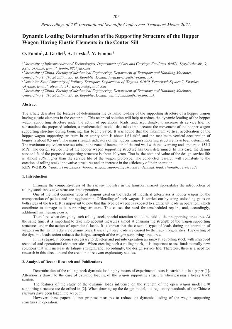
705

Proceedings of 25th International Scientific Conference. Transport Means 2021. Dynamic Loading Determination of the Supporting Structure of the Hopper Wagon Having Elastic Elements in the Center Sill O. Fomin1, J. Gerlici2, A. Lovska3, Y. Fomina4 1University of Infrastructure and Technologies, Department of Cars and Carriage Facilities, 04071, Kyrylivska str., 9, Kyiv, Ukraine, E-mail: fomin1985@ukr.net 2University of Zilina, Faculty of Mechanical Engineering, Department of Transport and Handling Machines, Univerzitna 1, 010 26 Zilina, Slovak Republic, E-mail: juraj.gerlici@fstroj.uniza.sk 3Ukrainian State University f Railway Transport, Department of Wagons, 61050, Feuerbach Square 7, Kharkov, Ukraine, E-mail: alyonalovskaya.vagons@gmail.com 4University of Zilina, Faculty of Mechanical Engineering, Department of Transport and Handling Machines, Univerzitna 1, 010 26 Zilina, Slovak Republic, E-mail: yuliia.fomina@fstroj.uniza.sk Abstract The article describes the features of determining the dynamic loading of the supporting structure of a hopper wagon having elastic elements in the center sill. This technical solution will help to reduce the dynamic loading of the hopper wagon supporting structure under the action of operational loads, and, accordingly, to increase its service life. To substantiate the proposed solution, a mathematical model, that takes into account the movement of the hopper wagon supporting structure during bouncing, has been created. It was found that the maximum vertical acceleration of the hopper wagon supporting structure in an empty state is about 1.63 m/s2, and the maximum vertical acceleration of bogies is about 8.5 m/s2. The main strength indicators of the hopper wagon supporting structure have been determined. The maximum equivalent stresses arise in the zone of interaction of the end wall with the overhang and amount to 153.3 MPa. The design service life of the hopper wagon supporting structure has been determined. In this case, the design service life of the proposed supporting structure is about 40 years. That is, the obtained value of the design service life is almost 20% higher than the service life of the wagon prototype. The conducted research will contribute to the creation of rolling stock innovative structures and an increase in the efficiency of their operation. KEY WORDS: transport mechanics; hopper wagon; supporting structure; dynamic load; strength; service life 1. Introduction

Ensuring the competitiveness of the railway industry in the transport market necessitates the introduction of rolling stock innovative structures into operation.

One of the most common types of wagons used on the tracks of industrial enterprises is hopper wagon for the transportation of pellets and hot agglomerate. Offloading of such wagons is carried out by using unloading gates on both sides of the track. It is important to note that this type of wagon is exposed to significant loads in operation, which contribute to damage to its supporting structure. This causes the need for unscheduled repairs, and, accordingly, additional maintenance costs.

Therefore, when designing such rolling stock, special attention should be paid to their supporting structures. At the same time, it is important to take into account measures aimed at ensuring the strength of the wagon supporting structures under the action of operational loads. It is known that the essential types of loads during the operation of wagons on the main tracks are dynamic ones. Basically, these loads are caused by the track irregularities. The cycling of the dynamic loads action reduces the fatigue strength of the wagon supporting structures.

In this regard, it becomes necessary to develop and put into operation an innovative rolling stock with improved technical and operational characteristics. When creating such a rolling stock, it is important to use fundamentally new solutions that will increase its fatigue strength, and, accordingly, the design service life. Therefore, there is a need for research in this direction and the creation of relevant exploratory studies.

2. Analysis of Recent Research and Publications

Determination of the rolling stock dynamic loading by means of experimental tests is carried out in a paper [1]. Attention is drawn to the case of dynamic loading of the wagon supporting structure when passing a heavy track section.

The features of the study of the dynamic loads influence on the strength of the open wagon model C70 supporting structure are described in [2]. When drawing up the design model, the regulatory standards of the Chinese railways have been taken into account.

However, these papers do not propose measures to reduce the dynamic loading of the wagon supporting structures in operation.

706Improvement of freight wagon supporting structures and requirements for them are given in a paper [3]. These

improvement measures are aimed at increasing the wagon service life. At the same time, this improvement is aimed at strengthening the wagon supporting structure, and not at reducing its dynamic loading in operation.

The analysis of the freight wagon dynamic properties is carried out in [4]. The finite element method was used as a computational one. When drawing up the computational model, the multidimensional system of the freedoms of a wagon was taken into account.

The study of the vehicle dynamics under shock loading of supporting structures is carried out in a paper [5]. Mathematical models to determine the acceleration acting on vehicles under impact conditions are presented. However, the paper does not propose measures to reduce the vehicle dynamic loading in operation.

Determination of possible ways to improve the technical and economic performance of wagons is carried out in a paper [6]. At the same time, these implementations are considered on the example of BCNHL freight cars. At the same time, the paper does not consider measures to reduce the dynamic loading of the wagon supporting structures in operation.

Measures to reduce the dynamic loading of the wagon supporting structures in operation by using flexible linings are described in the papers [7, 8]. Developed mathematical models are confirmed by computer simulation.

However, the issue of improving the service life of the hopper wagon supporting structure is not given attention to in these papers.

3. Purpose and Main Objectives of the Article

The purpose of the article is to describe the features of determining the dynamic loading of the hopper wagon with elastic elements in the center sill supporting structure. To achieve this goal, the following tasks have been identified:

– to propose measures of improvement of the hopper wagon supporting structure;– to determine the dynamic loading of the hopper wagon supporting structure;– to determine the strength of the hopper wagon supporting structure;– to calculate the design service life of the hopper wagon supporting structure.

4. The Main Material of the Article

To reduce the dynamic loading of the hopper wagon supporting structure and increase the fatigue strength under operating conditions, it is proposed to add elastic elements in it. The placement of elastic elements is assumed in the center sill along its length between the rear stops of the automatic coupler. To achieve that, it is proposed to use a U-shaped section instead of the standard section of the center sill (Fig. 1).

a b

Fig. 1 Section of the hopper wagon center sill a a standard center sill; b a center sill with elastic elements

The hopper wagon supporting structure with elastic elements in the center sill is shown in Fig. 2.

Fig. 2 The supporting structure of the hopper wagon

having elastic elements in the center sillFig. 3 The computational scheme of the hopper wagon

To determine the dynamic loading of the hopper wagon supporting structure, mathematical simulation has been carried out taking into account the proposed measures. The studies were carried out in the XZ plane. The computational scheme of the hopper wagon is shown in Fig. 3.

In this case, the hopper wagon was considered as a system consisting of three rigid bodies, that is a supporting structure and two bogies of 18-100 model with spring sets, which have a stiffness and a coefficient of relative friction.

It is taken into account that the following constraints are imposed:– the motion of the wagon body and bogies along the track axis are the same;

707– wheel sets move without sliding;– due to the absence of elastic elements in the axle-box suspension, the bouncing of the bogies is determined

by the bouncing of the wheelsets.It is taken into account that the wagon motion is described by the equations

2

1 1 1,1 1 1,2 3 1,3 5 1 22 ;TPd d dM q C q C q C q F sign sign

dt dtdt(1)

2

2 2 2,1 1 2,2 2 2,3 3 2,2 2 1 1 2 1 22 ;frd d d d dM q C q C q C q B q F sign k

dt dt dt dtdt(2)

2

3 3 3,1 1 3,2 2 3,3 3 3,3 3 2 3 4 3 42 ,frd d d d dM q C q C q C q B q F sign k

dt dt dt dtdt(3)

where is inertial coefficients of the oscillatory system elements (wagon body and two bogies); j is the elasticity characteristic of the oscillatory system elements; B j is the scattering function; q are generalized coordinates corresponding to translational displacement relative to the vertical axis, respectively, of the wagon body, the first and second bogies; k is the spring suspension stiffness; kb is the stiffness of elastic elements that are placed in the center sill; k is the stiffness of the track; is the damping coefficient; Ffr is the force of absolute friction in the coil spring group; is a deformation of elastic elements of spring suspension; (t) are irregularities of the track.

It is assumed in the motion Eqs. (1)-(3):Z1 ~ q1 is a coordinate characterizing the translational movements of the body relative to the vertical axis;Z2 ~ q2 is a coordinate characterizing the translational displacements of the first bogie in the direction of motion

relative to the vertical axis;Z3 ~ q3 is a coordinate characterizing the translational displacements of the second bogie in the direction of

motion relative to the vertical axis.When doing this the connection between the body and the bogie was described as a series elastic connection:

.b T T

b T T

k k kk k k

(4)

The input parameters of the model are the technical characteristics of the hopper wagon supporting structure, spring suspension, as well as the disturbing action.

It is assumed that the wagon moves in an empty state through a rail joint irregularity, which is described by a periodic function [9]:

1 cos ,2ht t (5)

where h is the depth of inequality; is the vibration frequency, which is determined by the formula =2 V/L (V is the wagon motion speed, L is the length of the inequality).

Differential equations of motion were solved in the MathCad software package [10-13]. In this case, the initial displacements and speeds are set equal to zero [14-17].

The solution of the model in the MathCad software was defined as:

2

4

6

1 2 1,1 1 1,2 3 1,3 5

1

1 1 2 1 2 2,1 1 2,2 3 2,2 4

2

2 3 4 3 4 3,1 1 3,3 5 3,3 6

3

( , )TP

TP

TP

yyy

F sign sign C y C y C y

MF t y

F sign k C y C y B y

M

F sign k C y C y B y

M

Cii C yy2 1 1 11 1signsign11 2 1,1 11 2 1,1 12 1,11 2 1 1 12 1 11 2 1 1 11 11

k1 11 1kkkkk1 1 1 2 2,1C2 2,111 CCC2 2 111 ,,

kkk22 kk2 kk CC y3 4 3,14 3,13,133 C yC4 3 133 C yC

(6)

0, , , , .Z rkfixed Y tn tk n FWith 1 1 3 3 5 5 2 1 4 3 6 5, , , , , .y q y q y q y y y y y y1 4 3 6 5.5y y y y y1 4 3 6 51 4 3 61 4 3 6 54 31 4 3 6y y y y1 4 3 61 4 33 6

The obtained results are shown in Figs. 4 and 5.

708

Fig. 4 Acceleration of the hopper wagon supporting

structure in the center of massFig. 5 Acceleration of bogies

The maximum vertical acceleration of the hopper wagon supporting structure in the empty state is about 1.63 m/s2 (0.16g), and maximum vertical acceleration of bogies is about 8.5 m/s2 (0.85g). Taking into account the proposed solution, it becomes possible to reduce the vertical accelerations acting on the supporting structure of the hopper wagon by almost 20%. The wagon movement is assessed as “excellent” [18, 19].

To determine the main strength indicators of the hopper wagon supporting structure with elastic elements in the center sill, a finite element analysis calculation was carried out in the SolidWorks Simulation software package (CosmosWorks). The finite element model of the hopper wagon supporting structure is shown in Fig. 6. Spatial isoparametric tetrahedrons were used as finite elements [12, 13, 20]. To determine the optimal number of elements, a graphic-analytical method was used. The number of nodes in the model was 125684 and the number of elements was 373595. The maximum element size was 60 mm, and the minimum one was 12 mm. The percentage of elements with an aspect ratio of less than three was 7.69, and the percentage of elements with an aspect ratio of more than ten was 32.9. The minimum number of elements in a circle was 12; the ratio of increasing the size of elements was 1.8. Thematerial of the wagon supporting structure is steel 09G2S with the endurance limit of w = 490 MPa and the yield stress of y = 345 MPa.

vst

l

vst

l

Fig. 6 Finite-element model of the hopper wagon supporting structure

Fig. 7 Calculation model of the hopper wagon supporting structure

The calculation model of the hopper wagon supporting structure is shown in Fig. 7. When drawing up the design scheme, it was taken into account that the supporting structure is affected by the vertical static load v

st, taking into account the use of the full carrying capacity with the conventional load, as well as the lateral pressure of the bulk cargo

l. The fastening of the model was carried out in the areas when the body is supported on the bogies.The results of the strength analysis of the hopper wagon supporting structure are shown in Figs. 8 and 9.

Fig. 8 The stress state of the hopper wagon supporting

structure Fig. 9 Displacements in the nodes of the hopper wagon

supporting structure

709 In this case, the maximum equivalent stresses arise in the place of the end wall with the overhang interaction and

amount to 153.3 MPa. The maximum displacements occur in the end parts of the unloading gates and are equal to 1.2 mm. So the strength of the hopper wagon supporting structure is provided [18, 19].

To determine the design service life of the hopper wagon supporting structure, the method described in a book [21] was used:

1 0/,

/

mD

e sw dv

n NB f k K

(7)

where -1D is the average value of the endurance limit; n is the permissible safety factor; m is an indicator of the degree of the fatigue curve; N0 is the test base; B is a coefficient characterizing the time of object continuous operation in seconds; fe is the effective frequency of dynamic stresses; sw is the stress from static weight load; kdv is the coefficient of vertical dynamics; is the sensitivity coefficient; K is the overall fatigue strength reduction factor.

The following input parameters were taken in the calculations: -1D = 245 MPa; n = 2; m = 8; N0 = 107; B = 3.07 106 s; fe = 2.7 Hz; sw = 153.3 MPa; kdc = 0.35; /K = 0.2.

Calculations have shown that the design service life of the proposed hopper wagon supporting structure is about 40 years. That is, the obtained value of the design service life is almost 20% higher over the service life of the wagon prototype.

5. Discussion of Research Results

To improve the service life of the hopper wagon, it is proposed to introduce elastic elements into its supporting structure. By reducing the dynamic loading of the hopper wagon supporting structure, the stresses arising in it are also reduced, and, accordingly, the service life is improved.

To substantiate the proposed solution, a mathematical model of dynamic loading is built. It has been established that, taking into account the improvement measures, it becomes possible to reduce the vertical accelerations acting on the supporting structure of the hopper wagon by almost 20%. It is important to note that this mathematical model takes into account the vertical displacements of the hopper wagon supporting structure in a flat coordinate system.

The main strength indicators of the hopper wagon supporting structure have been determined. The maximum equivalent stresses are 153 MPa. The design service life of the hopper wagon supporting structure is about 40 years.

With further research in this direction, the obtained value of the design service life should be refined by determining the longitudinal loading of the hopper wagon supporting structure. In addition, it is important to conduct a full-scale experiment on the loading of the hopper wagon supporting structure, taking into account the proposed improvement measures.

6. Conclusions

Measures to improve the supporting structure of the hopper wagon are proposed. These measures include the introduction of elastic elements into the center sill. This will help to reduce the dynamic loading of the hopper wagon supporting structure in operation.

The dynamic loading of the hopper wagon supporting structure has been determined. For this, a mathematical model, taking into account the displacements of the hopper wagon supporting structure in the vertical plane, has been developed.

The maximum vertical acceleration of the hopper wagon supporting structure in the empty state is about 1.63 m/s2 (0.16g), and the maximum vertical acceleration of bogies is about 8.5 m/s2 (0.85g). Taking into account the proposed solution, it becomes possible to reduce the vertical accelerations acting on the supporting structure of the hopper wagon by almost 20%. The wagon movement is assessed as “excellent”.

The strength of the hopper wagon supporting structure has been determined. The calculation was carried out using the finite element method in the SolidWorks Simulation software package. In this case, the maximum equivalent stresses arise in the zone of interaction of the end wall with the overhang and amount to 153.3 MPa. The maximum displacements occur in the end parts of the unloading gates and are equal to 1.2 mm. So the strength of the hopper wagon supporting structure is ensured.

The design service life of the hopper wagon supporting structure has been calculated. It has been established that its design service life is about 40 years. That is, the obtained value of the service life is almost 20% higher than the service life of the wagon prototype. Acknowledgement

This publication was issued thanks to supporting the Cultural and Educational Grant Agency of the Ministry of Education of the Slovak Republic in the project No. KEGA 036ŽU-4/2021: Implementation of modern methods of computer and experimental analysis of properties of vehicle components in the education of future vehicle designers.

710 References 1. Ermolenko, I.Y.; Zheleznyak, V.N. 2016. Studying the dynamics of rolling stock using an experimental laboratory

car when driving along difficult sections of the East Siberian Railway, Modern technologies, System Analysis. Modeling 4(52): 199-203. (In Russ.).

2. Chen, Ch.; Han, M.; Han, Y. 2012. Study of Railway Freight Vehicle Body’s Dynamic Model Based on Goods Loading Technical Standards, Procedia Engineering 29: 3572-3577.

3. P aczek, M.; Wróbel, A.; Buchacz, A. 2016. A concept of technology for freight wagons modernization, IOP Conf. Series: Materials Science and Engineering 161(2016). doi:10.1088/1757-899X/161/1/012107.

4. Haraka, S.S.; Sharma, S.C.; Harsha, S.P. 2014. Structural dynamic analysis of freight railway wagon using finite element method, Procedia Materials Science 6: 1891-1898.

5. Zamecnik, J.; Jagelcak, J. 2015. Evaluation of wagon impact tests by various measuring equipment and influence of impacts on cargo stability, Communications 4: 21-27.

6. Shukla, Ch.P.; Bharti, P.K. 2015. Study and Analysis of Doors of BCNHL Wagons, International Journal of Engineering Research & Technology (IJERT) 4(04): 1195-1200. doi: https://doi.org/10.17577/ijertv4is041031.

7. Fomin, O.; Lovska, A. 2020. Improvements in passenger car body for higher stability of train ferry, Engineering Science and Technology an International Journal 23(6): 1455-1465. https://doi.org/10.1016/j.jestch.2020.08.010.

8. Lovska, A.; Fomin, O. 2020. A new fastener to ensure the reliability of a passenger coach car body on a railway ferry, Acta Polytechnica 60(6): 478-485.

9. Domin, Y.V.; Chernyak, G.Y. 2003. Fundamentals of car dynamics. Kiev: KUETT, 2003. 269 p. (In Russ.) 10. Fomin, O.; Kulbovskiy, I.; Sorochinska, E.; Sapronova, S.; Bambura, O. 2017. Experimental confirmation of

the theory of implementation of the coupled design of center girder of the hopper wagons for iron ore pellets, Eastern-European Journal of Enterprise Technologies 5(1-89): 11-18. doi: 10.15587/1729-4061.2017.109588.

11. Kondratiev, A.; Gaidachuk, V.; Nabokina, T.; Tsaritsynskyi, A. 2020. New possibilities in creating of effective composite size-stable honeycomb structures designed for space purposes, Advances in Intelligent Systems and Computing 1113: 45-59. https://doi.org/10.1007/978-3-030-37618-5_5.

12. Vatulia, G.L.; Lobiak, O.V.; Deryzemlia, S.V.; Verevicheva, M.A.; Orel, Ye.F. 2019. Rationalization of cross-sections of the composite reinforced concrete span structure of bridges with a monolithic reinforced concrete roadway slab, IOP Conference Series: Materials Science and Engineering 664: 012014. doi:10.1088/1757-899X/664/1/012014.

13. Vatulia, G.; Komagorova, S.; Pavliuchenkov, M. 2018. Optimization of the truss beam. Verification of the calculation results, MATEC Web of Conferences 230: 02037. doi: 10.1051/matecconf/201823002037.

14. Lovska, A.O. 2015. Computer simulation of wagon body bearing structure dynamics during transportation by train ferry, Eastern-European Journal of Enterprise Technologies 3: 9-14.

15. Lovska, A.; Fomin, O.; Píšt k, V.; Ku era, P. 2020. Dynamic load modelling within combined transport trains during transportation on a railway ferry, Applied Science 10: 5710. doi:10.3390/app10165710.

16. Fomin, O.; Lovska, A. 2020. Establishing patterns in determining the dynamics and strength of a covered freight car, which exhausted its resource, Eastern-European Journal of Enterprise Technologies 6(7-108): 21-29. doi: 10.15587/1729-4061.2020.217162.

17. DSTU 7598:2014. Freight wagons. General requirements for calculations and design of new and modernized cars of 1520 mm gauge (non-self-propelled). Kyiv, 2015. 162 p. (In Russ.).

18. GOST 33211-2014. Freight cars. Requirements to structural strength and dynamic qualities. Moscow, 2016. 54 p. (In Russ.).

19. Lovska, A.; Fomin, O.; Ku era, P.; Píšt k, V. 2020. Calculation of loads on carrying structures of articulated circular-tube wagons equipped with new draft gear concepts, Applied Science 10(7441). doi:10.3390/app10217441.

20. Goolak, S., Gerlici,J., Tkachenko,V., Sapronova,S., Lack,T., Kravchenko,K. 2019. Determination of Parameters of Asynchronous Electric Machines with Asymmetrical Windings of Electric Locomotives, Communications - Scientific letters of the University of Zilina 21 (2): 24-31. https://doi.org/10.26552/com.C.2019.2.24-31

21. Ustich, P.A.; Karpych, V.A.; Ovechnikov, M.N. 1999. Reliability of non-traction rail rolling stock. Moscow, 415 p. (In Russ.).

711

Proceedings of 25th International Scientific Conference. Transport Means 2021.

Vehicle Security Barriers for Building Protection

P. Dvo ák1, P. Ma as2, J. Štoller3

1University of Defence, Kounicova 65, 662 10 Brno, Czech Republic, E-mail: petr.dvorak@unob.cz2University of Defence, Kounicova 65, 662 10 Brno, Czech Republic, E-mail: pavel.manas@unob.cz3University of Defence, Kounicova 65, 662 10 Brno, Czech Republic, E-mail: jiri.stoller@unob.cz

Abstract

The article deals with the issue of security barriers against vehicle ramming attacks. The paper focuses on the current state of available technical measures that can be taken to mitigate efficiently the effects of vehicle ramming attack against a protected building or a structure. Particularly at the military bases, the vehicle security barriers are one of the key measures of force protection, which consist of a diverse range of measures and capabilities with the aim to protect personnel, their equipment, buildings, facilities and services. It also mentions the problem of blast protection as some vehicle security barriers provide the protected facility with varying degrees of resistance against blast effects of explosives.KEY WORDS: force protection; military base; moving vehicle; security barrier; vehicle ramming attack

1. Introduction

A well-thought system of vehicle security barriers is one of the most significant parts of any building protection, both civilian and military. Security barriers in the military environment are a crucial part of an area called force protection (FP). According to [1], the definition of FP is: All measures and means to minimize the vulnerability of personnel, facilities, equipment, materiel, operations, and activities from threats and hazards in order to preserve freedom of action and operational effectiveness of the force, thereby contributing to mission success. It is necessary to mention, that in the context of [1], FP not only covers aspects of protecting the forces stationed at the military base but it overlaps outside of the base, when it is required to eliminate a potential threat. As a result, FP needs to achieve a balance between the protection of the personnel and their freedom of action. All of this must be done regardless of unrealistic expectations to avoid all risks, which might negatively influence the execution of the mission.

Building security barriers at the military base is one of the tasks that are covered by military engineering. Other tasks include: hardening of facilities, repairing airfields and routes, providing cover and concealment, determining stand-off distances within and around the military base (Fig. 1), route, airfield, and port clearances, mobility and countermobility measures, support to C-IED activities (Counter-Improvised Explosive Devices), as well as coordinating fire protection and supporting EOD activities (Explosive Ordnance Disposal) [1].

Fig. 1 Stand-off distances in military base perimeter [2]

712 2. Protective Infrastructure

The force protection model (Fig. 2) is used by commanders and staff to identify tasks, implement measures and effectively respond to incidents and attacks. The resulting measures, tasks, and activities generally fall into five categories: procedural, personnel, material, infrastructure, and information. The infrastructure category can be divided into three areas [1]:

Physical security measures – facility guards, fences, sensors, gates, lighting, and entry control points, which safeguards against destruction, espionage, sabotage and organized crime.

Protective measures – field fortifications, protective shelters, hardened buildings, security barriers and stand-off distances, which includes the defence, protection, and safe management of own ammunition storage areas.

Collective physical protective measures – theatre ballistic missile defence and surface based air defence against air threats, including aircraft, helicopters, remotely controlled systems and missiles.

In general, the above mentioned protective measures cover the entire infrastructure related to measures, tasks and activities that contribute to FP as well as planning, design, construction, and maintenance of the infrastructure and facilities, including appropriate blast and ballistic protection. It contains the determination of appropriate safety stand-off distances within and around the military base using security barriers, obstacles and fences. Fire protection is another very important protective measure that includes the design and construction of fire prevention and suppression systems within the infrastructure.

Fig. 2 Force protection model [1] 3. Military Base Perimeter

A well designed and maintained military base perimeter is a crucial part of force protection [3]. The military base perimeter consists of three main parts: perimeter protection, barrier protection and protection of buildings. The main importance of the base perimeter lies in the determination of appropriate safe stand-off distances within and around the military base using security barriers, obstacles and fences. They are all used both as vehicle security barriers and as blast protection. Most often they can be found at perimeter fortifications and at entry control points. Usually two types of basic building elements are used:

Defence wall – a modular system that consists of foldable units made from four vertical welded steel meshes, connected with four coils, with an inner layer made from geotextile; produced in a wide range of dimensions; characteristics may vary based on the fill material, e.g. concrete, crushed rock, gravel, sand; cross section of the structure can be designed precisely against the defined threat; units are stackable but the height of walls should not exceed two times the base width; intersecting walls are necessary for the stability of high thin structures; can be built into flood protection; some types of units are recoverable [4].

T-wall – a prefabricated building structural element made from steel reinforced concrete with a cross section resembling an inverted letter "T"; produced worldwide with different dimensions and usually named according to its height, e.g. Jersey (0.81 m), Texas (3.66 m), Alaska (6.10 m); elements creating the wall are connected vertically through tongue and groove; higher barrier walls can be reinforced by a connecting cable at the top of the element; razor wire for higher protection is sometimes attached at top of the wall; use of heavy machinery for installation is deemed to be an obvious disadvantage.

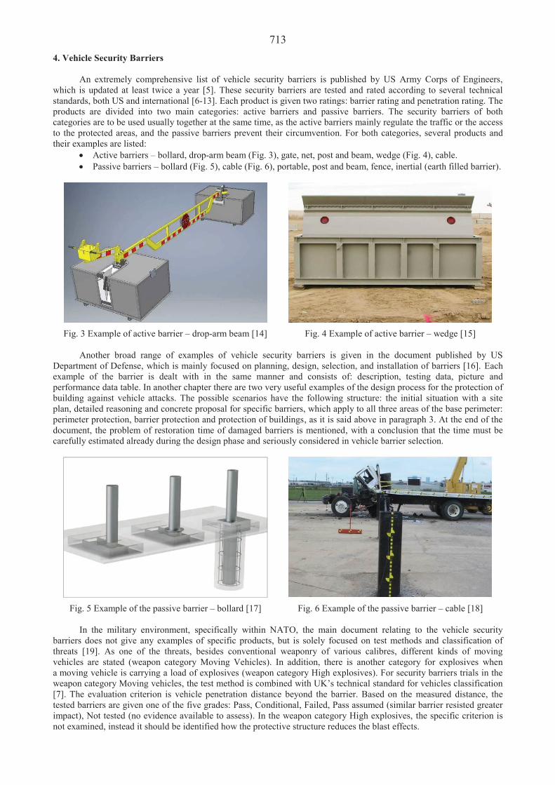
713 4. Vehicle Security Barriers

An extremely comprehensive list of vehicle security barriers is published by US Army Corps of Engineers, which is updated at least twice a year [5]. These security barriers are tested and rated according to several technical standards, both US and international [6-13]. Each product is given two ratings: barrier rating and penetration rating. The products are divided into two main categories: active barriers and passive barriers. The security barriers of both categories are to be used usually together at the same time, as the active barriers mainly regulate the traffic or the access to the protected areas, and the passive barriers prevent their circumvention. For both categories, several products and their examples are listed:

Active barriers – bollard, drop-arm beam (Fig. 3), gate, net, post and beam, wedge (Fig. 4), cable. Passive barriers – bollard (Fig. 5), cable (Fig. 6), portable, post and beam, fence, inertial (earth filled barrier).

Fig. 3 Example of active barrier – drop-arm beam [14] Fig. 4 Example of active barrier – wedge [15]

Another broad range of examples of vehicle security barriers is given in the document published by US Department of Defense, which is mainly focused on planning, design, selection, and installation of barriers [16]. Each example of the barrier is dealt with in the same manner and consists of: description, testing data, picture and performance data table. In another chapter there are two very useful examples of the design process for the protection of building against vehicle attacks. The possible scenarios have the following structure: the initial situation with a site plan, detailed reasoning and concrete proposal for specific barriers, which apply to all three areas of the base perimeter: perimeter protection, barrier protection and protection of buildings, as it is said above in paragraph 3. At the end of the document, the problem of restoration time of damaged barriers is mentioned, with a conclusion that the time must be carefully estimated already during the design phase and seriously considered in vehicle barrier selection.

Fig. 5 Example of the passive barrier – bollard [17] Fig. 6 Example of the passive barrier – cable [18]

In the military environment, specifically within NATO, the main document relating to the vehicle security barriers does not give any examples of specific products, but is solely focused on test methods and classification of threats [19]. As one of the threats, besides conventional weaponry of various calibres, different kinds of moving vehicles are stated (weapon category Moving Vehicles). In addition, there is another category for explosives when a moving vehicle is carrying a load of explosives (weapon category High explosives). For security barriers trials in the weapon category Moving vehicles, the test method is combined with UK’s technical standard for vehicles classification [7]. The evaluation criterion is vehicle penetration distance beyond the barrier. Based on the measured distance, the tested barriers are given one of the five grades: Pass, Conditional, Failed, Pass assumed (similar barrier resisted greater impact), Not tested (no evidence available to assess). In the weapon category High explosives, the specific criterion is not examined, instead it should be identified how the protective structure reduces the blast effects.

714 5. Conclusions

As it has been already concluded in the previous paper on a similar subject [20], the prevailing type of threat against our forces in military operations is the vehicle ramming attack. The attack is usually carried out against the main entrance to the military base, which is a crucial part of the military base perimeter. The threat is typically connected with the blast of varying amounts of explosives carried by the vehicle. To properly design a military base perimeter, where the vehicle barriers are one of the most important parts, it is necessary to rigorously follow the force protection process that results in the development and implementation of force protection measures. In conclusion it is essential to highlight three facts: the barriers, both active and passive, must be used simultaneously, as one type complements the other; the restoration time of damaged barriers must be considered in vehicle barrier selection; last but not least, the designated barriers must be certified in accordance with the appropriate technical standard. Acknowledgement

Presented work has been prepared with the support of the Ministry of Defence of the Czech Republic, Partial Project for Institutional Development, VARoPs - Military Autonomous and Robotic Systems. References 1. ATP-3.14 Allied Joint Doctrine for Force Protection, Edition A, Version 1. NATO Standardization Office. Dated

April 02, 2015, 80 p. 2. Štoller, J.; Zezulová, E. 2011. Barrier Protection of Czech Armed Forces Military Base in Missions Abroad. In:

ICMT´11 - International Conference on Military Technologies 2011. Brno: University of Defence, 261-270. ISBN 978-80-7231-787-5.

3. Zezulová, E.; Hasilová, K.; Komárková, T.; Stoniš, P.; Štoller, J.; Anton, O. 2021. NDT Methods Suitable for Evaluation the Condition of Military Fortification Construction in the Field, Applied Sciences 10(22): 8161. [online cit.: 2021-07-29]. Available from: https://www.mdpi.com/2076-3417/10/22/8161

4. Hesco Bastion Mil Recoverable [online cit.: 2021-07-29]. Available from: https://www.hesco.com/products/mil-units/mil/

5. DoD Anti-ram Vehicle Barrier List. US Army Corps of Engineers, Nebraska. Dated March, 2021, 30 p. [online cit.: 2021-07-29]. Available from: https://usace.contentdm.oclc.org/digital/collection/p16021coll11/id/5178

6. ASTM F2656M-20 Standard Test Method for Crash Testing of Vehicle Security Barriers. American Society for Testing and Materials, United States, 2020.

7. PAS 68:2013 Impact Test Specifications for Vehicle Security Barrier Systems. British Standards Institution, United Kingdom, 2013, 36 p.

8. PAS 69:2013 Guidance for the Selection, Installation and Use of Vehicle Security Barrier Systems. British Standards Institution, United Kingdom, 2013, 48 p.

9. CWA 16221:2010 Vehicle Security Barriers. Performance Requirements, Test Methods and Guidance on Application. European Committee for Standardization, 2010, 98 p.

10. IWA 14-1:2013 Vehicle Security Barriers – Part 1: Performance Requirement, Vehicle Impact Test Method and Performance Rating. International Organization for Standardization, 2013, 46 p.

11. IWA 14-2:2013 Vehicle Security Barriers – Part 2: Application. International Organization for Standardization, 2013, 58 p.

12. DoS SD-STD-02.01. Specification for Vehicle Crash Testing of Perimeter Barriers and Gates. U.S. Department of State. Dated April, 1985.

13. DoS SD-STD-02.01 Revision A. Test Method for Vehicle Crash Testing of Perimeter Barriers and Gates. U.S. Department of State. Dated March, 2003.

14. Drop & Swing Crash Beams DACB-PAM-400 [online cit.: 2021-07-29]. Available from: https://www.barrier1.us/ astm-m30-k4-model

15. Road Blocker DSP K12 [online cit.: 2021-07-29]. Available from: https://www.perimeterprotection.net/perimeter-protection-products/road-blocker-dsp-k12/

16. UFC 4-022-02 Unified Facilities Criteria – Selection and Application of Vehicle Barriers, Change 1. Dated August 09, 2010. United States Department of Defense. [online cit.: 2021-07-29]. Available from https://www.wbdg.org/ffc/dod/unified-facilities-criteria-ufc/ufc-4-022-02

17. Post and Cable Fences M50/P1 (K12) [online cit.: 2021-07-29]. Available from: https://atlasbarriers.com/post-and-cable-rail-fence/

18. Safety Bollards G-1600 Series [online cit.: 2021-07-29]. Available from: https://www. gibraltarperimetersecurity.com/bollards/

19. ATP-3.12.1.8 Test Procedures and Classification of the Effects of Weapons on Structures, Edition A, Version 1. NATO Standardization Office. Dated June 10, 2016, 69 p.

20. Ma as, P.; Štoller, J.; Dvo ák, P. 2020. Security Barriers against Moving Vehicles, In: Proceedings of the 24th International Scientific Conference Transport Means 2020 Part II: 781-784. [online cit.: 2021-07-29]. Available from: https://transportmeans.ktu.edu/proceedings-transport-means-2020/

715

Proceedings of 25th International Scientific Conference. Transport Means 2021. Safety Study of Operation on More than One Type Under Air Operator Certificate R. Matyáš1, V. Socha1,2, L. Hanáková1,2, J. Honzek1, M. Kalivodová1

1Department of Air Transport, Czech Technical University in Prague, Horská 3, 12800, Prague, Czech republic, E-mail: matyarom@fd.cvut.cz, sochavla@fd.cvut.cz, hanaklen@fd.cvut.cz, honzeja@fd.cvut.cz, kalivodova@fd.cvut.cz 2Department of Information and Communication Technologies in Medicine, Czech Technical University in Prague, Studni kova 7, 12800, Prague, Czech republic, E-mail: vladimir.socha@fbmi.cvut.cz, lenka.hanakova@fbmi.cvut.cz Abstract Presented article deals with the problematics of operation on more than one type under air operator certificate operations. Multi-type operations have always been often discussed. It is a subject where two fundamental aspects of commercial aviation come into a clash. On one side, the financial requirements of operators always strive to lower operating costs. Thus, an increase in the flexibility of flight crew planning and the lowering of crew training costs can be a strategic win for the company. On the other side lie the safety requirements laid down by the controlling authorities, which play a significant role in protecting the passengers, people on the ground, and the crew. The text focuses on the legislative, operative, and safety problems tied with operations on more than one type. Basic operational restrictions and procedures are laid down according to the European regulations. This article considers the two types for multi-type operations: the Cessna Citation Model 680 Sovereign and Model 700 Longitude. These aircraft belong to the same category of mid-size business jets and remarkably similar in dimensions, performance, and cabin configuration. It is thanks to these similarities that these two types seem to be ideal candidates for multi-type operations. The differences of both aircraft will be examined and analyzed. The safety study is based on the differences observed between the two types. The safety study identifies and evaluates individual hazards and risks of multi-type operations on the C680 and C700. The methodology and process used for the safety study are based on the operator's safety management manual. Operational restrictions and procedures are defined. Among these restrictions, we can find crew planning restrictions, standard operating procedures for the flight crew, and a syllabus draft for additional differential training on both types. The text also suggests procedures for continual safety monitoring during operations on more than one type. KEY WORDS: aircraft; operations; safety study; certificate 1. Introduction

In today’s competitive times any operational advantage can make a huge difference between a great success on the market or bankruptcy. Since the early beginnings of airline transport operators have been trying to one up each other in almost any field of their trade. From lowering maintenance costs, to reducing the number of required flight crew to a mere pilot and co-pilot. Each of these steps enable the airline companies to lower their fares or increase their sales margins [1,2]. One of these cost saving strategies is the effective planning of flight crew [3]. How can you most effectively keep all aircraft flying to satisfy the market need, but at the same time keep the number of crews as low as possible to save on salaries? Well, there are many variables, but through some analytics you will usually get an optimal number of crews per aircraft [4]. Now depending on the type of operation, you will usually get a number ranging from 1 to 6 or 7 crews per aircraft. But now add another variable to the mix. Let us imagine a fleet that is composed of more than one aircraft type. For example, one type serves short range, continental routes, while a second type serves long range, intercontinental routes. Now how many crews do we need? Simple answer: treat both type fleets as independent entities and have enough crews for both. Well, that would indeed be simple, but would that be the most cost-effective solution? Airlines in the past have quickly found out that by using one pilot to fly more than one type, you greatly increase the flexibility of crew planning. In this article we will perform a safety study on the matter. Our two-candidate aircraft will be the Cessna Citation Model 680 Sovereign and Model 700 Longitude. Initially we will have a look at the legislative structure and later we will perform the safety study and suggest necessary steps, restrictions and procedures that should be adapted to make the Citation multi-type operation safe.

In the past, it was quite normal for pilots to fly multiple aircraft types simultaneously during a given time in their career. But as technology went forward, aircraft types became increasingly more difficult to master and with that came a decrease in multi-type operations. Now do not imagine that all of the sudden pilots forgot how to aviate and were not capable of managing more types at once, but newly created legislative structures made this task much more difficult, often laying restrictions on operators, to only allow a pilot to operate on one type and one type only.

With the introductions of the Airbus line of A319/320/321/330/340 in the end of the 20th century [5] the world got a whole new look at multi-type operations. Boeing also was not far behind with their new models 757 and 767 [5,6]. Both companies set forward to create a line of aircraft that would be nearly identical in handling and operating procedures and would enable operators to plan their crews on both types.

716 In the case of Airbus this concept was branded as cross-crew-qualification, believing that the characteristics of

their aircraft types were so similar, that flight crew would have little to no problems operating both types simultaneously. Under this concept, flight crew are required to absolve initial flight training on one of the Airbus types and later that same crew would be able to complete a shortened flight training taking credit from the previous type. Once complete, the crew would be eligible two fly both types under certain conditions. Boeing went a step further with their 757/767 and gave both types a common type rating, meaning that if you complete the type rating on one type, you are eligible to fly the other one almost right away.

With more experience in multi-type operations, regulators of aviation authorities have started accepting exceptions in the field of operations on more than one type. In today's time it is perfectly legal to operate more than one type under air operator certificate (AOC) operations, but operators must follow set rules and more importantly, have to prove that the operations will be safe.

Although multi-type operations offer great benefits, like more flexible crew planning, lower required number of crew etc., it is still important to remember that safety always comes first. Without doubt multi-type operations come with their own hazards and risks and it is necessary to address all of them before operation commences.

Based on the above mentioned, it is clear that a safety study shall be conducted identifying possible hazards and risks that could be caused by the differences that have been found between the two aircraft. The safety study also serves as a list of the differences including possible hazards and risks. Following text describes the procedure of creating a safety study for a specific AOC holder that would like to operate types Citation Sovereign and Longitude under one AOC using procedure of flying on more than one type. 2. Methods

The two types considered for multi-type operations are the Cessna Citation Model 680 Sovereign and Model 700 Longitude. Both of these aircraft belong to the same category of mid-size business jets and remarkably similar in dimensions, performance, and cabin configuration. It is thanks to these similarities that these two types seem to be ideal candidates for multi-type operations. The safety study that follows later in this article will be based on the differences observed between the two types.

EASA regulations have taken a firm stance on operations on more than one type, saying that under specific conditions it is indeed possible. We can find such requirements in PART ORO (Organisation Requirements for Air Operators) [7]. Subparts Part ORO.FC.140 and FC.240 specifically focus on operations on more than one type. Furthermore, AMC1 and AMC2 of subpart Part.ORO.FC.240 suggest means of compliance with the EASA regulations. Basic operational restrictions and procedures should be based on these regulations and suggestions.

EASA requires the operator to specify minimum required experience levels and more. Also, EASA regulators are expecting from operators a safety study and special operating procedures and restrictions. An exempt from AMC1 requires the following minimum flight crew experience:

During one duty only one type will be operated. Only two types will be operated under multi-type operations. Before commencing multi-type operations, the pilot will have at least 500 at the relevant crew position. After completing flight training for the new type, the pilot will fly at least 50 hours and 20 sectors before

returning to fly the original type. Recent experience will be monitored for both aircraft independently. It is suggested that the operator provides additional difference training to the pilots.

The whole process starts with defining operator difference requirements (ODR). In ODR, an operator nominates the “base aircraft” to which the differences of a “difference aircraft” are compared, such as aircraft systems, procedures, handling characteristics and aircraft management. ODRs serve as justification for operating more than one type or variant and subsequent differences/familiarisation or reduced type rating for crew members.

Based on ODRs, each difference is analysed and described in more detail since each of these differences may be a root cause for a hazard which has an associated risk for an accident or incident to happen. The probabilities of barriers failing before the accident occurs have been discussed with subject matter experts who have significant experience in safety management.

The outcome of the safety study is an initial level of risk, a mitigation which will improve the probability that the barriers will not fail in avoiding/recovering the accident and a final level of risk, which describes if the risk is tolerable or not.

Levels of risk are as follows: Unacceptable, acceptable under specific conditions, tolerable. When the level of safety is assessed as unacceptable, the operation shall not continue and halt immediately. Further procedures are then established by the Safety Action Group (SAG) of an operator. Before re-commencing operations, mitigation measures must be implemented. This level is named in the results as ST - stop.

If the safety level is assessed as acceptable under specific conditions, SAG designs a plan for risk mitigation and time frame of its implementation. Operations may continue within the approved time frame. If the level of risk is not decreased during the testing period, management needs to re-assess the operations. This level is named in the results as I - improve. Tolerable level of safety has three subcategories A – accept, when the risk is completely tolerable; M - monitor, when the risk is monitored by safety department and S – secure. It is recommended to improve procedures for

717 mitigation of risk and the risk level is monitored to prevent further escalation.

3. Results

Due to the different airframe, wings and stabilizers construction, there can be a difference in the flight abilities between the types C680 and C700. The majority of the operating speeds for the type C700 are higher than for the C680 type and the attention should be given to the greater swept angle of the wings of the C700 aircraft. Similarly, the C700 has the T-tail shaped stabilizers that can be a cause of the deep-stall [1]. In the simultaneous operations of the C680 and C700, there is a risk of interchanging the flight abilities of both types that can result in LOC-I. from the given description there was identified the hazard “LOC-I, (Root/Cause: Different flight characteristics, T-Tail, Higher sweep)”, see Table. For the mitigation of this hazard, there is a proposal for the UPRT training on top of the standard training programme. During this training, there should be an emphasis given on the impact of the interchanging of the flight abilities. For example: the flight on the C700 aircraft with the operating speeds of the C680, the identification for the deep stall on C700, emphasis of the stall characteristics of the high swept ankle wings.

For the load calculations of both aircraft a Cessnav application is used from the aircraft producer. There is a risk of interchanging the aircraft within the application and receiving the incorrect outcomes, that can result in the incorrect balancing and overshooting of maximum weights. In such cases there is a risk of departure outside the flight envelope than can result in extreme cases with LOC-I. From the description there was a hazard “Hazard: LOC-I, (R/C: Incorrect W&B)”, identified (see Table). For the mitigation of these hazards, it is proposed that the calculations would be performed both by the CPT and the FO and the result would be compared.

Further, the C700 aircraft is, compared to the C680 equipped with the pusher and electronically operated rudder. These systems can have uneven flight characteristics in the critical phase of the flight and their mishandling can result in the LOC-I. From the described, there was a hazard “LOC-I, (R/C: Stick pusher and fly-by-wire rudder system)”, see Table identified. For the mitigation, it was proposed, the crew to be trained on the differences between these two systems and the emphasis should be put on them also during the UPRT training.

The type C700 is also equipped with the automatic spoilers that are opened autonomously during the landing. Also, this system can automatically close the spoilers during the flight if it is decided so by the system logic. There is a risk that the crew of C680 will be expecting the automatic operations of the spoilers and when not done, there is a risk of RE during the landing or the in-flight LOC-I. As the hazard there was identified: “RE & LOC-I, (R/C: Automatic ground spoilers and Spoiler autostow)”. For the mitigation it is proposed for the operator to define the manuals for the spoiler usage on both types and for the C700 to require the manipulation of the spoiler control stick for the preservation of the habits.

The types C700 and C680 have different operating speeds and their interchanging can result in the exceeding of the flight envelope. In some cases such exceeding can result in the structural damages and/or LOC-I. The hazard in this case is the “LOC-I, (R/C: Flight envelope exceedance)”. See Table.

The C700 and C680 have slightly different de-icing systems and their operating manuals. In the case of the deicing manual interchanging there is a risk of ice accretion on the wings that can in the extreme cases result in the loss of lift and LOC-I. The hazard is “LOC-I, (R/C: Icing on wing surface due to crew incompetence)”. For the mitigation of these hazards it is proposed for the crews to receive the training for the differences in the de-icing systems and also for their UPRT training to include the flight with the accreted ice.

The C700 is equipped with the Power Reserve system, which adds power to a functioning engine when the other power unit is lost. This system can be activated manually by the crew under certain abnormal conditions. If the crew forgets to activate this system in flight, or if it will not be handled properly, it can eventually result in the LOC-I due to loss of performance. A possible hazard is "LOC-I, (R / C: Power Reserve function)". For this hazard mitigation, it is suggested that flights without activation of the Power Reserve be included in the UPRT training and the need for this system to be emphasized.

The C680 is equipped with the EMER STOW function for emergency closing of reverse thrust reversers. The C700 aircraft no longer has this system, and if they are accidentally opened in flight, it is necessary to consider a sharp deterioration in flight characteristics. Failure to master these characteristics could result in loss of control and the LOC-I . The hazard is therefore named as "LOC-I, (R / C: EMER. STOW removed)". To mitigate this hazard, it is suggested that the flights with open thrust reversers on the C700 be included in UPRT training and emphasis should be placed on this risk.

Unlike the C680, the C700 is equipped with an automatic side vibration damper (Yaw Damper). There is a risk that the crew of the C680 will forget to manually turn on the YD after take-off and a Dutch Roll will occur at higher levels. As a last resort, a failed Dutch move may result in LOC-I. The identified hazard, also reflected in Table is "LOC-I, (R / C: YD Engagement)". To mitigate this hazard, it is proposed that the operator introduce a mandatory post-take-off callout to control the YD activation.

Some Memory items are different between both types. For example, for the C700, memory items are not defined in the event of an engine fire or are different when the thrust reverser is opened in flight. In case of omission or exchange of memory items between types of the flight control may be lost, so the hazard is identified as “LOC-I, (R / C: Memory items)”. To mitigate this hazard, it is proposed that the operator creates memory items above the standard framework, which will be more restrictive than the memory items for each type. In the case of different memory items, it is suggested that more emphasis is placed on this difference in differential training.

718 Table

Safety analysis with identified hazards and mitigations along with assessed initial and final level of risk (R/C – root / cause; A – accept; M – monitor; S – secure; I – improve; ST – stop)

HAZARD AND R/C

Estimated frequency

of the triggering

event

Barriers will fail in

AVOIDING occurrence

Barriers will fail in RECOVERING

the situation before the

ACCIDENT

Accident severity

would be

INITIAL LEVEL of RISK

MITIGATION

Estimated frequency

of the triggering

event

Barriers will fail in

AVOIDING occurrence

Barriers will fail in RECOVERING

the situation before the

ACCIDENT

Accident severity

would be

FINAL LEVEL of RISK

LOC-I Diff. flight

char.

About every 1000

flights

Once every 250 times

Once every 100 times SEVERE M Additional

UPRT

Almost Every 2500

flights

Once every 500 times

Once every 250 times SEVERE A

LOC-I Incorrect

W&B

Almost every 500

flights

Once every 250 times

Once every 500 times CATAS. I

Crosscheck loading by CPT

and FO

Almost every

500 flights

Once every 5000 times

Once every 500 times CATAS. M

LOC-I Stick pusher

& FbW rudder

About every

10 000 flights

Once every 100 times

Once every 100 times SEVERE M

Additional difference

training and UPRT

About every

10 000 flights

Once every 250 times

Once every 250 SEVERE A

RE & LOC-I

Automatic Spoilers

About every 1000

flights

Once every 100 times

Once every 500 times CATAS. I

Company procedure for spoiler usage

About every 1000

flights

Once every 2500 times

Once every 500 times CATAS. M

LOC-I Flight

envelope

Almost every

50 flights

Once every 25 times

Once every 500 times MOD M

Flight envelope limits on

placards in cockpit

Almost every 250

flights

Once every 100 times

Once every 500 times MOD A

LOC-I Icing

Almost every 100

flights

Once every 100 times

Once every 1000 times CATAS. ST

Additional UPRT and Icing

awareness course

Almost every 100

flights

Once every 1000 times

Once every 2500 times CATAS. S

LOC-I Power reserve

Almost every 5 000 flights

Once every 100 times

Once every 250 times MOD. A Additional

UPRT

Almost every 5 000 flights

Once every 250 times

Once every 500 times MOD. A

LOC-I YD

engagement

Every flight

Once every 100 times

Once every 250 times MOD. S

Company callout, e.g. YD

engaged

Every flight

Once every 500 times

Once every 1000 times MOD. M

LOC-I EMER.

Stow

About every

100 000 flights

Once every 500 times

Once every 1000 times SEVERE A

Additional difference

training and UPRT

About every

100 000 flights

Once every 1000 times

Once every 2000 times SEVERE A

LOC-I Memory

items

Almost every 7500 times

Once every 50 times

Once every 250 times SEVERE S Company

memory items

Almost every 7500 times

Once every 250 times

Once every 250 times SEVERE M

GCOL A/C

dimensions

Almost every 750

times

Once every 100 times

Once every 10 times MOD. S

Dimension placards placed

in cockpit

Almost every 750

times

Once every 500 times

Once every 10 times MOD. M

RAMP Apron

collision

Almost every 750

times

Once every 100 times

Once every 10 times MOD. S Wing walker

Almost every 750

times

Once every 1000 times

Once every 50 times MOD. A

RAMP Servicing

Every flight

Once every 10 times

Once every 500 times LIGHT S

Placards on servicing panels and cabin door

Every flight

Once every 100 times

Once every 500 times LIGHT M

RAMP Parking brake

Every flight

Once every 50 times

Once every 1000 times MOD. S

Crosscheck parking brake

by crew

Every flight

Once every 500 times

Once every 1000 times MOD. M

RAMP Cargo door

Almost every

10 flights

Once every 50 times

Once every 10 times LIGHT S

Cargo loading under

supervision

Almost every

10 flights

Once every 250 times

Once every 10 times LIGHT M

RAMP Fuelling

panel

Every flight

Once every 10 times

Once every 1000 times LIGHT S Fuelling under

supervision Every flight

Once every 250 times

Once every 1000 times LIGHT A

FUEL Fuelling

panel

Every flight

Once every 10 times

Once every 1000 times LIGHT S

Fuel loading crosscheck by

crew

Every flight

Once every 250 times

Once every 1000 times LIGHT A

FUEL & LOC-I

Fuel transfer & Xflow

Every flight

Once every 100 times

Once every 1000 times MOD. S

Additional difference training

Every flight

Once every 500 times

Once every 1000 times MOD. M

RE Emergency

braking

Almost every 5000

flights

Once every 50 times Practically always MOD. M

Additional difference training

Almost every 5000

flights

Once every 250 times Practically always MOD. A

RE High app speed & ground spoilers

Every flight

Once every 250 times

Once every 100 times MOD. S

Company procedure for spoiler usage

Every flight

Once every 2500 times

Once every 100 times MOD. M

SCF Diff.

procedures & panel layout

Every flight

Once every 100 times

Once every 250 times LIGHT M

Additional difference training

Every flight

Once every 250 times

Once every 500 times LIGHT A

719 Airplanes have different dimensions (span, wheelbase, etc.). During taxiing, you may approach a size-restricted

taxiway or stand, resulting in contact with an airport sign or obstacle, so the hazard identified is “GCOL, (R / C: Different dimensions)”. To mitigate this hazard, it is proposed that the operator places a visible board with the dimensions of the aircraft in the cockpit.

During guidance to the stand, a collision with an obstacle (RAMP) may occur, due to poor guidance from ground personnel who can swap type dimensions. The identified hazard is therefore "RAMP, (R / C: Collision on apron during handling / marshalling)". To mitigate this hazard, it is proposed that the operator introduces into the procedures the possibility of requesting a so-called wing walker by the crew. The wing walker will assist ground personnel in guiding the aircraft to the stand and will guard the wing or other parts of the aircraft that are at risk of collision. The wing walker can be a crew member or a ground staff member.

The C700 has different procedures for servicing systems (fuel, water, compressed air) and a new system for opening deck doors. When handling the aircraft on the stand, the system (RAMP) can be damaged either by the ground personnel or by the crew itself. The hazard is “RAMP, (R / C: Incorrect servicing or door handling)”. To mitigate this hazard, it is proposed that tables with proper handling are placed on the service door and deck door.

Both types have different ways of applying the parking brake. Improper braking of the aircraft without the use of logs can cause the aircraft to move spontaneously and collide on the stand. The identified hazard in this case is “RAMP, (R / C: Different parking brake system)”. To mitigate this hazard, it is suggested that the brake control always be confirmed by the second crew member. The C700 also has a cargo door located above the trailing edge of the wing. If the luggage is handled incorrectly, there is a risk of damaging the trailing edge of the wing on the stand, which results in the hazard "RAMP, (R / C: Different cargo door position)". To mitigate this hazard, it is always suggested that one crew member be present when loading luggage and that ground personnel be alerted to the risk of damage to the trailing edge.

The C700 is equipped with a refueling panel, which is used to control the filling and control the amount of fuel and oil. Improper handling can damage the filling systems or fill the wrong amount of fuel. Aircraft also have different fuel tank volumes. There is a risk of filling or scheduling the wrong amount, which can cause an emergency due to lack of fuel. From this, the hazards “RAMP, (R / C: Filling panel)” and “FUEL, (R / C: Felling panel)” is identified. To mitigate the first hazard, it is suggested that a crew member be always present when refueling and check the correct setting of the refueling panel. To mitigate another of these hazards, it is proposed that the crew jointly verify before the flight that the fuel on board is appropriate for the flight. For example, OFP [2] or an aircraft application planning application can be used for control.

The aircraft have Different Fuel transfer and crossflow. Incomprehension or confusion of system characteristics can result in a fuel imbalance on board (FUEL) and, in extreme cases, loss of control of the aircraft along the longitudinal axis and LOC-I. To mitigate this hazard, it is suggested that crews receive training on the differences between the two fuel systems of the two types, while drawing attention to the risk of fuel imbalance.

Aircraft have Different emergency brake handling. The incomprehension or change of control may result in brake failure or failure to initiate braking. In extreme cases, the brakes may lock or and the aircraft excurses the track. To mitigate this hazard, it is proposed that crews receive training on the differences between emergency braking systems and the risk of confusion between types.

The C700 has Higher approach speeds and automatic spoilers than the C680. There is a risk that the crew of the C680 will land at a higher speed (adequate for the C700) and forget to extend the lift spoilers (a system that is automatic on the C700). In such an event, there is an extreme risk of runway excursion. To mitigate this hazard, it is proposed that the operator defines uniform procedures for the use of spoilers on both aircraft. Thus, with the C700, where operation is automatic, it still required manipulation of the spoiler control lever to maintain habits. Company procedure for spoiler usage.

There are differences in systems and procedures between airplanes. These differences do not necessarily constitute an immediate risk, but their ignorance or confusion may cause an abnormal operating situation or damage to the system. An example of such an abnormal situation may be a poorly executed procedure for starting the drive unit. They might result in extreme cases in the damage to the system (SCF), but it should not endanger the health of the crew and passengers. To mitigate this hazard, it is suggested that crews receive training on the differences between the two types of systems and procedures. 4. Discussion and Conclusions

A total of 21 significant differences have been identified between the two aircraft. Most of these differences are minor e.g.: different handle or panel locations and slightly different dimensions. The biggest difference between the types might be the fact that the C700 Longitude has more automation than the C680 Sovereign. Other than that, the types are quite similar and most importantly have an almost identical avionics suite, the Garmin G5000 (Citation Sovereign+ models).

As seen in Table, most final levels of risk are either Acceptable, Monitor or Secure. An Acceptable Level of risk does not require any further action to be taken and is perfectly tolerable. A Monitor level of risk should be monitored further so that it does not degrade to a lower level of risk. A Secure level of risk should be monitored further so that it does not degrade to a lower level of risk and it is suggested that additional mitigation procedures are adopted. From the point of the view of the safety study, multi-pilot operation on the C680 and C700 is tolerable and acceptable under

720 certain conditions.

As previously described results show, multi-type operation of the Citation Sovereign and Longitude is tolerable and if the necessary mitigations and operational procedures and restrictions are followed should be considered safe. The restrictions regarding experience requirements have been established by the EASA regulations and necessary operational procedures and training has been suggested by the safety study and its mitigations.

Even though this article is primarily aimed at two Cessna Citation types a similar approach can be used for any two types which would be considered for multi-type operations. Acknowledgement

Authors would like to thank safety specialist and pilots participating in research and helped with expert evaluation and validation of the paper results. References 1. Cacchiani, V.; Salazar-González, J.J. 2020. Heuristic approaches for flight retiming in an integrated airline

scheduling problem of a regional carrier, Omega 91:102028. 2. Lagos, C.; Delgado, F.; Klapp, M.A. 2020. Dynamic optimization for airline maintenance operations,

Transportation Science 54(4): 998-1015. 3. Barnhart, C.; Cohn, A. 2004. Airline schedule planning: Accomplishments and opportunities, Manufacturing &

service operations management 6(1): 3-22. 4. Fennell, P. 2017. Crew planning. In Airline Operations, London: Routledge, 125-139. 5. Newhouse, J. 2007. Boeing versus Airbus. New York: Knopf Doubleday Publishing Group, 272 p. 6. Klansnic, J. E.; Dittenberger, R. J. 1981. Boeing 757/767 Commonality Design Philosophy (No. 810845). SAE

Technical Paper. 7. European Union Aviation Safety Agency. 2014 Part-ORO - Organisation Requirements for Air Operations.

721

Proceedings of 25th International Scientific Conference. Transport Means 2021. Study of Dynamics Characteristics and Comfort Parameters of Passenger Car with Independently Rotating Wheels G. Vai i nas1, S. Steiš nas2 1Vilnius Gediminas Technical University, Saul tekio al. 11, 10223, Vilnius, E-mail: gediminas.vaiciunas@vilniustech.lt 2Vilnius Gediminas Technical University, Saul tekio al. 11, 10223, Vilnius, E-mail: stasys.steisunas@vilniustech.lt Abstract The authors of an article compare the dynamic characteristics of cars with one-piece wheel sets and wheel sets with independently rotating wheels by comparing Nadal criterion values and their laws of change when the car runs on various curves and straight sections of the railway. The studies show that in curves of low radius, laws of change of Nadal criterion values are fundamentally different than in straight railway sections; it has a significant impact on the comparison of dynamic parameters of passenger cars with one-piece wheel sets and wheel sets with independently rotating wheels. The authors use Sperling’s comfort index to assess the riding comfort. They compare the riding comfort of passenger cars with one-piece wheel sets and wheel sets with independently rotating wheels based on Sperling’s comfort index. KEY WORDS: passenger car, dynamic characteristics, Nadal criterion, Sperling’s comfort index 1. Introduction

The authors of this article have observed in their previous works, that rolling stock derailment issue and various related researches in the world of science is not a new phenomenon [1, 2]. Scientists often study the influence of the wheel running surface, its flange geometry and wheel dynamics on the derailment of a train [3]. In order to examine this issue in more detail, the phenomenon of flange climbing on the rail is usually examined [4]. The scientists concluded that this regularity is best described by the classical derailment equation [5], as it deals with wheel and rail friction slip. In addition, approximate analytical formula describes the impact of wheel/rail scroll forces ([6]. Chinese researchers tested derailment due to wheel impacts on the bench as a type of dynamic derailment by estimating wheel jump height, lateral impact force, and vertical wheel load. Analyzed factors: speed of wheel set side impact, wheel flange angle, wheel/rail friction coefficient, vertical load on the wheel and impact time interval during wheel set derailment [7]. It is very important to study low-radius track curves (180–300 m) in small-area countries or mountainous areas. There is a big difference in the rolling radius of the wheel sets and it greatly determines the rolling laws [8] Scientific papers also focus on the effect of car wheel and rail friction modifier on road curves and its influence on car rolling [9, 10]. Studies on the effect of wheel defects on rolling stock dynamics must be mentioned as a specific area of research [11]. However, as transport is focused towards passenger service, one of the key issues must be passenger comfort studies [12]. One of the passenger comfort indicators is Sperling’s comfort index.

An objective of the following study is to examine the dynamic characteristics of cars with one-piece wheel sets and wheel sets with independently rotating wheels by using available scientific expertise and computer equipment, as well as test when Sperling’s comfort index can be used to assess the riding comfort. 2. Methodology of the Study

Computer simulation with “Universal Mechanism” (UM) software package was selected for the research for several reasons. The researches with this software package allow performing many more researches in a relatively short time compared with researches using real rolling stock. The software allows analysis of vehicle dynamics depending on wheel and rail profiles, rolling stock suspension, chassis and railway parameters. The passenger car model consists of a body, two bogies and four pairs of wheel sets. Passenger car structure is modelled with two types of wheel sets: with one-piece wheel sets and wheel sets with independently rotating wheels (IRW).

Wheel set provided in Fig. 1 has six degrees of freedom that allow the entire wheel set to rotate and move in X, Y and Z axes. Wheel set with IRW is provided in Fig. 1.

Wheel set provided in Fig. 1 is not integral and consists of 4 parts: axle, two wheels and bearing. The wheels of this wheel set can rotate independently, thus the mechanism has seven degrees of freedom. The wheel profiles of both types of used wheel sets are UIC510-2 type profile. The bogie provided in Fig. 3 consists of two wheel sets, frame, four axle boxes and double spring suspension.

Main technical details of the examined car are provided in Table 1.

722

Fig. 1 Wheel set with independently rotating wheels

Table 1 Car model parameters

Characteristics Value Car body mass, kg 54 700 Wheel set mass, kg 2000

Suspension type Spring with hydraulic dampers Distance between automatic clutches, mm 2 475

Wheel set base, mm 2 400 Body width, mm 2 218 Body length, mm 3 920

Wheel rolling radius, m 0.475 Half sleeper width, m 1.2

During the car simulation, it is assumed that all bodies are rigid and can move in X, Y and Z axes. Passenger car

suspension models are presented in Fig. 2 and Fig. 3.

Fig. 2 Passenger car with one-piece wheel sets suspension model

Fig. 3 Passenger car with independently rotating wheels model

Horizontal and vertical irregularities in 1000 m section of modelled track are provided in Fig. 4.

a

b

Fig. 4 a Vertical irregularities of modelled track; b Horizontal irregularities of modelled track

723 Track irregularities provided in Fig. 4 were measured in real UIC 60 railway and were selected from the list of

track irregularities provided in UM software package, since they correspond to the real irregularities of the selected rail profile. 200 m and 2900 m radius track curves and 1000 m length straight section were designed for the study.

The calculations of the stability criteria are performed by estimating the contact forces of the wheel and rail (provided in Fig. 5 below).

Fig. 5 Contact forces of wheel and rail

Nadal criterion is widely used for derailment. It takes into account the shape of the wheel set wheel, the contact angle and the coefficient of friction, but it does not take into account the longitudinal forces and angle of curve where it is moved. It is a criterion describing traffic safety. Other issue is passenger comfort. Comfort is described by Sperling’s comfort index.

Nadal criterion is widely used for derailment. It takes into account the shape of the wheel set wheel, the contact angle and the coefficient of friction, but it does not take into account the longitudinal forces and angle of curve where it is moved. Nadal criterion is calculated according to formula [12]:

0

tan1 tan

y y

z y

Fq

F, (1)

where yy

FN

; – contact angle.

Own and forced oscillations occur during the movement of vehicle on railway track at respective speed. Forced oscillations appear due to unevenness of railway track or damaged vehicle wheels (flats, crumbles). Such defects cause the forced oscillations of vehicle bogie and their impact to body is transmitted via primary and secondary suspension. The recurrence of these oscillations is called vehicle vibration and can affect the comfort of passenger vehicles negatively. Vibrations worsen the well-being of passengers and reduce the working capacity of passenger service staff. Therefore, it is necessary to assess the vibration intensity considering its harmful impact to human. During the reduction of general vibration level, it is necessary to take into account the vibration frequencies, since some vibration frequencies are harmful to human body. The impact of vibration and noise on the passenger determines his/her travel comfort described by the entire set of parameters – vibration frequency and amplitude, noise level, air humidity and temperature, etc. [12, 13]. During the assessment of vehicle vibration level and taking into account the passenger comfort, Sperling’s comfort index smooth running indicator can be used [14]:

110

10

1

f

i

n

Z Zi

W W , where 1

22 6.67iz i iW a B f , (2)

where a – acceleration, cm/s2; f – vibration frequency, Hz, o B(f) – frequency and vibration direction coefficient influencing the passenger‘s well-being:

22 2

2 22 3

1,911 0,25

1 0,277 1,563 0.0368

f fB f k

f f f, (3)

where k = 0.737, if oscillations are horizontal, and 0,588 if oscillations are vertical. The smooth running indicators calculated based on (2)–(3) are compared with standard assessment scale. The quality of vehicle carrier is finally assessed according to comparative results. 3. The Results of Calculations

Nadal criterion and Sperling’s comfort index at different running speeds were calculated in different track sections:

724 in 200 m radius curve; in 2900 m radius curve; in straight section. 3.1. The Results of Nadal Criterion Calculation

During the simulation, the maximum values of passenger car Nadal criterion were calculated to determine the maximum speed of passenger car models during movement in 200 m, 2900 m radius “S“ type curves and straight track section. Calculation results are provided in Figs. 6, 7 and 8 respectively.

Fig. 6 Maximum Nadal criterion values in 200 m radius curve

The chart provided in Fig. 6 shows that passenger car model with IRW in 200 m radius curve has lower maximum Nadal values when moving at speed from 45 km/h to 80 km/h and ~ 90 km/h than the model with one-piece wheel set (OPW). At all other speed of movement, maximum Nadal criteria values of model with OPW are lower than the model with IRW. The model with IRW reached the largest permissible Nadal criterion value at 95 km/h speed, when the maximum established value of model with OPW is 0.65 at the same speed. Model with OPW reached the largest permissible Nadal criterion value at 107 km/h speed.

Fig. 7 Nadal criterion values in 2900 m radius curve

The chart provided in Fig. 7 shows that the maximum Nadal criterion values of passenger car model with OPW are lower compared to the model with IRW at all established movement speeds in 2900 m radius curve, unlike the graphs provided in Fig. 7. The model with IRW reached the largest permissible Nadal criterion value at 200 km/h speed. Model with OPW reached the largest permissible Nadal criterion value at 255 km/h speed at the same section.

The chart provided in Fig. 8 shows that the maximum values of passenger car model with OPW are lower compared to the model with IRW at all established movement speeds. The model with IRW reached the largest permissible Nadal criterion value at 205 km/h seed. Model with OPW reached the largest value at 290 km/h speed at the same section.

0,00

0,25

0,50

0,75

1,00

40 50 60 70 80 90 100 110 120The

mea

ning

of t

he N

adal

cr

iterio

n

Speed, km/h

One-piece wheelset Wheelset with independently rotating wheelPermissible limit of the Nadal criterion

0

0,25

0,5

0,75

1

160 180 200 220 240 260

The

mea

ning

of t

he N

adal

crit

erio

n

Speed, km/h

One-piece wheelset Wheelset with independently rotating wheelPermissible limit of the Nadal criterion

725

Fig. 8 Nadal criterion values in 1000 m length straight section 3.2. The Results of Sperling’s Comfort Index Calculation

During the study, Sperling’s comfort index in lateral and vertical directions at different speed were calculated in different track sections. The obtained values of indicators are provided in Figs. 9-14.

Fig. 9 Sperling’s comfort index values in vertical direction in 200 m radius curve

Fig. 10 Sperling’s comfort index values in lateral direction in 200 m radius curve

0

0,25

0,5

0,75

1

160 180 200 220 240 260 280 300

The

mea

ning

of t

he N

adal

cr

iterio

n

Speed, km/h

One-piece wheelset Wheelset with a freely rotating wheelPermissible limit of the Nadal criterion

0

1

2

3

4

40 50 60 70 80 90 100

The

mea

ning

of

Sper

ling’

s co

mfo

rt in

dex

Speed, km/h

Wheelsets with independently rotating wheelsOne-piece whelsetsPermissible limit of the Sperling’s comfort index

0

1

2

3

4

40 50 60 70 80 90 100

The

mea

ning

of t

he

Sper

ling’

s com

fort

inde

x

Speed, km/h

One-piece wheelsetWheelset with a independently rotating wheelPermissible limit of the Sperling’s comfort index

726

Fig. 11 Sperling’s comfort index values vertical direction in 2900 m radius curve

Fig. 12 Sperling’s comfort index values in lateral direction in 2900 m radius curve

Fig. 13 Sperling’s comfort index values vertical direction in straight section

0

1

2

3

4

165 170 175 180 185 190 195 200 205

The

mea

ning

of t

he

Sper

ling’

s co

mfo

rt in

dex

Speed, km/h

One-piece wheelset

Wheelset with a independently rotating wheel

Permissible limit of the Sperling’s comfort index

0

1

2

3

4

165 170 175 180 185 190 195 200 205

The

mea

ning

of t

he

Sper

ling’

s co

mfo

rt in

dex

Speed, km/hOne-piece wheelsetWheelset with a independently rotating wheelPermissible limit of the Sperling’s comfort index

0

1

2

3

4

175 180 185 190 195 200 205 210 215

The

mea

ning

of t

he

Sper

ling’

s com

fort

inde

x

Speed, km/hOne-piece wheelsetWheelset with a independently rotating wheel

727

Fig. 14 Sperling’s comfort index values in lateral direction in straight section

The charts provided in Fig. 10 show that Sperling’s comfort index values were lower in 200 m radius curve in vertical direction for model with independently rotating wheel compared to model with one-piece wheel set only at 75 km/h speed. At maximum 90 km/h speed, the model with independently rotating wheel reached the value of 1.97 of Sperling’s comfort index; model with one-piece wheel reached the value 1.87 of Sperling’s comfort index at the same speed. The charts provided in Fig. 10 show that Sperling’s comfort index values were lower in 200 m radius curve in lateral direction for model with independently rotating wheel compared to model with one-piece wheel set from 80 km/h to 90 km/h speed (90 km/h is the speed limit for model with independently rotating wheel due to reached threshold value of Nadal criterion). At 90 km/h speed, model with independently rotating wheel reached 2.43 Sperling’s comfort index value and model with one-piece wheel set reached 2.48 Sperling’s comfort index value. The charts provided in Fig. 12 show that Sperling’s comfort index values were similar or the same in 2900 m radius curve in lateral direction for model with independently rotating wheel and model with one-piece wheel set from 170 km/h to 200 km/h (200 km/h is the speed limit for model with independently rotating wheel due to reached threshold value of Nadal criterion). At 200 km/h speed, model with independently rotating wheel reached 2.51 Sperling’s comfort index value and model with one-piece wheel set reached 2.49 Sperling’s comfort index value. The charts provided in Fig. 11 show that model with one-piece wheel set and model with independently rotating wheel reached threshold values of Sperling’s comfort index only in 2900 m radius curve in lateral direction: model with independently rotating wheel reached threshold values at 185 km/h speed, model with one-piece wheel set – at 210 km/h speed. The charts provided in Fig. 14 show that Sperling’s comfort index values were similar or the same in straight track section in lateral direction for model with independently rotating wheel compared to model with one-piece wheel set from 180 km/h to 210 km/h (210 km/h is the speed limit for model with independently rotating wheel due to reached threshold value of Nadal criterion). At 210 km/h speed, model with independently rotating wheel reached 2.25 Sperling’s comfort index value and model with one-piece wheel set reached 2.24 Sperling’s comfort index value. The charts provided in Fig. 14 show that Sperling’s comfort index values were lower in lateral direction in straight track section for model with independently rotating wheel compared to model with one-piece wheel set only at 210 km/h speed (210 km/h is also the speed limit for model with independently rotating wheel due to reached threshold value of Nadal criterion). At 210 km/h speed, model with independently rotating wheel reached 2.98 Sperling’s comfort index value and model with one-piece wheel set reached 3.05 Sperling’s comfort index value. 4. Conclusions

It is possible to compare the dynamic characteristics of cars with one-piece wheel sets and wheel sets with an independently rotating wheel by comparing Nadal criterion values, however, the comfort cannot be assessed by this criterion. Only Sperling’s comfort index can be used to assess the comfort.

One of the easiest methods to compare the dynamic characteristics of cars with one-piece wheel sets and wheel sets with an independently rotating wheel is to compare Nadal criterion values of the car running through various railway curves and straight sections. Research performed by the authors has shown that this method is operative.

After having calculated Nadal criterion values, it was found that as the speed of the car increases in the straight section, the values increase with a regularity close to the linear, however, Nadal criterion values for wheel sets with independently rotating wheel are approximately twice a s large as for the car with one-piece wheel sets.

Regularity of the distribution of Nadal criterion values is totally different in 200 meters radius railway curves compared to straight sections. In such case, Nadal criterion values for wheel sets with independently rotating wheel are lower than the values for the car with one-piece wheel sets if the speed is less than 70 km/h.

2,7

2,8

2,9

3

3,1

3,2

3,3

175 180 185 190 195 200 205 210 215

The

mea

ning

of t

he S

perl

ing’

s com

fort

in

dex

Speed, km/h

One-piece wheelset Wheelset with a independently rotating wheelPermissible limit of the Shperlig criterion

728 To sum up the results of study, it can be stated that the use of available scientific expertise and examination of

dynamic properties of passenger cars with one-piece wheel sets and wheel sets with independently rotating wheel with computer software helped to find that Nadal criterion values largely reflect these properties under the various running conditions of the car.

The studies of Sperling’s comfort index values show that there are no big differences of significance of Sperling’s comfort index for the dynamics in vertical direction when comparing a passenger car with one-piece wheel sets and wheel sets with an independently rotating wheel both when the car runs in curves and in a straight section.

During the study of Sperling’s comfort index in lateral direction in 2900 m radius curve, index values exceed the permissible values at 180-190 km/h car running speed.

The possible direction of further studies is to examine the chassis dynamics of a passenger car by selecting such values of damping and stiffness of the primary and secondary suspension of the car that Nadal criterion values would be permissible for the car with independently rotating wheel in the widest possible speed range. References 1. Vai i nas, G.; Steiš nas, S.; Dižo J. 2020. The Nadal criterion study of a passenger car with independently rotating

wheels, Transport Means 2020. Proceedings of the 24th international scientific conference, 878-883. 2. Steiš nas, S. 2017. Study of dynamic process of car wheelsets with skating impact to the rails. PhD thesis. Vilnius,

VGTU. 162 p. 3. Kalker, J.J. 1982. A fast algorithm for the simplified theory of rolling contact, Vehicle System Dynamics

11(1): 1-13. 4. Weinstock, H. 1984. Wheel climb derailment criteria for evaluation of rail vehicle safety, In: Paper no. Winter annual

meeting of the American Society of Mechanical Engineers, 94-105. 5. Jalil, R. 1996. Another look at the single wheel derailment criteria, In: Proceedings of the IEEE/ASME Joint Railroad

Conference, 17-22. 6. Elkins, J.; Wu, H. 2000. Angle of attack and distance-based criteria for flange climb derailment, In: Proceedings of

16th IAVSD symposium “The dynamics of vehicles on roads and on tracks – supplement to vehicle system dynamics“ 33: 293-305.

7. Huang, C.; Zeng, J.; Liang, S. 2013. Carbody hunting investigation of a high-speed passenger car, Journal of Mechanical Science and Technology 27(8): 2283-2292.

8. Matsumoto, A. 2005. Improvement of bogie curving performance by using friction modifier to rail/wheel interface, Wear 258(7): 1201-1208.

9. Vai i nas, G; Bureika, G.; Steiš nas, S. 2018. Research on metal fatigue of rail vehicle wheel considering the wear intensity of rolling surface, Maintenance and Reliability 20(1): 24-29.

10. Vai i nas, G; Bureika, G.; Steiš nas, S. 2020. Rail vehicle axle-box bearing damage detection considering the intensity of heating alteration, Maintenance and Reliability 22(4): 724-729.

11. Taletavi ius, R. 2019. Rolling stock driving stability study. Master thesis. Vilnius. VGTU. 73 p. 12. Graa, M.; Nejlaoui, M.; Houidi, A.; Affi, Z.; Romdhane, L. 2015. Modeling and simulation for vertical rail vehicle

dynamic vibration with comfort evaluation. Metaphysics Modelling and Simulation for Systems Design and Monitoring, Applied Condition Monitoring 2: 47-57.

13. Dižo, J.; Steišunas, S.; Blatnický, M. 2017. Vibration analysis of a coach with the wheel-flat due to suspension parameters changes, Procedia Engineering 192: 107-112.

14. Steiš nas, S.; Bureika G.; Vai i nas G.; Bogdevi ius M.; Lunys O. 2018. Estimation of ambient temperature impact on vertical dynamic behavior of passenger rail vehicle with damaged wheels, Journal of Mechanical Science and Technology, Seoul 32: 5179-5188.

729

Proceedings of 25th International Scientific Conference. Transport Means 2021. The Impact of Speedometers on Traffic Safety J. Ondrus1, E. Kolla2, K. ulík3, M. Gogolova4 1University of Zilina, Univerzitna 8215/1, 010 26 Žilina, Slovakia, E-mail: jan.ondrus@fpedas.uniza.sk 2University of Zilina, Univerzitna 8215/1, 010 26 Žilina, Slovakia, E-mail: eduard.kolla@uzvv.uniza.sk 3University of Zilina, Univerzitna 8215/1, 010 26 Žilina, Slovakia, E-mail: kristian.culik@fpedas.uniza.sk 4University of Zilina, Univerzitna 8215/1, 010 26 Žilina, Slovakia, E-mail: martina.gogolova@fpedas.uniza.sk Abstract The aim of the paper is to introduce the information speedometer with image recording GEM CDU 2605 ZEUS LPR METEO, to perform an analysis of the traffic situation in a selected section with an emphasis on the benefits of the device. This speedometer is located at the beginning of the road II/583, just behind the town of Žilina in the direction towards Terchová. If we take into account the evaluated data generated by the speedometer, we can consequently project the respective traffic solutions in the given area, or we may install such technical means that would calm down the traffic. Subsequent operation of these devices can contribute to the increase in the safety and smoothness of the road transport, including transport monitoring, reducing the number of accidents as well as reducing the number of engine exhaust emissions. KEY WORDS: GEM CDU 2605 ZEUS LPR METEO speedometer, traffic safety, intensity, velocity, driver 1. Description and Location of the Speedometer

The GEM CDU 2605 ZEUS LPR METEO speedometer is an informative speedometer that displays the

instantaneous velocity of vehicles in the incoming direction with the recognition of the vehicle registration number and collects individual statistics (see Fig. 1). It contains a video recording device for predefined recording conditions, i.e. a predefined inscription can be displayed on the additional board at the bottom, e.g. display of the vehicle registration number that has exceeded the velocity limit [1]. The feature reflects the data related to the measured velocity speed, place and time. The record includes a set of features with detailed trace of the vehicle upon exceeding velocity [2]. This METEO model is supplemented by a weather station for recording meteorological data at the place where the display board is installed and at predefined intervals sends meteorological data and a visual record of the situation to a designated e-mail address in order to evaluate the communication status (see Fig. 1) [3, 4].

Fig. 1 GEM CDU 2605 ZEUS LPR METEO speedometer and its location

The device is equipped with the installed WIFI data transfer via the selected GSM network. SW SYDO Traffic Tiny features additional functions, e.g. on-line automatically alert for overspeeding. Variable data are used to determine the congestion of roads with the possibility of determining the hour and day of the most frequent exceeding of the maximum permitted velocity [5, 6].

The basic tasks of the device are as follows: – To display the actual velocity to the driver; – To provide meteorological data to the communications manager; – To offer traffic data; – To preserve recorded photographs; – To record transport offenses. Thanks to the speedometer installation it is anticipated that drivers would slow down in front of the measuring

device in approximately 30% of the vehicles measured and reduce the velocity behind the measuring device in approximately 60 to 90% of the vehicles [2, 9]. The main usability is mainly in places with reduced velocity and so in places with a high traffic accidents incidence. Speedometer supports safety in over-crowded locations (such as schools,

730 cities, shopping centres, office buildings etc. This speedometer shall immediately display the driver his/her instantaneous velocity and inform others of the velocity of passing vehicles, which are not more than 80 m in front of the radar [7]. The speedometer is situated at the beginning of the road II/583 (just behind the town of Žilina), where it continues eastwards under Dube , where it connects with the branch II/583B, leading from the road I/18. It bypasses Tepli ka nad Váhom, the KIA car plant, Gbe any and continues towards Terchová (see Fig. 1).

This section is problematic especially during the rush hour, due to the high intensity of traffic of not only cars, but also trucks coming from KIA and other suppliers based in this area (MOBIS, GLOVIS, HYUNDAI STEEL Slovakia, etc.). Another negative is the high velocity of the vehicles, as it is a relatively wide and straight road towards Terchová. The device is mounted on a public lighting pole at a height of approximately four meters, just before the pedestrian crossing [5, 8]. It is fastened in the standard way with stainless Bandimex cable ties [5]. 2. Data Processing

SW SYDO Traffic Tiny is part of the equipment of the speedometer utilising which individual data can be collected and statistically evaluated. [10] The application allows to statistically display data in the form of graphs or images and there is the possibility to export data for their use in other applications such as Microsoft Excel.

It is very important for the device to have the software configured correctly, especially in terms of the accuracy of the data obtained. In particular, vehicle categorization requires very precise settings through default settings. .The device then automatically classifies the vehicle into one of the categories (PC-passenger cars, V-vans, T-trucks, CoV-combinations of vehicles), while storing the relevant photograph of such a vehicle in its memory.

The categorization of vehicles is done through the so-called "Virtual gatesways" which, after a vehicle has passed, evaluate the type of the vehicle on the basis of the height, width and length of the vehicle passed. The gateway entered by the vehicle automatically estimates its category due to the percentage of the space occupied by such vehicle. The respective record is then passed on to the control unit. It is important to notify that in case of incorrect setting of the crossing gates, the data will be distorted and inaccurate [11, 12, 13]. In this case, the system can evaluate the car as a truck and the like.

The speedometer has recorded and gathered the respective data during the entire traffic survey. Then these have been recorded and gathered by means of the application SYDO Traffic Tiny.

The goal of .this paper was to compare and evaluate the transport intensity within the selected week in October 2019. Simultaneously, the data on the exceedances of individual velocities in the monitored section for a time period, the behaviour of drivers when observing the speedometer and other were also evaluated.

The vehicles are classified into four categories, namely "passenger cars" (hereinafter referred to as "PC"); "vans" (hereinafter referred to as "V"); "trucks" (hereinafter referred to as "T") and "combinations of vehicles" (hereinafter referred to as "CoV"). The traffic intensity is differentiated separately for the incoming and outgoing vehicles, as well as for the total intensity on the individual days of the selected week in October 2019.

Table 1

Traffic intensity in the specified week [processes by the authors]

In the direction In the opposite direction

Date PC V T CoV Total PC V T CoV Total Total

Monday 7th October 2019 3 920 249 324 588 5 081 4 945 1 023 393 617 6 978 12 059

Tuesday 8th October 2019 4 786 326 267 788 6 167 4 235 577 230 370 5 412 11 579

Wednesday 9th October 2019 4 485 283 313 597 5 678 4 275 740 411 468 5 894 11 572

Thursday 10th October 2019 4 260 391 358 1 293 6 302 4 391 1 048 540 785 6 764 13 066

Friday 11th October 2019 6 159 479 413 1 711 8 762 5 236 915 674 1 129 7 954 16 716

Saturday 12th October 2019 3 786 352 205 860 5 203 4 439 556 307 490 5 792 10 995

Sunday 13th October 2019 3 023 174 32 396 3 625 4 088 542 208 177 5 015 8 640

Total 30 419 2 254 1 912 6 233 40 818 31 609 5 401 2 763 4 036 43 809 84 627 The above Table 1 indicates that the total transport intensity (both directions) from 7th October 2019 to 13th

October 2019 was at the level of 84 627 vehicles, which represents 40 818 incoming vehicles (48.2%) and 43 809 outgoing vehicles (51.8%) of the total transport intensity in the specified section. The highest daily transport intensity (both directions) was on Friday, 11th October 2019 and represented the value of 16 716 vehicles. The lowest daily

731 transport intensity (both directions) was on Sunday, 13th October 2019 and amounted to 8 640 vehicles.

The highest number of trucks in both directions was recorded on 11th October 2019 (i.e. on Friday) at 1 087; the lowest number on 13th October 2019 (i.e. on Sunday) at 240. On the same day, the highest number of combinations of vehicles was also recorded (2 840); as well as its lowest number, namely 573. The highest number of vans in both directions was recorded on 10th October 2019 (i.e. on Thursday) at 1 439; the lowest number on 13th October 2019 (i.e. on Sunday) at 716.

From Table 1, it is also possible to determine the number of vehicles belonging to each category. In the selected week, 62 028 passenger cars (73.3%), 7 655 vans (9.0%), 4 675 trucks (5.5%) and 10 269 combinations of vehicles (12.2%) passed through the given road section (see Fig. 2).

Fig. 2 Proportion of individual vehicle categories [processed by the authors] 3. Evaluation of Vehicle Velocities

The basic function of the speedometer is to measure vehicle velocities, either in the direction or in the opposite direction to the “radar head” [11]. Using the SYDO Traffic Tiny software, it is possible to obtain data on the average hourly velocities of vehicles, but also on exceeding the selected velocity. Furthermore, the device is able to measure or precisely to calculate, whether a particular vehicle in front of the measuring device has increased its velocity or decreased it or by how much it has increased or decreased its velocity. 3.1. Overspeeding

The SYDO Traffic Tiny software is also able to sort vehicles based on their overspeeding in the selected distance. According to the selected velocity criteria, it will create a set-list of vehicles that exceeded the selected individual velocity in the direction and in the opposite direction to the device and the share of individual categories within the whole selected week (see Table 2).

Table 2

Vehicle overspeeding [processes by the authors]

Velocity [km/h]

Number of vehicles in the

direction

Number of vehicles in the

opposite direction

Number of vehicles in both

directions

Share [%]

> 0 40 818 43 809 84 627 100.0

> 10 40 780 31 631 72 411 85.6

> 20 40 769 31 608 72 377 85.5

> 30 40 750 31 543 72 293 85.4

> 40 40 674 31 460 72 134 85.2

> 50 40 470 31 306 71 776 84.8

> 60 38 235 29 580 67 815 80.1

> 70 19 172 16 408 35 580 42.0

> 80 5 031 4 998 10 029 11.9 > 90 1 401 1 392 2 793 3.3 > 100 500 520 1 020 1.2

Based on this information, it can therefore be stated that only 58% of drivers (49,047) comply with the

maximum permitted velocity in a given section, which is 70 km/h in a given road profile. The alarming fact is that up to 35,580 drivers (42%) violated road traffic regulations and exceeded the maximum permitted velocity. In the

732 investigated week, up to 2,793 vehicles with a velocity of more than 90 km/h passed through the section.

The table also demonstrates the fact that vehicles traveling in the direction of the measuring device exceeded the velocity more frequently than vehicles traveling in the opposite direction. There were 2,786 more overspeeding vehicles in the direction than in the opposite direction. 3.2. The Change in the Vehicles Velocity

The speedometer can also detect acceleration or deceleration of vehicles exceeding the maximum permitted velocity of 70 km/h in the direction of the “radar head”. The speedometer is comparing two velocities samples of the vehicles and, consequently, it determines whether the vehicle has accelerated or cut down the velocity.

The first velocity of the vehicle is measured when the vehicle is approximately 70 meters in front of the device and is transported close to the device in approximately 5 seconds. The second velocity is recorded when the vehicle is at a visible distance in front of the device of approximately 10 meters. Only vehicles that have exceeded the permitted velocity limit at any time in front of the measuring device are included in the statistics.

Table 3

Vehicle velocity change [processes by the authors]

Vehicle velocity change [km/h]

Vehicle deceleration [%]

Vehicle acceleration [%]

0 to 1.9 39.3 4.0 2 to 5.9 36.9 7.4 6 to 9.9 3.5 2.7

10 to 14.9 0.8 1.3 15 to 19.9 0.3 0.4 20 to 24.9 0.1 0.3 25 to 29.9 0.01 2.4 30 to 34.9 0.01 0.01

35 and more 0.01 0.6 Total 80.9 19.1

The statistics show changes in velocity in front of the device, in other words it determines by what value the

vehicles are accelerating or decelerating. It is not stated at what original velocity they slow down or accelerate. Only the magnitude of the velocity change is determined.

In Table 3, the psychological effect produced by the speedometer can be observed. In the direction from the end of the town of Žilina towards Terchová, up to 76.2% of vehicles reduced their velocity by 0 - 5.9 km/h. In total, up to 80.9% of vehicles exceeding 70 km/h reduced their velocity in front of the speedometer. This value clearly indicates the positive effect of the speedometer on the velocity of vehicles, i.e. on the traffic safety.

The drivers who drove below the maximum permitted velocity and found it out were trying to accelerate to reach the permitted velocity limit. In many cases, they even exceeded this velocity. Especially for this reason, up to 11.4% of vehicles in front of the speedometer increased the velocity by 0.0 - 5.9 km/h.

In extreme cases, there were also vehicles that increased their velocity by more than 35 km/h, representing 0.6% (141 vehicles). This was most likely to occur during night hours, when some vehicles in a given section exceeded the velocity of 100 km/h. 19.1% of all vehicles that exceeded the max. permitted velocity increased their velocity in front of the speedometer (see Fig. 3).

Fig. 3 Graphical representation of the change in the velocity of the drivers in front of the measuring device [processed by the authors]

733 4. Conclusions

Traffic surveys mainly serve as a basis for solving and assessing suitability and quality of transport, for solving and designing an optimum outlook arrangement in traffic, for analysing the current traffic situation and actually solving each engineering work. Traffic surveys aim to capture data that accurately reflect the real-world traffic situation in the area. It may be counting the number of vehicles on a road, their classification or collecting journey time information for example, but there are many other types of data that traffic surveys collect [14, 15]. In recent years, the manual approach has been largely replaced by new modern types of data collecting (speedometers, automatic traffic counters, etc.). The main advantage of speedometer or vehicle counter is their easy installation and data collection.

The aim of this paper was to analyse the traffic flow on the selected sections of the road II/583, just behind the town of Žilina towards Terchová. Using the speedometer, selected transport data were obtained, such as e.g. the number of vehicles, transport intensity, velocity, etc. The device incorporates a statistical module for traffic data as well as the corresponding Sydo Traffic Tiny evaluation software. It goes without mentioning, that the virtual passing gateways must be set properly.

The task of the measuring device is to raise the situation of transport in the localities of cities, i.e. increasing transport safety in selected localities, improving transport flow, reducing the number of accidents, reducing road deaths, reducing emissions and improving living standards in town and villages.

This speedometer serves as a light retarder for road traffic prevention. Positioning of these devices in the most accessible locations will also allow the creation of load maps, including .their on-line sharing. Acknowledgement

This paper was developed under the support of project: MSVVS SR - VEGA No. 1/0245/20 Poliak, M.: Identification of the impact of a change in transport related legislation on the competitiveness of carriers and carriage safety.

"This publication was realized with support of Operational Program Integrated Infrastructure 2014 - 2020 of the project: Innovative Solutions for Propulsion, Power and Safety Components of Transport Vehicles, code ITMS 313011V334, co-financed by the European Regional Development Fund".

References 1. ulík, K.; Kalašová, A.; Harantová, V. 2019. Creating a virtual environment for practical driving tests, In

International Conference on Transport Systems Telematics, Springer, Cham: 95-108. 2. Kubjatko, T.; Görtz, M.; Macurova, L.; Ballay, M. 2018. Synergy of forensic and security engineering in relation

to the model of deformation energies on vehicles after traffic accidents, Transport Means 2018 - Proceedings of the International Conference, 1342-1348.

3. GEMOS CZ, SYDO Traffic (Instruction Manual) 4. Korfant, M.; Gogola, M. 2017. Possibilities of Using Traffic Planning Software in Bratislava, Procedia

Engineering 192: 433-438. 5. http://www.gemos.cz/data/letak-meranie-rychlosti.pdf 6. Veternik, M.; Gogola, M. 2017. Examining of correlation between demographic development of population and

their travel behaviour, Procedia Engineering 192: 929-934. 7. Böhm, K.; Kubjatko, T.; Paula, D.; Schweiger, H.-G. 2020. New developments on EDR (Event Data Recorder)

for automated vehicles, Open Engineering 10(1): 140-146. 8. Kubanova, J.; Kubasakova, I. 2020. Security Risks in the Trucking Sector, Transportation Research Procedia

44: 234-239. 9. Thallinger, G.; Krebs, F.; Kolla, E.; Vertal, P.; Kasanicky, G.; Neuschmied, H.; Ambrosch, K.-E. 2018. Near-

Miss Accidents – Classification and Automatic Detection. Lecture Notes of the Institute for Computer Sciences, Social-Informatics and Telecommunications Engineering, LNICST 222: 144-152.

10. King, J. 2018. Speedometer app videos to provide real-world velocity-time graph data 1: Rail travel, Physics Education 53(2): 023006.

11. Lehtonen, E.; Malhotra, N.; Starkey, N. J.; Charlton, S.G. 2020. Speedometer monitoring when driving with a speed warning system, European Transport Research Review 12(1): 16.

12. Skeivalas, J.; Paršeli nas, E.; Putrimas, R.; Šlikas, D. 2019. On statistical estimations of vehicle speed measurements, Metrology and Measurement Systems 26(3): 551-559.

13. Jagel ák, J.; Kiktová, M.; Kubá ová, J. 2017. Legislative conditions for intermodal transport in Slovakia, In MATEC Web of Conferences 134: 00020. EDP Sciences.

14. Software SYDO Traffic Tiny 15. Jagel ák, J.; Kiktová, M.; Stopková, M. 2018. The application of the verified gross mass of intermodal loading

units in the conditions of the Slovak Republic, NAŠE MORE: znanstveni asopis za more i pomorstvo 65(4 Special issue): 218-223.

734

Proceedings of 25th International Scientific Conference. Transport Means 2021.

A Comparative Analysis of the Number of Commodities Transported by Air in European Countries B. Kozicki1, Sz. Mitkow2 1Military University of Technology, Kaliskiego 2, 00-908 Warsaw 46, Poland, E-mail: bartosz.kozicki@wat.edu.pl 2Military University of Technology, Kaliskiego 2, 00-908 Warsaw 46, Poland, E-mail: szymon.mitkow@wat.edu.pl Abstract The study presents a comparative analysis of the number of commodities transported by air transport in 27 European countries from January 2018 to September 2020. Data on the number of transported goods in tons and indices of dynamics on a constant basis were analyzed. The above-mentioned data / indices were grouped, specified and compiled on bar charts - to discover the regularities that make them work. KEY WORDS: air transport of commodities, COVID-19, multidimensional comparative analysis, economic security. JEL: C51, E31, E37, E64. 1. Introduction

Air transport is considered to be the youngest and the most dynamically developing sector of the market economy. One of the important aspects of air transport management is ensuring the safety of people and the goods transported. This type of transport is characterized by a high level of safety, resulting from large and systematic financial outlays. Ensuring safety is associated with continuous training, care for the quality of means of transport, improvement of technology [5].

The aim of the article is to conduct a comparative analysis of the number of goods transported by air in terms of the impact of the COVID-19 pandemic in 27 European countries. The object of the research is goods transported by air in tons. The research period covers the years between 2018-2020. The study used research methods in the form of literature analysis on air freight, COVID-19 and economic security, as well as comparative analysis.

The study consists of an introduction, two substantive points, a summary and conclusions. 2. Analysis of the Literature on the Subject of Research

The analysis of the literature shows that transport is interpreted as a production process aimed at covering a distance [2]. It affects the functioning, including the development, of individual elements of national economies.

Air transport is considered the most modern - it allows cargo to be transported in the shortest possible time. It is mainly used for the transport of goods with a short expiry date or those defined as goods of urgent need [19].

Since 2020, a decrease in the number of tons of goods transported by air has been observed in the world, including in Europe. The reason was the infectious disease COVID-19 pandemic announced on March 11, 2020 [18]. The first cases of COVID-19 were observed in Wuhan, China in December 2019 [14]. This disease has led to the introduction of numerous restrictions by individual countries: closing borders, restricting free movement, wearing face masks, using disinfectants and others [10, 13, 15, 16]. This, in turn, affected e.g. an increase in unemployment [4] and inflation.

The study investigated the declines in the number of air cargo transported in tons in 27 European countries using a multidimensional comparative analysis. According to uniewska and Tarczy ski, a multidimensional comparative analysis consists in ordering a relatively homogeneous set of objects in order to make decisions regarding the selection of objects in compliance with a predetermined criterion [7]. Methods of grouping and selecting data were used in the study. The very selection of variables is extremely important as it affects the results of the research carried out. Therefore, the researcher should strive to obtain high-quality data. According to K. Nermend, data quality is influenced by: credibility, adequacy, comparability and completeness [8].

In the study in order to achieve the purpose of the work, the following standards were calculated: arithmetic mean [3], median, standard deviation [6, 11, 12]. Additionally, dynamics indices with a constant base were used in various explanatory groups and groups of variables explanatory. Data ranking was also performed the results of which are outlined on a bar chart.

Evaluation of the multidimensional comparative analyzes carried out may have an impact on economic security in the individual 27 European countries considered in the study [17]. Economic security refers to free access to markets, financial and natural resources that ensure the stable development of security entities and the maintenance of their international position [9]. Ensuring economic security requires continuous data analyzes and their evaluation in terms of making decisions related to allocating financial outlays, signing international agreements, implementing tools aimed at counteracting crisis and other situations. The second substantive point was devoted to a comparative analysis of the number of goods transported by air in 27 European countries.

735 3. A Comparative Analysis of the Number of Goods Transported by Air in European Countries

The multivariate data analysis was started with drawing a bar chart of the number of goods transported by air in 27 European countries in Fig. 1.

2018-01 2018-02 2018-03 2018-04 2018-05 2018-06 2018-07 2018-08 2018-09 2018-10 2018-11 2018-12 2019-01 2019-02 2019-03 2019-04 2019-05 2019-06 2019-07 2019-08 2019-09

2019-10 2019-11 2019-12 2020-01 2020-02 2020-03 2020-04 2020-05 2020-06 2020-07 2020-08 2020-09

Ger

man

y

Uni

ted

Kin

gdom

Fran

ce

Net

herl

ands

Bel

gium

Lux

embo

urg

Spai

n

Swit

zerl

and

Aus

tria

Den

mar

k

Finl

and

Nor

way

Port

ugal

Irel

and

Hun

gary

Cze

chia

Icel

and

Rom

ania

Cyp

rus

Bul

gari

a

Lit

huan

ia

Lat

via

Slov

akia

Mal

ta

Slov

enia

Est

onia

Cro

atia

1 2 3 4 5 6 7 8 9 10 11 12 13 14 15 16 17 18 19 20 21 22 23 24 25 26 27

050 000

100 000150 000200 000250 000300 000350 000400 000450 000

Fig. 1 Bar chart of the number of goods transported by air in 27 European countries on a monthly basis from January 2018 to September 2020 in tons

For illustrative purposes, the data on the number of transported goods in tons was ranked from the largest to the

smallest, based on the median of each of the 27 countries considered. The ranking (median number of transported goods in tons from January 2018 to September 2020 from the highest value to the lowest) is as follows: Germany 403,067 tons of goods; Great Britain 217,119 tons; France 196,300 tons; the Netherlands 142 384 tons; Belgium 121,333 tons; Luxembourg 71,931 tons; Spain 63,549 tons; Switzerland 38,043 tons; Austria 23,749 tons; Denmark 22,463 tons; Finland 17 053 tons; Norway 14 679 tons; Portugal 13 771 tons; Ireland 12,184 tons; Hungary 7,881 tons; the Czech Republic 7,338 tons; Iceland 4 532 tons; Romania 3 621 tons; Cyprus 4,498 tons; Bulgaria 2,352 tons; Lithuania 2 055 tons; Latvia 2 015 tons; Slovakia 1,847 tons; Malta 1,382 tons; Slovenia 957 tons; Estonia 906 tons and Croatia 888 tons of goods.

The observations of the data presented in Figure 1 show that in June 2020 in France a strong one-off increase in the number of goods transported by air to the level of 362,983 tons was observed. In May, the number of goods transported in France was 218,978 tons while in July it was 130,656 tons. The increase in June compared to May 2020 was by 65.76%. On the other hand, the decrease in July compared to June 2020 was by 277.82%.

Fig. 1 shows that from March to September 2020 there are declines in the number of goods transported by air in European countries where the number of goods transported is the highest one. In the remaining countries presented in Figure 1 the data are hardly readable due to the disproportion in quantity.

This became the basis for further research in the field of analysis of the decline in the number of goods transported by air from January 2018 to September 2020. For this purpose, indices of dynamics with a constant base were calculated for the period from January 2018 to September 2020 (the number of goods transported by air in respective 27 European countries in January 2018 was assumed as a constant). The results are outlined in Fig. 2.

Fig. 2 shows that the arithmetic mean of the dynamics indices based on a constant number of goods transported by air in tons in 2018 in the 27 analyzed European countries was 108% and it was higher than the median which reached the level of 107%. In 2019, there was a decrease in the arithmetic mean of dynamics indices based on a constant number of goods transported by air in tons in 27 analyzed European countries to 106% and the median to 104%. In 2020 (from January to September), as a result of the outbreak of the infectious disease COVID-19 in 27 analyzed European countries, further stronger declines in dynamics indices were observed based on a constant number of goods transported by air in tons, to 95% and the median to 92%.

For illustrative purposes, the level of dynamics indices based on a constant number of goods transported by air in 27 European countries in the period from the month in which the COVID-19 pandemic was announced (from March to September 2020) was examined. The arithmetic mean in the analyzed period was 85% while the median was 84%. The standard deviation from the arithmetic mean reached the level of 23% and it was higher than the other time series under consideration (2018 12%; 2019 18%; 2020 from January to September 16%).

736

2018-01 2018-02 2018-03 2018-04 2018-05 2018-06 2018-07 2018-08 2018-09 2018-10 2018-11 2018-12 2019-01 2019-02 2019-03 2019-04 2019-05 2019-06 2019-07 2019-08 2019-09 2019-10 2019-11 2019-12 2020-01 2020-02 2020-03 2020-04 2020-05 2020-06 2020-07 2020-08 2020-09

Ger

man

y

Uni

ted

Kin

gdom

Fran

ce

Net

herla

nds

Bel

gium

Luxe

mbo

urg

Spai

n

Switz

erla

nd

Aus

tria

Den

mar

k

Finl

and

Nor

way

Portu

gal

Irel

and

Hun

gary

Cze

chia

Icel

and

Rom

ania

Cyp

rus

Bul

garia

Lith

uani

a

Latv

ia

Slov

akia

Mal

ta

Slov

enia

Esto

nia

Cro

atia

0%

20%

40%

60%

80%

100%

120%

140%

160%

180%

200%

100%

85%

77%

91%

119%

108%

87%

69%

105%

78% 94%

95%

111%

100%

106% 94%

77%88%

85%

81%

114%

69%

127%

36%

78%

90%81%

Fig. 2 Bar chart with deviations of the dynamics indices based on a constant number of goods transported by air in 27 European countries on a monthly basis from January 2018 to September 2020 in tons (constant - the number of goods transported by air in each of the 27 European countries in January 2018 100%)

The next stage of the research will be a multidimensional analysis of the time series of dynamics indices based on

a constant number of goods transported by air in 27 analyzed European countries from March to September 2020. To achieve this goal the box a box lot chart was drawn (Fig. 3).

Arithmetic average Arithemtic average +- Standard error Arithmetic average+-1,96*standard error Random data

Belg

ium

Bulg

aria

Czec

hia

Denm

ark

Germ

any

Esto

nia

Irela

nd

Spai

n

Fran

ce

Croa

tia

Cypr

us

Latv

ia

Lithu

ania

Luxe

mbo

urg

Hung

ary

Mal

ta

Neth

erla

nds

Aust

ria

Portu

gal

Rom

ania

Slov

enia

Slov

akia

Finl

and

Icela

nd

Norw

ay

Switz

erla

nd

Unite

d Ki

ngdo

m

20%60%

100%140%180%

Fig. 3 A box lot chart of dynamics indices based on a constant number of goods transported by air in 27 European countries on a monthly basis from March to September 2020 in tons (constant arithmetic mean of the number of goods transported by air in 2019 - 100%)

The data compiled in Fig. 3 shows that in the period from March to September 2020 the arithmetic mean of the

dynamics indices based on a constant number of goods transported by air in tons (constant - arithmetic mean of the number of goods transported by air in respective 27 European countries in 2019 in tons) in the five European countries considered was above 100%. They include: Slovakia 128%; Lithuania 112%; Belgium 110%; Malta 110% and Luxembourg 103%. In the remaining 22 European countries the arithmetic mean was lower than 100%. These countries are: Germany 94%; France 92%; Ireland 92%; Slovenia 91%; Norway 90%; the Netherlands 88%; Romania 88%; Hungary 87%; Iceland 83%; Estonia 81%; Bulgaria 76%; Austria 71%; Cyprus 71%; Great Britain 71%; the Czech Republic 68%; Denmark 67%; Croatia 67%; Latvia 64%; Spain 61%; Portugal 53%; Finland 49% and Switzerland 49%.

737 The highest standard deviations from the arithmetic mean were recorded in three out of 27 analyzed European

countries. They include: Malta 58%; France 43% and Slovakia 31%. In the remaining countries, in each of the 24 analyzed European countries, the standard deviation was lower than 18%.

Considering the dependent variables in the form of months from March to September 2020 it was observed that the lowest arithmetic mean of dynamics indices based on a constant number of goods transported by air in tons was visible in April and amounted to 72%. The following months are ranked as follows: August 78%; May 82%; June 83%; July 85%; March 86% and September 88%. On the other hand, the highest standard deviation from the arithmetic mean was observed in the following dependent variables: April 33%; June 32%; May 30%; July 22%, August 20%; March 20% and September 20%.

Then, for illustrative purposes the ranking of 27 countries was created due to the decrease in the number of goods transported by air in tons in the same months of March September in 2019-2020. The results are presented in Fig. 4.

Uni

ted

Kin

gdom

Ger

man

y

Spai

n

Switz

erla

nd

Net

herl

ands

Fran

ce

Finl

and

Den

mar

k

Port

ugal

Aus

tria

Cze

chia

Nor

way

Hun

gary

Lat

via

Cyp

rus

Icel

and

Bul

gari

a

Irel

and

Rom

ania

Cro

atia

Est

onia

Slov

enia

Mal

ta

Lith

uani

a

Slov

akia

Lux

embo

urg

Bel

gium

1 2 3 4 5 6 7 8 9 10 11 12 13 14 15 16 17 18 19 20 21 22 23 24 25 26 27

-400 000-300 000-200 000-100 000

0100 000

Fig. 4 Bar chart of the difference in the number of goods transported by air in 27 European countries in tons in the same month March-September in 2019-2020

The data summarized in Fig. 4 shows that the decrease in 2020 compared to 2019 in the same months of March

September in the 27 analyzed European countries in the air transport of goods was by 1,329,412 tons. The standard deviation from the arithmetic mean was 104 690.3 tons. The ranking of differences (from the largest to the smallest) of losses in the transport of goods by air in European countries in the same time periods March-September in 2019-2020 in tons is as follows: Great Britain (-447,807); Germany (-200,324); Spain (-174,224); Switzerland (-138,428); France (-119,011); the Netherlands (-117,781); Finland (-69,294); Denmark (-55,312); Portugal (-53,379); Austria (-50,306); the Czech Republic (-17,214); Norway (-9359); Hungary (-7583); Cyprus (-5216); Latvia (-5153); Ireland (-4980); Iceland (-4867); Bulgaria (-4288); Romania (-2707); Croatia (-2494); Estonia (-1088); Slovenia (-631). Only in the five analyzed European countries out of 27 there was an increase: Malta (1008); Lithuania (1751); Slovakia (3401); Luxembourg (22,140) and Belgium (133,724).

The next stage of the research is to conduct a comparative analysis of the number of goods transported by air in 27 European countries in the identical time periods from March to September in 2018-2020. The test results are presented in Fig. 5.

2018 2019 20208 400 000

8 800 000

9 200 000

9 600 000

10 000 000

Fig. 5 Bar chart of the number of goods transported by air in 27 European countries in total on an annual basis in the identical time periods from March to September in 2018-2020 in tons

The data presented in Fig. 5 shows that the number of transported goods in tons in the same time periods from

March to September in 2018-2020 was systematically decreasing. The strongest decrease was observed in 2020 when the number of goods transported by air in the 27 analyzed countries amounted to 8,543,953 tons while in 2019 it reached the level of 9,873,365 tons. In 2020, compared to 2019, there was a decrease by 1,329,412 tons of goods. In 2020 goods were transported in an amount corresponding to 86.54% of the amount of goods transported in 2019. 4. Summary and Conclusions

The analyzes show that the COVID-19 pandemic has led to a decline in the number of goods transported by air in

the 27 European countries concerned.

738 Considering the identical months of March-September in 2018-2020, it was observed that the strongest decrease

in the number of goods transported by air in 27 analyzed European countries was in 2020 - 8,543,953 tons were transported while in 2019 - 9,873,365 tons. In 2020, compared to 2019, there was a decrease by 1,329,412 tons of goods. The standard deviation from the arithmetic mean of the drops amounted to 104 690.3 tons. In 2020, 13.46% less goods were transported than in 2019.

The biggest losses were recorded in the following European countries: Great Britain (-447,807); Germany (-200,324); Spain (-174,224); Switzerland (-138,428); France (-119,011); the Netherlands (-117,781); Finland (-69,294); Denmark (-55,312); Portugal (-53,379); Austria (-50,306); the Czech Republic (-17,214); Norway (-9359); Hungary (-7583); Cyprus (-5216); Latvia (-5153); Ireland (-4980); Iceland (-4867); Bulgaria (-4288); Romania (-2707); Croatia (-2494); Estonia (-1088); Slovenia (-631). Only in the five analyzed European countries out of 27 there was an increase: Malta (1008); Lithuania (1751); Slovakia (3401); Luxembourg (22,140) and Belgium (133,724).

The conducted research shows that in the period from March to September 2020 the arithmetic mean of the dynamics indices based on a constant number of goods transported by air in tons (constant - arithmetic mean of the number of goods transported by air in individual 27 European countries in 2019 in tons) in the five analyzed European countries reached a level higher than 100% (Slovakia - 128%; Lithuania - 112%; Belgium - 110%; Malta - 110% and Luxembourg - 103%) while in others it was below 100%. The lowest level of dynamics indices was recorded in the following European countries: Switzerland - 49%; Finland - 49%; Portugal - 53%; Spain - 61%; Latvia - 64%; Croatia - 67%; Denmark - 67%; the Czech Republic - 68% and Great Britain - 71%. These countries saw the largest decrease in the dynamics of freight transport.

The conclusion of the analyzes carried out is that the COVID-19 pandemic has led to major changes in the global economy including the air cargo transport sector. These changes result from the long-term reduction in the number of goods transported by air in tons which directly influences financial resources including revenues, costs, the number of means of transport used, employment and many other aspects. The air transport sector, like other related sectors, requires changes such as the signing of international agreements aimed at increasing the dynamics of transport and returning to the state observed before the COVID-19 pandemic. References 1. Bielecka, A. 2017. Statystyka dla menad erów. Teoria i praktyka, Piaseczno: Wydawnictwo Nieoczywiste – imprint

GAB Media. 2. Jacyna, M.; Lewczuk, K. 2016. Projektowanie systemów logistycznych, Warszawa: Wydawnictwo Naukowe PWN

S.A. 3. Kot, S.M.; Jakubowski, J.; Soko owski, A. 2011. Statystyka, Warszawa: Difin. 4. Kozicki, B.; Górnikiewicz, M. 2020. Unemployment Rate in Poland and USA during COVID-19 Pandemic: A

Case Study, European Research Studies Journal, 187-200. 202010.35808/ersj/1861. 5. Kwasiborska, A. (red.) 2016. Bezpiecze stwo transportu lotniczego. Wybrane aspekty, Oficyna Wydawnicza

ASPRA-JR, Pu tusk. 6. Luszniewicz, A. 2003. Statystyka w zarz dzaniu, Bia ystok: Wydawnictwo Wy szej Szko y Finansów i Zarz dzania

w Bia ymstoku. 7. uniewska, M.; Tarczy ski, W. 2006. Metody wielowymiarowej analizy porównawczej na rynku kapita owym,

Warszawa: Wydawnictwo Naukowe PWN S.A. 8. Nermend, K. 2017. Metody analizy wielokryterialnej i wielowymiarowej we wspomaganiu decyzji, Wydawnictwo

Naukowe PWN, Warszawa. 9. Nurzy ska, A. 2016. Bezpiecze stwo us ug w mi dzynarodowym transporcie lotniczym przewozów pasa erskich,

Katowice: Wydawnictwo Naukowe SOPHIA. 10. Pike, T.W.; Saini, V. 2020. An international comparison of the second derivative of COVID-19 deaths after

implementation of social distancing measures. 03-04-2020, Available from: https://doi.org/10.1101/ 2020.03.25.20041475.

11. Pu aska-Turyna, B. 2011. Statystyka dla ekonomistów. Wydanie III zmienione, Warszawa: Difin. 12. Rabiej, M. 2018. Analizy statystyczne z programami Statistica i Exel, Gliwice: Wydawnictwo HELION. 13. Satomi, E.; et al., April 2020. Alocação justa de recuros de saúde escassos diante da pandemia de COVID-19,

Considerações éticas, Einstein (São Paulo 18(2):1-5, DOI: 10.31744/einstein_journal/2020AE5775). 14. Tia, H.; et al. 2020. An investigation of transmission control measures during the first 50 days of the COVID-19

epidemic in China, Science, May 8, 368(6491): 638-642. 15. Yan, Y.; et al. 2020. The First 75 Days of Novel Coronavirus (SARS-CoV-2) Outbreak: Recent Advances,

Prevention, and Treatment, Int J Environ Res Public Health, 17(7). 16. Zhu, N.; Zhang, D.; Wang, W.; Li, X.; Yang, B.; Song, J.; et al. 2020. A Novel Coronavirus from Patients with

Pneumonia in China, 2019, New England Journal of Medicine 382(8): 727-733. 17. European Commission [online cit.: 2021-03-12]. Available from: https://ec.europa.eu/. 18. Puls Medycyny [online cit.: 2021-03-10]. Available from: https://pulsmedycyny.pl/who-grozba-pandemii-

koronawirusa-jest-realna-984550. 19. ShipHub [online cit.: 2021-03-17]. Available from: https://www.shiphub.pl/transport-lotniczy/.

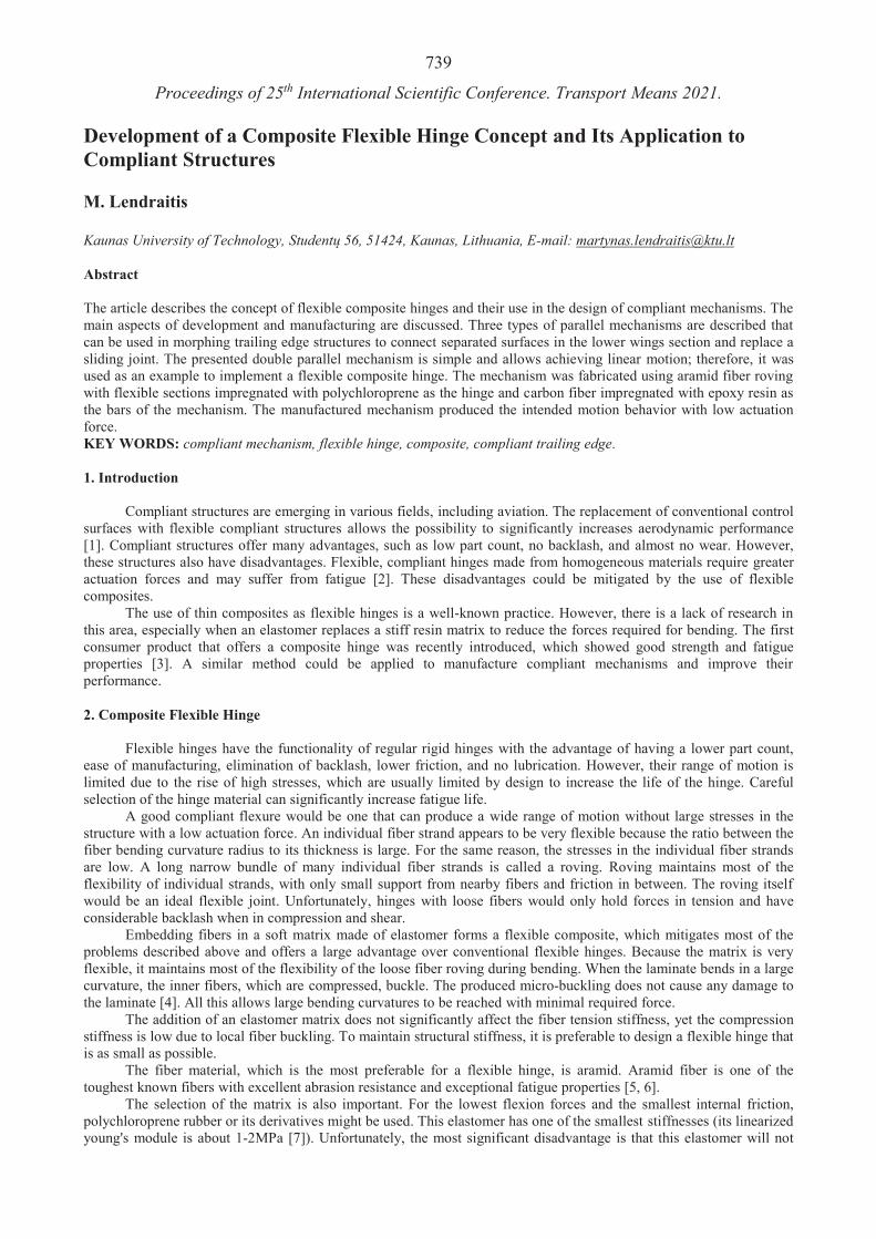
739

Proceedings of 25th International Scientific Conference. Transport Means 2021. Development of a Composite Flexible Hinge Concept and Its Application to Compliant Structures M. Lendraitis Kaunas University of Technology, Student 56, 51424, Kaunas, Lithuania, E-mail: martynas.lendraitis@ktu.lt Abstract The article describes the concept of flexible composite hinges and their use in the design of compliant mechanisms. The main aspects of development and manufacturing are discussed. Three types of parallel mechanisms are described that can be used in morphing trailing edge structures to connect separated surfaces in the lower wings section and replace a sliding joint. The presented double parallel mechanism is simple and allows achieving linear motion; therefore, it was used as an example to implement a flexible composite hinge. The mechanism was fabricated using aramid fiber roving with flexible sections impregnated with polychloroprene as the hinge and carbon fiber impregnated with epoxy resin as the bars of the mechanism. The manufactured mechanism produced the intended motion behavior with low actuation force. KEY WORDS: compliant mechanism, flexible hinge, composite, compliant trailing edge. 1. Introduction

Compliant structures are emerging in various fields, including aviation. The replacement of conventional control surfaces with flexible compliant structures allows the possibility to significantly increases aerodynamic performance [1]. Compliant structures offer many advantages, such as low part count, no backlash, and almost no wear. However, these structures also have disadvantages. Flexible, compliant hinges made from homogeneous materials require greater actuation forces and may suffer from fatigue [2]. These disadvantages could be mitigated by the use of flexible composites.

The use of thin composites as flexible hinges is a well-known practice. However, there is a lack of research in this area, especially when an elastomer replaces a stiff resin matrix to reduce the forces required for bending. The first consumer product that offers a composite hinge was recently introduced, which showed good strength and fatigue properties [3]. A similar method could be applied to manufacture compliant mechanisms and improve their performance.

2. Composite Flexible Hinge

Flexible hinges have the functionality of regular rigid hinges with the advantage of having a lower part count, ease of manufacturing, elimination of backlash, lower friction, and no lubrication. However, their range of motion is limited due to the rise of high stresses, which are usually limited by design to increase the life of the hinge. Careful selection of the hinge material can significantly increase fatigue life.

A good compliant flexure would be one that can produce a wide range of motion without large stresses in the structure with a low actuation force. An individual fiber strand appears to be very flexible because the ratio between the fiber bending curvature radius to its thickness is large. For the same reason, the stresses in the individual fiber strands are low. A long narrow bundle of many individual fiber strands is called a roving. Roving maintains most of the flexibility of individual strands, with only small support from nearby fibers and friction in between. The roving itself would be an ideal flexible joint. Unfortunately, hinges with loose fibers would only hold forces in tension and have considerable backlash when in compression and shear.

Embedding fibers in a soft matrix made of elastomer forms a flexible composite, which mitigates most of the problems described above and offers a large advantage over conventional flexible hinges. Because the matrix is very flexible, it maintains most of the flexibility of the loose fiber roving during bending. When the laminate bends in a large curvature, the inner fibers, which are compressed, buckle. The produced micro-buckling does not cause any damage to the laminate [4]. All this allows large bending curvatures to be reached with minimal required force.

The addition of an elastomer matrix does not significantly affect the fiber tension stiffness, yet the compression stiffness is low due to local fiber buckling. To maintain structural stiffness, it is preferable to design a flexible hinge that is as small as possible.

The fiber material, which is the most preferable for a flexible hinge, is aramid. Aramid fiber is one of the toughest known fibers with excellent abrasion resistance and exceptional fatigue properties [5, 6].

The selection of the matrix is also important. For the lowest flexion forces and the smallest internal friction, polychloroprene rubber or its derivatives might be used. This elastomer has one of the smallest stiffnesses (its linearized young's module is about 1-2MPa [7]). Unfortunately, the most significant disadvantage is that this elastomer will not

740 contribute to compression stiffness, and the overall mechanism might have a larger backlash. Therefore, when polychloroprene is used as a matrix, the small hinge size is crucial.

Silicone rubber is another good matrix alternative. It is more than twice as stiff as polychloroprene and can be used more easily. Unfortunately, silicone has poor surface adhesion, so that only with special treatment sufficient bonding could be achieved [8].

Polyurethane is another good alternative that has been used to design flexible hinges [9]. Polyurethane rubber has superior adhesion properties compared to silicone. Additionally, it has good abrasion resistance and can be made in various stiffnesses, comparable to silicone rubber. Therefore, polyurethane rubber is the most promising matrix material for the use of flexible composite joints. However, in this paper, polychloroprene type rubber will be used to manufacture flexible joints. This is due to the lower stiffness, good adhesion, cost, and availability to purchase. 2. Parallel Mechanism

The guided sliding motion is popular in mechanical systems. One of the easiest ways to achieve it is to use guide rails with a slider, which may or may not have bearings. The hinged mechanism allows producing the same linear motion with slightly less friction. Such motion can be achieved with Sarrus or two Peaucellier–Lipkin linkage mechanisms. Unfortunately, they are too complex.

The complexity of the mechanism could be reduced by using a simple parallel mechanism with four bars, in which the main opposite moving bars have the same length, forming a parallelogram. This ensures that the motion of the moving bars remains parallel (Fig. 1, a). However, because of the circular motion of the bars, transverse motion is introduced. This transverse motion in a rigid mechanism is proportional to the length of the bars and the translation motion length.

2 2h l l d (1) where l – is bar length; d – translation motion; h – transverse motion.

When d<<l, the transverse motion is small; therefore, such a mechanism can replace the slider joint in some applications.

The transverse motion could be eliminated by connecting two parallel mechanisms in series through one common rigid bar. In a double parallel mechanism, the base remains in the same line during motion (Fig. 1, b).

a

b

Fig. 1 Parallel mechanism diagrams displayed as pseudo-rigid bodies with torsional springs at flexible hinge locations: a – single parallel mechanism; b – double parallel mechanism The kinematics of parallel mechanisms with small flexible hinges can be easily modeled using the pseudo-rigid

body method, where the bars are assumed to be rigid, and the hinges are replaced with torsional springs. The proposed composite flexible hinge requires only a small amount of force for the actuation compared to traditional flexible hinges, allowing the assumption of small stiffness springs. Therefore, when the motion is small, some of the nonlinearities can be ignored, and for modeling, rigid body kinematics can be used with sufficient accuracy. 3. Application in Morphing Trailing Edge

The mechanism described in the previous chapter has useful properties and can be used as a compliant structure. We will investigate its use for the compliant trailing edge.

741 Trailing edge morphing structures tend to have large variations in surface length. To deal with it, the surface is

commonly disjointed (separated) and connected with a slider joint [10–12]. A slider joint restricts transverse motion and allows only longitudinal motion.

a b c

Fig. 2 Three types of mechanisms connecting the separated wing surface are shown; a – single parallel mechanism; b – double parallel mechanism; c – morphing skin from a chain of double parallel mechanisms

Typically, sliding joints need to be long enough to allow a full range of motion. In addition, it needs to hold a

significant amount of transverse loading resulting from aerodynamic forces. Therefore, the friction in the joint might be considerable. A thick sliding joint lip might also interfere with aerodynamics if it sticks out of the surface. As explained above, a similar sliding motion could be achieved with a mechanism.

3.1. Single Parallel Mechanism

When the required lower wing surface motion is small, the single parallel mechanism might produce sufficient

motion. To produce motion and restriction similar to those of a slider joint, the bottom and top mechanism bars must be fixed to the separated wing surface (Fig. 2, a). Only because a single mechanism is used, the top bar must be fixed to a rigid structure. This should not be an issue when the front section of the morphing wing is made from a rigid structure.

A relatively large mechanism can be fitted if the wing is thick enough, allowing a wide range of motion. Unfortunately, the size of the mechanism will also be limited by the internal structure of the trailing edge compliant mechanism and other existing inner structures. The transverse surface motion is not entirely restricted due to the flexibility of the bars, flexible hinges, and arc motion of the mechanism. However, the deformation in the transverse directions is small and is mainly dictated by the stiffness of the cantilever beam used for mounting.

3.2. Double Parallel Mechanism

By adding a second mechanism in series, the overall range of motion could be increased. Using a pair of these

mechanisms allows the mounting locations to be on the surface for both separated surfaces (Fig. 2, b). This adds an advantage that during the sliding motion, the surface stays in the same line. This is the main advantage, why this configuration should be investigated further. Additionally, the allowable motion in this configuration is double when the bar lengths of the mechanism are fixed. Unfortunately, the transverse stiffness in this configuration is poorer. Its stiffness is dictated mainly by the upper beam, which is bent as a cantilever. Therefore, this element should be significantly thicker than the rest of the bars. 3.3. Morphing Skin from Double Parallel Mechanisms

Conventional corrugated skin has large bending stiffness in the span-wise direction and relatively low stiffness in the chord-wise direction. However, the corrugate skin must be either very tall or very long to produce a large chord-wise motion. Reducing both dimensions reduces the overall range of motion and increases actuation forces. Under tension, an element of corrugated skin exhibits similar behavior to a parallel mechanism. However, the corrugated element also produces a large rotation distorting the surface, where the double parallel mechanism mostly does not. Additionally, the force needed to move the double parallel mechanism is significantly lower.

To maintain sliding motion without distortion on the surface, double link parallel mechanisms could be added in series. A full morphing skin could be constructed using multiple segments of double parallel mechanisms (Fig. 2, c). This type of skin would be superior compared to similar corrugated skin. 4. Use Case Example

The manufacturing of a concept of double parallel mechanism made with a flexible composite hinge will be discussed in this section. The size of the conceptual mechanism was determined to be small; the main bar length (height of the mechanism) is 15 mm, the spacing between the bars, and the depth of the mechanism is 10 mm. The top beam is

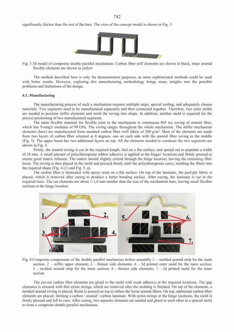
742 significantly thicker than the rest of the bars. The view of the concept model is shown in Fig. 3.

Fig. 3 3d model of composite double parallel mechanism. Carbon fiber stiff elements are shown in black, inner aramid flexible elements are shown in yellow The method described here is only for demonstration purposes, as more sophisticated methods could be used

with better results. However, exploring this manufacturing methodology brings many insights into the possible problems and limitations of the design. 4.1. Manufacturing

The manufacturing process of such a mechanism requires multiple steps, special tooling, and adequately chosen materials. Two segments need to be manufactured separately and then connected together. Therefore, two outer molds are needed to position stiffer elements and mold the roving into shape. In addition, another mold is required for the precise positioning of two manufactured segments.

The main flexible material for flexible joint in the mechanism is continuous 805 tex roving of aramid fiber, which has Young's modulus of 99 GPa. The roving ranges throughout the whole mechanism. The stiffer mechanism elements (bars) are manufactured from standard carbon fiber twill fabric of 200 g/m2. Most of the elements are made from two layers of carbon fiber oriented at 0 degrees, one on each side with the aramid fiber roving in the middle (Fig. 3). The upper beam has two additional layers on top. All the elements needed to construct the two segments are shown in Fig. 4.

Firstly, the aramid roving is cut in the required length, laid on a flat surface, and spread out to populate a width of 10 mm. A small amount of polychloroprene rubber adhesive is applied at the hinges' locations and firmly pressed to ensure good matrix infusion. The matrix should slightly extend through the hinge location, leaving the remaining fiber loose. The roving is then placed in the mold and pressed firmly until the polychloroprene cures, molding the fibers into the required shape (Fig. 4 (1) and Fig. 5, a).

The carbon fiber is laminated with epoxy resin on a flat surface. On top of the laminate, the peel-ply fabric is placed, which is removed after curing to produce a better bonding surface. After curing, the laminate is cut in the required sizes. The cut elements are about 1-1,4 mm smaller than the size of the mechanism bars, leaving small flexible sections at the hinge location.

Fig. 4 Composite components of the double parallel mechanism before assembly 1. – molded aramid strip for the main section; 2. – stiffer upper element; 3. – thinner side elements; 4. – 3d printed outer mold for the main section; 5. – molded aramid strip for the inner section; 6. – thinner side elements; 7. – 3d printed mold for the inner section The cut-out carbon fiber elements are glued to the mold with weak adhesive at the required locations. The gap

clearance is ensured with thin nylon strings, which are removed after the molding is finished. On top of the elements, a molded aramid roving is placed. Resin is poured on top to infuse the loose aramid fibers. On top, additional carbon fiber elements are placed, forming a carbon / aramid / carbon laminate. With nylon strings at the hinge locations, the mold is firmly pressed and left to cure. After curing, two separate elements are sanded and glued to each other in a special mold to form a composite double parallel mechanism.

743

a

b

Fig. 5 a – Aramid roving laid out on the outer mold and imbedded with polychloroprene at the hinge locations; b – Manufactured mechanism

Fig. 6 Motion of the manufactured mechanism in tension and compression

The manufactured mechanism can be seen in Fig. 5, b. Moreover, the mechanism produces expected motion

when it is pulled or pushed. This can be seen in Fig. 6. 3. Conclusions

A flexible composite hinge concept was introduced by describing the main design aspects and materials. Additionally, a new concept of single and double sliding mechanisms was introduced to replace sliding mechanisms in a compliant morphing trailing edge design. Compliant double sliding mechanisms offer low actuation force, large linear motion, and the prospect of a fully compliant trailing edge.

The preliminary concept of the flexible composite hinge was applied to a double parallel mechanism and successfully manufactured. The described manufacturing method could be easily scaled up to build small mechanisms and a full morphing skin or even to replace some compliant members in a compliant morphing structure. However, the manufacturing method requires a large number of manufacturing steps. Therefore, it needs to be improved.

The concepts of the hinge and the mechanism need to be investigated further to determine the force required for actuation, the structural stiffness of the mechanism, fatigue, and other properties. References 1. Kota, S.; Flick, P.; Collier, F. 2016. Flight testing of the FlexFloilTM adaptive compliant trailing edge. In 54th

AIAA Aerospace Sciences Meeting. American Institute of Aeronautics and Astronautics Inc, AIAA. 2. Malka, R.; Desbiens, A.L.; Chen, Y.; Wood, R.J. 2014. Principles of microscale flexure hinge design for

enhanced endurance, IEEE International Conference on Intelligent Robots and Systems, 2879-2885. 3. Composite talon hinges. [online cit.: 2021-07-21] available from: https://www.talon.com.au/Hinge. 4. López Jiménez, F.; Pellegrino, S. 2012. Folding of fiber composites with a hyperelastic matrix, International

Journal of Solids and Structures 49(3-4): 395-407. 5. KEVLAR ® aramid fiber technical guide. [online cit.: 2021-07-22] available from: https://www.dupont.com/

content/dam/dupont/amer/us/en/safety/public/documents/en/Kevlar_Technical_Guide_0319.pdf 6. Abdin, Y.; Jain, A.; Lomov, S.V.; Carvelli, V. 2015. Fatigue analysis of carbon, glass and other fibres, Fatigue of

Textile Composites, 85-104. 7. Bouaziz, R., Truffault, L.; Borisov, R.; Ovalle, C.; Laiarinandrasana, L.; Miquelard-Garnier, G.; Fayolle, B.

2020. Elastic properties of polychloroprene rubbers in tension and compression during ageing, Polymers 12(10): 1-14.

8. Lee, J.-H.J.S.J. 2018. Adhesion between Surfaces Treated with Aramid Fiber and Silicone/Fluorine Rubber, Textile Science and Engineering 55(5): 349-355.

9. Rowbottom, C.; Moore, L.A.; Baechle, D.M. 2020. Composite Living Hinges for Robotic Applications. 10. Shili, L.; Wenjie G.; Shujun, L. 2008. Optimal Design of Compliant Trailing Edge for Shape Changing, Chinese

Journal of Aeronautics 21: 187-192. 11. Moulton, B.C.; Hunsaker, D.F.; Moulton, H. 2021. 3D-Printed Wings with Morphing Trailing-Edge Technology,

AIAA Scitech Forum Virtual Event. 12. Hao, F.; Tang, T.; Gao, Y.; Li, Y.; Yi, S.; Lu, J. 2021. Continuous morphing trailing-edge wing concept based on

multi-stable nanomaterial, Chinese Journal of Aeronautics 34(7): 219-231.

744

Proceedings of 25th International Scientific Conference. Transport Means 2021. Implementation of Smart and Digital Technologies to Aviation A. Novák1, I. Coskun2, J. Zýka3, T. Lusiak4 1Unversity of Žilina, Univerzitná 8215/1, 01026, Žilina, Slovakia, E-mail: Andrej.Novak@fpedas.uniza.sk 2Unversity of Žilina, Univerzitná 8215/1, 01026, Žilina, Slovakia, E-mail: ilkkancoskun@gmail.com 3University College of Business in Prague, Spálená 76/14, 110 00, Praha 1, Czech Republic, E-mail: zyka@vso-prahal.eu 4Lublin University of Technology, Nadbystrzycka 38 D, 20 – 618 Lublin, Poland, E-mail: t.lusiak@pollub.pl Abstract The aim of the paper is to examine the application of digital transformation in aviation and Industry 4.0 at airports, and compare two large samples of smart airports to see how well they meet the criteria for a ´Smart Airport´. Most of the world's airports have already been providing extremely smart services; such as real-time navigation around the airport, fully automated parking systems, internal control and data processing at the airport through robots, smart kiosks, beacons, smart analysis and mobile applications. The second part of the paper looks at the aviation industry, Industry 4.0, digital transformation, and Smart Airport concepts. KEY WORDS: Airports, Aviation, Smart Technology, Sensors. 1. Introduction

Smart airport is a term that refers to the smart infrastructure at the airport. Smart cities are derived from the concepts of smart building and smart factories. Global smart airport infrastructure is divided into endpoint devices including communication systems, passenger, cargo and baggage handling, air traffic control systems, security systems and others. Endpoint devices are further divided into sensors, tags, IP phones and video conferencing [1]. SITA defines smart airports as areas where sustainable smart technologies are used in terms of passenger, airline and airport operations. Key companies such as IBM Corporation, Cisco and Siemens AG dominate the global smart airport market. Other companies such as Raytheon, Amadeus IT Group and QinetiQ are also identified as emerging companies in the market. Companies such as Honeywell and SITA are among those promising a strong position and growth in the smart airport market [2]. These leading companies are currently focusing on integrating products to create a new customer base, and as part of this strategy, they are conducting strategic partnerships and acquisitions. The airport concept has undergone major changes with the development of new IT systems and distribution channels. The airport is no longer a place where passengers take off and land, airports have been currently transforming into giant conglomerates, comparable with shopping centres, a number of infrastructure facilities and even into an entire settlement. The modern airport is a kind of a local landmark that first welcomes you on arrival in the country, allowing you to make or continue an interesting and exciting journey that can be planned with all your preferences in mind. At the same time, the high social and commercial status of the airport requires a strong intellectual ecosystem. Here, airlines, logistics systems, control and security services, in short, all components that make it possible to speak about smart airports must work in a coordinated manner. Modern airports should not only get bigger they must also get smarter, delving deep into current limitations and problems in order to become technologically advanced and build an infrastructure with all the necessary resources to support next-generation smart technologies. Industry 4.0 and digital transformation are described as revolution. It is inevitable that this new revolution, which will change across all sectors, will also affect aviation systems that are directly related to technology. As a result of changes in the aviation industry in recent years, freight, and passenger traffic by airlines around the world is growing faster than other modes of transport. As a result of this rapid growth, competition between businesses operating in this sector is gradually increasing. As a result, with this competition and sector liberalization in many countries around the world, low-cost airlines have also begun to proliferate. The rapid growth of air transport creates a need for excess capacity at many airports, and as a result, it becomes necessary to rethink airport policies. While 90% of aviation activities take place on the ground, that is, at airports, only 10% of them take place in the air. With large aircraft, the rate of increase in the number of aircraft landings and take-offs decreases very slowly, while passenger and freight traffic increase rapidly. On the other hand, the rapid development of technology has led to significant changes in the aviation industry. This change was expressed as the Industry 4.0 and a digital transformation. A concept of smart airports for airports was revealed as a reflection of this change, this conception is an important element of aviation industry. Although the rate of technology turnover in the aviation sector is the highest compared to other sectors, airports must adapt to these technological changes to be sustainable.

Most of the world's airports have been already providing extremely smart services, such as a real-time navigation around the airport, fully automated parking systems, internal control and data processing at the airport through robots, smart kiosks, beacons, smart analysis and mobile applications. This list can be continued. It is estimated that the global

745 smart airport market will grow by around 10% annually and exceed US $ 25 billion by 2025 [3]. The potential of connected IoT resources in both operational functionality and customer relationships cannot be overemphasized. These facilities primarily provide real-time monitoring of the health and safety of airport systems, track traffic and resources, support digital marketing and remote sensors to monitor smart displays, runways and environmental conditions. Recently, the most common are IP cameras for facial recognition and biometric systems, digitized baggage release and collection systems, passenger tracking and self-check-in. The task of managing this complex layer of intersecting technologies can only be solved if the individual subsystems in which they are embedded have a clearly organized and seamless interaction. Regardless of which digital tools, platforms and systems airports choose to use, today it is impossible to realize their full potential without proper network and communication modules operating according to uniform criteria and standards. Otherwise, the load on new systems, devices and network resources will significantly increase and vulnerable gaps will arise, these will inevitably negatively affect the quality of the passenger service. There is a lot of talk about the need to consolidate and expand communication between aviation industry players, but this priority is particularly important for airports in the context of developing cost-effective IP-based solutions for most systems. Such tools can provide immediate effective interaction between different technological processes and intelligent systems in the aviation community and simplify IT management. With the concept of smart airports used for today's technological airports, applications that will create added value for all stakeholders of the sector are tried to be created. Smart airports will have to use multiple combinations of digital and automation technology to combine new technological solutions. In order to provide customers with a customer-focused experience, smart airport stakeholders need to go beyond mutual data sharing and provide expanded cooperation in every process from strategic planning to operational decision process. With the system to be provided, passengers will be included in the process, and the same data will be shared and enriched with various users in order to maximize the control of their access level to their personal information. With smartphones, social media, airport sensors and new applications, more data will be provided faster than in the past. With new artificial intelligence information management tools such as predictive analytics, strong new insights are created and emerging trends and formations are determined [4]. The airports of tomorrow will be environmentally friendly to passengers, built on collaboration and innovation. This will create critical roles for airports, especially in customer interaction, unit management, collaboration and delivery, etc. Effective management of these facilities, information and communication technology infrastructure will become the core competence of smart airports. Rapid technological change, heightened service expectations and the demand for free high-speed wireless connections will, of course, increase the costs of maintaining and developing the airport's IT infrastructure [5]. Contrary to popular belief, digital transformation is not only about technology, but also about business transformation in the digital world. It is both the introduction and integration of new technologies. The goal of airport digital transformation is to provide the best experience for all stakeholders involved in the process, to achieve an integration of services and systems, as well as all stakeholders such as airlines, security, customs, concessions, ground services, and ensuring smooth airport operations [6]. 2. Challenge for Aviation in 20 Years Horizon

Advances in technology, digital and engineering sectors and fields keep on virtually changing every industry. The aviation industry has also undergone big changes in recent years with growing demand for air travel, rapid technological innovation and mind-blowing projects. The growth in air travel is particularly affecting international travel and air transport. The number of passengers is expected to increase to 7.8 billion by 2036, and over the next 20 years, the aviation industry will provide 97.8 million jobs and contribute $ 5.7 trillion to the global economy. Leading industry leaders have been working on a number of challenges. Heavy aircraft weight, high fuel consumption and, above all, too much carbon emissions lead to new searches. Airplane manufacturers and airlines are trying to keep pace with change through rapid innovation. Designers are turning to more radical solutions and the latest technology. Artificial intelligence is not the subject of Oscar-nominated science fiction films today; it has become a reality with profound socio-economic impact on countries around the world. In aeronautical engineering that has inspired science fiction novels and pushed the boundaries of imagination with various designs in films, we're now talking about drones, electric planes, flying taxis, and satellites powered by wireless technology. Unmanned aerial vehicles (Drones) are aircraft that are remotely controlled or controlled by on-board computers. Drones can do incredible things today, offering new opportunities as well as rediscovering old jobs. In 2016, the Federal Aviation Administration (FAA) clarified the legal space for the use of business drones by publishing a guide to the commercial use of drones. Drones, whose uses in civil aviation have continued to expand since 2016, today include agriculture, architecture, construction, package distribution, maintenance, emergency response, engineering, environmental monitoring and surveillance, media, education. wireless Internet and GSM services. It is used in many industries [7, 8].

As it seems, the rapid growth in aviation creates a demand above the capacity at many airports and as a result, there is a need to revise airport-related policies. While 90% of aviation smart activities take place on the ground, i.e. at airports, only 10% of them take place in the air. With the use of large aircraft, the number of aircraft landing and take-offs decreases very slowly, while passenger and cargo traffic increases rapidly. On the other hand, rapid technological developments have led to significant changes in the aviation industry. This change has been expressed as the Industry 4.0 and a digital transformation. As a reflection of this change, it has revealed the concept of smart airports for airports, which is an important element of the aviation industry.

7463. Industry 4.0 vs. Challenge for Aviation

Industry 4.0 is the current industrial transformation of people, new technologies, innovations to achieve smart industrial and manufacturing goals at the intersection of automation, data cloud, robots, cyber-physical systems, artificial intelligence, big data, the Internet of things and semi-autonomous industrial technologies. (see Fig. 1) Airports today, like many other industries, have turned to digital technology to offer and develop applications that will enhance the passenger experience. Due to the combination of airport business goals and changing passenger expectations, there has been a marked increase in digital adoption over the past few years, especially at central airports. However, while what is meant by future passenger experiences in research is not fully expressed, our work can be defined as processes that minimize human error and simplify transaction processes with interactive relationships between passengers and different technologies [9]. There are several key points in developing digital strategies for the future passenger experience at airports. Digital transformation should be prioritized in airport operations, security, airport capacity management, and relations with passengers and stakeholders. Since the improvements that will be made to these points will subsequently entail other processes, the efficiency will be automatic. Today, the increase in the number of airports using digital technology has brought with it new applications.

(Single space Fig. 1 Smart Airport with Industry 4.0 technology. (Source: authors)

4. Selected Smart Airport Solutions

Smart airport solutions include many applications, some of which are used more intensively while others less frequently. These applications are self-service kiosks, self-boarding, internal navigation, autonomous vehicles, digital processing of vouchers, smart wearable devices, biometric services, RFID baggage tags, automatic baggage delivery and lost property kiosks, advanced analytics in baggage handling, smart doors, personnel planning and scheduling, GSE management, HR and training are the management process. These smart airport applications are examined in detail below. (see Fig. 3)

4.1. Self-Service Kiosks

Self-Service Kiosks are computer terminals that eliminate the need for ground personnel for passenger use. Previously, airlines used special kiosks only for their own passengers. Today, kiosks serve registrations from more than one airline. Kiosks serving multiple check-in applications provide many benefits as the use of these kiosks is limited in space utilization in the region, which eliminates the cost of airlines as they purchase these services directly from a ground handling agent, ground handling agents have less ground staff under passenger control and save time as passengers can use any kiosk instead of looking for sample kiosks. Ground handling agents have organized self-check-in for flights and, together with their staff, support road passengers at the entrance to encourage self-check-in at kiosks[10].

4.2. Self-Boarding

Fast gates allow passengers to scan their boarding pass at the entrance to their own lines. After checking the

747 boarding pass, the doors open and the passenger can board the plane. In this statement, ground personnel are not involved in boarding passengers and are instructed to intervene in screening duties or in special situations. This helps to reduce the need for ground personnel and thus ground handling agents can further reduce operating costs. Contemporary literature argues that personal management had a positive effect on customer satisfaction as it significantly reduced the transaction time on the report [11].

4.3. Internal Navigation

After the expiration of the article, internal navigation of the terminal, internal navigation for passengers with

disabilities, services for transit passengers and at the airport were considered. The review of this technology may be accompanied by previous audit reports.

Currently, ground handling agents offer special assistance services for elderly passengers, people with disabilities and unaccompanied minors. This aspect of directing internal communication has not yet been described in the literature. Indoor navigation technologies could disrupt the market for airport ancillary services if passengers adopt the technology and instead use a mobile device for navigation instead of receiving dedicated assistance services [12].

4.4. Autonomous Vehicles

The recent articles have reported on some of the applications of GSE autonomous vehicles. It also reported on

advanced applications of autonomous technology in cars, trucks, public transport, industrial and military services. No articles have been written yet on self-service cars in airport terminals. However, it can be believed that self-driving cars in the airport terminal could provide new opportunities for providing special assistance to passengers. Currently, ground personnel use a shuttle or wheelchair to transport these passengers. It is believed that manual and visual control systems, power wheelchairs or ground personnel using the shuttle will diminish [13].

4.5. Digital Processing of Vouchers

Digital vouchers are a term used in the travel industry, coupons, vouchers, coupons are financial and web forms

used in booking transactions between hotels and agencies. In the aviation industry, this term is used to refer to free cash coupons for meals, hotel stays, airport transfers, provided to passengers by a company (or a company named by a ground handling company) in the event of a flight. Coupons are personalized. In turn, the airlines reach a specific agreement on accommodation and fees. Meal vouchers are often offered to multiple providers and typically include a maximum refund. Some providers who collectively accept these vouchers are saving their airlines from this process by using electronic data processing. Companies that do not receive many vouchers or use an electronic system often physically send vouchers to the airline or ground handling agent to receive payment. Digital voucher transactions are believed to significantly reduce transaction costs for service providers, airlines and ground handling agents. Vouchers related to customer satisfaction after disruption and service improvement have been extensively studied in the literature. However, there is no publication yet describing digital voucher processing [14].

4.6. Smart Wearable Devices

Smart wearables are most commonly used in smartwatches. Smartwatches are miniature computers with a bracelet and a set of timekeeping sensors that are widely used by passengers at airports. Using smartwatches, passengers can be alerted to gate changes or flight delays and scan their boarding passes if they are late. Since the smartwatch is permanently attached to your wrist, the ground handling agent can use this channel to broadcast real-time information to send messages to passengers, audio announcements, and other mobile devices other than traditional visual display monitors. There are examples of smartwatches and pilot projects. For example, a major US airline announced that it is experimenting with smart glasses and smartwatches to greet passengers by name, provide real-time travel information, and initiate check-in before the passenger arrives at the front door of the terminal. However, there are no articles describing the use of smartwatches in passenger transport.

4.7. Biometric Services

The biometrics is an automatic human identification system using physiological features (face, fingerprints, hand geometry, handwriting, iris, retina, veins, voice). Current research shows that a variety of biometric services are available at airports. These; airport security, biometric travel documents, airport access control, security biometrics, baggage claim biometrics, airport migration systems and non-stop travel [15].

4.8. RFID Baggage Tags

The Radio Frequency Identification (RFID) provide remote identification and do not require line of sight, unlike

barcode technology. The benefits of RFID baggage tags are widely discussed in the current literature; RFID tags can shorten baggage tracking, baggage route during air travel, or baggage on the wrong route. In addition, RFID tags can

748 contain additional data such as manufacturer, product type, and even measure environmental factors such as temperature. RFID systems can identify tags in the same area without human assistance. RFID tags embedded in barcoded tags can eliminate the need for manual inspection and guidance by ground handling agents. Currently, RFID tags are placed on paper and then attached to the trunk as paper tags. Self-labelling is one of the latest baggage labelling ideas. Passengers can tag their luggage, print luggage tags at home, and track their luggage using their smartphones. In this context, digital baggage tags are becoming increasingly important. Digital luggage tags are a digital alternative to traditional paper luggage tags. Luggage receives a permanent luggage tag with a digital barcode. Airlines or ground handling agents can remotely change this barcode if the flight plan changes or the passenger re-arrives. Along with a tracking device located inside the luggage, passengers can monitor their luggage in real time using their smartphone [16].

4.9. Automatic Baggage Delivery and Lost Items Kiosks

The passengers can use fully automatic labelled or labelled baggage claim machines in conjunction with electronic baggage tags without any interaction with ground or airline personnel. Some airports already have bag drop machines. Lost items kiosks are self-service computer devices that report lost baggage. It connects to the global lost baggage database and helps passengers report delayed or lost baggage upon arrival. To report lost baggage, the passenger scans the boarding pass, identifies the missing item, and enters delivery contact information when the baggage is found. Passengers can get the latest report information by going to the website and entering their report numbers [17].

4.10. Advanced Baggage Handling Analytics

The contracts for work between ground handling agents and airlines require reliable data on the speed and efficiency of baggage handling systems such as on-time baggage delivery (first baggage, last baggage), handling times and baggage handling accuracy. In addition, ground handling agents collect and maintain data on baggage operations and develop simulations and models to understand the behaviour and performance of baggage handling systems in the past.

4.11. Smart Gate and Entrance Doors

The most passengers use status-based or class-of-service access instead of membership. Passengers with Business Class or First Class tickets must present their boarding pass when entering the lounge. Certain card members may be granted lounge access rights. Cardholders must present their cards to enter the hall. Also, some passengers are allowed to take guests with them. Ground handling agents should be aware of these rules for different airlines and lounge clubs. In addition, lounge personnel should be able to immediately apply these rules when a particular passenger attempts to enter the lounge. The access port connects to the back-end application that contains the rules page. When a passenger passes or scans a boarding pass, the application applies the rule sheet and decides if the passenger can enter the lounge.

4.12. Personnel Scheduling and Scheduling

With labour costs of airport ground operations accounting for 60 to 80 percent of total costs, automation of personnel scheduling and scheduling is a top priority for every ground handling agent. Advances in research on airport ground personnel assignment and task scheduling can be traced back to previous audit reports. Automated centralized scheduling for planning and scheduling personnel is the most common approach described in the literature. This approach builds on previous demand modelling and phasing out planning understanding. Typically, the planning process starts six months in advance, using the flight schedule for the next season (winter or summer). The overall flight plan evaluation is done through the production management system and can only represent the distribution of flights by month, airline and destination [18].

5. Conclusions

There are 3 main factors in the digital transformation of airports: 1. Alterations and transformation of aviation operations, 2. Changing and transforming the experience and needs of passengers, 3. Increase in non-aviation revenues. With all these changes and transformations, passenger awareness and the adaptation of web technologies to our

lives with the Internet requires the use of IT technologies at airports. The concept of Industry 4.0 and digital transformation is a concept that is often found in both academic research and industrial environments. This new concept, which has been particularly talked about in the international academic literature, is also called the 4th industrial revolution. It is inevitable that this new revolution, which will change across all sectors, will also affect aviation systems that are directly related to technology. With this revolution, major changes began to occur, especially in airport

749 systems, and the concept of smart airports emerged. Aviation and airports are predicted to undergo much more radical changes with digital transformation in the future. Airports are large projects that affect the socio-economic activities of the region in which they are located. Airports are fixed capital investments with very large capital and no alternative uses. The aviation sector is one of the sectors with the highest technology turnover rates and airports need to adapt to these changes to be sustainable. It is also important to scientifically study the digital transformation of aviation and airports.

Currently, a passenger who wants to follow the progress of his / her journey, receive information about his / her flight and changes, if any, on his / her mobile device before leaving home, receive information from kiosks when he / she arrives at the airport, automatically go through the procedure check-in and baggage and travel to your destination as soon as possible. Since airports are places where time competes, it is important to manage the entire process well and have timely access to data. In this sense, as an example of a digital airport concept and marketing approaches, there are technological developments that enable electronic and virtual shopping at the airports of Istanbul, Dubai, Qatar and Singapore Changi. Acknowledgement

This paper is published as an output of the project VEGA 1/0695/21 Air transport and COVID-19: Research of the crises impacts with a focus on the possibilities to revitalize the industry. References 1. Chesher, M.; Kaura, R.; Linton, P. 2013. Electronic Business And Commerce. Second Edition, London: Springer. 2. Angelakis, V.; Tragos, E.; and Pöols, H. C. 2017. Designing, Developing, And Facilitating Smart Cities, Sweden:

Springer. 3. Kazda, A.; Badanik, B.; Tomova, A.; Laplace, I.; Lenoir, N. 2013. Future airports development strategies,

Komunikacie 15(2): 19-24. 4. Popa, D.; Popa, A.; Codescu, M. 2016. Smart Airport Structure and Elements. Buletinul AGIR, Supliment, 1-6 5. Koman, G.; Kubina, M.; Holubcik, M.; Soviar, J. 2018. Possibilities of Application a Big Data in the Company

Innovation Process, Communications in Computer And Information Science 877: 646-657. doi:10.1007/978-3-319-95204-8_54.

6. ACI (Airports Council International). 2017. Airport Digital Transformation Best Practice, [online cit.: 2021-05-10]. Available from: http://www.aci.aero/media/aabcf490-613e-44ab-b98c-339377de0cd0/ki_0Cg/Publications/2017/ Digital%20IT%20Transformation/Airport_Digital_Transformation.pdf

7. Sedlá ková, A.N.; Lokaj, P. 2017. Comparative analysis of U-fly and value alliance and global alliances, Paper presented at the Transportation Research Procedia 28: 27-36. doi: 10.1016/j.trpro.2017.12.165

8. Sedlá kova, A.N.; Svecova, D. 2018. The Regional Airports' Problems in the Slovak Republic: The Case Study of Zilina Airport, Paper presented at the MATEC Web of Conferences, 236 doi:10.1051/matecconf/201823602001

9. Nagy, E.; Csiszár, C. 2016. Airport Smartness Index – evaluation method of airport information services, Osterreichische Zeitschrift Fur Verkehrswissenschaft 63: 25-30.

10. Wittmer, A. 2011. Acceptance Of Self-Service Check-in At Zurich Airport, Research in Transportation Business And Management.

11. Jaffer, S.; Timbrell, G. 2014. Digital Strategy in Airports, 25th Australasian Conference On Information System, Australasian Conference On Information System.

12. Odijk, D.; Kleijer, F. 2008. Can GPS Be Used for Location-Based Services at Schiphol Airport, The Netherlands? 5th Workshop on Positioning, Navigation and Communication 2008, WPNC'08.

13. Morris, R.; Hemann, G. 2016. Self-Driving Aircraft Towing Vehicles: A Preliminary (August 2016), Report The Case for Autonomous Towing.

14. Mccollough, M.; Yadav, M. 2000. An Empirical Investigation of Customer Satisfaction After Service Failure and Recovery, Journal of Service Research, 3(2). doi:10.1177/109467050032002

15. Heracleous, L.; Wirtz, J. 2006. Biometrics: The Next Frontier in Service Excellence, Productivity and Security in The Service Sector, Managing Service Quality 16(1): 12-22. doi.10.1108/09604520610639937.

16. Devries, P. 2008. The State of RFID for Effective Baggage Tracking in The Airline Industry, International Journal of Mobile Communications, 6(2). doi:10.1504/IJMC.2008.016574

17. Jaffer, S.; Timbrell, G. 2014. Digital Strategy in Airports, 25th Australasian Conference on Information System, Australasian Conference on Information System, 1-11. Available from: https://eprints.qut.edu.au/79347/13/ JafferTimbrell2014_ACIS.pdf

18. Ip, W.H.; Chung, N.; Ho, G. 2010. Using Integer Programming for Airport Service Planning in Sta. Scheduling, International Journal of Engineering Business Management. doi:10.5772/9716

750

Proceedings of 25th International Scientific Conference. Transport Means 2021. Assessment of Railway Infrastructure Development in Central-Eastern Europe Using Taxonomic Method A. Massel Instytut Kolejnictwa, ul. Chlopickiego 50, 04-275 Warsaw, Poland, E-mail: amassel@ikolej.pl Abstract

The paper presents the concept of infrastructure development measure IDM. The measure has been defined according to taxonomic method, which is particularly useful for multi-dimensional classification of various objects. In this case the objects of research are railway networks located in specified area (country, region) or the networks managed by different infrastructure managers. Diagnostic variables can be basic technical and operational characteristics, describing key parameters and the level of infrastructure utilisation. Definition of these variables is, to large extent, subject to data availability.

The value of synthetic measure of development is usually in the range from 0 to 1. This method allows for comparative analyses, either in static terms (comparing the infrastructure parameters and condition at specified moment), or in dynamic terms (researching the long-term changes in the condition and characteristics of infrastructure). The concept of IDM has been verified using real data concerning railway infrastructure from selected countries in Central-Eastern Europe. The proposal for infrastructure development measure five-parameter (IDM5) has been defined and tested using the real data from the Central-Eastern European railways. KEY WORDS: infrastructure, railway, development, measure, taxonomy, network. 1. Introduction

The object of research form the railway networks from selected Central-European countries: Bulgaria, the Czech Republic, Hungary, Poland, Romania and Slovakia. The selection of these particular countries and their railways can be justified with three fundamental reasons:

1. In all these countries the model of economy with the state ownership and the central planning dominated from the end of World War II (or, more precisely, a few years later) till 1989. Moreover, all states of the region, although formally recognized according to international law, were (through membership in the Council for Mutual Economic Assistance - Comecon) highly dependent from the Soviet Union in their key economic decisions. The heavy industry, in particular mining and steel industry have been developed in all European Comecon countries. This growth was reflected in increased demand for transport till 1989.

2. After 1989 all analysed countries have undergone a political, social and economic transformation. As a result of these processes, significant changes have occurred in practically all spheres of live and in all sectors of economy. The changes in heavy industry have been reflected in decreased usage of freight transport. Moreover, growing motorisation rate resulted in lower demand for public transport, including railway passenger services.

3. In 2004-2007 all Central-Eastern European countries joined the European Union. The accession (so called “big bang”) resulted in acceptance of the EU legislation, also in the field of transport and infrastructure. Simultaneously the EU membership has increased opportunities for co-financing large infrastructure projects, including modernisation of railway infrastructure. However significant differences concerning the investment priorities adopted by particular countries (and infrastructure managers) are clearly visible. These differences have been reflected in the overall current condition of railway infrastructure and its overall performance.

2. Principles of the Taxonomic Method

Taxonomy is the branch of science concerned with classification, especially of organisms and with systematics. Also term ‘numerical taxonomy’ is frequently used. It refers to the application of various mathematical procedures to numerically encoded character state data for organisms under study. Taxonomy was invented in XVIII century by Carl Linnaeus and originally used for classification of plants and animals. However the field of application of the taxonomic method gradually increased. Original linear ordering method was presented by Z. Hellwig in 1968 as a measure of economic development. This method allows for ranking of objects, which are described in a multi-dimensional feature space. This method of linear ordering was used by Hellwig to create a measure of economic development of countries of the World. It is was presented in an unpublished UNESCO report under the title Procedure of Evaluating high Level Manpower Data and Typology of Countries by Means of the Taxonomic Method, in which 15 countries were characterised with 6 variables [1, 3]. Field of application of relative taxonomy methods is relatively wide. They have been used for example in the research of the living conditions of the cities and communes or in the study of technical infrastructure development in rural areas across the provinces of Poland [2, 4].

751The are several methods for definition of synthetic variables with set of diagnostic variables. The potential

variables are usually verified from the point of view of their variability and the degree of cross-correlation. The aim of such verification is simplification of the model through elimination of the variables with the poor discriminating power, and the variables duplicating information. Taking into account the above mentioned aim, the first step in the verification of the set of potential variables is checking the value of the coefficient of variation (CV):

jj gr

j

SCV CV

x, (1)

where CVj - coefficient of variation of the variable j; Sj - standard deviation of the variable j; - average value of the variable j.

The threshold value of the coefficient of variation CVgr is usually set at the level 0.1 (10%). The diagnostic variables can be accepted only if their coefficient of variation is at least equal to CVgr.

In the next step the correlation between potential variables is researched. If the number of variables is k, and the variables are designated as X1, X2, X3, …, Xk, the correlation matrix R will be as follows:

12 1

12 2

1 2

11

1

k

k

k k

r rr r

R

r r

1kr11k1k

2kr2r

111

. (2)

If the cross-correlation coefficient of the two variables exceeds the threshold value (for example 0.5 or 0.7), one of these variables should be excluded from the set of diagnostic variables.

The process of the formulation of the development measure according to Hellwig is initiated with the definition of the observation matrix X = [xij]. This matrix contains the values of the variables (j = 1, 2, …, m) for the particular objects (i = 1, 2, …, n). These diagnostic variables have to be normalized (standardized).

ij jij

j

x xz

S, (3)

where xij – value of the variable j, for object i,The development model (benchmark) is defined as an abstract object P0 characterised by the highest values for

stimulants, the lowest values for destimulants. The standardized coordinates of the development model are as follows:

0 j ijz max z , when j S ; (4)

0 j ijz min z , when j D . (5)

In above equations S means the set of stimulants, while D – the set of destimulants. Next step is the calculation of the multidimensional (taxonomic) distances for each analysed object (network), using Euclidean metrics, which are expressed by the following formula:

2

0 01m

i ij jjd z z , j = 1, 2, …., m; i = 1, 2, …., n. (6)

Finally the values of the aggregate variable (synthetic measure) are calculated for all objects (i = 1, 2, …, n) according to Hellwig:

0

0

1 ii

dd

d, (7)

where d0 – critical distance between particular unit and the development model (benchmark), calculated as

0 0 02 ,d d S 0 01

1 niid d

n,

2

0 0 01

1 niiS d d

n; n – number of objects.

The values of the synthetic development measure defined in the specified way are usually contained in the range <0,1>. The fact, that the di value for particular object is close to 1 means, that this object is close to the benchmark, characterised with the optimum values of variables. Conversely, very low (or even negative) di value reflects the situation, in which level of development of specified is significantly lower, than in the case of remaining objects.

752 The final step of objects classification procedure with the utilisation of taxonomic methods is their split into

development groups. Two parameters can be used as the criteria for limits: the arithmetic average and the standard deviation of synthetic measure sd.

group I, including objects with very high values of the synthetic measure i dd d s ;

group II, including objects with high values of the synthetic measure d id s d d ;

group III, including objects with moderate values of the synthetic measure i dd d d s ;

group IV, including objects with the lowest values of the synthetic measure i dd d s . 3. Definition of Infrastructure Development Measure

The paper shows the applicability of taxonomic method for analyses of railway infrastructure development. Two time horizons have been selected for comparative analysis of the railway networks in the Central-Eastern Europe, i.e. 1989 and 2019. The definition of infrastructure development indicators has been determined mainly through data availability. Some data is available from statistical journals of particular countries, in specialised statistic publications and in the UIC statistics. The part of data, however requires browsing several sources, like official network statements, public train timetables, but also duty timetables as well as publications in technical and scientific journals. Important source of data are usually IT systems, used by infrastructure managers [5].

Taking into account the data availability, the initial list of 6 diagnostic variables describing the basic infrastructure parameters:

X1 – geographical network density [km/100 km2]; X2 – percentage of double-track and multi-track line sections [%]; X3 – percentage of electrified lines [%], X4 – percentage of main tracks with the speed higher than specified threshold (for example 120 km/h) [%]; X5 – the largest value of sectional speed Vs (start-to-stop) [km/h]; X6 – the average route extension for railway connections between the capital city and all regional administrative

centres. In order to identify the variables with the poor discriminating power, the correlation coefficients rij have been

calculated for all pairs of X1, …, X6 variables. These coefficients cover both time horizons, with respective data treated together and are listed in the Table 1.

Table 1

Correlation coefficients of diagnostic variables rij

X1 X2 X3 X4 X5 X6

X1 1.000 -0.275 -0.633 -0.268 0.113 -0.536 X2 -0.275 1.000 0.405 0.452 0.363 -0.286 X3 -0.633 0.405 1.000 0.780 0.350 0.371 X4 -0.268 0.452 0.780 1.000 0.786 0.167 X5 0.113 0.363 0.350 0.786 1.000 -0.316 X6 -0.536 -0.286 0.371 0.167 -0.316 1.000 It is clearly visible, that the variable X4 (the share of tracks with maximum speed higher than 120 km/h) has strong

correlation with variables X3 (share of electrified lines) and X5 (the highest value of sectional speed Vs. The correlation coefficients r34 = r43, as well as r45 = r54 exceed 0.7. Therefore the variable X4 was excluded from the set of the diagnostic variables and only five variables remained for further analysis: X1, X2, X3, X5, X6. The five-parameter infrastructure development measure can be designated as IDM5. For the railway network i respective value of IDM(i) can be calculated according to formula:

0

0

5 1 idIDM i

d, (8)

where 2

0 01m

i ij jjd z z ; j = 1, 2, …., m; i = 1, 2, …., n; zij – value of standardised variable j for the object (railway

network) i; zoj – coordinates of the development model (benchmark); m – number of diagnostic variables (in this particular case m = 5); n – number of railway networks; d0 – critical distance of the object (network) from the benchmark,

0 0 02d d S . 4. Calculation of IDM5 Values for the Railway Networks in Central-Eastern Europe

The data set (before standardisation) for the analysis of level of railway infrastructure development for selected

753 Central-Eastern European countries in the year 1989 has been presented in Table 2. It should be noted, that the numbers for Czechoslovakia have been accordingly split into two republics (Czech and Slovak).

Table 2

The values of 5 parameters (variables) of railway infrastructure in 1989

Country X1 X2 X3 X5 X6

Bulgaria 3.87 22.3 60.7 100.5 1.50 Czech Republic 11.98 20.5 27.1 97.9 1.33 Poland 8.52 34.3 41.3 110.5 1.20 Romania 4.76 26.0 32.2 97.5 1.39 Slovakia 7.46 27.6 34.3 94.2 1.34 Hungary 8.42 16.8 28.7 111.6 1.24 Benchmark 11.98 34.3 60.7 111.6 1.20

Similar set of data, consisting of the values of 5 diagnostic variables for all analysed networks in the year 2019 has

been contained in Table 3. In both tables (Table 2 and Table 3), the cells containing benchmark values have been highlighted.

Table 3

The values of 5 parameters (variables) of railway infrastructure in 2019

Country X1 X2 X3 X5 X6

Bulgaria 3.63 24.6 71.2 121.5 1.50 Czech Republic 12.14 20.6 33.6 140.2 1.33 Poland 6.15 45.4 61.8 150.3 1.20 Romania 4.52 27.1 37.4 116.4 1.39 Slovakia 7.39 28.0 43.8 144.7 1.34 Hungary 8.33 15.7 41.4 124.2 1.24 Benchmark 12.14 45.4 71.2 150.3 1.20

It should be noted, that in 2019 in case of three diagnostic variables (the share of double-track railway lines, the

maximum value of start-to-stop speed and the average route extension for rail connections between the capital and the regional centres), the Polish railway network has proved to be a benchmark. In case of network density absolute benchmark forms the Czech network and in case of electrification – the Bulgarian one.

In Table 4 the final results of classification of Central-Eastern European railway networks have been presented, with respective values of infrastructure development measure IDM5 and their ranks.

Table 4

The IDM5 values for Central-Eastern European railway networks

Country IDM5 1989

Rank 1989

IDM5 2019

Rank 2019

Bulgaria 0,176 6 0,157 6 Czech Republic 0,263 4 0,349 3 Poland 0,653 1 0,646 1 Romania 0,208 5 0,164 5 Slovakia 0,304 2 0,440 2 Hungary 0,285 3 0,276 4

The analysis of IDM5 values confirms, that the Polish railway network has proved to be the most developed, either

in the year 1989, or in the year 2019. Comparison of IDM5 values from analysed 30-year period show significant progress made by the Slovak (increase of IDM5 from 0.304 to 0.440) and the Czech railways (increase of IDM5 from 0.263 to 0.349). On the other hand, the negative changes have been observed in case of Romanian and Bulgarian railway networks. 5. Conclusions

The concept of infrastructure development measure IDM has been developed and defined according to taxonomic method. It has been verified using the real data concerning the railway infrastructure in Central-Eastern Europe in two time horizons.

The method allows for comparative analyses of infrastructure development, either in static terms (comparing the infrastructure parameters and condition at specified moment), or in dynamic terms (researching the long-term changes in the condition and characteristics of infrastructure).

754 Diagnostic variables can be basic technical and operational characteristics, describing key parameters and the level

of infrastructure utilisation. Practically, the only limitation is availability of data concerning particular networks (infrastructure managers) and their consistency.

In the opinion of the author, potential for further research exists. First of all it is possible to define another set of diagnostic variables. Their selection should depend on available infrastructure data and reflect key decisive preferences (for example relative importance of technical parameters versus operational parameters). Moreover, the method can be used to compare the level of infrastructure development in the administrative regions or regional units of infrastructure manager. Another field of application of IDM is the assessment of the rail passenger transport offer in various countries or regions (either in terms of quality of train services or their quantity).

References 1. B k, A. 2016. Porz dkowanie liniowe obiektów metod Hellwiga i TOPSIS - analiza porównawcza (Linear ordering

of objects using Hellwig and TOPSIS method). Prace Naukowe Uniwersytetu Ekonomicznego we Wroc awiu nr 426, Taksonomia 26, Klasyfikacja i analiza danych - teoria i zastosowania, Wroc aw, 22-31 (in Polish).

2. B k, I.; Szczeci ska, B. 2015. Application of Taxonomic Methods in Study of Living Conditions in Rural Communes of Zachodniopomorskie Voivodeship, Journal of Agribusiness and Rural Development 35(1): 7-15. https://doi.org/10.17306/JARD.2015.1.

3. Hellwig, Z. 1968. Zastosowanie metody taksonomicznej do typologicznego podzia u krajów ze wzgl du na poziom rozwoju oraz zasoby i struktur wykwalifikowanych kadr (Adoption of taxonomic method for typological classification of countries taking into account level of development and the structure of qualified human resources), Przegl d Statystyczny 4: 307-327 (in Polish).

4. Lira, J.; G owicka-Wo oszyn, R.; Wo oszyn, A. 2014. The application of relative taxonomy methods to the study of technical infrastructure development in rural areas across the provinces of Poland, Quantitative Methods in Economics XV(2): 330-338.

5. Skrzy ski, E.; Ochoci ski, K. 2017. Systemy informatyczne w infrastrukturze kolejowej (IT systems in Railway Infrastructure), Problemy Kolejnictwa (Railway Reports) 61 (176): 61-78. (in Polish).

755

Proceedings of 25th International Scientific Conference. Transport Means 2021. Study of the Physical Adhesion Coefficient in the «Wheel-rail» Frictional Contact M. Kovtanets1, O. Sergienko2, V. Nozhenko3, O. Prosvirova4, T. Kovtanets5 1Volodymyr Dahl East Ukrainian National University, Central Avenue 59-a, 93400, Severodonetsk, Ukraine, E-mail: kovtanetsm@gmail.com 2Volodymyr Dahl East Ukrainian National University, Central Avenue 59-a, 93400, Severodonetsk, Ukraine, E-mail: sergienko.o.v@gmail.com 3Volodymyr Dahl East Ukrainian National University, Central Avenue 59-a, 93400, Severodonetsk, Ukraine, E-mail: vladymyrnozhenko@gmail.com 4Volodymyr Dahl East Ukrainian National University, Central Avenue 59-a, 93400, Severodonetsk, Ukraine, E-mail: prosvirova@ukr.net 5Volodymyr Dahl East Ukrainian National University, Central Avenue 59-a, 93400, Severodonetsk, Ukraine, E-mail: kovtanect@gmail.com Abstract The methodology for conducting research on the locomotive wheelsets physical adhesion coefficient distribution is developed in the article. The influence of the leading wheelsets on the physical coefficient of adhesion of the following wheelset was determined by simulating this process with the corresponding number of wheel passes along the same section of the rail under different frictional states of contact between the wheel and the rail: clean and dry, wetted with water, contaminated with lubricants. The research was carried out at the stand created at the Department of railway and road transport, lift and care systems. Based on the obtained experimental results, it was found that for wheelsets of a locomotive moving on a clean and dry rail, the physical coefficient of adhesion on each of them is practically equal. For a rail covered with water or lubricant, it can be seen that the effect of cleaning the greasy rail with the wheelsets in front is more significant than for a rail covered with water. KEY WORDS: locomotive, wheelsets, coefficient of adhesion, skidding, traction qualities 1. Introduction

Currently, rational methods of operation, repair, maintenance and modernization of rolling stock are becoming increasingly important in railway transport, since the cost of current repairs of traction rolling stock significantly exceeds the increase in the fleet in operation. It should also be noted that the technical condition of the rolling stock is deteriorating. Studies of the conditions for the most complete realization of the adhesion force of the wheels of the rolling stock with the rails and measures that ensure these conditions are of great practical value. Important technical and economic indicators of the efficiency of locomotive traction, such as weight, speed of transported goods, etc., depend on the magnitude and stability of the adhesion coefficient values [1].

One of the directions in the field of increasing the efficiency of traction rolling stock is to reduce the loss of traction energy associated with the instability of the values of the coefficient of adhesion of wheels to rails.

The adhesion coefficient remains one of the main indicators of the functional efficiency of a locomotive as a traction vehicle. Increased energy consumption and intense wear on wheels and rails are the most pressing problems in rail transport. Stable adhesion of the wheels of locomotives to the rails is not always realized, which requires a large consumption of sand, as the most effective and widespread way of increasing the adhesion of wheelsets to the rails.

It is known that the physical coefficient of adhesion is influenced by a number of factors. Most of them can be considered the same for all wheelsets of a locomotive. Differences, as practice shows, can only take place in connection with the so-called effect of cleaning the rail by the wheel in front.

Based on the foregoing, the aim of the article is to develop a research methodology for the distribution of the physical coefficient of adhesion on wheelsets of a locomotive. 2. Research Results

The studies were carried out at a stand created at Department of Railway and Road Transport, Lift and Care Systems of Volodymyr Dahl East Ukrainian National University [2, 3, 4].

The influence of the leading wheelsets on the physical coefficient of adhesion of the following wheelset was determined by simulating this process with the corresponding number of wheel passes along the same section of the rail. The first passage of the wheel corresponded to the movement of the first wheelset, the second passage corresponded to the second wheelset, etc. That is, the physical coefficient of adhesion of the wheel to the rail, measured, for example, after two preliminary passes of the wheel over this section, will correspond to the physical coefficient of adhesion of the third wheelset.

756 The physical coefficient of adhesion was determined by the following method. The wheel was decelerated by

locking the axle, a vertical load was created stP =115 kN. With the help of jack, mounted on frame and bracket, rail was imparted a longitudinal force. The force is transmitted from the jack to the rail through the dynamometer, the lever and the chain. When the longitudinal force exceeds the adhesion limit, the wheel slip occurs in the contact, which corresponds to the maximum adhesion force. In this case, the physical coefficient of adhesion is determined by the formula [5]:

iP

PP

st

nbsl0 , (1)

where slP – force on the dynamometer at the moment of slipping when the rail is braked; nbP – same, when the rail is not braked; i – gear ratio of the linkage.

The tests were carried out on a retired, work-hardened rail with little rolling. Before the experiments, the contacting surfaces were treated to ensure the appropriate state of contact: clean, dry, wetted with water, contaminated with lubricants.

The influence of the traction force realized by the front wheel on the cleaning effect was investigated. Its relative

value, equal to 0st

aFK , ranged from 0 to 1.0 with intermediate values: 0.4; 0.6; 0.8. During the next passage of

the rail, one of the specified values was maintained 0st

aF

.

As a result of decoding the oscillograms of recording the process of adhesion in the contact of the wheel with the rail and processing the experimental data, on average, 120 values of the physical coefficient of adhesion were obtained, which determine its value under each wheelset of a six-axle locomotive when it implements a traction force from 0 to the maximum value. These values were obtained for each of the three states of the rail surface: clean - dry, poured with water, oily. Mathematical processing of the experimental results made it possible to determine the mathematical expectation and standard deviation of the physical coefficient of adhesion on the first wheelset of the locomotive bogie in the direction of travel for each of the three states of the rail (Table 1).

Table 1

Experiment results

Symbol Parameter name Rail surface condition

clean, dry wet oily

01M

01S

The mathematical expectation of the physical adhesion coefficient

Standard deviation

0,57

0,008

0,41

0,018

0,16

0,027

The distribution functions of the physical coefficient of adhesion (Fig. 1) are subject to the normal distribution law

and have for each state of the rail

20

20

20

1812 0,5701

1543 0,4101

1033 0,1801

c

,

lean,

d

50 ;

22,2 ;

dry

wette

oil .ed 18 8

f e

f e

f e

(2)

The obtained values were used to determine the maximum adhesion force maxaF . In Figs. 2-3 show the experimental values of the dependence of the physical coefficient of adhesion on each

wheelset on the realized coefficient of traction by the front axles for a rail watered with water and for an oiled rail [6, 7]. For wheelsets of a locomotive moving on a clean - dry rail, the physical coefficient of adhesion on each of them

is practically equal to its value for the first axle 01 = 0.54. Moreover, its value does not change from the value of the traction force realized. Thus, all wheelsets of a locomotive moving on clean dry rails have approximately the same physical coefficient of adhesion. For a rail poured with water, it is characteristic that the contacting conditions before each subsequent wheelset of the locomotive will change. Moreover, this change depends on the magnitude of the tractive effort realized by the wheelsets in front. The same phenomena are observed for the oiled rail.

This can be explained by the improvement in the frictional state of the «wheel-rail» contact due to its mechanical cleaning and entrainment of contaminants, as well as due to the evaporation of water or a change in the state of the oil film.

757 The effect of cleaning the rail with the wheels in front is determined by finding the correlation dependences 0

on k for every wheelset as follows: 2 3

0i a bk ck dk ; (3) where 0 – physical adhesion coefficient for wheelset i; k – traction coefficient; a, b, c, d are equation coefficients.

Fig. 1 Laws of distribution of the physical coefficient of adhesion: 1 – dry rail; 2 – wetted rail; 3 – oiled rail

Fig. 2 Experimental values of the physical coefficient of adhesion from the realized tractive effort for wheelsets 2-6 (wetted rail)

758

Fig. 3 Experimental values of the physical coefficient of adhesion from the realized tractive effort forwheelsets 2-6 (oiled rail) To find the coefficients a, b, c, d a system of normal equations using the least squares method was composed:

2 3

2 3 4

2 2 3 4 5

3 3 4 5 6

;

;

;

.

oi

oi

oi

oi

an b k c k d k

a k b k c k d k

k a k b k c k d k

k a k b k c k d k

; (4)

Substituting experimental data into this system of equations and solving it, the following regression equations was

obtained: for wetted rail:

2 30,2

2 303

2 304

2 305

2 306

I 0,41 0,05 0,138 0,143 ;

0,418 0,064 0,122 0,117 ;

IV 0,421 0,067 0,148 1,1

I

4

I whee

6 ;

0,422 0,055 0,122 0,122 ;

0,424 0,0619 0,131 0,19 .

lset

III

V

V 6

k k k

k k k

k k k

k k

k k k

; (5)

for oiled rail:

759

2 302

2 303

2 304

2 305

2 306

I

,

0,1668 0,02081 0,0487 0,05 ;

0,1707 0,0255 0,0511 0,0636 ;

0,1738 0 032 0,0838

I wheelse

0

0,0856 ;

0,1

V

4368 0,0296 0,665 0,07 ;

,1786 0,036 0,084 0,0I 89

t

III

I

.

V

V

k k k

k k k

k k k

k k k

k k k

(6)

In the practice of calculations, it is more convenient to use the dependence on the wheelset number for fixed values

of k. By analogy with the previous reasoning, the regression equation is also obtained: for wetted rail:

2 30

2 30

2 30

2 30

0

1,0 0,2953 0,1354 0,0314 0,00238 ;

0,8 0,342 0,072 0,0164 0,0011 ;

0,6 0,3607 0,04744 0,0093 0,00059 ;

0,4 0,37069 0,03517 0,0064 0,000398 ;

0 0,384 0,01824 0,002

i

i

i

i

i

k i i i

k i i i

k i i i

k i i i

k i 2 39 0,000157 .i i

(7)

for oiled rail:

2 30

2 30

2 30

2 30

2 30

1,0 0,1133 0,056 0,013 0,007 ;

0,8 0,1316 0,034 0,0064 0,00043 ;

0,6 0,142 0,022 0,0044 0,00033 ;

0,4 0,144 0,02 0,0041 0,00032 ;

0 0,151 0,011 0,0018 0,0001 .

i

i

i

i

i

k i i i

k i i i

k i i i

k i i i

k i i i

(8)

Closeness of the correlation between 0 and k in each of the obtained equations, is investigated by determining

the correlation relations [5]:

2

2

22

ˆ

ok

oijoiji

oij oiji

nR

n, (9)

where n – number of test points; 0 – value of the physical adhesion coefficient calculated from the theoretical relationship (3) for each k; ij0 – overall average of the physical coefficient of friction at the point k.

Correlation (correlation ratio iR i0 ) between the value of the physical coefficient of adhesion and the number of the wheelset i was similarly determined. The obtained correlation ratios have values for all equations from 0.631 to 0.786. This indicates that the correlation between the physical coefficient of adhesion of the wheelset and the coefficient of the use of the traction force, realized in front of the moving wheelset, is quite close.

Thus, the value of 0 for each moving wheelset of the locomotive is mainly determined by the amount of tractive effort created by the wheelsets in front [8, 9].

Correlation relations for regression equations describing dependence i0 on the wheelset number i at fixed values of k, have values from 0.58 to 0.81, and the larger k, the greater the correlation ratio.

Experimental data (Figs. 4 and 5) indicate a significant increase in the physical coefficient of adhesion on the following locomotive axles.

So when the locomotive is freewheeling (k = 0) on rails poured with water, the values of the physical coefficient of adhesion for its wheelsets are respectively equal: 01 = 0.40; 02 = 0.41; 03 = 0.418; 04 = 0.421; 05 = 0.423;

06 = 0.424. The most significant difference in physical friction coefficient of 2.5% is observed between the first and second

axles. In the future, on the next wheelsets, the rail cleaning effect weakens, amounting to 1.9 ... 0.4%. A change in the tractive effort on the moving wheelsets in front causes a change in the values of the physical

coefficient of adhesion for subsequent wheelsets. So, for example, when the wheel implements a tractive effort equal to

760 0.6 of the maximum value, the physical coefficient of adhesion for the first wheelset is 0.40, for the second, 0.421, for the third, 0.436, and for the sixth, 0.443. That is, the difference for wheelsets of a locomotive can be 2 ... 5%. Under these conditions, the most significant difference between the values for the first and second wheelset remains – 5%.

a b

Fig. 4 Dependence of the coefficient of adhesion on wheelsets on the coefficient of traction: a – wetted rail; b – oiled rail

a b

Fig. 5 Dependence of the physical coefficient of adhesion on the serial number of the wheelset at fixed values: a – wetted rail; b – oiled rail

The greatest effect of cleaning the rail is observed under conditions close to skidding in front of the moving axle.

In this case, the physical coefficient of adhesion on the next axle in the direction of travel increases by 5.5%. Comparing the experimental results obtained for a rail poured with water and for an oiled rail, it can be seen that

the effect of cleaning an oiled rail by the wheelsets in front is more significant than for a rail poured with water. So, in coasting mode, the difference in values 0 for the first and sixth wheels is 10%. For a mode close to skidding (k > 1), this difference is up to 30%. At the same time, on an oiled rail, the greatest cleaning effect is also observed between the first and second wheelset, it’s up to 16%.

3. Conclusions

Based on the obtained results, it can be concluded that there is a significant difference in the physical coefficient of adhesion on the wheelsets of the locomotive. The greatest cleaning effect of the rail is observed under conditions close to skidding in front of the moving axle. In this case, the physical coefficient of adhesion on the next axle in the direction of travel increases by 5.5%.

The experimental results obtained for a rail poured with water and for an oiled rail showed that the effect of cleaning an oiled rail with the wheelsets in front is more significant than for a rail poured with water. So, in coasting mode, the difference in values 0 for the first and sixth wheels is 10%. For a mode close to skidding (k > 1), this difference is up to 30%. At the same time, on an oiled rail, the greatest cleaning effect is also observed between the first

761 and second wheelset, it’s up to 16%.

It is advisable to use the obtained dependencies in the development and design of new structures of locomotives and the study of their tractive qualities. Acknowledgement

The study was carried out as part of the technical task of the research work DN-01-20 «Theory and practice of a systematic approach to creating a new rolling stock of railways with multifunctional control of thermomechanical loading «wheel-block-rail» to improve safety, energy and resource conservation» (state registration 0120U102220). References 1. Lubyagov, A.M.; Mogilevsky, V.A.; Shcherbak, P.N.; Vyshepan, A.L. 1999. Stabilization of the friction process

in the wheel-rail contact zone, RGUPS Bulletin. Rostov on Don 1: 27-31. 2. Gorbunov, M.I.; Kovtanets, M.V.; Kravchenko, K.O.; Kara, S.V.; Prosvirova, O.V.; Gorbunov, M.M. 2013.

Patent of Ukraine 82903 on a utility model Stand for the study of the coupling of the wheel with the rail and testing of the elements of the axle spring suspension G01M 1/04, applicant and owner of Volodymyr Dahl East Ukrainian National University, u201214566, published 27.08.2013, bulletin 16. 3 p.

3. Gorbunov, M.; Kovtanets, M.; Kovtanets, T. 2020. Experimental study of the limit-maximum adhesion coefficient, The proceedings of the 24nd International Scientific Conference Transport Means 2020, 382-386.

4. Gorbunov, N.I.; Kovtanets, M.V.; Kovtanets, T.N. 2019. The energy effect of a two-phase flow on the contact zone of the driving wheel with the rail is a method for controlling the coupling characteristics of a locomotive: Monograph. Odessa: Kuprienko S.V. – 181 p.

5. Gorbunov, M.I.; Kovtanets, M.V.; Sergienko, O.V.; Kovtanets, T.M. 2020. Substantiation of the concept of improvement of railway facilities on the basis of decision theory: Monograph. Odessa: Kuprienko S.V. – 98 p.

6. Kostyukevich, A.I.; Gorbunov, N.I.; Kovtanets, M.V. 2013 Experimental verification of the effectiveness of jet-abrasive impact on rails to improve the frictional properties of the contact «wheel-rail», Bulletin of the Volodymyr Dahl East Ukrainian National University. P.1, 18(207): 33-37.

7. Kostukevich, A.; Gorbynov, N.; Nozgenko, V.; Kovtanets, M.; Tsiganovski, I. 2012. Friction interaction management in two-point «wheel-rail» tribocontact. Silesian University of Technology Faculty of Transport (Poland), Transport Problems 7(3): 53-59.

8. Gorbunov, M.; Kovtanets, M.; Kostyukevich, A.; Nozhenko, V.; Vai i nas, G.; Steiš nas, S. 2018. Development of the theory and methodology of controlling the local tribological contact thermomechanical loading, The Proceedings of the 22nd International Scientific Conference Transport Means 2018, 1383-1388.

9. Gorbunov, M.; Prosvirova, O.; Kovtanets, M.; Steiš nas, S.; Fomin, O. 2019. Experimental study of brake frictional contact properties under the impact of local cooling and surfaces cleaning, Proceedings of the 23nd International Scientific Conference Transport Means 2019, 1281-1284.

762

Proceedings of 25th International Scientific Conference. Transport Means 2021. Introduction of Aircraft with Electric Engine into General Aviation L. Capoušek Czech Technical University in Prague, Horská 3, 120 00, Praha 2, Czech Rep., E-mail: ladislav.capousek@fd.cvut.cz Abstract This paper is focused on a summary of forthcoming changes in training for general aviation pilots. I focused on changes associated with the introduction of a new class all-electric aircraft with electric engines and how this group of aircraft will change flight training. The conclusions are based on the Notice of Proposed Amendment 2020-14 made by EASA, which is a regulation frame for the forthcoming changes. I also mentioned major aspects that might be the most important in the process of introduction of electric aircraft into the general aviation segment. KEY WORDS: electric aircraft, general aviation, PART-FCL 1. Introduction

The development of alternative propulsion in aviation has been a phenomenon of the last few years. The field of general aviation seems to be suitable for the introduction of these new technologies because it is not as burdened by regulatory obligations as commercial air transport. The development and certification of the first electric aircraft are currently underway. For example, EASA certified the Pipistrel Velis Electro aircraft in 2020, and in the United States, several manufacturers are retrofitting existing electric piston aircraft. Regulatory authorities are also responding to this development, preparing the first regulations concerning the certification and operation of electric aircraft.

2. Electric Aircraft 2.1. Possible Concepts

There are several possible concepts of alternative propulsion for aircraft. The basic division can be as follows[3]: All-electric - electricity is stored in batteries and drives an electromotor or electric motors that power the

propulsor of an aircraft. Turbo electric - a turboshaft engine similar to current engines of a similar category, powers a generator that

supplies electricity to the electric motor which powers the aircraft propulsor. Hybrid parallel - a combination of a classic drive and a battery-powered electric motor, where the energy from

the electric motor is mechanically fed to a turbo propeller or a jet engine. Hybrid serial - turboshaft engine generates electric power, this is further increased if necessary by battery

energy, and this electric power powers the electromotor which drives the propulsor. Fuel cell - the combination of oxygen and hydrogen in the fuel cell generates electricity, which powers the

electric motor which drives the aircraft propulsor. 2.2. Concept Suitable for GA

However, the concept of all electrical or fuel cell seems to be the only suitable one for the use in the field of general aviation. Other concepts seem to be too operationally demanding for GA. The starting point for such a conclusion is the minimal expansion of turbo engines in GA. Therefore, it cannot be assumed that various alternative engines with even greater maintenance complexity would be suitable for the GA area. Rough estimate is that there were 14,000 turbo prop engines used worldwide, on the other hand just Rotax 912 engine was manufactured in more than 50,000 units. Therefore, it can be estimated that in the current GA they are certainly represented by less than 3%. The given disproportion is caused by higher acquisition and operating costs. It is therefore essential for any alternative drive that the complexity of its maintenance is as low as possible because the price sensitivity of GA operators is considerable. Given that the combination of a piston engine and batteries brings only a minimal benefit and no manufacturer is currently considering it for general aviation. Nowadays it seems that currently the only alternative drive for the GA area is the all-electric concept.

The use of a fuel cell in that context is essentially just another form of storing electricity. Although energy storage from a fuel cell has its advantages - especially higher energy density. The energy density of a fuel cell can be over one kilowatt per kilogram. This is approximately 5x more than current Li-Ion batteries. But the overall energy density of the electric cell drive will be lower. It is necessary to add the insulation weights for the hydrogen tank and distribution system, as well as the system for draining the emerging water. In the real aviation environment, according to [2], the total value of energy in one kg of a system with a hydrogen cell could be 2 - 4 greater than in one kg of a

763battery system. Operationally, therefore, hydrogen cells seem more advantageous, but the economic aspect is less positive. The price of hydrogen capable of supplying the same amount of energy is higher than the price of conventional AVGAS fuel. In contrast, the price of electricity is about a third of the price of AVGAS. Therefore, our assumption is that due to higher costs, for the price-sensitive GA segment, fuel cells will not expand at current hydrogen prices. For the rest of this article, we assume that the concept that will be used in GA will be an all-electric concept.

3. Specifics of All-Electric Aircraft operation in the GA

3.1. Positive Effects for All-Electric Aircraft Operators

In this chapter, we will try to summarize the possible positive effects of the introduction of all-electric aircraft in the field of general aviation. A basic comparison of aircraft operation on AVGAS and all-electric can be found in [1]. The benefits are in environmental impacts, but for most GA operators more importantly, in fuel cost savings. The price of fuel converted to 1 kWh is based on [1] up to 5 times cheaper. EUR 0.144 for electricity and EUR 0.7 for AVGAS [1]. Purchase price of the aircraft will be, at least for next few years, higher for electric version. Given that there is currently a minimum of certified aircraft, the comparison is somewhat limited. The price comparison is therefore limited to a comparison of the price of the Pipistrel Alpha aircraft, which is supplied both in the classic version with the Rotax engine and in the all-electric version with an electric motor and a 12Ah battery. This type is not yet EASA certified. According to the information from [9], the price of the cheapest version with combustion engine is 83,000 EUR and the cheapest electric version is 125,000 EUR, i.e. 42,000 euros in favour of the combustion version.

According to consumption information for AVGAS version is 50 l / 210 minutes. Thus, the return on the difference in fuel price would be about 3,000 flight hours. However, another important factor enters the economic balance sheet. The engine version requires engine overhaul and the electric version requires battery replacement.The mentioned Pipistrel alpha aircraft has a battery with a capacity of 21 kWh. The estimated minimum price of batteries for 2020 in the automotive industry was about 120 EUR / kwh. But it is necessary to mention here that the batteries used in Pipistrel aircraft are based on so-called cylindrical Li-Ion type cells which use the NMC chemistry (Nickel Manganese Cobalt). Due to other materials for anode I electrolyte and much higher production complexity estimate that the price for 1kwh is between 250 and 350 EUR. Using a conservative estimate of the higher price for a 21kWh battery, our estimate of the price of such a battery, including cooling, is approximately 7600 EUR.

The lifespan of such a battery is difficult to estimate - it depends on the temperatures at which it is operated and the degree of average discharge in each cycle. For the simplicity of the following calculation, let us assume a life value of 2000 cycles, which, due to the endurance of the aircraft, represents about 1500 flight hours.

The premise for the future is that with increasing production, the price of electric aircraft is likely to fall.In Fig. 1 one operating costs under the following assumptions, according to [19]:Electrical - fuel costs per flight hour 5,6 EUR - battery replacement every 1500 hours – 7600 EURAvgas version - Fuel costs EUR 28 EUR per flight hour, engine overhaul costs EUR 10000 after 2000 hours.

Purchase price 125000 EUR and 83000 EUR. Other costs are the same for both versions and the electric motor does not require overhaul. The graph shows that until the first engine overhaul, the operation of a conventional aircraft is more economically advantageous, but after the first 2000 hours, the total necessary investment in electrical operation is smaller.

Fig. 1 Operating costs

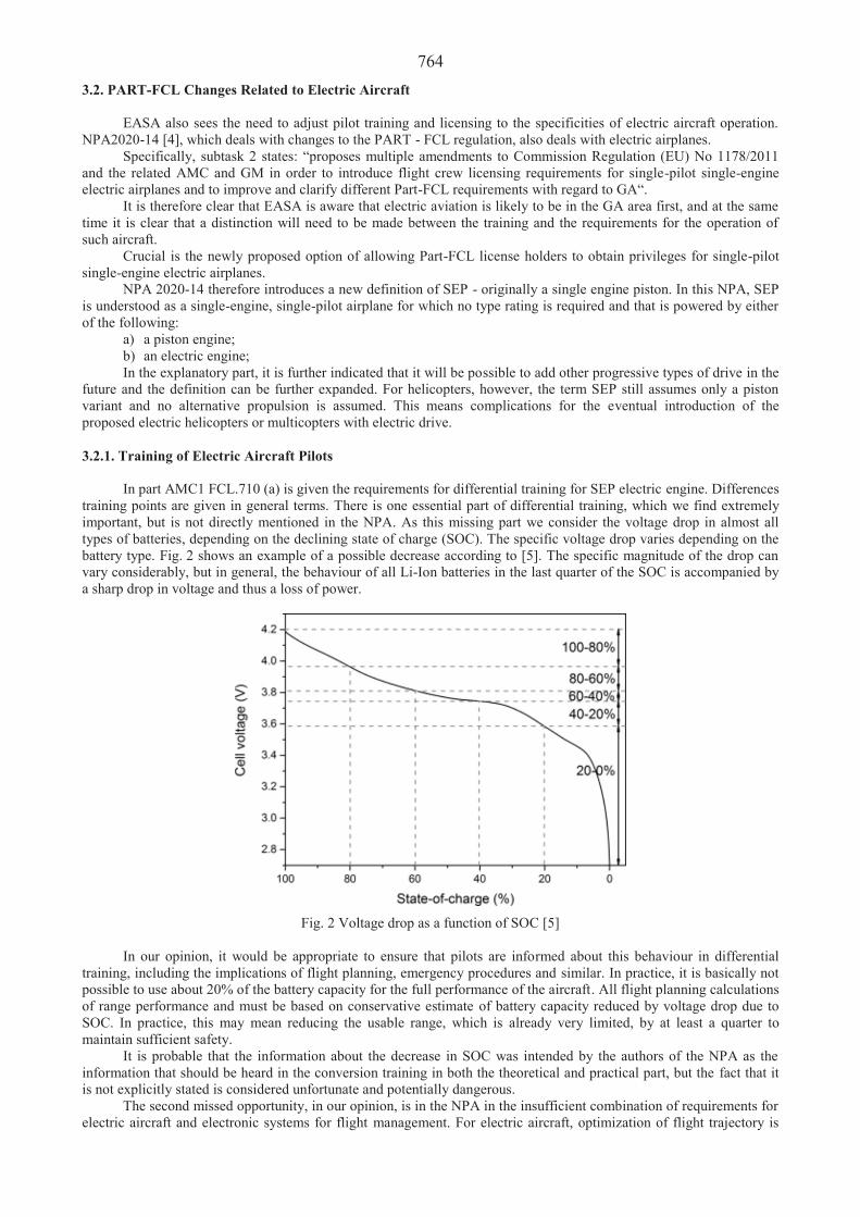
764 3.2. PART-FCL Changes Related to Electric Aircraft

EASA also sees the need to adjust pilot training and licensing to the specificities of electric aircraft operation. NPA2020-14 [4], which deals with changes to the PART - FCL regulation, also deals with electric airplanes.

Specifically, subtask 2 states: “proposes multiple amendments to Commission Regulation (EU) No 1178/2011 and the related AMC and GM in order to introduce flight crew licensing requirements for single-pilot single-engine electric airplanes and to improve and clarify different Part-FCL requirements with regard to GA“.

It is therefore clear that EASA is aware that electric aviation is likely to be in the GA area first, and at the same time it is clear that a distinction will need to be made between the training and the requirements for the operation of such aircraft.

Crucial is the newly proposed option of allowing Part-FCL license holders to obtain privileges for single-pilot single-engine electric airplanes.

NPA 2020-14 therefore introduces a new definition of SEP - originally a single engine piston. In this NPA, SEP is understood as a single-engine, single-pilot airplane for which no type rating is required and that is powered by either of the following:

a) a piston engine; b) an electric engine; In the explanatory part, it is further indicated that it will be possible to add other progressive types of drive in the

future and the definition can be further expanded. For helicopters, however, the term SEP still assumes only a piston variant and no alternative propulsion is assumed. This means complications for the eventual introduction of the proposed electric helicopters or multicopters with electric drive. 3.2.1. Training of Electric Aircraft Pilots

In part AMC1 FCL.710 (a) is given the requirements for differential training for SEP electric engine. Differences training points are given in general terms. There is one essential part of differential training, which we find extremely important, but is not directly mentioned in the NPA. As this missing part we consider the voltage drop in almost all types of batteries, depending on the declining state of charge (SOC). The specific voltage drop varies depending on the battery type. Fig. 2 shows an example of a possible decrease according to [5]. The specific magnitude of the drop can vary considerably, but in general, the behaviour of all Li-Ion batteries in the last quarter of the SOC is accompanied by a sharp drop in voltage and thus a loss of power.

Fig. 2 Voltage drop as a function of SOC [5]

In our opinion, it would be appropriate to ensure that pilots are informed about this behaviour in differential training, including the implications of flight planning, emergency procedures and similar. In practice, it is basically not possible to use about 20% of the battery capacity for the full performance of the aircraft. All flight planning calculations of range performance and must be based on conservative estimate of battery capacity reduced by voltage drop due to SOC. In practice, this may mean reducing the usable range, which is already very limited, by at least a quarter to maintain sufficient safety.

It is probable that the information about the decrease in SOC was intended by the authors of the NPA as the information that should be heard in the conversion training in both the theoretical and practical part, but the fact that it is not explicitly stated is considered unfortunate and potentially dangerous.

The second missed opportunity, in our opinion, is in the NPA in the insufficient combination of requirements for electric aircraft and electronic systems for flight management. For electric aircraft, optimization of flight trajectory is

765 essential, especially with regard to very limited range. Any extension of the route or, for example, sub-optimal shifting to the aerodrome circuit means either a reduction in the usability of the airplane or a reduction in safety. For electric aircraft, the use of a greater degree of digitization of the information in the joint together with greater use of GNSS and VFR routes, and a more suitable organization of air traffic control in low hights, as indicated in [6, 7, 8] seems to be a very suitable option to optimize range. Using a system of automatic calculation of range based on combination of GNSS position and real time measurement SOC, could be a technically relatively easy solution to ensure greater safety for flights with electric aircraft, which will often be very close to the range limit. Unfortunately, the NPA does not require or anticipate any of the above progressive technologies in the delivery of electric aircraft. In training, pilots do not come across what they will later encounter in practice, when they will try to maximize the range of electric aircraft by using technologies and procedures to which they will not be optimally trained. At least some of these concerns could be addressed in RMT.0573 ‘Fuel procedures and planning. 4. Conclusions

In order for the GA segment to truly benefit from the introduction of electric aircraft, two fundamental

conditions should be met. The operation should be cheaper and there should be a clear training framework on how to ensure the usability of electric aircraft despite their fundamental range limitations. Both conditions seem to be achievable and therefore nothing prevents the development of electric flying in the GA area. References 1. Hospodka, J.; Bínová, H.; Pleninger, S. Assessment of All-Electric General Aviation Aircraft, Energies 2020

13: 6206, doi:10.3390/en13236206. 2. Kadyk, T.; Schenkendorf, R.; Hawner, S.; Yildiz, B.; Römer, U. Design of Fuel Cell Systems for Aviation:

Representative Mission Profiles and Sensitivity Analyses, Front. Energy Res. 2019 7(35), doi:10.3389/fenrg.2019. 00035.

3. Brelje, B.J.; Martins, J.R.R.A. Electric, Hybrid, and Turboelectric Fixed-Wing Aircraft: A Review of Concepts, Models, and Design Approaches, Progress in Aerospace Sciences 2019, 104: 1-19, doi:10.1016/j.paerosci.2018. 06.004.

4. EASA NPA 2020-14 – accessible form - https://www.easa.europa.eu/document-library/notices-of-proposed-amendment/npa-2020-14

5. Patsios, C.; Wu, B.; Chatzinikolaou, Efstratios; Rogers, Daniel; Wade, Neal; Brandon, Nigel; Taylor, Phil 2016. An integrated approach for the analysis and control of grid connected energy storage systems, Journal of Energy Storage 5: 48-61. 10.1016/j.est.2015.11.011.

6. Hospodka, J.; Polánecká, A. 2015. GNSS for VFR flights, Paper presented at the Transport Means - Proceedings of the International Conference, 555-558. Retrieved from www.scopus.com

7. Bulusu, V.; Sengupta, R. Improving Productivity of Low-Altitude Airspace: Speed vs Direction Control, in IEEE Transactions on Intelligent Transportation Systems, doi: 10.1109/TITS.2020.3046103.

8. Rostáš, J.; Škultéty, F. 2017. Are today’s pilots ready for full use of GNSS technologies? Transportation Research Procedia, 28: 217-225. ISSN 2352-1465, doi.org/10.1016/j.trpro.2017.12.188.

9. https://www.pipistrel-prices.com/

766

Proceedings of 25th International Scientific Conference. Transport Means 2021. Aerodynamic Analysis of a Rocket Using CFD Techniques S. Kvietkait 1, S. Kilikevi ius2, A. Fedaravi ius3

1Kaunas University of Technology, Student 56, 51424, Kaunas, Lithuania, E-mail: saule.kvietkaite@ktu.lt 2Kaunas University of Technology, Student 56, 51424, Kaunas, Lithuania, E-mail: sigitas.kilikevicius@ktu.lt 3Kaunas University of Technology, Student 56, 51424, Kaunas, Lithuania, E-mail: algimantas.fedaravicius@ktu.lt Abstract This study is a continuation of the research and development of a solid propellant rocket, capable of supersonic speeds [1]. This paper extends previous work by investigating the influence of different geometric configurations on the rocket’s drag. For this purpose, three rocket models were prepared: original rocket, smooth-surfaced seamless rocket model, and slender rocket model. Models were created using SOLIDWORKS software and imported into Ansys to create the fluid domain and perform mesh refinement. Ansys Fluent software was used for the computational fluid dynamics (CFD) investigation in a range of Mach numbers from 0.25 to 2 to obtain the drag force, the drag coefficient and the pressure. The simulation results for all three models were presented and compared. KEY WORDS: rocket, computational aerodynamics, drag force, drag coefficient 1. Introduction

The drag of a rocket is one of the main parameters that determine the speed and range of a flight. Advances in computational fluid dynamics (CFD) and computational structural dynamics (CSD) analysis led to the increased investigation of the design of slender rockets. A high thrust-weight and slenderness ratio is needed for the development of faster, more manoeuvrable, and more accurate rockets or missiles [2, 3].

In a previous work, the aerodynamic properties of a solid-propellant rocket were analysed [1]. The aim of the current study is to extend the aerodynamic analysis by investigating the influence of different geometric configurations on the rocket’s drag. As composite materials could provide great strength to mass ratio [4, 5], a rocket with seamless connections of the fuselage sections will be considered as one of the models which will be compared to the original and the slender rocket models.

This paper presents an analysis of rocket aerodynamic parameters based on geometry changes when composite materials are used, applying CFD techniques.

2. Rocket Models

In this study, a solid-propellant rocket with a length of 1.6 m and a diameter of 0.096 m was investigated. To perform the CFD analysis, three 3D models of this rocket were created using SOLIDWORKS software. The first model, model 1, was based on the original rocket and had an unmodified configuration (Fig. 1, a). Due to the connection rings on the fuselage, this model had the highest reference area (0.00958 m2). Model 2 was a modification of model 1, with a smooth surface without connection rings between the fuselage sections. This was done assuming that the nose and fuselage sections are made of composite materials instead of metal and allow for a seamless connection, longer sections (Fig. 1, b). Subsequently, model 3 was a modification of model 2 with an elongated fuselage, which allowed one to create a slender rocket (Fig. 1, c). A slenderness ratio of 23 was selected after the literature analysis [6, 7]. For both model 2 and model 3 the reference area was 0.00847 m2.

a b c

Fig. 1 Types of rocket models used in the study: a model 1; b model 2; c model 3

3. CFD Simulation

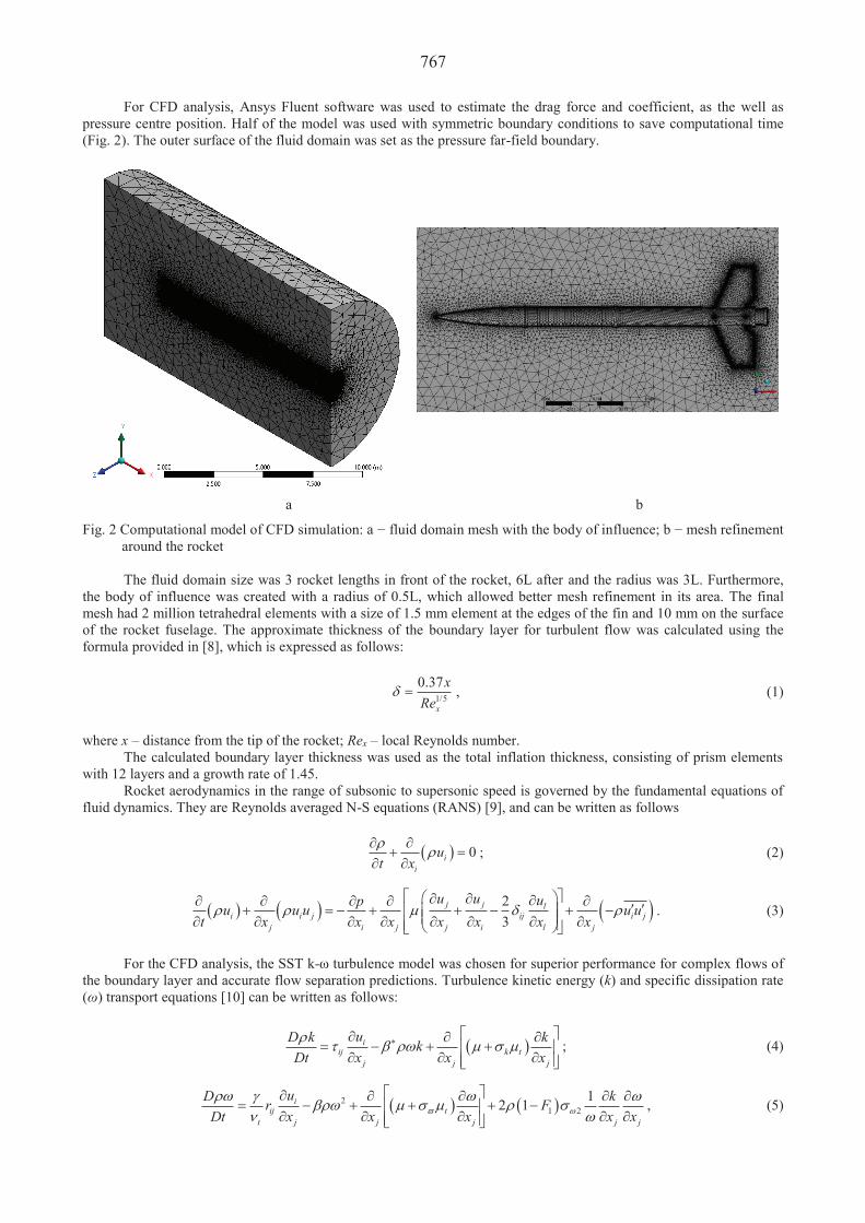
767

For CFD analysis, Ansys Fluent software was used to estimate the drag force and coefficient, as the well as pressure centre position. Half of the model was used with symmetric boundary conditions to save computational time (Fig. 2). The outer surface of the fluid domain was set as the pressure far-field boundary.

a b

Fig. 2 Computational model of CFD simulation: a fluid domain mesh with the body of influence; b mesh refinement around the rocket The fluid domain size was 3 rocket lengths in front of the rocket, 6L after and the radius was 3L. Furthermore,

the body of influence was created with a radius of 0.5L, which allowed better mesh refinement in its area. The final mesh had 2 million tetrahedral elements with a size of 1.5 mm element at the edges of the fin and 10 mm on the surface of the rocket fuselage. The approximate thickness of the boundary layer for turbulent flow was calculated using the formula provided in [8], which is expressed as follows:

1/5

0.37

x

xRe

, (1)

where x – distance from the tip of the rocket; Rex – local Reynolds number.

The calculated boundary layer thickness was used as the total inflation thickness, consisting of prism elements with 12 layers and a growth rate of 1.45.

Rocket aerodynamics in the range of subsonic to supersonic speed is governed by the fundamental equations of fluid dynamics. They are Reynolds averaged N-S equations (RANS) [9], and can be written as follows

0ii

ut x

; (2)

23

j j li i j ij i j

j i j j i l j

u u upu u u u ut x x x x x x x

. (3)

For the CFD analysis, the SST k- turbulence model was chosen for superior performance for complex flows of

the boundary layer and accurate flow separation predictions. Turbulence kinetic energy (k) and specific dissipation rate ( ) transport equations [10] can be written as follows:

iij k t

j j j

uD k kkDt x x x

; (4)

21 2

12 1iij t

t j j j j j

uD kr FDt x x x x x

, (5)

768 where ij is the shear stress; F1 is blending function; is eddy viscosity; *, i are the constants.

The conditions were selected in a standard atmosphere when the air temperature is 15°C and the pressure is 101 325 Pa. For the fluid, the air was selected with properties of an ideal gas. A pressure-based solver was used to solve the governing equations due to better convergence.

4. Results

The simulation was carried out in the range of Mach numbers from 0.25 to 2. Total air pressure distribution and velocity were obtained. Fig. 3 shows the airflow at a Mach number of 2.

a b

c d

e f

Fig. 3 Total pressure and velocity at a Mach number of 2: a and b are model 1 rocket; c and d are model 2 rocket; e and f are model 3 simulation results The simulation showed that for all three models the drag force had very close values in the subsonic speed

zone (Fig. 4). When the Mach number increased to transonic speed (M > 0.85), the separation of results was observed, with a greater increase for model 1 rocket. In this zone (0.85 < M < 1.2) drag starts to increase sharply due to the unstable formation of the shock waves. This was more prominent in the model 1 rocket due to the protruding connection rings on the fuselage. In the range of supersonic speed, the flow stabilises and the increase in drag force was almost linear. The maximum drag force at a Mach number of 2 for model 1 rocket was 958.77 N. Due to the smooth, seamless fuselage, drag force values for models 2 and 3 were lower and similar, 886.41 N, and 892.51 N respectively.

A similar trend was observed with the drag coefficient. The drag coefficient up to the transonic speed was close to constant, with an average value around 0.319. As the velocity reaches around 1 M, the coefficient distinctly increases to the maximum value and starts to drop at supersonic speed. The maximum value (0.439) for model 1 rocket was observed at a Mach number of 1.1. For rocket models 2 and 3 the maximum value was reached at a Mach number of 1, 0.443 and 0.451, respectively.

769

Fig. 4 Drag force and drag coefficient versus Mach number

The location of the centre of pressure along the x-axis was investigated (Fig. 5). The distance from the rocket nose tip to the centre of mass was 1.22 m [1] for models 1 and 2, and for model 3 it was 1.58 m. For all three models,the location of the centre of pressure was almost constant in the subsonic and transonic speed ranges. For models 1 and 2, it was 1.85 calibre from the centre of the mass and 2 calibres for model 3, which shows that the models are stable.From Mach number 1.25 it sharply increased and reached maximum value at a Mach number of 1.5 then dropped to the minimal value at a Mach number of 1.75, rising again at a Mach number of 2. Such behaviour was observed with all three models of the rocket. For models 1 and 2 the maximum distance was 2.12 and 1.88 m from the rocket tip respectively. For both models, the minimum distance was 0.31 and 0.42 m from the tip. In the range of supersonic speed, the change of pressure centre position was smaller for the slender rocket than for models 1 and 2. For model 3, the maximum distance was 2.22 m at a Mach number of 1.5, while at a Mach number of 1.75, the centre of pressure was1.12 m from the tip in front of the centre of mass.

Fig. 5 Change in pressure centre position along the x-axis

5. Conclusions

A computational fluid dynamic simulation was performed to investigate the aerodynamic parameters of the three rocket models. The original rocket, model 1, showed the highest drag force (958.77 N) at a Mach number of 2. At thesame speed, models 2 and 3 had a drag force of 886.41 N, and 892.51 N respectively. This implies that the structure with the connection rings on the fuselage created a higher drag force than the seamless models.

The drag coefficient was the highest for model 3 in the subsonic speed region. The maximum values for all three models were similar, 0.439 for model 1, 0.443 and 0.451 for models 2 and 3.

The pressure centre position was investigated. For models 1 and 2, the pressure centre was 1.85 calibre from the centre of mass in the subsonic and transonic speed ranges. At a Mach number of 1.5 pressure centre moved further from the centre of mass, the distance was 2.12 and 1.88 m from the rocket tip respectively. At a Mach number of 1.75, the pressure centre distance was 0.31 and 0.42 m from the tip.

For the slender rocket model (model 3) the lowest centre of the pressure distance was 1.12 m from the tip in front of the centre of mass at a Mach number of 1.75, and the maximum distance was 2.22 m at a Mach number of 1.5.For model 3, the change in the pressure centre position was lower than for models 1 and 2.

770 References 1. Fedaravi ius, A.; Kilikevi ius, S.; Survila, A.; Ra kauskas, S. 2018. Research and development of a rocket with

predefined parameters, Proc. of 22nd International Scientific Conference Transport Means, 3: 1432-1434. 2. Tihomirov, D.; Raveh, D.E. 2019. Nonlinear Aerodynamic Effects on Static Aeroelasticity of Flexible Missiles.

AIAA Scitech 2019 Forum San Diego, California. American Institute of Aeronautics and Astronautics. Available from: https://arc.aiaa.org/doi/10.2514/6.2019-0486

3. Hua, R.H.; Ye, Z.Y.; Wu, J. 2017. Effect of elastic deformation on flight dynamics of projectiles with large slenderness ratio, Aerospace Science and Technology 71: 347-359.

4. Devaraju, S.; Alagar, M. 2021. Polymer Matrix Composite Materials for Aerospace Applications. Brabazon, Dermot (ed.), Encyclopedia of Materials: Composites. Oxford Elsevier, 947-969. Available from: https://www.sciencedirect.com/science/article/pii/B9780128197240000525

5. Engelhardt, R.; Ehard, S.; Wolf, T.; Oelhafen, J.; Kollmannsberger, A.; Drechsler, K. 2019. In Situ Joining of Unidirectional Tapes on Long Fiber Reinforced Thermoplastic Structures by Thermoplastic Automated Fiber Placement for Scientific Sounding Rocket Applications, Procedia CIRP 85: 189-194.

6. Hua, R.; Yuan, X.; Tang, Z.; Ye, Z. 2019. Study on flight dynamics of flexible projectiles based on closed-loop feedback control, Aerospace Science and Technology 90: 327-341.

7. Li, H.; Ye, Z.Y. 2019. Effects of rotational motion on dynamic aeroelasticity of flexible spinning missile with large slenderness ratio, Aerospace Science and Technology 94: 105384.

8. Anderson, J. 2017. Fundamentals of Aerodynamics (6th edition), New York: McGraw-Hill Education, 275 p. 9. Hinze, J.O. 1975. Turbulence. McGraw-Hill Publishing Co., New York, 790 p. 10. Menter, F. 1993. Zonal Two Equation k-w Turbulence Models For Aerodynamic Flows, 23rd Fluid Dynamics,

Plasmadynamics, and Lasers Conference, American Institute of Aeronautics and Astronautics. Available from: https://arc.aiaa.org/doi/10.2514/6.1993-2906

771

Proceedings of 25th International Scientific Conference. Transport Means 2021.

Analysis of the off-the-shelf Vehicle Cameras within Forensic Videoanalysis Framework V. Adamová1, E. Kolla2

1University of Žilina, Univerzitná 8215/1, 010 26 Žilina, E-mail: veronika.adamova@fbi.uniza.sk 2University of Žilina, Univerzitná 8215/1, 010 26 Žilina, E-mail: kolla@uniza.sk Abstract The primary role of vehicle camera is monitoring and recording various situations related to road safety in the form of visual or audiovisual recording. These are the so-called vehicle cameras usually installed on the windscreen or rear window of the vehicle. The market for these devices has boomed in recent years and they are becoming increasingly popular among road vehicle drivers. The motivations for installing cameras in a vehicle can be different. For example, the advantageous premiums that insurance companies offer if the vehicle is equipped with a vehicle camera for the purpose of collecting records that may become evidence in court proceedings. Another reason is risky jobs associated with fast driving. Their installation is also frequent to ensure the supervision of vehicles and employees on the road and for efficient fleet management or to increase legal certainty for civilian drivers. Within this article, we focused on the analysis of the current offer of vehicle cameras available on the market in terms of their technical specifications and parameters. The purpose of this article is to compile a quantitative evaluation, on the basis that we will know technical specification and parameters of the currently offered vehicle cameras on the market. This article is produced as a part of research project supported by Grant System of University of Zilina, in which we focus on the experimental testing of vehicle cameras in terms of their resistance to the influence of selected environmental factors. In order to be able to test a relevant sample of cameras, it was necessary to collect data and conduct a survey of as many vehicle cameras as possible, from which only a certain small representative group was selected. Among the technical specifications, we focused on examining the resolution, field of view, frame rate, maximum storage capacity, G-sensor, GPS module, optical sensor, rear camera modules, and last but not least, the price of these devices was examined. The results presented in this article simultaneously represent the fulfillment of a partial task within the project solution and are important material in the procurement of a testing sample. KEY WORDS: vehicle cameras; technical specification; parameters; road safety; forensic video-analysis 1. Introduction

The history of use of vehicle cameras went through several waves of development, not only in terms of technical progress, but above all the purpose of their use [1, 2]. The impetus for their mass procurement was frequent insurance fraud, which led drivers to the need to increase their legal certainty, prevent false allegations of accidents, and thus reduce the risk of involvement in traffic accidents [1]. Gradually, the installation of vehicle camera became a frequent mechanism for driver protection, and video recordings helped to raise awareness of illegal activities [2].

Compared to the first prototypes, current models are more compact and less conspicuous, it is even possible to meet the concept of cameras built into the vehicle. Advances in technology as well as the mass production of smartphones have contributed to the sharp increase in the use of vehicle cameras. These have mainly resulted in improved visual output as well as improved cost-effectiveness. The sharp increase in the purchase of vehicle cameras has also brought a significant benefit to the insurance industry, which results from a simpler and more objective examination of the insured event [2].

In addition to the above-mentioned benefits resulting from the use of a vehicle camera, these devices also have an irreplaceable place in the field of forensic research. The use of vehicle cameras from the point of view of the extraction of digital footage for criminal purposes helps to objectify the analysis and reconstruction of accidents. This is then a precondition for the right determination of the legal liability of the parties involved. Among other things, objectively reconstructed traffic accidents can provide for road managers or contracting authorities with road safety inspections, documents and analyses suitable for increasing the level of road safety and managing traffic and transport infrastructure.

The importance of the use of camera systems in road transport is substantiated by several publications, in which the authors emphasize the ability of the camera to store the spatio-temporal information about the objects that are captured by the camera in two-dimensional view. The increasing implementation of cameras in road vehicles has also increased the amount of digital image data available with recorded traffic accidents, which is suitable for in-depth analysis, as described [3-5]. Videos often provide an overview of pre-accident events, the collision itself and the events after the accident and in the context of forensic accident reconstruction and analysis they can offer more accurate and complex source of usable accident data than traditional forensic method, for example methods based on deformation energies (i.e. as presented in [6] and [7]).

In addition to visually captured events, the vehicle camera also provides a number of other equally important

772information. If the camera is equipped with additional sensors, it is also possible to extract GPS data on the camera / vehicle position via GPS sensor, time data, vehicle speed data at a given time, data obtained via motion sensor, data automatically saved after an impact recorded by the accelerometer, etc. [8].

At present, according to several Internet sources, it is possible to observe a growing trend of sales in the vehicle camera market [9-11]. These positive prospects and predictions not only in the European but also in the global market are mainly due to the growing trend of road accidents as well as vehicle theft. Another factor is the constant decrease in the purchase price of the vehicle camera and the sale of cars, which is recording a growing trend until 2019 [9].

For the purpose of this article, the result part provides basic theoretical material on the technical specification of vehicle cameras, which is supplemented by a statistical evaluation, based on which we will know the offer of vehicle cameras on the domestic market.

2. Material and Methods

For the purposes of statistical processing and evaluation of the current offer of vehicle cameras on the domestic market, 391 samples of vehicle cameras from various manufacturers were collected. The current number of manufacturers of vehicle cameras offered on the Slovak market can be considered numerous. Up to 82 different manufacturers or brands that offer and sale these devices were identified. Information about available vehicle cameras was obtained mainly from Internet sources and from electronics retailers in Slovak or Czech online stores. To supplement the missing information on the parameters of the cameras, or for the purpose of data verification, the data were also obtained from the official websites of vehicle camera manufacturers. The entire sample of vehicle cameras together with their specifications isprocessed in the form of table in MS Excel program. As part of the collection of parameter data, we focused mainly on the collection of data related to - maximum resolution, frame rate, maximum storage capacity, field of view, battery capacity, optical sensor manufacturer, GPS module, G - sensor, rear camera and price of device. Before moving on to the evaluation of the data itself, it is important for objectivity to mention that some specifications of vehicle cameras were not mentioned and listed in the available technical lists that led to an incomplete table processing. Therefore, in the statistical processing, we focused only on the set of samples for which the given specification was known, or the unknowned specifiication within the graphic processing are listed as “not specified”. The outcomes are presented in the next part of the paper, only basic statistical tools was used for the graphic processing.

3. Results

Based on the market research, it can be stated that all cameras installed in civilian vehicles is currently designed as digital cameras. For a graphic demonstration and an approximation of the individual components of the vehicle camera, photographs of the sample of an older vehicle camera model are shown.

Several different manufacturers and brands of vehicle cameras were identified as part of the survey. The following graph shows the brands that have 7 and more models in their vehicle camera portfolio. The largest representatives of vehicle cameras on the Slovak market are - Mio, Navitel, DOD, Neoline, XBLITZ and others (see Fig. 1). The total number of identified manufacturers who specialize in the production of such equipment is 82.

Fig. 1 Representation of vehicle camera manufacturers in terms of the quantity of models offered

The shape of modern models of vehicle cameras is specially designed for efficient and discreet surveillance, with resulting their compactness of the body. The dimensions, weight of the cameras, their face, electronics, as well as how the cameras are mounted to the windshield of the vehicle vary depending on the manufacturers and also on the models themselves. Therefore, the vehicle cameras of different looks are offered on the market (see Fig. 2). Surveillance circumstances require a special approach in their construction. In general, cameras installed in vehicles should be able to withstand very demanding conditions such as vibration, shock, bumps on the road and temperature fluctuations [12]. The inside of the camera body usually consists of the following basic scheme - lens, optical sensor, power supply, motherboard with integrated electronic components such as processor, SD card slot, GPS module, input for GPS antenna, accelerometer and other.

31 31

2016 16 13 13 12 11 11 10 9 9 8 7

05

101520253035

Qua

ntity

of m

odel

s on

the

mar

ket

Manufacturers of vehicle cameras

773

Fig. 2 Various tipes and models of vehicle cameras - from left to right: Blaupunkt BP3.0 FHD GPS, DOD RC500S, MIO MiVue 733 WIFI, Sjcam SJDASH+, Navitel R600 GPS, Niceboy Pilot X + GPS, Xiaomi 70Mai Dash cam Pro Plus, GitUp Viofo A119 V2

As regards the maximum resolution of vehicle cameras and the frame rate, it was found on the basis of the market survey that the majority of these cameras recorded video in Full HD resolution. In addition to the maximum resolution of 1920x1080 (the most frequent), the camera usually allows the user to switch to the 1280 × 720 format. Among the examined samples of cameras, there were also cameras with a maximum resolution of 2560 × 1440, 3840 × 2160, 4096 × 2160 and others. In terms of frame rate, the majority of vehicle cameras belong to the group with a frame rate of 30 fps. However, there were rare cases when the frame rate was 15, 24, 25, 27, or even 60 fps.

Generally, digital cameras are devices in which light rays strike an optical sensor. Optical part of vehicle cameras usually consists of lens and optical sensor. The vast majority of vehicle cameras are two types of optical sensors operating on the basis of either CMOS (Complementary Metal-Oxide Semiconductor) or CCD (Charged-Coupled Device) [13].The CMOS sensor is more often present in vehicle cameras, especially due to its smaller size, higher speed, lower power consumption and relatively higher noise resistance. These cameras usually have smaller and more compact dimensions, which predetermines their more frequent use within a group of vehicle cameras and can be powered either by a battery or to the vehicle's electrical system. Cameras equipped with a CCD sensor are larger, require additional components and logic circuits, so they are less compact, on the other hand, their advantage is that the output is a better image [12].

In the context of the compact dimensions of vehicle cameras, the lens is characterized by certain specifications, mainly in that it is firmly attached to the camera body and has an manually uncontrollable focal length. Another characteristic feature of the lenses of these cameras is the wide-angle field of view. Based on a survey, it was found that the field of view of 360 cameras (31 cameras did not specify this parameter) ranges from 60 ° to 360 °, with the most frequent angle being 140 °. For statistical processing we used a graph histogram and we sorted 360 samples into 5 different groups according to the field of view (see Fig. 3).

Fig. 3 Left side – example of vehicle camera lens, right side – number of vehicle cameras in terms of field of view

A wide field of view of about 140° is achieved by a combination of a short camera focal length and the use of panoramic lenses, and causes captured objects that have real solid, sharp edges to appear curved, curved in the image. This phenomenon is called radial distortion of the lens. For the reconstruction and analysis of the accident, this is a problem that must be taken into account or removed. An extreme case can be the effect of so-called "Fisheye" [13]. Regarding the lens material, 6-layer glass is preferred over plastic. It is also more durable and has better durability.Another important feature of cameras is the aperture and shutter. The aperture is usually fixed. Vehicle cameras are characterized by a relatively high aperture number (from f / 2.8 to f / 1.6). The shutter as part of the optical system is a regulating function that determines when and how light is transmitted and also determines the exposure time. It is usually set automatically by the camera according to the light intensity. The user has limited options in setting it [13].

774Videorecording of the vehicle camera is stored on a recording medium located in the SD card slot. Within vehicle

cameras, we most often encounter SD cards and microSD cards [13]. As the memory card is usually not included in the package of the vehicle camera, the user purchases it himself. Its size is selected based on the specification in the parameters of the cameras. The maximum storage capacity of a supported SD card can be 16GB, 32GB, 64GB, 128GB or 256GB. Based on a survey of the Slovak market for vehicle cameras, it was found that the most frequented size of the supported memory card is a 32GB SD card, which occurred up to 145 cases in a total of 391 camera samples, the second most frequently supported SD card was a card with 128 GB memory (79) and others –128GB (71), 256GB (26), 16GB (3), 4GB (1) and for 66 samples, the memory card size was not specified (Fig. 4).

Fig. 4 Left side – example of location of SD card slot on the motherboard, rigth side - percentage distribution of vehicle

cameras according to the maximum size of supported SD card

Because of the vehicle cameras generally record video in a loop, it is required that the memory cards have a high durability against a large number of recording cycles. Permanent storage usually occurs when the user of the camera manually saves the event in question or if the camera is equipped with an accelerometer. In such cases, the record is stored a few seconds before and a few seconds after the impact, or after manually pressing the record button. If the camera is not equipped with advanced video compression, e. g. compression standard H.264 and full resolution recording is set, the speed of filling the capacity of the SD card increases rapidly [14]. The website [15] states that the majority of vehicle cameras in 2019 used a smaller size SD card and only a small specialized group of cameras used a standard (larger) type of SD card. There are several alternatives of memory cards on the market, among the most famous are manufacturers such as Samsung, Sandisk or Kingston [15]. Depending on the quality of the storage medium (SD card) and the data rate of the camera, a combination of low quality of memory card and increased data rate may result in some frames being skipped, either periodically / regularly or randomly. This fact must be taken into account, e.g. in the analysis and reconstruction of a traffic accident from the videorecording [13].

As part of statistical processing, we focused on the issue of batteries only on the battery capacity that the cameras have. Determining how many cameras have the capacitor and how many Li-Ion or Li-Pol batteries was not possible, as we did not get to this information from the usually available specifications. The capacity of the rechargeable battery is generally given in mAh. Standard battery values for vehicle cameras are most often between 100 - 300 mAh. The higher the capacity, the longer the battery life. On the basis of the survey, it was found that the most common battery capacity ranges from 100 -300 mAh (111), in 52 samples the capacity was identified as higher than 300 mAh and in 6 samples lower than 100 mAh (see Fig. 5). Up to 222 samples, battery capacity was not mentioned.

Fig. 5 Left side – example of battery in model vehicle camera, right side – number of vehicle cameras in terms of battery

capacity

Vehicle cameras are usually powered and charged via the charging cable / power adapter via the vehicle's 12V network. At present, it is quite common for the camera to start in recording mode simultaneously and automatically after the vehicle has been put into operation, i.e. immediately after the engine has been started. Cameras are usually equipped with a backup power supply for storing files when the camera is not connected to the vehicle's electrical network. Either Li-Ion or Li-Pol batteries or capacitors are used for this purpose. The batteries are generally small and are designed to emergency power the camera. They have a shorter life due to rapid wear (regular charging and discharging) and they are cheaper choice, which is why many manufacturers reach for lower quality batteries in order to reduce costs. Another problem is the risk of the battery overheating, swelling and leaking due to temperature fluctuations, which can damage

17%

0%000000%%000000000%0%0%%%%1%

37%18%

20%

7% Not specified

16 GB

32 GB

64 GB

128 GB

256 GB

775the camera and cause it to explode. Capacitors are more reliable and heat resistant [16].

Other unmentioned camera components include an LCD display. In practice, the use of the LCD display is often limited to the control and setting of camera parameters, with the exception of control via a mobile application, but it should be added that the actual setting changes can be made only to a limited extent. As for other additional functions of cameras in vehicles, these are e.g. function of automatic switching on of the camera and commissioning when starting the vehicle, loudspeaker, GPS module together with GPS antenna, G-sensor (acceleration sensor used to detect the impact and then lock part of the recording in the event of an impact), motion sensor (sensor that provides recording during parking mode in case of motion detection in front of the camera lens), LED / IR illumination (provides a light source at a very short distance from the camera, in practice this function did not work, as the light is reflected from the windshield and its performance is not enough) [14].

Within the framework of statistical processing, selected parameters of GPS module and G-sensor were examined. When examining the GPS module, it was found that 43% (165) of the total number of samples are equipped with a GPSmodule, 58% (226) are not equipped with a GPS module, or these are cameras for which it is possible to purchase this additional function (see Fig. 6). The G-sensor or the impact sensor is nowadays a standard complementary function of the vehicle camera (see Fig. 6). By survey, it was found that the vast majority of these cameras are equipped with this feature. Thus, in the case of e. g. impact, the camera should be able to automatically save video permanently, as the so-called emergency video.

Fig. 6 Left side – redistribution of vehicles cameras according to the availability of GPS module, right side - redistribution

of vehicles cameras according to the availability of G-sensor

We can find vehicle cameras of various price categories on the market. In general, it can be stated that the price varies and increases depending on the quality and functionality (Fig. 7).

Fig. 7 Redistribution of vehicle cameras according to price categories

We are mainly talking about optical properties (optical sensor, night vision, optical stabilization and others) GPS modules, accelerometers. The software features of the camera processor also play an important role. Other functions such as parking mode, motion detection, speed camera detection, ADAS systems and more can be reflected in the price of the device. On a sample of 391 cameras, we found that the price of most cameras is up to € 100. It is also possible to findvery cheap cameras, but their quality can be doubted. More expensive cameras are usually offered as sets together with the rear camera, or they are often cameras equipped with a quality optical sensor (e.g. Sony Starvis) and a processor (e.g.Novatek, Hisilicon). the cheapest camera on the domestic market costs 8.50 € (Extreme Miror XDR103) and the most expensive 599 € (BlackVUE DR900S-2CH 4K CLOUD).

4. Conclusion

Based on the survey, it was found that the offer of vehicle cameras on the Slovak market is relatively saturated and the potential buyer can choose the equipment according to their requirements and purpose of use. The topicality of this issue is directly conditioned by the high frequency of use of vehicle camera systems and the irreplaceability of digital

42%58%

WithGPS

WithoutGPS

31323 55

0

100200

300

400

Yes No Not Specified

Qua

ntity

G-sensor

776 tracks, especially optical recording, which is the only one that allows the preservation of visual information about the spatial context of the analyzed event. Camera devices for monitoring the situation on the road have become widely used in recent years, not only among civilian drivers, but also security companies have started to offer their services in the field of vehicle monitoring from the use of simple to complex monitoring systems adapted for remote surveillance. In the context of complex perception, cameras also have a place in their implementation in systems such as EDR. In principle, however, the output of any camera system is a video recording, which in certain conditions becomes evidence and ends up in the hands of an analyst of the relevant expert field. Acknowledgement

This paper was created with the support of the project KOR/1095/2020, “Proposal of methodology for measurement of selected physical quantities in dynamic stress of vehicle cameras”. References 1. Štitilis, D.; Laurinaitis, M. 2016. Legal regulation of the use of dashboard cameras: Aspects of privacy protection,

In: Comput, Law Secur. Rev 32: 316-326. 2. The Evolution & History Of Dash Cams [online cit.: 2021-02-16]. Available from: https://wiredsmart.io/dash-

cams/evolution-and-history/. 3. Wong, W.T.; Tao, C.H.; Cheng, Y.K.; Wong, K.H.; Tam, C.N. 2014. Application of cross-ratio in traffic accident

reconstruction, Forensic Sci. Int. 235: 19-23. 4. Han, I. 2016. Car speed estimation based on cross-ratio using video data of car-mounted camera (black box), Forensic

Sci. Int. 269: 89-96. 5. Moser, A.; Burg, H. 2017. Estimation of vehicle speed using video images and laserscanner data in PC-Crash, EVU,

93-98. 6. Kubjatko, T.; Gortz, M.; Macurova, L. 2018. Synergy of forensic and security engineering in relation to the model

of deformation energies on vehicles after traffic accidents, International Scientific on Conference Transport Means, 1342-1348.

7. Kohut, P.; Kasanicky, G. 2013. Evaluation of crash tests of the institute of forensic engineering, University of Zilina, aimed at ees, Komunikácie 15(2): 124-130.

8. Lallie, H.S. 2020. Dashcam forensics: A preliminary analysis of 7 dashcam devices, Forensic Science International: Digital Investigation 33: 200910.

9. Dash Board Camera Market by Product [online cit.: 2021-02-17]. Available from: https://www.marketsandmarkets. com/Market-Reports/dash-board-camera-market-40438274.html.

10. Dashboard Camera Market Size, Share & Trends Analysis Report By Technology [online cit.: 2021-02-17]. Available from: https://www.grandviewresearch.com/industry-analysis/dashboard-camera-market.

11. Dash Board Camera Market by Product [online cit.: 2021-02-17].Available from: https://www.marketsandmarkets.com/Market-Reports/dash-board-camera-market-40438274.html.

12. Nilsson, F. 2017. Intelligent network video : understanding modern surveillance systems, New York: Taylor & Francis Group, LLC. ISBN 9781466555211.

13. Ivor, J.; Kolla, E. 2019. Záznam z autokamery ako dôkaz v trestnom konaní, Informa no-technické prostriedky v trestnom konaní – možnosti a perspektívy, 92-108. ISBN 978-80-7502-363-6.

14. Neviete si vybra kameru do auta / športovú kameru pod a parametrov? [online cit.: 2021-02-20]. Available from: https://www.tssgroup.sk/aktuality/zaujimavosti/neviete-si-vybrat-kameru-do-auta-sportovu-kameru-podla-parametrov).

15. The Best MicroSD Cards for Dash Cams in 2020 [online cit.: 2021-02-22]. Available from: https://carcamcentral.com/ guide/recommended-microsd-cards-for-dash-cameras.

16. Dash Cam Battery vs Capacitor [online cit.: 2021-02-21]. Available from: https://dashcameras.net/battery-vs-capacitor/.

777

Proceedings of 25th International Scientific Conference. Transport Means 2021. Use of Meteorological Data for the Optimization of Cross-Country Soaring I. Kameníková1, M. Seitl2

1Czech Technical University in Prague, Faculty of Transportation Sciences, Department of Air Transport, Horská 3, 128 03 Prague, Czech Republic, E-mail: kamenive@fd.cvut.cz 2Czech Technical University in Prague, Faculty of Transportation Sciences, Department of Air Transport, Horská 3, 128 03 Prague, Czech Republic, E-mail: seitlmar@fd.cvut.cz Abstract The aim of this paper is to optimize meteorological data utilization focused on the successful cross – country soaring flights planning, pre – flight preparation and flying tactics. The theoretical part analyses specific meteorological phenomena, soaring weather forecast and meteorological data implementation to improve the cross – country soaring flight planning. The practical part of the thesis contains statistical elaboration of “VUT Martina Horá ka” cross – country track. The goal of this statistical elaboration is to allocate the most likely thermals appearance along the track according to specific weather conditions. KEY WORDS: Gliding, thermal convection, meteorology, cross – country soaring, pre – flight preparation, cross – country flight planning 1. Introduction

Soaring is very popular in the Czech Republic.The popularity is based on the deep – rooted tradition of this sport among domestic pilots. Many pilots like soaring because of its sporting value and flying in harmony with nature. Modern technologies push the gliding performance forward, thus improving the possibilities of the weather forecasting and monitoring. Nowadays, pilots have a huge amount of meteorological data available and is necessary to be able effectively process these data. It is essential to understand atmospheric processes and precise analysis of weather data during pre – flight preparation. Knowledge of specific weather phenomena, soaring weather forecast and meteorological data implementation is a basic prerequisite for the correct choice of flight tactics and could help pilots to gain a significant advantage during their cross – country soaring tracks.

The goal of this paper is to optimize meteorological data utilization focused on the successful cross – country soaring flights planning, pre – flight preparation and flying tactics. The optimization will help pilots to improve their aviation meteorology knowledge, pre – flight meteorological data processing and cross – country flight performance. The definition of these terms is also necessary for the research in the practical part. The essence of the practical part is a statistical elaboration of specific flight data to allocate the most likely thermals appearance along the track according to selected weather conditions. “VUT Martina Horá ka” cross – country track was selected for the statistical elaboration because of its location and the satisfying amount of available data.

2. Soaring Weather Phenomena

This theoretical chapter consists of the specific soaring meteorological phenomena analysis. The aim of the chapter is to improve aviation meteorology knowledge for glider pilots and the definition of these phenomena is also necessary for the research in the subsequent theoretical and practical parts. Pilots must determine if weather conditions are safe, and if current conditions support a soaring flight. Glider pilots face a multitude of decisions, starting with the decision to take to the air. There is no point in trying to soar until weather conditions favor vertical speeds greater than the minimum sink rate of the aircraft and in the section “Thermal Soaring Weather” is explained the principle of convective circulation. The analysis includes following subchapters: Atmosphere, Thermal Soaring Weather, Lifecycle of a typical thermal with Cu cloud [1], Thunderstorms, Ridge Soaring Weather, Mountain Wave Soaring Weather, Types of Cloud important for Soaring.

2.1. Meteorological Data Acquisition

The goal of this part is to provide meteorological data acquisition for the purpose of pre – flight preparation of

soaring tracks. Weather-related information can be found on the Internet, including sites directed toward aviation. These sites can be found using a variety of Internet search engines. It is important to verify the timeliness and source of the weather information provided by the Internet sites to ensure the information is up to date and accurate [1]. The data sources described in this chapter are four different meteorological servers with public access. Three of them are Czech and one is German. This chapter is focused on detailed description of available products and possible use of these products for the purpose of soaring flights planning. The origin of data sources is mostly a combination of various weather forecast

778 models.

Czech Hydrometeorological Institute is a major national meteorological organization within the Environmental Ministry of the Czech Republic. CHMI website contains a huge amount of various meteorological, climatological, hydrological and air quality content. For glider pilots are important these sections: Aerological Diagram (see Fig. 1), Aviation Weather Forecast, Aladin Forecast, Synoptics (see Fig. 2). Radar and Satellite Data, Web Cameras [2]. Flymet is a Czech website primarily focused on the soaring weather forecast. The website has its own weather forecast model and unique interface. Very interesting is a unique calculation of the potential flight distance with self – developed algorithm developed for the Czech Republic [3]. Windy is a Czech weather forecast and monitoring website. It uses two global weather forecast models (GFS and ECMWF) and additional available local forecast models. The website description is divided into two parts: weather forecast data and actual weather data. Both bring a huge amount of very useful meteorological information for soaring purposes [4]. TopMeteo is a German weather forecast and monitoring website. The vision of this website is the preparation, display and operation availability of weather information that everyone can understand. The website is primarily focused on the aviation weather forecast [5].

Fig. 1 Aerological Diagram [2]

Fig. 2 Forecast synoptic chart [2]

2.2. Use of Meteorological Data for Cross – Country Soaring

The aim of this chapter is to implement weather forecast and monitoring data to Cross – Country flight preparation and tactics. In this part are used meteorological data from the weather forecast models. These data are subjected to the detailed analysis. The chapter is divided to three subparts. The first subpart is focused on the evaluation of the data from weather forecast models. It describes weather forecast monitoring methods and determination of the forecasted weather

779 situation suitability for the cross – country flight. These methods consist of synoptic situation analysis, study of the weather forecast maps, precise interpretation of aerological diagrams, precipitation, cloud distribution forecast and wind forecast. A special part is devoted to the proper meteogram data interpretation. The second subpart is focused on the current weather interpretation based on observing the sky. It describes methods used often in the past based on weather monitoring and forecasting only from the actual sky view. The method can be very useful in combination with the modern weather forecast features. This interpretation in primary determined for soaring weather usage in terms of thermal convection, cloud distribution, precipitation forecast and the air temperature. The third part is focused on the actual weather monitoring during the cross – country soaring flight. This part describes proper methods how to find an uplift in many different weather situations and how to use it. This subpart explains the issue of choosing the right tactics of the cross – country soaring flight with respect to different weather and topographic situations. These methods contain proper evaluation of the wind speed and direction effects, cloud distribution and the part of the day in connection with the thermal convection characteristics.

3. Statistical Elaboration of “VUT Martina Horá ka” Cross – Country Track

The practical part is focused on statistical elaboration of selected cross – country track, which is a 300 kilometers

long FAI triangle. The track is located in Eastern Bohemia and it is a very popular cross – country soaring track among the pilots. This region is characteristic by many mountainous parts and inhomogeneous surface. The aim of the statistical elaboration is to allocate the most likely thermals appearance along the track according to specific weather conditions.For the elaboration were selected three different weather situations. Total number of forty four flights were processed into tables containing information about the date, sailplane, airport of departure, average speed, part of the triangle, time, vertical speed, altitude of entering the thermal current, altitude reached and location. All flight data in IGC format were obtained from www.cpska.cz website. Statistical processing identified the areas that are most active in terms of rising currents. They were drawn with colored symbols in the shape of a four-pointed star in the map materials in Fig. 3, Fig. 4, Fig. 5.

The first weather situation was observed on the 8th of August 2020 and on the 19th of July 2014. The Czech Republic was under the influence of the ridge of higher air pressure between northern and southern Europe. The air was unstable and only local Cu clouds development were observed. 8th August was characteristic by a low speed northeasterly wind and 19th of July 2014 was characteristic by a low speed southeasterly wind. Flight data of twelve pilots and seven different airports of departure were used for the statistical elaboration of this weather situation. Fig. 3 shows the most likely thermals appearance along the track according to the first weather situation.

Fig. 3 Weather Situation No. 1 The second weather situation was observed on the 8th of August 2020 and on the 4th of July 2020.The Czech

Republic was behind the undulating cold front and the weather is affected by the ridge of high air pressure. The air was unstable and Cu clouds development occurs. The wind blew from the southwest and the speed was increasing with altitude. Flight data of twelve pilots were used for the statistical elaboration of this weather situation. All pilots were participated at Safari Cup 2020 soaring competition. Fig. 4 shows the most likely thermals appearance along the track

780 according to the second weather situation.

Fig. 4 Weather Situation No. 2

The third weather situation was observed on the 8th of August 2020 and on the 11th of July 2019. The Czech Republic was in front of a high pressure ridge in front of a warm front. Along its edge was flowing the cold air. The air was unstable and Cu clouds development occurs. The wind blew from the southwest and the speed was slightly increasing with altitude. Flight data of twenty pilots were used for the statistical elaboration of this weather situation. All pilots were participated Junior Gliding Champion ship of the Czech Republic soaring competition. Fig. 5 shows the most likely thermals appearance along the track according to the third weather situation.

Fig. 5 Weather Situation No. 3

4. Discussion The work was a statistical processing of the line "East Bohemian universal three-piece Martin Horá ek" with a

focus on the occurrence of thermal currents and their effective using with respect to the weather situation. Three weather situations were chosen for the sample statistical processing, which are very advantageous for gliding in the conditions of Central Europe. A total of forty-four different flights were processed, which after statistical processing, determined the

781 most thermally active areas of the selected route in certain weather situations. The aim of the paper was to create statistical data processing that will help in the following seasons, glider pilots will improve their sports performances not only on the "VUT Martin Horá ek" cross - contry track. The acquired knowledge can be applied in other suitable gliding areas. In a similar way it is possible to process any other route for which there is a sufficient amount of flight data. The topic of this work is very specific in our conditions and evaluation of flight data in order to determine the most advantageous thermal locations for glider pilots is a unique processing. 5. Conclusion

The purpose of this project was tooptimize meteorological data utilization. The theoretical part could be very

helpful for any glider pilot. It improves their aviation meteorology knowledge, pre – flight meteorological data processing and cross – country flight performance. The processing and consolidation of the obtained information will certainly move the performance of glider pilots forward and will help even less experienced pilots to achieve the required average speeds. It is also important to define all theoretical terms for practical part of the paper. The practical part of this paper could be used as a manual, how to create any cross – country soaring track statistical elaboration. The knowledge and methodology described in the text could be used for further research and for improving soaring performance.

References 1. Glider Flying Handbook [online cit.: 2021-05-10]. U.S. Department of Transportation, Federal Aviation

Administration, 2013. Avilable from: www.faa.gov 2. eský hydrometeorologický ústav [online cit.: 2021-05-10]. Available from: http://portal.chmi.cz/ 3. Flymet [online cit.: 2021-05-10]. Available from: http://flymet.meteopress.cz/ 4. Windy [online cit.: 2021-05-10]. Available from: https://www.windy.com/ 5. TopMeteo [online cit.: 2021-05-10]. Available from: https://europe.topmeteo.eu/

782

Proceedings of 25th International Scientific Conference. Transport Means 2021. Application of the Automated System at the Change of Technology of Work of Reference Stations on the Railway H. Kyrychenko1, Yu. Berdnychenko2, O. Strelko3, R. Shcherbyna4 1State University of Infrastructure and Technologies, 9 Kyrylivska Street, Kyiv, postal code 04071, Ukraine, E-mail: babichanya@ukr.net 2State University of Infrastructure and Technologies, 9 Kyrylivska Street, Kyiv, postal code 04071, Ukraine, E-mail: yb08@ukr.net 3State University of Infrastructure and Technologies, 9 Kyrylivska Street, Kyiv, postal code 04071, Ukraine, E-mail: olehstrelko@gmail.com 4State University of Infrastructure and Technologies, 9 Kyrylivska Street, Kyiv, postal code 04071, Ukraine, E-mail: r.shcherbina@gmail.com Abstract The change in the technology of operation of railway stations in their interaction with the access tracks is due to the redistribution of work between railway stations, which is currently taking place on the railway network of Ukraine, including when implementing measures to close inactive stations. Changes in the order of processing trains, cars, documents, and information should be carried out using automated systems that operate at all railway stations in the country. KEY WORDS: reference station; interaction of station and access track; work technology; automated workplace 1. Introduction

The modern rail freight market requires improved management efficiency, increased flexibility, and speed of decision-making. Improving the efficiency of freight transportation, reducing losses in the operation of inactive stations is an extremely important production problem [1-3]. Depending on the volume and nature of work, freight stations, as well as other railway stations, except for passenger's, are divided into six classes: extracurricular, 1, 2, 3, 4, 5 class. On the railway network, along with large and medium-sized stations, there are inactive stations open for freight and commercial operations in public places. Execution of cargo and commercial work at these stations does not allow to use effectively a complex of technical means of railway transport, interferes with the mechanization of loading and unloading works, leads to unprofitable maintenance of operational staff, complicates the management of freight and train work. Nevertheless, for the closure of such stations, it is necessary to provide a comprehensive feasibility study. The supply of cars to the points of loading and unloading at such stations leads to economic losses [4]. Reference stations in railway terminology are stations where a certain type of work is redistributed and transferred from the nearest stations with a small amount of work - inactive. At the same time, the organization of railway work and the technology of servicing users of railway services (railway customers) are also changing. In connection with the redistribution of work, there is a question of changing the technology of processing cars, cargo and timely information about the relevant operational events. 2. Literature Review and Defining Problem

Rail transport depends on the objective economic conditions that exist in the country. This dependence is currently reducing the scope of freight transported by rail. [5-10]. This causes a decrease in the efficiency of all divisions of the railway and the deterioration of its performance. Besides, the railway has an outdated technical, infrastructural base [11-14]. Thus, increasing the efficiency of work is considered in the plane of changing the organization of work.

On the other hand, the closure of inactive stations serving remote enterprises located in small towns and rural areas is hampering the future development of these regions and depriving the railway of financial revenues at present. Access roads connecting the railway and the freight owner become unusable if the stations are closed. Similar problems are observed in other countries. Thus, American experts are discussing the preservation of "short-lines" [15]. In some ways, "short-lines" are analogs of long- distance access tracks of Ukrainian railways. They serve enterprises that are city- forming and on the functioning of which the life of small towns and districts depends. Analyzing the possibilities of short lines, experts note that they are a natural extension of highways [16].

To preserve the created infrastructure - access tracks and stations, which is a significant part of the railway transport system, it is advisable to consider changing the organization of work on servicing cargo owners at inactive stations.

One of the ways to improve the technology of work, without capital investment and significant expenses, is the

783 implementation of automated technologies that allow the use of existing information resources. It should be noted that Ukraine has created a unique database that reproduces the model of the transportation process [17]. There are a lot of works related to identifying ways to improve the efficiency of railway station technology when it interacts with access roads. This issue has been widely covered in the publications of both domestic and foreign scientists [18]. Thus, [19] it is noted that 54% of freight stations of PJSC "Ukrzaliznytsia" account for 3% of freight work, from 70% of stations are sending several freight cars per day. Therefore, it makes sense for the carrier to localize freight stations and consolidate shipments to reduce their costs. In [20] the author emphasizes that the problem of the closure of inactive stations is not only an economic problem but also a social and political one.

The purpose of the article is to develop changes to the technology of accounting for railway customer service operations. The task solved in this work is to develop new technology for processing documents for cars and information about operations with them, using automated systems, including with the help of a mobile automated workstation of the station receiver (workstation of the receiver). 3. Presenting Main Material

The uniqueness of the railway information system is due to compliance with the basic requirement - the formation of reporting, accounting, financial, including tax invoices, is carried out based on information about operations with cars and data of transport documents. The interaction between the client and the railway is formalized and described in one of the subsystems of the unified automated freight management system of Ukrzaliznytsia (AFMS UZ-E) [21]. This subsystem is shown in Fig. 1, which describes the terms of contracts for the service of railway customers and enters the data of the actual work with it, is a model of the access tracks (MAT). This subsystem is linked to other databases of the general information system such as the car model, the single electronic customer file (ECF), the database of cars delayed on approaches to the station or at the destination station (Delay model) and includes data on the availability and type of agreements with the client, description of the capacity of cargo fronts, etc. (Certification system). The relationship of the subsystem data and the main content of the information is conditionally shown in Fig. 1.

The interface through which the user operates with the MAT is implemented in the automated workstation of the transceiver-railway employee, which records the time and numbers of cars participating in freight operations. The peculiarity of the system is that all the processes of forming reporting and financial documents on the interaction of the railway and the client take place not at the station directly but in the information field automated passenger traffic management system of Ukrzaliznytsia. This property of the automated system is proposed to be used when changing the technology of stations, including inactive. Namely, to enter data on operations with cars, which are fed and picked up from the client from a certain place with the help of the mobile workstation of the transceiver. These works can be performed by an appointed railway employee whose mobile device is identified in the system and whose electronic signature is certified in the computer center.

United automated freight management system of

Ukrzaliznytsia

Access road model

Car model Car delays model

The only card index of clients

Agreements model

Accrual model

technological center for processing

transportation documents

Delay workstation

Workstation Certification

PC certification

Delay workstation

Characteristics of PC, fronts, PC scheme

Receiver workstation

Accounting and financial documents GU-45, GU-46, KOO-4

Fig. 1 Average monthly rolling stock circulation time

784The analysis of the stations' work [22] identified a significant number of inactive stations with an average daily

load or (and) unloading of 2-3 cars per day. On the other hand, it should be noted that even though the main income of JSC Ukrzaliznytsia receives from cargo owners, efficiency is measured in indicators [23], which are not directly related to the quality of service recipients.

The challenge in this paper is to keep customer service where it is currently. It is proposed to change the technology of processing cars, documents, information about operations with them with the use of automated systems.

For this purpose, the composition of services and the technology of forming documents confirming the implementation of operations for financial settlements for the service are analyzed. The operations with documents and information carried out directly by the executor and those that take place in information systems without the participation of the employee are defined.

So, you can identify three types of actions when accounting for services provided to the client:1. Recording the time of operations with cars and indicating their numbers by an employee who is directly at

the place where the events take place in the form of a monument form GU-45.2. Recording the time of operations with cars and indicating their numbers by an employee who is not at the

place of their implementation, enters data into the system, for example, acts of delay of cars form GU-23 and GU-23a.3. The formation of accounting documents and information for the calculation of the fee - is in the automated

system, without human intervention, the information of the board GU-46, GU-46a.To solve the problem, changes in the technology of accounting for railway customer service operations are

proposed. Actions of type 1 should be performed using a mobile workstation of the transceiver (workstation software). Actions of types 2 and 3 should be carried out at reference stations.

The implementation of such technology on a practical example - stations (SS) is considered. At - VI stations, which is a reference, and station VII, which is inactive and without staff, the scheme is shown in Fig. 2.

Operations for the preparation of cars, documents, and cargoes take place at station VI (Fig. 3). Car transfer operations to and from the client have been carried out at station VII. The transfer of information about events with the car and cargo can take place from the place of physical operations when using the workstation software.

The only automated freight management system of

UkrzaliznytsiaStation

attendance “V ”

Station attendance “V ”

State isabsent

Functions on the station VI-control of the station VII: Acceptance and delivery of goodsDelivery-removal of carsRegistration of transportation documentsShunting workTechnical inspectionCommercial reviewRegistration of GU-45 monuments and GU-23 delay actsCalculations of information f.GU-46, f.GU-46a

Automated workplace PZ

Legend::- Existing technologies;- The technologies of improvement are offered.

Fig. 2 Scheme of information transfer for registration of reporting and financial documents on the basis of data of themobile workstation software

VV

Kl1

Kl2

Kl...Kln

L

Fig. 3 Layout of stations VI and VII, from which the freight owner joins the railway by access tracks

The technology of information transfer from the places of transfer operations is proposed to be introduced atreference and inactive stations with other operating conditions, namely - station C, which is a reference, and B, which isinactive - is shown in Figs. 4 and 5.

785The only automated freight

management system of Ukrzaliznytsia-

Station attendance “ ”

- Acceptance and delivery of goods- Delivery-removal of cars by client- Registration of transportation documents- Commercial review- Technical inspection- Registration of GU-45 monuments and GU-23 delay acts- Calculations of information f.GU-46, f.GU-46a

Automated workplace

PZ

Legend::- Existing technologies;- The technologies of improvement are offered.

Functions of st. “B”- Managament of DC “B”- Shunting locomotive operation

Station attendance “ ” Functions

1. Acceptance and delivery of goods2. Delivery-removal of cars by client3. Commercial review4. Technical inspection5. Registration of transportation documents6. Registration of GU-45 monuments and GU-23 delay acts7. Calculations of information f.GU-46, f.GU-46a

Fig. 4 Layout of redistribution of functions for processing cars, goods, and information at stations C and B

C B

Kl1

Kl2

Kl...Kln

L B

Fig. 5 Layout of stations C and B with access roads to customers

The mobile workstation of the transceiver allows to carry out the following functions:full-time write-off of car numbers;registration of acceptance operations;operation of system data online directly on

tracks, including review of data of technical passports, field letter, etc.Mobile workstation, combined with a common information system, is an additional source of information about

the characteristics of cars and goods and allows you to effectively use the information in customer service and in theinternal technological processes of the railway.

4. Conclusions

The technology of forming documents and lists of services provided to clients by reference and adjacent stations, including low-activity ones, is analyzed. The study identified three types of operations with documents and information that interact with the workplaces of railway employees and those that take place in information systems without the participation of employees. Studies suggest that the development of new technologies for processing documents on cars and information about operations with them, using an automated system, including a mobile workstation of the receiver, which can determine certain actions without access to services and their employees provides a rational organization of work railways with service users and preservation of the created infrastructure.

Changing the technology of work will prevent the closure of inactive stations serving small towns and seasonal businesses in rural areas, create conditions for maintaining the existing access roads and create conditions for future business development in these regions.

References

1. Zorina, O.I. 2010. Metodychni pidkhody do vyznachennia malodiialnosti zaliznychnykh dilianok, Zbirnyk naukovykh prats Derzhavnoho ekonomiko-tekhnolohichnoho universytetu transportu 16: 196-199 (in Ukrainian).

2. Kozachenko, D.; Skalozub, V.; Gera, B.; Hermaniuk, Y.; Korobiova, R.; Gorbova, A. 2019. A model of transit freight distribution on a railway network, Transport Problems 14. http://dx.doi.org/10.20858/tp.2019.14.3.2

3. Butko, T.; Prokhorchenko, A.; Prokhorchenko, H.; Muzykin, M.; Nesterenko, H. 2019. Determining the Rational Motion Intensity of Train Traffic Flows on the Railway Corridors with Account for Balance of Expenses on Traction Resources and Cargo Owners, Transport and Telecommunication 20(3): 215-228. https://doi.org/10.2478/ttj-2019-0018.

4. Lomotko, D.V.; Prymachenko, H.O.; Kovalova, O.V.; Shkurenko, O.V.; Hryhorova, Y.I. 2021. Use of modern logistics technologies in terms of saving resources, In: IOP Conference Series: Materials Science and Engineering 1021(1): 012041. https://doi.org/10.1088/1757-899X/1021/1/012041

786 5. Zakryttia «malodiialnykh» vantazhnykh stantsii. [online cit.: 2021-01-20]. Available from:

https://www.ukrinform.ua/rubric-economy/2830750-ak-at-ukrzaliznica-pilae-gilku-na-akij-sidit.html (in Ukrainian). 6. Lovska, A.; Fomin, O.; Horban, A.; Radkevych, V.; Skok, P.; Skliarenko, I. 2019. Investigation of the dynamic

loading of a body of passenger cars during transportation by rail ferry, EUREKA: Physics and Engineering (4): 91-100. http://dx.doi.org/10.21303/2461-4262.2019.00950

7. Kozachenko, D.; Bobrovskyi, V.; Demchenko, Y. 2018. A method for optimization of time intervals between rolling cuts on sorting humps, Journal of Modern Transportation 26(3): 189-199. https://doi.org/10.1007/s40534-018-0161-2

8. Lomotko, D.; Arsenko, D.; Konovalova, O.; Ischuka, O. 2019. Methods of infrastructure management for optimization of grain transport organization, Procedia Computer Science 149: 500-507. https://doi.org/10.1016/ j.procs.2019.01.168.

9. Prokhorchenko, A.; Panchenko, A.; Parkhomenko, L.; Nesterenko, H.; Muzykin, M.; Prokhorchenko, H.; Kolisnyk, A. 2019. Forecasting the Estimated TIME of Arrival for a Cargo Dispatch Delivered by a Freight Train Along a Railway Section, Eastern-European Journal of Enterprise Technologies 3(3): 30-38. https://doi.org/ 10.15587/1729-4061.2019.170174.

10. Klimenko, I.; Kalivoda, J.; Neduzha, L. 2020. Influence of Parameters of Electric Locomotive on its Critical Speed. In: Gopalakrishnan K., Prentkovskis O., Jackiva I., Junevi ius R. (eds) TRANSBALTICA XI: Transportation Science and Technology. TRANSBALTICA 2021. Lecture Notes in Intelligent Transportation and Infrastructure. Springer, Cham. https://doi.org/10.1007/978-3-030-38666-5_56

11. Ukrzaliznytsia vykliuchyt zi spysku malodiialnykh 77 stantsii. [online cit.: 2021-01-21]. Available from: https://www.ukrinform.ua/rubric-economy/3014720-ukrzaliznica-viklucit-zi-spisku-malodialnih-77-stancij.html (in Ukrainian)

12. Sapronova, S.; Tkachenko, V.; Fomin, O.; Hatchenko, V.; Maliuk, S. 2017. Research on the safety factor against derailment of railway vehicles, Eastern-European Journal of Enterprise Technologies 6/7(90): 19-25. https://doi.org/10.15587/1729-4061.2017.116194.

13. Aharkov, O.V.; Tverdomed, V.M.; Boiko, V.D.; Kovalchuk, V.V.; Strelko, O.H. 2019. Influence of the structural design of rail fastenings on ensuring the stability of track gauge in operating conditions, In: IOP Conference Series: Materials Science and Engineering 708(1): 012001. https://doi.org/10.1088/1757-899X/ 708/1/012001.

14. Zelenko, Y.; Zelenko, D.; Neduzha, L. 2020. Contemporary principles for solving the problem in noise reduction from railway rolling stock, In: IOP Conference Series: Materials Science and Engineering 985(1): 012015. https://doi.org/10.1088/1757-899X/985/1/012015

15. Progressiverailroading. [online cit.: 2021-01-21]. Available from: https://www.progressiverailroading.com/ RailPrime/details/Tallies-totals-and-other-trend-data-in-the-freight-transportation-rea

16. Progressiverailroading. [online cit.: 2021-01-20]. Available from: https://www.progressiverailroading.com/ RailPrime/details/CPs-pivot-to-growth-strategy-will-continue-to-pay-off-Creel

17. Skalozub, V.V.; Zhukovytskyi, Y.V.; Klymenko, A.P. 2018. Sozdanye yntellektualnykh system podderzhky pryniatyia reshenyi v edynoi avtomatyzyrovannoi systeme upravlenyia hruzovymy zheleznodorozhnymy perevozkamy Ukrainy Systemni tekhnolohii 3: 153-162. (in Ukraine).

18. Kyrylenko, O.M. 2016. Osoblyvosti diialnosti operatoriv rukhomoho skladu zaliznychnoho transportu z urakhuvanniam funktsionuvannia malodiialnykh dilnyts, Ekonomichnyi visnyk Natsionalnoho hirnychoho universytetu 3(55): 108-112 (in Ukrainian).

19. Zapara, V.M.; Shcherbyna, T.V.; Lytvynenko, V.O.; Tynyk, T.V. 2018. Konservatsiia malodiialnykh vantazhnykh stantsii yak reahuvannia na znachni zminy obsiahiv roboty, Zbirnyk Naukovykh Prats UkrDUZT 177:143-145 (in Ukrainian).

20. Kyrylenko, O.M. 2016. Ctpatehichne pozytsionuvannia malodiialnykh dilnyts v systemi zaliznychnoho tpancpoptu, Ekonomichnyi Visnyk 2: 107-111 (in Ukraine).

21. Strelko, O.H.; Kyrychenko, H.I.; Berdnychenko, Y.A.; Sorochynska, O.L.; Pylypchuk, O.Y. 2019. Application of Information Technologies for Automation of Railway and Cargo Owner Interaction, In: IOP Conference Series: Materials Science and Engineering 582(1): 012029. https://doi.org/10.1088/1757-899X/582/1/012029

22. Kyrychenko, H.; Strelko, O.; Berdnychenko, Y.A. 2021. Influence of Existing Operational Conditions on Compliance with Car Handling Standards, In: IOP Conference Series: Earth and Environmental Science 666(4): 042054. https://doi.org/10.1088/1755-1315/666/4/042054.

23. Kozachenko, D.N. 2013. Mathematical model for estimating of technical and technological indicators of railway stations operation, Nauka y Prohress Transporta (3 (45)): 22-28 https://doi.org/10.15802/stp2013/14540.

787

Proceedings of 25th International Scientific Conference. Transport Means 2021. Investigation of the Image Recognition System for the Short-Range Air Defence System RBS-70 Field Simulator A. Fedaravi ius1, K. Jasas2, A. Survila3 1Kaunas University of Technology, Student 56, 51424, Kaunas, Lithuania, E-mail: algimantas.fedaravicius@ktu.lt 2Kaunas University of Technology, Student 56, 51424, Kaunas, Lithuania, E-mail: karolis.jasas@ktu.edu 3Kaunas University of Technology, Student 56, 51424, Kaunas, Lithuania, E-mail: arvydas.survila@ktu.lt Abstract This article provides an analysis of the image recognition system for the short-range air defence system RBS-70 field simulator. During the investigation has been researched firing unit for the guiding principle of the missile. Depending on the results of the research has been developed a schematic diagram of the training equipment, image processing unit, and algorithm of target detection and coordinate calculation. This research description provides the main field training equipment’s components and the features of its operation for the proper image recognition. KEY WORDS: MANPADS field simulator, Image recognition system, Air defence personnel training equipment. 1. Introduction

States are investing billions for the acquisition of the advanced armament technics in order to keep national

defence. One of the most important defence capabilities of the state is ground-based air defence (GBAD). GBAD systems are basically divided into three levels: short-range air defence (SHORAD), medium-range air defence (MRAD), and long-range air defence (LORAD). The most widespread is SHORAD, due to some tactical characteristics, also due to the cheaper price for the maintenance and missile acquisition of the systems. This system is an anti-aircraft weapon system designed for defence against low altitudes, primarily helicopters and low-flying close-air support (CAS) aircraft. Basically, air defence systems are quite complex systems, for the operators. Therefore, the system's operators shall be trained properly. For the effective use of available air defence systems in practice, it is necessary to have a well-developed methodology for training specialists in air defence systems and training equipment. Today, virtual computer simulators are successfully used to train specialists servicing air defence systems. Virtual computer simulators are very useful for initial training and support for aiming skills. However, virtual simulators are very different from shooting in the field and do not establish conditions near to battle. After deep analysis of the existing training equipment and stages for the air defence personnel training, was found a huge requirement to have field training equipment that can simulate realistic shooting conditions. This invention will maximally mimic real-time firing conditions, will be safe, effective, and will save lots of money intended for the missile acquisition.

Using field training equipment for the SHORAD systems are fully consistent with live shooting exercises, both the firing unit and the target can be real, aircraft and air defence systems. The field training equipment consists of two parts: a shooting device and a target, on which the training equipment is mounted. The benefit of this simulator is that the firing exercise with the training equipment completely corresponds with the natural firing, the pyrotechnic charge simulates missile launch, and the smoke generator simulates target firing. Both, the target and the shooting device can be any real object with a possibility to install simulator equipment. This is a cheap and safe method of firing exercises: the target is not destroyed or damaged and is completely safe for the personnel of an aircraft or other flying object. Shooting exercises can be carried out at any time without additional and difficult planning’s without special permissions for combat shooting. This field simulator will create new training for the aircraft pilots, training to avoid missiles.

SHORAD field simulator is a complex system, consisting of lots of subsystems. All subsystems shall be properly selected, evaluated, and adapted. This paper presents the investigation of the image recognition subsystem for the short-range air defence system RBS-70 field simulator. The image recognition system is one of the most essential in this field simulator due to the accurate target positioning and detection.

2. RBS-70 Firing Unit: Guidance Principle of the Missile

One of the most common short-range air defence systems in the Lithuanian Armed Forces is the RBS-70. The

RBS-70 system (Fig. 1) is a mobile anti-aircraft missile complex. The system consists of a stand (3), a sight (2), and a container with a missile (1). RBS-70 anti-aircraft missiles are constantly updating, i.e., increasing the missile flight distance [1].

RBS 70 Short Range Air Defence system uses the sight for active target tracking. When the RBS-70 missile is launched, it is ejected from a container at a speed of 50 m/s. The RBS-70 is then activated, which operates for 6 seconds, accelerating the missile to supersonic speed (M = 1.6). The operator's task is to keep the target in sight of the stabilized sight. The laser beam emitted by the guidance unit forms a "corridor" in the centre of which the missile is

788 moving. Low power used by the guidance system and absence of radiation before the missile launch make effective detection of RBS-70 difficult. Command guidance of the missile by the operator increases its interference immunity and allows it to hit even energetically manoeuvring targets [3].

Fig. 1 RBS-70 short-range air defense system [1] Fig. 2 Guidance principle of the missile [2] The missile is guided towards the target by a guidance laser beam generated in the sight. The guidance beam

forms a guidance corridor. Within this, the missile senses its exact position to the centreline of the guidance corridor. The distance of the missile from the centreline continuously determines the magnitude of an error signal. This signal guides the missile towards the centreline.

During the entire engagement sequence, the centreline of the guidance corridor is aimed by the operator at the target. This is made possible because the line of sight in the telescope coincides with the guidance corridor centreline (Fig. 2). The tracking of the target is done manually by the operator (RBS-70, 1st generation) or semi-automatically (RBS-70 NG), where the operator provides only rough tracking, and the precise target aiming is executed automatically using image processing algorithms. This type of guidance requires aiming at a target all the time of missile flight.

3. Field Training Equipment for RBS-70 System

The idea of the training equipment is shown in (Fig. 3) [4-5]. The RBS-70 training equipment consists of RBS-70 Firing Unit (1), Pyrotechnic Charge (2), Ground Shooting Unit (3), Target (4), and Onboard Target Unit (5).

The mode of operation of the training equipment is based on the interaction between Ground Shooting Unit and Onboard Target Unit. During the exercise, a simulated shot is fired, but a real missile is not launched. Shot signal triggered by the Ground Control Unit (GCU) (3.4). It activates Pyrotechnic Charge. A small explosion imitates a missile launch. GCU begins to simulate a missile flight to a target. The GCU microcontroller reads data from the GPS Receiver (3.6) from Ground Shooting Unit and receives data from another GPS Receiver (5.4) from Onboard Target Unit with the help of RF transceivers (3.5, 5.3). These data refine the simulation.

Fig. 3 Schematic diagram of the training equipment

789 The video camera and Image Processing Unit are registering information about the targeting process. The

trajectory of a missile flight highly depends on the coordinates of the target detected by the Image Processing Unit. These data also refine the missile flight simulation. In the simulation, when missile-target contact occurs, the Ground Control Unit sends a signal to the Onboard Target Unit where the Onboard Control Unit turns ON the smoke generator. Thus, the target is destroyed! If the Missile does not hit the target, all training systems receive a signal to restart the exercise.

The training equipment maximally simulates the operation of the combat RBS-70 system - the procedures for loading, launching, and aiming missile and simulates the external ballistics of a real combat missile. The training equipment does not use an RBS-70 laser.

4. Image Processing Unit

The Image Processing Unit is one of the most important parts of the trainer. The image of the target tracked by

the RBS 70 operator is directed to the CCD progressive video camera through the optical system of the sight and the eyepiece beam splitter. The video signal is transmitted from the camera to the Image Processing Unit. The simulated trajectory of a missile flight highly depends on the coordinates of the target detected by the Image Processing Unit. The diagram of this unit is shown in Fig. 4.

Fig. 4 Image processing unit with other supporting equipment The monochrome video signal from the progressive video camera enters the Video Front-End integrated circuit

(TW9912) [6]. Here, the image is decoded and digitized by the ADC converter. The image frame is written to the SRAM 1 memory. Video decoder also extracts video sync signals, which are further used for Image processing unit synchronization. The next frame from the video signal is also decoded, compared with what was written before (subtraction is performed between the corresponding pixels), and the result is written to another SRAM 2 memory as a buffer. Because the target detection algorithm allows parallel calculations to be performed, other algorithm operations are performed with little delay. More about the algorithm will be in section 5 “Algorithm of target detection and coordinate calculation”. All calculations are performed with a single frame (40 ms) delay. When a target is detected, its mask (black - no and white - target) is placed on that frame (a logical operation is performed) and the image is transmitted to the Video Encoder, the digital signal is converted by DAC to analogue and through the video buffer to the external video monitor.

The coordinates of the target are calculated by the microcontroller SMT32 and transmitted to another Ground Control Unit. The image processing unit is used FPGA integrated circuit [7-8]. FPGA means a field-programmable gate array. It is based around a matrix of configurable logic blocks (CLBs) connected via programmable interconnects. FPGA can be reprogrammed to desired application or functionality requirements after manufacturing. FPGA is specialized logic for implementing various commonly used functions, such as integer arithmetic. It will be used for fast arithmetic operations. In the Image Processing Unit, the FPGA performs logical and arithmetic operations, thus greatly speeding up calculations.

790 5. Algorithm of Target Detection and Coordinate Calculation

This relatively simple algorithm for finding the coordinates of a target in an image was chosen for the following

reasons: the algorithm must be fast (calculation speed - 25-30 frames per second). implementation of the algorithm would require as little FPGA and microcontroller resources as possible. all images have one common feature - the background (sky) is blurred, and the target is bright and contrasting,

mostly black. Background subtraction is the most common algorithm for moving object detection [9]. Establishing the

background, then subtracts the current frame image from the background. If the pixel threshold is greater than or equal to a certain threshold, it is determined that the pixel area of these positions in the current image is the foreground motion area, otherwise, it is the background area. The flowchart of the target detection algorithm is shown in Fig. 5. The algorithm starts with the frame difference method. It is a differential operation in the two adjacent frames in the video sequence.

A smoothing filter is applied to the result. Various smoothing filters were tested to eliminate noise and smooth the image – Gaussian, median and averaging [10]. The averaging filter was chosen. It fully met the conditions, it is very fast, and does not require many IC resources. The average filter works by moving through the image pixel by pixel, replacing each value with the average value of neighboring pixels, including itself. When smoothing the image, the histogram of the image result is also calculated at the same time. The histogram is used automatically to set the threshold level. After threshold processing, a binary image is obtained. The dilation method (morphology) fills the gap in the broken target image. After dilation processing is performed, the image is segmented, and the target is detected. Then the coordinates of the target are found.

Fig. 5 Target detection flowchart. The coordinates are not determined by finding the center of gravity of the target, but by calculating the rectangle

surrounding the object and finding the coordinates of its center. This requires less computational resources. The algorithm was developed and tested with OpenCV (open-source computer vision library), which is a library application software for computer vision and machine learning. OpenCV includes many images processing functions, machine learning algorithms, and libraries for computer vision applications. 6. Conclusions

The analysis has shown that the image recognition system for the short-range air defence system RBS-70 field

simulator is a very complex system. During this study was developed training equipment for the RBS-70 system concept was. A prototype of a real-time video image recognition algorithm has been developed. Training equipment for the RBS-70 system is a good example of a mechatronic system because it consists of electronics, computers, telecommunications, and control systems. References 1. Dugalic, A. 2018. NG stand mechanical interface analysis for vehicle integrated RBS 70 NG [online cit.: 2021-09-

04]. Available from: http://www.diva-portal.org/smash/get/diva2:1236120/FULLTEXT02.pdf 2. Top war, Sistema de misiles antiaéreo portátil RBS-70 [online cit.: 2021-09-09]. Available from:

791 https://es.topwar.ru/20304-perenosnoy-zenitnyy-raketnyy-kompleks-rbs-70.html

3. Missilery info, Portable anti-aircraft missile system RBS-70 [online cit.: 2021-09-09]. Available from: https://en.missilery.info/missile/rbs70

4. Fedaravi ius, A.(išrad.); Jasas, K. (išrad.); Survila, A. (išrad.) Lauko treniruoklis raketin ms oro gynybos sistemoms / išrad jai: A. Fedaravi ius, K. Jasas, A. Survila; savininkas: Kauno technologijos universitetas. LT 6725 B. 2020-04-10.

5. Fedaravi ius, A.; Grimaila, V.; Jasas, K.; Survila, A. 2019. Investigation and development of the data transferring of the field training equipment for the short-range air defence systems, Proceedings of the 23rd International Scientific Conference Transport Means 2019, 1409-1414. ISSN 1822-296X. eISSN 2351-7034.

6. Waykole T.S.; Jain, Y.K. 2014. Detecting and tracking of moving objects from video, Int. J. Comput. Appl. 81: 23-28.

7. Donald G. Bailey. Image Processing Using FPGAs. Mdpi AG, ISBN: 978-3038979180, 2019, 204 p. 8. Baker, M.; Goldblatt, K.; Knapp, S. 2003. Spartan-3 Platform FPGA Handbook. XILINX, 399 p. 9. Zhangping Lu; Defei Kong; Xiaolei Li 2013. A Method for Moving Object Detection Based on Background

Subtraction and Three-Frame Differencing, Computer Measurement and Control 21(12): 3315-3318. 10. Solomon, C.; Breckon, T. 2010. Fundamentals of Digital Image Processing: A Practical Approach with Examples

in Matlab, John Wiley & Sons, Ltd, 344 p. ISBN: 978-0-470-84472-4.

792

Proceedings of 25th International Scientific Conference. Transport Means 2021. Localization of Airport Protection Systems Against UAVs Z. Korecki1, T. Hoika2 1University of Defence in Brno, Kounicova 65, 602 00, Brno, Czech Republic, E-mail: zbysek.korecki@unob.cz 2University of Defence in Brno, Kounicova 65, 602 00, Brno, Czech Republic, E-mail: tomas.hoika@unob.cz

Abstract The unmanned aerial vehicles operation is experiencing rapid growth, and advanced technologies allow flights beyond the direct the pilot supervision. Managed airports in the Czech Republic, including military airports, can be exposed to two possible threats - an unmanned aerial vehicle in the airport area and a laser attack. Possible solutions to risky situations of drone movement in the airport area require thorough research, comprehensive design, and later application of equipment capable of detection, identification, and eventual elimination of unmanned systems. The aim of the article is to perform a literature search of available detection devices and to prepare a proposal for the suitable detection systems of unmanned aerial vehicles implementation of for controlled airports in the Czech Republic, specifically for the airport Nám š nad Oslavou. KEY WORDS: unmanned aerial vehicle, detection system, detection, LKNA 1. Introduction

Unmanned aerial vehicles can be divided into different categories according to the user, type of propulsion, maximum take-off weight, and type.

The year 2020 was a turning point in the organization of the operation of drones in the Member States of the European Union. The comprehensive set of rules adoption ensuring the safety, security, and sustainability of drone operations will help to promote investment, innovation, and growth in the sector [1].

The main change is the registration of drone operators in the new Civil Aviation Authority's register for drones with a maximum take-off weight of 250 g, drones with a weight of less than 250 g and a camera and drones with an impact energy above 80 joules [2].

The use of suitable detection systems of unmanned aerial vehicles for controlled airports in the Czech Republic -LKNA, and connection to the ATM system is a way to cut the risks associated with the UAVs operation. Current state of knowledge in the field of detection of unmanned aerial vehicles

Detection can be divided into detecting cooperating and cooperating targets. The cooperating unmanned system transmits information about its position, altitude and speed, when the ground

unit is equipped to receive such a signal (GPS tracker - Secondary Surveillance Radar (SSR) and ADS - Automatic Dependent Surveillance).

A non-cooperating target that does not communicate with the ground station must be located by other means, such as a primary radar, an acoustic sensor, an infrared sensor, or a camera system.

In the near future, drone air traffic control (UTM) should be developed and implemented, which would make it possible to separate legally moving drones from illegal flights while meeting the requirement for remote identification. UTM should be separated from conventional air traffic control (ATM). However, all services, protocols, responsibilities, and requirements are still only in the design phase, so it is proper to consider the detection systems introduction that can give enough information for the current ATM [3]. 2. Detection Systems

The rapid increase in the endangered air traffic possibility by unmanned aerial vehicles was reflected in the increased interest of manufacturers of detection systems in the use of different detection characteristics.

The 360 RF Detector & Direction Finder is suitable for use in built-up environments. The reflecting surface of the 0.5 m2 drone allows detection at a distance of 10 km and detects small drones at 3 km. The lightweight, portable radar can simultaneously detect up to 200 drones in 360 ° coverage. Its use is rather for the temporarily reserved space protection [4].

DeTect offers three detection technologies, which can work individually or together for multi-layer protection. The Harrier drone surveillance radar is a primary surveillance radar designed to detect small, low-flying drones. The ability to capture targets is up to 3.2 km for small commercially used drones and 22.5 km (14 miles) for large drones. A more efficient display can be achieved by connecting to third-party sensors (acoustic sensors, camera sensors, etc.) [5]. The Robin radar system's ELVIRA detection system can automatically detect, track and classify various types of drones, namely multicopters. The ability to detect a flying target is in the range of 3 - 5 km.

793 The rotating radar covers 360 ° and can follow the route of flying drones, automatically classify drones and distinguish them from other flying objects.

The rotating radar covers 360° and can follow the route of flying drones and automatically classify them. The company Aaronia offers detection by monitoring the spectrum from the available mobile version, associated

with the AARTOS X3 Laptop, or AARTOS X9 PRO with long-range and accuracy used at international airports [6]. The detection system choice is realized by: 1. Environmental analysis. 2. Method of detection of unmanned systems. 3. Levels of detection complexity. 4. Intensities of protection.

2.1. Design of the Location of the Selected Detection System

Based on the selected detection system, the theoretical antenna and receiver locations for the Nám š nad Oslavou airports were analysed.

It is a military public international airport with a licensed operation of civil aircraft. The airport has the status of "OPEN SKIES" for the Czech Republic.

It operates Instrument Flight Rules (IFR) and Visual Flight Rules (VFR). Class D airspace is standardly established above the airport. The Air Traffic Control of the Army of the Czech

Republic contractually provides the ATS service for civil airport operations. When the Military Aerodrome Control Tower (MTWR) is out of service, the MCTR ceases to exist, and the airspace class changes to G and E.

The vertical air traffic services airspace boundary is 5000 ft (1520 m) above the above mean sea level (AMSL). Airport protection zone with height restrictions of buildings has a direct connection with the operation of UAVs.

For the take-off and landing area protection zone, it has the shape of a trapezoid and for instrument runways with code number 3 or 4 extends up to a distance of 15 000 m. The slope of this protection zone for tracks with these code numbers is then 2% (approximate angle 1.15 °) until it reaches a height of 150 m above the runway threshold level (approximately 7,500 m from the runway threshold). Then the protection zone continues horizontally.

LKNA Airport is located outside the urban development, and the height restriction of buildings is not definitely limited.

2.2. Selection of Systems for Future Work

The detection system was selected based on the following parameters: density of normal operation; spectrum monitoring with minimization of interference to other instruments at the airport; sufficient reach to protect large areas; 360 ° coverage with one antenna.

2.3. Parameters of the Selected System

The AARTOS X9 PRO system uses 32 IsoLOG 3D DF-160 antenna to detect unmanned aerial vehicles and to detect radio frequency. The system parameters are in Table 1.

Table 1

IsoLOG 3D DF-160 antenna specifications [7]

Parameters Sector 16 Antennas 32 Frequency range 400 MHz (20 MHz) – 8 GHz (20 GHz) Tracking accuracy 1° až 3° Internal GPS Yes Internal low noise preamplifier Yes Operating temperature -30–60 °C Storage temperature -40–70 °C Dimensions 960 × 960 × 380 mm Weight Approximately 25 kg RF output N (50 Ohm)

The system is equipped with ultra-wideband monitoring with an unlimited number of receivers and a range of 5-

14 km. The field of action can be 360° domed or focused on 1–16 sectors. When scanning one sector, the range is up to 50 km. In the case of deployment of multiple antennas connected via analyser to a central computer, the system uses

794 signal triangulation for greatest accuracy during detection [8].

The AARTOS X9 PRO detection system uses RTSA Suite PRO software for spectrum monitoring. The stable SW version offers official support and updates and is a suitable version for use at the airport. The system requirements are listed in Table 2.

Table 2

ELVIRA radar specifications [9]

Parametry Technology FMCW Radar Frequency 9650 MHz X-Band Device range 5 km Small drone detection range 3 km Classification of small drones 1100 m Performance 4 W Rotation speed 45 rpm Scanning speed 1.3 s ° Scope of coverage 360 Dimensions 918 mm diameter x 1060 mm height Radar weight 72 Kg

The ELVIRA system can be easily integrated into third-party security systems. Traces of flying objects and

possible alarms triggered after radar interception can thus be added as a layer to airport security systems. The system sends data using Extensible Markup Language (XML), which allows it to be structured. The company also provides a unified binary standardized protocol ASTERIX (All-purpose Structured Eurocontrol

Radar Exchange).

2.4. Location of Systems

The system consists of four elements: RF Detection, radars, jammers and cameras. RF Detection can detect a drone at a distance of 14 kilometres because it uses Real time frequency monitoring. The system automatically distinguishes drones from manned aircraft or birds. It detects any drone before it invades protected areas, thanks to real time frequency monitoring. When the drone approaches a border, the radar spots it and then classifies it as a potential threat. So that

countermeasures such as recording and saving position of the oncoming drone can be initiated at a very early stage because AARTOS can determine a display its flight direction, altitude, speed, and type as well as the operator location. The system triggers an alarm as soon as the remote control sends a signal.

Then the jammer is activated to immobile and ground the drone, interfering with its signal. However, there is another option. The system’s additional features, it is also possible to take control of the drone and land it safety in a defining area.

Appropriate coverage of areas, especially the end area of the runway, and descent paths, presupposes the antennas placement in height (3 m and more).

The distance between the individual antennas must not exceed 3 km [10]. The design of the final place of the detection system on the LKNA is shown in Fig. 1. The antenna of the AARTOS X9 PRO detection system will be located on the roof of the nearest runway building

the airport control tower. The assumed area covered by AARTOS X9 PRO is a circle with a radius of 10 km (Fig. 2). In an area where the

system has data from both antennas, it is able to find the drone exact location and altitude. The system can cover the entire protection zone of the take-off and landing area. It also provides detection in the airport itself and its immediate surroundings [11].

Detection accuracy is affected by several factors. The used IsoLOG 3D DF 160 antenna has an accuracy of up to 1° and meets the Class A of the International Telecommunication Union (ITU). However, detection also depends on the height of the antenna, the signal strength, the presence of objects on the link between the antenna and the drone.

Another factor determining accuracy is the number of antennas. The proposal for the analyzed airports is the use of 8 antennas, which will cover the area of interest.

If the proposed number of IsoLOG 3D DF antennas is used, it is necessary that each of the antennas has its own Spektran V6 analyzer [11] with SW RTSA Suite PRO.

The entry of the UAV into the defined zone activates the jammer for the grounding of the drone. When using more than two antennas, the visualization is extended by the height of the drone, and the image is in 3D.

The 3D model of the terrain, runway, taxiways, and buildings allows a realistic view of the monitored area. The software also offers simultaneous display of all detected drones and their pilots, automatic classification, real-time data recording.

795

Fig. 1 Deployment of IsoLOG 3D DF-160 antennas and ELVIRA mobile system at LKNA airport

Fig. 2 AARTOS X9 PRO coverage

2.5. Involvement of Systems in Airport Operation

The static system AARTOS X9 PRO information (Fig. 3) is fed to the central monitoring computer at the control workplace of the airport LKNA. The proposal envisages the use of three levels of alarm zones:

1st degree - green zone - ANS warning when registering the drone movement in the range of antennas around the airport - 14 km;

2nd degree - yellow zone - the radius of the zone 3 - 4 km with the centre at the aerodrome reference point and rectangles delimiting most of the vicinity of the descent paths (1.5 km);

3rd degree - red zone - comprising the airport area and the descent paths.

Fig. 3 Design of AARTOS X9 PRO alarm zones The ELVIRA mobile radar information will be transmitted to the control station, where the threat will be evaluated,

and immediate decisions will be made. UAV grounding or physical destruction are offered solutions.

796 3. Conclusions

In recent years, there has been a rapid development of unmanned aerial vehicles, which can endanger air traffic. The unmanned vehicle detection systems integration increases the detecting probability of approaching drone. The

detection system should be able, depending on the defined protection zones [12], to do drone identification, transmission of information to the control centre, and air traffic control.

The technology of the detection system must enable the quick identification of the UAV and recommend a solution - take control and land in a controlled way in the airport area, or do neutralization. Neutralization methods can be classified mainly as destructive or non-destructive. However, most non-destructive methods can quickly become obsolete due to the robust development of drone safety and navigation solutions. Anti-drone systems can be defined in stages - detection, identification, and neutralization, but responding properly to a focused attack will need more accurate and effective systems. Anti-drone systems must include a set of neutralization solutions that will guarantee the defence reliability.

The possibilities of destructive and non-destructive anti-drone systems being developed will also require changes in legislation.

The anti-drone system has two phases: drone identification and drone neutralization. The key variables are the reaction time, which is crucial for deciding how to neutralize the drones. The preparing a response algorithm complexity is due to the uncertainty of estimating the risk of an illegal drone

attack. The reaction time is based on knowledge of the average response time, the neutralization method, the UAV distance from the critical safety point, and the speed of the drone.

However, the neutralization of UAVs by the destructive method raises concerns about the damage caused by the uncontrolled impact of the drone on the ground.

In the area of risk management, it will be necessary to design impact areas within the project's anti-drone system and to design critical access points according to their deployment.

Acknowledgement

I wish to express my deep sense of gratitude to Miloslav Bauer for providing me an opportunity to do our project dealing with airport security.

I sincerely thank to Jan Kalvoda for his guidance and encouragement in carrying out security project. I also wish to express my gratitude to the Dean of Faculty of Military technology. References 1. Petrova, T.; Petrov, Z. 2020. Long Term Development Perspectives for UAV Potential, International E-Journal of

Advances in Social Sciences 6(16): 45-53. 2. Valavanis, K.P.; Vachtsevanos, G.J. (Eds.). 2015. Handbook of unmanned aerial vehicles (Vol. 1). Dordrecht:

Springer Netherlands. 3. Dvo ák, Z.; erkerevac, Z.; Kelemen, M.; Soušek, R. 2010. Enhancing of security on critical accident locations

using telematics support, 414-417 [print]. ISBN 978-1-934272-85-5 4. Sathyamoorthy, D. 2015. A review of security threats of unmanned aerial vehicles and mitigation steps, J. Def. Secur

6(1): 81-97. 5. Lykou, G.; Moustakas, D.; Gritzalis, D. 2020. Defending airports from UAS: A survey on cyber-attacks and

counter-drone sensing technologies, Sensors 20(12): 3537. 6. The Harrier industrial 6&7 Series aircraft, https://vulcanuav.com/wp-content/uploads/2019/10/Harrier-X series-2019-

sm.pdf 7. AARTOS DATASHEET: Aaronia. [online cit.: 2021-03-20]. Available from: https://downloads.aaronia.com/

datasheets/solutions/drone_detection/Aaronia_AARTOS_Drone_Detection_System.pdf 8. AARTOS: Drone detection system. [online cit.: 2021-03-24]. Available from: www.nqdefense.com/products/anti-

drone system/?gclid=EAIaIQobChMIrrLwir7Y8AIVjbt3Ch3QQgylEAAYASAAEgJbmfD_BwE 9. AARTOS DATASHEET: Aaronia. [online cit.: 2021-03-24]. Available from: https://downloads.aaronia.com/

datasheets/solutions/drone_detection/Aaronia_AARTOS_Drone_Detection_System.pdf 10. AARTOS DATASHEET: Aaronia. 2020. [online cit.: 2021-03-25]. Available from: https://downloads.aaronia.com/

datasheets/solutions/drone_detection/Aaronia_AARTOS_Drone_Detection_System.pdf 11. AARONIA: Spectran V6 X. [online cit.: 2021-03-26]. Available from: https://aaronia.com/spectrum analyzers/

spectran-v6-usb-real-time/ 12. Za ski, K.; Kozuba, J.; Rajchel, J. 2018. Security in air transport Selected problems. Monography, Silesian

University of Technology.

797 Proceedings of 25th International Scientific Conference. Transport Means 2021.

Methods of Intelligent Data Processing of the System of Control and Diagnostics of Electric Power Transport Objects

H. Holub1, I. Kulbovskyi2, V. Kharuta3, M. Tkachuk4, O. Tymoshchuk5

1State University of Infrastructure and Technologies, Kyrylivska str., 9, 04071 Kyiv, Ukraine, E-mail: golub.galina@ukr.net 2State University of Infrastructure and Technologies, Kyrylivska str., 9, 04071 Kyiv, Ukraine, E-mail: kulbovskiy@ukr.net 3National Transport University, M.Omelianovycha - Pavlenka str., 1, 01010 Kyiv, Ukraine, E-mail: kharuta_vitaliy@ukr.net 4South-Western Railway Regional Branch of Ukrzaliznytsia JSC, Lysenko str., 6, 01034 Kyiv, Ukraine, E-mail: tkachuk@sw.uz.gov.ua 5State University of Infrastructure and Technologies, Kyrylivska str., 9, 04071 Kyiv, Ukraine, E-mail: mnielena7@gmail.com Abstract The issues of intellectual energy tasks, which set the task of data processing, which would allow to build models on the basis of the found interrelations, to describe the peculiarities of the functioning of real power supply systems, are considered. Variants and ways of their decision, thanks to various methods of intellectual data processing are resulted. The information accumulated in the knowledge bases can help solve management problems, but its effective use requires automated processing. The analysis of methods of intellectual information processing is carried out in the work. In the modern world of information technology there is a steady increase in interest in methods of intelligent data processing. These trends are determined, on the one hand, by the growing amount of information stored and, on the other hand, by the ever-increasing demand for information services related to the processing of this data. The paper proposes a method of data processing based on the identification of emergency modes of power systems based on the corresponding parametric images of processes, which allows to obtain similar in structure algorithms for identifying modes for power systems of different types and purposes. The algorithm provides pre-processing of data to reduce the parametric image of the emergency mode to a standard form of matrix representation in the frequency domain. The method also presents a model of the system of control and diagnostics of the modes of operation of the power supply network, which shows the information connections between the components of the systems and their object. KEY WORDS: intelligent data processing, information technologies, methods, algorithm, power supply system, control, diagnostics 1. Introduction

To solve some problems of intelligent energy requires the processing of primary data, which will allow on the basis of the found relationships to build models that can describe the features of the real power supply systems.

Primary data - raw data arrays obtained by observing a dynamic system or object, reflecting its state at specific points in time.

In the case of the railway power supply system, the source of primary data are monitoring devices - various sensors and elements of the automated system of commercial electricity metering.

The processed data have an informational value, ie they are no longer data, but information. The huge amount of information accumulated in knowledge bases can be useful in solving various management

tasks. This requires effective means of comprehensive analysis of the collected data and finding patterns in them. This task due to its complexity requires modern information processing technologies.

2. Research Materials and Results

Traditionally, the processing of information from databases is the use of statistical methods to test pre-formulated hypotheses and Online Analytical Processing (OLAP) to work with relational databases, namely the rapid (operational) response to analytical queries. Such approaches to data analysis have a number of disadvantages.

Statistical methods use averaged values. Based on them, it is difficult to determine the true state of processes in the study area. Sampling averaging leads to the operation of fictitious values and to the neglect of atypical observations (eg, peak values), which in turn reduces the reliability of the study results. This approach is not effective for tasks where the main criterion of the final results is accuracy, such as forecasting. In particular, the forecasting of electricity consumption by the traction substation critically depends on the data on which the process is based, because the accuracy

798 of the forecast depends on the purchase price of electricity. Certain atypical meanings describe unique but important phenomena and may be of interest for research. Even the mere identification of these observations can help to interpret the essence of the studied objects or phenomena. Exceptional events can be leading in the further development and behavior of complex systems as a traction power supply network.

The use of classical methods of information processing, although not lost relevance, and narrow specialization does not allow them to be effectively used to solve problems of processing knowledge bases of the railway power industry.

With the development of computer technology, a group of data mining (DM) technologies is gaining popularity, which previously did not have wide practical application due to the large number of calculations required to perform algorithms. The increase in the computing power of processors has eliminated the gravity of this problem. Now a qualitative analysis can be performed in a reasonable time [1, 2].

The accumulation of a large amount of retrospective information was the impetus for the development of intellectual analysis. Today, data mining is actually synonymous with data mining.

By definition, data mining is the application of certain algorithms to extract models from data. These models are previously unknown, practically useful relationships (trends, structures, dependencies, or patterns) that can be interpreted by the user.

OLAP-systems provide information that is easy to view and create reports, but in analytical processing OLAP products are able to perform only the simplest actions and in practice can be used only for the preparation of material [3]. While OLAP is more suitable for interpreting retrospective data, DM uses retrospective data to obtain information about the future. Unlike most statistical methods, DM operates with real values. And while statistical methods are suitable mainly for confirming or refuting hypotheses, DM methods based on analysis can independently build hypotheses, find hidden rules and patterns among a set of data that the user is unable to predict. Given that the most difficult task is to formulate a relationship hypothesis, the advantage of DM is obvious.

The results of data processing using statistical tools and OLAP-tools can contribute to a better understanding of the nature of patterns, so the use of DM does not preclude their use [4]. Intelligent analysis combines the latest advances in information technology with mathematical tools, so DM methods can be classified as technological, statistical and cybernetic. Most DM methods are based on proven methods in machine learning, pattern recognition and statistics. Among the many DM methods, there are actually only a few fundamental ones. All others are complementary or hybrids of the main.

DM is the use of pattern recognition technologies, as well as statistical and mathematical methods. Templates display fragments of multifaceted relationships in data. These patterns are patterns inherent in subsamples of data that can be compactly expressed in a human-readable form. The search for patterns is carried out by methods that are not limited by a priori assumptions about the structure of the sample and the type of distribution of values of the analyzed indicators [5].

Data mining technologies are a step in the process of knowledge discovery in databases (KDD) and are part of the concept of information storage and organization of intelligent computing.

The data in the repository is integrated into a single structure at different levels of detail, which provides the necessary measures for the user to summarize the information. In this concept, the main place is given to metadata - data about data. The repository also contains the results of information conversion, summarization and verification [6-8].

KDD is the application of data analysis and detection algorithms that, within acceptable limits of computational efficiency, create a list of templates (or models).

The KDD process is interactive and iterative. During the research, the following modern fundamental DM approaches were considered, which can be used for

the tasks of intellectualization of the railway power supply system: 1. Statistical methods, which are an indispensable component in the selection and analysis of data and evaluation

of acquired knowledge. They are used to evaluate DM results to separate useful data from negative ones. Statistical methods are proposed to be used in the process of data cleaning, to detect "foreign" information, as well as to assess distortions. Statistical methods can also be used to work with missing data using estimation tools.

2. Methods for transactions and relational database. As you know, a transaction is a logical unit of work with data, which is a separate sequence of operations with the database. Intelligent association rules search is popular for use in database transactions and relational databases.

3. Methods of artificial intelligence (Artificial intelligence (AI)). AI methods are widely used in DM. Much attention is paid to the methods of pattern recognition, machine learning and neural networks. Other methods in AI, such as knowledge acquisition, knowledge representation, and retrieval, are related to different stages of the process in DM.

4. Genetic algorithm. The genetic algorithm is a relatively new software paradigm inspired by Darwin's theory of evolution. Genetic algorithms are suitable for solving problems that require optimization according to a certain calculated criterion. This paradigm can be applied to DM tasks.

5. Graphic methods DM. DM visuals have proven the value of search data analysis, and they also have good potential for working with a large database. This approach requires human integration into the DM process.

6. Decision trees. They are mainly used for predictive modeling, classification of data sets according to given rules and tasks of regression analysis [9].

7. To make a decision, you must answer the question of the form "value Y < x?" in the nodes of the tree, starting from the root.

8. Hybrid methods. The idea of algorithms based on hybrid methods is a combination of several methods to find

799an approximate solution without quality guarantees. The main feature of such systems is the use of a separate module for decision-making, which, for example, receives information from the neural network and structured data from the expert system. The use of such systems is justified in the automation of analytical processes of processing a large array of data with subsequent aggregation, as well as in the automation of complex technological processes.

In recent decades, mathematical methods of identification have been significantly developed, using, as a source, the so-called "image" or "image" of an object [10], or event, ie a set of parameter values that characterize the considered mode. An urgent task is to develop methods for identifying ES emergency modes by their parametric images, based on set theory, modern methods of image processing and intelligent data processing, with the properties of scalability of thedeveloped methods and unification of identification algorithms.

In this case, the desired properties are achieved by an effective targeted combination of these approaches and theoretical positions.

According to the developed method, the identification process is due to the selection of common features (parameters) and their storage, for further comparison with the next emergency mode and assigning it to a particular class or several classes of existing, or the formation of a reference emergency mode and a new a class that provides a flexible and scalable classification system. This approach is implemented using formalization according to set theory, according to which between two sets can be established a mutually unique correspondence, if they consist of the same number of elements. The possibility of comparison and quantification of sets is based on the concept of mutually unambiguous correspondence, which consists in the identity of the cardinal numbers of equal sets.

To comprehensively solve the problem of identifying emergency modes (EM), establishing the causes of accidents, identifying abnormal modes, as well as the implementation of preventive control, it is necessary to process information on analog signals that characterize the modes of operation of the ES. Since simple methods of logical conditions and conclusions can be used for processing a set of discrete signals, in the framework of this work, only sets of analog signals are considered for EM identification.

The whole set of possible emergency modes is characterized by changes in analog signals. In this case, subsets of accidents with a common set are characterized by the same subsets of signals. In this regard, the process of identifying the emergency mode can be reduced by highlighting the common features. To reduce the identification time, the total set of parameters for all alarm modes is determined according to the expression:

z iA A

iA . (1)

If zA , then the search for EM that have common parameters by which the group is determined, for further identification. In real operating conditions, it is not possible to describe all emergency modes An so the set is subject to description Ap and the system is consistently trained with the onset of a new emergency mode. According to these conditions and judgments, the total set of parameters that is determined depends on the operating time of the system. The process of determining the set of parameters Az(t), is carried out constantly with the receipt of the parameters of each new EM:

1 1 ( ) ( ),l l lz zA t A t t( ),l((((( (2)

where 1 ( )lA t – many parameters of the new emergency mode received at the time 1lt ; 1 ( )z lA t - the set obtained by the intersection (2) at the time tl.

11 .z l lz z lt A t t (3)

Therefore, the first set obtained by intersecting the sets of parameters of the modes that occurred is formed.If the result (3) is an empty set:

1 ,z lA t (4)

then

2 2 ,l lz l zA t A t t ,ltl (5)

the second set of section begins to form.The process of searching for em, the sets of parameters of which give a non-empty intersection with the set of this

emergency mode, while the process of forming the set 2zA t , as well as sets 1

zA t , continues constantly. With the receipt of the parameters of the new EM ( )i l pA t , for which the following relations are fulfilled:

8001

2,

i l p l

i l

z

lzp

A t A t

A t A t

1lA t1l

2lzA t2

zz

(6)

begins to form a new common set by determining the intersections with other sets of parameters of the emergency modes that occurred.

Emergencymode

parameters1

Emergencymode

parameters2

Commonparameter

area

Emergencymode

parameters

Commonparameter

area Commonparameter

area

Fig. 1 Diagram of determining the intersection of sets of parameters of the emergency mode

The given search process is shown in Fig. 1 is a diagram illustrating the intersection of the sets of parameters of the emergency mode Ai and the emergency modes registered by the system A1, A2. As a result, areas of common parameters are selected, which are stored by the system for further comparison with subsequent emergency modes. Thus, when real-time identification, a set is constantly formed:

( ) ( ) .ziA t A t (7)

All elements of the set (7) change over time and the change process occurs with the arrival of a new emergency mode, which has not yet occurred during the entire operation of the system.

To speed up the identification process, the elements of the set are distributed according to the number ( )zA t by the number of covered emergency modes the most common characteristics that are assigned to them. With the receipt of analog signals indicating the emergency mode, which occurred for the first time, a set of parameters is formed for further comparison with the elements of the set ( )zA t . In this case, the elements of the set (7) are arranged in sequence in descending order of the number of elements of the set:

1 2 .zn

z zA t A t A tnzA tnzz (8)

Therefore, from the beginning the first set is compared, by definition of section and accordingly belonging of an emergency mode to existing:

1 11

11, at

.0, c in other ase s

i l l ll

zi

zA t A t A tA t

1lA t1l (9)

The unit indicates that 1i lA t belongs to the group of emergency modes that form 1zA t , zero indicates the need

for comparison with the next set 2zA t . Thus, the definition of the group to which the emergency mode belongs, is the

formation of the set:

801

11

, at ,

0, in other case s

k k kl i l l l

iz z z

lA t A t A t A t

A t llkA tkk

ll (10)

where k – pointer to the group of accidents, the intersection of the sets of which gives kzA t .

The methods considered in the work allow to build solutions that have the desired properties of scalability, adaptability and flexibility in relation to the structure of the diagnosed power systems. However, the obtained solutions are effective in terms of the required computing power and fast compared to the direct method, which allows their application in the problems of "on-line" diagnosis.

3. Conclusions

All modern fundamental approaches of DM which can be used for tasks of intellectualization of system of power supply of the railway are considered.

Methods and algorithmic means of processing and organization of information space represented by sets of multidimensional data sets with reference to the time domain are given.

The data which are considered as parametric images of processes received from microprocessor devices of registration of parameters of power systems are presented.

Based on the methods, mode identification algorithms for power systems of different types and purposes are presented, which provide pre-processing of data to reduce the parametric image of the emergency mode to the standard form of matrix representation in the frequency domain.

It is determined that due to the methods of intelligent data processing it is possible to operate diagnostic systems both in "off-line" and in "on-line" modes.

References

1. Petrenko, A. 2008. Grid i intelektualna obrobka danykh Data Mining, Problemno i Funktsionalno Oriyentovani Kompyuterni Systemy ta Merezhi 4: 97-110 (in Ukrainian).

2. Tekuch, N. 2007. Aktualnost i kharakternyye osobennosti primeneniya tekhnologii data mining dlya resheniya korporativnykh zadach, Programmnyye Produkty i Sistemy 4: 41-43 (in Russian).

3. Kulbovskyi, I.; Sapronova, S.; Holub, H., Tkachenko V.; Afanasieva, I.; Safronov, O. 2019. Development of a model for managing the quality of repair and maintenance of rolling stock in transport infrastructure projects, 23rd International Scientific Conference on Transport Means 2019, 201-205. ISSN 1822296X.

4. Stasiuk, A., Goncharova, L. 2017. Dyferentsiyni matematychni modeli doslidzhennya kompyuternoyi arkhitektury vserezhymnoyi systemy keruvannya dystantsiyi elektropostachannya zaliznyts, Kibernetika i Systemnyy Analiz 53(1): 184-192. (in Ukrainian).

5. Haydenko, O. 2016. Intelektualna obrobka baz znan hospodarstva elektropostachannya zaliznyts, Zbirnyk naukovykh prats Derzhavnoho ekonomiko-tekhnolohichnoho universytetu transportu: Transportni systemy i tekhnolohiyi 28: 147-153 (in Ukrainian).

6. Kulbovskyi, I.; Bakalinsky, O.; Sorochynska, O.; Kharuta, V.; Holub, H.; Skok, P. 2019. Implementation of innovative technology for evaluating high-speed rail passenger transportation, EUREKA, Physics and Engineering 2019(6): 63-72. DOI 10.21303/2461-4262.2019.001006

7. Sherepa, T. 2005. Informatsiyna tekhnolohiya vydilennya ta obrobky znanu CDS/ISIS-sumisnykh bazakh danykh,Bibl. Visnyk 5: 8-13 (in Ukrainian).

8. Stasiuk, A.; Goncharova, L.; Golub, G. 2017. Method for assessing cybersecurity of distributed computer networks for control of electricity consumption of power supply distances, Journal of Automation and Information Sciences 7(49): 48-57. DOI 10.1615/JAutomatInfScien.v49.i7.40.

9. Fayyad, U.; Djorgovski, S.; Weir N. 1996. From Digitized Images to On-Line Catalogs: Data Mining a Sky Survey,AI Magazine 17(2): 51-66.

10. Bilan, S.; Voronko, I. 2012. Pidvyshchennya efektyvnosti funktsionuvannya informatsiyno-diahnostychnoho kompleksu «Rehina» na osnovi identyfikatsiyi avariynykh rezhymiv elektrychnykh merezh v realnomu chasi, Zbirnyk naukovykh prats Derzhavnoho ekonomiko-tekhnolohichnoho universytetu transportu: Transportni systemy i tekhnolohiyi 21: 117-122 (in Ukrainian).

802

Proceedings of 25th International Scientific Conference. Transport Means 2021.

A Review of Options Regarding Improvements in the Performance Parameters of the ‘Belarus 112H-01’ Mini-Tractor

N. Dobrzinskij General Jonas Žemaitis Military Academy of Lithuania, Silo g. 5A, LT-10322 Vilnius, Lithuania, E-mail: nikolaj.dobrzinskij@lka.lt

Abstract

This paper presents a potential classification of mini-tractors, and reviews potential ways in which slippage of the driving wheels could possibly be reduced under realistic operating conditions. The paper also analyses various ways and means being used to prevent the tractor wheels slipping while agricultural activities are being carried out. Since the physical and mechanical properties of the soil are often highly varied and inconsistent, the task of reducing slippage in the mini-tractor’s wheels is considered to be a particularly high-priority issue in terms of deciding upon fuel consumption levels for this particular model of tractor. The paper under consideration also analyses specific construction features of the 4x4 wheel drive on the Belarus 112H-01 mini-tractor, which serve to influence its performance indicators. A review is being carried out in terms of vertical loads on the wheels and the mini-tractor’s propensity to suffer from wheel slippage, along with the traction forces which are developed within this area of questioning. The paper also examines the torque being applied by the Belarus 112H-01 4x4 mini-tractor, which is supposed to be distributed towards both driving axles of the transmission in proportion to the multiplication products of the wheel grip coefficient, the vertical load, and the rolling radius of the wheel. The paper also offers options when it comes to improving the tractive efficiency of the mini-tractor while using the model of engine that is currently available to it. KEY WORDS: mini-tractor, classification, tractive efficiency, ballasting. 1. Introduction

There are plenty of small farms in Lithuania which own agricultural parcels that are somewhat small in size, often

with a total area of less than three hectares. They are distinguished mainly by their irregular shapes. Moreover, they often happen to be discontinuous, being composed of even smaller parcels, which makes the task of operating powerful and high-performing tractors a difficult process, and sometimes even impossible. Such farms do not usually generate a high income, often amounting to the equivalent of two ‘Economic Size Units’, therefore making the acquisition of any powerful tractors a financially huge challenge for the owners of such farms. For this reason the majority of small farm owners often engage in agricultural and husbandry activities which involve the use of horses or the acquisition of small, powered implements such as motor cultivators, walking tractors, or mini-tractors. Such low-level attempts at mechanisation help to increase productivity levels of and yields from agricultural farms, especially when using multipurpose attachments and the various implements which come with mini-tractors. An especially distinctive role, when it comes to the array of available machinery and the various attachments which can be deployed when using such machinery, is played by mini-tractors with their low traction levels of force (up to 2 kN). Despite the huge relevance of this form of machinery being used in fields around the country, scientific research is almost entirely absent in terms of issues which relate to increasing cost-effectiveness and operating efficiency for these mini-tractors. All of the currently-available researcher papers deal with huge and highly-productive tractors, those with an engine power that is above 15 kW, and with a mass of over one tonne. All of the scientific laws which can be associated with the operating efficiency of mini-tractors can be presumed to be the same as those which have been observed in scientific research papers when using big tractors.

The relevance of the article. For the purposes of carrying out agricultural production activities in small agricultural farms, and in order to eliminate inefficient manual labour, the use of conventional highly powerful agricultural machinery is either impossible or is a highly complicated process. Given this fact, mini-tractors with their various implements are increasingly being used in place of larger vehicles, both in terms of numbers and also frequency, consequently raising the need for an analysis of the economic and performance indicators which can be related to such increased use.

The objective of the research paper: the Belarus 112H-01 mini-tractor (Fig. 3) , and operating this tractor model on small agricultural farms.

Tasks set for the research paper: to suggest a probable classification of mini-tractors and offer options in terms of improving the traction power of the Belarus 112H-01 mini-tractor.

This article deals with the analysis of two groups: the classification of mini-tractors and their tractive efficiency. Problems which belong to the area of tractive efficiency are theoretically examined here, whereas any conclusions which can be obtained will contribute towards solving any problems that have been identified.

8032. The Classification and Structure of Mini-Tractors

As a result of examining the structure of various mini-machinery items which have been produced in various countries, and taking into consideration the functional similarities of conventional tractors in relation to mini-tractors in regards to carrying out various agricultural activities, the mini-tractor category should include all form of machinery with an engine power of up to 15kW, with a laden mass which remains below one tonne, and with an intended use which covers small agricultural operations, transportation, husbandry, or municipal operations. These are all operational areas which could require the use of various implements which would make possible the mechanisation of areas of human manual labour and, moreover, would allow all of those working processes which could be carried out through the use of various mechanical implements to be controlled and managed by a single tractor operator.

Taking into consideration aforementioned operating conditions in regards to mini-tractors, any classification of such mini-tractors should be carried out by using as a basis the following factors:

a general schematic of the structure of a mini-tractor;a scheme involving interactions between the operator and the mini-tractor, and then between the mini-tractor

and the object which is the focus of its attention;the application of a mini-tractor in terms of the implementation of technically-advanced operations.

Fig. 1 presents a graphic which contains the suggested classification for mini-tractors.

Fig. 1 The classification of mini-tractors

Other distinguishing characteristics of mini-tractors may include their mass and potentially-generated tractioneffort, as well as the type of engine installed and its power output. Another distinguishing feature of mini-tractors is the way in which they are able to carry out all of the required technical working operations at a speed of up to 8km/h, and all of the implements which need to be mounted are designed to be used at speeds of up to 5km/h on average. As for transportation, their top operating speed is no more than 20km/h. Mini-tractors make possible the use of mounted, semi-mounted, semi-trailing, and trailing implements which are attached using the three-point or two-point attachment system.

3. Tractive Efficiency

When a mini-tractor is operated under variable conditions in terms of carrying out its various agricultural operations, its maximum efficiency during operations depends upon the experience and skill of the tractor operator. All of the implements which can be attached to a mini-tractor are designed and manufactured to allow agricultural activities to be carried out at a ground speed of up to 5 km/h, whereas an average lawn mower features a speed of up to 8 km/h. The performance levels of any tractor will be influenced by a good many factors, including the total engine load, slippage in the mini-tractor’s wheels, rolling resistance, laden mass, and the distribution of that laden mass between the front and rear axles. Experience gained through the operation of mini-tractors shows that, during ploughing-related activities, wheels often slip, therefore exceeding permissible limits. Sometimes full-blown wheel slip occurs which can force a mini-tractor to a complete stop. Excessive wheel slip in a mini-tractor quite obviously reduces work efficiency levels, while

Mini-tractors

Uniaxial wheel tractors

Power equipment

Motor milling machine

Motor plough Lawn mower Mower Motor cultivator Motor scrapers Powered (auger)

drills Trenching machine And so on

Walking Tractors

Two-axle wheel tractors

Two WD

with front steering wheels

with foldable frame

with rear steering wheels

Four WD

with front steering wheels

with foldable frame

with rear steering wheels

Crawler tractors

Tracks along the entire tractor length

Connected in the centre via foldable frame

One wheeled axle, another one with tracks

804also increasing time consumption and compacting the soil under the min-tractor’s wheels. On the other hand, any minor wheel slip in a mini-tractor which is carrying a rated load serves to decrease the reliability of the transmission and the durability of any implements.

Tractive efficiency is classed as being the fraction of power which is available for each axle and which is actually delivered to an implement through the drawbar. Power is transmitted most efficiently to surfaces which do not deform under pressure and where traction is great enough to prevent the wheels from slipping (Fig. 2). Tractive efficiency on soil is limited both by rolling resistance and by wheel slip. Maximum power is available at the peak of each of the curves in Fig. 2, where the tractor parameters are commonly optimised to allow slippage of between 8-15 percent. Power is limited by excessive rolling resistance on the left-hand side of the curves and by excessive wheel slip on the right-hand side of the curves. Maximum tractive efficiency results from a compromise between minimising rolling resistance and minimising wheel slip [1].

Fig. 2 Maximum power is available at the peak of curve:

a compromise between rolling resistance and wheel slip [1]

Fig. 3 A general view of the Belarus 112H-01 mini-tractorwhich is under consideration here

The main parameter which should be taken into consideration when ballasting a mini-tractor is the selection of the correct mass in order to prevent the wheels from slipping by a figure of less than 12% when under maximum load, as such a level of wheel slip is considered an appropriate overload protection for the transmission and engine in a mini-tractor. Wheel slippage does not preclude the carrying out of any intended agricultural activities when using a tractor.

Wheel slippage can be reduced by ballasting a mini-tractor, selecting an appropriate tyre pressure, using larger tyres or dual tyres, or using tyres with developed soil hooks.

Ballast should be distributed between the front and rear of the tractor, in correct proportions in order to achievemaximum tractive efficiency and stability (Table 1). The location of the drawbar on a tractor results in weight transfer from the front axle to the rear axle when the tractor is pulling an implement. Weight transfer is especially evident in a two-wheel-drive tractor when the front end becomes so light that steering becomes difficult [1].

In the case of large tractors with a mass which exceeds that of the tractor operator by several hundred times, weight distribution between axles is not so significant. However, when considering the fact that mini-tractors are much more lightweight than powerful, heavy tractors, when the tractor operator is seated an appropriate axle mass distribution is achieved for a mini-tractor (see Table 2).

Table 1Front and rear weight distribution [1]

Tractor design / implement type Weight distributionFront axle Rear axle

Two-wheel drive / trailing implement 25% 75%Two-wheel drive / semi-mounted implement 30% 70%Two-wheel drive / mounted implement 35% 65%Front-wheel assist / trailing implement 40% 60%Front-wheel assist / mounted implement 45% 55%Four-wheel drive / trailing implement 55% 45%Four-wheel drive / mounted implement 60% 40%

805

Table 2 Belarus 112H-01 mini-tractor front and rear weight distribution

According to recommendations [2, 3] in a previous scientific research paper, the following equation is suggested

as being ideal for use in the calculation of the traction force of a tractor, as developed by the driving forces of the tractor wheels while taking into consideration the operating modes being used by the tractor’s engine:

e tr tr vT fT

r

M iF F

r, (1)

where: Me effective engine torque, Nm; itr transmission ratio; tr transmission efficiency factor; v efficiency factor of a tractor drive train; rr rolling radius of a drive wheel, in m. Ff T tractor’s rolling resistance force, in N.

The maximum exploited traction force of a mini-tractor which can be generated (see Table 3) depending upon a mini-tractor’s weight and interaction with the ground’s surface can be expressed using the following equation:

TR p yp g ygF R R , (2)

where p and g coefficients of rear and front wheel grip on soil or road respectively; Ryp and Ryg front and rear axle support reaction forces respectively.

Table 3

Available options for the utilisation of the potential traction offered by the drive wheels on a Belarus 112H-01 mini-tractor

Com

bina

tion

of d

rivin

g w

heel

s

Engi

ne

torq

ue, M

e,

N/m

Driv

e w

heel

lo

ad fa

ctor

Tran

smis

sio

n ef

ficie

ncy

fact

or,

tr

Gea

rbox

d

rive

Ope

ratin

g sp

eed ,

v in

km

/h.

Coe

ffic

ient

s of

whe

el

grip

on

soil

or ro

ad,

Engi

ne

over

load

co

effic

ient

Trac

tion

forc

e ge

nera

ted

by th

e Tr

actio

n fo

rce

utili

sed

by

4WD 26.4 1 0.92 I 2.96 0.5 1.1 11,849 3,438 4WD 26.4 1 0.92 II 6.33 0.5 1.1 5,091 3,438 4WD 26.4 1 0.92 III 9.13 0.5 1.1 3,530 3,438 FWD 26.4 0.52 0.92 III 9.13 0.5 1.1 3,530 1,787 FWD 26.4 0.52 0.92 IV 17.72 0.5 1.1 1,818 1,787 The value of the laden mass of a mini-tractor ensures that any wheel slippage in a mini-tractor does not exceed the

permissible range of between 8-15 percent when carrying out any work under selected conditions with the established traction force. When evaluating the available engine power output of a mini-tractor, the mass can be selected according to the following equation [4]:

3600e p tr

T

Pm

f vg, (3)

where mT mass of a tractor in kg, Pe engine power in kW, p overload coefficient, tr coefficient of transmission efficiency, ground speed km/h, load coefficient of driving wheels (in the case of all-wheel-drive = 1), grip coefficient, the coefficient of rolling resistance in a mini-tractor, - the ground speed of a mini-tractor in km/h,

gravity in m/s2. The calculation results in 860 kg mass for a mini-tractor. The manufacturer allows for a maximum permissible

load of 460 kg for each axle - front and rear - on a mini-tractor, resulting in a total tractor mass of 920 kg. However, in this case the mass of a mini-tractor exceeds the laden mass for a mini-tractor as calculated based on its engine power. When taking into consideration the above propositions, the maximum laden mass of a mini-tractor should not exceed

Tractor design / implement type

Weight distribution Front axle Rear axle

Mini-tractor with a mass of 500 kg / no wheel ballast / no operator 65% 35% 500kg mini-tractor / with 33 kg ballast on axles and wheels / no operator 63% 37% 500kg mini-tractor / with 33 kg ballast on axles and wheels / with a 100 kg operator

54% 46%

500kg mini-tractor / with 33 kg ballast on axles and wheels / with a 100 kg operator / with a mounted implement of 34 kg

52% 48%

806

860 kg. However, the bottom line of Table 2 shows a laden mass for a mini-tractor of 700 kg, which means that ballast of 80 kg can be added over each axle of a mini-tractor. 4. Conclusions

The above examination of the structural data for a Belarus 112H-01 mini-tractor has shown that the laden mass of a mini-tractor positively affects weight distribution between its axles with respect to carrying out agricultural operations, and this distribution is reliant upon the tractor operator’s mass, wheel ballast, the mounted implements being used, and the weight of the tractor operator.

A mini-tractor has a power reserve when using lower gearbox drives. The engine’s power reserve should be utilised by increasing the tractor’s traction force in terms of its grip on the

ground’s surface and by loading axles with additional ballast.

References 1. Casady, William W. 1997. Tractor Tire and Ballast Management. University of Missouri Extension.

Extension.missouri.edu, Columbija, MO 2. Damanauskas,V.; Janulevi ius, A.; Pupinis G. 2010. Traktoriaus balastini masi , oro sl gio padangose ir darbo

rodikli priklausomybi tyrimai s jos darbuose, Research papers of Lithuanian University of Agriculture 42(2-3): 9-21.

3. Janulevi ius, A.; Pupinis, G.; Damanauskas, V. 2013. Effect of tires’ pressure on the kinematic mismatch of a four-wheeldrive tractor, MECHANIKA 19(1): 73-80. ISSN 1392 - 1207.

4. Giedra, K.; Janulevi ius, A. 2005 Tractor ballasting in field transport work, Transport, 146-153, link to this article: ttps://doi.org/10.1080/16484142.2005.9638012

807

Proceedings of 25th International Scientific Conference. Transport Means 2021. The Methodology of Counter-UAS System Comparison T. Tlu ho 1, J. Kraus2, Š. Hulínská3 1Czech Technical University in Prague, Department of Air Transport, Horská 3, 128 03 Prague 2, Czech Republic, E-mail: tluchto2@fd.cvut.cz 2Czech Technical University in Prague, Department of Air Transport, Horská 3, 128 03 Prague 2, Czech Republic, E-mail: kraus@fd.cvut.cz 3Czech Technical University in Prague, Department of Air Transport, Horská 3, 128 03 Prague 2, Czech Republic, E-mail: hulinsar@fd.cvut.cz Abstract The paper is focused on developing a method by which UAS detection systems can be compared and determining the most appropriate UAS detection systems for potential customers. The method is based on a comparison of the specific values of individual UAS detection systems, which vary in their relevance to the different potential customers. Depending on personal preferences, everyone then sets the weight of the given values. Each potential customer has different requirements, claims, and criteria for selecting the UAS detection system, so the method is designed for compatibility in each situation. This means that any potential customer will be able to follow this method and any selection of UAS detection systems can be used for comparison. KEY WORDS: Unmanned Aircraft; Unmanned Aircraft System; UAS; Counter-UAS; Security; methodology 1. Introduction

In today's technology-rich world, we face many problems, threats and illegal acts. One of these threats is unmanned aircraft systems (UAS), which are quite often a neglected topic for discussion. The number of UAS is currently increasing, and therefore it is desirable to regulate their movement, monitor it, and try to reduce threats associated with it. With their numbers constantly increasing, the percentage of risks and possible threats is growing. To prevent possible hazards, it is necessary to select and subsequently acquire a UAS detection system from several possible ones in the current market. We used to deal with these systems primarily in the field of military aviation, but today they also affect the civil sphere as the developments in recent years have made enormous progress. That is why UAS are becoming increasingly available and popular in the civil sphere. Easy and affordable availability means that many users are not sufficiently informed about UAS safe operation and thus expose themselves and their surroundings to significant hazards. Protection and detection against UAS are therefore essential.

We live in a time when it is not important to have an overview only of UAS that cooperate, but it is important to have an overview mainly of those UAS that appears to be a potential threat and do not show any effort to cooperate with the authorities [1]. These uncooperative UAS pose threats such as terrorist attacks, espionage of strategic sites, objects or persons, smuggling of substances and materials across national borders or beyond the perimeter of prisons and other facilities, or disruption of air traffic and much more. The greatest risk from the point of view of disruption of air traffic is the possibility of jeopardising aircraft during take-off and landing, which involves endangering the pilot, the crew and the entire society. These threats lead to the introduction of protection in the form of UAS detection systems with possible integration of the elimination function. 2. Counter UAS Technologies and Systems

To provide an effective defence against UAS, the location and identification of potentially hazardous UAS must be ensured in the first place. Larger size UAS can be easily detected using conventional airport radars. Detection of small UAS, however, is more complex, resulting in the small size of the reflecting surface [2].

Today, many companies around the world are engaged in the production and development of UAS detection systems for the identification of UAS. UAS detection systems are often a combination of several types of sensors and methods evaluating the presence of UAS. Methods used for detection may be e.g. reception of reflected waves, formation of acoustic waves, heat emission, optical visibility or others [3]. UAS detection systems can operate continuously 24 hours a day and can only respond if the airspace is disturbed.

The technologies used for UAS detection can be radars, radio-frequency detectors (RF), electro-optical sensors (EO), infrared sensors (IR), acoustic sensors and also their combinations. Radar detects the presence of UAS by their radar signature. This occurs when the aircraft encounters RF pulses emitted by the detection element [4]. RF detectors detect, locate, and in some cases identify nearby UAS by scanning for the frequencies on which most UAS are known to operate. This type of detection is suitable for any use, as communication between the unmanned aircraft (UA) and the transmitter takes place on almost every UAS. EO sensors detect UAS based on their visual signature. IR sensors work

808 similarly, but detection is based on their heat signature. Acoustic systems detect UAS based on the unique sounds made by their motors. These are then compared to existing sounds contained in the library of sounds produced by known UA [4]. The last option is a combination of these methods. By combining different types of sensors, it is possible to provide a more robust detection, tracking, and identification capability.

The detection is however only the first, although the most important part. The second major part is elimination. To be able to eliminate the threat created by UAS, lawful and safe elimination measure need to be used. There are few options such as the use of jamming the communication between UA and control station or jamming the navigation signal GNSS. These could have negative impacts on the rest of aviation [5], therefore reasonable use is needed. Some other elimination possibilities are using drone nets, or predators.

Individual UAS detection systems are very diverse in today's market. An example of existing UAS detection systems is clearly demonstrated in the counter-drone systems database in document by Arthur Holland Michael's COUNTER-DRONE SYSTEMS 2nd Edition [4]. 3. Methodology

The design of the method for comparing detection options considers not only the criteria themselves but also their individual weights. This means that the method of comparison defines how to allocate individual weights to the criteria. As a result, individual potential customers will know which criteria will be more important for comparing selected UAS detection systems and which, on the contrary, are important, but their weight in comparison will be lower.

In the first instance, two sets of criteria are laid down according to which each entity will be guided in selecting and comparing UAS detection systems against UAS. The first group is the exclusion criteria, according to which the potential customer gets a shortlist of UAS detection systems to which the selection criteria will be applied. The exclusion criteria are used to reduce the wider choice of UAS detection systems. These criteria have limit values chosen by each potential customer according to personal preferences. Setting limit values for specific criteria will then exclude UAS detection systems exceeding the limits. The exclusion criteria are as follows:

cost; detection range; weight; detection technology; integration of elimination function; country of origin and platform type (ground-solid, ground-mobile, manual placement, positioning on an unmanned system).

For the cost criterion, a capital limit value is set which may not be exceeded. For the second criterion, the minimum required detection range needed to be set. The weight will be determined as the maximum possible based on the load capacity of the objects of potential customers. For detection technologies, it is important if the detection technology is usable in the specific environment or not. The fifth criterion also addresses the question of whether or not the UAS detection system fulfils the possibility of integrating the elimination function. Furthermore, if for any reason the potential customer cannot establish cooperation with the manufacturer of the UAS detection systems or is not interested in a trade for reasons known to him, the system will be excluded from the wider selection. For a platform type criterion, the potential customer shall remove UAS detection systems that interact with platform types that do not meet its requirements. All UAS detection systems that do not meet the criteria will be discarded and will not be further considered.

After the application of the exclusion criteria with limit values, there is a narrower selection of UAS detection systems to which the selection criteria will then be applied. These criteria are mostly the same as above:

cost; detection range; weight; detection technology; integration of elimination function and country of origin.

The cost here gives us the amount of money that is needed to acquire one of the UAS detection systems. Not every potential customer has an unlimited budget when purchasing a UAS detection system or other services, and therefore costs can be one of the main criteria that will play a crucial role in the comparison. Detection range is a criterion that plays a role in detecting an object at a certain distance from the location of the UAS detection system. Potential customers differ in their requirements and need to configure the detection system according to their needs. An example is an airport that surrounds a large area, so this potential customer will search for UAS detection systems that will have a long-range. The weight indicates how difficult it will be to integrate the UAS detection system in a specific potential customer's space. Not everyone has their parcels of suitable size and possible load for the location of the UAS detection system. Detection technology is the criterion according to which the potential customer decides whether the UAS detection system technology is the one it requires for its needs or plays no role for the potential customer and therefore the UAS detection system may have any detection technology. In the case of integration of the elimination function, the potential customer shall decide whether the UAS detection system has precisely the elimination function

809 that the potential customer requires for its purposes or the potential customer does not care about those elimination functions and can therefore integrate the UAS detection system with any function on the market. Some countries of origin have already been excluded from the wider selection and the question now is whether the countries of origin of the narrower selection are preferred or the potential customer no longer cares where the UAS detection system comes from.

The next step is to allocate individual weightings based on personal preference. As 6 criteria are defined to guide each potential customer, the maximum possible weighting to be given to a single criterion is 6. Weights will be assigned to each criterion by decreasing the weighting preference of each criterion until all 6 weightings are exhausted. Subsequently, the allocated weights are multiplied with the relevant value defined for the criteria.

To multiply the weighting by the values assigned to each criterion, it is necessary to define them first. The weightings for the criteria were defined at the logical discretion of the author of the paper. For each criterion was created a table. Values associated with specific weights are shown in the tables. Subsequently, the potential customer selects a specific value based on his data for specific UAS detection systems. The detailed division together with all the tables can be seen in chapter 4 “Results”.

The final step is to compare the resulting values, and select the best possible match of the UAS detection system/UAS detection systems. 4. Results

The result of the research is a final useful methodology for comparing the UAS detection systems. The proposed method of comparing detection systems against UAS consists of evaluating the subjective priorities of the entity in the selection, comparison with the criteria, redistribution of weights, multiplication with individually defined values, overall comparison and subsequent selection of the best possible match and consists of 5 steps.

Step 1 is to establish exclusion criteria values. Step 2 is to compare all possible UAS detection systems against the values from Step 1 and exclude the systems

out of range. Step 3 is determining the preference of criteria. The potential customer allocates weightings to specific criteria

on a discretionary basis. Step 4 is to fill real values of the systems, which remained in the selection into Tables 1 to 7. Cost – values according to the following distribution in Table 1 will be multiplied by 10 000 000 in case the limit

for cost is not set by the potential customer. In the event that the limit value is set, these values will be multiplied by that limit value.

Table 1 Table defining the values for the cost criterion

Value Price from [EUR] Price to [EUR] 7 0 10 000 000 / limit * 0,01 6 10 000 000 / limit * 0,01 (+1) 10 000 000 / limit * 0,04 5 10 000 000 / limit * 0,04 (+1) 10 000 000 / limit * 0,1 4 10 000 000 / limit * 0,1 (+1) 10 000 000 / limit * 0,2 3 10 000 000 / limit * 0,2 (+1) 10 000 000 / limit * 0,5 2 10 000 000 / limit * 0,5 (+1) 10 000 000 / limit * 1 1 10 000 000 / limit * 1 (+1) +

Detection range – the values according to the following distribution will be multiplied by 50 000 in case the limit

for detection range according to Table 2 is not set by the potential customer. If the limit value is set, these values will be multiplied by this very fixed limit value according to Table 3.

Table 2 Table defining the values for the detection range criterion

Value Range from [m] Range to [m] 7 0 50 000 * 0,01 6 50 000 * 0,01 (+1) 50 000 * 0,04 5 50 000 * 0,04 (+1) 50 000 * 0,1 4 50 000 * 0,1 (+1) 50 000 * 0,2 3 50 000 * 0,2 (+1) 50 000 * 0,5 2 50 000 * 0,5 (+1) 50 000 * 1 1 50 000 * 1 (+1) +

810 Table 3

Table defining the values for the limit detection range criterion

Value Range from [m] Range to [m] 1 limit * 1 limit * 1,2 2 limit * 1,2 (+1) limit * 1,4 3 limit * 1,4 (+1) limit * 1,6 4 limit * 1,6 (+1) limit * 1,8 5 limit * 1,8 (+1) limit * 2 6 limit * 2 (+1) limit * 2,5 7 limit * 2,5 (+1) +

Weight – values according to the following distribution in Table 4 will be multiplied by 10 000 in case the limit

for weight is not set by the potential customer. If the limit value is set, those values will be multiplied by that limit value.

Table 4 Table defining the values for the cost criterion

Value Weight from [kg] Weight to [kg] 7 0 10 000 / limit * 0,01 6 10 000 / limit * 0,01 (+1) 10 000 / limit * 0,04 5 10 000 / limit * 0,04 (+1) 10 000 / limit * 0,1 4 10 000 / limit * 0,1 (+1) 10 000 / limit * 0,2 3 10 000 / limit * 0,2 (+1) 10 000 / limit * 0,5 2 10 000 / limit * 0,5 (+1) 10 000 / limit * 1 1 10 000 / limit * 1 (+1) +

Detection technology — assigned weight multiplied by the value according to the distribution in Table 5.

Table 5

Table defining the values for the detection technology criterion

Value Case 0 if it is the preferred detection technology 1 if the potential customer has no preferences

Integration of elimination function — assigned weight multiplied by value according to the distribution in

Table 6.

Table 6 Table defining the values for the integration of elimination function criterion

Value Case 0 if it is the preferred integration of elimination function 1 if the potential customer has no preferences

Country of origin — assigned weight multiplied by value according to the distribution in Table 7.

Table 7

Table defining the values for the country of origin criterion

Value Case 0 if it is the preferred country of origin 1 if the potential customer has no preferences

Step 5 is to evaluate if the system is acceptable for use. The UAS detection system may become unsatisfactory,

meaning that the UAS detection system with required parameters is not available on the current market and the next one needs to be selected. However, there will always be limits to a certain value that has been requested.

This method can be applied to any selection of counter UAS systems. The proposed method for comparing UAS detection systems appears to be useful. After it was defined, the

method was validated on two model examples according to which its application could be seen in practice. These examples have been defined so that each has different requirements for selecting a UAS detection system.

811 5. Discussion

This paper deals with the comparison of UAS detection systems. The objectives of this paper were met, to design a method for comparing UAS detection systems. The established method describes how to compare effectively the selection of UAS detection systems and how to select the most suitable one for the potential customer. The results of the work show that the method is designed correctly also according to the consultation of counter UAS security experts from Václav Havel Airport Prague.

As already mentioned, the method is applicable to any selection of UAS detection systems and can therefore be used by any potential customer. The potential customer shall place his selection of UAS detection systems in the specified method and, following the correct defined procedure, shall in effect determine which UAS detection system/UAS detection systems appear to be the most suitable for him. This method is created because there is no other method to solve this problem. UAS numbers are constantly increasing, along with the UAS detection systems needed to monitor them. The method will therefore help to select the UAS detection system from several available options in the current market. 6. Conclusions

Threats and risks associated with the operation of UAS are becoming more frequent and need to be truly addressed and not ignored. UAS in both the commercial and non-commercial spheres have grown in popularity at a considerable rate and can be expected to develop and grow in the coming years. Such potentially large traffic needs to be regulated, monitored and reduced. Counter-UAS systems aimed at detecting UAS will be used for such cases.

The main theme of this paper is UAS detection systems, and above all the creation of a method for comparing them. As an additional criterion for the selection of UAS detection systems, the execution time and delivery date of the UAS detection system would be useful. However, this criterion had to be abandoned as this information cannot be traced anywhere and is not provided by suppliers. It should also be noted that the proposed method fails to consider the problems associated with the location of the UAS detection system for specific potential customers.

The development and growth of unmanned systems will increase in the future due to their considerable potential for exploitation. As their numbers increase, their operation will also need to be corrected and UAS detection systems will be a more discussed topic and their acquisition will be considered by a more potential customer. Acknowledgement

This paper was supported by Department of Air Transport Faculty of Transportation Sciences Czech Technical University in Prague and the Grant Agency of the Czech Technical University in Prague, grant No. SGS21/135/OHK2/2T/16. References 1. Kleczatský, A.; Hulínská, Š.; Kraus, J. 2020. Procedures for Prevention of Unauthorized Incursion into UAS

Geographical Zones, Proceedings of the 22nd International Conference on New Trends in Civil Aviation 2020, Prague: 75-79.

2. Haddad, A.G.; Ahmed Humais, M.; Werghi, N.; Shoufan, A. 2020. Long-Range Visual UAV Detection and Tracking System with Threat Level Assessment, 46th Annual Conference of the IEEE Industrial Electronics Society, IECON 2020.

3. Wang, J.; Liu, Y.; Song, H. 2021 Counter-Unmanned Aircraft System(s) (C-UAS): State of the Art, Challenges, and Future Trends, IEEE Aerospace and Electronic Systems Magazine 36(3): 4-29.

4. Arthur Holland Michel Counter-drone systems 2nd Edition. [online]. 2019. Dostupné z: https://dronecenter. bard.edu/files/2019/12/CSD-CUAS-2nd-Edition-Web.pdf

5. Pleninger, S.; Hospodka, J.; Pilmannova, T.; Topkova, T.; Lukes, P.; Steiner, J.; Kraus, J. 2020. Jamming of GNSS Receiver on B737 MAX Aircraft and Its Impact on ADS-B Technology, Proceedings of the 22nd International Conference on New Trends in Civil Aviation 2020, Prague: 123-128.

812

Proceedings of 25th International Scientific Conference. Transport Means 2021. Using Measuring System Viewpointsystem® by Perception of Road Accident M. Rédl1, J. Ondruš2, M. Felcan3 1University of Žilina, Institute of Forensic Research and Education, Ul. 1. mája 32, 010 26 Žilina, Slovak Republic, E-mail: miro.redl@gmail.com 2University of Žilina, Faculty of Operation and Economics of Transport and Communications, Department of Road and Urban Transport, Univerzitná 8215/1, 010 26 Žilina, Slovak Republic, E-mail: jan.ondrus@fpedas.uniza.sk 3Academy of Police Force Bratislava, Department of Administrative Law, Ul. Sklabinská 8414/1, 835 17 Bratislava – Ra a, Slovak Republic, E-mail: miroslav.felcan@akademiapz.sk Abstract During analysis of road accidents, especially by different relative collisions of two vehicles it is important to evaluate all possibilities, how can driver percept have given road accident from different aspects. There are existing different measuring systems for eye movement, which are useful for the identification of missing views into a certain place of the scene, wrong and insufficient optical information, or useless view fixations. One of the measuring systems, which is often used for the detection of driver’s eye movement is Viewpointsystem®. The article deals with possibilities by using this measuring system for identification of driver’s eye movement by the perception of the situation in traffic. The article starts with a description of measuring system itself, continues with outputs in relation human-road-vehicle, and with hardware and software accessories. In a relation to determine the crucial moment of collision, there are considered differences in drivers’ view of navigation during day and during night. With practical examples is analysed a situation in free nature (straight direction and left bend curve). On special examples is analysed situation during driving thorough a village (populated, thickly populated and unpopulated). KEY WORDS: collision situation, driver, road accident, perception, viewpointsystem® 1. Introduction

Intensive road transport is linked to several negative phenomena, including road accidents characterised by

extensive material damage, light, or severe consequences for the health of road users, as well as irreplaceable loss of human life. Road accidents have stochastic character and therefore for their initiation have effect different influences and intersections of usually difficult-to-predict circumstances from the surrounding environment and the behaviour of road users. The most common causes of various collision situations are human factor failure, technical failure of the vehicle, unfavourable climatic conditions, unsatisfactory road condition. [7]

The analysis of road traffic accidents, which is the field of forensic engineering in the field of road transport, deals with the examination of the causes and events of various road traffic collision situations. When analysing of road accidents, one of the key parameters is the evaluation of the driver's ability to perceive different traffic situations, all associated stimuli, density of optical information, accident, and pre-accident events according to different aspects. Within the visual perception of information, for the driver it is a process of peripheral perception, visual attention, potential eye adaptation, foveal perception and recognition, decision, and possible response to the impulse in case of danger (e.g., leaving the original vehicle movement, changing direction or speed of movement). Different driver navigation strategies vary depending on light conditions, during the time of day and from driving in the dark, during the night [3, 5].

Various certified measuring systems composed of hardware and software equipment are used to perform a high-quality technical analysis (reconstruction) of the direction of movement of the eyes of drivers and other road users. They make it possible to analyse in detail the ability of the participants to perceive the traffic situation in a comprehensive way and based on the video recording produced, it is then possible to evaluate the area of central vision of road users in relation to time. The selected Viewpointsystem® as an analysis of the direction of movement of road users' eyes, may also be used to identify dangerous road safety sections.

2. Definition of Measuring System Viewpointsystem®

Viewpointsystem® can be defined as a measuring system of the direction of movement of the drivers' eyes to

identify all forms of omitted views to certain locations of the surrounding area, failed (distorted) or insufficient optical information, unnecessary visual fixations and excessive optical information (optically complicated situations as the main cause of the accident, among other circumstances). In particular, the perception-perceptual, physiological, and psychological attributes of perception are investigated. The physiology of human vision may be graphically illustrated in relation to a given place to eliminate the existing risks of road accidents and the associated hazards in accordance with legal and technical standards in the field of road traffic [9].

Viewpointsystem® allows to analyse the behaviour of human vision with accuracy from 15 angular minutes

813 (spatially) or 40 thousandths of a second (time). Very often, with the usual state of the road, the limits of the driver's psychical performance regarding the reception of information are exceeded and this limit is exceeded several times in the area of visual - physiological perception. Sections of roads with a high degree of optical complexity, as well as with a high density of optical information provided, are a frequent impulse for failures in the transmission of optical information, failure of optical information and various forms of unseemliness. In the person-road-vehicle relationship, the Viewpointsystem® measuring system may also be used to detect and eliminate safety defects and potential hazards in the event of a road accident and also as part of a (preventive) road safety inspection by the nominated road inspectors [9].

The hardware accessories of the measuring system consist of individual parts, which are eye-tracking glasses and a recording unit. Using sensitive electronic sensors built into glass of glasses (Fig. 1), the system can monitor eye movements, motion directions, uncontrolled (saccadic) eye movements, as well as individual blinks. For use in night mode, the glasses are equipped with LEDs, which are built into the frame of the glasses. A camera is built into the front of the glasses frame to make video recording of the scene. All information obtained from the glasses is then recorded in the memory of the recording unit, which can later be transferred to the PC. It is also possible to play individual recordings from the glasses in the recording unit (Fig. 2).

Fig. 1 Eye-tracking glasses [10] Fig. 2 Recording unit [10]

To process individual eye view direction records and to statistically evaluate the necessary parameters, there is a Fact finder software accessory that offers a variety of special visualization functions such as circle, point-fog, navigation, star, saccades, fixation, density, and bubbles (Fig. 3).

Fig. 3 List of visual functions in Fact finder [10]

Individual types of visualization functions show, for example, a chronological sequence of view and fixation based on the use of variable-size colour circles, visual acuity using two concentric circles, accumulation of several fixation points in a small area of vision of 3°, an overview of significant navigation points and objects with high attractiveness for peripheral detection, an overview of the sequence of individual views, areas of parafoveal vision, etc. [10].

3. Determining the Decisive Moment for a Collision Situation — Practical Examples

While driving, the driver pays attention not only to directional driving, but has to also focus on the complex of different events, situations and circumstances. It must evaluate the movement of other road participants (pedestrians, cyclists, motorcyclists, other vehicles), observe traffic signs, traffic lights as well as the data displayed on the dashboard, evaluate the situation in the rear-view mirror, etc. [1].

Any purposeful action by the driver, including the execution of a defensive manoeuvre, expects hazard recognition. If the hazard recognition is not clearly indicated, then there are not correct driver reactions to the given situation. The perception of individual road elements and its characteristics in direct day/night comparison is also especially important. During driving in a day light, dangerous objects are detected in most cases by the driver in such a way, that visual

814 perception of distant objects predominates and during night driving the driver's navigational behaviour is influenced using dimmed-beam or main-beam headlamps [4, 6].

The following two practical examples of determining the decisive moment during the day (in light) and during the night (in the dark) in the open nature conditions explain and compare situation on a straight road and in a left-hand bend situation. Individual visualizations of driver view strategy have been recorded and evaluated using Viewpointsystem and other raster analysis functions. Data from the measuring system were obtained during the experiment in the real environment of the vehicle tests. All displayed points in a certain time (view duration approx. 2 s) have been considered in relation to their position, in the driver's field of view. The context of psychological perception and the limits of recognition or decision in dangerous situations, as well as the reaction in different lighting conditions, have also been specified.

In the first example, the driver was driving about 60 km/h, in a straight road, before road gradient (Fig. 4). While driving during the day, the driver was orientated mainly by using of horizontal markings on the road (centre line) and vegetation (trees or bushes) at the roadside. While driving during the night, the driver was orientated only by the edge lines of the directional pillars, which were important due to their light reflection.

Fig. 4 Driver navigation points during the day (left) and night (right) when driving straight in direction [8]

The driver's navigational behaviour was also demonstrated in the distribution of the views, which shows a bigger distribution during the day due to fixation points, and at night this distribution is significantly limited. During the day, navigation points are visible from about 120 m, and during the night this distance is reduced to 40–50 m, which corresponds to the illuminated area by the headlights [8].

The second example shows a navigation to left-hand corner (Fig. 5), which was observed by the driver about 6,5 s before reaching its peak.

Fig. 5 Driver's navigational points during the day (left) and night (right) when driving in a left-hand corner [8]

815 At the current driving speed of the driver, this corresponds to approx. 140 m. Navigation usually takes place using

singular reflective road signs and directional pillars at an exceedingly long distance. Up to 85% of navigational views range between 8.43° and 4.13° from the view central axis. During the night, the driver navigates in the border area of the reflector cone (distance approx. 77 m). The distribution of navigational views with values of 4,64° – 3,09° from the central axis of vision is smaller than in daylight and indicates a limited focus on certain objects and navigation in the road area [8]. 4. Determining the Decisive Moment for a Collision Situation — Special Examples

The following example shows the different navigational behaviour of the driver during the day's driving and during night driving in the populated area (Fig. 6). Light conditions and visibility when driving at night are a "worst case" scenario, as wet roads and mirroring have significantly worsened conditions for visual navigation.

Fig. 6 Driver's navigational points during the day (left) and night (right) while driving in a populated area [8]

When driving during the day, the driver continuously followed distant points alternately with control views to the nearby area of the vehicle. At the crossroad, he performed a control view on her border of the crossroad. During the driving of the night, the driver was orientated mainly in the near of the vehicle, where he was under the influence of distraction caused by large road mirroring and light points. At the crossroad area, he did not take any control view. The location of street lighting was a significant distraction [8].

Fig. 7 shows the difference in driver driving during the day and during the night through a densely populated area (built-up village) as well as the recognition of danger (crossing the level crossing) and the driver's behaviour when driving during the day and night in an unpopulated area (free nature).

Fig. 7 Driver navigation points during the day and night when driving in a densely populated area (top) and in an uninhabited area (bottom) [8]

816 During the day's driving, the driver navigated through terraced housebuilding and vegetation on both sides of the

road. The distribution of the views was oriented remotely, the navigation points are located in a straight area of the road, about 140–160 m in front of the current position of the vehicle. Approximately 25 m before reaching the level railroad crossing, the driver focused with control views towards the tracks. After passing them, a widely spaced, remotely oriented view with a focus on the curve was recognizable within the visual navigation.

During the night ride, the influence of various forms of lighting affecting the visual strategy of the views was recognisable. The driver oriented the distribution of viewpoints over a short distance of about 60-80 m (dimmed beams and street lighting) in front of his position (in the village the view and lighting conditions are improved). Related to the level of railroad crossing, control views were carried out towards the tracks. Due to worse visibility, the driver was oriented on the local road only by using of directional pillars, as secondary navigation points. During the night driving, the driver assessed the visual range with the dimmed beams for this section as insufficient, so he decided to switch to the high beams. This action was immediately recognisable, as the distribution of the navigation points was greatly enhanced due to the improved visibility of the directional pillars. Navigation was oriented over about 80-90 m [8].

5. Conclusions

In cases where at the same time there are different factors entering the area of the driver perception field, there

may be a situation where the driver is overloaded with the density of available information and thus increases the potential risk of a collision situation. This is particularly the case for driving under reduced visibility, which may be influenced by unsuitable viewing conditions, exceeding of the allowed speed limit, poor estimation of distance, distance, and nature of corners. Other factors include movements, light points, and glare, which affect eye view directions, priorities related to the order of viewing of different objects, optical perception, and the course of the driver's reaction action [2, 6].

In the analysis of the specific circumstances of a traffic accident (before the collision situation and during the accident), it is possible to use measurement systems, so-called eye-movement analysis of road users. For this purpose, "Viewpointsystem" is conceived, through which it is possible to analyse the overall character of the visually perceived scene, the way of transmitting the direction of view of road users, as well as evaluate the beginning of some unusual phenomenon, the moment of hazard recognition, the effective moment of reaction, until the stage of implementation of the defensive manoeuvre. This measurement system can also be used to carry out preventive checks and local traffic measures, to identify risks and dangerous sections from the point of view of road safety. By carrying out an analysis of risks and dangerous sections, it is possible not only to find possible defects regarding the construction and transport solution on the road, but also to propose preventive measures to prevent or reduce road accidents.

Two practical cases in the wild, during day and night driving, in a straight road and in a left-hand road bend, as well as special cases in a populated, densely populated, and unpopulated area, have been described and compared in the context of determining the decisive moment for a collision situation. Specific visualizations of the driver's point of view distribution were recorded and evaluated using Viewpointsystem® during the experiment performed in the real environment of the vehicle tests.

It can be concluded that, in the example of direct driving, there are significant differences in the choice of driver navigation points in relation to the distance of sight and the width of the driver's field of vision during day and night driving. During the day, navigation points are visible from about 120 m and at night from a distance of about 50 m from the current position of the driver. The navigational frequency of views in the dark is much lower. During the day's driving, the driver is guided mainly by horizontal road markings and vegetation at the edge of the road. During night driving, the driver shall be guided mainly by horizontal traffic signs and reflective directional pillars which are located at greater distances.

According to the example of left-hand bend driving, in this case the driver's orientation takes place during the night in its immediate propinquity (77 m) and while driving during the day, navigation is almost twice the distance (140 m). During the day's driving, the driver's view distribution shows a higher selection of fixation points, and a much larger number of objects are used for navigation. During night driving, the distribution of the driver's navigational views is limited to certain objects and road space. The navigation points are mainly horizontal road markings and reflective directional pillars located at greater spacing distances.

As regards determining the decisive moment for a collision situation focusing on specific examples in the village, the driving cases in a populated, densely populated, and unpopulated area were described and compared. Attention was focused on the driver's navigational behaviour in those sections during day and night driving. While driving during the day, in the light, the driver in the populated area orientated himself with views of distant objects alternately with control views of the nearby area. According to this example, it is clear, that the recognition of danger while driving at night is limited by the driver based on very reduced visibility and light conditions ('worst case' scenario). Many light points during driving at night cause distractions on wet roads, longer viewing times and other perception priorities are created. Information optically inconspicuous is not perceived because it is overlapped (masked).

In other examples, the driver orientated himself during the day's driving using in-line building construction and vegetation at both edges of the road. The distribution of the views can be described as remotely oriented since navigation during the day took place at a distance of about 140-160 m in front of the current position of the vehicle. The driver focused with control views towards the tracks and the view remotely focused on the corner. The driver's navigation while driving at night was oriented to the distribution of views over a short distance, namely approx. 50 m (passing beams) or ccc 80-90 m (high beams). When driving at night in the village, a narrower distribution of the driver's points of view is

817 recognisable, resulting in fewer views of the periphery. Due to poor visibility, bend curvature cannot be detected when using dipped-beam headlamps. The use of high-beam lights shows an extension of the driver's navigational view. Thanks to better lighting, more navigation points are objectively available.

In general, the selection of navigation points depends to a large extent on the ambient conditions involved while driving. The offer of a high number of navigation points when driving during the day causes a high complexity of information income, as only part of the navigation points are available at night. All light points have a high priority during the day and night when perceived and affect the length of time the driver fixes the view. Moving and illuminated objects on the periphery of the field of view get visual attention both during the day and at night. References 1. Ballay, M.; Macurová, L.; Kohút, P.; opiak, M. 2018. Development of road safety status and the evaluation

criterion causes of specific traffic accidents, Paper presented at the Transport Means - Proceedings of the International Conference, 765-770.

2. Boratto, L.; Manca, M.; Lugano, G.; Gogola, M. 2020. Characterizing user behavior in journey planning, Computing 102(5): 1245-1258.

3. ulík, K.; Kalašová, A. 2021. Statistical Evaluation of BIS-11 and DAQ Tools in the Field of Traffic Psychology, Mathematics 9(4): 433.

4. Gogola, M.; Hocova, M. 2016. Deurbanisation and Mobility, Transportation Research Procedia 14: 1193-1200. 5. Kasanický, G.; Kohút, P. 2004. Impact dynamics theory for the analysis and simulation of collisions, Žilina:

University of Žilina, EDIS, 350 pp. ISBN 80-8070-312-4 6. Kohút, P.; Kasanický, G. 2013. Evaluation of crash tests of the Institute of forensic engineering, University of Zilina,

aimed at ees. Komunikacie 15(2): 124-130. 7. Kohút, P.; Macurová, .; Sventeková, E.; Ballay, M. 2019. Safety Analysis of Pedestrian as the users of Road

Traffic in the Slovak Republic, Paper presented at the Transport Means - Proceedings of the International Conference, 446-452.

8. Pfleger, E.; Jechlinger, Ch. 2010. Disclosure of the differences in the navigation and viewing behaviour at day and night with viewpointsystem - ViewingAnalysis based on real Examples, In: Proceedings – 19th EVU Congress – Prague, Czech Republic, 2010.

9. Rábek, V. 2014. Vnímaní a rozhodování ú astník silni ního provozu - denní doba. Sborník tuzemských a p evzatých cizojazy ných publikací, Univerzita Pardubice, pp. 350. ISBN 978-80-904944-2-8

10. TPM – Viewpoint Vista Technical Manual (user manual). [online cit.: 2021-05-12] Available from: https://www.docs.oracle.com

818

Proceedings of 25th International Scientific Conference. Transport Means 2021. Comparative Analysis of Possible Aircraft Payload Transportation Method, Suitable for the LatLaunch Reusable Launch Vehicle Operation

S. Kravchenko1,2, N. Kuleshov1,2, V. Shestakov1,2, N. Panova1,2, I. Blumbergs1 1Riga Technical University, 1 Kalku, street, Riga, LV-1658, Latvia, E-mail: sergey@cvsys.eu 2Cryogenic and vacuum systems, Andreja iela 7/9, Ventspils, LV-3601, Latvia, E-mail: sergey@cvsys.eu Abstract One of the directions for creating promising launch vehicles is the creation of aerospace systems in which an aircraft, used as a transport and launch platform is carrying the launch vehicle. Two such systems have already been developed and are in operation, these are Orbital ATK - Northrop Grumman launch vehicle Pegasus and Virgin Orbit launch vehicle LauncherOne. The use of an aircraft as a transport and launch platform provides a number of advantages for such systems in comparison with conventional launch vehicles - from a significantly lower cost of a launch complex to a deduction in the mass of fuel required for a launch vehicle. These benefits will be described in this article. However, the mentioned launch vehicles launched from the platform aircrafts are disposable. The Institute of Aeronautics (AERTI) of the Riga Technical University MSTF is developing the LatLaunch aerospace system for launching small satellites in LEO, the concept of which combines the advantages of an aircraft transport and launch platform and a partially reusable launch vehicle, which will further reduce the cost of delivering payload to Earth orbit. One of the first significant issues in the creation of an aerospace transport system is the choice of a base platform aircraft. To a large extent, this choice is determined by the method of transporting the payload (launch vehicle) that is acceptable for a given aircraft. This article provides a comparative analysis of possible systems for transporting launch vehicles by aircraft, evaluating their advantages and disadvantages, and also ranking them based on an assessment of the possibilities of their use for launching a launch vehicle and transporting it to the launch site. The possibility of further use of the aviation platform in the interests of the mission, after the launch of the launch vehicle, was also assessed. The article can be useful for designers of launch vehicles and aerospace systems for launching payloads into low-earth orbit. KEY WORDS: aircraft transportation, transport and launch platform, launch vehicles 1. Introduction

The use of an aircraft-based platform for launch vehicles, instead of a traditional ground-based launch complex, provides a number of technical and economic advantages when creating a system for launching small satellites into low-earth orbit (hereinafter referred to as LEO).

For a generalized estimate of the costs of fuel, energy, mass of the launch vehicle, the concept of specific increments of the launch vehicle velocity V is used, where the velocity increment, created by the engines of the launch vehicle stages, V, required to perform an orbital manoeuvre (for example, launching a satellite into LEO), is the sum of the calculated target final velocity of the spacecraft in-orbit Vsat and virtual velocity increments required to compensate for various losses in the launching process:

V = Vsat + Vg + Vd + Vc + Vp ± Vrot, (1) where V vector value of the required launcher velocity, m/s; Vsat required orbit velocity, m/s; Vg gravity velocity losses, m/s; Vd aerodynamic drag loses, m/s; Vc velocity loses for the transformation of initial speed vector direction to the required orbit velocity vector direction (control velocity loses or steering velocity loses), m/s; Vp velocity losses for the compensation of engine pressure losses, compensating atmospheric pressure, m/s; Vrot projection of the Earth's rotation velocity vector, m/s.

For launching into LEO a satellite with a velocity Vsat, which is the same for all launch methods and determined by the satellite target orbit, and in the case of the Earth's orbits it lies between the minimal orbiting velocity of 7.8 km/s and the escape velocity of 11.2 km/s, the launch vehicle should reach V 15 20% higher than Vsat.

It is the magnitude of the modulus of the velocity increment vector V that is decisive in calculating the required fuel mass and the necessary characteristics of the stage and all launch vehicle engines thrust and specific impulse requirements, when solving the inverse problem of the Tsiolkovsky equation:

e

VVi

f

Me

M, (2)

where Ve the working fluid exhaust velocity, m/s; Mi the initial launching system or its stage mass, kg; Mf the final

819 launching system or its stage mass, kg.

In paper [1] it has been shown, that launching from aircraft-based platform created on the basis of a serial jet aircraft, for example, Airbus A-319 have much advantages:

– Firstly, it provides a decrease in the required value of the characteristic velocity of the maneuver for launching the satellite into orbit V, according to the minimum estimate, by 370 m/s, and according to the average estimate it can reach 580 m/s. The value of losses V at launch from the platform aircraft will be reduced by 20-35%, and V in general will decrease by 4-7%, which will provide a significant reduction in the weight and cost of the launch vehicle;

– Secondly, a launch using a platform aircraft does not require a special ground infrastructure, and prelaunch preparation can be carried out at any airport;

– Third, the platform aircraft can play the role of a command and measurement complex that controls the launch in the preorbital flight segment;

– Finally, when using a platform aircraft, the launch of the launch vehicle into orbit can be carried out over the water area of the World Ocean, free of navigation, which eliminates the danger for people and settlements. It eliminates the need to organize large exclusion zones (possible zones of an emergency fall of the launch vehicle or its stages).

2. The Problems of Ensuring the Launch of a Launch Vehicle from a Platform Aircraft

With all the advantages of launching from a platform aircraft, the question arises of choosing a concept for the

technical implementation of mechanical, pneumohydraulic and electrical connections between the platform aircraft and the launch vehicle, which provides a solution of launch problem.

It should be noted that in order to solve the problems of launching satellites of commercial interest into near-earth orbit, the mass of the launch vehicle, which must be connected to the platform aircraft, will be at least 10 tons.

Among the many problems that need to be solved in the course of such a development, three main ones can be distinguished, approaches to solve which lead to the development of basic design requirements and constrains of the platform and launch vehicle design:

– Providing a reliable mechanical connection between the platform aircraft and the launch vehicle. This connection should not significantly degrade the aerodynamic characteristics of the platform. It must withstand significant accelerations acting on the system of platform aircraft - launch vehicle during take-off, climb, flight in turbulence, emergency landing. Such a connection should not allow the possibility of mechanical damage to the platform aircraft and/or the launch vehicle during take-off and landing;

– Ensuring a reliable procedure for separating the platform aircraft and the launch vehicle. Such a procedure should not violate the platform aircraft and the launch vehicle aerodynamic stability, lead to a loss of their orientation in space, create the possibility of damage to the platform aircraft by the torch of the launch vehicle engines or damage to the launch vehicle by the exhaust jet of the turbojet engines of the platform aircraft, or create other threats to an emergency. In addition, the separation system must be capable of reliable reuse;

– Ensuring the stable operation of numerous electrical and possibly pneumatic connections between the launch vehicle and the platform aircraft. Such connections must be stable with repeated use or be low-cost, quick-change and quick-disconnect.

In the course of the analysis of possible connection options between the platform aircraft and the launch vehicle, various connection diagrams were considered. Within the framework of this article, it is difficult to give a detailed analysis of all the available connections options in relation to the solution of at least three of the above-mentioned problems, but we consider it necessary at least to cite all the connection options that have been found. 3. Known Types of Connections Between the Launch Vehicle and Platform Aircraft 3.1. Payload Suspension Systems Related to the Platform Aircraft Wings

The first of the considered schemas is a schema with the mounting of the carrier on the wings / under the wings of the platform, which is the most traditional and common arms suspension scheme in military aviation (Fig. 1).

Fig. 1 Payload suspension related to the wings

820 However, in relation to the problem of dropping the launch vehicle, this scheme can be treated as dangerous,

since when the launch vehicle separates, the centring of the platform aircraft is significantly violated and a significant torque is created, destabilizing the platform. That is, when the launch vehicle, commensurate with a mass of the aircraft is separated from one wing, the platform aircraft is experiencing a sharp turn on the axes of roll and pitch.

An analysis was carried out by the ratio of masses of a typical military carrier aircraft and a combat missile for a start-up case with a suspension on one wing. The analysis showed that the average ratio of the masses of the separated ammunition and the subsonic carrier aircraft in the case when the ammunition is removing at one moment only from one wing, is about 1 to 17 and more. In regard to high-precision ammunition with a laser illumination or television guidance system, for which sharp acceleration are invalid due to the possibility of losing the target, as well as to ammunition used on supersonic speeds, this ratio increases to 1 to 30 or more (for high-precision ammunition usually more than 1 to 50).

Based on the analysis, it is proposed to introduce as a criterion the possibility of using a launch vehicle suspension under the wing of the platform aircraft ratio of their masses 1 to 25, which according to statistical data is sufficiently safe for the implementation of the launch with the load separation from one wing.

Thus, with a launch vehicle mass 10 tons, the mass of the platform aircraft should be 250 or more tons. With a decrease in this ratio, even 1 to 13, the effects of the loss of centering and subsequent instability can be

catastrophic. So, when the North American X-15 plane with the maximum take-off weight of 15420 kg suspended under the wing of the Boeing B-52 Stratofortress platform with a take-off weight of 220,000 kg, despite the adopted special measures - an abnormal X-15 suspension device was manufactured, which was mounted on the wing B-52, as close as possible to the fuselage (Fig. 2), there was a significant loss of stability and emergency situations, and avoid the catastrophe was determined due to the skill of pilots [2].

Easy to implement this schema is very attractive, so work on the sustainability of the platform aircraft when the launch vehicle is separated from the wing, intensively was carried out, especially after the powerful 3-D data processing systems appear to solve the trajectory tasks and the tasks of spatial stabilization of the aircraft flying after pulse impact in real time without implementing experiments in real flight i.e. without the participation of the pilot.

Thus, Virgin Orbit company (USA) has been developed launching system for the launch of small satellites (Fig. 3), where the re-equipped Boeing 747 is used as a platform aircraft, equipped with a non-standard flight control system and a special stabilization system, as well as a carrier suspension unit, and equipment of pre-trap and accompaniment on the initial flight segment, which has a flight mass of more, then 400 tons, and as a launch vehicle - a two-stage LauncherOne missile [3] with flight mass 25.8 tons with the mass ratio 1 to 15 (Fig. 3). During the project development in 2012 a new concept of computer processing of flight data and the control of the platform is proposed to stabilize it, by creating a special processor station, essentially integrated into onboard avionics of the basic platform and directly performing steering drives, which made it possible to achieve significant progress and start flight tests in 2019.

Fig. 2 X-15 mounted on a pylon attached to the wing of a B-52

Fig. 3 Virgin Orbit LauncherOne launch vehicle docked to Boeing – 747 platform aircraft

On 10.07.2019, tests on the discharge of mass-dimensional equivalent of the LauncherOne were carried out. It is

not yet known whether the stated maximum full mass of the launch vehicle has been confirmed during tests, but on video recording [4] it can be seen as the plane changes the corners of the roll and pitch, and the control system with the help of the aileron is performed by a turn compensation maneuver. In the future, the aircraft control system was finalized, which allowed 17.01.2021 to perform the first successful flight, which ended with the removal of 10 microsatellites to a low earth orbit.

Thus, the payload suspension systems, related to the platform aircraft wings in spite the seemed ease of technical implementation requires deep intervention in the platform aircraft on board avionics and can be implemented only in conditions of deep and interested cooperation with the aircraft manufacturer.

821 3.2. Launch Vehicle Suspension Over the Platform Aircraft Fuselage

Such a schema cannot be applied on a platform with a single tail and requires the use of a twin tail or twin-boom

airframe (Fig. 4).

Fig. 4 Launch vehicle suspension over the platform aircraft fuselage

Such a schema creates a danger to the platform aircraft, since for separation it requires to start the launch vehicle engine in close proximity to the aircraft - platform, or the use of the launch booster, or the creation of a different technical means of throw away the launch vehicle on a safe distance with a significantly greater horizontal velocity than the platform aircraft.

We could not find a serial-produced in Europe or USA an aircraft with twin tail or twin-boom of sufficient carrying capacity.

Also, trying to find a safe for the aircraft-platform solution to solve the problem of separation of the carrier and the platform, we could not simulate anything other than the option with the "slipping" of the carrier in the rear side with a speed loss (with the acceleration of the platform aircraft).

In connection with the two difficulties specified, this schema was rejected.

3.3. Twin-Fuselage Platform Aircraft A schema with a twin-fuselage platform aircraft White Knight 2 with a launch vehicle suspension in the centre

of a common wing, used by Virgin Galactic to launch Spaceship 1 and 2 spacecrafts (Fig. 5).

Fig. 5 Virgin Galactic Scaled Composites White Knight 2 This scheme is the most successful from all points of view, but it requires the creation of a special platform

aircraft as Virgin Galactic Scaled Composites White Knight 2 or 1, which will require significant budget - according to Reuters "Roughly $ 1.3 Billion Development Costs for Virgin's Space Businesses" [5]. For this reason, this scheme is not acceptable for the budget launch system project. 3.4. Dropping the Launch Vehicle from the Cargo Aircraft Ramp

A schema with a dropping of the launch vehicle from the freight compartment of the platform - cargo aircraft

equipped with a ramp was considered. At the airport that performs the preparation of the mission, the launch vehicle is placed in the cargo compartment on the equipment intended for landing heavy equipment, or in the design of the carrier, there are devices for rolling and stretching from the ramp, stabilization of the payload position after separation from the aircraft, as well as emergency salvation of the aircraft and payload in case of failures when launching the launch vehicle, such as e.g. in [6].

When the platform - cargo aircraft comes to the launch area it dropping out the launch vehicle (one of the options is dropping using an exhaust parachute (Fig. 6). When a platform aircraft flights on a safe distance, the launch vehicle engine is started, its separation from the equipment that provides emergency rescue of the launch vehicle and its payload in the event of a rocket engine failure (if the separation, flight stabilization and emergency rescue systems are not integrated in the launch vehicle itself). Next, the launch vehicle continues an independent flight, and the auxiliary equipment (in case it present) can land with a parachute system.

822

Fig. 6 Cargo aircraft with ramp ejecting the payload with a help of exhaust parachute [6]

During the analysis of the advantages and disadvantages of the schema two fundamental disadvantages were identified:

1. Such a solution can be used for launch vehicles with small stabilizer wings, but cannot be used to launch cruise launch vehicles (supersonic or hypersonic aircraft stages), since the wingspan of the launch vehicle located in the cargo compartment of an aircraft is limited by the dimensions of the cargo compartment and cargo hatch. Therefore, a very complex and expensive mechanism for opening and fixing the wing, capable of functioning at supersonic and hypersonic speeds, must be used in the design of the winged carrier;

2. The separation of the launch vehicle and the platform aircraft is carried out by slowing down its flight - by pulling it out of the cargo compartment using an exhaust parachute. In this case, there is a significant loss of speed of the carrier due to braking and the need to further stabilize the position of the launch vehicle to start the engines and continue the flight.

In this regard, it was decided to abandon that approach, since a winged carrier is being developed within the framework of the LatLaunch project. However, for projects of launching small missiles with small tail (stabilizer wings) such a schema can be interesting.

3.5. Glider Towing

An approach was considered in which the launch vehicle at the flight stage before starting its own engines is a

glider, and the platform aircraft is a glider tow plane. The glider-towing schema (Fig. 7) was tested by NASA at altitudes up to 12000 m and towing speeds up to 530 km/h with a total flight duration of more than 5 hours in the framework of the ECLIPSE experiment [7].

Fig. 7 NASA ECLIPSE glider towing experiment [7]

During the tests, a Lockheed C-141 Starlifter was used as a platform aircraft (towing vehicle), and a Convair F-106 Delta Dart aircraft with a total mass of about 15,000 kg was used as a demonstration launch vehicle model. As a

823 connection in the demonstration flight, a high-strength nylon towing cable with a length of about 300 m with a glider undocking mechanism was used.

The glider had a remote control. The experiment has shown the fundamental feasibility of such approach. During the simulation and experiment, pulsations and vibrations of the cable were identified, the possibility of loop formation as a result of maneuvering. These problems are fundamentally solvable, but they require the organization of constant manual control of piloting the towed vehicle or the development of a complex control system.

In terms of the complexity of development, such a control system seems to be somewhat inferior to the control system necessary for the implementation of the first scheme (with a suspension under the wing), and most importantly, it does not require intervention in the avionics of the platform aircraft, since the problem being solved (maintaining a constant cable tension and preventing formation of loops) can be completely solved by the avionics of the glider (launch vehicle).

It should be noted that such approach is the only that does not impose restrictions on the launch vehicle overall dimensions and, above all, the wingspan of the glider (launch vehicle).

In this regard, it was decided to use this scheme as a possible solution for the LatLunch project.

3.6. Launch Vehicle Suspension Under the Fuselage of a Platform Aircraft Such an approach for the launch vehicle start is used in the world's first private launching system Pegasus

developed by Orbital ATK - Northrop Grumman Corporation, USA [8] (Fig. 8).

Fig. 8 Orbital ATK Pegasus

The Pegasus is an aircraft-launched rocket with a winged first stage and a tail unit and 2 or 3 separable additional rocket stages. The Pegasus project was developed in 1985-1990 by a team led by Antonio Elias, a former Massachusetts Institute of Technology professor who previously took part in the development of the STS Space Shuttle. The design of the wings and part of the fuselage was developed by Burt Rutan, a developer of unique aviation and space solutions, including the first private suborbital manned spacecraft SpaceShipOne, and Virgin Atlantic GlobalFlyer, which made a non-stop flight around the Earth without refuelling.

This schema implements the simplicity and other advantages of the suspension under the wing, but is free of its main disadvantage - when the carrier is separated, there is no significant violation of the centring of the masses, and therefore the appearance of torque along the roll axis and unbalance along the pitch axis can be minimized.

The disadvantage of such approach is the limitation of the vertical dimension (cross-section) of the launch vehicle by the distance from the platform aircraft fuselage to the airfield, while the carrier contour should recede to the smaller side from the airfield line during take-off and landing, when the horizontal axis of the aircraft has a positive angle with respect to the airfield plane.

4. Selection of Possible LatLaunch Platform Aircraft

The problem of the launch vehicle cross-section limitation determines the impossibility of using most serial

aircraft as a platform for a carrier suspension under the fuselage. Nevertheless, there are a number of models of jet commercial aircraft of sufficient carrying capacity and a fuselage height suitable for this purpose.

LatLaunch is a European project, therefore, as a base platform aircraft, EU-made aircraft are considered, first of all the Airbus aircrafts. We analysed serially produced aircraft of Airbus: A300, A310, A318, A319, A320, A321, A319, A340, A321, A330, A340 and A350 of various modifications, from the point of view of carrying capacity and dimensions of the under fuselage space [9-18]. In accordance with the manufacturer's data, 3D models of these aircrafts were made in the Solid Works environment and 3D modelling of the under fuselage space was carried out at various pitch angles during take-off and landing. The data on flight range and loading options, aircraft cost, operating costs and the presumptive possibility of conversion for use as a launch platform was also analysed.

As a result of the analysis, it was found that the largest vertical dimension of the carrier can be realized by the A318 and A319 aircraft, but according to the A319, there is also data on its re-equipment for fixing massive equipment in the lower part of the fuselage, which practically makes it possible to fix the carrier suspension unit. A 319 modification A319MPA [19] (Fig. 9) can be easily equipped with removable under-fuselage suspension unit, which can allow to maintain the ability to use the aircraft for its intended purpose in the period between launches.

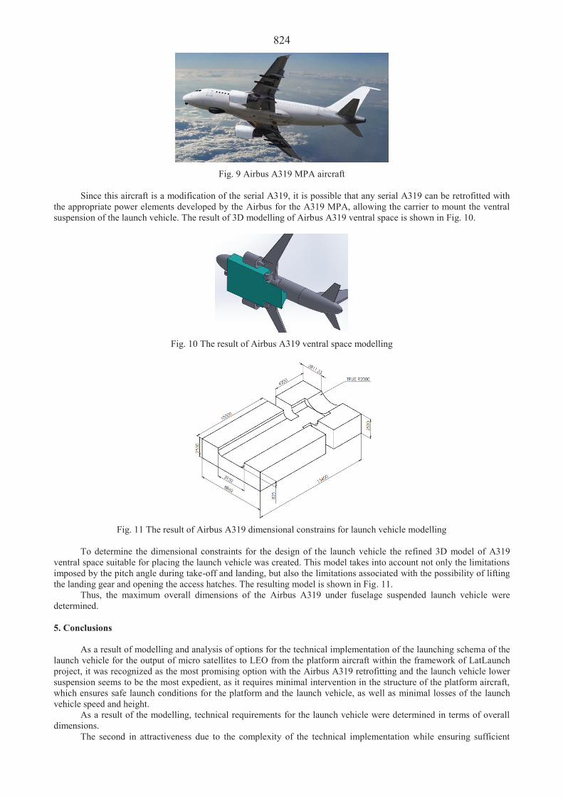
824

Fig. 9 Airbus A319 MPA aircraft

Since this aircraft is a modification of the serial A319, it is possible that any serial A319 can be retrofitted with the appropriate power elements developed by the Airbus for the A319 MPA, allowing the carrier to mount the ventral suspension of the launch vehicle. The result of 3D modelling of Airbus A319 ventral space is shown in Fig. 10.

Fig. 10 The result of Airbus A319 ventral space modelling

Fig. 11 The result of Airbus A319 dimensional constrains for launch vehicle modelling

To determine the dimensional constraints for the design of the launch vehicle the refined 3D model of A319 ventral space suitable for placing the launch vehicle was created. This model takes into account not only the limitations imposed by the pitch angle during take-off and landing, but also the limitations associated with the possibility of lifting the landing gear and opening the access hatches. The resulting model is shown in Fig. 11.

Thus, the maximum overall dimensions of the Airbus A319 under fuselage suspended launch vehicle were determined. 5. Conclusions

As a result of modelling and analysis of options for the technical implementation of the launching schema of the launch vehicle for the output of micro satellites to LEO from the platform aircraft within the framework of LatLaunch project, it was recognized as the most promising option with the Airbus A319 retrofitting and the launch vehicle lower suspension seems to be the most expedient, as it requires minimal intervention in the structure of the platform aircraft, which ensures safe launch conditions for the platform and the launch vehicle, as well as minimal losses of the launch vehicle speed and height.

As a result of the modelling, technical requirements for the launch vehicle were determined in terms of overall dimensions.

The second in attractiveness due to the complexity of the technical implementation while ensuring sufficient

825 launch safety is the fifth variant of the glider-towing scheme, and finally, the third possible variant is the first scheme with the suspension of the carrier under the wing of the platform aircraft. Acknowledgement

The authors are grateful for the support of the Latvian Council of Science, within the framework of whose Project No. Lzp-2018/2-0344 “Design and modelling of Aerospace System for Launching pico- and nano- Satellites to Low Earth Orbit”, the discussed research was performed. References: 1. Urbahs, A.; Kravchenko, S.; Urbaha, M.; Carjova, K.; Panova, N. 2019. Latlaunch – aircraft-based launching

system for budget orbiting small satellites to low earth orbit, Proceedings of the 2-nd Aviation and Space Congress KLIK, Kielce-Cedzyna, 211-214.

2. Jenkins, D. 2007. X-15 extending the frontiers of flight. Washington D.C.: National Aeronautics and Space Administration, 681 p.

3. 2020. LauncherOne service guide. Long Beach: Virgin Orbit, LLC, 57 p. 4. Flight test [online cit. 19-05-2021]. Available from: https://twitter.com/virgin_orbit/status/1149024243503394816 5. Johnson, E.M. 2018. Virgin Galactic completes crewed space test, more flights soon. Reuters: Science news,

December 13, 2018. 6. Sarigul-Klijn, M.; Sarigul-Klijn, N.; Hudson, G.; Holder, L.; Fritz, D.; Webber, C.; Liesman, G.; Shell, D.;

Gionfriddo, M. 2007. Flight Testing of a Gravity Air Launch Method to Enable Responsive Space Access, AIAA Space, 6146.

7. Eclipse glider towing experiment report [online cit. 19-05-2021]. Available from: https://www.nasa.gov/centers/ dryden/history/pastprojects/Eclipse/index.html

8. 2020. Pegasus User’s Guide. Chandler: Northrop Grumman Space Systems Sector, 113 p. 9. 2002. Airbus 300-600 Airplane characteristics for Airport planning AC. Blagnac: Airbus SAS, 192 p. 10. 2002. Airbus A310 Airplane characteristics for Airport planning AC. Blagnac: Airbus SAS, 313 p. 11. 2005. Airbus A318 Aircraft characteristics Airport and maintenance planning AC. Blagnac: Airbus SAS, 290 p. 12. 2005. Airbus A319 Aircraft characteristics Airport and maintenance planning AC. Blagnac: Airbus SAS, 357 p. 13. 2005. Airbus A320 Aircraft characteristics Airport and maintenance planning AC. Blagnac: Airbus SAS, 397 p. 14. 2005. Airbus A321 Aircraft characteristics Airport and maintenance planning AC. Blagnac: Airbus SAS, 392 p. 15. 2005. Airbus A330 Aircraft characteristics Airport and maintenance planning AC. Blagnac: Airbus SAS, 642 p. 16. 2005. Airbus A340-200/300 Aircraft characteristics Airport and maintenance planning AC. Blagnac: Airbus SAS,

404 p. 17. 2005. Airbus A340-500/600 Aircraft characteristics Airport and maintenance planning AC. Blagnac: Airbus SAS,

411 p. 18. 2005. Airbus A350 Aircraft characteristics Airport and maintenance planning AC”. Blagnac: Airbus SAS, 405 p. 19. A319 MPA Maritime Patrol Aircraft [online cit. 19-05-2021]. Available from: https://www.naval-

technology.com/projects/a319mpa/

826

Proceedings of 25th International Scientific Conference. Transport Means 2021. The Model Proposal of Counter-UAS System Solution Mich. erný1, J. Kraus2, Š. Hulínská3 1Czech Technical University in Prague, Department of Air Transport, Horská 3, 128 03 Prague 2, Czech Republic, E-mail: tluchto2@fd.cvut.cz 2Czech Technical University in Prague, Department of Air Transport, Horská 3, 128 03 Prague 2, Czech Republic, E-mail: kraus@fd.cvut.cz 3Czech Technical University in Prague, Department of Air Transport, Horská 3, 128 03 Prague 2, Czech Republic, E-mail: hulinsar@fd.cvut.cz Abstract

The aim of this paper is to propose a defence strategy of Vaclav Havel airport Prague against UAS. The first part addresses the importance of the largest airport in the Czech Republic and the resulting need for its protection. The following section defines the CUAS and explains the different approaches towards the cooperative and noncooperative drones concerning safety and security. The paper also divides individual CUAS systems according to the technologies they use and determines if they are suitable for use at a public international airport. Afterward the defence strategy was created from suitable options including both active and passive surveillance systems. In the end, the evaluation of the proposal was done in terms of range, scalability, and economy. KEY WORDS: Unmanned Aircraft; Unmanned Aircraft System; UAS; Counter-UAS; Security 1. Introduction

Unmanned aircraft systems (UAS), sometimes referred to as drones, have received a great deal of attention lately. They are used by security forces, for example, to monitor driver´s behaviour on the roads or to comply with the ban on entering designated areas. In the civil sector, they are used in agriculture as well as in technical inspections of the infrastructure and buildings. The popularity of unmanned systems due to the built-in camera is still rising among the general public. Buying a drone is very simple and does not require passing any difficult exams. People who operate drones often do not realize that there are many rules for flying. They also do not respect reserved areas where flying is strictly prohibited. Because of these people, there is a growing need to monitor and regulate the operations of UAS.

CUAS (Counter Unmanned Aircraft System) includes systems that are capable of detecting, tracking, identifying and eliminating UAS. These may be already proven systems that have been just slightly modified for use within CUAS, but also systems specially developed for this purpose. At the theoretical level, there are only two ways to intervene against UAS. The first option is to physically destroy the drone using a firearm, missile, energy pulse or net. The second possibility lies in the use of imperfections in the construction of UAS. An unmanned aircraft is a very complex system that contains a large number of individual sensors, navigation equipment and also a central computer, which is responsible for processing incoming data and their subsequent transmission. Each of these subsystems is prone to interference or deception. Most commercial UASs use radio wave technology for remote control. Using our own RF sensors allows us to determine the exact frequency on which that given UAS operates. By disrupting this frequency, we can interrupt communication between the UAS and its operator, and even take control of the drone. The UAS sensors can also be confused by, for example, sending a false GPS signal, which allows us to direct the aircraft to a certain area, where there will be a subsequent action against it [1].

In relation to air transport, the importance of CUAS can be compared to the importance of biological protection of airports. This is a service provided by the airport in order to increase air traffic safety. This activity employs a large number of people around the world and entails enormous financial costs. It is estimated that annual collisions with wildlife cause damage worth more than $ 1.2 billion [2]. With the progressive development of unmanned systems and their growing numbers, it is likely that, in addition to the control of birds around airports, new groups will emerge to protect airports from UAS. According to the FAA, in 2019 a traffic-threatening UAS was observed near the airport on average 250 times a month. The year before it had been only 159. That means that there had been an increase of more than 57% [7]. So far there are few accidents caused by a collision with UAS annually, however, we can observe an upward trend. This problem is most likely to be given more attention when a more serious accident occurs, in which there is great damage to property or personal health. 2. Methodology

International airports are currently threatened by intentional but also unintentional attacks by the UASs. Aviation fans use onboard cameras to shoot videos of commercial aircraft during take-offs and landings. Due to the desire for the best shots, they fly their UAS as close as possible to the flight paths, thus increasing the risk of a collision. They often

827 use commercially available drones, which can be purchased in electronic stores. These are mainly multicopters that users choose for their great controllability and flight stability [1].

Václav Havel Airport Prague has been chosen for this project because it is the largest and busiest airport in the Czech Republic. It served almost 18 million passengers in 2019. It is also the home base of Czech Airlines and Smartwings. On top of that, this airport was chosen because its traffic has already been disrupted by UASs in the past. This happened in 2016. The crew of the arriving aircraft observed the UAS in the area in front of the runway threshold. Due to the dangerous safety and security situation, other scheduled flights had to be diverted to other airports.

The proposed CUAS concept should be able to cover the entire area of Václav Havel Airport Prague. Ideally, the UAS detection limit should extend to a sufficient distance outward the airport perimeter. As a result, the UAS will be detected even before it violates the airport's security zone. Thanks to early warning, the system will be able to respond and evaluate the appropriate response to the threat in a timely manner. The UAS collision with a manned aircraft in the vicinity of the airport is to occur mainly at low altitudes. That means during take-offs and landings. The system should therefore be able to detect UAS beyond the perimeter of the airport, mainly in the directions of the runways.

As this is a proposal to secure a large international airport, certain limitations arise. In the first place, it is not possible to use systems that use projectiles to physically eliminate the infringing UAS. It is not allowed to shoot inside or near the airport, due to the possibility of interference with airport equipment, aircraft or people involved. A similar restriction applies to the use of a laser. Although it is not a system using projectiles, the risk of accidental intervention and consequent collateral damage persists. When using a launching net, care must be taken to ensure that the subsequent fall of the UAS does not cause further damage to the ground. Radio wave jammers are also an unsatisfactory solution, as UASs usually operate on the frequencies on which airport radars operate. During the intervention against the UAS directly at the airport, the radars of the airport control service would also be disabled, which could disrupt navigation in the vicinity of the airport.

Other unsuitable detectors are acoustic. The main reason is the high level of noise around airports. Due to the frequent occurrence of fog in the vicinity of Václav Havel Airport Prague, the use of optical sensors is to some extent limited as well. The use of acoustic and optical systems would also increase the maintenance requirements of these systems. It would be necessary to constantly update the libraries of known drone silhouettes and sounds.

The resulting CUAS concept is also restricted by the limited places where individual systems can be installed. The area of the airport is large, however, it consists mainly of operating areas, such as runways and taxiways. There must be no structures or obstacles in their immediate vicinity that would endanger air traffic. The tallest building at Václav Havel Airport Prague is the control tower, which reaches a height of 50 meters. The presence of this tower and other buildings, such as terminals, is complicating the use of radars and optical detectors. The waves emitted by the radar cannot penetrate the obstacles and thus catch, for example, the UAS behind it. This phenomenon is called radar shadow. In the design, it is necessary to compensate for this fact by using more antennas, which fill the blind spots due to the overlapping fields of view. 3. Results

In the previous part of this paper, the methodology of selecting suitable systems was outlined. Based on the requirements defined, systems from ApolloShield, Eagle.One and Hensoldt have been selected. The combination of these systems created a whole package making it possible to detect, identify and if needed eliminate the intruder.

The ApolloShield system consists of two segments. The first part consists of a device capable of detecting radio waves used for remote control of UAS. The system makes it possible to detect and identify the most well-known types of drones. Each UAS has its own specific ID that the system can recognize. This can then be used to track down the operator. After recognizing the specific UAS, ApolloShield will start to send a fake Go-Home signal for that type of UAS. The second part of the system is a cloud control centre, with which the entire system can be easily controlled. The screen displays the individual detected UASs along with information about them. This could be the name of the manufacturer and the type of machine, the ID and its location on the map. You can then start transmitting the Go-Home signal. As the system can distinguish individual UASs from each other, this solution makes it possible to determine UAS that are allowed to be located in a given airspace. The first prototypes achieved UAS detection only in the hundreds of meters. The latest version of the ApolloShield system achieves a detection range of up to 3 km. Individual devices can be combined into one system in order to increase the protected area. Thanks to OpenAPI, the system can also communicate with CUAS systems from other manufacturers [3].

In this concept, the installation of three units of this system is planned proposed in Fig. 1. It is possible to install one unit at both ends of RWY 06/24. The third unit of the ApolloShield system would be located at the southern threshold of runway 12/30. Thanks to the detection range of 3 km, this concept will cover the entire area of Václav Havel Airport Prague. Thanks to the overlapping fields of view of the individual units, the accuracy of the entire system is increased. By placing them in front of the thresholds of individual runways, we maximize their reach in the runway directions outside the airport.

The eliminating role in the proposed defence strategy will be performed by the Eagle.One multicopter. It is powered by 8 electric motors and the lightweight carbon construction makes it possible to reach a speed of around 80 kph. During the development, emphasis was placed on the redundancy of the propulsion so the system is, therefore, able to function even after the failure of two motors. Lithium-polymer batteries allow UAS to operate for up to 40 minutes. At the bottom of the UAS is an attached air cannon capable of firing a net up to a distance of 10 meters.

828 The net, unlike competing systems, remains attached to the Eagle.One multicopter, which in turn holds the intruder UAS, preventing it from falling to the ground. This can prevent potential collateral damage on the ground. However, it is also important to realize that this limits the use of Eagle.One to some extent. This limits the weight of the target that Eagle.One can intercept and still be able to fly. The manufacturer states that its system is capable of capturing a target flying at a speed up to 62 kph, which can weigh slightly more than 15 kg [4]. For emergencies, Eagle.One is equipped with a parachute to prevent its destruction in case of an unforeseen event.

Fig. 1 Installation locations of the ApolloShield units

The home base was chosen near the Terminal 2 building, as it is close to the geometric centre of Václav Havel Airport Prague. The maximum speed of 80 kph allows it to reach any point of the airport in less than 2 minutes. Thanks to the battery life of 40 minutes, the intruder drone can also be chased back to its operator. It is important to have at least one multicopter as a backup, so that in the event of a failure, the other is always ready. It also allows you to strike against two intruding UASs at the same time.

Another company chosen for this project was Hensoldt. Hensoldt has introduced their family of CUAS systems called XPeller. The system ideal for the permanent installation is referred to by the manufacturer as XPeller Guard. Hensoldt offers detection subsystems such as radars, optical detectors, RF sensors in combination with emergency subsystems. The mutual control and interconnection of the system is ensured by the central control unit C2 [5]. A whole family of Spexer surveillance radars have been designed to monitor protected areas. There are currently three models - Spexer 360, 500 and 2000. While the Spexer 360 is able to cover the entire 360° of the surrounding area, later models 500 and 2000 cover only 120° sector. This is compensated by a much higher detection range. All 3 models operate on X band frequencies (8 - 12 GHz). Doppler radar allows you to determine if fast-moving parts such as propellers are part of the target. This process can distinguish a UAS from a flying bird [6].

Radar Spexer 360 is not suitable for use in large areas, such as Václav Havel Airport. Due to the short-range, it would be necessary to install multiple antennas. In the vicinity of operating areas, they could create obstacles to flying or taxing airplanes. Therefore, more powerful Spexer 500 and Spexer 2000 radars were chosen when creating the defence strategy. By installing the Spexer 2000 model on the terminal building, detection up to a distance of 9 km would be achieved. The limited azimuthal coverage of 120 ° can be compensated by placing three antennas next to each other. An area of radar shadow is created behind the airspace control tower building. This can be covered by installing an additional Spexer 500 radar antenna to the area of Stará Ruzyn in Fig. 2. This proposal meets the requirements for UAS detection within the entire area of Václav Havel Airport. As UAS flying within 5.5 km of the reference airport is prohibited under certain conditions, it is useful to be able to control this circular area.

829

Fig. 2 Installation of Spexer 500 covers the area of the radar shadow (orange) created behind the ATC tower

From the very beginning of the proposal, emphasis was placed on the possibility of easily extending the security system in the event of further airport development. The next planned extension of Václav Havel Airport Prague is the construction of a new parallel runway 06R/24L. The proposal allows its complete coverage to the same extent as the existing RWY 06/24 without significant system changes.

ApolloShield and Eagle.One have an OpenAPI interface, which allows them to be connected into one larger system. Although Spexer radars are not equipped with OpenAPI, they are adapted for integration to a larger protection system using the C2 control unit. Additional ApolloShield antennas as well as Spexer radar antennas can be easily installed if required.

4. Discussion

For higher efficiency of detection and verification, it is necessary to combine several systems together.

Nowadays, hopes are mostly placed on radars, RF detectors and cameras. Radars and RF detectors are designed to detect UAS. The cameras are responsible for verifying that it is indeed a UAS, not a flying bird. Currently, only these three technologies are being considered for use in the security of civil airports. Unless another technology is developed, the improvement of these concepts will only depend on the gradual development of these three sub-technologies.

The final defence strategy was presented directly at Václav Havel Airport Prague. The proposed concept was found to be correct and feasible in real operation. The installation of the ApolloShield system in the area of the runway thresholds was especially acknowledged. Experiments carried out at Václav Havel Airport show that when RF sensors are installed in the vicinity of buildings, the range and overall performance of the sensors decrease. Furthermore, tests have shown that in a real environment, radars do not reach the table ranges specified by the manufacturer.

The design was developed for use in very specific conditions of an international airport. These conditions can be characterized as a large area, of which the buildings occupy only a small part. At the same time, systems that create the risk of collateral damage to property and health cannot be used. The proposed system could also be used, for example, in the protection of solar power plants or water reservoirs serving as sources of drinking water. Both of these examples are similar to airports in that they occupy a large area that does not contain a large number of obstacles that would complicate the use of radar. At the same time, when we act against the infringing UAS, we do not want it to fall. In the case of a solar power plant, sensitive equipment could be damaged. In the case of a water reservoir, there would be a risk of toxic substances leaking from the UAS into the source of drinking water.

5. Conclusions

The main theme of this paper was to propose a defence strategy for Václav Havel Airport Prague against UAS. Threats to civil aviation from unmanned aircraft systems have been defined. Subsequently, the available systems were compared and those that could be used safely in the protection of the international airport were selected. When creating the design, the focus was on unintentional airspace violations along with not very sophisticated targeted attacks.

The requirement of the proposal to protect Václav Havel Airport Prague against UAS was that its entire area is to

830 be covered. The solution described in this paper meets this requirement. Due to the use of Spexer 2000 radars, our design allows the detection of intruding UAS up to the distances of 9 km from the airport reference point. This allows the control of areas that are used mainly during take-offs and landings of aircraft. The biggest problem was the radar shadow created behind the air traffic control tower. By placing the radar antenna north of the tower, a blind area south of the ATC tower was created. As a result, the radar shadow does not interfere with the hazardous area of any of the runways.

It has not been possible to use the full potential of ApolloShield, as aviation authorities do not currently allow the use of RF transmitters within an airport. They are doing so out of fear that other RF devices within the airport could be disrupted. The Eagle.One can operate fully autonomously. This includes navigating and flying close to the target, as well as following action against the intruder. However, the current legislation does not allow the autonomous operation of UAS within the civil sector. The need for a human remote pilots will increase time and reduce the overall effectiveness of intervention against UAS. The intervention against the infringing UAS is also complicated by the fact that, according to current legislation, the intervention can only be carried out by the army and police members. It would speed up the whole process if this power was extended to members of the airport security. They are currently in charge of protecting the perimeter of Václav Havel Airport.

In the future, it can be assumed that the growing number of UAS among the public will have a negative impact on civil aviation. Acknowledgement

This paper was supported by Department of Air Transport Faculty of Transportation Sciences Czech Technical University in Prague and the Grant Agency of the Czech Technical University in Prague, grant No. SGS21/135/OHK2/2T/16.

References 1. Nichols, Randall K.; Mumm, Hans C.; Lonstein, Wayne D.; Ryan, Julie J.C.H; Carter, Candice; Hood, John-

Paul 2020. Counter Unmanned Aircraft Systems Technologies and Operations, NPP eBooks 31. https://newprairie press.org/ebooks/31

2. Allan, John R.; Orosz, Alex P. 2001. The costs of birdstrikes to commercial aviation, Bird Strike Committee-USA/Canada, Third Joint Annual Meeting, Calgary, AB. 2. https://digitalcommons.unl.edu/birdstrike2001/2

3. ApolloShield [online]. [cit. 2021-6-17]. https://www.apolloshield.com/ 4. Eagle.One [online]. [cit. 2021-6-17]. https://eagle.one/en/ 5. HENSOLDT SPEXER® 360: Surveillance Radar for Security Applications. In: HENSOLDT [online]. 2019, s. 1-2

[cit. 2021-6-17]. https://uk.hensoldt.net/fileadmin/HENSOLDT_2019/Products/Radar_IFF_Datalink/SPEXER_360_ 13062019_V2_low_res.pdf

6. SPEXER® 2000 Coastal: Security Radar for Coastal Surveillance. In: Hensoldt [online]. s. 1-2 [cit. 2021-6-17]. ISBN 0817 E 0812. https://www.hensoldt.net/fileadmin/HENSOLDT_2019/Products/Radar_IFF_Datalink/0812_17 _Spexer2000_Coastal_E_intranet.pdf

7. ASSURE UAS Airborne Collision Severity Evaluation Final Report. ASSURE [online]. [cit. 2021-6-17]. https://www.assureuas.org/projects/completed/sUASAirborneCollisionReport.php

831

Proceedings of 25th International Scientific Conference. Transport Means 2021. Comparison of Mechanical Properties of Carbon-Based Composites E. Popardovská1, M. Cúttová2 1Armed Forces Academy of Gen. M. R. Štefánik, Demänovská cesta 393, Liptovský Mikuláš, Slovak Republic, E-mail: eva.popardovska@aos.sk 2Armed Forces Academy of Gen. M. R. Štefánik, Demänovská cesta 393, Liptovský Mikuláš, Slovak Republic, E-mail: miroslava.cuttova@aos.sk Abstract The article deals with the comparison of mechanical properties of carbon-based composites. This article compares two types of composites - short-fiber reinforced polymer composite (SFRPC) – polymer matrix with short carbon fibers and material for 3D printing additive technology – filament of polyethylene terephthalate (PET) with carbon. Both materials were tested using static tensile testing equipment. The results are shown in graphs. In conclusion, the use of these materials is described. KEY WORDS: composite, carbon fiber, mechanical properties 1. Introduction

The article is focused on the research of the mechanical properties of the materials which 20 vol. % of carbon fibers are contained. In this case, two materials are compared.

The first is short-fiber reinforced polymer composite (SFRPC). It is a system of polymer (commonly epoxy resin) matrix, reinforced by short carbon fibers [1, 2]. Composite can be created by oriented fibers, or by randomly oriented fibers – see Fig. 1.

Fig. 1 Oriented and random situated short fibers

The second is 3D printing material. It is a filament based on polyethylene terephthalate (PET) reinforced with carbon fibers [3] use for Fused Deposition Modelling (FDM) – Fig. 2. FDM uses material extrusion, where a filament of solid thermoplastic material is pushed through a heated nozzle (1), melting it in the process. The printer deposits the material (2) on a build platform (3) along a predetermined path, where the filament cools and solidifies to form a solid object [4, 5].

Fig. 2 3D printing technology – Fused Deposition Modelling [6] 2. Specimen’s Production

Different length of carbon fibers in specimens of SFRPC were taken for experimentation. Short reinforcing fibers are made from carbon fiber fabric with density 160 g/m2 – see Fig. 3 and Fig. 4.

832

Fig. 3 Carbon fiber fabric – 160 g/m2

Fig. 4 Randomly oriented short reinforcing carbon fibers

Polymer matrix consists of epoxy resin LH 289 and epoxy hardener H 505 in ratio 10 g resin and 3 g hardener. Based on constant volume of polymer matrix and the different length of reinforcing fibers the following specimens were made – see Table 1.

Table 1 Specimens of short-fiber reinforced polymer composite

Number of specimens

Fiber length[mm]

Percentage of fiber [%]

Fiber weight [g]

1 5 20 2.62 10 20 2.63 5 (50%) + 10 (50%) 20 2.6

Specimens by using the compression moulding method were fabricated. First, the specimen mold was created using by 3D printing technology. The shape and dimensions of the form are determined for the following mechanical test - tensile strength [7] according to standard STN EN ISO 527-2/1A – see Fig. 5.

a b

Fig. 5 Specimen form: a – ISO dimensions; b – 3D model

Mechanical properties of SFRPC with 3D printing material were compared. For production of second type of specimens, the PET filament reinforced with 20 vol. % of carbon fibers was used. The main advantages of reinforcedPET filament are thermal and chemical resistance, very high stiffness and toughness, water resistance, good tribological properties and recyclability. Its main disadvantage is the lower resistance to UV radiation, so it is not suitable to expose it to sunlight for a long time. Its typical applications are technical and precision parts in automobile, industrial and appliances industry [8].

At first, a 3D model of specimen in CAD software was made. The dimensions are determined according to standard STN EN ISO 527-2/1A (Fig. 5a). Then, real specimen by 3D printer was printed. Parameters for print arelisted in the following – Table 2. They depend on the type of filament used.

833 Table 2

3D printing parameters

General printing parameters Specimen orientation 0 °

Layer height 0.2 mm Fill pattern Rectilinear

Speed for print moves First layer speed 35 mm/s

Infill speed 45 mm/s Maximum print speed 60 mm/s

Temperature Extruder 250 °C

Bed 80 °C

Fig. 6 Tensile testing equipment FP – 10

After manufacture of the composite specimens, they were tested using by static tensile testing equipment FP – 10 (Fig. 6), at an ambient temperature 23°C. The maximum tensile load of this equipment is 10kN. The speed of the test is 10 mm/s. The test was terminated automatically when the maximum cross-member displacement of 20 mm was reached. 3. Results

The results of the tensile tests are shown on the following figure – Fig. 7.

a b

Fig. 7 Tensile test curve: a – SFRPC; b – PET with carbon fibers For the strength of short-fiber composite material (consist of polymer matrix reinforced by carbon fiber) the

length of fibers has a significant effect. In a tensile test of a composite material with 20 vol. % of carbon fibers with different lengths (5 mm, 10 mm, and mixed 5+10 mm), a brittle fracture occurs – see Fig. 7, a. The strength of this composite with shorter carbon fibers is higher. Shorter fibers (5 mm) can be more evenly distributed in the matrix volume than longer fibers (10 mm) that clump together. During the tensile test of specimen with a fiber length of 10

834 mm, the composite material breaks mainly at the clusters. In the case of a composite material made of mixed short and long carbon fibers (5+10 mm), the strength of the composite material increases due to larger number of short fibers – Table 3.

For comparison, printing material PET with 20 vol. % of carbon fibers is a flexible material – see Fig. 7, b. The tensile strength of material PET with CF is twice lower than that the composite material with short carbon fibers (5 mm) – Table 3.

Table 3

Tensile test results

Number of specimens Type of material Maximum

force [N] Maximum

stress [MPa] 1 5 mm 3 185 79.6 2 5+10 mm 2 987 74.7 3 10 mm 2 715 67.9 4 PET with CF 1 550 38.8

4. Conclusions

According to the measured results, the best carbon-based composite material in terms of strength is composed of short carbon fibers (5 mm). In practice, short carbon fibers (which are waste from carbon fabric) can be used in the production of these types of composite materials. Subsequently, they can be applied to the production of various structural components, for example to produce unmanned ground vehicles.

For production of structurally complex parts, it is possible to use PET material with carbon fibers despite the lower strength. Due to easier production of complex construction parts by using 3D printing technology.

Acknowledgement

The research is funded by the research project “VV-13 Additional camouflage shields based on polymer composite materials” and “VV-2 Unmanned remote controlled ground vehicle platform for reconnaissance in building interiors”. References 1. Flemming, T.; Kress, G.; Flemming, M. 1996. A new aligned short-carbon-fiber-reinforced thermoplastic prepreg,

Journal of Advanced Composite Materials 5(2): 151-159. https://doi.org/10.1163/156855196X00068. 2. Epaarachchi, J.; Ku, H.; Gohel, K. 2009. A simplified empirical model for prediction of mechanical properties of

random short fiber/vinylester composites, Journal of Composite Materials: 779-788. https://doi.org/10.1177/ 0021998309346383.

3. PET – Polyethyleneterephthalate PET CF20 [online cit.: 2021-08-22]. Available from: https://akro-plastic.com/productfilter/details/7428/

4. The types of 3D printing technology. 3D printing technology guide. [online cit.: 2021-02-07]. Available from: https://all3dp.com/1/types-of-3d-printers-3d-printing-technology/

5. Cúttová, M.; Lukášik, P. 2018. Possibilities of using 3D printing in industrial applications, Transfer: Využívanie nových poznatkov v strojárskej praxi. Tren ín: Tren ianska univerzita Alexandra Dub eka v Tren íne. ISBN 978-80-8075-827-1.

6. The 9 different types of 3D printers [online cit.: 2021-08-25]. Available from: https://3dinsider.com/3d-printer-types/

7. Gábrišová, Z.; Švec, P.; Brusilová, A. 2020. Effect of mechanical properties on wear resistance of Si3N4 - SiC ceramic composite, Advances in Science and Technology Research Journal 14(4): 156-167. ISSN 2299-8624.

8. Arko-plastic, datasheet PET CF20 [online cit.: 2021-08-28]. Available from: https://akro-plastic.com/productfilter/details/7428/

835

Proceedings of 25th International Scientific Conference. Transport Means 2021. The Multimodal Transport Portfolio: Service Development Research E. Valionien 1, B. Pla ien 2, L. Kaštaunien 3 1Lithuanian Maritime Academy, I. Kanto str. 7, 92123, Klaip da, Lithuania, E-mail: e.valioniene@lajm.lt 2Lithuanian Maritime Academy, I. Kanto str. 7, 92123, Klaip da, Lithuania, E-mail: b.placiene@lajm.lt 3Lithuanian Maritime Academy, I. Kanto str. 7, 92123, Klaip da, Lithuania, E-mail: l.kastauniene@gmail.com Abstract The concentration of multimodal transport companies operating in the maritime transportation business is high and thus brings forth two competitiveness tendencies: the demand for multimodal transport services rises with increasing freight movement in ports, and vice versa, and it is obvious that market competitiveness growth is also related to freight traffic, and the intensity of competition in the market can be assessed in inverse proportion to changes in freight flows. Since the maritime transport sector operates as an ecosystem subject to uncertain and changing environmental conditions, maintaining its competitive advantage must also be an ongoing process aimed at responding in a timely manner to the shift in freight flow. In order to continually control the company's competitive adjustment, there is a need for a specific methodology that has been proposed by the authors, based on research results and verified in a case study of a selected multimodal transportation company operating in Klaipeda State Seaport. The methodology of multimodal transportation services has been formulated on indices calculated on the basis of descriptive statistics, based on the logistics services’ quality analysis and division of services portfolio into basic, extended and value-added packages; and a practical example of service quality and development portfolio interpretation through data visualisation techniqes, to be further recommended for businesses. On a case-by-case basis, even low used multimodal freight services have been shown to be added value to the company's loyal and important customers. The study highlighted a negative impact of excessive workload on the quality of services, restrained logistical connectivity due to human error, also found an insufficient material resource factor was at play. KEYWORDS: maritime transportation, multimodal logistics services, logistics services assessment and development 1. Introduction

The concentration of multimodal transport businesses in the maritime transport sector is high and leads to two tendencies of competitiveness: the demand for multimodal transport services grows with increasing freight flows in ports, and vice versa, thus it is obvious that growth of market competitiveness is also related to freight movement, whereas the intensity of competition in the market can be assessed in inverse proportion to changes in freight flows.

Since the maritime transport sector functions as an ecosystem subject to uncertain and changing environmental conditions, sustaining its competitive advantage must be an ongoing process aimed at responding in a timely manner to changes in freight flow. Multimodal freight services are a part of logistics services depending on the specifics of a logistics chain, where the qualitative and value-added service parameters depend on the level of integration of different transport systems, existing partnership networks and selected logistics chain infrastructure. It can be seen that these parameters define the specificity of logistics services, therefore, in competition for a larger share of services in the market, multimodal freight companies need to constantly assess the quality parameters of services provided, as the demand for services in the market goes up.

It should also be noted that Lithuanian transport and logistics services providers are faced with economic growth and high-level service demand in the European market. Based on the market observation published by the Bank of Lithuania (2019), in Lithuania 5.2 per cent of the total employed in 2008–2018 worked in transport on average, compared to an average share of 2.7 per cent in the EU [1]. However, the COVID 19 pandemic also posed a major challenge to the global and EU economies in regard to service provision, with freight flows redistributed and multimodal transport intensifying even faster than in the pre-crisis period. As maritime transport accounts for about 90% of world trade, it is natural that the demand for multimodal freight in the global supply chain is about a similar proportion, so the role of the seaport in the transport chain is defined as ensuring the logistical connectivity of multimodal freight, it also refers to partial qualitative function of multimodal services [2]. On the other hand, as the seaport is an ecosystem and the service providers operating there are part of this ecosystem, therefore analysis of multimodal transport portfolio should also refer to quality service providers as one of the components of the seaport's attractiveness in the global international trade market, what allows to prove the relevance of the topic and the pending issue. Therefore this investigation aims to develop a feasibility methodology for multimodal transport portfolio development that could be applicable in the multimodal transport business sector, in order to implement the continuous monitoring of customer satisfaction.

2. Construction of Feasibility Assessment Method for Multimodal Transport Portfolio Development

Meeting customer needs is one of the key challenges of the economy and is no exception in the multimodal

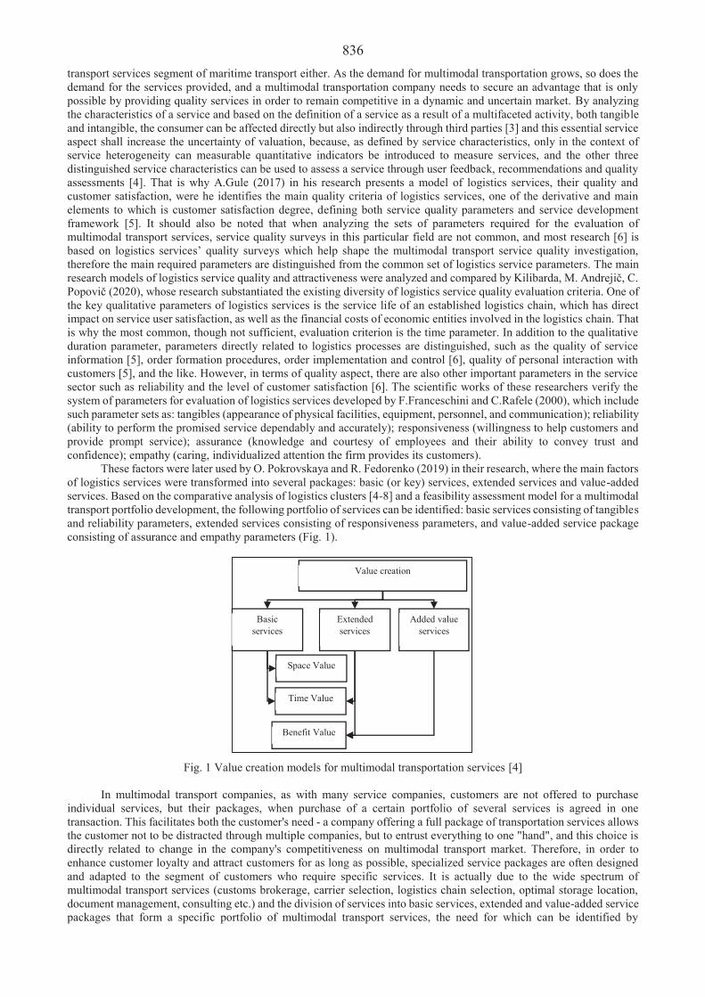
836transport services segment of maritime transport either. As the demand for multimodal transportation grows, so does the demand for the services provided, and a multimodal transportation company needs to secure an advantage that is only possible by providing quality services in order to remain competitive in a dynamic and uncertain market. By analyzing the characteristics of a service and based on the definition of a service as a result of a multifaceted activity, both tangible and intangible, the consumer can be affected directly but also indirectly through third parties [3] and this essential service aspect shall increase the uncertainty of valuation, because, as defined by service characteristics, only in the context of service heterogeneity can measurable quantitative indicators be introduced to measure services, and the other three distinguished service characteristics can be used to assess a service through user feedback, recommendations and quality assessments [4]. That is why A.Gule (2017) in his research presents a model of logistics services, their quality and customer satisfaction, were he identifies the main quality criteria of logistics services, one of the derivative and main elements to which is customer satisfaction degree, defining both service quality parameters and service development framework [5]. It should also be noted that when analyzing the sets of parameters required for the evaluation of multimodal transport services, service quality surveys in this particular field are not common, and most research [6] is based on logistics services’ quality surveys which help shape the multimodal transport service quality investigation,therefore the main required parameters are distinguished from the common set of logistics service parameters. The main research models of logistics service quality and attractiveness were analyzed and compared by Kilibarda, M. Andreji , C. Popovi (2020), whose research substantiated the existing diversity of logistics service quality evaluation criteria. One of the key qualitative parameters of logistics services is the service life of an established logistics chain, which has direct impact on service user satisfaction, as well as the financial costs of economic entities involved in the logistics chain. That is why the most common, though not sufficient, evaluation criterion is the time parameter. In addition to the qualitative duration parameter, parameters directly related to logistics processes are distinguished, such as the quality of service information [5], order formation procedures, order implementation and control [6], quality of personal interaction with customers [5], and the like. However, in terms of quality aspect, there are also other important parameters in the service sector such as reliability and the level of customer satisfaction [6]. The scientific works of these researchers verify the system of parameters for evaluation of logistics services developed by F.Franceschini and C.Rafele (2000), which includesuch parameter sets as: tangibles (appearance of physical facilities, equipment, personnel, and communication); reliability (ability to perform the promised service dependably and accurately); responsiveness (willingness to help customers and provide prompt service); assurance (knowledge and courtesy of employees and their ability to convey trust and confidence); empathy (caring, individualized attention the firm provides its customers).

These factors were later used by O. Pokrovskaya and R. Fedorenko (2019) in their research, where the main factors of logistics services were transformed into several packages: basic (or key) services, extended services and value-added services. Based on the comparative analysis of logistics clusters [4-8] and a feasibility assessment model for a multimodal transport portfolio development, the following portfolio of services can be identified: basic services consisting of tangibles and reliability parameters, extended services consisting of responsiveness parameters, and value-added service packageconsisting of assurance and empathy parameters (Fig. 1).

Fig. 1 Value creation models for multimodal transportation services [4]

In multimodal transport companies, as with many service companies, customers are not offered to purchase individual services, but their packages, when purchase of a certain portfolio of several services is agreed in one transaction. This facilitates both the customer's need - a company offering a full package of transportation services allows the customer not to be distracted through multiple companies, but to entrust everything to one "hand", and this choice is directly related to change in the company's competitiveness on multimodal transport market. Therefore, in order to enhance customer loyalty and attract customers for as long as possible, specialized service packages are often designed and adapted to the segment of customers who require specific services. It is actually due to the wide spectrum of multimodal transport services (customs brokerage, carrier selection, logistics chain selection, optimal storage location, document management, consulting etc.) and the division of services into basic services, extended and value-added service packages that form a specific portfolio of multimodal transport services, the need for which can be identified by

Value creation

Basic services

Extended services

Added value services

Space Value

Time Value

Benefit Value

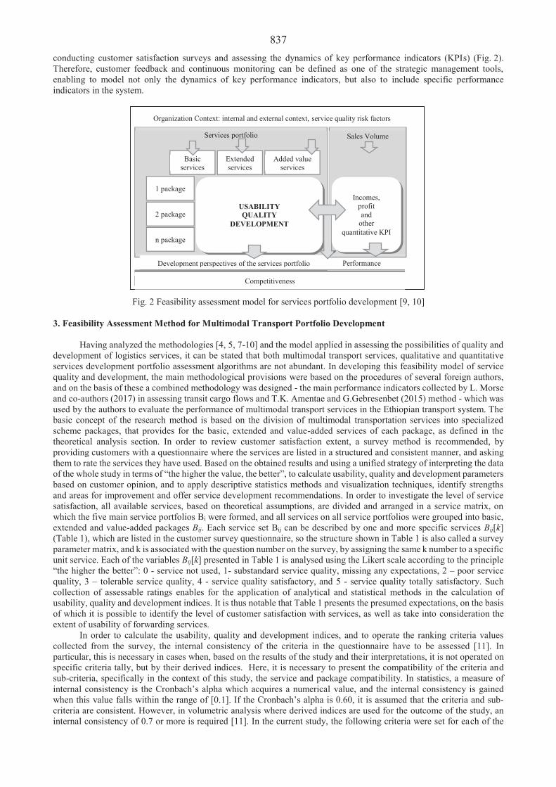
837conducting customer satisfaction surveys and assessing the dynamics of key performance indicators (KPIs) (Fig. 2).Therefore, customer feedback and continuous monitoring can be defined as one of the strategic management tools, enabling to model not only the dynamics of key performance indicators, but also to include specific performance indicators in the system.

Fig. 2 Feasibility assessment model for services portfolio development [9, 10]

3. Feasibility Assessment Method for Multimodal Transport Portfolio Development

Having analyzed the methodologies [4, 5, 7-10] and the model applied in assessing the possibilities of quality and development of logistics services, it can be stated that both multimodal transport services, qualitative and quantitative services development portfolio assessment algorithms are not abundant. In developing this feasibility model of service quality and development, the main methodological provisions were based on the procedures of several foreign authors, and on the basis of these a combined methodology was designed - the main performance indicators collected by L. Morse and co-authors (2017) in assessing transit cargo flows and T.K. Amentae and G.Gebresenbet (2015) method - which was used by the authors to evaluate the performance of multimodal transport services in the Ethiopian transport system. The basic concept of the research method is based on the division of multimodal transportation services into specialized scheme packages, that provides for the basic, extended and value-added services of each package, as defined in the theoretical analysis section. In order to review customer satisfaction extent, a survey method is recommended, by providing customers with a questionnaire where the services are listed in a structured and consistent manner, and asking them to rate the services they have used. Based on the obtained results and using a unified strategy of interpreting the dataof the whole study in terms of “the higher the value, the better”, to calculate usability, quality and development parameters based on customer opinion, and to apply descriptive statistics methods and visualization techniques, identify strengths and areas for improvement and offer service development recommendations. In order to investigate the level of service satisfaction, all available services, based on theoretical assumptions, are divided and arranged in a service matrix, on which the five main service portfolios Bi were formed, and all services on all service portfolios were grouped into basic, extended and value-added packages Bij. Each service set Bij can be described by one and more specific services Bij[k] (Table 1), which are listed in the customer survey questionnaire, so the structure shown in Table 1 is also called a survey parameter matrix, and k is associated with the question number on the survey, by assigning the same k number to a specific unit service. Each of the variables Bij[k] presented in Table 1 is analysed using the Likert scale according to the principle “the higher the better”: 0 - service not used, 1- substandard service quality, missing any expectations, 2 – poor service quality, 3 – tolerable service quality, 4 - service quality satisfactory, and 5 - service quality totally satisfactory. Such collection of assessable ratings enables for the application of analytical and statistical methods in the calculation of usability, quality and development indices. It is thus notable that Table 1 presents the presumed expectations, on the basis of which it is possible to identify the level of customer satisfaction with services, as well as take into consideration the extent of usability of forwarding services.

In order to calculate the usability, quality and development indices, and to operate the ranking criteria values collected from the survey, the internal consistency of the criteria in the questionnaire have to be assessed [11]. In particular, this is necessary in cases when, based on the results of the study and their interpretations, it is not operated on specific criteria tally, but by their derived indices. Here, it is necessary to present the compatibility of the criteria and sub-criteria, specifically in the context of this study, the service and package compatibility. In statistics, a measure of internal consistency is the Cronbach’s alpha which acquires a numerical value, and the internal consistency is gained when this value falls within the range of [0.1]. If the Cronbach’s alpha is 0.60, it is assumed that the criteria and sub-criteria are consistent. However, in volumetric analysis where derived indices are used for the outcome of the study, an internal consistency of 0.7 or more is required [11]. In the current study, the following criteria were set for each of the

Services portfolio

Basicservices

Extended services

Added value services

1 package

2 package

n package

USABILITYQUALITY

DEVELOPMENT

Performance Development perspectives of the services portfolio

Sales Volume

Organization Context: internal and external context, service quality risk factors

Incomes,profit and

other quantitative KPI

Competitiveness

838 service packages: cronbach alpha [B1] = 0.93; cronbach alpha [B2] = 0.86; cronbach alpha [B3] = 0.92; cronbach alpha [B4] = 0.86; cronbach alpha [B5] = 0.70.

Table 1

System of Variables defining the structure of multimodal transportation services portfolio

Services portfolio Services packages 1. Basic services 2. Extended services 3. Added value services

B1 Customs broker services B11 [1], B11 [3], B11 [4], B11 [6]

B12 [2], B12 [7], B12 [9], B12 [12], B12 [14], B12 [15]

B13 [5], B13 [8], B13 [10], B13 [11], B13 [13]

B2 Special purpose services and Container preparation

B21 [20], B21 [22] B22 [16], B22 [18], B22 [19], B22 [22]

B23 [17], B23 [23]

B3 Freight loading, reloading and storage services

B31 [24] B32 [25], B32 [26], B32 [27], B32 [28], B32 [32]

B33 [29], B33 [30], B33 [31], B33 [33]

B4 Container transport and delivery services in the destination country

B41 [34], B41 [36], B41 [38], B41 [40]

B42 [37], B42 [39], B42 [42], B42 [43], B42 [44], B42 [45]

B43 [35], B43 [41]

B5 Customer service culture and customer interaction

B51 [46], B51 [47], B51 [49]

B52 [48] -

Subject to internal compatibility of criteria and sub-criteria, indicators of usability, quality and development of

multimodal transport services are calculated based on the algorithm below. In order to assess a service usability, quality and development index based on the results of the survey, each criterion is calculated as follows:

1 l

Lkl

ij

bB k

L, (1)

when L is the number of customers using k services, and b_ (k_l) is the estimate of each respondent of k services from the range [1.5], moreover, the constraint Bij [z] [0.5], i = 1,…, I = 5; j = 1,…, J = 3; z = 1,…., Z = 49 applies, where: Bij- i service package level j service quality index, calculated as per below formula:

1k

ijzij

B kB

k. (2)

Assuming that only the services used are considered, i.e. each service has a different number of respondents who

have used it. In this case, the overall quality index of package i is calculated as follows:

3 11

kijz

i j

B kB

k. (3)

The above algorithm is applied to calculate the usability and quality indices of a service / set of services / service

package. Using the same analytical logic, the service development feasibility index is analyzed, only the number of all respondents L = 49, both users and non-users, is taken into consideration in order to assess potential service areas on the open market that may undermine the company's competitiveness in terms of service availability.

Table 2

Alternatives for Interpreting the Calculated Values and Data Visualization Colours

Right asymmetry Left asymmetry Resume

The index is less than the median The index is less than the mean

The service or service package is one of the business’ weaknesses and therefore calls for urgent improvement

The rating index is higher than the median but lower than the mean

The index is greater than the mean, but less than the median The service is quite developed, but can be improved

Index is higher than the mean The index is higher than the median Can be improved if necessary, yet this IS one of the

competitive advantages For calculation of service usability index, the relative share of customers who have used the service is calculated,

and the usability of the service package is the average of the services j that comprise the service package. The obtained service package indices, designating the division of services into packages according to the extent of services, are

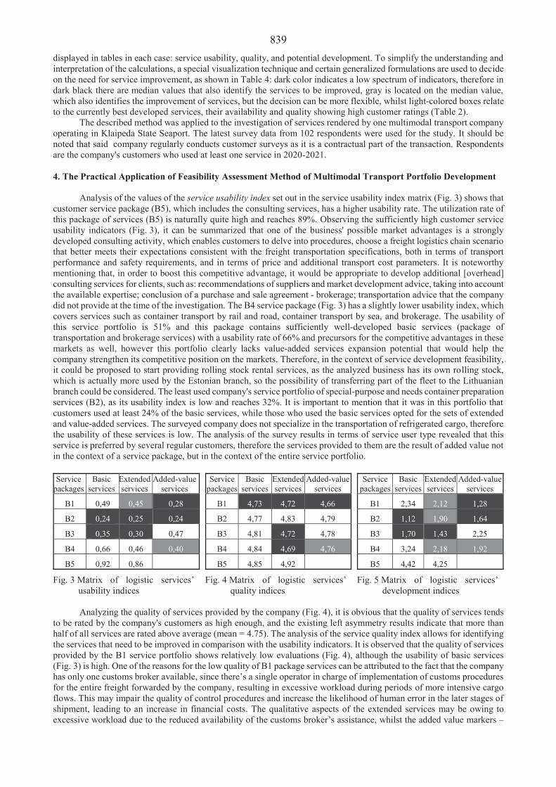
839 displayed in tables in each case: service usability, quality, and potential development. To simplify the understanding and interpretation of the calculations, a special visualization technique and certain generalized formulations are used to decide on the need for service improvement, as shown in Table 4: dark color indicates a low spectrum of indicators, therefore in dark black there are median values that also identify the services to be improved, gray is located on the median value, which also identifies the improvement of services, but the decision can be more flexible, whilst light-colored boxes relate to the currently best developed services, their availability and quality showing high customer ratings (Table 2).

The described method was applied to the investigation of services rendered by one multimodal transport company operating in Klaipeda State Seaport. The latest survey data from 102 respondents were used for the study. It should be noted that said company regularly conducts customer surveys as it is a contractual part of the transaction. Respondents are the company's customers who used at least one service in 2020-2021. 4. The Practical Application of Feasibility Assessment Method of Multimodal Transport Portfolio Development

Analysis of the values of the service usability index set out in the service usability index matrix (Fig. 3) shows that

customer service package (B5), which includes the consulting services, has a higher usability rate. The utilization rate of this package of services (B5) is naturally quite high and reaches 89%. Observing the sufficiently high customer service usability indicators (Fig. 3), it can be summarized that one of the business' possible market advantages is a strongly developed consulting activity, which enables customers to delve into procedures, choose a freight logistics chain scenario that better meets their expectations consistent with the freight transportation specifications, both in terms of transport performance and safety requirements, and in terms of price and additional transport cost parameters. It is noteworthy mentioning that, in order to boost this competitive advantage, it would be appropriate to develop additional [overhead] consulting services for clients, such as: recommendations of suppliers and market development advice, taking into account the available expertise; conclusion of a purchase and sale agreement - brokerage; transportation advice that the company did not provide at the time of the investigation. The B4 service package (Fig. 3) has a slightly lower usability index, which covers services such as container transport by rail and road, container transport by sea, and brokerage. The usability of this service portfolio is 51% and this package contains sufficiently well-developed basic services (package of transportation and brokerage services) with a usability rate of 66% and precursors for the competitive advantages in these markets as well, however this portfolio clearly lacks value-added services expansion potential that would help the company strengthen its competitive position on the markets. Therefore, in the context of service development feasibility, it could be proposed to start providing rolling stock rental services, as the analyzed business has its own rolling stock, which is actually more used by the Estonian branch, so the possibility of transferring part of the fleet to the Lithuanian branch could be considered. The least used company's service portfolio of special-purpose and needs container preparation services (B2), as its usability index is low and reaches 32%. It is important to mention that it was in this portfolio that customers used at least 24% of the basic services, while those who used the basic services opted for the sets of extended and value-added services. The surveyed company does not specialize in the transportation of refrigerated cargo, therefore the usability of these services is low. The analysis of the survey results in terms of service user type revealed that this service is preferred by several regular customers, therefore the services provided to them are the result of added value not in the context of a service package, but in the context of the entire service portfolio.

Service packages

Basic services

Extended services

Added-value services

B1 0,49 0,45 0,28

B2 0,24 0,25 0,24

B3 0,35 0,30 0,47

B4 0,66 0,46 0,40

B5 0,92 0,86

Fig. 3 Matrix of logistic services’ usability indices

Service packages

Basic services

Extended services

Added-value services

B1 4,73 4,72 4,66

B2 4,77 4,83 4,79

B3 4,81 4,72 4,78

B4 4,84 4,69 4,76

B5 4,85 4,92

Fig. 4 Matrix of logistic services’ quality indices

Service packages

Basic services

Extended services

Added-value services

B1 2,34 2,12 1,28

B2 1,12 1,90 1,64

B3 1,70 1,43 2,25

B4 3,24 2,18 1,92

B5 4,42 4,25

Fig. 5 Matrix of logistic services’ development indices

Analyzing the quality of services provided by the company (Fig. 4), it is obvious that the quality of services tends

to be rated by the company's customers as high enough, and the existing left asymmetry results indicate that more than half of all services are rated above average (mean = 4.75). The analysis of the service quality index allows for identifying the services that need to be improved in comparison with the usability indicators. It is observed that the quality of services provided by the B1 service portfolio shows relatively low evaluations (Fig. 4), although the usability of basic services (Fig. 3) is high. One of the reasons for the low quality of B1 package services can be attributed to the fact that the company has only one customs broker available, since there’s a single operator in charge of implementation of customs procedures for the entire freight forwarded by the company, resulting in excessive workload during periods of more intensive cargo flows. This may impair the quality of control procedures and increase the likelihood of human error in the later stages of shipment, leading to an increase in financial costs. The qualitative aspects of the extended services may be owing to excessive workload due to the reduced availability of the customs broker’s assistance, whilst the added value markers –

840 by that of the guarantee procedures. It should be noted that warranty granting is another big issue to consider, as the tariffs for guarantees on customs procedures granted by many companies vary, it would thus be an option to consider signing a contract with another guarantor.

The qualitative estimates of the high usability B5 package services (Fig. 3) also exceed the mean (Fig. 4, average B5 = 4.85). This situation can be explained by the fact that the management do focus on advancing the professional communication and managerial competencies of their sales staff. It should also be noted that low-used services in the B2 service portfolio are also rated as high-quality, which confirms the recommendation that company management should prioritize high quality value-added aspect for maintaining major customer loyalty. It is therefore recommended to maintain and strengthen competitiveness in B2 portfolio not based on services usability, but through their qualitative added value. The management attention should be drawn to the qualitative parameters of high-usability B4 portfolio services (Fig. 4), since one of the lower qualitative scores falls on the extended B4 portfolio of services, which leads to an assumption that in order to increase competitive advantage and retain users, it is necessary to focus on the qualitative parameters of these services. In this portfolio, services that pertain to the the destination country intro, filing of bill of lading and container status / location renewal are likely underestimated.

Investigation on service demand indicators, by applying the services development indices (Fig. 5), indicates that the service development demand of the low-use service portfolio B2 is quite high (inversely proportional to the numerical value of the index), therefore low-use services must be maintained as a means of adding value to loyal customers. It should also be noted that the overall assessment of the development portfolio is 1.55; and it is the basic services in this portfolio that need expansion the most, therefore the managers need to analyze the possibilities of attracting more customers transporting refrigerated and bulk / unpackaged containerised goods, complemented by competitive new services. Also, the development demand shows that the B3 service package needs to be optimized (Fig. 5) – i.e. cargo loading, reloading and storage services. The lowest service development demand marker of the B3 package is value-added services, as they are used more often by customers. These include services like container weighing, brokerage services etc. The construction or acquisition of storage facilities could also push towards the development of the B1 portfolio, as it would be possible to immediately plan to grant the warehouses a special status - as customs warehouse. Goods can be stored indefinitely in customs warehouses, and when goods are imported, it is often not known how they will be disposed of in the future. Therefore, it is possible to warehouse such merchandise in customs storage until a buyer is found, which could also develop value-added services with the lowest demand index - 1.28. It is also possible to split a large consignment into parts in a customs facility and sell it out to different buyers. And, most importantly, there is no need to pay import duties and other mandatory taxes during the storage of goods. These taxes are paid when the goods are used for consumption (Customs of the Republic of Lithuania). Based on the results of the study, it can be stated that the total utilization of the service portfolio is lower than the average utilization rate of services, therefore it requires enhanced marketing tools and/or revision of the service portfolio structure. The service quality index is quite high and above the average, so the quality parameters of individual services need to be reviewed, whilst service portfolio upgrade and development are in high demand. 5. Conclusions

The analysis of the factors shaping the competitiveness of logistics services companies dealing in freight transportation in the maritime transport sector revealed that in addition to technological innovations that determine the length of the logistics chain, service quality parameters are also important. And by combining them with usability and development demand scores, can add to the competitive advantage of these businesses.

A combination of descriptive statistics and visualization methodology based on the parameters used in logistics service quality surveys, and research models based on service integrity and value-added exclusivity parameters, can be used to structure the competitiveness of a multimodal transport company operating in the maritime transport sector. The developed method proposes to collect data from the customer satisfaction survey on how satisfied they are with the services received, for calculation of indices of usability, quality and development need of the service portfolio and its service packages and services, on the basis of which recommendations can be processed.

Having applied the developed methodology to the case of the opted multimodal transport service company, it was found that company's service portfolio (B2) showed a relatively low point of usability, however, it was rated by customers with high quality indicators. Since there’s been an obvious and significant request from customers side to expand these services, the company is therefore offered to maintain low-usability services as a value added factor for loyal customers. To increase the customs broker staff, thereby reducing their workload per se and increasing the offer of advisory services for clients on customs procedures, thus raising the quality and usability parameters of the service package. References 1. Lietuvos ekonomikos apžvalga. Vilnius: Lietuvos bankas, 2019. Assessed: https://www.lb.lt/uploads/documents/

files/musu-veikla/ekonomikos-analize-prognozes/Lietuvos_ekonomikos_apzvalga_2019-09.pdf 2. Rushton, A.; Baker, P.; Crousher, P. 2010. The handbook of logistics & distribution management. London: Kogan

Page. 3. Ska kauskien , I.; Vestert , J. 2018. Paslaugos sampratos aktualizavimas šiuolaikin je vadyboje. Mokslas- Lietuvos

ateitis / Science- future of Lithuania 10: 1-9.

841 4. Gargasas, A.; M gien , I. 2018. Logistini paslaug vert s k rimas ir vertinimas, Management theory and studies

for rural business and infrastructure development 40(2): 187-197. 5. Gule, A. 2017. Models and Methods of measuring quality of logistic service, Procedia Engineering 18: 255-264. 6. Kilibarda, M.; Andreji , M.; Popovi , V. 2020. Research in logistic service quailty: a systemiatic literature review.

Transport V35, I 2: 224-235. 7. Franceshini, F.; Rafele, C. 2000. Quality evaluation in logistic services, International Journal of Agile Management

Systems 2(1): 49-53. 8. Pokrovksaya, O.; Fedorenko, R. 2019. Methods of rating assessment for terminal and logistics complexes. XII

International Scientific Conference on Agricultural Machinery Industry– IOP Conf. Series: Earth and Environmental Science 403: 012199.

9. Morse, L.; Trompet, M.; Barron, A.; Graham, D. J. 2017. Development of a key performance indicator system to benchmark relative paratansit performance, Journal of the Transportation Research Board 2650: 1-8.

10. Amentae, T.K.; Gebresenbet, G. 2015. Evaluation of performance of intermodal import-export freight transport system in Ethiopia, Journal of Service Science and Management 8: 57-70.

11. Pakalniškien , V. 2012. Tyrimo ir vertinimo priemoni patikimumo ir validumo nustatymas. Vilnius: VU leidykla.

842

Proceedings of 25th International Scientific Conference. Transport Means 2021. Assessment of the Quality of Connections on the Rail Transport Network: a Case Study V. upták1, J. Pe man1

1Institute of Technology and Business in eské Bud jovice, Okružní 517/10, 370 01 eské Bud jovice, Czech Republic, E-mail: luptak@mail.vstecb.cz Abstract The presented article and scientific study deals with the evaluation of the quality of connection in passenger transport on the selected transport network. The transport network, which is analyzed and researched is the railway transport network, on the territory of the Pilsen Region in the Czech Republic. The presented methodology for evaluating the quality of the transport network in passenger transport is generally applicable to different types of transport network (rail, road, air and integrated transport systems) and their combination. The resulting effect of the evaluation of a given transport network serves to objectify and evaluate existing timetables and to compare timetables either ex post or ex ante. The presented methodology serves mainly for customers of transport services in the public interest and for increasing the quality of connections on the transport network. KEY WORDS: transport network, speed of achievement, quality in railway transport 1. Introduction

The EU pays systematic attention to the quality of passenger transport [1, 2]. Quality is perceived differently by users and transportation service providers or organizers of transport as well as by society. The needs and expectations of customers are met by establishing procedures under the provisions of the Regulation of the European Parliament and Council Regulation (EC) No. 1371/2007 on rail passengers’ rights and obligations [3, 4]. The cornerstone of transport services is to provide travel opportunities by creating links and connections. Often, after the introduction of the new timetable under discussion whether it is better or worse, each approach is evaluated in a subjective manner. The authors solved some partially problematic of rail passenger quality services [5, 6]. At present, there is no methodology for assessing train timetables from the transportation point of view as a whole. We evaluate specific trains and connections in the stations only, but not the quality of the connection from point A to point B. The aim of this paper is to introduce a new methodology for the assessment of timetables in terms of passenger traffic focused on connectivity and linking [7, 8]. From the passenger’s point of view, it is necessary to assess the availability of travelling opportunities between selected points on the rail network. The travel offer from A to B is in principle affected by travel time, number of transfers (changing the transport means), and number of travel opportunities. Connectivity and linking also affect several factors. This is an outcome for setting of draft criteria for connection evaluation [9, 10]. Introduced study is designed in purview of the set up a tool for an objective evaluation of the quality of public transport service. Specifically, the aspects of availability and time of the transport services in selected geographical area are closed to the Standard EN 13816 [11].

2. Proposal of a New Methodology for Evaluating the Quality of the Transport Network

Any new methodology for the comprehensive assessment of the quality of network connectivity should be based on predetermined and well-defined steps [12, 13]. The interconnection of individual indicators must enable the assessment of connectivity, and therefore the quality of transport, on equal terms [14]. This implies that all connections within a selected network must be taken into consideration [15, 16]. The assessment procedure itself includes individual steps as follows: 1. Determining a transport network; 2. Identifying a set of transport connections; 3. Defining the relevant tariff points on a defined transport network; 4. Selecting search engines for transport connections; 5. Specifying the assessment qualitative indicators; 6. Assessment of individual connections; 7. Assessment of average indicators within a specific route; 8. Comprehensive assessment of a particular indicator within a transport network. The suggested methodology is also vividly presented in the following flowchart (see Fig. 1) [17-24]

843

Fig. 1 Flowchart for assessing the quality of transport network connectivity

3. Case Study

1. Step – choosing a specific network - for the needs of the research was chosen the network of the Czech Railway Administration – Správa železnic. The study included all carriers providing passenger rail transport in the Pilsen region and the examined date was December 10, 2020.

2. Step – selection of transport points - in this step the selected city was defined, in our case Domažlice and according to the next step according to the flow chart, other points on the network were identified. Points were selected according to the importance of settlements in the Pilsen region.

3. Step - choosing relevant traffic points on the network- - For the purposes of the research, 17 tariff points were set, to which the transport connection will be assessed. Within the Plze tariff point, Plze main railway station was selected as the destination station and the nearest railway station - Ka ez - was designated for the Zbiroh tariff point. The specified date for the assessment was set for Thursday, December 10, 2020. The following cities were selected from the selected tariff points: Plze , Ný any, Planá u Mar. Spa, Rokycany, Pob žovice, Horaž ovice p edm stí, Klatovy, Zbiroh, He manova Hu , Svojšín, Bor, Kasejovice, Mladotice, Radnice, Bezdružice, Železná Ruda-Alžb tín and Kožlany. The distribution of individual target points within the Pilsen region is shown in Fig. 2.

4. Step – choosing a search engine- All searched connections were found via the web application https://idos.idnes.cz of the company CHAPS spol. s r.o., Brno. The correctness of the individual connections found, especially for transport requiring several transfers, was randomly checked by searching for connections by individual sections without transfers. The search for connections continued until the Czech Railways connections were reduced due to the COVID-19 epidemic.

County townsSelected district townsTransport hubsEnd-to-end transport hubsJunctions and turning pointsSupply for missing sectionsCentres of tourism

Assess the quality of transport network connectivity

1. Determine a transport network

2. Identify a set of connections

3. Define relevant tariff points within the transport network

4. Select a search engine for connections

5. Specify assessment indicators

6. Assess individual connections

7. Assess average indicators within a specific route

8. Comprehensively assess particular indicator within a transport network

Does the search engine fully support the search for connections within the selected transport

network?

844

Fig. 2 Plan of the railway network in the region of Plze with marked tariff points

5. and 6. Steps - choosing indicators and assessing separate sessions– The Domažlice - Plze hlavní nádraží connection was used as an example. Nine connections were found within 24 hours. On this transport route, 25 connections in 24 hours were identified on the examined day. From the point of view of serving the area, the Domažlice - Plze route is the most important. It is a connection of Domažlice with the regional town. This corresponds to a relatively large number of connections. It is possible to use line no. 180 or as an alternative to track no. 185 and no. 170, which is a slightly longer connection and with a transfer. The fastest connection with a driving time of 48 min is provided by express (connections No. 7, 9, 11, 14, 16, 21 and 24) at 8:01, 10:01, 12:01, 14:01, 16:01, 18:01 and 20:01. Individual trains running on line no. 180 offers significantly better comfort than connections to other destination tariff points - even most

Table 1

Quality indicators of the connection of Domažlice – Plze

Serial number of n-th connection

Station/stop X departure [hh:min]

Station Xj arrival [hh:min]

Average waiting time Wi [h]

Connection distance Li [km]

Transport means (types)

Transport time Tp [h]

Number of transfers Np

Transfer time Tw [h]

Start-stop achieving time TD [h]

Travel speed VP [km.h-1]

Start-stop achieving speed VD [km.h-1]

1 3:45 4:57 3:51 59 Os 1:12 0 0 5:03 49.17 11.68 2 4:30 5:42 0:22 59 Os 1:12 0 0 1:34 49.17 37.46 3 5:30 6:42 0:30 59 Os 1:12 0 0 1:42 49.17 34.71 4 6:11 7:31 0:20 59 Os 1:20 0 0 1:40 44.25 35.22 5 6:51 7:51 0:20 59 Sp 1:00 0 0 1:20 59.00 44.25 6 7:25 8:42 0:17 59 Os 1:17 0 0 1:34 45.97 37.66 7 8:01 8:49 0:18 59 Ex 0:48 0 0 1:06 73.75 53.64 8 8:34 9:42 0:16 59 Os 1:08 0 0 1:24 52.06 41.89 9 10:01 10:49 0:43 59 Ex 0:48 0 0 1:31 73.75 38.69 10 10:34 11:43 0:16 59 Os 1:09 0 0 1:25 51.30 41.40 11 12:01 12:49 0:43 59 Ex 0:48 0 0 1:31 73.75 38.69 12 12:34 13:42 0:16 59 Os 1:08 0 0 1:24 52.06 41.89 13 13:24 14:42 0:25 59 Os 1:18 0 0 1:43 45.38 34.37 14 14:01 14:49 0:18 59 Ex 0:48 0 0 1:06 73.75 53.23 15 14:34 15:42 0:16 59 Os 1:08 0 0 1:24 52.06 41.89 16 15:27 16:42 0:26 59 Os 1:15 0 0 1:41 47.20 34.88 17 16:01 16:49 0:17 59 Ex 0:48 0 0 1:05 73.75 54.46 18 16:36 17:42 0:17 59 Os 1:06 0 0 1:23 53.64 42.40 19 16:38 18:19 0:01 88 Os, R 1:41 1 2 1:42 52.28 51.76 20 17:38 18:57 0:30 59 Os 1:19 0 0 1:49 44.81 32.48 21 18:01 18:49 0:11 59 Ex 0:48 0 0 0:59 73.75 59.50 22 18:08 20:22 0:03 88 Os, R 2:14 1 27 2:17 39.40 38.40 23 19:25 20:42 0:38 59 Os 1:17 0 0 1:55 45.97 30.65 24 20:01 20:49 0:18 59 Ex 0:48 0 0 1:06 73.75 53.64 25 20:02 21:54 0:00 88 Os, Os 1:52 1 5 1:52 47.14 46.93 Average values per session 0.12 1.4 1:39 55.85 41.27

845 passenger trains have the option of connecting to Wi-Fi or a 230 V socket. The shortest time to reach (0:59) is realized by connection no. 21 at 18:01. The connection via Klatovy can be used rather theoretically because they are consuming 20-55 minutes more time than the slowest direct passenger train on line 180 and trains leave from Domažlice within 1 - 7 minutes after the direct train to Pilsen. Practical use is in case of missed train by passengers or in case of an emergency on line no. 180.

7. Step – evaluating connections of the specific network - Each session must be provided with average indicators for further assessment. Session Domažlice - Plze comprises the average number of changes øNp = 0.12, average time for changes øTw = 1.40 hours, average travel time øTd = 1:34 hours, relocation speed øVP = 55.85 km.h-1 and travel speed øVD = 41.27 km.h-1.

Fig. 3 Travel speed indicators for session Domažlice - Plze

Fig. 3 interprets the resulting values from the research of the selected transport route Domažlice - Plze . Specifically, it is a indicator of travel speed. The average travel speed on transport session Domažlice - Plze equals to 41.27 km.h-1. This figure is required for a comprehensive assessment of the connection quality from Domažlice to the examined tariff points within the region of Plze .

8. Step – Evaluating connection on the specific network – As part of the connection quality evaluation, the following table compares the indicators, number of connections, average number of transfers, average time to reach, average speed of relocation, average speed to reach and average time of transfer. These criteria were evaluated for all routes from Domažlice to selected 17 target tariff points (Table 2).

Table 2 Overall evaluation on the network according to the monitored parameters

From station Domažlice to: Number of i

Average b f

Average time h hh

Average d

Average d

Average i i iKlatovy 10 0.10 2:05 45.25 22.24 0.5

Rokycany 20 1.05 2:21 46.00 35.86 25.0 Plze 25 0.12 1:39 55.85 41.27 1.4 Planá u Mar. Lázní 22 0.77 3:00 47.10 40.11 18.5 Mladotice 7 1.00 4:06 41.65 25.64 29.0 Horaž ovice p edm. 18 1.06 3:08 46.52 38.17 26.2 Železná Ruda-Alžb tín 8 1.00 3:49 34.26 20.94 46.6 Pob žovice 11 0.00 1:36 42.47 16.06 0.0 Bor 6 0.00 3:39 35.65 18.82 0.0 Svojšín 12 1.08 3:35 43.25 32.85 53.6 Bezdružice 9 1.11 4:21 36.23 27.64 41.6 He manova Hu 17 1.24 2:24 38.35 27.83 30.0 Ný any 17 0.12 1:37 53.07 32.54 3.4 Kasejovice 7 2.00 4:00 47.26 29.49 28.6 Zbiroh 18 1.17 2:50 47.66 37.98 33.6 Radnice 10 1.10 3:39 40.30 27.30 34.3 Kožlany 4 3.00 9:10 36.24 23.00 149.8

4. Conclusions

The most numerous number of connections (25) is to Pilsen, which is the most important destination station for the inhabitants of Domažlice. In addition to the fact that Pilsen is a regional city and in terms of connections, Domažlice is a service seat (greater variety of services, administrative bodies of the regional city, university seat, etc.) and also a transfer station for other directions (eg. to Prague). The second highest number of connections to Planá u Mariánských Lázní, which is due to the higher number of connections from Pilsen to Planá u Mariánských Lázní and at the same time the possibility of using an alternative route on line no. 184. Higher numbers of connections are in the case of destination

0102030405060

1 2 3 4 5 6 7 8 9 10111213141516171819202122232425Star

t-sto

p ac

hiev

ing

spee

d V D

i[km

.h-1

]

Serial number of n-th connection

846 stations on route III. transit corridor (Mosty u Jablunkova - Cheb). The destination stations with a higher number of connections also include Horaž ovice p edm stí, where, similarly to the destination station Planá u Mariánských Lázní, there is a relevant alternative route (via Klatovy using line no. 185). 17 connection is also in the case of Ný any and He manova Hu , this is due to the fact that Ný any lies no. 180 from Pilsen to Domažlice (resp. To Furth im Wald). He manova Hu then lies at the end of regional line no. 181, which originally served as a siding from Ný any. There is a low number of connections (below 10) at destination points that do not have a residential connection to Domažlice - Mladotice, Železná Ruda - Alžb tín, Bor, Bezdružice, Kasejovice and Kožlany. In the case of the destination station Železná Ruda - Alžb tín, it is appropriate to improve transport services mainly due to the attractiveness of the destination station (summer and winter tourist activities.

References 1. Cerna, L.; Zitricky, V.; Ponicky, J. 2016. Income and price elasticity of demand for transport services in rail

passenger transport in the Slovak republic, Mathematical Methods in Economics - MME, 126-131. 2. Vojtek, M.; Kendra, M.; Zitrický, V.; Daniš, J. 2017. Principles of logistics applied to railway passenger transport,

MATEC Web of Conferences. 3. Kostolná, M.; Kone ný, V. 2014. Quality standardization of transport services in public passenger transport, Logi –

Scientific Journal on Transport and Logistics 5: 5-10. 4. Zitrický, V.; Gašparík, J.; Pe ený, L. 2015. The methodology of rating quality standards in the regional passenger

transport, Transport Problems 10: 59-72. 5. Záhumenská, Z.; Gašparík, J. 2017. Supporting the Connection the Logistics Centers to Rail Network, Procedia

Engineering, pp. 976. 6. Kendra, M.; Masek, J.; Ponicky, J.; Skrucany, T. 2016. Proposal of Methodology for Calculating the Quantity of

Validation Machines in Railway Transport, Transportation Research Procedia, pp. 1977. 7. Gasparik, J.; Siroky, J.; Peceny, L.; Halas, M. 2014. Methodology for assessing the quality of rail connections on

the network, Komunikacie 16(2): 25-30. 8. Skrúcaný, T.; Kendra, M.; Stopka, O.; Milojevi , S.; Figlus, T.; Csiszár, C. 2019. Impact of the electric mobility

implementation on the greenhouse gases production in Central European countries, Sustainability (Switzerland) 11(18).

9. Skrúcaný, T.; Stopková, M.; Stopka, O.; Kalašová, A.; Ov iarik, P. 2021. User’s determination of a proper method for quantifying fuel consumption of a passenger car with compression ignition engine in specific operation conditions, Open Engineering 11(1): 151-160.

10. Skrucany, T.; Stopkova, M.; Stopka, O.; Milojevi , S. 2020. Design of a daily-user methodology to detect fuel consumption in cars with spark ignition engine, Applied Engineering Letters 5(3): 80-86.

11. Jurkovi , M.; Kalina, T. 2021. Waterway agenda information system, Nase More 68(1): 35-40. 12. Jurkovi , M.; Pito ák, M.; Kalina, T.; Zgútová, K.; Neslušan, M. 2020. Analysis of magnetic anisotropy and non-

homogeneity of s235 ship structure steel after plastic straining by the use of barkhausen noise, Materials 13(20): 1-17.

13. Dedík, M.; echovi , T.; Gašparík, J.; Majer ák, J. 2019. Rationalization of the passenger transport system as an important transport system, Transportation Research Procedia, pp. 193.

14. Fedorko, G.; Molnár, V.; Blaho, P.; Gašparík, J.; Zitrický, V. 2020. Failure analysis of cyclic damage to a railway rail – A case study, Engineering Failure Analysis, 116.

15. Široký, J.; Nachtigall, P.; Tischer, E.; Gašparík, J. 2021. Simulation of railway lines with a simplified interlocking system, Sustainability (Switzerland) 13(3): 1-16.

16. Fedorko, G.; Molnar, V.; Vasil, M;. Hanzl, J. 2018. Application of the tecnomatix plant simulation program to modelling the handling of ocean containers using the AGV system, Nase More 65(4) Special issue: 230-236.

17. Hanzl, J.; Bartuška, L.; Šedivý, J.; Kus, T.; K s, M.; Novotný, J. 2018. Possibilities of using tracking methods for trains in the Czech Republic, MATEC Web of Conferences.

18. Potkány, M.; Hlatká, M.; Debnár, M.; Hanzl, J. 2018. Comparison of the lifecycle cost structure of electric and diesel buses, Nase More 65(4) Special issue: 270-275.

19. Bartuška, L.; Stopka, O.; Ližbetin, J. 2015. Methodology for determining the traffic volumes on urban roads in the Czech Republic, Transport Means - Proceedings of the International Conference, 215-218.

20. Ližbetin, J.; Stopka, O.; N mec, F. 2016. Methodological assessment of environmental indicators in combined transport in comparison with direct road freight transport, Transport Means - Proceedings of the International Conference, 151-155.

21. Šimková, I.; Kone ný, V.; Liš ák, S.; Stopka, O. 2015. Measuring the quality impacts on the performance in transport company, Transport Problems 10(3): 113-124.

22. Stopka, O.; erná, L.; Zitrický, V. 2016. Methodology for measuring the customer satisfaction with the logistics services, Nase More 63(3): 189-194.

23. Stopka, O.; Chovancová, M.; Ližbetin, J.; Klapita, V. 2016. Proposal for optimization of the inventory level using the appropriate method for its procurement, Nase More 63(3): 195-199.

24. Stopka, O.; Kampf, R.; Kolá , J.; Kubasáková, I. 2014. Identification of Appropriate Methods for Allocation Tasks of Logistics Objects in a Certain Area, Nase More 61(1-2): 1-6.

847

Proceedings of 25th International Scientific Conference. Transport Means 2021. The Cross-Regional Impact on the Transport Infrastructure of Small Town: the Case Study of Town Senec M. Gogola1, S. Kuba ák2, Mik. erný3, J. Ondruš4 1University of Zilina, Univerzitna 8215/1, 010 26 Žilina, Slovakia, E-mail: marian.gogola@fpedas.uniza.sk 2University of Zilina, Univerzitna 8215/1, 010 26 Žilina, Slovakia, E-mail: stanislav.kubalak@fpedas.uniza.sk 3University of Zilina, Univerzitna 8215/1, 010 26 Žilina, Slovakia, E-mail: mikulas.cerny@stud.uniza.sk 4University of Zilina, Univerzitna 8215/1, 010 26 Žilina, Slovakia, E-mail: jan.ondrus@stud.uniza.sk Abstract Currently, most the cities have problems with traffic and transport systems solving, no matter of city or town size. Especially small towns have problems with regional traffic impact on their transport infrastructure. To solve this, there is the need to consider the cross regional relationship, region feature and location of the town. This paper describes the traffic problems of Senec town, which is located in the Bratislava region with strong economic power and attractivity. The authors analyse the traffic, demographical and economical features, and potential transport system solutions on regional scale. The solution framework was applied in the transport master plan with forecasting of the future scenarios. The proposals are supported with a transport model with evaluation potential risks and benefits. KEY WORDS: transport system, town, transport modelling, forecast, crossregional 1. Introduction

In recent years, due to rising living standards and systematic economic favouring of car traffic, individual traffic

has flourished and the current communication network is no longer suitable [1, 2] Traffic collapses, congestion, accidents and other negative environmental impacts are gradually becoming a regular part of life [1]. The situation in transport is deteriorating, despite large investments in infrastructure development.

The basis for traffic planning and modelling is the analysis of quantitative traffic flow data. The following are commonly used for traffic flow modelling: microscopic, macroscopic and mesoscopic traffic flow models. These models represent an effective method of assessing and examining the current situation as well as possible solutions for improvement. Microscopic models reported in the literature [3, 4] deal with the behaviour of individual vehicles or drivers in the traffic flow. Each vehicle in the traffic flow is modelled using a separate ordinary differential equation. The microscopic model is a system that consists of individual vehicles as the smallest unit. The most common type of microscopic model is the car following model. The following car model describes the behaviour of the i-th vehicle depending on a certain previous vehicle and works with the speeds of individual vehicles and the distances between them [11].

Macroscopic models reported in the available literature [5-8] focus on the aggregated behaviour of the traffic flow and include three parameters: traffic density (number of vehicles per unit of length per lane), speed and intensity (number of vehicles passing a point per unit time). The main characteristic of macroscopic models is the aggregated traffic flow between the zone of origin and the zone of destination. This traffic flows between zones, which are usually represented by an OD matrix, are used to assign traffic. Various transmission assignment methods have been developed [9]. The outputs of the macroscopic model can be used mainly for the analysis of the current state, forecasts for the future, assessment of other alternative solutions, the impact of planned construction and traffic restrictions on the emergence of congestion and others [11].

Mesoscopic models are a combination of microscopic and macroscopic models and therefore act as a link between the two approaches [10]. Other studies dealing with traffic modelling include [12-15]. The conducted work was implemented in the Transport master plan of Senec town. 2. The Analysis of Current Status of Transport Infrastructure

The basic transport network of the Senec town currently consists of a system of transport infrastructure consisting of the supra-regional road network of the D1 motorway, roads II / 503 in the axis Pezinok - Šamorín, roads I / 61 in the axis Trnava –Bratislava, roads I / 62 in the Sládkovi ovo-Bratislava axis, the southern part of the city bypass along the road I / 62, road III / 1043 Boldog, road III / 1044 Reca, roads III / 1049 direction Krmeš. In addition, another issue is related to fact that the road III / 1045 between the municipalities of Boldog and Reca also belongs to the cadastre of Senec town, but this road is eccentrically situated outside the basic transport network of the Senec town.

The current connection to supra-regional transport includes several options, whether connected to the motorway or to roads I to III. classes. The basic problem affecting the situation in the town of Senec is transit traffic volume from surrounded area. The citizens from surrounded villages are commuting to Bratislava or Senec using the transport

848network of Senec town. This also contribute to the overloading of traffic conditions in centre of town.

3. Impact of Demography

The development of the population itself is related to the current state of the city of Senec and its job opportunities in terms of attendance to the capital Bratislava. The population has been rising slightly in recent years, while in 1993 there were 14,775 inhabitants, in 2018 already 19,567, which represents an increase of 32%, but compared to the 70s of the last century, the city experienced a jump (Fig. 1). The number of households in the town of Senec is 2,124, which is the situation at the end of 2019.

One of the most important factors influencing the demand for transport is the population itself. If we look at the trend since 1970, the population has multiplied (Fig. 2).

Fig. 1 Population development in years 1970 – 2019, source: [16]

Senec is situated in the Bratislava region, which is the strong economical region in the Slovakia. In comparison with other regions of Slovakia, the economic activity rate (65.8%) and the employment rate (77.1%) were the highestand the unemployment rate (2.3%) the lowest. The average nominal monthly earnings is by 30% higher than the national average [16, 17]. In terms of gross domestic product (GDP) Bratislavský kraj is the most efficient region within Slovakia Slovak statistics. The regional gross domestic product reached EUR 25 450 mill. at current prices in 2018. The volume of regional GDP represented 28.4% of national GDP [16, 18]. The regional GDP per capita was equal EUR 38 836 at current prices and 2.4 times higher than the national average.

In addition, the surrounding municipalities, which use the transport network of the city of Senec, have a tendency for population growth, which is also related to the increase in transit car traffic. This fact cannot be underestimated, especially when forecasting the future state of intensity on the roads that lead from the surrounding area through the town of Senec. The surrounding villages are also interesting for newly immigrants, who usually come to Bratislava or Trnava.

Fig. 2 Population development of selected surrounding municipalities, source: [16]

Due to fact, of job opportunities, the citizens are choosing the settlement around the Bratislava with good time accessibility. From the point of view of the spatial arrangement of the population, we can see considerable disproportions (see Fig. 3), while it is still true that the majority of the population lives in the built-up part of the city, which, however, may not apply e.g. about 20 years.

849

Fig. 3 Population for individual streets, source: own processing based on data from the city of Senec, source: authors

However, in addition to the inhabitants themselves, the town also temporarily lives employees of surrounding companies, workers, or residents from other towns and villages from other parts of Slovakia, while the total number of people is estimated at 25.000 [19]. During the summer season, the population of Senec doubles due to tourists.

The problem of the city of Senec is the fact that the current state of car traffic is characterized by the gradual rise of individual car traffic (IAD). In terms of population development and the number of registered passenger cars, it can be seen that there are currently fewer people per passenger car than was the case, for example, 10 years ago. This, of course, contributes to a heavier load on the transport network.

In addition, the surrounding municipalities, which use the transport network of the city of Senec, have a tendency for population growth, which is also related to the increase in transit car traffic. This fact cannot be underestimated, especially when forecasting the future state of intensity on roads that lead from the surrounding area through the town of Senec. The surrounding villages are also interesting for newly immigrants, who usually come to Bratislava or Trnava [20]. 3.1. The Data and Methodology

We have conducted several transport surveys. The classified volume counts survey served to analyse the traffic volume in various segments and types of vehicle for 24 hours. Additional we have conducted the origin-destination survey, to analyse the internal, external or transit volume. The counting sites are depicted on the Fig. 4.

Fig. 4 The counting sites in OD traffic survey, source: authors

These surveys were supplemented by parking survey and daily household survey. During the day, total of 130 thousand vehicles were identified with the determination of the most traffic parts if transport network. The transit traffic account for 20 % of total daily traffic. The load of the transport network reaches the highest values in the afternoon after 15:00. The highest values of transit traffic were recorded between:

motorway feeder and road I / 62; Seneca route and route I / 62; Seneca road and highway feeder; Trnava route and Senec south.

850

The town of Senec thus represents an important transport hub through which traffic flows out of and out of the region. There are mixing the traffic relationships from various microregions determined by Senec region, Trnava region, Pezinok region and surrounding area around city of Bratislava. The most problematic traffic parts shows the Fig. 5.

Fig. 5 The peak traffic volume, source: authors In order to enhance the transport network of Senec town, the new possibilities to solve the traffic were proposed.

The transport measures focused mainly on the issue of the crossregional traffic affecting the Senec town. The proposed solution were focused on the redirecting of transit traffic from city center out of city transport network. That means the huge transit traffic should be carried mainly by city ring and also other part of new roads that will redirect the traffic. The following Fig. 6 shows the design of the supra-regional transport network of the city of Senec.

a b

Fig. 6 Supra-regional transport network of the city of Senec (a) current (b) proposed source: authors

4. The Modelling Results

The outlook forecast was processed in a macroscopic traffic model of the town of Senec. It models the prospective state on the basis of available data and determinants of the land development, which were known during the processing Transport Master plan. For the outlook years 2030 and 2040, it is assumed that the population can gradually increase and attack the limit of 25 thousand (minimum variant), or even 30 thousand inhabitants and more for the maximum variant. For the year 2040, with the current development, the forecast estimates about 40 thousand inhabitants, which together with tourists during the summer season can represent the level of 50 - 60 thousand inhabitants. It is only logical that for this reason it is very important to prepare and plan the future transport infrastructure, as well as the method of service for the city itself. Considering the future trend of population increasing in regional scale, the new transport infrastructure planning is also needed.

The future scenarios were modelled in following scenarios: nothing to change scenario; BAU- business as usually scenario;

851

Maximal scenario (development of the new infrastructure). The Nothing to change scenario or zero variant represents for the years 2025 and 2030 a state when only a

minimum of measures will be implemented. For the zero state 2025, it will be true that no investment projects will be implemented, and the outlook intensity will increase. It will be similar for the year 2030, where the traffic intensity will reach critical values, especially in the case of connections to supra-regional infrastructure. As part of the zero variant, we also checked the situation with implementation of traffic signalisation at centre junctions, where the simulation showed a swelling of the traffic flow.

The BAU scenario considers some extension of transport network (e.g. city ring, bypass), but in limited way. We can notice that the position of the bypass will help transit traffic in particular, Fig. 7. But internal traffic will continue to grow. The maximal scenario envisages that in 2030, in addition to the planned roads, newly designed roads will also be built. This new road segments will connect the directly the regional traffic to motorway. They will also lighten the internal transport network. In addition, they will connect the western part of the city (holiday and leisure resort) direct to the national road system with no need to transit through centre.

A b

Fig. 7 Forecast for 2030 scenario (a) without (b) with project, source: authors

The increase in traffic intensity can be seen mainly on the bypass, as well as on newly planned locations. In this case, it is appropriate to implement the connection to road I / 61. The modelling results showed a significant reduction in traffic in the city centre and its diversion to the outer bypass. Another important role can be played by future road sections, which are to connect in particular the new city districts that are planned to be built in the future. From the economical perspective, the future estimation of the needed transport infrastructure accounts with approx. 20 mil. Euro what is issue which can not be addressed only to Senec town, but also to the regional government and state level. Therefore, the proposed measures are also divided into the various levels of responsibility (from the town level – the low investments linked to reorganisation of traffic, to high investments related to the building of the new road segments in crossregional scale.

5. Conclusions

The presented article describes transport relations of interregional significance, which affect the transport network of the small town of Senec. If new road sections are not implemented, the internal transport network will be congested with traffic and movement in the city centre will deteriorate. The biggest current problems are caused by transit transport through regional significance. this is mainly due to the increase in population in this area and also to the way of traffic behaviour. This is mainly due to the growing trend of individual motoring. From this point of view, it is also important to think about sustainable regional public transport in this area, which could reduce cross-regional traffic. Acknowledgement

This publication was realized with support of Operational Program Integrated Infrastructure 2014 - 2020 of the project: Innovative Solutions for Propulsion, Power and Safety Components of Transport Vehicles, code ITMS 313011V334, co-financed by the European Regional Development Fund

References 1. Timilsina, G.R.; Dulal, H.B. 2011. Urban road transportation externalities: costs and choice of policy

instruments, The World Bank Research Observer 26(1): 162-191. 2. Kindberg, T.; Chalmers, M.; Paulos, E. 2007. URBAN COMPUTING-Guest Editor's Introduction, IEEE

852

Pervasive Computing 6(3): 18-19. 3. Chandler, R E.; Herman, R.; Montroll, E.W. 1958. Traffic dynamics: studies in car following, Operations

Research 6(2): 165-184. 4. Bando, M.; Hasebe, K.; Nakayama, A.; Shibata, A.; Sugiyama, Y. 1995. Dynamical model of traffic congestion

and numerical simulation, Physical Review E 51(2): 1035. 5. Whitham, G. Linear and nonlinear waves; Wiley: New York, NY, USA 6. Payne, H.J. 1979. FREFLO: A macroscopic simulation model of freeway traffic, Transportation Research Record,

(722). 7. Richards, P.I. 1956. Shock waves on the highway. Operations Research 4(1): 42-51. 8. Lighthill, M.J.; Whitham, G.B. 1955. On kinematic waves II. A theory of traffic flow on long crowded

roads, Proceedings of the Royal Society of London. Series A. Mathematical and Physical Sciences 229 (1178): 317-345.

9. Patriksson, M. 2015. The traffic assignment problem: models and methods. Courier Dover Publications. 10. Jamshidnejad, A.; Papamichail, I.; Papageorgiou, M.; De Schutter, B. 2017. A mesoscopic integrated urban

traffic flow-emission model, Transportation Research Part C: Emerging Technologies 75: 45-83. 11. Topic. [online cit.: 2021-05-10]. Available from: http://kds.vsb.cz/krivda/www-di(vb3-dos)/02-dopr-proud.pdf 12. Sun, J.; Liu, H.; Ma, Z. 2019. Modelling and simulation of highly mixed traffic flow on two-lane two-way urban

streets, Simulation Modelling Practice and Theory 95: 16-35. 13. Shi, J.; Hu, Y.; Li, S.; Li, Z.; Zhang, X.; Mao, C. 2015. Simulation and analysis of road construction traffic flow

in urban road networks, Advances in mechanical engineering 7(11): 1687814015618176. 14. Harantová, V.; Kalašová, A.; Kubíková, S. 2021. Use of Traffic Planning Software Outputs When a New

Highway Section Is Put into Operation, Sustainability 13(5): 2467. 15. Yang, D.; Zhou, X.; Su, G.; Liu, S. 2018. Model and simulation of the heterogeneous traffic flow of the urban

signalized intersection with an island work zone, IEEE Transactions on intelligent transportation systems 20(5): 1719-1727.

16. The Slovak statistics office, https://slovak.statistics.sk/, 2019 Accessed by 16.4.2021 17. ulík, K.; Harantová, V.; Kalašová, A. 2019. Traffic Modelling of the Circular Junction in the City of Žilina,

Advances in Science and Technology, Research Journal 13(4). 18. ulík, K.; Kalašová, A.; Harantová, V. 2019. Creating a virtual environment for practical driving tests, In

International Conference on Transport Systems Telematics, Springer, Cham: 95-108. 19. Kohút, P.; Macurová, .; Sventeková, E.; Ballay, M. 2019. Safety Analysis of Pedestrian as the users of Road

Traffic in the Slovak Republic, Transport Means - Proceedings of the International Conference, 2019, 446-452. 20. Ondrus, J.; Dicova, J. 2013. Potential of prediction quantification and trends in transport requirements as tool of

transport management and development, Transport and Telecommunication 14(4): 316-324.

853

Proceedings of 25th International Scientific Conference. Transport Means 2021. Assessment of the Stellite Valve Clearance in a Dual-Fuel CI Engine Powered by Natural Gas and Diesel P. Cybulko1, B. Szczucka – Lasota2, T. W grzyn3 1Medgal sp. z o. o., Niewodnicka 26A, 16 – 001 Ksiezyno, Poland E-mail: piotr.cybulko@gmail.com 2Silesian University of Technology, Krasinskiego 8, 40 – 019 Katowice, Poland 3Silesian University of Technology, Krasinskiego 8, 40 – 019 Katowice, Poland Abstract An analysis of the literature on the use of natural gas shows a significant increase in the number of natural gas-powered vehicles, both in road and sea transport, and diesel-fueled vehicles adapted to run on natural gas. Due to its combustion parameters, natural gas has a much more degrading effect on the exhaust valve seat than conventional liquid fuels. Such development forces the constant development of engines in vehicles fueled with natural gas, which means that the direction of research related to the improvement of engines and their modification is necessary and current. In addition to new vehicles, consumers relatively often decide to adapt used vehicles powered by diesel or gasoline to the requirements of natural gas-fired engines. Modifications to engines must take into account the properties of the new fuel. Specifically chemical combustion processes, determine the properties of the environment (temperature, pressure, etc.) where elements work. Modifications to power units must take into account the properties of the new fuel. Fuel, and more specifically chemical combustion processes, determine the properties of the environment (temperature, pressure, etc.) where this elements works. In this way, they affect the condition of structural elements, determining their durability and the time of their safe use. It was considered important to recognize the properties of natural gas in terms of its impact on the operational properties of the seat of exhaust valves as selected elements of the drive unit The article presents the measurement of valve clearance in dual-fuel engine powered by diesel and natural gas. The tests were carried out on an engine dynamometer. KEY WORDS: natural gas engine, valve seat,

1. Introduction

One of the visible effects of the strategy to move away from conventional liquid fuels is the increasing use of

natural gas in the transport sector. According to the US Energy Information Administration (EIA) scenario, the consumption of natural gas will increase by approx. 32% in 2050 compared to the level of consumption in 2020 [1]. Also, the International Energy Agency (IMO) predicts an increase in demand for natural gas by 1.4% year by year in the years 2021 - 2040. During this time, the share of natural gas in the global energy mix will increase from 23% to 25%. Natural gas is also expected to overtake coal to become the second largest energy source used. It is predicted that the increase in demand in 48% will be caused by the demand in Asian countries, mainly China [2]. In the head to quest for a low-carbon economy and an energy system supported by renewable energy sources, climate policy may require a shift away from oil, which provides almost all of the energy needs of transport. Natural gas react to a much more degrading degree on the seat of exhaust valves than conventional liquid fuels. Accelerated valve seat wear requires more frequent valve replacement on a natural gas engine. 2. Damages in the Seat Valve in Engines Powered by Diesel and Natural Gas

The effect of the temperature in the combustion chamber is one of the most degrading factors that affects the valve. The seat of the exhaust valve, which is in the path of exhaust gases leaving the cylinder interior, is most vulnerable to the degrading effect of the temperature generated by the combustion of natural gas in the combustion chamber. Accelerated degradation of the face of the exhaust valve in a natural gas engine results from a higher valve temperature for engines powered by this fuel, amounting to 750°C, compared to the exhaust gas temperature in an engine powered by diesel oil (600°C) and petrol (approx. 700°C) [3, 4]. The temperature distribution in the valve head is shown in Fig. 1.

Fig. 2 shows the area of the starting process of stellite coating degradation. The developing crack leads to a loss of tightness in the combustion chamber and the formation of a channel.

Through the channels the moving flue gas additionally erodes the internal walls of the channel. In order to ensure the tightness of the combustion chamber, the valve clearance is designed in the form of a minimum distance between certain element. The valve clearance changes its values as the operating temperature of the engine increases. Too low value of valve clearance leads to valves not closing. On the other hand too large value of clearance valve results in increased engine noise [7]. A very similar destruction mechanism of the conical sealing surface occurs in valves with an Inconel-protected face. These valves are used in vehicles adapted by the manufacturer to fueled by natural gas. Fig. 3

854 shows the head of an engine fueled with natural gas with damaged valves, in which the valve seat surface has been padded with inconel.

Fig. 1 An exemplary simulated temperature distribution and isotherm distribution in the cross-section of the outlet valve plug a) diesel fueled engine b) petrol fueled engine (based on [3])

Fig. 2 An example of the structure of a stellite coating with the visible area proving the starting process of degradation [5]

Fig. 3 The damaged valves of the engine (fueled with natural gas) [6]

There are 12 exhaust valves installed in the head. The 6 exhaust valves show significant material losses in the valve seat. The degradation process of the exhaust valve seat in a natural gas engine is very similar to the destruction of

855 the conical sealing surface of a diesel engine valve (Fig. 3). Pitting was forming as a result of a reduction in hardness as a result of the impact of natural gas combustion temperature on the valve seat surface. 3. Experimental

The engine dynamometer is a tool for determining the speed characteristics of the engine. It consists of an engine placed on a laboratory stand, equipped with a brake and a device controlling the engine operation and measuring its operating parameters. The brake generates a certain amount of torque that loads the crankshaft of the engine. Own research was carried out on an engine dynamometer. The laboratory stand used to simulate the distance traveled is shown in Fig. 4.

Fig. 4 The test stand (1 - drive unit, 2 - brake) [8]

The method of determining the maximum power on the test stand was carried out in accordance with the PN-88 / S-02005 Automobile engines. The test stand consisted of the following elements:

CI engine Hino H series 165 HP B53 No: UFH408218, adapted to powered by natural gas (dual - fuel); Brake (EMX-200/6000) cooled by water.

The tested engine was specified by the technical data specified by manufacturer: numbers of cylinders – 6, OHV; engine displacement – 6,890 cm3; maximum power – 133,2 kW (180 KM), at rotation speed 2800 rpm; maximum torque – 670 Nm, at rotation speed 1600 rpm.

The water – cooled brake ATM 200/6000 has the following parameters: maximum power – 200 kW; maximum rotation speed – 8000 rpm; maximum torque – 700 Nm.

The tested engine dynamometer is shown in Fig. 5.

Fig. 5 View of the engine dynamometer with the tested engine installed

The distance between the valve lever and the valve stem was used to evaluate the distance a calibrated precision

blade feeler gauge with a measuring range of 0.03 - 0.10 mm (tolerance acc. to DIN 2275) and a certified precision blade feeler gauge with a measuring range of 0.05 - 1.00 mm (tolerance according to DIN 2275). Clearance measurement valve took place indirectly and consisted in summing the thickness the correct plates of both feeler gauges used for the measurement. Because the construction of the head was measured in two directions, perpendicular to the axis valve (Fig. 6).

856

Fig. 6 Measurement of valve clearance with marked directions of use of the feeler gauge

Fig. 7 The engine head

Measurements were made in the order of firing in two cylinders directions on each valve due to the design of the

engine head (Fig. 7). After measurement, if the valve clearances have a value other than the allowable valve clearance by the manufacturer, they had to be adjusted to the value face value.

4. Results and Discussion

The results of the valve clearance measurements, along the successive sections corresponding to the estimated

length of the distance traveled by the vehicle, are presented in Fig. 8.

Fig. 8 Measurements of the deviation valve clearance comparison to nominal clearance as a function of distance The values of the measurement results in the initial period of tests vary in the range from 0.21 to 0.18 mm for

valves with a face protected with a stellite layer. The plotted reference curves shows the variable nature of the function. According to literature data, elements of machines and devices in the initial running-in process wear quickly, however, it is a harmless process, because after running in, there is a long stable working process called the period of normal wear [9-13].

Lavene's test was performed to verify the assumption of equal variance for the two considered.

857

Fig. 9 Arithmetic mean of deviations from the nominal value of valve clearances broken down by the type of seat surface with 95% confidence intervals

Fig. 9 shows separate confidence intervals for the mean deviations of the clearances from the nominal value. In

order to confirm the calculations, Tukey's reasonable significant difference (RIR) test (p = 0.00011) and Scheffe (p = 0.00000) were performed at the significance level = 0.05. 5. Conclusions

The registered changes in the clearance value differ from the nominal value of 0.25 mm recommended by the manufacturer, proving the system change value clearance valve, during this period of operation is estimated at 16 to 28% for valves with a face protected with a stellite layer. The wear processes occurring in the friction pair are reflected in the results of the valve clearance measurements. Initially, the slope of the function is more steeply increasing, then at the end of the predicted stage I it reaches a certain value, after which its character changes to a flatter one (stage II), gently increasing. The observed changes result from the running-in process of the elements cooperating in the friction pair. According to literature data, the next period (stage III) begins when the permissible clearance of a given friction pair is exceeded. The clearance measurements can be used as a guideline for forecasting wear of the friction pair elements. Based on the analysis of variance Anova, it can be concluded that the clearance values is differ from = 0.05. It should be noted that numerous publications on the wear occurring in valve seat confirm that the operating conditions directly affect the contact surface of the friction pairs [14, 15]. As the wear profile can vary from one location to the periphery of the seat pad, even on the same valve, modeling the overall wear profile is considered impractical, especially for multiphase materials (such as the analyzed stellite layers) [16]. According to the data presented by them, annealing in the temperature range of 540-925°C (operating temperature of the face of exhaust valves in natural gas vehicles) may cause the separation of the hard and brittle sigma phase ( negatively affecting the corrosion resistance and plasticity of alloys. Its transformation during heating into the more favorable Cr phase (BCC) takes place during heating at higher temperatures, however, it should be emphasized that the nature of engine loads and the temperature during exploitation are variable, which prevents the transformation of the analyzed sigma phase. References 1. U.S. Department of Energy. 2020. Raport: Effects of Changes in Natural Gas Prices and Renewable Capital Costs

on the Electric Sector in Asia, Independent Statistics & Analysis, , Washington, DC 20585. 2. Moore, J.; Henbest, S. 2020 Transport, New Energy Outlook 2020, Executive Summary, Detroit, 3. Kim, C.U. 2006. Review on technology trend of valve seat industries. HMC Internal Report. 4. Wi niewski, S. 1972. Obci enia cieplne silników t okowych, Wydawnictwa Komunikacji i czno ci, Warszawa. 5. Liu, R.; Yang, Q.; Gao, F. 2012. Tribological Behavior of Stellite 720 Coating under Block-on-Ring Wear Test,

Materials Sciences and Applications 3(11): 756-762. 6. Khan, M.I.; Khan, M.A.; Shakoor, A. 2018. failure analysis of the exhaust valve from a heavy duty natural gas

engine, Engineering Failure Analysis 85(1): 77-88. 7. Komorska, I.; Stanik, Z. 2011. Diagnozowanie uszkodzenia zaworu wylotowego silnika spalinowego na podstawie

analizy falowej drga , Silniki spalinowe 50(3). 8. Rychter, M. 2004. Monitorowanie silnika o zap onie samoczynnym w systemie OBD na podstawie emisji spalin w

kontek cie poprawy w a ciwo ci ekologicznych silnika, Rozprawa doktorska, Politechnika Pozna ska, Pozna . 9. Lasocki, J. 2004. Ocena cyklu istnienia samochodu ze wzgl du na jego eksploatacj , rozprawa doktorska, Wydzia

Samochodów i Maszyn Roboczych, Politechnika Warszawska.

858 10. Szczepa ski, T. 2015. Metoda oceny u ytkowych w a ciwo ci silnika spalinowego w stanach dynamicznych,

rozprawa doktorska, Wydzia Samochodów i Maszyn Roboczych, Politechnika Warszawska. 11. Zimmermann, M. Vorlesung Schadensanalyse Reibung und Verschleiß, Technische Uniwersitat Dresen, pp. 1-58

dost pne na https://tu-dresden.de/ing/maschinenwesen/ifww/wpc/ressourcen/dateien/verschleiss?lang=en [online cit.: 2021-05-02]

12. Rocha, C.A.; Sales, W.F.; Sperb de Barcellos C.; Abrão, A.M. 2004. Evaluation of the wear mechanisms and surface parameters when machining internal combustion engine valve seats using PCBN tools, Journal of Materials Processing Technology 145(3): 397-406.

13. Peter, J.A. 2009. Wear model for diesel engine exhaust valves, Blau Materials Science and Technology, U.S. Department of Energy, Report of the United States Government.

14. Schaefer, S.K.; Larsen, J.M.; Jenkins Y.; Wang, L.F. 1997. Evolution of Heavy Duty Engine, Valves - Materials and Design, in: [ H. A. Bolton i J. M. Larsen, Valvetrain System Design and Materials], ASMn International, Materials Park, Ohio.

15. Garbala, K.; Cybulko, P. 2020 W a ciwo ci struktury oraz analiza porównawcza mikrotwardo ci przylgni zaworu wydechowego wzmacnianej stellitem oraz faz mi dzymetaliczn Fe3Al.Apar. Bad. Dydakt. 25(3).

16. Adhe, K.M.; Kain, V.; Madangopal, K.; Gadiyar, H.S. 1996. Influence of sigma-phase formation on the localized corrosion behavior of a duplex stainless steel, Journal of Materials Engineering and Performance 5.

859

Proceedings of 25th International Scientific Conference. Transport Means 2021. Theoretical and Experimental Studies of Dynamic Loads Influence on the Adhesion Coefficient of Wheel and Rail M. Kovtanets1, O. Sergienko2, O. Prosvirova3, T. Kovtanets4 1Volodymyr Dahl East Ukrainian National University, Central Avenue 59-a, 93400, Severodonetsk, Ukraine, E-mail: kovtanetsm@gmail.com 2Volodymyr Dahl East Ukrainian National University, Central Avenue 59-a, 93400, Severodonetsk, Ukraine, E-mail: sergienko.o.v@gmail.com 3Volodymyr Dahl East Ukrainian National University, Central Avenue 59-a, 93400, Severodonetsk, Ukraine, E-mail: prosvirova@ukr.net 4Volodymyr Dahl East Ukrainian National University, Central Avenue 59-a, 93400, Severodonetsk, Ukraine, E-mail: kovtanect@gmail.com Abstract The paper analyzes factors significantly affecting the value of the adhesion coefficient. Investigations of vertical and horizontal dynamic load influence on the maximum coefficient of adhesion for three states of frictional contact «wheel-rail» have been carried out. As a result of the experimental and theoretical studies, the dependences of the adhesion safety factor on the coefficient of vertical dynamics and relative to horizontal slipping were obtained. The method of determining the traction qualities of a locomotive using the criterion of the coefficient of safety for adhesion has been verified. KEY WORDS: locomotive, wheel, rail, coefficient of adhesion, dynamic loads, traction, slipping 1. Introduction

The adhesion has a complex physical nature of the contact molecular-mechanical interaction of wheels with rails. Moreover, the locomotive is a complex dynamic nonlinear oscillatory system subject to random disturbances, which complicates the numerical determination of the forces causing adhesion.

Among the factors that significantly affect the value of the adhesion coefficient, it is customary to include the following [1-3]:

contamination on the rail head; contact area between the wheel and rail; geometric parameters of the track (curves, ups and downs); influence of external environment (temperature, humidity and others).

Finally, the calculation of adhesion is also a technical and economic problem, which is solved from the standpoint of conflicting requirements: on the one hand, with an increase in the load from the wheelset on the rails, the weight norms and the carrying capacity of the roads increase, which increases the economy and traction performance, and on the other hand, they increase the destruction of rails, wear of tires and rails, which reduces the efficiency of traction and may lead to disruptions in train traffic. For example, it is known that 98% of rail fractures occur due to contact stresses. Wheel slipping determines the wear and service life of wheelsets by 90%. According to statistical observations, for every 10 thousand km of run, the thickness of the wheel rims for electric locomotives decreases from 0.5 to 1.5 mm. All this together generates uncertainty and complicates the construction of a computational model of the traction force for adhesion, which would be sufficiently reliable by the nature of adhesion, universal in taking into account the factors acting on the entire road network, and, finally, satisfying the technical and economic requirements.

The purpose of the article is the research of vertical and horizontal dynamic load on the maximum coefficient of adhesion and presentation of graphical dependencies for three states of contact between a wheel and a rail. 2. Research Results

The main indicator that determines the potential for contact of a wheel with a rail in adhesion is usually considered to be the physical coefficient of adhesion, equal to the ratio of the maximum adhesion force developed by a single wheel when starting off with a constant vertical load and the absence of any dynamic disturbances to this load.

Almost all data on the physical coefficient of adhesion were obtained experimentally. In laboratory conditions, when steel friction against steel, its values reach 0.6-0.7 [3]. However, in practice, physical adhesion coefficients measured on railways have a significant scatter and rarely exceed values of 0.40-0.45; even lower values down to 0.06 have been recorded [4, 5]. The main reason for their decrease is contamination of the rolling surfaces of rails and wheels with oils, dust in combination with water, sand residues, fallen leaves, surface wear products, etc.

The decrease in the traction capabilities of the wheel-rail contact with the increase in rolling speed is explained by two main reasons. First, an increase in the intensity of dynamic processes in the wheel-rail system. Secondly, the

860 phenomena associated with the duration of contact and the ductility of the wheel and rail materials. As for the last reason, the possibilities of its elimination seem to be very limited, while the first, associated with the dynamic characteristics of the crew, is quite manageable.

The studies were carried out in the mode of realizing the traction force between the wheel and the rail. The tests were preceded by the preparation of the contact surfaces of the wheel and the rail to ensure its three states: clean dry (I), wetted with water (II), contaminated with lubricants (III). The sequence of the experiment is as follows [6, 7].

The stand flywheel is spun by an electric motor, accumulating kinetic energy. After turning off the electric motor and corresponding switchings of the torque converter, the torque from the flywheel is transferred to the wheel, which implements it in contact with the rail. This creates a braking force on the rails. During the tests, the vertical and horizontal components of the forces from the wheel to the rail are created using a press vibrator and a hydraulic system.

The range of changes in the values of the dynamics coefficient dk and relative cross slipping y in the conducted experiments was determined based on the analysis of a priori information on the operational characteristics of the locomotive and taking into account the capabilities of the developed bench installation. Wherein dk was measured from 0 to 0.4, and y from 0 to 1%. The vertical dynamic load and the horizontal transverse speed of the wheel along the rail changed according to the harmonic law: (1 sin ); cos 2 cos 2 ,g st d yP P k wt V Aw wt A f ft (1) where dstkP – amplitude of vertical load; A – amplitude of wheel movements relative to the rail; f – transverse vibration frequency.

The experimental values of the maximum adhesion coefficient are determined by the formula:

.max inmax

st

F FP

, (2)

where .c maxF – maximum adhesion force measured at the moment of the beginning of skidding by a strain gauge on a magnetic rail brake; Fin – inertial coating on the adhesion force given by the expression rrin wmF , where rm – rail mass (mr = 810 kg); rw – acceleration of the rail at the moment of measuring the adhesion force.

To experimentally evaluate the effect of dynamic forces in the «wheel-rail» contact on the realizable value of the maximum adhesion force, we will use the method of the theory of planning experiments, which allows us to significantly reduce the number of experiments and obtain a mathematical model of the process under study and evaluate the joint and independent influence of each of the observed factors on the process. The method of planning experiments involves choosing factors, their levels and intervals of variation, determining the response of the system, compiling a planning matrix and obtaining regression equations.

In relation to the tasks of this article, we consider the coefficient of vertical dynamics and the relative speed of the cross-sliding of the wheel relative to the rail as variable factors, which are maintained at a given level during the experiments.

Each factor can take one or several values in the experience – levels. The number of states of the research object required for the implementation of all possible combinations of factor levels is determined by the formula [1, 8, 9]: EN U , (3) where N – states number; U – levels number; E – factors number.

As a response in experiments, we select the maximum adhesion coefficient max. Solution of the problem, i.e. determination of the dependence of the maximum coefficient of adhesion max from

the factors under study, we obtain in the form of the equation: 1,..., ky f x x , (4) where f – response function; kxx ,1 – factors; maxy .

We consider the coefficient of vertical dynamics and relative slipping as the factors under study. To construct an experiment plan, we select a starting point (basic or zero level), around which experimental points

are determined that are symmetrical about the zero level. The results of the experiment with the selected set of factors allow us to build a model used to determine the values at other points in the factor space.

We present the real and code values of the factors under study in Table 1.

861Table 1

Real and coded values of the investigated factors

Factor Coded value Real valueX1 X2 kd y, %

Variation interval 1 1 0,2 0,5Main level 0 0 0,2 0,5Upper level 1 1 0,4 1,0Lower level -1 -1 0,0 0,0

We begin the search for a mathematical model by considering all possible states of the system under study, which is under the influence of two factors, for this we implement a plan for a full factorial experiment (FFE) of type 2. Let us construct a matrix of planning and experimental results for various states of wheel-rail contact (Table 2).

Table 2Matrix of planning and experimental results for different states of wheel-rail contact

Plan matrix Contact stateExperiment x0 plan x1, x2

x1 x2 iyiy 2is y iyiy 2

is y iyiy 2is y

1 1 1 1 1 0,296 0,0013 0,235 0,0019 0,089 0,002262 1 -1 1 -1 0,394 0,001 0,279 0,0016 0,106 0,001983 1 1 -1 -1 0,456 0,0012 0,313 0,0015 0,119 0,002134 1 -1 -1 1 0,55 0,009 0,388 0,00108 0,156 0,00176

1,696 0,0044 1,216 0,00554 0,47 1,0081

The experimental values of the adhesion coefficient were determined from the oscillograms according to the formula (2).

Checking the coefficient of adhesion coefficient according to Pearson's criterion showed its indicator as a random variable taken from the general population with a normal distribution.

The average value of the adhesion coefficient for all levels of factors was determined for the same rail speeds by the formula:

1 2 ...i i ini

y y yy

n, (5)

where n is the number of experiments at a given level of factors and speed of movement ( n = 80). The experiment reproducibility error is:

2

1

1

n

i

y

y ys

n. (6)

In order to eliminate erroneous results, the ratio i

i

syy

, which was compared with t - Student's t distribution at

5% significance level. The results were rejected if the ratio was greater than the table value t - distribution.The homogeneity of dispersions was checked according to the Cochran test at a 5% significance level. 2

2

1

ˆ max

ˆn

i

SGS y

. Obtained criterion values for all three contact states GI = 0,409; GII = 0,415; GIII = 0,308 do not exceed

the tabular values, which means that the hypothesis of the homogeneity of variances is not rejected.The dispersion of adhesion coefficient reproducibility was determined by the formula

2

2 1

N

ii

S yS y

N; (7)

0011,04044,02

IyS ; 0013,04

0054,02IIyS ; 002,0

40081,02

IIIyS .

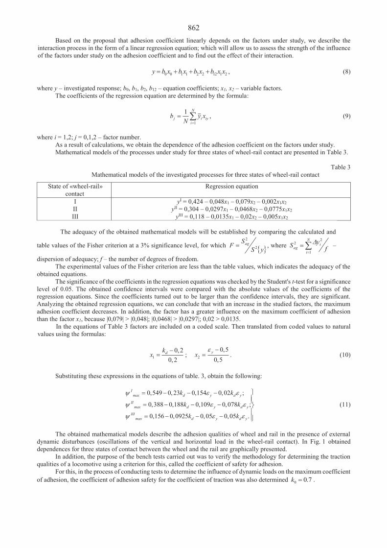
862 Based on the proposal that adhesion coefficient linearly depends on the factors under study, we describe the

interaction process in the form of a linear regression equation; which will allow us to assess the strength of the influence of the factors under study on the adhesion coefficient and to find out the effect of their interaction. 0 0 1 1 2 2 12 1 2y b x b x b x b x x , (8) where – investigated response; b0, b1, b2, b12 – equation coefficients; x1, x2 – variable factors.

The coefficients of the regression equation are determined by the formula:

1

1 N

j i iyi

b y xN

, (9)

where i = 1,2; j = 0,1,2 – factor number.

As a result of calculations, we obtain the dependence of the adhesion coefficient on the factors under study. Mathematical models of the processes under study for three states of wheel-rail contact are presented in Table 3.

Table 3 Mathematical models of the investigated processes for three states of wheel-rail contact

State of «wheel-rail» contact

Regression equation

I II III

yI = 0,424 – 0,048x1 – 0,079x2 – 0,002x1x2 yII = 0,304 – 0,0297x1 – 0,0468x2 – 0,0775x1x2

yIII = 0,118 – 0,0135x1 – 0,02x2 – 0,005x1x2

The adequacy of the obtained mathematical models will be established by comparing the calculated and

table values of the Fisher criterion at a 3% significance level, for which yS

SF ag2

2

, where N

i

iag f

yS1

22 –

dispersion of adequacy; f – the number of degrees of freedom. The experimental values of the Fisher criterion are less than the table values, which indicates the adequacy of the

obtained equations. The significance of the coefficients in the regression equations was checked by the Student's t-test for a significance

level of 0.05. The obtained confidence intervals were compared with the absolute values of the coefficients of the regression equations. Since the coefficients turned out to be larger than the confidence intervals, they are significant. Analyzing the obtained regression equations, we can conclude that with an increase in the studied factors, the maximum adhesion coefficient decreases. In addition, the factor has a greater influence on the maximum coefficient of adhesion than the factor x1, because |0,079| > |0,048|; |0,0468| > |0,0297|; 0,02 > 0,0135.

In the equations of Table 3 factors are included on a coded scale. Then translated from coded values to natural values using the formulas:

10,2

0,2dk

x ; 2

0,50,5

yx . (10)

Substituting these expressions in the equations of table. 3, obtain the following:

0,549 0,23 0,154 0,02 ;

0,388 0,188 0,109 0,078 ;

0,156 0,0925 0,05 0,05 .

Imax d y d y

IImax d y d y

IIImax d y d y

k k

k k

k k

(11)

The obtained mathematical models describe the adhesion qualities of wheel and rail in the presence of external

dynamic disturbances (oscillations of the vertical and horizontal load in the wheel-rail contact). In Fig. 1 obtained dependences for three states of contact between the wheel and the rail are graphically presented.

In addition, the purpose of the bench tests carried out was to verify the methodology for determining the traction qualities of a locomotive using a criterion for this, called the coefficient of safety for adhesion.

For this, in the process of conducting tests to determine the influence of dynamic loads on the maximum coefficient of adhesion, the coefficient of adhesion safety for the coefficient of traction was also determined 7.00k .

863

a b

c

Fig. 1 Theoretical (correlational) dependences of the maximum adhesion coefficient on the coefficient of vertical and horizontal load: a – clean dry rail; b – rail wetted with water; c – rail contaminated with lubricants

In Fig. 2 shows the dependence of the adhesion safety factor on the vertical dynamics coefficient kd and relative

to horizontal slipping y , plotted for mean values 7.0 obtained in experiments. Analysis of the results obtained indicates a significant effect of dynamic loads on the coefficient of safety for adhesion. So an increase in the coefficient of vertical dynamics from 0 to 0.4 decreases 7.0 by 17%, and an increase in the relative cross slipping from 0 to 1.0% reduces 7.0

by 25%.

Fig. 2 Experimental dependences of the coefficient of safety for adhesion on the coefficient of vertical dynamics kd and relative to horizontal slip y

3. Conclusions

Comparing the two methods for assessing the influence of dynamic loads on the traction qualities of the wheel-to-

864 rail tribological contact based on the maximum values of the coefficient of adhesion and the values of the coefficient of safety for adhesion, it can be concluded that the results are similar. So with an increase kd and y values as maximum adhesion coefficient max and the coefficient of safety for adhesion 7.0 decrease. Moreover, if with growth of kd from 0 to 0,3 max decreases by 12.7%, then 7.0 decreases by 10%; with growth y from 0 to 1,0% max is decreased by 28%, and 7.0 for 20%, those. The difference of these estimates in absolute values is 2...8%, leaving their character unchanged.

This conclusion can serve as confirmation of the expediency of applying the developed criterion – the coefficient of safety for adhesion – for a comparative assessment of the traction qualities of locomotives and its individual wheelsets. Acknowledgement

The study was carried out as part of the technical task of the research work DN-01-20 «Theory and practice of a systematic approach to creating a new rolling stock of railways with multifunctional control of thermomechanical loading «wheel-block-rail» to improve safety, energy and resource conservation» (state registration 0120U102220). References 1. Gorbunov, N.I.; Kovtanets, M.V.; Kovtanets, T.N. 2019. The energy effect of a two-phase flow on the contact zone

of the driving wheel with the rail is a method for controlling the coupling characteristics of a locomotive: Monograph. Odessa: Kuprienko S.V. – 181 p.

2. Gorbunov, M.; Kovtanets, M.; Kovtanets, T. 2020. Experimental study of the limit-maximum adhesion coefficient, The proceedings of the 24nd International Scientific Conference Transport Means 2020, 382-386.

3. Luzhnov, Y.M. 2003. Adhesion of wheels and rails. Nature and patterns. M.: Intext. 144. 4. Kostyukevich, A.I.; Gorbunov, N.I.; Kovtanets, M.V. 2013 Experimental verification of the effectiveness of jet-

abrasive impact on rails to improve the frictional properties of the contact «wheel-rail». Bulletin of the Volodymyr Dahl East Ukrainian National University. P.1, 18(207): 33-37.

5. Gorbunov, M.; Kovtanets, M.; Bureika, G.; Kovtanets, T. 2019. Reducing the wheel-rail system wear intensity with thermomechanical impact, Proceedings of the 23nd International Scientific Conference. Transport Means 2019, 1260-1265.

6. Gorbunov, N.I., Kovtanets, M.V., Nozhenko, E.S., Prosvirova, O.V. 2018. Analysis and development of ways to improve the adhesion qualities of locomotives. Collection of scientific papers, DUIT, Transport Systems and Technologies, VIP. 31. 59-72.

7. Gorbunov, M.I.; Kovtanets, M.V.; Kravchenko, K.O.; Kara, S.V.; Prosvirova, O.V.; Gorbunov, M.M. 2013. Patent of Ukraine 82903 on a utility model Stand for the study of the coupling of the wheel with the rail and testing of the elements of the axle spring suspension G01M 1/04, applicant and owner of Volodymyr Dahl East Ukrainian National University, u201214566, published 27.08.2013, bulletin 16. 3 p.

8. Gorbunov, M.I.; Kovtanets, M.V.; Kravchenko, E.A.; Chernikov, V.D. 2013. Theoretical analysis of the degree of influence of jet-abrasive flow parameters on the coefficient of friction of a wheel with a rail. Bulletin of the Volodymyr Dahl East Ukrainian National University 4(193): 63-67.

9. Gorbunov, M.; Pistek, V.; Kovtanets, M.; Nozhenko, O.; Kara, S.; Ku era, P. 2017. Research to improve traction and dynamic quality of locomotives, JVE International LTD. Vibroengineering Procedia 13: 159-164.

865

Proceedings of 25th International Scientific Conference. Transport Means 2021. Research of the Characteristics of Wheel and Rail Contact under the Influence of Design and Operational Factors K. Kravchenko1, J. Gerlici2, J. Harusinec3, O. Kravchenko4 1University of Zilina, Univerzitna 1, 010 26, Zilina, Slovak Republic; E-mail: kateryna.kravchenko@fstroj.uniza.sk, 2University of Zilina, Univerzitna 1, 010 26, Zilina, Slovak Republic; E-mail: juraj.gerlici@fstroj.uniza.sk 3University of Zilina, Univerzitna 1, 010 26, Zilina, Slovak Republic; E-mail: jozef.harusinec@fstroj.uniza.sk 4Zhytomyr Polytechnic State University, 103, Chudnivska str., 10005, Zhytomyr, Ukraine, E-mail: avtoap@ukr.net Abstract Redistribution of static loads from wheelsets onto rails during operation is one of the main reasons for the deterioration of traction qualities of a locomotive, they accelerated wear and increased impact on the track. The article presents an analysis of structural and operational factors affecting the realizable traction force of a locomotive. An assessment of the effect of vertical load on the parameters of the wheel-rail contact patch has been made. A design is proposed for redistributing the loads from the wheelsets onto the rails in the starting and braking modes. A device for automatic weighing of the load on wheelsets of a locomotive bogie is developed. KEY WORDS: coefficient to the utilization of the adhesion weight, loading device, contact patch, axle load 1. Introduction

The running gear of the operation rail traction rolling stocks and its regulation units does not allow full implementation of traction and braking forces of the vehicle. It's connected with the change in static weighing out during operation and dynamic redistribution during the implementation of the traction force. This increases the possible unevenness of the axle loads. This leads to a change in the area of the wheel-rail contact patch. Also, the normal stresses at each point of contact change. Reducing the vertical force on the first wheelset is the reason for the incomplete use of the adhesion weight of the traction rail vehicle, a decrease in the maximum traction force realized by the wheelset [1-3].

During operation, the mass of the locomotive changes due to the consumption of fuel, sand, and other equipment materials, as well as due to the repair and replacement of various equipment. For various types of locomotives, such a change can reach 4 - 6 tons, and in some cases up to 10 tons. Table 1 shows the values of the mass of equipment materials, by the value of which the mass of the locomotive can change during trips.

Table 1

Service masses and masses of equipment materials for locomotives

Locomotive series Power, kW Service weight, t Equipment weight, t E3 2 × 1472 2 × 126 2 × 8.14

2 E10L 2 × 2208 2 × 130 2 × 10.16

2 E116 2 × 2252 2 × 138 2 × 10.25

2 E121 2 × 2942 2 × 150 2 × 10.75

2 E126 4413 230 15.5

E136 4412 200 15.8

2 E116UP 2 × 2450 2 × 139 2 × 10.347

E114I 1801 120 7.04

E 150 3100 135 7.46

E 2 883 120 8.83

E 103 588 90 5.12

The estimation of the wheelsets unloading is determined by the coefficient to the utilization of the adhesion weight = Qilim / Qst (Qilim - load on rails from the most unloaded axle, Qst – static load) (Fig. 1). The adhesion coefficient o is

inversely proportional to : o = Ft / Pad· (Ft is the tangential traction force of the traction rail vehicle; Pad is the adhesion weight of the locomotive).

866

a b

Fig. 1 Assessment of the impact of the construction (a) parameters of the vehicle and the parameters changed during operation (b) on the coefficient to utilization of adhesion weight, in %

Redistribution of axel loads depends on a number of factors [1 - 18], which can be divided into: operational: o1 - change in the weight of the first wheelset; o2 - change in body weight due to the

consumption of equipment materials; o3 is the force created by the additional loading device; o4 - stiffness for the spring suspension 1st stage; o5 - stiffness for the spring suspension 2nd stage; o6 - the frictional force of the friction vibration damper; o7 - stiffness of the parts connecting the damper to the axle box; o8 - stiffness of the extreme supports of the second stage of spring suspension; o9 - stiffness of all supports of the second stage of spring suspension; o10 - adjustable spring suspension; o11 is the frequency of twitching disturbances from the action of the constant and variable components of the tractive efforts; o12 – railway tire wear along the rolling circle of the first wheelset,

and construction: d1 - distance from the center of the bogies to the external supports; d2 - elastic longitudinal bond; d3 - the ratio of the stiffness of the spring suspension 1st and 2nd stage; d4 - bogie wheelbase;

d5 - the angle of inclination of the spring suspension 1st stage guides to the horizontal; d6 - the distance between the first and second wheelsets; d7 - body weight; d8 - bogie weight; d9 - location of traction electric motors;

d10 - a type of connection between the bogie frame and the wheelset; d11 - location of the pivot joint above the plane of the railhead; d12 - distance from the bogie center to the internal supports of the rail vehicle.

The analysis of factors affecting the coefficient to the utilization of the adhesion weight of the rail vehicle is presented in Fig. 1 a and b. When designing and creating locomotives with high traction and braking qualities, it is necessary to select the parameters of the running gear taking into account the influence of the factors indicated in Fig. 1 a and b. Such actions will reduce the negative redistribution of loads from wheelsets to the rail. 2. Assessment of the Influence of Some Operational and Structural Factors on Characteristics of Wheel and Rail

Contact of the Shunting Diesel Locomotive TEM103

For the calculation, two programs were used, compiled in a FORTRAN 2008 language. The first program (POISK) was used to determine the coordinates of the points of pristine contact between the wheelset and the rail track. The second program (NRD) uses the data obtained in the first program (POISK). In the NZD program, the function of the initial clearance is derived, and the inertial decision of the normal contact task is performed.

The programs use the following conventions: P - vertical axel load; Y1, Y2 - points coordinates of initial tangency; – angle for solving in the points of initial tangency; Yl, Hl - lateral displacement and rotation angle of the wheel pair relative by the rail; M1, M2 - mesh surface size; Sx, Sy - surface mesh step; E is the specified solution accuracy; C1, C2 - codes of the shape of the contacting surfaces; A - the accuracy of solving the equation of initial tangency points; ccy - offset of the system origin along the axis; K - coefficient value all; Nc - the iteration cycles number to achieve a given solution accuracy; Fk is the contact spot area; ASP is the average specific pressure at the contact.

Initial data for calculations: - the unworn wheel profile; - the diesel rail vehicle TEM103; - GOST52366-2005. Table 2 and Fig. 2 present the calculating of the contact problem results by the 1-st wheelset of the diesel rail

vehicle TEM103. The calculation presented with working additional loading device. The rotation angle of the wheelset relative by the rail is 0º, the lateral displacement is 0 mm, the vertical load from the 1st wheel in the direction of driving on the rail is 103000 N. On the Fig. 2, presents the distribution of specific pressures over the contact elements, the maximum of which for this contact is 650 MPa. The contact spot shape is present in Fig. 2, b. All calculations are

867 summarized in Table 3.

Table 2 Initial and calculation data of contact task solving

Initial data P, kgf Y2, mm Y1, mm , rad Yl, mm Hl, 10292 0.04 -798 0.0000E+00 0.00 0.0

M1 M2 SX, mm SY, mm E C1 C2 A, mm 16.0 22.0 1.0 1.0 11 0.00 0.00 0.1941E+00

Calculation data ccy K Nc Fk, mm2 ASP, kgf/mm2 - 0.1890e-03 22 239.0 43.1

a b

Fig. 2 Contact pressure distribution, kgf/mm2: a – numerically (the calculation by the NRD program); b – schematically (MadCad)

Table 3

Modelling the i-th wheelset contact patch of the rail vehicle TEM103

The result in Table 3 presents that with an increase in the vertical load from 88 kN to 132 kN, the contact patch

area increases from 211 mm2 to 281 mm2. The average specific pressure increases from 426 MPa to 478 MPa. The maximum pressure from - 620 MPa to 680 MPa.

The changed locomotive parameters during operation are a negative influence on the wheel-rail contact. For the 1-st wheel pair, there is a decrease in the contact patch area by 8%. In turn, the use of additional loading devices for the 1-st wheel pair can increase the contact area by 7%.

868 3. Constructive Solution for the Redistribution of Vertical Axel Loads

To increase the vertical load in the implementation of the tractive effort, the additional loading device was modernized (Fig. 3), which was introduced on the TEM103 shunting diesel locomotive of LLC HC "Luganskteplovoz" [15-18].

Fig. 3 Installing a loading device on the bogie The loading device is mounted on frame 1 of the bogie (Fig. 3). When starting off the rail vehicle with the help

of the "Increase adhesion" button located on one of the control panels, the additional loading device is activated. The air is supplied to cavity A of cylinder 2 with the cover 14 under a pressure of 0.4 MPa. The piston 15 with rod 3 move upward. The release spring 16 is compressed. The lever 5, rotating about axis 12, through the rod 13 and the rollers 8, 9 support on the skids 10 welded to the frame 11 of the rail vehicle. With further movement of piston 15, the force from rod 3 through fork 4, the lever 5, the axle 12, and bracket 6 with the suspension 7 is transferred to the transverse beam of the bogie frame 1, increasing the load on the wheelset located on the side of the transverse beam.

The use of an additional loading device makes it possible to increase the coefficient of utilization of the adhesion weight, however, when it reaches 11 km / h, its efficiency decreases. Therefore, at a speed of 11 km/h, the control unit 18, connected to speedometer 17, is triggered. From cavity A of cylinder 2 through the solenoid valve 19, the air is released, and, under the action of the release spring 16, piston 15 returns to its original position.

To assess the redistribution of vertical loads from wheelsets onto rails during operation and further changes in the force of the loading device, weighing systems have been developed directly on the locomotive. The automatic weighing system is based on the method of measuring the mass of the crew by the total electrical signal from the primary measuring transducers, which can be used as a strain gauge sensor operating for bending of the BP-04 type. The weighing system consists of a block of primary measuring transducers I, which are installed on the axle box under the spring blocks of spring suspension, a control unit and electronic processing of the automatic weighing signal II, a remote communication unit with a control panel in the driver's cab III and a control unit for additional loading devices IV on the bogie frame (Fig. 4).

When the locomotive is operating, the primary pressure transducers 1 perceive the load P. At the output of the transducers, a signal appears proportional to the load at a specific point. The summation of these signals is carried out in measuring unit 2, from the output of which the signal goes to the amplifier 3, and then to the analog-to-digital converter 4 and the measuring unit 5. The device is powered from the rechargeable battery 6 through the voltage stabilizer 7. Warning sound and light signals about the degree redistribution of loads are supplied by signal unit 8. The received information is fed to the remote transmission unit 9 in the driver's cab. The transmitted information in a digital code is registered by the receiving unit 10, processed in the receiving register 11 with the issuance of a command for the necessary redistribution of the efforts of the additional loaders 12 and, using the address decoder 13, is written into the corresponding register for the redistribution of loads by a specific bogie 14. The adder records the general change in loads of the carriage part 15.

869

Fig. 4 Block diagram of a device for automatic weighing of the load on wheelsets of a locomotive bogie

4. Conclusions

In the process of a theoretical study of the contact patch, it was found that the use of a loading device makes it possible to increase the contact patch area by 7%, while the change in vertical loads from the action of operational factors reduces it by 8%. So the use of additional loading devices makes it possible to almost completely use the traction capabilities of the locomotive when starting off, even taking into account the influence of all the considered operational factors. When a speed of 11 km / h is reached, it is necessary to turn off the additional loading device. Acknowledgement

This publication was issued thanks to supporting the Cultural and Educational Grant Agency of the Ministry of Education of the Slovak Republic in the project No. KEGA 036ŽU-4/2021: Implementation of modern methods of computer and experimental analysis of properties of vehicle components in the education of future vehicle designers. References 1. Fufryanskij, N.A.; Dolganov, A.N.; Nestrahov A.S. and other 1988. Development of locomotive traction,

Moscow: Transport, 344 . (in Russian). 2. Vikhlyaeva, N.V.; Gorbunov N.I. 1984. On the influence of the stiffness of the body supports on the use of the

adhesion mass of a diesel locomotive, Design and Manufacture of Transport Vehicles 16: 41-45. (in Russian). 3. Konyaev, A.N. 1972. Research of traction properties and efficiency of diesel locomotives of high sectional power in

order to improve them, Thesis abstract of PhD, Moskow, 29 p. (in Russian). 4. Tasang, E.H.; Yakovenko, V.V.; Shafran, E.N. 2000. Traction-adhesion properties of the locomotive, Scientific

Journal «Bulletin of East Ukrainian State University» 7(29): 36-39. (in Russian). 5. Tkachenko, V.; Sapronova, S.; Kulbovskiy, I.; Fomin, O. 2017. Research of resistance to the motion of vehicles

related to the direction by railway, Eastern-European Journal of Enterprise Technologies 5(7/89): 65-72. 6. Smetank, L.; Št'astniak P.; Harušinec J. 2017. Wear research of railway wheelset profile by using computer

simulation, MATEC Web of Conferences, 22nd Slovak-Polish Scientific Conference on Machine Modelling and Simulations, MMS 2017, 157: Article number 03017.

7. Dižo, J.; Steišunas, S.; Blatnický, M. 2017. Vibration Analysis of a Coach with the Wheel-flat Due to Suspension Parameters Changes, 12th International Scientific Conference of Young Scientists on Sustainable, Modern and Safe Transport, TRANSCOM 192: 107-112.

8. Voronko, V.A. 2005. Justification of the choice of the parameters of shunting and industrial diesel locomotives taking into account operating conditions, Thesis PhD abstract, Moscow, 16 p. (in Russian).

9. Gorobchenko, O.M. 2007. Improvement of traction characteristics of locomotives by increasing the coefficient of use of coupling mass. Thesis PhD abstract, Kharkiv, 17 p. (in Russian).

10. Golishevsky, A.G.; Kashura, A.L.; Vivdenko, Yu.G. 2000. Influence of operational factors on the traction qualities of a locomotive, Scientific Journal «Bulletin of East Ukrainian State University» 7(29): 76-79. (in Russian).

870 11. Gorsky, A.V.; Vorobiev, A.A.; Buinosov, A.P. 1990. System for monitoring the diameters of wheelset tires,

Information collection TSNIITEITYazhmash 9: 38-40. (in Russian). 12. Saburov, F.F.; Bakholdin, V.I.; Ignatenko, G.I.; Kruchek V.A. 1993. Energy indicators of a locomotive with a

mono-motor drive at different diameters of wheelsets, Bulletin of VNTTI 3: 78-93. (in Russian). 13. Volpert, A.G. 1979. Influence of parameters of frictional vibration dampers on traction properties of locomotives,

Bulletin of VNIIZhT 7: 16-18. (in Russian). 14. Ivanov, V.N.; Belyaev, A.I.; Oganyan E.S. 1979. Increasing the utilization coefficient of the coupling weight of a

diesel locomotive, Bulletin of VNIIZhT 7: 13-16. (in Russian). 15. Patent UA 87915. 2009. Loading device. Bulletin 16: 4 p. 16. Patent UA 37890. Locomotive bogie. 2008. Bulletin 23: 6 p. 17. Patent UA 40369. Loading device. 2008. Bulletin 23: 6 p. 18. Patent UA 41434. Loading device. 2009. Bulletin 10: 6 p.

871

Proceedings of 25th International Scientific Conference. Transport Means 2021. Energy Efficiency Comparative Studies of Organic Rankine Cycle Implementation for a Sea Ferry S. Lebedevas1, T. epaitis2, O. Klyus3

1Faculty of Marine Technology and Natural Sciences, Marine Engineering Department, Klaipeda University, E-mail: sergejus.lebedevas@ku.lt 2Faculty of Marine Technology and Natural Sciences, Marine Engineering Department, Klaipeda University, E-mail: tomas.cepaitis@wsy.lt 3Faculty of Machnical Engineering at Maritime University of Szczecin, Waly Chrobrego 1-2, 70-500 Szczecin, Poland, E-mail: o.klyus@am.szczecin.pl Abstract One of the most effective solutions for the de-carbonization of maritime transport is the conversion of a ship's power plant's secondary heat sources into electricity using a cogeneration cycle. The publication presents the application of the common Rankine cogeneration cycle implemented to a ferry with Wartsila 12V46F power plant in ISO8178 (E3) load cycle modes, research and optimization of energy efficiency for a wide range of working fluids (R134a; R141b; R142b; R245fa; Isopentane). The implementation strategy of the cogeneration cycle is mostly revealed with a turbogenerator with a variable geometry turbine, ensuring a constant degree of pressure drop and working fluid flow interface in the wide load range of the power plant 25-100%. Significant advantages were not found between the evaluated Wet, Isentropic, Dry type liquids (R134a, R141b, R142b, R245fa, Isopentane) in terms of ORC energy performance with a 10% difference. The use of a variable geometry turbogenerator turbine with Dry type (R134a) working fluid is characterized by the highest ORC energy efficiency up to 15% and an increase in power plant (including turbogenerator generated mechanical) by 6.2%. KEY WORDS: Organic Rankine Cycle, heat recovery, energy efficiency, main engine load cycle 1. Introduction

The problem of maritime transport decarbonization, as a component of the general problem of reducing CO2

emissions in the transport sector, is being addressed on the normative basis of IMO standards. At 2011 July, Marine Environment Protection Committee introduced Energy Efficiency Design Index (EEDI) requirement which was implemented in 2013 January 1st and will be stringent by three phases every 5 years starting from 2015 [1, 2]. This requirement implementation estimates of potentially reduce CO2 emissions from 10% to 50% per transport work.

Recent several studies [3], reports and papers conclude that none of operational and design measures could have effective potential compared to the waste heat recovery systems as the approximately 50% energy of the fuel is wasted through exhaust gases and cooling jacket [4-7]. Exhaust gas temperatures of various type marine engines are between 260-450o C which makes it possible to receive such amount of steam in utilization system boilers that it would be possible to use it to increase energy efficiency up to 10% and to provide household consumer needs of heat and electricity as a pair. The temperature of exhaust gases decreases in low-speed marine diesel engines to a level of 250-300 C, and at partial loading conditions it is also significantly lower, which will complicate energy regeneration in waste heat utilization boilers with water as a working fluid [8, 9].

The use of organic working fluids with a significantly lower boiling point in comparison with water is free of the aforementioned disadvantages and at the same time significantly expands the temperature range of the cogeneration cycle. This case creates conditions for increasing energy efficiency indicators. However, although this technology is widely used in onshore plants, implementation of cogeneration cycles to maritime transport is lacking researches in order to properly assess energy aspects for practical application [10]. The mentioned aspects are related to the cycle energy efficiency indicators of the power plant in a wide operating load range and in connection with this, necessity to choose a rational strategy for managing the operational indicators of the cycle with the load modes of the main power plant, likewise the influence of the strategy for the realization of working fluid supply characteristics and the influence of the cycle realization depending on external conditions. No less important is the technological substantiation of the working fluid type, which to the greatest extent meets the requirements of achieving high energy efficiency and operational indicators of the cycle [11].

In order to increase the energy indicators of the cogeneration cycle for marine transport use, it is rational to expand the study of its energy indicators for alternative use of various types of working fluids (Wet, Dry, Isentropic) [12-14]. The listed tasks by the authors were examined in the study of the carried out comparative model studies of the organic Rankine cycle as part of a medium-speed medium speed four-stroke power engine.

872 2. Methodological Aspects of the Research

The applied organic Rankine cycle scheme in the studies is presented in Fig. 1. Simulation of thermodynamic

cycle performed in thermal engineering software Thermoflow which is the leading simulation tool for power and cogeneration industries. It allows to design cogeneration cycles from chosen components with user set properties and run this cycle simulation, receive results of desired parameters. (https://www.thermoflow.com/). In Thermoflow software classic single stage pressure organic Rankine cycle with recuperator exchanger to improve the energy efficiency indicators of cycle was designed. The following principles are (Fig. 1): the working fluid is heated and evaporated in a regenerative heat exchanger (pos. 3) to the state of saturated vapor; saturated vapor of the working material is supplied to the heat exchanger (pos. 12), in the turbogenerator turbine (pos. 6) regeneration of superheated working fluid vapor energy into mechanical work takes place, from the condenser (pos. 1) the working fluid leaves in the state of the saturated liquid (by applying saturation condensation pressure according outboard water temperature).

Fig. 1 Single stage pressure organic Rankine cycle with recuperator scheme in software Thermoflow: 1 – condenser; 2 – outboard; 3 – heat exchanger (recuperator); 4 – working fluid pump; 5 – seachest inlet; 6 – turbine; 7 – exhaust gas inlet; 8 – sea water pump; 11 – working fluid tank; 14 – atmosphere Ferry with power plant of two medium speed four-stroke main engines. Main specific engine parameters listed in

Table 1:

Table 1 List of medium speed four-stroke main engine specific parameters

Cylinder bore 460 mm Piston stroke 580 mm

Cylinder output 1200 kW/cyl Number of cylinder quantity 12

Speed 600 rpm Piston speed 11.6 m/s

Research performed main diesel engine working at specific test type E3 cycle load modes of ISO 8178, see Table 2.

Table 2

List of medium speed four-stroke main parameters at specific test type E3 cycle load modes of ISO 8178

Load modes Pe, kW n, rmp be, g/kWh Gair, kg/s Gf, kg/s Tg, °C 100% 1200 600 178,7 26,1 0,72 366 75% 900 545 188,7 23,35 0,54 309 50% 600 478 190,6 18,8 0,384 273 25% 300 378 197,0 14,5 0,2 255

Working fluids selection of this research consists of R134a; R141b; R142b; R123; R245fa; Isopentane fluids and

can be classified to three categories according slope of the saturated vapor curve in T-S diagram. Evaluation of energy indicators of the cogeneration cycle by differentially setting flow of the working material in

the system Gw.fl. in the load modes of the power plant, in order to achieve maximum energy utilization of the exhaust gas

873 (decreasing the exhaust gas temperature to the dew point 120 C); simulating a turbogenerator design with a fixed geometry turbine characterized by hydrodynamic relationship between working fluid flow Gw.fl. and the degree of pressure drop in the turbine turbogenerator T; evaluation of energy indicators of the cogeneration cycle improving possibilities by changing fixed geometry turbine design of the turbogenerator to a turbine with variable geometry (ensuring T = const at different working material flow (Gw.fl.).

The evaluation of different organic working materials in the cogeneration Rankine cycle was performed according to the change of the energy efficiency index of the running engine, the effective COP, including the components, by evaluating the additional form eR of mechanical energy generation power of the turbogenerator powerplant balance.

The cogeneration cycle COP structure includes energy transformation efficiency parameters in characteristic cycle nodes: . . .eR h ex tg r T ad m . (1)

The eR is obtained from the compared solution . . . .f uex g ex gQ G H Q and 3600

f u ee

G HP , as a result we

get:

.. . .

ex ge mh ex tg r T ad

e

QR , (2)

where Qex.g – relative part of the exhaust gas energy of power plant the heat balance kJ/h; h.ex – thermal COP of the exhaust gas heat exchanger; tg.r – the relative COP of the turbogenerator; T.ad, m – turbogenerator internal (adiabatic) and mechanical COP; – exhaust heat recovery factor; Hu – lower calorific value of fuel used by the traction engine, kJ/kg; Gf – hourly fuel consumption of the main engine, kg/h; e - main power plant coefficient of performance. Exhaust heat recovery factor is determined according the ratio of the enthalpy of exhaust gas before htg1 and after htg2 the heat

exchanger and the enthalpy of exhaust gas at dew point htg2: 1 2'

1 2

tg tg

tg tg

h hh h

.

The thermal efficiency of the turbogenerator is determined by the ratio of the enthalpies of the working fluid before htg1 and after htg2 the turbine and the enthalpy of the working fluid htg2 corresponding to the boiling temperature:

1 2. '

1 2

R Rtg r

R R

h hh h

.

These fixed values are accepted in the calculations (fixed values according specific to existing models): 0,7;Tad 0,95m ; . ( ) 0,97h ex exhaustgasheatexchanger ; . ( ) 0,97h ex condenser ; . ( ) 0,95h ex recuperatorheatexchanger pressure drop in exhaust

gas heat exchanger 2%; pressure drop in recuperator heat exchanger 2%. In an analysis of the cogeneration cycle components, turbine power generated by the turbogenerator Pgen was

determined in parallel by several analytical dependencies. Pgen it is expedient to describe in several forms, first of all, to evaluate their possible improvement in order to identify the factors determining the efficiency of the cogeneration cycle, on the other hand - to determine the relationship between the turbogenerator operating parameters for their reasonable choice:

. . 1 2

3600w fl tg tg

gen

G h hP , (3)

Gw.fl. – working material flow, kg/h; htg1; htg2 – working material enthalpy before and behind the turbogenerator turbine, kJ/kg.

Then the total mechanical energy generated by ME (main engine) with the COP of turbogenerator mechanical

energy is calculated 3600e tg

eu f

P P

H G and its change:

3600 3600e tg tge

ee u f u f e

P P Pe PH G H G P

. (4)

The efficiency of the cogeneration cycle in terms of power according to energy efficiency appliance – COP of the

turbogenerator is described by the equation:

. . ..

3600ex g tg r T ad mh ex exhaustgas

gen

QP . (5)

874

The above stated equation (Eq. (2)) eR is obtained from the compared solution . .ex g f u ex gQ G H q and

3600f u e

e

G HP , as a result we get a function from relative values: .

. . .ex g

h ex tg r T ad mee

Q.

When performing comparative studies of the prediction of the cycle efficiency, the value of Gw.fl. hall be antecedent as a constant with the main engine running at rated nominal power, provided that the exhaust gas temperature outside the regenerative heat exchanger does not fall below the dew point. If there is a need to reduce Gw.fl. in part-load engine load modes due to the same condition, it is performed at the interface with T changes.

When performing cogeneration cycle comparisons at the level when the turbogenerator type and its actual characteristics are not identified, the second turbocharger equation is used to determine the relationship between Gw.fl. and

T [15]

3. Results

The analysis consisted of several operational strategies: (Gw.fl.- T ) = const the flow rate of the working fluid material and the pressure expansion of the turbogenerator in

its turbine are constant in all load conditions of the power plant from 25% to 100% of the rated power. (Gw.fl = var) ( T = const) The strategy in all load power plant modes, cogeneration cycle COP ( . .cog c ) is constant

unlike Gw.fl. = const strategy Gw.fl. = var. The maximum value of the working material flow is limited by the dew point Tex.g. corresponding to the level of

the exhaust gases of the power plant leaving the heat exchanger (pos.12, Fig. 1). When the temperature drops below ~ 120oC, conditions are formed for a condensation of sulfuric acid from sulfur oxides in the exhaust gas occurs [15].

a b

Fig. 2 ORC energy indicator . .cog c comparison of strategies Gw.fl. = const ( ); Gw.fl.=var ( ); blue line – dry fluid; red line – isentropic/dry fluids; green line – wet/isentropic fluids

a b

Fig. 3 ORC energy indicator Pgen comparison of strategies Gw.fl. = const ( ); Gw.fl. = var ( ); blue line – dry fluid; red line – isentropic/dry fluids; green line – wet/isentropic fluids

875

Fig. 4 ORC realization strategy influence to ship power plant COP increase e ; Gw.fl. = const ( );

Gw.fl. = var ( ); blue line – dry fluid; red line – isentropic/dry fluids; green line – wet/isentropic fluids The equal relative change of the . .cog c parameter (Fig. 2, b) forms the basis for predicting the expected effect for

another working fluid based on the evaluation results of one working fluid, including converting the relative change of . .cog c to absolute.

Compared with Gw.fl. = const strategy the energy efficiency (Pgen) of the turbogenerator the increase is from 470 to 570 kW (Fig. 3, a). The maximum increase of Pgen is independent of working fluid type and characteristic are equal of R134a (Wet), R142b (Isentropic), Isopetane (Dry) fluids. Interestingly, with a different effect of Pgen increase, its relative change for all evaluated working fluids is the same (Fig. 3, b).

In addition, the intensity of the increase in Pgen increases with the increase of the power plant load regime in connection with the increase of the internal energy potential Qex.g. of the exhaust gas.

According to the performed verification, the correlation coefficient between Pgen and Qex.g. is equal to 0.5 (determination ratio R2 = 0.98).

The influence e of the increase of the power plant COP (Fig. 4) in the logical sequence was achieved the

largest Pgen increase effect in the mode – Pe nom up to 3-4%. The comparative evaluation of the energy parameters of the cogeneration cycle using different types of working

fluids was performed . .cog c genP in the graphical form Fig. 5.

Fig. 5 Comparative evaluation of working fluid type to energy indicators according ORC

4. Conclusions

Regeneration of secondary heat sources in marine power plants in the cogeneration cycle is considered as one of the effective ways to decarbonize maritime transport when estimating the energy potential of the exhaust gas and cooling system close to half of the heat balance of the power plant.

Optimization factor of cogeneration cycle fulfilling the parameters became operational strategies: working fluid flow and the expansion pressure in turbine adjustment for a constant and variable geometry type of turbine, as well as evaluating the influence of overboard water temperature.

876

The best indicators of cycle efficiency . .cog c and generated mechanical energy Pgen were obtained by implementing the strategy of differentiated regulation of the working fluid flow control in order to maximize energy potential of the utilization from the exhaust gas in different load modes, and the implementation of the pressure drop rate

T = const in a variable geometry turbine model: the cogeneration cycle . .cog c acquires the maximum value in the whole load range for all working fluids – 15% (R134a), 8.8% (Isopentane), and the respective power plant COP and _ .e plant increase by 6.2% and 5.3 %.

Due to the limited number of working fluids, there is a lack of data in order to declare energy advantage assessments for different types. Preliminary, it can be stated that Wet (R134a) and Isentropic (R141b) have better parameters, about 10% lower energy efficiency cycle efficiency indicators are typical for Dry (R145fa, Isopentane) type working fluid, although one of Isentropic representatives - R142b also has similar decrease in . .cog c parameter. Acknowledgement

Acknowledgement to “Thermoflow software developers. References 1. Smith, T.W.P; Jalkanen, J.; Anderson, B.; Corbet, J.; Faber, J.; Hanyama, S.; Parker, S. 2014. International

Maritime Organization, Third IMO GHG study 2014, London, UK. 2. IMO. Annex 5, Resolution MEPC.245(66), Guidelines on the Method of Calculation of the Attained Energy

Efficiency Design Index (EEDI) for New Ships; IMO, EU: London, UK, 2015. 3. Det Norske Veritas. Energy management study, Tech. rep. Det Norske Veritas; 2015. 4. Bombarda, P.; Invernizzi, C.M.; Pietra, C. 2010. Heat recovery from Diesel engines: A ther- modynamic

comparison between Kalina and ORC cycles. Appl Therm Eng; 30: 212-219. https://doi.org/10.1016/ j.applthermaleng.2009.08.006

5. Ancic, I.; Sestan, A.; Vladimir, N.; Klisaric, V. 2014. Influence of new power sources on the Attained EEDI. In Proceedings of the International Conference on Influence on Ship Design, London, UK.

6. Ancic, I.; Sestan, A. 2015. Influence of the required EEDI reduction factor on the CO2 emission from bulk carriers, Energy Policy 84: 107-116.

7. Schmid, H. 2014. Less Emissions through Waste Heat Recovery, In Proceedings of the Green Ship Technology Conference, London, UK.

8. Nagelhout, E. 2012. COMBINED HEAT AND POWER (CHP) Smart Power Generation - District Heating Solutions, WÄRTSILÄ POWER PLANTS.

9. Waste Heat Recovery System (WHRS) for Reduction of Fuel Consumption, Emissions and EEDI, MAN Energy Solutions.

10. Singh, D.V.; Pedersen, E. 2016. A review of waste heat recovery technologies for maritime applications, Energy Conversion and Management 111: 315-328.

11. Mahmoudi, A.; Fazli, M.; Morad, M.R. 2018. A recent review of waste heat recovery by Organic Rankine Cycle, Applied Thermal Engineering 143: 660-675.

12. Andreasen, J.; Larsen, U.; Haglind, F. Design of organic Rankine cycles using a nonconventional optimization approach, in: Proceedings of the 28th International Conference on Efficiency, Cost, Optimization, Simulation and Environmental Impact of Energy Systems, Pau, France, 1-12.

13. Soffiato, M.; Frangopoulos, C.A.; Manente, G.; Rech, S.; Lazzaretto, A. 2015. Design optimization of ORC systems for waste heat recovery on board a LNG carrier, Energy Convers Manag 92: 523-34.

14. Kalikatzarakis, M.; Frangopoulos, C.A. 2015. Multi-criteria selection and thermo-economic optimization of an organic Rankine cycle system for a marine application, Int J Thermodyn18(2): 133-141.

15. Sergey Ushakov; Harald Valland; Jørgen B. Nielsen; Erik Hennie 2013. Effects of high sulphur content in marine fuels on particulate matter emission characteristics, Journal of Marine Engineering & Technology 12(3): 30-39, DOI: 10.1080/20464177.2013.11020283

877

Proceedings of 25th International Scientific Conference. Transport Means 2021. Identification of Illegal Air Transport in the European Regulatory Environment A. Polanecka Czech Technical University in Prague, Faculty of Transportation Sciences, Department of Air Transport, Horska 3, 128 03, Prague, Czech Republic, E-mail: polanann@fd.cvut.cz Abstract This article describes the phenomenon of illegal commercial air transport and identifies the forms it can take. It further discusses the risk involved in legal and illegal air transport as well as provides an overview of recent accidents in the European Union where illegal air transport might have been a contributing factor. The last part compares the lack of initiatives to identify and deal with the problem at the European Union level as compared to the approach adopted by selected national authorities in other parts of the world. KEY WORDS: illegal air transport; illegal air charter; air taxi; cost-shared flights, familiarization flights 1. Introduction

While the term “commercial air transport” is most often associated with airline operations, most legal systems classify as such any transport of passengers and/or goods for remuneration or in exchange of any benefits of value. At the same time, applicable laws offer provisions for limited carriage of passengers in other forms than commercial air transport as long as such activities are limited in scope or in the amount of compensation sought by the provider of such service. With respect to the requirements on such other forms of passenger carriage, all of the forms discussed further require their providers to comply with more relaxed rules, which, as a consequence, lowers their costs and allows such services to be either offered at significantly lower rates, or increases the margins on income obtained from such activities.

However, the provision of other forms of passenger carriage may result in tax avoidance, directly and indirectly. Direct avoidance occurs where a tax, e.g. the air passenger duty, would be applicable to commercial air transport while the carriage of passengers by other means is not subject to the tax. Indirect avoidance results from the non-standard arrangements between the provider of the service and, for example, the pilot who carries out such flight, and who is provided compensation for his/her work in other means than a paid job, which can result in less or no income tax paid both on the side of the “employer” and the “employee”.

Besides financial aspects, the safety standards may be lowered due to both lower requirements on operations per se as well as the fact that national authorities may carry out less oversight of this kind of flight operations. As discussed further, general aviation shows higher accident rates which are attributable to a combination of less pilot experience and qualifications, less stringent requirements on maintenance and less demanding operational rules, which are all considered appropriate to the purpose and scope of general aviation, but are not acceptable to commercial air transport where the passenger is a consumer with little knowledge of the risks he/she is undertaking when buying such a service.

Tolerating illegal air transport distorts the commercial air transport market and puts properly certified operators at a cost disadvantage while consumers may be oblivious to the nature of service they have purchased and the level of protection and compensation offered in the case of an accident. Therefore it is important that the phenomenon of illegal or misdeclared air transport is recognized and acted upon by overseeing bodies and that tools are developed for transparent distinction between other legal forms of passenger carriage where appropriate, legal commercial air transport and illegal or semi-legal activities.

This article identifies the regulatory environment in which commercial air transport and other forms of passenger transport are performed in the common EU regulatory system and shows the approach adopted by the authorities of other comparable markets, namely the United States and the United Kingdom. 2. Regulatory Background in EASA Member States

The European market is to a large extent regulated by common requirements. The safety aspects including commercial air operator certification and the certification or oversight of other aviation undertakings are covered by a comprehensive set of regulations and legal acts stemming from Regulation (EU) 2018/1139 [1]. As a result, the definition of the various forms of operation that involve carrying passengers in exchange for remuneration are essentially the same in all EASA (European Union Aviation Safety Agency) member states. The financial aspects, namely the tax obligations of individual air transport enterprises, are covered by European Union (EU) directives at the high level, but detailed further by national law system as a result of the fact that in the area of tax systems, the European Union does not publish common regulations binding to individual entities in member states. Instead, directives require member states to adopt common principles, which is done by adopting national laws compliant with those directives but

878 specifying additional provisions including specific tax rates within each member state. Non-EU EASA member states cannot be anticipated to maintain commonality with EU tax directives. As a consequence, the taxation of air transport, salaries etc. may differ among EU as well as EASA states, but there is no evidence that tax rate differences would cause a significant competitive advantage in the area of commercial air transport in one country compared to another.

Regulation (EU) 2018/1139 defines commercial air transport as aircraft operation to transport passengers, cargo or mail for remuneration or other valuable consideration [1]. This essentially means that whenever the operator of the aircraft receives monetary or non-monetary compensation in exchange for operating a flight with passengers, cargo or mail on board, such operation is considered commercial air transport. In broader terms, positioning, i.e. empty flights not carrying any of the above but associated to the carriage of such items (i.e. flights to the place of loading or from the place of unloading) are generally considered to be operated under commercial air transport too, as they are invoiced to the entity ordering such flight and hence paid for. However, there are other underlying issues such as less stringent crew duty time limitations that force operators to declare them as non-commercial, altough they are paid for. The EU aviation regulatory framework does not directly address empty flights paid for by the customer of a preceding or onward flight, hence it largely remains up to the operator to operate such a flight commercially or non-commercially. In terms of safety, as such a flight does not involve any service being provided to a consumer and physical damage can only be caused to the operator itself or third parties, there is no particular interest on the side of oversight bodies, competition or cosumer protection initiatives to regulate such flights and force them into commercial air transport.

Regulation (EU) 965/2012 [2] provides derogations which allow certain types of operations to be conducted in accordance with requirements on non-commercial operations. It is commonly understood that these operations are considered non-commercial operations, althought the exact wording of the legislative act does not exclude these activities from the definition of commercial air transport, it only stipulates that the operational and organizational requirements on such operations are governed by those parts of the regulation that are otherwise applicable to non-commercial operations rather than those required of commercial air transport operators. This discussion has little practical impact on safety as the aplicability of operational rules is explicitly stated in the regulation, however, it would deserve a discourse on the impact on tax obligations and the assessment of the operator’s area of economic activity. The derogation from commercial air transport requirements, which is essentially an alleviation from the applicable operating rules, defines three types of activities than can still be subject to remuneration or other forms of compensation: cost-shared flights, competition and display flights and certain activities undertaken by a flight school or an organization promoting aerial sport or leisure flying [2]. Of these activities, familiarization flights and aerobatic flights are those where uncertainty about their nature is likely to arise, as they clearly involve carriage of passengers. The other exempted activities include parachute dropping and sailplane towing, where the distinction from air transport is obvious as they require the presence of parachute jumpers or a sailplane. Another aspect worth noting is that for a flight school or a leisure organization to be able to provide passenger-carrying flights under the non-commercial operating requirements, such an activity is operated with their own aircraft or under dry-lease terms, i.e. the given organization retains all responsibilities of an operator, staffs the flights with their own crews and does not engage in further sub-leases or arrangements to have the flights operated by another operator. Furthemore, unless such activities are provided for its own members, they must remain marginal and not take place of the main activity the organization undertakes. 3. Definition of Illegal Commercial Air Transport

In general terms, illegal commercial air transport encompasses any flight that, according to its nature, would be covered by the defition of commercial air transport, i.e. carries passengers, cargo or mail, where the operator is compensated for the carriage, in monetary terms, provision of valuable services or exchange of valuable goods, but the operator does not hold an air operator certificate and, at the same time, the flight does not meet the criteria of the exempted operations stated in paragraph 2 above. Flights that are operated under an existing air operator certificate but do not meet the applicable requirements laid down in regulation (EU) 965/2012 are not considered illegal commercial air transport, the operator exercises privileges granted to it, only with the caveat of not being compliant with the terms of its approval and hence facing various penalties from administrative proceedings to financial penalties to, in the most extreme case of non-comformity, certificate or approval revocation. However, identification and elimination of illegal commercial air transport necessitates further differentiation in the form of illegality of such operations.

3.1. Explicit Illegal Commercial Air Transport

For the purpose of this article, explicit illegal commercial air transport is such where the operator does not fall within any of the exempted categories, does not hold an air operator certificate or holds an operator certificate for other types of operations, e.g. with a different type of aircraft or a particular airframe not covered by the certificate and where it is unlikely that the operator provides the flights in good faith that either no certification is needed for such flights or the certificate it has is applicable. Continued operations in this manner usually require relatively thorough knowledge of applicable regulations and ways of avoiding them or ways of disguising such operations under other approvals such as flight schools, specialized operations or, in the terms of some countries, aerial work. This in turn requires some organizational structure, on the background, the operator is run in an efficient way similar to an air operator certificate holder, i.e. has multiple crews (employees or free-lance staff) to staff flights to meet demand, it is likely to operate more than one aircraft in this manner, flights are advertised as on-demand through dedicated channels and the operator is usually very skilled at keeping only those records that support the non-commercial semblance of the flight while proof

879 of payment is often destroyed or not issued with proper identification details, or the contract is drafted in such a manner that the customer, often unknowingly, takes responsibility of the flight. One such example that was identified as a result of an accident in the United States was Platinum Jet, an operator that provided charter flights which would fall under the provisions of Federal Aviation Administration (FAA) Part 135 operations. In the EU regulatory system, an air operator certificate would be needed for such operations and all commercial air transport requirements as defined by regulation (EU) (965/2012) would apply. The operator did not hold the respective certification but entered into a partnership with another Part 135 operator. While the operational set-up was overtly presented as such where Platinum Jet would advertise the business and ensure crews who would be trained according to the other properly certified operator’s requirements, standards and approval and the operations would comply with the procedures thereof, some of the flights including the one involved in the accident were operated by crews that had not received all the training, did not comply with duty time limitations and generally were not operated in accordance with the other company’s approval [3, 4]. Other forms of explicit illegal air transport are organized business activities where a company intentionally pairs aircraft owners, individual operators (pilots) and customers and acts as an intermediary so that the responsibility and accountability remains with the pilot or the customer through a contract which one or another may not fully understand and they therefore provide or make use of the service in good faith that either the intermediary or the other party of the contract is either legal to provide such service or assumes responsibility for the flight [5]. However, while in the US legal system the FAA was able to defend its view that the intermediary was actually involved in the fraud, in the EU environment, aviation authorities would have little room for initiating prosecution against an intermediary and would have to take action against the operator, i.e. directly the pilot, as the intermediary would not be directly involved in the operation.

3.2. Unintentional Illegal Air Transport

Unintentional illegal air transport results from either not understanding the applicable regulations or from believing that the nature of the flight belongs to non-commercial operations or is covered by one of the exemptions. The simplest form of this activity is a situation when a private owner, himself or herself a licenced pilot but not having the organizational structure of an air operator certificate holder and not holding the certificate as such offers to provide his/her own services to a friend, colleague or any other entity, who in return pays for the flight or, even more implicitly, provides another service or product in exchange for such transport. In a more organized form, holders of approved training organization certificates might at times be tempted to offer familiarization flights that amount for more operational time and/or more income than their main activity, in which case the activity temporarily exceeds the conditions for the exemption and should be classified as commercial air transport. Less common situations may arise where an otherwise legal air operator certificate holder operates an aircraft that is to be entered into its certificate or has been withdrawn but administrative errors or lack of updated information results in operations of such a flight. 3.3. Misdeclared Air Transport

Misdeclared air transport, in this article, is such air transport where the flight is operated under one of the exemptions, i.e. the operator believes that the flight is covered by the derogation, while it is not. It is frequently up to the operator and the overseeing authority to present evidence to defend each one’s point of view, as naturally exempted operators tend to see the aspects that qualify for the exemptions while the authority, their competition or possibly victims of an incident or accident may tend to put more emphasis on those aspects that qualify for commercial air transport. In this category, shared-cost flights can be found if the pilot, who is supposed to share the cost of the flight, seeks most costs to be covered than those that are eligible. However, probably the most common practice is the use of familiarization flights where the customers show little potential for further involvement in leisure or sport flying or flight training and their sole purpose is to get from one place to another or to enjoy a sightseeing flight.

Regarding cost sharing, it is important to note that regulation (EU) 965/2012 only requires that cost be shared among all the occupants including the pilot himself/herself and that such costs represent only the direct costs of the flight such as fuel, aircraft rental or airport fees [2]. There is no specific proportion of costs to be shared by the pilot, i.e. the operator, and the matter of assessing whether the covered costs are only direct costs can be difficult as there is no general requirement for the pilot to keep accounting books, invoices or otherwise record the cost structure.

4. Risks of Illegal Air Transport

In terms of statistics, EASA has presented data that indicate the non-commercial operations show a higher accident probability than commercial air transport. While the statistics presented in the Annual Safety Review 2020 [6] cannot be compared with certainty – the data for commercial air transport only cover large aeroplanes and do not follow commercial operations with other categories of aeroplanes, while non-commercial accident data are divided between complex and non-complex aircraft. Within this in mind, data on commercial operations are comparable to data on non-commercial complex aircraft operations, however, a large proportion of suspected illegal air transport is undertaken with non-complex aircraft. Even if non-complex aircraft commercial data were included, the comparison would not be fully representative, as the proportion of these aircraft in legal and document air transport is much smaller than the proportion of non-commercial flights with these aircraft. However, the data available indicate that commercial air transport is safer than non-commercial operations. For 2019, the last year available, the accident rate among commercial

880 air operations with large aeroplanes amounted to 4 per 1 million flights, or the probability of an accident of 4×10-6. The yearly average for the period between 2015 and 2019 reached 3.2×10-6 [6]. The accident rate for non-commercial complex operations cannot be determined from the data as there is only reference to the absolute value of accidents, but not the number of flights executed. However, comparing the data to small (non-complex) aeroplanes for the same periods, the 2019 accident rate was 6.09 accidents per 100 000 flights, i.e. a probability of 60.9×10-6 and the 2015–2019 average was 73.6×10-6 [6]. While it cannot be ascertained from the data provided whether the increased risk is due to organizational factors, i.e. would be attributable to the lack of proper company management, training, standard operating procedures and other requirements that constitute the difference between commercial and non-commercial operational requirements, or whether it is due to the fact that the size and design of the small aircraft covered by the statistics entails higher risk due to frequent occurrence of single-engine equipment or piston engines, the risk to the customer is evident and it is estimated, based on the above data, to be approximately 10 times higher than in legal commercial air transport.

It could be concluded from the data presented above that, in the first place, the safety of non-commercial operations should be improved. While this would theoretically be possible by imposing more stringent requirements comparable to those of commercial air transport, it is important to leverage the interests of all stakeholders. In non-commercial operations, the stakeholders are, in the first place, leisure pilots, flight schools that cater to both leisure pilots and future airline pilots, private persons who use their own or rented aircraft as an individual means of travel etc. These persons are generally aware of the risks they undertake when engaging in these activities, and, to a large extent, can control the risk by not operating in conditions or areas where they do not feel proficient to do so. On the other hand, customers of illegal air commercial air transport should not be taken into consideration when considering whether the risk is acceptable, instead, it needs to be ensured that they are referred to those service providers that hold the appropriate certification and hence are compliant with the more stringent commercial air transport requirements.

4.1. Overview of Suspected Illegal Air Transport in EASA States in 2016–2019

As part of this research paper, reports of accidents in years 2016 to 2019 listed in EASA Safety Annual Review 2020 [6] of non-complex airplanes and non-complex helicopters in non-commercial operations have been investigated. As the purpose of the investigation in accordance with international standard, namely ICAO Annex 13, is to prevent future accidents and incidents, not to investigate illegal acts or criminal offences, these reports are not classified according to suspected illegal air transport nor is this aspect explicitly evaluated. However, several factors were taken into account to assess whether the respective flight could have been illegal air transport, explicit, unintentional or misdeclared. These aspects included:

1. The explicit mentioning of passengers on board; and 2. The lack of relationship between the passengers and the pilot (e.g. pilot and instructor, family members,

friends etc.); and 3. The fact that the preceding flight to the place of passenger boarding was an empty flight and the destination

was different from the base of the aircraft, base of the pilot etc.; or 4. Explicit evidence of advertising the flights, existing information on chartering the flight or evidence of

previous attempts to provide the flights commercially. Based on these criteria, the following number of accidents reported and accidents suspected to be illegal air

transport were identified as summarized in Table [10-15].

Table Number of Accidents and Suspected Commercial Illegal Air Transport Accident

Year Airplanes Helicopters Accident number Suspected illegal Accident number Suspected illegal 2016 4 1 47 0 2017 5 1 33 0 2018 6 0 53 2 2019 3 0 47 0

The table above does not include one high-profile illegal air transport case in 2019 where a famous football

player was a victim of an air accident caused by inappropriately qualified pilot lacking experience in the weather conditions the flight was operated in [7]. The reason for this is that the flight was performed by a US-registered aircraft that does not fall within the scope of EASA reporting.

5. Oversight of Illegal Commercial Air Transport

It is evident from the data presented in part 4 above that there is a potential for improving safety by proper oversight of commercial air transport and focusing on illegal operations. The purpose is not to eliminate other forms of flight operations for remuneration, but differentiate between users of flight services who willingly and knowingly accept the increased risk of non-commercial operations and those who, in good faith, purchase the services in the role of consumers, not acquainted with the inherent risk of general aviation.

881 The most advanced oversight program has been found in the US, where the FAA operates the Safer Air Charter

Operations initiative [8]. This is a multi-layered approach where the authority promotes certified operations and helps consumers identify illegal operators, which is done through a questionnaire identifying typical signs of such operations such as lack of travel documents and proof of payment, various lease contracts and other wording indicating that the consumer assumes responsibility for the flight or by publishing a list of approved operators. At the next level, it has prepared a questionnaire for customers who might have travelled on an illegal flight to ascertain the status of the flight, and, at the last stage, it has collected evidence and imposed penalties or initiated prosecution of suspected illegal operators. In the EU, there is no such coordinated initiative. The most systematic approach has been adopted by the UK (now not a member of the EU), whose national civil aviation authority runs an awareness campaign to that of the FAA, albeit it could not have been confirmed whether any illegal operations have been identified and prosecuted [9].

There is no such coordinated approach on the side of the EU, even though EASA as the common aviation safety agency of the member states would be best positioned to both draft regulatory documents to assess illegal air transport as well as to promote awareness about the risk associated with different types of paid forms of transport. It is necessary to develop a thorough system of identifying suspected illegal operations, collecting evidence and prosecuting such undertakings to enhance the safety of operations. 6. Conclusions

This paper has identified the phenomenon of illegal commercial air transport within the EU and the different forms it can take, from organized for-profit businesses to less obvious forms often unintentionally performed by individuals with a lack of awareness of the status of their flights. It has shown that the risk of an accident increases in non-commercial operations and that there are indications of illegal air transport leading to accidents and unnecessary loss of lives in the EU. Possible approaches to tackle the problem have been identified based on foreign experience, in particular from the US and the UK. The research will continue to develop a performance-based tool to identify illegal operations and to collect evidence to carry out proper oversight. References 1. European Parliament, Council of the European Union. Regulation (EU) 2018/1139 of July 2018 on common rules in

the field of civil aviation and establishing a European Union Aviation Safety Agency [online cit.: 2021-06-19]. Available from: https://eur-lex.europa.eu/eli/reg/2018/1139/oj

2. European Commission. Regulation (EU) 965/2012 of October 5 laying down technical requirements and administrative procedures related to air operations pursuant to Regulation (EC) No 216/2008 of the European Parliament and of the Council [online cit.: 2021-06-19]. Available from: http://data.europa.eu/eli/reg/2012/965/oj

3. Drewniak, M. 2009. Charter Flights Director of Defunct Private Jet Company Admits Using Unqualified Pilots [online cit.: 2021-06-22]. Available from: https://www.justice.gov/archive/usao/nj/Press/files/pdffiles/2009/ sing0707%20rel.pdf

4. Founders Of Luxury Charter Jet Company Sentenced To Prison In Illegal Flight Scheme [online cit.: 2021-06-22]. Available from: https://www.justice.gov/archive/usao/nj/Press/files/Brassington,%20Michael%20and%20Paul%20 Sentencing%20News%20Release.html

5. On Petition for Review of an Order of the Federal Aviation Administration [online cit.: 2021-06-23]. Available from: https://www.faa.gov/about/initiatives/safe_charter_operations/media/Decision_Flytenow.pdf

6. European Union Aviation Safety Agency. 2020. Annual Safety Review 2020 [online cit.: 2021-06-18]. Available from: https://www.easa.europa.eu/sites/default/files/dfu/easa_asr_2020.pdf

7. Emiliano Sala plane crash: UK investigators publish final report [online cit.: 2021-06-23]. Available from: https://www.dw.com/en/emiliano-sala-plane-crash-uk-investigators-publish-final-report/a-52761189.

8. Safer Air Charter Operations [online cit.: 2021-06-18]. Available from: https://www.faa.gov/about/initiatives/ safe_charter_operations/

9. Civil Aviation Authority UK. Making Sure Your Flight Is Legal [online cit.: 2021-06-24]. Available from: https://www.caa.co.uk/Consumers/Guide-to-aviation/Making-sure-your-flight-is-legal/

10. Final Report No. 4-02/2-17(3-2018) [online cit.: 2021-06-25]. Available from: https://www.taiib.gov.lv/en/media/ 83/download

11. Relazione D’Inchiesta [online cit.: 2021-06-25]. Available from: https://ansv.it/wp-content/uploads/2020/12/ Relazione-N109W-3.pdf

12. Passage dans des nuages en descente, collision avec la vegetation puis un bâtiment [online cit.: 2021-06-25]. Available from: https://www.bea.aero/docspa/2014/hb-c141002/pdf/hb-c141002.pdf

13. Untersuchungsberich [online cit.: 2021-06-25]. Available from: https://www.bmk.gv.at/dam/jcr:0873c6cf-0943-4bc1-8c05-de87793b0d14/140405_enstrom_280fx_gz85206.pdf

14. Untersuchungsberich [online cit.: 2021-06-25]. Available from: https://www.bfu-web.de/DE/Publikationen/ Untersuchungsberichte/2018/Bericht_18-1533-3X_F172_Wasserkuppe.pdf?__blob=publicationFile

15. AAIB Bulletin: 3/2019 [online cit.: 2021-06-25]. Available from: https://assets.publishing.service.gov.uk/media/ 5f5a2f348fa8f5106b23a9f6/Cessna_152_G-UFCO_03-19.pdf

882

Proceedings of 25th International Scientific Conference. Transport Means 2021.

Modeling of Virtual Traffic Situations

P. Verta , G. Kasanický

Institute of forensic research and education, University of Zilina, Univerzitná 8215/1 010 26 Žilina, Slovakia,E-mail: peter.vertal@usi.sk

Abstract

The paper describes the application of a virtual evaluation technique method based on stochastic simulations for modeling critical traffic situations. In the stochastic simulation approach, we have may simulate behavior of the driver also different conditions for the vehicle, include border conditions of the model. Driver and vehicle characteristics, vehicle trajectories, and traffic situations are also drawn from a virtual situation, as well as environmental variables. Base on basic and well know information about environment influence and physical potential of the car is possible to simulate the traffic scenario as a turn-left situation onto a T-shape junction. Right input model for stochastic simulation might lead to a result, which helps to find up the new solution for injuries mitigation, mortalities reduction and collision avoidance or at least compare this method with real in depth accident data.KEY WORDS: principal direction of force, stochastic simulation, traffic accident

1. Introduction

Stochastic simulation is well known tool. I would like to present the possibilities of this tool in the area of traffic accident investigation and reconstruction. For stochastic simulation was used a mathematical model of traffic situation onto junction. A mathematical model was implemented in the virtual environment in PC Crash 9.2 accident simulations software. PC Crash 9.2 software provides possibilities to simulate different scenes base on physics rules.

1.1. Street Scenario Modeling

The scenario of particular simulation is basic scenario turning left situation onto urban area t-shape junction. As the picture has below shown, the blue car is driving straight to the junction onto a priority way line. The driver of the blue car can see the red car in the middle of the junction. In a moment of recognition obstacle in priority line, the red car is located into the junction in the position as Fig. 1. Various scenarios were taking into account for the stochastic simulations.

2. Driver and Vehicle Modeling

The velocity of the blue car, when the driver of the blue car recognizes the red car, is for each simulation constant 50 km/h (maximum velocity in urban area). Because the red car is located at 0.6 m in the blue car line, it could be appearing for the driver of the blue car, that the red car may become an obstacle in the line and that driver of the red car has intent to turn left.

Fig. 1 Traffic scenario of critical situation onto junction

Various scenarios were taken into account for the stochastic simulations. The driver of the blue car can recognize the red car from various distances before the junction. After recognition of the red car, the driver of the blue car has

883 reaction time tr = 1 s a then fully breaking with decceleration of a = 9.81 m/s2. Red car in the position as picture below may standing (vred = 0 km/h), moving constantly (vred = constant km/h) or moving with acceleration (accred > 0 m/s2).

For stochastic simulations was taken into account for the blue car, that the shortest distance to the reaction of the driver before the collision with the red car is 14 m (1). The 14 m is approximately a distance for reaction time tr = 1 s for 50 km/h (13,88 m/s).

min rS t v = 13,88 m 14 m [1]. (1)

The longest distance to the reaction of the blue car in various stochastic situations is 22 m. The distance sb of 24

meters is safety distance to stop the blue car before the contact with red car and avoidance the accident. Braking time of fully deceleration from 50 km/h to 0 km/h is tb = 1,42 s.

13 88 1 429 81b

v ,t ,a .

s [2]; (2)

2

23 772

bb

a ts v t , m 24 m (3)

The start conditions of the red car were 0, 5, 10, 15, 20 and 25 km/h in location as Fig. 1 shown. Velocity higher

than 25 km/h will lead to the unstability of the blue car.

7 5 0 8 9 81 7 67v R g . . . . m/s 28 km/h [3]. (4)

The potential influence of the mass of the vehicle was taken into account. Three different combinations of vehicle scenarios were thought. The first category was priority way vehicle with weight 1000 kg with a collision with giving way vehicle of weight 2000 kg. The second category was priority way vehicle with weight 2000 kg with the collision of giving way vehicle of weight 1000 kg. The last category was a vehicle of priority way with weight 2000 kg with a collision with giving way vehicle of weight 1000 kg. 2.1. Principal Direction of Force PDOF

The PDOF (Fig. 2) is measured relative to the direction the center mass was traveling on impact, typically along the longitudinal axis of the vehicle for which the PDOF is being determined. When the PDOF angle is expressed as a positive number it identifies a PDOF that intersects the longitudinal axis from the right, while a PDOF expressed as a negative number identifies an angle intersecting the longitudinal axis from the left.

Fig. 2 Measure of principal directional of force 2.2. Result of Simulations

The different modeling conditions lead to simulated 180 potentional critical traffic cases onto the turn left

scenario. Base on 180 modeling cases from PC Crash 9.2 simulation, charts were made (Fig. 3-4). From 180 scenarios, accident scenario occur into 129 cases. In 51 cases cars miss contact and situations were evaluated as safe. The highest probability of contact area onto priority way car is in location of 11-12-1 hours. It means in frontal crash situations.

884

Fig. 3 Distribution of PDOF of priority way car

The give way car distribution of PDOF is shown in Fig. 4. The highest probability of impact area onto giving way car is located into 2-3-4 hours. In total 71 cases lays in this area. Area 2-3-4 hours is an area of a side impact. Crash situations occurred in 58 cases in the area of frontal crash 1-12-1 hours.

Fig. 4 Distribution of PDOF of priority way car

Fig. 5 Distribution of PDOF according of speed of give way car

885 The paper has shown a mathematical model of the critical situation onto junction. The model may be to compare

with real data’s from accidents. If the model will be comparable with a real traffic accident database, the simulation could be used for the evaluation of traffic accident. If we know the damage of the car, we can investigate the velocity of the vehicle (Fig. 5). We can see that dependency on the velocity of giving way car has influence to the principal directional of force. The probability of accident also depends of the speed of giving way car. With raise velocity of give way car also raise the probability of avoidance the accident. But with higher velocity raise angle of principal directional of force and it leads to side impact. The stiffness of the frontal part of cars is higher than the side part [3]. Side impact will occur in less case, but consequences from side impact will lead to serious injuries. 3. Conclusions

High probability in case of turn-left junction scenario is that principal direction of force for priority way car will

be from -28° to 5° and principal directions of force for giving way car will be from 5° to 75°. Lower speed of giving way car will lead to fontal impact with priority way car. With rising velocity of give way car also raise the probability of avoidance of accident. But with higher velocity raise the angle of principal directional of force of give way car and it leads to side impact. The stiffness of frontal part of cars is higher than side part. Side impact will occurred in less case but consequences from side impact will lead to serious injuries. References

1. Kasanický, G.; Kohút, P.; Lukášik, M. 2001. Teória pohybu a rázu pri analýze a simulácii nehodového deja,

EDIS, Žilina. 2. Bradá , A.; a kol. 1999. Soudní inženýrství, AKADEMICKÉ NAKLADATELSTVÍ CERM s.r.o., Brno. 3. Burg, H.; Moser, A. 2009. Handbuch Verkehrsunfallrekonstruktion. Vieweg Verlag Wiesbaden.

886

Proceedings of 25th International Scientific Conference. Transport Means 2021.

Modeling of Metrological Support of Qualimetric Measurements on Transport

I. Kulbovskyi1, H. Holub2, S. Sapronova3, O. Bambura4 1State University of Infrastructure and Technologies, Kyrylivska str., 9/3, 04071 Kyiv, Ukraine, E-mail: kulbovskiy@ukr.net 2State University of Infrastructure and Technologies, Kyrylivska str., 9/3, 04071 Kyiv, Ukraine, E-mail: golub.galina@ukr.net 3State University of Infrastructure and Technologies, Kyrylivska str., 9/3, 04071 Kyiv, Ukraine, E-mail: doc.sapronova@gmail.com 4State University of Infrastructure and Technologies, Kyrylivska str., 9/3, 04071 Kyiv, Ukraine, E-mail: bambura_olja@ukr.net Abstract The issues of metrological support of qualimetric measurements on transport are covered and the main problems of measurements are determined. There is a problem with the metrological support of measuring individual characteristics of a product, which evaluates the quality of these products and measuring product quality in a comprehensive sense. Thus, the measurement of product quality is almost absent, even if the values of the relevant characteristics are measured fairly reliably. Qualimetry is defined as combining quantitative quality assessment methods used to justify quality management decisions. Given this statement, it is proposed to solve the problem of metrological support of qualimetric measurements by modeling measurement processes, which combines the methodology of qualimetry and metrology, significantly expand the possibilities of qualimetry in terms of reliability and accuracy of product quality assessments. The main tasks of qualimetry for evaluating virtual measures of product quality are considered and analyzed. A system model of product evaluation in qualimetric measurements based on criteria is presented. The concept by means of which increase of quality of production is reached is defined. The methodology is used, which is aimed at solving the metrological support of qualimetric measurements of production processes in transport through modeling. KEY WORDS: qualimetry, metrology, methodology, quality, products, rolling stock, modeling. 1. Introduction

Scientific view on the emergence of new forms and methods of organizing work to improve and ensure product quality. Quality management is based on quantitative methods, which requires the use of qualimetry. Modern conditions of competition, characterized by increased competition, the cause of which lies in globalization, which requires manufacturers to compete with each other not only within a country but also globally, requires companies to improve product quality for its competitiveness. Metrological support for measuring individual characteristics of a product, which evaluates the quality of these products, and metrological support for measuring product quality in the comprehensive sense of the term is virtually absent, even if the values of the relevant characteristics are measured fairly reliably. One of the most modern quality systems is a quality management system based on the concept of "six sigma", in particular its DMAIC model [1].

The impact of product quality on the competitiveness of goods, producers, the economy as a whole determines the positive role of quality in the development of society. A scientific view of the emergence of new forms and methods of organizing work to improve and ensure quality has created, at one time, a comprehensive quality management system. Quality management is largely based on quantitative methods, which requires the use of qualimetry.

Qualimetry combines quantitative quality assessment methods that are used to substantiate quality management decisions and related issues. The most important issue of qualimetry is the objective establishment of the level of quality. Recently, qualimetry has begun its intensive development due to the massive tasks of product quality assessment.

This is also influenced by modern conditions of competition, characterized by increased competition, the cause of which lies in globalization, which requires manufacturers to compete with each other not only within a country but also globally, requires companies to improve product quality for its competitiveness.

Product quality as a set of product characteristics (process, service) related to its ability to meet the established and anticipated needs must meet the requirements of DSTU 2925-94. 2. Research Materials and Results

Any measurement is performed to compare the measured value with a measure that stores and reproduces a certain

887physical value of a given value. The specificity of qualimetric measurements is the lack of specific physical measures of product quality, which is the main problem of metrological support of this issue [2].

In Fig. 1. the main criteria for assessing product quality are presented. As we see, there are a significant number of such criteria.

Metrological support for measuring individual characteristics (properties) of a product, which evaluates the quality of these products in the complex sense of the term is virtually absent, even if the values of the relevant characteristics are measured fairly reliably.

Among the main practical and theoretical problems of qualimetry should be noted:a. development of quality assessment principles;b. development of methods for measuring the quality of the studied products in accordance with the required

accuracy;c. with. determination of optimal quality indicators, their rationing, development of technical conditions standards

for new products;d. the choice of measuring equipment (ME), necessary for the implementation of the developedmethods of

measuring product quality indicators;e. development of methods of metrological verification of used ME;f. choice of certification models;g. production certification;h. analysis of metrological support for determining product quality indicators;i. substantiation of choice, establishment of structure and systematization of indicators of quality of researched

production and their distribution on groups;j. establishing requirements for the accuracy of determining the quality indicators of the studied products.

Fig. 1 lassification of product evaluation criteria for qualimetric measurements

To objectively assess the level of quality, it is necessary to legally address the following issues:k. development and implementation of the necessary regulatory and technical documents (NTD) and standards

for the regulation of quality indicators;l. harmonization of state standards of Ukraine, which regulate the solution of the above tasks, with the relevant

international standards.The solution of the set tasks should be carried out in stages by creating a virtual measure of product quality [3-5]:

Criteria of functional

completeness

Criteria of manufacturability

Criteria of social orientation

Material consumption

criteria

Labor intensity criteria

Ergonomic criteria

Environmental criteria

Criteria for cost-effectiveness of

resources

Criteria of technical efficiency

Reliability criteria

Functional criteria Performance criteria

Criteria for assessing product quality in accordance with its characteristics

888 m. selection of the optimal product quality management system to establish the composition and systematization

of quality indicators of the studied products; n. distribution of quality indicators by groups depending on the functional purpose of products and consumer

needs; o. development of methods for measuring individual quality indicators of the studied products; p. creation of a virtual measure of the quality of the studied products and development of methods determining

the level of product quality. The normative and technical basis for the creation of modern quality systems are the international standards of the

ISO 9000 series. In Ukraine, the standards of the DSTU ISO 9000 series are in force, in particular, the standards of DSTU ISO 9001-2001.

The most modern quality system is a quality management system based on the concept of "six sigma" (Six Sigma). It is a set of various tools and techniques to improve the process. It was first used in Motorola 3 in the mid-1980s.

This concept is aimed at identifying and eliminating the causes of defects and minimizing deviations in production, resulting in improved quality of products. Each such project is executed in a certain sequence, aims to achieve certain goals, such as reducing material costs, reducing the time of the technological process, reducing pollution, improving the performance of products, etc.

The concept of six sigma consists of two methodologies. These methodologies consist of five steps and are abbreviated as:

DAMAIC - used for projects aimed at improving existing production processes. DMADV - used for projects aimed at creating new products DMAIC and DMADV methodologies through which quality management takes place provide for the

implementation of stages. As there are currently a large number of working transport infrastructure projects, we will focus in more detail on

the DMAIC methodology. The methodology of DMAIC and DMADV through which quality management takes place involves the

implementation of the following stages: define, measure, analyze, improve, control. At the stage of "definition" the context of the project of creation of quality system is established, problems and

tasks are formulated, priority directions of actions for achievement of success are defined. At the "measurement" stage, a number of properties (characteristics) of the object under study are selected, which most fully determine its quality, methods of measuring these properties and the necessary measuring equipment are selected, and appropriate measurements and processing of measurement results are performed [3]. In fact, at this stage, the systematization of quality indicators of the studied products by destination groups. At the stage of "analysis" based on the measurement results establish the relationship cause - defect in the process or system, ie determine the functional relationship between the initial parameter of the system F ie the measured quality of the object, and the initial parameters (factors) Ti i = 1,…,n, required to obtain the output parameter F:

,iF f T (1)

where is the error or uncertainty of the obtained value of the output parameter of the system F.

At the stage of "improvement" improve the output parameters of the system Ti to obtain the expected (desired) value of the output parameter F ie improve specific product characteristics. These characteristics are then diagnosed, the main sources of change identified and key changes made to the quality system design [6]. At the "management" stage, the finalized quality system is documented and monitored using statistical analysis methods. Methods of quality system control and monitoring of the implementation of proven results are being introduced. Depending on the obtained results of monitoring the quality system, its further improvement is possible, ie return to the previous stages of the process. Achieving the goal in the quality management system based on the concept of "six sigma" is based on the principle of CTQ - "critical - to - quality". Theoretically, the purpose of the quality management system, ie to obtain the optimal value of the quality indicator F or its mathematical expectation, clearly corresponds to the value obtained in the business process of this indicator. However, the real value of any quality indicator of any business process (creation of certain products, financial transactions or services) is a random variable, ie its repeated values Fj, j = 1,…, m always differ and always have a certain scattering (variance) of the actually obtained values of the quality index Fj around its mathematical expectation.

The appearance of a value of the quality index Fj is characterized by the density of distribution of its values p(F) and in practice is reflected by the normal distribution law (Gaussian distribution). The measure of scattering of the values of the quality index Fj around its mathematical expectation is the standard deviation , and the smaller the scattering and, accordingly, the greater the probability of obtaining a higher value of the quality indicator.

Therefore, at this stage it is first necessary to define and systematize the quality indicators of the studied products and distribute them into groups depending on the functional purpose of products and consumer needs, as, for example, were systematized and distributed quality indicators of natural gas [7].

According to DSTU 2681-94 measurement is a reflection of measured values by their values by experiment and calculations with the help of special technical means. The numerical estimate of the size of the measured quantity T found by means of measurement is called as a result of measurement t, and the difference between them - an absolute error t,

889 ie .t t T .

However, for the specified measurement technique, it is necessary to have an exemplary measure of the measured value, which is absent in qualimetric measurements. Therefore, the issue of creating a virtual measure of product quality is the subject of further analysis.

In accordance with DSTU 2925-94, the level of product quality is a relative characteristic of product quality, which is based on the comparison of values obtained as a result of evaluation of product quality indicators and basic sample values of these indicators. To assess the level of quality

Products in qualimetry use a complex method using one of two generalized quality indicators - quality profile or complex quality indicator.

Assessment of the level of product quality is more appropriate to perform on the quality profile, which is a set of individual indicators of product quality, because it, compared with a comprehensive quality indicator, more fully reflects the quality of products [8].

Profile quality profiles for which research is conducted, it is convenient to systematize as follows: – a comprehensive quality profile that reflects the quality of the product as a whole object; – group quality profile, which is formed depending on the functional purpose of the studied products and the

needs of consumers for different groups of product quality indicators; – investigated quality profiles. These include physicochemical properties of products, the numerical values of

which are determined experimentally; – basic quality profiles, with which the studied product quality profiles are compared when determining the level

of its quality. Numerical values [9] of unit quality indicators, of which they consist, are determined by theoretical calculations, taking into account the relevant needs of consumers of these products. Therefore, the basic quality profile can be considered a virtual measure of the quality of the studied products.

3. Conclusions

The article considers the main tasks of qualimetry with assessments of the level of quality. The article analyzes the problems of metrological provision of quality measurements in rolling stock infrastructure

projects. The solution of a number of problems of metrological maintenance of qualimetric measurements with use of virtual quality measures is offered.

The research method is considered, such as the analysis of the legal framework regarding the considered issue and the existing problems with the implementation of the DMAIC model.

The results obtained in this work can be used to improve the infrastructure of transport projects. References

1. Motalo, V. 2008. Problemy metrolohichnoho zabezpechennya kvalimetrychnykh vymiryuvan , Vymiryuval na

tekhnika ta metrolohiya 68: 190-195. (in Ukrainian). 2. Kulbovskyi, I.; Sapronova, S.; Holub, H.; Tkachenko, V.; Afanasieva, I.; Safronov, O. 2019. Development of a

model for managing the quality of repair and maintenance of rolling stock in transport infrastructure projects, 23rd International Scientific Conference on Transport Means 2019, 201-205. ISSN 1822296X.

3. Kulbovskyi, I.; Bakalinsky, O.; Sorochynska, O.; Kharuta, V.; Holub, H.; Skok, P. 2019. Implementation of innovative technology for evaluating high-speed rail passenger transportation, EUREKA, Physics and Engineering 2019(6): 63-72. DOI 10.21303/2461-4262.2019.001006.

4. International vocabulary of metrology: Basic and general concepts and associated terms (VIM-3). JCGM 200:2008 (E/F). – 90 .

5. Svyrkyn, M. 1997. Ot simeystva standartov ISO 9000 vseobshchemu menedzhmentu kachestva. Standarty y kachestvo, 9. (in Ukrainian).

6. Stasiuk, A.; Goncharova, L.; Golub, G. 2017. Method for assessing cybersecurity of distributed computer networks for control of electricity consumption of power supply distances, Journal of Automation and Information Sciences 7(49): 48-57. DOI 10.1615/JAutomatInfScien.v49.i7.40.

7. Motalo, A.; Motalo, V. 2011. Analiz osnovnykh problem teoriyi kvalimetrychnykh vymiryuvan, Standartyzatsiya, sertyfikatsiya, yakist 1: 60-64. (in Ukrainian).

8. Motalo, V. 2012. Vykorystannya metodolohiyi bahatovymirnoho shkalyuvannya u kvalimetrychnykh vymiryuvannyakh, Metrolohiya ta prylady 3: 61-66. (in Ukrainian).

9. Davison, Mark L. 1987. Multidimensional scaling / Mark L. Davison. – Minnesota: University of Minnesota, 254 .

890

Proceedings of 25th International Scientific Conference. Transport Means 2021.

Comparative Studies of Ammonia Combustion Cycle Parameters in Marine Compression Ignition Engines M. Drazdauskas1, S. Lebedevas2, O. Klyus3 1Klaipeda University, Bijunu 17, Klaipeda, Lithuania, E-mail: medienabaldams@gmail.com 2Klaipeda University, Bijunu 17, Klaipeda, Lithuania, E-mail: Sergejus.Lebedevas@ku.lt 3Faculty of Mechanical Engineering at Maritime University of Szczecin, Waly Chrobrego 1-2, 70-500, Szczecin, Poland, E-mail: o.klyus@am.szczecin.pl Abstract Ammonia is one of the viable fuel alternatives in terms of transport decarbonisation, however, its properties are different from conventional fuels – diesel (higher ignition temperature, lower calorific value, lower flame spread rate). In addition, the use of ammonia in diesel engines has only been studied experimentally and to a limited extent. Therefore, its application to CI engines is related to complex studies and optimization of combustion cycle parameters. Based on experimental data available in the literature, in the publication are presented dual ammonia – diesel fuel heat release characteristic analysis of I. Vibe model form of factors. The relations of m-form factor and -ammonia combustion duration parameters for comparative fuel blends D80/A20, D60/A40, D40/A60, D20/A80 compared to D100 were evaluated. It was found that increasing energy value of ammonia in dual fuel balance above 40%, its combustion character is approaching to a two phase. The obtained results form the basis for planned rational numerical studies in order to improve energy efficiency of ammonia operated CI engines and reduce (NOx, CO, HC) emissions. KEY WORDS: Ammonia fuel, dual fuel engine, heat release characteristic, logarithmic anamorphosis.

1. Introduction

As the intensity of global transport increases, so does environmental pollution with harmful emissions and greenhouse gas CO2 from internal combustion engines [7]. According to statistics, the marine transport sector alone accounts for 2,7% of global CO2 emissions, therefore, to reduce the negative effects of climate change, it is necessary to reduce CO2 emissions [3]. To achieve this, International Maritime Organization has issued MARPOL 73/78 Annex VI regulation for greenhouse gas emissions from ships [1]. Its aim is to increase the energy efficiency design index (EEDI) for new ships by using one of the efficient technologies – alternative fuels including ammonia. According to the forecast of classification society DNV-GL, ammonia used in maritime transport can account for up to 40% of total energy consumption in the sector in 2040 due to the tightening of IMO requirements for air pollution from ships [2]. Currently, market leading marine engine manufacturers are working to adapt internal combustion engines to ammonia. For example, company “Wartsila” announce it is testing ammonia on SI and CI engines and in 2022 will start testing under real ship operating conditions [5]. In the meantime, the company “MAN ES” claims to have successfully transferred its engine MAN B&W ME-LGIP designed for liquefied petroleum gas to run on ammonia and expects to launch onto the market an ammonia propulsion system by 2024 [4].

Companies’ technologies are kept in secret (know-how), however adaptation of already operating diesel engines fleet justifies the need to continue experimental and numerical research of CI parameters of its combustion cycle. The main advantage to use ammonia in ICE is related to completely zero CO2 emissions because the chemical elemental composition of ammonia does not contain C atoms. Also in terms of operation emissions, ammonia complies with regulations for SOx and CO2 emissions specified in MARPOL 73/78 Annex VI, as its chemical composition does not contain sulfur or carbon atoms. However, its use as a fuel poses a significant problem: due to fuel bound nitrogen, NOx emissions increase several times compared to diesel emissions and exceed the limit specified in IMO regulation. In addition, ammonia has poor auto ignition properties and relatively low lower calorific value (~2,5 times lower than diesel). On this basis, for energetically and ecologically efficient use of ammonia in CI engines, it is expedient to study and determine the regularities of its combustion cycle parameters and measures for their optimization. The results of research conducted by KU are presented in this publication. 2. Methodology

Analytical studies of combustion characteristics of ammonia and diesel fuel mixture were performed using results of experimental studies of scientists from Iowa State University [6]. The publication presents experimental data of heat release rate in differential graphical form of engine running in dual fuel modes D80/A20; D60/A40, D40/A60, D20/A80. The data are processed with help of computer software “WIBE”, which converts data to integral form x and performs analysis by setting the parameters m and according to prof. I. I. Vibe mathematical model of heat release [9]. The software gives the results of heat release calculation in integral (1), differential (2) and logarithmic (3) forms:

891

1

1

min

zc

x e ; (1)

1

1m

incz

m

in

z z

mdx c ed

; (2)

1lg lg 2,303 lg 1 lg lg1 zx c

m. (3)

Based on heat release results, the software calculates m and parameters. The analysis of these parameters change

at different dual fuel compositions is further performed using logarithmic anamorphosis of analytical form [8]. Using this method, it is possible to acceptably accurately define the nature of the combustion process, and also to determine the m and parameters based on logarithmic anamorphosis formulas (4, 5). To ensure the reliability of results, parameters were calculated using I.I. Vibe model in the “WIBE” software and recalculated using formulas of the logarithmic anamorphosis method (4, 5). It can be stated that when performing calculations to determine combustion process parameters m and , both methodologies calculate quite accurately, and the maximum error of the results reaches up to 1,5%.

1 1Bm ctgA

; (4)

exp(2,303 )z A . (5) 3. Results and Discussion

The dependences of heat release rate on crankshaft rotation angle are graphically presented in Fig.1 for different

combinations of diesel and ammonia fuel mixture at the same engine power. For comparison, to reveal differences between engine operation on diesel-ammonia mixture and normal operation, the authors also present a heat release rate curve for operating mode with 100% diesel fuel as shown in Fig. 1. Computer software “WIBE” is used to determine combustion process parameters m and and to evaluate the character of the combustion (single-phase or two-phase). The analysis of logarithmic anamorphosis of x = f(y) is implemented in the software. The results of logarithmic anamorphosis to evaluate combustion character of dual fuel blends are presented graphically in Figs. 2-6. It was observed that at D100 and D80/A20 mode single-phase combustion character predominates, respectively, logarithmic anamorphosis curve shape is close to linear as shown in Figs. 2-3. By increasing the proportion of ammonia according to energy value from 40% to 80% (Figs. 4-6), a break in the logarithmic anamorphosis curve is observed (for example, D60/A40 at -4,5 abscissa). This indicates that combustion character is two-phase, at the beginning of combustion diesel burns kinetically with the occurrence of many local radical zones, and later from the -4,5 abscissa the volumetric ammonia combustion begins. For verification, according to the logarithmic anamorphosis method, additionally, two trendlines were added to separate sections of the curve from abscissa -8,8 to -4,5 and from -4,5 to -0,4 (Fig. 4). The graph shows that after separation, both curves become close to linear meaning single-phase combustion character.

Fig. 1 Heat release rate data of constant power output operations at various ammonia and diesel fuel combinations, compared to data using 100% diesel fuel [6]

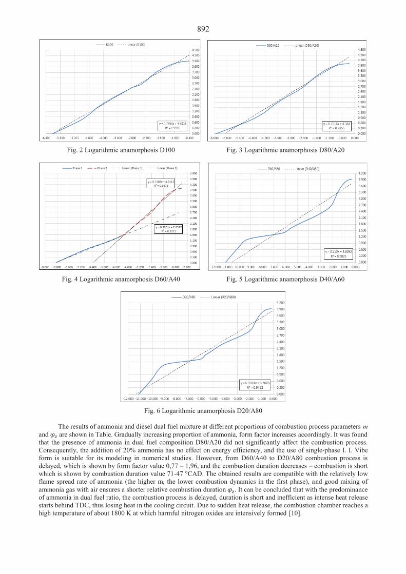
892

Fig. 2 Logarithmic anamorphosis D100 Fig. 3 Logarithmic anamorphosis D80/A20

Fig. 4 Logarithmic anamorphosis D60/A40 Fig. 5 Logarithmic anamorphosis D40/A60

Fig. 6 Logarithmic anamorphosis D20/A80

The results of ammonia and diesel dual fuel mixture at different proportions of combustion process parameters m and are shown in Table. Gradually increasing proportion of ammonia, form factor increases accordingly. It was found that the presence of ammonia in dual fuel composition D80/A20 did not significantly affect the combustion process. Consequently, the addition of 20% ammonia has no effect on energy efficiency, and the use of single-phase I. I. Vibe form is suitable for its modeling in numerical studies. However, from D60/A40 to D20/A80 combustion process is delayed, which is shown by form factor value 0,77 – 1,96, and the combustion duration decreases – combustion is short which is shown by combustion duration value 71-47 °CAD. The obtained results are compatible with the relatively low flame spread rate of ammonia (the higher m, the lower combustion dynamics in the first phase), and good mixing of ammonia gas with air ensures a shorter relative combustion duration . It can be concluded that with the predominance of ammonia in dual fuel ratio, the combustion process is delayed, duration is short and inefficient as intense heat release starts behind TDC, thus losing heat in the cooling circuit. Due to sudden heat release, the combustion chamber reaches a high temperature of about 1800 K at which harmful nitrogen oxides are intensively formed [10].

893 Table

Calculated m ir parameters at various dual diesel – ammonia fuel combinations in „WIBE“ software

Combination Parameter

D100 D80/A20 D60/A40 D40/A60 D20/A80

m 0,36 0,33 0,77 1,75 1,96 94,4 98,0 70,8 46,5 47,5

4. Conclusions

At the next stage of research, the study of the regularity of m and cycle execution parameters is planned to use obtained analytical results in numerical modeling of CI engine parameters already operating on dual ammonia-diesel fuel. Determining combustion process parameters of ammonia-diesel fuel mixture is crucial for further research, as it allows quite simply model theoretical engine operation process to achieve energy efficiency and environmental protection optimization.

Using logarithmic anamorphosis methodology, the combustion character of the dual ammonia-diesel fuel mixture at different fuel mixture proportions was determined. It was observed that at D100 and D80/A20 mode single-phase combustion character predominates, respectively, logarithmic anamorphosis curve shape is close to linear. By increasing the proportion of ammonia according to energy value from 40% to 80%, a break in the logarithmic anamorphosis curve is observed. This indicates that the combustion character is two-phase. The analysis of logarithmic anamorphosis of dual fuel modes allows defininig the nature of the combustion process. The determined two-phase combustion character of the ammonia-diesel mixture will further be analyzed in subsequent doctoral studies using combustion cycle modeling software “AVL BOOST” and “IMPULS”. References 1. Chircop, A. 2019. The IMO initial strategy on reduction of GHG emissions from international shipping: A

commentary [online cit.: 2021-07-20]. Available from: https://brill.com/view/journals/estu/34/3/article-p482_7.xml 2. DNV-GL maritime forecast to 2050 [online cit.: 2021-07-21]. Available from: https://www.anave.es/images/

documentos/DNVGL_2020_Maritime_Forecast_to_2050_WEB.pdf 3. International energy agency – transport [online cit.: 2021-07-24]. Available from: https://www.iea.org/topics/transport 4. MAN B&W two-stroke engine operating on ammonia [online cit.: 2021-07-24]. Available from: https://www.man-

es.com/marine/products/planningtools-and-downloads/technical-papers 5. Cord, J.D. 2020. Successful tests pave the way for ammonia as a future marine fuel [online cit.: 2021-07-26].

Available from: https://www.wartsila.com/insights/article/successful-tests-pavethe-way-for-ammonia-as-a-future-marine-fuel

6. Reiter, A.J.; Kong, S.C. 2011. Combustion and emissions characteristics of compression-ignition engine using dual ammonia-diesel fuel [online cit.: 2021-08-05]. Available from: https://www.sciencedirect.com/science/article/ abs/pii/S0016236 11000414X

7. Kyunghyun, R. 2014. Performance characteristics of compression-ignition engine using high concentration of ammonia mixed with dimethyl ether [online cit.: 2021-08-08]. Available from: https://www.sciencedirect.com/ science/article/abs/pii/S0306261 913006326

8. Ivanchenko, A.A.; Makurov, V.A.; Shchennikov, I.A. 2014. Selecting a mathematical model for describing characteristics of the fuel burnup at operational development marine diesel engine with common rail system [online cit.: 2021-08-24]. Available from: https://journal.gumrf.ru/files/articles/24/31-37.pdf

9. Mollenhauer, K.; Tschöke, H. 2010. Handbook of diesel engines page 22-27 [online cit.: 2021-08-20]. Available from: https://link.springer.com/book/10.1007/978-3-540-89083-6

10. Miller, B. 2015. Nitrogen oxides formation and control [online cit.: 2021-08-18]. Available from: https://www.sciencedirect.com/science/article/pii/B9780128015667000051?via%3Dihub

894

Proceedings of 25th International Scientific Conference. Transport Means 2021. Integration and Verification Approach of the Metamorphosis Mobile Space Testing Facility S. Kravchenko, N. Kuleshov, V. Shestakov, N. Panova, S. Bratarchuk Cryogenic and vacuum systems, Andreja iela 7/9, Ventspils, LV-3601, Latvia, E-mail: sergey@cvsys.eu Abstract When an idea passes from paper to a laboratory, the first question arises - will the product work in space? And the second: will it operate without negative influence on the other spacecraft systems? To get a positive answer to those questions, a new product must be validated and verified in the space environment. Without testing capability, it is possible to sell only ideas, not products. In 2016 SIA Cryogenic and vacuum systems proposed to establish Metamorphosis mobile space testing facility, which is the trailer based thermal vacuum test facility and the team, which helps to develop test plans, prepare and perform tests, make test reports and it is done in customer workshop. Such an idea has no analogs worldwide. 28.06.2018 the European Commission awarded our company for the Mobile space testing facility on demand by the Seal of excellence. We invited Riga Technical University Institute of Aeronautics, who have experience in intermodal transport to be a partner in European Regional Development Fund Project No. 1.1.1.1/18/A/133 “Prototype development of transportable in multimodal traffic mobile space testing facility Metamorphosis”. This project is under implementation since May 2019. The main difference of the developed facility from the existing ones is the ability to maintain operational characteristics in the conditions of intermodal transport, i.e. in conditions of vibration, shock, linear and angular acceleration and displacement. Taking it into consideration, 2 flexible software instruments were developed: The model of a vacuum system and The model of cryogenic system, which help us to take into account the effect of elements changing (vibration dampers, flanges, hoses, feedthroughs etc.) to provide the sufficient mechanical design for facility operation in shock and vibration conditions. Alongside with flexible design approach, we performed several tests for vacuum system design verification. In April, 2021 the Metamorphosis facility prototype integration process will start. This paper is discussed the questions, concerning the facility integration and verification approach. KEY WORDS: thermal vacuum test, environmental conditions simulation, mobile test complex 1. Introduction

The idea of creating a mobile test facility, which is key in the project, arose as a response to the request of a growing number of market players in the developing space industry. In recent years, many new startups, university student teams have appeared, wishing to bring their ideas to the level of a product of the space industry, in other words, to raise their TRL from 1-3 to 5-7 and higher. Such advancement implies repeated passing of testing, validation and verification procedures of the product, including tests in operational conditions.

For small and young companies that do not have a significant budget and a large staff, it is quite difficult to prepare a test plan, find funds and opportunities for testing, prepare a test report and other necessary documents.

In 2017, Latvian company Cryogenic and vacuum systems Ltd applied for the Horizon-2020 SME phase 1 and received a grant from the European Commission (contract No. 776938) for the feasibility stage of the project for the provision of integrated services related to the preparation and testing of space industry products by means of a mobile testing complex performing tests right in the client's workshop (project “Metamorphosis - mobile space testing facility on demand”). The contract provided for the development of a business plan, during which more than 600 respondents from the EU were interviewed, 104 of them answered that they need such a service, and 45 expressed their readiness to an immediate order. In 2018, Cryogenic and vacuum systems Ltd applied for the Horizon-2020 SME phase 2, based on the developed business plan and was awarded by European Commission with the Seal of Excellence.

For the further development of the project, it was necessary to bring its TRL from 2-3 to 6-7, as well as to provide training for both the project team and for potential customers of services - new enterprises in the space industry.

It was also necessary to solve a number of technical problems associated with the intermodal transport of the future space facility. We invited Riga Technical University Institute of Aeronautics, who have experience in intermodal transport to be a partner in European Regional Development Fund Project No. 1.1.1.1/18/A/133 “Prototype development of transportable in multimodal traffic mobile space testing facility Metamorphosis”. This project is under implementation since May 2019.

2. The Mobile Space Testing Facility Specific

The target element of the spacecraft life cycle is its intended use. Therefore, the main elements of the cycle of

development and testing, in accordance with the requirements of the ESA ECSS and NASA standards systems, are the

895development and testing of space technology, taking place in conditions as close as possible to the real parameters of outer space.

The study and modelling of the results of the impact on space technology of a complex of factors of outer space, reflecting the properties of the environment during the period of its intended use, is carried out in the process of its testing in the facilities (systems) for simulation of outer space environmental conditions.

These facilities are the most complex, inaccessible and expensive equipment, therefore the heart of the Metamorphosis test complex is precisely the thermal vacuum test stand, although, of course, the test complex may include other necessary facilities (vibration stand, acoustic stand, etc.)

The main guiding documents defining the requirements for such tests are set out in [1] and [2]. They indicate the need for space environmental testing, otherwise called thermal vacuum tests (thermostating, thermal cycling, electrical, pneumatic, etc.) at all stages of Qualification testing, Acceptance testing, Protoflight testing for all elements of the space mission, please see Table 2.6-1 from GSFC-STD-7000 standard, Table.

TableGSFC-STD-7000 Test requirements

Where “T” is test required, “A” is analysis required, tests may be required to substantiate the analysis, “T/A” is test required if analysis indicates possible condensation, “T, A” is test is not required at this level of assembly if analysis verification is established for non-tested elements.

Requirements for quantitative and qualitative indicators for modeling space conditions are also established by the standard [3].

The consequences of neglecting quantitative and qualitative requirements for thermal vacuum tests are well described in the article [4], where statistics of the US space industry are collected, confirming that, on average, during space environmental testing, 4.1 the value of fatal defects for a space mission are detected, and this number is increasing for new developments until 6.

The main difference of the developed facility from the existing ones is the ability to maintain operational characteristics in the conditions of intermodal transport, i.e. in conditions of vibration, shock, linear acceleration and angular displacement of the supporting structure of the vacuum chamber.

In the course of the analysis of the vulnerability of a conventional thermal vacuum facility structure in the conditions of intermodal transportation, the main technical risks and the parts most vulnerable to these influences were identified.

The greatest risks are exposed to:– high-vacuum pumping system - vacuum valves, turbomolecular pumps, Stirling and Gifford-McMahon

cryocoolers in cryogenic pumps - risk of pinching, jamming and displacement of parts;– vacuum seals - risk of damage (cuts and scratches) as a result of exposure to mating parts;– thin-walled pipelines of cryogenic and vacuum systems with linear expansion joints, membrane bushings,

cryogenic shrouds panels, vacuum chamber body - the risk of destruction due to low-cycle fatigue (here the elements are indicated in decreasing order of risk);

– standard bellows, unloading and compensating spring elements of the cryogenic screen, fastening systems for the test object - the risk of failure due to high-cycle fatigue;

– a simulator of solar radiation, optical feedthroughs - the risk of damage to optical elements under mechanical influences, the risk of violation of the adjustment of optical systems;

– Van Allen belts simulator - the risk of destruction of standard ceramic high-voltage vacuum feedthroughs, the risk of violation of the tuning of ion-optical and electro-optical systems.

This list is considering components of a highest risk, but is far from exhaustive. With a complete analysis of the number of elements, systems and components, required additional checks or design and technological measures to protect against destruction of the impact of the specified mechanical loads amounted to 538 units.

For further work, all components exposed to risks were divided into 2 groups:– components for which it is possible to purchase options in vibration-shockproof performance and which, at

the same time, satisfy the budgetary constraints of the project. For this group, market analyzes, consultations with manufacturers and procurement were undertaken;

– elements requiring special design and technological measures to prevent damage and / or destruction. This

896 group presented the greatest challenge.

The work on the creation of elements of the 2nd group requires a clear definition of the specifics of the operating conditions - special design requirements that distinguish the unit for the stationary test facility from the mobile space environments testing facility (here and after MSTF). 3. Special Design Requirements for MSTF, their Validation and Verification

The features of the design requirements of the MSTF are determined by the operating conditions, while the main factor of negative impact on the structure is vibration and shock loads, in this regard, one of the main tasks was to determine the possible values of vibration and shock effects during intermodal transportation.

As a result of the analysis of regulatory and research documentation, it was decided to mainly be guided in the design and calculations by the maximum data of the IMO / ILO / UNECE Code of Practice for Packing of Cargo Transport Units (CTU Code) chapter 5, without a table for railway transport, setting the value of the calculated acceleration in the direction of travel 0.8 g, in the opposite direction 0.5 g, in the lateral direction - 0.8 g, vertically upwards - 0.5 g and vertically downwards - 1 g.

The CTU Code does not regulate air cargo loads. At the same time, Volume II of the Agreement concerning the International Carriage of Dangerous Goods by

Road (ADR) (section 9.7.3.2) establishes structural standards for the calculation of vehicles carrying dangerous goods (in particular, liquid nitrogen) for resistance to mechanical stress (acceleration in the direction of movement 2 g, in the lateral direction – 1 g, vertically upward – 1 g and vertically downward – 2 g) however, the MSTF is transported without refuelling with liquid nitrogen and therefore the direct application of these rules is not mandatory. Nonetheless it was decided to be guided by the ADR requirements in the design and construction of the cryogenic system, the general system of lodgements and supports of the MSTF vacuum chamber.

However, these loads are actually only observed on Highways, speed roads, and modern public roads with hard surface.

At the same time, it was taken into account that the EU is constantly improving the road network, that is, repair and reconstruction of roads. There are significant sections with road repairs and detours on unpaved roads, and for unpaved roads and local roads there is no document regulating vehicle loading. The limiting impacts for temporary roads and hard-surface structures are also not regulated.

This factor is quite important, since, for example, during the repair of the European highway Warsaw-Bialystok, for almost 4 years, sections of many kilometres with gravel cover were involved in bypassing. This situation is typical for most of the countries of Eastern Europe and the Baltic states.

When driving on roads with crushed stone, dirt roads and temporary roads with a hard surface, as well as on roads in emergency condition, the nature and sequence of loads cannot be predicted, however, a number of studies provide data that the actual loads on emergency and unpaved roads are significant. exceed the values set in the CTU Code. In particular, in [5] data are given based on the results of a test drive on a truck on dirt roads in the Czech Republic, while the peak acceleration values recorded by the researchers in the direction of travel reach ± 5 g, in the lateral direction + 2.5 / -4.5 g, and in the vertical direction + 5.5 g.

Thus, the factor of uncertainty and technical risk in the implementation of the project was identified. To minimize this factor, a decision was made to reduce the possibility of the indicated technical risk

manifestation - along with the application of more stringent design standards, it is necessary to conduct tests in real operating conditions, since the possibility of guaranteed verification of the prototype's ability to operate under conditions of intermodal transportation will be achieved only when passing full-scale tests in real operating conditions.

4. A Variational Mathematical Model of a Vacuum Pumping System is a Tool That Makes It Possible to Design

MSTF for Intermodal Transportation After analysing the technical risks and determining the physical impacts, we came to the conclusion that the

greatest number of design improvements in comparison with the structures of stationary testing facilities require the design of a vacuum chamber with a vacuum pumping system.

To ensure stability under load conditions, it is necessary to analyse a large number of variations in the design of these elements, and a change in each element (for example, the length of the bellows expansion joint) will lead to a significant change in the conductivity of the vacuum system, and therefore in the required pump capacity, which will lead to an increase in the mass of the pumps, and this, in turn, increases the mass of the supporting and damping elements, the forces on the frame, etc. That is, a small change in the design of one element in this case can lead to a significant change in the design of the entire MSTF.

In this regard, it was decided to create a variable physical and mathematical model of the vacuum system of Metamorphosis MSTF.

The SCILAB 6.1.0 software was used as a modelling environment. To create a model, it was necessary to determine the composition of the vacuum pumping system and create a

certain generalized design appearance of the MSTF vacuum chamber. It was taken into account that one of the mandatory types of tests is leakage control by comparing the leak flow

of the tested object with the test leak using a helium mass spectrometric leak detector, thus, the high-vacuum pumping

897 device must have a sufficient pumping rate for helium.

Turbomolecular and diffusion pumps satisfy such requirements, but the latter is poorly applicable for intermodal transportation, since the nitrogen trap required to prevent the migration of oil vapours from the diffusion pump into the volume of the vacuum chamber will not be filled with nitrogen in the transport position, and during rolling and shock it is possible spillage of oil from the pump volume into the volume of the vacuum chamber or high-vacuum seal.

The disadvantage of a turbomolecular pump, which consists in a significantly higher price for the same pumping rate for water vapour, nitrogen and oxygen compared to a cryogenic pump, will be compensated for by the presence in the vacuum chamber of cryogenic shrouds filled during operation with liquid nitrogen, which, having a developed surface, will perform the functions of a cryogenic pump. For example, for a significant decrease in the partial pressure of water vapour, it is sufficient to supply nitrogen to the cryogenic shroud, which optically overlaps the high-vacuum pumping nozzle, and the required compensation of the thermal regime can be carried out by a controlled infrared source with a reflector.

According to the manufacturers of turbomolecular pumps, the greatest resistance to shocks and vibrations during transportation is achieved when the pump is in a vertical position, with the inlet flange upward [6, 7].

The simplest and most effective method for monitoring of the MSTF chamber's operability under conditions of intermodal transportation is to transport the vacuum chamber in an evacuated state with control of the residual pressure.

If the leakage during transportation does not exceed the calculated rate, then upon arrival at the destination, the MSTF vacuum chamber can be used immediately.

In addition, this method greatly facilitates the provision of vacuum hygiene, preventing contamination of the vacuum chamber and system during transportation. In this regard, it was necessary to separate the vacuum chamber from the vacuum pumping system by high-vacuum and fore-vacuum valves or gates.

The calculation model was based on the following initial generalized design layout, Fig. 1.

Fig. 1 Computational layout diagram: 1 - high-vacuum outlet; 2 vibration decoupling; 3 vacuum seal; 4 high-vacuum pump; 5 fitting for connecting the shutter of the forevacuum pump; 6 body of the vacuum chamber; 7 the cryogenic shroud; 8 optical feedthrough for inputting radiation from the Solar simulator; 9 lodgements and connections for camera mounting; 10 removable front cover The mathematical model includes three blocks: – gas load calculation unit; – block for calculating the conductivity of structural elements; – a unit for calculating the characteristics of vacuum pump, pumping speed and time. The gas load on the vacuum pumping system is defined as the total gas flow Q , entering the pumped out

volume:

Q = Ql + Qge + Q + Qd + Qin, (1) where Ql flow of gases flowing from the atmosphere through leaks and connections, m3 Pa·s-1; Qge gas flow due to adsorptive gas release from structural materials, m3 Pa·s-1; Qp flow due to permeability of the walls of the vacuum

898 chamber, m3 Pa·s-1; Qd gas flow due to diffusion of accumulated gas from the chamber material, m3 Pa·s-1; Qin is the gas flow from the gas, existing in the vacuum chamber before the start of pumping, m3 Pa·s-1.

The block for calculating the gas load includes modules corresponding to the source of the gas load and making it possible to simulate the temporal changes in the flow values when the characteristics of the sources of gas release or leakage change:

– module for determining the geometric characteristics of gas load sources; – module for calculating the flow of gases flowing from the atmosphere through leaks and connections; – module for calculating the gas flow caused by adsorptive gas release from structural materials; – module for calculating the flow of gases due to permeation of the walls of the vacuum chamber; – module for calculating the gas flow due to the diffusion of accumulated gas from the material; – module for calculating the flow of gases that were in the vacuum chamber before the start of pumping. In this case, both the gas load from the vacuum chamber, including cryogenic shrouds, vacuum inlets and other

elements of the vacuum pumping system, and the gas load from the test specimen, in-chamber electrical equipment, infrared heaters, etc. are taken into account.

The total conductivity of the vacuum system and the vacuum chamber C is defined as the conductivity of the series-connected elements of the vacuum system Ci:

1

1 1n

i iC C. (2)

The conductivity is determined for each element by determining the Clausing coefficients [8–11]. The block for calculating the conductivity includes: – module for determining the geometric characteristics of the elements of the gas path; – module for determining the free path of molecules and the Knudsen number in the elements of the gas path; – module for calculating the conductivity of the elements of the gas path (the calculation for the corresponding

elements is carried out in the molecular, in the transient and in the viscous modes of gas flow). The calculation of the pumping time is carried out taking into account the change in conductivity and pumping

rate depending on the gas flow mode in the viscous, transient and molecular modes, based on the obtained value of the Knudsen number. The evacuation time T was determined as the sum of time intervals Ti (evacuation from atmospheric pressure to the pressure of the viscous mode boundary, from the viscous mode boundary pressure to the transient mode boundary pressure, etc. to the operating or limiting system pressure):

1

n

ii

T T . (3)

For each time interval, the effective pumping rate S0i was determined:

0p

ip

S CS

S C, (4)

where Sp is the pumping speed m3/h and C is the vacuum system total conductivity (2).

In this case, the pumping time in each of the indicated ranges Ti was determined as follows:

1

0

02

0

ln

ii

ii

iii

i

QPSVTQS PS

. (5)

where V is the total volume of the MSTF vacuum chamber and vacuum lines, m3; P1i is the initial pressure of the determined pumping time segment, Pa and the P2i is the final pressure of the determined pumping time segment.

The pressure in the vacuum chamber for the corresponding time interval Pi was calculated as follows:

0

ii

i

QP

S. (6)

An example of simulation results is shown in Fig. 2. In Fig. 2 pressure is in mbar and time is in seconds.

899

Fig. 2 Pressure graph after 1 pumping hour till the reaching the required pressure The resulting model made it possible to change the geometric and other characteristics of the constituent parts of

the vacuum chamber and the vacuum pumping system in a wide range, which is important, since it allows you to select vibration decouples and carry out the layout based on the conditions of maximum resistance to vibration and shock effects.

5. Verification of the Calculation Results at the Moment

The simulation results made it possible to proceed to the creation and verification of the characteristics of the

vacuum pumping system. At present, the MSTF vacuum chamber, together with cryogenic shrouds, is in the process of manufacturing, but a 1.2 m3 vacuum chamber, available in our company, was used to test the vacuum pumping system.

The view of the vacuum pumping system, mounted for checking before being connected to the vacuum chamber, is shown in Fig. 3.

In Fig. 4 shows a view of a vacuum chamber used for testing with an integrated vacuum pumping system during testing.

Fig. 3 MSTF Vacuum pumping system in the process of integration Fig. 4 MSTF vacuum system during first tests

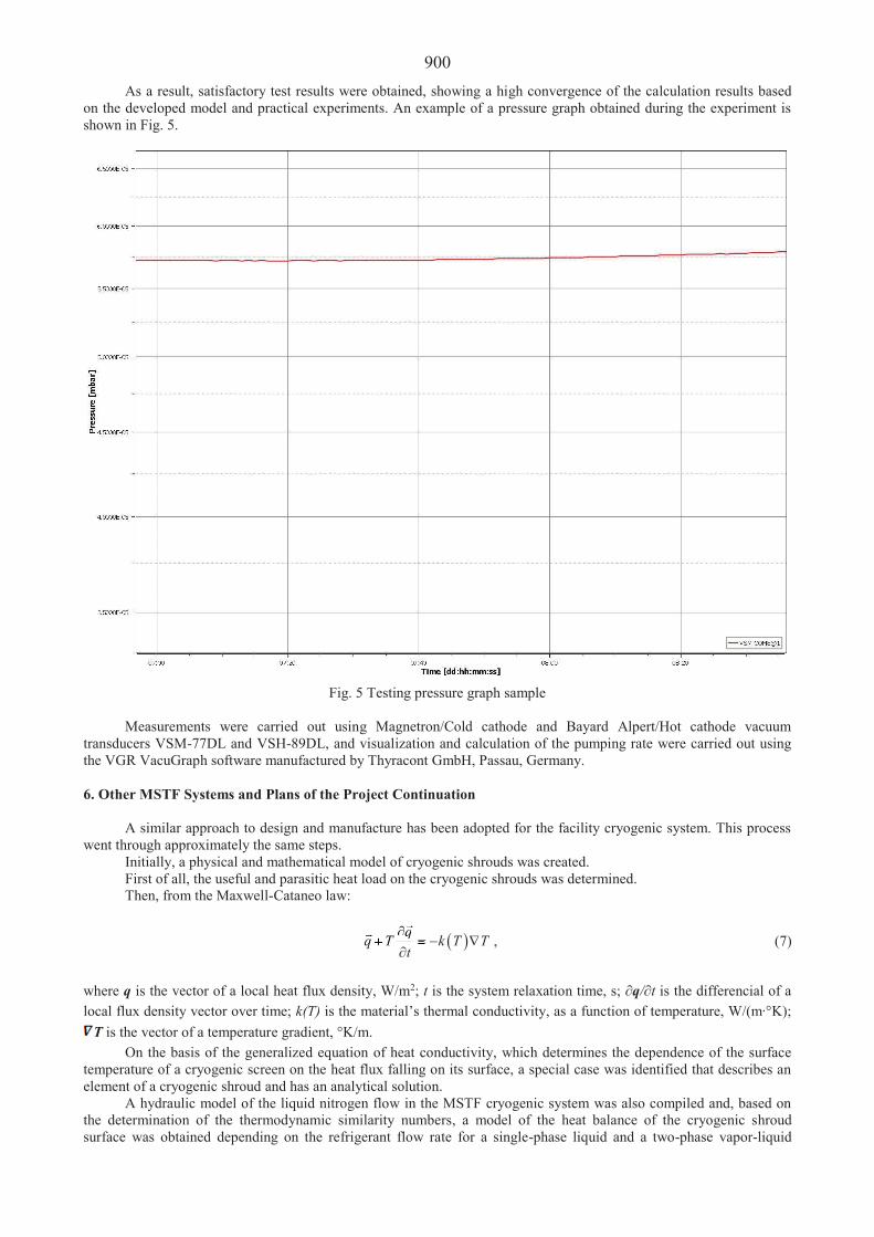
900As a result, satisfactory test results were obtained, showing a high convergence of the calculation results based

on the developed model and practical experiments. An example of a pressure graph obtained during the experiment is shown in Fig. 5.

Fig. 5 Testing pressure graph sample

Measurements were carried out using Magnetron/Cold cathode and Bayard Alpert/Hot cathode vacuum transducers VSM-77DL and VSH-89DL, and visualization and calculation of the pumping rate were carried out using the VGR VacuGraph software manufactured by Thyracont GmbH, Passau, Germany.

6. Other MSTF Systems and Plans of the Project Continuation

A similar approach to design and manufacture has been adopted for the facility cryogenic system. This process went through approximately the same steps.

Initially, a physical and mathematical model of cryogenic shrouds was created.First of all, the useful and parasitic heat load on the cryogenic shrouds was determined.Then, from the Maxwell-Cataneo law:

qq T k T Ttqq T qTT qq , (7)

where q is the vector of a local heat flux density, W/m2; t is the system relaxation time, s; q/ t is the differencial of a local flux density vector over time; k(T) is the material’s thermal conductivity, as a function of temperature, W/(m °K);

T is the vector of a temperature gradient, °K/m.On the basis of the generalized equation of heat conductivity, which determines the dependence of the surface

temperature of a cryogenic screen on the heat flux falling on its surface, a special case was identified that describes an element of a cryogenic shroud and has an analytical solution.

A hydraulic model of the liquid nitrogen flow in the MSTF cryogenic system was also compiled and, based on the determination of the thermodynamic similarity numbers, a model of the heat balance of the cryogenic shroud surface was obtained depending on the refrigerant flow rate for a single-phase liquid and a two-phase vapor-liquid

901 mixture of liquid nitrogen. The use of this model has made it possible to expand the range of technical solutions that ensure the stability of cryogenic shrouds and cryogenic systems to shock and vibration mechanical loads.

We hope that in August - September 2021 we will assemble a vacuum chamber with vacuum pumping and cryogenic systems on a special chassis that allows installing the MSTF Metamorphosis facility prototype into a regular cargo bus or small truck. This will allow us to proceed to test in real operating conditions and achieve the result - proof of the MSTF concept. 7. Conclusions

The approaches to the development of MSTF Metamorphosis presented in the paper allow to creation a whole class of new space industrial instruments - high-vacuum systems resistant to intermodal transport, including mobile test facilities.

The proposed approach to modelling, which allows flexibly varying various physical characteristics of the vacuum chamber and other components, provides the choice of mechanical damping, decoupling and protective elements that should ensure stable operation of the MSTF under vibration and shock conditions during intermodal transportation.

The creation of MCTF will provide services for the preparation and conduct of tests, interpretation and presentation of the results obtained to many startups and university teams in the EU. Acknowledgement

The authors are grateful for the support of the Central Finance and Contracting Agency (CFCA) of Latvia, and for the European Regional Development Fund, within the framework of whose Project No. 1.1.1.1/18/A/133 “Prototype development of transportable in multimodal traffic mobile space testing facility Metamorphosis” the discussed research is developed and the MSTF facility prototype is designed and manufactured. References: 1. ECSS Standard. 2012. ECSS-E-ST-10-03C Space engineering. Testing. Noordwijk: ECSS Secretariat ESA-ESTEC

Requirements & Standards Division, 128 p. 2. NASA. 2013. GSFC-STD-7000 General Environmental Verification Standard. Maryland: NASA Goddard Space

Flight Center, 337 p. 3. ISO. 2016. ISO 17851:2016 Space systems - Space environment simulation for material tests - General principles

and criteria. Geneva: International Standard Organization, 36 p. 4. Wright, C.P.; Arnheim, B.L. 2000. Insight into the value of system level thermal vacuum testing. El Segundo, CA:

Cross Program Research Office of the Aerospace Corporation, 281-290. 5. Vlkovský, M.; Šmerek, M.; Michálek, J. 2017. Cargo Securing During Transport Depending on the Type of a

Road, Proceedings IOP Conference Series: Materials Science and Engineering 245(4): 042001. DOI: https://doi.org/ 10.1088/1757-899X/245/4/042001

6. Umrath, W.; Adam, H.; Bolz, A.; Boy, H.; Dohmen, H.; et al. 2007. Fundamentals of Vacuum Technology. Cologne: Oerlickon Leybold vacuum, 188 p.

7. The Vacuum Technology Book. 2013. Volume III Vacuum Generation. Asslar: Pfeiffer Vacuum GmbH, 475 p. 8. Clausing, P. 1971. The Flow of Highly Rarefied Gases through Tubes of Arbitrary Length, Journal of Vacuum

Science and Technology 8(5): 756, https://doi.org/10.1116/1.1316379 9. Saksaganski, G.L. 1988. Molecular Flow in Complex Vacuum Systems, New York: Gordon and Breach, 162 p. 10. Nesterov, S.B.; Burmistrov, A.V.; Androsov, A.V.; et al. 2012. Metody rascheta slozhnykh vakuumnykh sistem

(Calculation of Complex Vacuum Systems). Moscow: Tekhnosfera, 384 p. (in Russian). 11. Fomin, M.V.; Chernyshev, O.R. 2018. Modular calculation of the conductance of complex vacuum systems with

free-molecular gas flow, Russian Engineering Research 38(8): 579-580.

902

Proceedings of 25th International Scientific Conference. Transport Means 2021. Investigation of the Adhesion of Snow Car Tyres to the Road Surface D. Juodvalkis1, R. Skvireckas2 1Kaunas University of Applied Engineering Sciences, Tvirtov s av. 35, 5015, E-mail: darius.juodvalkis@edu.ktk.lt 1Kaunas, Lithuania, Kaunas University of Technology, Studentu 56, 51424, E-mail: darius.juodvalkis@ktu.lt 2Kaunas University of Applied Engineering Sciences, Tvirtov s av. 35, 5015, E-mail: ramunas.skvireckas@edu.ktk.lt 2Kaunas, Lithuania, Kaunas University of Technology, Studentu 56, 51424, E-mail: ramunas.skvireckas @ktu.lt Abstract Car tyres are adapted to different weather conditions. During the winter season, it is recommended to operate the cars with snow tyres, and the summer with summer tyres. In this study, experiments were performed to determine the dependences of snow tyre grip on the road to ambient temperature. The studies were performed with tyres of different manufacturers and at ambient temperatures from -7°C to 17°C. The adhesion coefficients for different tyres at different ambient temperatures have been calculated and the braking distances of the car have been predicted. KEY WORDS: braking distance, adhesion coefficient, snow tyre. 1. Introduction

Tyres are a key component of a car that ensures good grip on the road surface. How fast the car accelerates or stops depends on how well the tyre grips to the road. Tyres not only ensure safety on the road, but also increase comfort, the amount of fuel used by the car also depends on the type of tyres.

In countries with warm weather it is possible to drive with the same summer type tyres all year round but in countries with harsher climates (including Lithuania) there is a challenge - changing tyres depending on the season (summer and winter). A significant number of drivers for economic reasons choose to drive with snow (universal) tyres during the warm season but such behavior is risky. It is not for nothing that tyres are produced depending on the seasons and they have different performance characteristics. Research has shown [1] that the frictional interface reduces tyre wear under the best adhesion conditions and increases wear under minimal adhesion conditions. This means that snow tyres wear faster at high temperatures and summer tyres more at low temperatures. When using snow tyres during the warm season drivers are reckless as they have poorer grip on the road surface, wear faster and use more fuel, and endanger themselves and others by driving with the same tyres all year round because the tyres are less effective in gripping the road surface [2].

Studies of the dependence of tyre adhesion to road temperature on outdoor temperature have shown that higher road and ambient temperatures resulted in lower hysterical friction and, conversely, lower tyre slip ratios and higher macrotexture resulted in higher friction [3]. Dutch researchers have produced a 200-page report on safe driving interfaces with tyres and one of their laboratory studies on the use of summer tyres in winter has found that snow tyres have better road safety performance compared to summer tyres when used at temperatures below -7 degrees, on snowy or icy roads [2].

The aim of the study was to determine the dependences of the adhesion of universal car tyres to the road surface on the ambient air temperature.

2. Research Methodology and Equipment

The experiments were carried out in March because it is at this time of year that very different weather conditions occur, from negative temperatures to positive ones. The aim of the research was to determine the adhesion of the car tyres to the road surface and the braking distance at different outdoor temperatures. During the research the road conditions were good - the road surface was dry and there was no precipitation. Tyre temperature was measured only once during each experiment - after driving, when stopped.

The studies were performed at ambient temperatures: -7°C, -1°C, 8°C ir 17°C. The experiments were performed on modern cars equipped with efficient ABS and during the experiments braking was extreme, i.e. under ABS.

The studies were performed with tyres from different manufacturers „Bridgestone Blizzak Ice“ and „Goodyear Ultra Grip Ice 2“ (Fig. 1). The tread depth of used tyres was about 7 mm, the tyres were made in 2017. Looking at the tread pattern of the tyres used in the studies, it can be seen that the tread patterns are different. For example, the “Bridgestone“ tread design, according to the manufacturer, was designed to deal effectively with aquaplaning which can also occur on icy roads, so the „Blizzak ICE“ was developed using a „Multicell“ rubber compound that allows water to be absorbed by the tyre effectively adhere, and the sidewall grooves remove water more quickly from the tyre-road contact area [4]. „Goodyear“ tyres have a directional Christmas tree-shaped tread pattern that maintains optimal contact with extremely slippery road surfaces and provides good performance when driving on ice. The block notches improve lateral

903force transmission during maneuvering, and the open side grooves along with the saw-tooth-shaped tread edges improve the displacement of scorched snow and water, thus improving performance when driving through deep snow.

a b

Fig. 1 Tyres used in the studies: a „Bridgestone Blizzak Ice“; b „Goodyear Ultra Grip Ice 2“

The „iAccel“ mobile app was chosen to measure vehicle acceleration and braking. „iAccel“ works with „iPhones“ and „Android“ devices. During the test the results can be displayed on the screen (Fig. 2) and stored in a CSV file to facilitate export for further analysis. During the study the device was installed in the vehicle so that the long edge of the device was perpendicular to the direction of travel. Upon arrival at the test site, the program was run on the device. The program uses a combination of GPS, accelerometer, and other sensors, and the test ensures that all sensors receive the right signals to get the most accurate data possible.

Fig. 2 „iAccel“ program visual report

For more accurate experimental results each experiment was performed 4 times and then the mathematical average of the obtained results was calculated [5]:

i

i, (1)

here i – results of i test; i – quantity of the tests.A total of 32 field experimental braking tests were performed (Fig. 3).

Fig. 3 Variation of adhesion coefficient for a tyre „Goodyear Ultra Grip Ice 2“ during braking

After carrying out the experimental runs and having the necessary data we calculate the tyre adhesion coefficient[5]:

904

2

2x m

ac A v

am g

, (2)

here aa – deceleration (m/s2); Cx – aerodynamic drag coeficient of the vehicle; Am – drag area (m2); – air density (kg/m3); v – vehicle speed (m/s); g – acceleration of gravity (m/s2).

By calculating the coefficient of adhesion of a tyre under certain conditions it is possible to calculate the predicted braking distance of the vehicle at a given initial speed and under specific road conditions and tyres [6]:

20

2brakingv

Sg

, (3)

here Sbraking – braking distance (m); v – initial speed (m/s); – friction coeficient; g – acceleration of gravity (m/s2).

3. Research Results

From data obtained during field experiments the adhesion coefficients of „Bridgestone Blizzak Ice“ and „Goodyear

Ultra Grip Ice 2“ at different ambient temperatures were calculated (Table 1).

Table 1 Calculated friction coefficients

Type of tyre

Friction coefficient ( ) -7°C -1°C 8°C 17°C Overall

„Bridgestone Blizzak Ice“ 0.784 0.801 0.756 0.729 0.766 „Goodyear Ultra Grip Ice 2“ 0.825 0.853 0.801 0.734 0.815

Overall 0.805 0.826 0.778 0.731 0.788 While analyzing the results presented in Table 1, we notice that the best adhesion to the road surface is ensured by

„Goodyear Ultra Grip Ice 2“ tyres at ambient temperature of -1°C. The worst adhesion to the road surface was recorded for „Bridgestone Blizzak Ice“ tyres at an ambient temperature of 17°C. Assessing the overall values of the coefficient of adhesion at different temperatures, „Goodyear Ultra Grip Ice 2“ tyres provide about 10 percent better traction than „Bridgestone Blizzak Ice tyres“.

The dependences of the variation of the coefficient of adhesion for different tyres and the total tested tyres on the ambient temperature are presented in Fig. 4.

Fig. 4 Dependences of the coefficient of adhesion on the ambient temperature: 1 tyres „Bridgestone Blizzak Ice“; 2 tyres „Goodyear Ultra Grip Ice 2“; 3 – total Analyzing the results obtained and calculated during the experiments performed, which are presented in Fig. 4 we

can observe that, as could be expected, the tyres of both manufacturers ensure the best adhesion to the road surface at an ambient temperature of -1°C. As the ambient and road surface temperatures increase, the adhesion of the tyres to the road surface decreases, as does the differences between the tyres of different manufacturers. From Fig. 4 we can conclude that the optimal ambient temperature for these tyres at which they ensure maximum adhesion to the road surface is about 0°C. As the ambient temperature decreases, the adhesion of the tyres to the road surface decreases slightly, but this is unavoidable with any type of tyre. As the ambient temperature increases, the adhesion of the tyres to the road surface

905 decreases significantly, which means that at ambient temperatures of 5°C and above, a different type of tyre should be chosen to ensure better adhesion to the road surface. Such tyres could be summer type tyres or universal tyres made of solid rubber. The results obtained confirm the results obtained by other scientists and researchers, who state that it is not optimal to operate cars with snow tyres in warm weather and summer tyres should be chosen. In these studies, the adhesion properties of summer tyres to the road surface and their dependence on the ambient temperature have not been studied, therefore it is not possible to say exactly where the limit is when it would be optimal to use summer tyres. However, it must be emphasized that when operating cars with snow tyres and at high ambient temperatures (5°C and above), drivers should appreciate poorer tyre grip and possibly a longer braking distance.

Table 2 shows the calculated (3) predicted braking distances of a car with two different types of tyres at different ambient temperatures and different initial vehicle speeds.

Table 2

Calculated braking distance

In the results presented in Table 2 we notice that when the initial speed of the car is low - up to 50 km/h, the length of the braking distance also differs slightly. At an initial speed of 100 km/h, the possible extension of the stopping distance at different temperatures is about 10%, which can make a 6 m extension of the braking distance.

4. Conclusions

Field experiments aimed at determining the adhesion of snow tyres to the road surface at different ambient temperatures have shown that the studied tyre models ensure optimal adhesion to the road surface at -1°C.

When ambient temperatures are positive and increases, the adhesion of snow tyres to the road surface deteriorates. Similar trends were observed with both sets of tyres from different manufacturers used in the investigation. The coefficient of adhesion between the tyre and the road surface at an ambient temperature of 17°C is 10 – 15% lower than at -1°C.

By predicting the length of the braking distance of the car operated with snow tyres at an initial speed of 100 km/h and an ambient temperature of 17°C, a braking distance 6 m longer is possible compared to the braking distance at an ambient temperature -1°C.

In case of positive ambient temperatures and in order to achieve optimal adhesion of the tyres to the road surface universal or summer tyres of solid mixtures should be chosen. When operating a car with snow tyres and a positive ambient temperature drivers should appreciate poorer tyre grip and a potentially longer braking distance. References 1. Fwa, T.F.; et al. 2009. Effectiveness of Tire-Tread Patterns in Reducing the Risk of Hydroplaning. [online cit.: 2021-

04-15]. Available from: https://doi.org/10.3141/2094-10 2. Jansen, S.; et al. Study on some safety-related aspects of tyre use. [online cit.: 2021-04-22]. Available from:

https://ec.europa.eu/transport/road_safety/sites/default/files/pdf/tyre10062014/discussion_document.pdf 3. Anupam, K.; et al. 2013. Influence of temperature on tire-pavement friction analyses. In Transportation Research

Record 2369(no. February): 114-124. Available from: https://doi.org/10.3141/2369-13 4. Brigestone tires. [online cit.: 2021-03-15]. Available from: https://www.bridgestone.lt/psr/ziemines-padangos-

blizzak/ice 5. Sabri, M.; Fauza, A. 2018. Analysis of vehicle braking behaviour and distance stopping. IOP Conference Series:

Materials Science and Engineering 309(1): 012020. 10.1088/1757-899X/309/1/012020. 6. Maftei, Alexandru, Dontu, Andrei; Lidia, Gaiginschi; Agape, Iulian 2019. Influence of speed bumps on braking

distance, IOP Conference Series: Materials Science and Engineering 572: 012098. 10.1088/1757-899X/572/1/012098.

906

Proceedings of 25th International Scientific Conference. Transport Means 2021.

Study of Ridesharing Services in Vilnius, Lithuania J. Ginavi ien 1, I. Sprogyt 2

1Vilnius College of Technologies and Design, Antakalnio str. 54, Vilnius, Lithuania, E-mail: j.ginaviciene@vtdko.lt 2Vilnius College of Technologies and Design, Antakalnio str. 54, Vilnius, Lithuania, E-mail: i.sprogyte@vtdko.lt Abstract Ridesharing is made possible due to the advance of communication technologies. As they increase in popularity, the particular features for ride sharing systems are social networks to reveal trip activity and regional features. As modern consumers, students tend to choose not only high-quality transport but also, they prefer the desirable quality of transportation services. The main aim of this research is to compare the factors of ridesharing service in Vilnius, Lithuania in the 2019 and 2021 studies. These studies were a quantitative analysis. In 2019 and in 2021 the same number of respondents completed a questionnaire about factors that affect their evaluation of ridesharing services. The respondents were 161 Transport Logistics students of Vilnius College of Technologies and Design. According to the findings obtained, the opportunity to order the meal, to pay by online banking, safety are significant factors in order to ensure customer satisfaction of ridesharing service. KEY WORDS: ridesharing services, customer satisfaction, student's opinion 1. Introduction

Ridesharing provides flexible transportation for everyone and generates value for a customer. Nowadays, as all the world lives in Covid -19 pandemic, this sharing service is important too. This article discusses the possibilities of ridesharing services in Lithuania and comparison 2019 and 2021 customer’s opinions. The first section of the article is dedicated to the scientific discussion about the concept of ridesharing services. The second section is dedicated to comparing ridesharing services customers’ opinions. The aim of paper is to analyse and compare customers’ opinions of ridesharing services in Vilnius in studies done in 2019 and 2021 years. The methods for research include the comparative analysis of scientific literature, questionnaires, empirical data grouping, comparison. 2. Concept of Ridesharing

Ridesharing aims to bring together travellers with similar routes and schedules. Vehicle allocation, price strategy, route planning, waiting time for passengers, and other factors all determine the experience of ridesharing systems.

Ridesharing services have different implications. Firstly, it can make the environment better by using the vehicles not for one person but by utilizing the empty seats of cars. It is very important for less noise and less fuel consumption. One study suggests that ridesharing services could solve traffic jams, bring down transportation fees.

The rapid growth of the ridesharing service shows that the appeal among consumers is self-evident. The ridesharing services appear to compete with taxis for their increasing ubiquity as a convenient means of transportation. The success of ridesharing depends on having a sufficient number of participants, drivers to change their routes in order to increase system benefits, Additionally, the characteristics and choices of users should be considered when attempting to implement a successful ride-sharing system in real-life. In the end, users consider only their own benefits, not ridesharing services benefits.

The ridesharing services have and disadvantages such as traffic congestion worsen by the day, the global warming accelerates. Participants lose interest in ridesharing services if they fail to find a trip of vehicle. However, many drivers are not willing to change their routes because doing so may lead to a significant increase in their travel time. Likewise, long processing times cause long waiting times for users.

Customer satisfaction is important because satisfied customers usually buy more. By buying more, they act as a network, which allows you to reach potential customers by sharing experiences. This means that customer satisfaction is a significant aspect in terms of the success of ridesharing services [6].

In other studies authors found that reliability, sensitivity, price and satisfaction directly affected customer loyalty [7]. They used six variables of reliability, uninterrupted service, safety, convenience, availability and driving behaviour. Variables were studied to investigate customer satisfaction with services. In a series of regression analyses, they found that service, convenience, availability and reliability affect customer satisfaction.

After the literature review the ridesharing services benefits for the participants are: price, service quality, reliability, empathy, responsiveness, service, consumer’s emotion, personal factors, situational factors, perception of equity or fairness and service features [1-10].

This paper proposes a ridesharing participant benefit that aims to overcome the afore mentioned challenges.

907 3. Comparative Analysis in 2019-2021 Students’ Satisfaction of the Ridesharing Services in Vilnius, Lithuania

Research

As the demand for shuttle service grows, it is becoming more and more pronounced and less avoidable in the market. The research reveals the factors used by companies to improve their services and analyse their customer base - starting with the implementation of innovations, ending with the constant retention of customers and the expansion of the circle of new customers.

As Balachandran & Hamzah (2017) [ 3 ] stated that one of the advantages by conducting survey through email or internet is that this way is faster and more convenient than telephone interview. Due to this reason, in this research used method was a survey online.

Data collection method - a questionnaire survey, which was carried out electronically, through www.apklausa.lt and sent to the students via their personal e-mails.

Questionnaire items were compiled structured, containing response options. Most issues have been concluded using the Likert scale, as more useful information for the investigation can be collected in response to these types of questions.

Survey sampling bias is calculated according to the Paniott formula:

12

1

N

n , (1)

where n – sample size, 2 – bias probability, N – Research totality, that ensures approximately 5% probability of bias.

Total respondents were 161 students (1-4 course) who study in Vilnius College of Technologies and Design, in Transport Logistics program 2019-2020, 2020-2021 and who were willing to complete a survey. Both genders participated in the study. 2019 male respondents much more 23,3% and much less 16,7% than 2021

2019 and 2021 researches overlook the majority of respondents were aged between 18-23 years old, but 2019 more 6,2% than 2021. The second smaller age group of respondents were between 24-30 years old which is much more 8,3% in 2021 than in 2019. The third age group of respondents was 31- 40- year-old more much 0,6% in 2019 than in 2021. The data would seem to suggest that 18-23 years old respondents were the most willing to use ridesharing services. It can be explained by mentioning that 18-23 years young people are not enough financially stable (financial dependency from parents, student loans, etc.). Students may be trying to find the best solution considering the price and quality of affordable transportation service but further research should be done in order to support this statement.

Both researches shown that the majority of respondents is between less than 380 €, which 2019 much more 5,2 than 2021. The second are 301-500 € much more 5,4% 2019 then 2021. The third group is 501-700 € more less 2019 than 2021 2,9%. The fourth rank is 701-1000 € which less 4,9% than in 2021. The fifth rank is 1001-1500 € less 2, 9% than 2021. The finished rank is more than 15001€ remained the same in both years of the study. Statistically speaking students whose income is less than 380 € are more willing to choose ridesharing service in comparison with others.

Fig. 1 What modes of transport do you use (multiple options available)?

The ridesharing users were using Bolt service more much 5,8% 2021. But the ridesharing users were using Etransport more much 6,4% 2019 than 2021 It means most of the ridesharing users prefer to use Bolt not Etransport. The reason is the affordable price and the convenience.

Most respondents were using car (private or official) modes of transport, but less 1,2% than 2019. The second is public transport (buses, trolleybus, trains) and user were using much more 2,4% than 2019. The third group of respondents were using ridesharing (Bolt, Uber, Yandex, Etransport). Such results may have the effect of not having the same opportunity

908 to call the ridesharing everywhere in Fig. 1.

The majority of respondents said the most acceptable type of payment is paying by credit card. But it’s less 2,7% than in 2019. The most popular type of payment is paying by online banking much more 16,5% than in 2019. Respondents were asked what type of payment is more acceptable in Fig. 2.

Fig. 2 The types of payment

Most respondents chose entertainment as the most common purpose of travel when choosing ridesharing, but 2021 less 38,9% than 2019. It was affected by a pandemic, quarantine, because of closed entertainment venues. The second most popular choice is shopping much more 2021 38,8% than 2019. The third choice is home less 2021 than 2019 is 11,5%. in Fig. 3.

Fig. 3 What is the most common purpose of travel when choosing transportation services?

It is important to notice the frequency of using ridesharing services. Most respondents use the service less than once a month. It is much more 7,5% in 2021 than in 2019. Meanwhile, respondents were using ridesharing services few times in a week much more 10 % in 2021 than in 2019. Respondents are using this services’ one in a month much more 1,7% 2021 then 2019. Respondents were using ridesharing services in less in a week less 1,2% 2021 than 2019 and respondents are using services for every day less 2% 2021 than 2019. According to statistics, the most popular answer was using ridesharing service less than one time in a month.

Respondents had to evaluate the criteria in accordance w i t h importance. The ridesharing services users mentioned that one of the most popular reasons to choose such services is not wanting to drive drunk. The second criteria for 2019 research was no need to look for a parking space, but 2021 research was speed. The third is the reliability of both researches. Unpopular answers both researches were the severity of a taxi call, and the ability to evaluate the driver after the trip

2019 and 2021 researches ‘results showed that the most important driver’s criteria are honesty, the driver’s ability t o orientate in the environment, punctuality. Less remarkable for the ridesharing driver’s criteria are communicative and going fast. It means most of the ridesharing services drivers must drive safely, orient in roads, be punctual and responsible. in Fig. 4.

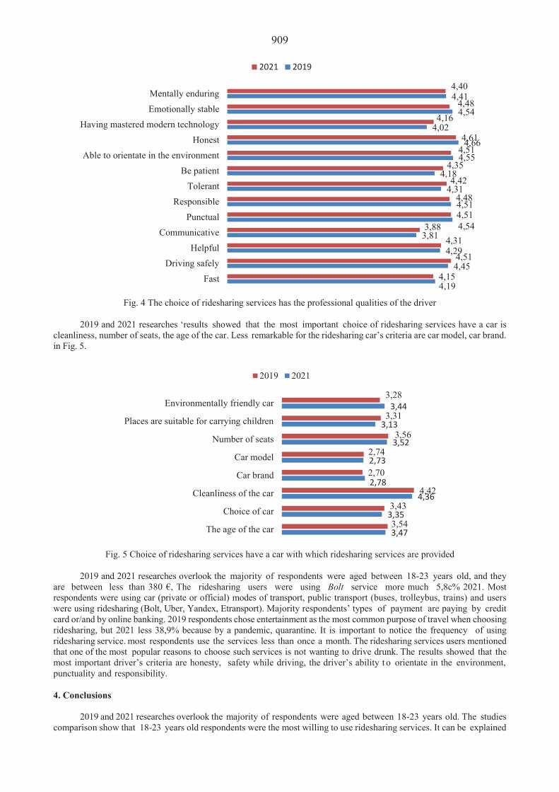
909

Fig. 4 The choice of ridesharing services has the professional qualities of the driver

2019 and 2021 researches ‘results showed that the most important choice of ridesharing services have a car is

cleanliness, number of seats, the age of the car. Less remarkable for the ridesharing car’s criteria are car model, car brand. in Fig. 5.

Fig. 5 Choice of ridesharing services have a car with which ridesharing services are provided

2019 and 2021 researches overlook the majority of respondents were aged between 18-23 years old, and they

are between less than 380 €, The ridesharing users were using Bolt service more much 5,8c% 2021. Most respondents were using car (private or official) modes of transport, public transport (buses, trolleybus, trains) and users were using ridesharing (Bolt, Uber, Yandex, Etransport). Majority respondents’ types of payment are paying by credit card or/and by online banking. 2019 respondents chose entertainment as the most common purpose of travel when choosing ridesharing, but 2021 less 38,9% because by a pandemic, quarantine. It is important to notice the frequency of using ridesharing service. most respondents use the services less than once a month. The ridesharing services users mentioned that one of the most popular reasons to choose such services is not wanting to drive drunk. The results showed that the most important driver’s criteria are honesty, safety while driving, the driver’s ability t o orientate in the environment, punctuality and responsibility.

4. Conclusions

2019 and 2021 researches overlook the majority of respondents were aged between 18-23 years old. The studies comparison show that 18-23 years old respondents were the most willing to use ridesharing services. It can be explained

4,19

4,454,29

3,814,54

4,514,31

4,18

4,554,66

4,024,54

4,41

4,15

4,51

4,313,88

4,51

4,48

4,424,35

4,514,61

4,164,48

4,40

FastDriving safely

HelpfulCommunicative

PunctualResponsible

TolerantBe patient

Able to orientate in the environmentHonest

Having mastered modern technologyEmotionally stableMentally enduring

2021 2019

3,47

3,35

4,362,78

2,73

3,52

3,13

3,44

3,54

3,434,42

2,70

2,74

3,56

3,31

3,28

The age of the car

Choice of car

Cleanliness of the car

Car brand

Car model

Number of seats

Places are suitable for carrying children

Environmentally friendly car

2019 2021

910 that young people are not enough financially stable. Students may be trying to find the best solution considering the price and quality of affordable transportation service but further research should be done in order to support this statement. Both researches shown that the majority of respondents is between less than 380 €. Statistically speaking students whose income is less than 380 € are more willing to choose ridesharing service in comparison with others The ridesharing users were using Bolt service more in the 2021 than Etransport. The reason is the affordable price and the convenience. The majority of respondents said the most acceptable type of payment is paying by online banking in 2021 study, but paying by credit card were more important in 2019. Due to Covid -19 pandemic, the ridesharing services in 2021 was more used for shopping than in 2019.

The survey showed that Lithuanian ridesharing companies, when competing with each other and comparing their activities, in order to take into account the wishes and answers of customers are the main factors for competitive advantage. References 1. Abd Elmeguid, S.M.; Ragheb, M.A.; Tantawi, I.P.; Elsamadicy, A.M. 2018. Customer satisfaction in sharing

economy the case of ridesharing service in Alexandria, Egypt, The Business and Management Review 9(4): 373-382. 2. Aydin, O.F.; Gokasar, I.; Kalan, O. 2020. Matching algorithm for improving ride-sharing by incorporating route

splits and social factors, PLoS ONE 15(3): 1-23. 3. Balachandran, I.; Hamzah, I.B. 2017. Influence of customer satisfaction on ride-sharing services in Malaysia,

International Journal of Accounting & Business Management 5(2): 187-196. 4. Gajjar, B.N. 2013. Factors Affecting Consumer Behavior, International Journal of Research in Humanities and Social

Sciences 1(2): 10-15. 5. Hussein, A.A. 2016. Service Quality Practices and Customer Satisfaction in Taxi Companies in Nairobi. Master’s

Thesis - Business Administration in Operations Management, School of Business, University of Nairobi. 6. Khadka, K.; Maharjan, S. 2017. Customer satisfaction and customer loyalty. Thesis, 73. 7. Khuong, M.N.; Dai, N.Q. 2016. The Factors Affecting Customer Satisfaction and Customer Loyalty — A Study of

Local Taxi Companies In Ho Chi Minh City, Vietnam, International Journal of Innovation, Management And Technology 7(5): 228-233.

8. Shen, B.; Zheng, W.; Carley, K.M. 2018. Urban Activity Mining Framework for Ride Sharing Systems Based on Vehicular Social Networks, Networks & Spatial Economics 18(3): 705-734.

9. Toader, B.; Moawad, A.; Hartmann, T.; Viti, F. 2021. A Data-Driven Scalable Method for Profiling and Dynamic Analysis of Shared Mobility Solutions, Journal of Advanced Transportation, 1-15.

911

Proceedings of 25th International Scientific Conference. Transport Means 2021. Application of the Clustering Challenge to New Railway Lines G. Vai i nas Vilnius Gediminas Technical University, Saul tekio al. 11, 10223, Vilnius, E-mail: gediminas.vaiciunas@vilniustech.lt Abstract The paper examines the possibility of adapting the clustering problem solving methodology by identifying the locations where the centers of newly constructed (or additionally connected) international railway lines could be located. The centers may be provided for the maintenance machinery base, the rolling stock depot, the freight terminal or for the purpose of line management. In order to solve the problem of clustering of an international railway line, depending on the intended purpose of the centers of weighted , it is suggested to evaluate such indicators as gross domestic product, population, area and length of railway network of countries. The Amsterdam-Tallinn route is an example. In doing so, the author proposes a methodology for identifying disproportionate areas away from socio-economic centers where the related problems of railroad development may arise. KEY WORDS: railway, international railway lines, railway network, socio-economic indicators, clustering of railway lines 1. Introduction

The association of countries into political, economic or military unions gives rise to the need for new transport

links. For example, with the change of the European Union structure (accession by one country and secession by others), new trade routes are forming, and with the change of the NATO structure, new needs for the transportation of military freight emerge. For some countries, these railway sections are more important, and for others, of less significance, and therefore are a permanent subject of doubts and debate. Therefore, a natural need arises to have a reasonable methodology for answering these questions. This need is especially relevant when investigating the significance of Eastern European railway lines [1, 2]. It is also important to analyse possible line extensions [3]. However, such issues are relevant not only to Eastern European countries but also to countries such as Great Britain [4], this topic is not the whim of the author of this article. In different countries, geographic conditions, with varying need for tunnels, bridges, trenches, track formations and peculiarities for the operation of the given structures, are diverse. The given structures are ordered by different customers and designed by different designers, and therefore their operation parameters are different. It is obvious that the whole railway line should be perceived as a uniform topographic system, although in different countries, different systems and databases for processing topographic information are valid [5]. Climate changes in the countries also make an impact. In warmer countries, the railway is covered by sand, and in northern regions, by snow. [6]. One of the key parameters that should be assessed is the longevity of railway bridges and other structures. In the whole railway line, the service time of structures should be systemised [7]. Some authors emphasize the significance of railway structures for the environment. For example, with the ageing of structures, they pollute the environment, and this process must be controlled [8]. However, the very same issue of information systemizing for the entire railway line remains. If climate is different in various countries it is necessary to analyse the diversity of probability of track formations, bridges and other structures being washed away by rain water. Wash-away processes of the given structures have been investigated, and based on statistical data, methodologies have been created to forecast their indicators [9]. When deciding what issues should be evaluated while investigating the distribution of significance of a railway line for respective countries, the conclusion increasingly rises up that it is hardly expedient to conduct in-depth research. Lithuanian research studies decided that a study should be started from the indicators that are noncomplicated, yet cover a broader range of issues. The indicator representing the social aspect could be the number of residents in a country, the indicator representing the economic aspect would be the country’s gross domestic product, the geographic one would be area of the country and the indicator of the impact on the infrastructure could be the aggregate length of existing railway lines in the country. Researchers analysed the distribution of significance of the railway line Rail Baltica (constructed across Poland, Lithuania, Latvia and Estonia) and of the container train Viking route (going across Lithuania, Belarus and Ukraine) by countries [10]. The use of railway infrastructure, whether freight or passengers, shall be subject to a charge. Depending on the infrastructure and economic characteristics of the country, this charge is different. There are also differences in the methodology used to calculate this charge, which can be read separately in the literature [11]. The railway lines are influenced by the cultural and political diversity of the countries it crosses. Particularly peculiar are countries located on regional borders such as Turkey or Azerbaijan (on the border between Europe and Asia). In countries such as these, the priority given to rail transport as a rule has recently been recognized. More developed road transport. The peculiarities of rail transport in such countries are analyzed in the literature [12]. Rail freight carries only part of the route. They are usually transported to the terminal by road transport, which means that cargo is reloaded at terminals. Depending on the type of cargo being transported, the need for transhipment facilities varies. To determine where those places should be, various theories and

912 insights are being developed [13]. When examining the peculiarities of passenger transport by rail, it has been observed that, although in theory rail transport is superior to road transport, it often loses the competitive battle. There are different reasons for this in different countries, and up to 37 different reasons have been found in different studies [14]. Different countries have different railway history and tradition, and therefore the ratio of the crossing line to the railways already existing in the countries is different. In some countries passenger transport by rail is more prevalent and in others rail freight transport. The scientific literature contains knowledge of the features of their interfaces [15]. Some countries also have their own regional economic and transport characteristics due to their size. Even a country like Germany has such differences. The regional differences described in the literature are particularly pronounced when examining the Chinese transport system, for example [16, 17]. Research shows that the availability of rail transport in the region is not enough, the issue of rail accessibility is very important. The relationship between rail and other modes of transport is examined [18]. The possibility of developing a railway line running through various countries is also relevant. In this case, they are faced with different legal bases and cultural environment of the countries. The availability of land at rail access also has its own specificities in different countries [19]. Student of Vilnius Gediminas Technical University in his final master thesis investigated the principles of formation and deployment of railway maintenance machine park [20, 21]. The upgrading of the fleet of railway maintenance machines raises the question of where to base the newly purchased machines. On the one hand, machine storage areas should be concentrated in centers, on the other hand, they should be as close as possible to the workstations. In the work mentioned above, four alternatives for the location of railway maintenance machines were created in the example of Lithuanian railways: with one center, with two centers, with three centers and with four centers. The student referred to the railway maintenance machine base centers as the centers of weighted , the location close to the corresponding centers of weighted of the roads to be repaired (in kilometers).

A simplified diagram of the region's railways is shown in Fig. 1.

Fig. 1 Simplified railway scheme for the region

In the simplified scheme, stations are marked with the first letters of location names (the location names themselves

would probably not tell the reader anything), as well as the distances between stations. This railway region is located 50-100 km west of Vilnius (for example, the sign “Kau” means Kaunas - the second largest city in Lithuania about 100 km west of the Lithuanian capital Vilnius). Fig. 1 shows a variant with a single center and is marked with a circle at station Zhe (locality Zeimiai). Knowing the alternatives to the arrangement of railway maintenance machines, it is possible to determine for each alternative the average idle mileage of the machines in question (how much the machines will have to travel from the station to the workplace), which is one of the evaluation criteria. Also, the number of centers for each alternative can be used to estimate the total length of rails needed to base road maintenance machines. Their overall length is also an evaluation criterion. With at least two criteria, alternatives can be compared using multi-criteria evaluation methods. Using the multiple criteria evaluation methods - the sum sum method, the weighted average method and the simple weighting method - four alternatives for railway maintenance machine placement have been evaluated in the example of Lithuanian railways: one center, two centers, three centers and four centers. A similar question arises with the construction of new railway lines: where to locate the base of the road maintenance machines, the railway infrastructure management centers, and finally where to place the passenger service, business or shopping centers? As the development of the railway lines is an important detail in the context of European (especially Central European) integration, the issue of the location of the mentioned objects becomes relevant. The author of this article proposes to use - to adapt the clustering problem solving methodology. It should be noted that the previously described methodology for locating rail maintenance machines also shows signs of a clustering problem. 2. The Essence of Clustering Problem and Application Possibilities

The essence of the classical clustering problem is that for an area with a set of points, it is necessary to create an

optimal number of centers so that the sum of the points distance to its own center is the smallest. An example of a graphical representation of a clustering problem condition is shown in Fig. 2.

913

Fig. 2 Example of graphical clustering problem representation form

The axes of the graph in Fig. 2 may include, for example, geographical coordinates (they may be local, based on a reference system adopted in the problem), or other values. Mathematically, the objective function of the clustering problem would be:

1 1k n

ijj i x min , (1)

where xij – the distance from point i to center j.

It is understood that as the number of centers increases, this amount decreases. Another question, what can be the maximum number of centers?

If the number of centers is not limited, the solution of the problem should be that the number of centers is equal to the number of points (each point has its own center), the sum (Eq. (1)) would then be 0. Mathematically, this is an ideal solution, but in practice clustering will not make sense in this case. To address this paradox, one can limit the possible number of centers k. Another way is to allow the number of centers to increase until the sum of the points to its center decreases more intensively than the number of centers increases:

1 11 11 1

1k n

ijj ik n

ijj i

x kkx

. (2)

The method of limiting the number of centers is used when, for example, there are limited resources for setting up

centers. The way to allow the number of centers to increase as long as they increase is the amount of point distances to their center decreases more intensively than the number of centers that are appropriate when the issue of resource centers is not relevant. In other words, it is more of a mathematical principle than an economic one. For economic tasks, it is possible to set weighted values of what distance reduction compensates for one additional center created. The location of the centers is determined as follows. When the center is single, its location is in the center of weighted of the points field. To create two centers, the set of points is divided into two parts (usually, evenly), and the center of weighted of each part is created. The distance of each point to the centers is then checked. If the distance to the center to which this point belongs is less than the distance to the other center, the point and remains assigned to that center; if less than the distance to another center, the point is assigned to another center. This checks each point. Once the points have been redistributed, the position of each center must be corrected and must be in the corresponding center of weighted . This check is repeated until all points are assigned to closer centers and the centers are in the center of weighted of the point groups. Then, if the number of centers needs to be increased (checked according to the one selected from the above conditions), each group of points is divided in half, and each center is re-created. In this way, the number of centers is multiplied until it reaches the limit. This method can be used to determine recommended locations for centers for newly created rail corridors. Applying the clustering problem solving methodology to the railway lines, one fundamental difference has to be noticed: the typical methodology deals with the two-coordinate system, while with the railway lines the coordinate system is one-dimensional. One of the newly created railway corridors in Europe is the Amsterdam-Tallinn corridor (Fig. 3 [22], on the map North at the top).

914

Fig. 3 Railway corridor Amsterdam – Tallinn

The Amsterdam-Tallinn railway corridor consists of the newly constructed Rail Baltica line (Tallinn-Warsaw) and the existing line from Warsaw via Berlin to Amsterdam. The total length of the line is over 1880 km. The line passes through Holland, Germany, Poland, Lithuania. Latvia and Estonia. 3. Clustering of the Amsterdam - Tallinn Railway Corridor

Track clustering is the identification of centers of weighted where it is appropriate to concentrate the supplies for

maintenance and operation of the line. These are the centers for rail maintenance machines, rolling stock depots, as well as control and administration centers. Centers for a railway line can be defined in terms of various coordinates - the length of the line, the economic and social characteristics of the countries crossing the line. The characteristics of the countries passing through the line are given in Table [23; 24].

Table Indicators of countries crossing the Amsterdam - Tallinn railway line

Indicators Countries

EST LV LT PL DE BE Length of Amsterdam-Tallinn corridor, 229 245 335 341 556 180

GDP, billion dollars 47.306 60.73 102 1287 4444 550 Population, million 1.305 1,934 2.91 38.43 83 11.4

Area sq. M. km 44226 64589 65300 312696 357112 30528 Railway length in the country, km 1018 1934 1767 23420 40826 3518

The following section analyzes the data in Table, first examining the weighted percentages by country. The first

and simplest indicator is the length of the railway. The percentage distribution of Amsterdam-Tallinn rail corridor lengths by country is shown in Fig. 4

Fig. 4 Percentage by country breakdown of Amsterdam - Tallinn rail corridor

915 It is natural for Central Europe to have the largest share of the railway line passing through Germany and Poland

(about 29.5% and 18.1% respectively), while Belgium, Estonia and Latvia have the smallest share (around 9.5, 12.1 and 13% respectively. %). For issues where railway length is relevant (eg rail diagnostics or environmental monitoring), weighting centers can be determined by rail length based on the data analyzed in Fig. 2.

Occasionally, the development of the railways in the region is important when identifying centers. For example, in determining the location of rolling stock depots, not only the length of the line in question is relevant, but also the development of the railway network in the region, since the rolling stock maintained at the depots can be operated there. The percentage distribution of the total rail network length by country is shown in Fig. 5.

Fig. 5 Percentage of the total length of the railway network by country

Germany and Poland are also leading in terms of rail network development (around 56.3% and 32.3% respectively), with Estonia and Lithuania accounting for the lowest shares (1.4% and 2.4% respectively). This distribution shows that in terms of the development of the rail network, the centers of the line are well advanced to the West. Some of the centers on the line are dedicated to economic objects other than railways (for example small logistics centers for local cargoes accepted for agricultural production). It is appropriate to identify the locations of such centers according to the area of the countries crossing the railways. The percentage distribution of the countries passing through the Amsterdam - Tallinn corridor is shown in Fig. 6.

Fig. 6 The percentage distribution of the countries passing through the Amsterdam - Tallinn corridor

As Germany and Poland are the largest countries in terms of area in the Central European region, they are the most important in terms of area (Germany 40.8% and Poland 35.8%). The locations of the centers involved in passenger transport must be determined by the distribution of the population. The percentage distribution of the population of the countries crossing the Amsterdam - Tallinn corridor is shown in Fig. 7.

Fig. 7 The percentage distribution of the population of the countries crossing the Amsterdam - Tallinn corridor Fig. 7 shows the same leaders as in the previous ones: Germany 59.8%, Poland 27.7%. The railways close to your

ports devote a significant part of their activities to freight transport to and from ports. The Amsterdam-Tallinn railway corridor runs from the port city to the port city, as well as parallel to the North Sea, along the Baltic Sea, so the freight related to sea transport on this line will certainly be carried. Rail freight indicators are usually related to the size of countries' gross domestic product. The percentages of the countries' gross domestic product by countries passing through the Amsterdam - Tallinn corridor are shown in Fig. 8.

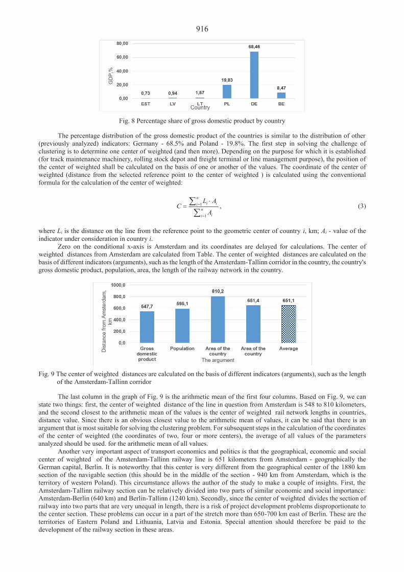
916

Fig. 8 Percentage share of gross domestic product by country

The percentage distribution of the gross domestic product of the countries is similar to the distribution of other (previously analyzed) indicators: Germany - 68.5% and Poland - 19.8%. The first step in solving the challenge of clustering is to determine one center of weighted (and then more). Depending on the purpose for which it is established (for track maintenance machinery, rolling stock depot and freight terminal or line management purpose), the position of the center of weighted shall be calculated on the basis of one or another of the values. The coordinate of the center of weighted (distance from the selected reference point to the center of weighted ) is calculated using the conventional formula for the calculation of the center of weighted:

1

1

ni ii

nii

L AC

A, (3)

where Li is the distance on the line from the reference point to the geometric center of country i, km; Ai - value of the indicator under consideration in country i.

Zero on the conditional x-axis is Amsterdam and its coordinates are delayed for calculations. The center of weighted distances from Amsterdam are calculated from Table. The center of weighted distances are calculated on the basis of different indicators (arguments), such as the length of the Amsterdam-Tallinn corridor in the country, the country's gross domestic product, population, area, the length of the railway network in the country.

Fig. 9 The center of weighted distances are calculated on the basis of different indicators (arguments), such as the length of the Amsterdam-Tallinn corridor

The last column in the graph of Fig. 9 is the arithmetic mean of the first four columns. Based on Fig. 9, we can

state two things: first, the center of weighted distance of the line in question from Amsterdam is 548 to 810 kilometers, and the second closest to the arithmetic mean of the values is the center of weighted rail network lengths in countries, distance value. Since there is an obvious closest value to the arithmetic mean of values, it can be said that there is an argument that is most suitable for solving the clustering problem. For subsequent steps in the calculation of the coordinates of the center of weighted (the coordinates of two, four or more centers), the average of all values of the parameters analyzed should be used. for the arithmetic mean of all values.

Another very important aspect of transport economics and politics is that the geographical, economic and social center of weighted of the Amsterdam-Tallinn railway line is 651 kilometers from Amsterdam - geographically the German capital, Berlin. It is noteworthy that this center is very different from the geographical center of the 1880 km section of the navigable section (this should be in the middle of the section - 940 km from Amsterdam, which is the territory of western Poland). This circumstance allows the author of the study to make a couple of insights. First, the Amsterdam-Tallinn railway section can be relatively divided into two parts of similar economic and social importance: Amsterdam-Berlin (640 km) and Berlin-Tallinn (1240 km). Secondly, since the center of weighted divides the section of railway into two parts that are very unequal in length, there is a risk of project development problems disproportionate to the center section. These problems can occur in a part of the stretch more than 650-700 km east of Berlin. These are the territories of Eastern Poland and Lithuania, Latvia and Estonia. Special attention should therefore be paid to the development of the railway section in these areas.

917 4. Conclusions

When solving the problem of clustering for a railway line, depending on the intended purpose of the centers of weighted , it is necessary to evaluate such indicators as gross domestic product, population, area and length of the railway network of the country.

Coordinates of the centers of weighted may be calculated by two methods: at each step of the calculation of the centers of weighted , the values of all parameters analyzed may be used separately or only the index average.

The geographical, economic and social center of weighted of the Amsterdam-Tallinn railway line is 651 kilometers from Amsterdam, which is not very close to the geographical center of the railway section. As a result, there is a risk of project development problems in the disproportionate part of the stretch. Therefore, special attention should be paid to the development of the railway line in areas remote from the center (East Poland, Lithuania, Latvia and Estonia).

Based on the approach of solving the problem of clustering, areas disproportionate to the socio-economic centers can be identified, where the related problems of railway line development are possible. References 1. Sinkevi ius, G.; Vai i nas, G; Dailydka, S. 2016. Study of “Rail Baltica” significance for the development of

internationalization processes, VIII International Scientific Conference “Transport problems”, Katowice, 543-552. 2. Vai i nas, G.; Sinkevi ius, G. 2016. Research on the influence of the extension of “Rail Baltica” to Hamburg on the

railway line for the region of Eastern Europe Kaunas University of Technology, 705-713. 3. Vai i nas, G.; Steiš nas, S. 2017. Investigation of priority directions of rail baltica extension from Warsaw, Procedia

Engineering „Transbaltica-2017“, 40-45 4. Givoni, M. 2012. The accessibility impact of a new High-Speed Rail line in the UK – a preliminary analysis of

winners and losers, Journal of Transport Geography 25: 105-114. 5. Sužiedelyt -Visockien , J. 2006. Improvement of railway topographic plans updating technologies, Transport

21(2): 119-122. 6. Zakeri, J.A. 2012. Investigation on railway track maintenance in sandy-dry areas, Structure and Infrastructure

Engineering 8(2): 135-140. 7. Pipinato, A.; Pellegrino, C. 2012. Modena Assessment procedure and rehabilitation criteria for the riveted railway

Adige Bridge, Structure and Infrastructure Engineering 8(8): 747-764. 8. Jiyeol, I.; Kyungik, G. 2016. Characteristics of non-point source pollutants on railway bridges, Desalination and

Water Treatment 57(2): 684-693. 9. Jiyeol, I.; Kookhwan, C.; Kyungik, G. 2016. Determination of the first-flush criteria from railway bridge area,

Desalination and Water Treatment 57(2): 694-708. 10. Vai i nas, G.; .; . 2018. A study of the importance of the Viking container train for

countries, Odessa National Marine University, 24-26. 11. Sánchez Borràs, M.; López Pita, A. 2011. Rail Infrastructure Charging Systems for High Speed Lines in Europe,

Transport Reviews 31: 49-68. 12. Sutcliffe, B. 2007. Pro rail Policies in Turkey: A Policy Shift? Transport Reviews 27: 485-498. 13. Wiegmans, B.; Hekkert, M.; Langstraat M. 2007. Can Innovations in Rail Freight Transhipment Be Successful?

Transport Reviews 27: 103-122. 14. Blainey, S.; Hickford, A.; Preston, J. 2012. Barriers to Passenger Rail Use: A Review of the Evidence, Transport

Reviews 32: 675-696. 15. Ziolkowski, M.F. 2012. The ties that bind: freight and passenger high-speed rail are interdependent, Journal of

Transport Geography 22: 292-294. 16. Wu, J.; Nash, Ch.; Wang, D. 2014. Is high speed rail an appropriate solution to China’s rail capacity problems?

Journal of Transport Geography 40(C): 100-111. 17. Chen, Zh.; Haynes, K. 2017. Impact of high-speed rail on regional economic disparity in China, Journal of Transport

Geography 65(C): 80-91. 18. Yu, M.; Fan, W. 2018. Accessibility impact of future high speed rail corridor on the piedmont Atlantic megaregion,

Journal of Transport Geography 73: 1-12. 19. Jiang, R.; Lu, Q.; Peng Z. 2018. A station-based rail transit network vulnerability measure considering land use

dependency, Journal of Transport Geography 66(1): 10-18. 20. Ramanauskas, M. 2018. Investigation of the effectiveness of the use of the fleet of railway repair machinery. Master's

theses. 64 p. 21. Ramanauskas M.; Vai i nas G. 2018. Strategy for the formation of a railway car flleet, Proceedings of the 21th

Conference for Junior Researchers "Science – Future of Lithuania" "Transport engineering and management". 22. Rail Baltica. https://en.wikipedia.org/wiki/Rail_Baltica (2020) 23. Central Intelligence Agency. The World Factbook

https://www.cia.gov/library/publications/the-world-factbook/rankorder/2147rank.html (2020) https://www.cia.gov/library/publications/the-world-factbook/rankorder/2121rank.html (2020)

24. World population https://countrymeters.info/en/World (2020)

918

Proceedings of 25th International Scientific Conference. Transport Means 2021.

The Theory of Leading Lines A. Raynov1, E. Maliuha2 1National University «Odessa Maritime Academy», Didrihsona 8, 65000, Odessa, Ukraine, E-mail: raynovaleksandr@gmail.com 2National University «Odessa Maritime Academy», Didrihsona 8, 65000, Odessa, Ukraine, E-mail: eduard241965@gmail.com Abstract Terms and conditions of safe navigation on leading lines have been grounded either using eye steering or automated navigational systems for determination of ship’s position latitude and longitude. A procedure for the assessment of safe navigation on leading lines has been developed. KEY WORDS: leading lines, main characteristics, human eye resolving power, latitude and longitude determination accuracy, an observer on the vessel, mathematical model, leading line design, leading beacons. 1. Introduction

The issue of the safety of sailing on alignments appeared before the authors while working on the concept of

updating and creating AtoNs Network on difficult areas of the Dnieper, using modern technologies [1]. Currently, the size of ships has increased significantly and numerous offshore technologies have been developed. Therefore, the requirements for the accuracy of determining the coordinates of the vessel's location have increased. In this regard, new means of navigational determination of the vessel's location have appeared, especially such as dynamic positioning systems, in which an accuracy of 1 m is ensured. Under these conditions, the existing approach to the theory of the alignments and its implementation in practice may not ensure the navigation of the ship safely. One striking example of this is the taking the ground of the VLCC "Sea Empress" tanker with a cargo of 130 thousand tons of oil on an approaching alignment of the port of Milford Haven on February 15, 1996, when the pilot and captain visually seemed the vessel to be on the line of alignment. In fact, the tanker appeared on the rocks, that led to the largest oil spill in the history of Great Britain [2].

All this requires the development of a new approach both to ensuring navigation safety when sailing on alignments and to the device of leading lines.

In Ukraine and in the CIS countries in the last century, the theory of leading lines was based on the linear sensitivity of the line [3], determined using the human eye resolving power, which was taken to be the same for everyone and equal to one angular minute. It has now been established that the human eye resolving power depends on the individual features of the eye and the observer himself, as well as on the contrast of objects and the conditions of visual work - at night or during the day [4]. For example, according to [5], the average human eye resolving power obtained from the experiment is 9 '.

The modern theory of leading lines [6, 7] is based on the following preconditions, which are also the basis for a computer model for the leading lines design:

1) the measuring optical tool for assessing the location of the vessel on the alignment is the human eye, that is, the measurement is carried out "on the eye";

2) the alignment shall be regarded as a straight line passing through the two leading beacons and indicating that the vessel is in a safe position on that line;

3) for sure determination by observer that the leading beacons are not on the central line of the alignment serves the value of lateral displacement in the perpendicular direction from the central line of the alignment (Off-Axis Distance), calculated in meters;

4) the relative accuracy of the leading line is estimated by the value of the Cross-Track Factor (CTF), determined in percent.

The disadvantages of this approach are as follows. First, the accuracy of the leading lines is based on such a measuring optical instrument as the human eye, the

error of which is not determined and remains unknown. Secondly, it does not take into account the limitations or general characteristics of any leading line as a standard

for visually determining the position of the vessel relatively to the centerline of the alignment. The error value inherent in each leading line is not defined.

Thirdly, the line of the alignment is not considered as a position line. The need to present the line of the alignment as the line of the position is related to the fact that the existing scientific approach to assessing the accuracy of determining the location of the vessel is based on the use of the concept of "location of the vessel" instead of the concept of "latitude and longitude of the location of the observer on the vessel." At the same time, the accuracy of the

919 vessel's location is estimated by the area of probable finding of true position lines formed by an ellipse or a circle of errors, according to table values of standard measurement errors [8]. All this prevents further improvement of the techniques, methods and means of determining the location of the vessel. In addition, the approach from the position of "location of the vessel" instead of "latitude and longitude of the location of the vessel" led to an absurd position, when the figure of errors can be built both before the beginning of observations and without observations at all!

The first steps to eliminate these shortcomings in world shipping practice have already been taken. So, in the STANAG 4278 standard adopted by NATO countries [9], when solving navigation problems, errors in the separate determination of latitude and longitude have already been accepted for the characteristic of the accuracy of the ship's location. However, the issues of how to define them remained unresolved.

Fourth, there is no mathematical model linking the coordinates - the latitude and longitude of the place of the leading beacons and the location of the ship. Such a model is necessary to automate the process of navigation of the vessel on leading lines. This is especially the case for dynamic positioning systems, in which two navigation systems automatically control the coordinates of the ship's location.

Based on the above, the authors identified and outlined the goals and objectives of the study. The purpose of the article is to theoretically substantiate the conditions for safe navigation on the leading line, both with the help of ocular pilotage and with the help of automated navigation systems for determining the location of the vessel.

The purpose of the article is to determine the methodology for assessing the safety of navigation on the leading line.

2. Presentation of Studying Materials

Leading lines have a common characteristic inherent in all alignments, and an error inherent in each alignment. They appear when ocular pilotage is on leading lines.

For determination of general characteristic and error of leading line consider Fig. 1.

Fig. 1 Diagram of leading line: A the location of the rear leading beacon; B the location of the front leading beacon; C the location of the observer on the vessel; AD central line of the alignment; ACB = the general characteristic of the leading line, as the angle at which the leading beacons are seen by the observer from the vessel combined; AB = dc distance between leading beacons; AC = d1 distance between vessel and the rear leading beacon; AC = d2 distance between the vessel and the front leading beacon; BAC = an error of the leading line as the angle limiting the sector between the direction from the vessel on the rear leading beacon and the central line of the alignment within which on the vessel observer will be seemed that it is on the central line of the alignment From the triangle ABC we get:

2 2 2

1 2 1 22d cos .d = d +d d (1)

The condition of the observer's apparent presence on the ship on the line of the alignment, that is, when dc = d1 - d2, is obtained from (1) at cos = 1.

Thus, the general characteristic of the leading line will be the angle , within which the observer on the vessel will seem to be on the central line of the alignment. Note that the angle at which cos = 1 can be in the range of 0' to 10'. Then error of leading line is determined from ABC triangle as:

2 .d= arcsin sind

(2)

Thus, the error inherent in each leading line is directly proportional to the magnitude of the general characteristic

of the leading line and the distance between the vessel and the front leading beacon and is inversely proportional to the magnitude of the distance between the leading beacons.

The ability to determine the error of the leading line allows you to proceed to consider the line of the alignment as the line of the position on which the vessel is located.

920 On the basis of [10], the ship's eye navigation on the navigation track can be represented as a ship's ergatic

function in a rectangular coordinate system on a plane in the form of a straight line equation passing through the point with the desired coordinates of the ship and the place of the object to which the eye bearing is taken: 0 0 ,tg (3) where and the latitude and longitude of the observer's location on the vessel; 0 and 0 the latitude and longitude of the rear leading beacon (from the principle of "consider yourself closer to danger"); angle between direction of the central line of the alignment and axis of abscissa.

After differentiation (3) according to , and , transformations and transition to finite increments, we obtain: 2

0sec ; (4)

20cosec , (5)

where and are errors in determining the latitude and longitude of the observer's location on the ship, m;

error in determination of the direction of the central line of the alignment, rad. Thus, the formulae (4) and (5) demonstrate an obvious dependence of errors in the latitude and longitude of the

vessel's position when sailing along the alignment not only on the error of the alignment, but also on the coordinates of both the ship and the rear leading beacon, as well as on the direction of the cental line of the alignment.

Formulae (4) and (5) are acceptable when using maps with a rectangular coordinate system, in which the scales along the abscissa and ordinate axes are the same. For example, this is the Universal Transverse Mercator System used in dynamic positioning systems.

On vessels, the laying of measured bearing is carried out on nautical chart of the mercator projection, on which the scale of the coordinate axes depends on the latitude of the location. At the same time: 0 1 cos ;d (6)

0 1 sin sec ,md (7)

where 0( ) / 2m middle latitude as the half-sum of latitude of the position of the observer on the vessel and the rear leading beacon, deg.; d1 distance between vessel and rear leading beacon, miles.

After substitution of formulae (6) and (7) in formulae (4) and (5) we obtain expressions for the sensitivity of the vessel's ergatic function, the navigation of the vessel on the leading line, linking the error of the leading line with the errors of determining the latitude and longitude of the observer's position on the vessel, depending on the coordinates of the ship's location relative to the rear leading beacon, the distance to it and the direction of the center line of the alignment when using nautical chart: 1sec sec ;mk tg d (8)

1cosec ,k ctg d (9)

where k is the coefficient of conversion of angular measures to radians; = error of the leading line, determined from expression (2).

Analysis of formulae (8) and (9) shows that a change in under certain conditions can lead to a multiple increase in and/or . For example, even an insignificant value at values close to zero will lead to a multiple increase in

. This suggests that if it seems to observer that the vessel is on the line of the alignment, it does not guarantee that the vessel will be in a safe area.

Formulae (8) and (9) characterize errors in determining the latitude and longitude of the observer's position on the vessel and, taking into account formula (2), are converted to:

21sec sec ;m

dk tg d arcsin sin

d (10)

21cosec ,

dk ctg d arcsin sin

d (11)

To assess the probable location of the vessel during eye-sight navigation on the leading line in formulae (10) and

(11), we replace angle at which the leading beacons are seen from the vessel combined with the standard error of the human eye resolving power . The confidence interval for assessing the accuracy of determining the location of the

921vessel will depend on the accepted confidence probability P, the influence of which will affect through the coefficient t [11]. When determing the value of t, it is important to take into account of law of distribution of random variable [12]. Then the probable location of the vessel will be estimated by a rectangle with the sides ± and ± , calculated according to the formulas:

21sec sec ;m

dt k tg d arcsin sin

d(12)

21cosec .

dt k ctg d arcsin sin

d(13)

In fact, the vessel has significant dimensions - width and length, by the amount of which the errors in determining the latitude and longitude of the observer's position on the vessel will increase. In this case, formulae (12) and (13) will consist of two terms and will take a slightly different form.

Thus, we obtained formulas for estimating the confidence interval of the error in determining the latitude and longitude of the ship's location during eye-sight navigation on the leading line. The value of this confidence interval depends on:

1) the accepted confidence probability;2) direction of the central line of the alignment;3) the distance between the vessel and the rear leading beacon;4) the distance between the vessel and the front leading beacon;5) standard error of the human eye resolving power;6) distance between leading beacons;7) the width and length of the vessel.It is possible to eliminate the influence of the observer's error - the human eye resolving power on the accuracy

of holding the vessel on the central line of the alignment by automating the process of sailing the vessel along the alignment.

To do this, we will build a mathematical model connecting the latitude and longitude of the position of the leading beacons and the vessel. This model is designed to ensure the safety of the ship's navigation on the leading line using automatic navigation systems for determining the location of the ship.

Let us assume that at the initial point with coordinates 1 and 1 at the central line of the leading line, the vessel is located, and at the points with coordinates n, n and 3, 3 are the front and rear leading beacons of the leading line. This data is loaded into the mathematical model of the vessel's dynamic positioning system.

At the same time, the values n, n and 3, 3 can change based on production need. And the values 1 and 1 areautomatically measured using one of the navigation systems in the dynamic positioning systems. Such a situation exists, for example, in offshore vessels with dynamic positioning systems that are engaged in laying a pipeline or cable, digging trenches, etc.

The condition under which all three points lie on the same line - the center line of the alignment, is described by the second-order determiner:

1 1

3 1 3 1

0.n n (14)

From (14) we obtain a system of expressions describing the ship's navigation on the central line of the leading line:

1 3 1 3 1 1

1 1 3 1 1 3 1 1 1 1

3 3

0

0

0

n n

n n

n i i i i i i n i i

, (15)

where i and i are the measured latitude and longitude of the vessel's location as a point located in the diametrical plane of the vessel; i i and i changes in measured coordinates of the vessel during its movement along the central line of the alignment; i = 1, 2,..., m - is the number of measurements of the coordinates of the vessel's location during its movement along the alignment.

The control parameter in the algorithm described by expression (15) will be the vessel's course K, which should be equal to the direction of the cental line of the alignment. The condition for this is equality:

/ .i itg (16)

922 where = 90o - K - an angle between the direction of the central line of the alignment and abscissa axis. The relationship between the errors in determining the direction of the central line of the alignment and and the errors in the measurements of latitude and longitude of the vessel's location is found after differentiation (16) by , and : 2 1cos ;i (17)

1cos sin .i (18)

Considering that S is the distance traveled by the vessel, when its coordinates change by the values and , we get: cos .i S (19)

After substitution (19) in (17) and (18) we obtain:

1cos ;S (20)

1sin .S (21)

Let us accept and for estimating the root-mean-square errors of determining the direction of the central line of the alignment due to errors in measurements of the latitude and longitude of the vessel's location. Then the estimate of the total standard error of determining the direction of the central line of the alignment due to errors in the single measurement of the latitude and longitude of the vessel's location is determined by the formula:

2 2 . (22)

After substitution (20) and (21) in (22) we obtain:

2 2 2 2 2cos sin ,S (23)

where S is the length of the section of the central line of the alignment on which the vessel will be retained on the central line of the alignment at the given values of , and for the time between two measurements of the latitude and longitude of the vessel's location.

The values of and are determined based on the operational requirements for the accuracy of retaining the vessel on the central line of the alignment. The required values of and will determine the selection of the navigation system by which the position of the vessel to retain it on the central line of the alignment will be determined.

There are no data on separate errors in measurements of the latitude and longitude of the vessel's location using automatic navigation systems. Therefore, to simplify the calculations, we accept that = , and replace them with an estimate of the standard error .

On the other hand, the accuracy of retaining the vessel on course depends on the features of the gyrocompass. Estimation of accuracy of vessel's retaining on course as standard error of gyrocompass course is known in literature [8]. Then, with the known values and a, the volue length of the central line portion of the alignment S on which the vessel will be retained on the central line of the alignment is obtained from (23) after replacing = = : / .S (24)

We assume that the vessel's location is determined using a navigation system with a period between definitions t. Then from (24) we get: / ,V t (25)

where V is the speed of movement of the vessel, at which it will be retained on the central line of the alignment at the given values , t and .

From (25) we obtain an expression for determining the maximum period of time through which it is necessary to determine the coordinates of the vessel's location in order to retain it on the central line of the alignment at the specified speed of vessel's movement, the accuracy of determining its coordinates and the accuracy of retaining on the course: / .t V (26)

923 As an example, consider the problem of determining the time interval in which that is necessary to determine the

coordinates of the vessel's location using a navigation system so that the vessel is retained on the central line of the alignment.

For the initial take the following data: vessel speed V = 10 knots; estimation of the root-mean-square error of determining the coordinates of the vessel's location using the navigation system = 1 m; assessment of a standard error of retaining of the vessel on a course with autosteering = 1.0º.

By substituting this data into formula (26), we obtain t = 6 s. In practice, such a periodicity of determining the coordinates of the vessel's location is quite ensured, for example, with the help of DGPS.

3. Conclusions

So, we justified the conditions for safe navigation on the leading line, both using eye steering and using

automated systems for determining the vessel's location, as well as obtained a methodology for: 1) assessing the safety of navigation of the ship on existing leading lines and 2) designing the alignments.

For existing leading lines, which have the distance between the leading beacons, the fairway width and the fairway undercarriage, this technique allows you to solve such problems as:

1) regulation of the vessel's speed movement on the alignment; 2) determination of the required human eye resolving power; 3) determining the distance between the leading beacons to which the rear leading beacon should be moved to

reduce the error of the leading line. 4) assessment of vessel navigation on the leading line during transition planning. 5) When designing leading lines using formulas (12), (13) and (26), the following tasks can be solved by

definition: 6) direction of the central line of the alignment; 7) the distance between the front and rear leading beacons; 8) width of the leading lines undercarriage; 9) start of the leading lines undercarriage; 10) the accuracy of the navigation system, by means of which it is necessary to determine the coordinates of the

vessel's location to retain it on the central line of the alignment; 11) safe vessel's speed movement along the alignment; 12) order of fairway fencing with buoys.

References 1. Gladkykh, I.; Raynov, A.; Oleynik, J.; Shepel, V. 2020. Creation of Aton’s network on critical sections of the

Dnieper River, Transport Means - Proceedings of the International Conference, 634-639. 2. Report of the Chief Inspector of Marine Accidents into the grounding and subsequent salvage of the tanker “Sea

Empress” at Milford Haven between 15 and 21 February 1996. - London: MAIB (Marine Accident Investigation Branch). The Stationery Office, 1997. - 177 .

3. , . . 1959. , . .: , 172 . 4. , . . 1982. . .: , 177 . 5. . VI

( ) « »: / . . . - .:

+, 2011, 238 . 6. The Design f Leading Lines. Guideline 1023. Edition 1.1 December 2005. – Association Internationale de

Signalisation Maritime (AISM), International Association of Marine Aids to Navigation and Lighthouse Authorities (IALA). - Saint Germain en Laye, France. – 40 p.

7. ( – 2000) 9106. – : , 2001, 327 . 8. , . . 1969. . .: , 256 . 9. Standardization within NATO on the Methods of Expressing Navigational Accuracies. Journal of Navigation /

Volume 44 / Issue January, 01st 1991, The Royal Institute of Navigation, London. – 1991. 133-139. 10. , . .; , . . 2017.

. : c . . / , . 27. – : « », . 15-25. 11. The Use of Aids to Navigation in the Design of Fairways. IALA Guideline 1078. Edition 1 June 2011. – Association

Internationale de Signalisation Maritime (AISM), International Association of Marine Aids to Navigation and Lighthouse Authorities (IALA). - Saint Germain en Laye, France. 42 p.

12. , . .; , . . 2018. . : . . / , . 28. – : « », c. 159-175.

924

Proceedings of 25th International Scientific Conference. Transport Means 2021. Methodology for Assessing the Ecological Safety of Cars R. Zaripov1, N. Sembaev2, P. Gavrilovs3 1Torighyrov University, Faculty of Engineering, 140000, Pavlodar, Kazakhstan, E-mail: ramis.zaripov@mail.ru 2Torighyrov University, Faculty of Engineering, 140000, Pavlodar, Kazakhstan, E-mail: n.sembaev@mail.ru 3Riga Technical university, Institute of transport, Paula Valdena street 1, Riga LV-1048, Latvia, E-mail: pavels.gavrilovs@rtu.lv Abstract

The article deals with the problems associated with the environmental safety of cars. In particular, the ways of reducing the toxicity of exhaust gases are considered.

The analysis of the initial and subsequent stages for the study and standardization of the emission values of the main toxic components of the internal combustion engine is carried out. It is concluded that it is necessary to develop an objective comprehensive methodology for assessing the environmental and economic performance of vehicles in the development and implementation of various measures to reduce emissions. The development of a methodology for investigating emissions of harmful substances by the method of assessing the total indicator of emissions, taking into account their relative aggressiveness, is reflected. KEY WORDS: Environmental safety, exhaust gases, toxicity, harmful emissions, alternative fuels

1. Introduction

The problematic issues of protecting the environment from harmful substances (explosives) pollution in road transport and industry are now priorities for governments, scientific organizations and businesses.

The constant increase in the mass of emissions of harmful substances due to the growth of the car fleet in the world has stimulated international legislation (UN Rules) to periodically update standards and tighten regulatory requirements for the emission of harmful substances by motor vehicles. So, the maximum permissible emissions (MPE) of harmful substances CO, CH, IECH in the international UN Regulations were tightened in several stages: for the period from 1972 to 1986, they were tightened by about 2.5 times, and from 1986 to 1992, the second stage, for the categories of the most mass-produced cars by about 5 times.

New standards for the release of explosives with the timing of their introduction are shown in Table 1.

Table 1 Standards for the emission of harmful substances with exhaust gas by passenger cars according to UN Regulation No. 83

Environmental lass of automotive equipment

Year of introduction Emissions of harmful substances with exhaust gases, g / km Europe Kazakhstan NOX PM

Euro-1 1992 2,72 0,97 Euro-2 1996 2006 2,2 0,5 Euro-3 2000 2008 2,3 0,2 0,15 Euro-4 2005 2012 1,0 0,1 0,08 Euro-5 2009 2014 1,5 0.1 0.06 0.005 Euro-6 2014 2018 0,50 0.1 0.06 0.005

It should be particularly noted that these regulatory requirements for cars could not be met without the use of

exhaust gas neutralization systems. Since the neutralizers did not allow the use of leaded gasoline (the maximum permissible concentration of lead should not exceed 0.015 mg / l of gasoline), the old requirements of UN Regulation 15.04 of 1982 were in effect for countries and individual regions until the full transition to the supply of unleaded gasoline.

The analysis of the conducted studies allowed us to identify and note that a number of researchers pay attention to the need to assess them by the total amount of explosive emissions when carrying out work to reduce explosive emissions. Therefore, a number of developers and researchers use the method of simple total mass of explosives [1].

One more circumstance should be noted. If we analyze the publications for several years, it turns out that the relative aggressiveness of different harmful components of exhaust gas varies greatly over different years, in most cases it increases.

Currently, there are already more than 900 million cars in the world and this figure increases by another 55-60 million annually, and the annual global consumption of crude oil is about 3.4 billion tons. Experts predict a twofold increase in the number of vehicles over the next 20 years and the same increase in oil consumption. If the global car fleet continues to grow at this rate, the proven oil reserves will last for about 40 years, and natural gas for 60 years. The

925 implementation of an active energy-saving policy in almost all spheres of human activity, the development and consistent implementation of an energy-saving program, and the use of non-traditional fossil fuels from renewable energy sources is the main task of almost all countries of the world [2-3].

Table 2 shows the volume of air oxygen consumption and the release of various substances during the complete combustion of 1 kg of fuel, in kg.

Table 2

Oxygen consumption volumes

Fuel Consumption 2

Yield of substances as a result of combustion 2 N2 CO2

Hydrogen 7,94 8,94 26,41 - Compressed natural gas 3,13 2,25 13,28 2,8 Liquefied petroleum gas 3,47 1,59 12,0 3,0 Methanol 1,5 1,13 4,98 1,37 Dimethyl Ether 1,92 1,08 - 1,84 Gasoline 3,04 1,46 11,74 3,1 Diesel fuel 3,34 1,29 11,39 3,16 Fuel oil 3,17 0,87 10,4 3,5

Currently, in Kazakhstan and abroad, work is being carried out within the framework of the Green Economy [4]

program to expand the use of cars with combined power plants, which reduce CO2 emissions by 25-35%, and electric vehicles in the conditions of their operation in cities, as well as an intersectoral program for the phased introduction of hydrogen energy in the transport complex. The latter implies the creation of an infrastructure for the use of hydrogen in transport, which will require significant financial investments and in the long term should be completed by 2030.

2. Development of a Methodology for an Objective Assessment of the Environmental Safety of Cars

Development of a methodology for an objective assessment of the environmental safety of cars based on the total

emission of harmful substances with exhaust gases, taking into account their relative aggressiveness. In the initial period of work to reduce emissions of harmful substances (HE) with exhaust gases (EG), and at

present, various methods of reducing emissions of explosives from exhaust gases of engines are used, which differ not only in the way they are implemented, but also in the results. Each method has its own qualitative and quantitative indicators of the impact on the composition of the exhaust gases. However, both quantitative and qualitative data are a necessary condition, but not sufficient for an objective assessment of the environmental safety of cars with new engines and power plants.

Based on the above, in order to increase the objectivity and stability of calculations for determining the total toxicity of exhaust gases and to obtain a logical comparability of the compared environmental measures to reduce the emission of explosives with exhaust gases, it is proposed to use an "independent indicator" as a base - the MPC of which is conditionally assumed to be equal to 1 mg/m. In this case, the MPC of CO and SO2 and their possible changes will be taken into account in the assessment of total toxicity, taking into account their relative aggressiveness together with other explosives, and will significantly increase the objectivity of the calculations and the effectiveness of the studied anti-toxic (environmental) measures.

The calculation of the relative aggressiveness of the studied explosives is carried out according to the formula

1n

ii i

MPCAMPC MPC

, (1)

where MPCi is the studied harmful substance during the day in the atmospheric air.

Comparing this constant value - 1 mg/m, with the established sanitary norms MPCi for various normalized harmful substances, as well as for non-normalized harmful substances by international standards, we currently obtain the following values (Table 3) of the relative degree of aggressiveness (harmfulness) of various emitted harmful substances with exhaust gases.

Table 3 Values of aggressiveness of various explosives in relation to the basic independent indicator MPC

Normalized HE Indirectly normalized HE in fuel Non-normalized HE CO - 0,33 Pb - 3333 CHO-333 CH - 6,3 SO2 - 20 Benzapiren - 106 NOx - 25,0 Aromatic hydrocarbons - 10 SP - 50

926 Thus, the total mass of the emitted harmful substances, reduced to the MPCn conditional independent base

substance, in this case is determined by the formula:

2

60 33 6 3 25 50 3333 20 333 10he CO CH NO SP Pb SO CHO bnMPC , M , M M M M M M M . (2) Using this calculation, it is possible to determine the significance of each explosive, its share in the total emission

of explosives from exhaust gas when analyzing the effectiveness of anti-toxic measures or new car designs and their power plants during tests under Regulation No. 49 (in g/kwh) or during tests under Regulation No. 83 (in g/km).

Based on the results of comparative experimental tests and calculated studies of the environmental hazard of cars and engines when operating on various fuels for the emission of harmful substances with exhaust gases

The results of comparative experimental tests are shown in Fig. 1.

Fig.1 The results of comparative experimental tests

The solution of environmental problems to reduce the emissions of explosives from the exhaust gas of cars with internal combustion engines, further improvement of their design and the anti-toxic systems used, also significantly depends on the fuels (energy carriers) used.

Thus, the methodology allows us to objectively assess the relative environmental (economic) efficiency of using various methods to reduce emissions of harmful substances from the exhaust gas of cars. Studies of various combinations of these methods allow us to predict the effectiveness of their application in the future, that is, to determine the moment when it is economically and environmentally appropriate to use a particular technical measure or alternative fuel in the development of new energy-efficient technologies for obtaining alternative fuels (energy carriers).

Calculated studies of environmental safety and energy efficiency of various internal combustion engines and new combined power plants (CES) of cars for the full life cycle [5-7].

For automakers, until now and in the near future, there remains the question of choosing a power plant for cars in the future, which would provide a replacement for existing traditional gasoline and diesel engines in order to improve the environmental safety of cars and, above all, for the emission of explosives.

For the study, the most promising and widespread types of combined power plants in production in 2010-2020 were considered:

– traditional (petrol); – combined with a sequential circuit for switching on power elements; – combined with a parallel circuit for switching on power elements. Four variants of the types of combined power plants, conventionally named: traditional, parallel, serial and

optimized parallel, were analyzed. The indicators of power plants were studied in relation to a five-seat passenger car with front-wheel drive, with a body weight complete with a transmission and a running gear of 720 kg. The coefficient of aerodynamic drag of the car was adopted 0.335, the frontal area-2.0 m2, the rolling radius of the wheels-0.282 m. The mileage for the full life cycle of the car was assumed to be 200000 km. Based on preliminary calculations and analysis, the characteristics of the power plant components were selected so that the cars developed a maximum speed of at least 150 km/h and an acceleration time to 100 km / h of no more than 14 seconds.

The traditional power plant includes an internal combustion engine (ICE) with spark ignition and distributed injection, in combination with cooling, starting, intake and exhaust systems, as well as a three-component catalytic converter. The rated power of the internal combustion engine is 58 kW. The car with this power plant met the Euro-3 standards for emissions of normalized explosives.

The parallel power plant includes: Internal combustion engine with a rated power of 30 kW and a 14 kW permanent magnet motor generator mounted on the crankshaft, a set of 50 nickel-metal hydride batteries, each of which has a capacity

927 of 6.5 Ah and a voltage of 7.2 V. The power plant is equipped with cooling, intake, exhaust, and exhaust gas neutralization systems and meets the requirements of Euro-3 standards.

The sequential powerplant includes: Internal combustion engine with a rated power of 15 kW and an electric generator installed on the crankshaft with a rated power of 35 kW, a set of 100 nickel-metal hydride batteries, each of which has a capacity of 6.5 Ah and a voltage of 7.2 V, a traction electric motor with permanent magnets with a rated power of 49 kW. The car with such a power plant met the requirements of the Euro-3 standards.

It should be noted that a four-cylinder engine with a working volume of 1.7 liters was adopted as the basic internal combustion engine for a traditional power plant. The internal combustion engine indicators for other types of power plants were recalculated as follows. It was assumed that the speeds of the crankshaft, at which the rated torque and rated power are achieved, respectively, are the same for all engines. It was also assumed that the specific fuel consumption and emissions of harmful substances in all engines are the same at a given speed and load value, expressed as a percentage of the nominal. Thus, by changing the value of the rated load (so as to provide the necessary rated power), the values of fuel consumption and emissions for each engine operating mode were recalculated in the field of the multi-parameter characteristics of the internal combustion engine. In other words, the indicators of the basic internal combustion engine were scaled for each type of power plant, that is, the engines were not specially optimized for operation as part of combined power plants.

In order to fully assess the advantages of using combined power plants (CES), the fourth version of the power plant, conventionally called optimized parallel, was included in the consideration. This version of the characteristics of the elements corresponds to the version of the parallel power plant, but has an internal combustion engine that meets the standards of Euro-4, and provides fuel consumption at the level of 4.1 liters/100 km.

The indicators of various types of power plants were calculated using the methodology for assessing the environmental safety of various power plants over the full life cycle. For the calculations, the European driving cycle was used, in accordance with the requirements of UN Regulation 83-04. The weight of the cargo was 136 kg. The results of calculations of fuel consumption and emissions of harmful substances are shown in Table 4.

Table 4

Fuel consumption and emissions of explosives and GHG when the vehicle is operated on various types of power plants when tested according to UN Regulation No. 83-04

Unit Measurement Index Traditional Parallel Serial Optimized Parallel Fuel consumption l/100 km 6,8 5,31 5,28 4,13

emission g / km g/km 0,277 0,161 0,102 0,1 CO emission g / km g/km 1,265 0,715 0,417 1,0 N x emission g / km g/km 0,12 0,127 0,124 0,08 CO2 emission g / km g/km 138,72 108,324 107,712 84,191 SO2 emission g / km g/km 0,102 0,079 0,079 0,062

Emissions of harmful substances into the atmosphere over the full life cycle of various types of power plants are

shown in Fig. 2.

Fig. 2 Emissions of harmful substances into the atmosphere over the full life cycle of various types of power plants

It can be noted that the use of a parallel power plant reduces the total emission of explosives by 16%, and an optimized parallel one by 20% compared to the traditional one. The improvement in the performance of the parallel circuit compared to the traditional one is due to two factors: reduced fuel consumption and emissions of harmful substances during operation. The sequential scheme, despite the lower fuel consumption, has a 1.5% higher total emission compared to the traditional scheme, which is associated with higher emissions at the production stage (due to the use of a large number of non-ferrous metals(copper and nickel).

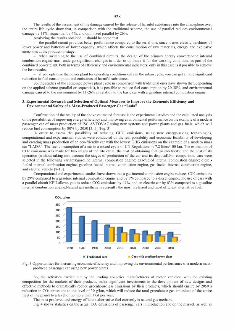
928 The results of the assessment of the damage caused by the release of harmful substances into the atmosphere over

the entire life cycle show that, in comparison with the traditional scheme, the use of parallel reduces environmental damage by 11%, sequential by 4%, and optimized parallel by 26%.

Analyzing the results obtained, it should be noted that: – the parallel circuit provides better performance compared to the serial one, since it uses electric machines of

lower power and batteries of lower capacity, which affects the consumption of raw materials, energy and explosive emissions at the production stage;

– when switching to the use of combined circuits, the design of the primary energy converter-the internal combustion engine must undergo significant changes in order to optimize it for the working conditions as part of the combined power plant, both in terms of efficiency and environmental indicators; only in this case is it possible to achieve the best results;

– if you optimize the power plant for operating conditions only in the urban cycle, you can get a more significant reduction in fuel consumption and emissions of harmful substances.

So, the studies of the combined power plant cycle in comparison with traditional ones have shown that, depending on the applied scheme (parallel or sequential), it is possible to reduce fuel consumption by 20-38%, and environmental damage caused to the environment by 11-26% in relation to the basic car with a gasoline internal combustion engine.

3. Experimental Research and Selection of Optimal Measures to Improve the Economic Efficiency and

Environmental Safety of a Mass-Produced Passenger Car “Lada”

Confirmation of the reality of the above estimated forecast is the experimental studies and the calculated analysis of the possibilities of improving energy efficiency and improving environmental performance on the example of a modern passenger car of mass production of JSC AVTOVAZ using new systems and power plants and gas fuels, which will reduce fuel consumption by 80% by 2050 [3, 5] (Fig. 3).

In order to assess the possibility of reducing GHG emissions, using new energy-saving technologies, computational and experimental studies were conducted on the real possibility and economic feasibility of developing and creating mass production of an eco-friendly car with the lowest GHG emissions on the example of a modern mass car "LADA". The fuel consumption of a car in a mixed cycle of UN Regulations is 7.2 liters/100 km. The estimation of CO2 emissions was made for two stages of the life cycle: the cost of obtaining fuel (or electricity) and the cost of its operation (without taking into account the stages of production of the car and its disposal).For comparison, cars were selected in the following variants:gasoline internal combustion engine; gas-fueled internal combustion engine; diesel-fueled internal combustion engine; gasoline-fueled internal combustion engine, gas-fueled internal combustion engine, and electric vehicle [8-10].

Computational and experimental studies have shown that a gas internal combustion engine reduces CO2 emissions by 29% compared to a gasoline internal combustion engine and by 5% compared to a diesel engine.The use of cars with a parallel circuit KEU allows you to reduce CO2 emissions by 44%, and an electric car by 63% compared to a gasoline internal combustion engine.Natural gas methane is currently the most preferred and most efficient alternative fuel.

Fig. 3 Opportunities for increasing economic efficiency and improving the environmental performance of a modern mass-produced passenger car using new power plants So, the activities carried out by the leading countries manufacturers of motor vehicles, with the existing

competition for the markets of their products, make significant investments in the development of new designs and effective methods to dramatically reduce greenhouse gas emissions by their products, which should ensure by 2050 a reduction in CO2 emissions to the level of 30 g/km, which will reduce the total greenhouse gas emissions of the entire fleet of the planet to a level of no more than 3 Gt per year.

The most preferred and energy-efficient alternative fuel currently is natural gas methane. Fig. 4 shows statistics on the actual CO2 emissions of passenger cars in production and on the market, as well as

CO2, g/km

929 those planned for production and recently coming to the market with CEU.

Fig. 4 CO2 emissions from domestic and foreign passenger cars, including those with CEU

4. Conclusions

The results of the theoretical and experimental studies allow us to draw the following conclusions: 1. An analysis of the current state of work to reduce environmental damage from explosive and greenhouse gas

emissions has shown that there are difficulties in objectively assessing the effectiveness of environmental and economic results (in terms of damage) when comparing existing and new car designs with different power plants running on different energy carriers.

2. The developed methodology for assessing the environmental hazard of cars based on the total indicator of explosive emissions, taking into account their relative aggressiveness, allows you to objectively compare various design innovations (measures) for their environmental effectiveness.

3. The production of electric vehicles and cars with power plants running on compressed air, cryogenic nitrogen and hydrogen should be developed as priority areas for the preservation of the urban air environment without pollution of its explosives and GHG.

4. To reduce the global pollution of the planet's atmosphere, it is necessary to develop and create new cost-effective technologies for obtaining energy from solar energy, wind energy, i.e. renewable energy sources available in unlimited quantities (volumes).

References 1. Zaripov, R.Yu.; Gavrilov, P.; Karku, A.D.; Serikpaev, T.M. 2019.

, Nauka i tekhnika Kazakhstana 1: 75-84.(in Russion). 2. Toshiaki Tanaka «Global Energy and Envirommental Jssues, Reflected in Toyota s Advanced Powertrain

Development», Toyoto, Motor Corporation, Aichi, Japan. 3. OECD (2016), The Economic Consequence of Outdoor Air Pollution, OECD Publishing, Paris. http://dx.doi.org/

10.1787/9789264257474-en . 4. On the Concept for the transition of the Republic of Kazakhstan to a "green economy". Decree of the President of the

Republic of Kazakhstan No. 577 dated May 30, 2013 5. Rensselar, J.V. 2012. Power to Spare: Hydraulic Hybrids, Tribology and Lubrication Technology 68(2). 6. Schechter, M.M. 1999. New Cycles for Automobile Engines. SAE Paper. 1999-010623. 7. Huang, K.D.; Tzeng, S.C.; Chang, W.C. 2005. Energy-Saving Hybrid Vehicle Using a Pneumatic-Power System,

Applied Energy 81(1). 8. Dvigateli vnutrennego sgoraniya: Teoriya porshnevykh i kombinirovannykh dvigateley Pod redaktsiey A.S. Orlina,

M.G. Kruglova [Internal combustion engines: Theory of reciprocating and combined engines], Moscow, Mashinostroenie Publ., 1983, 372 p.

9. Wallace, W. 1967-68. High-Output Medium-Speed Diesel Engine Air and Ex-haust System Flow Losses, Proceedings of the Institution for Mechanical Engineers 182: 134-144.

10. Benson, R.S. 1960. Experiments on a Piston Controlled Port, The Engineer 210: 875-880.

CO2, g/km

930

Proceedings of 25th International Scientific Conference. Transport Means 2021. Modelling of Unbound Base Layer Aggregate Shape and Structure by Discrete Numerical Methods V. Filotenkovas1, A. Vaitkus2

1Vilnius Gediminas Technical University, Saul tekio al. 11, LT-10223 Vilnius, Lithuania E-mail: vilius.filotenkovas@vilniustech.lt 2Road Research Institute of Faculty of Environmental Engineering, Vilnius Gediminas Technical University, Linkmen str. 28, LT-08217 Vilnius, Lithuania, E-mail: audrius.vaitkus@vilniustech.lt Abstract From the point of view of road network infrastructure, the load-bearing capacity of the pavement structure is ensured by general safety, durability, smoothness, noise, economy and other requirements. However, in most cases, these aspects are considered only in the pavement layers of road structures. To date, scientific work has been done to review the upper layers of road construction, i.e. functionality of asphalt or other pavement layers, but little is known about the performance of the base layers. Hence the need to implement an optimal base layer design model. The functionality of unbound base layers, exclusively for the upper base layers, depends not only on the compaction grade and layer thickness, but also on unbound material type, shape, fines content and mechanical properties of aggregates. The response of the pavement structure to loads is expressed through deformations and stresses, which are determined by analytical models. Two typical numerical models are used in the mechanics of materials: continuum and particle interactions. The aim of this research is to define, analyse and systematize the results of scientific research of discrete numerical methods used to model unbound base layers, aggregates based on their shape and structure. Based on the results of the research, conclusions and recommendations for further research of the effect of particle shape and structure on the stiffness modulus of upper unbound base layer are presented. KEYWORDS: unbound base layer, particle shape, particle structure, aggregates, discrete numerical method. 1. Introduction

Recently, a number of studies have been carried out to analyse the resilient behaviour of unbound base layer aggregates. Several factors such as strain level, grain size, fine content, particle type, water content are reported to affect the resilient behaviour of these materials. However, pavement performance is not entirely evident as a result of complex aggregate modelling. Over the last few years, research has focused on numerical modelling as a consequence of computer processor improvements [2]. A road structure's response to loads results in deformations and stresses. This determines analytical patterns in pavement design. Two typical numeric models are employed in materials mechanics: continuum and particle interactions (micromechanical) [25].

In the case of a micromechanical model, the mechanical properties of the test object are determined by structural defects such as cracks, particle orientation, component distribution, etc. To evaluate mentioned parameters various models, such as the micro crack spread model, are used. In this case, the investigation of the stress and strain function of test objects with different structures is performed with an idealized representative volume in order to determine the influence of microstructural defects on the macrostructure. This method of analysis is difficult to use due to the complex microstructure inherent in the structure of the base layer of the chippings and the interaction between the faults in the structure. Therefore, without proper model simplifications, the calculated results poorly with the experimental data. Using a continuum model, the internal mechanical properties of a composite are characterized by averaged values of mechanical properties. In solving this problem by the discrete element method the averaged values of the state variables is determined. This approach allows for a significant simplification of the numerical model, but does not reflect the discrete nature of the micro and meso properties, and the results need to be calibrated based on physical experiments [25].

Four simplified numerical models are used in road engineering: multilayer elastic method, equivalent thickness method, finite element method and discrete element method [14]. However, due to the irregular geometry of the aggregates, the finite element and discrete element methods are most commonly used [25].

Composite materials can be modeled with finite element method as a heterogeneous continuum by detailing the individual structural components. This method of analysis requires large calculation resources due to the complex internal structure of the particle composite, so the application of this method to the analysis of the composite is inefficient. In order to exploit the potential of finite element method, simpler models suitable for composite analysis need to be found.

An alternative to continuum models is discrete element methods. Discrete element modelling (DEM) is gaining increasing popularity in geotechnical and pavement engineering for its capacity to model granular materials, which are composed of distinct particles that demonstrate the complex macro- micro-mechanical behaviour during loading. It describes the composite as a particle system and is based on the mechanical interaction of individual particles. The ability to more accurately describe the discrete properties of a particle composite is a major advantage of the method. The

931 disadvantages of the method are the high calculation volumes and the lack of universal models for describing composite geometry and internal interactions.

Existing discrete element method models examine directly contacting particles, or form a dummy discrete constant continuum [25]. 2. Use of Finite Element Model for the Calculation of the Unbound Base Layers of Pavement Structures

The upper layers of asphalt pavement are regarded linearly elastic as mechanical empirical models of long-term deformations are used to calculate and model the reactions of the layers of road pavement structures. In numerical models, however, stress-dependent unbound mineral material layers are used as nonlinear elastic layers [1].

The elasticity modulus of unbound mineral materials is determined by the stresses imposed by traffic loads. The dependency of the vertical modulus of elasticity on traffic-induced stresses was discovered to be designable using a linear elastic model by separating the mineral base layers into many layers, each with its own vertical modulus of elasticity indicating the magnitude of the stresses. Although, a linear elastic model cannot directly model the dependency of the horizontal modulus of elasticity component on the stresses induced by traffic loads. The use of a finite element model, which allows for the calculation of the layer's anisotropic behavior in vertical and horizontal directions based on traffic pressures, would allow for a more precise estimation of the relationship between estimated and measured layer deflections [5].

In current flexible pavement construction design procedures or mechanical empirical (M-E) pavement design, predicting ruts and other disruption has become a problem [2]. These techniques provide a more accurate picture of the coating structures and the factors that influence their functionality. The pavement structure is analysed using mechanical-empirical methods based on current traffic loads and environmental factors, with the goal of limiting stresses, deformations, or impacts to the pavement structure without overdoing the norms or critical conditions. Mechanical-empirical methods usually consist of two steps: measuring stresses and strains using a reaction response model and empirically comparing the measured reactions to the predicted coating life or coating quality. Repeated traffic loads operating on road pavement systems necessitate the use of mathematical calculations to deduce damage and wear reactions [4, 16]. The mechanical-empirical approach, on the other hand, has more benefits than pure empirical design methods because it allows for the quantification of various kinds of defects with the smallest possible errors. Pavement efficiency forecasting procedures may be used for surface maintenance and reconstruction programs, as well as analysing the life cycle costs of pavement structures, in addition to the design of new pavement structures [1].

Granular materials are described by their elastic parameters (modulus and Poisson's ratios) when using the mechanistic design procedure. All of the material and structure parameters used in the empirical design methods are expected to be met in this situation, as are the shear strength and permanent deformation requirements.

There is strong proof that the modulus in the vertical direction differs from that in the horizontal direction for unbound granular materials (i.e. they are anisotropic). The vertical modulus of unbound granular materials is assumed to be double the horizontal modulus in the mechanistic modelling process. Physically, this phenomenon is due to the fact that pavement materials are typically compacted in horizontal layers, resulting in a desired particle orientation. Although there is no universal method for describing anisotropic behavior, it has been discovered that using anisotropy in the pavement model improves the match between estimated and measured deflections. However, it is unclear if this is due purely to the anisotropic behavior of these materials or to their stress-dependent behavior [5].

Granular materials' modulus is determined not only by their inherent properties, but also by the stress degree at which they work and the stiffness of the underlying layers. As a result, the modulus of vertically loaded pavement materials decreases with depth, with the modulus of the subgrade playing a role. Iterative analyses using a finite element model would allow for the stress-dependent structure of granular material modulus to be taken into account, but it would not account for the degree of support offered by underlying layers.

Furthermore, since such models are not readily accessible to pavement designers. Ausroads [5] implies technique that employs a linear elastic layer model, with the granular layers partitioned into many sublayers and each given a modulus value. Sublayering is needed for granular materials put directly on the in situ subgrade or selected subgrade material and it should be done as follows:

Division of the total thickness of unbound granular materials into five equal thickness sublayers. The estimation minimum vertical modulus of the top sublayer by calculating using equation:

/125

2total granular thickness

top granular sublayer underlying materialE E . (1)

The modulus ratio of adjacent sublayers is given by equation:

15

top granular sublayer

underlying material

ER

E. (2)

The modulus of each sublayer will then be determined based on the modulus of the adjacent underlying

sublayer, starting with the subgrade or upper sublayer of a known modulus subgrade content. Vertical modulus measured

932 for each sublayer must not surpass the maximum modulus that the granular material in that sublayer will produce due to its intrinsic properties. If this is not the case, a material with a higher modulus should be used in this sublayer, or a different pavement configuration should be chosen.

As suggested by Ausroads [5], other elastic parameters needed for each sublayer for all granular materials can be determined using the following relationships: 0,5 ; / 1H V VE E F E . (3) 3. Discrete Numerical Models Used for the Calculation of the Unbound Base Layers of Pavement Structures

Cundall and Strack initially suggested to model granular materials using the DEM [9]. Since that time, DEM-based design models have been used in a variety of areas of soil and rock mechanics, granular flow and powder mechanics. The DEM was also used to model a number of experiments of unbound base layer granular materials [31].

Cundall’s developed Discrete Element Method is a numeric method that can be used to examine the movement of individual and independent objects. The DEM enables finite displacements and discrete body rotations, including full detachment, and automatically recognizes new contacts as the calculation progresses [8]. When compared to the displacement of the whole unbound base layer, individual particles have relatively small deformation, it is not necessary to model with precision the deformation of the particles to obtain a good approximation of the overall mechanical behavior. It should be noted that this assumption generally applies to unbound aggregates, making the DEM an appropriate tool for investigating the behaviour of these materials. In DEM, the contact forces and displacements within a particulate assembly can be found through a series of calculations by tracking the movement of individual particles. Newton's second law is used to measure a particle's motion due to forces acting on it, and the force-displacement law is used to calculate interaction forces based on displacements [9]. During a DEM simulation, certain elements come into interaction and others differ at each time step. This interaction identification must be done during the whole study. Contact identification can be done analytically for elements with basic shapes like spheres or ellipses. However, as the shape of specific particles (discrete elements) deviates from basic forms, the contact detection mechanism becomes considerably more complex. Calculating and updating contact forces during a DEM simulation takes a lot of time and effort. Fig. 1 schematically represents the key components of a DEM simulation.

Fig. 1 Flow chart showing the main principles of DEM (discrete element model)

The DEM is a flexible instrument that can be used to model even the most complex applications. Ullidtz [27] used 2D DEM simulations to model the reaction of granular materials to applied stresses, taking into account the effects of angular particle sizes, particle size distributions, particle adhesive forces, and various stress directions. Even when the external loading is compressive, tensile stresses and tensile cracks will form, according to the simulations. Modelling bound materials like asphalt and concrete is also possible with the DEM. Buttlar and You [6], for example, used the DEM to replicate the indirect tensile test. Their findings are somewhat similar to those of the experiment.

To model the resilient modulus test, Zeghal [32] used a two dimensional discrete element method (2D DEM). Used model correctly predicted that the resilient modulus of granular materials increases as the deviator stress and confining pressure rise. The confining stress raised the resilient modulus more than the deviator stress did. This tendency has been validated by other computational simulations and physical experiments: the estimated Mr from the simulations is within 10% of the actual results obtained in laboratory. Other numerical models and physical observations have confirmed this pattern ([28, 17]). The error margin seems to be very limited as compared to other 2D DEM models ([29, 26]). Uthus et al. [28] used a 3D DEM to model the resilient modulus test and found that the

Velocities

Position

Contacts Forces

Acceleration

Newton’s Laws

Contact Mechanics

933simulation findings are quantitatively very similar to the results of the same group's physical resilient modulus tests on spherical particles. The study conducted by these groups found that DEM is a promising method for modelling resilient modulus testing of unbound materials, as shown by the consensus between experimental and simulated performance.

The resilient modulus is often affected by the applied stresses [17]. With the pressure and/or deviator stresses, the resilient modulus rises. Hicks and Monismith [13] used experiments to establish a bulk stress to monitor the combined effect of the confining pressure and the deviator stress (Fig. 2):

1 2 3 3 c d , (4)

where c is the confining pressure and d is the maximum deviator stress. The Mr increases were modeled as a power law function of the bulk stress:

21

krM k , (5)

where k1 and k2 are analytical constants that vary depending on the granular aggregate type. Zeghal's [32] 2D models and their experimental findings all backed up the power law model.

Fig. 2 Scheme of typical cross-section of flexible pavement and base layer affected stresses ( d – deviator stress, 3 – confining stress)

The Witczak–Uzan Universal model was modified to account for increasing stiffness with the stresses in an unbound aggregate layer in the Mechanistic-Empirical Pavement Design Guide, which includes specific analysis of both the bulk stress u and octahedral shear stresses oct:

2 221 2 1 3 2 3

1 23 3oct d . (6)

This model relates the Mr to u and oct normalised by the atmospheric pressure pa:

2 2

1 1k k

octr a

a a

M k pp p

, (7)

where k 1, k 2 and k 3 are empirically determined constants in the Universal model that depend on the type of granular aggregates [31].

For discrete element modelling, there are many computer software programs available, such as BALL [9], EDEM [11], Particle Flow Code (PFC) [19] and open source codes like Yade [15], MUSEN [12] and LIGGGHTS® [7]. PFC is one of the most widely used general-purpose Distinct Element Modelling platforms [21].

4. Discrete Numerical Models Used to Calculate the Properties of Aggregate Particles Used in Unbound Base Layers

Resilient modulus is stress-dependent [17]. Dastich and Dawson [10] used Hertz's principle to understand why granular materials are so dependent. Each granular particle is represented by a sphere, and the contact region between the spheres increases as the stress added to the specimen increases. As a result, the resistance to the sphere's centre being closed increases [22].

The correlation coefficients at various wavelengths are obtained, allowing quantitative evaluation of the correlationship between aggregate wear surface micro-texture levels at various wavelengths and kinetic friction coefficients. Since strong correlation coefficients (0.85 and 0.84) are observed at these two wavelengths, it shows that there are important associations between micro-texture levels of 32 m and 2 m wavelengths and kinetic friction coefficients. However, since mean roughness involves surface texture components that have less effect on

934kinetic friction coefficients across aggregates, the correlation coefficient between wear surface mean roughness and friction coefficients at different wear stages is not high. Since the kinetic friction coefficient is determined by both the aggregate material property and its surface characteristic, there is no clear connection between the surface texture property and the kinetic friction coefficient of various aggregate forms. The comparison of the micro-texture levels and their distribution obtained in this study with the traditionally used surface mean roughness shows that the micro -texture levels and their distribution can detect levels of the exact texture scales greatly affecting the aggregate kinetic friction coefficient, while the surface mean roughness can only reflect the global surface property [31].

It was found that the Mr increases linearly with the modulus of elasticity of the particle materials in the investigated range. Although, effects from our resilient modulus model and experiments would be more quantitatively comparable if used with experimental data for spherical particles. Furthermore, simulations of various sizes of spherical and aspherical particles will aid in distinguishing between size and shape results [31].

DEM models, on average, appear to underestimate experimental performance. While the physical measurements, particle sizes and shapes, stress levels, and loading procedures of the simulations and laboratory experiments are virtually identical, there are also major variations between the two methods. It's impossible to catch all of the nuances in real materials, for example. Mineralogy, anisotropy, and microscopic roughness of aggregate particles are all factors that can influence the outcome [28].

Body, pieces, and contacts form the particle flow code (PFC) model. Ball, clump, and wall are the three fundamental entities. Each body is made up of many parts. Internal force and moment (Fc and Mc) work on the two pieces in an equal and opposite manner at the interface point (Fig. 3). Contacts between two walls, on the other hand, are unlikely to form. Ball-ball, ball-pebble, pebble-pebble, ball-facet, or pebble-facet are the various types of interactions [24]. Forces that occur at contacts interfere between the balls, clumps, and walls. For each ball and clump, motion equations are satisfied. The artificial granular material (as balls or clumps) is compacted and contained using velocity boundary conditions applied to the surrounding walls.

Fig. 3 Scheme of acting forces and moments in contact of two particles

All deformation happens at the rigid bodies' contacts in the PFC model system. It is necessary to create interaction models that describe the action of particles and facets as they make contact. A force -displacement law comparing the generalized internal force to the relative motion at the contact is given by the contact -model formulation. Linear, linear contact bond, linear parallel bond, hertz contact, hysteretic contact, smooth-joint contact, flat joint, rolling resistance linear, burger's model, and hill contact model are some of the contact models that PFC can use [24]. Interaction model defines the actions of each contact type.

Cundall and Strack [9] created a linear model composed of linear springs and dashpots, which applies to this model. To acquire new contact forces, the force-displacement law is applied to each of the contacts at the start of each stage. Equation 8 can be used to decompose the contact force vector Fi into regular and shear components with respect to the contact plane.

n si i iF F F , (8)

where niF and s

iF represent the contact force vector's normal and shear components, respectively. The force -displacement rule uses the normal (Kn) and shear stiffness (Ks) at the contact to connect these two components of force to the respective components of relative displacement. The standard touch force vector is determined using the following formula:

n n ni iF K U n , (9)

where Kn the normal stiffness, Un the overlapping displacement magnitude of two contacting entities and the unit

935 normal vector. The normal vector's direction is determined by the element type: I for ball-to-ball contact, the normal vector is directed along the line defining the shortest distance between the ball centre and the wall, and (ii) for ball -to-wall contact, the normal vector is directed along the line defining the shortest distance between the ball centre and the wall. The shear contact power, on the other hand, is calculated incrementally. The cumulative shear contact force is set to zero when the contact is made. Shear force is increased by relative shear displacement at the contact point of two interacting pieces. The shear force-increment vector is determined using the following formula: ,s S S

i iF K V t (10) where Ks the shear stiffness at the contact and s

iV the shear component of the contact velocity and t the timestep. Finally, the final shear contact force is determined by adding the previous shear force vector and the shear elastic force-increment vector at the start of the time step.

previouss s s

i i iF F F . (11)

The force-displacement law connects the contact forces and relative displacements in the natural and shear

directions in the stiffness model. PFC3D® supports two types of contact stiffness models: linear models and Hertz-Mindlin models. The linear contact-stiffness model assumes that the normal (Kn) and shear stiffness (Ks) of two contacting entities (ball to ball or ball to wall) function in sequence. The following calculations can be used to quantify the contact stiffness for the linear contact model.

A B

n n nA B

n n

K KK

K K;

A BS S S

A BS S

K KK

K K, (12)

where the superscripts [A] and [B] denote the two entities in contact.

The elastic properties of the two touching spheres, i.e. shear modulus (G) and Poisson's ratio ( ), describe the generalized Hertz-Mindlin model. The natural and shear stiffness are overlooked in the PFC3D® model for the Hertz-Mindlin model, and walls are believed to be rigid. For ball-to-wall contacts, only the ball's elastic properties are used, and for ball-to-ball contacts, the mean values of the elastic properties of the two touching balls are used. Furthermore, the Hertz-Mindlin model lacks a tensile force definition, making it incompatible with any bonding model. It's also worth noting that in PFC3D, interaction between a ball with the linear model and a ball with the Hertz model is not permitted [19].

While field or laboratory testing may be used to determine the properties of unbound aggregate products, the deformation and failure process of unbound aggregate cannot be completely understood from a macroscopic perspective. DEM has been commonly used to analyse the behavior of unbound aggregate materials from multiscale views in order to investigate the properties. Although, since its introduction into geo-technique engineering, DEM has seen major advancements in recent years. The most important benefit is that DEM can explain the explicit movement and interaction of individual particles while still taking into account the dynamic constitutive relationship of materials using simplistic touch models. Phusing and Suzuki [23] investigated particle displacements using DEM in the limit stress-path state. It showed that particle displacement was not completely determined by the loading direction and loading times. Particle flow code three dimension (PFC3D) was used to model the complex behavior of unbound aggregate materials in a flexible membrane boundary with spherical particles [21]. When DEM simulations of repeated loading tests were performed with uniform spherical grains to analyse the sensitive parameters for the resilient behavior of aggregates, a fair agreement was reached between the laboratory experiments and the DEM simulation test. The spherical particles used in DEM, on the other hand, created several variations from actual irregular aggregates [28]. This paper introduced the use of an image-aided DEM approach to realistically model the micromechanical interactions of aggregate particles, including size and shape effects. The DEM method and the inventive use of membrane elements covering the cylindrical aggregate specimen in the DEM model were used to replicate laboratory fast shear (triaxle compression) experiments. By minimizing the variations between DEM-simulated triaxial shear strength findings and experimental ones, the mentioned experimental test results were used to decide required micro-mechanical parameters for the DEM model. The DEM method confirms that it could accurately model the nonlinear stress-strain behavior of unbound aggregate products, including dilatancy effects, based on DEM test results. The projected deviator stresses were very similar to those observed in the experiments, meaning that the evolved DEM model would accurately replicate the shear strength behavior of unbound aggregate materials. The calibrated DEM model has the ability to optimize the size and shape properties of different forms of unbound aggregates to achieve desired shear strength in future research (or rutting resistance) [30].

The use of the actual particle approach is recommended by Ning Li and others. The aggregate's structure and mesoscopic characteristics were reconstructed using the particle modelling technique [18]. To construct the actual particle shape, four key steps were added in Li’s research. To begin, the scanning image of aggregate in three dimensions was obtained using the X-ray Computed Tomography (CT) scanning technique. Second, the individual scanning images were processed using the MATLAB software. During this method, the Fourier function, spherical harmonics, and aggregate

936morphological features (shape, angular, texture, and so on) were obtained. In order to establish aggregate geometry structure, the processed images were converted into the STL (stereo-lithography) format file. Third, using the Particle Flow Code PFC5.0 software, the data in the STL file was transformed into the particle geometry form contour. Finally, the ‘clump' command was used to fill the particle shape contour with pebbles to create the actual particle prototype.

It was discovered that both the permanent deformation obtained from laboratory tests and the actual particle model alternated with loading. The ball model, on the other hand, did not reveal this pattern. These results suggest that the actual particle model will more accurately represent the laboratory tests' permanent deformation characteristics. The ball is smooth in the numerical simulation, with no edges or corners. Despite the fact that the coefficient of friction was fixed, the balls dislocated and migrated even more quickly when loaded [20]. In a very short time, the structure had achieved equilibrium. The actual particles were difficult to move under the loading due to their angularity, which made stress development more possible in certain zones. The non-interlocked particles relocated and rotated under constant loading after the tension reached a certain level, causing changes in the microstructure. The deformation then increased slowly but steadily.

a b

Fig. 4 Examples of templates for: a DEM Ball model; b DEM Real particle shape model [18]

5. Conclusions

Due to the irregular geometry of the aggregates, the finite element and discrete element methods are the most commonly used numerical models are used in road engineering.

Iterative analyses using a finite element model would allow for the stress-dependent structure of granular material modulus to be taken into account, but it would not account for the degree of support offered by underlying layers. Furthermore, such models are not readily accessible to pavement designers.

In the discrete element method, the contact forces and displacements within a particulate assembly can be found through a series of calculations by tracking the movement of individual particles. However, as the shape of specific particles (discrete elements) deviates from basic forms, the contact detection mechanism becomes considerably more complex. Calculating and updating contact forces during a DEM simulation takes a lot of time and effort.

A number of experiments have used numerical modelling based on image processing, X-ray scanning, or random generation to predict the realistic shapes of aggregates. The newest results show that aggregate size and shape had significant effects on mechanical properties. According to the findings, aggregate morphology has a major impact on the mechanical properties of unbound aggregate and stone-based paving materials. As a result, in computational simulations of dynamic repeated load tests of aggregate, it is important and reasonable to assume the realistic shape of aggregate. The consistent results demonstrate that the established discrete element model with actual particle shapes is capable of simulating laboratory testing.

For discrete element modelling, there are many computer software programs available, such as BALL, EDEM and open source codes like Yade, MUSEN and LIGGGHTS®, but Particle Flow Code (PFC) is mostly used.

References

1. Ahmed, A.; Erlingsson, S. 2013. Evaluation of permanent deformation models for unbound granular materials using accelerated pavement tests, Road Materials and Pavement Design, 14(1): 178-195, DOI: 10.1080/14680629.2012.755936

2. ARA, Inc., ERES Consultants Division. (2004). Guide for mechanistic-empirical design of new and rehabilitated pavement structures (Final report, NCHRP Project 1-37A). Washington, DC: Transportation Research Board of the National Academies. Retrieved September 10, 2014, from www.trb.org/mepdg/ [Google Scholar].

3. Arulrajah, A.; et al. 2020. Discrete element analysis of recycled concrete aggregate responses during repeated load triaxial testing, Transportation Geotechnics 23: 100356, ISSN 2214-3912, https://doi.org/10.1016/j.trgeo.2020.100356.

4. Askari, E. 2021. Mathematical models for characterizing non-Hertzian contacts, Applied Mathematical Modelling90: 432-447.

5. Austroads 2018. Guide to Pavement Technology Part 2: Pavement Structural Design. 6. Buttlar, W.G.; You, Z. 2001. Discrete Element Modeling of Asphalt Concrete: Microfabric Approach,

Transportation Research Record 1757(1): 111-118. doi: 10.3141/1757-13.7. CFDEMresearch GmbH (2017). “LIGGGHTS(R)-PUBLIC Documentation, Version 3.X”. Available from

https://www.cfdem.com/media/DEM/docu/Manual.html

937 8. Cundall, P.A.; Hart, R.D. 1992. Numerical modelling of discontinua. Engineering computations. 9. Cundall, P.; Strack, O. 1979. A discrete numerical model for granular assemblies, Geotechnique 29(1): 47-65.

https://doi.org/10.1680/geot.1979.29.1.47, https://doi.org/10.1680/geot.1980.30.3.331 10. Dastich, I.; Dawson, A. 1995. Techniques for Assessing the Nonlinear Resilient Response of Unbound Granular-

Layered Structures, Geotechnical Testing Journal 18(1): 50-57. Retrieved from https://doi.org/10.1520/GTJ10121J 11. DEM Solutions. 2011. “EDEM 2.4 User Guide”. Available from http://tm.spbstu.ru/images/2/28/EDEM2.4_user_

guide.pdf 12. Dosta, M.; Skorych, V. 2020. MUSEN: An open-source framework for GPU-accelerated DEM simulations,

SoftwareX 12: 100618, ISSN 2352-7110, https://doi.org/10.1016/j.softx.2020.100618. 13. Hicks, R.; Monismith, C. 1971. Factors influencing the resilient response of granular materials. Highway Research

Record. 14. Kleizien , R. 2016. Nestandžios dangos konstrukcijos modeliavimas vertinant tampriai klampias asfalto savybes:

Daktaro disertacija : Technologijos mokslai, statybos inžinerija (02T). Vilnius: Technika. 15. Kozicki, J.; Donzé, F.V. 2009. YADE-OPEN DEM: an open-source software using a discrete element method to

simulate granular material, Engineering Computations 26(7): 786-805. 16. Lai Z., et al. 2021. A semianalytical Hertzman frictional contact model in 2D, Applied Mathematical Modelling

92: 546-564. 17. Lekarp, F.; Isacsson, U.; Dawson, A. 2000. State of the Art. I: Resilient Response of Unbound Aggregates, Journal

of Transportation Engineering-asce - J TRANSP ENG-ASCE. 126. 10.1061/(ASCE)0733-947X(2000)126:1(66). 18. Li, N.; et al. 2020. Numerical simulation of dynamic repetitive load test of unbound aggregate using precision

unbound material analyzer, Road Materials and Pavement Design 21(6): 1675-1693, DOI: 10.1080/14680629.2019.1567374

19. Mahmud, S. 2017. Effect of Particle Size Distribution and Packing Characteristics on Railroad Ballast Shear Strength: A Numerical Study Using the Discrete Element Method. Boise State University Theses and Dissertations. 1310. https://doi.org/10.18122/B29D8K

20. McDowell, G.R.; et al. 2006. Discrete element modelling of geogrid-reinforced aggregates, Proceedings of the Institution of Civil Engineers - Geotechnical Engineering 159(1): 35-48.

21. Mehmet, B.C.; Khalid, A.A. 2014. Dynamic analysis of kinematic behavior of granular materials in triaxial testing using DEM with flexible membrane boundary, Acta Geotechnica 9(2): 287-298.

22. Nguyen, B.; et al. 2016. Possible simplified method for the determination of the resilient modulus of unbound granular materials, Road Materials and Pavement Design 17(4): 841-858, DOI: 10.1080/14680629.2015.1130162

23. Phusing, D.; Suzuki, K. 2015. Cyclic behaviors of granular materials under generalized stress condition using DEM, Journal of Engineering Mechanics 141(10): 04015034.

24. Potyond, D. 2019. Pavement-Design Package for PFC3D [pdPkg15], Itasca Consulting Group, Inc., Technical Memorandum ICG16-8528-15TM (April 1, 2019), Minneapolis, Minnesota.

25. Rimša, V. 2014. Daleli kompozito diskretusis modelis: Daktaro disertacija. Vilnius: Vilniaus Gedimino technikos universitetas. Prieiga per eLABa – nacionalin Lietuvos akademin elektronin biblioteka

26. Tanaka, H.; et al. 2000. Simulation of soil deformation and resistance at bar penetration by the Distinct Element Method, Journal of Terramechanics - J TERRAMECH. 37: 41-56. 10.1016/S0022-4898(99)00013-0.

27. Ullidtz, P. 2001. Distinct Element Method for Study of Failure in Cohesive Particulate Media, Transportation Research Record 1757(1): 127-133. doi: 10.3141/1757-15.

28. Uthus, L.; et al. 2008. Discrete element modelling of the resilient behaviour of unbound granular aggregates, International Journal of Pavement Engineering 9(6): 387-395, DOI: 10.1080/10298430802169382

29. Williams, J.R.; Rege, N. 1997. Coherent vortex structures in deforming granular materials, Mech. Cohes. Frict. Mater. 2: 223-236. https://doi.org/10.1002/(SICI)1099-1484(199707)2:3<223::AID-CFM30>3.0.CO;2-F

30. Xiao, Y.; et al. 2014. DEM Approach for Engineering Aggregate Gradation and Shape Properties Influencing Mechanical Behavior of Unbound Aggregate Materials, Geotechnical Special Publication, 2898-2910. 10.1061/9780784413272.281.

31. Yohannes, B.; et al. 2014. Mechanistic modelling of tests of unbound granular materials, International Journal of Pavement Engineering 15(7): 584-598, DOI: 10.1080/10298436.2013.775442.

32. Zeghal, M. 2004. Discrete-element method investigation of the resilient behavior of granular materials, Journal of Transportation Engineering 130: 503-509.

938

Proceedings of 25th International Scientific Conference. Transport Means 2021.

Development and Application of Mechanism for Real Rollover Crash Tests P. Verta 1, J. Janura2, G. Kasanický3, J. Bernát4 1University of Žilina, 1. mája 32, Žilina, 010 26, Slovakia, E-mail: peter.vertal@usi.sk 2University of Žilina, 1. mája 32, Žilina, 010 26, Slovakia, E-mail: juraj.janura@gmail.com 3University of Žilina, 1. mája 32, Žilina, 010 26, Slovakia, E-mail: gustav.kasanicky@usi.sk 4University of Žilina, 1. mája 32, Žilina, 010 26, Slovakia, E-mail: juro.bernat@gmail.com Abstract This paper is dealing with the topic of a vehicle rollover that is considered to be one of the most dangerous types of traffic vehicle crash. The key point of the article is the introduction of a mechanism designed for vehicle rollover simulation tests. The purpose of this simulation test is to research vehicle passive safety and its influence on vehicle passengers. Design of mechanism allows to tow and guide the vehicle by the other one, after reaching desired speed to release the towed vehicle and to secure change of its travel direction. In combination with a suitable road profile, the rollover of the vehicle is reached. The article also describes a technical explanation of the mechanism itself and a list of component functions. There is also mentioned a real crash test of the vehicle, where this mechanism was used and rollover accident simulation executed. The purpose of this crash test was an analysis of data gathered from internal and external sensors, however, there are many other safety research tests, where this rollover mechanism could be effectively applied. KEY WORDS: accident, rollover, rollover mechanism, crash test 1. Introduction

The overall number of traffic accidents in the European Union in a period of 2000 - 2020 has decreasing tendency

however ambitious plan for significant reduction has not been reached. There can be observed a difference between the actual and desired value of the relative decrease in road accidents deaths which is about 18% worse in comparison with targeted value [1]. The decreasing trend stagnated in 2013, then in following years number of fatalities was fluctuating around 26 000 cases. European Commission’s 2001 White paper target was halving the number of accident fatalities between 2000 and 2010 to number 29 600. It was reached later in 2012. In following white paper published in 2011 was the target again to reduce the number of fatalities by half from 2010 to 2020. The target to reach less than 14 800 fatalities in 2020 was also not reached as a real result was 18 800 [2]. However, these goals have not been achieved, Europe is with an average of 51 road deaths per 1 million inhabitants the road safest region in the world [3].

Rollover accidents belong to accidents type with most serious health consequences. Accessible data analysis shows that for occupant’s head, neck and spine injuries caused by impacts with the upper vehicle interior are 35% portion of all injury harm. Most of the European countries are missing information regarding rollover accidents. Only a few of them can provide official statistical data as Great Britain with CCIS database, GIDAS database for Germany and some global information from investigating database from Spain. Occurrence of the rollover accidents in Europe has been observed in 4-5% of all accident cases and with a 15% portion of all fatal crashes. One half of the cases took place after an initial impact [4]. These figures show the real severity of rollover accidents which should become an important topic for further research in order to enhance traffic safety.

2. Rollover Accidents

The European, US and Australian New Car Assessment Program (NCAP) and the Insurance Institute for Highway Safety (IIHS) produce ratings of new vehicles’ performance. It consists of various dynamic crash tests as a frontal, side, rear crashes, evaluation of vehicle handling and other tests. On the other hand, there are no dynamic based crashworthiness ratings regarding rollover crashes [5]. In the US is the situation with rollover accidents investigation different. This type of accident is the subject of research and testing of US NCAP. According to US classification eight different scenarios of rollover events are known [6].

Trip-over type is when the lateral motion is suddenly stopped by an obstacle for example pavement, which results in a rollover.

Flip-over when the vehicle rotates along its longitudinal axis by an object such as a turned guardrail. Bounce-over type when the vehicle bounces back off the object following with overturning in close distance

of that object. Turn-over when centrifugal forces resulting from high steering with normal road surface friction (mostly

related to the vehicle with a higher center of gravity). Fall-over when the vehicle rotates along the longitudinal axis as the result of traversing the slopes downwards

and with the center of gravity becomes outboards of its wheels (similar like Flip-over but it includes negative slope).

939 Climb-over when the vehicle climbs up and over the fixed object high enough to lift the vehicle completely off

the ground and rollover occurs on the opposite side of approaching the object. Collision with another vehicle when the rollover happened right after the impact of vehicles. End-over-end when the vehicle rotates primarily along its lateral axis [6].

According to statistics there are several differences between European and US rollover data. The vehicle types portions in the US and Europe are different, for example in the US are much more SUV, MPV and Pick-up types of vehicles with a high center of gravity, resulting in a more significant tendency for a rollover accidents. Also, remarkable differences can be observed in the road environment such as type of traffic barriers, road side objects, congestion level or building proximity. From a general point of view also legislation has various differences which affect the vehicle design or driver’s habits. Though there are many factors that differ in both regions, there are certain common statements to be concluded. Occupant ejection is an important factor, especially when serious injuries are considered, it takes place mostly through the side window. Also, the risk of injury is significantly higher in the case of unrestrained occupants. Most of the rollovers involve one complete roll or less and occurs along the longitudinal axis of the vehicle. All those statements are very similar in the US and in Europe [4]. 2.1. NHTSA Static Rollover Evaluation

Rollover resistance is one of the factors for rollover evaluation which has been developed by NHTSA - National Highway Traffic Safety Administration. It is five star rating system to inform customers about rollover resistance. This system has been implemented in NCAP. It is an exponential statistical model and regression analysis correlating Static stability factor SSF (SSF is index counted as vehicle’s track width, T, divided by twice of the height of gravity center) with crash data. The ratings are based on average rollover curve calculated using a dataset of single-vehicle crash. This average rollover curve defines rollover risk, which is the probability of rollover in case of single vehicle crash. It is partitioned into five parts which indicate the number of stars in the rating. If SSF of the vehicle belongs to rollover probability range of 0-10%, according to average rollover curve, it receives five star rating which is the best possible. The probability range of 10-20% corresponds to four stars and so on. One star rating receives the vehicle which has a rollover probability higher than 40%. For reference, most SUV types of vehicles receives a two or three stars ratings, while lower passenger cars get four or five stars [7].

In conclusion, SSF is an important scientifically based static indicator of vehicle rollover propensity in out-of-control situations [7]. 2.2. NHTSA Dynamic Rollover Resistance Evaluation

According to conclusion of interested parties, it is believed that static metrics such as SSF are valuable for the evaluation of vehicle rollover propensity. On the other hand, SSF does not provide information on how a vehicle gets out of control, a complex understanding of the whole procedure from initial to the final stage is missing. For this reason, dynamic testing is needed. To understand the loss-of-control phase is important to take into consideration factors such as driver intervention, vehicle design, tires type or stability control, which could significantly affect the likelihood of loss of control before rollover [7].

Fig. 1 Fishhook steering diagram [8]

The result of rollover research performed by NHTSA was the definition of dynamic test maneuver in order to evaluate rollover resistance. Among all eight variants of dynamic test maneuvers the Fishhook was the most appropriate fulfilling the need for objectivity, capability, repeatability and perform ability. The Fishhook maneuver test contains two sequences, where the vehicle is driven first with left-right steering and then in the second phase right left steering, using

940 a programmable steering machine to obtain a certain level of lateral acceleration. The test is carried out repeatedly with a gradually rising maneuver entrance speed from 35 mph until the two-wheel lift is observed. According to Fig.1 it is seen that the test has specified exact time points and other related parameters such as steering angle. The test sequence is terminated if the vehicle generates two-wheel lift and the maneuver entrance speed is 45 mph or lower. If no two-wheel lift is detected during the initial left-right sequence, right- left tests were performed. If two-wheel lift was detected during right-left sequence with maneuver entrance speed of 45 mph or lower, the test was terminated. Test series was considered to be complete if both sequences were executed at maximum maneuver entrance speed 50 mph without two-wheel lift [8].

2.3. Repeatable Rollover Dynamic Testing Method

Until now, two dynamic repeatable testings have been introduced. Both produce consistent results, which correspond with each other using the finite element analysis tools. The first method is the Controlled Rollover Impact System (CRIS), the second one is Jordan Rollover System (JRS). Other rollover physical tests, for example, dolly rollover, steered vehicle, ramp rollover and drop testing have been used for a long time but these methods do not have the capability of controlled initial impact conditions like CRIS and JRS [9].

A) Controlled Rollover Impact System (CRIS) Consists of a tractor and trailer at the back of which is installed a fixture holding the vehicle (Fig. 2). The fixture

height is adjustable in order to reach vertical velocity according to actual needs. The travelling speed of the tractor controls the horizontal impact vehicle speed. To reach a rotational velocity of the testing vehicle, this fixture contains also a drive system for this purpose [9].

Fig. 2 Controlled Rollover Impact System [9]

Fig. 3 Jordan Rollover System [9]

B) Jordan Rollover System This system has a pneumatic dynamic impact sled with a special platform underneath in the role of the road surface

(Fig. 3). The rotation of the vehicle is secured by pneumatic driven pistons and regulated by a pulley system. Later the pistons are disconnected from the rotational system in order to reach free roll during impact. The initial impact conditions are managed by mechanical settings in the rotational drive system and the pneumatic system. The exact moment of releasing is electro-mechanically controlled in order to get desired impact location and angle. For preventing further roof contact after impact was executed, there are special restrain belts [9]. 3. Mechanism for Rollover Simulation Test

Now days used solutions for rollover tests are mostly too complicated and suitable for usage only at testing tracks, where road surface variability such as lateral / longitudinal slope is limited. Tested vehicles are towed mostly by rope implemented in the testing track. Release and guidance of the tested vehicle are secured by remote control of electronic or electro-mechanic elements.

This technical solution of rollover mechanism significantly eliminates above mentioned disadvantages. One of the main components is towing rod fixed to the towing vehicle and connected through the housed joint to the towed vehicle. It contains also the releasing device which is activated by releasing board, fixed on the road surface. Releasing device is

941 mechanically connected to the steering actuator, which directly moves with the steering wheel of the towed vehicle. The steering actuator consists of the spring mechanism connected to the rope mechanism which affects steering wheel movements through the rope pulley. This rollover mechanism allows towing and following rollover of the towed vehicle at the standard sites such as roads or parking areas, which are not primarily assigned for testing. Preparing of the testing area is not complicated, only minimal road surface intervention is necessary as fixing releasing board to the road. Towed vehicle is connected to the towing vehicle by towing rod. It secures forward force, lateral guidance and following the release of the towed vehicle after driving through releasing board. By the moment of release, also steering device is activated. Accumulated energy in the spring mechanism allows through the rope pulley steering of the towed vehicle in defined direction and intensity. Towing mechanism remains connected to the towing vehicle during all test phases.

The purpose of the proposed technical solution is a possibility for accident simulation such as crash or rollover of the vehicles and verification of the passive safety level [10].

Detailed composition of the mechanism for rollover simulation test It consists of two main parts (Figs. 4-5). The first part is towing device 1.3 which helps accelerate, guide and

release the towed vehicle 1.2 from towing vehicle 1.1. There is central towing rod 2.1, two rods for stabilization 2.3 and joints. Towing mechanism is produced from material according to EN 10305-5.

Fig. 4 Mechanism general overview [10]

Fig. 5 Mechanism top view [10]

Meaning of numbers: 1.1 towing vehicle; 1.2 towed vehicle; 1.3 towing devices; 1.4 steering actuator; 2.1 towing rods; 2.2 releasing

device; 2.3 stabilization rod; 2.4 mechanical joints of towing mechanism and steering actuator; 2.5 releasing board; 3.1 spring mechanism; 3.2 rope mechanism; 3.3 rope pulley mechanism; A direction of spring force after activation of the steering actuator; B direction of rope movement after activation of the steering actuator; C direction of moving of the steering wheel [10].

The second part is steering actuator 1.4 which consists of spring mechanism 3.1, rope pulley mechanism 3.3 and rope mechanism 3.2 inside of the vehicle. Rope pulley mechanism 3.3 is together with rope mechanism 3.2 made from Bowden steel rope with a diameter 3 mm fixed to the steel base plate. The base plate is attached to the body of the towed vehicle by four bolts M10 1.2. The movement of rope in rope guidance is secured by springs, which are activated in the certain time period after the release moment. A number of springs and their force depends on the required force for rotation of the steering wheel and covering of all parasite forces in rope pulley mechanism 3.3 and rope mechanism 3.2, estimation is a force higher than 650 N. Spring mechanism 3.1 is fixed with the console in area of the rear axle of towed vehicle 1.2. By moving of towing vehicle 1.1 is the stability of towed vehicle secured by stabilization rods 2.3. After contact of releasing device 2.2 with releasing board 2.5 the release of towed vehicle happened 1.2 and also activation of spring mechanism 3.1 in direction A, rope pulley mechanism 3.3 and then rope mechanism 3.2 in direction B. In conclusion steering of the towed vehicle is reached in direction C, which means right side yaw from straight route [10].

942 4. Real Rollover Crash Test with Using of Mechanism

The aim of the test was to simulate an accident of a vehicle that leaves the road at a high speed and then rolls over. Toyota RAV4 was used as a testing vehicle (Fig. 6). The other car pulled the Toyota and increased its speed to the desired value. After reaching desired speed and driving through releasing board, the releasing device has been activated and then the testing vehicle was mechanically disconnected from towing vehicle (Fig. 7). The actual speed of the testing vehicle has been detected by light gates at was measured at speed 97,3 km/h. Consequently, after disconnection of the vehicle, the steering actuator proceeded with steering, which leads to rapid vehicle direction change. In combination with a suitable road profile as it was in this case, the vehicle driven to the ditch resulted in a desired rollover crash. The objective of this rollover crash test was data analysis from internal and external sensors. Of course, there are many other research purposes where this mechanism can be successfully used.

Fig. 6 Test documentation – disconnection moment and steering of the vehicle

Fig. 7 Test documentation – road leaving and rollover maneuver 5. Conclusions

Rollover crashes belong to the accident group with high severity of injuries. So the rollovers accidents are more likely to produce fatalities than other accidents. Unfortunately, evaluation of these accidents is very limited in the EU due to the lack of a comprehensive uniform European accident database [4].

Future complex research will be necessary in order to improve the current situation. Various circumstances should be investigated such as occupants’ restraining, vehicle active and passive safety features, road condition and other accident affecting points.

The above described mechanism for rollover simulation test can be a very useful tool for further analysis and research of rollover accidents with the possibility to obtain important data, which will help to improve safety situation and thus may also save lives.

References 1. Road deaths in the European Union – latest data [online cit.: 2021-06-21]. Available from: https://etsc.eu/

euroadsafetydata/ 2. Road safety statistics – characteristics at national and regional level [online cit.: 2021-06-20]. Available from:

https://ec.europa.eu/eurostat/statistics-explained/index.php?title=Road_safety_statistics_-_characteristics_at_ national_and_regional_level&oldid=463733#General_overview

3. Road safety: Europe’s roads are getting safer but progress remains too slow [online cit.: 2021-06-21]. Available from: https://ec.europa.eu/transport/media/news/2020-06-11-road-safety-statistics-2019_en

4. Improvement of Rollover Safety for Passenger [online cit.: 2021-06-21]. Available from: https://trimis.ec.europa.eu/ sites/default/files/project/documents/20100318_180718_75129_Rollover_Final_PublicReport_Annex.pdf

5. Friedman, D.; Grzbieta, R. 2009. A proposed rollover and comprehensive rating system, 09-0515. 6. Gugler, J.; Steffan, H.; Lutter, G.; Fleischer, S. 2005. Rollover Scenarios in Europe, 77-84. 7. NHTSA 2002 The National Highway Traffic Safety Administration’s rating system for rollover resistance: an

assessment / Committee for the Study of a Motor Vehicle Rollover Rating System 2002067171 8. NHTSA; 2004 A Demonstration of the Dynamic Tests Developed for NHTSA’s NCAP Rollover Rating System, DOT

HS 809 705 9. Friedman, K.; Hutchinson, J. 2008 Review of existing repeatable vehicle rollover dynamic physical testing methods,

Proceedings of IMECE2008, 68751. 10. Patent document from “Ú ad pr myslového vlastnictví – Užitný vzor 33853”

943

Proceedings of 25th International Scientific Conference. Transport Means 2021. Rickshaws as a Sustainable Alternative to Urban Passenger Transport in Szczecin K. Ka kosz Maritime University of Szczecin, Wa y Chrobrego 1-2, 70-500, Szczecin, Poland, E-mail: 25911@s.am.szczecin.pl Abstract This paper discusses a three-wheeled means of transport, the rickshaw, which is very popular in Asian countries. Nowadays, this environmentally-friendly vehicle more and more often proves it worth in road traffic, and not only in the Far East. It should be emphasised that it offers an undoubted advantage of generating zero emissions, owing to which it is gaining ground in Europe. The research carried out included an analysis of urban public transport and its negative environmental impacts. Furthermore, based on surveys, the understanding of rickshaws by Szczecin citizens was examined, and the potential for the introduction of rickshaws in the Szczecin agglomeration was identified in the context of protecting the urban environment. The objective of the paper was to analyse and assess the possibilities of adopting a supplementary solution in the form of a wheeled vehicle, the rickshaw, as a new means of public transport in cities, as well as its impact on the environment and on the functioning of urban traffic. KEY WORDS: public transport, sustainable logistics, cities, rickshaw. 1. Introduction

Nowadays, transport vehicles releasing dangerous chemicals such as particulate pollutants, carbon dioxide or sulphur dioxide, pose a major threat to the urban environment. They cause the formation of greenhouse gases in the atmosphere, adding to the risk of global warming. To prevent this from happening, innovative solutions must be introduced in the area passenger transport. Modern countries tend to forget about good old solutions that have the potential to minimise or even eliminate emissions from fuels in the passenger transport segment in cities. One of them could be an old transport vehicle originating from Asia, the rickshaw, which is a wheeled vehicle driven solely by human power, whose original purpose was to carry passengers. This subject was examined on the basis of a detailed survey of the Szczecin community carried out to identify the citizens’ knowledge about rickshaws. This additionally enabled the identification of key locations where the transport solution concerned should be introduced. 2. Urban Public Transport

Over time, urban areas, originally meaning concentrations of people where economic, cultural and religious aspects were developing, have grown into prevailing locations for any kind of human activity globally. Currently, cities have taken the form of a system that represents a collection of interdependent units consisting of two main systems: a physical system (roads and infrastructure) and a human system (traffic, inhabitant interactions and activities) [1].

Transport is a fundamental daily life activity in any city. It can be defined in a variety of ways, including the following [2]:

a) Urban transport (understood as mass transit) means permanent and public collective transport commissioned by a transport organisation body of a local government exclusively within one municipality or several municipalities based on an arrangement between municipalities, or within municipalities forming a communal association of municipalities;

b) Urban transport (understood as a transport organisation body of a local government) is an organisational unit of a municipality, association of municipalities or provincial government whose purpose is to deal with any organisational matters in the area of urban transport.

It must be noted that every city has a different infrastructure and layout of urban areas. For that reason, before a transport system as a whole is organised, a special plan should be designed, which may include a number of subsystems (such as buses, trams, metro etc.) [3]. A wide range of innovative methods is used to address the emerging threats to the operation of the transport system, such as transport clusters in supply chains that minimise road traffic [4].

Public transport is an important process in any city, and it must possess such characteristics as [5]: accessibility for any kinds of travelling groups or individuals; being publicly advertised; a permanent time schedule and service period; a published fare schedule; a permanent schedule of routes and stops.

Urban public transport largely addresses the problem of road congestion caused by excessive numbers of road users in cities, and it facilitates the efficient movement of a large number of passenger streams. Functional urban transport

944 of goods is emerging as a strong competitor to individual transport [5].

Furthermore, it should be noted that every region has different terrain features and development style, therefore when designing the passenger transport system for a specific area, the dimensions of this area should be identified, such as [6]:

a) The spatial dimension – the surroundings must be examined before proceeding with route planning, as travelling along specific routes is the main feature of social activity when satisfying transport needs;

b) The administrative dimension – passenger transport is a process included in the main scope of activities and responsibilities of self-governmental administration (according to the applicable law);

c) The social dimension – in urban transport there is a lot of interaction between passengers, which helps strengthen relationships and promote cultural, social, scientific or technical values, adding variety to societal life in the area concerned;

d) The economic dimension – transport fosters continued economic growth, and promotes the economic and social development of individual areas.

In geographically large cities, the design of a proper urban transport plan is quite a feat, and the process may lead to what is commonly referred to as ‘overabundance’ of collective transport vehicles. The more active transport vehicles are operated in cities, the more dangerous chemicals are generated, causing harm to the inhabitants and the entire urban surroundings. 3. Negative Environmental Impacts of Urban Transport

In spite of differences such as the style and manner of carriage as well as the kind of objects carried by urban public transport and urban transport of goods, both transport systems generate similar negative consequences for the urban environment.

This is due to the increased demand for products which results in increased production, and therefore a higher demand for transport services. This situation aggravates the transport challenges in the environmental context, generating pollution, congestion, waste and leading to increased numbers of road accidents and intensified consumption of fossil fuels. Considering the importance of transport for societal and economic life, it should be environmentally friendly as much as possible, and organised in a sustainable manner [7].

When identifying the main risks for urban environments, road transport vehicles are usually the leading threat. They release dangerous chemicals, in consequence of which other pollutants are generated, such as CO , CO, NO , SO , CHX, and PM (particulate matter) [1].

The presence of the above-mentioned chemicals results in threats reaching a global scale. They lead to the formation of greenhouse gases, which contribute to global warming. The issue at stake has the potential to affect a wide range of factors, such as population health, GDP, increased waste decomposition time or rising sea level. The problems referred to above may also escalate and lead to a collapse of farming [1].

Urban transport in cities generates a range of localised threats as well. One of them is the noise level generated by both road transport vehicles and point infrastructure (such as traffic lights), which is increasing year by year, resulting in a gradually growing migration of a large portion of urban citizens to less populated areas. Most of the public identify noise as undesirable sound that affects the health and environment. Noise leads to fatigue, irritability, anxiousness, impaired mental capacity, and in some cases also to aggressive behaviours [8].

In view of the negative impact of air pollution on human health and lives and on the entire ecosystem, air pollution from transport must be immediately minimised [9]. For many years, the society has been introducing various solutions to reduce the number of threats posed by urban transport to cities. One of the legal bases setting out the requirements for pollutant emissions from motor vehicles and their specific spare parts to reduce the pollution generated by vehicles operating in road traffic is Regulation (EC) No 715/2007 of the European Parliament and of the Council of 20 June 2007 on type approval of motor vehicles with respect to emissions from light passenger and commercial vehicles (Euro 5 and Euro 6) and on access to vehiclerepair and maintenance information [10]. 4. Characterisation of Urban Passenger Transport in Szczecin

Szczecin is a city located in the north-western part of Poland and the capital of the West Pomerania Province. The agglomeration has a population of 398.3 thousand people over an area of 301 km². There are 673.4 km of district and municipal paved roads which are used by inhabitants as well as other stakeholder groups (such as non-inhabitants who work in the area of Szczecin, or tourists) on a daily basis. Furthermore, there are 575 passenger cars registered per 1,000 inhabitants [11].

Szczecin is one of the largest cities in Poland in terms of geographical area, and therefore planning of urban transport routes was a difficult task for city authorities. Due to the large number of routes which must reach every residential area in the city, there are as many as 85 bus routes (daily and nightly), as well as 9 tram routes (daily only). This entails the generation of a large amount of harmful chemicals and increased noise. Fig. 1 shows a noise map of Szczecin with the LDWN indicator for noise generated by road traffic for 2019.

945

Fig. 1 Noise generated by road traffic in 2019 – the LDWN indicator. Source: http://geoportal.szczecin.pl/mapa/ [accessed on 27.08.2021]

CO emissions also pose a considerable threat to the functioning of the city. In view of the fact that exhaust gas

emission levels increase year by year, the authorities of the entire region created a special “Low-carbon economy plan for the Szczecin Municipality” in 2020, setting objectives for the Szczecin Municipality in the context of low-carbon economy until 2020, such as [12]:

a) To reduce CO emissions in the area of the Szczecin Municipality by 3.90% by 2020 relative to the 2013 baseline;

b) To reduce final energy consumption by 1.90% by 2020 relative to the 2013 baseline; c) To grow the share of renewable energy in the area of the Szczecin Municipality by 0.13% by 2020 relative to

the 2013 baseline; d) To reduce air pollution in accordance with the provisions of the Air Protection Plan for the Szczecin

Agglomeration and to achieve an average pollution reduction of 83.7% (including a reduction of CO by ~41.1%) in relation to the current figures as a result of the implementation of measures identified in the application for the Kawka Programme in which Szczecin is participating.

An example of an important solution employed in support of sustainable urban mobility within the entire Szczecin agglomeration is the Szczecin Metropolitan Railway (SKM), currently under development, routed along the existing railroads. In 2018, EU funding was granted for the project. The main purpose of SKM will be to provide efficient communication links between all residential areas in Szczecin and the towns of the Szczecin Metropolitan Area, such as Police, Goleniów, Stargard and Gryfino [13].

Year after year, new solutions are emerging to eliminate undesirable urban threats. However, the society tends to forget about old and proven methods to improve the natural environment within cities. One of them could be cycle rickshaws, which have been used globally ever since mid-19th century. 5. Rickshaw

The main goal pursued by any society is the continuous migration to various destinations, sometimes far away. Over time, people started looking for a way to cover any distance in a faster and more comfortable manner. In late 17th and early 18th century, an idea was born in Japan to combine wheeled carts with cabs, using horse power to pull the carts behind. A few years later the invention was transformed, and a bike was connected to the cart instead of the cab. This enabled the creation of a faster and more comfortable human-powered transport vehicle, called a rickshaw. This innovative transport solution for that time became popular on other continents as well [14].

Fig. 2 Cycle rickshaw [Source: Photo by Tomasz Loga]

946 Fig. 2 shows a modern version of a rickshaw, which is also called a ‘bike taxi’, defined as a ‘light two-wheeled

vehicle with one or two seats, popular in Far East countries’. Nowadays, rickshaws have many uses, such as [14]: carriage of passengers and goods; marketing (product/business advertising placed on a vehicle); tourism (sightseeing tours); business (food bike); environmental protection (waste collection and disposal).

Rickshaw is an environmentally-friendly means of transport, as it does not generate any dangerous chemicals, and further it economical to purchase and maintain. Today, cycle rickshaws used for passenger transport are common in many European cities. Fig. 3 shows one of the many rickshaws that carry passengers for a charge within Barcelona in Spain.

In Poland, rickshaws have been a popular means of goods transport for a few years. Delivery persons carrying goods on three-wheeled bikes can be spotted in many cities. For example, DPD carries courier mail using rickshaws. Fig. 4 shows a rickshaw operating in Wroc aw.

Fig. 3 A passenger rickshaw in Barcelona [Source: own photo]

Fig. 4 A rickshaw for carrying goods in Wroc aw [Source: own photo]

In some locations in Poland, rickshaws are used as means of passenger transport. For example in 2018, S upsk city

authorities joined the EU-funded Interreg South Baltic 2014-2020 in the framework of the project Cargo Bikes in Urban Mobility (CoBiUM) (Fig. 5). Owing to this collaboration, bike sheds with passenger rickshaws for hire popped up across the city [15].

Fig. 5 A bike shed with a rickshaw in S upsk [Source: own photo]

6. Rickshaws as a Sustainable Alternative to Urban Public Transport in Szczecin

Considering that Szczecin is modelled as a polycentric city, the main challenge for urban transport is a strong inflow of vehicles into perceived central locations.

Based on a survey conducted among 132 inhabitants of Szczecin and its surroundings, an attempt was made to determine whether the introduction of a cycle rickshaw as a new means of transport in Szczecin would attract the interest of potential stakeholder groups. The objective of the survey was to hear the opinion of the Szczecin community on exhaust gas emissions from passenger transport as well as check their understanding of and opinion on a rickshaw as a means of transport. Subsequently, respondents were asked to choose locations in Szczecin where rickshaws could be most widely used. Table presents the findings of the survey.

947

Table Survey results [Source: own work]

Questions Most popular answer Age range 21 to 40 years (72%) Education University (56.1%) Do you believe that exhaust gas emissions from passenger transport in Szczecin are too high?

Yes (63.6%)

Which means of urban transport do you prefer when moving around Szczecin?

Tram (78%) Bus (56.8%)

Do you agree that the linear infrastructure in cities is suitably adapted for zero-emission transport vehicles?

No (68.2%)

Have you ever come across the term ‘rickshaw’? Yes (80.3%) A rickshaw is a ‘light two-wheeled vehicle with one or two seats, popular in Far East countries’. If there were an option to take a rickshaw, would you use it?

Yes (43.9%)

Have you ever seen rickshaws being used in cities? Yes (56.1%) Do you believe that a rickshaw is a good sustainable transport solution that will prove effective in enclosed areas?

Yes (60.6%)

Please specify where, according to you, rickshaws could be most widely used as a new type of urban transport.

ródmie cie [city centre] (56.1%) Plac Rod a [Rod a Square] (43.9%)

Plac Grunwaldzki [Grunwaldzki Square] (43.9%)

To summarise, a rickshaw is a means of urban transport that is known to the citizens of Szczecin. A large part of the respondents (43.9%) would be willing to take a rickshaw. The locations identified by the respondents are in the central part of the city. This is where most hazardous chemicals are released and the noise level is at its highest. Used as a new transport solution, rickshaws would help minimise environmental threats in key locations across Szczecin and change the transport habits of citizens to make them healthier and more sustainable. 7. Conclusions

Identification of key locations specified by the respondents interested in using rickshaws as a sustainable alternative to urban passenger transport in Szczecin was a crucial element of the research. The conclusions of the study are that:

Year by year, a progressive development of zero-emission means of transport can be observed in Europe, often supported and funded by the EU;

To reduce the constantly increasing exhaust gas emission levels, the authorities of Szczecin and the surrounding towns and villages created a special “Low-carbon economy plan for the Szczecin Municipality”, setting objectives for the Szczecin Municipality in the context of low-carbon economy until 2020;

63.6% of the respondents believe that the emissions of dangerous chemicals in Szczecin are too high; According to 68.2% of the citizens who answered the survey, the city does not have a convenient linear

infrastructure for zero-emission means of transport such as bikes or scooters; 43.9% of the respondents are willing and ready to support the natural environment and transform their existing

transport habits towards environmentally friendly ones; what is more, 60.6% of them believe that rickshaws will prove their worth in enclosed areas. References 1. Kijewska, K. 2016. Procesy dystrybucyjne w zrównowa onej logistyce miejskiej, BEL Studio, Warsaw. 2. Wyszomirski, O. 2007. Transport Miejski – Ekonomika i Organizacja, Uniwersytet Gda ski, Gda sk. 3. Zalewska, A. 2017 Dobór rodków transportu komunikacji zbiorowej do tras przejazdów oraz potrzeb pasa erów,

Autobusy 6/2017. 4. Dzhuguryan, T.; Deja, A.; Wi nicki, B.; Jó wiak, Z. 2020. The Design of Sustainable City Multi-Floor

Manufacturing Processes Under Uncertainty in Supply Chains, Sustainability 12: 9439. 5. Gramza, G. 2011. Wybrane zagadnienia oceny jako ci miejskiego publicznego transportu zbiorowego, Autobusy

12/2011 6. Pietrzak, O. 2016. Systemy transportu pasa erskiego w regionach funkcjonowanie, kszta towanie, rozwój. Przyk ad

województwa zachodniopomorskiego, BEL Studio. 7. Galkin, A.; Olkhova, M.; Iwan S.; Kijewska, K.; Ostashevskyi, S.; Lobashov, O. 2021. Planning the Rational

Freight Vehicle Fleet Utilization Considering the Season Temperature Factor, Sustainability 13: 3782. 8. Szo tysek, J.; Twaróg, S. 2012. Problematyka ha asu we wspó czesnych miastach, Uniwersytet Ekonomiczny

948 w Katowicach, STUDIA MIEJSKIE vol. 6.

9. Pietrzak, O.; Pietrzak, K. 2021. The Economic Effects of Electromobility in Sustainable Urban Public Transport, Energies 14: 878.

10. Ja -Nowopolska, M. 2014. Wybrane dzia ania prowadz ce do ograniczenia emisji spalin z samochodów osobowych, Przegl d prawa ochrony rodowiska 1/2014.

11. https://szczecin.stat.gov.pl/ 12. Uchwa a Nr XVIII/576/20 z dnia 26 maja 2020 r. (Resolution No. XVIII/576/20 of 26 May 2020). 13. Wiktorowska-Jasik, A.; Kaup, M.; Deja, A. 2019. Solutions applied in the implementation of sustainable urban

mobility on the example of the Szczecin agglomeration, Transport Means – Proceedings of the International Conference, 752-756.

14. https://www.thailand-trip.org/pl/veloriksha-kak-ustroena-istoriya-sekret-populyarnosti 15. Program Interreg Po udniowy Ba tyk 2014 – 2020 Podr cznik Programu, Interreg South Baltic, European Union.

949

Proceedings of 25th International Scientific Conference. Transport Means 2021. A Hybrid Method for Traffic Flow Forecasting Using Neural Networks and Window Method V. Danchuk1, S. Taraban2 1National Transport University, M. Omelianovycha-Pavlenka 1, 01010, Kyiv, Ukraine, E-mail: vdanchuk@ukr.net 2State Enterprise “State Road Transport Research Institute”, Peremohy Avenue 57, Kiev, 03113, Ukraine, E-mail: sm_taraban@ukr.net Abstract

Forecasting the dynamics of traffic flows on the road networks of large cities is an important function of intelligent transportation systems. Accurate and timely forecasting can effectively reduce traffic congestion, reduce accidents, and provide a comfortable travel environment. One of the most promising directions for solving this problem is the use of artificial neural networks. Currently, there are a large number of papers that present the results of using neural networks with classical and deep learning methods to predict of temporal, as well as spacio-temporal series of traffic. However, in most cases, the models obtained as a result of training either have a low forecast accuracy or difficulty in interpreting the results. In this paper, we propose a hybrid method for predicting the dynamics of traffic flow intensity, which is based on the joint use of the apparatus of neural networks and the window method. Here, two adjacent windows with fixed time intervals, exceeding the empirical data of time series of traffic intensity, form an element of the training set of the neural network at each training step, which moves along the time series with certain step. This approach allows you to create a forecast of the dynamics of traffic intensity with both short-term (up to 30 minutes) and long-term (twenty-four hours) horizons. The proposed approach has been tested on the example of sections of the road network in Kyiv city. The results show that this approach makes it possible to predict the dynamics of traffic flows with satisfactory accuracy. KEY WORDS: intelligent transportation system, artificial neural networks, dynamics of traffic flows, urban road network 1. Introduction

The steady increase in the number of vehicles in the context of limited opportunities for urban road networks and imperfect traffic organization lead to a further exacerbation of transport problems in large cities of the world, an increase in environmental pollution. Traffic jams on the streets and roads of cities are increasingly becoming the cause of not only temporary, but also large economic costs. Optimization of traffic in real time is one of the key urban tasks, where intelligent transportation systems (ITS) play an increasingly important role in its solution. Accordingly, the effective use of ITS as automated control systems that integrate information, transport and telecommunication technologies should be based on the use of modern intelligent information decision support systems. In turn, within the framework of such systems, the formation of effective scenarios for managing transport processes is impossible without adequate forecasting of the dynamics of traffic flows on road networks. Accurate and timely forecasting can effectively reduce congestion, reduce accidents, and provide a comfortable travel environment.

Traditional traffic flow prediction approaches can be divided into two categories [1]: prediction method which is based on traditional mathematics and physics, such as ARIMA model [2], time series model [3], Kalman filtering model, and exponential smoothing model. But it is hard to actually apply these prediction methods to make timely and accurate prediction, due to the difficulty in constructing and solving the mathematical model utilized in these methods. The other kind is the approaches without mathematical models, including neural networks [4], nonparametric regression [5], and support vector machines (SVM) [6, 7] which do not need to build a complex model and only utilizes real-world dataset to make predictions.

One of the most promising directions for solving this problem is the use of artificial neural networks (NN). Currently, there are a large number of works that present the results of using neural networks with classical and deep learning methods for short-term forecasting of time series, as well as space-time series of traffic. In recent years, a breakthrough in deep learning algorithms has led to their use in transport systems that contain large amounts of data.

In [8], it is used the architecture of a Boltzmann machine with deep constraints and a recurrent neural network, and traffic congestion was predicted based on the global positioning system (GPS) data from a taxi. Here, to get the best forecasting accuracy for Intelligent Transportation Systems, raw data preprocessing is suggested.

In [9], a hybrid model was developed to predict the traffic flow, the FIFO filter classified the data into clusters and made an approximate prediction, and the architecture of the feed-forward layered neural network was optimized using evolutionary strategies to provide accurate prediction.

[10] proposes a hybrid multimodal deep learning method for short-term traffic flow prediction that can jointly and adaptively study the spatial-temporal correlation and long-term temporal interdependencies of multimodal traffic data

950 using an auxiliary multimodal deep learning architecture.

In [11], a multi-branch deep learning-based method TFFNet (Traffic Flow Forecasting Network) is proposed for short-term city-wide traffic forecasting. This method can simulate space-time dependencies using a fully convolutional architecture. Thanks to deep residual learning introduced in TFFNet, this method can use deep convolutional structures to extract hierarchical spatial characteristics from shallow to deep, allowing spatial dependencies to be modeled from near to distant regions.

In [1], to predict short-term traffic flow, a deep machine learning architecture was proposed, consisting of three modules: a pre-training module, a classification module, and a fine-tuning module. The effectiveness of the proposed architecture clearly indicates the effectiveness of predicting traffic flow compared to the well-established FCM, DLA and NN models. Separating the incident from the traffic stream helps to optimize the weights and increase the efficiency of the function learning. However, the use of the classification module increases the computation time, although it speeds up the operation time of the fine tuning module.

In [12], using the example of the analysis of urban traffic flows, the problem of neural network forecasting of processes with changing laws of their behavior and imperfection of time series samples is considered. To improve the forecast accuracy, they analyze the applicability of self-learning recurrent neural networks with controlled elements and a spiral structure of layers. Such methods, in contrast to known solutions, allow you to continuously train neural networks and predict processes. For forecasting, you can constantly take into account the properties of the observed processes.

Summing up it should be said that the models and methods presented here have the following advantages: end-to-end learning reduces the dependencies of the existing model and its previous experience and can yield a complex structured output; prediction accuracy can be fine-tuned by increasing or reducing the residual units when considering different application scenarios; a multi-branch network architecture or ensemble learning policy makes the fusion of external factors feasible and effective.

However, these methods have some drawbacks: in most cases, the models obtained as a result of training have either low forecast accuracy or difficulty in interpreting the results; impossibility of prediction in real time.

Real-time prediction plays an important role in the functioning of intelligent transportation systems. Therefore, it places higher demands on the real-time forecasting ability of the available forecasting methods.

Meanwhile, it should also be noted that on the basis of the results of experimental studies on the highways of Germany, England, the USA, B. Kerner developed a theory of three phases of the dynamics of traffic flows ((free flow, synchronized flow, wide moving jam or traffic jam) [13]. Within the framework of this theory, it is believed that the observed effects of phase transitions, hysteresis of changes in velocity during these transitions, and other nonlinear effects are due to the manifestation of synergetic effects are due to the non-equilibrium, non-stationary dynamics of traffic flows.

Here, it must be admitted that in recent years there has been a rapid development of theoretical concepts, models, methods for the synergetic description of non-linear non-equilibrium dissipative processes and phenomena occurring in systems of various physical nature, for example, in the field of phase transitions of molecular crystals, self-organization of enterprise activities under the influence of external stochastic and deterministic changes in the factors of the non-linear market environment, when carrying out route optimization using a modified ant algorithm under conditions of non-stationary non-equilibrium dynamics of traffic flows (see, for example, [14-16].

It is known [17] that the modes of operation of such non-linear non-equilibrium systems (in our case, the dynamics of the traffic flow in a synchronized mode) have specific properties with strange attractors, the totality of which defines the concept of deterministic chaos. This leads to a significant decrease in the horizon for accurate prediction of the behavior of these systems.

Thus, all the currently existing methods for predicting the dynamics of traffic flow in a synchronized mode, in principle, cannot significantly increase the forecast horizon when applying any modifications of these methods. This is especially important for the development of methods for daily forecasting of the dynamics of the traffic flow intensity.

In this regard, in this article we propose a hybrid method for predicting the dynamics of traffic flow intensity, based on the joint use of the apparatus of neural networks and the window method. Here, two adjacent windows with fixed time intervals exceeding the empirical data of time series of traffic intensity form an element of the training sample of the neural network at each training step. This element moves along the time series with a certain step. This approach makes it possible to forecast the dynamics of traffic intensity with both short-term and long-term (daily) forecast horizons. 2. Research Methodology

The daily variation of the intensity of traffic flows is a non-stationary time series, the regularities of behavior of which are determined by the influence of both deterministic and stochastic factors. The non-stationarity of the daily variation is manifested in the presence of a stochastic trend and a deterministic trend. Here, the deterministic trend is associated with unpredictable traffic incidents and other fluctuations that lead to a sharp, significant increase in traffic density. Forecasting of such time series can be realized, in particular, on the basis of the NN [18].

Neural networks are adaptive systems for processing and analyzing data. The use of NN for forecasting the intensity involves the following stages: formation of a database on the intensity of traffic flows (during the day, week, month, year); database rationing; removal of cyclical regularities from empirical time series, which will allow NN to identify non-trivial (non-periodic) regularities; teaching NS of different architecture; selection of the optimal NM; forecasting of intensity for different forecast horizons. The algorithm for applying the neural network for forecasting is presented by the following block diagram (Fig. 1).

951

Fig. 1 The block diagram of using neural networks

According to the proposed algorithm, the set of input data (xi) and output data (yi) enters the Block of Training (BT) of the neural network, in which various model architectures and methods of training them are considered, and a connection is established between the variables xi and yi. The optimal NN model, which has the smallest learning error, is used to solve a number of problems, in particular for forecasting. To do this, a new set of input data of the variable is sent to the Block of Forecasting (BF) of the neural network, in which the optimal NN model builds a forecast of the output variable, based on the pre-established dependencies between the variables xi and yi.

If there is a hidden dependence in the time sequence of the empirical series (between the observed intensity values), then by training the NN model on these data, it is possible to identify the corresponding regularities between the components of the time series and build an intensity forecast.

To predict changes in the intensity of traffic flows during the day, an integrated method was proposed, including the NN apparatus and the window method [19]. In our studies, the window is a period of time (the time over which the change in the intensity of traffic flows was recorded), which is used for training NN. According to the proposed method, two windows Wx and Wy are opened with fixed sizes n and m, which have access to the historical data of the empirical time series. According to the time series of empirical data, Wx and Wy are moved with a given step k, starting from the first element. In this case, the data within the window is fed to the input of the NN model, and the data within the window is fed to the output of the corresponding model. At each step k, its own pair Wx and Wy (Wx > Wy) is formed, which is used as an element of the training sample of the neural network. We obtain each next pair of windows as a result of displacement Wx and Wy n one step along the empirical time series. It is assumed that there are hidden dependencies in the time sequence, which are a sets of observations. The neural network, which learning from these observations and, accordingly, adjusting its coefficients, tries to extract these dependencies and form the necessary forecast function.

3. Results and Discussion

To form the input data base of neural networks, systemic empirical observations for the intensity of traffic flows

on the main streets of the Shevchenko district of Kiev (Artema st., Shcherbakova st., O. Teligi st., etc.) were carried out. The input data consist of the changes in the intensity xi, which are presented in the window

ixW , and the changes in the

intensity yi, which are presented in the window iyW ). Stationary observation posts were located on sections of streets and

roads, taking into account of their structural features, and of the availability of technical means for organizing and regulating traffic here. The design features of the street and road sections included the presence and number of street and road intersections, access to residential areas, etc.). Accordingly, the technical means of organizing and regulating traffic included road signs, information boards, road markings, transport and pedestrian barriers of various types, traffic light equipment, etc. Surveys were carried out during the period of the day 6: 00-24: 00 hours. on those days of the week for which a certain regularity of the daily variation of the intensity remains. The nature of the change in the intensity of the daily course on the road sections where there are regulated and unregulated intersections is shown on Fig. 2.

The obtained experimental values formed a database that was used in the process of training the NN. The training sample is represented by a pair of windows -

ixW and iyW in the empirical time series. As a result of numerous

combinations of sizes n and m, it has been determined that the optimal size ixW is a time period 1:00 h;

iyW - 30 min.

xi = x1, x2, …, xn yi = y1, y2, …, yn

Neural Networks

xj = x1, x2, …, xn

An Optimal Neural Network

Model

yj = y1, y2, …, yn

A Block of Training

A Block of Forecasting

ii yx WW ,

jxW

jyW

952

Fig. 2 The daily variation of the intensity of traffic flow

In order to construct a forecast of the dynamics of the intensity of traffic flows, it is necessary to create a number

of NN models with a corresponding (characteristic) pair ixW and

iyW . Depending on the placement of the window xW in

the empirical time series, the model trained on a pair ixW and

iyW will reproduce the corresponding window period yW .

We moved along the empirical time series with a given step k (1.00). In this case, the predicted values t

jyW obtained at

the output of the corresponding model of neural networks were fed to the input jxW of the next model for forecasting

1tjy

W in the time ( 1t ). This allows in the process of numerous iterations to predict the behavior (dynamics) of the entire

time series. One of the factors that can affect the forecasting accuracy is the data format of the variables ix , iy entering BT of

the neural network. To eliminate unnecessary redundancy and inconsistency of data, it is necessary to carry out preliminary processing of the database - normalization of data changes in the intensity of traffic flows. In our case, the empirical data (variable ix and iy ) of each pair

ixW and iyW the empirical time series were brought into a single range

of values [0 ... 1]:

x x b ai minx a

x xmax min, (1)

where ix is the data to be normalized; ,min maxx x - variable data range ix ; ba, the range into which the variable data

ix and iy will be reduced. The peculiarity of NN is their ability to train from data coming from the environment. The training procedure takes

place using an interactive process of adjusting synaptic weights and network thresholds. In the training process, for each pair

ixW and iyW with a step of k (1:00 hour), numerous architectures of the NN models were searched along the empirical

time series. It has been established that the optimal architecture for predicting the daily dynamics of the intensity of traffic flows is a multilayer perceptron (MLP), the structure of which includes 2 input elements, 9 - hidden, 1 - output.

Within the framework of this work, 34 NN models were created for the empirical time series (18 hours of continuous observations of the intensity). The consistent application of these models allows for step-by-step forecasting of the dynamics of the intensity of traffic flows for a period of 6: 00-24: 00 hours.

The adequacy of the NN models, as well as the possibility of their practical use for predicting the dynamics of intensity, was verified by comparing model estimates of intensity with experimental data that were not included in the training set of the corresponding models. In Fig. 3 shows the dynamics of the intensity of traffic flows for a period of a day, obtained experimentally, and by neural network simulation.

For all predictive points, the correlation coefficient (R) is in the area of strong connection (Fig. 3), while the value of the relative error for the intensity of traffic flows, which are characterized by a certain unpredictability, did not exceed 15%.

0

500

1000

06:00 10:00 14:00 18:00 22:00time (hour)

traffi

c in

tens

ity (v

ehic

les

per h

our)

953

Fig. 3 Dynamic of traffic intensity ( empirical data; NN forecasting data)

4. Conclusions

Accurate and timely forecasting dynamics of traffic intensity can effectively reduce traffic congestion, reduce accidents, and provide a comfortable travel environment. One of the most promising directions for solving this problem is the use of artificial neural networks. Currently, there are a large number of papers that present the results of using neural networks with classical and deep learning methods to predict of temporal, as well as spatio-temporal series of traffic. However, in most cases, the models obtained as a result of training either have a low forecast accuracy or difficulty in interpreting the results.

We propose a hybrid method for predicting the dynamics of traffic flow intensity, which is based on the joint use of the apparatus of neural networks and the window method. In this case, empirical data within the first window, which exceeds the second window in terms of the study time interval, are fed to the input of the NN model, and empirical data within the second window are fed to the output of this model. Each next pair of windows is obtained as a result of displacement by a certain step along the empirical time series. In this case, the predicted values, which are obtained at theoutput of the corresponding neural network model, are fed to the input of the next forecasting model for the next time period. In the training process, for each pair of windows with a step of k (1:00 hour), optimal architectures of the NN models were searched along the empirical time series. This allows in the process of numerous iterations to predict quite correctly the dynamics of the traffic flow intensity of the entire time series. This approach allows us to create a forecast of the dynamics of traffic intensity with both short-term (up to 30 minutes) and long-term (twenty-four hours) horizons.

The accuracy of such forecasting depends on the length of the period for which the forecast is made and the size of the input data array (observation of the intensity) for the HH models. This method allows us to operate obtain information about behavior of traffic flows on the streets and roads of the city and can be an effective means of forecastingas part of the automated traffic control subsystem within the framework of the ITS operation.

The proposed approach has been tested on the example of sections of the road network in Kyiv city. The results show that this approach makes it possible to predict the dynamics of traffic flows with satisfactory accuracy. In the future,we will look at a more complex model architecture, especially for simulation time proximity, periods and trends in order to more accurately capture time dependences. Also, this method can be applied to predict spatio-temporal series of traffic.

References

1. Jing Bai; Yehua Chen. 2019. A Deep Neural Network Based on Classification of Traffic Volume for Short-Term Forecasting, Mathematical Problems in Engineering, 1-10.

2. Van der Voort, M.; Dougherty, M.; Watson, S. 1996. Combining Kohonen maps with ARIMA time series models to forecast traffic flow, Transportation Research Part C: Emerging Technologies 4(5): 307-318.

3. Moorthyand, C.K.; Ratcliffe, B.G. 1988. Short term traffic forecasting using time series methods, Transportation Planning and Tech-nology 12(1): 45-56.

4. Ma, J.; Li, X.-D.; Meng, Y. 2009. Research of urban traffic flow forecasting based on neural network, Acta Electronica Sinica 37(5): 1092-1094.

5. Smith, .L.; Demetsky, M.J. 1994. Short-term traffic flow prediction: neural network approach, Transportation Research Record 1453: 98-104.

6. Castro-Neto, M.; Jeong, Y.-S.; Jeong, M.-K.; Han, L.D. 2009. Online-SVR for short-term traffic flow prediction under typical and atypical traffic conditions, Expert Systems with Applications 36(3): 6164-6173.

0

200

400

600

07:00 07:30 08:00

time (hour)

traffi

c in

tens

ity (v

ehic

les

per h

our)

The Optimal NeuralNetwork Model - MLP 2-9-1

R = 0,79549

Actual dataForecasting

954 7. Clark, S. 2003 Traffic prediction using multivariate nonparametric regression, Journal of Transportation Engineering

129(2): 161-168. 8. Ma, X.; Yu, H.; Wang, Y.; Wang, Y. 2015. Large-scale transportation network congestion evolution prediction using

deep learning theory, PLoS ONE 10(3): 1-17. 9. Srinivasan, D.; Wai Chan, C.; Balaji, P.G. 2009. Computational intelligence-based congestion prediction for a

dynamic urban street network, Neurocomputing 72(10-12): 2710-2716. 10. Shengdong Du; Tianrui Li; Xun Gong and Shi - Jinn Horng 2018. A Hybrid Method for Traffic Flow Forecasting

Using Multimodal Deep Learning. Machine Learning (cs.LG); Systems and Control (eess.SY). arXiv:1803.02099. Available from: https://arxiv.org/abs/1803.02099.

11. Shangyu Sun; Huayi Wu; Longgang Xiang. 2020. City-Wide Traffic Flow Forecasting Using a Deep Convolutional Neural Network, Sensors 20(2):421: 1-15.

12. Osipov, V.; Nikiforov, V.; Zhukova, N.; Miloserdov, D. 2020. Urban traffic flows forecasting by recurrent neural networks with spiral structures of layers, Neural Computing and Applications 32: 14885-14897.

13. Kerner, B.S. 2009. Introduction to Modern Traffic Flow Theory and Control: The Long Road to Three-Phase Traffic Theory, Berlin: Springer, 265 p.

14. Puchkovska, G.O.; Makarenko, S.P.; Danchuk, V.D.; Kravchuk, A.P.; Baran, J.; Kotelnikova, E.N.; Filatov, S.K. 2002. Dynamics of molecules and phase transitions in the crystals of pure and binary mixtures of paraffins, J. of Mol. Struct. 614(1): 159-166.

15. Danchuk, V.D.; Kozak, L.S.; Danchuk, M.V. 2015. Stress testing of business activity using the synergetic method of risk assessment, Actual Problems of Economics 171(9): 189-198.

16. Danchuk, V.; Bakulich, O.; Svatko, V. 2019 Building optimal routes for cargo delivery in megacities, Transport and Telecommunication 20(2): 142-152.

17. nishchenko, V.S. 1997. Deterministic chaos, Soros Educational Journal 6: 70-76. 18. Haitao Yuan; Guoliang Li. 2021. A Survey of Traffic Prediction: from Spatio-Temporal Data to Intelligent

Transportation, Data Science and Engineering 6: 63-85. 19. Mytsel, A.A.; Yefremova Ye.A. 2006. Forecasting price dynamics in the stock market, Bulletin of the Tomsk

Polytechnic University, Tom 309(8): 197-201. Available from: http://earchive.tpu.ru/handle/11683/1486.

955

Proceedings of 25th International Scientific Conference. Transport Means 2021. Review of Methods and Models for Estimating Ship Emissions in Port G. Šilas1, P. Rapalis2

1Klaip da University, Bij n 17, 91225 Klaip da, Lithuania, E-mail: giedrius.silas@gmail.com 2Klaip da University, Bij n 17, 91225 Klaip da, Lithuania, E-mail: paulius.rapalis@ku.lt

Abstract The paper presents methods which can be effectively applied to evaluate ships pollution in ports. Every method which can be used to evaluate ships emissions in ports advantages and limitations were evaluated. The paper covers direct and distant, statistical evaluation methods as well as newly created methods based on artificial neural networks. It was established that distant ship pollution evaluation viability is growing if unmanned aerial vehicles are used. However, further research is still needed. Statistical models are easily used to obtain emissions; however, they tend to have large errors while evaluating emissions in port. New artificial neural network-based models seem to be promising. For now, these models are focused to evaluate ships fuel consumption forecasting. They have high accuracy and can be used for emission estimation in the future. KEY WORDS: waterborne transport, air pollution, ship pollution evaluation, port pollution 1. Introduction

Over the last few decades, the growth of waterborne transport has led to an increase in shipping emissions, which

contributes to the environmental problems caused by air pollution, such as climate change, ozone layer depletion, acid rain [19, 46, 52]. The main pollutants generated by ships which operate in port are nitrogen oxides (NOx), sulfur oxides (SOx), carbon dioxide (CO2), volatile organic compounds (VOCs), carbon monoxide (CO) and particulate matter (PM) [2, 13, 39, 58]. In addition to the mentioned climate problems, these pollutants also have an impact on public health. It is estimated that 4.2 million people die each year from ambient air pollution caused diseases: stroke, heart disease, lung cancer and chronic respiratory diseases [25, 65]. According to the International Maritime Organization’s (IMO) Third Greenhouse Gas Study, shipping accounts for 2.7% of CO2, 15% of NOx, 13% of SOx, of total annual global emissions of these pollutants [6, 57]. More than 90 percent world trade takes place by sea, as maritime transport is the most economical way to transport bulk goods and raw materials [35, 50].

There is a lot of effort being made to reduce air pollution from ships. One of those IMO International Convention for the Prevention of Pollution from Ships - MARPOL Convention [23]. Annex VI of the MARPOL Convention regulates the content of sulfur oxides, nitrogen oxides and particulate matter in exhaust gases. Following the entry into force of this document, the global sulfur content of marine fuels should not exceed 3.5% from 2012 and from 1 January 2020. this amount was reduced to 0.5%. However, in Sulfur Emission Control Areas (SECAs), such as the Baltic Sea or the North Sea, these requirements are more stringent. Here, from 2010, ships had to use fuel with no more than 1% sulfur content, and from January 2015 use fuel with no more than 0.1% sulfur content [4, 6, 7, 35, 41]. The limits for sulfur oxides in MARPOL Annex VI are mandatory for the whole fleet, but the limits for nitrogen oxides only apply to new ships, depending on the engine rated speed and year of installation. For this reason, the impact of IMO regulations on NOx is limited [46]. Boersma et al. (2015) [9] state that emissions of nitrogen oxides from shipping continue to increase in Europe. Shipping has a particularly significant impact on air pollution in port cities, where ship traffic is heavy, and many ships are standing at berths with generators switched on. However, while shipping in seaports is a significant source of pollution, monitoring air pollution from ships is extremely difficult.

2. Ship Emissions Evaluation Methods

2.1. Methods for Direct Measuring of Ship Emissions

Estimating emissions from ships is a rather complex task, both for direct measurements and for statistical methods

without direct contact with ship. According to Chu-Van et al., (2018) [14] there are three main direct methods for measuring the composition of ship emissions: test-bed, ship plume measurements, and measurements onboard the ships. Methods for measuring ship plume emissions can be terrestrial and airborne. In the case of ground-based measurement methods downwind placed equipment measure through port sailing ship plume [8, 51, 55, 56]. Wang et al. (2019) [64] in their studies used a stationary measuring station with built-in analyzers to determine air pollution from ships. In this way, it is possible to estimate the exhaust gas plumes of ships operating in the port at that time quite accurately. However the disadvantage of this method is that the results may be affected by other activities in the port, which may completely disguise shipping activities [56]. The method is also sensitive to environmental conditions, such as wind direction, wind speed, atmospheric pressure, precipitation [51, 55]. These issues can be avoided by using mobile equipment that can be

956 attached to airborne transport such as helicopters or unmanned aerial vehicles. With the rapid development of unmanned aerial vehicle and microsensor technologies, they can be widely used for direct measurement of ship's plume [3, 10, 54, 66]. However, these methods are also not without their drawbacks. One of them is price - sensors and the aircraft themselves are usually more expensive than stationary station equipment. The results will also depend on the ability of the pilot or the person controlling the unmanned aircraft to make the measurements correctly [18, 41]. Plume measurements makes it possible to estimate changes in the concentration of harmful components in the environment due to a change in the ship's exhaust gas plume. This is an important parameter for assessing the impact of shipping on port city residents and the environment during berthing or sailing in port, and for assessing some fuel properties (e.g., sulfur content of fuels in terms of SO2 / CO2 ratio). However, the measurement of the plumes does not make it possible to estimate the emissions in units of mass over time (kg/h). It can be attained by using reverse Gaussian plume calculation model [1]. With accurate environmental data and many measurement points, reverse modeling can be performed [1, 15, 33, 37], however, in the measurement conditions of ships, this is difficult to do due to the movement of the ship. Also, the detection error increases as you move away from the object being measured when the exhaust gas is diluted. Aircraft measurement is used here, when the measurement is performed near the source of the loop and the equipment used has a high measurement frequency [1]. There is little research on the extensive development and analysis of such emission assessment methods.

Another method of direct emissions measuring would be measuring equipment installation on board. The limitations of the latter method are legal and technological. The legal restrictions would be such that access to the ship is not possible in international waters, this requires recourse to the flag State, with which ship sailing [6]. These emission estimation methods are often complicated by the need to get the consent of the port or port companies, the shipowners and captains [4]. In addition, ships are a high-risk area, especially tankers, which are subject to specific rules on occupational safety and even the equipment used. Technological limitations are primarily the data required. It is also necessary to measure not only the exhaust gas concentrations but also the exhaust gas flow when measuring the exhaust gas concentrations directly in the exhaust path and estimating the emissions (kg/h). Measuring the exhaust gas flow under ship conditions is difficult due to many factors: high flow, high temperature, pulsation due to engine operation, solid soot fraction in the flow, and so on. Another solution for estimating the flow is to calculate the exhaust gas flow from the other parameters: engine fuel consumption and air flow. It is worth noting that marine engines rarely have air metering equipment, and the accuracy of fuel metering equipment is poor. In addition, it is necessary to know the elemental composition of the fuel for this assessment, and the air content is calculated from the engine characteristics and load, which again complicates the measurements [38, 42]. This method requires a lot of time and human resources to measure each ship, so to build a meaningful database would make the method unacceptable. For the reasons mentioned above, these methods are used less frequently.

2.2. Methods for Calculating Ship Emissions in Port

In most cases, ship emissions, especially in ports, are determined by calculation. Here, calculations are made either

fuel-based or activity-based [2, 5, 16, 36]. According to the European Environment Agency manual for the calculation of air emissions – EMEP [11, 17], ship emissions are calculated by one of the three tiers (Tier 1, Tier 2, Tier 3).

Fuel-based calculations (Tier 1 and Tier 2 calculations), which are based on the amount of fuel sold in specific ports, do not make it possible to estimate how much fuel was used at a particular point of movement [34]. In many cases, fuel-based calculations are useful for the preliminary assessment of local pollution, but the results should be confirmed by activity-based calculations [62]. Ship activity-based calculations are more complex and require much more information than first- or second-stage calculations. Often one source is not enough for these calculations and several need to be used to gather as much information as possible about the ship's position, speed and technical parameters [12, 22, 40, 48]. Ship technical parameters are collected from ship registers, and ship movement information is collected from the Automatic Identification System (AIS) database and information from port authorities [47, 69]. It is also necessary to estimate the emission factor for each pollutant assessed, using both ship-based and fuel consumption-based calculations. These coefficients can be selected using databases, scientific articles and calculated [20, 45, 49, 63, 67]. In addition, calculations based on ship activity take into account pollution not only from main engines but also from auxiliary engines and heaters [21, 68]. Emission calculations based on ship statistics are user-friendly, but have a large margin of error of 10-25% depending on the pollutant under assessment, up to 50% during maneuvering and up to 40% in port [11].

AIS data are used as a basis for emission calculations in the STEAM (Ship Traffic Emission Assessment Model) models. As in the EMEP calculations, the technological parameters of the ships are required here [20, 26, 61]. The model as input data requires not only the technical parameters of the main engines, but the parameters of all systems that use fuel. As a result, STEAM modeling provides instantaneous fuel consumption and selected pollutant emissions for each selected vessel separately [28]. The model has been modified several times. The first modification to STEAM 2 was presented by Jalkanen et al. (2012) [27], which states that this model uses a more modern engine resistance and balancing scheme that allows more accurate estimation of PM and CO emissions. This modification of the model is more versatile than the first in describing the effects of changes in vessel speed and movement, engine load and fuel quantity, and vessel performance. The STEAM 3 modification was submitted in 2017. This modification of the STEAM model addressed the following issues: the lack of information on the technical specifications of some ships and the lack of satellite data in some regions. The STEAM 3 modifications also allowed the modeling of international emission control areas, treatment plants and two types of fuel systems [29]. A similar model, the C-port, is specifically designed for preliminary assessment

957 of ship emissions in ports and modeling of dispersion. The model combines ship emission factors based on statistical indicators [17] and integrated dispersion models [24]. Such a model is very convenient for the preliminary assessment of air pollution in ports, but its accuracy strictly depends on the available database - statistical pollution indicators.

The assessment of ship engine load and fuel consumption is quite complex and requires a parallel assessment of many parameters. Artificial neural network models have recently been selected for the estimation and optimization of marine fuel consumption and emissions. A number of scholars have presented similar studies in their publication [30, 31, 32, 43, 44, 53, 59, 60]. Various studies using neural network algorithms attempt to estimate and predict various parameters: the forces acting on the ship [44], engine load [60], fuel consumption [32, 43, 59], plan routes [30] and model emissions [53]. Data collected during direct measurements were used to train the latter model, and the results obtained in the artificial neural network model are almost identical to the results of direct measurements. The results obtained using neural networks and machine learning technologies have high accuracy and are not inferior to traditional ones [7]. However, they are easier to install and expand. Given both the technological differences of ships and the conditions in which ships operate and the number of forces acting on them, the use of artificial neural network algorithms may in the future become one of the main tools not only in ship route planning but also in fuel consumption and emissions assessment.

The main disadvantage of using such methods is the need for large arrays of ship parameter data. However, this is well served by on-board parameter monitoring and warning systems, the data of which are excellent for training neural networks [32].

3. Conclusions

In the port environment, the simplest way to estimate ship emissions is from statistical models, but due to the specifics of the ship's activities in the port and the environmental factors, the errors they generate are remarkably high (up to 50%) and can lead to overestimation or underestimation.

Flipchart measurements using unmanned aerial vehicles and reverse flipchart calculations are an advanced direction that would allow for measurement-based accounting in the future, but so far this area is too little explored to be widely used.

The main engine of progress in the improvement of the calculation is the forecasting of marine fuel consumption, where neural network and machine learning technologies have recently been actively used and high accuracy indicators have been achieved. By combining them with emission estimation models, neuronal fit-based emission prediction models can be developed in the future. These models would feature ease of use of statistical models but close accuracy to direct measurements.

References 1. Aliabadi, A.A.; Thomas, J.L.; Herber, A.B.; Staebler, R.M.; Leaitch, W.R.; Schulz, H.; Law, K.S.; Marelle, L.;

Burkart, J.; Willis, M.D.; Bozem, H.; Hoor, P.M.; Köllner, F.; Schneider, J.; Levasseur, M.; Abbatt, J.P.D. 2016. Ship emissions measurement in the Arctic by plume intercepts of the Canadian Coast Guard icebreaker Amundsen from the Polar 6 aircraft platform, Atmospheric Chemistry and Physics 16(12): 7899-7916.

2. Alver, F.; Saraç, B.A.; Alver ahin, Ü. 2018. Estimating of shipping emissions in the Samsun Port from 2010 to 2015, Atmospheric Pollution Research 9(5): 822–828.

3. Anand, A.; Wei, P.; Gali, N. K.; Sun, L.; Yang, F.; Westerdahl, D.; Zhang, Q.; Deng, Z.; Wang, Y.; Liu, D.; Shen, Y.; Fu, Q.; Liu, J.; Zhang, C.; Ho, A.M.H.; Louie, P.; Lau, B.L.; Ning, Z. 2020. Protocol development for real-time ship fuel sulfur content determination using drone based plume sniffing microsensor system, Science of the Total Environment 744: 140885.

4. Australian Maritime College. 2016. Development of a Methodology to Measure and Assess Ship Emissions. 5. Bacalja, B.; Kr um, M.; Sliškovi , M. 2020. A line ship emissions while manoeuvring and hotelling—a case study

of port split, Journal of Marine Science and Engineering 8(11): 1-18. 6. Balzani Lööv, J.M.; Alfoldy, B.; Gast, L.F.L.; Hjorth, J.; Lagler, F.; Mellqvist, J.; Beecken, J.; Berg, N.;

Duyzer, J.; Westrate, H.; Swart, D.P.J.; Berkhout, A.J.C.; Jalkanen, J.P.; Prata, A.J.; Van Der Hoff, G.R.; Borowiak, A. 2014. Field test of available methods to measure remotely SOx and NOx emissions from ships, Atmospheric Measurement Techniques 7(8): 2597-2613.

7. Beecken, J.; Mellqvist, J.; Salo, K.; Ekholm, J.; Jalkanen, J.P.; Johansson, L.; Litvinenko, V.; Volodin, K.; Frank-Kamenetsky, D.A. 2015. Emission factors of SO2, NOx and particles from ships in Neva Bay from ground-based and helicopter-borne measurements and AIS-based modeling, Atmospheric Chemistry and Physics 15(9): 5229-5241.

8. Beecken, J. 2015. Remote Measurements of Gas and Particulate Matter Emissions from Individual Ships. 9. Boersma, K.F.; Vinken, G.C.M.; Tournadre, J. 2015. Ships going slow in reducing their NOx emissions: Changes

in 2005-2012 ship exhaust inferred from satellite measurements over Europe, Environmental Research Letters 10(7). 10. Burgués, J.; Marco, S. 2020. Environmental chemical sensing using small drones: A review, Science of the Total

Environment 748: 141172. 11. Carlo, T.; Riccardo, D.L.; Rypdal, K.; Webster, A.; Fridell, E.; Reynolds, G.; Fontelle, J.-P.; Lavender, K.;

Kilde, N.; Hill, N.; Thomas, R.; Winther, M. 2019. EMEP/EEA air pollutant emission inventory guidebook 2019 -

958 Update Oct. 2020: Vol. 1.A.3 (Issue 01).

12. Chen, D.; Zhao, Y.; Nelson, P.; Li, Y.; Wang, X.; Zhou, Y.; Lang, J.; Guo, X. 2016. Estimating ship emissions based on AIS data for port of Tianjin, China, Atmospheric Environment 145: 10-18.

13. Cheng, Y.; Wang, S.; Zhu, J.; Guo, Y.; Zhang, R.; Liu, Y.; Zhang, Y.; Yu, Q.; Ma, W.; Zhou, B. 2019. Surveillance of SO2 and NO2 from ship emissions by MAX-DOAS measurements and the implications regarding fuel sulfur content compliance, Atmospheric Chemistry and Physics 19(21): 13611-13626.

14. Chu-Van, T.; Ristovski, Z.; Pourkhesalian, A.M.; Rainey, T.; Garaniya, V.; Abbassi, R.; Jahangiri, S.; Enshaei, H.; Kam, U.S.; Kimball, R.; Yang, L.; Zare, A.; Bartlett, H.; Brown, R.J. 2018. On-board measurements of particle and gaseous emissions from a large cargo vessel at different operating conditions, Environmental Pollution 237: 832-841.

15. Ding, J.; van der A, R.J.; Mijling, B., Jalkanen, J.P., Johansson, L.; Levelt, P.F. 2018. Maritime NOx Emissions Over Chinese Seas Derived From Satellite Observations, Geophysical Research Letters 45(4): 2031-2037.

16. El-Taybany, A.; Moustafa, M.M.; Mansour, M.; Tawfik, A.A. 2019. Quantification of the exhaust emissions from seagoing ships in Suez Canal waterway, Alexandria Engineering Journal 58(1): 19-25.

17. EMEP 2013. EMEP/EEA air pollutant emission inventory guidebook 2013: Technical guidance to prepare national emission inventories, EEA Technical Report 12/2013, 23.

18. Explicit ApS. 2018. Airborne Monitoring of Sulphur Emissions from Ships in Danish Waters 2001: 1-30. 19. Eyring, V.; Isaksen, I.S.A.; Berntsen, T.; Collins, W.J.; Corbett, J.J.; Endresen, O.; Grainger, R.G.;

Moldanova, J.; Schlager, H.; Stevenson, D.S. 2010. Transport impacts on atmosphere and climate: Shipping, Atmospheric Environment 44(37): 4735-4771.

20. Goldsworthy, L.; Goldsworthy, B. 2015. Modelling of ship engine exhaust emissions in ports and extensive coastal waters based on terrestrial AIS data - An Australian case study, Environmental Modelling and Software 63: 45-60.

21. Huang, L.; Wen, Y.; Geng, X.; Zhou, C.; Xiao, C. 2018. Integrating multi-source maritime information to estimate ship exhaust emissions under wind, wave and current conditions, Transportation Research Part D: Transport and Environment 59: 148-159.

22. Huang, L.; Wen, Y.; Geng, X.; Zhou, C.; Xiao, C.; Zhang, F. 2017. Estimation and spatio-temporal analysis of ship exhaust emission in a port area, Ocean Engineering 140: 401-411.

23. International Maritime Organization 1973. International Convention for the Prevention of Pollution from Ships (MARPOL), [online cit.: 2021-01-15]. Available from: https://www.imo.org/en/About/Conventions/Pages/ International-Convention-for-the-Prevention-of-Pollution-from-Ships-(MARPOL).aspx

24. Isakov, V.; Barzyk, T.; Arunachalam, S.; Naess, B.; Seppanen, C.; Monteiro, A.; Sorte, S. 2017. Web-based air quality screening tool for near-port assessments: Example of application in porto, portugal, HARMO 2017 - 18th International Conference on Harmonisation within Atmospheric Dispersion Modelling for Regulatory Purposes, Proceedings 2017-October, 258-262.

25. Jahangiri, S.; Nikolova, N.; Tenekedjiev, K. 2018. An improved emission inventory method for estimating engine exhaust emissions from ships, Sustainable Environment Research 28(6): 374-381.

26. Jalkanen, J.P., Brink, A.; Kalli, J.; Pettersson, H.; Kukkonen, J.; Stipa, T. 2009. A modelling system for the exhaust emissions of marine traffic and its application in the Baltic Sea area, Atmospheric Chemistry and Physics 9(23): 9209-9223.

27. Jalkanen, J.P.; Johansson, L.; Kukkonen, J.; Brink, A.; Kalli, J.; Stipa, T. 2012. Extension of an assessment model of ship traffic exhaust emissions for particulate matter and carbon monoxide, Atmospheric Chemistry and Physics 12(5): 2641-2659.

28. Johansson, L.; Jalkanen, J.P.; Kalli, J.; Kukkonen, J. 2013. The evolution of shipping emissions and the costs of regulation changes in the northern EU area, Atmospheric Chemistry and Physics 13(22): 11375-11389.

29. Johansson, L.; Jalkanen, J.P.; Kukkonen, J. 2017. Global assessment of shipping emissions in 2015 on a high spatial and temporal resolution, Atmospheric Environment 167: 403-415.

30. Jurdana, I.; Krylov, A.; Yamnenko, J. 2020. Use of artificial intelligence as a problem solution for maritime transport, Journal of Marine Science and Engineering 8(3).

31. Karagianidis, P.; Themelis, N.; Zaraphonitis, G.; Spandonidis, C.; Giordamlis, C. 2019. Ship Fuel Consumption Prediction using Artificial Neural Networks, 13th Conf. Hellenic Institute of Marine Technology, November, 70-78.

32. Kim, Y.; Jung, M. 2021. Development of a Fuel Consumption Prediction Model Based on Machine Learning Using Ship In-Service Data.

33. Kura, B.; Jilla, A. 2019. Feasibility of the inverse-dispersion model for quantifying drydock emissions, Atmosphere 10(6): 1-15.

34. Kwon, Y.; Lim, H.; Lim, Y.; Lee, H. 2019. Implication of activity-based vessel emission to improve regional air inventory in a port area, Atmospheric Environment 203: 262-270.

35. Ledoux, F.; Roche, C.; Cazier, F.; Beaugard, C.; Courcot, D. 2018. Influence of ship emissions on NOx, SO2, O3 and PM concentrations in a North-Sea harbor in France, Journal of Environmental Sciences (China) 71: 56-66.

36. Lonati, G.; Cernuschi, S.; Sidi, S. 2010. Air quality impact assessment of at-berth ship emissions: Case-study for the project of a new freight port, Science of the Total Environment 409(1): 192-200.

37. Lushi, E.; Stockie, J. M. 2010. An inverse Gaussian plume approach for estimating atmospheric pollutant emissions from multiple point sources, Atmospheric Environment 44(8): 1097-1107.

38. Makarevi iene, V.; Lebedevas, S.; Rapalis, P.; Gumbyte, M.; Skorupskaite, V.; Žaglinskis, J. 2014. Performance

959 and emission characteristics of diesel fuel containing microalgae oil methyl esters, Fuel, 120.

39. Merico, E.; Donateo, A.; Gambaro, A.; Cesari, D.; Gregoris, E.; Barbaro, E.; Dinoi, A.; Giovanelli, G.; Masieri, S.; Contini, D. 2016. Influence of in-port ships emissions to gaseous atmospheric pollutants and to particulate matter of different sizes in a Mediterranean harbour in Italy, Atmospheric Environment 139: 1-10.

40. Merico, E.; Gambaro, A.; Argiriou, A.; Alebic-Juretic, A.; Barbaro, E.; Cesari, D.; Chasapidis, L.; Dimopoulos, S.; Dinoi, A.; Donateo, A.; Giannaros, C.; Gregoris, E.; Karagiannidis, A.; Konstandopoulos, A.G.; Ivoševi , T.; Liora, N.; Melas, D.; Mifka, B.; Orli , I.; … Contini, D. 2017. Atmospheric impact of ship traffic in four Adriatic-Ionian port-cities: Comparison and harmonization of different approaches, Transportation Research Part D: Transport and Environment 50: 431-445.

41. Ministry of Environment and Food of Denmark. 2018. Remote sensing of sulphur and particle pollution from ships – from a cost-efficient approach (Issue 2031).

42. Mollenhauer, K.; Tschöke, H. (Eds.). 2010. Handbook of Diesel Engines, Springer Berlin Heidelberg. 43. Moreira, L.; Vettor, R.; Soares, C.G. 2021. Neural Network Approach for Predicting Ship Speed and Fuel

Consumption. 44. Namgung, H.; Kim, J.S. 2020. Vessel trajectory analysis in designated harbor route considering the influence of

external forces, Journal of Marine Science and Engineering 8(11): 1-12. 45. Ng, S.K.W.; Loh, C.; Lin, C.; Booth, V.; Chan, J.W.M.; Yip, A.C.K.; Li, Y.; Lau, A.K.H. 2013. Policy change

driven by an AIS-assisted marine emission inventory in Hong Kong and the Pearl River Delta, Atmospheric Environment 76: 102-112.

46. Nunes, R.A.O.; Alvim-Ferraz, M.C.M.; Martins, F.G.; Sousa, S.I.V. 2017. The activity-based methodology to assess ship emissions - A review, Environmental Pollution 231(1): 87-103.

47. Port of LA. 2007. Port of Los Angeles Inventory of Air Emissions. 48. Progiou, A.G.; Bakeas, E.; Evangelidou, E.; Kontogiorgi, C.; Lagkadinou, E.; Sebos, I. 2020. Air pollutant

emissions from Piraeus port: External costs and air quality levels, Transportation Research Part D: Transport and Environment 91: 102586.

49. Qiao, B.; He, W.; Tian, Y.; Liu, Y.; Cai, O.; Li, Y. 2017. Ship emission reduction effect evaluation of air pollution control countermeasures, Transportation Research Procedia 25: 3606-3618.

50. Ramacher, M.O.P.; Karl, M.; Bieser, J.; Jalkanen, J.-P.; Johansson, L. 2019. Urban population exposure to NO&lt;sub&gt;x&lt;/sub&gt; emissions from local shipping in three Baltic Sea harbour cities &amp;ndash; a generic approach, Atmospheric Chemistry and Physics Discussions 2: 1-45.

51. Rapalis, P.; Žemgulis, M.; Jonika, L. 2018. Emisij iš laiv Klaip dos uoste nustatymo nuotoliniu b du galimybi apžvalga, 11-Oji Nacionalin J ros Moksl Ir Technologij Konferencija J ROS IR KRANT TYRIMAI 2018, January, 97-100.

52. Saraço lu, H.; Deniz, C.; K l ç, A. 2013. An Investigation on the Effects of Ship Sourced Emissions in Izmir Port, Turkey, The Scientific World Journal, 218324.

53. Schaub, M.; Baldauf, M.; Hassel, E. 2020. Prediction of PM emissions during transient operation of marine diesel engines using artificial neural networks, 167-174.

54. Shen, L.; Wang, Y.; Liu, K.; Yang, Z.; Shi, X.; Yang, X.; Jing, K. 2020. Synergistic path planning of multi-UAVs for air pollution detection of ships in ports, Transportation Research Part E: Logistics and Transportation Review 144: 102128.

55. Smailys, V.; Rapalis, P.; Strazdauskiene, R.; Ešmantaite, V. 2013. Air pollution by NOx from ships passing Klaipeda port channel, Transport Means - Proceedings of the International Conference, 97-100.

56. Smailys, V.; Strazdauskiene, R.; Bereisiene, K. 2016. Evaluation of a Possibility to Identify Port Pollutants Trace in Klaipeda City Air Pollution Monitoring Stations, Environmental Research, Engineering and Management 4(50): 66-75.

57. Smith, T.W.P.; Jalkanen, J.P.; Anderson, B.A.; Corbett, J.J.; Faber, J.; Hanayama, S.; O’Keeffe, E.; Parker, S.; Johansson, L.; Aldous, L.; Raucci, C.; Traut, M.; Ettinger, S.; Nelissen, D.; Lee, D.S.; Ng, S.; Agrawal, A.; Winebrake, J.J.; Hoen, M.A. 2014. Third IMO Greenhouse Gas Study 2014, International Maritime Organization (IMO), 327.

58. Sorte, S.; Rodrigues, V.; Borrego, C.; Monteiro, A. 2020. Impact of harbour activities on local air quality: A review, Environmental Pollution 257:113542.

59. Sun, C.; Wang, H.; Liu, C.; Zhao, Y. 2019. Dynamic prediction and optimization of Energy Efficiency Operational Index (EEOI) for an operating ship in varying environments, Journal of Marine Science and Engineering 7(11):402.

60. Theodoropoulos, P.; Spandonidis, C.C.; Themelis, N.; Giordamlis, C. 2021. Evaluation of Different Deep-Learning Models for the Prediction of a Ship ’ s Propulsion Power, Journal of Marine Science and Engineering 9(2): 116.

61. Tichavska, M.; Tovar, B.; Gritsenko, D.; Johansson, L.; Jalkanen, J.P. 2019. Air emissions from ships in port: Does regulation make a difference? Transport Policy 75: 128-140.

62. Toscano, D.; Murena, F. 2019. Atmospheric ship emissions in ports: A review. Correlation with data of ship traffic, Atmospheric Environment: X 4: 100050.

63. US ICF International. 2009. Current Methodologies in Preparing Mobile Source Port-Related Emission Inventories. Final report.

64. Wang, X.; Shen, Y.; Lin, Y.; Pan, J.; Zhang, Y.; Louie, K.K.P.; Li, M.; Fu, Q. 2019. Atmospheric pollution from

960 ships and its impact on local air quality at a port site in Shanghai, Atmospheric Chemistry and Physics 19(9): 6315-6330.

65. WHO. 2018. World Health Organisation. Ambient air pollution: health impacts. [online cit: 2021-01-15]. Available from: https://www.who.int/teams/environment-climate-change-and-health/air-quality-and-health/ambient-air-pollution

66. Yuan, H.; Xiao, C.; Wang, Y.; Peng, X.; Wen, Y.; Li, Q. 2020. Maritime vessel emission monitoring by an UAV gas sensor system, Ocean Engineering 218: 108206.

67. Zhang, Y.; Yang, X.; Brown, R.; Yang, L.; Morawska, L.; Ristovski, Z.; Fu, Q.; Huang, C. 2017. Shipping emissions and their impacts on air quality in China, Science of the Total Environment 581-582: 186-198.

68. Zhao, J.; Zhang, Y.; Patton, A.P.; Ma, W.; Kan, H.; Wu, L.; Fung, F.; Wang, S.; Ding, D.; Walker, K. 2020. Projection of ship emissions and their impact on air quality in 2030 in Yangtze River delta, China, Environmental Pollution 263: 114643.

69. Zou, Z.; Zhao, J.; Zhang, C.; Zhang, Y.; Yang, X.; Chen, J.; Xu, J.; Xue, R.; Zhou, B. 2020. Effects of cleaner ship fuels on air quality and implications for future policy: A case study of Chongming Ecological Island in China, Journal of Cleaner Production 267: 122088.

961 Author’s Index

A Adamová V., 771 Aftaniuk A., 627 Aftaniuk V., 627 B Bambura O., 886 Bažant M., 666 Berdnychenko Yu., 782 Berlov O., 598 Bernát J., 938 Bielec A., 654 Biliaiev M., 598, 638 Biliaieva V., 598, 638 Blatnický M., 562 Bloombergs I., 555, 818 Bondarenko I., 644, 684 Borodulin A., 579 Bratarchuk S., 894 Burmaka I., 579 Buromenska M., 589 C Capoušek L., 762 Chymshyr V., 695 Chrzan M., 631, 690 Cybulko P., 853 Coskun I., 744 Cúttová M., 831

epaitis T., 871 erný Mich., 826 erný Mik., 847 ulík K., 729

D Dagilis M., 649 Danchuk V., 949 Danylyan A., 695 Demjanenko I., 699 Dižo J., 562 Dobrzinskij N., 802 Drazdauskas M., 890 Dušek J., 622 Dvoracek R., 672 Dvo ák P., 711 F Fandáková M., 584 Fedaravi ius A., 766, 787 Fedorov D., 579 Felcan M., 812 Filotenkovas V., 930

Fomin O., 705 Fomina Y., 705 Furch J., 677 G Gajanova L., 549 Gavrilovs P., 924 Gavura T., 609 Gerlici J., 705, 865 Ginavi ien J., 906 Gogola M., 847 Gogolova M., 729 H Hanáková L., 609, 715 Harusinec J., 865 Hoika T., 792 Holub H., 797, 886 Honzek J., 715 Hulínská Š., 807, 826 J Janak L., 672 Janoskova K., 662 Janura J., 938 Jasas K., 787 Juodvalkis D., 658, 902 K Kalivodová M., 715 Kalnina R., 699 Kameníková I., 777 Kasanický G., 882, 938 Ka kosz K., 943 Kaštaunien L., 835 Kavan Š., 622 Keršys A., 644 Keršys R., 604, 684 Kharuta V., 797 Kilikevi ius S., 649, 766 Kyrychenko H., 782 Kiris O., 627 Klyus O., 871, 890 Kolla E., 729, 771 Kone ný V., 677 Kordek J., 584 Korecki Z., 792 Kornaszewski M., 631, 690 Koshel O., 589 Koš álová J., 567 Kovtanets M., 755, 859 Kovtanets T., 859,755 Kozachyna V., 598, 638 Kozicki B., 734 Kral P., 662 Kraus J., 807, 826

962 Kravchenko K., 865 Kravchenko O., 562, 865 Kravchenko S., 555, 818, 894 Kuba ák S., 847 Kudela P., 584 Kulbovskyi I., 797, 886 Kuleshov N., 555, 818, 894 Kvietkait S., 766 L Lebedevas S., 871, 890 Leitner B., 593 Lendraitis M., 739 Lovska A., 705

upták V., 842 Lusiak T., 744 Luskova M., 593 M Majerova J., 549 Maliuha E., 918 Ma as P., 711 Mashykhina P., 598 Maslov I., 695 Massel A., 750 Matyáš R., 609, 715 Mitkow Sz., 734 N Nadanyiova M., 549 Neduzha L., 604, 644, 684 Novák A., 744 Novák Sedlá ková A., 616 Nowakowski J., 654 Nozhenko V., 755 O Oladipo M., 638 Olexa P., 609 Ondruš J., 729, 812, 847 P Paj k M., 573 Pal ák M., 584 Panova N., 555, 818, 894 Pavelek R., 672 Pe man J., 842 Petrychenko O., 579 Pla ien B., 835 Pniewski R., 631, 690 Polanecka A., 877 Popardovská E., 831 Prosvirova O., 755, 859 R Radkevich M., 589

Raynov A., 918 Rapalis P., 955 Rédl M., 812 Remencová T., 616 Rusakova ., 638 S Sapronova S., 589, 886 Seitl M., 777 Sembaev N., 924 Sergienko O., 755, 859 Shcherbyna R., 782 Shestakov V., 555, 818, 894 Skvireckas R., 902 Snížková K., 609 Socha V., 609, 715 Soczówka A., 573 Sprogyt I., 906 Steiš nas S., 721 Strelko O., 782 Suraja K., 699 Survila A., 787 Szczucka – Lasota B., 853 Š Šilas G., 955 Štoller J., 711 T Taraban S., 949 Tylova G., 672 Tymoshchuk O., 797 Tiron-Vorobiova N., 695 Tyshchenko S., 598 Titov D., 555 Tiutkin O., 604 Tkachenko V., 589 Tkachuk M., 797 Tlu ho T., 807 V Vai i nas G., 721, 911 Vaitkus A., 930 Valionien E., 835 Verta P., 882, 938 Vichova K., 672 Vy ítal T., 666 W W grzyn T., 853 Z Zaripov R., 924 Zýka J., 744

963

Contents Preface 548 J. Majerova, M. Nadanyiova, L. Gajanova, Before and after COVID-19 car brands: Longitudinal Study of Car Brands Value Sources in Slovak Republic

549

N. Kuleshov, S. Kravchenko, V. Shestakov, I. Bloomberg, D. Titov, N. Panova. Modelling the Overall, Mass and Aerodynamic Characteristics of the First and Second Stages of the System for Launching Micro- and Nanosatellites into Low Earth Orbits

555

M. Blatnický, J. Dižo, O. Kravchenko. Design of a Track Chassis of the Locust 1203 Skid-steer Loader 562 J. Koš álová. Tactile Modifications at the Platforms with Rail – Bus Transfer Hubs 567 A. Soczówka, M. Paj k. Infrastructural and Organizational Problems of Suburban Trams in ód after 1989

573

I. Burmaka, A. Borodulin, D. Fedorov, O. Petrychenko. External Control of the Divergence Process Taking into Account the Form of the Safety Domain

579

P. Kudela, M. Fandáková, M. Pal ák, J. Kordek. Utilization of Modern Methods for Documentation of Traffic Accidents in Road Transport

584

O. Koshel, S. Sapronova, V. Tkachenko, M. Buromenska, M. Radkevich. Research of Freight Cars Malfunctions in Operation

589

M. Luskova, B. Leitner. Increasing Resilience of Critical Infrastructure Subjects Providing Transport Services

593

M. Biliaiev, V. Kozachyna, V. Biliaieva, O. Berlov, P. Mashykhina, S. Tyshchenko. Watering of Cargo for Reducing Dust Emissions from Coal Wagon

598

O. Tiutkin, R. Keršys, L. Neduzha. Comparative Analysis of Options for Strengthening the Railway Subgrade with Vertical Elements

604

L. Hanáková, V. Socha, K. Snížková, T. Gavura, P. Olexa, R. Matyáš. Influence of Fatigue on Pilot’s Physical Activity During 24-hour Experiments

609

A. Novák Sedlá ková, T. Remencová. Adoption of Digital Technologies at Regional Airports in the Slovak Republic

616

Š. Kavan, J. Dušek. Selected Elements of Railway Security in the Czech Republic 622 V. Aftaniuk, O. Kiris, A. Aftaniuk. Numerical Study of Gas Flows in the Diffuser Blades of a Marine Engine Turbocharger

627

M. Kornaszewski, R. Pniewski, M. Chrzan. Acquisition of Practical Knowledge During Trainings in Poland by Railway Traffic Specialists

631

M. Biliaiev, . Rusakova, V. Biliaiev , V. Kozachyna, M. Oladipo. Road with Fan for Reducing Exposure to Traffic Emissions

638

I. Bondarenko, A. Keršys, L. Neduzha. Assessment of the Railway Track Deformability Behaviour as the Parameter of Operational Availability Function

644

M. Dagilis, S. Kilikevi ius. Development of Aeroservoelastic Analysis Method for High Flexibility Aircraft

649

A. Bielec, J. Nowakowski. Oil Spectrometric Analysis as a Monitoring Tool in the Wear of an Aircraft Piston Engine

654

964 D. Juodvalkis. Research of the ABS Effect on Car Braking Distance under Different Conditions 658 P. Kral, K. Janoskova. Evaluation of Suburban Bus Transport Performance in a Selected Region of the Slovak Republic During the Covid-19

662

T. Vy ítal, M. Bažant. Algorithm for Train Overtaking at Railway Stations within Railway Line Simulation Models with Parameter Fine-tuning

666

R. Dvoracek, R. Pavelek, L. Janak, G. Tylova, K. Vichova. Optimization of the Intersection with Regard to Safety in Mikulov

672

J. Furch, V. Kone ný. Product and its Life Cycle Cost Analysis 677 I. Bondarenko, R. Keršys, L. Neduzha. Studying of Dynamic Parameters Impulse Impact of the Vehicle Taking into Account the Track Stiffness Variations

684

R. Pniewski, M. Chrzan, M. Kornaszewski. Fuzzy Logic Inference in the Diagnosis and Maintenance of Railway Traffic Control Systems

690

A. Danylyan, N. Tiron-Vorobiova, I. Maslov, V. Chymshyr. Ways to Improve the Cooling System of the Main Engines of Ship

695

R. Kalnina, I. Demjanenko, K. Suraja. Perspective of Sustainable Shipping – Eco-ships 699 O. Fomin, J. Gerlici, A. Lovska, Y. Fomina. Dynamic Loading Determination of the Supporting Structure of the Hopper Wagon Having Elastic Elements in the Center Sill

705

P. Dvo ák, P. Ma as, J. Štoller. Vehicle Security Barriers for Building Protection 711 R. Matyáš, V. Socha, L. Hanáková, J. Honzek, M. Kalivodová. Safety Study of Operation on More than One Type Under Air Operator Certificate

715

G. Vai i nas, S. Steiš nas. Study of Dynamics Characteristics and Comfort Parameters of Passenger Car with Independently Rotating Wheels

721

J. Ondrus, E. Kolla, K. ulík, M. Gogolova. The Impact of Speedometers on Traffic Safety 729 B. Kozicki, Sz. Mitkow. A Comparative Analysis of the Number of Commodities Transported by Air in European Countries

734

M. Lendraitis. Development of a Composite Flexible Hinge Concept and Its Application to Compliant Structures

739

A. Novák, I. Coskun, J. Zýka, T. Lusiak. Implementation of Smart and Digital Technologies to Aviation 744 A. Massel. Assessment of Railway Infrastructure Development in Central-Eastern Europe Using Taxonomic Method

750

M. Kovtanets, O. Sergienko, V. Nozhenko, O. Prosvirova, T. Kovtanets. Study of the Physical Adhesion Coefficient in the «Wheel-rail» Frictional Contact

755

L. Capoušek. Introduction of Aircraft with Electric Engine into General Aviation 762 S. Kvietkait , S. Kilikevi ius, A. Fedaravi ius. Aerodynamic Analysis of a Rocket Using CFD Techniques 766 V. Adamová, E. Kolla. Analysis of the off-the-shelf Vehicle Cameras within Forensic Videoanalysis Framework

771

I. Kameníková, M. Seitl. Use of Meteorological Data for the Optimization of Cross-Country Soaring 777 H. Kyrychenko, Yu. Berdnychenko, O. Strelko, R. Shcherbyna. Application of the Automated System at the Change of Technology of Work of Reference Stations on the Railway

782

965 A. Fedaravi ius, K. Jasas, A. Survila. Investigation of the Image Recognition System for the Short-Range Air Defence System RBS-70 Field Simulator

787

Z. Korecki, T. Hoika. Localization of Airport Protection Systems Against UAVs 792 H. Holub, I. Kulbovskyi, V. Kharuta, M. Tkachuk, O. Tymoshchuk. Methods of Intelligent Data Processing of the System of Control and Diagnostics of Electric Power Transport Objects

797

N. Dobrzinskij. A Review of Options Regarding Improvements in the Performance Parameters of the ‘Belarus 112H-01’ Mini-Tractor

802

T. Tlu ho , J. Kraus, Š. Hulínská. The Methodology of Counter-UAS System Comparison 807 M. Rédl, J. Ondruš, M. Felcan. Using Measuring System Viewpointsystem® by Perception of Road Accident

812

S. Kravchenko, N. Kuleshov, V. Shestakov, N. Panova, I. Blumbergs. Comparative Analysis of Possible Aircraft Payload Transportation Method, Suitable for the LatLaunch Reusable Launch Vehicle Operation

818

Mich. erný, J. Kraus, Š. Hulínská. The Model Proposal of Counter-UAS System Solution 826 E. Popardovská, M. Cúttová. Comparison of Mechanical Properties of Carbon-Based Composites 831 E. Valionien , B. Pla ien , L. Kaštaunien . The Multimodal Transport Portfolio: Service Development Research

835

V. upták, J. Pe man. Assessment of the Quality of Connections on the Rail Transport Network: a Case Study

842

M. Gogola, S. Kuba ák, Mik. erný, J. Ondruš. The Cross-Regional Impact on the Transport Infrastructure of Small Town: the Case Study of Town Senec

847

P. Cybulko, B. Szczucka – Lasota, T. W grzyn. Assessment of the Stellite Valve Clearance in a Dual-Fuel CI Engine Powered by Natural Gas and Diesel

853

M. Kovtanets, O. Sergienko, O. Prosvirova, T. Kovtanets. Theoretical and Experimental Studies of Dynamic Loads Influence on the Adhesion Coefficient of Wheel and Rail

859

K. Kravchenko, J. Gerlici, J. Harusinec, O. Kravchenko. Research of the Characteristics of Wheel and Rail Contact under the Influence of Design and Operational Factors

865

S. Lebedevas, T. epaitis, O. Klyus. Energy Efficiency Comparative Studies of Organic Rankine Cycle Implementation for a Sea Ferry

871

A. Polanecka. Identification of Illegal Air Transport in the European Regulatory Environment 877 P. Verta , G. Kasanický. Modeling of Virtual Traffic Situations 882 I. Kulbovskyi, H. Holub, S. Sapronova, O. Bambura. Modeling of Metrological Support of Qualimetric Measurements on Transport

886

M. Drazdauskas, S. Lebedevas, O. Klyus. Comparative Studies of Ammonia Combustion Cycle Parameters in Marine Compression Ignition Engines

890

S. Kravchenko, N. Kuleshov, V. Shestakov, N. Panova, S. Bratarchuk. Integration and Verification Approach of the Metamorphosis Mobile Space Testing Facility

894

D. Juodvalkis, R. Skvireckas. Investigation of the Adhesion of Snow Car Tyres to the Road Surface 902 J. Ginavi ien , I. Sprogyt . Study of Ridesharing Services in Vilnius, Lithuania 906 G. Vai i nas. Application of the Clustering Challenge to New Railway Lines 911

966 A. Raynov, E. Maliuha. The Theory of Leading Lines 918 R. Zaripov, N. Sembaev, P. Gavrilovs. Methodology for Assessing the Ecological Safety of Cars 924 V. Filotenkovas, A. Vaitkus. Modelling of Unbound Base Layer Aggregate Shape and Structure by Discrete Numerical Methods

930

P. Verta , J. Janura, G. Kasanický, J. Bernát. Development and Application of Mechanism for Real Rollover Crash Tests

938

K. Ka kosz. Rickshaws as a Sustainable Alternative to Urban Passenger Transport in Szczecin 943 V. Danchuk, S. Taraban. A Hybrid Method for Traffic Flow Forecasting Using Neural Networks and Window Method

949

G. Šilas, P. Rapalis. Review of Methods and Models for Estimating Ship Emissions in Port 955

ISSN 1822-296 X (print) ISSN 2351- 7034 (online)

Design by Rasa Džiaugien , Rolandas Makaras, Robertas Keršys, Saul Kvietkait

Cover Design by Publishing House „Technologija“

Transport Means 2021 Sustainability: Research and Solutions

Proceedings of the 25th International Scientific Conference (PART II)

SL 344. 2021-11-19. 53 printer‘s sheets (Part II). Edition: 26 copies. Order No. 85.

Printing House “Technologija”, Student 54, LT-51424, Kaunas

ISSN 1822-296X (print)ISSN 2351-7034 (online)

tran

spo

rtm

eans

.ktu

.ed

u