Operator Means and Applications

Chapter 0

Operator Means and Applications

Pattrawut Chansangiam

Additional information is available at the end of the chapter

http://dx.doi.org/10.5772/46479

1. IntroductionThe theory of scalar means was developed since the ancient Greek by the Pythagoreans untilthe last century by many famous mathematicians. See the development of this subject ina survey article [24]. In Pythagorean school, various means are defined via the methodof proportions (in fact, they are solutions of certain algebraic equations). The theory ofmatrix and operator means started from the presence of the notion of parallel sum as a toolfor analyzing multi-port electrical networks in engineering; see [1]. Three classical means,namely, arithmetic mean, harmonic mean and geometric mean for matrices and operators arethen considered, e.g., in [3, 4, 11, 12, 23]. These means play crucial roles in matrix and operatortheory as tools for studying monotonicity and concavity of many interesting maps betweenalgebras of operators; see the original idea in [3]. Another important mean in mathematics,namely the power mean, is considered in [6]. The parallel sum is characterized by certainproperties in [22]. The parallel sum and these means share some common properties. Thisleads naturally to the definitions of the so-called connection and mean in a seminal paper [17].This class of means cover many in-practice operator means. A major result of Kubo-Andostates that there are one-to-one correspondences between connections, operator monotonefunctions on the non-negative reals and finite Borel measures on the extended half-line. Themean theoretic approach has many applications in operator inequalities (see more informationin Section 8), matrix and operator equations (see e.g. [2, 19]) and operator entropy. The conceptof operator entropy plays an important role in mathematical physics. The relative operatorentropy is defined in [13] for invertible positive operators A, B by

S(A|B) = A1/2 log(A−1/2BA−1/2)A1/2. (1)

In fact, this formula comes from the Kubo-Ando theory–S(·|·) is the connection correspondsto the operator monotone function t �→ log t. See more information in [7, Chapter IV] and itsreferences.

In this chapter, we treat the theory of operator means by weakening the original definition ofconnection in such a way that the same theory is obtained. Moreover, there is a one-to-onecorrespondence between connections and finite Borel measures on the unit interval. Eachconnection can be regarded as a weighed series of weighed harmonic means. Hence, everymean in Kubo-Ando’s sense corresponds to a probability Borel measure on the unit interval.

©2012 Chansangiam, licensee InTech. This is an open access chapter distributed under the terms of theCreative Commons Attribution License (http://creativecommons.org/licenses/by/3.0), which permitsunrestricted use, distribution, and reproduction in any medium, provided the original work is properlycited.

Chapter 8

2 Will-be-set-by-IN-TECH

Various characterizations of means are obtained; one of them is a usual property of scalarmean, namely, the betweenness property. We provide some new properties of abstractoperator connections, involving operator monotonicity and concavity, which include specificoperator means as special cases.

For benefits of readers, we provide the development of the theory of operator means. InSection 2, we setup basic notations and state some background about operator monotonefunctions which play important roles in the theory of operator means. In Section 3, weconsider the parallel sum together with its physical interpretation in electrical circuits.The arithmetic mean, the geometric mean and the harmonic mean of positive operatorsare investigated and characterized in Section 4. The original definition of connection isimproved in Section 5 in such a way that the same theory is obtained. In Section 6, severalcharacterizations and examples of Kubo-Ando means are given. We provide some newproperties of general operator connections, related to operator monotonicity and concavity, inSection 7. Many operator versions of classical inequalities are obtained via the mean-theoreticapproach in Section 8.

2. Preliminaries

Throughout, let B(H) be the von Neumann algebra of bounded linear operators acting on aHilbert space H. Let B(H)sa be the real vector space of self-adjoint operators on H. EquipB(H) with a natural partial order as follows. For A, B ∈ B(H)sa, we write A � B if B − A is apositive operator. The notation T ∈ B(H)+ or T � 0 means that T is a positive operator. Thecase that T � 0 and T is invertible is denoted by T > 0 or T ∈ B(H)++. Unless otherwisestated, every limit in B(H) is taken in the strong-operator topology. Write An → A to indicatethat An converges strongly to A. If An is a sequence in B(H)sa, the expression An ↓ A meansthat An is a decreasing sequence and An → A. Similarly, An ↑ A tells us that An is increasingand An → A. We always reserve A, B, C, D for positive operators. The set of non-negativereal numbers is denoted by R+.

Remark 0.1. It is important to note that if An is a decreasing sequence in B(H)sa such thatAn � A, then An → A if and only if 〈Anx, x〉 → 〈Ax, x〉 for all x ∈ H. Note first that thissequence is convergent by the order completeness of B(H). For the sufficiency, if x ∈ H, then

‖(An − A)1/2x‖2 = 〈(An − A)1/2x, (An − A)1/2x〉 = 〈(An − A)x, x〉 → 0

and hence ‖(An − A)x‖ → 0.

The spectrum of T ∈ B(H) is defined by

Sp(T) = {λ ∈ C : T − λI is not invertible}.

Then Sp(T) is a nonempty compact Hausdorff space. Denote by C(Sp(T)) the C∗-algebra ofcontinuous functions from Sp(T) to C. Let T ∈ B(H) be a normal operator and z : Sp(T) → C

the inclusion. Then there exists a unique unital ∗-homomorphism φ : C(Sp(T)) → B(H) suchthat φ(z) = T, i.e.,

• φ is linear

• φ( f g) = φ( f )φ(g) for all f , g ∈ C(Sp(T))

164 Linear Algebra – Theorems and Applications

Operator Means and Applications 3

• φ( f ) = (φ( f ))∗ for all f ∈ C(Sp(T))

• φ(1) = I.

Moreover, φ is isometric. We call the unique isometric ∗-homomorphism which sends f ∈C(Sp(T)) to φ( f ) ∈ B(H) the continuous functional calculus of T. We write f (T) for φ( f ).

Example 0.2. 1. If f (t) = a0 + a1t + · · ·+ antn, then f (T) = a0 I + a1T + · · ·+ anTn.

2. If f (t) = t, then f (T) = φ( f ) = φ(z) = φ(z)∗ = T∗

3. If f (t) = t1/2 for t ∈ R+ and T � 0, then we define T1/2 = f (T). Equivalently, T1/2 is theunique positive square root of T.

4. If f (t) = t−1/2 for t > 0 and T > 0, then we define T−1/2 = f (T). Equivalently, T−1/2 =

(T1/2)−1 = (T−1)1/2.

A continuous real-valued function f on an interval I is called an operator monotone function ifone of the following equivalent conditions holds:

(i) A � B =⇒ f (A) � f (B) for all Hermitian matrices A, B of all orders whose spectrumsare contained in I;

(ii) A � B =⇒ f (A) � f (B) for all Hermitian operators A, B ∈ B(H) whose spectrums arecontained in I and for an infinite dimensional Hilbert space H;

(iii) A � B =⇒ f (A) � f (B) for all Hermitian operators A, B ∈ B(H) whose spectrums arecontained in I and for all Hilbert spaces H.

This concept is introduced in [20]; see also [7, 10, 15, 16]. Every operator monotone function isalways continuously differentiable and monotone increasing. Here are examples of operatormonotone functions:

1) t �→ αt + β on R, for α � 0 and β ∈ R,

2) t �→ −t−1 on (0, ∞),

3) t �→ (c − t)−1 on (a, b), for c /∈ (a, b),

4) t �→ log t on (0, ∞),

5) t �→ (t − 1)/ log t on R+, where 0 �→ 0 and 1 �→ 1.

The next result is called the Löwner-Heinz’s inequality [20].

Theorem 0.3. For A, B ∈ B(H)+ and r ∈ [0, 1], if A � B, then Ar � Br. That is the map t �→ tr isan operator monotone function on R+ for any r ∈ [0, 1].

A key result about operator monotone functions is that there is a one-to-one correspondencebetween nonnegative operator monotone functions on R+ and finite Borel measures on [0, ∞]via integral representations. We give a variation of this result in the next proposition.

Proposition 0.4. A continuous function f : R+ → R+ is operator monotone if and only if thereexists a finite Borel measure μ on [0, 1] such that

f (x) =∫[0,1]

1 !t x dμ(t), x ∈ R+. (2)

165Operator Means and Applications


Here, the weighed harmonic mean !t is defined for a, b > 0 by

a !t b = [(1 − t)a−1 + tb−1]−1 (3)

and extended to a, b � 0 by continuity. Moreover, the measure μ is unique. Hence, there is aone-to-one correspondence between operator monotone functions on the non-negative reals and finiteBorel measures on the unit interval.

Proof. Recall that a continuous function f : R+ → R+ is operator monotone if and only ifthere exists a unique finite Borel measure ν on [0, ∞] such that

f (x) =∫[0,∞]

φx(λ) dν(λ), x ∈ R+

where

φx(λ) =x(λ + 1)

x + λfor λ > 0, φx(0) = 1, φx(∞) = x.

Consider the Borel measurable function ψ : [0, 1] → [0, ∞], t �→ t1−t . Then, for each x ∈ R+,

∫[0,∞]

φx(λ) dν(λ) =∫[0,1]

φx ◦ ψ(t) dνψ(t)

=∫[0,1]

xx − xt + t

dνψ(t)

=∫[0,1]

1 !t x dνψ(t).

Now, set μ = νψ. Since ψ is bijective, there is a one-to-one corresponsence between the finiteBorel measures on [0, ∞] of the form ν and the finite Borel measures on [0, 1] of the form νψ.The map f �→ μ is clearly well-defined and bijective.

3. Parallel sum: A notion from electrical networksIn connections with electrical engineering, Anderson and Duffin [1] defined the parallel sum oftwo positive definite matrices A and B by

A : B = (A−1 + B−1)−1. (4)

The impedance of an electrical network can be represented by a positive (semi)definitematrix. If A and B are impedance matrices of multi-port networks, then the parallel sumA : B indicates the total impedance of two electrical networks connected in parallel. Thisnotion plays a crucial role for analyzing multi-port electrical networks because many physicalinterpretations of electrical circuits can be viewed in a form involving parallel sums. This isa starting point of the study of matrix and operator means. This notion can be extended toinvertible positive operators by the same formula.

Lemma 0.5. Let A, B, C, D, An, Bn ∈ B(H)++ for all n ∈ N.

(1) If An ↓ A, then A−1n ↑ A−1. If An ↑ A, then A−1

n ↓ A−1.



(2) If A � C and B � D, then A : B � C : D.

(3) If An ↓ A and Bn ↓ B, then An : Bn ↓ A : B.

(4) If An ↓ A and Bn ↓ B, then lim An : Bn exists and does not depend on the choices of An, Bn.

Proof. (1) Assume An ↓ A. Then A−1n is increasing and, for each x ∈ H,

〈(A−1n − A−1)x, x〉 = 〈(A − An)A−1x, A−1

n x〉 � ‖(A − An)A−1x‖‖A−1n ‖‖x‖ → 0.

(2) Follow from (1).

(3) Let An, Bn ∈ B(H)++ be such that An ↓ A and Bn ↓ A where A, B > 0. Then A−1n ↑ A−1

and B−1n ↑ B−1. So, A−1

n + B−1n is an increasing sequence in B(H)+ such that

A−1n + B−1

n → A−1 + B−1,

i.e. A−1n + B−1

n ↑ A−1 + B−1. By (1), we thus have (A−1n + B−1

n )−1 ↓ (A−1 + B−1)−1.

(4) Let An, Bn ∈ B(H)++ be such that An ↓ A and Bn ↓ B. Then, by (2), An : Bn is a decreasingsequence of positive operators. The order completeness of B(H) guaruntees the existence ofthe strong limit of An : Bn. Let A′

n and B′n be another sequences such that A′

n ↓ A and B′n ↓ B.

Note that for each n, m ∈ N, we have An � An + A′m − A and Bn � Bn + B′

m − B. Then

An : Bn � (An + A′m − A) : (Bn + B′

m − B).

Note that as n → ∞, An + A′m − A → A′

m and Bn + B′m − B → B′

m. We have that as n → ∞,

(An + A′m − A) : (Bn + B′

m − B) → A′m : B′

m.

Hence, limn→∞ An : Bn � A′m : B′

m and limn→∞ An : Bn � limm→∞ A′m : B′

m. By symmetry,limn→∞ An : Bn � limm→∞ A′

m : B′m.

We define the parallel sum of A, B � 0 to be

A : B = limε↓0

(A + εI) : (B + εI) (5)

where the limit is taken in the strong-operator topology.

Lemma 0.6. For each x ∈ H,

〈(A : B)x, x〉 = inf{〈Ay, y〉+ 〈Bz, z〉 : y, z ∈ H, y + z = x}. (6)

Proof. First, assume that A, B are invertible. Then for all x, y ∈ H,

〈Ay, y〉+ 〈B(x − y), x − y〉 − 〈(A : B)x, x〉= 〈Ay, y〉+ 〈Bx, x〉 − 2Re〈Bx, y〉+ 〈By, y〉 − 〈(B − B(A + B)−1B)x, x〉= 〈(A + B)y, y〉 − 2Re〈Bx, y〉+ 〈(A + B)−1Bx, Bx〉= ‖(A + B)1/2y‖2 − 2Re〈Bx, y〉+ ‖(A + B)−1/2Bx‖2

� 0.



With y = (A + B)−1Bx, we have

〈Ay, y〉+ 〈B(x − y), x − y〉 − 〈(A : B)x, x〉 = 0.

Hence, we have the claim for A, B > 0. For A, B � 0, consider A + εI and B + εI whereε ↓ 0.

Remark 0.7. This lemma has a physical interpretation, called the Maxwell’s minimum powerprinciple. Recall that a positive operator represents the impedance of a electrical network whilethe power dissipation of network with impedance A and current x is the inner product 〈Ax, x〉.Consider two electrical networks connected in parallel. For a given current input x, the currentwill divide x = y+ z, where y and z are currents of each network, in such a way that the powerdissipation is minimum.

Theorem 0.8. The parallel sum satisfies

(1) monotonicity: A1 � A2, B1 � B2 ⇒ A1 : B1 � A2 : B2.

(2) transformer inequality: S∗(A : B)S � (S∗AS) : (S∗BS) for every S ∈ B(H).

(3) continuity from above: if An ↓ A and Bn ↓ B, then An : Bn ↓ A : B.

Proof. (1) The monotonicity follows from the formula (5) and Lemma 0.5(2).

(2) For each x, y, z ∈ H such that x = y + z, by the previous lemma,

〈S∗(A : B)Sx, x〉 = 〈(A : B)Sx, Sx〉� 〈ASy, Sy〉+ 〈S∗BSz, z〉= 〈S∗ASy, y〉+ 〈S∗BSz, z〉.

Again, the previous lemma assures S∗(A : B)S � (S∗AS) : (S∗BS).

(3) Let An and Bn be decreasing sequences in B(H)+ such that An ↓ A and Bn ↓ B. ThenAn : Bn is decreasing and A : B � An : Bn for all n ∈ N. We have that, by the jointmonotonicity of parallel sum, for all ε > 0

An : Bn � (An + εI) : (Bn + εI).

Since An + εI ↓ A + εI and Bn + εI ↓ B + εI, by Lemma 3.1.4(3) we have An : Bn ↓ A : B.

Remark 0.9. The positive operator S∗AS represents the impedance of a network connectedto a transformer. The transformer inequality means that the impedance of parallel connectionwith transformer first is greater than that with transformer last.

Proposition 0.10. The set of positive operators on H is a partially ordered commutative semigroupwith respect to the parallel sum.

Proof. For A, B, C > 0, we have (A : B) : C = A : (B : C) and A : B = B : A. The continuityfrom above in Theorem 0.8 implies that (A : B) : C = A : (B : C) and A : B = B : A for allA, B, C � 0. The monotonicity of the parallel sum means that the positive operators form apartially ordered semigroup.



Theorem 0.11. For A, B, C, D � 0, we have the series-parallel inequality

(A + B) : (C + D) � A : C + B : D. (7)

In other words, the parallel sum is concave.

Proof. For each x, y, z ∈ H such that x = y + z, we have by the previous lemma that

〈(A : C + B : D)x, x〉 = 〈(A : C)x, x〉+ 〈(B : D)x, x〉� 〈Ay, y〉+ 〈Cz, z〉+ 〈By, y〉+ 〈Dz, z〉= 〈(A + B)y, y〉+ 〈(C + D)z, z〉.

Applying the previous lemma yields (A + B) : (C + D) � A : C + B : D.

Remark 0.12. The ordinary sum of operators represents the total impedance of two networkswith series connection while the parallel sum indicates the total impedance of two networkswith parallel connection. So, the series-parallel inequality means that the impedance of aseries-parallel connection is greater than that of a parallel-series connection.

4. Classical means: arithmetic, harmonic and geometric means

Some desired properties of any object that is called a “mean” M on B(H)+ should have aregiven here.

(A1). positivity: A, B � 0 ⇒ M(A, B) � 0;

(A2). monotonicity: A � A′, B � B′ ⇒ M(A, B) � M(A′, B′);(A3). positive homogeneity: M(kA, kB) = kM(A, B) for k ∈ R+;

(A4). transformer inequality: X∗M(A, B)X � M(X∗AX, X∗BX) for X ∈ B(H);

(A5). congruence invariance: X∗M(A, B)X = M(X∗AX, X∗BX) for invertible X ∈ B(H);

(A6). concavity: M(tA+(1− t)B, tA′ +(1− t)B′) � tM(A, A′)+ (1− t)M(B, B′) for t ∈ [0, 1];

(A7). continuity from above: if An ↓ A and Bn ↓ B, then M(An, Bn) ↓ M(A, B);

(A8). betweenness: if A � B, then A � M(A, B) � B;

(A9). fixed point property: M(A, A) = A.

In order to study matrix or operator means in general, the first step is to consider three classicalmeans in mathematics, namely, arithmetic, geometric and harmonic means.

The arithmetic mean of A, B ∈ B(H)+ is defined by

A� B =12(A + B). (8)

Then the arithmetic mean satisfies the properties (A1)–(A9). In fact, the properties (A5) and(A6) can be replaced by a stronger condition:

X∗M(A, B)X = M(X∗AX, X∗BX) for all X ∈ B(H).



Moreover, the arithmetic mean satisfies

affinity: M(kA + C, kB + C) = kM(A, B) + C for k ∈ R+.

Define the harmonic mean of positive operators A, B ∈ B(H)+ by

A ! B = 2(A : B) = limε↓0

2(A−1ε + B−1

ε )−1 (9)

where Aε ≡ A + εI and Bε ≡ B + εI. Then the harmonic mean satisfies the properties(A1)–(A9).

The geometric mean of matrices is defined in [23] and studied in details in [3]. A usageof congruence transformations for treating geometric means is given in [18]. For a giveninvertible operator C ∈ B(H), define

ΓC : B(H)sa → B(H)sa, A �→ C∗AC.

Then each ΓC is a linear isomorphism with inverse ΓC−1 and is called a congruencetransformation. The set of congruence transformations is a group under multiplication. Eachcongruence transformation preserves positivity, invertibility and, hence, strictly positivity. Infact, ΓC maps B(H)+ and B(H)++ onto themselves. Note also that ΓC is order-preserving.

Define the geometric mean of A, B > 0 by

A # B = A1/2(A−1/2BA−1/2)1/2 A1/2 = ΓA1/2 ◦ Γ1/2A−1/2 (B). (10)

Then A # B > 0 for A, B > 0. This formula comes from two natural requirements: Thisdefinition should coincide with the usual geometric mean in R+: A # B = (AB)1/2 providedthat AB = BA. The second condition is that, for any invertible T ∈ B(H),

T∗(A # B)T = (T∗AT) # (T∗BT). (11)

The next theorem characterizes the geometric mean of A and B in term of the solution of acertain operator equation.

Theorem 0.13. For each A, B > 0, the Riccati equation ΓX(A−1) := XA−1X = B has a uniquepositive solution, namely, X = A # B.

Proof. The direct computation shows that (A # B)A−1(A # B) = B. Suppose there is anotherpositive solution Y � 0. Then

(A−1/2XA−1/2)2 = A−1/2XA−1XA−1/2 = A−1/2YA−1YA−1/2 = (A−1/2YA−1/2)2.

The uniqueness of positive square roots implies that A−1/2XA−1/2 = A−1/2YA−1/2, i.e.,X = Y.

Theorem 0.14 (Maximum property of geometric mean). For A, B > 0,

A # B = max{X � 0 : XA−1X � B} (12)

where the maximum is taken with respect to the positive semidefinite ordering.



Proof. If XA−1X � B, then

(A−1/2XA−1/2)2 = A−1/2XA−1XA−1/2 � A−1/2BA−1/2

and A−1/2XA−1/2 � (A−1/2BA−1/2)1/2 i.e. X � A # B by Theorem 0.3.

Recall the fact that if f : [a, b] → C is continuous and An → A with Sp(An) ⊆ [a, b] for alln ∈ N, then Sp(A) ⊆ [a, b] and f (An) → f (A).

Lemma 0.15. Let A, B, C, D, An, Bn ∈ B(H)++ for all n ∈ N.

(1) If A � C and B � D, then A # B � C # D.

(2) If An ↓ A and Bn ↓ B, then An # Bn ↓ A # B.

(3) If An ↓ A and Bn ↓ B, then lim An # Bn exists and does not depend on the choices of An, Bn.

Proof. (1) The extremal characterization allows us to prove only that (A # B)C−1(A # B) � D.Indeed,

(A # B)C−1(A # B) = A1/2(A−1/2BA−1/2)1/2 A1/2C−1 A1/2(A−1/2BA−1/2)1/2 A1/2

� A1/2(A−1/2BA−1/2)1/2 A1/2 A−1 A1/2(A−1/2BA−1/2)1/2 A1/2

= B

� D.

(2) Assume An ↓ A and Bn ↓ B. Then An # Bn is a decreasing sequence of strictly positiveoperators which is bounded below by 0. The order completeness of B(H) implies that thissequence converges strongly to a positive operator. Since A−1

n � A−1, the Löwner-Heinz’sinequality assures that A−1/2

n � A−1/2 and hence ‖A−1/2n ‖ � ‖A−1/2‖ for all n ∈ N. Note

also that ‖Bn‖ � ‖B1‖ for all n ∈ N. Recall that the multiplication is jointly continuousin the strong-operator topology if the first variable is bounded in norm. So, A−1/2

n Bn A−1/2n

converges strongly to A−1/2BA−1/2. It follows that

(A−1/2n Bn A−1/2

n )1/2 → (A−1/2BA−1/2)1/2.

Since A1/2n is norm-bounded by ‖A1/2‖ by Löwner-Heinz’s inequality, we conclude that

A1/2n (A−1/2

n Bn A−1/2n )1/2 A1/2

n → A1/2(A−1/2BA−1/2)1/2 A1/2.

The proof of (3) is just the same as the case of harmonic mean.

We define the geometric mean of A, B � 0 by

A # B = limε↓0

(A + εI) # (B + εI). (13)

Then A # B � 0 for any A, B � 0.



Theorem 0.16. The geometric mean enjoys the following properties

(1) monotonicity: A1 � A2, B1 � B2 ⇒ A1 # B1 � A2 # B2.(2) continuity from above: An ↓ A, Bn ↓ B ⇒ An # Bn ↓ A # B.(3) fixed point property: A # A = A.(4) self-duality: (A # B)−1 = A−1 # B−1.(5) symmetry: A # B = B # A.(6) congruence invariance: ΓC(A) # ΓC(B) = ΓC(A # B) for all invertible C.

Proof. (1) Use the formula (13) and Lemma 0.15 (1).

(2) Follows from Lemma 0.15 and the definition of the geometric mean.

(3) The unique positive solution to the equation XA−1X = A is X = A.

(4) The unique positive solution to the equation X−1 A−1X−1 = B is X−1 = A # B. But thisequstion is equivalent to XAX = B−1. So, A−1 # B−1 = X = (A # B)−1.

(5) The equation XA−1X = B has the same solution to the equation XB−1X = A by takinginverse in both sides.

(6) We have

ΓC(A # B)(ΓC(A))−1ΓC(A # B) = ΓC(A # B)ΓC−1 (A−1)ΓC(A # B)

= ΓC((A # B)A−1(A # B))= ΓC(B).

Then apply Theorem 0.13.

The congruence invariance asserts that ΓC is an isomorphism on B(H)++ with respect to theoperation of taking the geometric mean.

Lemma 0.17. For A > 0 and B � 0, the operator(

A CC∗ B

)

is positive if and only if B − C∗A−1C is positive, i.e., B � C∗A−1C.

Proof. By setting

X =

(I −A−1C0 I

),

we compute

ΓX

(A CC∗ B

)=

(I 0

−C∗A−1 I

)(A CC∗ B

)(I −A−1C0 I

)

=

(A 00 B − C∗A−1C

).

Since ΓG preserves positivity, we obtain the desired result.



Theorem 0.18. The geometric mean A # B of A, B ∈ B(H)+ is the largest operator X ∈ B(H)sa forwhich the operator (

A XX∗ B

)(14)

is positive.

Proof. By continuity argumeny, we may assume that A, B > 0. If X = A # B, then the operator(14) is positive by Lemma 0.17. Let X ∈ B(H)sa be such that the operator (14) is positive. ThenLemma 0.17 again implies that XA−1X � B and

(A−1/2XA−1/2)2 = A−1/2XA−1XA−1/2 � A−1/2BA−1/2.

The Löwner-Heinz’s inequality forces A−1/2XA−1/2 � (A−1/2BA−1/2)1/2. Now, applyingΓA1/2 yields X � A # B.

Remark 0.19. The arithmetric mean and the harmonic mean can be easily defined formultivariable positive operators. The case of geometric mean is not easy, even for thecase of matrices. Many authors tried to defined geometric means for multivariable positivesemidefinite matrices but there is no satisfactory definition until 2004 in [5].

5. Operator connectionsWe see that the arithmetic, harmonic and geometric means share the properties (A1)–(A9) incommon. A mean in general should have algebraic, order and topological properties. Kuboand Ando [17] proposed the following definition:

Definition 0.20. A connection on B(H)+ is a binary operation σ on B(H)+ satisfying thefollowing axioms for all A, A′, B, B′, C ∈ B(H)+:

(M1) monotonicity: A � A′, B � B′ =⇒ A σ B � A′ σ B′

(M2) transformer inequality: C(A σ B)C � (CAC) σ (CBC)

(M3) joint continuity from above: if An, Bn ∈ B(H)+ satisfy An ↓ A and Bn ↓ B, then An σ Bn ↓A σ B.

The term “connection" comes from the study of electrical network connections.

Example 0.21. The following are examples of connections:

1. the left trivial mean (A, B) �→ A and the right trivial mean (A, B) �→ B

2. the sum (A, B) �→ A + B

3. the parallel sum

4. arithmetic, geometric and harmonic means

5. the weighed arithmetic mean with weight α ∈ [0, 1] which is defined for each A, B � 0 byA�α B = (1 − α)A + αB

6. the weighed harmonic mean with weight α ∈ [0, 1] which is defined for each A, B > 0 byA !α B = [(1 − α)A−1 + αB−1]−1 and extended to the case A, B � 0 by continuity.



From now on, assume dimH = ∞. Consider the following property:

(M3’) separate continuity from above: if An, Bn ∈ B(H)+ satisfy An ↓ A and Bn ↓ B, thenAn σ B ↓ A σ B and A σ Bn ↓ A σ B.

The condition (M3’) is clearly weaker than (M3). The next theorem asserts that we can improvethe definition of Kubo-Ando by replacing (M3) with (M3’) and still get the same theory. Thistheorem also provides an easier way for checking a binary opertion to be a connection.

Theorem 0.22. If a binary operation σ on B(H)+ satisfies (M1), (M2) and (M3’), then σ satisfies(M3), that is, σ is a connection.

Denote by OM(R+) the set of operator monotone functions from R+ to R+. If a binaryoperation σ has a property (A), we write σ ∈ BO(A). The following properties for a binaryoperation σ and a function f : R+ → R+ play important roles:

(P) : If a projection P ∈ B(H)+ commutes with A, B ∈ B(H)+, then

P(A σ B) = (PA) σ (PB) = (A σ B)P;

(F) : f (t)I = I σ (tI) for any t ∈ R+.

Proposition 0.23. The transformer inequality (M2) implies

• Congruence invariance: For A, B � 0 and C > 0, C(AσB)C = (CAC) σ (CBC);

• Positive homogeneity: For A, B � 0 and α ∈ (0, ∞), α(A σ B) = (αA) σ (αB).

Proof. For A, B � 0 and C > 0, we have

C−1[(CAC) σ (CBC)]C−1 � (C−1CACC−1) σ (C−1CBCC−1) = A σ B

and hence (CAC) σ (CBC) � C(A σ B)C. The positive homogeneity comes from thecongruence invariance by setting C =

√αI.

Lemma 0.24. Let f : R+ → R+ be an increasing function. If σ satisfies the positive homogeneity,(M3’) and (F), then f is continuous.

Proof. To show that f is right continuous at each t ∈ R+, consider a sequence tn in R+ suchthat tn ↓ t. Then by (M3’)

f (tn)I = I σ tn I ↓ I σ tI = f (t)I,

i.e. f (tn) ↓ f (t). To show that f is left continuous at each t > 0, consider a sequence tn > 0such that tn ↑ t. Then t−1

n ↓ t−1 and

lim t−1n f (tn)I = lim t−1

n (I σ tn I) = lim(t−1n I) σ I = (t−1 I) σ I

= t−1(I σ tI) = t−1 f (t)I

Since f is increasing, t−1n f (tn) is decreasing. So, t �→ t−1 f (t) and f are left continuous.



Lemma 0.25. Let σ be a binary operation on B(H)+ satisfying (M3’) and (P). If f : R+ → R+ is anincreasing continuous function such that σ and f satisfy (F), then f (A) = I σ A for any A ∈ B(H)+.

Proof. First consider A ∈ B(H)+ in the form ∑mi=1 λiPi where {Pi}m

i=1 is an orthogonal familyof projections with sum I and λi > 0 for all i = 1, . . . , m. Since each Pi commutes with A, wehave by the property (P) that

I σ A = ∑ Pi(I σ A) = ∑ Pi σ Pi A = ∑ Pi σ λiPi

= ∑ Pi(I σ λi I) = ∑ f (λi)Pi = f (A).

Now, consider A ∈ B(H)+. Then there is a sequence An of strictly positive operators in theabove form such that An ↓ A. Then I σ An ↓ I σ A and f (An) converges strongly to f (A).Hence, I σ A = lim I σ An = lim f (An) = f (A).

Proof of Theorem 0.22: Let σ ∈ BO(M1, M2, M3′). As in [17], the conditions (M1) and (M2)imply that σ satisfies (P) and there is a function f : R+ → R+ subject to (F). If 0 � t1 � t2,then by (M1)

f (t1)I = I σ (t1 I) � I σ (t2 I) = f (t2)I,

i.e. f (t1) � f (t2). The assumption (M3’) is enough to guarantee that f is continuous byLemma 0.24. Then Lemma 0.25 results in f (A) = IσA for all A � 0. Now, (M1) and the factthat dimH = ∞ yield that f is operator monotone. If there is another g ∈ OM(R+) satisfying(F), then f (t)I = I σ tI = g(t)I for each t � 0, i.e. f = g. Thus, we establish a well-definedmap σ ∈ BO(M1, M2, M3′) �→ f ∈ OM(R+) such that σ and f satisfy (F).

Now, given f ∈ OM(R+), we construct σ from the integral representation (2) in Proposition0.4. Define a binary operation σ : B(H)+ × B(H)+ → B(H)+ by

A σ B =∫[0,1]

A !t B dμ(t) (15)

where the integral is taken in the sense of Bochner. Consider A, B ∈ B(H)+ and set Ft = A !t Bfor each t ∈ [0, 1]. Since A � ‖A‖I and B � ‖B‖I, we get

A !t B � ‖A‖I !t ‖B‖I =‖A‖‖B‖

t‖A‖+ (1 − t)‖B‖ I.

By Banach-Steinhaus’ theorem, there is an M > 0 such that ‖Ft‖ � M for all t ∈ [0, 1]. Hence,∫[0,1]

‖Ft‖ dμ(t) �∫[0,1]

M dμ(t) < ∞.

So, Ft is Bochner integrable. Since Ft � 0 for all t ∈ [0, 1],∫[0,1] Ft dμ(t) � 0. Thus, A σ B is a

well-defined element in B(H)+. The monotonicity (M1) and the transformer inequality (M2)come from passing the monotonicity and the transformer inequality of the weighed harmonicmean through the Bochner integral. To show (M3’), let An ↓ A and Bn ↓ B. Then An !t B ↓A !t B for t ∈ [0, 1] by the monotonicity and the separate continuity from above of the weighedharmonic mean. Let ξ ∈ H. Define a bounded linear map Φ : B(H) → C by Φ(T) = 〈Tξ, ξ〉.



For each n ∈ N, set Tn(t) = An !t B and put T∞(t) = A !t B. Then for each n ∈ N ∪ {∞},Φ ◦ Tn is Bochner integrable and

〈∫

Tn(t) dμ(t)ξ, ξ〉 = Φ(∫

Tn(t) dμ(t)) =∫

Φ ◦ Tn(t) dμ(t).

Since Tn(t) ↓ T∞(t), we have that 〈Tn(t)ξ, ξ〉 → 〈T∞(t)ξ, ξ〉 as n → ∞ for each t ∈ [0, 1]. Weobtain from the dominated convergence theorem that

limn→∞

〈(An σ B)ξ, ξ〉 = limn→∞

〈∫

Tn(t) dμ(t)ξ, ξ〉

= limn→∞

∫〈Tn(t)ξ, ξ〉 dμ(t)

=∫〈T∞(t)ξ, ξ〉 dμ(t)

= 〈∫

T∞(t)dμ(t)ξ, ξ〉

= 〈(A σ B)ξ, ξ〉.So, An σ B ↓ A σ B. Similarly, A σ Bn ↓ A σ B. Thus, σ satisfies (M3’). It is easy to see thatf (t)I = I σ (tI) for t � 0. This shows that the map σ �→ f is surjective.

To show the injectivity of this map, let σ1, σ2 ∈ BO(M1, M2, M3′) be such that σi �→ f where,for each t � 0, I σi (tI) = f (t)I, i = 1, 2. Since σi satisfies the property (P), we have I σi A =f (A) for A � 0 by Lemma 0.25. Since σi satisfies the congruence invariance, we have that forA > 0 and B � 0,

A σi B = A1/2(I σi A−1/2BA−1/2)A1/2 = A1/2 f (A−1/2BA−1/2)A1/2, i = 1, 2.

For each A, B � 0, we obtain by (M3’) that

A σ1 B = limε↓0

Aε σ1 B

= limε↓0

A1/2ε (I σ1 A−1/2

ε BA−1/2ε )A1/2

ε

= limε↓0

A1/2ε f (A−1/2

ε BA−1/2ε )A1/2

ε

= limε↓0

A1/2ε (I σ2 A−1/2

ε BA−1/2ε )A1/2

ε

= limε↓0

Aε σ2 B

= A σ2 B,

where Aε ≡ A + εI. That is σ1 = σ2. Therefore, there is a bijection between OM(R+) andBO(M1, M2, M3′). Every element in BO(M1, M2, M3′) admits an integral representation (15).Since the weighed harmonic mean possesses the joint continuity (M3), so is any element inBO(M1, M2, M3′). �The next theorem is a fundamental result of [17].



Theorem 0.26. There is a one-to-one correspondence between connections σ and operator monotonefunctions f on the non-negative reals satisfying

f (t)I = I σ (tI), t ∈ R+. (16)

There is a one-to-one correspondence between connections σ and finite Borel measures ν on [0, ∞]satisfying

A σ B =∫[0,∞]

t + 1t

(tA : B) dν(t), A, B � 0. (17)

Moreover, the map σ �→ f is an affine order-isomorphism between connections and non-negativeoperator monotone functions on R+. Here, the order-isomorphism means that when σ i �→ fi fori = 1, 2, A σ 1B � A σ 2B for all A, B ∈ B(H)+ if and only if f1 � f2.

Each connection σ on B(H)+ produces a unique scalar function on R+, denoted by the samenotation, satisfying

(s σ t)I = (sI) σ (tI), s, t ∈ R+. (18)

Let s, t ∈ R+. If s > 0, then s σ t = s f (t/s). If t > 0, then s σ t = t f (s/t).

Theorem 0.27. There is a one-to-one correspondence between connections and finite Borel measureson the unit interval. In fact, every connection takes the form

A σ B =∫[0,1]

A !t B dμ(t), A, B � 0 (19)

for some finite Borel measure μ on [0, 1]. Moreover, the map μ �→ σ is affine and order-preserving.Here, the order-presering means that when μi �→ σi (i=1,2), if μ1(E) � μ2(E) for all Borel sets E in[0, 1], then A σ1 B � A σ2 B for all A, B ∈ B(H)+.

Proof. The proof of the first part is contained in the proof of Theorem 0.22. This map is affinebecause of the linearity of the map μ �→ ∫

f dμ on the set of finite positive measures and thebijective correspondence between connections and Borel measures. It is straight forward toshow that this map is order-preserving.

Remark 0.28. Let us consider operator connections from electrical circuit viewpoint. Ageneral connection represents a formulation of making a new impedance from two givenimpedances. The integral representation (19) shows that such a formulation can be describedas a weighed series connection of (infinite) weighed harmonic means. From this point ofview, the theory of operator connections can be regarded as a mathematical theory of electricalcircuits.

Definition 0.29. Let σ be a connection. The operator monotone function f in (16) is called therepresenting function of σ. If μ is the measure corresponds to σ in Theorem 0.27, the measureμψ−1 that takes a Borel set E in [0, ∞] to μ(ψ−1(E)) is called the representing measure of σ in theKubo-Ando’s theory. Here, ψ : [0, 1] → [0, ∞] is a homeomorphism t �→ t/(1 − t).

Since every connection σ has an integral representation (19), properties of weighed harmonicmeans reflect properties of a general connection. Hence, every connection σ satisfies thefollowing properties for all A, B � 0, T ∈ B(H) and invertible X ∈ B(H):



• transformer inequality: T∗(A σ B)T � (T∗AT) σ (T∗BT);• congruence invariance: X∗(A σ B)X = (X∗AX) σ (X∗BX);• concavity: (tA + (1 − t)B) σ (tA′ + (1 − t)B′) � t(A σ A′) + (1 − t)(B σ B′) for t ∈ [0, 1].

Moreover, if A, B > 0,

A σ B = A1/2 f (A−1/2BA−1/2)A1/2 (20)

and, in general, for each A, B � 0,

A σ B = limε↓0

Aε σ Bε (21)

where Aε ≡ A + εI and Bε ≡ B + εI. These properties are useful tools for deriving operatorinequalities involving connections. The formulas (20) and (21) give a way for computing theformula of connection from its representing function.

Example 0.30. 1. The left- and the right-trivial means have representing functions given byt �→ 1 and t �→ t, respectively. The representing measures of the left- and the right-trivialmeans are given respectively by δ0 and δ∞ where δx is the Dirac measure at x. So, theα-weighed arithmetic mean has the representing function t �→ (1 − α) + αt and it has(1 − α)δ0 + αδ∞ as the representing measure.

2. The geometric mean has the representing function t �→ t1/2.3. The harmonic mean has the representing function t �→ 2t/(1 + t) while t �→ t/(1 + t)

corrsponds to the parallel sum.

Remark 0.31. The map σ �→ μ, where μ is the representing measure of σ, is notorder-preserving in general. Indeed, the representing measure of � is given by μ = (δ0 +δ∞)/2 while the representing measure of ! is given by δ1. We have ! � � but δ1 � μ.

6. Operator means

According to [24], a (scalar) mean is a binary operation M on (0, ∞) such that M(s, t) liesbetween s and t for any s, t > 0. For a connection, this property is equivalent to variousproperties in the next theorem.

Theorem 0.32. The following are equivalent for a connection σ on B(H)+:

(i) σ satisfies the betweenness property, i.e. A � B ⇒ A � A σ B � B.(ii) σ satisfies the fixed point property, i.e. A σ A = A for all A ∈ B(H)+.(iii) σ is normalized, i.e. I σ I = I.(iv) the representing function f of σ is normalized, i.e. f (1) = 1.(v) the representing measure μ of σ is normalized, i.e. μ is a probability measure.

Proof. Clearly, (i) ⇒ (iii) ⇒ (iv). The implication (iii) ⇒ (ii) follows from the congruenceinvariance and the continuity from above of σ. The monotonicity of σ is used to prove (ii) ⇒(i). Since

I σ I =∫[0,1]

I !t I dμ(t) = μ([0, 1])I,



we obtain that (iv) ⇒ (v) ⇒ (iii).

Definition 0.33. A mean is a connection satisfying one, and thus all, of the properties in theprevious theorem.

Hence, every mean in Kubo-Ando’s sense satisfies the desired properties (A1)–(A9) in Section3. As a consequence of Theorem 0.32, a convex combination of means is a mean.

Theorem 0.34. Given a Hilbert space H, there exist affine bijections between any pair of the followingobjects:

(i) the means on B(H)+,

(ii) the operator monotone functions f : R+ → R+ such that f (1) = 1,

(iii) the probability Borel measures on [0, 1].

Moreover, these correspondences between (i) and (ii) are order isomorphic. Hence, there exists an affineorder isomorphism between the means on the positive operators acting on different Hilbert spaces.

Proof. Follow from Theorems 0.27 and 0.32.

Example 0.35. The left- and right-trivial means, weighed arithmetic means, the geometricmean and the harmonic mean are means. The parallel sum is not a mean since its representingfunction is not normalized.

Example 0.36. The function t �→ tα is an operator monotone function on R+ for each α ∈ [0, 1]by the Löwner-Heinz’s inequality. So it produces a mean, denoted by #α, on B(H)+. By thedirect computation,

s #α t = s1−αtα, (22)

i.e. #α is the α-weighed geometric mean on R+. So the α-weighed geometric mean on R+ isreally a Kubo-Ando mean. The α-weighed geometric mean on B(H)+ is defined to be the meancorresponding to that mean on R+. Since tα has an integral expression

tα =sin απ

π

∫ ∞

0

tλα−1

t + λdm(λ) (23)

(see [7]) where m denotes the Lebesgue measure, the representing measure of #α is given by

dμ(λ) =sin απ

π

λα−1

λ + 1dm(λ). (24)

Example 0.37. Consider the operator monotone function

t �→ t(1 − α)t + α

, t � 0, α ∈ [0, 1].

The direct computation shows that

s !α t ={((1 − α)s−1 + αt−1)−1, s, t > 0;0, otherwise,

(25)



which is the α-weighed harmonic mean. We define the α-weighed harmonic mean on B(H)+ tobe the mean corresponding to this operator monotone function.

Example 0.38. Consider the operator monotone function f (t) = (t − 1)/ log t for t > 0, t �= 1,f (0) ≡ 0 and f (1) ≡ 1. Then it gives rise to a mean, denoted by λ, on B(H)+. By the directcomputation,

s λ t =

⎧⎨⎩

s−tlog s−log t , s > 0, t > 0, s �= t;s, s = t0, otherwise,

(26)

i.e. λ is the logarithmic mean on R+. So the logarithmic mean on R+ is really a mean inKubo-Ando’s sense. The logarithmic mean on B(H)+ is defined to be the mean correspondingto this operator monotone function.

Example 0.39. The map t �→ (tr + t1−r)/2 is operator monotone for any r ∈ [0, 1]. Thisfunction produces a mean on B(H)+. The computation shows that

(s, t) �→ srt1−r + s1−rtr

2.

However, the corresponding mean on B(H)+ is not given by the formula

(A, B) �→ ArB1−r + A1−rBr

2(27)

since it is not a binary operation on B(H)+. In fact, the formula (27) is considered in [8], calledthe Heinz mean of A and B.

Example 0.40. For each p ∈ [−1, 1] and α ∈ [0, 1], the map

t �→ [(1 − α) + αtp]1/p

is an operator monotone function on R+. Here, the case p = 0 is understood that we takelimit as p → 0. Then

s #p,α t = [(1 − α)sp + αtp]1/p. (28)

The corresponding mean on B(H)+ is called the quasi-arithmetic power mean with parameter(p, α), defined for A > 0 and B � 0 by

A #p,α B = A1/2[(1 − α)I + α(A−1/2BA−1/2)p]1/p A1/2. (29)

The class of quasi-arithmetic power means contain many kinds of means: The mean #1,α is theα-weighed arithmetic mean. The case #0,α is the α-weighed geometric mean. The case #−1,α isthe α-weighed harmonic mean. The mean #p,1/2 is the power mean or binomial mean of order p.These means satisfy the property that

A #p,α B = B #p,1−α A. (30)

Moreover, they are interpolated in the sense that for all p, q, α ∈ [0, 1],

(A #r,p B) #r,α (A #r,q B) = A #r,(1−α)p+αq B. (31)



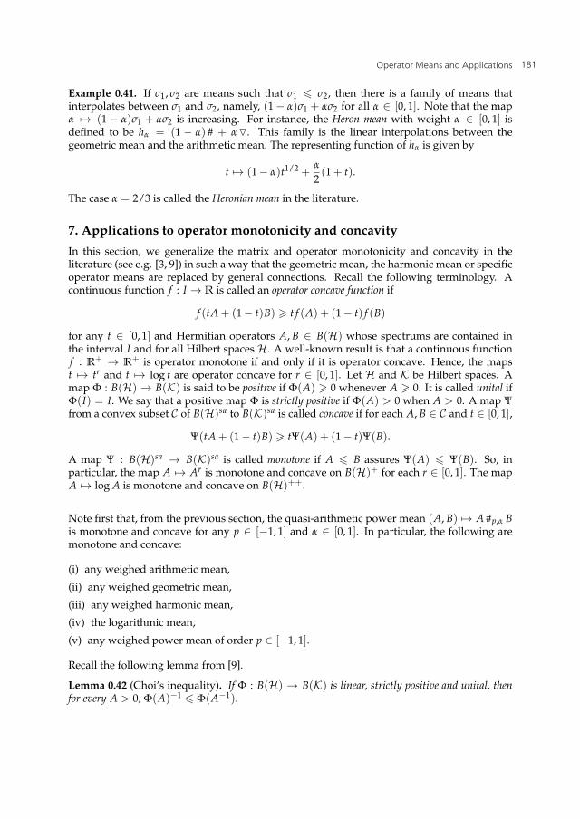
Example 0.41. If σ1, σ2 are means such that σ1 � σ2, then there is a family of means thatinterpolates between σ1 and σ2, namely, (1 − α)σ1 + ασ2 for all α ∈ [0, 1]. Note that the mapα �→ (1 − α)σ1 + ασ2 is increasing. For instance, the Heron mean with weight α ∈ [0, 1] isdefined to be hα = (1 − α) # + α�. This family is the linear interpolations between thegeometric mean and the arithmetic mean. The representing function of hα is given by

t �→ (1 − α)t1/2 +α

2(1 + t).

The case α = 2/3 is called the Heronian mean in the literature.

7. Applications to operator monotonicity and concavityIn this section, we generalize the matrix and operator monotonicity and concavity in theliterature (see e.g. [3, 9]) in such a way that the geometric mean, the harmonic mean or specificoperator means are replaced by general connections. Recall the following terminology. Acontinuous function f : I → R is called an operator concave function if

f (tA + (1 − t)B) � t f (A) + (1 − t) f (B)

for any t ∈ [0, 1] and Hermitian operators A, B ∈ B(H) whose spectrums are contained inthe interval I and for all Hilbert spaces H. A well-known result is that a continuous functionf : R+ → R+ is operator monotone if and only if it is operator concave. Hence, the mapst �→ tr and t �→ log t are operator concave for r ∈ [0, 1]. Let H and K be Hilbert spaces. Amap Φ : B(H) → B(K) is said to be positive if Φ(A) � 0 whenever A � 0. It is called unital ifΦ(I) = I. We say that a positive map Φ is strictly positive if Φ(A) > 0 when A > 0. A map Ψfrom a convex subset C of B(H)sa to B(K)sa is called concave if for each A, B ∈ C and t ∈ [0, 1],

Ψ(tA + (1 − t)B) � tΨ(A) + (1 − t)Ψ(B).

A map Ψ : B(H)sa → B(K)sa is called monotone if A � B assures Ψ(A) � Ψ(B). So, inparticular, the map A �→ Ar is monotone and concave on B(H)+ for each r ∈ [0, 1]. The mapA �→ log A is monotone and concave on B(H)++.

Note first that, from the previous section, the quasi-arithmetic power mean (A, B) �→ A #p,α Bis monotone and concave for any p ∈ [−1, 1] and α ∈ [0, 1]. In particular, the following aremonotone and concave:

(i) any weighed arithmetic mean,

(ii) any weighed geometric mean,

(iii) any weighed harmonic mean,

(iv) the logarithmic mean,

(v) any weighed power mean of order p ∈ [−1, 1].

Recall the following lemma from [9].

Lemma 0.42 (Choi’s inequality). If Φ : B(H) → B(K) is linear, strictly positive and unital, thenfor every A > 0, Φ(A)−1 � Φ(A−1).



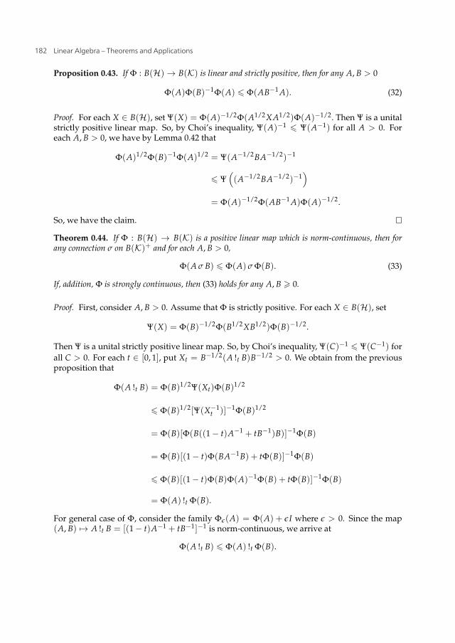
Proposition 0.43. If Φ : B(H) → B(K) is linear and strictly positive, then for any A, B > 0

Φ(A)Φ(B)−1Φ(A) � Φ(AB−1 A). (32)

Proof. For each X ∈ B(H), set Ψ(X) = Φ(A)−1/2Φ(A1/2XA1/2)Φ(A)−1/2. Then Ψ is a unitalstrictly positive linear map. So, by Choi’s inequality, Ψ(A)−1 � Ψ(A−1) for all A > 0. Foreach A, B > 0, we have by Lemma 0.42 that

Φ(A)1/2Φ(B)−1Φ(A)1/2 = Ψ(A−1/2BA−1/2)−1

� Ψ((A−1/2BA−1/2)−1

)

= Φ(A)−1/2Φ(AB−1 A)Φ(A)−1/2.

So, we have the claim.

Theorem 0.44. If Φ : B(H) → B(K) is a positive linear map which is norm-continuous, then forany connection σ on B(K)+ and for each A, B > 0,

Φ(A σ B) � Φ(A) σ Φ(B). (33)

If, addition, Φ is strongly continuous, then (33) holds for any A, B � 0.

Proof. First, consider A, B > 0. Assume that Φ is strictly positive. For each X ∈ B(H), set

Ψ(X) = Φ(B)−1/2Φ(B1/2XB1/2)Φ(B)−1/2.

Then Ψ is a unital strictly positive linear map. So, by Choi’s inequality, Ψ(C)−1 � Ψ(C−1) forall C > 0. For each t ∈ [0, 1], put Xt = B−1/2(A !t B)B−1/2 > 0. We obtain from the previousproposition that

Φ(A !t B) = Φ(B)1/2Ψ(Xt)Φ(B)1/2

� Φ(B)1/2[Ψ(X−1t )]−1Φ(B)1/2

= Φ(B)[Φ(B((1 − t)A−1 + tB−1)B)]−1Φ(B)

= Φ(B)[(1 − t)Φ(BA−1B) + tΦ(B)]−1Φ(B)

� Φ(B)[(1 − t)Φ(B)Φ(A)−1Φ(B) + tΦ(B)]−1Φ(B)

= Φ(A) !t Φ(B).

For general case of Φ, consider the family Φε(A) = Φ(A) + εI where ε > 0. Since the map(A, B) �→ A !t B = [(1 − t)A−1 + tB−1]−1 is norm-continuous, we arrive at

Φ(A !t B) � Φ(A) !t Φ(B).



For each connection σ, since Φ is a bounded linear operator, we have

Φ(A σ B) = Φ(∫[0,1]

A !t B dμ(t)) =∫[0,1]

Φ(A !t B) dμ(t)

�∫[0,1]

Φ(A) !t Φ(B) dμ(t) = Φ(A) σ Φ(B).

Suppose further that Φ is strongly continuous. Then, for each A, B � 0,

Φ(A σ B) = Φ(limε↓0

(A + εI) σ (B + εI)) = limε↓0

Φ((A + εI) σ (B + εI))

� limε↓0

Φ(A + εI) σ Φ(B + εI) = Φ(A) σ Φ(B).

The proof is complete.

As a special case, if Φ : Mn(C) → Mn(C) is a positive linear map, then for any connection σand for any positive semidefinite matrices A, B ∈ Mn(C), we have

Φ(AσB) � Φ(A) σ Φ(B).

In particular, Φ(A) #p,α Φ(B) � Φ(A) #p,α Φ(B) for any p ∈ [−1, 1] and α ∈ [0, 1].

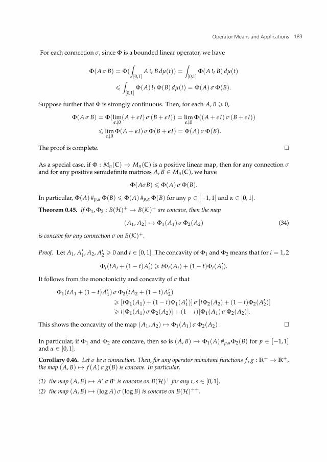
Theorem 0.45. If Φ1, Φ2 : B(H)+ → B(K)+ are concave, then the map

(A1, A2) �→ Φ1(A1) σ Φ2(A2) (34)

is concave for any connection σ on B(K)+.

Proof. Let A1, A′1, A2, A′

2 � 0 and t ∈ [0, 1]. The concavity of Φ1 and Φ2 means that for i = 1, 2

Φi(tAi + (1 − t)A′i) � tΦi(Ai) + (1 − t)Φi(A′

i).

It follows from the monotonicity and concavity of σ that

Φ1(tA1 + (1 − t)A′1) σ Φ2(tA2 + (1 − t)A′

2)

� [tΦ1(A1) + (1 − t)Φ1(A′1)] σ [tΦ2(A2) + (1 − t)Φ2(A′

2)]

� t[Φ1(A1) σ Φ2(A2)] + (1 − t)[Φ1(A1) σ Φ2(A2)].

This shows the concavity of the map (A1, A2) �→ Φ1(A1) σ Φ2(A2) .

In particular, if Φ1 and Φ2 are concave, then so is (A, B) �→ Φ1(A) #p,αΦ2(B) for p ∈ [−1, 1]and α ∈ [0, 1].

Corollary 0.46. Let σ be a connection. Then, for any operator monotone functions f , g : R+ → R+,the map (A, B) �→ f (A) σ g(B) is concave. In particular,

(1) the map (A, B) �→ Ar σ Bs is concave on B(H)+ for any r, s ∈ [0, 1],

(2) the map (A, B) �→ (log A) σ (log B) is concave on B(H)++.



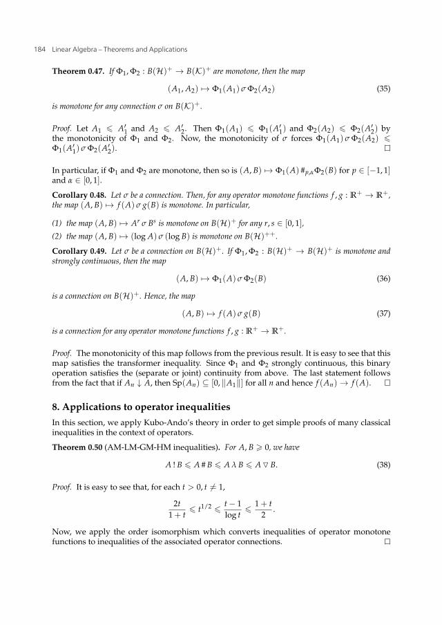
Theorem 0.47. If Φ1, Φ2 : B(H)+ → B(K)+ are monotone, then the map

(A1, A2) �→ Φ1(A1) σ Φ2(A2) (35)

is monotone for any connection σ on B(K)+.

Proof. Let A1 � A′1 and A2 � A′

2. Then Φ1(A1) � Φ1(A′1) and Φ2(A2) � Φ2(A′

2) bythe monotonicity of Φ1 and Φ2. Now, the monotonicity of σ forces Φ1(A1) σ Φ2(A2) �Φ1(A′

1) σ Φ2(A′2).

In particular, if Φ1 and Φ2 are monotone, then so is (A, B) �→ Φ1(A) #p,αΦ2(B) for p ∈ [−1, 1]and α ∈ [0, 1].

Corollary 0.48. Let σ be a connection. Then, for any operator monotone functions f , g : R+ → R+,the map (A, B) �→ f (A) σ g(B) is monotone. In particular,

(1) the map (A, B) �→ Ar σ Bs is monotone on B(H)+ for any r, s ∈ [0, 1],

(2) the map (A, B) �→ (log A) σ (log B) is monotone on B(H)++.

Corollary 0.49. Let σ be a connection on B(H)+. If Φ1, Φ2 : B(H)+ → B(H)+ is monotone andstrongly continuous, then the map

(A, B) �→ Φ1(A) σ Φ2(B) (36)

is a connection on B(H)+. Hence, the map

(A, B) �→ f (A) σ g(B) (37)

is a connection for any operator monotone functions f , g : R+ → R+.

Proof. The monotonicity of this map follows from the previous result. It is easy to see that thismap satisfies the transformer inequality. Since Φ1 and Φ2 strongly continuous, this binaryoperation satisfies the (separate or joint) continuity from above. The last statement followsfrom the fact that if An ↓ A, then Sp(An) ⊆ [0, ‖A1‖] for all n and hence f (An) → f (A).

8. Applications to operator inequalitiesIn this section, we apply Kubo-Ando’s theory in order to get simple proofs of many classicalinequalities in the context of operators.

Theorem 0.50 (AM-LM-GM-HM inequalities). For A, B � 0, we have

A ! B � A # B � A λ B � A� B. (38)

Proof. It is easy to see that, for each t > 0, t �= 1,

2t1 + t

� t1/2 � t − 1log t

� 1 + t2

.

Now, we apply the order isomorphism which converts inequalities of operator monotonefunctions to inequalities of the associated operator connections.



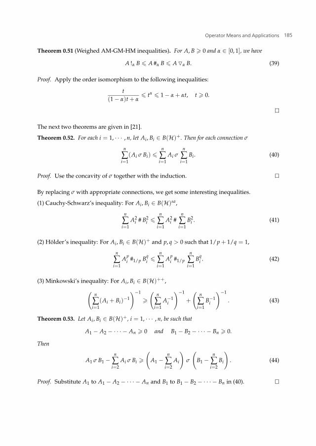
Theorem 0.51 (Weighed AM-GM-HM inequalities). For A, B � 0 and α ∈ [0, 1], we have

A !α B � A #α B � A�α B. (39)

Proof. Apply the order isomorphism to the following inequalities:

t(1 − α)t + α

� tα � 1 − α + αt, t � 0.

The next two theorems are given in [21].

Theorem 0.52. For each i = 1, · · · , n, let Ai, Bi ∈ B(H)+. Then for each connection σ

n

∑i=1

(Ai σ Bi) �n

∑i=1

Ai σn

∑i=1

Bi. (40)

Proof. Use the concavity of σ together with the induction.

By replacing σ with appropriate connections, we get some interesting inequalities.

(1) Cauchy-Schwarz’s inequality: For Ai, Bi ∈ B(H)sa,

n

∑i=1

A2i # B2

i �n

∑i=1

A2i #

n

∑i=1

B2i . (41)

(2) Hölder’s inequality: For Ai, Bi ∈ B(H)+ and p, q > 0 such that 1/p + 1/q = 1,

n

∑i=1

Api #1/p Bq

i �n

∑i=1

Api #1/p

n

∑i=1

Bqi . (42)

(3) Minkowski’s inequality: For Ai, Bi ∈ B(H)++,

(n

∑i=1

(Ai + Bi)−1

)−1

�(

n

∑i=1

A−1i

)−1

+

(n

∑i=1

B−1i

)−1

. (43)

Theorem 0.53. Let Ai, Bi ∈ B(H)+, i = 1, · · · , n, be such that

A1 − A2 − · · · − An � 0 and B1 − B2 − · · · − Bn � 0.

Then

A1 σ B1 −n

∑i=2

Ai σ Bi �(

A1 −n

∑i=2

Ai

)σ

(B1 −

n

∑i=2

Bi

). (44)

Proof. Substitute A1 to A1 − A2 − · · · − An and B1 to B1 − B2 − · · · − Bn in (40).



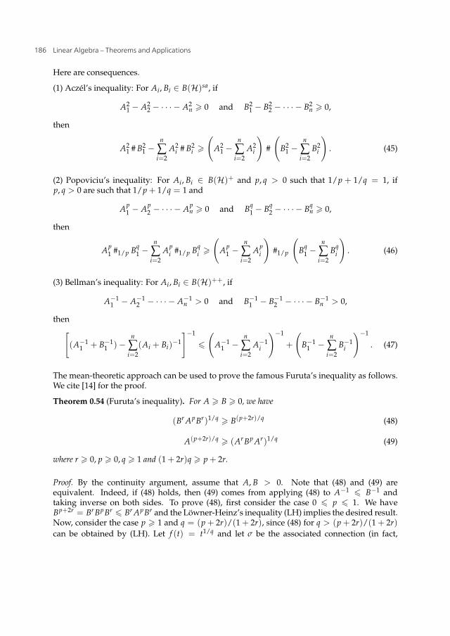
Here are consequences.

(1) Aczél’s inequality: For Ai, Bi ∈ B(H)sa, if

A21 − A2

2 − · · · − A2n � 0 and B2

1 − B22 − · · · − B2

n � 0,

then

A21 # B2

1 −n

∑i=2

A2i # B2

i �(

A21 −

n

∑i=2

A2i

)#

(B2

1 −n

∑i=2

B2i

). (45)

(2) Popoviciu’s inequality: For Ai, Bi ∈ B(H)+ and p, q > 0 such that 1/p + 1/q = 1, ifp, q > 0 are such that 1/p + 1/q = 1 and

Ap1 − Ap

2 − · · · − Apn � 0 and Bq

1 − Bq2 − · · · − Bq

n � 0,

then

Ap1 #1/p Bq

1 −n

∑i=2

Api #1/p Bq

i �(

Ap1 −

n

∑i=2

Api

)#1/p

(Bq

1 −n

∑i=2

Bqi

). (46)

(3) Bellman’s inequality: For Ai, Bi ∈ B(H)++, if

A−11 − A−1

2 − · · · − A−1n > 0 and B−1

1 − B−12 − · · · − B−1

n > 0,

then[(A−1

1 + B−11 )−

n

∑i=2

(Ai + Bi)−1

]−1

�(

A−11 −

n

∑i=2

A−1i

)−1

+

(B−1

1 −n

∑i=2

B−1i

)−1

. (47)

The mean-theoretic approach can be used to prove the famous Furuta’s inequality as follows.We cite [14] for the proof.

Theorem 0.54 (Furuta’s inequality). For A � B � 0, we have

(Br ApBr)1/q � B(p+2r)/q (48)

A(p+2r)/q � (ArBp Ar)1/q (49)

where r � 0, p � 0, q � 1 and (1 + 2r)q � p + 2r.

Proof. By the continuity argument, assume that A, B > 0. Note that (48) and (49) areequivalent. Indeed, if (48) holds, then (49) comes from applying (48) to A−1 � B−1 andtaking inverse on both sides. To prove (48), first consider the case 0 � p � 1. We haveBp+2r = BrBpBr � Br ApBr and the Löwner-Heinz’s inequality (LH) implies the desired result.Now, consider the case p � 1 and q = (p + 2r)/(1 + 2r), since (48) for q > (p + 2r)/(1 + 2r)can be obtained by (LH). Let f (t) = t1/q and let σ be the associated connection (in fact,



σ = #1/q). Must show that, for any r � 0,

B−2r σ Ap � B. (50)

For 0 � r � 12 , we have by (LH) that A2r � B2r and

B−2r σ Ap � A−2r σ Ap = A−2r(1−1/q)Ap/q = A � B = B−2r σ Bp.

Now, set s = 2r + 12 and q1 = (p + 2s)/(1 + 2s) � 1. Let f1(t) = t1/q1 and consider the

associated connection σ1. The previous step, the monotonicity and the congruence invarianceof connections imply that

B−2s σ1 Ap = B−r[B−(2r+1) σ1 (Br ApBr)]B−r

� B−r[(Br ApBr)−1/q1 σ1 (Br ApBr)]B−r

= B−r(Br ApBr)1/qB−r

� B−rB1+2rB−r

= B.

Note that the above result holds for A, B � 0 via the continuity of a connection. The desiredequation (50) holds for all r � 0 by repeating this process.

AcknowledgementThe author thanks referees for article processing.

Author detailsPattrawut ChansangiamKing Mongkut’s Institute of Technology Ladkrabang, Thailand

9. References[1] Anderson, W. & Duffin, R. (1969). Series and parallel addition of matrices, Journal of

Mathematical Analysis and Applications, Vol. 26, 576–594.[2] Anderson, W. & Morley, T. & Trapp, G. (1990). Positive solutions to X = A − BX−1B,

Linear Algebra and its Applications, Vol. 134, 53–62.[3] Ando, T. (1979). Concavity of certain maps on positive definite matrices and applications

to Hadamard products, Linear Algebra and its Applications, Vol. 26, 203–241.[4] Ando, T. (1983). On the arithmetic-geometric-harmonic mean inequality for positive

definite matrices, Linear Algebra and its Applications, Vol. 52-53, 31–37.[5] Ando, T. & Li, C. & Mathias, R. (2004). Geometric Means, Linear Algebra and its

Applications, Vol. 385, 305–334.[6] Bhagwat, K. & Subramanian, A. (1978). Inequalities between means of positive

operators, Mathematical Proceedings of the Cambridge Philosophical Society, Vol. 83, 393–401.[7] Bhatia, R. (1997). Matrix Analysis, Springer-Verlag New York Inc., New York.[8] Bhatia, R. (2006). Interpolating the arithmetic-geometric mean inequality and its

operator version, Linear Algebra and its Applications, Vol. 413, 355–363.



[9] Bhatia, R. (2007). Positive Definite Matrices, Princeton University Press, New Jersey.[10] Donoghue, W. (1974). Monotone matrix functions and analytic continuation, Springer-Verlag

New York Inc., New York.[11] Fujii, J. (1978). Arithmetico-geometric mean of operators, Mathematica Japonica, Vol. 23,

667–669.[12] Fujii, J. (1979). On geometric and harmonic means of positive operators, Mathematica

Japonica, Vol. 24, No. 2, 203–207.[13] Fujii, J. (1992). Operator means and the relative operator entropy, Operator Theory:

Advances and Applications, Vol. 59, 161–172.[14] Furuta, T. (1989). A proof via operator means of an order preserving inequality, Linear

Algebra and its Applications, Vol. 113, 129–130.[15] Hiai, F. (2010). Matrix analysis: matrix monotone functions, matrix means, and

majorizations, Interdisciplinary Information Sciences, Vol. 16, No. 2, 139–248,[16] Hiai, F. & Yanagi, K. (1995). Hilbert spaces and linear operators, Makino Pub. Ltd.[17] Kubo, F. & Ando, T. (1980). Means of positive linear operators, Mathematische Annalen,

Vol. 246, 205–224.[18] Lawson, J. & Lim, Y. (2001). The geometric mean, matrices, metrices and more, The

American Mathematical Monthly, Vol. 108, 797–812.[19] Lim, Y. (2008). On Ando–Li–Mathias geometric mean equations, Linear Algebra and its

Applications, Vol. 428, 1767–1777.[20] Löwner, C. (1934). Über monotone matrix funktionen. Mathematische Zeitschrift, Vol. 38,

177–216.[21] Mond, B. & Pecaric, J. & Sunde, J. & Varosanec, S. (1997). Operator versions of some

classical inequalities, Linear Algebra and its Applications, Vol. 264, 117–126.[22] Nishio, K. & Ando, T. (1976). Characterizations of operations derived from network

connections. Journal of Mathematical Analysis and Applications, Vol. 53, 539–549.[23] Pusz, W. & Woronowicz, S. (1975). Functional calculus for sesquilinear forms and the

purification map, Reports on Mathematical Physics, Vol. 8, 159–170.[24] Toader, G. & Toader, S. (2005). Greek means and the arithmetic-geometric mean, RGMIA

Monographs, Victoria University, (ONLINE: http://rgmia.vu.edu.au/monographs).


Operator Means and Applications

Documents

Transcript of Operator Means and Applications