TRANSPORT PROTOCOLS

655

CHAPTER

TRANSPORT PROTOCOLS

20.1 Connection-Oriented Transport Protocol Mechanisms

20.2 TCP

20.3 TCP Congestion Control

20.4 UDP

20.5 Recommended Reading and Web Sites

20.6 Key Terms, Review Questions, and Problems

20

656 CHAPTER 20 / TRANSPORT PROTOCOLS

KEY POINTS

• The transport protocol provides an end-to-end data transfer servicethat shields upper-layer protocols from the details of the interveningnetwork or networks. A transport protocol can be either connectionoriented, such as TCP, or connectionless, such as UDP.

• If the underlying network or internetwork service is unreliable, suchas with the use of IP, then a reliable connection-oriented transportprotocol becomes quite complex. The basic cause of this complexity isthe need to deal with the relatively large and variable delays experi-enced between end systems. These large, variable delays complicatethe flow control and error control techniques.

• TCP uses a credit-based flow control technique that is somewhat dif-ferent from the sliding-window flow control found in X.25 andHDLC. In essence, TCP separates acknowledgments from the man-agement of the size of the sliding window.

• Although the TCP credit-based mechanism was designed for end-to-end flow control, it is also used to assist in internetwork congestioncontrol. When a TCP entity detects the presence of congestion in theInternet, it reduces the flow of data onto the Internet until it detectsan easing in congestion.

The foregoing observations should make us reconsider the widely held view that birdslive only in the present. In fact, birds are aware of more than immediately presentstimuli; they remember the past and anticipate the future.

—The Minds of Birds, Alexander Skutch

In a protocol architecture, the transport protocol sits above a network orinternetwork layer, which provides network-related services, and just below applica-tion and other upper-layer protocols. The transport protocol provides services totransport service (TS) users, such as FTP, SMTP, and TELNET. The local transportentity communicates with some remote transport entity, using the services of somelower layer, such as the Internet Protocol. The general service provided by a trans-port protocol is the end-to-end transport of data in a way that shields the TS userfrom the details of the underlying communications systems.

We begin this chapter by examining the protocol mechanisms required to pro-vide these services. We find that most of the complexity relates to reliable connec-tion-oriented services. As might be expected, the less the network service provides,the more the transport protocol must do. The remainder of the chapter looks at twowidely used transport protocols: Transmission Control Protocol (TCP) and UserDatagram Protocol (UDP).

Refer to Figure 2.5 to see the position within the TCP/IP suite of the protocolsdiscussed in this chapter.

20.1 / CONNECTION-ORIENTED TRANSPORT PROTOCOL MECHANISMS 657

20.1 CONNECTION-ORIENTED TRANSPORTPROTOCOL MECHANISMS

Two basic types of transport service are possible: connection oriented and connec-tionless or datagram service. A connection-oriented service provides for the estab-lishment, maintenance, and termination of a logical connection between TS users.This has, so far, been the most common type of protocol service available and has awide variety of applications. The connection-oriented service generally implies thatthe service is reliable. This section looks at the transport protocol mechanismsneeded to support the connection-oriented service.

A full-feature connection-oriented transport protocol, such as TCP, is verycomplex. For purposes of clarity we present the transport protocol mechanisms inan evolutionary fashion. We begin with a network service that makes life easy forthe transport protocol, by guaranteeing the delivery of all transport data units inorder and defining the required mechanisms.Then we will look at the transport pro-tocol mechanisms required to cope with an unreliable network service. All of thisdiscussion applies in general to transport-level protocols. In Section 20.2, we applythe concepts developed in this section to describe TCP.

Reliable Sequencing Network Service

Let us assume that the network service accepts messages of arbitrary length and,with virtually 100% reliability, delivers them in sequence to the destination. Exam-ples of such networks are as follows:

• A highly reliable packet-switching network with an X.25 interface

• A frame relay network using the LAPF control protocol

• An IEEE 802.3 LAN using the connection-oriented LLC service

In all of these cases, the transport protocol is used as an end-to-end proto-col between two systems attached to the same network, rather than across aninternet.

The assumption of a reliable sequencing networking service allows the use ofa quite simple transport protocol. Four issues need to be addressed:

• Addressing

• Multiplexing

• Flow control

• Connection establishment/termination

Addressing The issue concerned with addressing is simply this: A user of a giventransport entity wishes either to establish a connection with or make a data transferto a user of some other transport entity using the same transport protocol. The tar-get user needs to be specified by all of the following:

• User identification

• Transport entity identification


• Host address

• Network number

The transport protocol must be able to derive the information listed abovefrom the TS user address. Typically, the user address is specified as (Host, Port). ThePort variable represents a particular TS user at the specified host. Generally, therewill be a single transport entity at each host, so a transport entity identification is notneeded. If more than one transport entity is present, there is usually only one ofeach type. In this latter case, the address should include a designation of the type oftransport protocol (e.g., TCP, UDP). In the case of a single network, Host identifiesan attached network device. In the case of an internet, Host is a global internetaddress. In TCP, the combination of port and host is referred to as a socket.

Because routing is not a concern of the transport layer, it simply passes theHost portion of the address down to the network service. Port is included in a trans-port header, to be used at the destination by the destination transport protocol entity.

One question remains to be addressed: How does the initiating TS user knowthe address of the destination TS user? Two static and two dynamic strategies sug-gest themselves:

1. The TS user knows the address it wishes to use ahead of time. This is basicallya system configuration function. For example, a process may be running that isonly of concern to a limited number of TS users, such as a process that collectsstatistics on performance. From time to time, a central network managementroutine connects to the process to obtain the statistics. These processes gener-ally are not, and should not be, well known and accessible to all.

2. Some commonly used services are assigned “well-known addresses.” Examplesinclude the server side of FTP, SMTP, and some other standard protocols.

3. A name server is provided. The TS user requests a service by some generic orglobal name. The request is sent to the name server, which does a directorylookup and returns an address. The transport entity then proceeds with the con-nection. This service is useful for commonly used applications that change loca-tion from time to time. For example, a data entry process may be moved from onehost to another on a local network to balance load.

4. In some cases, the target user is to be a process that is spawned at requesttime. The initiating user can send a process request to a well-known address.The user at that address is a privileged system process that will spawn thenew process and return an address. For example, a programmer has devel-oped a private application (e.g., a simulation program) that will execute ona remote server but be invoked from a local workstation. A request can beissued to a remote job-management process that spawns the simulationprocess.

Multiplexing Multiplexing was discussed in general terms in Section 18.1. Withrespect to the interface between the transport protocol and higher-level protocols,the transport protocol performs a multiplexing/demultiplexing function. That is,multiple users employ the same transport protocol and are distinguished by portnumbers or service access points.


1Recall from Chapter 2 that the blocks of data (protocol data units) exchanged by TCP entities arereferred to as TCP segments.

The transport entity may also perform a multiplexing function with respect tothe network services that it uses. Recall that we defined upward multiplexing as themultiplexing of multiple connections on a single lower-level connection, and down-ward multiplexing as the splitting of a single connection among multiple lower-levelconnections (Section 18.1).

Consider, for example, a transport entity making use of an X.25 service. Whyshould the transport entity employ upward multiplexing? There are, after all, 4095virtual circuits available. In the typical case, this is more than enough to handle allactive TS users. However, most X.25 networks base part of their charge on virtualcircuit connect time, because each virtual circuit consumes some node bufferresources. Thus, if a single virtual circuit provides sufficient throughput for multipleTS users, upward multiplexing is indicated.

On the other hand, downward multiplexing or splitting might be used toimprove throughput. For example, each X.25 virtual circuit is restricted to a 3-bit or 7-bit sequence number. A larger sequence space might be needed forhigh-speed, high-delay networks. Of course, throughput can only be increasedso far. If there is a single host-node link over which all virtual circuits are mul-tiplexed, the throughput of a transport connection cannot exceed the data rateof that link.

Flow Control Whereas flow control is a relatively simple mechanism at thelink layer, it is a rather complex mechanism at the transport layer, for two mainreasons:

• The transmission delay between transport entities is generally long comparedto actual transmission time. This means that there is a considerable delay inthe communication of flow control information.

• Because the transport layer operates over a network or internet, the amountof the transmission delay may be highly variable. This makes it difficult toeffectively use a timeout mechanism for retransmission of lost data.

In general, there are two reasons why one transport entity would want to restrainthe rate of segment1 transmission over a connection from another transport entity:

• The user of the receiving transport entity cannot keep up with the flow of data.

• The receiving transport entity itself cannot keep up with the flow of segments.

How do such problems manifest themselves? Presumably a transport entity hasa certain amount of buffer space. Incoming segments are added to the buffer. Eachbuffered segment is processed (i.e., the transport header is examined) and the dataare sent to the TS user. Either of the two problems just mentioned will cause thebuffer to fill up.Thus, the transport entity needs to take steps to stop or slow the flowof segments to prevent buffer overflow.This requirement is difficult to fulfill becauseof the annoying time gap between sender and receiver.We return to this point subse-quently. First, we present four ways of coping with the flow control requirement. Thereceiving transport entity can


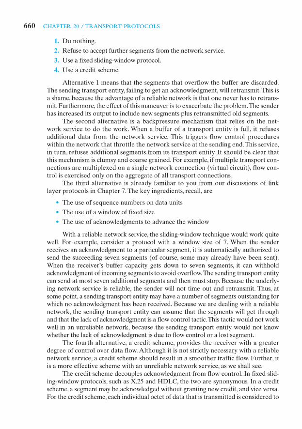
1. Do nothing.

2. Refuse to accept further segments from the network service.

3. Use a fixed sliding-window protocol.

4. Use a credit scheme.

Alternative 1 means that the segments that overflow the buffer are discarded.The sending transport entity, failing to get an acknowledgment, will retransmit.This isa shame, because the advantage of a reliable network is that one never has to retrans-mit. Furthermore, the effect of this maneuver is to exacerbate the problem.The senderhas increased its output to include new segments plus retransmitted old segments.

The second alternative is a backpressure mechanism that relies on the net-work service to do the work. When a buffer of a transport entity is full, it refusesadditional data from the network service. This triggers flow control procedureswithin the network that throttle the network service at the sending end.This service,in turn, refuses additional segments from its transport entity. It should be clear thatthis mechanism is clumsy and coarse grained. For example, if multiple transport con-nections are multiplexed on a single network connection (virtual circuit), flow con-trol is exercised only on the aggregate of all transport connections.

The third alternative is already familiar to you from our discussions of linklayer protocols in Chapter 7. The key ingredients, recall, are

• The use of sequence numbers on data units

• The use of a window of fixed size

• The use of acknowledgments to advance the window

With a reliable network service, the sliding-window technique would work quitewell. For example, consider a protocol with a window size of 7. When the senderreceives an acknowledgment to a particular segment, it is automatically authorized tosend the succeeding seven segments (of course, some may already have been sent).When the receiver’s buffer capacity gets down to seven segments, it can withholdacknowledgment of incoming segments to avoid overflow.The sending transport entitycan send at most seven additional segments and then must stop. Because the underly-ing network service is reliable, the sender will not time out and retransmit. Thus, atsome point, a sending transport entity may have a number of segments outstanding forwhich no acknowledgment has been received. Because we are dealing with a reliablenetwork, the sending transport entity can assume that the segments will get throughand that the lack of acknowledgment is a flow control tactic.This tactic would not workwell in an unreliable network, because the sending transport entity would not knowwhether the lack of acknowledgment is due to flow control or a lost segment.

The fourth alternative, a credit scheme, provides the receiver with a greaterdegree of control over data flow. Although it is not strictly necessary with a reliablenetwork service, a credit scheme should result in a smoother traffic flow. Further, itis a more effective scheme with an unreliable network service, as we shall see.

The credit scheme decouples acknowledgment from flow control. In fixed slid-ing-window protocols, such as X.25 and HDLC, the two are synonymous. In a creditscheme, a segment may be acknowledged without granting new credit, and vice versa.For the credit scheme, each individual octet of data that is transmitted is considered to


have a unique sequence number. In addition to data, each transmitted segmentincludes in its header three fields related to flow control: sequence number (SN),acknowledgment number (AN), and window (W). When a transport entity sends asegment, it includes the sequence number of the first octet in the segment data field.Implicitly, the remaining data octets are numbered sequentially following the firstdata octet. A transport entity acknowledges an incoming segment with a return seg-ment that includes with the following interpretation:

• All octets through sequence number are acknowledged; the nextexpected octet has sequence number i.

• Permission is granted to send an additional window of octets of data;that is, the j octets corresponding to sequence numbers i through

Figure 20.1 illustrates the mechanism (compare Figure 7.4). For simplicity, weshow data flow in one direction only and assume that 200 octets of data are sent ineach segment. Initially, through the connection establishment process, the sendingand receiving sequence numbers are synchronized and A is granted an initial creditallocation of 1400 octets, beginning with octet number 1001.The first segment trans-mitted by A contains data octets numbered 1001 through 1200. After sending 600octets in three segments, A has shrunk its window to a size of 800 octets (numbers1601 through 2400).After B receives these three segments, 600 octets out of its orig-inal 1400 octets of credit are accounted for, and 800 octets of credit are outstanding.Now suppose that, at this point, B is capable of absorbing 1000 octets of incomingdata on this connection. Accordingly, B acknowledges receipt of all octets through1600 and issues a credit of 1000 octets. This means that A can send octets 1601

i + j - 1.W = j

SN = i - 1

1AN = i, W = j2,

A may send 1400 octets

A shrinks its transmit window with eachtransmission

B is prepared to receive 1400 octets, beginning with 1001

B acknowledges 3 segments (600 octets) but is only prepared to receive 200 additional octets beyond the original budget (i.e., B will accept octets 1601 through 2600)

B acknowledges 5 segments (1000 octets) andrestores the original amount of credit

A adjusts its window with each credit

A exhausts its credit

A receives new credit

Transport Entity A Transport Entity B

...1000

1001

1001 2400 2401... ...1000 1001 2400 2401...

...2600 2601 4000 4001...

...2600 2601 4000 4001...

...1000 1601 2401...

...1000 1001 2001 2401...

...1600 1601 2001 2601...

...1600 1601 2601...

...1600 1601 2001 2601...

...1600 1601 2600 2601...

SN � 1001

SN � 1401

SN � 1201

SN � 2001

SN � 2401

SN � 2201

SN � 1801

SN � 1601

AN � 2601, W � 1400

AN � 1601, W� 1000

Figure 20.1 Example of TCP Credit Allocation Mechanism


(a) Send sequence space

(b) Receive sequence space

� � �

Window of octetsthat may be transmittedData octets already transmitted

Octets not yetacknowledgedData octets so far acknowledged

Last octettransmitted

Last octetacknowledged

(AN � 1)

Initial sequencenumber (ISN)

Window shrinks fromtrailing edge assegments are sent

Window expandsfrom leading edgeas credits are received

� � �

Window of octetsthat may be acceptedData octets already received

Octets not yetacknowledgedData octets so far acknowledged

Last octetreceived

Last octetacknowledged

(AN � 1)

Initial sequencenumber (ISN)

Window shrinks fromtrailing edge assegments are received

Window expandsfrom leading edgeas credits are sent

Figure 20.2 Sending and Receiving Flow Control Perspectives

through 2600 (5 segments). However, by the time that B’s message has arrived at A,A has already sent two segments, containing octets 1601 through 2000 (which waspermissible under the initial allocation). Thus, A’s remaining credit upon receipt ofB’s credit allocation is only 600 octets (3 segments). As the exchange proceeds, Aadvances the trailing edge of its window each time that it transmits and advances theleading edge only when it is granted credit.

Figure 20.2 shows the view of this mechanism from the sending and receivingsides (compare Figure 7.3). Typically, both sides take both views because data maybe exchanged in both directions. Note that the receiver is not required to immedi-ately acknowledge incoming segments but may wait and issue a cumulativeacknowledgment for a number of segments.

The receiver needs to adopt some policy concerning the amount of data it per-mits the sender to transmit. The conservative approach is to only allow new seg-ments up to the limit of available buffer space. If this policy were in effect in Figure20.1, the first credit message implies that B has 1000 available octets in its buffer,and the second message that B has 1400 available octets.

A conservative flow control scheme may limit the throughput of the transportconnection in long-delay situations.The receiver could potentially increase through-put by optimistically granting credit for space it does not have. For example, if areceiver’s buffer is full but it anticipates that it can release space for 1000 octetswithin a round-trip propagation time, it could immediately send a credit of 1000. If


the receiver can keep up with the sender, this scheme may increase throughput andcan do no harm. If the sender is faster than the receiver, however, some segmentsmay be discarded, necessitating a retransmission. Because retransmissions are nototherwise necessary with a reliable network service (in the absence of internet con-gestion), an optimistic flow control scheme will complicate the protocol.

Connection Establishment and Termination Even with a reliable networkservice, there is a need for connection establishment and termination procedures tosupport connection-oriented service. Connection establishment serves three mainpurposes:

• It allows each end to assure that the other exists.

• It allows exchange or negotiation of optional parameters (e.g., maximum seg-ment size, maximum window size, quality of service).

• It triggers allocation of transport entity resources (e.g., buffer space, entry inconnection table).

Connection establishment is by mutual agreement and can be accomplished by asimple set of user commands and control segments, as shown in the state diagram ofFigure 20.3. To begin, a TS user is in an CLOSED state (i.e., it has no open transportconnection).The TS user can signal to the local TCP entity that it will passively wait for

CLOSED

SYN SENT LISTEN

ESTAB

FIN WAIT CLOSE WAIT

CLOSED

Active openSend SYN

EventAction

Receive SYNSend SYN

CloseSend FIN

CloseSend FIN

Close Close

Passive open

Receive SYN

Receive FIN

Receive FIN

State

Legend:

Figure 20.3 Simple Connection State Diagram


a request with a Passive Open command. A server program, such as time-sharing or afile transfer application, might do this. The TS user may change its mind by sending aClose command. After the Passive Open command is issued, the transport entity cre-ates a connection object of some sort (i.e., a table entry) that is in the LISTEN state.

From the CLOSED state, a TS user may open a connection by issuing an ActiveOpen command, which instructs the transport entity to attempt connection establish-ment with a designated remote TS user, which triggers the transport entity to send aSYN (for synchronize) segment. This segment is carried to the receiving transportentity and interpreted as a request for connection to a particular port. If the destina-tion transport entity is in the LISTEN state for that port, then a connection is estab-lished by the following actions by the receiving transport entity:

• Signal the local TS user that a connection is open.

• Send a SYN as confirmation to the remote transport entity.

• Put the connection object in an ESTAB (established) state.

When the responding SYN is received by the initiating transport entity, it toocan move the connection to an ESTAB state.The connection is prematurely abortedif either TS user issues a Close command.

Figure 20.4 shows the robustness of this protocol. Either side can initiate aconnection. Further, if both sides initiate the connection at about the same time, it isestablished without confusion. This is because the SYN segment functions both as aconnection request and a connection acknowledgment.

The reader may ask what happens if a SYN comes in while the requested TSuser is idle (not listening). Three courses may be followed:

• The transport entity can reject the request by sending a RST (reset) segmentback to the other transport entity.

• The request can be queued until the local TS user issues a matching Open.

• The transport entity can interrupt or otherwise signal the local TS user tonotify it of a pending request.

System AState/(command)

System BState/(command)

(Passive open)LISTEN

CLOSED

System AState/(command)

System BState/(command)

CLOSED

(Active open)SYN SENT

ESTAB

CLOSED


ESTAB


ESTAB

CLOSED

ESTAB

(a) Active/passive open (b) Active/active open

SYNSYN

SYN

SYN

Figure 20.4 Connection Establishment Scenarios


Note that if the third mechanism is used, a Passive Open command is notstrictly necessary but may be replaced by an Accept command, which is a signalfrom the user to the transport entity that it accepts the request for connection.

Connection termination is handled similarly. Either side, or both sides, mayinitiate a close. The connection is closed by mutual agreement. This strategyallows for either abrupt or graceful termination. With abrupt termination, data intransit may be lost; a graceful termination prevents either side from closing theconnection until all data have been delivered. To achieve the latter, a connectionin the FIN WAIT state must continue to accept data segments until a FIN (finish)segment is received.

Figure 20.3 defines the procedure for graceful termination. First, consider theside that initiates the termination procedure:

1. In response to a TS user’s Close primitive, a transport entity sends a FIN seg-ment to the other side of the connection, requesting termination.

2. Having sent the FIN, the transport entity places the connection in the FIN WAITstate. In this state, the transport entity must continue to accept data from theother side and deliver that data to its user.

3. When a FIN is received in response, the transport entity informs its user andcloses the connection.

From the point of view of the side that does not initiate a termination,

1. When a FIN segment is received, the transport entity informs its user of thetermination request and places the connection in the CLOSE WAIT state. Inthis state, the transport entity must continue to accept data from its user andtransmit it in data segments to the other side.

2. When the user issues a Close primitive, the transport entity sends a respondingFIN segment to the other side and closes the connection.

This procedure ensures that both sides have received all outstanding data andthat both sides agree to connection termination before actual termination.

Unreliable Network Service

A more difficult case for a transport protocol is that of an unreliable network ser-vice. Examples of such networks are as follows:

• An internetwork using IP

• A frame relay network using only the LAPF core protocol

• An IEEE 802.3 LAN using the unacknowledged connectionless LLC service

The problem is not just that segments are occasionally lost, but that seg-ments may arrive out of sequence due to variable transit delays. As we shall see,elaborate machinery is required to cope with these two interrelated network defi-ciencies.We shall also see that a discouraging pattern emerges.The combination ofunreliability and nonsequencing creates problems with every mechanism we havediscussed so far. Generally, the solution to each problem raises new problems.Although there are problems to be overcome for protocols at all levels, it seems


that there are more difficulties with a reliable connection-oriented transport pro-tocol than any other sort of protocol.

In the remainder of this section, unless otherwise noted, the mechanisms dis-cussed are those used by TCP. Seven issues need to be addressed:

• Ordered delivery

• Retransmission strategy

• Duplicate detection

• Flow control

• Connection establishment

• Connection termination

• Failure recovery

Ordered Delivery With an unreliable network service, it is possible that seg-ments, even if they are all delivered, may arrive out of order. The required solutionto this problem is to number segments sequentially. We have seen that for datalink control protocols, such as HDLC, and for X.25, each data unit (frame, packet)is numbered sequentially with each successive sequence number being one morethan the previous sequence number. This scheme is used in some transport proto-cols, such as the ISO transport protocols. However,TCP uses a somewhat differentscheme in which each data octet that is transmitted is implicitly numbered. Thus,the first segment may have a sequence number of 1. If that segment has 200 octetsof data, then the second segment would have the sequence number 201, and so on.For simplicity in the discussions of this section, we will continue to assume thateach successive segment’s sequence number is 200 more than that of the previoussegment; that is, each segment contains exactly 200 octets of data.

Retransmission Strategy Two events necessitate the retransmission of a seg-ment. First, a segment may be damaged in transit but nevertheless arrive at its des-tination. If a checksum is included with the segment, the receiving transport entitycan detect the error and discard the segment. The second contingency is that a seg-ment fails to arrive. In either case, the sending transport entity does not know thatthe segment transmission was unsuccessful. To cover this contingency, a positiveacknowledgment scheme is used: The receiver must acknowledge each successfullyreceived segment by returning a segment containing an acknowledgment number.For efficiency, we do not require one acknowledgment per segment. Rather, acumulative acknowledgment can be used, as we have seen many times in this book.Thus, the receiver may receive segments numbered 1, 201, and 401, but only send

back. The sender must interpret to mean that the segmentwith and all previous segments have been successfully received.

If a segment does not arrive successfully, no acknowledgment will be issuedand a retransmission is in order. To cope with this situation, there must be a timerassociated with each segment as it is sent. If the timer expires before the segment isacknowledged, the sender must retransmit.

So the addition of a timer solves that problem. Next problem: At what valueshould the timer be set? Two strategies suggest themselves.A fixed timer value could

SN = 401AN = 601AN = 601


be used, based on an understanding of the network’s typical behavior. This suffersfrom an inability to respond to changing network conditions. If the value is too small,there will be many unnecessary retransmissions, wasting network capacity. If thevalue is too large, the protocol will be sluggish in responding to a lost segment. Thetimer should be set at a value a bit longer than the round trip time (send segment,receive ACK). Of course, this delay is variable even under constant network load.Worse, the statistics of the delay will vary with changing network conditions.

An adaptive scheme has its own problems. Suppose that the transport entitykeeps track of the time taken to acknowledge data segments and sets itsretransmission timer based on the average of the observed delays.This value cannotbe trusted for three reasons:

• The peer transport entity may not acknowledge a segment immediately. Recallthat we gave it the privilege of cumulative acknowledgments.

• If a segment has been retransmitted, the sender cannot know whether thereceived acknowledgment is a response to the initial transmission or theretransmission.

• Network conditions may change suddenly.

Each of these problems is a cause for some further tweaking of the transport algo-rithm, but the problem admits of no complete solution. There will always be someuncertainty concerning the best value for the retransmission timer.We return to thisissue in Section 20.3.

Incidentally, the retransmission timer is only one of a number of timers neededfor proper functioning of a transport protocol. These are listed in Table 20.1,together with a brief explanation.

Duplicate Detection If a segment is lost and then retransmitted, no confusionwill result. If, however, one or more segments in sequence are successfully delivered,but the corresponding ACK is lost, then the sending transport entity will time out andone or more segments will be retransmitted. If these retransmitted segments arrivesuccessfully, they will be duplicates of previously received segments. Thus, thereceiver must be able to recognize duplicates. The fact that each segment carries asequence number helps, but, nevertheless, duplicate detection and handling is notsimple. There are two cases:

• A duplicate is received prior to the close of the connection.

• A duplicate is received after the close of the connection.

Table 20.1 Transport Protocol Timers

Retransmission timer Retransmit an unacknowledged segment

2MSL (maximum segment Minimum time between closing one connection andlifetime) timer opening another with the same destination address

Persist timer Maximum time between ACK/CREDIT segments

Retransmit-SYN timer Time between attempts to open a connection

Keepalive timer Abort connection when no segments are received


The second case is discussed in the subsection on connection establishment.We deal with the first case here.

Notice that we say “a” duplicate rather than “the” duplicate. From the sender’spoint of view, the retransmitted segment is the duplicate. However, the retransmit-ted segment may arrive before the original segment, in which case the receiverviews the original segment as the duplicate. In any case, two tactics are needed tocope with a duplicate received prior to the close of a connection:

• The receiver must assume that its acknowledgment was lost and thereforemust acknowledge the duplicate. Consequently, the sender must not get con-fused if it receives multiple acknowledgments to the same segment.

• The sequence number space must be long enough so as not to “cycle” in less thanthe maximum possible segment lifetime (time it takes segment to transit network).

Figure 20.5 illustrates the reason for the latter requirement. In this example, thesequence space is of length 1600; that is, after the sequence numbers cycleback and begin with For simplicity, we assume the receiving transport entitymaintains a credit window size of 600. Suppose that A has transmitted data segmentswith 201, and 401. B has received the two segments with and

but the segment with is delayed in transit. Thus, B does not sendany acknowledgments. Eventually, A times out and retransmits segment When the duplicate segment arrives, B acknowledges 1, 201, and 401 with

Meanwhile, A has timed out again and retransmits which Backnowledges with another Things now seem to have sorted themselvesout and data transfer continues.When the sequence space is exhausted,A cycles backto and continues.Alas, the old segment makes a belated appearanceand is accepted by B before the new segment arrives.When the new segment

does arrive, it is treated as a duplicate and discarded.It should be clear that the untimely emergence of the old segment would

have caused no difficulty if the sequence numbers had not yet wrapped around.The larger the sequence number space (number of bits used to represent thesequence number), the longer the wraparound is avoided. How big must thesequence space be? This depends on, among other things, whether the networkenforces a maximum packet lifetime, and the rate at which segments are beingtransmitted. Fortunately, each addition of a single bit to the sequence numberfield doubles the sequence space, so it is rather easy to select a safe size.

Flow Control The credit allocation flow control mechanism described earlier isquite robust in the face of an unreliable network service and requires little enhance-ment. As was mentioned, a segment containing acknowledges alloctets through number and grants credit for an additional j octets beginningwith octet i. The credit allocation mechanism is quite flexible. For example, supposethat the last octet of data received by B was octet number and that the lastsegment issued by B was Then

• To increase credit to an amount when no additional data havearrived, B issues

• To acknowledge an incoming segment containing m octets of data without granting additional credit, B issues 1AN = i + m, W = j - m2.1m 6 j2

1AN = i, W = k2.k 1k 7 j21AN = i, W = j2. i - 1

i - 11AN = i, W = j2

SN = 1SN = 1

SN = 1SN = 1

AN = 601.SN = 201,AN = 601.

SN = 1SN = 1.

SN = 1SN = 401,SN = 201SN = 1,

SN = 1.SN = 1600,


TransportEntity A

TransportEntity B

A times out andretransmits SN � 201

Obsolete SN � 1arrives

A times out andretransmits SN � 1

AN � 601, W � 600

AN � 601, W � 600

AN � 801, W � 600

AN � 1001, W � 600

AN � 1201, W � 600

AN � 1401, W � 600

AN � 1, W � 600

AN � 201, W � 600

SN � 201

SN � 401

SN � 1

SN � 201

SN � 601

SN � 801

SN � 1001

SN � 1201

SN � 1401

SN � 1

SN�

1

Figure 20.5 Example of Incorrect Duplicate Detection

If an ACK/CREDIT segment is lost, little harm is done. Future acknowledg-ments will resynchronize the protocol. Further, if no new acknowledgments areforthcoming, the sender times out and retransmits a data segment, which triggers anew acknowledgment. However, it is still possible for deadlock to occur. Consider asituation in which B sends temporarily closing the window. Sub-sequently, B sends but this segment is lost. A is awaiting theopportunity to send data and B thinks that it has granted that opportunity. To over-come this problem, a persist timer can be used.This timer is reset with each outgoingsegment (all segments contain the AN and W fields). If the timer ever expires, theprotocol entity is required to send a segment, even if it duplicates a previous one.Thisbreaks the deadlock and assures the other end that the protocol entity is still alive.

1AN = i, W = j2,1AN = i, W = 02,


Connection Establishment As with other protocol mechanisms,connection estab-lishment must take into account the unreliability of a network service. Recall that a con-nection establishment calls for the exchange of SYNs, a procedure sometimes referredto as a two-way handshake. Suppose that A issues a SYN to B. It expects to get a SYNback, confirming the connection. Two things can go wrong: A’s SYN can be lost or B’sanswering SYN can be lost.Both cases can be handled by use of a retransmit-SYN timer(Table 20.1).After A issues a SYN, it will reissue the SYN when the timer expires.

This gives rise, potentially, to duplicate SYNs. If A’s initial SYN was lost, thereare no duplicates. If B’s response was lost, then B may receive two SYNs from A.Further, if B’s response was not lost, but simply delayed, A may get two respondingSYNs. All of this means that A and B must simply ignore duplicate SYNs once aconnection is established.

There are other problems to contend with. Just as a delayed SYN or lost responsecan give rise to a duplicate SYN, a delayed data segment or lost acknowledgment cangive rise to duplicate data segments, as we have seen in Figure 20.5. Such a delayed orduplicated data segment can interfere with data transfer, as illustrated in Figure 20.6.

A initiates a connection

New connection opened

A begins transmission

B accepts and acknowledges

Connection closed

Obsolete segment SN � 401 is accepted;valid segment SN � 401 is discarded as duplicate

A BSYN

SYN

SYN

SYN

SN � 1

SN�

401

SN � 201

SN � 1

SN � 201

SN � 401

Figure 20.6 The Two-Way Handshake: Problem with Obsolete DataSegment


Assume that with each new connection, each transport protocol entity begins number-ing its data segments with sequence number 1. In the figure, a duplicate copy of segment

from an old connection arrives during the lifetime of a new connection andis delivered to B before delivery of the legitimate data segment One way ofattacking this problem is to start each new connection with a different sequence numberthat is far removed from the last sequence number of the most recent connection. Forthis purpose, the connection request is of the form SYN where i is the sequencenumber of the first data segment that will be sent on this connection.

Now consider that a duplicate SYN i may survive past the termination of theconnection. Figure 20.7 depicts the problem that may arise. An old SYN i arrivesat B after the connection is terminated. B assumes that this is a fresh request andresponds with SYN j, meaning that B accepts the connection request and will begintransmitting with Meanwhile, A has decided to open a new connec-tion with B and sends SYN k. B discards this as a duplicate. Now both sides havetransmitted and subsequently received a SYN segment, and therefore think that avalid connection exists. However, when A initiates data transfer with a segmentnumbered B rejects the segment as being out of sequence.

The way out of this problem is for each side to acknowledge explicitly theother’s SYN and sequence number. The procedure is known as a three-way hand-shake. The revised connection state diagram, which is the one employed by TCP, isshown in the upper part of Figure 20.8. A new state (SYN RECEIVED) is added.In this state, the transport entity hesitates during connection opening to assure thatthe SYN segments sent by the two sides have both been acknowledged before theconnection is declared established. In addition to the new state, there is a controlsegment (RST) to reset the other side when a duplicate SYN is detected.

Figure 20.9 illustrates typical three-way handshake operations. In Figure 20.9a,transport entity A initiates the connection, with a SYN including the sending

k + 1.

SN = j + 1.

i + 1,

SN = 401.SN = 401

A B

Obsolete SYN i arrives

Connection closed

B responds; A sends new SYN

B discards duplicate SYN

B rejects segment as out of sequence

SYN i

SYN k SYN j

SN � k � 1

Figure 20.7 Two-Way Handshake: Problem with Obsolete SYN Segments


sequence number, i. The value i is referred to as the initial sequence number (ISN)and is associated with the SYN; the first data octet to be transmitted will havesequence number The responding SYN acknowledges the ISN with

and includes its ISN. A acknowledges B’s SYN/ACK in its first datasegment, which begins with sequence number Figure 20.9b shows a situationin which an old SYN i arrives at B after the close of the relevant connection. Bassumes that this is a fresh request and responds with SYN j, When Areceives this message, it realizes that it has not requested a connection and thereforesends an RST, Note that the portion of the RST message is essen-tial so that an old duplicate RST does not abort a legitimate connection establish-ment. Figure 20.9c shows a case in which an old SYN/ACK arrives in the middle of

AN = jAN = j.

AN = i + 1.

i + 1.1AN = i + 12 i + 1.

LISTEN

CLOSE WAIT

LAST ACK

CLOSED

CLOSED

SYN RECEIVED

ESTAB

CLOSING

TIME WAIT

SYN SENT

FIN WAIT

FIN WAIT2

ReceiveACK of SYN

ReceiveACK of SYN

ReceiveACK of FIN

ReceiveACK of FIN

SV = state vectorMSL = maximum segment lifetime

Active open oractive open with data

Initialize SV; send SYN

CloseClear SV

CloseSend FIN

CloseSend FIN

Unspecified passive open orfully specified passive open

Initialize SV

CloseClear SV

Receive SYNSend SYN, ACK

Timeout(2 MSL)

Receive SYN, ACKSend ACK

Receive FIN, ACK of SYNSend ACK

Receive FINSend ACK

Receive FINSend ACK

Receive FINSend ACK

Receive FIN, ACKSend ACK

Receive SYNSend SYN, ACK

Figure 20.8 TCP Entity State Diagram


a new connection establishment. Because of the use of sequence numbers in theacknowledgments, this event causes no mischief.

For simplicity, the upper part of Figure 20.8 does not include transitions in whichRST is sent. The basic rule is as follows: Send an RST if the connection state is not yetOPEN and an invalid ACK (one that does not reference something that was sent) isreceived. The reader should try various combinations of events to see that this connec-tion establishment procedure works in spite of any combination of old and lost segments.

Connection Termination The state diagram of Figure 20.3 defines the use of asimple two-way handshake for connection establishment, which was found to be unsat-isfactory in the face of an unreliable network service. Similarly, the two-way handshake

(a) Normal operation

A initiates a connection

A initiates a connectionOld SYN arrives at A; A rejects

A acknowledges and begins transmission

A acknowledges and begins transmission


(b) Delayed SYN

(c) Delayed SYN, ACK

Obsolete SYN arrives

A rejects B's connection



A BSYN i

SN � i � 1, AN � j � 1

RST, AN � j

SN i � 1, AN � j � 1

RST, AN � k

SYN i

SYN j, AN � i � 1

SYN i


SYN k, AN � p


Figure 20.9 Examples of Three-Way Handshake


defined in that diagram for connection termination is inadequate for an unreliable net-work service. Misordering of segments could cause the following scenario.A transportentity in the CLOSE WAIT state sends its last data segment, followed by a FIN seg-ment, but the FIN segment arrives at the other side before the last data segment. Thereceiving transport entity will accept that FIN, close the connection, and lose the lastsegment of data.To avoid this problem, a sequence number can be associated with theFIN, which can be assigned the next sequence number after the last octet of transmit-ted data.With this refinement, the receiving transport entity, upon receiving a FIN, willwait if necessary for the late-arriving data before closing the connection.

A more serious problem is the potential loss of segments and the potential pres-ence of obsolete segments. Figure 20.8 shows that the termination procedure adopts asimilar solution to that used for connection establishment. Each side must explicitlyacknowledge the FIN of the other, using an ACK with the sequence number of theFIN to be acknowledged. For a graceful close, a transport entity requires the following:

• It must send a FIN i and receive

• It must receive a FIN j and send

• It must wait an interval equal to twice the maximum expected segment lifetime.

Failure Recovery When the system upon which a transport entity is runningfails and subsequently restarts, the state information of all active connections is lost.The affected connections become half open because the side that did not fail doesnot yet realize the problem.

The still active side of a half-open connection can close the connection using akeepalive timer. This timer measures the time the transport machine will continue toawait an acknowledgment (or other appropriate reply) of a transmitted segment afterthe segment has been retransmitted the maximum number of times. When the timerexpires, the transport entity assumes that the other transport entity or the interveningnetwork has failed, closes the connection, and signals an abnormal close to the TS user.

In the event that a transport entity fails and quickly restarts, half-open connec-tions can be terminated more quickly by the use of the RST segment.The failed sidereturns an RST i to every segment i that it receives. When the RST i reaches theother side, it must be checked for validity based on the sequence number i, becausethe RST could be in response to an old segment. If the reset is valid, the transportentity performs an abnormal termination.

These measures clean up the situation at the transport level. The decision asto whether to reopen the connection is up to the TS users. The problem is one ofsynchronization. At the time of failure, there may have been one or more outstand-ing segments in either direction. The TS user on the side that did not fail knowshow much data it has received, but the other user may not, if state informationwere lost. Thus, there is the danger that some user data will be lost or duplicated.

20.2 TCP

In this section we look at TCP (RFC 793), first at the service it provides to the TSuser and then at the internal protocol details.

AN = j + 1.

AN = i + 1.

20.2 / TCP 675

TCP Services

TCP is designed to provide reliable communication between pairs of processes(TCP users) across a variety of reliable and unreliable networks and internets. TCPprovides two useful facilities for labeling data: push and urgent:

• Data stream push: Ordinarily, TCP decides when sufficient data have accu-mulated to form a segment for transmission. The TCP user can require TCPto transmit all outstanding data up to and including that labeled with a pushflag. On the receiving end, TCP will deliver these data to the user in thesame manner. A user might request this if it has come to a logical break inthe data.

• Urgent data signaling: This provides a means of informing the destinationTCP user that significant or “urgent” data is in the upcoming data stream. It isup to the destination user to determine appropriate action.

As with IP, the services provided by TCP are defined in terms of primitives andparameters.The services provided by TCP are considerably richer than those providedby IP, and hence the set of primitives and parameters is more complex. Table 20.2 listsTCP service request primitives, which are issued by a TCP user to TCP, and Table 20.3lists TCP service response primitives, which are issued by TCP to a local TCP user.

Table 20.2 TCP Service Request Primitives

Primitive Parameters Description

Unspecified source-port, [timeout], [timeout-action], Listen for connection attempt atPassive Open [precedence], [security-range] specified security and precedence

from any remote destination.

Fully Specified source-port, destination-port, destination- Listen for connection attempt at specifiedPassive Open address, [timeout], [timeout-action], security and precedence from specified

[precedence], [security-range] destination.

Active Open source-port, destination-port, destination- Request connection at a particularaddress, [timeout], [timeout-action], security and precedence to a specified[precedence], [security] destination.

Active Open source-port, destination-port, destination- Request connection at a particularwith Data address, [timeout], [timeout-action], security and precedence to a specified

[precedence], [security], data, data-length, destination and transmit data with thePUSH-flag, URGENT-flag request.

Send local-connection-name, data, data-length, Transfer data across named connection.PUSH-flag, URGENT-flag, [timeout],[timeout-action]

Allocate local-connection-name, data-length Issue incremental allocation for receivedata to TCP.

Close local-connection-name Close connection gracefully.

Abort local-connection-name Close connection abruptly.

Status local-connection-name Query connection status.

Note: Square brackets indicate optional parameters.


Table 20.4 provides a brief definition of the parameters involved. The two passive open commands signal the TCP user’s willingness to accept a connection request. Theactive open with data allows the user to begin transmitting data with the opening ofthe connection.

TCP Header Format

TCP uses only a single type of protocol data unit, called a TCP segment. The headeris shown in Figure 20.10. Because one header must serve to perform all protocolmechanisms, it is rather large, with a minimum length of 20 octets. The fields are asfollows:

• Source Port (16 bits): Source TCP user. Example values are Telnet � 23;A complete list is maintained at http://www.iana.org/

assignments/port-numbers.

• Destination Port (16 bits): Destination TCP user.

• Sequence Number (32 bits): Sequence number of the first data octet in thissegment except when the SYN flag is set. If SYN is set, this field contains theinitial sequence number (ISN) and the first data octet in this segment hassequence number ISN + 1.

TFTP = 69; HTTP = 80.

Table 20.3 TCP Service Response Primitives

Primitive Parameters Description

Open ID local-connection-name, source-port, Informs TCP user of connection name destination-port, destination-address assigned to pending connection

requested in an Open primitive

Open Failure local-connection-name Reports failure of an Active Open request

Open Success local-connection-name Reports completion of pending Open request

Deliver local-connection-name, data, data-length, Reports arrival of dataURGENT-flag

Closing local-connection-name Reports that remote TCP user has issued aClose and that all data sent by remote userhas been delivered

Terminate local-connection-name, description Reports that the connection has been termi-nated; a description of the reason for termination is provided

Status local-connection-name, source-port, Reports current status of connectionResponse source-address, destination-port,

destination-address, connection-state,receive-window, send-window, amount-awaiting-ACK, amount-awaiting-receipt,urgent-state, precedence, security, timeout

Error local-connection-name, description Reports service-request or internal error

Not used for Unspecified Passive Open.=…

……

20.2 / TCP 677

• Acknowledgment Number (32 bits): Contains the sequence number of thenext data octet that the TCP entity expects to receive.

• Data Offset (4 bits): Number of 32-bit words in the header.

• Reserved (4 bits): Reserved for future use.

• Flags (6 bits): For each flag, if set to 1, the meaning is

CWR: congestion window reduced.

ECE: ECN-Echo; the CWR and ECE bits, defined in RFC 3168, are used forthe explicit congestion notification function; a discussion of this function isbeyond our scope.

URG: urgent pointer field significant.

Table 20.4 TCP Service Parameters

Source Port Local TCP user

Timeout Longest delay allowed for data delivery before automatic connection termi-nation or error report; user specified

Timeout-action Indicates whether the connection is terminated or an error is reported to theTCP user in the event of a timeout

Precedence Precedence level for a connection. Takes on values zero (lowest) throughseven (highest); same parameter as defined for IP

Security-range Allowed ranges in compartment, handling restrictions, transmission controlcodes, and security levels

Destination Port Remote TCP user

Destination Address Internet address of remote host

Security Security information for a connection, including security level, compartment,handling restrictions, and transmission control code; same parameter asdefined for IP

Data Block of data sent by TCP user or delivered to a TCP user

Data Length Length of block of data sent or delivered

PUSH flag If set, indicates that the associated data are to be provided with the datastream push service

URGENT flag If set, indicates that the associated data are to be provided with the urgentdata signaling service

Local Connection Name Identifier of a connection defined by a (local socket, remote socket) pair;provided by TCP

Description Supplementary information in a Terminate or Error primitive

Source Address Internet address of the local host

Connection State State of referenced connection (CLOSED, ACTIVE OPEN, PASSIVEOPEN, ESTABLISHED, CLOSING)

Receive Window Amount of data in octets the local TCP entity is willing to receive

Send Window Amount of data in octets permitted to be sent to remote TCP entity

Amount Awaiting ACK Amount of previously transmitted data awaiting acknowledgment

Amount Awaiting Receipt Amount of data in octets buffered at local TCP entity pending receipt bylocal TCP user

Urgent State Indicates to the receiving TCP user whether there are urgent data availableor whether all urgent data, if any, have been delivered to the user

678

Source Port Destination Port

Checksum Urgent Pointer

Sequence Number

Acknowledgment Number

Options � Padding

Reserved WindowDataoffset

0Bit: 4 8 16 3120

oct

ets

URG

ACK

PSH

RST

SYN

FIN

ECE

CWR

Figure 20.10 TCP Header

20.2 / TCP 679

ACK: acknowledgment field significant.

PSH: push function.

RST: reset the connection.

SYN: synchronize the sequence numbers.

FIN: no more data from sender.

• Window (16 bits): Flow control credit allocation, in octets. Contains the num-ber of data octets, beginning with the sequence number indicated in theacknowledgment field that the sender is willing to accept.

• Checksum (16 bits): The ones complement of the ones complement sum of allthe 16-bit words in the segment plus a pseudoheader, described subsequently.2

• Urgent Pointer (16 bits): This value, when added to the segment sequencenumber, contains the sequence number of the last octet in a sequence ofurgent data.This allows the receiver to know how much urgent data is coming.

• Options (Variable): An example is the option that specifies the maximum seg-ment size that will be accepted.

The Sequence Number and Acknowledgment Number are bound to octetsrather than to entire segments. For example, if a segment contains sequence num-ber 1001 and includes 600 octets of data, the sequence number refers to the firstoctet in the data field; the next segment in logical order will have sequence num-ber 1601. Thus, TCP is logically stream oriented: It accepts a stream of octets fromthe user, groups them into segments as it sees fit, and numbers each octet in thestream.

The Checksum field applies to the entire segment plus a pseudoheader pre-fixed to the header at the time of calculation (at both transmission and reception).The pseudoheader includes the following fields from the IP header: source and des-tination internet address and protocol, plus a segment length field. By including thepseudoheader, TCP protects itself from misdelivery by IP. That is, if IP delivers apacket to the wrong host, even if the packet contains no bit errors, the receiving TCPentity will detect the delivery error.

By comparing the TCP header to the TCP user interface defined in Tables 20.2and 20.3, the reader may feel that some items are missing from the TCP header; thatis indeed the case. TCP is intended to work with IP. Hence, some TCP user parame-ters are passed down by TCP to IP for inclusion in the IP header. The precedenceparameter can be mapped into the DS (Differentiated Services) field, and the secu-rity parameter into the optional security field in the IP header.

It is worth observing that this TCP/IP linkage means that the required mini-mum overhead for every data unit is actually 40 octets.

TCP Mechanisms

We can group TCP mechanisms into the categories of connection establishment,data transfer, and connection termination.

2A discussion of this checksum is contained in Appendix K.


Connection Establishment Connection establishment in TCP always uses athree-way handshake. When the SYN flag is set, the segment is essentially a requestfor connection and functions as explained in Section 20.1. To initiate a connection,an entity sends a SYN, where X is the initial sequence number. Thereceiver responds with SYN, by setting both the SYN andACK flags. Note that the acknowledgment indicates that the receiver is now expect-ing to receive a segment beginning with data octet acknowledging the SYN,which occupies Finally, the initiator responds with If thetwo sides issue crossing SYNs, no problem results: Both sides respond withSYN/ACKs (Figure 20.4).

A connection is uniquely determined by the source and destination sockets(host, port). Thus, at any one time, there can only be a single TCP connectionbetween a unique pair of ports. However, a given port can support multiple connec-tions, each with a different partner port.

Data Transfer Although data are transferred in segments over a transport con-nection, data transfer is viewed logically as consisting of a stream of octets. Henceevery octet is numbered, modulo Each segment contains the sequence numberof the first octet in the data field. Flow control is exercised using a credit allocationscheme in which the credit is a number of octets rather than a number of segments,as explained in Section 20.1.

Data are buffered by the transport entity on both transmission and reception.TCP normally exercises its own discretion as to when to construct a segment fortransmission and when to release received data to the user.The PUSH flag is used toforce the data so far accumulated to be sent by the transmitter and passed on by thereceiver. This serves an end-of-block function.

The user may specify a block of data as urgent. TCP will designate the end ofthat block with an urgent pointer and send it out in the ordinary data stream. Thereceiving user is alerted that urgent data are being received.

If, during data exchange, a segment arrives that is apparently not meant for thecurrent connection, the RST flag is set on an outgoing segment. Examples of this sit-uation are delayed duplicate SYNs and an acknowledgment of data not yet sent.

Connection Termination The normal means of terminating a connection is agraceful close. Each TCP user must issue a CLOSE primitive. The transport entitysets the FIN bit on the last segment that it sends out, which also contains the last ofthe data to be sent on this connection.

An abrupt termination occurs if the user issues an ABORT primitive. In thiscase, the entity abandons all attempts to send or receive data and discards data in itstransmission and reception buffers. An RST segment is sent to the other side.

TCP Implementation Policy Options

The TCP standard provides a precise specification of the protocol to be usedbetween TCP entities. However, certain aspects of the protocol admit several possi-ble implementation options. Although two implementations that choose alternativeoptions will be interoperable, there may be performance implications. The designareas for which options are specified are the following:

232.

AN = Y + 1.SN = X.X + 1,

SN = Y, AN = X + 1SN = X,

20.2 / TCP 681

• Send policy

• Deliver policy

• Accept policy

• Retransmit policy

• Acknowledge policy

Send Policy In the absence of both pushed data and a closed transmission win-dow (see Figure 20.2a), a sending TCP entity is free to transmit data at its own con-venience, within its current credit allocation. As data are issued by the user, they arebuffered in the transmit buffer.TCP may construct a segment for each batch of dataprovided by its user or it may wait until a certain amount of data accumulates beforeconstructing and sending a segment. The actual policy will depend on performanceconsiderations. If transmissions are infrequent and large, there is low overhead interms of segment generation and processing. On the other hand, if transmissions arefrequent and small, the system is providing quick response.

Deliver Policy In the absence of a Push, a receiving TCP entity is free to deliverdata to the user at its own convenience. It may deliver data as each in-order segmentis received, or it may buffer data from a number of segments in the receive bufferbefore delivery. The actual policy will depend on performance considerations. Ifdeliveries are infrequent and large, the user is not receiving data as promptly as maybe desirable. On the other hand, if deliveries are frequent and small, there may beunnecessary processing both in TCP and in the user software, as well as an unneces-sary number of operating system interrupts.

Accept Policy When all data segments arrive in order over a TCP connection,TCP places the data in a receive buffer for delivery to the user. It is possible, how-ever, for segments to arrive out of order. In this case, the receiving TCP entity hastwo options:

• In-order: Accept only segments that arrive in order; any segment that arrivesout of order is discarded.

• In-window: Accept all segments that are within the receive window (seeFigure 20.2b).

The in-order policy makes for a simple implementation but places a burden onthe networking facility, as the sending TCP must time out and retransmit segmentsthat were successfully received but discarded because of misordering. Furthermore,if a single segment is lost in transit, then all subsequent segments must be retrans-mitted once the sending TCP times out on the lost segment.

The in-window policy may reduce transmissions but requires a more complexacceptance test and a more sophisticated data storage scheme to buffer and keeptrack of data accepted out of order.

Retransmit Policy TCP maintains a queue of segments that have been sent butnot yet acknowledged. The TCP specification states that TCP will retransmit a seg-ment if it fails to receive an acknowledgment within a given time.A TCP implemen-tation may employ one of three retransmission strategies:


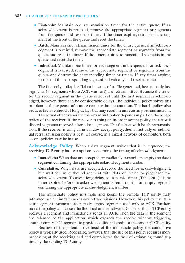
• First-only: Maintain one retransmission timer for the entire queue. If anacknowledgment is received, remove the appropriate segment or segmentsfrom the queue and reset the timer. If the timer expires, retransmit the seg-ment at the front of the queue and reset the timer.

• Batch: Maintain one retransmission timer for the entire queue. if an acknowl-edgment is received, remove the appropriate segment or segments from thequeue and reset the timer. If the timer expires, retransmit all segments in thequeue and reset the timer.

• Individual: Maintain one timer for each segment in the queue. If an acknowl-edgment is received, remove the appropriate segment or segments from thequeue and destroy the corresponding timer or timers. If any timer expires,retransmit the corresponding segment individually and reset its timer.

The first-only policy is efficient in terms of traffic generated, because only lostsegments (or segments whose ACK was lost) are retransmitted. Because the timerfor the second segment in the queue is not set until the first segment is acknowl-edged, however, there can be considerable delays. The individual policy solves thisproblem at the expense of a more complex implementation. The batch policy alsoreduces the likelihood of long delays but may result in unnecessary retransmissions.

The actual effectiveness of the retransmit policy depends in part on the acceptpolicy of the receiver. If the receiver is using an in-order accept policy, then it willdiscard segments received after a lost segment. This fits best with batch retransmis-sion. If the receiver is using an in-window accept policy, then a first-only or individ-ual retransmission policy is best. Of course, in a mixed network of computers, bothaccept policies may be in use.

Acknowledge Policy When a data segment arrives that is in sequence, thereceiving TCP entity has two options concerning the timing of acknowledgment:

• Immediate: When data are accepted, immediately transmit an empty (no data)segment containing the appropriate acknowledgment number.

• Cumulative: When data are accepted, record the need for acknowledgment,but wait for an outbound segment with data on which to piggyback theacknowledgment. To avoid long delay, set a persist timer (Table 20.1); if thetimer expires before an acknowledgment is sent, transmit an empty segmentcontaining the appropriate acknowledgment number.

The immediate policy is simple and keeps the remote TCP entity fullyinformed, which limits unnecessary retransmissions. However, this policy results inextra segment transmissions, namely, empty segments used only to ACK. Further-more, the policy can cause a further load on the network. Consider that a TCP entityreceives a segment and immediately sends an ACK. Then the data in the segmentare released to the application, which expands the receive window, triggeringanother empty TCP segment to provide additional credit to the sending TCP entity.

Because of the potential overhead of the immediate policy, the cumulativepolicy is typically used. Recognize, however, that the use of this policy requires moreprocessing at the receiving end and complicates the task of estimating round-triptime by the sending TCP entity.

20.3 / TCP CONGESTION CONTROL 683

20.3 TCP CONGESTION CONTROL

The credit-based flow control mechanism of TCP was designed to enable a desti-nation to restrict the flow of segments from a source to avoid buffer overflow atthe destination. This same flow control mechanism is now used in ingenious waysto provide congestion control over the Internet between the source and destina-tion. Congestion, as we have seen a number of times in this book, has two maineffects. First, as congestion begins to occur, the transit time across a network orinternetwork increases. Second, as congestion becomes severe, network or inter-net nodes drop packets. The TCP flow control mechanism can be used to recog-nize the onset of congestion (by recognizing increased delay times and droppedsegments) and to react by reducing the flow of data. If many of the TCP entitiesoperating across a network exercise this sort of restraint, internet congestion isrelieved.

Since the publication of RFC 793, a number of techniques have been imple-mented that are intended to improve TCP congestion control characteristics.Table 20.5 lists some of the most popular of these techniques. None of these tech-niques extends or violates the original TCP standard; rather the techniques rep-resent implementation policies that are within the scope of the TCP specification.Many of these techniques are mandated for use with TCP in RFC 1122(Requirements for Internet Hosts) while some of them are specified in RFC 2581.The labels Tahoe, Reno, and NewReno refer to implementation packages avail-able on many operating systems that support TCP. The techniques fall roughlyinto two categories: retransmission timer management and window management.In this section, we look at some of the most important and most widely imple-mented of these techniques.

Retransmission Timer Management

As network or internet conditions change, a static retransmission timer is likely tobe either too long or too short. Accordingly, virtually all TCP implementationsattempt to estimate the current round-trip time by observing the pattern of delay

Table 20.5 Implementation of TCP Congestion Control Measures

Measure RFC 1122 TCP Tahoe TCP Reno NewReno

RTT Variance Estimation

Exponential RTO Backoff

Karn’s Algorithm

Slow Start

Dynamic Window Sizing on Congestion

Fast Retransmit

Fast Recovery

Modified Fast Recovery �

��

��

��

��

��

��

��


for recent segments, and then set the timer to a value somewhat greater than theestimated round-trip time.

Simple Average A simple approach is to take the average of observed round-triptimes over a number of segments. If the average accurately predicts future round-trip times, then the resulting retransmission timer will yield good performance. Thesimple averaging method can be expressed as

(20.1)

where RTT(i) is the round-trip time observed for the ith transmitted segment, andARTT(K) is the average round-trip time for the first K segments.

This expression can be rewritten as

(20.2)

With this formulation, it is not necessary to recalculate the entire summation eachtime.

Exponential Average Note that each term in the summation is given equalweight; that is, each term is multiplied by the same constant Typically, wewould like to give greater weight to more recent instances because they are morelikely to reflect future behavior. A common technique for predicting the next valueon the basis of a time series of past values, and the one specified in RFC 793, is expo-nential averaging:

(20.3)

where SRTT(K) is called the smoothed round-trip time estimate, and we defineCompare this with Equation (20.2). By using a constant value ofindependent of the number of past observations, we have a circum-

stance in which all past values are considered, but the more distant ones have lessweight.To see this more clearly, consider the following expansion of Equation (20.3):

Because both and are less than one, each successive term in the precedingequation is smaller. For example, for the expansion is

The older the observation, the less it is counted in the average.The smaller the value of the greater the weight given to the more recent

observations. For virtually all of the weight is given to the four or fivemost recent observations, whereas for the averaging is effectivelyspread out over the ten or so most recent observations. The advantage of using a

a = 0.875,a = 0.5,

a,

10.1282RTT1K - 12 + ÁSRTT1K + 12 = 10.22RTT1K + 12 + 10.162RTT1K2 +

a = 0.8,11 - a2a

a211 - a2RTT1K - 12 + Á + aK11 - a2RTT112SRTT1K + 12 = 11 - a2RTT1K + 12 + a11 - a2RTT1K2+

a 10 6 a 6 12,SRTT102 = 0.

SRTT1K + 12 = a * SRTT1K2 + 11 - a2 * RTT1K + 12

1/1K + 12.

ARTT1K + 12 =K

K + 1ARTT1K2 +

1K + 1

RTT1K + 12

ARTT1K + 12 =1

K + 1 aK + 1

i = 1RTT1i2


small value of is that the average will quickly reflect a rapid change in the observed quantity. The disadvantage is that if there is a brief surge in thevalue of the observed quantity and it then settles back to some relatively constant value, the use of a small value of will result in jerky changes in theaverage.

Figure 20.11 compares simple averaging with exponential averaging (for twodifferent values of ). In part (a) of the figure, the observed value begins at 1, growsgradually to a value of 10, and then stays there. In part (b) of the figure, the

a

a

a

(a) Increasing function

0

2

4

6

8

10

2019181716151413121110987654321

a � 0.5

a � 0.875

Simple average

Observed value

Obs

erve

d or

ave

rage

val

ue

Time

0

5

10

15

20

2019181716151413121110987654321

(b) Decreasing function

a � 0.5

a � 0.875

Simple average

Observed value

Obs

erve

d or

ave

rage

val

ue

Time

Figure 20.11 Use of Exponential Averaging


observed value begins at 20, declines gradually to 10, and then stays there. Notethat exponential averaging tracks changes in RTT faster than does simple averag-ing and that the smaller value of results in a more rapid reaction to the change inthe observed value.

Equation (20.3) is used in RFC 793 to estimate the current round-trip time.Aswas mentioned, the retransmission timer should be set at a value somewhat greaterthan the estimated round-trip time. One possibility is to use a constant value:

where RTO is the retransmission timer (also called the retransmission timeout)and is a constant. The disadvantage of this is that is not proportional toSRTT. For large values of SRTT, is relatively small and fluctuations in theactual RTT will result in unnecessary retransmissions. For small values of SRTT,

is relatively large and causes unnecessary delays in retransmitting lost segments. Accordingly, RFC 793 specifies the use of a timer whose value is pro-portional to SRTT, within limits:

(20.4)

where UBOUND and LBOUND are prechosen fixed upper and lower bounds onthe timer value and is a constant. RFC 793 does not recommend specific valuesbut does list as “example values” the following: between 0.8 and 0.9 and between 1.3 and 2.0.

RTT Variance Estimation (Jacobson’s Algorithm) The technique speci-fied in the TCP standard, and described in Equations (20.3) and (20.4), enables aTCP entity to adapt to changes in round-trip time. However, it does not cope wellwith a situation in which the round-trip time exhibits a relatively high variance.[ZHAN86] points out three sources of high variance:

1. If the data rate on the TCP connection is relatively low, then the transmissiondelay will be relatively large compared to propagation time and the variancein delay due to variance in IP datagram size will be significant.Thus, the SRTTestimator is heavily influenced by characteristics that are a property of thedata and not of the network.

2. Internet traffic load and conditions may change abruptly due to traffic fromother sources, causing abrupt changes in RTT.

3. The peer TCP entity may not acknowledge each segment immediately becauseof its own processing delays and because it exercises its privilege to use cumu-lative acknowledgments.

The original TCP specification tries to account for this variability by multiply-ing the RTT estimator by a constant factor, as shown in Equation (20.4). In a stableenvironment, with low variance of RTT, this formulation results in an unnecessarilyhigh value of RTO, and in an unstable environment a value of may be inade-quate to protect against unnecessary retransmissions.

A more effective approach is to estimate the variability in RTT values and touse that as input into the calculation of an RTO.A variability measure that is easy toestimate is the mean deviation, defined as

b = 2

ba

b

RTO1K + 12 = MIN1UBOUND, MAX1LBOUND, b * SRTT1K + 1222

¢

¢¢¢

RTO1K + 12 = SRTT1K + 12 + ¢

a


where E[X] is the expected value of X.As with the estimate of RTT, a simple average could be used to estimate

MDEV:

where ARTT(K) is the simple average defined in Equation (20.1) and AERR(K) isthe sample mean deviation measured at time K.

As with the definition of ARRT, each term in the summation of ADEV isgiven equal weight; that is, each term is multiplied by the same constant

Again, we would like to give greater weight to more recent instancesbecause they are more likely to reflect future behavior. Jacobson, who proposedthe use of a dynamic estimate of variability in estimating RTT [JACO88], sug-gests using the same exponential smoothing technique as is used for the calcula-tion of SRTT. The complete algorithm proposed by Jacobson can be expressedas follows:

(20.5)

As in the RFC 793 definition [Equation (20.3)], SRTT is an exponentiallysmoothed estimate of RTT, with equivalent to Now, however, instead ofmultiplying the estimate SRTT by a constant [Equation (20.4)], a multiple of theestimated mean deviation is added to SRTT to form the retransmission timer. Basedon his timing experiments, Jacobson proposed the following values for the constantsin his original paper [JACO88]:

After further research [JACO90a], Jacobson recommended using and this isthe value used in current implementations.

Figure 20.12 illustrates the use of Equation 20.5 on the same data set usedin Figure 20.11. Once the arrival times stabilize, the variation estimate SDEVdeclines. The values of RTO for both and are quite conservative aslong as RTT is changing but then begin to converge to RTT when it stabilizes.

Experience has shown that Jacobson’s algorithm can significantly improveTCP performance. However, it does not stand by itself. Two other factors must beconsidered:

f = 4f = 2

f = 4,

f = 2

h = 1/4 = 0.25

g = 1/8 = 0.125

a.11 - g2

RTO1K + 12 = SRTT1K + 12 + f * SDEV1K + 12 SDEV1K + 12 = 11 - h2 * SDEV1K2 + h * ƒ SERR1K + 12 ƒ SERR1K + 12 = RTT1K + 12 - SRTT1K2 SRTT1K + 12 = 11 - g2 * SRTT1K2 + g * RTT1K + 12

1/1K + 12.

=K

K + 1ADEV1K2 +

1K + 1

ƒ AERR1K + 12 ƒ

ADEV1K + 12 =1

K + 1 aK + 1

i = 1ƒ AERR1i2 ƒ

AERR1K + 12 = RTT1K + 12 - ARTT1K2

MDEV1X2 = E[ ƒ X - E[X] ƒ ]


0

5

10

15

20

25

2019181716151413121110987654321

0

10

20

30

40

50

RTO, f � 2

RTO, f � 4

SDEV

Observedvalue

2019181716151413121110987654321

(a) Increasing function

(b) Decreasing function

Obs

erve

d or

ave

rage

val

ueO

bser

ved

or a

vera

ge v

alue

Time

Time

RTO, f � 2

RTO, f � 4

SDEV

Observedvalue

Figure 20.12 Jacobson’s RTO Calculation

1. What RTO value should be used on a retransmitted segment? The exponentialRTO backoff algorithm is used for this purpose.

2. Which round-trip samples should be used as input to Jacobson’s algorithm?Karn’s algorithm determines which samples to use.

Exponential RTO Backoff When a TCP sender times out on a segment, itmust retransmit that segment. RFC 793 assumes that the same RTO value will beused for this retransmitted segment. However, because the timeout is probably due


to network congestion, manifested as a dropped packet or a long delay in round-triptime, maintaining the same RTO value is ill advised.

Consider the following scenario. There are a number of active TCP connec-tions from various sources sending traffic into an internet. A region of congestiondevelops such that segments on many of these connections are lost or delayed pastthe RTO time of the connections. Therefore, at roughly the same time, many seg-ments will be retransmitted into the internet, maintaining or even increasing thecongestion. All of the sources then wait a local (to each connection) RTO time andretransmit yet again. This pattern of behavior could cause a sustained condition ofcongestion.

A more sensible policy dictates that a sending TCP entity increase its RTOeach time a segment is retransmitted; this is referred to as a backoff process. In thescenario of the preceding paragraph, after the first retransmission of a segment oneach affected connection, the sending TCP entities will all wait a longer time beforeperforming a second retransmission.This may give the internet time to clear the cur-rent congestion. If a second retransmission is required, each sending TCP entity willwait an even longer time before timing out for a third retransmission, giving theinternet an even longer period to recover.

A simple technique for implementing RTO backoff is to multiply the RTO fora segment by a constant value for each retransmission:

(20.6)

Equation (20.6) causes RTO to grow exponentially with each retransmission. Themost commonly used value of q is 2. With this value, the technique is referred to asbinary exponential backoff. This is the same technique used in the EthernetCSMA/CD protocol (Chapter 16).

Karn’s Algorithm If no segments are retransmitted, the sampling process forJacobson’s algorithm is straightforward. The RTT for each segment can be includedin the calculation. Suppose, however, that a segment times out and must be retrans-mitted. If an acknowledgment is subsequently received, there are two possibilities:

1. This is the ACK to the first transmission of the segment. In this case, the RTT issimply longer than expected but is an accurate reflection of network conditions.

2. This is the ACK to the second transmission.

The sending TCP entity cannot distinguish between these two cases. If the sec-ond case is true and the TCP entity simply measures the RTT from the first transmis-sion until receipt of the ACK, the measured time will be much too long.The measuredRTT will be on the order of the actual RTT plus the RTO. Feeding this false RTT intoJacobson’s algorithm will produce an unnecessarily high value of SRTT and thereforeRTO. Furthermore, this effect propagates forward a number of iterations, since theSRTT value of one iteration is an input value in the next iteration.

An even worse approach would be to measure the RTT from the second trans-mission to the receipt of the ACK. If this is in fact the ACK to the first transmission,then the measured RTT will be much too small, producing a too low value of SRTTand RTO.This is likely to have a positive feedback effect, causing additional retrans-missions and additional false measurements.

RTO = q * RTO


3These algorithms were developed by Jacobson [JACO88] and are also described in RFC 2581. Jacobsondescribes things in units of TCP segments, whereas RFC 2581 relies primarily on units of TCP data octets,with some reference to calculations in units of segments. We follow the development in [JACO88].

Karn’s algorithm [KARN91] solves this problem with the following rules:

1. Do not use the measured RTT for a retransmitted segment to update SRTTand SDEV [Equation (20.5)].

2. Calculate the backoff RTO using Equation (20.6) when a retransmission occurs.

3. Use the backoff RTO value for succeeding segments until an acknowledgmentarrives for a segment that has not been retransmitted.

When an acknowledgment is received to an unretransmitted segment, Jacob-son’s algorithm is again activated to compute future RTO values.

Window Management

In addition to techniques for improving the effectiveness of the retransmissiontimer, a number of approaches to managing the send window have been examined.The size of TCP’s send window can have a critical effect on whether TCP can beused efficiently without causing congestion. We discuss two techniques found in vir-tually all modern implementations of TCP: slow start and dynamic window sizing oncongestion.3

Slow Start The larger the send window used in TCP, the more segments that asending TCP entity can send before it must wait for an acknowledgment. This cancreate a problem when a TCP connection is first established, because the TCP entityis free to dump the entire window of data onto the internet.

One strategy that could be followed is for the TCP sender to begin sendingfrom some relatively large but not maximum window, hoping to approximate thewindow size that would ultimately be provided by the connection. This is riskybecause the sender might flood the internet with many segments before it realizedfrom timeouts that the flow was excessive. Instead, some means is needed of gradu-ally expanding the window until acknowledgments are received. This is the purposeof the slow start mechanism.

With slow start, TCP transmission is constrained by the following relationship:

(20.7)

wherewindow, in segments. This is the number of segments that

TCP is currently allowed to send without receiving further acknowl-edgments.

window, in segments. A window used by TCP duringstartup and to reduce flow during periods of congestion.

amount of unused credit granted in the most recent acknowledg-ment, in segments.When an acknowledgment is received, this value iscalculated as window/segment_size, where window is a field in theincoming TCP segment (the amount of data the peer TCP entity iswilling to accept).

credit = the

cwnd = congestion

awnd = allowed

awnd = MIN[credit, cwnd]


4Kleinrock refers to this phenomenon as the long-tail effect during a rush-hour period. See Sections 2.7and 2.10 of [KLEI76] for a detailed discussion.

When a new connection is opened, the TCP entity initializes Thatis, TCP is only allowed to send 1 segment and then must wait for an acknowledg-ment before transmitting a second segment. Each time an acknowledgment to newdata is received, the value of cwnd is increased by 1, up to some maximum value.

In effect, the slow-start mechanism probes the internet to make sure that theTCP entity is not sending too many segments into an already congested environ-ment. As acknowledgments arrive, TCP is able to open up its window until the flowis controlled by the incoming ACKs rather than by cwnd.

The term slow start is a bit of a misnomer, because cwnd actually grows expo-nentially. When the first ACK arrives, TCP opens cwnd to 2 and can send two seg-ments. When these two segments are acknowledged, TCP can slide the window 1segment for each incoming ACK and can increase cwnd by 1 for each incomingACK. Therefore, at this point TCP can send four segments. When these four areacknowledged, TCP will be able to send eight segments.

Dynamic Window Sizing on Congestion The slow-start algorithm hasbeen found to work effectively for initializing a connection. It enables the TCPsender to determine quickly a reasonable window size for the connection. Mightnot the same technique be useful when there is a surge in congestion? In particular,suppose a TCP entity initiates a connection and goes through the slow-start proce-dure. At some point, either before or after cwnd reaches the size of the credit allo-cated by the other side, a segment is lost (timeout). This is a signal that congestionis occurring. It is not clear how serious the congestion is. Therefore, a prudent pro-cedure would be to reset and begin the slow-start process all over.

This seems like a reasonable, conservative procedure, but in fact it is not con-servative enough. Jacobson [JACO88] points out that “it is easy to drive a networkinto saturation but hard for the net to recover.” In other words, once congestionoccurs, it may take a long time for the congestion to clear.4 Thus, the exponentialgrowth of cwnd under slow start may be too aggressive and may worsen the conges-tion. Instead, Jacobson proposed the use of slow start to begin with, followed by alinear growth in cwnd. The rules are as follows. When a timeout occurs,

1. Set a slow-start threshold equal to half the current congestion window; that is,set

2. Set and perform the slow-start process until In thisphase, cwnd is increased by 1 for every ACK received.

3. For increase cwnd by one for each round-trip time.

Figure 20.13 illustrates this behavior. Note that it takes 11 round-trip times torecover to the cwnd level that initially took 4 round-trip times to achieve.

Fast Retransmit The retransmission timer (RTO) that is used by a sending TCPentity to determine when to retransmit a segment will generally be noticeablylonger than the actual round-trip time (RTT) that the ACK for that segment willtake to reach the sender. Both the original RFC 793 algorithm and the Jacobson

cwnd Ú ssthresh,

cwnd = ssthresh.cwnd = 1

ssthresh = cwnd/2.

cwnd = 1

cwnd = 1.


0

20

15

10

5

161514131211109876543210Round-trip times

cwnd

Timeoutoccurs

Threshold

Figure 20.13 Illustration of Slow Start and Congestion Avoidance

algorithm set the value of RTO at somewhat greater than the estimated round-triptime SRTT. Several factors make this margin desirable:

1. RTO is calculated on the basis of a prediction of the next RTT, estimated frompast values of RTT. If delays in the network fluctuate, then the estimated RTTmay be smaller than the actual RTT.

2. Similarly, if delays at the destination fluctuate, the estimated RTT becomesunreliable.

3. The destination system may not ACK each segment but cumulatively ACKmultiple segments, while at the same time sending ACKs when it has any datato send. This behavior contributes to fluctuations in RTT.

A consequence of these factors is that if a segment is lost, TCP may be slow toretransmit. If the destination TCP is using an in-order accept policy (see Section6.3), then many segments may be lost. Even in the more likely case that the destina-tion TCP is using an in-window accept policy, a slow retransmission can cause prob-lems. To see this, suppose that A transmits a sequence of segments, the first of whichis lost. So long as its send window is not empty and RTO does not expire,A can con-tinue to transmit without receiving an acknowledgment. B receives all of these seg-ments except the first. But B must buffer all of these incoming segments until themissing one is retransmitted; it cannot clear its buffer by sending the data to anapplication until the missing segment arrives. If retransmission of the missing seg-ment is delayed too long, B will have to begin discarding incoming segments.

Jacobson [JACO90b] proposed two procedures, called fast retransmit and fastrecovery, that under some circumstances improve on the performance provided byRTO. Fast retransmit takes advantage of the following rule in TCP. If a TCP entityreceives a segment out of order, it must immediately issue an ACK for the last in-ordersegment that was received. TCP will continue to repeat this ACK with each incoming

20.4 / UDP 693

segment until the missing segment arrives to “plug the hole” in its buffer.When the holeis plugged,TCP sends a cumulative ACK for all of the in-order segments received so far.

When a source TCP receives a duplicate ACK, it means that either (1) the seg-ment following the ACKed segment was delayed so that it ultimately arrived out oforder, or (2) that segment was lost. In case (1), the segment does ultimately arriveand therefore TCP should not retransmit. But in case (2) the arrival of a duplicateACK can function as an early warning system to tell the source TCP that a segmenthas been lost and must be retransmitted. To make sure that we have case (2) ratherthan case (1), Jacobson recommends that a TCP sender wait until it receives threeduplicate ACKs to the same segment (that is, a total of four ACKs to the same seg-ment). Under these circumstances, it is highly likely that the following segment hasbeen lost and should be retransmitted immediately, rather than waiting for a timeout.

Fast Recovery When a TCP entity retransmits a segment using fast retransmit, itknows (or rather assumes) that a segment was lost, even though it has not yet timedout on that segment. Accordingly, the TCP entity should take congestion avoidancemeasures. One obvious strategy is the slow-start/congestion avoidance procedureused when a timeout occurs. That is, the entity could set ssthresh to cwnd/2, set

and begin the exponential slow-start process until andthen increase cwnd linearly. Jacobson [JACO90b] argues that this approach isunnecessarily conservative. As was just pointed out, the very fact that multipleACKs have returned indicates that data segments are getting through fairly regu-larly to the other side. So Jacobson proposes a fast recovery technique: retransmitthe lost segment, cut cwnd in half, and then proceed with the linear increase of cwnd.This technique avoids the initial exponential slow-start process.

RFC 2582 (The NewReno Modification to TCP’s Fast Recovery Mechanism)modifies the fast recovery algorithm to improve the response when two segmentsare lost within a single window. Using fast retransmit, a sender retransmits a seg-ment before timeout because it infers that the segment was lost. If the sender subse-quently receives an acknowledgement that does not cover all of the segmentstransmitted before fast retransmit was initiated, the sender may infer that two seg-ments were lost from the current window and retransmit an additional segment.Thedetails of both fast recovery and modified fast recovery are complex; the reader isreferred to RFCs 2581 and 2582.

20.4 UDP

In addition to TCP, there is one other transport-level protocol that is in common useas part of the TCP/IP protocol suite: the user datagram protocol (UDP), specified inRFC 768. UDP provides a connectionless service for application-level procedures.Thus, UDP is basically an unreliable service; delivery and duplicate protection arenot guaranteed. However, this does reduce the overhead of the protocol and may beadequate in many cases. An example of the use of UDP is in the context of networkmanagement, as described in Chapter 22.

The strengths of the connection-oriented approach are clear. It allows connec-tion-related features such as flow control, error control, and sequenced delivery.Connectionless service, however, is more appropriate in some contexts. At lower

cwnd = ssthresh,cwnd = 1


Source Port Destination Port

Length Checksum

0Bit: 16 31

8 oc

tets

Figure 20.14 UDP Header

layers (internet, network), a connectionless service is more robust (e.g., see discus-sion in Section 10.5). In addition, it represents a “least common denominator” ofservice to be expected at higher layers. Further, even at transport and above there isjustification for a connectionless service. There are instances in which the overheadof connection establishment and termination is unjustified or even counterproduc-tive. Examples include the following:

• Inward data collection: Involves the periodic active or passive sampling ofdata sources, such as sensors, and automatic self-test reports from securityequipment or network components. In a real-time monitoring situation, theloss of an occasional data unit would not cause distress, because the nextreport should arrive shortly.

• Outward data dissemination: Includes broadcast messages to network users,the announcement of a new node or the change of address of a service, and thedistribution of real-time clock values.

• Request-response: Applications in which a transaction service is provided by acommon server to a number of distributed TS users, and for which a singlerequest-response sequence is typical. Use of the service is regulated at the appli-cation level, and lower-level connections are often unnecessary and cumbersome.

• Real-time applications: Such as voice and telemetry, involving a degree ofredundancy and/or a real-time transmission requirement.These must not haveconnection-oriented functions such as retransmission.

Thus, there is a place at the transport level for both a connection-oriented anda connectionless type of service.

UDP sits on top of IP. Because it is connectionless, UDP has very little to do.Essentially, it adds a port addressing capability to IP.This is best seen by examining theUDP header, shown in Figure 20.14. The header includes a source port and destina-tion port. The Length field contains the length of the entire UDP segment, includingheader and data. The checksum is the same algorithm used for TCP and IP. For UDP,the checksum applies to the entire UDP segment plus a pseudoheader prefixed to theUDP header at the time of calculation and which is the same pseudoheader used forTCP. If an error is detected, the segment is discarded and no further action is taken.

The Checksum field in UDP is optional. If it is not used, it is set to zero. How-ever, it should be pointed out that the IP checksum applies only to the IP headerand not to the data field, which in this case consists of the UDP header and the userdata. Thus, if no checksum calculation is performed by UDP, then no check is madeon the user data at either the transport or internet protocol layers.

20.6 / KEY TERMS, REVIEW QUESTIONS,AND PROBLEMS 695

20.5 RECOMMENDED READING AND WEB SITES

[IREN99] is a comprehensive survey of transport protocol services and protocol mecha-nisms, with a brief discussion of a number of different transport protocols. Perhaps thebest coverage of the various TCP strategies for flow and congestion control is to be foundin [STEV94]. An essential paper for understanding the issues involved is the classic[JACO88].

checksumcreditdata stream pushduplicate detectionexponential averageflow controlKarn’s algorithmmultiplexing

portretransmission strategysequence numberslow startsocketTCP congestion controlTCP implementation policy

options

Transmission Control Protocol(TCP)

transport protocolurgent data signalingUser Datagram Protocol (UDP)

IREN99 Iren, S.; Amer, P.; and Conrad, P. “The Transport Layer: Tutorial and Survey.”ACM Computing Surveys, December 1999.

JACO88 Jacobson, V. “Congestion Avoidance and Control.” Proceedings, SIGCOMM’88, Computer Communication Review, August 1988; reprinted in Computer Com-munication Review, January 1995; a slightly revised version is available atftp.ee.lbl.gov/papers/congavoid.ps.Z

STEV94 Stevens, W. TCP/IP Illustrated, Volume 1: The Protocols. Reading, MA:Addison-Wesley, 1994.

Recommended Web sites:

• Center for Internet Research: One of the most active groups in the areas covered inthis chapter. The site contains many papers and useful pointers.

• TCP Maintenance Working Group: Chartered by IETF to make minor revisions toTCP and to update congestion strategies and protocols. The Web site includes all rele-vant RFCs and Internet drafts.

• TCP-Friendly Web site: Summarizes some of the recent work on adaptive conges-tion control algorithms for non-TCP-based applications, with a specific focus onschemes that share bandwidth fairly with TCP connections.

20.6 KEY TERMS, REVIEW QUESTIONS,AND PROBLEMS

Key Terms


Review Questions

20.1. What addressing elements are needed to specify a target transport service (TS) user?20.2. Describe four strategies by which a sending TS user can learn the address of a receiv-

ing TS user.20.3. Explain the use of multiplexing in the context of a transport protocol.20.4. Briefly describe the credit scheme used by TCP for flow control.20.5. What is the key difference between the TCP credit scheme and the sliding-window

flow control scheme used by many other protocols, such as HDLC?20.6. Explain the two-way and three-way handshake mechanisms.20.7. What is the benefit of the three-way handshake mechanism?20.8. Define the urgent and push features of TCP.20.9. What is a TCP implementation policy option?

20.10. How can TCP be used to deal with network or internet congestion?20.11. What does UDP provide that is not provided by IP?

Problems

20.1 It is common practice in most transport protocols (indeed, most protocols at alllevels) for control and data to be multiplexed over the same logical channel on aper-user-connection basis. An alternative is to establish a single control transportconnection between each pair of communicating transport entities. This connectionwould be used to carry control signals relating to all user transport connectionsbetween the two entities. Discuss the implications of this strategy.

20.2 The discussion of flow control with a reliable network service referred to a backpres-sure mechanism utilizing a lower-level flow control protocol. Discuss the disadvan-tages of this strategy.

20.3 Two transport entities communicate across a reliable network. Let the normalizedtime to transmit a segment equal 1. Assume that the end-to-end propagation delay is3, and that it takes a time 2 to deliver data from a received segment to the transportuser. The sender is initially granted a credit of seven segments. The receiver uses aconservative flow control policy, and updates its credit allocation at every opportu-nity. What is the maximum achievable throughput?

20.4 Someone posting to comp.protocols.tcp-ip complained about a throughput of 120kbps on a 256-kbps link with a 128-ms round-trip delay between the United Statesand Japan, and a throughput of 33 kbps when the link was routed over a satellite.a. What is the utilization over the two links? Assume a 500-ms round-trip delay for

the satellite link.b. What does the window size appear to be for the two cases?c. How big should the window size be for the satellite link?

20.5 Draw diagrams similar to Figure 20.4 for the following (assume a reliable sequencednetwork service):a. Connection termination: active/passiveb. Connection termination: active/activec. Connection rejectiond. Connection abortion: User issues an OPEN to a listening user, and then issues a

CLOSE before any data are exchanged.20.6 With a reliable sequencing network service, are segment sequence numbers strictly

necessary? What, if any, capability is lost without them?20.7 Consider a connection-oriented network service that suffers a reset. How could this

be dealt with by a transport protocol that assumes that the network service is reliableexcept for resets?

20.6 / KEY TERMS, REVIEW QUESTIONS,AND PROBLEMS 697

20.8 The discussion of retransmission strategy made reference to three problems associ-ated with dynamic timer calculation.What modifications to the strategy would help toalleviate those problems?

20.9 Consider a transport protocol that uses a connection-oriented network service. Sup-pose that the transport protocol uses a credit allocation flow control scheme, and thenetwork protocol uses a sliding-window scheme. What relationship, if any, shouldthere be between the dynamic window of the transport protocol and the fixed win-dow of the network protocol?

20.10 In a network that has a maximum packet size of 128 bytes, a maximum packet lifetimeof 30 s, and an 8-bit packet sequence number, what is the maximum data rate per con-nection?

20.11 Is a deadlock possible using only a two-way handshake instead of a three-way hand-shake? Give an example or prove otherwise.

20.12 Listed are four strategies that can be used to provide a transport user with the addressof the destination transport user. For each one, describe an analogy with the PostalService user.a. Know the address ahead of time.b. Make use of a “well-known address.”c. Use a name server.d. Addressee is spawned at request time.

20.13 In a credit flow control scheme such as that of TCP, what provision could be made forcredit allocations that are lost or misordered in transit?

20.14 What happens in Figure 20.3 if a SYN comes in while the requested user is inCLOSED? Is there any way to get the attention of the user when it is not listening?

20.15 In discussing connection termination with reference to Figure 20.8, it was stated thatin addition to receiving an acknowledgement of its FIN and sending an acknowledge-ment of the incoming FIN, a TCP entity must wait an interval equal to twice the max-imum expected segment lifetime (the TIME WAIT state). Receiving an ACK to itsFIN assures that all of the segments it sent have been received by the other side.Sending an ACK to the other side’s FIN assures the other side that all its segmentshave been received. Give a reason why it is still necessary to wait before closing theconnection.

20.16 Ordinarily, the Window field in the TCP header gives a credit allocation in octets.When the Window Scale option is in use, the value in the Window field is multipliedby a where F is the value of the window scale option. The maximum value of Fthat TCP accepts is 14. Why is the option limited to 14?

20.17 Suppose the round-trip time (RTT) between two hosts is 100 ms, and that both hostsuse a TCP window of 32 Kbytes. What is the maximum throughput that can beachieved by means of TCP in this scenario?

20.18 Suppose two hosts are connected with each other by a means of a 100 mbps link, andassume the round-trip time (RTT) between them is 1 ms. What is the minimum TCPwindow size that would let TCP achieve the maximum possible throughput betweenthese two hosts? (Note: Assume no overhead.)

20.19 A host is receiving data from a remote peer by means of TCP segments with a pay-load of 1460 bytes. If TCP acknowledges every other segment, what is the minimumuplink bandwidth needed to achieve a data throughput of 1 MBytes per second,assuming there is no overhead below the network layer? (Note: Assume no optionsare used by TCP and IP.)

20.20 Analyze the advantages and disadvantages of performing congestion control at thetransport layer, rather than at the network layer.

20.21 Jacobson’s congestion control algorithm assumes most packet losses are caused byrouters dropping packets due to network congestion. However, packets may be alsodropped if they are corrupted in their path to destination. Analyze the performanceof TCP in a such lossy environment, due to Jacobson’s congestion control algorithm.

2F,


20.22 One difficulty with the original TCP SRTT estimator is the choice of an initial value.In the absence of any special knowledge of network conditions, the typical approachis to pick an arbitrary value, such as 3 seconds, and hope that this will converge quicklyto an accurate value. If this estimate is too small, TCP will perform unnecessaryretransmissions. If it is too large,TCP will wait a long time before retransmitting if thefirst segment is lost. Also, the convergence may be slow, as this problem indicates.a. Choose and and assume all measured RTT

and no packet loss. What is SRTT(19)? Hint: Equation (20.3)can be rewritten to simplify the calculation, using the expression

b. Now let and assume measured RTT and no packet loss. What is SRTT(19)?

20.23 A poor implementation of TCP’s sliding-window scheme can lead to extremely poorperformance. There is a phenomenon known as the Silly Window Syndrome (SWS),which can easily cause degradation in performance by several factors of 10. As anexample of SWS, consider an application that is engaged in a lengthy file transfer, andthat TCP is transferring this file in 200-octet segments.The receiver initially provides acredit of 1000.The sender uses up this window with 5 segments of 200 octets. Now sup-pose that the receiver returns an acknowledgment to each segment and provides anadditional credit of 200 octets for every received segment. From the receiver’s point ofview, this opens the window back up to 1000 octets. However, from the sender’s pointof view, if the first acknowledgment arrives after five segments have been sent, a win-dow of only 200 octets becomes available. Assume that at some point, the sender cal-culates a window of 200 octets but has only 50 octets to send until it reaches a “push”point. It therefore sends 50 octets in one segment, followed by 150 octets in the nextsegment, and then resumes transmission of 200-octet segments. What might now hap-pen to cause a performance problem? State the SWS in more general terms.

20.24 TCP mandates that both the receiver and the sender should incorporate mechanismsto cope with SWS.a. Suggest a strategy for the receiver. Hint: Let the receiver “lie” about how much

buffer space is available under certain circumstances. State a reasonable rule ofthumb for this.

b. Suggest a strategy for the sender. Hint: Consider the relationship between themaximum possible send window and what is currently available to send.

20.25 Derive Equation (20.2) from Equation (20.1).20.26 In Equation (20.5), rewrite the definition of so that it is a function of

Interpret the result.20.27 A TCP entity opens a connection and uses slow start. Approximately how many

round-trip times are required before TCP can send N segments.20.28 Although slow start with congestion avoidance is an effective technique for coping

with congestion, it can result in long recovery times in high-speed networks, as thisproblem demonstrates.a. Assume a round-trip time of 60 ms (about what might occur across a continent)

and a link with an available bandwidth of 1 Gbps and a segment size of 576 octets.Determine the window size needed to keep the pipe full and the time it will taketo reach that window size after a timeout using Jacobson’s approach.

b. Repeat (a) for a segment size of 16 Kbytes.

SERR1K + 12. SRTT1K + 12

values = 3 secondsSRTT102 = 1 second11 - an2/11 - a2.values = 1 second

SRTT102 = 3 seconds,a = 0.85

TRANSPORT PROTOCOLS

Documents

Transcript of TRANSPORT PROTOCOLS