PATHS: analysis of PATH duration statistics and their impact on reactive MANET routing protocols

(Wireless Ad-Hoc Networks and Routing Protocols)
A MAJOR PROJECT REPORT
SUBMITTED IN PARTIAL FULFILLMENT OF THE REQUIREMENT
FOR THE DEGREE
B.TECH. (ELECTRONICS & TELECOMMUNICATION)
By
AKSHAY GUPTA (A1607108113)
VYOMA SHARMA (A1607108045)
YATIN BATRA (A1607108059)BATCH (2008-12)
UNDER THE GUIDANCE OF
(Prof. R.K. Kapur)
AMITY INSTITUTE OF TELECOM TECHNOLOGY & MANAGEMENT
AMITY UNIVERSITY UTTAR PRADESH

DURING DECEMBER, 2011-APRIL, 2012
Page1

Comments of the Project Guide

Page1

Comments of the Project Guide

BONAFIDE CERTIFICATE
Certified that this project entitled “Wireless Ad-Hoc Networks and Routing
Protocols” submitted by (Akshay Gupta (A1607108113), Vyoma Sharma
(A1607108045) and Yatin Batra (A1607108059) of Amity Institute of
Telecom Technology & Management, Amity University, Uttar Pradesh in
the partial fulfillment of the requirement for the award of B.Tech
(Electronics & Telecommunication) degree is a record of students own
study carried under my supervision & guidance.
Prof. R. K. Kapur
(Name & Signature of the Project Guide)H.O.D.- B.Tech.(E&T)

ABSTRACTAn ad-hoc network is a collection of wireless mobile hosts
forming a temporary network without the aid of any stand-alone
infrastructure or centralized administration. Mobile Ad-hoc
networks are self-organizing and self-configuring multi-hop
wireless networks where, the structure of the network changes
dynamically. Each node has wireless communication capability
and some level of intelligence for signal processing and
networking of the data.
The various characteristic features of the Ad-hoc Networks are:
Power consumption constrains for nodes using batteries or
energy harvesting
Ability to cope with node failures
Infrastructureless
Dynamic network topology
Should be very fast
Routing latency as low as possible
No network clogging
All the towers (i.e. Nodes) in the network should share the
information about the status of the towers.
To govern these networks and issues of passing the messages
across the network, an authority a routing protocol needs to be
implemented. These protocols are different from one another in
many aspects like the algorithm and other implementations. These
protocols obviously behave differently in different conditions.
So to choose the best one for the required purpose is the need
for the most optimal functionality.
This project is all about the distinguishing various parameters
of the routing protocols for the same purpose. These protocols
will be simulated in NS-2 software to determine the parameters
like throughput, delay, packet delivery ratio, etc.
Page1

AcknowledgementWe would like to express profound gratitude to our mentor and
guide Prof. Col. R. K. Kapur, for his constant support,
encouragement, supervision and useful suggestions throughout the
course of this project. His moral support and continues guidance
helped us to complete our work successfully.
We also acknowledge the facilities extended to us by the library
staff and the computer laboratory staff. We are highly indebt to
the authors of books and research articles for the help that we
have received from them.
Above all we have no words to express our gratefulness towards
our faculties and staff for their blessings and confidence they
infused in us. Finally, we are grateful to all those who
extended their help in the completion of this project directly
and indirectly.

Page1

TABLE OF CONTENTSCHAPTER NO. TITLE PAGE NO.
1. Introduction 1
1.1 Ad-hoc Network
2
1.2 Ad-hoc Network Routing Protocol
3
1.2.1 Proactive Routing Protocol
3
1.2.2 Reactive Routing Protocol
3
1.2.3 Hybrid Routing Protocol
4
1.2.4 Hierarchical Routing Protocol
4
1.3 Protocols used for Simulation 5
1.3.1 DSR 5
1.3.2 AODV 7
1.4 Type of Ad-hoc Network : MANET
9
1.5 Reason for selecting DSR and AODV
9
2. Technological Utilities
10
2.1 Network Simulator
11
2.2 Network Animator (NAM)
11
2.3 TCL Script 12
2.4 X-Graph 13
3. Learning TCL 14
3.1 First TCL Script
16
3.2 Second TCL Script
18
3.3 Third TCL Script 22
3.4 TCL Script for Dynamic Network
29
4. NS-2 Simulation
34
4.1 Simulation Scenario
35
Page1

4.2 Various Parameters to Compare Routing
Protocol
36
4.3 AODV code (Scenario 1)
37
4.4 DSR code (Scenario 1)
44
4.5 AODV code (Scenario 2)
52
4.6 DSR code (Scenario 2)
57
4.7 .AWK Scripts 62
4.7.1 genthroughput.awk
62
4.7.2 e2edelay.awk
63
5. Conclusion
66
5.1 Tabular Representation of the
Simulation
Results 67

5.2 Conclusions Drawn
67
6. Problems Faced
69
Appendix – A 70
Appendix – B 80
Appendix – C 86
References
88
Chapter – 1
Page1

INTRODUCTION
AD-HOC NETWORKS
Page2
1. An ad-hoc network is a self-configuring network of
wireless links connecting mobile nodes. These nodes may be
routers and/or hosts. The mobile nodes communicate directly
with each other and without the aid of access points, and
therefore have no fixed infrastructure. They form an
arbitrary topology, where the routers are free to move
randomly and arrange themselves as required.
2. Each node or mobile device is equipped with a
transmitter and receiver. They are said to be purpose-
specific, autonomous and dynamic. This compares greatly
with fixed wireless networks, as there is no master slave
relationship that exists in a mobile ad-hoc network. Nodes
rely on each other to established communication, thus each
node acts as a router. Therefore, in a mobile ad-hoc
network, a packet can travel from a source to a destination
either directly, or through some set of intermediate packet
forwarding nodes. Ad-hoc networks are highly vulnerable to
security attacks and dealing with this is one of the main
challenges of developers of these networks today. In an ad-
hoc network, nodes must act as both terminals and routers
for other nodes. Because there are no dedicated nodes, a
secure routing protocol is needed.
3. Use of ad-hoc networks can increase mobility and
flexibility, as ad-hoc networks can be brought up and torn
Page3

down in a very short time. Ad-hoc network can be very
economical as they eliminate fixed infrastructure costs and
reduce power consumption at mobile nodes. As ad-hoc
networks support multi-hop, communication beyond LOS (line
of sight) is possible at high-frequencies. Short
communication links (multi-hop node-to-node communication
instead of long-distance node to central base station
communication) helps in keeping the radio emission levels
low. This reduces interference levels, increases spectrum
reuse efficiency and makes it possible to use unlicensed
unregulated frequency bands.
Ad-Hoc Network Routing Protocols
4. An ad-hoc routing protocol is a convention, or
standard, that controls how nodes decide which way
to route packets between computing devices in a mobile ad
hoc network.
5. In ad-hoc networks, nodes are not familiar with
the topology of their networks. Instead, they have to
discover it. The basic idea is that a new node may announce
its presence and should listen for announcements broadcast
Page4

by its neighbors. Each node learns about nodes nearby and
how to reach them, and may announce that it, too, can reach
them. In a wider sense, ad hoc protocol can also be used
literally, that is, to mean an improvised and often
impromptu protocol established for a specific purpose.
6. The following lists of protocols are some ad-hoc
network routing protocols.
a) PRO-ACTIVE (Table-Driven) ROUTING PROTOCOL
This type of protocols maintains fresh lists of
destinations and their routes by periodically
distributing routing tables throughout the network. The
main disadvantages of such algorithms are:
i. Respective amount of data for maintenance.
ii. Slow reaction on restructuring and failures.
Example of pro-active routing protocol:
Optimized Link State Routing Protocol (OLSR)
Hierarchical State Routing protocol (HSR)
Intra-zone Routing Protocol (IZRP)
b) REACTIVE (ON-DEMAND) ROUTING PROTOCOL
This type of protocols finds a route on demand by
flooding the network with Route Request packets. The
main disadvantages of such algorithms are:
i. Excessive flooding can lead to network clogging.
Page5

ii. High latency time in route finding.
Examples of reactive algorithms are:
Ad hoc On-demand Distance Vector (AODV)
Dynamic Source Routing (DSR)
Reliable Ad hoc On-demand Distance Vector
Routing Protocol
c) HYBRID (BOTH PRO-ACTIVE AND REATIVE) ROUTING PROTOCOL
This type of protocols combines the advantages of
proactive and of reactive routing. The routing is
initially established with some proactively prospected
routes and then serves the demand from additionally
activated nodes through reactive flooding. The choice for
one or the other method requires predetermination for
typical cases.
The main disadvantages of such algorithms are:
i. Advantage depends on number of nodes activated
ii. Reaction to traffic demand depends on gradient
of traffic volume
Examples of hybrid algorithms are:
HWMP (Hybrid Wireless Mesh Protocol)
HRPLS (Hybrid Routing Protocol for Large Scale
Mobile Ad Hoc Networks with Mobile Backbones)
ZRP (Zone Routing Protocol)
Page6
d) HIERARCHIAL ROUTING PROTOCOL
With this type of protocols the choice of proactive and
of reactive routing depends on the hierarchic level where
a node resides. The routing is initially established with
some proactively prospected routes and then serves the
demand from additionally activated nodes through reactive
flooding on the lower levels.
Examples of hierarchical routing algorithms are:
CBRP (Cluster Based Routing Protocol)
CEDAR (Core Extraction Distributed Ad hoc
Routing)
FSR (Fisheye State Routing protocol)
Protocols Used For Simulation7. There are number of ad-hoc protocols which can be used for
the simulation purposes but we have specifically used three
protocols for our project. These protocols are listed below.
a) DSR- DYNAMIC SOURCE ROUTING PROTOCOL
i. The Dynamic Source Routing protocol (DSR) is a simple
and efficient routing protocol designed specifically
for use in multi-hop wireless ad hoc networks of
mobile nodes. DSR allows the network to be completely
self-organizing and self-configuring, without the
Page7
need for any existing network infrastructure or
administration.
ii. Determining source routes requires accumulating the
address of each device between the source and
destination during route discovery. The accumulated
path information is cached by nodes processing the
route discovery packets. The learned paths are used
to route packets. To accomplish source routing, the
routed packets contain the address of each device the
packet will traverse. This may result in high
overhead for long paths or large addresses,
like IPv6. To avoid using source routing, DSR
optionally defines a flow id option that allows
packets to be forwarded on a hop-by-hop basis.
iii. This protocol is truly based on source routing
whereby all the routing information is maintained
(continually updated) at mobile nodes. It has only
two major phases, which are Route Discovery and Route
Maintenance. Route Reply would only be generated if
the message has reached the intended destination node
(route record which is initially contained in Route
Request would be inserted into the Route Reply).
iv. To return the Route Reply, the destination node must
have a route to the source node. If the route is in
the Destination Node's route cache, the route would
be used. Otherwise, the node will reverse the route
based on the route record in the Route Request
Page8

message header (this requires that all links are
symmetric). In the event of fatal transmission, the
Route Maintenance Phase is initiated whereby the
Route Error packets are generated at a node. The
erroneous hop will be removed from the node's route
cache; all routes containing the hop are truncated at
that point. Again, the Route Discovery Phase is
initiated to determine the most viable route.
v. Dynamic source routing protocol (DSR) is an on-demand
protocol designed to restrict the bandwidth consumed
by control packets in ad hoc wireless networks by
eliminating the periodic table-update messages
required in the table-driven approach.
vi. The major difference between this and the other on-
demand routing protocols is that it is beacon-less
and hence does not require periodic hello packet
(beacon) transmissions, which are used by a node to
inform its neighbors of its presence.
vii. The basic approach of this protocol (and all other
on-demand routing protocols) during the route
construction phase is to establish a route by
flooding RouteRequest packets in the network. The
destination node, on receiving a RouteRequest packet,
responds by sending a RouteReply packet back to the
source, which carries the route traversed by the
RouteRequest packet received.
Page9
ADVANTAGES AND DISADVANTAGES OF DSR
viii. This protocol uses a reactive approach which
eliminates the need to periodically flood the network
with table update messages which are required in a
table-driven approach. In a reactive (on-demand)
approach such as this, a route is established only
when it is required and hence the need to find routes
to all other nodes in the network as required by the
table-driven approach is eliminated. The intermediate
nodes also utilize the route cache information
efficiently to reduce the control overhead.
ix. The disadvantage of this protocol is that the route
maintenance mechanism does not locally repair a
broken link. Stale route cache information could also
result in inconsistencies during the route
reconstruction phase. The connection setup delay is
higher than in table-driven protocols. Even though
the protocol performs well in static and low-mobility
environments, the performance degrades rapidly with
increasing mobility. Also, considerable routing
overhead is involved due to the source-routing
mechanism employed in DSR. This routing overhead is
directly proportional to the path length.
b) AODV- ON-DEMAND DISTANCE VECTOR ROUTING PROTOCOL
Page10

i. The Ad hoc On Demand Distance Vector (AODV) routing
algorithm is a routing protocol designed for ad hoc
mobile networks. AODV is capable of both uni-cast and
multicast routing. It is an on demand algorithm,
meaning that it builds routes between nodes only as
desired by source nodes. It maintains these routes as
long as they are needed by the sources.
ii. The AODV Routing protocol uses an on-demand approach
for finding routes, that is, a route is established
only when it is required by a source node for
transmitting data packets. It employs destination
sequence numbers to identify the most recent path.
in AODV, the source node and the intermediate nodes
store the next-hop information corresponding to each
flow for data packet transmission. In an on-demand
routing protocol, the source node floods
the RouteRequest packet in the network when a route is
not available for the desired destination. It may
obtain multiple routes to different destinations from
a single RouteRequest.
iii. AODV uses a destination sequence number (DestSeqNum) to
determine an up-to-date path to the destination. A
node updates its path information only if
the DestSeqNum of the current packet received is
greater or equal than the last DestSeqNum stored at
the node with smaller hop count.
Page11

iv. When an intermediate node receives a RouteRequest, it
either forwards it or prepares a RouteReply if it has
a valid route to the destination. The validity of a
route at the intermediate node is determined by
comparing the sequence number at the intermediate
node with the destination sequence number in the
RouteRequest packet. If a RouteRequest is received
multiple times, which is indicated by the BcastID-
SrcID pair, the duplicate copies are discarded. All
intermediate nodes having valid routes to the
destination, or the destination node itself, are
allowed to send RouteReply packets to the source
v. Every intermediate node, while forwarding a
RouteRequest, enters the previous node address and
its BcastID. A timer is used to delete this entry in
case a RouteReply is not received before the timer
expires. This helps in storing an active path at the
intermediate node as AODV does not employ source
routing of data packets. When a node receives a
RouteReply packet, information about the previous
node from which the packet was received is also
stored in order to forward the data packet to this
next node as the next hop toward the destination.
vi. The AODV routing protocol is designed for mobile ad
hoc networks with populations of tens to thousands of
mobile nodes. AODV can handle low, moderate, and
Page12

relatively high mobility rates, as well as a variety
of data traffic levels. AODV is designed for use in
networks where the nodes can all trust each other,
because it is known that there are no malicious
intruder nodes. AODV has been designed to reduce the
dissemination of control traffic and eliminate
overhead on data traffic, in order to improve
scalability and performance.
ADVANTAGES AND DISADVANTAGES OF AODV
vii. The main advantage of this protocol is having routes
established on demand and that destination sequence
numbers are applied for find the latest route to the
destination. The connection setup delay is lower.
viii. One disadvantage of this protocol is that
intermediate nodes can lead to inconsistent routes
if the source sequence number is very old and the
intermediate nodes have a higher but not the latest
destination sequence number, thereby having stale
entries. Also, multiple RouteReply packets in
response to a single RouteRequest packet can lead to
heavy control overhead. Another disadvantage of AODV
is unnecessary bandwidth consumption due to periodic
beaconing.
Page13

Type of Ad-Hoc Network: MANET8. A mobile ad-hoc network (MANET) is a self-configuring network of
mobile routers (and associated hosts) connected by wireless links
—the union of which form an arbitrary topology. The routers are
free to move randomly and organize themselves arbitrarily; thus,
the network's wireless topology may change rapidly and
unpredictably. MANETs are usually set up in situations of
emergency for temporary operations or simply if there are no
resources to set up elaborate networks. These types of networks
operate in the absence of any fixed infrastructure, which makes
them easy to deploy, at the same time however, due to the absence
of any fixed infrastructure, it becomes difficult to make use of
the existing routing techniques for network services, and this
poses a number of challenges in ensuring the security of the
communication, something that is not easily done as many of the
demands of network security conflict with the demands of mobile
networks, mainly due to the nature of the mobile devices (e.g.
low power consumption, low processing load). Many of the ad hoc
routing protocols that address security issues rely on implicit
trust relationships to route packets among participating nodes.
Reasons for Selecting AODV and DSR
1. For the purpose of comparative study of Reactive routing
protocols in Ad-Hoc networks.
Page14

2. These are the two most commonly used protocols with renowned
algorithms and implementations
Chapter - 2
Technological Utilities
Page15
NETWORK SIMULATOR (NS)i. Network Simulator is a discrete event simulator targeted at
networking research. Ns provides substantial support for
simulation of TCP, routing, and multicast protocols over
wired and wireless (local and satellite) networks. In
communication and computer network research, network
simulation is a technique where a program models the
behavior of a network either by calculating the interaction
between the different network entities (hosts/routers, data
links, packets, etc) using mathematical formulas, or
Page16

actually capturing and playing back observations from a
production network. The behavior of the network and the
various applications and services it supports can then be
observed in a test lab; various attributes of the
environment can also be modified in a controlled manner to
assess how the network would behave under different
conditions. When a simulation program is used in conjunction
with live applications and services in order to observe end-
to-end performance to the user desktop, this technique is
also referred to as network emulation.
ii. They however be close enough so as to give you a meaningful
insight into how your network is working, and how changes
will affect its operation.
iii. It is a software program that imitates the working
of a computer network.
NAMi. Nam is a tcl based animation tool for viewing network
simulation traces and real world packet trace data. The
first step to use nam is to produce the trace file. The
trace file should contain topology information, e.g., nodes,
links, as well as packet traces. The detailed format is
described in the TRACE FILE section. During a ns simulation,
user can produce topology configurations, layout
information, and packet traces using tracing events in ns.
Page17

When the trace file is generated, it is ready to be animated
by nam.
TCL Script i. Tcl, the Tool Command Language, is an interpreted scripting
language. It is used by the NS-2 network simulator to build
simulation scenarios. A Tcl language is a C++ is a compiled
programming language. A C++ program needs to be compiled
Page18

(i.e., translated) into the executable machine code. Since
the executable is in the form of machine code, C++ program
is very fast to run. However, the compilation process can be
quite annoying. Every tiny little change like adding “int x =
0;” will take few seconds.
X-Graphi. The xgraph program draws a graph on an X display given data
read from either data files or from standard input if no
files are specified. It can display up to 64 independent
data sets using different colors and/or line styles for each
set. It annotates the graph with a title, axis labels, grid
lines or tick marks, grid labels, and a legend. There are
options to control the appearance of most components of the
graph.
Page19

Chapter – 3
Learning TCL
Page20

1. In order to learn the new programming language TCL. We
firstly focused on the following attributes of NS-2 and
afterward the following TCL scripts. The attributes
includes:
i. Node: Nodes are created from 'n' trace event in trace
Page21
file. It represents a source/host/router, etc.nam
will terminate if there are duplicate definition for
the same node. Node may have many shapes, (circle,
square, and hexagon), but once created it cannot
change its shape. Node may also have many colours;
it can change its colour during animation.
ii. Link: Links are created between nodes to form a
network topology. Nam links are internally simplex,
but it is invisible to the users. The trace event 'l'
creates two simplex links and other necessary setups,
hence it looks to users identical to a duplex link.
Link may have many colors, it can change its colour
during animation.
iii. Queue: Queue needs to be constructed in nam between
two nodes. Unlike link, nam queue is associated to a
simplex link. The trace event 'q' only creates a
queue for a simplex link. In nam, queues are
visualized as stacked packets. Packets are stacked
along a line, the angle between the Line and the
horizontal line can be specified in the trace event
'q'.
iv. Packet: Packet is visualized as a block with an
arrow. The direction of the arrow shows the flow
direction of the packet. Queued packets are shown as
little squares. A packet may be dropped from a queue
or a link. Dropped packets are shown as rotating
squares, and disappear at the end of the screen.
Page22

Dropped packets are not visible during backward
animation.
v. Agent: Agents are used to separate protocol states
from nodes. They are always associated with nodes. An
agent has a name, which is a unique identifier of the
agent. It is shown as a square with its name inside,
and a line link the square to its associated node.
vi. TCP: TCP is a dynamic reliable congestion protocol
which is used to provide reliable transport of
packets from one host to another host by sending
acknowledgements on proper transfer or loss of
packets. Thus TCP requires bi-directional links in
order for acknowledgements to return to the source.
vii. UDP: The User datagram Protocol is one of the main
protocols of the Internet protocol suite.UDP helps
the host to send messages in the form of datagram’s
to another host which is present in an Internet
protocol network without any kind of requirement for
channel transmission setup. UDP provides a unreliable
service and the datagram’s may arrive out of order,
appear duplicated, or go missing without notice. UDP
assumes that error checking and correction is either
not necessary or performed in the application,
avoiding the overhead of such processing at the
network interface level. Time-sensitive applications
often use UDP because dropping packets is preferable
to waiting for delayed packets, which may not be an
Page23
option in a real-time system.
viii. Flush-trace: It is a simulator method that dumps the
traces on the respective files.
ix. Close: It is used to close the trace files
x. Finish: In ns we end the program by calling the
'finish' procedure.
xi. DropTail: If the buffer capacity of the output queue
is exceeded then the last packet arrived is dropped,
thus we use a 'DropTail' option.
xii. Proc: It is used to declare a procedure.
xiii. Exit: closes the application and returns 0 as zero(0)
is default or clean exit.
xiv. Global: It is used to tell what variables are being
used outside the procedure.
xv. Exec: It is used to execute the nam visualization.
First TCL script2. We started with basic example for better understanding of
the tool and the language. We named it 'example1.tcl'.
i. We started with creation of a simulator object.
This is done with the command:
set ns [new
Simulator]
Page24

ii. Now we open a file for writing that is going to be
used for the nam trace data.
set nf [open
out.nam w]
$ns namtrace-all
$nf
iii. The first line opens the file 'out.nam' for writing
and gives it the file handle 'nf'. In the second line
we tell the simulator object that we created above to
write all simulation data that is going to be
relevant for nam into this file.
iv. The next step is to add a 'finish' procedure that
closes the trace file and starts nam.
proc finish {} {
global ns nf
$ns flush-
trace
close $nf
exec nam
out.nam &
exit 0
Page25

}
v. The last line finally starts the simulation.
$ns
run
Code:
set ns [new Simulator]
set nf [open out.nam w]
$ns namtrace-all $nf
proc finish {} {
global ns nf
$ns flush-trace
close $nf
exec nam out.nam &
exit 0
}
$ns at 5.0 "finish"
$ns run
Second TCL script with two nodes
Page26
and one link3. We defined a very simple topology with two nodes that are
connected by a link. The following two lines define the two
nodes.
i. (Note: we insert the code in this section before the
line '$ns run', or even better, before the line '$ns
at 5.0 "finish"')
set n0 [$ns
node]
set n1 [$ns
node]
i. A new node object is created with the command '$ns
node'. The above code creates two nodes and assigns
them to the handle 'n0' and 'n1'.
ii. The next line connects the two nodes.
$ns duplex-link $n0 $n1 1Mb 10msDropTail
iii. This line tells the simulator object to connect
the nodes n0 and n1 with a duplex link with the
bandwidth 1Megabit, a delay of 10ms and a DropTail
queue.
Page27
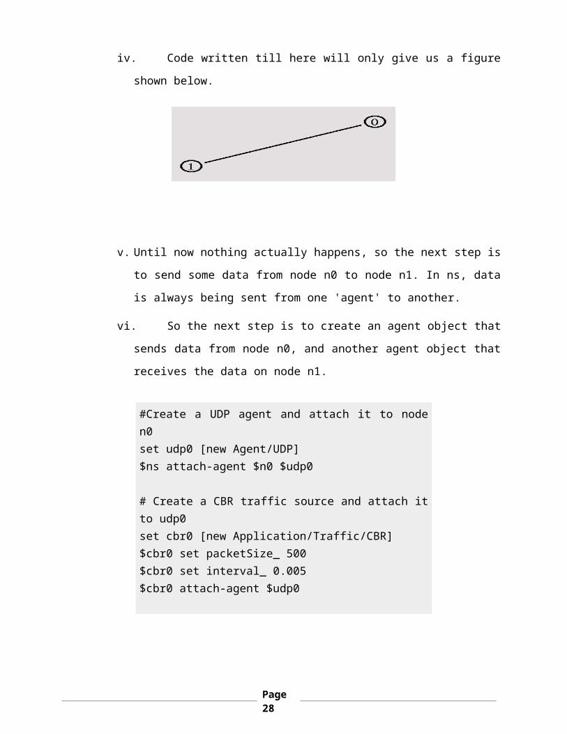
iv. Code written till here will only give us a figure
shown below.
v. Until now nothing actually happens, so the next step is
to send some data from node n0 to node n1. In ns, data
is always being sent from one 'agent' to another.
vi. So the next step is to create an agent object that
sends data from node n0, and another agent object that
receives the data on node n1.
#Create a UDP agent and attach it to noden0set udp0 [new Agent/UDP]$ns attach-agent $n0 $udp0
# Create a CBR traffic source and attach itto udp0set cbr0 [new Application/Traffic/CBR]$cbr0 set packetSize_ 500$cbr0 set interval_ 0.005$cbr0 attach-agent $udp0
Page28

n0 n1
udp
cbr
null
vii. These lines create a UDP agent and attach it to
the node n0, then attach a CBR traffic generator to the
UDP agent. CBR stands for 'constant bit rate'.
viii. The packet Size is being set to 500 bytes and a
packet will be sent every 0.005 seconds (i.e. 200
packets per second).
ix. The next lines create a Null agent which acts as
traffic sink and attach it to node n1.
x. Now the two agents have to be connected with each
other.
set null0 [new
Agent/Null]
$ns attach-agent $n1
$null0
$ns connect $udp0
$null0
Page29
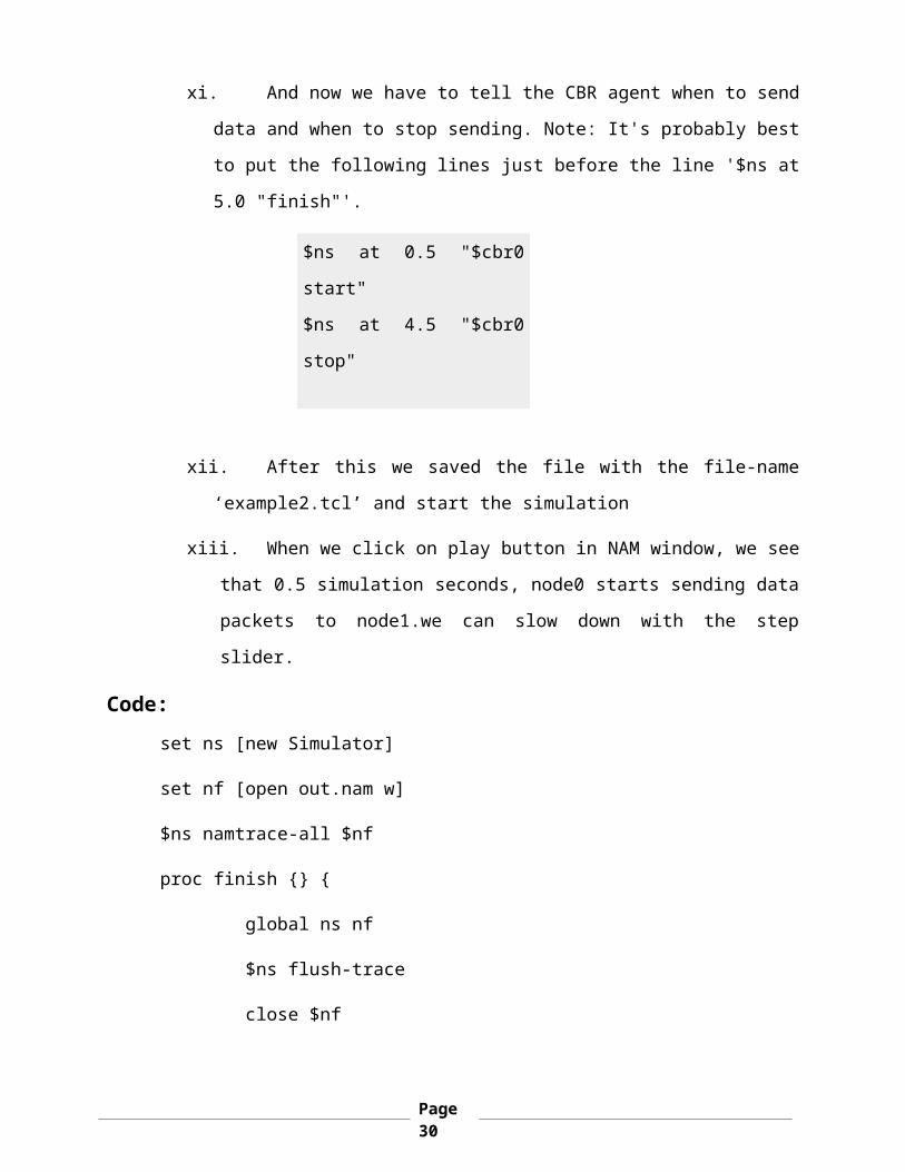
xi. And now we have to tell the CBR agent when to send
data and when to stop sending. Note: It's probably best
to put the following lines just before the line '$ns at
5.0 "finish"'.
$ns at 0.5 "$cbr0
start"
$ns at 4.5 "$cbr0
stop"
xii. After this we saved the file with the file-name
‘example2.tcl’ and start the simulation
xiii. When we click on play button in NAM window, we see
that 0.5 simulation seconds, node0 starts sending data
packets to node1.we can slow down with the step
slider.
Code:set ns [new Simulator]
set nf [open out.nam w]
$ns namtrace-all $nf
proc finish {} {
global ns nf
$ns flush-trace
close $nf
Page30

exec nam out.nam &
exit 0 }
set n0 [$ns node]
set n1 [$ns node]
$ns duplex-link $n0 $n1 1Mb 10ms DropTail
set udp0 [new Agent/UDP]
$ns attach-agent $n0 $udp0
set cbr0 [new Application/Traffic/CBR]
$cbr0 set packetSize_ 500
$cbr0 set interval_ 0.005
$cbr0 attach-agent $udp0
set null0 [new Agent/Null]
$ns attach-agent $n1 $null0
$ns connect $udp0 $null0
$ns at 0.5 "$cbr0 start"
$ns at 4.5 "$cbr0 stop"
$ns at 5.0 "finish"
$ns run
Page31
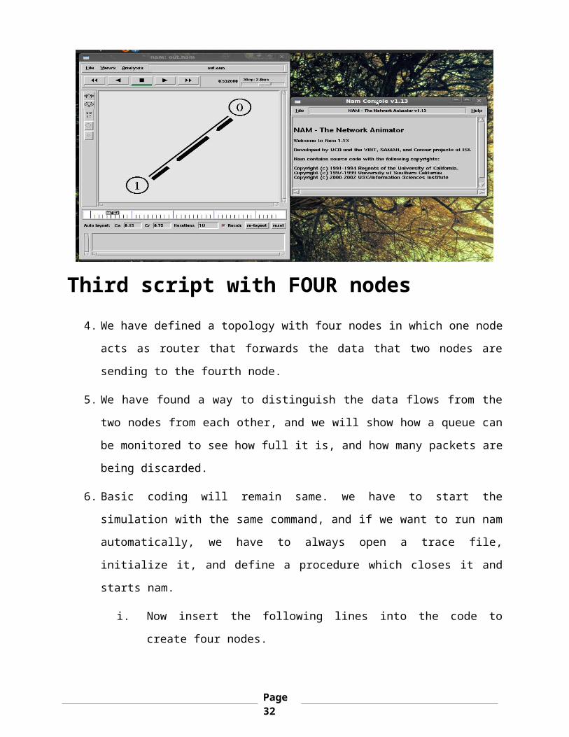
Third script with FOUR nodes4. We have defined a topology with four nodes in which one node
acts as router that forwards the data that two nodes are
sending to the fourth node.
5. We have found a way to distinguish the data flows from the
two nodes from each other, and we will show how a queue can
be monitored to see how full it is, and how many packets are
being discarded.
6. Basic coding will remain same. we have to start the
simulation with the same command, and if we want to run nam
automatically, we have to always open a trace file,
initialize it, and define a procedure which closes it and
starts nam.
i. Now insert the following lines into the code to
create four nodes.
Page32

set n0 [$ns
node]
set n1 [$ns
node]
set n2 [$ns
node]
set n3 [$ns
node]
ii. The following piece of Tcl code creates three duplex
links between the nodes.
$ns duplex-link $n0 $n2 1Mb 10ms
DropTail
$ns duplex-link $n1 $n2 1Mb 10ms
DropTail
$ns duplex-link $n3 $n2 1Mb 10ms
DropTail
iii. The topology in the nam window will look like the
picture below.
Page33

iv. Now we create two UDP agents with CBR traffic sources
and attach them to the nodes n0 and n1. Then we
create a Null agent and attach it to node n3.
#Create a UDP agent and attach it to node
n0
set udp0 [new Agent/UDP]
$ns attach-agent $n0 $udp0
# Create a CBR traffic source and attach it
to udp0
set cbr0 [new Application/Traffic/CBR]
$cbr0 set packetSize_ 500
$cbr0 set interval_ 0.005
$cbr0 attach-agent $udp0
#Create a UDP agent and attach it to node
n1
set udp1 [new Agent/UDP]
$ns attach-agent $n1 $udp1
# Create a CBR traffic source and attach it
to udp1
set cbr1 [new Application/Traffic/CBR]
$cbr1 set packetSize_ 500
Page34

$cbr1 set interval_ 0.005
$cbr1 attach-agent $udp1
set null0 [new Agent/Null]
$ns attach-agent $n3 $null0
v. The two CBR agents have to be connected to the Null
agent.
$ns connect $udp0 $null0
$ns connect $udp1 $null0
vi. We want the first CBR agent to start sending at 0.5
seconds and to stop at 4.5 seconds while the second
CBR agent starts at 1.0 seconds and stops at 4.0
seconds.
vii. We noticed that there was
more traffic on the links
from n0 to n2 and n1 to n2
$ns at 0.5 "$cbr0
start"
$ns at 1.0 "$cbr1
start"
$ns at 4.0 "$cbr1
stop"
$ns at 4.5 "$cbr0
stop"
Page35

than the link from n2 to n3 can carry. A simple
calculation confirms this: We are sending 200 packets
per second on each of the first two links and the
packet size is 500 bytes. This results in a bandwidth
of 0.8 megabits per second for the links from n0 to
n2 and from n1 to n2. That's a total bandwidth of
1.6Mb/s, but the link between n2 and n3 only has a
capacity of 1Mb/s, so obviously some packets are
being discarded.
viii. Add the following two lines to your CBR agent
definitions.
ix. Now we added the following piece
of code to our Tcl script, preferably at the
beginning after the simulator object has been
created, since this is a part of the simulator setup.
$ns colour 1
Blue
$ns color 2
Red
x. This code allows you to set different colours for
each flow id.
$udp0 set class_
1
$udp1 set class_
2
Page36
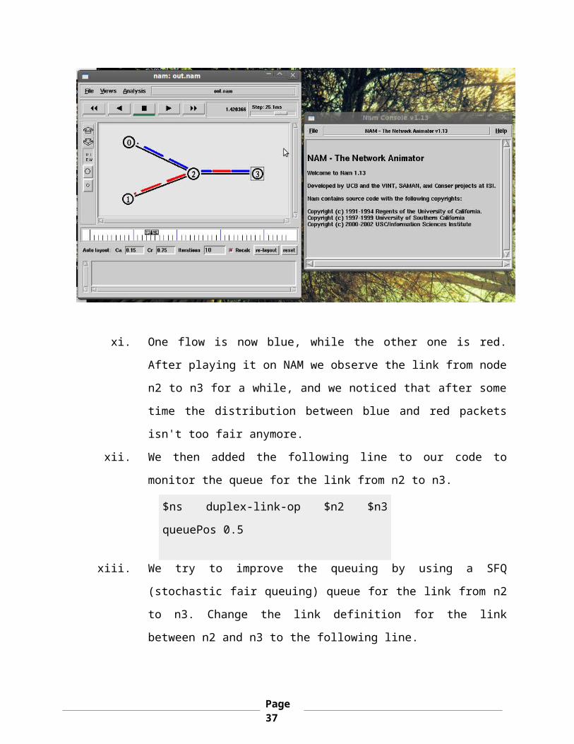
xi. One flow is now blue, while the other one is red.
After playing it on NAM we observe the link from node
n2 to n3 for a while, and we noticed that after some
time the distribution between blue and red packets
isn't too fair anymore.
xii. We then added the following line to our code to
monitor the queue for the link from n2 to n3.
$ns duplex-link-op $n2 $n3
queuePos 0.5
xiii. We try to improve the queuing by using a SFQ
(stochastic fair queuing) queue for the link from n2
to n3. Change the link definition for the link
between n2 and n3 to the following line.
Page37

n0
n1
n2 n3
sender
sender
router receiver
$ns duplex-link $n3 $n2 1Mb 10ms
SFQ
xiv. The queuing should be 'fair' now. The same amount of
blue and red packets should be dropped.
Code:
Page38
set ns [new Simulator]
$ns color 1 Blue
$ns color 2 Red
set no [open ot.nam w]
$ns namtrace-all $no
proc finish {} {
global ns no
close $no
exec nam ot.nam &
exit 0
}
set n0 [$ns node]
set n1 [$ns node]
set n2 [$ns node]
set n3 [$ns node]
$ns duplex-link $n0 $n2 1Mb 1ms DropTail
$ns duplex-link $n1 $n2 1Mb 1ms DropTail
$ns duplex-link $n3 $n2 1Mb 10ms SFQ
$ns duplex-link-op $n0 $n2 orient right-down
$ns duplex-link-op $n1 $n2 orient right-up
$ns duplex-link-op $n2 $n3 orient right
set udp [new Agent/UDP]
Page39

$ns attach-agent $n0 $udp
set udp1 [new Agent/UDP]
$ns attach-agent $n1 $udp1
$udp set class_ 1
$udp1 set class_ 2
set cbr [new Application/Traffic/CBR]
$cbr set packetSize_ 200
$cbr set interval_ 0.002
$cbr attach-agent $udp
set null [new Agent/Null]
$ns attach-agent $n3 $null
set cbr1 [new Application/Traffic/CBR]
$cbr1 set packetSize_ 200
$cbr1 set interval_ 0.002
$cbr1 attach-agent $udp1
$ns connect $udp $null
$ns connect $udp1 $null
$ns at 0.5 "$cbr start"
$ns at 1.0 "$cbr1 start"
$ns at 4.0 "$cbr1 stop"
$ns at 4.5 "$cbr stop"
$ns at 5.0 "finish"
Page40
$ns run
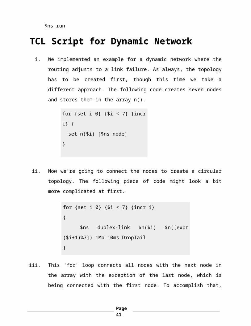
TCL Script for Dynamic Networki. We implemented an example for a dynamic network where the
routing adjusts to a link failure. As always, the topology
has to be created first, though this time we take a
different approach. The following code creates seven nodes
and stores them in the array n().
for {set i 0} {$i < 7} {incr
i} {
set n($i) [$ns node]
}
ii. Now we're going to connect the nodes to create a circular
topology. The following piece of code might look a bit
more complicated at first.
iii. This 'for' loop connects all nodes with the next node in
the array with the exception of the last node, which is
being connected with the first node. To accomplish that,
for {set i 0} {$i < 7} {incr i}
{
$ns duplex-link $n($i) $n([expr
($i+1)%7]) 1Mb 10ms DropTail
}
Page41

we have used the '%' (modulo) operator.
iv. When you run the script now, the topology might look a bit
strange in nam at first, but after you hit the ‘re-layout'
button it should look like the picture below:
v. The next step is to send some data from node n(0) to node
n(3).
#Create a UDP agent and attach it to node
n(0)
set udp0 [new Agent/UDP]
$ns attach-agent $n(0) $udp0
# Create a CBR traffic source and attach it
to udp0
set cbr0 [new Application/Traffic/CBR]
$cbr0 set packetSize_ 500
$cbr0 set interval_ 0.005
Page42

$cbr0 attach-agent $udp0
set null0 [new Agent/Null]
$ns attach-agent $n(3) $null0
$ns connect $udp0 $null0
$ns at 0.5 "$cbr0 start"
$ns at 4.5 "$cbr0 stop"
vi. When we start the scrip, we observed that the traffic
takes the shortest path from node 0 to node 3 through
nodes 1 and 2, as could be expected.
vii. Now we added another interesting feature. We let the link
between node 1 and 2 (which is being used by the traffic)
go down for a second.
$ns rtmodel-at 1.0 down $n(1)
$n(2)
$ns rtmodel-at 2.0 up $n(1)
$n(2)
viii. We see that between the seconds 1.0 and 2.0 the link will
be down, and all data that is sent from node 0 is lost.
ix. We will now show how to use dynamic routing to solve that
'problem'. Add the following line at the beginning of your
Page43
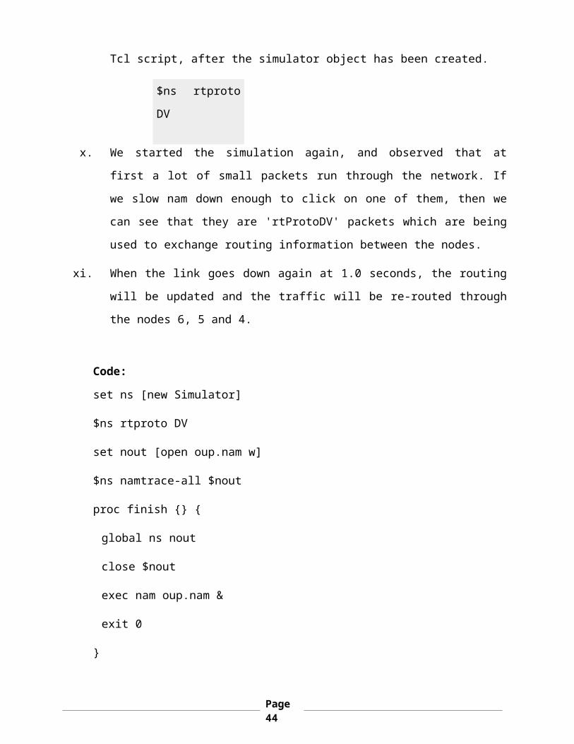
Tcl script, after the simulator object has been created.
$ns rtproto
DV
x. We started the simulation again, and observed that at
first a lot of small packets run through the network. If
we slow nam down enough to click on one of them, then we
can see that they are 'rtProtoDV' packets which are being
used to exchange routing information between the nodes.
xi. When the link goes down again at 1.0 seconds, the routing
will be updated and the traffic will be re-routed through
the nodes 6, 5 and 4.
Code:
set ns [new Simulator]
$ns rtproto DV
set nout [open oup.nam w]
$ns namtrace-all $nout
proc finish {} {
global ns nout
close $nout
exec nam oup.nam &
exit 0
}
Page44

for {set i 0} {$i < 7} {incr i} {
set n($i) [$ns node]
}
for {set i 0} {$i < 7} {incr i} {
$ns duplex-link $n($i) $n([expr ($i+1)%7]) 1Mb 10ms DropTail
}
set udp [new Agent/UDP]
$ns attach-agent $n(0) $udp
set cbr [new Application/Traffic/CBR]
$cbr set packetSize_ 500
$cbr set interval_ 0.005
$cbr attach-agent $udp
set null [new Agent/Null]
$ns attach-agent $n(3) $null
$ns connect $udp $null
$ns at 0.5 "$cbr start"
$ns rtmodel-at 1.0 down $n(1) $n(2)
$ns rtmodel-at 2.0 up $n(1) $n(2)
$ns at 4.5 "$cbr stop"
$ns at 5.0 "finish"
$ns run
Page45

Page46

Chapter – 4
NS-2 Simulation
Page47

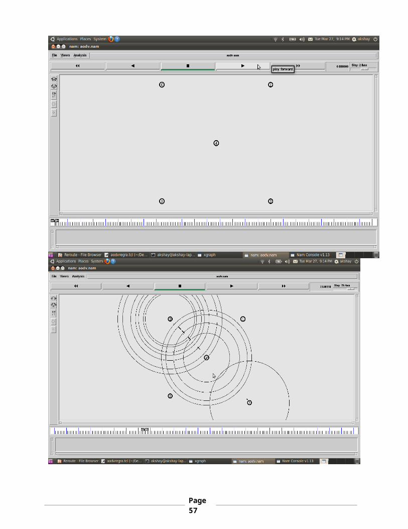
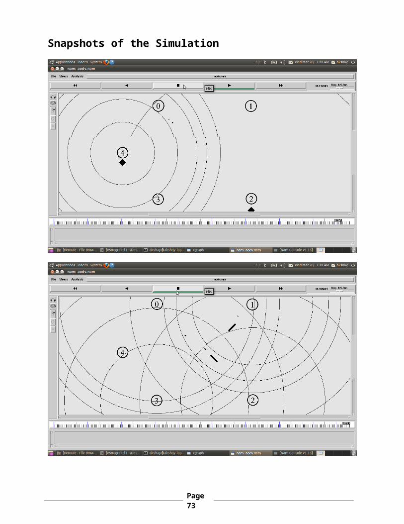
Simulation Scenarios1. It is a plot of 500x500, in this there are 5 wireless nodes,
out of which 4 nodes (node 0, 1, 2 and 3) are positioned at
the edges and the node 4 at the centre of the plot. At time
1.0 sec the nodes at the edges start to move towards the
centre with a speed of 10 m/s till 18.0 sec. The centre node
starts to move towards the left at 15.0 sec with a speed of
10m/s. There are 2 source nodes (node 0 and 1) and 2 sink
nodes (node 2 and 3). The traffic is of type TCP, generated
by the FTP APPLICATION Agent. The source nodes 0 and 1 start
to transmit at the 5.0 and 5.5 sec. The total simulation
time is 25.0 sec and all the nodes are reset at the time
instant 25.00 sec. The simulation generates a trace file in
which all packets and network events are traced and the nam
file traces all the node movements. Two other files are also
generated which store the output for the xgraph utility to
generate the graph.
2. It is a plot of 500x500, in this there are 5 wireless nodes,
out of which 4 nodes (node 0, 1, 2 and 3) are positioned at
the edges and the node 4 at the centre of the plot. At time
Page48

1.0 sec the nodes at the edges start to move towards the
centre with a speed of 10 m/s till 18.0 sec. The centre node
starts to move towards the left at 15.0 sec with a speed of
18m/s. There are 2 source nodes (node 0 and 1) and 2 sink
nodes (node 2 and 3). The traffic is of type TCP, generated
by the FTP APPLICATION Agent. The source nodes 0 and 1 start
to transmit at the 5.0 and 5.5 sec. The total simulation
time is 28.0 sec and all the nodes are reset at the time
instant 28.00 sec. The simulation generates a trace file in
which all packets and network events are traced and the nam
file traces all the node movements. Two other files are also
generated which store the output for the xgraph utility to
generate the graph.
Various Parameters to compare the
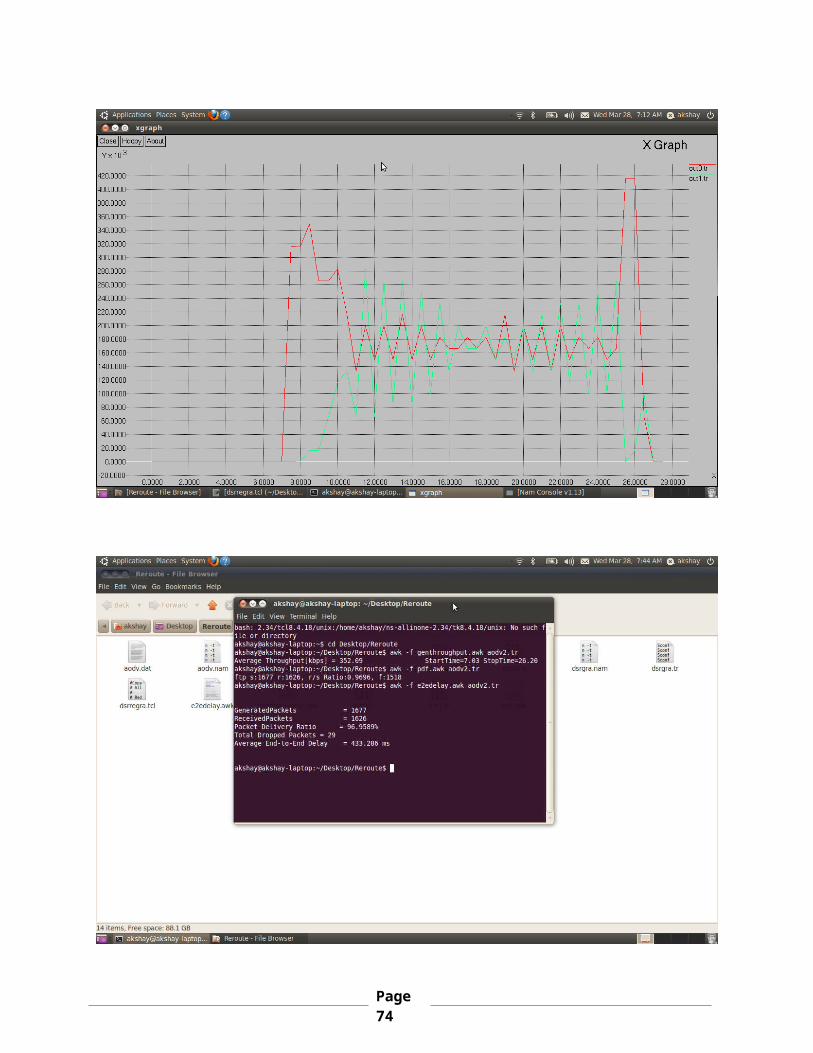
Routing Protocols1. Throughput: It is the total amount of data transferred
across the network in the data packets. Here we have
Page49
calculated the average throughput in bytes.
2. Delay: This is the amount of delay the packet faces when
transmitted through the network. In our project we have
considered taking average node to node delay.
3. Packet Delivery Ratio: It is defined as the ratio of number
of packets received to the number of packets sent.
4. Number of lost packets: These are the number of packets lost
during the transmission through the network.
Page50
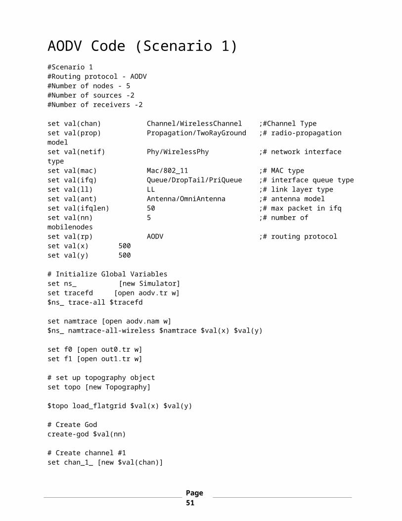
AODV Code (Scenario 1)#Scenario 1#Routing protocol - AODV#Number of nodes - 5#Number of sources -2 #Number of receivers -2
set val(chan) Channel/WirelessChannel ;#Channel Typeset val(prop) Propagation/TwoRayGround ;# radio-propagation modelset val(netif) Phy/WirelessPhy ;# network interface typeset val(mac) Mac/802_11 ;# MAC typeset val(ifq) Queue/DropTail/PriQueue ;# interface queue typeset val(ll) LL ;# link layer typeset val(ant) Antenna/OmniAntenna ;# antenna modelset val(ifqlen) 50 ;# max packet in ifqset val(nn) 5 ;# number of mobilenodesset val(rp) AODV ;# routing protocolset val(x) 500set val(y) 500
# Initialize Global Variablesset ns_ [new Simulator]set tracefd [open aodv.tr w]$ns_ trace-all $tracefd
set namtrace [open aodv.nam w]$ns_ namtrace-all-wireless $namtrace $val(x) $val(y)
set f0 [open out0.tr w]set f1 [open out1.tr w]
# set up topography objectset topo [new Topography]
$topo load_flatgrid $val(x) $val(y)
# Create Godcreate-god $val(nn)
# Create channel #1 set chan_1_ [new $val(chan)]
Page51
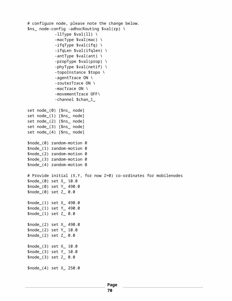
# configure node, please note the change below.$ns_ node-config -adhocRouting $val(rp) \
-llType $val(ll) \-macType $val(mac) \-ifqType $val(ifq) \-ifqLen $val(ifqlen) \-antType $val(ant) \-propType $val(prop) \-phyType $val(netif) \-topoInstance $topo \-agentTrace ON \-routerTrace ON \-macTrace ON \-movementTrace OFF\-channel $chan_1_
set node_(0) [$ns_ node]set node_(1) [$ns_ node]set node_(2) [$ns_ node]set node_(3) [$ns_ node]set node_(4) [$ns_ node]
$node_(0) random-motion 0$node_(1) random-motion 0$node_(2) random-motion 0$node_(3) random-motion 0$node_(4) random-motion 0
# Provide initial (X,Y, for now Z=0) co-ordinates for mobilenodes$node_(0) set X_ 10.0$node_(0) set Y_ 490.0$node_(0) set Z_ 0.0
$node_(1) set X_ 490.0$node_(1) set Y_ 490.0$node_(1) set Z_ 0.0
$node_(2) set X_ 490.0$node_(2) set Y_ 10.0$node_(2) set Z_ 0.0
$node_(3) set X_ 10.0$node_(3) set Y_ 10.0$node_(3) set Z_ 0.0
Page52
$node_(4) set X_ 250.0$node_(4) set Y_ 250.0$node_(4) set Z_ 0.0
for {set i 0} {$i < $val(nn)} {incr i} {$ns_ initial_node_pos $node_($i) 20
}
# Now produce some simple node movements$ns_ at 0.0 "record"
$ns_ at 1.0 "$node_(1) setdest 300.0 300.0 15.0"$ns_ at 1.0 "$node_(0) setdest 200.0 300.0 15.0"$ns_ at 1.0 "$node_(3) setdest 200.0 200.0 15.0"$ns_ at 1.0 "$node_(2) setdest 300.0 200.0 15.0"
$ns_ at 15.0 "$node_(4) setdest 100.0 250.0 10.0"
$ns_ at 18.0 "$node_(1) setdest 499.0 499.0 5.0"$ns_ at 18.0 "$node_(0) setdest 10.0 499.0 5.0"$ns_ at 18.0 "$node_(3) setdest 10.0 10.0 5.0"$ns_ at 18.0 "$node_(2) setdest 499.0 10.0 5.0"
# Setup traffic flow between nodes# TCP connections between node_(0) and node_(2)set tcp [new Agent/TCP]$tcp set class_ 2set sink [new Agent/TCPSink]$ns_ attach-agent $node_(0) $tcp$ns_ attach-agent $node_(2) $sink$ns_ connect $tcp $sinkset ftp [new Application/FTP]$ftp attach-agent $tcp$ns_ at 5.0 "$ftp start"
# TCP connections between node_(1) and node_(3)set tcp1 [new Agent/TCP]$tcp set class_ 2set sink1 [new Agent/TCPSink]$ns_ attach-agent $node_(1) $tcp1$ns_ attach-agent $node_(3) $sink1$ns_ connect $tcp1 $sink1set ftp1 [new Application/FTP]$ftp1 attach-agent $tcp1$ns_ at 5.5 "$ftp1 start"
Page53
# Tell nodes when the simulation endsfor {set i 0} {$i < $val(nn) } {incr i} { $ns_ at 25.0 "$node_($i) reset";}$ns_ at 25.0 "stop"$ns_ at 25.01 "puts \"NS EXITING...\" ; $ns_ halt"
proc stop {} { global ns_ tracefd f0 f1 $ns_ flush-trace close $tracefd close $f0 close $f1 exec nam aodv.nam & exec xgraph out0.tr out1.tr -geometry 800x400}
proc record {} { global sink sink1 f0 f1 #Get an instance of the simulator set ns [Simulator instance] #Set the time after which the procedure should be called again set time 0.5 #How many bytes have been received by the traffic sinks? set bw0 [$sink set bytes_] set bw1 [$sink1 set bytes_] #Get the current time set now [$ns now] #Calculate the bandwidth (in MBit/s) and write it to the files puts $f0 "$now [expr $bw0/$time*8/1000000]" puts $f1 "$now [expr $bw1/$time*8/1000000]" #Reset the bytes_ values on the traffic sinks $sink set bytes_ 0 $sink1 set bytes_ 0 #Re-schedule the procedure $ns at [expr $now+$time] "record"}
puts "Starting Simulation..."$ns_ run
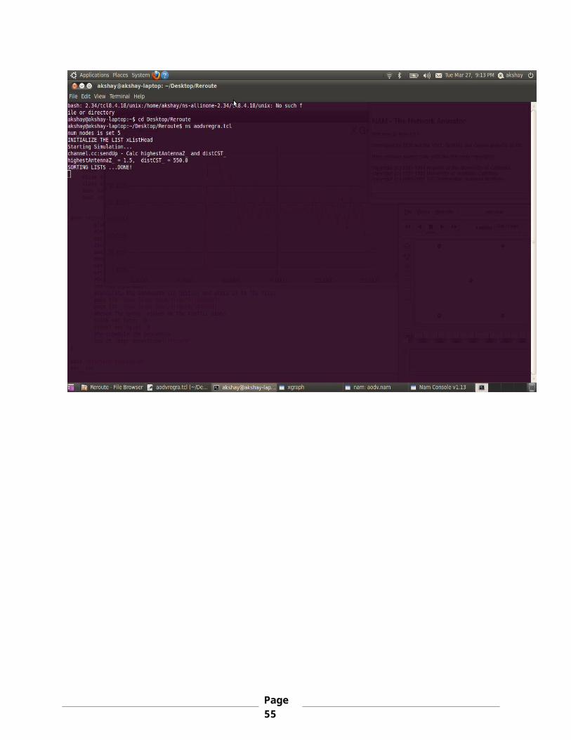
Snapshots of the Simulation
Page54
Page55

Page56
Page57

Page58

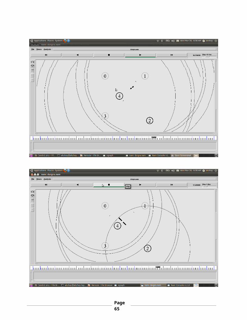
Page59

DSR Code (Scenario 1)#Scenario 1#Routing protocol - DSR#Number of nodes - 5#Number of sources -2 #Number of receivers -2set val(chan) Channel/WirelessChannel ;#Channel Typeset val(prop) Propagation/TwoRayGround ;# radio-propagation modelset val(netif) Phy/WirelessPhy ;# network interface typeset val(mac) Mac/802_11 ;# MAC typeset val(ifq) Queue/DropTail/PriQueue ;# interface queue typeset val(ll) LL ;# link layer typeset val(ant) Antenna/OmniAntenna ;# antenna modelset val(ifqlen) 50 ;# max packet in ifqset val(nn) 5 ;# number of mobilenodesset val(rp) DSR ;# routing protocolset val(x) 500set val(y) 500
# Initialize Global Variablesset ns_ [new Simulator]set tracefd [open dsrgra.tr w]$ns_ trace-all $tracefd
set namtrace [open dsrgra.nam w]$ns_ namtrace-all-wireless $namtrace $val(x) $val(y)
set f0 [open out0.tr w]set f1 [open out1.tr w]
# set up topography objectset topo [new Topography]
$topo load_flatgrid $val(x) $val(y)
# Create Godcreate-god $val(nn)
# Create channel #1 and #2set chan_1_ [new $val(chan)]
Page60

# configure node, please note the change below.$ns_ node-config -adhocRouting $val(rp) \
-llType $val(ll) \-macType $val(mac) \-ifqType $val(ifq) \-ifqLen $val(ifqlen) \-antType $val(ant) \-propType $val(prop) \-phyType $val(netif) \-topoInstance $topo \-agentTrace ON \-routerTrace ON \-macTrace ON \-movementTrace OFF\-channel $chan_1_
set node_(0) [$ns_ node]set node_(1) [$ns_ node]set node_(2) [$ns_ node]set node_(3) [$ns_ node]set node_(4) [$ns_ node]
$node_(0) random-motion 0$node_(1) random-motion 0$node_(2) random-motion 0$node_(3) random-motion 0$node_(4) random-motion 0
# Provide initial (X,Y, for now Z=0) co-ordinates for mobilenodes$node_(0) set X_ 10.0$node_(0) set Y_ 490.0$node_(0) set Z_ 0.0
$node_(1) set X_ 490.0$node_(1) set Y_ 490.0$node_(1) set Z_ 0.0
$node_(2) set X_ 490.0$node_(2) set Y_ 10.0$node_(2) set Z_ 0.0
$node_(3) set X_ 10.0$node_(3) set Y_ 10.0$node_(3) set Z_ 0.0
$node_(4) set X_ 250.0
Page61
$node_(4) set Y_ 250.0$node_(4) set Z_ 0.0
for {set i 0} {$i < $val(nn)} {incr i} {$ns_ initial_node_pos $node_($i) 20
}
# Now produce some simple node movements# Node_(1) starts to move towards node_(0)
$ns_ at 0.0 "record"
$ns_ at 1.0 "$node_(1) setdest 300.0 300.0 15.0"$ns_ at 1.0 "$node_(0) setdest 200.0 300.0 15.0"$ns_ at 1.0 "$node_(3) setdest 200.0 200.0 15.0"$ns_ at 1.0 "$node_(2) setdest 300.0 200.0 15.0" $ns_ at 15.0 "$node_(4) setdest 100.0 250.0 10.0"
$ns_ at 18.0 "$node_(1) setdest 499.0 499.0 5.0"$ns_ at 18.0 "$node_(0) setdest 10.0 499.0 5.0"$ns_ at 18.0 "$node_(3) setdest 250.0 250.0 5.0"
# Setup traffic flow between nodes# TCP connections between node_(0) and node_(2)set tcp [new Agent/TCP]$tcp set class_ 2set sink [new Agent/TCPSink]$ns_ attach-agent $node_(0) $tcp$ns_ attach-agent $node_(2) $sink$ns_ connect $tcp $sinkset ftp [new Application/FTP]$ftp attach-agent $tcp$ns_ at 5.0 "$ftp start"
# TCP connections between node_(1) and node_(3)set tcp1 [new Agent/TCP]$tcp set class_ 2set sink1 [new Agent/TCPSink]$ns_ attach-agent $node_(1) $tcp1$ns_ attach-agent $node_(3) $sink1$ns_ connect $tcp1 $sink1set ftp1 [new Application/FTP]$ftp1 attach-agent $tcp1$ns_ at 5.5 "$ftp1 start"
Page62

# Tell nodes when the simulation endsfor {set i 0} {$i < $val(nn) } {incr i} { $ns_ at 25.0 "$node_($i) reset";}$ns_ at 25.0 "stop"$ns_ at 25.01 "puts \"NS EXITING...\" ; $ns_ halt"
proc stop {} { global ns_ tracefd f0 f1 $ns_ flush-trace close $tracefd close $f0 close $f1 exec nam dsrgra.nam & exec xgraph out0.tr out1.tr -geometry 800x400}
proc record {} { global sink sink1 f0 f1 #Get an instance of the simulator set ns [Simulator instance] #Set the time after which the procedure should be called again set time 0.5 #How many bytes have been received by the traffic sinks? set bw0 [$sink set bytes_] set bw1 [$sink1 set bytes_] #Get the current time set now [$ns now] #Calculate the bandwidth (in MBit/s) and write it to the files puts $f0 "$now [expr $bw0/$time*8/1000000]" puts $f1 "$now [expr $bw1/$time*8/1000000]" #Reset the bytes_ values on the traffic sinks $sink set bytes_ 0 $sink1 set bytes_ 0 #Re-schedule the procedure $ns at [expr $now+$time] "record"}
puts "Starting Simulation..."$ns_ run
Page63

Snapshots of the Simulation
Page64
Page65

Page66

Page67

Page68

ADOV Code (Scenario 2)#Scenario 2#Routing protocol - AODV#Number of nodes - 5#Number of sources -2 #Number of receivers -2set val(chan) Channel/WirelessChannel ;#Channel Typeset val(prop) Propagation/TwoRayGround ;# radio-propagation modelset val(netif) Phy/WirelessPhy ;# network interface typeset val(mac) Mac/802_11 ;# MAC typeset val(ifq) Queue/DropTail/PriQueue ;# interface queue typeset val(ll) LL ;# link layer typeset val(ant) Antenna/OmniAntenna ;# antenna modelset val(ifqlen) 50 ;# max packet in ifqset val(nn) 5 ;# number of mobilenodesset val(rp) AODV ;# routing protocolset val(x) 500set val(y) 500
# Initialize Global Variablesset ns_ [new Simulator]set tracefd [open aodv2.tr w]$ns_ trace-all $tracefd
set namtrace [open aodv2.nam w]$ns_ namtrace-all-wireless $namtrace $val(x) $val(y)
set f0 [open out0.tr w]set f1 [open out1.tr w]
# set up topography objectset topo [new Topography]
$topo load_flatgrid $val(x) $val(y)
# Create Godcreate-god $val(nn)
# Create channel #1 set chan_1_ [new $val(chan)]
Page69
# configure node, please note the change below.$ns_ node-config -adhocRouting $val(rp) \
-llType $val(ll) \-macType $val(mac) \-ifqType $val(ifq) \-ifqLen $val(ifqlen) \-antType $val(ant) \-propType $val(prop) \-phyType $val(netif) \-topoInstance $topo \-agentTrace ON \-routerTrace ON \-macTrace ON \-movementTrace OFF\-channel $chan_1_
set node_(0) [$ns_ node]set node_(1) [$ns_ node]set node_(2) [$ns_ node]set node_(3) [$ns_ node]set node_(4) [$ns_ node]
$node_(0) random-motion 0$node_(1) random-motion 0$node_(2) random-motion 0$node_(3) random-motion 0$node_(4) random-motion 0
# Provide initial (X,Y, for now Z=0) co-ordinates for mobilenodes$node_(0) set X_ 10.0$node_(0) set Y_ 490.0$node_(0) set Z_ 0.0
$node_(1) set X_ 490.0$node_(1) set Y_ 490.0$node_(1) set Z_ 0.0
$node_(2) set X_ 490.0$node_(2) set Y_ 10.0$node_(2) set Z_ 0.0
$node_(3) set X_ 10.0$node_(3) set Y_ 10.0$node_(3) set Z_ 0.0
$node_(4) set X_ 250.0
Page70
$node_(4) set Y_ 250.0$node_(4) set Z_ 0.0
for {set i 0} {$i < $val(nn)} {incr i} {$ns_ initial_node_pos $node_($i) 20
}
# Now produce some simple node movements$ns_ at 0.0 "record"
$ns_ at 1.0 "$node_(1) setdest 300.0 300.0 15.0"$ns_ at 1.0 "$node_(0) setdest 200.0 300.0 15.0"$ns_ at 1.0 "$node_(3) setdest 200.0 200.0 15.0"$ns_ at 1.0 "$node_(2) setdest 300.0 200.0 15.0"
$ns_ at 15.0 "$node_(4) setdest 100.0 250.0 15.0"
$ns_ at 18.0 "$node_(1) setdest 499.0 499.0 5.0"$ns_ at 18.0 "$node_(0) setdest 10.0 499.0 5.0"$ns_ at 18.0 "$node_(3) setdest 10.0 10.0 5.0"$ns_ at 18.0 "$node_(2) setdest 499.0 10.0 5.0"
# Setup traffic flow between nodes# TCP connections between node_(0) and node_(2)set tcp [new Agent/TCP]$tcp set class_ 2set sink [new Agent/TCPSink]$ns_ attach-agent $node_(0) $tcp$ns_ attach-agent $node_(2) $sink$ns_ connect $tcp $sinkset ftp [new Application/FTP]$ftp attach-agent $tcp$ns_ at 5.0 "$ftp start"
# TCP connections between node_(1) and node_(3)set tcp1 [new Agent/TCP]$tcp set class_ 2set sink1 [new Agent/TCPSink]$ns_ attach-agent $node_(1) $tcp1$ns_ attach-agent $node_(3) $sink1$ns_ connect $tcp1 $sink1set ftp1 [new Application/FTP]$ftp1 attach-agent $tcp1$ns_ at 5.5 "$ftp1 start"
Page71

# Tell nodes when the simulation endsfor {set i 0} {$i < $val(nn) } {incr i} { $ns_ at 28.0 "$node_($i) reset";}$ns_ at 28.0 "stop"$ns_ at 28.01 "puts \"NS EXITING...\" ; $ns_ halt"
proc stop {} { global ns_ tracefd f0 f1 $ns_ flush-trace close $tracefd close $f0 close $f1 exec nam aodv2.nam & exec xgraph out0.tr out1.tr -geometry 800x400}
proc record {} { global sink sink1 f0 f1 #Get an instance of the simulator set ns [Simulator instance] #Set the time after which the procedure should be called again set time 0.5 #How many bytes have been received by the traffic sinks? set bw0 [$sink set bytes_] set bw1 [$sink1 set bytes_] #Get the current time set now [$ns now] #Calculate the bandwidth (in MBit/s) and write it to the files puts $f0 "$now [expr $bw0/$time*8/1000000]" puts $f1 "$now [expr $bw1/$time*8/1000000]" #Reset the bytes_ values on the traffic sinks $sink set bytes_ 0 $sink1 set bytes_ 0 #Re-schedule the procedure $ns at [expr $now+$time] "record"}
puts "Starting Simulation..."$ns_ run
Page72
Snapshots of the Simulation
Page73
Page74

DSR Code (Scenario 2)#Scenario 2#Routing protocol - DSR#Number of nodes - 5#Number of sources -2 #Number of receivers -2set val(chan) Channel/WirelessChannel ;#Channel Typeset val(prop) Propagation/TwoRayGround ;# radio-propagation modelset val(netif) Phy/WirelessPhy ;# network interface typeset val(mac) Mac/802_11 ;# MAC typeset val(ifq) Queue/DropTail/PriQueue ;# interface queue typeset val(ll) LL ;# link layer typeset val(ant) Antenna/OmniAntenna ;# antenna modelset val(ifqlen) 50 ;# max packet in ifqset val(nn) 5 ;# number of mobilenodesset val(rp) DSR ;# routing protocolset val(x) 500set val(y) 500
# Initialize Global Variablesset ns_ [new Simulator]set tracefd [open dsr2.tr w]$ns_ trace-all $tracefd
set namtrace [open dsr2.nam w]$ns_ namtrace-all-wireless $namtrace $val(x) $val(y)
set f0 [open out0.tr w]set f1 [open out1.tr w]
# set up topography objectset topo [new Topography]
$topo load_flatgrid $val(x) $val(y)
# Create Godcreate-god $val(nn)
Page75
# Create channel #1 set chan_1_ [new $val(chan)]
# configure node, please note the change below.$ns_ node-config -adhocRouting $val(rp) \
-llType $val(ll) \-macType $val(mac) \-ifqType $val(ifq) \-ifqLen $val(ifqlen) \-antType $val(ant) \-propType $val(prop) \-phyType $val(netif) \-topoInstance $topo \-agentTrace ON \-routerTrace ON \-macTrace ON \-movementTrace OFF\-channel $chan_1_
set node_(0) [$ns_ node]set node_(1) [$ns_ node]set node_(2) [$ns_ node]set node_(3) [$ns_ node]set node_(4) [$ns_ node]
$node_(0) random-motion 0$node_(1) random-motion 0$node_(2) random-motion 0$node_(3) random-motion 0$node_(4) random-motion 0
# Provide initial (X,Y, for now Z=0) co-ordinates for mobilenodes$node_(0) set X_ 10.0$node_(0) set Y_ 490.0$node_(0) set Z_ 0.0
$node_(1) set X_ 490.0$node_(1) set Y_ 490.0$node_(1) set Z_ 0.0
$node_(2) set X_ 490.0$node_(2) set Y_ 10.0$node_(2) set Z_ 0.0
$node_(3) set X_ 10.0$node_(3) set Y_ 10.0
Page76
$node_(3) set Z_ 0.0
$node_(4) set X_ 250.0$node_(4) set Y_ 250.0$node_(4) set Z_ 0.0
for {set i 0} {$i < $val(nn)} {incr i} {$ns_ initial_node_pos $node_($i) 20
}
# Now produce some simple node movements$ns_ at 0.0 "record"
$ns_ at 1.0 "$node_(1) setdest 300.0 300.0 15.0"$ns_ at 1.0 "$node_(0) setdest 200.0 300.0 15.0"$ns_ at 1.0 "$node_(3) setdest 200.0 200.0 15.0"$ns_ at 1.0 "$node_(2) setdest 300.0 200.0 15.0"
$ns_ at 15.0 "$node_(4) setdest 100.0 250.0 15.0"
$ns_ at 18.0 "$node_(1) setdest 499.0 499.0 5.0"$ns_ at 18.0 "$node_(0) setdest 10.0 499.0 5.0"$ns_ at 18.0 "$node_(3) setdest 10.0 10.0 5.0"$ns_ at 18.0 "$node_(2) setdest 499.0 10.0 5.0"
# Setup traffic flow between nodes# TCP connections between node_(0) and node_(2)set tcp [new Agent/TCP]$tcp set class_ 2set sink [new Agent/TCPSink]$ns_ attach-agent $node_(0) $tcp$ns_ attach-agent $node_(2) $sink$ns_ connect $tcp $sinkset ftp [new Application/FTP]$ftp attach-agent $tcp$ns_ at 5.0 "$ftp start"
# TCP connections between node_(1) and node_(3)set tcp1 [new Agent/TCP]$tcp set class_ 2set sink1 [new Agent/TCPSink]$ns_ attach-agent $node_(1) $tcp1$ns_ attach-agent $node_(3) $sink1$ns_ connect $tcp1 $sink1set ftp1 [new Application/FTP]
Page77

$ftp1 attach-agent $tcp1$ns_ at 5.5 "$ftp1 start"
# Tell nodes when the simulation endsfor {set i 0} {$i < $val(nn) } {incr i} { $ns_ at 28.0 "$node_($i) reset";}$ns_ at 28.0 "stop"$ns_ at 28.01 "puts \"NS EXITING...\" ; $ns_ halt"
proc stop {} { global ns_ tracefd f0 f1 $ns_ flush-trace close $tracefd close $f0 close $f1 exec nam dsr2.nam & exec xgraph out0.tr out1.tr -geometry 800x400}
proc record {} { global sink sink1 f0 f1 #Get an instance of the simulator set ns [Simulator instance] #Set the time after which the procedure should be called again set time 0.5 #How many bytes have been received by the traffic sinks? set bw0 [$sink set bytes_] set bw1 [$sink1 set bytes_] #Get the current time set now [$ns now] #Calculate the bandwidth (in MBit/s) and write it to the files puts $f0 "$now [expr $bw0/$time*8/1000000]" puts $f1 "$now [expr $bw1/$time*8/1000000]" #Reset the bytes_ values on the traffic sinks $sink set bytes_ 0 $sink1 set bytes_ 0 #Re-schedule the procedure $ns at [expr $now+$time] "record"}
puts "Starting Simulation..."$ns_ run
Page78

Snapshot of the Simulation
Page79
.AWK Scripts
Page80
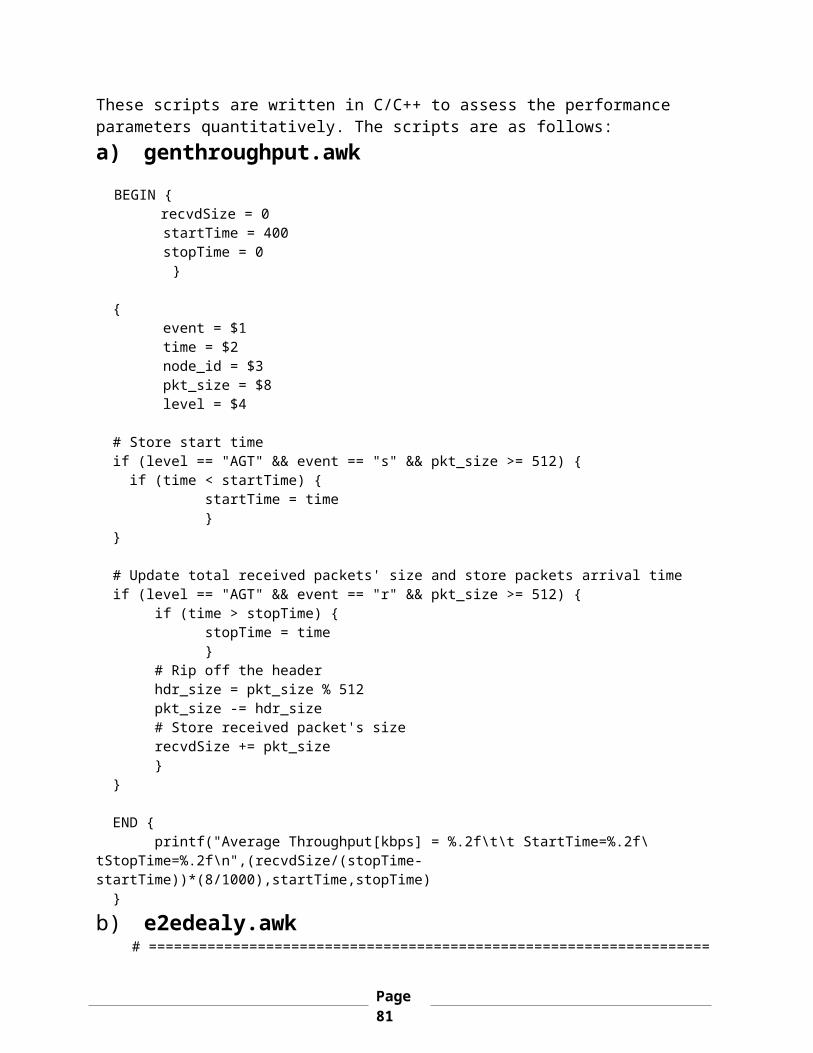
These scripts are written in C/C++ to assess the performance parameters quantitatively. The scripts are as follows:a) genthroughput.awk
BEGIN { recvdSize = 0 startTime = 400 stopTime = 0
} { event = $1 time = $2 node_id = $3 pkt_size = $8 level = $4 # Store start time if (level == "AGT" && event == "s" && pkt_size >= 512) { if (time < startTime) { startTime = time } } # Update total received packets' size and store packets arrival time if (level == "AGT" && event == "r" && pkt_size >= 512) { if (time > stopTime) { stopTime = time } # Rip off the header hdr_size = pkt_size % 512 pkt_size -= hdr_size # Store received packet's size recvdSize += pkt_size } } END { printf("Average Throughput[kbps] = %.2f\t\t StartTime=%.2f\tStopTime=%.2f\n",(recvdSize/(stopTime-startTime))*(8/1000),startTime,stopTime) }b) e2edealy.awk
# ===================================================================
Page81
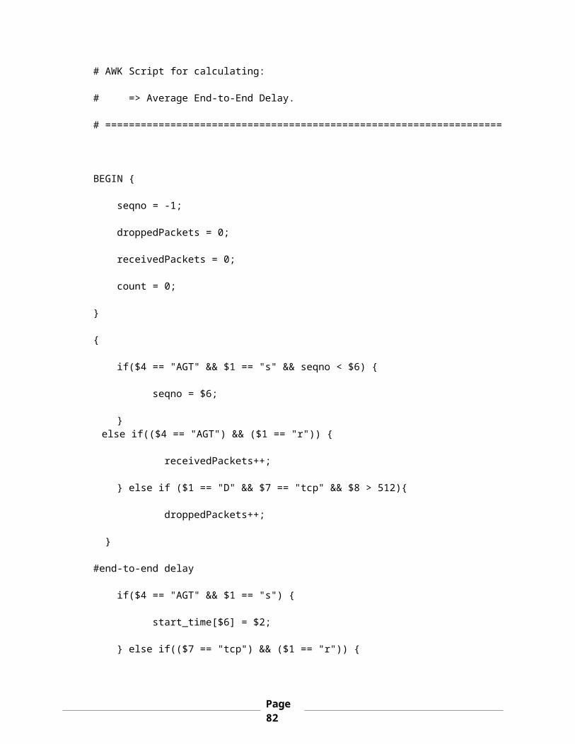
# AWK Script for calculating:
# => Average End-to-End Delay.
# ===================================================================
BEGIN {
seqno = -1;
droppedPackets = 0;
receivedPackets = 0;
count = 0;
}
{
if($4 == "AGT" && $1 == "s" && seqno < $6) {
seqno = $6;
} else if(($4 == "AGT") && ($1 == "r")) {
receivedPackets++;
} else if ($1 == "D" && $7 == "tcp" && $8 > 512){
droppedPackets++;
}
#end-to-end delay
if($4 == "AGT" && $1 == "s") {
start_time[$6] = $2;
} else if(($7 == "tcp") && ($1 == "r")) {
Page82

end_time[$6] = $2;
} else if($1 == "D" && $7 == "tcp") {
end_time[$6] = -1;
}
}
END { for(i=0; i<=seqno; i++) {
if(end_time[i] > 0) {
delay[i] = end_time[i] - start_time[i];
count++;
}
else
{
delay[i] = -1;
}
}
for(i=0; i<=seqno; i++) {
if(delay[i] > 0) {
n_to_n_delay = n_to_n_delay + delay[i];
}
}
n_to_n_delay = n_to_n_delay/count;
Page83
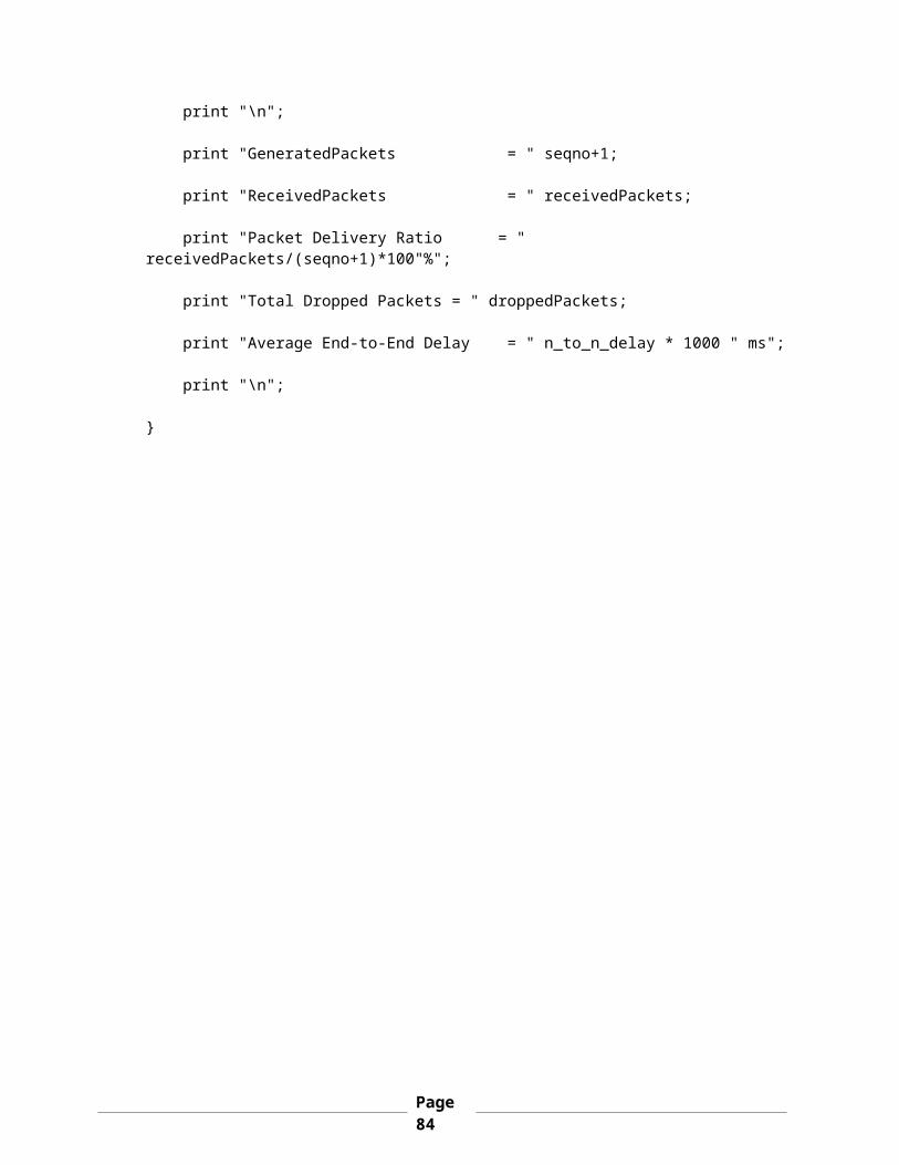
print "\n";
print "GeneratedPackets = " seqno+1;
print "ReceivedPackets = " receivedPackets;
print "Packet Delivery Ratio = " receivedPackets/(seqno+1)*100"%";
print "Total Dropped Packets = " droppedPackets;
print "Average End-to-End Delay = " n_to_n_delay * 1000 " ms";
print "\n";
}
Page84
Chapter – 5
Conclusion
Page85
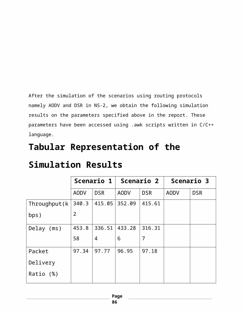
After the simulation of the scenarios using routing protocols
namely AODV and DSR in NS-2, we obtain the following simulation
results on the parameters specified above in the report. These
parameters have been accessed using .awk scripts written in C/C++
language.
Tabular Representation of the
Simulation ResultsScenario 1 Scenario 2 Scenario 3AODV DSR AODV DSR AODV DSR
Throughput(k
bps)
340.3
2
415.05 352.09 415.61
Delay (ms) 453.8
58
336.51
4
433.28
6
316.31
7
Packet
Delivery
Ratio (%)
97.34 97.77 96.95 97.18
Page86
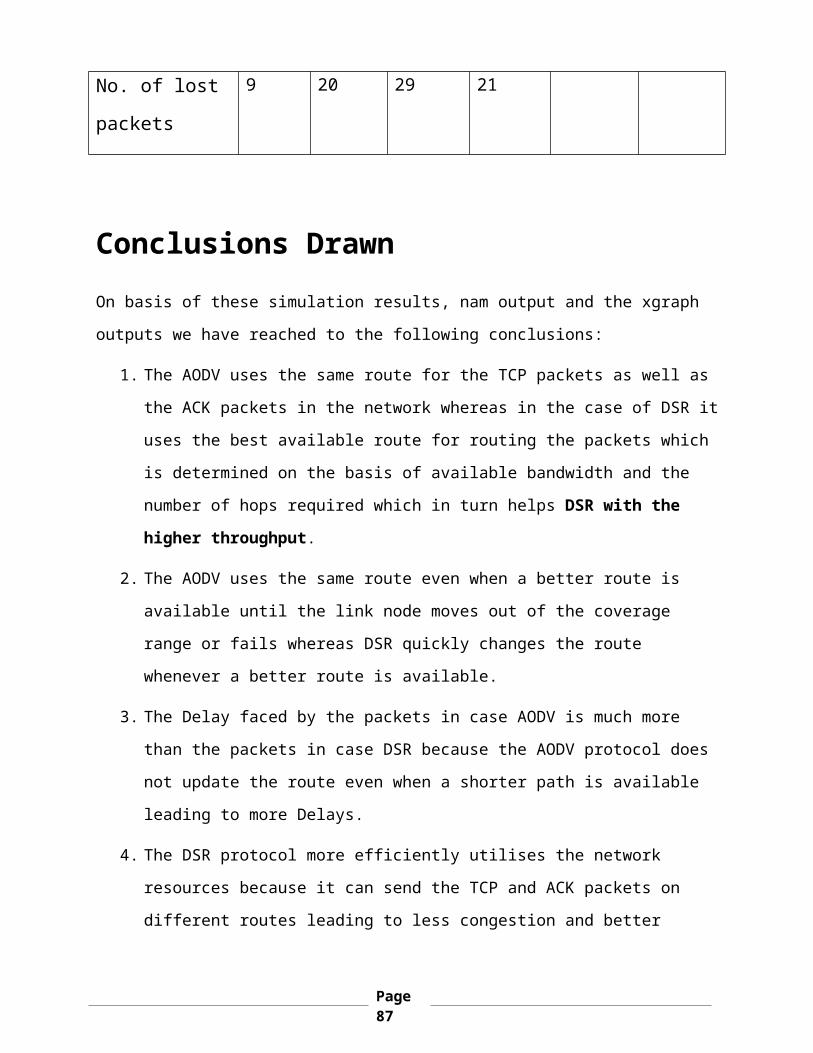
No. of lost
packets
9 20 29 21
Conclusions DrawnOn basis of these simulation results, nam output and the xgraph
outputs we have reached to the following conclusions:
1. The AODV uses the same route for the TCP packets as well as
the ACK packets in the network whereas in the case of DSR it
uses the best available route for routing the packets which
is determined on the basis of available bandwidth and the
number of hops required which in turn helps DSR with the
higher throughput.
2. The AODV uses the same route even when a better route is
available until the link node moves out of the coverage
range or fails whereas DSR quickly changes the route
whenever a better route is available.
3. The Delay faced by the packets in case AODV is much more
than the packets in case DSR because the AODV protocol does
not update the route even when a shorter path is available
leading to more Delays.
4. The DSR protocol more efficiently utilises the network
resources because it can send the TCP and ACK packets on
different routes leading to less congestion and better
Page87
delivery whereas AODV as you can see has congested the
central node because it sends both the TCP as well as the
ACK packet on the same route.
5. AODV will be better solution in the scenarios with higher
number of nodes with less number of sources and DSR works
better with more number of sources as it helps better
utilization of network resources.
Page88

Problems Faced1. After the synopsis presentation of the project which was
held in December, 2011 we all started with the project with
installing NS2 on our machines using cygwin platform. On
windows vista we were successful in our installation but on
compiling the OTCL codes we got no results. This was because
the output video format of NS2 is not supported by windows.
So after reading the tutorial NS by Example we got to know
that the videos are supported by either Mac or Linux
(Ubuntu). So we installed Ubuntu and then the NS-
2. While we working on the NS-2, the version of NS-2 we had
installed was not able to run xgraph files and its folders
were distributed in the whole OS, so we downloaded “NS2.34
allinone” which helped us install NS2 in home folder and all
its files were located there only and all the utilities are
present in it.
3. While simulating the scripts with the scenario and node
movement files the simulations were unsuccessful, so we
wrote the scenario and node movement codes ourselves in the
main TCL script.
Page89
Appendix-AInstalling Ubuntu 10.04 on Windows
Vista Computer
Back-up your data: Although this may seem obvious, but it is
important to backup files to an external backup medium
before attempting a dual-boot install, in case hard drive
becomes corrupted during the process. External hard drives,
USB flash drives and multiple DVDs or CDs are all useful for
Page90

this purpose. Secondly create sufficient unallocated space for
Ubuntu 10.04 at end of hard disk (use Shrink in Disk
Management).
i. Still in Disk Management, create a new formatted
partition using all the unallocated space.
ii. Note the new partition Type (Primary or Logical)
used by Disk Management.
Installing other operating systems on your Windows Vista
computer may invalidate your warrantee. It's important to
follow the instructions exactly as stated and you should have
a properly working Windows.
Make disk space available for Linux Ubuntu
The very first step is to divide the single 160 GB disk on
your computer usually had Windows Vista (150 GB, Primary and
NTFS). The Windows Vista drive was shrunk leaving about 32
GB Unallocated space at the end of the disk (to the right)
and a formatted partition created there. After
repartitioning it had: Windows Vista (124 GB, Primary and
NTFS), New (32 GB, Primary and FAT32) for the installation
of Linux.
i. Decide first on how much disk space you wish to
allocate to Linux and if you will create an extra
partition (/home) for your Linux data. This data
Page91
partition can be left intact if you ever wish to
reinstall Linux at a later time.
ii. Restart computer correctly (that means close all
programs before you restart computer).
iii. Open Disk Management in Windows Vista (right-click
Computer, select Manage, click Disk Management).
o Right-click the Windows Vista volume, and
click Shrink Volume.
In enter the amount of space to shrink in
MB: enter enough for Ubuntu.
Click the Shrink button (it may take some
time!).
Note: If Shrink does not give you sufficient unallocated
space, read Shrink the Windows Vista Partition for
instructions on how to complete this task successfully.
Then return here.
iv. Still in Disk Management, right-click the new
Unallocated disk area, and select New Simple
Volume. Use all the available space to create a
new partition - Format the partition. Close Disk
Management. The new partition Type (Primary or
Logical) used by Disk Management.
v. Restart to Windows Vista two times.
Open Disk Management and check that the
change made is correct.
Page92
Creating Partitioning for Linux Ubuntu in Hard Disk
In Prepare partitions, if you have more than one hard disk,
you must first select the correct disk. /dev/sda is the
first physical hard disk. /dev/sdb is the second hard disk
in your computer. Do not select the wrong one. Identify and
highlight the new partition you created (it should be the
bottom one) and click the Delete button. This will create
free space. Next create a partition for Ubuntu. Highlight
the newly created free space, and click the Add button. The
Create partition window will open.
i. In Type for the new partition (if present), select the
Type you identified in Disk Management (Logical or
Primary) (do NOT select Primary if you already
have 3 Primaries - doing so makes the remaining
Free Space Unusable!).
ii.In New partition size ..., enter 6000 (or 23000 if not
using /home).
iii. In Location for the new partition, select Beginning.
iv.In Use as: select EXT3 journaling file system.
v. In Mount Point, select / (a forward slash).
vi.Click the OK button.
Make a note of the Device name allocated to the EXT3
partition, like /dev/hda3 or /dev/sda3. Now highlight the
newly-sized free space, and click the Add button. The Create
partition window will open again. Now create the Swap
partition.
Page93

i. In Type for the new partition (if present), select
Logical.
ii. In New partition size ..., use twice RAM size or all
available space if not creating a /home partition.
iii. In Location for the new partition, select Beginning.
iv. In Use as:, select Swap area. A Mount Point is not
set for Linux's swap file partition.
v. Click the OK button.
Guide to show that how Ubuntu is installed on your desktop?
The following steps explain about the installation of Ubuntu
on your desktop.
Step 1: Installing Ubuntu
i. Download an Ubuntu LiveCD image (.iso) from Ubuntu
Downloads and burn it to a disc using
BurningIsoHowto).
ii. Insert the LiveCD into your CD-ROM drive and
reboot your PC.
iii. If the computer does not boot from the CD (e.g.
Windows starts again instead), reboot and check
your BIOS settings by pressing F12 or ESC. Select
"boot from CD".
iv. Bootup from the Linux Ubuntu 10.04 live CD to its
desktop. Wait for the CD to load….!!!
Page94
`
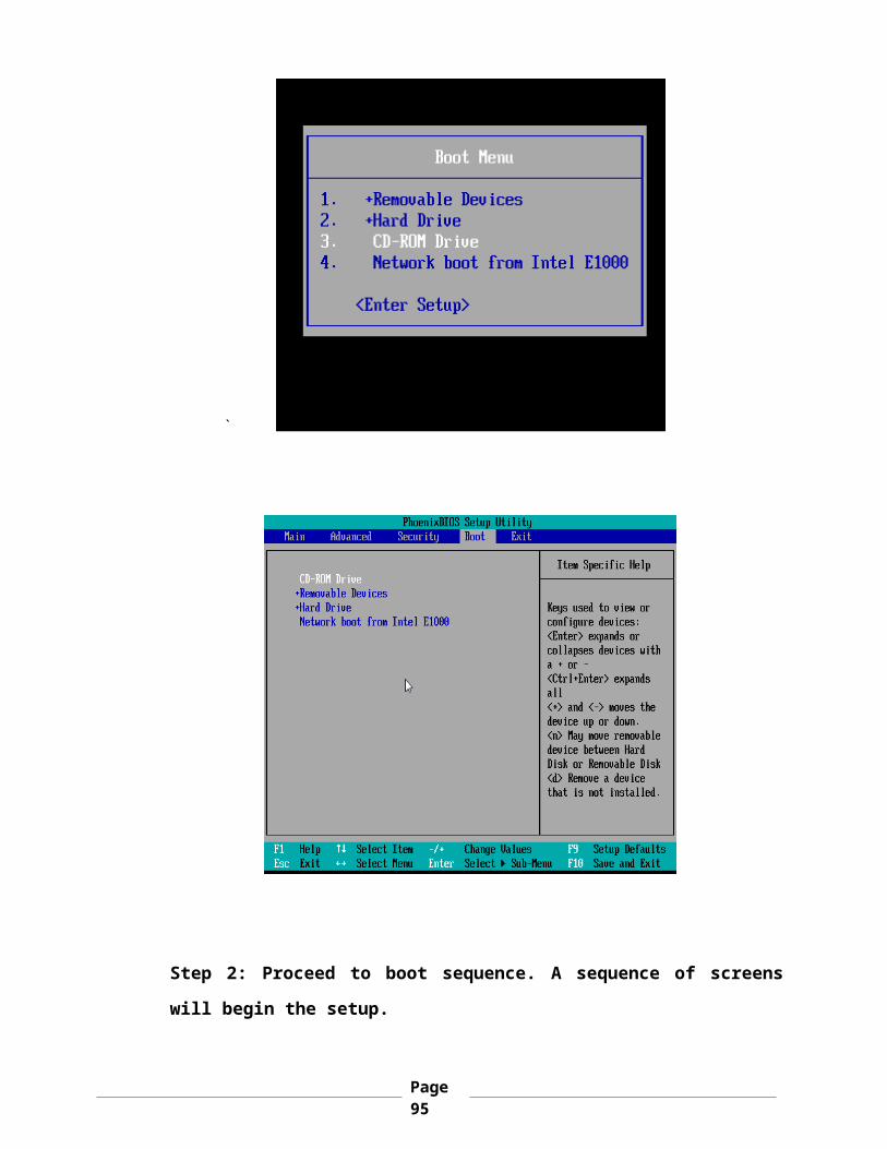
Step 2: Proceed to boot sequence. A sequence of screens
will begin the setup.
Page95

Step 3: Follow the setup prompts as they configure your
Ubuntu installation
i. In the “Welcome screen”, select your Language, and
click Forward.
ii. In the “Where are you”, select your Time Zone, and
click Forward.
iii. In the “Keyboard layout”, select your Country, and
click Forward.
Page96

Page97

Step 4: In Prepare disk space, specify partitions
manually, and click Forward.
Step 5: Continue with the wizard, fill out the forms and
click Forward
i. Read the contents of the Ready to install window
and click “Install”.
Page98

Step 6: Click through to begin setup. Follow the on-screen
prompts.
Page99

The CD will be ejected; remove it and press the "Enter" key to
reboot. The computer will be restarted and, in a few seconds, you
will see the Ubuntu boot splash...
Adding Ubuntu to the Windows Bootloader
1. At this point, you technically have a working Ubuntu/Windows
dual-boot. But you're going to see two menus, and it's not
going to be pretty. The following instructions will clear
that up for you.
2. The following below mentioned steps will guide you through
the windows boot-loader process.
Page100

i. When your PC reboots, you'll see Ubuntu's GRUB2
menu with a multitude of choices. You want to
select the "Ubuntu, with Linux 2.6.32-38-generic"
as shown in the screenshot below, to boot the
Ubuntu.
ii. At the login screen, click on your username
and input your password. Click the "Log In" button
or hit Enter...
Page101

3. A congratulations message saying you have successfully
created a dual-boot of Windows Vista and Linux Ubuntu 10.04
on your computer will appear on your screen.
Appendix-BSteps for Installing NS-2 on
Ubuntu 10.04
Page102

1. We have downloaded NS2 version 2.34 -all in one.
2. We have placed the ns-allinone-2.34.tar.gz package in
our home folder (/home/Vyoma). Right click the package and
extract the contents in the same folder.
Page103
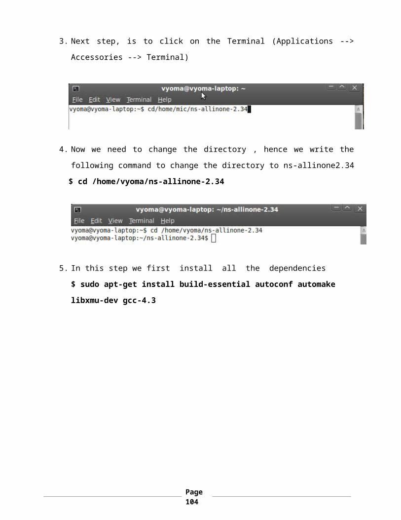
3. Next step, is to click on the Terminal (Applications -->
Accessories --> Terminal)
4. Now we need to change the directory , hence we write the
following command to change the directory to ns-allinone2.34
$ cd /home/vyoma/ns-allinone-2.34
5. In this step we first install all the dependencies
$ sudo apt-get install build-essential autoconf automake
libxmu-dev gcc-4.3
Page104
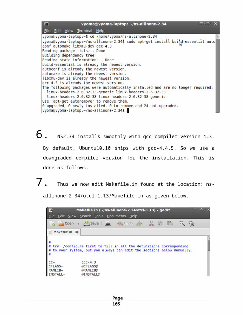
6. NS2.34 installs smoothly with gcc compiler version 4.3.
By default, Ubuntu10.10 ships with gcc-4.4.5. So we use a
downgraded compiler version for the installation. This is
done as follows.
7. Thus we now edit Makefile.in found at the location: ns-
allinone-2.34/otcl-1.13/Makefile.in as given below.
Page105
8. Find the line that says:
CC= @CC@
and change it to:
CC= gcc-4.3
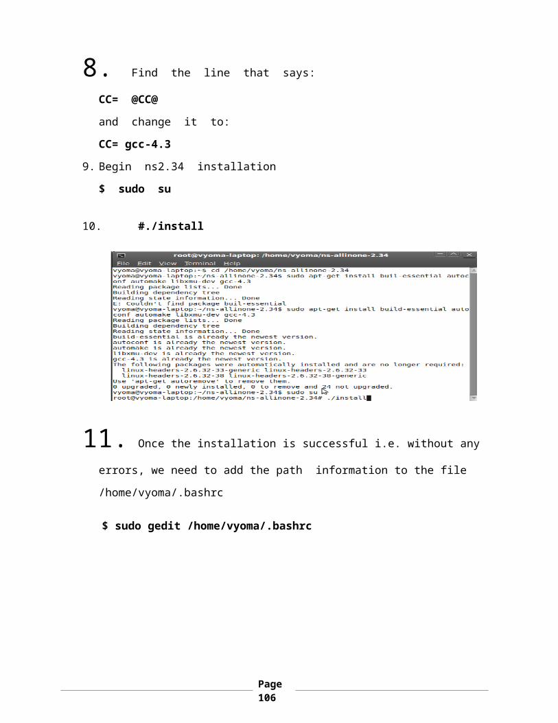
9. Begin ns2.34 installation
$ sudo su
10. #./install
11. Once the installation is successful i.e. without any
errors, we need to add the path information to the file
/home/vyoma/.bashrc
$ sudo gedit /home/vyoma/.bashrc
Page106

12. Append the following lines to the file
/home/vyoma/.bashrc (after replacing the instances where
you find vyoma with your username)
#LD_LIBRARY_PATH
OTCL_LIB=/home/vyoma/ns-allinone-2.34/otcl-1.13
NS2_LIB=/home/vyoma/ns-allinone-2.34/lib
X11_LIB=/usr/X11R6/lib
USR_LOCAL_LIB=/usr/local/lib
export LD_LIBRARY_PATH=$LD_LIBRARY_PATH:$OTCL_LIB:$NS2_LIB:
$ X11_LIB:$USR_LOCAL_LIB
#TCL_LIBRARY
TCL_LIB=/home/vyoma/ns-allinone-2.34/tcl8.4.18/library
USR_LIB=/usr/lib
export TCL_LIBRARY=$TCL_LIB:$USR_LIB
Page107

#PATH
XGRAPH=/home/vyoma/ns-allinone-2.34/bin:/home/vyoma/ns-
allinone-
2.34/tcl8.4.18/unix:/home/vyoma/ns-allinone-2.34/tk8.4.18/un
ix
#the above two lines beginning from xgraph and ending with
unix should come on the same line
NS=/home/vyoma/ns-allinone-2.34/ns-2.34/
NAM=/home/vyoma/ns-allinone-2.34/nam-1.14/
PATH=$PATH:$XGRAPH:$NS:$NAM
13. For the changes to take effect immediately, do the
following:
$ sudo su
# source /home/vyoma/.bashrc
Page108
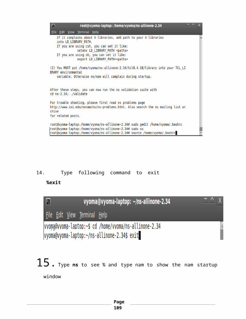
14. Type following command to exit
%exit
15. Type ns to see % and type nam to show the nam startup
window
Page109

Appendix-C
BOOTABLE DISK
Page110
A boot disk is a removable digital data storage medium from
which a computer can load and run (boot) an operating
system or utility program. The computer must have a built-in
program which will load and execute a program from a boot
disk meeting certain standards.
Boot disks are used for:
Operating system installation
Data recovery
Data purging
Hardware or software troubleshooting
Customizing an operating environment
Software demonstration
Administrative access in case of lost password is
possible with an appropriate boot disk with some
operating systems
Games (e.g. for Amiga home computers)
While almost all modern computers can boot from a hard drive
containing the operating system and other software, they
would not normally be called boot disks. CD-ROMs are the
most common forms of media used, but other media, such as
magnetic or paper tape drives, zip drives, and more
recently USB flash drives can be used. The
computer's BIOS must support booting from the device in
question.
FILE SYSTEM
Page111
A file system (or file system) is a means to organize data
expected to be retained after a program terminates by
providing procedures to store, retrieve and update data, as
well as manage the available space on the device(s) which
contain it. A file system organizes data in an efficient
manner and is tuned to the specific characteristics of the
device. There is usually a tight coupling between the
operating system and the file system. Some file systems
provide mechanisms to control access to the data
and metadata. Ensuring reliability is a major responsibility
of a file system. Some file systems provide a means for
multiple programs to update data in the same file at nearly
the same time.
Without a file system programs would not be able to access
data by file name or directory and would need to be able to
directly access data regions on a storage device.
File systems are used on data storage devices such as hard
disk drives, floppy disks, optical discs, or flash
memory storage devices to maintain the physical location of
the computer files. They may provide access to data on a
file server by acting as clients for a network
protocol (e.g. NFS, SMB, or 9P clients), or they may be
virtual and exist only as an access method for virtual data
(e.g. procfs). This is distinguished from a directory
service and registry.
Page112

REFERENCES
1. The network simulator manual- ns-2. http:// www.
isi.edu/nsnam/ns/.
2. NS by Example, http://nile.wpi.edu/NS/
Page113

3. D. B. Johnson and D. A. Maltz, “Dynamic source routing in
ad-hoc wireless networks,” in Mobile Computing, (ed. T.
Imielinski and H. Korth), Kluwer Academic Publishers, 1996.
4. S.R. Das, R. Castaneda, J. Yan, and R. Sengupta,
“Comparative performance evaluation of routing protocols for
mobile, ad hoc networks", In 7th Int. Conf. on Computer
Communications and Networks (IC3N), pp: 153–161, October
1998.
5. Perkins,C.E., E. M. Royer, S. R. Das and M.K. Marine,
Performance comparison of two on-demand routing protocols
for ad hoc networks”, IEEE Personal Communications, 2001,
pp: 16-28.
6. Yinfei Pan, Department of Computer Science, SUNY Binghamton,
“Design Routing Protocol Performance Comparison in NS2: AODV
comparing to DSR as Example”.
7. M.Saravana karthikeyan, K.Angayarkanni, and Dr.S.Sujatha,
Member, IAENG, “Throughput Enhancement in Scalable MANETs
using Proactive and Reactive Routing Protocols”.
8. Anurag Malik, Shivanshu Rastogi, Sajendra Kumar, Associate
Professor, Moradabad Institute of Technology, Moradabad,
“Performance Analysis of Routing Protocol in Mobile Ad Hoc
Network using NS-2”.
9. Satveer Kaur, CSE Department, SLIET, “Performance Comparison
of DSR and AODV Routing Protocols with Efficient Mobility
Model in Mobile Ad-Hoc Network”
10. Vahid Ayatollahi Tafti, Abolfazl Gandomi, “Performance
of QOS Wireless Mobile Ad-Hoc Network Routing Protocols “,
Page114
IJCSNS International Journal of Computer Science and Network
Security, VOL.8 No.6, June 2008.
11. Per Johansson, Tony Larsson, Nicklas Hedman, Ericsson
Radio Systems AB “Scenario-based Performance Analysis of
Routing Protocols for Mobile Ad-hoc Networks”
12. Charles E. Perkins, “Ad Hoc On Demand Distance Vector
(AODV) Routing”.02.txt, November 1998.
13. Raghupathy Sivakumar, Prasun Sinha and Vaduvur
Bharghavan, “Core Extraction Distributed Ad hoc Routing
(CEDAR) Specification”.
14. Azzedine Boukerche, Parallel Simulation and Distributed
Systems (PARADISE) Research Laboratory Dept. of Computer
Science, University of North of Texas, “A Simulation Based
Study of On-Demand Routing Protocols for Ad hoc Wireless
Networks”
15. Das, S.R., R. Castaeda and J. Yan, “Simulation-based
performance evaluation of routing protocols for mobile ad
hoc networks.”, Mobile Networks and Applications, 2000,
pp:179-189.
Page115

Page116
Copyright © 2022 FDOKUMEN