arX

iv:c

ond-

mat

/930

9006

v1 8

Sep

199

3

Charge and Spin Gap Formation

in Exactly Solvable Hubbard Chains with Long-Range Hopping

Florian Gebhard and Andreas Girndt

Dept. of Physics and Materials Sciences Center, Philipps University, D-35032 Marburg, Germany

Andrei E. Ruckenstein

Serin Physics Laboratory, Rutgers University, P.O. Box 849, Piscataway, NJ 08855-0849

(December 10, 2013)

Abstract

We discuss the transition from a metal to charge or spin insulating phases

characterized by the opening of a gap in the charge or spin excitation spec-

tra, respectively. These transitions are addressed within the context of two

exactly solvable Hubbard and tJ chains with long range, 1/r hopping. We

discuss the specific heat, compressibility, and magnetic susceptibility of these

models as a function of temperature, band filling, and interaction strength.

We then use conformal field theory techniques to extract ground state corre-

lation functions. Finally, by employing the g-ology analysis we show that the

charge insulator transition is accompanied by an infinite discontinuity in the

Drude weight of the electrical conductivity. While the magnetic properties

of these models reflect the genuine features of strongly correlated electron

systems, the charge transport properties, especially near the Mott-Hubbard

transition, display a non-generic behavior.

PACS1993: 71.27.+a, 71.30.+h, 05.30.Fk

Typeset using REVTEX

1

I. INTRODUCTION

Recently1 we introduced a Hubbard-like model which describes spin-1/2 Fermions on a

chain of L sites, hopping with long-range amplitude, tl,m = it(−1)l−m [d(l −m)]−1. Here,

d(l −m) = (L/π) sin[π(l −m)/L] is the chord distance between sites l and m on the chain

closed into a ring (the lattice spacing a is set to unity). In the thermodynamic limit,

L→ ∞, and for a fixed distance, (l−m), the purely imaginary hopping tl,m = t∗m,l becomes

tl,m → it/(l −m), leading to the Hubbard Hamiltonian with “1/r-hopping”,

H = T + UD =L∑

l 6=m=1,σ

tl,mc+l,σcm,σ + U

L∑

l=1

nl,↑nl,↓ . (1)

Here U is the strength of the usual local Hubbard2 interaction. For even L we choose

antiperiodic boundary conditions, so that the dispersion relation is linear in wave vector,

namely, ǫ(k) = tk for k = ∆(m + 1/2) (∆ = 2π/L, m = −L/2, . . . , L/2 − 1). For U = 0

the Fermi sea is the ground state with all k-states from k = −π to keF = π(n − 1) filled3,

where n = (N↑ + N↓)/L is the total particle density (the “filling”). Note that the kinetic

and potential energy operators are respectively odd and even under partity, and thus parity

is, in general, not a good quantum number in our model.

In the large U limit the Hamiltonian (1) becomes the 1/r-tJ model including “pair-

hopping” terms (PD=0 projects onto the subspace with no double occupancies)4:

HtJ = PD=0

{T +

∑

l 6=m

2|tl,m|2U

[Sl · Sm − 1

4nlnm

]

−∑

l 6=n 6=m6=l

tl,ntn,m

U

∑

σσ′

(σσ′) c+lσ c+n−σcn−σ′ cmσ′

}PD=0 . (2)

As usual, nl = nl,↑ + nl,↓, and Sl is the spin-1/2 vector operator (S+l = c+l,↑cl,↓, S

−l = c+l,↓cl,↑,

Szl = (nl,↑ − nl,↓)/2). At half filling, where the first and third terms in (2) vanish, the

model (2) reduces to the (parity symmetric) (1/r)2-Heisenberg model introduced by Haldane

and Shastry5, with J = 4t2/U .

In Ref. 1 we conjectured the full excitation spectrum and associated degeneracies, and

were thus able to calculate the free energy. The exact solution allowed us to identify two zero

2

temperature (T = 0) phase transitions: the first was a Mott-Hubbard2,6 metal-to-charge-

insulator transition (MCIT) in the half-filled 1/r-Hubbard model. This was signaled by the

opening of a charge gap for U > Uc = W where W = 2πt is the electron bandwidth. The

second, a metal-to-spin insulator transition (MSIT) was associated with the opening of a

spin gap in the 1/r-tJ model (2) for J > Jc = 2W/ [(1 − n)π2].

In this paper we clarify the nature of these transitions and attempt to separate the fea-

tures due to the special form of the dispersion in (1) from more generic properties which

may be expected to survive for other dispersions and/or in higher dimensions. The plan

of the paper is as follows: we start in section II by recalling the form of our exact solu-

tion for the spectrum and ground state energies, from which we identify the location of

the MCIT and MSIT. In section III we discuss the thermodynamic properties of our two

models, namely the specific heat, compressibility, and magnetic susceptibility. In sec. IV

we use conformal field theory techniques to extract the long-range behavior of ground state

correlation functions. Sec. V contains a discussion of the connection with the “g-ology”

approach to one-dimensional systems, which we exemplify by calculating the Drude weight

in the frequency dependent electrical conductivity for the 1/r-Hubbard model. Finally, a

summary and conclusions are presented in sec. VI.

II. GROUND STATE PROPERTIES AND EXCITATION SPECTRA

We recall the effective Hamiltonian, introduced in ref. 1,

Heff =∑

−π<K<π

{∑

σ

hsK,σn

sK,σ + hd

KndK + he

KneK + JK

[ndK−∆n

eK − ns

K−∆,↑nsK,↓

]}(3)

which describes spin (sKσ; SzK = ±1/2, CK = 0) and charge (dK, eK; SK = 0, Cz

K = ±1/2)

degrees of freedom in an occupation number representation with a hard core constraint,

∑σ n

sK,σ +nd

K+neK = 1 for each K. Furthermore, hs

K,σ = (tK)/2−µσ, hdK = −(tK)/2−2µ+U ,

heK = −(tK)/2, and JK =

[t(2K − ∆) − U +

√(2πt)2 + U2 − 2tU(2K − ∆)

]/2 ≥ 0. The

chemical potential in the presence of an external magnetic field is given by µσ = µ −

3

σ(gµBH0)/2. In the following we will set µB ≡ 1, and g = 2. To be precise, we also restrict

ourselves to t ≥ 0 and U ≥ −2πt in which case we were allowed to identify Kmin−∆ ≡ Kmax

because JK vanishes for K = Kmin = −∆(L− 1)/2.

Note that, formally, the entire spectrum appears to display spin-charge separation at all

energies in the sense that the Hamiltonian splits up into independent spin and charge contri-

butions (“strong” spin-charge separation). In reality, however, spin and charge excitations

are coupled by the constraint,∑

σ nsK,σ + nd

K + neK = 1; and spin-charge separation only oc-

curs at sufficiently low energies/temperatures, where spin and charge excitations contribute

independently to various physical properties.

As already discussed above, we will concentrate on the physics of two special limits:

(i) the 1/r-Hubbard model in the vicinity of half filling, n <∼ 1, and (ii) the 1/r-tJ model

for n < 1. The latter is obtained by taking the limit U → ∞ of (3) which projects out all

double occupancies (hdK → ∞). With the help of the completeness constraint one arrives at

the tJ effective Hamiltonian,

HefftJ = Heff

t + HeffJ =

∑

−π<K<π

[(−tK)ne

K − JKnsK−∆,↑n

sK,↓

], (4)

where, for J = 4t2/U ≪ 1, the exchange coupling, JK(U/t), reduces to JK =

(J/4)[π2 − (K − ∆/2)2

]. Below, we will adopt the usual standpoint for the tJ model7,

and treat J as an independent parameter.

A. 1/r-Hubbard Model

From eq. (3) we can immediately extract the form of eigenstates in an occupation number

representation in terms of the effective spin (sK,σ) and charge (eK, dK) degrees of freedom.

For example, the ground state is expressed symbolically as

ground state: [↑↓] . . . [↑↓]∣∣∣∣KF =π(2n−1)

◦ . . . ◦

where ↑, ↓, •, and ◦ represent sK,↑, sK,↓, dK, eK, respectively. We brace those pairs at K−∆

and K which contribute an interaction JK8. The ground state can be regarded as a short-

4

range RVB state in K-space obtained by filling K states with [↑↓]-pairs from K = −π+∆/2

to K = KF − ∆/2, where KF = π(2n − 1) . Although the real-space structure of the

ground state wave function is not immediately apparent, it should be clear, however, that

it also consists of long-range (overlapping) singlet pairs. In fact, the recently constructed

wave functions for the U = ∞ limit (the “1/r-t-model”)9 are genuine RVB states10 of the

Gutzwiller-Jastrow type.

The corresponding ground state energy density, e0(n), can easily be obtained by apply-

ing the effective Hamiltonian (3) to the symbolic ground state wave function given above:

e0(n) = (1/2π)∫KF

−π dK [J(K)/2]+(1/2π)∫ πKFdK(−tK), where the factor 1/2 in the first term

takes into account the fact that only every second K value contributes to the first integral.

A simple calculation then gives

e0(n ≤ 1) =Un−W (1 − n)n

4− 1

24WU

[(W + U)3 −

((W + U)2 − 4WUn

)3/2], (5)

where W = 2πt is the bandwidth. Using particle-hole symmetry11 we obtain e0(n ≥ 1) =

e0(2 − n) + U(n− 1), and correspondingly, for the chemical potential at zero temperature,

µ(n < 1) = ∂e0(n < 1)/∂n, µ(n > 1) = U − µ(2 − n). From (5) one can easily see that

∆µc ≡ µ+(n = 1) − µ−(n = 1) = (limn→1+ − limn→1−)µ(n) becomes finite for U > Uc = W :

∆µc = U −Uc. Equivalently, the charge compressibility, κ = ∂n/∂µ at n = 1 vanishes for U

above Uc, as expected at a Mott metal-to-charge-insulator transition (MCIT).

We are now in the position to identify the low-lying spin and charge excitations which

we discuss separately for the half-filled and less than half-filled cases:

1. Half-filling: n = 1

We begin with the spin excitations. The four degenerate S = 0, S = 1 lowest-lying spin

excitations are represented by

spin-exc: [↑↓] . . . [↑↓]σ∣∣∣∣K1

[↑↓] . . . [↑↓]σ′∣∣∣∣K2

[↑↓] . . . [↑↓] .

5

For K2 = K1+∆ there is a triplet excitation only. In the thermodynamic limit the excitation

energy is given by δES(K1,K2) = [J(K1) + J(K2)] /2, and we may thus identify the lowest-

lying spin excitation with two spinons. They are characterized as spin-1/2 objects which

always come in pairs, and are separated in K-space by an even multiple of ∆. We thus

rescale K = 2K′ to retain the proper spacing ∆ = 2π/L of K′ values. The spinons then have

the dispersion relation,

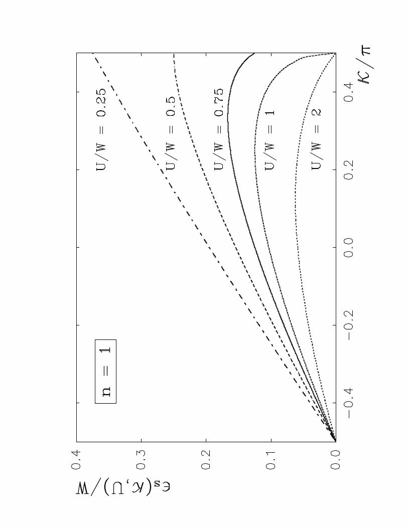
ǫs(K) = J(2K)/2 =(√

W 2 + U2 − 4WUK/π + 2WK/π − U)/4 ≥ 0 ; |K| < π/2 , (6)

which we depict in fig. 1. The spin excitations are always gapless at K = −π/2, and at

K = π/2 for U/W > 1. Their corresponding velocities at K = ±π/2 can now be calculated

from vs(K) = ∂ǫs(K)/∂K as

vRs ≡ vs(K = −π/2) =

vF

U/W + 1for all U/W (7a)

vLs ≡ vs(K = π/2) = − vF

U/W − 1for U/W > 1 . (7b)

Here, vF = t is the Fermi velocity of the bare particles. The density of states

for spin excitations is then calculated as Ds(E) = (1/L)∑

−π/2<K<π/2 δ (E − ǫs(K)) =

1/(2π)∫ π/2−π/2 dK δ (E − ǫs(K)). With the help of eqs. (7), for low energies we obtain

Ds(E → 0) =

1/(2πvR

s

)for U/W < 1

1/(2πvR

s

)+ 1/

(2π|vL

s |)

for U/W > 1

. (8)

We next turn to the charge excitations. We restrict ourselves to a fixed particle number

(Cz = 0) and we only obtain two of the four C = 0, C = 1 lowest-lying states. These charge

excitations are represented by

charge-exc: [↑↓] . . . [↑↓] ◦∣∣∣∣K1

[↑↓] . . . [↑↓] •∣∣∣∣K2

[↑↓] . . . [↑↓] .

For K2 = K1 + ∆ there is a low lying triplet excitation (C = 1, Cz = 0), with the singlet

excitation (C = 0, Cz = 0) always at high energy (anti-bound state). Again, we may identify

the lowest-lying charge excitation with two chargeons. In the half-filled case we always get

6

a pair of a holon and a doublon which are separated by an even multiple of ∆ = 2π/L.

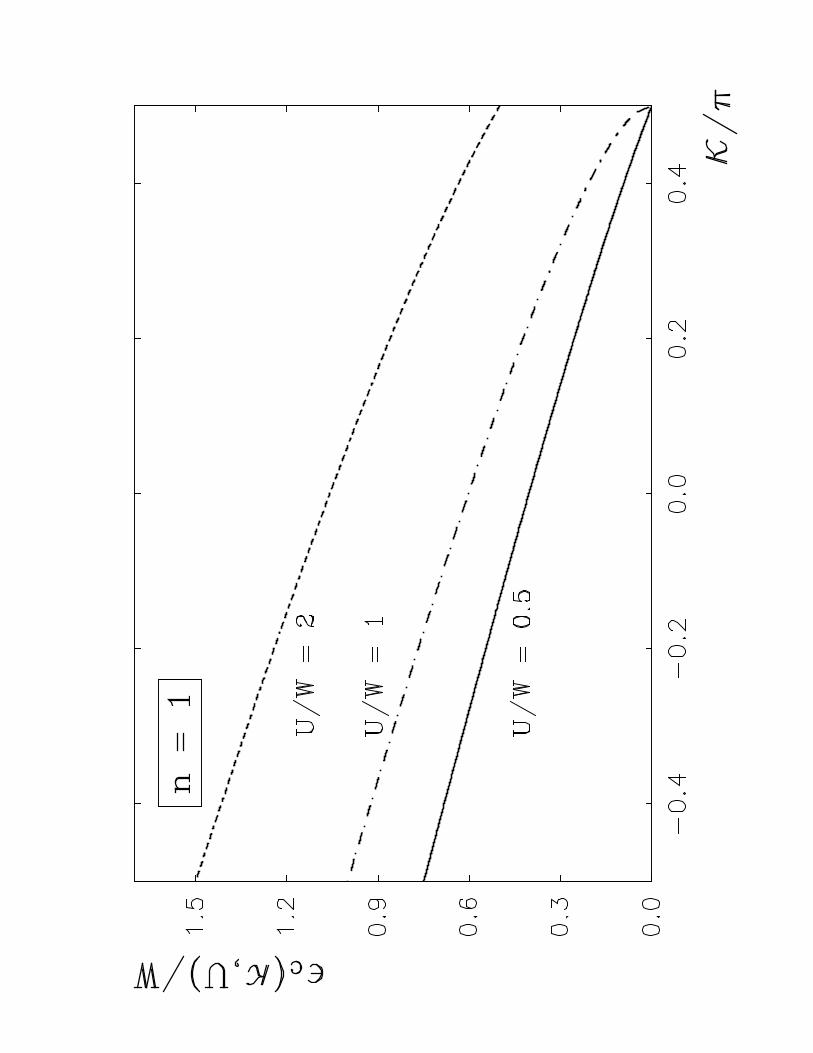
Rescaling K = 2K′ leads to the chargeon dispersion relation,

ǫc(K) =(√

W 2 + U2 − 4WUK/π − 2WK/π + U)/4 ≥ 0 ; |K| < π/2 , (9)

as depicted in fig. 1. The charge excitations are gapless at K = π/2 for U/W < 1, with a

velocity given by

vLc = − vF

1 − U/Wfor U/W < 1 . (10)

For U > W a gap, 2ǫc(π/2) = U−W ≡ ∆µc, opens in the charge spectrum. Correspondingly,

the density of states for charge excitations at low energies takes the form

Dc(E → 0) =

1/(2π|vL

c |)

for U/W < 1

O [exp (−E/∆µc)] for U/W > 1

. (11)

At this point a peculiarity of our model becomes evident: the charge velocity increases as

a function of U/W and eventually diverges at U = Uc = W . The effective charge mass m∗c

which is connected to the density of states or the velocities by m∗c/m = Dc(0)/D0(0) =

vF/|vLc | decreases as a function of U/W . This is in contrast to the Brinkman-Rice scenario

for the Mott-Hubbard transition in that case m∗c/m increases and charge excitations tend

to localize close to the transition12,13. Indeed, for the Hubbard model with nearest-neighbor

hopping (cosine dispersion) m∗c(n, U) diverges at the MCIT for U > 0 when the transition

is approached from below half-filling (n→ 1−)14.

2. Less than half-filling: n < 1

In this case there are only right-moving spinons with velocity vRs , eq. (7a). The spinons

are further restricted to −π/2 < K < KF/2 with KF = π (2n− 1). The lowest-lying charge

excitations are now given by holons alone while the doublons are always gaped:

charge-exc: [↑↓] . . . [↑↓] ◦∣∣∣∣K

[↑↓] . . . [↑∣∣∣∣KF

↓] ◦ . . . ◦ .

7

Although holons need not come in pairs, they are still separated by an even multiple of ∆

in K-space. Rescaling again we find for the charge excitation

ǫh(K) = ǫs(K) − ǫs(KF/2) + t(KF − 2K) − π/2 < K < KF/2 . (12)

The holons are gapless at K = KF/2, and the corresponding velocity, vLc = ∂ǫh(K)/∂K

∣∣∣KF /2

,

leads to

vLc = −vF

1 +U

√(W + U)2 − 4WUn

. (13)

In turn, this implies that the density of states for charge excitations at low energies still

remains

Dc(E → 0) =1

2π|vLc |

. (14)

3. Ground-state compressibility and magnetic susceptibility

The results for the ground state energy density e0(n), eq. (5), allow us to calculate the

chemical potential µ = ∂e0(n)/∂n and the T = 0 compressibility κ = ∂n/∂µ. By turning on

a small external magnetic field H0 we can also obtain e0(m,n) (see Appendix A, eq. (A4)),

and the magnetic susceptibility, χ = ∂m/∂H0, where the magnetization density, m, is related

to H0 by H0 = ∂e0(m,n)/∂m. We summarize our results as follows:

(i) n < 1 or (n = 1, U/W < 1):

µ =U −W (1 − 2n) −

√(W + U)2 − 4WUn

4(15a)

κ =1

π|vLc |

=2

W(1 + U/

√(W + U)2 − 4WUn

) (15b)

m = χH0 (15c)

χ =1

πvRs

=2

W

(1 +

U

W

). (15d)

8

(ii) n = 1, U/W > 1:

µ(n = 1−) =W

2(16a)

µ(n = 1+) = U − W

2(16b)

∆µc = U −W (16c)

κ = 0 (16d)

m = χH0 (16e)

χ =1

πvRs

+1

π|vLs |

=4U

W 2. (16f)

The system is an incompressible charge insulator at half-filling and U > W . Note that in

the limit n → 1− the compressibility stays finite for U > W (for U = W , κ = 4√

1 − n/W

for n <∼ 1). This is, nevertheless, consistent with eq. (16d) since, in contrast with the

situation of the usual Hubbard model15,14, in our case the function n(µ) is not differentiable

at µ(n = 1−) and µ(n = 1+).

We further note that eqs. (15b), (15d), and (16f) are the generic behavior expected

of a “Luttinger-Liquid”16, a point which we exploit in our discussion of the ground-state

correlation functions (sec. IV) and the Drude conductivity (sec. V).

B. 1/r-tJ Model

Since the case of half-filling has already been considered by Haldane17, here we will be

mainly interested in the less that half-filled situation. From the effective tJ Hamiltonian (4)

it is easy to see that the hole kinetic energy favors all particles to be as close to K = −π

as possible while the exchange interaction JK = (J/4)[π2 − (K − ∆/2)2

]tries to distribute

the particles symmetrically around K = 0. We thus expect a transition at some critical Jc

in this case.

In general, the ground state can be represented as

ground state: ◦ . . . ◦∣∣∣∣K1

[↑↓] . . . [↑↓]∣∣∣∣K2

◦ . . . ◦

9

where K2 = K1 + 2πn has to be determined from the minimization of the ground state

energy. We find (see appendix A)

e0(n, J ≤ Jc) = −Wn(1 − n)

2− Jπ2n2(3 − 2n)

12

= −Jcπ2n

12

[(J

Jc− 1

)n(3 − 2n) + 3 − 3n+ n2

](17a)

with K1 = −π and

e0(n, J ≥ Jc) = −W2n

2π2J− Jπ2n(3 − n2)

24

= −J2c π

2n

24J

[(3 − n2

)(J2

J2c

− 1

)+ 2

(3 − 3n+ n2

)](17b)

with K1 = −π (n+ 2W/(π2J)) > −π. Here, Jc = 2W/(π2(1 − n)) is the critical coupling.

Note that Jc is proportional to 1/(1 − n), i.e., it decreases with increasing (hole) doping.

Below we discuss the two cases, J < Jc and J > Jc, separately:

1. J < Jc

For J < Jc we can make use of the 1/r-Hubbard model results (sec. IIA). In particular,

ǫs(K) = J((π/2)2 −K2)/2 for −π/2 < K < KF/2, and the spinon velocity at K = −π/2 is

vRs = Jπ/2 . (18)

It is amusing to note that this is precisely the result for the Heisenberg-chain with nearest-

neighbor interactions18. This is consistent with the fact that the Gutzwiller projected Fermi

sea |ψ0〉 = PD=0|Fermi-sea〉19, the ground state wave function of the 1/r-tJ model, is also

an excellent trial state for the Heisenberg chain with nearest neighbor interaction20,21, as

well as for the nearest neighbor supersymmetric tJ model (J = 2t)22. As in sec. IIA the

corresponding low energy density of states is given by

Ds(E → 0) =1

2πvRs

for J < Jc . (19)

For 0 < J < Jc, the holon velocity is calculated as

10

vLc = − (2t+ Jπ(2n− 1)/2) = −(π/2) [(1 − n) (Jc − J) + nJ ] . (20)

Note that the limit J → 0 is peculiar: precisely at J = 0 we have a free gas of holons with

ǫh(K, J = 0) = −2t(K − KF/2) for −π/2 < K < KF/2, but with allowed K-values spaced

by ∆/2. On the other hand, the limit J → 0 only gives half of the excitations since the

K values are now spaced by ∆ rather than ∆/2. This is because, for J > 0, half of the

J = 0 excitations develop a gap, corresponding to the energy required to break a spinon

pair, J(KF ) > 0. Consequently, the low energy density of states for charge excitations,

Dc(E → 0) =1

2π|vLc |

for 0 < J < Jc , (21)

is only half as big for J → 0 as for J = 0.

2. J > Jc

For J > Jc the lowest-lying spin excitation can be represented as

spin-exc: ◦ . . . ◦ σ∣∣∣∣K◦ . . . ◦ σ′

∣∣∣∣K′

◦ . . . ◦∣∣∣∣K1

[↑↓] . . . [↑↓] ◦ ◦∣∣∣∣K2

◦ . . . ◦ .

In the present case nothing can be said about the ground state wave function in terms of the

original Fermions, since the link to the 1/r-Hubbard model can no longer be made. Again,

the spinons come in pairs but they can now have arbitrary separation in the region outside of

K1 < K,K′ < K2. A single spinon has the excitation energy ǫs(K) = t(K−K2)+J(K2)/2 =

t(K −K1) + J(K1)/2 and thus, a gap proportional to J − Jc opens in spinon spectrum:

∆µs = 2ǫs(−π)

=π2(1 − n)

4

(1 − Jc

J

)[J(1 + n) − Jc(1 − n)] . (22)

J = Jc then corresponds to the onset of a metal-to-spin-insulator transition (MSIT).

For J > Jc a charge excitation is represented by

charge-exc.: ◦ . . . ◦ [↑∣∣∣∣K1

↓] . . . [↑↓] ◦∣∣∣∣K

[↑↓] . . . [↑↓]∣∣∣∣K2

◦ . . . ◦

11

and, after rescaling K, the excitation energy for K1/2 < K < K2/2 is ǫh(K) = t(K2 − 2K) +

(J(2K) − J(K2)) /2. The corresponding velocities are

vRc = −vL

c = Jπn/2 (23)

at K = K1/2 and K = K2/2, respectively. We see that, for low energies, the gapless exci-

tations are parity-symmetric although the underlying Hamiltonian itself does not conserve

parity. The low energy density of states for charge excitations,

Dc(E → 0) =1

2πvRc

+1

2π|vLc |

=2

Jπ2nfor J > Jc . (24)

doubles at the MSIT.

3. Ground-state compressibility and magnetic susceptibility

The T = 0 chemical potential, compressibility, magnetization, and magnetic susceptibi-

lity can be calculated from eqs. (17), (A5), (A8), and (A9) of appendix A . As in the case

of the 1/r-Hubbard model we summarize our results (Jc = 2W/(π2(1 − n))):

(i) J < Jc:

µ = −W (1 − 2n)

2− Jπ2n(1 − n)

2

= −π2(1 − n)Jc

4

[2n(J

Jc

− 1)

+ 1]

(25a)

κ =1

π|vLc |

=2

π2 [(1 − n) (Jc − J) + nJ ](25b)

m = χH0 (25c)

χ =1

πvRs

=2

π2J. (25d)

(ii) J > Jc:

µ = − W 2

2π2J− Jπ2

8(1 − n2)

= −π2J2

c (1 − n)

8J

[(1 + n)

(J2

J2c

− 1

)+ 2

](26a)

12

κ =1

πvRc

+1

π|vLc |

=4

Jπ2n(26b)

∆µs =π2(1 − n)

4

(1 − Jc

J

)[J(1 + n) − Jc(1 − n)] (26c)

m = 0 for H0 < Hc0 = ∆µs/2 (26d)

χ = 0 . (26e)

The system is a spin insulator for J/Jc > 1. Note that the compressibility κ doubles at

the transition because another low-energy charge excitation replaces the spin mode which

becomes gaped at J = Jc.

III. THERMODYNAMICAL PROPERTIES

As noted in Ref. 1, the effective Hamiltonian, (3), is equivalent to a classical Ashkin-

Teller type model in the presence of an inhomogeneous “magnetic field”23, with periodic

boundary conditions. The thermodynamic properties of our system can then be calculated

by transfer-matrix techniques24. We define the abbreviations SK,σ = exp(−βhs

K,σ

), DK =

exp(−βhd

K

), EK = exp (−βhe

K), and PK = exp (−βJK) where β = 1/kBT (kB ≡ 1) is the

inverse temperature. The transfer matrix between sites K − ∆ and K,

FK−∆,K =

SK,↑ SK,↓P−1K DK EK

SK,↑ SK,↓ DK EK

SK,↑ SK,↓ DK EKPK

SK,↑ SK,↓ DK EK

,

has two vanishing eigenvalues; the remaining two eigenvalues are given by

λK± =

1

2

[XK ±

√X2

K − 4[SK,↑SK,↓

(1 − P−1

K

)+DKEK (1 − PK)

] ],

where we introduced the abbreviation XK = SK,↑ + SK,↓ +DK +EK. The partition function

for all chemical potentials µ, magnetic fields H0, interaction strengths U/W , and tempera-

tures T ,

13

ZL =

∏

−π<K<π

λK+

+

∏

−π<K<π

λK−

, (27)

leads, in the thermodynamic limit (Nσ, L → ∞, nσ = Nσ/L = fixed), to the free energy

density f(µ,H0, U/W, T ) = limL→∞ [− lnZL/(βL)],

f(µ,H0, U/W, T ) = − 1

β

∫ π

−π

dK2π

lnλK+ . (28)

Here we made use of the fact that λK− < λK

+ 25. This general form (28) remains valid

for the 1/r-tJ model (2) if we set DK ≡ 0. From eq. (4) it is easy to see that at half-

filling the problem is equivalent to an Ising model on a ring with nearest-neighbor coupling,

JK = (J/4)(π2 − (K − ∆/2)2), and one thus recovers all of Haldane’s results for the spin-

chain17.

A. 1/r-Hubbard model at half filling

First note that at half-filling (n = 1, i.e.11, µ(T ) = U/2) without external field the

spectrum is completely specified in terms of independent spin and charge excitations. In

fact, the free-energy in that case has the simple spin-charge separated form

f(n = 1, U/W, T ) = −U/2 + e0(n = 1)

− 2

2πβ

∫ π/2

−π/2dK{ln [1 + exp (−βǫs(K))] + ln [1 + exp (−βǫc(K))]} (29)

where the dispersion relations for the spin (“up” and “down” spinons) and charge (holons

and doublons) excitations were already given in eqs. (6), (9) (see figure 1). Note that the

rescaling of K-values gives an additional factor of two in front of the integral such that (29)

corresponds to the result of two independent free fermion systems for charge and spin.

1. Specific heat

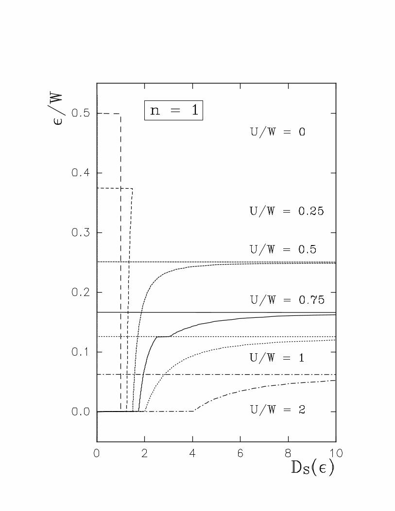
The spinon and chargeon densities of states, Ds,c(E) = 1/(2π)∫ π/2−π/2 dKδ (E − ǫs,c(K)),

are shown in figure 2a and 2b, respectively. Already before the MCIT the density of states

14

for the spinons develops a van-Hove singularity at U = W/2. This could be interpretated as

the formation of the lower (spinon) and upper (chargeon) Hubbard band which are, however,

not yet separated.

Given the densities of states, the internal energy density u(n = 1, T ) can be obtained from

u(n = 1, T ) = e0(n = 1) + 2∫∞0 dE [Ds(E) +Dc(E)]Ef(E), where f(E) = [exp(βE) + 1]−1

is the Fermi-Dirac distribution function. The specific heat cv = −β2∂u/∂β is then given by

cv(n = 1, T ) = 4T∫ ∞

0dx (Ds(2xT ) +Dc(2xT ))

(x

cosh x

)2

. (30)

At low temperatures this reduces to cv(n = 1, T → 0) = γ(n = 1)T with

γ(n = 1) =π2

3[Ds(0) +Dc(0)] . (31)

This Luttinger Liquid relation16, which remains valid for all fillings, will allow us to identify

the conformal charge of the conformal field theory that governs the low energy behavior of

our model (see sec. IV).

The behavior of the Sommerfeld coefficient γ as a function of the interaction parameter,

U/W , can be extracted from eqs. (7), (8), (10), and (11):

γ(n = 1) =π2

3D0(0)

1 for U/W < 1

U/W for U/W > 1(32)

where D0(0) = 2/W is the non-interacting density of states. Note that γ(n = 1) is

unrenormalized below the MCIT. The reason is that the increase in the density of states

for spin excitations is exactly compensated by the decrease in the density of states for the

charge excitations. This precise cancellation of the two contributions is a peculiarity of our

model and does not occur in the conventional Hubbard model. In a realistic scenario for the

Mott-Hubbard transition we expect a growing effective charge mass (or, equivalently, Dc(0))

because the transport of charge becomes more difficult due to the Coulomb repulsion14. Also,

the spin transport should become less effective because the spin exchange energy smoothly

reduces from O(t) to O(J = 4t2/U) and we thus also expect an increasing effective spin

15

mass (or Ds(0)). Consequently, there should be an increase of γ below the MCIT in any

realistic Hubbard-type model.

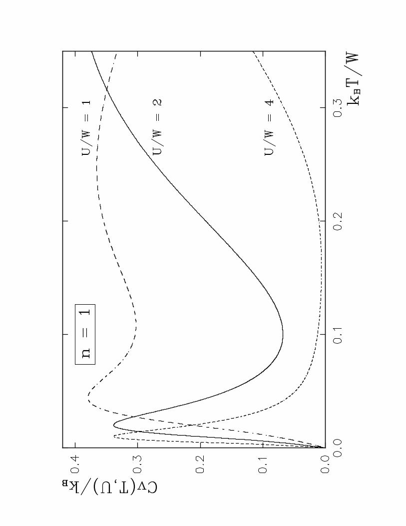
The specific heat as a function of temperature is shown in fig. 3. The general structure

of cv(T ) reflects the behavior of the density of states (see fig. 2). Even before the MCIT,

at U = W/2, the specific heat develops a two peak structure which reflects the van-Hove

singularity in the density of states for spin excitations. As already seen in eq. (32), the

Sommerfeld factor is continuous at the transition. Well above the transition (U >> W )

the lower and upper Hubbard bands are well separated, which is reflected in a narrow

low-temperature peak in cv(T ) and a broad maximum around T = O(U). In spite of the

peculiarities of our model the overall shape of cv(T ) is expected to be generic for any Hubbard

model with a smooth dispersion relation, in the absence of perfect nesting.

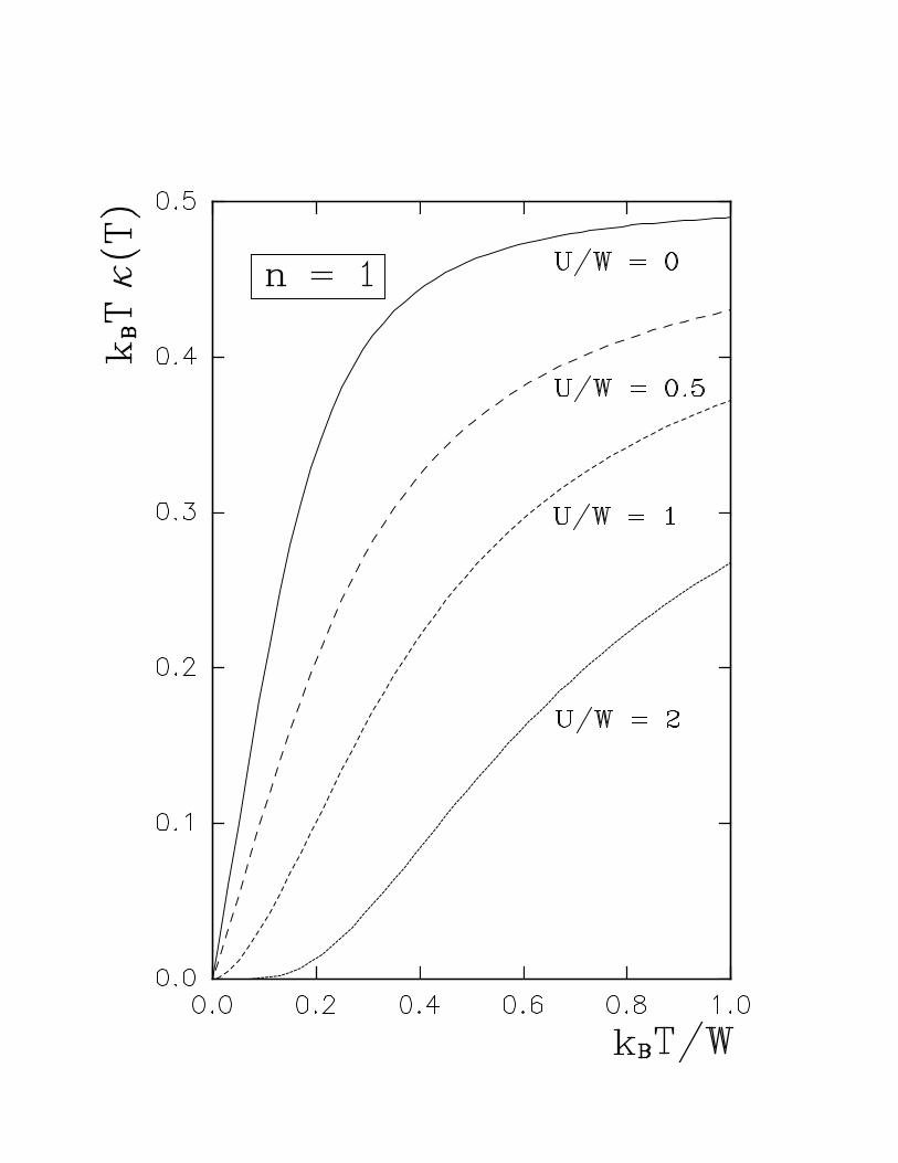
2. Compressibility

Next we discuss the isothermal compressibility κ(T ) = ∂n/∂µ which is related to the

particle number fluctuation by κ(n = 1, T ) = T 〈(∆N)2〉/L = − (∂2/∂µ2) f(µ, T )∣∣∣∣µ=U/2

.

Here, ∆N ≡ N − 〈N〉. A direct calculation gives

κ(n = 1, T ) =β

π

∫ π/2

−π/2dK [exp (−βǫs(K)) + exp (βǫc(K))]−1 . (33)

Note that the compressibility probes the system slightly away from half-filling. It is thus

seen that not only the chargeon dispersion ǫc(K) but also the spinon dispersion ǫs(K) enters

the expression for the compressibility. Therefore, strong charge-spin separation, in the sense

of a completely decoupled response of charge and spin excitations to an external force, does

not exist even at half-filling. It is only for T → 0 that the spinons do not contribute to the

compressibility (or holons to the magnetic susceptibility), as can be seen from eqs. (15b),

(15d), and (16f).

The fluctuation of the particle density at half-filling is shown in figure 4. At low tempera-

tures and below the MCIT the fluctuations are linear in temperature, i.e., the compressibility

16

is constant and given by (15b). Above the transition the charge gap opens, and there are

only exponentially small particle number fluctuations at low temperatures. At high tem-

peratures the fluctuations saturate at Tκ(n = 1, T → ∞) = 1/2. This is the classical value

for spin-1/2 electrons on a lattice where on average half of the sites are doubly occupied or

empty.

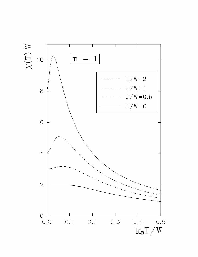
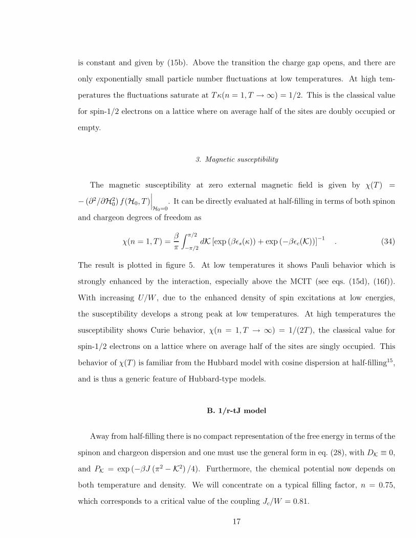
3. Magnetic susceptibility

The magnetic susceptibility at zero external magnetic field is given by χ(T ) =

− (∂2/∂H20) f(H0, T )

∣∣∣∣H0=0

. It can be directly evaluated at half-filling in terms of both spinon

and chargeon degrees of freedom as

χ(n = 1, T ) =β

π

∫ π/2

−π/2dK [exp (βǫs(κ)) + exp (−βǫc(K))]−1 . (34)

The result is plotted in figure 5. At low temperatures it shows Pauli behavior which is

strongly enhanced by the interaction, especially above the MCIT (see eqs. (15d), (16f)).

With increasing U/W , due to the enhanced density of spin excitations at low energies,

the susceptibility develops a strong peak at low temperatures. At high temperatures the

susceptibility shows Curie behavior, χ(n = 1, T → ∞) = 1/(2T ), the classical value for

spin-1/2 electrons on a lattice where on average half of the sites are singly occupied. This

behavior of χ(T ) is familiar from the Hubbard model with cosine dispersion at half-filling15,

and is thus a generic feature of Hubbard-type models.

B. 1/r-tJ model

Away from half-filling there is no compact representation of the free energy in terms of the

spinon and chargeon dispersion and one must use the general form in eq. (28), with DK ≡ 0,

and PK = exp (−βJ (π2 −K2) /4). Furthermore, the chemical potential now depends on

both temperature and density. We will concentrate on a typical filling factor, n = 0.75,

which corresponds to a critical value of the coupling Jc/W = 0.81.

17

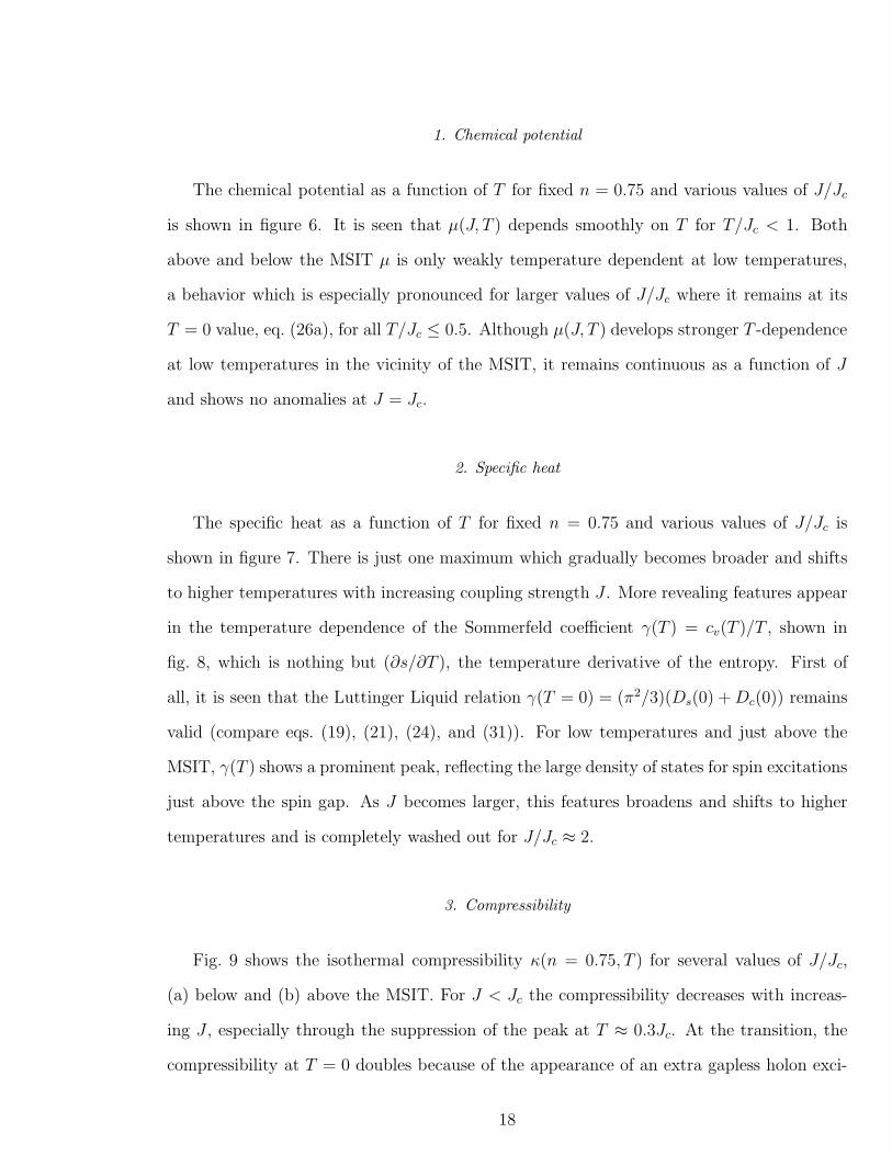
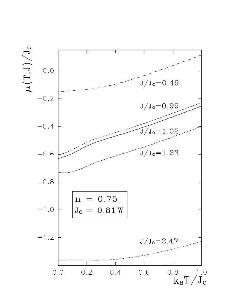
1. Chemical potential

The chemical potential as a function of T for fixed n = 0.75 and various values of J/Jc

is shown in figure 6. It is seen that µ(J, T ) depends smoothly on T for T/Jc < 1. Both

above and below the MSIT µ is only weakly temperature dependent at low temperatures,

a behavior which is especially pronounced for larger values of J/Jc where it remains at its

T = 0 value, eq. (26a), for all T/Jc ≤ 0.5. Although µ(J, T ) develops stronger T -dependence

at low temperatures in the vicinity of the MSIT, it remains continuous as a function of J

and shows no anomalies at J = Jc.

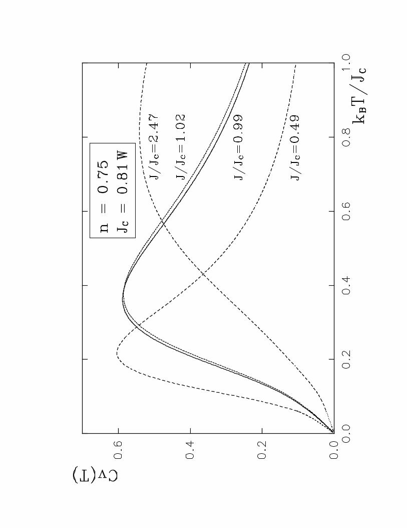
2. Specific heat

The specific heat as a function of T for fixed n = 0.75 and various values of J/Jc is

shown in figure 7. There is just one maximum which gradually becomes broader and shifts

to higher temperatures with increasing coupling strength J . More revealing features appear

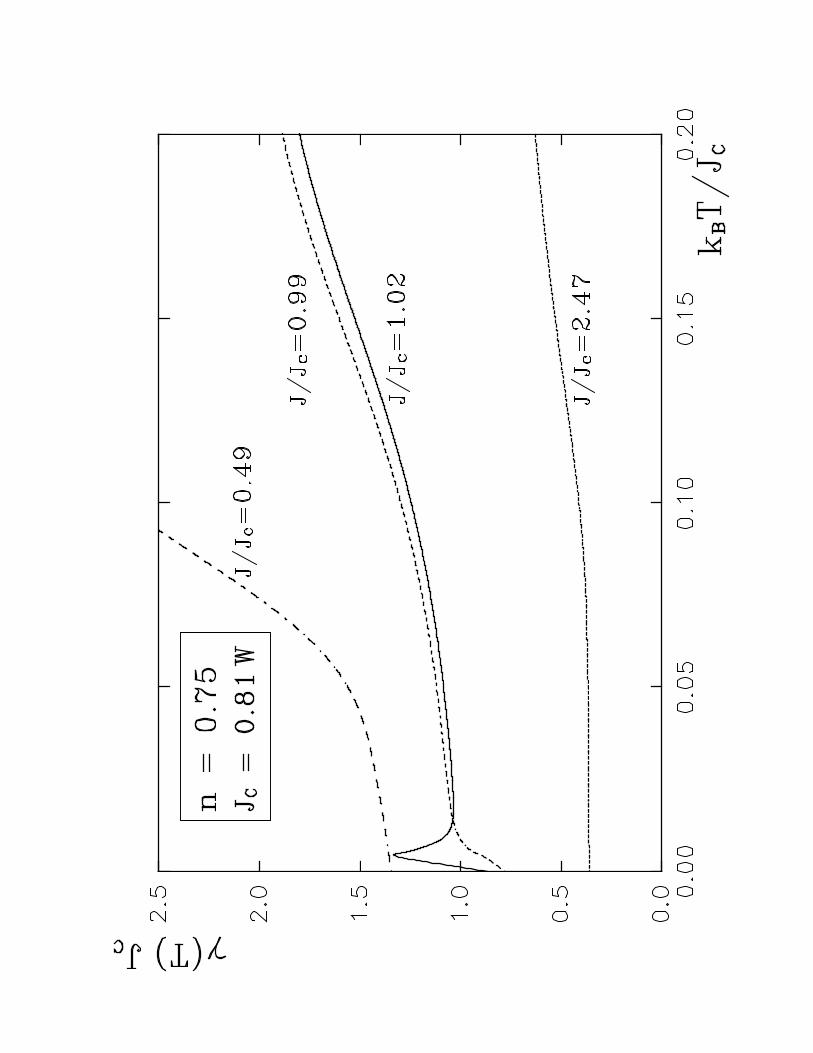
in the temperature dependence of the Sommerfeld coefficient γ(T ) = cv(T )/T , shown in

fig. 8, which is nothing but (∂s/∂T ), the temperature derivative of the entropy. First of

all, it is seen that the Luttinger Liquid relation γ(T = 0) = (π2/3)(Ds(0) +Dc(0)) remains

valid (compare eqs. (19), (21), (24), and (31)). For low temperatures and just above the

MSIT, γ(T ) shows a prominent peak, reflecting the large density of states for spin excitations

just above the spin gap. As J becomes larger, this features broadens and shifts to higher

temperatures and is completely washed out for J/Jc ≈ 2.

3. Compressibility

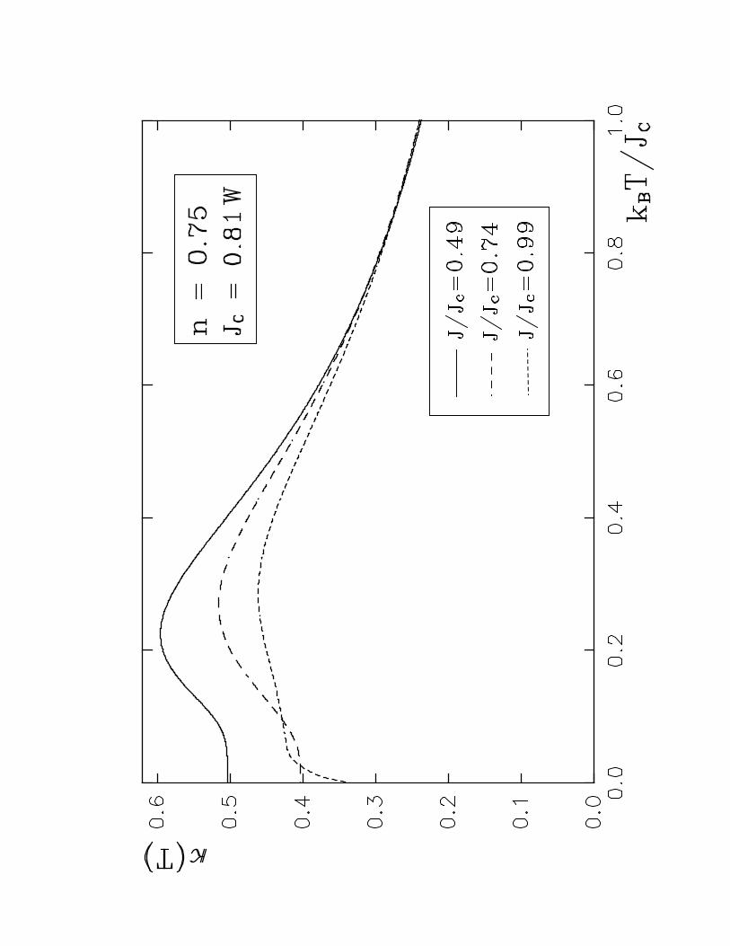
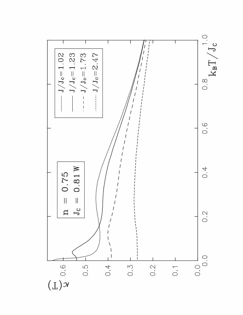
Fig. 9 shows the isothermal compressibility κ(n = 0.75, T ) for several values of J/Jc,

(a) below and (b) above the MSIT. For J < Jc the compressibility decreases with increas-

ing J , especially through the suppression of the peak at T ≈ 0.3Jc. At the transition, the

compressibility at T = 0 doubles because of the appearance of an extra gapless holon exci-

18

tation in the spectrum (see sec. II B 3). Just below the transition this additional density of

states for charge excitations is already present at low but finite energies and causes a sharp in-

crease in the slope of κ(T ) for low temperatures such that the compressibility for J/Jc = 0.99

is actually higher than for J/Jc = 0.74 in a temperatures region around T/Jc = 0.1. Above

the transition the additional density of states for gapless charge excitations results in a new

low temperature peak, which broadens and shifts to higher temperatures (and is eventually

completely suppressed) as J is further increased above the MSIT.

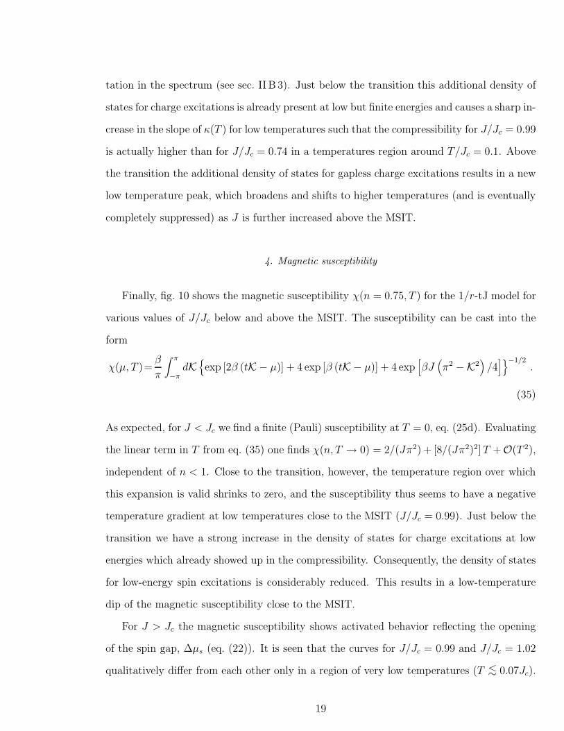
4. Magnetic susceptibility

Finally, fig. 10 shows the magnetic susceptibility χ(n = 0.75, T ) for the 1/r-tJ model for

various values of J/Jc below and above the MSIT. The susceptibility can be cast into the

form

χ(µ, T )=β

π

∫ π

−πdK

{exp [2β (tK − µ)] + 4 exp [β (tK − µ)] + 4 exp

[βJ

(π2 −K2

)/4]}−1/2

.

(35)

As expected, for J < Jc we find a finite (Pauli) susceptibility at T = 0, eq. (25d). Evaluating

the linear term in T from eq. (35) one finds χ(n, T → 0) = 2/(Jπ2) + [8/(Jπ2)2]T +O(T 2),

independent of n < 1. Close to the transition, however, the temperature region over which

this expansion is valid shrinks to zero, and the susceptibility thus seems to have a negative

temperature gradient at low temperatures close to the MSIT (J/Jc = 0.99). Just below the

transition we have a strong increase in the density of states for charge excitations at low

energies which already showed up in the compressibility. Consequently, the density of states

for low-energy spin excitations is considerably reduced. This results in a low-temperature

dip of the magnetic susceptibility close to the MSIT.

For J > Jc the magnetic susceptibility shows activated behavior reflecting the opening

of the spin gap, ∆µs (eq. (22)). It is seen that the curves for J/Jc = 0.99 and J/Jc = 1.02

qualitatively differ from each other only in a region of very low temperatures (T <∼ 0.07Jc).

19

IV. CONFORMAL FIELD THEORY APPROACH AND CORRELATION

FUNCTIONS

Since we do not know how to express the original electron operators in terms of the

eigenstates of our effective Hamiltonian, we cannot directly calculate any correlation func-

tions for our model. Fortunately, away from any phase transitions, our model belongs to the

class of Luttinger Liquids16 for which the low temperature/energy behavior is dominated

by two gapless excitations for charge and spin with linear spectrum and different veloci-

ties vs, vc (charge-spin separation). It is then natural to attempt to calculate the low energy

behavior of various correlation functions of our model by recasting our results within the

framework of conformal field theory26–29 and g-ology14,30–32 techniques, both of which have

proved extremely powerful in extracting the physics of the Luttinger Liquid fixed point. In

this section we focus on the former approach and leave for the next section the discussion

of g-ology.

It is well known that T = 0 can often be viewed as the “critical point” in two-dimensional

classical or one-dimensional quantum field theories: correlation functions decay algebraically

instead of exponentially for long times and/or distances, i.e., there is no intrinsic length scale.

The assumption that, in addition to linearizing the fermionic spectrum, conformal invariance

also holds at low energies/temperatures restricts the behavior of the lowest order 1/L-

corrections to the ground state energy density (EL0 ), and the energies (EL

h±) and momenta

(PLh±) of low-lying states of system of finite size, L. In turn, this information is sufficient

to determine the long range, long time behavior of correlation functions. [An equivalent

approach which is based on a Landau expansion around the ground state for Bethe-Ansatz

solvable problems gives the same results33]. In particular, for a one component Fermi gas

with a linear spectrum conformal invariance implies:

EL0 − Lǫ0 = −πcv

6L(36a)

ELh± −EL

0 =2π

Lv(N+ +N− + h+ + h−

)(36b)

20

PLh± − PL

0 =2π

L

(h+ − h− +N+ −N−

)+ P∞

h . (36c)

Here, c is the conformal charge, v is the velocity of the the right- and left-moving elemen-

tary excitations, h± are their conformal dimensions, P∞h is the momentum of the sound

excitations in the thermodynamic limit, and N± are integers27–29.

A particularly simple way of determining the conformal charge from the Sommerfeld

coefficient of the specific heat is due to Affleck34. For a one-component system with right-

and left-moving elementary excitations

γ =π

3

c

v=π2

3cD(0), (37)

where D(0) is the density of states for low energies.

The information of eqs. (36) and (37) determines the large distance x, long-time t be-

havior of correlation functions of the (primary) fields Φh±(x, t) as follows27–29

〈Φh±(x, t)Φh±(0, 0)〉 =exp (−iP∞

h x)

(x− ivt)2h+

(x+ ivt)2h− . (38)

We are interested in the long-range behavior of the spin-spin correlation function

CSS(r, t), the density-density correlation function CNN(r, t), and the one-particle Green’s

function Gσ(x, t),

CSS(r, t) =1

L

L∑

l=1

〈(nl+r,↑(t) − nl+r,↓(t)) (nl,↑ − nl,↓)〉 (39a)

CNN(r, t) =

[1

L

L∑

l=1

〈(nl+r,↑(t) + nl+r,↓(t)) (nl,↑ + nl,↓)〉]−(n

2

)2

(39b)

Gσ(r, t) =−i2π

1

L

L∑

l=1

〈T cl,σc+l+r,σ(t)〉 (39c)

where T is the time-ordering operator. The only remaining task in computing the asymp-

totic behavior of these correlation functions is identifying the appropriate (primary) fields

associated with the physical operators of interest.

In what follows we use our exact results to carry out the procedure outlined above.

21

A. 1/r-Hubbard model

1. Conformal Charge

The obvious generalization of (37) to a two-component system with charge and spin

excitations is to replace D(0) by (Ds(0) +Dc(0)). As could have been expected, comparing

with eq. (31) gives c = 135.

We note that, since this identification requires finite spin and charge velocities, it breaks

down at the MIT. This could have been inferred from the excitation spectra for charge and

spin (eqs. (6), (9)) which are no longer linear near K = π/2 but behave as ω ∝ kα with

α = 1/2. This is reflected in the finite size corrections to the ground state energy which

behave as√

1/L instead of 1/L. More precisely, from eq. (B3), one obtains for half-filling

(EL0 − Lǫ0)(n = 1) =

√1

L

W

2

∞∑

s=1

(−1)s(

1

πs

)3/2 ∫ πsL

0dy

sin y√y

. (40)

A similar breakdown of conformal invariance occurs in the context of superintegrable chiral

N -state Potts models36 for N ≥ 3.

It is also worth pointing out that, as shown in appendix B, even away from the transition,

there are some additive corrections to the usual formula (36a) in our case. More precisely,

we find

EL0 − Lǫ0 = − π

6L

[vR

s − vF + |vLc | − vF

](41)

(for n = 1 and U > W one has to read vLs instead of vL

c ). It is easy to see that the

corrections guarantee that there are no 1/L corrections present at U = 0 where E0 = Lǫ0 is

the exact result for all L. This requirement follows from the fact that in our case the entire

spectrum of the kinetic energy operator T can be obtained from N−1 independent spin-1/2

SU(2) algebras in each sector with fixed total momentum Q: TNQ ≡ t(Q− π) +W

∑N−1i=1 F z

i

(N even). Thus, in this case the algebraic structure is much simpler than the usual Virasoro

algebra26,27; this invalidates the conventional arguments based on conformal invariance and

justifies the absence of finite size correction in the strict U = 0 limit.

22

2. Conformal dimensions

According to eqs. (36b), (36c), in order to identify the conformal dimensions we need to

consider those lowest-lying states with the quantum numbers of the physical excitation of

interest. We will consider two- and one-particle excitations which determine the long-range

behavior of the spin-spin and density-density correlation functions, and one-particle Green’s

function, respectively.

a. n < 1: Away from the transition the lowest-lying two-spinon excitation is obtained

from the ground state by breaking a [↑↓]-pair at K = −π + ∆/2 and K = −π + 3∆/2, and

placing the electrons into the S = 1, Sz = 0 state at the same K points. The corresponding

excitation energy is

ELh+

s− EL

0 = J(K = −π + 3∆/2) =2π

LvR

s + O(1/L2

), (42)

corresponding to h+s = 1 (only right-moving spinons). Furthermore,

PLh+

s− PL

0 = π +1

2[(−π + ∆/2) (−π + 3∆/2)] =

2π

Lh+

s (43)

where we took into account1 that each bound spin-pair contributes a momentum of π, and

each unbound spin at K adds K/2. As a result, P∞h+

s= 0.

The charge excitation can be treated analogously and one finds (again for n < 1)

ELh−

c− EL

0 = (−t)(KF − 3∆/2) + t(KF + ∆/2) + J(KF − ∆/2) − J(KF + ∆/2)

=2π

L|vL

c | + O(1/L2

)(44)

PLh−

c− PL

0 =1

2[− (KF − 3∆/2) + (KF + ∆/2)] =

2π

L, (45)

implying h−c = 1, P∞h−

c= 0.

Finally, the one-particle excitation from the N -particle ground state is given by the

N + 1-particle ground state:

ground state (N + 1 particles): σ [↑↓] . . . [↑∣∣∣∣KF

↓] ◦ . . . ◦

23

We then find,

ELN+1,0 − EL

N,0 = t(KF + ∆/2) +

K−∆/2∑′

K=−π+3∆/2

(J(K) − J(K + ∆)

)

= µ(n) +2π

L

[vR

s

4+

|vLc |4

]+ O

(1/L2

)(46)

PLN+1,0 − PL

N,0 =1

2[(−π + ∆/2) + (KF + ∆/2)] =

π

L+ π(n− 1) , (47)

and correspondingly, hcN = hs

N = 1/4, P∞N = π(n − 1) = ke

F (keF is the electronic Fermi

momentum).

b. n = 1: Below the transition (U/W < 1) the same results as for n < 1 apply.

Above the transition (U/W > 1) we have no gapless charge excitations. This implies that

all correlation function involving charge excitations (density-density correlation function,

one-particle Green’s function) decay exponentially because their excitation energies always

involve the charge gap ∆µc.

On the other hand, we have additional spin excitations. Besides the excitation with two

right-moving spinons (h+s = 1, P∞

h+s

= 0) we also find the corresponding excitation with two

left-moving spinons (h−s = 1, P∞h−

s= 0). Furthermore, we may split the two spinons to form

the excited state

spin-exc.: σ[↑↓] . . . [↑↓]σ′

leading to

ELh±

s− EL

0 =

π−∆/2∑′

K=−π+3∆/2

J(K) −π−3∆/2∑′

K=−π+5∆/2

J(K)

=2π

L

[vR

s

4+

|vLc |4

]+ O

(1/L2

)(48)

PLh±

s− PL

0 = π +1

2[(−π + ∆/2) + (π − ∆/2)] = π . (49)

This gives h+s = h−s = 1/4, and P∞

hs= π.

24

3. Correlation functions at large times and distances

a. n < 1 or (n = 1 and U/W < 1): According to the results in the last subsection and

the general formulae from conformal field theory (38) we are now in position to deduce the

long-range behavior of correlation functions:

CSS(x, t) ∼ A

(1

x− vRs t

)2

(50a)

CNN(x, t) ∼ B

(1

x+ |vLc |t

)2

(50b)

Gσ(x, t) ∼ e−ikeF

x

2π

1√

(x− vRs t) + i/Λt

1√

(x+ |vLc |t) + i/Λt

(50c)

where Λt is a cut-off parameter (Λt = Λsgnt).

Note that the two-particle correlation functions are of the Fermi Liquid form, with

renormalized velocities. On the other hand, the one-particle Green’s function displays Lut-

tinger Liquid behavior involving square-root singularities rather than the conventional quasi-

particle asymptotic form, 1/ (x− vF t). Consequently, the Fourier transformed one-particle

Green’s function shows no quasiparticle peak, i.e., there is no contribution proportional to

δ(ω − vFk) in the one-particle spectral function.

In fact, the form of Gσ(ω, k) is very interesting but rather complicated. A detailed

analysis of its properties was given recently in refs. 37,38. Nevertheless, we can already

see by dimensional analysis that there is a step-discontinuity in the momentum distribution

nk,σ = 〈c+k,σck,σ〉 = (−i)∑r exp(ikr)G(r, t = 0−) at k = keF = π(n− 1). Our model provides

a novel example of a system which displays a discontinuity in nk,σ in the absence of single-

electron like quasi-particle excitations. Such systems have been termed “free Luttinger

Liquids”16 or “Gutzwiller Liquids”1. This unusual behavior would reflect itself, for example,

in the dependence of the Kondo-temperature on the Kondo coupling impurity embedded in

a “Gutzwiller Liquid”39.

b. n = 1 and U/W > 1: The charge-charge correlation function and the one-particle

Green’s function decay exponentially, while the spin-spin correlation function has the asymp-

25

totic behavior

CSS(x, t) ∼ A1

(1

x− vRs t

)2

+ A2

(1

x+ |vLs |t

)2

+ A3exp (iπx)

√(x− vR

s t) (x+ |vLs |t)

. (51)

Due to the mixture of right- and left-moving spinons, an additional structure (“2kF -

oscillations”) appears in CSS(x, t), indicating strong antiferromagnetic correlations beyond

the MCIT.

4. Equal-time correlation functions

Conformal field theory only allows us to calculate the long-range (large x and t) behavior

of correlation functions. On the other hand, the large x behavior at t = 0, involves contri-

butions from all frequencies. From eqs. (50) it is already clear that the low-frequency modes

lead to a 1/x2 decay for the equal-time spin-spin or density-density correlation function.

What can be said about the high-frequency contributions?

a. n < 1 or n = 1 and U/W < 1: We know that there is a sharp cut-off wave vector

for both charge- and spin-excitations. In particular, no spin-excitations are possible above

KF = π(2n− 1). The highest momentum spin excitation of the ground state is

maximum Q spin-exc.: σ[↑↓] . . . [↑↓]σ′

∣∣∣∣KF

◦ . . . ◦

with Q = π+[(KF − ∆/2) + (−π + ∆/2)] /2 = nπ. This corresponds to a sharp edge in the

correlation function as a function of momentum q at q = Q (for n < 1 or n = 1 and U/W < 1

the correlation functions do not diverge at q = Q). As in ordinary Fermi Liquids, this reflects

itself in long-range oscillations in real space: CSS(r, t = 0) ∼ A1/r2 + A2 cos(πnr)/r2. The

same argument applies to the t = 0 density-density correlation function which also shows

long-range 2kF -oscillations3. Finally, the single-particle momentum distribution shows step

discontinuities at both ends of the U = 0 Fermi “surface”.

b. n = 1 and U/W > 1: In this regime, the entire large distance behavior is already

contained in the large momentum-transfer modes which are also gapless. More explicitly,

for large r we find

26

CSS(r) ∼ A1(−1)r

r+ A2

1

r2(52)

which shows strong antiferromagnetic correlations above the MCIT. The slow oscillating

decay of CSS(r) corresponds to a logarithmic divergence of the spin-spin correlation function

in momentum space near q = π.

B. 1/r-tJ model

1. Conformal Charge

As expected, eq. (31) implies c = 135. Note that the formulae (36) cannot be applied

exactly at the MSIT, J = Jc. At the transition we have both gapless right-moving spin-

excitations and gapless right- and left-moving charge-excitations with finite velocities vRs =

Jcπ/2, vRc = −vL

c = Jcπn/2. Nevertheless, the correct form of the 1/L correction at J = Jc,[EL

0 − Lǫ0](J = Jc) = − [π/(6L)]πnJc, does not contain a contribution from all these three

gapless excitations. Rather, since a finite density of spin-excitations produces an effective

gap for the charge excitations and vice versa, only one of the two excitations, spin or charge,

should be taken into account at J = Jc. More precisely, the factor, πnJc in the 1/L correction

to the energy can be written in either of two forms, πnJc = vRs (J → J−

c ) + |vLc (J → J−

c )| −

|vLc (J = 0)| (for the origin of the term vL

c (J = 0) see the discussion for the 1/r-Hubbard

model, eq. (41)), or πnJc = vRc (J → J+

c ) + |vLc (J → J+

c )|. In other words, the correct

value of the 1/L corrections is obtained by taking the limit from either above or below the

transition.

2. Conformal dimensions

a. J < Jc: We can again use all results from the 1/r-Hubbard model in the limit of

large U/W . For two-particle excitations we then obtain h+s = 1, P∞

h+s

= 0; h−c = 1, P∞h−

c= 0.

Note that for half-filling we have additional excitations which give h±s = 1/4, P∞h±

s= π. For

27

the one-particle excitations all excitations involving charges at gaped for n = 1, while for

n < 1 we have hcN = hs

N = 1/4, P∞N = π(n− 1) = ke

F .

b. J > Jc: Since above the transition we have no gapless spin excitations, all correla-

tion functions involving spin excitations (spin-spin correlation function, one-particle Green’s

function) decay exponentially. On the other hand, we have additional charge excitations:

besides the right-moving holon near K1 (h+c = 1, P∞

h+c

= 0) we also find a left-moving holon

near K2 (h−c = 1, P∞h−

c= 0). Furthermore, we can have a left-moving holon near K1 and a

right-moving holon near K2. These excitations obey h±c = 1/2, P∞h±

c= ±(K2 −K1) = ±2πn.

3. Correlation functions at large times and distances

For J < Jc we obtain the same results as for the Hubbard model away from the transition,

while J > Jc both the spin-spin correlation function and the one-particle Green’s function

decay exponentially. On the other hand, the charge-charge correlation function behaves

asymptotically like (vc = vRc = −vL

c = Jπn/2)

CNN(x, t) ∼ B1

[(1

x− vct

)2

+(

1

x+ vct

)2]

+B2

[exp (i2πnx)

(x− vct)+

exp (−i2πnx)(x+ vct)

]. (53)

Note that since in this case large momentum-transfer excitations are also gapless, CNN(x, t)

displays “4kF -oscillations”3.

4. Equal-time correlation functions

For J < Jc we know that the exact wave function is the Gutzwiller-projected Fermi-sea,

in which case all ground state correlation functions are explicitly known21,40 for all densities n

and distances r. In particular21,

CSS(r 6= 0) =(−1)r

πr[Si (πr) − Si (πr (1 − n))] (54)

where Si(x) =∫ x0 dt sin t/t is the sine-integral. At half-filling, the asymptotic behavior21,

CSS(r >∼ 5) ≃ (−1)r/(2r), reflects the strong antiferromagnetic correlations. The formulae

28

for the density-density correlation function are rather involved but they show the expected

large-distance behavior

CNN(r) ∼ B1

r2+B2

r2cos (πnr) +

B3

r4cos (2πnr) . (55)

The momentum distribution is found to have a jump discontinuity40 of size nkeF,+

− nkeF,−

=√

1 − n. It is comforting that all general considerations from conformal field theory are

verified in a limit where a complete description of the ground state properties is available.

For J > Jc, both spin-spin correlation function and the one-particle Green’s function

decay exponentially. The large momentum transfer processes for the density-density corre-

lation function are no longer gaped and the large distance behavior even at t = 0 can be

deduced from conformal field theory. We find

CNN(r) ∼ 2B11

r2+ 2B2

cos 2πnr

r. (56)

The momentum transform of the density-density correlation function shows a logarithmic

divergence at q = 2πn.

V. g-OLOGY APPROACH AND CHARGE TRANSPORT PROPERTIES IN THE

1/r-HUBBARD MODEL

At low energies/temperatures normal electronic systems in one dimension can be de-

scribed by a continuum field theory30. The essential idea is to linearize the electron excitation

spectrum near the two Fermi points, resulting in left- and right-moving fermions (momen-

tum and/or energy transfer cutoffs ΛB, Λ, must then be introduced to regularize integrals).

These two species of fermions interact via several scattering channels characterized by cou-

pling constants gi, i = 1, . . . , 4 which can also be spin-dependent (“g-ology” Hamiltonian).

The two large momentum transfer processes are described by g1, which parametrizes the

scattering process which interchanges right- and left-moving particles (“backscattering”),

and g3, which represents the scattering of two left-moving particles into two right-moving

29

particles and vice versa (“Umklapp-scattering”). The remaining processes, described by g2

and g4, involve a small momentum transfer, between a left-moving and a right-moving elec-

tron (g2), and between electrons on the same branch (g4). The model with g2 and g4 only is

the Luttinger model41 which has been solved exactly42,30,16.

In general, there is no recipe to link the g-ology coupling constants to the parameters

of a given lattice Hamiltonian without solving the lattice model exactly14. Moreover, this

identification is only valid for interactions strengths smaller than the cutoff. In the case of

the Hubbard model with cosine dispersion the Mott-Hubbard transition happens at half-

filling for U = 0+43, so that the entire low-energy physics, including the physics of the

transition, can be described within g-ology14. More generally, this approach is applicable

to a wide class of one-dimensional electron systems, the so-called Luttinger Liquids, the

low energy behavior of which is controlled by a weak coupling fixed point16. Below we will

restrict ourselves to the discussion of the metallic phase (n < 1, or n = 1 and U/W < 1)

of the 1/r-Hubbard model, although a similar treatment can be also given for the metallic

phase of the t− J model.

A. Identification of the g-ology parameters

The 1/r-Hubbard model is particularly simple as it describes only right-moving electrons

which are, however, hopping on a lattice. It is thus immediately evident that, in the context

of g-ology, the corresponding low-energy physics is described by a pure g4-model (“chiral

Luttinger model”), with a Hamiltonian

Hg4=∑

k,σ

(hvFk) a+k,σak,σ +

1

L

∑

q

1

2

∑

σ,σ′

gσ,σ′

4 ρσ(q)ρσ′(−q) . (57)

Here, ρσ(q) =∑

k a+k−q,σak,σ, the system volume (length of the ring) is V = La, hvF ≡ ta, and

all terms of the Hamiltonian are understood to be normal ordered with respect to the ground

state of the non-interacting Hamiltonian, H0 = Hg4≡0. The coupling matrix in (57) can be

decomposed as gσ,σ′

4 = g‖4δσ,σ′ + g⊥4 δσ,−σ′ . For sufficiently small values of U (U/W << 1) the

lattice plays no role, and we may obviously identify g‖4 = O(U2), g⊥4 = U .

30

After bosonization16,30,42 the Hamiltonian (57) becomes diagonal in the new bosonic

operators for charge (αk) and spin (βk) and thus, the pure g4-model is a “non-interacting”

Luttinger Liquid or a “Gutzwiller Liquid”1. As discussed above, such a model does have a

jump discontinuity in the momentum distribution although it is not a Fermi Liquid. The

bosonic version of the g4-Hamiltonian now reads

Hcg4

=∑

k

(uck) α+k αk (58a)

Hsg4

=∑

k

(usk) β+k βk , (58b)

with

|uc| = vF

[1 +

gc4

2πhvFa−1

](58c)

|us| = vF

[1 +

gs4

2πhvFa−1

](58d)

gc4 = g

‖4 + g⊥4 (58e)

gs4 = g

‖4 − g⊥4 . (58f)

To leading order in U/W , gc4 = U = −gs

4, and thus, |uc| = vF (1 + U/W ), |us| = vF (1 −

U/W )31. Note that the lattice provides the natural cut-off parameters, Λ = W and ΛB =

π/a.

It is amusing that, for our model, there is a way of extending the g-ology solution beyond

the perturbative regime. In particular, by identifying the velocities, |uc,s|, with the velocities

of the charge and spin excitations found in our exact solution, eqs. (13), (7a), we can extract

parameters gc,s4 for all values of U/W (U/W ≤ 1 for n = 1). The resulting expressions read

(n = N/La):

gc4 = U

W√

(W + U)2 − 4WUna> 0 (59a)

gs4 = −U W

U +W< 0 . (59b)

For na = 1 (half-filling) gc4 → ∞ for U → W−, reflecting the MCIT in the exact solution. The

identification (59), for which we give a different argument in appendix C (for n = 1), allows

31

us to follow the solution all the way to the MCIT by using the g-ology parametrization.

This clarifies the fact that, in our model, the MCIT is not caused by the the relevance of

g3-processes at half-filling as in the Hubbard model with cosine dispersion (perfect nesting

property), but rather, it arises as a pure renormalization of gc4 due to the presence of the

lattice.

B. Conductivity at zero temperature: Drude weight

In this section we make use of the g-ology approach to calculate the zero temperature

Drude weight, Dc, of the zero-frequency peak of the real part of the conductivity,

Re [σ(ω)] = Dcδ(ω) for ω → 0. (60)

In the non-interacting limit, D0 = e2ta2/(πh2).

To obtain the electrical conductivity we start with the charge-charge Green’s function

(ρ(q) = ρ↑(q) + ρ↓(q) is the density operator in momentum space),

χNN(q, t) =−iLa

〈T ρ(q, t)ρ(−q, 0)〉 (61)

the retarded part of which is easily obtained from the g-ology analysis30,44,14,32:

χNNret (q, ω) =

q

π

1

ω − vLc q + iη

. (62)

This form becomes exact for our model for small values of q and ω, and implies that the

low-energy charge transport is entirely dominated by holons, eq. (10). As a check one may

calculate the zero temperature compressibility as κ(T = 0) = limq→0 limω→0 χNNret (q, ω) =

1/(π|vL

c |)

in agreement with our direct calculation, eq. (15b).

Up to constant prefactors which we will put back in the end, the electrical conductivity

follows from the generalized Einstein relation,

σret(q, ω) =iω

q2χNN

ret (q, ω), (63)

32

which can be derived using the linear response formula for σret(q, ω) and the continuity

equation, −qj(q, ω) = ωn(q, ω) (see also appendix D). The real part of the conductivity can

then be calculated from Re [σret(q, ω)] = |vLc |δ(ω − vL

c q),

σ(ω) = limq→0

Re [σret(q, ω)] = |vLc |δ(ω) . (64)

Adding back the constant prefactors gives then the final expression for the Drude weight

Dc = D0|vL

c |vF

= D0

1 +U

√(W + U)2 − 4WUna

. (65)

Note that in our model the Drude weight increases with interaction. In fact, at half-

filling, Dc is seen to diverge as σdc(ω) = σ0(ω)/ (1 − U/W ) for small ω and U/W < 1. At the

same time, the compressibility goes to zero, in such a way that the product, κDc, remains

constant. This behavior is in contrast to the MCIT observed in the Hubbard model with

nearest-neighbor hopping, where, at finite U the MCIT can be approached from the metallic

state by increasing the filling, n → 1−, U > 014. In that case, the compressibility diverges

and the conductivity tends to zero.

In fact, it is clear that for any realistic dispersion the conductivity is bounded from above

(“f-sum rule”45,46) and cannot diverge:∫∞−∞ dωReσ(ω) ≤ F <∞. As shown in appendix D,

F is finite whenever the bare dispersion ǫ(k) has a finite second derivative with respect to k

everywhere. It is thus seen that it is our discontinuous dispersion relation ǫ(k) = t(kmod2π)

which allows for a diverging conductivity.

Finally, we note that since we do not know how a physical vector potential couples to

the effective particles of our exact solution one cannot reliably determine the Drude weight

by twisting the boundary conditions47,46, corresponding to adding a flux, Φ, through the

ring. In fact, if we naively replace all values K by K+Φ/(La) to determine the ground state

energy EL0 (Φ), and try to evaluate

D ?=e2La

h2

∂2EL0 (Φ)

∂Φ2

∣∣∣∣∣Φ=0

(66)

we would obtain the incorrect result for the Drude weight,

33

D = D0

[vR

s

vF− 1 +

|vLc |vF

− 1

]

= Ds + Dc , (67)

which involves contributions from both charge and spin excitations.

VI. SUMMARY AND CONCLUSION

Above we discussed various aspects of the physics of two exactly solvable models of one

dimensional lattice fermions: the 1/r-Hubbard model and a related 1/r-tJ model. The

special feature of these models is that, due to absence of perfect nesting, they display non-

trivial metal-to-charge-insulating and spin-insulating states, respectively, at a finite value of

the coupling constants.

The 1/r-Hubbard model thus provides for an explicit realization of Mott’s and Hubbard’s

ideas2,6 albeit in a rather pathological model in which the dispersion has a jump discontinuity

at the zone boundaries. This peculiarity allows for a diverging Drude weight when the

MCIT is approach from the metallic side, associated with the vanishing of the charge mass

at the transition. While the behavior in the charge sector in the 1/r-Hubbard model is

rather non-generic, the spin sector reflects the expected physics of correlated Fermi systems:

for example, the magnetic susceptibility strongly increases with interaction and develops a

strong low-temperature peak at the spin-exchange energy scale J = 4t2/U . After the MCIT

the static spin-spin correlation function displays strong antiferromagnetic correlations with

a logarithmic divergence in momentum space at q = π .

The 1/r-tJ model with pair-hopping terms displays a metal-to-spin-insulator transi-

tion at Jc = 4t/(π(1 − n)). The spin liquid state is described by the Gutzwiller projected

Fermi-sea and provides an exactly solvable example of a genuine RVB-state. At the MSIT, si-

multaneously with the opening of a spin gap, the zero-frequency “spin-conductivity” (Drude

weight for spin transport) drops to zero, after having increased with J/t (to a finite value)

on the spin liquid side. The MSIT appears as a pure level-crossing effect, and thus should

34

not be interpreted as a Mott-type transition6.

We also found that, with a few changes related to the high symmetry of the spectrum in

the non-interacting (U = 0 and J = 0) models, conformal field theory is applicable in the

metallic and spin liquid states (i.e., away from transitions). Using conformal field theory

and g-ology techniques allowed us to calculate long-distance/time properties of ground state

correlation functions. The two-particle sector shows Fermi Liquid behavior. However, the

single-particle Green’s function does not lead to a quasi-particle peak in the spectral function,

even though the jump discontinuity in the momentum distribution survives. Such systems

are referred to as “free Luttinger Liquids” or “Gutzwiller Liquids”. Within the g-ology

approach the 1/r-Hubbard model is identifyed as a “pure g4-model” or “chiral Luttinger

model”. In our model the MCIT is driven by short distance lattice effects which lead to a

divergence of the interaction parameter gc4 at the MCIT.

Despite their conceptual shortcomings the two models provide instructive examples for

strongly correlated electron systems. Although a rigorous proof is still missing we think that

our models and results can be used to check the capability of numerical techniques and the

applicability of various approximations48.

ACKNOWLEDGMENTS

F.G. would like to thank his colleagues at Rutgers University for their hospitality during

a visit, and the Deutsche Forschungsgemeinschaft (DFG) for traveling funds. This research

was supported in part by a grant from the U.S. Department of Energy, Office of Basic Energy

Sciences, Division of Materials Research (D.L.C.), and by ONR Grant # N00014-92-J-1378

and a Sloan Foundation Fellowship (A.E.R.).

35

APPENDIX A: CALCULATION OF GROUND STATE PROPERTIES IN THE

PRESENCE OF A MAGNETIC FIELD

In this appendix we calculate some ground state properties in the presence of a weak

magnetic field H0, and will eventually let H0 → 0.

1. 1/r-Hubbard Model

In the presence of a magnetic field we will have a finite magnetization. Spin pairs will be

broken and turned into the direction of the magnetic field. The positions of these unpaired

spins is determined by the spinon dispersion (6). From the discussion above and figure 1 it

is clear that they will always be located around K = −π. For n = 1 and U/W > 1 there are

also some upturned spins around K = π. We exemplify the calculation for the latter case.

For n = 1, U/W > 1, and m > 0 the ground state is represented by

ground state: ↑ . . . ↑∣∣∣∣K1

[↑↓] . . . [↑↓]∣∣∣∣K2

↑ . . . ↑

where the magnetization m is given by K1 − K2 = 2π(m − 1). The ground state energy

density is calculated as e0(n = 1,K1,K2) = (1/2π)∫K2

K1dK [J(K)/2] where the additional

factor 1/2 took into account that only every second K value contributes to the integral. We

are only interested in small fields and expand K1,2 = ∓π(1 − η1,2) with η1,2 ≪ 1. To second

order we then obtain with the help of eqs. (5), (7a), and (7b)

e0(η1, η2, n = 1) = e0(n = 1) +π

8

(η2

1vRs + η2

2|vLs |)

. (A1)

Using m = (η1 + η2)/2 we minimize e0(n = 1, η1, η2)−mH0 with respect to η1,2, and obtain

η1,2 = (2H0)/(π|vL,Rs |). The magnetization becomes

m = H0

((πvR

s ))−1

+(π|vL

s |)−1

)=

4H0U

W 2(A2)

and the ground state energy reads

e0(m→ 0, n = 1) = e0(n = 1) +1

8

W 2

Um2 . (A3)

36

A similar calculation gives the ground state energy density for n < 1 or n = 1, U/W < 1

as

e0(m,n < 1) =U(n−m) −W [(1 − n)n + (1 −m)m]

4

− 1

24WU

[((W + U)2 − 4WUm

)3/2 −((W + U)2 − 4WUn

)3/2]

(A4)

which is valid for all m. Note that the limits H0 → 0 and n → 1 do not commute beyond

the metal-to-insulator transition, just as in the usual Hubbard model28.

2. 1/r-tJ Model

The ground state representation in the presence of a (not too big) magnetic field is given

by

ground state: −π

∣∣∣∣ ↑ . . . ↑∣∣∣∣Km

◦ . . . ◦∣∣∣∣K1

[↑↓] . . . [↑↓]∣∣∣∣K2

◦ . . . ◦∣∣∣∣π

with K2 − K1 = 2π(n − m) and Km = π(2m − 1). A straightforward integration gives

e0(K1,K2,Km) = (−t/(4π)) [K21 −K2

m + π2 −K22]− (J/(16π)) [π2(K2 −K1) − (K3

2 −K31)/3].

We have to minimize e0(K1,K2,Km)−µn−H0m with respect to K1,K2,Km, where we have

to distinguish the cases (i) K1 = Km, and (ii) K1 > Km to allow for a transition at some

J = Jc.

(i) K1 = Km: we are below the transition, and we see that K2 = π(2n − 1), Km =

π(2m − 1). In this case we can find the ground state energy density even without the

minimization procedure. For small external fields it has the simple form

e0(n,m, J < Jc) = −Wn(1 − n)

2− Jπ2(n−m)

12

[3(n+m) − 2(n2 + nm+m2)

]. (A5)

By differentiating this expression with respect tom gives the connection between the external

magnetic field H0 and the (small) magnetization density m

m = H0

(πvR

s

)−1. (A6)

37

(ii) K1 > Km: from the minimization equations one easily finds that K1 + K2 =

−4W/(πJ). We thus get a solution

K1 > Km , if J > Jc(m) =2W

π2(1 − n−m). (A7)

Note that the presence of a magnetic field stabilizes the spin-liquid phase where spin-

excitations are gapless: Jc(m) > Jc(m = 0) ≡ Jc. The ground state energy density then

reads

e0(n,m, J > Jc(m)) =W 2

2π2J(n−m) − W

2m(1 −m) − Jπ2

24(n−m)

[3 − (n−m)2

]. (A8)

By differentiating this expression with respect tom gives the connection between the external

magnetic field H0 and the (small) magnetization density m

H0 = Hc0 +mπ2 [Jc + n(J − Jc)] (A9a)

Hc0 =

π2(1 − n)

8

(1 − Jc

J

)[J(1 + n) − Jc(1 − n)] . (A9b)

It now takes a finite magnetic field Hc0 to magnetize the system. The spin gap is ∆µs = 2Hc

0

(see (22)) because we break a pair of spins (S = 0) to form an Sz = S = 1 state.

APPENDIX B: 1/L CORRECTIONS FOR THE GROUND STATE ENERGY OF

THE 1/r-HUBBARD MODEL

The ground state energy for finite system sizes L (even) and a finite particle number N

(even) is calculated for n ≤ 1 as EL0 = −∑′

−π<K<KFJK +

∑KF <K<π(−t)K. The prime

indicates that only every second of the K = ∆(m + 1/2) m = −L/2, . . . , L/2 − 1) has to

be taken (KF = ∆(N − L/2)). After rescaling m = 2r − L/2 + 1 the sums give

EL0 = L

[Un

4− Wn(1 − n)

4

]− 1

2

N/2−1∑

r=0

√W 2 + U2 − 4WU(2r + 1)/L . (B1)

To calculate the sum we use the Poisson sum formula (see, e.g., Ref. 49)

N/2−1∑

r=0

h(r + 1/2) =∫ N/2

0dx h(x) + 2

∞∑

s=1

(−1)s∫ N/2

0dx h(x) cos (2πxs) , (B2)

38

do the first integral and a partial integration in the second, and arrive at

EL0 − Lǫ0 = −

∞∑

s=1

(−1)s 2WU

Lπs

∫ N/2

0dx

sin (2πxs)√

(W + U)2 − 8WUx/L. (B3)

Away from U = W and n = 1 we can do further and further partial integrations in the

integral on the right hand side of this equation, and generate an expansion in 1/L. Keeping

only the first term gives

EL0 − Lǫ0 = −

∞∑

s=1

(−1)s

s2

WU

Lπ2(W + U)

1 − 1

√1 − 4WUn/ (W + U)2

+ O

(1/L2

). (B4)

Doing the remaining sum and rearranging terms (vF = t = W/(2π) is the Fermi velocity)

gives

EL0 − Lǫ0 =

π

6LvF

U

U +W− U√

(W + U)2 − 4WUn

. (B5)

With the help of eqs. (7) and (10) this can be cast into the form of eq. (41).

APPENDIX C: EFFECTIVE g4-PARAMETERS AT HALF-FILLING FROM THE

SCREENED ELECTRON-ELECTRON INTERACTION

There is a rather simple recipe to obtain gc,s4 for all U/W < 1 without referring to the

exact solution. At half-filling we know that keF = 0 lies symmetrically around the upper and

lower band edge (±W/2 at k = ±π/a). For a pure g4-model one can exactly calculate the

screened electron-electron interaction with the help of Ward-identities30,44,32. One finds

Dc,s4 (k, ω) = gc,s

4

ω − vFk

ω − |uc,s|k. (C1)

The effective interaction integrated over all times is given by the ω = 0 contribution which

gives

Dc,s4 (k, 0) = gc,s

4

vF

|uc,s|= gc,s

4

1

1 + gc,s4 /W

. (C2)

If we now demand that the time-integrated part of the screened interaction has to stay

unrenormalized at its value for small U/W , Dc4(k, 0) = U and Ds

4(k, 0) = −U , we find that

39

gc4 = U

1

1 − U/W(C3a)

gs4 = −U 1

1 + U/W(C3b)

which is indeed the correct result. So far, we have not been able to obtain a general form

for gc,s4 away from half-filling, without appealing to the exact solution.

APPENDIX D: f-SUM RULE FOR GENERAL DISPERSION RELATIONS

1. Current operator

For a Hamiltonian H = T + V we assume that the interaction only contains density

operators nr. We omit spin indices in the following. The particle density operator n(q) =

∑r e

iqrnr =∑

k c+k+q ck then commutes with V . We expand the exponential in the particle

density operator n(q) for small momenta q (this step could cause problems in the case of

long-range hopping). The continuity equation then reads

i∂

∂tn(q) = −q

∑

r

∂r

∂tnr = −q

∑

r

v(r)n(r) . (D1)

The sum on the right-hand side is identified with the particle current operator

j = limq→0

−iq

∂

∂tn(q) . (D2)

Using the Heisenberg equations of motion we can calculate j as

j = limq→0

∑

k

c+k+q ck

(ǫ(k + q) − ǫ(k)

q

). (D3)

If the dispersion relation is differentiable, this reduces to the standard expression for the

current operator involving the group velocity ∂ǫ(k)/∂k. Our linear dispersion relation is

not differentiable at |k| = π. Instead we may think that the linear dispersion relation is

the result of a limiting process where we start with a differentiable dispersion ǫ(k) which

becomes ever steeper near |k| = π. This corresponds to ever faster left-moving electrons

near |k| = π, in addition to the right-moving electrons for |k| < π. From this viewpoint

40

it becomes clear that we have to expect a singular contribution from these “left-moving”

electrons. Indeed, we find for q > 0

j(q) =W

2π

∑

k

c+k+qck − W

q

∑

π−q<k<π

c+k+q ck (D4)

and j(−q) = j+(q). Now let q → 0 and assume that we may approximately replace c+k+q ≈

c+k . For the minimum q = ∆ = 2π/L one has j(q = ∆) = W/(2π)[N − Lc+−π+∆/2cπ−∆/2

].

As “the current at q = 0” one may define

j =1

2

(j(q = ∆) + j(q = −∆)

)

= W/(2π)[N − (L/2)

(c+−π+∆/2cπ−∆/2 + c+π−∆/2c−π+∆/2

)]. (D5)

We obviously get an extensive (i.e., singular) contribution from the states near the Brillouin

zone boundary.

2. f-sum rule

We are interested in the real part of the transverse conductivity for small q at temperature

T = 0

Re [σ(ω, q → 0)] =e2

Lωlimq→0

Re{∫ t

−∞dt′eiω(t−t′)〈

[j+(q, t), j(q, t′)

]〉}

. (D6)

Using the continuity equation (D1), the equation of motion (in t) (eq. (D3)), and integrating

by parts (in t′) one finds

Re [σ(ω, q → 0)] = − e2

Lωq2Re{(−i) 〈

[[ρ+(q, t), T

], ρ(q, t′)

]〉eiω(t−t′)

∣∣∣t

−∞

−(−i)(−iω)∫ t

−∞dt′eiω(t−t′)〈

[[ρ+(q, t), T

], ρ(q, t′)

]〉}. (D7)

The first term in {. . .} is purely imaginary and drops out. To obtain the f-sum rule we

integrate over all ω. This gives

F (q) ≡∫ ∞

−∞dωRe [σ(ω, q → 0)]

= −πe2

Lq2〈[[ρ+(q), T

], ρ(q)

]〉 (D8)

41

because the expression (D7) only depended on (t− t′). The double commutator gives

[[ρ+(q), T

], ρ(q)

]=∑

k

c+k ck

[ǫ(k) − ǫ(k + q) + ǫ(k) − ǫ(k − q)

]

Thus,

F (q) =πe2

L

∑

k

{1

q

[ǫ(k + q) − ǫ(k)

q+ǫ(k − q) − ǫ(k)

q

]}〈nk〉 (D9)

and F = limq→0 F (q). For twice differentiable dispersion relations this reduces to F =

(πe2/L)∑

k〈nk〉 [∂2ǫ(k)/∂k2]. In particular, for a cosine dispersion, F = πe2〈−T 〉/L which

is the standard result45,46.

For the linear dispersion we get

F (q) =πe2W

Lq2

∑

−π<k<−π+q

〈nk〉 −∑

π−q<k<π

〈nk〉

. (D10)

The minimum value of q is ∆ = 2π/L. Thus

F ≡ F (∆) = Le2

4π

[〈nπ−∆/2〉 − 〈n−π+∆/2〉

]. (D11)

The f-sum rule is thus extensive and leaves room for a diverging Drude weight. This can

only happen, if the dispersion relation ǫ(k) is not twice differentiable with respect to k.

42

REFERENCES

1 F. Gebhard and A.E. Ruckenstein, Phys. Rev. Lett. 68, 244 (1992).

2 J. Hubbard, Proc. R. Soc. London, Ser. A 276, 238 (1963).

3 The diameter of the Fermi body is πn as usual. This is the wave vector that enters in the

long distance behavior of correlation functions, and is identified with “πn = 2kF”.

4 P.W. Anderson in Solid State Physics, ed. by F. Seitz and D. Turnbull, vol. 14, p. 99

(1963); J.E. Schrieffer and P.A. Wolff, Phys. Rev. 149, 491 (1966); A.B. Harris and

R.V. Lange, Phys. Rev. 157, 295 (1967).

5 F.D.M. Haldane, Phys. Rev. Lett. 60, 635 (1992); B.S. Shastry, Phys. Rev. Lett. 60, 639

(1992).

6 N.F. Mott, Rev. Mod. Phys. 40, 677 (1968); Metal-Insulator Transitions, (Taylor & Fran-

cis, London, 1974).

7 P.W. Anderson, G. Baskaran, Z. Zou, and T. Hsu, Phys. Rev. Lett. 58, 2790 (1987);

F.C. Zhang and T.M. Rice, Phys. Rev. B 37, 3759 (1988); F.C. Zhang, C. Gros, T.M. Rice,

and H. Shiba, Supercond. Sci. and Techn. 1, 36 (1988).

8 The configurations [•◦] and [↑↓] represent charge (C = Cz = 0) and spin singlets (S =

Sz = 0).

9 D.F. Wang, Q.F. Zhang, and P. Coleman, (unpublished) (1993).

10 P.W. Anderson, Science 235, 1196 (1987).

11 In a grand canonical ensemble we use c+k,σ 7→ c−k,−σ. The kinetic energy operator is invari-

ant, and D −∑σ µσNσ 7→ D −∑

σ µσNσ + (L −∑σ Nσ)(U −∑

σ µσ). At half-filling this

must be an operator identity so that we have to fix∑

σ µσ = 2µ = U .

12 W.F. Brinkman and T.M. Rice, Phys. Rev. B 2, 4302 (1970).

43

13 D. Vollhardt, Rev. Mod. Phys. 56, 99 (1984).

14 H.J. Schulz, Phys. Rev. Lett. 64, 2831 (1990); Int. J. Mod. Phys. B 5, 57 (1991); Pro-

ceedings of the Adriatico Research Conference and Miniworkshop on “Strongly Correlated

Electron Systems II, ed. by G. Baskaran et al. (Progress in High Temperature Supercon-

ductivity – Vol. 29, World Scientific, Singapore, 1991); C.F. Coll, Phys. Rev. B 9, 2150

(1974).

15 H. Shiba and P.A. Pincus, Phys. Rev. B 5, 1966 (1972); H. Shiba, Prog. Theor. Phys. 48,

2171 (1972); H. Shiba, Phys. Rev. B 6, 930 (1972).

16 F.D.M. Haldane, J. Phys. C 14, 2585 (1981); Phys. Rev. Lett. 45, 1358 (1980); 47, 1840

(1981).

17 F.D.M. Haldane, Phys. Rev. Lett. 66, 1529 (1991).

18 J. des Cloizeux and J.J. Pearson, Phys. Rev. 128, 2131 (1962).

19 The unique ground state at U = 0 (Fermi sea) and for U > 0 contain one and the same

configuration with no double occupancy. It is the only one to survive for U → ∞, hence

the Gutzwiller projected Fermi sea is the exact ground state for the 1/r-tJ model at all

fillings.

20 H. Yokoyama and H. Shiba, J. Phys. Jpn. 56, 1490 (1987); ibid. 3570 (1987); ibid. 3582

(1987); ibid. 57, 2482 (1988); C. Gros, R. Joynt, and T.M. Rice, Phys. Rev. B 36, 381

(1987); C. Gros, Phys. Rev. B 38, 931 (1988).

21 F. Gebhard and D. Vollhardt, Phys. Rev. Lett. 59, 1472 (1987); Phys. Rev. B 38, 6911

(1988).

22 H. Yokoyama and M. Ogata, Phys. Rev. Lett. 67, 3610 (1991).

23 J. Ashkin and E. Teller, Phys. Rev. 64, 178 (1943).

24 L. Onsager, Phys. Rev. 65, 117 (1944); see also R.J. Baxter, Exactly solved models in

44

statistical mechanics, (Academic Press, New York, 1982).

25 There is always a true gap between λ−K and λ+K so that the contribution of the λ−K to the

free energy density does not show up in a 1/L-expansion.

26 A. A. Belavin, A.M. Polyakov, and A.B. Zamolodchikov, Nucl. Phys. B 241, 333 (1984).

27 J.L. Cardy, Nucl. Phys. B 270 [FS16], 186 (1986); H.W. Blote, J.L. Cardy, and

M.P. Nightingale, Phys. Rev. Lett. 56, 742 (1986); A.D. Mirnov and A.V. Zabrodin,

Phys. Rev. Lett. 66, 534 (1991).

28 H. Frahm and V.E. Korepin, Phys. Rev. B 42, 10553 (1990); B 43, 5653 (1991).

29 N. Kawakami and S.-K. Yang, Phys. Lett. 148A, 359 (1990); Phys. Rev. Lett. 65, 2309

(1990); Prog. Theor. Phys. Suppl. 107, 59 (1992).

30 J. Solyom, Adv. Phys. 28, 201 (1979).

31 J. Voit, Phys. Rev. B 45, 4027 (1992).

32 W. Metzner and C. di Castro, Phys. Rev. B 47, 16107 (1993).

33 J. Carmelo and A.A. Ovchinnikov, J. Phys. C 3, 757 (1991); J.M.P. Carmelo, P. Horsch,

and A.A. Ovchinnikov, Phys. Rev. B 45, 7899 (1992); J.M.P. Carmelo and P. Horsch,

Phys. Rev. Lett. 68, 871 (1992).

34 I. Affleck, Phys. Rev. Lett. 56, 746 (1986).

35 Note that our model is chiral, i.e., the density of states is only half as big as in the usual

case.

36 G. Albertini, B.M. McCoy, J.H.H. Perk, S. Tang, Nucl. Phys. B 314, 741 (1989); R.J. Bax-

ter, J. Stat. Phys. 57, p. 1 (1989).

37 V. Meden and K. Schonhammer, Phys. Rev. B 46, 15753 (1992), and unpublished (1993).

38 J. Voit, Phys. Rev. B 47, 6740 (1993), and unpublished (1993).

45

39 D.-H. Lee and J. Toner, Phys. Rev. Lett. 69, 3378 (1992), and private communication.

40 W. Metzner and D. Vollhardt, Phys. Rev. Lett. 59, 121 (1987); Phys. Rev. B 37, 7382

(1988).

41 J.M. Luttinger, J. Math. Phys. 4, 1154 (1963).

42 D.C. Mattis and E.H. Lieb, J. Math. Phys. 6, 304 (1965).

43 E.H. Lieb and F.Y. Wu, Phys. Rev. Lett. 20, 1445 (1968).

44 E.H. Rezayi, J. Sak, and J. Solyom, Phys. Rev. B 20, 1129 (1979); ibid. B 23, 1342

(1981); K. Penc and J. Solyom, Phys. Rev. B 44, 12690 (1991).

45 See, e.g., D. Pines and P. Nozieres, Theory of Quantum Liquids (Benjamin, New York,

1966); P.F. Maldague, Phys. Rev. B 16, 2437 (1977).

46 B.S. Shastry and B. Sutherland, Phys. Rev. Lett. 65, 243 (1990).

47 W. Kohn, Phys. Rev. 133, A 171 (1964); for recent applications, see C.A. Stafford,

A.J. Millis, and B.S. Shastry, Phys. Rev. B 43, 13660 (1991); R.M. Fye, M.J. Martins,

D.J. Scalapino, J. Wagner, and W. Hanke, Phys. Rev. B 45, 7311 (1992).

48 F. Gebhard and A. Girndt, “Comparison of Variational Approaches for the Exactly Solv-

able 1/r-Hubbard model”, available as preprint cond-mat/9307036 from the preprint li-

brary cond-mat@babbage.sissa.it (accepted for publication in Z. Phys. B).

49 L.D. Landau and E.M. Lifshits, Statistical Physics, part 1, Course on Theoretical Physics

Vol. V, § 60 (3rd edition, Pergamon Press, New York, 1980).

46

FIGURES

FIG. 1. Dispersion relations for (a) spinons, see eq. (6), and (b) chargeons, see eq. (9), in the

1/r-Hubbard model for (a) U/W = 0.25, 0.5, 0.75, 1, 2, and (b) U/W = 0.5, 1, 2.

FIG. 2. Total density of states (a) Ds of the spinons and (b) Dc of the chargeons for the

U/W -values of fig. 1 in the 1/r-Hubbard model (note the change in energy scale); the energy gap

in Dc for U > W is only half as big as the true gap because the chargeons always come in pairs.

FIG. 3. Specific heat as a function of temperature for the half-filled 1/r-Hubbard model

for various values of U/W (a) below (U/W = 0, 0.5, 0.75, 1), (b) above (U/W = 1, 2, 4) the

metal-to-charge-insulator transition.

FIG. 4. Fluctuation of the particle density kBTκ(n = 1, T ) for the half-filled 1/r-Hubbard

model as a function of temperature for U/W = 0, 0.5, 1, 2.

FIG. 5. Magnetic susceptibility χ(n = 1, T ) for the half-filled 1/r-Hubbard model as a function

of temperature for U/W = 0, 0.5, 1, 2.

FIG. 6. Chemical potential µ(n = 0.75, T ) in the 1/r-tJ model as a function of temperature

for J/Jc = 0.5, 0.99, 1.02, 1.2, 2; the metal-to-spin-insulator transition happens at Jc = 0.81W .

FIG. 7. Specific heat cv(n = 0.75, T ) in the 1/r-tJ model as a function of temperature for

J/Jc = 0.49, 0.99, 1.02, 2.47.

FIG. 8. Sommerfeld coefficient γ(n = 0.75, T ) in the 1/r-tJ model as a function of temperature

for J/Jc = 0.49, 0.99, 1.02, 2.47.

FIG. 9. Compressibility κ(n = 0.75, T ) in the 1/r-tJ model as a function of temperature (a)

below (J/Jc = 0.49, 0.74, 0.99) and (b) above (J/Jc = 1.02, 1.23, 1.73, 2.47) the MSIT.

FIG. 10. Magnetic susceptibility χ(n = 0.75, T ) in the 1/r-tJ model as a function of tempera-

ture for J/Jc = 0.49, 0.74, 0.99, 1.02, 1.23, 2.47.

47