arX

iv:1

106.

0356

v1 [

mat

h-ph

] 2

Jun

201

1

Universal Luttinger Liquid Relations in the

1D Hubbard Model

G. Benfatto1 P. Falco2 V. Mastropietro1

June 3, 2011

Abstract

We study the 1D extended Hubbard model with a weak repulsive short-range interactionin the non-half-filled band case, using non-perturbative Renormalization Group methods andWard Identities. At the critical temperature, T = 0, the response functions have anomalouspower-law decay with multiplicative logarithmic corrections. The critical exponents, thesusceptibility and the Drude weight verify the universal Luttinger liquid relations. Borelsummability and (a weak form of) Spin-Charge separation is established.

Contents

1 Main Results 21.1 Introduction . . . . . . . . . . . . . . . . . . . . . . . . . . . . . . . . . . . . . . . 21.2 Extended Hubbard Model and Physical Observables . . . . . . . . . . . . . . . . 31.3 Anomalous exponents and logarithmic corrections . . . . . . . . . . . . . . . . . . 61.4 The Luttinger liquid relations . . . . . . . . . . . . . . . . . . . . . . . . . . . . . 71.5 Spin Charge separation . . . . . . . . . . . . . . . . . . . . . . . . . . . . . . . . 81.6 Borel summability . . . . . . . . . . . . . . . . . . . . . . . . . . . . . . . . . . . 81.7 Contents of the paper . . . . . . . . . . . . . . . . . . . . . . . . . . . . . . . . . 9

2 RG Analysis for the Hubbard Model 112.1 Functional integral representation . . . . . . . . . . . . . . . . . . . . . . . . . . . 112.2 Multiscale analysis for the effective potential . . . . . . . . . . . . . . . . . . . . 122.3 The flow of the running coupling constants . . . . . . . . . . . . . . . . . . . . . 162.4 The flow of renormalization constants . . . . . . . . . . . . . . . . . . . . . . . . 222.5 Proof of Theorem 1.1 . . . . . . . . . . . . . . . . . . . . . . . . . . . . . . . . . . 242.6 Proof of Theorem 1.4 . . . . . . . . . . . . . . . . . . . . . . . . . . . . . . . . . . 26

3 RG Analysis of the Effective Model 273.1 Introduction . . . . . . . . . . . . . . . . . . . . . . . . . . . . . . . . . . . . . . . 273.2 Ward Identities in the g1,⊥ = 0 case . . . . . . . . . . . . . . . . . . . . . . . . . 283.3 Schwinger-Dyson and Closed equations. . . . . . . . . . . . . . . . . . . . . . . . 303.4 The two point function . . . . . . . . . . . . . . . . . . . . . . . . . . . . . . . . . 313.5 The four point functions and the densities correlations . . . . . . . . . . . . . . . 333.6 Fine tuning of the parameters of the effective model . . . . . . . . . . . . . . . . 35

4 Spin-Charge Separation 36

1Dipartimento di Matematica, Universita di Roma “Tor Vergata”, 00133 Roma, Italy.2School of Mathematics, Institute for Advanced Study, Princeton, New Jersey 08540

1

5 Susceptibility and Drude weight 37

A The g1 map 41

B Symmetries of the Effective Model and RG Flow 43

C Vanishing of the Beta Function 46

1 Main Results

1.1 Introduction

The Hubbard model, see e.g. [1], describing interacting spinning fermions on a lattice, plays thesame role in quantum many body theory as the Ising model in classical statistical mechanics,that is it is the simplest model displaying many real world features: it is however much moredifficult to analyze. While our understanding of the Hubbard model in higher dimensions atzero temperature is really poor (except for special choices of the lattice as in [2] and [3]), thesituation is better in d = 1, when the model furnishes an accurate description of real systems,like quantum wires or carbon nanotubes [4].

The one dimensional Hubbard model (from now on the Hubbard model tout court) canbe exactly solved by Bethe ansatz, as shown by Lieb and Wu [5]: the system is insulating inthe half filled band case while it is a metal otherwise and the elementary excitations are notelectronlike, a phenomenon which is nowadays called electron fractionalization [6]. Recently in[7] a strategy for a proof that the lowest energy state of Bethe ansatz form is really the groundstate has been outlined (see also [8]). This method is however of little utility for understandingthe asymptotic behavior of correlations; and does not apply in studying the ground state of aslight generalization of the model, the extended Hubbard model, that consists in replacing thelocal quartic interaction with a short-ranged one. Other approaches has been therefore developedto get more insights into the physical properties of the Hubbard model.

Under certain drastic approximations, like replacing the sinusoidal dispersion relation with alinear relativistic one and neglecting certain terms called backward and umklapp interactions (seeafter (2.25) for their definition), one obtains the spinning Luttinger Model, which is exactly solv-able in a stronger sense, [9], [10]: all its Schwinger functions, at distinct points, can be explicitlycomputed. This model, describing interacting fermions, can be exactly mapped in a model oftwo kinds of free bosons, describing the propagation of charge or spin degrees of freedom andwith different velocities (spin-charge separation); again, a phenomenon of electron fractional-ization which has received a considerable attention in the context of high Tc superconductors[11]. Moreover, as in spinless Luttinger model, the correlations have a power law decay rate withinteraction dependent exponents.

However, neglecting the lattice effects and backscattering or umklapp interactions is notsafe, and indeed the mapping to free bosons is not expected to be true in the Hubbard model.A somewhat more realistic effective description can be obtained by including the backwardinteraction in the spinning Luttinger Model, so obtaining the g-ology model. This system is nomore solvable; however, a perturbative Renormalization Group (RG) analysis, [12], shows that,in the repulsive case, such extra coupling is marginally irrelevant, i.e. becomes negligible overlarge space-time scales. In [13] the necessity of implementing Ward Identities in a RG approachwas emphasized, in order to go beyond purely perturbative results, but the analysis was limitedto the Luttinger model and no attempt was done to include the effects of nonlinear bands. In[14] it was observed that the correlations of the repulsive g-ology model would qualitatively differfrom the Luttinger model ones for the presence of multiplicative logarithmic corrections.

A new point of view, that extended previous ideas of Kadanoff, [15], and Luther and Peschel,[16], was proposed by Haldane, [17], and is nowadays known as Luttinger Liquid Conjecture. The

2

idea is to exploit the concept of universality, a basic notion in statistical physics saying that thecritical properties are largely independent from the details of the model, at least inside a certainclass of models. In the present case, as the exponents are non trivial functions of the coupling,universality has a meaning more subtle than usual; it does not mean that the exponents are thesame (the exponents do depend on the details of the model), but that the exponents and certainthermodynamic quantities verify a set of universal relations which are identical to the Luttingermodel ones. Such relations give an exact determination of physical quantities in terms of afew measurable parameters. The validity of such relations has been checked in certain specialsolvable spinless fermionic lattice models [17], but a proof of their validity in the Hubbard model(or in the non solvable extended Hubbbard model) is an open problem. It should be remarkedthat, even thought the Hubbard model differs from the spinning Luttinger model for irrelevantor marginally irrelevant terms in the Renormalization Group sense (in the weak non half filledband case), this would not imply at all the validity of the same relations as in the Luttingermodel; irrelevant terms do renormalize the exponents and the thermodynamic quantities.

Starting from the 90’s, the methods developed in constructive Quantum Field Theory (QFT)for the analysis of QFT models in d = 1 + 1 [18, 19] were applied to interacting non relativisticspinless fermionic systems in the continuum [20], so establishing the anomalous dimension in anon solvable model, by combining Renormalization Group methods with non perturbative infor-mation coming from the exact solution of the Luttinger model; the extension to spinning fermionswas done in [21]. An important technical advance was achieved in [22, 23], by implementing WardIdentities based on local symmetries with Renormalization Group methods. A well known diffi-culty in any Wilsonian Rermalization Group approach is that the momentum cut-offs break thelocal symmetries on which Ward Identities are based; in [22, 23] it was developed a techniqueallowing to rigorously take into account the extra terms produced in the Ward Identities by thecut-offs, so that interacting non relativistic fermions in d = 1 were constructed without any useof exact solutions [23, 24, 25]. The main outcome, with respect to the early RenormalizationGroup analysis [12], is that the results are exact (the lattice and non linear bands are fully takinginto account) and non-perturbative; and physical observables are written in terms of convergentexpansions so that they can be computed with arbitrary precision. The complexity of such ex-pansions made however impossible to verify explicitly the universal Luttinger Liquid relationsin [26]; they have finally been proven for interacting spinless fermions on the lattice (the XXZchain and extended versions) in [27, 28] through Ward identities; this fact appears to be relatedto a non-perturbative version of the Adler-Bardeen theorem of the non renormalization of theanomalies, [29]. In this paper we will extend such ideas to spinning fermions in the Hubbardmodel; as we will see, the extension is rather non trivial and new phenomena take place.

1.2 Extended Hubbard Model and Physical Observables

Let β > 0 be the inverse temperature, −µ the chemical potential and C = −[L/2], . . . , |[(L −1)/2]L a one dimensional lattice of L sites. The extended Hubbard model [30] describes fermionshopping on C with a short-range density-density interaction; the Hamiltonian plus the chemicalpotential term is

H = −1

2

∑

x∈Cs=±

(a+x,sa−x+1,s+ a+x,sa

−x−1,s)+µ

∑

x∈Cs=±1

a+x,sa−x,s+λ

∑

x,y∈Cs,s′=±1

v(x− y)a+x,sa−x,sa

+y,s′a

−y,s′ (1.1)

where a±x,s are fermionic creation and annihilation operators at site x with ’spin’ s, and v(x) is

a smooth, even potential such that |v(x)| ≤ Ce−κ|x| (short range condition); periodic boundaryconditions are assumed: aεL+1,s = aε1,s.

The set-up of the Grand Canonical Ensemble is standard, and we remind it concisely; moredetails are, for example, in [31]. If Ox is a monomial in the operators aεx,s, ε, s = ±, or in

3

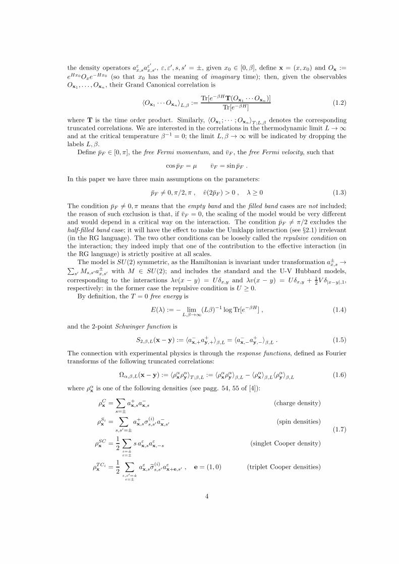
the density operators aεx,saε′

x,s′ , ε, ε′, s, s′ = ±, given x0 ∈ [0, β], define x = (x, x0) and Ox :=

eHx0Oxe−Hx0 (so that x0 has the meaning of imaginary time); then, given the observables

Ox1 , . . . , Oxn, their Grand Canonical correlation is

〈Ox1 · · ·Oxn〉L,β :=

Tr[e−βHT(Ox1 · · ·Oxn)]

Tr[e−βH ](1.2)

where T is the time order product. Similarly, 〈Ox1 ; · · · ;Oxn〉T ;L,β denotes the corresponding

truncated correlations. We are interested in the correlations in the thermodynamic limit L→ ∞and at the critical temperature β−1 = 0; the limit L, β → ∞ will be indicated by dropping thelabels L, β.

Define pF ∈ [0, π], the free Fermi momentum, and vF , the free Fermi velocity, such that

cos pF = µ vF = sin pF .

In this paper we have three main assumptions on the parameters:

pF 6= 0, π/2, π , v(2pF ) > 0 , λ ≥ 0 (1.3)

The condition pF 6= 0, π means that the empty band and the filled band cases are not included;the reason of such exclusion is that, if vF = 0, the scaling of the model would be very differentand would depend in a critical way on the interaction. The condition pF 6= π/2 excludes thehalf-filled band case; it will have the effect to make the Umklapp interaction (see §2.1) irrelevant(in the RG language). The two other conditions can be loosely called the repulsive condition onthe interaction; they indeed imply that one of the contribution to the effective interaction (inthe RG language) is strictly positive at all scales.

The model is SU(2) symmetric, as the Hamiltonian is invariant under transformation a±x,s →∑s′ Ms,s′a

±x,s′ with M ∈ SU(2); and includes the standard and the U-V Hubbard models,

corresponding to the interactions λv(x − y) = Uδx,y and λv(x − y) = Uδx,y + 12V δ|x−y|,1,

respectively: in the former case the repulsive condition is U ≥ 0.By definition, the T = 0 free energy is

E(λ) := − limL,β→∞

(Lβ)−1 logTr[e−βH ] , (1.4)

and the 2-point Schwinger function is

S2,β,L(x− y) := 〈a−x,+a+y,+〉β,L = 〈a−x,−a+y,−〉β,L . (1.5)

The connection with experimental physics is through the response functions, defined as Fouriertransforms of the following truncated correlations:

Ωα,β,L(x− y) := 〈ραxραy〉T ;β,L := 〈ραxραy〉β,L − 〈ραx〉β,L〈ραy〉β,L (1.6)

where ραx is one of the following densities (see pagg. 54, 55 of [4]):

ρCx =∑

s=±

a+x,sa−x,s (charge density)

ρSix =

∑

s,s′=±

a+x,sσ(i)s,s′a

−x,s′ (spin densities)

(1.7)

ρSCx =1

2

∑

s=±ε=±

s aεx,saεx,−s (singlet Cooper density)

ρTCix =

1

2

∑

s,s′=±ε=±

aεx,sσ(i)s,s′a

εx+e,s′ , e = (1, 0) (triplet Cooper densities)

4

where i = 1, 2, 3 and

σ(1) =

(0 11 0

)σ(2) =

(0 −ii 0

)σ(3) =

(1 00 −1

)

σ(1) =

(1 00 0

)σ(2) =

(0 11 0

)σ(3) =

(0 00 1

)

When the interaction is off (λ = 0), all functions Ωα(x−y) have power law decay for large |x−y|with the same exponent; as we will see, turning on the interaction removes such degeneracy: somecorrelations are enhanced by the presence of interaction and others are depressed, so that theexponents become different.

Define the Fourier transform of the response functions as

Ωα(p) := limβ,L→∞

∫ β/2

−β/2

dx0∑

x∈C

eipx Ωα,β,L(x) (1.8)

where p = (p, p0), with p ∈ 2πL C and p0 ∈ 2π

β Z. The susceptibility is given by 1

κ := limp→0

ΩC(p, 0) . (1.9)

The paramagnetic part of the current Jx is defined as

Jx =1

2i

∑

s=±

[a+x+1,sa−x,s − a+x,sa

−x+1,s] (1.10)

while the diamagnetic part is

τx = −1

2

∑

s=±

[a+x,sa−x+1,s + a+x+1,sa

−x,s] (1.11)

The Drude weight is defined as

D = −〈τx〉 − limp0→0

limp→0

limβ,L→∞

∫ β/2

−β/2

dx0∑

x∈Λ

eipx〈JxJ0〉T ;L,β ≡ limp0→0

limp→0

D(p) (1.12)

where the first term is a constant independent from x. If one assumes analytic continuation inp0 around p0 = 0, one can compute the conductivity in the linear response approximation by

the Kubo formula, that is σ = limω→0 limδ→0D(−iω+δ,0)

−iω+δ . Therefore, a nonvanishing D indicatesinfinite conductivity.

The conservation law

∂ρCx∂x0

= eHx0 [H, ρx]e−Hx0 = −i∂(1)x Jx ≡ −i[Jx,x0 − Jx−1,x0] , (1.13)

where ∂(1)x denotes the lattice derivative, implies exact relations, called Ward identities (WI),

between the Schwinger functions, the density correlations and the vertex functions, defined as

G2,1ρ (x,y, z) = 〈ρ(C)

x a−y a+z 〉T and G2,1

j (x,y, z) = 〈Jxa−y a+z 〉T . Some Ward Identities, which willplay an important role in the following, are

−ip0G2,1ρ (k,k+ p)− i(1− e−ip)G2,1

j (k,k+ p) = S2(k) − S2(k+ p) (1.14)

−ip0ΩC(p)− i(1− e−ip)Ωj,ρ(p) = 0 (1.15)

−ip0Ωρ,j(p)− i(1− e−ip)D(p) = 0 (1.16)

where Ωj,ρ(x,y) = 〈ρCx Jy〉T,β,L.1in a fermion system, κ = κcρ

2, where κc is the compressibility and ρ the density, see e.g. (2.83) of [32]

5

1.3 Anomalous exponents and logarithmic corrections

In the free case, λ = 0, pF determines the position of the two singularities of the Fourier transformof S2, which are at k = (±pF , 0); whereas vF is the velocity of the large-distance leading termof S2,

S2(x) ∼∑

ω=±

e−iωpF x

vFx0 + iωx.

In the following theorem we see that, when the interaction is turned on, λ > 0, the singularitiesof the Fourier transform of S2 are moved into new positions, k = (±pF , 0), with pF = pF +O(λ).Moreover, the power law decay of S2(x) and the response functions is strongly modified: thedecay exponent is changed (anomalous dimension) and there are logarithmic corrections.

Theorem 1.1 If the conditions (1.3) are satisfied, there exist λ0 > 0 such that, if 0 < λ < λ0,there exist continuous functions

pF ≡ pF (λ) = pF +O(λ) vF ≡ vF (λ) = sin pF (λ) +O(λ)

(depending also of the other parameters of the model, like v(x) and µ), such that, setting

x := (x, vFx0) , L(x) = 1 + bλv(2pF ) log |x| , b = 2(π sin pF )−1

Ω0(x) :=x20 − x2

x20 + x2, S0(x) :=

vFx0 cos pF − x sin pF|x|

(1.17)

the large |x| asymptotics of the two-points Schwinger function is

S2(x) ∼[S0(x) +R2(x)

] L(x)ζz|x|1+η (1.18)

where R2(x) is a continuous function of λ and x, such that |R2(x)| ≤ Cϑλ1−ϑ, for some positive

constants Cϑ and ϑ < 1. Besides, the large |x| asymptotics of the correlations are

for α = C, Si Ωα(x) ∼Ω0(x) +Rα(x)

π2|x|2 + cos[2pFx]L(x)ζα

π2|x|2Xα

[1 + Rα(x)

]

for α = SC Ωα(x) ∼ −[Ω0(x) + Rα(x)

]cos(2pFx)

L(x)ζα

π2|x|2Xα

− 1

π2

L(x)ζα

|x|2Xα[1 +Rα(x)]

for α = TCi Ωα(x) ∼ −v2F

π2

L(x)ζα

|x|2Xα[1 +Rα(x)] (1.19)

with the functions Rα(x) and Rα(x) having the same properties of R2(x). Moreover, the critical

exponents η and Xα, are continuous functions of λ, while the exponents ζSC and ζα of thelogarithmic corrections could also depend on x (we can not exclude it), but satisfy the bounds

|ζSC | ≤ Cλ and |ζα − ζα| ≤ Cλ, for a suitable constant C, with

ζz = 0 , ζC = −3

2, ζSi

=1

2, ζSC = −3

2, ζTCi

=1

2(1.20)

In the free λ = 0 case the response functions decay for large distance with power laws ofexponent equal to 2. The interaction partially removes such degeneracy by producing anomalousexponents which are (in general) non trivial functions of the coupling (see Theorem 1.2); inparticular the response to charge and spin densities are enhanced by the interaction, while theresponse to triplet Cooper densities are depressed. While the presence of non universal exponents

6

is a common feature with the Luttinger model, the presence of logarithmic corrections is a strikingdifference. Such corrections remove the degeneracy in the response of charge and spin densities:the response to spin density is dominating. Note on the other hand that the exponents of thenon oscillating part of charge or spin density correlations are the same as in the free case; alsologarithmic corrections are excluded.

Similar formulas have been derived in the physical literature [14] under the g-ology approxima-tion, that is replacing the Hubbard model with the continuum g-ology model describing fermionswith linear dispersion relation. The existence of anomalous exponents was proved previously inTheorem 1 of [24] (see also [21]), and the absence of logarithmic corrections in the non oscillatingpart of charge or spin density correlations was also previously proved in [33]. The above theoremimproves such results, as it proves for the first time the existence of logarithmic corrections anduniversal relations.

1.4 The Luttinger liquid relations

Theorem 1.2 Under the same conditions of Theorem 1.1, there exist continuous functions

K ≡ K(λ) = 1− cλ+O(λ3/2), K ≡ K(λ) = 1− cλ+O(λ3/2) (1.21)

with c = [v(0)− v(2pF )](π sin pF )−1, such that the critical exponents satisfy the extended scaling

formulas

4η = K +K−1 − 2 , 2XC = 2XSi= K + 1 ,

2XTCi= 2XSC = K−1 + 1 , 2XSC = K +K−1 .

(1.22)

Moreover

ΩC(p) =K

πv

v2p2

p20 + v2p2+A(p)

D(p) =v

πK

p20p20 + v2p2

+B(p)

(1.23)

with A(p), B(p) continuous and vanishing at p = 0, v = sin pF + O(λ) and K = 1 + O(λ);therefore the Drude weight D (1.12) and the susceptibility κ (1.9) are O(λ) close to their freevalues and verify the Luttinger liquid relation

v2 = D/κ (1.24)

The above Theorem says that, even if the logarithmic corrections alter the power law decayof the spinning Luttinger model, the exponents verify the same universal relations (1.22), inagreement with the Luttinger liquid conjecture [15, 16, 17]. Such relations say that the knowledgeof a single exponents implies the determination of all the others.

The Fourier transform of the density correlation is similar to the free one, the interactionproducing a renormalization of the velocity and of the amplitude K. The susceptibility andthe Drude weight are finite, saying that the system has a metallic behavior (contrary to whathappens in the half-filled band case).

Besides the universal relations involving the critical exponents, there is also the universalrelation (1.24), which relates the susceptibility and the Drude weight to the charge velocity vappearing in (1.23); this relation was conjectured in [17] (in the spinless case, but the extensionto the spinning case is straightforward, see e.g. [4]). In the notation of [17], vN = πκ−1, vJ = D

πso that (1.24) takes the form

vNvJ = v2 (1.25)

7

The validity of (1.22), (1.24) is a rather remarkable universality property following from thecombination of conservation laws of the Hubbard model and Ward Identities coming from theasymptotic gauge invariance of the effective theory. Wether a similar relation holds also for thespin conductivity is an interesting open problem.

1.5 Spin Charge separation

Theorem 1.3 Under the same condition of Theorem 1.1, the Fourier transform of the 2-pointSchwinger function is given by

S2(k + pωF ) = Z(k)SM,ω(k)[1 +R(k)] , pωF = (ωpF , 0) (1.26)

where

|R(k)| ≤ Cλ2

1 + a|λ log |k|| , a ≥ 0 , (1.27)

Z(k) = L(|k|−1)ζz [1 +R′(k)] , |R′(k)| ≤ C|λ| (1.28)

L(t), t ≥ 1, is the function defined in Theorem 1.1 and SM,ω(k) is a function whose Fouriertransform is of the form

SM,ω(x) =1

2πvF

[v2ρx20 + (x1/vF )

2]−ηρ/2

(vρx0 + iωx1/vF )1/2(vσx0 + iωx1/vF )1/2eC+O(1/|x|) (1.29)

with vρ,σ = 1 +O(λ), ηρ = O(λ2), vρ − vσ = cvλ+O(λ2), with cv 6= 0.

The above theorem says that the two point function can be written, up to a logarithmiccorrection, as the 2-point function of the spinning Luttinger model, a model which shows thephenomenon of spin-charge separation (see also [25]). A manifestation of spin charge separationis that the 2-point function is factorized in the product of two functions, similar to Schwingerfunctions of particles with different velocities. In this sense, the above theorem says that thespin-charge separation occurs approximately also in the Hubbard model, but is valid only atlarge distances and up to logarithmic corrections. Similar expressions are true also for thedensity correlations (the explicit formulae are in §5 and are not reported here for brevity). Inthe spinning Luttinger model vρ = v, where v is the velocity appearing in (1.23); in the presentcase we can verify this identity only at the lowest order in λ, and whether this identity holds ornot in the Hubbard model is an interesting open problem.

1.6 Borel summability

In §2.6 we shall prove the following Theorem.

Theorem 1.4 Given δ ∈ (0, π/2), there exists ε ≡ ε(δ) > 0, such that the free energy, theSchwinger functions and the density correlations are analytic in the set

Dε,δ = λ ∈ C : |λ| < ε, |Arg λ| < π − δ (1.30)

and continuous in the closure, Dε,δ. Moreover, if f(λ) is one of these functions, there exist threeconstants c0, c1, κ, and a family of functions fh(λ), h ≤ 0, analytic in the set

D(h)ε,δ := Dε,δ

⋃l ∈ C : |λ| < c0

1 + |h|

(1.31)

such that

|fh(λ)| ≤ c1e−κ|h| , f(λ) =

0∑

h=−∞

fh(λ) (1.32)

By using the Lemma in [19], see pag. 466, this Theorem implies that all the functions satisfythe Watson Theorem, see pag. 192 of [34]. Hence they are Borel summable in the usual meaning.

8

1.7 Contents of the paper

The paper is organized in the following way.

1. In §2.1–2.3 we resume the RG analysis of the extended Hubbard model given in [35, 24].The fermionic field is decomposed as a sum of fields ψ(h), h integer and ≤ 1. The fieldψ(1) is associated to the momenta far from the Fermi points, while the fields ψ(h) withh ≤ 0 are supported closer and closer to the two Fermi points, hence are more and moresingular in the infrared region. The iterative integration of such fields, accompanied bya free measure renormalization (the field strength renormalization), leads to a sequenceof effective potentials V (h), expressed as renormalized expansions in a set of 5 runningcouplings ~vh = (νh, δh, g1,h, g2,h, g4,h), whose flow is driven by a recursive relation calledbeta function. The coupling νh is associated to the only relevant term (in the usual RGlanguage) present in the effective potentials (the others are marginal) and describes thechange of the Fermi momentum due to the interaction; in order to control its flow, wechange the chemical potential µ in µ− ν and we compensate this operation by adding tothe interaction a counterterm ν

∑x,s a

+x,sa

−x,s. The value of ν is then chosen, by an iterative

argument, so that νh → 0 as h→ −∞; this will implicitly determine the interacting Fermimomentum. This procedure works since one can prove, under the conditions of Theorem1.1, the convergence of expansions in the running couplings, by using two crucial technicaltools: the determinant bounds for fermionic truncated expectations and the partial vanish-ing of the beta function (see (2.45) below for the definition), which implies the convergenceof ~vh to ~v−∞ = (0, δ−∞, 0, g2,−∞, g4,∞). This limit can be seen as characterizing a point ina set of fixed points, depending on 3 parameters, of the RG transformation, suitably scaled;of course, the chosen fixed point depends on all details of the model.

2. In Appendix A a property of the effective couplings flow is proved, implying the conver-gence of our expansions in the set Dε,δ, defined in (1.30). At this point, as explained in§2.6, simple dimensional arguments allow us to prove Theorem 1.4 and then the Borelsummability of the free energy and all the correlation functions.

3. In §2.4–2.5 the analysis is extended to the 2-point function and to the response functions,which are expressed in terms also of renormalizations of the density operators. In partic-ular, from the flow of these renormalizations one obtains the critical exponents and thelogarithmic corrections appearing in (1.19). The critical exponents only depend on vF and~v−∞, what will play a crucial role in the subsequent analysis. This is apparently not truefor the logarithmic corrections; such corrections, absent in the spinless case, are due to theweaker convergence of the effective couplings to their limiting values.

4. The Luttinger liquid relations (1.22) or (1.23) can be checked directly by the expansionsat lowest orders, but the complexity of such expansions makes essentially impossible theirproof at any order. Similarly, the partial vanishing of the beta function, on which theRG analysis is based, cannot be proven directly from the expansions. Such properties arerelated to the asymptotic validity of certain symmetries, and our strategy consists in theintroduction of a suitable effective model, for which such symmetries are exact, and inshowing that certain quantities computed in the effective model coincides, with a properchoice of its parameters, with analogues quantities in the extended Hubbard model. Theeffective model is introduced in §3.1 and is expressed directly in terms of functional integralswith linear dispersion relation; the model has an infrared and an ultraviolet momentumcut-off, and several interactions are present, non local and short ranged (both in spaceand time). The model can be consider a variation of the g-ology models introduced inthe physical literature, the main difference being that the cut-offs are on space and timemomentum components, what is of advantage for our approach (but makes the model notaccessible to bosonization techniques).

9

5. The non locality of the interaction allows us the removal of the ultraviolet cut-off and aRenormalizaton Group analysis in the infrared region can be performed (similar to thatperformed in the Hubbard model), leading to convergent expansions in the effective cou-plings, see Appendix B. A first use of the effective model is in the proof of the partialvanishing of the beta function of the extended Hubbard model; a proof of this propertywas already given in [24], but we present here a simplified version of it (the main noveltyis that the ultraviolet cut-off in the effective model is removed), see Appendix C. WardIdentities and Schwinger-Dyson equations, with corrections due to the infrared cut-off,can be combined in the absence of back-scattering interactions to get relations implyingthe partial vanishing of the Beta function of the effective model; from this fact and usingthe symmetry properties in Appendix B, we can derive the partial vanishing of the betafunction of the extended Hubbard model. Note the remarkable fact that a model withno back-scattering interaction and not spin-symmetric is used to prove properties of theHubbard model, which is spin symmetric and in which the back-scattering interaction ispresent.

6. If the back-scattering coupling is set equal to zero and both the infrared and ultraviolet cut-offs are removed, the model becomes exactly solvable, in the sense that the Schwinger func-tions verify a set of closed equations, obtained combining Ward Identities and Schwinger-Dyson equations, derived in §3.2–3.5. The non locality of the interaction has the effectthat the anomalies in the Ward Identities verify the Adler-Bardeen non renormalizationproperty, see [36], [28], so that they can be exactly computed; therefore also the criticalexponents, which are expressed in terms of such anomalies, can be exactly computed andthe analogue of the relations (1.22) for the effective model are obtained.

7. In §3.6 we prove that the limiting values ~v−∞ of the effective couplings of the effectivemodel with no back-scattering coincide with that of the Hubbard model, if a suitable finetuning of the bare couplings of the effective model is done. Since the critical exponentsonly depend on ~v−∞ and have the same functional dependence on it as in the Hubbardmodel, this implies that also the critical exponents coincide. Therefore we can prove that(1.19) is satisfied for the extended Hubbard model, with the critical exponents verifyingthe relations (1.22).

8. In §4 the proof of Theorem 1.3 is presented. By using the closed equation of the effectivemodel in the limit of removed cut-offs, we can prove for it the exact Spin-Charge separa-tion. We show that this implies the approximate Spin-Charge separation for the extendedHubbard model.

9. Finally, in §5 we compute the Drude weight and the susceptibility and we prove the Lut-tinger liquid relation (1.24). The proof is based on the fact that these quantities are relatedto the Fourier transform of some density correlations. However, the bounds obtained inTheorem 1.1 in coordinate space do not allow us to exclude logarithmic singularities. Inorder to prove their finiteness, we use the Ward Identities of the Hubbard model (1.14),(1.15), (1.16), combined with the information coming from the effective model, keeping inthis case also the backward interactions; this works since, even if the effective model is notcompletely solvable in that case, the Fourier transforms of the density correlations can bestill exactly computed from the Ward Identities. We can prove that, by a suitable finetuning of the couplings of the effective model, the Fourier transforms of the current anddensity operators coincide up to a constant and a renormalization, whose values are fixedby the Ward Identities (1.14), (1.15), (1.16): this implies (1.24).

10

2 RG Analysis for the Hubbard Model

2.1 Functional integral representation

The analysis of the Hubbard model correlations is done by a rigorous implementation of the RGtechniques. To begin with, we need a functional integral representation of the model, becausethe RG techniques are optimized for that. We give here a concise description of it; a thoroughdiscussion is in Sec 2 of [24]. The main object to study is the functional W(J, η) ≡ WM ;L,β(J, η),defined by

eW(J,η) =

∫P (dψ)e−V(ψ)+

∑α

∫dxJα

xραx+∑

s

∫dx[η+

x,sψ−x,s+ψ

+x,sη

−x,s] (2.1)

where ψ±x,s and η±x,s are Grassmann variables and the fermionic density operators ραx are de-

fined as in (1.7), with ψ±x,s in place of a±x,s, J

αx are commuting variables,

∫dx is a short form

for∑

x∈C

∫ β/2−β/2 dx0, P (dψ) is a Grassmann Gaussian measure in the field variables ψ±

x,s with

covariance (the free propagator) given by∫P (dψ) ψεx,sψ

εy,s′ = 0 ,

∫P (dψ) ψ−

x,sψ+y,−s = 0 ,

∫P (dψ) ψ−

x,sψ+y,s = gM (x− y) :=

1

βL

∑

k∈DL,β

χ(γ−Mk0)eik0δM e−ik(x−y)

−ik0 + (cos pF − cos k). (2.2)

In the above formulae, χ(t) is a smooth compact support function equal to 1 for |t| < 1 andequal to 0 if |t| ≥ γ, for a given scaling parameter γ > 1, fixed throughout the paper; M is apositive integer; DL,β := DL ×Dβ , DL := 2π

L C, Dβ := 2πβ (Z+ 1

2 );

V(ψ) = λ∑

s,s′=±

∫dxdy ψ+

x,sψ−x,sv(x− y)ψ+

y,s′ψ−y,s′ (2.3)

with v(x − y) = δ(x0 − y0)v(x − y). Due to the presence of the ultraviolet cut-off γM , theGrassmann integral has a finite number of degree of freedom, hence it is well defined. The timeshift in (2.2), δM := β/

√M , is introduced in order to take correctly into account the discontinuity

of g(x) at x = 0: our definition guarantees that, fixed L and β, limM→∞ gM (x) = g(x) for x 6= 0,while limM→∞ gM (0, 0) = g(0, 0−), as it is to be for Proposition 2.1 below.

If λ = 0, the Hubbard model correlations can be easily calculated by using (2.2), hence theyare singular at momenta (ωpF , 0), ω = ±1. Since in the interacting theory, λ 6= 0, the positionof the singularity is expected to change by O(λ), when the first of conditions (1.3) is satisfied,we add to the interaction a counterterm

νN (ψ) = ν∑

s=±

∫dx ψ+

x,sψ−x,s

and, to leave unchanged W(J, η) in (2.1), we subtract the same term from the free measure, thathas then a covariance:

gM (x) =1

βL

∑

k∈DL,β

χ(γ−Mk0)eik0δM e−ikx

−ik0 + (cos pF − cos k), (2.4)

where pF is the interacting Fermi momentum defined such that

cos pF = µ− ν .

We introduce the following Grassmann integrals:

SM,β,Ln (x1, s1, ε1; ....;xn, sn, εn) =

∂n

∂η−ε1x1,s1 ...∂η−εnxn,sn

W(J, η)∣∣∣0,0

(2.5)

11

It is well known that such Grassmann integrals, called Schwinger functions, can be used tocompute the thermodynamical properties of the model with Hamiltonian (1.1). This followsfrom the following proposition.

Proposition 2.1 For any finite β and L, there exists a complex disc, centered in the origin,DL,β, such that, if λ ∈ DL,β,

Tr[e−βHTaε1x1,s1 · · · aεnxn,sn ]

Tr[e−βH]|T = lim

M→∞SM,β,Ln (x1, s1, ε1; ....;xn, sn, εn) ; (2.6)

besides both members are analytic in λ in the same disc. A similar statement holds for thedensity correlations.

The proof of this theorem can be done exactly as in the spinless case, see [35]. The mainpoint, strictly related with the fact that we are treating a fermionic problem, is that, for Land M finite, the l.h.s. of (2.6) is the ratio of the traces of two matrices whose coefficientsare entire functions of λ, hence it is the ratio of two entire functions of λ. Then, it may havea singularity only if Tr[e−βH] vanishes, which certainly does not happen in a neighborhood ofλ = 0 small enough. On the other hand, it is rather easy to prove that also the r.h.s. of (2.6)is analytic in a small neighborhood of λ = 0 and that its Taylor coefficients coincide with thoseof the l.h.s.. This follows from the fact that the UV singularity of the free propagator is verymild and can be controlled with a trivial resummation, in the RG expansion, of the tadpoleterms (see pag. 1383 of [35]). In this resummation, the only important thing to check is thatlimM→∞ gM (0, 0) = g(0, 0−) (otherwise the perturbative expansions of the two sides of (2.6)would not coincide).

The RG analysis will allow to prove that the analyticity domain is indeed of the form Dβ,L = ...

λ, |λ| ≤ cε0 min(log β)−1, (logL)−1⋃|λ| ≤ ε0, | argλ| < π2 + δ, with c, ε0 > 0, 0 < δ < π/2

independent of β and L.

2.2 Multiscale analysis for the effective potential

We will briefly recall here the RG analysis for interacting fermionic systems on the lattice asdeveloped in [35] and [24] in the spinless and the spinning case, respectively. Note that theproof of many technical points do not depend on the spin, hence we shall refer to [35] for thecorresponding details.

Let T be the one dimensional torus, ‖k − k′‖T the usual distance between k and k′ in T and‖k‖T = ‖k − 0‖T. We introduce a positive function χ(k′) ∈ C∞(T × R), k′ = (k0, k

′), suchthat χ(k′) = χ(−k′) = 1 if |k′| < t0 = a0vF /γ and = 0 if |k′| > a0vF , where vF = sin pF ,a0 = min pF2 ,

π−pF2 and |k′| =

√k20 + v2F ‖k′‖2T. The above definition is such that the supports

of χ(k − pF , k0) and χ(k + pF , k0) are disjoint and the C∞ function on T×R

f1(k) := 1− χ(k − pF , k0)− χ(k + pF , k0) (2.7)

is equal to 0, if v2F ‖[|k| − pF

]‖2T+ k20 < t20. We define also, for any integer h ≤ 0,

fh(k′) = χ(γ−hk′)− χ(γ−h+1k′) (2.8)

which has support t0γh−1 ≤ |k′| ≤ t0γ

h+1 and equals 1 at |k′| = t0γh; then

χ(k′) =

0∑

h=hL,β

fh(k′) (2.9)

wherehL,β := min

h : t0γ

h+1 > |km|

for km = (π/β, π/L) . (2.10)

12

For h ≤ 0 we also define

fh(k) = fh(k − pF , k0) + fh(k + pF , k0) (2.11)

(for h = 1 the definition is (2.7)). This definition implies that, if h ≤ 0, the support of fh(k) is theunion of two disjoint sets, A+

h and A−h . In A

+h , k is strictly positive and ‖k − pF ‖T ≤ t0γ

h ≤ t0,while, in A−

h , k is strictly negative and ‖k + pF ‖T ≤ t0γh. The label h is called the scale or

frequency label. Note that

1 =1∑

h=hL,β

fh(k) (2.12)

and that, since pF is not uniquely defined at finite volume (we are interested only to the zerotemperature limit), then we can redefine it as (2π/L)(nF +1/2), with nF = [LpF /(2π)]. Hence,if D′

L ≡ 2πL (C + 1

2 ) and D′L,β = D′

L ×Dβ , we can write:

g(x− y) = g(1)(x− y) +∑

ω=±

0∑

h=hL,β

e−iωpF (x−y)g(h)ω (x− y) (2.13)

where

g(1)(x − y) =1

βL

∑

k∈DL,β

e−ik(x−y) f1(k)

−ik0 + (cos pF − cos k)(2.14)

g(h)ω (x − y) =1

βL

∑

k′∈D′L,β

e−ik′(x−y) fh(k

′)

−ik0 + Eω(k′)(2.15)

andEω(k

′) = ωvF sink′ + cos pF (1− cos k′) (2.16)

Notice we have dropped the important phase factor eik0δM from g, for it plays no explicit rolein the following analysis, since the limit N → ∞ is taken before the limits L → ∞ and β →∞. As consequence of fundamental properties of the Grassmann Gaussian integration, thedecomposition of the covariance (2.13) implies a decomposition of the field

ψεx,s = ψε,(1)x,s +∑

ω=±

0∑

h=hL,β

eiωpF εxψε,(h)x,ω,s (2.17)

where fields with different scale labels or different label ω are independent, and the covariance

of ψ(1) is g(1), while the covariance of ψ(h)ω is g

(h)ω . Basically the label ω refers to either two

branches of the dispersion relation.Let us now describe the perturbative expansion of the functional W(J, η) defined in (2.1); for

simplicity we shall consider only the case η = 0. We can write:

eW(J,0) =

∫P (dψ≤0)

∫P (dψ(1)) e−V(ψ)−νN (ψ)+

∑α

∫dxJ(α)

xρ(α)x =

= e−LβE0

∫P (dψ≤0) e−V(0)(ψ≤0)+B(0)(ψ≤0,J)

(2.18)

where, if we put x = (x1, . . . ,x2n), ω = (ω1, . . . , ω2n) and ψx,ω =∏ni=1 ψ

+xi,ωi

∏2ni=n+1 ψ

−xi,ωi

,

the effective potential V(0)(ψ) can be represented as

V(0)(ψ) =∑

n≥1

∑

ω

∫dxW

(0)ω,2n(x)ψx,ω (2.19)

13

the kernels W(0)ω,2n(x) being analytic functions of λ and ν near the origin; if |ν| ≤ C|λ| and we

put k = (k1, . . . ,k2n−1), their Fourier transforms satisfy, for any n ≥ 1, the bounds, see §2.4 of[35],

|W (0)ω,2n(k)| ≤ Cn|λ|max1,n−1 (2.20)

A similar representation can be written for the functional B(0)(ψ≤0, J), containing all termswhich are at least of order one in the external fields, including those which are independent onψ≤0.

The integration of the scales h ≤ 0 is done iteratively in the following way. Suppose that wehave integrated the scale 0,−1,−2, .., j, obtaining

eW(J,0) = e−LβEj

∫PZj ,Cj

(dψ≤j)e−V(j)(√Zjψ

≤j)+B(j)(√Zjψ

≤j ,J) (2.21)

where, if we put Cj(k′)−1 =

∑jh=hL,β

fh(k′), PZj ,Cj

is the Grassmann integration with propa-gator

1

Zjg(≤j)ω (x− y) =

1

Zj

1

βL

∑

k∈D′L,β

e−ik(x−y)C−1j (k)

−ik0 + Eω(k′)(2.22)

V(j)(ψ) is of the form

V(j)(ψ) =∑

n≥1

∑

ω

∫dxW

(j)ω,2n(x)ψx,ω (2.23)

and B(j)(ψ≤j , J) contains all terms which are at least of order one in the external fields, includingthose which are independent on ψ≤j . For j = 0, Z0 = 1 and the functional V(0) and B(0) areexactly those appearing in (2.18).

First of all, we define a localization operator in the following way:

LV(j)(√Zjψ) = γjnjFν(

√Zjψ) + ajFα(

√Zjψ) + zjFz(

√Zjψ)

+ l1,jF1(ψ) + l2,jF2(√Zjψ) + l4,jF4(

√Zjψ)

(2.24)

where

Fν =∑

ω,s

∫dxψ+

x,ω,sψ−x,ω,s , F1 =

1

2

∑

ω,s,s′

∫dxψ+

x,ω,sψ−x,−ω,sψ

+x,−ω,s′ψ

−x,ω,s′

Fα =∑

ω,s

∫dxψ+

x,ω,sDψ−x,ω,s , F2 =

1

2

∑

ω,s,s′

∫dxψ+

x,ω,sψ−x,ω,sψ

+x,−ω,s′ψ

−x,−ω,s′ (2.25)

Fz =∑

ω,s

∫dxψ+

x,ω,s∂0ψ−x,ω,s , F4 =

1

2

∑

ω,s

∫dxψ+

x,ω,sψ−x,ω,sψ

+x,ω,−sψ

−x,ω,−s

and Dψx,ω,s =∫dkeikx Eω(k)ψ

+k,ω,s (see definition (2.16)). Note that

l4,0 = 2λv(0) +O(λ2) l2,0 = 2λv(0) +O(λ2) l1,0 = 2λv(2pF ) +O(λ2) (2.26)

and in writing (2.24) the SU(2) spin symmetry has been used. In the case of local interactions,v(p) = 1. F1 in (2.25) is called backward interaction while F2, F4 are the forward interactions;the umklapp interaction, defined analogously as (B.1) below, is not present in LV(j), as well asother terms quadratic in the fields. The reason is that the condition pF 6= 0, π2 , π says that suchterms are vanishing for j smaller than a suitable constant (depending on pF and λ), because theycannot satisfy the conservation of the momentum, so there is no need to localize them (moredetails are in [24]).

14

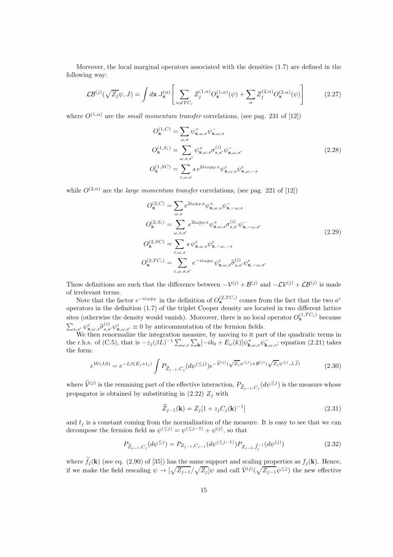
Moreover, the local marginal operators associated with the densities (1.7) are defined in thefollowing way:

LB(j)(√Zjψ, J) =

∫dx J (α)

x

[ ∑

α6=TCi

Z(1,α)j O(1,α)

x (ψ) +∑

α

Z(2,α)j O(2,α)

x (ψ)

](2.27)

where O(1,α) are the small momentum transfer correlations, (see pag. 231 of [12])

O(1,C)x =

∑

ω,s

ψ+x,ω,sψ

−x,ω,s

O(1,Si)x =

∑

ω,s,s′

ψ+x,ω,sσ

(i)s,s′ψ

−x,ω,s′ (2.28)

O(1,SC)x =

∑

ε,ω,s

s e2iεωpF xψεx,ω,sψεx,ω,−s

while O(2,α) are the large momentum transfer correlations, (see pag. 221 of [12])

O(2,C)x =

∑

ω,s

e2iωpF xψ+x,ω,sψ

−x,−ω,s

O(2,Si)x =

∑

ω,s,s′

e2iωpF xψ+x,ω,sσ

(i)s,s′ψ

−x,−ω,s′

(2.29)

O(2,SC)x =

∑

ε,ω,s

s ψεx,ω,sψεx,−ω,−s

O(2,TCi)x =

∑

ε,ω,s,s′

e−iεωpFψεx,ω,sσ(i)s,s′ψ

εx,−ω,s′

These definitions are such that the difference between −V(j) +B(j) and −LV(j) +LB(j) is madeof irrelevant terms.

Note that the factor e−iεωpF in the definition of O(2,TCi)x comes from the fact that the two aε

operators in the definition (1.7) of the triplet Cooper density are located in two different lattice

sites (otherwise the density would vanish). Moreover, there is no local operator O(1,TCi)x because∑

s,s′ ψεx,ω,sσ

(i)s,s′ψ

εx,ω,s′ ≡ 0 by anticommutation of the fermion fields.

We then renormalize the integration measure, by moving to it part of the quadratic terms inthe r.h.s. of (C.5), that is −zj(βL)−1

∑ω,s

∑k[−ik0 +Eω(k)]ψ

+k,ω,sψ

−k,ω,s; equation (2.21) takes

the form:

eW(J,0) = e−Lβ(Ej+tj)

∫PZj−1,Cj

(dψ(≤j))e−V(j)(√Zjψ

≤j)+B(j)(√Zjψ

≤j ,J,J) (2.30)

where V(j) is the remaining part of the effective interaction, PZj−1,Cj(dψ≤j) is the measure whose

propagator is obtained by substituting in (2.22) Zj with

Zj−1(k) = Zj [1 + zjCj(k)−1] (2.31)

and tj is a constant coming from the normalization of the measure. It is easy to see that we candecompose the fermion field as ψ(≤j) = ψ(≤j−1) + ψ(j), so that

PZj−1,Cj(dψ≤j) = PZj−1,Cj−1(dψ

(≤j−1))PZj−1,f−1j

(dψ(j)) (2.32)

where fj(k) (see eq. (2.90) of [35]) has the same support and scaling properties as fj(k). Hence,

if we make the field rescaling ψ → [√Zj−1/

√Zj ]ψ and call V(j)(

√Zj−1ψ

≤j) the new effective

15

potential, we can write the integral in the r.h.s. of (2.30) in the form∫PZj−1,Cj−1(dψ

(≤j−1))

∫PZj−1,f

−1j

(dψ(j))e−V(j)(√Zj−1ψ

(≤j))+B(j)(√Zj−1ψ

(≤j),J,J)

By performing the integration over ψ(j), we finally get (2.21), with j − 1 in place of j. In orderto analyze the result of this iterative procedure, we note that LV(j)(ψ) can be written as

LV(j)(ψ) = γjνjFν(ψ) + δjFα(ψ) + g1,jF1(ψ) + g2,jF2(ψ) + g4,jF4(ψ) (2.33)

where νj = (√Zj/

√Zj−1)nj , δj = (

√Zj/

√Zj−1)(aj − zj) and gi,j = (

√Zj/

√Zj−1)

2li,j ,i = 1, 2, 4, are called the running coupling constants (r.c.c.) on scale j.

In Theorem (3.12) of [35] it is proved that the kernels of V(j) and B(j) are analytic as functionsof the r.c.c., provided that they are small enough. One has then to analyze the flow of the r.c.c.(the beta function) as j → −∞. We shall now summarize the results, following §4 and §5 of [24]with some improvement.

2.3 The flow of the running coupling constants

Define vector notations for the r.c.c.,

~vh ≡ (v1,h, v2,h, v4,h, vδ,h, vν,h) = (g1,h, g2,h, g4,h, δh, νh) ≡ (~gh, δh, νh) . (2.34)

The r.c.c. satisfy a set of recursive equations, which can be written in the form

vα,j−1 = Aαvα,j + β(j)α (~vj ; ..., ~v0;λ, ν) (2.35)

with Aν = γ, Aα = 1 for α 6= ν. These equations have been already analyzed in [24], where ithas been proved that, if λ is real positive and small enough, then it is possible to choose ν sothat, fixed ϑ < 1, |νh| ≤ Cλγϑh, ∀h ≤ 0, and 0 < g1,h < λ(1 + aλ|h|)−1, for some a > 0, whilethe other r.c.c. stay bounded by Cλ and converge for h→ −∞. In this paper, in order to proofBorel summability of perturbation theory, we extend the proof to complex values of λ, restrictedto the set Dε,δ defined in (1.30); this implies that we need an analysis a bit more precise of theflow equations (2.35).

To begin with, we put ν1 ≡ ν and we suppose that the sequence νhh≤1 are known functionsof λ, analytic in Dε,δ, such that

|νh| ≤ C|λ|γϑh , h ≤ 1 (2.36)

and study the flow equations of the other variables. The idea is that this restricted flow hasproperties such that, by a fixed point argument, the sequence νhh≤1, satisfying the last equa-tion of (2.35), can be uniquely determined. Since this point can be treated in the same way asin spinless case (see §4.3 of [35]), we shall give for granted this result. Hence, from now on, weshall define vj = (g1,j , g2,j, g4,j , δj) and we shall consider the restriction of (2.35) to vj .

The next step is to extract from the functions β(j)α the leading terms for j → −∞. Observe

that the propagator g(j)ω of the single scale measure PZj−1,f

−1j

, can be decomposed as

g(j)ω (x) =1

Zjg(j)D,ω(x) + r(j)ω (x) (2.37)

where g(j)D,ω is the Dirac propagator (with cutoff) and describes the leading asymptotic behavior

g(j)D,ω(x) :=

1

βL

∑

k∈DL,β

e−ikxfj(k)

−ik0 + ωvFk, (2.38)

16

while the remainder r(j)ω satisfies, for any q > 0 and 0 < ϑ < 1, the bound

|r(j)ω (x)| ≤ γ(1+ϑ)j

Zj

Cq,ϑ1 + (γj |x|)q . (2.39)

Let us now call ZD,j the values of Zj one would obtain by substituting V(0) with LV(0) in (2.18)

and by using for the single scale integrations the propagator (2.37) with r(i)ω (x) ≡ 0 for any i ≥ j.

It can be proved by an inductive argument, see §4 of [35], that, if all the r.c.c. stay of order λ,

∣∣∣∣ZjZj−1

− ZD,j

ZD,j−1

∣∣∣∣ ≤ Cε2jγϑj (2.40)

whereεj = max|λ|, max

0≥h≥j|~gh|, max

0≥h≥j|δh| .

It is then convenient to decompose the functions β(j)α as

β(j)α (~vj ; ..., ~v0;λ, ν) = β(j)

α (vj , ...,v0) + β(j)α (~vj ; ..., ~v0;λ) (2.41)

where β(j)α (vj , ...,v0) is given by the sum of all trees containing only endpoints with r.c.c. δh, ~gh,

0 ≥ h ≥ j, modified so that the propagators g(h)ω and the wave function renormalizations Zh,

0 ≥ h ≥ j, are replaced by g(h)D,ω and ZD,h; β

(j)α contains the correction terms together with the

remainder of the expansion.

Lemma 2.2

|β(j)α (~vj ; ..., ~v0;λ)| ≤

Cε2jγ

ϑj if α 6= δ

(c ε0 + Cε2j )γϑj if α = δ

(2.42)

As showed in [24], this lemma is basically a consequence of (2.40) and (2.36). Therefore the

leading term in (2.41) is β(j)α , that we further decompose as

β(j)α (vj , ...,v0) = β(j)

α (vj) + rα,j(vj , ...,v0) (2.43)

where β(j)α (v) = β

(j)α (v, ...,v). We can write:

β(j)α (vj) =

∑

i=0,1

b(j)α,i(vj) + b

(j)α,≥2(vj) (2.44)

where b(j)α,i(vj) is the contribution of order i in g1,j, wile b

(j)α,≥2(vj) is the contributions of all trees

with at least two endpoints of type g1. The crucial property is the following lemma.

Lemma 2.3 (partial vanishing of the beta function)

|b(j)α,i(vj)| ≤ Cε2jγϑj , i = 0, 1 (2.45)

The above property was proven in §5.3 of [24], extending the proof for the spinless case in

[37, 23], and it will be reviewed in App. C. Now, let us extract from β(j)α (vj) the second order

contributions, which all belong to b(j)α,≥2(vj); we get:

β(j)α (vj) = −aαg21,j +

∑

i=0,1

b(j)α,i(vj) + rα,j(vj) (2.46)

17

with a1 = a > 0, a2 = a/2, a4 = aδ = 0, and, for some b1 > 0,

|rα,j(vj)| ≤ b1εj |g1,j|2 . (2.47)

In the limit L, β = ∞, if g(≥h)D,ω ≡ ∑0

j=h g(j)D,ω,

a = 2 limh→−∞

1

|h|

∫dk

(2π)2g(≥h)D,+ (k)g

(≥h)D,− (k) =

log γ

πvF(2.48)

Let us now analyze in more detail the functions r(j)α (vj , ...,v0), which appear in (2.43). If we

define, for j′ ≥ j + 1,

D(j,j′)α (vj , ...,v0) = β(j)

α (vj , ...,vj ,vj′ , ...,v0)− β(j)α (vj , ...,vj ,vj , ...,v0) (2.49)

we can decompose r(j)α (vj , ...,v0) in the following way:

rα,j(vj , ...,v0) =

0∑

j′=j+1

D(j,j′)α (vj , ...,v0) (2.50)

Note that D(j,j′)α (vj , ...,v0) is obtained from β

(j)α (vj , ...,v0), by changing the values of the r.c.c.

in the following way: the r.c.c. associated to endpoints of scales lower than j′ are put equal tothe corresponding r.c.c. of scale j; those of scale greater than j′ are left unchanged; at leastone of the r.c.c. vr,j′ is substituted with vr,j′ − vr,j . By using the short memory property (seee.g. (4.31) of [35]), we can show that , if εj is small enough,

|D(j,j′)α (vj , ...,v0)| ≤ b3εjγ

−(j′−j)ϑ|vj′ − vj | (2.51)

for some b3 > 0. If we insert in the flow equation (2.35) the equations (2.41), (2.43), (2.46),(2.50) and use the bounds (2.42), (2.45), (2.47) and (2.51), we get, if εj is small enough,

|vj−1 − vj | ≤ (a+ b1εj)|g1,j |2 + (c ε0 + b2ε2j)γ

ϑj + b3εj

0∑

j′=j+1

γ−ϑ(j′−j)|vj′ − vj | (2.52)

for some b2 > 0. The form of this bound implies that, in order to control the flow, it is sufficientto prove that g1,j goes to 0 as j → −∞ so fast that |g1,j |2 is summable on j. Hence, we have tolook more carefully to the flow equation of gi,j . By proceeding as before, we can write

g1,j−1 = g1,j − ag21,j + r1,j + r1,j + r1,j (2.53)

|r1,j | ≤ b2ε2jγϑj , |r1,j | ≤ b1εj|g1,j |2 , |r1,j | ≤ b3εj

0∑

j′=j+1

γ−ϑ(j′−j)|vj′ − vj | (2.54)

It is easy to show that, if ε0 is small enough, there is a constant c4, such that, if g1,0 ∈ Dε0,δ

and c4|j0||g1,0|2 ≤ |g1,0|2−η, η < 1, then, for j ≥ j0,

g1,j ∈ D2ε0,δ/2 , |g1,0|/2 ≤ |g1,j| ≤ 2|g1,0| , εj ≤ 2ε0 (2.55)

Hence we put j0 = −(c4|g1,0|1/2)−1 and suppose ε0 so small that

εj0γϑ2 j0 ≤ 2c5|g1,j0 |γ

ϑ2 j0 ≤ |g1,j0 |3 (2.56)

where we also used the fact that, since v(2pF ) > 0, ε0 ≤ c5|g1,0|, for some constant c5.

18

Lemma 2.4 If g1,0 ∈ Dε0,δ and j ≥ j0, then, if ε0 is small enough,

|vj−1 − vj | ≤ 2a|g1,j|2 + 2cε0γϑ2 j (2.57)

Proof - We shall proceed by induction. By (2.55), if ε0 is small enough, c ε0 + b2ε2j ≤ (3/2)c ε0

and a + b1εj ≤ 3a/2; hence, (2.57) is true for j = 0. Let us suppose that (2.57) is verified forj > h > 0. By (2.55), if j ≥ h ≥ j0, |g1,j |/|g1,h| ≤ 4; hence, by using (2.52) and (2.57), we get:

|vh−1 − vh| ≤ (3/2)a|g1,h|2 + (3/2)c ε0γϑh+

b3εh

0∑

j=h+1

γ−ϑ(j−h)(j − h) maxh<j′≤j

[2a|g1,j′ |2 + 2cε0γ

ϑ2 j

′]

≤ |g1,h|2[(3/2)a+ 64ab3ε0

∞∑

n=0

n γ−ϑn

]+ γ

ϑ2 hε0

[(3/2)c+ 4cb3ε0

∞∑

n=0

nγ−ϑ2 n

]

Hence, (2.57) is verified also for j = h, if ε0 is small enough.

The previous analysis implies that the flow is essentially trivial up to values of j of order|g1,0|−1/2 (or even |g1,0|−η, 0 < η < 1). If j ≤ j0, we write (2.53) in the form

g1,j−1 = g1,j − aj g21,j , aj ≡ a− r1,j + r1,j + r1,j

g21,j(2.58)

and we define Aj0 = 0 and, for j < j0,

Aj =1

j0 − j

j0∑

j′=j+1

aj′ g1,j =g1,j0

1 +Ajg1,j0(j0 − j)(2.59)

Lemma 2.5 There are constants c1, c2, c3 such that, if g1,0 ∈ Dε0,δ and it ε0 is small enough,then the following bounds are satisfied, for all j < j0.

εj ≤ c3ε0 (2.60)

|vj − vj+1| ≤ c1|g1,j+1|2 (2.61)

|g1,j − g1,j | ≤ |g1,j |3/2 (2.62)

|aj − a| ≤ c2|g1,j0 | (2.63)

Proof - We shall proceed by induction. By using (2.56), (2.57) and (2.55), we see that thebounds (2.60) and (2.61) are satisfied for j = j0, if c3 ≥ 2, c1 ≥ 3a and 4cε0 ≤ a. Moreover,g1,j0 = g1,j0 and, by proceeding as in the proof of Lemma 2.4 and using (2.56), it is easy to provethat there is a constant c2, such that

|aj0 − a| ≤ c2|g1,j0 |

Hence, all the bounds are verified (for ε0 small enough) for j = j0, if c1 ≥ 3a, c2 ≥ c2 and c3 ≥ 2.Suppose that they are verified for j0 ≥ j ≥ h.

The validity of (2.62) for j = h − 1 follows from Prop. A.2, which only rests on the bound(2.63) for j ≥ h. On the other hand, (2.62) implies that, if ε0 is small enough, 2−1|g1,j| ≤ |g1,j | ≤2|g1,j|; hence, using (2.59), we get, for j > h

∣∣∣∣g1,jg1,h

∣∣∣∣ ≤ 4|1 +Ahg1,j0(j0 − h)||1 +Ajg1,j0(j0 − j)| (2.64)

19

Let us now define, as in App. A, Aj = αj + iβj , αj = ℜAj , and suppose that

2c2ε0 ≤ a/2 (2.65)

so that, by (2.55), αj ≥ a/2, |βj | ≤ 2c2ε0, |Aj | ≤ 3a/2, for j > h. By proceeding as in theproof of the bound (A.8) in App. A, we get, if j > h and |Arg g1,0| ≤ π − δ, δ > 0 (so that|Arg g1,j0 | ≤ π − δ/2, see (2.55)),

|1 + g1,j0αj(j0 − j)| ≥ 1

3sin(δ/2)[1 + |g1,j0 |αj(j0 − j)]

and, if we put 1 +Ajg1,j0(j0 − j) = 1 + αjg1,j0(j0 − j) + wj , we choose ε0 so that

|wj ||1 + g1,j0αj(j0 − j)| ≤

6c2ε0|g1,j0 |(j0 − j)

sin(δ/2)|g1,j0 |(a/2)(j0 − j)=

12c2ε0a sin(δ/2)

≤ 1

2(2.66)

Then, by using (2.64), we get∣∣∣∣g1,jg1,h

∣∣∣∣ ≤24

sin(δ/2)

1 + (3a/2)|g1,j0|(j0 − h)|1 + (a/2)|g1,j0 |(j0 − j)| ≤ Cδ(j − h) (2.67)

for some constant Cδ, only depending on δ and a. Moreover, since εh ≤ c3ε0, then c ε0 + b2ε2h ≤

2c ε0 and a+ b1εj ≤ 2a, ifb2c

23ε0 ≤ c , and b1c3ε0 ≤ a (2.68)

Hence, by using the bounds (2.52), (2.61), (2.56) and (2.67), we get

|vh−1 − vh| ≤ 2a|g1,h|2 + 2c ε0γ−ϑ(j0−h)|g1,j0 |2 + c1b3εh

0∑

j=h+1

γ−ϑ(j−h)(j − h) maxh<j′≤j

|g1,j′ |2

≤ |g1,h|2[2a+ 2c ε0C

2δ maxn≥0

γ−nϑn2 + c1εhb3C2δ

∞∑

n=0

γ−ϑnn3

]

It follows that (2.61) is satisfied also for j = h, if

2a+ 2c ε0C2δ maxn≥0

γ−nϑn2 + 2c1c3ε0b3C2δ

∞∑

n=0

γ−ϑnn3 ≤ c1 (2.69)

Moreover, by using (2.61) and |g1,j | ≤ 2|g1,j|, we get, for some b4 > 0, only depending on a,under the condition (2.65):

εh−1 ≤ ε0 +

0∑

j=h

|vj−1 − vj | ≤ ε0 + b4c1ε0

so that εh−1 ≤ c3ε0, if1 + b4c1 ≤ c3 (2.70)

The bound for ah−1 − a can be done in the same way; it is easy to see that

|ah−1 − a| ≤[b1c3 + b2c

23ε0C

2δ maxn≥0

γ−nϑn2 + 2c1c3b3C2δ

∞∑

n=0

γ−ϑnn3

]ε0 (2.71)

Hence, (2.63) is verified for j = h− 1, if

c2 ≡ 2c C2δ maxn≥0

γ−nϑn2 + 2c1c3b3C2δ

∞∑

n=0

γ−ϑnn3 ≤ c2 (2.72)

20

The conditions (2.65), (2.66), (2.68), (2.69), (2.70) and (2.72) can be all satisfied, by taking, for

example, c1 = 4a, c3 = 1 + 4ab4 and c2 = maxc2, c2, if ε0 is small enough.

Lemma 2.5 implies that, if g1,0 ∈ Dε,δ, with ε small enough (how small depending on δ), g1,jgoes to 0, as j → −∞, and

∑0j=h |g1,j |2 ≤ Cδ−1|λ|, uniformly in h. This is an easy consequence

of the condition (2.62) and the condition v(2pF ) > 0; note that the power 3/2 in the r.h.s. of(2.62) could be replaced 2 − η, η > 0, but 2 is not allowed. The form of the flow (2.35) thenimplies also that g2,j, g4,j and δj converge, as j → −∞, to some limits g2,−∞, g4,−∞ and δ−∞

of order λ, such that

g2,−∞ = g2,0 −1

2g1,0 +O(|λ|3/2) = [2v(0)− v(2pF )]λ+O(|λ|3/2) (2.73)

g4,−∞ = g4,0 +O(λ2) = 2λv(0) +O(λ2)

δ−∞ = O(λ) (2.74)

Let us now suppose that λ is a (small) positive number; the previous bounds imply that g1,j > 0,for any j ≤ 0. The following Lemma will allow to control the logarithmic corrections to the powerlaw fall-off of the correlations.

Lemma 2.6 There are four sequences wi,h, δi,h, i = 1, 2, h ≤ j0, such that

j0∑

j=h

g1,j = (1 + w1,h)1

alog[1 + ag1,j0(j0 − h)] + δ1,h (2.75)

j0∑

j=h

[g2,j − g2,−∞

]= (1 + w2,h)

1

2alog[1 + ag1,j0(j0 − h)] + δ2,h (2.76)

with|wi,h| ≤ Cλ , |δi,h| ≤ Cλ1/2 (2.77)

|wi,h−1 − wi,h| ≤Cλ

[1 + ag1,j0(j0 − h)] log[1 + ag1,j0(j0 − h)](2.78)

Proof - Let us put g0 = g1,j0 , and a(s) the function of s ≥ 0, such that a(s) = aj0−n, ifn ≤ s < n+ 1. Then, by using (2.59), (2.62) and (2.63), it is easy to see that

∣∣∣∣∣∣

j0∑

j=h

g1,j − Ij0−h

∣∣∣∣∣∣≤ Cλ1/2 , In =

∫ n

0

dsg0

1 + g0∫ s0 dt a(t)

(2.79)

On the other hand, (2.63) also implies that a(s) = a+ λr(s), with |r(s)| ≤ C; hence

In =

∫ n

0

dsg0

1 + g0as− λ

∫ n

0

dsg20

∫ s0dt r(t)

[1 + g0∫ s0 dt a(t)][1 + g0as]

implying that∣∣∣∣In − 1

alog(1 + ag0n)

∣∣∣∣ ≤4Cλ

a2

∫ ag0n

0

dxx

(1 + x)2<

4Cλ

a2log(1 + ag0n)

Hence there is a constant wn such that In = (1/a + wn) log(1 + ag0n), with |wn| ≤ Cλ; thisbound, together with the bound in (2.79), proves (2.77) for i = 1. To prove (2.78), note that

|In+1 − In| ≤∫ n+1

n

dsg0

1 + g0a2 s

=2

alog

(1 +

ag02 + ag0n

)

21

In+1 − In = (1/a+ wn+1) log

(1 +

ag01 + ag0n

)+ (wn+1 − wn) log(1 + ag0n)

so that, if λ is small enough,

|wn+1 − wn| log(1 + ag0n) ≤(3

a+ Cλ

)log

(1 +

ag01 + ag0n

)≤ 4g0

1 + ag0n

To prove (2.77) and (2.78) for i = 2, note that, by (2.46) and Lemma 2.5, if j ≤ j0,

g2,j − g2,−∞ =

j∑

h=−∞

[a2+O(λ)

]g21,h =

[a2+O(λ)

] ∫ ∞

|j|

dsg20

(1 + ag0s)2+O(g

3/21,j )

=

[1

2+O(λ)

]g1,j +O(g

3/21,j )

Hence, the proof of (2.77) is almost equal to the previous one, while the proof of (2.78) needs a

slightly different algebra; we omit the details.

2.4 The flow of renormalization constants

The renormalization constant of the free measure satisfies

Zj−1

Zj= 1 + β(j)

z (~gj , δj , ..., ~g0, δ0) + β(j)z (~vj ; .., ~v0;λ) ; (2.80)

while the renormalization constants of the densities, for α = C, Si, SC, TCi and i = 1, 2, satisfythe equations

Z(i,α)j−1

Z(i,α)j

= 1 + β(j)(i,α)(~gj, δj , ..., ~g0, δ0) + β

(j)(i,α)(~vj ; .., ~v0;λ) . (2.81)

In these two formulas, by definition, the β(j)t functions, with t = z or (i, α), are given by a sum

of multiscale graphs, containing only vertices with r.c.c. ~gh, δh, 0 ≥ h ≥ j, modified so that

the propagators g(h)ω and the renormalization constants Zh, Z

(i,α)h , 0 ≥ h ≥ j, are replaced by

g(h)D,ω, Z

(D)h , Z

(D,i,α)h (the definition of Z

(D,i,α)h is analogue to the one of Z

(D)h ); the β

(j)t functions

contain the correction terms together the remainder of the expansion. Note that, by definition,

the constants Z(D)j are exactly those generated by (2.80) and (2.41) with β

(j)z = β

(j)α = 0. Note

also that |β(j)z | ≤ Cv2jγ

ϑj , while |β(j)(i,α)| ≤ Cvjγ

ϑj .

By using (2.80) and (2.81), we can write

Z(1,α)j−1

Zj−1=Z

(1,α)j

Zj

[1 + β

(j)z,(1,α)(~gj , δj) + β

(j)z,(1,α)(~vj ; .., ~v0;λ)

](2.82)

with |βz,(1,α)| ≤ Cvjγϑj . If we define β

(j)z,(1,α)(~g, δ) the value of β

(j)z,(1,α)(~gj, δj ; ...;~g0, δ0) at

(~gi, δi) = (~g, δ), j ≤ i ≤ 0 and β(j,≤1)z,(1,α)(~g, δ) the sum of its terms of order 0 and 1 in g1,h, it

turns out that

|β(1)(j)1,α (~gj , δj)| ≤ C[max|g1||g2|, |g4|, |δ|]2γϑh , if α = C (2.83)

22

This bound, as crucial as the analogous bound (2.45), has been proved in [33]; the proof will

be sketched in App. C. The bound (2.83), together with∑0

k=j |g1,k|2 ≤ C|λ| and the fact that

Z(1,Si)h = Z

(1,C)h by the SU(2) spin symmetry, imply that

∣∣∣∣∣Z

(1,α)j

Zj− 1

∣∣∣∣∣ ≤ C|ε2j | , α = C, Si (2.84)

Regarding the flow of the other renormalization constants, we can write

Z(t)j = γ−ηtjZ

(t)j (2.85)

where Z(z)j = Zj and, by definition,

ηt ≡ limj→−∞

ηt,j := logγ

[1 + β

(0,j)t (g2,−∞, g4,−∞, δ−∞; ...; g2,−∞, g4,−∞, δ−∞)

](2.86)

Note that the exponents ηt are functions of ~v−∞ only, an observation which will play a crucialrole in the following. Moreover, by an explicit first order calculation, we see that

ηt =

(2πvF )−1g2,−∞ +O(λ2) t = (2, C), (2, Si)

−(2πvF )−1g2,−∞ +O(λ2) t = (2, SC), (2, TCi)

O(λ2) otherwise

(2.87)

while

Z(t)h−1

Z(t)h

= 1 +O(g1,hλ) + r(t)h , t = z, (1, α), α 6= TCi

Z(2,C)h−1

Z(2,C)h

= 1− ag1,h +a

2(g2,h − g2,−∞) +O(g1,hλ) + r

(2,C)h

Z(2,Si)h−1

Z(2,Si)h

= 1 +a

2(g2,h − g2,−∞) + O(g1,hλ) + r

(2,Si)h (2.88)

Z(2,SC)h−1

Z(2,SC)h

= 1− a

2g1,h −

a

2(g2,h − g2,−∞) +O(g1,hλ) + r

(2,SC)h

Z(2,TCi)h−1

Z(2,TCi)h

= 1 +a

2g1,h −

a

2(g2,h − g2,−∞) +O(g1,hλ) + r

(2,TCi)h

where a and g1,h are defined as in (2.48) and (2.59), respectively, and∑0h=−∞ |r(t)h | ≤ C|λ|2.

Let us define:

q(h)t =

log Z(t)h

log(1 + ag1,0|h|)(2.89)

Hence, by using (2.75), (2.76) and (2.77), we get

|q(h)t | ≤ Cλ , t = z, (1, α), α 6= TCi

|q(h)t − 1

2ζα| ≤ Cλ , t = (2, α)

(2.90)

where the constants ζα are those of (1.20).

23

2.5 Proof of Theorem 1.1

In order to prove the representation (1.19) of the density correlations Ωα(x), we can proceedexactly as in §5 of [35], where a similar problem was treated in all details; hence we shall onlydescribe the result. We can write for Ωα(x − y) a convergent tree expansion, whose trees havetwo endpoints associated to density operators (special endpoints) and an arbitrary number ofinteraction endpoints (normal endpoints). As one could expect, Ωα(x−y) behaves, as |x−y| →∞, as the function Ωα(x − y) calculated by taking only the trees with two special endpoints ofscale h ≤ 0 and no normal endpoints. This function can be obtained by the following procedure.Let us consider the expression

〈O(1,α)x ;O(1,α)

y 〉TD + 〈O(2,α)x ;O(2,α)

y 〉TD

where the operators O(i,α)x , i = 1, 2, are those defined in (2.28) and (2.29) and 〈 · 〉TD is the

truncated expectation evaluated with covariance∑

h Z−1h g

(h)D,ω. Hence, this expression can be

written as a sum of terms, each one proportional to Z−1h g

(h)D,ω(x− y) Z−1

h′ g(h′)D,ω′(x− y), for some

values of h, h′, ω and ω′. Ωα(x − y) is obtained by multiplying each one of these terms by

[Z(1,α)h∨h′ ]2 (h ∨ h′ = maxh, h′), if it appears in the calculation of 〈O(1,α)

x O1,αy 〉TD, otherwise by

[Z(2,α)h∨h′ ]2. Let us consider first the case α = C; we have

ΩC(x) = Ω(1,C)(x) + cos(2pFx)Ω(2,C)(x)

Ω(1,C)(x) = 2∑

ω

∑

h,h′

[Z(1,C)h∨h′ ]2

ZhZh′

g(h)D,ω(x)g

(h′)D,ω(x) (2.91)

Ω(2,C)(x) = 4∑

h,h′

[Z(2,C)h∨h′ ]2

ZhZh′g(h)D,+(x)g

(h′)D,−(x)

Let us now observe that, for any N > 0, |g(h)D,ω(x)| ≤ CNγh[1 + (γh|x|)N ]−1. Hence, if |x| ≥ 1,

in the previous sums the main contribution is given by the terms with |h| and |h′| of the samesize as logγ |x|, so that one expects that the asymptotic behavior of Ω(i,C)(x), i = 1, 2, is the

same of the the function Ω(i,C)(x), obtained by the substitutions of γ−h and γ−h′

with |x| inthe asymptotic expressions of the renormalization constants, given by (2.85) and (2.88), that is

[Z(i,C)h∨h′ ]2

ZhZh′

→ |x|2(ηi,C−ηz)[1 + f(λ) log |x|

]2(q(hx)i,C

−q(hx)z

)

(2.92)

where the coefficients q(h)t are defined as in (2.89), hx = infh : γh|x| ≥ 1, and, by (2.26),

(2.48), (2.59) and Lemma 2.6,

f(λ) =ag1,j0log γ

=2λv(2pF )

πvF+O(λ3/2) (2.93)

In order to justify the substitution (2.92), let us put ηi = 2(ηi,C − ηz) and qi(x) any continuous

interpolation between 2[q(hx)i,C − q

(hx)z ] and 2[q

(hx−1)i,C − q

(hx−1)z ]. Note that, thanks to the bounds

(2.77) and (2.78), qi(x) is a bounded function of order λ, defined up to fluctuations bounded,for |x| ≥ 1, by Cλ[L(x) logL(x)]−1, with L(x) = 1 + f(λ) log |x|; hence, its precise definition

24

modifies the following expressions only for a factor 1 +O(λ). Let us now note that

|Ω(i,C)(x)− Ω(i,C)(x)| ≤ CN |x|ηi−2[1 + f(λ) log |x|]qi(x)∑

h,h′

γh|x|1 + (γh|x|)N

γh′ |x|

1 + (γh′ |x|)N ·

·

∣∣∣∣∣∣(γh|x|)ηz (γh′ |x|)ηz(γh∨h′ |x|)2ηi,C

[L(|x|)L(γ|h|)

]q(h)z

[L(|x|)L(γ|h′|)

]q(h′)z

[L(|x|)

L(γ|h∨h′|)

]−2q(h∨h′)i,C chch′

c2h∨h′

− 1

∣∣∣∣∣∣(2.94)

whereL(t) = 1 + f(λ) log t , ch = L(γ|h|)q

(h)z /Z

(z)h , ch = L(γ|h|)−q

(h)i,C/Z

(i,C)h

By (2.88), (2.75) and (2.76), ch = 1+O(λ1/2) and ch = 1+O(λ1/2). On the other hand, if r > 0and t 6= 0,

|rt − 1| ≤ |t log r|(rt + r−t)

and, if q 6= 0,

∣∣∣∣[L(|x|)L(γ|h|)

]q− 1

∣∣∣∣ ≤ Cq

[|f(λ) log(γh|x|)|+ |f(λ) log(γh|x|)||q|+1

]

These two bounds, together with the bound

0∑

h=−∞

(γhr)α| log(γhr)|β1 + (γhr)N

≤ CN,α,q

valid for any β, r > 0, a > 0 and N > α, imply that

|Ω(i,C)(x) − Ω(i,C)(x)| ≤ CNλ1/2|x|ηi−2[1 + f(λ) log |x|]qi(x) (2.95)

By the remark after (2.59), the factor λ1/2 can be improved up to λ1−ϑ, ϑ < 1.By proceeding as in §5 of [35], it is possible to prove that a bound of this type is satisfied also

from the sum over all the other trees. Hence, in order to complete the proof of (1.19) in the caseα = C, we have only to calculate Ω(1,C)(x) and Ω(2,C)(x). By using (2.84), we see that η1,C = ηz

and q(h)1,C = q

(h)z , so that, if we define XC = 1− η2,C − ηz and ζC(x) = 2[q2,C(x)− qz(x)], we get

Ω(1,C)(x) = 2∑

ω

gD,ω(x)gD,ω(x)

Ω(2,C)(x) = 4|x|2(1−XC)[1 + f(λ) log |x|]ζC(x)gD,+(x)gD,−(x)

(2.96)

where gD,ω(x) =∑0

h=−∞ g(h)D,ω(x). On the other hand, it is easy to see that, for any N ≥ 2,

gD,ω(x) =1

2π

1

vFx0 + iωx+O(|x|−N )

It follows that, up to terms that we put in the “remainder” RC(x),

Ω(1,C)(x) =1

π2x2Ω0(x) , Ω(2,C)(x) =

L(x)ζC(x)

π2|x|2XC(2.97)

where the functions Ω0(x) and L(x) are defined as in Theorem 1.1. Hence, by using (2.87) and(2.93), we get (1.19) for α = C, together with the fact that ζC(x) = −3/2+O(λ), in agreementwith (1.20), and 2XC = 2 − bλ+ O(λ2), in agreement with (1.22). Note also that, in Theorem

25

1.1, we have modified the function f(λ) by erasing the terms of order greater than 1 in λ; theonly effect of this modification is a change of the function RC(x), which does not change itsbound.

The proof of (1.19) in the other cases is done in the same way. In particular, in the case α = Siwe have to use again the bound (2.84), while the fact that there is no oscillating contribution tothe leading term of ΩTCi

is due to the fact there is no local marginal term which can produceit, by the remark after §2.29.

Finally, the proof of the scaling relations (1.22) follows from the important fact, proved in§3.6, that they are the same as those of the effective model. Hence they follow from the explicitcalculations of §3.5.

2.6 Proof of Theorem 1.4

First consider the free energy (1.4), We can decompose it as E(λ) =∑0h=−∞Eh(λ), where

Eh(λ) is the contribution of the trees whose root has scale h, hence depends only on the runningcouplings ~vj with scale j > h. The tree expansion implies that there exists ε0, such that, if

λh = maxj≥h

|~vj | ≤ ε0 (2.98)

then |Eh| ≤ c2γ2hε0, with c2 independent of h. The analysis of §2.3 implies that, given δ ∈

(0, π/2), there exists ε such that, if λ ∈ Dε,δ, the condition (2.98) is verified uniformly in h;then it is easy to see that E(λ) is analytic in Dε,δ and continuous in its closure. The domainof analyticity of Eh(λ) is in fact larger; the form of the beta function immediately implies thatthere exist two constants c3 and c such that λ0 ≤ c3|λ| and, if λh ≤ ε0, then λh−1 ≤ λh + cλ2h;hence, if c3|λ| ≤ minε0/2, 1/[4c(|h|+ 1)], then, if j > h and λj ≤ 2λ0,

λj−1 ≤ λ0 + |j|cλ2j ≤ λ0(1 + 4|j|cλ0) ≤ 2λ0

It follows that Eh(λ) is analytic in the set (1.31), with c0 = c−13 minε0/2, 1/(4c), and that

|Eh(λ)| ≤ c1γ2h, with c1 = c2ε0; hence E(λ) satisfies (1.32) with κ = 2 log γ.

Let us now consider the 2-point Schwinger function S2(x). By using the tree expansion(similar to that written in [20] for the infrared part of the spinless continuous Fermi gas), we

can write S2(x) =∑0

h=−∞ S2,h(x), where S2,h(x) is the contribution of the trees whose root hasscale h. By proceeding as in §6 of [20], we can prove that, if (2.98) is verified (possibly with asmaller ε0), then, for any N > 0,

|S2,h(x)| ≤ cN

0∑

h=h+1

γ−h−h

2γh

Zh

1

1 + (γh|x|)N ,

∣∣∣∣1

Zh

∣∣∣∣ ≤ γ|h|4 (2.99)

with cN independent of h. Hence, if we define hx so that γhx |x| ∈ [1, γ), then, if hx > h

|S2,h(x)| ≤ c2

hx∑

h=h+1

γ−h2 γ

34 hγ

h2 +

0∑

h=hx

γ−h2 γ

34 hγ

h2 γ2(hx−h)

≤ c2 γ

h2 γ

hx

4 (2.100)

and a similar bound holds for hx < h so that

|S2,h(x)| ≤ csγh2 (1 + |x|)−1/4 (2.101)

and we can proceed as in free energy case, so proving (1.32) for S2(x), with c1 = cs(1 + |x|)−1/4

and κlog γ = 1

2 (this value could be improved up to any value smaller than 1, at the price of

lowering ε0 down to 0).

26

The previous argument can be extended to the generic 2n-point Schwinger function, by usingthe same strategy used in §2.3 of [38] to analyze the corresponding tree expansion in the caseof the Thirring model. The proof of the Theorem in the case of the density correlations is verysimilar to that of the 2-point function case, if one uses the description of the tree expansion givenin §5 of [35]. We shall not give any further detail; the idea at the base of the proof is alwaysthat, in the tree expansion of the correlations at fixed space-time points, the contribution of thetrees with the root at scale h must decrease exponentially with the distance from some fixedscale depending on the space-time points.

3 RG Analysis of the Effective Model

3.1 Introduction

We introduce an effective model (related to the g-ology model introduced in [12] but differingbecause the interaction is time-dependent), describing fermions with linear dispersion relationand a non-local interaction; such model will be used to prove the crucial bounds (2.45) and (2.83)(on which the previous analysis is based) and for the proof of the Luttinger liquid relations (1.22),together with Theorems 1.2 and 1.3. The model is expressed in terms of the following Grassmannintegral:

eW[l,N ](φ,J) =

∫PZ(dψ

[l,N ]) exp

−V (

√Zψ[l,N ]) +

∑

ω,s

∫dxJx,ω,sψ

[l,N ]+x,ω,s ψ

[l,N ]−x,ω,s

+∑

ω,s

∫dx[ψ[l,N ]+

x,ω,s φ−x,ω,s + φ+x,ω,sψ

[l,N ]−x,ω,s ]

,

(3.1)

where x ∈ Λ and Λ is a square subset of R2 of size γ−l, say γ−l/2 ≤ |Λ| ≤ γ−l, PZ(dψl,N ) is the

fermionic measure with propagator

g[l,N ]D,ω (x− y) =

1

Z

1

L2

∑

k

eik(x−y) χ[l,N ](|k|)

−ik0 + ωck, k = (ck, k0) , c = vF (1 + δ) (3.2)

where Z > 0 and δ are two parameters, to be fixed later, vF is defined as in Theorem 1.1 andχl,N (t) is a cut-off function depending on a small positive parameter ε, nonvanishing for all kand reducing, as ε → 0, to a compact support function equal to 1 for γl ≤ |k| ≤ γN+1 andvanishing for |k| ≤ γl−1 or |k| ≥ γN+1 (its precise definition can be found in (21) [22]); γl isthe infrared cut-off and γN is the ultraviolet cut-off. The limit N → ∞, followed from the limitl → −∞, will be called the limit of removed cut-offs. The interaction is

V (ψ) = g1,⊥V1,⊥(ψ) + g‖V‖(ψ) + g⊥V⊥(ψ) + g4V4(ψ) (3.3)

with

V1,⊥(ψ) =1

2

∑

ω,s

∫dxdyh(x − y)ψ+

x,ω,sψ−x,ω,−sψ

−y,−ω,sψ

+y,−ω,−s

V‖(ψ) =1

2

∑

ω,s

∫dxdyh(x − y)ψ+

x,ω,sψ−x,ω,sψ

+y,−ω,sψ

−y,−ω,s

V⊥(ψ) =1

2

∑

ω,s

∫dxdyh(x − y)ψ+

x,ω,sψ−x,ω,sψ

+y,−ω,−sψ

−y,−ω,−s

V4(ψ) =1

2

∑

ω,s

∫dxdyh(x − y)ψ+

x,ω,sψ−x,ω,sψ

+y,ω,−sψ

−y,ω,−s

(3.4)

27

where h(x− y) is a rotational invariant potential, of the form

h(x− y) =1

L2

∑

p

h(p)eip(x−y) , (3.5)

with |h(p)| ≤ Ce−µ|p|, for some constants C, µ, and h(0) = 1.The model with g1,⊥ = 0 is invariant under the global phase transformation ψ±

x,ω,s →e±iαω,sψ±

x,ω,s, with the constant phase αω,s depending both on ω and s. However, if g1,⊥ 6= 0,

the model is only invariant under the transformation ψ±x,ω,s → e±iαωψ±

x,ω,s with the phase inde-pendent of s.

The removal of the ultraviolet cut-off is controlled by an easy extension of the analysis givenin §2 of [36] or in §3 of [39] for a spinless model with interaction λV‖(ψ); the presence of the otherterms (including the g3-interaction considered in App. B) produces more lengthy expressionsbut introduces no extra difficulties. The crucial idea is to use an improvement respect to thepower counting bounds due to the non-locality of the interaction, and to use that the ”fermionicboubble” (see (2.39) of [36] or (3.17) of [28]) is exactly vanishing.

Regarding the removal of the infrared cut-off, we perform a multiscale analysis very similarto the one given in §2, that we shall sketch in App. B and App. C (we will refer to §4 of [24]for more details). It turns out that the infrared cut-off cannot be removed by this technique forall values of the couplings, but we are able to consider only two situations leading to a boundedflow:

1. the case g1,⊥ = 0

2. the case g‖ = g⊥ − g1,⊥ and g1,⊥ > 0

In the first case, when the ultraviolet and infrared cut-offs are removed, the model becomesexactly solvable, a property related to the invariance under the local phase transformationψ±x,ω,s → e±iαx,ω,sψ±

x,ω,s. Indeed, as we will see in §3.2–§3.5, the functional integrals generatingthe correlations can be exactly computed, up to corrections which are proved to be vanishing inthe removed cutoffs limit. This will allow us to prove (2.45) and that the exponents of this modeland the Hubbard model (also analyzed via functional integrals) are the same, if the parametersof the effective model are suitable chosen (see §3.6 below), so that the universal relations (1.22)follow. In the second case the model is not solvable, but still some correlations can be exactlycomputed, see §5, and this, again via a fine tuning of the effective model parameters, allows usto prove the relation (1.24).

3.2 Ward Identities in the g1,⊥ = 0 case

In the g1,⊥ = 0 case we can derive a set of Ward Identities (WI). If we make in the generatingfunctional (3.1) the gauge transformation ψεx,ω,s → eiαx,ω,sψεx,ω,s, we obtain, in the limit ofremoved cutoffs, the functional Ward identity (WI):

Dµ(p)∂W(J, η)

∂Jp,µ,s−D−µ(p)

∑

σ,r

νµσsr (p)∂W(J, η)

∂Jp,−σ,r=

−D−µ(p)J−p,µ,s

4πZ2c+ Bp,µ,s(J, η)

(3.6)

where Dµ(p) = −ip0 + cωp,

Bp,µ,s(J, η) =1

Z

∫dk

(2π)2

[η+k+p,µ,s

∂W∂η+k,µ,s

− ∂W∂η−k+p,µ,s

η−k,µ,s

]

28

and

νωs (p) =[δω,1

(δs,−1g⊥ + δs,1g‖

)+ δω,−1δs,−1g4

] h(p)4πc

(3.7)

Summing (3.6) over s we obtain the charge Ward identity:

[Dµ(p)− ν4(p)D−µ(p)

]∑

s

∂W∂Jp,µ,s

− 2νρ(p)D−µ(p)∑

s

∂W∂Jp,−µ,s

=∑

s

[−D−µ(p)

Jp,µ,s4πZ2c

+Bp,µ,s(J, η)

] (3.8)

withν4(p) = g4h(p)/(4πc), 2νρ(p) = (g‖ + g⊥)h(p)/(4πc)

Multiplying (3.6) by s and summing over s we obtain the spin Ward identity:

[Dµ(p) + ν4(p)D−µ(p)

]∑

s

s∂W

∂Jp,µ,s− 2νσ(p)D−µ(p)

∑

s

s∂W

∂Jp,−µ,s

=∑

s

s

[−D−µ(p)

Jp,µ,s4πZ2c

+Bp,µ,s(J, η)

] (3.9)

with2νσ(p) = (g‖ − g⊥)h(p)/(4πc) (3.10)

The proof of (3.8) and (3.9) with J = 0 is essentially identical the one in §2 of [36] or in §3of [39], while the presence of the term linear in J in the r.h.s. is explained in Sec. IV B of [40](see also App. A of [27]); hence, we will omit here the details.

Note the presence, in the WI (3.8) and (3.9), of the νσ, νρ, ν4 terms, which are calledanomalies; they appear as a consequence of the breaking of local symmetries in the functionalintegral (3.1), due the momentum cut-off χl,N(k) in the fermionic integration. This symmetrybreaking produces extra terms in the WI which do not vanish when the cut-offs are removed.Note also that such anomalies are linear in the coupling. Such a property is called anomaly nonrenormalization, and is crucially related to the non locality of the interaction [36]; in presence oflocal interactions, like in the massless Thirring model, it can be violated [38]. Another importantpoint to be stressed is that (3.8) is true also when g1,⊥ > 0, while (3.9) is not; this remark willbe used in the proof of Theorem 1.2.

By some other simple algebra we obtain from (3.13),(3.14) the identity

∂W∂Jp,µ′,s′

=∑

µ,s

Mρµ′,µ(p) + s′sMσ

µ′,µ(p)

2

[−D−µ(p)

J−p,µ,s

4πZ2c+Bp,µ,s(J, η)

](3.11)

where, if γ = ρ, σ, and setting ν4,ρ = −ν4,σ = ν4,

Mγµ′,µ(p) =

[D−µ(p)− ν4,γ(p)Dµ(p)

]δµ′,µ +

[2νγ(p)Dµ(p)

]δµ′,−µ

[D+(p)− ν4,γD−(p)

][D−(p)− ν4,γ(p)D+(p)

]− 4ν2γ(p)D+(p)D−(p)

=uγ,+(p)δµ′,µ + wγ,+(p)δµ′,−µ

−ivγ,+(p)(p0 + iµvγ(p)cp1

) +uγ,−(p)δµ′,µ + wγ,−(p)δµ′,−µ

−ivγ,+(p)(p0 − iµvγ(p)cp1

)

(3.12)

for

uγ,µ(p) =1

2

[1− ν4,γ(p)

vγ,+(p)+ µ

1 + ν4,γ(p)

vγ,−(p)

]

wγ,µ(p) = νγ(p)

[1

vγ,+(p)− µ

1

vγ,−(p)

] (3.13)

29

v2γ,µ(p) =(1− µν4,γ(p)

)2

− 4ν2γ(p) , vγ(p) = vγ,−(p)/vγ,+(p) (3.14)

By doing suitable functional derivatives of the functional WI (3.8), we can get many WIbetween the correlation functions. For example, if we make two derivatives w.r.t η+p+k,ω,s and

η−k,ω,s in both sides of (3.8), we sum over µ and we put η = J = 0, we get the following chargevertex Ward identity:

−ip0[1− 2νρ(p)− ν4(p)

]Gρ;ω,s(p;p+ k) + cp1

[1− 2νρ(p) + ν4(p)

]Gj;ω,s(p;p+ k)

=1

Z[G2;ω,s(k) −G2;ω,s(p+ k)]

(3.15)

where

Gρ;ω,s(p;p+ k) =∑

µ,t

∂3W∂Jp,µ,t∂η

+p+k,ω,s∂η

−k,ω,s

(3.16)

Gj;ω,s(p;p+ k) =∑

µ,t

µ∂3W

∂Jp,µ,t∂η+p+k,ω,s∂η

−k,ω,s

(3.17)

G2;ω,s =∂2W

∂η+k,ω,s∂η−k,ω,s

(3.18)

In a similar way, the functional WI (3.11) can be used to obtain a closed expression for thecorrelations of the density operator ρx,ω,s = ψ+

x,ω,sψ−x,ω,s. In fact, if we take (3.11) with η = 0

and we perform a derivative w.r.t. J−p,µ,s, we obtain:

〈ρp,ω′,s′ ρ−p,ω,s〉T = −D−ω(p)h(p)

4πZ2c

Mρω′,ω(p) + s′sMσ

ω′,ω(p)

2(3.19)

which implies that

〈ρx,ω′,s′ρy,ω,s〉T =1

2

[Gρω′,ω(x− y) + s′sGσω′,ω(x− y)

](3.20)

where

Gγω′,ω(x− y) =1

4πZ2c

∫dp

(2π)2eip(x−y) p

20 + c2p2

Dω(p)Mγω′,ω(p)

3.3 Schwinger-Dyson and Closed equations.

By substituting the Ward Identities found in the previous section in the Schwinger-Dyson equa-tions, one get a set of closed equations, up to corrections which are vanishing in the limit ofremoved cut-offs; this is due to the non locality of the interaction and the proof is essentiallyidentical to the one in [36] or in §4 of [39] for the spinless case. The presence of the spin makeshowever the resulting closed equations much more complex, and new properties emerge fromtheir solution, like the spin-charge separation phenomenon.

Given any F (ψ) which is a power series in the field, the Wick Theorem says that, if < · >denotes the expectation w.r.t. the free measure,

〈ψ−k,ω,sF (ψ)〉0 = gD,ω(k)〈

∂F (ψ)

∂ψ+k,ω,s

〉0. (3.21)

It follows that

∂eW

∂η+k,ω,s(0, η) = 〈ψ−

k,ω,seV(ψ,0,η)〉0 = gD,ω(k)〈

∂

∂ψ+k,ω,s

eV(ψ,η)〉0 (3.22)

30

Hence, by using (3.3) and (3.7), we find, in the removed cutoffs limit:

Dω(k)∂eW

∂η+k,ω,s(0, η) =

1

Zη−k,ω,se

W(0,η)

− Z∑

ω′,s′

∫dp

(2π)24πcνωω

′

ss′ (p)∂2eW

∂Jp,−ω′,s′∂η+k+p,ω,s

(0, η)

(3.23)

that we shall call the Schwinger-Dyson equation. Let us now take the WI in the form (3.11),with J = 0 and µ′ = −ω′, derive it w.r.t. η+p+k.ω,s and insert the resulting expression in (3.23);we obtain the following closed equation

Dω(k)∂eW

∂η+k,ω,s=

1

Zη−k,ω,se

W −∑

µ,t

∫dpdq

(2π)4F−ωµ−ω,st(p)·

·[η+q+p,µ,t

∂2eW

∂η+q,µ,t∂η+k+p,ω,s

− ∂2eW

∂η+k+p,ω,s∂η−q+p,µ,t

η−q,µ,t

],

(3.24)

where, if Mγω,ω′ is defined as in (3.12),

Fµω,s(p) = 4πc∑

ω′,s′

νωω′

ss′ (p)M s′

ω′,ωµ(p) , M sµ,µ′ =

1

2(Mρ

µ,µ′ + sMσµ,µ′)

3.4 The two point function

By using (3.24), we easily get:

〈ψ−x,ω,sψ

+y,ω′,s′〉 = δω,ω′δs,s′Sω(x− y)

where Sω(x) is the solution of the equation:

(∂ωSω) (x)− F−−ω,+(x)Sω(x) =

1

Zδ(x) , (3.25)

with ∂ω = ∂x0 + iωc∂x1. The solution of (3.25) is:

Sω(x) = e∆−+(x|0)gω(x) , gω(x) =

1

2πZ

1

cx0 + iωx, (3.26)

having defined ∆εs such that ∂xω∆

εs(x|z) = F ε−ω,s(x):

∆εs(x|z) =

∫dk

(2π)2e−ikx − e−ikz

Dω(k)F ε−ω,s(−k) = ∆ε

ρ(x|z) + s∆εσ(x|z) . (3.27)

for

∆ερ(p) = gρh(−p)

Mρ−ω,−ωε(−p)

Dω(p)+g42h(−p)

Mρω,−ωε(−p)

Dω(p)

∆εσ(p) = gσh(−p)

Mσ−ω,−ωε(−p)

Dω(p)− g4

2h(−p)

Mσω,−ωε(−p)

Dω(p)

In order to evaluate the asymptotic behavior of ∆εs(x|0), we need to study functions of the type

Iω,ε(x) =

∫d2p

(2π)2a(p)

e−ip·x − 1

(p0 + iωcp1)[v+(p)p0 − iεωv−(p)cp1](3.28)

31

where a(p) and vs(p) > 0 are even smooth functions of fast decrease. It is easy to show that

Iω,ε(x) =a(0)

v+(0)Iω,ε(x) +A+O(1/|x|) (3.29)

where A is a real constant and, if v = v−(0)/v+(0),

Iω,ε(x) =

∫ +1

−1

dp1(2πc)

∫ +∞

−∞

dp0(2π)

e−i(pox0+p1x1/c) − 1

(p0 + iωp1)(p0 − iεωvp1)

One can see that, if v > 0, v 6= 1 and x 6= 0,

Iω,ε(x) =1

2πc(1 + εv)[F (x0, ωx1/c) + εF (vx0,−εωx1/c)]

where

F (x0, x1) =

∫ 1

0

dp1p1

[e−p1(|x0|+isgn(x0)x1) − 1

]= ln |z|+ iArg

(sgn(x0)z

)+B +O(1/z)

where z = x0 + ix1, B is a real constant and |Arg(z)| ≤ π. Since

Arg(sgn(x0)z

)= Arg(z)− ϑ(x0)sgn(x1)π

the function F (x) (considered only for |x| > 1) is discontinuous at x0 = 0, while Iω,ε(x) iscontinuous. We can then write

Iω,ε(x) = − 1

2πc(1 + εv)[log(x0 + iωx1/c) + ε log(vx0 − iεωx1/c)] + C +O(1/|x|) (3.30)

where C is again a real constant. By using (3.12), (3.28), (3.29) and (3.30), one can easily checkthat

∆εγ(x|0) =−

Hεγ,ε

4πcln(v2γx

20 + (x1/c)

2)−Hεγ,− +Hε

γ,+

4πcln

x0 + iωx1/c

vγx0 + iωx1/c

+ Cεγ +O(1/|x|)(3.31)

for

H+γ,ε =

2gγuγ,ε + g4,γwγ,εvγ,+ + εvγ,−

=εgγ

vγ,+vγ,−

H−γ,ε =

2gγwγ,ε + g4,γuγ,εvγ,+ − εvγ,−

= − 4πε

2νγ,+νγ,−

[1− (vγ,− − εvγ,+)

2

4

]

where C±γ are real constants and vγ = vγ,+(0)/vγ,−(0) (and g4,ρ = g4 while g4,σ = −g4).

By using (3.13) and (3.14),

H+γ,+

4πc=

νγvγ,+vγ,−

=ζγ2

H+γ,− +H+

γ,+

4πc= 0 (3.32)

H−γ,−

4πc=

1− 14 (vγ,+ + vγ,−)

2

2vγ,+vγ,−=ηγ2

H−γ,− +H−

γ,+

4πc= −1

2(3.33)

Note that this expression is continuous in vγ = 1, as one expects, and that, at least at smallcoupling, ηγ ≥ 0.

32

By using (3.26) and (3.27), we finally get

Sω(x) =1

2πZ

(c2v2ρx20 + x21)

−ηρ/2(c2v2σx20 + x21)

−ησ/2

(cvρx0 + iωx1)1/2(cvσx0 + iωx1)1/2eC+O(1/|x|) (3.34)

where C is a real constant O(g) and z1/2 = |z|1/2eiArg(z)/2. Note that the leading term is welldefined and continuous at any x 6= 0.

Note also that, if g4 = 0, vρ = vσ = 1 and ηρ = ησ ≡ η/2, so that

Sω(x) =1

2πZ

(c2x20 + x21)−η/2

cx0 + iωx1eC+O(1/|x|) (3.35)

If we also put g⊥ = 0 and g‖ = λ, we get for η the value found for the regularized Thirringmodel, that is η = 2τ2/(1− τ2), with τ = λ/(4πc); see eq. (4.21) of [39].

3.5 The four point functions and the densities correlations

We want to calculate the truncated correlations 〈O(t)x O

(t)y 〉T of the local quadratic operators O

(t)x ,

t = (1, α) or (2, α), defined as the analogous operators of the Hubbard model, see (2.28) and(2.29); note that pF has no special meaning in the effective model, but it is left there since wewant to compare the correlations in the two models.

Our UV regularization implies that 〈O(t)x 〉 = 0 for any t; hence we can make the calculation

very simply, by using the explicit expressions of the four points functions which follow from theclosed equation (3.24) and then evaluating them so that the two coordinates corresponding toeach O(t) operator coincide, if this is meaningful. This works for all values of t, except (1, C) and(1, S3), where there is a singularity, related to the fact that the operators ρx,ω,s = ψ+

x,ω,sψ−x,ω,s

are not well defined in the limit N → ∞, because of the singularity of the free propagator atx = 0. However, in these cases we can use directly the WI (3.19) for the density correlations,

which allows us to calculate correctly, in the limit N → ∞, the correlations of O(1,C)x and O

(1,S3)x ,

by using (3.20), (3.12) and the equations (3.28), (3.29), (3.30). We get, for |x| > 1,

Gγω,ω(x) ≃1− v2γ8π2c2Z2

[uγ,+

vγ,+ − vγ,−

1

(vγx0 + iωx1/c)2− uγ,−vγ,+ + vγ,−

1

(vγx0 − iωx1/c)2

]

Gγ−ω,ω(x) ≃1− v2γ8π2c2Z2

[wγ,+

vγ,+ − vγ,−

1

(vγx0 + iωx1/c)2− wγ,−vγ,+ + vγ,−

1

(vγx0 − iωx1/c)2

]

the corrections being of order 1/|x|3. This implies that, for |x| > 1,

〈O(1,C)0 O(1,C)

x 〉T =v2ρ(1− ν4 + 2νρ) + (1 + ν4 − 2νρ)

2πZ2c2vρ,+vρ,−

v2ρx20 − x2/c2

(v2ρx20 + x2/c2)2

+O(1/|x|3) (3.36)

while 〈O(1,S3)0 O

(1,S3)x 〉T is obtained from this expression, by replacing ν4 with −ν4 and νρ with

νσ (hence also vρ, vρ,+ and vρ,− with vσ, vσ,+ and vσ,−).One can see, see Lemma 4.1 of [41], that the same result could be obtained starting from the

four point function, if we take the limit ε → 0 of the expression obtained by the substitution ofthe density operator ρx,ω,s with the regularization

ρεx,ω,s =

∫duδε(u− x)ψ+

x,ω,sψ−u,ω,s

where δε(x) is a smooth approximation of the delta function, rotational invariant (in agreementwith our UV regularization), whose support does not contain the point x = 0.

33

In order to calculate the other correlations, we first note that the only four points functionsdifferent from zero are those defined by the equation

Gω1,ω2s1,s2 (x,y,u,v) = 〈ψ−

x,ω1,s1ψ−y,ω2,s2ψ

+u,ω2,s2ψ

+v,ω1,s1〉

By (3.24), Gω1,ω2s1,s2 (x,y,u,v) is the solution of the equation:

(∂xω1

Gω1,ω2s1,s2

)(x,y,u,v) = δ(x− v)Sω2(y − u)− δω1,ω2δs1,s2δ(x− u)Sω1(y − v)+

[− F−ω1ω2

−ω1,s1s2(x− y) + F−ω1ω2−ω1,s1s2(x− u) + F−

−ω1,+(x− v)]Gω1,ω2s1,s2 (x,y,u,v)

(3.37)

For the two-points correlation of O(2,α)x we are interested in the case ω1 = −ω2 = ω. For

Gωs (x,y,u,v) = Gω,−ωs′,ss′ (x,y,u,v) we find

Gωs (x,y,u,v) = e−

[∆+

s (x−y|v−y)−∆+s (x−u,v−u)

]Sω(x − v)S−ω(y − u) . (3.38)

Therefore, for α = C, S3 we set x = u, y = v and s = +, while for α = S1.S2 we set s = −;for TC1, TC3 we set u = v, x = y and s = +; while for TC2, SC we set s = −.

For the two-points correlation of O(1,α)x , α 6= C, S3, we are interested in the case ω1 = ω2 = ω.

If Gωs (x,y,u,v) = Gω,ωs′,ss′(x,y,u,v) we find

Gωs (x,y,u,v) = e−

[∆−

s (x−y|v−y)−∆−s (x−u,v−u)

]Sω(x− v)Sω(y − u)

− δs,+e−

[∆−

+(x−y|u−y)−∆−+(x−v,u−v)

]Sω(x− u)Sω(y − v) .

(3.39)

For α = SC we set x = y, u = v and s = −; for α = S1, S2 we set x = u, y = v and s = −; forα = S3, C we set x = u, y = v and s = +.

Therefore, it is easy to see, by using (3.27) and (3.34), that, for |x| > 1,

〈O(2,α)0 O(2,α)

x 〉T =1

π2Z2c2cos(2pFx)

mα

(v2ρx20 + x2/c2)xρ,t

1

(v2σx20 + x2/c2)xσ,t

+O(1/|x|3) , ∀α

〈O(1,SC)0 O(1,SC)

x 〉T = − 1

π2Z2c2cos(2pFx)

(v2ρx20 + x2/c2)2ηρ

v2ρx20 − x2/c2

(v2ρx20 + x2/c2)2

+O(1/|x|3) (3.40)

〈O(1,α)0 O(1,α)

x 〉T =1

π2Z2c21

(v2σx20 + x2/c2)2ησ

v2σx20 − x2/c2

(v2σx20 + x2/c2)2

+O(1/|x|3), α = S1, S2

where mα = 1, if α = C, Si, while mα = 0, if α = SC, TCi, and

xγ,t =

ηγ − ζγ + 1/2 t = (2, C), (2, S3)

ηγ − s(γ)ζγ + 1/2 t = (2, S1), (2, S2)

ηγ + ζγ + 1/2 t = (2, TC1), (2, TC3)

ηγ + s(γ)ζγ + 1/2 t = (2, SC), (2, TC2)

(3.41)

Let us now consider the special case gσ = 0 (i.e. ησ = ζσ = 0), which we use as a effective

model for the Hubbard model. In this case, the equations (3.40) imply that 〈O(t)0 O

(t)x 〉 decays,

for |x| → ∞, as |x|−2Xt , with

2Xt =

2 + 2ηρ − 2ζρ t = (2, C), (2, Si)

2 + 2ηρ + 2ζρ t = (2, SC), (2, TCi)

2 + 4ηρ t = (1, SC)

2 t = (1, C), (1, Si)

(3.42)

34

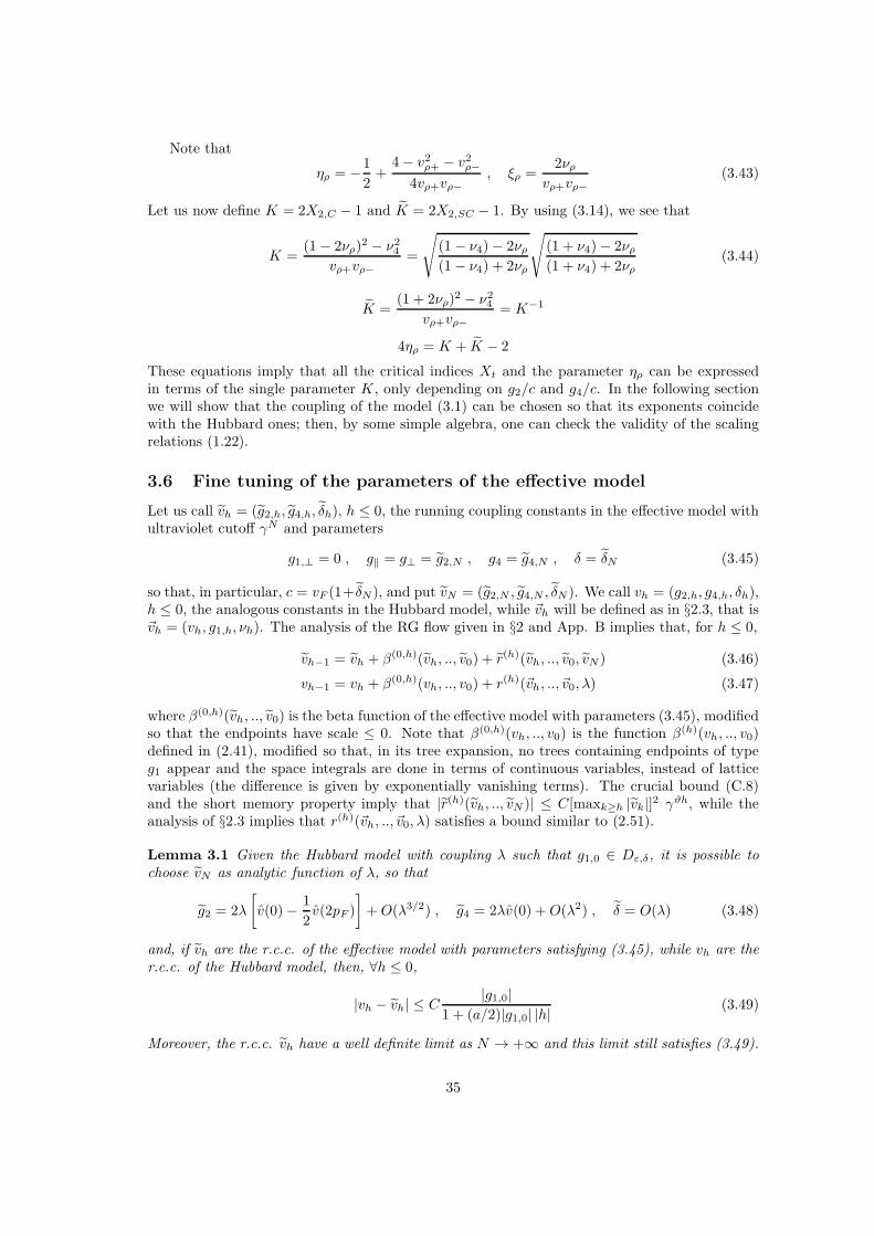
Note that

ηρ = −1

2+

4− v2ρ+ − v2ρ−4vρ+vρ−

, ξρ =2νρ

vρ+vρ−(3.43)

Let us now define K = 2X2,C − 1 and K = 2X2,SC − 1. By using (3.14), we see that

K =(1− 2νρ)

2 − ν24vρ+vρ−

=

√(1− ν4)− 2νρ(1− ν4) + 2νρ

√(1 + ν4)− 2νρ(1 + ν4) + 2νρ

(3.44)

K =(1 + 2νρ)

2 − ν24vρ+vρ−

= K−1

4ηρ = K + K − 2

These equations imply that all the critical indices Xt and the parameter ηρ can be expressedin terms of the single parameter K, only depending on g2/c and g4/c. In the following sectionwe will show that the coupling of the model (3.1) can be chosen so that its exponents coincidewith the Hubbard ones; then, by some simple algebra, one can check the validity of the scalingrelations (1.22).

3.6 Fine tuning of the parameters of the effective model

Let us call vh = (g2,h, g4,h, δh), h ≤ 0, the running coupling constants in the effective model withultraviolet cutoff γN and parameters

g1,⊥ = 0 , g‖ = g⊥ = g2,N , g4 = g4,N , δ = δN (3.45)

so that, in particular, c = vF (1+ δN), and put vN = (g2,N , g4,N , δN ). We call vh = (g2,h, g4,h, δh),h ≤ 0, the analogous constants in the Hubbard model, while ~vh will be defined as in §2.3, that is~vh = (vh, g1,h, νh). The analysis of the RG flow given in §2 and App. B implies that, for h ≤ 0,

vh−1 = vh + β(0,h)(vh, .., v0) + r(h)(vh, .., v0, vN ) (3.46)

vh−1 = vh + β(0,h)(vh, .., v0) + r(h)(~vh, .., ~v0, λ) (3.47)

where β(0,h)(vh, .., v0) is the beta function of the effective model with parameters (3.45), modifiedso that the endpoints have scale ≤ 0. Note that β(0,h)(vh, .., v0) is the function β(h)(vh, .., v0)defined in (2.41), modified so that, in its tree expansion, no trees containing endpoints of typeg1 appear and the space integrals are done in terms of continuous variables, instead of latticevariables (the difference is given by exponentially vanishing terms). The crucial bound (C.8)and the short memory property imply that |r(h)(vh, .., vN )| ≤ C[maxk≥h |vk|]2 γϑh, while theanalysis of §2.3 implies that r(h)(~vh, .., ~v0, λ) satisfies a bound similar to (2.51).

Lemma 3.1 Given the Hubbard model with coupling λ such that g1,0 ∈ Dε,δ, it is possible tochoose vN as analytic function of λ, so that

g2 = 2λ

[v(0)− 1

2v(2pF )

]+O(λ3/2) , g4 = 2λv(0) +O(λ2) , δ = O(λ) (3.48)

and, if vh are the r.c.c. of the effective model with parameters satisfying (3.45), while vh are ther.c.c. of the Hubbard model, then, ∀h ≤ 0,

|vh − vh| ≤ C|g1,0|

1 + (a/2)|g1,0| |h|(3.49)

Moreover, the r.c.c. vh have a well definite limit as N → +∞ and this limit still satisfies (3.49).

35

Proof - We have seen in the previous sections that the flows (3.46) and (3.47) have well definedlimits v−∞ and v−∞, as h → −∞, if the initial values are small enough and g1,0 ∈ Dε,δ.Moreover, the proof of this property for the flow (3.46) implies that v−∞ is a smooth invertiblefunction of vN , such that v−∞ = vN +O(v2N ); let us call vN (v−∞) = v−∞ +O(v2−∞) its inverse.It is also clear that vN (v−∞) has a well defined limit as N → ∞, that we shall call v(λ), andthat this is true also for the r.c.c. vh, h ≤ 0.

The previous remarks, together with (2.73) and (2.74), imply that it is possible to choosevN , satisfying (3.48), so that

v−∞ − v−∞ = 0 (3.50)

In order to prove (3.49), we note that, because of the bound (C.8) and the short memory property,in the effective model with couplings satisfying (3.48),

|vh − v−∞| ≤ Cλ2γϑh (3.51)

On the other hand, from Lemma 2.4 and 2.5

|vh − v−∞| ≤ C

h∑

j=−∞

[|g1,j |2 + λγϑ2 j ] ≤ C1

|g1,0|1 + (a/2)|g1,0| |h|

(3.52)

These two bounds immediately imply (3.49).

Let us now note that the critical indices of the effective model can be calculated in terms ofv−∞ by the same procedure used for the Hubbard model in §2.4 and that we get an equation

like (2.86), with the same function β(0,j)t . Hence, the above lemma allows us to conclude that the

critical indices in the Hubbard model and in the effective model coincide, provided that the valueof v = limN→∞ vN is chosen properly. It follows that all the indices are given by the equations(3.42), with

νρ =g2(λ)

4πc= λ

v(0)− v(2pF )/2

2π sin pF+O(λ3/2)

ν4 =g4(λ)

4πc= λ

v(0)

2π sin pF+O(λ2)

(3.53)

where (3.48) has been used, together with c = sin pF +O(λ). Moreover, (3.53) and (3.44) implythat K = 1− 2λ[v(0)− v(2pF )/2]/(π sin pF ) +O(λ3/2), in agreement with (1.21).

4 Spin-Charge Separation

If k 6= 0, the Fourier transform S2(k + ωpF ) of the two-point Schwinger function S2(x) in theHubbard model can be written as a tree expansion, in a way similar to eq. (2.64) of [38], whomwe shall refer to for the notation:

S2(k+ pωF ) =

∞∑

n=0

0∑

j0=−∞

∑

τ∈Tj0,n,2,0

∑

P∈P|Pv0 |=2

G2τ,ω(k) (4.1)

where pωF = (ωpF , 0), ω = ±. Here G2τ,ω(k) represents the contribution of a single tree τ with n

endpoints and root of scale j0; if |k| ∈ [γhk , γhk+1), it obeys the bound:

|G2τ,ω(k)| ≤ Cγ−(hk−j0)

γ−hk

Zhk

∞∑

n=0

0∑

j0=−∞

∑

τ∈Tj0,n,k

∑

P∈P|Pv0 |=2

(C|λ|)n∏

v not e.p.

γ−dvZhv

Zhv−1, (4.2)

36

where Tj0,n,k denotes the family of trees whose special vertices (those associated with the externallines) have scale hk or hk+1. Moreover, dv > 0, except for the vertices belonging to the pathconnecting the root with v∗, the higher vertex (of scale h∗) preceding both the two specialendpoints, where dv can be equal to 0. These vertices can be regularized by using a factorγ−(h∗−j0), extracted from the factor γ−(hk−j0), so that we can safely perform the sum over allthe trees with a fixed value of h∗ and we get

|S2(k+ pωF )| ≤ Cγ−hk

Zhk

hk∑

h∗=−∞

γ−(hk−h∗) ≤ C

γ−hk

Zhk

(4.3)

A similar bounds can be obtained for the effective model with g1⊥ = 0 and couplings chosen asin Lemma 3.1. We shall call SMω (k) and Zh the two-point function Fourier transform and therenormalization constants, respectively, in this model.

Let us put

S2(k+ pωF ) =1

Zhk

G2ω(k) , SMω (k) =

1

Zhk

G2,Mω (k) (4.4)

We can write

S2(k+ pωF ) =Zhk

Zhk

G2ω(k)

Zhk

=Zhk

Zhk

SMω (k) +1

Zhk

[G2ω(k) − G2,M

ω (k)] (4.5)

Note now that G2ω(k) differs from G2,M

ω (k) for three reasons:

1) the propagators are different, which produces a difference exponentially small thanks to(2.39), (2.40) and the short memory property;

2) the r.c.c. vh and vh are different, which produces a difference of order g1,hk, thanks to

(3.49) and the short memory property;

3) in the tree expansion of G2ω(k) and of the ratios Zj/Zj−1 there are trees with endpoints

of type g1, not present in the tree expansion of G2,Mω (k) and Zj/Zj−1; this fact produces

again a difference of order g1,hk.

These remarks, together with the fact that there is no tree with only one endpoint in the treeexpansion, implies that

∣∣∣∣1

Zhk

[G2ω(k)− G2,M

ω (k)]

∣∣∣∣ ≤ C|λg1,hk|γ

−hk

Zhk

(4.6)

For similar reason, we have

Zhk

Zhk

=

0∏

j=hk

Zhj

Zhj−1

Zh0

Zh0

= [1 +O(λ2)]eO(λ)

∑0j=h

kg1,j = [1 +O(λ)]L(|k|−1)O(λ) (4.7)

where L(t), t ≥ 1, is the same function defined in Theorem 1.1.Theorem 1.3 easily follows from (4.6), (4.7) and the explicit expression (3.34) of Sω(x) in the

effective model, applied to the case gσ = 0, c = vF (1 + δ).

5 Susceptibility and Drude weight

The effective model is not invariant under a gauge transformation with the phase dependingboth on ω and s, if g1,⊥ > 0; however, it is still invariant under a gauge transformation with the

37

phase only depending on ω. This is true, in particular, if the interaction is spin symmetric, thatis if g‖ = g⊥− g1,⊥, see item d in App. B. Since also the Hubbard model is spin symmetric, it isnatural to see if one can use this “restricted ” gauge invariance to get some useful information onthe asymptotic behavior of the Hubbard model, by comparing it with the effective model withg1,⊥ > 0.

Let us put g⊥ ≡ g2, g1⊥ ≡ g1 and g‖ = g2 − g1. We want to show that we can choosethe parameters of the effective model g1, g2, g4, δ, so that the running coupling constants areasymptotically close to those of the Hubbard model. This result is stronger of the similar onecontained in Lemma 3.1, since now all the running couplings are involved, and this implies alsothat the values of g2, g4 and δ are different with respect to the analogous constants defined inLemma 3.1. The main consequence of these considerations is that we can use the restricted WIof this new effective model to get non trivial information on some Hubbard model correlationfunctions, not plagued by logarithmic corrections.

Let ~lh = (g1,h, g2,h, g4,h, δh), h ≤ 0, be the running coupling constants appearing in the inte-gration of the infrared part of the effective model. The smoothness properties of the integrationprocedure imply that, in the UV limit, ~l0 is a smooth invertible function of the interaction param-eters ~l = (g1, g2, g4, δ), whose inverse we shall call ~l(~l0); hence we can fix the effective model by

giving the value of ~l0 and by putting ~l = ~l(~l0). In a similar way we call ~gh = (g1,h, g2,h, g4,h, δh),h ≤ 0, the running couplings of the Hubbard model with coupling λ.

We now define ~xh = ~lh−~gh, h ≤ 0. By using the decomposition (2.41) for ~gh and the similar

one for ~lh, we can write

~xh−1 = ~xh + [~β(1)h (~gh, .., ~g0)− ~β

(1)h (~lh, ..,~l0)] + ~β

(2)h (~gh, νh...~g0, ν0, λ) + ~β

(3)h (~lh, ..,~l0,~l) (5.1)

where ~β(1)h coincides with the function β(h) defined in (2.41). In the usual way, one can see that

|~β(1)h (~gh, .., ~g0)− ~β

(1)h (~lh, ..,~l0)| ≤ C

[|λ|+ sup

k≥h|~lk|

] 0∑

k=h

γ−ϑ(k−h)|~xk| (5.2)

and that |~β(2)h | ≤ C|λ|γϑh, |~β(3)

h | ≤ C[supk≥h |lk|]2. Note that the different power in the couplingof these two bounds is due to the terms linear in λ in the beta function for δh, which are presentin the Hubbard model, while similar terms are absent in the effective model, see remark after(B.9) in App. B.

We want to show that, given λ positive and small enough, it is possible to choose ~l0, hence~x0, so that ~x−∞ = 0; we shall do that by a simple fixed point argument. Note that ~x−∞ = 0 ifand only if

~xh = −h∑

h=−∞

[~β(1)h (~gh, .., ~g0)− ~β

(1)h (~lh, ..,~l0)] + ~β

(2)h + ~β

(3)h (5.3)

We consider the Banach space Mϑ, ϑ < 1, of sequences ~x = ~xhh≤0 with norm ‖~x‖ =supk≤0 |~xk|γ−(ϑ/2)k and the operator T : Mϑ → Mϑ, defined as the r.h.s. of (5.3). Givenξ > 0, let Bξ = ~x ∈ Mϑ : ‖~x‖ ≤ ξλ; if λ is small enough, say λ ≤ ε0 and ξλ ≤ ε0, and~lh = ~gh + ~xh, the functions ~β

(1)h (~lh, ..,~l0) and ~β

(3)h (~lh, ..,~l0,~l) are well defined and satisfy the

bounds above, even if ~x is not the flow of the effective model corresponding to ~l0. Hence, wehave:

γ−(ϑ/2)h|T(~x)h| ≤ c0λ(ξλ + 1)h−1∑

k=−∞

γϑ2 k ≤ c1λ(1 + ξλ) (5.4)

38

so that Bξ is invariant if ξ = 2c1 and λ ≤ ε1 = minε0, ε0/(2c1), 1/(2c1). Moreover

T(~x)h −T(~x′)h =

h∑

h=−∞

[~β

(1)h (~gk + ~xkk≥h)− ~β

(1)h (~gk + ~x′kk≥h)]

+ [~β(3)h (~gk + ~x′kk≥h)− ~β

(3)h (~gk + ~xkk≥h)]

and |T(~x)h − T(~x′)h| ≤ c2λ‖x − x′‖, thanks to the fact that all the terms in the r.h.s. of thisequation are of the second order in the running couplings. It follows that, if c2λ < 1, T isa contraction in Bξ, so that (5.3) has a unique solution ~x(0) in this set; moreover, if we put~lh = ~gh + ~x

(0)h , ~lhh≤0 is the flow of the effective model corresponding to a value of ~l such that

|~gh −~lh| ≤ C|λ|γ ϑ2 h (5.5)

Finally, this solution is such that ~l is equal to ~g0 at the first order; hence, by using (2.26), we get

g1 = 2λv(2pF ) +O(λ2) , g2 = 2λv(0) +O(λ2) , g4 = 2λv(0) +O(λ2) , δ = O(λ) (5.6)

Thanks to the bound (5.5), this choice of ~l, allows us to extend to the Hubbard modelLemma 1 of [27], proved for the spinless fermion model. Hence, we can say that there are

constants Z = 1 +O(λ2), Z3 = 1 +O(λ) and Z3 = vF +O(λ) such that, if κ ≤ 1 and |p| ≤ κ,

ΩC(p) = Z23 〈ρpρ−p〉(g) +Ac + o(p)

D(p) = −Z23〈jpj−p〉(g) +Aj + o(p)

(5.7)

where 〈·〉(g) denotes the expectation in the effective model satisfying (5.5), Ac and Aj are suitableO(1) constants and

ρx =∑

ω,s

ψ+x,ω sψx,ω s jx =

∑

ω,s

ωψ+x,ω sψx,ω s . (5.8)

Moreover, if we put pωF = (ωpF , 0) and we suppose that 0 < κ ≤ |p|, |k′|, |k′−p| ≤ 2κ, 0 < ϑ < 1,then

G2,1ρ (k′ + pωF ,k

′ + p+ pωF ) = Z3〈ρpψk′,ωψ+k′+p,ω〉

(g)[1 +O(κϑ)]

G2,1j (k′ + pωF ,k

′ + p+ pωF ) = Z3〈jpψk′,ωψ+k′+p,ω〉

(g)[1 +O(κϑ)] (5.9)

S2(k′ + pωF ) = 〈ψ−

k′,ω,σψ+k,ω,σ〉

(g)[1 +O(κϑ)] .

where G2,1ρ (x) and G2,1

j (x) are defined after (1.13), while the functions 〈ρpψk′,ωψ+k′+p,ω〉

(g) and

〈jpψk′,ωψ+k′+p,ω〉

(g) coincide with the functions (3.16) and (3.17), respectively, with c = vF (1+δ).As already mentioned, if g1 > 0, the effective model is still invariant under a spin-independentphase transformation; hence the WI (3.6) is satisfied, if we sum both sides over s and we substituteνµs (p) with

νµs (p) = δω,1[δs,−1g2 + δs,1(g2 − g1)] + δω,−1δs,−1g4h(p)

4πc, c = vF (1 + δ) (5.10)

Therefore we get the a WI similar to (3.15), that is

− ip0[1− ν4(p)− 2νρ(p)]〈ρpψk′,ωψ+k′+p,ω〉

(g)+ cp[1 + ν4(p)− 2νρ(p)]〈jpψk′,ωψ

+k′+p,ω〉

(g)

=1

Z

[〈ψ−

k,ω,σψ−k,ω,σ〉

(g) − 〈ψ−k+p,ω,σψ

−k+p,ω,σ〉

(g)]

(5.11)

39

where

ν4(p) = g4h(p)

4πc, νρ(p) =

g2 − g1/2

4πch(p) (5.12)

By replacing (5.9) in (5.11), and comparing with (1.14) we get, if ν4(0) ≡ ν4, νρ(0) = νρ

Z3

Z= (1− ν4 − 2νρ) ,

Z3

Z= c(1 + ν4 − 2νρ) (5.13)

Moreover, by proceeding as in derivation of (3.19), we get:

Dω(p)〈ρ(c)p,ωρ(c)−p,ω′〉(g) − ν4(p)D−ω(p)〈ρ(c)p,ωρ

(c)−p,ω′〉(g)

−2νρ(p)D−ω(p)〈ρ(c)p,−ωρ(c)−p,ω′〉(g) = −δω,ω′

D−ω(p)

2πZ2c

(5.14)

Hence, by some simple algebra, we get:

〈ρ(c)p,ωρ(c)−p,ω〉(g) =

1

2πZ2cv2ρ,+

D−ω(p)[D−ω(p)− ν4Dω(p)]

p20 + c2v2ρp2

+O(p) (5.15)

〈ρ(c)p,ωρ(c)−p,−ω〉(g) =

1

2πZ2cv2ρ,+

2νρDω(p)D−ω(p)

p20 + c2v2ρp2

+O(p) (5.16)

wherevρ = vρ,−/vρ,+ , v2ρ,µ = (1− µν4)

2 − 4ν2ρ (5.17)

Therefore the charge and current density correlations are given by:

〈ρ(c)p ρ(c)−p〉(g) =

1

πZ2cv2ρ,+

−p20(1 − ν4 + 2νρ) + c2p2(1 + ν4 − 2νρ)

p20 + c2v2ρp2

+O(p)

〈j(c)p j(c)−p〉(g) =

1

πZ2cv2ρ,+

−p20(1 − ν4 − 2νρ) + c2p2(1 + ν4 + 2νρ)

p20 + c2v2ρp2

+O(p)

(5.18)

From the WI (1.14) we see that

ΩC(0, p0) = 0 , D(p, 0) = 0 (5.19)

and this fixes the values of the constants Ac and Aj in (5.7), so that

ΩC(p) =Z23

πZ2cv2ρ,+[(1 + ν4 − 2νρ) + v2ρ(1− ν4 + 2νρ)]

c2p2

p20 + v2ρ c2p2

+ o(p)

D(p) =Z23

πZ2cv2ρ,+v2ρ

[(1 + ν4 + 2νρ) + v2ρ(1 − ν4 − 2νρ)]p20

p20 + v2ρ c2p2

+ o(p)

(5.20)

If we insert (5.13) in the previous equations, we get, for the susceptibility (1.9) and the Drudeweight (1.12), the values

κ =(1 − ν4 − 2νρ)

2

πcv2ρ,+v2ρ

[(1 + ν4 − 2νρ) + v2ρ(1 − ν4 + 2νρ)] =K

πcvρ

D =c(1 + ν4 − 2νρ)

2

πv2ρ,+v2ρ

[(1 + ν4 + 2νρ) + v2ρ(1 − ν4 − 2νρ)] =Kcvρπ

(5.21)

where

K =(1− 2νρ)

2 − ν24vρ+vρ−

=

√(1− ν4)− 2νρ(1− ν4) + 2νρ

√(1 + ν4)− 2νρ(1 + ν4) + 2νρ

(5.22)

40

so thatκ

D=

1

c2v2ρ(5.23)

and this completes the proof of Theorem 1.2.

Remark We are unable to see if cvρ = vF (1 + δ)vρ coincides with the velocity cvρ = vF (1 +

δ)vρ appearing in the two-point function asymptotic behavior (3.34), with vρ given (see (3.14))by

vρ =((1 + ν4)

2 − 4ν2ρ)

((1 − ν4)2 − 4ν2ρ)(5.24)

with νρ and ν4 defined as in (3.53). In fact, it is easy to see that δ is equal to δ at the firstorder and this is true also for vρ and vρ by (5.6), (5.12) and (3.53); however, our arguments arenot able to exclude that the two velocities are different. Moreover, (5.22) and (3.44) imply thatK = K at first order, but they also could be different. Note that the equality of K and K, wouldimply that κ = K/v, with v = cvρ being the charge velocity, a relation proposed in [17] which,together with (1.22) and (1.24), would allow the exact determination of the exponents in termsof the susceptibility and the Drude weight.

A The g1 map

Let us consider the following map on the complex plane:

gn+1 = gn − ang2n (A.1)

where an is a sequence depending on g0, such that, if |g0| is small enough,

an = a+ σn , |σn| ≤ c0|g0| , (A.2)

for some positive constants a and c0. We want to study the trajectory of the map (A.1), underthe condition that

g0 ∈ Dε,δ = z ∈ C : |z| < ε, |Arg (z)| ≤ π − δ , δ ∈ (0, π/2) (A.3)

We shall first study the properties of a sequence gn, which turns out to be a good approximationof gn. Let us define:

An =1

n

n−1∑

k=0

ak (A.4)

Lemma A.1 Given δ ∈ (0, π/2), there exists ε0(δ) such that, if ε ≤ ε0(δ) and g0 ∈ Dε,δ, thesequence

gn =g0

1 + g0nAn(A.5)

at any step n ≥ 0 is well defined and does not exit the larger domain Dε1,δ1 , for ε1 = 2ε/(sin δ)and δ1 = δ/2.

Proof - First of all, we choose ε so that

c0ε ≤ a/2 ⇒ a/2 ≤ ℜ an ≤ 3a/2 , |ℑ an| ≤ c0|g0| (A.6)

where c0 is the constant defined in (A.2); we can write

An = αn + iβn , αn ≥ a/2 , |βn| ≤ c0|g0| . (A.7)

41

Define zn := 1 + g0nAn := 1 + g0nαn + wn; then, if g0 ∈ Dε,δ,

|1 + g0nαn| ≥ max

sin δ,

sin δ

3(1 + |g0|nαn)

(A.8)

In fact, it is trivial to show that |1 + g0nαn| ≥ sin δ; on the other hand, if |g0|nαn ≥ 2,

|1 + g0nαn| ≥ |g0|nαn − 1 = (|g0|nαn + 2|g0|nαn − 3)/3 ≥ (|g0|nαn + 1)/3

By using (A.8), we get|wn|

|1 + g0nαn|≤ 6c0a sin δ

|g0| . (A.9)

It follows that, if ε is small enough,

|zn| ≥1

2sin δ (A.10)

so that, in particular, the definition (A.5) is meaningful.Now we want to prove that gn ∈ Dε1,δ1 , with ε1 = 2ε/(sin δ) and δ1 = δ/2, if ε is small

enough. Let g0 = ρ0eiθ0 ; by using (A.8) and (A.9), we see that, if ε is small enough,

|gn| ≤2 |g0|

|1 + αng0n|≤ 2ε

sin δ; (A.11)

besides it is easy to see that

∣∣∣∣Arg(

g01 + αng0n

)∣∣∣∣ =∣∣∣∣Arg

(ρ0

e−iθ0 + αnρ0n

)∣∣∣∣ ≤ |θ0| ≤ π − δ .

Then, since gn = ρ0e−iθ0+αnρ0n

(1 + wn), with wn of order g0, for ε small enough,

|Arg (gn)| ≤ π − δ/2 (A.12)

Proposition A.2 Given δ ∈ (0, π/2), there exists ε0(δ), such that, if ε ≤ ε0(δ) and g0 ∈ Dε,δ,then

gn ∈ Dε2,δ2 , ε2 =3ε

sin δ, δ2 =

δ

4(A.13)

Moreover, if gn is defined as in (A.5),

|gn − gn| ≤ |gn|3/2 (A.14)

Proof - We shall proceed by induction on the condition (A.14), which is true for n = 0. Supposethat it is true for n ≤ N ; then, by using (A.11) and (A.12), we see that, if ε is small enough andn ≤ N ,

|gn| ≤ 3|gn|/2 ≤ 3ε/ sin δ , |Arg (gn)| ≤ π − δ/4 (A.15)

which proves (A.13). Moreover, by (A.1), if ε is small enough,

|gN+1| ≤ 2|gN | ≤ 3|gN | (A.16)

Note now that

1

gn+1− 1

gn=

an1− angn

= an + a2ngn +∆n =1

gn+1− 1

gn+ a2ngn +∆n (A.17)

42

where ∆n is a quantity which can be bounded by c1|gn|2, for some constant c1. We can rewrite(A.17) in the form

1

gn+1− 1

gn+1=

1

gn− 1

gn+ a2ngn +∆n (A.18)

By using (A.6), (A.8), (A.9), (A.15), (A.16) and (A.18), we get, if ε is small enough,

|gN+1 − gN+1| = |gN+1| |gN+1|∣∣∣∣

1

gN+1− 1

gN+1

∣∣∣∣

≤ 3|gN | |gN+1|N∑

n=0

[6a2|gn|+9

4c1|gn|2] ≤ c2|gN |3/2

|g0|1/2(1 + a

2 |g0|N)1/2

N∑

n=0

|g0|1 + a

2 |g0|n

≤ |gN |3/2c3|g0|1/2

(1 + a2 |g0|N)1/2

log(1 +

a

2|g0|N

)≤ |gN |3/2

(A.19)

where c2 and c3 are two suitable constants.

B Symmetries of the Effective Model and RG Flow

The RG analysis of the effective model will be done by exploiting some symmetry properties ofa more general model, obtained by adding to the interaction (3.3) the term g3V3(ψ), with

V3(ψ) =1

2

∑

ω,s

∫dxdyh(x − y)ψ+

x,ω,sψ+x,ω,−sψ

−y,−ω,sψ

−y,−ω,−s (B.1)

The integration of the positive (ultraviolet) scales N,N − 1, .., 0 is essentially identical to theone described in §2 of [29] or §3 of [39], for the spinless case; it does not need any localizationprocedure.

The integration of the infrared scales is done in a way similar to the one in the Hubbard modeldescribed in §2. However, before starting the multiscale IR integration, we have to perform sometechnical operations, which will make possible to compare the flow of the running couplings withthat of the Hubbard model.

After the integration of the UV scales up to j = 1, the free measure propagator is given by

g[l,1]D,ω(x), defined as in (3.2) with N = 1. In this expression, the velocity c has the role of theFermi velocity vF of the Hubbard model. In order to match the asymptotic behavior of the twomodels, we can not choose c = vF ; for this reason we introduced the parameter δ. However,it is not possible to compare the RG flows of the two models if the two velocities are different;hence, we have to move from the free measure to the interaction the term proportional to δ.Moreover, since also the cutoff function χ[l,1](|(k0, ck)|) depends on δ, we have to “modify” it inχ[l,1](|(k0, vFk)|).

The simplest way of performing these operations without introducing spurious singularitiesis the following one. We start with a free measure of the form

P (dψ[l,1]) = N−1 exp

− Z

L2

∑

k,ω,s

Cl(k)[−ik0 + ωvF (1 + δ)k]ψ+[l,1]k,ω,sψ

−[l,1]k,ω,s

(B.2)

where Cl(k) = χ[l,1](|(k0, ck)|)−1. We can move to the scale 1 effective interaction the term

−δ ZL2

∑

k,ω,s

ωvF kψ+[l,1]k,ω,sψ

−[l,1]k,ω,s = −δVδ(ψ) , with

43

Vδ(ψ) =∑

ω,s

∫dxψ+

x,ω,s(iωvF∂x)ψ−x,ω,s (B.3)

The new free measure differs from (B.2) because δ is multiplied by ul(k) = 1 − χ[l,1](|(k0, ck)|).On the other hand, since δ will be chosen of order λ, χ[l,1](|(k0, ck)|) and χ[l,1](|(k0, vFk)|) differonly for values of k of size γ or γl and

ul(k) = 0 , if χ[l+1,0](|(k0, vF k)|) > 0 (B.4)

Hence, we can write

χ[l,1](|(k0, ck)|) = χ(1)(k) + χ[l+1,0](|(k0, vFk)|) + χ(l)(k) (B.5)

with χ(1)(k) and χ(l)(k) smooth functions, whose support is on values of k of size γ or γl,respectively; moreover, if we define

Cl(k) =[χ[l+1,0](|(k0, vFk)|+ χ(l)(k))

]−1

(B.6)

then Cl(k) = 1, if 1 ≥ |(k0, vFk)| ≥ γl+1 and Cl(k)−1χ(l)(k) ≤ 1. It follows that the free measure

P (dψ[l,1]) can be written as P (dψ(1))P (dψ[l,0]), where ψ(1) is a field whose covariances has thesame scale properties of ψ(1), while

P (dψ[l,0]) = N−1 exp

− Z

L2

∑

k,ω,s

Cl(k)[−ik0 + ωvF (1 + ul(k)δ)k]ψ+[l,0]k,ω,s ψ

−[l,0]k,ω,s

(B.7)

The integration of the single scale field ψ(1) can be done without any problem. At this point, westart the multiscale integration of the field ψ[l,0], by performing the effective potential localizationand the free measure renormalization as in the Hubbard model. Thanks to the support propertiesof ul(k), the steps from j = 0 to j = l+1 will give the same result we should get if the propagator

of ψ[l,0] were equal to1

Z

1

L2

∑

k

eikxχl,0(|(k0, vFk)|)−ik0 + ωvFk

This means that the renormalized single scale propagator will have the form (2.38), correspondingto the leading behavior of the single scale propagator in the Hubbard model. This property isnot true only in the last step, j = l, but this is not a problem, since we have to study the RGflow at fixed j and l → −∞ and, moreover, the contribution of the IR scale fluctuations to theSchwinger functions at fixed space-time coordinates vanishes as l → −∞.

Let us now analyze in more detail the RG flow of the effective model for h ≤ 0. The maindifference with respect to the Hubbard model is that (2.24) has to be replaced by

V (j)(√Zjψ) = g1,⊥,jF1,⊥(

√Zjψ) + g‖,jF‖(

√Zjψ)+

+g⊥,jF⊥(√Zjψ) + g3,jF3(

√Zjψ) + g4,jF4(

√Zjψ) + δjVδ(

√Zjψ)

(B.8)

where the functions Fα(ψ) are defined as the functions Vα(ψ) of (3.4) with h(x−y) = δ(x−y);the absence of local terms proportional to ψ+ψ− is a consequence of the oddness in k of the freepropagator. The running couplings verify equations of the form

gα,h−1 − gα,h = B(h)α (~gh, δh, ..~g0, δ0, ~g, δ)

δh−1 − δh = B(h)δ (~gh, δh, ..~g0, δ0, ~g, δ)

(B.9)

where α = 1 ⊥, ‖,⊥, 3, 4 and ~gj = (g1,⊥,j, g3,j , g‖,j , g⊥,j , g4,j). Note that the functions B(h)α

and B(h)δ are of the second order in their arguments; in the case of B

(h)δ , this follows from the

44

structure of V (ψ) (see (3.4)), which does not allow to build Feynman graphs of the first orderin ~g. For the same reason

δ0 = δ +O(ε20) , ε0 = max|~g|, |δ| (B.10)

and this relations can be inverted, if ε0 is small enough.

There are some symmetries which is important to exploit. For notational simplicity, we willwrite (G1,⊥, G3, G‖, G⊥, G4,∆) or (~G,∆) in place of (~gh, δh, ..~g0, δ0, ~g, δ) .

a. Spin U(1). Free measure and interactions are invariant under the transformation

ψεx,ω,s → eiεαsψεx,ω,s

where αs is a spin-dependent angle. This means that the only possible local effectiveinteractions must have as many ψ+

s as ψ−s , for each given s. Therefore, all the allowed

local quartic interactions are the ones listed in (3.4); it is also clear from the symmetriesω → −ω and s→ −s that they must occur in the same linear combinations.

b. Particle-hole symmetry. The free measure is invariant if the particle hole switching involves

the spin s′ only, i.e. ψεk,ω,s → ψ−ss′ε−ss′k,ω,s; interactions are not invariant and we find:

B(h)1,⊥(G1,⊥, G3, G‖, G⊥, G4,∆) = −B(h)

3 (−G3,−G1,⊥, G‖,−G⊥,−G4,∆) (B.11)

B(h)‖ (G1,⊥, G3, G‖, G⊥, G4,∆) = B

(h)‖ (−G3,−G1,⊥, G‖,−G⊥,−G4,∆)

B(h)⊥ (G1,⊥, G3, G‖, G⊥, G4,∆) = −B(h)

⊥ (−G3,−G1,⊥, G‖,−G⊥,−G4,∆)

B(h)4 (G1,⊥, G3, G‖, G⊥, G4,∆) = −B(h)

4 (−G3,−G1,⊥, G‖,−G⊥,−G4,∆)

(B.12)

B(h)∆ (G1,⊥, G3, G‖, G⊥, G4,∆) = B

(h)∆ (−G3,−G1,⊥, G‖,−G⊥,−G4,∆) (B.13)

c. Chiral U(1). The free measure is invariant under the transformation

ψεk,ω,s → eiεαω ψεk,ω,s (B.14)

for αω a chirality-dependent angle. All the interactions are U(1) invariant, but for V3;if g3 = 0, then an interaction V3 won’t be generated by the flow. This fact can be seenalso graph by graph. Indeed, in the graphs for B‖, B⊥, B4 and Bδ, the number of thehalf-lines ψ+

ω has to equal the number of the half-lines ψ−ω (regardless the spin label); this

can only happen when there is an even number of interactions V3. Therefore these threebeta functions are even in G3 and then, by (B.12) and (B.13), also even in G1,⊥; hence, ifα = ‖,⊥, 4, δ,

B(h)α (G1,⊥, G3, G‖, G⊥, G4,∆) = B(h)

α (G21,⊥, G

23, G‖, G⊥, G4,∆) (B.15)

where G2α denotes the tensor gα,jgα,j′j.j′≥h. By a similar argument, B

(h)3 has to be odd

in G3 and B(h)1 even; then, by (B.11), B

(h)1 is also odd in G1 and B

(h)3 even, so that

B(h)1,⊥(G1,⊥, G3, G‖, G⊥, G4,∆) = G1,⊥B

(h)(G21,⊥, G

23, G‖, G⊥, G4,∆)

B(h)3 (G1,⊥, G3, G‖, G⊥, G4,∆) = G3B(h)(G2

3, G21,⊥, G‖,−G⊥,−G4,∆)

(B.16)

where GαB(h)α is a shorthand for

∑j≥h gα,jB

(h,j)α .

In this way we have found two invariant surfaces in the space of the interaction parameters(~g, δ):

C1 = ~g, δ : g1,⊥ = 0 C3 = ~g, δ : g3 = 0

45

d. Spin SU(2). It is convenient to rewrite the interaction as

V (ψ) = g1,⊥(V1,⊥(ψ)− V‖(ψ)

)+ (g‖ + g1,⊥ − g⊥)V‖(ψ)+

+ g⊥(V⊥(ψ) + V‖(ψ)

)+ g3V3(ψ) + g4V4(ψ) + δhVδ(ψ)

(B.17)

It is evident that V1,⊥−V‖, V⊥+V‖, V3 V4 and Vδ, as well as the free measure, are invariantunder the transformation of the fields

ψ−k,ω,s →

∑

s′

Us,s′ψ−k,ω,s′ , ψ+

k,ω,s →∑

s′

ψ+k,ω,s′U

†s′,s

for U ∈ SU(2). While V‖ isn’t: if g‖ + g1 − g⊥ = 0 it will remain zero. Thus we find fourother invariant surfaces:

C1,+ = ~g, δ : g1,⊥ = g⊥ − g‖ , C3,+ = ~g, δ : g3 = g⊥ + g‖

C1,− = ~g, δ : −g1,⊥ = g⊥ − g‖ , C3,− = ~g, δ : −g3 = g⊥ + g‖(in fact C1,−, C3,+ and C3,− are obtained form C1,+ through (B.11), (B.12), (B.15) and(B.16)). C3,+ is also called Fowler invariant (see [12], page 220).

e. Vector-Axial Symmetry. All the terms in V (ψ), but V1(ψ) and V3(ψ), are invariant underthe transformation

ψεx,ω,s → eiεϑω,sψεx,ω,s

therefore the surface g1,⊥ = g3 = 0 is invariant.

Finally we consider the flow of Zh and the renormalization constant Z(1)h associated with

the density operator ρx,ω,s = ψ+x,ω,sψ

−x,ω,s in the generating functional (3.1); Z

(1)h is defined

as Z(1,C)h in (2.27). It is easy to see, by using the symmetry properties of the model as be-

fore, that Zh−1/Zh = 1 + B(h)z (~G,∆) and Z

(1)h−1/Z

(1)h = 1 + B

(h)ρ (~G,∆), with B

(h)α (~G,∆) =

B(h)α (G2

1, G23, G‖, G⊥, G4,∆) for α = z, ρ. Hence

Z(1)h−1

Zh−1=Z

(1)h

Zh[1 + B(h)(~G,∆)] (B.18)

withB(h)(~G,∆) = B

(h)2 (G2

1,⊥, G23, G‖, G⊥, G4,∆) (B.19)

C Vanishing of the Beta Function

We recall the main ideas of the proof of (2.45) and (2.83) (see [22],[23],[24],[33] for more details).We consider the model (3.1) with g1,⊥ = 0; δ, g‖ and g⊥ are small but arbitrary parameters. We

take the limit N → ∞ at fixed l; if |k| = γl (so that, in particular, fl(k) = 1)

Sω(k) ≡ 〈ψ−k,ω,sψ

+k,ω,s〉l =

1

ZlDl,ω(k)[1 +W

(l)2 (k)] (C.1)

where 〈 · 〉l denotes the expectation with propagator (3.2),

Dl(k) = −ik0 + ωvF (1 + δl)k

and|W (l)

2 (k)| ≤ C(ε2l + glγϑl) (C.2)

46

with gl = maxh≥lmax|g2,h|, |g4,h| and εl = maxj≥lmaxgj, |δj |, Note that we have included

in Dl(k) a correction of the free Fermi velocity due to the local term δlVδ, so that W(l)2 (k) does

not contain terms of order εl, except those associated to irrelevant terms. Moreover, by theanalogue of (112) of [22]

〈ρp,ω,sψ−k,ω,sψ

+k−p,ω,s〉l = Z

(1)l Sω(k)Sω(k− p)[1 +W

(l)2,1(k)] (C.3)

where |W (l)2,1(k)| ≤ C(ε2l + glγ

ϑl). In §3.2 we have written the WI directly in the l → −∞ limit,but they are true also when l is finite, up to corrections studied in detail in §4 of [22] and §4 of[23]; using the bounds is such papers for the corrections we derive from the finite l analogue of(3.6)

DN(p)〈ρp,ω,sψ−k,ω,sψ

+k−p,ω,s〉l = Sω(k− p)− Sω(k) +DN (p)Rl(k,p) (C.4)

where k and k− p are of size γl,

DN(k) = −ik0 + ωvF (1 + δ)k

and

|Rl(k,p)| ≤ Cγ−2lZ(1)l

Z2l

(ε2l + glγϑl)

Hence, if we put k = k and p = 2k, with |k| = γl, we get DN (k)[Z(1)l /Zl] = Dl(k)[1 + ∆(k)],

with |∆(k) ≤ C(ε2l + glγϑl), which implies that δl = δ+O(ε2l ) and Z

(1)l /Zl = 1+O(ε2l ). On the

other hand, the value of δh is independent of the infrared cutoff, if h ≥ l+1, and |δl+1−δl| ≤ Cε2l .It follows that, for any j ∈ [l, N ] and uniformly in the cutoffs,

δj = δ +O(ε2j ) (C.5)

Z(1)j

Zj= 1 +O(ε2j ) (C.6)

In the same way, we can also use the the Schwinger-Dyson equation combined with theWard Identities with a finite infrared cut-off; we get (3.24) with a correction term, which can bebounded as in §4 of [23]. If we restrict the resulting expression to the four point function withmomenta at the infrared scale, we get, see [23],[24]

g‖,j = g‖ +O(ε2j ) , g⊥,j = g⊥ +O(ε2j) , g4,j = g4 +O(ε2j ) (C.7)

Let us call b(j)α (g‖, g⊥, g4, δ) the function which is obtained by B

(j)α (~gh, δh, ..~g0, δ0, ~g, δ) (defined

in (B.9)), by subtracting the contribution of the trees containing endpoints of scale grater than 0and by putting (~gj , δj) = (0, 0, g‖, g⊥, g4, δ), ∀j = h, . . . .0 (the value of the r.c.c. is independentof the scale). Then, by Lemma 3.4 of [37], we get the bound:

∣∣∣b(j)α (g‖, g⊥, g4, δ)∣∣∣ ≤ C[max|g‖|, |g⊥|, |g4|, |δ|]2γϑj , α = ‖,⊥, 4, δ (C.8)

In we define in a similar way the function b(j)(g‖, g⊥, g4, δ) in terms of B(j) (~gj , δj , ..~g0, δ0, ~g, δ)(defined in (B.19)), (C.6) implies the bound

∣∣∣b(j)(g‖, g⊥, g4, δ)∣∣∣ ≤ C[max|g‖|, |g⊥|, |g4|, |δ|]2γϑj (C.9)

The bounds (C.8) and (C.9) allow to show that, in the model (3.1), the infared cut-off can beremoved by an analysis very similar to the one in §2.3-2.4.

47

Let us now consider the Hubbard model. In (2.41) we have written its Beta function as sum oftwo terms, the second of which is asymptotically negligible, by (2.42); the first term, denoted in

(2.41) by β(j)α (~gj , δj ; ...;~g0, δ0) ≡ β

(j)α (G1, G2, G4,∆) (using a notation similar to that used after

(B.9)) coincides with the Beta function of the effective model on the invariant surface C1,+ ∩ C3,if we subtract from it the contribution of the trees containing endpoints of scale grater than 0.Hence, by using (B.15) and (B.16), we get

β(j)1 (G1, G2, G4,∆) = G1β

(j)1⊥(G

21, 0, G2 −G1, G2, G4,∆)

β(j)2 (G1, G2, G4,∆) = β

(j)⊥ (G2

1, 0, G2 −G1, G2, G4,∆)

β(j)4 (G1, G2, G4,∆) = β

(j)4 (G2

1, 0, G2 −G1, G2, G4,∆)

β(j)δ (G1, G2, G4,∆) = β

(j)δ (G2

1, 0, G2 −G1, G2, G4,∆)

(C.10)

where β(j)α (G2

1, 0, G2 −G1, G2, G4,∆) denotes the value of B(j)α (G2

1, 0, G2 −G1, G2, G4,∆), afterthe subtraction of the trees containing endpoints of scale grater than 0. Therefore, if α 6= 1,

the contributions of order 0 and 1 in G1 of β(j)α (~G,∆) are the same as the contributions of the

same order of β(j)α (0, 0, G2 − G1, G2, G4,∆). By using (C.8), one sees immediately that these

contributions are of order γϑj as functions of j, so that (2.45) is proved. In the same way, using(C.9) and (B.19) we can prove (2.83).

This completes the proof of the boundedness of the RG flow in the Hubbard model, as wellas in the effective model with g1,⊥ > 0 and g‖ = g⊥ − g1,⊥. Note that, in order to prove theboundedness of the flow of the spin-symmetric Hubbard model, we need information from a nonspin symmetric model; in fact, we have derived (2.45) from the model (3.1) with g⊥ 6= g‖ andg1,⊥ = 0.

Acknowledgements G.B. and V.M. acknowledge the financial support of MIUR, PRIN 2008.V.M. gratefully acknowledges also the financial support from the ERC Starting Grant CoMBoS-239694. The work of P.F. is supported by the Giorgio and Elena Petronio Fellowship Fund.

References

[1] E.H. Lieb. The Hubbard model: some rigorous results and open problems. In XI Int.Congress Math. Phys., pages 392–412. International Press, 1995.

[2] Feldman, Knorrer J.H., and Trubowitz E. A two dimensional fermi liquid. Comm. Math.Phys, 247:1–319, 2004.

[3] A. Giuliani and V. Mastropietro. The 2D Hubbard model on the honeycomb lattice. Comm.Math. Phys., 293:301–346, 2010.

[4] T. Giamarchi. Quantum Physics in one dimension. Oxford University Press, 2004.

[5] E.H. Lieb and F.Y. Wu. Absence of Mott transition in the 1D Hubbard model. Phys. Rev.Lett., 20:1445–1449, 1968.

[6] P.W. Anderson. When the electron falls apart. Physics Today, 50(10):42–47, 1997.

[7] E.H. Lieb and FY Wu. The one-dimensional hubbard model: a reminiscence* 1. PhysicaA: Statistical Mechanics and its Applications, 321(1-2):1–27, 2003.

[8] P. Goldbaum. Existence of solutions to the bethe ansatz equations for the 1d hubbardmodel: finite lattice and thermodynamic limit. Comm. Math. Phys., 258:217–337, 2005.

48

[9] D. Mattis and E.H. Lieb. Exact solution of a many fermion system and its associated bosonfield. J. Math. Phys., 6:304–3129, 1965.

[10] D. Mattis. Band theory of magnetism in metals in context of exactly soluble models. Physics,1:183–193, 1964.

[11] P.W. Anderson. The Theory of Superconductivity in the High-Tc Cuprate Superconductors.Princeton University Press, Princeton, 1997.

[12] J. Solyom. The Fermi gas model of one-dimensional conductors. Adv. Phys., 28:201–303,1979.

[13] C. Di Castro and W. Metzner. Ward identities and the beta function in the luttinger liquid.Phys. Rev. Lett., 67(27):3852–3855, 1991.

[14] T. Giamarchi and H.J. Schulz. Correlation functions of one-dimensional quantum systems.Phys. Rev. B, 39(7):4620–4629, 1989.

[15] L.P. Kadanoff and F.J. Wegner. Some critical properties of the Eight-Vertex Model. Phys.Rev. B, 4:3989–3993, 1971.

[16] A. Luther and I. Peschel. Calculation of critical exponents in two dimensions from quantumfield theory in one dimension. Phys. Rev. B, 12:3908–3917, 1975.

[17] F.D.M. Haldane. General relation of correlarion exponents and application to the anisotropicS=1/2 Heisenberg chain. Phys. Rev. Lett., 45:1358–1362, 1980.

[18] K. Gawedski and A. Kupiainen. Gross–Neveu model through convergent perturbation ex-pansions. Comm. Math. Phys., 102:1–30, 1985.

[19] A. Lesniewski. Effective action for the Yukawa2 quantum field theory. Comm. Math. Phys.,108:437–467, 1987.

[20] G. Benfatto, G. Gallavotti, A. Procacci, and B. Scoppola. Beta functions and Schwingerfunctions for a many fermions system in one dimension. Comm. Math. Phys., 160:93–171,1994.

[21] F. Bonetto and V. Mastropietro. Beta function and anomaly of the Fermi surface for a d = 1system of interacting fermions in a periodic potential. Comm. Math. Phys., 172:57–93, 1995.

[22] G. Benfatto and V. Mastropietro. On the density-density critical indices in interactingFermi systems. Comm. Math. Phys., 231:97–134, 2002.

[23] G. Benfatto and V. Mastropietro. Ward identities and chiral anomaly in the Luttingerliquid. Comm. Math. Phys., 258:609–655, 2005.

[24] V. Mastropietro. Rigorous proof of Luttinger liquid behavior in the 1d Hubbard model. J.Stat. Phys., 121:373–432, 2005.

[25] P. Falco and V. Mastropietro. Renormalization group and asymptotic spin-charge separationfor chiral Luttinger liquids. J. Stat. Phys., 131:79–116, 2008.

[26] F.D.M. Haldane. Luttinger liquid theory of one-dimensional quantum fluids: I. propertiesof the Luttinger model and their extension to the general 1D interacting spinless Fermi gas.J. Phys. C, 14:2585–2609, 1981.

[27] G. Benfatto and V. Mastropietro. Universality relations in non-solvable quantum spinchains. J. Stat. Phys., 138:1084–1108, 2010.

49

[28] G. Benfatto, P. Falco, and V. Mastropietro. Universal relations for nonsolvable statisticalmodels. Phys. Rev. Lett., 104:075701, Feb 2010.

[29] V. Mastropietro. Nonperturbative Adler-Bardeen theorem. J. Math. Phys., 48:022302, 32,2007.

[30] J. Hubbard. Electron correlations in narrow energy bands. II. The degenerate band case.Proceedings of the Royal Society of London. Series A, Mathematical and Physical Sciences,277(1369):237–259, 1964.

[31] G.D. Mahan. Many-Particle Physics. Kluver Academic/Plenum, New York, 2000.

[32] D. Pines and P. Nozieres. The theory of quantum liquids. Benjiamin, New-York, 1966.

[33] V. Mastropietro. The absence of logarithmic divergences in the spin and charge densitycorrelations of the 1d Hubbard model. J. Phys. A, 40:3347–3368, 2007.

[34] G. Hardy. Divergent series. Oxford University Press, London, 1949.

[35] G. Benfatto and V. Mastropietro. Renormalization group, hidden symmetries and approx-imate Ward identities in the XY Z model. Rev. Math. Phys., 13:1323–1435, 2001.

[36] V. Mastropietro. Non-perturbative aspects of chiral anomalies. J. Phys. A, 40:10349–10365,2007.

[37] G. Benfatto and V. Mastropietro. Ward identities and vanishing of the beta function ford = 1 interacting Fermi systems. J. Statist. Phys., 115:143–184, 2004.

[38] G. Benfatto, P. Falco, and V. Mastropietro. Functional integral construction of the massiveThirring model: verification of axioms and massless limit. Comm. Math. Phys., 273:67–118,2007.

[39] G. Benfatto, P. Falco, and V. Mastropietro. Extended scaling relations for planar latticemodels. Comm. Math. Phys., 292:569–605, 2009.

[40] P. Falco. Vector and Axial Anomaly in the Thirring-Wess model. J. Math. Phys., 51:082306,2010.

[41] G. Benfatto, P. Falco, and V. Mastropietro. Massless sine-Gordon and massive Thirringmodels: proof of Coleman’s equivalence. Comm. Math. Phys., 285:713–762, 2009.

50