arX

iv:c

ond-

mat

/050

4170

v1 [

cond

-mat

.str

-el]

7 A

pr 2

005

Magnetic field effects on low dimensional electron systems: Luttinger liquid behaviour

in a Quantum Wire

S. Bellucci 1 and P. Onorato 1 2

1INFN, Laboratori Nazionali di Frascati, P.O. Box 13, 00044 Frascati, Italy.2Dipartimento di Scienze Fisiche, Universita di Roma Tre, Via della Vasca Navale 84, 00146 Roma, Italy

(Dated: February 2, 2008)

We discuss the effects of a strong magnetic field in Quantum Wires. We show how the presence of amagnetic field modifies the role played by electron electron interaction producing a strong reductionof the backward scattering corresponding to the Coulomb repulsion. We discuss the consequencesof this and other effects of magnetic field on the Tomonaga-Luttinger liquids and especially on theirpower-law behaviour in all correlation functions.

The focal point is the rescaling of all the repulsive terms of the interaction between electronswith opposite momenta, due to the edge localization of the electrons and to the reduction of thelength scale. Because of the same two reasons there are some interesting effects of the magneticfield concerning the backward scattering due to the presence of one impurity and the correspondingconductance. As an effect of the magnetic field we find also a spin polarization induced by acombination of electrostatic forces and the Pauli principle, quite similar to the one observed in largeQuntum Dots.

PACS numbers: 73.21.Hb, 71.10.Pm,73.21.La

I. INTRODUCTION

In the last 20 years progresses in semiconductor devicefabrication and carbon technology allowed the construc-tion of several new devices at the nanometric scale andmany novel transport phenomena have been revealed inmesoscopic low-dimensional structures.

Molecular beam epitaxy allows one to construct in-teresting two-dimensional devices in heterostructures be-tween different thin semiconducting layers (a strong elec-tric field creates a two dimensional electron gas (2DEG)at the interface) while other techniques (such as the elec-tron beam lithography) for the deposition of metallicgates allow us to confine electrons in small devices withcontrollable size and contact transparency1.

Semiconductor Quantum Wires (QWs) are quasi one-dimensional(1D) devices where the electron waves are insome ways analogous to electromagnetic waves in waveg-uides. They are made from a 2DEG at the interfaceof a GaAs : AlGaAs heterojunction where a quasi onedimensional electron gas can be formed by etching theheterojunction into a wire of width, say, 1000A1.

The transport in QWs is connected to three dif-ferent regimes, the two ones at very low tempera-tures correspond to the typical single electron tun-nelling (Coulomb blockade) and to Ballistic Transport(where the Landauer-Buttiker formalism applies )2,3,4

while when the correlation is strong the Tomonaga-Luttinger5,6,7,8 liquid regime dominates.

Experiments with short one-dimensional (1D) conduc-tors (QWs, narrow ballistic channels, quantum pointcontacts in a 2DEG and Carbon Nanotubes) havedemonstrated9,10 that their conductance is quantized ininteger multiples of 2e2/h. However, this simple step-likeform for the conductance as a function of the Fermi en-

ergy, occurs when the transition between the wide leadsand the narrow channel is adiabatic11.

The ballistic transport characterizes the motion of elec-trons in nanometric regions in semiconductor structuresat very high electric field when velocities are much higherthan their equilibrium thermal velocity. We suppose thatballistic electrons are not subjected to scattering withothers electrons. A general model for near-equilibriumballistic transport is due to the Landauer3 and Buttiker4

contributions that are condensed in the so called Lan-dauer formula. This formula expresses the conductanceof a system at very low temperatures and very small biasvoltages in terms of the quantum mechanical transmis-sion coefficients. The conductance is calculated directlyfrom the energy spectrum by relating it to the numberof forward propagating electron modes at a given Fermienergy.

Electron transport in QWs attracts considerable inter-est also because of the fundamental importance of theelectron-electron (e-e) interaction in 1D systems: the e-einteraction in a 1D system is expected to lead to the for-mation of a Tomonaga-Luttinger (TL) liquid with prop-erties very different from those of the non-interactingFermi gas8,12,13.

In the TL model two types of fermions right moversand left movers are coupled by an interaction of strengthg. The interaction between electrons in one-dimensionalmetals gives several singular properties not present inconventional (Fermi liquid) metals: (i) a continuous mo-mentum distribution function n(k), varying with k as|k−kF |α with an interaction-dependent exponent α, con-sequence of the lack of fermionic quasi-particles; (ii) asimilar power-law behaviour in all correlation functions;(iii) charge-spin separation: the elementary excitationsof a TL liquid are not quasi-particles, with charge e and

2

spin 1/2 but collective charge and spin density fluctua-tions with bosonic character, i.e. so-called spinons andholons. These spin and charge excitations propagate withdifferent velocities which lead to the separation of spinand charge.

The interest in TL liquids increased in recent yearsbecause of several new physical realizations, includingquantum Hall edge systems5,14,15, carbon nanotubes16,17,and semiconductor QWs18,19 in particular. Most of theseexperiments concentrated on the power-law behavior ofthe electron tunneling.

The low-energy behavior of Luttinger liquids is dra-matically affected by impurities and Carbon nanotubesenable experimentalists nowadays to analyze systemswith a single impurity in an otherwise perfectly pure one-dimensional metal.

Because of the electron-electron interaction thebackscattering amplitude generated by the impuritygrows at low energy scales, so that the impurity acts asan increasingly high barrier20. A power-law singularityof the 2kF density response function in a Luttinger liquidcan confirm this behavior. As a consequence, universalscaling behavior is expected in the low energy limit, withexponents depending only on bulk parameters of the sys-tem, rather than on the impurity strength.

A Luttinger liquid in strong magnetic field can be dra-matically modified by spin effects. The presence of astrong magnetic field acting on a many electron systemcan induce a spin polarization. In semiconducting de-vices this polarization is not an effect of Zeeman couplingbut it could be a result of the Coulomb exchange or aconsequence of a transverse electric field always presentat the interface (Rashba effect)21,22,23. In fact the SpinOrbit (SO) coupling due to the electric field in the zdirection is stronger than the Zeeman term of interac-tion connected to a magnetic field acting on the systembecause of the strong reduction of the effective electronmass (m∗ = 0.068m0). The Zeeman spin splitting termis g∗µBB where g∗ is the effective magnetic factor forelectrons in this geometry (very low in GaAs) and µB

is the Bohr magneton with the bare mass. So the massrenormalization reduces by a factor 10 the SO couplingand by a factor 100 the Zeeman spin splitting.

The spin behavior of an electron liquid under the ef-fect of a strong magnetic field was accurately studied ina different nanometric semiconducting device, the Quan-tum Dots (QDs), which are small structures (typicallyless than 1µm in diameter) containing from one to a fewthousand electrons. In QDs the electronic spins alignwhen a strong magnetic field is present and it is knownthat magnetism occurs not because of direct magneticforces (Zeeman coupling or SO coupling), but rather be-cause of a combination of electrostatic forces and thePauli principle as was proven in the last decade in severalexperiments25.

In this paper we present a study of the magnetic fielddependence of Luttinger liquids in QWs. In section IIwe introduce the model for a QW under the action ofa magnetic field. In section III we discuss the effect ofthe magnetic field on the kinetic and interaction coeffi-cients as well as on the derived parameters. In particularwe analyze the effects of the magnetic field on the criti-cal coefficient α which characterizes the transport of theWire because it determines the power law behaviour ofthe Density of the States. In section III we also discussthe effects of one impurity by analyzing the effects ofmagnetic field on the conductance. In section IV we ana-lyze how a spin polarization could be observed in QWs inanalogy with what happens in large QDs; we also discussthe effects on Luttinger liquid behaviour due to the spinpolarization which implies the transition from a spinfulLuttinger liquid to a spinless one.

II. HAMILTONIAN AND MICROSCOPIC

APPROACH

A QW is usually defined by a parabolic confining po-tential along one of the directions in the plane22,23,26:V (x) = me

2ω2

dx2. We also consider a uniform magneticfield B along the z direction which allows a free choicein the gauge determination. We choose the gauge sothat the system has a symmetry along the y direction,A = (0, Bx, 0), so that the single particle Hamiltonian is

H = mev

2

2+

meω2d

2x2 (1)

where mevy = py − eBx/(mec) and mevx = px.In order to solve the Hamiltonian for QWs we in-

troduce the cyclotron frequency ωc = eBmc and the to-

tal frequency ωT =√

ω2d + ω2

c and point out that py =vy + eBx/(mec) commutes with the Hamiltonian

H =ω2

d

ω2T

p2y

2me+

p2x

2me+

mω2T

2(x − x0)

2, (2)

where x0 =ωcpy

ω2T

me. The classical Hamilton equations give

us the orbital motion in the special case of vanishing x(0)

x(t) = x0 + R cos(ωT t)y(t) = vdt − ωc

ωTR sin(ωT t) + y(0)

(3)

where the drift velocity is vd =ω2

dpy

ω2T

me. We obtain py =

me(y(0) + ωcx(0)), y(0) = 0 and R = x(0)− x0 from theboundary conditions. The two different motions alongthe Wire are localized on the two different edges, as wecan argue from the introduction of ±py → ±vd. Theseare also known in quantum mechanics as edge states26.

3

The quantum mechanics approach to the single par-ticle Hamiltonian in eq.(2) gives two term: a quantizedharmonic oscillator and a quadratic free particle-like dis-persion. This kind of factorization does not reflect itselfin the separation of the motion along each axis becausethe shift in the center of oscillations along x depends onthe momentum ky. Therefore each electron in the systemhas a definite single particle wave function

ϕn,ky(x, y) = un (x − x0(ky))

eikyy

√

2πLy

,

un (x − γωk) =1

σω√

πe− (x−γωk)2

2σ2ω hn (x − γωk) .

Here hn (x − x0(ky)) is the n Hermite polynomial shifted

by x0(ky) = γωky where γω = ωchω2

Tme

and σω =√

hmeωT

.

In what follows we assume σ0 =√

hmeωd

(corresponding

to zero magnetic field) as the characteristic length of thesystem when the magnetic field vanishes.

Now we are ready to give a simple expression of thefree electron energy depending on both the y momentumk and the chosen subband n:

εn,k =ω2

d

2meω2T

h2k2 + hω2T (n +

1

2)

Below we limit ourselves to electrons in a single channel(n = 0), where N electrons occupy the lowest energylevels. We obtain the value of the Fermi wavevector askF = N

4δk where δk = 2π

L .The typical Luttinger model starts from the hypothesis

that the Fermi surface consists of two Fermi points, inthe neighborhood of which the dispersion curve can beapproximated by straight lines with equations

εk ≈ vF (|k| − kF ) ≡ vF k. (4)

In our case we obtain a field-dependent free Fermi veloc-ity

vF =ω2

d

meω2T

hkF ≈ ω2d

meω2c

hkF , (5)

where the approximation is valid for very strong fields.We introduce different operators for the electrons be-

longing to each branch: right going operators c†R,k,s

and

left going ones c†L,k,s

for electrons with k > 0 (k < 0). In

terms of these operators the free and interaction Hamil-tonians can be written as

H0 = vF

∑

k,s

kc†R,k,s

cR,k,s + vF

∑

k,s

kc†L,k,s

cL,k,s (6)

Hint =1

L

∑

k,k′,q,s,s′

(

V s,s′

k,p (q)c†k+q,sc†p−q,s′cp,s′ck,s

)

.(7)

Here ck ≡ cR,k if k > 0 and ck ≡ cL,k if k < 0, while

V s,s′

k,p (q) is the Fourier transform of the electron electroninteraction.

The scattering processes are usually classified accord-ing to the different electrons involved and the couplingstrengths labelled with g are often taken as constants.In fact, as discussed in detail by Solyom13, we can sub-

stitute V s,s′

k,p (q) with 8 constants. In general we shouldtake into account the dependence on k, p and q, howeverin a model with a bandwidth cut-off, where all momentaare restricted to a small region near the Fermi points,the momentum dependence of the coupling is usually ne-glected.

We can write gs,s′

4 for k and p in the same branch

and small q (transferred momentum): gs,s′

4 correspondsto the Forward Scattering in the same branch. We use

gs,s′

2 for the Forward Scattering involving two branches

where k and p are opposite and q is small. The Backward

Scattering (gs,s′

1 ) involves electrons in opposite brancheswith large transferred momentum (of order 2kF ). We donot take into account the effects of Umklapp scattering

(gs,s′

3 ).The model described above, with linear branches and

constant interaction in momentum space is known as TLmodel and corresponds to a very short range interaction(Dirac delta). The presence of a long range interaction ina 1D electron system introduces in the model an infrareddivergence and is quite difficult to solve. We reported thesolutions for the case of Carbon Nanotubes obtained witha Renormalization Group approach and a DimensionalCrossover in some recent papers27, and in the future wewill apply that formalism to the case of a QW in thepresence of magnetic field.

Below we limit ourselves to the TL model and ourmain results refer to the short range interaction, withthe aim of giving a qualitative explanation of the effectsof a strong transverse magnetic field.

III. LUTTINGER LIQUID PARAMETERS

A. Effective parameters

All properties of a TL liquid can be described in termsof only two effective parameters per degree of freedomwhich take over in 1D the role of the Landau parametersfamiliar from Fermi liquid theory.

In particular the low-energy properties of a homoge-neous 1D electron system could be completely specifiedby the TL coefficients corresponding to the interaction(gs,σ

i ) and the kinetic energy (vF ) in the limit of idealTL liquid.

Four TL parameters, depending on g and vF , char-acterize the low energy properties of interacting spinfulelectrons moving in one channel: the parameter Kν fixesthe exponents for most of the power laws and vν is the

4

velocity of the long wavelength excitations: ν = ρ forthe charge and ν = σ for the spin. The parameters24

Kρ and vρ/σ are easily obtained as functions of gs,σi and

vF by various techniques found in textbooks13.

Kν =

√

πvF + gν4 − gν

2

πvF + gν4 + gν

2

(8)

vν =

√

[

vF +gν4

π

]2

−(

gν2

π

)2

(9)

α =1

2

[

(vF +gσ4

π)

1

vσ+ (vF +

gρ4

π)

1

vρ− 2

]

(10)

where gσi = 1

2(g

‖i − g⊥i ) and gρ

i = 12(g

‖i + g⊥i ). Here α

denotes the critical exponent which characterizes manyproperties of the transport behaviour of a 1D device (e.g.the zero bias conductance as a function of T , which iswell described by a power law behavior G = T α). Inthis paper we discuss microscopic estimates of the valuesof these quantities in semiconductor QWs when a strongtransverse magnetic field is present.

B. Coupling Constants

At the end of the previous section we discussed howthe electron electron repulsion has a very simple and de-

tailed representation in the TL model13 where the gs,s′

icoefficients contain all the information about the inter-action. In this subsection we want evaluate the g co-efficients which characterize the Hamiltonian eq.(7). Inorder to do that, we have to calculate the ”‘Fourier trans-

form” V n,n′

k,k′ (q, ωc) of the effective interaction startingfrom some models. This is our crucial problem and givesus the g coefficients. In this article we limit ourselves tothe one channel model (n = n′ = 0) and we introducethe magnetic field dependent effective potentials

Us,−sk,p,q (y −y′, ωc) =

∫ ∞

∞dxdx′U(|r − r

′|)

× u0 (x − γωk)u0 (x − γωp)

× u0 (x′ − γω(k + q)) u0 (x′ − γω(p − q)) .

These potentials only depend on y − y′ and on the 1Dfermion quantum numbers.

Now we are ready to calculate the ”‘Fourier transform”in order to obtain V (q). A central question regards thespin effects on the coupling strength. In the Hartree-Fock approximation the so called direct term correspondsto q = 0 (V (0)) while the exchange one corresponds toq = p − k (V (q)). Is evident that the electron electronrepulsion is less for electrons with the same spin (V ↑↑

q =

V (0)−V (q))than for electrons with opposite spins (V ↑↓q =

V (0)).

In order to analyze the effects of the range of the inter-action we introduce a function for the electron electron

potential depending on a parameter r. This general in-teraction model, ranges from the very short range one tothe infinity long range one and eliminates the divergenceof the Coulomb repulsion

U(x − x′ , y − y′) =

(

g0σ20/π + g∞r2

)

r2

× exp

[

− (x − x′)2 + (y − y′)2

r2

]

, (11)

where g0 and g∞ are the copuling constant correspondingto the two different limits of r (r → 0 delta functionU = g0σ

20δ(|x − x

′|) and constant interaction r → ∞U = g∞).

So we can calculate Vk,p(q, ωc) by a simple integral

Vk,p(q, ωc) =

(

g0σ20/π + g∞r2

)√π

Ly

(

√

r2 + 2σ2ω

)

× exp

[

−q2 r2

4− γ2

ω

(

q2

2σ2ω

+(k − p + q)2

r2 + 2σ2ω

)]

.(12)

Thus we put

g(r, ω) =

(

g0σ20/π + g∞r2

)√π

Ly

(

√

r2 + 2σ2ω

) .

Some details about the comparison between Coulomb in-teraction and the model of electron electron interactionin eq.(11) are given in appendix.

Now we are ready to calculate the coefficients in eq.(7).(a) The so called forward scattering in the same branch

(g4) involves electrons with p ∼ k, i.e. δk = |p−k| ≪ kF :

for parallel spins we have g‖4 ≈ Vδk(0)−Vδk(δk) while for

orthogonal spins we just have V (0)

Vδk(0) = g(r, ω) exp

[

−γ2ω

(

δk2

r2 + 2σ2ω

)]

≈ g(r, ω).

So we can assume g‖4 ≈ 0 and g⊥4 ≈ g(r, ω).

(b) The forward scattering between opposite branches,which is usually called g2 and corresponds to p ∼−kF , k ∼ kF → δk ≈ 2kF , where a small momentumis transferred q ∼ 0, gives as a first approximation

g‖2 = g⊥2 ≈ V2kF

(0) = g(r, ω) exp

[

−γ2ω

(

4k2F

r2 + 2σ2ω

)]

.

(c) For the backward scattering g1, p ∼ −kF , k ∼kF → δk ≈ 2kF with a large momentum transferredq ≈ 2kF , we have

Vδk(0) = g(r, ω) exp

[

−4k2F

(

r2

4+

γ2ω

2σ2ω

+4γ2

ω

r2 + 2σ2ω

)]

.

Now we can discuss the effects of a magnetic field onthe interaction terms and the kinetic coefficient.

5

0 0.5 1 1.5 2ΩcΩ0

0.5

1

1.5

2EgHr

,0L

r=0.1

- - - vFHΩcL

——— gHr,ΩcL

Critical fieldΩc

FIG. 1: Graphic calculation of the critical field: the spintransition is due to the simultaneous reduction of the Fermivelocity and increasing of the electron electron repulsion. Inthe y-axis we report the energy E in units of g(r, 0), for astarting value vF = 2g(r, 0).

I)A strong reduction of the Fermi velocity when themagnetic field increases is very clear, as displayed inFig.(1) where vF (ωC) is reported.

II)The forward scattering between electrons in thesame branch increases with the magnetic field as shownin Fig.(2) (g4 ∝ g(r, ωc)). We can also observe that thelong range component of this interaction is less affectedby the growing field Fig.(3).

III)The backscattering (g1) is strongly reduced by themagnetic field and it gives a smaller contribution to thephysics of the system when the magnetic field increases.Also in this case the effect is smoothed if the interactionhas long range but is however strong.

IV)The forward scattering (g2) between oppositebranches has a strong reduction if we consider the shortrange component while the effect is not so clear if we takeinto account long range interactions.

The dependence of the coupling constants gi on themagnetic field shows a competitive effect of the currentlocalization against the reduction of the characteristiclength σω.

The localization of the electrons on the opposite edgesof the wire is responsible for the strong reduction of thetwo constant g2 and g1, especially when we consider ashort range interaction. The localization is clearly seenin eq.(2), where we introduced x0 as a function of the

0 0.5 1 1.5 2ΩcΩ0

0

0.2

0.4

0.6

0.8

1

1.2

1.4

g ig

iHr,

0L

r=0.1

- - - gIHr,ΩcL

-×-×-× g2Hr,ΩcL

——— gHr,ΩcL

FIG. 2: Scaling of the interaction with the magnetic field fora short range of interaction r = 0.1. Each value of g(ω) isrenormalized with respect to the value at zero magnetic field(ωc = 0).

0 0.5 1 1.5 2ΩcΩ0

0

0.2

0.4

0.6

0.8

1

g ig

iHr,

0L

r=2

- - - gIHr,ΩcL

-×-×-× g2Hr,ΩcL

——— gHr,ΩcL

FIG. 3: Scaling of the interaction with the magnetic fieldfor a long range of interaction r = 2. Each value of g(ω) isrenormalized with respect to the value at zero magnetic field(ωc = 0).

6

FIG. 4: The critical exponent calculated following textbooksin the limit of exactly solvable model: the range of interactiondetermines either a vanishing or a divergent α.

momentum, i.e. of the drift velocity. So we can concludethat electrons with opposite drift velocities are localizedin the opposite edges and a reduction in the interactionhas to be observed, due to the distance between the op-posite currents. Obviously this discussion is not valid ifthe range of the interaction is not finite.

The effects of the localization on the coupling constantsare partially mitigated by the reduction of the lengthscale σω due to the growth of the magnetic field. Thetypical length of the system reduces with the magneticfield and increases the effective charge density of the elec-tron liquid. As we know, all coupling constants dependon g(r, ωc) and follow its behavior when the magneticfield increases. However, just the interaction betweenelectrons in the same branch is really enhanced by themagnetic field if we take in account the localization.

Because of the discussed failure of the TL model for along range interaction, in order to obtain the followingresults we limit ourselves to the small range (r) case.

C. The critical exponent α

Because of our knowledge of the coupling constants weare ready to approach the problem of calculating the crit-ical exponent α which characterizes the transport prop-erties of the 1D electron systems. In fact, from the trans-port measurements it is possible to evaluate the TunnelDensity of States with its typical power law dependence.Usually the backscattering effect is not included in themodels27 or is taken in to account as a perturbation8,

FIG. 5: The critical exponent calculated the intermediateregime, where 1/4 < ωc/ωd < 3/4, the log-log plot shows

the agreement with the exponential behaviour α ≈ α0e−η

ωcωd

so that here we do not consider g1 more. The role of g2

is very crucial in order to determine the critical expo-nent α12which characterizes the linear temperature de-pendence of the resistance above a crossover temperatureTc in a TL liquid. When g2 vanishes the so called chiralLuttinger liquid with also α null appears (in that casethe spin-charge separation of excitation is present but nocorrelation characterizes the Ground State).

The dependence of α on the magnetic field is our mainprediction and strongly depends on the effective range ofinteraction. In the calculation we introduced the field-dependent coefficients in eq.(10)13. In Fig.(4) we showthe strong suppression of α when the magnetic field in-creases for a small range potential. Results were ob-tained for values of the magnetic field ωc < ωd because aswe show in the next section the behaviour of the TL liq-uid is strongly modified in the high magnetic field regime.So we can discuss the behaviour of the critical exponentjust in the weak magnetic field limit and in an interme-diate one for a very short range interaction. For a verylow magnetic field we can calculate

α = α0 − α0

A4− 2πv0

F

(A + 2πv0F )ω2

d

−14− 4hk2

F

meωd

ω2d

ω2c

where A = g0σ0√πLy

and v0F = hkF

me. In the intermediate

regime, where 1/4 < ωc/ωd < 3/4, the critical exponentreduces as follows

α ≈ α0e−η ωc

ωd

where the constant η is a quite complicated function de-pending on A , v0

F and kF . This behaviour is clearlyseen in Fig.(5). Now we can answer the question, howthe magnetic field alters the Density of States exponentsin the limit of short range interaction: the attenuation

7

of the forward scattering between opposite branches dueto the localization of the edge states is responsible forthe reduction of the critical exponent. This effect dom-inates and characterizes the TL liquid below a value ofthe magnetic field where the spin polarization crossovertakes place. At higher fields, as we discuss in the nextsection, the spin polarization causes a further reductionof α.

In Fig.(4) we also show the critical exponent calculatedfor a long range interaction by using the TL model. Aswe discussed at the end of sec. II, the TL model failswhen it is applied to the long range interaction becauseit intrinsically refers to a short range interaction. Thedivergent behaviour of the exponent when the magneticfield increases confirms the failure of the model in treat-ing the long range interaction.

D. Impurity and Backward scattering

Now we want to shortly discuss how the magnetic fieldacts on the TL liquid when also an impurity is presentin the wire. We do not give details about calculationsdiscussed in refs.(15,20,28) where the problem is mappedonto an effective field theory using bosonization and thenapproached by using a Renormalization Group analy-sis. The usual calculations start from a TL model witha scattering potential at the middle point of the wire(x = 0 and y = 0) in which only forward scattering isincluded as electron electron interaction. Two oppositelimits are usually considered: the weak potential limit andthe strong potential or weak tunneling limit. The calcu-lation usually starts from the transmission probabilityobtained for non-interacting electrons with a Dirac deltamodel for the impurity (V (y) = V0δ(y)) with

|t|2 ≈ 1

1 + ( V0

hvF)2

.

As discussed by Kane and Fisher20 the Born approxi-mation can be used in the small barrier limit for non-interacting electrons. This hypothesis allows us an easycalculation of the term which plays a central role in thescattering: V (2kF ) i.e. the Fourier transform of thepotential at 2kF . In fact29 the terms which representscattering with momentum transfer q ≪ 2kF do not af-fect the conductance in any noticeable way, because theydo not transfer particles between kF and −kF . On theother hand, the terms which represent scattering with|q| ≃ 2kF are expected to affect the conductance, becausethey change the direction of propagation of the particles.So we introduce a potential in order to describe the im-purity localized at the center of the wire

V (x, y) = U0

σ0

R0

ex2+y2

R20

where R0 and U0 represent, respectively, the range andthe strength of the impurity potential.

V (2kF ) =

√2V0R0e

−kF2

(

2 R20+

γω2

σω2

)

√

1

2 R20

+ 1σ2

ωσω

2

The strong reduction of the electron backward scatteringdue to the impurity depends on the magnetic field andis clearly due to the discussed localization of the edgestates. This allows us to consider the weak potentiallimit, in order to proceed to the Renormalization Groupanalysis. The RG equation for V = V (2kF ) can be foundas follows:

dV

dℓ=

(

1 − 1

2(Kρ + Kσ)

)

V = (1 − gK)V

where E = E0e−ℓ is the renormalized cut-off and E0 is

the original one. In absence of magnetic field we canconclude that in our case, where gK < 1 correspondingto repulsive electron electron interaction, V (ℓ) scales toinfinity. Thus at very low temperature (T = 0) we havea perfect reflection. However we can write a formulafor the weak potential limit which gives the conductanceas a function of V0, gK and the temperature T if thetemperature is T ≫ 0

GWL =e2

h

(

1 − c0V20 T 2gK−2 + ...

)

(13)

where ... represent higher orders in V and T as in ref.15.As we know from the previous discussion the magneticfield acts on eq.(13) by modifying both gk and V0. Theformula eq.(13) rescales the conductance to 0 (total re-flection) for gK < 1 and temperature below a thresholdtemperature. In the limit of validity of the eq.(13) we de-fine the threshold temperature as the one for which theconductance vanishes

Ts ≈ (c0V20 )

− 12gK−2 .

As we show in Fig.(6) we obtain a strong reduction ofthe value of Ts, due to the reduction of the single parti-cle backscattering and to the rescaling of gK which ap-proaches the value 1 corresponding to the marginal caseof free electrons.

IV. MAGNETIC INDUCED PHASE

TRANSITION: THE SPIN POLARIZATION

In this section we want to discuss what happens at verystrong magnetic field when a spin transition takes placein a low dimensional electron liquid.

The spin behaviour of an electron liquid in the presenceof a growing transverse magnetic field was studied withsome details in QDs. In 1996 Klein et al.30,31,32 measuredthe position of the conductance peaks as a function of themagnetic field in a large QD in the Coulomb Blockade

8

FIG. 6: The strong reduction in the value of the thresholdtemperature T , due to the reduction of the single particlebackscattering and to the rescaling of gK . The values arerelated to the value T0, corresponding to the threshold tem-perature at zero magnetic field.

regime33. The positions of the peaks, due to a singleelectron tunneling, allowed them to measure the groundstate (GS) energy of a many electron QD. The growthof the magnetic field yields a crossing between energylevels so that also the GS has a different spin polarization.From the measurements Klein et al. could deduce thatwhen the magnetic field is above a threshold value, thespins flip one by one and the orbital momentum increases.

This phenomenon has a quite general explanation inthe Hartree-Fock approximation and gives a very inter-esting phases succession by increasing magnetic field. Ingeneral we can calculate the spin transition field corre-sponding to the first spin flip in the dot, and a second”critical field” corresponding to the flip of the last spin.

Below we show that the magnetic field induced spinpolarization takes place also in QWs and discuss the the-oretical explanation in the general case. The physicalmechanism which induces the transitions is very simple:the kinetic energy, proportional to the Fermi velocity, isstrongly reduced by the magnetic field while the electronelectron repulsion is strongly enhanced by the growingfield, especially the repulsion between electrons with op-posite spins (this is due to the Hund’s rule).

For any model with constant interaction we can find ageneral condition for the spin flip and we obtain that theelectron spins flip all at the same critical field. The dis-crepancy between the observed data and the predictionof this model will be better discussed in a following ar-

FIG. 7: A) Unpolarized state with each state doubly occupied.B) Electrons at the Fermi surface flip their spins by jumpingfrom the kF = ±Nδk/4 doubly occupied to the nearest emptylevels ±(kF +δk): First Splin Flip. C) Electrons at the bottomof the subband k = 0 flip their spins by jumping to the firstempty state: Last Spin Flip. D) The fully polarized state.

ticle and is due to the failure of the constant interactionmodel especially for the dot. The condition in order toallow a spin flip is

vF (ωc)δk = g⊥4 (ωc) − g‖4(ωc).

We explain in details the case of the electrons near theFermi surface and the opposite one of the electrons in thebottom of the subband at k = 0, as we show in Fig.(7).The two electrons at the Fermi surface can flip their spinsonly by jumping from the kF = ±Nδk/4 doubly occupiedto the nearest empty levels ±(kF + δk). This transitionis energetically provided if the growth in kinetic energy2vF δk is equal to the reduction in interaction energy withone half of the remaining (N − 2) having spin up and

the other half with spin down (2(g⊥4 (ωc) − g‖4(ωc))). In

the same way we can discuss what happens for two elec-trons which jump from the bottom of the subband k = 0to the first empty state, which now has all the levelssingly occupied, so that the difference in kinetic energyis 2vF (N

2− 1)δk, while the gain in interaction energy is

given by the spin flip (N −2)(g⊥4 (ωc)−g‖4(ωc)). Thus, we

9

0 0.5 1 1.5 2ΩcΩ0

0.5

1

1.5

2EgHr

,0L

r=2

- - - vFHΩcL

——— gHr,ΩcL

Critical fieldΩc

FIG. 8: Graphic calculation of the critical field for a longrange interaction: the spin transition is due to the simulta-neous reduction of the Fermi velocity and increasing of theelectron electron repulsion.

can conclude that all the spins flip at the same criticalvalue of the magnetic field, provided we can consider theinteraction as a constant.

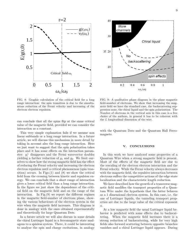
This very simple explanation fails if we assume nonlinear subbands or a long range interaction. In a futurearticle, we will discuss this mechanism in more detail bytaking in account also the long range interaction. Herewe just want to suggest that the spin polarization takesplace and it has some effects on the interaction param-eter: g⊥i disappears and the Fermi wavevector doublesyielding a further reduction of g1 and g2. We limit our-selves to show how the strong magnetic field has the effectof reducing the Fermi velocity and increasing the electronelectron repulsion until a critical phenomenon (spin tran-sition) occurs. In Figs.(1) and (8) we show the criticalfield from the crossing between kinetic and repulsion en-ergy. We can conclude that a short range of interactiongives a lower critical field than a long range interaction.In the figure we just show the dependence of the criti-cal field on the magnetic field and on the range of theinteraction. In Fig.(9) we report the different regimesin the magnetic field-number of electrons plane, show-ing the various behaviours of the electron system in thewire when the magnetic field increases. This diagram isdone in analogy with the ones obtained experimentallyand theoretically for large Quantum Dots.

In a future article we will also discuss in some detailsthe chiral Luttinger liquid in a ferromagnetic state anal-ogous to a spinless system. There, it could be interestingto analyze the spin and charge excitations, in analogy

FIG. 9: A qualitative phase diagram in the plane magneticfield-number of electrons. We show that increasing the mag-netic field we have the standard case, the backscattering sup-pression zone, the chiral liquid and the spin polarization. TheNumber of electrons in the vertical axis in this case is a freechoice of the authors, in general it has to be coherent withthe L longitudinal dimension of the wire.

with the Quantum Dots and the Quantum Hall Ferro-magnets.

V. CONCLUSIONS

In this work we have analyzed some properties of aQuantum Wire when a strong magnetic field is present.Most of the effects of the magnetic field are due tothe rescaling of the electron electron interaction and theFermi velocity. While the Fermi velocity always decreaseswith the magnetic field, the repulsive interaction betweenelectrons suffers the competitive actions of the edge statelocalization and the characteristic length reduction.

We have described how the growth of a transverse mag-netic field modifies the transport properties of a Quan-tum Wire under the hypothesis that the latter behavesas a 1 dimensional electron system. In this case, i.e. theone of Luttinger liquids, the tunneling transport prop-erties are due to the large value of the critical exponentα.

At a low magnetic field the usual Luttinger liquid be-havior is predicted with some effects due to backscat-tering. When the magnetic field increases there is astrong reduction of backscattering, while for very highfields also forward scattering between opposite branchesvanishes and a chiral Luttinger liquid appears. During

10

the growth of the magnetic field the critical exponent isstrongly reduced. A further rise of the field can cause thespin polarization which takes place as in a large QD, i.e.it does not depend on Zeeman or spin orbit effects butis due to the combined effect of the interaction and themagnetic field.

We also have discussed how the presence of one impu-rity can affect the conductance in the wire. The back-ward scattering reduction and the rescaling of the elec-tron electron interaction could favor the weak potentiallimit (strong tunneling) by raising the temperature atwhich the wire becomes a perfect insulator (G = 0).

In the future we wish to analyze further the possibleextension of this formalism to the study of Carbon Nan-otubes and discuss with more detail the properties of aLuttinger liquid in a fully polarized state.

Acknowledgments

This work is partly supported by the Italian ResearchMinistry MIUR, National Interest Program under grantCOFIN 2002022534.

APPENDIX A: COMPARISON BETWEEN

COULOMB INTERACTION AND MODEL

In this appendix we discuss the difference between theFourier transforms of the Coulomb interaction and of themodel (eq.(11)).

We point out that the potential in the form of eq.(11)allows exact integration, in order to obtain the Fouriertransform, and it regularizes the divergence appearing inthe Coulomb potential. This function could be optimizedvarying the range parameter r, so that it could be quitesimilar to the Coulomb potential. The function g(δk, ωc)is plotted for a very short range (r = 0.1) and for variousvalues of magnetic field in Fig.(10).

The Coulomb potential is not so easy to integrate: wegive its transform obtained by a numerical integration

with a sort of regularization near the divergence, andnormalized with respect to the value obtained at zeromagnetic field (g(0, 0) = 1). Also in this case we showin Fig.(10) the Fourier transform for various values ofmagnetic field.

Now we can conclude that the model fits well theCoulomb interaction, if we choose a short range parame-ter: Fig.(10) shows this good agreement.

We can conclude that a magnetic field in the limit ofshort range gives

g(0, ωc) ≈ g(0, 0)

√

ωT

ω0

so that we have the strongest interaction between elec-trons with quite similar momentum. From Fig.(10.a) and

FIG. 10: a)On the left, the Fourier transform for variousvalues of magnetic field of the model of interaction with ashort range (0.1). b)On the right, the Coulomb potentialcase obtained with a numerical calculation and normalizedwith respect to the value obtained at zero magnetic field(g(0, 0) = 1). A comparison shows a good agreement andan analogous magnetic field dependence.

Fig.(10.b) we can also argue that the function V (δk) de-cays very rapidly when δk increases for high magneticfields.

1 T. J. Thornton, Rep. Prog. Phys. 58, 311 (1995).2 C. W. J. Beenakker and H. van Houten Quantum transport

in Semiconductor Nanostructures, vol. 44 of Solid statephysics (Academic Press, New York, 1991).

3 R. Landauer, IBM J. Res. Dev. 1, 223 (1957).4 M. Buttiker, IBM J. Res. Dev. 32, 317 (1988).5 C. L. Kane and M. P. A. Fisher, Phys. Rev. B 46, 15233

(1992)6 A. V. Moroz, K. V. Samokhin and C. H. W. Barnes, Phys.

Rev. Lett. 84, 4164 (2000).7 A. V. Moroz and C. H. W. Barnes, Phys. Rev. B 61, R2464

(2000).8 A. De Martino and R. Egger, Europhys. Lett. 56, 570

(2001).

9 B. J. van Wees, H. van Houten, C. W. J. Beenakker, J. G.Williamson, L. P. Kouwenhoven, D. van der Marel and C.T. Foxon,, Phys. Rev. Lett. 60, 848 (1988).

10 D. A. Wharam, T. J. Thornton, R. Newbury, M. Pepper,H. Ahmed, J. E. F. Frost, D. G. Hasko, D. C. Peacock, D.A. Ritchie and G. A. C. Jones, J. Phys.: Condens. Matter21, L209 (1988).

11 L. I. Glazman, G. B. Lesovik, D. E. Khmel’nitskii and R. I.Shekhter, Pis’ma Zh. Eksp. Teor. Fiz. 48, 218 (1988); L. I.Glazman and M. Jonson, Phys. Rev. B 41, 10686 (1990).

12 S. Tomonaga, Prog. Theor. Phys. 5, 544 (1950); J. M. Lut-tinger, J. Math. Phys. 4, 1154 (1963); D. C. Mattis andE. H. Lieb, J. Math. Phys. 6, 304 (1965).

13 For a review see J. Solyom, Adv. Phys. 28, 201 (1979)

11

and J. Voit, Rep. Prog. Phys. 57, 977 (1994).14 A. H. MacDonald, Phys. Rev. Lett. 64, 220 (1990); X.-G.

Wen, Phys. Rev. Lett. 64, 2206 (1990); Phys. Rev. B 41,12838 (1990); Phys. Rev. B 43, 11025 (1991); Int. J. Mod.Phys. B 6, 1711 (1992); U. Zulicke and A. H. MacDonald,Phys. Rev. B 54, 16813 (1996).

15 A. Furusaki and N. Nagaosa, Phys. Rev. B 47, 4631 (1993).16 S. J. Tans, M. H. Devoret, H. Dai, A. Thess, R. E. Smalley,

L. J. Geerligs and C. Dekker, Nature 386, 474 (1997); M.Bockrath, D. H. Cobden, J. Lu, A. G. Rinzler, G. Andrew,R. E. Smalley, L. Balents and P. L. McEuen, Nature 397,598 (1999); Z. Yao, H. W. J. Postma, L. Balents, and C.Dekker, Nature 402, 273 (1999).

17 R. Egger and A. O. Gogolin, Phys. Rev. Lett. 79, 5082(1997); C. Kane, L. Balents and M. P. A. Fisher, ibid. 79,5086 (1997).

18 S. Tarucha, T. Honda and T. Saku, Solid State Comm. 94,413 (1995).

19 A. Yacoby, H. L. Stormer, N. S. Wingreen, L. N. Pfeiffer,K. W. Baldwin and K. W. West, Phys. Rev. Lett. 77, 4612(1996); O. M. Auslaender, A. Yacoby, R. de Picciotto, K.W. Baldwin, L. N. Pfeiffer and K. W. West, Phys. Rev.Lett. 84, 1764 (2000); M. Rother, W. Wegscheider, R. A.Deutschmann, M. Bichler and G. Abstreiter, Physica E 6,551 (2000).

20 C. L. Kane and M. P. A. Fisher, Phys. Rev. Lett. 68, 1220(1992); C. L. Kane and M. P. A. Fisher, Phys. Rev. B 46,7268 (1992)

21 E. I. Rashba, Fiz. Tverd. Tela (Leningrad) 2, 1224 (1960)[Sov. Phys. – Solid State 2, 1109 (1960)]; Yu. A. Bychkovand E. I. Rashba, Pis’ma Zh. Eksp. Teor. Fiz. 39, 66 (1984)[JETP Lett. 39, 78 (1984)].

22 M. Governale and U. Zulicke Phys. Rev. B 66, 073311(2002).

23 S. Bellucci and P. Onorato, Phys. Rev. B 68, 245322(2003).

24 W. Hausler, L. Kecke, and A. H. MacDonald,cond-mat/0108290

25 S. Tarucha, D. G. Austing, T. Honda, R. J. van der Hageand L. P. Kouwenhoven, Phys. Rev. Lett. 77, 3613 (1996);T.H. Oosterkamp, J. W. Janssen, L. P. Kouwenhoven, D.G. Austing, T. Honda and S. Tarucha, Phys. Rev. Lett.82, 2931 (1999).

26 V. Marigliano Ramaglia, F. Ventriglia and G. P. Zucchelli,Phys. Rev. B 48, 2445 (1993).

27 S. Bellucci and J. Gonzalez, Eur. Phys. J. B 18, 3 (2000);S. Bellucci, Path Integrals from peV to TeV, eds. R. Casal-buoni, et al. (World Scientific, Singapore, 1999) p.363,hep-th/9810181; S. Bellucci and J. Gonzalez, Phys. Rev.B 64, 201106(R) (2001); S. Bellucci, J. Gonzalez andP. Onorato, Nucl. Phys. B 663 [FS], 605 (2003); S. Bel-lucci, J. Gonzalez and P. Onorato, Phys. Rev. B 69,085404 (2004); S. Bellucci and P. Onorato, Phys. Rev.B 71, 075418 (2005), cond-mat/0501051; S. Bellucci, J.Gonzalez, P. Onorato, cond-mat/0501201.

28 V. Meden, W. Metzner, U. Schollwock and K. Schonham-mer, Phys. Rev. B 65, 045318 (2002); V. Meden, S. Ander-gassen, W. Metzner, U. Schollwock and K. Schonhammer,Europhys. Lett. 64, 769 (2003).

29 H. J. Schulz, cond-mat/9503150.30 O. Klein, C. de C. Chamon, D. Tang, D. M. Abusch-

Magder, X.-G. Wen, M. A. Kastner and S. J. Wind, Phys.Rev. Lett. 74, 785 (1995).

31 O. Klein, D. Goldhaber-Gordon, C. de C. Chamon and M.A. Kastner, Phys. Rev. B 53, 4221 (1996).

32 O. Klein et al., in Quantum Transport in Semiconductor

Submicron Structures, ed. Kramer (1996).33 This phenomenon was observed in a transverse conduc-

tance measure where the peaks in the conductance corre-spond to the chemical potential of the N-electron system.