three-band to one-band Hubbard model - kth .diva

Master of Science Thesis

Deriving an extended one-band Hubbard modelfor cuprate superconductors

Karl-Oskar BacklundApril 2011

Abstract

The so-called three-band Hubbard model is generally believed to be a good model for fermions on aCuO2 lattice and to contain key features allowing to understand high-temperature superconductivityin the cuprates. A simpler and more popular model is the one-band Hubbard model. In this thesis,an extended one-band Hubbard model is derived from the three-band model.

First, some mathematical background is given, as well as an introduction to Hubbard-like models.Then, to derive the extended one-band Hubbard model, the CuO2 lattice is divided into clusters ofone Cu and two O sites, and a variant of the Feshbach method is used to replace each such clusterby a single lattice site. To find a suitable one-band model, all Hamiltonian matrix elements arematched between the two models. Finally, different sets of three-band parameters are considered,and it is studied how this affects the parameters in the extended one-band Hubbard model.

Sammanfattning

Den sa kallade treband-Hubbardmodellen antas allmant vara en god modell for fermioner i ett CuO2-gitter och innehalla viktiga egenskaper for forstaelsen av hogtemperatursupraledning i kuprater.En enklare och popularare modell ar enband-Hubbardmodellen. I den har avhandlingen harleds enutokad enband-Hubbardmodell fran treband-Hubbardmodellen.

Forst diskuteras viss matematisk bakgrund och en introduktion till Hubbardmodellen ges. Sedan,for att harleda den utokade enband-Hubbardmodellen, delas CuO2-gittret in i grupper om en Cu-och tva O-atomer, och en variant av Feshbach-metoden anvands for att ersatta varje sadan gruppmed en enda gitterpunkt. For att hitta en passande enband-modell matchas Hamiltonoperatorns allamatriselement mellan de tva modellerna. Slutligen beaktas olika parametrar for treband-modellen,for att studera hur detta paverkar parametrarna i den utokade enband-Hubbardmodellen.

iii

Acknowledgements

First and foremost I would like to thank my supervisor Edwin Langmann for his guiding and supportthroughout the work with this thesis. From him, I have gained valuable insight in what it is to doscience. In particular, he has encouraged me to understand every step in the process as deeply aspossible. In addition, I want to thank Per Hakan Lundow and Jonas de Woul, at the departmentof Theoretical Physics at the Royal Institute of Technology, for helping out with vital steps in mywork. Last but not least, I would like to thank my friends Pontus Lans and Saddaf Shabbir, forsaving me several hours each, providing their LaTex and Matlab skills, respectively.

Contents

1 Introduction and outline 1

2 Mathematical tools 3

2.1 Second quantization . . . . . . . . . . . . . . . . . . . . . . . . . . . . . . . . . . . . 3

2.1.1 Fermion systems – annihilation and creation operators . . . . . . . . . . . . . 4

2.1.2 The number operator N . . . . . . . . . . . . . . . . . . . . . . . . . . . . . . 6

2.1.3 Fock spaces and tensor products . . . . . . . . . . . . . . . . . . . . . . . . . 7

2.2 Matrix representation in quantum physics . . . . . . . . . . . . . . . . . . . . . . . . 8

2.2.1 Observables and eigenvalues . . . . . . . . . . . . . . . . . . . . . . . . . . . . 9

2.2.2 Commutating operators – block diagonal matrices . . . . . . . . . . . . . . . 9

2.2.3 Matrix representation of fermion systems . . . . . . . . . . . . . . . . . . . . 12

2.3 Feshbach Method . . . . . . . . . . . . . . . . . . . . . . . . . . . . . . . . . . . . . . 12

3 The Hubbard model on small clusters 15

3.1 Solving the Hubbard model on two sites . . . . . . . . . . . . . . . . . . . . . . . . . 15

3.2 Complexity increases rapidly . . . . . . . . . . . . . . . . . . . . . . . . . . . . . . . 18

4 Three-band Hubbard model 21

4.1 One-cluster energies and states . . . . . . . . . . . . . . . . . . . . . . . . . . . . . . 24

4.2 The full Hamiltonian . . . . . . . . . . . . . . . . . . . . . . . . . . . . . . . . . . . . 25

5 Matching the Hubbard models 27

5.1 Associating states . . . . . . . . . . . . . . . . . . . . . . . . . . . . . . . . . . . . . . 27

5.1.1 Ignoring high-energy three-band states . . . . . . . . . . . . . . . . . . . . . . 27

iv

v

5.1.2 Associating states between the models . . . . . . . . . . . . . . . . . . . . . . 29

5.2 Finding the one-band Hubbard Hamiltonian . . . . . . . . . . . . . . . . . . . . . . . 29

5.2.1 Ansatz for the one-band Hubbard Hamiltonian . . . . . . . . . . . . . . . . . 31

5.2.2 Matching matrix elements – finding the parameters . . . . . . . . . . . . . . . 32

5.3 Varying the three-band model parameters . . . . . . . . . . . . . . . . . . . . . . . . 35

5.3.1 Other sets of three-band parameters . . . . . . . . . . . . . . . . . . . . . . . 35

5.3.2 Varying each three-band parameter separately . . . . . . . . . . . . . . . . . 36

6 Conclusion 43

References 45

A Notation and terminology 47

B Mathematical details 49

B.1 Solution of three-band model on one cluster . . . . . . . . . . . . . . . . . . . . . . . 49

B.1.1 n = 0 . . . . . . . . . . . . . . . . . . . . . . . . . . . . . . . . . . . . . . . 49

B.1.2 n = 1 . . . . . . . . . . . . . . . . . . . . . . . . . . . . . . . . . . . . . . . 50

B.1.3 n = 2, sz = 0 . . . . . . . . . . . . . . . . . . . . . . . . . . . . . . . . . . . 52

B.1.4 n = 2, sz = +1/− 1 . . . . . . . . . . . . . . . . . . . . . . . . . . . . . . . 55

B.1.5 Summary: Energies in one cluster . . . . . . . . . . . . . . . . . . . . . . . . 56

B.2 Proof of Proposition 5.2.1 . . . . . . . . . . . . . . . . . . . . . . . . . . . . . . . . . 58

C Matlab codes 66

C.1 The Hubbard model – a simple example . . . . . . . . . . . . . . . . . . . . . . . . . 66

C.1.1 Energies in the two-sites case . . . . . . . . . . . . . . . . . . . . . . . . . . . 66

C.1.2 Energies in the L-sites case . . . . . . . . . . . . . . . . . . . . . . . . . . . . 67

C.2 Three-band to one-band model . . . . . . . . . . . . . . . . . . . . . . . . . . . . . . 70

C.2.1 Solving one cluster . . . . . . . . . . . . . . . . . . . . . . . . . . . . . . . . . 70

C.2.2 Matching three-band to one-band model . . . . . . . . . . . . . . . . . . . . . 74

Chapter 1

Introduction and outline

Superconductivity, the phenomenon of vanishing resistivity at temperatures below a certain criticaltemperature Tc, was first observed in 1911 (see for example [8]). The so-called BCS theory, presentedin 1957 [2], is a successful quantum theory for superconductivity in materials with Tc ≈ 30 Kand lower. One generally refers to superconductivity explained by BCS Theory as ”conventionalsuperconductivity”.

During the 1980s materials were found in which superconductivity was observed at higher tem-peratures (a pioneering paper awarded by the Nobel Prize is [3]), and the term high-temperaturesuperconductivity (HTSC) was introduced. Since then, superconducting materials with increasingTc have been discovered. Notably, Tc values up to 138 K have been observed (see for example [8, p.295]).

Until recent years and the discovery of iron-based superconductors (see for example [13]), all ma-terials featuring HTSC were so-called cuprates. The common feature of these cuprates is that theyconsist of CuO2 layers sandwiched between layers of other atoms. The layers in-between serve todope the CuO2 layers with either electrons or holes. The detailed structure of these CuO2 layers isdiscussed in Chapter 4.

The so-called three-band Hubbard model is generally believed to be a good model for the fermions(electrons or holes) in a CuO2 layer (see for example [14, p. 3759], [1, p. 2] and [6, p. 2794]), andthereby to contain the key features to understand HTSC in the cuprates. In this model, fermionsreside on both Cu and O atoms in the CuO2 layer. The three-band Hubbard model can be reducedto the less complex one-band Hubbard model or, simply, the Hubbard model. Here, fermions areconsidered only on the Cu sites, thereby removing the degrees of freedom associated with the Osites.

While the one-band Hubbard model is less detailed than the three-band model, it is easier forcomputational studies, with methods such as exact diagonalization or quantum Monte Carlo [1, p.2], or with a restricted Hartree-Fock approach, as carried out in [5]. The Hubbard model can beextended to include additional terms, and we refer to this as extended one-band Hubbard models.Even though a large number of studies have been carried out on one-band Hubbard models, thereis still much left to be understood regarding their behavior. Considerably fewer studies have beencarried out for the more complex three-band Hubbard model.

1

2 Introduction and outline

It is often assumed that the terms of small magnitude, in an extended Hubbard model, can beignored . However, there are indications [9, p. 1] that these ”small terms” may play an importantrole, and it is therefore interesting to revisit how they are obtained. In this thesis, we derive anextended one-band Hubbard model from the three-band model, using a variant of the Feshbachmethod (see for example [10]).

Throughout the derivation, we will use the set of three-band model parameters in [1, p. 5]. Thereader should be aware of the uncertainties of these values. After having derived the one-bandmodel, we assume different sets of three-band parameters (guided by [11, Table VI] and [12, SectionII]), and see how the extended one-band model parameters are changed.

In Chapter 2, we discuss some of the mathematical formalisms and techniques used in the thesis.In Chapter 3 we introduce the Hubbard model, and study it in some simple examples. In Chapter4 and 5 we carry out the procedure of deriving an extended one-band Hubbard model, and wepresent the result in Chapter 6. In Appendix A, we fix our notation. Appendix B contains furthermathematical details, and all Matlab programs are attached in Appendix C.

Chapter 2

Mathematical tools

2.1 Second quantization

The formalism used in this thesis is called second quantization. In this section, we give a briefintroduction to second quantization, and in particular, we introduce the annihilation and creationoperators. We recall that the central objects in a quantum theory are quantum states and operators.The states are represented by state vectors in a Hilbert space, and parallel vectors (i.e. differingonly by a scale factor λ) represent the same states. All observable quantities – for example position,energy and momentum – are represented by operators acting on this Hilbert space.

In the first quantization formalism, also referred to as ”quantum mechanics”, the (time independent)quantum mechanical state of one particle is, in position representation, the complex-valued wavefunction ψ(r). The absolute square of the wave function represents the probability density of theparticle, i.e. |ψ(r)|2dr is the probability of finding the particle within the volume element dr aroundthe coordinate r. From this, it follows that one condition that has to be posed upon ψ(r) is thenormalization condition:

∫|ψ(r)|2dr = 1, where the integral is taken over the full space. The

normalization conditions means that, with probability one, the particle will be found anywhere inspace.

Now, consider a system of an arbitrary number N particles. The wave function now takes theform ψ(r1, r2, · · · , rN ), where (r1, r2, · · · , rN ) is a vector in the 3N-dimensional space, and is suchthat |ψ(r1, r2, · · · , rN )|2

∏Ni=1 dri is the probability of finding the N particles in the 3N-dimensional

volume∏Ni=1 dri around the coordinate (r1, r2, · · · , rN ) in the 3N-dimensional space. Thus, the

integral of |ψ(r1, r2, · · · , rN )|2 over all space is 1.

A fundamental concept in quantum mechanics is indistinguishable particles: If particles are char-acterized be the same quantum numbers, such as mass, charge and spin, they can be indistinguish-able. Assume a state ψ(r1, r2, · · · , rN ) representing N indistinguishable particles. Interchangingtwo coordinates in ψ corresponds to swapping two particle with each other. Since the particles areindistinguishable, this action must result in the same state, and thus the new wave function mustdiffer from the original only by a scalar factor (this freedom pertains since parallel vectors representthe same state). Carrying out this procedure twice, we get

3

4 Mathematical tools

ψ(r1, · · · , rj , · · · , rk, · · · , rN ) = λψ(r1, · · · , rk, · · · , rj , · · · , rN ) = (2.1)

= λ2ψ(r1, · · · , rj , · · · , rk, · · · , rN ),

i.e. λ2 = 1, and thus λ = ±1. This leads to the conclusion that there exist only two types ofquantum mechanical particles: Those where λ = 1 (called bosons) and those where λ = −1 (calledfermions). In this thesis, we are exclusively studying fermions (electrons or holes, i.e. the absence ofelectrons). A fundamental property of fermions is that it is not possible for more than one particleto occupy the same one-particle state: if rj = rk, then ψ = 0. This feature of fermions is referredto as the Pauli exclusion principle.

In the first quantization formalism we need to find a wave function ψ(r1, r2, · · · , rN ) obeying therelation λ = −1. It is in principle possible to construct such wave functions from one-particle wavefunctions ψi(ri) as follows:

ψ(r1, r2, · · · , rN ) =∑

ν1,··· ,νN

Aν1,ν2,··· ,νNψν1(r1)ψν2(r2) · · ·ψνN (rN ),

where νi denotes the state of particle i, and Aν1,ν2,··· ,νN are certain complex numbers. The fullprocess of constructing these states, including how the complex numbers Aν1,ν2,··· ,νN are deter-mined, is found on for example in [4, Chapter 1.2]. Looking at the nature of the complex numbersAν1,ν2,··· ,νN , it becomes clear that this first quantization formalism will be very complex as thenumber of particles increases. A more convenient formalism is described below.

2.1.1 Fermion systems – annihilation and creation operators

The basic concept of the second quantization formalism is to define states in which the indistin-guishable particles may be found, and to count how many particles there are in each state. Anothername for second quantization is consequentially ”occupation number representation”. In this thesis,we will restrict ourselves to cases where there are a finite number L of states that may be occupiedby one fermion. The reasoning is the following:

Assume that we have a collection of L single-particle quantum states that may be occupied byfermions: ψ1, ψ2, · · · , ψL. Now, instead of constructing a many-particle wave function from thesesingle-particle wave functions (as we did in the first quantization formalism), we define the followingsecond quantization state:

|n〉 = |n1, n2, · · · , nL〉, (2.2)

where ni ∈ N is the number of particles in state ψi, and∑

j nj = n is the total number of fermions.

In the following, we will need the annihilation operator ai and the creation operator a†i , the Her-mitian adjoint 1 of ai, associated with one-particle state ψi. We will now define these operators.

1The Hermitian adjoint A† of any operator A on a Hilbert space H satisfies 〈A†x|y〉 = 〈x|Ay〉 for any elements xand y in H with 〈· · · | · · · 〉 the scalar product in H.

2.1 Second quantization 5

First, we postulate the anti-commutator relations for ai and a†i :

aj , ak = 0, aj , a†k = δjk ∀j, k ∈ 1, 2, · · · , L (2.3)

We show2 below that (2.3) implies a†j , a†k = 0:

a†j , a†k = a†ja

†k + a†ka

†j = (akaj)

† + (ajak)† = (akaj + ajak)

† = (ak, aj)† = 0† = 0 (2.4)

Furthermore, we define the empty state Ω, and the action of any annihilation operator ai upon thisempty space:

Ω = |n1 = 0, n2 = 0, · · · , nL = 0〉, aiΩ = 0, 〈Ω|Ω〉 = 1 (2.5)

The physical interpretation of (2.5) is that the empty state cannot be further emptied. (2.3) and(2.5) provide the full definition of the fermion system.

The action of the creation operator a†i on the empty state is

a†iΩ = |n1 = 0, n2 = 0, · · · , ni = 1, · · · , nL = 0〉, (2.6)

i.e. a fermion is created in one-particle state ψi. Now, we can write any state (2.2) expressed increation operators acting on the empty state:

|n〉 ≡ (a†1)n1(a†2)

n2 · · · (a†L)nLΩ (2.7)

ni ∈ 0, 1.

We refer to states such as (2.7) as pure states, and one can show that they provide a completeorthonormal basis, i.e. that any state can be written as a linear combination of states in (2.7).

The order in which the creations operators are applied in (2.7) is essential. One has to agree

upon an unambiguous order convention, in this case ”i < j ⇒ a†i is applied to the left of a†j”. This

necessity is a consequence of the anti-commutator relations (2.4): since a†ia†j = −a†ja

†i , the state |n〉

is determined only up to a factor (−1) unless we specify the order.

We note that the Pauli exclusion principle follows directly from the anti-commutator relations: If oneattempts to create a fermion in the single-particle state i, by applying a†i to a state |n〉 where ni = 1,

2We use the following properties of the Hermitian adjoint of the product and of the sum of two operators: (AB)† =B†A†, and (A+ B)† = A† + B†


one will somewhere end up with the product a†ia†i . But (2.4) tells us that a†i , a

†i = 2a†ia

†i = 0, and

the result would thus be zero. The conclusion is that, in a pure state, each single particle state canbe occupied only by either zero or one particle.

From the definition in (2.3) and (2.5), it also follows what result one gets when acting with an

annihilation operator a†i on a state |n〉. We look separately on the cases where ni = 0 and ni = 1,i.e. when the single-particle state ψi is non-occupied and occupied, respectively:

If ni = 0 :

ai|n〉 = ai(a†1)n1 · · · (a†i )

0 · · · (a†N )nN |Ω〉 = ai(a†1)n1 · · · I · · · (a†N )nN |Ω〉 =

= (−1)ξ0(a†1)n1 · · · (a†N )nN aiΩ︸︷︷︸

=0

= 0 (2.8)

If ni = 1 :

ai|n〉 = ai(a†1)n1 · · · a†i · · · (a

†N )nNΩ = (−1)ξ1(a†1)

n1 · · · aia†i · · · (a†N )nNΩ =

= (−1)ξ1(a†1)n1 · · · (1− a†iai) · · · (a

†N )nNΩ =

= (−1)ξ1(a†1)n1 · · · I · · · (a†N )nNΩ− (−1)ξ1(a†1)

n1 · · · a†i (−1)ξ2 · · · (a†N )nN aiΩ︸︷︷︸=0

=

= (−1)ξ1 |n′〉 (2.9)

ξ0 =∑k 6=i

nk; ξ1 =

i−1∑k=1

nk; ξ2 = ξ0 − ξ1

When there is no particle in state ψi, acting with ai on |n〉 results in zero. When there is a particlein ψi, acting with ai on |n〉 yields (with a possible factor −1) |n′〉, the same state except that theparticle in state ψi has been annihilated.

2.1.2 The number operator N

We define the number operator on the system of L sites as follows:

N =

L∑i=1

Ni; Ni = a†iai (2.10)

Acting with Ni on the state |n〉, using (2.8) and (2.9), gives

2.1 Second quantization 7

Ni|n〉 =a†iai(a†1)n1 · · · (a†i )

ni · · · (a†N )nNΩ = a†i (−1)ξ1(a†1)n1 · · · ai(a†i )

ni · · · (a†N )nNΩ =

=

a†i0 = 0, if ni = 0

a†i (−1)ξ1(a†1)n1 · · · I · · · (a†N )nNΩ, if ni = 1

=

=

a†i0 = 0, if ni = 0

(−1)2ξ1(a†1)n1 · · · a†i · · · (a

†N )nNΩ = |n〉, if ni = 1

,

which shows that the states |n〉 are eigenstates to Ni with eigenvalue ni: Ni|n〉 = ni|n〉. We maynow extend to the full operator N , acting on |n〉:

N |n〉 =L∑i=1

Ni|n〉 =L∑i=1

ni|n〉 = n|n〉 (2.11)

n = n1 + n2 + · · ·+ nL

The states |n〉 are eigenstates to N , with eigenvalue n, the total particle number.

2.1.3 Fock spaces and tensor products

We now look closer into the mathematical formalism used when single-particle systems are combinedto a larger system.

Consider a fermion system with a single one-particle state. For a second quantized quantum me-chanical state to be well defined, we require that it is an eigenstate to the number operator N ,with an eigenvalue that is zero or a positive integer. This requirement demands that we have aninteger number of particles in our system. As we have previously discussed, a fermion state may beoccupied by at most one fermion. In other words, the eigenvalue n may be only 0 or 1. Our statesare thus vectors a Hilbert space Hone, which is of dimension two: there are only two possible statesin the Hilbert space.

Now consider a system of two single-particle fermion states ψi and ψj , that both may be eitherempty or occupied. We realise that there are four different situations where both ni and nj are welldefined: ni = 0, nj = 0, ni = 1, nj = 0, ni = 0, nj = 1 and ni = 1, nj = 1. These four statesspan1 the Hilbert space Htwo: Any state in Htwo may be obtained by a linear combination of thesefour pure states. We thus conclude that Htwo is of dimenstion four2. By repeating this reasoning,we can see that adding another single particle fermion state to our system will always double thenumber of pure states. The general conclusion is that states in a system with L single-particle stateswill be represented by vectors in a Hilbert space HL of dimension 2L.

A formal way to combine the Hilbert spaces of L single-particle systems is the tensor product ⊗:

1We use the word ”span” in this context as synonymous to ”provide a complete orthonormal basis to”2The dimension of any Hilbert space H is equal to the number of states in a complete basis of H.


HL = Hone ⊗ · · · ⊗ Hone︸︷︷︸L times

(2.12)

We refer to HL as the Fock space, and introducing the direct sum1 ⊕ we may also write

HL = F0 ⊕F1 ⊕ · · · ⊕ FL, (2.13)

where Fk is the subspace of HL spanned by all pure states states with particle number n = k.

In this thesis we will use tensor product both between Hilbert spaces (as above) and betweenvectors. Below, we state two useful properties of the tensor product between vectors:

(v1 ⊗ v2)(w1 ⊗ w2) = v1v2 ⊗ w1w2

(2.14)

〈v1 ⊗ v2|w1 ⊗ w2〉(H1⊗H2) = 〈v1|w1〉H1〈v2|w2〉H2 , where:

(2.15)

v1, w1 ∈ H1; v2, w2 ∈ H2; (v1 ⊗ v2) ∈ (H1 ⊗H2)

〈· · · | · · · 〉(··· ) is the inner product in respective Hilbert space.

2.2 Matrix representation in quantum physics

Throughout the thesis, we will associate operators with matrices and states with vectors. In thissection, we therefore give some background to this matrix formulation of quantum physics. Fora more exthausive introduction, see for example [7, p. 146-153]. In Section 2.2.3, we also give aconcrete vector and matrix representation of the fermion system described in Section 2.1.1. Thisrepresentation will be of use when we carry out numerical calculations in Matlab.

Consider a Hilbert space H representing a quantum system, and assume that we have defined acomplete orthonormal basis of states |n〉 on H. Then, any operator2 O on H may be representedby a matrix, whose elements are

Onm = 〈n|O|m〉, (2.16)

i.e. the inner product (as defined on H) between the state |n〉 and the state resulting from actingwith O on |m〉. In this manner, the O matrix representation is constructed:

1The direct sum U ⊕ V of two vector spaces is defined as the sum of subspaces in which U and V have only thezero vector in common

2Our general notation convention is that operators A are written with a hat, and their matrix representation A, insome basis, is written without hat. However, in Chapters 4 and 5 we will write the Hamiltonian operators H withouthat, as well as their matrix representation.

2.2 Matrix representation in quantum physics 9

O =

O1,1 O1,2 · · · O1,L

O2,1 O2,2 · · · O2,L...

.... . .

...OL,1 OL,2 · · · OL,L

, (2.17)

where L = dim(H).

2.2.1 Observables and eigenvalues

We call an observable a measurable physical quantity of a system. It is a fundamental postulateof quantum mechanics that all physical observables are represented by self-adjoint 1 2 operators ona Hilbert space H, and the expectation value of an operator A in a state Ψ ∈ H is 〈Ψ|A|Ψ〉. Inmatrix formulation, this postulate means that all physical observables are represented by self-adjointmatrices3. Self-adjoint matrices have real eigenvalues.

The explicit elements in the matrix representation O, as in (2.17), of any operator O depend on thechoice of basis |n〉. We will be interested in finding the matrix’ eigenvalues, an inherent property ofthe operator O, independent of the choice of basis.

2.2.2 Commutating operators – block diagonal matrices

The eigenvalue problem in matrix representation,

Ov = Ev, (2.18)

can be simplified in an interesting special case which we will discuss in this section. We remindourselves that, given the matrix O, the task is to find vectors vi and corresponding scalars Ei suchthat (2.18) holds. Now, let’s assume that in a certain basis, O can be written as follows:

O =

O1,1 · · · O1,a 0 · · · 0...

. . ....

.... . .

...Oa,1 · · · Oa,a 0 · · · 0

0 · · · 0 Oa+1,a+1 · · · Oa+1,L...

. . ....

.... . .

...0 · · · 0 OL,a+1 · · · OL,L

(2.19)

If we just use regular matrix multiplication, Equation (2.18) can in this case be re-written as follows:

1A self-adjoint operator O is equal to its adjoint O†2An example of an operator that is not self adjoint is the annihilation operator ai. Its adjoint is the creation

operator a†i , and we clearly have ai 6= a†i . From this it follows that the eigenvalues of ai do not correspond to anyphysical observable, and nor do those of a†i .

3A self-adjoint matrix is equal to its conjugate transpose, meaning that for every matrix element Onm it holds thatOmn = (Onm)∗, the ∗ denoting usual complex conjugate.


∑ai=1O1,ivi + 0 + · · ·+ 0∑ai=1O2,ivi + 0 + · · ·+ 0

...∑ai=1Oa,ivi + 0 + · · ·+ 0

0 + · · ·+ 0 +∑L

i=a+1Oa+1,ivi0 + · · ·+ 0 +

∑Li=a+1Oa+2,ivi

...

0 + · · ·+ 0 +∑L

i=a+1OL,ivi

= E

v1v2...vava+1

va+2...vL

(2.20)

In (2.20), there are L equations to simultaneously be solved. However, we note that the a firstequations are decoupled1 from the (L− a) last equation. Therefore, solving (2.20) is equivalent tosolving two equations:

∑a

i=1O1,ivi∑ai=1O2,ivi

...∑ai=1Oa,ivi

= E

v1...va

and

∑L

i=a+1Oa+1,ivi∑Li=a+1Oa+2,ivi

...∑Li=a+1OL,ivi

= E

va + 1...vL

, (2.21)

which, rewritten on matrix form is:

Oa1va1 = va1 and OLa+1v

La+1 = vLa+1 (2.22)

Oji ≡ Ok,li≤k,l≤j ; vji = (vi, vi+1, · · · , vj)

The first equation in (2.22) has a solutions – eigenvalues Ek with corresponding eigenvectors (va1)k– and the second equation has (L− a) solutions.

If a matrix O has the form described in (2.19), we say that it has block-diagonal form. We introducethe notation of the direct sum ⊕ of matrices to describe a block-diagonal matrix with M blocks:

⊕Mi=1 Oi =

O1

O2

. . .

OM

, (2.23)

where the matrices Oi are square matrices diagonally located in O, and all other elements of O arezero. The reasoning for separating equation Ov = Ev may be extended to the case where O hasM blocks, as in (2.23):

1More precisely, we mean that if an element vi appears with a non-zero coefficient in the first a equations, it doesnot appear in the L− a last equations, and vice versa.

2.2 Matrix representation in quantum physics 11

O = ⊕Mi=1Oi =⇒ Ov = Ev⇔

O1v

D11 = EvD1

1

O2vD2D1+1 = EvD2

D1+1...OMvMDM−1+1 = EvMDM−1+1

(2.24)

where Di −Di−1 is the number of rows (and columns) in Oi (with D0 ≡ 0)

Diagonal blocks in a matrix O on a Hilbert space H have a physical interpretation: They correspondto subspaces of H in which all states share a common eigenvalue, unique to that block, with respectto an operator P that commute with O: [O, P ] = 0. We say that such an operator P representsa symmetry of O, and we may use the following result to find a basis in which O, the matrixrepresentation of O is block-diagonal:

Proposition 2.2.1 Consider O, an observable on a Hilbert space H, and a complete orthonormalbasis ψn in H, such that each ψn is an eigenstate to another observable P on H, Pψn = pnψn,ordered such that p1 = p2 = · · · = pD1 , pD1+1 = pD1+2 = · · · = pD2 , · · · , pDM−1

= · · · = pDM , withpDj 6= pDk for j 6= k and 0 ≡ D0 < D1 < D2 < · · · < DM ≡ dim(H).

Then, O = ⊕Mi=1Oi is the matrix representation of O, Oi expressed in the basis ψkDi−1<k≤Di ;i ∈ 1, · · · ,M.

Proof Choose any two basis states ψn and ψm such that pn 6= pm. Then, since [P , O] = 0, we have

P Oψn = OPψn = Opnψn = pnOψn,

and Oψn is thus also an eigenstate to P with the same eigenvalue pn as ψn. Thus, Oψn may bewritten as a linear combination of basis states ψkDi−1<k≤Di , with pDi = pn. All these states ψkare orthogonal to ψm, and thus the matrix element Om,n = 〈ψm|O|ψn〉 is zero. ψn and ψm arearbitrarily chosen basis states possessing different eigenvalues pn and pm, and we conclude that thematrix representation O, expressed in ψn,must be block-diagonal.

In practice, given an operator P such as above, the challenge will often be to find a suitable basisψn such as described above.

Proposition 2.2.1 may be used for several symmetries to the same operator: If there exists anotheroperator P ′ such that [P ′, O] = 0, we may regard every subspace Hi in the above reasoning asconsisting of yet smaller subspaces, each corresponding to unique eigenvalues p′i of P ′, and finda basis ψ′n such as described above, and carry out the same procedure in order to make the Omatrix consist of an even larger number of even smaller blocks.

Later, we will use Proposition 2.2.1 to find a basis in which the Hamiltonian matrix is block-diagonal.We will use, among others, the number operator N , representing the symmetry.


2.2.3 Matrix representation of fermion systems

We will now define a vector and matrix representation of the fermion system discussed in Section2.1.1, defined by the annihilation and creation operators ai and a†i , and the empty space Ω. In theHilbert space HL representing the system of L single particle states (that may be either empty oroccupied with a fermion), we will represent the annihilation and creation operators with matrices.We make the following definitions:

I2 =

(1 00 1

); σ3 =

(1 00 −1

); σ+ =

(0 10 0

); σ− =

(0 01 0

)e0 =

(01

), (2.25)

and define the following representations:

ai = σ3 ⊗ · · · ⊗ σ3︸︷︷︸i−1 times

⊗σ− ⊗ I2 ⊗ · · · ⊗ I2︸︷︷︸L−i times

a†i = σ3 ⊗ · · · ⊗ σ3︸︷︷︸i−1 times

⊗σ+ ⊗ I2 ⊗ · · · ⊗ I2︸︷︷︸L−i times

Ω = e0 ⊗ · · · ⊗ e0︸︷︷︸L times

(2.26)

One can show, using the rules for multiplications of tensor products in (2.14), that the identifications(2.26) preserve the following essential properties of the fermion system:

(ai)† = a†i : (i.e. a†i is the hermitian adjoint of ai)

ai, a†j = δi,j

ai, aj = 0 ∀ i, j

aiΩ = 0

We will use the above representation when using Matlab to calculate numerical values of Hamiltonianmatrix elements.

2.3 Feshbach Method

In this section, we present and discuss the Feshbach technique, which can be used to ”partition”eigenvalue problems. For a more extensive discussion of this method, see for example [10]. InSection 5.1.1, we will use this technique to eliminate high-energy states in the three-band Hubbardmodel.

2.3 Feshbach Method 13

Consider the Schrodinger equation on a Hilbert space H of dimension1 M:

HΨ = EΨ (2.27)

With a given complete orthonormal basis fii∈1,2,··· ,M, (2.27) may be expressed as

Hc = Ec (2.28)

c = (c1, · · · , cM); Ψ =M∑i=1

cifi,

with H the matrix of expectation values of H in fi: Hij = 〈fi|H|fj〉.

Now consider a subspace HA ⊂ H, spanned by the following subset to fi: fiMAi=1 ; MA <M,

and let HB = H \HA, spanned by fiMi=MA+1. Using this notation, we can now rewrite (2.28) as

HAA HAB

HBA HBB

(cAcB

)= E

(cAcB

)(2.29)

Using regular matrix multiplication, we can rewrite equation (2.29) into two equations

HAAcA +HABcB = EcA

HBAcA +HBBcB = EcB (2.30)

From the second equation in (2.30) we get2 cB = (EIBB −HBB)−1HBAcA which, inserted into thefirst equation, gives an effective Hamiltonian

Heff = HAA +HAB(EIBB −HBB)−1HBA, (2.31)

and an equation

Heff (E) cA = E cA (2.32)

Equation (2.32) has exactly the same form as (2.28) [10, p. 971], but instead of an equation inM dimensions we now have an equation in MA <M dimensions. This reduction of dimensions,

1We will in this thesis be concerned only with finite-dimensional Hilbert spaces. However, for the technique outlinedin this section, it would not be a problem if H would be an infinite Hilbert space.

2Provided that (EIBB −HBB)−1 exists See [10] for more discussion on the existence of this inverse matrix.


however, comes at the cost that the linear equation in (2.28) is replaced by a an equation (2.32)where the left hand side depends on E in a non-trivial way.

There are several3 techniques to solve equation (2.32) by, for example, iteration procedures. Whenusing this technique in Section 5.1.1 we will, however, do the approximation that Heff (E) ≈ HAA,avoiding the dependence of E. This is equivalent to setting all elements in HAB to zero.4 It wouldbe interesting to take also into account the terms HAB(EIBB − HBB)−1HBA, but this is left tofuture work.

Looking at the form of Heff in (2.31), we can see that the accuracy of our approximation dependsboth on the magnitude (preferably small) of the elements in the off-diagonal matrices HAB andHBA, and on the difference (preferably large) between the energy E and the elements of HBB.

3See for example [10, p. 970].4In the case where H is self-adjoint this implies that all elements in HBA are zero, too.

Chapter 3

The Hubbard model on small clusters

In this chapter, we introduce the Hubbard model, and study it in simple examples. We will firstconsider a two-sites system, and thereafter study how the complexity grows with the number ofsites in the system.

3.1 Solving the Hubbard model on two sites

Consider two sites on which fermions can reside (See Figure 3.1). A fermion with spin σ ∈ ↑, ↓ is

annihilated (created) on site i by the annihilation (creation) operator a(†)i,σ. To get an understanding

of the Hubbard model, we now want to study it in this simple case. We will define the Hamiltonianmatrix in some basis, and diagonalize it to find the energy eigenvalues. The Hubbard Hamiltonianon the two-sites system is defined as

H = −t∑σ=↑,↓

(a†2,σa1,σ + a†1,σa2,σ) +∑i=1,2

ni,↑ni,↓, (3.1)

where ni,σ = a†i,σai,σ, t is the amplitude of the energy for a fermion hopping from one site to theother and U corresponds to the Coulomb interaction between two fermions residing on the samesite. Note that ”hopping” is, in the second quantization formalism, manifested as annihilating afermion on one site and creating one on the other.

Including spin, there are four single-particle states that may either be occupied or empty. Thus,there are 16 pure states, all eigenstates to the particle number operator N with eigenvalue rangingfrom 0 (both sites empty) to 4 (both sides occupied with one ↑ and one ↓ fermion).

t1 2

Figure 3.1: Two sites system. Fermions may reside either on site 1 or 2, and it is possible to hopfrom one site to the other.

15

16 The Hubbard model on small clusters

As discussed in Section 2.2.2, we want to find operators that commute with H to help find a basis inwhich the matrix representation of H is block-diagonal with as many and as small blocks as possible.Since [ai,σ, nj,σ′ ] = [a†i,σ, nj,σ′ ] = 0 ∀ i, j, σ, σ′, and since on this system the total particle number

operator N = n1,↑+ n1,↓+ n2,↑+ n2,↓ and the total spin operator Sz = 12(n1,↑+ n2,↑)− 1

2(n1,↓+ n2,↓),

we can conclude that [N ,H] = [Sz, H] = 0 holds. Guided by the structure of the Hamiltonian in(3.1) 1, we define the following operator T and show that it commutes with H:

T T † = T †T = I; T ai,σT† = ai+1,σ; TΩ = Ω; 2 + 1 ≡ 1 (3.2)

To show that [T ,H] = 0, we treat each term individually:

1) T(a†2,σa1,σ + a†1,σa2,σ

)= T a†2,σT

†T a1,σT†T + T a†1,σT

†T a2,σT†T =

= a†1,σa2,σT + a†2,σa1,σT =(a†1,σa2,σ + a†2,σa1,σ

)T

2) T ni,σ = T a†i,σT†T ai,σT

†T = a†i+1,σai+1,σT = ni+1,σT , and thus:

T (n1,↑n1,↓ + n2,↑n2,↓) = (n2,↑n2,↓ + n1,↑n1,↓) T and we conclude that:

[T , H] = 0

We use the three symmetries of H represented by the operators N , Sz and T to define a completeorthonormal basis in which the states are eigenstates to these three operators, and with differenteigenvalues. Below we present this basis, along with the eigenvalues2 for each of the states:

1More precisely, the fact that it seems equivalent for any fermion to reside on site 1 as on site 22Our standard notation is that we use lowercase letters for eigenvalues (for example n and sz), but to avoid

confusion with the hopping amplitude, we let T be the eigenvalues associated with T

3.1 Solving the Hubbard model on two sites 17

State Eigenvalue n Eigenvalue sz Eigenvalue Tf1 = Ω 0 0 1

f2 = 1/√

2(a†1,↑ + a†2,↑

)Ω 1 +1/2 1

f3 = 1/√

2(a†1,↑ − a

†2,↑

)Ω 1 +1/2 −1

f4 = 1/√

2(a†1,↓ + a†2,↓

)Ω 1 −1/2 1

f5 = 1/√

2(a†1,↓ − a

†2,↓

)Ω 1 −1/2 −1

f6 = a†1,↑a†2,↑Ω 2 +1 −1

f7 = 1/√

2(a†1,↑a

†1,↓ + a†2,↑a

†2,↓

)Ω 2 0 1

f8 = 1/√

2(a†1,↑a

†2,↓ + a†2,↑a

†1,↓

)Ω 2 0 1

f9 = 1/√

2(a†1,↑a

†1,↓ − a

†2,↑a

†2,↓

)Ω 2 0 −1

f10 = 1/√

2(a†1,↑a

†2,↓ − a

†2,↑a

†1,↓

)Ω 2 0 −1

f11 = a†1,↓a†2,↓Ω 2 −1 −1

f12 = 1/√

2(a†1,↑a

†1,↓a

†2,↑ + a†1,↑a

†2,↑a

†2,↓

)Ω 3 +1/2 1

f13 = 1/√

2(a†1,↑a

†1,↓a

†2,↑ − a

†1,↑a

†2,↑a

†2,↓

)Ω 3 +1/2 −1

f14 = 1/√

2(a†1,↑a

†1,↓a

†2,↓ + a†1,↓a

†2,↑a

†2,↓

)Ω 3 −1/2 1

f15 = 1/√

2(a†1,↑a

†1,↓a

†2,↓ − a

†1,↓a

†2,↑a

†2,↓

)Ω 3 −1/2 −1

f16 = a†1,↑a†1,↓a

†2,↑a

†2,↓Ω 4 0 1

Creating the Hamiltonian matrix in this basis, Hij = 〈fi|H|fj〉, we get the 16× 16 matrix

H =

0 0 . . .

0 −t . . ....

. . . +t−t

+t0

U −2t−2t 0

U 00 0

0U + t

U − tU + t

U − t2U

, (3.3)

where the only nonzero off-diagonal elements are found in the n = 2, sz = 0, T = 1 sector. Thus,to find all energy eigenvalues, we only need to solve one characteristic equation; all other eigenvalues


are directly found on the diagonal. We solve the characteristic equation (U−E)(−E)−(−2t)(−2t) =

0⇒ E = U2 ±√

U2

4 + 4t2, and then list all eigenvalues of H, in the order of appearance in the matrix:

E = 0,−t, t,−t, t, 0, U2

+

√U2

4+ 4t2,

U

2−√U2

4− 4t2, U, 0, 0, U + t, U − t, U + t, U − t, 2U (3.4)

We may now assign some values to the parameters t and U to get an idea of the energies. Wechoose t = 1 eV and U = 3 eV and get the following energies, sorted by the particle number of theirrespective eigenstate (all energies in eV):

n = 0 : E = 0

n = 1 : E = −1,−1, 1, 1

n = 2 : E = −1, 0, 0, 0, 3, 4

n = 3 : E = 2, 2, 4, 4

n = 4 : E = 6 (3.5)

We see that the ground level energy −1 eV is three-fold degenerate: Two eigenstates with n = 1and one with n = 2 share this energy eigenvalue. We keep t fixed at 1 eV, vary U such thatU/t ∈ 0, 1, · · · , 8, and plot the energies found in Figure 3.2. We find, for example, that fort/U < 3, the ground state has particle number n = 2, and for t/U > 3 it has particle number n = 1.

3.2 Complexity increases rapidly

One may generalize the Hamiltonian in (3.1) to apply to systems consisting of more than two sites.A natural extension is to let the system be a ring of L sites, where the fermions may hop to both”neighbor” sites in the ring. See Figure 3.3 for the cases where L = 3, 4, 5. A natural extension ofthe Hamiltonian in (3.1) to a fermion system on a ring of L sites is:

H = −tL∑i=1

∑σ

(a†i+1,σai,σ + a†i,σai+1,σ) +

L∑i=1

ni,↑ni,↓; L+ 1 ≡ 1 (3.6)

When adding one site to the ring, we add two available single-fermion states (including spin), andit thus increases the dimension of the Hilbert space by a factor 22 = 4. For a ring with L sites, theHilbert space of the fermion states is of dimension 4L. We realize that the complexity of finding thefermion energies, i.e. diagonalizing the Hamiltonian matrix, grows rapidly. To illustrate this, we letMatlab solve the Hubbard problem for a ring of L sites, and observe the calculation time that theprogram needs to build the matrix and find its energies. The full code is found in Appendix C.1.2.We have adapted the code such that it handles the case treated in Section 3.1 (where L = 2), too.Inserting t = 1 eV and U = 3 eV, we verify that the Matlab program yields the same energies aswe found analytically in Section 3.1.

3.2 Complexity increases rapidly 19

0 2 4−2

−1

0

1

2U/t =0

0 2 4−2

0

2

4U/t =1

0 2 4−2

0

2

4U/t =2

0 2 4−2

0

2

4

6U/t =3

0 2 4−5

0

5

10U/t =4

0 2 4−5

0

5

10U/t =5

0 2 4−5

0

5

10

15U/t =6

0 2 4−5

0

5

10

15U/t =7

0 2 4−10

0

10

20U/t =8

Figure 3.2: Fermion energies in the Hubbard model on a two sites system, with t = 1 eV and Uvarying from 0 to 8 eV. Each circle represents an eigenstates to H, its energy (in eV) is markedon the y-axis, and its particle number 0− 4 on the x-axis. Note that the scale on the y-axis variesbetween the different plots.

1

2

31

2 3

4 1

2

3

4

5

Figure 3.3: Rings with 3, 4 and 5 sites. Fermions can hop according to the black lines.


Below, we present the times that Matlab needs to solve the Hubbard problem on a ring of L sites,for different L:

L Size of H matrix Time to solve Lowest energy (with t = 1 eV and U = 3 eV)

2 16× 16 2.2 s −1 eV

3 64× 64 4.3 s −2 eV

4 256× 256 30 s −3.50(9) eV

5 1024× 1024 Out of memory - -

6 4096× 4096 - - - -

Admittedly, one can write a more efficient Matlab code and/or use a more powerful computer. Asan example, it is worth mentioning that our code doesn’t use any symmetry to obtain a block-diagonal matrix form of H. However, this example shows that it soon becomes unmanageable forany hardware to solve the problem, as the number of sites increases. As one is often interested insystems with a large number of sites (thermodynamic limit) it is clear that the method describedabove is very restricted and other methods should be found.

Chapter 4

Three-band Hubbard model

We intend to find all elements in the matrix representation of the three-band Hubbard HamiltonianH1, representing the energy of fermions on a CuO2 lattice of the type found in the cuprates. Thestructure of this lattice is described in Figure 4.1. In the next chapter, we will match each of thesematrix elements to a corresponding matrix element in an extended one-band Hubbard Hamiltonian.

In line with [1, p. 4], it is assumed that a fermion on a Cu site will be in the 3dx2−y2 orbital, andon an oxygen site in a 2pδ orbital, δ = x or δ = y. 2. Further, we assume that there are L Cu sites,each assigned with a label i ∈ 1, · · ·L. The three-band Hamiltonian is then 3

H = (εd − µ)∑i,σ

ndi,σ + (εp − µ)∑l,σ

npl,σ+

+ tpd∑〈i,l〉,σ

αpdi,l (p†l,σdi,σ + d†i,σpl,σ) + tpp

∑〈l,l′〉,σ

αppl,l′(p†l,σpl′,σ + p†l′,σpl,σ)+

+ Udd∑i

ndi,↑ndi,↓ + Upd

∑〈i,l〉,σ,σ′

ndi,σnpl,σ′+

+ Upp∑l

npl,↑npl,↓, (4.1)

where l runs over all O sites, 〈i, l〉 over all nearest-neighbor Cu-O pairs and 〈l, l′〉 over all nearest-neighbor O-O pairs, and σ, σ′ ∈ ↑, ↓.

1From now, we will omit the hat over the three-band Hubbard Hamiltonian. The reason is that in Chapter 5, wewill match it to an extended one-band model denoted H, and to keep the hat it would thus not be practical. It willbe made clear when we refer to the operator H, or its matrix representation in a certain basis.

2δ = x, y depending on the position with respect to the Cu site: O atoms having their nearest-neighbor Cu sitesabove and below are in the 2py orbital, and O atoms with the nearest Cu sites on both sides are in 2px orbital, xbeing the horizontal and y the vertical axis in Figure 4.1.

3We us the following notation: d(†)i,σ annihilates (creates) a fermion on a Cu site i and p

(†)l,σ annihilates (creates) a

fermion on an O site. ndi,σ = d†i,σdi,σ and npl,σ = p†l,σpl,σ. See Appendix A for notation conventions

21

22 Three-band Hubbard model

O

Cu OO

O

Figure 4.1: Structure of the CuO2 lattice. Cu sites are black circles and O sites are red bullets.O sites are found on half the distance between any two Cu sites. We let the unit distance be theshortest distance between two Cu sites, and note that given a Cu site at i = (ix, iy), next-neighboringCu sites are found at i+ x, i− x, i+ y and i− y, where x and y are the unit vectors in the horizontaland vertical directions, respectively.

εd and εp are the on-site energies on Cu and O sites, respectively. Udd, Upp and Upd measure theCoulomb repulsion between two electrons sitting either on the same site (Udd and Upp) or on twonearest-neighbor Cu-O sites (Upd).

tpd and tpp are the amplitudes of Cu-O and O-O hopping, respectively. αpdi,l ∈ −1, 1 and αl,l′ ∈−1, 1 are sign factors 1, as illustrated in Figure 4.2. We choose the chemical potential to be zero,and use the parameter values in [1, p. 5] as our reference: εd = 0, εp − εd = 3.0, tpd = 1, Udd =8.0, Upd = 0.5, Upp = 3.0, all energies in eV 2 3

Our strategy is to divide the lattice into smaller clusters, and consider the Hamiltonian actingonly on that subspace. We will find the eigenvalues and corresponding eigenstates to this subspaceHamiltonian, and thereafter combine these states and energies for all the clusters on the lattice.This will give the full Hamiltonian matrix in the Hilbert space of the whole CuO2 lattice.

We choose each cluster to consist of one Cu atom and two neighboring O atoms. There will betwo types of such clusters: horizontally oriented and vertically oriented. As a consequence, Cu-Ohopping to the left within horizontal clusters, and downwards within vertical clusters, will haveαpd = 1, whereas hopping to the right and upwards will have αpd = −1. We also note that thereis no O-O hopping within a cluster. Finally, we note that this choice of clusters leads to that onlynearest-neighbor clusters are coupled in the global Hamiltonian, and that each cluster interior inthe lattice has four nearest-neighbors. See Figure 4.3 for an illustration.

1The magnitude tpd and tpp is determined by the integral of the overlapping wave functions. The differing signsare due to the structure of the 2px, 2py and 3dx2y2 orbitals. We use the same sign convention as [1]

2It only has an interesting physical meaning to define the difference εp−εd between the on-site energies. To equallyvary the magnitudes of both εp and εd is equivalent to merely choosing the zero energy level

3The fact that εp − εd > 0 tells us that we are considering a system dopes with holes, and not electrons. Forelectrons, we would have εd > εp [6, p. 2794].

4.1 23

+

+

+

+

+

+

+

+

+

− − −

− − −

− − −

−

−

−

−

−

−

−

−

−

+

+

+

+

+

+

+

+

+

+

+

+

+

+

+

+

+

+

+

+

+

+

+

+

+

+

+

−

−

−

−

−

−

−

−

−

−

−

−

−

−

−

−

−

−

Figure 4.2: Hopping sign convention. Cu sites are black circles and O sites are red bullets. αpdi,l = 1

for Cu-O connections drawn in full blue lines and along which there is a plus sign, and αpdi,l = −1

for dashed red lines with a minus sign. Accordingly for αppl,l′ and O-O connections.

Figure 4.3: Part of lattice divided into clusters. Cu atoms are black circles and and O atoms arered bullets. Full lines represent αpdi,l = 1 for Cu-O connections and αppl,l′ = 1 for O-O connections,

while dashed lines represent αpdi,l = −1 or αppl,l′ = −1.


4.1 One-cluster energies and states

We associate with each cluster the label i, the index of the Cu site which is part of the cluster.

To find a suitable notation for the Hamiltonian acting on one cluster, we associate with the horizontaland the vertical clusters, the unit vectors n = (1, 0) and n = (0, 1) (where n = (nx, ny)), respectively,the unit being the smallest distance between two Cu atoms, as described in Figure 4.1. Further, wedenote di,σ ≡ di,0,σ and pi∓n/2,σ ≡ pi,±,σ. This way, we may express the Hamiltonian Hi, acting oncluster i, with a formula valid for both horizontal and vertical clusters:

Hi =εd∑σ

nd0,σ + εp∑σ

(np+,σ + np−,σ

)+ tpd

∑σ

(p†+,σ − p†−,σ)d0,σ + d†0,σ(p+,σ − p−,σ)+

+ Uddnd0,↑n

d0,↓ + Upp(n

p+,↑n

p+,↓ + np−,↑n

p−,↓) + Upd

∑σ,σ′

nd0,σ(np+,σ′ + np−,σ′), (4.2)

where we on the right hand side have suppressed the index i, common to all operators.

The states in one cluster are vectors in a Hilbert space of dimension 26 = 64. To find the energiesand states amounts to finding the 64 eigenvalues and 64 eigenstates of the 64 × 64 Hamiltonianmatrix. The fact that Hi commutes with N and Sz will allow us to define a basis in which the matrixwill be block-diagonal. In fact, it is possible to define operators representing further symmetries thatsimplifies the matrix even more. We carry out the solution of the one cluster problem in AppendixB.1; we give details about the analytical solution in the subspaces where n = 0, 1, 2, and we useMatlab to find all energies.

For reasons that soon will become clear, we focus on the four (normalized) eigenstates A†i,aiΩ to Hi

having the lowest energies Eai . They are (energies in eV): 2

A†i,1Ω, E1 = 0; A†i,2Ω, E2 = −0.56(2); A†i,3Ω, E3 = −0.56(2) and A†i,4Ω, E4 = 2.03(7), where wehave defined the following operators:

A†i,1 =I (4.3)

A†i,2 =− 0.92(9)d0,↑ + 0.26(1)(p†+,↑ − p

†−,↑

)A†i,3 =− 0.92(9)d0,↓ + 0.26(1)

(p†+,↓ − p

†−,↓

)A†i,4 =0.44(2)

[d†0,↑

(p†−,↓ − p

†+,↓

)+(p†−,↓ − p

†+,↓

)d†0,↓

]+ 0.12(7)

(p†+,↑p

†+,↓ + p†−,↑p

†−,↓

)−

− 0.22(3)(p†+,↑p

†−,↓ + p†−,↑p

†+,↓

)+ 0.29(6)d†0,↑d

†0,↓,

2In accordance with our notation convention (see Appendix A), the last significant digit is surrounded by aparenthesis. For example: −0.5625 < −0.56(2) < −0.5615

4.2 The full Hamiltonian 25

Figure 4.4: The four cluster combinations. Full lines represent hopping where αpd = 1 (For Cu-Ohopping) or αpp = 1 (For O-O hopping), and dotted lines represent αpd = −1 or αpp = −1

where the common index i again has been suppressed on the right hand sides. While we havepresented only the four lowest-energy states here, we computed 64 eigenstates A†i,aiΩ)ai∈1,2,··· ,64to Hi, constituting a complete orthonormal basis in the subspace of cluster i.

4.2 The full Hamiltonian

The sum of the operators in (4.2),∑L

i=1Hi, represents the sum of energies in all clusters, isolatedfrom each other. To get the full Hamiltonian, (4.1), the terms that constitute the interactionbetween neighboring clusters need to be added in. There are four different types of cluster pairs〈i, j〉, as illustrated in Figure 4.4.

We let Hij be the interaction Hamiltonian between clusters i and j, which gives the full Hamiltonian

H =∑i

Hi +∑〈i,j〉

Hij (4.4)

The explicit expression for each Hi,j will depend not only on i and j, but also what type A-D ofcluster pair 〈i, j〉 is. We note, however, that all Hij :s contain terms that depend on Upd, tpd andtpp.

The full Hamiltonian in matrix notation is a 64L × 64L matrix, whose elements are Hn,m =〈Ψn|H|Ψm〉 in some basis |Ψn〉.

We could construct a complete orthonormal basis in H, the Hilbert space of the fermion stateson the whole lattice, by combining the one-cluster states (A†aiΩ)ai∈1,2,··· ,64. The fact that the

states A†aiΩ are eigenstates to their respective Hi simplifies this procedure. To find the energiesrepresenting the full system amounts to diagonalizing this 64L×64L matrix. The complexity of thistask grows very fast with the size L of the lattice, and it soon becomes unmanageable. (See Section3.2 for an example of how the complexity grows in a similar system.) In Chapter 5, we show howeach element in the matrix representation of the three-band Hamiltonian can be reproduced by anextended one-band model.

Chapter 5

Matching the Hubbard models

We want to replace the clusters, each consisting of one Cu site and two O sites, with one singlelattice site. This procedure is illustrated in Figure 5.1: Each cluster, with a Cu site labeled i ∈1, 2, · · · , L, is replaced with a site labeled i. For this new one-band model, with an HamiltonianH, to represent the low-energy states of the three-band model, with Hamiltonian H as in Equation(4.1), appropriately, it is necessary that it is done in such a way that every matrix element Hn,m isreproduced in the matrix element Hn,m. The matrix elements depend not only on the operators,but also on the choice of basis states. Consequentially, we have to find a matching both betweenthe basis states, and between the operators H and H .

We will first define an association of basis states, and thereafter find the one-band Hubbard modelHamiltonian H.

5.1 Associating states

As illustrated in Figure 5.1, we want to replace the state in each cluster with a state on one singlesite. Taking spin into account, we want to replace the system with six accessible single-particlestates by a system with two accessible single-particle states. In other words, we want to replace,in each cluster, the Hilbert space Hi of dimension 26 = 64 with a reduced Hilbert space Hi,red ofdimension 22 = 4.

In Section 5.1.1, we will make the approximation that the states in each cluster i will be in eitherof the following four states: A†i,1Ω, A

†i,2Ω, A

†i,3Ω or A†i,4Ω, with A†i,ai as in Equation (4.3).

5.1.1 Ignoring high-energy three-band states

In Section 4.1, we solved the isolated problem of each cluster. That is, we found states A†i,aiΩ with

corresponding energies Eai (ai ∈ 1, 2, · · · , 64), such that Hi is diagonal in the basis A†i,aiΩ.Using these states, we may construct a complete orthonormal basis in H, the Hilbert space spannedby all possible pure fermion states on the whole CuO2 lattice:

27

28 Matching the Hubbard models

i i+ 1i− 1 i i+ 1i− 1

Figure 5.1: Clusters collapsed to sites. To the left: a part of the CuO2 lattice, with the divisioninto nine clusters. To the right: Each cluster is replaced by a single site, the state on which willreplace the state in the corresponding cluster, when we match the two models. The cluster whoseCu-atom has index i is replaced by site i. (The index assignment is arbitrarily chosen here, andonly to illustrate the matching principle.)

|aFull〉 =

L∏i=1

A†i,aiΩ (5.1)

aFull = (a1, a2, · · · , aL); ai ∈ 1, 2, · · · , 64

Now consider HA ⊂ H, spanned by the following basis:

|a〉 =

L∏i=1

A†i,aiΩ (5.2)

a = (a1, a2, · · · , aL); ai ∈ 1, 2, 3, 4

We apply the partitioning method outlined in Section 2.3:

H|Ψ〉 = E|Ψ〉 on H is equivalent to Heff |ΨA〉 = EΨA on HA, with the effective Hamiltonian:

Heff = HAA +HAB(E −HBB)−1HBA (5.3)

We make our key approximation:

Heff = HAA (5.4)

5.2 Finding the one-band Hubbard Hamiltonian 29

This approximation amounts to treating the terms linking different CuO2-clusters in leading orderperturbation theory. We stress that the approximation (5.4) is highly non-trivial. It would be ofgreat interest to examine the validity of this approximation in greater detail. That is, however,beyond the scope of this project.

5.1.2 Associating states between the models

We have now determined a basis that spans HA, and we have assumed that this is the regime thatwe are interested in, by approximating Heff = HAA.

We now observe that the four states in which we are interested have the following quantum numbers,respectively: n = 0, sz = 0, n = 1, sz = 1

2, n = 1, sz = −12, n = 2, sz = 0. This allows us

to make the following identification: three-band model operators in cluster i are identified with theone-band operators on site i 1

A†i,1 ←→ A†i,1 = I

A†i,2 ←→ A†i,2 = a†i,↑

A†i,3 ←→ A†i,3 = a†i,↓

A†i,4 ←→ A†i,4 = a†i,↑a†i,↓ (5.5)

Note that each identification preserves n and sz . By the straightforward analogy of the basis in(5.2), a complete orthonormal basis in the one-band Hilbert space H is constituted by the states:

|a〉 =L∏i=1

A†i,aiΩ (5.6)

a = (a1, a2, · · · , aL); ai ∈ 1, 2, 3, 4

5.2 Finding the one-band Hubbard Hamiltonian

Equation (5.5) now defines how three-band model states are associated with states in the extendedone-band model. To ensure that each matrix element is exactly reproduced, it remains to define anextended one-band Hubbard Hamiltonian H.

1In each of the identifications (5.5), we could add an arbitrary phase factor eiθai ; θai ∈ R. We have, implicitly in(5.5), set θai = 0∀ ai. Other choices of θai would give an equivalent identification, as long as we take the phase factorinto account when matching the three-band to one-band matrix elements in Section (5.2.2). For the same reason,when we calculate the three-band matrix elements using Matlab, we make sure that Matlab uses the correct phases.(See Appendix C.2.2 for the code.)


We remind ourselves that the task is to find a one-band Hamiltonian H such that all elements inthe three-band matrix H are exactly reproduced. The following proposition considerably simplifiesthis task:

Proposition 5.2.1 Consider the three-band Hamiltonian H =∑

iHi+∑〈i,j〉Hij on H, the Hilbert

space of fermion states on the CuO2 lattice. Assume that the choice of division into clusters definedin Figure 4.3 and the identification (5.5) between three-band and one-band creation operators areused. Furthermore, assume that the the same ordering is used for both models: let the cluster withthe Cu site labeled i in the three-band model be associated with the site labeled i in the one-bandmodel. To find a one-band Hubbard model Hamiltonian H, such that every matrix element 〈a′|H|a〉equals the corresponding matrix element 〈a′|H|a〉 , it is then sufficent to match the following matrixelements, for all nearest-neighbor pairs 〈i, j〉 of clusters/sites:

〈ΩAj,a′jAi,a′i |1TiHi + 1

TjHj +Hij |A†i,aiA

†j,aj

Ω〉 =

= 〈ΩAj,a′j Ai,a′i |1TiHi + 1

TjHj + Hij |A†i,aiA

†j,aj

Ω〉,where Ti is the number of 〈i, j〉 pairs in which cluster/site i takes part (Ti = 4 for interior latticeclusters/sites), Hi and Hi are the parts of the Hamiltonians acting only on cluster/site i, and Hij

and Hij are the parts of the Hamiltonians representing the interaction energy between clusters/sitesi and j.

Proof See Appendix B.2

Since we have assumed that each cluster i can be found in one of only four different states A†i,aiΩ,the state on two clusters i and j, whose combined Hilbert space is the tensor product hi⊗hj , is one

of the following 16 cases: A†i,aiΩ ⊗ A†j,aj

Ω = A†i,aiA†j,aj

Ω. We now want to find all elements in the16× 16 matrix representing the three-band Hamiltonian, and match them to the 16× 16 elementsin the one-band Hamiltonian matrix. Due to that H and H (as we will choose it in our ansatz)conserve particle number and spin, the number of nonzero elements is considerably reduced. Welabel the 16 states as follows, in order to obtain a matrix with a block-diagonal form:

Ψ1 = A†i,1A†j,1Ω; Ψ2 = A†i,2A

†j,1Ω; Ψ3 = A†i,1A

†j,2Ω; Ψ4 = A†i,3A

†j,1Ω; Ψ5 = A†i,1A

†j,3Ω;

Ψ6 = A†i,2A†j,2Ω; Ψ7 = A†i,4A

†j,1Ω; Ψ8 = A†i,2A

†j,3Ω; Ψ9 = A†i,3A

†j,2Ω; Ψ10 = A†i,1A

†j,4Ω;

Ψ11 = A†i,3A†j,3Ω; Ψ12 = A†i,4A

†j,2Ω; Ψ13 = A†i,2A

†j,4Ω;

Ψ14 = A†i,4A†j,3Ω; Ψ15 = A†i,3A

†j,4Ω; Ψ16 = A†i,4A

†j,4Ω (5.7)

It follows from the matching (5.5) that each three-band two-clusters states in (5.7) are identified

with the corresponding one-band two-cluster state Ψk = A†i,aiA†j,aj

Ω.


5.2.1 Ansatz for the one-band Hubbard Hamiltonian

We propose the following ansatz for an extended one-band Hubbard model Hamiltonian on twosites i and j 1. Assume that the operator that we want to find satisfies particle number and spinconservation, and that it is invariant under the transformations ↑↔↓ (swapping all spins) and i↔ j(interchanging sites i andj):

H = HHopping + Hµ + HU + HInteraction,

where

HHopping = −∑σ=↑,↓

(a†i,σaj,σ + a†j,σai,σ) [t+X(ni,−σ + nj,−σ) + Zni,−σnj,−σ]

Hµ = −µ(ni + nj)

HU = U(ni,↑ni,↓ + nj,↑nj,↓)

HInteraction =V

2ninj +

∑σ

W (ni,↑ni,↓nj,σ + nj,↑nj,↓ni,σ) +W ′′ni,↑ni,↓nj,↑nj,↓

When trying to match all elements, it turns out that we need to add terms to the hopping andinteraction parts of H that measure the difference between the particle numbers on site i and j,and thereby break the i↔ j interchange invariance:

∑σ

εijW′ (ni,↑ni,↓nj,σ − nj,↑nj,↓ni,σ)

−∑σ=↑,↓

(a†i,σaj,σ + a†j,σai,σ)εijX′((ni,−σ − nj,−σ)),

where εij ∈ −1, 12. The full one-band Hamiltonian ansatz on two sites i and j thus reads:

H =−∑σ=↑,↓

(a†i,σaj,σ + a†j,σai,σ)[t+ (X + εijX

′)ni,−σ + (X − εijX ′)nj,−σ) + Zni,−σnj,−σ]−

− µ(ni + nj) + U(ni,↑ni,↓ + nj,↑nj,↓)+

+V

2ninj +

∑σ=↑,↓

(W + εijW′)ni,↑ni,↓nj,σ + (W − εijW ′)nj,↑nj,↓ni,σ +W ′′ni,↑ni,↓nj,↑nj,↓ (5.8)

1Throughout this chapter, we call the one-band operator on two sites H, avoiding indexes i and j. We do so to beable to separate between the parts Hi and Hj of H that act only on site i or j and the part Hij which couples i withsite j. In Chapter 6, H is the extended one-band Hamiltonian on the whole CuO2 lattice

2εij is introduced in order to take account for the arbitrary assignments of i and j in a given nearest-neighborspair of clusters. The role of this sign factor becomes clearer in Section 5.2.2


Figure 5.2: Labelling convention i and j for cluster combination types A/D and B/C. Full linesrepresent hopping where αpd = 1 (For Cu-O hopping) or αpp = 1 (For O-O hopping), and dottedlines represent αpd = −1 or αpp = −1

Below we make clear which parts of H that act on one cluster only (Hi and Hj), and which parts(Hij)that couple two clusters:

H = Hi + Hj + Hij , where:

Hi + Hj = Hµ + HU

Hij = HV + HW + H ′W + HW ′′ + Ht + HX + HX′ + HZ , (5.9)

where we use an obvious short-hand notation for the different terms of the Hamiltonian in (5.8).

5.2.2 Matching matrix elements – finding the parameters

In this section, we construct the 16× 16 one-band Hamiltonian matrix h whose elements are

hk,l = 〈Ψk|Hi

Ti+Hj

Tj+ Hij |Ψl〉

where Ti is the number of next-neighbor pairs in which site i takes place (see Proposition 5.2.1). Wewill consider only cases where both i and j are interior lattice sites, each surrounded by four othersites, and thus Ti = Tj = 4.1 As previously discussed, there are four types of cluster combinationsin the three-band model (see Figure 4.4). However, studying these different types, we find that typeA is equivalent to type D, and type B is equivalent to type C (this is more easily seen if rotatingA and B by 90 degrees). Thus, it is sufficient to carry out the matching for the type A and type Bcluster combinations. We also have to decide upon an assignment of labels i and j to each of theclusters in the pair under consideration. We choose the convention illustrated in Figure 5.2.

1In the thermodynamique limit of number of lattice sites, the fraction between interior site and border sitesapproaches one. Furthermore, when carrying out the numerical calculation, we find that the one-band parametervalues found do not change when we set Ti = 3 (sites on the border) or Ti = 2 (corner sites).


The ordering of the states Ψk in (5.7) is chosen such that h will be block-diagonal, where thediagonally oriented blocks with nonzero elements are the following: h11 (where n = sz = 0);h32 (n =1, sz = 1

2);h54 (n = 1, sz = −12);h66 (n = 2, sz = 1);h107 (n = 2, sz = 0);h1111 (n = 2, sz = −1);h1312 (n =

3, sz = 12);h1514 (n = 3, sz = −1

2);h1616 (n = 4, sz = 0), where hnm ≡ hk,lm≤k,l≤n

We get the following results2:

h11 = 0

h32 = h54 =

(−µ/Ti −t−t −µ/Ti

)h66 = h1111 = −2µ/Ti + V/2

h107 =

(−2µ+ U)/Ti −(t+X +X ′) (t+X +X ′) 0−(t+X +X ′) −2µ/Ti + V/2 0 −(t+X −X ′)(t+X +X ′) 0 −2µ/Ti + V/2 (t+X −X ′)

0 −(t+X −X ′) (t+X −X ′) (−2µ+ U)/Ti

h1312 = h1514 =

((−3µ+ U)/Ti + V + (W +W ′) (t+ 2X + Z)

(t+ 2X + Z) (−3µ+ U)/Ti + V + (W −W ′)

)h1616 = (−4µ+ 2U)/Ti + 2V + 4W +W ′′ (5.10)

We use Matlab to calculate numerical values of the corresponding three-band model parameters,and find the one-band parameters from the following equations:

µ = −h2,2t = −h2,3V = h6,6 + 2µ

U = h7,7 + 2µ

X = (h7,9 + h9,10)/2− tX ′ = (h7,9 − h9,10)/2W = (h12,12 + h13,13)/2 + 3µ− U − 2V

W ′ = (h12,12 − h13,13)/2W ′′ = h16,16 + 4µ− 2U − 4V − 4W

(5.11)

Inserting the values found with Matlab 3 we find the following parameters for both type A and Bcluster combinations: 4

2For clarity, we use Ti in for all matrix elements, keeping in mind that Ti = Tj = 4.3The full code for cluster combinations of type A/D and type B/C is found in Appendix C.2.24We also verify that the numerical results satisfy the additional constraints that follow from the form of h: h1,1 =

0; h2,2 = h3,3 = h4,4 = h5,5; h6,6 = h8,8 = h9,9 = h11,11; h7,7 = h10,10; h7,8 = −h7,9; h7,10 = h8,9 = 0; h8,10 =−h9,10; h12,12 = h14,14; h13,13 = h15,15; h12,13 = h13,13 and hk,l = hl,k ∀k, l


µ = 0.56(2)

U = 3.16(0)

t = −0.31(1)

X = −0.12(0)

X ′ = −0.16(7)

Z = 0.04(4)

V = 0.05(9)

W = 0.07(0)

W ′ = 0.09(6)

W ′′ = −0.14(9) (5.12)

We do the same procedure again, but with the labelling conversed from Figure 5.2: i → j andj → i. We find the same result as in (5.12), expect that X ′ → −X ′ and W ′ → −W ′. This confirmsour expectation: The only terms in H that depend on the assignment of labels i and j, for a givencluster pair 〈i, j〉, are HX′ and HW ′ . The pattern of horizontal and vertical clusters, together withthe above results from matching cluster combinations of type A, B, C and D now allows us to defineεij as follows: In the below figure, the sign of εij , in the extended one-band Hamiltonian (5.8) actingon two sites i and j, is εij = 1 if the arrow points from i to j, and εij = −1 if the arrow points fromj to i:

↑ ↓ ↑ ↓ ↑→ • ← → • ← → • ←↓ ↑ ↓ ↑ ↓

← → • ← → • ← →↑ ↓ ↑ ↓ ↑

→ • ← → • ← → • ←↓ ↑ ↓ ↑ ↓

← → • ← → • ← →↑ ↓ ↑ ↓ ↑

(5.13)

In the above, circles are sites i where the Cu site labeled i (in the three-band model) is part ofa horizontally oriented cluster, and bullets are sites i where the Cu site with label i appears in avertically oriented cluster.

We write down the expression for the extended one-band Hubbard model on the full CuO2 latticein Chapter 6.

5.3 Varying the three-band model parameters 35

5.3 Varying the three-band model parameters

The values of the parameters in the three-band Hubbard model are not precisely determined.Throughout our calculations, we have used the values given in [1, p. 5], and the one-band pa-rameter values in (5.12) correspond to that specific choice of three-band parameters.

In this section, we study how the one-band parameters are varied are obtained when using otherparameter values in the three-band model.

5.3.1 Other sets of three-band parameters

In this section, we use one set of three-band parameters found in [12, Section II]) and three sets ofparameters from [11, Table VI]. More precisely, we take, from [11, Table VI], the sets of parametersreferred to as ”Present”, ”HSC” and ”SJ”. In the below table, the complete sets of three-bandparameters are listed. We call the parameters used previously in our calculations, from [1, p. 5],”Arrigoni”, and the parameters from [12, Section II] ”Raimondi”, while the three parameter setsfrom [11, Table VI] are named ”McMahan” (called ”Present” in [11, Table VI]), ”HSC” and ”SJ”.Note that in these calculations, we set the chemical potential µ to zero. (All energies in eV)

Parameter Arrigoni Raimondi McMahan HSC SJ

εp − εd 3.0 3.51 3.5 3.6 1.5

tpd 1.0 1.3 1.5 1.3 1.07

tpp 0.5 0.65 0.6 0.65 0.53

Udd 8.0 9.1 9.4 10.5 9.0

Upd 0.5 1.3 0.8 1.5 1.5

Upp 3.0 3.9 4.7 3.6 6.0

µ 0 0 0 0 0

Below, we present the values of the one-band parameters obtained when using each of the above setsof three-band parameters. Note that the first row corresponds to [1], and the one-band parametersare the same as listed in (5.12).

Three-band parameters used µ U t X X ′ Z

Arrigoni 0.56(2) 3.16(0) -0.31(1) -0.12(0) -0.16(7) 0.04(4)

Raimondi 0.78(7) 4.17(3) -0.43(3) -0.14(4) -0.19(8) 0.04(3)

McMahan1990 1.00(0) 3.79(7) -0.51(8) -0.12(9) -0.21(2) 0.05(4)

HSC 0.77(3) 4.51(7) -0.42(6) -0.14(8) -0.21(3) 0.05(5)

SJ 0.93(9) 2.87(6) -0.48(6) -0.04(8) -0.14(4) 0.03(8)


Three-band parameters used V W W ′ W ′′

Arrigoni 0.05(9) 0.07(0) 0.09(6) -0.14(9)

Raimondi 0.17(0) 0.16(5) 0.23(9) -0.35(1)

Present 0.11(9) 0.08(6) 0.13(6) −0.18(4)

HSC 0.19(2) 0.20(8) 0.29(7) −0.47(0)

SJ 0.30(1) 0.12(7) 0.28(6) -0.43(7)

5.3.2 Varying each three-band parameter separately

In this section, we start off with the three-band parameters from [1, p. 5]. We then vary one of theparameters, while keeping the others fixed, and study what happens to the one-band parameters.The results are presented both graphically, and by listing the results in tables.

Varying εp − εd

We fix all three-band parameters except εp − εd at the values from [1, p. 5]: tpd = 1, tpp = 0.5,Udd = 8, Upd = 0.5, Upp = 3 and µ = 0. The table below gives the one-band parameters thatresult from setting εp to each of the values in the far left column (and εd = 0). Figure 5.3 plots allone-band parameters in units of t = 1 (t is not plotted).

εp µ U t X X ′ Z V W W ′ W ′′

2 0.73(2) 2.41(1) -0.39(4) -0.08(6) -0.15(0) 0.03(8) 0.08(3) 0.05(2) 0.09(0) -0.12(9)2.5 0.63(8) 2.77(9) -0.34(9) -0.10(5) -0.16(0) 0.04(2) 0.07(0) 0.06(2) 0.09(4) -0.14(1)3 0.56(2) 3.16(0) -0.31(1) -0.12(0) -0.16(7) 0.04(4) 0.05(9) 0.07(0) 0.09(6) -0.14(9)

3.5 0.50(0) 3.54(9) -0.27(8) -0.13(2) -0.17(2) 0.04(4) 0.04(9) 0.07(6) 0.09(8) -0.15(2)4 0.45(0) 3.93(8) -0.25(0) -0.14(1) -0.17(4) 0.04(1) 0.04(2) 0.07(9) 0.09(7) -0.15(1)

Varying tpd

We fix all parameters except tpd: εp − εd = 3, tpp = 0.5, Udd = 8, Upd = 0.5, Upp = 3 and µ = 0.The table below gives the one-band parameters that result from setting tpd to the values in the farleft column. Figure 5.4 plots all one-band parameters in units of t = 1.

tpd µ U t X X ′ Z V W W ′ W ′′

0.8 0.37(9) 3.23(5) -0.22(1) -0.12(2) -0.14(9) 0.03(3) 0.04(5) 0.08(4) 0.10(5) -0.17(6)1 0.56(2) 3.16(0) -0.31(1) -0.12(0) -0.16(7) 0.04(4) 0.05(9) 0.07(0) 0.09(6) -0.1488

1.3 0.87(3) 3.07(0) -0.44(8) -0.11(0) -0.18(5) 0.04(9) 0.07(5) 0.05(3) 0.08(5) -0.11441.5 1.09(8) 3.02(2) -0.53(9) -0.10(3) -0.19(2) 0.04(9) 0.08(3) 0.04(5) 0.07(8) -0.09(6)1.7 1.33(4) 2.98(1) -0.62(8) -0.09(6) -0.19(8) 0.04(8) 0.09(0) 0.03(8) 0.07(1) -0.08(1)


1 1.5 2 2.5 3 3.5 4 4.5−20

−15

−10

−5

0

5

Value of three−band parameter εp − ε

d (eV)

µ/tU/tX/t

X′/tZ/tV/tW/t

W′/t

W′ ′/t

Figure 5.3: Plots of one-band parameter in units of t = 1, when varying the three-band parameterεp − εd. (Colors in electronic version)

0.8 0.9 1 1.1 1.2 1.3 1.4 1.5 1.6 1.7 1.8−16

−14

−12

−10

−8

−6

−4

−2

0

2

Value of three−band parameter tpd

(eV)

µ/tU/tX/t

X′/tZ/tV/tW/t

W′/t

W′ ′/t

Figure 5.4: Plots of one-band parameter in units of t = 1, when varying the three-band parametertpd, (Colors in electronic version)


0 0.1 0.2 0.3 0.4 0.5 0.6 0.7 0.8 0.9−14

−12

−10

−8

−6

−4

−2

0

2

Value of three−band parameter tpp

µ/tU/tX/t

X′/tZ/tV/tW/t

W′/t

W′ ′/t

Figure 5.5: Plots of one-band parameter in units of t = 1, when varying the three-band parametertpp (Colors in electronic version)

Varying tpp

We fix all parameters except tpp: εp − εd = 3, tpd = 1, Udd = 8, Upd = 0.5, Upp = 3 and µ = 0. Thetable below gives the one-band parameters that result from setting tpp to the values in the far leftcolumn. Figure 5.5 plots all one-band parameters in units of t = 1.

tpp µ U t X X ′ Z V W W ′ W ′′

0 0.56(2) 3.16(0) -0.24(3) -0.05(7) -0.16(7) 0.10(2) 0.05(9) 0.07(0) 0.09(6) -0.14(9)0.2 0.56(2) 3.16(0) -0.27(0) -0.08(2) -0.16(7) 0.07(9) 0.05(9) 0.07(0) 0.09(6) -0.14(9)0.5 0.56(2) 3.16(0) -0.31(1) -0.12(0) -0.16(7) 0.04(4) 0.05(9) 0.07(0) 0.09(6) -0.14(9)0.8 0.56(2) 3.16(0) -0.35(2) -0.15(7) -0.16(7) 0.00(9) 0.05(9) 0.07(0) 0.09(6) -0.14(9)

Varying Udd

We fix all parameters except Udd: εp − εd = 3, tpd = 1, tpp = 0.5, Upd = 0.5, Upp = 3 and µ = 0.The table below gives the one-band parameters that result from setting Udd to the values in the farleft column. Figure 5.6 plots all one-band parameters in units of t = 1.

Udd µ U t X X ′ Z V W W ′ W ′′

8 0.56(2) 3.16(0) -0.31(1) -0.12(0) -0.16(7) 0.04(4) 0.05(9) 0.07(0) 0.09(6) -0.14(9)8.6 0.56(2) 3.20(9) -0.31(1) -0.12(0) -0.17(2) 0.04(9) 0.05(9) 0.07(2) 0.09(9) -0.15(6)9.6 0.56(2) 3.27(4) -0.31(1) -0.11(9) -0.17(8) 0.05(6) 0.05(9) 0.07(4) 0.10(2) -0.16(5)10.4 0.56(2) 3.31(7) -0.31(1) -0.11(9) -0.18(1) 0.06(0) 0.05(9) 0.07(5) 0.10(3) -0.17(1)


7.5 8 8.5 9 9.5 10 10.5 11−12

−10

−8

−6

−4

−2

0

2

Value of three−band parameter Udd

µ/tU/tX/t

X′/tZ/tV/tW/t

W′/t

W′ ′/t

Figure 5.6: Plots of one-band parameter in units of t = 1, when varying the three-band parameterUdd (Colors in electronic version)

Varying Upd

We fix all parameters except Upd: εp − εd = 3, tpd = 1, tpp = 0.5, Udd = 8, Upp = 3 and µ = 0. Thetable below gives the one-band parameters that result from setting Upd to the values in the far leftcolumn. Figure 5.7 plots all one-band parameters in units of t = 1.

Upd µ U t X X ′ Z V W W ′ W ′′

0 0.56(2) 2.76(4) -0.31(1) -0.11(9) -0.16(9) 0.04(6) 0 0 0 00.5 0.56(2) 3.16(0) -0.31(1) -0.12(0) -0.16(7) 0.04(4) 0.05(9) 0.07(0) 0.09(6) -0.14(9)1 0.56(2) 3.54(4) -0.31(1) -0.12(0) -0.16(5) 0.04(2) 0.11(8) 0.14(2) 0.19(6) -0.30(7)

1.5 0.56(2) 3.91(1) -0.31(1) -0.11(9) -0.16(3) 0.04(0) 0.17(7) 0.21(8) 0.29(9) -0.47(8)

Varying Upp

We fix all parameters except Upp: εp − εd = 3, tpd = 1, tpp = 0.5, Udd = 8, Upd = 0.5 and µ = 0.The table below gives the one-band parameters that result from setting Upp to the values in the farleft column. Figure 5.8 plots all one-band parameters in units of t = 1.

Upp µ U t X X ′ Z V W W ′ W ′′

3. 0.56(2) 3.16(0) -0.31(1) -0.12(0) -0.16(7) 0.04(4) 0.05(9) 0.07(0) 0.09(6) -0.14(9)3.6 0.56(2) 3.17(8) -0.31(1) -0.11(9) -0.16(6) 0.04(4) 0.05(9) 0.07(0) 0.09(6) -0.14(7)4.2 0.56(2) 3.19(4) -0.31(1) -0.11(8) -0.16(6) 0.04(3) 0.05(9) 0.07(0) 0.09(6) -0.14(6)4.8 0.56(2) 3.20(7) -0.31(1) -0.11(7) -0.16(5) 0.04(3) 0.05(9) 0.06(9) 0.09(5) -0.14(5)


0 0.2 0.4 0.6 0.8 1 1.2 1.4 1.6 1.8−14

−12

−10

−8

−6

−4

−2

0

2

Value of three−band parameter Upd

µ/tU/tX/t

X′/tZ/tV/tW/t

W′/t

W′ ′/t

Figure 5.7: Plots of one-band parameter in units of t = 1, when varying the three-band parameterUpd (Colors in electronic version)

2.5 3 3.5 4 4.5 5 5.5 6 6.5 7 7.5−12

−10

−8

−6

−4

−2

0

2

Value of three−band parameter Upp

µ/tU/tX/t

X′/tZ/tV/tW/t

W′/t

W′ ′/t

Figure 5.8: Plots of one-band parameter in units of t = 1, when varying the three-band parameterUpp (Colors in electronic version)


0 0.1 0.2 0.3 0.4 0.5 0.6 0.7 0.8 0.9 1−12

−10

−8

−6

−4

−2

0

2

Value of three−band parameter µ

µ/tU/tX/t

X′/tZ/tV/tW/t

W′/t

W′ ′/t

Figure 5.9: Plots of one-band parameter in units of t = 1, when varying the three-band chemicalpotential µ (Colors in electronic version)

Varying µ, the chemical potential

We fix all three-band parameters: εp − εd = 3, tpd = 1, tpp = 0.5, Udd = 8, Upd = 0.5 andµ = 0. The table below gives the one-band parameters that result from varying µ3B, the chemicalpotential in the threee-band model, between the values in the far left column. We see that addingan energy ∆µ to the chemical potential µ3B in the three-band model will result in adding the sameenergy ∆µ to the one-band model chemical potential µ1B, while all other one-band parametersremain unchanged. Since the association between three-band model and one-band model statespreserve particle number, this was expected, and the result is a good consistency check. This is alsoillustrated in Figure 5.9.

µ3B µ1B U t X X ′ Z V W W ′ W ′′

0 0.56(2) 3.16(0) -0.31(1) -0.12(0) -0.16(7) 0.04(4) 0.05(9) 0.07(0) 0.09(6) -0.14(9)0.3 0.86(2) 3.16(0) -0.31(1) -0.12(0) -0.16(7) 0.04(4) 0.05(9) 0.07(0) 0.09(6) -0.14(9)0.6 1.16(2) 3.16(0) -0.31(1) -0.12(0) -0.16(7) 0.04(4) 0.05(9) 0.07(0) 0.09(6) -0.14(9)1 1.56(2) 3.16(0) -0.31(1) -0.12(0) -0.16(7) 0.04(4) 0.05(9) 0.07(0) 0.09(6) -0.14(9)

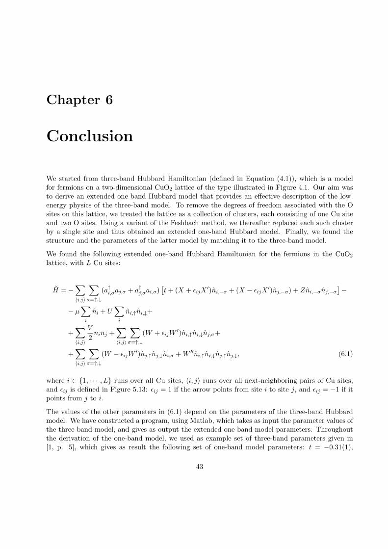
Chapter 6

Conclusion

We started from three-band Hubbard Hamiltonian (defined in Equation (4.1)), which is a modelfor fermions on a two-dimensional CuO2 lattice of the type illustrated in Figure 4.1. Our aim wasto derive an extended one-band Hubbard model that provides an effective description of the low-energy physics of the three-band model. To remove the degrees of freedom associated with the Osites on this lattice, we treated the lattice as a collection of clusters, each consisting of one Cu siteand two O sites. Using a variant of the Feshbach method, we thereafter replaced each such clusterby a single site and thus obtained an extended one-band Hubbard model. Finally, we found thestructure and the parameters of the latter model by matching it to the three-band model.

We found the following extended one-band Hubbard Hamiltonian for the fermions in the CuO2

lattice, with L Cu sites:

H =−∑〈i,j〉

∑σ=↑,↓

(a†i,σaj,σ + a†j,σai,σ)[t+ (X + εijX

′)ni,−σ + (X − εijX ′)nj,−σ) + Zni,−σnj,−σ]−

− µ∑i

ni + U∑i

ni,↑ni,↓+

+∑〈i,j〉

V

2ninj +

∑〈i,j〉

∑σ=↑,↓

(W + εijW′)ni,↑ni,↓nj,σ+

+∑〈i,j〉

∑σ=↑,↓

(W − εijW ′)nj,↑nj,↓ni,σ +W ′′ni,↑ni,↓nj,↑nj,↓, (6.1)

where i ∈ 1, · · · , L runs over all Cu sites, 〈i, j〉 runs over all next-neighboring pairs of Cu sites,and εij is defined in Figure 5.13: εij = 1 if the arrow points from site i to site j, and εij = −1 if itpoints from j to i.

The values of the other parameters in (6.1) depend on the parameters of the three-band Hubbardmodel. We have constructed a program, using Matlab, which takes as input the parameter values ofthe three-band model, and gives as output the extended one-band model parameters. Throughoutthe derivation of the one-band model, we used as example set of three-band parameters given in[1, p. 5], which gives as result the following set of one-band model parameters: t = −0.31(1),

43

44 Conclusion

X = −0.12(0), X ′ = −0.16(7), Z = 0.04(4), µ = 0.56(2), U = 3.16(0), V = 0.05(9), W = 0.07(0),W ′ = 0.09(6) and W ′′ = −0.14(9) .

Finally, we tried other sets of three-band model parameters, to see how the one-band model parame-ters were changed. In particular, we varied each one of the three-band parameters individually, whilefixing the others. The results of these tests are presented in Section 5.3.2. We found, for example,that changing the Cu-O hopping term tpd in the three-band Hubbard model changes not only thehopping term parameters (t, X, X ′ and Z), but also the Coulomb interaction terms (U , V W W ′

and W ′′). Also, changing the on-site energies or the Coulomb interaction terms in the three-bandmodel affects not only the interaction terms in the one-band model, but also the hopping terms.The O-O hopping term parameter tpp in the three-band model, however, appears only in interactionbetween clusters, and consequentially it affects only the hopping terms of the extended one-bandHubbard model. Finally, changing the chemical potential µ in the three-band model changes only,and by the same amount, µ in the one-band model.

It would be interesting to study the extended one-band Hubbard model found in this thesis. Inparticular, it is of interest to examine the effect the smaller terms (X, X ′, Z, V , W , W ′ and W ′′).

References

[1] E. Arrigoni, M. Aichhorn, M. Daghofer, and W. Hanke. Phase diagram and single-particlespectrum of CuO2 high-Tc layers: Variational cluster approach to the three-band Hubbardmodel. New Journal of Physics, 11(055066):1–13, 2009.

[2] J. Bardeen, L. N. Cooper, and J. R. Schrieffer. Theory of Superconductivity. Physical ReviewLetters, 108:1175–1204, 1957.

[3] J. Bednorz and K. Muller. Possible High Tc Superconductivity in the Ba-La-Cu-O System.Zeitschrift fur Physik B, 64:189–193, 1986.

[4] H. Bruus and K. Flensberg. Many-Body Quantum Theory in Condensed Matter Physics – AnIntroduction. Oxford Graduate Texts, 2004.

[5] J. de Woul. A restricted Hartree-Fock study of the 2D Hubbard model. Master’s thesis, RoyalInstitute of Technology, 2007.

[6] V. Emery. Theory of High-Tc Superconductivity in Oxides. Physical Review Letters, 58:2794–2797, 1987.

[7] S. Gasiorowicz. Quantum Physics. Wiley, third edition, 2003.

[8] C. Kittel. Introduction to Solid State Physics. John Wiley & Sons, eighth edition, 2005.

[9] E. Langmann. Effective one-band models for the cuprates. Unpublished paper.

[10] P.-O. Lowdin. Studies in Perturbation Theory. IV. Solution of Eigenvalue Problem by Projec-tion Operator Formalism. Journal of Mathematical Physics, 3:969–971, 1962.

[11] A. McMahan, J. F. Annett, and R. M. Martin. Cuprate parameters from numerical Wannierfunctions. Physical Review B, 42:6268–6282, 1990.

[12] R. Raimondi and J. Jefferson. Effective single-band models for the high-Tc cuprates. II. Roleof apical oxygen. Physical Review B, 53:8774–8788, 1996.

[13] Z.-A. Ren, G.-C. Che, X.-L. Dong, J. Yang, W. Lu, W. Yi, X.-L. Shen, Z.-C. Li, L.-L. Sun,F. Zhou, and Z.-X. Zhao. Superconductivity and phase diagram in iron-based arsenic-oxidesReFeAsO1−δ (Re = rare-earth metal) without fluorine doping. EPL Journal, 83(17002):1–4,July 2008.

[14] F. C. Zhang and T. M. Rice. Effective Hamiltonian for the superconducting Cu oxides. PhysicalReview B, 37:3759–3761, 1987.

45

46 References

Appendix A

Notation and terminology

In this appendix we fix the notation used throughout the thesis.

When a numerical value appears (predominantly, it will be an energy expressed in eV), regardless ofthe number of digits given, we use a parenthesis to highlight the last significant digit. For example,we would write 3.37(3) for a numerical value in the range 3.3725 < 3.37(3) < 3.3735.

We use the letter a for creation and annihilation operators, such that ai annihilates, and a†i creates,a fermion in state i. We will often refer to states as sites on a lattice, and we then define the spinof the electron too, since on each site there can be one fermion with spin ↑ and one with spin ↓.In these cases, the operator that annihilates (creates) a fermion with spin σ on site i is denoted

a(†)i,σ, σ ∈ ↑, ↓.

We predominantly use the word fermion, which may refer to either an electron or a hole. If therelevant interpretation is electron or hole depends on whether the system in question is doped withholes or electrons1.

For the particle number operator (or just number operator), we will use both the notation N (whenwe talk about the number operator alone) and n (when the number operator is part of a Hamiltonianoperator). Without index, n (or N) refers to the number operator on the global system in question

(any ambiguities will be explained in the text), while ni,σ = a†i,σai,σ refers to the number operator

on site i and spin σ. We will also use the shortened notation ni = ni,↑+ ni,↓ such that n =∑L

i=1 nifor a lattice with L sites. Regardless of whether N or n is used, we use n to represent the particlenumber eigenvalues.

We define the spin operator Szi = 12ni,↑−

12ni,↓ on site i, and the global spin operator Sz =

∑Li=1 S

zi .

The eigenvalues of Sz and Szi will be denoted sz and szi , respectively.

We will use σ to denote the spin of a fermion, σ ∈ ↑, ↓. The opposite spin is sometimes indicatedwith a minus sign: − ↑=↓ and − ↓=↑.

Ω always denotes the empty state, i.e. NΩ = 0. In some places, Ω will have an index that indicates

1As described in the introduction, the cuprates consist of CuO2 sandwiched between layers of other materials thatserve to dope the CuO2 layers with electrons or holes

47

48 Notation and terminology

in what Hilbert space that specific (empty) state belongs. In these instances, the indices will beexplained in the text.

We call a pure state a fermion state in a system of L sites (i.e. with 2L accessible single-particlestates, including the spin degree of freedom) a state of the following type:

(a†1,↑)n1,↑(a†1,↓)

n1,↓(a†2,↑)n2,↑ · · · (a†L,↑)

nL,↑(a†L,↓)nL,↓Ω; ni,σ ∈ 0, 1 ∀ i, σ (A.1)

The pure states in (A.1) are eigenstates to N , with corresponding eigenvalue n =∑L

i=1 ni, and to

Sz, with eigenvalue sz = 12

∑i ni,↑ − ni,↓.

The commutator between any two operators A and B is [A,B] = AB−BA and the anticommutatorbetween A and B is A,B = AB +BA.

For the three-band Hubbard model, we use the following identifications, to clearly distinguishbetween annihilation (and creation) operators for Cu sites and for O sites

d(†)i,σ = a

(†)i,σ site i a Cu site, annihilating (creating) an electron in the d orbit

p(†)l,σ = a

(†)l,σ site l an O site, annihilating (creating) an electron in the p orbit,

ndi,σ = d†i,σdi,σ; npl,σ = p†i,σpi,σ

Apart from annihilation and creation operators, the general convention is to indicate operatorswith hats above them, and their matrix representations without hats. For example: A is the matrixrepresentation (in some basis) of the operator A. However H is the three-band Hamiltonian operatorand H is the Hamiltonian operator in the extended one-band Hubbard model. We make this choice,to avoid having a hat and a tilde over the same symbol.

We use brackets [· · · ] for citation of references (listed in the end of the thesis). Parenthesizes (· · · )are used to refer to equations, and when referring to sections or chapters, only the number is used.

Appendix B

Mathematical details

B.1 Solution of three-band model on one cluster

In this appendix, we carry out the solution of the three-band Hubbard problem on one cluster. Wegive details of the analytical solution in the subspaces whose states have particle number n = 0, n = 1and n = 2. We confirm these results by finding the same solutions numerically using Matlab. WithMatlab, we also find the remaining energy eigenvalues, whose eigenstates have particle numbern = 3, 4, 5, 6, and we present a complete list of the energies in each sector. In particular, we notethat the energies associated with these higher-particle number states are considerably higher thanthose of the low-particle states. We use this to argue the validity of the approximation that onlythe four lowest-energy states will be occupied.

In the three-sites clusters there are six different states that may or may not be occupied by a fermion,taking into account spin. In matrix representation, finding the fermion energies and correspondingeigenstates in cluster i thereby amounts to finding the eigenvalues and eigenstates of a 64 × 64matrix, whose elements are found by Hkl = 〈Pk|Hi|Pl〉, where |Pk〉 and |Pl〉 are any states in abasis that needs to be defined, and k, l ∈ 1, 2, ..., 64. Furthermore, the Hamiltonian Hi in (4.2)commutes with the number operator N and the spin operator Sz, and as long as we don’t mixstates with different particle number n or sz in the same basis state, this allows us to construct amatrix with block-diagonal form (see Section 2.2.2 for more details), and thus solve each of theseblock individually.

We say that the system is in a pure state if it is in one of the following states:(d†0,↑)

n0,↑(d†0,↓)n0,↓(p†+,↑)

n+,↑(p†+,↓)n+,↓(p†−,↑)

n−,↑(p†−,↓)n−,↓Ω, with ni,σ ∈ 0, 1. Note that we omit

the index i, common to all creation operators on cluster i.

B.1.1 n = 0

The n = 0 sector is trivial, containing only one state: the empty state Ω. It is an eigenstate toHi, with eigenvalue 0. We hence have one energy eigenvalue E0 = 0, with the corresponding stateA†i,0Ω = Ω, where A†i,0 = I.

49

50 Mathematical details

B.1.2 n = 1

There are three pure states in the n = 1, sz = 12 sector:

d†0,↑Ω, p†+,↑Ω, p

†−,↑Ω,

and three in the n = 1, sz = −12 sector:

d†0,↓Ω, p†+,↓Ω, p

†−,↓Ω

We solve sector n = 1, sz = 12, and thereafter note that the solution corresponds exactly to the

one of n = 1, sz = −12, interchanging only ↑→↓.

Instead of naively using the set of three pure states as our basis, we can construct a better basis,which will divide the 3× 3 block into two smaller sub-blocks. We first note that

Hid†0,↑Ω = εdHd

†0,↑Ω + tpd(p

†+,↑Ω− p

†−,↑Ω)

Hi1√2

(p†+,↑Ω− p†−,↑Ω) =

1√2εp(p

†+,↑Ω− p

†−,↑Ω) +

√2d†0,↑Ω

Choosing the two normalized states d†0,↑Ω and 1√2(p†+,↑Ω − p

†−,↑Ω) in our basis will give a block-

diagonal matrix: when acted upon with Hi, they only return each other, and the interaction withthe rest of the matrix will be zero. Finally, we choose the third normalized basis state to be1√2(p†+,↑Ω + p†−,↑Ω), and we show that these states are orthogonal:

〈 1√2

(p†+,↑Ω + p†−,↑Ω)| 1√2

(p†+,↑Ω− p†−,↑Ω)〉 =

1

2

(〈p†+,↑Ω|p

†+,↑Ω〉 − 〈p

†+,↑Ω|p

†−,↑Ω〉+ 〈p†−,↑Ω|〈p

†+,↑〉 − 〈p

†−,↑Ω|p

†−,↑Ω〉

)=

1

2(1 + 0 + 0− 1) =0

〈d†0,↑Ω|1√2

(p†+,↑Ω + p†−,↑Ω

)〉 =

1√2

(〈d†0,↑Ω|p

†+,↑Ω〉+ 〈d†0,↑Ω|p

†−,↑Ω〉

)=

1√2

(0 + 0) =0

〈d†0,↑Ω|1√2

(p†+,↑Ω− p

†−,↑Ω

)〉 =

1√2

(〈d†0,↑Ω|p

†+,↑Ω〉 − 〈d

†0,↑Ω|p

†−,↑Ω〉

)=

1√2

(0− 0) =0

The following thus constitutes a complete orthonormal basis in the n = 1, sz = 12 sector:

B.1 Solution of three-band model on one cluster 51

ψ1 = d†0,↑Ω; ψ2 =1√2

(p†+,↑Ω− p

†−,↑Ω

); ψ3 =

1√2

(p†+,↑Ω + p†−,↑Ω

) (B.1)

We construct the elements Hn=1,sz= 1

2

kl = 〈ψk|Hiψl〉 of the 3× 3 Hamiltonian matrix, and get:

Hn=1,sz= 12 =

εd√

2tpd 0√2tpd εp 00 0 εp

,

ad find that ψ3 is an eigenstate to Hi, with eigenvalue εp. To find the eigenvalues and eigenstates

corresponding to the block Hn=1,sz= 121≤k,l≤2, we solve the corresponding characteristic equation:

det(

(Hn=1,sz= 12)1≤i,j≤2 − E × I

)= 0

(εd − E)(εp − E)− 2t2pd = 0

E2 − E (εd + εp) + εpεd − 2t2pd = 0

E1,2 =εd + εp

2±√

(εd + εp)2

4− εdεp + 2t2pd

We thus have the following energy eigenvalues in the n = 1, sz = 12 sector:

E1 =εd + εp

2−√

(εd + εp)2

4− εdεp + 2t2pd

E2 =εd + εp

2+

√(εd + εp)2

4− εdεp + 2t2pd

E3 =εp

The eigenstates in the Hn=1,sz= 121≤k,l≤2 sector are found by solving the equation:

(εd

√2tpd√

2tpd εp

)(Ci,1Ci,2

)= Ei

(Ci,1Ci,2

); i ∈ 1, 2,

where Ci,1 and Ci,2 are the coefficients of ψ1 and ψ2 respectively, in eigenstate i:Ψi = Ci,1ψ1 + Ci,2ψ2. We find the following:

Ψi = Ci,1

(ψ1 +

Ei − εd√2tpd

ψ2

)

We insert the assumed values of our parameters [1, p. 5] and choose the values of C1,1 and C2,1

such that Ψ1 and Ψ2 are normalized. The complete solution for the sector n = 1, sz = 12 is:


Energy Eigenstate

−0.56(2) −0.92(9)d†0,↑Ω + 0, 26(1)(p†+,↑Ω− p

†−,↑Ω

)3.00(0) 1√

2

(p†+,↑Ω + p†−,↑Ω

)3.56(2) 0.36(9)d†0,↑Ω + 0.65(7)

(p†+,↑Ω− p

†−,↑Ω

)Since the Hamiltonian Hi is unchanged under the interchange of ↑↔↓ we can, choosing a basiscorresponding to (B.1), just changing ↑→↓, carry out the same procedure, and find the solution ofthe n = 1, sz = −1

2 sector:

Energy Eigenstate

−0.56(2) −0.92(9)d†0,↓Ω + 0, 26(1)(p†+,↓Ω− p

†−,↓Ω

)3.00(0) 1√

2

(p†+,↓Ω + p†−,↓Ω

)3.56(2) 0.36(9)d†0,↓Ω + 0.65(7)

(p†+,↓Ω− p

†−,↓Ω

)

B.1.3 n = 2, sz = 0

Using the short-hand notation |kl〉 ≡ a†i,k,↑a†i,l,↓Ω

1, k, l ∈ 0,+,−, the pure states in the system ofcluster i are:

|00〉, |0+〉, |0−〉, |+ 0〉, |+ +〉, |+−〉, | − 0〉, | −+〉, | − −〉

As in the n = 1 sectors, we want to find a better basis than the pure states, in order to make the9× 9 matrix block-diagonal, and solve each block individually.

To find a better basis, we act with Hi on each of the pure states:

H|00〉 (−εd + Udd)|00〉 +tpd(|0+〉 − |0−〉+ |+ 0〉 − | − 0〉)H|0+〉 (εp + εd + Upd)|0+〉 +tpd(|00〉+ |+ +〉 − | −+〉H|0−〉 (εp + εd + Upd)|0−〉 +tpd(−|00〉 − | − −〉+ |+−〉H|+ 0〉 (εp + εd + Upd)|+ 0〉 +tpd(|00〉+ |+ +〉 − |+−〉H| − 0〉 (εp + εd + Upd)| − 0〉 +tpd(−|00〉 − | − −〉+ | −+〉H|+−〉 −εp|+−〉 +tpd(|0−〉 − |+ 0〉H| −+〉 −εp| −+〉 +tpd(−|0+〉+ | − 0〉H|+ +〉 (−εp + Upp)|+ +〉 +tpd(|0+〉+ |+ 0〉H| − −〉 (−εp + Upp)| − −〉 +tpd(−|0−〉 − | − 0〉

(B.2)

Guided by the results in (B.2), we choose the following basis states, labeled ei; i ∈ 1, 2, · · · 9. Thischoice gives a block-diagonal matrix with four blocks. Further down, we discuss this division intoblocks further, and show that it reflects the symmetries of the one-cluster Hamiltonian Hi.

1We use di,0,σ = ai,0,σ and pi,±,σ = ai,±,σ


e1 = 1√4[(|0+〉 − |0−〉)− (|+ 0〉 − | − 0〉)]

e2 = |00〉e3 = 1√

4[(|0+〉 − |0−〉) + (|+ 0〉 − | − 0〉)]

e4 = 1√2(|+ +〉+ | − −〉)

e5 = 1√2(|+−〉+ | −+〉)

e6 = 1√2(|+−〉 − | −+〉)

e7 = 1√4[(|0+〉+ |0−〉)− (|+ 0〉+ | − 0〉)]

e8 = 1√2(|+ +〉 − | − −〉)

e9 = 1√4[(|0+〉+ |0−〉) + (|+ 0〉+ | − 0〉)]

(B.3)

The nine states ei are normalized and mutually orthogonal, and thus span the nine-dimensionalsubspace that represents the n = 2, sz = 0 sector of the fermion system.

The Hamiltonian matrix in the n = 2, sz = 0 sector, expressed in the basis ei, is:

Hn=2,sz=0 =A⊕B ⊕ C ⊕D, where

A =(εp + εd + Upd

)B =

2εd + Udd 2tpd 0 0

2tpd εp + εd + Upd√

2tpd −√

2tpd0

√2tpd 2εp + Upp 0

0 −√

2tpd 0 2εp

C =

(2εp

√2tpd√

2tpd εp + εd + Upd

)D =

(2εp + Upp

√2tpd√

2tpd εp + εd + Upd

)

In block A, we readily have one eigenstate and energy:

E1 = εp + εd + Upd;1

2((|0+〉 − |0−〉)− (|+ 0〉 − | − 0〉)) (B.4)

In block B, the characteristic equation that we need to solve is a fourth-degree polynomial equation,which we solve numerically using Matlab. We present the results together with the solutions of theother blocks further down.

In block C, the characteristic equation gives the energies:

(2εp − E)(εp + εd + Upd − E)− 2t2pd = 0, with solutions

E6,7 =3εp + εd + Upd

2±√

(3εp + εd + Upd)2

4− 2εp(εp + εd + Upd) + 2t2pd


The characteristic equation for the block D matrix is:

(2εp + Upp − E)(εp + εd + Upd − E)− 2t2pd = 0, with solutions

E8,9 =3εp + εd + Upp + Upd

2±√

(3εp + εd + Upp + Upd)2

4− (2εp + Upp)(εp + εd + Upd) + 2t2pd

The above equations give the energy eigenvalues, and from there we find the corresponding eigen-states by solving the equations CΨi = EiΨi and DΨj = EjΨj , i ∈ 6, 7, j ∈ 8, 9.

The above solution gives the following complete set of energies and eigenstates to the n = 2, sz = 0sector. We still use the notation convention that |kl〉 ≡ a†i,k,↑a

†i,l,↓Ω, and the below table gives

that coefficient that multiply each of these pure states in the linear combination that constitutesrespective eigenstate. The far right column tells us to which of the blocks in Hn=2,sz=0 that eacheigenstate comes from:

Energy Eigenstate coefficients of the pure states Block|00〉 |0+〉 |0−〉 | + 0〉 | + +〉 | +−〉 | − 0〉 | − +〉 | − −〉

2.03(7) 0.29(6) -0.44(2) 0.44(2) -0.44(2) 0.12(7) -0.22(3) 0.44(2) -0.22(3) 0.12(7) B2.86(3) 0 -0.45(6) -0.45(6) 0.45(6) 0 0.29(1) 0.45(6) -0.29(1) 0 C3.15(8) 0 -0.48(6) -0.48(6) -0.48(6) 0.16(6) 0 -0.48(6) 0 -0.16(6) D

3.5 0 0.5 -0.5 -0.5 0 0 0.5 0 0 A6.33(4) 0.26(4) -0.11(0) 0.11(0) -0.11(0) 0.08(3) 0.65(9) 0.11(0) 0.65(9) 0.08(3) B6.63(7) 0 -0.20(5) -0.20(5) 0.20(5) 0 -0.64(5) 0.20(5) 0.64(5) 0 C8.49(2) -0.80(3) -0.09(9) 0.09(9) -0.09(9) 0.38(9) 0.07(9) 0.09(9) 0.07(9) 0.38(9) B9.34(2) 0 -0.11(8) -0.11(8) -0.11(8) -0.68(7) 0 -0.11(8) 0 0.68(7) D9.63(6) -0.44(4) -0.18(2) 0.18(2) -0.18(2) -0.57(1) 0.10(0) 0.18(2) 0.10(0) -0.57(1) B

It is interesting to note that the division into sub-blocks A, B, C and D reflects two symmetriesof the Hamiltonian Hi on one cluster: It is possible to define two operators that commute withHi, to which the states in (B.3) are eigenstates, and where each block is associated with a uniquecombination of eigenvalues. These operators are the +←→ − ”site swap” operator T and the ”spinflip” operator F , both defined below:

T T † = T †T = I

T p+,σT† = (−1)p−,σ

T p−,σT† = (−1)p+,σ

T d0,σT† = d0,σ

TΩ = Ω

F F † = F †F = I

F ak,σF† = ak,−σ

FΩ = Ω

, where − ↑=↓, − ↓=↑, k ∈ 0,+,−, a±,σ = p±,σ and a0,σ = d0,σ The basis states in (B.3) areeigenstates of T and F , and they can be classified according the their eigenvalues associated with


these two operators: Block A: t = 1, f = 1; block B: t = 1, f = −1; block C: t12 = −1, f = 1 andblock D: t12 = −1, f = −1.

I checked that T and F commute with the one cluster Hamiltonian.

B.1.4 n = 2, sz = +1/− 1

We will carry out the solution for the n = 2, sz = +1 sector, and thereafter the solution of then = 2, sz = −1 sector.

We denote the three pure states in the n = 2, sz = +1 sector as follows:

a†0,↑a†+,↑Ω ≡ |0+〉

a†0,↑a†−,↑Ω ≡ |0−〉

a†+,↑a†−,↑Ω ≡ |+−〉

In analogy with the process carried out in the n = 1, sz = 12 and n = 2, sz = 0 sectors, we act

with Hi on each of the pure states to help us make a good choice of basis, that makes the matrixblock-diagonal. We find:

Hi|0+〉 =(εd + εp + Upd)|0+〉+ tpd|+−〉Hi|0−〉 =(εd + εp + Upd)|0−〉+ tpd|+−〉

Hi|+−〉 =2εp|+−〉+ tpd (|0+〉+ |0−〉) ,

such that the following choice of basis

e1 =1√2

(|0+〉 − |0−〉)

e2 =1√2

(|0+〉+ |0−〉)

e3 =|+−〉,

will make the the matrix block-diagonal, each elements found by Hkl = 〈ek|Hi|el〉:

Hn=2,sz= 12 =

εd + εp + Upd 0 0

0 εd + εp + Upd√

2tpd0

√2tpd 2εp

We conclude that e1 is an eigenstate to Hn=2,sz= 1

2 with energy eigenvalue εd + εp + Upd. To find

the two other energies, we solve the characteristic equation:


det

(εd + εp + Upd − E

√2tpd√

2tpd 2εp − E

)=0

(εd + εp + Upd − E)(2εp − E)− 2t2pd =0

E2,3 =εd + εp + Upd

2±√

(εd + εp + Upd)2

4− 2εp(εd + εp + Upd) + 2t2pd (B.5)

The eigenstates in this subsector are linear combinations of e2 and e3, where the coefficients Ck,2and Ck,3 before each of the basis states are determined by:

(εd + εp + Upd − E

√2tpd√

2tpd 2εp − E

)(Ck,2Ck,3

)= Ei

(Ck,2Ck,3

); k ∈ 2, 3 (B.6)

We solve (B.6), insert the parameter values into (B.5), and choose the eigenstates to be normalized.The complete solution to the n = 2, sz = 1 sector is then:

Energy State

2.86(2) −0.64(5)(d†0,↑p

†+,↑Ω + d†0,↑p

†−,↑Ω

)+ 0.41(1)p†+,↑p

†−,↑Ω

3.50(0) 1√2

(d†0,↑p

†+,↑Ω− d

†0,↑p†−,↑Ω

)6.63(7) 0.29(1)

(d†0,↑p

†+,↑Ω + d†0,↑p

†−,↑Ω

)+ 0.91(2)p†+,↑p

†−,↑Ω

Since Hi is unchanged upon changing the spin, we directly get the results for the n = 2, sz = 1sector:

Energy State

2.86(2) −0.64(5)(d†0,↓p

†+,↓Ω + d†0,↓p

†−,↓Ω

)+ 0.41(1)p†+,↓p

†−,↓Ω

3.50(0) 1√2

(d†0,↓p

†+,↓Ω− d

†0,↓p†−,↓Ω

)6.63(7) 0.29(1)

(d†0,↓p

†+,↓Ω + d†0,↓p

†−,↓Ω

)+ 0.91(2)p†+,↓p

†−,↓Ω

B.1.5 Summary: Energies in one cluster

Having looked at details of the solution in the sectors where n = 0, 1, 2, and having found theexplicit expressions for the eigenstates in these sectors, we list all energy eigenvalues to the one-cluster problem, found with Matlab: 1

1The Matlab code is found in Appendix C.2.1.


Quantum numbers Energies

n = 0 0

n = 1,sz = 12 −0.56(2), 3.00(0), 3.56(3)

n = 1,sz = −12 −0.56(2), 3.00(0), 3.56(3)

n = 2,sz = 0 2.03(7), 2.86(3), 3.15(8), 3.50(0), 6.33(4), 6.63(7), 8.49(2), 9.34(2), 9.63(6)

n = 2,sz = 1 2.86(3), 3.50(0), 6.63(7)

n = 2,sz = −1 2.86(3), 3.50(0), 6.63(7)

2 < n ≤ 6 5.92(5), 5.92(5), 6.62(8), 6.62(8), 7.00(0), 7.00(0), 7.00(0),7.00(0), 9.26(8), 9.26(8), 9.57(9), 9.57(9), 12.00(0), 12.00(0),12.03(7), 12.37(2), 12.37(2), 12.73(2), 12.73(2), 12.86(3), 12.86(3),12.86(3), 13.15(8), 13.49(6), 13.49(6), 13.50(0), 13.50(0), 13.50(0),16.33(4), 16.63(8), 16.63(8), 16.63(8), 18.49(2), 19.34(2), 19.43(8),19.43(8), 19.63(7), 23.00(0), 23.00(0), 23.56(2), 23.56(2), 30.00(0)

We see that the four lowest-energy eigenstates are found in the sectors n = 1, sz = 12, n =

1, sz = −12, n = 0, sz = 0 and n = 2, sz = 0, respectively. In Chapter 5, we will associate

each of these three-band states on a cluster with a one-band model state on a site: We will arguethat the three-band Hubbard model may be replaced with an extended one-band Hubbard model,where each cluster is regarded as a single lattice site, on which there can be one ↑ fermion and one↓ fermion.

It is worth to note that we can consider ourselves lucky to find this feature in our list of energies.If we would have found, for example, that the four lowest states were all found in the n = 1sector, the above explained matching between three-band and one-band states would not have beenpossible.

We sum up by listing the explicit expressions for the four lowest-energy eigenstates to Hi, theHamiltonian on a cluster i. We name these states them A†i,aiΩ; ai ∈ 1, 2, 3, 4, where the A†i,aiare defined below. We will keep this notation convention when we make the matching to one-bandstates.

State Energy

A†i,1 = I 0

A†i,2 = −0.92(9)d†0,↑ + 0.26(1)(p†+,↑ − p

†−,↑

)−0.56(2)

A†i,3 = −0.92(9)d†0,↓ + 0.26(1)(p†+,↓ − p

†−,↓

)−0.56(2)

A†i,4 = 0.44(2)[d†0,↑

(p†−,↓ − p

†+,↓

)+(p†−,↓ − p

†+,↓

)d†0,↓

]+

+0.12(7)(p†+,↑p

†+,↓ + p†−,↑p

†−,↓

)− 2.03(7)

−0.22(3)(p†+,↑p

†−,↓ + p†−,↑p

†+,↓

)+ 0.29(6)d†0,↑d

†0,↓


B.2 Proof of Proposition 5.2.1

Our strategy will be to consider a general model, which may represent both the three-band and theextended one-band Hubbard model. We will show that any matrix element in this general modelcan be written as one common sum of matrix elements on the form〈ΩAj,a′jAi,a′i |

1TiHi + 1


†j,aj

Ω〉 (in the three-band model) or

〈ΩAj,a′j Ai,a′i |1TiHi + 1

TjHj + Hij |A†i,aiA

†j,aj

Ω〉 (in the one-band model).

Having proved this, we conclude that to ensure that every matrix element Hn,m in the three-bandmodel is equal to its one-band correspondent Hn,m, it is sufficient to match elements such as theones above.

A general model

Consider L identical fermion systems, each with l sites where an ↑ spin and one ↓ spin fermion canreside, such that each system has 2l single-particle states that may or may not be occupied by afermion. We agree upon an order in which we label the Hilbert spaces representing each of the Lsystems: H1,H2, · · · ,HL. We then construct the combined Hilbert space representing all fermionsystems as the tensor product of the subspaces, respecting this agreed upon order:

H = H1 ⊗H2 ⊗ · · · ⊗ HL (B.7)

Each of the subspaces Hi is of dimension 22l. It follows from (B.7) that H is (22×L×l)-dimensional.

Moreover, consider a complete orthonormal basis in each of the subspaces Hi:

ω†i,diΩdi∈1,2,3,··· ,22l, (B.8)

We demand that ω†i,diΩ is a linear combination of pure states in Hi, all of which have the same

eigenvalue ndi of Ni, such that: Niω†di

Ω = ndiω†di

Ω. We may now construct states d, that form anorthonormal basis in H:

|d〉 = ω†1,d1ω†2,d2

· · ·ω†L,dLΩL (B.9)

d = (d1, d2, · · · , dL); di ∈ 1, 2, · · · 22l

Before we prove that (B.9) is a complete orthonormal basis in H, we introduce the notion of thedeg operator, defined as follows:

deg(di) ≡

0, if ndi , the particle number of ω†i,diΩ, is even

1, if ndi is odd(B.10)

B.2 Proof of Proposition 5.2.1 59

Furthermore, it follows from the orthonormality of the states ω†i,diΩ, and from the fact that for

i 6= j, ω†i,di and ω†j,di have no creation operators in common, that the following relations hold:

ω†i,diω†j,dj

=(−1)deg(di)·deg(dj)ω†j,djω†i,di

; i 6= j

ωi,diωj,dj =(−1)deg(di)·deg(dj)ωj,djωi,di ; i 6= j

ωi,diω†j,dj

=(−1)deg(di)·deg(dj)ω†j,djωi,di ; i 6= j

ωi,d′iω†i,di

=δd′i,di + (−1)deg(d′i)deg(di))ω†i,diωi,d′i (B.11)

Using this, we now show that the states in (B.9) are normalized and mutually orthogonal:

〈d′|d〉 =

= 〈ΩωL,d′LωL−1,d′L−1· · ·ω1,d′1

|ω†1,d1ω†2,d2

· · ·ω†L,dLΩ〉 =

= 〈ΩωL,d′L · · ·ω2,d′2|(δd′1,d1

+ (−1)deg(d′1)deg(d1))ω†1,d1

ω1,d′1

)ω†2,d2

· · ·ω†L,dLΩl〉 =

= δd′1,d1〈ΩωL,d′L · · ·ω2,d′2

|ω†2,d2· · ·ω†L,dLΩl〉+ (−1)deg(d

′1)deg(d1))〈· · · | · · ·ω1,d′1

Ω︸︷︷︸=0

〉

= δd′1,d1〈ΩωL,d′L · · ·ω3,d′3

|(δd′2,d2

+ (−1)deg(d′2)deg(d2))ω†2,d2

ω2,d′2

)ω†3,d3

· · ·ω†L,dLΩl〉 =

...

=

L∏i=1

δd′i,di〈Ω|Ω〉 =

L∏i=1

δd′i,di = δd′,d

The states d are thus normalized and mutually orthogonal. Noting that there are (22l)L = 22×L×l

different such states, the same as the dimension of H, we conclude that they constitute a completeorthonormal basis in H.

Now, consider an operator O on H, with the following properties:


O =

L∑i=1

Oi +∑〈i,j〉

Oij +∑〈i,j〉

O′ij , (B.12)

where 〈i, j〉 runs over an arbitrary number of pairs of subspaces Hi and Hj , and

Oi is such that ω†i,diΩ is an eigenstate to Oi ∀ di, and [Oi, ωj,dj ] = [Oi, ω†j,dj

] = 0 ∀ i 6= j,

Oij =l∑

s=1

l∑s′=1

∑mV

V(s,s′mV )(ni,s,↑)mi,↑(ni,s,↓)

mi,↓(nj,s′,↑)mj,↑(nj,s′,↓)

mj,↓ ,

where mV takes on all values mV = (mi,↑,mi↓,mj,↑,mj,↓); mi,σ ∈ 0, 1,

O′ij =

l∑s=1

l∑s′=1

∑σ=↑,↓

(a†i,s,σaj,s′,σ + a†j,s′,σai,s,σ

)[∑mT

T(s,s′,mT )(ni,s,−σ)mi,−σ(nj,s′,−σ)mj,−σ

],

where mT takes on all values mT = (mi,−σ,mi,−σ); mj,−σ ∈ 0, 1,

and V(s,s′mV ) and T(s,s′,mT ) are complex numbers. It follows from the anti-commutator relations forcreation and annihilation operators that

[ω†k,dk , ni,s,σ] = 0 ∀ k 6= i; ∀ dk, s, σ, and

[ω†k,dk , a†i,s,σai,s,σ] = 0 ∀ k 6= i, j; ∀ dk, s, s′σ (B.13)

We now consider any element of O, the matrix representation of O in the basis |d〉:

Od′,d = 〈d′|O|d〉 =L∑i=1

〈d′|Oi|d〉+∑〈i,j〉

〈d′|Oij |d〉+∑〈i,j〉

〈d′|O′ij |d〉 =

=∑〈i,j〉

(1

Ti〈d′|Oi|d〉+

1

Tj〈d′|Oj |d〉+ 〈d′|Oij |d〉+ 〈d′|O′ij |d〉

), (B.14)

where Ti is the number of 〈i, j〉 pairs in the original sum∑〈i,j〉 in (B.12), of which Hi is part. This

factor is needed when we change to a common sum.

We study each of the terms in (B.14) individually1:

1We assume, without loss of generality, that i < j


〈d′|Oi|d〉 = 〈ΩωL,d′L · · ·ωi,d′i · · ·ω1,d′1|Oi|ω†1,d1

· · ·ω†i,di · · ·ω†L,dL

Ω〉 =

= use that [Oi, ωj,dj ] = 0 ∀ i 6= j and (B.11) to move operators

ωk,d′k where k 6= i to the right =

=

(i−1∏k=1

δd′k,dk

)〈ΩωL,d′L · · ·ωi,d′i |Oi|ω

†i,di· · ·ω†L,dLΩ〉 =

=

(i−1∏k=1

δd′k,dk

)(−1)[deg(d

′i)+deg(di)]

∑Lk=i+1 deg(dk)

(L∏

k=i+1

δd′k,dk

)〈Ωωi,d′i |Oi|ω

†i,di

Ω〉 =

= Due to that ω†i,diΩ is an eigenstate to Oi,

the above may be nonzero only if d′i = di. We can thus set deg(d′i) = deg(di) =

=

∏k 6=i

δd′k,dk

(−1)2deg(di)∑Lk=i+1 deg(dk)︸︷︷︸

=1

〈Ωωi,d′i |Oi|ω†i,di

Ω〉 =

=

∏k 6=i

δd′k,dk

〈Ωωi,d′i |Oi|ω†i,diΩ〉 (B.15)

〈d′|Oij |d〉 = 〈ΩωL,d′L · · ·ωj,d′j · · ·ωi,d′i · · ·ω1,d′1|Oij |ω†1,d1

· · ·ω†i,di · · ·ω†j,dj· · ·ω†L,dLΩ〉 =

= use (B.13) and (B.11), and move operators

ωk,d′k where k 6= i to the right =

=

∏k 6=i,j

δd′k,dk

× (−1)[deg(d′i)+deg(di)]

∑Lk=i+1 deg(dk)×

× (−1)[deg(d′j)+deg(d

′i)+deg(di)+deg(dj)]

∑Lk=j+1 deg(dk)×

× 〈Ωωj,d′jωi,d′i |Oij |ω†i,diω†j,djΩ〉 =

= Due to the structure of Oij , described in (B.12), ω†i,diω†j,dj

Ω is an

eigenstates to Oij ,

and the above may be nonzero only if d′i = di and d′j = dj

. We can thus set deg(d′i) = deg(di) and deg(d′j) = deg(dj) =

=

∏k 6=i,j

δd′k,dk

(−1)2deg(di)∑j−1k=i+1 deg(dk)︸︷︷︸

=1

× (−1)2(deg(di)+deg(dj))∑Lk=j+1 deg(dk)︸︷︷︸

=1

×

× 〈Ωωj,d′jωi,d′i |Oij |ω†i,diω†j,djΩ〉 =

=

∏k 6=i,j

δd′k,dk

〈Ωωj,d′jωi,d′i |Oij |ω†i,diω†j,djΩ〉 (B.16)


〈d′|O′ij |d〉 = 〈ΩωL,d′L · · ·ωj,d′j · · ·ωi,d′i · · ·ω1,d′1|O′ij |ω

†1,d1· · ·ω†i,di · · ·ω

†j,dj· · ·ω†L,dLΩ〉 =

= Use (B.13) and (B.11) and move operators

ωk,d′k where k 6= i, j to the right =

=

∏k 6=i,j

δd′k,dk

× (−1)[deg(d′i)+deg(di)]

∑j−1k=i+1 deg(dk)×

× (−1)[deg(d′j)+deg(d

′i)+deg(di)+deg(dj)]

∑Lk=j+1 deg(dk)×

× 〈Ωωj,d′jωi,d′i |O′ij |ω

†i,diω†j,djΩ〉 = (B.17)

The situation for the deg(di) factors in (B.17) is more delicate than in (B.15) and (B.16). To

examine the case where 〈Ωωj,d′jωi,d′i |O′ij |ω

†i,diω†j,djΩ〉 is non-zero, we first note that the factor[∑

mTT(s,s′,mT )(ni,s,−σ)mi,−σ(nj,s′,−σ)mj,−σ

]has ω†i,diω

†j,dj

Ω as eigenstate. Thus, the action of this

[· · · ] factor does not change ndi or ndj . Furthermore, acting with a†i,s,σaj,s′,σ (or a†j,s′,σai,s,σ) on

ω†i,diω†j,dj

Ω will result in that ni,s,σ → ni,s,σ + 1 and nj,s′,σ → nj,s′,σ − 1 (or ni,s,σ → ni,s,σ − 1 and

nj,s′,σ → nj,s′,σ + 1), and all other ni,s′′,σ′ = nj,s′′,σ′ = 0; s′′ 6= s, s′; σ′ 6= σ.

To have a non-zero result for 〈Ωωj,d′jωi,d′i |O′ij |ω

†i,diω†j,djΩ〉, it is thus necessary that deg(d′i)+deg(d′j) =

deg(di) + deg(dj), and additionally that deg(d′i) = deg(di)± 1, with + for the a†i,s,σaj,s′,σ term and

− for the a†j,s′,σai,s,σ term. This allows us to make the following, in the case where

〈Ωωj,d′jωi,d′i |O′ij |ω

†i,diω†j,djΩ〉 6= 0:

deg(d′i) + deg(d′j) + deg(di) + deg(dj) = 2 (deg(di) + deg(dj)) , an even number, and

deg(d′i) + deg(di) = 2deg(di)± 1, an odd number

Using this, we may now rewrite (B.17):

〈d′|O′ij |d〉 =

∏k 6=i,j

δd′k,dk

× (−1)∑j−1k=i+1 deg(dk)〈Ωωj,d′jωi,d′i |O

′ij |ω

†i,diω†j,djΩ〉 (B.18)

Finally, we note that terms such as in (B.15) can be modified

〈d′|Oi|d〉 =

∏k 6=i

δd′k,dk

〈Ωωi,d′i |Oi|ω†i,diΩ〉 =

=

∏k 6=i,j

δd′k,dk

〈Ωωj,d′jωi,d′i |Oi|ω†i,diω†j,djΩ〉, for an arbitrary j > i (B.19)


Using the results (B.15)-(B.19), we can now write the last sum in (B.14) as

〈d′|O|d〉 =

=∑〈ij〉

∏k 6=i,j

δd′k,dk

〈Ωωj,d′jωi,d′i | 1Ti Oi +1

TjOj + Oij + (−1)

∑j−1k=i+1 deg(dk)O′ij |ω

†i,diω†j,djΩ〉 (B.20)

Any matrix element can thus be expressed as a sum of terms in each of which the non-trivialarguments are matrix elements obtained when considering only two two subspaces Hi and Hj .

We will now show that the three-band and the extended one-band Hubbard models both are specialcases of the above described model.

The three-band Hubbard model as a special case

The three-band Hubbard model on the whole CuO2 lattice is a special case of the general modeldescribed in Equations (B.7), (B.8) and (B.12). We see this if we do the following identifications:

l = 3. There are three sites in each cluster.

The Hilbert space representing the fermion states on the whole lattice is a tensor product ofthe Hilbert spaces representing the state in each cluster.

A†i,aiΩai∈1,2,··· ,64 is a complete orthonormal basis in Hi, and fulfills the condition that

every state A†i,aiΩ is a linear combination of pure states, all of which with the same particlenumber nai

Each one-cluster operatorHi has the property thatHiA†i,ai

Ω = EiA†i,ai

Ω, and that [Hi, A†j,aj

] =

0 ∀ i 6= j, and is thus an operator of type Oi in (B.12).

The Hamiltonian Hij , coupling a given pair 〈i, j〉 of clusters, contains interaction (Upd) terms and

hopping (tpd and tpp) terms. This operator Hij is an operator of type Oij + O′ij in (B.12):

We obtain Hij for a type A/D of cluster pair 〈i, j〉, with the labeling convention in FigureB.1, with the following values of the parameters Vs,s′,mV

and T(s,s′,mT ) in (B.12):1

V(−,0,[1,0,1,0]) = V(−,0,[1,0,0,1]) = V(−,0,[0,1,1,0]) = V(−,0,[0,1,0,1]) = Upd,T(−,0,[0,0]) = tpd, T(−,−,[0,0]) = tpp, T(−,+,[0,0]) = −tpp, and Vs,s′,mV

= T(s,s′,mT ) = 0 for all othercombinations of s,s′, mV and mT .

We obtain Hij for a type B/C of cluster pair 〈i, j〉, with the labeling convention in Figure B.1,with the following values of if the parameters Vs,s′,mV

and T(s,s′,mT ) in (B.12):V(+,0,[1,0,1,0]) = V(+,0,[1,0,0,1]) = V(+,0,[0,1,1,0]) = V(+,0,[0,1,0,1]) = Upd,T(+,0,[0,0]) = −tpd, T(+,+,[0,0]) = tpp, T(+,−,[0,0]) = −tpp, and Vs,s′,mV

= T(s,s′,mT ) = 0 for allother combinations of s,s′, mV and mT .

1Since we label the sites in a three-band model cluster as 0, + and −, we have s, s′ ∈ 0,+,−


Figure B.1: Illustration of the four types of cluster pair combinations. In this figure, we have usedthat types A and D of cluster combinations are equivalent, as are types B and C. The labelingconvention for i and j, for both types of cluster pairs is shown. Full lines represent αpd = 1 orαpp = 1, and dashed lines represent αpd = −1 or αpp = −1, αpd being the Cu-O hopping sign andαpp = 1 the O-O hopping sign.

If the labeling i and j is chosen oppositely from as is done in Figure B.1, the identifications ofV(s,s′,mV ) and T(s,s′,mT ) will differ from the above, in both the case of A/D and B/C clusterpairs. The process however remains the same, and we omit the explicit expressions for thesecases.

The extended one-band Hubbard model as a special case

l = 1. Each subspace is one site.

The Hilbert space representing the fermion states on the whole lattice is a tensor product ofthe Hilbert spaces representing the states on each site.

A†i,aiΩai∈1,2,3,4 is a complete orthonormal basis in Hi, and fulfills the condition that every

state A†i,aiΩ is a linear combination of pure states, all of which with the same particle numbernai .

Each operator Hi = −µni + Uni,↑ni,↓ fulfills that A†i,aiΩ is an eigenstate to Hi, and that

[Hi, A†j,aj

] = 0 ∀ j 6= i. H is thus of type Oi.

In the ansatz for an extended one-band Hamiltonian in Equation (5.9), the part Hij is anoperator of the type Oij+O′ij . This is seen by assigning the following values to the parameters

Vs,s′,mVand T(s,s′,mT ) in (B.12):2 V[1,0,1,0] = V[1,0,0,1] = V[0,1,1,0] = V[0,1,0,1] = V

2 , V[1,1,1,0] =V[1,1,0,1] = W + εijW

′, V[1,0,1,1] = V[0,1,1,1] = W − εijW ′, V1,1,1,1 = W ′′, T[0,0] = −t, T[1,0] =−(X + εijX

′), T[0,1] = −(X − εijX ′) and T[1,1] = −Z

2Since, in the one-band model case, l = 1, i.e. there is only one site in each subspace Hi, the indexes s and s′ donot vary in the operator Oij + O′ij , and are omitted.


Concluding the proof

We have now shown that in a certain class of models, defined in Equations (B.7), (B.8) and (B.12),

any element in O, the matrix representation of an operator O, in a basis ω†i,diΩ, can be writtenas the sum in (B.20). Furthermore, we have shown that the three-band Hubbard model, with the

basis A†i,aiΩai∈1,2,··· ,64, and the one-band Hubbard model, with the basis A†i,aiΩai∈1,2,3,4, arespecial cases of this general model.

Now, let |a〉 =∏Li=1A

†i,ai

Ω, ai ∈ 1, 2, 3, 4, and |a〉 =∏Li=1 A

†i,ai

Ω, ai ∈ 1, 2, 3, 4. Then for any

three-band model matrix element Ha′,a and corresponding one-band matrix element Ha′,a:

Ha′,a =

=∑〈i,j〉

∏k 6=i,j

δa′k,ak

〈ΩAj,a′jAi,a′i | 1TiHi +1

TjHj +Hij + (−1)

∑j−1k=i+1 deg(ak)H ′ij |A

†i,aiA†j,ajΩ〉, and

(B.21)

Ha′,a =

=∑〈i,j〉

∏k 6=i,j

δa′k,ak

〈ΩAj,a′j Ai,a′i | 1Ti Hi +1

TjHj + Hij + (−1)

∑j−1k=i+1 deg(ak)H ′ij |A

†i,aiA†j,ajΩ〉 (B.22)

Lastly, we note that due to the fact that any state A†i,aiA†j,aj

Ω (A†i,aiA†j,aj

Ω) is an eigenstate to

Hi (Hi), Hj (Hj) and Hij (Hij), the contributions of these operators can be non-zero only indiagonal terms, i.e. terms where a′i = ai and a′j = aj . H ′ij and H ′ij , on the contrary, will givenon-zero contribution only to off-diagonal terms with a′i 6= ai and a′j 6= aj . Therefore, when we set

(B.21)=(B.22) to find the one-band Hamiltonian H, the factor(−1)∑j−1k=i+1 deg(ak) will appear only in

off-diagonal matrix elements, and then it will cancel out. Therefore, we can conclude that to ensurethat each three-band model matrix element Ha′,a is equal to the corresponding one-band elementHa′,a, it is sufficient to match elements such as

〈ΩAj,a′jAi,a′i |1

TiHi +

1

TjHj +Hij +H ′ij |A

†i,aiA†j,ajΩ〉 =

=〈ΩAj,a′j Ai,a′i |1

TiHi +

1

TjHj + Hij + H ′ij |A

†i,aiA†j,ajΩ〉,

which finalizes the proof of Proposition 5.2.1.

Appendix C

Matlab codes

C.1 The Hubbard model – a simple example

C.1.1 Energies in the two-sites case

The following Matlab code uses the analytical solution of the Hubbard model, defined and solvedin Section 3.1. In the code, we keep the hopping amplitude parameter t fixed at 1 eV, and vary theinteraction parameter U such that U/t ∈ 0, 1, · · · , 8. The program plots the eigenvalues in eachof these instances. This plot is shown in Figure 3.2

1 clear, close all2 clc3

4 E = [];5 t=1; % Fixing t = 1 eV6 for n=0:87 U = n*t; % Varying U8 I = []; Es = [];9 %We insert the solution obtained analytically. The vector Ei below

10 %contains the energies of the eigenstates with n=i.11 E0 = 0;12 E1 = [−t −t t t];13 E2 = [0 U/2−sqrt(4*tˆ2+Uˆ2/4) U/2+sqrt(4*tˆ2+Uˆ2/4) U 0 0];14 E3 = [U−t U−t U+t U+t];15 E4 = 2*U;16 Ev = [E0 E1 E2 E3 E4 n]';17 E = [E Ev];18 end19

20 % The j:th column of E now contains the energies as obtained with the j:th21 % input value of U.22

23 X = [0 1 1 1 1 2 2 2 2 2 2 3 3 3 3 4']; %Used as x−axis.24

25 for m=1:length(E(1,:))26 % Below, plotting energy values from lowest to highest, with section.27 Ratio = num2str(E(end,m));

66

C.1 The Hubbard model – a simple example 67

28 Titeln = strcat('U/t =',Ratio); %Plot title29 subplot(3,3,m)30 plot(X, E(1:end−1,m), 'o')31 title(Titeln)32 hold on, grid on33 if m == length(E(1,:)) %Making a PDF on the last loop.34 print('−dpdf',['Figure Twositesenergies' num2str(m)])35 end36 end

C.1.2 Energies in the L-sites case

The following code solves the Hubbard model Hamiltonian in Section 3.2 on L sites located in aring (a link in the case where L=2). In addition, it tells us the time spent by the program to findthe solution.

1 clear all2 close all3 clc4 profile on5

6 %Solving the Hubbard model problem on a ring of m sites (link, when m=2).7

8 l = 2; %Number of sites9 m = 2*l; %Number of accessible one−particle states, including spin

10 t = 1; %Strength of the hopping term11 U = 3; %Strength of the interaction term12

13 % For one state, containing zero or one particles14 o = [0;1]; %We let this represent an empty one−particle state15 c = [0 1;0 0]; %Creation operator16 a = [0 0;1 0]; %Annihilation operator17 I = eye(2);18 Im = [1 0;0 −1]; % Ensuring CAR relations19

20 %For the system of m one−particle states, creating the empty state:21

22 G= [1];23 for i=1:m24 G = kron(G,o); %Tensor product of all states empty25 end26

27 %Making one creation and one annihilation operator for each state28 C =[];29 A =[];30 tic31 for i = 1:m %Number of sites, including spin32 Ci = 1;33 Ai = 1;34 for j=1:(i−1)35 Ci = kron(Ci,Im);36 Ai = kron(Ai,Im) ;37 end38 Ci = kron(Ci,c);

68 Matlab codes

39 Ai = kron(Ai,a);40 for j=(i+1):m41 Ci = kron(Ci,I);42 Ai = kron(Ai,I);43 end44 A = cat(3,A,Ai);45 C = cat(3,C,Ci);46 end47

48 buildingoperatorstime=toc;49

50 % Z will contain m [2ˆm,2ˆm]−matrices that will multiply the ground51 % state, to obtain the basis.52

53 Z = [];54 Z(:,:,1:m) = C; % In the n=1 sector, there are m=6 possible states.55

56 k=(1:m)'; %used to keep track of where to add next operator57 n=[0;ones(length(k),1)];% Will identify each sector with specific n.58 s=[0;zeros(length(k),1)]; % Will identify each subsector specific sˆz59

60 for i=2:length(k)+161 s(i)= 0.5*(−1)ˆ(mod(i,2)); %setting spin: + for odd, − for even.62 end63

64 tic65 for i=2:m %Each loop is a sector with a certain n66 Ztemp = [];67 ktemp=[];68 stemp=[];69 for j=1:length(k) % There are k elements in previous sector70 for h=k(j)+1:m % To add the correct number of operators71 T = Z(:,:,end−length(k)+j)*C(:,:,h); %Creating...72 Ztemp = cat(3,Ztemp,T); %...and saving the operator.73 ktemp = [ktemp;h]; % Adding to the counter74 n=[n;i]; % Save the particle number75 spin = 0.5*(−1)ˆ(mod(h,2)+1); % Identifying the spin of C(:,:,h)76 stemp=[stemp;s(end−length(k)+j)+spin]; % Adding spin77 end78 end79 Z = cat(3,Z,Ztemp); %Saving away the operators in this sector.80 k = ktemp; %Saving the counter, to next loop81 s = [s; stemp]; %Saving the spin82 end83 buildingbasistime=toc;84

85 % Z has dimension [64,64,63]. It has sixty three 64x64 matrices86

87 B=zeros(2ˆm,2ˆm); % Each of B:s column vectors will be a basis state88 B(:,1) = G; % Ground state in column 189

90 for i=1:2ˆm−191 B(:,i+1)=Z(:,:,i)*G; % Column 2−64 are created.92 end93

94 % We have our basis B, in which we now will express the [64,64] Hamiltonian

C.1 The Hubbard model – a simple example 69

95 % matrix H:96

97 H = spalloc(2ˆm,2ˆm,2ˆm); % Pre−allocating a 2ˆm x 2ˆm matrix98

99 tic100

101 % Pre−allocate arrays to fasten102

103 qw=2ˆm;104 dt=spalloc(qw*(m−2),qw*(m−2),qwˆ2*(m−2));105 du=spalloc(qw*m/2,qw*m/2,qwˆ2*m/2);106

107 % Create 2D matrices with square matrices on the diagonal108

109 for i=1:m−2110 dt((i−1)*qw+1:i*qw,(i−1)*qw+1:i*qw) =...111 C(:,:,i)*A(:,:,i+2) + C(:,:,i+2)*A(:,:,i);112 end113 for i=1:2:m114 du((ceil(i/2)−1)*qw+1:ceil(i/2)*qw,(ceil(i/2)−1)*qw+1:ceil(i/2)*qw)=...115 C(:,:,i)*A(:,:,i)*C(:,:,i+1)*A(:,:,i+1);116 end117

118 % Used to obtain i=L <−−> i=1 hopping:119 Mcorrup = C(:,:,1)*A(:,:,m−1) + C(:,:,m−1)*A(:,:,1);120 Mcorrdown = C(:,:,2)*A(:,:,m) + C(:,:,m)*A(:,:,2);121

122 % Looping to create the 2ˆm * 2ˆm Hamiltonian matrix:123

124 for p=1:2ˆm125 for q=1:2ˆm126 if n(q)==n(p) && s(q)==s(p) % If we're in the same sector127 Htcorrup=0; Htcorrdown=0;128

129 %The hopping term130 bpp=kron(eye(m−2),B(:,p)');131 bqq=kron(eye(m−2),B(:,q));132 Kt=bpp*dt*bqq;133

134 %The interaction term135 bpp=kron(eye(m/2),B(:,p)');136 bqq=kron(eye(m/2),B(:,q));137 Ht=t*sum(sum(Kt));138 Ku=bpp*du*bqq;139 Hu=U*sum(sum(Ku));140

141 %Correcting for the last term, hopping site l <−−> site 1:142 Htcorrup = Htcorrup + t* B(1:end,p)' * Mcorrup * B(1:end,q);143 Htcorrdown = Htcorrdown + t* B(1:end,p)' *...144 Mcorrdown * B(1:end,q);145

146 if m == 4 % Making sure we don't double count in case l=2147 Htcorrup = 0;148 Htcorrdown = 0;149 end150 % The full H(p,q) matrix element:

70 Matlab codes

151 H(p,q) = H(p,q) + Ht + Htcorrup + Htcorrdown + Hu;152 end153 end154 disp(strcat(num2str(p),' / ',num2str(2ˆm)));155 end156 hamiltoniantime=toc;157

158 tic159

160 E = eig(H); % Diagonalising the Hamiltonian matrix.161

162 eigenvaluetime=toc;163 times=[l buildingoperatorstime...164 buildingbasistime hamiltoniantime eigenvaluetime];165 totaltime = l+buildingoperatorstime +...166 buildingbasistime+hamiltoniantime+eigenvaluetime;167

168 disp(' l oper basis hamil eigen')169 disp(times)170 disp('Total time')171 disp(totaltime)

C.2 Three-band to one-band model

C.2.1 Solving one cluster

The following Matlab code solves the three-band Hubbard model on one-cluster. On rows 12-19,we specify the three-band parameters. We get the eigenvalues as diagonal entries in the 64 × 64matrix E, and the eigenvectors as columns in the 64× 64 matrix V. It is worth mentioning that theprogram uses the 64 pure states as basis, in the following order:

Ω;

p†+,↑Ω, p†+,↓Ω, d

†0,↑Ω, d

†0,↓Ω, p

†−,↑Ω, p

†−,↓Ω;

p†+,↑p†+,↓Ω, p

†+,↑d

†0,↑Ω, · · · , p

†+,↑p

†−,↓Ω, p

†+,↓d

†0,↑Ω, · · · , p

†−,↑p

†−,↓Ω;

p†+,↑p†+,↓d

†0,↑Ω, p

†+,↑p

†+,↓d

†0,↓Ω, · · · , d

†0,↓p†−,↑p

†−,↓Ω

p†+,↑p†+,↓d

†0,↑d

†0,↓Ω, · · · , d

†0,↑d

†0,↓p†−,↑p

†−,↓Ω;

p†+,↑p†+,↓d

†0,↑d

†0,↓p†−,↑Ω, · · · , p

†+,↓d

†0,↑d

†0,↓p†−,↑p

†−,↓Ω

p†+,↑p†+,↓d

†0,↑d

†0,↓p†−,↑p

†−,↓Ω (C.1)

1 clear all2 close all3 clc4

5 format long6

C.2 Three-band to one-band model 71

7 l = 3 ; %Number of sites in one cluster8 m = 2*l; %Number of accessible fermion states, including spin9

10 % Parameters of the Three band Hubbard model:11

12 Ed = 0; %Onsite potential on Cu site13 Ep = 3; %Onsite potentiel on O site14 Tpd = 1; %Hopping amplitude Cu <−−> O15 Tpp = 0.5; %Hopping amplitude O <−−> O16 Udd= 8; %Interaction between fermions both residing on a Cu site17 Upd= 0.5; %Interaction between fermions on neighbouring Cu−O pairs18 Upp= 3; %Interaction between fermions both residing on an O site19 Chem = 0; %Chemical Potential20

21 % Elements to represent the fermion system on each accesible state:22 o = [0;1]; %Representing an empty one−particle state23 c = [0 1;0 0]; %Creation operator. c*o = [1;0], the occupied state24 a = [0 0;1 0]; %Annihilation operator, a*o = 025 I = eye(2);26 Im = [1 0;0 −1]; % Ensuring CAR relations27

28 %For n one−particle states, creating the ground state, a [2ˆm,1] vector:29

30 G = 1;31 for i=1:m32 G = kron(G,o); % kron(A,B) does tensor product between A and B33 end34

35 % Making one creation and one annihilation operator for each accessible36 % one−particle state:37

38 tic39

40 C =[];41 A =[];42

43 for i = 1:m44 Ci = 1;45 Ai = 1;46 for j=1:(i−1)47 Ci = kron(Ci,Im);48 Ai = kron(Ai,Im);49 end50 Ci = kron(Ci,c);51 Ai = kron(Ai,a);52 for j=(i+1):m53 Ci = kron(Ci,I);54 Ai = kron(Ai,I);55 end56 A = cat(3,A,Ai); %Saving annihilation operators in a 3D array57 C = cat(3,C,Ci); %...and likewise with the creation operators58 end59

60 buildingoperatorstime = toc;61

62 % The 6 creation and 6 annihilation operators are now stored in

72 Matlab codes

63 % these two [2ˆ6,2ˆ6,6] arrays. We use these to define our basis:64

65 tic66

67 % Z will contain the [2ˆ6,2ˆ6]−matrices that will multiply the ground68 % state, to obtain the basis.69

70 Z = [];71

72 Z(:,:,1:m) = C; % In the n=1 sector, there are m=6 possible states.73

74 k=(1:m)'; % Used to keep track of where to add next operator75 n=[0;ones(length(k),1)]; % Will identify each sector with specific n.76 s=[0;zeros(length(k),1)]; % Will identify each subsector specific sˆz77

78 for i=2:length(k)+179 s(i)= 0.5*(−1)ˆ(mod(i,2)); %setting spin: + for odd, − for even.80 end81

82 for i=2:m %Each loop is a sector with a certain n83 Ztemp = [];84 ktemp=[];85 stemp=[];86 for j=1:length(k) % There are k elements in the previous sector87 for h=k(j)+1:m % To add the correct number of operators88 T = Z(:,:,end−length(k)+j)*C(:,:,h); % Creating...89 Ztemp = cat(3,Ztemp,T); % ...and saving the operator.90 ktemp = [ktemp;h]; % Adding to the counter91 n=[n;i]; % Save the particle number92 spin = 0.5*(−1)ˆ(mod(h,2)+1); % Identifying the spin of C(:,:,h)93 stemp=[stemp;s(end−length(k)+j)+spin]; % Adding spin94 end95 end96 Z = cat(3,Z,Ztemp); % Saving the operators in this sector.97 k = ktemp; % Saving the counter, to next loop98 s = [s; stemp]; % Saving the spin99 end

100

101 % Z has dimension [64,64,63]. It has sixty three 64x64 matrices102

103 B=zeros(2ˆm,2ˆm); % Each of B:s column vectors will be a basis state104 B(:,1) = G; % Ground state in column 1105

106 for i=1:2ˆm−1107 B(:,i+1)=Z(:,:,i)*G; % Column 2−64 are created.108 end109

110 buildingbasistime = toc;111

112 % We have our basis B, in which we now will express the [64,64] Hamiltonian113 % matrix H:114

115 tic116

117 H = zeros(length(B(1,:)),length(B(1,:))); % Pre−allocating space118 Ox = [1 2 5 6]; % We label the sites in the cluster as follows:


119 Cu = [3 4]; % [O upspin O down Cu up Cu down O up O down] = [1 2 3 4 5 6]120

121 Hopsigns = [1 1 −1 −1]; % Signs of the hopping term differ122

123 for p=1:length(B(1,:))124 for q=1:length(B(1,:)) % H(p,q) = <B(:,p) |H |B(:,q)>125

126 Ht=0; % Set to zero at the beginning of each loop127 Hu=0;128

129 for i=1:m−2 % Hopping energy for Cu <−−> O hopping130 Ht = Ht + Tpd * Hopsigns(i) * B(1:end,p)' *...131 ( C(:,:,i)*A(:,:,i+2) + C(:,:,i+2)*A(:,:,i) )...132 * B(1:end,q);133 end134

135 for i=1:length(Ox) % Onsite energy on Oxygen136 Hu = Hu + Ep * B(1:end,p)' *...137 C(:,:,Ox(i))*A(:,:,Ox(i)) * B(1:end,q);138 end139 for i=1:length(Cu) % Onsite energy on Copper140 Hu = Hu + Ed * B(1:end,p)' *...141 C(:,:,Cu(i))*A(:,:,Cu(i)) * B(1:end,q);142 end143

144 for i=1:4:5 % Interaction energy on the Oxygen sites145 Hu = Hu + Upp * B(1:end,p)' *...146 C(:,:,i)*A(:,:,i)*C(:,:,i+1)*A(:,:,i+1) * B(1:end,q);147 end148 for i=3 % Interaction energy on the Copper sites149 Hu = Hu + Udd * B(1:end,p)' *...150 C(:,:,i)*A(:,:,i)*C(:,:,i+1)*A(:,:,i+1) * B(1:end,q);151 end152

153 for i=1:length(Ox) % Interaction term between <O,Cu> sites154 for j=1:length(Cu)155 Hu = Hu + Upd * B(1:end,p)' *...156 C(:,:,Ox(i))*A(:,:,Ox(i)) *...157 C(:,:,Cu(j))*A(:,:,Cu(j)) * B(1:end,q);158 end159 end160

161 if p == q162 Hu = Hu −Chem*n(p); % Add Chemical potential163 end164

165 H(p,q) = H(p,q) + Ht + Hu; %This is the full H(p,q) term.166 end167 end168

169 buildinghamiltoniantime = toc;170

171 tic172 [V,E]=eig(H); % Solving the one cluster problem173

174 solvingeigenequationtime = toc;

74 Matlab codes

175

176 % E is diagonal. E(i,i) is the i:th eigenvalues of H. The i:th column of V,177 % V(:,i), is the i:th eigenstate of H.

C.2.2 Matching three-band to one-band model

The code in Appendix C.2.1 solved the one-cluster problem. It gives a diagonal matrix E, whereE(i,i) is the i:th eigenvalue, and a matrix V, whose i:th column represents the i:th eigenstate. Thefollowing code is added to the above , uses its results, and combines the states and energies to findnumerical values to the elements1 〈ΩAj,ajAi,ai | 1TiHi + 1


†j,aj

Ω〉; ai ∈ 1, 2, 3, 4 of

the 16× 16 three-band Hamiltonian matrix on two clusters.

Note that in the solution of the one-cluster problem, there is a degree of freedom in choosing theeigenstates: Consider A†i,aiΩ, a normalized eigenstate to the one-cluster Hamiltonian Hi. Then

A†i,aiΩ = eiθA†i,aiΩ; θ ∈ R is also a normalized eigenstate with the same eigenvalue. It turns outthat Matlab chooses, when running the same piece of code, θ = 0 sometimes and θ = π sometimes, ina seemingly arbitrary manner. Moreover, the lowest energy is two fold degenerate (corresponding to

eigenstates A†2Ω and A†3Ω), and Matlab will interchangably order these two eigenstates as · · · , A†2Ω,

A†3Ω, · · · , and as · · · , A†3Ω, A†2Ω, · · · , as it seems arbitrarily.

For the above reasons, rows 1-41 in the first code below ensure that Matlab has defined the samefour eigenvectors (taking the phase factor into account) in the same order as in our convention:

A†1Ω, A†2Ω, A

†3Ω, A

†4Ω. After that, the code combines one-cluster states into two-cluster states.

Cluster combination type A and D

The below code treats the cluster combination type A (and D which is equivalent to A, see Figure4.4) with the i and j labelling convention described in Figure 5.2.

1 % 1: Ensuring that the degenerate n=1,s=1/2 and n=1,s=−1/2 eigenstates2 % are ordered as in our convention:3

4 if abs(V(4,1)) < 0.000001 % If this is zero, the order is wrong5 V(:,[1,2]) = V(:,[2,1]);6 end7

8 % 2: Now we know the order is according to convention. Ensuring phase:9

10 % If any eigenvector is not real, abort:11 if isreal(V(1,3)) == 0 | | isreal(V(4,1)) == 0 | | ...12 isreal(V(5,2)) == 0 | | isreal(V(17,4)) == 013 disp('Error, complex eigenvalue')14 exit15 end16

17 % 3: Now we know vectors are real. Ensuring sign convention:

1Hij being the part of the three-band Hamiltonian H, that couple clusters i and j, consisting of terms withcoefficients tpd, tpp and Upd


18

19 if V(1,3) < 0 % n=0 (should be = 1)20 V(:,3) = −V(:,3);21 end22 if V(4,1) > 0 % n=1, sˆz = 1/2 (should be negative)23 V(:,1) = −V(:,1);24 end25 if V(5,2) > 0 % n=1, sˆz = −1/2 (should be negative)26 V(:,2) = −V(:,2);27 end28 if V(17,4) < 0 % n=2, sˆz = 0 (should be positive)29 V(:,4) = −V(:,4);30 end31

32 % 4: Finally, we order the four states with lowest energy33 % according to n and sˆz: 0,0,1,1/2,1,−1/2,2,034

35 RV = V(:,1:4);36 Es = E(1:4,1:4);37

38 RV(:,[1,3])=RV(:,[3,1]);39 Es([1,3],[1,3])=Es([3,1],[3,1]);40 RV(:,[2,3])=RV(:,[3,2]);41 Es([2,3],[2,3])=Es([3,2],[3,2]);42

43 % What we need are the operators A1, A2, A3 and A4, and not the states that44 % result from acting with these operators on the ground state. I.e., in the45 % equation A(i)*G = S(i) we search the operator A(i) and not the state S(i).46 % Therefore, we need to do this:47

48 AS = zeros(64,64,4); %We'll put our four operators here49

50 AS(:,:,1) =eye(64); %The first is the identity operator.51

52 for i = 2:453 ASi = zeros(64,64);54 for j = 1:6355 ASi = ASi + RV(j+1,i)*Z(:,:,j);56 end57 AS(:,:,i) = ASi;58 end59

60 % States in the two cluster system are represented by tensor products of61 % one−cluster states. We label the two clusters (cluster i and cluster62 % j) and define an order convention i<j. Using the below 64x6463 % matrix (Imtwo)ˆparticle number of state j, we ensure that CAR relations64 % are respected.65

66 Imtwo = sparse(kron(kron(kron(Im,Im),Im),kron(kron(Im,Im),Im)));67 Itwo = sparse(eye(64));68

69 Gtwo = sparse(kron(G,G)); %Empty two−cluster state70

71 Number = [0 1 1 2]'; %Denoting the particle number of each state72 Spin = [0 0.5 −0.5 0]'; % Denoting the spin of each state73

76 Matlab codes

74 % Creating the two−cluster states:75

76 Rtwo = sparse(2ˆm*2ˆm,4*4); % Pre−allocate space77 Etwo = zeros(4*4,1);78

79 % n=0, s=080 Rtwo(:,1) = kron(AS(:,:,1),Itwo)*kron(Imtwoˆ(Number(1)),AS(:,:,1))*Gtwo;81 Etwo(1) = Es(1,1) + Es(1,1);82

83 % n=1,s=0.584 Rtwo(:,2) = kron(AS(:,:,2),Itwo)*kron(Imtwoˆ(Number(1)),AS(:,:,1))*Gtwo;85 Etwo(2) = Es(2,2) + Es(1,1);86

87 Rtwo(:,3) = kron(AS(:,:,1),Itwo)*kron(Imtwoˆ(Number(2)),AS(:,:,2))*Gtwo;88 Etwo(3) = Es(1,1) + Es(2,2);89

90 % n=1,s=−0.591 Rtwo(:,4) = kron(AS(:,:,3),Itwo)*kron(Imtwoˆ(Number(1)),AS(:,:,1))*Gtwo;92 Etwo(4) = Es(3,3) + Es(1,1);93


97 % n=2,s=198 Rtwo(:,6) = kron(AS(:,:,2),Itwo)*kron(Imtwoˆ(Number(2)),AS(:,:,2))*Gtwo;99 Etwo(6) = Es(2,2) + Es(2,2);

100

101 % n=2, s=0102 Rtwo(:,7) = kron(AS(:,:,4),Itwo)*kron(Imtwoˆ(Number(1)),AS(:,:,1))*Gtwo;103 Etwo(7) = Es(4,4) + Es(1:1);104




114 % n=2, s=−1115 Rtwo(:,11) = kron(AS(:,:,3),Itwo)*kron(Imtwoˆ(Number(3)),AS(:,:,3))*Gtwo;116 Etwo(11) = Es(3,3) + Es(3,3);117

118 % n=3, s=0.5119 Rtwo(:,12) = kron(AS(:,:,4),Itwo)*kron(Imtwoˆ(Number(2)),AS(:,:,2))*Gtwo;120 Etwo(12) = Es(4,4) + Es(2,2);121


125 % n=3, s=−0.5126 Rtwo(:,14) = kron(AS(:,:,4),Itwo)*kron(Imtwoˆ(Number(3)),AS(:,:,3))*Gtwo;127 Etwo(14) = Es(4,4) + Es(3,3);128

129 Rtwo(:,15) = kron(AS(:,:,3),Itwo)*kron(Imtwoˆ(Number(4)),AS(:,:,4))*Gtwo;


130 Etwo(15) = Es(3,3) + Es(4,4);131

132 % n=4, s=0133 Rtwo(:,16) = kron(AS(:,:,4),Itwo)*kron(Imtwoˆ(Number(4)),AS(:,:,4))*Gtwo;134 Etwo(16) = Es(4,4) + Es(4,4);135

136 %Rtwo now constains 16 states, each represented by a 4096−column137 %vector.138

139 %Now, create our creation operators acting on the two−cluster states. C140 %and A are (64,64,6)−arrays for one cluster. We need to manufacture141 %corresponding (4096,4096,12)−arrays for the two−cluster situation.142 %Following the same rules as we did when creating the C and A arrays, and143 %using the associativity of the tensor product:144

145 tic146

147 %Pre−allocating memory. The operators will be placed one next to the other148 %in two 4096 x 12*4096−matrices.(there are 12 A−operators and 12149 %C−operators)150

151 Atwo=sparse(2ˆ12,12*2ˆ12);152 Ctwo=sparse(2ˆ12,12*2ˆ12);153

154 % Creating and saving the operators:155

156 for i=1:6157 Atwo(:,(i−1)*2ˆ12+1:i*2ˆ12)=kron(sparse(A(:,:,i)),eye(2ˆ6));158 Ctwo(:,(i−1)*2ˆ12+1:i*2ˆ12)=kron(sparse(C(:,:,i)),eye(2ˆ6));159 Atwo(:,(6+i−1)*2ˆ12+1:(6+i)*2ˆ12)=kron(Imtwo,sparse(A(:,:,i)));160 Ctwo(:,(6+i−1)*2ˆ12+1:(6+i)*2ˆ12)=kron(Imtwo,sparse(C(:,:,i)));161 end162

163 creatingtwoclusteroperatorstime=toc;164

165 Htwo = zeros(16,16);166

167 e pd = + 1; %The sign factor for Tpd hopping168 e plus = − 1; %One of the sign factors for Tpp hopping169 e minus = + 1; %THe other sign factor for Tpp hopping170

171 tic172

173 Ti = 4; %The number of <ij> pairs in which i and j take part.174

175 % We create H |Rtwo(l)> first, and then multiply <Rtwo(k) | from the left176 % Numbers are such that i,k = k and j,k = k+6; k = 1,2,...,6177

178 for l = 1:16179

180 Hop75 = Atwo(:,(7−1)*2ˆ12+1:7*2ˆ12)*Rtwo(:,l);181 Hop75 = Ctwo(:,(5−1)*2ˆ12+1:5*2ˆ12)*Hop75; % 7−>5 Tpp hopping term182 Hop57 = Atwo(:,(5−1)*2ˆ12+1:5*2ˆ12)*Rtwo(:,l);183 Hop57 = Ctwo(:,(7−1)*2ˆ12+1:7*2ˆ12)*Hop57; % 5−>7 Tpp hopping term184

185 Hop86 = Atwo(:,(8−1)*2ˆ12+1:8*2ˆ12)*Rtwo(:,l);

78 Matlab codes

186 Hop86 = Ctwo(:,(6−1)*2ˆ12+1:6*2ˆ12)*Hop86; % 8−>6 Tpp hopping term187 Hop68 = Atwo(:,(6−1)*2ˆ12+1:6*2ˆ12)*Rtwo(:,l);188 Hop68 = Ctwo(:,(8−1)*2ˆ12+1:8*2ˆ12)*Hop68; % 6−>8 Tpp hopping189

190 Hop115 = Atwo(:,(11−1)*2ˆ12+1:11*2ˆ12)*Rtwo(:,l);191 Hop115 = Ctwo(:,(5−1)*2ˆ12+1:5*2ˆ12)*Hop115; % 11−>5 Tpp hopping192 Hop511 = Atwo(:,(5−1)*2ˆ12+1:5*2ˆ12)*Rtwo(:,l);193 Hop511 = Ctwo(:,(11−1)*2ˆ12+1:11*2ˆ12)*Hop511; % 5−>11 Tpp hopping194

195 Hop126 = Atwo(:,(12−1)*2ˆ12+1:12*2ˆ12)*Rtwo(:,l);196 Hop126 = Ctwo(:,(6−1)*2ˆ12+1:6*2ˆ12)*Hop126; % 12−>6 Tpp hopping197 Hop612 = Atwo(:,(6−1)*2ˆ12+1:6*2ˆ12)*Rtwo(:,l);198 Hop612 = Ctwo(:,(12−1)*2ˆ12+1:12*2ˆ12)*Hop612; % 6−>12 Tpp hopping199

200 Hop95 = Atwo(:,(9−1)*2ˆ12+1:9*2ˆ12)*Rtwo(:,l);201 Hop95 = Ctwo(:,(5−1)*2ˆ12+1:5*2ˆ12)*Hop95; % 9−>5 Tpd hopping202 Hop59 = Atwo(:,(5−1)*2ˆ12+1:5*2ˆ12)*Rtwo(:,l);203 Hop59 = Ctwo(:,(9−1)*2ˆ12+1:9*2ˆ12)*Hop59; % 5−>9 Tpd hopping204

205 Hop106 = Atwo(:,(10−1)*2ˆ12+1:10*2ˆ12)*Rtwo(:,l);206 Hop106 = Ctwo(:,(6−1)*2ˆ12+1:6*2ˆ12)*Hop106; % 10−>6 Tpd hopping207 Hop610 = Atwo(:,(6−1)*2ˆ12+1:6*2ˆ12)*Rtwo(:,l);208 Hop610 = Ctwo(:,(10−1)*2ˆ12+1:10*2ˆ12)*Hop610; % 6−>10 Tpd hopping209

210 Inter59 = Atwo(:,(5−1)*2ˆ12+1:5*2ˆ12)*Rtwo(:,l);211 Inter59 = Ctwo(:,(5−1)*2ˆ12+1:5*2ˆ12)*Inter59;212 Inter59 = Atwo(:,(9−1)*2ˆ12+1:9*2ˆ12)*Inter59;213 Inter59 = Ctwo(:,(9−1)*2ˆ12+1:9*2ˆ12)*Inter59; %Upd 5−9(up−up))214

215 Inter510 = Atwo(:,(5−1)*2ˆ12+1:5*2ˆ12)*Rtwo(:,l);216 Inter510 = Ctwo(:,(5−1)*2ˆ12+1:5*2ˆ12)*Inter510;217 Inter510 = Atwo(:,(10−1)*2ˆ12+1:10*2ˆ12)*Inter510;218 Inter510 = Ctwo(:,(10−1)*2ˆ12+1:10*2ˆ12)*Inter510; %Upd 5−10 (up−down)219

220 Inter69 = Atwo(:,(6−1)*2ˆ12+1:6*2ˆ12)*Rtwo(:,l);221 Inter69 = Ctwo(:,(6−1)*2ˆ12+1:6*2ˆ12)*Inter69;222 Inter69 = Atwo(:,(9−1)*2ˆ12+1:9*2ˆ12)*Inter69;223 Inter69 = Ctwo(:,(9−1)*2ˆ12+1:9*2ˆ12)*Inter69; %Upd 6−9 (down−up)224

225 Inter610 = Atwo(:,(6−1)*2ˆ12+1:6*2ˆ12)*Rtwo(:,l);226 Inter610 = Ctwo(:,(6−1)*2ˆ12+1:6*2ˆ12)*Inter610;227 Inter610 = Atwo(:,(10−1)*2ˆ12+1:10*2ˆ12)*Inter610;228 Inter610 = Ctwo(:,(10−1)*2ˆ12+1:10*2ˆ12)*Inter610; %Upd 6−10(down−down)229

230 for k = 1:16231

232 % Add the onsite energy of each of the two clusters:233 if k == l234 Htwo(k,l) = Htwo(k,l) + (1/Ti)*Etwo(k); % Note: T i = T j = 4235 end236

237 % Hopping and interaction::238 Htwo(k,l) = Htwo(k,l) + Rtwo(:,k)' *...239 (e plus*Tpp*(Hop57+Hop75+Hop68+Hop86) +...240 e minus*Tpp*(Hop115+Hop511+Hop126+Hop612) +...241 e pd*Tpd*(Hop95+Hop59+Hop106+Hop610) +...


242 Upd*(Inter59 + Inter510 + Inter69 + Inter610));243 end244 end245

246 creatingtwoclustermatrixelementstime=toc;247

248 %Below we calculate the one−band parameter values:249

250 %Mu, chemical potential:251 P1 = − Ti*Htwo(2,2);252

253 % U, interaction on one specific site254 P4 = Ti*Htwo(7,7) + 2*P1;255

256 % t, the hopping amplitude257 P2 = − Htwo(2,3);258 % X, additional hopping term: n i + n j259 P5 = (Htwo(7,9)+Htwo(9,10))/2−P2;260 % X', additional hopping term: n i − n j261 P6 = (Htwo(7,9)−Htwo(9,10))/2;262 %Z, additional hopping parameter: n i*n j263 P9 = Htwo(12,13)−P2−2*P5;264

265

266 % V, interaction between neighbouring sites:267 P3 = 2*Htwo(6,6)+4*P1/Ti;268 % W, additional interaction parameter: n i + n j269 P7 = (Htwo(12,12)+Htwo(13,13))/2+(3*P1−P4)/Ti−P3;270 % W', additional interaction parameter: n i − n j271 P8 = (Htwo(12,12)−Htwo(13,13))/2;272 %W'', addtnl interact. param n i*n j:273 P10 = Htwo(16,16)+(4*P1−2*P4)/Ti−2*P3−4*P7;274

275 % The total time for the program to run:

Cluster combination type A and D – reversed labeling

To do the matching on a cluster combination of type A/D, but with the opposite labeling conventioncompared to Figure 5.2, i→ j and j → i, the below code replaces rows 167-244 in the above code:

1 e pd = + 1; %The sign factor for Tpd hopping2 e plus = − 1; %One of the sign factors for Tpp hopping3 e minus = + 1; %THe other sign factor for Tpp hopping4

5 tic6


9 %Adding all the terms for each of the 16*16 elements.10 for l = 1:1611

12 Hop11 1 = Atwo(:,(11−1)*2ˆ12+1:11*2ˆ12)*Rtwo(:,l);13 Hop11 1 = Ctwo(:,(1−1)*2ˆ12+1:1*2ˆ12)*Hop11 1; %11−>1 Tpp hopping term14 Hop1 11 = Atwo(:,(1−1)*2ˆ12+1:1*2ˆ12)*Rtwo(:,l);

80 Matlab codes

15 Hop1 11 = Ctwo(:,(11−1)*2ˆ12+1:11*2ˆ12)*Hop1 11; %1−>11 Tpp hopping term16

17 Hop12 2 = Atwo(:,(12−1)*2ˆ12+1:12*2ˆ12)*Rtwo(:,l);18 Hop12 2 = Ctwo(:,(2−1)*2ˆ12+1:2*2ˆ12)*Hop12 2; %12−>2 Tpp hopping term19 Hop2 12 = Atwo(:,(2−1)*2ˆ12+1:2*2ˆ12)*Rtwo(:,l);20 Hop2 12 = Ctwo(:,(12−1)*2ˆ12+1:12*2ˆ12)*Hop2 12; %2−>12 Tpp hopping21

22 Hop11 3 = Atwo(:,(11−1)*2ˆ12+1:11*2ˆ12)*Rtwo(:,l);23 Hop11 3 = Ctwo(:,(3−1)*2ˆ12+1:3*2ˆ12)*Hop11 3; %11−>3 Tpd hopping24 Hop3 11 = Atwo(:,(3−1)*2ˆ12+1:3*2ˆ12)*Rtwo(:,l);25 Hop3 11 = Ctwo(:,(11−1)*2ˆ12+1:11*2ˆ12)*Hop3 11; %3−>11 Tpd hopping26


32 Hop11 5 = Atwo(:,(11−1)*2ˆ12+1:11*2ˆ12)*Rtwo(:,l);33 Hop11 5 = Ctwo(:,(5−1)*2ˆ12+1:5*2ˆ12)*Hop11 5; %11−>5 hopping. (Tpp)34 Hop5 11 = Atwo(:,(5−1)*2ˆ12+1:5*2ˆ12)*Rtwo(:,l);35 Hop5 11 = Ctwo(:,(11−1)*2ˆ12+1:11*2ˆ12)*Hop5 11; %5−>11 hopping. (Tpp)36


42 Inter11 3 = Atwo(:,(11−1)*2ˆ12+1:11*2ˆ12)*Rtwo(:,l);43 Inter11 3 = Ctwo(:,(11−1)*2ˆ12+1:11*2ˆ12)*Inter11 3;44 Inter11 3 = Atwo(:,(3−1)*2ˆ12+1:3*2ˆ12)*Inter11 3;45 Inter11 3 = Ctwo(:,(3−1)*2ˆ12+1:3*2ˆ12)*Inter11 3; %Upd 11−3 (up−up)46

47 Inter11 4 = Atwo(:,(11−1)*2ˆ12+1:11*2ˆ12)*Rtwo(:,l);48 Inter11 4 = Ctwo(:,(11−1)*2ˆ12+1:11*2ˆ12)*Inter11 4;49 Inter11 4 = Atwo(:,(4−1)*2ˆ12+1:4*2ˆ12)*Inter11 4;50 Inter11 4 = Ctwo(:,(4−1)*2ˆ12+1:4*2ˆ12)*Inter11 4; %Upd 11−4 (up−down)51

52 Inter12 3 = Atwo(:,(12−1)*2ˆ12+1:12*2ˆ12)*Rtwo(:,l);53 Inter12 3 = Ctwo(:,(12−1)*2ˆ12+1:12*2ˆ12)*Inter12 3;54 Inter12 3 = Atwo(:,(3−1)*2ˆ12+1:3*2ˆ12)*Inter12 3;55 Inter12 3 = Ctwo(:,(3−1)*2ˆ12+1:3*2ˆ12)*Inter12 3; %Upd 12−3 (down−up)56

57 Inter12 4 = Atwo(:,(12−1)*2ˆ12+1:12*2ˆ12)*Rtwo(:,l);58 Inter12 4 = Ctwo(:,(12−1)*2ˆ12+1:12*2ˆ12)*Inter12 4;59 Inter12 4 = Atwo(:,(4−1)*2ˆ12+1:4*2ˆ12)*Inter12 4;60 Inter12 4 = Ctwo(:,(4−1)*2ˆ12+1:4*2ˆ12)*Inter12 4; %Upd 12−4 (down−up)61

62 for k = 1:1663

64 % Add the onsite energy of each of the two clusters:65 if k == l66 Htwo(k,l) = Htwo(k,l) + (1/Ti)*Etwo(k); %Note: T i = T j = 467 end68

69 % The interaction between clusters:70 Htwo(k,l) = Htwo(k,l) + Rtwo(:,k)' *...


71 (e plus*Tpp*(Hop11 1+Hop1 11+Hop12 2+Hop2 12) +...72 e minus*Tpp*(Hop11 5+Hop5 11+Hop12 6+Hop6 12) +...73 e pd*Tpd*(Hop11 3+Hop3 11+Hop12 4+Hop4 12) +...74 Upd*(Inter11 3 + Inter11 4 + Inter12 3 + Inter12 4));75 end76 end

Cluster combination type B and C

To instead do the matching on a cluster combination of type B (and C, which is equivalent to B,see Figure 4.4), with the i and j labelling convention described in Figure 5.2, the following codereplaces row 167-244 in the first code:

1 e pd = − 1; %The sign factor for Tpd hopping2 e plus = + 1; %One of the sign factors for Tpp hopping3 e minus = − 1; %The other sign factor for Tpp hopping4

5 tic6


9 for l = 1:1610

11 Hop71 = Atwo(:,(7−1)*2ˆ12+1:7*2ˆ12)*Rtwo(:,l);12 Hop71 = Ctwo(:,(1−1)*2ˆ12+1:1*2ˆ12)*Hop71; %7−>1 Tpp hopping term13 Hop17 = Atwo(:,(1−1)*2ˆ12+1:1*2ˆ12)*Rtwo(:,l);14 Hop17 = Ctwo(:,(7−1)*2ˆ12+1:7*2ˆ12)*Hop17; %1−>7 Tpp hopping term15

16 Hop82 = Atwo(:,(8−1)*2ˆ12+1:8*2ˆ12)*Rtwo(:,l);17 Hop82 = Ctwo(:,(2−1)*2ˆ12+1:2*2ˆ12)*Hop82; %8−>2 Tpp hopping term18 Hop28 = Atwo(:,(2−1)*2ˆ12+1:2*2ˆ12)*Rtwo(:,l);19 Hop28 = Ctwo(:,(8−1)*2ˆ12+1:8*2ˆ12)*Hop28; %2−>8 Tpp hopping20

21 Hop11 1 = Atwo(:,(11−1)*2ˆ12+1:11*2ˆ12)*Rtwo(:,l);22 Hop11 1 = Ctwo(:,(1−1)*2ˆ12+1:1*2ˆ12)*Hop11 1; %11−>1 Tpp hopping23 Hop1 11 = Atwo(:,(1−1)*2ˆ12+1:1*2ˆ12)*Rtwo(:,l);24 Hop1 11 = Ctwo(:,(11−1)*2ˆ12+1:11*2ˆ12)*Hop1 11; %1−>11 Tpp hopping25

26 Hop122 = Atwo(:,(12−1)*2ˆ12+1:12*2ˆ12)*Rtwo(:,l);27 Hop122 = Ctwo(:,(2−1)*2ˆ12+1:2*2ˆ12)*Hop122; %12−>2 Tpp hopping28 Hop212 = Atwo(:,(2−1)*2ˆ12+1:2*2ˆ12)*Rtwo(:,l);29 Hop212 = Ctwo(:,(12−1)*2ˆ12+1:12*2ˆ12)*Hop212; %2−>12 Tpp hopping30

31 Hop91 = Atwo(:,(9−1)*2ˆ12+1:9*2ˆ12)*Rtwo(:,l);32 Hop91 = Ctwo(:,(1−1)*2ˆ12+1:1*2ˆ12)*Hop91; %9−>1 hopping. (Tpd)33 Hop19 = Atwo(:,(1−1)*2ˆ12+1:1*2ˆ12)*Rtwo(:,l);34 Hop19 = Ctwo(:,(9−1)*2ˆ12+1:9*2ˆ12)*Hop19; %1−>9 hopping. (Tpd)35

36 Hop102 = Atwo(:,(10−1)*2ˆ12+1:10*2ˆ12)*Rtwo(:,l);37 Hop102 = Ctwo(:,(2−1)*2ˆ12+1:2*2ˆ12)*Hop102; %10−>2 hopping. (Tpd)38 Hop210 = Atwo(:,(2−1)*2ˆ12+1:2*2ˆ12)*Rtwo(:,l);39 Hop210 = Ctwo(:,(10−1)*2ˆ12+1:10*2ˆ12)*Hop210; %2−>10 hopping. (Tpd)40

41 Inter19 = Atwo(:,(1−1)*2ˆ12+1:1*2ˆ12)*Rtwo(:,l);

82 Matlab codes

42 Inter19 = Ctwo(:,(1−1)*2ˆ12+1:1*2ˆ12)*Inter19;43 Inter19 = Atwo(:,(9−1)*2ˆ12+1:9*2ˆ12)*Inter19;44 Inter19 = Ctwo(:,(9−1)*2ˆ12+1:9*2ˆ12)*Inter19; %Upd 1−9 (up−up)45

46 Inter110 = Atwo(:,(1−1)*2ˆ12+1:1*2ˆ12)*Rtwo(:,l);47 Inter110 = Ctwo(:,(1−1)*2ˆ12+1:1*2ˆ12)*Inter110;48 Inter110 = Atwo(:,(10−1)*2ˆ12+1:10*2ˆ12)*Inter110;49 Inter110 = Ctwo(:,(10−1)*2ˆ12+1:10*2ˆ12)*Inter110; %Upd 1−10 (up−down)50

51 Inter29 = Atwo(:,(2−1)*2ˆ12+1:2*2ˆ12)*Rtwo(:,l);52 Inter29 = Ctwo(:,(2−1)*2ˆ12+1:2*2ˆ12)*Inter29;53 Inter29 = Atwo(:,(9−1)*2ˆ12+1:9*2ˆ12)*Inter29;54 Inter29 = Ctwo(:,(9−1)*2ˆ12+1:9*2ˆ12)*Inter29; %Upd 2−9 (down−up)55

56 Inter210 = Atwo(:,(2−1)*2ˆ12+1:2*2ˆ12)*Rtwo(:,l);57 Inter210 = Ctwo(:,(2−1)*2ˆ12+1:2*2ˆ12)*Inter210;58 Inter210 = Atwo(:,(10−1)*2ˆ12+1:10*2ˆ12)*Inter210;59 Inter210 = Ctwo(:,(10−1)*2ˆ12+1:10*2ˆ12)*Inter210; %Upd 2−10 (down−down)60

61 for k = 1:1662


68 % The interaction between clusters:69 Htwo(k,l) = Htwo(k,l) + Rtwo(:,k)' *...70 (e plus*Tpp*(Hop17+Hop71+Hop28+Hop82) +...71 e minus*Tpp*(Hop11 1+Hop1 11+Hop122+Hop212) +...72 e pd*Tpd*(Hop91+Hop19+Hop102+Hop210) +...73 Upd*(Inter19 + Inter110 + Inter29 + Inter210));74 end75 end

Cluster combination type B and C – reversed labeling

To do the matching on a cluster combination of type B/C, but with the opposite labeling conventioncompared to Figure 5.2, i→ j and j → i, the below code replaces rows 167-244 in the above code:

1 e pd = − 1; %The sign factor for Tpd hopping2 e plus = + 1; %One of the sign factors for Tpp hopping3 e minus = − 1; %The other sign factor for Tpp hopping4

5 tic6


9 for l = 1:1610

11 Hop7 1 = Atwo(:,(7−1)*2ˆ12+1:7*2ˆ12)*Rtwo(:,l);12 Hop7 1 = Ctwo(:,(1−1)*2ˆ12+1:1*2ˆ12)*Hop7 1; %7−>1 Tpp hopping term13 Hop1 7 = Atwo(:,(1−1)*2ˆ12+1:1*2ˆ12)*Rtwo(:,l);14 Hop1 7 = Ctwo(:,(7−1)*2ˆ12+1:7*2ˆ12)*Hop1 7; %1−>7 Tpp hopping term


15

16 Hop8 2 = Atwo(:,(8−1)*2ˆ12+1:8*2ˆ12)*Rtwo(:,l);17 Hop8 2 = Ctwo(:,(2−1)*2ˆ12+1:2*2ˆ12)*Hop8 2; %8−>2 Tpp hopping term18 Hop2 8 = Atwo(:,(2−1)*2ˆ12+1:2*2ˆ12)*Rtwo(:,l);19 Hop2 8 = Ctwo(:,(8−1)*2ˆ12+1:8*2ˆ12)*Hop2 8; %2−>8 Tpp hopping20






46 Inter7 4 = Atwo(:,(7−1)*2ˆ12+1:7*2ˆ12)*Rtwo(:,l);47 Inter7 4 = Ctwo(:,(7−1)*2ˆ12+1:7*2ˆ12)*Inter7 4;48 Inter7 4 = Atwo(:,(4−1)*2ˆ12+1:4*2ˆ12)*Inter7 4;49 Inter7 4 = Ctwo(:,(4−1)*2ˆ12+1:4*2ˆ12)*Inter7 4; %Upd 7−4 (up−down)50



61 for k = 1:1662


68 % The interaction between clusters:69 Htwo(k,l) = Htwo(k,l) + Rtwo(:,k)' *...70 (e plus*Tpp*(Hop1 7+Hop7 1+Hop2 8+Hop8 2) +...

84 Matlab codes

71 e minus*Tpp*(Hop7 5+Hop5 7+Hop8 6+Hop6 8) +...72 e pd*Tpd*(Hop7 3+Hop3 7+Hop8 4+Hop4 8) +...73 Upd*(Inter7 3 + Inter7 4 + Inter8 3 + Inter8 4));74 end75 end

three-band to one-band Hubbard model - kth .diva

Documents

Transcript of three-band to one-band Hubbard model - kth .diva