
Fully-Integrated Ultra-Wideband Radar System for Medical ...
Upload
khangminh22Category
view
2download
0
Next Generation Wideband Antenna Arrays forCommunications and Radio Astrophysics
CHRISTOS KOLITSIDAS
Doctoral Thesis in Electrical EngineeringSchool of Electrical Engineering
KTH Royal Institute of TechnologyStockholm, Sweden 2017

TRITA-EE 2017:167ISSN 1653-5146ISBN 978-91-7729-612-6
KTH School of Electrical EngineeringSE-100 44 Stockholm
SWEDEN
Akademisk avhandling som med tillstånd av Kungliga Tekniska högskolan framläggestill offentlig granskning för avläggande av teknologie doktorsexamen mandågen den 11december 2017 kl. 13:00 i Kollegiesalen, Brinellvägen 8, Kungliga Tekniska högskolan,Stockholm.
© Christos Kolitsidas, December 2017
Tryck: Universitetsservice US AB

iii
To my wife Katerina

iv
Επιστήμη ποιητική ευδαιμονίας
Πλάτων
v
Abstract
Wideband, wide-scan antenna arrays are a promising candidate for the futurewireless networks and as well as an essential part of experimental radio astrophysics.Understanding the underline physics of the element performance in the array envi-ronment is paramount to develop and improve the performance of array systems.The focus of this thesis is to develop novel wideband antenna array technologies anddevelop new theoretical insights of the fundamental limits of antenna arrays. Thedeveloped methodologies have also been extended to include a radio astrophysicsapplication for the global 21cm experiment.
Investigating the fundamental antenna array limits and extracting general per-formance measures can provide a priori estimates for any application of arrays. Inthis thesis, a general measure for antenna arrays, the array figure of merit is pro-posed. This measure couples bandwidth, height from the ground plane and reflectioncoefficient in a bounded quantity. An extension of the array figure of merit that isable to provide matching, bandwidth and directivity/gain limits is also introduced.
The soft Vivaldi array is introduced as a novel wideband, wide-scan angle ar-ray technology. Periodic structure loading has been utilized to improve the array’sperformance and mold the electromagnetic wave behavior to our benefit. The softcondition has been utilized in the same manner as the conventional soft-horn an-tenna at the Vivaldi element. An integrated matching layer in the form of periodicstrip loading is introduced. A single polarized soft Vivaldi array prototype has beendeveloped fabricated and measured. The developed finite array has been loadedwith a soft condition in the periphery to mitigate edge effects. The results indicatedimproved cross-polarization and side-lobe levels.
A new class of wideband antenna arrays, the Strongly Coupled AsymmetricDipole Array (SCADA) was also proposed in this thesis. Exploiting asymmetry inthe array element introduces an additional degree of freedom that improves band-width and scanning performance. A novel methodology for terminating finite arraysis also proposed. The theory and an experimental antenna array is presented withgood agreement between measured and simulated results. An effort to integrate avertical wide angle matching layer was also addressed and a prototype array withthis concept is presented.
In the last part of this thesis, a methodology for the detection of the globalcosmological 21cm signal from the Epoch of Reionization (EoR) is developed. Themain sources of errors in this experiment, the foregrounds and the antenna chro-maticity are evaluated. A new algorithmic methodology for extracting the globalEoR signal is proposed. The method is based on piecewise polynomial fitting andhas successfully been applied and evaluated. An antenna array that is based on themethodologies described in this thesis has been developed and evaluated with theproposed algorithm.
Keywords: array figure of merit, fundamental limits, wideband array, widescan-angle array, strongly coupled asymmetric dipole array, periodic loading, softVivaldi array, 21cm Cosmology, Epoch of Reionization.

vi
Sammanfattning
Bredbandiga gruppantenner med stor utstyrningsvinkel är en av de lovande kan-didaterna för nästa generations trådlösa kommunikationsnätverk samt en väsentligdel av experimentell radioastrofysik. Att förstå de bakomliggande fysikaliska princi-perna hos gruppantennens element är avgörande för att kunna utveckla och förbättraprestandan hos ett gruppantennsystem. Denna avhandling är fokuserad på att ut-veckla nya bredbandstekniker samt nya teoretiska insikter om de grundläggandegränserna för gruppantenner. De här utvecklade metoderna har förutom kommuni-kationstillämpningar också tillämpats på en radioastrofysik tillämpning i det globala21cm experimentet.
Att undersöka de fundamentala gränserna för gruppantenner och att utrönaallmängiltiga mått på deras prestandaegenskaper kan möjliggöra a priori uppskatt-ningar om gruppantenns tillämpbarhet för dess planerade användning. I den häravhandlingen föreslås ett allmänt kvalitetsmått på gruppantenner: gruppantennkva-liten. Detta mått kopplar samman främst bandbredd, reflektionskoefficienten medantennens tjocklek över ett jordplanet. En utvidgning av begreppet gruppantennkva-liten, presenters också i avhandlingen det kopplar samman bandbredd, matchningmed antennens direktivitet/förstärkningsfaktor.
En Vivaldi-gruppantenn med mjuka ytor introduceras här som en ny sorts bred-bandig gruppantenn med stor utstyrningsvinkel. I antennen har en periodisk be-lastning inkluderats för att förbättra dess egenskaper, och för att forma antennenselektromagnetiska utstrålning till vår fördel. Den mjuka ytan på elementet har an-vänds på ett liknande sätt som det välkända korrigerade Vivaldihornets design, ochhar integrerats direkt i elementets design. Den här utvecklade ändliga gruppantennenhar också en mjuk yta på dess yttre delar för att minska kanteffekternas påverkanav antennprestandan. Resultaten indikerade både förbättrad korspolarisations ochlägre sidlobsnivåer hos antennen.
En ny klass av bredbandiga gruppantenner har utvecklas i denna avhandling, denkallas en Starkt Kopplad Asymmetrisk Dipol-gruppAntennen - SCADA. Genom attutnyttja geometrisk asymmetri i antennelementet introduceras ytterligare en frihets-grad som möjliggör förbättrad bandbredd och utstyrning. Vidare presenteras här enny metod för impedansterminering av ändliga gruppantenner. Både SCADA-teorinsamt dess verifiering i forma av en experimentell gruppantenn presenteras här. Teori,simulering och experiment visar god överenskommelse, vilket validerar idéerna. Enprototyp av ett matchande skikt som stöder stor utstyrbarhet har integrerats medgruppantennprototypen och presenteras i avhandlingen.
I den sista delen av avhandling utvecklas också en metod för detektering av denglobala kosmologiska 21 cm-signalen från universums rejoniseringsepok - EoR. Hu-vudkällorna för mätfel i detta experiment utvärderas, de är antennens kromaticitetenoch förgrundsstrålningen. En ny algoritmbaserad metod för att extrahera den globa-la EoR-signalen föreslås. Metoden är baserad på anpassning med multipla polynomoch har med framgång tillämpats och utvärderats. En gruppantenn som baseras påde metoder som beskrivs i avhandling har också föreslagits och dess prestanda harutvärderats med den föreslagna metoden.

vii
Nyckelord: Gruppantennkvaliten, fundamentala begränsningar, bredbandigaantenner, stor utstyrningsvinkel, gruppantenn med starkt kopplad asymmetriskadipoler, periodisk belastning, Vivaldi-gruppantenn med mjuk yta, 21cm kosmologi,Rejoniseringsepoken.

viii
Preface
This thesis is in partial fulfillment for the degree of Doctor of Philosophy at KTH RoyalInstitute of Technology, Stockholm, Sweden.
The work in this thesis was carried at the Department of Electromagnetic Engineeringat the School of Electrical Engineering at KTH during September 2012 till December 2017.Professor Lars Jonsson has been the main advisor and parts of this thesis have been co-supervised by Associate Professor Oscar Quevedo-Teruel, Dr. Eloy de Lera Acedo atCambridge University, Cavendish Lab, UK, Assistant Professor Andrés Alayón Glazunovat Chalmers and Dr. Patrik Persson from Ericsson Research.
The thesis was supported by VINNOVA Excellence Research Centers Chase andChaseOn though the projects Next Generation Antenna Arrays (NGAA, 2016) and Inte-grated Antennas (ChaseON, 2017).

ix
Acknowledgements
The PhD thesis is the last leg of a five year long journey. It is a journey to discovery thatsets off without a clear destination and path, but once it’s revealed, your world is neverthe same. Now, that my journey has come to an end, I feel the need to make an attemptto acknowledge all the people that were alongside me.
First and foremost, I would like to thank my main supervisor, Professor Lars Jonsson,for taking the chance with me, his continue support during my PhD studies, the interestingand stimulating discussions and the opportunity to work in several different researchtopics. Also, my co-supervisor, Associate Professor Oscar Quevedo-Teruel for his energy,continuous support and positivity. It was a breeze to have you on board. My co-supervisorfrom Ericsson, Dr. Patrik Persson for the invaluable suggestions and his positive push fora successful outcome of the project. During my last year of the PhD studies, I visited theCavendish Lab of Cambridge University and had the opportunity to work with Dr. Eloyde Lera Acedo. Dr. de Lera introduced me to the magnificent world of radio astrophysicsand guided me to a different application of antenna arrays. I would like to thank him forhis hospitality in UK, his guidance and our stimulating discussions. Last, but certainlynot least, I would like to thank Assistant Professor Andrés Alayón Glazunov for ourfruitful collaboration, our talks and his continuous support. It was great to have all ofyou on board and I learned a lot from each of you.
The CHASE center and VINNOVA are greatly acknowledged for the financial sup-port of the project. In particular, I would like to acknowledge our partners in the project"Next Generation Antenna Arrays" Ericsson, RUAG and CHALMERS. Professor Mari-anna Ivashina, Associate Professor Rob Maaskant, Dr. Johan Wettergren and Dr. AndersStjernman, who were always there to support the project and see it to a successful out-come.
I would like to thank and acknowledge Dr. Lei Wang, who joined our department dur-ing my last year. Our collaboration, discussions and knowledge exchange were stimulatingand exciting. My former supervisor, first mentor and collaborator, Professor George Kyr-iacou, who transfered to me his passion for antennas and microwaves and introduced meto the field of applied Maxwellian physics.
The enthusiasm and support of Stefan Engström from the Radio HW technologyresearch at Systems and Technology from Ericsson is greatly acknowledged. His positivityand vision helped me grow and focalize my energy and I am very grateful to him. Thecollaboration with Peter Scott from Ericsson was productive and efficient.
My friends and colleagues at the department of Electromagnetic Engineering: Sajeesh,Elena, Per, Mauricio, David, Kun, Jan-Henning, Fatemeh, Peyman, Du Mian, Janne,Mahsa, Andrei, Shuai, Qingbi, Mrunal, Patrik, Marianna and Henrik. It is great to knowyou all, you have been the core of the department. My friends and colleagues from the EESchool Ilia, Fransisco, Victor, Dimitri and Boules, it is a privilege to know you and I willalways value our times together. My friend and collaborator from afar, Petro. Special

x
thanks to Ruslan for the help on proof reading the thesis.I would also like to thank our head of the department, Professor Rajeev Thottappillil
for his support and guidance. Dr. Nathaniel Taylor is gratefully acknowledged, I wasalways learning something new with every interaction that we had. His support with theLinux server was always prompt and effective. Professor Martin Norgren for the internalreview of the thesis.
Peter Lönn for the technical support. Carin Norberg, Ulrika Pettersson, Brigitt Hög-berg and Emmy Axén for the administration. Jesper Freiberg, for many mechanical partsneeded during my constructions and his engineering input.
The "kids," Oskar, Oskar, Martin and Gustaf who took a chance with me during theirbachelor and showed interest for the antenna world. We had a great journey togetherand we were the starting point of a new tradition at the ETK department for the APSstudent design competition.
My friends in Greece and especially, Vasoula, Panagioti, George and Stavro that eventhough we are far, we always feel close. You have always been there for me and have beenan anchor to my life.
My family, my mother Katerina, my father Gianni and my two sisters Panagiota andAnastasia, my parents in-law, Mary and Giorgo and my uncle and aunt, Thanasi andLitsa. Your love, guidance and support has been a pillar.
My wife Katerina, for her infinite love and understanding to all of my late nights. Ilove you and you are the one who made all this possible.
Christos Kolitsidas,Stockholm, 2017

xi
List of Publications
This thesis is based on the following journal papers.
I. Jonsson, B.L.G., C.I. Kolitsidas, and N. Hussain, "Array Antenna Limitations,"Antennas and Wireless Propagation Letters, IEEE , vol.12, pp.1539,1542, 2013.
II. Kolitsidas, C. I. and B.L.G. Jonsson, "Gain, Matching and Bandwidth Limits ofAntenna Arrays," to be submitted in AWPL.
III. Kolitsidas, C. I., Petros Bantavis, B.L.G. Jonsson and George Kyriacou, "TheSoft Vivaldi Antenna Array with an Integrated Matching Layer," to be submittedin TAP.
IV. Kolitsidas, C. I. and B.L.G. Jonsson, "The Strongly Coupled Asymmetric DipoleArray (SCADA) with an E-plane Edge Termination," submitted in TAP.
V. Kolitsidas, C. I. and Eloy de Lera Acedo, "Antenna Calibration and ForegroundModeling Errors in 21-cm Global Experiments," to be submitted in MNRAS.
Patents related to the thesis.
VI. Kolitsidas, C. I. B.L.G Jonsson and Stefan Engström, "A Broadband Antenna,"PCT/SE2017/050482.
VII. Kolitsidas C. I., Petros Bantavis, George Kyriacou, B.L.G Jonsson and StefanEngström, "A Broadband Antenna with Soft Surfaces," PCT/SE2017/050483.
Parts of this thesis have been presented in the following conference papers.
VIII. Kolitsidas, C. I., Petros Bantavis, George Kyriacou and B.L.G. Jonsson, "UtilizingPeriodic Structure Loading on Wideband Antenna Arrays for Next Generation BaseStation Applications," APS 2017, abstract.
IX. Kolitsidas, C. I. and B. L. G. Jonsson, "Cross-Polarization Degradation in ArrayAntennas Employing Asymmetrical Elements and Possible Improvements," APS2016, abstract.
X. Kolitsidas, C.I., Jonsson, B.L.G., "Strongly Coupled Asymmetric Dipole Antenna(SCADA) Array," Swedish Microwave Days, March 2016, Linkoping, Sweden.
XI. Kolitsidas, C. I. and B. L. G. Jonsson, "Polarization Aspects on a WidebandAntenna Array Based on Asymmetrical Elements," 2016 10th European Conferenceon Antennas and Propagation (EuCAP), Davos, 2016, pp. 1-3.

xii
XII. Kolitsidas, C.I., Jonsson, B.L.G., Persson, P. and Stjerman, A., "Exploiting asym-metry in a capacitively loaded strongly coupled dipole array," Antennas and Prop-agation Conference (LAPC), 2014 Loughborough, pp.723,726, 10-11 Nov. 2014.
XIII. Jonsson, B.L.G.and C.I. Kolitsidas, "On methods to estimate bandwidth per-formance for array antennas with ground plane," General Assembly and ScientificSymposium (URSI GASS), 2014 XXXIth URSI, pp.1,4, 16-23 Aug. 2014
XIV. Kolitsidas, C.I and Jonsson, B.L.G., "Rectangular vs. equilateral triangular lat-tice comparison in a T-slot loaded strongly coupled dipole array," General Assemblyand Scientific Symposium (URSI GASS), 2014 XXXIth URSI, pp.1,4, 16-23 Aug.2014
XV. 1Kolitsidas, C.I. and Jonsson, B.L.G., "Edge Effects in a Strongly Coupled DipoleElement Array in Triangular Lattice," PIERS Proceedings, pp. 487 - 490, August25-28, Guangzhou, 2014.
XVI. Kolitsidas, C.I.; Jonsson, B.L.G., "Bandwidth Enhancement through StructuralOptimization in a Strongly Coupled Dipole Array" Swedish Microwave Days, March2014, Goteborg, Sweden.
XVII. Kolitsidas, C.I. and Jonsson, B.L.G., "A Study of Partial Resonance Control forEdge Elements in a Finite Array," PIERS Proceedings, pp. 253 - 256, August 12-15,Stockholm, 2013.
XVIII. Kolitsidas, C.I. and Jonsson, B.L.G., "Investigation of compensating the groundplane effect through array’s inter-element coupling," Antennas and Propagation (Eu-CAP), 2013 7th European Conference on , vol., pp.1264,1267, 8-12 April 2013.
During the PhD thesis the author took part in other projects that resulted in thefollowing journal papers by the Author which are not included in the thesis.
XIX. Kolitsidas C. I. and B.L.G Jonsson, "A Strongly Coupled Asymmetric DipoleArray (SCADA) with an Integrated BaLun and Matching Layer," in preparationfor TAP.
XX. Kolitsidas C. I. and Lei Wang, "A Transverse Magnetic Substrate IntegratedWaveguide," in preparation for MTT.
XXI. Kolitsidas, C. I. and Oscar Quevedo-Teruel, "A Bespoke Leaky Lens AntennaDesigned on Gap-waveguide Technology and Transformation Optics," in preparationfor TAP.
1Best Paper Award in PIERS 2014

xiii
XXII. Dahlberg O., C. I. Kolitsidas,, B.L.G. Jonsson and Andrés Alayón Glazunov, "A28-port MIMO Cube for Micro Base Station Applications" to be submitted in TAP.
XXIII. O. Björkqvist, O. Dahlberg, G. Silver, 2 C. I. Kolitsidas, O. Quevedo-Teruel andB.L.G Jonsson, "Wireless Sensor Network Utilizing RF Energy Harvesting for SmartBuilding Applications," under review at IEEE AP magazine.
XXIV. Petros Bantavis, Kolitsidas, C. I., Tzihat Empliouk, Marc Le Roy, B.L.G. Jonssonand George Kyriacou, "A Hybrid Cost-effective Wideband Switched Beam AntennaSystem for a Small Cell Base Station ," submitted in TAP.
XXV. Martin Matsson, C. I. Kolitsidas and B.L.G Jonsson, "A Differential Dual BandDual-Polarized Rectenna for RF Energy Harvesting," submitted in AWPL.
Other conference publications by the Author not included in the thesis.
XXVI. Oskar Björkqvist, Kolitsidas, C. I., Oskar Dahlberg, Gustaf Silver, Martin Matts-son and B. L. G. Jonsson, "A Novel Efficient Multiple Input Single Output RFEnergy Harvesting Rectification Scheme," 2017 IEEE International Symposium onAntennas and Propagation & USNC/URSI National Radio Science Meeting, SanDiego, CA, 2017, pp. 1605-1606.
XXVII. Petros Bantavis, Kolitsidas, C. I., B.L.G. Jonsson, Tzihat Empliouk and GeorgeKyriacou, "A Wideband Switched Beam Antenna System for 5G Femtocell Ap-plications," 2017 IEEE International Symposium on Antennas and Propagation &USNC/URSI National Radio Science Meeting, San Diego, CA, 2017, pp. 929-930.
XXVIII. Gustaf Silver, Kolitsidas, C. I., Oskar Björkqvist, Martin Matsson, Oskar Dahlbergand B.L.G. Jonsson, "Exploiting Antenna Array Configurations for Efficient Si-multaneous Wireless Information and Power Transfer," 2017 IEEE InternationalSymposium on Antennas and Propagation & USNC/URSI National Radio ScienceMeeting, San Diego, CA, 2017, pp. 1083-1084.
XXIX. Martin Mattsson, Kolitsidas, C. I., Gustaf Silver, Oskar Björkqvist, Oskar Dahlbergand B. L. G. Jonsson, " A high gain Dual-Polarized Differential Rectenna for RFEnergy Harvesting," 2017 IEEE International Symposium on Antennas and Propa-gation & USNC/URSI National Radio Science Meeting, San Diego, CA, 2017, pp.1609-1610.
XXX. Oskar Dahlberg, Kolitsidas, C. I., Martin Mattsson, Gustaf Silver, Oskar Björkqvistand B. L. G. Jonsson, "A Novel 32 Port Cube MIMO Combining Broadside and End-fire Radiation Patterns for Full Azimuthal Coverage - A Modular Unit Approach
21st Prize in Student Design Contest at APS 2016 where the Author was the team mentor and projectleader of the team Trielectric

xiv
for a Massive MIMO System," 2017 IEEE International Symposium on Antennasand Propagation & USNC/URSI National Radio Science Meeting, San Diego, CA,2017, pp. 1641-1642.
XXXI. Kolitsidas, C.I., Jonsson, B.L.G., Oskar Björkqvist, Oskar Dahlberg and GustafSilver "Sensors Utilizing Intentional and Non - Intentional RF Sources for EnergyHarvesting" Indo-Swedish Colloqium 2-5 December 2015, Chennai, India.
XXXII. F. E. Fakoukakis, T. Empliouk, C.I. Kolitsidas, G. A. Ioannopoulos, and G. A.Kyriacou, "Ultra-wideband Butler Matrix Fed MIMO Antennas," PIERS Proceed-ings, 2815 - 2819, July 6-9, Prague, 2015.
XXXIII. Kolitsidas, C.I. and Jonsson, B.L.G., "Adaptive Null Steering Using Model Pre-dictive Control Scheme," Antennas and Propagation Society meeting Vancouver2015, abstract.
XXXIV. Kolitsidas, C.I., C.S. Lavranos, and G. A. Kyriacou "Design of a Wideband RFFront End Based on Multilayer Technology," PIERS Proceedings, 733 - 737, August19-23, Moscow, RUSSIA 2012.
XXXV. Paraskevopoulos, A.S., C.I. Kolitsidas, F.E. Fakoukakis and G. A. Kyriacou"Analysis and Design of Ferroelectric Phase Shifters Appropriate for Printed PhasedArrays," PIERS Proceedings, 407 - 411, August 19-23, Moscow, RUSSIA 2012.
XXXVI. Kolitsidas, C.I. F. E. Fakoukakis, D. G. Drogoudis, M. Chrysomallis and G. A.Kyriacou "Angular Localization of Interfering Sources Using a Butler Matrix DrivenCircular Array," EMC Europe Workshop 2009, pp. 215-218, Athens, Greece.
XXXVII. Kolitsidas, C.I. and G. A. Kyriacou "Ultra Wide Band Beamforming Networksfor Switched Beam Phased Arrays," 5th Conference of Electrical Engineering andCompute Science, 2012 Xanthi Greece.
XXXVIII. 3 Kolitsidas, C.I. F. E. Fakoukakis, D. G. Drogoudis, C. S. Lavranos and G.A. Kyriacou "Development of a Full 360 Azimuth Coverage Direction of ArrivalMeasurement Unit," 8th Mediterranean Microwave Symposium, pp. 35-39, 2008Damascus, Syria.
Technical reports.
XXXIX. Kolitsidas, C.I., "Literature review: Wideband/Multiband Antenna Arrays forBase Station Applications," http://urn.kb.se/resolve?urn=urn:nbn:se:kth:diva-140606,pp.1-36, 2013.
3Best Paper Award in MMS 2008

xv
Contribution to the Journal Publications
For the journal papers included in the thesis
• In paper I. I have produced the coding for the calculations, the comparative antennaarray study is based on my literature review from XXXIX. and I had a moderatecontribution to the manuscript in particular for the filtering part.
• In paper II. I developed the concept, performed the coding, simulations, preparedthe figures and the manuscript. All authors reviewed and edited the manuscript.
• In paper III. I developed the concept, performed simulations and measurements,prepared the figures and the main body of the manuscript. P. B. helped me in themanuscript and wrote part of the introduction. All authors reviewed and edited themanuscript.
• In paper IV. I developed the concept, performed the coding, simulations and mea-surements, prepared the figures and the manuscript. All authors reviewed andedited the manuscript.
• In paper V. The initial concept was developed by Dr. Acedo and he supervised thework. I have contributed the last part of the concept of piecewise polynomial fittingI have produced all the coding figures and manuscript. All authors reviewed andedited the manuscript.
For the journal papers not included in this thesis.
• In paper XIX. I developed the concept, performed the coding, simulations andmeasurements, prepared the figures and the manuscript. All authors reviewed andedited the manuscript.
• In the paper XX. the concept was equally developed from C.K. and L.W. I havecarried the all the simulations produced the figures and the main body of themanuscript. All authors reviewed and edited the manuscript.
• In the paper XXI. the concept was developed by O.O.-T. I have carried the allthe simulations produced the figures and the manuscript. All authors reviewed andedited the manuscript.
• In paper XXII. I developed the concept and supervised the work. O.D. performedsimulations and measurements, prepared the figures and the manuscript. A.A.Gprovided the coding and supervised the MIMO part of the work. All authors re-viewed and edited the manuscript.

xvi
• In paper XXIII. I developed the concept and supervised the work and wrote themanuscript. O.B, O.D. and G.S. performed simulations and measurements, pre-pared the figures. All authors reviewed and edited the manuscript.
• In paper XXIV. I developed the concept and partly supervised the work. Theconcept was based in XXXIIV. and my post graduate thesis. P.D. performed thesimulations prepared the figures and part of the manuscript. I have performed themeasurements and construction. All authors reviewed and edited the manuscript.
• In paper XXV I developed the concept and supervised the work. M.M performedthe simulations, carried out the construction, measurements and the main body ofthe manuscript. All authors reviewed and edited the manuscript.

Contents
Contents xvii
List of Acronyms xix
1 Introduction 11.1 Motivation of the Thesis and Applications . . . . . . . . . . . . . . . . . . 21.2 Thesis Outline . . . . . . . . . . . . . . . . . . . . . . . . . . . . . . . . . 4
2 Antenna Array Theory 62.1 Arrays of Antennas - General Case . . . . . . . . . . . . . . . . . . . . . . 72.2 Infinite Array Analysis . . . . . . . . . . . . . . . . . . . . . . . . . . . . . 102.3 Embedded Element Pattern . . . . . . . . . . . . . . . . . . . . . . . . . . 11
3 Overview of Wideband Antenna Arrays 133.1 Connected Dipoles/Slots - Capacitive Coupled Arrays (Current Sheet Ar-
ray Concept) . . . . . . . . . . . . . . . . . . . . . . . . . . . . . . . . . . 153.2 Vivaldi Antenna Arrays . . . . . . . . . . . . . . . . . . . . . . . . . . . . 173.3 Fragmented Array Antennas . . . . . . . . . . . . . . . . . . . . . . . . . . 193.4 Conclusions . . . . . . . . . . . . . . . . . . . . . . . . . . . . . . . . . . . 20
4 Fundamental Limitations of Antenna Arrays 214.1 A Scattering Perspective of Antenna Arrays - Absorption Limit . . . . . . 224.2 The Array Figure of Merit . . . . . . . . . . . . . . . . . . . . . . . . . . . 234.3 Integrating the Array Figure of Merit with Lattice Information and Direc-
tivity Limits . . . . . . . . . . . . . . . . . . . . . . . . . . . . . . . . . . . 254.4 Conclusions . . . . . . . . . . . . . . . . . . . . . . . . . . . . . . . . . . . 26
5 Periodic Loading on Vivaldi Arrays 275.1 Soft and Hard Surfaces . . . . . . . . . . . . . . . . . . . . . . . . . . . . . 285.2 The Soft Vivaldi Array . . . . . . . . . . . . . . . . . . . . . . . . . . . . . 285.3 Conclusions . . . . . . . . . . . . . . . . . . . . . . . . . . . . . . . . . . . 35
xvii

CONTENTS xviii
6 Strongly Coupled Dipole Arrays 366.1 Strongly Coupled Dipole Arrays with Symmetric and Asymmetric Elements 376.2 Strongly Coupled Asymmetric Dipole Array - SCADA . . . . . . . . . . . 37
6.2.1 Unit Cell Element Design . . . . . . . . . . . . . . . . . . . . . . . 396.3 A SCADA Prototype with a Proposed E-plane Edge Termination . . . . . 426.4 Integrating the Matching Layer on Strongly Coupled Dipole Array . . . . 466.5 On the Evaluation of Antenna Arrays with the Array Figure of Merit . . 516.6 Conclusions . . . . . . . . . . . . . . . . . . . . . . . . . . . . . . . . . . . 52
7 Antennas and Calibration Methods for the 21cm Global CosmologicalExperiment 547.1 Antenna Temperature . . . . . . . . . . . . . . . . . . . . . . . . . . . . . 577.2 Sky Models . . . . . . . . . . . . . . . . . . . . . . . . . . . . . . . . . . . 597.3 Impact on the Antenna Radiation Pattern Measurement Errors and Filter-
ing Strategies . . . . . . . . . . . . . . . . . . . . . . . . . . . . . . . . . . 607.4 Piecewise Polynomial Fitting Based on the Antenna Chromaticity . . . . 617.5 Application of the Theory . . . . . . . . . . . . . . . . . . . . . . . . . . . 627.6 Conclusions . . . . . . . . . . . . . . . . . . . . . . . . . . . . . . . . . . . 65
8 Contributions, Future Work & Discussion on Sustainability 668.1 Contribution . . . . . . . . . . . . . . . . . . . . . . . . . . . . . . . . . . 668.2 Future Work and extensions . . . . . . . . . . . . . . . . . . . . . . . . . . 678.3 Discussing the Sustainability of a Wirelessly Connected Society . . . . . . 68
8.3.1 The Major Unsustainable Factors of Mobile Networks and PossibleExit Strategies . . . . . . . . . . . . . . . . . . . . . . . . . . . . . 69
Bibliography 71
List of Figures 85
List of Tables 88

List of Acronyms
AWGN Additive White Gaussian NoiseBalUn Balanced UnbalancedBAVA Balanced Antipodal Vivaldi AntennaC-H f Convolution - Hamming FilterCMB Cosmic Microwave Backgroundco-pol Co-polarizationCPS CoPlanar StripsCPW CoPlanar WaveguideCSA Current Sheet Arraycx-pol Cross-polarizationDmBAVA Doubly mirrored Balanced Antipodal Vivaldi AntennaEEP Embedded Element PatternEoR Epoch of ReionizationFF Far FieldFFS Frequency Selective SurfaceGA Genetic AlgorithmHERA Hydrogen Epoch of Reionization ArrayIEP Isolated Element PatternIoT Internet of ThingsML Mismatch LossPA Power AmplifierPCB Printed Circuit BoardRF Radio FrequencySCADA Strongly Coupled Asymmetric Dipole ArraySCDA Strongly Coupled Dipole ArraySG f Savitzky Golay filterSKA Square Kilometer ArraySKALA Square Kilometer Array Low-instrument ArrayWAIM Wide Angle Impedance Matching
xix

Chapter 1
Introduction
A group of antennas is commonly referred to as an antenna array. This grouping can offerseveral advantages when compared to a single antenna. Controlling the excitation of eachelement separately introduces an additional degree of freedom that gives the ability forthe array to produce any desired radiation pattern. The resulting radiation pattern is acollective effect of many antenna elements and can be directive and narrow, cosecant or ingeneral of any arbitrary form. It can also be scanned in a specific direction depending onthe excitation. The antenna array excitation is typically referred to as beamforming, [1].When the amplitude excitation is constant (i.e., isophoric) and only the phase is variedthey are referred as phased arrays. An additional advantage of antenna arrays is the powerdistribution over a large number of elements enabling power pooling. Antenna arrays havefound application in radar, satellite communications, communication networks and radioastrophysics applications.
This flexibility of antenna arrays makes them an attractive candidate for many wirelessapplications. Radars were amongst the first applications that exploited antenna arraysas early as during the second world war. The electronic scanning ability of arrays gavethe possibility to have radars with no mechanically moving parts and the first phasedarrays were installed on aircrafts and ships. Satellite communications are also anotherapplication of antenna arrays. Arrays give the ability to produce either contour beams inthe shape of continents and/or simultaneous multi-beams, [2].
Modern wireless communications networks are currently driven by a continuous de-mand for larger capacity, higher data rates and better quality of service. In addition,the rise of Internet of Things (IoT) will increase exponentially the number of wirelesslyconnected devices further demanding capacity and advanced capabilities. Antenna arraysare at the heart of this revolution and will be the core of base stations in future wirelessnetworks.
Another application of antenna arrays is radioastronomy. This is one of the oldestfields of application and have already been deployed in various forms, i.e. as reflector
1

CHAPTER 1. INTRODUCTION 2
feeders or as conventional antenna arrays. Two large ongoing projects involving antennaarrays for radio astronomy the Hydrogen Epoch of Reionization Array (HERA), [3] andthe Square Kilometer Array (SKA), [4]. Both instruments are aiming to probe our cosmicdawn. The SKA project, when finalized, will be the largest array ever build and thelargest, in terms of overall size, instrument of the world.
1.1 Motivation of the Thesis and Applications
The increasing demands of modern wireless communication networks, 5G and beyond, interms of capacity and service capabilities motivates this thesis to develop antenna arraysable to support this. In addition, instrumentation for probing the properties of our earlyuniverse to shed light upon the underlying physics is a strong motivator for this thesis.This thesis is motivated by these two applications, communication networks and radioastrophysics. Even though these two applications seem far apart they share a number ofsimilarities and have a common foundations. The theories and models developed in thiswork can generally be applied and transfered to other applications of antenna arrays. Thespecific examples developed here are aimed towards the above mentioned applications i.e.,radio base stations and radio astrophysics. The prototypes for the wireless communicationnetworks are motivated by our industrial partners from Ericsson AB and RUAG SpaceAB.
(a) (b)
Figure 1.1: (a) Next generation wireless of network capabilities (b) Examples of therequired beam capabilities.
A general scheme of the requirements of the future wireless networks is illustrated inFig. 1.1(a). In this illustration, dedicated beams to users or groups of users are requiredto serve the user needs. In the current network configuration, the azimuthal space iscovered with three wide beams with a 120 field of view. This limits the possibility to
CHAPTER 1. INTRODUCTION 3
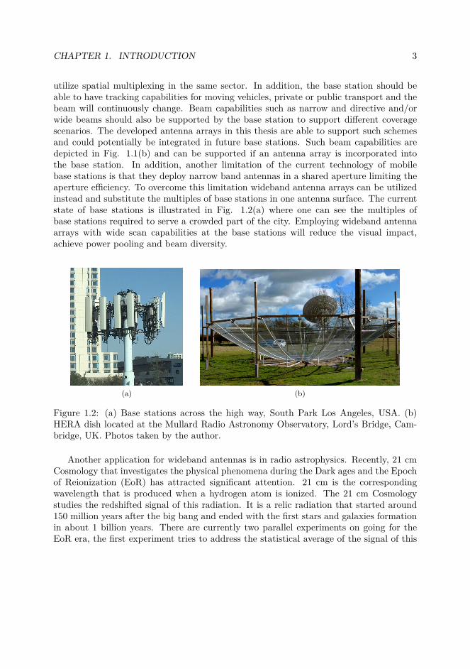
utilize spatial multiplexing in the same sector. In addition, the base station should beable to have tracking capabilities for moving vehicles, private or public transport and thebeam will continuously change. Beam capabilities such as narrow and directive and/orwide beams should also be supported by the base station to support different coveragescenarios. The developed antenna arrays in this thesis are able to support such schemesand could potentially be integrated in future base stations. Such beam capabilities aredepicted in Fig. 1.1(b) and can be supported if an antenna array is incorporated intothe base station. In addition, another limitation of the current technology of mobilebase stations is that they deploy narrow band antennas in a shared aperture limiting theaperture efficiency. To overcome this limitation wideband antenna arrays can be utilizedinstead and substitute the multiples of base stations in one antenna surface. The currentstate of base stations is illustrated in Fig. 1.2(a) where one can see the multiples ofbase stations required to serve a crowded part of the city. Employing wideband antennaarrays with wide scan capabilities at the base stations will reduce the visual impact,achieve power pooling and beam diversity.
(a) (b)
Figure 1.2: (a) Base stations across the high way, South Park Los Angeles, USA. (b)HERA dish located at the Mullard Radio Astronomy Observatory, Lord’s Bridge, Cam-bridge, UK. Photos taken by the author.
Another application for wideband antennas is in radio astrophysics. Recently, 21 cmCosmology that investigates the physical phenomena during the Dark ages and the Epochof Reionization (EoR) has attracted significant attention. 21 cm is the correspondingwavelength that is produced when a hydrogen atom is ionized. The 21 cm Cosmologystudies the redshifted signal of this radiation. It is a relic radiation that started around150 million years after the big bang and ended with the first stars and galaxies formationin about 1 billion years. There are currently two parallel experiments on going for theEoR era, the first experiment tries to address the statistical average of the signal of this

CHAPTER 1. INTRODUCTION 4
radiation, the global EoR, and the other one tries to find the minor fluctuations. The workin this thesis, is aimed towards the detection of the global EoR signal, that yet remainsundetected. The redshifted signal is calculated to be expected in the frequency range from100-200 MHz, whereas if one includes the dark ages and the null experiment any probeshould be operable from 40-250 MHz. This provides the first similarity with the widebandantenna arrays for base stations. In addition, the radio sky is contaminated with spuriousradiation, namely the foregrounds that is more than six orders of magnitude stronger thanthe expected EoR. To cancel strong sky radio sources and scan only in electromagneticallycold patches of the sky a wide-scan antenna array is required as well. A HERA prototypethat will be used to probe the EoR is depicted in Fig. 1.2(b).
The two applications, even that initially seem unrelated, the means required to achieveeither wideband wide-scan capability for wireless communication networks or for thedetection of 21-cm cosmological signal are the same, antenna arrays.
1.2 Thesis Outline
This thesis is organized as follows:• Chapter 2 gives the basic antenna array theory that is used in this thesis. The
concepts of infinite array analysis, planar arrays and embedded element pattern are dis-cussed.• A literature review and discussion on wideband antenna elements is provided in
Chapter 3. Antenna arrays for radio astronomy applications are also included in thischapter.• The fundamental limitation of antenna arrays are extracted in Chapter 4. We
propose an general measure for antenna arrays, the array figure of merit. This measurecouples bandwidth, height from the ground plane and reflection coefficient in a boundedquantity. We also propose an extension of the array figure of merit that is able to providebandwidth and directivity/gain limits.• Periodic structure loading on arrays is discussed in Chapter 5. We propose three
different periodic loadings aspects, element loading and edge loading in the form of a softcondition and an integrated lensing layer with a period structure. This is applied in aVivaldi antenna array and a demonstrator is fabricated and measured. Good agreementbetween simulations and measurements was achieved.• In Chapter 6, we propose a new class of antenna arrays, the Strongly Coupled
Asymmetric Dipole Array - SCADA. A novel method for terminating finite arrays is alsoproposed. The basic theory and an experimental antenna array is presented. Good agree-ment between measured and simulated results is observed. The Chapter concludes withanother demonstrator that addresses an integrated lensing layer with periodic loading. Asymmetric demonstrator was manufactured and measured with good agreement with thepredicted simulated values.

CHAPTER 1. INTRODUCTION 5
• Chapter 7 deals with an astrophysics application of antennas and antenna arrays. Wepropose a new method for extracting the global 21-cm cosmological signal from the Epochof Reionization - EoR. The method is based on piecewise polynomial fitting. An arraybased on the theory of Chapter 6 has been developed and can serve as instrumentationfor this experiment. The proposed extraction method of the cosmological signal hasbeen applied and evaluated for several classes of antennas such as reflectors, dipole andlog-periodic antennas as well as the proposed array.• We conclude in Chapter 8 with a summary of the thesis, the conclusions and the
contributions. A general discussion on the impact on sustainability of the current researchis also presented.
Chapter 2
Antenna Array Theory
This chapter is about introducing the basic theory, properties and terminology of antennaarrays to the unfamiliar readers. Despite the different applications and forms of antennaarrays the underlying theory and assumptions are the same. Arrays are a set of antennascoordinated to produce the desired radiation pattern or patterns. In the general case, eachelement in the array is considered to have two degrees of freedom for individual controlits amplitude and its phase. The control of the amplitude and phase can be performedeither in the radio frequency (RF) domain - analogue beamforming, in the baseband -baseband beamforming (typically digital) or both - hybrid beamforming.
Antenna arrays revolutionized the radar systems during the 20th century where anelectronically reconfigurable beam was in need. Their origin and initial developmentwas a result of the requirement to obtain multiple directive beams that could be usedboth as a communication and tracking system. An overview of the history of antennaarrays can be found in [5]. Even though, the initial application of arrays where mainlydefense applications, they are an integral part of modern wireless communication networksand find application in other fields such as satellite communications, biomedical imagingand medical treatment therapies. An example for a current state of the art medicalapplication is microwave hyperthermia, [6]. This technique has been proposed for cancertreatment. Utilizing an antenna array that focuses the electromagnetic energy to thetumor, microwave hyperthermia has shown potential for cancer treatment.
In this chapter, the general theory of antenna arrays is introduced. We start from thegeneral case of a random array lattice and the special case with an illustration for thelinear antenna array is shown. We discuss the planar arrays and the two conventionalarray lattices: the rectangular and the triangular that are the basis of this thesis. Theinfinite array analysis, that is the starting point for each design is discussed and theconnection with a finite array is given. Finally, the embedded element pattern of a finitearray’s element is defined and the connection for its calculation from the infinite arrayanalysis is given.
6
CHAPTER 2. ANTENNA ARRAY THEORY 7
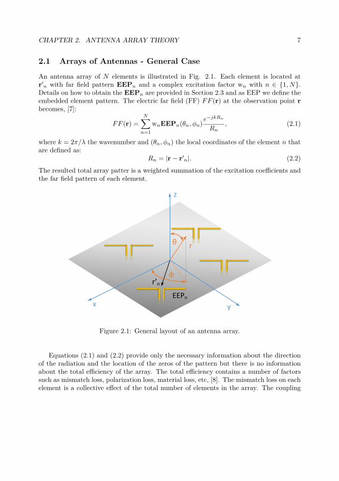
2.1 Arrays of Antennas - General Case
An antenna array of N elements is illustrated in Fig. 2.1. Each element is located atr′n with far field pattern EEPn and a complex excitation factor wn with n ∈ 1, N.Details on how to obtain the EEPn are provided in Section 2.3 and as EEP we define theembedded element pattern. The electric far field (FF) FF (r) at the observation point rbecomes, [7]:
FF (r) =N∑n=1
wnEEPn(θn, φn)e−jkRn
Rn, (2.1)
where k = 2π/λ the wavenumber and (θn, φn) the local coordinates of the element n thatare defined as:
Rn = |r− r′n|. (2.2)
The resulted total array patter is a weighted summation of the excitation coefficients andthe far field pattern of each element.
x y
z
φ
θ r
r n
EEPn
Figure 2.1: General layout of an antenna array.
Equations (2.1) and (2.2) provide only the necessary information about the directionof the radiation and the location of the zeros of the pattern but there is no informationabout the total efficiency of the array. The total efficiency contains a number of factorssuch as mismatch loss, polarization loss, material loss, etc, [8]. The mismatch loss on eachelement is a collective effect of the total number of elements in the array. The coupling

CHAPTER 2. ANTENNA ARRAY THEORY 8
coefficients Smn are calculated through the scattering parameters – S-parameters. Eachcoupling coefficient Smn relates amplitudes of the incident wave at port n and the outgoingwave at port m. The mismatch loss (ML) at each port n has the collective influence ofall other N − 1 ports and can then be written as:
ML = 1− |Γn|2, (2.3)
where Γn is the active reflection coefficient at each port n and is given as:
Γn =N∑m=1
Smnwn. (2.4)
The reflection coefficient is defined as the active reflection coefficient. It is different forevery element of the array and is dependent on the excitation of the array. Note that for anantenna array the outgoing wave represents power returning back to the feeding system,while radiated power is accounted for as system-network loses. Hence, the outgoing wavescontribute to the active reflection coefficient.
From the aforementioned discussion, to characterize an antenna array the knowledgeof both EEPn and Smn is required. The computational cost of these two quantities isenormous as for each element of the array a full electromagnetic solution is required.
In order to reduce the computational space, several simplifications can be made toobtain an insight and compute the far field. The first approximation is to remove thecoordinate dependence of each EEPn(θn, φn). We observe that in the case that if r r′n|∀r′n the fields at the observation point seem to come from the same direction andθn ≈ θ, φn ≈ φ and Rn ≈ r. In the exponential term, the phase of Rn must be consideredand a two term Taylor series expansion is required as Rn ≈ r − r · r′n. The secondapproximation that is typically applied is the assumption that all element patterns areidentical. This condition holds true only in the case of negligible mutual coupling in afinite array or a uniform environment as in the case of the infinite array. Then, we obtain:
EEPn(θ, φ) = EEP(θ, φ). (2.5)
Equation (2.1) is reduced to:
FF (θ, φ) = EEP(θ, φ)e−jkr
r
N∑n=1
wne−jkr·r′n , (2.6)
where we can define the array factor as:
AF =N∑n=1
wne−jkr·r′n . (2.7)
CHAPTER 2. ANTENNA ARRAY THEORY 9
z
x
θο
w1 w2 w5w4w3
d
Δφ
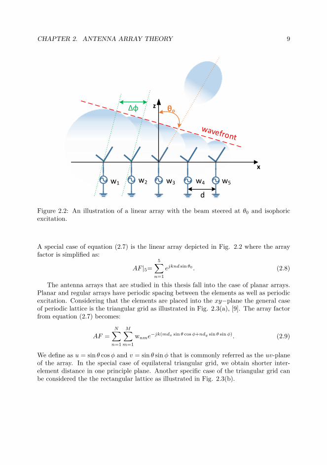
Figure 2.2: An illustration of a linear array with the beam steered at θ0 and isophoricexcitation.
A special case of equation (2.7) is the linear array depicted in Fig. 2.2 where the arrayfactor is simplified as:
AF |5=5∑
n=1ejknd sin θ0 . (2.8)
The antenna arrays that are studied in this thesis fall into the case of planar arrays.Planar and regular arrays have periodic spacing between the elements as well as periodicexcitation. Considering that the elements are placed into the xy−plane the general caseof periodic lattice is the triangular grid as illustrated in Fig. 2.3(a), [9]. The array factorfrom equation (2.7) becomes:
AF =N∑n=1
M∑m=1
wnme−jk(mdx sin θ cosφ+ndy sin θ sinφ). (2.9)
We define as u = sin θ cosφ and v = sin θ sinφ that is commonly referred as the uv-planeof the array. In the special case of equilateral triangular grid, we obtain shorter inter-element distance in one principle plane. Another specific case of the triangular grid canbe considered the the rectangular lattice as illustrated in Fig. 2.3(b).

CHAPTER 2. ANTENNA ARRAY THEORY 10
B
C
A D
x
y
b
α
dx
dy
mth element
nth element
dt
(a)
B
A
C
D
x
y
b
α
dx
dy
mth element
nth element
dr
(b)
Figure 2.3: Planar array grid (a) triangular and (b) rectangular.
2.2 Infinite Array Analysis
In the previous section, we have separated the behavior of the array factor and theelement pattern. However, we have not yet indicated how the element can be designed.In the previous approximation, it was assumed that the element pattern is identical toall elements. That assumption holds true only in an infinite array, where every elementwill have the same electromagnetic environment. To analyze the behavior of the element,we can utilize infinite array analysis where the element is treated as a unit cell. Anillustration of an infinite array of dipoles is depicted in Fig. 2.4(a) and the correspondingunit cell in Fig. 2.4(b).
The analysis of the infinite array is based on the Floquet’s theorem, [1], and forits application to antenna array theory, two assumptions are made i) the array’s latticeneeds to be in a canonical form as in either of the depicted in Fig. 2.3 and ii) a uniformamplitude excitation is required, hence in equation (2.9) wnm = w0. Providing that thesetwo conditions hold, then the electric and magnetic fields denoted as f can be writtenaccording to Floquet’s theorem as:
f(x+ dx, y + dy, z) = f(x, y, z)e−jk(dxu+dyv). (2.10)
From the unit cell analysis we can calculate the active reflection coefficient Γ at a specific

CHAPTER 2. ANTENNA ARRAY THEORY 11
... ...... ......
...... ... ...
... ... ...
Unit cell area
(a)dx
dy
(b)
Figure 2.4: (a) Illustration of an infinite array of dipoles. (b) Unit cell.
direction (u, v)→ (θ, φ) as Fourier series by expanding equation (2.4)
Γ(u, v) =∞∑
m=−∞
∞∑n=−∞
Smne−jk(mdxu+ndyv). (2.11)
This is a two dimensional Fourier series and the coupling coefficients Smn can be foundas Fourier coefficients as:
Smn =∫ λ
2dx
− λ2dx
∫ λ2dy
− λ2dy
Γ(u, v)ejk(mdxu+ndyv)dudv. (2.12)
Calculation of the mutual coupling will provide the information about the active reflectioncoefficient for any arbitrary angle (θ, φ). The connection between the active reflectioncoefficient and the element pattern is discussed in the following section.
2.3 Embedded Element Pattern
An isolated antenna is commonly characterized in free space conditions. This is typicallyreferred to as the isolated element pattern (IEP). Once the antenna is inserted into thearray environment, mutual coupling phenomena occur and the behavior of the antennaelement is altered from the initial IEP. The mutual coupling on the array environmentinduces currents in the neighboring elements affecting the near field of the antenna and byextension the input impedance of the element. The induced currents will also contributeto the far field pattern of the element, and the overall pattern will appear altered dueto the mutual coupling. To calculate the mutual coupling typically requires full wavesimulation that is computationally costly.
The farfield of an antenna inserted into an array environment, which takes into accountthe mutual coupling phenomena is referred as Embedded Element Pattern (EEP) or active
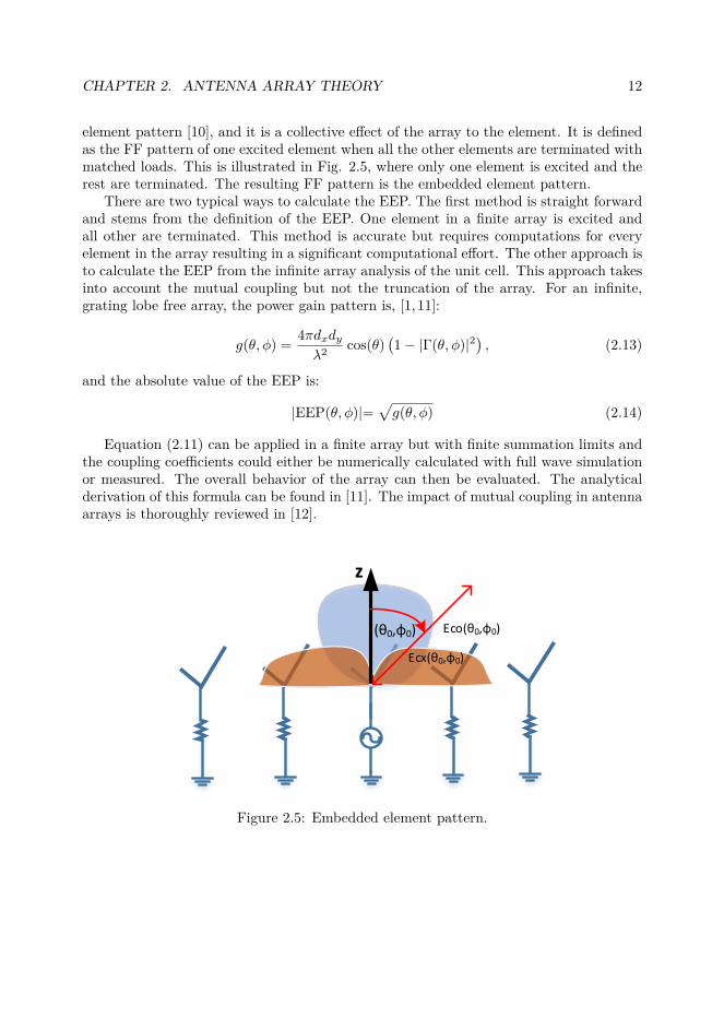
CHAPTER 2. ANTENNA ARRAY THEORY 12
element pattern [10], and it is a collective effect of the array to the element. It is definedas the FF pattern of one excited element when all the other elements are terminated withmatched loads. This is illustrated in Fig. 2.5, where only one element is excited and therest are terminated. The resulting FF pattern is the embedded element pattern.
There are two typical ways to calculate the EEP. The first method is straight forwardand stems from the definition of the EEP. One element in a finite array is excited andall other are terminated. This method is accurate but requires computations for everyelement in the array resulting in a significant computational effort. The other approach isto calculate the EEP from the infinite array analysis of the unit cell. This approach takesinto account the mutual coupling but not the truncation of the array. For an infinite,grating lobe free array, the power gain pattern is, [1, 11]:
g(θ, φ) = 4πdxdyλ2 cos(θ)
(1− |Γ(θ, φ)|2
), (2.13)
and the absolute value of the EEP is:
|EEP(θ, φ)|=√g(θ, φ) (2.14)
Equation (2.11) can be applied in a finite array but with finite summation limits andthe coupling coefficients could either be numerically calculated with full wave simulationor measured. The overall behavior of the array can then be evaluated. The analyticalderivation of this formula can be found in [11]. The impact of mutual coupling in antennaarrays is thoroughly reviewed in [12].
z
(θ0,φ0) Eco(θ0,φ0)
Ecx(θ0,φ0)
Figure 2.5: Embedded element pattern.
Chapter 3
Overview of Wideband AntennaArrays
The last decades has been shown that wideband antenna arrays can provide useful andappealing characteristics such as high data rates for both military and commercial appli-cations, pulse emitting signals and simultaneous transmission and reception of differentwireless protocols. Wheeler, in 1947, [13] stated the fundamental limitation on smallantennas and suggested the concept of ideal antenna. Unfortunately, antenna propertiescomes as trade-offs, for example size and bandwidth is a known trade off, [14]. Widebandwide scan angle array designs remain a very active research area since they are far fromtheir fundamental limits [15], [16]. As the demand for wireless communications increases,it is highly important to study, model and implement novel antenna design approaches.
When designing a wideband phased array the first and most important step is theelement selection. Most of the limitations of the antenna element are inherited by thearray and significantly affect the overall performance. Thus, selecting an element withwideband characteristics and scanning abilities is necessary. The main physical constraintwhen designing a wideband array is the interelement spacing. This comes as a result fromthe onset of grating lobes (Nyquist theorem - spatial sampling) which corresponds to thearray lattice of the array. The inter-element spacing is analog to λ
1+cos θ where θ is thescanning angle and λ the free space wave length to avoid grating lobes, [8]. Thus, forregular grids and scanning angles up to endfire the interelement spacing is λhf
2 while forthe broadside beam corresponds to λhf, where hf denotes the high frequency of operation.This means that the scanning capabilities of the antenna array and the interelementspacing is the first compromise that the antenna designer has to make. Furthermore asthe array scans, the active impedance and the embedded element pattern varies withrespect to the scan angle. The resonances of the array structure also shift with frequency,which limits the operational bandwidth of the array.
Three independent groups [17–19] have proposed a different approach to design and
13
CHAPTER 3. OVERVIEW OF WIDEBAND ANTENNA ARRAYS 14
develop wideband arrays. They independently drew the same conclusion, that strong cou-pling is necessary to achieve wideband performance. Here, a short introductory discussionover each of these approaches is given.
The first approach [17] developed at Electroscience laboratory of Ohio State Universityin collaboration with Harris Corporation. This approach is commonly known as thecurrent sheet array (CSA) and it consists of capacitevely coupled simple printed dipoleelements over a ground plane. This is the first unconventional approach that intentionallyintroduced inter-element coupling. The initial current sheet concept was conceived byWheeler [20], in 1958. It was not until 2002 that a realization was developed at OhioState University by Munk et al. , based on his studies at frequency selective surfaces [21].A similar approach based on connected slots was developed by Lee et al. [22]. Similarlyto the connected slots, the connected dipole array that was developed by Neto et al. [23].
The second approach [18] have many similarities with the conventional design since itincorporates the Vivaldi element, which is a well-known wideband radiator. This approachdemonstrated that it is possible to design arrays with Vivaldi elements with VSWR <2 at scanning angles up to 60 over 10:1 bandwidth. An important conclusion of thisresearch is the requirement of electrical connection between adjacent elements to obtainwideband and wide scan properties. This allows currents to flow undisrupted across thestructure and suppresses undesired resonances. Thus, strongly coupled Vivaldi elementshave better performance as compared to the uncoupled ones. Here, one should take intoaccount that the electrical connection creates manufacturing challenges, in particular fordual polarized Vivaldi arrays.
The third approach [19] was developed at Georgia Tech Research Institute (GTRI).The suggested solution was to treat the aperture as a blank canvas and determine theconductor placement through a global optimization procedure. This approach originateda new class of arrays that are usually called fragmented arrays. Here, once again, thesenewly developed elements are electrically connected to the neighboring elements, hencestrong inter-element coupling is introduced in the design. In order to obtain even morebandwidth of the structure and have unidirectional radiation patterns, they placed thefragmented array over multiple dielectric layers and resistive cards that create a widebandback-plane. This is also their main disadvantage, since half of the power is absorbed in theback-plane. Measurements have shown that the fragmented array can achieve bandwidthsof 33:1 [24], however such number are achieved only with resistive sheet loading thatseverely affects the array’s radiation efficiency.
The common ground to all aforementioned technologies is that they all introducedstrong coupling between the elements in order to achieve wideband and wide angularscan performance. However, the analysis and prediction of the strongly coupled elementsand a systematic design procedure based on this approach remains open. In the followingsections, a more extensive discussion will be given on these three technologies providingthe most significant contributions on each field.
CHAPTER 3. OVERVIEW OF WIDEBAND ANTENNA ARRAYS 15
3.1 Connected Dipoles/Slots - Capacitive Coupled Arrays(Current Sheet Array Concept)
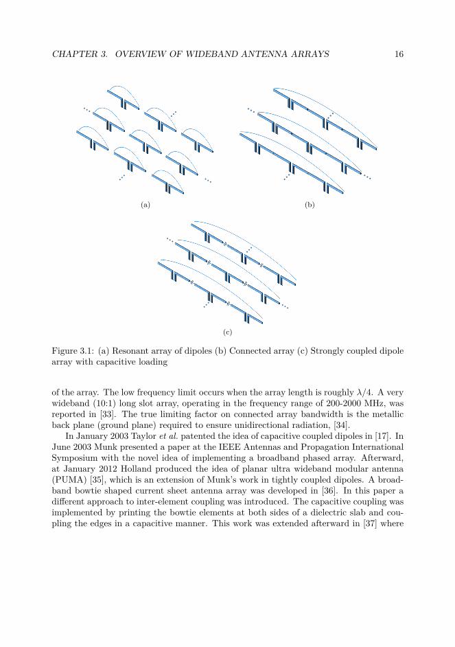
The last decade a radically different design approach has arisen for broadband arrayswhere the adjacent elements are intentionally coupled. A simple way to enhance thecoupling between neighboring elements is to electrically connect them one to another. Aconnected array can be briefly described as an array of dipoles or slots which are electri-cally connected to each other. In this way, the array is no longer composed of separatedresonant elements, but can be considered as a single antenna that is fed periodically.The current distribution on resonant narrowband elements is sinusoidal and frequencydependent, as shown in Fig. 3.1(a). As a contrast, connected arrays achieve widebandperformance since there is no disruption in current flow between the adjacent elements, ascan be seen at Fig. 3.1(b). When a connected array is capacitively loaded the bandwidthis further enhanced due the the cancellation of the inductance of the ground plane. Theconfiguration of a capacitively loaded strongly coupled dipole array is illustrated in Fig.3.1(c). In a finite array the lowest operational frequency is then determined mainly bythe array size.
Another attractive feature of connected arrays is their capability to achieve goodpolarization purity. The polarization purity is mainly influenced by the feeding of theelement. Mainly, two different approaches for the feeding have been developed. Thefirst approach is to place a feed organizer and excite the dipole with a 180 hybrid,[25]. This resulted in large structures that are extended below the ground plane. Thesecond approach is to directly embed the BalUn between the dipole and the ground plane,[26]. This lowers the polarization purity and also affects the structure of the array, [27].Furthermore, wideband BalUn are also large structures. Connected arrays/capacitivecoupled arrays have emerged as one of the most promising technologies for widebandapplications as they have low cross polarization and wideband performance.
An intuitive design was developed in Ohio State University in cooperation with Har-ris Corporation by Munk et al. In this design approach the inter-element coupling wasimplemented with an inter-digital capacitor, [28]. The strongly coupled dipole array isa descendant from frequency selective surfaces (FSS) [21]. Similarly, FSS use capacitiveloading in order to obtain continuous currents in the structure, thus realizing the contin-uous current sheet proposed by Wheeler [20], [29]. The capacitive loading in the currentsheet array plays a dual role. First, it allows continuous currents along the structure, andsecond, it partially counteracts the inductive behavior of the ground plane.
An expansion of the connected dipole concept to the dual structure (slots) has beenpresented in [22]. Analytical expressions for the Green’s functions were derived for longslot arrays in [30] and [31] based on the spectral representation of the field for each slot[32]. This work demonstrated that the achievable bandwidth is theoretically infinite forconnected arrays in free space. In practice, it is limited only by the dimensions of thearray. In realistic designs, the bandwidth is not infinite, but is limited by the dimensions
CHAPTER 3. OVERVIEW OF WIDEBAND ANTENNA ARRAYS 16
(a) (b)
(c)
Figure 3.1: (a) Resonant array of dipoles (b) Connected array (c) Strongly coupled dipolearray with capacitive loading
of the array. The low frequency limit occurs when the array length is roughly λ/4. A verywideband (10:1) long slot array, operating in the frequency range of 200-2000 MHz, wasreported in [33]. The true limiting factor on connected array bandwidth is the metallicback plane (ground plane) required to ensure unidirectional radiation, [34].
In January 2003 Taylor et al. patented the idea of capacitive coupled dipoles in [17]. InJune 2003 Munk presented a paper at the IEEE Antennas and Propagation InternationalSymposium with the novel idea of implementing a broadband phased array. Afterward,at January 2012 Holland produced the idea of planar ultra wideband modular antenna(PUMA) [35], which is an extension of Munk’s work in tightly coupled dipoles. A broad-band bowtie shaped current sheet antenna array was developed in [36]. In this paper adifferent approach to inter-element coupling was introduced. The capacitive coupling wasimplemented by printing the bowtie elements at both sides of a dielectric slab and cou-pling the edges in a capacitive manner. This work was extended afterward in [37] where
CHAPTER 3. OVERVIEW OF WIDEBAND ANTENNA ARRAYS 17
the characteristic modes were derived for tightly coupled antenna arrays. By exiting thearray according to the characteristic mode it is possible to compensate the edge effects.Finally there is an effort of realizing a tightly coupled spiral array in [38], that indicatedthe possibility for tightly coupled circularly polarized arrays.
The average bandwidth of the aforementioned arrays is 4:1 with scan angles up to45. The capacitive coupled dipoles perform better in terms of bandwidth. By adding su-perstrates acting as wide angle impedance matching (WAIM) layers further improvementcan be obtained, [39]. Here, it is worth mentioning that the approach in [17] does not usea BalUn for the feeding of the dipole. Each dipole arm is fed with a separate line and thedifferential mode is obtained by external 180 hybrid coupler and a feed organizer. Somerecent developments are [40–43].
3.2 Vivaldi Antenna Arrays
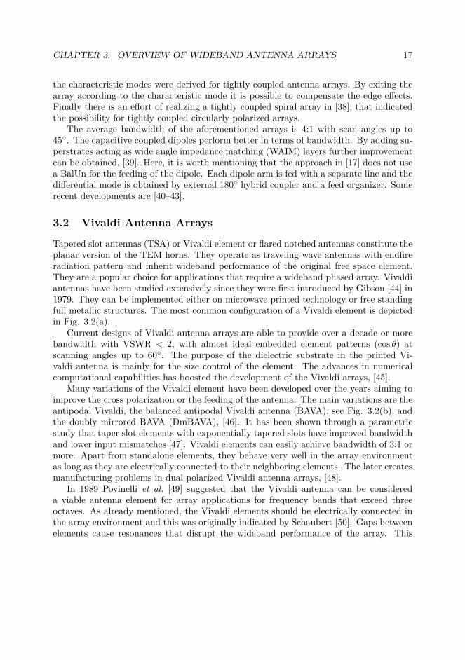
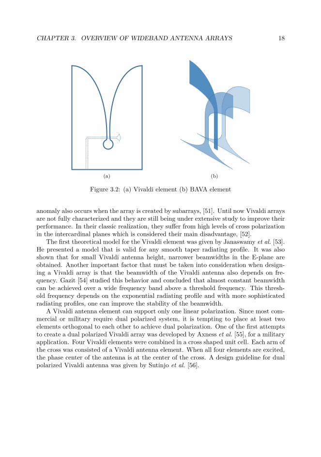
Tapered slot antennas (TSA) or Vivaldi element or flared notched antennas constitute theplanar version of the TEM horns. They operate as traveling wave antennas with endfireradiation pattern and inherit wideband performance of the original free space element.They are a popular choice for applications that require a wideband phased array. Vivaldiantennas have been studied extensively since they were first introduced by Gibson [44] in1979. They can be implemented either on microwave printed technology or free standingfull metallic structures. The most common configuration of a Vivaldi element is depictedin Fig. 3.2(a).
Current designs of Vivaldi antenna arrays are able to provide over a decade or morebandwidth with VSWR < 2, with almost ideal embedded element patterns (cos θ) atscanning angles up to 60. The purpose of the dielectric substrate in the printed Vi-valdi antenna is mainly for the size control of the element. The advances in numericalcomputational capabilities has boosted the development of the Vivaldi arrays, [45].
Many variations of the Vivaldi element have been developed over the years aiming toimprove the cross polarization or the feeding of the antenna. The main variations are theantipodal Vivaldi, the balanced antipodal Vivaldi antenna (BAVA), see Fig. 3.2(b), andthe doubly mirrored BAVA (DmBAVA), [46]. It has been shown through a parametricstudy that taper slot elements with exponentially tapered slots have improved bandwidthand lower input mismatches [47]. Vivaldi elements can easily achieve bandwidth of 3:1 ormore. Apart from standalone elements, they behave very well in the array environmentas long as they are electrically connected to their neighboring elements. The later createsmanufacturing problems in dual polarized Vivaldi antenna arrays, [48].
In 1989 Povinelli et al. [49] suggested that the Vivaldi antenna can be considereda viable antenna element for array applications for frequency bands that exceed threeoctaves. As already mentioned, the Vivaldi elements should be electrically connected inthe array environment and this was originally indicated by Schaubert [50]. Gaps betweenelements cause resonances that disrupt the wideband performance of the array. This
CHAPTER 3. OVERVIEW OF WIDEBAND ANTENNA ARRAYS 18
(a) (b)
Figure 3.2: (a) Vivaldi element (b) BAVA element
anomaly also occurs when the array is created by subarrays, [51]. Until now Vivaldi arraysare not fully characterized and they are still being under extensive study to improve theirperformance. In their classic realization, they suffer from high levels of cross polarizationin the intercardinal planes which is considered their main disadvantage, [52].
The first theoretical model for the Vivaldi element was given by Janaswamy et al. [53].He presented a model that is valid for any smooth taper radiating profile. It was alsoshown that for small Vivaldi antenna height, narrower beamwidths in the E-plane areobtained. Another important factor that must be taken into consideration when design-ing a Vivaldi array is that the beamwidth of the Vivaldi antenna also depends on fre-quency. Gazit [54] studied this behavior and concluded that almost constant beamwidthcan be achieved over a wide frequency band above a threshold frequency. This thresh-old frequency depends on the exponential radiating profile and with more sophisticatedradiating profiles, one can improve the stability of the beamwidth.
A Vivaldi antenna element can support only one linear polarization. Since most com-mercial or military require dual polarized system, it is tempting to place at least twoelements orthogonal to each other to achieve dual polarization. One of the first attemptsto create a dual polarized Vivaldi array was developed by Axness et al. [55], for a militaryapplication. Four Vivaldi elements were combined in a cross shaped unit cell. Each arm ofthe cross was consisted of a Vivaldi antenna element. When all four elements are excited,the phase center of the antenna is at the center of the cross. A design guideline for dualpolarized Vivaldi antenna was given by Sutinjo et al. [56].
CHAPTER 3. OVERVIEW OF WIDEBAND ANTENNA ARRAYS 19
Another variation of the traditional Vivaldi antenna is the Balanced Antipodal VivaldiAntenna (BAVA) [57]. Arrays with BAVA elements suffer from the same resonances thatlimit the bandwidth [58]. In [46] it was indicated that dual polarized Doubly mirroredBalanced Antipodal Vivaldi Antenna (DmBAVA) array can provide a bandwidth over twooctaves with moderate scanning abilities of±45. Following up on the last mentioned workand by using the same principal as the traditional Vivaldi array design and electricallyconnect the DmBAVA elements Elsallal et al. created an electrically small DmBAVAantenna array operating at 1.8-18 GHz, [59].
In 2007, a Vivaldi like three dimensional element was developed for array applications,[60], that is called BOR-element. The design is very compact, fully metallic and it hasthe possibility of placing some of the Tx/Rx components inside the metal cavity of theelement. More recent developments can be found in [61, 62] with efforts to improve thecross polarization (cx-pol) levels.
3.3 Fragmented Array Antennas
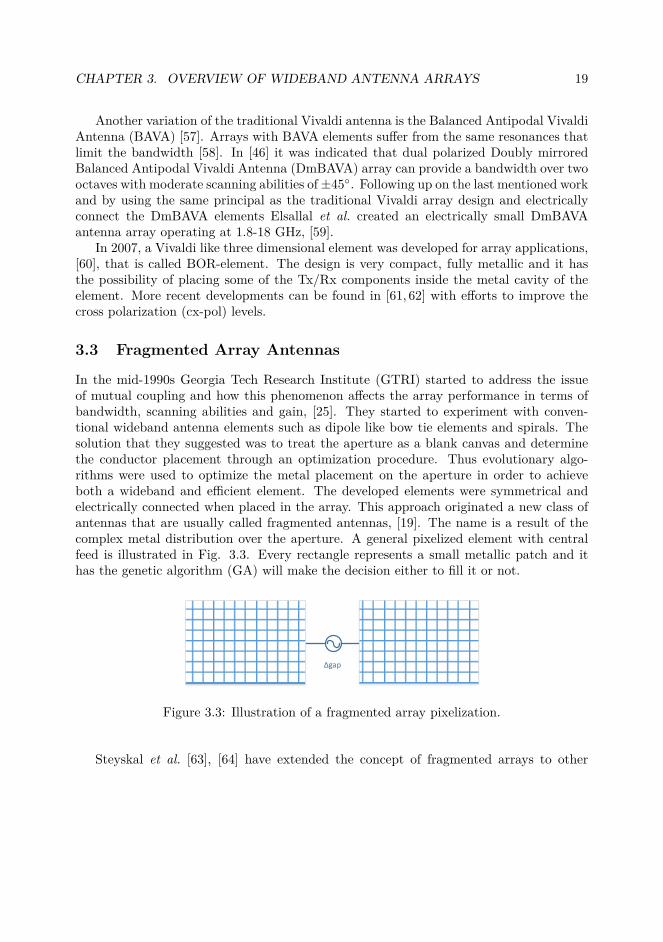
In the mid-1990s Georgia Tech Research Institute (GTRI) started to address the issueof mutual coupling and how this phenomenon affects the array performance in terms ofbandwidth, scanning abilities and gain, [25]. They started to experiment with conven-tional wideband antenna elements such as dipole like bow tie elements and spirals. Thesolution that they suggested was to treat the aperture as a blank canvas and determinethe conductor placement through an optimization procedure. Thus evolutionary algo-rithms were used to optimize the metal placement on the aperture in order to achieveboth a wideband and efficient element. The developed elements were symmetrical andelectrically connected when placed in the array. This approach originated a new class ofantennas that are usually called fragmented antennas, [19]. The name is a result of thecomplex metal distribution over the aperture. A general pixelized element with centralfeed is illustrated in Fig. 3.3. Every rectangle represents a small metallic patch and ithas the genetic algorithm (GA) will make the decision either to fill it or not.
Δgap
Figure 3.3: Illustration of a fragmented array pixelization.
Steyskal et al. [63], [64] have extended the concept of fragmented arrays to other
CHAPTER 3. OVERVIEW OF WIDEBAND ANTENNA ARRAYS 20
applications and smaller arrays. Their designs use pixelated structures with a set numberof pixels for a given element, and a GA determines if the pixel is conducting or not. Thisis a binary design decision for each pixel in the array element. The genetic algorithmoptimizes the element design layout of an infinite array using the Floquet theory. TheGTRI design uses square pixels [65] and small plus shapes [19] as pixel elements.
Through this research effort two important conclusions were drawn. First; the elec-trical connection between the adjacent elements improves the performance in terms ofbandwidth. Second conclusion was that the total array size dictates the operating band-width of the array. A rule of thumb for wideband performance is that at least λ/12thickness is required. The same rule is applied to the strongly coupled dipole designprocedure. The arrays described in [65] are mostly without ground plane.
3.4 Conclusions
The current state of the art on wideband antenna arrays was presented in this chapter.The three major classes of wideband arrays were reviewed and analyzed. Planar structuresthat can achieve constant input impedance like the current sheet array require a groundplane to radiate only in one half plane. The available thickness is hence a limiting factor forall wideband array designs over a ground plane apart from the Vivaldi array. An infiniteground plane increases the directivity of the antenna. It is known [66,67] that bandwidthtimes directivity is bounded above by charge separation (polarizability). Recent progresson bandwidth limitations for these arrays are discussed in [15,68]. Methods to address theissue of the ground plane limitation is either to put absorbers as resistive cards betweenthe antenna and the ground plane or to add an artificial frequency selective surface (FSS)as a band stop filter. The main drawback for adding such structures is the negative impacton the radiation efficiency of the array. This literature survey motivates the developmentson this thesis for the communications part.
Chapter 4
Fundamental Limitations of AntennaArrays1
Antenna array design is a difficult, lengthy and computationally expensive procedure andany analytical insight that can be provided a priori could potentially speed up the process.The typical design procedure starts with the unit cell of the array. Understanding thefundamental limitations in antenna arrays in unit cell design can provide great inputon the design procedure and provide initial parameter trade-off relations on the primarydesign parameters. The primary design parameters can then be defined according to thespecific’s application constraints and demands.
The important parameters that define the characteristics and behavior of every arrayare: the operational bandwidth BW , the scanning performance, the active reflectioncoefficient Γs, the volume of each unit cell and lattice information, the aperture efficiencyAe, and the maximum operational frequency for grating lobe free region fmax → λmin.Coupling these parameters in an analytical, yet physically insightful relation can be thestarting of every array design.
In literature, several efforts have been made to constrain some of these parametersseparately or combinations and depend on the approach taken, [69–71]. The first andmost famous limitation in antennas that can and also be applied in an antenna array ele-ment is for matching limits at the matching network. In the 1950s Fano, [72], developedthe fundamental limits of broadband matching of an arbitrary load that was based on anintegral relation of the reflection coefficient. This integral relation is typically referred asa sum-rule and is based in the property that any holomorphic function in the complexhalf plane is bounded. Sum-rules have been used in several cased to bound propertiesof structures. In [73], Rozanov utilized the sum-rule to extract thickness limits on artifi-cial radar materials. The limitations of high impedance surfaces and frequency selectivesurfaces have been extracted in [74] and [75], respectively.
1Partial content of this chapter is reproduced from author’s Papers I and II.
21
CHAPTER 4. FUNDAMENTAL LIMITATIONS OF ANTENNA ARRAYS 22
The aperture efficiency is typically connected to the uniform aperture illuminationand can provide maximum directivity limits, [1], whereas the grating lobe free region inregular arrays stems from the spatial sampling connecting to the Nyquist theorem, [8]and has a dependency of the maximum scan angle.
In this chapter, the Array Figure of Merit - AFM is presented. It is a general quanti-tative measure of antenna arrays based on the unit cell behavior for arrays that are placedabove a ground plane. The AFM is a sum-rule based result and relates the BW , theoverall thickness of the element above the ground plane, the active reflection coefficientand the scanning ability of the array. The AFM is further extended relating in additionthe maximum unit cell’s directivity, the efficiency and lattice information.
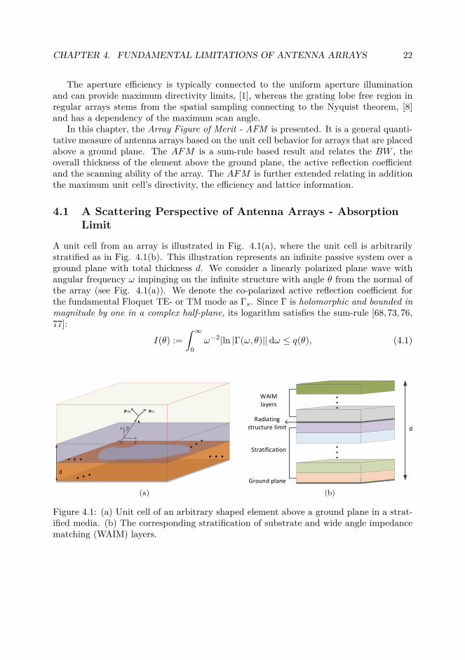
4.1 A Scattering Perspective of Antenna Arrays - AbsorptionLimit
A unit cell from an array is illustrated in Fig. 4.1(a), where the unit cell is arbitrarilystratified as in Fig. 4.1(b). This illustration represents an infinite passive system over aground plane with total thickness d. We consider a linearly polarized plane wave withangular frequency ω impinging on the infinite structure with angle θ from the normal ofthe array (see Fig. 4.1(a)). We denote the co-polarized active reflection coefficient forthe fundamental Floquet TE- or TM mode as Γs. Since Γ is holomorphic and bounded inmagnitude by one in a complex half-plane, its logarithm satisfies the sum-rule [68, 73, 76,77]:
I(θ) :=∫ ∞
0ω−2|ln |Γ(ω, θ)|| dω ≤ q(θ), (4.1)
. . .. . .d
θ
k
pTEpTM
y
z
x
(a)Ground plane
Radiating structure limit
•
•
•
•
•
•
Stratification
WAIMlayers
d
(b)
Figure 4.1: (a) Unit cell of an arbitrary shaped element above a ground plane in a strat-ified media. (b) The corresponding stratification of substrate and wide angle impedancematching (WAIM) layers.
CHAPTER 4. FUNDAMENTAL LIMITATIONS OF ANTENNA ARRAYS 23
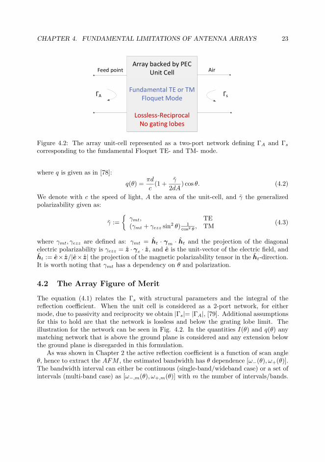
Array backed by PECUnit Cell
Fundamental TE or TM Floquet Mode
Lossless-ReciprocalNo gating lobes
ΓA Γs
Feed point Air
Figure 4.2: The array unit-cell represented as a two-port network defining ΓA and Γscorresponding to the fundamental Floquet TE- and TM- mode.
where q is given as in [78]:q(θ) = πd
c(1 + γ
2dA ) cos θ. (4.2)
We denote with c the speed of light, A the area of the unit-cell, and γ the generalizedpolarizability given as:
γ :=γmt, TE(γmt + γezz sin2 θ) 1
cos2 θ , TM (4.3)
where γmt, γezz are defined as: γmt = ht · γm · ht and the projection of the diagonalelectric polarizability is γezz = z · γe · z, and e is the unit-vector of the electric field, andht := e× z/|e× z| the projection of the magnetic polarizability tensor in the ht-direction.It is worth noting that γmt has a dependency on θ and polarization.
4.2 The Array Figure of Merit
The equation (4.1) relates the Γs with structural parameters and the integral of thereflection coefficient. When the unit cell is considered as a 2-port network, for eithermode, due to passivity and reciprocity we obtain |Γs|= |ΓA|, [79]. Additional assumptionsfor this to hold are that the network is lossless and below the grating lobe limit. Theillustration for the network can be seen in Fig. 4.2. In the quantities I(θ) and q(θ) anymatching network that is above the ground plane is considered and any extension belowthe ground plane is disregarded in this formulation.
As was shown in Chapter 2 the active reflection coefficient is a function of scan angleθ, hence to extract the AFM , the estimated bandwidth has θ dependence [ω−(θ), ω+(θ)].The bandwidth interval can either be continuous (single-band/wideband case) or a set ofintervals (multi-band case) as [ω−,m(θ), ω+,m(θ)] with m the number of intervals/bands.
CHAPTER 4. FUNDAMENTAL LIMITATIONS OF ANTENNA ARRAYS 24
Assuming only the operational interval there is no loss of generality since in the elementis mostly mismatched outside its operational band(s) and the integral tends to zero. Wecan rewrite equation (4.1) as:
IG(θ) :=∫ ω+,m(θ)
ω−,m(θ)ω−2|ln |ΓA(ω, θ)||dω ≤ q(θ). (4.4)
We define the array figure of merit for an array with scan range θ ∈ [θ0, θ1] as:
η0 := maxθ∈[θ0,θ1]
IG(θ)q(θ) ≤ 1. (4.5)
To evaluate the equation (4.5) the integral has to be approximated. We define as|ΓA,maxm |= max |Γs| |θ ∈ [θ0, θ1];ω ∈ [ω−,m, ω+,m] with the only requirement that ω+,m ≤ωG, where ωG is the onset of grating lobe. Finally, taking only the first order approxima-tion for the q factor as was shown in [78] we can define the array figure of merit, η, forthe TE and TM single and multi-band cases respectively as follows for the TE- and TM-Floquet modes.
TE-Floquet mode, multiband case:
ηTEM =c∑Mm=1 | ln|ΓA,maxm ||(ω−1
−,m − ω−1+,m)
πµsd cos θ1≤ 1. (4.6)
TE-Floquet mode, singleband case:
ηTE = | ln|ΓA,max||(BW − 1)2π2µs(d/λhf) cos θ1
≤ 1 (4.7)
TM-Floquet mode, multiband case:
ηTMM =cos θ1 · c
∑Mm=1 | ln|ΓA,maxm ||(ω
−1−,m − ω−1
+,m)πµsd
≤ 1 (4.8)
TM-Floquet mode, singleband case:
ηTM = | ln|ΓA,max||(BW − 1) cos θ12π2µs(d/λhf)
≤ 1 (4.9)
We have denoted as 1 < BW = ω+/ω− and λhf = 2πc/ω+. The relations (4.6) - (4.9)provide trade-off relations between thickness, scan-range bandwidth and active reflectioncoefficient level.

CHAPTER 4. FUNDAMENTAL LIMITATIONS OF ANTENNA ARRAYS 25
4.3 Integrating the Array Figure of Merit with LatticeInformation and Directivity Limits
In a finite array with aperture area A, the overall aperture defines the maximum gainthat can be achieved in any given frequency. In a planar array configuration consistingof M × N elements in a regular grid with corresponding unit cell dimensions dx and dywe obtain:
G = 4πAλ2 = MN
4πdxdyλ2 , (4.10)
and we can define the embedded element gain as:
GEE = 4πdxdyλ2 . (4.11)
It is known that for dense arrays with small element spacing the radiation intensity of theelement follows a cos θ shape, [80], as is the aperture projection. The maximum embeddedelement gain that can be achieved in a unit cell with spacing below the grating lobe limit(λmin) can be then stated as:
GEE,max = 4πdxdyλ2min
. (4.12)
We observe that the equations (4.6) - (4.9) have a λmin dependency and we can couplethe maximum gain and lattice dx and dy to the AFM. Presenting for brevity the modifiedequations (4.7) and (4.9) we obtain:
ηTE =| ln|ΓA,max||(BW − 1)
√dxdy
π3/2µsd√GEE,max cos θ1
(4.13)
ηTM =| ln|ΓA,max||(BW − 1)
√dxdy cos θ1
π3/2µsd√GEE,max
(4.14)
where we have coupled the lattice information and the maximum element gain in theAFM. Here, we can also utilize the fact that G = ηeD where ηe is the elements efficiency.It is remarkable to note that with the theoretical maximum directivity D = 4 at the twoextreme cases of regular square lattice and equilateral triangular lattice with correspond-ing efficiencies ηe,r = π/4 and ηe,t = π/2
√3, [81,82], respectively the equations (4.7) and
(4.9) are recovered. The ηe,r and ηe,t represent the maximum efficiency on a rectangularand triangular lattice respectively. Equations (4.13) and (4.14) represent a more effectiveand general quantitative tool to calculate the AFM with arbitrary lattice information,max simulated/measured directivity and efficiency.

CHAPTER 4. FUNDAMENTAL LIMITATIONS OF ANTENNA ARRAYS 26
4.4 Conclusions
Designing an antenna array requires a significant lengthy computational effort. Anyestimation that can provide early information about the design can be integrated into thedesign process. In this chapter, the fundamentals of sum rule identities have been brieflydiscussed and their application for a priori estimates. We have developed a sum-rulebased result, the array figure of merit (AFM). This estimate was extracted for TE- andTM-polarization case of an infinite array over a ground plane. The AFM relates BW ,scan performance, active reflection coefficient with the array’s total thickness overt theground. Both the single band and the multi band cases were presented. In addition, theAFM was extended to include lattice information, Directivity and efficiency of a unitcell. In this extension in a single formula all the important design parameters of an arrayare connected and the trading relations can be extracted.
Chapter 5
Periodic Loading on Vivaldi Arrays 1
Modern wireless communications demand high data rates, reliable user experience anda seamless link. With the arrival of Internet of Things (IoT) that will interconnect thephysical and the human world through sensors, further requirements appear and a massivenumber of devices will have a network connection. The base station should then be ableto communicate and support not only the conventional communication protocols utilizedtoday but protocols for sensing devices, automated cars, smart buildings etc. It is imper-ative then to have base stations that are able to cover all these different communicationbands with the same interface. Wideband antenna arrays are an excellent candidate tosupport all the new requirements.
In this Chapter, periodic structures are utilized in combination with Vivaldi antennaarrays. The Vivaldi arrays have a long and successful history as a wideband antennaarrays. The two main disadvantages of the classic design are high cross polarization inthe intercardinal D-plane of the array and edge radiation from the edge elements. Weintroduce a soft condition along the Vivaldi flare in order to confine the traveling waveinside the flaring. This approach has a dual impact; it miniaturizes the element andreduces the levels of cross polarization. In addition, we utilize one more soft conditionalong the outer array edges that acts as a spatial filter for the edge born waves. This softsurface reduces the back radiation and the side-lobes of the array. Finally, a matching layeris introduced on top of the Vivaldi element that positively impacts the active matchingand scanning performance. The matching layer is implemented as periodic strip loadingthat continues after the Vivaldi flaring. These innovative structural modifications arebased in the physical insight on the Vivaldi element operation and target to improve theperformance with proper guiding wave manipulation.
The basic properties of the soft and hard conditions are introduced in this Chapterand the developed array is presented along with the measurement results.
1Partial content of this chapter is reproduced from author’s Paper III and Patent VI.
27
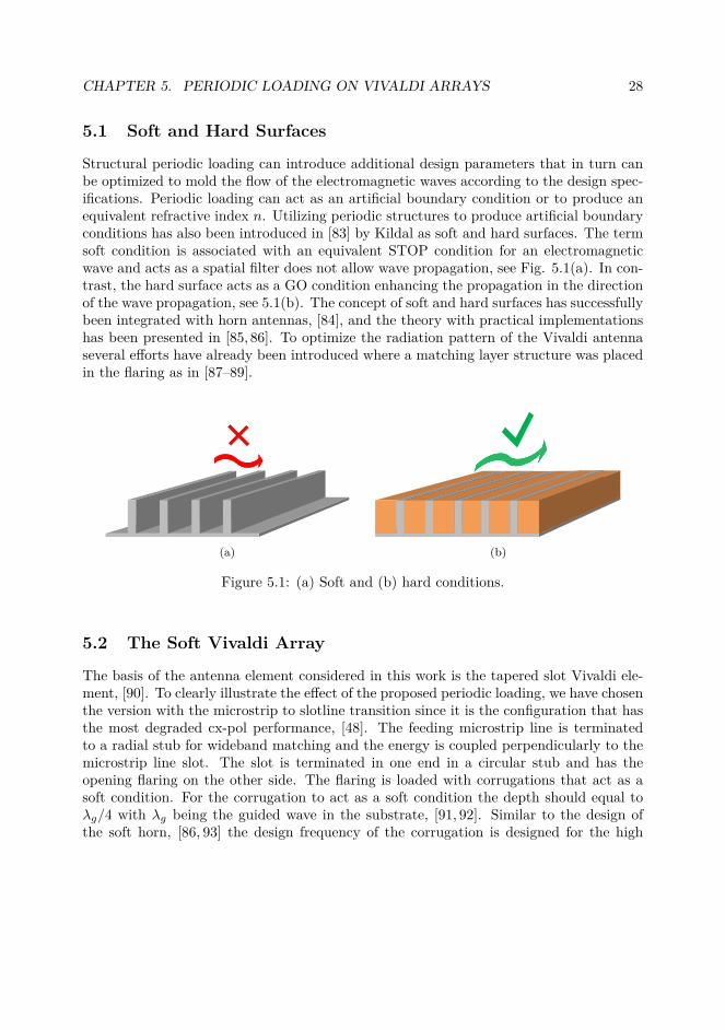
CHAPTER 5. PERIODIC LOADING ON VIVALDI ARRAYS 28
5.1 Soft and Hard Surfaces
Structural periodic loading can introduce additional design parameters that in turn canbe optimized to mold the flow of the electromagnetic waves according to the design spec-ifications. Periodic loading can act as an artificial boundary condition or to produce anequivalent refractive index n. Utilizing periodic structures to produce artificial boundaryconditions has also been introduced in [83] by Kildal as soft and hard surfaces. The termsoft condition is associated with an equivalent STOP condition for an electromagneticwave and acts as a spatial filter does not allow wave propagation, see Fig. 5.1(a). In con-trast, the hard surface acts as a GO condition enhancing the propagation in the directionof the wave propagation, see 5.1(b). The concept of soft and hard surfaces has successfullybeen integrated with horn antennas, [84], and the theory with practical implementationshas been presented in [85, 86]. To optimize the radiation pattern of the Vivaldi antennaseveral efforts have already been introduced where a matching layer structure was placedin the flaring as in [87–89].
(a) (b)
Figure 5.1: (a) Soft and (b) hard conditions.
5.2 The Soft Vivaldi Array
The basis of the antenna element considered in this work is the tapered slot Vivaldi ele-ment, [90]. To clearly illustrate the effect of the proposed periodic loading, we have chosenthe version with the microstrip to slotline transition since it is the configuration that hasthe most degraded cx-pol performance, [48]. The feeding microstrip line is terminatedto a radial stub for wideband matching and the energy is coupled perpendicularly to themicrostrip line slot. The slot is terminated in one end in a circular stub and has theopening flaring on the other side. The flaring is loaded with corrugations that act as asoft condition. For the corrugation to act as a soft condition the depth should equal toλg/4 with λg being the guided wave in the substrate, [91, 92]. Similar to the design ofthe soft horn, [86, 93] the design frequency of the corrugation is designed for the high
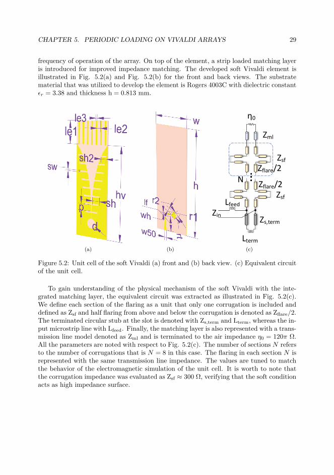
CHAPTER 5. PERIODIC LOADING ON VIVALDI ARRAYS 29
frequency of operation of the array. On top of the element, a strip loaded matching layeris introduced for improved impedance matching. The developed soft Vivaldi element isillustrated in Fig. 5.2(a) and Fig. 5.2(b) for the front and back views. The substratematerial that was utilized to develop the element is Rogers 4003C with dielectric constantεr = 3.38 and thickness h = 0.813 mm.
(a) (b)
Lfeed
Lterm
Zin
.
....
.
..
Zsf
Zml
η0
Zsf
Zflare/2
Zflare/2
Zs,term
N
(c)
Figure 5.2: Unit cell of the soft Vivaldi (a) front and (b) back view. (c) Equivalent circuitof the unit cell.
To gain understanding of the physical mechanism of the soft Vivaldi with the inte-grated matching layer, the equivalent circuit was extracted as illustrated in Fig. 5.2(c).We define each section of the flaring as a unit that only one corrugation is included anddefined as Zsf and half flaring from above and below the corrugation is denoted as Zflare/2.The terminated circular stub at the slot is denoted with Zs,term and Lterm, whereas the in-put microstrip line with Lfeed. Finally, the matching layer is also represented with a trans-mission line model denoted as Zml and is terminated to the air impedance η0 = 120π Ω.All the parameters are noted with respect to Fig. 5.2(c). The number of sections N refersto the number of corrugations that is N = 8 in this case. The flaring in each section N isrepresented with the same transmission line impedance. The values are tuned to matchthe behavior of the electromagnetic simulation of the unit cell. It is worth to note thatthe corrugation impedance was evaluated as Zsf ≈ 300 Ω, verifying that the soft conditionacts as high impedance surface.

CHAPTER 5. PERIODIC LOADING ON VIVALDI ARRAYS 30
2.0 2.5 3.0 3.5 4.0 4.5 5.0 5.5Frequency (GHz)
0
1
2
3
4
5
6
7
8
VSWR
Broadside60) E∘ lane60) H∘ lane45) D∘ laneBroadside eq. circuit
(a)
0 20 40 60 80θ (deg)
−20
−15
−10
−5
0
5
Directivit
(dBi)
f = 1.8 GHz E-planef = 2.4 GHz E-planef = 3.2 GHz E-planef = 4.4 GHz E-planef = 5.4 GHz E-plane
(b)
0 20 40 60 80θ (deg)
−20
−15
−10
−5
0
5
Directivity
(dBi)
f = 1.8 GH H-planef = 2.4 GHz H-planef = 3.2 GHz H-planef = 4.4 GHz H-planef = 5.4 GHz H-plane
(c)
Figure 5.3: (a) Unit cell VSWR. Embedded element pattern from unit cell analysis (b)E-plane and (c) H-plane.
The electrical dimensions of the unit cell are summarized as 1.42λhf for the overallheight of the element placed in a square lattice of 0.43λhf × 0.43λhf . The resulted activeVSWR from the final optimized unit cell simulation for the soft Vivaldi element with theintegrated matching layer is shown in Fig. 5.3(a). We observe that the array is capableof scanning up to ±60 in both E- and H-plane with excellent VSWR performance. TheVSWR for the broadside case as extracted from the equivalent circuit analysis is also illus-trated and good agreement between electromagnetic and circuit simulations is observed.The inconsistency with the rippling is attributed to the small number of discretization ofthe flaring that does not follow a continuous profile and is approximated with only eightsections. The simulated embedded element patterns for E- and H-plane from a unit cellsimulation are depicted in Fig. 5.3(b) and Fig. 5.3(c) respectively. The dimensions of theunit cell from Fig. 5.2 are summarized at the Table 5.1.
Table 5.1: Dimensions in mm of the prototype with the integrated matching layer asdepicted in Fig. 5.2 and Fig. 5.4.
le1 = 16 p = 4 h = 79.4 lf = 10.6le2 = 2.434 sh = 6.242 r1 = 3.7 rt = 6.305le3 = 1.2 hv = 63.4 r2 = 3.67 tl = 320.8sh2 = 4.26 d = 6 wh = 0.55 tw = 224sw = 1.1 w = 24.8 w50 = 1.79ep = 4.1 ed = 10.14 edge = 36.4
To eliminate the edge radiation of the finite array a soft condition is utilized againin the array and is depicted in Fig. 5.4(a) and in detail in Fig. 5.4(b). The elementnumbering of the array is illustrated in Fig. 5.4(c). This soft condition is implemented inthe form of corrugations and its purpose is to eliminate the edge currents and confine the
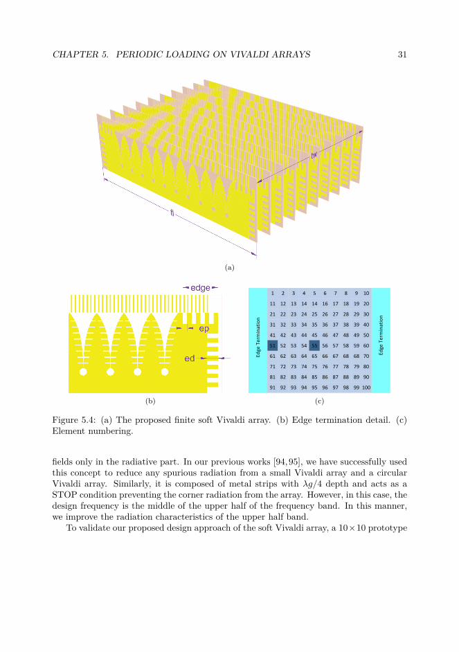
CHAPTER 5. PERIODIC LOADING ON VIVALDI ARRAYS 31
(a)
(b)
1 2 3 4 5 6 7 8 9
11 12 13 14 14 16 17 18 19
21 22 23 24 25 26 27 28 29
31 32 33 34 35 36 37 38 39
41 42 43 44 45 46 47 48 49
51 52 53 54 55 56 57 58 59
Edge
Ter
min
atio
n
Edge
Ter
min
atio
n
10
20
30
40
50
60
61 62 63 64 65 66 67 68 68
71 72 73 74 75 76 77 78 79
81 82 83 84 85 86 87 88 89
91 92 93 94 95 96 97 98 99
70
80
90
100
(c)
Figure 5.4: (a) The proposed finite soft Vivaldi array. (b) Edge termination detail. (c)Element numbering.
fields only in the radiative part. In our previous works [94,95], we have successfully usedthis concept to reduce any spurious radiation from a small Vivaldi array and a circularVivaldi array. Similarly, it is composed of metal strips with λg/4 depth and acts as aSTOP condition preventing the corner radiation from the array. However, in this case, thedesign frequency is the middle of the upper half of the frequency band. In this manner,we improve the radiation characteristics of the upper half band.
To validate our proposed design approach of the soft Vivaldi array, a 10×10 prototype

CHAPTER 5. PERIODIC LOADING ON VIVALDI ARRAYS 32
(a) (b) (c)
Figure 5.5: (a) Side view of the constructed array. Array during measurement phase, (b)and (c) constructed array mounted in the anechoic chamber.
was fabricated and measured. The front and the back view of the final proposed arrayis depicted in Fig. 5.5(a). The prototype was mounted in a aluminum frame, whichwas connected with the mounting interface at the anechoic chamber for the rotator. Theprototype is composed of ten PCB cards of a ten element linear array. The PCBs werestabilized in the frame with a plexiglass frame as is shown in Fig. 5.5(a). The arraywas mounted and measured in the anechoic chamber as depicted in Fig. 5.5(b) and Fig.5.5(c). We calculated the radiation pattern of the array post processing the measureddata for each embedded element pattern. For the frequencies, 1.8, 3, 4, 5.2 GHz for bothE- and H-plane the simulated and measured radiation patterns are depicted in Fig. 5.6.Excellent agreement is achieved between simulated and measured results. Moreover, thearray is able to steer the beam even up to ±60.
All the coupling coefficients were measured with respect to element 55 and the datawere post processed. The contour plots are presented for the measured active VSWRfor the E- and H- planes in Fig. 5.7(a) and Fig. 5.7(b). The active reflection coefficientis calculated and then converted to the VSWR value. The contour plots show that thedeveloped array is capable to scan the beam up to ±60 while keeping the active VSWRbelow 2.5 except for two regions at 2.9 GHz and ±45 that the active VSWR takesvalues around 3.5. The two field contour plots are fairly symmetric implying the goodconstruction and assembly of the prototype.
The measured contour plots for the D-plane are presented in the Fig. 5.9 for theelements 51 and 55 from the middle row. The normalization has been performed withrespect to the maximum of the embedded pattern at each frequency. Our measured resultsare limited to -30 dB due to the cx-pol level of the probe utilized for measurements. It isobserved that the maximum measured cx-pol value in the D-plane is -10 dB which can beconsidered acceptable for most applied cases. An inconsistency between measurementsand simulations is found in the cx-pol level for the central element as depicted in Fig.5.9(c) and Fig. 5.9(d). We observe that for the frequency range [3.6-3.9] GHz the cx-pol value increases to -10 dB for θ ∈ [−40, 40]. This was traced to the impact of the
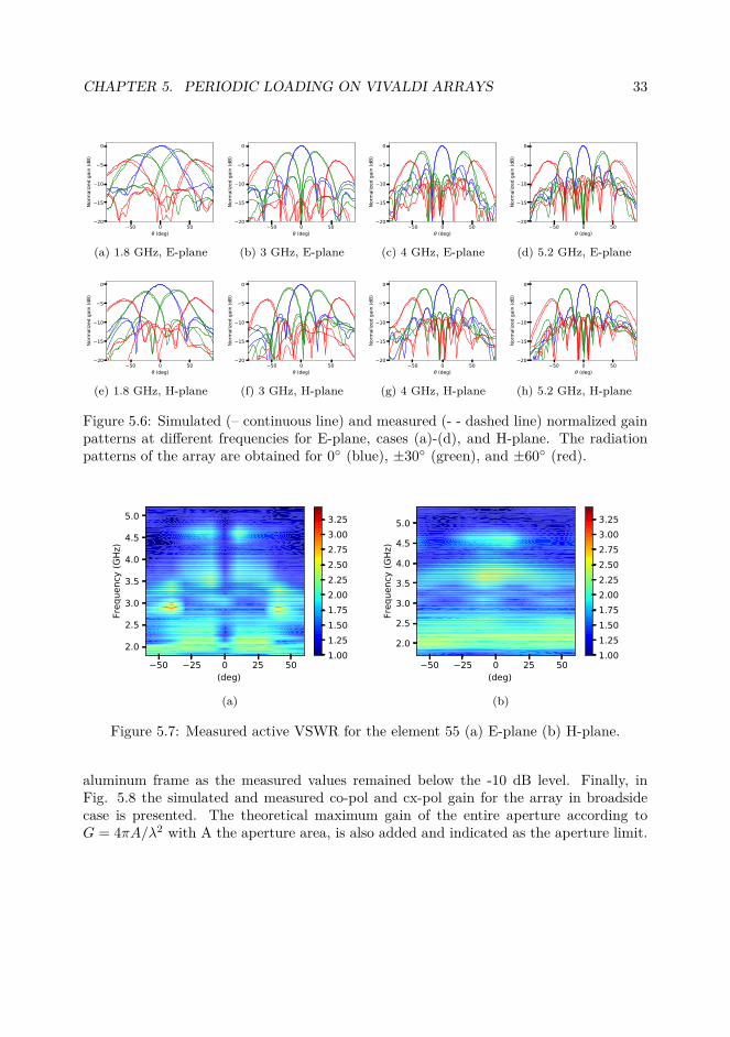
CHAPTER 5. PERIODIC LOADING ON VIVALDI ARRAYS 33
−50 0 50θ (deg)
−20
−15
−10
−5
0
Norm
alize
d ga
in (d
B)
(a) 1.8 GHz, E-plane
−50 0 50θ (deg)
−20
−15
−10
−5
0
Norm
alize
d ga
in (d
B)
(b) 3 GHz, E-plane
−50 0 50θ (deg)
−20
−15
−10
−5
0
Norm
alize
d ga
in (d
B)
(c) 4 GHz, E-plane
−50 0 50θ (deg)
−20
−15
−10
−5
0
Norm
alize
d ga
in (d
B)
(d) 5.2 GHz, E-plane
−50 0 50θ (deg)
−20
−15
−10
−5
0
Norm
alize
d ga
in (d
B)
(e) 1.8 GHz, H-plane
−50 0 50θ (deg)
−20
−15
−10
−5
0
Norm
alize
d ga
in (d
B)
(f) 3 GHz, H-plane
−50 0 50θ (deg)
−20
−15
−10
−5
0
Norm
alize
d ga
in (d
B)
(g) 4 GHz, H-plane
−50 0 50θ (deg)
−20
−15
−10
−5
0
Norm
alize
d ga
in (d
B)
(h) 5.2 GHz, H-plane
Figure 5.6: Simulated (– continuous line) and measured (- - dashed line) normalized gainpatterns at different frequencies for E-plane, cases (a)-(d), and H-plane. The radiationpatterns of the array are obtained for 0 (blue), ±30 (green), and ±60 (red).
−50 −25 0 25 50θ (deg)
2.0
2.5
3.0
3.5
4.0
4.5
5.0
Freq
uenc
y (G
Hz)
1.001.251.501.752.002.252.502.753.003.25
(a)
−50 −25 0 25 50θ (deg)
2.0
2.5
3.0
3.5
4.0
4.5
5.0
Freq
uenc
y (G
Hz)
1.001.251.501.752.002.252.502.753.003.25
(b)
Figure 5.7: Measured active VSWR for the element 55 (a) E-plane (b) H-plane.
aluminum frame as the measured values remained below the -10 dB level. Finally, inFig. 5.8 the simulated and measured co-pol and cx-pol gain for the array in broadsidecase is presented. The theoretical maximum gain of the entire aperture according toG = 4πA/λ2 with A the aperture area, is also added and indicated as the aperture limit.
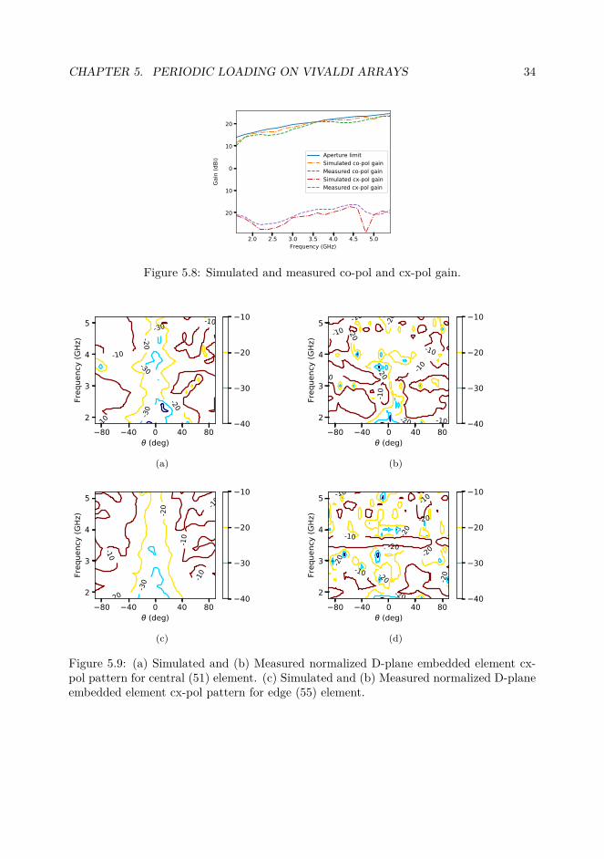
CHAPTER 5. PERIODIC LOADING ON VIVALDI ARRAYS 34
2.0 2.5 3.0 3.5 4.0 4.5 5.0Frequency (GHz)
−20
−10
0
10
20
Gain
(dBi
) Aper ure limi Simula ed co-pol gainMeasured co-pol gainSimulated cx-pol gain Measured cx-pol gain
Figure 5.8: Simulated and measured co-pol and cx-pol gain.
80 40 0 40 80 (deg)
2
3
4
5
Freq
uenc
y (G
Hz)
-30
-30
-30
-30
-30 -30-20 -20-20
-20
-20
-10
-10
-10
-10
-10
-10
-10
40
30
20
10
(a)
80 40 0 40 80 (deg)
2
3
4
5Fr
eque
ncy
(GHz
)
-30
-20-20
-20
-20
-20
-20
-20 -20
-20
-20
-20
-20
-10-10
-10
-10
-10
-10
-10
-10 -10
-10
40
30
20
10
(b)
80 40 0 40 80 (deg)
2
3
4
5
Freq
uenc
y (G
Hz)
-30
-30-30
-20
-20
-20
-20
-20
-20
-20
-20
-20-20
-20
-10
-10
-10
-10
40
30
20
10
(c)
80 40 0 40 80 (deg)
2
3
4
5
Freq
uenc
y (G
Hz)
-40
-30
-30
-30
-20 -20-20
-20
-20
-20
-20 -20
-20
-20-20
-20
-20
-20-20
-20-20
-10 -10
-10
-10
-10-10
-10-10
40
30
20
10
(d)
Figure 5.9: (a) Simulated and (b) Measured normalized D-plane embedded element cx-pol pattern for central (51) element. (c) Simulated and (b) Measured normalized D-planeembedded element cx-pol pattern for edge (55) element.

CHAPTER 5. PERIODIC LOADING ON VIVALDI ARRAYS 35
5.3 Conclusions
The soft Vivaldi element was introduced and its performance in the array environmentwas studied. The integration of a soft condition with the Vivaldi element, equivalentlyto the soft horn, improved the cx-pol performance in the upper half of the operationalfrequency band. The design of the element was completed with an integrated matchinglayer in the form of strip loading. The addition of the matching layer further improvedthe bandwidth performance in broadside as well as while the array is scanned. In thedeveloped finite array the edges along the E-plane were loaded with a soft condition toeliminate any spurious radiation from the array’s edge. The constructed array was in goodagreement with the simulations. Excellent beam performance was observed for ±60 aswell as good agreement between measured and simulated gain. It is worth noting thatthe soft Vivaldi is not limited as an array element and could also be developed as a standalone element.

Chapter 6
Strongly Coupled Dipole Arrays1
During the last decade, a new concept of wideband antenna array systems has emergedbased on strong inter-element coupling. This capability stems from their support tocontinuous current modes along the array. They are the practical implementation of theWheeler’s concept of current sheet array (CSA) and there primarily two major antennaarray technologies: the capacitively coupled dipoles, [96], and connected dipoles/slots,[97].
In this chapter of the thesis we are based on the CSA concept and we extended intotwo axis. Inspired by [98,99] where the properties for non-symmetric elements have beenstudied, we develop a framework for a novel class of antenna arrays: the strongly coupledasymmetric dipole array - SCADA. Based on this methodology a wideband single polar-ized, SCADA demonstrator was developed, constructed and validated. The frameworkof this method is generic and can be applied in different frequency bands. The SCADAelement is a novel element combing the CSA with the fragmented array with no sym-metry constraints. The antenna element operates in more than a 6:1 bandwidth ratiowith VSWR≤ 2 and with up to 60 scanning performance at the H-plane. Our analysishas been extended to finite arrays and a novel termination method was also validatedin this prototype. The proposed termination method aims for the E-plane edge of thearray and is a combination of alternating low and high impedances with dummy elementsat the arrays edges. The spatial frequency of the terminating elements is double of themaximum operable frequency of the array.
The chapter concludes with a proposed methodology to overcome the expensive su-perstrate required for the array’s scanning performance. A novel topology is introducedwhere the superstrate is integrated in a uniplanar structure along the E-plane of the array.A prototype was constructed and measured with good agreement between the simulationsand measurements.
1Partial content of this chapter is reproduced from author’s Paper IV and Patent VII.
36
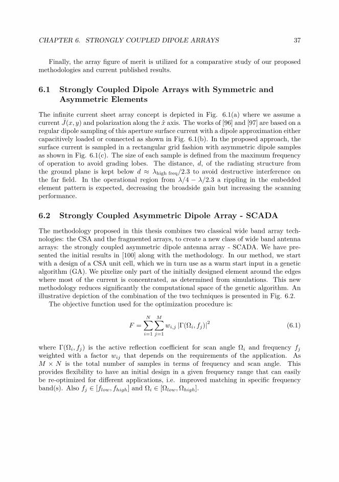
CHAPTER 6. STRONGLY COUPLED DIPOLE ARRAYS 37
Finally, the array figure of merit is utilized for a comparative study of our proposedmethodologies and current published results.
6.1 Strongly Coupled Dipole Arrays with Symmetric andAsymmetric Elements
The infinite current sheet array concept is depicted in Fig. 6.1(a) where we assume acurrent J(x, y) and polarization along the x axis. The works of [96] and [97] are based on aregular dipole sampling of this aperture surface current with a dipole approximation eithercapacitively loaded or connected as shown in Fig. 6.1(b). In the proposed approach, thesurface current is sampled in a rectangular grid fashion with asymmetric dipole samplesas shown in Fig. 6.1(c). The size of each sample is defined from the maximum frequencyof operation to avoid grading lobes. The distance, d, of the radiating structure fromthe ground plane is kept below d ≈ λhigh freq/2.3 to avoid destructive interference onthe far field. In the operational region from λ/4 − λ/2.3 a rippling in the embeddedelement pattern is expected, decreasing the broadside gain but increasing the scanningperformance.
6.2 Strongly Coupled Asymmetric Dipole Array - SCADA
The methodology proposed in this thesis combines two classical wide band array tech-nologies: the CSA and the fragmented arrays, to create a new class of wide band antennaarrays: the strongly coupled asymmetric dipole antenna array - SCADA. We have pre-sented the initial results in [100] along with the methodology. In our method, we startwith a design of a CSA unit cell, which we in turn use as a warm start input in a geneticalgorithm (GA). We pixelize only part of the initially designed element around the edgeswhere most of the current is concentrated, as determined from simulations. This newmethodology reduces significantly the computational space of the genetic algorithm. Anillustrative depiction of the combination of the two techniques is presented in Fig. 6.2.
The objective function used for the optimization procedure is:
F =N∑i=1
M∑j=1
wi,j |Γ(Ωi, fj)|2 (6.1)
where Γ(Ωi, fj) is the active reflection coefficient for scan angle Ωi and frequency fjweighted with a factor wij that depends on the requirements of the application. AsM × N is the total number of samples in terms of frequency and scan angle. Thisprovides flexibility to have an initial design in a given frequency range that can easilybe re-optimized for different applications, i.e. improved matching in specific frequencyband(s). Also fj ∈ [flow, fhigh] and Ωi ∈ [Ωlow,Ωhigh].
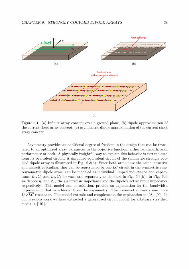
CHAPTER 6. STRONGLY COUPLED DIPOLE ARRAYS 38
x
yz
Jx(x,y)
(a)
... ...... ......
...... ... ...
... ... ...
Unit cell area
(b)
... ......
Unit cell areawith asymmetric element
... ......... ......
... ......
(c)
Figure 6.1: (a) Infinite array concept over a ground plane, (b) dipole approximation ofthe current sheet array concept, (c) asymmetric dipole approximation of the current sheetarray concept.
Asymmetry provides an additional degree of freedom in the design that can be trans-lated to an optimized array parameter to the objective function, either bandwidth, scanperformance or both. A physically insightful way to explain this behavior is extrapolatedfrom its equivalent circuit. A simplified equivalent circuit of the symmetric strongly cou-pled dipole array is illustrated in Fig. 6.3(a). Since both arms have the same inductiveand capacitive loading, they can be represented by one LC circuit in the symmetric case.Asymmetric dipole arms, can be modeled as individual lumped inductance and capaci-tance L1, C1 and L2, C2 for each arm separately as depicted in Fig. 6.3(b). In Fig. 6.3,we denote η0 and Zin the air intrinsic impedance and the dipole’s active input impedancerespectively. This model can, in addition, provide an explanation for the bandwidthimprovement that is achieved from the asymmetry. The asymmetry inserts one more1/√LC resonance. This model extends and complements the explanation in [98], [99]. In
our previous work we have extracted a generalized circuit model for arbitrary stratifiedmedia in [101].

CHAPTER 6. STRONGLY COUPLED DIPOLE ARRAYS 39
Strongly CoupledAsymmetricDipole Array
CurrentSheet Array
FragmentedArrays
Figure 6.2: Illustration of the combination of the two array classes into the new SCADAclass.
Zin
l
L
n0
C
n0
(a)
Zin
l
L1
n0
C1
n0
L2C2
(b)
Figure 6.3: (a) Symmetric and (b) asymmetric dipole unit cell equivalent circuit
6.2.1 Unit Cell Element DesignThe methodology starts with a design of a symmetric element. This initial design haspreviously been developed in our previous works [102,103] as a good candidate. The initialsolution is depicted in Fig. 6.4(a). The capacitive loading at the unit cell is achieved withparasitic patches and the inter-element gap as illustrated in Fig. 6.4(b). The detailedview and the corresponding dimensioning parameters of the element is depicted in Fig.6.4(c). The substrate of the design is a Rogers RO4003C (εr = 3.55, tan δ = 0.0027 &h = 1.52 mm). A wide angle impedance matching (WAIM) layer of RO5880LZ (εr = 1.98)has also been utilized to improve the scan performance. The dimensions of the element

CHAPTER 6. STRONGLY COUPLED DIPOLE ARRAYS 40
Table 6.1: Dimensions in mm of the initial design as depicted in Fig. 6.4.
δ = 0.6 s = 0.3 Cl = 2 w = 11wT1 = 2 Tl = 8 wT2 = 2 wT3 = 9l = 9.52 hWAIM = 18 g=1.825
illustrated in Fig. 6.4 are summarized in Table 6.1.
(a)
h
Unit Cell
Top layer
Bottom layer
Dipole input
(b)
sw
δ
l
cl
Tl
wT1
wT2gwT3
(c)
Figure 6.4: (a) Array unit cell with T-slot loaded dipole, WAIM layer with preview of toplayer and bottom layer (b) Capacitive dipole loading (c) Schematic of the initial elementwith the corresponding dimensional variables.
Pixelated
E-plane symmetry
H-plane symmetry
areas
Pixelated
areas
(a) (b)
Figure 6.5: (a) Dipole symmetries and pixelated areas (b) Design after optimization
In our design, we pixelize the highlighted areas as in Fig. 6.5(a). The best geometryfound after several runs of the GA is depicted in Fig. 6.5(b). We have set in the costfunction wij = 1 fj ∈ [0.7, 4.2] GHz sampled in 20 equispaced points and Ωi ∈ 0, 45.In each pixelated area we use only 3× 6 pixels. The total number of possible geometriescorresponds in this case to 272. If the entire aperture of the element illustrated in Fig.6.5(a) had been pixelized with the same discretization, there are 2234 possible geometries.
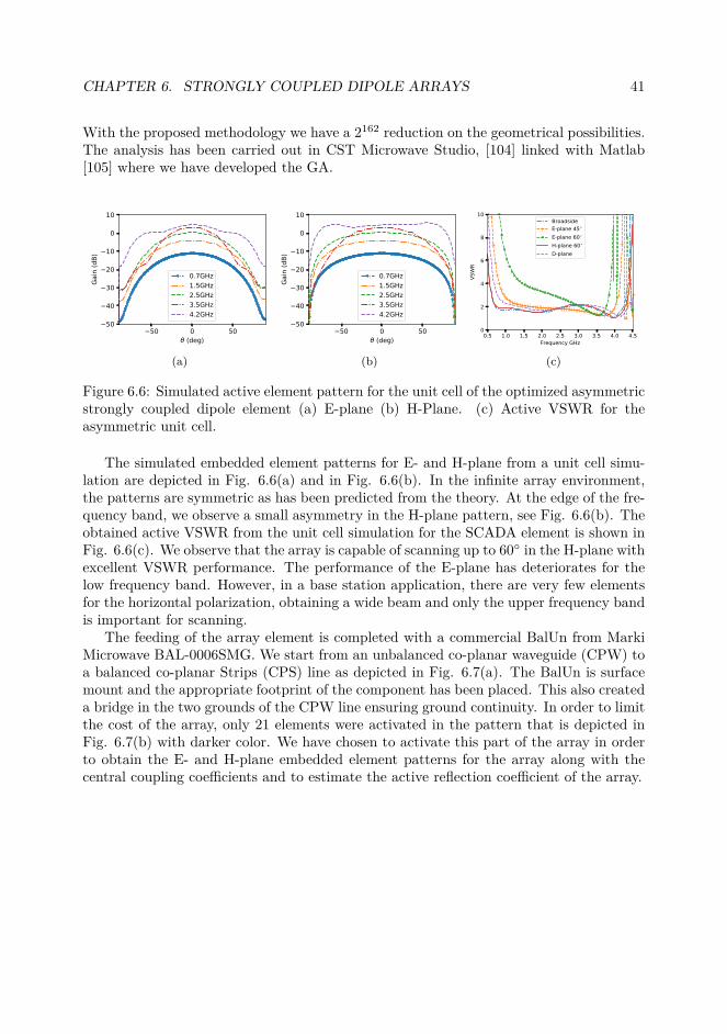
CHAPTER 6. STRONGLY COUPLED DIPOLE ARRAYS 41
With the proposed methodology we have a 2162 reduction on the geometrical possibilities.The analysis has been carried out in CST Microwave Studio, [104] linked with Matlab[105] where we have developed the GA.
50 0 50 (deg)
50
40
30
20
10
0
10
Gain
(dB)
0.7GHz1.5GHz2.5GHz3.5GHz4.2GHz
(a)
50 0 50 (deg)
50
40
30
20
10
0
10
Gain
(dB)
0.7GHz1.5GHz2.5GHz3.5GHz4.2GHz
(b)
0.5 1.0 1.5 2.0 2.5 3.0 3.5 4.0 4.5Frequency GHz
0
2
4
6
8
10
VSW
R
BroadsideE-plane 45E-plane 60H-plane 60D-plane
(c)
Figure 6.6: Simulated active element pattern for the unit cell of the optimized asymmetricstrongly coupled dipole element (a) E-plane (b) H-Plane. (c) Active VSWR for theasymmetric unit cell.
The simulated embedded element patterns for E- and H-plane from a unit cell simu-lation are depicted in Fig. 6.6(a) and in Fig. 6.6(b). In the infinite array environment,the patterns are symmetric as has been predicted from the theory. At the edge of the fre-quency band, we observe a small asymmetry in the H-plane pattern, see Fig. 6.6(b). Theobtained active VSWR from the unit cell simulation for the SCADA element is shown inFig. 6.6(c). We observe that the array is capable of scanning up to 60 in the H-plane withexcellent VSWR performance. The performance of the E-plane has deteriorates for thelow frequency band. However, in a base station application, there are very few elementsfor the horizontal polarization, obtaining a wide beam and only the upper frequency bandis important for scanning.
The feeding of the array element is completed with a commercial BalUn from MarkiMicrowave BAL-0006SMG. We start from an unbalanced co-planar waveguide (CPW) toa balanced co-planar Strips (CPS) line as depicted in Fig. 6.7(a). The BalUn is surfacemount and the appropriate footprint of the component has been placed. This also createda bridge in the two grounds of the CPW line ensuring ground continuity. In order to limitthe cost of the array, only 21 elements were activated in the pattern that is depicted inFig. 6.7(b) with darker color. We have chosen to activate this part of the array in orderto obtain the E- and H-plane embedded element patterns for the array along with thecentral coupling coefficients and to estimate the active reflection coefficient of the array.
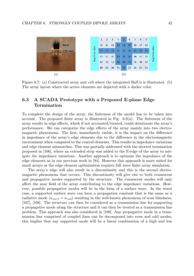
CHAPTER 6. STRONGLY COUPLED DIPOLE ARRAYS 42
(a) (b)
Figure 6.7: (a) Constructed array unit cell where the integrated BalUn is illustrated. (b)The array layout where the active elements are depicted with a darker color.
6.3 A SCADA Prototype with a Proposed E-plane EdgeTermination
To complete the design of the array, the finiteness of the model has to be taken intoaccount. The proposed finite array is illustrated in Fig. 6.8(a). The finiteness of thearray results in edge effects, which if not accounted/treated, could deteriorate the array’sperformance. We can categorize the edge effects of the array mainly into two electro-magnetic phenomena. The first, immediately visible, it is the impact on the differencein impedance of the array’s edge elements due to the difference in the electromagneticenvironment when compared to the central elements. This results in impedance variationsand edge element mismatches. This was partially addressed with the shorted terminationproposed in [106], where an extended strip was added to the E-edge of the array to mit-igate the impedance variations. Another approach is to optimize the impedance of theedge elements as in our previous work in [94]. However this approach is more suited forsmall arrays as the edge element optimization requires full wave finite array simulation.
The array’s edge will also result in a discontinuity and this is the second electro-magnetic phenomena that occurs. This discontinuity will give rise to both evanescentand propagative modes supported by the structure. The evanescent modes will onlyaffect the near field of the array contributing to the edge impedance variations. How-ever, possible propagative modes will be in the form of a surface wave. In the worstcase, a supported surface wave can have a propagation constant that is the same as aradiative mode (κsurf = κrad) resulting in the well-known phenomena of scan blindness,[107], [108]. The structure can then be considered as a transmission line for supportinga propagative mode along the structure and it can then be treated as a transmission lineproblem. This approach was also considered in [109]. Any propagative mode in a trans-mission line comprised of coupled lines can be decomposed into even and odd modes,this implies that any supported mode will be a linear combination of a high and low
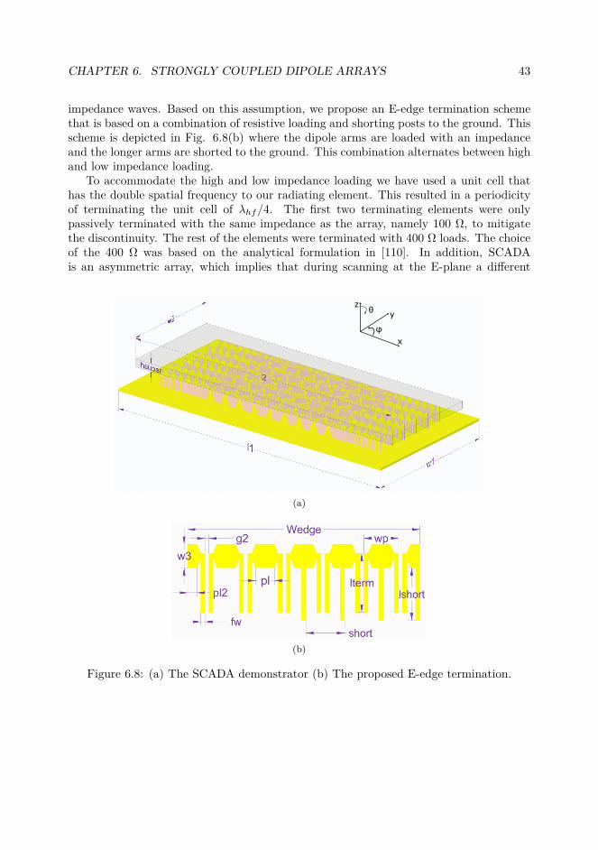
CHAPTER 6. STRONGLY COUPLED DIPOLE ARRAYS 43
impedance waves. Based on this assumption, we propose an E-edge termination schemethat is based on a combination of resistive loading and shorting posts to the ground. Thisscheme is depicted in Fig. 6.8(b) where the dipole arms are loaded with an impedanceand the longer arms are shorted to the ground. This combination alternates between highand low impedance loading.
To accommodate the high and low impedance loading we have used a unit cell thathas the double spatial frequency to our radiating element. This resulted in a periodicityof terminating the unit cell of λhf/4. The first two terminating elements were onlypassively terminated with the same impedance as the array, namely 100 Ω, to mitigatethe discontinuity. The rest of the elements were terminated with 400 Ω loads. The choiceof the 400 Ω was based on the analytical formulation in [110]. In addition, SCADAis an asymmetric array, which implies that during scanning at the E-plane a different
x
y
zθ
φ
(a)
(b)
Figure 6.8: (a) The SCADA demonstrator (b) The proposed E-edge termination.
CHAPTER 6. STRONGLY COUPLED DIPOLE ARRAYS 44
Table 6.2: Dimensions in mm of the SCADA demonstrator with the E-termination asdepicted in Fig. 6.8.
w1=310 l2 = 594 lterm = 27.45w2 = 297 g2 = 1.83 hsuper = 0.3w3 = 11 pl = 8.8 Wedge = 107.93l1 = 640 pl2 = 4.4 short = 18.5fw = 2 wp = 16.175 lshort = 24.5
environment will occur for positive and negative θ values. To symmetrize the array’senvironment, the proposed termination is the same for the two array edges.
The proposed array termination, even though developed for the SCADA, is not limitedto asymmetric elements and can be also applied to classic symmetric arrays. In a realisticantenna array system that is aimed for base-station application, the front-to-back ratiobecomes a critical parameter as well as the efficiency. The proposed edge termination istackling both problems for the most of the operational bandwidth.
To validate the method, the resulted optimized asymmetric design and the proposededge termination were combined and a SCADA demonstrator was fabricated and mea-sured. The array was fabricated in standard PCB technology and was mounted in analuminum frame connected with the mounting for the rotator at the anechoic chamber.A copper plate was utilized as a finite ground plane for soldering ease. For the super-strate, slabs of RD/Duroid 5880LZ were used. Note, that the simulation results for thefinite array were performed with 18.5mm thickness of the superstrate to account for theadhesive bonding of multiple layers of RD/Duroid 5880LZ. The constructed array withthe integrated BalUn is illustrated in Fig. 6.9(a) without the superstrate. The arraywas mounted and measured in an anechoic chamber as illustrated in Fig. 6.9(b) and Fig.6.9(c). The chamber utilized is a spherical near field/far field operable between 2-40 GHz.However, it can still be utilized below 2GHz with lower accuracy.
The embedded element patterns were measured only for the active elements as illus-trated in Fig. 6.7(b). The obtained simulated and measured array patterns for frequen-cies 0.8, 1.8, 2.8 and 3.8 GHz for both E- and H-plane are presented in Fig. 6.10. Goodagreement between measured and simulated results is observed and excellent scanningperformance up to ±60. It is noted that the ±60 beams are not presented as the smallsize of the constructed antenna array did not allow more than 2 dB beam cross-over in the±30 case. In addition, the realized measured gain of the array is similar to the simulatedwhen the effect of the integrated BalUn is calibrated.
The coupling coefficients from all active elements with respect to the central element(element 25 from Fig. 6.7(b)) are measured and the results are post processed. Thecontour plots for the measured active reflection coefficient are illustrated in Fig. 6.11(a)and Fig. 6.11(b) for the E- and H-plane. We observe that the array is kept below -10dBfor scanning performance up to ±70 for both planes.

CHAPTER 6. STRONGLY COUPLED DIPOLE ARRAYS 45
(a) (b) (c)
Figure 6.9: (a) Array on construction phase without the supestrate. Array during mea-surement phase (b) mounted in the chamber (c) mounted in the chamber and the mea-surement probe.
100 50 0 50 100 (deg)
20
15
10
5
0
Norm
alize
d ga
in (d
Bi)
(a) 0.8 GHz, E-plane
100 50 0 50 100 (deg)
20
15
10
5
0
Norm
alize
d ga
in (d
Bi)
(b) 1.8 GHz, E-plane
100 50 0 50 100 (deg)
20
15
10
5
0
Norm
alize
d ga
in (d
Bi)
(c) 2.8 GHz, E-plane
100 50 0 50 100 (deg)
20
15
10
5
0
Norm
alize
d ga
in (d
Bi)
(d) 3.8 GHz, E-plane
100 50 0 50 100 (deg)
20
15
10
5
0
Norm
alize
d ga
in (d
Bi)
(e) 0.8 GHz, H-plane
100 50 0 50 100 (deg)
20
15
10
5
0
Norm
alize
d ga
in (d
Bi)
(f) 1.8 GHz, H-plane
100 50 0 50 100 (deg)
20
15
10
5
0
Norm
alize
d ga
in (d
Bi)
(g) 2.8 GHz, H-plane
100 50 0 50 100 (deg)
20
15
10
5
0
Norm
alize
d ga
in (d
Bi)
(h) 3.8 GHz, H-plane
Figure 6.10: Simulated (– line) and measured (- - line) normalized gain patterns atfrequencies 0.8 GHz, 1.8 GHz, 2.8 GHz, 3.8 GHz for E-plane, cases (a)-(d), and H-plane,cases (c)-(d) for 0 (blue), ±30 (green), and ±60 (red), except cases (a) and (e) thatthe ±60 beam patterns are not depicted.
The SCADA employs asymmetric elements, which implies that there is a higher ex-pected cx-pol level as compared with the corresponding symmetric case. The measuredand simulated normalized D-plane cx-pol patterns for the central (el. 25) and edge ele-ment (el. 21) are illustrated in Fig. 6.12. The normalization has been performed with

CHAPTER 6. STRONGLY COUPLED DIPOLE ARRAYS 46
60 40 20 0 20 40 60 (deg)
1.0
1.5
2.0
2.5
3.0
3.5
4.0
Freq
uenc
y (G
Hz)
-22
-22
-22
-22
-22
-22
-18
-18
-18
-18
-18
-18
-18
-18 -18
-18
-18
-14
-14
-14
-14
-14
-14
-14
-14 -14-14
-14
-14
-14-1
4
-10
-10
-10
-10
-10
-10
-10
-6
-6
22
18
14
10
6
(a)
60 40 20 0 20 40 60 (deg)
1.0
1.5
2.0
2.5
3.0
3.5
4.0
Freq
uenc
y (G
Hz)
-22
-22
-22
-22
-22
-22
-22
-22
-22
-18-18
-18
-18
-18
-18
-18 -18
-14
-14
-14
-14
-14
-14
-14
-14
-10
-10
-10
-10
-10
-10
-10
-6
-6
-6 -6
22
18
14
10
6
(b)
Figure 6.11: Measured active reflection coefficient contour plot in dB for the (a) E-planeand (b) H-plane of SCADA for the central element, element 25.
respect to the maximum of the embedded pattern at each frequency. Our measured re-sults are limited to -30 dB due to the cx-pol level of the probe utilized for measurements.It is observed that the maximum measured cx-pol value in the D-plane is -10dB whichcan be considered acceptable for most of applications since this is the worst case. A largedeviation between measured and simulated result for the element 25 is observed for therange between 1-2 GHz. This is due to the higher reflections of the anechoic chamber.
6.4 Integrating the Matching Layer on Strongly Coupled DipoleArray
In a conventional array design, when a wide angle impedance matching (WAIM) layer isincorporated, the resulting prototype requires a relatively thick dielectric of low dielectricconstant and low loss. In the developed SCADA prototype, the cost of the superstratewas three times the cost of the remaining PCB. To overcome the overbearing cost of thesuperstrate, the method utilized in Chapter 5 when a matching layer was integrated in theVivaldi array is applied to a similar fashion at the strongly coupled dipole array (SCDA).To validate the approach we apply the methodology to a symmetric unit cell. A similarapproach was also recently adopted in [111] where they utilized an integrated frequencyselective surface (FSS). After optimization the resulted unit cell is illustrated in Fig. 6.13for the front and back view with the dimensions tabulated at the Table 6.3.
The resulted superstrate can be considered a graded index metasurface for optimalmatching to the air impedance by adjusting the length and the adjacent distances of the
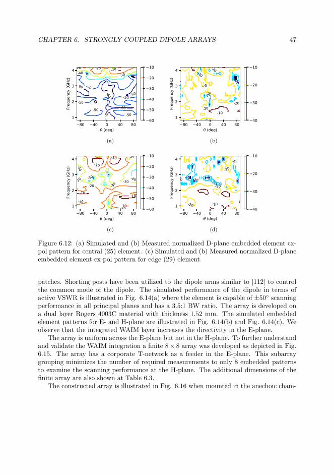
CHAPTER 6. STRONGLY COUPLED DIPOLE ARRAYS 47
80 40 0 40 80 (deg)
1
2
3
4Fr
eque
ncy
(GHz
)
-60
-60
-60
-60
-60
-50
-50-50
-50
-50
-40 -30
-20 -20-20
60
50
40
30
20
10
(a)
80 40 0 40 80 (deg)
1
2
3
4
Freq
uenc
y (G
Hz)
-30
-30
-30 -30
-30
-30
-30
-30
-30
-20
-20
-20
-20
-20
-20
-20
-20-20
-10 -10
40
30
20
10
(b)
80 40 0 40 80 (deg)
1
2
3
4
Freq
uenc
y (G
Hz)
-40
-40
-30-30
-30
-30
-20
-20
-20
-20
-10
-10
-10
-10
-10
60
50
40
30
20
10
(c)
80 40 0 40 80 (deg)
1
2
3
4
Freq
uenc
y (G
Hz)
-40-30
-30
-30
-30
-30
-30 -30-30-30
-20-20
-20
-20
-20
-20 -10
-10
-10
-10
40
30
20
10
(d)
Figure 6.12: (a) Simulated and (b) Measured normalized D-plane embedded element cx-pol pattern for central (25) element. (c) Simulated and (b) Measured normalized D-planeembedded element cx-pol pattern for edge (29) element.
patches. Shorting posts have been utilized to the dipole arms similar to [112] to controlthe common mode of the dipole. The simulated performance of the dipole in terms ofactive VSWR is illustrated in Fig. 6.14(a) where the element is capable of ±50 scanningperformance in all principal planes and has a 3.5:1 BW ratio. The array is developed ona dual layer Rogers 4003C material with thickness 1.52 mm. The simulated embeddedelement patterns for E- and H-plane are illustrated in Fig. 6.14(b) and Fig. 6.14(c). Weobserve that the integrated WAIM layer increases the directivity in the E-plane.
The array is uniform across the E-plane but not in the H-plane. To further understandand validate the WAIM integration a finite 8× 8 array was developed as depicted in Fig.6.15. The array has a corporate T-network as a feeder in the E-plane. This subarraygrouping minimizes the number of required measurements to only 8 embedded patternsto examine the scanning performance at the H-plane. The additional dimensions of thefinite array are also shown at Table 6.3.
The constructed array is illustrated in Fig. 6.16 when mounted in the anechoic cham-
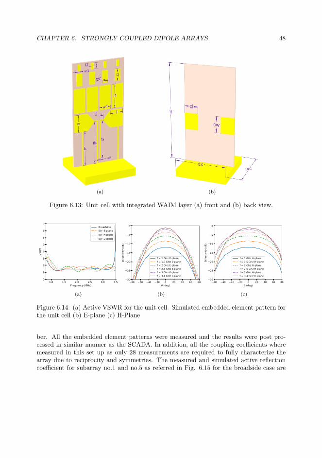
CHAPTER 6. STRONGLY COUPLED DIPOLE ARRAYS 48
(a) (b)
Figure 6.13: Unit cell with integrated WAIM layer (a) front and (b) back view.
1.0 1.5 2.0 2.5 3.0 3.5Frequency (GHz)
0
1
2
3
4
5
6
7
8
VSWR
Broadside50( E∘ lane50( H∘ lane50( D∘ lane
(a)
−80 −60 −40 −20 0 20 40 60 80θ (deg)
−30
−25
−20
−15
−10
−5
0
Directivit
(dB)
f = 1 GHz E-planef = 1.5 GHz E-planef = 2 GHz E-planef = 2.5 GHz E-planef = 3 GHz E-planef = 3.4 GHz E-plane
(b)
−80 −60 −40 −20 0 20 40 60 80θ (deg)
−30
−25
−20
−15
−10
−5
0
Directivity
(dB)
f = 1 GH H-planef = 1.5 GH H-planef = 2 GH H-planef = 2.5 GH H-planef = 3 GH H-planef = 3.4 GH H-plane
(c)
Figure 6.14: (a) Active VSWR for the unit cell. Simulated embedded element pattern forthe unit cell (b) E-plane (c) H-Plane
ber. All the embedded element patterns were measured and the results were post pro-cessed in similar manner as the SCADA. In addition, all the coupling coefficients wheremeasured in this set up as only 28 measurements are required to fully characterize thearray due to reciprocity and symmetries. The measured and simulated active reflectioncoefficient for subarray no.1 and no.5 as referred in Fig. 6.15 for the broadside case are

CHAPTER 6. STRONGLY COUPLED DIPOLE ARRAYS 49
Figure 6.15: Developed 8 × 8 array with integrated WAIM layer and corporate feednetwork. Numbering from 1 to 8 from the front side view.
Table 6.3: Dimensions in mm of the demonstrator with the integrated WAIM layer asdepicted in Fig. 6.13 and Fig. 6.15.
w1 = 7.2 l1 = 15 dx = 33.6 lfs = 27.2 al = 389w2 = 3.6 l2 = 7.5 dy = 33.6 fa = 24.2 aw = 409w3 = 1.8 l3 = 3.75 cl = 9.02 fl = 2.4w = 11 l = 8.41 cw = 11 pl = 268.8wf = 0.6 ls = 22 lt = 65 ph = 145
(a) (b) (c)
Figure 6.16: Photos of the constructed array when mounted on the anechoic chamber.
depicted in Fig. 6.17. The measured curve is a result of post processing when the arrayis mounted on the fixture for the anechoic chamber that is not accounted in simulations.Good agreement is observed between measurements and simulations. The scanning per-formance of the array is illustrated in Fig. 6.18 for the same subarrays. It is observed
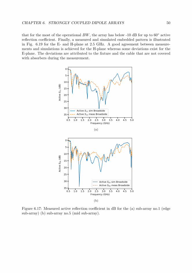
CHAPTER 6. STRONGLY COUPLED DIPOLE ARRAYS 50
that for the most of the operational BW , the array has below -10 dB for up to 60 activereflection coefficient. Finally, a measured and simulated embedded pattern is illustratedin Fig. 6.19 for the E- and H-plane at 2.5 GHz. A good agreement between measure-ments and simulations is achieved for the H-plane whereas some deviations exist for theE-plane. The deviations are attributed to the fixture and the cable that are not coveredwith absorbers during the measurement.
0.5 1.0 1.5 2.0 2.5 3.0 3.5 4.0 4.5 5.0Frequency (GHz)
−35
−30
−25
−20
−15
−10
−5
0
Activ
e S 1
1 (dB
)
Active S11 sim BroadsideActive S11 meas Broadside
(a)
0.5 1.0 1.5 2.0 2.5 3.0 3.5 4.0 4.5 5.0Frequency (GHz)
−35
−30
−25
−20
−15
−10
−5
0
Activ
e S 5
5 (dB
)
Active S55 sim BroadsideActive S55 meas Broadside
(b)
Figure 6.17: Measured active reflection coefficient in dB for the (a) sub-array no.1 (edgesub-array) (b) sub-array no.5 (mid sub-array).
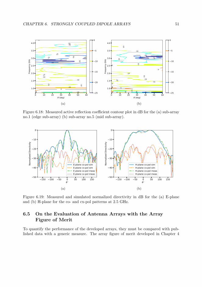
CHAPTER 6. STRONGLY COUPLED DIPOLE ARRAYS 51
0 10 20 30 40 50 60 (deg)
1.0
1.5
2.0
2.5
3.0
3.5
4.0
Freq
uenc
y GH
z
-25 -25-25-25
-25-25
-20
-20 -20-20
-20 -20-15
-15
-15
-15
-15
-15
-15
-15
-10
-10
-10
-10
-10-10
-10-10 -10 -10
-10
-10
-10
-10
-10
-10
-10
-10
-10-10
-10
-10
-10
-5
-5
-5
-5
-5
25
20
15
10
5
0
(a)
0 10 20 30 40 50 60 (deg)
1.0
1.5
2.0
2.5
3.0
3.5
4.0
Freq
uenc
y GH
z
-25
-25
-25
-25-25 -25
-20
-20
-20
-20
-15
-15
-15
-15
-15
-15
-15
-15 -1
5
-10
-10-10
-10
-10
-10
-10
-10-10
-10
-10
-10-10
-10
-10
-10
-10
-10
-10
-10
-10-10
-10
-5
-5
-5
-5
-5
-5
-5-5
25
20
15
10
5
0
(b)
Figure 6.18: Measured active reflection coefficient contour plot in dB for the (a) sub-arrayno.1 (edge sub-array) (b) sub-array no.5 (mid sub-array).
−150 −100 −50 0 50 100 150θ∘
−50
−40
−30
−20
−10
0
Norm
alize
d∘Directivity
E-plane∘co-pol∘simE-plane∘cx-pol∘simE-plane∘co-pol∘measE-plane∘cx-pol∘meas
(a)
−150 −100 −50 0 50 100 150θ∘
−50
−40
−30
−20
−10
0
Norm
alize
d∘Directivity
H-plane∘co-pol∘simH-plane∘cx-pol∘simH-plane∘co-pol∘measH-plane∘cx-pol∘meas
(b)
Figure 6.19: Measured and simulated normalized directivity in dB for the (a) E-planeand (b) H-plane for the co- and cx-pol patterns at 2.5 GHz.
6.5 On the Evaluation of Antenna Arrays with the ArrayFigure of Merit
To quantify the performance of the developed arrays, they must be compared with pub-lished data with a generic measure. The array figure of merit developed in Chapter 4

CHAPTER 6. STRONGLY COUPLED DIPOLE ARRAYS 52
0.5 1 1.5 2 2.5 3 3.5
0.2
0.3
0.4
0.5
0.6
0.7
0.8
[114]
[115][116]
SCADA
Int. matching layer
[112]
[111][41]
[117]
[118]
[119]Soft Vivaldi
[28]
[120,121]
[122]
d/λhf
ηTE
Figure 6.20: Array figure of merit for a selection of published antennas. All points arefor H-plane data.
is an excellent qualitative measure. An illustrative comparative graph with referencedliterature is given in Fig. 6.20. The SCADA outperforms every reference showing thatthe additional degree of freedom of the asymmetry and the developed design methodologycan bring us a step closer to the theoretical limit. The arrays were grouped and the (•)was used to indicated arrays based on CSA. This graph in an updated version of thecurrent state of the art literature presented in our previous work in [113]. The error barsrepresents uncertainties in the calculated ηTE based on the available data.
6.6 Conclusions
In this chapter, the basic theory of strongly coupled dipole arrays has been quicklyoverviewed. An extension to asymmetric dipole elements was illustrated and a method-ology for designing was proposed. The resulted methodology is a new class of antennaarrays referred as Strongly Coupled Asymmetric Dipole Array and is a combination oftwo wideband techniques, the CSA and the fragmented arrays. A prototype was con-structed and validated for the SCADA case. To further reduce manufacturing costs alongwith possible weight issues the technique of integrating the matching layer as previouslyintroduced in Chapter 6 was applied. A SCDA prototype with an integrated WAIM layer

CHAPTER 6. STRONGLY COUPLED DIPOLE ARRAYS 53
was developed, constructed and measured. A sub-array feed network was also integratedin this prototype. Good agreement between measurements and simulations was observedwith scanning abilities up to 60 and bandwidth more than 6:1 in the SCADA case andmore than 3.5 in the SCDA with an integrated matching layer.
Chapter 7
Antennas and Calibration Methodsfor the 21cm Global CosmologicalExperiment1
The low-frequency radio sky from 40-200 MHz has attracted a lot of scientific interest as itcan reveal significant information about our cosmic evolution. The λ21-cm experimentsaims to detect the radiation due to the redshifted signal from the era when the firststars, galaxies, supernovae and black holes were formed. This era is known as s theCosmic Dawn and followed by the Epoch of Reionization (EoR), when the Inter GalacticMedium (IGM) underwent a violent phase when from neutral (Dark Ages) transitionedto fully ionized. Probing the 21-cm spin temperature of the hydrogen (resting frequencyνH = 1420 MHz) contained in the IGM can provide a window in our cosmic line. Thiscosmic window could potentially reveal the fluctuations of the universe ionization bydetecting the emission or absorption of the brightness temperature of the redshifted 21-cm line, [123]. An illustration of the cosmic line that we aim to probe is illustrated inthe Fig. 7.1, where the cosmic lines start since the Big Bang to the present day. Thewindow begins after the Recombination Era till the end of the Reionization on about 1billion years after the Big Bang.
To study the Epoch of Reionization, there two main approaches providing differentinsights. The first type of experiment is focused on capturing the statistical fluctuationsof the 21-cm signal [123–127] and eventually produce an image of the radio sky illustratingareas with high and low ionization. This experiment is based on radio interferometers andthere are currently efforts aimed to detect these fluctuations such as the Precision Arrayto Probe the Epoch of Reionization Array (PAPER), [128], the Murchinson WidefieldArray (MWA), [129], the Low Frequency Array (LOFAR), [130], the Hydrogen Epoch of
1Partial content of this chapter is reproduced from author’s Paper V.
54

CHAPTER 7. ANTENNAS AND CALIBRATION METHODS FOR THE 21CMGLOBAL COSMOLOGICAL EXPERIMENT 55
Big Bang
Cosmic Microwave Background
Recombination – protonscombine with electrons
and form hydrogen
150 Million Years
1 Billion years
Dark ages Epoch of Reionization
First stars form
Figure 7.1: Illustration of our current understanding of the evolution of the universe withfocus on the epochs of interest in this thesis.
Reionization Array (HERA), [131], and the Square Kilometer Array (SKA), [132], [129]).The spatial average of the 21-cm line provides different information [126,133–138] and
as introduced in [139], an antenna with beamwidth larger than few degrees is capable tocapture the global (average) 21-cm cosmological signal. Efforts such as the Experimentto detect the Global EoR Signal (Edges), [140], Broadband Instrument for Global Hydro-gen Reionization (BIGHORNS), [141], the Shaped Antenna Measurement of BackgroundRadio Spectrum (SARAS), [142], [143], are dipole-like based experiments aimed for theglobal EoR signal. The Dark Ages Radio Explorer (DARE), [144] will be the first satellitebased experiment to probe the Dark Ages and Cosmic Dawn. The DARE satellite willorbit from the lunar farside to avoid any terrestrial radio interference.
The 21cm line is ideal for probing the early universe during the ionization of the IGM.Hydrogen consists of a proton and an electron. The spins of the two particles can either bealigned in parallel or anti-parallel representing two configurations of the hydrogen atom.There is a 6 µeV energy difference between the two states. When a hyperfine transition
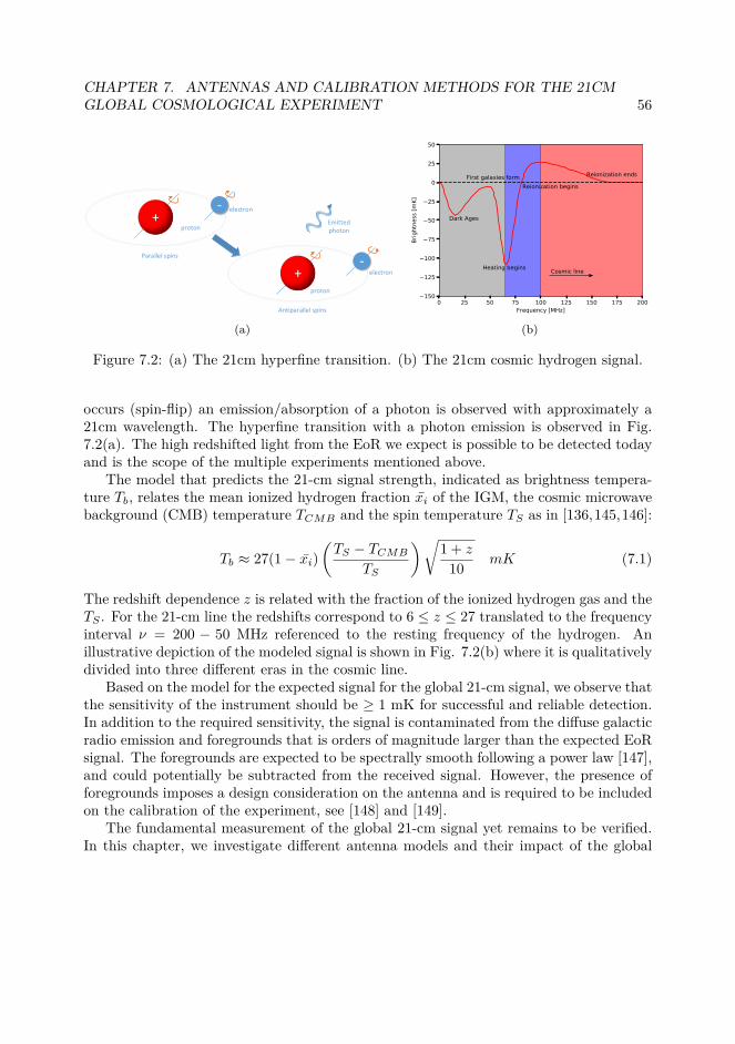
CHAPTER 7. ANTENNAS AND CALIBRATION METHODS FOR THE 21CMGLOBAL COSMOLOGICAL EXPERIMENT 56
+-
+-
proton
electron
Parallel spins
proton
electron
Antiparallel spins
Emitted photon
(a)
0 25 50 75 100 125 150 175 200Frequency [MHz]
150
125
100
75
50
25
0
25
50
Brig
htne
ss [m
K]
Dark Ages
First galaxies form
Heating begins
Reionization begins
Reionization ends
Cosmic line
(b)
Figure 7.2: (a) The 21cm hyperfine transition. (b) The 21cm cosmic hydrogen signal.
occurs (spin-flip) an emission/absorption of a photon is observed with approximately a21cm wavelength. The hyperfine transition with a photon emission is observed in Fig.7.2(a). The high redshifted light from the EoR we expect is possible to be detected todayand is the scope of the multiple experiments mentioned above.
The model that predicts the 21-cm signal strength, indicated as brightness tempera-ture Tb, relates the mean ionized hydrogen fraction xi of the IGM, the cosmic microwavebackground (CMB) temperature TCMB and the spin temperature TS as in [136,145,146]:
Tb ≈ 27(1− xi)(TS − TCMB
TS
)√1 + z
10 mK (7.1)
The redshift dependence z is related with the fraction of the ionized hydrogen gas and theTS . For the 21-cm line the redshifts correspond to 6 ≤ z ≤ 27 translated to the frequencyinterval ν = 200 − 50 MHz referenced to the resting frequency of the hydrogen. Anillustrative depiction of the modeled signal is shown in Fig. 7.2(b) where it is qualitativelydivided into three different eras in the cosmic line.
Based on the model for the expected signal for the global 21-cm signal, we observe thatthe sensitivity of the instrument should be ≥ 1 mK for successful and reliable detection.In addition to the required sensitivity, the signal is contaminated from the diffuse galacticradio emission and foregrounds that is orders of magnitude larger than the expected EoRsignal. The foregrounds are expected to be spectrally smooth following a power law [147],and could potentially be subtracted from the received signal. However, the presence offoregrounds imposes a design consideration on the antenna and is required to be includedon the calibration of the experiment, see [148] and [149].
The fundamental measurement of the global 21-cm signal yet remains to be verified.In this chapter, we investigate different antenna models and their impact of the global

CHAPTER 7. ANTENNAS AND CALIBRATION METHODS FOR THE 21CMGLOBAL COSMOLOGICAL EXPERIMENT 57
Antenna zenith
Brightness Temperature distribution Tsky
Celestial sphere
𝑟0
(a)
Antenna efficiency
Receiver gain
Tant
Tsys
(b)
Figure 7.3: (a) Antenna beam and the celestial sphere (b) Antenna temperature systemdecomposition.
21-cm signal detection as well as different foreground modeling and scaling. We proposea spectral index map for optimal foreground scaling. Finally, a piecewise polynomialfitting algorithm is proposed as an alternative approach to the 21-cm signal detection.We verify this approach with proposed capacitively loaded dipole array designed for the21-cm global experiment.
7.1 Antenna Temperature
The global EoR experiment is based on the measuring the system temperature as capturedby an antenna pointing at the sky and a receiver as illustrated in Fig. 7.3(a). In a giventime t the overall system temperature is given for a direction n as in [150]:
Tsys(t, ν, n) = Trec(t, ν) + η(t, ν)Tant + (1− η(t, ν))T0, (7.2)
where ν is the frequency, Trec is the receiver’s temperature, Tant the antenna temperaturemultiplied with an efficiency η(t, ν) that combines the receiver gain and the antennaefficiency. We denote as T0 the physical antenna temperature. Note that we disregardany temporal efficiency dependency factors such as metal oxidization, amplifier drift etc,since they are slow varying and can be accounted by recalibrating the system in regulartime periods. We follow a similar system decomposition for the system temperature asin [150] depicted in Fig. 7.3(b). This definition isolates the impact of the foregroundsand the antenna pattern response. Isolating the antenna pattern - foreground responsewe can study its impact at the antenna temperature.
The antenna temperature Tant is defined as:
Tant(ν, n) = 14π
∫ΩD(s, n)Tsky(s)dΩ (7.3)
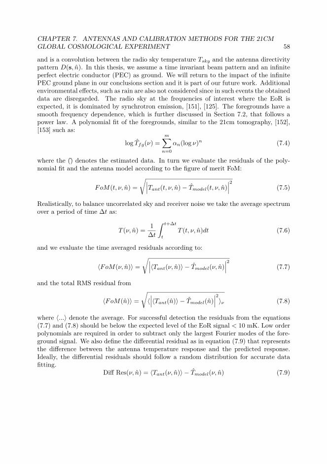
CHAPTER 7. ANTENNAS AND CALIBRATION METHODS FOR THE 21CMGLOBAL COSMOLOGICAL EXPERIMENT 58
and is a convolution between the radio sky temperature Tsky and the antenna directivitypattern D(s, n). In this thesis, we assume a time invariant beam pattern and an infiniteperfect electric conductor (PEC) as ground. We will return to the impact of the infinitePEC ground plane in our conclusions section and it is part of our future work. Additionalenvironmental effects, such as rain are also not considered since in such events the obtaineddata are disregarded. The radio sky at the frequencies of interest where the EoR isexpected, it is dominated by synchrotron emission, [151], [125]. The foregrounds have asmooth frequency dependence, which is further discussed in Section 7.2, that follows apower law. A polynomial fit of the foregrounds, similar to the 21cm tomography, [152],[153] such as:
log Tfg(ν) =m∑n=0
αn(log ν)n (7.4)
where the () denotes the estimated data. In turn we evaluate the residuals of the poly-nomial fit and the antenna model according to the figure of merit FoM:
FoM(t, ν, n) =√∣∣∣Tant(t, ν, n)− Tmodel(t, ν, n)
∣∣∣2 (7.5)
Realistically, to balance uncorrelated sky and receiver noise we take the average spectrumover a period of time ∆t as:
T (ν, n) = 1∆t
∫ t+∆t
t
T (t, ν, n)dt (7.6)
and we evaluate the time averaged residuals according to:
〈FoM(ν, n)〉 =√∣∣∣〈Tant(ν, n)〉 − Tmodel(ν, n)
∣∣∣2 (7.7)
and the total RMS residual from
〈FoM(n)〉 =√〈∣∣∣〈Tant(n)〉 − Tmodel(n)
∣∣∣2〉ν (7.8)
where 〈...〉 denote the average. For successful detection the residuals from the equations(7.7) and (7.8) should be below the expected level of the EoR signal < 10 mK. Low orderpolynomials are required in order to subtract only the largest Fourier modes of the fore-ground signal. We also define the differential residual as in equation (7.9) that representsthe difference between the antenna temperature response and the predicted response.Ideally, the differential residuals should follow a random distribution for accurate datafitting.
Diff Res(ν, n) = 〈Tant(ν, n)〉 − Tmodel(ν, n) (7.9)
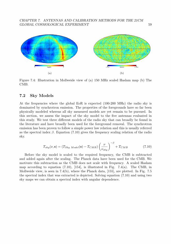
CHAPTER 7. ANTENNAS AND CALIBRATION METHODS FOR THE 21CMGLOBAL COSMOLOGICAL EXPERIMENT 59
2 4log(K)
(a)
2.7245 2.72549Kelvin
(b)
Figure 7.4: Illustration in Mollweide view of (a) 150 MHz scaled Haslam map (b) TheCMB.
7.2 Sky Models
At the frequencies where the global EoR is expected (100-200 MHz) the radio sky isdominated by synchrotron emission. The properties of the foregrounds have so far beenphysically modeled whereas all sky measured models are yet remain to be pursued. Inthis section, we assess the impact of the sky model to the five antennas evaluated inthis study. We test three different models of the radio sky that can broadly be found inthe literature and have broadly been used for the foreground removal. The synchrotronemission has been proven to follow a simple power law relation and this is usually referredas the spectral index β. Equation (7.10) gives the frequency scaling relation of the radiosky.
Tsky(ν, s) = (TSky Model(s)− TCMB)(
ν
νsky
)−β+ TCMB (7.10)
Before the sky model is scaled to the required frequency, the CMB is subtractedand added again after the scaling. The Planck data have been used for the CMB. Wemotivate this subtraction as the CMB does not scale with frequency. A scaled Haslammap according to equation (7.10), [154], is illustrated in Fig. 7.4(a). The CMB, inMollweide view, is seen in 7.4(b), where the Planck data, [155], are plotted. In Fig. 7.5the spectral index that was extracted is depicted. Solving equation (7.10) and using twosky maps we can obtain a spectral index with angular dependence.

CHAPTER 7. ANTENNAS AND CALIBRATION METHODS FOR THE 21CMGLOBAL COSMOLOGICAL EXPERIMENT 60
7.3 Impact on the Antenna Radiation Pattern MeasurementErrors and Filtering Strategies
To accurately calibrate the instrument detailed understanding for the antenna radiationpattern are required. Typical antenna measurements take place in a controlled environ-ment such as an anechoic chamber. However, in the case of the global EoR cosmologicalexperiment, due to the physical antenna size, a novel measurement method performed inopen space with the help of a drone that carries a probe and a spectrum analyzer, [156]and [157], has started to emerge. In conventional antenna measurements, performed in ananechoic chamber, it has been shown in [158] and [159] that even in an anechoic environ-ment there is an uncertainty error for every measurement point that can vary from 0.1 dBto 0.5 dB. This uncertainty will impact the calibration of the instrument by increasing theuncertainty levels. To simulate similar conditions, a random noise signal can be addedto the magnitude of the simulated radiation patterns as additive white gaussian noise(AWGN). The calculation flow chart is illustrated in Fig. 7.6. It is worth noting that weassume far field measurements and we do not use the phase of the measured signal. In thecase that a near field system is used, then the phase of the measured data will be takeninto account since a Fourier transform is required to obtain the far field data from nearfield measurements. Additionally to the impact of the measurement uncertainty filteringstrategies of the measured data are explored. Filtering the measured radiation pattern isalso based on the fact that the far field function is a smooth function that cannot supportspatial harmonics greater than λ/D where D is the diameter of the smallest sphere thatencloses the antenna, [8]. This implies that no variations greater than λ/D are expectedin the far field measurements. The value for the smallest λ/D corresponds to the higherorder spatial harmonic that is supported by the structure. This relation will provide thelength of the moving filtering window.
2 4.25Spectral Index β
Figure 7.5: The spectral index β with angular dependence.

CHAPTER 7. ANTENNAS AND CALIBRATION METHODS FOR THE 21CMGLOBAL COSMOLOGICAL EXPERIMENT 61
Input beam Finite array excitation/
Post processed beam
Project beam to the celestial sphere from
station location
Scale 408 Haslam map
Integrate beam and
Haslam map
Antenna temperature
FoM Inject AWGN
Figure 7.6: Calculating methodology and FoM evaluation.
The first smoothing filter utilized in this work is a convolution filter with Hammingwindow, [160] and [161]. The Hamming window is one of the most commonly usedwindows as it provides a good trade off between stop band attenuation and pass bandtransition. We denote the convolution filter with Hamming window as C-H filter. Theother smoothing filter utilized is the Savitzky Golay filter, [162] and [163], denoted hereas S.G. filter. The basic principle of this filter is that each data point is smoothed bytaking into account the average of its neighboring values (linear), however higher orderbasis sets are possible to be utilized. The motivation for these two filters (C-H and S.G.)stems from their respective behavior, the C-H filter is able to preserve the shape of a loworder smooth function hence, it is more applicable to low angular resolution antennas. Incontrast, the S.G. filter with 3rd order polynomial is more suitable for the high angularresolution antennas as it can preserve better the peak values where the C-H filter alwaysprovides an underestimation.
7.4 Piecewise Polynomial Fitting Based on the AntennaChromaticity
The foregrounds contaminate severely the global EoR signal and the polynomial fittingproposed in Section 7.1 results in residuals that cannot distinguish the global EoR signal.To overcome this limitation and keep integration times short, we propose a piecewisepolynomial fitting scheme that follows the behavior of the antenna temperature in fre-quency. In [164], there is a discussion that the bandwidth reduction will result is lowerresiduals however the motivation was to focus on the peaks of the EoR signal. Since theantenna chromaticity will impact the antenna temperature in a non systematic way, thiswill influence the magnitude of the residuals across the frequency interval. The impacton the antenna of the beam chromaticity, denoted here as T ′ν , can be analyzed by taking

CHAPTER 7. ANTENNAS AND CALIBRATION METHODS FOR THE 21CMGLOBAL COSMOLOGICAL EXPERIMENT 62
the gradient of the time averaged antenna temperature 〈Tant〉t.
T′
ν = ∇〈Tant〉t, (7.11)
where from the above equation we can further define the antenna chromatic figure of merit(CFoM) as the number of inflection points - IP in the overall bandwidth of observationof the T ′ν .
CFoM = No. of inflection points Tν|∂2〈Tant〉t∂ν2 = 0. (7.12)
For an antenna of no chromatic effect, in the bandwidth of operation, this is equal tozero. The antenna temperature then follows the power law of the spectral index. Weapproximate the 〈Tant〉t with a piecewise logarithmic polynomial fit based on the CFoMin the total bandwidth [νlow, νhight] such as:
log Tfg =
∑mn=0 αn (log ν1)n for ν1 ∈ [νlow, ν1st IP ]
.
.
.∑mn=0 αn (log νi)n for νi ∈ [νith IP , νhigh]
(7.13)
Using this methodology, one is able to obtain a polynomial fitted curve in part of thebandwidth that can result in very low residuals. This is a general method and is notdependent on the antenna type.
7.5 Application of the Theory
To illustrate the developed theory, we have developed a fully populated array based on themethods developed in Chapter 6. The array is a dual polarized, capacitivly loaded dipolearray (CLDA) consisting of a 25 × 25 rectangular grid. The unit cell of the developedarray is illustrated in Fig. 7.7(a) and the corresponding active reflection coefficient forthe unit cell in Fig. 7.7(b). We explore a wideband array design as a global EoR probe.This approach can serve as an excellent reference case for smooth antenna beam patterns.However, in a practical implementation the main drawback of the system is the increasedcomplexity. In addition, an antenna array can potentially allow us to track better coldpatches of the sky, reducing observation times and potentially avoid regions of the skywith high contaminating brightness.
For a realistic scenario, the antenna is located in the South African Karoo radio astron-omy reserve with coordinates approximately 30S and 21E and the date is considered the22nd of July 2018. To properly evaluate the time span of observation where the galacticcenter is below the horizon, a single day is simulated and illustrated as waterfall diagramin Fig. 7.8(a) for the antenna temperature. The optimal observation time is from 0:00

CHAPTER 7. ANTENNAS AND CALIBRATION METHODS FOR THE 21CMGLOBAL COSMOLOGICAL EXPERIMENT 63
(a)
50 75 100 125 150 175 200 225 250Frequency (MHz)
0
2
4
6
8
10
VSWR
Broad ide45∘ E∘plane
(b)
Figure 7.7: (a) CLDA unit cell (b) VSWR performance.
to 4:00 LST. The corresponding beam CLDA beam projected into the celestial sphere isdepicted in Fig. 7.8(b).
In continuance, we apply the theory from Sections 7.2, 7.4 and 7.3 for the case of theCLDA. The model has been simulated for a week’s data for every MHz in the 50-250 MHzrange and every 15 minutes during the observation time found from the waterfall diagram.The evaluation of the sky models is depicted in Fig. 7.9(a) where we observe that wecan obtain lower than 10 mK residual for a 6th polynomial order. The corresponding
0 4 8 12 16 20 24LST(h)
50
75
100
125
150
175
200
225
250
Freq
uenc
y (M
Hz)
0
2400
4800
7200
9600
12000
14400
16800
19200
21600
Antenn
a tempe
rature (K
)
(a)1e-05 1
(b)
Figure 7.8: (a) Waterfall diagram for the antenna temperature for a single day (b) Nor-malized CLDA directivity pattern projected into the celestial sphere.

CHAPTER 7. ANTENNAS AND CALIBRATION METHODS FOR THE 21CMGLOBAL COSMOLOGICAL EXPERIMENT 64
100 120 140 160 180 200Frequency (MHz)
0
10
20
30
40
50
60
SFoM
(ν) i (m
K)
CLDA SFoM(ν)NF|n=5CLDA SFoM(ν)NF|n=6CLDA SFoM(ν)DSDS|n=5CLDA SFoM(ν)DSDS|n=6
(a)
100 120 140 160 180 200Frequency (MHz)
−100
−75
−50
−25
0
25
50
75
100
Diffe
ent
ial
esid
ual (
mK)
CLDA Dif. es n=3CLDA Dif. es n=4CLDA Dif. es n=5
(b)
Figure 7.9: (a) Residual for the CLDA for different sky models (b) Differential residualsafter piecewise polynomial fit.
Table 7.1: 〈FoM(n)〉 in mK for the 5th polynomial order for antenna models with simu-lated pattern noise and filtering.
CLDAIdeal pattern 4.4080.5dB beam noise 5.2810.1dB beam noise 4.6230.5dB noise S.G. filter 4.5110.1dB noise S.G. filter 4.4540.5dB noise C-H filter 4.4660.1dB noise C-H filter 4.421
residuals after the proposed piecewise polynomial fitting algorithm are depicted in Fig.7.9(b). It is observed that is significantly reduced for the 5th polynomial order openingpossibilities for detecting the EoR signal. Finally, a summary table is added to show theoverall performance of the CLDA with the pattern uncertainty and filtering strategiesproposed in this thesis for a 5th polynomial order. The overall residual, in most cases, isapproximately 4.5 mK and can achieve detection.
CHAPTER 7. ANTENNAS AND CALIBRATION METHODS FOR THE 21CMGLOBAL COSMOLOGICAL EXPERIMENT 65
7.6 Conclusions
We have investigated the implications at the global EoR experiment from the foregroundeffect. We have have proposed a new method for scaling the all sky Haslam map with anangular dependent spectral index. The impact to the detection of the global 21-cm signalof a noisy sky model was also evaluated.
A general measure, the CFoM was also introduced in this study as an indicator for theoverall antenna chromaticity across the entire frequency of operation. A low CFoM canalso be interpreted that the power spectrum of the antenna beam does not contaminate theglobal EoR. A general piecewise polynomial fitting algorithm was proposed as a strategyfor antennas with high CFoM . It was shown that there is probability of detection ofthe global signal even with an antenna with high CFoM . Even though the proposedalgorithm was applied only to the antenna directivity, our work can be applied to theentire receiver chain. This can provide an exit strategy for possible non linearities thatare introduced from radical factors such as the antenna efficiency or receiver gain.
Finally, we have investigated the impact of measurement uncertainty of the antennabeam patterns. Two different filtering strategies of such uncertainties were also evalu-ated, the Savitzky Golay filter and a convolution filter with Hamming window. The SGfilter maintains the maxima of the filtered function and is more suited for high angularresolution antennas. The C-H filter reserves the shape of the filtered function is bettersuited for low angular resolution antennas, such as dipoles.

Chapter 8
Contributions, Future Work &Discussion on Sustainability
8.1 Contribution
Wideband, wide-scan antenna arrays are promising candidates for the future wirelessnetworks and will be an essential part of radio astrophysics. Understanding the underlyingphysics of the element performance in the array environment is paramount to developand improve the performance of array systems. This thesis investigates the fundamentalantenna array limits, proposes two novel antenna array structure the SCADA and the softvivaldi and extends the application of the strongly coupled array applied to the global21cm experiment. The main contributions are:• The fundamental limitation of antenna arrays are extracted. We propose a general
measure for antenna arrays, the array figure of merit. This measure relates bandwidth,height from the ground plane and reflection coefficient in a bounded quantity. We alsopropose an extension of the array figure of merit that is able to provide matching, band-width and directivity/gain limits.• The soft Vivaldi element was introduced in this thesis. It was proposed that periodic
structure loading on arrays can be used as a tool to improve the array’s performance andmold the electromagnetic’s wave behavior to our benefit. We have proposed three differentperiodic loadings, (i) element loading and (ii) edge loading in the form of a soft conditionand an (iii) integrated matching layer with a period structure. A prototype of the softVivaldi antenna array was fabricated and measured. Good agreement between simulationsand measurements was achieved.• A new class of antenna arrays, the Strongly Coupled Asymmetric Dipole Array
- SCADA is proposed in this thesis. The SCADA is a combination of a current sheetarray and the fragmented array with the additional degree of freedom of asymmetry. Anovel method for terminating finite arrays is also proposed. The basic theory and an
66

CHAPTER 8. CONTRIBUTIONS, FUTURE WORK & DISCUSSION ONSUSTAINABILITY 67
experimental prototype SCADA antenna array is presented. Good agreement betweenmeasured and simulated results is observed. The integration of the matching layer intothe strongly coupled dipole arrays was also explored here. A prototype that addressesthe integrated matching layer with periodic loading was developed. The prototype wasmanufactured and measured with good agreement with the predicted simulated values.• We have extended our approach of strongly coupled dipoles to an astrophysics ap-
plication of antennas. We propose a new method for extracting the global signal from theEpoch of Reionization (EoR). The method is based on piecewise polynomial fitting thatfollows the chromatic behavior of the antenna. A capacitive loaded dipole array (CLDA)was introduced and its potential for the 21-cm global experiment was shown. The impactof far field pattern measurement errors was also evaluated and filtering strategies wereexplored. The 408 Haslam map was scaled with a new approach that takes into accountthe angular dependence of the spectral index and the Cosmic Microwave Background.The proposed methodology was able to produce residuals in the order of the cosmologicalsignal with only 4 days of observation.
8.2 Future Work and extensions
Antenna arrays will gradually be incorporated to all future wireless networks. Arrays canoffer the best performance with the best flexibility when compared to any other solution.However, their main drawback is cost due to the requirement for having an Rx/Tx chainbehind every element. Recent advances in the lithographic methods have reduced thecost significantly but not to the point that one can afford feeding every element. To thataspect, a future work could be to develop sub-arraying techniques suitable for widebandantenna arrays contrary to the current literature.
Another possible extension is to extend the current work to millimeter wave frequen-cies. The current demand for data rates is already pushing the providers to deploynetworks in 27 GHz and beyond. Scaling an array to millimeter waves poses significantchallenges and especially in the proposed methodologies where the inter-element spacingis kept below λ/2.
Further investigations on how to integrate periodic structures in more than the pro-posed cases could also be pursued. The periodic structure loading provides unique ca-pabilities and control over the electromagnetic behavior. In addition, investigating waysto improve the bandwidth performance of the periodic structures is also a path worthtaking.
The MIMO performance behavior of the developed arrays should be investigated. Thedeveloped arrays offer advanced beam and bandwidth capabilities but they are developedto be strongly coupled. This inherently degrades the MIMO performance of the sys-tem. However, one can still pursue the decoupling but not in the classic sense of theantenna port. Investigating virtual antenna ports that correspond to the beam behavioror decoupling networks from sub-arrays is a promising way forward.

CHAPTER 8. CONTRIBUTIONS, FUTURE WORK & DISCUSSION ONSUSTAINABILITY 68
A next logical step after the development of these arrays is the integration with anRx/Tx chain to each element. Pursuing deep antenna and active component integrationcan eventually reduce the manufacturing costs and could also be ideal for on-chip solutionto higher frequencies. This however remains a very challenging task and requires multi-physics understanding of the integrated passive active components.
Radio astrophysics is an open question field as it tries to give answers to fundamentalquestions of the origins of the universe. To this time, the 21cm global cosmologicalsignal yet remains to be detected. Further development of the proposed algorithm andintegration to an experiment should be pursued. Designing beamforming algorithms withlow to no chromaticity remains an open question. The latter could also be applied incommunication networks. Finally, fundamental understanding on the electromagneticproperties of the antennas used in the global experiment is needed to tailor our designfor the global 21cm signal detection.
1.0%
43.0%
42.0%
3.0%11.0%
Year 2002: 151 Megatons of CO2
IPTV and broadband modemsMobile NetworksFixed Narrowband networksFixed Broadband networksMobile phones
(a)
8.0%
52.0%
20.0%
14.0%6.0%
Year 2020: 349 Megatons of CO2
IPTV and broadband modemsMobile NetworksFixed Narrowband networksFixed Broadband networksMobile phones
(b)
Figure 8.1: Carbon footprint of telecommunications industry. (a) For the year 2002 totalestimated 151 Megatons. (b) Projected for the year 2020, estimated 349 Megatons.
8.3 Discussing the Sustainability of a Wirelessly ConnectedSociety
Antennas are at the heart of every wireless system and their impact on the overall systemefficiency is instrumental. The following discussion has been tailored around wirelesscommunications networks and their integration to a more sustainable environment. We
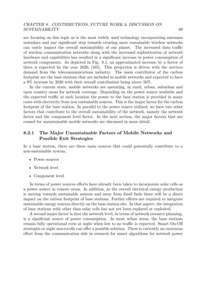
CHAPTER 8. CONTRIBUTIONS, FUTURE WORK & DISCUSSION ONSUSTAINABILITY 69
are focusing on this topic as is the most widely used technology incorporating antennasnowadays and any significant step towards creating more sustainable wireless networkscan vastly impact the overall sustainability of our planet. The increased data trafficof wireless communication networks along with the increased sophistication of networkhardware and capabilities has resulted in a significant increase in power consumption ofnetwork components. As depicted in Fig. 8.1, an approximated increase by a factor ofthree is expected by the year 2020, [165]. This projection is driven with the servicesdemand from the telecommunications industry. The main contributor of the carbonfootprint are the base stations that are included in mobile networks and expected to havea 9% increase by 2020 with their overall contribution being above 50%.
In the current state, mobile networks are operating, in rural, urban, suburban andopen country areas for network coverage. Depending on the power source available andthe expected traffic at each location the power to the base station is provided in manycases with electricity from non sustainable sources. This is the major factor for the carbonfootprint of the base station. In parallel to the power source utilized, we have two otherfactors that contribute to the overall sustainability of the network, namely the networkfactor and the component level factor. In the next section, the major factors that arecaused for unsustainable mobile networks are discussed in more detail.
8.3.1 The Major Unsustainable Factors of Mobile Networks andPossible Exit Strategies
In a base station, there are three main sources that could potentially contribute to anon-sustainable system.
• Power sources
• Network level
• Component level
In terms of power sources efforts have already been taken to incorporate solar cells asa power source in remote areas. In addition, as the overall electrical energy productionis moving towards sustainable sources and away from fossil fuels there will be a directimpact on the carbon footprint of base stations. Further efforts are required to integratesustainable energy sources directly on the base station site. In that aspect, the integrationof base stations with other than solar cells has not yet been explored or exploited.
A second major factor is that the network level, in terms of network resource planning,is a significant source of power consumption. In most urban areas, the base stationsremain fully operational even at night when low to no traffic is expected. Smart On-Offstrategies or night macrocells can offer a possible solution. There is currently an enormouseffort from the communication side in research for smart algorithms for network power
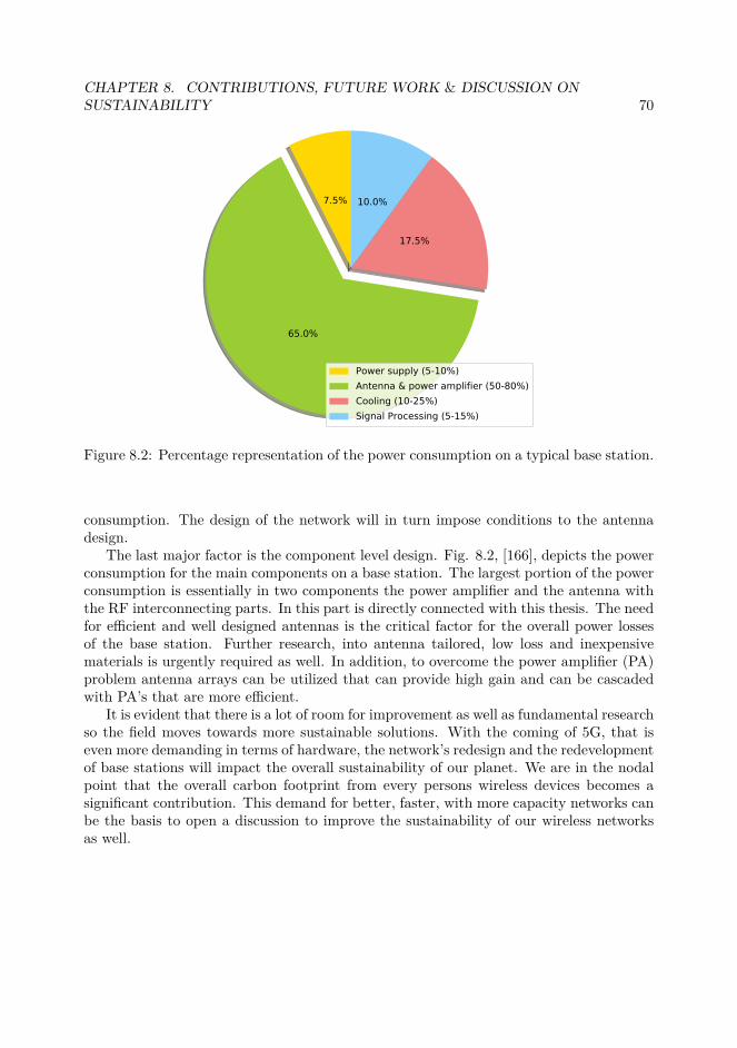
CHAPTER 8. CONTRIBUTIONS, FUTURE WORK & DISCUSSION ONSUSTAINABILITY 70
7.5%
65.0%
17.5%
10.0%
Power supply (5-10%)Antenna & power amplifier (50-80%)Cooling (10-25%)Signal Processing (5-15%)
Figure 8.2: Percentage representation of the power consumption on a typical base station.
consumption. The design of the network will in turn impose conditions to the antennadesign.
The last major factor is the component level design. Fig. 8.2, [166], depicts the powerconsumption for the main components on a base station. The largest portion of the powerconsumption is essentially in two components the power amplifier and the antenna withthe RF interconnecting parts. In this part is directly connected with this thesis. The needfor efficient and well designed antennas is the critical factor for the overall power lossesof the base station. Further research, into antenna tailored, low loss and inexpensivematerials is urgently required as well. In addition, to overcome the power amplifier (PA)problem antenna arrays can be utilized that can provide high gain and can be cascadedwith PA’s that are more efficient.
It is evident that there is a lot of room for improvement as well as fundamental researchso the field moves towards more sustainable solutions. With the coming of 5G, that iseven more demanding in terms of hardware, the network’s redesign and the redevelopmentof base stations will impact the overall sustainability of our planet. We are in the nodalpoint that the overall carbon footprint from every persons wireless devices becomes asignificant contribution. This demand for better, faster, with more capacity networks canbe the basis to open a discussion to improve the sustainability of our wireless networksas well.

Bibliography
[1] Bhattacharyya, Phased Array Antennas: Floquet Analysis, Synthesis, BFNs, andActive Array Systems, 2006.
[2] Schneider, Hartwanger, and Wolf, “Antennas for multiple spot beam satellites,”CEAS Space Journal, vol. 2, no. 1-4, pp. 59–66, 2011.
[3] DeBoer, Parsons, Aguirre, Alexander et al., “Hydrogen epoch of reionization array(HERA),” Publications of the Astronomical Society of the Pacific, vol. 129, no. 974,p. 045001, 2017.
[4] Tingay, “The science and technology of the square kilometre array,” IOP ConferenceSeries: Materials Science and Engineering, vol. 67, no. 1, p. 012018, 2014.
[5] Sarkar, Mailloux, Oliner, Salazar-Palma, and Sengupta, History of Wireless, 2006.
[6] Nguyen, Abbosh, and Crozier, “Microwave hyperthermia for breast cancer treat-ment using electromagnetic and thermal focusing tested on realistic breast modelsand antenna arrays,” IEEE Transactions on Antennas and Propagation, vol. 63,no. 10, pp. 4426–4434, Oct 2015.
[7] Hansen, Phased Array Antennas, ser. Wiley Series in Microwave and Optical Engi-neering. Wiley, 2009.
[8] Balanis, Antenna theory: analysis and design. Wiley-Interscience, 2005.
[9] Amitay, Galindo, and Wu, Theory and analysis of phased array antennas. Wiley-Interscience, 1972.
[10] Pozar, “The active element pattern,” IEEE Transactions on Antennas and Propa-gation, vol. 42, no. 8, pp. 1176–1178, 1994.
[11] Craeye and Arts, “On the receiving cross section of an antenna in infinite linearand planar arrays,” Radio Science, vol. 39, no. 2, pp. n/a–n/a, 2004, rS2010.
71

BIBLIOGRAPHY 72
[12] Craeye and González-Ovejero, “A review on array mutual coupling analysis,” RadioScience, vol. 46, no. 2, pp. n/a–n/a, 2011, rS2012.
[13] Wheeler, “Fundamental limitations of small antennas,” Proceedings of the IRE,vol. 35, no. 12, pp. 1479–1484, Dec 1947.
[14] Chu, “Physical limitations of omni-directional antennas,” Journal of AppliedPhysics, vol. 19, pp. 1163–1175, dec 1948.
[15] Jonsson, Kolitsidas, and Hussain, “Array antenna limitations,” IEEE Antennas andWireless Propagation Letters, vol. 12, pp. 1539–1542, 2013.
[16] Tayli and Gustafsson, “Physical bounds for antennas above a ground plane,” IEEEAntennas and Wireless Propagation Letters, vol. 15, pp. 1281–1284, 2016.
[17] Taylor, Munk, and Durham, “Wideband phased arrays and associated methods,”US Patent 6512487, Jan. 2003.
[18] Schaubert, Kasturi, Boryssenko, and Elsallal, “Vivaldi antenna arrays for widebandwidth and electronic scanning,” in Antennas and Propagation, 2007. EuCAP2007. The Second European Conference on, Nov. 2007, pp. 1–6.
[19] Maloney, Kesler, Harms, and Smith, “Fragmented aperture antennas and broadbandantenna ground planes,” US Patent 6323803, 2001.
[20] Wheeler, “Simple relations derived from a phased-array antenna made of an infinitecurrent sheet,” IEEE Transactions on Antennas and Propagation, vol. 13, no. 4,pp. 506–514, 1965.
[21] Munk, Frequency Selective Surfaces: Theory and Design. Wiley, 2005.
[22] Lee, Livingston, and Koenig, “Wide band long slot array antennas,” in Antennasand Propagation Society International Symposium, 2003. IEEE, vol. 2, 2003, pp.452–455 vol.2.
[23] Neto, Cavallo, Gerini, and Toso, “Scanning performances of wideband connectedarrays in the presence of a backing reflector,” IEEE Transactions on Antennas andPropagation, vol. 57, no. 10, pp. 3092–3102, 2009.
[24] Maloney, Baker, Lee, Kiesel, and Acree, “Wide scan, integrated printed circuitboard, fragmented aperture array antennas,” in 2011 IEEE International Sympo-sium on Antennas and Propagation (APSURSI), 2011, pp. 1965–1968.
[25] Balanis, Modern Antenna Handbook. Wiley, 2011.
BIBLIOGRAPHY 73
[26] Doane, Sertel, and Volakis, “A wideband, wide scanning tightly coupled dipolearray with integrated balun (TCDA-IB),” IEEE Transactions on Antennas andPropagation, vol. 61, no. 9, pp. 4538–4548, Sept 2013.
[27] Cavallo, “Connected arrays analysis and design,” PhD thesis, Nov 2011.
[28] Jones and Rawnick, “A new approach to broadband array design using tightlycoupled elements,” in IEEE 2007 Military Communications Conference - MILCOM,Oct 2007, pp. 1–7.
[29] Wheeler, “The radiation resistance of an antenna in an infinite array or waveguide,”Proceedings of the IRE, vol. 36, no. 4, pp. 478–487, 1948.
[30] Neto and Lee, “Infinite bandwidth long slot array antenna,” IEEE Antennas andWireless Propagation Letters, vol. 4, pp. 75–78, 2005.
[31] ——, “Ultrawide-band properties of long slot arrays,” IEEE Transactions on An-tennas and Propagation, vol. 54, no. 2, pp. 534–543, 2006.
[32] Neto and Maci, “Green’s function for an infinite slot printed between two homo-geneous dielectrics. i. magnetic currents,” IEEE Transactions on Antennas andPropagation, vol. 51, no. 7, pp. 1572–1581, 2003.
[33] Lee, Livingston, and Nagata, “A low profile 10:1 (200-2000 MHz) wide band longslot array,” in Antennas and Propagation Society International Symposium, 2008.AP-S 2008. IEEE, 2008, pp. 1–4.
[34] Dardenne and Craeye, “Simulation of the effects of a ground plane on the radiationcharacteristics of self-complementary arrays,” in IEEE 2003 International Sympo-sium on Antennas and Propagation Society, vol. 1, 2003, pp. 383–386 vol.1.
[35] Holland and Vouvakis, “The planar ultrawideband modular antenna (PUMA) ar-ray,” IEEE Transactions on Antennas and Propagation, vol. 60, no. 1, pp. 130–140,2012.
[36] Salman, Psychoudakis, Volakis, Paulsen, and West, “Broadband bowtie-shaped cur-rent sheet antenna array,” in Antennas and Propagation (APSURSI), 2011 IEEEInternational Symposium on, 2011, pp. 94–95.
[37] Tzanidis, Sertel, and Volakis, “Characteristic excitation taper for ultrawidebandtightly coupled antenna arrays,” IEEE Transactions on Antennas and Propagation,vol. 60, no. 4, pp. 1777–1784, 2012.
[38] ——, “Interwoven spiral array (ISPA) with a 10:1 bandwidth on a ground plane,”IEEE Antennas and Wireless Propagation Letters, vol. 10, pp. 115–118, 2011.

BIBLIOGRAPHY 74
[39] Magill and Wheeler, “Wide-angle impedance matching of a planar array antenna bya dielectric sheet,” in 1965 Antennas and Propagation Society International Sym-posium, vol. 3, Aug 1965, pp. 164–169.
[40] Moulder, Sertel, and Volakis, “Ultrawideband superstrate-enhanced substrate-loaded array with integrated feed,” IEEE Transactions on Antennas and Propa-gation, vol. 61, no. 11, pp. 5802–5807, 2013.
[41] Novak and Volakis, “Ultrawideband antennas for multiband satellite communica-tions at uhf-ku frequencies,” IEEE Transactions on Antennas and Propagation,vol. 63, no. 4, pp. 1334–1341, April 2015.
[42] Kindt and Vouvakis, “Low-cost end-point modular PUMA array,” in IEEE Anten-nas and Propagation Society, AP-S International Symposium (Digest), vol. 2015-October, 2015, pp. 2513–2514.
[43] Kindt, Mital, and Vouvakis, “3:1-Bandwidth millimeter-wave PUMA array,” in2016 IEEE Antennas and Propagation Society International Symposium, APSURSI2016 - Proceedings, 2016, pp. 1867–1868.
[44] Gibson, “The vivaldi aerial,” in Microwave Conference, 1979. 9th European, 1979,pp. 101–105.
[45] Paraschos, Kindt, Schaubert, and Vouvakis, “Radiation and coupling studies offinite-size dual polarized vivaldi arrays using a domain decomposition fem,” in 2008IEEE Antennas and Propagation Society International Symposium, July 2008, pp.1–4.
[46] Elsallal and Schaubert, “On the performance trade offs associated with modularelement of single and dual polarized dmbava,” in Proceedings of the 2006 AntennaApplications Symposium, Monticello, IL, sept. 2006, pp. 166–187.
[47] Shin and Schaubert, “A parameter study of stripline-fed vivaldi notch-antenna ar-rays,” IEEE Transactions on Antennas and Propagation, vol. 47, no. 5, pp. 879–886,May 1999.
[48] Gross, Frontiers in Antennas: Next Generation Design & Engineering, ser.McGraw-Hill’s AccessEngineering. Mcgraw-hill, 2011.
[49] Povinelli and Grove, “Wideband apertures for active planar multifunction phasedarrays,” in Radar Conference, 1989., Proceedings of the 1989 IEEE National, 1989,pp. 125–128.
[50] Schaubert, “A gap-induced element resonance in single-polarized arrays of notchantennas,” in Antennas and Propagation Society International Symposium, 1994.AP-S. Digest, vol. 2, 1994, pp. 1264–1267 vol.2.

BIBLIOGRAPHY 75
[51] Schaubert, Kasturi, Elsallal, and van Cappellen, “Wide Bandwidth Vivaldi AntennaArrays - Some Recent Developments,” in 2006 European Conference on Antennasand Propagation: EuCAP, ser. ESA Special Publication, vol. 626, Oct. 2006.
[52] Logan, “Low cross polarization vivaldi arrays,” PhD thesis, Sept. 2016.
[53] Janaswamy and Schaubert, “Analysis of the tapered slot antenna,” IEEE Transac-tions on Antennas and Propagation, vol. 35, no. 9, pp. 1058–1065, 1987.
[54] Gazit, “Improved design of the vivaldi antenna,” IEE Proceedings H Microwaves,Antennas and Propagation, vol. 135, no. 2, pp. 89–92, 1988.
[55] Axness, Coffman, Kopp, and Haver, “Shared aperture technology development,”John Hopkins APL Technical digest, vol. 17, 1996.
[56] Sutinjo and Tung, “The design of a dual polarized vivaldi array,” Microwave Jour-nal, vol. 47, no. 9, pp. 152–161, 2004.
[57] Langley, Hall, and Newham, “Balanced antipodal vivaldi antenna for wide band-width phased arrays,” IEE Proceedings Microwaves, Antennas and Propagation, vol.143, no. 2, pp. 97–102, 1996.
[58] Elsallal and Schaubert, “Parameter study of a single isolated element and infinitearrays of balanced antipodal Vivaldi antennas,” in Proceedings of the 2004 AntennaApplications Symposium, Monticello, IL, sept. 2004, pp. 45–69.
[59] Elsallal and Mather, “An ultra-thin, decade (10:1) bandwidth, modular bava arraywith low cross-polarization,” in Antennas and Propagation (APSURSI), 2011 IEEEInternational Symposium on, 2011, pp. 1980–1983.
[60] Holter, “Dual-polarized broadband array antenna with BOR-elements, mechani-cal design and measurements,” IEEE Transactions on Antennas and Propagation,vol. 55, no. 2, pp. 305–312, Feb 2007.
[61] Logan and Vouvakis, “Decade-bandwidth low cross-polarization UWB array,” in2016 IEEE Antennas and Propagation Society International Symposium, APSURSI2016 - Proceedings, 2016, pp. 437–438.
[62] ——, “Low cross-polarization ultra-wideband arrays (student submission),” in IEEEInternational Symposium on Phased Array Systems and Technology, 2017.
[63] Steyskal and Hanna, “Design aspects of fragmented patch elements for phased ar-rays,” in Antennas and Propagation Society International Symposium, 2007 IEEE,2007, pp. 141–144.

BIBLIOGRAPHY 76
[64] Thors, Steyskal, and Holter, “Broad-band fragmented aperture phased array ele-ment design using genetic algorithms,” IEEE Transactions on Antennas and Prop-agation, vol. 53, no. 10, pp. 3280–3287, 2005.
[65] Friederich, Pringle, Fountain, Harms, Denison, Kuster, Blalock, Smith, Maloney,and Kesler, “A new class of broadband planar apertures,” Proceedings of 2001 An-tenna Applications Symposium, pp. 561–587, 2001.
[66] Gustafsson, Sohl, and Kristensson, “Physical limitations on antennas of arbitraryshape,” Proceedings of the Royal Society A: Mathematical, Physical and EngineeringScience, vol. 463, no. 2086, pp. 2589–2607, 2007.
[67] Gustafsson, Cismasu, and Jonsson, “Physical bounds and optimal currents on an-tennas,” IEEE Transactions on Antennas and Propagation, vol. 60, no. 6, pp. 2672–2681, 2012.
[68] Doane, Sertel, and Volakis, “Matching bandwidth limits for arrays backed by a con-ducting ground plane,” IEEE Transactions on Antennas and Propagation, vol. 61,no. 5, pp. 2511–2518, 2013.
[69] Gustafsson, Sohl, and Kristensson, “Physical limitations on antennas of arbitraryshape,” Proceedings of the Royal Society A: Mathematical, Physical and EngineeringSciences, vol. 463, no. 2086, pp. 2589–2607, 2007.
[70] Yaghjian and Stuart, “Lower bounds on the Q of electrically small dipole antennas,”IEEE Transactions on Antennas and Propagation, vol. 58, no. 10, pp. 3114–3121,2010.
[71] Vandenbosch, “Simple procedure to derive lower bounds for radiation Q of elec-trically small devices of arbitrary topology,” IEEE Transactions on Antennas andPropagation, vol. 59, no. 6 PART 2, pp. 2217–2225, 2011.
[72] M Fano, “Theoretical limitations of the broadband matching of arbitraryimpedances,” vol. 249, 08 2005.
[73] Rozanov, “Ultimate thickness to bandwidth ratio of radar absorbers,” IEEE Trans-actions on Antennas and Propagation, vol. 48, no. 8, pp. 1230–1234, 2000.
[74] Brewitt-Taylor, “Limitation on the bandwidth of artificial perfect magnetic con-ductor surfaces,” IET Microwaves, Antennas & Propagation, vol. 1, no. 1, p. 255,2007.
[75] Gustafsson, Sohl, Larsson, and Sjöberg, “Physical bounds on the all-spectrum trans-mission through periodic arrays,” EPL (Europhysics Letters), vol. 87, no. 3, p.34002, 2009.

BIBLIOGRAPHY 77
[76] Bernland, Luger, and Gustafsson, “Sum rules and constraints on passive systems,”Journal of Physics A: Mathematical and Theoretical, vol. 44, no. 14, p. 145205,2011.
[77] Doane, Sertel, and Volakis, “Bandwidth limits for lossless, reciprocal PEC-backedarrays of arbitrary polarization,” IEEE Transactions on Antennas and Propagation,vol. 62, no. 5, pp. 2531–2542, 2014.
[78] Gustafsson and Sjoberg, “Physical bounds and sum rules for high-impedance sur-faces,” IEEE Transactions on Antennas and Propagation, vol. 59, no. 6 PART 2,pp. 2196–2204, 2011.
[79] Pozar, Microwave Engineering, 4th Edition. Wiley, 2011.
[80] Hannan, “The element-gain paradox for a phased-array antenna,” IEEE Transac-tions on Antennas and Propagation, vol. 12, no. 4, pp. 423–433, 1964.
[81] Johansson, “Fundamental limits for focal-plane array efficiency,” vol. 75, p. 34, 011995.
[82] Skobelev, Phased Array Antennas with Optimized Element Patterns, ser. ArtechHouse antennas and propagation library. Artech House, 2011.
[83] Kildal, “Artificially soft and hard surfaces in electromagnetics,” IEEE Transactionson Antennas and Propagation, vol. 38, no. 10, pp. 1537–1544, Oct 1990.
[84] Love, “Electromagnetic horn antennas,” IEEE Press, New York, 1976.
[85] Lier and Kildal, “Soft and hard horn antennas,” IEEE Transactions on Antennasand Propagation, vol. 36, no. 8, pp. 1152–1157, 1988.
[86] Lier, “Review of soft and hard horn antennas, including metamaterial-based hybrid-mode horns,” IEEE Antennas and Propagation Magazine, vol. 52, no. 2, pp. 31–39,2010.
[87] Huang, Yang, Wu, Zhao, and Liu, “A high-gain antipodal vivaldi antenna withmulti-layer planar dielectric lens,” Journal of Electromagnetic Waves and Applica-tions, vol. 0, no. 0, pp. 1–10, 2017.
[88] Zhou and Cui, “Directivity enhancement to vivaldi antennas using compactlyanisotropic zero-index metamaterials,” IEEE Antennas and Wireless PropagationLetters, vol. 10, pp. 326–329, 2011.
[89] Nassar and Weller, “A novel method for improving antipodal vivaldi antenna per-formance,” IEEE Transactions on Antennas and Propagation, vol. 63, no. 7, pp.3321–3324, 2015.
BIBLIOGRAPHY 78
[90] Shin and Schaubert, “A parameter study of stripline-fed vivaldi notch-antenna ar-rays,” IEEE Transactions on Antennas and Propagation, vol. 47, no. 5, pp. 879–886,May 1999.
[91] Rajo-Iglesias, Quevedo-Teruel, and Inclan-Sanchez, “Planar soft surfaces and theirapplication to mutual coupling reduction,” IEEE Transactions on Antennas andPropagation, vol. 57, no. 12, pp. 3852–3859, Dec 2009.
[92] Rajo-Iglesias, Caiazzo, Inclan-Sanchez, and Kildal, “Comparison of bandgaps ofmushroom-type ebg surface and corrugated and strip-type soft surfaces,” IET Mi-crowaves, Antennas Propagation, vol. 1, no. 1, pp. 184–189, February 2007.
[93] Thomas, “Design of corrugated conical horns,” IEEE Transactions on Antennasand Propagation, vol. 26, no. 2, pp. 367–372, Mar 1978.
[94] Bantavis, Kolitsidas, Jonsson, Empliouk, and Kyriacou, “A wideband switchedbeam antenna system for 5G femtocell applications,” in 2017 IEEE InternationalSymposium on Antennas and Propagation USNC/URSI National Radio ScienceMeeting, July 2017, pp. 929–930.
[95] Dahlberg, Kolitsidas, Mattsson, Silver, Bjorkqvist, and Jonsson, “A novel 32 portcube mimo combining broadside and endfire radiation patterns for full azimuthalcoverage - a modular unit approach for a massive mimo system,” in 2017 IEEE In-ternational Symposium on Antennas and Propagation USNC/URSI National RadioScience Meeting, July 2017, pp. 1641–1642.
[96] Munk, Finite Antenna Arrays and FSS, ser. Wiley - IEEE. Wiley, 2003.
[97] Neto, Cavallo, Gerini, and Toso, “Scanning performances of wideband connectedarrays in the presence of a backing reflector,” IEEE Transactions on Antennas andPropagation, vol. 57, no. 10, pp. 3092–3102, Oct 2009.
[98] Steyskal, “On the merit of asymmetric phased array elements,” IEEE Transactionson Antennas and Propagation, vol. 61, no. 7, pp. 3519–3524, July 2013.
[99] Bhattacharyya, “Active element pattern symmetry for asymmetrical element ar-rays,” in 2007 IEEE Antennas and Propagation Society International Symposium,June 2007, pp. 5953–5956.
[100] Kolitsidas, Jonsson, Persson, and Stjerman, “Exploiting asymmetry in a capaci-tively loaded strongly coupled dipole array,” in 2014 Loughborough Antennas andPropagation Conference (LAPC), Nov 2014, pp. 723–726.
[101] Kolitsidas and Jonsson, “Investigation of compensating the ground plane effectthrough array’s inter-element coupling,” in 2013 7th European Conference on An-tennas and Propagation (EuCAP), April 2013, pp. 1264–1267.

BIBLIOGRAPHY 79
[102] ——, “Rectangular vs. equilateral triangular lattice comparison in a t-slot loadedstrongly coupled dipole array,” in 2014 XXXIth URSI General Assembly and Sci-entific Symposium (URSI GASS), Aug 2014, pp. 1–4.
[103] ——, “Edge effects in a strongly coupled dipole element array in triangular lattice,”in PIERS Proceedings, Guangzhou, Aug 2014, pp. 487 – 490.
[104] Computer Simulation Technology-Microwave Studio CST ® MWS ® 2016.
[105] Matlab ® 2014.
[106] Tzanidis, Sertel, and Volakis, “UWB low-profile tightly coupled dipole array with in-tegrated balun and edge terminations,” IEEE Transactions on Antennas and Prop-agation, vol. 61, no. 6, pp. 3017–3025, June 2013.
[107] Kildal, Foundations of Antenna Engineering: A Unified Approach for Line-of-sightand Multipath, ser. Artech House antennas and electromagnetics analysis library.Artech House, 2015.
[108] Ellgardt, “A scan blindness model for single-polarized tapered-slot arrays in trian-gular grids,” IEEE Transactions on Antennas and Propagation, vol. 56, no. 9, pp.2937–2942, Sept 2008.
[109] Cavallo, Syed, and Neto, “Equivalent transmission line models for the analysis ofedge effects in finite connected and tightly coupled arrays,” IEEE Transactions onAntennas and Propagation, vol. 65, no. 4, pp. 1788–1796, April 2017.
[110] Neto, Cavallo, and Gerini, “Edge-born waves in connected arrays: A finite× infiniteanalytical representation,” IEEE Transactions on Antennas and Propagation,vol. 59, no. 10, pp. 3646–3657, Oct 2011.
[111] Yetisir, Ghalichechian, and Volakis, “Ultrawideband array with 70 scanning usingfss superstrate,” IEEE Transactions on Antennas and Propagation, vol. 64, no. 10,pp. 4256–4265, Oct 2016.
[112] Holland and Vouvakis, “The planar ultrawideband modular antenna (puma) array,”IEEE Transactions on Antennas and Propagation, vol. 60, no. 1, pp. 130–140, Jan2012.
[113] Jonsson, Kolitsidas, and Hussain, “Array antenna limitations,” IEEE Antennas andWireless Propagation Letters, vol. 12, pp. 1539–1542, 2013.
[114] Kindt and Pickles, “Ultrawideband all-metal flared-notch array radiator,” IEEETransactions on Antennas and Propagation, vol. 58, no. 11, pp. 3568–3575, Nov2010.
BIBLIOGRAPHY 80
[115] Huss, Gunnarsson, Andersson, and Erickson, “A wideband, wide angle scan, mi-crostrip array antenna element,” in 2005 European Microwave Conference, vol. 3,Oct 2005, pp. 4 pp.–.
[116] Gustafsson, “Use of dielectric sheets to increase the bandwidth of a planar self-complementary antenna array,” in 2006 IEEE Antennas and Propagation SocietyInternational Symposium, July 2006, pp. 2413–2416.
[117] Infante, Luca, and Teglia, “Low-profile ultra-wide band antenna array element suit-able for wide scan angle and modular subarray architecture,” in 2010 IEEE In-ternational Symposium on Phased Array Systems and Technology, Oct 2010, pp.157–163.
[118] Elsallal and Mather, “An ultra-thin, decade (10:1) bandwidth, modular "bava" arraywith low cross-polarization,” in 2011 IEEE International Symposium on Antennasand Propagation (APSURSI), July 2011, pp. 1980–1983.
[119] Syed, Cavallo, Shivamurthy, and Neto, “Wideband, wide-scan planar array of con-nected slots loaded with artificial dielectric superstrates,” IEEE Transactions onAntennas and Propagation, vol. 64, no. 2, pp. 543–553, Feb 2016.
[120] Maloney, Baker, Lee, Kiesel, and Acree, “Wide scan, integrated printed circuitboard, fragmented aperture array antennas,” in 2011 IEEE International Sympo-sium on Antennas and Propagation (APSURSI), July 2011, pp. 1965–1968.
[121] Friederich, Pringle, Fountain, Harms, Denison, Kuster, Blalock, Smith, Maloney,and Kesler, “A new class of broadband, planar apertures,” in Antennas and Appli-cations Symposium, 2001.
[122] Schaubert, Kasturi, Boryssenko, and Elsallal, “Vivaldi antenna arrays for widebandwidth and electronic scanning,” in The Second European Conference on An-tennas and Propagation, EuCAP 2007, Nov 2007, pp. 1–6.
[123] Madau, Meiksin, and Rees, “21 centimeter tomography of the intergalactic mediumat high redshift,” The Astrophysical Journal, vol. 475, no. 2, p. 429, 1997.
[124] Zaldarriaga, Furlanetto, and Hernquist, “21 Centimeter Fluctuations from CosmicGas at High Redshifts,” The Astrophysical Journal, vol. 608, no. 2, pp. 622–635,2004.
[125] McQuinn, Zahn, Zaldarriaga, Hernquist, and Furlanetto, “Cosmological ParameterEstimation Using 21 cm Radiation from the Epoch of Reionization,” The Astro-physical Journal, vol. 653, p. 815, 2006.
[126] Furlanetto, “The global 21-centimeter background from high redshifts,” MonthlyNotices of the Royal Astronomical Society, vol. 371, no. 2, pp. 867–878, 2006.

BIBLIOGRAPHY 81
[127] Morales and Wyithe, “Reionization and Cosmology with 21-cm Fluctuations,” An-nual Review of Astronomy and Astrophysics, vol. 48, no. 1, pp. 127–171, 2010.
[128] Parsons, Backer, Foster, Wright et al., “The precision array for probing the epochof re-ionization: Eight station results,” The Astronomical Journal, vol. 139, no. 4,pp. 1468–1480, 2010.
[129] Dillon, Liu, Williams, Hewitt et al., “Overcoming real-world obstacles in 21 cmpower spectrum estimation: A method demonstration and results from earlyMurchison Widefield Array data,” Physical Review D - Particles, Fields, Gravi-tation and Cosmology, vol. 89, no. 2, 2014.
[130] Haarlem, Wise, Gunst, Heald, Mckean, Hessels, and Bruyn, “Astrophysics LOFAR: The LOw-Frequency ARray,” Astronomy and Astrophysics, vol. 556, p. A2, 2013.
[131] DeBoer, Parsons, Aguirre, Alexander et al., “Hydrogen epoch of reionization array(HERA),” Publications of the Astronomical Society of the Pacific, vol. 129, no. 974,p. 045001, 2017.
[132] Carilli, Furlanetto, Briggs, Jarvis, Rawlings, and Falcke, “Probing the dark ageswith the Square Kilometer Array,” New Astronomy Reviews, vol. 48, no. 11-12, pp.1029–1038, 2004.
[133] Shaver, Windhorst, Madau, and Bruyn, “Can the reionization epoch be detectedas a global signature in the cosmic background?” Arxiv preprint astro-ph, vol. 390,pp. 1–12, 1999.
[134] Gnedin and Shaver, “Redshifted 21 Centimeter Emission from the Pre-ReionizationEra. I. Mean Signal and Linear Fluctuations,” The Astrophysical Journal, vol. 608,p. 611, 2004.
[135] Sethi, “H I signal from re-ionization epoch,” Monthly Notices of the Royal Astro-nomical Society, vol. 363, no. 3, pp. 818–830, 2005.
[136] Pritchard and Loeb, “Constraining the unexplored period between the dark agesand reionization with observations of the global 21 cm signal,” Physical Review D- Particles, Fields, Gravitation and Cosmology, vol. 82, no. 2, 2010.
[137] Morandi and Barkana, “Studying cosmic reionization with observations of the global21-cm signal,” Monthly Notices of the Royal Astronomical Society, vol. 424, no. 4,pp. 2551–2561, 2012.
[138] Mirocha, Harker, and Burns, “Interpreting the global 21 cm signal from high red-shifts. i. model-independent constraints,” The Astrophysical Journal, vol. 777, no. 2,p. 118, 2013.

BIBLIOGRAPHY 82
[139] Bittner and Loeb, “Measuring the Redshift of Reionization with a Modest Array ofLow-Frequency Dipoles,” eprint arXiv, vol. 1006, p. 5460, 2010.
[140] Monsalve, Rogers, Bowman, and Mozdzen, “Calibration of the edges high-bandreceiver to observe the global 21 cm signature from the epoch of reionization,” TheAstrophysical Journal, vol. 835, no. 1, p. 49, 2017.
[141] Sokolowski, Tremblay, Wayth, Tingay et al., “BIGHORNS - Broadband Instrumentfor Global HydrOgen ReioNisation Signal,” Publications of the Astronomical Societyof Australia, vol. 32, p. e004, 2015.
[142] Patra, Subrahmanyan, Raghunathan, and Udaya Shankar, “SARAS: A precisionsystem for measurement of the cosmic radio background and signatures from theepoch of reionization,” Experimental Astronomy, vol. 36, no. 1-2, pp. 319–370, 2013.
[143] Patra, Subrahmanyan, Sethi, Shankar, and Raghunathan, “Saras measurement ofthe radio background at long wavelengths,” The Astrophysical Journal, vol. 801,no. 2, p. 138, 2015.
[144] Burns, Lazio, Bale, Bowman, Bradley, Carilli, Furlanetto, Harker, Loeb, andPritchard, “Probing the first stars and black holes in the early universe with thedark ages radio explorer (dare),” Advances in Space Research, vol. 49, no. 3, pp.433–450, 2012.
[145] Pritchard and Loeb, “Evolution of the 21cm signal throughout cosmic history,”Physical Review D, vol. 78, p. 103511, 2008.
[146] Fan, Carilli, and Keating, “Observational constraints on Cosmic Reionization,”Annu. Rev. Astro. Astrophys., vol. 44, no. 1, p. 84, 2006.
[147] Oliveira-Costa, Tegmark, Gaensler, Jonas, Landecker, and Reich, “A model of dif-fuse Galactic radio emission from 10 MHz to 100 GHz,” Monthly Notices of theRoyal Astronomical Society, vol. 388, no. 1, pp. 247–260, 2008.
[148] Bernardi, McQuinn, and Greenhill, “Foreground model and antenna calibrationerrors in the measurement of the sky-averaged λ21 cm signal at z ∼ 20,” TheAstrophysical Journal, vol. 799, no. 1, p. 11, 2015.
[149] Mozdzen, Bowman, Monsalve, and Rogers, “Limits on foreground subtraction fromchromatic beam effects in global redshifted 21 cm measurements,” Monthly Noticesof the Royal Astronomical Society, vol. 455, no. 4, pp. 3890–3900, 2016.
[150] Warnick, Ivashina, Maaskant, and Woestenburg, “Unified definitions of efficienciesand system noise temperature for receiving antenna arrays,” IEEE Transactions onAntennas and Propagation, vol. 58, no. 6, pp. 2121–2125, June 2010.
BIBLIOGRAPHY 83
[151] Matteo, Perna, Abel, and Rees, “Radio foregrounds for the 21 centimeter tomog-raphy of the neutral intergalactic medium at high redshifts,” The AstrophysicalJournal, vol. 564, no. 2, p. 576, 2002.
[152] Pritchard and Loeb, “Constraining the unexplored period between the dark agesand reionization with observations of the global 21 cm signal,” Phys. Rev. D, vol. 82,p. 023006, Jul 2010.
[153] Wang and Hu, “Redshift space 21 cm power spectra from reionization,” The Astro-physical Journal, vol. 643, no. 2, p. 585, 2006.
[154] Haslam, C. G. T.; Salter, “A 408 MHz all-sky continuum survey. II - The atlas ofcontour maps,” Astronomy and Astrophysics Supplement Series, vol. 47, pp. 1, 2,4–51, 53–142, 1982.
[155] Planck, “Planck 2015 results. xi. cmb power spectra, likelihoods and robustness ofparameters,” Astronomy and astrophysics : a European journal, vol. 594, 2016.
[156] Lera Acedo, Razavi-Ghods, Troop, Drought, and Faulkner, “SKALA, a log-periodicarray antenna for the ska-low instrument: design, simulations, tests and systemconsiderations,” Experimental Astronomy, vol. 39, no. 3, pp. 567–594, 2015.
[157] Pupillo, Naldi, Bianchi, Mattana et al., “Medicina array demonstrator: calibra-tion and radiation pattern characterization using a UAV-mounted radio-frequencysource,” Experimental Astronomy, vol. 39, no. 2, pp. 405–421, 2015.
[158] Pivnenko, Pallesen, Breinbjerg, Castaner et al., “Comparison of antenna measure-ment facilities with the DTU-ESA 12 GHz validation standard antenna within theEU antenna centre of excellence,” IEEE Transactions on Antennas and Propagation,vol. 57, no. 7, pp. 1863–1878, 2009.
[159] Saporetti, Foged, Castaner, Pivnenko, Cornelius, and Heberling, “Description andresults: Antenna measurement facility comparisons [measurements corner],” IEEEAntennas and Propagation Magazine, vol. 59, no. 3, pp. 108–116, 2017.
[160] Antoniou, Digital Signal Processing: Signals, Systems, and Filters. McGraw Hill,2006.
[161] Proakis and Manolakis, Digital Signal Processing. Pearson, 2007.
[162] Luo, Ying, and Bai, “Savitzky-Golay smoothing and differentiation filter for evennumber data,” Signal Processing, vol. 85, no. 7, pp. 1429–1434, 2005.
[163] Schafer, “What is a savitzky-golay filter?” IEEE Signal Processing Magazine,vol. 28, no. 4, pp. 111–117, 2011.

BIBLIOGRAPHY 84
[164] Monsalve, Rogers, Bowman, and Mozdzen, “Calibration of the edges high-bandreceiver to observe the global 21 cm signature from the epoch of reionization,” TheAstrophysical Journal, vol. 835, no. 1, p. 49, 2017.
[165] 2008, “Climate change: Commission welcomes final adoption of europe’s climateand energy package.”
[166] Blume, Zeller, and Barth, “Approaches to energy efficient wireless access networks,”in 2010 4th International Symposium on Communications, Control and Signal Pro-cessing (ISCCSP), March 2010, pp. 1–5.

List of Figures
1.1 (a) Next generation wireless of network capabilities (b) Examples of the re-quired beam capabilities. . . . . . . . . . . . . . . . . . . . . . . . . . . . . . 2
1.2 (a) Base stations across the high way, South Park Los Angeles, USA. (b) HERAdish located at the Mullard Radio Astronomy Observatory, Lord’s Bridge,Cambridge, UK. Photos taken by the author. . . . . . . . . . . . . . . . . . . 3
2.1 General layout of an antenna array. . . . . . . . . . . . . . . . . . . . . . . . . 72.2 An illustration of a linear array with the beam steered at θ0 and isophoric
excitation. . . . . . . . . . . . . . . . . . . . . . . . . . . . . . . . . . . . . . . 92.3 Planar array grid (a) triangular and (b) rectangular. . . . . . . . . . . . . . . 102.4 (a) Illustration of an infinite array of dipoles. (b) Unit cell. . . . . . . . . . . 112.5 Embedded element pattern. . . . . . . . . . . . . . . . . . . . . . . . . . . . . 12
3.1 (a) Resonant array of dipoles (b) Connected array (c) Strongly coupled dipolearray with capacitive loading . . . . . . . . . . . . . . . . . . . . . . . . . . . 16
3.2 (a) Vivaldi element (b) BAVA element . . . . . . . . . . . . . . . . . . . . . . 183.3 Illustration of a fragmented array pixelization. . . . . . . . . . . . . . . . . . 19
4.1 (a) Unit cell of an arbitrary shaped element above a ground plane in a strat-ified media. (b) The corresponding stratification of substrate and wide angleimpedance matching (WAIM) layers. . . . . . . . . . . . . . . . . . . . . . . . 22
4.2 The array unit-cell represented as a two-port network defining ΓA and Γscorresponding to the fundamental Floquet TE- and TM- mode. . . . . . . . 23
5.1 (a) Soft and (b) hard conditions. . . . . . . . . . . . . . . . . . . . . . . . . . 285.2 Unit cell of the soft Vivaldi (a) front and (b) back view. (c) Equivalent circuit
of the unit cell. . . . . . . . . . . . . . . . . . . . . . . . . . . . . . . . . . . . 295.3 (a) Unit cell VSWR. Embedded element pattern from unit cell analysis (b)
E-plane and (c) H-plane. . . . . . . . . . . . . . . . . . . . . . . . . . . . . . . 30
85
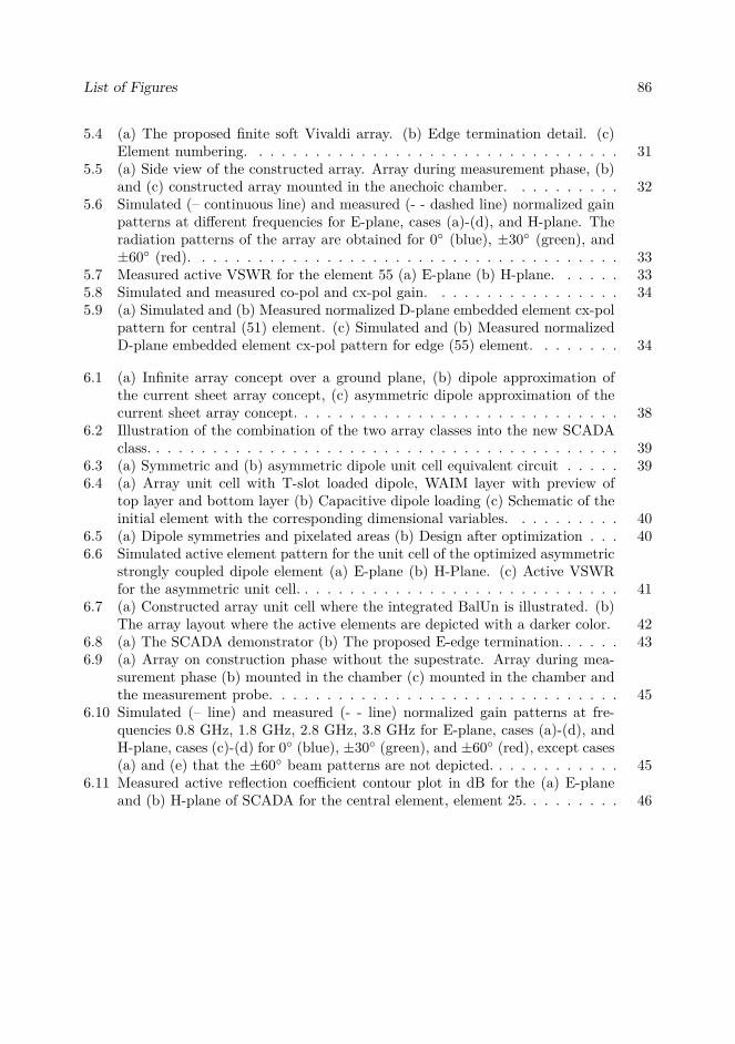
List of Figures 86
5.4 (a) The proposed finite soft Vivaldi array. (b) Edge termination detail. (c)Element numbering. . . . . . . . . . . . . . . . . . . . . . . . . . . . . . . . . 31
5.5 (a) Side view of the constructed array. Array during measurement phase, (b)and (c) constructed array mounted in the anechoic chamber. . . . . . . . . . 32
5.6 Simulated (– continuous line) and measured (- - dashed line) normalized gainpatterns at different frequencies for E-plane, cases (a)-(d), and H-plane. Theradiation patterns of the array are obtained for 0 (blue), ±30 (green), and±60 (red). . . . . . . . . . . . . . . . . . . . . . . . . . . . . . . . . . . . . . 33
5.7 Measured active VSWR for the element 55 (a) E-plane (b) H-plane. . . . . . 335.8 Simulated and measured co-pol and cx-pol gain. . . . . . . . . . . . . . . . . 345.9 (a) Simulated and (b) Measured normalized D-plane embedded element cx-pol
pattern for central (51) element. (c) Simulated and (b) Measured normalizedD-plane embedded element cx-pol pattern for edge (55) element. . . . . . . . 34
6.1 (a) Infinite array concept over a ground plane, (b) dipole approximation ofthe current sheet array concept, (c) asymmetric dipole approximation of thecurrent sheet array concept. . . . . . . . . . . . . . . . . . . . . . . . . . . . . 38
6.2 Illustration of the combination of the two array classes into the new SCADAclass. . . . . . . . . . . . . . . . . . . . . . . . . . . . . . . . . . . . . . . . . . 39
6.3 (a) Symmetric and (b) asymmetric dipole unit cell equivalent circuit . . . . . 396.4 (a) Array unit cell with T-slot loaded dipole, WAIM layer with preview of
top layer and bottom layer (b) Capacitive dipole loading (c) Schematic of theinitial element with the corresponding dimensional variables. . . . . . . . . . 40
6.5 (a) Dipole symmetries and pixelated areas (b) Design after optimization . . . 406.6 Simulated active element pattern for the unit cell of the optimized asymmetric
strongly coupled dipole element (a) E-plane (b) H-Plane. (c) Active VSWRfor the asymmetric unit cell. . . . . . . . . . . . . . . . . . . . . . . . . . . . . 41
6.7 (a) Constructed array unit cell where the integrated BalUn is illustrated. (b)The array layout where the active elements are depicted with a darker color. 42
6.8 (a) The SCADA demonstrator (b) The proposed E-edge termination. . . . . . 436.9 (a) Array on construction phase without the supestrate. Array during mea-
surement phase (b) mounted in the chamber (c) mounted in the chamber andthe measurement probe. . . . . . . . . . . . . . . . . . . . . . . . . . . . . . . 45
6.10 Simulated (– line) and measured (- - line) normalized gain patterns at fre-quencies 0.8 GHz, 1.8 GHz, 2.8 GHz, 3.8 GHz for E-plane, cases (a)-(d), andH-plane, cases (c)-(d) for 0 (blue), ±30 (green), and ±60 (red), except cases(a) and (e) that the ±60 beam patterns are not depicted. . . . . . . . . . . . 45
6.11 Measured active reflection coefficient contour plot in dB for the (a) E-planeand (b) H-plane of SCADA for the central element, element 25. . . . . . . . . 46

List of Figures 87
6.12 (a) Simulated and (b) Measured normalized D-plane embedded element cx-polpattern for central (25) element. (c) Simulated and (b) Measured normalizedD-plane embedded element cx-pol pattern for edge (29) element. . . . . . . . 47
6.13 Unit cell with integrated WAIM layer (a) front and (b) back view. . . . . . . 486.14 (a) Active VSWR for the unit cell. Simulated embedded element pattern for
the unit cell (b) E-plane (c) H-Plane . . . . . . . . . . . . . . . . . . . . . . . 486.15 Developed 8×8 array with integrated WAIM layer and corporate feed network.
Numbering from 1 to 8 from the front side view. . . . . . . . . . . . . . . . . 496.16 Photos of the constructed array when mounted on the anechoic chamber. . . 496.17 Measured active reflection coefficient in dB for the (a) sub-array no.1 (edge
sub-array) (b) sub-array no.5 (mid sub-array). . . . . . . . . . . . . . . . . . 506.18 Measured active reflection coefficient contour plot in dB for the (a) sub-array
no.1 (edge sub-array) (b) sub-array no.5 (mid sub-array). . . . . . . . . . . . 516.19 Measured and simulated normalized directivity in dB for the (a) E-plane and
(b) H-plane for the co- and cx-pol patterns at 2.5 GHz. . . . . . . . . . . . . 516.20 Array figure of merit for a selection of published antennas. All points are for
H-plane data. . . . . . . . . . . . . . . . . . . . . . . . . . . . . . . . . . . . . 52
7.1 Illustration of our current understanding of the evolution of the universe withfocus on the epochs of interest in this thesis. . . . . . . . . . . . . . . . . . . 55
7.2 (a) The 21cm hyperfine transition. (b) The 21cm cosmic hydrogen signal. . . 567.3 (a) Antenna beam and the celestial sphere (b) Antenna temperature system
decomposition. . . . . . . . . . . . . . . . . . . . . . . . . . . . . . . . . . . . 577.4 Illustration in Mollweide view of (a) 150 MHz scaled Haslam map (b) The CMB. 597.5 The spectral index β with angular dependence. . . . . . . . . . . . . . . . . . 607.6 Calculating methodology and FoM evaluation. . . . . . . . . . . . . . . . . . 617.7 (a) CLDA unit cell (b) VSWR performance. . . . . . . . . . . . . . . . . . . . 637.8 (a) Waterfall diagram for the antenna temperature for a single day (b) Nor-
malized CLDA directivity pattern projected into the celestial sphere. . . . . . 637.9 (a) Residual for the CLDA for different sky models (b) Differential residuals
after piecewise polynomial fit. . . . . . . . . . . . . . . . . . . . . . . . . . . . 64
8.1 Carbon footprint of telecommunications industry. (a) For the year 2002 to-tal estimated 151 Megatons. (b) Projected for the year 2020, estimated 349Megatons. . . . . . . . . . . . . . . . . . . . . . . . . . . . . . . . . . . . . . . 68
8.2 Percentage representation of the power consumption on a typical base station. 70

List of Tables
5.1 Dimensions in mm of the prototype with the integrated matching layer asdepicted in Fig. 5.2 and Fig. 5.4. . . . . . . . . . . . . . . . . . . . . . . . . . 30
6.1 Dimensions in mm of the initial design as depicted in Fig. 6.4. . . . . . . . . 406.2 Dimensions in mm of the SCADA demonstrator with the E-termination as
depicted in Fig. 6.8. . . . . . . . . . . . . . . . . . . . . . . . . . . . . . . . . 446.3 Dimensions in mm of the demonstrator with the integrated WAIM layer as
depicted in Fig. 6.13 and Fig. 6.15. . . . . . . . . . . . . . . . . . . . . . . . . 49
7.1 〈FoM(n)〉 in mK for the 5th polynomial order for antenna models with simu-lated pattern noise and filtering. . . . . . . . . . . . . . . . . . . . . . . . . . 64
88
Copyright © 2022 FDOKUMEN