Ultra-Wideband Microwave Imaging of

Heterogeneities

Matthew Yedlin a,b,∗, Anthony Cresp b, Christian Pichot b,Ioannis Aliferis b, Jean-Yves Dauvignac b, Stephane Gaffet c,

Guy Senechal d

aDepartment of Electrical and Computer Engineering, University of BritishColumbia, 2332 Main Mall, UBC Campus, Vancouver, Canada

bLaboratoire d’Electronique, Antennes et Telecommunications, Universite de NiceSophia – Antipolis, CNRS ; 250, rue Albert Einstein, FR-06560 Valbonne, France

cUMR Geosciences Azur, CNRS / UNSA / IRD / UPMC, Sophia – Antipolis,CNRS ; 250, rue Albert Einstein, FR-06560 Valbonne, France

dUMR 5212, Modelisation et Imagerie en Geosciences, Pau IPRA – Universite dePau et des Pays de l’Adour, BP 1155, FR-64013 Pau Cedex, France

Abstract

The technique of time-reversal acoustics was applied to image a bottle filled withsaline, using an eight element Vivaldi antenna array with frequency bandwidth 2 to8 GHz. At these short length scales, a smooth three-dimensional image of the bottlewas obtained, with the usual limitations imposed by limited offset and frequency.Time snapshots of the wavefield evolution in reversed time are presented for tworeal data sets. The first, shows the focusing for the single target of the bottle, whilethe second demonstrates the principle for two targets.

Key words: three-dimensional reverse-time imaging, ground penetrating radar,ultra-wideband imaging, migration

∗ Corresponding Author: Department of Electrical and Computer Engineering, Uni-versity of British Columbia, 2332 Main Mall, Vancouver, B.C., Canada.Tel.: 1 604 822 8236; fax: 1 604 822 5949

Email address: matty@ece.ubc.ca (Matthew Yedlin).

Preprint submitted to Journal of Applied Geophysics 5 August 2008

hal-0

0366

568,

ver

sion

1 -

26 M

ay 2

009

Author manuscript, published in "Journal of Applied Geophysics 68, 1 (2009) 17-25" DOI : 10.1016/j.jappgeo.2008.08.005

1 Introduction

Considerable effort and expertise has been expended in using microwaves as anenergy probe to obtain images of the interior of a target which is illuminated bysuch energy. There are two major areas of the use of microwaves for imagingtarget objects. One is the interior imaging of dielectric objects, via inversescattering as applied to the well-known exterior scattering problem and theother is the employment of ground penetrating radar (GPR) for imaging thenear surface of the earth as presented by numerous authors (Munk and Sheets,1997; Sneddon et al., 2002; Johnson and Poeter, 2003; Yarovoy et al., 2003;Daniels, 2004).

In the field of inverse scattering as is utilized for dielectric imaging, fields ofapplication encompass the detection of tumors in medicine (Miyakawa et al.,1999, 2004; Holmes et al., 2000) and non-destructive testing of concrete struc-tures (Pastorino et al., 2001; Marklein et al., 2002; Caorsi et al., 2004). Theprincipal algorithms used in these applications include diffraction tomographyat 3 GHz (Bolomey et al., 1982; Pichot et al., 1985) and non-linear inversiontechniques introduced by Pichot et al. (2004).

In this paper we present the application of microwave imaging to the exteriorscattering problem, in which we use ultra-wideband (UWB) electromagneticradiation (2 to 8 GHz) to illuminate a target consisting of a bottle of waterfilled with saline, which has a dielectric constant with real and imaginary parts.The radiated energy is recorded by an eight element exponentially taperedslot antenna (ETSA) array. To obtain the image of the scattering target,instead of using traditional inverse scattering techniques, which are generallyvery computationally intensive, we employ the reverse-time techniques of Finkand co-workers (Fink et al., 2000; Derode et al., 2002; Fink, 2006). For theexterior scattering problem, the technique of Fink has a complete analogywith the principles used in reverse-time migration, (Baysal et al., 1983; Changand McMechan, 1987, 1990; Wapenaar et al., 2005) in which the backgroundscattering models employed have a correlation length that is comparable orlarger than the propagation wavelength. The scattering data presented hereinare very localized and well-suited for the reverse-time algorithms, though theimages we obtain are not complete inversions yielding the dielectric structureof the scattering object. The reverse-time propagation of the single-targetscattering data are presented as a snapshot sequence. For comparison, a two-target snapshot sequence is also presented.

2

hal-0

0366

568,

ver

sion

1 -

26 M

ay 2

009

Fig. 1. View of the eight element exponentially tapered slot antenna array connectedto an eight to one multiplexer

2 Methods

2.1 Experimental Configuration for Ultra-Wideband Imaging

For the scattering experiment described in this research, we used a lineareight element array (Figure 1) of symmetric antipodal antennas, members ofthe exponentially tapered slot class, also known as Vivaldi antennas (Gibson,1979; Guillanton et al., 1998; Guillanton, 2000). Each exponentially taperedslot antenna (ETSA) was constructed on a Duroid substrate, with copperetching done using printed circuit technology. These antennas have a band-width from 1.4 GHz to 20 GHz with a reflection coefficient magnitude lessthan −10 dB over the entire band and therefore, they fall into the categoryof Ultra-Wideband (UWB) antennas. Their gain at 5 GHz is of the order of7 dB and at 9.5 GHz it is 10 dB. A detailed study by Chatelee (2006) hasdemonstrated that the inter-antenna coupling does not degrade the perfor-mance significantly if radiation frequencies are considered above 2.5 GHz.

3

hal-0

0366

568,

ver

sion

1 -

26 M

ay 2

009

2.2 Data Acquisition

The eight element array was deployed by sequentially using one antenna as atransmitter and then receiving scattered energy by the entire array, with arrayelements heretofore labeled by the letters A to H. The entire array was drivenby a two-port vector analyzer HP8720B with a bandwidth from .01 to 20 GHzand a frequency resolution of 100 kHz. Since only two ports were available,an electromechanical multiplexer (Guillanton, 2000) was employed. For thescattering experiment the bandwidth chosen was 2 to 8 GHz with frequencybinning of 15 MHz.

Two sets of data were collected. First a background set of data was collectedwithout the scattering target in place. Then a set of data was collected with thetarget in place. In the experimental setting considered, there was no interactionbetween the target scatterer and the background, enabling us to obtain thescattered electromagnetic field from the target via a simple subtraction of thetwo data sets. All data, collected in the frequency domain, was then inverseFourier transformed to obtain the time response.

2.3 Imaging Algorithm

In the scattering experiments we describe in this research, an incident wave,generated by a transmitter, impinges on a target, which creates a scatteredwave. The scattered wave is complicated, consisting of reflections, refractions,diffractions and surface waves. Our objective is to refocus the scattered wavecreated by the target and thus image the target, which is viewed as an effectiveensemble of secondary sources. One of the principal accepted algorithms forthis type of imaging is the application of generalized least squares methodswhich yields the target structure.

We have chosen an alternative method, a variant of that originally created byFink (2006) and applied to the refocusing of recorded scalar wavefields backto the source of the recorded scalar wavefield. The Fink technique, which isextremely effective in imaging heterogeneous media, is based on reciprocityand can be decomposed into two basic steps. In the first step, data recordedby an array of receivers, is time-reversed. In the second step, the time-reverseddata is retro-propagated from each receiver back into the medium in which thesource is located. If the medium is non-attenuating then it is intuitively clearthat the retro-propagated waves will constructively interfere at the source,yielding the focused source image. However, if the retro-propagation is per-formed on a computer, in which the velocity is an unknown parameter, thefocus will have a distribution centered at the wrong location. In addition, if the

4

hal-0

0366

568,

ver

sion

1 -

26 M

ay 2

009

array of receivers does not surround the source and is not sufficiently dense,the focus will be blurred.

Schematically, the time reverse algorithm is shown in Figure 2, in which tworeceivers obtain the scattered signal from a single transmitter. In Figure 2b,the scattered arrivals are presented in time-reversed fashion with t

′ = T − t.The retro-propagated and summed signals are shown in Figure 2c. Here theyinterfere constructively at the target location defined by t

′ = T − r0

c. With the

proper choice of the speed c, we note that the scattered signals constructivelyinterfere at the right location in time.

Mathematically, in a kinematic context, the foregoing procedure can be de-scribed as follows. First define the point source signal leaving the source asδ(t). The signal leaving the scatterer is given by δ

(

t − r0

c

)

, while the one ar-

riving at receiver 1 can be written as δ

(

t − r0+r1

c

)

and, in a similar way, the

signal at receiver 2 is δ

(

t − r0+r2

c

)

. Time-reversal corresponds to a change of

variable: the new time variable, t′ = T − t, reverses the time and contains

information on T , an appropriate stopping time.

In the example taken here, after time reversal, the source is located at timet′ = T , the scatterer at t

′ = T − r0

c, while arrivals at receivers 1,2 correspond

to t′ = T − r0+r1

cand t

′ = T − r0+r2

c, respectively.

Upon propagation of the time-reversed pulses, the signal from each receiveris appropriately delayed, resulting to a convolution with a delta function. Forreceiver 1, this operation gives:

δ

(

T −

[

t′ +

r0 + r1

c

])

∗ δ

(

t′ −

r1

c

)

= δ

(

T − t′ −

r0

c

)

(1)

while for receiver 2,

δ

(

T −

[

t′ +

r0 + r2

c

])

∗ δ

(

t′ −

r2

c

)

= δ

(

T − t′ −

r0

c

)

. (2)

We obtain the image by summing up contributions like 1 and 2.

Our algorithm is based on time-reversal followed by retro-propagation and isextended to consider vector wavefields. We assume that the scattered dataoriginates from an ensemble of non-interacting point scatterers. We call theseCSP’s (Candidate Scattering Points). We model the radiated field by the CSPas a short dipole with each dipole having the same amplitude. The receiversare also modeled as short dipoles. In fact, the retro-propagation is done usingthe Green’s function for the requisite wave propagation. Mathematically, we

5

hal-0

0366

568,

ver

sion

1 -

26 M

ay 2

009

replacemen

t

amplitu

de

t = 0 t = r0

ct = r0+r1

ct = r0+r2

ct = T

(a)

t′ = T − t

amplitu

de

t = T t′ = T − r0

ct′ = T − r0+r1

ct′ = T − r0+r2

ct′ = 0

(b)

t′ = T − t

amplitu

de

t = T t′ = T − r0

ct′ = 0

(c)

Fig. 2. (a) Schematic of a transmitted wave travelling a distance r0 to the target andrecorded at two receivers respectively located at a distance r1 and r2 from the target.Shown here is the complete idealized delta function time series—the transmitteddata leaving the source, the arrival time at the scatterer and the arrival time ateach receiver. b) Time-reversed version of a). c) Retropropagation of time-reverseddata back to the scatterer with the resultant constructive interference at t′ = T − r0

c.

write the frequency domain Green’s function as

E = −jZ0Idl

2πk0

cos θ

(

jk0

r2+

1

r3

)

e−jk0rar

+jZ0Idl

4πk0

sin θ

(

−k

20

r+

jk0

r2+

1

r3

)

e−jk0raθ

(3)

where I is the dipole current, dl is the dipole length, Z0 is the impedanceof free space and k0 is the free space wave number, which is assumed to be

6

hal-0

0366

568,

ver

sion

1 -

26 M

ay 2

009

known.

We note that the Green’s function can be rewritten in terms of impulse func-tions, their derivatives and integrals, so that the retro-propagation can becarried out efficiently. The algorithm for imaging used in this research is sum-marized below as follows:

For each imaging experiment:

For each transmission from the array elements (A-H)

For each Candidate Scattering Point (CSP)

For each receiving antenna (A-H)

1. Compute the distance from the antenna to the CSP;

2. Time reverse the received signal;

3. Retropropagate the signal to the CSP using the

dipole Green’s function,

with the distance from step 1;

4. Weight the data computed in step 3;

5. Accumulate the data computed in step 4.

end

end

Differentiate the accumulated data with respect to time

and compute the integrated energy

end

end

The foregoing description of the imaging algorithm assumes that the secondarysource dipole and the receiving dipole lie in the same plane, in this case z = 0.If we are imaging CSP’s at z 6= 0, we must project the secondary dipole vectoronto the receiving dipole, after doing the weighting in step 4.

3 Results

3.1 Results for UWB Reverse-Time Imaging

In this Section we present the results of using the reverse time imaging algo-rithm described above to the scattering data collected using the techniquesdescribed in Section 2.2. Figure 3 shows the experimental configuration of thearray, with the target symmetrically positioned a distance 40 cm from thecenter of the array. The ETSA spacing is 5 cm with a total array length of35 cm. Given that the performance of the antenna elements is not significantlyaffected by mutual coupling in the frequency band of interest, 2 to 8 GHz, eachelement may be considered as an independent transmitter/receiver. For the

7

hal-0

0366

568,

ver

sion

1 -

26 M

ay 2

009

A

B

C

D

E

F

G

H

35 cm 5 cm40 cm

Fig. 3. Schematic of scattering experiment from the eight element Vivaldi antennaarray. The target bottle is located 40 cm from the array and can be considered tobe in the far field.

geometry of Figure 3, with the largest dimension, D, of each ETSA of theorder of 10 cm, we find that for frequencies between 2 and 5.3 GHz, we are inthe far-field while for frequencies between 5.3 and 8 GHz, we are in the radi-ating near-field region. Thus we use the complete vector for the infinitesimaldipole to include all the relevant terms.

Figure 4 shows a single transmission experiment with antenna A as the trans-mitter and antennas A through H as receivers. The scattered hyperbolic arrivalfrom the target, located at 40 cm from the center of the array, is very clear andhas been obtained by subtracting the background scattered field, as describedpreviously. The arrivals are essentially pulses, due to the large bandwidth of6 GHz. We note that antenna A, the transmitter, also acting as a receiver,has a spurious arrival near 0 ns, possibly due to the network analyzer cali-bration, since a separate circuit is used to obtain a response from an antennathat is used in transmission and reception. This artifact will be evident in alltransmission experiments presented.

Shown to the right of the differentially processed data is the image obtainedusing the retro-propagation algorithm described earlier. At each candidatescattering point, the summed time-reversed, retropropagated data is squaredthen integrated over time, with the total integral assigned to the pixel repre-senting the CSP. This energy image in normalized to the maximum and thenconverted to dB. Figure 4 is the image of the scatterer in the z = 0 plane,

8

hal-0

0366

568,

ver

sion

1 -

26 M

ay 2

009

B C D E F G H0.0

0.5

1.0

1.5

2.0

2.5

3.0

3.5

4.0

4.5

5.0

tim

e(n

s)A

0 dB0

0 5

10

10 15

20

20 25

30

30 35

40

50

60

70

−2

−4

−6

−8

−10

−12

−14

−16

−18

−20

antenna array (cm)

pro

pag

atio

n(c

m)

Fig. 4. Antenna A is the transmitter with scattered data, seen as a hyperbolicarrival, on the left, recorded by the whole array. On the right is the normalizedimage, expressed in dB relative to the maximum, with the white circle representingthe bottle in the z = 0 plane.

with the cross-section of the target shown by the white circle. The same dataand image format are shown in Figure 5 through 11, sequentially presented toillustrate the data and image obtained, as each antenna functions as a trans-mitter, with the whole array receiving. A final image is shown in Figure 12.The image on the left was obtained by stacking the images obtained from theeight transmission experiments, scaling by the maximum value and convertingto dB and the one on the right is −3 dB threshold, meaning that all powervalues, less than half of the maximum, associated with a particular CSP, areassigned the deepest blue.

So far, we have presented images of the target at z=0. We expect that themethod will work at other levels of z, since the target has limited extent inthe z direction (z = 0 is in the middle of the target, which has a total heightof 35 cm). In Figure 13, six panels are presented that show the target imageat increments of 5 cm. The format of presentation is the same as Figure 12,normalized and thresholded at −3 dB. We would expect the target to disap-pear at z = 17.5 cm. We note that indeed somewhere, between the z = 15 andz = 20 cm panels, the target is much weaker, if we compare the normalizeddB values. To obtain the images in this figure, the extra step of polarizationprojection was done, since the secondary sources and the receiving antennas,modeled as dipoles, are not co-planar.

9

hal-0

0366

568,

ver

sion

1 -

26 M

ay 2

009

A C D E F G H0.0

0.5

1.0

1.5

2.0

2.5

3.0

3.5

4.0

4.5

5.0

tim

e(n

s)B

0 dB0

0 5

10

10 15

20

20 25

30

30 35

40

50

60

70

−2

−4

−6

−8

−10

−12

−14

−16

−18

−20

antenna array (cm)

pro

pag

atio

n(c

m)

Fig. 5. Same images as in Fig. 4 with antenna B as transmitter.

A B D E F G H0.0

0.5

1.0

1.5

2.0

2.5

3.0

3.5

4.0

4.5

5.0

tim

e(n

s)

C

0 dB0

0 5

10

10 15

20

20 25

30

30 35

40

50

60

70

−2

−4

−6

−8

−10

−12

−14

−16

−18

−20

antenna array (cm)

pro

pag

atio

n(c

m)

Fig. 6. Same images as in Fig. 4 with antenna C as transmitter.

3.2 Retropopagation Movies

In Figure 14, a sequence of twelve energy snapshots is shown, whose computa-tion is based on the algorithm described in Subsection 2.3. The first snapshotin the sequence is Figure 14a while the snapshot corresponding to the bestfocus at the scatterer, located at a distance 40 cm from the front of the arrayand centered at 17.5 cm, corresponds to Figure 14j.

10

hal-0

0366

568,

ver

sion

1 -

26 M

ay 2

009

A B C E F G H0.0

0.5

1.0

1.5

2.0

2.5

3.0

3.5

4.0

4.5

5.0

tim

e(n

s)D

0 dB0

0 5

10

10 15

20

20 25

30

30 35

40

50

60

70

−2

−4

−6

−8

−10

−12

−14

−16

−18

−20

antenna array (cm)

pro

pag

atio

n(c

m)

Fig. 7. Same images as in Fig. 4 with antenna D as transmitter.

A B C D F G H0.0

0.5

1.0

1.5

2.0

2.5

3.0

3.5

4.0

4.5

5.0

tim

e(n

s)

E

0 dB0

0 5

10

10 15

20

20 25

30

30 35

40

50

60

70

−2

−4

−6

−8

−10

−12

−14

−16

−18

−20

antenna array (cm)

pro

pag

atio

n(c

m)

Fig. 8. Same images as in Fig. 4 with antenna E as transmitter.

A second sequence is shown in Figure 15, in which twelve energy snapshots arealso presented, for the case of two targets. The first target is the same as thatused in Figure 14 but located at a distance of 43 cm and at a lateral distanceof 21 cm, while the second target is a metallic cylinder of radius 2 cm, locatedat 37.5 cm from the front of the array and at a lateral distance of 7.5 cm. Inthis example, it is not as easy to pinpoint the snapshot corresponding to thebest focus, due to the fact that the time for best focusing is not identical for

11

hal-0

0366

568,

ver

sion

1 -

26 M

ay 2

009

A B C D E G H0.0

0.5

1.0

1.5

2.0

2.5

3.0

3.5

4.0

4.5

5.0

tim

e(n

s)F

0 dB0

0 5

10

10 15

20

20 25

30

30 35

40

50

60

70

−2

−4

−6

−8

−10

−12

−14

−16

−18

−20

antenna array (cm)

pro

pag

atio

n(c

m)

Fig. 9. Same images as in Fig. 4 with antenna F as transmitter.

A B C D E F H0.0

0.5

1.0

1.5

2.0

2.5

3.0

3.5

4.0

4.5

5.0

tim

e(n

s)

G

0 dB0

0 5

10

10 15

20

20 25

30

30 35

40

50

60

70

−2

−4

−6

−8

−10

−12

−14

−16

−18

−20

antenna array (cm)

pro

pag

atio

n(c

m)

Fig. 10. Same images as in Fig. 4 with antenna G as transmitter.

the two targets. A better focusing criterion will be the center of attention forfuture work.

12

hal-0

0366

568,

ver

sion

1 -

26 M

ay 2

009

A B C D E F G0.0

0.5

1.0

1.5

2.0

2.5

3.0

3.5

4.0

4.5

5.0

tim

e(n

s)H

0 dB0

0 5

10

10 15

20

20 25

30

30 35

40

50

60

70

−2

−4

−6

−8

−10

−12

−14

−16

−18

−20

antenna array (cm)

pro

pag

atio

n(c

m)

Fig. 11. Same images as in Fig. 4 with antenna H as transmitter.

0 dB0

0

10

10

20

20

30

30

40

50

60

70

−2

−4

−6

−8

−10

−12

−14

−16

−18

−20

antenna array (cm)

pro

pag

atio

n(c

m)

0 dB0

0

10

10

20

20

30

30

40

50

60

70

−0.5

−1.0

−1.5

−2.0

−2.5

−3.0

antenna array (cm)

pro

pag

atio

n(c

m)

Fig. 12. Stacked images, at z = 0 of the previous eight experiments, normalized andconverted to dB. The one on the left is a full scale image whereas the other one isa −3 dB threshold image.

4 Discussion

The results of Section 3.1 clearly show promise in imaging scatterers in anexterior experiment, that is, when an isolated scatterer can be illuminatedusing a UWB array. The images obtained are blurred due to aperture effects

13

hal-0

0366

568,

ver

sion

1 -

26 M

ay 2

009

0 dB0

0 5

10

10 15

20

20 25

30

30 35

40

50

60

70

−0.5

−1.0

−1.5

−2.0

−2.5

−3.0

(a)

0 dB0

0 5

10

10 15

20

20 25

30

30 35

40

50

60

70

−0.5

−1.0

−1.5

−2.0

−2.5

−3.0

(b)

0 dB0

0 5

10

10 15

20

20 25

30

30 35

40

50

60

70

−0.5

−1.0

−1.5

−2.0

−2.5

−3.0

(c)

replacemen

0 dB0

0 5

10

10 15

20

20 25

30

30 35

40

50

60

70

−0.5

−1.0

−1.5

−2.0

−2.5

−3.0

(d)

0 dB0

0 5

10

10 15

20

20 25

30

30 35

40

50

60

70

−0.5

−1.0

−1.5

−2.0

−2.5

−3.0

(e)

0 dB0

0 5

10

10 15

20

20 25

30

30 35

40

50

60

70

−0.5

−1.0

−1.5

−2.0

−2.5

−3.0

(f)

Fig. 13. Stacked images, at different z levels, of the eight target illuminations, nor-malized and converted to dB, with a −3 dB threshold scale; a) z = 5 cm; b)z = 10 cm; c) z = 15 cm; d) z = 20 cm; e) z = 25 cm; f) z = 30 cm. The horizon-tal axis corresponds to the antenna array and the vertical one to the propagationdistance, both in centimeters.

and the limited bandwidth of 6 GHz. More resolved images can be obtainedby using a wider bandwidth and by employing a larger array size, an effortthat is already underway at LEAT.

The reverse-time algorithm can also be improved using a more sophisticatedmodel of the receiving antenna, which is currently modeled as an electricallysmall dipole. Despite the simplifications of the re-radiating process and themodel for the antennas, initial images were obtained that approximately con-form to the target.

The initial success of the employment of these high-frequency Vivaldi anten-nas indicate the promise of using a lower frequency antenna as an alternative

14

hal-0

0366

568,

ver

sion

1 -

26 M

ay 2

009

0 dB0

0

10

10

20

20

30

30

40

50

60

−2−4−6−8−10−12−14−16−18−20

(a)

0 dB0

0

10

10

20

20

30

30

40

50

60

−2−4−6−8−10−12−14−16−18−20

(b)

0 dB0

0

10

10

20

20

30

30

40

50

60

−2−4−6−8−10−12−14−16−18−20

(c)

0 dB0

0

10

10

20

20

30

30

40

50

60

−2−4−6−8−10−12−14−16−18−20

(d)

0 dB0

0

10

10

20

20

30

30

40

50

60

−2−4−6−8−10−12−14−16−18−20

(e)

0 dB0

0

10

10

20

20

30

30

40

50

60

−2−4−6−8−10−12−14−16−18−20

(f)

0 dB0

0

10

10

20

20

30

30

40

50

60

−2−4−6−8−10−12−14−16−18−20

(g)

0 dB0

0

10

10

20

20

30

30

40

50

60

−2−4−6−8−10−12−14−16−18−20

(h)

0 dB0

0

10

10

20

20

30

30

40

50

60

−2−4−6−8−10−12−14−16−18−20

(i)

0 dB0

0

10

10

20

20

30

30

40

50

60

−2−4−6−8−10−12−14−16−18−20

(j)

0 dB0

0

10

10

20

20

30

30

40

50

60

−2−4−6−8−10−12−14−16−18−20

(k)

0 dB0

0

10

10

20

20

30

30

40

50

60

−2−4−6−8−10−12−14−16−18−20

(ℓ)

Fig. 14. Twelve sequential snapshots, a) to l), of retropropagated scattered energyfrom a plastic bottle target, of radius 4 cm, filled with saline. The target is locatedat 40 cm from the front of the antenna array and laterally at the array center.The horizontal axis corresponds to the antenna array and the vertical one to thepropagation distance, both in centimeters.

15

hal-0

0366

568,

ver

sion

1 -

26 M

ay 2

009

0 dB0

0

10

10

20

20

30

30

40

50

60

−2−4−6−8−10−12−14−16−18−20

(a)

0 dB0

0

10

10

20

20

30

30

40

50

60

−2−4−6−8−10−12−14−16−18−20

(b)

0 dB0

0

10

10

20

20

30

30

40

50

60

−2−4−6−8−10−12−14−16−18−20

(c)

0 dB0

0

10

10

20

20

30

30

40

50

60

−2−4−6−8−10−12−14−16−18−20

(d)

0 dB0

0

10

10

20

20

30

30

40

50

60

−2−4−6−8−10−12−14−16−18−20

(e)

0 dB0

0

10

10

20

20

30

30

40

50

60

−2−4−6−8−10−12−14−16−18−20

(f)

0 dB0

0

10

10

20

20

30

30

40

50

60

−2−4−6−8−10−12−14−16−18−20

(g)

0 dB0

0

10

10

20

20

30

30

40

50

60

−2−4−6−8−10−12−14−16−18−20

(h)

0 dB0

0

10

10

20

20

30

30

40

50

60

−2−4−6−8−10−12−14−16−18−20

(i)

0 dB0

0

10

10

20

20

30

30

40

50

60

−2−4−6−8−10−12−14−16−18−20

(j)

0 dB0

0

10

10

20

20

30

30

40

50

60

−2−4−6−8−10−12−14−16−18−20

(k)

0 dB0

0

10

10

20

20

30

30

40

50

60

−2−4−6−8−10−12−14−16−18−20

(ℓ)

Fig. 15. Twelve snapshots of the energy retropropagated as a function of reversetime for the two-target case, consisting of a plastic bottle filled with saline and anadjacent metal cylinder. The horizontal axis corresponds to the antenna array andthe vertical one to the propagation distance, both in centimeters.

16

hal-0

0366

568,

ver

sion

1 -

26 M

ay 2

009

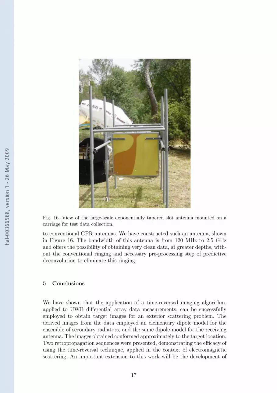
Fig. 16. View of the large-scale exponentially tapered slot antenna mounted on acarriage for test data collection.

to conventional GPR antennas. We have constructed such an antenna, shownin Figure 16. The bandwidth of this antenna is from 120 MHz to 2.5 GHzand offers the possibility of obtaining very clean data, at greater depths, with-out the conventional ringing and necessary pre-processing step of predictivedeconvolution to eliminate this ringing.

5 Conclusions

We have shown that the application of a time-reversed imaging algorithm,applied to UWB differential array data measurements, can be successfullyemployed to obtain target images for an exterior scattering problem. Thederived images from the data employed an elementary dipole model for theensemble of secondary radiators, and the same dipole model for the receivingantenna. The images obtained conformed approximately to the target location.Two retropropagation sequences were presented, demonstrating the efficacy ofusing the time-reversal technique, applied in the context of electromagneticscattering. An important extension to this work will be the development of

17

hal-0

0366

568,

ver

sion

1 -

26 M

ay 2

009

an appropriate stopping condition, in order to obtain the image with the bestfocus.

Acknowledgments

The authors would like to thank Jean-Louis Le Sonn, Laurent Brochier andFranck Perret for making the data collection possible.

References

Baysal, E., Kosloff, D., Sherwood, J., 1983. Reverse time migration. Geo-physics 48, 1514.

Bolomey, J.-C., Izadnegahdar, A., Jofre, L., Pichot, C., Peronnet, G.,Solaimani, M., November 1982. Microwave Diffraction Tomography forBiomedical Applications. IEEE Transactions on Microwave Theory andTechniques 30 (11), 1998–2000.

Caorsi, S., Massa, A., Pastorino, M., Donelli, M., June 2004. Improvedmicrowave imaging procedure for nondestructive evaluations of two-dimensional structures. IEEE Transactions on Antennas and Propagation52 (6), 1386–1397.

Chang, W., McMechan, G., 1987. Elastic reverse-time migration. Geophysics52, 1365.

Chang, W., McMechan, G., 1990. 3D acoustic prestack reverse-time migration1. Geophysical Prospecting 38 (7), 737–755.

Chatelee, V., December 2006. Developpement d’un systeme d’imagerie mi-croonde multistatique ultra large bande. Application a la detection d’objetsen regime temporel et frequentiel. Ph.D. thesis, Universite de Nice SophiaAntipolis.

Daniels, D. J., 2004. Ground Penetrating Radar, 2nd Edition. No. 15 in IEERadar, Sonar, Navigation and Avionics Series. The Institution of ElectricalEngineers, London.

Derode, A., Tourin, A., Fink, M., May 2002. Time reversal versus phase conju-gation in a multiple scattering environment. Ultrasonics 40 (1–8), 275–280.

Fink, M., July-August 2006. Time-reversal acoustics in complex environments.Geophysics 71 (4), SI151–SI164.

Fink, M., Cassereau, D., Derode, A., Prada, C., Roux, P., Tanter, M., Thomas,J.-L., Wu, F., December 2000. Time-reversed acoustics. Reports on Progressin Physics 63 (12), 1933–1995.

Gibson, P., September 17–21, 1979. The Vivaldi aerial. In: Proceedings of the9th European Microwave Conference. Brighton, UK, pp. 101–105.

Guillanton, E., December 2000. Etude d’un systeme d’imagerie microonde

18

hal-0

0366

568,

ver

sion

1 -

26 M

ay 2

009

multistatique-multifrequence pour la reconstruction d’objets enfouis. Ph.D.thesis, Universite de Nice Sophia Antipolis.

Guillanton, E., Dauvignac, J.-Y., Pichot, C., Cashman, J., November 1998. Anew design tapered slot antenna for ultra-wideband applications. Microwaveand Optical Technology Letters 19 (4), 286–289.

Holmes, J. F., Jacques, S. L., Hunt, J. M., 2000. Adapting atmospheric LI-DAR techniques to imaging biological tissue. In: Proceedings of SPIE —the International Society for Optical Engineering. Vol. 3927. pp. 226–231.

Johnson, R. H., Poeter, E. P., 2003. Interpreting DNAPL saturations in alaboratory-scale injection with GPR data and direct core measurements.Tech. rep., U.S. Geological Survey.URL http://pubs.usgs.gov/of/2003/ofr-03-349/

Marklein, R., Mayer, K., Hannemann, R., Krylow, T., Balasubramanian, K.,Langenberg, K., Schmitz, V., December 2002. Linear and nonlinear inversionalgorithms applied in nondestructive evaluation. Inverse Problems 18 (6),1733–1759.

Miyakawa, M., Ishida, T., Watanabe, M., September 1–5, 2004. Imaging ca-pability of an early stage breast tumor by CP-MCT. In: Proceedings of the27th Annual International Conference of the IEEE Engineering in Medicineand Biology Society (IEMBS 2004). Vol. 2. pp. 1427–1430.

Miyakawa, M., Orikasa, K., Ishi, N., Bertero, M., Boccacci, P., October 1999.Numerical analysis of CP-MCT and image restoration by the computedprojection. Vol. 2. p. 1109.

Munk, J., Sheets, R., 1997. Detection of underground voids in Ohio by use ofgeophysical methods. Tech. rep., U.S. Geological Survey.

Pastorino, M., Caorsi, S., Massa, A., May 21–23; 2001. A global optimizationtechnique for microwave nondestructive evaluation. In: Proceedings of the18th IEEE Instrumentation and Measurement Technology Conference (imtc2001). Vol. 3. pp. 1916–1920.

Pichot, C., Dauvignac, J.-Y., Aliferis, I., Le Brusq, E., Ferraye, R., Chatelee,V., May 14, 2004. Recent Nonlinear Inversion Methods and MeasurementSystem for Microwave Imaging. In: Proceedings of the IEEE InternationalWorkshop on Imaging Systems and Techniques. Stresa, Italy, pp. 95–99.

Pichot, C., Jofre, L., Peronnet, G., Bolomey, J.-C., April 1985. Active Mi-crowave Imaging of Inhomogeneous Bodies. IEEE Transactions on Antennasand Propagation 33 (4), 416–425.

Sneddon, K. W., Powers, M. H., Johnson, R. H., Poeter, E. P., 2002. ModelingGPR data to interpret porosity and DNAPL saturations for calibration ofa 3-D multiphase flow simulation. Tech. rep., U.S. Geological Survey.URL http://pubs.usgs.gov/of/2002/ofr-02-451/

Wapenaar, K., Fokkema, J., Snieder, R., 2005. Retrieving the Green’s functionin an open system by cross correlation: A comparison of approaches (L). TheJournal of the Acoustical Society of America 118, 2783.

Yarovoy, A., Ligthart, L. P., Schukin, A., Kaploun, I., May 2003. Full-polarimetric video impulse radar for landmine detection: experimental ver-

19

hal-0

0366

568,

ver

sion

1 -

26 M

ay 2

009

ification of main ideas. In: Proceedings of the 2nd International Workshopon Advanced GPR. Delft, Netherlands, pp. 148–155.

20

hal-0

0366

568,

ver

sion

1 -

26 M

ay 2

009