arX

iv:0

911.

0702

v2 [

cond

-mat

.sof

t] 1

1 A

ug 2

010

Spatial and temporal dynamical heterogeneities approaching the bi-nary colloidal glass transition

Takayuki Narumi, a Scott V. Franklin,b Kenneth W. Desmond,c Michio Tokuyama,d and Eric R.Weeks∗c

We study concentrated binary colloidal suspensions, a model system which has a glass transition as the volume fractionφ ofparticles is increased. We use confocal microscopy to directly observe particle motion within dense samples withφ rangingfrom 0.4 to 0.7. Our binary mixtures have a particle diameterratio dS/dL = 1/1.3 and particle number ratioNS/NL = 1.56,which are chosen to inhibit crystallization and enable long-time observations. Near the glass transition we find that particledynamics are heterogeneous in both space and time. The most mobile particles occur in spatially localized groups. The lengthscales characterizing these mobile regions grow slightly as the glass transition is approached, with the largest length scales seenbeing∼ 4 small particle diameters. We also study temporal fluctuations using the dynamic susceptibilityχ4, and find that thefluctuations grow as the glass transition is approached. Analysis of both spatial and temporal dynamical heterogeneityshow thatthe smaller species play an important role in facilitating particle rearrangements. The glass transition in our sampleoccurs atφg ≈ 0.58, with characteristic signs of aging observed for all samples withφ > φg.

1 Introduction

As the temperature of a glass-forming liquid is lowered, theviscosity rises by many orders of magnitude, becoming exper-imentally difficult to measure, with little change in the struc-ture1–3. The origin of the slowing dynamics is not yet clear,despite much prior work. One intriguing observation is thatas a sample approaches the glass transition, the motion withinthe sample becomes spatially heterogeneous4,5. While overallmotion within the sample slows, some regions exhibit fasterdynamics than the rest, and over time these mobile regions ap-pear and disappear throughout the sample. Particles withinthemobile region move cooperatively, forming spatially extendedclusters and strings6.

One technique for studying the glass transition is the use ofcolloidal suspensions7. These are composed of small solidparticles suspended in a solvent. The particles need to besmall enough to undergo Brownian motion, so particle diam-eters are typically 10− 5000 nm. The key control param-eter is the volume fractionφ. For a monodisperse sample(all particles similar in size), the sample becomes glassy forφ > φg ≈ 0.587,8. The glass transition in colloidal samples hasbeen studied extensively by light scattering, microscopy,andother techniques. Colloidal samples exhibit many behaviorsseen in molecular glasses, such as dramatic increases in vis-cosity9,10, strongly slowing relaxation time scales8,11–16, mi-

a Department of Applied Quantum Physics and Nuclear Engineering, KyushuUniversity, Fukuoka, Japan 819-0395. E-mail: narumi@athena.ap.kyushu-u.ac.jpb Department of Physics, Rochester Institute of Technology,Rochester, NY14623-5603c Department of Physics, Emory University, Atlanta, Georgia30322d WPI Advanced Institute for Material Research and Instituteof Fluid Sci-ence, Tohoku University, Sendai, Japan 980-8577

croscopic disorder17, spatially heterogeneous dynamics18–21,aging behavior for glassy samples13,22–27, and sensitivity tofinite size effects28,29. Light scattering allows careful study ofthe average behavior of millions of colloidal particles, whilemicroscopy techniques observe the detailed behavior of a fewthousand particles. These complementary techniques have re-sulted in connections between different aspects of glassy be-havior: for example, showing that aging is temporally andspatially heterogeneous22,23, and connecting dynamical het-erogeneity with the slowing relaxation time scales8,13,19,20,30.

In this paper, we study the glass transition of binary col-loidal suspensions using confocal microscopy. We use binarysuspensions (mixtures of two particle sizes) to inhibit crystal-lization. This allows us to take data over many hours, a timescale in which a monodisperse sample would crystallize31,32.Furthermore, this lets us investigate the role the two particlespecies play in the dynamics; prior work has suggested thatsmall particles play a lubricating role in the local dynamics33.Prior studies have also seen a connection between the localstructure and the mobility of particles34–37. Using a binarysample results in more obvious structural variations due tospatial variability of the composition, helping highlighthowstructure influences the dynamics.

The confocal microscope enables direct visualization of theinterior of the sample, and we follow the motion of severalthousand colloidal particles within each sample38. Particlesmove in spatially heterogeneous groups, and we character-ize this motion using two-particle two-time correlation func-tions39–41 that have previously been used on monodispersesuspensions42. From these we extract a length scale for theheterogeneity, which increases as the glass transition is ap-proached. By simultaneously tracking both large and smallparticles, we can observe the similarities and differencesbe-

1–12 | 1

tween the two species’ dynamics. In particular, we see thatsmall local composition fluctuations influence mobility. Asmight be expected, regions with more large particles tend tobeless mobile, while those with more small particles tend to bemore mobile. Additionally, we study temporal heterogeneityusing a different correlation function, the dynamic susceptibil-ity χ4

43–45, which has not been previously applied to colloidaldata. As measured by this correlation function, the temporalheterogeneity increases as the glass transition is approached.

2 Experimental Method

We prepare suspensions of poly-(methyl-methacrylate)(PMMA) colloids stabilized sterically by a thin layer ofpoly-12-hydroxystearic acid7. We use a binary mixture witha large particle mean radiusaL = 1.55 µm and small particlemean radiusaS = 1.18 µm, the same size particles used in aprior study by our group28. The polydispersity is 5%; eachindividual particle species can crystallize in a monodispersesuspension. Separately from the polydispersity, the mean par-ticle radii each have an uncertainty of±0.02µm. The numberratio of small particles to large particles isNS/NL = 1.56,resulting in a volume fraction ratioφS/φL ≈ 0.70. The controlparameter is the total volume fractionφ = φS+ φL. Crystal-lization and segregation were not observed to occur during thecourse of our measurements. All particles are fluorescentlydyed and suspended in a density- and index-matched mixtureof decalin and cyclohexyl bromide to prevent sedimentationand allow us to see into the sample. Particles are slightlycharged as a result of the dyeing process and this particularsolvent mixture32. Nonetheless, we use the hard spherevolume fractionφ as the control parameter. The hard sphereradii (aL,aS) are determined from diffusion measurements ofthe individual species at dilute concentrations (φ < 0.01).

Suspensions are sealed in microscope chambers and con-focal microscopy is used to observe the particle dynamics atambient temperature38,46. A representative two-dimensionalimage is shown in Fig. 1. A volume of 55×55×20µm3 canbe taken at speeds of up to 1 Hz. (As will be shown later,in these concentrated samples, particles do not move signifi-cantly on this time scale.) To avoid influences from the walls,we focus at least 25µm away from the coverslip.

Within each three-dimensional image, we identify bothlarge and small particles. This is accomplished with a singleconvolution that identifies spherical, bright regions47; the con-volution kernel is a three-dimensional Gaussian with a widthchosen to match the size of the image of a large particle. Eachlocal maximum after the convolution is identified as a parti-cle47. The distribution of particle brightnesses is bimodal withlittle overlap, and so small and large particles can be easily dis-tinguished. Our method is the same as is often used to measureparticle positions in two dimensions, which normally achieves

Fig. 1 A two-dimensional image of our sample taken by a confocalmicroscope. The scale bar represents 10µm.

sub-pixel resolution in particle positions47. However, giventhat a single convolution kernel is used to identify both particletypes, when applied to our binary samples we do not achievesub-pixel accuracy. Instead, our uncertainty in locating parti-cle positions is linked to the pixel size and is 0.2µm in x andy,and 0.3µm in z. We do have accurate discrimination betweenlarge and small particles with this method, with less than 1%of the particles misidentified, checked by visual inspection.For a few particles, it is hard to distinguish if they are largeor small (because they are small but unusually bright, or largebut unusually dim). These particles are assigned to the sizethat they appear to be the majority of the time.

After identifying the particle positions, they are trackedus-ing standard software46,47. The key requirement is that parti-cles move less between time steps than their interparticle spac-ing, which is easily satisfied in our dense glassy samples. Wetake images once every 10 - 150 s, depending on the volumefraction, in each case making sure that the acquisition rateissufficiently rapid to capture all particle movements.

3 Results and Discussion

3.1 Structural characteristics

We begin by looking at the structure of the binary sample.Shown in Fig. 2 is the pair correlation functiong(r) of a sam-ple with volume fractionφ = 0.57. g(r) relates to the likeli-hood of finding a particle a distancer away from a referenceparticle. The three curves correspond to small-small, small-

2 |

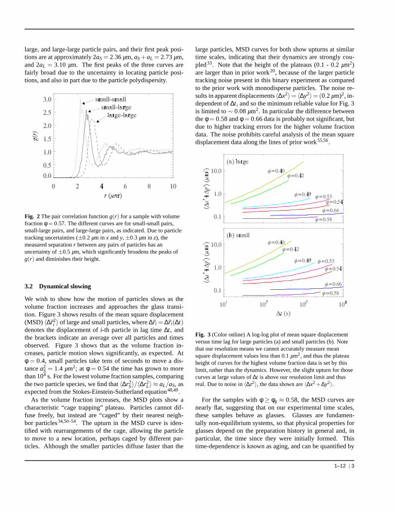
large, and large-large particle pairs, and their first peak posi-tions are at approximately 2aS= 2.36µm, aS+aL = 2.73µm,and 2aL = 3.10 µm. The first peaks of the three curves arefairly broad due to the uncertainty in locating particle posi-tions, and also in part due to the particle polydispersity.

Fig. 2 The pair correlation functiong(r) for a sample with volumefractionφ = 0.57. The different curves are for small-small pairs,small-large pairs, and large-large pairs, as indicated. Due to particletracking uncertainties (±0.2 µm in x andy, ±0.3 µm in z), themeasured separationr between any pairs of particles has anuncertainty of±0.5 µm, which significantly broadens the peaks ofg(r) and diminishes their height.

3.2 Dynamical slowing

We wish to show how the motion of particles slows as thevolume fraction increases and approaches the glass transi-tion. Figure 3 shows results of the mean square displacement(MSD) 〈∆~r2

i 〉 of large and small particles, where∆~r i = ∆~r i(∆t)denotes the displacement ofi-th particle in lag time∆t, andthe brackets indicate an average over all particles and timesobserved. Figure 3 shows that as the volume fraction in-creases, particle motion slows significantly, as expected.Atφ = 0.4, small particles take tens of seconds to move a dis-tancea2

S = 1.4 µm2; at φ = 0.54 the time has grown to morethan 104 s. For the lowest volume fraction samples, comparingthe two particle species, we find that〈∆r2

S〉/〈∆r2L〉 ≈ aL/aS, as

expected from the Stokes-Einstein-Sutherland equation48,49.As the volume fraction increases, the MSD plots show a

characteristic “cage trapping” plateau. Particles cannotdif-fuse freely, but instead are “caged” by their nearest neigh-bor particles34,50–54. The upturn in the MSD curve is iden-tified with rearrangements of the cage, allowing the particleto move to a new location, perhaps caged by different par-ticles. Although the smaller particles diffuse faster thanthe

large particles, MSD curves for both show upturns at similartime scales, indicating that their dynamics are strongly cou-pled33. Note that the height of the plateaus (0.1 - 0.2µm2)are larger than in prior work20, because of the larger particletracking noise present in this binary experiment as comparedto the prior work with monodisperse particles. The noise re-sults in apparent displacements〈∆x2〉= 〈∆y2〉=(0.2µm)2, in-dependent of∆t, and so the minimum reliable value for Fig. 3is limited to∼ 0.08µm2. In particular the difference betweentheφ = 0.58 andφ = 0.66 data is probably not significant, butdue to higher tracking errors for the higher volume fractiondata. The noise prohibits careful analysis of the mean squaredisplacement data along the lines of prior work55,56.

Fig. 3 (Color online) A log-log plot of mean square displacementversus time lag for large particles (a) and small particles (b). Notethat our resolution means we cannot accurately measure meansquare displacement values less than 0.1µm2, and thus the plateauheight of curves for the highest volume fraction data is set by thislimit, rather than the dynamics. However, the slight upturnfor thosecurves at large values of∆t is above our resolution limit and thusreal. Due to noise in〈∆z2〉, the data shown are〈∆x2+∆y2〉.

For the samples withφ ≥ φg ≈ 0.58, the MSD curves arenearly flat, suggesting that on our experimental time scales,these samples behave as glasses. Glasses are fundamen-tally non-equilibrium systems, so that physical properties forglasses depend on the preparation history in general and, inparticular, the time since they were initially formed. Thistime-dependence is known as aging, and can be quantified by

1–12 | 3

0.1

1

<∆r

2 i>(

µm2 )

101

102

103

104

∆t (s)

early

middle

late

large particles

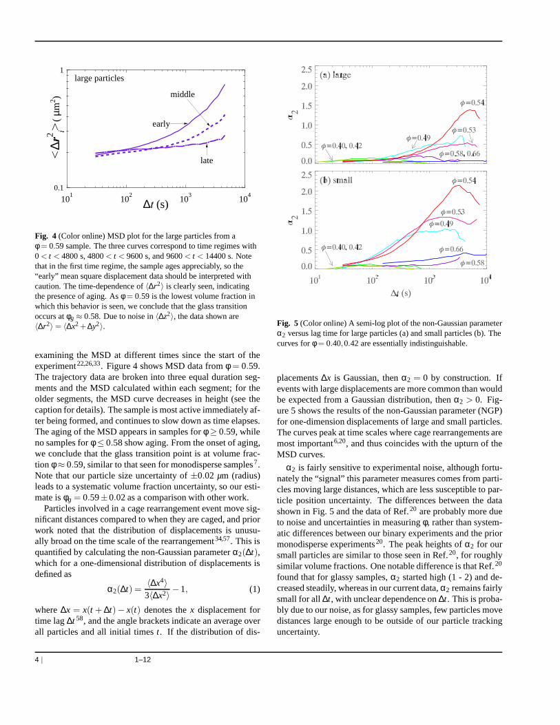
Fig. 4 (Color online) MSD plot for the large particles from aφ = 0.59 sample. The three curves correspond to time regimes with0< t < 4800 s, 4800< t < 9600 s, and 9600< t < 14400 s. Notethat in the first time regime, the sample ages appreciably, sothe“early” mean square displacement data should be interpreted withcaution. The time-dependence of〈∆r2〉 is clearly seen, indicatingthe presence of aging. Asφ = 0.59 is the lowest volume fraction inwhich this behavior is seen, we conclude that the glass transitionoccurs atφg ≈ 0.58. Due to noise in〈∆z2〉, the data shown are〈∆r2〉= 〈∆x2+∆y2〉.

examining the MSD at different times since the start of theexperiment22,26,33. Figure 4 shows MSD data fromφ = 0.59.The trajectory data are broken into three equal duration seg-ments and the MSD calculated within each segment; for theolder segments, the MSD curve decreases in height (see thecaption for details). The sample is most active immediatelyaf-ter being formed, and continues to slow down as time elapses.The aging of the MSD appears in samples forφ ≥ 0.59, whileno samples forφ ≤ 0.58 show aging. From the onset of aging,we conclude that the glass transition point is at volume frac-tion φ ≈ 0.59, similar to that seen for monodisperse samples7.Note that our particle size uncertainty of±0.02 µm (radius)leads to a systematic volume fraction uncertainty, so our esti-mate isφg = 0.59±0.02 as a comparison with other work.

Particles involved in a cage rearrangement event move sig-nificant distances compared to when they are caged, and priorwork noted that the distribution of displacements is unusu-ally broad on the time scale of the rearrangement34,57. This isquantified by calculating the non-Gaussian parameterα2(∆t),which for a one-dimensional distribution of displacementsisdefined as

α2(∆t) =〈∆x4〉

3〈∆x2〉−1, (1)

where∆x = x(t + ∆t)− x(t) denotes thex displacement fortime lag∆t 58, and the angle brackets indicate an average overall particles and all initial timest. If the distribution of dis-

Fig. 5 (Color online) A semi-log plot of the non-Gaussian parameterα2 versus lag time for large particles (a) and small particles (b). Thecurves forφ = 0.40,0.42 are essentially indistinguishable.

placements∆x is Gaussian, thenα2 = 0 by construction. Ifevents with large displacements are more common than wouldbe expected from a Gaussian distribution, thenα2 > 0. Fig-ure 5 shows the results of the non-Gaussian parameter (NGP)for one-dimension displacements of large and small particles.The curves peak at time scales where cage rearrangements aremost important6,20, and thus coincides with the upturn of theMSD curves.

α2 is fairly sensitive to experimental noise, although fortu-nately the “signal” this parameter measures comes from parti-cles moving large distances, which are less susceptible to par-ticle position uncertainty. The differences between the datashown in Fig. 5 and the data of Ref.20 are probably more dueto noise and uncertainties in measuringφ, rather than system-atic differences between our binary experiments and the priormonodisperse experiments20. The peak heights ofα2 for oursmall particles are similar to those seen in Ref.20, for roughlysimilar volume fractions. One notable difference is that Ref. 20

found that for glassy samples,α2 started high (1 - 2) and de-creased steadily, whereas in our current data,α2 remains fairlysmall for all∆t, with unclear dependence on∆t. This is proba-bly due to our noise, as for glassy samples, few particles movedistances large enough to be outside of our particle trackinguncertainty.

4 | 1–12

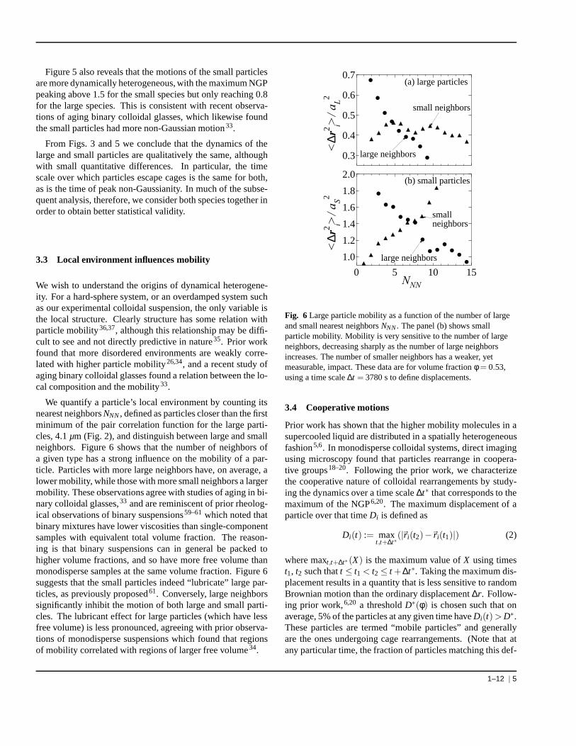
Figure 5 also reveals that the motions of the small particlesare more dynamically heterogeneous, with the maximum NGPpeaking above 1.5 for the small species but only reaching 0.8for the large species. This is consistent with recent observa-tions of aging binary colloidal glasses, which likewise foundthe small particles had more non-Gaussian motion33.

From Figs. 3 and 5 we conclude that the dynamics of thelarge and small particles are qualitatively the same, althoughwith small quantitative differences. In particular, the timescale over which particles escape cages is the same for both,as is the time of peak non-Gaussianity. In much of the subse-quent analysis, therefore, we consider both species together inorder to obtain better statistical validity.

3.3 Local environment influences mobility

We wish to understand the origins of dynamical heterogene-ity. For a hard-sphere system, or an overdamped system suchas our experimental colloidal suspension, the only variable isthe local structure. Clearly structure has some relation withparticle mobility36,37, although this relationship may be diffi-cult to see and not directly predictive in nature35. Prior workfound that more disordered environments are weakly corre-lated with higher particle mobility26,34, and a recent study ofaging binary colloidal glasses found a relation between thelo-cal composition and the mobility33.

We quantify a particle’s local environment by counting itsnearest neighborsNNN, defined as particles closer than the firstminimum of the pair correlation function for the large parti-cles, 4.1µm (Fig. 2), and distinguish between large and smallneighbors. Figure 6 shows that the number of neighbors ofa given type has a strong influence on the mobility of a par-ticle. Particles with more large neighbors have, on average, alower mobility, while those with more small neighbors a largermobility. These observations agree with studies of aging inbi-nary colloidal glasses,33 and are reminiscent of prior rheolog-ical observations of binary suspensions59–61which noted thatbinary mixtures have lower viscosities than single-componentsamples with equivalent total volume fraction. The reason-ing is that binary suspensions can in general be packed tohigher volume fractions, and so have more free volume thanmonodisperse samples at the same volume fraction. Figure 6suggests that the small particles indeed “lubricate” largepar-ticles, as previously proposed61. Conversely, large neighborssignificantly inhibit the motion of both large and small parti-cles. The lubricant effect for large particles (which have lessfree volume) is less pronounced, agreeing with prior observa-tions of monodisperse suspensions which found that regionsof mobility correlated with regions of larger free volume34.

2.0

1.8

1.6

1.4

1.2

1.0

<∆r

2 i>/

aS

2

151050NNN

large neighbors

smallneighbors

(b) small particles

0.7

0.6

0.5

0.4

0.3

<∆r

2 i>/

aL

2

small neighbors

large neighbors

(a) large particles

Fig. 6 Large particle mobility as a function of the number of largeand small nearest neighborsNNN. The panel (b) shows smallparticle mobility. Mobility is very sensitive to the numberof largeneighbors, decreasing sharply as the number of large neighborsincreases. The number of smaller neighbors has a weaker, yetmeasurable, impact. These data are for volume fractionφ = 0.53,using a time scale∆t = 3780 s to define displacements.

3.4 Cooperative motions

Prior work has shown that the higher mobility molecules in asupercooled liquid are distributed in a spatially heterogeneousfashion5,6. In monodisperse colloidal systems, direct imagingusing microscopy found that particles rearrange in coopera-tive groups18–20. Following the prior work, we characterizethe cooperative nature of colloidal rearrangements by study-ing the dynamics over a time scale∆t∗ that corresponds to themaximum of the NGP6,20. The maximum displacement of aparticle over that timeDi is defined as

Di(t) := maxt,t+∆t∗

(|~r i(t2)−~r i(t1)|) (2)

where maxt,t+∆t∗ (X) is the maximum value ofX using timest1, t2 such thatt ≤ t1 < t2 ≤ t +∆t∗. Taking the maximum dis-placement results in a quantity that is less sensitive to randomBrownian motion than the ordinary displacement∆r. Follow-ing prior work,6,20 a thresholdD∗(φ) is chosen such that onaverage, 5% of the particles at any given time haveDi(t)>D∗.These particles are termed “mobile particles” and generallyare the ones undergoing cage rearrangements. (Note that atany particular time, the fraction of particles matching this def-

1–12 | 5

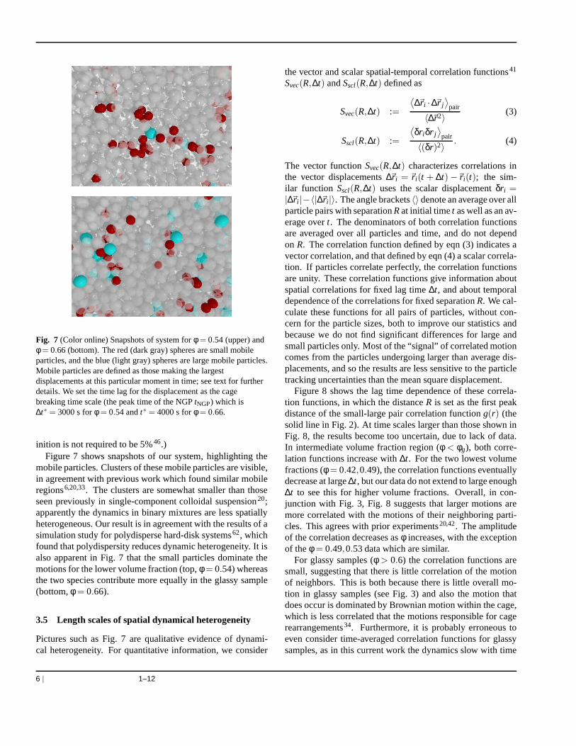
Fig. 7 (Color online) Snapshots of system forφ = 0.54 (upper) andφ = 0.66 (bottom). The red (dark gray) spheres are small mobileparticles, and the blue (light gray) spheres are large mobile particles.Mobile particles are defined as those making the largestdisplacements at this particular moment in time; see text for furtherdetails. We set the time lag for the displacement as the cagebreaking time scale (the peak time of the NGPtNGP) which is∆t∗ = 3000 s forφ = 0.54 andt∗ = 4000 s forφ = 0.66.

inition is not required to be 5%46.)Figure 7 shows snapshots of our system, highlighting the

mobile particles. Clusters of these mobile particles are visible,in agreement with previous work which found similar mobileregions6,20,33. The clusters are somewhat smaller than thoseseen previously in single-component colloidal suspension20;apparently the dynamics in binary mixtures are less spatiallyheterogeneous. Our result is in agreement with the results of asimulation study for polydisperse hard-disk systems62, whichfound that polydispersity reduces dynamic heterogeneity.It isalso apparent in Fig. 7 that the small particles dominate themotions for the lower volume fraction (top,φ = 0.54) whereasthe two species contribute more equally in the glassy sample(bottom,φ = 0.66).

3.5 Length scales of spatial dynamical heterogeneity

Pictures such as Fig. 7 are qualitative evidence of dynami-cal heterogeneity. For quantitative information, we consider

the vector and scalar spatial-temporal correlation functions41

Svec(R,∆t) andSscl(R,∆t) defined as

Svec(R,∆t) :=

⟨

∆~r i ·∆~r j⟩

pair

〈∆~r2〉(3)

Sscl(R,∆t) :=

⟨

δr iδr j⟩

pair

〈(δr)2〉. (4)

The vector functionSvec(R,∆t) characterizes correlations inthe vector displacements∆~r i = ~r i(t + ∆t)−~r i(t); the sim-ilar function Sscl(R,∆t) uses the scalar displacementδr i =|∆~r i |−〈|∆~r i |〉. The angle brackets〈〉 denote an average over allparticle pairs with separationRat initial timet as well as an av-erage overt. The denominators of both correlation functionsare averaged over all particles and time, and do not dependon R. The correlation function defined by eqn (3) indicates avector correlation, and that defined by eqn (4) a scalar correla-tion. If particles correlate perfectly, the correlation functionsare unity. These correlation functions give information aboutspatial correlations for fixed lag time∆t, and about temporaldependence of the correlations for fixed separationR. We cal-culate these functions for all pairs of particles, without con-cern for the particle sizes, both to improve our statistics andbecause we do not find significant differences for large andsmall particles only. Most of the “signal” of correlated motioncomes from the particles undergoing larger than average dis-placements, and so the results are less sensitive to the particletracking uncertainties than the mean square displacement.

Figure 8 shows the lag time dependence of these correla-tion functions, in which the distanceR is set as the first peakdistance of the small-large pair correlation functiong(r) (thesolid line in Fig. 2). At time scales larger than those shown inFig. 8, the results become too uncertain, due to lack of data.In intermediate volume fraction region (φ < φg), both corre-lation functions increase with∆t. For the two lowest volumefractions (φ = 0.42,0.49), the correlation functions eventuallydecrease at large∆t, but our data do not extend to large enough∆t to see this for higher volume fractions. Overall, in con-junction with Fig. 3, Fig. 8 suggests that larger motions aremore correlated with the motions of their neighboring parti-cles. This agrees with prior experiments20,42. The amplitudeof the correlation decreases asφ increases, with the exceptionof theφ = 0.49,0.53 data which are similar.

For glassy samples (φ > 0.6) the correlation functions aresmall, suggesting that there is little correlation of the motionof neighbors. This is both because there is little overall mo-tion in glassy samples (see Fig. 3) and also the motion thatdoes occur is dominated by Brownian motion within the cage,which is less correlated that the motions responsible for cagerearrangements34. Furthermore, it is probably erroneous toeven consider time-averaged correlation functions for glassysamples, as in this current work the dynamics slow with time

6 | 1–12

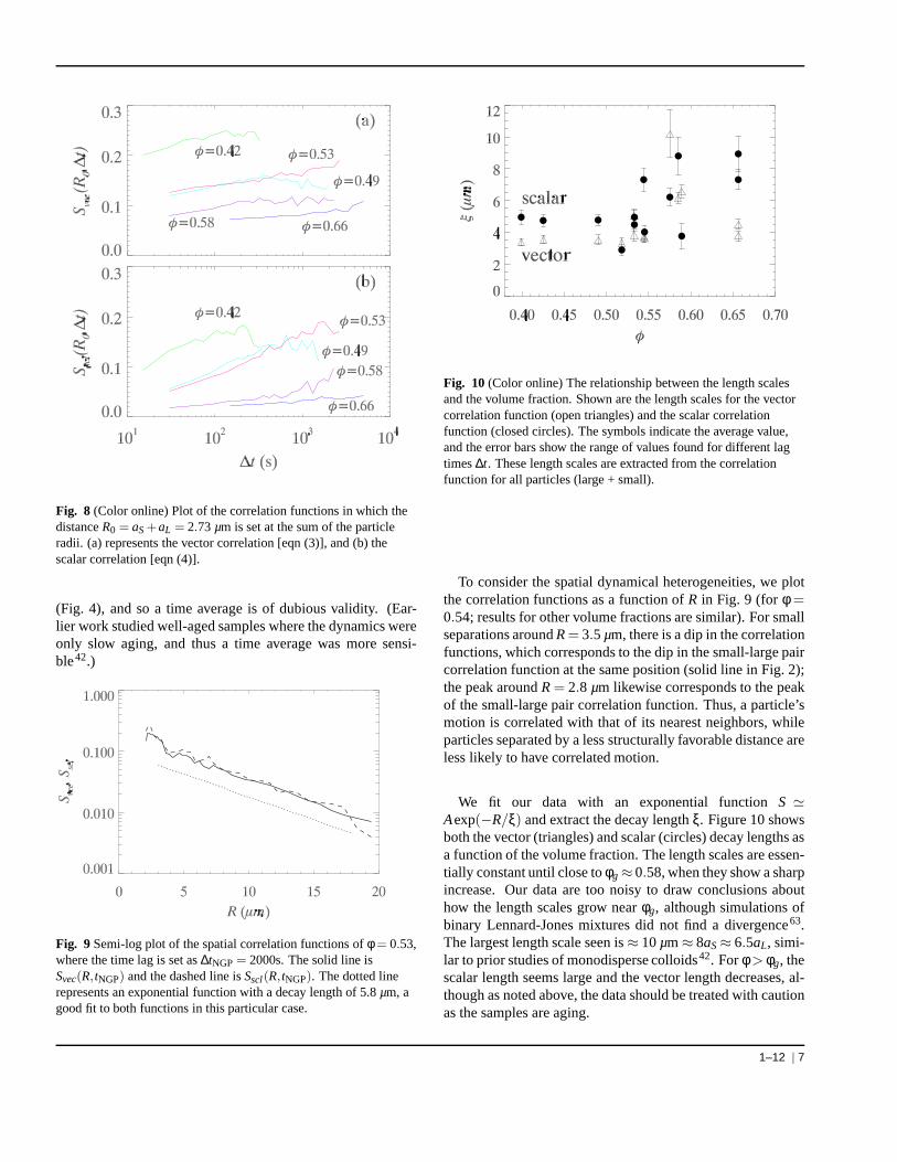
Fig. 8 (Color online) Plot of the correlation functions in which thedistanceR0 = aS+aL = 2.73 µm is set at the sum of the particleradii. (a) represents the vector correlation [eqn (3)], and(b) thescalar correlation [eqn (4)].

(Fig. 4), and so a time average is of dubious validity. (Ear-lier work studied well-aged samples where the dynamics wereonly slow aging, and thus a time average was more sensi-ble42.)

Fig. 9 Semi-log plot of the spatial correlation functions ofφ = 0.53,where the time lag is set as∆tNGP= 2000s. The solid line isSvec(R, tNGP) and the dashed line isSscl(R, tNGP). The dotted linerepresents an exponential function with a decay length of 5.8 µm, agood fit to both functions in this particular case.

Fig. 10 (Color online) The relationship between the length scalesand the volume fraction. Shown are the length scales for the vectorcorrelation function (open triangles) and the scalar correlationfunction (closed circles). The symbols indicate the average value,and the error bars show the range of values found for different lagtimes∆t. These length scales are extracted from the correlationfunction for all particles (large + small).

To consider the spatial dynamical heterogeneities, we plotthe correlation functions as a function ofR in Fig. 9 (for φ =0.54; results for other volume fractions are similar). For smallseparations aroundR= 3.5 µm, there is a dip in the correlationfunctions, which corresponds to the dip in the small-large paircorrelation function at the same position (solid line in Fig. 2);the peak aroundR= 2.8 µm likewise corresponds to the peakof the small-large pair correlation function. Thus, a particle’smotion is correlated with that of its nearest neighbors, whileparticles separated by a less structurally favorable distance areless likely to have correlated motion.

We fit our data with an exponential functionS ≃Aexp(−R/ξ) and extract the decay lengthξ. Figure 10 showsboth the vector (triangles) and scalar (circles) decay lengths asa function of the volume fraction. The length scales are essen-tially constant until close toφg ≈ 0.58, when they show a sharpincrease. Our data are too noisy to draw conclusions abouthow the length scales grow nearφg, although simulations ofbinary Lennard-Jones mixtures did not find a divergence63.The largest length scale seen is≈ 10µm≈ 8aS≈ 6.5aL, simi-lar to prior studies of monodisperse colloids42. Forφ> φg, thescalar length seems large and the vector length decreases, al-though as noted above, the data should be treated with cautionas the samples are aging.

1–12 | 7

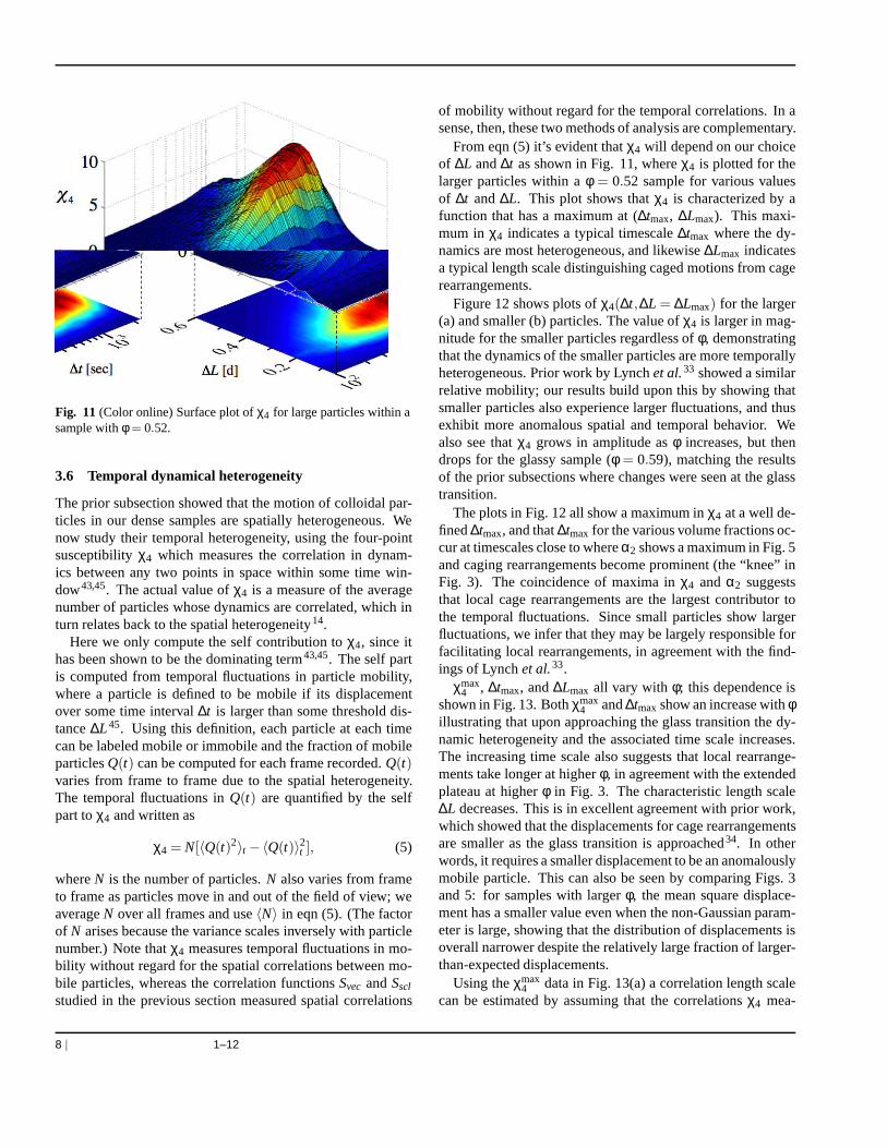
Fig. 11 (Color online) Surface plot ofχ4 for large particles within asample withφ = 0.52.

3.6 Temporal dynamical heterogeneity

The prior subsection showed that the motion of colloidal par-ticles in our dense samples are spatially heterogeneous. Wenow study their temporal heterogeneity, using the four-pointsusceptibilityχ4 which measures the correlation in dynam-ics between any two points in space within some time win-dow43,45. The actual value ofχ4 is a measure of the averagenumber of particles whose dynamics are correlated, which inturn relates back to the spatial heterogeneity14.

Here we only compute the self contribution toχ4, since ithas been shown to be the dominating term43,45. The self partis computed from temporal fluctuations in particle mobility,where a particle is defined to be mobile if its displacementover some time interval∆t is larger than some threshold dis-tance∆L45. Using this definition, each particle at each timecan be labeled mobile or immobile and the fraction of mobileparticlesQ(t) can be computed for each frame recorded.Q(t)varies from frame to frame due to the spatial heterogeneity.The temporal fluctuations inQ(t) are quantified by the selfpart toχ4 and written as

χ4 = N[〈Q(t)2〉t −〈Q(t)〉2t ], (5)

whereN is the number of particles.N also varies from frameto frame as particles move in and out of the field of view; weaverageN over all frames and use〈N〉 in eqn (5). (The factorof N arises because the variance scales inversely with particlenumber.) Note thatχ4 measures temporal fluctuations in mo-bility without regard for the spatial correlations betweenmo-bile particles, whereas the correlation functionsSvec andSscl

studied in the previous section measured spatial correlations

of mobility without regard for the temporal correlations. In asense, then, these two methods of analysis are complementary.

From eqn (5) it’s evident thatχ4 will depend on our choiceof ∆L and∆t as shown in Fig. 11, whereχ4 is plotted for thelarger particles within aφ = 0.52 sample for various valuesof ∆t and∆L. This plot shows thatχ4 is characterized by afunction that has a maximum at (∆tmax, ∆Lmax). This maxi-mum in χ4 indicates a typical timescale∆tmax where the dy-namics are most heterogeneous, and likewise∆Lmax indicatesa typical length scale distinguishing caged motions from cagerearrangements.

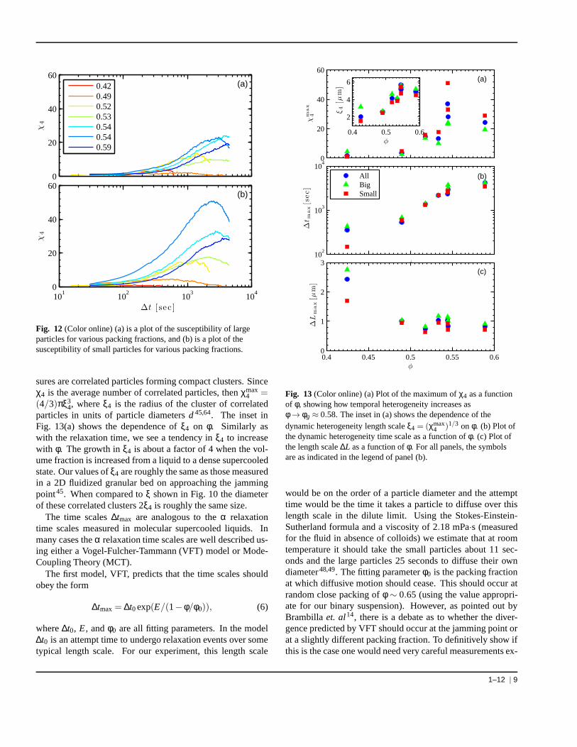
Figure 12 shows plots ofχ4(∆t,∆L = ∆Lmax) for the larger(a) and smaller (b) particles. The value ofχ4 is larger in mag-nitude for the smaller particles regardless ofφ, demonstratingthat the dynamics of the smaller particles are more temporallyheterogeneous. Prior work by Lynchet al.33 showed a similarrelative mobility; our results build upon this by showing thatsmaller particles also experience larger fluctuations, andthusexhibit more anomalous spatial and temporal behavior. Wealso see thatχ4 grows in amplitude asφ increases, but thendrops for the glassy sample (φ = 0.59), matching the resultsof the prior subsections where changes were seen at the glasstransition.

The plots in Fig. 12 all show a maximum inχ4 at a well de-fined∆tmax, and that∆tmax for the various volume fractions oc-cur at timescales close to whereα2 shows a maximum in Fig. 5and caging rearrangements become prominent (the “knee” inFig. 3). The coincidence of maxima inχ4 andα2 suggeststhat local cage rearrangements are the largest contributortothe temporal fluctuations. Since small particles show largerfluctuations, we infer that they may be largely responsible forfacilitating local rearrangements, in agreement with the find-ings of Lynchet al.33.

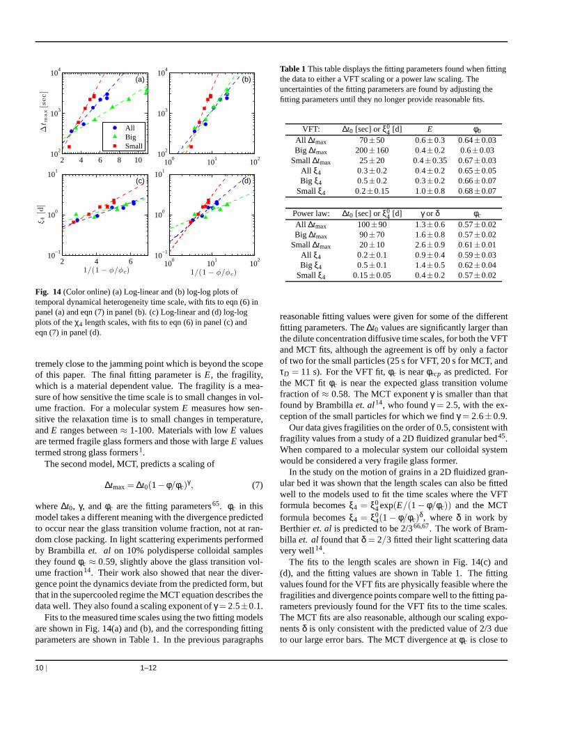
χmax4 , ∆tmax, and∆Lmax all vary with φ; this dependence is

shown in Fig. 13. Bothχmax4 and∆tmaxshow an increase withφ

illustrating that upon approaching the glass transition the dy-namic heterogeneity and the associated time scale increases.The increasing time scale also suggests that local rearrange-ments take longer at higherφ, in agreement with the extendedplateau at higherφ in Fig. 3. The characteristic length scale∆L decreases. This is in excellent agreement with prior work,which showed that the displacements for cage rearrangementsare smaller as the glass transition is approached34. In otherwords, it requires a smaller displacement to be an anomalouslymobile particle. This can also be seen by comparing Figs. 3and 5: for samples with largerφ, the mean square displace-ment has a smaller value even when the non-Gaussian param-eter is large, showing that the distribution of displacements isoverall narrower despite the relatively large fraction of larger-than-expected displacements.

Using theχmax4 data in Fig. 13(a) a correlation length scale

can be estimated by assuming that the correlationsχ4 mea-

8 | 1–12

0

20

40

60

χ4

(a)0.42

0.490.520.530.540.540.59

101

102

103

104

0

20

40

60

∆t [ sec ]

χ4

(b)

Fig. 12 (Color online) (a) is a plot of the susceptibility of largeparticles for various packing fractions, and (b) is a plot ofthesusceptibility of small particles for various packing fractions.

sures are correlated particles forming compact clusters. Sinceχ4 is the average number of correlated particles, thenχmax

4 =(4/3)πξ3

4, whereξ4 is the radius of the cluster of correlatedparticles in units of particle diametersd45,64. The inset inFig. 13(a) shows the dependence ofξ4 on φ. Similarly aswith the relaxation time, we see a tendency inξ4 to increasewith φ. The growth inξ4 is about a factor of 4 when the vol-ume fraction is increased from a liquid to a dense supercooledstate. Our values ofξ4 are roughly the same as those measuredin a 2D fluidized granular bed on approaching the jammingpoint45. When compared toξ shown in Fig. 10 the diameterof these correlated clusters 2ξ4 is roughly the same size.

The time scales∆tmax are analogous to theα relaxationtime scales measured in molecular supercooled liquids. Inmany cases theα relaxation time scales are well described us-ing either a Vogel-Fulcher-Tammann (VFT) model or Mode-Coupling Theory (MCT).

The first model, VFT, predicts that the time scales shouldobey the form

∆tmax= ∆t0exp(E/(1−φ/φ0)), (6)

where∆t0, E, andφ0 are all fitting parameters. In the model∆t0 is an attempt time to undergo relaxation events over sometypical length scale. For our experiment, this length scale

0

20

40

60

χm

ax

4

(a)

0.4 0.5 0.6

2

4

6

φ

ξ4

[µm

]

102

103

104

∆t m

ax

[sec]

φ

(b)All

BigSmall

0.4 0.45 0.5 0.55 0.60

1

2

3

φ

∆L

max

[µm

]

(c)

Fig. 13 (Color online) (a) Plot of the maximum ofχ4 as a functionof φ, showing how temporal heterogeneity increases asφ → φg ≈ 0.58. The inset in (a) shows the dependence of thedynamic heterogeneity length scaleξ4 = (χmax

4 )1/3 on φ. (b) Plot ofthe dynamic heterogeneity time scale as a function ofφ. (c) Plot ofthe length scale∆L as a function ofφ. For all panels, the symbolsare as indicated in the legend of panel (b).

would be on the order of a particle diameter and the attempttime would be the time it takes a particle to diffuse over thislength scale in the dilute limit. Using the Stokes-Einstein-Sutherland formula and a viscosity of 2.18 mPa·s (measuredfor the fluid in absence of colloids) we estimate that at roomtemperature it should take the small particles about 11 sec-onds and the large particles 25 seconds to diffuse their owndiameter48,49. The fitting parameterφ0 is the packing fractionat which diffusive motion should cease. This should occur atrandom close packing ofφ ∼ 0.65 (using the value appropri-ate for our binary suspension). However, as pointed out byBrambilla et. al14, there is a debate as to whether the diver-gence predicted by VFT should occur at the jamming point orat a slightly different packing fraction. To definitively show ifthis is the case one would need very careful measurements ex-

1–12 | 9

2 4 6 8 1010

2

103

104

∆t m

ax

[sec]

(a)

AllBigSmall

100

101

102

102

103

104

(b)

2 4 610

−1

100

101

1/(1 − φ/φc)

ξ 4[d

]

(c)

100

101

102

10−1

100

101

1/(1 − φ/φc)

(d)

Fig. 14 (Color online) (a) Log-linear and (b) log-log plots oftemporal dynamical heterogeneity time scale, with fits to eqn (6) inpanel (a) and eqn (7) in panel (b). (c) Log-linear and (d) log-logplots of theχ4 length scales, with fits to eqn (6) in panel (c) andeqn (7) in panel (d).

tremely close to the jamming point which is beyond the scopeof this paper. The final fitting parameter isE, the fragility,which is a material dependent value. The fragility is a mea-sure of how sensitive the time scale is to small changes in vol-ume fraction. For a molecular systemE measures how sen-sitive the relaxation time is to small changes in temperature,andE ranges between≈ 1-100. Materials with lowE valuesare termed fragile glass formers and those with largeE valuestermed strong glass formers1.

The second model, MCT, predicts a scaling of

∆tmax= ∆t0(1−φ/φc)γ, (7)

where∆t0, γ, andφc are the fitting parameters65. φc in thismodel takes a different meaning with the divergence predictedto occur near the glass transition volume fraction, not at ran-dom close packing. In light scattering experiments performedby Brambillaet. al on 10% polydisperse colloidal samplesthey foundφc ≈ 0.59, slightly above the glass transition vol-ume fraction14. Their work also showed that near the diver-gence point the dynamics deviate from the predicted form, butthat in the supercooled regime the MCT equation describes thedata well. They also found a scaling exponent ofγ= 2.5±0.1.

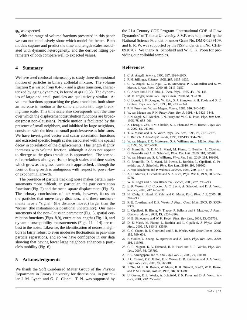
Fits to the measured time scales using the two fitting modelsare shown in Fig. 14(a) and (b), and the corresponding fittingparameters are shown in Table 1. In the previous paragraphs

Table 1This table displays the fitting parameters found when fittingthe data to either a VFT scaling or a power law scaling. Theuncertainties of the fitting parameters are found by adjusting thefitting parameters until they no longer provide reasonable fits.

VFT: ∆t0 [sec] orξ04 [d] E φ0

All ∆tmax 70±50 0.6±0.3 0.64±0.03Big ∆tmax 200±160 0.4±0.2 0.6±0.03

Small∆tmax 25±20 0.4±0.35 0.67±0.03All ξ4 0.3±0.2 0.4±0.2 0.65±0.05Big ξ4 0.5±0.2 0.3±0.2 0.66±0.07

Smallξ4 0.2±0.15 1.0±0.8 0.68±0.07

Power law: ∆t0 [sec] orξ04 [d] γ or δ φc

All ∆tmax 100±90 1.3±0.6 0.57±0.02Big ∆tmax 90±70 1.6±0.8 0.57±0.02

Small∆tmax 20±10 2.6±0.9 0.61±0.01All ξ4 0.2±0.1 0.9±0.4 0.59±0.03Big ξ4 0.5±0.1 1.4±0.5 0.62±0.04

Smallξ4 0.15±0.05 0.4±0.2 0.57±0.02

reasonable fitting values were given for some of the differentfitting parameters. The∆t0 values are significantly larger thanthe dilute concentration diffusive time scales, for both the VFTand MCT fits, although the agreement is off by only a factorof two for the small particles (25 s for VFT, 20 s for MCT, andτD = 11 s). For the VFT fit,φc is nearφrcp as predicted. Forthe MCT fit φc is near the expected glass transition volumefraction of≈ 0.58. The MCT exponentγ is smaller than thatfound by Brambillaet. al14, who foundγ = 2.5, with the ex-ception of the small particles for which we findγ = 2.6±0.9.

Our data gives fragilities on the order of 0.5, consistent withfragility values from a study of a 2D fluidized granular bed45.When compared to a molecular system our colloidal systemwould be considered a very fragile glass former.

In the study on the motion of grains in a 2D fluidized gran-ular bed it was shown that the length scales can also be fittedwell to the models used to fit the time scales where the VFTformula becomesξ4 = ξ0

4exp(E/(1− φ/φc)) and the MCTformula becomesξ4 = ξ0

4(1− φ/φc)δ, whereδ in work by

Berthieret. al is predicted to be 2/366,67. The work of Bram-billa et. al found thatδ = 2/3 fitted their light scattering datavery well14.

The fits to the length scales are shown in Fig. 14(c) and(d), and the fitting values are shown in Table 1. The fittingvalues found for the VFT fits are physically feasible where thefragilities and divergence points compare well to the fitting pa-rameters previously found for the VFT fits to the time scales.The MCT fits are also reasonable, although our scaling expo-nentsδ is only consistent with the predicted value of 2/3 dueto our large error bars. The MCT divergence atφc is close to

10 | 1–12

φg, as expected.With the range of volume fractions presented in this paper

we can not conclusively show which model fits better. Bothmodels capture and predict the time and length scales associ-ated with dynamic heterogeneity, and the derived fitting pa-rameters of both compare well to expected values.

4 Summary

We have used confocal microscopy to study three-dimensionalmotion of particles in binary colloidal mixture. The volumefractionφ is varied from 0.4-0.7 and a glass transition, charac-terized by aging dynamics, is found atφ ≈ 0.58. The dynam-ics of large and small particles are qualitatively similar.Atvolume fractions approaching the glass transition, both showan increase in motion at the same characteristic cage break-ing time scale. This time scale also corresponds with the timeover which the displacement distribution functions are broad-est (most non-Gaussian). Particle motion is facilitated bythepresence of small neighbors, and inhibited by large neighbors,consistent with the idea that small particles serve as lubricants.We have investigated vector and scalar correlation functionsand extracted specific length scales associated with the spatialdecay in correlation of the displacements. This length slightlyincreases with volume fraction, although it does not appearto diverge as the glass transition is approached. The tempo-ral correlations also give rise to length scales and time scaleswhich grow as the glass transition is approached, although theform of this growth is ambiguous with respect to power-lawor exponential growth.

The presence of particle tracking noise makes certain mea-surements more difficult, in particular, the pair correlationfunctions (Fig. 2) and the mean square displacement (Fig. 3).The primary conclusions of our work, however, focus onthe particles that move large distances, and these measure-ments have a “signal” (the distance moved) larger than the“noise” (the instantaneous positional uncertainty). Our mea-surements of the non-Gaussian parameter (Fig. 5, spatial cor-relation functions (Figs. 8,9), correlation lengths (Fig.10, anddynamic susceptibility measurements (Figs. 11 - 14) are ro-bust to the noise. Likewise, the identification of nearest neigh-bors is fairly robust to even moderate fluctuations in pair-wiseparticle separations, and so we have confidence in our datashowing that having fewer large neighbors enhances a parti-cle’s mobility (Fig. 6).

5 Acknowledgments

We thank the Soft Condensed Matter Group of the PhysicsDepartment in Emory University for discussions, in particu-lar J. M. Lynch and G. C. Cianci. T. N. was supported by

the 21st Century COE Program “International COE of FlowDynamics” of Tohoku University. S.V.F. was supported by theNational Science Foundation under Grant No. DMR-0239109,and E. R. W. was supported by the NSF under Grant No. CHE-0910707. We thank A. Schofield and W. C. K. Poon for pro-viding our colloidal samples.

References

1 C. A. Angell,Science, 1995,267, 1924–1935.2 F. H. Stillinger,Science, 1995,267, 1935–1939.3 C. A. Angell, K. L. Ngai, G. B. McKenna, P. F. McMillan and S. W.

Martin, J. App. Phys., 2000,88, 3113–3157.4 G. Adam and J. H. Gibbs,J. Chem. Phys., 1965,43, 139–146.5 M. D. Ediger,Annu. Rev. Phys. Chem., 2000,51, 99–128.6 C. Donati, J. F. Douglas, W. Kob, S. J. Plimpton, P. H. Poole and S. C.

Glotzer,Phys. Rev. Lett., 1998,80, 2338–2341.7 P. N. Pusey and W. van Megen,Nature, 1986,320, 340–342.8 W. van Megen and P. N. Pusey,Phys. Rev. A, 1991,43, 5429–5441.9 P. N. Segre, S. P. Meeker, P. N. Pusey and W. C. K. Poon,Phys. Rev. Lett.,

1995,75, 958–961.10 Z. Cheng, J. Zhu, P. M. Chaikin, S.-E. Phan and W. B. Russel,Phys. Rev.

E, 2002,65, 041405.11 T. G. Mason and D. A. Weitz,Phys. Rev. Lett., 1995,75, 2770–2773.12 E. Bartsch,J. Non-Cryst. Solids, 1995,192-193, 384–392.13 W. van Megen, T. C. Mortensen, S. R. Williams and J. Muller, Phys. Rev.

E, 1998,58, 6073–6085.14 G. Brambilla, D. E. M. El Masri, M. Pierno, L. Berthier, L. Cipelletti,

G. Petekidis and A. B. Schofield,Phys. Rev. Lett., 2009,102, 085703.15 W. van Megen and S. R. Williams,Phys. Rev. Lett., 2010,104, 169601.16 G. Brambilla, D. E. Masri, M. Pierno, L. Berthier, L. Cipelletti, G. Pe-

tekidis and A. Schofield,Phys. Rev. Lett., 2010,104, 169602.17 A. van Blaaderen and P. Wiltzius,Science, 1995,270, 1177–1179.18 A. H. Marcus, J. Schofield and S. A. Rice,Phys. Rev. E, 1999,60, 5725–

5736.19 W. K. Kegel and A. van Blaaderen,Science, 2000,287, 290–293.20 E. R. Weeks, J. C. Crocker, A. C. Levitt, A. Schofield and D. A. Weitz,

Science, 2000,287, 627–631.21 H. Konig, R. Hund, K. Zahn and G. Maret,Euro. Phys. J. E, 2005,18,

287–293.22 R. E. Courtland and E. R. Weeks,J. Phys.: Cond. Matt., 2003,15, S359–

S365.23 L. Cipelletti, H. Bissig, V. Trappe, P. Ballesta and S. Mazoyer, J. Phys.:

Condens. Matter, 2003,15, S257–S262.24 N. B. Simeonova and W. K. Kegel,Phys. Rev. Lett., 2004,93, 035701.25 D. El Masri, M. Pierno, L. Berthier and L. Cipelletti,J. Phys.: Cond.

Matt., 2005,17, S3543–S3549.26 G. C. Cianci, R. E. Courtland and E. R. Weeks,Solid State Comm., 2006,

139, 599–604.27 P. Yunker, Z. Zhang, K. Aptowicz and A. Yodh,Phys. Rev. Lett., 2009,

103, 115701.28 C. R. Nugent, K. V. Edmond, H. N. Patel and E. R. Weeks,Phys. Rev.

Lett., 2007,99, 025702.29 P. S. Sarangapani and Y. Zhu,Phys. Rev. E, 2008,77, 010501.30 J. C. Conrad, P. P. Dhillon, E. R. Weeks, D. R. Reichman and D. A. Weitz,

Phys. Rev. Lett., 2006,97, 265701.31 J. Zhu, M. Li, R. Rogers, W. Meyer, R. H. Ottewill, Sts-73, W. B. Russel

and P. M. Chaikin,Nature, 1997,387, 883–885.32 U. Gasser, E. R. Weeks, A. Schofield, P. N. Pusey and D. A. Weitz, Sci-

ence, 2001,292, 258–262.

1–12 | 11

33 J. M. Lynch, G. C. Cianci and E. R. Weeks,Phys. Rev. E, 2008, 78,031410.

34 E. R. Weeks and D. A. Weitz,Phys. Rev. Lett., 2002,89, 095704.35 J. C. Conrad, F. W. Starr and D. A. Weitz,J. Phys. Chem. B, 2005,109,

21235–21240.36 A. Widmer-Cooper, P. Harrowell and H. Fynewever,Phys. Rev. Lett.,

2004,93, 135701.37 A. Widmer-Cooper and P. Harrowell,J. Phys.: Cond. Matt., 2005,17,

S4025–S4034.38 V. Prasad, D. Semwogerere and E. R. Weeks,J. Phys.: Cond. Matt., 2007,

19, 113102.39 P. H. Poole, C. Donati and S. C. Glotzer,Physica A: Statistical and The-

oretical Physics, 1998,261, 51–59.40 C. Donati, S. C. Glotzer and P. H. Poole,Phys. Rev. Lett., 1999,82, 5064–

5067.41 B. Doliwa and A. Heuer,Phys. Rev. E, 2000,61, 6898–6908.42 E. R. Weeks, J. C. Crocker and D. A. Weitz,J. Phys.: Cond. Matt., 2007,

19, 205131.43 S. C. Glotzer, V. N. Novikov and T. B. Schrø der,J. Chem. Phys., 2000,

112, 509–512.44 N. Lacevic, F. W. Starr, T. B. Schroder and S. C. Glotzer,J. Chem. Phys.,

2003,119, 7372–7387.45 A. S. Keys, A. R. Abate, S. C. Glotzer and D. J. Durian,Nature Physics,

2007,3, 260–264.46 A. D. Dinsmore, E. R. Weeks, V. Prasad, A. C. Levitt and D. A.Weitz,

App. Optics, 2001,40, 4152–4159.47 J. C. Crocker and D. G. Grier,J. Colloid Interf. Sci., 1996,179, 298–310.48 A. Einstein,Annalen der Physik (Leipzig), 1905,17, 549–560.49 W. Sutherland,Phil. Mag., 1905,9, 781–785.50 E. Rabani, D. J. Gezelter and B. J. Berne,J. Chem. Phys., 1997, 107,

6867–6876.51 B. Doliwa and A. Heuer,Phys. Rev. Lett., 1998,80, 4915–4918.52 A. Kasper, E. Bartsch and H. Sillescu,Langmuir, 1998,14, 5004–5010.53 E. R. Weeks and D. A. Weitz,Chem. Phys., 2002,284, 361–367.54 P. M. Reis, R. A. Ingale and M. D. Shattuck,Phys. Rev. Lett., 2007,98,

188301.55 K. L. Ngai and R. W. Rendell,Phil. Mag. B, 1998,77, 621–631.56 W. van Megen, V. A. Martinez and G. Bryant,Phys. Rev. Lett., 2009,102,

168301.57 W. Kob, C. Donati, S. J. Plimpton, P. H. Poole and S. C. Glotzer, Phys.

Rev. Lett., 1997,79, 2827–2830.58 A. Rahman,Phys. Rev., 1964,136, A405–A411.59 R. L. Hoffman,J. Rheology, 1992,36, 947–965.60 P. D’Haene and J. Mewis,Rheologica Acta, 1994,33, 165–174.61 S. R. Williams and W. van Megen,Phys. Rev. E, 2001,64, 041502.62 T. Kawasaki, T. Araki and H. Tanaka,Phys. Rev. Lett., 2007,99, 215701.63 T. Narumi and M. Tokuyama,Phil. Mag., 2008,88, 4169–4175.64 P. Sarangapani, J. Zhao and Y. Zhu,J. Chem. Phys., 2008,129, 104514.65 W. Gotze,J. Phys.: Cond. Matt., 1999,11, A1–A45.66 L. Berthier, G. Biroli, J. P. Bouchaud, W. Kob, K. Miyazakiand D. R.

Reichman,J. Chem. Phys., 2007,126, 184503.67 L. Berthier, G. Biroli, J. P. Bouchaud, W. Kob, K. Miyazakiand D. R.

Reichman,J. Chem. Phys., 2007,126, 184504.

12 | 1–12