Customer Churn Prediction for PC Games - Kth Diva Portal Org

IN DEGREE PROJECT MATHEMATICS,SECOND CYCLE, 30 CREDITS

, STOCKHOLM SWEDEN 2019

Customer Churn Prediction for PC GamesProbability of churn predicted for big-spenders using supervised machine learning

VALGERDUR TRYGGVADOTTIR

KTH ROYAL INSTITUTE OF TECHNOLOGYSCHOOL OF ARCHITECTURE AND THE BUILT ENVIRONMENT

Customer Churn Prediction for PC Games

Probability of churn predicted for big-spenders using supervised machine learning VALGERDUR TRYGGVADOTTIR

Degree Projects in Optimization and Systems Theory (30 ECTS credits) Degree Programme in Applied and Computational Mathematics (120 credits) KTH Royal Institute of Technology year 2019 Supervisor at Echo State: Josef Falk Supervisor at KTH: Xiaoming Hu Examiner at KTH: Xiaoming Hu

TRITA-SCI-GRU 2019:254 MAT-E 2019:68

Royal Institute of Technology School of Engineering Sciences KTH SCI SE-100 44 Stockholm, Sweden URL: www.kth.se/sci

Abstract

Paradox Interactive is a Swedish video game developer and publisher which hasplayers all around the world. Paradox’s largest platform in terms of amount ofplayers and revenue is the PC. The goal of this thesis was to make a churn predic-tion model to predict the probability of players churning in order to know whichplayers to focus on in retention campaigns. Since the purpose of churn prediction isto minimize loss due to customers churning the focus was on big-spenders (whales)in Paradox PC games.

In order to define which players are big-spenders the spending for players over a12 month rolling period (from 2016-01-01 until 2018-12-31) was investigated. Theplayers spending more than the 95th-percentile of the total spending for each pe-riod were defined as whales. Defining when a whale has churned, i.e. stopped beinga big-spender in Paradox PC games, was done by looking at how many days hadpassed since the players bought something. A whale has churned if he has notbought anything for the past 28 days.

When data had been collected about the whales the data set was prepared fora number of different supervised machine learning methods. Logistic Regression, L1Regularized Logistic Regression, Decision Tree and Random Forest were the meth-ods tested. Random Forest performed best in terms of AUC, with AUC = 0.7162.The conclusion is that it seems to be possible to predict the probability of churningfor Paradox whales. It might be possible to improve the model further by investi-gating more data and fine tuning the definition of churn.

Keywords: Customer churn prediction, whales, data analysis, machine learning,binary classification.

i

Sammanfattning

Paradox Interactive är en svensk videospelutvecklare och utgivare som har spelareöver hela världen. Paradox största plattform när det gäller antal spelare och intäk-ter är PC:n. Målet med detta exjobb var att göra en churn-predikterings modell föratt förutsäga sannolikheten för att spelare har "churnat" för att veta vilka spelarefokusen ska vara på i retentionskampanjer. Eftersom syftet med churn-predikteringär att minimera förlust på grund av kunderna som "churnar", var fokusen på spelaresom spenderar mest pengar (valar) i Paradox PC-spel.

För att definiera vilka spelare som är valar undersöktes hur mycket spelarna spenderarunder en 12 månaders rullande period (från 2016-01-01 till 2018-12-31). Spelarnasom spenderade mer än 95:e percentilen av den totala spenderingen för varje perioddefinierades som valar. För att definiera när en val har "churnat", det vill sägaslutat vara en kund som spenderar mycket pengar i Paradox PC-spel, tittade manpå hur många dagar som gått sedan spelarna köpte någonting. En val har "churnat"om han inte har köpt något under de senaste 28 dagarna.

När data hade varit samlad om valarna var datan förberedd för ett antal olikamaskininlärningsmetoder. Logistic Regression, L1 Regularized Logistic Regression,Decision Tree och Random Forest var de metoder som testades. Random Forest varden metoden som gav bäst resultat med avseende på AUC, med AUC = 0, 7162.Slutsatsen är att det verkar vara möjligt att förutsäga sannolikheten att Paradoxvalar "churnar". Det kan vara möjligt att förbättra modellen ytterligare genom attundersöka mer data och finjustera definitionen av churn.

Nyckelord: Kund churn prediktering, valar, dataanalys, maskinlärning, binär klas-sificering.

iii

Preface

This master thesis was completed in the Department of Mathematics which is a partof the School of Engineerings Sciences at KTH Royal Institute of Technology. Thethesis was done in collaboration with the consulting company Echo State and thevideo game developer and publisher Paradox Interactive.

Acknowledgement

I would like to thank Christoffer Fluch for contacting me on LinkedIn and togetherwith Josef Falk giving me the opportunity to do this project. I want to thank Josefand Markus Ebbesson for being my supervisors at Echo State and giving me inspi-ration and helping me with their technical knowledge. I am also greatful for thewarm welcome by all the others working at Echo State.

At Paradox Interactive I would like to thank Mathias Von Plato for the guidanceand feedback throughout the project, Anabel Silva Rojas for the help with collectingand understanding the data, Alexander Hofverberg for helping me with his knowl-edge in Machine Learning and RStudio and Alessandro Festante for his help fromthe beginning of the project. In addition I thank all the others from the data andanalytics teams at Paradox for creating a friendly and good work atmosphere.

I would like to thank to Xiaoming Hu, my supervisor and examinor at KTH, for hisgenerous support. I owe all the teachers I have had throughout my education mysincerest gratitude for helping me getting the knowledge I have today.

Finally, I want to thank my family, boyfriend, Björgvin R. Hjálmarsson, roomate,Laufey Benediktsdóttir and friends for always being supportive and believing in me.

v

Table of Contents

Abstract i

Sammanfattning ii

Preface iv

Acknowledgement v

Table of Contents vi

List of Tables ix

List of Figures x

List of Abbreviations xi

1 Introduction 11.1 Thesis objectives . . . . . . . . . . . . . . . . . . . . . . . . . . . . . 11.2 Thesis disposition . . . . . . . . . . . . . . . . . . . . . . . . . . . . . 21.3 Programming Languages . . . . . . . . . . . . . . . . . . . . . . . . . 2

2 Background 32.1 Organization . . . . . . . . . . . . . . . . . . . . . . . . . . . . . . . 32.2 Revenue . . . . . . . . . . . . . . . . . . . . . . . . . . . . . . . . . . 42.3 Games . . . . . . . . . . . . . . . . . . . . . . . . . . . . . . . . . . . 42.4 Players . . . . . . . . . . . . . . . . . . . . . . . . . . . . . . . . . . . 5

3 Literature Review 73.1 Related Works . . . . . . . . . . . . . . . . . . . . . . . . . . . . . . . 7

vi

TABLE OF CONTENTS vii

3.2 Churn Definitions . . . . . . . . . . . . . . . . . . . . . . . . . . . . . 93.3 Whale Definitions . . . . . . . . . . . . . . . . . . . . . . . . . . . . . 103.4 Algorithms used for Churn Modeling . . . . . . . . . . . . . . . . . . 103.5 Data used for Churn Modeling . . . . . . . . . . . . . . . . . . . . . . 11

4 Theory 134.1 Supervised Machine Learning . . . . . . . . . . . . . . . . . . . . . . 13

Notation . . . . . . . . . . . . . . . . . . . . . . . . . . . . . . . . . . 13Training and Test Set . . . . . . . . . . . . . . . . . . . . . . . . . . . 14Methods to Estimate f . . . . . . . . . . . . . . . . . . . . . . . . . . 15Training and Test error . . . . . . . . . . . . . . . . . . . . . . . . . . 16The Bias-Variance Trade-off . . . . . . . . . . . . . . . . . . . . . . . 16

4.2 Model Selection . . . . . . . . . . . . . . . . . . . . . . . . . . . . . . 18Cross-Validation . . . . . . . . . . . . . . . . . . . . . . . . . . . . . . 18Feature Selection . . . . . . . . . . . . . . . . . . . . . . . . . . . . . 19Dimension Reduction . . . . . . . . . . . . . . . . . . . . . . . . . . . 20

4.3 Model Assessment . . . . . . . . . . . . . . . . . . . . . . . . . . . . . 20Confusion Matrix . . . . . . . . . . . . . . . . . . . . . . . . . . . . . 20Evaluation Metrics . . . . . . . . . . . . . . . . . . . . . . . . . . . . 21

The ROC Curve and AUC . . . . . . . . . . . . . . . . . . . . 224.4 Learning Algorithms . . . . . . . . . . . . . . . . . . . . . . . . . . . 23

Logistic Regression . . . . . . . . . . . . . . . . . . . . . . . . . . . . 23Single Predictor . . . . . . . . . . . . . . . . . . . . . . . . . . 23Multiple Predictors . . . . . . . . . . . . . . . . . . . . . . . . 25L1 Regularized Logistic Regression . . . . . . . . . . . . . . . 26

Decision Tree . . . . . . . . . . . . . . . . . . . . . . . . . . . . . . . 26Random Forest . . . . . . . . . . . . . . . . . . . . . . . . . . . . . . 28

5 Method 315.1 Business Understanding . . . . . . . . . . . . . . . . . . . . . . . . . 32

Definitions . . . . . . . . . . . . . . . . . . . . . . . . . . . . . . . . . 32Whales . . . . . . . . . . . . . . . . . . . . . . . . . . . . . . . 32Churn . . . . . . . . . . . . . . . . . . . . . . . . . . . . . . . 34

5.2 Data Understanding . . . . . . . . . . . . . . . . . . . . . . . . . . . 345.3 Data Preparation . . . . . . . . . . . . . . . . . . . . . . . . . . . . . 355.4 Modeling . . . . . . . . . . . . . . . . . . . . . . . . . . . . . . . . . . 365.5 Evaluation . . . . . . . . . . . . . . . . . . . . . . . . . . . . . . . . . 38

6 Results 39

viii TABLE OF CONTENTS

6.1 L1 Regularized Logistic Regression . . . . . . . . . . . . . . . . . . . 39Pre-Processing . . . . . . . . . . . . . . . . . . . . . . . . . . . . . . 39Model Selection . . . . . . . . . . . . . . . . . . . . . . . . . . . . . . 40

Hyperparameter Tuning . . . . . . . . . . . . . . . . . . . . . 40Model Assessment . . . . . . . . . . . . . . . . . . . . . . . . . . . . . 41

6.2 Decision Tree . . . . . . . . . . . . . . . . . . . . . . . . . . . . . . . 42Pre-Processing . . . . . . . . . . . . . . . . . . . . . . . . . . . . . . 42Model Selection . . . . . . . . . . . . . . . . . . . . . . . . . . . . . . 42


6.3 Random Forest . . . . . . . . . . . . . . . . . . . . . . . . . . . . . . 44Pre-processing . . . . . . . . . . . . . . . . . . . . . . . . . . . . . . . 44Model Selection . . . . . . . . . . . . . . . . . . . . . . . . . . . . . . 44


7 Discussion 477.1 Findings . . . . . . . . . . . . . . . . . . . . . . . . . . . . . . . . . . 477.2 Further studies . . . . . . . . . . . . . . . . . . . . . . . . . . . . . . 497.3 Conclusion . . . . . . . . . . . . . . . . . . . . . . . . . . . . . . . . . 50

Bibliography 51

List of Tables

4.1 The confusion matrix. . . . . . . . . . . . . . . . . . . . . . . . . . . . . 20

5.1 Libraries used for data preparation in RStudio. . . . . . . . . . . . . . . 365.2 Libraries used for modeling and evaluation in RStudio. . . . . . . . . . . 38

6.1 Final results from the models. . . . . . . . . . . . . . . . . . . . . . . . . 396.2 Evaluation metrics according to chosen thresholds for L1 Regularized

Logistic Regression. . . . . . . . . . . . . . . . . . . . . . . . . . . . . . . 416.3 Evaluation metrics according to chosen thresholds for Decision Tree. . . . 436.4 Values of mtry used in grid search. . . . . . . . . . . . . . . . . . . . . . 446.5 Evaluation metrics according to chosen thresholds for Random Forest. . . 45

ix

List of Figures

4.1 Supervised machine learning. . . . . . . . . . . . . . . . . . . . . . . . . 154.2 Training and test error as a function of model complexity. . . . . . . . . 174.3 5-fold cross-validation. . . . . . . . . . . . . . . . . . . . . . . . . . . . . 184.4 The ROC curve and AUC. . . . . . . . . . . . . . . . . . . . . . . . . . . 224.5 An example of how Linear Regression and Logistic Regression can look

like. . . . . . . . . . . . . . . . . . . . . . . . . . . . . . . . . . . . . . . 24

5.1 CRISP-DM Model. . . . . . . . . . . . . . . . . . . . . . . . . . . . . . . 31

6.1 The log(λ) plotted as a function of the cross-validation error. . . . . . . . 406.2 The log(λ) plotted as a function of the parameter values. . . . . . . . . . 406.3 ROC curve and AUC for L1 Regularized Logistic Regression. . . . . . . . 416.4 The cp as a function of cross-validation error. . . . . . . . . . . . . . . . 426.5 The Decision Tree. . . . . . . . . . . . . . . . . . . . . . . . . . . . . . . 426.6 ROC curve and AUC for Decision Tree. . . . . . . . . . . . . . . . . . . . 436.7 Class errors and OOB error as a function of number of trees grown. . . . 456.8 ROC curve and AUC for Random Forest. . . . . . . . . . . . . . . . . . . 46

x

List of Abbreviations

ANN Artificial Neural Network

AUC Area Under the ROC Curve

CRM Customer Relationship Management

CV Cross-validation

DLC Downloadable Content

DT Decision Tree

FN False Negative

FP False Positive

FPR False Positive Rate

MSE Mean Squared Error

OOB Out-of-bag

PCA Principal Component Analysis

RF Random Forest

RFM Recency, Frequency, Monetary

ROC Receiver Operating Characteristic

SVM Support Vector Machine

TN True Negative

TNR True Negative Rate

TP True Positive

Chapter 1

Introduction

Nowadays, data is collected and created continuously and hence a huge amountof data is available. In the gaming industry telemetry data of player behavior iscollected and this makes it possible to monitor how each player plays a game. Inorder to develop a profitable game it is important to analyze this data since thereare many games on the market competing for players [1]. This can be done by usingdata mining to investigate CRM (Customer Relationship Management) objectives.The aim of CRM is to get profitable customers, keep them happy so they don’tleave, and if they do leave then devise ways to get them back. These objectivesmay by summarized as (a) acquisition, (b) retention, (c) churn minimization and(d) win-back [2]. It has been shown that retaining existing customers is more cost-efficient than acquiring new users [3]. Churn prediction is therefore important inorder to know which customers to target in retention campaigns.

The Swedish video game developer and publisher, Paradox Interactive, has a lotof available data about their users which they want to use to predict churn. Theterm churn means that a player has left the game permanently, i.e. the player is nota customer anymore. Churn prediction is used to find the probability of a playerchurning [4]. This makes it possible to extend the player’s lifetime in a game, i.e.prevent the user from leaving.

1.1 Thesis objectives

The purpose of churn prediction is to minimize loss due to customers churning andconsequently the focus should be on players who increase profits for the companywhen they are retained. This means it is more cost-efficient to target paying playersrather than all users when predicting churn [5].

1

2 CHAPTER 1. INTRODUCTION

So-called whales are big-spenders and are the group of players which spend the mostmoney on games. Therefore, "whale watching" is important for Paradox Interactivesince the company doesn’t want to lose their most valuable customers [1]. Thepurpose of this thesis is to answer the following research questions:

• Question 1:What is a good way to define which players are Paradox whales, i.e. playersthat are big spenders in Paradox PC games?

• Question 2:What is a good way to define if a Paradox whale has churned or not?

• Question 3:Which supervised machine learning model gives the best performance in pre-dicting the probability of a whale churning?

The goal of this work is that Paradox Interactive can use the model to identify bigspenders and see which ones of them are most likely to churn. This would helpthe company focus its customer retention efforts on the customers that are from abusiness perspective most important to retain.

1.2 Thesis disposition

The thesis will be structured as follows: Chapter 2 has a short description of ParadoxInteractive’s background. Chapter 3 follows with a literature review where relatedworks are discussed. In addition, definitions of whales, churn and the data andalgorithms commonly used for churn prediction are presented. In Chapter 4 thetheory behind the model is described in detail. Chapter 5 goes through the methodused for the model. The results are shown in Chapter 6. And finally Chapter 7discusses the results and presents the main conclusions.

1.3 Programming Languages

The data needed for this thesis is kept in a cloud-built data warehouse. SQL querieswere used to collect data from the data warehouse. RStudio was used for dataanalysis and cleaning as well as for programming the churn prediction model.

Chapter 2

Background

Paradox Interactive is a Swedish company which publishes video strategy gamesand has players all around the world [6]. The company was established in 2004 butits history goes back to 1998. It all started in a company called Target games whichwas a board game company based in Sweden. Later this company became ParadoxEntertainment which finally became Paradox Interactive [7]. The company focusesmainly on the PC and console platform but have also released games on mobile [8].

2.1 Organization

The organization of Paradox Interactive is split into three fields: studios, publishingand White Wolf [9].

• Paradox has five internal development studios which are located in Stockholmand Umeå in Sweden, Delft in the Netherlands and Seattle and Berkeley inthe USA. In addition there is a mobile development team in Malmö. [8].

• The publishing section publishes titles that are developed internally, by Para-dox Studios, as well as titles developed by independent studios [7].

• In 2015 Paradox Interactive bought White Wolf Publishing which has devel-oped games for 25 years. White Wolf also develops books, card games and TVseries and focuses on connecting the product releases to each other [7, 10].

3

4 CHAPTER 2. BACKGROUND

2.2 Revenue

The largest part of Paradox‘s revenues come from selling games. Games are soldthrough digital distributors such as Steam, App Store and Google Play as well asthrough Paradox’s website (www.paradoxplaza.com). When a game is sold througha digital distributor the amount paid by the user is divided between Paradox andthe distributor but when sold through the company’s website Paradox receives thefull amount [11].

The revenue from games can be divided into four categories [11]:

• One-time payment : The payment when players buy the game for the firsttime, i.e. base game.

• Add-ons : Additional content, such as upgrades, new worlds, equipment ormusic, for games that are already released.

• Expansion packs : Updated versions or extensions of an existing game.

• Licenses : Third parties can get the right to develop new products for certainbrands.

Add-ons and expansion packs are also called downloadable content (DLC).

The revenue for 2018 was 1,127.7 million SEK and is mostly attributed to thegames Cities: Skylines, Crusader Kings II, Europa Universalis IV, Hearts of Ironand Stellaris. This is a 39% increase from the year 2017. Currently, the biggestmarkets for Paradox games are in the USA, UK, China, Germany, France, Russiaand Scandinavia. [8].

2.3 Games

Paradox’s games portfolio has a broad range of brands with more than 100 titles,which fall into three categories: strategy, management and role-playing games [8, 12].This makes Paradox special compared to other gaming companies since they canspread their risks among different projects. Most of the revenue from 2018 camefrom established games, i.e. base games and DLCs for games that were released inthe years before. Therefore, the risks for revenue and profit fluctuations over timeand reliance on new game releases are reduced [8].

2.4. PLAYERS 5

All of the games published and developed by Paradox Interactive have the followingthings in common. The games are re-playable and hence have sandbox environmentswhich makes each game session unique. They are intellectually challenging but stillaccessible as well as encouraging curiosity. In addition there should always be moreto discover about the games’ subjects behind the scenes. Finally, the gameplay iscomplemented by visuals, not the other way around [13].

The most important brands include Age of Wonders, Cities: Skylines, CrusaderKings, Europa Universalis, Stellaris, Hearts of Iron, Magicka, Prison Architect andthe World of Darkness catalogue of brands [8].

2.4 Players

Most of Paradox’s players come from western Europe or the USA and every monthover three million players play a Paradox game. Paradox’s largest platform in termsof amount of players and revenue is the PC [8].

Paradox interacts with their players through different channels each day. The com-pany has five YouTube channels and over two million followers on social media. Inaddition Paradox has developed their own forum where players can express theiropinions and discuss about the games. Every month there are more than 375,000active users on the forum. The players therefore have an important role when itcomes to developing products [8].

Players that play Paradox games don’t need an account to play. However, a Para-dox account is needed in order to post on the forum. There are many benefits inhaving an account, such as getting special deals and occasionally getting a gameor DLC for free [14]. In the year 2017 there were over seven million players witha Paradox account but in 2018 this number increased to over nine million players.These players spend more time playing games and more money on expansions andnew games than those who don’t have an account on average [8].

Chapter 3

Literature Review

In this chapter there will first be an overview of previous works related to thisthesis. Churn predictions have been studied in industries such as mobile telecom-munications, insurance and banking as well as in the gaming industry [15]. Theperformance of a model predicting churn depends on both the quality of the dataand which learning algorithm is chosen. Hence, the related studies about churnprediction focus on these terms [16]. In addition some studies focus more on howthe target group and churn is defined. Therefore a further investigation of commondefinitions of whales and churn will be done next. Finally the data and methodsthat are commonly used for churn prediction will be stated.

3.1 Related Works

The expected profit from preventing churn for online games was considered in [5].According to this paper the focus should not only be on maximizing accuracy whenmaking a churn prediction model but also on maximizing the profits expected frompreventing churn. The results showed that it is more cost-efficient to focus on loyalcustomers than all the players in a churn prediction. Additionally, the study showsthat social relations influences churn and that the weekly playtime of churners typ-ically starts to decrease around ten weeks before they churn.

In [17], churn was predicted for high-value players in free-to-play casual social games.The purpose of this article was twofold, to predict churn for high-value players andto investigate the business impact of the model. For churn prediction Artificial Neu-ral Network (ANN) performed best in terms of AUC (area under the ROC curve).A/B testing was used to measure the business impact where in-game currency wasgiven for free. The results showed however, that this did not have a noticeable

7

8 CHAPTER 3. LITERATURE REVIEW

impact on churn rates.

A similar approach was used in [4]. The focus was on early churn prediction sincemost of the players in social online games leave the game in early days. In additionchurn prevention was investigated. Only data from the players’ first day in the gamewas used which made the prediction challenging. The classification algorithm thatperformed best in terms of AUC and F1 score for churn prediction was GradientBoosting. The churn prevention was done by sending personalized push notificationswith information about the game. There was no cost associated with this step incontrast to what was done in [17]. The result showed that by using this methodchurn can be reduced up to 28%.

In [18] Survival Analysis was used to predict churn for whales. Usually binaryclassification is used to tackle this problem but the drawback is that these methodscan not predict the exact time when players churn. However, with Survival Analysisthe output is the probability of churn as a function of time and the focus is on whenthe churn event happens. The results show that by using survival ensembles theaccuracy of churn prediction improves.

The data available in online games is often only data about the user behaviour.Login records are therefore something that publishers can always rely on havingfrom all games. RFM (recency, frequency, monetary) analysis which is a simpletime series’ feature representation can be used to make predictions only from logindata, but it has its drawbacks. In this article a frequency analysis approach for fea-ture representation from login records is used to predict churn. The results showedthat it is possible to increase profits from retention campaigns 20% more than ifRFM was used [19].

In many industries churners are a small proportion of the customers and hencechurn is a rare event. This causes the data set to have an imbalanced class dis-tribution which is a problem for classification methods used to predict churn. In[16] state-of-the-art techniques to handle class imbalance in churn predictions werecompared.

3.2. CHURN DEFINITIONS 9

3.2 Churn Definitions

In markets such as telecommunication there is a contractual relationship with thecustomer which makes the definition of churn a well-defined event since the cus-tomers cancel the service when they want to leave permanently [19]. In these in-dustries late customer churn is usually what is investigated [4].

In the gaming industry the churn event is more difficult to define. Most of theliterature about churn prediction in gaming is about free-to-play games, both mo-bile and online games. In these games players don’t need to pay anything to startplaying but they have the possibility to make in-app purchases. In free-to-playgames there is not a contractual relationship with the customer like in other indus-tries as mentioned before. This makes it easy for the players to leave the game [17].New players in these games usually leave the game in early days. Hence, early churnprediction is important for free-to-play games[4].

In the gaming industry a player is usually defined as a churner according to acertain inactivity time. Deciding how long this inactivity period can be before aplayer will be defined as a churner is a difficult task. If the period is too long thensome players that have churned will be mis-classified as not churned. This will in-crease false negatives (FN) and will have the effect that players that could have beenretained will be lost and this will decrease profits. If the period is too short playersthat have not churned will be mis-classified as churners, that is false positives (FP)will increase which results in increased costs. [5].

The definition of churn varies a lot between different fields and also depends onthe goal and data available each time. According to [17] and [4] players in free-to-play games have churned if they have not played the game for 14 days. Forfree-to-play mobile social games a player has churned if he has not connected to thegame for 10 days in a row [18]. For loyal customers, in online games, a user willbe defined as a churner if he does not buy an update within a certain time. It isassumed that he is not interested in the game anymore and has left it [5]. To definechurn in [17] the distribution of inactivity days, that is days between logins, wasinvestigated for high-value players.

10 CHAPTER 3. LITERATURE REVIEW

3.3 Whale Definitions

In [18] the target group was whales, i.e. top spenders. There are three reasons forwhy they focus on this group when predicting churn for mobile social games. Thefirst reason is that they don’t behave like the other players. According to this arti-cle, whales play almost every day and are therefore usually the most active players.Hence, by looking at their inactivity time it is possible to define these players aschurned if they have been inactive for a certain period of time. The second reason isthat there is more data available about their activity since they are active so often.Therefore, whales are more likely to stay in the game when something has been donein order to retain them. The last reason is that 50% of the in-app purchases revenuescome from their spending although whales are only 10% of paying customers.

According to [17] whales, or high-value-players, in free-to-play casual social gamesare defined as the players that have spent more than the 90-th percentile of totalrevenue the last 90 days. This means that these players are in the top 10% of payingplayers according to their spending over the last 90 days.

In [5], for free-to-play casual social online games, loyalty grades were assigned toplayers according to how much they spend and play a game each week in order todefine which players were long-term loyal customers. For a thirty week period thegrade change for each player was monitored and the users that maintained a highgrade were defined as loyal customers.

3.4 Algorithms used for Churn Modeling

According to published studies, churn prediction is usually modeled as a binary clas-sification problem. Unfortunately, there seems to be no algorithm that outperformsthe others for churn predictions in general [16].

According to [15] the five classification methods that are used most in the telecom-munication industry to predict churn are Logistic Regression, Decision Trees (DT),Naïve Bayes, Support Vector Machines (SVM) and multi-layer Artificial NeuralNetworks (ANN). In recent years ensemble methods have become popular amongresearchers since they improve model performance compared to single classificationmodels. The four main types of ensemble methods are Bagging, Boosting, RandomForest (RF) and Hybrid ensemble [16].

3.5. DATA USED FOR CHURN MODELING 11

This is in compliance with methods that are mentioned in papers investigatingchurn predictions for the gaming industry. In [17] a single hidden layer ANN, Lo-gistic Regression, DT and SVM were compared on two data sets. ANN performedbest in terms of AUC. The AUC for one data set was 0.815 while for the other itwas 0.930. In [4] Logistic Regression, DT, RF, Naïve Bayes and Gradient Boostingwere compared. Gradient Boosting gave the best performance with AUC of 0.83.RF and Logistic Regression also performed quite well but Decision Tree had theworst performance.

3.5 Data used for Churn Modeling

The data which is usually used for churn prediction in the gaming industry can bedivided into three categories. The first category is data about activity in the game,for example logins per day. The second category is data related to revenue, that isdata about when and what each player is buying. The third category is data aboutthe player himself, for example where he is from, how old he is and for how long hehas played the game [17].

Chapter 4

Theory

The field of Machine Learning has a wide range of methods to understand data andlearn from it. These methods can be divided into two main categories: supervisedand unsupervised machine learning. In supervised machine learning a model istrained on a set of features or predictors (input) with a known response (output).The goal is to be able to use the model to predict the response from previouslyunseen data. However, in unsupervised learning the output is unknown but themethods can be used to learn the structure and relationships from the data [20, 21].

4.1 Supervised Machine Learning

Supervised learning can be split into regression and classification. Usually regres-sion is used for quantitative (continuous) response variables whereas classificationis used for qualitative (categorical) response variables. When a qualitative responseis predicted each observation is assigned to a category or class, i.e. the observationis classified. However, classification methods often first predict the probability ofbelonging to each class and in that sense behave like methods used for regression[21]. The focus will be on classification in the following sections.

Notation

The input data is the matrix X ∈ Rn×p, with n observations and p features:

X =

x1,1 x1,2 . . . x1,p

x2,1 x2,2 . . . x2,p...

... . . . ...xn,1 xn,2 . . . xn,p

, (4.1)

13

14 CHAPTER 4. THEORY

where xi,j is the value of the ith observation and jth feature, i = 1, 2, . . . , n andj = 1, 2, . . . , p. Observations are written as xTi and features as Xj:

xTi =[xi,1 xi,2 . . . xi,p

], i = 1, 2, . . . , n (4.2)

Xj =[x1,j x2,j . . . xn,j

]T, j = 1, 2, . . . , p (4.3)

Equation 4.1 can therefore be rewritten as:

X =

xT1

xT2...xTn

=[X1 X2 . . . Xp

], (4.4)

The response is defined as Y ∈ Rn×1:

Y =[y1 y2 . . . yn

]T(4.5)

The relationship between the input X and the response Y is:

Y = f(X) + ε, (4.6)

where ε is the irreducible error, which is random and independent ofX with E[ε] = 0

[20, 21]. This error will be explained in more detail in Section 4.1.

Supervised machine learning is used to estimate the function f . The estimationfor f is represented by f and is used to predict the output Y from the input dataX [21]:

Y = f(X) (4.7)

Training and Test Set

The goal is to have a model that predicts the output as correctly as possible. Inorder to know if the algorithm is performing well the predicted responses, Y, canbe compared to the known responses, Y. This process is referred to as training orlearning in supervised machine learning. If the model is trained on the whole dataset the errors can only be checked for that data which makes it impossible to knowif the model will perform well on unseen data, which is the ultimate goal. Hence,the original data set has to be split into a training set and test set [22].

4.1. SUPERVISED MACHINE LEARNING 15

Figure 4.1: Supervised machine learning.

The matrix Z corresponds to the original data set which consists of the input dataX and the corresponding output Y:

Z =[X Y

](4.8)

The observations, zi = (xi, yi), are split randomly into the training and test setsaccording to some proportion, where the larger proportion is the training set. Theproportion depends on the amount of data available [22]. This means that theoriginal data set has n observations, the training set hasm observations (m < n) andthe test set has n−m observations (see Figure 4.1, drawn in Microsoft PowerPoint).The training set will be used to train the model how to estimate f and the unseentest set will be used to evaluate the performance of the model [21, 22].

Methods to Estimate f

There are two different approaches used by supervised machine learning methodsto estimate the function f : parametric and non-parametric methods. Parametricmethods make assumption about the shape of f . This simplifies the problem ofestimating the function greatly since only a set of parameters need to be estimated.These methods are therefore easy to understand. A drawback to this approach isthat the correct shape of f usually does not match the assumptions that were made.Parametric methods produce a small range of shapes in order to estimate f and aretherefore restrictive methods [21].


In contrast, non-parametric methods do not make any assumptions about the shapeof f and hence the danger of the estimation being very different from f is avoided.Non-parametric methods are flexible since they produce a wide range of shapes forestimating f . A drawback is that a huge amount of observations are needed for agood estimate of f [21].

There is a trade-off between interpretability and flexibility which means that whenflexibility increases the interpretability decreases [21].

Training and Test error

The accuracy of the estimated function f is determined from the training error rate,i.e. the proportion of incorrectly classified labels:

Training error rate =1

m

∑i

I(yi 6= yi), i ∈ {training data}, (4.9)

where m is the number of observations in the training set, yi is the class labelpredicted by f for the ith observation and I is an indicator function:

I(yi 6= yi) =

1, if yi 6= yi (misclassified)

0, if yi = yi (correctly classified)(4.10)

The test error is given by the following equation:

Test error rate =1

n−m∑i

I(yi 6= yi), i ∈ {test data}, (4.11)

where n−m is the number of observations in the test data set.

Generally, test error rate is of more interest than the training error rate. The goal isthat the model performs well on previously unseen data and therefore the test errorshould be minimized. A classifier with a small test error is a good classifier [21].

The Bias-Variance Trade-off

The bias-variance trade-off term explains the connection between model complexityand training and test error. The term will be explained from the regression’s pointof view. In contrast to classification, where the test error is determined from themisclassification rate (Equation 4.11), the test error for regression is computed bythe mean squared error (MSE):

MSE =1

n−m∑i

(yi − f(xi))2, i ∈ {test data} (4.12)

4.1. SUPERVISED MACHINE LEARNING 17

The expected test MSE can be split into two terms: reducible and irreducible errors(see Equation 4.6). The expected test MSE is given by:

E[(yi − f(xi))2] = Var(f(xi)) + [Bias(f(xi))]2︸︷︷︸reducible

+ V ar(ε)︸︷︷︸irreducible

, i ∈ {test data} (4.13)

The irreducible error is an error that can not be reduced since there can be variablesthat would be helpful for predicting Y which are not measured and can thereforenot be used. However, the reducible error can be minimized by estimating f moreaccurately [21].

The reducible error can further be split into two terms: variance and the squaredbias. Variance corresponds to how much f would change if the estimation would beperformed for a different training data set. Bias on the other hand represents howwell the estimate, f , matches f . There is a trade-off between variance and bias, soif variance increases bias decreases and the other way around. The goal is to haveboth bias and variance as low as possible [21]....

Figure 4.2: Training and test error as a function of model complexity.

In Figure 4.2 [20] the connection between bias and variance, model complexity andtraining and test error is presented. When model complexity is low the estimate,f fits the training data really poorly. This means that both the training and testerrors will be high. This results in high bias and low variance. In contrast, whenthe model complexity is high f fits the training data very well. This means that themodel has been trained too well, i.e. has memorized the training data and therefore


also the noise. This phenomenon is called overfitting. This leads to poor perfor-mance in predicting the response from previously unseen data, causing a large testerror and low bias [21, 22].

Model complexity and the risk of overfitting can be reduced by using cross-validation,feature selection and dimension reduction. The process where a suitable flexibilityof a model is selected, is called model selection, whereas model assessment is theprocess where the performance of the model is evaluated (see Figure 4.1) [21].

4.2 Model Selection

Cross-Validation

In order to know when the learning process of the algorithm should be stoppedbefore it overfits, one more set of data is needed: the validation set. This set will beused to validate the learning [22]. This process is called cross-validation (CV) andis used to estimate the test error and select the flexibility level of a model [21]....

Figure 4.3: 5-fold cross-validation.

4.2. MODEL SELECTION 19

Different methods for cross-validation exist but the focus will be on k-fold CV. Thetraining set is split randomly into k-folds that are approximately of the same size.A common choice is k = 5 or k = 10. One of the folds is used as a validationset and the k − 1 folds are used for training (see Figure 4.3, drawn in MicrosoftPowerPoint). The test error is computed on the validation set. This process isperformed k times, where each time a different fold is used for validation . The testerror is estimated as the average of the test errors from the k validation sets and iscalled the cross-validation error [21, 22]:

CV(k) =1

k

k∑i=1

I(yi 6= yi). (4.14)

In order to decide the appropriate flexibility of a model hyperparameter tuning hasto be done. This is commonly done with a process called grid search. A gridof the tuning parameter that should be optimized is defined and cross-validationis performed for each value in the grid. The value that gives the lowest cross-validation error is chosen and the model is re-fit according the selected value of thetuning parameter [20, 21].

Feature Selection

Feature selection is used to select the features that are important and exclude ir-relevant variables in order to make a model less complex and hence reducing thevariance [21]. Subset and shrinkage methods for feature selection will be explainedshortly in the following.

In subset methods a subset of the p available features are selected and used tofit the model. One such method is Forward Subset Selection. It starts with no fea-tures and then adds features to the subset one-at-a-time. The feature that is addedeach time is the one that improves the fit the most. This continues until all of thep features are in the subset [21].

In shrinkage methods on the other hand all of the p features are used to fit a modelwhile shrinking the estimated parameters towards zero. This reduces variance andin some cases if the parameters are estimated to be exactly zero these methods per-form variable selection. This is the case in L1 Regularized Logistic Regression whichwill be explained further in Section 4.4 [21].


Dimension Reduction

Feature selection methods use a subset of the original features or shrink their es-timated parameters towards zero in order to reduce the complexity of a model.Dimension reduction methods on the other hand, transform the p features by com-puting M < p different linear combinations of them which are then used to fit amodel [21]. A drawback is that these methods reduce interpretability.

4.3 Model Assessment

When the model has been trained to perform as well as possible the next step is totest how it performs on unseen data.

Confusion Matrix

There are four possible outcomes for a classification model. These outcomes can berepresented in a confusion matrix [23]. The matrix can be seen in Figure 4.1.

Actual Values

Positive Negative

Predicted ValuesPositive TP FP

Negative FN TN

Table 4.1: The confusion matrix.

• True Positive (TP): The number of positive instances classified correctly aspositive.

• False Positive (FP): The number of negative instances classified wrongly aspositive.

• True Negative (TN): The number of negative instances classified correctlyas negative.

• False Negative (FN): The number of positive instances classified wronglyas negative.

4.3. MODEL ASSESSMENT 21

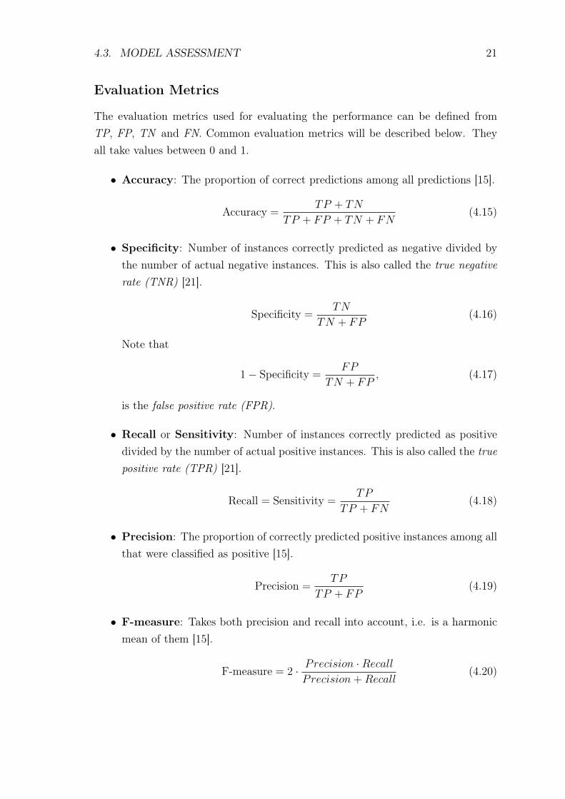
Evaluation Metrics

The evaluation metrics used for evaluating the performance can be defined fromTP, FP, TN and FN. Common evaluation metrics will be described below. Theyall take values between 0 and 1.

• Accuracy: The proportion of correct predictions among all predictions [15].

Accuracy =TP + TN

TP + FP + TN + FN(4.15)

• Specificity: Number of instances correctly predicted as negative divided bythe number of actual negative instances. This is also called the true negativerate (TNR) [21].

Specificity =TN

TN + FP(4.16)

Note that

1− Specificity =FP

TN + FP, (4.17)

is the false positive rate (FPR).

• Recall or Sensitivity: Number of instances correctly predicted as positivedivided by the number of actual positive instances. This is also called the truepositive rate (TPR) [21].

Recall = Sensitivity =TP

TP + FN(4.18)

• Precision: The proportion of correctly predicted positive instances among allthat were classified as positive [15].

Precision =TP

TP + FP(4.19)

• F-measure: Takes both precision and recall into account, i.e. is a harmonicmean of them [15].

F-measure = 2 · Precision ·RecallPrecision+Recall

(4.20)


Accuracy is generally not the most informative metric for the results. The pairsspecificity and sensitivity (Equations 4.16 and 4.18) and recall and precision (Equa-tion 4.18 and 4.19) are better for measuring the performance of a classifier [22].

There is a trade-off between precision and recall, so when one increases the otherdecreases. It is therefore better to use the F-measure to see how the classifier isperforming [22].

A drawback with accuracy, precision and F-measure is that they are affected ifthe class distribution changes. This is because these metrics are computed from val-ues from both columns in the confusion matrix. However, specificity and sensitivitywill not be affected by a change in the class distribution [23]. Hence, the focus willbe on these metrics and the ROC curve and the AUC.

The ROC Curve and AUC

Since the goal is to find probability of churn the response will be predicted as aquantitative output, i.e. probabilities ∈ [0, 1]. A threshold value can then be de-cided in order to assign the predicted probabilities the corresponding class labels.If the probability is higher than this threshold the observation will be assigned tothe positive class, otherwise it will be assigned to the negative class [20, 23].

Figure 4.4: The ROC curve and AUC.

4.4. LEARNING ALGORITHMS 23

The ROC (receiver operating characteristic) curve has FPR on the x-axis and TPRon the y-axis and is used to compare classifiers for all threshold values [17]. Eachpoint on the curve represents the performance of a probabilistic classifier for dif-ferent threshold values [19]. By changing the threshold the TPR (sensitivity) andFPR (1-specificity) can be adjusted [21].

Figure 4.4 (drawn in Microsoft PowerPoint) shows an example of what the ROCcurve looks like. The diagonal line y = x shows what the ROC curve looks like ifthe classes were guessed randomly [23]. In order to compare classifiers by looking atthe ROC curve the AUC (area under the ROC curve) can be computed. The AUCcan take values between 0 and 1. The AUC for the diagonal line is 0.5 and hence inorder for a classifier to be better than random guessing the AUC has to be greaterthan that. The goal is to maximize AUC in order to get a good classifier [17, 19].

4.4 Learning Algorithms

Churn prediction is commonly modeled as a binary classification problem and hencethe focus will be on supervised machine learning algorithms that suit that approach.Firstly, Logistic Regression, which is a parametric method, will be explained. Sec-ondly, the tree-based methods Decision Tree and Random Forest, which are non-parametric methods, will be explained.

Logistic Regression

Logistic Regression predicts the probability of the output Y belonging to a certainclass rather than directly predicting the response of Y. The response is binary:

Y =

0, if an observation belongs to the negative class

1, if an observation belongs to the positive class(4.21)

The method models the relationship between p(X) = P(Y = 1|X) and X [21].

Single Predictor

First the focus will be on predicting a binary response from one feature. In LinearRegression the relationship between p(X) and X is assumed to be linear:

p(X) = β0 + β1X, (4.22)

where β0 (intersect) and β1 (slope) are unknown parameters. When a binary classifi-cation is performed by fitting a straight line to a binary output some of the predicted


probabilities can be p(X) < 0 and p(X) > 1. This is a problem since probabilitiesshould be between 0 and 1 [21].

In order to get outputs within the interval [0, 1], Logistic Regression is used. Therelationship between p(X) and X is modeled according to the logistic function:

p(X) =eβ0+β1X

1 + eβ0+β1X(4.23)

The function has an S-shaped curve which makes sure that the probabilities arebetween 0 and 1 (see Figure 4.5 [21]).

Figure 4.5: An example of how Linear Regression (left plot) and Logistic Regression(right plot) can look like. The x-axis is the single predictor and the y-axis is theprobability of belonging to the positive class.

The logistic function can be rewritten to the form:

p(X)

1− p(X)= eβ0+β1X. (4.24)

The quantity on the left-hand side is called the odds and can take values in theinterval [0,∞]. The logarithm is taken of both sides in Equation 4.24:

log(p(X)

1− p(X)) = β0 + β1X. (4.25)

Log-odds or logit is what the quantity on the left-hand side is called. The righthand side is the same as in Equation 4.22, i.e. the logit is linear in X. From this itcan be seen that Logistic Regression assumes there is a linear relationship betweenthe log-odds of p(X) and the feature X, i.e. the method estimates linear decisionboundaries [20, 21].


The unknown parameters β0 and β1 are estimated from the training set by themaximum likelihood function

`(β0, β1) =∏i:yi=1

p(xi)∏

i′:yi′=0

(1− p(xi′)) (4.26)

The estimated parameters, β0 and β1, should maximize this function. In otherwords, the goal of the maximum likelihood method is to estimate β0 and β1 so thatthe predicted probability, p(xi), is close to zero for an observation that should belongto the negative class and close to one for an observation that should belong to thepositive class [21].

Multiple Predictors

Now the functions used for Logistic Regression above will be extended for multiplefeatures. Equation 4.24 becomes:

log(p(X)

1− p(X)) = β0 + β1X1 + β2X2 + . . .+ βpXp. (4.27)

The logistic function can therefore be written as:

p(X) =eβ0+β1X1+β2X2+...+βpXp

1 + eβ0+β1X1+β2X2+...+βpXp(4.28)

Similarly to when there is a single predictor the parameters, β0, β1, β1, . . . , βp, areestimated with the maximum likelihood function [21].

The logistic regression algorithm is summarized below.

Logistic Regression [21]:Learning

• The parameters β0, β1, β1, . . . , βp are estimated from the training set bythe maximum likelihood function (Equation 4.26).

Prediction

• β0, β1, β2 . . . βp are plugged into the logistic function (Equation 4.28) topredict p(X) for previously unseen data.


L1 Regularized Logistic Regression

A common problem in a two-class Logistic Regression is that the data is perfectlyseparable, i.e. a feature or features perfectly predict the output. This causes theestimated parameters from the maximum likelihood to be undefined [20]. L1 Regu-larized Logistic Regression or Lasso can be used to overcome this problem.

The log likelihood for Logistic Regression is given by:

`(β) =N∑i=1

{yilog(p(xi)) + (1− yi)log(1− p(xi))}

=N∑i=1

{yi(β0 + βTxi)− log(1 + eβ0+βTxi)} (4.29)

The penalized version with the L1 penalty is used in the shrinkage method Lassoand is written as:

`(β) =N∑i=1

{yiβTxi − log(1 + eβTxi)} − λ

p∑j=i

|βj|︸︷︷︸L1 penalty

, (4.30)

where β0, β1, β1, . . . , βp, are estimated by maximizing this function and hence the λhas to be chosen carefully [20].

As stated in Section 4.2 estimated parameters are shrunken towards zero whenusing shrinkage methods. When Lasso is used the L1 penalty forces some of theestimated parameters to be exactly zero. This happens when λ is large enough.Because of this effect, Lasso performs feature selection.

Decision Tree

Decision Trees (DT) can be used both for regression and classification and are easyto interpret and represent graphically.

A tree is grown using a recursive binary splitting where the feature space is split intoJ simpler regions, R1, R2, . . . , RJ . This tree is then used to predict the output ofpreviously unseen data [21, 22]. The DT algorithm is explained in more detail below.


Decision Tree [21]:Learning: Growing a DT

• Start with all the features from the training set. This is called the rootnode of the tree and is at the top.

• The feature space is split on the most informative feature. This createstwo child nodes according to the splitting. These nodes are connectedto the root node by branches.

• This process is repeated recursively for each node, where the correspond-ing feature space is split by the most informative feature.

• The process continues until a stopping criterion is met. These nodes arecalled leafs and indicate the regions R1, R2, . . . , RJ .

PredictionThe region where the new observation belongs is found from the grown DT.Two approaches are commonly used to predict the class of the new observation:

1. The majority vote of the class labels of the training observations in theregion is used to determine the class.

2. The proportions of each class in the region, i.e. the probability of be-longing to a class, is computed.

The second approach is usually of more interest.

...The most informative feature for classification is found by computing the gini index :

Gini index =K∑k=1

pl,k(1− pl,k), (4.31)

where pl,k stands for the proportion of training observations in the region l thathave class k. The gini index measures the total variance among the K classes [21].

Cross-entropy is also commonly used to find the feature to split:

Cross-entropy = −K∑k=1

pl,klog(pl,k) (4.32)


From Equation 4.31 it can be seen that the gini index is low when the majorityof observations are from the same class. This is also the case with cross-entropy(Equation 4.32). These two measures are therefore used to measure node purityor the quality of a split [21]. The most informative feature which is used for thesplitting is the one that has the lowest gini index or cross-entropy.

A drawback with DTs is that there is a large risk they will overfit since they use allthe features that are given to them [22]. This leads to high variance. Pruning can beused to reduce variance. Pruning methods are split into two categories: pre-pruningand post-pruning. In pre-pruning the tree building stops before it is complete. Thetree is built until the test error no longer decrease more than some threshold bymaking a split. In post-pruning the complete tree is first built and then the tree ispruned back in order to reduce the test error for unseen observations [21, 24].

Using a single DT does not result in a good prediction accuracy compared to otherclassification algorithms. However, by combining trees and averaging the results re-duces the variance and hence improves the predictive performance. Various methodsexist for doing this and one of them is Random Forest [21].

Random Forest

Random Forest (RF) is an ensemble method. For classification, a number of deci-sion trees are built on bootstraps of the training set where majority voting of classlabels or average of class proportions among trees is used to predict the outcome.

Bootstrap replicate will first be defined and then the RF algorithm will be stated....

Bootstrap replicate [21]:

• A bootstrap data set, Z∗1, is created by selecting randomly n observa-tions from the original data set, Z, which has n observations.

• The same observation can appear more than once in the same bootstrapset since the sampling is done with replacement.

• This is repeated B times so B different bootstrap sets are created:Z∗1,Z∗2, . . . ,Z∗B.

...


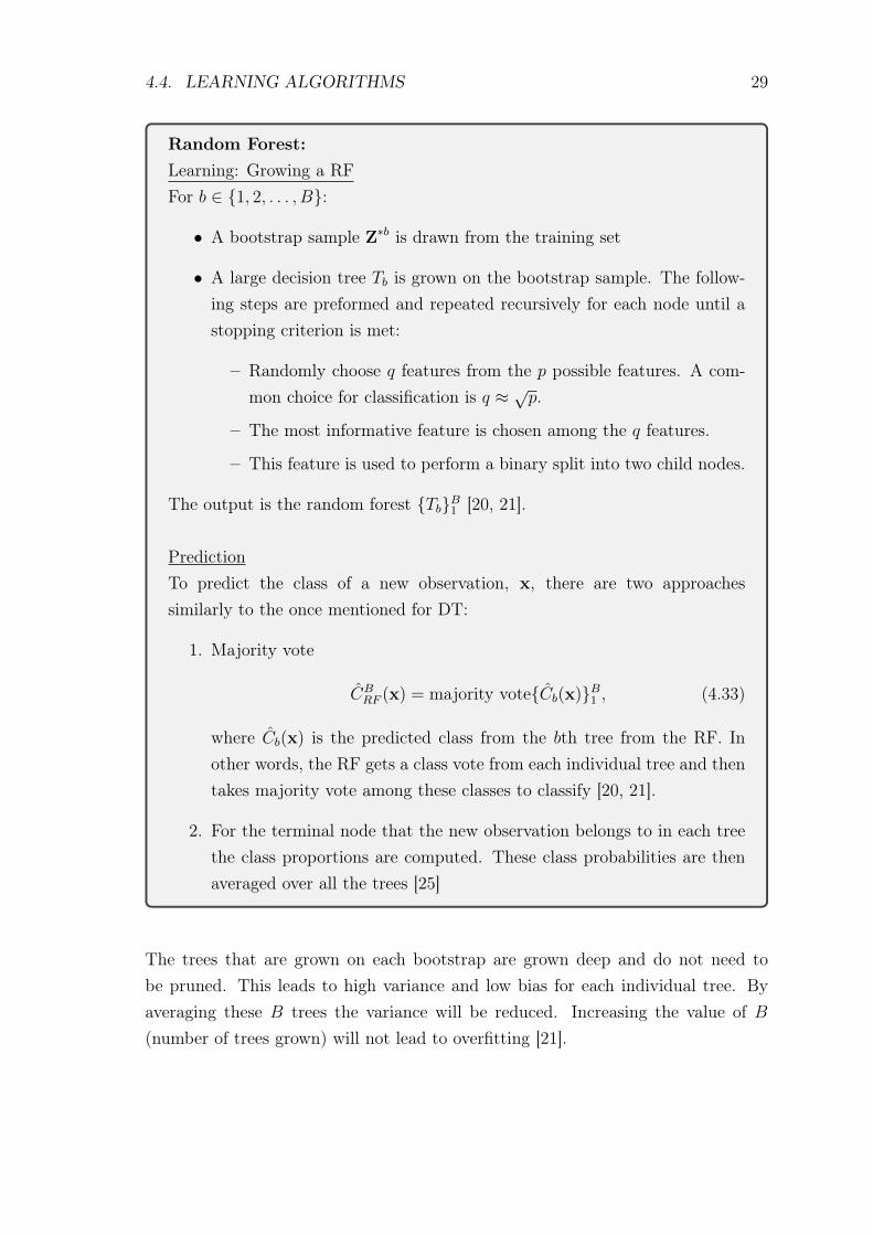
Random Forest:Learning: Growing a RFFor b ∈ {1, 2, . . . , B}:

• A bootstrap sample Z∗b is drawn from the training set

• A large decision tree Tb is grown on the bootstrap sample. The follow-ing steps are preformed and repeated recursively for each node until astopping criterion is met:

– Randomly choose q features from the p possible features. A com-mon choice for classification is q ≈ √p.

– The most informative feature is chosen among the q features.

– This feature is used to perform a binary split into two child nodes.

The output is the random forest {Tb}B1 [20, 21].

PredictionTo predict the class of a new observation, x, there are two approachessimilarly to the once mentioned for DT:

1. Majority vote

CBRF (x) = majority vote{Cb(x)}B1 , (4.33)

where Cb(x) is the predicted class from the bth tree from the RF. Inother words, the RF gets a class vote from each individual tree and thentakes majority vote among these classes to classify [20, 21].

2. For the terminal node that the new observation belongs to in each treethe class proportions are computed. These class probabilities are thenaveraged over all the trees [25]

...The trees that are grown on each bootstrap are grown deep and do not need tobe pruned. This leads to high variance and low bias for each individual tree. Byaveraging these B trees the variance will be reduced. Increasing the value of B(number of trees grown) will not lead to overfitting [21].


The reason for only choosing q features among the p available is because this decor-relates the trees. When all features are used, the process is called Bagging. If thereis one very strong feature and the others are moderately strong the collection ofbagged trees would all be very similar to each other since most of the trees woulduse the strong feature as the first split. This causes the predictions from these treesto be highly correlated. Taking the average of correlated trees does not reduce thevariance as much as averaging uncorrelated trees, which is the case in RF (q < p)[21].

The test error of a RF can be estimated without using CV. As described above,when creating each bootstrap sample n observations are chosen randomly from theoriginal data set and sampling is done with replacement. This means that some ob-servations will appear many times in the same bootstrap and some will not appearat all. The observations that are not used to grow the corresponding tree, Tb, arecalled out-of-bag (OOB). This means that it is possible to predict the output for theith observation from trees that were grown on bootstraps where the ith observationdid not appear. This is done for all the observations and an overall OOB classifica-tion error is computed which is an estimate of the test error [21].

A single tree is easier to interpret than a RF. However, variable importance canbe accessed for RF. For classification trees the decrease of the gini index (Equation4.31) due to splitting over a certain feature can be added up and averaged over allB trees. High values correspond to important features [21].

Chapter 5

Method

The Cross-Industry Standard Process for Data Mining (CRISP-DM Model) de-scribed in [26] was followed in this thesis. This process can be seen in Figure5.1 [27] and what was done in each stage will be described in detail in the followingsections. The query language SQL was used to collect data from the database wherethe data is stored and RStudio was used to prepare the data and for creating themodel.

Figure 5.1: CRISP-DM Model.

31

32 CHAPTER 5. METHOD

5.1 Business Understanding

In this first step of the process the thesis objectives were discussed with Paradox.As stated in Section 1.1 the goal of this thesis is to identify whales and predictthe probability of them churning. By doing this, Paradox can target the group ofwhales that are likely to churn in order to retain them and hence increase revenues.In order to reach this goal the definition of Paradox whales and when they churnhad to be decided.

Definitions

From Sections 3.2 and 3.3 it is clear that the definitions of whales and when theychurn are not universally agreed upon. Rather, these tend to be defined in relationto the particular project and circumstances at hand. This is also the approach usedin the current work.

The following constraints were considered:

• Paradox PC games (exclude console and mobile). These games are premiumgames which means that they are not free-to-play.

• Players with a Paradox account.

• Player has to be a Paradox customer before the period in question starts.This makes sure new customers that start within the period are excluded. Theterm Paradox customer means that the player has to either have a Paradoxaccount or have purchased something connected to a PC game. The reason forthis definition is that a player can make a purchase before creating an accountand it is important to include those players as well.

Whales

After discussing with the company it was decided to look at how much players spendover 12 months since there are fluctuations in spending depending on seasons andnew releases. It was also decided to look at spending only on DLCs (add-ons andexpansions).

5.1. BUSINESS UNDERSTANDING 33

In order to state the definition of whales for this thesis two other definitions will bestated first.

Definition 5.1: PercentileThe value which q percent of the observations from a data set are less thanor equal to is called the q-th percentile of the data set, q ∈ (0 : 100) [28].

...

Definition 5.2: Rolling Twelve Month WindowWithin the company it is assumed that a month is 30 days and therefore atwelve month window is defined to be 360 days. Rolling window means thatfor each day that passes the window should move by one day.

...It was decided to look at spending in each window from 2016-01-01 until 2018-12-31:

2016-01-01 2016-12-26

First window

2016-01-02 2016-12-27

Second window

...

2018-01-05 2018-12-31

Last window

From these two definitions above whales can now be defined.

Definition 5.3: WhalesFor each time period in the rolling twelve month window the 95-th percentileof the players’ spending on DLCs is calculated. The players that spend morethan this value are defined as whales. If a player fulfills this condition in atleast one window he will always be defined as a whale.


Churn

Since the target group of this thesis is big spenders the focus was on their purchasebehaviour rather than playing behaviour. It was decided to investigate how manydays had passed since the whales’ last purchase (including all products for PCgames):

Last purchase 2018-12-31

Days since last purchase

The distribution of the days since last purchase for the whales was plotted in orderto decide how many days were allowed to pass from their last purchase before theyare defined as churners. In addition the average number of days between purchaseswas investigated. This was discussed with Paradox and decided to choose 28 daysas the limit....

Definition 5.4: Churn of WhalesA whale has churned if he has not bought anything for more than 28 days,i.e. 4 weeks. Churn here means that the player is not a whale anymore, i.e.he has stopped being a big spender for Paradox PC games.

5.2 Data Understanding

Getting an understanding of the data was the most time consuming part of thisproject. In order to be able to define whales and when they churn some data anal-ysis had to be done first. Therefore, going back and forth from this second stepof the process and the first step was needed (see Figure 5.1). When the BuisnessUnderstanding was complete the whales were filtered out according to Definition5.3 and labeled as churners (1) and non-churners (0) according to Definition 5.4.The next step was then to collect information about these players.

The data that was collected can be divided into three categories as mentioned inSection 3.5. An example of what kind of features were collected:

• Activity in games: Number of days played, session time and inactivity time.

5.3. DATA PREPARATION 35

• Purchase behaviour: Number of purchases, which products were purchased,amount spent and time between purchases.

• Player information: Anonymized game platform ID and country.

Since the data was labeled according to if 28 days had passed from the last purchaseor not the feature "date of last purchase" had to be removed from the data set.Similarly, it was decided to collect data until 28 days before 2018-12-31 in order notto have information from the "future".

5.3 Data Preparation

After all the data had been collected the data preparation was performed in RStudio.First some of the information collected had to be transformed such that each row(observation) was connected to a whale ID and each column (feature) containedinformation about the corresponding whale. When all of the data had this formatit was joined into a data frame (which is a table) combined from an ID column, theinput X (Equation 4.1) and the output Y (Equation 4.5), the class labels:

ID1 x1,1 x1,2 . . . x1,p y1

ID2 x2,1 x2,2 . . . x2,p y2...

...... . . . ...

...IDn xn,1 xn,2 . . . xn,p yn

=[ID Z

](5.1)

The following data preparation was done:

• All the whales have not been Paradox customers for the same amount of time.Therefore the amount spent by each whale had to be divided by the numberof days since they bought for the first time, i.e. amount spent per day.

• Similarly, the session time for each whale had to be divided by the number ofdays since they played for the first time, i.e. session time per day

• Some rows had too many missing values and were therefore removed from thedata set.

• The format of date columns was changed into five new categorical columns:year (2013-2018), month (1-12), week (1-4), day (1-7) and isWeekend (0/1).


The data was next split randomly into a training set, 34of the observations, and a

test set, 14of the observations. The ID column was removed from the training set

since it should not go into the learning algorithm.

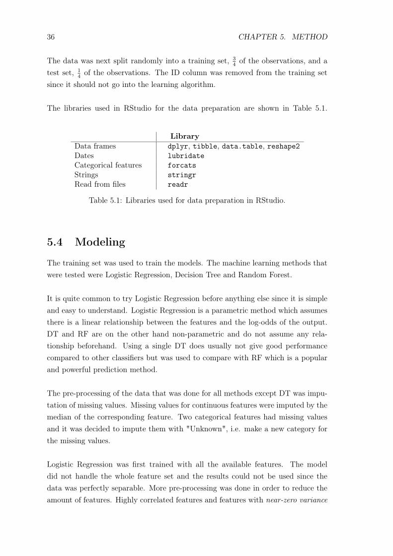
The libraries used in RStudio for the data preparation are shown in Table 5.1.

LibraryData frames dplyr, tibble, data.table, reshape2Dates lubridateCategorical features forcatsStrings stringrRead from files readr

Table 5.1: Libraries used for data preparation in RStudio.

5.4 Modeling

The training set was used to train the models. The machine learning methods thatwere tested were Logistic Regression, Decision Tree and Random Forest.

It is quite common to try Logistic Regression before anything else since it is simpleand easy to understand. Logistic Regression is a parametric method which assumesthere is a linear relationship between the features and the log-odds of the output.DT and RF are on the other hand non-parametric and do not assume any rela-tionship beforehand. Using a single DT does usually not give good performancecompared to other classifiers but was used to compare with RF which is a popularand powerful prediction method.

The pre-processing of the data that was done for all methods except DT was impu-tation of missing values. Missing values for continuous features were imputed by themedian of the corresponding feature. Two categorical features had missing valuesand it was decided to impute them with "Unknown", i.e. make a new category forthe missing values.

Logistic Regression was first trained with all the available features. The modeldid not handle the whole feature set and the results could not be used since thedata was perfectly separable. More pre-processing was done in order to reduce theamount of features. Highly correlated features and features with near-zero variance

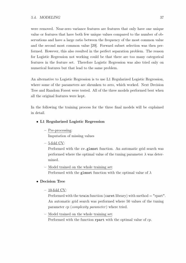
5.4. MODELING 37

were removed. Near-zero variance features are features that only have one uniquevalue or features that have both few unique values compared to the number of ob-servations and have a large ratio between the frequency of the most common valueand the second most common value [29]. Forward subset selection was then per-formed. However, this also resulted in the perfect separation problem. The reasonfor Logistic Regression not working could be that there are too many categoricalfeatures in the feature set. Therefore Logistic Regression was also tried only onnumerical features but that lead to the same problem.

An alternative to Logistic Regression is to use L1 Regularized Logistic Regression,where some of the parameters are shrunken to zero, which worked. Next DecisionTree and Random Forest were tested. All of the three models performed best whenall the original features were kept.

In the following the training process for the three final models will be explainedin detail.

• L1 Regularized Logistic Regression

– Pre-processing:Imputation of missing values

– 5-fold CV:Performed with the cv.glmnet function. An automatic grid search wasperformed where the optimal value of the tuning parameter λ was deter-mined.

– Model trained on the whole training set:Performed with the glmnet function with the optimal value of λ

• Decision Tree

– 10-fold CV:Performed with the train function (caret library) with method= "rpart".An automatic grid search was performed where 50 values of the tuningparameter cp (complexity parameter) where tried.

– Model trained on the whole training set:Performed with the function rpart with the optimal value of cp.


• Random Forest

– Pre-processing:Imputation of missing values

– 5-fold CV:Performed with the train function (caret library) with method= "parRF".A grid search was performed for the tuning parameter mtry (numberof randomly selected features at each split) where four values close toq =√p where tried.

– Model trained on the whole training set:Performed with the function randomForest with the optimal value ofmtry.

No feature selection methods were needed since glmnet, rpart, parRF and randomForestperform feature selection automatically.

A summary of the libraries used in RStudio for modeling and evaluation can beseen in Table 5.2.

LibraryTraining and predicting caretL1 Regularized LR glmnetDecision Tree rpartRandom Forest randomForestROC curve pROC

Table 5.2: Libraries used for modeling and evaluation in RStudio.

5.5 Evaluation

To evaluate the performance of the models the test data set was used. The test setwas pre-processed according to the training set. In order to make predictions fromthe trained models the predict function (caret library) was used. The evaluationmetric AUC was used to compare classifiers. Different probability threshold valueswere compared for the other evaluation metrics listed in Section 4.3.

Chapter 6

Results

The final data set has 75 features and 106944 observations. 27 features are contin-uous and the remaining 48 are categorical. The majority class is non-churners. Thedata was split randomly into a training set, 3

4of the observations, and a test set, 1

4

of the observations.

The results from the methods L1 Regularized Logistic Regression, Decision Treeand Random Forest will be explained in the following sections. The AUC evalua-tion metric was used to compare the classifiers and the best results obtained fromeach machine learning method can be seen in Table 6.1.

AUCL1 Regularized LR 0.6855Decision Tree 0.6655Random Forest 0.7162

Table 6.1: Final results from the models.

6.1 L1 Regularized Logistic Regression

Pre-Processing

First missing values were imputed. Continuous features were imputed by the medianof the corresponding feature and categorical features with "Unknown". The libraryglmnet was used to perform the L1 Regularized Logistic Regression (Lasso). Theglmnet function only works for numerical features and therefore one-hot-encoding,where categorical features are encoded to numerical, is done automatically whenusing the function. This increased the features from 75 to 168.

39

40 CHAPTER 6. RESULTS

Correlation analysis is not needed since Lasso picks one of the correlated features anddiscards the others, i.e. shrinks their parameters to zero. Scaling is not needed sincethe glmnet function also performs scaling automatically but returns the parameterson the original scale [30].

Model Selection

Hyperparameter Tuning

The glmnet method has two tuning parameters, λ and α. The value of α was heldconstant at 1, to use the Lasso shrinkage method, while hyperparameter tuning wasperformed with 5-fold CV to find the optimal value of λ.

Figure 6.1: The log(λ) plotted as a func-tion of the cross-validation error. Theerror bars on the plot correspond to theupper and lower standard deviations.The top axis correspond to the numberof non-zero features.

Figure 6.2: The log(λ) plotted as a func-tion of the parameter values. The topaxis correspond to the number of non-zero features.

From Figure 6.1 the log(λ) for the values tried by cv.glmnet can be seen as a func-tion of the cross-validation error (Equation 4.14). According to [30] the two verticallines correspond to λmin, which gives the minimum value of the cross-validationerror, and λ1se, which results in the most regularized model where the misclassifica-tion error is within one standard deviation of the minimum error. In Figure 6.2 thelog(λ) is plotted as a function of the parameter values. Moving to the right moreparameters are shrunken to zero, hence reducing the number of non-zero parame-ters.

6.1. L1 REGULARIZED LOGISTIC REGRESSION 41

The optimal value was λmin = 0.0006726743 and this caused 55 parameters tobe shrunk to zero, i.e. the features were reduced from 168 to 113. The final modelwas then trained on the whole training set with α = 1 and λ = λmin.

Model Assessment

The performance was evaluated on the test set and the results for a few differentthresholds can be seen in Table 6.2. The AUC was 0.6855 and the ROC curve canbe seen in Figure 6.3.

Threshold0.3 0.4 0.5 0.6 0.7

Accuracy 0.5544 0.6357 0.6569 0.6451 0.6218Sensitivity 0.8463 0.6251 0.3966 0.2202 0.1005Specificity 0.3534 0.6431 0.8363 0.9378 0.9809Precision 0.4742 0.5468 0.6253 0.7092 0.7840F1 0.6078 0.5833 0.4853 0.3361 0.1782TP 9230 6817 4325 2402 1096FN 1676 4089 6581 8504 9810TN 5595 10180 13238 14845 15528FP 10235 5650 2592 985 302

Table 6.2: Evaluation metrics according to chosen thresholds for L1 RegularizedLogistic Regression.

Figure 6.3: ROC curve and AUC for L1 Regularized Logistic Regression.


6.2 Decision Tree

Pre-Processing

No pre-processing had to be done. The rpart method uses an inbuilt default actionfor handling missing values. This action only removes rows if the response variableor all the features are missing. This means that rpart has the ability to partiallyretain missing observations [31].

Model Selection


Decision Trees are built by choosing each time the most informative feature to splitthe feature space. Therefore, the first feature chosen is the most important feature.Decision Trees use all features by default but usually pruning is performed. In therpart library which is used the parameter cp (complexity parameter) can be tunedto control the post-pruning of the tree. This means that all features are used andthe tree is fully grown and then pruned back according to the value of cp whichcontrols the number of splits made [31].

Figure 6.4: The cp as a function of cross-validation error.

Figure 6.5: The Decision Tree.

The value of cp was tuned by using 10-fold CV where 50 different values for cpwere tried. From Figure 6.4 it can be seen how the cross-validation error (Equation4.14) changes as cp decreases and the number of splits increases. The optimal value

6.2. DECISION TREE 43

was cp = 0.000488878 which allowed the tree to split 60 times. The tree was thenbuilt according to this cp value on the whole training set (see Figure 6.5).

Model Assessment


Threshold0.3 0.4 0.5 0.6 0.7


Table 6.3: Evaluation metrics according to chosen thresholds for Decision Tree.

Figure 6.6: ROC curve and AUC for Decision Tree.


6.3 Random Forest

Pre-processing

Missing values had to be imputed. Continuous features were imputed by the medianof the corresponding feature and categorical features with "Unknown".

Model Selection


Random Forest chooses q ≈ √p features randomly from the available features eachtime and chooses the most informative one of them to split the feature space. Thevalue of q is a tuning parameter for parRF (caret library) which is called mtry, i.e.how many features should be chosen at random each time.

Since there are 75 features q ≈√75 = 8.660254. Therefore it was decided to

use the grid mtry = c(8, 10, 12, 15). The grid search was performed by using 5-foldCV and the optimal value was mtry = 15 (see Table 6.4).

mtry Accuracy8 0.670008010 0.670294712 0.670344515 0.6703445

Table 6.4: Values of mtry used in grid search.

The model was then trained with this value of mtry on the whole training set withthe randomForest function. The model was trained with ntree = 1500 but fromFigure 6.7 it can be seen that a smaller amount of trees, for example 1000, couldhave been chosen.

6.3. RANDOM FOREST 45

Figure 6.7: Class errors and OOB error as a function of number of trees grown.Green: Class error for the positive class, i.e. FP/TP. Red: Class error for thenegative class, i.e. FN/TN. Black: OOB error.

Model Assessment


Threshold0.3 0.4 0.5 0.6 0.7


Table 6.5: Evaluation metrics according to chosen thresholds for Random Forest.

............................................................................................................................................................................................................................................................................................................................................................................................................................................................................................


Figure 6.8: ROC curve and AUC for Random Forest.

Chapter 7

Discussion

7.1 Findings

The main findings of this project are the answers to the research questions statedin Section 1.1. In the following the questions will be answered.

Question 1:What is a good way to define which players are Paradox whales, i.e. players thatare big spenders in Paradox PC games?

In order to take seasonal fluctuations and new releases into account it was de-cided to look at spending on DLCs for players with a Paradox account over a 12month rolling period. The players spending more than the 95th-percentile of thetotal spending by the players for each period were defined as whales.

When this definition was decided a histogram of cohorts vs. amount spent overa 12 month period was plotted. The amount spent by each player (fulfilling theconstraints mentioned in Section 5.1) over this period was summed up and then theplayers where divided into 20 cohorts. The first cohort corresponds to the playersspending less than the 5th-percentile, the second cohort the once that spent morethat the 5th-percentile but less then the 10th-percentile and so on until the lastcohort, the whales, which corresponds to the players spending more than the 95th-percentile. Each bar on the histogram corresponds to one cohort. The histogramexhibited exponential-like growth and hence the height difference between the lastand the second last bar was much larger than between the second last bar andthe bar before. This showed clearly that one group of players spend the most andtherefore the conclusion is that this definition is good for Paradox whales.

47

48 CHAPTER 7. DISCUSSION

Question 2:What is a good way to define if a Paradox whale has churned or not?

"A Paradox whale has churned if he has not bought anything for 28 days" wasthe definition that was used in this thesis. The definition was decided according tothe distributions of days since last purchase for the players where the end date was2018-12-31 (since data was collected until then). This approach has its drawbackssince this distribution of days since last purchase would look different if the enddate was for example 2018-07-31 instead of 2018-12-31. Defining the churn event isa difficult task since many factors have an impact on when players buy, for exam-ple seasons and releases of game products. A further investigation on the playerspurchase behaviours, releases and seasonal fluctuations would have to be taken intoaccount in order to get a better churn definition.

Question 3:Which supervised machine learning model gives the best performance in predictingthe probability of a whale churning?

The model that performed best in terms of AUC was Random Forest with AUC =

0.7162. This method outperformed both L1 Regularized Logistic Regression andDecision Tree. It was expected that the performance of the DT would be worsethan RF since RF is an ensemble method that combines many DT and averagesthem. The reason for L1 Regularized Logistic Regression performing worse thanRF could be that the linear relationship Logistic Regression is assuming does notexplain the data well.

The accuracy for Random Forest was highest when the probability threshold was0.5 (Table 6.5), but as stated in Section 4.3 accuracy is not the most interestingevaluation metric. The main focus was on having a balance between sensitivityand specificity and trying to get both metrics as high as possible. The trade-offbetween FP and FN, i.e. marketing costs for retaining players and the loss whenplayers churn, has to be considered when an appropriate probability threshold ischosen. The focus is on retaining players that are likely to churn, hence the focusshould be more on minimizing the FN. For the thresholds shown in Table 6.5, 0.4is probably the best choice since sensitivity is high, 0.7335, and specificity is higherthan random, 0.5689.

7.2. FURTHER STUDIES 49

7.2 Further studies

Investigating the definition of churn and collecting more data about the whales couldpossibly improve the performance of the model.

Defining churn is a difficult task when there is not a contractual relationship be-tween the customers and the company since human behaviour can be random. Thedefinition used in this thesis only looked at how many days had passed since theplayers last made a purchase. It is obvious that more things have to be taken intoaccount to make the definition better. One important thing that should be lookedinto is whether a whale has already bought everything available from the inventoryand that is the reason for why the player has not bought anything for 28 days. Inaddition seasonal fluctuations and peaks in spending because of releases should betaken into account.

More data about the whales could possibly improve the performance of the model.No information about player behaviour within each game was used in this work.Having information about weather the player is doing well or not and more gamespecific data probably play a big role in weather the players stop spending much onParadox PC products or not.

Another suggestion is to look at one PC game at a time. The games can be re-ally different and some games have more products that are possible to buy thanothers. It is assumed that this has a great impact on both the purchase and play-ing behaviour of the players. Therefore it might be better to make separate churnmodels for each game.

It would also be interesting to do a further investigation on the cohorts close tothe whale cohort. These players spend a lot of money but not enough to be definedas whales. It might be possible to turn these players into whales.

Finally, more machine learning methods should be tried such as SVM, Naïve Bayesand Gradient Boosting as suggested by literature (Section 3.4). It might be thecase that these methods manage to capture the patterns in the data better than themethods tried here.

50 CHAPTER 7. DISCUSSION

7.3 Conclusion

The conclusion is that it seems to be possible to predict the probability of churningfor Paradox whales. The model that gave the best performance was Random Forestwith AUC = 0.7162. It is concluded that this model can be a good basis for a churnmodel for Paradox. The performance of the model is acceptable but can be furtherimproved. By investigating the definition of churn, collecting more game specificdata about the players and try other machine learning methods it might be possibleto achieve better performance.

Bibliography

[1] M. Seif El-Nasr, A. Drachen, and A. Canossa, Game Analyt-ics Maximizing the Value of Player Data. Springer, 2013. [Online].Available: https://link-springer-com.focus.lib.kth.se/content/pdf/10.1007%2F978-1-4471-4769-5.pdf

[2] V. Kumar and J. A. Petersen, Statistical Methods in Customer RelationshipManagement. John Wiley & Sons, Ltd, 2012. [Online]. Available:www.wiley.com.

[3] P. Bertens and A. Guitart Andafricaand Andafrica Periáñez, “Games andBig Data: A Scalable Multi-Dimensional Churn Prediction Model,” IEEEConference on Computational Intelligence and Games (CIG), pp. 33–36, 2017.[Online]. Available: https://arxiv.org/pdf/1710.02262.pdf

[4] M. Miloševí, N. Živí, and I. Andjelkoví, “Early churn predictionwith personalized targeting in mobile social games,” Expert SystemsWith Applications, vol. 83, pp. 326–332, 2017. [Online]. Available:http://dx.doi.org/10.1016/j.eswa.2017.04.056

[5] E. Lee, B. Kim, S. Kang, B. Kang, Y. Jang, and H. K. Kim,“Profit Optimizing Churn Prediction for Long-term Loyal Customer inOnline games,” 2018. [Online]. Available: http://www.ieee.org/publications_standards/publications/rights/index.html

[6] “About us | Paradox Interactive.” [Online]. Available: https://www.paradoxplaza.com/about-us-static-info-ca.html

[7] “Our business | Paradox Interactive - Global Games Publisher.” [Online].Available: https://www.paradoxinteractive.com/en/our-business/

51

https://link-springer-com.focus.lib.kth.se/content/pdf/10.1007%2F978-1-4471-4769-5.pdf


www.wiley.com.

https://arxiv.org/pdf/1710.02262.pdf

http://dx.doi.org/10.1016/j.eswa.2017.04.056

http://www.ieee.org/publications_standards/publications/rights/index.html


https://www.paradoxplaza.com/about-us-static-info-ca.html

https://www.paradoxplaza.com/about-us-static-info-ca.html

https://www.paradoxinteractive.com/en/our-business/

52 BIBLIOGRAPHY

[8] “Annual Report 2018,” Tech. Rep., 2019. [Online]. Available: www.paradoxinteractive.com

[9] “This is Paradox | Paradox Interactive - Global Games Publisher.” [Online].Available: https://www.paradoxinteractive.com/en/this-is-paradox/

[10] “White Wolf | Paradox Interactive - Global Games Publisher.” [Online].Available: https://www.paradoxinteractive.com/en/white-wolf/

[11] “Revenue model | Paradox Interactive - Global Games Publisher.” [Online].Available: https://www.paradoxinteractive.com/en/revenue-model/

[12] “Paradox: "If a game can’t be played for 500 hours we probably shouldn’t bepublishing it".” [Online]. Available: https://www.gamesindustry.biz/articles/2018-05-31-paradox-if-a-game-cant-be-played-for-500-hours-we-probably-shouldnt-be-publishing-it

[13] “Game Pillars | Paradox Interactive - Global Games Publisher.” [Online].Available: https://www.paradoxinteractive.com/en/game-pillars/

[14] “Sign up | Paradox Interactive Forums.” [Online]. Avail-able: https://forum.paradoxplaza.com/forum/index.php?register&_ga=2.160588602.646327372.1556914089-1315729764.1556914089

[15] T. Vafeiadis, K. Diamantaras, G. Sarigiannidis, and K. Chatzisavvas, “Acomparison of machine learning techniques for customer churn prediction,”2015. [Online]. Available: http://dx.doi.org/10.1016/j.simpat.2015.03.003

[16] B. Zhu, B. Baesens, and S. K. L. M. Vanden Broucke, “An empiricalcomparison of techniques for the class imbalance problem in churn prediction,”Information Sciences, vol. 408, pp. 84–99, 2017. [Online]. Available:http://dx.doi.org/10.1016/j.ins.2017.04.015

[17] J. Runge and P. Gao, Chum Prediction for High-Value Players in Casual Social Games. [Online]. Avail-able: https://ieeexplore-ieee-org.focus.lib.kth.se/ielx7/6919811/6932856/06932875.pdf?tp=&arnumber=6932875&isnumber=6932856&ref=

[18] Periáñez, A. Saas, A. Guitart, and C. Magne, “Churn Prediction in MobileSocial Games: Towards a Complete Assessment Using Survival Ensembles,”2016. [Online]. Available: http://www.yokozunadata.com/research/churn.pdf

[19] E. G. Castro and M. S. G. Tsuzuki, “Churn Prediction in OnlineGames Using Players’ Login Records: A Frequency Analysis Approach,”

www.paradoxinteractive.com

www.paradoxinteractive.com

https://www.paradoxinteractive.com/en/this-is-paradox/

https://www.paradoxinteractive.com/en/white-wolf/

https://www.paradoxinteractive.com/en/revenue-model/

https://www.gamesindustry.biz/articles/2018-05-31-paradox-if-a-game-cant-be-played-for-500-hours-we-probably-shouldnt-be-publishing-it

https://www.gamesindustry.biz/articles/2018-05-31-paradox-if-a-game-cant-be-played-for-500-hours-we-probably-shouldnt-be-publishing-it

https://www.paradoxinteractive.com/en/game-pillars/

https://forum.paradoxplaza.com/forum/index.php?register&_ga=2.160588602.646327372.1556914089-1315729764.1556914089

https://forum.paradoxplaza.com/forum/index.php?register&_ga=2.160588602.646327372.1556914089-1315729764.1556914089

http://dx.doi.org/10.1016/j.simpat.2015.03.003

http://dx.doi.org/10.1016/j.ins.2017.04.015

https://ieeexplore-ieee-org.focus.lib.kth.se/ielx7/6919811/6932856/06932875.pdf?tp=&arnumber=6932875&isnumber=6932856&ref=

https://ieeexplore-ieee-org.focus.lib.kth.se/ielx7/6919811/6932856/06932875.pdf?tp=&arnumber=6932875&isnumber=6932856&ref=

http://www.yokozunadata.com/research/churn.pdf

BIBLIOGRAPHY 53

IEEE TRANSACTIONS ON COMPUTATIONAL INTELLIGENCE ANDAI IN GAMES, vol. 7, no. 3, p. 255, 2015. [Online]. Available:http://www.ieee.org/publications_standards/publications/rights/index.html

[20] T. Hastie, R. Tibshirani, and J. Friedman, The Elements of StatisticalLearning: Data Mining, Inference, and Prediction. Springer, 2001.[Online]. Available: https://link-springer-com.focus.lib.kth.se/content/pdf/10.1007%2F978-0-387-21606-5.pdf

[21] G. James, D. Witten, T. Hastie, and R. Tibshirani, Springer Texts in StatisticsAn Introduction to Statistical Learning. Springer, 2013. [Online]. Available:http://www.springer.com/series/417

[22] S. Marsland, Machine Learning: An Algorithmic Perspective, 2nd ed. CRCPress LLC, 2014. [Online]. Available: https://ebookcentral-proquest-com.focus.lib.kth.se/lib/kth/reader.action?docID=1591570

[23] T. Fawcett, “An introduction to ROC analysis,” Pattern Recognition Letters,vol. 27, no. 8, pp. 861–874, 2006. [Online]. Available: www.elsevier.com/locate/patrec

[24] N. Patel, S. P. B. Patel, and A. Prof, “Study of Various DecisionTree Pruning Methods with their Empirical Comparison in WEKASaurabh Upadhyay,” Tech. Rep. 12, 2012. [Online]. Available: https://pdfs.semanticscholar.org/025b/8c109c38dc115024e97eb0ede5ea873fffdb.pdf

[25] W. O. Library, T. Dankowski, and A. Ziegler, “Calibrating randomforests for probability estimation,” 2016. [Online]. Available: https://onlinelibrary-wiley-com.focus.lib.kth.se/doi/pdf/10.1002/sim.6959

[26] C. Shearer, “The CRISP-DM Model: The New Blueprint for Data Mining,”Journal of Data Warehousing, vol. 5, pp. 13–22, 2000. [Online]. Available:www.dw-institute.com/journal.htm

[27] G. Kraljević and S. Gotovac, “Modeling Data Mining Applications for Predic-tion of Prepaid Churn in Telecommunication Services,” Automatika, vol. 51,no. 3, pp. 275–283, 4 2018.

[28] D. A. Wolfe and G. Schneider, Intuitive Introductory Statistics. Springer,2017. [Online]. Available: http://www.springer.com/series/417

[29] “nearZeroVar function | R Documentation.” [Online]. Available: https://www.rdocumentation.org/packages/caret/versions/6.0-84/topics/nearZeroVar




http://www.springer.com/series/417

https://ebookcentral-proquest-com.focus.lib.kth.se/lib/kth/reader.action?docID=1591570

https://ebookcentral-proquest-com.focus.lib.kth.se/lib/kth/reader.action?docID=1591570

www.elsevier.com/locate/patrec

www.elsevier.com/locate/patrec

https://pdfs.semanticscholar.org/025b/8c109c38dc115024e97eb0ede5ea873fffdb.pdf

https://pdfs.semanticscholar.org/025b/8c109c38dc115024e97eb0ede5ea873fffdb.pdf

https://onlinelibrary-wiley-com.focus.lib.kth.se/doi/pdf/10.1002/sim.6959

https://onlinelibrary-wiley-com.focus.lib.kth.se/doi/pdf/10.1002/sim.6959

www.dw-institute.com/journal.htm

http://www.springer.com/series/417

https://www.rdocumentation.org/packages/caret/versions/6.0-84/topics/nearZeroVar

https://www.rdocumentation.org/packages/caret/versions/6.0-84/topics/nearZeroVar

54 BIBLIOGRAPHY

[30] T. Hastie and J. Qian, “Glmnet Vignette,” Stanford, Tech. Rep., 2014. [Online].Available: http://web.stanford.edu/~hastie/glmnet/glmnet_alpha.html#intro

[31] T. M. Therneau and E. J. Atkinson, “An Introduction to RecursivePartitioning Using the RPART Routines,” Tech. Rep., 2019. [Online]. Available:https://cran.r-project.org/web/packages/rpart/vignettes/longintro.pdf

http://web.stanford.edu/~hastie/glmnet/glmnet_alpha.html#intro

https://cran.r-project.org/web/packages/rpart/vignettes/longintro.pdf

TRITA -SCI-GRU 2019:254

www.kth.se

Customer Churn Prediction for PC Games - Kth Diva Portal Org

Documents

Transcript of Customer Churn Prediction for PC Games - Kth Diva Portal Org