CER

N-A

CC

-201

8-00

5024

/10/

2018

CERN – EUROPEAN ORGANIZATION FOR NUCLEAR RESEARCH

KLYC. THE 1D/1.5D LARGE SIGNAL COMPUTER CODE FOR

THE KLYSTRON SIMULATIONS.

USER MANUAL.

Jinchi Cai, Igor Syratchev

European Organization for Nuclear Research, Geneva, Switzerland

Abstract

Almost all the accurate and efficient 2D large-signal codes for the klystron simulations are

proprietary and are not freely available to the wide klystron community. The klystron code

KlyC1D/1.5D has been developed at CERN recently, as an attempt to bridge the gap between

the fast, but approximate 1D models and the time/resource consuming PIC codes. Here the notation

1D/1.5D is related to the fact that in KlyC one can choose between a 1D or 2D map of the electric

field (RF cavities and space charge), whilst the particle motion is one-dimensional.

KlyC is available in the public domain. This manual should help the users to start with KlyC

simulations.

Geneva, Switzerland

24 October 2018

CLIC – Note – 1137

Introduction A number of computer codes for the klystrons simulations have been developed in the past. These codes can be split

into three categories depending on the complexity, completeness of the model and computational techniques being

used. 1D codes like AJDisk, and KlypWin operate in an idealized environment, where parameters of the RF cavities

and space charge forces do not depend on the transverse position of an individual electron trajectory. 2D large-signal

codes like TESLA, Klys2D and FCI account for all radial effects in the presence of an arbitrary solenoidal magnetic

field. To economize on computation time, these codes use different approximations or external simulations of the

electric field in RF cavities and drift tubes areas. Particle-In-Cell (PIC) codes like MAGIC2D/3D and CST/3D provide

complete and self-consistent field solutions using fine discretization in space and time throughout the entire device.

Unfortunately, the accurate and efficient 2D large-signal codes are proprietary and are not freely available to the wide

klystron community. The klystron code KlyC1D/1.5D has been developed at CERN recently, as an attempt to bridge

the gap between the fast, but approximate 1D models and the time/resource consuming PIC codes. Here the notation

1D/1.5D is related to the fact that KlyC can choose between a 1D or 2D map of the electric field, whilst the particle

motion is one-dimensional.

The KlyC computational algorithm is organized in such a way that the interaction between the electric field of the RF

cavities, the space charge field and the longitudinal particles movement are self-consistent. During the first iteration,

the electron beam will be modulated in the input cavity and propagate along the tube without taking the space charge

forces and the RF cavities electric field into account. During the next iteration, the obtained longitudinal charge density

modulation will generate initial distribution of the space charge field, excite the electric field in the cavities and the

drift tubes, which in turn will affect the beam dynamic. Such a process will be repeated until the gap voltage in the

output cavity is converged, providing specified residual difference between the two last iterations.

In KlyC/1D charged particles are represented by the disks. In KlyC/1.5D, the set of rings with different radii form the

equivalent array of charged particles at the emission plane. The rings radial spacing is equidistant and each ring has an

identical charge density, so that for the given beam radius, current in each ring will depend on the number of rings and

its radial position. Through the propagation along the tube, each ring will preserve its radial position. The

communication between the rings comes from the common RF field in the cavities and drifts to which they contribute

individually.

KlyC is available in the public Domain. To receive the access to the code and installation instructions, please contact

to the developers directly via emails: Jinchi.Cai@cern.ch ; Igor. Syratchev@cern.ch.

Content:

1. Getting started

2. RF cavities and Klystron layout

3. Model discretization settings

4. Plot settings

5. Start simulation

6. KlyC output graphics, animations and data

7. Bunched beam as a power source

8. KlyC internal optimizer(s) module

9. The batched jobs

10. Appendix I (E-field import from the other codes)

1. Getting started

After the KlyC installation into the selected folder, open the folder. The KlyC executable file is located in the

‘application’ folder. Double click on the file ‘KlyC.exe’ to start (One can also double click klc file to open KlyC by

choosing the default program as ‘KlyC.exe’ ):

The KlyC GUI window will be opened:

As an illustration, we will use next the 5 cavities, low perveance, 2 MW L-band klystron. The tube has been designed

using the ‘classical’ bunching method. First, we specify the operating frequency: ; the input power:

; the beam and drift tube parameters:

For the klystron simulations, the box located next to the value of the input power shall be checked. In the case of the

hollow beam, the ‘Inner Radius’ of the beam shall be specified as well (0.0 by default).

The KlyC particles emission algorithm is based on the model that uses emission from the metal surface (similar to the

one used in the PIC CST/3D). In this case the beam kinetic energy will be fractionally converted into the DC potential

of the beam space charge (the effect known as the space charge depression). The amount of converted energy will

depends on the beam power, the perveance and the drift tube filling factor (space charge). To enable such an emission

mechanism (recommended), the value of the ‘Image C’ shall be set to -1: If Image C = 0, then the

beam will have the full kinetic power as is specified in the beam parameters table.

In 2D simulations, by default, the current density across the beam cross-section is constant. The user can introduce the

radial variation of the beam current density as a linear function by specifying the chirp value: , In this case,

chirp () is defined as: 𝛼 =𝐽(𝑟𝑚2)−𝐽(𝑟𝑚1)

𝐽0=

𝐽(𝑟𝑚2)−𝐽(𝑟𝑚1)

𝐼0/𝜋/(𝑟𝑚22 −𝑟𝑚1

2 );

The klystron can be simulated using the option of the not perfectly matched RF load. In this case the normalized

amplitude (voltage) and phase of reflection shall be specified in:

KlyC supports multi-core processors (up to 4): For the 2D simulations this option allows to increase the

simulations speed by about 30% to 100%, depending on the case.

Upon completing the simulations, the KlyC can generate multiple graphics, animations and extract the data into text

file(s). All these can be enabled by using the corresponding buttons on a panel:

2. RF cavities and klystron layout.

The general cavities parameters and klystron layout can be introduced directly into a cavity parameters table:

The cavities types are as follows: 0 is the input cavity, 1 is the bunching cavities and -1 is the output cavity. If the

harmonic cavity is used, the harmonic number of this cavity shall be specified in a third column. The frequency

(column 4), the external Q factor (column 6) and the cavity position (column 9) have to be defined by the user.

In the simulations, KlyC uses 1D/2D maps of electric field in the drift tubes and cavity areas. KlyC suggests few

options to generate these maps.

1. Gaussian approximation.

In this case the user has to specify directly each cavity’s impedance (R/Q), beam coupling (M) and intrinsic Q factor

(Qin). Impedance and beam coupling are defined as:

Following, the longitudinal distribution of the normalized electric field will be reconstructed:

This electric field distribution holds only the longitudinal variation and is constant across the beam tunnel. This option

is similar to the one used in 1D computer code AJDisk.

2. KlyC internal cavity calculator.

The specially developed eigenmode solver is integrated into the KlyC. To facilitate the RF cavities parameters

calculation, the KlyC cavity calculator supports three the most common topologies of RF cavities that are used in the

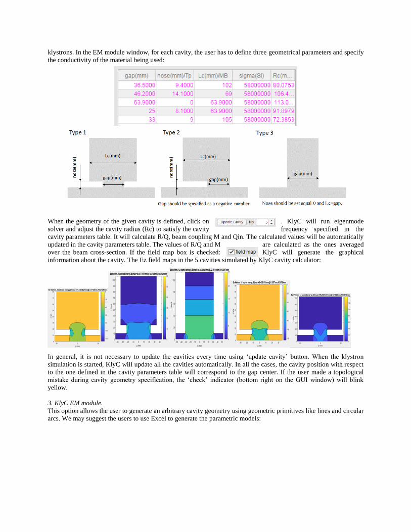
klystrons. In the EM module window, for each cavity, the user has to define three geometrical parameters and specify

the conductivity of the material being used:

When the geometry of the given cavity is defined, click on . KlyC will run eigenmode

solver and adjust the cavity radius (Rc) to satisfy the cavity frequency specified in the

cavity parameters table. It will calculate R/Q, beam coupling M and Qin. The calculated values will be automatically

updated in the cavity parameters table. The values of R/Q and M are calculated as the ones averaged

over the beam cross-section. If the field map box is checked: KlyC will generate the graphical

information about the cavity. The Ez field maps in the 5 cavities simulated by KlyC cavity calculator:

In general, it is not necessary to update the cavities every time using ‘update cavity’ button. When the klystron

simulation is started, KlyC will update all the cavities automatically. In all the cases, the cavity position with respect

to the one defined in the cavity parameters table will correspond to the gap center. If the user made a topological

mistake during cavity geometry specification, the ‘check’ indicator (bottom right on the GUI window) will blink

yellow.

3. KlyC EM module.

This option allows the user to generate an arbitrary cavity geometry using geometric primitives like lines and circular

arcs. We may suggest the users to use Excel to generate the parametric models:

The area with grey background contains the data that shall be copied (or directly generated) into designated txt file that

will be used by KlyC to generate and simulate the cavity. In the first line one shall specify the mode number to be

simulated, the mesh step length in z direction and the mesh step length in r direction (mm).The geometry should start

and finish with min (z) and min (r) points (bottom left corner). From that position, in a clockwise direction, the

geometry nodes (first column ‘Z’; second column ‘R’) and primitive’s type (third column) shall be introduced one by

one. All dimensions are in mm. The primitive’s type at its intersecting point (clockwise) shall be specified as follows:

- The straight vertical, or horizontal line: ‘0’

- The arc: +r or – r. Here r is arc radius, ‘+’ if the arc goes clockwise and ‘-’ if it goes anti-clockwise.

- The tilted line is defined as an arc of a very large (~ x100 of the line length itself) radius.

The file with geometry data shall be saved (created) in the same folder, where the klc project file is located.

To read the geometry file in KlyC, the name of the file without extension shall be typed into the last column (x,y,z,

Ez) of the parameters table and in the We(J) column the user shall put negative number (-1). Please check that drift

radius in the cavity file is the same as the one specified in the project. Note, keep ‘default’ in (x,y,z, Ez) column if the

parameters table and/or the KlyC cavity simulator are used only. Next we used the re-entrant cavity as an example:

Here (cavity #2) we specify the cavity type, harmonic number, frequency, position and material conductivity (sigma).

The cavity geometry name is ‘Re-ent_cav’ and We(J) = -1. When ‘cavity update’ button is pressed, the cavity will be

simulated:

In the column Rc(mm) KlyC will report on the frequency discrepancy between the simulated value and the one

specified in the table: (Fsim-f0)/f0. The user can tune the frequency by modifying the cavity geometry. To our

experience, it is not necessary to tune the frequency difference to be ‘0’, as for simulation KlyC will use the frequency

from the table (f0), whilst R/Q, M and Qin are slow varying functions with respect to the cavity frequency.

Even if the cavity simulations could be rather fast (few seconds), they will be repeated at every iteration for every

cavity. To avoid this, we recommend to run only few (2-3) iterations with box ‘txt output’ being checked. The KlyC

will save all the Ez field distribution(s) into txt files with names KlyCcavity# (# is a cavity number). Next, one can use

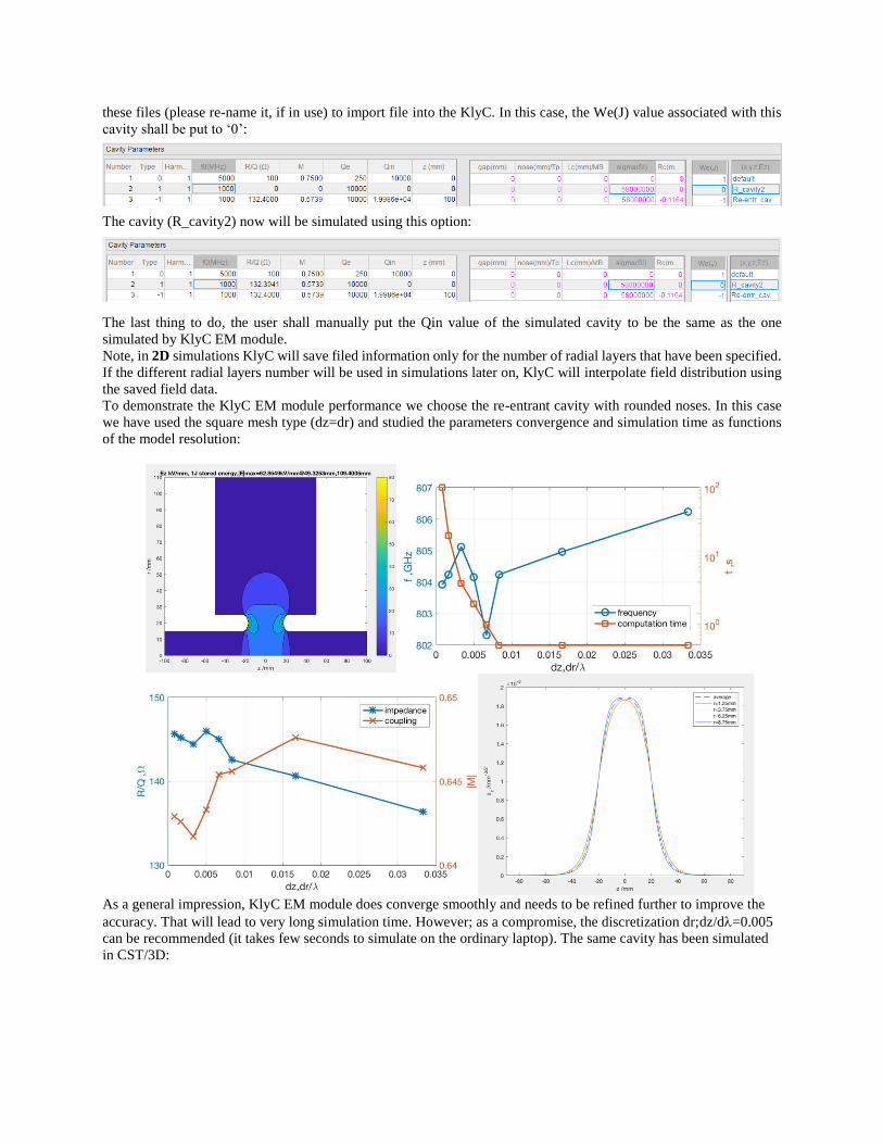
these files (please re-name it, if in use) to import file into the KlyC. In this case, the We(J) value associated with this

cavity shall be put to ‘0’:

The cavity (R_cavity2) now will be simulated using this option:

The last thing to do, the user shall manually put the Qin value of the simulated cavity to be the same as the one

simulated by KlyC EM module.

Note, in 2D simulations KlyC will save filed information only for the number of radial layers that have been specified.

If the different radial layers number will be used in simulations later on, KlyC will interpolate field distribution using

the saved field data.

To demonstrate the KlyC EM module performance we choose the re-entrant cavity with rounded noses. In this case

we have used the square mesh type (dz=dr) and studied the parameters convergence and simulation time as functions

of the model resolution:

As a general impression, KlyC EM module does converge smoothly and needs to be refined further to improve the

accuracy. That will lead to very long simulation time. However; as a compromise, the discretization dr;dz/d=0.005

can be recommended (it takes few seconds to simulate on the ordinary laptop). The same cavity has been simulated

in CST/3D:

The comparison between the two codes is shown next. The KlyC data is taken for dr;dz/d=0.005

Frequency. MHz R/Q, Ohms M Qin

CST/3D 801.9 147.6 0.647 19229

KlyC EM module 804.1 146.0 0.643 19337

The 0.2% difference in frequency is observed. However, KlyC uses the user defined frequency for simulations, so that

these results can be used as an information about the KlyC EM convergence accuracy. The R/Q, M and Qin

discrepancies stay within 1%. To our experience, such a difference can affect the tube performance at a level of 0.1%.

4. Filed map import from HFSS and/or CST.

This last option allows the user to design the cavity using eigenmode solvers of HFSS and/or CST. The instructions of

how to import the filed maps from these codes into the KlyC are given Appendix I.

3. Model discretization (accuracy) settings.

In the KlyC, the model discretization is controlled by selecting the number of spatial divisions per electronic

wavelength (Nz), the number of emitted particles per RF period (Nt) and the number of harmonics to be used in

calculations of the space charge field (Ns). Simulations will be completed when the requested iteration residual limit

is reached, or the number of iterations exceeds the specified limit. The residual limit is measured using the convergence

of the gap voltage in the output cavity. The iterations convergence process can be optimized by adjusting the iteration

relaxation parameter (0.5 by default). This parameter controls the weight which will be used by KlyC to account for

the result of the given iteration when moving to the consequent one. For every case relaxation parameter can be adjusted

(normally <0.5) to minimize the number of iterations (simulation time) to reach the convergent criteria. The model

accuracy settings which are recommended for the klystron optimization process are:

4. Plot settings

The output graphics and animations generated by KlyC can be controlled from the plot settings menu:

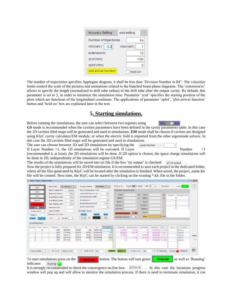
The number of trajectories specifies Applegate diagram, it shall be less than ‘Division Number in RF’. The velocities

limits control the scale of the pictures and animations related to the bunched beam phase diagrams. The ‘extension/rc’

allows to specify the length (normalized to drift tube radius) of the drift tube after the output cavity. By default, this

parameter is set to 2, in order to minimize the simulation time. Parameter ‘zcut’ specifies the starting position of the

plots which are functions of the longitudinal coordinate. The applications of parameter ‘zplot’, ‘plot arrival function’

button and ‘hold on’ box are explained later in the text.

5. Starting simulations.

Before running the simulations, the user can select between two regimes using switch.

GS mode is recommended when the cavities parameters have been defined in the cavity parameters table. In this case

the 1D cavities filed maps will be generated and used in simulations. EM mode shall be chosen if cavities are designed

using KlyC cavity calculator/EM module, or when the electric field is imported from the other eigenmode solvers. In

this case the 2D cavities filed maps will be generated and used in simulations.

The user can choose between 1D and 2D simulations by specifying the

If Layer Number =1, the 1D simulations will be executed. If Layer Number >1

(recommended 4, at least), the 2D simulations will be done. If 2D option is chosen, the space charge simulations will

be done in 2D, independently of the simulation regime GS/EM.

The results of the simulations will be saved into txt file if the box ‘txt output’ is checked: .

Now the project is fully prepared for 2D/EM simulation. It is recommended to save each project in the dedicated folder,

where all the files generated by KlyC will be located after the simulation is finished. When saved, the project_name.klc

file will be created. Next time, the KlyC can be started by clicking on the existing *.klc file in the folder.

To start simulations press on the button. The button will turn green as well as ‘Running’

indicator:

It is strongly recommended to check the convergence on line box: . In this case the iterations progress

window will pop up and will allow to monitor the simulation process. If there is need to terminate simulation, it can

be done by closing the convergence history window. When simulation is finished, the ‘Running’ indicator will turn

red.

6. KlyC output graphics, animations and data.

If requested, upon completion the simulation, KlyC will generate multiple graphics and animations. The animations

are generated as gif files and stored in the project folder.

Graphical output:

Animations:

To generate arrival functions (time and velocity), the ‘hold on’ box in the plot setting menu needs to be checked

before simulations have been started. Next, the position (zplot) at which the arrival functions will be calculated shall

be specified. Finally the arrival function plots will be generated after clicking on ‘plot arrival function’. If this

operations is repeated for the different zplot value, the new curves will be added to the pictures. The curves will be

saved into data files (with value of zplot in the file name) if ‘txt output’ box is checked.

Note, these calculations require storing a lot of data in a computer memory. That is why, one may consider to use this

option if only necessary. The memory cash can be emptied at any time by clicking on

The results of simulations are collected in the ‘Simulation results summary’ table:

The KlyC calculates the RF power production efficiency using the two methods. The first method (Eff.RF) is based

on the direct measurement of the output cavity gap voltage. In the second method (Eff.Bl) the beam power balance is

used. Here, the total lost power is calculated as a sum of the spent beam kinetic energy, DC/RF energy of the space

charge field in the spent beam and the Ohmic losses in all the klystron cavities. With increasing the model resolution

(Nz), the Eff.RF will normally converge to the Eff. Bl value. However this might require significant increasing of the

computation time. Thus, we recommend to use the efficiency based on the power balance calculations. ‘Pout’ and

‘Gain’ in the summary table are calculated using balanced power.

To calculate the power transfer curve in automated regime, check the ‘Power ramp’ box and select the number of

points for the simulation: . Next, specify the value of the maximum power to be used:

, set the itearations number to be larger than N_points x N_1 (N_1 is anticipated number of iterations

needed for single simulation) and start simulation:

In the presence of the reflected electrons, the KlyC will have problems with convergence. These reflected electrons

could be virtual: the ones that appear shortly during the iteration process only; or the real ones which will persist. The

KlyC indicates two types of abnormalities: reflected electrons (colored in yellow during iterations process), those who

reached the emission plane and trapped electrons (colored in blue), those who stay in the simulation volume for more

than 10 RF periods.

If these effects are numerical artefacts (virtual reflected electrons), the user can try to mitigate them by adjusting the

value of relaxation parameter and/or changing the number of layers in 2D simulations. Ultimately, the user can specify

position of the plane at which the reflected electrons will be absorbed. The position of the absorbing plane is specified

in the plot menu using zcut(mm). In the next example, zcut was set to be between the last bunching and the output

cavity:

7. Bunched beam as a power source.

ThKlyC allows to simulate RF circuit being excited by the bunched beam. This option can be used for the IOT design,

or for the individual studies of special RF output structures in electron devices. The cavity types here will be limited

to type ‘1’ and type ‘-1’. To enable this option, the ‘Pin’ box shall be unchecked and the KlyC GUI window will be

modified:

In the given example we have used the output cavity of the klystron that we have introduced before. Even the

parameters of first cavity in the table are not used (colored in dark grey), the user has to specify the cavity position, as

it will be used as a position of the emission plane.

The modulated current will be represented by individual bunches with constant charge distribution along the bunch.

The bunch separation is defined by the operating frequency and the bunch length is specified by the user in terms of

the operating wavelength RF phase by putting this value in ‘degree’ box.

In addition the user can choose, if the bunch should have velocity dispersion along the bunch length using the ‘chirp’

value. In this case KlyC will generate congregated bunch, where the velocity of the bunch head is lower than the

velocity of the bunch tail. The amplitude of congregation (0<chirp<1) will be used to generate the velocity dispersion:

𝑈(𝑡0) = 𝑈𝑎𝑣𝑒𝑟[1 + 𝑐ℎ𝑖𝑟𝑝 ∙ sin(𝜔𝑡 − 𝜋)], 0 < 𝜔𝑡 < 2𝜋

𝐼(𝑡0) =𝐼𝑎𝑣𝑒𝑟2𝛼

[sign(𝜔𝑡 − 𝜋 + 𝛼𝜋) − 𝑠𝑖𝑔𝑛(𝜔𝑡 − 𝜋 − 𝛼𝜋)], 𝛼 = 𝑑𝑒𝑔𝑟𝑒𝑒/360°

The average kinetic energy of the bunched beam is identical the equivalent DC beam kinetic energy specified in the

beam parameters table. In the next example we have studied how the RF power extraction efficiency depends on the

bunch congregation amplitude:

8. KlyC internal optimizer module.

The internal KlyC optimizer module supports Global and Local optimization routines, which are targeted to maximize

the RF power production efficiency. The variable parameters are the cavities frequencies tunings, the cavities positions

and the external Q factor of the output cavity. To operate optimizer, however, it is recommended that initial klystron

design shall be done manually to the extent, when the user decide that the design is already ‘good enough’.

The global optimizer uses a large group of individuals to be evaluated, which is rather time consuming. In this method,

each new generation is generated by its parental generation through selection, crossover and mutation operations to

ensure the improvement of fitness and diversity. The settings for Global/Local optimization shall defined in the

efficiency optimizer window:

First, the user has to specify the frequency and position variations boundaries (lines 1 and 2). Next, the cavity

‘separation/mm’ is used to avoid the situation when neighbor cavities come closer than this specified value (line 3).

The parameters window to modify the external Q factor can be chosen to be asymmetric (line 4). The tube layout for

every case in optimization will be saved (one by one) into project_name_opt.txt file if the simulated efficiency and

the minimal velocity of the electrons in the output cavity area have exceeded the specified values of eff. LB and ve/c

LB (line 5).

To select between the two regimes, the user should use the bottom right switch (line 6). For the Local optimizer the

only one case to start is needed, therefore, the population size (Individual) is not used for this optimizer. Without going

into details, the Max Ev(olution) shall be set to be large enough (50), so that the user can control the process and abort

it manually by closing the optimizer process window if the saturation becomes obvious. For the Global optimizer, we

recommend that the ‘Individual’ value shall be large as well (30) and again to abort simulations at any convenience.

In the next example we have used the high perveance S-band tube, which was initially designed in 1D using the

‘classical’ bunching technique (efficiency 45%). Next, the consequent Global and Local optimizations have been

applied. After 3 days of optimization, the final tube has reached the efficiency of 67% and RF circuit layout was

converted to be consistent with COM (core oscillation method) type klystrons.

9. The batched jobs

In the case if the parameters sweep, sensitivity analysis or just a few different tubes need to be simulated

in an automated manner, one can use the batched job option. Each project (job) has to have its individual

klc input file and all of them have to be placed in the same folder. To start such simulations, first open any

of the stored klc projects. Next press on the ‘RunAll’ button. The batched job toggle will turn ‘On’. The

jobs will be executed one by one following the files names order. The simulations status is indicated by the

progress meter on the instrumentation panel. To interrupt the process one need to switch the toggle to its

‘Off’ position and the simulations will be aborted when the running case is finished. The short summary

of batch simulations will be saved as ‘txt’ file, where some basic simulation results will be ready for

comparison. For each individual simulation, the results can also be saved if ‘txt output’ box is checked.

Appendix I. Field imported from other eigen solvers

Preparing data from CST:

1. Z direction should be the longitudinal direction and the gap center of the cavity shall be located at (0,0,0). The

cavity shall be introduced as an entire 3D object. No symmetry planes shall be used.

2. After the simulation is finished, plot field distribution for the selected mode.

3. Export plot data using Plot Data Export module

- Choose the name to save to the txt file. Choose the “Field in volume” at the bottom line.

- Choose the region (cubic sub-volume) and output precision (plot mesh) before pressing OK.

- Choose the name to save the txt file. (cavityefieldv1 in this example)

The generated data file (see above) shall be modified to be recognized by KlyC:

1. Delete the text header.

2. Remove the columns 4,5,7,8 and 9, so that column 6 will become column 4 (do it in Excel for example). The

processed file shall be save into the folder where the project is located.

In the CST eigenmode solver, the stored energy for any resonant mode is normalized to 1J by default. If one will use

some other method to generate filed distribution, the stored energy of resonant shall be calculated.

Put the name of the text file (without extension) with modified filed distribution in the last column of the cavities

parameter table (x,y,z,Ez) at a position of selected cavity and specify the value of stored energy (in joules) in the We(J)

column. Run the ‘update cavity’ to see if the import was successful and KlyC has calculated R/Q and M of the cavity.

Use the value of Qin simulated in the CST in the cavity parameters table.

Preparing data from HFSS

1. Generate the volume E-field plot of the chosen mode.

2. Choose the calculator in the post-processing menu.

2. Vector_E shall be copied to the stack before activating Export button.

3. Export field data by selecting a specific cubic region as shown above.

4. Change the type of exported data file to .txt and open it:

Raw Data Data processed

Note, that in HFSS that the geometry is normally specified in m. Next:

1) Delete the text header (the first 2 rows).

2) Delete columns 4 and 5, so that Ez(V/m) will become column 4..

3) The data in the first 3 columns shall be multiplied by 1000 to convert m into mm.

In the HFSS eigenmode solver, the stored energy for any resonant mode is normalized to 1J by default. Next, follow

the same sequence as it was explained above for the CST case.