Effective spin couplings in the Mott insulator of the honeycomb lattice Hubbard model

Effective Spin Couplings in the Mott Insulator of

the Honeycomb Lattice Hubbard Model

Hong-Yu Yang

Institute of Theoretical Physics, Ecole Polytechnique Federale de Lausanne, CH-1015

Lausanne, Switzerland

A. Fabricio Albuquerque

Instituto de Fısica, Universidade Federal do Rio de Janeiro, Cx.P. 68.528, CEP

21941-972 Rio de Janeiro-RJ, Brazil

Sylvain Capponi

Laboratoire de Physique Theorique, Universite de Toulouse and CNRS, UPS

(IRSAMC), F-31062 Toulouse, France

Andreas M. Lauchli

Institut fur Theoretische Physik, Universitat Innsbruck, A-6020 Innsbruck, Austria

Kai Phillip Schmidt

E-mail: [email protected]

Lehrstuhl fur Theoretische Physik I, Otto-Hahn-Straße 4, TU Dortmund, D-44221

Dortmund, Germany

Abstract. Motivated by the recent discovery of a spin liquid phase for the Hubbard

model on the honeycomb lattice at half-filling [11], we apply both perturbative and

non-perturbative techniques to derive effective spin Hamiltonians describing the low-

energy physics of the Mott-insulating phase of the system. Exact diagonalizations of

the so-derived models on small clusters are performed, in order to assess the quality

of the effective low-energy theory in the spin-liquid regime. We show that six-spin

interactions on the elementary loop of the honeycomb lattice are the dominant sub-

leading effective couplings. A minimal spin model is shown to reproduce most of the

energetic properties of the Hubbard model on the honeycomb lattice in its spin-liquid

phase. Surprisingly, a more elaborate effective low-energy spin model obtained by a

systematic graph expansion rather disagrees beyond a certain point with the numerical

results for the Hubbard model at intermediate couplings.

PACS numbers: 75.10.Kt, 71.10.Fd, 75.10.Jm, 75.40.Mg

arX

iv:1

207.

1072

v2 [

cond

-mat

.str

-el]

4 D

ec 2

012

Effective Spin Couplings in the Honeycomb Mott Insulator 2

1. Introduction

The quest for exotic quantum phases lacking conventional long-range order in dimensions

higher than one has recently attracted enormous interest, for fascinating unusual

properties, such as quantum number fractionalization and/or anyonic excitations, are

expected to emerge from certain spin Hamiltonians [1, 2]. In this context, magnetic

systems are an important playground, since exactly solvable models displaying such

properties have been recently introduced in the literature [1].

Common wisdom has it that, if experimental realizations of such exotic phases are

to be found, one should look at Hubbard-like systems deep into their strongly interacting

regime, on frustrated geometries disfavoring more conventional Neel order. Indeed,

in the limit of large on-site interactions U , where charge fluctuations are inhibited,

the Hubbard Hamiltonian maps to the Heisenberg model with nearest-neighbor (NN)

interactions only, for which numerical evidence for a gapped quantum spin liquid (QSL)

ground-state has been recently found on the highly frustrated kagome lattice [3].

An alternative route has been pursued in recent years, by focusing on two-

dimensional Hubbard models in the regime of intermediate U , where charge fluctuations

soften the Mott insulating phase. There is indeed convincing evidence that a QSL

phase is realized on the frustrated triangular lattice [4, 5, 6, 7, 8, 9, 10]. Sizeable

charge fluctuations manifest themselves as long-range and/or multi-body effective spin

interactions, beyond NN spin-exchange. In particular, it has been shown that four-

spin exchanges are the dominant correction to the Heisenberg model on the triangular

geometry, accounting for the emergence of a QSL in this case [5, 10].

Whichever of the aforementioned routes is followed, it appears that frustration is an

essential ingredient for a QSL. In face of this common expectation, the recent discovery

[11] of a QSL phase for the Hubbard model on the unfrustrated honeycomb lattice,

at half-filling and intermediate U , is consequently very surprising and has attracted

enormous interest. In particular, under the light of our previous discussion, the question

of what the effective spin interactions are for stabilizing a QSL in this case naturally

arises.

An effective spin model comprising terms of up to fourth-order in t/U is basically a

frustrated J1-J2 model, since four-spin interactions, the dominant corrections to the NN

Heisenberg model on square and triangular geometries [10], are strongly suppressed on

the honeycomb lattice, for it lacks length-four loops. Due to this fact, it has been argued

[12, 13, 14] that the emergence of a QSL can be simply accounted to the frustrating

next-NN coupling J2, a claim that has spurred a number of works on the so-called J1-

J2 model [15, 16, 17, 18, 19]. Although such studies differ in detail, they commonly

detect a quantum critical point, at J2/J1 ≈ 0.2, between long-range ordered Neel and a

magnetically disordered phase. The precise nature of this non-magnetic state remains

somehow unclear, albeit most numerical results point to a valence bond solid (VBS)

[15, 16, 17, 18]. However, and interestingly enough, in Ref. [19] a variational approach

finds that such VBS becomes unstable towards a gapped spin liquid if large enough


length scales are taken into account.

Independently of the nature of magnetically disordered phase stabilized for the J1-

J2 model, it is crucial to gauge its validity as a low-energy theory for the honeycomb

lattice Hubbard Hamiltonian in the intermediate range of t/U , where the QSL emerges.

Indeed, evidence indicating a more involved situation has been found in Ref. [20]: the

bare series expansion (of up to order 14th) is not converged for values of t/U leading

to the QSL. Furthermore, a non-perturbative derivation of effective spin interactions,

obtained via graph-based continuous unitary transformations [20], yields a relatively

small ratio J2/J1 < 0.2, insufficient to destabilize the long-range ordered Neel phase. It

is thus clear that a more thorough analysis is called for, this being our main goal in the

present work.

We employ three state-of-the-art methods to derive effective spin models for the

Hubbard model on the honeycomb lattice at half-filling, in order to identify dominant

effective interactions as a function of t/U . Interestingly, among the vast number of

effective spin couplings shooting up in the vicinity of the quantum phase transition to

the semi-metal, we find that the largest correction to the NN Heisenberg interaction are

six-spin interactions located on single hexagons; the frustrating next-NN exchange J2 is

considerably smaller. We assess the accuracy of the effective low-energy theory, for t/U

yielding the QSL, by performing exact diagonalizations (EDs) on small clusters.

We organize the paper as follows. In Sec. 2 we write down the Hubbard Hamiltonian

and a generic effective spin model, accordingly fixing the notation employed throughout

the paper. The methods used in deriving the low-energy spin model, namely perturbative

and graph-based continuous unitary transformations (respectively, pCUTs and gCUTs),

as well as the contractor renormalization (CORE) group, are described in Sec. 3. After

comparing the outcomes from both approaches in Sec. 3.3, we present results from EDs

in Sec. 4. Finally, we summarize our results in Sec. 5.

2. Model

We consider the single-band Hubbard model studied in Ref. [11], defined on a honeycomb

geometry and at half-filling, that reads

H = HU +Ht = U∑i

ni↑ni↓ − t∑〈i,j〉,σ

(c†iσcjσ + h.c.) . (1)

niσ = c†iσciσ is the occupation number operator for fermions with spin σ at the site

i of the honeycomb lattice, and t is the amplitude for hoppings taking place between

NN sites, 〈i, j〉, on this lattice. Quantum Monte Carlo (QMC) simulations [11] show

that a QSL phase is stabilized for moderately strong couplings, 0.233 . t/U . 0.286

(4.3 & U/t & 3.9), and it is our main purpose here to compute effective spin interactions

for Eq. (1) in this range.

Due to the SU(2) symmetry of the Hubbard Hamiltonian, a generic effective model

for its Mott insulating phase can be expressed in terms of products of spin-half operators


(~Si · ~Sj) as

Hspin = E0 +∑i,j

Jij

(~Si · ~Sj

)+∑i,j,k,l

Kijkl

(~Si · ~Sj

)(~Sk · ~Sl

)(2)

+∑

i,j,k,l,m,n

Lijklmn

(~Si · ~Sj

)(~Sk · ~Sl

)(~Sm · ~Sn

)+ . . . ,

where E0 denotes a constant energy shift. Jij, Kijkl and Lijklmn respectively denote

coupling constants for the various two-, four-, and six-spin exchanges and the . . . refer

to analogue expressions involving more than six spins. Unfortunately, however, the

situation is complicated by the fact that multi-spin exchanges involving eight or more

spins form an over-complete set of operators [21]. As a consequence, no unique solution

in terms of spin operators can be obtained. While the effective Hamiltonian remains

well defined in terms of matrix elements in the spin basis, it is only the algebraic

representation of the effective Hamiltonian in terms of spin operators that is not unique.

In the next section we will describe different approaches to derive such effective

low-energy models. Furthermore, we extract and discuss the most important corrections

to the nearest-neighbor Heisenberg exchange giving rise to a minimal magnetic model

capturing the essential physics of the full Mott phase. This minimal model as well as a

more elaborate effective spin model is then analysed afterwards.

3. Methods and Effective Models

In this section, we discuss details concerning the numerical methods employed in

obtaining the effective spin interactions for the Hubbard model, Eq. (1), at half-

filling and in the regime of strong to intermediate couplings. We start by the so-

called continuous unitary transformations which allow us to gain a global view on the

effective spin model and its most important spin interactions. Afterwards, we apply

the contractor renormalization technique to confirm the behaviour of the dominant

effective spin couplings. We find that both methods essentially agree when considering

the same minimal set of considered clusters in both calculations. The latter motivates

the definition of a minimal magnetic model.

3.1. CUTs and full effective spin model

We have calculated the dependence of the magnetic exchange couplings on t/U using

perturbative continuous unitary transformations (pCUTs) [22, 23, 24] along the lines of

Ref. [10, 25]. The pCUT provides the magnetic couplings as series expansions in t/U .

Note that the spectrum of the Hubbard model is symmetric at half filling under the

exchange t↔ −t and therefore only even order contributions are present [26]. We have

determined all two-spin, four-spin and six-spin interactions up to order 14. In order 14

one has to calculate 345 topologically different graphs.

The bare series do not converge in the spin-liquid region of the Mott phase [20].

This is different to the recently analysed case of the Hubbard model on the triangular


lattice [10, 20] where the intermediate non-magnetic phase is already realized for smaller

ratios of the bandwidth W to the interaction U . It is therefore mandatory to apply

resummation schemes of the series which is very complicate to be performed reliably for

the full set of exchange couplings. We have therefore applied the recently developped

graph-based continuous unitary transformations (gCUTs) [20] in order to derive non-

perturbatively the effective spin model. In the following we use the gCUT results to

study the physics of the full low-energy spin model. The pCUT results are only used to

analyze the most important terms in the effective model.

The general properties of the gCUT are discussed in Ref. [20]. Here we only mention

the specific approach for the current problem. The basic idea is to use a CUT to map

H unitarily to an effective Hamiltonian Heff which has the special property that the

block without double occupancies representing the effective low-energy spin model is

decoupled from the rest of the Hamiltonian. The convergence of the gCUT is not

triggered by a small parameter but it relies on the fact that the correlation length of

charge fluctuations is finite in the Mott insulator.

In the gCUT one generates all topologically distinct connected graphs Gν of the

lattice and one sorts them by their number of sites n. On each graph Gν a CUT

is implemented by setting up the finite number of flow equations [27, 28, 29]. A

continuous auxiliary variable l is introduced defining the l-dependent Hamiltonian

HGν (l):=U †(l)HGνU(l). Then the flow equation is given by

∂lHGν (l) = [η(l), HGν (l)] , (3)

where η(l):=−U †(l)(∂lU(l)) is the anti-Hermitian generator of the unitary transforma-

tion. At the end of the flow l =∞ one obtains an effective graph-dependent Hamiltonian

HGνeff .

We have used the generator introduced by Wegner [27]

ηWegner(l) =[Hd(l), Hnd(l)

], (4)

where the diagonal part Hd is given by all matrix elements between states with the same

number of double occupancies and Hnd denote all remaining non-diagonal processes. We

stop the flow for each graph once the residual off-diagonality (ROD) is below 10−9. Here

the ROD is defined as the square root of the sum of all non-diagonal elements which

connect to the low-energy subspace. Finally, one obtains the effective spin model Hspin in

the thermodynamic limit by substraction of subcluster contributions and by embedding

back the graphs on the honeycomb lattice [20].

The numerical effort scales exponentially with the number of sites n of a given

graph. Here we have treated all graphs up to 7 sites. This amounts to solving up to

one million differential equations for the most demanding symmetry sector of a single

graph for each value of t/U . Physically, one captures all charge fluctuations on this

length scale. Let us remark that it is of course possible to only include a restricted set

of graphs in the gCUT calculation. This will be used below for a direct comparison with

CORE. Finally, one obtains for a given t/U the effective spin model non-perturbatively.


A view on the full effective spin model obtained by gCUTs for different values of

t/U is shown in Fig. 1. Let us remark that for gCUT(7) the full low-energy model can be

uniquely expressed in terms of spin operators, because multi-spin interactions involving

more than six sites are not yet allowed for this cluster size.

There are several implications which can be directly read off from Fig. 1. First,

only at rather small values of t/U . 0.1 a clear hierarchy in the amplitudes of the

effective spin operators can be seen. This corresponds to the purely perturbative regime

where the importance of terms is fully given by the perturbative order where a spin

coupling appears for the first time. In this regime the frustrated next-nearest neighbor

Heisenberg exchange J2 (order 4 perturbation theory) is the leading correction to the

dominant Heisenberg interaction J1 (order 2 perturbation theory).

Second, the situation changes drastically in the intermediate coupling regime where

the spin-liquid phase is realized. Here, no clear hierarchy in the amplitudes of the

effective spin couplings can be detected. One is rather confronted with a proliferating

number of terms which is likely a consequence of the fact that the metal-insulator

transition is second order. Consequently, the charge gap closes continuously and one

expects an increasing number of effective spin couplings on increasing length scales

when approaching the quantum critical point. Let us note that this is different for the

Hubbard model on the triangular lattice [10]. In this case the metal-insulator transition

is first order and one has no diverging length scale upon approaching the Mott transition

from the insulating side.

Third, and despite the complexity of the full effective spin model, one still expects

that most of the properties of the Mott phase should be contained in a minimal

magnetic model where one only considers the most important spin couplings having

the largest amplitudes. Some evidences for this strategy are given in the next section by

analysing such a minimal magnetic model. Interestingly, we find that the perturbative

hierarchy is not valid anymore for intermediate couplings: the most important correction

to J1 is not J2 but rather six-spin interactions located on hexagons. These six-spin

interactions arise in order six perturbation theory and they originate dominatly from

ring exchange processes around the shortest loop of even length on the honeycomb lattice

corresponding to hexagons. Let us remark that this is very similar to the Hubbard model

on the triangular lattice [10]. Here the most elementary loop of even length is a four-

site plaquette. Consequently, four-spin interactions on the elementary plaquette are the

dominant correction to the Heisenberg model.

In the remainder of this paper we are aiming at a minimal magnetic model

which contains only the most important spin interactions in the regime of strong to

intermediate coupling. In this parameter regime, the minimal model should display the

low-energy properties of the Hubbard model on the honeycomb lattice. Additionally, we

expect that going beyond the minimal model by considering the full graph decomposition

used by gCUT (or alternatively by CORE) yields successfully even better results. The

most important effective exchanges are depicted in Fig. 2: NN (J1) and next-NN (J2)

two-spin interactions appearing in the J1-J2 model, and the six-spin terms with couplings


Figure 1. (Color online) Coefficients of all gCUT(7) terms in the effective Hamiltonian

for different U/t in units 1/U . Terms with different number of spin operators 0, 2, 4, or

6 are separated by vertical solid lines. Each block containing the same number of spin

operators is sorted by the size of the coefficient. Here each spatially symmetric coupling

is also shown. Dashed blue boxes highlight the most important couplings. Most left

box refers to the three equivalent couplings J1, the middle box corresponds to the

six equivalent couplings J2, and the most right box includes the six-spin interactions

L1, L2, · · · , L5 on a hexagon.

L1, L2, · · · , L5. The corresponding gCUT and pCUT amplitudes for these couplings are

displayed in Fig. 3.

One clearly sees that the bare series of the six-spin interactions are not converged

in the interesting regime of intermediate t/U confirming the conclusion obtained in

Ref. [20]. In contrast, the results obtained by gCUT and self-similar extrapolation of

the pCUT series are in fair agreement for all displayed couplings.

In the following we want to further strengthen these findings by using CORE as an

alternative tool to derive effective low-energy models.

3.2. Contractor renormalization and minimal model

It is also possible to derive non-perturbative effective theories by relying on the

CORE technique [30]. CORE is a real-space renormalization procedure, applicable

to generic lattice models, where effective models are derived by truncating local degrees-

of-freedom. Such construction requires the exact computation of low-lying eigenstates

on finite connected graphs, similarly to what happens in the previously discussed gCUT

procedure; implementation details are discussed in the literature [30, 31]. The resulting


J1

0

1

2

3

4

5

J2

0

1

2

3

4

5

L1

0

1

2

3

4

5

L2

0

1

2

3

4

5

L3

0

1

2

3

4

5

L4

0

1

2

3

4

5

L5

0

1

2

3

4

5

Figure 2. (Color online) Dominant effective spin interactions for the Hubbard model

on the honeycomb lattice at half-filling [Eq. (1)]: NN and next-NN two-spin couplings

(J1 and J2, respectively), and six-spin exchange terms with couplings L1, L2, · · · , L5.

0 0.1 0.2 0.3t / U

0

0.02

0.04

0.06

0.08

0.1

J 2 /

J1

gCUT(7)

gCUT(6)

gCUT(5)

pCUT(Bare14)

pCUT(Bare12)

pCUT(Bare10)

Self-similar

(a)

QSL

0 0.1 0.2 0.3t / U

-0.3

-0.2

-0.1

0

0.1

0.2

0.3

L1

-5 /

J1

gCUT(6)

gCUT(7)

pCUT(Bare14)

Self-similar

(b)

QSL

L4

L3

L1

L2

L5

Figure 3. (Color online) The relative gCUT and pCUT amplitudes J2/J1 (left) and

Li/J1 (right) as a function of t/U . Thin solid lines refer to the bare pCUT series. Black

solid lines correspond to self-similar extrapolants as discussed in Ref. [20]. Symbols

denote results obtained by gCUTs.

effective Hamiltonian is given as a cluster expansion

Heff =∑g

hcg , (5)

where the sum takes place over a set of graphs g, and hcg corresponds to the connected

term that is obtained by substracting contributions from embedded sub-clusters [30, 31].

Such expansion must naturally be truncated at a certain maximum range [32], but its

accuracy can in principle be controlled by analyzing the convergence of terms in the

effective model with increasing range.


(a)

0

1

(b)

1

0 2

(d)

0

1

2

3

4

5

(c) 0

12

3

Figure 4. Clusters considered in the CORE expansion, ordered according to the

maximum range for effective interactions [32] and comprising: (a) two, (b) three, (c)

four and (d) six sites.

Since it is our goal here to obtain effective spin interactions for the Hubbard model

[Eq. (1)] at half-filling, we select single sites as elementary blocks in the CORE expansion

[30, 31] and retain only singly-occupied states on all sites.

The clusters used in the CORE calculation are shown in Fig. 4. Here two setups

are considered: i) The first choice of clusters does not contain the four-site star graph

displayed in Fig. 4(c). It therefore corresponds to the leading term of a full graph

expansion in terms of hexagons. ii) The second choice contains additionally the four-

site star cluster [Fig. 4(c)]. In the hexagon expansion mentioned before such a graph

would be included only on the level of three-hexagon clusters. Later we see that gCUT

(restricted to exactly the same graphs) yields almost identical results for both choices

of clusters. The second choice can then be regarded as an intermediate step between

the minimal one-hexagon calculation and the full gCUT(7) calculation which includes

all graphs shown in Fig. 4 as a subset.

We start by discussing the first choice. The lowest-order contribution to the NN

spin-exchange J1 is simply computed by solving the Hubbard model on a two-site cluster

[Fig. 4(a)]: in this case only eigen-energies are required, since J1 exactly corresponds to

the singlet-triplet gap:

J(2)1 =

U

2

(√1 +

16t2

U2− 1

). (6)

Although trivially obtained, this result is non-perturbative, reducing to the well-known

limit J1 ' 4t2/U only when t/U � 1 [see Fig. 5(b)]. Let us mention that the same

non-perturbative result is obtained when calculating J(2)1 with gCUT(2).

Longer-range couplings, along with corrections to shorter-ranged ones, are

obtainable from the analysis of the larger clusters depicted in Fig. 4(b-d). In particular,

in Fig. 5(a) we plot bare effective couplings, obtained by considering the six-site cluster

in Fig. 4(d), as a function of t/U . Here the notion ’bare couplings’ corresponds to the

effective exchange couplings of a single cluster without considering substractions and

embeddings. We first focus on the next-NN coupling J2 and notice that, particularly in

the range 0.233 . t/U . 0.286 ((4.3 & U/t & 3.9)) where a QSL appears [11], J2 . 0.1J1

and therefore this frustrating interaction is not large enough [15, 16, 17, 18, 19] to

account for the absence of long-range Neel order before a semi-metal phase is stabilized


0 0.05 0.1 0.15 0.2 0.25 0.3t / U

0

0.05

0.1

0.15

0.2

0.25

0.3Effective exchanges / U

4 t 2 / U

J1

J2

L1

-L2

L3

L4

-L5

(a)

QSL

0

0.1

0.2

0.3

J 1 / U

4 t2 / U

J1

(2)

J1

(3)

J1

(4)

J1

(6)

0 0.1 0.2 0.3t / U

0

0.005

0.01

0.015

J 2 / U

J2

(3)

J2

(4)

J2

(6)

QSL

QSL

(b)

(c)

Figure 5. (Color online) (a) Bare amplitudes for of all terms in the effective

Hamiltonian for Eq. (1) as a function of t/U , as obtained from the CORE procedure

applied to the six-site cluster depicted in Fig. 4(d). For clarity sake, only dominant

couplings are shown, following the notation from Fig. 2; all remaining terms have very

small amplitudes and lie in the filled region at the bottom-left corner. (b-c) Results

for the two-spin exchanges J1 and J2, as a function of t/U , obtained from indicated

clusters (we label the results according to the number of sites in a given cluster; see

Fig. 4). For each cluster, contributions from embedded clusters comprising lesser sites

are subtracted, following the standard CORE recipe [30, 31]. In both panels, the

shaded region corresponds to the QSL phase [11].

[20]. However, we also notice that, remarkably, much larger magnitudes are associated

to the six-spin terms with couplings L1, L2, · · · , L5 depicted in Fig. 2 (we also briefly

remark that the signs for their amplitudes are in agreement with those obtained from a

decomposition of the cyclic 6-spin permutation, cf. Ref. [33]). Furthermore, we observe

that the amplitudes for longer-range two-spin, as well as four-spin, terms are found to be

negligible in comparison to J1 and L1, L2, · · · , L5 [34]. One is thus inclined to conclude

that such six-spin interactions are the main ingredients in stabilizing a QSL in the phase

diagram for Eq. (1), a conjecture we aim at testing in Sec. 4.

Let us mention that such six-spin interactions on local hexagons are generated in

order six perturbation theory. In this order the couplings L1-L5 have the same absolute

prefactor with an alternating sign which exactly corresponds to the six-spin interactions

contained in the six-spin ring exchange permutation operator. But we stress that the

latter operator also contains two-spin and four-spin interactions of the same magnitude

which one has to contrast with our finding, both perturbatively and non-perturbatively,


of suppressed two- and four-spin interactions. The full non-perturbative contribution

of a single hexagon is therefore dominated by the six-interactions having the largest

exchange couplings. Finally, we note that the nonperturbatively obtained couplings

L1-L5 have different prefactors as can be seen in Fig. 5.

We proceed by analyzing the dependence of the effective couplings on the maximum

range of the clusters. In order to do so, for each cluster depicted in Fig. 4 we subtract

connected contributions from shorter-ranged, embedded, sub-clusters, according to the

standard CORE recipe [30, 31]. We plot results for the two-spin exchanges with

couplings J1 and J2 as a function of t/U respectively in Figs. 5(b) and (c), and find

a seemingly fast convergence with increasing cluster range up to the six-site cluster

depicted in Fig. 4(d). Furthermore, the data in Figs. 5(b) and (c) is in good agreement

with gCUT results, as we discuss below in Sec. 3.3.

Finally, we comment on the fact that a few clusters larger than the ones in Fig. 4,

such as the one comprising ten sites and forming an edge-sharing double hexagon, are

amenable to numerical diagonalization, in principle implying that our CORE expansion

could be extended to even longer ranges than considered here. To this end a full graph

decomposition must be implemented for the CORE approach which will be left as a

task for future research. Here we would rather like to focus on the most minimal setup

to describe the low-energy physics of the Hubbard model.

3.3. Minimal effective model

We compare now the effective models obtained from gCUT (Sec. 3.1) and CORE

(Sec. 3.2). We first remark that both approaches yield qualitatively similar effective

Hamiltonians, that display as dominant terms the two- and six-spin exchanges depicted

in Fig. 2 (see Figs. 3 and 5). We therefore focus on such terms, that may be regarded

as defining a minimal effective model, and plot their amplitudes, as a function of t/U in

Fig. 6. Let us mention that we do not show the constant term of the effective models

which also displays a t/U dependence and which one therefore has to keep in the exact

diagonalization when comparing to the Hubbard model. Here three different sets of

graphs are considered: i) the leading graphs of a hexagon expansion not including the

four-site star graph (CORE and gCUT), ii) the leading graphs of a hexagon expansion

including the four-site star graph (CORE and gCUT), and iii) all graphs comprising up

to seven sites (gCUT).

We notice that results from both methods are in good quantitative agreement up

to couplings stabilizing the QSL phase [11] and beyond the perturbative regime [20]

for all three choices. Especially, CORE and gCUT yield almost identical results for

the restricted graph sets i) and ii). This is likely a consequence of the fact that the

structure of the low-energy subspace is rather constraint due to the high symmetry of

the considered clusters (the four-site graph as well as the six-site graph has a rotational

symmetry) plus the number of different spin couplings defined on these graphs is rather

small.


0

0.1

0.2

J 1 /

U

CORE 3 graphs

gCUT 3 graphs

CORE 4 graphs

gCUT 4 graphs

gCUT(7)

0

0.005

0.01

0.015

0.02

J 2 /

U

0

0.02

0.04

0.06

L1 /

U

-0.08

-0.06

-0.04

-0.02

0

L2 /

U

0

0.02

0.04

0.06

L3 /

U

0.1 0.2 0.3t / U

0

0.02

0.04

0.06

0.08

L4 /

U

0.1 0.2 0.3t / U

-0.08

-0.06

-0.04

-0.02

0

L5 /

U

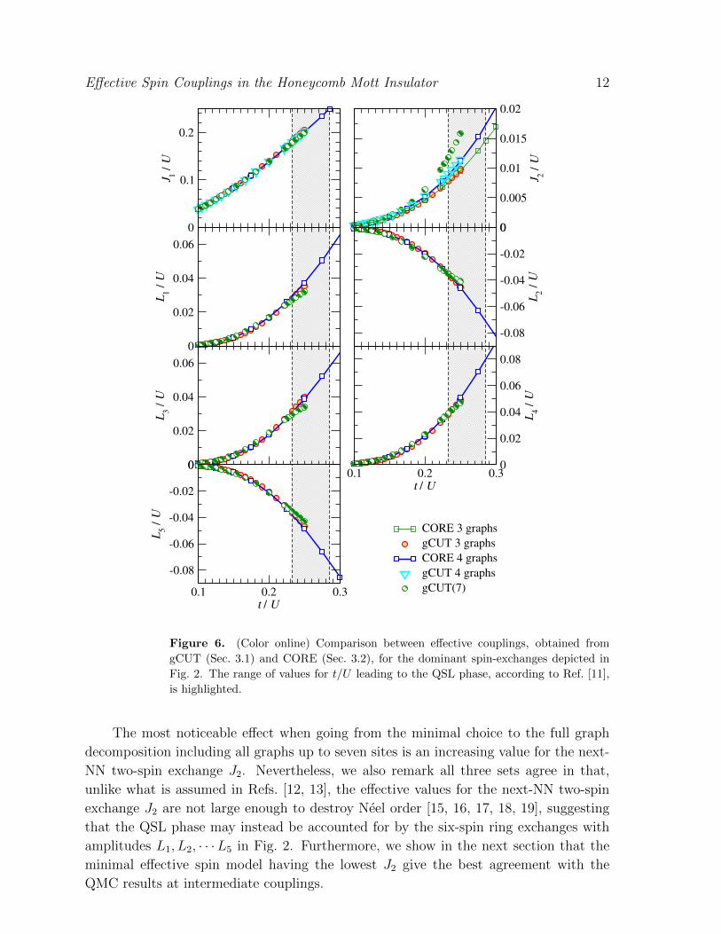
Figure 6. (Color online) Comparison between effective couplings, obtained from

gCUT (Sec. 3.1) and CORE (Sec. 3.2), for the dominant spin-exchanges depicted in

Fig. 2. The range of values for t/U leading to the QSL phase, according to Ref. [11],

is highlighted.

The most noticeable effect when going from the minimal choice to the full graph

decomposition including all graphs up to seven sites is an increasing value for the next-

NN two-spin exchange J2. Nevertheless, we also remark all three sets agree in that,

unlike what is assumed in Refs. [12, 13], the effective values for the next-NN two-spin

exchange J2 are not large enough to destroy Neel order [15, 16, 17, 18, 19], suggesting

that the QSL phase may instead be accounted for by the six-spin ring exchanges with

amplitudes L1, L2, · · ·L5 in Fig. 2. Furthermore, we show in the next section that the

minimal effective spin model having the lowest J2 give the best agreement with the

QMC results at intermediate couplings.


4. Exact diagonalizations

We turn now our attention to the characterization of the effective spin model derived

in the previous sections, either with gCUT method or CORE algorithm. Our goal is

to show that a reasonably simple and compact effective spin model can describe rather

well the energetics of the Hubbard model. In order to do so, we will make a systematic

comparison of the low-energy properties, and of the local quantities such as double

occupancy or bond kinetic energy, that we compute using the exact diagonalization

(ED) technique. More precisely, we have used a standard Lanczos algorithm to obtain

the ground-state energy for various clusters at fixed total Sz, and we have made use of

all space symmetries (translations and point-group, when available).

4.1. Study of the minimal effective model

We start by discussing the properties of the minimal effective spin model obtained for

the minimal set of graphs not including the four-site star graph. We stress again that

CORE and gCUT give essentially identical low-energy spin models for this choice of

graphs. In the following we use the effective model obtained via the CORE algorithm

(Sec. 3.2).

We start by comparing the low-energy spectra for the Hubbard [Eq. (1)] and the

effective (Sec. 3) models on an N = 18 cluster for two values of t/U : t/U = 0.05 (deep

into the Neel phase) and t/U = 0.25 (QSL phase, according to Ref. [11]). In Fig. 7(a-b),

we plot so-called Anderson tower of states for the Hubbard model. As we only make use

of Sz symmetry (instead of the total spin), we plot the energy states versus Sz(Sz + 1),

so that degenerate states with identical energies correspond to spin multiplets. We have

also computed the one-particle gap, ∆1P = (E0(N/2 + 1) +E0(N/2−1)−2E0(N/2))/2,

where E0(Nf ) is the ground-state energy with Nf fermions. For t/U = 0.05 [Fig. 7(a)],

the so-called Anderson tower of states is typical of a collinear Neel state [35] with a

lowest excitation increasing as S(S + 1) (with a slope that should decrease as 1/N),

followed by spin-wave excitations (with energy scale 1/√N). Moreover, on the scale

of the figure, all states correspond to spin excitations since ∆1P is quite large [36].

The same behaviour is reproduced qualitatively and quantitatively by the effective spin

model, as expected and shown in Fig. 7(c). Note that in the case of the effective spin

model, we have been able to label each eigenstate with its total spin value S so that we

plot levels as a function of S(S + 1).

When increasing t/U to 0.25, a distinct picture emerges [Fig. 7(b)] . While the first

excitations still correspond to S = 1 and S = 2 states at the Γ point, there is no longer a

straight S(S + 1) line of excitations and, even more importantly, the gap ∆1P to charge

excitations is substantially lowered, beyond which a description solely based on spin

degrees-of-freedom is no longer valid. However, according to QMC results [11], for this

coupling the one-particle gap should remain finite in the thermodynamic limit, so that

our effective spin model could still describe the physics at the lowest energies: indeed,

its low-energy spectrum, plotted in Fig. 7(d), reproduces the lowest spin excitations


Figure 7. (Color online) (a-b) Low-energy spectrum of the Hubbard model vs

Sz(Sz + 1) obtained for t/U = 0.05 (a) and t/U = 0.25 (b) on an N = 18 honeycomb

cluster. Values for twice the one-particle gap, 2∆1P , are given [in (b), such value is

indicated by the horizontal dashed line]. (c-d) Low-energy spectrum for the CORE

effective model (see main text) vs S(S+1), obtained on the same 18-site cluster, again

for t/U = 0.05 (c) and t/U = 0.25 (d). In all panels, different symbols correspond to

different points in the Brillouin zone: Γ point at the center, 6-fold degenerate A point

and 2-fold degenerate K point at the corners [see inset in (b)]. Lowest energy levels in

all cases are zoomed in in the insets.


quite accurately. Furthermore, while the quantum numbers seen in the tower-of-states

are consistent with standard collinear magnetic ordering, the lowest spin excitations do

not display a clear S(S + 1) behaviour, which might be an indication that there is no

magnetic ordering.

It would also be desirable to compute correlators for the ground-state of the effective

model, but this is quite involved since one would also need to renormalize the operators

when deriving an effective Hamiltonian [30, 31, 10, 20]. Nevertheless, some observables

may straightforwardly be obtained from the ground-state energy per site, e0, by relying

on the Feynman-Hellmann theorem. For instance, the electronic double occupancy per

site can be computed from ED of the effective model involving only spin degrees-of-

freedom, as it has been done in Ref. [10] using :

〈n↑n↓〉 =de0

dU(7)

Results are shown in Fig. 8(a) and compared both to the exact result of the Hubbard

model on N = 18 cluster and to QMC data [37]. Since this is a local quantity, its finite

size effects are rather small as expected. We observe a good agreement not only for small

t/U (deep in the Neel phase), but also in the interesting regime t/U ' 0.25 where QSL

is expected to emerge. As a side remark, let us emphasize that the discrepancy between

results on the Hubbard model and with the CORE effective one on N = 18 can be

attributed to the role of short-length loops (of length 6) that exist on this small cluster,

and are not captured by the effective model (see Ref. [10, 15] for a similar discussion).

In fact, effective model results agree quite well with the data obtained on a much larger

lattice with QMC.

In Ref. [11], the analysis of the behaviour of the kinetic energy density Ekin =

〈−t∑〈ij〉,σ(c†iσcjσ +h.c.)〉/N versus U was also discussed in the context of the formation

of local moments at strong U/t, in contrast with the itinerant regime for small U/t,

whereas the QSL is stabilized in between. Using Feynman-Hellmann theorem again, we

can simply compute this quantity as

dEkindU

= −U d2e0

dU2. (8)

We have chosen a grid of U/t going from 3 to 8 by step of 0.1 and computed the ground-

state energy for various clusters. Using a finite-difference approximation, we obtain the

derivative of the kinetic energy that we plot against t/U in Fig. 8(b). Our first comment

is that we have some agreement with the exact QMC data [11] that show a maximum

around 0.14 for U/t ' 5.0, although this quantity is expected to be quite sensitive to

details since it is a second derivative of the ground-state energy. Note that QMC data

are also quite noisy in this large t/U region, and we refer to the original publication [11]

for additional data : the point is that a maximum of order 0.15 is reached for t/U ' 0.2.

Our second remark is that we observe an anomaly around t/U = 0.3 which could signal

that our CORE truncation is not safe beyond this value. This gives us confidence that

at least for t/U ' 0.25, our approach could make sense, and this includes the spin liquid

phase. Last, since we observe this change of curvature around U/t = 4.5 in a spin-only


0.15 0.2 0.25t / U

0.04

0.08

0.12

0.16

⟨n↑

n↓

⟩

Hubb. ED - N = 18

CORE 3 graphs N = 18



Hubb. QMC - N = 72

0.15 0.2 0.25t / U

0.08

0.1

0.12

0.14

0.16

dE

kin

/ d

U

QSL

(a) (b)

QSL

Figure 8. (Color online) (a) Double occupancy per site obtained obtained with the

minimal CORE effective model (3 graphs) on finite clusters with N = 18 to N = 30.

(b) Derivative of the kinetic energy, as a function of t/U , obtained from the ground-

state energy of the effective model [Eq. (8)] on the same clusters. In both cases,

comparison is made to ED (N = 18) and QMC (N = 72) [37] data of the Hubbard

model.

model, it seems to us that the virtual charge fluctuations giving rise to our effective

low-energy model are sufficient to account for this phenomenon. Additionally, it might

be not surprising that we underestimate this effect by our minimal magnetic model,

because we expect that the large number of neglected additional spin operators as well

as small renormalizations of the treated spin couplings could well lead to an enhanced

itineracy of the ground state at intermediate t/U values.

As a conclusion on this part, while we are clearly not able to reach system lengths

where QSL behavior is expected to occur – which would require several hundred sites –

our simple effective model is able to reproduce both the low-energy properties and the

ground-state local properties. It suggests that these properties may not be linked to the

presence of a QSL and are robust short-distance features.

4.2. Study beyond the minimal model

The results of the last subsections are very promising. CORE and gCUT give an almost

identical minimal effective spin model which is obtained from the single hexagon graph

and which compares well to the results obtained by QMC for the Hubbard model on

the honeycomb lattice.

In the following we want to go beyond this minimal choice of graphs and we would

like to see whether the above findings are confirmed and strengthened. We therefore

compare the above results for the minimal model to exact diagonalizations for the


0.15 0.2 0.25t/U

-0.2

-0.1

0

E/N

[t]

QMC L=15

CORE 3 graphs N=24

CORE 4 graphs N=24

gCUT(7) N=24

QSL

Figure 9. (Color online) Ground-state energy per site as a function of t/U . A

comparison is made to ED (N = 18) and QMC (N = 72) [37] data of the Hubbard

model.

effective spin models obtained i) by including the four-site star graph to the minimal

set and ii) by including all graphs up to seven sites. For case i) we again use results

from the CORE algorithm, but we stress that the gCUT on the restricted set of graphs

gives basically the same low-energy model. For the second case the results of gCUT(7)

are used.

We start by comparing the ground-state energy per site as a function of t/U which

is displayed in Fig. 9. It can be clearly seen that all three different sets of graphs give

a very similar energy per site in the full Mott phase which also agrees well with results

for the Hubbard model. This is promising, but it is also a consequence of the fact that

the ground-state energy per site is a rather unsensitive quantity.

We therefore turn to more sensitive quantities, namely the double occupancy per

site and the derivative of the kinetic energy as discussed in the last subsection for

the minimal effective model. Consequently, details of the considered effective spin

models matter which is most clearly seen for the derivative of the kinetic energy.

Interestingly and surprisingly, the agreement between results from the effective spin

model and results for the Hubbard model gets worst at intermediate couplings. Indeed,

already the minimal set of graphs plus the four-site star graph yields the wrong tendency.

Furthermore, exact diagonalization of the full effective spin model from gCUT(7) does

not even display the maximum in the derivative of the kinetic energy.

Altogether, we find that the inclusion of more graphs in our calculation gives a

reduced agreement at intermediate couplings in contrast to our expectation. This trend


0.15 0.2 0.25t / U

0.04

0.08

0.12

0.16

⟨n↑

n↓

⟩


CORE 4 graphs N=24

gCUT(7) N=24

Hubb. ED - N = 18

Hubb. QMC - N = 72

0.15 0.2 0.25t / U

0.08

0.1

0.12

0.14

0.16

dE

kin

/ d

U

QSL

(a) (b)

QSL

Figure 10. (Color online) (a) Double occupancy per site obtained obtained with

CORE effective model on finite clusters with N = 18 to N = 30. (b) Derivative of

the kinetic energy, as a function of t/U , obtained from the ground-state energy of the

effective model [Eq. (8)] on the same clusters. In both cases, comparison is made to

ED (N = 18) and QMC (N = 72) [37] data of the Hubbard model.

is most probably neither a numerical problem nor a difference between CORE and

gCUT, because both techniques agree quantitatively for both restricted set of graphs. In

our opinion there are basically two possible scenarios. First, an effective spin model can

still be reliably derived at intermediate couplings using a hexagon expansion. Indeed,

the minimal model only focusing on the leading one-hexagon graphs gives very nice

results. It might then be possible that the full graph decomposition used for the gCUT

by including all graphs up to seven sites does not give improved results, because the

relevant low-energy physics is contained in graphs with longer loops (these are exactly

the multi-hexagon graphs). Second, the trend seen in the full graph decomposition by

gCUT is a real effect, i.e. a controlled derivation of an effective low-energy spin model

for the QSL at intermediate couplings remains a big challenge.

5. Conclusions

Summarizing, we have derived effective spin Hamiltonians describing the low-energy

physics of the Hubbard model on the honeycomb lattice [Eq. (1)] at half-filling, that

has been recently shown to display a QSL phase [11]. The effective models, obtained

from the non-perturbative gCUT [20] and CORE [30, 31] methods, are in good mutual

agreement and seemingly well converged for the intermediate values of t/U yielding a

QSL [11]. We find that the effective next-NN two-spin frustrating exchange J2 is not

sizeable enough to destabilize Neel order [15, 16, 17, 18, 19] and therefore cannot account


for the existence of the QSL phase for Eq. (1). Instead, we find that the dominant sub-

leading terms in the effective model are six-spin exchanges (see Fig. 2), that may account

for the emergence of the QSL behavior.

Additionally, we have taken some first steps in trying to characterize the so-obtained

effective model, by performing exact diagonalizations on small clusters. While the so-

called Anderson tower of states is consistent with the occurrence of Neel order in the

strongly interacting limit of t/U → 0, the situation is less clear for t/U = 0.25 (that

according to Ref. [11] yields a QSL), possibly an indication of a magnetically disordered

state.

Naturally, it would be desirable to unambiguously show that the herein derived

effective model displays a QSL as its ground-state and possesses a gap to spin excitations.

However, the original results for the Hubbard model [11] indicate that such spin gap

is very small and thus one presumably needs to consider clusters comprising several

hundred sites, so to surpass the spin correlation length and convincingly establish the

nature of the ground-state.

In face of this limitation, we can only conclude that the minimal effective spin model

derived in the present work gives very promising results, but that a comprehensive

characterization of its ground-state is still missing. Accordingly, we hope that our

results may stimulate further work in trying to understand effects due to the six-spin

interactions L1, L2, · · ·L5 depicted in Fig. 2. Physically, one expects that these six-spin

interactions frustrate the Neel order leading to the stabilization of a QSL. One possible

strategy would be to deform the here obtained effective model and to study its phase

diagram in an enlarged parameter space, in the hope that the QSL would be further

stabilized and the spin correlation length would be reduced within reachable system

sizes.

Moreover, as shown by Lieb [38], the ground-state of the Hubbard model on

any bipartite lattice satisfies the Marshall-Peierls sign rule [39, 40] exactly for the

singly occupied configurations. By numerically diagonalizing the minimal effective

Hamiltonian derived from CORE, we have checked that this is also the case for the

spin model, which is a highly non-trivial result since a simple J1 − J2 spin model

on the honeycomb lattice strongly violates this rule in the intermediate region 0.2 <

J2/J1 < 0.4. While this property strongly constraints the nodes of the wavefunction,

it is however not clear if one could simulate the effective spin model with a quantum

Monte-Carlo algorithm without minus-sign problem. Such an opportunity would allow

to use spin QMC techniques which are far more efficient that fermionic QMC algorithm

and thus could reach much larger system size. Clearly, this point deserves future studies,

especially since Sorella et al. have recently challenged the existence of the quantum spin

liquid phase [41].


Acknowledgments

K.P.S. acknowledges ESF and EuroHorcs for funding through his EURYI. A. F. A. ac-

knowledges financial support from Faperj (Brazil). S. C. acknowledges IUF for funding

and KITP for hospitality. This research was supported in part by the National Science

Foundation under Grant No. NSF PHY11-25915. We acknowledge stimulating discus-

sions with F. Assaad, Z. Y. Meng, T. C. Lang, F. Mila, A. Muramatsu, A. Paramekanti,

S. Sorella and S. Wessel.

References

[1] Kitaev A Y 2003 Ann. Phys. (N.Y.) 303, 2

[2] Balents L 2010 Nature 464, 199

[3] Yan S, Huse D A, and White S R 2011 Science 332, 1173

[4] H. Morita, S. Watanabe, and M. Imada 2002 J. Phys. Soc. Jpn. 71 2109

[5] Motrunich O L 2005 Phys. Rev. B 72 045105

[6] Kyung B and Tremblay A M S 2006 Phys. Rev. Lett. 97 046402

[7] Sahebsara P and Senechal D 2008 Phys. Rev. Lett. 100 136402

[8] Tocchio L F, Becca F, Parola A, and Sorella S 2008 Phys. Rev. B 78 041101

[9] Yoshioka T, Koga A, and Kawakami N 2009 Phys. Rev. Lett. 103 036401

[10] Yang H Y, Lauchli A, Mila F, and Schmidt K P 2010 Phys. Rev. Lett. 105 267204

[11] Meng Z Y, Lang T C, Wessel S, Assaad, and Muramatsu A 2010 Nature 88, 487

[12] Wang F 2010 Phys. Rev. B 82 024419

[13] Cabra D C, Lamas C A, and Rosales H D 2011 Phys. Rev. B 83 094506

[14] Clark B K, Abanin D, and Sondhi S L 2011 Phys. Rev. Lett. 107 087204

[15] Albuquerque A F, Schwandt D, Hetenyi B, Capponi S, Mambrini M, and Lauchli A M 2011 Phys.

Rev. B 84 024406

[16] Reuther J, Abanin D, and Thomale R 2011 Phys. Rev. B 84 014417

[17] Oitmaa J and Singh R R P 2011 Phys. Rev. B 84 094424

[18] Mosadeq H, Shahbazi F, and Jafari S A 2011 J. Phys. Condens. Matter 23 226006

[19] Mezzacapo F and Boninsegni M 2012 Phys. Rev. B 85 060402

[20] Yang H Y and Schmidt K P 2011 Eur. Phys. Lett. 94 17004

[21] Klein D J 1980 J. Phys. A: Math. Gen. 13 3141

[22] Stein J 1997 J. Stat. Phys. 88 487

[23] Knetter C and Uhrig GS 2000 Eur. Phys. J. B 13 209

[24] Knetter C, Schmidt K P, and Uhrig GS 2003 J. Phys. A 36 7889

[25] Reischl A, Muller-Hartmann E, and Uhrig G S 2004 Phys. Rev. B 78 245124

[26] MacDonald A.-H., Girvin S M, and Yoshioka D 1988 Phys. Rev. B 37 9753

[27] Wegner F 1994 Ann. Phys. (Leipzig) 77 3

[28] G lazek S D and Wilson K G 1993 Phys. Rev. D 48 5863

[29] G lazek S D and Wilson K G 1994 Phys. Rev. D 49 4214

[30] Morningstar C J and Weinstein M 1996 Phys. Rev. Lett. 73 1873; 1996 Phys. Rev. D 54 4131

[31] Capponi S, Lauchli A, and Mambrini M 2004 Phys. Rev. B 70 104424

[32] Siu M S and Weinstein M 2007 Phys. Rev. B 75 184403

[33] Godfrin H and Osheroff D D 1998 Phys. Rev. B 38 4492

[34] Note that the pure 6-spin cyclic exchange on an hexagon does also contain 2- and 4-spin terms of

similar amplitudes (see Ref. [33]) which are not present here.

[35] Misguich G and Sindzingre P 2007, J. Phys.: Condens. Matter 19 145202, and references therein.

[36] For a fixed particle number, the threshold to particle-hole excitation is given by the optical gap


that we have not computed. Instead, we give the one-particle gap energy scale which is expected

to be of the same order of magnitude.

[37] We thank Ziyang Meng for providing us the QMC data on N=72 cluster.

[38] Lieb E H 1989 Phys. Rev. Lett. 62, 1201

[39] Marshall M 1955 Proc. R. Soc. London Ser. A 232, 48

[40] Lieb E and Mattis D 1962 J. Math. Phys. 3, 749

[41] Sorella S, Otsuka Y, and Yunoki S, arXiv:1207.1783, unpublished.

http://arxiv.org/abs/1207.1783

Effective spin couplings in the Mott insulator of the honeycomb lattice Hubbard model

Documents

Transcript of Effective spin couplings in the Mott insulator of the honeycomb lattice Hubbard model