A Fault-Tolerant Honeycomb MemoryCraig Gidney, Michael Newman, Austin Fowler, and Michael Broughton

Google Quantum AI, Santa Barbara, California 93117, USA

December 15, 2021

Recently, Hastings & Haah introduced a quantum memory defined on the honey-comb lattice [24]. Remarkably, this honeycomb code assembles weight-six parity checksusing only two-local measurements. The sparse connectivity and two-local measure-ments are desirable features for certain hardware, while the weight-six parity checksenable robust performance in the circuit model.

In this work, we quantify the robustness of logical qubits preserved by the honey-comb code using a correlated minimum-weight perfect-matching decoder. Using MonteCarlo sampling, we estimate the honeycomb code’s threshold in different error models,and project how efficiently it can reach the “teraquop regime” where trillions of quan-tum logical operations can be executed reliably. We perform the same estimates forthe rotated surface code, and find a threshold of 0.2%− 0.3% for the honeycomb codecompared to a threshold of 0.5%− 0.7% for the surface code in a controlled-not circuitmodel. In a circuit model with native two-body measurements, the honeycomb codeachieves a threshold of 1.5% < p < 2.0%, where p is the collective error rate of thetwo-body measurement gate - including both measurement and correlated data depo-larization error processes. With such gates at a physical error rate of 10−3, we projectthat the honeycomb code can reach the teraquop regime with only 600 physical qubits.

1 IntroductionGeometrically local codes have been tremendously successful in designing fault-tolerant quantummemories. They embed in nearest-neighbor layouts and can be highly robust. Most famous amongthese is the surface code [16, 30], which only requires 4-body measurements on a square qubitlattice and boasts one of the highest circuit-level thresholds among all quantum codes - typicallyestimated to be between 0.5%− 1.0% depending on the specifics of the noise model [42].

However, we can make things even more local. When encoding information into a subsystemof the codespace [2, 33], parity constraints can be collected using only 3- [6, 34] and even 2-body [2, 3, 5, 43] measurements. This is achieved by decomposing the parity constraints intonon-commuting measurements of the unprotected degrees of freedom. This added locality cansimplify quantum error-correction circuits by either sparsifying the physical layout or compactifyingthe syndrome circuit. While both of these qualities may be desirable at the hardware-level [7–9], the locality often comes at significant cost to the quality of error-correction. Intuitively, byreleasing degrees of freedom to increase locality, we also collect less information about the errorsoccurring. This manifests as high-weight parity constraints that can require a large assemblyof local measurements to determine. In the most extreme case, this can eliminate a thresholdaltogether [2].

From this perspective, Kitaev’s honeycomb model [31] is one of the most alluring candidates forbuilding a quantum code. This model supports 6-body operators that both commute with, and canbe built from, the non-commuting 2-local terms of its Hamiltonian. These operators are primedto serve as low-weight parity constraints for a quantum code requiring only 2-body measurements.

Craig Gidney: craig.gidney@gmail.comMichael Newman: mgnewman@google.com

1

arX

iv:2

108.

1045

7v2

[qu

ant-

ph]

13

Dec

202

1

Figure 1: The honeycomb code. The layout is a straightened-out hexagonal tiling of the torus with faces3-colored red (Pauli X), green (Pauli Y), and blue (Pauli Z). Edges are assigned the color of the faces theyspan between. There is a data qubit at each vertex and, optionally, a measurement ancilla qubit at the centerof each edge. Each edge represents a 2-body measurement and each face represents a 6-body parity check(stabilizer). Note that the parity checks commute with all of the edge operators, and so are preserved whenmeasuring them. As a static subsystem code, this construction protects no degrees of freedom.The code progresses in repeating rounds, with each round made up of three sub-rounds. In each sub-round, allthe edge parities of one type are measured: first red (X), then green (Y), then blue (Z). The 6-body parity checksare assembled as the product of the six edges that form their perimeter (measured in consecutive sub-rounds).The logical qubit’s two anti-commuting observables travel along paths highlighted in black and orange. As theedges along each observable’s path are measured, those measurement results are multiplied into the observableto prevent it from anti-commuting with the next sub-round’s edge measurements. Consequently, the specificobservables along each path change from sub-round to sub-round, cycling with a period of six sub-rounds (twofull rounds). Note that there is a second pair of nonequivalent anti-commuting logical observables, definedalong the same paths but offset by three sub-rounds, making for a total of two encoded logical qubits. Forsimplicity, in our analysis, we only consider preserving one of these two.

Unfortunately, as several authors have previously noted, a subsystem code defined directly fromthese constraints encodes no protected logical qubits [37, 43].

Fortunately, recent work by Hastings & Haah has alleviated this issue [24]. Rather than defin-ing a static subsystem code from the honeycomb model, their construction manifests ‘dynamic’logical qubits. These qubits are encoded into pairs of macroscopic anticommuting observables thatnecessarily change in time. Paired with fault-tolerant initialization and measurement, this con-struction - which Hastings & Haah call the honeycomb code - serves as an exciting new candidatefor a robust error-corrected quantum memory. A locally equivalent description of this dynamicmemory is summarized in Figure 1. In that layout, a distance-d honeycomb code can be realizedas a 1.5d× d periodic lattice of data qubits for d divisible by four.

1.1 Summary of ResultsWhile it is helpful to focus on thresholds - the quality of physical qubit required to scale a quantumcode - we are increasingly interested in the precise quantity of physical qubits required to hit target

2

Figure 2: Teraquop plots showing the physical qubits per logical qubit required to reach the teraquop regime(one-in-a-trillion per-logical-operation error rates) using both standard (uncorrelated) and correlated minimum-weight perfect-matching. SD6 is a standard circuit error model, SI1000 is a superconducting-inspired circuit errormodel, and EM3 is a circuit error-model with primitive two-body measurements (see Section 2). These valuesare extrapolated from the line fits in Figure 6. Highlighted regions correspond to values that the underlying linefit can be forced to imply while increasing its sum of squares error by at most one (in the natural basis). Somediscretization effects are visible due to the gaps between achievable code distances.

error rates. In this work, we run numerical simulations to estimate both thresholds and qubit countsrequired for finite-sized calculations at scale using the honeycomb memory (and for comparison,the surface code).

When entanglement is generated using two-qubit unitary gates, we find honeycomb code thresh-olds of 0.1% − 0.3%, depending on the specifics of the error model. This typically represents ap-proximately half the threshold of the surface code, which we run in the same model (see Figure 5).

We emphasize that, while two-local sparsely-connected codes can be desirable in hardware (e.g.to reduce crosstalk [8]), two-locality often greatly diminishes the quality of error-correction [2, 43].By comparison, our results show that the honeycomb memory remains surprisingly robust, andfurther, embeds in a lattice of average degree 12/5. We study its “teraquop regime” - informally,the ratio of physical qubits to logical qubits required to implement trillions of logical operationssuccessfully (see Section 2.1). Without considering its potential hardware advantages, the honey-comb memory requires between a 5×−10× qubit overhead to reach the teraquop regime comparedto the surface code at 10−3 error rates. However, this gap widens in a superconducting-inspiredmodel in which the measurement channel is the dominant error, as each parity check is assembledas the product of twelve measurements (compared with two in the surface code).

The picture changes qualitatively if entanglement is instead generated using native two-bodymeasurements - a context for which this code is optimized [24]. Direct two-body measurementshave been proposed and demonstrated experimentally in circuit QED [10–15, 22, 27, 29, 35, 38–41, 44], and are expected to be the native operation in Majorana-based architectures [9, 24, 32].In this setting, we observe a honeycomb code threshold between 1.5% and 2.0% - by comparison,previous work reported a surface code threshold of 0.237% in the same error model [9] (but usinga less accurate union-find decoder). Because of the proximity to the surface code’s threshold, thecomparative physical qubit savings of a teraquop honeycomb memory at a 10−3 error rate is severalorders of magnitude.

The reason for this reversal of relative performance is that the two-locality of the honeycombcode allows us to jointly measure the data qubits directly. This significantly reduces the number ofnoisy operations in a syndrome cycle compared with decomposing the four-body measurements ofthe surface code, and gracefully eliminates the need for ancilla qubits. As a result, with two-bodymeasurements at a physical error rate of 10−3, we project that a teraquop honeycomb memoryrequires only 600 qubits (see Figure 2). In Section 5, we remark on even further reductions to theteraquop qubit count of the honeycomb code that we did not consider.

3

Noisy Gate DefinitionAnyClifford2(p) Any 2-qubit Clifford gate, followed by a 2-qubit depolarizing channel of strength p.AnyClifford1(p) Any 1-qubit Clifford gate, followed by a 1-qubit depolarizing channel of strength p.

InitZ(p) Initialize the qubit as |0〉, followed by a bitflip channel of strength p.MZ(p) Precede with a bitflip channel of strength p, and measure the qubit in the Z-basis.

Measure a Pauli product PP on a pair of qubits and, with probability p, choose an errorMP P (p) uniformly from the set {I, X, Y, Z}⊗2 × {flip, no flip}.

The flip error component causes the wrong result to be reported.The Pauli error components are applied to the target qubits after the measurement.

Idle(p) If the qubit is not used in this time step, apply a 1-qubit depolarizing channel of strength p.ResonatorIdle(p) If the qubit is not measured or reset in a time step during which other qubits are

being measured or reset, apply a 1-qubit depolarizing channel of strength p.

Tables 1: Noise channels and the rules used to apply them. Noisy rules stack with each other - for example,Idle(p) and ResonatorIdle(p) can both apply depolarizing channels in the same time step. Note that our directmeasurement error model is not phenomenological - correlated errors are applied according to the support ofeach two-qubit measurement, coinciding with the error model in [9].

2 Error ModelsWe consider three noisy gate sets, each with an associated circuit-level error model controlled bya single error parameter p. The syndrome extraction sub-cycles are summarized diagrammaticallyin Figure 3.

Figure 3: Pipelining in honeycomb circuits. Left: 3 rounds (9 sub-rounds) of the EM3 honeycomb circuit, whichdoes not require pipelining. Vertical flat red/green/blue rectangles are XX/Y Y /ZZ parity measurements.Vertical black poles represent data qubits. Right: 3 rounds (9 sub-rounds) of the SD6 honeycomb circuit,which is pipelined (meaning operations from different rounds and sub-rounds occur during the same time step)to reduce depth. Vertical flat red/green/blue rectangles are CNOT gates targeting the measurement ancilla atthe center of an edge, with the color indicating the current transformed basis of the data qubit. Vertical blackpoles are data qubits. White, yellow, and black boxes are reset operations, measurement operations, and CZY X

operations (the Clifford operation that rotates -120 degrees around X + Y + Z) respectively. A sketchup filecontaining this 3d model is attached to the paper as an ancillary file named “3d_order.skp”.

The standard depolarizing model was chosen to compare to the wider quantum error-correctionliterature. The entangling measurements model was chosen to represent hardware in which theprimitive entangling operation is a measurement, as is expected e.g. in Majoranas [24, 32]. Thesuperconducting-inspired model was chosen to be representative of how we conceive of error con-tributions on Google’s superconducting quantum chip, where measurement and reset take an orderof magnitude longer than other gates [1].

2.1 Figures of meritFor each of these error models, we consider three figures of merit - the threshold, the lambda factor,and the teraquop qubit count - each of which depend on the code, decoder, and error model. Ofthese three, the threshold is the least indicative of overall performance. It is the physical errorparameter pthr below which, for any target logical error rate, there is some (potentially very large)number of qubits we can use to hit that target.

4

Abbreviation SD6 SI1000 EM3

Name StandardDepolarizing

SuperconductingInspired

EntanglingMeasurements

Noisy Gateset

CX(p)AnyClifford1(p)InitZ(p)MZ(p)Idle(p)

CZ(p)AnyClifford1(p/10)InitZ(2p)MZ(5p)Idle(p/10)ResonatorIdle(2p)

MP P (p)AnyClifford1(p)InitZ(p)MZ(p)Idle(p)

MeasurementAncillae Yes Yes No

HoneycombCycle Length 6 time steps 7 time steps (≈ 1000ns) 3 time steps

Table 2: The three noisy gate sets investigated in this paper. See Table 1 for the exact definitions of the noisygates. The superconducting-inspired acronym refers to an expected cycle time of about 1000 nanoseconds [1].Note that we still call SD6 “SD6” when applying it to the surface code, even though for this model the surfacecode cycle takes 8 time steps instead of 6.

A better metric is the lambda factor, which additionally depends on a physical error rate p.The lambda factor, Λ(p), is the (roughly distance-independent) error suppression obtained byincreasing the code distance by two, namely Λ(p) = pd

L(p)/pd+2L (p). The lambda factor is related

to the threshold as Λ(pthr) ≈ 1. The lambda factor in a superconducting quantum repetition codewas carefully studied in [1].

Finally, the most important metric is the so-called teraquop (trillion-quantum-operations) qubitcount. The teraquop qubit count can be extrapolated from the lambda factor, and takes intoaccount the total number of qubits required to realize a particular code. In particular, at aphysical error rate p, the teraquop qubit count T (p) is the number of physical qubits required tosuccessfully realize one trillion logical idle gates in expectation (where the idle gate is treated as drounds, the fundamental building block of a topological spacetime circuit). Put another way, thismetric sets a target physical qubit to logical qubit ratio for realizing a 1012 gate circuit volume.For example, with ∼ 103 · T (p) physical qubits, we could reliably implement a ∼ 103 logical qubitquantum circuit with ∼ 109 layers. We choose this particular size simply because we believe thatit is representative of the computational difficulty of solving important problems such as chemistrysimulation [36] and cryptography [21, 28] using a quantum computer.

3 MethodsIn order to simulate the honeycomb code, we combine two pieces of software. The first is Stim, ahigh performance stabilizer simulator that supports additional error-correction features [18]. Thesecond is an in-house minimum-weight perfect-matching decoder that uses correlations to enhanceperformance [17].

For each code and error model, we generate a Stim circuit file [19] describing the stabilizercircuit realizing a memory experiment. The circuit file contains annotations asserting that certainmeasurement sets have deterministic parities in the absence of noise (we call these measurement setsdetectors), as well as annotations stating which measurements are combined to retrieve the finalvalues of logical observables. Error channels are also annotated into the circuit, with associatedprobabilities.

Stim is capable of converting a circuit file into a detector error model file [20], which is easier fordecoders to consume. Stim does this by analyzing each error mechanism in the circuit, determiningwhich detectors the error violates and which logical observables the error flips. We refer to thedetectors violated by a single error as the error’s detection event set or as the error’s symptoms,and to the logical observables flipped by an error as the error’s frame changes. To get a “graph-like”error model, Stim uses automated heuristics to split each error’s symptoms into a combination ofsingle symptoms and paired symptoms that appear on their own elsewhere in the model. Stim

5

declares failure if it cannot perform the decomposition step, or if any annotated detector or logicalobservable is not actually deterministic under noiseless execution.

The decoder takes the graph-like detector error model and converts it into a weighted matchinggraph with edges and boundary edges corresponding to the decomposed two- and one-element de-tection event sets. See Figure 4 for an example of a honeycomb code matching graph. The decoderoptionally notes how errors with more than two symptoms have been decomposed into multiplegraph-like (edge-like) errors, and derives reweighting rules between the edges corresponding to thegraph-like pieces. These reweighting rules are used for correlated decoding.

Stim is also capable of sampling the circuit at a high rate, producing detection events whichare passed to the decoder. Having initialized into the +1-eigenspace of an observable, we declaresuccess when the decoder correctly guesses the logical observable’s measurement outcome basedon the detection event data provided to it.

Figure 4: The matching graph, computed automatically by Stim, for the 10-round 4x6-data-qubit SD6 honey-comb code circuit initializing and measuring the vertical observable. Nodes correspond to detectors (potentialdetection events) declared in the circuit. Edges correspond to error mechanisms that set off two detectionevents. Edges wrapping around due to the periodic boundary conditions are shown terminating in empty space.Nodes flipped by an error mechanism that sets off exactly one detection event are indicated by showing theassociated node as a large black box. Due to the periodic spatial boundaries, these only occur at the timeboundaries of the matching graph that’s missing initialization and terminal measurement detectors. Note thatfor an error to wrap around the lattice yielding a logical failure, at least four edges must be traversed, consis-tent with the expected effective distance of 4. Left: The connected component of the matching graph thatcorrects errors that commute with the observable we’re preserving. Center: The connected component of thematching graph that corrects errors that anti-commute with the observable we’re preserving. Edges highlightedin green correspond to errors that flip the specific logical observable annotated in the circuit. Right: Thecomplete matching graph. The graph has degree at most 12, similar to the surface code. By contrast, the EM3honeycomb circuits produce matching graphs with nodes of degree 18 due to additional correlated errors.

4 Results and DiscussionLogical error rates are presented in Figure 5 and Figure 6. Note that we report the logical errorrate per distance-d-round block, which can depress the threshold and lambda estimate relativeto reporting the logical error rate per cycle [42]. In the standard circuit model SD6, we observea threshold within 0.2% − 0.3% for the honeycomb code, which compares with a surface codethreshold within 0.5%− 0.7%. The relative performance of the honeycomb code is reduced in theSI1000 model, wherein we observe a threshold of 0.1%−0.15% compared to a surface code thresholdof 0.3% − 0.5%. This lower relative performance may be attributed to the proportionally noisiermeasurement channel. Within the honeycomb code, detectors are assembled as products of twelveindividual measurements. When measurements are the dominant error channel in the circuit, these

6

twelve-measurement detectors carry significant noise compared to the two-measurement detectorsin the surface code.

The EM3 error model flips the story. There, we observe a threshold of within 1.5% − 2% forthe honeycomb code. Unlike SD6 and SI1000, we elected not to simulate the surface code in thismodel, as there are several avenues for optimization already explored in previous work [9]. In anidentical error model, they report a threshold of 0.237%, significantly below the honeycomb code.Unfortunately, the two numbers are not directly comparable - in [9], a union-find decoder was used,which can result in lower thresholds. However, as the union-find decoder is moderately accurateby comparison [26], we do not expect this difference to change qualitatively.

Figure 5: Threshold plots showing failure rates per code cell for one of the observables in the honeycomb codeand the surface code under various error models. For more cases, see Figure 10 in the appendix. By “code cell”,we mean a spacetime region with a spacelike extent that realizes a code distance of d, and a timelike extent ofd rounds. We simulate 3d rounds (but report the error rate per d rounds) to minimize time-boundary effects.Our honeycomb code description on a torus only realizes distances that are multiples of four. Highlighted areascorrespond to hypotheses whose likelihoods are within a factor of 1000 of the maximum likelihood estimate.The large highlighted areas above threshold are due to aggressive termination of sampling when logical errorrates near 50% are detected, resulting in less samples.

The very high EM3 honeycomb code threshold stems from three factors. First, two-local codesbenefit greatly from a two-body measurement circuit architecture. Because of their two-locality,we can measure the data qubits directly without decomposing the effective measurement into aproduct of noisy gates. The result is a circuit with significantly less overall noise. Second, theparticular error model we adopted from [9] is somewhat atypical. The collective failure rate ofthe two-body measurement includes both the noise it introduces to data qubits as well as theaccuracy of its measurement - a demanding metric. While this does induce a richer correlatederror model, it introduces less overall noise than two error channels applied independently to thequbit support and measurement outcome (see Figure 8 in the appendix). However, we can stillinfer the excellent performance of the honeycomb code by comparing it to the surface code - we

7

make such comparisons to avoid differences in absolute performance that depend on error modeldetails [42]. Third, the honeycomb code is simply an excellent two-local code. While many othertwo-local codes involve high-weight parity checks [2, 43], the honeycomb supports parity checks ofweight six. As a result, these checks are less noisy and the resulting code is more robust.

Figure 6: Line fit plots projecting logical error rate as a function of code distance at various error rates. Formore cases, see Figure 9 in the appendix. This plot combines the logical error rates of both observables byassuming an error occurs if either fails independently, leading to a slight upper bound on the error. When anoise rate is above threshold (i.e. the logical error rate increases with code distance), no line fit is shown. Theline fits in this figure are used to generate the lambda plot (Figure 7) and the teraquop plot (Figure 2).

It is worth noting that both codes appear to achieve the full effective code distance in boththe SD6 and SI1000 models. However, the honeycomb code does not achieve the full distancein the EM3 model. This is because many of the two-body measurements fully overlap with theobservable, and so the effective distance of the code is halved due to correlated errors arising fromthese direct measurements.

However, the inclusion of ancilla qubits in the EM3 model would create two deleterious effects.First, it multiplies the total number of qubits at a particular code distance by 2.5×. Consequently,we only require 1.6× more qubits to achieve a particular effective distance without ancilla, ratherthan the 4× overhead required when only counting data qubits. Second, the inclusion of ancillaqubits generates significant overhead in syndrome circuit complexity. While increasing the effectivedistance is guaranteed to be more efficient in the low-p limit, it appears that entropic effectscontribute more in the 10−4−10−2 physical error regime. This can also be inferred from the curveof the logical error rates, as p → 10−4 shows the relative contribution of these low-weight failuremechanisms beginning to dominate the more numerous higher-weight failure mechanisms. Overall,it appears the trade-off is well worth it.

Figure 7 presents the error suppression factor lambda using both correlated and standard(uncorrelated) decoding. Here, it is clear that the surface code offers greater error suppressionin SD6 and SI1000, and that including correlations in the decoder boosts this error suppression.

8

Figure 7: Lambda plots showing the average factor by which the per-logical-operation error rate is suppressedwhen increasing the code distance by 2 (extrapolated from line fits in Figure 6). Because we increase thehoneycomb’s code distance in jumps of 4, these values are the square roots of the minimum increase in thatcase. Highlighted regions correspond to values that the underlying line fit can be forced to imply while increasingits sum of squares error by at most one (in the natural basis).

This latter point is important because including correlations does not significantly augment thethreshold - however, it is this below-threshold error suppression that we are most interested in.

Finally, Figure 2 presents the teraquop regime for each code. This combines the lambda factorfor each code with the total number of qubits required to realize that error suppression. At distance-d under an independent depolarizing model, the rotated surface code requires 2d2 − 1 data qubitsin total. This compares with either 1.5d2 qubits without ancillae, or 3.75d2 qubit with ancillae inthe honeycomb code - although it is worth noting that, while we protect only one logical qubit,two are encoded.

In line with the threshold and lambda estimates, we observe that the surface code is significantlymore qubit efficient in SD6 and SI1000 at all error rates. However, we observe that in EM3, at aphysical error rate of 10−3, we can achieve a teraquop memory using only 600 qubits.

It is important to note the shape of these curves. In particular, there is a large savings interaquop qubit count as the error rate diminishes near threshold. However, far below threshold,these gains taper off. Phrased in terms of lambda, it is extremely beneficial to operate at an errorrate with a lambda factor of 10 rather than 2, but achieving a lambda factor of 50 rather than 10is far less important.

5 ConclusionsIn this work, we numerically tested the robustness of the honeycomb code and compared it with thesurface code. We found that the honeycomb code is exceptionally robust among two-local codesin entangling unitary circuit models, and exceptionally robust among all codes when assumingprimitive two-body measurements. In presenting these results, we introduced the notion of theteraquop qubit count, which we believe is a good quantification of a code’s overall finite-sizeperformance. For comparison, we tested the surface code in two of the three models to providebaseline estimates for its teraquop regime as well.

Very recently, a planar version of the honeycomb code with boundary was proposed [23]. Tech-nical differences including modifications to the gate sequence, new error paths terminating atboundaries, and performance during logical gates more make this planar variant worthy of ad-ditional study. Note that the honeycomb code’s estimated teraquop qubit count is sensitive tochanges in the boundary conditions. For example, the periodic boundaries currently allow for two

9

logical qubits to be stored instead of one.1 However, in this work we did not count the secondlogical qubit, as we are unsure how viable using both logical qubits would be in the context of acomplete fault-tolerant computational system.

Also, shortly before completing this work, we realized that rotating/shearing the periodic lay-out [4] would use 25% fewer physical qubits to achieve the same code distance. However, we havenot simulated this layout, and this change may affect the lambda factor of the code. Of course,multiplying the estimated teraquop qubit count (at a 10−3 physical error rate) of 600 by 1/2 (forthe second logical qubit) and 3/4 (for the rotated/sheared layout) yields an encouraging number,but because of the preceding caveats, we do not do so here.

6 Author ContributionsCraig Gidney wrote code defining, verifying, simulating, and plotting results from the varioushoneycomb code circuits. Michael Newman reviewed the implementation of the code and thesimulation results, generated the surface code circuits to compare against, and handled most ofthe paper writing. Austin Fowler wrote the high performance minimum-weight perfect-matchingdecoder used by the simulations and helped check simulation results. Michael Broughton helpedscale the simulations over many machines.

7 AcknowledgementsWe thank Jimmy Chen for consulting on reasonable parameters to use for the superconducting-inspired error model. We thank Rui Chao for helping us understand the details of the EM3error model, and for helpful discussions on the gap in performance between the surface codeand the honeycomb code in this model. We thank Cody Jones for conversations on multi-qubitmeasurement and for feedback on an earlier draft. We thank Dave Bacon and Ken Brown forfeedback on an earlier draft. We thank Twitter user @croller for suggesting the name “teraquopregime”. Finally, we thank Hartmut Neven for creating an environment in which this work waspossible.

References[1] Google Quantum AI. Exponential suppression of bit or phase errors with cyclic error correc-

tion. Nature, 595(7867):383, 2021. DOI: 10.1038/s41586-021-03588-y.[2] Dave Bacon. Operator quantum error-correcting subsystems for self-correcting quantum mem-

ories. Physical Review A, 73(1):012340, 2006. DOI: 10.1103/PhysRevA.73.012340.[3] Héctor Bombín. Topological subsystem codes. Physical review A, 81(3):032301, 2010. DOI:

10.1103/PhysRevA.81.032301.[4] Héctor Bombín and Miguel A Martin-Delgado. Optimal resources for topological two-

dimensional stabilizer codes: Comparative study. Physical Review A, 76(1):012305, 2007.DOI: 10.1103/PhysRevA.76.012305.

[5] Hector Bombin, Guillaume Duclos-Cianci, and David Poulin. Universal topological phaseof two-dimensional stabilizer codes. New Journal of Physics, 14(7):073048, 2012. DOI:10.1088/1367-2630/14/7/073048.

[6] Sergey Bravyi, Guillaume Duclos-Cianci, David Poulin, and Martin Suchara. Subsystemsurface codes with three-qubit check operators. arXiv preprint arXiv:1207.1443, 2012. URLhttps://arxiv.org/abs/1207.1443.

[7] Christopher Chamberland, Aleksander Kubica, Theodore J Yoder, and Guanyu Zhu. Trian-gular color codes on trivalent graphs with flag qubits. New Journal of Physics, 22(2):023019,2020. DOI: https://doi.org/10.1088/1367-2630/ab68fd.

1The same holds true for the rotated toric code [4], although the halved distance of one of the two logical qubits(due to hook errors) makes this benefit less clear-cut.

10

[8] Christopher Chamberland, Guanyu Zhu, Theodore J Yoder, Jared B Hertzberg, and An-drew W Cross. Topological and subsystem codes on low-degree graphs with flag qubits.Physical Review X, 10(1):011022, 2020. DOI: 10.1103/PhysRevX.10.011022.

[9] Rui Chao, Michael E Beverland, Nicolas Delfosse, and Jeongwan Haah. Optimization of thesurface code design for majorana-based qubits. Quantum, 4:352, 2020. DOI: 10.22331/q-2020-10-28-352.

[10] JM Chow, L DiCarlo, JM Gambetta, A Nunnenkamp, Lev S Bishop, L Frunzio, MH Devoret,SM Girvin, and RJ Schoelkopf. Detecting highly entangled states with a joint qubit readout.Physical Review A, 81(6):062325, 2010. DOI: 10.1103/PhysRevA.81.062325.

[11] Alessandro Ciani and DP DiVincenzo. Three-qubit direct dispersive parity measurementwith tunable coupling qubits. Physical Review B, 96(21):214511, 2017. DOI: 10.1103/Phys-RevB.96.214511.

[12] Ben Criger, Alessandro Ciani, and David P DiVincenzo. Multi-qubit joint measurements incircuit qed: stochastic master equation analysis. EPJ Quantum Technology, 3(1):1–21, 2016.DOI: 10.1140/epjqt/s40507-016-0044-6.

[13] L. DiCarlo, J. M. Chow, J. M. Gambetta, Lev S. Bishop, B. R. Johnson, D. I. Schuster,J. Majer, A. Blais, L. Frunzio, S. M. Girvin, and et al. Demonstration of two-qubit algorithmswith a superconducting quantum processor. Nature, 460(7252):240–244, Jun 2009. ISSN 1476-4687. DOI: 10.1038/nature08121.

[14] David P DiVincenzo and Firat Solgun. Multi-qubit parity measurement in circuit quantumelectrodynamics. New Journal of Physics, 15(7):075001, Jul 2013. ISSN 1367-2630. DOI:10.1088/1367-2630/15/7/075001.

[15] S. Filipp, P. Maurer, P. J. Leek, M. Baur, R. Bianchetti, J. M. Fink, M. Göppl, L. Steffen, J. M.Gambetta, A. Blais, and A. Wallraff. Two-qubit state tomography using a joint dispersivereadout. Phys. Rev. Lett., 102:200402, May 2009. DOI: 10.1103/PhysRevLett.102.200402.

[16] A. G. Fowler, M. Mariantoni, J. M. Martinis, and A. N. Cleland. Surface codes: Towards prac-tical large-scale quantum computation. Phys. Rev. A, 86:032324, 2012. DOI: 10.1103/Phys-RevA.86.032324. arXiv:1208.0928.

[17] Austin G Fowler. Optimal complexity correction of correlated errors in the surface code. arXivpreprint arXiv:1310.0863, 2013. URL https://arxiv.org/abs/1310.0863.

[18] Craig Gidney. Stim: a fast stabilizer circuit simulator. Quantum, 5:497, July 2021. ISSN2521-327X. DOI: 10.22331/q-2021-07-06-497.

[19] Craig Gidney. The stim circuit file format (.stim). https://github.com/quantumlib/Stim/blob/main/doc/file_format_stim_circuit.md, 2021. Accessed: 2021-08-16.

[20] Craig Gidney. The detector error model file format (.dem). https://github.com/quantumlib/Stim/blob/main/doc/file_format_dem_detector_error_model.md, 2021.Accessed: 2021-08-16.

[21] Craig Gidney and Martin Ekerå. How to factor 2048 bit rsa integers in 8 hours using 20million noisy qubits. Quantum, 5:433, 2021. DOI: 10.22331/q-2021-04-15-433.

[22] Luke CG Govia, Emily J Pritchett, BLT Plourde, Maxim G Vavilov, R McDermott, andFrank K Wilhelm. Scalable two-and four-qubit parity measurement with a threshold photoncounter. Physical Review A, 92(2):022335, 2015. DOI: 10.1103/PhysRevA.92.022335.

[23] Jeongwan Haah and Matthew B Hastings. Boundaries for the honeycomb code. arXiv preprintarXiv:2110.09545, 2021. URL https://arxiv.org/abs/2110.09545.

[24] Matthew B Hastings and Jeongwan Haah. Dynamically generated logical qubits. Quantum,5:564, 2021. DOI: 10.22331/q-2021-10-19-564.

[25] Oscar Higgott. Pymatching: A fast implementation of the minimum-weight perfect matchingdecoder. arXiv preprint arXiv:2105.13082, 2021. URL https://arxiv.org/abs/2105.13082.

[26] Shilin Huang, Michael Newman, and Kenneth R Brown. Fault-tolerant weighted union-finddecoding on the toric code. Physical Review A, 102(1):012419, 2020. DOI: 10.1103/Phys-RevA.102.012419.

[27] Patrick Huembeli and Simon E Nigg. Towards a heralded eigenstate-preserving measure-ment of multi-qubit parity in circuit qed. Physical Review A, 96(1):012313, 2017. DOI:10.1103/PhysRevA.96.012313.

[28] Thomas Häner, Samuel Jaques, Michael Naehrig, Martin Roetteler, and Mathias Soeken. Im-proved quantum circuits for elliptic curve discrete logarithms. In Post-Quantum Cryptography:

11

11th International Conference, PQCrypto 2020, Paris, France, April 15–17, 2020, Proceed-ings, volume 12100, page 425. Springer Nature, 2020. DOI: 10.1007/978-3-030-44223-1_23.

[29] Joseph Kerckhoff, Luc Bouten, Andrew Silberfarb, and Hideo Mabuchi. Physical model ofcontinuous two-qubit parity measurement in a cavity-qed network. Physical Review A, 79(2):024305, 2009. DOI: 10.1103/PhysRevA.79.024305.

[30] A Yu Kitaev. Fault-tolerant quantum computation by anyons. Annals of Physics, 303(1):2–30, 2003. DOI: 10.1016/S0003-4916(02)00018-0.

[31] Alexei Kitaev. Anyons in an exactly solved model and beyond. Annals of Physics, 321(1):2–111, 2006. DOI: 10.1016/j.aop.2005.10.005.

[32] Christina Knapp, Michael Beverland, Dmitry I Pikulin, and Torsten Karzig. Modeling noiseand error correction for majorana-based quantum computing. Quantum, 2:88, 2018. DOI:10.22331/q-2018-09-03-88.

[33] David Kribs, Raymond Laflamme, and David Poulin. Unified and generalized approach toquantum error correction. Physical review letters, 94(18):180501, 2005. DOI: 10.1103/Phys-RevLett.94.180501.

[34] Aleksander Kubica and Michael Vasmer. Single-shot quantum error correction with the three-dimensional subsystem toric code. arXiv preprint arXiv:2106.02621, 2021. URL https://arxiv.org/abs/2106.02621.

[35] Kevin Lalumière, J. M. Gambetta, and Alexandre Blais. Tunable joint measurements in thedispersive regime of cavity qed. Physical Review A, 81(4), Apr 2010. ISSN 1094-1622. DOI:10.1103/physreva.81.040301.

[36] Joonho Lee, Dominic W. Berry, Craig Gidney, William J. Huggins, Jarrod R. Mc-Clean, Nathan Wiebe, and Ryan Babbush. Even more efficient quantum computationsof chemistry through tensor hypercontraction. PRX Quantum, 2:030305, Jul 2021. DOI:10.1103/PRXQuantum.2.030305.

[37] Yi-Chan Lee, Courtney G Brell, and Steven T Flammia. Topological quantum error correctionin the kitaev honeycomb model. Journal of Statistical Mechanics: Theory and Experiment,2017(8):083106, 2017. DOI: 10.1088/1742-5468/aa7ee2.

[38] William P Livingston, Machiel S Blok, Emmanuel Flurin, Justin Dressel, Andrew N Jordan,and Irfan Siddiqi. Experimental demonstration of continuous quantum error correction. arXivpreprint arXiv:2107.11398, 2021. URL https://arxiv.org/abs/2107.11398.

[39] Razieh Mohseninia, Jing Yang, Irfan Siddiqi, Andrew N Jordan, and Justin Dressel. Always-on quantum error tracking with continuous parity measurements. Quantum, 4:358, 2020. DOI:10.22331/q-2020-11-04-358.

[40] D. Ristè, J. G. van Leeuwen, H.-S. Ku, K. W. Lehnert, and L. DiCarlo. Initialization bymeasurement of a superconducting quantum bit circuit. Physical Review Letters, 109(5), Aug2012. ISSN 1079-7114. DOI: 10.1103/physrevlett.109.050507.

[41] Baptiste Royer, Shruti Puri, and Alexandre Blais. Qubit parity measurement by parametricdriving in circuit qed. Science advances, 4(11):eaau1695, 2018. DOI: 10.1126/sciadv.aau1695.

[42] Ashley M Stephens. Fault-tolerant thresholds for quantum error correction with the surfacecode. Physical Review A, 89(2):022321, 2014. DOI: 10.1103/PhysRevA.89.022321.

[43] Martin Suchara, Sergey Bravyi, and Barbara Terhal. Constructions and noise threshold oftopological subsystem codes. Journal of Physics A: Mathematical and Theoretical, 44(15):155301, 2011. DOI: 10.1088/1751-8113/44/15/155301.

[44] Lars Tornberg, Sh Barzanjeh, and David P DiVincenzo. Stochastic-master-equation analysis ofoptimized three-qubit nondemolition parity measurements. Physical Review A, 89(3):032314,2014. DOI: 10.1103/PhysRevA.89.032314.

12

A Detection Event FractionsOne measure of the amount of noise in a circuit is the detection event fraction, namely, the propor-tion of actual detection events to the total number of potential detection events. In Figure 8, weplot the detection event fraction for each combination of error model and code. Notably, the EM3error model has a detection fraction significantly lower than the other models in the honeycombcode. We compared a tweaked EM3 variant that separates the error due to the projective actionof the measurement on the data qubits from the error on the measurement outcome. The tweakedEM3 model replaces the 32-case correlated error that occurs with probability p during a paritymeasurement with two independent errors: a measurement-result-flipping error which occurs withprobability p and a two qubit depolarizing error with strength p applied to the qubits before themeasurement. This tweaked model gives a detection fraction that appears closer to other errormodels, and was in fact used in [6]. This suggests that grouping the measurement and data er-rors into a combined error budget may be overoptimistic. In particular, if these errors occurredindependently, they would each have to have probability ≈ p/2 to match the entropy in the EM3model (although the EM3 model produces more correlated errors). With that said, we expect thateven in the EM3 model, the detection event fraction for the surface code remains quite high [9].Of course, the various error models are coarse approximations of quantum noise under different(and sometimes projected) architectures. Consequently, we do not have the context to set the scaleof the parameters used in the EM3 model, and so we caution against comparing different modelsdirectly.

Figure 8: Detection fraction plots showing the average probability of a detector producing a detection eventduring simulated runs for various circuits, sizes, and noise parameters. Note that there is a slight initial uptickin detection event fraction, which quickly stabilizes at higher distances. This is due to nearby initialization andterminal measurement phases, which tend to be less noisy.

B Converting Disjoint Error Mechanisms into Independent Error Mech-anisms

The parity measurement error mechanism used for the EM3 error model is defined in terms ofdisjoint errors. Error models produced by Stim can only use independent error mechanisms. Thismismatch is handled by converting the disjoint cases into independent cases, using the formula

pind = 12 −

12

2n−1√1− pmix

where n is the number of basis errors (e.g. we use n = 5 because our basis errors are X1,Z1, X2, Z2, flip), pmix is the probability of choosing to apply one of the component errors in amaximally mixing channel, and pind is the probability of applying each error independently so

13

that the concatenation of the independent channels produces the same error distribution as themaximally-mixing channel [9].

C Additional DataTo avoid overloading the reader, figures in the main text of the paper show representative casesfor the data that we collected. For example, some figures show data from runs protecting oneobservable but not from runs protecting the other, and some figures show error rates when usingcorrelated matching but not when using standard matching. This appendix section includes moreexhaustive figures, showing data on all of the cases we tried.

We have also made the data we collected available in CSV format, attached to this paper asan ancillary file named honeycomb_memory_stats.csv. Each row in the CSV file summarizes howmany shots were taken and how many errors were seen for a particular code distance, error model,decoding strategy, etc.

For each case we considered, we took shots until reaching 100 million shots or 1000 errors, orseeing clear evidence of being above threshold (logical error rate near 50%); whichever came first.Often we took slightly more shots than needed because runs were batched and distributed overmultiple machines. In total, we spent roughly 10 CPU core years on the simulations.

All of the data and figures in the paper were generated using python code available online athttps://github.com/strilanc/honeycomb_threshold. The python code is also attached to thepaper as ancillary files with paths beginning with repo/.

Correlated matching was performed with an internal tool that is not part of the repository. Thismakes it more difficult to reproduce the data in this paper that is based on correlated matching,because correlated matching involves hand-tuned heuristics (although implementing the decoder in[17] would be a good start). It is more feasible to reproduce the data based on standard matchingsince the minimum-weight perfect-matching problem has well-defined solutions that other decodersshould agree on up to degeneracy (e.g. our code includes functionality for using PyMatching [25]to decode).

14

Figure 9: Exhaustive line fit plots projecting logical error rates as code distance is increased at different errorrates for the honeycomb code and the surface code using various noisy gate sets and either standard or correlateddecoding.

15

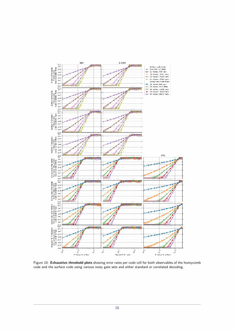
Figure 10: Exhaustive threshold plots showing error rates per code cell for both observables of the honeycombcode and the surface code using various noisy gate sets and either standard or correlated decoding.

16

D Example Honeycomb CircuitThe following is a Stim circuit file [19] describing a honeycomb memory experiment with 2×6 dataqubits and 335 rounds. The last round is terminated early, before its second sub-round. Thecircuit fault-tolerantly initializes the horizontal observable, preserves it through noise, and thenfault-tolerantly measures it.

The circuit includes coordinate annotations, noise annotations, and detector/observable anno-tations. The noise model is the “tweaked EM3" noise model mentioned in Figure 8 because thatnoise model produces the simplest circuit file.

Because copying code from PDF files is not reliable, this circuit is also attached to the paperas the ancillary file “example_honeycomb_circuit.stim".

# Annotate locations of qubits .QUBIT_COORDS (1, 0) 0QUBIT_COORDS (1, 1) 1QUBIT_COORDS (1, 2) 2QUBIT_COORDS (1, 3) 3QUBIT_COORDS (1, 4) 4QUBIT_COORDS (1, 5) 5QUBIT_COORDS (3, 0) 6QUBIT_COORDS (3, 1) 7QUBIT_COORDS (3, 2) 8QUBIT_COORDS (3, 3) 9QUBIT_COORDS (3, 4) 10QUBIT_COORDS (3, 5) 11

# Initialize data qubits into |+> state .R 0 1 2 3 4 5 6 7 8 9 10 11X_ERROR (0.001) 0 1 2 3 4 5 6 7 8 9 10 11TICKH 0 1 2 3 4 5 6 7 8 9 10 11DEPOLARIZE1 (0.001) 0 1 2 3 4 5 6 7 8 9 10 11TICK

# X sub −round . Compare X parities to X initializations .DEPOLARIZE2 (0.001) 9 3 2 1 4 5 0 6 7 8 11 10MPP (0.001) X9*X3 X2*X1 X4*X5 X0*X6 X7*X8 X11*X10OBSERVABLE_INCLUDE (1) rec [ -3]DETECTOR (0, 3, 0) rec [ -6]DETECTOR (1, 1.5 , 0) rec [ -5]DETECTOR (1, 4.5 , 0) rec [ -4]DETECTOR (2, 0, 0) rec [ -3]DETECTOR (3, 1.5 , 0) rec [ -2]DETECTOR (3, 4.5 , 0) rec [ -1]SHIFT_COORDS (0, 0, 1)TICK

# Y sub −round . Get X*Y=Z stabilizers for first time.DEPOLARIZE2 (0.001) 7 1 2 3 0 5 4 10 9 8 11 6MPP (0.001) Y7*Y1 Y2*Y3 Y0*Y5 Y4*Y10 Y9*Y8 Y11*Y6OBSERVABLE_INCLUDE (1) rec [ -6]SHIFT_COORDS (0, 0, 1)TICK

# Z sub −round . Get Y*Z=X stabilizers to compare against initialization .DEPOLARIZE2 (0.001) 11 5 0 1 4 3 2 8 7 6 9 10MPP (0.001) Z11*Z5 Z0*Z1 Z4*Z3 Z2*Z8 Z7*Z6 Z9*Z10OBSERVABLE_INCLUDE (1) rec [ -5] rec [ -2]DETECTOR (0, 0, 0) rec [ -12] rec [ -10] rec [ -7] rec [ -6] rec [ -5] rec [ -2]DETECTOR (2, 3, 0) rec [ -11] rec [ -9] rec [ -8] rec [ -4] rec [ -3] rec [ -1]SHIFT_COORDS (0, 0, 1)TICK

# X sub −round . Get Z*X=Y stabilizers for the first time.DEPOLARIZE2 (0.001) 9 3 2 1 4 5 0 6 7 8 11 10MPP (0.001) X9*X3 X2*X1 X4*X5 X0*X6 X7*X8 X11*X10OBSERVABLE_INCLUDE (1) rec [ -3]SHIFT_COORDS (0, 0, 1)TICK

# Stable state reached . Can now consistently compare to stabilizers from previous round .REPEAT 333 {

# Y sub −round . Get X*Y = Z stabilizers to compare against last time.DEPOLARIZE2 (0.001) 7 1 2 3 0 5 4 10 9 8 11 6MPP (0.001) Y7*Y1 Y2*Y3 Y0*Y5 Y4*Y10 Y9*Y8 Y11*Y6OBSERVABLE_INCLUDE (1) rec [ -6]DETECTOR (0, 2, 0) rec [ -30] rec [ -29] rec [ -26] rec [ -24] rec [ -23] rec [ -20] rec [ -12] rec [ -11] rec [ -8] rec [ -6] rec [ -5] rec [ -2]DETECTOR (2, 5, 0) rec [ -28] rec [ -27] rec [ -25] rec [ -22] rec [ -21] rec [ -19] rec [ -10] rec [ -9] rec [ -7] rec [ -4] rec [ -3] rec [ -1]SHIFT_COORDS (0, 0, 1)TICK

# Z sub −round . Get Y*Z = X stabilizers to compare against last time.DEPOLARIZE2 (0.001) 11 5 0 1 4 3 2 8 7 6 9 10MPP (0.001) Z11*Z5 Z0*Z1 Z4*Z3 Z2*Z8 Z7*Z6 Z9*Z10OBSERVABLE_INCLUDE (1) rec [ -5] rec [ -2]DETECTOR (0, 0, 0) rec [ -30] rec [ -28] rec [ -25] rec [ -24] rec [ -23] rec [ -20] rec [ -12] rec [ -10] rec [ -7] rec [ -6] rec [ -5] rec [ -2]DETECTOR (2, 3, 0) rec [ -29] rec [ -27] rec [ -26] rec [ -22] rec [ -21] rec [ -19] rec [ -11] rec [ -9] rec [ -8] rec [ -4] rec [ -3] rec [ -1]SHIFT_COORDS (0, 0, 1)TICK

# X sub −round . Get Z*X = Y stabilizers to compare against last time.DEPOLARIZE2 (0.001) 9 3 2 1 4 5 0 6 7 8 11 10MPP (0.001) X9*X3 X2*X1 X4*X5 X0*X6 X7*X8 X11*X10OBSERVABLE_INCLUDE (1) rec [ -3]DETECTOR (0, 4, 0) rec [ -30] rec [ -28] rec [ -25] rec [ -24] rec [ -22] rec [ -19] rec [ -12] rec [ -10] rec [ -7] rec [ -6] rec [ -4] rec [ -1]DETECTOR (2, 1, 0) rec [ -29] rec [ -27] rec [ -26] rec [ -23] rec [ -21] rec [ -20] rec [ -11] rec [ -9] rec [ -8] rec [ -5] rec [ -3] rec [ -2]SHIFT_COORDS (0, 0, 1)TICK

}

# Transversal measurement .H 0 1 2 3 4 5 6 7 8 9 10 11DEPOLARIZE1 (0.001) 0 1 2 3 4 5 6 7 8 9 10 11TICKX_ERROR (0.001) 0 1 2 3 4 5 6 7 8 9 10 11M 0 1 2 3 4 5 6 7 8 9 10 11OBSERVABLE_INCLUDE (1) rec [ -11] rec [ -5]

# Compare X data measurements to X parity measurements from last sub −round .DETECTOR (0, 3, 0) rec [ -18] rec [ -9] rec [ -3]DETECTOR (1, 1.5 , 0) rec [ -17] rec [ -11] rec [ -10]DETECTOR (1, 4.5 , 0) rec [ -16] rec [ -8] rec [ -7]DETECTOR (2, 0, 0) rec [ -15] rec [ -12] rec [ -6]DETECTOR (3, 1.5 , 0) rec [ -14] rec [ -5] rec [ -4]DETECTOR (3, 4.5 , 0) rec [ -13] rec [ -2] rec [ -1]

# Compare X data measurements to previous X stabilizer reconstruction .DETECTOR (0, 0, 0) rec [ -30] rec [ -28] rec [ -25] rec [ -24] rec [ -23] rec [ -20] rec [ -12] rec [ -11] rec [ -7] rec [ -6] rec [ -5] rec [ -1]DETECTOR (2, 3, 0) rec [ -29] rec [ -27] rec [ -26] rec [ -22] rec [ -21] rec [ -19] rec [ -10] rec [ -9] rec [ -8] rec [ -4] rec [ -3] rec [ -2]

17