arX

iv:0

807.

0972

v1 [

cond

-mat

.str

-el]

7 J

ul 2

008

Canonical representation for electrons and its application to the Hubbard model

Brijesh Kumar∗

School of Physical Sciences, Jawaharlal Nehru University, New Delhi 110067, India.

(Dated: July 7, 2008)

A new representation for electrons is introduced, in which the electron operators are written interms of a spinless fermion and the Pauli operators. This representation is canonical, invertibleand constraint-free. Importantly, it simplifies the Hubbard interaction. On a bipartite lattice,the Hubbard model is reduced to a form in which the exchange interaction emerges simply bydecoupling the Pauli subsystem from the spinless fermion bath. This exchange correctly reproducesthe large U superexchange. Also derived, for U = ±∞, is the Hamiltonian to study Nagaokaferromagnetism. In this representation, the infinite-U Hubbard problem becomes elegant and easierto handle. Interestingly, the ferromagnetism in Hubbard model is found to be related to the gaugeinvariance of the spinless fermions. Generalization of this representation for the multicomponentfermions, a new representation for bosons, the notion of a ‘soft-core’ fermion, and some interestingunitary transformations are introduced and discussed in the appendices.

PACS numbers: 71.10.Fd,75.10.Jm,05.30.Fk

I. INTRODUCTION

Strongly correlated electrons represent a large classof physical systems exhibiting a variety of novel phe-nomena1,2. The transition metal oxides, such as thehigh-TC superconducting cuprates3,4,5,6, or the colos-sal magneto-resistive manganites7, provide some of themost famous and actively investigated materials of thiskind. The common feature in all such materials is thedominant presence of local repulsion between electrons,with manifestly non-trivial consequences, such as theantiferromagnetic-insulating behavior at half-filling (theMott insulators), which can not be understood from theband-theory of solids8,9. Physics of these systems is in-trinsically non-perturbative, and hence difficult. TheHubbard model1,10,11,12,13, which describes a system oftight-binding electrons with on-site repulsion, allows thesimplest meaningful description of the strongly corre-lated electrons. Since the local repulsion U (also calledthe Hubbard interaction) and the hopping t (assumingnearest-neighbor) have opposing effects on the electrons,the ground state of the Hubbard model can be metal-lic/insulating, magnetic/non-magnetic or something else(yet unexplored), depending upon the ratio t/U , the elec-tron density ne, and the geometry of the lattice.

For sufficiently large U at half-filling (ne = 1), theHubbard model is known to systematically produce theantiferromagnetic exchange interaction and the insulat-ing ground state8. As t/U is increased, the insulat-ing phase undergoes a quantum transition to a metallicphase. Though there have been many elaborate studieson Hubbard model9,14, there is no final verdict as yet onthe nature of this metal-insulator transition (except inone dimension where the exact ground state is insulat-ing for any non-zero U15). Also, the search for a super-conducting ground state in purely repulsive lattice mod-els16,17,18 has become very important since the discoveryof superconductivity in cuprates and other strongly cor-related materials, but with no definite answer. Present

understanding of the Hubbard model is far from beingcomplete, and has been a subject of great research inter-est13. The main difficulty lies in the handling of the Hub-bard interaction. This has led to the development of nu-merous approximate methods. The Gutzwiller projectedvariational wavefunctions19,20, the dynamical mean-fieldtheory14, the slave-boson (fermion) approach21,22 or thecluster approximations23 are a few important ones tomention. Exact numerical diagonalization has also beenused to study Hubbard model on small lattices24. Themotivation to search for newer and more effective schemesof investigation, for a better understanding of the Hub-bard model (and the strongly correlated systems in gen-eral), is therefore very strong.

In this paper, we present a new canonical represen-tation for electrons, and demonstrate its usefulness forthe Hubbard model. The basic idea is to identify theindependent physical attributes of an electron, in termsof which the electron can be described as a composite.The two attributes of an electron are its spin and theFermi-ness. The spin defines the two-level structure ofthe electron which can be described using Pauli oper-ators. The Fermi attribute, which assigns the correctquantum statistics (anticommutation) to the electron, isdescribed in terms of a spinless fermion. In our descrip-tion, these two canonical degrees of freedom are com-bined to make the electron. An important feature of thisrepresentation is that it transforms the Hubbard inter-action (the particle-hole symmetric form) into the chem-ical potential for the spinless fermions. The simplifica-tion thus achieved further encourages us to investigatethe Hubbard model in this representation. We discusstwo very important cases, that is the superexchange forfinite U and the Nagaoka ferromagnetism25 for infiniteU , to highlight the physical usefulness of our represen-tation in describing strongly correlated electrons. Thepaper is organized as follows. In the next section, we in-troduce the representation, discuss its canonical nature,and derive the inverse representation. In section III, we

2

TABLE I: Local Hilbert spaces and the operators of the elec-tron, spinless fermion and a Pauli (two-level) system. Here,|0〉 and |ø〉 denote the vacua of the electron and the spinless

fermion, respectively. Operators fs and a satisfy the canoni-cal Fermi algebra, while σz and σ± are the Pauli operators.

Basis Operators

Electron {|0〉, | ↑〉, | ↓〉, | ↑↓〉} fs, f†s ; s =↑, ↓

fs|0〉 = 0

f†↑ |0〉 = | ↑〉f†↓ |0〉 = | ↓〉

f†↑ f

†↓ |0〉 = | ↑↓〉

f†↑ = | ↑〉〈0|+ | ↑↓〉〈↓ |f†↓ = | ↓〉〈0| − | ↑↓〉〈↑ |

Spinless {|ø〉, |1〉} a, a†

Fermiona|ø〉 = 0a†|ø〉 = |1〉 a† = |1〉〈ø|

Pauli {|+〉, |−〉} σ±, σz

Systemσ−|−〉 = 0σ+|−〉 = |+〉

σ+ = |+〉〈−|σz = |+〉〈+| − |−〉〈−|

discuss the Hubbard model. On a bipartite lattice, wereduce the model to a nice form in which a part of thehopping explicitly generates the exchange interaction in asimple decoupling scheme. For large U at half-filling, thisexchange interaction correctly reproduces Anderson’s su-perexchange8. In section IV, we present the Hamiltonianformulation of the Nagaoka ferromagnetism. In the ap-pendices, we discuss a few related but distinct topics.First, we generalize this representation for N -componentfermions in appendix A. Next, we write down a new rep-resentation for the bosons. In appendix C, we introducea unitary transformation with Majorana gauge, and de-

rive the Jordan-Wigner transformation26,27. Finally, weintroduce the notion of a ‘soft-core fermion’, and discussits basic properties.

II. NEW REPRESENTATION FOR

ELECTRONS

Consider the Hilbert space of electron on a single site.The four basis states which span this local electronicHilbert space are tabulated in Table I, where |0〉 denotes

the empty site, and f †↑ and f †

↓ are the creation operatorsof ↑ and ↓ electrons, respectively. Also consider a spin-less fermion and a two-level (Pauli) system, each hav-ing a two-dimensional Hilbert space (see Table I). Let aand a† be the annihilation and creation operators of thespinless fermion, and σz and σ± be the usual Pauli opera-tors describing the two-level system. Since the composite

TABLE II: A mapping between the states of the electron anda composite system of a spinless fermion and a Pauli system.

|0〉 ←→ |ø〉 |−〉| ↑〉 ←→ |1〉 |+〉| ↓〉 ←→ |1〉 |−〉| ↑↓〉 ←→ |ø〉 |+〉

Hilbert space of a spinless fermion and a Pauli system isfour-dimensional, we can define a one-to-one mapping be-tween the basis states of this composite Hilbert space andthat of the electron28,29. In Table II, we define one suchmapping, in which the one-electron states correspond tohaving one spinless fermion, and the empty or double-occupancy electronic states correspond to the vacuumof the spinless fermion. For the one-electron states, |+〉corresponds to ↑ spin, and |−〉 to ↓ spin of the electron.Otherwise, they correspond respectively to the double-occupancy or empty state. This mapping, which is mo-tivated by our idea of the electron as a composite of theFermi and Pauli degrees of freedom, results in the follow-ing new representation for the electron operators.

f †↑ = φ σ+ (1)

f †↓ = i

ψ

2− φ

2σz (2)

Here, φ = a†+ a, and iψ = a†− a. The operators φ and ψ(called the Majorana or real fermions) are Hermitian, and

satisfy the relations: φ2 = ψ2 = 1 and {φ, ψ} = 0, where{, } denotes the anti-commutator. As usual, the spinlessfermion operators commute with the Pauli operators. We

have derived Eqs. (1) and (2) using the definition of f †↑

and f †↓ in terms of the basis states (as given in Table I).

In this representation, the electron number operatorsare given as: n↑ = (1 + σz)/2 and n↓ = 1

2 +(

12 − n

)

σz ,

where n = a†a. The physical spin, S, of the electron,

which is defined as Sz = (n↑ − n↓)/2 and S+ = f †↑ f↓,

takes the form: S = n~σ/2. Similarly, the local pairing(the pseudo-spin operators), P can be written as: P =

(n− 1)~σ/2, where P+ = f †↑ f

†↓ and P z = (n↑ + n↓− 1)/2.

Also, S + P = ~σ/2 and SiPj = 0, where i, j = x, y, z.Here, σx = σ+ + σ− and σy = −i(σ+ − σ−). Physi-cally speaking, ~σ represents the spin of electron in thepresence of the spinless fermion. Otherwise, it representslocal pairing. These forms (especially that of S) are con-sistent with our intuitive picture in which an electron isenvisaged as a “composite” object made up of the Fermi

and the spin attributes. Furthermore, it is importantto note that

(

n↑ − 12

) (

n↓ − 12

)

= 12

(

12 − n

)

, that is theHubbard interaction between electrons transforms intothe number operator of the spinless fermion.

The new representation of the electron is canonical,constraint-free and invertible. It is canonical because theelectron operators satisfy the usual anti-commutation re-lations. It is obviously constraint-free because there are

3

no extra conditions to be satisfied by a or ~σ operators.This is a consequence of the one-to-one mapping betweenthe two Hilbert spaces. Since there are no excess or loststates, there is no constraint. Also, the spinless fermionand the Pauli operators can be represented uniquely interms of the electron operators. The inverse of the newrepresentation is given as:

a† = (1− n↑)f†↓ − n↑f↓ (3)

σz = 2n↑ − 1 (4)

σ+ = f †↑

(

f †↓ + f↓

)

(5)

The inverse representation is also consistent, because thefermion operator, a, satisfies the anti-commutation rela-tion and the Pauli operators satisfy the angular momen-tum algebra. The Pauli operators also satisfy the anti-commutation relation: {σi, σj} = 2δij for i, j = x, y, z.And of course, a and a† commute with ~σ.

The inverse representation gives us more insight intothe nature of the new objects. Equations (4) and (5)are same as the Majorana fermion representation of thespin-1/2 operators30. The spinless fermion [Eq. (3)] is ef-fectively a Gutzwiller-projected electron whose creationis equivalent to the creation or annihilation of ↓ elec-tron, subject to the absence or presence of ↑ electronrespectively. It is also like the Bogoliubov quasiparticlein the BCS theory as it mixes a particle with a hole.Surprisingly, the inverse representation has more famil-iar appearance, and hence, it is easier to appreciate. Wecan generate many equivalent forms of our representa-tion by making suitable unitary rotations. This gives usthe freedom of choosing a form that may serve us betterfor a given problem. For example, the unitary operator,U = 1− 2n↑n↓, transforms Eqs. (3-5) as follows.

U a†U† = b† = (1− n↑)f†↓ + n↑f↓ (6)

Uσ+U† = τ+ = −f †↑(f †

↓ − f↓) (7)

Or conversely, f †↑ = iψbτ

+, and f †↓ = (φb − iψb τ

z)/2,

where φb = b† + b and iψb = b† − b. We will use this andthe original form of the representation to convenientlydescribe the Hubbard model on a bipartite lattice.

III. HUBBARD MODEL AT HALF-FILLING

Consider the Hubbard model with nearest-neighborhopping on a lattice. Its Hamiltonian in terms of theelectron operators can be written as:

H = − t2

∑

r,δ

∑

s=↑,↓

(

f †r,sfr+δ,s + f †

r+δ,sfr,s

)

+U∑

r

(

nr↑ −1

2

) (

nr↓ −1

2

)

(8)

where r is summed over all the sites of a lattice, andδ is summed over the nearest-neighbors of a site. The

electron hopping is denoted by t, and U is the Hubbardinteraction. In Eq. (8), the factor of 1/2 in t is thereto undo the double-counting of the hopping due to theexplicit use of its Hermitian conjugate. Therefore, the twe use is same as the one commonly reported. The U -term in Eq. (8) is written in the particle-hole symmetricform31. The Hubbard model in the new representation[using Eqs. (1) and (2)] takes the following form.

H = −U2

∑

r

a†rar −

t

2

∑

r,δ

(

σ+rσ−r+δ − h.c.

)

φr φr+δ

− it4

∑

r,δ

(

σzrφr ψr+δ + σz

r+δ φr+δ ψr

)

+U

4L (9)

Here, L is the total number of lattice sites. In this form,the Hubbard interaction has taken the role of chemicalpotential for the spinless fermions, and the hopping hastransformed into a complicated spin-fermion interaction.The Hubbard model has thus turned into a problem ofspin-1/2 objects immersed in a grand-canonical bath ofspinless fermions, which are constantly being created andannihilated around an average fermion density decided byU . The total σz is however conserved, which is same theconservation of the total number of ↑-electrons.

Since the local gauge of the electron governs the flowof charge-current in a system, it is important to considerhow the new objects respond to such a local gauge trans-formation. This will give us an idea of the way charge

is carried by the new objects. Let f †r,s → eiθr f †

r,s bethe gauge transformation on electrons, under which thespinless fermions and the Pauli operators transform as:

a†r → (1− nr↑)f†r↓e

iθr − nr↑fr↓e−iθr (10)

σ+r → f †

r↑f†r↓e

i2θr + f †r↑fr↓ (11)

This implies that a spinless fermion carries one unit ofelectron or hole charge (of ↓ electron, to be more specific),and σ+

r carries a charge of two electrons or no charge atall. It can be understood by explicitly considering the ac-tion of a† and σ+ on the electronic states. For complete-ness, we also write the current density operator for theHubbard model in terms of the spinless fermions and the

Pauli operators, which is ~Jr = (iet/2)∑

δ δ(f†r,sfr+δ,s −

f †r+δ,sfr,s) = (iet/4)

∑

δ δ[ψrψr+δ + φrφr+δ(~σr · ~σr+δ)].

Interestingly, the current operator has nicer form as com-pared to hopping in the new representation, and it alsoreveals the exchange interaction. At this point, it maybe mentioned that Eq. (6) is same as Eq. (10) (with somefine tuning) for θr = π/2. In fact, the U in Eq. (6) wassuggested by this observation.

On a bipartite lattice, Eq. (9) can be transformed to amore elegant form by making a suitable unitary rotationon the operators on one sublattice. Let A and B denotethe two sublattices. We write the electron operators on

A-sublattice, in terms of a, a† and ~σ, as f †↑ = φaσ

+

and f †↓ = (iψa − φaσ

z)/2. The electrons on B-sublattice

4

are described in terms of b, b† and ~τ such that f †↑ =

iψbτ+ and f †

↓ = (φb − iψbτz)/2. The representation on

A-sublattice is in the original form [as in Eqs. (1) and (2)],while on B-sublattice, it is a unitary-transformed versionof the same [see Eqs. (6) and (7)]. The Hubbard modelon a bipartite lattice can therefore be written as:

H =U

4L− U

2

[

∑

R∈A

a†RaR

+∑

R∈B

b†RbR

]

(12)

− it2

∑

R∈A

∑

δ

[

ψa,Rφb,R+δ + ψb,R+δφa,R

(

~σR· ~τR+δ

)

]

This form of H is neat and suggestive32. It presentsthe dual role of hopping very clearly. While a part ofthe hopping contributes purely to the dynamics of thespinless fermion bath, the remaining part generates anSU(2) invariant exchange interaction33, whose strengthis determined by the fluctuations in the bath.

To gain further insight, we discuss the Hubbard modelin a decoupled form: H = HFermi +HPauli, where

HFermi = −U2

∑

R∈A

a†RaR +

U

2

∑

R∈B

bRb†R

(13)

−t∑

R∈A

∑

δ

(

a†Rb†R+δ + bR+δ aR

)

= −U2

∑

k

(

a†kak− b

kb†k

)

(14)

−tz∑

k

(

γk a†kb†−k

+ γ∗k b−kak

)

and

HPauli =tζ

2

∑

R∈A

∑

δ

(

~σR · ~τR+δ + 1)

(15)

This decoupled from is derived in the following way.First, we rewrite ~σ

R· ~τ

R+δ in Eq. (12) as −1 + (1 + ~σR·

~τR+δ), and include −ψb,R+δφa,R resulting from this into

the purely spinless fermion part ofH , which is now called

HFermi. Then, replace ψb,R+δφa,R [which is in multi-

plication with (1 + ~σR· ~τ

R+δ)] by its expectation valuein the ground state of HFermi. The resultant involvingonly Pauli operators is called HPauli. Thus, the bath ofspinless fermions in the decoupled picture is described byHFermi, and HPauli is the exchange Hamiltonian, where(~σR ·~τR+δ +1)/2 is the Dirac-Heisenberg exchange oper-ator on a nearest-neighbor bond. Note that the constant

term UL/4 has been absorbed in rewriting b†RbR

as bRb†R

.The validity of this decoupling can be tested against

the well-known superexchange interaction, 4t2/U , in thelimit of large U . The strength of the exchange interac-

tion, J , is given as: J = 2tζ, where ζ = −i〈ψb,R+δφa,R〉(uniform average on each nearest-neighbor bond) is de-termined purely by HFermi. Equation (14) is the mo-mentum space representation of HFermi, where γk =

0 10 20 30 40 50

U

0

0.2

0.4

0.6

0.8

1

1.2

J

Nearest-Neighbor ChainHoneycomb LatticeSquare LatticeSimple Cubic Lattice

4t2/U

FIG. 1: Antiferromagnetic exchange J as a function of U . Thesuperexchange interaction, 4t2/U (t = 1 in our calculation),is also plotted for comparison. For large U , all J → 4t2/U .

1z

∑

δ eik·δ = |γk|eiλk , and z is the nearest-neighbor co-

ordination. Since γ∗k

= γ−k, therefore, |γ−k| = |γk| andλ−k = −λk. Here, the wavevector k lies in the sublat-tice Brillouin zone, and the Fourier transformation of the

spinless fermions is defined as: aR

=√

2L

∑

keik·Rak,

and similarly for bk. The HFermi is diagonalized by ap-plying two unitary rotations in following way.

HFermi = Uθ Uλ Hfermi U†λ U

†θ (16)

=∑

k

Ek(

1− a†kak − b†kbk

)

The unitary operators in Eq. (16) are defined as: Uλ =∏

keiλk b

†

kbk , and Uθ =

∏

keθk(a†

kb†

−k−b−kak), where Uλ

absorbs the phase λk into bk, and Uθ diagonalizes the

ak, b†−kmixing. The quasi-particle dispersion, Ek =

√

U2

4 + (zt|γk|)2, is positive, and tan 2θk = zt|γk|/(U2 ).

The ground state of HFermi is given by a†kak

= b†kbk

=1, for all k. We calculate ζ in the ground state ofHFermi,

and find that J = 4zt2

L

∑

k

|γk|2

Ek

, which is certainly pos-itive. Hence, the exchange interaction in HPauli is anti-ferromagnetic. Explicitly on aD-dimensional hypercubic

lattice, where z = 2D and γk = 1D

∑Di=1 cos ki, we cor-

rectly retrieve Anderson’s superexchange, J → 4t2/|U |,for U ≫ 2zt. In Fig. 1, the calculated values of J areplotted as a function of U/t, for a few different bipartitelattices. The densities of a and b type spinless fermionsare calculated to be: na = nb = n = 1

2 + U2L

∑

k

1Ek

. For

U ≫ 2zt, n → 1, and for U → 0, n → 12 (see Fig. 2).

Both of these limiting cases give the expected values ofthe spinless fermion density. Since the local densitiesna,R and nb,R also take the uniform value n, the electrondensity can be calculated as: ne = 1 + 1−n

L

∑

rσzr, which

is equal to 1 when total σz = 0 (that is,∑

A σz+

∑

B τz =

0). Therefore, in the decoupled problem, the half-filling

5

0 10 20 30 40 50

U

0.5

0.6

0.7

0.8

0.9

1n

Nearest-Neighbor ChainHoneycomb LatticeSquare LatticeSimple Cubic Lattice

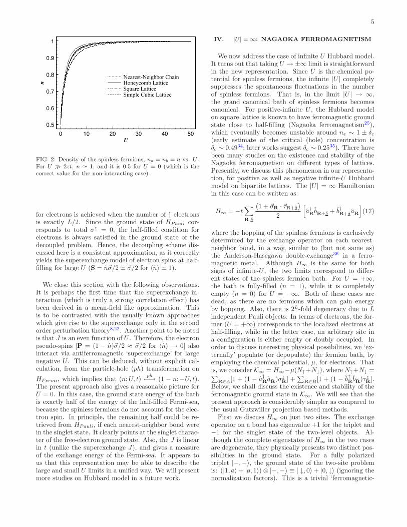
FIG. 2: Density of the spinless fermions, na = nb = n vs. U .For U ≫ 2zt, n ≃ 1, and it is 0.5 for U = 0 (which is thecorrect value for the non-interacting case).

for electrons is achieved when the number of ↑ electronsis exactly L/2. Since the ground state of HPauli cor-responds to total σz = 0, the half-filled condition forelectrons is always satisfied in the ground state of thedecoupled problem. Hence, the decoupling scheme dis-cussed here is a consistent approximation, as it correctlyyields the superexchange model of electron spins at half-filling for large U (S = n~σ/2 ≃ ~σ/2 for 〈n〉 ≃ 1).

We close this section with the following observations.It is perhaps the first time that the superexchange in-teraction (which is truly a strong correlation effect) hasbeen derived in a mean-field like approximation. Thisis to be contrasted with the usually known approacheswhich give rise to the superexchange only in the secondorder perturbation theory8,22. Another point to be notedis that J is an even function of U . Therefore, the electronpseudo-spins [P = (1 − n)~σ/2 ≈ ~σ/2 for 〈n〉 → 0] alsointeract via antiferromagnetic ‘superexchange’ for largenegative U . This can be deduced, without explicit cal-culation, from the particle-hole (ph) transformation on

HFermi, which implies that (n;U, t)ph←→ (1 − n;−U, t).

The present approach also gives a reasonable picture forU = 0. In this case, the ground state energy of the bathis exactly half of the energy of the half-filled Fermi-sea,because the spinless fermions do not account for the elec-tron spin. In principle, the remaining half could be re-trieved from HPauli, if each nearest-neighbor bond werein the singlet state. It clearly points at the singlet charac-ter of the free-electron ground state. Also, the J is linearin t (unlike the superexchange J), and gives a measureof the exchange energy of the Fermi-sea. It appears tous that this representation may be able to describe thelarge and small U limits in a unified way. We will presentmore studies on Hubbard model in a future work.

IV. |U | =∞: NAGAOKA FERROMAGNETISM

We now address the case of infinite U Hubbard model.It turns out that taking U → ±∞ limit is straightforwardin the new representation. Since U is the chemical po-tential for spinless fermions, the infinite |U | completelysuppresses the spontaneous fluctuations in the numberof spinless fermions. That is, in the limit |U | → ∞,the grand canonical bath of spinless fermions becomescanonical. For positive-infinite U , the Hubbard modelon square lattice is known to have ferromagnetic groundstate close to half-filling (Nagaoka ferromagnetism25),which eventually becomes unstable around ne ∼ 1 ± δc(early estimate of the critical (hole) concentration isδc ∼ 0.4934; later works suggest δc ∼ 0.2535). There havebeen many studies on the existence and stability of theNagaoka ferromagnetism on different types of lattices.Presently, we discuss this phenomenon in our representa-tion, for positive as well as negative infinite-U Hubbardmodel on bipartite lattices. The |U | = ∞ Hamiltonianin this case can be written as:

H∞ = −t∑

R,δ

(

1 + ~σR · ~τR+δ

)

2

[

a†RbR+δ + b†

R+δaR

]

(17)

where the hopping of the spinless fermions is exclusivelydetermined by the exchange operator on each nearest-neighbor bond, in a way, similar to (but not same as)the Anderson-Hasegawa double-exchange36 in a ferro-magnetic metal. Although H∞ is the same for bothsigns of infinite-U , the two limits correspond to differ-ent states of the spinless fermion bath. For U = +∞,the bath is fully-filled (n = 1), while it is completelyempty (n = 0) for U = −∞. Both of these cases aredead, as there are no fermions which can gain energyby hopping. Also, there is 2L-fold degeneracy due to Lindependent Pauli objects. In terms of electrons, the for-mer (U = +∞) corresponds to the localized electrons athalf-filling, while in the latter case, an arbitrary site ina configuration is either empty or doubly occupied. Inorder to discuss interesting physical possibilities, we ‘ex-ternally’ populate (or depopulate) the fermion bath, byemploying the chemical potential, µ, for electrons. Thatis, we consider K∞ = H∞−µ(N↑+N↓), where N↑+N↓ =∑

R∈A[1 + (1 − a†RaR

)σzR

] +∑

R∈B[1 + (1 − b†RbR

)τzR

].Below, we shall discuss the existence and stability of theferromagnetic ground state in K∞. We will see that thepresent approach is considerably simpler as compared tothe usual Gutzwiller projection based methods.

First we discuss H∞ on just two sites. The exchangeoperator on a bond has eigenvalue +1 for the triplet and−1 for the singlet state of the two-level objects. Al-though the complete eigenstates of H∞ in the two casesare degenerate, they physically presents two distinct pos-sibilities in the ground state. For a fully polarizedtriplet |−,−〉, the ground state of the two-site problemis: (|1, ø〉+ |ø, 1〉)⊗ |−,−〉 ≡ | ↓, 0〉+ |0, ↓〉 (ignoring thenormalization factors). This is a trivial ‘ferromagnetic-

6

metallic’ state with ↓magnetization. Similarly for |+,+〉,it is | ↑, ↑↓〉 + | ↑↓, ↑〉, which is also ferromagnetic (butwith respect to the fully-filled electron configuration).For the singlet state, (|+,−〉 − |−,+〉), the ground stateis: (|1, ø〉 − |ø, 1〉) ⊗ (|+,−〉 − |−,+〉) ≡ | ↑, 0〉 + |0, ↑〉+ | ↑↓, ↓〉+ | ↓, ↑↓〉, which is like a ‘non-magnetic’ metal-lic state. Also, in the singlet case, n↑ = n↓ = 1/2 andS = 0. This simple analysis suggests two qualitativelydifferent possibilities in the ground state of H∞.

Now we study K∞ on the full lattice. We explicitlyconsider the case of U = −∞ (that is, gradually fill theempty bath). The results for U = +∞ can be exactly in-ferred from the particle-hole transformation on the spin-less fermions, which states that the ground state for +veU for a given density n, is same as that of −ve U for 1−n,for a fixed t and m [where m = (

∑

A σz +

∑

B τz)/L]. To

establish the existence of ferromagnetic-metallic groundstate for U = −∞, consider one spinless fermion in theempty bath. The (only) energy, that it gains by hop-ping, can be maximized by having maximum and uniformhopping through each bond. While the fully-polarized‘ferromagnetic’ state of the Pauli subsystem fulfills thisrequirement, the same can not be achieved in any otherstate, for instance, a configuration of bond-singlets or anydeviation with respect to the fully polarized state. Thefully polarized Pauli subsystem therefore emerges as theonly choice which helps the fermion in gaining maximumkinetic energy. The same will be true for a finite densityof the spinless fermions, until the ‘ferromagnetic’ state ofthe Pauli subsystem becomes unstable. In terms of elec-trons, the ground state of a finite n fermion bath togetherwith ‘−’ polarized Pauli subsystem, corresponds to a ↓polarized ferromagnetic metal with the electron density,ne = n. Also, for the ‘+’ polarized Pauli subsystem, theelectronic ground state is ferromagnetic, but from thefully-filled side of the electron density (ne = 2−n). Thisanalysis further implies that the ground state of U = +∞Hubbard model is also ferromagnetic-metallic, as discov-ered by Nagaoka, around half-filling (ne = 1± n, for ‘+’or ‘−’ polarization respectively). Below we discuss theinstability of the ferromagnetic state. It is generally ahard problem. But in our framework, it actually becomesa much simpler problem.

As it appears from the structure of H∞, the spinlessfermions are happy to live with ferromagnetic Pauli sub-system for any density of electrons. But the Pauli sub-system itself is not comfortable with the change in ne, be-cause µ acts as an ‘external’ field for the Pauli operators.This induces ‘flips’ in the fully-polarized Pauli subsystemfor sufficiently populated fermion bath, thereby causingthe instability of the Nagaoka state. To work this out,

we write the Pauli operators in terms of α and β, the twohard-core bosons, such that: σz = −1 + 2α†α, σ+ = α†

and τz = −1 + 2β†β, τ+ = β†. The creation of a hard-core boson amounts to flipping |−〉 on the respective siteto |+〉, like a ‘magnon’. Rewriting K∞ in terms of α and

β separates the ferromagnetic part from the terms which

0 0.5 1 1.5 2

0

0.2

0.4

0.6

0.8

1 Nearest-Neighbor ChainHoneycomb LatticeSquare LatticeSimple Cubic Lattice

Electron Density, ne

Fer

rom

agn

etic

Ex

chan

ge,

χ

U=∞ U=∞U=−∞ U=−∞

FIG. 3: Metallic ferromagnetism in the infinite-U Hubbardmodel. The shaded region between ne = 0.5 and 1.5 is theNagaoka ferromagnetic state for U = +∞. Note the com-plementary existence (in the sense of electron filling) of theNagaoka ferromagnetism for U = +∞ and −∞.

cause flips, that is: K∞ = HFM +Hflips, where

HFM = −t∑

R∈A

∑

δ

(a†RbR+δ + b†

R+δaR) (18)

−µ∑

R∈A

a†RaR− µ

∑

R∈B

b†RbR

and

Hflips = t∑

R∈A

∑

δ

(

a†RbR+δ + b†

R+δaR

)

× (19)

[

(α†Rα

R+ β†

R+δβR+δ)− (α†RβR+δ + β†

R+δαR)

−2(α†RαR)(β†

R+δβR+δ)]

−2µ∑

R∈A

(1− a†RaR

)α†Rα

R

−2µ∑

R∈B

(1− b†RbR)β†

RβR

In the ferromagnetic state, Hflips is zero as all the two-level objects are in the same state, and only HFM ac-counts for the ground state for different ne, where ne = n.

Instability of the ferromagnetic state can be deter-mined by calculating the dispersion of exactly one ‘flip’,in the ground state of HFM for different values of µ.That is, we replace the fermion operator terms in Hflips

by their expectation values in the ground state of HFM ,and calculate the one-flip dispersion. That value of ne,for which the minimum of this dispersion becomes nega-tive, marks the instability for the Nagaoka state. By fol-lowing the above prescription, we get the following equa-tions for the spinless femion density, n, and the one-flip

7

dispersion, ǫ±k

.

n =1

L

∑

k

[Θ(−zt|γk| − µ) + Θ(zt|γk| − µ)] (20)

χ = − 2

zt

〈H∞〉L

(21)

=2

L

∑

k

|γk| [Θ(−zt|γk| − µ)−Θ(zt|γk| − µ)]

ǫ±k

= ztχ(1± |γk|)− 2µ(1− n) (22)

Here, χ is the ferromagnetic ground state energy pernearest-neighbor bond (in units of −t), and tχ is alwayspositive (for any sign of t). Since ztχ(1 ± |γk|) ≥ 0 and(1 − n) is also positive, therefore, ǫ±

kis certainly non-

negative for µ < 0, which implies a stable ferromagneticground state. For µ = 0+ however, ǫ−

kbecomes negative

at k = 0. Thus, the ferromagnetic ground state becomesunstable to the flips in the Pauli subsystem, and thereoccurs a first order transition in the ground state. Thestable ferromagnetic-metallic ground state (µ < 0) cor-responds to ne = n < 1/2, and the instability exactlyoccurs at ne = 1/2 (µ = 0). The same analysis for ‘+’ po-larized case gives the stable Nagaoka state for ne = 2−n,where 0 < n < 1/2. Using the particle-hole transforma-tion for spinless fermions, we further deduce that theNagaoka state for U = +∞ exists for 1/2 < ne < 1 (holedoping) and for 1 < ne < 3/2 (electron doping). Theseresults are presented in Fig. 3.

This simple analysis of a difficult problem is very en-couraging. It gives the essential physics, that is the fer-romagnetic ground state and its instability, in a verystraightforward manner. We could show the existence ofNagaoka state for both U = +∞ as well as −∞ Hubbardmodel. Of course, we would like to investigate (more ac-curately) whether the critical n is exactly 0.5 or slightlydifferent. But n = 0.5 appears to be a special fermiondensity for bipartite lattices (maximum ferromagneticexchange; also, corresponds to a non-magnetic metal-lic ground state). Further investigations of the Nagaokaferromagnetism for finite U case, and on non-bipartitelattices will be discussed elsewhere. Finally, an impor-tant point to note in the present discussion is that theferromagnetism in Hubbard model is strictly related tothe invariance of the spinless fermions under a globalgauge transformation, while the antiferromagnetic/non-magnetic states break this gauge invariance. This is anovel point of view for the strongly correlated electrons.

V. SUMMARY

• A new canonical and invertible representation forthe electrons, in terms of a spinless fermion and thePauli operators, is presented. It is further general-ized for the N -component fermions in appendix A.

• The Hubbard interaction in this representation acts

as the chemical potential for spinless fermions.On a bipartite lattice, the Anderson’s superex-change for large and positive (as well as negative)U is shown to correctly emerges from the spinlessfermion bath, within a simple decoupling scheme.

• A Hamiltonian is derived for studying Nagaoka fer-romagnetism in |U | =∞ Hubbard model. The ex-istence of the ferromagnetic-metallic state and itsstability is discussed. It is pointed out that the fer-romagnetism in Hubbard model respects the globalgauge invariance for the spinless fermions, while theantiferromagnetism necessarily violates it.

• The meaningful analysis of the two important casesof the Hubbard model is very encouraging for thenew representation, and demonstrates its useful-ness for studying strongly correlated electrons.

• A representation for bosons is discussed in ap-pendix B. The Jordan-Wigner transformation isderived in appendix C by introducing a unitarytransformation with a Majorana fermion as gauge.Finally, the notion of a soft-core fermion is intro-duced in appendix D.

Acknowledgments

I am deeply indebted to Professor Sriram Shastry forcritical discussions and constant encouragement.

APPENDIX A: GENERALIZATION TO

MULTICOMPONENT FERMIONS

Let f †i be ith component of an N -component fermion

operator. Its Hilbert space is 2N dimensional. In terms ofa spinless fermion and N − 1 two-level objects, both theequality of the Hilbert space dimensions and the anti-commutativity can be attained consistently for the N -component fermion, by defining a representation in thefollowing way.

f †1 = φ σ+

1 (A1)

f †i = φ

i−1∏

j=1

σzj σ

+i for i = 2, · · · , N − 1 (A2)

f †N =

iψ

2− φ

2

N−1∏

i=1

σzi (A3)

The operators f †i (for i = 1, N − 1) anticommute with

each other because σ+i anticommutes with σz

i , and f †N

anticommutes with the rest of f †i operators, because ψ

anticommutes with φ (in addition to the anticommuta-tion of σ+

i and σzi ). The inverse of this representation

8

[Eqs. (A1-A3)] is given as:

For i = 1, N − 2

σ+i = f †

i

N−1∏

j=i+1

(2nj − 1)(

f †N + fN

)

(A4)

σ+N−1 = f †

N−1

(

f †N + fN

)

(A5)

a† = f †N

[

1−∏N−1

i=1 (2ni − 1)

2

]

−

fN

[

1 +∏N−1

i=1 (2ni − 1)

2

]

(A6)

where ni = f †i fi. The similarity between Eqs. (A4-

A5) and the Jordan-Wigner transformation is notable,with the exception that the Jordan-Wigner does not

have an extra(

f †N + fN

)

operator [and no equivalent

of Eq. (A6)]. Moreover, Eqs. (A1) and (A2) are sim-ilar to the inverse Jordan-Wigner transformation [with-

out a φ and Eq. (A3)]. One can generate many equivalentrepresentations for the N -component fermion by makingsuitable unitary rotations37.

APPENDIX B: REPRESENTATION FOR

BOSONS

Let a† and a be the creation and annihilation operatorsof a canonical boson, acting on the Fock states, {|n〉, n =0, 1 . . . ,∞}. The operator a† can be written as:

a† =

∞∑

n=0

√n+ 1 |n+ 1〉〈n| (B1)

=

∞∑

m=0

√2m+ 1 |2m+ 1〉〈2m| (B2)

+

∞∑

m=0

√

2(m+ 1) |2(m+ 1)〉〈2m+ 1|

where n = 2m in the first summation in Eq. (B2), andn = 2m+1 for the second. This even-odd structure of theFock states allows us to write a composite representationof the boson operators by defining the following mapping.

|2m〉 := |m〉 ⊗ |e〉 (B3)

|2m+ 1〉 := |m〉 ⊗ |o〉 (B4)

The kets |e〉 and |o〉 stand respectively for the even andodd values of the original Fock state quantum number n,and the states {|m〉} define a ‘new’ Fock space. Substi-tuting this mapping in Eq. (B2) results in the followingrepresentation of a†.

a† =

√

2b†b+ 1 σ+ +√

2 b†σ− (B5)

Here, σ± are the Pauli operators defined in the Hilbert

space of |e〉 and |o〉, such that σ+ = |o〉〈e|. Operators b†

and b are the new canonical bosons, acting in the Fockspace spanned by {|m〉}, which commute with the Paulioperators. It is easy to check that Eq. (B5) satisfies thebosonic commutation relations. The harmonic oscillatorin terms of the original bosons takes the following formin the new representation.

a†a+1

2= 2

[

b†b+1

2

]

+1

2σz (B6)

The new form looks like a two-level atom in a quantizedsingle-mode radiation field (without atom-field coupling),which conversely suggests that an atom-field problem canbe exactly mapped to an equivalent field-only problem (akind of ‘unification’ of matter and radiation-field into anew radiation-field). Most direct and simple case of thisunification, present in Eq. (B6) itself, is when the fre-quency of radiation is twice the energy-difference betweenthe two atomic-levels [see right-hand side of Eq. (B6)].The presence of an atom-field interaction will further in-troduce non-trivial terms in the unified radiation field.The application of this representation to an atom-fieldinteraction problem will be discussed elsewhere38.

Let us write down the inverse of this representation.The Pauli operators, in terms of a and a†, are given as:

σz = − cosπa†a := −χ (B7)

σ+ =1− χ

2

1√a†a

a†1 + χ

2(B8)

Note that (1 ± χ)/2 are the projection operators of theodd and even states respectively, in the original Fockspace. Therefore, the meaning of Eq. (B8) is clear thatit connects an even |n〉 to an odd |n〉 and annihilates theodd states, consistent with the definition of σ+. Also,the Pauli operators in the above representation satisfythe necessary algebra. Interestingly, Eqs. (B7) and (B8)also give us an unconstrained new bosonic representationfor spin-1/2 operators. If we restrict the Fock space to|0〉 and |1〉 (hard-core constraint), then we retrieve theusual hard-core boson representation. Now to the boson

b† which, in terms of a and a†, is represented as:

b† =1√2

[

1− χ2

1√a†a

a†a†1− χ

2

]

+

1√2

[

1 + χ

2a†a†

1√a†a+ 1

1 + χ

2

]

(B9)

It is consistent with the fact that the number of b-bosonschanges by 1 when the number of a-bosons changes by 2.Besides, it satisfies the bosonic commutations, and com-mutes with σz and σ±, as in Eqs. (B7) and (B8). Hence,a canonical and invertible representation for bosons.

9

APPENDIX C: UNITARY TRANSFORMATIONS

WITH ‘MAJORANA’ GAUGE

We now introduce a new kind of gauge transformation,and show how it generates the Jordan-Wigner represen-tation (JW) for spin-1/2 operators. Usually, we know theJW as an intuitive mapping that was not derived. Here,we precisely do that: derive it. Consider σ+ in termsof the electron operators [as in Eq. (5)]. It is given as:

σ+ = f †↑ φ↓, where φ↓ = f †

↓ + f↓ is a Majorana fermion

corresponding to ↓ electron. Since φ2↓ = 1, therefore,

e±i π

2φ↓ = ±ei π

2 φ↓, and σ+ can be rewritten as:

σ+ = f †↑e

−i π

2(1−φ↓) = e−i π

2(1+φ↓)f †

↑ (C1)

where the ↓ electron Majorana fermion appears in thegauge. This observation motivates us to define a suitable‘Majorana’ gauge-transformation such that the phase

factor in Eq. (C1) is completely absorbed into f †↑ , thereby

transforming σ+ into f †↑ . We easily define such a trans-

formation as:

U(φ↓) = exp[

−iπ2(1 + φ↓)n↑

]

(C2)

= (1− n↑)− φ↓n↑

where n↑ = f †↑ f↑, and the expression in the second line

has been derived from the first by using the properties:(

1+φ↓

2

)2

=1+φ↓

2 and n2↑ = n↑. Clearly, U(φ↓) is both

unitary as well as Hermitian. It is a simple extension ofthe usual gauge transformation, achieved by allowing aMajorana fermion to be the phase. One can show now

that U†(φ↓)σ+U(φ↓) = f †

↑ , while σz remains the same,that is 2n↑ − 1. This is nice but unusual, because undera ‘normal’ unitary transformation, a canonical fermiontransforms into another canonical fermion. But here,under the Majorana gauge transformation, a canonicalfermion becomes a Pauli operator (hard-core boson) andvice-versa. This change in the canonical nature happensdue the fact that the gauge itself is a real fermion, not justa number. Next, we discuss the consequence of applyingthe Majorana gauge transformation [as in Eq. (C2)] on acollection of spin-1/2 objects.

Let there be L number of spin-1/2 objects describedin terms of the Pauli operators, σ+

l , where the integer

label l goes from 1 to L. In order to transform every σ+l

into a corresponding f †l↑, we must apply U(φl↓) for each l.

Since U(φl↓)U(φm↓) 6= U(φm↓)U(φl↓), it is important tokeep track of the order in which to make the local gaugetransformations. We can do this by defining an orderedunitary operator, U , as follows.

U = U(φL↓) · · · U(φ2↓) U(φ1↓) (C3)

In principle, we could define U in any order, but we justchoose to work with the above arrangement. Now, we

TABLE III: Algebra of the soft-core fermions, and its com-parison with that of the hard-core bosons. Here, [ , ] denotesa commutator, and { , } denotes an anticommutator.

Soft-Core Fermions Hard-Core Bosons

ˆ

Σ−,Σ+˜

= 1˘

σ−, σ+¯

= 1

Σz =˘

Σ+,Σ−¯

σz =ˆ

σ+, σ−˜

ˆ

Σz ,Σ±˜

= ±2Σ±ˆ

σz, σ±˜

= ±2σ±

Hilbert Space: ∞ dimensional 2 dimensional

Basis: {|n〉 : n = 0, 1, . . . } {|+〉, |−〉}

Σz |n〉 = (2n+ 1)|n〉 σz|±〉 = ±|±〉

Σ+|n〉 =√n+ 1|n+ 1〉 σ+|−〉 = |+〉

Σ−|0〉 = 0 σ−|−〉 = 0

apply U one by one on each σ+l , and get the following

answer, which is the JW transformation.

U†σ+1 U = f †

1↑ (C4)

U†σ+l U =

[

l−1∏

m=1

(1− 2nm↑)

]

f †l↑ (C5)

∀ l = 2 . . . L

We have thus derived the JW representation for spin-1/2 operators by applying a unitary transformation (withMajorana gauge) on the Majorana representation of thesame. The origin of the string of (1 − 2nl↑) in the JWrepresentation also becomes clear from the nature of U .

For σ+l , the operators U(φL↓) to U(φl+1↓) do nothing,

while U(φ↓) gives f †l↑. The rest which follow afterwards,

in the given order, contribute a factor of (1− 2n↑) each,

because every U(φm↓) (∀ m < l) that commutes past f †l↑

becomes U(−φm↓), and U(φm↓)U(−φm↓) = 1− 2nm↑.

APPENDIX D: SOFT-CORE FERMION

In this appendix, we introduce a new object, calledsoft-core fermion, which is an anticommuting counter-analog of the hard-core boson (the Pauli operators). Wedefine the raising operator Σ+ of a soft-core fermion as:

Σ+ = b†φ (D1)

where b† is the creation operator of a canonical boson,

and φ as usual denotes a Majorana fermion such that

φ = c† + c, where c and c† are the operators of a canoni-cal fermion. This definition of a soft-core fermion is mo-tivated by the Majorana representation [Eq. (5)] of σ+,

10

the hard-core boson. As the name suggests, a soft-corefermion anticommutes with other fermions and soft-corefermions, while behaving as a boson for itself. This lat-ter property implies no local constraint on the numberof such particles (opposite of the hard-core constraint),hence the name soft-core. Also, it commutes with otherbosons and hard-core bosons. The algebra of the soft-core fermions is presented in Table III, and comparedwith the hard-core bosons.

Interestingly, we can derive a JW type representationfor the soft-core fermions, in exactly the same way as wedid for the Pauli operators in the previous appendix. Wedefine a unitary transformation:

U(φ) = exp[

−iπ2(1 − φ)n

]

(D2)

=

[

1 + (−)n

2

]

− φ[

1− (−)n

2

]

such that U†(φ)Σ+U(φ) = b†. Here, n = b†b, and (−)n =eiπn = cos (πn). If n were the number operator of afermion, then Eq. (D2) correctly reduces to Eq. (C2).Next, we define an ordered unitary operator U for L such

soft-core fermions, U = U(φ1)U(φ2) · · · U(φL). Under U ,the soft-core fermions transform as:

U†Σ+1 U = b†1 (D3)

U†Σ+l U =

[

(−)P

l−1

m=1nm

]

b†l

∀ l = 2 . . . L (D4)

which is same as the JW transformation, but in termsof the bosons. We have thus presented the mathemati-cal structure of soft-core fermions, whose actual physicalusefulness is not obvious at present, but might becomeso in future.

∗ Electronic address: bkumar@mail.jnu.ac.in1 P. Fazekas, Lecture Notes on Electron Correlation and

Magnetism (World Scientific, 1999).2 S. Maekawa, T. Tohyama, S. E. Barnes, S. Ishihara,

W. Koshibae, and G. Khaliullin, Physics of Transition

Metal Oxides (Springer, 2004).3 J. G. Bednorz and K. A. Muller, Z. Phys. B 64, 189 (1986).4 P. W. Anderson, Science 235, 1196 (1987).5 T. V. Ramakrishnan, in Critical Problems in Physics,

edited by V. L. Fitch, D. R. Marlow, and M. A. E. De-menti (Princeton University Press, 1997).

6 P. A. Lee, N. Nagaosa, and X.-G. Wen, Rev. Mod. Phys.78, 17 (2006).

7 M. B. Salamon and M. Jaime, Rev. Mod. Phys. 73, 583(2001).

8 P. W. Anderson, Phys. Rev. 115, 2 (1959).9 M. Imada, A. Fujimori, and Y. Tokura, Rev. Mod. Phys.

70, 1039 (1998).10 J. Hubbard, Proc. Roy. Soc. London A 276, 238 (1963).11 M. C. Gutzwiller, Phys. Rev. Lett. 10, 159 (1963).12 J. Kanamori, Prog. Theor. Phys. 30, 275 (1963).13 A. Montorsi, ed., The Hubbard Model (World Scientific,

1992).14 A. Georges, G. Kotliar, W. Krauth, and M. J. Rozenberg,

Rev. Mod. Phys. 68, 13 (1996).15 E. H. Lieb and F. Y. Wu, Phys. Rev. Lett. 20, 1445 (1968).16 B. S. Shastry, J. Phys. A: Math. Gen. 30, L635 (1997).17 B. Kumar and B. S. Shastry, Phys. Rev. B 61, 10716

(2000).18 T. A. Maier, M. Jarrell, T. C. Schulthess, P. R. Kent, and

J. B. White, Phys. Rev. Lett. 95, 237001 (2005).19 M. C. Gutzwiller, Phys. Rev. 137, A1726 (1965).20 W. F. Brinkman and T. M. Rice, Phys. Rev. B 2, 4302

(1970).21 G. Kotliar and A. E. Ruckenstein, Phys. Rev. Lett. 57,

1362 (1986).22 Z. Zou and P. W. Anderson, Phy. Rev. B 37, 627 (1988).23 T. Maier, M. Jaime, T. Pruschke, and M. H. Hettler, Rev.

Mod. Phys. 77, 1027 (2005).24 E. Dagotto, Rev. Mod. Phys. 66, 763 (1994).

25 Y. Nagaoka, Phys. Rev. 147, 392 (1966).26 P. Jordan and E. Wigner, Z Phys. 47, 631 (1928).27 D. C. Mattis, Theory of Magnetism - I (Springer, 1988).28 A similar point of view as ours has been discussed earlier

by Feng et al39. However, they work in a double-occupancyprojected Hilbert space of the electron, and therefore get adifferent representation in terms of a spin-less fermion andthe two-level operators. It should be emphasized that theirrepresentation is not invertible, and is entirely differentfrom ours.

29 It may also be noted that Mattis and Nam40 introduced atransformation in which a pair of spin-1/2 objects werecombined to form another pair of spin-1/2 operators,through a non-linear relation. This however does not in-volve any Fermi variables, and is therefore different fromour representation.

30 B. S. Shastry, Phys. Rev. B 40, 1119 (1991).31 One can always add a chemical potential, U/2, to make

the U -term particle-hole symmetric. Since the nearest-neighbor hopping is also particle-hole symmetric on abipartite lattice, the Hubbard model is invariant underparticle-hole transformation, and the chemical potential isexactly zero at half-filling. In general, H is not invariantunder particle-hole transformation, as the hopping doesnot respect particle-hole symmetry on a non-bipartite lat-tice.

32 Equation (9) can be transformed into a form similar toEq. (12) also by performing π/2-gauge transformation onfs’s of, say, B-sublattice, and then using the identicalforms of the new representation on both the sublattices.The hopping on a nearest-neighbor bond is now written

as: −i t

2

h

ψaψb + φaφb (~σ · ~τ )i

.33 If the hopping for ↑ and ↓ electrons were taken to be

different (t↑ and t↓ respectively), then ~σ · ~τ in Eq. (12)becomes an anisotropic exchange interaction of the form:

σzτ z +t↑

t↓(σxτx + σyτy).

34 B. S. Shastry, H. R. Krishnamurthy, and P. W. Anderson,Phys. Rev. B 41, 2375 (1990).

35 W. von der Linden and D. M. Edwards, J. Phys.: Condens.

11

Matter 3, 4917 (1991).36 P. W. Anderson and H. Hasegawa, Phys. Rev. 100, 675

(1955).37 A representation for the N-component fermions, can be

generated by using a two-component representation, pair-wise for N fermion operators. For example, the electronoperators in a two-orbital problem can be written using

the two-component representation for spin and orbital de-grees of freedom successively (in any order).

38 B. Kumar (2008), submitted for publication.39 S. Feng, Z. B. Su, and L. Yu, Phys. Rev. B 49, 2368 (1994).40 D. C. Mattis and S. B. Nam, J. Math. Phys. 13, 1185

(1972).