arX

iv:0

805.

4390

v3 [

hep-

ex]

15

Jul 2

008

DESY–08–056

29 May 2008

Beauty photoproduction using decays into

electrons at HERA

ZEUS Collaboration

Abstract

Photoproduction of beauty quarks in events with two jets and an electron asso-

ciated with one of the jets has been studied with the ZEUS detector at HERA

using an integrated luminosity of 120 pb−1. The fractions of events containing b

quarks, and also of events containing c quarks, were extracted from a likelihood

fit using variables sensitive to electron identification as well as to semileptonic

decays. Total and differential cross sections for beauty and charm production

were measured and compared with next-to-leading-order QCD calculations and

Monte Carlo models.

The ZEUS Collaboration

S. Chekanov, M. Derrick, S. Magill, B. Musgrave, D. Nicholass1, J. Repond, R. Yoshida

Argonne National Laboratory, Argonne, Illinois 60439-4815, USA n

M.C.K. Mattingly

Andrews University, Berrien Springs, Michigan 49104-0380, USA

P. Antonioli, G. Bari, L. Bellagamba, D. Boscherini, A. Bruni, G. Bruni, F. Cindolo,

M. Corradi, G. Iacobucci, A. Margotti, R. Nania, A. Polini

INFN Bologna, Bologna, Italy e

S. Antonelli, M. Basile, M. Bindi, L. Cifarelli, A. Contin, S. De Pasquale2, G. Sartorelli,

A. Zichichi

University and INFN Bologna, Bologna, Italy e

D. Bartsch, I. Brock, H. Hartmann, E. Hilger, H.-P. Jakob, M. Jungst, O.M. Kind3,

A.E. Nuncio-Quiroz, E. Paul, U. Samson, V. Schonberg, R. Shehzadi, M. Wlasenko

Physikalisches Institut der Universitat Bonn, Bonn, Germany b

N.H. Brook, G.P. Heath, J.D. Morris

H.H. Wills Physics Laboratory, University of Bristol, Bristol, United Kingdom m

M. Capua, S. Fazio, A. Mastroberardino, M. Schioppa, G. Susinno, E. Tassi

Calabria University, Physics Department and INFN, Cosenza, Italy e

J.Y. Kim

Chonnam National University, Kwangju, South Korea

Z.A. Ibrahim, B. Kamaluddin, W.A.T. Wan Abdullah

Jabatan Fizik, Universiti Malaya, 50603 Kuala Lumpur, Malaysia r

Y. Ning, Z. Ren, F. Sciulli

Nevis Laboratories, Columbia University, Irvington on Hudson, New York 10027 o

J. Chwastowski, A. Eskreys, J. Figiel, A. Galas, M. Gil, K. Olkiewicz, P. Stopa, L. Zawiejski

The Henryk Niewodniczanski Institute of Nuclear Physics, Polish Academy of Sciences,

Cracow, Poland i

L. Adamczyk, T. Bo ld, I. Grabowska-Bo ld, D. Kisielewska, J. Lukasik, M. Przybycien,

L. Suszycki

Faculty of Physics and Applied Computer Science, AGH-University of Science and Technology,

Cracow, Poland p

A. Kotanski4, W. S lominski5

Department of Physics, Jagellonian University, Cracow, Poland

I

U. Behrens, C. Blohm, A. Bonato, K. Borras, R. Ciesielski, N. Coppola, S. Fang, J. Fourletova6,

A. Geiser, P. Gottlicher7, J. Grebenyuk, I. Gregor, T. Haas, W. Hain, A. Huttmann,

F. Januschek, B. Kahle, I.I. Katkov, U. Klein8, U. Kotz, H. Kowalski, E. Lobodzinska,

B. Lohr, R. Mankel, I.-A. Melzer-Pellmann, S. Miglioranzi, A. Montanari, T. Namsoo,

D. Notz9, A. Parenti, L. Rinaldi10, P. Roloff, I. Rubinsky, R. Santamarta11, U. Schneekloth,

A. Spiridonov12, D. Szuba13, J. Szuba14, T. Theedt, G. Wolf, K. Wrona, A.G. Yagues Molina,

C. Youngman, W. Zeuner9

Deutsches Elektronen-Synchrotron DESY, Hamburg, Germany

V. Drugakov, W. Lohmann, S. Schlenstedt

Deutsches Elektronen-Synchrotron DESY, Zeuthen, Germany

G. Barbagli, E. Gallo

INFN Florence, Florence, Italy e

P. G. Pelfer

University and INFN Florence, Florence, Italy e

A. Bamberger, D. Dobur, F. Karstens, N.N. Vlasov15

Fakultat fur Physik der Universitat Freiburg i.Br., Freiburg i.Br., Germany b

P.J. Bussey16, A.T. Doyle, W. Dunne, M. Forrest, M. Rosin, D.H. Saxon, I.O. Skillicorn

Department of Physics and Astronomy, University of Glasgow, Glasgow, United Kingdom m

I. Gialas17, K. Papageorgiu

Department of Engineering in Management and Finance, Univ. of Aegean, Greece

U. Holm, R. Klanner, E. Lohrmann, P. Schleper, T. Schorner-Sadenius, J. Sztuk, H. Stadie,

M. Turcato

Hamburg University, Institute of Exp. Physics, Hamburg, Germany b

C. Foudas, C. Fry, K.R. Long, A.D. Tapper

Imperial College London, High Energy Nuclear Physics Group, London, United Kingdom m

T. Matsumoto, K. Nagano, K. Tokushuku18, S. Yamada, Y. Yamazaki19

Institute of Particle and Nuclear Studies, KEK, Tsukuba, Japan f

A.N. Barakbaev, E.G. Boos, N.S. Pokrovskiy, B.O. Zhautykov

Institute of Physics and Technology of Ministry of Education and Science of Kazakhstan,

Almaty, Kazakhstan

V. Aushev20, M. Borodin, I. Kadenko, A. Kozulia, V. Libov, M. Lisovyi, D. Lontkovskyi,

I. Makarenko, Iu. Sorokin, A. Verbytskyi, O. Volynets

Institute for Nuclear Research, National Academy of Sciences, Kiev and Kiev National

University, Kiev, Ukraine

II

D. Son

Kyungpook National University, Center for High Energy Physics, Daegu, South Korea g

J. de Favereau, K. Piotrzkowski

Institut de Physique Nucleaire, Universite Catholique de Louvain, Louvain-la-Neuve, Belgium q

F. Barreiro, C. Glasman, M. Jimenez, L. Labarga, J. del Peso, E. Ron, M. Soares,

J. Terron, M. Zambrana

Departamento de Fısica Teorica, Universidad Autonoma de Madrid, Madrid, Spain l

F. Corriveau, C. Liu, J. Schwartz, R. Walsh, C. Zhou

Department of Physics, McGill University, Montreal, Quebec, Canada H3A 2T8 a

T. Tsurugai

Meiji Gakuin University, Faculty of General Education, Yokohama, Japan f

A. Antonov, B.A. Dolgoshein, D. Gladkov, V. Sosnovtsev, A. Stifutkin, S. Suchkov

Moscow Engineering Physics Institute, Moscow, Russia j

R.K. Dementiev, P.F. Ermolov †, L.K. Gladilin, Yu.A. Golubkov, L.A. Khein, I.A. Korzhavina,

V.A. Kuzmin, B.B. Levchenko21, O.Yu. Lukina, A.S. Proskuryakov, L.M. Shcheglova,

D.S. Zotkin

Moscow State University, Institute of Nuclear Physics, Moscow, Russia k

I. Abt, A. Caldwell, D. Kollar, B. Reisert, W.B. Schmidke

Max-Planck-Institut fur Physik, Munchen, Germany

G. Grigorescu, A. Keramidas, E. Koffeman, P. Kooijman, A. Pellegrino, H. Tiecke,

M. Vazquez9, L. Wiggers

NIKHEF and University of Amsterdam, Amsterdam, Netherlands h

N. Brummer, B. Bylsma, L.S. Durkin, A. Lee, T.Y. Ling

Physics Department, Ohio State University, Columbus, Ohio 43210 n

P.D. Allfrey, M.A. Bell, A.M. Cooper-Sarkar, R.C.E. Devenish, J. Ferrando, B. Foster,

K. Korcsak-Gorzo, K. Oliver, A. Robertson, C. Uribe-Estrada, R. Walczak

Department of Physics, University of Oxford, Oxford United Kingdom m

A. Bertolin, F. Dal Corso, S. Dusini, A. Longhin, L. Stanco

INFN Padova, Padova, Italy e

P. Bellan, R. Brugnera, R. Carlin, A. Garfagnini, S. Limentani

Dipartimento di Fisica dell’ Universita and INFN, Padova, Italy e

B.Y. Oh, A. Raval, J. Ukleja22, J.J. Whitmore23

Department of Physics, Pennsylvania State University, University Park, Pennsylvania

16802 o

III

Y. Iga

Polytechnic University, Sagamihara, Japan f

G. D’Agostini, G. Marini, A. Nigro

Dipartimento di Fisica, Universita ’La Sapienza’ and INFN, Rome, Italy e

J.E. Cole24, J.C. Hart

Rutherford Appleton Laboratory, Chilton, Didcot, Oxon, United Kingdom m

H. Abramowicz25, R. Ingbir, S. Kananov, A. Levy, A. Stern

Raymond and Beverly Sackler Faculty of Exact Sciences, School of Physics, Tel Aviv

University, Tel Aviv, Israel d

M. Kuze, J. Maeda

Department of Physics, Tokyo Institute of Technology, Tokyo, Japan f

R. Hori, S. Kagawa26, N. Okazaki, S. Shimizu, T. Tawara

Department of Physics, University of Tokyo, Tokyo, Japan f

R. Hamatsu, H. Kaji27, S. Kitamura28, O. Ota29, Y.D. Ri

Tokyo Metropolitan University, Department of Physics, Tokyo, Japan f

M. Costa, M.I. Ferrero, V. Monaco, R. Sacchi, A. Solano

Universita di Torino and INFN, Torino, Italy e

M. Arneodo, M. Ruspa

Universita del Piemonte Orientale, Novara, and INFN, Torino, Italy e

S. Fourletov6, J.F. Martin, T.P. Stewart

Department of Physics, University of Toronto, Toronto, Ontario, Canada M5S 1A7 a

S.K. Boutle17, J.M. Butterworth, C. Gwenlan30, T.W. Jones, J.H. Loizides, M. Wing31

Physics and Astronomy Department, University College London, London, United Kingdom m

B. Brzozowska, J. Ciborowski32, G. Grzelak, P. Kulinski, P. Luzniak33, J. Malka33, R.J. Nowak,

J.M. Pawlak, T. Tymieniecka, A. Ukleja, A.F. Zarnecki

Warsaw University, Institute of Experimental Physics, Warsaw, Poland

M. Adamus, P. Plucinski34

Institute for Nuclear Studies, Warsaw, Poland

Y. Eisenberg, D. Hochman, U. Karshon

Department of Particle Physics, Weizmann Institute, Rehovot, Israel c

E. Brownson, T. Danielson, A. Everett, D. Kcira, D.D. Reeder, P. Ryan, A.A. Savin,

W.H. Smith, H. Wolfe

Department of Physics, University of Wisconsin, Madison, Wisconsin 53706, USA n

S. Bhadra, C.D. Catterall, Y. Cui, G. Hartner, S. Menary, U. Noor, J. Standage, J. Whyte

Department of Physics, York University, Ontario, Canada M3J 1P3 a

IV

1 also affiliated with University College London, UK2 now at University of Salerno, Italy3 now at Humboldt University, Berlin, Germany4 supported by the research grant no. 1 P03B 04529 (2005-2008)5 This work was supported in part by the Marie Curie Actions Transfer of Knowledge

project COCOS (contract MTKD-CT-2004-517186)6 now at University of Bonn, Germany7 now at DESY group FEB, Hamburg, Germany8 now at University of Liverpool, UK9 now at CERN, Geneva, Switzerland

10 now at Bologna University, Bologna, Italy11 now at BayesForecast, Madrid, Spain12 also at Institut of Theoretical and Experimental Physics, Moscow, Russia13 also at INP, Cracow, Poland14 also at FPACS, AGH-UST, Cracow, Poland15 partly supported by Moscow State University, Russia16 Royal Society of Edinburgh, Scottish Executive Support Research Fellow17 also affiliated with DESY, Germany18 also at University of Tokyo, Japan19 now at Kobe University, Japan20 supported by DESY, Germany21 partly supported by Russian Foundation for Basic Research grant no. 05-02-39028-

NSFC-a22 partially supported by Warsaw University, Poland23 This material was based on work supported by the National Science Foundation, while

working at the Foundation.24 now at University of Kansas, Lawrence, USA25 also at Max Planck Institute, Munich, Germany, Alexander von Humboldt Research

Award26 now at KEK, Tsukuba, Japan27 now at Nagoya University, Japan28 Department of Radiological Science, Tokyo Metropolitan University, Japan29 now at SunMelx Co. Ltd., Tokyo, Japan30 PPARC Advanced fellow31 also at Hamburg University, Inst. of Exp. Physics, Alexander von Humboldt Research

Award and partially supported by DESY, Hamburg, Germany32 also at Lodz University, Poland33 Lodz University, Poland34 now at Lund Universtiy, Lund, Sweden† deceased

V

a supported by the Natural Sciences and Engineering Research Council of

Canada (NSERC)b supported by the German Federal Ministry for Education and Research

(BMBF), under contract numbers 05 HZ6PDA, 05 HZ6GUA, 05 HZ6VFA

and 05 HZ4KHAc supported in part by the MINERVA Gesellschaft fur Forschung GmbH, the Is-

rael Science Foundation (grant no. 293/02-11.2) and the U.S.-Israel Binational

Science Foundationd supported by the Israel Science Foundatione supported by the Italian National Institute for Nuclear Physics (INFN)f supported by the Japanese Ministry of Education, Culture, Sports, Science

and Technology (MEXT) and its grants for Scientific Researchg supported by the Korean Ministry of Education and Korea Science and Engi-

neering Foundationh supported by the Netherlands Foundation for Research on Matter (FOM)i supported by the Polish State Committee for Scientific Research, project no.

DESY/256/2006 - 154/DES/2006/03j partially supported by the German Federal Ministry for Education and Re-

search (BMBF)k supported by RF Presidential grant N 8122.2006.2 for the leading scientific

schools and by the Russian Ministry of Education and Science through its

grant for Scientific Research on High Energy Physicsl supported by the Spanish Ministry of Education and Science through funds

provided by CICYTm supported by the Science and Technology Facilities Council, UKn supported by the US Department of Energyo supported by the US National Science Foundation. Any opinion, findings

and conclusions or recommendations expressed in this material are those of

the authors and do not necessarily reflect the views of the National Science

Foundation.p supported by the Polish Ministry of Science and Higher Education as a scien-

tific project (2006-2008)q supported by FNRS and its associated funds (IISN and FRIA) and by an

Inter-University Attraction Poles Programme subsidised by the Belgian Federal

Science Policy Officer supported by the Malaysian Ministry of Science, Technology and Innova-

tion/Akademi Sains Malaysia grant SAGA 66-02-03-0048

VI

1 Introduction

The production of heavy quarks in ep collisions at HERA is an important testing ground

for perturbative Quantum Chromodynamics (pQCD) since the large b-quark and c-quark

masses provide a hard scale that allows perturbative calculations. When Q2, the negative

squared four-momentum exchanged at the electron or positron1 vertex, is small, the re-

actions ep → e bbX and ep → e ccX can be considered as a photoproduction process in

which a quasi-real photon, emitted by the incoming electron interacts with the proton.

The corresponding leading-order (LO) QCD processes are the direct-photon process, in

which the quasi-real photon enters directly in the hard interaction, and the resolved-

photon process, in which the photon acts as a source of partons which take part in the

hard interaction. For heavy-quark transverse momenta comparable to the quark mass,

next-to-leading-order (NLO) QCD calculations in which the massive quark is generated

dynamically [1, 2] are expected to provide reliable predictions for the photoproduction

cross sections.

Beauty and charm quark production cross sections have been measured using several

different methods by both the ZEUS [3–18] and the H1 [19–30] collaborations. Both the

deep inelastic scattering (DIS) and photoproduction measurements are reasonably well

described by NLO QCD predictions.

Most of the previous measurements of b-quark production used muons to tag semileptonic

decays of the B hadrons. The identification of electrons close to jets is more difficult

than for muons, but the electrons can be identified down to lower momenta. A first

measurement of b-quark photoproduction from semileptonic decays to electrons (e−) was

presented in a previous publication [6], which used the e+p collision data from the 1996–

1997 running period corresponding to an integrated luminosity of 38 pb−1. This paper

presents an extension of this measurement exploiting semileptonic decays to electrons as

well as to positrons for data taken with both e−p and e+p collisions using three times

the integrated luminosity. The production of electrons from semileptonic decays (eSL),

in events with at least two jets (jj) in photoproduction, ep → e bbX → e jj eSLX′, was

measured in the kinematic range Q2 < 1 GeV2 and 140 GeV < Wγp < 280 GeV, where

Wγp is the centre-of-mass energy of the γp system. The likelihood method used to extract

the b-quark cross sections also allowed the corresponding c-quark cross sections to be

extracted. This paper provides a complementary study to the measurements using muon

decays.

1 Hereafter unless explicitly stated both electrons and positrons are referred to as electrons.

1

2 Experimental set-up

This analysis was performed with data taken from 1996 to 2000, when HERA collided

electrons or positrons with energy Ee = 27.5 GeV with protons of energy Ep = 820 GeV

(1996–1997) or 920 GeV(1998–2000). The corresponding integrated luminosities are 38.6±0.6 pb−1 at centre-of-mass energy

√s = 300 GeV, and 81.6 ± 1.8 pb−1 at

√s = 318 GeV.

A detailed description of the ZEUS detector can be found elsewhere [31]. A brief outline

of the components that are most relevant for this analysis is given below.

Charged particles were tracked in the central tracking detector (CTD) [32], which operated

in a magnetic field of 1.43 T provided by a thin superconducting coil. The CTD consisted

of 72 cylindrical drift chamber layers, organised in nine superlayers covering the polar-

angle2 region 15◦ < θ < 164◦. The transverse-momentum resolution for full-length tracks

is σ(pT )/pT = 0.0058pT ⊕ 0.0065 ⊕ 0.0014/pT , with pT in GeV. The pulse height of the

sense wires was read out in order to estimate the ionisation energy loss per unit length,

dE/dx (see Section 3).

The high-resolution uranium–scintillator calorimeter (CAL) [33] consisted of three parts:

the forward (FCAL), the barrel (BCAL) and the rear (RCAL) calorimeters. Each part

was subdivided transversely into towers and longitudinally into one electromagnetic sec-

tion and either one (in RCAL) or two (in BCAL and FCAL) hadronic sections. The

smallest subdivision of the calorimeter is called a cell. The CAL energy resolutions,

as measured under test-beam conditions, are σ(E)/E = 0.18/√E for electrons and

σ(E)/E = 0.35/√E for hadrons, with E in GeV.

The luminosity was measured from the rate of the bremsstrahlung process ep → eγp,

where the photon was measured in a lead–scintillator calorimeter [34] placed in the HERA

tunnel at Z = −107 m.

3 dE/dx Measurement

A central tool for this analysis was the dE/dx measurement from the CTD. The pulse

height of the signals on the sense wires was used to measure the specific ionisation. This

pulse height was corrected for a number of effects [35]. Such as a factor 1/ sin θ due to

2 The ZEUS coordinate system is a right-handed Cartesian system, with the Z axis pointing in the

proton beam direction, referred to as the “forward direction”, and the X axis pointing left towards

the centre of HERA. The coordinate origin is at the nominal interaction point. The pseudorapidity

is defined as η = − ln(

tan θ

2

)

, where the polar angle, θ, is measured with respect to the proton beam

direction. The azimuthal angle, φ, is measured with respect to the X axis.

2

the projection of the track onto the direction of the signal wire, the space-charge effect

caused by the overlap of the ionisation clouds in the avalanche, and the dependence of

the pulse shape on the track topology. An additional correction was needed for hits close

to the end-plates of the CTD. If a hit followed a previous one on the same wire within

100 ns, its pulse could be distorted: such hits were rejected. The event topology was used

to identify additional double hits that could not be resolved; the dE/dx measurement

was corrected accordingly.

The dE/dx value of a track was calculated as the truncated mean value of the individual

measurements, corrected as discussed above, after rejecting the lowest 10% and the highest

30% of the measurements. Hits where the measured pulse height was in saturation were

always rejected in forming the mean. Corrections were applied for the finite number

of hits and whenever more than 30% of the hits were saturated. The corrected dE/dx

measurement was normalised in units of mip (minimum ionising particles) such that the

minimum of the dE/dx distribution was 1.0 mip. Electrons are expected to have a mean

value of about 1.4 mip in the momentum range studied here.

Different samples of identified particles were used to calibrate and validate the dE/dx

measurement. The samples used for calibration were:

• e± from photon conversions, J/ψ decays and DIS electrons;

• π± from K0 decays with 0.4 GeV < p < 1 GeV, where p is the measured track momen-

tum.

The samples used for validation were:

• π± from K0 outside the momentum range used for the calibration sample,

as well as π± from ρ0, Λ and D∗ decays;

• K± from φ0 and D∗ decays;

• p, p from Λ decays;

• cosmic µ±.

Typical sample purities were above 99% for the calibration samples and well above 95%

for the validation samples [35].

After all corrections, the measured dE/dx depended only on the ratio of the particle’s

momentum to its mass, βγ. This is illustrated in Fig. 1. It shows the specific energy loss

as a function of βγ, for the different samples of identified particles, e±, µ±, π±, K±, p, p.

All particle types are well described using a single physically motivated parametrisation

of the mean energy loss as a function of βγ with five free parameters following Allison

and Cobb (AC) [36].

3

Given the quality of the description of the mean dE/dx by the AC parametrisation,

the measurements can be used to determine residuals on dE/dx. As an example, the

distribution of residuals for a sample of tracks with the number of hits after truncation,

ntrunc, equal to 23 is shown in Fig. 2. The dE/dx resolution is typically 11% for tracks that

pass at least five superlayers. It improves to about 9% for tracks that pass all superlayers.

4 Monte Carlo simulation

To evaluate the detector acceptance and to provide the signal and background distri-

butions, Monte Carlo samples of beauty, charm and light-flavour events generated with

Pythia 6.2 [37] were used.

The production of bb-pairs was simulated following the standard Pythia prescription

with the following subprocesses [38]:

• direct and resolved photoproduction with a leading-order massive matrix element;

• b excitation in both the proton and the photon with a leading-order massless matrix

element.

The CTEQ4L [39] parton distributions were used for the proton, while GRV-G LO [40] was

used for the photon. The b-quark mass parameter was set to 4.75 GeV. The production of

charm and light quarks was simulated for both direct and non-direct photoproduction with

leading-order matrix elements in the massless scheme using the same parton distributions

as for the bb samples.

The generated events were passed through a full simulation of the ZEUS detector based

on Geant 3.13 [41]. The ionisation loss in the CTD was treated separately using a

parametrisation of the measured data distributions based on the calibration sample [38,

42]. The final Monte Carlo events had to fulfil the same trigger requirements and pass

the same reconstruction programme as the data.

5 Data selection

Events were selected online with a three-level trigger [31, 43] which required two jets

reconstructed in the calorimeter.

The hadronic system (including the decay electron) was reconstructed from energy-flow

objects (EFOs) [44] which combine the information from calorimetry and tracking, cor-

rected for energy loss in inactive material. Each EFO was assigned a reconstructed four-

momentum qi = (piX , p

iY , p

iZ , E

i), assuming the pion mass. Jets were reconstructed from

4

EFOs using the kT algorithm [45] in the longitudinally invariant mode with the massive

recombination scheme [46] in which qjet =∑

i qi and the sum runs over all EFOs. The

transverse energy of the jet was defined as EjetT = Ejet · pjet

T /pjet, where Ejet, pjet and pjet

T

are the energy, momentum and transverse momentum of the jet, respectively. The trans-

verse energy, EjetT , is therefore always larger than the transverse momentum, pjet

T , used in

a previous publication [5].

Dijet events were selected as follows:

• at least two jets with EjetT > 7(6) GeV for the highest (second highest) energetic jet

and pseudorapidity of both jets |ηjet| < 2.5;

• the Z coordinate of the reconstructed primary vertex within |ZVtx| < 50 cm;

• 0.2 < yJB < 0.8, where yJB = (E − PZ)/(2Ee) is the Jacquet-Blondel estimator [47]

for the inelasticity, y, and E − PZ =∑

iEi − pi

Z , where the sum runs over all EFOs;

• no scattered-electron candidate found in the calorimeter with energy E ′e > 5 GeV and

ye < 0.9, with ye = 1 − E′

e

2Ee(1 − cos θ′e), where θ′e is the polar angle of the outgoing

electron.

These cuts suppress background from high-Q2 events and from non-ep interactions, and

correspond to an effective cut of Q2 < 1 GeV2.

6 Identification of electrons from semileptonic decays

Electron candidates were selected among the EFOs by requiring tracks fitted to the pri-

mary vertex and having a transverse momentum, peT , of at least 0.9 GeV in the pseu-

dorapidity range |ηe| < 1.5. Only the EFOs consisting of a track matched to a single

calorimetric cluster were used. To reduce the hadronic background and improve the

overall description, at least 90% of the EFO energy had to be deposited in the electro-

magnetic part of the calorimeter. Electron candidates were required to have a track with

ntrunc > 12 to ensure a reliable dE/dx measurement. An additional preselection cut of

dE/dx > 1.1 mip was applied to reduce the background. Candidates in the angular re-

gion corresponding to the gaps between FCAL and BCAL as well as between RCAL and

BCAL were removed using a cut on the EFO position [48].

Electrons from photon conversions were tagged and rejected based on the distance of

closest approach of a pair of oppositely charged tracks to each other in the plane perpen-

dicular to the beam axis and on their invariant mass [6]. Untagged conversion background

and electrons from Dalitz decays were estimated from Monte Carlo studies.

The electron candidate was required to be associated to a jet using the following proce-

dure:

5

• the jet had to have EjetT > 6 GeV and |ηjet| < 2.5;

• the distance ∆R =√

(ηjet − ηe)2 + (φjet − φe)2 < 1.5;

• in case of more than one candidate jet, the jet closest in ∆R was chosen.

For the identification of electrons from semileptonic heavy-quark decays, variables for

particle identification were combined with event-based information characteristic of heavy-

quark production. For a given hypothesis of particle, i, and source j, the likelihood, Lij,

is given by

Lij =∏

l

Pij(dl) ,

where Pij(dl) is the probability to observe particle i from source j with value dl of a

discriminant variable. The particle hypotheses i ∈ {e, µ, π,K, p} and sources, j, for

electrons from semileptonic beauty, charm decays and background, j ∈ {b, c,Bkg}, were

considered. For the likelihood ratio test, the test function, Tij was defined as

Tij =αiα

′jLij

∑

m,n

αmα′nLmn

.

The αi, α′j denote the prior probabilities taken from Monte Carlo. In the sum, m,n run

over all particle types and sources defined above. In the following, T is always taken

to be the likelihood ratio for an electron originating from a semileptonic b-quark decay:

T ≡ Te,b, unless otherwise stated. The following five discriminant variables were combined

in the likelihood test:

• dE/dx, the average energy loss per unit length of the track in the CTD;

• EEMC/ECAL, the fraction of the EFO energy taken from the calorimeter information,

ECAL, which is deposited in the electromagnetic part, EEMC;

• ECAL/ptrack: the EFO energy divided by the track momentum.

In order to distinguish between electrons from semileptonic b-quark and c-quark decays

and other electron candidates, the following additional observables were used:

• prel⊥ , the transverse-momentum component of the electron candidate relative to the

direction of the associated jet defined as

prel⊥ =

|~pjet × ~pe||~pjet|

,

where ~pe is the momentum of the electron candidate. The variable prel⊥ can be used

to discriminate between electrons from semileptonic b-quark decays and from other

sources, because its distribution depends on the mass of the decaying particle. It is

not possible to distinguish charm from light-flavour decays with this variable;

6

• ∆φ, the difference of azimuthal angles of the electron candidate and the missing trans-

verse momentum vector defined as

∆φ = |φ(~pe) − φ(~6pT )| ,

where ~6pT is the negative vector sum of the EFO momentum transverse to the beam

axis,~6pT = −

(∑

i pix,

∑

i piy

)

,

and the sum runs over all EFOs. The vector ~6pT is used as an estimator of the di-

rection of the neutrino from the semileptonic decay. The variable ∆φ can be used to

discriminate semileptonic decays of b quarks and c quarks from other sources.

The shapes of the charm- and light-quark prel⊥ distributions in the Monte Carlo were

corrected [5] using a dedicated background sample in the data. The value of the correction

increased with prel⊥ and was 15% at prel

⊥ = 1.5 GeV, where the purity of the b contribution

is highest. For the ∆φ distribution a correction was determined in a similar way, but in

this case the maximal correction was only of the order of 5%.

In Fig. 3 the distributions of the five input variables used in the likelihood are shown for

electrons from b-quark and c-quark decays and for electron candidates from other sources.

A clear difference in shape between signal and background can be seen.

7 Signal extraction

The electron candidates in the Monte Carlo samples were classified as originating from

beauty, charm or background. The beauty sample also contains the cascade decays b →c → e, but not b → τ → e and b → J/ψ → e+e− that have been included in the

background sample. Test functions (see Section 6) were calculated separately for the

three samples. The fractions of the three samples in the data, fDATAe,b , fDATA

e,c , fDATABkg , were

obtained from a three-component maximum-likelihood fit [49] to the T distributions. The

constraint fDATAe,b + fDATA

e,c + fDATABkg = 1 was imposed in the fit. The fit range of the test

function was restricted to −2 lnT < 10 to remove the region dominated by background

and where the test function falls rapidly. The χ2 for the fit is χ2/ndf = 13/12 and the

b-quark and c-quark measurements have a correlation coefficient of −0.6. The result of

the fit is shown in Fig. 4 and corresponds to a scaling of the cross section predicted by

the beauty Monte Carlo by a factor of 1.75±0.16 and the charm Monte Carlo by a factor

of 1.28±0.13. These factors are applied to Figs. 5–8 and denoted as “PYTHIA (scaled)”.

A fit over the whole T range gave consistent cross sections and was used as a cross-check.

The distributions of the five variables that entered the likelihood are shown in Fig. 5.

The description of all variables is reasonable. These distributions are dominated by the

7

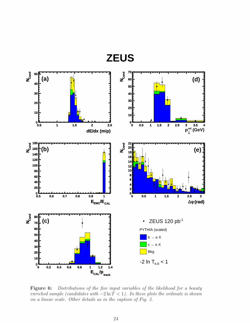
background contribution. In order to select a beauty-enriched sample, a cut of −2 lnT < 1

was applied. The resulting distributions are shown in Fig. 6. A likelihood for semileptonic

charm can also be constructed, Te,c. The distributions of the likelihood for a sample

satisfying −2 lnTe,c < 1.5 are shown in Fig. 7. Good agreement is observed in both cases.

To demonstrate the quality of the data description by the Monte Carlo, the distributions of

EjetT and ηjet of the jet associated with the electron and of the pe

T of the electron candidates

are compared in Fig. 8a)–c). In Fig. 8d)–i) the same distributions are compared for the

beauty- and charm enriched-samples. Some differences are observed in the jet variables,

mainly in the region dominated by background. The agreement significantly improves for

samples enriched in beauty and charm signal.

8 Cross section determination

The cross sections have been measured in the kinematic rangeQ2 < 1 GeV2, 0.2 < y < 0.8,

with at least two jets with EjetT > 7(6) GeV, |ηjet| < 2.5 and an electron from a semileptonic

decay with peT > 0.9 GeV in the range |ηe| < 1.5.

The differential beauty cross section for a variable, v, was determined separately for each

bin, k, from the relative fractions in the data obtained from the fit and the acceptance

correction, Abvk

, calculated using the Monte Carlo,

dσb

dvk

=NDATA · fDATA

e,b (vk)

Abvk· L · ∆vk

,

where NDATA is the number of electron candidates found in the data, L is the integrated

luminosity and ∆vk is the bin width.

In order to determine the acceptance, the jet-finding algorithm was applied to the MC

events after the detector simulation and at hadron level. The acceptance is defined as

A =Nobs

e

Nhade

,

where Nobse is the number of electrons from semileptonic decays reconstructed in the

Monte Carlo satisfying the selection criteria detailed in Sections 5 and 6, and Nhade is the

number of electrons from semileptonic decays produced in the signal process that satisfy

the kinematic requirements using the Monte Carlo information at the generator level.

At hadron level, the kT algorithm was applied to all final-state particles with a lifetime

of τ > 0.01 ns and the electron was associated to its parent jet using the generator

information.

8

All cross sections were measured separately for the two centre-of-mass energies√s = 300

and 318 GeV. Additionally, the cross sections were calculated with the whole data set and

were corrected to√s = 318 GeV. The correction factor of ≈ 2% was determined with LO

as well as NLO calculations.

The charm cross sections were measured using the same procedure.

9 Systematic uncertainties

The systematic uncertainties were calculated by varying the analysis procedure and then

redoing the fit to the likelihood distributions. The following sources were the main con-

tributors to the systematic uncertainty (the first value in parentheses is the uncertainty

for beauty, while the second is that for charm):

• the systematic uncertainty on the description of the dE/dx information was estimated

by looking at the differences between the various calibration and validation samples.

Variations in the mean, width and shape of the distributions were evaluated and used

as a measure of the uncertainty [35]. The resulting uncertainty was found to be (+1−5%

/ +10−3 %);

• the changes in the correction to the prel⊥ distribution in various kinematic ranges were

taken as a measure of its uncertainty. For prel⊥ = 1.5 GeV the variation was 20% of the

correction. The changes led to a systematic uncertainty of (+3−6% / +10

−5 %).

In addition, the correction to the charm distribution was varied from zero to that of

the background sample. This led to an uncertainty of (+6−4% / +7

−1%);

• a shift of the CAL energy scale in the Monte Carlo simulation by ±3% (±2% / ±5%);

• reweighting of the direct and non-direct contributions in the Monte Carlo to provide

a better description of the data (+1% / +3%);

• the estimated residual number of electrons left in the sample from photon conversions

as well as from Dalitz decays were varied by 25% and 20% respectively [50]. This led

to systematic uncertainties of (±1% / ∓4%) due to photon conversions and (±1% /

∓1%) due to Dalitz decays.

These systematic uncertainties were added in quadrature separately for the negative and

the positive variations to determine the overall systematic uncertainty of +8−9% for the

beauty and +17−9 % for the charm cross sections. Since no significant dependence of the

systematic uncertainties on the kinematic variables was observed, the same uncertainty

was applied to each data point. A 2% overall normalisation uncertainty associated with

the luminosity measurement was included.

9

A series of further checks were made. The cut on the transverse momentum of the

electron candidate was varied by ±3%, which is the momentum uncertainty for a track

with pT = 0.9 GeV. The ∆φ correction was varied within its uncertainty. The cut on

∆R to associate the decay electron with a jet was varied between 1.5 and 1.0. The

effect of the gaps between FCAL and BCAL as well as between RCAL and BCAL was

investigated by varying the cut on the EFO position. Various tests of the signal-extraction

method were made: e.g. using the likelihood without the EEMC/ECAL or ECAL/ptrack

variables; applying the fit on a signal-enriched sample by making tighter cuts on the input

variables and varying the fit range. The prior probabilities were recalculated after the

fit and used as the input for a second fit iteration. Separate fits were made for electron

and positron candidates for each of the lepton beam particles (e− and e+) separately

as well as for the combined sample. All variations were found to be consistent with

the expected fluctuations due to statistics; therefore they have not been added to the

systematic uncertainty.

10 Theoretical predictions and uncertainties

QCD predictions at NLO, based on the FMNR programme [51], are compared to the

data. The programme separately generates processes containing point-like and hadron-

like photon contributions, which have to be combined to obtain the total cross section.

The bb and the cc production cross sections were calculated separately. The parton

distribution functions were taken from CTEQ5M [52] for the proton and GRV-G HO

[40] for the photon. The heavy-quark masses (pole masses) were set to mb = 4.75 GeV

and mc = 1.6 GeV. The strong coupling constant, Λ(5)QCD, was set to 0.226 GeV. The

renormalisation, µR, and factorisation, µF , scales were chosen to be equal and set to

µR = µF =√

p2T +m2

b(c), where pT is the average transverse momentum of the heavy

quarks.

The Peterson fragmentation function [53], with ǫb = 0.0035 and ǫc = 0.035 [54], was used

to produce beauty and charm hadrons from the heavy quarks. For the bb and cc cross

sections, the decays into electrons were simulated using decay spectra from Pythia.

For beauty, both the contributions from prompt and from cascade decays, excluding

b → τ → e and b → J/ψ → e+e−, are taken into account in the effective branching

fraction. The values were set to 0.221 for the bb and to 0.096 for the cc cross sections [55].

For the systematic uncertainty on the theoretical prediction, the masses and scales were

varied simultaneously to maximise the change in the cross section using the values:

mb = 4.5, 5.0 GeV, mc = 1.35, 1.85 GeV and µR = µF = 12

√

p2T +m2

b(c), 2√

p2T +m2

b(c).

10

The effects of different parton density functions as well as variations of ǫb within the un-

certainty of 0.0015 had a small effect on the cross-section predictions and were neglected.

The parameter ǫc was varied between 0.02 and 0.07 and the contribution was added in

quadrature to the systematic uncertainty. The uncertainty on the electron decay spectra,

evaluated from comparisons to experimental measurements [56, 57] and to a simple free-

quark decay model, was found to be small compared to the total theoretical uncertainty

and was neglected.

The uncertainty on the NLO QCD predictions for the total cross section are +25% and

−15% for beauty and +45% and −28% for charm.

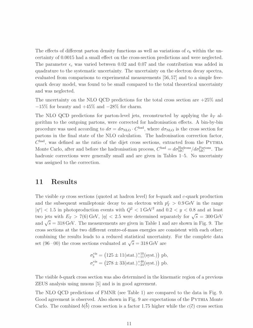
The NLO QCD predictions for parton-level jets, reconstructed by applying the kT al-

gorithm to the outgoing partons, were corrected for hadronisation effects. A bin-by-bin

procedure was used according to dσ = dσNLO · Chad, where dσNLO is the cross section for

partons in the final state of the NLO calculation. The hadronisation correction factor,

Chad, was defined as the ratio of the dijet cross sections, extracted from the Pythia

Monte Carlo, after and before the hadronisation process, Chad = dσHadronsMC /dσPartons

MC . The

hadronic corrections were generally small and are given in Tables 1–5. No uncertainty

was assigned to the correction.

11 Results

The visible ep cross sections (quoted at hadron level) for b-quark and c-quark production

and the subsequent semileptonic decay to an electron with peT > 0.9 GeV in the range

|ηe| < 1.5 in photoproduction events with Q2 < 1 GeV2 and 0.2 < y < 0.8 and at least

two jets with ET > 7(6) GeV, |η| < 2.5 were determined separately for√s = 300 GeV

and√s = 318 GeV. The measurements are given in Table 1 and are shown in Fig. 9. The

cross sections at the two different centre-of-mass energies are consistent with each other;

combining the results leads to a reduced statistical uncertainty. For the complete data

set (96 – 00) the cross sections evaluated at√s = 318 GeV are

σvisb =

(

125 ± 11(stat.)+10−11(syst.)

)

pb,

σvisc =

(

278 ± 33(stat.)+48−24(syst.)

)

pb.

The visible b-quark cross section was also determined in the kinematic region of a previous

ZEUS analysis using muons [5] and is in good agreement.

The NLO QCD predictions of FMNR (see Table 1) are compared to the data in Fig. 9.

Good agreement is observed. Also shown in Fig. 9 are expectations of the Pythia Monte

Carlo. The combined b(b) cross section is a factor 1.75 higher while the c(c) cross section

11

is a factor of 1.28 higher than the Pythia prediction (see Section 7). These factors are

used to scale the Pythia predictions in the following figures.

Differential cross sections as a function of peT and ηe, x

obsγ , Ejet 1

T and ηjet 1 are shown in

Figs. 10, 11 and 12, respectively. The variable xobsγ is defined as

xobsγ =

∑

i=1,2(Ejet i − pjet i

Z )

E − pZ

,

where the sum is over the two highest-energy jets, and corresponds at leading order to the

fraction of the exchanged-photon momentum in the hard scattering process. The figures

also show the NLO QCD and the scaled Pythia predictions. The cross-section values

are given in Tables 2–4. Both the predictions from the NLO QCD calculations as well as

the scaled Pythia cross sections describe the data well.

The differential cross sections as a function of the transverse energy of the jet associated

with the electron from the semileptonic decay, Ee jetT , were also determined. These cross

sections are shown in Fig. 13 and given in Table 5. The good agreement with the NLO

QCD prediction allows the cross section as a function of pbT to be extracted [6]. The

resulting cross section is shown in Fig. 14 and is also compared with previous ZEUS

measurements [3, 5, 6]. The results presented here overlap in pbT with these previous

measurements and have comparable or smaller uncertainties, giving a consistent picture

of b-quark production in ep collisions in the photoproduction regime.

12 Conclusions

Beauty and charm production have been measured in dijet photoproduction using semilep-

tonic decays into electrons. The results were obtained by simultaneously extracting the

b- and c-quark cross sections using a likelihood ratio optimised for b-quark production.

One of the most important variables in the likelihood was the dE/dx measurement in the

central tracking detector.

The results were compared to both NLO QCD calculations as well as predictions from

Monte Carlo models. The NLO QCD predictions are consistent with the data. The Monte

Carlo models describe well the shape of the differential distributions in the data. The

results on b-quark production are also in agreement with a previous less precise ZEUS

measurement using semileptonic decays into electrons. Within the momentum range

covered by previous ZEUS measurements using decays into muons, good agreement is

found.

The cross section as a function of the transverse momentum of the b quarks has been

measured over a wide range. The measurements agree well with the previous values,

12

giving a consistent picture of b-quark production in ep collisions in the photoproduction

regime, and are well reproduced by the NLO QCD calculations.

Acknowledgements

We thank the DESY Directorate for their strong support and encouragement. The re-

markable achievements of the HERA machine group were essential for the successful

completion of this work. The design, construction and installation of the ZEUS detector

have been made possible by the effort of many people who are not listed as authors.

13

References

[1] M. Gluck, E. Reya and A. Vogt, Phys. Rev. D 45, 3986 (1992).

[2] S. Frixione, P. Nason and G. Ridolfi, Nucl. Phys. B 454 (1995);

S. Frixione et al., Phys. Lett. B 348, 633 (1995).

[3] ZEUS Collab., S. Chekanov et al., Eur. Phys. J. C 50, 1434 (2007).

[4] ZEUS Collab., S. Chekanov et al., Phys. Lett. B 599, 173 (2004).

[5] ZEUS Collab., S. Chekanov et al., Phys. Rev. D 70, 12008 (2004). Erratum-ibid

D 74, 59906 (2006).

[6] ZEUS Collab., J. Breitweg et al., Eur. Phys. J. C 18, 625 (2001).

[7] ZEUS Collab., S. Chekanov et al., Phys. Lett. B 649, 111 (2007).

[8] ZEUS Collab., S. Chekanov et al., Preprint DESY-07-52

(arXiv:0704.3562v1 [hep-ex]), 2007. Accepted by JHEP.

[9] ZEUS Collab., S. Chekanov et al., Nucl. Phys. B 729, 492 (2005).

[10] ZEUS Collab., S. Chekanov et al., Eur. Phys. J. C 44, 351 (2005).

[11] ZEUS Collab., S. Chekanov et al., Phys. Rev. D 69, 012004 (2004).

[12] ZEUS Collab., S. Chekanov et al., Phys. Lett. B 565, 87 (2003).

[13] ZEUS Collab., J. Breitweg et al., Eur. Phys. J. C 12, 35 (2000).

[14] ZEUS Collab., J. Breitweg et al., Phys. Lett. B 481, 213 (2000).

[15] ZEUS Collab., J. Breitweg et al., Eur. Phys. J. C 6, 67 (1999).

[16] ZEUS Collab., J. Breitweg et al., Phys. Lett. B 401, 192 (1997).

[17] ZEUS Collab., J. Breitweg et al., Phys. Lett. B 407, 402 (1997).

[18] ZEUS Collab., M. Derrick et al., Phys. Lett. B 349, 225 (1995).

[19] H1 Collab., A. Aktas et al., Eur. Phys. J. C 47, 597 (2006).

[20] H1 Collab., A. Aktas et al., Eur. Phys. J. C 45, 23 (2006).

[21] H1 Collab., A. Aktas et al., Phys. Lett. B 621, 56 (2005).

[22] H1 Collab., A. Aktas et al., Eur. Phys. J. C 40, 349 (2005).

[23] H1 Collab., A. Aktas et al., Eur. Phys. J. C 41, 453 (2005).

[24] H1 Collab., C. Adloff et al., Phys. Lett. B 467, 156 (1999).

[25] H1 Collab., A. Aktas et al., Eur. Phys. J. C 51, 271 (2007).

[26] H1 Collab., A. Aktas et al., Eur. Phys. J. C 50, 251 (2006).

14

[27] H1 Collab., A. Aktas et al., Eur. Phys. J. C 38, 447 (2005).

[28] H1 Collab., C. Adloff et al., Phys. Lett. B 528, 199 (2002).

[29] H1 Collab., C. Adloff et al., Nucl. Phys. B 545, 21 (1999).

[30] H1 Collab., S. Aid et al., Nucl. Phys. B 472, 32 (1996).

[31] ZEUS Collab., U. Holm (ed.), The ZEUS Detector. Status Report (unpublished),

DESY (1993), available on http://www-zeus.desy.de/bluebook/bluebook.html.

[32] N. Harnew et al., Nucl. Instr. and Meth. A 279, 290 (1989);

B. Foster et al., Nucl. Phys. Proc. Suppl. B 32, 181 (1993);

B. Foster et al., Nucl. Instr. and Meth. A 338, 254 (1994).

[33] M. Derrick et al., Nucl. Instr. and Meth. A 309, 77 (1991);

A. Andresen et al., Nucl. Instr. and Meth. A 309, 101 (1991);

A. Caldwell et al., Nucl. Instr. and Meth. A 321, 356 (1992);

A. Bernstein et al., Nucl. Instr. and Meth. A 336, 23 (1993).

[34] J. Andruszkow et al., Preprint DESY-92-066, DESY, 1992;

ZEUS Collab., M. Derrick et al., Z. Phys. C 63, 391 (1994);

J. Andruszkow et al., Acta Phys. Pol. B 32, 2025 (2001).

[35] D. Bartsch, Energy-loss measurement with the ZEUS Central Tracking Detector.

Ph.D. Thesis, Universitat Bonn, Bonn, Germany, Report BONN-IR-2007-05, 2007,

available on http://www-zeus.physik.uni-bonn.de/german/phd.html.

[36] W.W.M. Allison and J.H. Cobb, Annual Review of Nuclear & Particle Science

30, 253 (1980).

[37] T. Sjostrand et al., Comp. Phys. Comm. 135, 238 (2001);

E. Norrbin and T. Sjostrand, Eur. Phys. J. C 17, 137 (2000);

T. Sjostrand, L. Lonnblad, and S. Mrenna, Preprint hep-ph/0108264, 2001.

[38] O.M. Kind, Production of Heavy Flavours with Associated Jets at HERA. Ph.D.

Thesis, Universitat Bonn, Bonn, Germany, Report BONN-IR-2007-04, 2007,

available on http://www-zeus.physik.uni-bonn.de/german/phd.html.

[39] H.L. Lai et al., Phys. Rev. D 55, 1280 (1997).

[40] M. Gluck, E. Reya and A. Vogt, Phys. Rev. D 46, 1973 (1992).

[41] R. Brun et al., geant3, Technical Report CERN-DD/EE/84-1, CERN, 1987.

[42] R. Zimmermann, Kalibrierung und Charakterisierung der dE/dx-Information der

Zentralen Driftkammer bei ZEUS. Diploma Thesis, Universitat Bonn, Bonn,

Germany, Report BONN-IB-2007-10, 2007, available on

http://www-zeus.physik.uni-bonn.de/german/diploma.html.

15

[43] W.H. Smith, K. Tokushuku and L.W. Wiggers, Proc. Computing in High-Energy

Physics (CHEP), Annecy, France, C. Verkerk and W. Wojcik (eds.), p. 222.

CERN, Geneva, Switzerland (1992). Also in preprint DESY 92-150B.

[44] ZEUS Collab., J. Breitweg et al., Eur. Phys. J. C 1, 81 (1998);

G.M. Briskin, Diffractive Dissociation in ep Deep Inelastic Scattering. Ph.D.

Thesis, Tel Aviv University, Report DESY-THESIS 1998-036, 1998.

[45] S.D. Ellis and D.E. Soper, Phys. Rev. D 48, 3160 (1993).

[46] S. Catani et al., Nucl. Phys. B 406, 187 (1993).

[47] F. Jacquet and A. Blondel, Proceedings of the Study for an ep Facility for Europe,

U. Amaldi (ed.), p. 391. Hamburg, Germany (1979). Also in preprint DESY 79/48.

[48] M. Jungst, Elektronidentifikation mit dem ZEUS-Detektor und Bestimmung des

Beauty-Produktionsquerschnitts. Diploma Thesis, Universitat Bonn, Bonn,

Germany, Report BONN-IB-05-15, 2005, available on

http://www-zeus.physik.uni-bonn.de/german/diploma.html.

[49] R. Barlow and C. Beeston, Comp. Phys. Comm. 77, 219 (1993).

[50] W. Verkerke, Measurement of Charm Production Deep Inelastic Scattering. Ph.D.

Thesis, University of Amsterdam, 1998. Unpublished.

[51] S. Frixione et al., Nucl. Phys. B 412, 225 (1994);

S. Frixione et al., Adv. Ser. Direct. High Energy Phys. 15, 609 (1998).

[52] CTEQ Collab., H.L. Lai et al., Eur. Phys. J. C 12, 375 (2000).

[53] C. Peterson et al., Phys. Rev. D 27, 105 (1983).

[54] P. Nason and C. Oleari, Nucl. Phys. B 565, 245 (2000).

[55] Particle Data Group, W.-M. Yao et al., J. Phys G 33, 1 (2006).

[56] BELLE Collaboration, K. Abe et al., Phys. Lett. B 547, 181 (2002);

BABAR Collaboration, B. Auert et al., Phys. Rev. D 67, 031101 (2003).

[57] CLEO Collaboration, N.E. Adam et al., Phys. Rev. Lett. 97, 251801 (2006).

16

σvisb σNLO

b Chadb σvis

c σNLOc Chad

c

(pb) (pb) (pb) (pb)

96—97 101±18+8−9 81+

−2012 0.81 253±58+44

−22 360+−

160100 1.00

98—00 139±16+11−12 88+

−2213 0.81 260±40+45

−23 380+−

170110 1.01

96—00 125±11+10−11 88+

−2213 0.81 278±33+48

−24 380+−

170110 1.01

Table 1: Total cross sections for electrons from b or c quarks in photoproductionevents, Q2 < 1 GeV 2 and 0.2 < y < 0.8, with at least two jets with Ejet

T > 7(6) GeV ,|ηjet| < 2.5 and the subsequent semileptonic decay to an electron with pe

T > 0.9 GeVand |ηe| < 1.5. The values are given separately for

√s = 300 GeV (96—97) and√

s = 318 GeV (98—00) as well as for the complete data set (96—00) extrapolatedto

√s = 318 GeV . The first error is statistical and the second is systematic. In

addition, the NLO QCD prediction and its uncertainty is given, after applying theappropriate hadronisation correction (Chad

b , Chadc ).

peT dσb/dp

eT dσNLO

b /dpeT Chad

b dσc/dpeT dσNLO

c /dpeT Chad

c

( GeV) (pb/ GeV) (pb/ GeV) (pb/ GeV) (pb/ GeV)

0.9 : 2.1 56.3±9.6+4.3−5.0 34+

−117 0.78 117±26+20

−10 177+−

7138 1.02

2.1 : 3.3 24.0±3.7+1.8−2.1 16.8+

−5.93.5 0.79 54.4±9.0+9.5

−4.8 80+−

4223 0.98

3.3 : 4.5 11.9±2.6+0.9−1.1 9.9+

−3.62.3 0.84 26.0±5.8+4.5

−2.3 36+−

2714 0.99

4.5 : 8.0 4.7±1.9+0.4−0.4 3.3+

−1.40.9 0.94 1.5±2.7+0.3

−0.1 7.5+−

9.54.0 0.99

ηe dσb/dηe dσNLO

b /dηe Chadb dσc/dη

e dσNLOc /dηe Chad

c

(pb) (pb) (pb) (pb)

-1.5 : -0.5 26.4±4.6+2.0−2.4 16.7+

−6.63.6 0.75 51±12+9

−4 111+−

6633 0.98

-0.5 : 0.0 53.4±9.1+4.1−4.8 39.5+

−13.88.3 0.81 152±25+26

−13 192+−

10053 1.01

0.0 : 0.5 57.7±11.6+4.4−5.1 41.9+

−13.99.0 0.82 187±36+33

−16 165+−

8243 1.02

0.5 : 1.5 42.4±8.7+3.2−3.8 28.1+

−10.16.3 0.84 36±24+6

−3 90+−

5126 1.02

Table 2: Differential electron cross sections as a function of peT and ηe for the

complete data set. For further details see the caption of Table 1.

xobsγ dσb/dx

obsγ dσNLO

b /dxobsγ Chad

b dσc/dxobsγ dσNLO

c /dxobsγ Chad

c

(pb) (pb) (pb) (pb)

0.00 : 0.45 51±17+4−5 28+

−1810 1.07 70±35+12

−6 122+−

10856 1.16

0.45 : 0.75 166±25+13−15 81+

−5028 2.27 227±49+40

−20 216+−

17885 1.32

0.75 : 1.00 216±31+17−19 166+

−4730 0.55 715±79+124

−63 920+−

370190 0.90

Table 3: Differential cross sections as a function of xobsγ for the complete data

set. For further details see the caption of Table 1.

17

Ejet 1T dσb/E

jet 1T dσNLO

b /Ejet 1T Chad

b dσc/Ejet 1T dσNLO

c /Ejet 1T Chad

c

( GeV) (pb/ GeV) (pb/ GeV) (pb/ GeV) (pb/ GeV)

7 : 10 16.8±2.5+1.3−1.5 10.1+

−3.21.9 0.59 45.9±7.3+8.0

−4.0 72+−

4319 0.99

10 : 13 12.0±1.9+0.9−1.1 9.4+

−3.72.3 0.97 28.0±4.7+4.9

−2.4 35+−

1412 1.07

13 : 16 8.3±1.6+0.6−0.7 5.1+

−2.01.1 1.18 5.9±3.4+1.0

−0.5 11.7+−

7.02.9 1.03

16 : 30 1.00±0.38+0.08−0.09 1.00+

−0.390.08 1.22 1.5±1.1+0.3

−0.1 1.8+−

1.20.5 0.89

ηjet 1 dσb/dηjet 1 dσNLO

b /dηjet 1 Chadb dσc/dη

jet 1 dσNLOc /dηjet 1 Chad

c

(pb) (pb) (pb) (pb)

-1.0 : -0.25 24.9±5.2+1.9−2.2 17.5+

−6.12.7 0.82 73±14+13

−6 99+−

6426 0.95

-0.25 : 0.5 47.6±8.2+3.7−4.2 42.6+

−12.77.7 1.01 177±24+31

−15 164+−

7535 1.05

0.5 : 1.5 49.3±7.8+3.8−4.4 30.4+

−7.96.1 0.91 71±17+12

−6 106+−

4132 1.04

1.5 : 2.5 23.7±5.5+1.8−2.1 9.2+

−3.62.4 0.76 8±15+1

−1 35+−

2312 1.01

Table 4: Differential cross sections for the most energetic jet as a function of Ejet

T

and ηjet for the complete data set. For further details see the caption of Table 1.

Ee jetT dσb/E

e jetT dσNLO

b /Ee jetT Chad

b dσc/Ee jetT dσNLO

c /Ee jetT Chad

c

( GeV) (pb/ GeV) (pb/ GeV) (pb/ GeV) (pb/ GeV)

6 : 10 16.1±1.8+1.2−1.4 12.3+

−5.13.0 0.67 42.2±5.2+7.3

−3.7 64+−

3818 1.00

10 : 15 6.6±1.3+0.5−0.6 5.4+

−1.81.1 1.00 22.3±4.2+3.9

−2.0 19.6+−

7.55.5 1.06

15 : 30 2.1±0.6+0.2−0.2 1.08+

−0.400.26 1.21 0.3±1.9+0.1

−0.1 1.7+−

1.20.5 0.87

Table 5: Differential cross sections of Ee jet

T for the jet associated to the electronfrom beauty or charm decays for the complete data set. For further details see thecaption of Table 1.

18

1.0

1.1

1.2

1.3

1.4

1.5

1.6

1.7

1 10 102

103

104

βγ

<dE

/dx>

(m

ip)

e

πKp

µ

ZEUS

Figure 1: The mean dE/dx measured in the CTD, 〈dE/dx〉, as a function ofβγ for different samples of identified particles as denoted in the figure. The curveshows a physically motivated parametrisation of the 〈dE/dx〉 dependence on βγ.

19

pred) / dE/dx

pred - dE/dx

obs(dE/dx

-1 -0.5 0 0.5 1

Tra

cks

0

200

400

600

800

DATA

= 23 )trunc

( n

ZEUS

pred) / dE/dx

pred - dE/dx

obs(dE/dx

-1 -0.5 0 0.5 1

Tra

cks

1

10

210

310

Figure 2: Distribution of the relative difference between the observed (dE/dxobs)and predicted (dE/dxpred) specific energy loss for the track sample with ntrunc = 23.The inset shows the same distribution with a logarithmic ordinate scale.

20

dE/dx (mip)0.5 1 1.5 2 2.5

Arb

itra

ry U

nit

s

-410

-310

-210

-110

dE/dx (mip)0.5 1 1.5 2 2.5

Arb

itra

ry U

nit

s

-410

-310

-210

-110 (a)

(GeV)relp0 0.5 1 1.5 2 2.5 3 3.5 4

Arb

itra

ry U

nit

s

-310

-210

-110

1

0 0.5 1 1.5 2 2.5 3 3.5 4

Arb

itra

ry U

nit

s

-310

-210

-110

1

(d)

CAL/EEMCE0.5 0.6 0.7 0.8 0.9 1

Arb

itra

ry U

nit

s

-410

-310

-210

-110

1

CAL/EEMCE0.5 0.6 0.7 0.8 0.9 1

Arb

itra

ry U

nit

s

-410

-310

-210

-110

1(b)

(rad)φ∆0 0.5 1 1.5 2 2.5 3

Arb

itra

ry U

nit

s-110

(rad)φ∆0 0.5 1 1.5 2 2.5 3

Arb

itra

ry U

nit

s-110

(e)

track/pCALE

0 0.2 0.4 0.6 0.8 1 1.2 1.4

Arb

itra

ry U

nit

s

-410

-310

-210

-110

1

track/pCALE

0 0.2 0.4 0.6 0.8 1 1.2 1.4

Arb

itra

ry U

nit

s

-410

-310

-210

-110

1

(c)

e X→b e X →c

Bkg

Figure 3: Normalised distributions of the five input variables used in the likelihoodfor the electron candidates extracted from the Monte Carlo, without applying thecuts on dE/dx and EEMC/ECAL. The solid line shows the distribution for electronsfrom semileptonic b-quark decays, the dashed line for c-quark decays and the dottedline the background (Bkg).

21

-2 ln T-110 1 10

Can

dN

10

210

310

410

510

ZEUS

PYTHIA (scaled)

e X→b

e X→c

Bkg

-1ZEUS 120 pb

-2 ln T-110 1 10

Can

dN

10

210

310

410

510

Figure 4: The distribution of the likelihood ratio for electron candidates, Ncand,in data compared to the Monte Carlo expectation after the fit described in the text.The arrow indicates the region included in the fit (−2 lnT < 10). The shaded areasshow the fitted contributions from b quarks, c quarks and background as denoted inthe figure.

22

dE/dx (mip)0.5 1 1.5 2 2.5

Can

dN

1

10

210

310

410

dE/dx (mip)0.5 1 1.5 2 2.5

Can

dN

1

10

210

310

410 (a)

(GeV)relp0 0.5 1 1.5 2 2.5 3 3.5 4

Can

dN

210

310

410

0 0.5 1 1.5 2 2.5 3 3.5 4

Can

dN

210

310

410(d)

CAL/EEMCE0.5 0.6 0.7 0.8 0.9 1

Can

dN

1

10

210

310

410

510

CAL/EEMCE0.5 0.6 0.7 0.8 0.9 1

Can

dN

1

10

210

310

410

510(b)

(rad)φ∆0 0.5 1 1.5 2 2.5 3

Can

dN

210

310

410

(rad)φ∆0 0.5 1 1.5 2 2.5 3

Can

dN

210

310

410 (e)

track/pCALE

0 0.2 0.4 0.6 0.8 1 1.2 1.4

Can

dN

1

10

210

310

410

track/pCALE

0 0.2 0.4 0.6 0.8 1 1.2 1.4

Can

dN

1

10

210

310

410 (c)PYTHIA (scaled)

e X→b

e X →c

Bkg

< 10e,b-2 ln T

-1ZEUS 120 pb

ZEUS

Figure 5: Distributions of the five input variables of the likelihood for the electroncandidates used in the fit (−2 lnT < 10). All cuts have been applied except dE/dx >1.1 in a) and EEMC/ECAL > 0.9 in b) (the cuts are indicated in the figure). Theshaded areas show the contributions from b quarks, c quarks and background asdenoted in the figure, after applying the scale factors from the fit.

23

ZEUS

dE/dx (mip)0.5 1 1.5 2 2.5

Can

dN

0

10

20

30

40

50

dE/dx (mip)0.5 1 1.5 2 2.5

Can

dN

0

10

20

30

40

50

(a)

(GeV)relp0 0.5 1 1.5 2 2.5 3 3.5 4

Can

dN

0

10

20

30

40

50

60

70

0 0.5 1 1.5 2 2.5 3 3.5 4C

and

N0

10

20

30

40

50

60

70

(d)

CAL/EEMCE0.5 0.6 0.7 0.8 0.9 1

Can

dN

0

20

40

60

80

100

120

140

160

180

CAL/EEMCE0.5 0.6 0.7 0.8 0.9 1

Can

dN

0

20

40

60

80

100

120

140

160

180

(b)

(rad)φ∆0 0.5 1 1.5 2 2.5 3

Can

dN

024

68

1012

14

1618

2022

(rad)φ∆0 0.5 1 1.5 2 2.5 3

Can

dN

024

68

1012

14

1618

2022

(e)

track/pCALE

0 0.2 0.4 0.6 0.8 1 1.2 1.4

Can

dN

0

10

20

30

40

50

60

70

80

track/pCALE

0 0.2 0.4 0.6 0.8 1 1.2 1.4

Can

dN

0

10

20

30

40

50

60

70

80

(c)PYTHIA (scaled)

e X→b

e X →c

Bkg

< 1e,b-2 ln T

-1ZEUS 120 pb

Figure 6: Distributions of the five input variables of the likelihood for a beautyenriched sample (candidates with −2 lnT < 1). In these plots the ordinate is shownon a linear scale. Other details as in the caption of Fig. 5.

24

ZEUS

dE/dx (mip)0.5 1 1.5 2 2.5

Can

dN

0

50

100

150

200

250

300

350

dE/dx (mip)0.5 1 1.5 2 2.5

Can

dN

0

50

100

150

200

250

300

350

(a)

(GeV)relp0 0.5 1 1.5 2 2.5 3 3.5 4

Can

dN

0

100

200

300

400

500

600

700

800

0 0.5 1 1.5 2 2.5 3 3.5 4

Can

dN

0

100

200

300

400

500

600

700

800

(d)

CAL/EEMCE0.5 0.6 0.7 0.8 0.9 1

Can

dN

0

200

400

600

800

1000

1200

CAL/EEMCE0.5 0.6 0.7 0.8 0.9 1

Can

dN

0

200

400

600

800

1000

1200

(b)

(rad)φ∆0 0.5 1 1.5 2 2.5 3

Can

dN

0

50

100

150

200

250

(rad)φ∆0 0.5 1 1.5 2 2.5 3

Can

dN

0

50

100

150

200

250(e)

track/pCALE

0 0.2 0.4 0.6 0.8 1 1.2 1.4

Can

dN

0

50

100

150

200

250

300

350

track/pCALE

0 0.2 0.4 0.6 0.8 1 1.2 1.4

Can

dN

0

50

100

150

200

250

300

350

(c)PYTHIA (scaled)

e X→b

e X →c

Bkg

< 1.5e,c-2 ln T

-1ZEUS 120 pb

Figure 7: Distributions of the five input variables of the likelihood for a charmenriched sample (candidates with −2 lnTe,c < 1.5). In these plots the ordinate isshown on a linear scale. Other details as in the caption of Fig. 5.

25

ZEUS

(GeV)e jetTE

10 15 20 25 30

/ G

eVC

and

N

1

10

210

310

410

10 15 20 25 30

/ G

eVC

and

N

1

10

210

310

410 (a)

(GeV)e jetTE

10 15 20 25 30

/ G

eVC

and

N

0

5

10

15

20

25

10 15 20 25 30

/ G

eVC

and

N

0

5

10

15

20

25(d)

(GeV)e jetTE

10 15 20 25 30

/ G

eVC

and

N

0

50

100

150

200

250

300

10 15 20 25 30

/ G

eVC

and

N

0

50

100

150

200

250

300(g)

e jetη-2 -1.5 -1 -0.5 0 0.5 1 1.5 2

Can

dN

10

210

310

e jetη-2 -1.5 -1 -0.5 0 0.5 1 1.5 2

Can

dN

10

210

310

(b)

e jetη-2 -1.5 -1 -0.5 0 0.5 1 1.5 2

Can

dN

02

4

68

1012

14

16182022

e jetη-2 -1.5 -1 -0.5 0 0.5 1 1.5 2

Can

dN

02

4

68

1012

14

16182022

(e)

e jetη-2 -1.5 -1 -0.5 0 0.5 1 1.5 2

Can

dN

0

20

40

60

80

100

e jetη-2 -1.5 -1 -0.5 0 0.5 1 1.5 2

Can

dN

0

20

40

60

80

100 (h)

(GeV)eT

p2 4 6 8 10

/ G

eVC

and

N

1

10

210

310

410

(GeV)eT

p2 4 6 8 10

/ G

eVC

and

N

1

10

210

310

410(c)

(GeV)eT

p2 4 6 8 10

/ G

eVC

and

N

0

5

10

15

20

25

30

35

40

(GeV)eT

p2 4 6 8 10

/ G

eVC

and

N

0

5

10

15

20

25

30

35

40

(f)

(GeV)eT

p2 4 6 8 10

/ G

eVC

and

N

0

50

100

150

200

250

PYTHIA (scaled)

e X→b

e X →c

Bkg

-1ZEUS 120 pb

(GeV)eT

p2 4 6 8 10

/ G

eVC

and

N

0

50

100

150

200

250 (i)

< 10e,b-2 ln T < 1e,b-2 ln T < 1.5e,c-2 ln T

Figure 8: Distributions of Ee jet

T and ηe jet

T of the jet associated with the electron,and pe

T of the electron candidate. Figures a)-c) contain all electron candidatessatisfying −2 lnTe,b < 10; d)-f) and g)-i) show the same distributions for the beauty(−2 lnTe,b < 1) and charm (−2 lnTe,c < 1.5) enriched samples, respectively. Otherdetails as in the caption of Fig. 5.

26

(GeV)s

300 310 320

(p

b)

vis

σ

210

310

300 310 320

210

310

ZEUS

−1ZEUS 120 pb e X→b e X→c

NLO QCDPYTHIA

Figure 9: Total cross sections for electrons from b and c quarks in photoproductionevents, Q2 < 1 GeV 2 and 0.2 < y < 0.8, with at least two jets with ET > 7(6) GeV ,|η| < 2.5 and the subsequent semileptonic decay to an electron with pT > 0.9 GeVand |η| < 1.5. The measurements are shown as points. The inner error bar showsthe statistical uncertainty and the outer error bar shows the statistical and sys-tematic uncertainties added in quadrature. The solid line shows the NLO QCDprediction after hadronisation corrections, with the theoretical uncertainties indi-cated by the band; the dashed line shows the prediction from Pythia.

27

ZEUS

(GeV)eT

p1 2 3 4 5 6 7 8

(p

b/G

eV)

e T/d

pbσd 10

210

(GeV)eT

p1 2 3 4 5 6 7 8

(p

b/G

eV)

e T/d

pbσd 10

210(a)

eη-1.5 -1 -0.5 0 0.5 1 1.5

(p

b)

e η/d bσd

0

20

40

60

80

100

120 -1ZEUS 120 pb e X →b

NLO QCD

PYTHIA x 1.75

eη-1.5 -1 -0.5 0 0.5 1 1.5

(p

b)

e η/d bσd

0

20

40

60

80

100

120 (b)

(GeV)eT

p1 2 3 4 5 6 7 8

(p

b/G

eV)

e T/d

pcσd

1

10

210

(GeV)eT

p1 2 3 4 5 6 7 8

(p

b/G

eV)

e T/d

pcσd

1

10

210

(c)

eη-1.5 -1 -0.5 0 0.5 1 1.5

(p

b)

e η/d cσd

0

100

200

300

400

500 -1ZEUS 120 pb

e X →c

NLO QCDPYTHIA x 1.28

eη-1.5 -1 -0.5 0 0.5 1 1.5

(p

b)

e η/d cσd

0

100

200

300

400

500 (d)

Figure 10: Differential cross sections as a function of a), c) the transversemomentum and b), d) the pseudorapidity of the electrons. Plots a) and b) are for b-quark production while c) and d) are for c-quark production. The measurements areshown as points. The inner error bar shows the statistical uncertainty and the outererror bar shows the statistical and systematic uncertainties added in quadrature.The solid line shows the NLO QCD prediction after hadronisation corrections, withthe theoretical uncertainties indicated by the band; the dashed line shows the scaledprediction from Pythia.

28

ZEUS

obsγx

0 0.2 0.4 0.6 0.8 1

(p

b)

ob

sγ

/dx

bσd 210

310

obsγx

0 0.2 0.4 0.6 0.8 1

(p

b)

ob

sγ

/dx

bσd 210

310 -1ZEUS 120 pb

e X →b NLO QCDPYTHIA x 1.75

(a)

obsγx

0 0.2 0.4 0.6 0.8 1

(p

b)

ob

sγ

/dx

cσd

210

310

obsγx

0 0.2 0.4 0.6 0.8 1

(p

b)

ob

sγ

/dx

cσd

210

310

-1ZEUS 120 pb e X →c

NLO QCDPYTHIA x 1.28

(b)

Figure 11: Differential cross sections as a function of xobsγ . a) shows the dis-

tribution for electrons from b-quark production while b) shows c-quark production.Other details as in the caption of Fig. 10.

29

ZEUS

(GeV)jet 1TE

10 15 20 25 30

(p

b/G

eV)

jet

1

T/d

Ebσd

1

10

(GeV)jet 1TE

10 15 20 25 30

(p

b/G

eV)

jet

1

T/d

Ebσd

1

10

(a)

jet 1η-1 0 1 2

(p

b)

jet

1η

/d bσd

0

50

100 -1ZEUS 120 pb

e X →b

NLO QCD

PYTHIA x 1.75

jet 1η-1 0 1 2

(p

b)

jet

1η

/d bσd

0

50

100(b)

(GeV)jet 1TE

10 15 20 25 30

(p

b/G

eV)

jet

1

T/d

Ecσd

1

10

210

(GeV)jet 1TE

10 15 20 25 30

(p

b/G

eV)

jet

1

T/d

Ecσd

1

10

210(c)

jet 1η-1 0 1 2

(p

b)

jet

1η

/d cσd

0

100

200

300

400 -1ZEUS 120 pb

e X →c NLO QCD

PYTHIA x 1.28

jet 1η-1 0 1 2

(p

b)

jet

1η

/d cσd

0

100

200

300

400

(d)

Figure 12: Differential cross sections as a function of a), c) the transverseenergy and b), d) the pseudorapidity of the highest-energy jet. Plots a) & b) showthe distributions for electrons from b-quark production while plots c) & d) showthose for c-quark production. Other details as in the caption of Fig. 10.

30

ZEUS

(GeV)e jetTE

10 15 20 25 30

(p

b/G

eV)

jet

1

T/d

Ebσd

1

10

-1ZEUS 120 pb e X →b

NLO QCDPYTHIA x 1.75

(a)

(GeV)e jetTE

10 15 20 25 30

(p

b/G

eV)

e je

t

T/d

Ecσd

-110

1

10

210 -1ZEUS 120 pb

e X →c NLO QCD

PYTHIA x 1.28

(b)

Figure 13: Differential cross sections for a) b-quark and b) c-quark productionas a function of the transverse energy of the jet associated to the electron. Otherdetails as in the caption of Fig. 10.

31

(GeV)bT

p0 5 10 15 20 25

(p

b/G

eV)

b T/d

pσd

1

10

210

e→ b -1ZEUS 120 pb

µ D* → b ZEUS 96-00

µ → b ZEUS 96-00

e→ b ZEUS 96-97

NLO QCD

| < 2b

η|

ebX)→ (ep b

T/dpσd

2 < 1 GeV2Q0.2 < y < 0.8

ZEUS

Figure 14: Differential cross section for b-quark production as a function oftransverse momentum, pb

T , compared to the results of previous ZEUS measurementsas indicated in the figure. The measurements are shown as points. The inner errorbar shows the statistical uncertainty and the outer error bar shows the statisticaland systematic uncertainties added in quadrature. The solid line shows the NLOQCD prediction from the FMNR program with the theoretical uncertainty shown asthe shaded band.

32