REGULAR ARTICLE

A localized electrons detector for atomic and molecular systems

Hugo J. Bohorquez • Russell J. Boyd

Received: 19 November 2009 / Accepted: 14 January 2010 / Published online: 9 February 2010

� Springer-Verlag 2010

Abstract The local value of the single-particle momen-

tum provides a direct three-dimensional representation of

bonding interactions in molecules. It is given exclusively in

terms of the electron density and its gradient, and therefore

is an ideal localized electrons detector (LED). The results

introduced here extend to molecular systems our study of

the single-particle local momentum in atomic systems

(Bohorquez and Boyd in J Chem Phys 129:024110, 2008;

Chem Phys Lett 480:127, 2009). LED is able to clearly

identify covalent and hydrogen bonding interactions by

depicting distinctive regions around the bond critical

points, emerging as a complementary tool in conventional

atoms in molecules studies. The local variable we introduce

here is an intuitively interpretable 3D electron-pairs locator

in atoms and molecules that can be computed either from

theoretical or experimentally derived electron densities.

Keywords Electron pairs � Electron localization �Chemical bond � Quantum topology � Electron momentum �Electron kinetic energy � Local quantum value �Theoretical methods

1 Introduction

‘‘Sometimes it seems to me that a bond between two

atoms has become so real, so tangible, so friendly,

that I can almost see it. Then I awake with a little

shock, for a chemical bond is not a real thing. It does

not exist. No one has ever seen one. No one ever can.

It is a figment of our own imagination.’’ Charles A.

Coulson

Electronic bonding interactions are not directly obser-

vable, as Coulson asserts, but our intuitive perception of

molecular phenomena in the three-dimensional space

demands such a representation. With a similar perspective

Lewis conceived the idea of electron pairs [1]. It is reason-

able to think that an adequate representation of chemical

bonding should be given by a physical observable defined in

coordinate space. The electron density is the best choice

because it is a local function defined within the exact many-

body theory, and it is also an experimentally accessible scalar

field. Its paramount role in the description of many-body

problems is supported by the Hohenberg–Kohn theorem [2].

Although the Hohenberg–Kohn theorem guarantees that

all the molecular information is encoded in the electron

density, the physical description of chemical systems

requires additional postulates for extracting observable

information in terms of atomic contributions. This is

achieved by the quantum theory of atoms in molecules

(QTAIM) introduced by Bader [3]. The proper open system

concept provides a quantum topological partitioning of the

molecular space into chemically transferable molecular

fragments for which the energy and all other measurable

properties can be precisely defined [4].

The localization of electron pairs is elusive within the

electron density topology analysis, because a direct link

between the local maxima in the electron density and the

electron pairs of the Lewis model has not been established,

despite the fact that the Laplacian of the electron density

provides some information about electron localization [5].

Several attempts to depict electron localization from different

perspectives have been proposed in recent years. The variety

H. J. Bohorquez (&) � R. J. Boyd

Department of Chemistry, Dalhousie University,

Halifax, NS B3H 4J3, Canada

e-mail: hugo.j.bohorquez@dal.ca

123

Theor Chem Acc (2010) 127:393–400

DOI 10.1007/s00214-010-0727-5

of proposals for assessing that single task leads to the logical

question of why the conventional analysis seems to be

insufficient to fully explain electron localization in molecules.

We identify two main causes: one is interpretation, and

the other is of a practical nature. The conventional analyses

consist mainly of the study of the Laplacian of the electron

density [6], and the electron localization function (ELF) [7].

Both approaches entail conceptual and practical limitations.

The Laplacian provides information about local concen-

tration or depletion of electron density, but its values are not

bounded, and it fails to correctly produce atomic shells for

atoms beyond the third row [8]. A direct link between ELF

and QTAIM is still missing, whereas an homeomorphic

relationship1 with the Laplacian has been suggested [5].

The electron localization function, by construction,

provides values within the [0, 1] range, and its topological

analysis by Silvi and Savin [9] made ELF a preferred tool

for the study of electronic bonding interactions. In spite of

its formally sound derivation from the electronic pair

probability, ELF interpretation is not straightforward and

the respective plots are far from intuitively evident, a fea-

ture to be expected of an ideal representation of chemical

bonding interactions. Additionally, ELF fails to provide

insight for non-covalent bonding interactions, limiting even

more its application for the study of unconventional bond-

ing situations and weak intermolecular interactions.

In the present paper, we introduce a variable that has the

ability to detect electron pairs inside an electron density

distribution, and overcomes the limitations of the other

analyses. Our localized electrons detector (LED) depends

exclusively on the electron density and its gradient. Here

we show how this variable consistently fits within the

conventional atoms in molecules analysis, by providing

complementary information about the physics of bonding

interactions and their local symmetries. The present work

extends to molecular systems our previous investigation of

this local variable in atomic systems. We have shown that

LED correctly provides atomic shell structures [10], and an

atomic radius scale that can be experimentally derived

[11], among other interesting results. Herein we illustrate

its application to molecular systems.

In the following section, we examine the variables

involved in ELF in order to show that its key ingredient is the

single-particle kinetic energy density, which is connected to

our LED by a quantum theorem (see Sect. III A in Ref. [10]).

Several important features of this variable, including its

bounded character, and its direct connection to QTAIM are

discussed in the second part of Sect. 2. In Sect. 3, we show the

results of the proposed analysis with several examples,

showing how LED identifies the presence of electron shells,

and the different bonding interactions adequately. This

graphical representation of bonding regions in coordinate

space provides distinctive graphical representations for

covalent and hydrogen bonding interactions as well.

In summary, LED provides an orbital-free and intui-

tively interpretable three-dimensional electron-pair locali-

zation scalar function that is easy to compute from either

theoretically computed or experimentally derived electron

densities.

2 Theoretical considerations

In this section, we show that the single-particle kinetic

energy local momentum eP is linked to one of ELF’s key

components, as an alternative to its derivation introduced

in Ref. [10] from the local quantum theory [12].

The ELF was introduced by Becke and Edgecombe [7]

as a ‘‘simple measure of electron localization in atomic and

molecular systems’’. Two terms of a Taylor series expan-

sion of the spherically averaged conditional same-spin pair

probability density provide the main ELF equation, i.e. the

kinetic energy density variable

DðrÞ ¼ sðrÞ � j rð Þ ð1Þ

where the first term is the orbital or positive-definite kinetic

energy density

sðrÞ ¼ �h2

2me

X

i

rwiðrÞj j2 ð2Þ

and the second term is the single particle or von

Weizsacker kinetic energy density

jðrÞ ¼ �h2

8me

rqðrÞ � rqðrÞqðrÞ ð3Þ

D in Eq. 1 is proportional to the Fermi hole mobility

function of Luken and Culberson [13] and is related to the

curvature of the Fermi hole as shown by Dobson [14].

Becke and Edgecombe identify the localization of an

electron with the probability density to find an electron in

the vicinity of a second same-spin reference electron. The

smaller the probability density D, the higher the

localization of the electrons. In order to get values in

the range from 0 to 1, ELF is defined as the Lorentzian

mapping ðLÞ of the core variable v, i.e.

gðrÞ¼: L vðrÞð Þ ¼ 1

½1þ v2ðrÞ� ð4Þ

with vðrÞ ¼ DðrÞ=DhðrÞ, where

DhðrÞ ¼3�h2

5með6p2Þ2=3qðrÞ5=3 ð5Þ

is the kinetic energy density of the free electron gas asso-

ciated with the electron density q.

1 Two functions are said to be homeomorphic if one can be

continuously transformed into the other.

394 Theor Chem Acc (2010) 127:393–400

123

Becke and Edgecombe interpreted the ratio v as a con-

venient dimensionless localization index calibrated with

respect to the uniform electron gas.2 In this sense, ELF is a

local measure of the effect of the Pauli exclusion principle

as reflected by the kinetic energy density: in the regions of

space where this effect is smaller than the kinetic energy

density of a uniform electron gas of identical density, ELF

is close to 1, whereas where the local parallel spin pairing

is higher, ELF is low.

But the only measure of the electron localization present

in ELF is the expression D, as was recently pointed out by

Gatti [15]. However, he adds, ELF cannot yield the value

of D because its dependence on the electron density via the

free electron gas term Dh. In this sense, ELF is a relative

measure of the electron localization. It is, in fact, a relative

measure of the bosonic character of the electron density,

because D is the excess kinetic energy electrons have

compared to a system of bosons of the same density. This

interpretation of ELF was introduced by Silvi and Savin

[16], who also introduced a generalized kinetic density

version of ELF and its topological analysis [9].

In order to illustrate these observations, the variables

involved in ELF are plotted in Fig. 1 for the bonding ðr 2½rBCP;RF �Þ and non-bonding regions ðr [ RFÞ of fluorine

molecule, where rBCP ¼ 0 is the position of the bond

critical point (BCP), and the fluorine nucleus is located at

RF ¼ 1:35 a.u. In Fig. 1 these two points are indicated at

the top. Figure 1a shows the local values3 of the variables

involved in D; s=q (in blue) and j/q (in purple). Figure 1b

shows the Lorentzian mapping of the local variable4

D=q;LðD=qÞ (in green), and the ELF, g (in red).

The two electron shells of fluorine are clearly visible

with j/q and D=q, while ELF is unable to depict them.

Even LðD=qÞ shows more clearly than g the location of

core electrons from the valence electrons, in accordance

with Gatti’s observation. The local value of the single

particle kinetic energy, j/q, provides additional chemical

information not given by the other variables: the location of

the BCP at j/q = 0, which is relevant for the study of

topological properties in molecules; and the polarization

of non-bonding regions, which is relevant for intermolec-

ular interactions studies.

Electron pairs are stable groups of electrons that unlike

free electrons, have integer spin and therefore behave as

composite bosons. Atomic shells and covalent bonding

interactions fit within that description. Recently, the

bosonic character of electron pairs was experimentally

confirmed [17]. A localized pair behaves as a single par-

ticle, and therefore its kinetic energy is given by the von

Weizsacker kinetic energy, j. Therefore, its local value

(j/q) detects those regions of space where the molecule

exhibits a marked single-particle character, providing in

this way a direct measure of electron pairing. Conse-

quently, this function is able to identify electron shells and

covalent bonding interactions. Hence we propose the study

of the bosonic character of atomic and molecular electron

densities as a direct measure of their localized pairs.

A closer examination of j/q depicted in Fig. 1 for di-

fluorine reveals the existence of four different regions that

can be identified going from the BCP to a long distance

from the nucleus (*10 a.u.), along the molecular axis:

• The interatomic bonding region, characterized by a

continuous approach of j/q?0 as r! rbcp, and s � j.

A local maximum value in j/q is located between the

BCP and the core region.

• The core electron region is characterized by a contin-

uous approach of j/q to its absolute maximum, j/

q ? Z2/2 (in a.u.) as r! RAðr 6¼ RAÞ.5• A non-bonding region, characterized by a local max-

imum in j/q for which the outer zone of the valence

shell is polarized and where s&j.

• A molecular boundary region that is characterized by

the asymptotic limit j ? s, i.e. j/q has a limiting value

that depends on the molecular ionization energy.6

These four distinct regions can be identified in any pair

of atoms connected by a gradient path within a molecule.

Here we are interested in the first three mainly, because its

direct relation with the presence of bonding interactions.

Hence, the limiting values of eP define three different

spatial regions chemically relevant for the study of any

molecular system: covalent ð eP ’ 0Þ, located around a

BCP, core ð eP. ZApoÞ, located around the nuclear attrac-

tors, and valence regions ðffiffiffiffiffiffiffiffiffiffiffiffi

2meIZ

p. eP � ZpoÞ;7 which

includes polarized regions and valence shell electrons

around the nucleus with atomic number Z.2 This is an arbitrarily chosen reference variable, found also in the

Fermi hole mobility function by Luken and Culberson [13], but

instead of a division they made a subtraction, also arbitrarily choosing

the uniform electron gas as a reference. While this choice seems

physically sound, valence electrons behave as a non-interacting

electron gas in crystals mainly and therefore its inclusion in other

molecular systems is not entirely justified.3 These are bounded variables unlike their respective kinetic

densities, s and j, and have units of energy per particle, not energy

per volume. For more details on the local values in quantum

chemistry, see Ref. [10] and references therein.4 It means, replacing D=q instead of v in Eq. 4.

5 Notice that at the nucleus there is a critical point of the electron

density and hence j RAð Þ ¼ 0, but the neighbor points obey the limit.6 Gaussian functions exhibit difficulties for reproducing the expo-

nential decay, and therefore this limiting behavior is very sensitive to

basis set selection [18].7 Hydrogen is the only atom for which this relationship does not

apply becauseffiffiffiffiffiffiffiffiffiffiffiffi

2meIZ

p¼ 1:4142 a.u., which may be a consequence of

its lack of a inner closed shell.

Theor Chem Acc (2010) 127:393–400 395

123

Although we make reference to the kinetic energy s, no

explicit knowledge of this property is necessary for the

bonding analysis provided by the single particle local value

j/q, as we show in the next section.

2.1 The single particle kinetic energy density

and QTAIM

In our study of the single particle operators in atomic

systems [10], we have shown that the expectation value of

the single particle kinetic energy density, hji, is equivalent

to the variance of the momentum operator, P ¼ �i�hr,

minus its classical estimate P, i.e.

j rð Þ ¼ 1

2meVarw P� P

� �

ð6Þ

where eP � P� P is the fluctuation of the electronic

momentum, whose single-particle expression applied to

the electron density gives [10, 12, 19]

ePðrÞ ¼ � �h

2

rqðrÞqðrÞ ð7Þ

which leads to

jðrÞh i ¼Z

ePðrÞ � ePðrÞ2me

qðrÞdr ð8Þ

This equation implies that j/q can be expressed in terms of

the local momentum component eP by j=q ¼ eP � eP=2me.

This means that eP provides at least the same information as

j/q. Additional information arises from the fact that eP is a

vector variable.

The vector field (Eq. 7) eP points in the direction of

maximum decrease in the electron density, and its magni-

tude eP is sensitive to local charge depletion. We have

found that atomic shells are limited by the radial distances

from the nucleus where a change in the concavity of eP

occurs, i.e. distances for which the condition o2eP=or2 ¼ 0

is satisfied [10]. The electronic-shell populations are in

excellent agreement with those obtained with ELF [20] and

s [21, 22], confirming the robustness of eP for depicting

electron pairs in atoms.

For graphical analysis purposes, it is also convenient

that eP is totally bounded by physically meaningful values.

The lowest limit occurs at those points where the critical

points of the electron density are located, i.e. for all those

points that obey eP ¼ 0. Kato’s cusp condition imposes a

limit to electron velocities near the nucleus of an atom A

[23], RA, making eP finite and numerically equal to the

atomic number ZA, when atomic units are used.8

limr!RA

eP rð Þ ¼ p0ZA ð9Þ

This velocity is used in the estimation of relativistic

corrections for atomic systems [24]. Valence electron

speeds in atoms are limited by the ionization energy IA [10]

limrj j!1

eP rð Þ ¼ffiffiffiffiffiffiffiffiffiffiffiffi

2meIA

p

ð10Þ

This equation determines a natural boundary for an atom

that leads to an experimentally based atomic radii scale

[11]. Given the general validity of the exponential decay, it

is expected that molecular regions depicted by eP rð Þ are

similarly bounded.eP exhibits some additional practical advantages for

topological analysis. In particular, it has a direct connection

with the local variables studied in QTAIM, as we antici-

pated in Ref. [10]. This vector field runs anti-parallel to the

Fig. 1 Variables involved in

ELF for the ground state of F2.

Top local values s/q and j/q in

coordinate space. Bottom ELF gand the Lorentzian map of the

local value D=q;LðD=qÞ in

coordinate space. The BCP is

located at the left side of the

graphic, and the figure is

centered at the fluorine atom

8 p0 ¼ �h=a0 is the atomic unit of momentum.

396 Theor Chem Acc (2010) 127:393–400

123

gradient of the electron density rq, hence depicting the

same electron density gradient paths, but with opposite

direction, i.e. they have opposite direction tangent vectors

at every given point of the 3D space: rq=jrqj ¼ �eP=jePj.The gradient paths of the electron density connect the

nuclei with BCPs, giving rise to an operative definition of

molecular structure [25].

The electron density gradient fieldrq can be interpreted

as the fluctuation of the current density vector fieldeJ ¼ 1

me

ePq, or equivalently

eJðrÞ ¼ � �h

2merqðrÞ ð11Þ

The local flux of the current density fluctuation eJðrÞ is

given by the divergence operator,

r � eJðrÞ ¼ � �h

2mer2qðrÞ ¼ 2

�hLðrÞ ð12Þ

This equation indicates that the Laplacian of the electron

density, L, effectively identifies local concentrations or

depletion of electron density, just as QTAIM prescribes

[3, 26].

There are two forces governing chemical structures, the

Feynman force exerted on the nuclei and the Ehrenfest

force exerted on the electrons. The virial theorem relates

the virial of the Ehrenfest force to the kinetic energy of the

electrons, the virial including a contribution from the virial

of the Feynman forces acting on the nuclei. The local virial

theorem is given in terms of the Laplacian of the electron

density by Bader [3]

LðrÞ ¼ �2GðrÞ � VðrÞ ð13Þ

or equivalently in terms of the current fluctuation (Eq. 11),

�h

2r � eJðrÞ ¼ �2GðrÞ � VðrÞ ð14Þ

where GðrÞ is the positively defined kinetic energy density,

and VðrÞ is the virial density.

The integral form of the virial, �2G ¼ V, requires that

the net flux of the current density vanish, which is granted

by the divergence theorem applied to the current densityZ

r � eJðrÞdr ¼I

eJðrÞ � nds ¼ 0 ð15Þ

In order to make this condition valid for any given

atomic basin region, X, the local flux of the current densityeJ over the surface of this region ðoXÞ must vanish, which

leads to the local zero-flux condition at the interatomic

surface9

eJ roXð Þ � n roXð Þ ¼ 0 ð16Þ

that finally gives, after using Eq. 11,

rq roXð Þ � n roXð Þ ¼ 0 ð17Þ

which defines those points roX located on the basin surface

oX. The molecular space can be exhaustively partitioned

into the atomic basins defined by Eq. 17, as stated by

QTAIM.

Equations 11–17 show that eP is consistent with QTAIM

definitions of structure in terms of bond paths and that of

proper open system. Additionally, and this is the main

claim made here, eP also reveals the single-particle char-

acter of localized electrons within the electron density by

depicting the atomic shell structures and the symmetry of

bonding interactions, as illustrated in the following section.

3 Localized electrons in molecules

The study of eP can be made for ground and excited states

equally, as no particular assumptions about the state of the

molecule are required for its derivation [10]. This is a

practical advantage of the study of our LED over DFT-

inspired localization functions, which are valid only for

ground states, as imposed by the Hohenberg–Kohn

theorem.

In order to get numerical results for molecular systems,

we used wavefunctions extracted from Gaussian 09 pro-

gram (G09) [28] and a modified Fortran code to compute

LED. A script that computes LED from cube files gene-

rated with the Cubegen routine in G03 is available. All the

examples discussed in the present paper where computed at

MP2/pVDZ level of theory, unless otherwise stated.

Figure 2 shows the LED graphics for the ground and

first excited states of the diatomic hydrogen molecule.10

The isocontour eP ¼ 0:98 a.u. for the bonding state of H2

defines a valence region that encloses both nuclei. In the

middle, in red, is located the BCP, inside a covalent region

(orange) given by eP. 0:3 a.u. The symmetry of this region

indicates that this is a shared bonding interaction, that is

characterized topologically by a negative Laplacian

(r2qbcp = - 0.7563, qbcp = 0.248 a.u).

On the other hand, the same valence region for the

ungerade state reveals three disconnected surfaces: the two

spherical cores centered at the nuclei, and a flat-shaped

surface enclosing the BCP. This covalent region (orange)

has the shape of a disc located perpendicularly to the

gradient path, which is characteristic of a closed-shell

interaction. Topologically, it corresponds to a positive

9 A similar derivation is discussed by Delle Site in Ref. [27].

10 Molecular graphics images were produced using the UCSF

Chimera package from the Resource for Biocomputing, Visualization,

and Informatics at the University of California, San Francisco

(supported by NIH P41 RR-01081) [29]. QTAIM computations were

done using AIMAll (Version 09.11.08), by Todd A. Keith, 2009

(http://aim.tkgristmill.com).

Theor Chem Acc (2010) 127:393–400 397

123

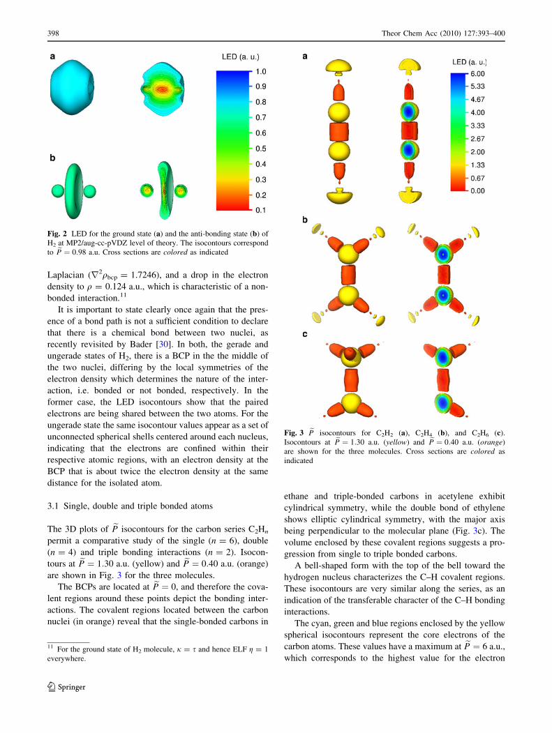
Laplacian (r2qbcp = 1.7246), and a drop in the electron

density to q = 0.124 a.u., which is characteristic of a non-

bonded interaction.11

It is important to state clearly once again that the pres-

ence of a bond path is not a sufficient condition to declare

that there is a chemical bond between two nuclei, as

recently revisited by Bader [30]. In both, the gerade and

ungerade states of H2, there is a BCP in the the middle of

the two nuclei, differing by the local symmetries of the

electron density which determines the nature of the inter-

action, i.e. bonded or not bonded, respectively. In the

former case, the LED isocontours show that the paired

electrons are being shared between the two atoms. For the

ungerade state the same isocontour values appear as a set of

unconnected spherical shells centered around each nucleus,

indicating that the electrons are confined within their

respective atomic regions, with an electron density at the

BCP that is about twice the electron density at the same

distance for the isolated atom.

3.1 Single, double and triple bonded atoms

The 3D plots of eP isocontours for the carbon series C2Hn

permit a comparative study of the single (n = 6), double

(n = 4) and triple bonding interactions (n = 2). Isocon-

tours at eP ¼ 1:30 a.u. (yellow) and eP ¼ 0:40 a.u. (orange)

are shown in Fig. 3 for the three molecules.

The BCPs are located at eP ¼ 0, and therefore the cova-

lent regions around these points depict the bonding inter-

actions. The covalent regions located between the carbon

nuclei (in orange) reveal that the single-bonded carbons in

ethane and triple-bonded carbons in acetylene exhibit

cylindrical symmetry, while the double bond of ethylene

shows elliptic cylindrical symmetry, with the major axis

being perpendicular to the molecular plane (Fig. 3c). The

volume enclosed by these covalent regions suggests a pro-

gression from single to triple bonded carbons.

A bell-shaped form with the top of the bell toward the

hydrogen nucleus characterizes the C–H covalent regions.

These isocontours are very similar along the series, as an

indication of the transferable character of the C–H bonding

interactions.

The cyan, green and blue regions enclosed by the yellow

spherical isocontours represent the core electrons of the

carbon atoms. These values have a maximum at eP ¼ 6 a.u.,

which corresponds to the highest value for the electron

Fig. 2 LED for the ground state (a) and the anti-bonding state (b) of

H2 at MP2/aug-cc-pVDZ level of theory. The isocontours correspond

to eP ¼ 0:98 a.u. Cross sections are colored as indicated

Fig. 3 eP isocontours for C2H2 (a), C2H4 (b), and C2H6 (c).

Isocontours at eP ¼ 1:30 a.u. (yellow) and eP ¼ 0:40 a.u. (orange)

are shown for the three molecules. Cross sections are colored as

indicated

11 For the ground state of H2 molecule, j = s and hence ELF g = 1

everywhere.

398 Theor Chem Acc (2010) 127:393–400

123

momentum in the neighborhood of a carbon atom, as given

by Kato’s cusp condition (Eq. 9).

The yellow isocontours located outside the hydrogen

bonding regions in Fig. 3 show the electron polarization in

the valence region around the hydrogen atoms. Their size

decreases from a big semisphere in acetylene to a tiny

spheroid for the aliphatic two-carbon alkane, following an

inverse order with respect to the C–C bond order of the

three molecules.

3.2 Hydrogen bonded systems

The increasing interest in hydrogen-bonded systems has

created a need for theoretical tools that can visualize these

important types of chemical interactions. ELF fails to

provide such information, while the single-particle local

momentum correctly detects the presence of hydrogen

bonding and provides graphical insight into these systems,

as illustrated here.

Extreme hydrogen bonding interactions can be ade-

quately studied by the isoelectronic series FHF ion,

HF���HF, and Ne���HF, as suggested by Legon [31]. In the

ion–molecule complex (FHF)-, the binding energy borders

a covalent bonding interaction with an energy of *167 kJ/

mol [32], while HF���HF is a typical hydrogen bond with a

dissociation energy *19 kJ/mol dominated by electrostatic

forces [33], and in Ne���HF there is a weak interaction with

a very low binding energy 3 kJ/mol [34], dominated by

dispersive and inductive forces. The LED plots for these

three molecules correctly depict the nature of their

respective bonding interactions, as shown in Fig. 4.

The valence regions, as given by the isocontours eP ¼1:6 a.u. (dark yellow), reveal significant similarities, in

spite of their chemical differences. These contours are

disjoint regions, each enclosing a ten-electron subsystem,

with greater open sides toward the place where the bonding

interactions takes place. The symmetrical shapes of these

valence regions suggest an agreement with the premise of

VSEPR model, acording to which the valence electron

pairs surrounding an atom mutually repel each other, and

therefore adopt an arrangement that minimizes this repul-

sion. In Fig. 4 this seems to be true for the inner valence

regions located around the atoms in each HF subsystem, as

well for the whole complexes. In other words, these results

indicate that LED displays the expected behavior of the

valence electron pairs.

The covalent regions corresponding to the isocontoureP ¼ 0:6 a.u. are shown in Fig. 4 in red orange. The

covalent region of (FHF)- (a) reveals a different character

to the other two molecules. In this molecule, each H–F

Fig. 4 LED isocontours for the

20-electrons hydrogen-bonded

isolectronic series: (FHF)- ion–

molecule complex (a), HF���HF

(b), and Ne���HF (c). The

covalent regions are in redorange ( eP ¼ 0:6 a.u.) and the

valence regions ( eP ¼ 1:6 a.u.)

are in dark yellow, according to

the LED color key

Theor Chem Acc (2010) 127:393–400 399

123

covalent region resembles more a covalent bond, which can

explain its high binding energy, and it is confirmed by the

Laplacian value of r2qbcp = -1.7208 (qbcp = 0.150),

characteristic of a shared interaction.

On the other hand, the hydrogen bonds in the other two

molecules show closed-shell interaction features, with

r2qbcp = 0.1234, qbcp = 0.022 for HF���HF, and

r2qbcp = 0.0179, qbcp = 0.002 for Ne���HF. This large

decrease in the electron density at the BCP (one order of

magnitude in each case) is consistent with the hydrogen

bond energy strengths.

The cross sections show a conserved character of the HF

bonding interaction in these molecules, while the valence

shells of those atoms directly involved in the bonding

interactions are visible distorted. The neon atom seems to

be only partially polarized in the same direction of the

dipole moment of the hydrogen fluoride (c), an indication

of the electrostatic nature of this hydrogen bonding

interaction.12

4 Conclusions

The single particle kinetic energy provides the electronic

localization of electron pairs in molecules, and hence its

associated momentum eP is an ideal localized electrons

detector (Eq. 7). We provide conclusive evidence about

how LED depicts the regions where electrons are spatially

confined in pairs, as in the case of bonding regions and

atomic shells. Unlike D in ELF, the magnitude of the

vector field eP, is bounded, has direct (not relative) physical

interpretation, and is easily obtainable without knowing the

orbital expansion of the electron density. We found that

LED isocontours ð ePÞ depicts the same kind of symmetries

around the BCPs that are given by the Laplacian of the

electron density. It means that LED is able to show three-

dimensionally the different kinds of bonding interactions

identified by the topological analyses: the closed shell and

the shared interactions. In the examples discussed here we

include QTAIM values of the Laplacian and electron

density in order to confirm that the visual depiction pro-

vided by LED differentiates these two main bonding

interactions, but LED plots can be used as a tool to identify

bonding interactions prior to any subsequent QTAIM

analysis, which is usually a more demanding task.

By studying the single-particle local momentum eP, we

show that this variable provides a direct analysis of intra

and extra molecular bonding interactions. This analysis

agrees with the intuitive notion of the location of bonding

interactions in molecules.

Acknowledgments We thank the referees for providing construc-

tive comments and help in improving the contents of this paper.

Professors Cherif Matta and Andreas Savin, and our colleage Gavin

Heverly-Coulson are gratefully acknowledged for helpful discussions

and suggestions. The financial support of the Natural Sciences and

Engineering Research Council of Canada and an ACEnet Fellowship,

is gratefully aknowledged. Computational facilities are provided in

part by ACEnet, the regional high performance computing consortium

for universities in Atlantic Canada. ACEnet is funded by the Canada

Foundation for Innovation (CFI), the Atlantic Canada Opportunities

Agency (ACOA), and the provinces of Newfoundland and Labrador,

Nova Scotia, and New Brunswick.

References

1. Lewis GN (1916) J Am Chem Soc 38:762

2. Hohenberg P, Kohn W (1964) Phys Rev B 136:864

3. Bader RFW (1990) Atoms in molecules. A quantum theory.

Oxford University Press, New York

4. Bader RFW (1994) Phys Rev B 49:13348

5. Bader RFW, Johnson S, Tang TH, Popelier PLA (1996) J Phys

Chem 100:15398

6. Bader RFW, Essen H (1984) J Chem Phys 80:1943

7. Becke AD, Edgecombe KE (1990) J Chem Phys 92:5397

8. Shi Z, Boyd RJ (1988) J Chem Phys 88:4375

9. Silvi B, Savin A (1994) Nature 371:683

10. Bohorquez HJ, Boyd RJ (2008) J Chem Phys 129:024110

11. Bohorquez HJ, Boyd RJ (2009) Chem Phys Lett 480:127

12. Luo SL (2002) Int J Theor Phys 41:1713

13. Luken WL, Culberson JC (1982) Int J Quantum Chem 16:265

14. Dobson JF (1991) J Chem Phys 94:4328

15. Gatti C (2005) Z Kristallogr 220:399

16. Silvi B, Savin A (1994) Mineral Mag 58A:842

17. Samuelsson P, Buttiker M (2002) Phys Rev Lett 89:046601

18. Kohout M, Savin A, Preuss H (1991) J Chem Phys 95:1928

19. Cohen L (1996) Phys Lett A 212:315

20. Kohout M, Savin A (1996) Int J Quant Chem 60:875

21. Navarrete-Lopez AM, Garza J, Vargas R (2008) J Chem Phys

128:104110

22. Schmider HL, Becke AD (2000) J Mol Struct (Theochem) 527:51

23. Kato WA (1957) Commun Pure Appl Math 10:151

24. Pyykko P (1988) Chem Rev 88:563

25. Nguyen-Dang TT, Bader RFW (1982) Physica A 114:68

26. Matta CF, Boyd RJ (eds) (2007) The quantum theory of atoms in

molecules. From solid state to DNA and drug design. Wiley-

VCH, New York

27. Site LD (2000) Int J Mod Phys B 14:1891

28. Frisch MJ, Trucks GW, Schlegel HB, Scuseria GE, Robb MA,

Cheeseman JR, Scalmani G, Barone V, Mennucci B, Petersson

GA et al (2009) Gaussian 09 revision A.1. Gaussian Inc.,

Wallingford

29. Pettersen EF, Goddard TD, Huang CC, Couch GS, Greenblatt

DM, Meng EC, Ferrin TE (2004) J Comput Chem 13:1605

30. Bader RFW (2009) J Phys Chem A 113:10391

31. Arunan E, Scheiner S (2007) Chem Int 29:16

32. Elgobashi N, Gonzalez L (2006) J Chem Phys 124:174308

33. Klopper W, Quack M, Suhm M (1998) J Chem Phys 108:10096

34. Meuwly M, Hutson JM (1999) J Chem Phys 110:833812 In fact this effect is also very small as the dipole moment of

Ne���HF is l = 1.963 D, while the value for HF alone is l = 1.946

D.

400 Theor Chem Acc (2010) 127:393–400

123