ATOMIC DATA

Title : will be set by the publisherEditors : will be set by the publisher

EAS Publications Series, Vol. ?, 2010

ATOMIC DATA

Keith Butler1

Abstract. A brief summary of some aspects of atomic physics theoryuseful for stellar atmospheres is given.

1 Introduction

I cannot hope to go into any amount of detail in this short introduction. Theinterested reader should refer to any of the excellent text books that are out there.On the other hand I would hope to give a brief overview of what atomic physicistscan provide for stellar atmospheres and how they do it. For some sections I givereferences where more detail on the subject at hand is to be found.

For any type of transition, time dependent perturbation theory gives Fermi’sGolden Rule

Wba = 2π| 〈Ψb|V |Ψa〉 |2.which is the transition rate for the transition from state a with wavefunctionΨa to state b and wavefunction Ψb caused by a perturbation V . So if V andthe wavefunctions are known then the transition probability can be calculated.Examples for V are the position operator r to calculate oscillator strengths or theCoulomb potential 1/r for collisional data.

So the first problem is how are the wavefunctions to be found?

2 Hydrogen wavefunctions

Hydrogenic wavefunctions are useful not only for hydrogenic ions but in everycase in which the angular momentum is large (or the quantum defect is small)or the active electron is far enough from the atomic nucleus. Thus hydrogenicwavefunctions are an essential tool in the study of atomic systems.

The Schrodinger equation for a central potential is[

− h2

2µ∇2

r + V (r)

]

ψ(r) = Eψ(r). (2.1)

1 Unisternwarte Munchen

c© EDP Sciences 2010DOI: (will be inserted later)

2 Title : will be set by the publisher

Solutions of the hydrogenic Schrodinger equation (V (r) = −z/r) in spherical co-ordinates are

Ψ = Ylm(θ, φ)Rnl(r).

• finite mass gives µ = meM/(me +M)

• nlm are the quantum numbers

• n > l, m = −l . . . l

• n and l are integers

• l = 0 1 2 3 4 . . .s p d f g . . . .

• Ylm are spherical harmonics. Integrals over these give the radiative selectionrules for instance

• Rnl are the radial functions (Lagrange polynomials)

Setting u = rR, the radial equation simplifies to

[

−1

2

d2

dr2+l(l + 1)

2r2+ V

]

u =E

2u.

in atomic units (e = h = m = 1) and E in Rydberg units.In the hydrogenic case V = −z/r and further substituting ρ = zr, ǫ = −λ2 =

E/z2 gives[

d2

dρ2− l(l + 1)

ρ2+

2

ρ− λ2

]

u = 0.

So all hydrogenic atoms satisfy the same wave equation provided we decrease thesize of the atom by a factor z and at the same time increase the ionization energiesby a factor z2.

The solutions of this equation are the wavefunctions being sought. Their prop-erties are known and some examples are illustrated in fig. 1 With these functionsvarious atomic properties can be obtained

〈r〉nlm =n2

z

1 +1

2

[

1− l(l+ 1)

n2

]

⟨

r2⟩

nlm=

n4

z2

1 +3

2

[

1− l(l+ 1)− 1/3

n2

]

⟨

1

r

⟩

nlm

=z

n2⟨

1

r2

⟩

nlm

=z2

n3(l + 12 )

⟨

1

r3

⟩

nlm

=z3

n3(l(l + 12 )(l + 1)

Keith Butler: Atomic Data 3

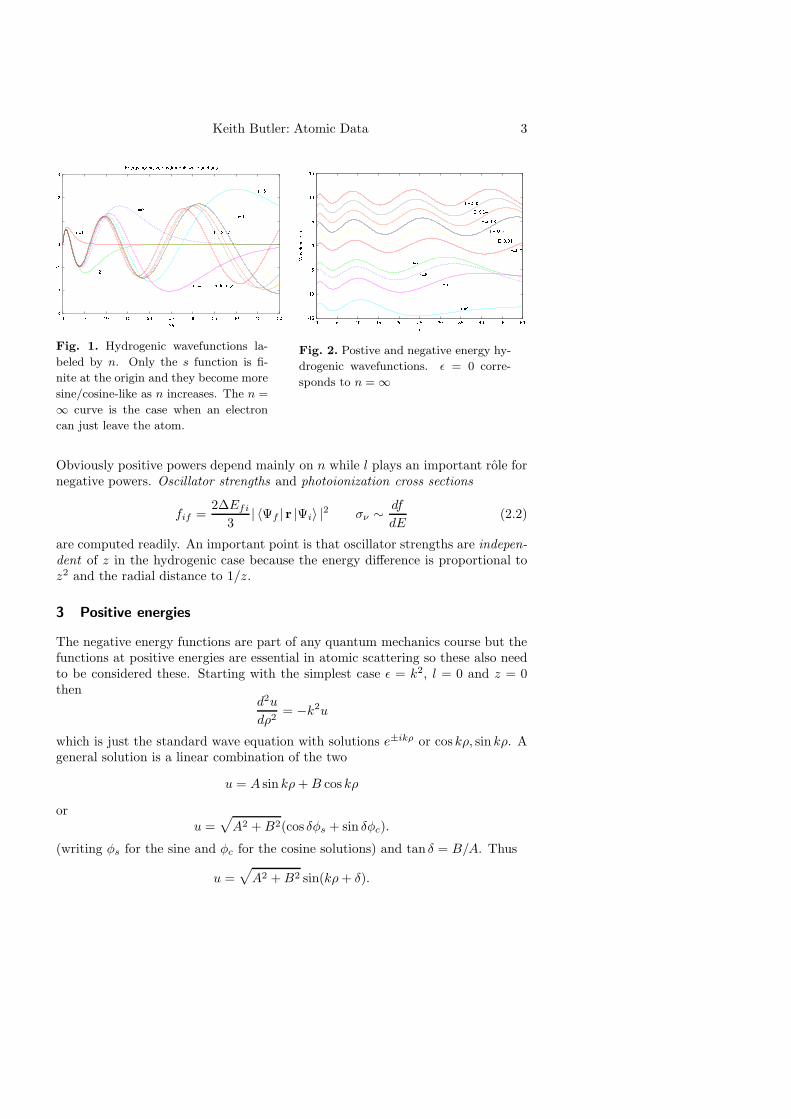
Fig. 1. Hydrogenic wavefunctions la-

beled by n. Only the s function is fi-

nite at the origin and they become more

sine/cosine-like as n increases. The n =

∞ curve is the case when an electron

can just leave the atom.

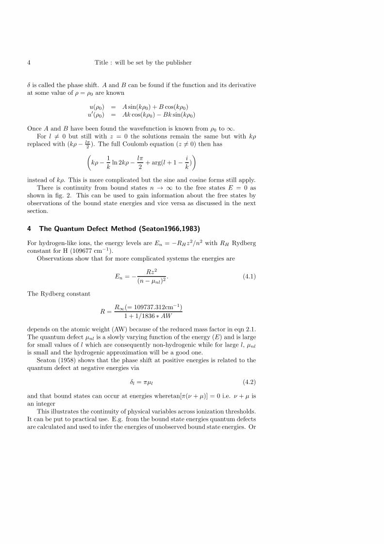
Fig. 2. Postive and negative energy hy-

drogenic wavefunctions. ǫ = 0 corre-

sponds to n = ∞

Obviously positive powers depend mainly on n while l plays an important role fornegative powers. Oscillator strengths and photoionization cross sections

fif =2∆Efi

3| 〈Ψf | r |Ψi〉 |2 σν ∼ df

dE(2.2)

are computed readily. An important point is that oscillator strengths are indepen-dent of z in the hydrogenic case because the energy difference is proportional toz2 and the radial distance to 1/z.

3 Positive energies

The negative energy functions are part of any quantum mechanics course but thefunctions at positive energies are essential in atomic scattering so these also needto be considered these. Starting with the simplest case ǫ = k2, l = 0 and z = 0then

d2u

dρ2= −k2u

which is just the standard wave equation with solutions e±ikρ or cos kρ, sin kρ. Ageneral solution is a linear combination of the two

u = A sin kρ+B cos kρ

oru =

√

A2 +B2(cos δφs + sin δφc).

(writing φs for the sine and φc for the cosine solutions) and tan δ = B/A. Thus

u =√

A2 +B2 sin(kρ+ δ).


δ is called the phase shift. A and B can be found if the function and its derivativeat some value of ρ = ρ0 are known

u(ρ0) = A sin(kρ0) +B cos(kρ0)u′(ρ0) = Ak cos(kρ0)−Bk sin(kρ0)

Once A and B have been found the wavefunction is known from ρ0 to ∞.For l 6= 0 but still with z = 0 the solutions remain the same but with kρ

replaced with (kρ− lπ2 ). The full Coulomb equation (z 6= 0) then has

(

kρ− 1

kln 2kρ− lπ

2+ arg(l + 1− i

k)

)

instead of kρ. This is more complicated but the sine and cosine forms still apply.There is continuity from bound states n → ∞ to the free states E = 0 as

shown in fig. 2. This can be used to gain information about the free states byobservations of the bound state energies and vice versa as discussed in the nextsection.

4 The Quantum Defect Method (Seaton1966,1983)

For hydrogen-like ions, the energy levels are En = −RHz2/n2 with RH Rydberg

constant for H (109677 cm−1).Observations show that for more complicated systems the energies are

En = − Rz2

(n− µnl)2. (4.1)

The Rydberg constant

R =R∞(= 109737.312cm−1)

1 + 1/1836 ∗AW

depends on the atomic weight (AW) because of the reduced mass factor in eqn 2.1.The quantum defect µnl is a slowly varying function of the energy (E) and is largefor small values of l which are consequently non-hydrogenic while for large l, µnl

is small and the hydrogenic approximation will be a good one.Seaton (1958) shows that the phase shift at positive energies is related to the

quantum defect at negative energies via

δl = πµl (4.2)

and that bound states can occur at energies wheretan[π(ν + µ)] = 0 i.e. ν + µ isan integer

This illustrates the continuity of physical variables across ionization thresholds.It can be put to practical use. E.g. from the bound state energies quantum defectsare calculated and used to infer the energies of unobserved bound state energies. Or


Table 1. Quantum defects for C IV s states.

The ionization energy is 520178.4 cm−1

(Moore1970

nl E(cm−1) n∗ µ2s .00 1.837 .1633s 302849.00 2.842 .1584s 401348.09 3.844 .1565s 445368.50 4.844 .1566s 468784.00 5.845 .1557s 482706.00 6.845 .1558s 491650.81 7.845 .1559s 497736.69 8.845 .155

Table 2. Comparison of quantum defect

method and Opacity Project (Peach et

al.,1988) f-values for C IV.

Lower Upper fQD fRM

2s 2p .2857 0.28552s 3p .1993 0.2032s 4p .0600 0.0612s 5p .0265 0.02702s 6p .0142 0.01452s 7p .0085 0.00872s 8p .0055 0.005652s 9p .0038 0.00392s 10p .0029 0.00282s 11p .0022 —

Fig. 3. Quantum defects for levels of C IV spdf states (Moore, 1970). Note the slow

variation in µ, that µ decreases with increasing l and that there are some problems with

the values at high n.

the values of the phase shifts can be deduced giving the positive energy functionsfrom which photoionization cross sections can be obtained. The values found inTable 1 for s electrons in C IV have been calculated using eqn 4.1 and are plottedin figure 3 together with data for other l values.

There are a few other points of interest here: it is possible to go in bothdirections so that calculated or observed phase shifts may be used to find boundstate energies etc: Coulomb functions with non-integer n are unphysical since theydo not obey the boundary conditions at small r. However, the length form of thef-value weights large r so the theory can be used to calculate oscillator strengthscheaply (Bates and Damgaard, 1949). As can be seen from Table 2 the methodworks well for one electron systems and cases in which a single electron does allthe work.


Fig. 4. df/dE from the f-values and

photoionization cross sections for C IV

from the QD theory. Note the continu-

ity from negative to positive energies.

0

0.1

0.2

0.3

0.4

0.5

0.6

6 8 10 12 14 16 18 20

Cro

ss s

ectio

n (M

b)

Photon Energy (Ryd)

Fig. 5. Comparison of quantum defect

and Opacity Project (Peach et al.,1988)

photoionization cross sections for C IV.

The theory can also be applied to photoionization cross sections (Burgess andSeaton 1960) in which the free state phase shifts are obtained from the bound stateenergies using the Seaton relation (eqn. 4.2). This is illustrated in fig. 4. fnl/n

∗3 =df/dE is plotted instead of the f-values themselves since this allows the continuityof the differential oscillator strength to be seen. Finally a comparison of results forthe photoionization cross section of the ground state of C IV from the QD and theR-matrix methods (fig.5) is made. Again the agreement is excellent re-emphasizingthe fact that QD atomic data can be accurate under certain circumstances.

5 Many electron systems

Having seen how to deal with a single electron tools to work with more complexsystems are needed. Even collisional excitation of hydrogen is a three-body prob-lem for which there are non analytical solutions. Thus methods for many electronsystems can only be approximate.

The next simplest system is an atom with two electrons, Helium. The Hamil-tonian is

[

−1

2∇2

r1− 1

2∇2

r2− Z

r1− Z

r2+

1

r12

]

Ψ(r1, r2) = EΨ(r1, r2).

The charge Z is two for Helium itself but the more general form is retained. Sincethe Hamiltonian does not change when the position vectors of the two electronsr1 and r2 are interchanged

Ψ(r1, r2) = ±Ψ(r2, r1).

When the + sign applies Ψ is said to be space symmetric, denoted by Ψ+. The −holds for space antisymmetric functions Ψ−.


However, the spins must be taken into account so the spin functions χ(1, 2)must be included and

Ψ(q1,q2) = Ψ(r1, r2)χ(1, 2).

These must be antisymmetric from the Pauli principle so a space symmetric func-tion will be combined with an antisymmetric spin function and vice versa. It turnsout that there are three possible symmetric spin functions (a triplet) with totalspin 1 and one antisymmetric function (a singlet) where the spin is zero.

If the total orbital angular momentum is L =∑

i li with eigenvalues L,ML,an energy term with a particular value of S =

∑

i si with eigenvalues S,MS .L is normally written as 2S+1L since for light elements LS-coupling is a goodapproximation. Here first the l s are coupled to give L and s s to give S and thenthe sum L + S is taken. The term has multiplicity (2S + 1) and L is denoted bya letter

L = 0 1 2 3 4 . . .S P D F G . . . .

When relativistic effects are taken into account, the levels of the terms are subjectto fine-structure splitting. L, S are then no longer good quantum numbers, con-stants of the motion, but the total angular momentum J = L+ S is. Such a levelis represented by

2S+1LJ .

5.1 Independent Particle Model

How are the energy levels of Helium to be obtained? It is a three-body system sothe solution must be approximate. The simplest approach is to treat the two elec-trons independently and to add the coupling between them later as a perturbation.This is a poor approximation for Helium since the electrons are stongly correlated(and in H− even more so) but works well for other systems, in particular for ions.

The very simplest approach is to set H = H0 +H ′ with

H0 = −1

2∇2

r1− Z

r1− 1

2∇2

r2− Z

r2≡ h1 + h2

H ′ =1

r12.

Here H ′ is the full interaction between the two electrons. h1 and h2 are then bothhydrogenic and the energies are known

E0n1n2

= −Z2

(

1

n21

+1

n22

)

The ground state energy n1 = n2 = 1 is −2Z2 = −8 Ryd. compares badly withthe observed value of −5.80 Ryd. In addition, the singlet and triplet states aredegenerate. Thus it is essential, as is obvious, to include 1/r12


The next simplest approximation is to rearrange the terms a little differently,add a potential V (r) for each electron to H0 and subtract the same potential fromH ′. Hopefully H ′ is then smaller. Writing

H0 = −1

2∇2

r1+ V (r1)−

1

2∇2

r2+ V (r2) ≡ h′1 + h′2

H ′ =1

r12− Z

r1− V (r1)−

Z

r2− V (r2).

With the Ansatz V (r) = −(Z−s)/r ≡ Ze/r where the screening constant s allowsfor the electron shielding the problem is still hydrogenic, the energies are as abovebut with an effective charge Ze. The ground state energy is −2Z2

e and s = 0.3reproduces the observed value. However this is just a fit and cannot be improvedsystematically.

5.2 N -electron systems

The Hamiltonian for an N -electron system is a straightforward generalization ofthat for Helium, namely

H =

N∑

i=1

(

−1

2∇2

ri+Z

ri

)

+

N∑

j>i=1

1

rij.

and the N -electron wavefunction

Ψ(q1,q2 . . .qN ) = Ψ(r1, r2 . . . rN )χ(1, 2, . . .N)

must be antisymmetric so that the Pauli exclusion principle is satisfied once more.The independent particle approximation can be made for the N -electron system

in the same way as for the two-electron system. Each electron then moves in aneffective potential that describes the average effect of its interaction with the other(N−1) electrons. They in turn ‘screen’ the nuclear charge. In choosing the effectivepotential it is necessary to consider that 1/r12 behaves like 1/r> where r> is thelarger of r1, r2. Then the potential will look like

V (ri) = −Zri

+ S(ri).

and S(ri is the screening function. There are two limits to take into account: 1)ri is largest, i.e. the ith electron is furthest from the nucleus. r> = ri and

V (r) = −Zri

+

N−1∑

j=1

1

ri= −Z −N + 1

ri.

The nucleus is fully screened and it is as if the atom is a point source with chargeZ −N + 1; 2) At the opposite extreme, ri is closer to the nucleus than any otherelectron and

V (ri) ≈ −Zri

+

⟨

N−1∑

j=1

1

rj

⟩

= −Zri

+ a constant


The electron “sees” the full nuclear charge. In between, S(ri) will be a complicatedfunction. Bearing these considerations in mind, the Hamiltonian is rearranged oncemore, adding and subtracting appropriate effective potentials

H = HC +H1

HC =

N∑

i=1

(

1

2∇2

ri+ V (ri)

)

≡N∑

i=1

hi

H1 =

N∑

j>i=1

1

rij−∑

i

(

Z

ri+ V (ri)

)

=∑

j>i=1

1

rij−∑

i

S(ri).

The advantage in doing this is that H1 is now (hopefully) small and can be treatedusing perturbation theory while at the same time HC is the sum of one electronHamiltonians which can be solved numerically once V (ri) is given.

Each solution of[

−1

2∇2

r + V (r)

]

ψnlml(r) = Enlψnlml

(r)

is called an orbital and looks like

ψnlmlms(q) = Rnl(r)Ylml

(θ, φ)χ 1

2,ms

The wavefunction is the product of a radial, an angular and a spin function withappropriate quantum numbers. At this level of approximation the Pauli principlestates that no two electrons can have the same set of 4 quantum numbers nlmlms.

5.3 Configurations, shells, sub-shells

Since each electron is treated independently it is clear that the total energy is thesum of the one-electron contributions

E =∑

nl

Enl,

(the energies are independent of ms,ml unless magnetic or electric fields are con-sidered). The distribution of the electrons among the orbitals is a configuration

and is written as (n1l1)t1(n2l2)

t2 . . . (nν lν)tν . E.g. the ground configuration (the

energetically lowest) of neutral oxygen is 1s22s22p4 This may be abbreviated to2p4 with 2 1s, 2 2s and 4 2p electrons when the meaning is clear. Note that thisis based on central field approximation and the configuration as a label for theenergy levels will only be good when the approximation holds. Also the electronsare indistinguishable so it makes no sense to talk about the 1s electrons. Electronswith the same value of nl belong to the same sub-shell and are equivalent. Theydiffer only in the ml,ms quantum numbers. In the same way, electrons with the


same n belong to the same shell. Since there are two possible values of ms and(2l+ 1) different values of ml the maximum occupancy of a sub-shell is 2(2l+ 1),e.g. 2p6.

5.4 Determination of possible terms

Note that for a closed sub-shell, only a 1S term is possible since ML =∑

imli =0, MS =

∑

imsi = 0. For non-equivalent electrons, the exclusion principle isautomatically satisfied, so that the addition rules for angular momenta can beused without further restriction

J = |J1 − J2|, . . . , |J1 + J2|

for J = L and J = S separately. Consider two electrons with l1, l2. Then

L = |l1 − l2| . . . |l1 + l2| (5.1)

and since s1 = s2 = 12 , S = 0 or 1. E.g. for npn′p, l1 = l2 = 1 and L = 0,1, or 2.

Thus the possible terms are1,3S,1,3P,1,3D.

If l1 = 1 and l2 = 2, (npn′d), on the other hand, L = 1, 2, 3 and the possibleterms are

1,3P,1,3D,1,3F. (5.2)

To work out the terms for three electrons, the two electron terms are known andthen the third electron is added systematicall, using (5.1) once more. For example,consider npn′p n′′d. The first two electrons give the terms listed in (5.2). The delectron has l = 2, s = 1

2 . If this is added to the 1S term (L′ = S′ = 0), a 2D term,L = 2, S = 1

2 , is found.Completing the table and adding a n′′d electron to

1P gives 2P, 2D, 2F1D gives 2S, 2P, 2D, 2F, 2G3S gives 2,4D3P gives 2,4P, 2,4D, 2,4F3D gives 2,4S, 2,4P,2,4D, 2,4F, 2,4G

The process can be continued but it is obvious that the number of possible termsgrows very rapidly.

5.5 Configuration Interaction

If the independent particle model is good then a single configuration is a gooddescription. However, H1 mixes configurations and terms with the same L and Svalues. e.g. the ground state of He I is Ψg = 1s2 1S but the corrections give

Ψg = a1(1s2) + a2(1s2s) + a3(1s3s) + · · ·+ ak(2s

2) + · · ·


with∑∞

i=1 a2i = 1. The 1s2s wavefunction will also be a sum over the same

configurations but with different coefficients

Ψ1s2s = b1(1s2) + b2(1s2s) + b3(1s3s) + · · · .

The independent particle model and single configuration make sense if a singlecoefficient is close to 1. This is true for for He as the coefficients are close to one.He itself is difficult to compute as the 1s orbitals in each configuration are verydifferent.

Configuration interaction uses

Ψ =∑

i

ciΦi. (5.3)

where the Φi are different configurations.The wavefunctions are optimized by

• 1. choosing a set of the Φi.

• 2. choosing a set of one-electron orbitals (with adjustable parameters inV (r)).

• 3. calculating the Hamiltonian matrix Hij = 〈Ψi|H |Ψj〉.• 4. diagonalizing the Hamiltonian to find the eigenvalues Ei and coefficientsci.

• 5. calculating e.g. the weighted sum∑N

i=1 giEi, gi is a weighting factor,e.g. the statistical weight or 1. Only a subset of the energy levels will beoptimized, the physical states. Other configurations are included to providecorrelation.

• 6. go back to 2 and adjust the parameters until this sum is a minimum.

The difficulty is that the sum over i runs over all bound and free states inprinciple so it must be truncated to fit into the available computers. A balancemust be found between what is doable and what is desireable. This will depend onthe purpose for which the wavefunctions are to be used. If highly accurate f-valuesare needed then there may be thousands of configurations involved, most simply ascorrelation. On the other hand if a scattering calculation is to be performed thenfewer configurations can be considered. The choice of configurations and orbitalsrequires some experience if the best is to be made of the available resources.

LS-coupling is appropriate for low-Z ions and relativistic effects can be includedvia perturbation theory. There are a number of fully relativistic packages includingGRASP2K (Jonsson et al.,2007) but they are generally more difficult to use.

These are some general purpose programs to look out for

• Cowan1981. The matrix elements Hij are sums of integrals. Least squaresfits to observed energies give these integrals and then radiative data (Cowan).Kurucz uses this. The data are ideal for opacity calculations because of theircompleteness. Data for individual ions and transitions can also be good.


• Multi-Channel-Hartree-Fock (MCHF, Froese Fischer et al.2007). A gener-alization of the Hartree-Fock approach to configuration interaction. Theone-electron orbitals are adjusted to give a self-consistent solution to theproblem so the V (ri are iterated to convergence. This gives the best solu-tion for any given set of configurations and one-electron orbitals. The atomicdata are generally of high-quality.

• CIV3 (Hibbert,1975) and AUTOSTRUCTURE (Badnell, 1986). The ma-jor difference between these is the radial wavefunctions. In CIV3, theseare analytical ‘Slater-type orbitals’ and are essentially asymptotic hydro-genic functions. The radial integrals can therefore be computed extremelyquickly. In AUTOSTRUCTURE the potential is chosen to be a statistical,Thomas-Fermi-Dirac-Amaldi model which ‘smears’ out the contributions ofthe electrons. AUTOSTRUCTURE and CIV3 are also used in the calcula-tion of ‘target’ wavefunctions for scattering calculations which is the subjectof the following sections.

6 Scattering theory

6.1 Cross sections

In an ideal scattering experiment, a uniform, monoenergetic beam consisting ofN particles per unit time per unit area perpendicular to the beam is scatteredoff a target. If the density in the target n is low enough only a single particle isinvolved in each collision. And if the target is thin enough multiple scatteringswill not occur. dN ′ is the number of particles scattered into the solid angle dΩcentred about a direction Ω

The number of scattered particles will be proportional to N , n and dΩ with aconstant of proportionality defined by

dN ′ = Nndσ

dΩ(θ, φ)dΩ,

the differential cross section. It is the ratio of the number of scattered particles dN ′

to the flux of incident particles with respect to the target and has the dimensionsof an area.

The total cross section is the integral of the differential cross section over allangles

σtot =

∫

dσ

dΩ(θ, φ)dΩ

6.2 Simple scattering theory

Scattering by a potential allows such quantities as the cross section, the collisionamplitude and so forth to be defined. Beginning with the Schrodinger equation


Incoming plane wave Outgoing spherical wave

Target

Fig. 6. A schematic view of a scattering experiment.

with V (r) is real and time-independent so that[

−1

2∇2 + V (r)

]

ψ(r) = Eψ(r).

E, the energy is written as 12k

2 = 12v

2. V is assumed to be of short range (atomsonly, no Coulomb potential). For large r, the equation

(∇2 + k2)ψ(r) = 0

has to be solved and asymptotically

ψ(r) ∼r→∞

ψinc(r) + ψsc(r).

This representation is intended to describe the situation shown in fig. 6 Amonoenergetic incident beam strikes the target atom. The beam is scattered bythe target particle into a solid angle dΩ where it is detected. As with water wavesstriking a rock, the outgoing waves will be spherically symmetric and differentfractions will be scattered into the different directions. The monoenergetic incidentbeam can be described by the plane wave

ψinc(r) = Aeik·r

(A is a constant) while the scattered beam is

ψsc(r) = Af(k, θ, φ)eikr

r.

f(k, θ, φ) is known as the scattering amplitude. Scattering theory shows that thedifferential cross section is

dσ

dΩ= |f(k, θ, φ)|2

with a total cross section

σtot =

∫

dσ

dΩdΩ.


Fig. 7. Two channels are shown with the target energy levels at the bottom of the shaded

regions where the channel energies are positive. The lines represent states with negative

channel energies. They can only occur at certain energies, the eigenvalues. The states

below the lowest target level are truly bound whereas those above will be a mixture of

a bound state from the second channel and a free state from the first. It is this mixing

that causes the resonances.

7 The close-coupling expansion (Burke & Seaton, 1971)

The close-coupling expansion is an attempt to mimic the scattering experimentas closely as possible. H is the simplest example and the spin is omitted for themoment. A stationary target atom has a wavefunction ψ(a|r1) with a ≡ nlm.These are the hydrogen bound state functions seen earlier. The scattered electronhas a wavefunction F (a|r2) which is the unknown of the problem. Then the close-coupling expansion is

Ψ(r1, r) =∑

ψ(a|r1)F (a|r).

each pair is a channel, in which the atom and the colliding electron are in a definitestate during the collision. Note the similarity to the configuration interactionexpansion eqn. 5.3 It is assumed that the bound states retain their characterduring the collisional process. The sum then ensures that all channels are puton equal footing and allows for mixing between them. This channel mixing givesresonances. See fig. 7 for s short explanation.

The close-coupling equations may be derived as follows. The functions satisfythe identity

∫

ψ∗(a|r1)[H − E]Ψ(r1, r) d3r1 = 0


since HΨ = EΨ. Some algebra later. . .

[∇2 + k2a]F (a|r) = 2∑

a′

Vaa′(r)F (a′|r)

If the target energy is denoted by Ea then the channel energies 12k

2a are defined by

E = Ea+12k

2a, E being the total energy. Vaa′ is shorthand for

∫

ψ∗(a|r1)V ψ(a′|r1) d3r1and involves the known bound states. This is a set of coupled differential equationsand can be solved using standard techniques.

Here it is assumed that the bound and scattered electrons are distinguishablewhich is not the case. The inclusion of this exchange complicates the situationand the close-coupling equations are now

[∇2 + k2a]F±(a|r) = 2

∑

a′

[Vaa′(r) ±Waa′(r)]F±(a′|r).

The exchange potential is more difficult to treat as it involves an integral over theunknown F functions. This leads to a set of coupled integro-differential equations.These can again be solved using standard techniques (replace integrations withsums and differentiations with differences) but the matrices rapidly become verylarge.

The exchange will be small for: large r as the bound state is close to thenucleus; large l, the scattered electron is far from the nucleus on average; large z,the electron is tightly bound; and for large E where the velocity of the scatteredelectron is high and hence the interaction time is small. Under such circumstancesthe problem is much simpler. In actual close-coupling calculations a combinationof both will be used, with exchange only being used for low l and low E.

7.1 Born approximation

Some simpler approximations can now be derived. Remember that

F (j, i) ∼r→∞

eiki·rδji +eikjr

rf(j, i)

i.e. and incoming plane wave (the first term) and an outgoing spherical wave.

[∇2 + k2j ]F (j, i|r) = 2∑

j′

Vjj′ (r)F (j′, i|r).

There are two indices because there are now two boundary conditions. The energyk2i large so that the contribution from the outgoing wave is small, the scatteredelectron is unaffected by the atom, and to a good approximation

F (j, i) ≃ eiki·rδji

an outgoing plane wave. Putting this into the RHS of (7.1) the first Born approx-imation is obtained

fB1(j, i) = − 1

2π(kj |Vji|ki).


The Born approximation will become valid at high energy. However, it is notknown how large the energy must be. In stellar atmospheres the Born approxima-tion is poor.

7.2 Distorted Wave

For the distorted wave approximation it is assumed that all the potentials exceptfor that directly coupling the two levels involved is small. The sum then reducesto a single term Vji and the equations are

[∇2 + k2i ]F (i, i) = 2ViiF (i, i)[∇2 + k2j ]F (j, i) = 2VjjF (j, i) + 2VjiF (i, i)

with solution

fDW (j, i) = − 1

2π

∫

F(j,−kj)VjiF(i,ki) d3r

The scattered electron wavefunctions are given by

[∇2 − 2Vii + k2i ]F(i, i) = 0

with the boundary conditions

F(i,ki) ∼r→∞

eiki·rδji +eikir

rfDW .

Here there is some back-reaction of the target on the incoming electron, the wave-function is distorted. There are several variants of the distorted wave method. Inparticular exchange may be included by replacing V by V ±W or ions may betreated if the plane waves are replaced by Coulomb functions.

7.3 Bethe approximation

The Bethe approximation is much used within the stellar atmosphere communityalthough it is only valid under rather limited circumstances. Starting with theDW approximation

σ(i→ j) =1

4π2gi

kjki

∫

|(kj |Vji|ki)|2 dkj ,

noting that

Vji = − 1

r2+

1

r12

and1

r12=

1

r2+

r1 · r2r32

.


Onnly the first two terms are retained in the expansion. r1 is the coordinate ofthe bound electron and r2 that of the scattered electron which is larger than r1.An integration over r1 gives

Vji(r2) =r2 · (j|r1|i)

r32.

The cross section is

σ(i→ j) =1

4π2

kjki

∫

|(kj |r2/r32 |ki)|2 dkj ×1

3gi|(j|r1|i)|2

But the first integral is the free-free Gaunt factor and the second is the oscillatorstrength so the cross section is simply related to the f-value by

σ(i→ j) =4π2

k2i

fji∆E

g(kj , ki).

The theory for the collisional ionization is similar and involves the photoionizationcross section a(Ek).

σion(i) =2

k2i α√3

∫ 1

2k2

i−I

0

a(Ek)g(kj , ki) dEk

I + Ek

Bethe’s expression for the Gaunt factor is found if plane waves are used. However,Seaton (1962) and van Regemorter (1962) used g as a fit parameter, fitting to theavailable data at the time. These formulae are still in use but they are only goodwhen fij large and at high temperatures. They should be avoided if at all possible.

7.4 Partial Wave Theory

While the previous boundary conditions are needed to give the observables directlyit is more convenient to use outgoing and incoming spherical wave functions asthis is more symmetric. The wavefunctions then behave like

φ±(klm|r) = k−1/2Ylm(r)e±(kr− 1

2lπ)

r.

This choice defines the S matrix, an incoming spherical wave gives rise to manyoutgoing waves

ΨS(al2m2|r1, r2) ∼r2→∞

ψ(a|r1)φ−(kal2m2|r2)−∑

a′l′2m′

2

ψ(a′|r1)φ+(ka′ l′2m′

2|r2)S(a′l′2m′

2, al2m2)

The plane waves must be expanded in terms of the spherical waves and then somealgebra gives

f(a′ka′ , aka) =2πi

(kaka′)1

2

∑

l′2m′

2

l2m2

Y ∗

l2m2(ka)Yl′

2m′

2(k′

a)il2−l′

2T (a′l′2m′

2, al2m2)


and T (α′, α) = δ(α′, α)− S(α′, α) is the transmission matrix.If LS coupling applies then l1,l2 are coupled to give L, the spin is included and

the cross section is then

Q(αiLiSi → αjLjSj) =π

k2i

∑

LSπ

lilj

(2L+ 1)(2S + 1)

2(2Li + 1)(2Si + 1)

∣

∣TLSπji

∣

∣

2

The collision strength is useful as it is symmetric in the upper and lower states iand j

Ω(i, j) =(2Li + 1)(2Si + 1)

πk2iQ

The downward collision rate is the convolution of this with a Maxwellian

qij = ne8.631× 10−6

wiT 1/2Υij .

Υij =∫∞

0 Ω(x)e−xdx (x = E/kT ) which varies slowly with temperature andwi is the statistical weight of the upper level.

7.5 The K matrix

This is not quite the end of the story. Computers do not like complex numbers soit is easier to use real functions

φ(cs)(klm|r) = k−1/2Ylm(r)

1

r

(

cos

sin

)

(kr − 1

2lπ)

The reactance matrix K given by

ΨK ∼ ΦS(α) +∑

α′

K(α′, α)ΦC(α).

2iΦs ∼ Φ+ − Φ− and 2Φc ∼ Φ+ +Φ− so S = (1 + iK)(1 − iK)−1 With only onechannel K = tan δ, where δ is the phase shift.

8 R-Matrix method (Burke & Seaton, 1971)

8.1 R-Matrix method for Hydrogen (Yu Yan & Seaton, 1985)

The R-matrix method was developed in nuclear physics by Wigner and Eisenbud(1947) and applied to atomic physics by Lane and Thomas (1958). The idea is thatfar from the nucleus the problem is simple while for r ≤ a (R-matrix boundary) itis complex. So first solutions within this R-matrix box are sought. This is a boundstate problem since a is finite. The equations are then energy independent andonly need to be solved once for each value of LS. The radial Schrodinger equationfor H is

(

− d2

dr2+l(l + 1)

r2− 2

r− E

)

FE(r) = 0


Table 3. Eigenvalues and functions for hydrogen, l = 0 (Yan & Seaton, 1985)

k ek fk(a)1 −1.007362 0.1361862 −0.232335 −0.7190543 1.093783 0.6885984 3.335493 −0.6616185 6.400272 0.6508586 10.272967 −0.645343

with boundary condition

F ′

E(a) = 0

F ′ being the derivative of F . Only solutions for a discrete set of energies E = ekexist and they are written as fk(r) (see Table 8.1)

These solutions are unphysical since the observer is at infinity. However, thephysical solutions, which are energy dependent, can be expanded in terms of fk

FE(r) =

∞∑

k=1

fk(r)AkE

Some more algebra shows that

FE(a) = R(E)F ′

E(a)

where the R-matrix is

R(E) =

∞∑

k=1

fk(a)(ek − E)−1fk(a).

and is a function of the energy. Thus if fk and ek are known then FE can becalculated at all energies.

8.2 Matching at r = a

The R-matrix gives the value of the physical function within the box. Out-side the problem is much simpler. In the simplest case the solutions are justCoulomb/Bessell functions which may be calculated rapidly for any energy. Fornegative energies only solutions that do not increase exponentially are physicallyacceptable. To find these Seaton (1985) developed a procedure that allows theeigenvalues to be found automatically. If the outer region functions are P then forr = a the FE and their derivatives F ′

E are a linear combination of these

F = PXF ′ = P ′X


From the inner region F = RF ′ so

PX = RP ′X

This will have non-trivial solutions only when

det[P −RP ′] = 0.

R comes from inner, complicated region, P from the outer and both can be calcu-lated rapidly. Thus the determinant is computed on a fixed energy mesh, a scanfor roots is performed and the roots are “polished”. The latter are the boundstate energies and thus the physical wavefunctions from r = 0 to r = ∞ have beenobtained.

The situation is simpler for free states since solutions are available for all pos-itive energies. For all channels open (all channel energies are positive)

P = S + CK

S and C are the sine and cosine-like Coulomb functions and K is the reactancematrix which is to be determined.

F = RF ′ at r = a

which gives immediately

K = (C −RC ′)−1(S −RS′).

The same can be done when some channels are closed although the expressionsare more complicated.

8.3 Summary of the R-matrix method

The diagonalisation of H gives R at any energy, then matching to the Coulombfunctions at r = a gives K or the bound states. K is sufficient for collisional databut if radiative data are needed then integrals such as

(Ψ|r|Ψ′) = (Ψ|r|Ψ′)I + (Ψ|r|Ψ′)O

are required. The inner integrals (. . .)I are linear combinations of integrals overknown basis functions. The latter are pre-calculated and stored and the innerintegrals are rapidly obtained. In the outer region the Ψ are linear combinationsof Coulomb functions and the necessary integrals are also found speedily.

8.4 Some examples and relativistic effects

There are a number of ways of including relativistic effects within the close-coupling approximation. The DARC program (Norrington and Grant,2007) isfully relativistic and gives the best results but the amount of available data is


0

2

4

6

8

10

12

14

16

18

20

1 1.5 2 2.5 3 3.5 4

Cro

ss s

ectio

n (M

b)

Photon Energy (Ryd)

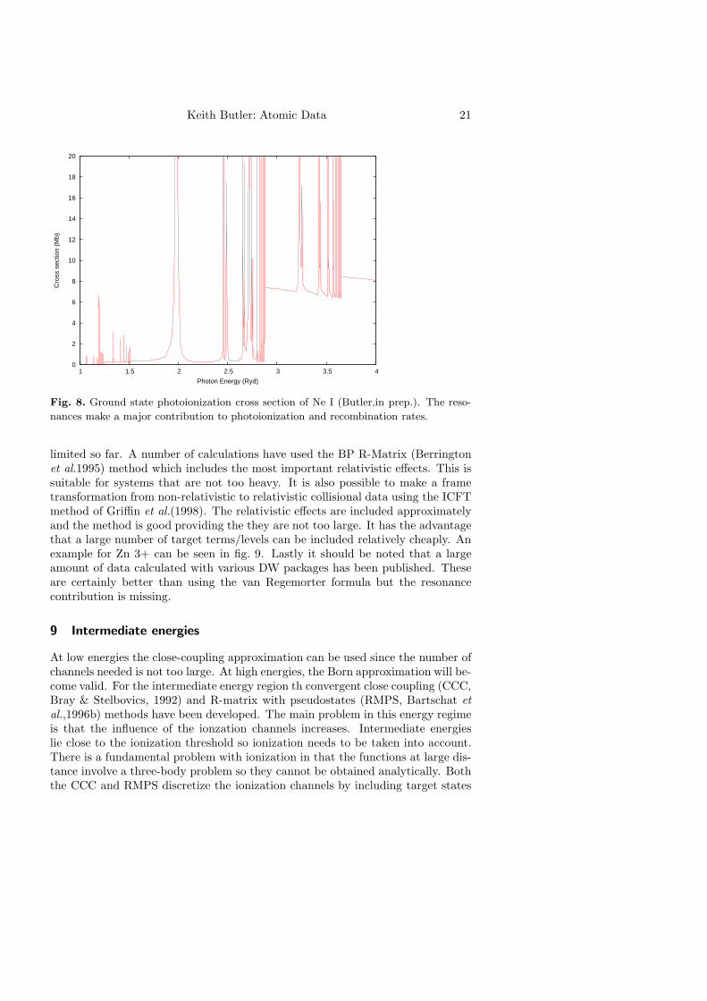
Fig. 8. Ground state photoionization cross section of Ne I (Butler,in prep.). The reso-

nances make a major contribution to photoionization and recombination rates.

limited so far. A number of calculations have used the BP R-Matrix (Berringtonet al.1995) method which includes the most important relativistic effects. This issuitable for systems that are not too heavy. It is also possible to make a frametransformation from non-relativistic to relativistic collisional data using the ICFTmethod of Griffin et al.(1998). The relativistic effects are included approximatelyand the method is good providing the they are not too large. It has the advantagethat a large number of target terms/levels can be included relatively cheaply. Anexample for Zn 3+ can be seen in fig. 9. Lastly it should be noted that a largeamount of data calculated with various DW packages has been published. Theseare certainly better than using the van Regemorter formula but the resonancecontribution is missing.

9 Intermediate energies

At low energies the close-coupling approximation can be used since the number ofchannels needed is not too large. At high energies, the Born approximation will be-come valid. For the intermediate energy region th convergent close coupling (CCC,Bray & Stelbovics, 1992) and R-matrix with pseudostates (RMPS, Bartschat et

al.,1996b) methods have been developed. The main problem in this energy regimeis that the influence of the ionzation channels increases. Intermediate energieslie close to the ionization threshold so ionization needs to be taken into account.There is a fundamental problem with ionization in that the functions at large dis-tance involve a three-body problem so they cannot be obtained analytically. Boththe CCC and RMPS discretize the ionization channels by including target states


0

2

4

6

8

10

12

14

0 0.2 0.4 0.6 0.8 1 1.2 1.4

Col

lisio

n S

tren

gth

Electron Energy (Ryd)

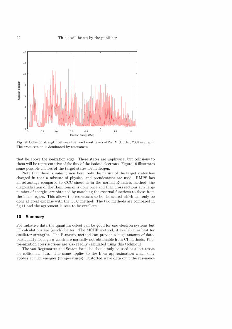
Fig. 9. Collision strength between the two lowest levels of Zn IV (Butler, 2008 in prep.).

The cross section is dominated by resonances.

that lie above the ionization edge. These states are unphysical but collisions tothem will be representative of the flux of the ionized electrons. Figure 10 illustratessome possible choices of the target states for hydrogen.

Note that there is nothing new here, only the nature of the target states haschanged in that a mixture of physical and pseudostates are used. RMPS hasan advantage compared to CCC since, as in the normal R-matrix method, thediagonalization of the Hamiltonian is done once and then cross sections at a largenumber of energies are obtained by matching the external functions to those fromthe inner region. This allows the resonances to be delineated which can only bedone at great expense with the CCC method. The two methods are compared infig.11 and the agreement is seen to be excellent.

10 Summary

For radiative data the quantum defect can be good for one electron systems butCI calculations are (much) better. The MCHF method, if available, is best foroscillator strengths. The R-matrix method can provide a huge amount of data,particularly for high n which are normally not obtainable from CI methods. Pho-toionization cross sections are also readily calculated using this technique.

The van Regemorter and Seaton formulae should only be used as a last resortfor collisional data. The same applies to the Born approximation which onlyapplies at high energies (temperatures). Distorted wave data omit the resonance


Fig. 10. Target states for CCC calculations

of H. The low energy states are the true

bound states for which collisional data are

required. Those close to and above the ion-

ization threshold at zero energy account for

the ionization channels. Different choices

show the convergence of the method (Bray

& Stelbovics, 1995).

Fig. 11. Comparion of RMPS and

CCC calculations for e− H scatter-

ing for L = 0, 1, 2, 3 (Bartschat et

al.,1996b). The curves are RMPS

results while the circles are CCC

data. The triangles were obtained

using the IERM method of Burke

et al.(1987)

contribution and are generally less reliable at low z. Thus if close-coupling dataare available these should be used. In particular, CCC and RMPS are the bestoption but calculations have been made for only a few ions.

References

Badnell, N.R. 1986, J. Phys. B: At. Mol. Phys., 19, 3827

Bartschat, K., Bray, I., Burke, P.G. & M P Scott 1996 J. Phys. B: At. Mol. Phys., 295493

Bartschat K., Hudson, E.T., Scott, M.P., Burke, P.G. & Burke, V.M, 1996, J. Phys. B:At. Mol. Phys., 29 115

Bates, D.R. & Damgaard, A. 1959, Phil. Trans. R. Soc. A, 242, 101

Berrington, K. A., Eissner, W. B. & Norrington, P. H. 1995, Comput. Phys. Commun.,92, 290

Bray, I. &Stelbovics A, 1992, Phys. Rev. Lett., 69 53

Bray, I. &Stelbovics A, 1995, Comput. Phys. Commun., 85, 1

Burgess, A. & Seaton, M.J. 1960, MNRAS, 120, 121

Burke P.G.& Seaton M.J. 1971, Methods in Computational Physics vol 10. ed B. Alder,S. Fernback & M. Rothenberg (New York: Academic Press) 1


Burke P.G., Noble C.J. & Scott M.P. 1987, Proc. R. Soc. A, 410 289

Cowan, R., 1981 Theory of Atomic Structure and Spectra

Froese Fischer, C., Tachiev, G., Gaigalas, G. & Godefroid, M.R. 2007, Comput. Phys.Commun. 176, 559

Griffin, D.C., Badnell, N.R. & Pindzola, M.S. 1998, J. Phys. B: At. Mol. Phys., 31, 3713

Hibbert, A. 2007, Comput. Phys. Commun. 9, 141

Jonsson, P., He, X., Froese Fischer, C. & Grant, I.P. 2007, Comput. Phys. Commun. 177,597

Lane, A.M. & Thomas, R.G. 1958, Rev. Mod. Phys., 30, 257

Moore, C.E., 1970 NSRDS-NBS 3, Sec. 3

Norrington, P. H. & Grant, I. P. 2007, Comput. Phys. Commun., in preparation

Peach G., Saraph, H.E. & Seaton, M.J. 1988, J. Phys. B: At. Mol. Phys., 21, 3669

Seaton, M.J 1958, MNRAS., 118, 504

Seaton, M.J 1962, Atomic and Molecular Processes, ed. D.R. Bates (Academic Press:New York), 375

Seaton, M.J 1966, Proc. Phys. Soc., 88, 801

Seaton, M.J 1983, RPPh, 46, 167

Seaton, M.J 1985, J. Phys. B: At. Mol. Phys., 18, 2111

van Regemorter, H. 1962, ApJ, 136, 906

Wigner, E.P. & Eisenbud, L. 1947, Phys. Rev., 72, 29

Yan, Y. & Seaton, M.J 1985, J. Phys. B: At. Mol. Phys., 18, 2577

ATOMIC DATA

Documents

Transcript of ATOMIC DATA